

Simulated Effects of Projected 2014–40 Withdrawals on Groundwater Flow and Water Levels in the New Jersey Coastal Plain
Links
- Document: Report (45.0 MB pdf) , HTML , XML
- Data Release: USGS data release - MODFLOW-2005 model used to analyze water-use scenarios in the New Jersey Coastal Plain
- NGMDB Index Page: National Geologic Map Database Index Page (html)
- Download citation as: RIS | Dublin Core
Abstract
Groundwater flow between 2014 through 2040 was simulated in the New Jersey Coastal Plain based on three withdrawal scenarios. Two of the scenarios were based on projected population trends and the assumption of water conservation; the nominal water-loss scenario projected a status quo in the efficiency of water loss in the delivery systems whereas the optimal water-loss scenario projected a better water-loss efficiency resulting in less withdrawals. The third scenario assumes that all wells will withdraw water at their full allocation level which is generally much more than reported withdrawals in 2013 or projected under the other two scenarios.
Maps and summaries of heads and drawdowns are presented for nine confined aquifers. All the aquifers have areas with heads below sea level by 2040. Of the three scenarios, the drawdowns are most extreme in the full allocation scenarios; there are large areas of head decline greater than 20 feet in 5 of the 9 confined aquifers. The exceptions are the Vincentown aquifer, despite some areas of large drawdown in the vicinity of wells, and the three Potomac-Raritan-Magothy (PRM) aquifers where withdrawals are regulated by Critical Area restrictions. The nominal and optimal water-loss scenarios have some areas of head declines; most are less than 15 feet. The simulation of these scenarios shows some extensive areas of head recovery as well—especially in the aquifers that are regulated by the Critical Area restrictions.
Budgets of inflow and outflow components were calculated for 44 hydrologic budget areas (HBAs). The budget analysis shows that the water movement is complex and varies based on the aquifer geometry and location of pumping wells. Flow components between the unconfined and confined parts of the system were summarized by HUC11 (hydrologic unit code 11) basins.
Introduction
The 1981 New Jersey Water Supply Management Act directs the Department of Environmental Protection (NJDEP) to develop and periodically revise the New Jersey Statewide Water Supply Plan to improve the management and protection of the State’s water supplies (NJDEP, 2017). The first New Jersey State Water Supply Plan, adopted by NJDEP in 1982, has been periodically updated. The latest Water Supply Plan (NJDEP, 2017) constitutes the second complete revision of the plan. The work described in this report is intended to help inform a new revision of the plan.
The initial water supply plan identified two areas in the New Jersey Coastal Plain (NJCP) where regional cones of depression (resulting from pumping of groundwater in populated areas) were causing saltwater intrusion and threatening the long-term reliability of the groundwater supply. These areas are referred to as Water-Supply Critical Areas. Critical Area 1 includes the Englishtown aquifer system, the Wenonah-Mount Laurel aquifer, and the upper and middle Potomac-Raritan-Magothy (PRM) aquifers in portions of Monmouth, Ocean, and Middlesex Counties (fig. 1). In Critical Area 1, purveyors with wells that pump 100,000 gallons per day (or more) were required to reduce their withdrawals to 50 percent or less of their 1983 withdrawal rate (CH2M HILL, Metcalf & Eddy, Inc., and New Jersey First, Inc., 1992). These restrictions went into effect in the 1990s (NJDEP, 2017). Critical Area 2 includes the upper, middle, and lower PRM aquifers and is centered on Gloucester, Camden, and Burlington Counties. Withdrawals were mandated to be reduced by 22 percent compared to those in 1988 in this area as alternate water supplies became available in the 1990s (Spitz and DePaul, 2008).
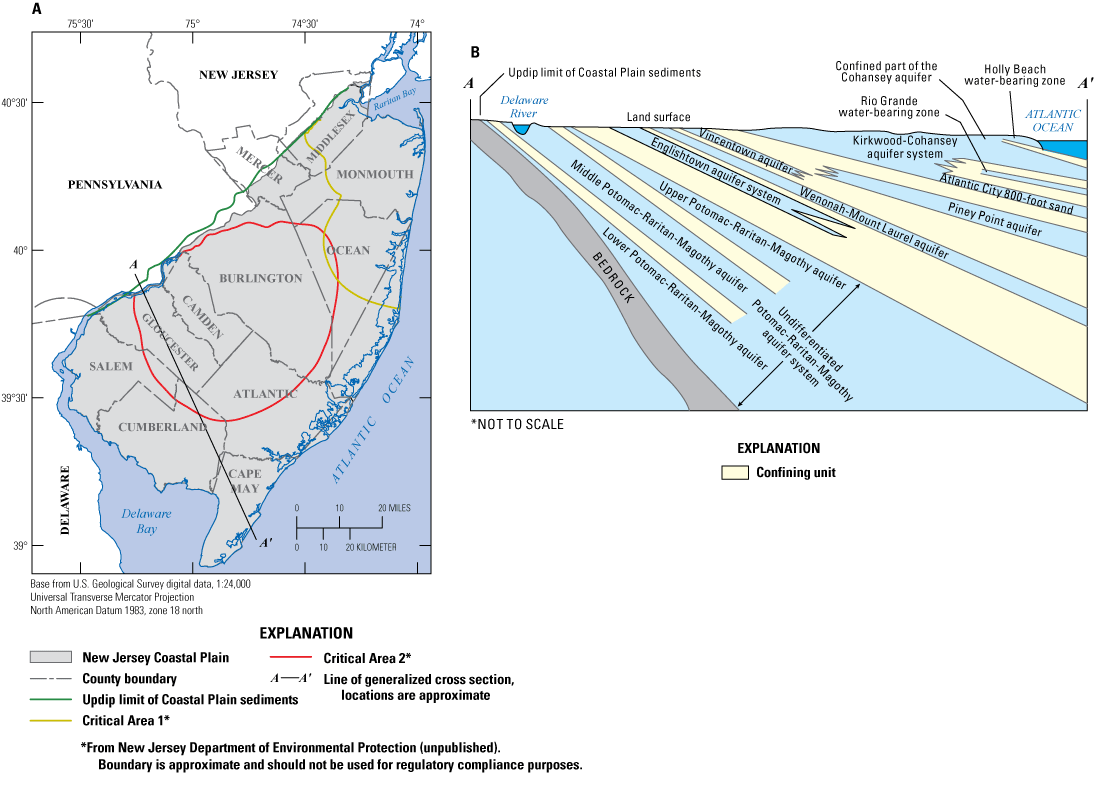
A, Map of model grid and Critical Areas in the New Jersey Coastal Plain, and B, generalized hydrogeologic section A–A’ through the Coastal Plain of southern New Jersey. Modified from Gordon and others (2021).
In 2018, the U.S. Geological Survey (USGS), in cooperation with the NJDEP, initiated a study to investigate the potential effects of projected 2014–2040 withdrawals in the confined NJCP aquifers based on analysis done by Rutgers University (Van Abs and others, 2018). The projected withdrawals will be used in the revised water-supply plan to estimate flow budgets within and outside areas of population growth, to quantify changes in simulated water levels in the confined aquifers, and to quantify the movement between unconfined and confined parts of the groundwater system for hydrologic unit code 11 (HUC11) boundaries in NJCP.
Purpose and Scope
This report describes simulated groundwater flows and water levels based on an extension of the most recent update of the NJCP groundwater model described in Gordon and Carleton (2023) using three scenarios of projected withdrawals for the time period 2014–40. Forty-one hydrologic budget areas (HBAs) were delineated based on hydrologic constraints in each of the nine major confined aquifers of the Coastal Plain as part of a similar effort to look at projected 2010 withdrawals based on the prior version of the model (Gordon, 2007). The HBAs coincide primarily with areas of large groundwater withdrawals, large water-level declines, and potential saltwater intrusion. Three additional HBAs will be considered in this report located in the Rio Grande water-bearing zone, which was not explicitly simulated in previous versions of the NJCP model.
The NJCP model of Gordon and Carleton (2023) was used as the base simulation for this report using files from the archive of Carleton and others (2023). In particular, the final stress period, representing conditions in 2013, was used for comparison with simulated water levels and flow budgets based on three withdrawal scenarios in the period 2014–40 for the nine confined aquifers. The three withdrawal scenarios are used to simulate a range of projected increases or decreases in groundwater withdrawals at existing wells. Results of these simulations are used to quantify the effects of projected changes in withdrawals on the groundwater flow system in the HBAs. Results are presented in a series of maps showing simulated water levels for 2040 and the simulated difference between water levels at the end of scenarios (2040) and the base simulation (2013). Flow-budget components in each of the 44 HBAs are quantified. Simulated water movement in the unconfined part of each HUC11 in the NJCP is quantified based on the cell-by-cell budgets from the numerical model.
Hydrogeologic Setting
The Coastal Plain sediments of New Jersey comprise a seaward-dipping wedge of alternating layers of gravel, sand, silt, and clay overlying crystalline bedrock extending from the updip limit of the coastal plain sediments to the Atlantic Ocean (fig. 1). The confined aquifers consist predominantly of sand but may also include interbedded silts and clays that range from approximately 50 to more than 600 feet thick and are separated by confining units; the confining units are composed predominantly of silts and clays and range in thickness from approximately 50 to 1,000 feet (Martin, 1998). The aquifers are recharged by precipitation in aquifer outcrop areas. Groundwater flows laterally downdip and (or) downward to underlying units. Water in the confined aquifers discharges to wells, to the Raritan or Delaware Bay, or to the Atlantic Ocean. Detailed descriptions of the hydrogeology of the NJCP aquifers and confining units are given in Zapecza (1989) and Martin (1998). The aquifers and corresponding geologic units are shown in figure 2. A generalized hydrogeologic section through the NJCP (fig. 1) shows the conceptual model of the aquifers and confining units in onshore areas.
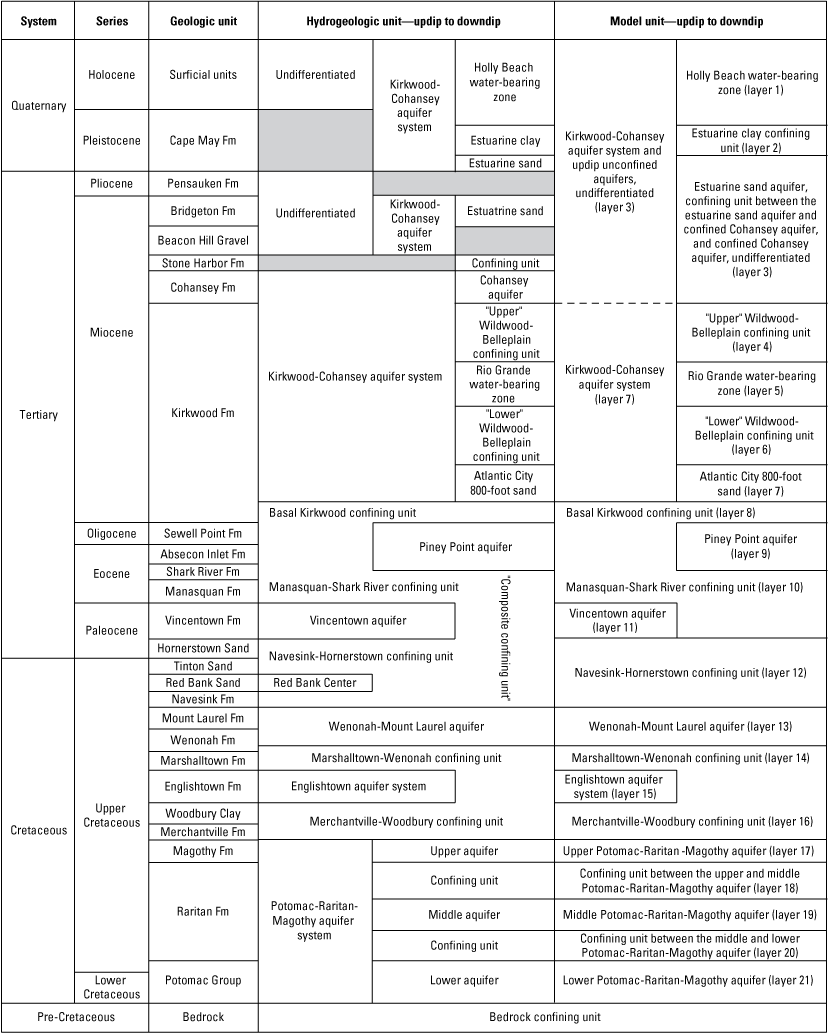
Stratigraphic columnar section showing hydrogeologic units and formations (Fm) for the New Jersey Coastal Plain. Modified from Gordon (2007) and Gordon and Carleton (2023, table 2).
Simulation of Projected 2014–40 Withdrawals
This study uses a recently completed groundwater model described in Gordon and Carleton (2023) to simulate the effects of three scenarios of projected groundwater withdrawals (nominal water-loss, optimal water-loss, and full allocation) over the time period from 2014–2040.
Description of Groundwater Model
The numerical groundwater model of the NJCP used in this work is described in Gordon and Carleton (2023) and archived in Carleton and others (2023). The NJCP model used here as the base simulation is the third in a line of groundwater models built to simulate transient groundwater flow and water levels in the NJCP. The first model (Martin, 1998) was developed as part of the Regional Aquifer-System Analysis program (Sun and Johnson, 1994) using the Trescott (1975) model as modified by Leahy (1982). That model simulated pre-development conditions as well as transient conditions from 1896 to 1990. The second model (Voronin, 2004) simulated transient conditions based on groundwater withdrawals from 1981 through 1998 using the program MODFLOW-96 (Harbaugh and McDonald, 1996). In addition to the time period, changes to the model included a finer spatial discretization and variable recharge. The most recent update (Gordon and Carleton, 2023) simulated transient conditions from 1980 to 2013 (each calendar year is represented by a separate stress period) using the program MODFLOW-2005 (Harbaugh, 2005). Some of the other noteworthy changes in the third version of the model are (1) the conversion from quasi- to fully three-dimensional, (2) the addition of annual recharge through the use of the Soil-Water-Balance (SWB) model (Westenbroek and others, 2010), and (3) the explicit simulation of the Rio Grande water-bearing zone and the underlying confining layer; these were simulated together with the Atlantic City 800-foot sand in previous model versions.
Recharge for the scenario models was based on the average recharge value of the last 10 years of the base simulation. The last two stress periods of the base simulation have less than this average recharge. The consequence of using the average recharge in the scenario models is increased simulated heads in and near the recharge areas compared to the end of the base simulation unless there is a corresponding increase in withdrawals from wells nearby. In other words, small recovery in heads in unconfined areas are likely due to the way the recharge is specified and should be expected.
An archive of the model inputs and output files for each of the simulations can be obtained from Kenefic and Kauffman (2024).
Groundwater Withdrawal Data
The withdrawals from the base simulation are described in Gordon and Carleton (2023). Reported annual pumping data were used to set withdrawal rates for the wells in the base simulation. If a well was not specified in the scenario withdrawals, the withdrawal rate from 2013 in the base simulation was used throughout the scenario models.
Projection of withdrawals for two of the three withdrawal scenarios used in this study, called “nominal water-loss” and “optimal water-loss,” were created by analysis done at Rutgers University (Van Abs and others, 2018). The basis for these two scenarios is summarized in the following paragraphs—further detail can be found in the Rutgers report. To assess future water demands, population and migration trends were used along with per capita water demands from various types of water users (for example, residential, commercial, industrial, and agricultural).
The Rutgers analysis (Van Abs and others, 2018) looked at two alternatives regarding per capita water demand. They first considered an alternative that assumed per capita water demand will remain the same. They also considered a second alternative: a conservation-based approach where withdrawals reflected reductions in demand owing to water-efficiency technology and standard water conservation behaviors. The commercial demands were assumed to track residential demands over time with a ten percent reduction used for the conservation scenario. Industrial and agricultural water demands were assumed to be steady for both scenarios.
Van Abs and others (2018) used the conservation alternative for per capita water demand as the basis for two other scenarios, nominal and optimal water-loss. These two scenarios, which are used in the simulations described in this report, are differentiated by assumptions related to water loss in public community water supply (PCWS) systems. Water loss is defined as the difference between the water that is delivered into PCWS systems and what is measured at the customer meters (Van Abs and others, 2018). Case studies were analyzed by Rutgers based on water-loss data for select PCWS systems supplied by NJDEP and the Delaware River Basin Commission. The water-loss scenarios were ultimately made based on system size (large [withdrawals greater than 300 million gallons per month], medium [withdrawals 30–300 million gallons per month], and small [withdrawals less than 30 million gallons per month]) and geology (bedrock or coastal plain). Rates of water loss generally increase as the system size decreases and water-loss rates were generally higher in areas with bedrock geology compared to the NJCP (Van Abs and others, 2018, fig. 5-7).
The nominal water-loss scenario assumes that all PCWS systems will achieve the current median values from systems reporting data; the optimal water-loss scenario assumes that all systems will achieve water-loss rates roughly equivalent to the better systems (25th percentile; Van Abs and others, 2018). In this report, water losses in both bedrock and coastal plain systems are evaluated, however all the systems simulated for this report are in the NJCP. The NJCP system rates of water loss for the nominal water-loss scenario are 10 percent for large and medium systems and 13 percent for small systems. For the optimal water-loss scenario, the water-loss rates are assumed to be 5 percent for all system sizes (Van Abs and others, 2018, table 5-5).
To make the withdrawal projections used in the nominal and optimal water-loss scenarios, Van Abs and others (2018, table 5-2) multiplied projected population trends for municipalities by per capita estimates of demand. They then added the water losses based on the percentages above to the projected demand. The resulting withdrawal projections for these scenarios are linear over the period from 2014–2040.
The third scenario for withdrawals considered in this report was a full allocation scenario. The withdrawal amounts were site specific from an allocation tool calculation done by the NJDEP Bureau of Water Allocation based on data from May 20, 2021 (Kenefic and Kauffman, 2024). For the full allocation scenario, the withdrawals were held constant through the simulations. This means there is a step change from the pumping used at the end of the base simulation in 2013.
Withdrawal projections for sites included in the model are reported in a data release (Kenefic and Kauffman, 2024). Withdrawals from the Delaware and Maryland parts of the simulated aquifers were kept constant at the 2013 levels from the base simulation.
The scenarios indicate that, between 2014 and 2040, withdrawals would increase 2.9 percent in the nominal water-loss scenario and decrease 1.3 percent in the optimal water-loss scenario but would increase more than two-fold for the full allocation scenario (fig. 3) compared to the withdrawals at the end of the base simulation. The nominal and optimal water-loss scenarios do not represent large changes in pumping over the 2014–40 period, remaining within the withdrawal variability that the base simulation reflects.
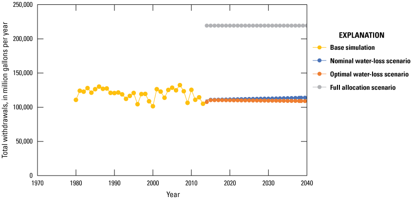
Line graph showing total groundwater withdrawals from the New Jersey Coastal Plain for the base simulation and three withdrawal scenarios: nominal water-loss, optimal water-loss, and full allocation.
At the end of the base simulation in 2013, the largest withdrawals are from layer three which mostly represents the unconfined Kirkwood-Cohansey aquifer system (fig. 4A). The biggest declines in withdrawals over time are in the upper, middle, and lower PRM aquifers and the Englishtown aquifer system (fig. 4), reflecting restrictions in the Critical Areas. Aquifers with increasing pumping over the time period of the base simulation are the Atlantic City 800-foot sand, the Wenonah-Mount Laurel aquifer, the Piney Point aquifer, and the Kirkwood-Cohansey aquifer system. Although the Wenonah-Mount Laurel aquifer is included in the Critical Area 1 restrictions, it is not included in Critical Area 2 yet saw increased usage in that area to replace lower withdrawals in the PRM aquifers. The Piney Point had a peak in withdrawals between 2006 and 2009 with declining withdrawals since then.
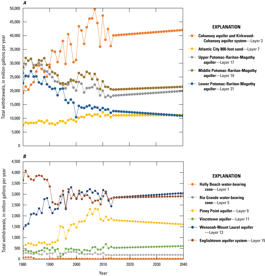
Line graph showing withdrawals by aquifer over time for the base simulation (1980–2013) and the nominal water-loss scenario (2014–40). A, aquifers with total withdrawals greater than 10,000 million gallons per day and, B, aquifers with total withdrawals less than 10,000 million gallons per day. Aquifers identified by name and their model layer number.
Figure 5 compares total withdrawals for the aquifers from the nominal and optimal water-loss scenarios to that of the full allocation scenario by calculating the percent of the full allocation that is projected to be withdrawn in the other two scenarios. Except for the Kirkwood-Cohansey aquifer system, the nominal and optimal water-loss scenarios indicate that aquifers with the largest withdrawals (fig, 4A) would use the highest percentage of the allocated withdrawals (fig. 5). The Kirkwood-Cohansey aquifer system, along with the relatively little used Holly Beach aquifer and Rio Grande water-bearing zone, would use the least amount of the full allocation.
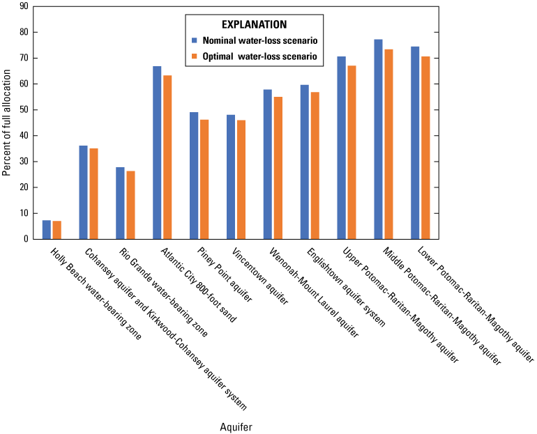
Bar chart showing the percent of the full allocation that is projected to be withdrawn in the nominal and optimal water-loss scenarios in the year 2040 by aquifer.
Description of Hydrologic Budget Areas
To analyze the flow budget for each of the confined aquifers in the NJCP, each confined aquifer and its outcrop area was divided into HBAs (table 1). The HBAs vary in areal extent and boundaries depending on the hydrologic conditions of the aquifer in which they were located. Apart from pumping in the unconfined Kirkwood-Cohansey aquifer system, the study placed almost all non-domestic groundwater withdrawals from the NJCP aquifers within these areas. Only the onshore freshwater portions of the confined aquifers (areas with chloride concentrations below 250 milligrams per liter [mg/L] as shown in Charles [2016] and Lacombe and Rosman [2001] for the Rio Grande water-bearing zone) were included in the HBAs, except HBA 27 in the Rio Grande water-bearing zone, HBA 3 in the Atlantic City 800-foot sand, HBA 21 in the middle PRM aquifer, and HBA 23 in the lower PRM aquifer. HBAs 3 and 21 contained active wells in areas where chloride concentrations exceed 250 mg/L. The New Jersey Secondary Drinking Water Standard Recommended Upper Limit (RUL) of 250 mg/L for chloride is the level above which the taste of water may become objectionable to the consumer and may also be associated with the presence of sodium in drinking water (Shelton, 2005). Elevated concentrations of sodium may have an adverse health effect on normal, healthy persons (Shelton, 2005).
Table 1.
Hydrologic budget areas (HBAs) in the confined aquifers of the New Jersey Coastal Plain.[Modified from Gordon (2007, table 2). mg/L, milligram per liter; N, no; Y, yes; n/a; not applicable]
Numbers 28 and 29 have not been assigned to allow for redefinition or addition of hydrologic budget areas at a later date.
Isochlors from Lacombe and Rosman (2001, fig. 2-7) and Charles (2016, figs. 4–12).
Forty-four HBAs have been designated—27 in the confined part of the aquifers (HBAs 1–27) and 17 in the outcrop areas (HBAs 30–46). HBA designations 28 and 29 are not assigned to any area; these numbers are available for any budget areas that may be designated in the future. Each HBA was delineated by various hydrologic boundaries, including aquifer extents, outcrop areas, the 250 mg/L isochlor (line of equal chloride concentration), Water-Supply Critical Areas, and groundwater divides. The HBAs and their locations are summarized in table 1. The boundaries of the individual HBA are described in detail in Gordon (2007).
Flow Budget Terms
For each HBA, each component of the flows in and out of the area were totaled using the cell-by-cell budget produced by the MODFLOW simulation. These included flows to or from each of the adjacent budget areas. For the flow to or from parts of the model downdip (south and east, see fig. 1), areas that are outside (fresher water) of the 250 mg/L isochlor line are summarized separately from the areas inside (saltier water) the 250 mg/L areas. Where the aquifers extend into the unconfined part of the system, there are budget areas defined. For the Rio Grande water-bearing zone and Atlantic City 800-foot sand (which transition into the Kirkwood-Cohansey aquifer system) and the Piney Point aquifer (which is entirely confined), the water moving in horizontally from updip (generally from the north and west) is labeled as lateral flow from updip. Vertical flow leaking to or from confining units both from above and below are summarized. Sources and sinks including wells, river leakage (Delaware River), and drain leakage (all other surface water features), as well as water in and out of storage, are summarized as well. In this report, each component of the flows in and out of a given HBA are summarized in flow budget tables and plots. They are expressed in million gallons per day and in percent.
Simulated Effects of Projected 2014–2040 Withdrawals
For each of the nine aquifers considered, results are presented for the changes in reported withdrawals used for the base simulation and in the projected withdrawals used for the scenarios, distribution of simulated heads, the simulated change in heads, and the flow components in the HBA at the end of the base simulation in 2040. Reported withdrawals for 2014–2020 are presented for comparison with the first seven years of the projected withdrawals used in the scenarios. When the change in head is referred to as drawdown, this is the amount of decline in heads—negative values of drawdown refer to an increase of head, or rising water levels in the aquifers.
To help summarize the effects of withdrawals on head in the HBA, the results from the base simulation and scenario simulations were used to calculate statistics about head and drawdown in the confined HBA. Plots show the median, 10th percentile, and minimum heads over time based on the model cells. The median shows the general condition in the HBA while the 10th percentile and minimum show the areas with the most impact from pumping. To demonstrate how things might change under the withdrawals projected for the three scenarios, a table is shown with the median, 90th percentile, and maximum drawdown in 2040 compared to the end of the base simulation. The median drawdown shows generally how the HBA will be impacted by changes in pumping where the 90th percentile and maximum are intended to show the areas with the most impact from pumping changes will occur. The calculations are done using the cells from the model grid identified to be part of the HBA of interest. Although lower heads often correlate with higher drawdown, the heads show more of the cumulative effect of pumping while the drawdowns focus more on changes in the period covered by the scenarios.
Rio Grande Water-Bearing Zone
The Rio Grande water-bearing zone was not included as a separate aquifer in prior versions of models of the NJCP. This study defined three budget areas within the inland part of the aquifer. Only three wells in the Rio Grande water-bearing zone had pumping data reported to the state in 2013 and were included in the base simulation and the scenarios. Other wells were included in some of the previous stress periods of the base simulations. Two of the wells are in the northern part of the aquifer and the other is in the south. HBA 25 was associated with the two wells in the north, HBA 27 was associated with the well in the south, and HBA 26 was in the unused part of the aquifer in between.
Trends of Withdrawals and Heads
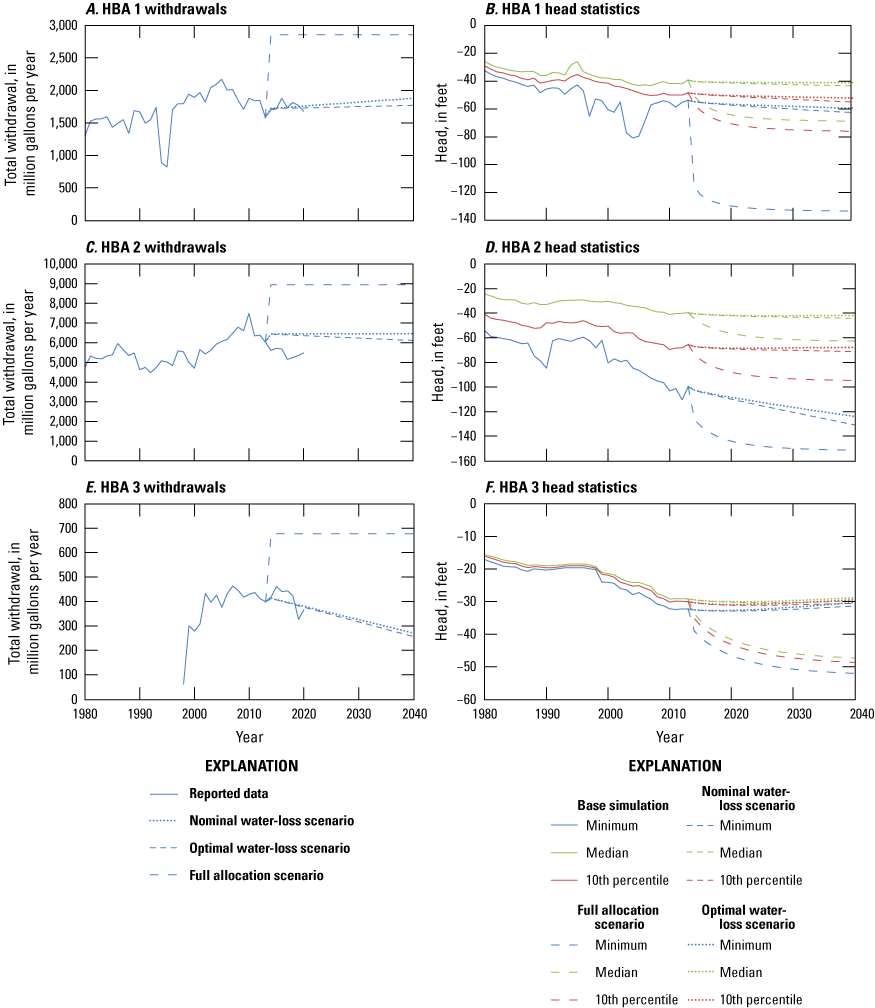
The base simulation includes withdrawal data from wells that became inactive over time. Only three wells are active in the area at the end of the simulation; however, pumping in the Rio Grande water-bearing zone as a whole increases slightly between 1980 and 2013 (fig. 6). Generally, pumping increases in HBA 27 and decreases in HBA 25 in the base simulation (figs. 6A, 6E). In both HBA 25 and HBA 27, the nominal and optimal water-loss scenarios indicate that projected pumping would be fairly steady through 2040 (figs. 6B, 6F). Under the optimal water-loss scenario, withdrawals would decrease slightly over time. The full allocation scenario indicates that projected withdrawals would increase by 186 percent for HBA 25 and 393 percent for HBA 27 (table 2) in comparison to the reported pumping in 2013 used in the base simulation (figs. 6A, 6E).
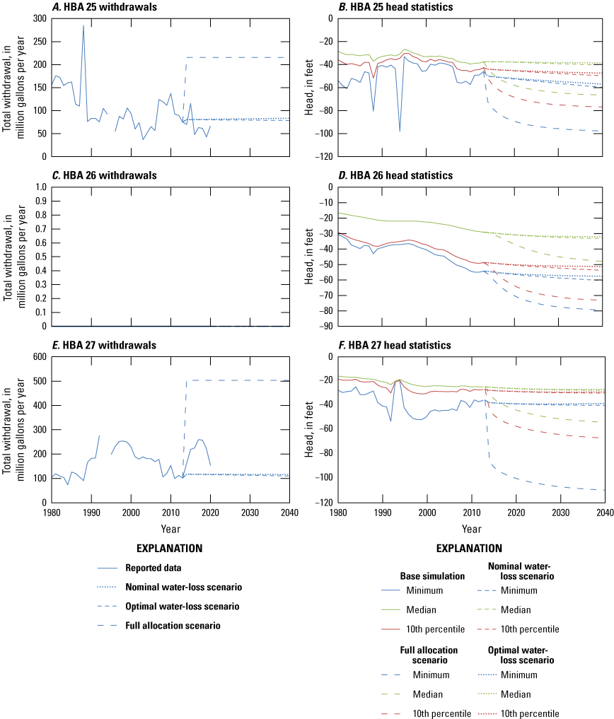
Line graphs showing withdrawals and median, 10th percentile, and minimum heads for model cells over time in hydrologic budget areas (HBA) in the Rio Grande water-bearing zone: A, withdrawals in HBA 25, B, head statistics in HBA 25, C, withdrawals in HBA 26, D, head statistics in HBA 26, E, withdrawals in HBA 27, and F, head statistics in HBA 27. Withdrawal data for 1993 and 1994 were unavailable and therefore not shown.
Table 2.
Summary of withdrawal trends in the Rio Grande water-bearing zone, Atlantic City 800-foot sand, Piney Point aquifer, Vincentown aquifer, and Wenonah-Mount Laurel aquifer.[Average withdrawals and slope given in million gallons per year. NJCP, New Jersey Coastal Plain; %, percent; —, no data]
The base simulation includes withdrawal data from wells that became inactive over time. Only three wells are active in the area at the end of the simulation; however, pumping in the Rio Grande water-bearing zone as a whole increases slightly between 1980 and 2013 (fig. 6). Generally, pumping increases in HBA 27 and decreases in HBA 25 in the base simulation (figs. 6A, 6E). In both HBA 25 and HBA 27, the nominal and optimal water-loss scenarios indicate that projected pumping would be fairly steady through 2040 (figs. 6B, 6F). Under the optimal water-loss scenario, withdrawals would decrease slightly over time. The full allocation scenario indicates that projected withdrawals would increase by 186 percent for HBA 25 and 393 percent for HBA 27 (table 2) in comparison to the reported pumping in 2013 used in the base simulation (figs. 6A, 6E).
For HBA 25, withdrawals decline in the first part of the base simulation, then spike in 1989 and an increase over several years in the mid-2000s (fig. 6A). After an initial spike in 2015, the reported pumping after the end of the base simulation is less than the projected pumping (fig. 6A). The response in heads shown in figure 6B reflects an inverse relation to the pumping. The large decline in the minimum head in 1994 reflects pumping in a well that is only included in the model for that stress period. Even though projected withdrawals decrease slightly in the optimal water-loss scenario (fig. 6A), there is still a slight decline in the heads for all three statistics (median, 10th percentile, and minimum) in HBA 25 (fig. 6B), likely reflecting an increase in pumping in the underlying Atlantic City 800-foot sand. In the full allocation scenario, the heads immediately decline sharply in response to the increased withdrawals and then continue to decline over time starting to level out by the year 2040 (fig. 6B).
For HBA 26, there is a general decline of heads over time across all three scenarios even though there are no pumping wells in the area (fig. 6D). The decline in heads reflects increased pumping in the underlying Atlantic City 800-foot sand and (for the full allocation scenario) in the adjacent budget areas (fig. 6D).
For HBA 27, overall, the heads shown in figure 6F decline slightly in the base simulation, despite a slight recovery starting around 1998 and a two-year spike upward in the 1990s when the area had no withdrawals (fig. 6E). For the nominal and optimal water-loss scenarios, all head statistics slightly decline over time, corresponding with a slight increase in pumping (fig. 6F). In the full allocation scenario, the heads, especially the minimum, decline quickly and then more gradually over time. The decline continues through until the end of the simulation in 2040 (fig. 6F).
Simulated Heads and Drawdown in 2040
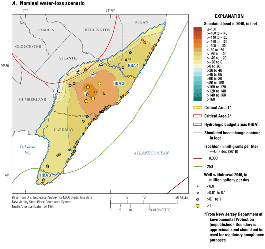
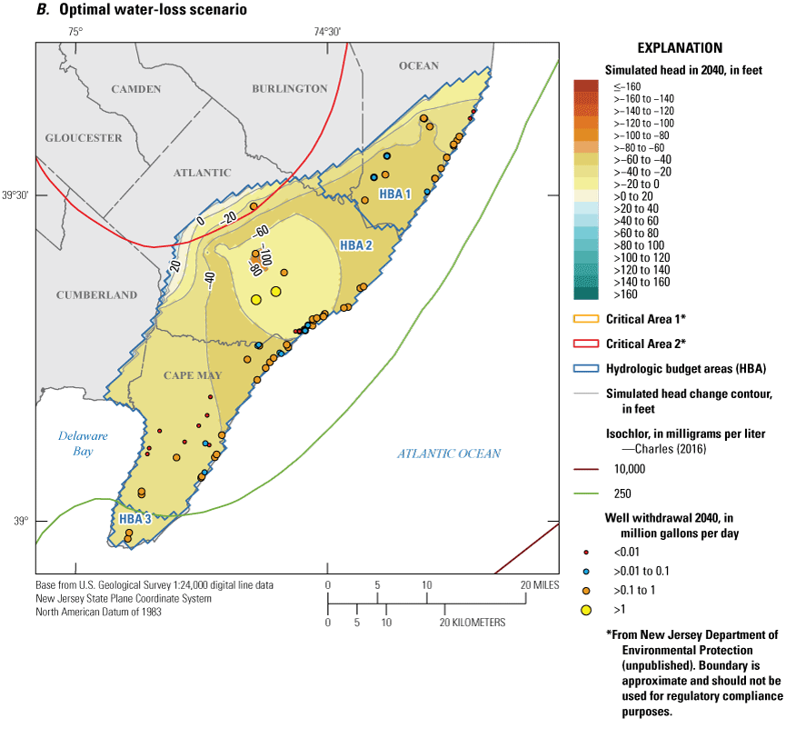
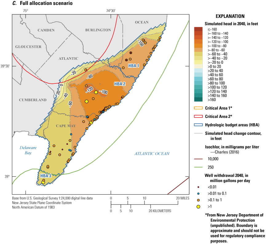
Figure 7A shows the simulated head distribution in 2040 for the Rio Grande water-bearing zone based on the nominal water-loss scenario. The large area with heads below −40 feet reflects a pumping center (area where wells are clustered) in the underlying Atlantic City 800-foot sand aquifer. The simulated head map for the nominal water-loss scenario looks very similar to that of the optimal water-loss scenario (fig. 7B). For the full allocation scenario, a noticeable decrease in the head surface can be seen on the map; the cone of depression around the main pumping wells are visible with the heads lower than −80 feet (fig. 7C).
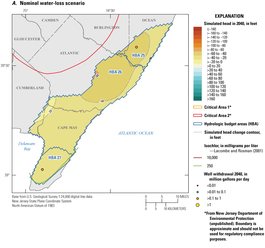

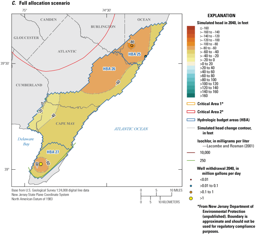
Maps showing hydrologic budget areas in the Rio Grande water-bearing zone and simulated potentiometric surface in 2040 for the three scenarios: A, nominal water-loss, B, optimal water-loss, and C, full allocation.
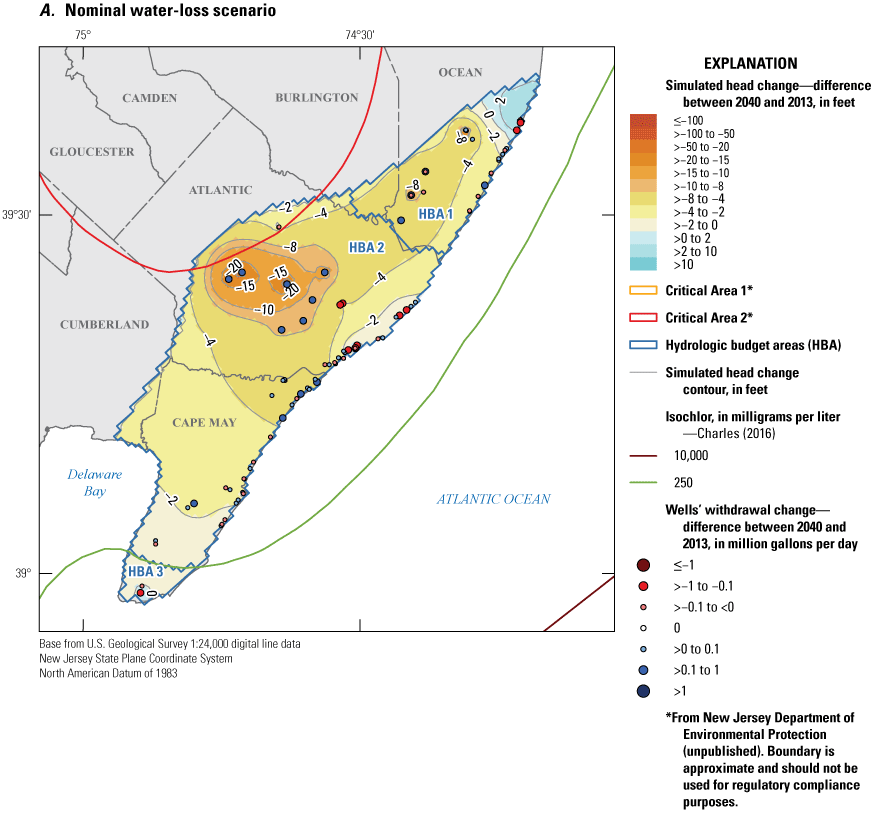
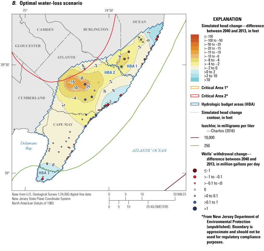
Figure 8A shows the simulated drawdown in the Rio Grande water-bearing zone from the end of 2013 through 2040 based on the nominal water-loss scenario. The drawdowns around the pumping wells are evident in figure 8A because the contour interval is smaller than the interval used in figure 7A. Note that, for the well closest to the coast in HBA 25 on the map, the head change is positive (fig. 8A) because the withdrawals from the well were projected to decrease (fig. 6A) so there is recovery rather than drawdown. The drawdown based on the optimal water-loss scenario is smaller compared to the nominal water-loss scenario (fig. 8B; table 3). For the full allocation scenario, the drawdown is generally much larger than the other two scenarios (fig. 8C; table 3). Most of the aquifer ranges from 15–50 feet of drawdown (change of head from the end of 2013 through 2040 is negative) with even larger amounts around the two largest pumping wells. In addition to effects from the pumping, the drawdown in the Rio Grande water-bearing zone is also being impacted by pumping in the Atlantic City 800-foot sand aquifer below.
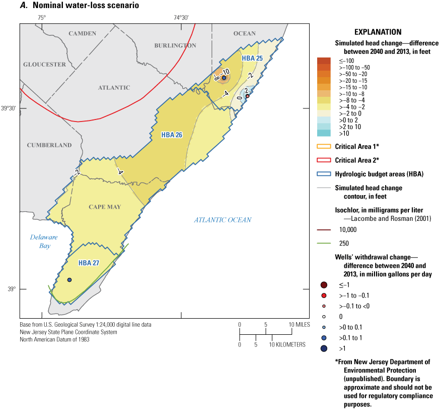
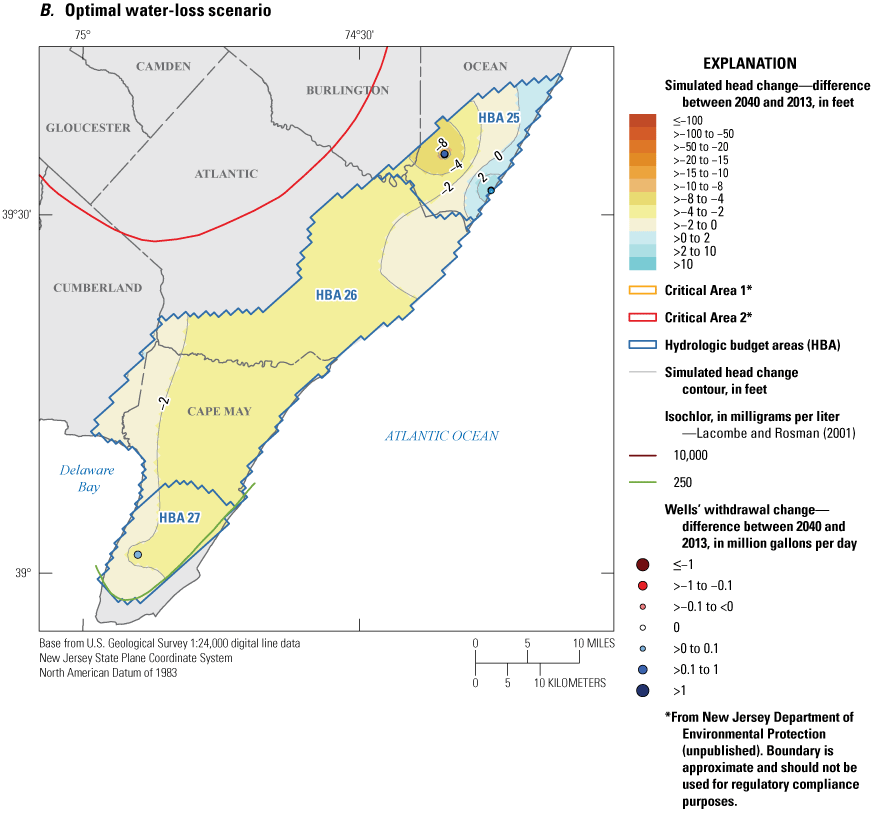
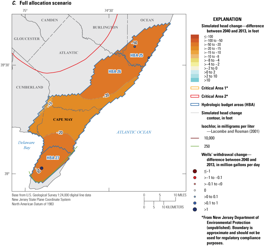
Maps showing the change in simulated water levels from the end of the base simulation (2013) to the end of the scenarios (2040) in the Rio Grande water-bearing zone and simulated potentiometric surface for the three scenarios: A, nominal water-loss, B, optimal water-loss, and C, full allocation.
Table 3.
Statistics for simulated drawdown from the end of 2013 through 2040 for budget areas in the Rio Grande water-bearing zone.Budget Analysis
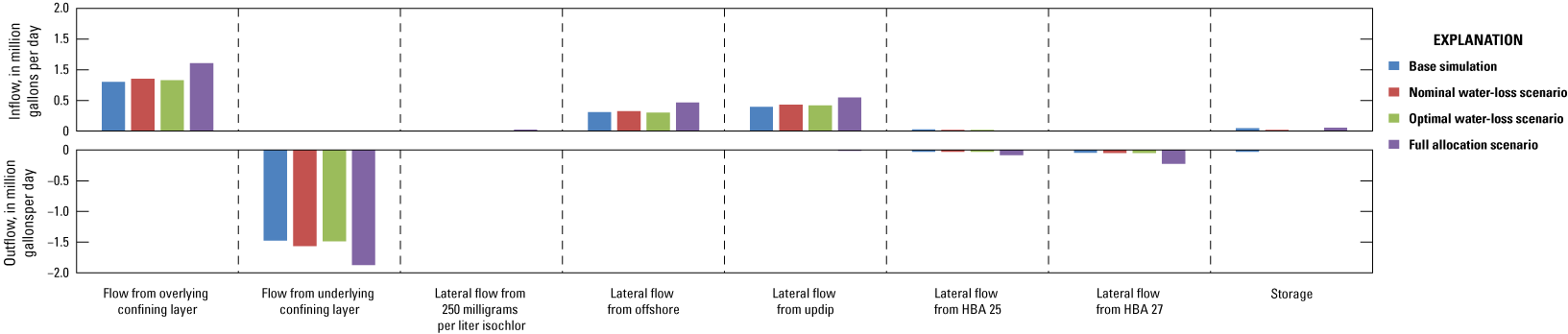
Figure 9 and table 4 show the budget components for HBA 25 and are discussed below. The outflow from HBA 25 is split between withdrawals from wells (58–83 percent) and flow to the Atlantic City 800-foot sand aquifer below (16–28 percent). Lateral flow from offshore is the largest inflow (61–66 percent) to HBA 25. Most of the rest of the inflow is lateral flow from updip (16–26 percent); this is water from the unconfined part of the Kirkwood-Cohansey aquifer system that flows through the confining unit updip from where the Rio Grande water-bearing zone pinches out. There is a small amount of inflow from HBA 26 (7–12 percent) and flow leaking through the confining unit above (4–5 percent). The budget components for HBA 25 are similar among the base simulation and nominal and optimal water-loss scenarios. For the full allocation scenario, the magnitude of outflow to wells is more than twice the amount of the other scenarios; the higher outflow to wells is balanced mostly by increased lateral inflow from offshore and from the adjacent HBA 26. Although there is likely ample freshwater offshore and there is no indication that there would be an issue on the time frame of the scenario, pumping at the level simulated in the full allocation scenario would eventually draw in salty water.
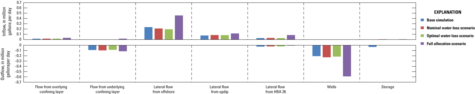
Graph showing simulated flow rates for the Rio Grande water-bearing zone, hydrologic budget area (HBA) 25.
Table 4.
Flow budget of the Rio Grande water-bearing zone, hydrologic budget area (HBA) 25.[Mgal/d, million gallons per day; %, percent of total]
Most outflow from HBA 26 (85–95 percent) goes to the confining unit below (and eventually to the Atlantic City 800-foot sand aquifer) with small amounts of water flowing out into HBA 25 (2–4 percent) and HBA 27 (3–10 percent) (fig. 10; table 5). Roughly half of the inflow (50–53 percent) is from the confining unit above HBA 26. There is close to equal amounts of inflow coming from offshore lateral flow (19–21 percent) and the confining unit updip from where the Rio Grande water-bearing zone pinches out (25–27 percent). The relative amounts of the budget components are similar among the base simulation and three scenarios although in the full allocation scenario, the magnitude of the inflows and outflows are generally higher.
Graph showing simulated flow rates for the Rio Grande water-bearing zone, hydrologic budget area (HBA) 26.
Table 5.
Flow budget of the Rio Grande water-bearing zone, hydrologic budget area (HBA) 26.[mg/L, milligram per liter; Mgal/d, million gallons per day; %, percent of total]
The outflow from HBA 27 is almost entirely (80–99 percent) to the well with only a small amount (1–19 percent) of leakage to the Atlantic City 800-foot sand aquifer below (fig. 11; table 6). Most of the inflow for HBA 27 is divided between lateral flow from the unconfined aquifer updip (38–49 percent) and from the offshore boundary that corresponds to the 250 mg/L isochlor (37–39 percent). A small amount of flow (12–16 percent) comes from HBA 26, which lies to the north of HBA 27. Comparing the scenarios, the relative amounts of the budget components are similar although the magnitude of the flows are higher for the full allocation scenario. In the full allocation scenario, there is some inflow (6 percent) from the underlying Atlantic City 800-foot sand in contrast to the base simulation and other two scenarios where water flows out of HBA 27 from the underlying confining layer.
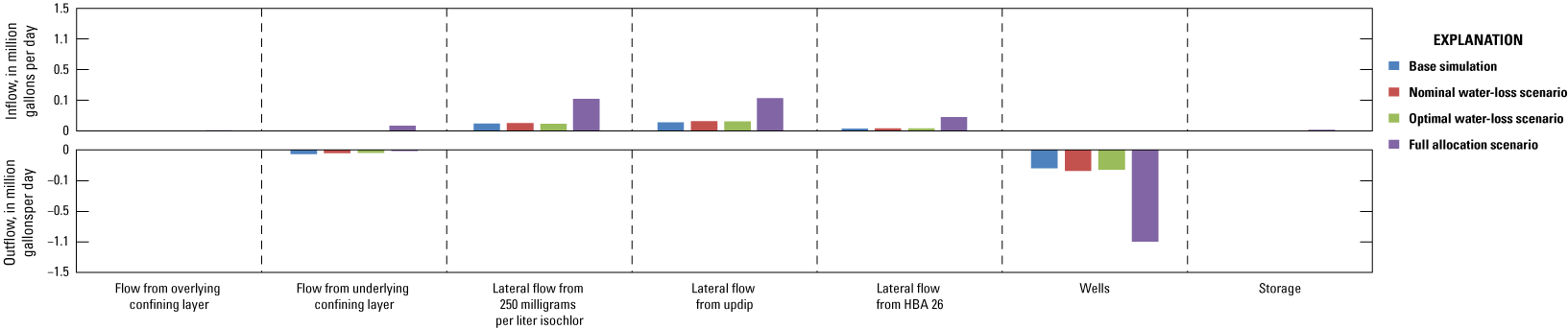
Graph showing simulated flow rates for the Rio Grande water-bearing zone, hydrologic budget area (HBA) 27.
Table 6.
Flow budget of the Rio Grande water-bearing zone, hydrologic budget area (HBA) 27.[mg/L, milligram per liter; Mgal/d, million gallons per day; %, percent of total]
Atlantic City 800-Foot Sand
There are three budget areas defined within the inland part of the Atlantic City 800-foot sand. Most of the withdrawals are in HBA 2 in the center of Atlantic County and along the coast with 58 wells in the area. There are 26 wells in HBA 1, mainly concentrated in the communities along the Atlantic Coast. HBA 3, located at the southern tip of Cape May County, is also much smaller in area compared to the other HBAs in the Atlantic City 800-foot sand. Only a small amount of pumping from two wells supplying a desalination plant occurs in HBA 3; the entire HBA lies outside of the 250 mg/L isochlor so the water quality is somewhat degraded in that area.
Trends of Withdrawals and Heads
Figure 12 shows withdrawal trends and trends of median, 10th percentile, and minimum heads from the base simulation and withdrawal scenarios for each budget area. Table 2 shows a summary of the past and projected withdrawals in each budget area. The well locations are shown in figure 13.
Line graphs showing withdrawals and median, 10th percentile, and minimum heads for model cells over time in hydrologic budget areas (HBA) in the Atlantic City 800-foot sand: A, withdrawals in HBA 1, B, head statistics in HBA 1, C, withdrawals in HBA 2, D, head statistics in HBA 2, E, withdrawals in HBA 3, and F, head statistics in HBA 3.
Maps showing hydrologic budget areas in the Atlantic City 800-foot sand aquifer and simulated potentiometric surface in 2040 for the three scenarios: A, nominal water-loss, B, optimal water-loss, and C, full allocation.
Most of the withdrawals in the Atlantic City 800-foot sand are in HBA 2 (table 2). Some pumping occurs in HBA 1 in the north, mainly concentrated in the communities along the Atlantic Coast.
Pumping in the base simulation increases from 1980 onwards, although pumping begins to decline in 2010 (fig. 12A). The nominal water-loss scenario indicates that pumping would increase 9-percent for HBA 1, be near steady for HBA 2, and decrease 34-percent in HBA 3 (where water quality is potentially an issue). The optimal water-loss scenario indicates that projected withdrawals would be lower in comparison, with a 3-percent increase in HBA 1, a 5-percent decrease in HBA 2, and a 38-percent decrease in HBA 3 (table 2). The full allocation scenario indicates withdrawals across all three HBAs would increase: 80 percent in HBA 1, 48 percent in HBA 2, and 70 percent in HBA 3 (table 2). When comparing the projected pumping for the first two scenarios to the reported pumping from 2014–2020, the actual numbers reflect the general trend of the scenarios in HBA 1 and HBA 3; however, the actual pumping is considerably less than the projected withdrawals in HBA 2 (fig. 12).
In the base simulation, head is shown to generally decline in all three budget areas in the Atlantic City 800-foot sand aquifer (fig. 12). In HBA 1, heads appear to have nearly leveled off in response to declining withdrawals at the end of the base simulation beginning around 2005 (figs. 12A, 12B). The simulations project the decline in head continues in HBA 1 for all three scenarios (fig. 12B). The nominal and optimal water-loss scenarios indicate that the decline is close to linear over time (fig. 12B). The full allocation scenario indicates that the simulated heads drop quickly in response to the step change in pumping and then continue declining approaching a steady state by 2040 (fig. 12B).
In the base simulation, the head in HBA 2 is generally in decline (fig. 12D). The nominal and optimal water-loss scenarios indicate that the decline in head in 2040 is slight over most of HBA 2: a median of 3.9 feet and 1.7 feet, respectively (fig. 12D). However, the drawdown (minimum head in fig. 12D) in HBA 2 continues linearly to reach a maximum of 31.1 feet in the nominal water-loss scenario and 24.3 feet in the optimal water-loss scenario (table 7). The optimal water-loss scenario indicates that the number of cells in HBA 2 with drawdown of at least a foot in 2040 drops to 68 percent compared to 99 percent of the cells in the nominal water-loss scenario (table 7). The full allocation scenario indicates that the heads drop quickly in response to the step change in pumping and then continue declining, approaching steady state by 2040 (fig. 12D). The median drawdown across HBA 2 is 23.4 feet with the maximum reaching 69.3 feet by 2040 for the full allocation scenario (table 7).
Table 7.
Statistics for simulated drawdown from the end of 2013 through 2040 for budget areas in the Atlantic City 800-foot sand aquifer.In HBA 3, heads are generally declining in the base simulation, especially after withdrawals start in the area in 1998. Once they start, the withdrawals are fairly consistent, and the head declines at a fairly consistent rate (figs. 12E, 12F). There is minimal difference in the statistics across HBA 3 (table 7), likely because there are only two active wells during the base simulation. The nominal and optimal water-loss scenarios (wherein withdrawals are projected to decline [fig. 12E]) indicate that heads continue to decline slightly before recovery begins (fig. 12F). By the end of the simulations in 2040, the simulated heads are at a similar level to simulated heads in 2013 for both of those scenarios (table 7). The full allocation scenario indicates that simulated heads drop quickly in response to the step change in pumping and then continue declining at a lessening rate until 2040. The median drawdown across HBA 3 is 18.0 feet and the maximum is 19.7 feet by 2040 for the full allocation scenario (table 7).
Simulated Heads and Drawdown in 2040
Figure 13A shows the simulated head distribution in 2040 for the Atlantic City 800-foot sand aquifer based on the nominal water-loss scenario. In the map, an area with low heads surrounds the largest pumping well in Atlantic County. An area of low heads can also be seen along the coast where many of the wells are located. Moving inland to the unconfined Kirkwood-Cohansey aquifer, heads increase. A similar pattern is seen in figures 13B and 13C, which show the optimal water-loss scenario and the full allocation scenario, respectively; however the overall head is slightly higher in the optimal water-loss scenario and lower in the full allocation scenario.
Figure 14A shows the simulated drawdown in Atlantic City 800-foot sand aquifer from the end of 2013 through 2040 based on the nominal water-loss scenario. The largest area of drawdown appears in central Atlantic County around the high-capacity wells. The map shows minimal drawdown in HBA 3 and a small part of HBA 2 in the lower part of Cape May County. In the northeastern tip of HBA 1, water levels are shown recovering in response to declining projected withdrawals. The relative pattern of drawdown for the optimal water-loss scenario, which appears in figure 14B, is similar to the nominal water-loss scenario but with smaller values (table 7). Additional areas of head recovery can be seen in figure 14B in HBA 3 and an area in HBA 2 about halfway up the coast.
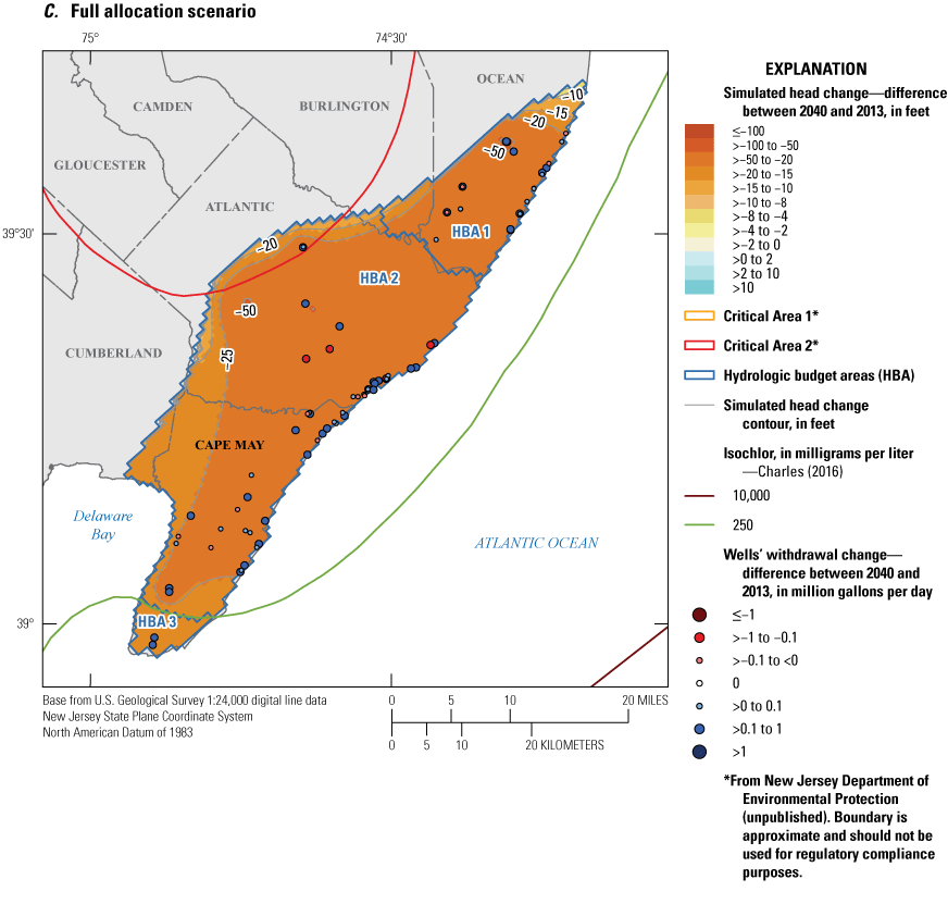
Maps showing change in simulated water levels from the end of the base simulation (2013) to the end of the scenarios (2040) in the Atlantic City 800-foot sand aquifer and simulated potentiometric surface for the three scenarios: A, nominal water-loss, B, optimal water-loss, and C, full allocation.
For the full allocation scenario, the drawdown is generally much larger than the other two scenarios (fig. 14C; table 7). Drawdown in most of the aquifer ranges from 20–50 feet (head change of −20 to −50 feet). All the cells in the HBA defined in the Atlantic City 800-foot sand are simulated to have at least 1 foot of drawdown in the full allocation scenario (table 7).
Budget Analysis
Figure 15 and table 8 show the budget components for HBA 1 and are discussed below. The outflow from the budget area is primarily (greater than 80 percent) withdrawals from wells. There is a small amount (7–11 percent) of outflow south into HBA 2 where the high-capacity wells are located. About half of the inflow to HBA 1 is lateral flow from offshore; and then most of the rest is from the unconfined part of the Kirkwood-Cohansey aquifer system updip. There is some inflow coming up through the confining layer from the Piney Point aquifer below (11–13 percent). Smaller amounts are leaking through the confining unit above from the Rio Grande water-bearing zone (11–13 percent) or flowing in laterally from HBA 2 (2–4 percent). The budget components are similar among the four runs with the exception being the full allocation scenario where the well withdrawal is higher and balances the inflow that comes mostly from lateral flow offshore and updip.
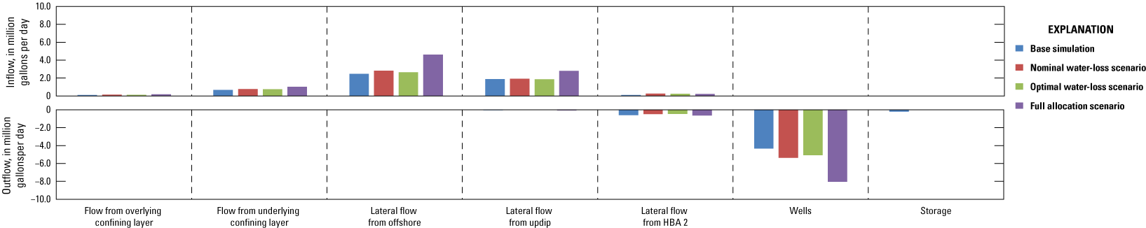
Graph showing simulated flow rates for the Atlantic City 800-foot sand, hydrologic budget area (HBA) 1.
Table 8.
Flow budget of the Atlantic City 800-foot sand, hydrologic budget area (HBA) 1.[Mgal/d, million gallons per day; %, percent of total]
Figure 16 and table 9 show the budget components for HBA 2 and are discussed below. The outflow from the budget area is almost entirely from withdrawals from wells (95–98 percent). Minor amounts of input come from storage (3 percent in the base simulation) and lateral flow from offshore and HBA 1. The largest inflow (58–61 percent) comes from lateral flow from offshore. The next largest inflow (19–21 percent) is lateral flow from the unconfined part of the Kirkwood-Cohansey aquifer system updip. There is also inflow (10–12 percent) that leaks downward through the confining unit from the Rio Grande water-bearing zone above. Some minor amounts (less than 5 percent) of inflow enters the budget area from the Piney Point aquifer below and from the adjacent budget areas. The budget components are similar among the four runs with the exception being the full allocation scenario where the inflows and outflows are generally higher.
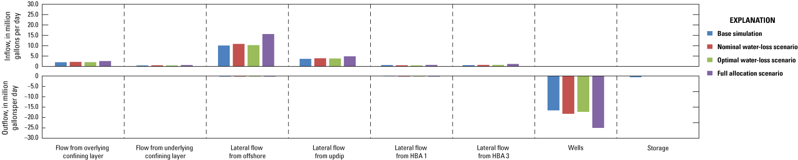
Graph showing simulated flow rates for the Atlantic City 800-foot sand, hydrologic budget area (HBA) 2.
Table 9.
Flow budget of the Atlantic City 800-foot sand, hydrologic budget area (HBA) 2.[Mgal/d, million gallons per day; %, percent of total]
Figure 17 and table 10 show the budget components for HBA 3 and are discussed below. The outflow from the budget area is split between flow to wells (51–65 percent) and lateral flow northward into HBA 2 (35–49 percent). Most of the inflow (97–98 percent) to the budget area is lateral flow from the 250 mg/L chloride isochlor indicating that water quality could worsen in this area (note this entire HBA is already beyond the 250 mg/L isochlor).
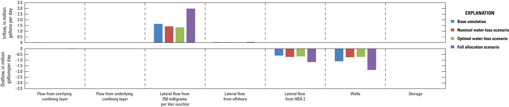
Graph showing simulated flow rates for the Atlantic City 800-foot sand, hydrologic budget area (HBA) 3.
Table 10.
Flow budget of the Atlantic City 800-foot sand, hydrologic budget area (HBA) 3.[mg/L, milligram per liter; Mgal/d, million gallons per day; %, percent of total]
Piney Point Aquifer
This study defined two budget areas in the Piney Point aquifer. The Piney Point aquifer is confined throughout its extent, so both of the HBA defined within the aquifer are confined. There are similar numbers of wells in the HBA, 18 in HBA 4 and 16 in HBA 5. However, most of the withdrawals are in HBA 4 in the northeastern part of the Piney Point aquifer in Ocean County near the coast of the Atlantic Ocean. The pumping wells in HBA 5 are spread throughout the more updip parts of the aquifer.
Trends of Withdrawals and Heads
Figure 18 shows withdrawal trends and trends of median, 10th percentile, and minimum heads from the base simulation and withdrawal scenarios for each budget area in the Piney Point aquifer. Table 2 shows a summary of the past and projected withdrawals in each budget area in the Piney Point aquifer.
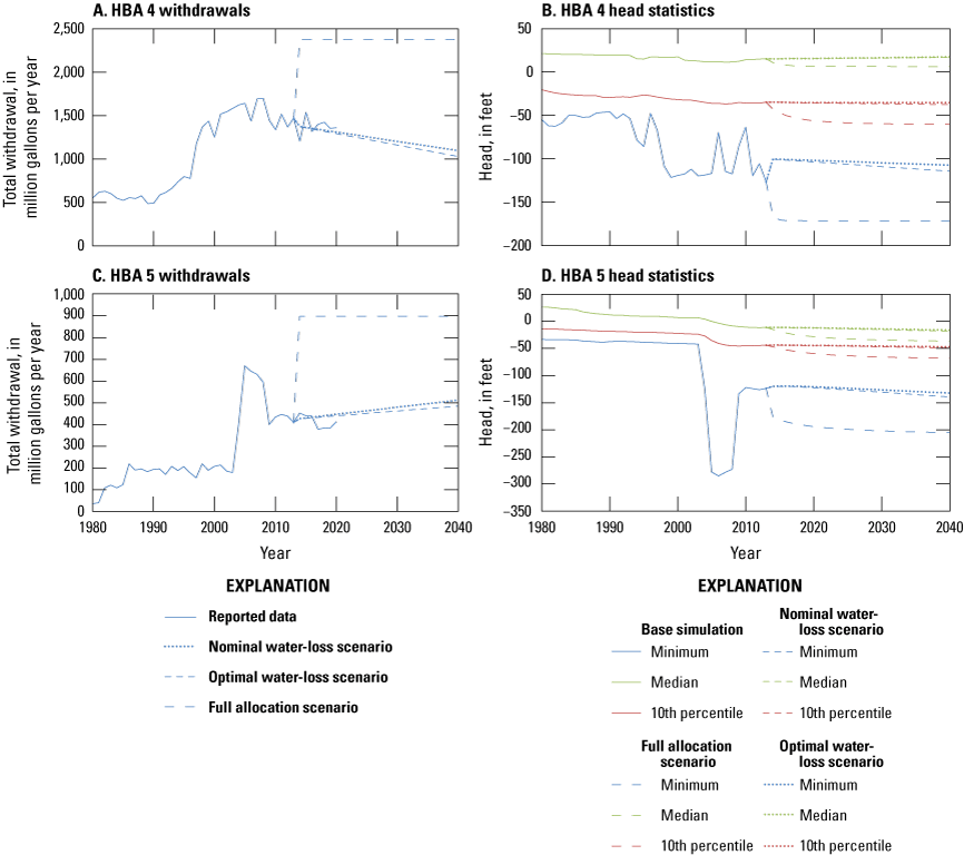
Line graphs showing withdrawals and median, 10th percentile, and minimum heads for model cells over time in hydrologic budget areas (HBA) in the Piney Point aquifer: A, withdrawals in HBA 4, B, head statistics in HBA 4, C, withdrawals in HBA 5, and D, head statistics in HBA 5.
Over the period of the base simulation, there has been a general increase in pumping over time in the Piney Point aquifer, although there has been a decline in pumping since around 2005. In HBA 4, the nominal and optimal water-loss scenarios both indicate withdrawals would decline (fig. 18A) 20 percent and 25 percent, respectively, by 2040 (table 2). In HBA 5, the nominal and optimal water-loss scenarios both indicate withdrawals increase (fig. 18C) 20 percent and 14 percent, respectively (table 2). For both HBA 4 and HBA 5, the full allocation scenario indicates withdrawals increase 62 and 119 percent (table 2), respectively.
In the base simulation, both budget areas in the Piney Point aquifer saw a slight decline in heads (figs. 18B, 18D). The head in areas near wells has fluctuated by 50 to more than 100 feet reacting to changes in pumping as reflected in the maximum head change (figs. 18B, 18D).
In HBA 4, the base simulation shows the median and 10th percentile heads slowly declining over time with a slight recovery after 2009 in response to declining pumping (figs. 18A, 18B). The nominal and optimal water-loss scenarios, although the total withdrawals for HBA 4 are projected to decline, indicate the head response is generally flat although the head continues to decrease at the model cell where simulated head is minimum in HBA 4 (fig. 18B). The scenarios show a median cell in HBA 4 recovers by 0.1 feet for both the nominal and optimal water-loss scenarios, with the maximum drawdown being 5.0 and 2.6 feet, respectively (table 11). The full allocation scenario indicates that heads quickly decline but then level out within 10 years (fig. 18B). The median drawdown in 2040 is 7.6 feet and the maximum is 122.1 feet for the full allocation scenario (table 11).
Table 11.
Statistics for simulated drawdown from end of 2013 through 2040 for budget areas in the Piney Point aquifer.In HBA 5, the withdrawals are projected to increase in all three scenarios. For the nominal and optimal water-loss scenarios, the simulated heads only decline slightly in response to the additional pumping (fig. 18D). For the nominal water-loss scenario in 2040, the median drawdown for all cells in HBA 5 is 4.9 feet and the maximum drawdown is 19.7 feet (table 11). For the optimal water-loss scenario in 2040, the median drawdown for all cells in HBA 5 is 3.4 feet and the maximum drawdown is 15.3 feet (table 11). The heads do not level out as quickly under the full allocation scenario as in HBA 4 but are close to steady at the end of the simulation. The median drawdown for cells in HBA 5 in the full allocation scenario is 19.8 and the maximum is 120.3 feet (table 11). The maximum drawdown is less, however, than the maximum simulated from 2007–2009 in the base simulation.
Simulated Heads and Drawdown in 2040
The general features of the head distribution in the Piney Point aquifer are similar for the three scenarios (fig. 19). The highest heads are on the updip boundary. The lowest heads are around the pumping centers in the northeast and southwest, and in an area on the southern part of the boundary between HBA 4 and HBA 5. This area, which has no pumping wells and low head, is where the confining layer between the Piney Point aquifer and the Atlantic City 800-foot sand above is relatively thin (fig. 1) and there is heavy pumping in the Atlantic City 800-foot sand (fig. 14).
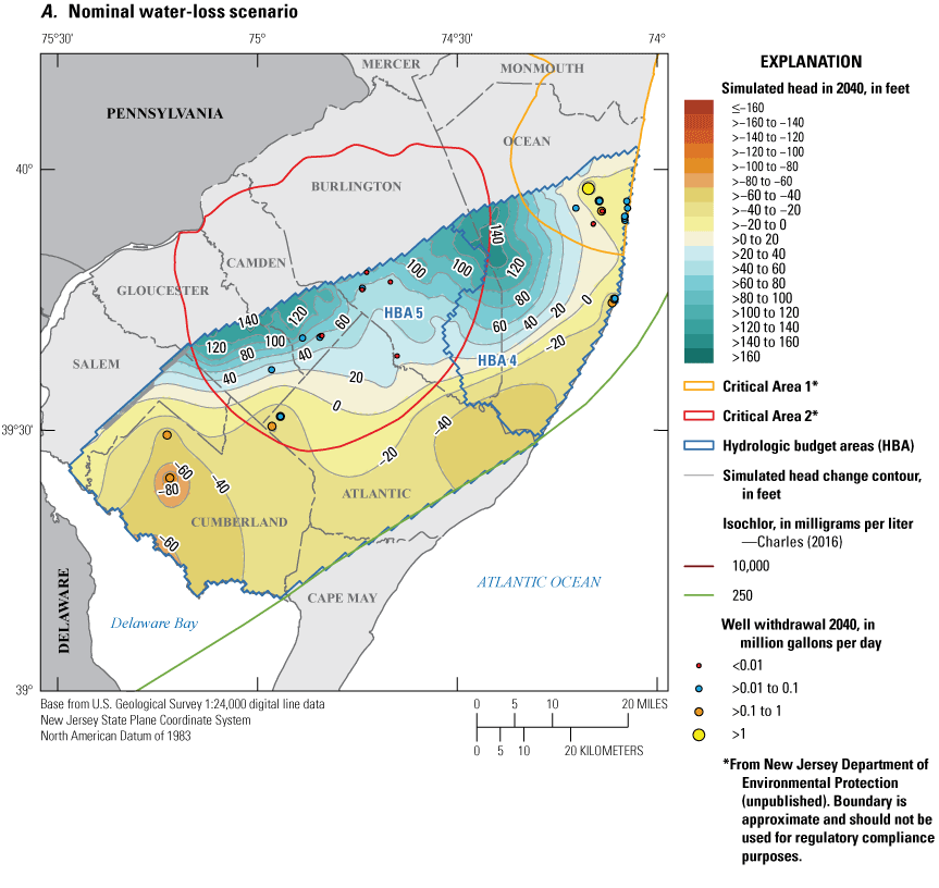
Maps showing hydrologic budget areas in the Piney Point aquifer and simulated potentiometric surface in 2040 for the three scenarios: A, nominal water-loss, B, optimal water-loss, and C, full allocation.
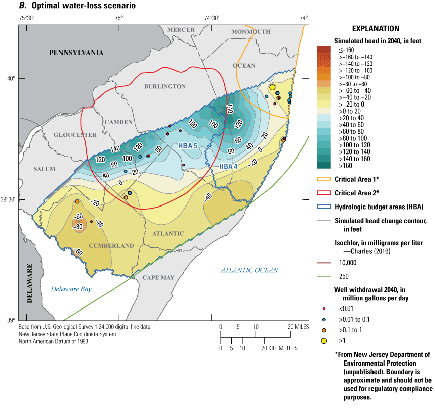
The heads are in recovery over the northern part of the aquifer, especially in the far northeast along the coast, in response to declining withdrawals in the area (fig. 20A). In the southern part of the aquifer, the largest areas of drawdown are around the pumping wells. The relative pattern of drawdown for the optimal water-loss scenario, which appears in figure 20B, is similar to the nominal water-loss scenario although the magnitude is slightly less (table 11). For the full allocation scenario, there are large areas with greater than 20 feet of head decline with cones of more than 50 feet of head decline in the vicinity of some wells, including the northeast where the other two scenarios simulate head recovery (fig. 20C). The area around the southern part of the boundary between HBA 4 and 5 also shows substantial head decline in response to increased pumping in the Atlantic City 800-foot sand (fig. 14). Even in the full allocation scenario, there remains some areas of slight head recovery. These areas have a strong connection to the unconfined aquifer, so the recovery likely reflects the small difference between the recharge in the last stress period of the base simulation and that used in the scenarios.
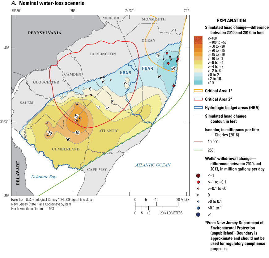
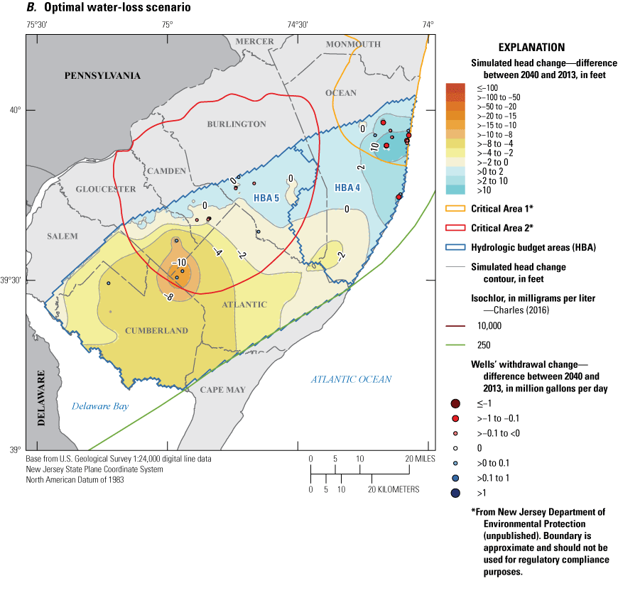
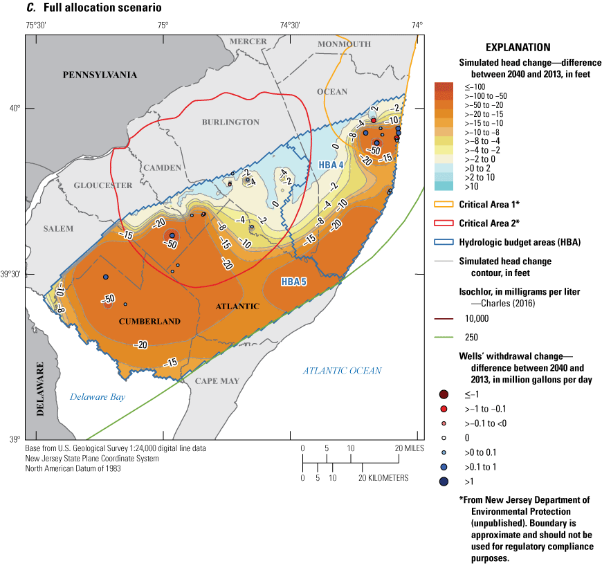
Maps showing the change in simulated water levels from the end of the base simulation (2013) to the end of the scenarios (2040) in the Piney Point aquifer and simulated potentiometric surface for the three scenarios: A, nominal water-loss, B, optimal water-loss, and C, full allocation.
Budget Analysis
As shown in figure 21 and table 12, the outflow from HBA 4 is mostly to the pumping wells (45–66 percent) and through the overlying confining layer (28–46 percent). The inflow is mostly (85–87 percent) from the overlying confining layer with a small component of lateral flow from offshore (5–10 percent), updip (3–5 percent), and HBA 5 (1–2 percent). Compared to the base simulation, there is less pumping and consequently less inflow from the overlying confining layer for the nominal and optimal water-loss scenarios and more pumping and inflow from the overlying confining layer for the full allocation scenario.
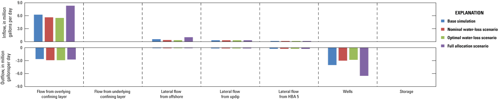
Graph showing simulated flow rates for the Piney Point aquifer, hydrologic budget area (HBA) 4.
Table 12.
Flow budget of the Piney Point aquifer, hydrologic budget area (HBA) 4.[Mgal/d, million gallons per day; %, percent of total]
Figure 22 and table 13 show the budget components for HBA 5 and are discussed below. The largest component (49–61 percent) of outflow in HBA 5 is flow to the overlying confining layer. The other main components of outflow are withdrawals from wells (20–36 percent) and flow to the underlying confining layer (11 percent). The inflow is mostly from the overlying confining layer (85–86 percent) with a small component of lateral flow from offshore (including some from the 250 mg/L isochlor), updip, and from HBA 4. The additional pumping from wells in the full allocation scenario is almost entirely offset by additional inflow from the overlying aquifer.
Graph showing simulated flow rates for the Piney Point aquifer, hydrologic budget area (HBA) 5.
Table 13.
Flow budget of the Piney Point aquifer, hydrologic budget area (HBA) 5.[mg/L, milligram per liter; Mgal/d, million gallons per day; %, percent of total]
Vincentown Aquifer
The study defined five budget areas within the Vincentown Aquifer. Two of these (HBA 6 and HBA 7) are in the confined part of the aquifer and the other three (HBA 30, HBA 31, and HBA 32) are in the unconfined part of the aquifer. Compared to the other aquifers in the NJCP, other than the Rio Grande water-bearing zone, the Vincentown aquifer has the least amount of withdrawals. A total of 41 wells had reported pumping in the area of the Vincentown aquifer where the HBA were defined. Twenty-five of these wells and most of the volume of water withdrawn were in HBA 6. Four wells were in HBA 7 with the remaining 12 in the unconfined HBA 30. HBA 31 and HBA 32 did not have any wells included in the simulations.
Trends of Withdrawals and Heads
The trend in withdrawals in HBA 6 is fairly constant over the base simulation despite some variability from year to year (fig. 23A). The nominal and optimal water-loss scenarios both project a modest increase in withdrawals into the future. The increase is within the variability reported (and used in the base simulation) between 1980 and 2013; it does not represent a large change compared to historical withdrawals. Reported pumping from 2014-2020 is mostly lower than the projected pumping, however, it is within the historical variability simulated in the base simulation.
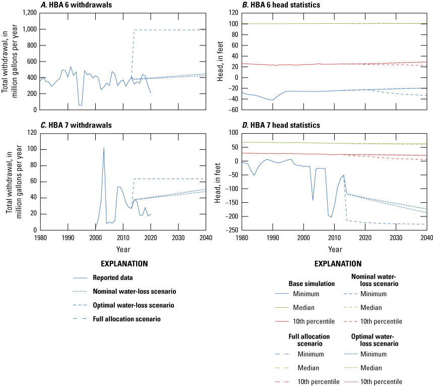
Line graphs showing withdrawals and median, 10th percentile, and minimum heads for model cells over time in hydrologic budget areas (HBA) in the Vincentown aquifer: A, withdrawals in HBA 6, B, head statistics in HBA 6, C, withdrawals in HBA 7, and D, head statistics in HBA 7.
In HBA 7, reported withdrawals in the base simulation begin in 1999 (fig. 23C). The withdrawals are small overall and show a lot of variability. Both the nominal and optimal water-loss scenarios project an increase in pumping. The full allocation scenario represents a near doubling of the current pumping; however even that is a relatively small amount.
Most of the pumping in the three unconfined budget areas is from HBA 30. In the nominal and optimal water-loss scenarios, there is no change in the pumping amounts for all the unconfined wells. The level of pumping in the full allocation scenario is higher than the other two scenarios, however it falls within the variability of historical pumping.
In the base simulation, the heads have been fairly constant over time (fig. 23B). This is due the narrow extent of the aquifer and proximity to the outcrop area. The simulated hydraulic conductivity is lower than some of the other aquifers, so what pumping exists can locally have bigger effects on the heads compared to aquifers with higher hydraulic conductivity.
In HBA 6, the median head is almost constant through the base simulation and all three scenarios (fig. 23B). The 10th percentile head is nearly constant as well, although heads increase (or recover) in the nominal and optimal water-loss scenarios despite the increase in total withdrawals projected through 2040 (fig. 23A). After a decline and quick recovery from 1980 to 1994, minimum head in HBA 6 continues a more gradual recovery in the nominal and optimal water-loss scenarios even though overall withdrawals increase (Figure 23B); this recovery reflects reduced pumping from wells in the areas with the most drawdown. Considering all the model cells, the maximum drawdown is simulated to be 12.0 feet for the nominal water-loss scenario and 8.4 feet for the optimal water-loss scenario (table 14). The full allocation scenario indicates the 10th percentile and minimum heads in HBA 6 are lower in comparison to the other scenarios (fig. 23B) with the maximum drawdown reaching 39.6 feet (table 14).
Table 14.
Statistics for simulated drawdown from the end of 2013 through 2040 for budget areas in the Vincentown aquifer.In HBA 7, the effects of pumping are limited to areas in close proximity to the wells (Fig. 24). Although the areal extent is not large, the drawdown in response to pumping can be large in areas near the wells. This pattern can be seen in the plots of head over time in figure 23D. The lines are nearly flat for both the median and 10th percentile heads in the base simulation and the scenarios, whereas the minimum fluctuates by more than 100 feet and has a downward trend. The maximum drawdown values are also large for all three scenarios—135.4 feet for the nominal water-loss scenario, 121.8 feet for the optimal water-loss scenario, and 176.9 feet for the full allocation scenario (table 14).
Simulated Heads and Drawdown in 2040
The general pattern of the simulated heads in the Vincentown aquifer is similar in all three scenarios: higher heads in the unconfined areas where the recharge occurs and lower heads in the vicinity of the pumping wells (fig. 24). There are two areas where prominent cones of depression show up around the pumping wells: one in the southwest and the other in the northeast. The one in the southwest is much more defined, as the simulated hydraulic conductivity is less there. There is a low area of head along the border of Camden and Burlington Counties in response to pumping in the underlying Wenonah-Mount Laurel aquifer. In the full allocation scenario, there are a few more wells with tight cones of depression around them.
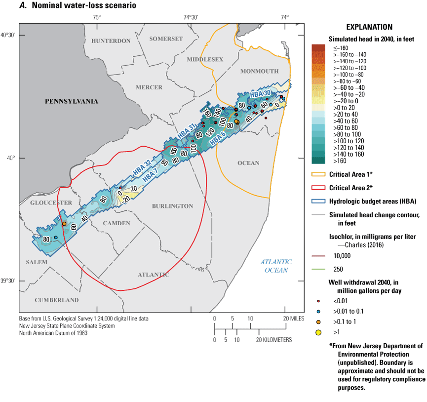


Maps showing hydrologic budget areas in the Vincentown aquifer and simulated potentiometric surface in 2040 for the three scenarios: A, nominal water-loss, B, optimal water-loss, and C, full allocation.
There is a large area with minimal change in head corresponding to the unconfined parts of the aquifer and in areas away from the high-capacity wells (fig. 25); this largely reflects the change from the base simulation’s recharge value in the final stress period to the average value used in the scenarios. The larger area of recovery along the downdip edge in the northeast is due to reduced pumping in a well that is located beyond the downdip limit of the aquifer. Some areas around the wells have a large amount of head decline, indicating that the cones are not just artifacts of the historical pumping but that the magnitudes of the cones of depression will increase under these scenarios. This pattern appears in all the scenarios, but the magnitude is greatest in the full allocation scenario with the maximum drawdown reaching 176.9 feet (table 14). Cones of depression can be seen in areas without pumping in the Vincentown aquifer where the confining unit is relatively thin and there are high-capacity wells in the underlying Wenonah-Mount Laurel aquifer.
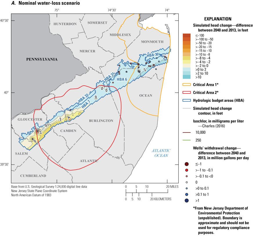

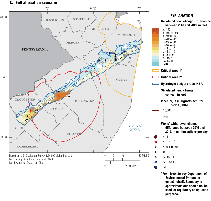
Maps showing change in simulated water levels from the end of the base simulation (2013) to the end of the scenarios (2040) in the Vincentown aquifer and simulated potentiometric surface for the three scenarios: A, nominal water-loss, B, optimal water-loss, and C, full allocation.
Budget Analysis
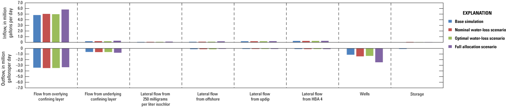
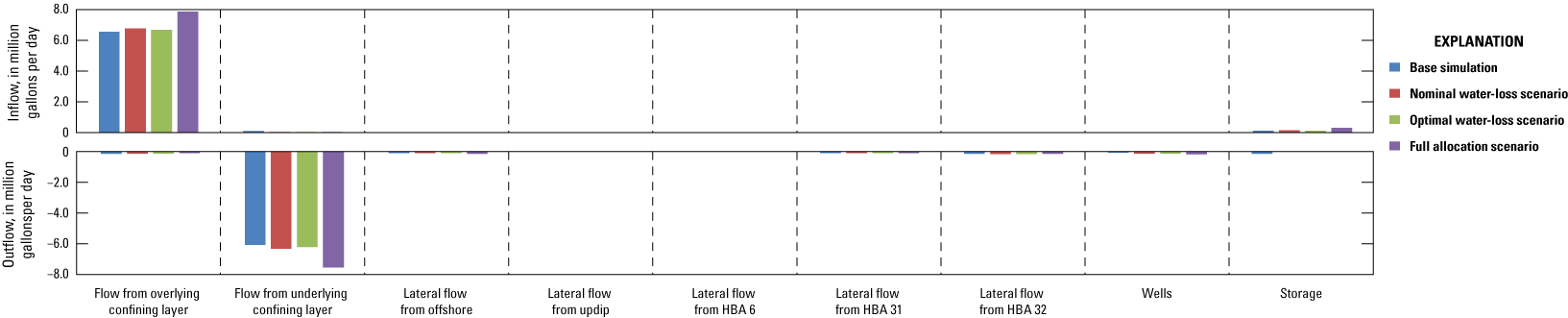
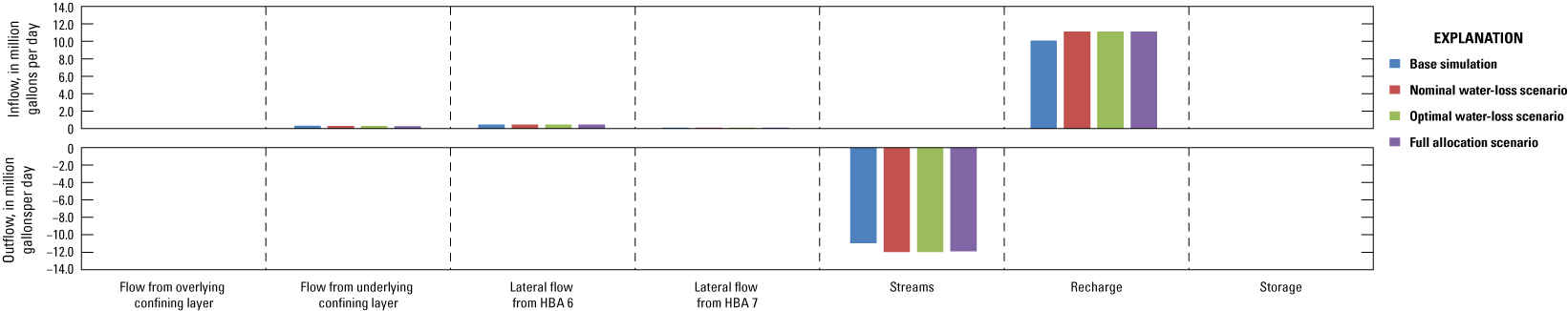
The largest component of the outflow (55–58 percent) from HBA 6 is flow out to the underlying confining layer above the Wenonah-Mount Laurel aquifer (fig. 26; table 15). Other components of outflow include lateral flow out to the unconfined HBA 30 (17–20 percent) and flow to wells (10–21 percent). The main component of inflow (99–100 percent) to HBA 6 is water leaking in from the unconfined Kirkwood-Cohansey aquifer system above through the confining layer.
Graph showing simulated flow rates for the Vincentown aquifer, hydrologic budget area (HBA) 6.
Table 15.
Flow budget of the Vincentown aquifer, hydrologic budget area (HBA) 6.[Mgal/d, million gallons per day; %, percent of total]
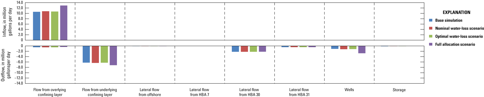
Almost all the inflow (96–98 percent) in HBA 7 of the Vincentown aquifer is from the overlying confining layer and the Kirkwood-Cohansey aquifer system above (fig. 27; table 16). Much of that flow passes down through the Vincentown aquifer and out through the underlying confining unit (89–92 percent). In contrast to many of the other HBAs, only a small amount (1–2 percent) of the total outflow is to wells.
Graph showing simulated flow rates for the Vincentown aquifer, hydrologic budget area (HBA) 7.
Table 16.
Flow budget of the Vincentown aquifer, hydrologic budget area (HBA) 7.[Mgal/d, million gallons per day; %, percent of total]
The main budget components in the unconfined areas of the Vincentown aquifer are inflow from recharge (92–97 report) and outflow to streams (fig. 28, table 17; fig. 29, table 18; fig. 30, table 19). There are some minor amounts (5 percent or less) of flow between adjacent HBAs to and from the underlying Wenonah-Mount Laurel aquifer.
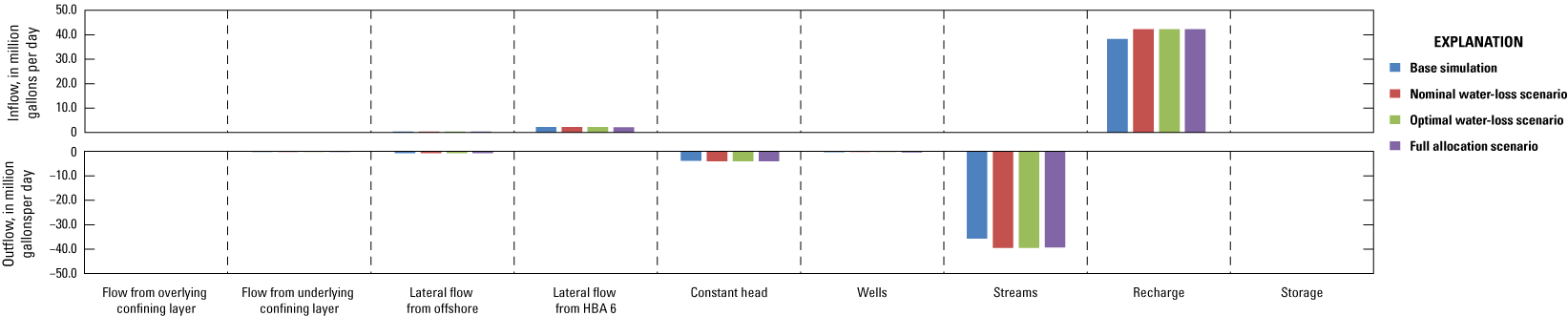
Graph showing simulated flow rates for the Vincentown aquifer, hydrologic budget area (HBA) 30.
Table 17.
Flow budget of the Vincentown aquifer, hydrologic budget area (HBA) 30.[Mgal/d, million gallons per day; %, percent of total]
Graph showing simulated flow rates for the Vincentown aquifer, hydrologic budget area (HBA) 31.
Table 18.
Flow budget of the Vincentown aquifer, hydrologic budget area (HBA) 31.[Mgal/d, million gallons per day; %, percent of total]
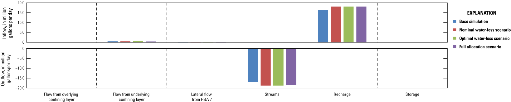
Graph showing simulated flow rates for the Vincentown aquifer, hydrologic budget area (HBA) 32.
Table 19.
Flow budget of the Vincentown aquifer, hydrologic budget area (HBA) 32.[Mgal/d, million gallons per day; %, percent of total]
Wenonah-Mount Laurel Aquifer
The study used 10 budget areas in the Wenonah Mount-Laurel aquifer. Five of these are confined (HBA 8–12) and the other five are unconfined (HBA 33–37). HBA 8 is partly in Critical Area 1 where pumping was required to be reduced in the mid-1980s—including in the Wenonah-Mount Laurel aquifer. There are 48 wells in HBA 8. HBA 9 is partly within, and HBA 10 and HBA 11 are entirely in Critical Area 2. There were 40, 39, and 44 wells, respectively, for these HBAs. The Wenonah-Mount Laurel aquifer was not included in the Critical Area 2 restrictions. Pumping was restricted in the deeper upper, middle, and lower PRM aquifers in this area. The restriction of pumping in the deeper aquifers has likely led to increased withdrawals in the Wenonah-Mount Laurel over time. HBA 12 was defined to be to southwest of Critical Area 2 and included 26 wells. There were seven wells in the unconfined HBA, two in HBA 35 and five in HBA 37. The other three unconfined HBAs did not have any wells included in the simulations.
Trends of Withdrawals and Heads
Pumping in HBA 8 in the period of the base simulation fluctuated by over 400 gallons per day until the mid-1990s when restrictions from the Critical Area 1 designation took effect (fig. 31A). From that point forward, there is a slight increase through the end of the base simulation. This increase is projected to continue at a reduced rate in the nominal (9 percent) and optimal (4 percent) water-loss scenarios. The full allocation scenario represents a 132-percent increase in withdrawals from 2013 (table 2).
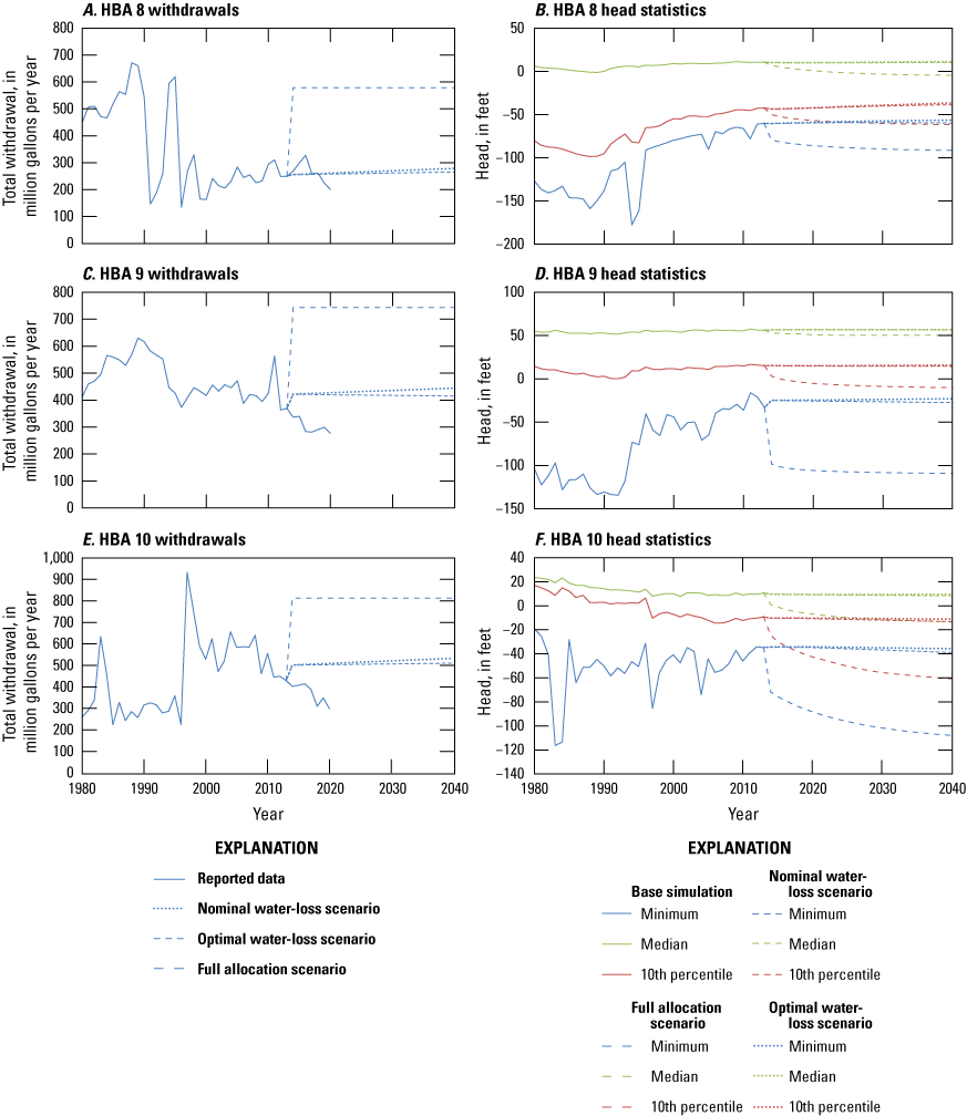
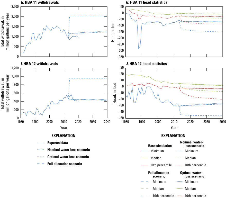
Line graphs showing withdrawals and median, 10th percentile, and minimum heads for model cells over time in hydrologic budget areas (HBA) in the Wenonah-Mount Laurel aquifer: A, withdrawals in HBA 8, B, head statistics in HBA 8, C, withdrawals in HBA 9, D, head statistics in HBA 9, E, withdrawals in HBA 10, F, head statistics in HBA 10, G, withdrawals in HBA 11, H, head statistics in HBA 11, I, withdrawals in HBA 12, and J, head statistics in HBA 12.
Pumping in HBA 9 declines from 1990 through the end of the base simulation (fig. 31C). In contrast, the nominal water-loss scenario projects an increase of 5.2 percent, and the optimal water-loss scenario projects a decrease of 1.4 percent (fig. 31D). The actual reported withdrawals from 2014 through 2020 have continued the general trend that was seen in the base simulation, declining by 28.6 percent over that time period, suggesting that the nominal and optimal water-loss scenarios may be overestimates. The full allocation scenario indicates a 101.5 percent increase from the 2013 pumping amount in HBA 9 (table 2).
Pumping in HBA 10 is fairly level from the mid-1980s through the mid-1990s, after which pumping increased by 300 percent (fig. 31E). A fairly steady decrease follows and continues through the end of the base simulation to 2020. Rather than reflecting this decline, both the nominal and optimal water-loss scenarios project a slight increase in pumping (6.1 and 1.8 percent, respectively). The full allocation scenario indicates an increase of 89.4 percent (table 2).
Withdrawals in HBA 11 increase until approximately 1998, at which time they level out and then start to decrease around 2005 (fig. 31G). The withdrawals are fairly steady from 2014 to 2020. Both the nominal and optimal water-loss scenarios indicate increasing withdrawals in HBA 11 (11.5 percent and 6.3 percent, respectively; table 2). The full allocation scenario indicates that withdrawals increase 121.9-percent compared to the last stress period of the base simulation in HBA 11 (table 2).
Withdrawals in HBA 12 increase fairly steadily through the period of the base simulation (fig. 31I). Both the nominal (−1.4 percent) and optimal (−6.1 percent) water-loss scenarios indicate withdrawals would see a small decline (table 2). The full allocation scenario indicates withdrawals would increase 107.9 percent over the last stress period of the base simulation in HBA 12 (table 2).
There is minimal pumping in the unconfined parts of the Wenonah Mount Laurel aquifer (table 2). This includes HBAs 33–37.
The simulated heads from the base simulation recover in the northeastern part (HBAs 8 and 9) likely reflecting restrictions in Critical Area 1. In the southwestern part (HBAs 10, 11, and 12) of the Wenonah-Mount Laurel aquifer heads decline (fig. 31) likely reflecting increased withdrawals in response to restrictions in the deeper aquifers in Critical Area 2. Across the aquifer, the nominal and optimal water-loss scenarios indicate that simulated heads are relatively stable in comparison to changes in the base simulation (fig. 31).
In HBA 8, the median head is almost constant through the later part of the base simulation and remains nearly constant for the nominal and optimal water-loss scenarios (figs. 31A, 31B). Figure 31B shows a general recovery in 10th percentile and minimum heads in HBA 8 since the early 1990s (with a few spikes downward) in response to the large decrease in withdrawals. Even with a slight increase in withdrawals, the nominal and optimal water-loss scenarios indicate there is still a small, continued recovery in simulated heads. The increase in projected withdrawals leads to modest drawdown increases of 1.3 feet for the nominal water-loss scenario, 0.1 feet for the optimal water-loss scenario in the 90th percentile drawdown, and 5.2 feet and 3.3 feet, respectively, for the maximum drawdown in HBA 8 (table 20). The full allocation scenario leads to decreasing heads and therefore increasing drawdowns to a maximum of 42.3 feet (table 20).
Table 20.
Statistics for simulated drawdown from the end of 2013 through 2040 for budget areas in the Wenonah-Mount Laurel aquifer.[HBA, hydrologic-budget area]
The heads are fairly stable in the latter part of the base simulation and continue to be stable for the nominal and optimal water-loss scenarios for most of the cells in HBA 9 (fig. 31D). The minimum head in HBA 9 increases from the early 1990s to the end of the base simulation, but the scenarios indicate that minimum head levels off for the nominal and optimal water-loss scenarios (fig. 31D). The drawdown numbers from table 20 tell a similar story, however, comparing the maximum drawdown values to the 90th percentile of the cells shows that there are areas where drawdown increases. The scenarios indicate the maximum drawdown for model cells in HBA 9 is 18.6 feet for the nominal water-loss scenario and 17.2 feet under the optimal water-loss scenario (table 20). The full allocation scenario indicates there are areas of substantial head declines. The heads quickly decline with the step increase in withdrawals and then continue a more gradual decline based on the 10th percentile and minimum heads of model cells in HBA 9 (fig. 31D). In this scenario, the maximum drawdown is 77.2 feet (table 20).
In HBA 10, the heads initially decline in the base simulation and then mostly level off starting around the year 2000, as the median and 10th percentile heads show (fig. 31F). The nominal and optimal water-loss scenarios indicate that the trend of mostly stable heads in HBA 10 continues. The cell with the minimum head in HBA 10 is more variable but there is no discernable trend, a pattern that continues in the nominal and optimal water-loss scenarios (fig. 31F). The maximum drawdown is 16.6 feet for the nominal water-loss scenario and 13.1 feet for the optimal water-loss scenario (table 20). The full allocation scenario indicates there is a decline in heads with the maximum drawdown reaching 73.1 feet in HBA 10 (table 20).
For HBA 11, heads recover in the last part of the base simulation in response to declining withdrawals (figs. 31G, 31H). The nominal and optimal water-loss scenarios indicate that some withdrawal increases are large enough to reverse that recovery and result in an overall slight decline in heads—although at the cell with the minimum head there is a small increase in head for the optimal water-loss scenario (fig. 31H). There are areas where localized drawdown happens in response to the projected withdrawals from the nominal and optimal water-loss scenarios (table 20). The scenarios indicate that the maximum drawdown in HBA 11 reaches 42.3 feet for the nominal water-loss scenario, 37.9 feet for the optimal water-loss scenario, and 111.5 for the full allocation scenario (table 20).
In HBA 12, there is a general decline in heads over the base simulation (fig. 31J). All three scenarios indicate heads continue to decline based on all three statistical measures except minimum head under the nominal and optimal water-loss scenarios where there is some recovery in HBA 12 (fig. 31J). Although the heads are projected to decline in HBA 12, the scenarios indicate that drawdowns are generally small by most of the statistical measures in comparison to the other confined budget areas in the Wenonah-Mount Laurel aquifer (table 20).
Simulated Heads and Drawdown in 2040
Figure 32 shows the simulated head distribution in 2040 for the Wenonah-Mount Laurel aquifer. The general pattern of simulated heads in the Wenonah-Mount Laurel aquifer is high along the outcrop areas and low in the downdip areas and especially where there are pumping wells. Note that the highest heads are in the confined part of the aquifer in HBA 8, indicating that the overlying confining layer’s properties do not isolate the aquifer from the unconfined system above. The lowest areas of head in the Wenonah-Mount Laurel aquifer are along the coast in Monmouth and Ocean Counties and around a cluster of pumping wells in Gloucester and Camden Counties. There are several other areas of depressed heads around pumping wells.
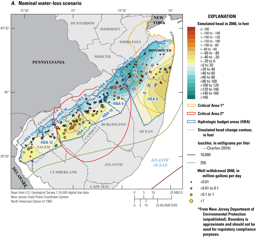


Maps showing hydrologic budget areas in the Wenonah-Mount Laurel aquifer and simulated potentiometric surface in 2040 for the three scenarios: A, nominal water-loss, B, optimal water-loss, and C, full allocation.
Figure 33 shows the simulated drawdown from the end of 2013 through 2040 in the Wenonah-Mount Laurel aquifer for the three withdrawal scenarios. In the northeastern part of the aquifer, heads recover over the nominal and optimal water-loss scenarios. This recovery is mostly in response to decreased withdrawals as a result of Critical Area 1 restrictions. There are some other areas of recovery in those scenarios in response to local decreases in pumping. Areas of drawdown exist in the vicinity of some of the pumping wells in HBA 9, HBA 10, and HBA 11, with the largest areas of drawdown occurring through the center of HBA 11.
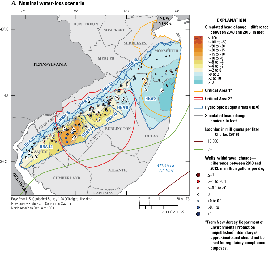
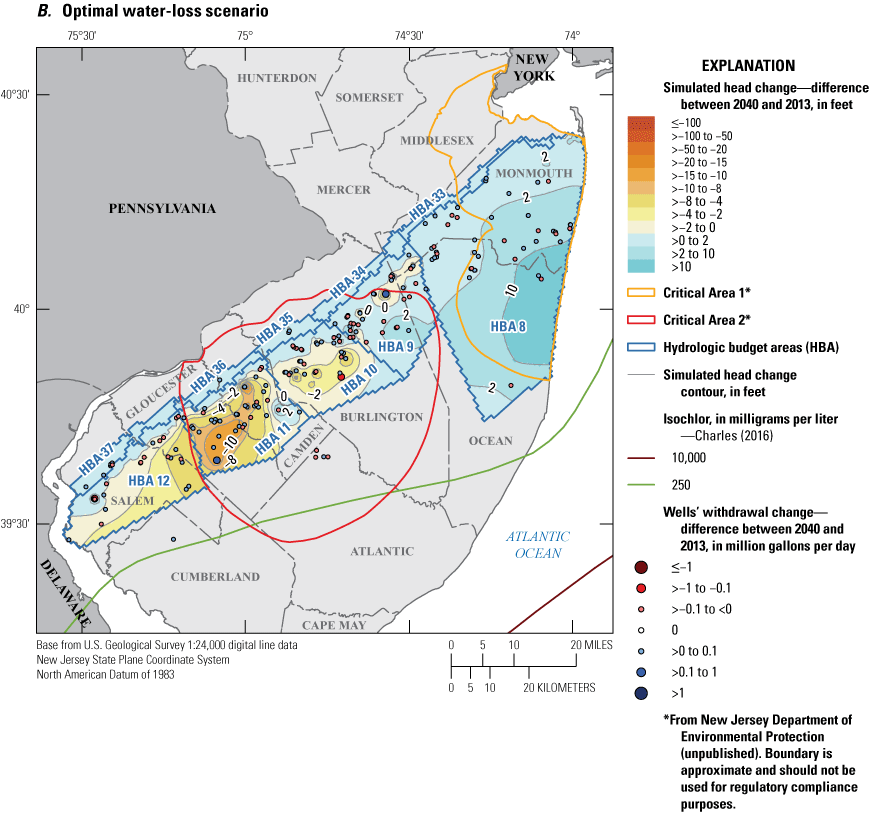

Maps showing the change in simulated water levels from the end of the base simulation (2013) to the end of the scenarios (2040) in the Wenonah-Mount Laurel aquifer and simulated potentiometric surface for the three scenarios: A, nominal water-loss, B, optimal water-loss, and C, full allocation.
In the full allocation scenario, there are many areas where the drawdown is greater than 20 feet throughout the aquifer. The largest amount of drawdown in HBA 10 and HBA 11 is greater than 50 feet of head decline. Across the unconfined areas and in a small area along the coast, there is a small (less than two feet) increase in heads across the simulation.
Budget Analysis
Figure 34 and table 21 show the net components of flow in and out of HBA 8 and are discussed below. For HBA 8, the primary source of inflow (57–59 percent) is from the overlying aquifer. Flow to and from the adjacent unconfined HBA 33 consists of 38–40 percent of total inflow and 42–48 percent of total outflow. The wells in HBA 8 account for less than ten percent of the outflow in the budget area. Other components of outflow include flow through the underlying confining layer to the Englishtown aquifer system (23–29 percent) and lateral flow to HBA 9 (17–19 percent). The components are similar between the scenarios, except for the full allocation scenario, in which there is more inflow from the overlying aquifer and outflow to the underlying aquifer and wells.
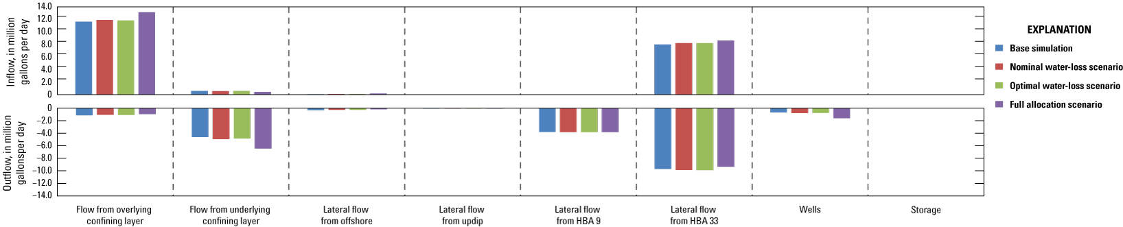
Graph showing simulated flow rates for the Wenonah-Mount Laurel aquifer, hydrologic budget area (HBA) 8.
Table 21.
Flow budget of the Wenonah-Mount Laurel aquifer, hydrologic budget area (HBA) 8.[Mgal/d, million gallons per day; %, percent of total]
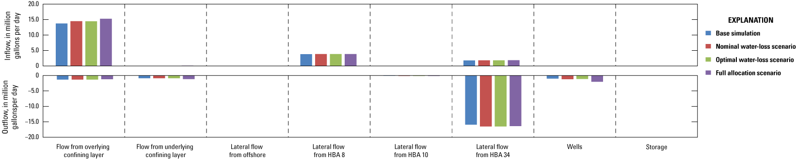
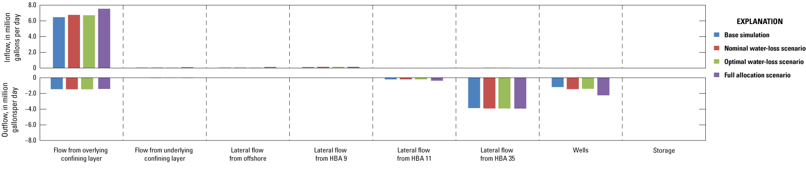
Figure 35 and table 22 show the budget components for HBA 9 and are discussed below. The two main components of inflow to HBA 9 are flow from the overlying aquifer (71–73 percent) and lateral flow from HBA 8 (18–20 percent). The main outflow of water (78–82 percent) is lateral flow to the unconfined HBA 34. Minor amounts of outflow are to the wells (5–10 percent), flow to the overlying confining unit (6–7 percent) and leakage to the underlying confining layer (4–6 percent). The near-zero components include flow to the offshore areas, lateral flow to HBA 10, and storage. The relative amounts of the budget components were similar among the base simulation and three scenarios.
Graph showing simulated flow rates for the Wenonah-Mount Laurel aquifer, hydrologic budget area (HBA) 9.
Table 22.
Flow budget of the Wenonah-Mount Laurel aquifer, hydrologic budget area (HBA) 9.[Mgal/d, million gallons per day; %, percent of total]
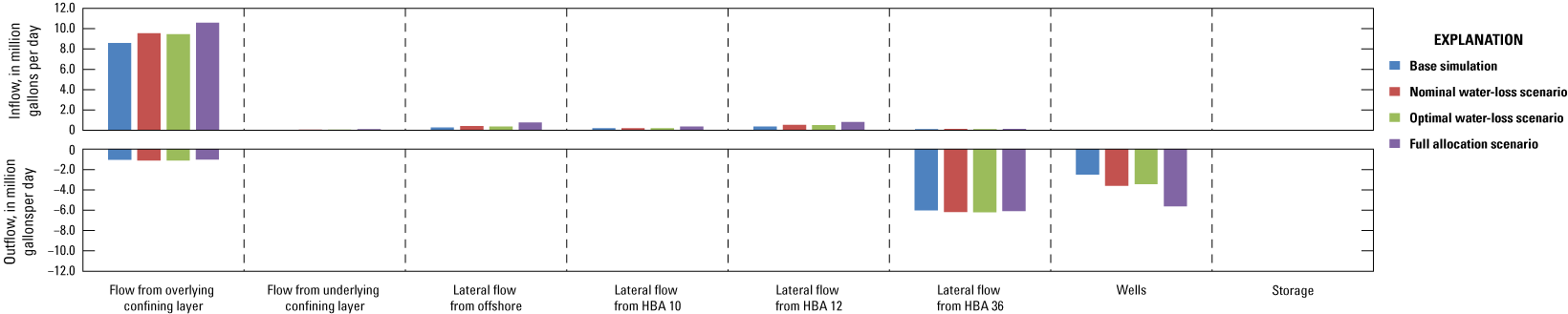
Figure 36 and table 23 show the budget components of flow in and out of HBA 10 and are discussed below. The main component of inflow (95–96 percent) to HBA 10 is flow from the overlying aquifer. The outflow is to the unconfined HBA 35 (49–58 percent), to wells (18–28 percent), and to the overlying confining layer (18–22 percent). Under the full allocation scenario there is increased leakage through the overlying confining layer to supply increased outflow to the wells. The net flows to the other components are small.
Graph showing simulated flow rates for the Wenonah-Mount Laurel aquifer, hydrologic budget area (HBA) 10.
Table 23.
Flow budget of the Wenonah-Mount Laurel aquifer, hydrologic budget area (HBA) 10.[Mgal/d, million gallons per day; %, percent of total]
Figure 37 and table 24 show the budget components of flow in and out of HBA 11 and are discussed below. The main component of inflow (83–90 percent) to HBA 11 is from the overlying confining layer with minor components from offshore (3–6 percent), HBA 10 (2–3 percent), and HBA 12 (4–6 percent). The largest outflow is to the unconfined HBA 36 (48–63 percent). Most of the other outflow is to the wells (26–44 percent). For the full allocation scenario, the outflow to the wells in HBA 11 is approaching that of flow to the unconfined HBA 36.
Graph showing simulated flow rates for the Wenonah-Mount Laurel aquifer, hydrologic budget area (HBA) 11.
Table 24.
Flow budget of the Wenonah-Mount Laurel aquifer, hydrologic budget area (HBA) 11.[Mgal/d, million gallons per day; %, percent of total]
Figure 38 and table 25 show the budget components of flow in and out of HBA 12 and are discussed below. The inflow is primarily (94–95 percent) from the overlying confining layer in HBA 12; some water also flows out to the overlying confining layer (13–17 percent). The largest component of outflow (48–57 percent) in HBA 12 is lateral flow to the unconfined HBA 37. The wells are the second largest component of outflow (13–25 percent) from HBA 12. The full allocation scenario has close to double the flow to wells both by magnitude and percentage. There is some outflow (4–5 percent) to the Delaware River where the model simulates a connection to the Wenonah-Mount Laurel aquifer in Salem County (fig. 38). There is some lateral outflow to HBA 11 (4–8 percent) and a small amount of outflow to areas offshore (2–3 percent).
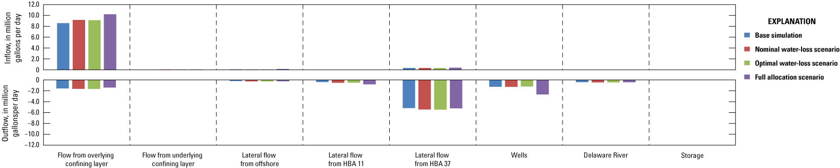
Graph showing simulated flow rates for the Wenonah-Mount Laurel aquifer, hydrologic budget area (HBA) 12.
Table 25.
Flow budget of the Wenonah-Mount Laurel aquifer, hydrologic budget area (HBA) 12.[Mgal/d, million gallons per day; %, percent of total]
The budgets for the unconfined hydrologic budget areas in the Wenonah-Mount Laurel aquifer are presented in figures 39–43 and tables 26–30. For all these unconfined budget areas, the main component of inflow is recharge (58–85 percent) and the main component of outflow is to the streams (39–95 percent). The second biggest inflow is from the adjacent confined HBA (11–29 percent). This reflects the leaky nature of the overlying confining unit in that the confined aquifer transmits part of the general recharge to discharge system. In HBA 33, the flow leaking to the confining layer below (36–37 percent) is only slightly less than the amount of flow to the modeled streams (39–41 percent). In the other HBA, there is some amount of flow in and out of the underlying confining layer that accounts for less than 10 percent of the total inflow and outflow.
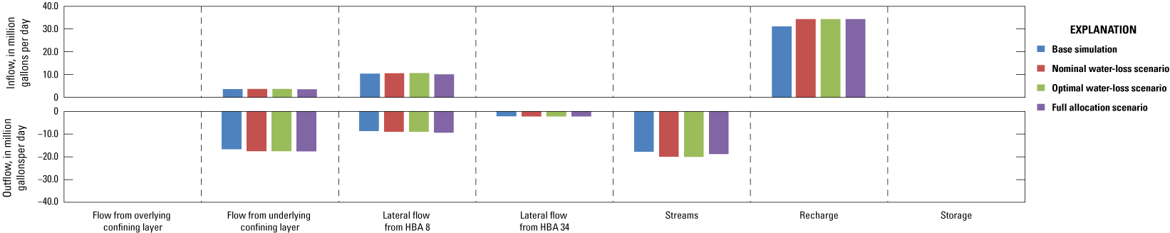
Graph showing simulated flow rates for the Wenonah-Mount Laurel aquifer, hydrologic budget area (HBA) 33.
Table 26.
Flow budget of the Wenonah-Mount Laurel aquifer, hydrologic budget area (HBA) 33.[Mgal/d, million gallons per day; %, percent of total]
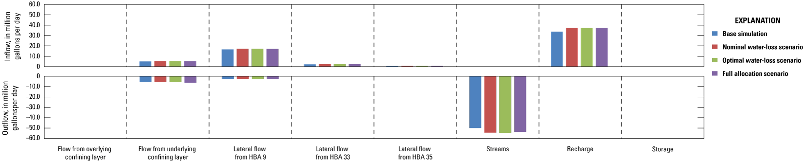
Graph showing simulated flow rates for the Wenonah-Mount Laurel aquifer, hydrologic budget area (HBA) 34.
Table 27.
Flow budget of the Wenonah-Mount Laurel aquifer, hydrologic budget area (HBA) 34.[Mgal/d, million gallons per day; %, percent of total]
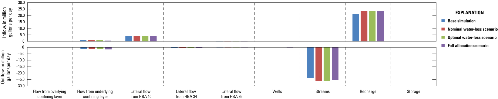
Graph showing simulated flow rates for the Wenonah-Mount Laurel aquifer, hydrologic budget area (HBA) 35.
Table 28.
Flow budget of the Wenonah-Mount Laurel aquifer, hydrologic budget area (HBA) 35.[Mgal/d, million gallons per day; %, percent of total]
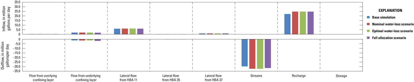
Graph showing simulated flow rates for the Wenonah-Mount Laurel aquifer, hydrologic budget area (HBA) 36.
Table 29.
Flow budget of the Wenonah-Mount Laurel aquifer, hydrologic budget area (HBA) 36.[Mgal/d, million gallons per day; %, percent of total]
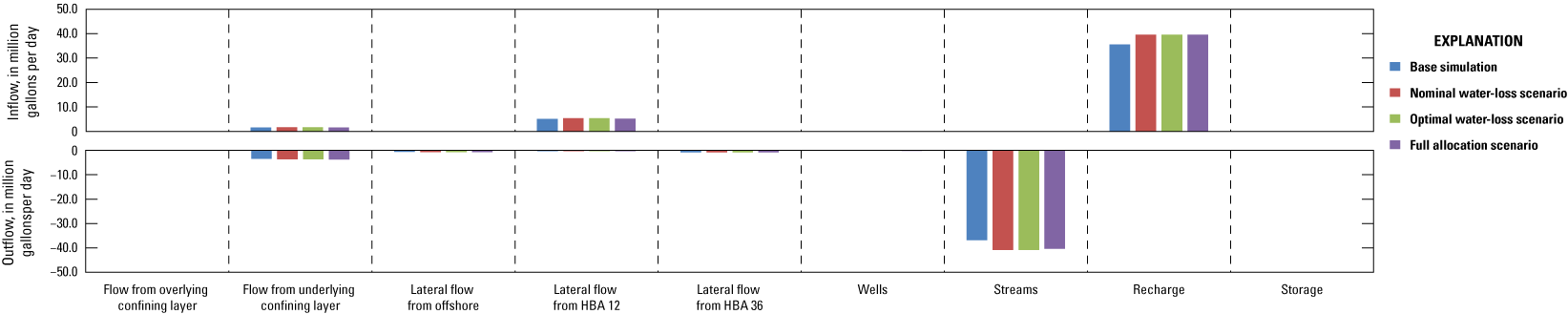
Graph showing simulated flow rates for the Wenonah-Mount Laurel aquifer, hydrologic budget area (HBA) 37.
Table 30.
Flow budget of the Wenonah-Mount Laurel aquifer, hydrologic budget area (HBA) 37.[Mgal/d, million gallons per day; %, percent of total]
Englishtown Aquifer System
The study defined two confined (HBA 13 and HBA 14) and two unconfined (HBA 38 and HBA 39) budget areas in the Englishtown aquifer system. HBA 13 is partially in Critical Area 1 where withdrawals are restricted in response to large drawdowns in the aquifer in the 1980s and prior. There are 110 wells in HBA 13. HBA 14 largely corresponds to Critical Area 2 where withdrawals are restricted in the deeper Potomac-Raritan-Magothy aquifer system. There are 51 wells in HBA 14. Withdrawals are minimal in the unconfined HBA with 5 wells in HBA 28 and one well in HBA 39.
Trends of Withdrawals and Heads
Figure 44 shows withdrawal trends and trends of median, 10th percentile, and minimum heads from the base simulation and each of the three withdrawal scenarios for each confined budget area in the Englishtown aquifer system. Table 31 shows a summary of the past and projected withdrawals in each budget area.
Table 31.
Summary of trends in withdrawals in the Englishtown aquifer system and the upper, middle, and lower Potomac-Raritan-Magothy aquifers.[Average withdrawals given in million gallons per year. NJCP, New Jersey Coastal Plain; %, percent; —, no data]
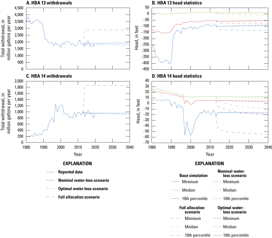
Line graphs showing withdrawals and median, 10th percentile, and minimum heads for model cells over time in hydrologic budget areas (HBA) in the Englishtown aquifer system: A, withdrawals in HBA 13, B, head statistics in HBA 13, C, withdrawals in HBA 14, and D, head statistics in HBA 14.
The effects of the Critical Areas can be seen in the withdrawal history of both HBA 13 and HBA 14, although with opposite effects. In HBA 13, the withdrawals decrease sharply in the early 1990s and remain fairly constant thereafter in response to restrictions from Critical Area 1 (fig. 44A). The consistent pumping is expected to continue with a small increase (3.8 percent) projected for the nominal water-loss scenario and a small decrease (1 percent) projected for the optimal water-loss scenario (table 31). These both fall within the variability seen in withdrawals over the last 15 years of the base simulation. In HBA 14, the withdrawals increase around 1990 at the time where withdrawals were restricted in the deeper PRM aquifer system owing to the Critical Area 2 restrictions (fig. 44C). The withdrawals in HBA 14 reach a peak around the turn of the century then decrease slightly around 2005, remaining fairly level through 2020. The nominal (0.5 percent decrease) and optimal (4.6 percent decrease) water-loss scenarios project near constant withdrawals (table 31). The full allocation scenario projects an 87 percent increase in withdrawals (table 31).
The simulated heads from the base simulation decline in the early part of the model. These declines are especially evident in the cells around wells, which is reflected by the 10th percentile and minimum heads in HBA 13 (fig. 44B). What follows is a sharp recovery in heads in the early 1990s because of Critical Area 1 restrictions. Heads continue to recover, though more gradually, through the end of the base simulation. The nominal and optimal water-loss scenarios indicate heads continue to recover through 2040, although at a relatively slower rate compared to that of the base simulation. The maximum amount of drawdown (table 32), however, indicates there are some areas with greater than 20 feet of head decline (maximum of 26.8 feet for nominal water-loss scenario and 21.4 feet for the optimal loss scenarios). For the full allocation scenario, there is some decline in heads; however, the magnitude of the decline does not reach levels seen early in the base simulation.
Table 32.
Statistics for simulated drawdown from the end of 2013 through 2040 for hydrologic budget areas in the Englishtown aquifer system.The heads in HBA 14 generally decline throughout the first part of the base simulation, leveling out in the 2000s after a big decline, especially as measured by the 10th percentile and minimum heads in the late 1990s (fig. 44B). The nominal water-loss scenario indicates there is a slight decline with a median drawdown of 0.9 feet and a maximum of 4.2 (table 32). The median value of zero in the optimal water-loss scenario indicates drawdown is minimal; the maximum drawdown is 3.5 feet (table 32). The full allocation scenario indicates there is substantial drawdown with the head quickly declining in 2014, then continuing to decline before leveling off by 2040 (fig. 44D). In 2040, the full allocation scenario indicates the median drawdown is 21.5 feet and the maximum is 35 feet (table 32).
Simulated Heads and Drawdown in 2040
Figure 45 shows the simulated head distribution in 2040 for the Englishtown aquifer system. The lowest heads in the Englishtown aquifer system are along the coast centered around the boundary between Monmouth and Ocean Counties. There are two other noticeable cones of depression: one to the northwest of the area of depressed head along the coast and the other in Camden County in the southwestern part of the aquifer in HBA 14. The heads are highest in the unconfined parts of the aquifer and in the confined aquifer just along the boundaries with the unconfined areas.
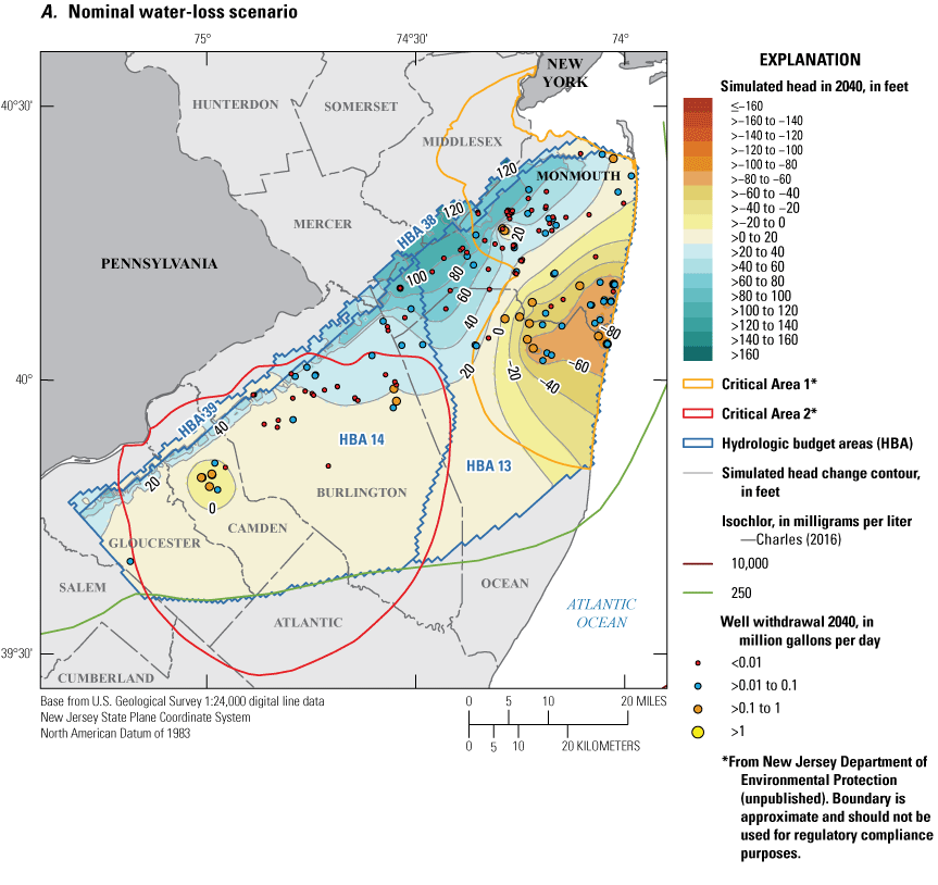
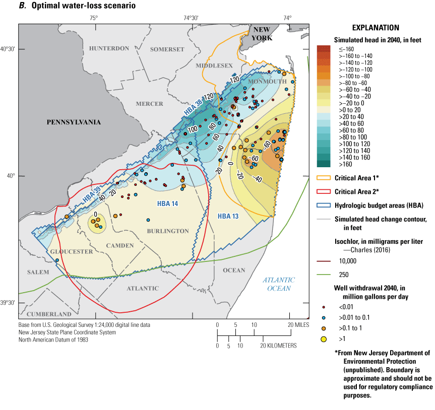
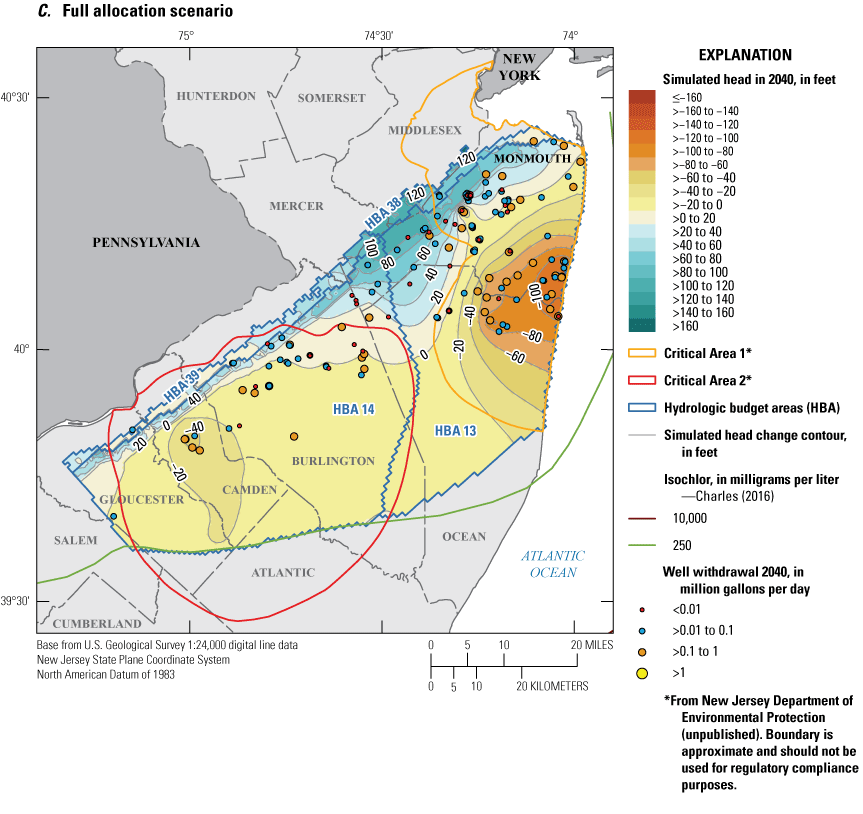
Maps showing hydrologic budget areas in the Englishtown aquifer system and simulated potentiometric surface in 2040 for the three scenarios: A, nominal water-loss, B, optimal water-loss, and C, full allocation.
Figure 46 shows the simulated drawdown from the end of the base simulation in 2013 through 2040 based on the projected water-use scenarios. The scenarios indicate that a large part of the Englishtown aquifer system sees little change for the optimal and nominal water-loss scenarios (less than two feet in either direction; figs. 46A, 46B). For those two scenarios, the places where the heads are lowest (figs. 46A, 46B) generally see some head recovery due to decreasing withdrawals in surrounding wells (figs. 45A, 45B). There are several areas close to wells where large amounts of drawdown are simulated, as indicated by the tightly spaced contours for the nominal and optimal water-loss scenarios (figs. 46A, 46B). In the full allocation scenario, areas with little simulated change are limited to the outcrop areas and a narrow strip of the confined aquifer that borders the outcrop (fig. 46C). Most of the confined part of the Englishtown aquifer system shows declines of greater than 15 feet with most of that area having drawdown of greater than 20 feet (fig. 46C).
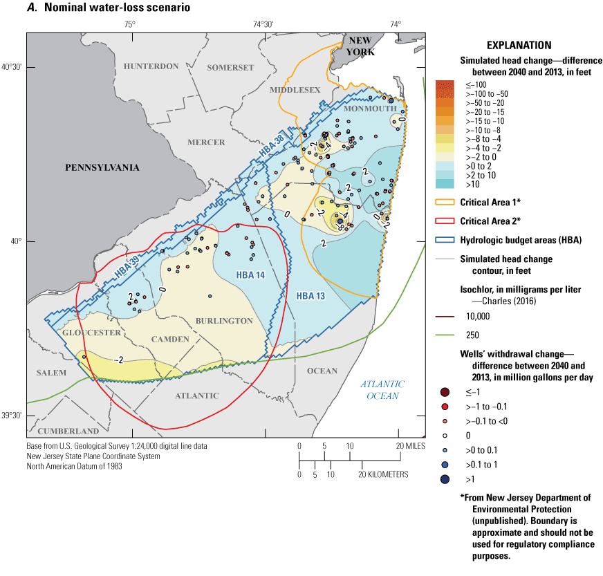
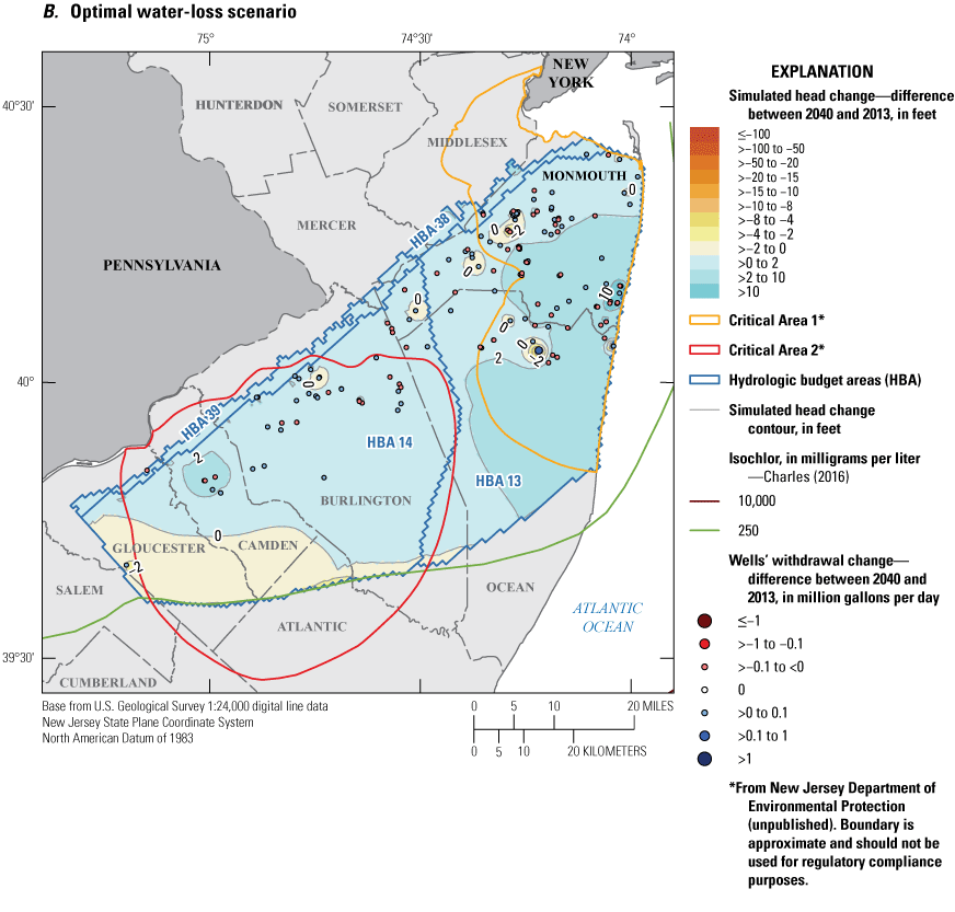
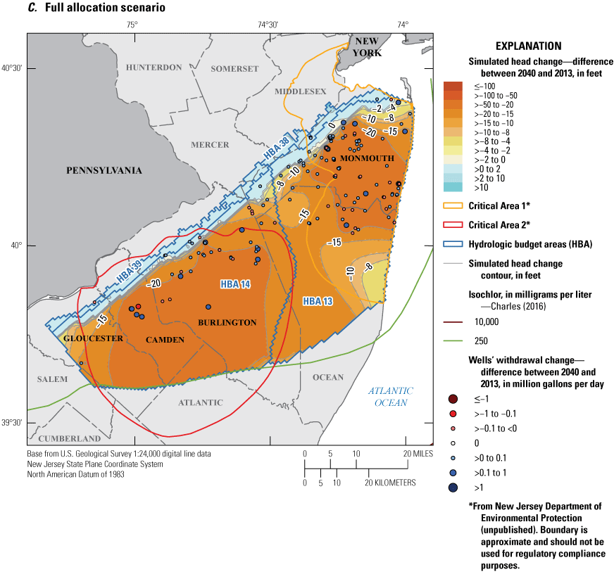
Maps showing the change in simulated water levels at the end of scenarios (2040) from the base simulation (2013) in the Englishtown aquifer system and simulated potentiometric surface in 2040 for the three scenarios: A, nominal water-loss, B, optimal water-loss, and C, full allocation.
Budget Analysis
Figures 47 and 48 and tables 33 and 34 show the budget components for HBA 13 and HBA 14 and are discussed below. In both areas, most of the inflow (92–94 percent) to the budget area is leakage from the overlying confining layer. In HBA 14, there is also some outflow (15–18 percent) to the overlying confining layer in places, as well. Most outflow in these budget areas, however, is split between flow to the adjacent budget areas (50–61 percent) and flow to wells (19–39 percent). The other budget components are minor (less than 5 percent). The full allocation scenario differs from the others because its increased pumping rate leads to greater amounts of inflow through the confining layer above and smaller amounts of outflow through the unconfined part of the aquifer.
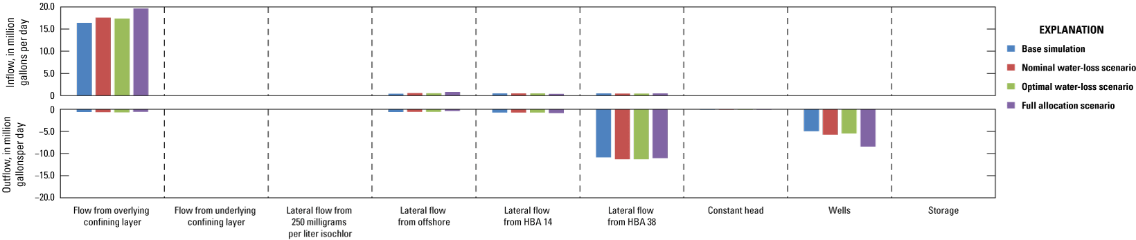
Graph showing simulated flow rates for the Englishtown aquifer system, hydrologic budget area (HBA) 13.
Table 33.
Flow budget of the Englishtown aquifer system, hydrologic budget area (HBA) 13.[mg/L, milligram per liter; Mgal/d, million gallons per day; %, percent of total]
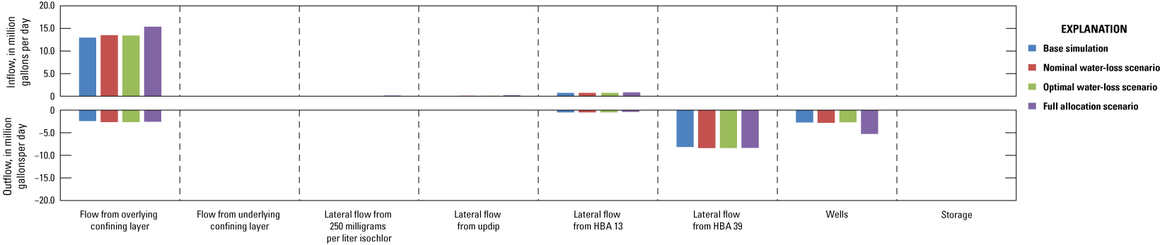
Graph showing simulated flow rates for the Englishtown aquifer system, hydrologic budget area (HBA) 14.
Table 34.
Flow budget of the Englishtown aquifer system, hydrologic budget area (HBA) 14.[mg/L, milligram per liter; Mgal/d, million gallons per day; %, percent of total]
The two unconfined budget areas in the Englishtown aquifer system, HBA 38 and HBA 39, have similar budgets (fig. 49, table 35; fig. 50, table 36). The main inflow is recharge (79–87 percent) and the main outflow is leakage to streams (93–96 percent). A small amount of inflow also comes from lateral flow from the adjacent confined HBA 13 (20–21 percent) and HBA 14 (11–12 percent).
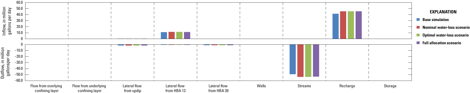
Graph showing simulated flow rates for the Englishtown aquifer system, hydrologic budget area (HBA) 38.
Table 35.
Flow budget of the Englishtown aquifer system, hydrologic budget area (HBA) 38.[Mgal/d, million gallons per day; %, percent of total]
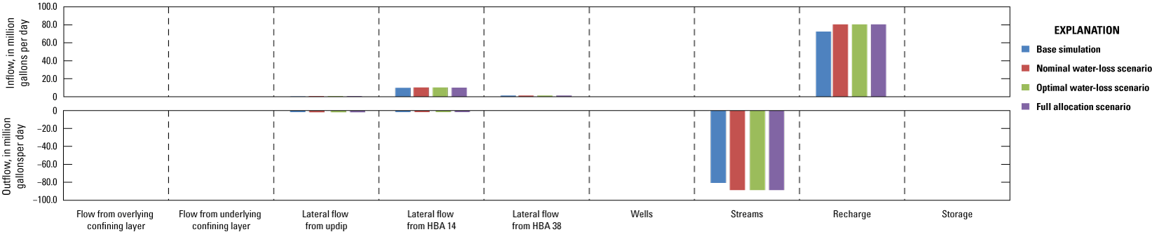
Graph showing simulated flow rates for the Englishtown aquifer system, hydrologic budget area (HBA) 39.
Table 36.
Flow budget of the Englishtown aquifer system, hydrologic budget area (HBA) 39.[Mgal/d, million gallons per day; %, percent of total]
Upper Potomac-Raritan-Magothy Aquifer
The study defined three confined (HBAs 15–17) and four unconfined budget areas (HBAs 40–43) in the upper Potomac-Raritan-Magothy aquifer. HBA 15 included areas restricted by the Critical Area 1. There were 98 wells included in the simulations from HBA 15. HBA 16 included areas restricted by Critical Area 2. There were 144 wells included in the simulations from HBA 16, the most of any HBA defined in this study across all the aquifers. HBA 17 was defined as a relatively small area to the southwest of Critical Area 2 and included 38 wells. Three of the four unconfined HBA in the upper PRM aquifer included pumping wells ranging from 68 in HBA 40 to 10 wells in HBA 42 to 6 wells in HBA 43.
Trends of Withdrawals and Heads
Figure 51 shows withdrawal trends and trends of median, 10th percentile, and minimum heads from the base simulation and withdrawal scenarios for each confined budget area in the upper PRM aquifer. Table 31 shows a summary of the past and projected withdrawals in each budget area.
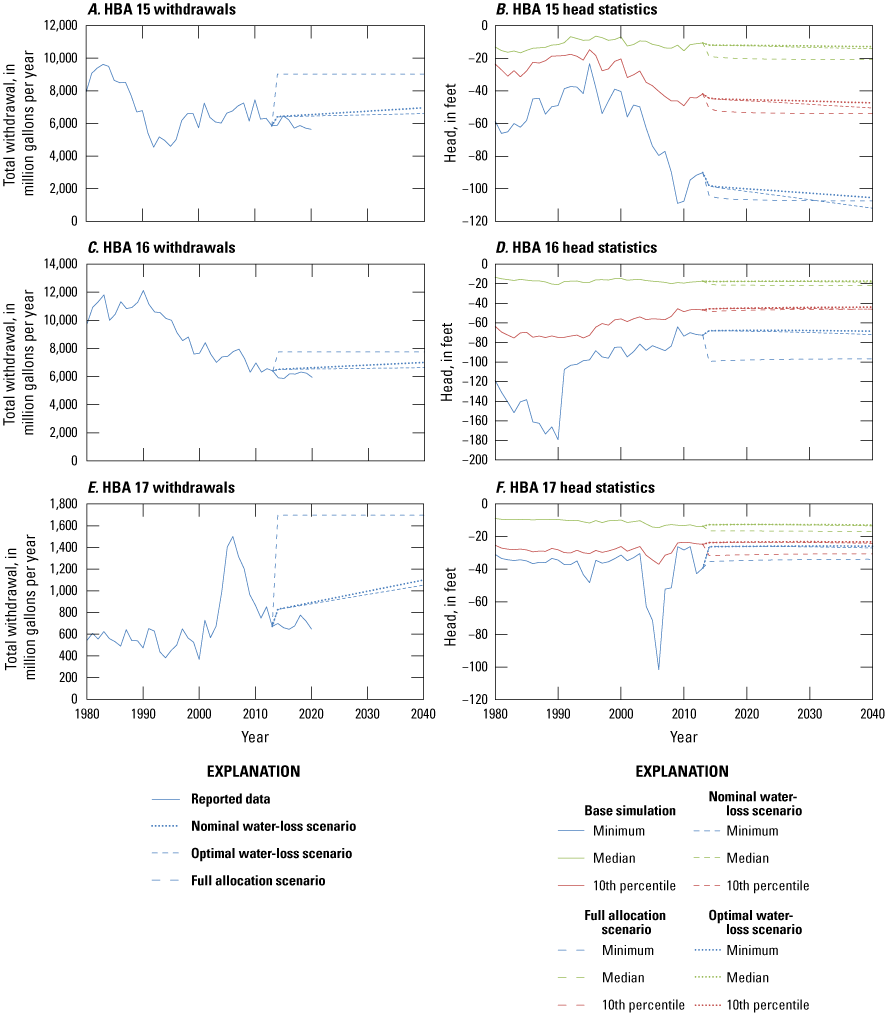
Line graphs showing withdrawals and median, 10th percentile, and minimum heads for model cells over time in hydrologic budget areas (HBA) in the upper Potomac-Raritan-Magothy aquifer: A, withdrawals in HBA 15, B, head statistics in HBA 15, C, withdrawals in HBA 16, D, head statistics in HBA 16, E, withdrawals in HBA 17, and F, head statistics in HBA 17.
In HBA 15, withdrawals decline in the late 1980s as a result of the Critical Area 1 restrictions then increase slightly in the 1990s (fig. 51A). After the turn of the century, the withdrawals are varied but show no noteworthy trend although there is a downward trend that starts in 2010 continuing through the end of the reported data in 2020. The nominal and optimal water-loss scenarios both show slight increases (8.4 percent and 3.1 percent, respectively [table 31]) over the 2014–40 period (fig. 51A). The full allocation scenario entails a 54-percent increase over 2013 withdrawals back up to the levels of the early 1980s (fig. 51A; table 31).
In HBA 16, withdrawals are generally in decline from the mid-1990s onwards in response to Critical Area 2 restrictions (fig. 51B). The nominal water-loss scenario indicates there would be a 7.4 percent increase in withdrawals from 2013 to 2040; for the optimal water-loss scenario, the corresponding value would be only 2.0 percent (table 31). The full allocation scenario indicates that withdrawals would increase 21 percent (table 31). This is small compared to most of the other areas, with the pumping in the last 5 years of the base simulation reaching 84 percent of the full allocation levels (table 31).
In HBA 17, there is a slight upward trend in withdrawals over the period of the base simulation punctuated by a spike in the early 2000s (fig. 51C). The scenarios indicate that an increase in pumping would continue for the nominal (32.5 percent) and optimal (27.1 percent) water-loss scenarios. The full allocation scenario indicates a step increase of 153 percent over 2013 withdrawals (table 31).
HBA 40 has a high amount of pumping compared to most of the other unconfined budget areas with a median value higher than the corresponding confined HBA 15 (table 31). The other unconfined budget areas in the upper PRM aquifer have little or no pumping.
The simulated heads in HBA 15 show recovery based on the reduction of pumping in the early 1980s; however, they decline once pumping increases in the late 1990s (fig. 51B). The median head declines slightly while the 10th percentile head declines approximately 20 feet and the minimum head declines more than 60 feet (fig. 51B). The projected withdrawal increases in the nominal and optimal water-loss scenarios lead to a median drawdown of 4.1 feet and 2.5 feet, respectively. The scenarios indicate the maximum drawdown is 21.8 feet for the nominal water-loss scenario and 15.4 feet for the optimal water-loss scenario. The full allocation scenario indicates the median drawdown is 9.7 feet and the maximum drawdown is 32.8 feet (table 37). Although the greatest drawdown is a result of the full allocation scenario (table 37), after 2032 the minimum head value for the nominal water-loss scenario is less than the minimum head value for the full allocation scenario (fig. 51B). This results from wells having higher projected withdrawals in the nominal water-loss scenario compared to the full allocation scenario.
Table 37.
Statistics for simulated drawdown from the end of 2013 through 2040 for budget areas in the upper Potomac-Raritan-Magothy aquifer.The median simulated heads in HBA 16 are fairly steady through the base simulation and the scenarios. After some initial decline, the 10th percentile and minimum heads also generally increase throughout the base simulation. The 10th percentile heads are fairly level in the scenario simulations. The minimum head declines a few feet in the nominal water-loss scenario and around 20 feet in the full allocation scenario (fig. 51D).
The simulated heads in HBA 17 are fairly stable over the period of the base simulation with the median value only declining slightly. The minimum simulated heads in HBA 17 do show a downward spike from 2004 to 2008 in response to the increase in pumping. The simulated heads are fairly level for all the scenarios. As shown in table 37, there are areas of drawdown in HBA 17 where maximum levels reach 13.4 feet in the nominal water-loss scenario, 12.3 feet in the optimal water-loss scenario, and 18.5 feet in the full allocation scenario. These drawdowns occur in areas with relatively high heads in the base simulation which is why they do not affect the 10th percentile and minimum heads shown in figure 51F.
Simulated Heads and Drawdown In 2040
Figure 52 shows the simulated head distribution in 2040 for the upper PRM aquifer. The head distribution is similar between all three scenarios. The highest heads are in the northwest part of the aquifer along the boundary of HBA 40 and 41 where the aquifer is unconfined or slightly confined (meaning, the confining layer is present but thin, or has a higher conductivity assigned than most of the confining layers). Heads are higher along the outcrop areas declining downdip with the lowest areas of head around pumping centers in central Ocean County and an area along the Gloucester and Camden County border. The heads in the full allocation scenario are lower than the other two but the patterns are similar.
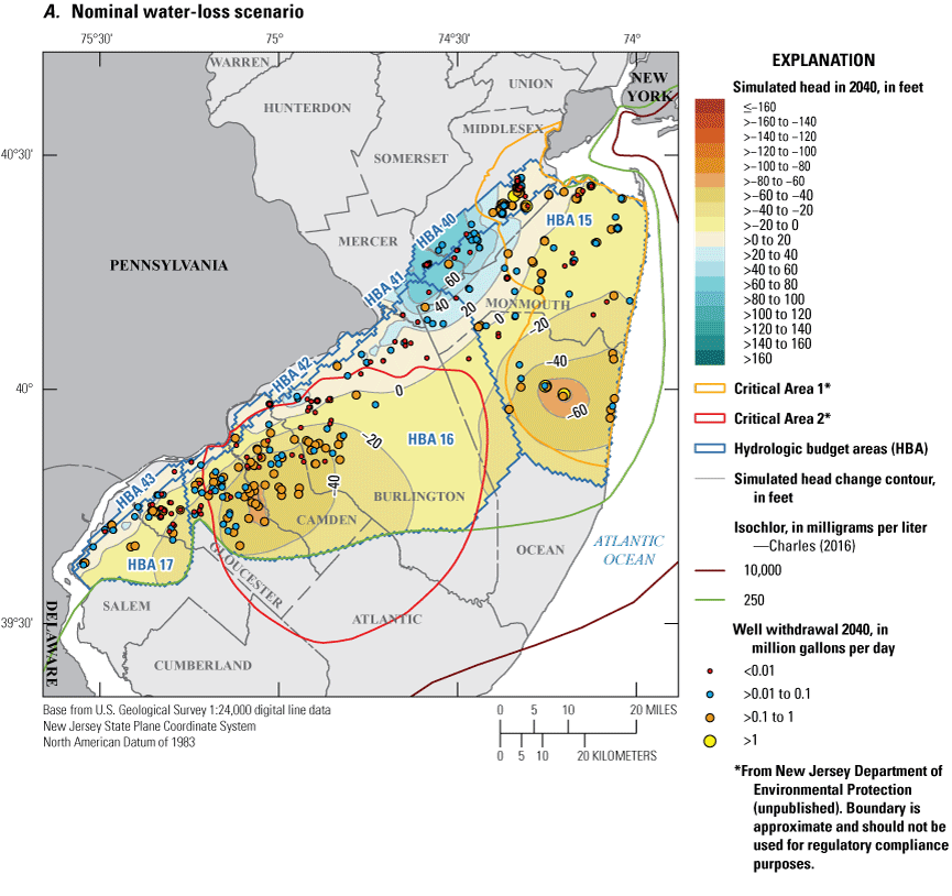

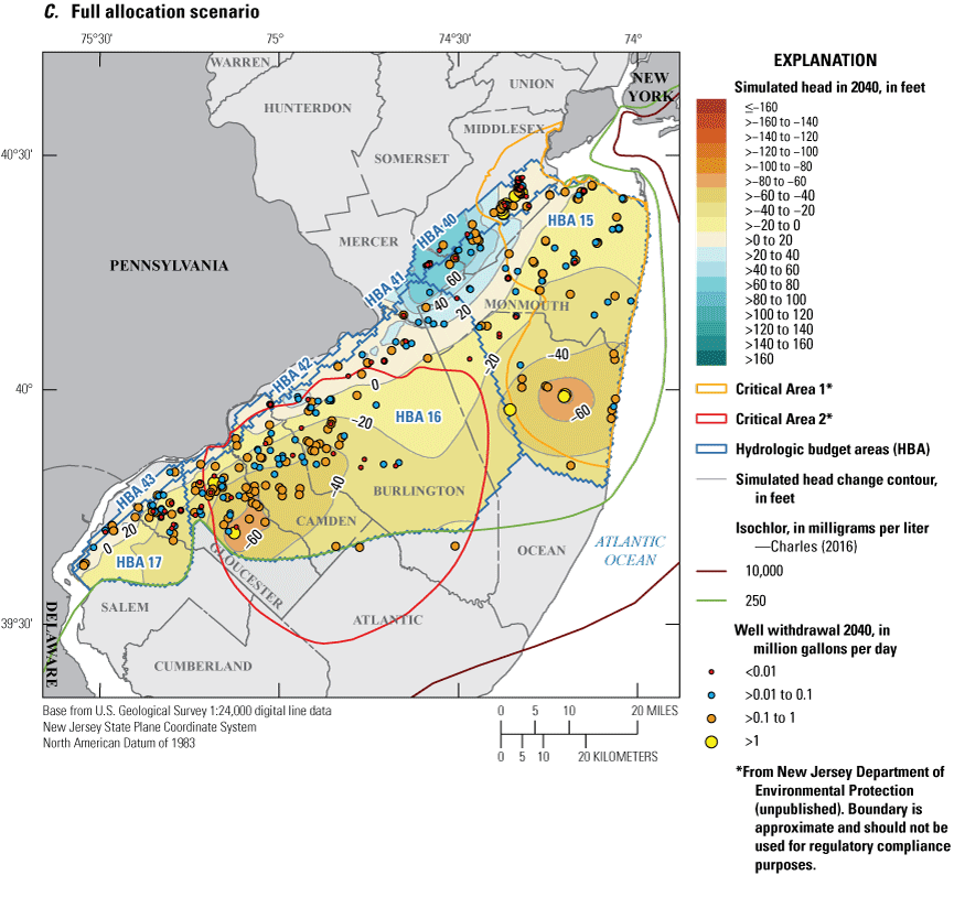
Maps showing the hydrologic budget areas in the upper Potomac-Raritan-Magothy aquifer and simulated potentiometric surface in 2040 for the three scenarios: A, nominal water-loss, B, optimal water-loss, and C, full allocation.
Figure 53A shows the simulated drawdown for the nominal water-loss scenario in the upper PRM aquifer from the end of the base simulation to the end of the scenario simulations in 2040. The biggest areas of decline are around clusters of wells in Ocean County. The area of declining heads extends out in a circular manner from these pumping centers, surrounding additional wells also; there are a few additional areas of drawdown in the aquifer further to the west. Areas of slightly rising heads (less than two feet) extend all along the outcrop areas owing to recharge with a few areas of bigger recoveries in Gloucester and Salem Counties where withdrawals have been reduced.
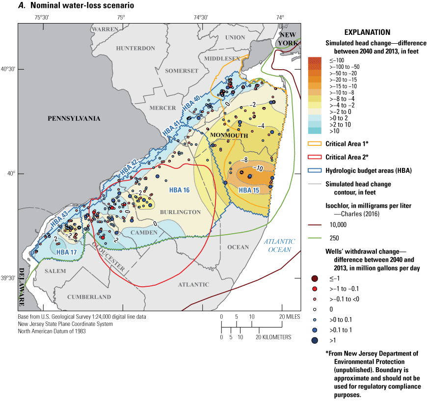
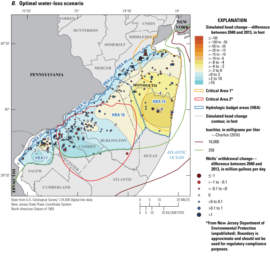
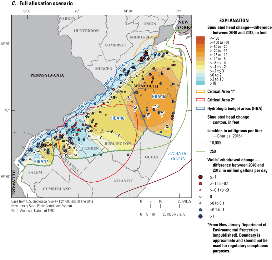
Maps showing the change in simulated water levels from the end of the base simulation (2013) to the end of the scenarios (2040) in the upper Potomac-Raritan-Magothy aquifer and simulated potentiometric surface in 2040 for the three scenarios: A, nominal water-loss, B, optimal water-loss, and C, full allocation.
Figure 53B shows the simulated drawdown for the optimal water-loss scenario in the upper PRM aquifer from the end of the base simulation to the end of the scenario simulations in 2040. The drawdowns are similar to (although smaller than) those in the nominal water-loss scenario. Areas of head decline greater than 10 feet are limited to tight circles around a few wells. Areas of head recovery greater than two feet extend further from wells in Gloucester and Salem Counties that are projected to pump less water.
Figure 53C shows the simulated drawdown for the full allocation scenario in the upper PRM aquifer from the end of the base simulation to the end of the scenario simulations in 2040. Generally, head declines are larger in the full allocation scenario. There is still some recovery (less than two feet) in the outcrop areas and areas with more substantial recovery (greater than 10 feet) in Camden County. Large amounts of recovery appear in an area where a number of wells pump less water compared to the base simulation and the other two scenarios.
Budget Analysis
Figure 54 and table 38 show the budget components for HBA 15 and are discussed below. The main source of inflow (83–86 percent) for the budget area is leakage through the overlying confining unit. Smaller amounts of inflow come from lateral flow offshore (7–9 percent) and from the adjacent HBA 16 (4–5 percent). The outflow is split between well pumping (35–43 percent), flow to the unconfined HBA 40 (31–35 percent), and flow to the underlying confining layer (24–27 percent). The scenarios are generally similar except for some additional leakage through the overlying confining unit in the full allocation scenario, which supplies the scenario’s increased pumping from wells.
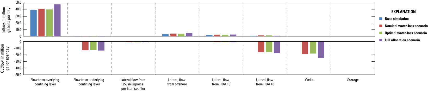
Graph showing simulated flow rates for the upper Potomac-Raritan-Magothy (PRM) aquifer, hydrologic budget area (HBA) 15.
Table 38.
Flow budget of the upper Potomac-Raritan-Magothy aquifer, hydrologic budget area (HBA) 15.[mg/L, milligram per liter; Mgal/d, million gallons per day; %, percent of total]
Figure 55 and table 39 show the budget components for HBA 16 and are discussed below. The main source of inflow (84–86 percent) for the budget area is flow through the overlying confining layer. Minor components of inflow include lateral flow from HBA 42 (5–6 percent), flow from the underlying confining layer (4–5 percent), lateral flow from the 250 mg/L isochlor (2 percent), and lateral flow from HBA 17 (2 percent). The biggest outflow is to the wells (28–31 percent) followed closely by lateral flow to the two unconfined budget areas (HBA 41 [10–11 percent] and HBA 42 [24–26 percent]), flow down to the underlying confining layer (17–18 percent), and flow to the overlying confining layer (13–14 percent).
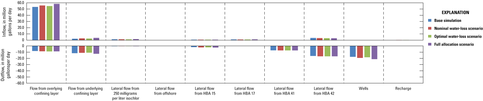
Graph showing simulated flow rates for the upper Potomac-Raritan-Magothy (PRM) aquifer, hydrologic budget area (HBA) 16.
Table 39.
Flow budget of the upper Potomac-Raritan-Magothy aquifer, hydrologic budget area (HBA) 16.[Storage is not shown because it made up less than 0.1 percent of the total flow in each scenario. mg/L, milligram per liter; Mgal/d, million gallons per day; %, percent of total]
Figure 56 and table 40 show the budget components for HBA 17 and are discussed below. The main source of inflow (96–98 percent) for the budget area is flow from the overlying confining layer. The outflow of the budget area is to wells (20–40 percent), lateral flow to the unconfined HBA 43 (30–43 percent), lateral flow to HBA 16 (10–12 percent), flow to the underlying confining layer (10–13 percent), and flow to the overlying confining layer (6–9 percent). There are minor amounts (less than two percent) of outflow going to offshore areas and the 250 mg/L isochlor.
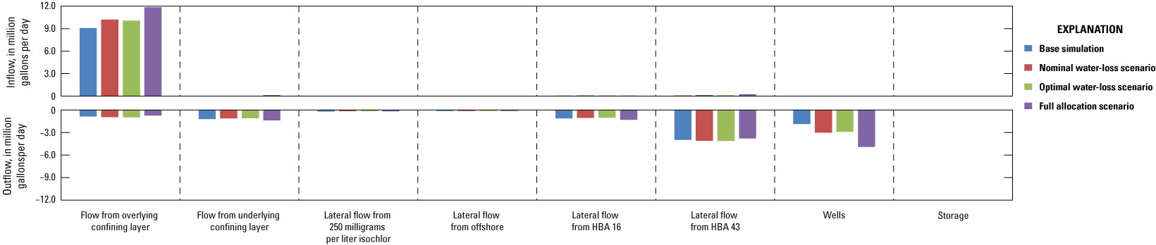
Graph showing simulated flow rates for the upper Potomac-Raritan-Magothy (PRM) aquifer, hydrologic budget area (HBA) 17.
Table 40.
Flow budget of the upper Potomac-Raritan-Magothy aquifer, hydrologic budget area (HBA) 17.[mg/L, milligram per liter; Mgal/d, million gallons per day; %, percent of total]
Figure 57 and table 41 show the budget components for HBA 40 and are discussed below. Although there is more pumping in this HBA than most of the unconfined HBAs, 71–83 percent of the outflow from the area is still dominated by flow to the streams. The wells account for a little over 10 percent of outflow in the base simulation and nominal and optimal water-loss scenarios, but they account for up to 21 percent in the full allocation scenario. In all the simulations, a minor amount of outflow (4–6 percent) goes to the underlying aquifer. The primary source of inflow (82–84 percent) to the budget area is recharge, with most of the remaining inflow coming from the adjacent HBA 15 (14–15 percent).
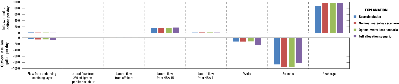
Graph showing simulated flow rates for the upper Potomac-Raritan-Magothy (PRM) aquifer, hydrologic budget area (HBA) 40.
Table 41.
Flow budget of the upper Potomac-Raritan-Magothy aquifer, hydrologic budget area (HBA) 40.[Storage and flow from the overlying confining layer are not shown because they made up less than 0.1 percent of total flow in each scenario. mg/L, milligram per liter; Mgal/d, million gallons per day; %, percent of total]
Figures 58 and 59, and tables 42 and 43 show the budget components for HBA 41 and HBA 42, respectively, and are discussed below. The components of the two budget areas are similar. In both areas, outflow consists mainly of flow to streams (83–87 percent) and leakage to the underlying confining layer (5–9 percent), with some additional flow going to the adjacent HBAs (7–8 percent from HBA 41 to HBA 40, and 6–7 percent from HBA 42 to HBA 16). The inflow comes primarily from recharge (54–69 percent) and lateral flow from HBA 16 (30–42 percent).
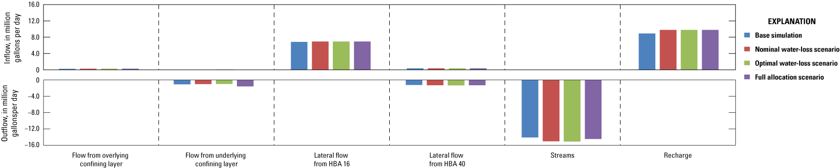
Graph showing simulated flow rates for the upper Potomac-Raritan-Magothy (PRM) aquifer, hydrologic budget area (HBA) 41.
Table 42.
Flow budget of the upper Potomac-Raritan-Magothy aquifer, hydrologic budget area (HBA) 41.[Storage and flow from the overlying confining layer are not shown because they made up less than 0.1 percent of total flow in each scenario. Mgal/d, million gallons per day; %, percent of total]
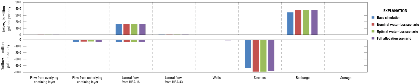
Graph showing simulated flow rates for the upper Potomac-Raritan-Magothy (PRM) aquifer, hydrologic budget area (HBA) 42.
Table 43.
Flow budget of the upper Potomac-Raritan-Magothy aquifer, hydrologic budget area (HBA) 42.[Mgal/d, million gallons per day; %, percent of total]
Figure 60 and table 44 show the budget components for HBA 43 and are discussed below. The main outflow is to the streams (79–82 percent). There is also some outflow to the Delaware River (5 percent) and wells (2–4 percent), lateral flow offshore (7 percent), and leakage to the underlying confining layer (2–3 percent). The inflow to the budget area primarily comes from recharge (82–85 percent). There is also some inflow coming from HBA 17 (15–18 percent).
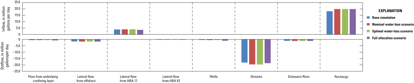
Graph showing simulated flow rates for the upper Potomac-Raritan-Magothy (PRM) aquifer, hydrologic budget area (HBA) 43.
Table 44.
Flow budget of the upper Potomac-Raritan-Magothy aquifer, hydrologic budget area (HBA) 43.[Storage and flow from the overlying confining layer are not shown because they made up less than 0.1 percent of total flow in each scenario. Mgal/d, million gallons per day; %, percent of total]
Middle Potomac-Raritan-Magothy Aquifer
The study used four confined (HBAs 18–21) and three unconfined (HBAs 44–46) budget areas in the middle PRM aquifer. HBA 18 included the area restricted by the Critical Area 1. Seventy wells were included in the simulations from HBA 18. HBA 19 included the areas restricted by Critical Area 2 and had 111 wells included. HBA 20 and HBA 21 lie to the southwest of Critical Area 2 and are divided by the 250 mg/L isochlor. HBA 20 included 31 wells. HBA 21 which was defined as the area beyond the 250 mg/L isochlor only included 3 wells.
Trends of Withdrawals and Heads
Figure 61 shows withdrawal trends and trends of median, 10th percentile, and minimum heads from the base simulation and withdrawal scenarios for each confined budget area in the middle PRM aquifer. Table 31 shows a summary of the past and projected withdrawals in each budget area.
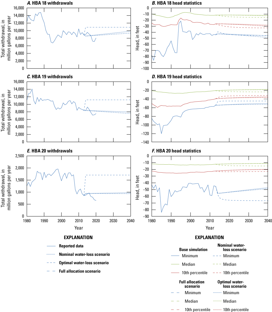
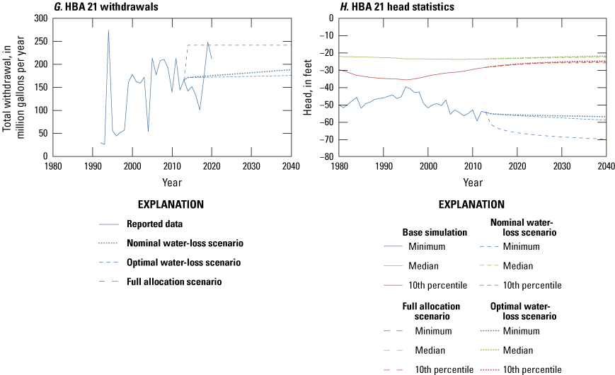
Line graphs showing withdrawals and median, 10th percentile, and minimum heads for model cells over time in hydrologic budget areas (HBA) in the middle Potomac-Raritan-Magothy aquifer: A, withdrawals in HBA 18, B, head statistics in HBA 18, C, withdrawals in HBA 19, D, head statistics in HBA 19, E, withdrawals in HBA 20, F, head statistics in HBA 20, G, withdrawals in HBA 21, and H, head statistics in HBA 21.
The withdrawals in HBA 18 start high in the base simulation, then decline around 1990 in response to Critical Area 1 restrictions (fig. 61A). The level of withdrawals is fairly stable during the 2000s. Both the nominal and optimal water-loss scenarios project an increase in the withdrawals over the scenario simulations (table 31). The scenarios indicate withdrawals would increase 14.8 percent for the nominal water-loss scenario and 9.4 percent for the optimal water-loss scenario. The full allocation scenario indicates withdrawals would increase a modest (compared to many of the other HBAs) 22.6 percent (table 31).
The withdrawals in HBA 19 generally decline throughout the period of the base simulation in response to the Critical Area 2 restrictions (fig. 61C). The nominal and optimal water-loss scenarios indicate withdrawals would continue to decline by 5.0 percent and 9.6 percent, respectively (table 31). The full allocation scenario indicates withdrawals would increase 33.9 percent (table 31).
The withdrawals in HBA 20 increase in the early period of the base simulation, then remained fairly steady with annual fluctuations around the mean before dropping by around 50 percent starting around 2008 (fig. 61E). The reported withdrawals continue to decline after the base simulation ends. The nominal water-loss scenario indicates withdrawals would see a small increase of 3.3 percent. The optimal water-loss scenario would see a slight decrease of 0.9 percent (table 31). The full allocation scenario indicates that such conditions would return levels to those seen throughout most of the base simulation, an increase of 98.9 percent (table 31).
The withdrawals in HBA 21 are small compared to the other confined budget areas in the middle PRM aquifer owing in part to it being located beyond the 250 mg/L isochlor where there is lower water quality. The withdrawal amounts fluctuate in the base simulation and in the years with reported data since the end of the simulation (fig. 61G). The scenarios indicate withdrawals would increase 9.9 percent for the nominal water-loss scenario and 2.8 percent for the optimal water-loss scenario (table 31). The full allocation scenario indicates that withdrawals would return levels to those seen throughout most of the base simulation and increase 45.6 percent (table 31).
The unconfined budget areas in the middle PRM aquifer do not account for a lot of pumping compared to the confined part of the aquifer. There are some pumping wells in the unconfined areas though, especially in HBA 45. Table 31 shows that the withdrawals for all three of the unconfined HBA in the middle PRM have all declined in the period from 2014 through 2020 compared to the period of the base simulation. The nominal and optimal water-loss scenarios project increases of 26.6 percent and 21.5 percent for HBA 44. The nominal and optimal water-loss scenarios project increases of 5.1 percent and 0.8 percent for HBA 45. The nominal water-loss scenario projects an increase of 2.1 percent and the optimal water-loss scenario projects a decrease of 3.8 percent for HBA 46 (table 31).
The simulated heads in HBA 18 respond to the changes in withdrawals. The median values of all the model cells in HBA 18 in the base simulation initially decline until 1988 when the withdrawals are reduced. At that point the heads recover until 1997 when they start another gradual decline that lasts until the end of the base simulation. The 10th percentile and minimum head trends are similar to the median, although the minimum statistic has some more abrupt changes up and down over several year periods (fig. 61B). The slight decline continues in the scenario simulations. The median drawdown ranges from 0.5 feet in the optimal water-loss scenario to 4.0 feet in the full allocation scenario. The maximum drawdown ranges from 9.8 feet in the optimal water-loss scenario to 25.1 feet in the full allocation scenario (table 45).
Table 45.
Statistics for simulated drawdown from the end of 2013 through 2040 for hydrologic budget areas in the middle Potomac-Raritan-Magothy aquifer.The median head in HBA 19 declined over the first 10–15 years of the base simulation and recovered over the remainder of the base simulation (fig. 61D). The 10th percentile and minimum heads behaved similarly although there are sharp changes, especially for the minimum head. The scenarios all show continued recovery except for the median statistic in the full allocation scenario. The full allocation scenario’s 10th percentile and minimum heads are noteworthy because they show more recovery than the other two scenarios, indicating that the full allocation withdrawals are less than the other two scenarios for some of the wells.
The heads in HBA 20 are fairly stable in the base simulation and in the scenarios based on the median and 10th percentile heads. The minimum head shows a lot of variability in the base simulation. Both the nominal and optimal water-loss scenario simulations indicate that the minimum heads recover. The full allocation scenario indicates the minimum heads initially decline and then level off. Although the head statistics show recovery, there are head declines in some areas (table 45). The maximum drawdowns are 8.2 feet, 7.8 feet, and 47.8 feet for the nominal water loss, optimal water loss, and full allocation scenarios, respectively.
In HBA 21, where there is a relatively small but sporadic amount of pumping, the median and 10th percentile heads decline slightly until around 2000 and then recover (fig. 61H). This recovery is simulated to continue for all three scenarios. The minimum head in HBA 21 follows a general trend that goes up through 1997 in the base simulation with some small deviations. It then declines for the remainder of the base and scenario simulations.
Simulated Heads and Drawdown in 2040
Figure 62 shows the simulated head distribution in 2040 for the middle PRM aquifer. The simulated head distribution in 2040 is similar in structure between the three scenarios. The highest heads are along the outcrop area in the northern part of the aquifer. The heads generally decrease moving downdip to the pumping centers. There are a few differences of note seen in the full allocation scenario compared to the other two scenarios which are similar to each other. Some of the wells have lower values in the full allocation scenario than the other two, and the maximum drawdown areas (less than −40 feet) are not as extreme in the full allocation scenario. The amount of area where the head is less than −20 feet is more extensive in the full allocation scenario, indicating that although some of the problem areas have been addressed by reducing the full allocation, in general this scenario leads to increased drawdown compared to the base simulation and the other scenarios.

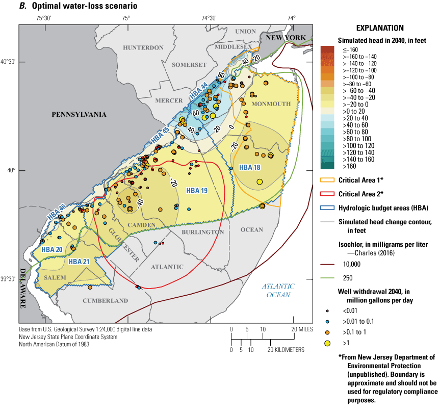
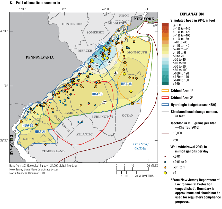
Maps showing hydrologic budget areas in the middle Potomac-Raritan-Magothy aquifer and simulated potentiometric surface in 2040 for the three scenarios: A, nominal water-loss, B, optimal water-loss, and C, full allocation.
Figure 63A shows the simulated drawdown for the nominal water-loss scenario in the middle PRM aquifer from the end of the base simulation in 2013 to the end of the scenario simulations in 2040. The biggest area of drawdown (greater than 10 feet) is in the center of HBA 18 in Ocean County around a cluster of wells. There are also a couple small drawdown areas on the western side of the aquifer. Much of the rest of the HBA of the aquifer is nearly unchanged or the head has recovered by a few feet. The optimal water-loss scenario is similar, although the simulated drawdown is slightly less than that of the nominal water-loss scenario (fig. 63B).
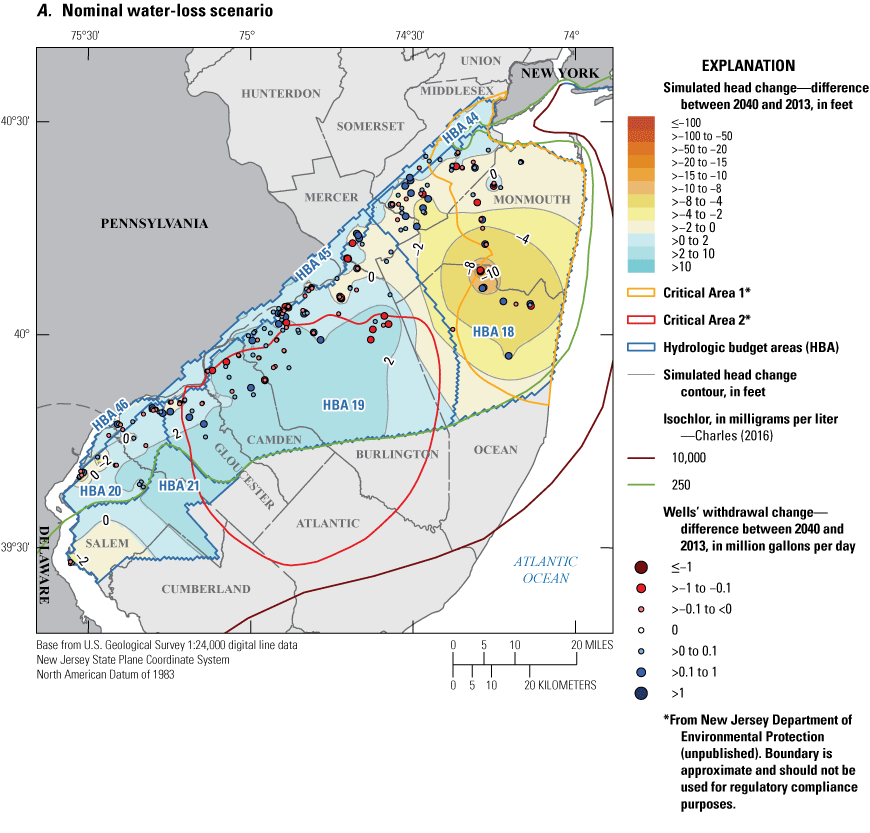
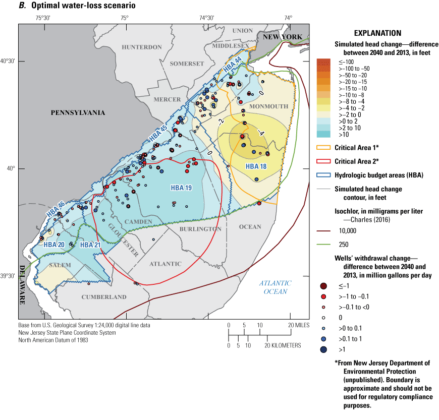
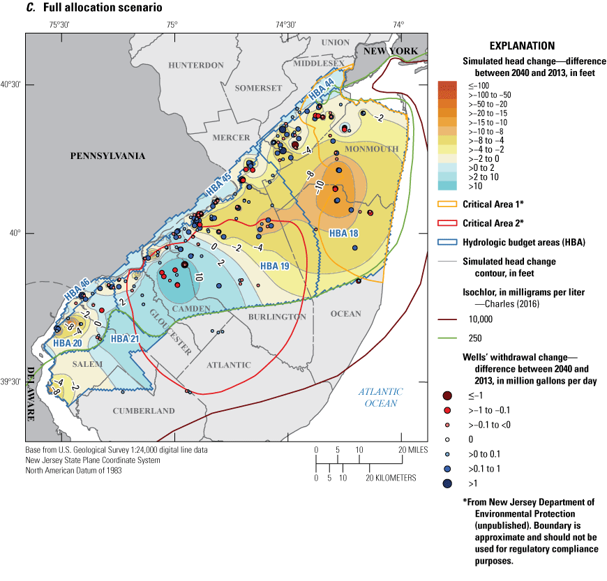
Maps showing change in simulated water levels from the end of the base simulation (2013) to the end of the scenarios (2040) in the middle Potomac-Raritan-Magothy aquifer and simulated potentiometric surface for the three scenarios: A, nominal water-loss, B, optimal water-loss, and C, full allocation.
Figure 63C shows the simulated drawdown for the full allocation scenario in the middle PRM aquifer from the end of the base simulation to the end of the scenario simulations in 2040. A large area of drawdown exists in the center of HBA 18 with the peak drawdown reaching over 15 feet. Some other areas of drawdown exist in the western part of the aquifer and along the outcrop area. A large area of recovery exists in the center of Camden County where the full allocation scenario produces lower withdrawals than that of the base simulation (fig. 61).
Budget Analysis
Figure 64 and table 46 show the budget components for HBA 18 and are discussed below. In HBA 18, the wells are the main source of outflow (82–89 percent). Other outflows include a flow to the overlying confining layers (5–6 percent), lateral flow to HBA 19 (3–4 percent) and HBA 44 (2–3 percent), and to storage (1 percent in the base simulation only). The largest source of inflow (56–57 percent) is from the overlying confining layer. Smaller amounts of lateral inflow come from the 250 mg/L isochlor (7 percent), offshore areas inside the 250 mg/L isochlor (7 percent), HBA 19 (5–7 percent), and HBA 44 (22–23 percent). The various components change in the different scenarios in the same way pumping from wells varies.
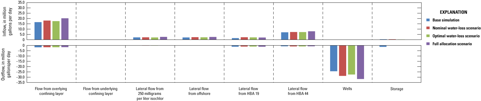
Graph showing simulated flow rates for the middle Potomac-Raritan-Magothy (PRM) aquifer, hydrologic budget area (HBA) 18.
Table 46.
Flow budget of the middle Potomac-Raritan-Magothy aquifer, hydrologic budget area (HBA) 18.[mg/L, milligram per liter; Mgal/d, million gallons per day; %, percent of total]
Figure 65 and table 47 show the budget components for HBA 19 and are discussed below. The outflow in HBA 19 is mostly split between flow to wells (40–50 percent) and flow to the underlying aquifer (38–43 percent). For the base simulation, there is an outflow component of water going to storage (13 percent). The largest source of inflow (52–56 percent) is lateral flow from the unconfined HBA 45, followed by leakage from the overlying confining layer (28–30 percent). There is some inflow (5–6 percent) from the 250 mg/L isochlor which could locally affect water quality in the wells. There are some small amounts (less than 3 percent) of flow exchange (both inflow and outflow) with HBA 18, HBA 20, and HBA 21 (which is beyond the 250 mg/L isochlor).
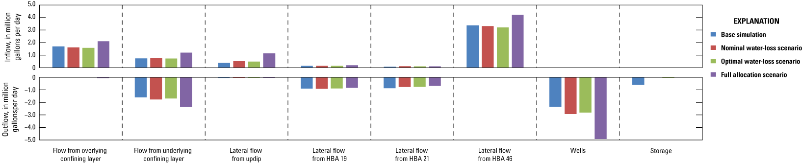
Graph showing simulated flow rates for the middle Potomac-Raritan-Magothy (PRM) aquifer, hydrologic budget area (HBA) 19.
Table 47.
Flow budget of the middle Potomac-Raritan-Magothy aquifer, hydrologic budget area (HBA) 19.[mg/L, milligram per liter; Mgal/d, million gallons per day; %, percent of total]
Figure 66 and table 48 show the budget components for HBA 20 and are discussed below. In HBA 20, the largest outflow (37–55 percent) is to the wells. Other smaller components of outflow are flow to the underlying confining layer (25–27 percent), lateral flow to HBA 19 (9–14 percent) and HBA 21 (8–14 percent), and to storage (9 percent in the base simulation only). The main source of inflow (47–53 percent) is from the unconfined HBA 46 and flow from the overlying confining layer (24–26 percent). Some of the inflow also comes from the underlying confining layer (11–13 percent) and lateral flow from updip (6–13 percent), which in this case is from the portions of the aquifer in Pennsylvania.
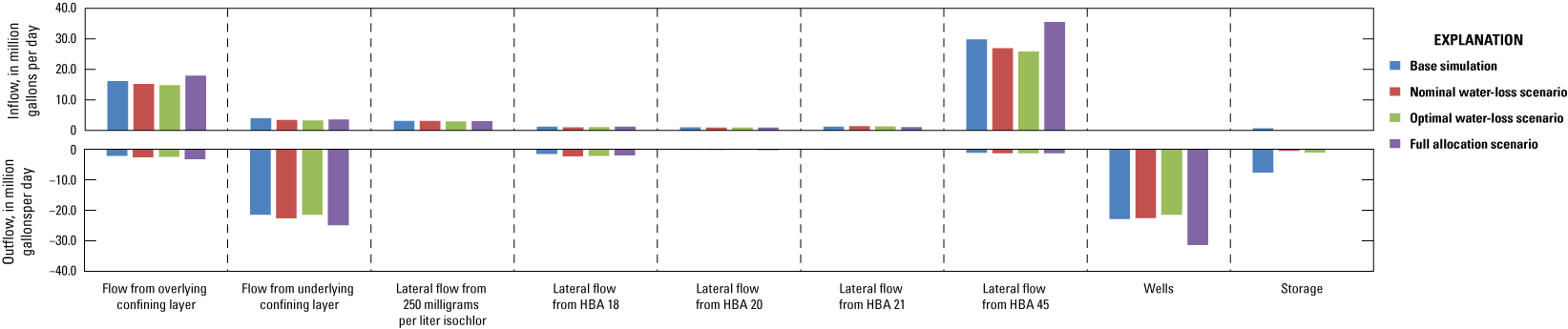
Graph showing simulated flow rates for the middle Potomac-Raritan-Magothy (PRM) aquifer, hydrologic budget area (HBA) 20.
Table 48.
Flow budget of the middle Potomac-Raritan-Magothy aquifer, hydrologic budget area (HBA) 20.[Mgal/d, million gallons per day; %, percent of total]
Figure 67 and table 49 show the budget components for HBA 21 and are discussed below. In HBA 21, the largest outflow (42–56 percent) is to HBA 19. Other outflows are flow to the pumping wells (18–27 percent), lateral flow to the 250 mg/L isochlor (9–10 percent), and flow to storage (4–20 percent). In the full allocation scenario, flow moves up through the confining layer to the overlying aquifer. The largest source of inflow (46–57 percent) to the budget area is lateral flow from the 250 mg/L isochlor (note that HBA 21 is outside the isochlor). The next largest component of inflow (26–33 percent) is flow from HBA 20, followed by flow from the underlying (3–7 percent) and the overlying (5–6 percent) confining layer, and lateral flow from HBA 19 (3–5 percent).
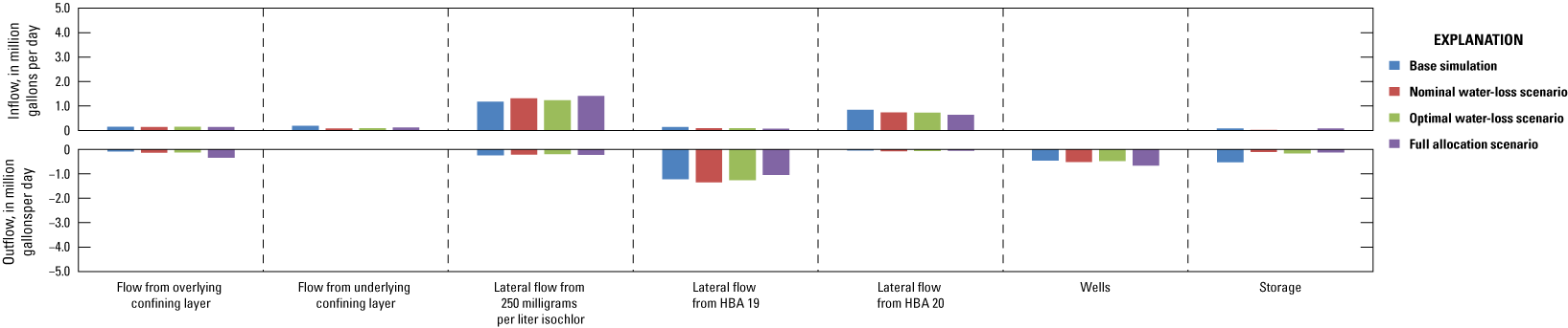
Graph showing simulated flow rates for the middle Potomac-Raritan-Magothy (PRM) aquifer, hydrologic budget area (HBA) 21.
Table 49.
Flow budget of the middle Potomac-Raritan-Magothy aquifer, hydrologic budget area (HBA) 21.[mg/L, milligram per liter; Mgal/d, million gallons per day; %, percent of total]
In the unconfined budget areas in the middle PRM (HBA 44, HBA 45, and HBA 46), the main source of inflow (66–96 percent) is from recharge (fig. 68, table 50; fig. 69, table 51; fig. 70, table 52). In HBA 45, there is some inflow (21–32 percent) that enters through leakage from the Delaware River. In HBA 44, outflow is mainly to the streams (76–78 percent) with a smaller amount (20–22 percent) going into HBA 18. In HBA 45, there are multiple outflows: flow to streams (20–25 percent), the river (24–31 percent), and wells (5–7 percent), lateral flow to HBA 19 (28–33 percent), and flow to the underlying aquifer (10–16 percent). HBA 46 also has multiple outflows: leakage to the Delaware River (30–38 percent), flow to streams (18–27 percent) and wells (7–15 percent), lateral flow to HBA 20 (20–25 percent), and flow to the underlying confining layer (9–12 percent).
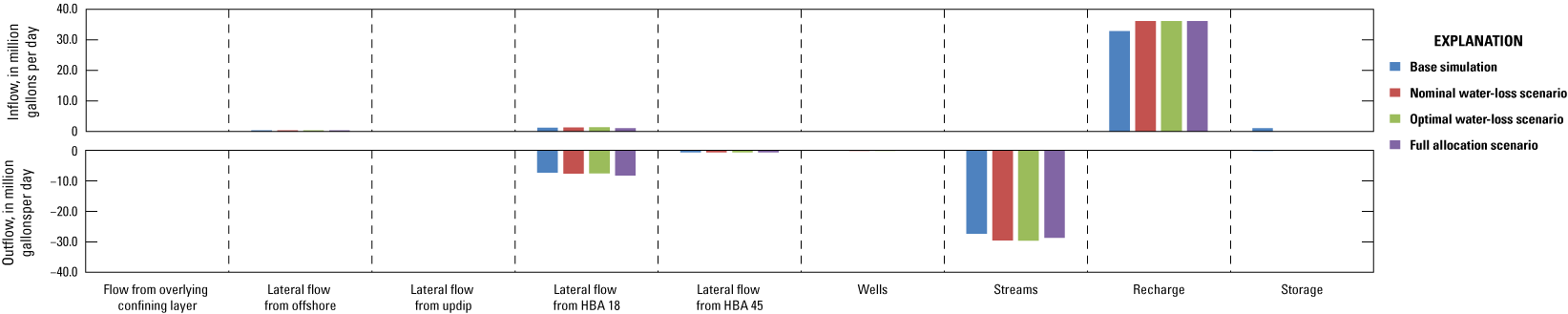
Graph showing simulated flow rates for the middle Potomac-Raritan-Magothy (PRM) aquifer, hydrologic budget area (HBA) 44.
Table 50.
Flow budget of the middle Potomac-Raritan-Magothy aquifer, hydrologic budget area (HBA) 44.[Flow from the underlying confining layer and lateral flow from the 250-milligram-per-liter isochlor are not shown because they made up less than 0.1 percent of total flow in each scenario. Mgal/d, million gallons per day; %, percent of total]
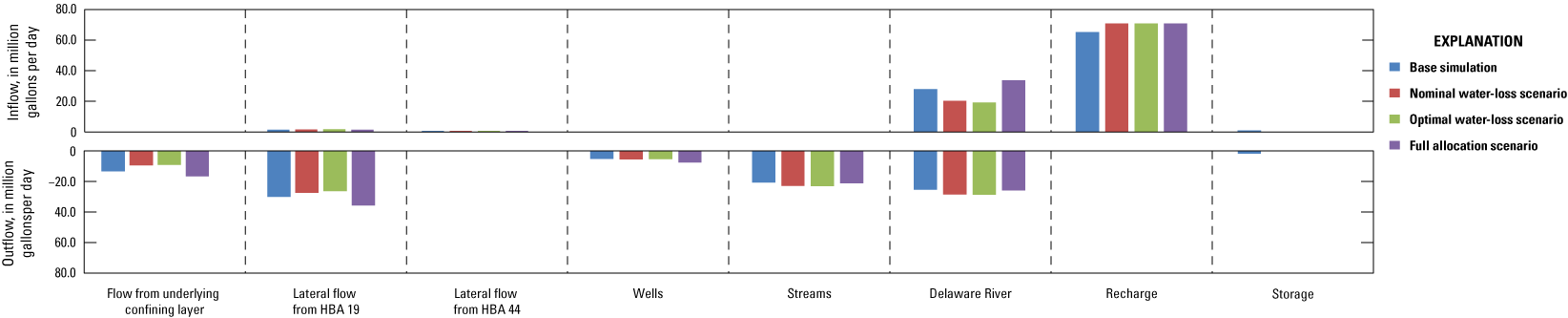
Graph showing simulated flow rates for the middle Potomac-Raritan-Magothy (PRM) aquifer, hydrologic budget area (HBA) 45.
Table 51.
Flow budget of the middle Potomac-Raritan-Magothy aquifer, hydrologic budget area (HBA) 45.[Flow from the overlying confining layer and lateral flow from HBA 46 are not shown because they made up less than 0.1 percent of total flow in each scenario. Mgal/d, million gallons per day; %, percent of total]
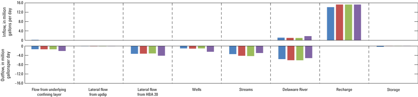
Graph showing simulated flow rates for the middle Potomac-Raritan-Magothy (PRM) aquifer, hydrologic budget area (HBA) 46.
Table 52.
Flow budget of the middle Potomac-Raritan-Magothy aquifer, hydrologic budget area (HBA) 46.[Flow from the overlying confining layer and lateral flow from HBA 45 are not shown because they made up less than 0.1 percent of the total flow in each scenario. Mgal/d, million gallons per day; %, percent of total]
Lower Potomac-Raritan-Magothy Aquifer
The study used three confined budget areas (HBAs 22–24) in the lower PRM aquifer. The outcrop area for the lower PRM is in Pennsylvania, so there are no unconfined budget areas delineated. HBA 22 included the area of the lower PRM aquifer that was part of the Critical Area 2 restrictions. There were 77 wells included in HBA 22. HBA 23, is beyond the 250 mg/L isochlor and includes 6 wells. HBA 24 was defined as a small area along the Delaware River on the west end of the aquifer that included 2 pumping wells in the simulations.
Trends of Withdrawals and Heads
Figure 71 shows withdrawal trends and trends of median, 10th percentile, and minimum heads from the base simulation and withdrawal scenarios for each budget area in the lower PRM aquifer. Table 31 shows a summary of the past and projected withdrawals in each budget area.
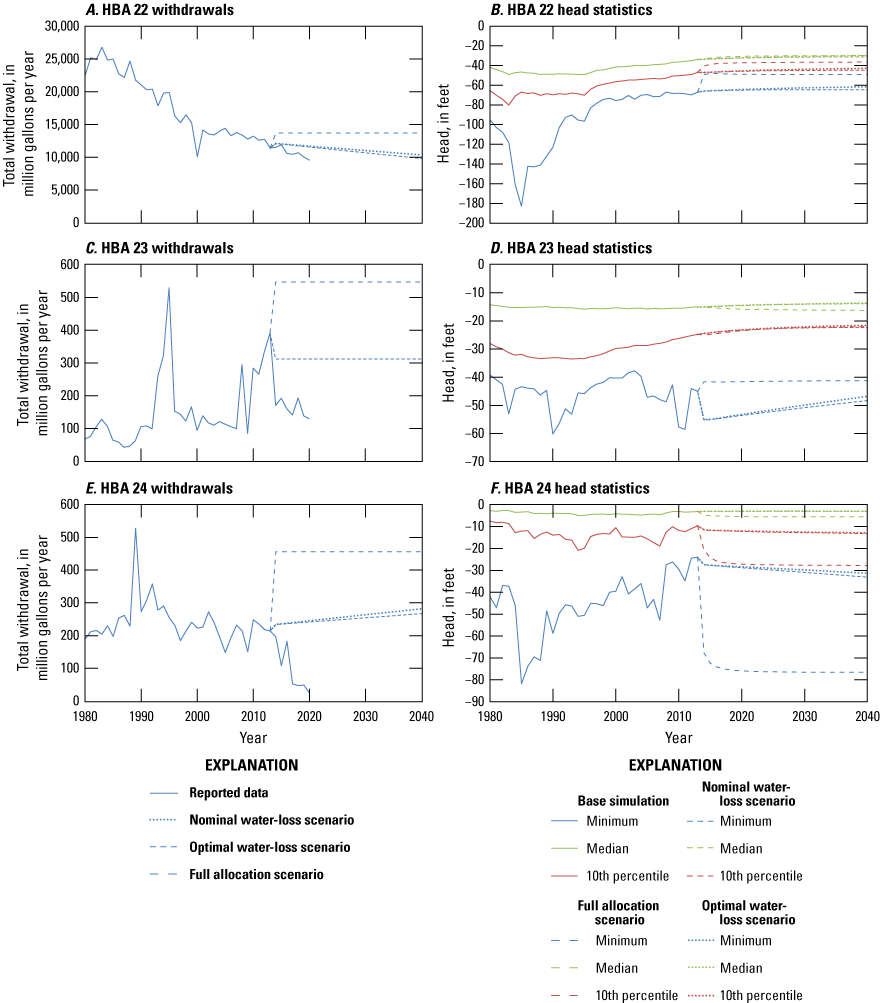
Line graphs showing withdrawals and median, 10th percentile, and minimum heads for model cells over time in hydrologic budget areas (HBA) in lower Potomac-Raritan-Magothy aquifer: A, withdrawals in HBA 22, B, head statistics in HBA 22, C, withdrawals in HBA 23, D, head statistics in HBA 23, E, withdrawals in HBA 24, and F, head statistics in HBA 24.
The withdrawals in HBA 22 decline after the first few years of the base simulation with some annual variability around the general trend (fig. 71A). The pumping rates in 2013 (around 12,500 million gallons per year) were less than half of the peak pumping rate from the 1980s (over 27,000 million gallons per year). The nominal (14.5 percent) and optimal (18.9 percent) water-loss scenarios project continued declines in pumping (table 31). Reported pumping in HBA 22 after 2013 also shows continuing declines at a rate even higher than that of the scenarios. The full allocation scenario indicates a relatively small increase in pumping of 20 percent (table 31).
The withdrawals in HBA 23, though fairly small, trend upward throughout the base simulation with a spike in the mid-1990s and a smaller one near the end of the simulation (fig. 71B). The projected withdrawals in HBA 23 are constant in the scenarios. In the nominal and optimal water-loss scenarios the withdrawals are 20.4 percent lower and in the full allocation scenario they are 39.6 percent higher compared to the 2013 withdrawals. The reported withdrawals since the end of the base simulation in 2013 show a decline (table 31).
The level of withdrawals in HBA 24 are not much different at the beginning and the end of the base simulations, though there is some variability from year-to-year over that time period (fig. 71C). Withdrawals are projected to increase in all three scenarios. The increase is linear in the nominal (20.2 percent) and optimal (14.2 percent) water-loss scenarios, and a step increase of 112.8 percent in the full allocation scenario (table 31).
The simulated heads in HBA 22 generally increase over the base simulation (fig. 71B). There is a brief period of declining head at the start of the base simulation, especially in the minimum head where the decline was close to 90 feet (fig. 71B). After the initial decline, the minimum head recovers steeply from 1985 until approximately 2000, then continues to recover more gradually. The head statistics for the scenarios are simulated to be rising slightly. The exception to this is the 10th percentile and minimum heads for the full allocation scenario, during which the heads increase by tens of feet at the beginning of the simulation. This indicates that, in areas with the lowest heads, the withdrawal levels used in the full allocation scenario were lower than the withdrawal levels used in the base simulation and the other two scenarios. Table 53 shows that there are cases of substantial drawdown in HBA 22 reaching a maximum drawdown of 22.6 feet. The median drawdown is negative for the full allocation scenario indicating head recovery over most of the area; 64 percent of the area had heads which increases by more than a foot (table 53).
Table 53.
Statistics for simulated drawdown from the end of 2013 through 2040 for hydrologic budget areas in the lower Potomac-Raritan-Magothy aquifer.The median head in HBA 23 is fairly constant throughout the base simulation (fig. 71D). The median head is simulated to increase slightly for the nominal and optimal water-loss scenarios. The 10th percentile heads initially decline then increase through the base simulation and all three scenarios. There is no discernable trend in the minimum head, however, it is much more variable than the median and 10th percentile heads because of changes in withdrawals from individual wells. In the full allocation scenario, there is some recovery in the minimum head mainly in the first stress period of the model, after which the minimum head is nearly constant. For the nominal and optimal water-loss scenarios, there is an initial decrease of about 10 feet and then a linear recovery in the minimum heads, reaching 7 and 8 feet in the nominal and optimal water-loss scenarios respectively. Although there are recoveries in head in the areas with the lowest heads, other parts of the budget areas experience drawdown in all three scenarios with maximum values of 3.3 feet for the nominal water-loss scenario, 1.8 feet for the optimal water-loss scenario, and 23.1 feet for the full allocation scenario (table 54).
For HBA 24, the median values of simulated head are generally flat throughout the period of the base simulation and the three scenarios (fig. 71C). The 10th percentile heads decline over the first part of the base simulation and then increase over the second half; the magnitude of these changes is fairly small. The minimum heads show more variability over the base simulation including a large downward spike in the mid-1980s, followed by a general increase in the minimum head. The nominal and optimal water-loss scenarios indicate there is a slight decline of a few feet in the minimum head over the length of the simulations. The full allocation scenario indicates a large decrease in the minimum head of 50 feet. Table 53 shows the maximum drawdown for the scenarios as 9.1 feet for the nominal water-loss scenario, 7.6 feet for the optimal water-loss scenario, and 55.2 feet for the full allocation scenario. Unlike the other two HBAs in the lower PRM aquifer, there are no cells where the heads are recovering by more than one foot for any of the three scenarios (table 53).
Simulated Heads and Drawdown in 2040
In the lower PRM aquifer, the head distribution is similar between the three scenarios with the heads in the eastern part of the aquifer lower than those in the west (fig. 72). The highest heads are along the Delaware River. The nominal and optimal water-loss scenarios produce a cone of depression along the border of Camden and Burlington Counties that does not appear in the full allocation scenario, indicating that projected pumping in those two scenarios is higher than full allocation scenario in some.
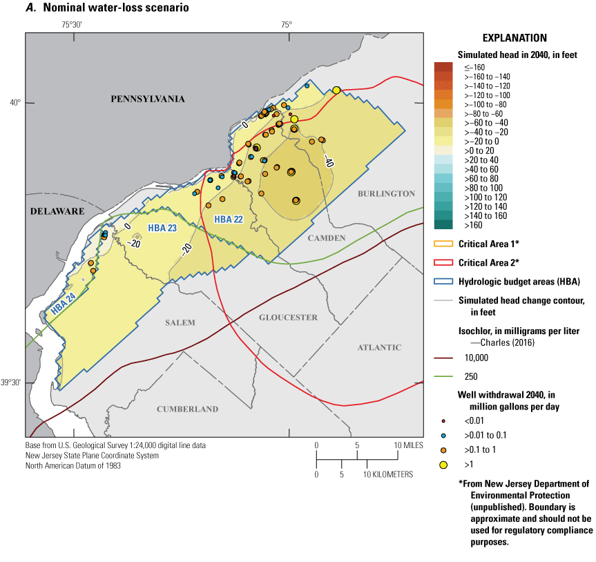
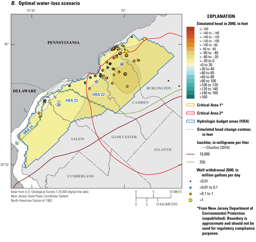
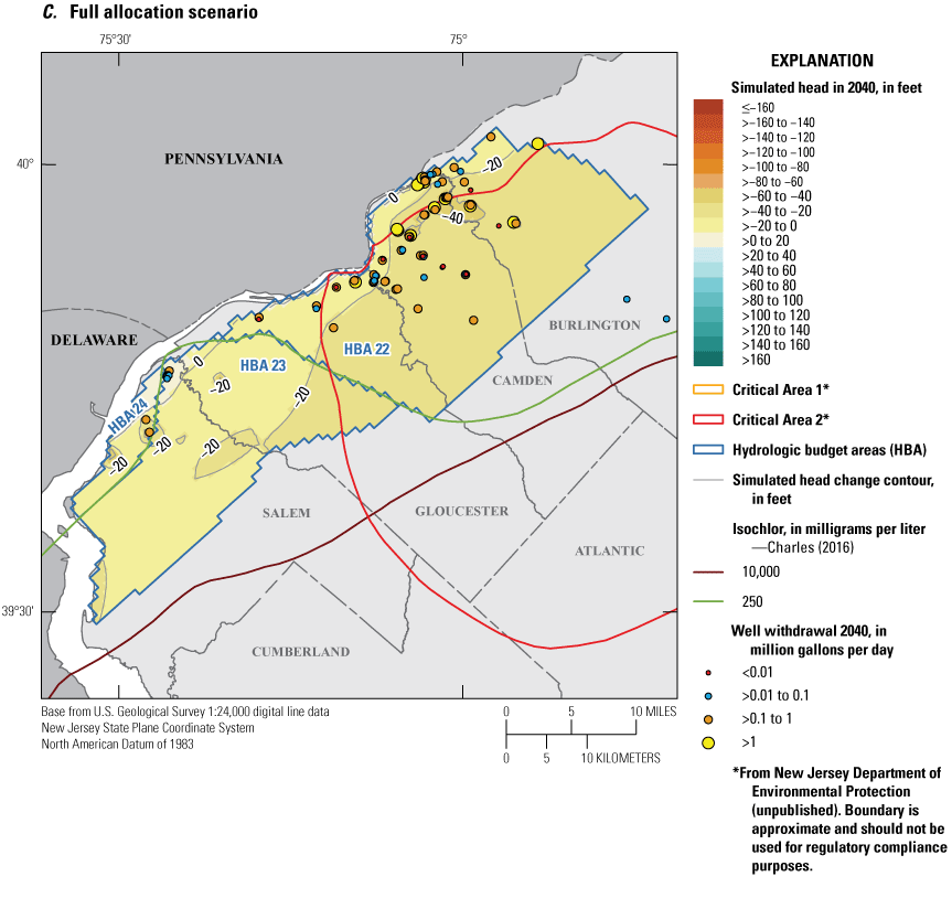
Maps showing hydrologic budget areas in the lower Potomac-Raritan-Magothy aquifer and simulated potentiometric surface in 2040 for the three scenarios: A, nominal water-loss, B, optimal water-loss, and C, full allocation.
Figure 73A and figure 73B show the head change for the nominal and optimal water-loss scenario in the lower PRM aquifer from the end of the base simulation to the end of the scenario simulations in 2040. These two scenarios show similar patterns. Apart from a couple areas in HBA 24 where there are small drawdowns around wells, the heads remain the same or recover because of previous decreases in pumping.

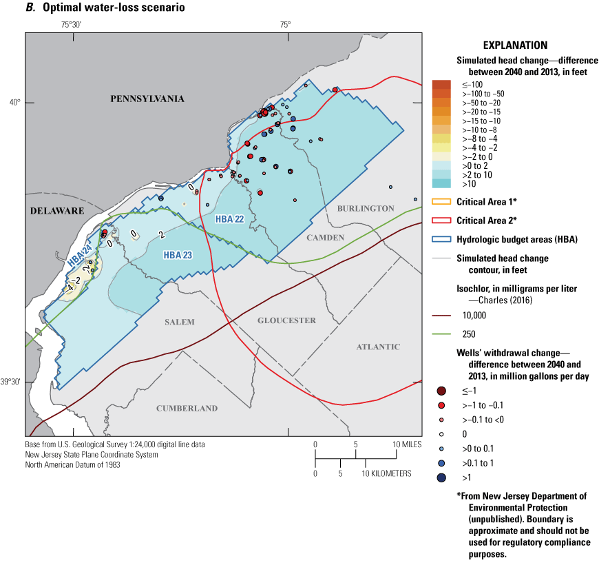
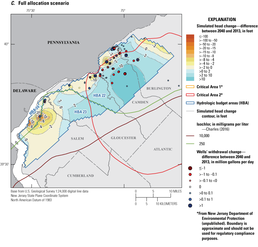
Maps showing change in simulated water levels from the end of the base simulation (2013) to the end of the scenarios (2040) in the lower Potomac-Raritan-Magothy aquifer and simulated potentiometric surface for the three scenarios: A, nominal water-loss, B, optimal water-loss, and C, full allocation.
Figure 73C shows the simulated drawdown for the full allocation scenario in the lower PRM aquifer from the end of the base simulation to the end of the scenario simulations in 2040. There is a substantial area of head recovery in the central to eastern part of the aquifer. Near some of the wells along the river there are drawdowns greater than 20 feet. The drawdown in HBA 24 reaches 50 feet for one of the wells and extends into HBA 23, which is beyond the 250 mg/L isochlor, indicating potential for water quality problems if pumping at full allocation is reached in this area.
Budget Analysis
Figure 74 and table 54 show the budget components for HBA 22 and are discussed below. The inflow in HBA 22 almost entirely comes from the overlying confining layer (96–97 percent). The outflow is mostly to the wells (87–90 percent). The other components of outflow are minimal (less than 2 percent) except for some flow to the overlying confining layer (10–12 percent). Although the flows are small compared to the overall budget of HBA 22, the lateral inflow from the 250 mg/L isochlor and HBA 23 (which is beyond the isochlor) are noteworthy in that they represent what could be degraded water quality and could be important if wells are located close to those boundaries. The flows in the optimal and nominal water-loss scenarios are less than the base simulation and the flows in the full allocation scenario are considerably higher than the base simulation.
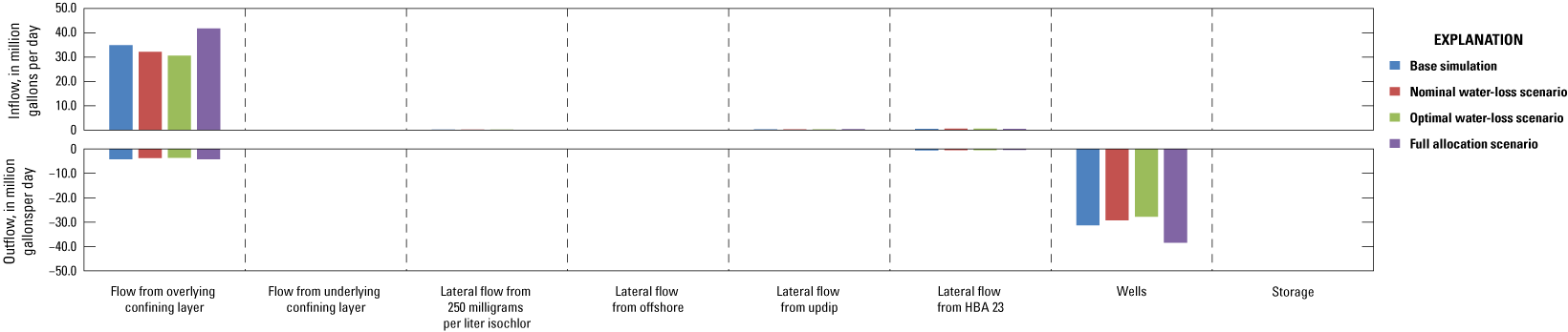
Graph showing simulated flow rates for the lower Potomac-Raritan-Magothy (PRM) aquifer, hydrologic budget area (HBA) 22.
Table 54.
Flow budget of the lower Potomac-Raritan-Magothy aquifer, hydrologic budget area (HBA) 22.[mg/L, milligram per liter; Mgal/d, million gallons per day; %, percent of total]
Figure 75 and table 55 show the budget components for HBA 23 and are discussed below. The primary source of inflow in HBA 23 is from the overlying confining layer (75–85 percent); smaller amounts come from lateral flow from HBA 22 (12–20 percent) and the 250 mg/L isochlor (3–5 percent). The main outflow is to wells (41–58 percent), however there is also lateral flow to HBA 22 (18–29 percent), flow to the overlying confining layer (15–17 percent), and lateral flow to the 250 mg/L isochlor (8–16 percent). Because the entire budget area is beyond the 250 mg/L isochlor, this is also how the downdip area is classified.
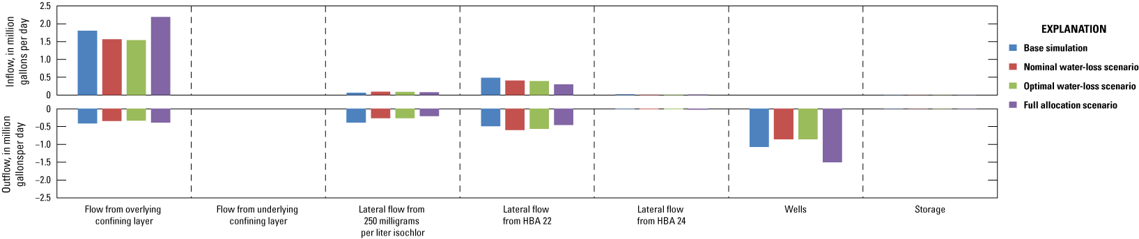
Graph showing simulated flow rates for the lower Potomac-Raritan-Magothy (PRM) aquifer, hydrologic budget area (HBA) 23.
Table 55.
Flow budget of the lower Potomac-Raritan-Magothy aquifer, hydrologic budget area (HBA) 23.[mg/L, milligram per liter; Mgal/d, million gallons per day; %, percent of total]
Figure 76 and table 56 show the budget components for HBA 24 and are discussed below. The primary inflow (90–93 percent) to HBA 24 is from the overlying confining layer. There is also a small component of the inflow that is classified as lateral flow from updip (6–8 percent) which in this case is from the aquifer in Pennsylvania. The outflow in HBA 24 is primarily to pumping wells (88–90 percent). There is also outflow to the overlying confining unit (6–10 percent). The projected pumping values and corresponding leakage through the overlying confining layer are smallest in the base simulation and largest in the full allocation scenario.
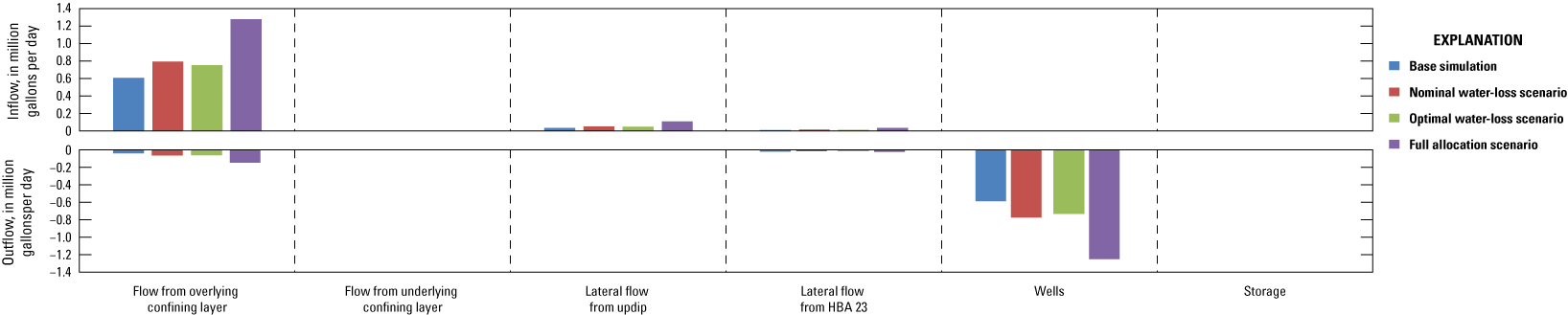
Graph showing simulated flow rates for the lower Potomac-Raritan-Magothy (PRM) aquifer, hydrologic budget area (HBA) 24.
Table 56.
Flow budget of the lower Potomac-Raritan-Magothy aquifer, hydrologic budget area (HBA) 24.[Mgal/d, million gallons per day; %, percent of total]
Comparison of Conditions in Confined Aquifers
One way to compare how stressed the conditions are in the various aquifers is to analyze the number of cells in the confined aquifers where the head is less than sea level. The lowest head boundary conditions for these confined aquifers are the Atlantic Ocean, Delaware Bay, and the Delaware River, all of which can be thought of as constant heads at or near sea level, were represented as zero feet in the model. Under natural conditions with no pumping, the heads in the aquifers are above zero with water flowing out to these features or streams with higher heads in the unconfined parts of the system. When water is withdrawn by wells, the head in wells must be lowered in a way that water will flow to the well. The more water that is withdrawn, the lower the head needs to be; the magnitude of drawdown needed to get a given amount of flow depends on the properties of the aquifer.
Box plots are presented to depict the distribution of head and drawdown in the confined aquifers to facilitate the comparison discussed above. The box plots are constructed using the simulated values for each cell in an HBA for each confined aquifer. The cells are the same size within the parts of the model domain where HBAs are defined so the distributions depicted can be thought of as area. For example, the median shown in the box plot is the value that half of the confined aquifer has a value above and half has a value below.
Figure 77 shows box plots that represent the distribution of simulated heads in each of the nine confined aquifers in the model where the HBA are defined. The Vincentown aquifer is the only confined aquifer where the median simulated head is greater than zero for all three scenarios (fig. 77D). For the Wenonah-Mount Laurel aquifer and the Englishtown aquifer system, the median simulated head goes below zero for the full allocation scenario only (figs. 77E, 77F). Only the Piney Point aquifer has an upper quartile line (representing the 75th percentile of head) that is greater than zero (fig. 77C). The minimum simulated head, represented in figure 77 either by the lower cap of the whisker or the lowest outlier, is less than −100 feet for at least one scenario in all but the middle and lower PRM aquifers (figs. 77H, 77I). Although generally the heads are highest in the Vincentown aquifer, the minimum simulated head also occurs in this aquifer for all three scenarios (fig. 77D). Apart from a few outliers in the Rio Grande water-bearing zone, all the simulated heads in that unit and the lower PRM aquifer are near zero feet or below (figs. 77A, 77I).
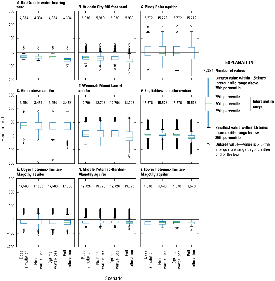
Boxplots of the statistical distribution of simulated heads in model cells for the confined aquifers where hydrologic budget areas are defined for the base simulation and the three water use scenarios: A, Rio Grande water-bearing zone, B, Atlantic City 800-foot sand, C, Piney Point aquifer, D, Vincentown aquifer, E, Wenonah-Mount Laurel aquifer, F, Englishtown aquifer system, and the, G, upper, H, middle, and I, lower Potomac-Raritan-Magothy aquifers.
Figure 78 shows boxplots of 2040 drawdown (calculated as the head in 2040 subtracted from the head in 2013) simulated in each model cell in the confined HBA. The most extensive areas of large drawdowns are for the full allocation scenario in the Rio Grande water-bearing zone, the Atlantic City 800-foot sand, the Piney Point aquifer, and the Englishtown aquifer system where all the median drawdowns are greater than 20 feet.
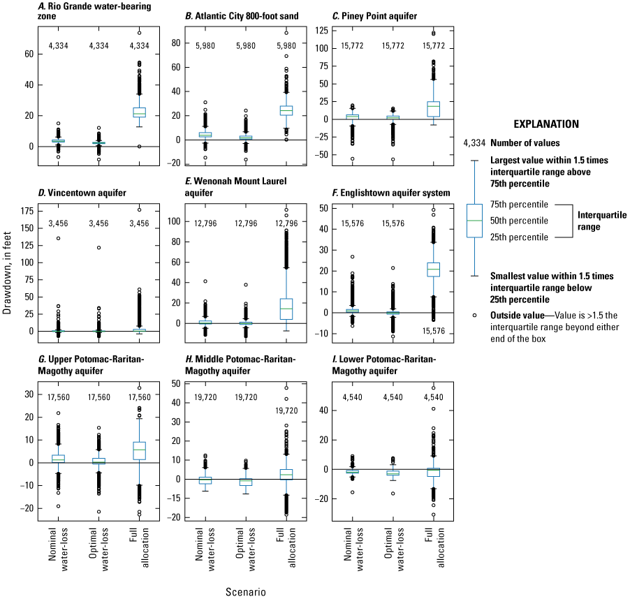
Boxplots showing the statistical distribution of simulated drawdown (head decrease from the end of 2013 through 2040) in model cells for the confined aquifers where hydrologic budget areas are defined for the three water use scenarios: A, Rio Grande water-bearing zone; B, Atlantic City 800-foot sand; C, Piney Point aquifer; D, Vincentown aquifer; E, Wenonah-Mount Laurel aquifer; F, Englishtown aquifer system; and the, G, upper, H, middle, and, I, lower Potomac-Raritan-Magothy aquifers.
For the nominal and optimal water-loss scenarios, most of the cells as represented by the boxes in figure 78 are fairly close to zero, indicating that there are no new large areas of significant drawdown by 2040. However, all the aquifers have at least some cells with greater than 10 feet of drawdown under these scenarios. There is a single cell which extends past 100 feet of drawdown in the Vincentown aquifer (fig. 78D). As expected, the drawdown is always slightly less for the optimal water-loss scenario, where less water is required to be pumped.
All the aquifers show at least some areas of head recovery as indicated by negative values in figure 78. Most of the biggest recoveries are seen in cells classified as outliers, although in the middle and lower PRM aquifers, almost the entire box falls below zero for the nominal and optimal water-loss scenarios indicating that greater than 75 percent of the model cells are simulated to have recovering heads.
Water Movement Between Confined and Unconfined Aquifers in HUC11 Basins
The water exchange between confined and unconfined parts of the system was quantified in HUC11 basins that had at least some area active in the New Jersey part of the models. The components of simulated flow that were quantified included recharge, flow to the confined aquifers, flow from the confined aquifers, the net flow to or from the confined aquifers, and the total, unconfined, and confined pumping amounts. A table of these results appears in the companion data release to this report (Kenefic and Kauffman, 2024).
Although the confining units included in the NJCP base simulation each have a model layer associated with them, in places the combination of the vertical hydraulic conductivity and layer thickness are such that they do not act as confining layers. This is especially the case in the unconfined Kirkwood-Cohansey aquifer system where the confining units are absent, but the layer must be continuous in the model. Because of this, and to maintain consistency for all aquifers and confining units, a criterion was developed to define where the aquifers are confined versus unconfined. The first condition used to determine whether a confining unit is effective in confining the aquifer below was if the aquifer below a confining unit has a head that was greater than one foot different than the aquifer above it. The second condition was a vertical conductance (computed as the vertical hydraulic conductivity divided by the thickness) in the confining units was less than 10-9 second-1. If the confining unit was considered effective by either of these conditions, then any underlying aquifers were considered to be confined. Figure 79 shows the uppermost model layer that forms an effective confining unit determined by this procedure.
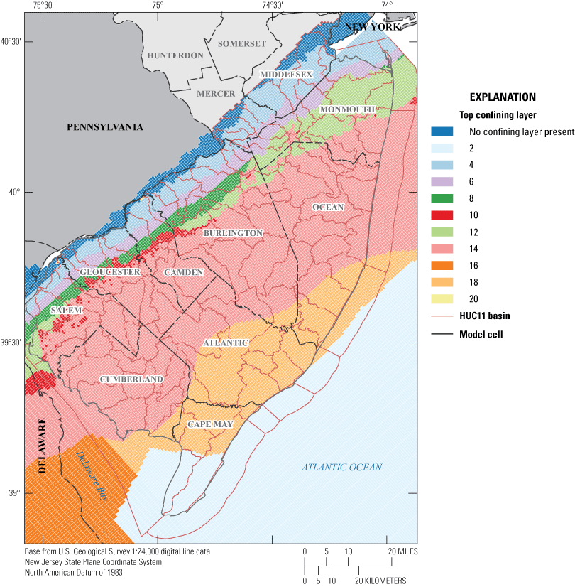
Map showing the topmost effective confining layer in the New Jersey Coastal Plain (NJCP) model.
Figure 80A shows the pumping in confined aquifers by HUC11 basin for the base simulation. The basins with the highest amounts of pumping are generally those along the Delaware River and along the Atlantic Ocean coast. The area in between, with less (compared to the coastal basins) or no pumping from confined aquifers, is where the Kirkwood-Cohansey aquifer system is the main source of groundwater.
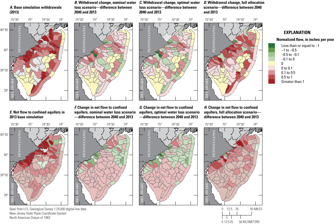
Summary of selected simulated flows for hydrologic unit code 11 (HUC11) basins. Simulated results include, A, pumping in the confined aquifers for the base simulation; change in confined pumping for, B, the nominal well loss scenario, C, the optimal well loss scenario, and D, the full allocation scenario; E, net flow from the unconfined to confined part of the system; and change in the net flow from the unconfined to confined parts of the system for, F, the nominal well loss scenario, G, the optimal well loss scenario, and H, the full allocation scenario.
Figure 80B shows how pumping from these confined aquifers changes, revealing no strong relationship between increases in pumping and location; the optimal water-loss scenario has a similarly weak spatial pattern (fig. 80C). As expected, there are substantial increases (greater than 0.5 inches per year) in the full allocation scenario largely corresponding to the basins with the highest pumping in the base simulation (fig. 80D).
The net flow moving from the unconfined to the confined aquifers are largest in the HUC11 basins along the Delaware River (fig. 80E). These are areas where there are large amounts of pumping in the confined aquifers and near the outcrop areas where the confining units are thinnest. In contrast, near the Atlantic Coast, although the net flow is generally downward, it is more spread out and not concentrated in the areas with the most confined-aquifer pumping. The confining units are generally thicker in this area compared to the area along the Delaware River.
The change in net flow from unconfined to confined is very similar between the nominal and optimal water-loss scenarios (fig. 80F). Many of the basins where the net flow is less in those two scenarios are at least in part in the two Critical Area restriction zones. In the full allocation scenario, all but a few basins on the edges show an increase in the net flow going from the unconfined to confined parts of the system (fig. 80H). The magnitude of the increases is largest in the basins along the Delaware River where magnitudes are high to begin with and also have large pumping increases. The large increases in confined-aquifer pumping in HUC11 basins along the Atlantic Coast do not correspond directly to large changes in the net flow from the unconfined to confined parts of the system, reflecting the more confined nature of that part of the system.
Limitations
The simulated scenarios presented in this report are based on the base simulation and the results are dependent on the conceptualization and framework on which that model was constructed (see the model limitation section in Gordon and Carleton [2023]). An average value was used for recharge throughout the scenario period; trends of heads in recharge areas (and nearby) are likely reflecting the difference between the average value and lower values in the last two stress periods of the base simulation. The boundary between unconfined and confined HBAs are retained from Gordon (2007) and are based on the outcrop areas of the formations; areas in the confined HBA just downdip of the unconfined HBA may be only weakly confined. As a result, recharge above thin parts of the confining layers moves through the confining layer into the confined HBA and then right back out laterally to the unconfined HBA. Using a criteria to define where the confining unit is effective would result in smaller budget components of leakage from the confining layer and out to the unconfined HBA compared to the approach that was used.
Summary and Conclusions
The New Jersey State Water Supply Plan is developed by the New Jersey Department of Environmental Projection (NJDEP) for assessing the State’s water-supply resources. The NJDEP is currently (2023) revising the plan. Forty-four hydrologic-budget areas (HBAs) in the confined aquifers and their unconfined outcrop areas were delineated by approximating boundaries based on various hydrologic, geohydrologic, and withdrawal conditions, such as aquifer extents, location of the 250 milligrams-per-liter isochlor (line of equal chloride concentration), aquifer outcrops, groundwater divides, and areas of large groundwater withdrawals.
A recently released groundwater flow model described by Gordon and Carleton (2023) was used to simulate groundwater flow in the New Jersey Coastal Plain (NJCP) for the period of 1980–2013. The conditions at the end of that simulation were used as a base for comparison and as an initial condition for simulation of three water-use scenarios of withdrawals from 2014 to 2040. Two scenarios were based on work done at Rutgers University (Van Abs and others, 2018) and project pumping at wells based on projected population trends and assumptions based on water conservation principles. The two modeled scenarios differed in how much water loss, or the difference between the quantity of water that is produced at wells and the quantity delivered to customers, was assumed. The nominal water-loss scenario was based on all systems achieving the current median reported water loss for public community water supply systems. The optimal water-loss scenario was based on all systems achieving roughly the same water loss as the current best performing systems. A third simulated scenario assumed water is withdrawn at the full allocation level of each well.
Comparing to the withdrawals in the first stress period of the scenario simulations in 2014, the optimal water-loss scenario projected a 1.3 percent decrease in withdrawals and the nominal water-loss scenario projected a 2.9 percent increase in withdrawals by the year 2040. These amounts are within the range of variability that was seen throughout the period of the base simulation. For individual aquifers, the biggest projected increases in withdrawals by percent were in the Vincentown (15.5 percent) and upper Potomac-Raritan-Magothy (PRM; 9.1 percent) aquifers. The two aquifers with the biggest projected decline in withdrawals by percent were the lower PRM (−13.5 percent) and Piney Point (−10.5 percent) aquifers, continuing trends that have been seen in data reported between 2014 and 2020. The nominal and optimal water-loss scenarios were closest to full allocation levels in the Atlantic City 800-foot sand and the upper, middle, and lower PRM aquifers, reaching 60–75 percent of full allocation withdrawals. The lowest nominal and optimal water-loss scenario withdrawals compared to the full allocation withdrawals were in the unconfined Kirkwood-Cohansey aquifer system and the Holly Beach aquifer along with the little used Rio Grande water-bearing zone (7–36 percent of the full allocation withdrawals).
For the nine confined aquifers in the NJCP, heads are generally higher along the unconfined and outcrop areas decreasing downdip and towards pumping centers. All the aquifers have areas with simulated heads below sea level—many of them throughout most of the extent of the aquifer.
Of the three scenarios, the drawdowns are most extreme in the full allocation scenario. There are large areas of head decline greater than 20 feet at the end of the full allocation simulation in 2040 in 5 of the 9 confined aquifers. The exceptions are the Vincentown, which does have some areas of large drawdown in the vicinity of wells, and the three PRM aquifers. Restrictions imposed by the Critical Area regulations are likely the reason why the PRM aquifers do not have large areas of drawdown. The nominal and optimal water-loss scenarios have some areas of head declines, though the magnitude of most of these declines are less than 15 feet. The simulation of these scenarios shows some extensive areas of head recovery, as well, especially in the aquifers that are regulated by the Critical Area restrictions.
Budgets of inflow and outflow components were calculated for 44 (27 confined, 17 unconfined) HBAs. The budget analysis shows that the water movement is complex and varies based on the aquifer geometry and location of pumping wells. Some common features include the following:
-
• Increased flows from offshore areas in the aquifers without outcrop areas.
-
• Flow through the overlying confining layers is a main source of flow to many of the HBAs. Most of this flow happens along the boundaries of the unconfined parts of the aquifers. These HBAs tend to also have a fair amount of flow that moves laterally to adjacent unconfined HBAs.
-
• The major components of flow are recharge and flow to streams in unconfined HBAs.
Flow components between the unconfined and confined parts of the system were summarized by HUC11 basins. Withdrawals from the confined aquifers were largest in the basins along the Delaware River and the Atlantic Coast. For basins with large withdrawal amounts from the confined aquifers, the net flows through the confining units were largest in the basins along the Delaware River where the outcrop is in close proximity and the confining units are thinner compared to the basins along the Atlantic Coast where the confining units are thicker, and the water drawn into wells comes from a larger area.
References Cited
Carleton, G.B., Gordon, A.D., Kenefic, L.F., Watt, M.K., and Buxton, D.E., 2023, MODFLOW–2005 used to simulate the regional groundwater flow system in the updated New Jersey Coastal Plain model, 1980–2013: U.S. Geological Survey data release, https://doi.org/10.5066/P9W6RXFC.
Charles, E.G., 2016, Regional chloride distribution in the Northern Atlantic Coastal Plain aquifer system from Long Island, New York, to North Carolina: U.S. Geological Survey Scientific Investigations Report 2016 –5034, 37 p. [Also available at https://doi.org/10.3133/sir20165034.]
CH2M HILL, Metcalf & Eddy, Inc., and New Jersey First, Inc., 1992, New Jersey statewide water supply master plan—Task 2 report—Water supply baseline data development and analyses: New Jersey Department of Environmental Protection, prepared by CH2M HILL, Metcalf & Eddy, Inc., and New Jersey First, Inc., [variously paged; 321 p.]. [Also available at https://doi.org/doi:10.7282/T3MS3SDN.]
Gordon, A.D., 2007, Simulated effects of projected 2010 withdrawals on ground-water flow and water levels in the New Jersey Coastal Plain—A task of the New Jersey Water Supply Plan 2006 Revision: U.S. Geological Survey Scientific Investigations Report 2007–5134, 116 p. [Also available at https://doi.org/10.3133/sir20075134.]
Gordon, A.D., Carleton, G.B., and Rosman, R., 2021, Water-level conditions in the confined aquifers of the New Jersey Coastal Plain, 2013: U.S. Geological Survey Scientific Investigations Report 2019–5146, 104 p., 9 pl., at https://doi.org/10.3133/sir20195146.
Gordon, A.D., and Carleton, G.B., 2023, Updates to the Regional Groundwater-Flow Model of the New Jersey Coastal Plain, 1980–2013: U.S. Geological Survey Scientific Investigations Report 2023–5066, 117 p., at https://doi.org/10.3133/sir20235066.
Harbaugh, A.W., and McDonald, M.G., 1996, User’s documentation for MODFLOW–96, an update to the U.S. Geological Survey modular finite-difference ground-water flow model: U.S. Geological Survey Open-File Report 1996–485, 56 p. [Also available at https://doi.org/10.3133/ofr96485.]
Harbaugh, A.W., 2005, MODFLOW–2005, The U.S. Geological Survey modular ground-water model—The ground-water flow process: U.S. Geological Survey Techniques and Methods, book 6, chap. A16, [variously paged]. [Also available at https://doi.org/10.3133/tm6A16.]
Kenefic, L.F., and Kauffman, L.J., 2024, MODFLOW-2005 model used to analyze water-use scenarios in the New Jersey Coastal Plain: U.S. Geological Survey data release, at https://doi.org/10.5066/P9JHGJA5.
Lacombe, P.J., and Rosman, R., 2001, Water levels in, extent of freshwater in, and water withdrawals from ten confined aquifers, New Jersey and Delaware Coastal Plain, 1998: U.S. Geological Survey Water-Resources Investigations Report 2000–4143, 10 sheets. [Also available at https://doi.org/10.3133/wri004143.]
Leahy, P.P., 1982, A three-dimensional ground-water-flow model modified to reduce computer-memory requirements and better simulate confining-bed and aquifer pinchouts: U.S. Geological Survey Water-Resources Investigations Report 82–4023, 59 p. [Also available at https://doi.org/10.3133/wri824023.]
Martin, M., 1998, Ground-water flow in the New Jersey Coastal Plain: U.S. Geological Survey Professional Paper 1404–H, 146 p. [Also available at https://doi.org/10.3133/pp1404H.]
New Jersey Department of Environmental Protection [NJDEP], 2017, New Jersey water supply plan 2017–2022: New Jersey Department of Environmental Protection, 484 p., accessed June 2, 2023, at https://www.nj.gov/dep/trends/. [Also available at https://www.nj.gov/dep/watersupply/wsp.html.]
Shelton, T.B., 2005, Interpreting drinking water quality analysis—What do the numbers mean? (6th ed.): New Brunswick, N.J., Rutgers Cooperative Research & Extension, 68 p. [Also available at https://doi.org/10.7282/T3GF0VBR; supersedes all previous editions.]
Spitz, F.J., and DePaul, V.T., 2008, Recovery of ground-water levels from 1988 to 2003 and analysis of effects of 2003 and full-allocation withdrawals in Critical Area 2, southern New Jersey: U.S. Geological Survey Scientific Investigations Report 2008–5142, 29 p., at https://doi.org/10.3133/sir20085142.
Sun, R.J., and Johnson, R.H., 1994, Regional aquifer-system analysis program of the U.S. Geological Survey, 1978–1992: U.S. Geological Survey Circular 1099, 126 p. [Also available at https://doi.org/10.3133/cir1099.]
Trescott, P.C., 1975, Documentation of finite-difference model for simulation of three-dimensional ground-water flow: U.S. Geological Survey Open-File Report 75–438, 103 p. [Also available at https://doi.org/10.3133/ofr75438.]
Van Abs, D.J., Jiayi, D., and Pierson, E., 2018, Water needs through 2040 for New Jersey public community water supply systems: New Brunswick, NJ, New Jersey Department of Environmental Protection Division of Water Supply & Geoscience, prepared by Rutgers University. [Also available at humeco.rutgers.edu/documents_PDF/NJwaterneeds.pdf.]
Voronin, L.M., 2004, Documentation of revisions to the regional aquifer system analysis model of the New Jersey Coastal Plain: U.S. Geological Survey Water-Resources Investigations Report 2003–4268, 49 p., 1 pl. [Also available at https://doi.org/10.3133/wri034268.]
Westenbroek, S.M., Kelson, V.A., Dripps, W.R., Hunt, R.J., and Bradbury, K.R., 2010, SWB—A modified Thornthwaite-Mather soil-water-balance code for estimating groundwater recharge: U.S. Geological Survey Techniques and Methods, book 6, chap. A31, 59 p., accessed March 11, 2013, at https://doi.org/10.3133/tm6A31.
Zapecza, O.S., 1989, Hydrogeologic framework of the New Jersey Coastal Plain: U.S. Geological Survey Professional Paper 1404–B, 49 p., 24 pls. [Also available at https://doi.org/10.3133/pp1404B.]
Datums
Vertical coordinate information is referenced to the North American Vertical Datum of 1988 (NAVD 88).
Horizontal coordinate information is referenced to the North American Datum of 1983 (NAD 83).
Altitude, as used in this report, refers to distance above the vertical datum.
Supplemental Information
Concentrations of chemical constituents in water are given in milligrams per liter (mg/L).
For more information, contact
Director, New Jersey Water Science Center,
3450 Princeton Pike
Suite 110
Lawrenceville, NJ 08648
Or visit our website at https://www.usgs.gov/centers/new-jersey-water-science-center.
Publishing support provided by the Baltimore Publishing Service Center.
Disclaimers
Any use of trade, firm, or product names is for descriptive purposes only and does not imply endorsement by the U.S. Government.
Although this information product, for the most part, is in the public domain, it also may contain copyrighted materials as noted in the text. Permission to reproduce copyrighted items must be secured from the copyright owner.
Suggested Citation
Kauffman, L.J., 2024, Simulated effects of projected 2014–40 withdrawals on groundwater flow and water levels in the New Jersey Coastal Plain: U.S. Geological Survey Scientific Investigations Report 2024–5028, 149 p., https://doi.org/10.3133/sir20245028.
ISSN: 2328-0328 (online)
Study Area
| Publication type | Report |
|---|---|
| Publication Subtype | USGS Numbered Series |
| Title | Simulated effects of projected 2014–40 withdrawals on groundwater flow and water levels in the New Jersey Coastal Plain |
| Series title | Scientific Investigations Report |
| Series number | 2024-5028 |
| DOI | 10.3133/sir20245028 |
| Publication Date | May 30, 2024 |
| Year Published | 2024 |
| Language | English |
| Publisher | U.S. Geological Survey |
| Publisher location | Reston, VA |
| Contributing office(s) | New Jersey Water Science Center |
| Description | Report: x, 149 p.; Data Release |
| Country | United States |
| State | New Jersey |
| Online Only (Y/N) | Y |
| Additional Online Files (Y/N) | N |