

Evaporation From the Interior of Lake Okeechobee—A Large Freshwater Lake in Florida, 2013–16
Links
- Document: Report (2.35 MB pdf) , HTML , XML
- Data Releases:
- USGS data release - Daily evaporation rates computed using five methods at the LZ40 platform in Lake Okeechobee, Florida, December 2012 to December 2016
- USGS South Florida Information Access Data Exchange website - Evapotranspiration data download
- USGS data release - Evaporation at LZ40 platform, Lake Okeechobee, Palm Beach County, Florida, November 16, 2012 - December 31, 2019
- NGMDB Index Page: National Geologic Map Database Index Page (html)
- Download citation as: RIS | Dublin Core
Abstract
In 2012, a platform at the approximate center of Lake Okeechobee in central Florida was instrumented to continuously measure evaporation with the Bowen-ratio energy-budget method as part of a long-term partnership between the South Florida Water Management District and the U.S. Geological Survey. The primary goal for the study was to quantify daily rates of open-water evaporation. A secondary goal was to assess differences in evaporation rates among alternate methods and determine if instrumentation and operational expenses associated with the Bowen-ratio method could be reduced.
Mean annual evaporation from Lake Okeechobee for 2013–16 was about 1,825 millimeters per year. Annual evaporation from 2013 to 2016 was 1,760, 1,840, 1,810, and 1,890 millimeters per year, respectively. These evaporation rates are among the highest rates observed in Florida based on scientifically vetted methods such as evaporation pans, lysimeters, eddy-covariance, or Bowen-ratio methods. The high evaporation rates are largely a result of frequent clear-sky conditions over the interior of Lake Okeechobee, which allows solar radiation to reach the water surface and drive open-water evaporation. Cloud formation over the interior of Lake Okeechobee is suppressed because of a relatively large heat capacity for water that buffers convective fluxes of air that form clouds while rising and cooling.
Estimated evaporation rates obtained using five alternative methods were compared to measured Bowen-ratio energy-budget daily, monthly, and annual evaporation: the Penman, Priestly-Taylor, Mass-Transfer, Simple, and Turc equations. All five methods performed relatively well (within 10 percent of the Bowen ratio annual totals). The Penman, Priestley-Taylor, and Mass-Transfer methods captured relatively large evaporation rates that occurred in the winter due to cold fronts, because these methods account for large wind speeds and vapor pressure deficits associated with the regional cold fronts. For operational implementation, the Simple, Mass-Transfer, or Turc methods are likely preferable because of their simplicity, limited data requirements, and improved accuracy for computing monthly and annual evaporation totals. The Turc equation computed monthly evaporation within 8 percent of the Bowen-ratio method, while requiring only air temperature and solar radiation data. The Simple equation achieved similar accuracy while requiring only solar radiation data.
Introduction
Water levels and water quality in large, shallow lakes can be responsive to changes in climate, surrounding land use, and water management, particularly in subtropical climates that experience large precipitation events (Havens and Steinman, 2015; Philips and others, 1993). Lake Okeechobee (fig. 1), for example, is located within subtropical south-central Florida, is the second largest freshwater lake entirely within the United States (about 1,732 square kilometers), and has a maximum depth of less than about 6 meters (m) (Shih, 1980; Abtew, 2001). The lake is managed by the U.S. Army Corps of Engineers and South Florida Water Management District (SFWMD). High precipitation in 2016 within the watershed of the lake attracted national attention (Cuevas, 2016; Ferris, 2016) because of extensive algae blooms that developed in response to nutrient enrichment from runoff and anoxic water-quality conditions.
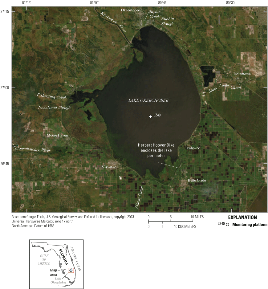
Location of the LZ40 platform within Lake Okeechobee and sources of water entering and leaving the lake.
In 2012, as part of a long-term partnership between the U.S. Geological Survey (USGS) and SFWMD, a platform (LZ40) was instrumented at the approximate center of Lake Okeechobee (fig. 1) to continuously measure evaporation with the Bowen-ratio energy-budget (BREB) method. This method has been applied widely in lake evaporation studies (Moreo and Swancar, 2013; Swancar and others, 2000), and within sparsely vegetated wetlands (German, 2000) where latent and sensible heat fluxes originate from a single source, such as a water surface. The primary goal for this study was to quantify daily rates of open-water evaporation in the interior of Lake Okeechobee. Secondarily, given the complexity and cost of the BREB method (Shoemaker and Sumner, 2006), simplified alternative approaches were sought that could reproduce the Bowen-ratio results reasonably well, while reducing instrumentation and operational expenses. This report documents the rates of evaporation obtained using the BREB method and the alternative approaches used to reproduce the Bowen-ratio results.
The study area is the interior of Lake Okeechobee (fig. 1). The LZ40 platform, located in the approximate center and deepest part of the lake, was chosen for recording meteorological data needed to compute open-water evaporation (fig. 1). The lake is enclosed by the Herbert Hoover Dike and surrounded mostly by wetlands, farmland (mostly sugar cane), and urban communities (Aumen and Havens, 1998). Water enters the lake through several sources, including precipitation and runoff, the Kissimmee River, Fisheating Creek, Taylor Creek, Nubbin Slough, and Nicodemus Slough; water exits the lake through evaporation, groundwater leakage, and numerous canals, including the Miami Canal to the south, the Caloosahatchee River to the west, and the Saint Lucie Canal to the east (Aumen and Havens, 1998; Steinman and others, 2002). Groundwater can move into or out of the lake; however, the net groundwater exchange is expected to be from the lake to the groundwater system because the Herbert Hoover Dike maintains the lake stage at an elevation higher than the surrounding land and groundwater table.
The climate in Florida near Lake Okeechobee is classified as humid subtropical to tropical savanna (Collins and others, 2017). The wet season begins in late May and lasts through October, with convective thundershowers that build around the perimeter of the lake during the day. Convective cloud formation with occasional rainfall forms around the perimeter of the lake because of the disparate heat capacities of water and land, which facilitate greater surface heating over land and, subsequently, enhanced convective rising of air masses that can then adiabatically cool and form clouds preferentially over land. During the late summer and early fall, tropical low-pressure zones and occasional hurricanes add to the seasonally heavy precipitation. The dry season begins in late October and lasts until late April. Occasional cold fronts from the north bring winter precipitation, but the winter months are mostly dry and sunny (Shoemaker and others, 2011).
Methods for Computing Lake Evaporation
Lake Okeechobee evaporation at the LZ40 platform was measured using the BREB approach (Bowen, 1926) and estimated with the “Simple” equation (Abtew 1996a, b), the Priestley-Taylor (PT) equation (Priestley and Taylor, 1972), a Penman (1948) combination equation, a calibrated Turc (1961) equation, and a Mass-Transfer equation (Harbeck, 1962; Jobson, 1972). USGS data collection at the LZ40 platform (fig. 2) began on November 15, 2012, with installation of meteorological instrumentation required for the BREB method. Meteorological and environmental variables, including precipitation, air temperature, relative humidity, wind speed, net radiation, incoming solar radiation, and a vertical profile of water temperature, were measured at 30-minute resolution until February 7, 2013, and at 15-minute resolution thereafter. Water temperature profiles started at the bottom of the lake and consisted of eight thermistors every 0.6 m vertically. Data for this study and the Bowen ratio and five alternate evaporation equations are available from Shoemaker and others (2024). Other standard micro-meteorologic data, such as air temperature and relative humidity, are publicly available in Wacker (2020). Data collected and stored prior to 2016 are available at South Florida Information Access website (https://sflwww.er.usgs.gov/exchange/evapotrans/index.php) for the LZ40 station (Wacker, 2017).
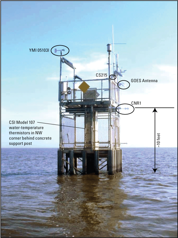
View looking northwest at LZ40 station in Lake Okeechobee on February 3, 2013. Installed equipment include the Geostationary Operational Environmental Satellite (GOES) data transmitting antenna, YWM 05103L wind speed and direction sensor, CS215 air temperature and relative humidity sensor, CNR1 four-component radiometer, and CSI Model 107 water temperature thermistors. Photograph by Mike Wacker (U.S. Geological Survey-retired).
Bowen-Ratio Energy-Budget
Bowen (1926) completed a pioneering study of evaporation that empirically defined the ratio of sensible to latent-heat flux (the Bowen ratio) as a function of temperature and vapor-pressure gradients between the atmosphere and any water surface. Lake evaporation rates (), in meters per second, were computed as follows:
whereis the energy used for daily evaporation, in watts per square meter;
is the latent heat of vaporization of water as a function of air temperature, in Joules per gram; and
is the density of water, in grams per cubic meter (Moreo and Swancar, 2013).
is computed using a rearranged form of the daily energy budget for the lake (eq. 2):
whereis mean daily net radiation to the lake surface at LZ40,
is mean daily energy advected into the lake from surface flows such as the Kissimmee River,
is mean daily energy advected into the lake from groundwater seepage,
is energy advected into the lake from precipitation,
is mean daily sensible heat flux from the lake, and
is the change in stored heat energy in the lake.
Daily net radiation () was estimated using the CNR1 four-component net radiometer (fig. 2). Daily advected energy from surface flows () was assumed to be negligible given the sparse water temperature data and measured daily inflows and outflows that never exceeded 1 percent of the total lake volume, based on daily flow data published by the SFWMD and available on the DBHYDRO website (South Florida Water Management District, 2023). Daily advected energy from groundwater () also was assumed to be negligible in the energy budget, because measurements of groundwater seepage and the temperature of groundwater beneath the lake were not available. Advected energy from precipitation () was computed as
whereis the energy flux associated with a given precipitation volumetric flux () of precipitation temperature (, in degrees Celsius;
ρw
is water density, in kilograms per cubic meter;
cw
is specific heat of water, in Joules per kilogram degree Celsius; and
Tb
is base temperature (Anderson, 1954), in degrees Celsius.
Rainfall was collected by the SFWMD at the site and used to assign values for . Precipitation temperature was assumed equal to the dew point temperature, computed as a function of air temperature and relative humidity. was assumed equal to the average water temperature at the LZ40 station during the study period, as measured by vertical temperature profiles (fig. 2). and are assumed to have constant values of 1,000 kilograms per cubic meter and 4,184 Joules per kilogram degree Celsius, respectively.
Sensible heat flux () was derived from the Bowen (Bowen, 1926) ratio () using the function
with Bowen’s ratio equal to whereis the psychrometric constant, in kilopascals per degree Celsius, computed as a function of atmospheric pressure and air temperature (Fritschen and Gay, 1979);
Tws
is the mean daily temperature of the water surface, in degrees Celsius;
is mean daily air temperature, in degrees Celsius;
is mean daily saturation vapor pressure at water surface, in kilopascals; and
is mean daily vapor pressure in air, in kilopascals.
Water surface temperatures from October 7, 2013 to February 14, 2014, were obtained from two sources: the DBHYDRO database (South Florida Water Management District, 2023) LZ40 surface-water temperature (DBKEY= IY025), and thermistors mounted on two buoys at the water surface (fig. 2). DBHYDRO is SFWMD’s environmental database that stores hydrologic data. The DBHYDRO data were used only when surface thermistor data from the buoy system were not available. For example, the USGS buoy system failed on October 7, 2013, causing thermistors to remain static in the water column about 2 m below the surface. The USGS buoy system to measure surface-water temperature was repaired on February 14, 2014.
Changes in heat energy stored within Lake Okeechobee were assumed to be represented by a single temperature profile at the station location; that is, areal variations in the temperature profile were not considered because of the cost and logistical issues associated with complete and repeated thermal surveys of the entire lake. The change in stored heat within the one-dimensional (vertical) lake control volume (Qs) for a given day is given by
whereD
is the depth of the lake at the LZ40 station, in meters; and
and
are integrated lake temperatures measured at the start (i-1) and end (i) of a day, respectively.
and were computed using a backward (1-day) moving average of submerged thermistors to minimize spurious values created by local thermal eddies in the vicinity of the LZ40 station. Combining equations 1–6 results in an equation to compute daily evaporation (), in millimeters per day (mm/d):
where(Anderson, 1954) was assumed equal to the average water temperature at the LZ40 station during the study period, as measured by vertical temperature profiles. Unrealistically large evaporation rates occurred when daily Bowen ratios were between −0.65 and −1.3 (German, 2000). These unrealistic values (4 percent of the evaporation dataset) were removed and replaced by assuming complete conversion of net radiation to evaporation. Negative values for were set to zero because negative values may represent dew formation, rather than lake evaporation. For reference, the sum of negative evaporation was −36 millimeters over the period of record (4 years) for this study.
Alternative Methods for Computation of Lake Evaporation
Five equations for lake evaporation were selected for comparison to the BREB monthly and annual results. The equations were chosen with the intention of reducing data requirements for computing evaporation in the interior of Lake Okeechobee. Prior knowledge of the sensitivity of various data types (Abtew, 1996a, b; German, 2000; Shoemaker and others, 2005; Shoemaker and Sumner, 2006; Shoemaker and others, 2011) guided selection of the equations. For example, the Simple, Priestley-Taylor, Penman, and Turc equations are based on components of the surface-energy budget that are known to explain much of the variability in evapotranspiration in the region (Abtew, 1996a, b; German, 2000), in particular, solar radiation, net radiation and (or) available energy. The Mass-Transfer equation was chosen because it is based on two variables to which computed evaporation showed sensitivity during preliminary analysis of the BREB results; specifically, wind speed and vapor pressure deficits.
The first equation is the “Simple” equation (Abtew 1996a, b), which is based on the concept that most of the variation in evaporation is explained by solar radiation. The Simple equation takes the form
whereis a coefficient dependent on surface type; and
is incoming solar radiation, in watts per square meter.
The value of is generally set to 0.53 (open water conditions); however, this variable was estimated by regression (tables 1 and 2) to minimize residuals from daily and monthly BREB estimates of evaporation.
Table 1.
Error statistics and calculated annual evaporation rates of Bowen-ratio energy method, Penman, Priestley-Taylor, Mass-Transfer, Turc, and Simple methods.[Period of record is from December 2012 to December 2016. SD, standard deviation; mm/yr, millimeter per year; NA, not available]
| Method | Calibration variable |
Value of variable |
Mean annual evaporation (mm per year) |
SD of residuals1 (mm per year) |
Percent bias2 | Absolute bias (mm per year) |
Reference | Data requirements3 |
|---|---|---|---|---|---|---|---|---|
| Bowen ratio | NA | NA | 1,788 | NA | NA | NA | Bowen (1926) | Rn, W, rainfall, Ta, Tw, Tsurface, Hum, stage |
| Penman4 | C1, C2 | 0.0, 1.21484 | 1,746 | 0.75 | −2 | 48 | Penman (1948) | Rn, W, rainfall, Ta, Tw, Hum, VPD, Ws, stage |
| Priestley-Taylor | a | 1.25016 | 1,747 | 0.76 | −2 | 47 | Priestley and Taylor (1972) | Rn, W, rainfall, Ta, Tw, Hum |
| Mass transfer | N | 0.00012 | 1,637 | 1.70 | −8 | 157 | Harbeck (1962) | Ws, VPD |
| Turc | Cu, Cs | 0.04664, 10.68370 | 1,775 | 2.51 | −1 | 19 | This study | Ta, Pyro |
| Simple | K1 | 0.709 | 1,740 | 2.46 | −3 | 54 | Abtew (1996a) | Pyro |
Computed as the mean daily residual divided by the Bowen-ratio mean-daily value, from November 16, 2012, to January 8, 2017.
Rn is net radiation, W is change in stored heat energy, Ta is air temperature, Tw is water temperature, Tsurface is lake surface temperature, Hum is relative humidity, stage is lake stage, Ws is wind speed, VPD is vapor pressure deficit, Pyro is incoming solar radiation.
See Shoemaker and Sumner (2006) for descriptions of the correction coefficients that debias the Penman equation.
Table 2.
Regression-defined coefficients and error statistics for the Penman, Priestley-Taylor, Mass-Transfer, Turc, and Simple methods, relative to monthly evaporation rates computed with the Bowen-Ratio Energy-Budget method.[The period of record is from December 2012 to December 2016. All errors were computed with evaporation rates in millimeters per month]
The Priestley-Taylor (PT) equation (Priestley and Taylor, 1972) estimates evaporation from an extensive wet surface under conditions of minimum advection. The PT equation takes the form
whereis the slope of the saturated vapor pressure with respect to temperature, in kilopascals per degree Celsius; and
α
is an empirically determined dimensionless coefficient equal to 1.26 for potential or well-watered conditions.
For this analysis, α was estimated by regression to minimize residuals from daily and monthly BREB estimates of evaporation (tables 1 and 2). Evaporation, in millimeters per day, was computed by dividing by .
The Penman (1948) combination equation is derived for evaporation from an open-water surface. This equation accounts for both energy budget and aerodynamic principles, and takes the form
whereis air density computed as a function of air temperature, in grams per cubic meter;
is the specific heat of moist air, in joules per gram per degree Celsius;
is the vapor pressure deficit, in kilopascals, where is saturation vapor pressure and is actual vapor pressure; and
is the aerodynamic resistance, in seconds per meter.
Evaporation, in millimeters per day, was computed by dividing by the product of and . Aerodynamic resistance for the Penman equation was estimated using an equation published by Shuttleworth (1993):
whereis the height, in meters, at which the wind speed is measured;
is displacement height, in meters;
is the roughness height for momentum, in meters;
is the roughness height for water vapor, in meters;
is von Karmen’s constant (0.4); and
is the horizontal wind speed, in meters per second, at sensor height .
The variable (Brutsaert, 1982) was estimated as 0.67 times an estimate of average wave height (0.45 m) visually observed during field work at the station. The variable was approximated as 0.0035 for the water surface. The variable was approximated as 0.1 (Jensen and others, 1990). The variables es and e were estimated as described by Allen and others (1998) using daily minimum and maximum air temperatures and relative humidity. The Penman equation was calibrated to daily and monthly BREB results using correction coefficients, as outlined in Shoemaker and Sumner (2006). A linear correction coefficient formulated as a function of relative humidity was effective for debiasing the Penman equation.
Turc (1961) simplified earlier versions of his equation (Turc, 1954) for climatic conditions in western Europe. Trajkovic and Kolakovic (2009) presented the adjusted Turc similar to the following equation:
whereis evaporation, in millimeters per day;
is a wind speed adjustment factor;
is a solar radiation adjustment factor; and
is incoming solar radiation, in watts per square meter.
The Mass-Transfer method (Anderson and others, 1950; Marciano and Harbeck, 1954; and Harbeck, 1962) is based on the assumption that evaporation is proportional to the product of the measured water-to-air vapor pressure differential and wind speed as
whereis the Mass-Transfer-estimated evaporation rate, in millimeters per day;
is the Mass-Transfer coefficient, in millimeters per day second per meter kilopascal; and
is wind speed, in meters per second.
Wind speed was measured from 3.6 to 5.1 m above the water surface, depending upon water levels in Lake Okeechobee. Wind speeds at 2 and 5 m above the water surface were calculated to be within 10 percent of each other during an assessment of error in evaporation introduced by not assuming a log profile in the vertical distribution of horizontal wind speed at heights >3.6 m above the lake surface. Furthermore, was estimated by regression between daily and monthly BREB values of evaporation and values estimated by equation 14. The value of is site-specific and represents a variety of effects, including the wind profile with height, roughness of the water surface, atmospheric stability, and averaging period during which the variables in the equation are measured (Harbeck, 1962; Jobson, 1972).
Results and Discussion
Evaporation rates from Lake Okeechobee are discussed in the context of seasonality and magnitude within this extensive open-water ecosystem. Implications of these results for water supply management are introduced. Results from daily and monthly calibration of the five alternate methods for computing evaporation are compared.
Lake Evaporation at LZ40
Using the BREB method, annual evaporation averaged 1,825 millimeters per year (mm/ yr) (averaging 5.0 mm/d) at the LZ40 platform in Lake Okeechobee during the 4-year study. Net radiation can be a helpful upper-limit check on the BREB evaporation rates by assuming net radiation converts solely into latent heat, the energy equivalent of evaporation. For example, annual evaporation would be 1,903 mm/yr (averaging 5.22 mm/d) if net radiation was converted solely into latent heat rather than sensible heat. BREB rates for calendar years 2013, 2014, 2015, and 2016 were 1,760, 1,840, 1,805, and 1,880 mm/yr, respectively. These evaporation rates are among the highest rates computed in Florida and are due to frequent clear-sky conditions over the interior of the lake. For comparison, Abtew (2001) estimated Lake Okeechobee evaporation as 1,320 mm/yr using evaporation pans adjacent to the perimeter of the lake, and calibrated empirical equations that were driven by solar radiation and air temperature. Cloud cover surrounding the perimeter of the lake likely reduced evaporation rates and calibration parameters () documented in the Abtew (2001) pan evaporation study. German (2000) estimated evapotranspiration rates in the Florida Everglades ranging from about 1,000 to 1,400 mm/yr using the BREB method. Price and others (2007) estimated a mean annual evaporation rate of about 1,700 mm/yr for Florida Bay during a 33-year period using vapor-flux and energy-budget based methods. Sumner (2001) estimated an annual evapotranspiration of about 900 and 1,000 mm in 1998 and 1999, respectively, over a cypress and pine forest in east-central Florida subjected to logging and natural fires. Swancar and others (2000) estimated evaporation rates of 1,450 and 1,422 mm/yr at Lake Starr in central Florida.
The high evaporation rates observed at LZ40 are explained by frequent clear skies over the interior of Lake Okeechobee (fig. 3) (Segal and others, 1997) that enhance evaporation by allowing more solar radiation to reach the lake’s water-surface than surrounding areas. Surface water has a greater heat capacity than land, which maintains cooler temperatures in the interior of the lake that inhibit convective cloud formation. In contrast, surrounding land areas heat more rapidly during the day and promote convective cloud formation. Frequent clear skies are also apparent over other large lakes in Florida, such as Lakes Apopka and George, as well as in the marine environment (fig. 3). These evaporation results and maps of cloud cover have implications for the design of water storage reservoirs. Specifically, storage reservoirs could benefit from smaller scales that do not suppress convective cloud formation and enhance evaporation of water in the interior of a reservoir caused by frequent exposure to relatively higher levels of solar radiation.
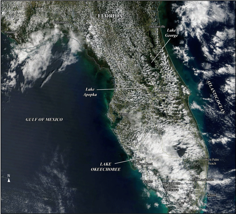
Satellite image of the Florida peninsula. Sparse cloud cover over Lake Okeechobee is informally referred to as the “donut hole.” Image courtesy of the National Atmospheric and Space Administration (NASA) Earth Science Data Systems Program. We acknowledge the use of imagery provided by services from NASA's Global Imagery Browse Services (GIBS), part of NASA's Earth Observing System Data and Information System (EOSDIS).
Seasonality was clearly observed in Lake Okeechobee evaporation rates, which increased in the summer with increasing vapor pressure gradients, air temperature, and solar and net radiation (fig. 4A–E). In general, evaporation declined in the winter as solar and net radiation decreased. Exceptions to this pattern included the occurrence of relatively cold air temperature events in the winter (fig. 4E), which occasionally created very large evaporation rates (fig. 4C; January 2013, 2014, 2015). These cold events documented in data releases by Wacker (2017, 2020) were associated with (1) increased wind speeds, (2) decreased humidity that increased vapor pressure deficits, and (3) abrupt changes in air temperature that initiated the release of heat energy stored in the lake (fig. 4C) for evaporation. In fact, similar to results from Shoemaker and others (2005) for the Everglades, available energy for evaporation increased considerably from changes in stored heat-energy in Lake Okeechobee, overwhelming low values of solar and net radiation.
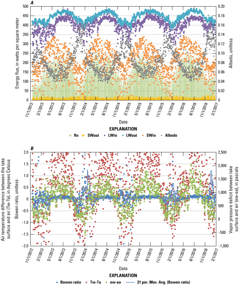
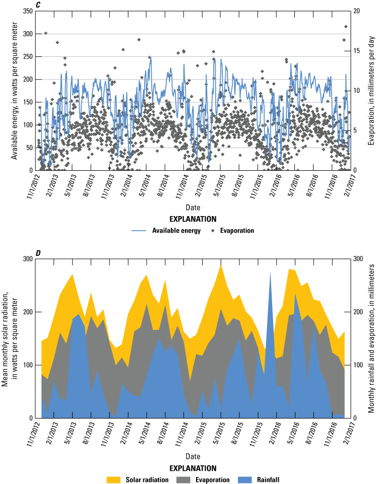
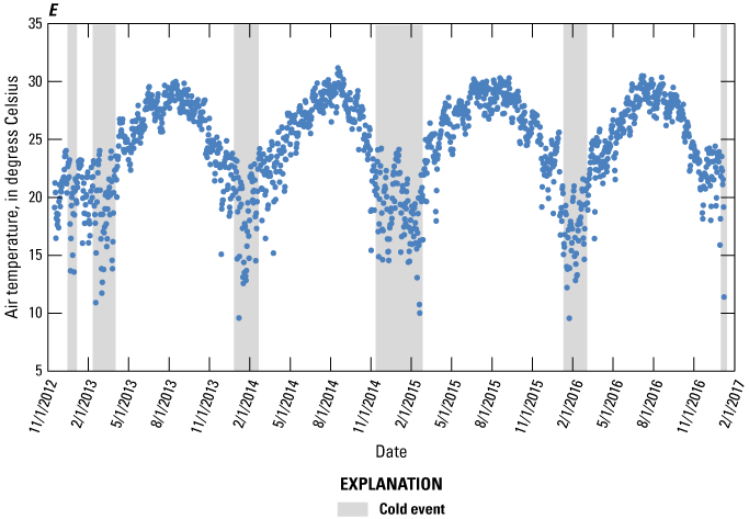
A, energy flux and albedo; B, air temperature difference between the lake surface and air, Bowen ratio, and vapor pressure deficit between lake surface and air; C, available energy and lake evaporation; D, mean monthly solar radiation, and monthly rainfall and evaporation; and E, air temperature at the LZ40 station. Rn, net radiation; SWout, outgoing shortwave radiation; LWin, incoming longwave radiation; LWout, outgoing longwave radiation; SWin, incoming shortwave radiation; albedo is lake albedo; “21 per. Mov Avg,” 21-day centered moving average of the Bowen ratio.
Comparison of Methods for Computing Evaporation at LZ40
The BREB method requires a large amount of input data to account for many variables that explain open-water evaporation and provide reliable results (German, 2000). This 4-year dataset for Lake Okeechobee provided an opportunity to compare and calibrate several other approaches for estimating evaporation from the lake. The goal of this analysis was to identify methods that could reproduce the BREB results reasonably well, while reducing input data, instrumentation, and operational expenses.
Calibration of all five methods to daily BREB evaporation rates represented annual evaporation reasonably well (table 1). Annual totals were all within ±10 percent of the BREB results. Calibration was performed by estimating single parameter values for the period of record that minimized sum-of-squared residuals from daily BREB evaporation rates. Notably, the Mass-Transfer method underestimated annual evaporation by about 8 percent (table 1). The Penman and Mass-Transfer methods accurately estimated relatively large evaporation rates that occurred when cold fronts passed through the study area in the winter (fig. 4C), because these methods accounted for large wind speeds and vapor pressure deficits that occurred during the passage of winter cold fronts. For operational implementation, the Simple, Mass-Transfer, and Turc methods have the benefit of simplicity and limited data requirements (table 1) for accurately computing annual evaporation totals.
The PT equation provided a comparable prediction of annual Lake Okeechobee evaporation relative to the BREB method. Regression estimated an α value of 1.25 (table 1), which is within 1 percent to the theoretical value of 1.26 established by Priestley and Taylor (1972). Annual evaporation totals were underestimated by 2 percent, and the standard error of daily residuals was 0.76 mm, a low value relative to those obtained using the other equations (table 1). Large evaporation rates of ~10 mm/d (fig. 4C) during cold fronts in January 2013, 2014, 2015, and 2016 were well represented because changes in stored heat-energy are accounted for in the PT equation (eq. 10). A limitation of the PT equation (eq. 10) is the data requirements, which include net radiation and changes in heat-energy stored in the lake. This study confirms findings in prior studies, such as Douglas and others (2009), that demonstrate the impressive performance of the PT equation compared to alternate formulations.
In practice, a single set of monthly regression coefficients for all five methods could be tractable and useful in future water-budgeting studies of Lake Okeechobee, as long as reasonable accuracy is maintained in the evaporation results. Thus, a single set of monthly coefficients was identified with regression for each alternate evaporation equation (table 2) by minimizing sum-of-squared residuals from monthly BREB evaporation totals. Accuracy statistics for evaporation are presented here to provide information on potential uncertainty (table 2).
Monthly evaporation rates were more problematic for fitting in the fall, winter, and early spring for every equation compared to late spring and summer (fig. 5, table 2). The Mass-Transfer method occasionally underestimated monthly evaporation by as much as −28 percent. Likewise, errors for the Penman and Priestley-Taylor equations were >10 percent in the winter. The Turc and Simple methods performed well, given the simplicity and limited data requirements for computing monthly evaporation totals, with errors ranging from −2 to 10 percent and −5 to 11 percent, respectively. The Turc equation has two calibration parameters (Cu and Cs) that were identified by regression for computing monthly evaporation at the LZ40 station. Future hydrologic studies could use these optimized parameters with the Turc and Simple equations to accurately compute evaporation from Lake Okeechobee using only air temperature and solar radiation for input data. The Simple equation requires only solar radiation for input data. As expected, there are errors for each method of computing evaporation (fig. 5). Nevertheless, the errors are likely acceptable for many analyses of water resources, including investigations of long-term seasonal trends, droughts that extend over several months, or predictions of declines in lake water levels.
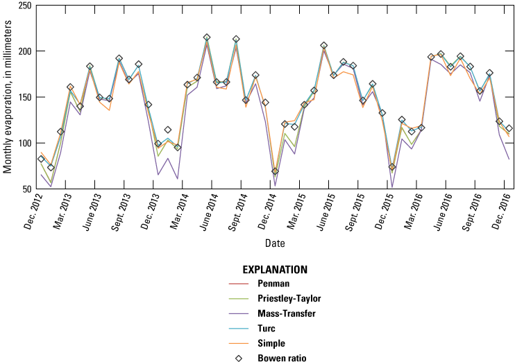
Comparison of monthly evaporation rates from the Bowen ratio and other equations at LZ40 in Lake Okeechobee. Monthly evaporation rates are derived from a single set of monthly regression coefficients.
Summary
A platform at the center of Lake Okeechobee in Florida was instrumented to continuously measure evaporation with the Bowen-ratio energy-budget method as part of a long-term partnership between the South Florida Water Management District and the U.S. Geological Survey. The primary goal for the study was to quantify daily rates of open-water evaporation. A secondary goal was to assess differences in evaporation rates among alternate methods and determine if instrumentation and operational expenses associated with the Bowen-ratio method could be reduced. The Bowen-ratio energy-budget results indicate that annual evaporation in the interior of Lake Okeechobee for 2013–16 averaged about 1,825 millimeters per year. Evaporation rates for calendar years 2013–16 were about 1,760, 1,840, 1,810, and 1,890 millimeters per year, respectively. These evaporation rates are among the largest rates reported in Florida. The large evaporation rates are explained by frequent clear skies over the interior of Lake Okeechobee because of the large surface area of the lake and abrupt change in heat capacity from land to water surrounding the perimeter of the lake. Surface water has a greater heat capacity than land, which maintains cooler lake temperatures that inhibit convective cloud formation and rainfall. Clear skies over the lake enhance evaporation by allowing more solar insolation to reach the lake's surface. In contrast, land areas surrounding the lake heat more rapidly during the day, which promotes convective cloud formation and rainfall.
Lake Okeechobee evaporation rates increased in the summer with increasing air temperature, solar radiation, and vapor pressure gradients. Evaporation declined in the winter with decreasing solar and net radiation. Exceptions were the passage of cold fronts in the winter, which occasionally created very large daily evaporation rates. Cold fronts were associated with (1) greater wind speeds, (2) drier air that accepted more water vapor, and (3) abrupt declines in air temperature that forced heat-energy stored in the lake to be available for evaporation.
Estimates of evaporation rates obtained using five alternate evaporation equations were compared to monthly and annual Bowen-ratio energy-budget results and reviewed for performance. All five equations estimated annual evaporation relatively well (within 10 percent of the Bowen ratio annual totals). The Penman, Priestley-Taylor, and Mass-Transfer methods adequately captured relatively large evaporation rates that occurred during the passage of cold fronts in the winter, because these methods account for either large wind speeds, large vapor-pressure deficits, and (or) large changes in available energy that occurred during the passage of cold fronts in the winter. For operational implementation, the Mass-Transfer, Simple, and Turc methods are likely preferable because of their computational simplicity and limited data requirements. The Turc and Simple equations were superior for computing monthly evaporation. The Turc equation computed monthly evaporation within 8 percent of the Bowen-ratio method, while requiring only air temperature and solar radiation data. The Simple equation achieved similar accuracy while requiring only solar radiation data. Future hydrologic studies and water management could benefit from the evaporation results, insights, and concepts introduced herein.
Acknowledgments
Mike Wacker (U.S. Geological Survey-retired) is acknowledged for collecting the raw data used in this study. Review comments from David M. Sumner (U.S. Geological Survey-retired) and Nick Sepulveda (U.S. Geological Survey-retired) improved the manuscript quality. Michelle Irizarry-Ortiz (U.S. Geological Survey) offered insights on the hydrology of Lake Okeechobee including prior studies of evaporation in the study area. Her extensive knowledge and expertise in hydrologic modeling and statistical hydrology were especially helpful.
References Cited
Abtew, W., 1996b, Lysimeter study of evapotranspiration from a wetland, in Camp, C.R.,Sadler, E.J., and Yoder, R.E., eds., Evapotranspiration and irrigation scheduling—International Conference, San Antonio, Tex., November 3–6, 1996, [Proceedings]: St. Joseph, Mich., American Society of Agricultural Engineers, 1,166 p.
Anderson, E.R., 1954, Energy-budget studies, in Water-loss investigations—Lake Hefner studies, technical report: U.S. Geological Survey Professional Paper 269, p. 71–119, accessed September 2017 at https://pubs.er.usgs.gov/publication/pp269.
Aumen, N.G., and Havens, K.E., 1998, Okeechobee lake, Florida, USA—Human impacts, research, and lake restoration, in Herschy, R.W., and Fairbridge, R.W., eds., Encyclopedia of Hydrology and Water Resources: Kluwer Academic Publishers, Dordrecht, p. 505–506, accessed May 6, 2024, at https://doi.org/10.1007/1-4020-4513-1_167.
Cuevas, M., 2016, Toxic algae bloom blankets Florida beaches, prompts state of emergency: Cable News Network [CNN], July 1, 2016, accessed September 2017 at https://www.cnn.com/2016/07/01/us/florida-algae-pollution/.
Ferris, R., 2016, Why are there so many toxic algae blooms this year: Cable News Network [CNN], July 26, 2016, accessed September 2017 at https://www.cnbc.com/2016/07/26/why-are-there-so-many-toxic-algae-blooms-this-year.html.
Havens, K.E., and Steinman, A.D., 2015, Ecological responses of a large shallow lake (Okeechobee, Florida) to climate change and potential future hydrologic regimes: Environmental Management, v. 55, no. 4, p. 763–775, accessed September 2017 at https://doi.org/10.1007/s00267-013-0189-3.
Moreo, M.T., and Swancar, A., 2013, Evaporation from Lake Mead, Nevada and Arizona, March 2010 through February 2012: U.S. Geological Survey Scientific Investigations Report 2013–5229, 40 p., accessed October 2017 at https://doi.org/10.3133/sir20135229.
Segal, M., Arritt, R.W., Shen, J., Anderson, C., and Leuthold, M., 1997, On the clearing of cumulus clouds downwind from lakes: Monthly Weather Review, v. 125, no. 4, p. 639–646, accessed April 20, 2024, at https://doi.org/10.1175/1520 0493(1997)125<0639:OTCOCC>2.0.CO;2.
Shoemaker, W.B., Sumner, D.M., and Castillo, A., 2005, Estimating changes in heat energy stored within a column of wetland surface water and factors controlling their importance in the surface energy budget: Water Resources Research, v. 41, no. 10, 18 p. accessed October 2017 at https://doi.org/10.1029/2005WR004037.
Shoemaker, W.B., Weber, B.J., and Daniels, A.M., 2024, Daily evaporation rates computed using five methods at the LZ40 platform in Lake Okeechobee, Florida, December 2012 to December 2016: U.S. Geological Survey data release, https://doi.org/10.5066/P9XDE78Y.
South Florida Water Management District, 2023, DBHYDRO (environmental data): South Florida Water Management District database, accessed August 1, 2017, at https://www.sfwmd.gov/science-data/dbhydro.
Steinman, A., Havens, K., and Hornung, L., 2002, The managed recession of Lake Okeechobee, Florida—Integrating science and natural resource management: Conservation Ecology, v. 6, no. 2, accessed April 20, 2024, at https://www.jstor.org/stable/26271894.
Wacker, M., 2017, Evapotranspiration data download: U.S. Geological Survey South Florida Information Access Data Exchange website, accessed August 1, 2019, at https://sflwww.er.usgs.gov/exchange/evapotrans/index.php.
Wacker, M.A., 2020, Evaporation at LZ40 platform, Lake Okeechobee, Palm Beach County, Florida, November 16, 2012 - December 31, 2019: U.S. Geological Survey data release, https://doi.org/10.5066/P9UB7N70.
Conversion Factors
International System of Units to U.S. customary units
Temperature in degrees Celsius (°C) may be converted to degrees Fahrenheit (°F) as follows:
°F = (1.8 × °C) + 32.
Temperature in degrees Fahrenheit (°F) may be converted to degrees Celsius (°C) as follows:
°C = (°F – 32) / 1.8.
For more information about this publication, contact
Director, Caribbean-Florida Water Science Center
U.S. Geological Survey
4446 Pet Lane, Suite 108
Lutz, FL 33559
For additional information, visit
https://www.usgs.gov/centers/car-fl-water
Publishing support provided by
Lafayette Publishing Service Center
Disclaimers
Any use of trade, firm, or product names is for descriptive purposes only and does not imply endorsement by the U.S. Government.
Although this information product, for the most part, is in the public domain, it also may contain copyrighted materials as noted in the text. Permission to reproduce copyrighted items must be secured from the copyright owner.
Suggested Citation
Shoemaker, W.B., and Wu, Q., 2024, Evaporation from the interior of Lake Okeechobee—A large freshwater lake in Florida, 2013–16: U.S. Geological Survey Scientific Investigations Report 2024–5040, 17 p., https://doi.org/10.3133/sir20245040.
ISSN: 2328-0328 (online)
Study Area
| Publication type | Report |
|---|---|
| Publication Subtype | USGS Numbered Series |
| Title | Evaporation from the interior of Lake Okeechobee—A large freshwater lake in Florida, 2013–16 |
| Series title | Scientific Investigations Report |
| Series number | 2024-5040 |
| DOI | 10.3133/sir20245040 |
| Publication Date | May 14, 2024 |
| Year Published | 2024 |
| Language | English |
| Publisher | U.S. Geological Survey |
| Publisher location | Reston, VA |
| Contributing office(s) | Caribbean-Florida Water Science Center |
| Description | Report: vi, 17 p., 3 Data Releases |
| Country | United States |
| State | Florida |
| Other Geospatial | Lake Okeechobee |
| Online Only (Y/N) | Y |