

Representation of Surface-Water Flows Using Gradient-Related Discharge in an Everglades Network
Links
- Document: Report (4.42 MB pdf) , HTML , XML
- Data Releases:
- USGS Water Data for the Nation - USGS National Water Information System database
- USGS Data Release - Gradient-Related Discharge in an Everglades Network (GARDEN) viewer
- Database: Database - South Florida Water Management District database
- NGMDB Index Page: National Geologic Map Database Index Page (html)
- Software Release: Gradient-Related Discharge in an Everglades Network (GARDEN) - Version 1.0.0 Initial release of the GARDEN flow vector tool for EDEN
- Download citation as: RIS | Dublin Core
Acknowledgments
The authors would like to thank Nicholas Aumen, Regional Science Advisor of the U.S. Geological Survey Southeast Region, for his assistance through the Greater Everglades Priority Ecosystem Sciences Program, and the other members of the U.S. Geological Survey Everglades Depth Estimation Network (EDEN) team: Saira Haider, Matthew Petkewich, and Bryan McCloskey for their devotion to EDEN development and operations, which has been essential to the continuation of EDEN and the development of new EDEN tools.
Abstract
The Everglades Depth Estimation Network interpolates water-level gage data to produce daily water-level elevations for the Everglades in south Florida. These elevations were used to estimate flow vectors (gradients and directions) and volumetric flow rates using the Gradient-Related Discharge in an Everglades Network (GARDEN) application developed by the U.S. Geological Survey in cooperation with the U.S. Army Corps of Engineers. Flow rates in both the east-west and north-south directions were computed on a 400-meter square grid using modified parameters in the Manning’s equation. The frictional resistance parameter in the Manning’s equation was calibrated to measured flow rates at coastal creeks fed by Everglades Depth Estimation Network boundary flows. Levees and other features that act as barriers to flow were defined as “no-flow” grid cells where vectors were set to zero.
The flow volume magnitudes were calibrated with 2020 daily values of coastal river flows, and verification was performed using 2021 data. Within a given day, the measured coastal river flows fluctuate more than the GARDEN boundary flows because of tidal and wind forcings. Because the GARDEN boundary flows were the upstream water source for the coastal rivers, calibration focused on matching average daily flow volumes rather than daily fluctuations. The Pearson’s correlation coefficient is 0.766 for the 2020 calibration period and 0.566 for the 2021 verification period.
Applying GARDEN to periods with hydraulic-control-structure releases allows the propagation of structure flows to be seen in the daily flow-vector maps along with the multiday response of flows farther downgradient. Flow vectors may be overestimated near control structures because of difficulties in resolving the water gradient downstream from the structure. Flow vectors farther from the structure are more accurate than those near the structure.
Introduction
Daily flow direction and magnitude in the Everglades are needed to determine the effects of structure operations on wetland flows and evaluate water-management and restoration changes. The Everglades Depth Estimation Network (EDEN; Haider and others, 2020) is an integrated network of water-level gages with an interpolation model that generates daily water-level and water-depth data and applications that compute derived hydrologic data across the freshwater part of an area informally referred to as the “greater Everglades” (fig. 1). The “greater Everglades” includes Water Conservation Areas 2A, 2B, 3A, and 3B, Big Cypress National Preserve, and Everglades National Park. The Explore and View EDEN (EVE) application (available at https://sofia.usgs.gov/eden/) can be used to view EDEN output. Water-level data at 247 gages, operated by Big Cypress National Preserve, Everglades National Park, the South Florida Water Management District, and the U.S. Geological Survey (USGS), are interpolated to a 400-meter (m) grid spacing (Pearlstine and others, 2007). The availability of daily data from EDEN support scientists and water managers in Federal and State agencies, as well as to those in academia. EDEN also provides information for ecological evaluation and makes this information available online. The EDEN Cape Sable Seaside Sparrow Viewer application (available at https://sofia.usgs.gov/eden/csss/) was developed to evaluate water depths and other important metrics in the sparrow habitats on a historical and real-time basis. The coastal salinity index uses statistics computed for salinity measured at coastal gages to assess hydrologic trends. Further details about the coastal salinity index are available at https://sofia.usgs.gov/eden/coastal/. Ecologists and water managers make extensive use of EDEN data to examine ecosystems and determine water-delivery effects (Liu and others, 2009; Palaseanu-Lovejoy and others, 2006; Pearlstine and others, 2007; Zhang and others, 2022). The addition of daily wetland flows will expand this utility and provide information to support scientists and decision makers.
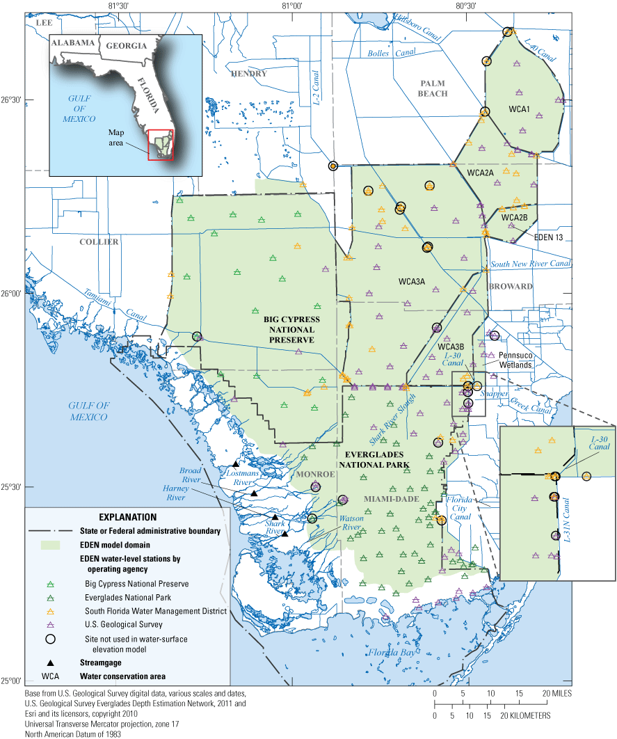
Everglades Depth Estimation Network (EDEN) area, water-level gages, and streamgages (modified from Patino and others, 2018).
The USGS, in cooperation with the U.S. Army Corps of Engineers, has developed the Gradient-Related Discharge in an Everglades Network (GARDEN) application (Swain and Adams, 2024; U.S. Geological Survey, 2024) to estimate surface-water flow vectors in the “greater Everglades.” GARDEN provides important information on surface-water flows to scientists and water managers that water levels alone do not. The effects of storms and water management on water deliveries can be more clearly identified and the supply of water to critical habitats delineated. The effectiveness of water management plans can be evaluated in real time, and computational models can be provided with better estimates of wetland flows for calibration. This report documents the representation of surface-water flows using the GARDEN application. Herein, the term “flows” will include flows in wetlands and in streams, rivers, canals, and through structures. The GARDEN application simulates flows in wetlands and is calibrated using flows in coastal rivers.
Previous Development of the Everglades Depth Estimation Network (EDEN)
EDEN was put into operational service in 2006 and reports daily water levels from 1991 to present (including real-time provisional output) (Patino and others, 2018). The water-level gage data are interpolated on the 400-m square grid, and water depths are estimated from a digital elevation model (DEM). EDEN is also coupled with several ecological habitat models that use the computed depths to evaluate hydroperiod and inundation variables that affect habitat suitability.
Daily water-level surface elevations and water depths of the “greater Everglades” area are provisionally posted online in real time, and quarterly and yearly verifications are performed. EDEN also includes rainfall and evapotranspiration data, hindcast datasets, benchmark data, ecological applications, statistical analyses, and data visualization tools (Patino and others, 2018). Version 3 of the EDEN algorithm was implemented in 2020, incorporates a conversion of code to the R programming language (R Core Team, 2024) to create a more efficient and portable code relative to version 2, and unlike version 2 does not rely on proprietary software (Haider and others, 2020). Additional revisions made for the version 3 model include updates to the interpolation model, the gage network, and groundwater-level estimations (Haider and others, 2020). A 50-m resolution DEM has been integrated into the EDEN water-depth surface computations, improving the horizontal resolution by a factor of 64. Areas not covered by the extent of the 50-m DEM were filled in at that resolution with data from other available sources, particularly in regions in and around streams, ponds, and canals (Haider and others, 2021). The 50-m data are rendered for special application areas and are not used in this GARDEN application. With continued advancements discussed herein, EDEN provides a platform upon which to add a simulation of flow vectors in the “greater Everglades,” supplying valuable information for scientists and water managers.
Methodology
A surface-water flow vector describes the direction and magnitude of flow and is computed from the east-west and north-south water-level gradients for a set of four grid cells; therefore, the surface-water flow vector is offset from the elevation data. This methodology is similar to those used in numerical models, where a velocity or flux vector is computed at the midpoint of four water-level locations (fig. 2). The water-level gradients are computed from the averages of the water levels upstream minus the average of the water levels downstream. The water-level gradient vectors in each direction, ∇Zx in the east-west direction and ∇Zy in the north-south direction, are computed as follows:
whereZi,j
is the water level in cell i,j, with i being the east-west notation and j being the north-south notation; and
w
is the horizontal dimension of an EDEN grid cell.
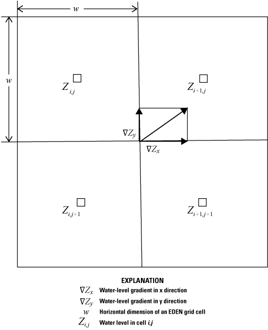
Grid scheme for Everglades Depth Estimation Network (EDEN) flow vectors. The “x” direction is east-west and the “y” direction is north-south.
GARDEN flow computations require a formulation that relates the water-level gradients computed by equations 1 and 2 to volumetric flowrates. Kadlec (1990) examined overland flow in the Houghton Lake wetland in Michigan and worked with a reformulation of Manning’s equation that considers the transition zone between turbulent and laminar flow and the resistance of emergent vegetation. This study developed modified parameters for the Manning’s equation:
whereQ
is the flow rate;
K, β, and α
are proportionality coefficients;
d
is the depth of flow; specifically, the average of the four depths in figure 2 (for cells i,j; i+1,j; i+1,j+1; i,j+1);
w
is the flow width; and
S
is the water surface gradient; the resultant of the vectors and in equations 1 and 2.
For Manning’s equation, K = 1/n in International System of Units and 1.49/n in U.S. customary units, where n is Manning’s friction factor, α = 1/2, and β = 5/3. Note that the β parameter incorporates the depth term associated with cross-sectional area of flow (wd) through the grid cell; for example, if β equals 5/3, then wd5/3 could be rewritten as (wd)d2/3. For the Houghton Lake wetland in Michigan, Kadlec (1990) obtained α = 0.71, and β = 2.5. The difference in Manning’s and Kaslec’s values of α is mainly due to the flow not being fully turbulent, and the difference in values of β is due to the effects of the emergent vegetation, which should be quite variable with vegetation type and size. This formulation has been the basis for most analyses of wetland flow (Chin, 2011; Choi and Harvey, 2014; Goodwin and Kamman, 2001; Jadhav and Buchberger, 1995; Tsihrintzis and Madiedo, 2000; Wasantha Lal, 2017; Wilsnack and others, 2001).
He and others (2010) examined the factors controlling flow across Shark River Slough in Everglades National Park, central to the EDEN study area. Daily averaged water velocity measurements, stage gradients, and water-depth data were used to develop the relationship between flow rate and gradient. Coefficients K, α, and β in equation 3 were evaluated using least-squares regression, with resulting values of K = 14.4, α = 0.66, and β = 1.12. Manning’s equation is not dimensionally homogeneous, meaning that the constant K must have dimensions such that the equation results in dimensions of volume per unit time. If the value of β is altered, the dimensions of K must change. The effective units of K are ft(2−β)s−1 and the original Manning’s equation assumes a value of β = 5/3, giving effective units for K of ft1/3s−1; however, with the modified value β = 1.12, the effective units of K are ft0.88s−1.
Aggregation of Flow Vectors
The EDEN grid has 57,073 active cells, so a map of flow vectors for every cell corner may be too dense to be a useful visual representation. Aggregating the vectors allows for varying the resolution and density of the map. The grid scheme in figure 2 can be altered so that the flow vectors for a larger set of cells are averaged to get the total flow for the aggregated group. For example, the three-by-three aggregation computes the average of nine flow vector points (fig. 3) and is calculated to occur over a spatial resolution of 1,200 m (3 times 400 m). At a larger scale, the five-by-five aggregation computes the average of 25 points over a spatial resolution of 2,000 m. For the purposes of the presentation used in this report, the three-by-three set of cells with a spatial resolution of 1,200 m is used.
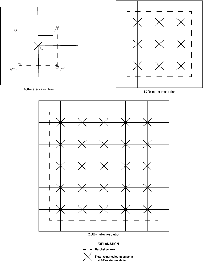
Aggregation of 400-meter grid cells to 1,200-meter and 2,000-meter resolutions for Everglades Depth Estimation Network (EDEN) flow vectors.
Barriers to Flow
The EDEN study area includes eight subdomains separated by a levee system that divides and controls the wetlands and conservation areas and results in water-level discontinuities (fig. 4). Water levels on opposing sides of levees or any other obstruction to flow are not used to calculate an intervening water-level gradient and surface-water flow vector. The subdomain boundaries shown in figure 4 are used as a basis to define the EDEN grid cells that are not used to compute flow (no-flow cells), except for the boundary between the NPS (Everglades National Park/Big Cypress National Preserve) and L67ext (Levee 67 extension) subdomains. The southern section of this boundary does not correspond to a levee and is only included to complete the subdomain. Additional no-flow cells are identified as areas with features that block flows or water-level data that are affected by nearby flow boundaries (fig. 5). If any of the four cells used to compute a vector is set to no-flow, the flow vector is set to zero. Thus, flow is not computed along or across a levee.
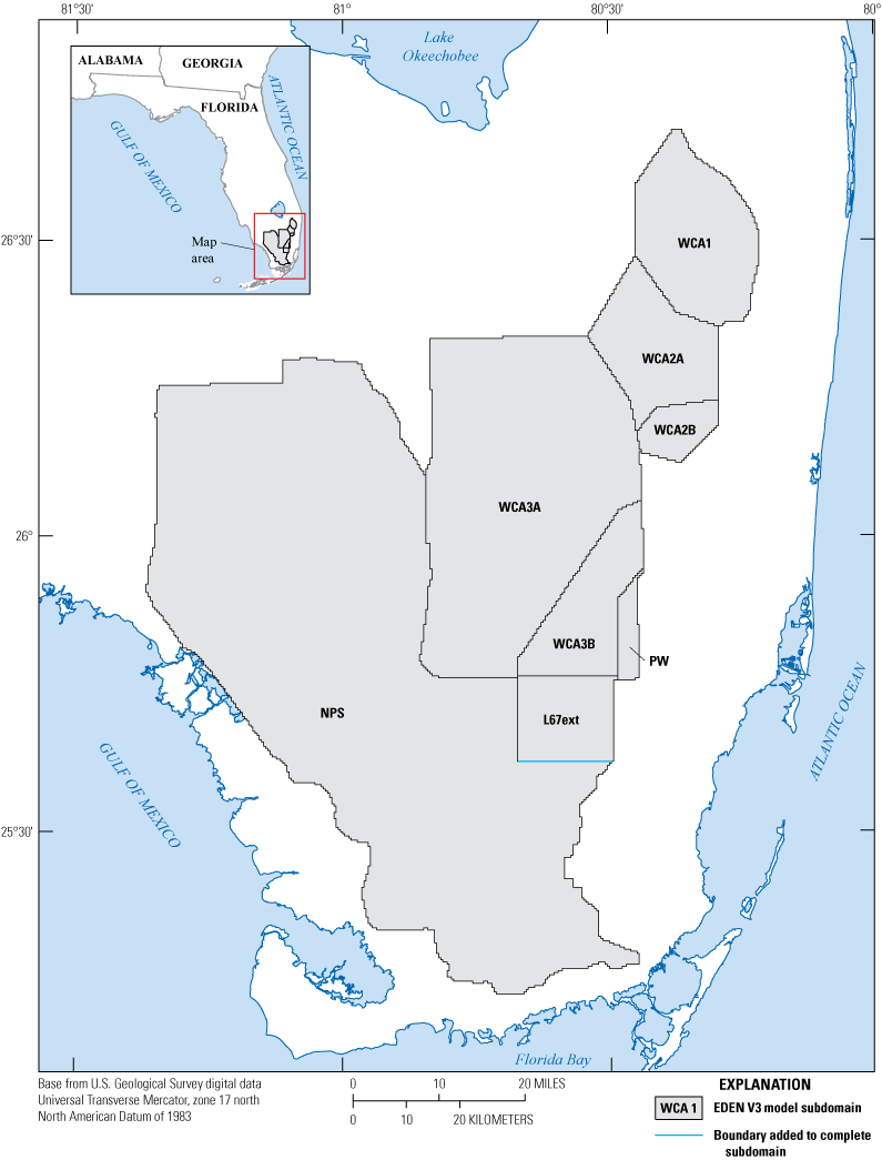
Eight Everglades Depth Estimation Network (EDEN) subdomains separated by water-level discontinuities caused by the major levee system (modified from Haider and others, 2020). WCA1, Water Conservation Area 1; WCA2A, Water Conservation Area 2A; WCA2B, Water Conservation Area 2B; WCA3A, Water Conservation Area 3A; WCA3B, Water Conservation Area 3B; PW, Pennsuco Wetlands; L67ext, Levee 67 extension; NPS, Everglades National Park and Big Cypress National Preserve.
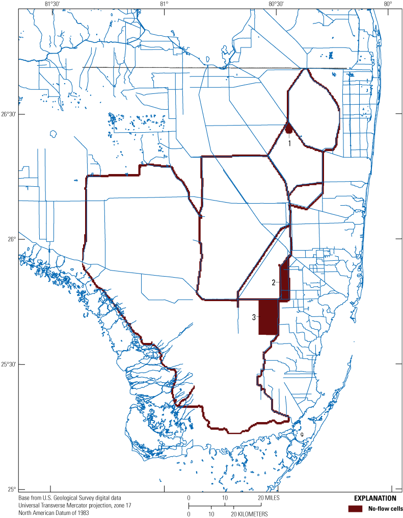
No-flow cells in Everglades Depth Estimation Network (EDEN) flow-vector computations, which occur at the domain boundary and along canals. Numbers 1, 2, and 3 indicate areas where flow vectors cannot be calculated; location 1 is characterized by a single gage near a corner of two levees that has nine flow structures (not shown), location 2 is a narrow area between a canal and a boundary, and location 3 has six gages in a cluster near a canal.
Further determination of no-flow cell locations was made by delineating locations where gradients were not representative of flow at the scale of the grid (hundreds of meters). Such cases may be due to a gage being heavily affected by local structure flows or additional obstructions to flows. Gradients calculated in these areas are affected by canal stage, which may not be the same as the stage in an adjacent wetland, resulting in erroneous flow vectors. Using data from the year 2020, areas with water-level gradients an order of magnitude larger than the average in EDEN are noted as consistently being affected by water-level interpolation to nearby canal levels. These locations are included in the no-flow areas shown in figure 5. Location 1 (fig. 5) is west of the L-31N canal and includes the enlarged inset map in figure 1. Location 2 (fig. 5) is east of L-30 in the Pennsuco Wetlands area (fig. 1). Location 1 (fig. 5) is at the northern corner of EDEN model subdomain WCA2A (fig. 4). Location 1 is characterized by a single gage near a junction of two levees that has nine flow structures (not shown), location 2 is a narrow area between a canal and a boundary, and location 3 has six gages in a cluster near a canal.
Calibration
The modified Manning’s equation was calibrated by using continuous flow measurement sites at coastal rivers in Everglades National Park, for the period January 1–December 31, 2020, to develop friction factors (K) for each river individually and for the total flow. The values of the coefficients K, α, and β in equation 3 depend on the location, vegetation, and the flow regime. For the GARDEN application, the coefficients can be calibrated by the equivalence of water-level gradient S in equation 3 with ∇Zx and ∇Zy from equations 1 and 2:
wherew
is the horizontal dimension of an EDEN grid cell, and
d
is the average depth of the four grid cells shown in figure 2.
One source of calibration data is the South Florida Water Management District’s computed discharge data at control structures (South Florida Water Management District, 2020), which is based on stages and rating curves upstream and downstream of the control structure. The total discharge in the cells directly downstream from the control structure can be equated to the discharge at the structure. However, multiple sources of flow affecting an area of the wetland or regional flow that is not associated with the structure can interfere with equating the measured structure flow with the wetland water-level gradient, increasing calibration uncertainty. The downstream stages at control structures often are not a good representation of water levels required to calculate a wetland gradient in an area. Considering these difficulties, flow data at control structures were not used to calibrate GARDEN.
Point velocities have been measured in the Everglades (Riscassi and Schaffranek, 2002; He and others, 2010), but measurements lacked adequate temporal and spatial continuity for inclusion in the calibration process. These measurements would have to be multiplied by the EDEN grid-cell widths to compare with computed values. This approach would assume that the point velocity is approximately equivalent to a daily average velocity for the area around the measurement, but the actual vertically averaged velocity is not known. In addition, these measurements are usually made at different locations and at different times, lacking temporal and spatial continuity, so they were not chosen for calibration.
Measured flow at coastal-river gages on the boundary of the EDEN study area provides a timeseries for calibration. Lostmans River, Broad River, Harney River, and Shark River have USGS continuous-discharge gages and receive flow from Everglades National Park along the EDEN domain boundary (figs. 1 and 6). The four coastal river gages measure discharge every 15 minutes and the data extend back as far as 2007 (table 1) (U.S. Geological Survey, 2016). For the calibration of the GARDEN flow vectors, the daily average flow out of one of these rivers should approximately match the sum of the computed GARDEN boundary flows upstream from the river for that day. The rivers monitored by these gages drain flow from Shark River Slough, a primary flow-way in Everglades National Park, so calibration includes flow characteristics important to the study domain. Given that spatially detailed studies have not been implemented in the EDEN domain, the calibration approach chosen is to utilize the timeseries of discharge from the four coastal gages shown on figure 6 to calibrate K values by fitting observed and modeled discharge for temporally averaged values. Potential sources of error include subdaily variations in river flow, groundwater interactions, rainfall, and evapotranspiration between the upstream EDEN cells and location of the river gages.
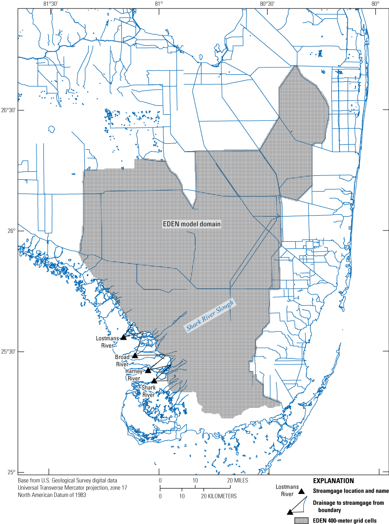
Location of coastal river gages used to calibrate Gradient-Related Discharge in an Everglades Network (GARDEN) flow vectors. EDEN, Everglades Depth Estimation Network.
Table 1.
Streamgages on the western boundary of Everglades National Park used for calibration of Gradient-Related Discharge in an Everglades Network (GARDEN) flow-vector algorithm.[Data are available from the USGS National Water Information System (U.S. Geological Survey, 2016). Dates shown as month, day, year. NAD 27, North American Datum of 1927; USGS, U.S. Geological Survey]
The three coefficients, K, α, and β, can vary with location, and K can vary with flow direction. With limited data, these coefficients are assumed to be stationary (constant) at a given measured-flow location. Values of α and β are taken from the literature, as described later, and K is used as the calibration parameter. The difference in coefficient values between measured-flow locations indicates frictional resistance variability, although each value is implicitly averaged over the drainage area of the coastal river. Spatial distributions of Everglades vegetation and frictional resistance have been mapped (Wang and others, 2007, fig. 4; Ruiz and others, 2017) but only cover part of the EDEN study area. Frictional resistance was examined in an area north of EDEN model subdomain WCA3A (fig. 4) using a wave-propagation technique (Wasantha Lal, 2017) and spatial variations determined, but also only cover part of the EDEN study area.
Calibrating GARDEN flow vectors to measured coastal flows requires delineating the boundary cell flows corresponding to each of the coastal rivers. The direction of the flow vectors near the known GARDEN area boundary indicates the river destination for different boundary grid cells, and the relative volumes of flow in each river can be used to estimate the distribution. Alternately, the total flows through the four rivers can be equated to the sum of the boundary flow vectors. Although this aggregates the frictional characteristics of the entire area together, it does remove the need to allocate flow vectors to individual rivers.
Implementation of GARDEN Python Version 3.12.3 Script (App)
The GARDEN page on the EDEN website (U.S. Geological Survey, 2024) presents the daily flow-vectors calculated using equations 4 and 5 in a command-line Python script (Python Software Foundation, Wilmington, Delaware). The script validates command-line arguments, fetches necessary EDEN water-level and depth data by means of the Xarray Python package (Hoyer and Hamman, 2017) (fig. 7), and then converts the data to imperial units (centimeters to feet). The main calculation is then performed by the NumPy package (Harris and others, 2020). For each day, (1) the water-level gradient is calculated for each two-by-two group of cells within the EDEN grid (see equations 1 and 2), (2) these calculated values are used in equations 4 and 5 to compute a grid of flow vectors, and (3) the resulting grid of vectors is aggregated using a sliding-window average to decrease the output resolution. The final grid of flow vectors is saved in two ways: (1) a vector-field plot (also called a quiver plot) is generated by the Matplotlib (Hunter, 2007) and Cartopy (Met Office, 2013) packages, showing each flow vector and its position in the Everglades, and (2) the components, magnitude, and coordinates of each flow vector are saved to a comma-separated values (CSV) file by the Pandas package (McKinney, 2010) (fig. 7). Results can be accessed at U.S. Geological Survey (2024).
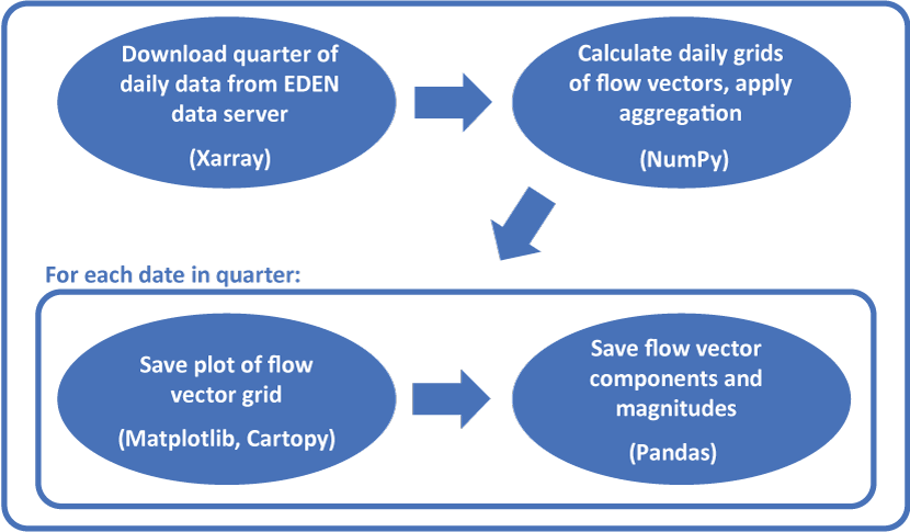
Calculation steps in the Gradient-Related Discharge in an Everglades Network (GARDEN) application. The names of the Python packages used to complete each step are shown in parentheses. EDEN, Everglades Depth Estimation Network.
Results
The flow vectors were computed from EDEN water-levels using equations 1, 2, 4, and 5. Flow vectors are not aggregated and remain at the 400-m resolution for flow calibration. Data from the four coastal rivers, Lostmans, Broad, Harney, and Shark Rivers, for the year 2020 were used to calibrate the flow vectors, and data from 2021 were used to validate the calibrated parameters. This scheme is automated to produce daily values for the EDEN web page.
Computed-Flow Vectors in 2020
Flow vectors at an aggregation of three-by-three 400-m cells to the 1,200-m scale were computed daily for the year 2020. The three-by-three cell aggregation scale is conducive to visualization of the entire EDEN area (fig. 8). The location of each surface-water flow vector is at the base of the arrow, and large flows can place the tip of the arrow in no-flow areas. Compared to dry-season flows on March 1, 2020, higher discharges and inundation are visible on August 1, 2020, during the wet season.
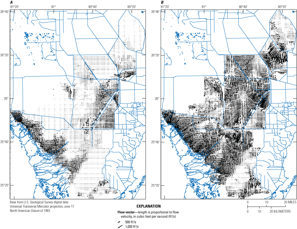
Computed daily Everglades Depth Estimation Network (EDEN) flow vectors for A, March 1, 2020, and B, August 1, 2020, aggregated to a 1,200-meter grid spacing.
Flow-Vector Calibration
Parameters used to compute flow vectors were calibrated using observed and simulated flows from January 1–December 31, 2020, at the four coastal river outflows (fig. 6), and EDEN boundary cells were selected with corresponding flows to each river. Cells were selected by trial and error to ensure that (1) the range of cells represents the likely flow path to each gage, and (2) the flow distribution among the coastal streams was similar to the distribution indicated by measured data from the gages.
Based on Kadlec (1990) and He and others (2010), coefficient values α = 0.71 and β = 1.12 were used in equations 4 and 5. The value of the coefficient K was calculated as a simple arithmetic average of calibrated K values for the sum of each daily measured and computed flow at each coastal river, as well as for total flows summed at all rivers for a value K = 45.59. The K value for individual coastal river flows ranged from 29.74 at Broad River to 64.26 at Shark River. These values correspond to Manning’s n values of 0.050–0.023, respectively. Although greater than most values assigned to rivers, these values are considerably smaller than values assigned to sites affected by emergent vegetation (He and others, 2010; Wang and others, 2007). However, field estimation of frictional resistance usually concentrates on small-scale measurements of flow or point measurements in the vegetation type of interest (He and others, 2010). Larger-scale flow regimes include subareas of lower vegetative resistance that can carry most of the flow. This results in a lower aggregate frictional resistance for larger-scale areas. Wasantha Lal (2017) computed frictional resistance by means of a wave-propagation technique in various stormwater treatment areas in the “greater Everglades” with flow widths ranging from 6,512 to 16,010 feet. Computed Manning’s n values varied greatly, from 0.18 to 1.42. Another consideration is that the frictional resistance represented by this calibration represents the southern end of Shark River Slough (fig. 6), which, as a major flow-way, may have a lower frictional resistance than areas elsewhere with denser vegetation.
With the area-average value K = 45.59, the flow vectors can be quantified as indicated in figure 8. The flow vectors are separated by 1,200 m (three cells), so the indicated flowrates are occurring on this scale. Flows at the EDEN boundaries were computed using GARDEN and compared to measured river flows for the 2020 calibration period (fig. 9). The measured flows at the coastal rivers fluctuate more than the upstream flows computed along the EDEN boundary by GARDEN, as the coastal-river flows are highly affected by wind and tide. The larger timescale variability in flow in the rivers are reflected in the EDEN boundary flow, although minimal variations are indicated in the boundary flow leading to Lostmans River.
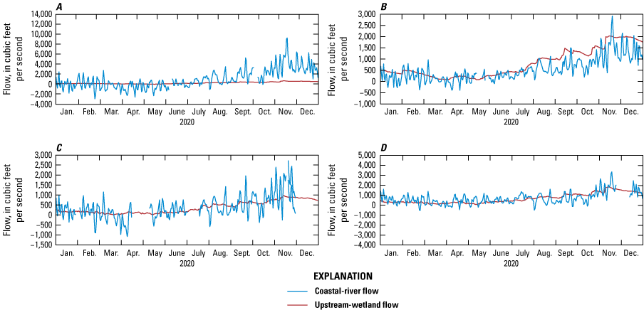
Measured daily coastal-river flows and upstream computed Everglades Depth Estimation Network (EDEN) boundary flows for the 2020 calibration period. A, Lostmans River; B, Broad River; C, Harney River; D, Shark River.
Flow-Vector Validation
To validate GARDEN output, streamflow vectors were calculated for 2021 and the boundary flow to the coastal rivers calculated (fig. 10). Similar to the 2020 calibration period, the longer-term fluctuations in river flows are indicated in the EDEN boundary flows, with the boundary flow upstream of Lostmans River showing little change. Cumulative flow for both 2020 and 2021 indicates the biggest difference between river and EDEN boundary flows occurs from November 2020 to April 2021 (fig. 11).
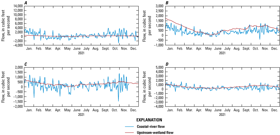
Measured daily coastal-river flows and upstream computed Everglades Depth Estimation Network (EDEN) boundary flows for verification. A, Lostmans River; B, Broad River; C, Harney River; D, Shark River.
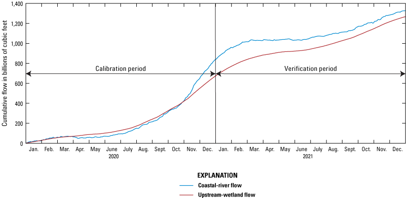
Cumulative values of measured coastal river flows and upstream computed Everglades Depth Estimation Network (EDEN) boundary flows.
The temporal variability in flow observed at the four coastal-river gages were not simulated in the flows computed by GARDEN at the EDEN boundary, as the upstream flow is not subject to coastal wind and tidal forcings. Despite these differences, the Pearson’s correlation coefficient between the EDEN boundary flows and the sum of the coastal river flows for the 2020 calibration period is 0.766. For the 2021 flows, the Pearson’s coefficient is 0.566. A Pearson's coefficient over 0.5 indicates that more than one half of the observed variance is explained by the computed data.
Example Application
Although there are many uses for the GARDEN application, one use is to examine the effects of control-structure discharge on wetland flow. The S12A, B, C, and D structures (S12s) discharge into Everglades National Park from the Tamiami Canal (fig. 1) and supply water to Shark River Slough. The combined flow through these structures for June 2020 is shown on figure 12. Flow releases were zero until June 2, 2020, and increased rapidly through June 4, 2020. The effect of these releases from the S12s on flow direction and magnitude in the adjoining wetlands is apparent in the EDEN flow vectors for select days on figure 13.
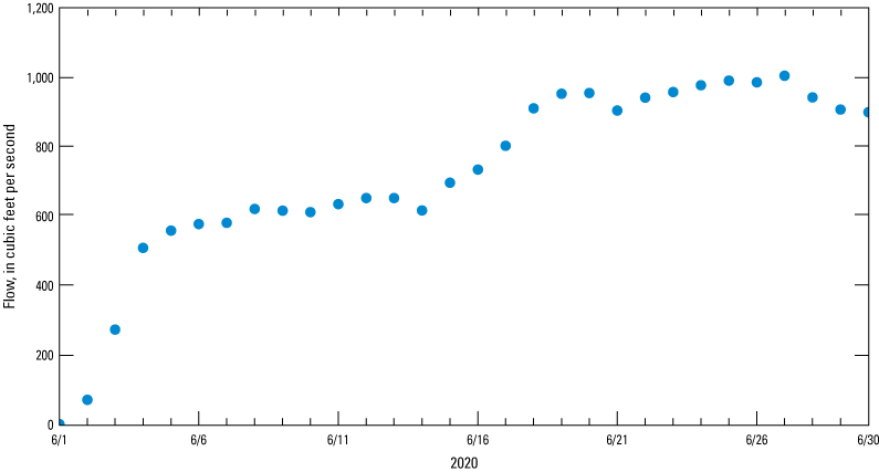
Total daily flow through S12A, B, C, and D observed in June 2020.
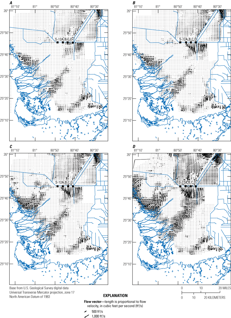
Wetland-flow vectors for select days in June 2020. A, June 2; B, June 3; C, June 4; D, June 18.
On June 2, 2020, little flow is indicated south of the S12s, because only 70 cubic feet per second (ft3/s) was flowing through the structures on that date (figs. 12 and 13). On the next day, June 3, flow south of the S12s increased to 273 ft3/s. Flow through S12A did not occur in June 2020, and the flow patterns reflect this (fig. 13; location on fig. 1). Although flow through the structure increased to 508 ft3/s on June 4, very low flow persists farther south of the structures with most of the flow from the S12s appearing to be going to storage in the adjacent wetlands. By June 18, the continuous path of flow vectors from the S12s structures to the coastal boundary indicates that the response of flows in Shark River Slough to flow releases during the dry season may take over a week.
Limitations
The GARDEN flow-vector maps indicate some limitations in the technique near control structures. The flow vectors in downstream cells closest to the S12 structures depict much higher flow than flow vectors in the adjacent cells to the south (fig. 13), which seems counterintuitive to the flow volumes reported at the structures (fig. 12). This inconsistency is caused by the water-level interpolation in EDEN, which uses a radial-basis function (RBF) that specifies eight nearest neighbor gages for the interpolation (Haider and others, 2020). The gages at the S12s measure the tail water, which is substantially higher than water levels in the nearby wetlands when the structure is discharging. Whereas an RBF interpolation assumes a linear water-surface gradient between measurement gages, the actual water level at the tail water of a discharging structure is substantially higher than in the adjacent wetland. Consequently, the water-level gradient calculated by the RBF is higher than the actual gradient. If the surface-water flow vectors directly south of the S12s are summed for June 4, 2020, they total 1,625 ft3/s, whereas flow vectors in the grid row 3 miles farther south sum to 573 ft3/s. The measured flow at the S12s for that date is 508 ft3/s, so the RBF-calculated values adjacent to the structures are too high and the interpolated values are much closer to measured values four grid cells to the south. When using EDEN flow-vector estimates, it is important to consider that flow vectors in proximity to a flow structure may be overestimated.
This limitation of the GARDEN model near flow structures can be generalized as uncertainty in the application of the RBF to interpolate water levels between field gages. The limitation is inherent to the sparsity of the field gage network. Areas with larger distances between gages have larger uncertainties. Because the gradient of the interpolated water surface is used to compute flow, these uncertainties become smaller when aggregating grid cells to a larger scale.
Other limitations of the GARDEN flow-vector technique include the following:
-
1. No temporal resolution for periods shorter than a day—Events such as precipitation and structure operations may make substantial flow changes on subdaily time scales, and using EDEN’s daily average water levels means that GARDEN cannot represent peak or minimum flow.
-
2. Approximation of frictional resistance—The calibration of flow magnitudes to coastal river flow does not consider spatial variations in frictional resistance and assumes the effective resistance at the boundary near the coastal rivers is typical of the domain. The magnitude of flow vectors must be considered to have uncertainty, and the relative magnitudes are more certain.
-
3. Assumed gradient and depth coefficients—The values of α and β, the coefficients for the gradient and depth terms, respectively, are set to values from Kadlec (1990) and He and others (2010) and not used as calibration parameters. The value of α reflects the flow in the transition zone between laminar and turbulent, and would vary with velocity and vegetation density, and β reflects the effect of emergent vegetation, which also varies spatially.
Summary
The water-level surfaces in the so-called “greater Everglades” interpolated from gage data by the Everglades Depth Estimation Network (EDEN) are used to estimate gradients and volumetric flows in the “greater Everglades” using the Gradient-Related Discharge in an Everglades Network (GARDEN) application, developed by the U.S. Geological Survey in cooperation the U.S. Army Corps of Engineers. GARDEN uses the 400-meter square grid of water levels from EDEN to compute water-level gradients in the east-west and north-south directions and applies them in a modified Manning’s equation to determine flow. The frictional resistance is estimated by calibrating the modified Manning’s equation to measured flows at four coastal rivers fed by EDEN boundary flows. Levees and other features that act as barriers to flow are defined as no-flow grid cells where vectors are set to zero. To vary the resolution of the wetland-flow vector map, grid cells can be aggregated into a larger-scale grid. Doing so allows for visualization of the entire domain without the density of plotted vectors interfering with map clarity.
Calibration of the flow-vector magnitudes was implemented for 2020 daily values and verification for 2021 data. The observed coastal-river flows fluctuate more than the GARDEN boundary flows because of tidal and wind forcings. Frictional terms are estimated daily and averaged to obtain a value that is applied to the entire domain. The Pearson’s correlation coefficient between observed coastal-river flow and computed GARDEN boundary flows is 0.766 for the 2020 calibration period and 0.566 for the 2021 verification period.
The application of GARDEN to simulating flow releases from the S12 control structures indicates that the response of wetland flows in Shark River Slough to control-structure releases during the dry season may take more than a week. Values of flow vectors may be overestimated within 3 miles of control structures because of difficulties in resolving the water-level gradient downstream from the structure. Results indicate that the flow vectors farther from the structure are more accurate than those near the structure.
The GARDEN application provides a tool that scientists and water managers can use to estimate flows and distributions in the “greater Everglades.” The response of the daily flow-vector map to water-management releases can be tracked spatially and temporally, and the efficiency of different water-management schemes to deliver water to specific areas can be assessed.
References Cited
Chin, D.A., 2011, Hydraulic resistance versus flow depth in Everglades hardwood halos: Wetlands, v. 31, no. 5, p. 989–1002, accessed October 16, 2023, at https://doi.org/10.1007/s13157-011-0214-3.
Choi, J., and Harvey, J.W., 2014, Relative significance of microtopography and vegetation as controls on surface water flow on a low-gradient floodplain: Wetlands, v. 34, no. 1, p. 101–115, accessed October 16, 2023, at https://doi.org/10.1007/s13157-013-0489-7.
Haider, S., Swain, E., Beerens, J., Petkewich, M., McCloskey, B., and Henkel, H., 2020, The Everglades Depth Estimation Network (EDEN) surface-water interpolation model, version 3: U.S. Geological Survey Scientific Investigations Report 2020–5083, 31 p., accessed October 16, 2023, at https://doi.org/10.3133/sir20205083.
Haider, S.M., Rocco, A., and Swain, E., 2021, Digital elevation model (DEM) at 50 m resolution for the Everglades Depth Estimation Network (EDEN): U.S. Geological Survey data release, accessed October 16, 2023, at https://doi.org/10.5066/P9DN34MB.
Harris, C.R., Millman, K.J., van der Walt, S.J., Gommers, R., Virtanen, P., Cournapeau, D., Wieser, E., Taylor, J., Berg, S., Smith, N.J., Kern, R., Picus, M., Hoyer, S., van Kerkwijk, M.H., Brett, M., Haldane, A., Fernández del Río, J., Wiebe, M., Peterson, P., Gérard-Marchant, P., Sheppard, K., Reddy, T., Weckesser, W., Abbasi, H., Gohlke, C., and Oliphant, T.E., 2020, Array programming with NumPy: Nature, v. 585, p. 357–362, accessed June 10, 2024, at https://doi.org/10.1038/s41586-020-2649-2.
He, G., Engel, V., Leonard, L., Croft, A., Childers, D., Laas, M., Deng, Y., and Solo-Gabriele, H.M., 2010, Factors controlling surface water flow in a low-gradient subtropical wetland: Wetlands, v. 30, p. 275–286, accessed October 16, 2023, at https://doi.org/10.1007/s13157-010-0022-1.
Hoyer, S., and Hamman, J., 2017, Xarray—N-D labeled arrays and datasets in Python: Journal of Open Research Software, v. 5, no. 1, article 10, 6 p., accessed June 11, 2024, at https://doi.org/10.5334/jors.148.
Jadhav, R.S., and Buchberger, S.G., 1995, Effects of vegetation on flow through free water surface wetlands: Ecological Engineering, v. 5, no. 4, p. 481–496, accessed October 16, 2023, at https://doi.org/10.1016/0925-8574(95)00039-9.
Kadlec, R.H., 1990, Overland flow in wetlands—Vegetation resistance: Journal of Hydraulic Engineering, v. 116, no. 5, p. 691–706, accessed October 16, 2023, at https://doi.org/10.1061/(ASCE)0733-9429(1990)116:5(691).
Liu, Z., Volin, J.C., Owen, V.D., Pearlstine, L.G., Allen, J.R., Mazzotti, F.J., and Higer, A.L., 2009, Validation and ecosystem applications of the EDEN water-surface model for the Florida Everglades: Ecohydrology, v. 2, p. 182–194, accessed June 11, 2024, at https://doi.org/10.1002/eco.
Met Office, 2013, Cartopy—A cartographic Python library with Matplotlib support: Exeter, United Kingdom, Met Office web page, accessed June 11, 2024, at http://scitools.org.uk/cartopy.
Patino, E., Conrads, P., Swain, E., and Beerens, J., 2018, Everglades Depth Estimation Network (EDEN)—A decade of serving hydrologic information to scientists and resource managers (ver. 1.1, January 2018): U.S. Geological Survey Fact Sheet 2017–3069, 6 p., accessed October 16, 2023, at https://doi.org/10.3133/fs20173069.
Pearlstine, L., Higer, A., Palaseanu, M., Fujisaki, I., and Mazzotti, F., 2007, Spatially continuous interpolation of water stage and water depths using the Everglades depth estimation network (EDEN): University of Florida IFAS Extension CIR1521/UW278, v. 2007, no. 18, 32 p., accessed June 11, 2024, at https://doi.org/10.32473/edis-uw278-2007.
R Core Team, 2024, R—A language and environment for statistical computing: Vienna, Austria, R Foundation for Statistical Computing website, accessed May 28, 2024, at https://www.R-project.org.
Riscassi, A.L., and Schaffranek, R.W., 2002, Flow-velocity, water-temperature and conductivity data collected in Shark River Slough, Everglades National Park, during 1999–2000 and 2000–2001 wet seasons: U.S. Geological Survey Open-File Report 2002–159, 32 p., accessed October 16, 2023, at https://doi.org/10.3133/ofr02159.
Ruiz, P.L., Giannini, H.C., Prats, M.C., Perry, C.P., Foguer, M.A., Arteaga-Garcia, A.A., Shamblin, R.B., Whelan, K.R., and Hernandez, M., 2017, The Everglades National Park and Big Cypress National Preserve Vegetation Mapping Project: Interim report—Southeast saline Everglades (region 2), Everglades National Park: National Park Service Natural Resource Report NPS/SFCN/NRR–2017/1494.
South Florida Water Management District, 2020, DBHYDRO (environmental data): South Florida Water Management District database, accessed June 20, 2024, at https://www.sfwmd.gov/science-data/dbhydro.
Swain, E., and Adams, T., 2024, Gradient-related discharge in an Everglades network (GARDEN) software: U.S. Geological Survey software release, accessed June 1, 2023, at https://doi.org/10.5066/P138WZSY.
Tsihrintzis, V.A., and Madiedo, E.E., 2000, Hydraulic resistance determination in marsh wetlands: Water Resources Management, v. 14, p. 285–309, accessed October 16, 2023, at https://doi.org/10.1023/A:1008130827797.
U.S. Geological Survey, 2016, USGS Water Data for the Nation: U.S. Geological Survey National Water Information System database, accessed May 17, 2024, at https:// doi.org/10.5066/F7P55KJN.
U.S. Geological Survey, 2024, Gradient-Related Discharge in an Everglades Network (GARDEN) viewer: U.S. Geological Survey, accessed May 28, 2024, at https://sofia.usgs.gov/eden/garden/.
Wang, J.D., Swain, E.D., Wolfert, M.A., Langevin, C.D., James, D.E., and Telis, P.A., 2007, Application of FTLOADDS to simulate flow, salinity, and surface-water stage in the southern Everglades, Florida: U.S. Geological Survey Scientific Investigations Report 2007–5010, 112 p., accessed October 16, 2023, at https://doi.org/10.3133/sir20075010.
Wasantha Lal, A.M., 2017, Mapping vegetation-resistance parameters in wetlands using generated waves: Journal of Hydraulic Engineering, v. 143, no. 9, 11 p., accessed October 16, 2023, at https://ascelibrary.org/doi/pdf/10.1061/(ASCE)HY.1943-7900.0001311.
Wilsnack, M.M., Welter, D.E., McMunigal, C.L., Montoya, A.M., and Obeysekera, J., 2001, The use of MODFLOW with new surface water modules for evaluating proposed water management system improvements in north Miami-Dade County, Florida, p. 89–99 in Panigrahi, B.K., and Singh, U.P., eds., Integrated surface and ground water management—Specialty Symposium on Integrated Surface and Ground Water Management at the World Water and Environmental Resources Congress 2001, Orlando, Fla., May 20–24, 2001, [Proceedings]: American Society of Civil Engineers, accessed October 16, 2023, at https://doi.org/10.1061/40562(267)10.
Zhang, B., Wdowinski, S., and Gann, D., 2022, Space-based detection of significant water-depth increase induced by Hurricane Irma in the Everglades wetlands using Sentinel-1 SAR backscatter observations: Remote Sensing, v. 14, no. 6, article 1415, accessed June 11, 2024, at https://doi.org/10.3390/rs14061415.
For more information about this publication, contact
Director, Caribbean-Florida Water Science Center
U.S. Geological Survey
4446 Pet Lane, Suite 108
Lutz, FL 33559
For additional information, visit
https://www.usgs.gov/centers/car-fl-water
Publishing support provided by
Lafayette Publishing Service Center
Disclaimers
Any use of trade, firm, or product names is for descriptive purposes only and does not imply endorsement by the U.S. Government.
Although this information product, for the most part, is in the public domain, it also may contain copyrighted materials as noted in the text. Permission to reproduce copyrighted items must be secured from the copyright owner.
Suggested Citation
Swain, E., and Adams, T., 2024, Representation of surface-water flows using Gradient-Related Discharge in an Everglades Network: U.S. Geological Survey Scientific Investigations Report 2024–5041, 19 p., https://doi.org/10.3133/sir20245041.
ISSN: 2328-0328 (online)
Study Area
| Publication type | Report |
|---|---|
| Publication Subtype | USGS Numbered Series |
| Title | Representation of surface-water flows using Gradient-Related Discharge in an Everglades Network |
| Series title | Scientific Investigations Report |
| Series number | 2024-5041 |
| DOI | 10.3133/sir20245041 |
| Publication Date | June 25, 2024 |
| Year Published | 2024 |
| Language | English |
| Publisher | U.S. Geological Survey |
| Publisher location | Reston, VA |
| Contributing office(s) | Caribbean-Florida Water Science Center |
| Description | Report: vi, 19 p.;2 Data Releases; Database; Software Release |
| Country | United States |
| State | Florida |
| Other Geospatial | Everglades |
| Online Only (Y/N) | Y |