

Wildland Fire Effects on Sediment, Salinity, and Selenium Yields in a Basin Underlain by Cretaceous Marine Shales near Rangely, Colorado
Links
- Document: Report (21.2 MB pdf) , HTML , XML
- Data Releases:
- USGS data release - Orthoimagery, digital elevation, digital terrain, final surface, and vegetation classification models for four stream catchments in western Colorado 2016
- USGS data release - Erosion rates and salinity and selenium yields in a basin near Rangely, Colorado following the 2017 Dead Dog wildfire as modeled by WEPP and measured from UAV
- Download citation as: RIS | Dublin Core
Abstract
Understanding and quantifying soil erosion from rangelands is a high priority for land managers, especially in areas underlain by Cretaceous Mancos Shale, which is a natural source of sediment, salinity, and selenium to surface waters in many areas of western Colorado and eastern Utah. The purpose of this report is to present the results of a U.S. Geological Survey study that assessed sediment, salinity, and selenium yields after the Dead Dog wildfire (fire began June 11, 2017) in northwestern Colorado. Two methodologies were used to quantify erosion, with different data requirements and analytical complexity. The first approach was the use of a process-based erosion model, the Watershed Erosion Prediction Project, which uses inputs of climate, topography, vegetation, and soils data from existing datasets to predict erosion, making this approach easily extensible to other areas. The second approach required more complex data collection and was used to measure erosion and deposition by differencing digital elevation models created from uncrewed aerial vehicle imagery collected in 2016 (pre-fire) and 2021 (post-fire). Sediment, salinity, and selenium yields were calculated from the volumetric estimates of erosion from both methods, and a discussion of factors that may have contributed to overall findings, including vegetation, fire effects, and soil characteristics, is included.
The two approaches yielded different outputs. Results from the Watershed Erosion Prediction Project model indicated that almost no erosion occurred after the Dead Dog fire. However, morphological changes in the study basin after the Dead Dog fire were visible in the pre- and post-fire imagery and measured in the digital elevation model differencing technique, with net erosion occurring in channel and landscape extents, though calculated erosion rates and salinity and selenium yields were relatively small. Visible and measured morphological changes consisted primarily of incision and deposition within stream channels and rill incision and expansion on steeper slopes. Widespread sheet erosion was not evident. Much of the new erosion originated within, and immediately below, previously vegetated areas that were then burned by the wildfire. Greater erosion rates and salinity and selenium yields were measured in the channel extent relative to the landscape extent. Calculated erosion rates ranged from 0.24 to 0.45 megagrams per hectare per year. These results indicate that the Dead Dog fire resulted in increased erosion in the study basin, yet these effects were relatively small based on the overall magnitude of modeled and measured erosion from the Watershed Erosion Prediction Project and the digital elevation model differencing technique. Minimal erosion in the basin is likely due to local site characteristics typical of soils derived from Mancos Shale, including the presence of robust physical crusts and biological soil crusts, and limitations of the methods based on data availability. Focusing uncrewed aerial vehicle flights on key areas (individual steep slopes, high-intensity burn areas, specific stream reaches) could likely increase understanding of erosional process with less effort and error than doing landscape-level flights.
Introduction
Soils derived from Cretaceous Mancos Shale are a natural source of sediment, salinity, and selenium to surface waters in many areas of western Colorado and eastern Utah. Marine shales are often in dryland areas where surface disturbance of the soil can greatly increase wind and water erosion (Barthès and Roose, 2002; Belnap and others, 2007). A large part of dryland areas in the Western United States have undergone some form of surface disturbance, including historical land use. For example, livestock grazing is the dominant land use by area in the Western United States, involving more than 50 percent of the land area (Bigelow and Borchers, 2017), and has been associated with increased regional atmospheric dust emissions (Nauman and others, 2018) and reduced water quality (Fleischner, 1994). Understanding and quantifying erosion from rangelands is a high priority for land managers, especially with projected increases in aridity and wildfires under climate change (Ault and others, 2016).
Higher temperatures and earlier spring snowmelt have increased the frequency and severity of wildfires in the Western United States, raising the risk of erosion (Litschert and others, 2012; Sankey and others, 2017; Wilson and others, 2021). Within fire scars, vegetation loss and changes to soil properties amplify the risk of erosion through runoff, debris flows, mudslides, and flash floods (Ebel and Martin, 2017; Kean and Staley, 2021). Erosion can be several orders of magnitude higher after wildfires compared to pre-fire conditions (Wagenbrenner and Robichaud, 2014; Noske and others, 2016), and these effects can last for 5–10 years post-fire while ground cover and vegetation regrow and soils regain the ability to absorb excess precipitation (Ebel and Martin, 2017). Increased runoff poses challenges to local rehabilitation efforts and municipal water treatment and has ecological effects through greater delivery of sediment, ash, and nutrients to rivers and streams (Silins and others, 2014; Hohner and others, 2016; Wilson and others, 2021). Consequently, mapping, measuring, and modeling soil erosion and runoff within burned areas may be increasingly important to land and water managers.
The Watershed Erosion Prediction Project (WEPP) is a process-based hydrology and erosion model used by researchers and land managers to predict soil erosion and surface runoff from croplands, rangelands, and forests (Laflen and others, 1997). The online platform for WEPP, WEPPcloud (Lew and others, 2022), provides several interfaces for different land use scenarios, including WEPPcloud-Disturbed (https://wepp.cloud/weppcloud/), which can predict the effects fire and land management practices have on soil erosion and runoff. WEPP model simulations can be run for thousands of small hillslope and watershed segments to generalize estimates of post-fire soil erosion in large-scale channel networks (Miller and others, 2011; Flanagan and others, 2012). Use of WEPPcloud can range from simple, where users specify input files including hillslope topography, soil texture, land cover, and climate from an abbreviated list of options and use default parameters for inputs like ground cover, channel properties, and saturated hydraulic conductivity, to more complex, where users can carefully parameterize the model when field measurements and calibration data are available (Lew and others, 2022). In this study, the simplest workflow of WEPPcloud was used with input files and default parameters that would be readily available to land managers after a fire.
Imagery collected using uncrewed aerial vehicles (UAVs) can be processed into orthomosaics (a single georeferenced image created by stitching multiple images together) and digital elevation models (DEMs) using structure from motion (SfM) photogrammetric techniques (Ullman, 1979). UAVs equipped with cameras have become invaluable tools for detecting morphological change across a variety of environments and earth surface processes. For example, imagery from UAVs has successfully been used to quantify changes from flooding (Akay and others, 2020; Forbes and others, 2020), landslides (Mauri and others, 2021), coastal dynamics (Turner and others, 2016), and glacial retreat and ablation (Lamsters and others, 2022). When applied to UAV imagery, SfM creates a dense point cloud, DEM, and orthomosaic that are georeferenced either indirectly from ground control points (GCPs) visible in the imagery or directly from camera positions and orientations recorded during flight (Peppa and others, 2019). Thus, DEMs from separate flights, or epochs, can be co-registered, and morphological change can be detected by differencing DEMs among epochs.
In 2016, the U.S. Geological Survey (USGS), in cooperation with the Bureau of Land Management, began a study to characterize sediment, salinity, and selenium distribution and storage in four study basins under differing land use histories in Stinking Water Gulch in the lower part of the White River Basin in Rio Blanco County, Colo. Preston and others (2021) applied SfM techniques to overlapping images from a UAV survey completed in 2016 to create DEMs for each study basin to explore similarities and differences in channel geomorphology. On June 11, 2017, the Dead Dog fire started approximately 10 miles north of Rangely, Colo., and burned more than 18,000 acres in the Stinking Water Gulch (National Interagency Fire Center, 2023). This provided an excellent opportunity to collect post-fire imagery for comparison to the 2016 data, which represented pre-fire conditions. In 2021, to help understand erosion effects caused by rangeland fire and address concerns about the potential effects of rangeland wildfire on sediment, salinity, and selenium loading, additional modeling and UAV surveys were completed by the U.S. Geological Survey in one study basin, the B2 study basin, which is shown in fig. 1.
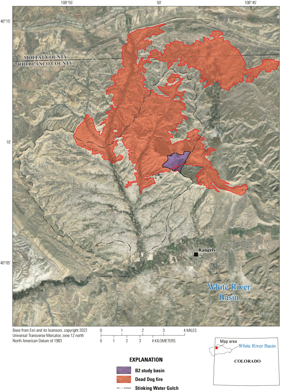
Location of the B2 study basin in northwestern Colorado with burn perimeter of the Dead Dog fire (Preston and others, 2023).
Purpose and Scope
The purpose of this report is to present the results of a USGS study that assessed sediment, salinity, and selenium yields in a basin after a rangeland wildfire in northwestern Colorado (fig. 1). This investigation is focused on a basin in Stinking Water Gulch near Rangely, Colo., that is predominantly used for rangeland grazing (Luke McCarty, Bureau of Land Management, written commun., 2022). This study uses pre- and post-fire UAV imagery collected in 2016 and 2021 and soil data collected in 2016 from multiple locations in the basin. The report includes (1) modeled erosion post-fire using a process-based erosion model (WEPPcloud); (2) measured post-fire volumetric soil erosion and deposition using a time series of UAV-derived DEMs; (3) calculation of salinity and selenium yields from modeled and measured erosion estimates; and (4) a discussion of factors that may contribute to differences between modeled and measured yields, including vegetation and soil characteristics. The analyses presented in this report enhance understanding of the effects of wildfire on sediment, salinity, and selenium loading in a basin underlain by Cretaceous Mancos Shale. Further, comparisons of different methodologies can aid land managers’ decision making regarding erosion monitoring and assessment in the future.
Study Area
The B2 study basin drains approximately 1.63 square kilometers of the Stinking Water Gulch in the lower part of the White River Basin in Colo. (fig. 1). The northeast one-third of the study basin is separated by an escarpment rim, below which are steep shale slopes and badlands. A first order ephemeral wash runs through the middle of the basin with a slope of 3.6 percent (USGS, 2023). Elevations range from 1,903 meters (m; above North American Vertical Datum of 1988) on top of the rim to 1,662 m in the lower basin. The closest municipality is Rangely, Colo., in Rio Blanco County (6,529 residents; U.S. Census Bureau, 2020).
The land surface within the B2 study basin is covered by sparse vegetation and biological soil crusts. Based on field surveys completed during the study, vegetation included shrubs (Atriplex canescens [fourwing saltbush], Sarcobatus vermiculatus [greasewood], Tamarix sp. [tamarisk], and Artemisia sp. [sagebrush]) near ephemeral washes and stream channels; annuals (Bromus tectorum [cheat grass] and Chorispora tenella [purple mustard]), Opuntia sp. (prickly pear cactus), and Yucca sp. (yuccas) along the terraces and hillslopes of the badlands; and Juniperus sp. (juniper) and Quercus gambelii (Gambel’s oak) on the higher elevation rim. Much of the basin and surrounding area is used for cattle and sheep grazing primarily during winter months when snow accumulation on the ground is sufficient to support water needs (Gale, 1908). Grazing allotments in the area are for sheep, with grazing generally taking place from late November through early April (Luke McCarty, Bureau of Land Management, written commun., 2022). Mean temperatures in Rangely from 1951 to 2021 ranged from minimum temperatures of −1 degree Celsius (°C) in January, to maximum temperatures of 37 °C in July. On average, almost 25.4 centimeters per year (cm/yr) of precipitation falls in Rangely, and the mean snowfall is 81.3 cm/yr (National Oceanic and Atmospheric Administration Regional Climate Centers, 2022).
The basin is underlain by Mancos Shale, which consists of massive, fossiliferous marine shales with interbedded sandstone, siltstone, and devitrified volcanic ash layers of Late Cretaceous age (Cross and Purington, 1899). Field observations from this study revealed the streambanks consist primarily of fine materials, dominated by silt- and clay-sized particles deposited in varying thicknesses. The particles are generally homogenous and very cohesive, which can increase the erosive forces needed to entrain streambank materials.
Approach and Methods
The approach of this study was to characterize sediment loss after a rangeland wildfire using two different methods. A process-based erosion model was used to compare erosion under unburned and burned scenarios to better understand the effect of fire on erosion. Erosion and deposition were also measured by differencing DEMs created from UAV imagery collected in 2016 (pre-fire) and 2021 (post-fire). Specifically, SfM photogrammetry was used to align and georeference UAV imagery and DEMs with two methods evaluated: aligning imagery from each epoch independently and co-aligning imagery from both epochs together. The relative elevational uncertainty between the 2016 and 2021 DEMs created from each approach was determined by measuring the vertical error on invariant rock surfaces. The DEMs with the least relative elevational uncertainty were then used to create a DEM of difference (DoD) to calculate volumetric change across the entire basin, and within larger stream channels in the lower basin. Volumetric change detection was limited to bare ground surfaces by masking areas covered with vegetation canopies identified from the 2016 imagery (Preston and others, 2021).
Sediment Sampling and Yield Calculations
Sediment, salinity, and selenium yields were calculated from the volumetric estimates of sediment loss from the process-based erosion model and the DoD differencing method. Sediment samples were collected to measure bulk density (the dry weight of soil divided by its volume) on the main stem of Stinking Water Gulch at a location with multiple geomorphic surfaces present above the streambed (Preston and others, 2023). A total of 5 samples (referred to as SWG1–5) were collected: 3 from the closest distance above the streambed, 1 from the intermediate surface above the streambed, and 1 from the farthest surface above the streambed. In each location, vegetation and the top layer of sediment were cleared before driving a cylinder of known volume into the soil. Cores were collected so that the cylinder was filled completely without compacting the sediment, following methods in Blake and Hartge (1986). Each core was placed in a pre-weighed drying tin and dried at 105 °C for at least 12 hours. The dry sediment weight was divided by cylinder volume to obtain density in grams per cubic centimeter (g/cm3). All bulk density measurements (n=5) were used to convert DoD volumetric erosion and deposition estimates to mass estimates. The mean erosion rate calculated from all sampling locations was used for calculating salinity and selenium yields.
Additional soil samples (n=3) collected within the B2 study basin (referred to as “Dead Dog Transect” [DDT] 1–3) were used to measure salinity (also referred to as total dissolved solids, or TDS) and selenium concentrations for estimating the yields of these constituents. Using residue-on-evaporation techniques, water-soluble leachates were analyzed for total dissolved solids at the USGS National Water Quality Laboratory in Lakewood, Colo. (Fishman and Friedman, 1989). The resulting concentrations were related to the original mass of the sample and the volume of dilution water to arrive at concentrations of salts in milligrams per kilogram (mg/kg) of dry soil. Selenium speciation in sediments was obtained by using sequential extractions, which provide the best available means for studying selenium speciation in solid phases (Zawislanski and others, 2003). The sum of all selenium species was used to calculate a yield for each sample. Separate salinity and selenium yields were calculated for each salinity and selenium sample using the modeled channel erosion rates for both unburned and burned scenarios.
Soil Surface Cover Surveys
A survey of soil surface cover, emphasizing biological soil crust, was performed across the entire B2 study basin in 2021 using the step-point transect method (Coulloudon and others, 1999). Although this survey was meant to represent post-fire biological soil crust conditions, much of the biocrust observed post-fire likely existed pre-fire, given the amount of time required for biocrusts to reestablish after disturbance (Zaady and others, 2016). Random site locations were generated using the Balanced Design Tool (https://jornada-data.shinyapps.io/balanced-design-tool/). At each site, the surveyor walked 10 steps in each of the 4 cardinal directions and noted the ground cover at a predetermined location on the toe of the shoe every two steps. Ground cover was recorded as litter (standing or on the ground), rock, bare ground, live plant base, light cyanobacteria-dominated crust, dark cyanobacteria-dominated crust, moss, or lichen (Preston and others, 2023). Light cyanobacteria-dominated crust was counted if bacterial filaments were both visible and aggregating the soil surface into a cohesive unit. Percent cover of each ground cover category was calculated for each site location and across the entire study basin.
Process-Based Erosion Model
The WEPPcloud-Disturbed (WEPP hereafter) interface was used to run the WEPP model to predict erosion at the hillslope and basin scale (Lew and others, 2022). WEPP uses the Topographic Parameterization program (TOPAZ; Garbrecht and Martz, 1997) and Terrain Analysis Using Digital Elevation Models (TauDEM; Wallis and others, 2009) tools to divide a basin into hillslopes and identify stream channels. To better delineate channels in the small basin, the minimum channel length was reduced from the 100-m default value to 60 m, and the critical source area was reduced from the default of 10 hectare (ha) to 4 ha. This led to higher channel density and smaller hillslopes, which may increase WEPP’s accuracy at the basin scale (Kampf and others, 2020). For each hillslope and reach, four input files are needed for WEPP to run: slope, soil, vegetation, and climate. Slope was derived by WEPP from the National Elevation Dataset (NED; USGS, 2018) 30-m grid DEM. Soil information was obtained by WEPP from the Soil Survey Geographic Database (SSURGO; Reybold and TeSelle, 1989) and the Digital General Soil Map of the United States (STATSGO; Reybold and TeSelle, 1989). Vegetation information was calculated by WEPP using the National Land Cover Database (NLCD; Homer and others, 2015). Finally, WEPP relies on several daily climate variables: precipitation depth, storm duration, ratio of time to peak intensity to total storm duration, ratio of storm peak intensity to average intensity, maximum temperature, minimum temperature, dew point, solar radiation, wind velocity, and wind direction. Precipitation and temperature values were derived by WEPP from Gridded Surface Meteorological dataset (gridMET; Abatzoglou, 2011) daily data that were corrected by WEPP to match Parameter-elevation Regressions on Independent Slopes Model (PRISM; Daly and others, 2008) monthly data. The other daily climate variables were generated by WEPP from the stochastic weather generator, CLImate GENerator (CLIGEN; Fullhart and others, 2021) based on the Rangely, Colo., CLIGEN station that is 8.1 km away.
Three model runs were completed using WEPP. First, WEPP was used to model erosion for 2016, the year before the fire. This run simulated erosion that occurred before the fire and provided an initial groundwater storage value (0 millimeters [mm]) that was used in the subsequent model runs. Second, WEPP was used to model erosion for 2017–21 under unburned conditions. Third, WEPP was used to model erosion for 2017–21 under burned conditions. The burned model run used the same basin delineation information (reaches, hillslopes, and catchments), slope information, and climate information as the 2017–21 unburned scenario but also included a burn severity raster. The burn severity map is used by WEPP to modify the soils and vegetation to represent post-fire conditions.
The burn severity raster (fig. 2) was created with imagery from the European Space Agency’s Sentinel-2 satellite platform (European Space Agency, 2020). Normalized Burn Ratio (NBR) was calculated using the near infrared (NIR; 0.76–0.90 micrometers [μm]) and short-wave infrared (SWIR; 2.08–2.35 μm) bands. Wildfires tend to decrease reflectance in the NIR region because of the conversion of vegetation to charcoal or ash. Smaller drops in reflectance or short-term increases in reflectance of the SWIR region of the electromagnetic spectrum are caused by the formation of white ash. NBR exploits the fact that NIR and SWIR reflectance are oppositely affected by wildfire (Fassnacht and others, 2021). The Differenced Normalized Burn Ratio (DNBR) was calculated by subtracting the NBR of a post-fire image, collected June 14, 2017, from the NBR of a pre-fire image, collected May 5, 2017, and classified as unburned, low-severity, moderate-severity, and high-severity fire. Finally, the values outside of the burned area were reclassified as unburned. The burn severity raster is found in Preston and others (2023).
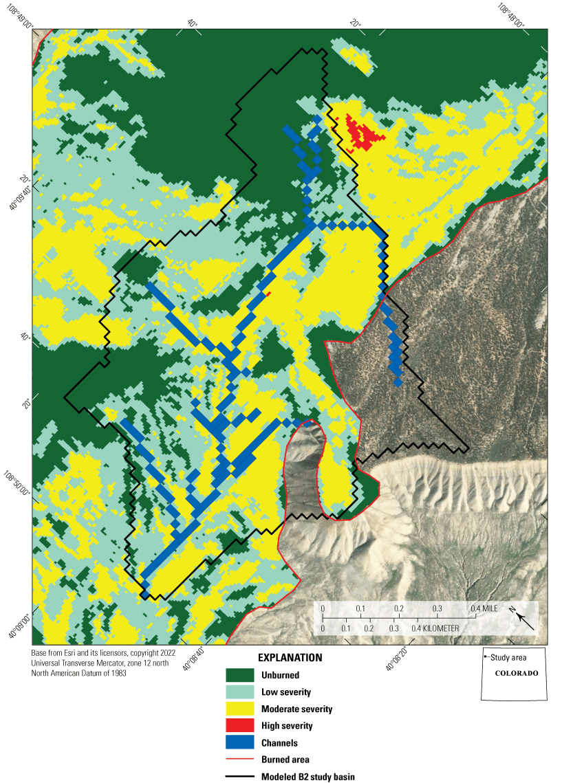
Burn severity map (Preston and others, 2023) used for Watershed Erosion Prediction Project model (Lew and others, 2022).
Measurement of Erosion by Differencing Digital Elevation Models
Erosion after the Dead Dog Fire was measured by comparing DEMs created from UAV imagery collected in 2016 and 2021. Two approaches to create DEMs were compared. In the first approach, UAV imagery was aligned independently using GCPs placed during each year prior to UAV flights. In the second approach, UAV imagery was co-aligned using natural GCPs (NGCPs) visible in imagery from both years. Accuracy of each approach was determined by comparing the errors between the 2016 and 2021 DEMs at 100 invariant check points.
Data Acquisition
The UAV imagery was acquired with a 3DR Solo (3D Robotics, Berkeley, Calif.) equipped with a Ricoh GR II (Ricoh Imaging Company, Tokyo, Japan) digital camera on September 1, 2016, and October 5 and 7, 2021. Totals of 13 and 15 flights were flown between 0938 and 1517 local time in 2016 and between 1150 and 1646 local time in 2021, respectively. Autonomous flight plans, consisting of parallel and perpendicular transects, were created in Mission Planner version 1.3.39 (ArduPilot Development Team, 2016) in 2016 and reused in 2021. Flight plans used terrain-following technology to maintain an approximate altitude of 120 m above ground level and a flight speed of 12 meters per second (m/s) for all flight lines. Digital photographs (images hereafter) were collected every 2 seconds during flights, with images planned for 66 percent forward lap, 50 percent side lap, and a ground sample distance (GSD; image resolution) of approximately 4.3 centimeters (cm). Images were geotagged using GeoSetter (GeoSetter, 2019) to match UAV telemetry data with time stamps on images.
Separate GCPs were used in 2016 and 2021. In 2016, 12 mesh GCPs (1.2 m × 1.2 m) were placed across the study area with center locations measured with a Trimble R8 Real-Time Kinematic Global Positioning System (GPS) (Trimble, Sunnyvale, Calif.) using a base station set up over a newly established point. In 2021, 12 GPS-enabled AeroPoints (Propeller Aerobotics USA, Denver, Colo.) GCPs were placed on October 5 at the approximate location of the 2016 GCPs. The accuracy of the AeroPoints was improved using a newly established base station point in 2021 measured with a Trimble R8S. However, an impending rainstorm on October 6 necessitated retrieval of AeroPoints that evening. The area above the escarpment rim became inaccessible after the rainstorm, so it was not possible to replace the seven GCPs located there before the October 7 flights. Therefore, only eight GCPs were imaged during 2021 UAV flights, as three targets above the escarpment rim were partially imaged on October 5. Absolute horizontal and vertical accuracies of 2016 GCPs were unknown, with values of 0.030 m used in image alignment. Absolute horizontal and vertical accuracies of 2021 GCPs were 0.017 m and 0.027 m, respectively, as calculated by Propeller Aerobotics.
Image Alignment
Images from the 2016 and 2021 UAV flights were aligned in Metashape (version 1.7.6; Agisoft, 2021), a photogrammetric software that uses SfM to develop three-dimensional (3D) structures from two-dimensional imagery sequences (Ullman, 1979). Before alignment, geotagged images (referred to as cameras in Metashape) from each year were imported into a single chunk in Metashape as separate geotagged images groups to allow visualization of camera locations in 3D space. Geotagged image locations that were not present both years and those in the upper basin where 2021 flights lacked ground control were removed. Totals of 1,906 and 1,892 images were retained from the 2016 and 2021 flights, respectively. Two approaches were evaluated for accuracy in aligning UAV images. In the first approach, images from each year were aligned independently using their respective GCPs. In the second approach, images from both years were co-aligned using estimated camera positions from the first approach and NGCPs identified on invariant surfaces. Locations of the GCPs used in both approaches (8 each in the 2016 and 2021 independently aligned imagery and 14 in the co-aligned imagery) are shown in fig. 3.
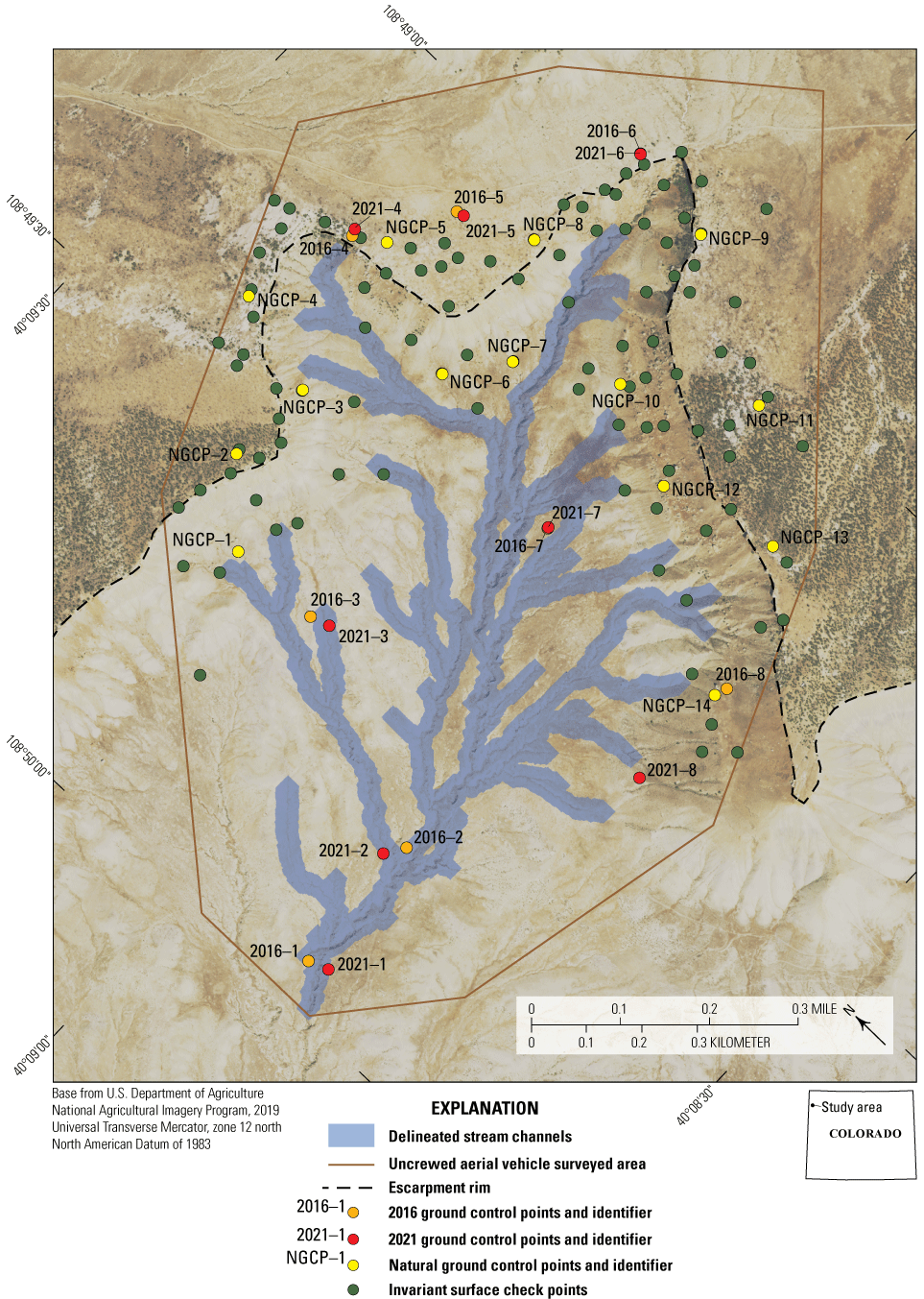
B2 study basin ground control point locations for independently aligned imagery from uncrewed aerial vehicle (UAV) flights on September 1, 2016, and October 5 and 7, 2021; natural ground control points for co-aligned 2016 and 2021 imagery; and invariant surface check points used to determine relative elevational uncertainty in digital elevation models. Landscape extent analyses were performed inside the UAV surveyed area, whereas channel extent analyses were performed only within delineated stream channels (Preston and others, 2021).
For the first approach, images from 2016 and 2021 were aligned independently in separate chunks in Metashape following methods described in Over and others (2021). The only difference in processing between years was identification and marking of GCPs. Ground control targets from 2016 were identified in images using the detect targets tool, with all eight targets correctly identified. The smaller AeroPoints targets used in 2021 could not be automatically detected; therefore, marker locations for the eight targets were placed on images manually. Estimated image positions from each independent alignment were exported as comma-separated values (CSV) files for use in the second alignment approach.
Separate dense point clouds, DEMs, and orthomosaics were created for each year in Metashape. Dense point clouds were created using the following settings: quality, high; depth filtering, aggressive; and calculate point confidence, enabled. Dense point clouds were filtered by confidence to remove low confidence points (0–1 out of 255). Next, DEMs for each year were built from their respective dense point clouds, and separate orthomosaics were built from respective DEMs. The DEMs and orthomosaics were then exported as tagged image file format (TIFF) files using a common extent and resolution between years (4.3 centimeters per pixel) to ensure alignment of data products across years (Preston and others, 2023).
For the second approach, the 2016 and 2021 images were co-aligned using four-dimensional (4D) SfM (Wood and others, 2022). Images were aligned in Metashape using methods in Over and others (2021); however, before alignment, estimated image positions from the 2016 and 2021 independently aligned imagery were imported to improve initial image positions. Next, 14 NGCPs, which consisted of visible features on invariant rock surfaces, were created in ArcGIS 10.8.1 (Esri, 2020; fig. 3). The NGCPs had to meet the following criteria: (1) the feature had to be visibly distinct in orthomosaics from both years, (2) features had to be smaller than a few pixels, and (3) pixels surrounding the center of the feature had to be within ± 3 cm of the feature on the respective yearly DEM. Points were manually placed at the center of each NGCP in the 2016 and 2021 orthomosaics. Lines were then created linking individual point locations between years with a midpoint created for each line. The horizontal and vertical coordinates of the midpoints were determined by the Calculate Geometry tool in ArcGIS and as the mean of the 2016 and 2021 DEMs, respectively. Hence, NGCPs were located equidistant between their respective locations, both horizontally and vertically, as calculated from the independently aligned orthomosaics and DEMs. Locations of NGCPs were imported into Metashape, and markers were manually placed on all images containing visible NGCPs.
The chunk containing the co-aligned imagery from 2016 and 2021 was duplicated twice to create new chunks to develop data products for each year. Appropriate images were removed so that each chunk contained only images for a given year but maintained tie points across years. Dense point clouds were created for each year and filtered by confidence using previously listed settings. Finally, DEMs and orthomosaics were created for each year and exported to the same extent and resolution of the independently aligned imagery.
Model Validation and Significant Change Detection
The quality of Metashape alignments for each alignment approach was determined using two metrics. The root mean square (RMS) reprojection error of the tie point cloud is commonly used to report the accuracy of alignment in Metashape, with values less than 0.3 pixels representing high-quality alignment (Over and others, 2021). Individual and mean errors of predicted GCP locations to measured values were also recorded.
The relative elevational uncertainty of DEMs from each alignment approach was determined from vertical errors at 100 independent check points on invariant surfaces using ArcGIS. Check points were manually placed on rock surfaces visible in the 2016 and 2021 orthomosaics to ensure points were on invariant surfaces, not under the vegetation canopy, and to provide the greatest spatial representation of error across the basin. Vertical errors were calculated as the difference between the 2016 and 2021 DEM for each alignment approach. Summary statistics of check point errors, including minimum, maximum, mean, and standard deviation (SD), were calculated for each alignment approach. Normality of check point errors by alignment approach was determined using Shapiro-Wilk tests (Shapiro and Wilk, 1965).
Identifying actual elevation change from DEM differencing, as opposed to relative uncertainty in DEMs from different epochs, is often done by identifying a minimum detectable change (MDC) threshold (Peppa and others, 2019; Hempel and others, 2021). When using an MDC threshold, a common approach is to use 3 SDs of the mean vertical error on invariant objects (Gillan and others, 2016), as 99.7 percent of the data should be within 3 SDs of the mean for normally distributed data. Therefore, DEM difference values outside this range represent significant changes in elevation between epochs. The MDC values for both alignment approaches were calculated from check point errors. Finally, the ratio of the MDC to GSD, which provides a measure of sensitivity of the MDC to the resolution of the initial imagery, was calculated for each alignment approach.
The DEMs with the least relative elevational uncertainty were used to create a significant change DoD using the raster package (Hijmans, 2022) in R (R Core Team, 2021). Land cover previously classified in the 2016 UAV imagery by Preston and others (2021) for the B2 study basin was resampled (using nearest neighbor) and clipped to the DoD resolution (4.22–4.30 cm) and extent (table 1) to mask nonbare ground pixels in the DoD. Then, DoD values below the MDC were reclassified to zero. Hence, after masking and reclassifying, only significant change pixels remained. However, visual inspection of the significant change DoD, as well as large minimum and maximum values, revealed unrealistic values for pixels along the escarpment rim, bordering large talus blocks, and for taller vegetation misclassified as bare ground. Therefore, pixels with elevational changes greater than a maximum detectable change threshold, calculated as 3 SDs of the mean of all significant change pixels, were also reclassified to zero.
Table 1.
Land cover as classified from uncrewed aerial vehicle imagery for the B2 study basin on September 1, 2016 (Preston and others, 2021).Calculating Volumetric Erosion Rates
Soil transport was calculated from elevational change observed in the DoD across the entire basin (landscape extent) and within larger stream channels in the main stem (channel extent) in the lower basin below the escarpment rim (fig. 3). For the landscape extent analysis, the sum of negative pixels, sum of positive pixels, and sum of all pixels were calculated from the DoD in R, and each sum was divided by the total pixels analyzed and multiplied by the GSD area of analyzed pixels to calculate the volume of material eroded, the volume of material deposited, and the net change between UAV epochs, respectively. For the channel extent analysis, stream channels were delineated in ArcGIS using several tools in the Spatial Analyst toolbox. First, the Fill tool was used to remove sinks in the DEM. Next, the Flow Direction tool was used to create a raster of flow direction on the filled DEM. Then, the Flow Accumulation tool was used to calculate the number of contributing pixels along the flow-direction raster. The Greater Than tool was then used to reclassify the accumulation raster to retain only values greater than 5 million, resulting in a single line of classified pixels that followed larger stream channels. Finally, the Expand tool was used to expand the classified pixels by 350 pixels (approximately 15 m) to encompass the entirety of the stream channels. The expanded raster was then manually cropped to exclude the upper basin, areas with large talus blocks, and channels not connected to the main stem. This raster was used to crop the DoD to the channel extent, with erosion, deposition, and net change volumes calculated as described above.
Erosion rates were calculated using the time elapsed between UAV epochs and the time elapsed between the start of the Dead Dog fire on June 11, 2017, and the 2021 UAV flights. Two separate linear erosion rates were calculated: one based on the assumption that the observed erosion had occurred since the first UAV epoch, and one which assumed all observed erosion had occurred post-fire. October 6, the midpoint of the October 5 and 7 flights, was used as the end date for erosion rate calculations. The significance of the difference in mean erosion rates between the landscape and channel extents across similar temporal periods was determined in R using a paired t-test with an alpha of 0.05. The UAV-based data, including the independently and co-aligned orthomosaics, DEMs, and associated ground control points, invariant check points, vegetation mask, large stream channel extent, and significant change DoD are available in Preston and others (2023).
Assessment of Sediment, Salinity, and Selenium Yields
The susceptibility of a landscape to soil erosion is affected by soil type, land cover, slope, and physical disturbance, such as current and historical land use. Understanding if, and how, certain disturbances like rangeland wildfires affect storage of sediment, salinity, and selenium in and around channel areas can be important to land managers facing changing climate on landscapes of Mancos Shale. The following sections discuss two methods for assessing erosion and deposition as well as limitations that may inhibit the analysis from conveying detailed interpretations. Also presented are estimated yields of sediment, salinity, and selenium and a discussion of how land use and soil cover may affect erosion potential.
Soil Surface Cover
The soil surface can be protected from the forces of wind and water by physical or biological crusts. Physical crusts are formed when soil bonds become increasingly stable as the salt, clay, or silt content of the soil increases (Chepil, 1951). Biological soil crusts are communities of cyanobacteria, algae, mosses, and lichens on the soil surface that increase surface stability by binding soil particles together (Belnap and others, 2007). Non-erodible soil surface elements like rocks, large soil aggregates, and vegetation can also affect erosion rates (Munson and others, 2011). Physical disturbance of any of these factors can lead to increased vulnerability to wind and water erosion.
Visual assessment verified that the soils in the B2 study basin had robust physical crusts typical of soils on Mancos Shale (Belnap and others, 2014; fig. 4). Evidence of physical crusting included vesicular pores, platy structure, and surface cracking. The presence of physical crusts was not recorded in the biological soil crust surveys, though it was generally present everywhere where light cyanobacteria was recorded. The soil surface was comprised largely of light cyanobacteria (62 percent average cover), bare ground (10 percent), plant litter (8.5 percent), rocks (8 percent), and plant bases (7 percent), whereas the cover of lichens, mosses, and dark cyanobacteria were relatively low (2.3, 1.6, 0.5 percent, respectively). Soil cover data are available in Preston and others (2023).
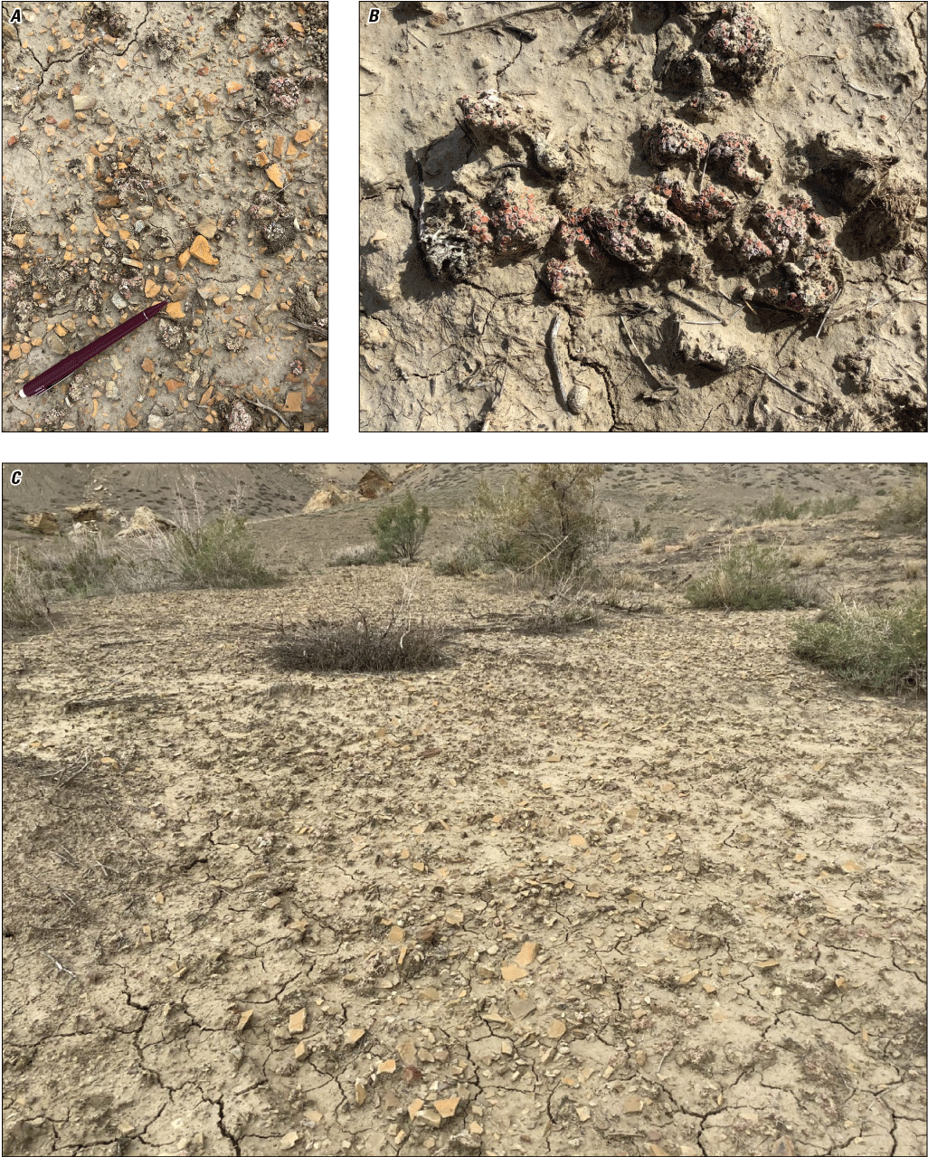
Soil surface cover in the B2 study basin, including A and B, light cyanobacteria, physical crust, rocks, and Psora dicipiens (a pink-colored lichen), and C, a zoomed-out view of the same area. Photographs by Natalie Day, U.S. Geological Survey.
Precipitation During the Study Period
A total of 1,020 mm of precipitation fell in Rangely after the fire but before the second UAV flight (Colorado Climate Center, 2022). This represents 236 mm of precipitation per year, which is close to average for Rangely. On July 20, 2017, shortly after the fire ignited (June 11), a storm delivered 28 mm of precipitation to Rangely (fig. 5). This was a large storm for the area and represents an annual exceedance probability of 0.20. There were other large storms on October 4, 2018 (25 mm) and September 9, 2020 (27 mm).
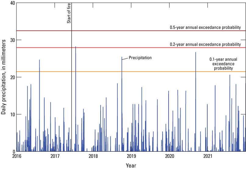
Daily precipitation at a weather station in Rangely, Colorado (8.1 kilometers away from study location) from 2016 to 2021; 0.5-, 0.2-, and 0.1-annual exceedance probabilities based on data from 1952 to 2021 (Colorado Climate Center, 2022); and the start of the Dead Dog fire (June 11, 2017).
Results of WEPPcloud Erosion Model
The WEPP erosion model uses inputs of slope, soil, vegetation, and climate data from existing datasets to predict erosion. The WEPP modeling effort complements the UAV measurements by providing a second set of erosion estimates; it also showcases a less-intensive data-collection method that could be applied easily by land managers. Modeled hillslope and channel erosion results are presented in tabular form.
Modeled Erosion Rates and Salinity and Selenium Yields
The modeled B2 study basin was 170 ha and contained 50 hillslopes ranging from 0.1 ha to 18 ha. The basin contained 23 channels ranging from 30 to 790 m in length. The land cover was 95.5 percent shrub/scrub, 3.1 percent evergreen forest, and 1.4 percent grasslands/herbaceous (fig. 6). Soil in the basin is primarily a silty clay loam in the Rentsac, Moyerson, and Mikim soil series. As shown in table 2, the fire affected hillslopes with shrub/scrub and evergreen forest land cover. Although small patches of high-severity fire were represented in the burn severity map (fig. 2), these areas were too small to be represented at the hillslope scale, and only hillslopes with low and moderate burn severity were included in the model (fig. 6).
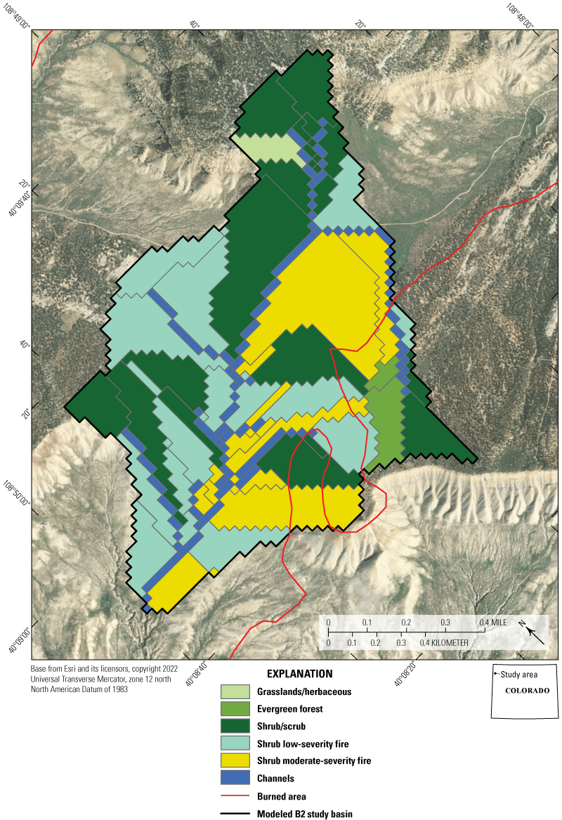
Land cover, burn severity (Preston and others, 2023), and burned area in the B2 study basin from the Watershed Erosion Prediction Project model (Lew and others, 2022).
Table 2.
Land cover for unburned and burned scenarios in the Watershed Erosion Prediction Project model (Lew and others, 2022).[NA, not applicable]
The 2016 unburned WEPP model run, which aimed to quantify erosion after the first flight but before the fire, showed virtually no erosion. For the unburned and burned 2017–21 model runs, minimal erosion occurred (table 3). The modeled annual stream discharge for the burned scenario was about 6 mm/yr greater than the unburned scenario, indicating the fire did have a small effect on the water budget. This small difference in simulated stream discharge was caused by differences in simulated base flow. Surface runoff did not occur in either model, which led to hillslope erosion not being predicted (table 3). The increase in stream discharge in the burned scenario led to slight increases in channel erosion (table 3) and salinity and selenium yields (table 4) compared to the unburned scenario. However, in both scenarios, the predicted channel erosion, salinity yield, and selenium yield were extremely small. Salinity yields were 0.00494 and 0.00513 kilograms per hectare per year (kg/ha/yr), and selenium yields were 1.61 and 1.67 milligrams per hectare per year (mg/ha/yr) in the unburned and burned scenarios, respectively (table 4).
Table 3.
Model estimates of multiple parameters for unburned and burned scenarios (Preston and others, 2023) using the Watershed Erosion Prediction Project model (Lew and others, 2022) from 2017 to 2021.[mm/yr, millimeter per year; kg/ha/yr, kilogram per hectare per year; kg/yr, kilogram per year]
Table 4.
Predicted salinity and selenium channel yield estimates (Preston and others, 2023) based on Watershed Erosion Prediction Project (Lew and others, 2022) modeled erosion rates and soil samples (Preston and others, 2023) collected from the Dead Dog study area.[TDS, total dissolved solids (salinity); mg/kg, milligram per kilogram; kg/ha/yr, kilogram per hectare per year; mg/ha/yr, milligram per hectare per year; DDT, Dead Dog transect]
Measured Sediment Loss from Digital Elevation Model Differencing
Temporal UAV imagery and resultant DEM differencing are increasingly being used to quantify morphological change across a variety of landscapes and earth surface processes. This approach requires accurate co-registration of DEMs through time; however, unresolved biases and internal uncertainties are prevalent in co-registered DEMs, even over invariant surfaces (Cook, 2017; Dall’Asta and others, 2017). Therefore, morphological change detection from UAV imagery is only possible above MDC thresholds (Peppa and others, 2019; Hempel and others, 2021), which are affected by factors that include the quality and resolution of the imagery, accuracy and placement of the GCPs, topographic slope, and surface roughness (Cook, 2017; James and others, 2017). The following section presents model validation, significant change detection, measured erosion rates, and salinity and selenium yields. It also includes a discussion of study results, limitations and challenges, and possible future applications.
Model Validation and Significant Change Detection
All Metashape models within this study produced accurate SfM models with RMS reprojection errors below 0.3 pixels and total GCP RMS errors of less than 1 pixel (which is equivalent to 4.3 cm; table 5; full GCP errors are in Preston and others, 2023). However, DEMs from the independently aligned imagery had greater relative elevational uncertainty than DEMs from the co-aligned imagery, as indicated by larger and more variable errors at 100 check points on invariant surfaces (table 6; fig. 7). Results from the Shapiro-Wilk test revealed that check point errors from the independently aligned imagery were not normally distributed (p-value=0.005) whereas errors from the co-aligned imagery were (p-value=0.094; fig. 7B, C). Additionally, there were no clear spatial patterns across the basin in the direction or magnitude of check point errors from the co-aligned imagery. Using 3 SDs from respective mean check point errors produced MDC thresholds of less than –14.9 cm and greater than 12.6 cm for DEMs created from independently aligned imagery, and less than –7.0 cm and greater than 6.4 cm for DEMs created from the co-aligned imagery (fig. 7A). Respective MDC:GSD ratios were 3.2 and 1.6.
Table 5.
The root mean square errors for tie points and ground control points for the different Metashape alignment types (Agisoft, 2021; Preston and others, 2023).[The 2016 and 2021 independently aligned imagery each used 8 GCPs, whereas the co-aligned imagery used 14 (fig. 3). RMS, root mean square; GCP, ground control point; cm, centimeter]
Table 6.
Minimum, maximum, mean, and standard deviation, in centimeters, of vertical errors at 100 invariant surface check points (fig. 3) for digital elevation models created from independently aligned and co-aligned uncrewed aerial vehicle imagery collected on September 1, 2016, and October 5 and 7, 2021.[DEM, digital elevation model]
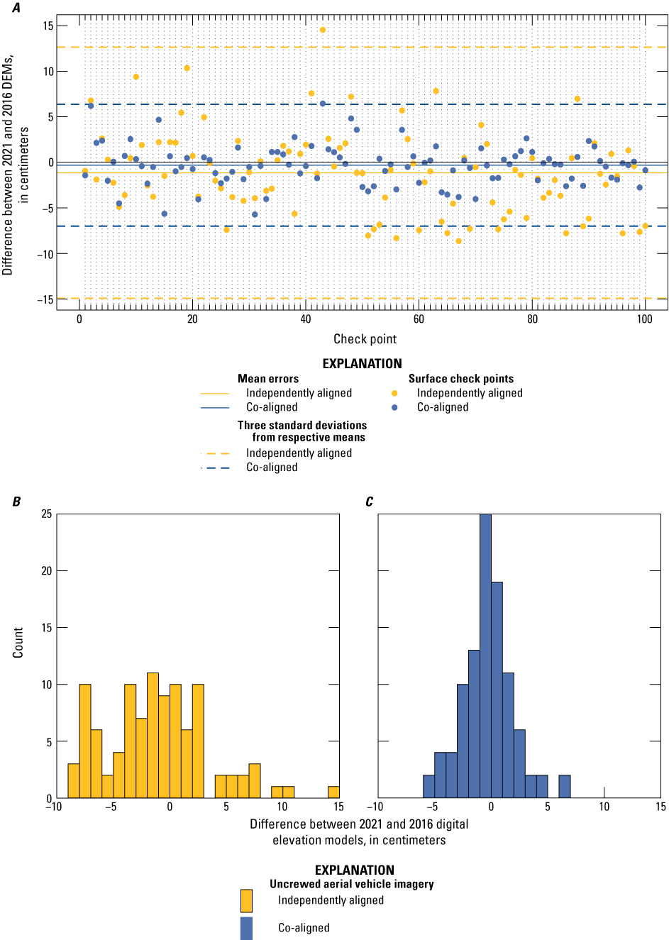
A–C, vertical errors observed at 100 invariant surface check points (fig. 3) for digital elevation models (DEMs) created from independently aligned (yellow points) and co-aligned (blue points) uncrewed aerial vehicle imagery collected on September 1, 2016, and October 5 and 7, 2021.
The significant change DoD was created with DEMs from the co-aligned imagery because of the lower (and normally distributed) error and MDC thresholds. In addition to removing values less than the MDC, the raw DoD also had significant change outliers removed, given the unrealistic minimum (−26.3 m) and maximum (19.4 m) values in the raw DoD. Visual inspection of the 2021 orthomosaic confirmed that these erroneously large values were due to misaligned pixels and not mass wasting. The raw DoD had a mean value of –15.3 cm with a SD of 29.8 cm for significant change pixels. Therefore, detectable change in the DoD was limited to greater than −104.6 cm and less than −7.0 cm and greater than 6.4 cm and less than 74.0 cm. Figure 8 shows the raw DoD (all measured changes) from the co-aligned imagery, whereas figure 9 shows only significant changes (after removing values greater than the maximum and less than the minimum detectable change thresholds). The significant change DoD was used for the landscape and channel analyses.
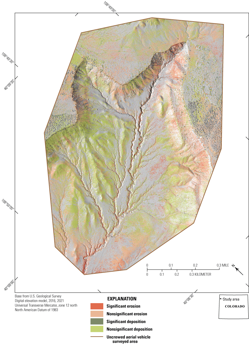
Raw digital elevation model of difference from uncrewed aerial vehicle flights on September 1, 2016, and October 5 and 7, 2021, showing significant and nonsignificant changes in elevation represented by erosion (negative change) and deposition (positive change).
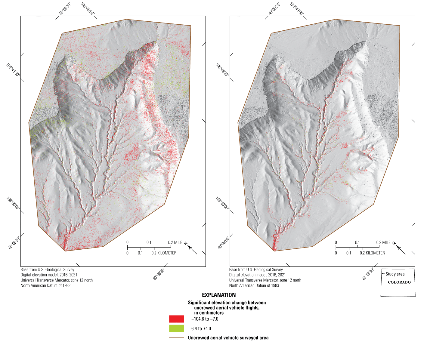
Digital elevation model of difference from uncrewed aerial vehicle flights on September 1, 2016, and October 5 and 7, 2021, showing only significant changes in elevation, represented by erosion (negative change) and deposition (positive change), used for A, landscape (full extent); and B, channel (areas along major drainages; fig. 3) analyses (Preston and others, 2023).
Measured Erosion Rates and Salinity and Selenium Yields
Erosion was measured in the significant change DoD at the landscape and channel extent (table 7) with greater relative erosion rates and salinity and selenium yields within the channel extent (table 8; fig. 10). Although the channel extent only constitutes 17.5 percent of the landscape extent, 28.2 percent of the net erosion observed across the landscape occurred within the established channels. Consequently, there were significantly greater erosion rates calculated in the channel extent between UAV epochs (mean=0.39, SD=0.016) and post-fire (mean=0.46, SD=0.018) than the landscape extent (mean=0.24 and SD=0.010, between UAV epochs; mean= 0.28 and SD=0.011, post-fire). The t-statistic (t) and its subscript (degrees of freedom) were t4=−54.996, p-value<0.005. Although salinity yields in the channel extent calculated between UAV epochs (mean=0.37, SD=0.36) and post-fire (mean=0.43, SD=0.41) were greater than the landscape extent (mean=0.23 and SD=0.22, between UAV epochs; mean=0.27 and SD=0.25, post-fire), this difference was not significant (p-value=0.22), likely because of the small sample size (n=3) and large variance in TDS values among samples. In contrast, there were significantly greater selenium yields calculated in the channel extent between UAV epochs (mean=120.9, SD=7.8) and post-fire (mean=139.5, SD=9.0) than the landscape extent (mean=74.4 and SD=4.8, between UAV epochs; mean=86.8 and SD=5.6, post-fire); t2=−26.847, p-value<0.005 (fig. 10).
Table 7.
Total volume of material, in cubic meters, eroded and deposited, and the calculated net change from the raw digital elevation model of difference and the significant change digital elevation model of difference after removing outliers (Preston and others, 2023).[Digital elevation models were created from uncrewed aerial vehicle flights on September 1, 2016, and October 5 and 7, 2021. DEM, digital elevation model]
Table 8.
Bulk density, total dissolved solids (TDS), and selenium concentrations for soil samples collected in 2016 (Preston and others, 2023).[Landscape and channel erosion rates and salinity and selenium yields were calculated from volumetric changes observed in the digital elevation model of difference for the period between uncrewed aerial vehicle epochs (September 1, 2016, to October 6, 2021) and post-fire (June 11, 2017, to October 6, 2021). g/cm3, gram per cubic centimeter; mg/kg, milligram per kilogram; mg/ha/yr, milligram per hectare per year; kg/ha/yr, kilogram per hectare per year; Mg/ha/yr, megagram per hectare per year; UAV, uncrewed aerial vehicle; SWG, Stinking Water Gulch; DDT, Dead Dog transect; —, no data]
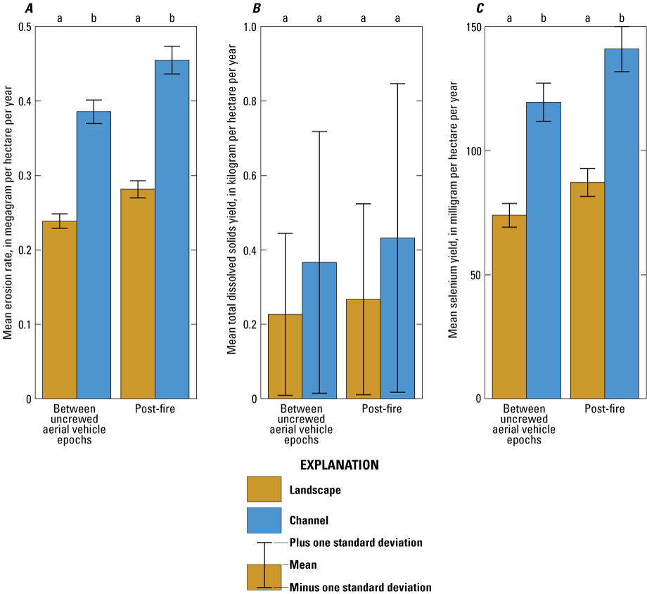
A, Mean erosion rates and B, salinity (in total dissolved solids) and C, selenium yields (Preston and others, 2023) calculated for the landscape and stream channel extents for the periods between uncrewed aerial vehicle (UAV) epochs (September 1, 2016, to October 6, 2021) and post-fire (June 11, 2017, to October 6, 2021). Error bars show the standard deviation of erosion rates (n=5), and TDS (n=3), and selenium yields (n=3) calculated from volumetric changes in UAV-derived digital elevation models between UAV epochs and analytical results from eight soil samples collected in 2016 (table 8). Letters a and b denote significant differences at the 0.05 level in mean values within each set of paired bar plots (paired t-test).
Discussion of WEPP and DEM Differencing Methods and Results
Results from the WEPP model indicated that almost no erosion occurred in either unburned or burned scenario (table 3), but this may be the result of using default input parameters and not calibrating the model to local conditions. In previous studies, the accuracy of WEPP-generated estimates of soil erosion ranged from reasonable (Miller and others, 2011; Dobre and others, 2022) to highly variable (Kampf and others, 2020). At the basin scale, WEPP models have been accurate within an order of magnitude when using default values in forested areas (Dobre and others, 2022); however, other studies have identified that WEPP can overestimate soil erosion in wet environments (Miller and others, 2011; Sankey and others, 2017). The accuracy of WEPP is less established in rangelands, though in light of observed erosion in post-fire UAV imagery and greater erosion estimates from the DoD method, soil erosion was likely underestimated by the WEPP model in the B2 study basin.
Future investigations could focus on parameterization and calibration of the WEPP model scenarios specific to the hydrologic and soil characteristics of the basin, though this would most likely require a substantial monitoring infrastructure. Specifically, the most sensitive vegetation parameters in WEPP are canopy cover and ground cover (Miller and others, 2011; Nearing and others, 1990; Srivastava and others, 2018), and reduced ground cover is the primary driver for increased erosion post-fire (Larsen and others, 2009). Calibration could also be approximated by creating a calibrated model in a nearby gaged basin and then using similar parameters in the ungaged basin (Dobre and others, 2022). In the absence of these efforts, a WEPP model may provide reasonable estimates at the basin scale and may help to identify spatial patterns (Miller and others, 2011; Sankey and others, 2017) but would need to be used with caution for quantitative investigations at the subbasin scale.
Morphological changes in the B2 study basin after the Dead Dog fire were visible in the pre- and post-fire UAV imagery (fig. 11) and measured in the significant change DoD, with net erosion occurring in the landscape and channel extents (table 7). Visible and measured morphological changes consisted primarily of incision and deposition within stream channels and rill (a small channel or gulley formed during soil erosion) incision and expansion on steeper slopes (fig. 12). Widespread sheet erosion was not evident or could not be detected within the MDC. Much of the new erosion originated within, and immediately below, previously vegetated and burned areas. Greater erosion rates and salinity and selenium yields were measured in the channel extent relative to the landscape extent (fig. 10). Calculated erosion rates (range: 0.24–0.45 Mg/ha/yr) were well within predicated median annual erosion rates (range: 0.1–2 Mg/ha/yr) for the Intermountain West after wildfire (Miller and others, 2011). However, these rates were similar to, or lower than, erosion rates reported by Jackson and Julander (1982) for 12 unburned basins underlain by Mancos Shale in Utah (range: 0.24 to 2.38 Mg/ha/yr, mean=1.26). Taken together, these results indicate that the Dead Dog fire clearly resulted in increased erosion, although, similar to WEPP-modeled erosion, the overall magnitude of measured erosion from the significant change DoD within the B2 study basin was relatively small. However, given that vegetation in the basin has generally not recovered (fig. 11), the potential for significant erosion likely remains high.
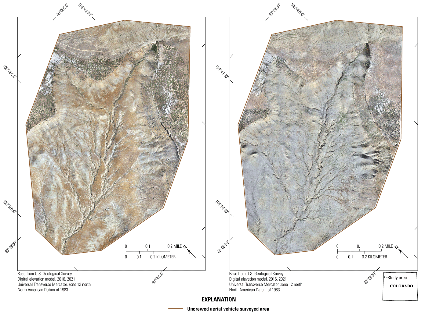
Pre- and post-fire orthomosaics from uncrewed aerial vehicle flights on A, September 1, 2016, and B, October 5 and 7, 2021 (Preston and others, 2023). Note burned trees above the escarpment rim and lack of grass (brown vegetation below escarpment rim) regrowth.
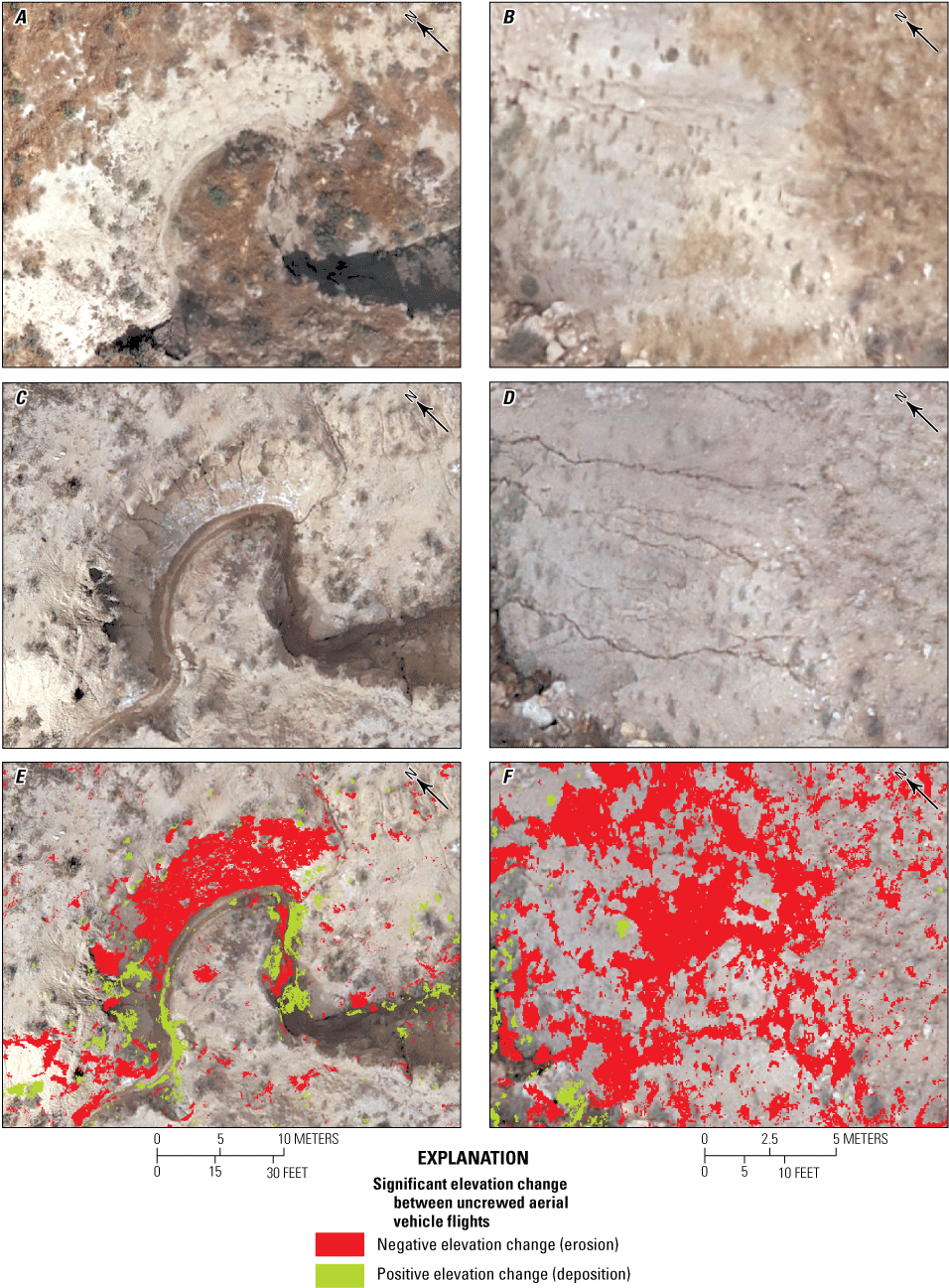
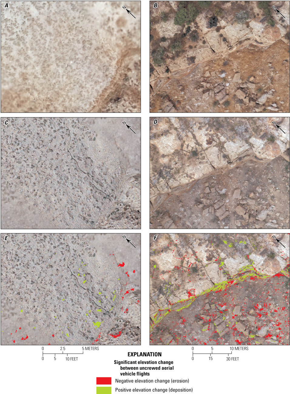
A, C, E, examples of erosion and deposition within the main channel, and B, D, F, examples of rill incision and expansion. A and B are September 1, 2016 (pre-fire) uncrewed aerial vehicle (UAV) imagery; C and D are October 5 and 7, 2021 (post-fire) UAV imagery; and E and F are the digital elevation model of difference overlain on 2021 UAV imagery, with red showing areas of erosion and light green showing areas of deposition (Preston and others, 2023). Note increased erosion in 2021 within soils that were vegetated or immediately below areas that were vegetated in 2016. UAV imagery by the U.S. Geological Survey.
The significant change DoD had MDC thresholds (less than −7.0 cm and greater than 6.4 cm) and an MDC:GSD ratio (1.6) comparable to or better than other studies examining morphological change with similar resolution imagery (Gillan and others, 2016; Meinen and Robinson, 2020). For example, Sanz-Ablanedo and others (2018) performed extensive testing on the accuracy of UAV-derived SfM products in relation to the number of GCPs and achieved the greatest vertical accuracy of 1.5 GSD by using 4 GCPs per 100 images. Here, similar accuracy was achieved using approximately 0.74 GCPs per 100 photographs (14 NGCPs for approximately 1,900 images), indicating that the use of camera positions from independent alignments (which provided improved starting locations for camera alignment) and NGCP locations located equidistant from respective independent alignments (which minimized the adjustment of each image set) greatly improved co-alignment of imagery. Indeed, a significant change DoD from the independently aligned imagery would have produced MDC thresholds nearly double those of the co-aligned imagery, which would have greatly reduced measured erosion. However, a limitation of using NGCPs is the availability of invariant objects. For example, although the NGCPs and check points were spatially distributed as much as possible, no invariant surfaces could be identified in the lower parts of the drainage basin to create either GCPs to improve alignment or check points to assess error in this region (fig. 3). Lack of GCPs in the lower part of the basin likely resulted in the positive bias, potentially from doming (in other words, convex warping; James and Robson, 2014) of the 2016 DEM, observed in much of this region despite mean vertical accuracy of the check points being slightly negative (−0.31 cm; figs. 3, 8). Reliance on invariant objects could be avoided by establishing permanent GCPs during the first UAV epoch.
Although the DoD had high vertical accuracy relative to GSD, the MDC values may still have been too great to capture much of the smaller scale morphological change that occurred between UAV epochs, especially rill incision and expansion. For example, incision and expansion of rills were visible in several areas from the UAV imagery, yet they were not always detected or were poorly represented in the significant change DoD (figs. 12, 13). There were three larger storms after the Dead Dog fire; however, annual precipitation was average during the 4-year period after the fire (fig. 5), which may have limited rill incision or expansion below the MDC. Furthermore, the positive bias in elevation uncertainty between 2016 and 2021 in the lower basin would further limit detection of small-scale rill features in this region, as would high surface roughness present in the B2 study basin (Cook, 2017). The inability to characterize small-scale erosion features likely underestimated net erosion. Given that steep uplands on Mancos Shale have the potential to contribute considerably more sediment and salinity than gently sloping piedmonts, through rill erosion (Jackson and Julander, 1982), higher resolution imagery capable of better characterizing small-scale rilling could greatly benefit future UAV-based studies of post-fire erosion in the Mancos Shale. For example, rill and gully erosion of greater than 4 cm was detectable in agriculture fields using UAV imagery with a GSD of 1.7 cm (Meinen and Robinson, 2020). Alternatively, the use of UAVs equipped with light detection and ranging sensors may provide better resolution of small-scale erosion and deposition features compared to UAV-derived photogrammetric products (Sankey and others, 2021).
A, C, E, examples of undetected morphological change (rill incision), and B, D, F, errors resulting from misalignment along the escarpment rim and talus blocks and misclassification of 2016 vegetation. A and B are uncrewed aerial vehicle (UAV) imagery from September 1, 2016; C and D are UAV imagery from October 5 and 7, 2021; and E and F are the digital elevation model of difference overlain on 2021 UAV imagery, with red showing areas of erosion and light green showing areas of deposition (Preston and others, 2023). UAV imagery by the U.S. Geological Survey.
The use of imagery collected in 2016 allowed for pre- and post-fire comparisons; however, use of pre-fire imagery proved challenging for modeling morphological change and reduced understanding of erosional dynamics. Based on the 2016 land cover classification, 52.2 percent of the study area was nonbare ground pixels, which precluded modeling most of the study area. Although it is possible to interpolate the land surface beneath vegetation (Gillan and others, 2014), this is often unreliable in areas with undulating terrain or expansive cover, or both, as seen in the B2 study basin (Preston and others, 2021). Yet it is precisely these burned areas that are likely to be a major source of increased erosion and salinity relative to already bare areas because of the loss of soil-protecting vegetation (Morris and Moses, 1987), fire-induced changes to soil properties that can cause the surface soil to seal or become hydrophobic (Shakesby and Doerr, 2006), and greater ion concentrations in soils beneath vegetation relative to interspace soil (Cadaret and others, 2016). Furthermore, the temporal offset between the 2016 imagery and the 2017 fire limited inference on post-fire erosion rates, as the amount of erosion during this period was unknown; hence, the calculation of two erosion rates: one between UAV epochs, and the other post-fire. The calculation of a linear rate for either period is likely overly simplistic because increased runoff and sediment yield are often greatest in the first 1 to 2 years post-fire (Robichaud, 2005), with recovery to pre-fire dynamics often occurring within 5 years (Wright and Bailey, 1982). However, the 2021 UAV imagery was collected more than 4 years post-fire with little vegetation regrowth observed (fig. 11), indicating the potential for increased erosion is still likely high after storms with large precipitation totals. Therefore, even in areas with existing imagery, collection of baseline imagery immediately after a wildfire could be highly beneficial for studies using repeated UAV flights to monitor post-fire erosion.
Finally, unrealistic values in the DoD necessitated thresholding the maximum potential change at 3 SDs of the mean of significant change pixels. Although most of these large DoD values were clearly erroneous, thresholding larger values may have masked some areas of real change. The two main errors observed were for pixels in burned vegetation that were misclassified as bare ground in 2016 (on the order of one to several meters) and misaligned pixels along the escarpment rim and large talus blocks (on the order of one to tens of meters; fig. 13F). Errors resulting from vegetation misclassification systematically produced negative DoD values (Preston and others, 2023), which would increase volumetric estimates, although this was minimally offset because of some small shrub growth that occurred post-fire that produced erroneous positive DoD values. In contrast, misalignment errors along the escarpment rim and talus blocks would be expected to be normally distributed around zero if the misalignment was random—a reasonable assumption given the normality of elevational uncertainties. Removing DoD outliers had a considerable effect on volumetric calculations for the landscape extent, but minimal effect for the channel extent (table 8). This is likely primarily due to cumulative vegetation misclassification errors throughout the burn area across the landscape extent, whereas the stream channel acted as fire refugia, with minimal burning of vegetation in the channel extent. Because the escarpment rim and areas with many talus blocks were manually excluded, errors associated with misaligned pixels were minimized in the channel extent. Therefore, focusing UAV flights on key areas (for example, individual steep slopes, high-intensity burn areas, specific stream reaches) would likely provide increased understanding of the erosional process with less effort and error than performing landscape-level flights.
Synthesis of Results and Next Steps
This research was designed to detect erosion after a wildfire in rangeland underlain by Mancos Shale and to characterize the effects of erosion on sediment, salinity, and selenium yields. The comparison of two methods, ranging in data requirements and analytical complexity, improved understanding of the limitations of the technology used to detect erosion. Widespread erosion was not detected in either method, although the WEPP model predicted considerably less erosion than that which was measured by the significant change DoD. WEPP predicted minimal erosion within the channel but did not show any hillslope erosion. Fine-scale erosion was visible in UAV imagery but often below the significant change DoD MDC threshold. Collection of higher resolution imagery for use in the DoD method could help better characterize small-scale erosion, but the roughness of the Mancos Shale may still challenge UAV-based approaches (Cook, 2017). In future UAV studies, it could be beneficial to do the first flight immediately after the fire instead of relying on pre-fire imagery, like was done in this study, to minimize vegetation interference.
In addition to limitations of the tested methodologies, the relatively small amount of erosion on the landscape may reflect soil characteristics or the absence of other soil disturbances like wind (Sankey and others, 2009; Vega and others, 2020). An analysis by Fick and others (2020) indicated that biological soil crusts were the most effective variable for explaining erosion differences between paired basins on Mancos Shale that had different grazing histories. Biological soil crusts were largely composed of light cyanobacteria, which, despite being considered an early successional or less-developed form, can promote soil aggregation and stabilization. Although the B2 study basin does have grazing during the winter, this can have a less detrimental effect on the biological soil crust community compared to year-round grazing (Belnap and others, 2006). The overall low fire severity across the landscape may have had minimal effect on biological soil communities, though the effect of fire on biological soil crusts was not investigated in this study and is an understudied field in general (McCann and others, 2021). It is likely that the fire had a greater effect on vegetation and subsequently erosion, as observed in the UAV imagery, where there was greater erosion below previously vegetated areas. Changing climate conditions can alter fire regimes (Westerling and others, 2006), and many dryland areas are invaded by exotic annual grasses (for example, cheat grass) that create a continuous distribution of fine fuels, increasing the frequency, spatial extent, and severity of fires (Pilliod and others, 2017). The findings in this report highlight the importance of improving techniques to measure erosion under vegetation and developing methods to detect and classify biological soil crusts with UAV imagery.
Summary
Cretaceous Mancos Shale–derived soils are a natural source of sediment, salinity, and selenium to surface waters in many areas of western Colorado and eastern Utah. Sedimentary marine shales are often located in dryland areas, where surface disturbance of the soil can greatly increase the wind and water erosion. Understanding and quantifying erosion from rangelands is a high priority for land managers, especially with projected increases in aridity and wildfires under climate change. Results of assessed sediment, salinity, and selenium yields after the Dead Dog fire in northwestern Colorado are presented in this report. This study used two methodologies to quantify erosion, with different data requirements and analytical complexity. Comparisons of different methodologies could benefit land managers’ decision making regarding erosion monitoring and assessment in the future.
The first methodology used is a process-based erosion model, the Watershed Erosion Prediction Project (WEPP), that uses existing datasets as inputs, including topography, soils, vegetation, and climate, making this approach convenient in situations where few data exist or resources for analysis are limited. The second approach used, which requires more complex data collection, measured erosion and deposition by differencing digital elevation models (DEMs) created from uncrewed aerial vehicle (UAV) imagery collected in 2016 (pre-fire) and 2021 (post-fire). Erosion estimates from the process-based erosion model and the DEM of difference (DoD) method were used to calculate sediment, salinity, and selenium yields in the basin.
Results from the WEPP model indicated that channel erosion, salinity yield, and selenium yield were miniscule and were not representative of observed erosion. Because erosion was observed in temporal UAV imagery and comparatively more erosion was estimated in the DoD method, it is likely the WEPP model underestimated erosion. This underestimation may be the result of using default input parameters and not calibrating the model to local conditions. In the absence of parameterization and calibration of a WEPP model scenario specific to the hydrologic and soil characteristics of the basin, WEPP can help to identify spatial patterns of erosion but would need to be used with caution for quantitative investigations.
Morphological changes after the Dead Dog fire were visible in the temporal UAV imagery and measured in the significant change DoD, with net erosion occurring in the landscape and channel extents. Widespread sheet erosion was not evident or could not be detected, though incision and deposition within stream channels and rill incision and expansion on steeper slopes was observed. Much of the new erosion originated within, and immediately below, areas where vegetation had burned. Greater erosion rates and salinity and selenium yields were measured in the channel extent relative to the landscape extent. Calculated erosion rates ranged from 0.24 to 0.46 megagrams per hectare per year, which were similar to, or lower than, erosion rates reported for 12 unburned basins underlain by Mancos Shale in Utah. Taken together, these results indicate that the Dead Dog fire clearly resulted in increased erosion; however, like WEPP-modeled erosion, the overall magnitude of measured erosion was relatively small. Limiting UAV flights to key areas (individual steep slopes, high-intensity burn areas, specific stream reaches) could likely provide increased understanding of the erosional process with less effort and error than performing landscape-level flights.
The relatively small amount of erosion on the landscape may also reflect soil characteristics or the absence of events that contribute to erosion, including soil disturbances. Post-fire visual assessments verified that the soils in the B2 study basin still supported robust physical crusts, typical of soils derived from Mancos Shale. Biological soil crusts were also present and were largely composed of light cyanobacteria, which, despite being considered an early successional or less-developed form, can promote soil aggregation and stabilization. The overall low fire severity across the landscape may have had minimal effect on biological soil communities, though the effect of fire on biological soil crusts is an understudied field. It is likely that the fire had a greater effect on vegetation, and subsequently erosion, as greater erosion was observed in the UAV imagery and significant change DoD below areas that were previously vegetated before the fire. The findings in this report highlight the importance of improving techniques to measure erosion under vegetation and developing methods to detect and classify biological soil crusts with UAV imagery.
Acknowledgments
The authors wish to thank several U.S. Geological Survey staff for assistance with data collection and this report. Christopher Holmquist-Johnson and Joseph Adams coordinated flight planning and uncrewed aerial vehicle image acquisition. Mike Kohn and Laura Hempel assisted with ground control point collection. The report was improved by review comments from Joel Sankey and Brandon Forbes.
References Cited
Abatzoglou, J.T., 2011. Development of gridded surface meteorological data for ecological applications and modelling: International Journal of Climatology, v. 33, no. 1, p. 121–131. [Also available at https://doi.org/10.1002/joc.3413.]
Agisoft, 2021, Agisoft Metashape Professional, version 1.7.6: Agisoft software release, accessed June 15, 2023, at www.agisoft.com.
Akay, S.S., Özcan, O., Balik Şanlı, F., Görüm, T., Şen, Ö.L., and Bayram, B., 2020, UAV-based evaluation of morphological changes induced by extreme rainfall events in meandering rivers: PLOS ONE, v. 15, no. 11, 29 p., accessed August 2, 2022, at https://doi.org/10.1371/journal.pone.0241293.
ArduPilot Development Team, 2016, Mission Planner (version 1.3.39): ArduPilot Dev Team software release, accessed June 2022 at https://ardupilot.org/planner/.
Ault, T.R., Mankin, J.S., Cook, B.I., and Smerdon, J.E., 2016, Relative impacts of mitigation, temperature, and precipitation on 21st-century megadrought risk in the American Southwest: Science Advances, v. 2, no. 10, article e1600873, 8 p., accessed July 2022 at https://doi.org/10.1126/sciadv.1600873.
Barthès, B., and Roose, E., 2002, Aggregate stability as an indicator of soil susceptibility to runoff and erosion; validation at several levels: CATENA, v. 47, no. 2, p. 133–149, accessed July 2022 at https://www.sciencedirect.com/science/article/pii/S0341816201001801. [Also available at https://doi.org/10.1016/S0341-8162(01)00180-1.]
Belnap, J., Phillips, S.L., Herrick, J.E., and Johansen, J.R., 2007, Wind erodibility of soils at Fort Irwin, California (Mojave Desert), USA, before and after trampling disturbance—Implications for land management: Earth Surface Processes and Landforms, v. 32, no. 1, p. 75–84, accessed July 2022 at https://doi.org/10.1002/esp.1372.
Belnap, J., Phillips, S.L., and Troxler, T., 2006, Soil lichen and moss cover and species richness can be highly dynamic—The effects of invasion by the annual exotic grass Bromus tectorum, precipitation, and temperature on biological soil crusts in SE Utah: Applied Soil Ecology, v. 32, no. 1, p. 63–76, accessed July 2022 at https://doi.org/10.1016/j.apsoil.2004.12.010.
Belnap, J., Walker, B.J., Munson, S.M., and Gill, R.A., 2014, Controls on sediment production in two U.S. deserts: Aeolian Research, v. 14, p. 15–24, accessed July 2022 at https://doi.org/10.1016/j.aeolia.2014.03.007.
Bigelow, D., and Borchers, A., 2017, Major uses of land in the United States, 2012: Economic Information Bulletin No. 178, U.S. Department of Agriculture, Economic Research Service, 69 p., accessed July 2022 at https://www.ers.usda.gov/publications/pub-details/?pubid=84879.
Blake, G.R., and Hartge, K.H., 1986, Bulk density, chap. 13 of Klute, A., ed., Methods of soil analysis, part 1—Physical and mineralogical methods, 2d ed., no. 9 of Agronomy: Madison, Wisc., American Society of Agronomy, Inc., accessed January 2023 at https://doi.org/10.2136/sssabookser5.1.2ed.c13.
Cadaret, E.M., Nouwakpo, S.K., McGwire, K.C., Weltz, M.A., and Blank, R.R., 2016, Experimental investigation of the effect of vegetation on soil, sediment erosion, and salt transport processes in the Upper Colorado River Basin Mancos Shale formation, Price, Utah, USA: CATENA, v. 147, p. 650–662, accessed July 2022 at https://doi.org/10.1016/j.catena.2016.08.024.
Chepil, W.S., 1951, Properties of soil which influence wind erosion—IV. State of dry aggregate structure: Soil Science, v. 72, no. 5, p. 387–402, accessed July 2022 at https://doi.org/10.1097/00010694-195111000-00007.
Colorado Climate Center, 2022, Climate data for Rangely 1E: Colorado State University Colorado Climate Center website, accessed December 2022 at https://climate.colostate.edu/.
Cook, K.L., 2017, An evaluation of the effectiveness of low-cost UAVs and structure from motion for geomorphic change detection: Geomorphology, v. 278, p. 195–208, accessed July 2022 at https://doi.org/10.1016/j.geomorph.2016.11.009.
Coulloudon, B., Eshelman, K., Gianola, J., Habich, N., Hughes, L., Johnson, C., Pellant, M., Podborny, P., Rasmussen, A., Robles, B., Shaver, P., Spehar, J., and Willoughby, J., 1999, Sampling vegetation attributes—Interagency technical reference: Bureau of Land Management, accessed October 2001 at https://www.blm.gov/noc/blm-library/technical-reference/sampling-vegetation-attributes.
Cross, C.W., and Purington, C.W., 1899, Telluride folio, Colorado: U.S. Geological Survey Geologic Atlas of the United States Folio 57, 4 map sheets, 18-p. text, accessed July 2022 at https://doi.org/10.3133/gf57.
Dall’Asta, E., Forlani, G., Roncella, R., Santise, M., Diotri, F., and Morra di Cella, U., 2017, Unmanned aerial systems and DSM matching for rock glacier monitoring: ISPRS Journal of Photogrammetry and Remote Sensing, v. 127, p. 102–114, accessed July 2022 at https://doi.org/10.1016/j.isprsjprs.2016.10.003.
Daly, C., Halbleib, M., Smith, J.I., Gibson, W.P., Doggett, M.K., Taylor, G.H., Curtis, J., Pasteris, P.P., 2008, Physiographically sensitive mapping of climatological temperature and precipitation across the conterminous United States: International Journal of Climatology, v. 28, no. 15, p. 2031–2064. [Also available at https://doi.org/10.1002/joc.1688.]
Dobre, M., Srivastava, A., Lew, R., Deval, C., Brooks, E.S., Elliot, W.J., and Robichaud, P.R., 2022, WEPPcloud—An online watershed-scale hydrologic modeling tool. Part II. Model performance assessment and applications to forest management and wildfires: Journal of Hydrology, v. 610, article 127776, 18 p., accessed August 2022 at https://doi.org/10.1016/j.jhydrol.2022.127776.
Ebel, B.A., and Martin, D.A., 2017, Meta-analysis of field-saturated hydraulic conductivity recovery following wildland fire—Applications for hydrologic model parameterization and resilience assessment: Hydrological Processes, v. 31, no. 21, p. 3682–3696, accessed June 2022 at https://doi.org/10.1002/hyp.11288.
European Space Agency, 2020, Missions, Sentinel-2: ESA Sentinel Online web page, accessed June 2023 at https://sentinel.esa.int/web/sentinel/missions/sentinel-2.
Fassnacht, F.E., Schmidt-Riese, E., Kattenborn, T., and Hernández, J., 2021, Explaining Sentinel 2-based dNBR and RdNBR variability with reference data from the bird’s eye (UAS) perspective: International Journal of Applied Earth Observation and Geoinformation, v. 95, article 102262, 19 p., accessed June 2022 at https://doi.org/10.1016/j.jag.2020.102262.
Fick, S.E., Belnap, J., and Duniway, M.C., 2020, Grazing-induced changes to biological soil crust cover mediate hillslope erosion in long-term exclosure experiment: Rangeland Ecology & Management, v. 73, no. 1, p. 61–72, accessed July 2022 at https://doi.org/10.1016/j.rama.2019.08.007.
Fishman, M.J., and Friedman, L.C., eds., 1989, Methods for determination of inorganic substances in water and fluvial sediments (3d ed.): U.S. Geological Survey Techniques of Water-Resources Investigations, book 5, chap. A1, 545 p., accessed June 22, 2020, at https://doi.org/10.3133/twri05A1.
Flanagan, D.C., Frankenberger, J.R., and Ascough, J.C., 2012, WEPP—Model use, calibration, and validation: Journal of the American Society of Agricultural and Biological Engineers, v. 55, no. 4, p. 1463–1477, accessed August 2021 at https://doi.org/10.13031/2013.42254.
Fleischner, T.L., 1994, Ecological costs of livestock grazing in Western North America: Conservation Biology, v. 8, no. 3, p. 629–644, accessed July 2022 at https://www.jstor.org/stable/2386504. [Also available at https://doi.org/10.1046/j.1523-1739.1994.08030629.x.]
Forbes, B.T., DeBenedetto, G.P., Dickinson, J.E., Bunch, C.E., and Fitzpatrick, F.A., 2020, Using small unmanned aircraft systems for measuring post-flood high-water marks and streambed elevations: Remote Sensing, v. 12, no. 9, article 1437, 21 p., accessed January 2023 at https://doi.org/10.3390/rs12091437.
Fullhart, A.T., Nearing, M.A., Armendariz, G., Weltz, M.A., 2021, Climate benchmarks and input parameters representing locations in 68 countries for a stochastic weather generator, CLIGEN: Earth System Science Data, v. 13, no. 2, p. 435–446. [Also available at https://doi.org/10.5194/essd-13-435-2021.]
Gale, H.S., 1908, Geology of the Rangely Oil District, Rio Blanco County, Colorado, with a section on the water supply: U.S. Geological Survey Bulletin 350, 61 p., 2 pls. [Also available at https://doi.org/10.3133/b350.]
GeoSetter, 2019, GeoSetter, version 3.5.3: GeoSetter software release, accessed June 20, 2023, at www.geosetter.de/en/main-en/.
Gillan, J.K., Karl, J.W., Barger, N.N., Elaksher, A., and Duniway, M.C., 2016, Spatially explicit rangeland erosion monitoring using high-resolution digital aerial imagery: Rangeland Ecology & Management, v. 69, no. 2, p. 95–107, accessed August 2022 at https://doi.org/10.1016/j.rama.2015.10.012.
Gillan, J.K., Karl, J.W., Duniway, M., and Elaksher, A., 2014, Modeling vegetation heights from high resolution stereo aerial photography—An application for broad-scale rangeland monitoring: Journal of Environmental Management, v. 144, p. 226–235, accessed August 2022 at https://doi.org/10.1016/j.jenvman.2014.05.028.
Hempel, L.A., Creighton, A.L., and Bock, A.R., 2021, Elevation and elevation-change maps of Fountain Creek, southeastern Colorado, 2015–20: U.S. Geological Survey Scientific Investigations Map 3481, 10 sheets, 12-p. pamphlet, accessed January 2022 at https://doi.org/10.3133/sim3481.
Hijmans, R.J., 2022, raster—Geographic data analysis and modeling—R package version 3.5-15: R Foundation for Statistical Computing software release, accessed June 2023 at https://CRAN.R-project.org/package=raster.
Hohner, A.K., Cawley, K., Oropeza, J., Summers, R.S., and Rosario-Ortiz, F.L., 2016, Drinking water treatment response following a Colorado wildfire: Water Research, v. 105, p. 187–198, accessed September 2022 at https://doi.org/10.1016/j.watres.2016.08.034.
Homer, C., Dewitz, J., Yang, L., Jin, S., Danielson, P., Xian, G., Coulston, J., Herold, N., Wickham, J., Megown, K., 2015, Completion of the 2011 National Land Cover Database for the conterminous United States—Representing a decade of land cover change information: Photogrammetric Engineering and Remote Sensing, v. 81, no. 5, p. 345–354, accessed June 2022 at https://www.ingentaconnect.com/content/asprs/pers/2015/00000081/00000005/art00002.
Jackson, W.L., and Julander, R.P., 1982, Runoff and water quality from three soil landform units on Mancos Shale: Journal of the American Water Resources Association, v. 18, no. 6, p. 995–1001. [Also available at https://doi.org/10.1111/j.1752-1688.1982.tb00107.x.]
James, M.R., and Robson, S., 2014, Mitigating systematic error in topographic models derived from UAV and ground-based image networks: Earth Surface Processes and Landforms, v. 39, no. 10, p. 1413–1420, accessed February 2022 at https://doi.org/10.1002/esp.3609.
James, M.R., Robson, S., d’Oleire-Oltmanns, S., and Niethammer, U., 2017, Optimising UAV topographic surveys processed with structure from-motion—Ground control quality, quantity, and bundle adjustment: Geomorphology, v. 280, p. 51–66, accessed February 2022 at https://doi.org/10.1016/j.geomorph.2016.11.021.
Kampf, S.K., Gannon, B.M., Wilson, C., Saavedra, F., Miller, M.E., Heldmyer, A., Livneh, B., Nelson, P., and MacDonald, L., 2020, PEMIP—Post-fire erosion model inter-comparison project: Journal of Environmental Management, v. 268, article 110704, accessed August 2022 at https://doi.org/10.1016/j.jenvman.2020.110704.
Kean, J.W., and Staley, D.M., 2021, Forecasting the frequency and magnitude of postfire debris flows across southern California: Earth’s Future, v. 9, no. 3, article e2020EF001735, accessed July 2021 at https://doi.org/10.1029/2020EF001735.
Laflen, J.M., Elliot, W.J., Flanagan, D.C., Meyer, C.R., and Nearing, M.A., 1997, WEPP-Predicting water erosion using a process-based model: Journal of Soil and Water Conservation, v. 52, no. 2, p. 96–102, accessed July 2021 at https://www.jswconline.org/content/52/2/96.
Lamsters, K., Ješkins, J., Sobota, I., Karušs, J., and Džeriņš, P., 2022, Surface characteristics, elevation change, and velocity of High-Arctic valley glacier from repeated high-resolution UAV photogrammetry: Remote Sensing, v. 14, no. 4, article 1029, accessed July 2022 at https://doi.org/10.3390/rs14041029.
Larsen, I.J., MacDonald, L.H., Brown, E., Rough, D., Welsh, M.J., Pietraszek, J.H., Libohova, Z., Benavides Solorio, J., and Schaffrath, K., 2009, Causes of post-fire runoff and erosion—Water repellency, cover, or soil sealing?: Soil Science Society of America Journal, v. 73, no. 4, p. 1393–1407, accessed August 2022 at https://doi.org/10.2136/sssaj2007.0432.
Lew, R., Dobre, M., Srivastava, A., Brooks, E.S., Elliot, W.J., Robichaud, P.R., and Flanagan, D.C., 2022, WEPPcloud—An online watershed-scale hydrologic modeling tool. Part I. Model description: Journal of Hydrology, v. 608, article 127603, 15 p., accessed August 2022 at https://doi.org/10.1016/j.jhydrol.2022.127603.
Litschert, S.E., Brown, T.C., and Theobald, D.M., 2012, Historic and future extent of wildfires in the Southern Rockies Ecoregion, USA: Forest Ecology and Management, v. 269, p. 124–133, accessed June 2022 at https://doi.org/10.1016/j.foreco.2011.12.024.
Mauri, L., Straffelini, E., Cucchiaro, S., and Tarolli, P., 2021, UAV-SfM 4D mapping of landslides activated in a steep terraced agricultural area: Journal of Agricultural Engineering, v. 52, no. 1, accessed June 2022 at https://doi.org/10.4081/jae.2021.1130.
McCann, E., Reed, S.C., Saud, P., Reibold, R.H., Howell, A., and Faist, A.M., 2021, Plant growth and biocrust-fire interactions across five North American deserts: Geoderma, v. 401, article 115325, 11 p., accessed June 2022 at https://doi.org/10.1016/j.geoderma.2021.115325.
Meinen, B.U., and Robinson, D.T., 2020, Mapping erosion and deposition in an agricultural landscape—Optimization of UAV image acquisition schemes for SfM-MVS: Remote Sensing of Environment, v. 239, article 111666, 10 p., accessed July 2022 at https://doi.org/10.1016/j.rse.2020.111666.
Miller, M.E., MacDonald, L.H., Robichaud, P.R., and Elliot, W.J., 2011, Predicting post-fire hillslope erosion in forest lands of the western United States: International Journal of Wildland Fire, v. 20, p. 982–999, accessed July 2022 at https://doi.org/10.1071/WF09142.
Morris, S.E., and Moses, T.A., 1987, Forest fire and the natural soil erosion regime in the Colorado Front Range: Annals of the Association of American Geographers, v. 77, no. 2, p. 245–254, accessed June 2022 at https://doi.org/10.1111/j.1467-8306.1987.tb00156.x.
Munson, S.M., Belnap, J., and Okin, G.S., 2011, Responses of wind erosion to climate-induced vegetation changes on the Colorado Plateau: Proceedings of the National Academy of Sciences, v. 108, no. 10, p. 3854–3859, accessed July 2022 at https://doi.org/10.1073/pnas.1014947108.
National Interagency Fire Center, 2023, Wildland fire incident locations: National Interagency Fire Center website, accessed March 2023 at https://data-nifc.opendata.arcgis.com/datasets/nifc::wildland-fire-incident-locations/explore?location=40.139275%2C-108.785406%2C12.91.
National Oceanic and Atmospheric Administration Regional Climate Centers, 2022, Applied Climate Information System online database: High Plains Regional Climate Center web page, accessed January 2022 at http://climod.unl.edu/.
Nauman, T.W., Duniway, M.C., Webb, N.P., and Belnap, J., 2018, Elevated aeolian sediment transport on the Colorado Plateau, USA—The role of grazing, vehicle disturbance, and increasing aridity: Earth Surface Processes and Landforms, v. 43, no. 14, p. 2897–2914, accessed July 2022 at https://doi.org/10.1002/esp.4457.
Nearing, M.A., Deer-Ascough, L., and Laflen, J.M., 1990, Sensitivity analysis of the WEPP hillslope profile erosion model: Transactions of the ASAE, v. 33, no. 3, p. 0839–0849, accessed June 2022 at https://doi.org/10.13031/2013.31409.
Noske, P.J., Nyman, P., Lane, P.N.J., and Sheridan, G.J., 2016, Effects of aridity in controlling the magnitude of runoff and erosion after wildfire: Water Resources Research, v. 52, no. 6, p. 4338–4357, accessed July 2022 at https://doi.org/10.1002/2015WR017611.
Over, J.R., Ritchie, A.C., Kranenburg, C.J., Brown, J.A., Buscombe, D., Noble, T., Sherwood, C.R., Warrick, J.A., and Wernette, P.A., 2021, Processing coastal imagery with Agisoft Metashape Professional Edition, version 1.6—Structure from motion workflow documentation: U.S. Geological Survey Open-File Report 2021–1039, 46 p., accessed June 2022 at https://doi.org/10.3133/ofr20211039.
Peppa, M.V., Mills, J.P., Moore, P., Miller, P.E., and Chambers, J.E., 2019, Automated co-registration and calibration in SfM photogrammetry for landslide change detection: Earth Surface Processes and Landforms, v. 44, no. 1, p. 287–303, accessed June 2022 at https://doi.org/10.1002/esp.4502.
Pilliod, D.S., Welty, J.L., and Arkle, R.S., 2017, Refining the cheatgrass–fire cycle in the Great Basin—Precipitation timing and fine fuel composition predict wildfire trends: Ecology and Evolution, v. 7, no. 19, p. 8126–8151, accessed October 2022 at https://doi.org/10.1002/ece3.3414.
Preston, T.M., Day, N.K., Adams, J.D., and Holmquist-Johnson, C.L., 2021, Orthoimagery, digital elevation, digital terrain, final surface, and vegetation classification models for four stream catchments in western Colorado 2016: U.S. Geological Survey data release, https://doi.org/10.5066/P91KRAAD.
Preston, T.M., Day, N.K., Longley, P.C., and Adams, J.D., 2023, Erosion rates and salinity and selenium yields in a basin near Rangely, Colorado following the 2017 Dead Dog wildfire as modeled by WEPP and measured from UAV: U.S. Geological Survey data release, https://doi.org/10.5066/P9ZA125K.
R Core Team, 2021, R—A language and environment for statistical computing, version 4.1.12: R Foundation for Statistical Computing software release, accessed June 2021 at https://www.r-project.org/.
Reybold, W.U., and TeSelle, G.W., 1989, Soil geographic data bases: Journal of Soil and Water Conservation, v. 44, no. 1, p. 28–29. [Also available at https://www.jswconline.org/content/44/1/28.]
Robichaud, P.R., 2005, Measurement of post-fire hillslope erosion to evaluate and model rehabilitation treatment effectiveness and recovery: International Journal of Wildland Fire, v. 14, no. 4, p. 475–485, accessed July 2022 at https://doi.org/10.1071/WF05031.
Sankey, J.B., Germino, M.J., and Glenn, N.F., 2009, Aeolian sediment transport following wildfire in sagebrush steppe: Journal of Arid Environments, v. 73, no. 10, p. 912–919, accessed March 2023 at https://doi.org/10.1016/j.jaridenv.2009.03.016.
Sankey, J.B., Kreitler, J., Hawbaker, T.J., McVay, J.L., Miller, M.E., Mueller, E.R., Vaillant, N.M., Lowe, S.E., and Sankey, T.T., 2017, Climate, wildfire, and erosion ensemble foretells more sediment in western USA watersheds: Geophysical Research Letters, v. 44, no. 17, p. 8884–8892, accessed January 2023 at https://doi.org/10.1002/2017GL073979.
Sankey, J.B., Sankey, T.T., Li, J., Ravi, S., Wang, G., Caster, J., Kasprak, A., 2021, Quantifying plant-soil-nutrient dynamics in rangelands—Fusion of UAV hyperspectral-LiDAR, UAV multispectral-photogrammetry, and ground-based LiDAR-digital photography in a shrub-encroached desert grassland: Remote Sensing of Environment, v. 253, article 112223, 18 p., accessed July 2022 at https://doi.org/10.1016/j.rse.2020.112223.
Sanz-Ablanedo, E., Chandler, J.H., Rodríguez-Pérez, J.R., and Ordóñez, C., 2018, Accuracy of unmanned aerial vehicle (UAV) and SfM photogrammetry survey as a function of the number and location of ground control points used: Remote Sensing, v. 10, no. 10, article 1606, 19 p., accessed June 2022 at https://doi.org/10.3390/rs10101606.
Shakesby, R.A., and Doerr, S.H., 2006, Wildfire as a hydrological and geomorphological agent: Earth-Science Reviews, v. 74, nos. 3–4, p. 269–307, accessed May 2022 at https://doi.org/10.1016/j.earscirev.2005.10.006.
Shapiro, S.S., and Wilk, M.B., 1965, An analysis of variance test for normality (complete samples): Biometrika, v. 52, nos. 3–4, p. 591–611, accessed May 2022 at https://doi.org/10.1093/biomet/52.3-4.591.
Silins, U., Bladon, K.D., Kelly, E.N., Esch, E., Spence, J.R., Stone, M., Emelko, M.B., Boon, S., Wagner, M.J., Williams, C.H., and Tichkowsky, I., 2014, Five‐year legacy of wildfire and salvage logging impacts on nutrient runoff and aquatic plant, invertebrate, and fish productivity: Ecohydrology, v. 7, no. 6, p.1508–1523, accessed July 2021 at https://doi.org/10.1002/eco.1474.
Srivastava, A., Wu, J.Q., Elliot, W.J., Brooks, E.S., and Flanagan, D.C., 2018, A simulation study to estimate effects of wildfire and forest management on hydrology and sediment in a forested watershed, northwestern U.S.: Transactions of the ASABE, v. 61, no. 5, p. 1579–1601, accessed August 2022 at https://doi.org/10.13031/trans.12326.
Turner, I.L., Harley, M.D., and Drummond, C.D., 2016, UAVs for coastal surveying: Coastal Engineering, v. 114, p. 19–24, accessed July 2021 at https://doi.org/10.1016/j.Coastaleng.2016.03.011.
U.S. Census Bureau, 2020, QuickFacts—Rio Blanco County, Colorado: U.S. Census Bureau website, accessed March 2023 at https://www.census.gov/quickfacts/fact/table/rioblancocountycolorado,CO/POP010220.
U.S. Geological Survey [USGS], 2018, National Elevation Dataset: U.S. Geological Survey, accessed June 2022 at https://www.usgs.gov/programs/national-geospatial-program/national-map.
U.S. Geological Survey [USGS], 2023, National Hydrography Dataset (NHD): U.S. Geological Survey, accessed March 20, 2023, at https://hydro.nationalmap.gov/arcgis/rest/services/nhd/MapServer.
Vega, S.P., Williams, C.J., Brooks, E.S., Pierson, F.B., Strand, E.K., Robichaud, P.R., Brown, R.E., Seyfried, M.S., Lohse, K.A., Glossner, K., Pierce, J.L., and Roehner, C., 2020, Interaction of wind and cold‐season hydrologic processes on erosion from complex topography following wildfire in sagebrush steppe: Earth Surface Processes and Landforms, v. 45, no. 4, p. 841–861, accessed March 2023 at https://doi.org/10.1002/esp.4778.
Wagenbrenner, J.W., and Robichaud, P.R., 2014, Post-fire bedload sediment delivery across spatial scales in the interior western United States: Earth Surface Processes and Landforms, v. 39, no. 7, p. 865–876, accessed July 2021 at https://doi.org/10.1002/esp.3488.
Wallis, C., Wallace, R., Tarboton, D.G., Watson, D.W., Schreuders, K.A.T., and Tesfa, T.K., 2009, Hydrologic terrain processing using parallel computing, in Anderssen, R.S., Braddock, R.D., and Newham, L.T.H., eds., 18th World IMACS Congress and MODSIM09 International Congress on Modelling and Simulation, Cairns, Australia, July 13–17, 2009 [Proceedings]: Modelling and Simulation Society of Australia and New Zealand and International Association for Mathematics and Computers in Simulation, 6 p. [Also available at https://www.mssanz.org.au/modsim09/F13/wallis.pdf.]
Westerling, A.L., Hidalgo, H.G., Cayan, D.R., and Swetnam, T.W., 2006, Warming and earlier spring increase western U.S. forest wildfire activity: Science, v. 313, no. 5789, p. 940–943, accessed June 2021 at https://doi.org/10.1126/science.1128834.
Wilson, C., Kampf, S.K., Ryan, S., Covino, T., MacDonald, L.H., and Gleason, H., 2021, Connectivity of post-fire runoff and sediment from nested hillslopes and watersheds: Hydrological Processes, v. 35, no. 1, article 13975, 17 p., accessed April 2022 at https://doi.org/10.1002/hyp.13975.
Wood, D.J.A., Preston, T.M., Powell, S., and Stoy, P.C., 2022, Multiple UAV flights across the growing season can characterize fine scale phenological heterogeneity within and among vegetation functional groups: Remote Sensing, v. 14, no. 5, article 1290, 28 p., accessed April 2022 at https://doi.org/10.3390/rs14051290.
Zaady, E., Eldridge, D.J., and Bowker, M.A., 2016, Effects of local-scale disturbance on biocrusts, part V of Weber, B., Büdel, B., and Belnap, J., eds., Biological soil crusts—An organizing principle in drylands, v. 226 of Canadell, J.G., Díaz, S., Heldmaier, G., Jackson, R.B., Levia, D.F., Schulze, E.-D., Sommer, U., and Wardle, D.A., eds., Ecological studies: Switzerland, Springer, p. 429–451. [Also available at https://doi.org/10.1007/978-3-319-30214-0_21.]
Zawislanski, P.T., Benson, S.M., TerBerg, R., and Borglin, S.E., 2003, Selenium speciation, solubility, and mobility in land-disposed dredged sediments: Environmental Science & Technology, v. 37, no. 11, p. 2415–2420, accessed May 2022 at https://doi.org/10.1021/es020977z.
Conversion Factors
International System of Units to U.S. customary units
Temperature in degrees Celsius (°C) may be converted to degrees Fahrenheit (°F) as follows:
°F = (1.8 × °C) + 32.
Datums
Vertical coordinate information is referenced to the North American Vertical Datum of 1988 (NAVD 88) using the Geoid 18 Model.
Horizontal coordinate information is referenced to the North American Datum of 1983 (NAD 83).
Altitude, as used in this report, refers to distance above the land surface.
Elevation, as used in this report, refers to distance above the vertical datum.
Publishing support provided by the Science Publishing Network,
Denver and Baltimore Publishing Service Centers
For more information concerning the research in this report, contact the
Director, USGS Colorado Water Science Center
Box 25046, Mail Stop 415
Denver, CO 80225
(303) 236-4882
Or visit the Colorado Water Science Center website at
Disclaimers
Any use of trade, firm, or product names is for descriptive purposes only and does not imply endorsement by the U.S. Government.
Although this information product, for the most part, is in the public domain, it also may contain copyrighted materials as noted in the text. Permission to reproduce copyrighted items must be secured from the copyright owner.
Suggested Citation
Day, N.K., Preston, T.M., and Longley, P.C., 2024, Wildland fire effects on sediment, salinity, and selenium yields in a basin underlain by Cretaceous marine shales near Rangely, Colorado: U.S. Geological Survey Scientific Investigations Report 2024–5043, 31 p., https://doi.org/10.3133/sir20245043.
ISSN: 2328-0328 (online)
Study Area
| Publication type | Report |
|---|---|
| Publication Subtype | USGS Numbered Series |
| Title | Wildland fire effects on sediment, salinity, and selenium yields in a basin underlain by Cretaceous marine shales near Rangely, Colorado |
| Series title | Scientific Investigations Report |
| Series number | 2024-5043 |
| DOI | 10.3133/sir20245043 |
| Publication Date | August 13, 2024 |
| Year Published | 2024 |
| Language | English |
| Publisher | U.S. Geological Survey |
| Publisher location | Reston, VA |
| Contributing office(s) | Colorado Water Science Center |
| Description | Report: vi, 31 p.; Data Release |
| Country | United States |
| State | Colorado |
| Online Only (Y/N) | Y |