

Simulation of Groundwater Flow in the Long Island, New York Regional Aquifer System for Pumping and Recharge Conditions From 1900 To 2019
Links
- Document: Report (65.4 MB pdf) , HTML , XML
- Additional Report Piece: Interactive geospatial data viewer - Long Island Groundwater Sustainability - Phase 1 Simulation Outputs
- Related Works:
- Interactive geospatial data viewer - Western Long Island Hydrogeologic Framework and Chloride Concentrations Viewer
- Scientific Investigations Report 2024–5048 - Hydrogeologic Framework and Extent of Saltwater Intrusion in Kings, Queens, and Nassau Counties, Long Island, New York
- Data Releases:
- USGS data release - Hydrogeologic framework and chloride data for Kings, Queens, and Nassau Counties, Long Island, New York
- USGS data release - MODFLOW 6 Model Used to Simulate Groundwater Flow in the Long Island, New York Regional Aquifer System for 1900–2019 Pumping and Recharge Conditions
- USGS data release - Simulations of the Long Island Aquifer System Response to Potential Changes in Future Hydrologic Conditions, Long Island, New York
- NGMDB Index Page: National Geologic Map Database Index Page (html)
- Download citation as: RIS | Dublin Core
Abstract
The U.S. Geological Survey has developed a transient, groundwater-flow model that simulates hydrologic conditions in the Long Island aquifer system as part of an ongoing (since 2016) multiyear, cooperative investigation with the New York State Department of Environmental Conservation. The goals of this investigation are to assist stakeholders and resource managers to evaluate the response of the hydrologic system to changes in future hydraulic stresses. Responses in the hydrologic system include changes in water levels in the hydrogeologic units; discharge to streams, coastal waters, and subsurface infrastructure; and the extent of saline groundwater in the aquifers. Hydraulic stresses include future water-supply management and changes in land use and infrastructure.
The numerical model synthesizes a diverse set of physiographic, geologic, climatic, land-use, and historical population, water use, and infrastructure data to physically represent the Long Island aquifer system from land surface to bedrock and to simulate annual hydrologic conditions between 1900 and 2019. A three-dimensional hydrogeologic framework was developed from existing and recently collected borehole geologic and geophysical data collected as part of a companion drilling program. Water-transmitting properties of the principal aquifer sediments were defined in three dimensions from new and existing lithologic logs. The distribution of recharge from precipitation was estimated from landscape characteristics and climate data. Anthropogenic recharge from wastewater, leaky infrastructure, and storm runoff were estimated from population, infrastructure, and pumping data.
Water-use data, including well locations, depths, and pumping rates, were obtained from historical sources and records and used to estimate pumping stresses continuously in time and space, at an annual average time scale. The data were incorporated into a three-dimensional numerical model using the U.S. Geological Survey finite difference modeling code MODFLOW 6; the model encompassed all of Long Island and surrounding surface waters and simulated historical hydrologic conditions from 1900 to 2019.
The calibration process involved trial and error adjustments using prior knowledge to improve general fit to observations followed by an inverse calibration to update and optimize input parameters, using an iterative ensemble smoother algorithm implemented in PEST++ version 5.0. This resulted in a model that generally was in good agreement with observed, dynamically varying hydrologic conditions from 1900 to 2019. The calibrated model was used to develop two base-case models for scenario testing of future, hypothetical conditions where one represented average-annual conditions, and one represented average-seasonal conditions from 2010 to 2019. The model representing average-annual conditions was modified further to represent an alternate sea-level position of 6 feet above the North American Vertical Datum of 1988, and the model representing average-seasonal conditions was modified to represent the average seasonal effects of a 5-year drought imposed upon current hydrologic conditions.
Recharge is the sole source of water to the aquifer system; groundwater discharges to coastal water and streams and is withdrawn by pumped wells. Model-estimated annual recharge ranged from about 11 inches in 1965 to 41 inches in 1983. On average, from 2010 to 2019, about 23 percent of water was pumped from wells, and about 47 and 27 percent discharged to coastal waters and streams, respectively; the remaining 4 percent was water that moved into storage in the aquifer matrix.
Water levels on Long Island vary naturally during time in response to changes in recharge; the amount of variation is largest in the interior of the island, in areas with highest water table altitudes near groundwater divides and lowest near streams and the coastal waters. The total range of water table altitudes on Long Island between 1900 and 2019 ranged from near 0 to more than 70 feet in western parts of Long Island. The largest range in altitudes is in New York City and is associated with areas of large historical withdrawals between the 1920s and the late 1980s. Water table altitudes generally varied by less than 10 feet in eastern Suffolk County, where the aquifer is under more natural conditions.
Saltwater intrusion is of great concern on Long Island, particularly in western Long Island where both the unconfined and confined parts of the aquifer system have been intruded in response to large-scale groundwater withdrawals; however, the volume of freshwater in the islandwide aquifer system only has changed by about 5 percent between 1900 and 2019. The decadal change in the freshwater volume was largest during the early and mid-20th century, corresponding to the largest historical pumping, but that volume change did not exceed 1 percent.
The negligible change in freshwater volume suggests that saltwater intrusion as of 2019 was limited at an islandwide scale but continues to occur in local areas of Queens and Nassau Counties, adversely affecting current water supplies and limiting future water supplies for affected communities. The regional groundwater model developed for this investigation is a tool that can be used to help determine the viability of current and future water supplies at a regional scale and can be used to support development of additional models at finer scale to support more focused assessments of groundwater sustainability.
Introduction
Long Island, New York, extends about 120 miles (mi) north-eastwards from Manhattan and Staten Island and is bordered by the Atlantic Ocean to the south and by Long Island Sound to the north (fig. 1). The island is about 25 mi wide at its widest point and is about 1,400 square miles (mi2) in total area. The island is densely populated, and in 2020 contained a population of about 8.1 million people residing within four counties (U.S. Census Bureau, 2021b). About 4.7 million people reside in Queens and Kings Counties—part of New York City—and about 2.9 million people reside to the east, in Nassau and Suffolk Counties. Land use generally changes from urbanized to rural, with densely urbanized landscapes in New York City and large areas of undeveloped or agricultural land in eastern Suffolk County.
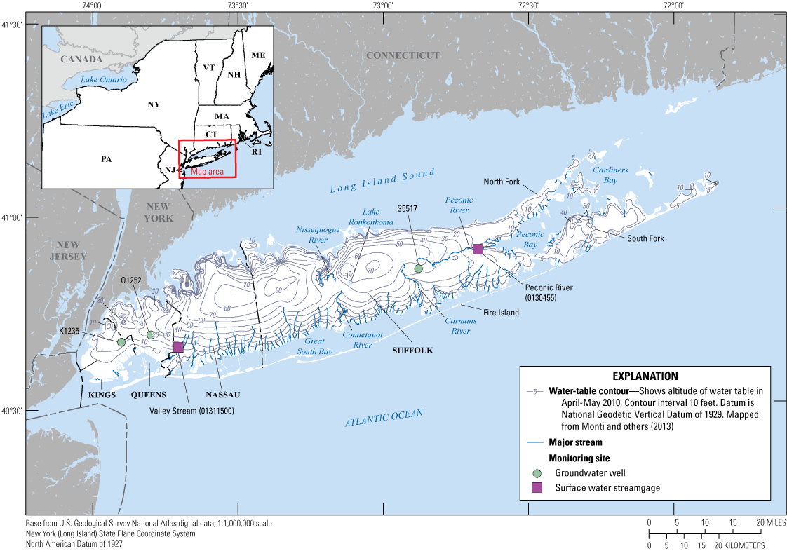
Map showing location and hydrography of Long Island, New York, and water table altitude, April to May 2010.
Long Island is underlain by unconsolidated sediments that comprise an important regional aquifer system. This system is the sole source of drinking water to nearly 3 million residents (U.S. Census Bureau, 2021a). The aquifer also provides freshwater discharge to streams, wetlands, and ponds throughout the region (fig. 1), which is necessary to maintain biological diversity and productivity in streams, estuaries, and salt marshes. Rapid population growth, however, has resulted in increased competition among agricultural, commercial, ecological, and residential demands for water resources. Water-resources managers are becoming concerned about possible long-term effects of these activities on the quantity and quality of water resources of the region as land development and water demand increase and as wastewater continues to be returned to these coastal-aquifer systems through domestic septic systems and centralized wastewater treatment facilities. Possible effects include the depletion of streamflow, lowering of surface-water levels in ponds and wetlands, decrease in freshwater flow to coastal waters, increase in the risk for saltwater intrusion, and degradation of water quality owing to land disposal of wastewater. Understanding the complex hydrologic system underlying Long Island, how the system has been historically affected by anthropogenic activities, and how the system may respond to future changes in both natural and anthropogenic stresses requires a detailed numerical model that is supported by a large set of diverse data.
In 2020, the U.S. Geological Survey (USGS) completed a regional-scale numerical model of the Long Island aquifer system that represents a synthesis of data on the physiography, geology, and hydrology of the Island (Walter and others, 2020). The model represents steady-state (average) conditions from 2005 to 2015 and is suitable for a regional-scale simulation of average water levels and groundwater discharge to receiving waters, hydrologic budgets, groundwater travel times to pumping wells and ecological receptors, and subsurface groundwater-age distribution for average hydrologic conditions. However, the aquifer system has been affected by changes in natural recharge, groundwater withdrawals, and land cover that have resulted in large changes in water levels and streamflow over time. A transient numerical model is needed to simulate the dynamic nature of the Long Island hydrologic system and to reproduce historical conditions and to simulate future conditions, including water-supply and wastewater management and climate change.
An improved understanding of the hydrologic response to these changes in stresses is needed to better evaluate the sustainability of the aquifer system as a safe and reliable source of water to the population and ecosystems on Long Island. Specifically, a transient model should represent time-varying hydraulic stresses (recharge and groundwater withdrawals); simulate changes in water levels, streamflows and hydrologic budgets (including aquifer storage); and account for a dynamic freshwater/saltwater interface that changes in response to those stresses.
The USGS began development of a three-dimensional transient model of the Long Island aquifer system upon completion of the steady-state model documented in Walter and others (2020) as part of the ongoing (since 2016) multiyear, cooperative investigation with the New York State Department of Environmental Conservation (NYSDEC). This transient model hindcasts historical conditions from 1900 to 2019 at an annual time scale and forecasts future hydrologic conditions at both annual and seasonal time scales. The model uses some of the hydrologic and geospatial data compiled and analyzed as part of the previous steady-state model of average 2005–15 conditions (Walter and others, 2020) but required additional information on historical conditions (1900–2005) and more recent and updated datasets developed after the previous modeling effort was completed (post-2015). These datasets included an updated geologic framework of western Long Island derived from geologic and geophysical data collected as part of the ongoing drilling program, a compilation of historical chloride data (Stumm and others, 2024), recharge estimates from a soil-water balance model from 1900 to 2019 (Finkelstein and others, 2022), and a compilation of historical pumping, water infrastructure, sewers and impervious surfaces, and observations of historical water levels and streamflows.
Purpose and Scope
This report documents the development and calibration of a three-dimensional, transient numerical model of the Long Island aquifer system and the use of that model to improve understanding of how the system will respond to changing natural and anthropogenic stresses during different time scales. The report describes the compilation and analysis of a diverse set of climatic, physiographic, geologic, hydrologic, and water-use data that underlie the numerical model and how those data are synthesized into a numerical model. The model simulation of historical hydrologic conditions from 1900 to 2019, as determined using historical water levels, streamflows, and chloride concentrations, and the calibration of model inputs using emerging inverse methods to best fit observed conditions, are also discussed in the report.
An updated overview of the geologic framework of western Long Island is presented in Stumm and others (2024), including the mapped extents and surface altitudes of the major glacial, preglacial Pleistocene, and Cretaceous units that comprise the Long Island aquifer system. The methods used to develop a three-dimensional hydrogeologic framework from the mapped framework are discussed in this report, along with modifications to an existing islandwide, grid-independent texture model developed from lithologic logs and methods used to incorporate that data as water-transmitting properties into the numerical model. Natural recharge to the aquifer determined by use of a soil-water balance model that utilized climate, soil, and land-use data is presented for human-influenced and natural landscapes from 1900 to 2019. Sources of anthropogenic recharge also are presented, including potential recharge from impervious surface runoff, leaky water-supply infrastructure, and wastewater return flow in sewered and unsewered areas, as are the methods and data sources used to estimate those recharge components. Historical groundwater withdrawals, the underlying data sources, and methods used to fill in data gaps are also described for 1900 to 2019. Historical water levels, streamflows, and chloride concentrations are discussed, along with the data sources and methods used in analyzing the data for use in calibration and verification of the numerical model.
The report documents the synthesis of the hydrologic data into a regional-scale, transient numerical model of the Long Island aquifer system. The model grid extent and discretization are presented, as are the locations and types of simulated hydrologic boundaries, the distribution of simulated recharge, and the locations of simulated pumping wells. The initial values of hydraulic parameters, including boundary leakances, horizontal and vertical hydraulic conductivity, and specific capacity and storage are presented, as well as the assumptions underlying them and comparisons to values in the literature. The use of a recently developed inverse calibration method to adjust these initial values to best match observed annual averaged water levels and streamflows is also discussed in detail. This discussion includes the parameterization of the model, implementation of inverse techniques, and fit between observations of water levels, streamflows, and their simulated equivalents. The agreement between simulated chloride concentrations for current and historical observations of chloride from water samples and estimates from borehole and surface geophysics is also presented in the report.
Important considerations when utilizing the model to make predictions of future hydrologic conditions are discussed, including potential errors associated with uncertainties in estimated input parameters and structural errors in the model design, hydrogeologic interpretations, and data gaps in estimates of pumping and anthropogenic recharge. The effect of parameter uncertainties on model predictions are quantified and illustrated using probabilistic methods and examples of the practical use of uncertainties in predicting hydrologic responses. Examples of structural error arising from data gaps in historical pumping are also presented. Descriptions are included on the modifications to the regional model that were implemented for the prediction of future hydrologic responses to changes in natural and anthropogenic stresses.
The report also includes analyses of changes in hydrologic conditions in the Long Island aquifer system in response to historical changes in sea level, recharge, groundwater withdrawals, and changes in water infrastructure from 1900 to 2019. Annual hydrologic budgets for the aquifer system that include changes in recharge, pumping, surface water discharge, and storage are discussed. The report also includes a discussion of the relative importance of historical changes in natural and anthropogenic stresses on the water table, streams, and the position of the freshwater/saltwater interface. This discussion includes maps of the current [2019] and historical changes in water table altitude and hydrographs of water levels and streamflows that illustrate time-varying hydrologic conditions at selected locations. Changes in the position of the boundary between fresh and saline groundwater (also known as the freshwater/saltwater interface) between 1900 and 2019 also are presented in maps and cross sections. The report also includes a discussion of general limitations associated with the use of numerical models, and limitations specific to the regional model of the Long Island aquifer system.
Hydrogeology
Long Island is underlain by unconsolidated sediments of late Pleistocene and late Cretaceous age that are, in turn, underlain by relatively impermeable crystalline bedrock of pre-Cambrian age (fig. 2). The maximum thickness of this wedge of unconsolidated sediments is more than 2,000 feet (ft) beneath the south-central part of the island. Long Island is at or near the southernmost advance of the continental ice sheet during the Wisconsinan glaciation, about 18,000 years before present (Smolensky and others, 1989). Glacial moraine sediments were deposited during periods of ice advance and retreat. These sediments formed morainal ridges that trend east-west along the spine of the island, which is bifurcated at the eastern end where two morainal ridges diverge to form the North and South Forks. The moraine deposits consist of poorly sorted sand, silt, and clay deposited marginal to the advancing ice sheet. Moraines are bounded generally to the south by glacial outwash deposits and to the north by ice-contact deposits.
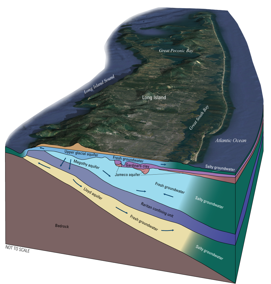
Three-dimensional schematic representation of major hydrologic units, generalized groundwater flow vectors, and the position of the freshwater/saltwater interface on central Long Island, New York.
Glacial outwash comprises fluvial sediments deposited in front of the ice margin and generally consist of well-sorted sand and gravel. Ice-contact deposits, which consist of sand, silt, and clay, were deposited within or near the margin of the retreating ice sheet. Pleistocene-age sediments on Long Island are underlain by upper Cretaceous-age sediments that were deposited in deltaic (fluvial and marsh) environments about 65 million years before present (Smolensky and others, 1989). These sediments represent the northern extent of the Northern Atlantic Coastal Plain aquifer system, a large wedge of mostly marine Cretaceous-age sediments that underlie the coastal plain of the mid-Atlantic region (Masterson and others, 2016). Only 3 of the 18 geologic units that compose the Northern Atlantic Coastal Plain aquifer system—the Magothy, Potomac, Potomac-Patapsco formations—underlie Long Island. The overlying units either were not deposited or were subsequently removed by erosion. The hydrogeologic equivalents of the Magothy, Potomac, and Potomac-Patapsco on Long Island are known as the Magothy aquifer, the Raritan confining unit, and the Lloyd aquifer, respectively. Cretaceous-age sediments are absent along the northern shore of Long Island where the units either pinch out or have been removed by erosion. Glacial sediments in these areas are either underlain by bedrock or by older Pleistocene-age fluvial and marine sediments deposited during interglacial periods, generally during the Illinoian period (Stumm, 2001; Stumm and others, 2002, 2004, 2024).
Glacial sediments comprise the surficial upper glacial aquifer, which has been an historically significant aquifer in western Long Island and remains an important source of water on eastern Long Island. The underlying Magothy aquifer and the contiguous Jameco aquifer in western Long Island make up an important aquifer that is the primary source of water in Nassau and Suffolk Counties. Two extensive fine-grained hydrogeologic units—the Gardiners clay and Raritan confining units—have hydraulic conductivity values several orders of magnitude lower than surrounding aquifers, and where present, the two confining units separate the groundwater flow system into three major aquifers: the Lloyd, the Jameco-Magothy, and the upper glacial aquifers (fig. 2; Franke and Cohen, 1972).
The Gardiners clay unit restricts vertical flow and creates confining conditions between the upper glacial aquifer and the Jameco and Magothy aquifers, predominately along the southern shore of the island. The Raritan confining unit restricts vertical flow between the Jameco and Magothy aquifers and confines the Lloyd aquifer in most areas of the island. The crystalline bedrock underlying the unconsolidated deposits is much less permeable than the overlying deposits, and the bedrock surface is considered the lower extent of the aquifer system (Smolensky and others, 1989).
The major hydrogeologic units (and their geologic equivalents) in descending order, are the upper glacial aquifer, Gardiners clay unit (Gardiners Clay), Jameco aquifer (Jameco Gravel), Monmouth greensand unit (Monmouth Group), Magothy aquifer (Magothy Formation and Matawan Group, undifferentiated), Raritan confining unit (clay member of the Raritan Formation), and the Lloyd aquifer (Lloyd Sand Member of the Raritan Formation; Smolensky and others, 1989). In addition to these major units, other Pleistocene-age units—the North Shore aquifer and North Shore confining unit—underlie Wisconsinan-age glacial sediments in some areas where Cretaceous-age units are absent (Stumm, 2001), and there are local confining units within the upper glacial aquifer (Doriski and Wilde-Katz, 1982; Krulikas and Koszalka, 1982; Schubert and others, 2004).
The Long Island aquifer system is a freshwater aquifer system that is bounded below by relatively impermeable bedrock, above by the water table, and laterally by saline groundwater. The position of the freshwater/saltwater interface in the largely unconfined upper part of the aquifer system generally represents a hydrostatic balance between freshwater and denser saltwater and likely is close to the shoreline (fig. 2). The freshwater/saltwater interface in the deep, confined Lloyd aquifer can be displaced seaward of the shoreline beneath the Raritan confining unit.
Precipitation, which is the sole source of natural recharge to the Long Island aquifer system, averaged about 47 inches per year (in/yr) ranging from about 28 in/yr to about 56 in/yr from 1900 to 2019 (Finkelstein and others, 2022). On average, about half of the precipitation on Long Island reaches the water table as aquifer recharge. The upper glacial aquifer is unconfined, as are the underlying Magothy and Jameco aquifers where the Gardiners clay is absent; the water table is a free surface that changes in response to changes in recharge. Water table altitudes exceed 60 ft in two areas, to the east and west of major surface-water drainages in the central part of the island (fig. 1). Areas of locally high water table altitudes also occur in parts of New York City, on necks and peninsulas in northern Nassau County, and on the North and South Forks in eastern Suffolk County.
Water levels and streamflows vary naturally with time in response to changes in hydrologic stresses, particularly recharge from precipitation (fig. 3). The correlation between natural recharge and hydrologic conditions (water levels and streamflows) is most pronounced in the unconfined aquifers and in generally undeveloped areas, such as eastern Suffolk County. The lowest water levels were recorded in well S5517 in eastern Suffolk County in the mid-1960s, which coincides with the largest drought for the period of record (1900 to 2019 for the purposes of this report); the highest water levels were observed in the early 1980s (fig. 3B), coinciding with a period of high precipitation and recharge (fig. 3A).
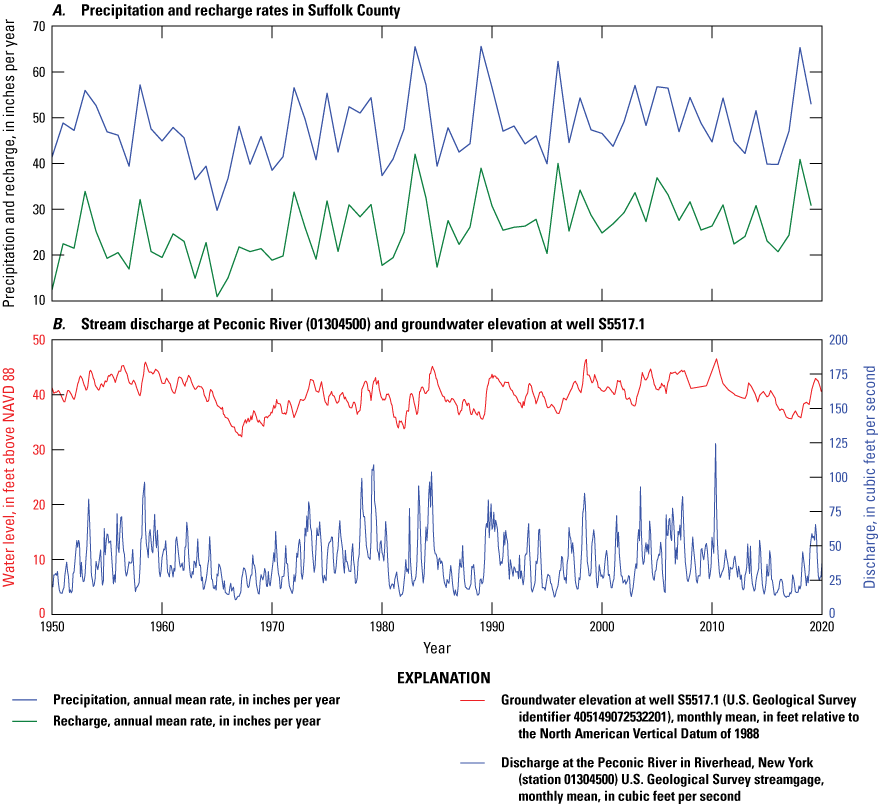
Graphs showing time series of A, precipitation and recharge in Suffolk County, New York, and B, water-level altitude in well S5517 and streamflow in the Peconic River in Riverhead, N.Y. (station 01304500) U.S. Geological Survey streamgage, from 1950 to 2019. Data are from U.S. Geological Survey (2020b). Locations of sites shown on figure 1.
Long Island is surrounded by saltwater from the Atlantic Ocean to the south and Long Island Sound to the north. The mainland of the island encompasses the area to the west of North and South Forks, which are separated by the Peconic and Gardiners Bays (fig. 1). The northwestern shore of the island has numerous peninsulas (or necks) with small intervening embayments, whereas the northeastern shore of Long Island generally is smooth, with few bays or coastal landforms. The southern shore of Long Island is separated by Great South Bay from Fire Island, the barrier island that lies off the southern coast mainland Long Island. Most surface drainage features on Long Island are along the southern shore. The largest surface drainages—the Carmans, Connetquot, Nissequogue, and Peconic Rivers—are in the central and eastern parts of the island. There are few natural ponds on the island, the largest of which is Lake Ronkonkoma in the central part of the island.
Long Island received, on average, about 2,600 cubic feet per second (ft3/s) of aquifer recharge from precipitation from 2005 to 2015 (Walter and others, 2020). Groundwater flows away from regional, inland groundwater divides toward streams and coastal receiving waters; these divides generally trend east-west on the main body of the island and extend onto the North and South Forks. About 28 percent of groundwater discharged to streams and fresh wetlands, and little less than half (about 46 percent) discharged to salt marshes and coastal receiving waters.
Groundwater is the sole source of drinking water for the residents of Nassau and Suffolk Counties. An annual average of about 660 ft3/s of groundwater, or about 20 percent of total recharge, was withdrawn for public, agricultural, and industrial uses from 2005 to 2015 (Walter and others, 2020). Most of the water that was withdrawn during this period (about 60 percent) was returned to the aquifer system as anthropogenic recharge.
Historical Background and Human Effects on the Aquifer System
Long Island was a generally densely populated island with a population of 8.1 million people in 2020 (U.S. Census Bureau, 2021a). Most of the population (about 64 percent) resided within New York City, in Kings and Queens Counties; the remainder resided east of New York City, in Nassau and Suffolk Counties. The first census of population on Long Island showed that it had a total population of about 37,000 people in 1790, with about three quarters of the population residing in Nassau and Suffolk Counties. The population of Long Island increased to about 1.5 million people by 1900, generally as part of the industrial revolution and rapid urbanization in and around New York City in the 19th century (fig. 4A). More than 90 percent of the Long Island population resided in New York City, in Kings and Queens Counties, in 1900.
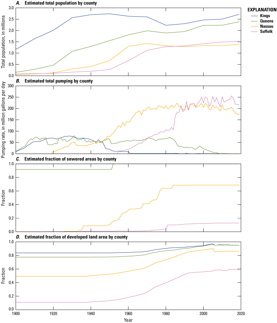
Graphs showing time series of A, population, B, pumping, C, fraction of sewered area, and D, fraction of developed land area from 1900 to 2019 on Long Island, New York. Population data are from U.S. Census Bureau (2021b); sewered data, from Finkelstein and others (2022); and pumping data, from New York Department of Environmental Conservation (2024).
Agriculture was prevalent in Nassau and Suffolk Counties in 1900; the two rural counties combined had only about 9 percent of the total population of the State. Population increased steadily through the first part of the 20th century, with a net increase in population in Nassau and Suffolk Counties to about 13 percent of the State total. The population in these two counties more than doubled to about 30 percent of the total population of the State between 1940 and 1960 primarily due to suburban development following the end of World War II (WWII) in 1945. The largest population increase was in Nassau County where the population increased by about 890,000 people. The population on Long Island increased throughout the remainder of the 20th century—the largest rate of increase was in Suffolk County—but decreased slightly in Kings County between 1960 and 2000. Suffolk County, which has exceeded the population in Nassau County since the mid-1980s, remains the fastest growing county on Long Island with an average rate of increase of about 5 percent per year since 2000. An increase in population affects the aquifer system in several ways, including withdrawal of groundwater for public supply, changes in the amount and distribution of recharge, and physical changes to the landscape and land-use activities.
Groundwater is the sole source of potable water for Nassau and Suffolk Counties; about 450 million gallons per day (Mgal/d) of groundwater was withdrawn from the Long Island aquifer system in 2015 (Walter and others, 2020). Water supply for Kings and Queens Counties comes from an extensive system of reservoirs in upstate New York, which began with major expansions of water infrastructure in 1917 and 1936 (Buxton and Shernoff, 1999). Groundwater was an important source of water in New York City, in Kings and Queens Counties, for much of the 20th century, before the importation of reservoir water.
Groundwater from wells supplemented surface water and ponded spring water as the source of potable water in Kings and Queens Counties in the late 19th century. Groundwater withdrawals from public-supply wells in New York City began in the early part of the 20th century and peaked in the early 1930s, when about 150 Mgal/d of groundwater was pumped from the aquifer system underlying New York City (fig. 4B). Groundwater withdrawals for public supply in Kings County ceased in 1947 because saline groundwater was discovered to have intruded (what is known as saltwater intrusion) into the aquifer system. Pumping in Queens County continued and exceeded 50 Mgal/d between the late 1940s and the early 1980s, though pumping generally moved eastward within the county due to saltwater intrusion during that period. Pumping for public supply varied annually but was generally constant at more than 50 Mgal/d between the 1910s early 1980s, and by the mid-1990s, the entirety of New York City was supplied from upstate reservoirs. Pumping of groundwater for other uses continued in Kings and Queens Counties until about 1960 and 2007, respectively.
Groundwater withdrawals for public supply in Nassau County began around 1920 and increased to about 50 Mgal/d by the mid-1940s, after which withdrawals increased rapidly to about 200 Mgal/d by 1970 (fig. 4B). The increase in pumping corresponds to the period of rapid suburbanization following WWII when the population of Nassau County more than doubled (fig. 4A). Pumping in Nassau County generally has been more constant since 1970, averaging about 200 Mgal/d (fig. 4B). Pumping from public-supply wells in Suffolk County began in the mid-1950s and increased at a generally steady rate to more than 100 Mgal/d by 1980. Groundwater withdrawals from public-supply wells nearly doubled to about 200 Mgal/d by 1990, likely due to the transition from onsite, private wells to large capacity, public-supply wells during that time. Suffolk County has had the largest groundwater withdrawals on Long Island since 2000; pumping in the county generally has fluctuated between 200 and 250 Mgal/d during that time.
Human activities also have affected the aquifer system through urbanization, changes to the landscape, and the development of water infrastructure. Monti and others (2024) estimated spatially variable historic land use on Long Island for the period 1900-2019 using land cover projections from Sohl and others (2014) and Sohl and others (2018). About 350 mi2 of the land area of Long Island was considered developed in 1900, which represented about 27 percent of the total land area. About 22 percent of the landscape was used for agriculture, either as crop land or pasture, and the remaining 50 percent was undeveloped land, generally maritime forests of pitch pine and red oak (fig. 5A). By 2019, a total of about 880 mi2 of Long Island was considered developed, or about 69 percent of total land area. Undeveloped land and land used for agriculture represented a total of about 5 and 26 percent, respectively, and was generally in eastern Suffolk County (fig. 5B).
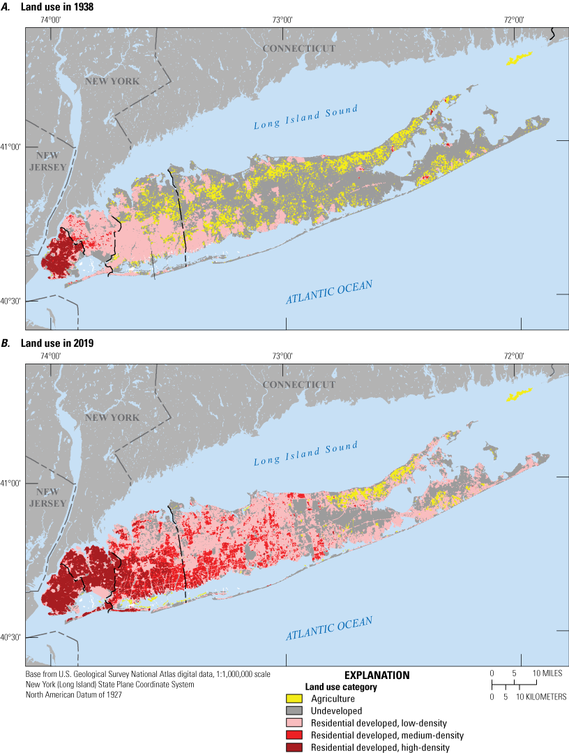
Maps showing land use in A, 1938 and B, 2019 on Long Island, New York. Data are from Monti and others (2024).
The history of development on Long Island since 1900 varies by county. High-density residential development, defined as a population density exceeding about 11,200 people per square mile, in 1900 was generally limited to densely populated areas of Kings County (fig. 5A ; Finkelstein and others, 2022). Remaining developed areas generally had low-density development (less than about 5,600 people per square mile). About 83 percent of land in Kings County was considered developed in 1900; most (about 70 percent) was considered high density development (fig. 5A). About 77 percent of land in Queens County was considered developed, most of which was considered low density development. The amount of developed land increased slightly since 1900 (fig. 4D) and in 2019, both counties were about 95 percent developed (fig. 5B), most of which (about 71 percent) is considered high-density development.
About 50 percent of Nassau County was considered developed, and about 20 percent of the county was used for agriculture in 1900 (fig. 5A). The largest rate of development was generally between the late 1960s and early 1990s when developed land increased from about 60 percent to about 85 percent (fig. 4D) due to a rapid suburbanization and associated conversion of forested and agricultural land to low- and medium-density residential development (fig. 5B). About 86 percent of Nassau County was developed in 2019, with undeveloped areas generally in the northeastern part of the county (fig. 5B). About 51 percent of developed land in Nassau County in 2019 was considered low density residential development (fig. 5B). Medium- and high-density residential development made up about 33 and 16 percent of developed in Nassau County, respectively.
Suffolk County is the most rural county on Long Island. About 90 mi2 of land in the county was considered developed in 1900, or about 10 percent of total land area (fig. 5A). About 27 percent of land in the county was used for agriculture and most land (about 62 percent) was undeveloped, likely forested, at that time (fig. 5A). Development in Suffolk County increased from less than 20 percent in the early 1960s to more than 50 percent of total land area in the early 1990s because of rapid suburbanization (fig. 4D). About 60 percent of Suffolk County was considered developed in 2019. Most of the developed land (about 85 percent) was considered low-density residential development (fig. 5B), and about 14 percent of developed land was considered medium-density residential development. Less than 1 percent of developed land in the county was high-density residential development. About 7 percent of the county was in agricultural use by 2019, primarily on the North Fork in eastern Suffolk County (fig. 5B). About 33 percent of Suffolk County remained forested in 2019, primarily in eastern Suffolk County (fig. 5B).
Natural recharge is the sole source of freshwater to the Long Island aquifer system and is affected by several characteristics of the landscape, including soil type and water capacity, land slope, and vegetative cover. Development affects recharge in different ways: impervious surfaces can impede the movement of water into the unsaturated zone and lower recharge to the water table in urbanized areas (fig. 6A), whereas the conversion of forested land to low-density residential development can increase recharge (Yang and others, 2015). Impervious surfaces generally coincide with areas with high-density residential development, including almost all of Kings and Queens Counties in New York City (fig. 4B).
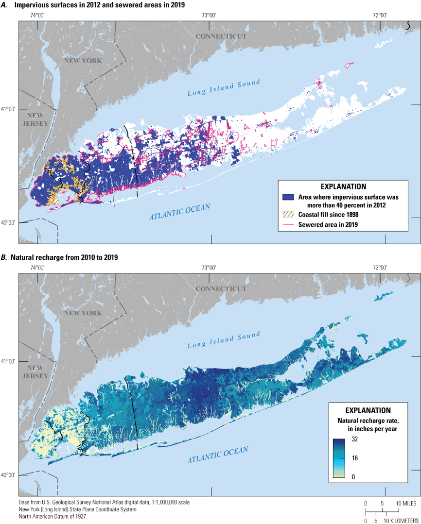
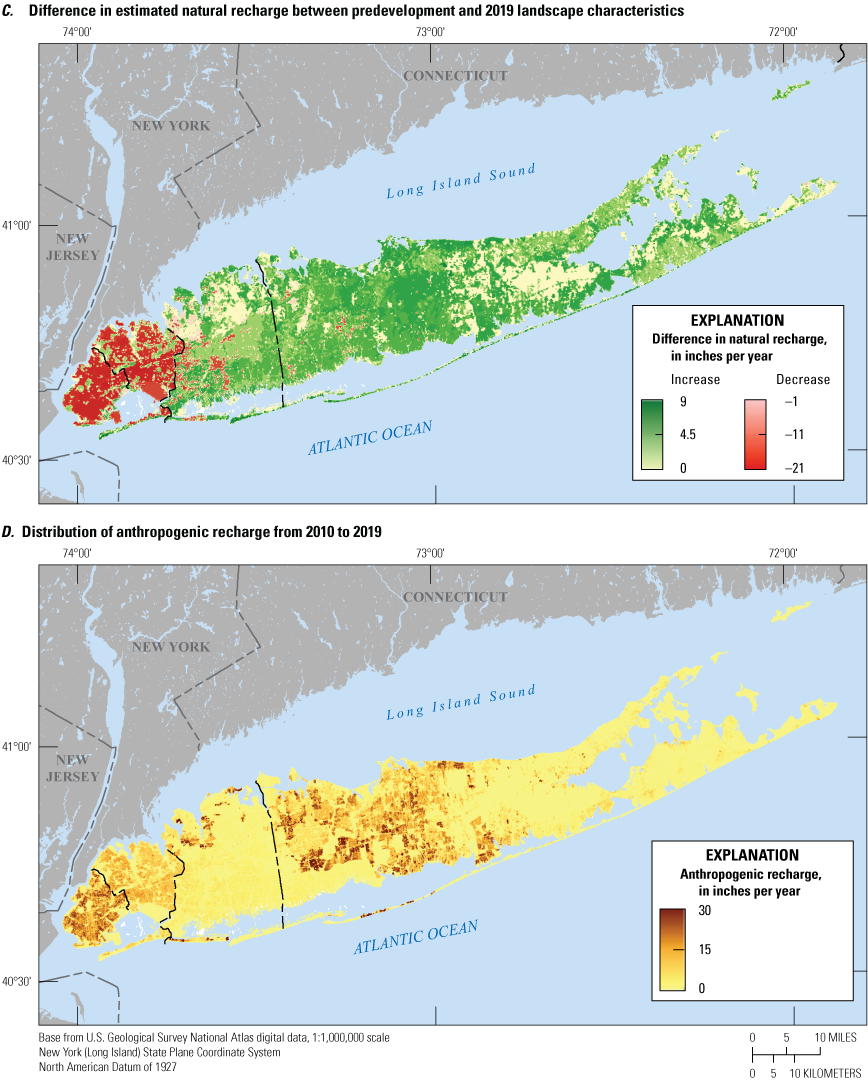
Maps showing A, areas with greater than 40 percent impervious surface in 2012 and sewered areas in 2019; B, natural recharge rates from 2010 to 2019; C, difference in estimated natural recharge between 1900 and 2019; and D, distribution of anthropogenic recharge from 2010 to 2019. Data are from Finkelstein and others (2022) and Veatch and others (1906).
Finkelstein and others (2022) estimated the average recharge on Long Island from 1900 to 2019 by use of a soil-water balance model (Westenbroek and others, 2010) that utilizes climate and spatial data. Natural recharge from 2010 to 2019 estimated using developed landscape characteristics averaged 20.5 in/yr across Long Island and varies spatially (fig. 6B). The lowest recharge rate is in Kings County where the average rate was about 6.6 in/yr, and the highest is in Suffolk County where the average recharge rate was about 23.2 in/yr. These soil-water balance estimates of recharge assume 2010–19 climate conditions. Estimated recharge using a soil-water balance model for the period before development in the 20th century (known as predevelopment), which assumes a uniformly forested landscape, averaged 19.2 in/yr, only slightly (about 1.3 in/yr) lower than the natural recharge estimated for 2010 to 2019.
The difference in natural recharge rates between developed and undeveloped landscapes varies across Long Island (fig. 6C). Natural recharge rates from 2010 to 2019 in Kings and Queens Counties (in New York City) and parts of southern Nassau County were substantially lower (exceeding a 20 in/yr deficit) than for predevelopment conditions owing to the high-density residential development and impervious surfaces in urbanized landscapes typical of that area. The average natural recharge rates in Kings and Queens Counties decreased by about 13.6 and 11.0 in/yr, respectively, due to development patterns. Conversely, recharge rates in parts of Nassau and Suffolk County were substantially higher (exceeding 8 in/yr) owing to the conversion of forested and agricultural land to low-density residential landscapes that generally are more efficient for aquifer recharge (Yang and others, 2015). Average natural recharge rates in Nassau County increased by about 1.6 in/yr from predevelopment conditions, and average recharge rates in Suffolk County increased by about 3.9 in/yr. Recharge rates estimated from the soil-water balance model in areas forested in 2019, which were generally in eastern Suffolk County, were the same for both developed and undeveloped landscapes (fig. 6C).
Most of the groundwater withdrawn from the aquifer for public supply (about 60 percent) was returned as anthropogenic recharge, either as wastewater return flow or as loss from compromised water-supply infrastructure. In 2019, about 84 percent of wastewater return flow on Long Island was discharged into sanitary sewers. Kings County has been fully sewered since the beginning of the 20th century; Queens County was about 90 percent sewered in 1900 and fully sewered by the mid-1950s (fig. 4C). Construction of sewers began in Nassau County in the mid-1930s, and about 10 percent of the county was sewered by 1950. The extent of sewered areas in Nassau County increased rapidly between 1950 and the mid-1980s, corresponding with the period of rapid suburbanization following WWII. About 70 percent of Nassau County was sewered by the mid-1980s, after the last phase of sewer construction. The remaining unsewered areas are in the northern part of the Nassau County.
The fraction of wastewater return flow that enters sanitary sewers increased in Nassau County from less than 2 percent in the mid-1930s to more than 90 percent by 1980. Construction of sewers in Suffolk County generally began in the mid-1930s, but the total of sewered area in the county was less than 1 percent by the mid-1950s and did not exceed 5 percent until 1980 (fig. 4C). Sewer expansions in the early 1980s doubled the fraction of sewered areas to about 10 percent by the mid-1980s. In 2019, the fraction of sewered areas remained low, at about 12 percent, and a total of about 85 percent of wastewater return flow recharged the aquifer in unsewered areas (Shaffer and Runkle, 2007). About 36 percent of Long Island was sewered in 2019, mostly in the densely populated areas in New York City, southern Nassau, and southwestern Suffolk County (fig. 6A). Most wastewater (about 84 percent) was discharged into sanitary sewers; the remaining 16 percent of wastewater was discharged into onsite septic systems, primarily in central and eastern Suffolk County and along the northern shore of both Nassau and Suffolk Counties. About 90 percent of wastewater discharged into sanitary sewers was treated and discharged into surface waters; the remaining 10 percent was treated and discharged onto land, mostly in inland areas of Suffolk County. Recharge from wastewater return flow was primarily in unsewered areas but also could occur in sewered areas through leaky or compromised sewer lines.
Pumped groundwater can also recharge the aquifer from leaky water-supply infrastructure; the amount of recharge from infrastructure is a function of the density and age of water lines. Misut and Monti (1999) reported that recharge from aging or compromised water-supply infrastructure in New York City was approximately 10 percent of the total water supplied to the area.
Anthropogenic recharge refers to the combination of recharge from wastewater return flow and leaky infrastructure and depends on several factors, including population density, the location of water infrastructure, and the age and mechanisms of return flow in sewered and unsewered areas. The average rate of anthropogenic recharge on Long Island was about 4.7 in/yr and varies across Long Island (fig. 6D). Anthropogenic recharge generally is largest in Kings and Queens Counties where high-density residential development results in substantial recharge from leaky infrastructure and also in central Suffolk County where extensive areas of low and medium density residential areas are not sewered and wastewater return flow recharges the aquifer system. Anthropogenic recharge is lower in rural areas of eastern Suffolk County and in sewered areas in Nassau County. Anthropogenic recharge accounts for more than 90 percent of total recharge in parts of Kings County. About 51 percent of total recharge in Kings and Queens Counties and about 13 percent in Nassau and Suffolk Counties is from anthropogenic sources.
Withdrawal of groundwater can affect the aquifer system by lowering the water table, and potentiometric surfaces in confined aquifers and depleting streamflows. The drawdown of the water levels from pumping has the potential to reverse hydraulic gradients and induce saltwater intrusion into freshwater portions of aquifers. Pumping in the northern part of Kings County and to the south in the Flatbush franchise resulted in a cone of depression as early as the mid-1930s (fig. 7A; Buxton and Shernoff, 1999). Water table altitudes in this area were as low as 30 ft below mean sea level, representing a drawdown of about 40 ft from nonpumping conditions. Although pumping in the county ended in 1947 in response to saltwater intrusion, water levels remained below sea level until the early 1960s. Water table altitudes below sea level were first observed in the western part of Queens County in the late 1930s due to pumping in the Woodhaven franchise (fig. 7B). The water table decreased to an altitude of 15 ft below mean sea level by the early 1960s, representing a drawdown of about 30 ft.
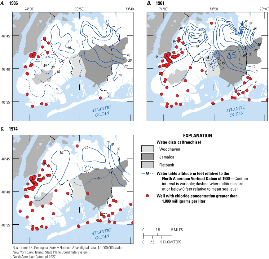
Maps showing water table altitude and well locations with chloride concentrations greater than 1,000 milligrams per liter in A, 1936, B, 1961, and C, 1974 on western Long Island, New York. Modified from Buxton and Shernoff (1999).
Water table altitudes below sea level were first observed in central Queens County by the early 1970s (fig. 7C; Buxton and Shernoff, 1999). Pumping in western Queens County ended in 1974 due to saltwater intrusion, after which water levels recovered to near sea level. Continued pumping from the Jamaica franchise in central Queens County resulted in water table altitudes 15 ft below sea level (fig. 7C; Buxton and Shernoff, 1999), which represents a drawdown of about 50 ft from nonpumping conditions. Pumping in central Queens County declined following an expansion of water-supply infrastructure to allow for the importation of water from upstate New York throughout Kings and Queens Counties and to preserve fresh groundwater resources in central Queens County.
Historical chloride data indicate that saltwater intrusion was observed in Kings County before 1920, and currently [2022] large areas along the coast in the aquifers underlying the county are intruded with saltwater (Stumm and others, 2024). Saltwater intrusion was observed along the entire southern coast of Queens County north of Jamaica Bay before 1960, and aquifers underlying the area remain affected by saltwater intrusion. Saltwater intrusion also has been observed in aquifers underlying southwestern Nassau County since the 1940s, and in some areas along the northern coast of the county since the 1960s. Before 1990 along the northern coast of Queens County, saltwater intrusion was first observed primarily in the Flushing area (Stumm and others, 2024). Parts of the Lloyd, Magothy, and upper glacial aquifers in New York City and western Nassau County remain intruded by saline groundwater, though large-scale pumping in New York City ceased by the early 1980s. The Lloyd and Magothy aquifers in Kings County remain intruded along the western and southern shores. In Queens County, groundwater with chloride concentrations exceeding 1,000 milligrams per liter (mg/L) in the Lloyd aquifer extends northward about 1 mi inland from Jamaica Bay, as well as southward by about 0.5 mi near Flushing Bay. The Magothy aquifer in Queens County also is intruded along the southern and northern coasts. Parts of the Magothy and Lloyd aquifers also are intruded beneath peninsulas along the northern shore of Nassau County due to historical and ongoing groundwater withdrawals (Stumm and others, 2024).
Anthropogenic perturbation of the western Long Island aquifer system by groundwater withdrawals and changes in recharge also is reflected in time-varying water levels and streamflows (fig. 8). Water levels and streamflows are strongly correlated with precipitation and recharge under natural conditions (fig. 3). Large groundwater withdrawals and the subsequent cessation of those withdrawals result in long-term trends in both water levels and streamflows that are not strongly correlated with recharge (fig. 8). Wells K1235 and K1263 in Kings County show an increase in water levels starting in the late 1940s (fig. 8B); this increase in water levels coincides with the cessation of pumping in that area (fig. 4B). Water levels in the wells increased by about 15 ft between the late 1940s and 1970 when recharge fluctuated but did not appear correlated to water level fluctuations (fig. 8A). Water levels in well Q1252 showed a steady decrease from about 27 ft in the early 1950s to 2 ft below sea level by 1970. The decline in water levels coincided with increases in withdrawals in Queens County to meet water demand following the cessation of pumping and an expansion of sewer systems to the west (fig. 4D). Groundwater withdrawals also affect streamflows. Flow in Valley Stream in southwestern Nassau County (fig. 1) decreased from between 5 and 10 ft3/s in the late 1950s to less than 2 ft3/s by the early 1960s (fig. 8B). This decrease in flows generally follows an increase in pumping and an expansion of sewer systems in western Nassau County starting in the mid-1950s (fig. 4D).
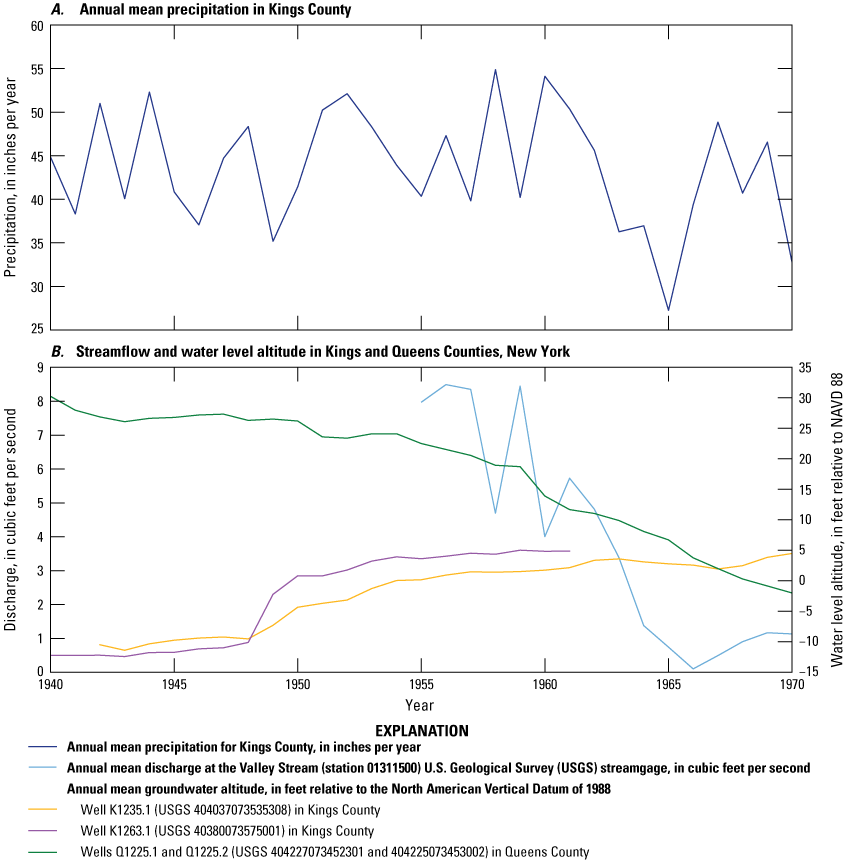
Graphs showing A, annual mean precipitation in Kings County and B, water level in wells K1235, K1263, and Q1225 and streamflow at the Valley Stream (station 01311500) U.S. Geological Survey streamgage from 1940 to 1970. Location of sites shown on figure 1. Data are from U.S Geological Survey (2020b).
Human activity has also affected the hydrologic system by altering natural hydrologic features, including the impounding of freshwater streams and the filling of coastal marshes and streams. A total of about 30 mi2 of coastal marshes and streams was filled before 1920. Most infilled areas are former coastal marshes along Jamaica Bay in southeast Kings and southern Queens Counties and along Flushing Bay and Newtown Creek in northwestern Queens County (fig. 6A). Additional infilled areas include freshwater bodies in central Queens County. Infilling of natural waters can affect groundwater discharge patterns, and filled areas near the coast that have been subsequentially developed could be at a higher risk of groundwater inundation and sea level rise.
Data Compilation and Analysis
A variety of data were compiled and analyzed for synthesis into a regional model of the Long Island aquifer system that simulates hydrologic conditions from 1900 to 2019. These data types include topographic and bathymetric altitudes, the spatial extent and thicknesses of major hydrogeologic units, estimates of the horizontal and vertical hydraulic conductivity of the aquifer sediments, estimates of recharge from spatial and climate data, historical water use and the distribution of associated infrastructure and return flow, and observations of historic hydrologic conditions, including water levels, streamflows, and chloride concentrations. Annually averaged water levels and streamflows were used to characterize hydrologic conditions from 1900 to 2019.
Physiography
The surface-water hydrography and geometry of the coast were determined from geographic information system (GIS) linework digitized from 1:24,000-scale topographic quadrangles (U.S. Geological Survey, 2020a). Most surface drainages are along the southern shore of the island, and many of those streams have artificial impoundments. The largest surface drainages—the Connetquot, Nissequogue, and Peconic Rivers—are in the central and eastern parts of the island (fig. 1). There are few natural ponds on the island. The northern shore of Nassau and western Suffolk Counties generally has few streams with large peninsulas, referred to locally as necks, separated by small embayments. There are numerous coastal streams along the southern shore, and a series of barrier islands are south of the western and central parts of the Long Island mainland.
The altitudes of land surface and the seabed were derived from a 1-m (3.3-ft) topobathymetric digital elevation model of the coastal regions of Massachusetts, Rhode Island, Connecticut, and New York (Danielson and Haines, 2017). The dataset is a collaboration between the USGS and the National Oceanic and Atmospheric Administration and combines data from 321 sources to create a seamless, internally consistent representation of land and seabed altitudes at a spatial resolution of 1 m (3.3 ft). These data were upscaled and mapped to the regional model grid; model cells have a horizontal discretization of 500 ft, and there are about 23,100 individual altitude measurements within each model cell. The mean and minimum values of these measurements were computed for each model cell to a distance 3 mi seaward of the coast (fig. 9). Mean land-surface altitudes range from sea level to more than 370 ft above sea level and exceed 200 ft above sea level in the north-central part of the island, in isolated areas in the eastern part of the Long Island mainland, and on the South Fork. Land-surface altitudes are highest in areas underlain by glacial moraines that have an east-west trend in the northern part of the Long Island mainland and extend onto the North and South Forks.
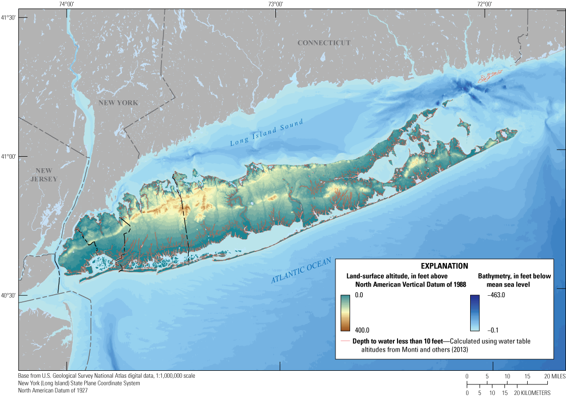
Maps showing topography, bathymetry, and areas with depth to groundwater less than 10 feet from April to May 2010 on Long Island, New York. Data are from Danielson and Haines (2017).
Topography along the northern shore of the island generally is steep, particularly in areas where moraines are adjacent to the shore. The topography to the south of the moraines is gently sloping to the southern shore of the island, generally corresponding to glacial outwash plains (fig. 9). Mean seabed altitudes range from sea level to more than 350 ft below sea level. The lowest seabed altitudes (deepest water) are in offshore areas of Long Island Sound, along the North Fork. The highest seabed altitudes (shallowest water) generally are in estuaries and bays along the southern shore of the island. The northern shore of Long Island generally is characterized by steep coastlines resulting from coastal erosion, whereas the southern shore is characterized by gently sloping topography with numerous small embayments.
The highest water table altitudes in 2010 exceeded 70 ft in two areas on the mainland of the island (fig. 1; Monti and others, 2013). The mean thickness of the unsaturated zone thickness, defined as the difference between land surface and the water table, is about 47 ft, and the unsaturated zone can be as thick as 300 ft in some areas underlain by moraines. The thickness of the unsaturated zone in 2010 was 10 ft or less across about 250 mi2, generally along the southern coast, near streams, and on barrier islands (fig. 9).
Hydrogeology
New and existing geologic data were collected, compiled, and analyzed to better define the hydrogeology of the Long Island aquifer system for synthesis into a groundwater flow model. The sources of the data include historical literature, compilation of existing data (lithologic and borehole geophysical logs), and collection of geologic data from ongoing (2017–2023) field efforts. These data were used to develop a hydrogeologic framework of the Long Island aquifer system and to estimate the water-transmitting properties of sediments of the major unconfined aquifers, including the upper glacial, Jameco, and Magothy aquifers.
Previous investigations of the extents and surface altitudes of major hydrogeologic units were used to develop a three-dimensional model of the hydrogeologic framework of the Long Island aquifer system (Walter and others, 2020). This information included maps of the surficial (Wisconsinan) glacial geology of Long Island (Cadwell and Muller, 1986; Cadwell, 1989), locally significant Wisconsinan confining units (Doriski and Wilde-Katz, 1982; Krulikas and Koszalka, 1982), pre-Wisconsinan Pleistocene marine, lacustrine, and fluvial units (Stumm, 2001; Stumm and others, 2002, 2004; Schubert and others, 2004), and the surfaces and extents of the bedrock and overlying Cretaceous formations (Smolensky and others, 1989).
A hydrogeologic framework was developed from existing lithologic and geophysical data and new data collected as part of an ongoing drilling and geologic mapping effort as part of the Long Island Groundwater Sustainability Project (LISUS; U.S. Geological Survey, 2024a). The field effort, to date [2024], focused on the western part of Long Island, including Kings, Queens, and Nassau Counties. This effort used lithologic and geophysical data from 643 existing wells of varying depths across Long Island (fig. 10). These data were augmented with information from 23 new (2017–22) wells, including 18 boreholes drilled to bedrock as part of the project and an additional 5 wells drilled as part of other investigations. The results of this investigation, including the extents and surfaces of major hydrogeologic units and the extent of saltwater intrusion, are documented in detail in Stumm and others (2024). The hydrogeologic framework also was updated with the results of mapping of the bedrock surface of New York City (DeMott and others, 2023).
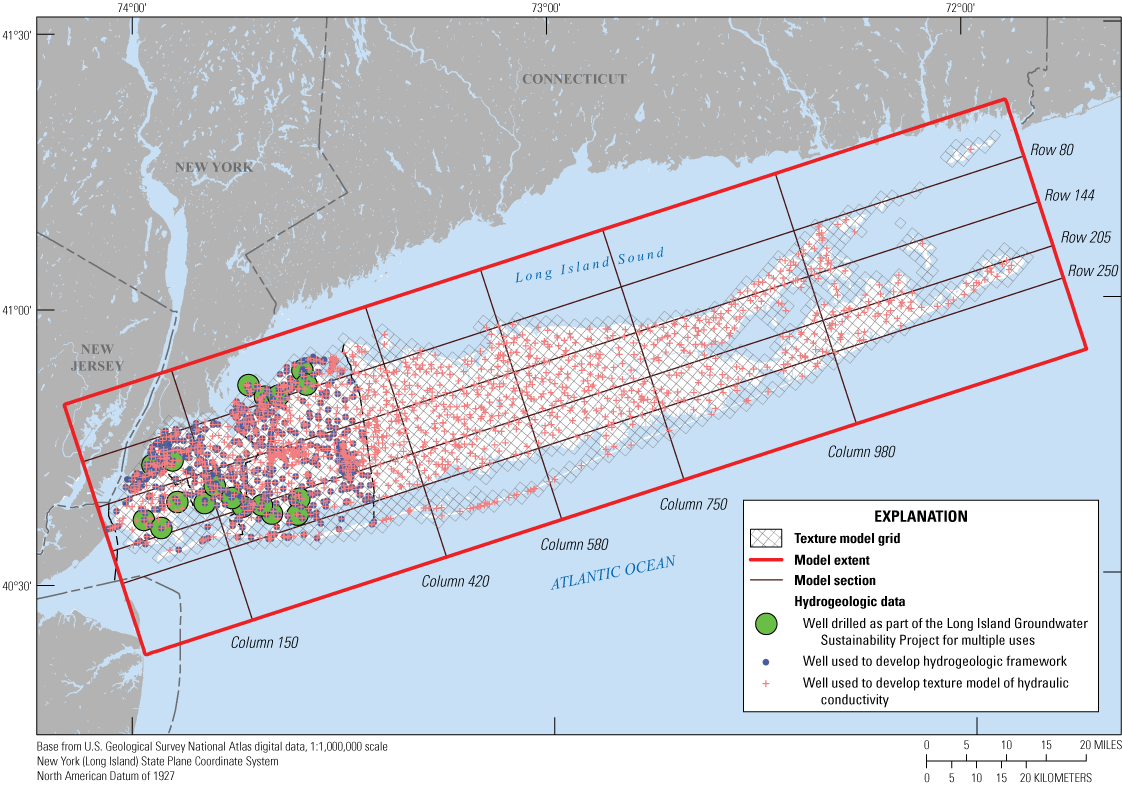
Map showing locations of wells and boreholes used to define the hydrogeologic framework and to develop a texture model of hydraulic conductivity for the aquifer system of Long Island, New York.
Hydraulic properties of aquifer sediments of importance to groundwater flow include horizontal and vertical hydraulic conductivity, specific yield in unconfined aquifers, specific storage in confined aquifers, and sediment porosity and dispersivity. These properties vary by hydrogeologic unit and within each unit. Direct measurements of hydraulic properties are focused primarily near major pumping centers, and consequently, field measurements of hydraulic properties are concentrated in areas of large groundwater withdrawals and for those particular aquifer units with the most use (McClymonds and Franke, 1972; Franke and Getzen, 1976; Lindner and Reilly, 1983; Prince and Schneider, 1989; Stumm, 2001; Stumm and others, 2002, 2004, 2024; Williams and others, 2020); as such, hydraulic property data are relatively sparse compared with the apparent heterogeneity of the regional hydrogeologic units.
Estimates of hydraulic properties made in previous numerical model investigations include Buxton and Smolensky (1999), Kontis (1999), Misut and Monti (1999), Misut and others (2004), Schubert and others (2004), and Monti and others (2009). Buxton and Smolensky (1999) provided a summary of the previous investigations of the hydraulic properties of the aquifer system. That synthesis of previous work represents the most comprehensive summary to date of the existing information on hydraulic properties of the major hydrogeologic units of the Long Island aquifer system. Stumm and others (2024) present a summary of the water-transmitting properties of major hydrogeologic units in western Long Island as determined from slug tests and nuclear magnetic resonance logs.
The relation between sediment characteristics and measured hydraulic conductivity, as compiled from previous investigations, was used to develop a three-dimensional texture model of hydraulic conductivity within the upper glacial, Jameco, and Magothy aquifers—the principal aquifers on Long Island—using lithologic logs from 1,769 wells across Long Island (Walter and Finkelstein, 2020). An augmented network of 1,846 wells was used to develop an updated texture model of those three principal aquifers for this investigation (fig. 10). The texture model defines a three-dimensional distribution of hydraulic conductivity that represents the heterogeneity of sediments in the major aquifers. The workflow used to develop the three-dimensional texture model from borehole data is presented in Walter and Finkelstein (2020) and consists of four steps:
-
1. assignment of vertically continuous hydraulic conductivity values in boreholes from lithologic descriptions and hydraulic conductivity look up tables derived from previous data;
-
2. identification of individual hydraulic conductivity points within a set of uniform 10-ft layers encompassing the aquifers;
-
3. interpolation of hydraulic conductivity within each layer using ordinary kriging; and
-
4. assignment of thickness-weighted mean hydraulic conductivity to the three-dimensional model grid.
Hydrogeologic Framework
A three-dimensional framework of the major hydrogeologic units underlying Long Island was developed from the extents, surface altitudes, and thicknesses of each unit. The hydrogeologic framework of western Long Island is based on new geologic mapping using lithologic and geophysical logs from existing (drilled before 2017) and new (drilled between 2017 and 2022) boreholes (Stumm and others, 2024). The framework underlying eastern Long Island (Suffolk County) is based on previously mapped extents and surface altitudes of the major hydrogeologic units underlying Long Island (Smolensky and others, 1989). Extents and surfaces in western Long Island (Kings, Queens, and Nassau County) were merged with extents and surfaces in eastern Long Island (Suffolk County) in a GIS framework to create islandwide spatial data layers that represent the geometry of the major hydrogeologic units. The extents and stratigraphic position of locally significant confining units also were obtained from previous investigations (Doriski and Wilde-Katz, 1982; Krulikas and Koszalka, 1982; Schubert and others, 2004). A total of 14 hydrogeologic units are represented in the updated framework (table 1). These include three Wisconsinan (glacial) depositional units—moraine, outwash, and ice-contact deposits—and three locally significant confining units within or near the base of the glacial sediments: the 20-foot clay, the Smithtown clay, and the North Fork clay units. There are four interglacial (pre-Wisconsinan) Pleistocene units represented: the Jameco aquifer, the North Shore aquifer, the North Shore confining unit, and the Gardiners clay unit. The framework includes four regional Cretaceous aquifers and confining units: the Lloyd aquifer, the lower Raritan confining unit, the upper Raritan aquifer, and the Magothy aquifer (Stumm and others, 2024).
Table 1.
Summary of major hydrogeologic units in the Long Island aquifer system, Long Island, New York.[Data modified from Stumm and others (2024)]
The bottom of the hydrogeologic framework is the surface of the underlying Precambrian crystalline bedrock. The bedrock surface has a southeast dip and the overlying sediments range in thickness from essentially zero in parts of northwest Queens County where small bedrock outcrops occur near the East River to more than 2,000 ft beneath Fire Island in south-central Suffolk County (fig. 11A). The top of the hydrogeologic system is land surface, which exceeds an altitude of 350 ft in north-central parts of Nassau County, generally associated with glacial moraines. Surficial geology was used to determine the extent of Wisconsinan glacial units, including moraines, outwash, and ice contact deposits (fig. 11A; Cadwell and Muller, 1986; Cadwell, 1989). Glacial moraines generally are in a narrow east-west-trending band on the northern part of the mainland of the island and extend onto the North and South Forks. Glacial outwash extends southward from the moraines; ice contact deposits extend northward, particularly in the northwestern part of the island (fig. 11A). Extensive fine-grained sediments within the generally sandy Wisconsinan glacial units include the 20-foot clay and Smithtown clay units. The 20-foot clay unit occurs within but near the base of glacial outwash sediments along the southern shore, generally between 20 and 40 ft below sea level, primarily in Nassau County (fig. 11B; Doriski and Wilde-Katz, 1982). The Smithtown clay unit in north-central Suffolk County is areally extensive and ranges in thickness between 50 and 100 ft; the surface altitude of the unit is between 75 ft above sea level to 50 ft below sea level (Krulikas and Koszalka, 1982). These clays likely are glaciolacustrine in origin and can locally confine underlying glacial sediments.
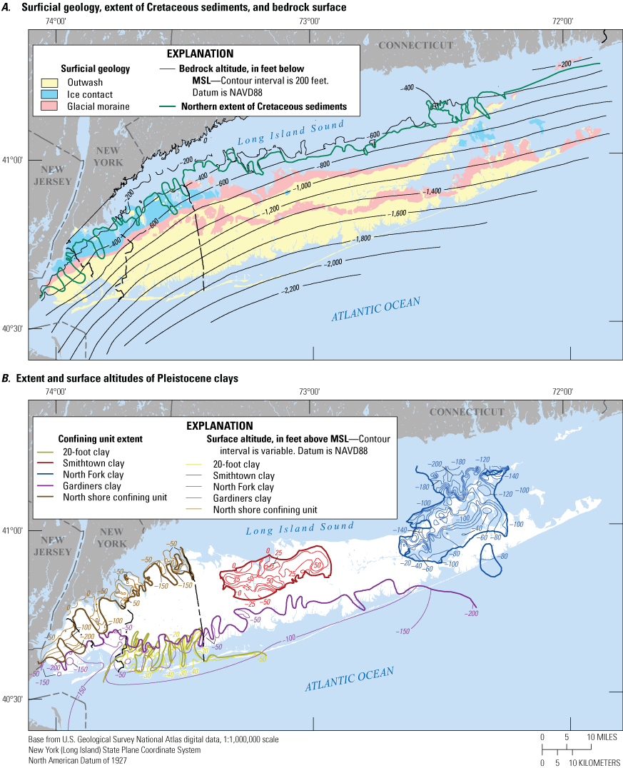
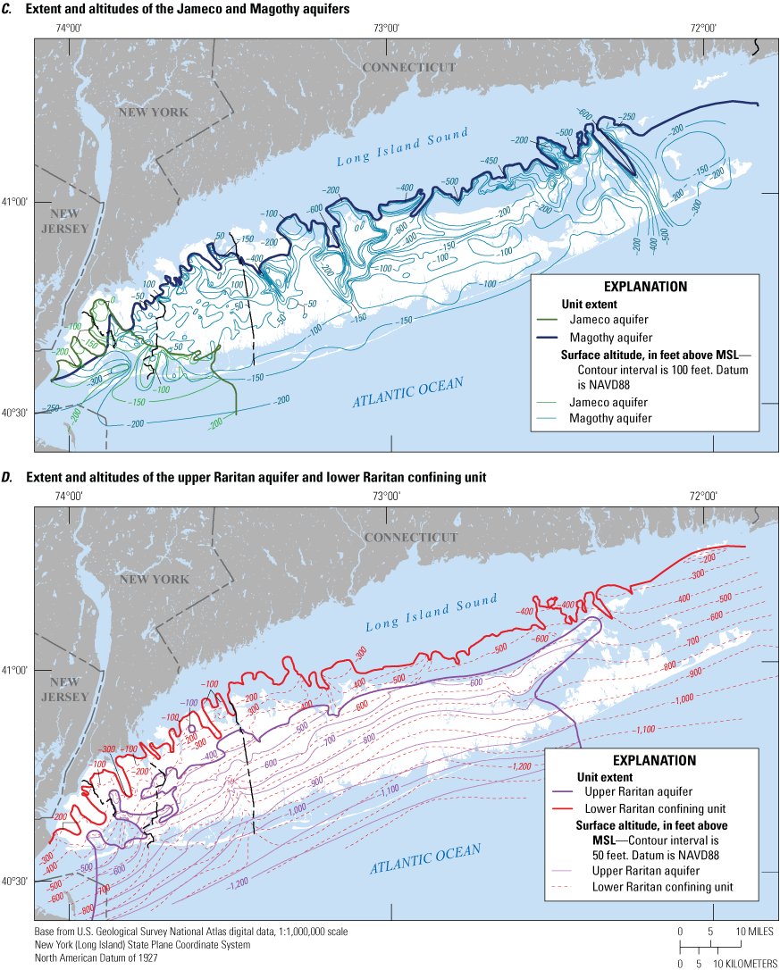
Map showing extents of A, surficial glacial geology and Cretaceous sediments and the extents and surface altitudes of B, glacial and Pleistocene clays, C, the Jameco and Magothy aquifers, D, the upper Raritan aquifer and lower Raritan confining unit, and E, the Lloyd aquifer and North Shore aquifers on Long Island, New York. Surficial geology from Cadwell (1989); bedrock altitudes, confining unit extents, and surface altitudes from Walter and others (2020), DeMott and others (2023), and Stumm and others (2024). NAVD88, North American Vertical Datum of 1988.
Glacial sediments in parts of Kings, Queens, and Nassau Counties are underlain by the North Shore confining unit where Cretaceous deposits are absent, likely removed by interglacial erosion (Stumm and others, 2024). The unit generally occurs beneath peninsulas and estuaries in northern Nassau County but extends inland in large areas of Kings and Queens Counties (fig. 11B). The North Shore confining unit is a complex assemblage of generally silt and clay sediments that was deposited in marine and lacustrine environments during interglacial periods. The unit has a surface altitude generally between sea level and 150 ft below sea level. The North Shore confining unit can be contiguous and in lateral hydraulic connection with adjacent Cretaceous formations.
The North Fork confining unit is an extensive lacustrine or marine fine-grained unit that underlies glacial sediments across most of the North Fork and parts of the South Fork and is as thick as 400 ft in some areas. The surface of the unit generally is between 50 and 150 ft below sea level (fig. 11B; Schubert and others, 2004). The Gardiners clay underlies glacial sediments along the southern shore of western and central Long Island and locally confines the underlying Magothy and Jameco aquifers in some areas. The surface altitude of the clay unit generally ranges from 50 to 100 ft below sea level (fig. 11B).
The upper glacial aquifer and Gardiners clay unit are underlain by Cretaceous sediments across most of Long Island, except where they have been removed by erosion along the northern shore of the island (fig. 11A). Cretaceous formations have surfaces that dip to the southeast and generally are at a maximum depth along the southern shore of central Suffolk County (fig. 11C–E).
The Magothy aquifer is the youngest of the Cretaceous formations on Long Island and is separated from the glacial sediments by an erosional unconformity, with several erosional channels. These sediments consist of sand, silt, and clay that were deposited in deltaic fluvial and marsh environments and generally coarsen with depth. The bottom of the Magothy aquifer generally is characterized by a basal gravel unit (Stumm and others, 2024). The Magothy aquifer has a surface altitude that ranges from 100 ft above sea level in north-central Nassau County to more than 600 ft below sea level in erosional channels in north-central Suffolk County and is about 1,000 ft thick in south central Suffolk County (fig. 11C).
The Magothy aquifer is overlain by the Pleistocene Jameco aquifer in parts of western Long Island where it is in hydraulic connection with the Magothy aquifer (fig. 11C). The Jameco aquifer generally consists of coarse-grained fluvial sand and gravel deposited before Wisconsinan glaciation. The surface altitude of the Jameco aquifer ranges from about sea level to about 150 ft below sea level in southern Queens County, where it is about 100 ft thick.
The Magothy aquifer is underlain by the Raritan confining unit throughout its extent; this unit also was deposited in deltaic environments during the late Cretaceous period. The unit has been mapped as a single unit in previous investigations (Smolensky and others, 1989; Franke and Cohen, 1972), but is mapped as two separate units in the hydrogeologic framework in this report because of recent geologic mapping (Stumm and others, 2024). Analyses of core samples from deep boreholes drilled in central Nassau County as part of remedial investigations indicated zones of laterally contiguous silt and sand sediments between basal gravel deposits at the bottom of the Magothy aquifer and the top of dense gray clay typical of the Raritan confining unit as it has been previously defined (Schubert and others, 2004). Further analyses of lithologic logs showed a similar pattern across much of Long Island, suggesting a separate, more permeable, Raritan unit above a lower, traditional Raritan confining unit. Although this unit has been referred to as the upper Raritan aquifer by Stumm and others (2024), it comprised mostly of silty sediments and is not used for water supply.
The surface of the upper Raritan aquifer is the bottom of the principal aquifer system of Long Island, which includes the upper glacial, Magothy, and Jameco aquifers (fig. 11D). The surface of the upper Raritan aquifer ranges from about 400 ft below sea level near its northern extent to 1,100 ft below sea level beneath Fire Island in south-central Suffolk County. The unit is at its maximum thickness of about 200 ft in that area. The upper Raritan aquifer is underlain throughout its extent by the Raritan confining unit, which consists of dense gray clay deposited in deltaic marsh environments in the late Cretaceous. The unit is more than 300 ft thick along the south-central shore of the island. The Raritan confining unit has estimated vertical hydraulic conductivity values that are several orders of magnitude lower than that of the Magothy and Lloyd aquifers and restricts vertical flow between the two units (Franke and Cohen, 1972).
The Cretaceous-age Lloyd aquifer underlies and is confined throughout its extent by the Raritan confining unit. The sediments generally consist of fine-grained sand with lenses of silt and clay lenses deposited in deltaic depositional environments, and like the Magothy aquifer, contain basal gravel zones. The surface of the Lloyd aquifer dips to the southeast and has an altitude that ranges from about 200 ft below sea level near the northern extent of the unit to about 1,500 ft below sea level beneath Fire Island in south-central Suffolk County (fig. 11E) where the unit is about 500 ft thick. The Lloyd aquifer is laterally contiguous and in hydraulic connection with the North Shore aquifer in discontinuous areas beneath peninsulas and estuaries along the northern shore of Nassau County and in parts of Kings and Queens Counties where it extends inland. The North Shore aquifer is of Pleistocene age and was deposited in fluvial environments before Wisconsinan glaciation and likely comprises the oldest Pleistocene sediments on Long Island. The North Shore aquifer is confined throughout its extent by the overlying North Shore confining unit, which is laterally contiguous with the Raritan confining unit. The surface altitudes of the North Shore aquifer range from about 50 to about 250 ft below sea level. The Lloyd and North Shore aquifers make up the principal confined aquifer system on Long Island and are underlain by impermeable bedrock, which is more than 2,000 ft below sea level beneath Fire Island in south-central Suffolk County (fig. 11A; Stumm and others, 2024).
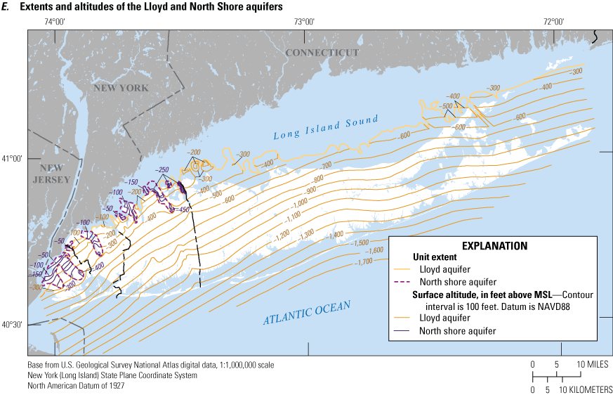
The extents and surface altitudes of these hydrogeologic units were used to develop a three-dimensional hydrogeologic framework of the Long Island aquifer system (table 1). Spatial data of recently mapped extents and surface altitudes on western Long Island (Stumm and others, 2024) were merged with those from previous investigations and used to develop raster images representing each unit. These were combined into a three-dimensional volume representing the aquifer system (fig. 12). A total of 14 hydrogeologic units are represented in the framework (table 1). The impermeable bedrock underlying the Long Island aquifer system has a southeastern dip, and the wedge of unconsolidated sediments that comprise the aquifer system thicken to the south and east (fig. 12). The aquifer system becomes thicker and less structurally complex from west to east (fig. 12 A–D).
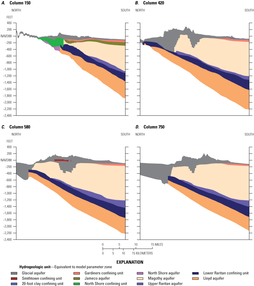
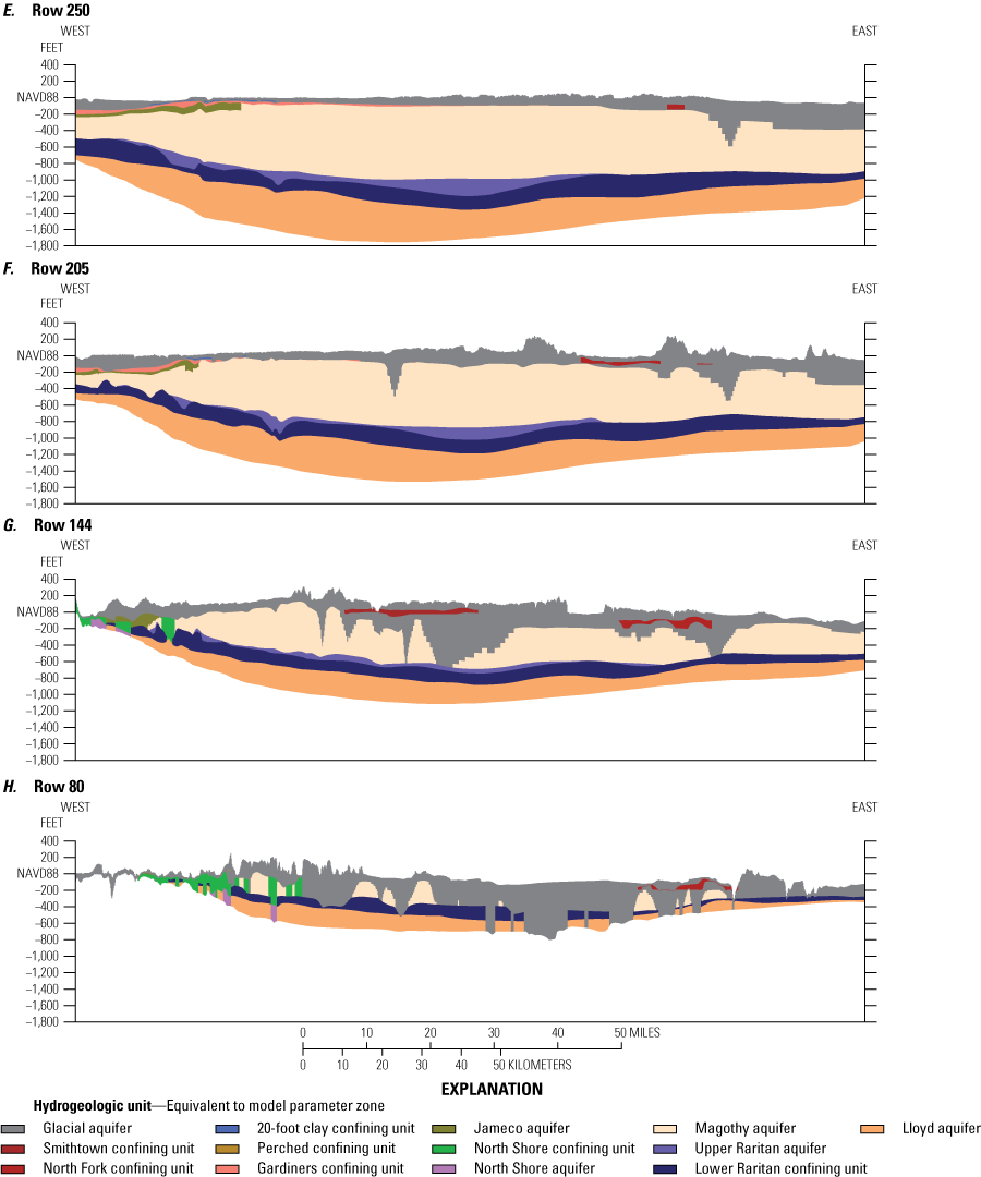
Cross section showing hydrogeologic units along A–D, north-south (down-dip sections) and E–H, east-west sections, Long Island, New York. Locations of columns and rows are shown on figure 10. Data are from Stumm and others (2024).
The aquifer system underlying Kings and Queens Counties is thinner, has more fine-grained sediments, and is generally characterized by more geologic complexity than in Nassau and Suffolk Counties. The hydrogeologic framework in this area includes the major Cretaceous units—the Magothy aquifer, the upper Raritan aquifer, the lower Raritan confining unit, and the Lloyd aquifer—as well as Pleistocene units, including the Gardiners clay and the Jameco aquifer, which are in stratigraphic continuity with Cretaceous sediments. The hydrogeologic framework in Kings and Queens Counties also includes the North Shore confining unit and the underlying North Shore aquifer, which are Pleistocene sediments that are laterally contiguous with the Cretaceous sediments in areas where the Cretaceous sediments have been removed by erosion (fig. 12A). Glacial sediments are thinnest in this area compared with Nassau and Suffolk Counties. The relatively thin aquifer system in Kings and Queens Counties, combined with the predominance of Pleistocene silt and clay sediments in the primary aquifers, results in a low aquifer transmissivity and a large hydrologic-system response to groundwater withdrawals.
The bottom of the aquifer system along the southern shore of the island in central Suffolk County is about 2,000 ft below sea level. The Cretaceous sediments are stratigraphically continuous; the surface of the Magothy aquifer has erosional channels and is absent along the northern shore (fig. 12B–D). Glacial sediments generally are thicker, particularly along the northern shore where the Magothy aquifer is absent and glacial sediments overlie deep Cretaceous sediments or ovelie bedrock where all Cretaceous sediments are absent (fig. 12B–D). Locally significant confining units are contained within the glacial sediments, including the Smithtown clay in north-central Suffolk County and the 20-foot clay along the southern shore of Nassau County (fig. 12B–C).
The aquifer system becomes thinner, and its framework is more complex from south to north (fig. 12E–H). The hydrogeologic framework along the southern shore of mainland Long Island is characterized by thick, stratigraphically continuous Cretaceous formations; the surface of the Cretaceous sediments generally is uneroded (fig. 12E). Cretaceous sediments abut preglacial units—the Jameco aquifer and Gardiners clay—in the western part of the aquifer system (fig. 12E–F). The southern shore of Long Island has extensive outwash plains, and the land surface is generally flat and underlain by glacial outwash sediments. These sediments generally are thin in the southern part of Long Island (fig. 12E–F) and contain the North Fork clay in the eastern part of the island (fig. 12F). Cretaceous sediments in the northern part of Long Island are substantially eroded with the presence of deep erosional channels; the Magothy aquifer is absent in some areas (fig. 12G). Cretaceous sediments are laterally contiguous with the North Shore confining unit and aquifer on western Long Island (fig. 12G). The topography is more variable in areas with glacial moraines and glacial sediments generally are thicker, particularly within erosional channels where glacial sediments have filled the channels. Glacial sediments contain the Smithtown clay in the central part of the island (fig. 12G). Most of the Magothy aquifer has been removed by erosion and occurs as discontinuous remnants along the northern shore of Long Island (fig. 12H). Parts of the deep Cretaceous units—the Lloyd aquifer and Raritan confining unit—also are absent and glacial sediments extend to bedrock. Old Pleistocene sediments—the North Shore confining unit aquifer—are contiguous with Cretaceous sediments in the western part of the aquifer system (fig. 12H).
Aquifer Properties
The hydraulic properties of importance to groundwater flow and transport and the response of the hydrologic system to changes in hydraulic stresses include horizontal and vertical hydraulic conductivity, storage, and porosity. Hydraulic conductivity refers to the ability of aquifer sediments to transmit water and affects the altitude of the water table and the distribution of groundwater flow and discharge. Aquifer storage refers to the capacity of the aquifer matrix to store water and affects the magnitude and timing of the response of the hydrologic system to changing stresses. Porosity refers to the volumetric fraction of open space in the aquifer and affects the rate of movement of water in the aquifer. The assignment of these properties in the regional model was made from previous investigations and from existing and recently collected data on the character of the aquifer sediments. The hydraulic conductivity of the principal aquifers—the upper glacial, Magothy, and Jameco aquifers—was assigned in the regional model from a texture model, which is a continuous, three-dimensional rendering of hydraulic conductivity derived from lithologic and geophysical data from wells and boreholes. Hydraulic conductivity in the remaining hydrogeologic units, where a paucity of data does not allow for development of a texture model, was assigned from previous investigations on Long Island and in similar Pleistocene and Cretaceous aquifers in the northeast and mid-Atlantic regions of the United States.
Previous Investigations
The spatial distribution of field measurements of hydraulic properties is concentrated primarily around major pumping centers and, consequently, is more readily available in areas of large groundwater use and for those aquifer units with the largest groundwater withdrawals (McClymonds and Franke, 1972; Franke and Getzen, 1976; Lindner and Reilly, 1983; Prince and Schneider, 1989; Stumm, 2001; Stumm and others, 2002, 2004; Williams and others, 2020). Estimates of hydraulic properties made in numerical model investigations include Buxton and Smolensky (1999), Kontis (1999), Misut and Monti (1999), Misut and others (2004), Schubert and others (2004), Monti and others (2009), Masterson and others (2016), and Walter and others (2020). Buxton and Smolensky (1999) provided a summary of the previous investigations of the hydraulic properties of the aquifer system. A more recent summary of water-transmitting properties in hydrogeologic units, including newly mapped units in western Long Island, is presented in Stumm and others (2024).
A review of previous investigations suggests that the upper glacial aquifer has a range of horizontal hydraulic conductivity from about 20 to 270 feet per day (ft/d). Hydraulic conductivity in glacial sediments differs for outwash, moraine, and ice-contact deposits. Values for the outwash deposits south of the moraines generally ranged from 130 to 270 ft/d; hydraulic conductivity within the moraine deposits generally was less than 135 ft/d. Stumm and others (2024) reported an average hydraulic conductivity of 200 ft/d for glacial sediments. The average hydraulic conductivity of the upper glacial aquifer was less than 25 ft/d where the Smithtown clay is present. The anisotropy (ratio of horizontal to vertical hydraulic conductivity) of the upper glacial aquifer was estimated to be 10:1; but local values could be as low as 3:1. The horizontal hydraulic conductivity of the Jameco aquifer ranged from 100 to 300 ft/d, and its anisotropy was estimated to be about 10:1; the aquifer generally had the highest hydraulic conductivity of any aquifer on Long Island. The hydraulic conductivity of the Magothy aquifer varied with depth; values for the upper part ranged from 35 to 90 ft/d, whereas values for the coarse basal zone were estimated to be as high as 230 ft/d. Stumm and others (2024) reported an average hydraulic conductivity of 120 ft/d for the Magothy aquifer. The hydraulic conductivity of the Lloyd aquifer ranged from 30 to 80 ft/d and generally was greatest in Nassau County. The anisotropy of the Lloyd aquifer was estimated to be 100:1 because of the highly stratified character of the aquifer. Stumm and others (2024) reported an average hydraulic conductivity value of the Lloyd aquifer of 55 ft/d.
Although data on the hydraulic conductivity of the confining units are scant, the high clay and silt content indicated values several orders of magnitude lower than in the aquifers. Franke and Cohen (1972) estimated the average vertical hydraulic conductivity of the confining units to be 0.001 ft/d; Reilly and others (1983) estimated a value of 0.0029 ft/d for the Gardiners clay. A vertical hydraulic conductivity value of 0.001 ft/d was estimated for the Gardiners clay, the Raritan confining unit, and the North Shore confining unit. A value of 0.01 ft/d was assumed for Pleistocene clay units, including the Smithtown clay, the 20-foot clay, and the North Fork clay units. The hydraulic conductivity of the Potomac confining unit, the Northern Atlantic Coastal Plain aquifer system equivalent of the Raritan confining unit, was estimated to be 0.001 ft/d (Masterson and others, 2016). Stumm and others (2024) reported average horizontal hydraulic conductivity in the Raritan and North Shore confining units of about 0.1 and 0.2 ft/d, respectively, as estimated from nuclear magnetic resonance logging. The hydraulic conductivity of the upper Raritan aquifer, as estimated from nuclear magnetic resonance logs, ranged from about 40 to about 110 ft/d (Stumm and others, 2024).
Previous estimates of specific yield (unconfined storage) for the glacial outwash deposits were 0.18 (Getzen, 1977), 0.22 (Reilly and Buxton, 1985), 0.24 (Warren and others, 1968), 0.24 (Perlmutter and Geraghty, 1963), and 0.30 (Franke and Cohen, 1972). Estimates as low as 0.10 have been proposed for morainal deposits; estimates for unconfined portions of the Magothy aquifer have been as low as 0.10 (Getzen, 1977; Reilly and Buxton, 1985). Specific yields ranged from 0.24 and 0.30 in glacial sediments on Cape Cod, Massachusetts (Walter and Whealan, 2005), and a specific yield of 0.26 was measured in glacial outwash on western Cape Cod (Moench and others, 2001). Stumm and others (2004) measured an average mobile water fraction in the upper glacial aquifer, by use of nuclear magnetic resonance logging, of 0.23. The mobile fraction of water approximates the fraction of drainable water and, therefore, specific yield, and the observed values are consistent with those from previous investigations. Mobile water fractions in the Magothy aquifer, which generally is unconfined, ranged from 0.25 to 0.28 (Stumm and others, 2024).
Specific storage for confined aquifers is a function of aquifer compressibility and is several orders of magnitude lower than unconfined storage. Specific storage generally ranges from 1.0×10⁻⁵ to 1.0×10⁻⁷. Moench and others (2001) estimated confined storage of 1.3×10⁻⁵ in glacial outwash on western Cape Cod. Additional estimates of specific storage applicable to Long Island were 6.0×10⁻⁷ (Getzen, 1977), 1.3×10⁻⁶ (Jacob, 1941), and 8×10⁻⁶ (Walter and others, 1996). Masterson and others (2016) reported specific storge of the equivalents for the Magothy and Lloyd aquifers of about 1.0×10⁻⁶ and a specific storage of 1.3×10⁻⁵ for the equivalent of the Raritan confining unit. Sediment porosity for sandy, unconsolidated sediments typical of aquifers on Long Island ranges from 0.25 to 0.40; porosity in clayey sediments typical of confining units ranges from 0.40 to 0.70 (Freeze and Cherry, 1979, p. 37). Garabedian and others (1988) measured a porosity of 0.39 in glacial outwash sediments on western Cape Cod. Stumm and others (2024) measured a total porosity in the upper glacial aquifer of 0.36, as represented by the combined fractions of mobile, capillary, and clay-bound water determined from nuclear magnetic resonance logging. Total porosity in the Magothy aquifer, as determined from nuclear magnetic resonance logs at four sites, ranged from 0.33 to 0.39. Values measured using nuclear magnetic resonance logging were generally consistent with values from tracer tests and literature values.
Lithologic Texture Model
The water-transmitting properties of the upper glacial, Jameco, and Magothy aquifers were estimated using lithologic and geophysical data from a set of 1,846 boreholes, representing the deepest borehole within each cell of a regular 1-mi2 grid of the Long Island aquifer system (fig. 10). The texture model developed for this investigation is an updated version of an existing texture model developed by Walter and Finkelstein (2020) that includes data from 77 additional boreholes. Standardized lithologic codes from the USGS Ground-Water Site Inventory (GWSI) System (U.S. Geological Survey, 2004) were assigned to each depth interval in each borehole. In total, 37,515 lithologic descriptions were included in the analysis. The descriptions were assigned one of 45 GWSI codes that were subsequently aggregated into 14 sediment codes with 7 codes for sediments of the upper glacial aquifer sediments and 7 codes for the sediments of the Magothy and Jameco aquifers and Monmouth greensand unit (Walter and Finkelstein, 2020). Each code was assigned a corresponding horizontal hydraulic conductivity derived from published field tests in the Long Island aquifer system (McClymonds and Franke, 1972; Franke and Getzen, 1976; Lindner and Reilly, 1983; Smolensky and others, 1989) and similar hydrogeologic environments on the coastal plain of Massachusetts (Guswa and Londquist, 1976; Guswa and LeBlanc, 1985; LeBlanc and others, 1986; Barlow, 1989; Barlow and Hess, 1993; Moench and others, 1996; Walter and others, 1996; Masterson and Barlow, 1997; Masterson and others, 1998).
The compiled data were used to create a quasi-three-dimensional texture model of the upper glacial, Magothy, and Jameco aquifers—the principal aquifers of the Long Island aquifer system—using the workflow presented in Walter and Finkelstein (2020). The texture model is considered quasi-three-dimensional because values are specified in full three-dimensional space, but hydraulic conductivities are only correlated horizontally within each layer and not to layers above or below. The remaining hydrogeologic units were excluded from the texture model owing to a paucity of data for those units. The hydraulic conductivity values assigned to each depth interval were used to estimate thickness-weighted mean hydraulic conductivity values in regular 10-ft intervals over the depth of each borehole; horizontal hydraulic conductivity values were computed using arithmetic means. These were combined to develop a database of X, Y, and Z coordinates and associated estimates of horizontal hydraulic conductivity; this database was sequentially queried to extract the X and Y coordinates of boreholes that extend to or beyond each layer in the texture model, and these point values then were used to develop an interpolated field of horizontal hydraulic conductivity for each altitude range by use of ordinary, spherical kriging (Oliver and Webster, 1990).
This process resulted in a two-dimensional raster of horizontal hydraulic conductivity for each 10-ft interval for the vertical thickness of each aquifer. These individual data rasters, when combined, created a quasi-three-dimensional array of values. Two sets of quasi-three-dimensional models were produced: a set of grids each with a thickness of 10 ft and uniform altitude between land surface and the top of the Magothy aquifer (representing the upper glacial aquifer) and a set of grids between the top of the Magothy aquifer and the top of the underlying Raritan confining unit (representing the Magothy and Jameco aquifers). Each of the grids representing the Magothy aquifer has a thickness of 10 ft and a variable altitude based on the altitude of the underlying surface of the Raritan confining unit such that each grid is a given multiple of 10 ft added to that surface (Walter and Finkelstein, 2020). These two models, when combined, fully define the distribution of estimated hydraulic conductivity for the upper glacial, Magothy, and Jameco aquifers.
The spatial distribution of hydraulic conductivity, as represented in the texture model, generally is consistent with the regional geology of the aquifer system. Glacial sediments show a distribution of estimated hydraulic conductivity that is consistent with their depositional history and mapped surficial geology. Estimated hydraulic conductivity generally is highest in the shallow parts of the upper glacial aquifer, in association with coarse-grained outwash (figs. 13A and 14). Estimated hydraulic conductivity of glacial sediments at an altitude of 5 ft below mean sea level generally is lower in inland areas of eastern Nassau and western Suffolk County where these sediments underlie hummocky terrain, suggesting an association with glacial moraines; this association also is consistent with the mapped surficial geology (Cadwell and Muller, 1986; Cadwell, 1989). Areas of low estimated hydraulic conductivity in the north-central part of Long Island also may represent glaciolacustrine sediments, which were deposited in proglacial lakes between moraines.
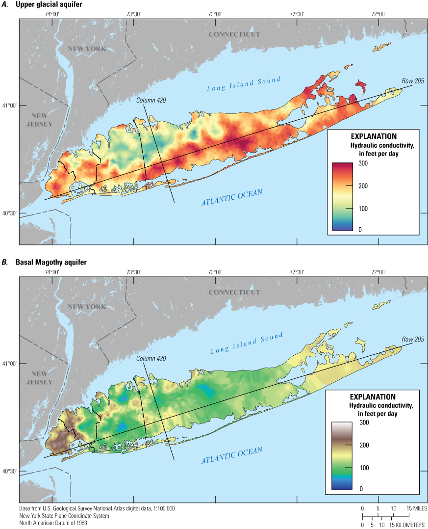
Maps showing the distribution of estimated horizontal hydraulic conductivity at A, 0 feet (mean sea level altitude in the upper glacial aquifer and B, the basal part of the Magothy aquifer on Long Island, New York. Cross sections are shown on figure 14.
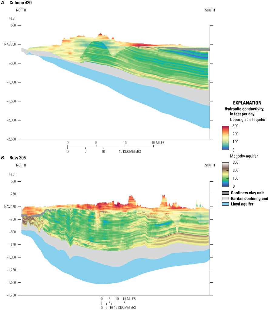
Cross sections showing vertical distribution of horizontal hydraulic conductivity along A, north-south (down-dip) section (column 420 of the model) and B, east-west section (row 205 of the model) for Long Island, New York. Locations of cross sections (rows and columns) are shown on figure 13. NAVD88, North American Vertical Datum of 1988.
Extensive fine-grained sediments, likely glaciolacustrine in origin, have been mapped in north-central and northeastern Suffolk County (Krulikas and Koszalka, 1982; Schubert and others, 2004). Estimated hydraulic conductivity to the south, within outwash sediments, generally is substantially higher than those of inland areas (fig. 13A). Estimated hydraulic conductivity in glaciolacustrine sediments generally is lower than in outwash sediments owing to a finer grain size. The vertical distribution of horizontal hydraulic conductivity also generally reflects geologic trends in and the depositional history of the glacial aquifer sediments (fig. 14). Glacial sediments generally become finer with depth, with lower values of hydraulic conductivity in interior parts of the island, and hydraulic conductivity generally is higher in the shallow parts of the glacial aquifer in association with coarse-grained outwash sediment.
The Cretaceous sediments are deltaic in origin and were deposited in a variety of depositional environments. Hydraulic conductivity values in the Magothy aquifer generally show a large degree of spatial heterogeneity (fig. 13B). Deposition of coarse-grained sediments occurred in fluvial environments within stream channels, and fine-grained sediments generally were deposited in overbank-marsh environments. These depositional environments and gradations between them resulted in repetitive sequences of coarse- to fine-grained sediments.
The Magothy aquifer also shows both horizontal and vertical distributions of estimated hydraulic conductivity that is consistent with its depositional history (figs. 13B and 14B). The Magothy sediments were deposited in sedimentary environments dominated by streams and coalescing deltas (Smolensky and others, 1989). Hydraulic conductivity values generally are highest in the basal part of the Magothy aquifer where the presence of coarse-grained sediments indicated deposition in high-energy fluvial environments, such as stream channels. Hydraulic conductivity generally is lower in the middle part of the aquifer where the presence of fine-grained sediments suggests deposition in low-energy environments, such as overbank marsh deposits.
Estimates of hydraulic conductivity of aquifer sediments, both from previous investigations and the lithologic texture model in combination with the hydrogeologic framework were used to assign horizontal hydraulic conductivity to each cell in the numerical model. Vertical hydraulic conductivity was calculated by explicitly coupling the value to horizontal hydraulic conductivity by use of estimated anisotropy ratios (horizontal to vertical hydraulic conductivity) from previous studies. Anisotropy ratios in the unconsolidated sediments are a function of grain size, heterogeneity, and sorting, and ratios range from 3:1 in coarse sand and gravel to 100:1 in clays. The ranges of horizontal hydraulic conductivity and the corresponding assumed anisotropy are as follows:
-
• Greater than 300 ft/d: 3:1
-
• 200 to less than (<) 300 ft/d: 4:1
-
• 125 to <200 ft/d: 5:1
-
• 70 to <125 ft/d: 10:1
-
• 30 to <70 ft/d: 10:1
-
• 10 to <30 ft/d: 30:1
-
• 1 to <10 ft/d: 10:1
-
• 0.01 to <1 ft/d: 50:1, and
-
• <0.01 ft/d: 100:1.
Table 2.
Aquifer properties for initial, prior, and conditioned models for Long Island, New York.[E−x, ×10−x]
Natural and Anthropogenic Recharge
Long Island has a temperate climate that is moderated by its proximity to ocean waters and typified by warm, humid summers and cool winters. Precipitation is the sole natural source of water to the Long Island aquifer system, with about half of it reaching the water table as aquifer recharge, and the remainder lost to evapotranspiration and surface runoff. Aquifer recharge is a function of climatological conditions (precipitation and temperature) and landscape characteristics (vegetation, soil properties, and land use); variations in these factors affect the rates and distribution of recharge. Total recharge to the aquifer system includes natural recharge from precipitation and from anthropogenic sources, such as wastewater return flow and leakage from water infrastructure.
Finkelstein and others (2022) used a soil-water balance (SWB) model code to estimate spatially variable, natural recharge for Long Island from 1900 to 2019. The SWB model developed by Westenbroek and others (2010) is based on a modified version of the Thornthwaite-Mather analytical method (Thornthwaite and Mather, 1957) that incorporates land slope, soil properties, land use, and daily climate data to account for processes that occur as water moves through unsaturated soils and sediments to the water table.
Precipitation on Long Island from 1900 to 2019 ranged from 28.3 in/yr in 1965, during a period of extreme drought, to 65.2 in/yr in 1983 and averaged about 47 in/yr. Recharge is correlated with precipitation and has a similar temporal pattern (fig. 15A). The estimated fraction of precipitation that recharges the aquifer at the water table was between about 25 and 57 percent and averaged about 42 percent from 1900 to 2019 (fig. 15B).
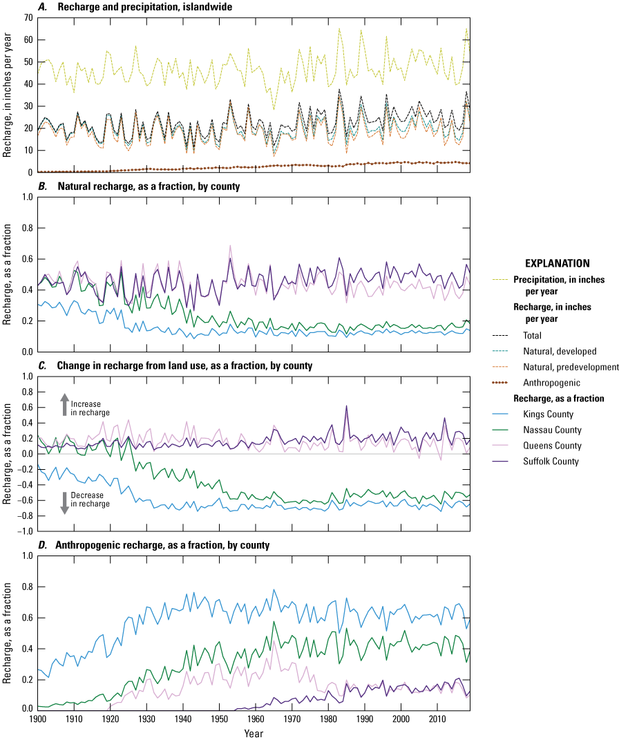
Graphs showing A, islandwide estimated total precipitation and rates of recharge by component, B, estimated fraction of natural recharge by county, C, estimated fraction of rejected recharge by county, and D, estimated fraction of anthropogenic recharge by county on Long Island, New York.
Estimated recharge from precipitation ranged from about 8.9 to about 34.7 in/yr and averaged about 19.8 in/yr during that period. The fraction of precipitation recharging the aquifer between 1900 and 2019 generally was lowest in Kings County where the average was about 16 percent, and highest in Suffolk County where the average was about 46 percent (fig. 15B). The fraction of precipitation recharging the aquifer decreased in the early 20th century in New York City (Kings and Queens Counties) due to urbanization and the expansion of impervious surfaces, and currently [2023] is 14 and 18 percent, respectively (fig. 15B). Kings and Queens Counties are the most urbanized and densely populated part of Long Island; impervious surfaces can intercept precipitation, resulting in more surface runoff and evaporation and less recharge at the water table (fig. 15C). The fraction of precipitation recharging the aquifer was similar in Nassau and Suffolk Counties until the mid-1980s when the fraction generally varied between 30 and 60 percent and averaged 44 percent in both areas (fig. 15B). The fraction of precipitation recharging the aquifer was higher in Suffolk County after the mid-1980s when the average fraction in Nassau and Suffolk Counties was about 41 and 49 percent, respectively. Suffolk County generally is characterized by large areas of low-density residential land use (fig. 5B), which can result in higher recharge rates (fig. 15B).
Recharge from precipitation varies spatially as a function of the distribution of precipitation and natural and human-influenced land characteristics. Recharge in 2019, when precipitation islandwide was about 54 in/yr, generally was less than 10 in/yr in parts of New York City and more than 30 in/yr in parts of north-central Suffolk County and on the South Fork (fig. 16A). Undeveloped land had recharge rates of about 25 in/yr. Recharge generally is lower in urbanized areas with impervious surfaces than in undeveloped areas and higher than undeveloped areas in areas with low-density residential development (Yang and others, 2015). Recharge to the aquifer in Kings and Queens Counties averaged 7.4 and 11.2 in/yr, respectively, during the period from 1900 to 2019. The recharge rates in Nassau and Suffolk County were substantially higher than in New York City and averaged 20.4 and 21.6 in/yr, respectively, during the same period (Finkelstein and others, 2022).
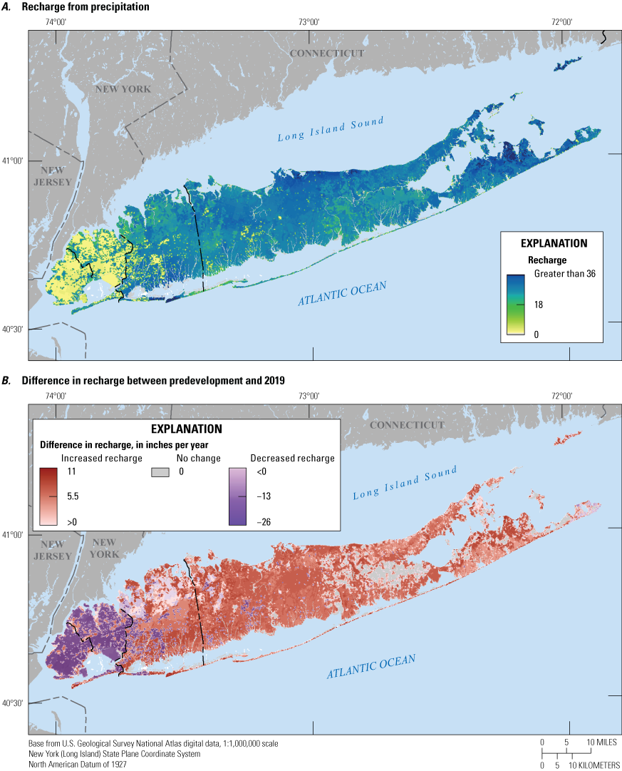
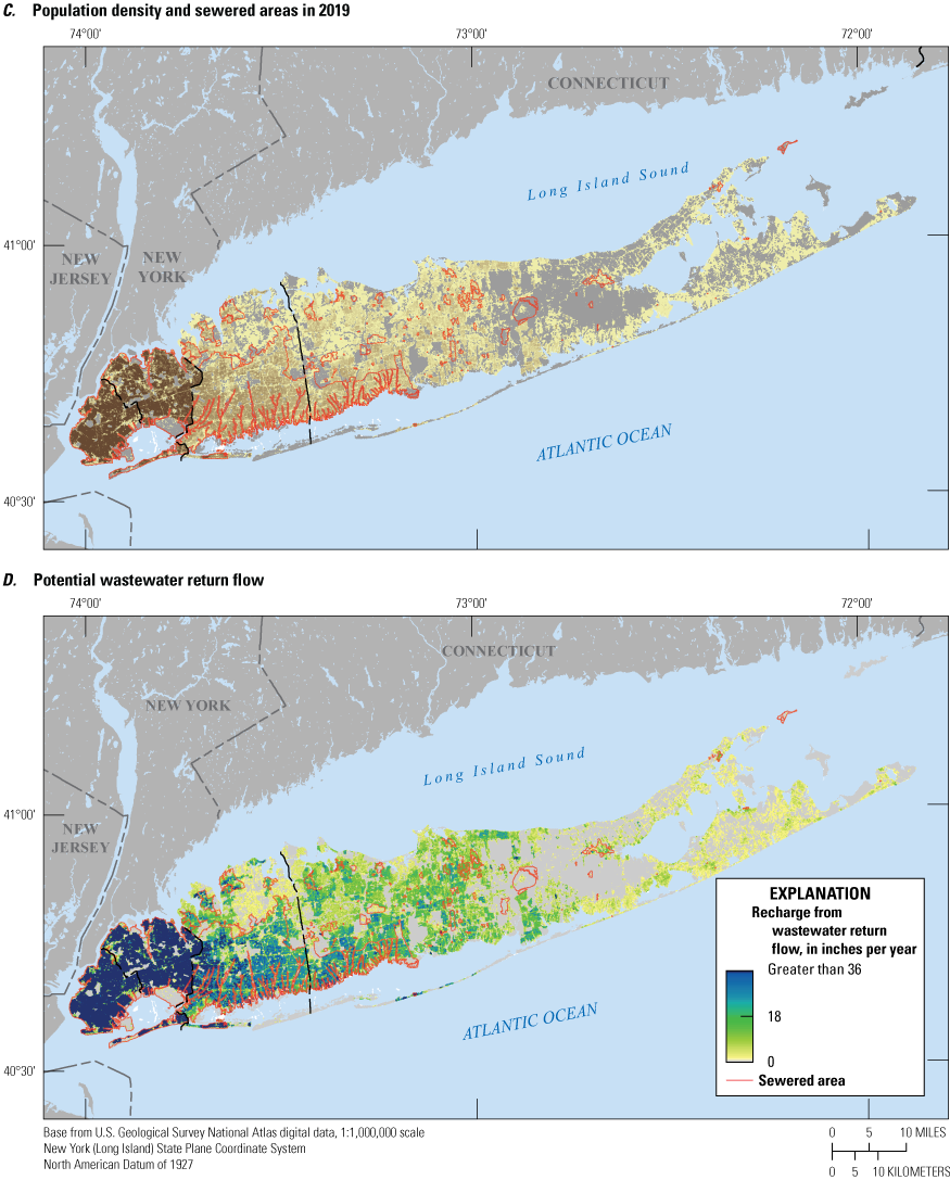
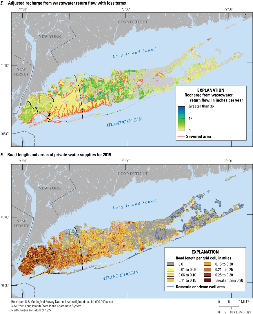
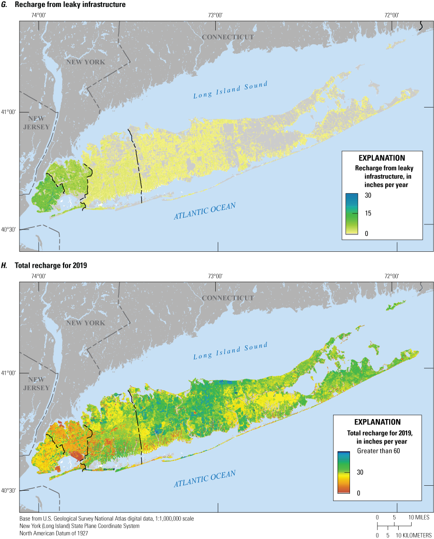
Maps showing A, recharge from precipitation, B, difference between predevelopment and developed recharge C, population density and sewered areas in 2019, D, recharge from wastewater return flow, E, adjusted recharge from wastewater return flow with loss terms, F, road length and areas of private water supplies for 2019, G, recharge from leaky infrastructure, and H, total recharge for 2019 on Long Island, New York. Data are from Finkelstein and others (2022) and Walter and others (2020).
The effects of human-influenced landscapes on recharge were determined by use of a modified SWB model (Finkelstein and others, 2022); the same climate and natural landscape data were used in combination with open forested (predevelopment) landscape characteristics, and the difference represents the effects of human landscapes on aquifer recharge. Predevelopment recharge rates between 1900 and 2019 were similar to estimated recharge at an islandwide scale, ranging from about 7.3 in/yr to about 34.5 in/yr and averaging about 18.5 in/yr (fig. 15A). However, the assumption of natural landscape characteristics resulted in a more uniform distribution of recharge that would generally be a function of spatially variable precipitation and temperature. The average recharge rates in all four counties were between 17.8 and 18.8 in/yr from 1900 to 2019 (Finkelstein and others, 2022). The difference in recharge between predevelopment and that estimated using developed landscape characteristics ranged from about −25 in/yr, indicating a deficit of recharge, to about 10.9 in/yr, indicating enhanced recharge resulting from development (fig. 16B). Recharge rates in Suffolk County generally were enhanced because of development, which is characterized by low-density residential development in central and eastern Long Island (fig. 5B). Recharge rates in natural, forested landscapes are unchanged (fig. 16B). Areas with a deficit of recharge from development generally are in Kings and Queens Counties and parts of Nassau County.
The largest recharge deficits from impervious surfaces are in the urbanized areas of New York City and southern Nassau County; however, much of the recharge potentially lost to impervious surfaces in Nassau County can recharge the aquifer through sumps, storm drains, and a network of more than 600 recharge basins. The deficit of recharge from impervious surfaces in urbanized areas was considered to be a potential source of recharge to the aquifer through stormwater infrastructure, although the details on the recharge mechanisms are unavailable. This potential component of recharge is referred to as rejected recharge (fig. 15C). The amount of potential rejected recharge from redirected impervious runoff ranged from 0 to about 25 in/yr in parts of New York City (fig. 16B) and could be a significant portion of recharge in urbanized areas. Recharge generally increased by between 10 and 30 percent as a result of changes in undeveloped land use in Nassau and Suffolk Counties, likely as a result of conversion of undeveloped land to low-density residential development (fig. 15C). Conversely, the fraction of recharge potentially lost to impervious surfaces in Kings and Queens Counties increased steadily between 1900 and about 1960 and was about 60 and 50 percent, respectively, in 2019. This water represents an additional source of potential recharge through stormwater infrastructure.
Long Island is a densely populated region with natural recharge enhanced by recharge from human sources. This enhanced recharge is referred to as anthropogenic recharge and includes recharge from wastewater return flow and from leaky infrastructure. These additional components vary spatially as a function of the type and age of water infrastructure and population density during time. Water that recharges the aquifer after human use is referred to as wastewater return flow and depends on population density and the location of sanitary sewers (fig. 16D).
Wastewater return flow from about 84 percent of Long Island’s population is discharged in areas served by sanitary sewers, which include all of New York City and most (about 90 percent) of Nassau County. About 23 percent of the population of Suffolk County is served by sanitary sewers, mainly in the southwestern part of the county (fig. 16D). Wastewater return flow in areas served by sewers is treated and generally discharged into surface waters, effectively removing it from the hydrologic system. However, a small fraction of this return flow likely recharges the aquifer in areas with aging infrastructure.
Wastewater return flow in unsewered areas, primarily in Suffolk County, is discharged into onsite septic systems and recharges the aquifer at the water table. The total amount of return flow available for recharge of the aquifer was estimated from spatially variable population density and an assumed per capita water use. Potential recharge from wastewater return flow was calculated from the number of people in each cell in a regular grid coincident with the numerical model and a per capita water use of 70 gallons per day (Walter and others, 2020).
The potential wastewater return flow was calculated for each year from 1900 to 2019 from U.S. Census Bureau data spatially distributed across the island by census block and building footprint data (U.S. Census Bureau, 2021b). The result is a gridded dataset of recharge values of the total potential recharge from wastewater across the entirety of Long Island that reflects population density (fig. 16D). Potential wastewater return flow needed to be adjusted by assumed loss terms to better estimate recharge likely at the water table. It was assumed that there was a consumptive loss of 10 percent before the discharge of wastewater (Shaffer and Runkle, 2007). It also was assumed that 5 percent of wastewater discharged into sewers, such as New York City, most of Nassau County, and southwestern Suffolk County (fig. 16C), leaked into the aquifer through aging or compromised infrastructure and that 90 percent of discharged wastewater in unsewered areas recharged the water table. The resulting distribution of recharge from wastewater return flow reflects both population density and wastewater infrastructure (fig. 16E). Wastewater return flow in populated areas was lowest in sewered areas of Nassau County where return flow generally was less than 2 in/yr but was slightly higher in sewered areas in New York City because of a higher population density and water use. Recharge from wastewater exceeded 20 in/yr in parts of Suffolk County in areas with low and medium density residential development not served by sanitary sewers.
Almost all (more than 99 percent) of the population of Long Island was served by public water supply; private water supplies were limited to small areas of eastern Suffolk County, the South Fork, and the northern shore of Nassau County (fig. 16F). Water from leaky water-supply infrastructure was an additional source of potential recharge to the aquifer system. Recharge from leaky infrastructure is a function of the spatial distribution of water-supply infrastructure and the amount of water pumped and distributed within each county and varies in space and time. The distribution of public-supply lines was estimated from the length of roads in populated areas, expressed as the fraction of road length in each cell to the total length of roads in the county containing the cell and the assumption that water lines and road length are correlated in developed areas. Road length density was largest in Kings and Queens County where population density was largest (fig. 16C). Areas with large road length density were also in densely populated areas in southern and central parts of Nassau County and in western and central parts of Suffolk County (fig. 16F).
The amount of potential recharge from leaky infrastructure in each cell was calculated by apportioning the total amount of pumping in the county containing the cell by the estimated fraction of road length. The potential recharge from leaky infrastructure was calculated for each year from 1900 to 2019. Pumping data from Nassau and Suffolk Counties was obtained from the NYSDEC (New York Department of Environmental Conservation, 2024), augmented with additional sources discussed in the “Water Use” section of this report.
Kings and Queens Counties imported water from reservoirs in upstate New York. Water use rates to calculate recharge from leaky infrastructure in New York City were estimated from population density; a per capita water use of 70 gallons per day per person was used because data on the amount of water imported into the two counties were insufficient or unavailable. The potential recharge rate was adjusted assuming a loss of 10 percent from water supply infrastructure. Potential recharge from leaky infrastructure generally reflected patterns of population and development and was largest in New York City (fig. 16G). About 700 Mgal/d of water was imported from a reservoir system in upstate New York and, assuming a 10 percent loss of water from the water distribution system, may result in about 70 Mgal/d of additional recharge to the water table in Kings and Queens Counties (Misut and Monti, 1999). The potential for recharge from leaky infrastructure in 2019 exceeded 10 in/yr in large parts of Kings County, which was the most urbanized and densely populated part of Long Island (fig. 16G). Potential recharge from leaky infrastructure exceeded 5 in/yr in most parts of Queens County and 3 in/yr in populated areas in parts of Nassau and Suffolk Counties.
Total recharge to the aquifer system is the sum of natural recharge and the two components of anthropogenic recharge. The fraction of anthropogenic recharge large in Kings and Queens Counties was large, and it increased steadily between 1900 and 1940. The fraction of total recharge derived from anthropogenic recharge was highest in Kings County where it averaged about 58 percent from 1900 to 2019 (fig. 15D). Anthropogenic recharge in Queens and Nassau Counties was, on average, about 30.9 and 14.2 percent of total recharge, respectively, during the same period. The fraction of total recharge from anthropogenic sources is lowest in Suffolk County, where it averaged 5.7 percent. The map of total recharge for 2019 (fig. 16H) reflects the combined spatial variability of the three components of recharge.
The lowest total recharge in 2019, about 15.5 in/yr, was in Queens County (fig. 16G) where natural recharge generally was low in urbanized areas (fig. 16A). Kings County had a low natural recharge rate (fig. 16A) but a high recharge rate from leaky infrastructure, resulting in a high total recharge rate (about 17.1 in/yr; fig. 16G). Total recharge rates were similar in Nassau County (23.8 in/yr) and Suffolk County (23.2 in/yr; fig. 16H). Natural recharge rates also were similar in the two counties. Recharge from leaky infrastructure was larger in developed areas of Nassau County, whereas recharge from wastewater return flow was larger in Suffolk County, resulting in similar total recharge rates. The highest total recharge rates generally were in central Suffolk County in unsewered areas with low to medium density residential development (fig. 16H). Total recharge from natural and anthropogenic sources was augmented in urbanized impervious areas by potential recharge from runoff through stormwater infrastructure, primarily in New York City (fig. 16B). Total recharge to the aquifer, therefore, was the sum of natural recharge from precipitation, recharge from wastewater return flow and leaky infrastructure, and recharge from stormwater runoff. Loss terms for potential anthropogenic recharge components—wastewater return flow, leaky infrastructure, and rejected recharge—were adjusted during model calibration to better match observed hydrologic conditions.
Water Use
Groundwater was the sole source of drinking water for Nassau and Suffolk Counties in 2019 and was an important source of drinking water for Kings and Queens Counties before the mid-1990s (Buxton and Shernoff, 1999). Data on the amount and location of groundwater withdrawals from 1900 to 2019 were compiled from several sources to develop a detailed, continuous record of the location, depth, volumetric rate, and purpose of groundwater withdrawals from the Long Island aquifer system. Thompson and Leggette (1936) compiled water use data for Kings and Queens Counties for the early part of the 20th century. Johnson and Waterman (1952) updated and extended public-supply water use in New York City from 1906 to 1952. Kilburn (1981) reported water-use data for Nassau County from 1920 to 1977. Chu and others (1997) compiled groundwater-withdrawal data from western Long Island from 1921 to 1995. Public-supply pumping data were compiled and augmented with industrial and commercial pumping data from 1906 to 2015 for New York City (Matthew Gamache, CDM Smith, written commun., 2017). Pumping data from Nassau County from 1980 to 2014 were compiled by the Nassau County Department of Public Works (NCDPW; Mike Flaherty, NCDPW, written commun., 2018). The Suffolk County Water Authority (SCWA) compiled monthly pumping data in Suffolk County from 1988 to 2015. (Daniel DeSalvo, Suffolk County Water Authority, written communication, February 24, 2011).
Groundwater-withdrawal data also were compiled from water purveyors, as scanned data, from 1920 to 2019. Data on public-supply, commercial, industrial, golf course, and agricultural pumping, including withdrawals and completion reports, were compiled by the NYSDEC from 1985 to 2015 (Jennifer Pilewski, NYSDEC, written communs., February 2017 to June 2022). NYSDEC data are available through the DEC Info Locator interactive map (New York State Department of Environmental Conservation, 2024). Well-construction data, including location, screen depth, and age were compiled from published sources; these data were augmented with data from other sources, including the USGS National Water Information System (NWIS) database (U.S. Geological Survey, 2020b). Georeferenced well locations were adjusted as needed using aerial photographs, and well-screen depths were estimated from well depth when that information was unavailable. These data on pumping rates and screen locations within the aquifer system were used to develop 86,939 average annual pumping records for a total of 2,942 wells from 1900 to 2019 (fig. 17). Gaps in data and possible missing pumping records from sequential years in some wells, particularly in the early part of the 20th century, were filled by linear interpolation between the previous and subsequent annual pumping estimates.
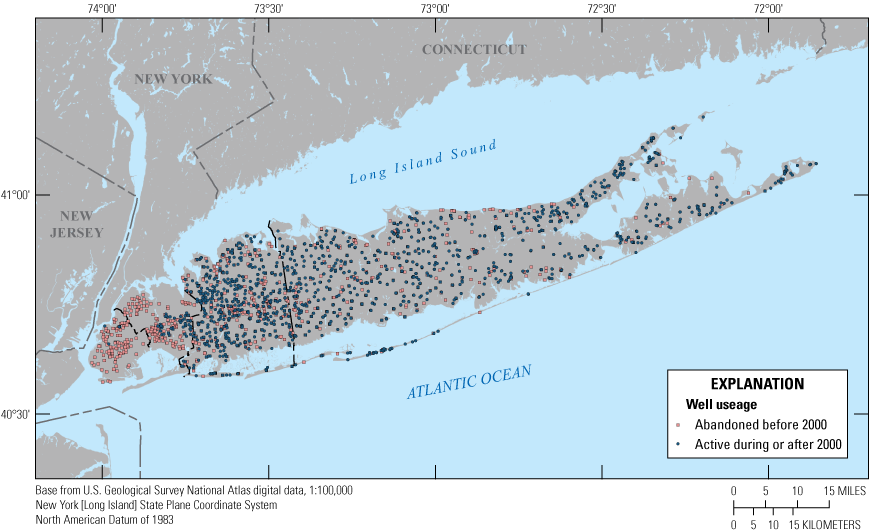
Map showing locations of groundwater wells from 1900 to 2019 on Long Island, New York, including wells that ceased operation before 2000. Data are from U.S. Geological Survey (2020b) and New York State Department of Environmental Conservation (2024).
Groundwater has been withdrawn from wells, at different times, throughout Long Island since about 1906; the period of operation and amount withdrawn has varied historically among wells as a function of local water-supply demand, water quality, and the importation of water from surface supplies in upstate New York. A total of 1,900 wells have been in operation at different times since 2000, and another 1,034 wells were abandoned before 2000 (fig. 17). Wells abandoned before 2000 primarily were in New York City and coastal parts of Nassau County and were abandoned as the result of saltwater intrusion into the freshwater aquifer system. Wells abandoned in the interior parts of Nassau and Suffolk Counties generally were abandoned as a result of contamination of the upper glacial and shallow parts of the Magothy aquifers from human activities.
Public-supply pumping in Kings County ceased in 1947 because of saltwater intrusion near major pumping centers but continued in Queens County until saltwater intrusion caused a cessation of public-supply withdrawals in the mid-1980s (fig. 18A). Groundwater withdrawals in Nassau County increased substantially after the mid-1940s because of rapid suburbanization and became generally constant after about 1980. Pumping for public supply in Suffolk County increased rapidly after the late 1960s because of suburbanization and the conversion of domestic water supplies to public service areas. Pumping in Suffolk County generally became more constant by the late 1990s. The largest amount of groundwater withdrawn from the Long Island aquifer system was in 1999 when about 475 Mgal/d of water was withdrawn from 1,184 wells in Nassau and Suffolk Counties (fig. 18A). In 2019, about 390 Mgal/d of groundwater was withdrawn from 1,115 wells.
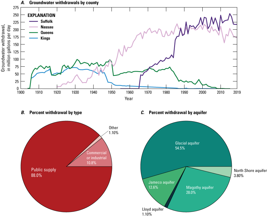
Graphs showing A, annual groundwater withdrawal rate, by county, from 1900 to 2019 and pie charts of groundwater withdrawals by B, type and C, aquifer from 1900 to 2019 on Long Island, New York. Data are from U.S. Geological Survey (2020b) and New York State Department of Environmental Conservation (2024).
Most groundwater withdrawn from Long Island aquifers before the early 1920s was for industrial or commercial uses in New York City; public supply was the largest use for groundwater after that period. About 88.0 percent of groundwater withdrawn from the aquifer system was used for public supply since pumping began in about 1904 (fig. 18B). About 10.8 percent of groundwater withdrawn was for commercial and industrial uses, with the remainder (about 1 percent) for other uses, such as agriculture or remedial systems. Pumping from private wells in 2019 accounted for less than 1 percent and was limited to rural parts of eastern Suffolk County (fig. 16F). The upper glacial aquifer was the surficial unconfined aquifer across Long Island and was the source of most (54.5 percent) groundwater withdrawn from the aquifer system since pumping began near the start of the 20th century (fig. 18C). About 28.0 percent was withdrawn from the underlying Magothy aquifer, and about 12.6 percent was withdrawn from the contiguous Jameco aquifer. The Lloyd aquifer, which is the deepest aquifer and is confined throughout its extent, supplied about 1.1 percent of the total groundwater withdrawn from the aquifer system. The North Shore aquifer, which is a confined aquifer contiguous with the Lloyd aquifer and is an important local aquifer along the northern shore for New York City and Nassau County, supplied about 3.8 percent of the total.
Hydrologic Conditions
Data on current and historical hydrologic conditions were compiled and processed for use in model calibration (history matching) and verification of simulation results, including water levels in wells, flow in streams, and chloride concentrations in groundwater. Groundwater levels and streamflows have been measured throughout Long Island since the early 1900s (U.S. Geological Survey, 2004). A total of 253,033 water-level measurements from 1,870 wells (fig. 19) were obtained from the NWIS database (U.S. Geological Survey, 2020b); the earliest measurements were made in 1907 in 14 wells in Nassau and Suffolk Counties. More extensive measurement of water levels began in the early 1930s and increased steadily until about 1950, when water levels were measured in 375 wells (fig. 20A). Measurement of water levels increased steadily after a drought in the mid-1960s and peaked in 1983 when 4,489 measurements were made in 785 wells (fig. 20).
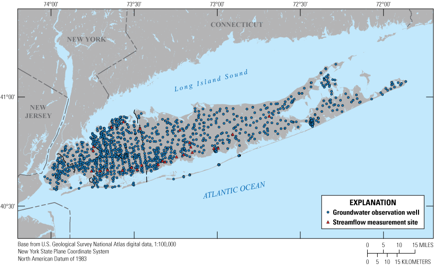
Map showing locations of groundwater observation wells and streamflow measurement sites, Long Island, New York. Data are from U.S. Geological Survey (2020b).
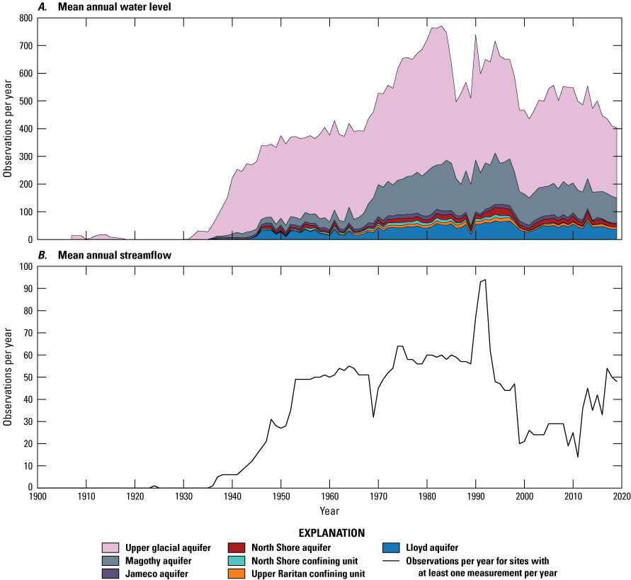
Graphs showing stacked time series of A, the number of mean annual water-level observations by aquifer for sites with at least one measurement per year and B, the number of mean annual streamflow observations for sites with at least one measurement per year, Long Island, New York. Data are from U.S. Geological Survey (2020b).
Data collection frequency and duration differed among the sites, with differing periods of record and total numbers of individual observations. These data were examined to identify observation wells with enough information to suitably represent average annual hydrologic conditions from 1900 to 2019, the period needed for calibration of the transient model to hydrologic conditions at an annual time scale. It was determined that inclusion of a mean water level in a well as an observation in the model calibration required a minimum of 12 measurements in a given year and a minimum of 5 consecutive years meeting that minimum threshold.
Streamflows have been measured in Long Island streams since the early 1900s. A total of 497,999 values of daily mean streamflow from 111 streamgaging sites were obtained from the NWIS database (U.S. Geological Survey, 2020b). The first streamflow measurement was in 1924. More extensive measurement of streamflows began in the late 1930s; daily mean streamflows were computed at more than 50 streamgage sites by the late 1950s. The number of daily mean values peaked in 1992 at 6,798 across 94 streamgage sites (fig. 20B). The number of daily values and the periods of record vary by streamgage site, and the data were examined to determine the suitability of data from each site for inclusion in the calibration of the average annual transient model. A threshold of a minimum of 100 measurements each year at a given site was used to identify those suitable for model calibration. The number of streamgages satisfying this criterion in a given year increased from 5 in the late 1930s to 20 in the early 1990s.
Measured and estimated chloride concentrations were compiled from several sources; a total of 43,205 chloride concentrations were compiled from 4,099 sites for model verification. Chloride concentrations in groundwater on Long Island have been measured since 1903. A total of 38,380 concentration measurements from 3,747 sites compiled from the NWIS database were augmented with 4,467 measured concentrations at 443 sites from historical sources. A total of 222 estimates of chloride concentrations using borehole geophysical techniques (electromagnetic logging) were compiled from 31 sites and from 6 sites using surface geophysical techniques (time-domain electromagnetic measurements; Stumm and others, 2021). These data were used to map chloride as isochlors aggregated by the upper glacial, Magothy, and Jameco aquifers above the Raritan clay and in the Lloyd and North Shore aquifers below the Raritan clay (Stumm and others, 2024). These mapped isochlors were used in a qualitative comparison with model-simulated chloride concentrations to verify that the numerical model reasonably represents saltwater intrusion in the aquifer system as currently understood and matches known chloride concentrations.
Development and Calibration of the Numerical Model
Numerical models provide a means to synthesize existing hydrogeologic information into an internally consistent mathematical representation of real systems and processes. Numerical models are useful tools for testing and improving conceptual models or hypotheses of groundwater flow systems (Konikow and Reilly, 1998). A numerical model calibrated to reasonably match observed hydrologic conditions can be used to predict how a hydrologic system will respond to future changes in hydraulic stresses.
A three-dimensional finite-difference groundwater flow model of the Long Island aquifer system was developed using the USGS finite-difference modeling program MODFLOW 6 (Langevin and others, 2017), a modified version of the USGS groundwater modeling software MODFLOW–NWT (Niswonger and others, 2011) and MODFLOW–2005 (Harbaugh, 2005). The model simulates time-varying (transient) hydrologic conditions, including water levels, streamflows, and chloride concentrations in groundwater, for average annual conditions from 1900 to 2019. The model incorporates the complex anthropogenic perturbations of the system from urbanization, changing land uses, pumping, and anthropogenic recharge.
The diverse datasets that were compiled and analyzed were used to define sets of initial model input parameters for hydraulic conductivity and natural and anthropogenic recharge. Optimal input parameters for the model were subsequently estimated by matching modeled and measured groundwater levels and streamflows using a version of the inverse-modeling Parameter Estimation (PEST) software suite (Doherty and Hunt, 2010) and observed hydrologic observations averaged for each year between 1900 and 2019. Model calibration (or history matching) used the iES (iterative ensemble smoother) implementation (White, 2018) of PEST++ (version 5.0; White and others, 2020b). A detailed description of the model parameter estimation process is presented in the “Estimation of Model Input Parameters” section of this report.
The model archive for the numerical model developed for this investigation contains the input and output files and the executable file needed to run the model (Jahn and others, 2024). The archive also contains georeferenced files that can be used to display the finite-difference model grid as well as the hydrologic data—water levels and streamflow sites—used in calibration of the three-dimensional groundwater flow model. Much of the model development process and the model calibration process was automated using Python (Van Rossum and Drake, 2009) to develop repeatable workflows. The Python-based package FloPy (Bakker and others, 2016) was used to automate model inputs and outputs, and the Python package pyEMU (White and others, 2016) was used to better facilitate and improve the efficiency of the model calibration process.
Model Design
The two principal components of the numerical model of the Long Island aquifer system are (1) the spatial extent and discretization of the model and (2) the representation of the intrinsic aquifer properties and hydraulic stresses in the model. The discretization of the model determines the resolution of the model with regards to the representation of the physical system, including hydrologic boundaries and the mapped hydrogeologic framework. Intrinsic aquifer properties—hydraulic conductivity, storage, and porosity—and hydraulic stresses, including recharge and pumping, are averaged within model cells; therefore, the resolution of the model affects the fidelity between modeled and actual properties. The resolution of the model also determines the appropriate uses of model predictions.
Model Discretization
To mathematically represent a real system, a numerical model is defined in discrete volumes within which intrinsic aquifer properties are constant and discrete intervals of time within which hydraulic stresses are constant. The finite-difference model grid consists of a grid of square model cells in which user-specified hydraulic parameters, model stresses, and boundary conditions within each cell are varied spatially. The numerical model of Long Island consists of 348 rows and 1,309 columns of regular cells that are 500 ft on a side, with a total area of 250,000 square feet per cell (about 2.3 hectares). The extent of the grid encompasses a total area of about 4,080 mi2 and includes all of Long Island and a large area of the surrounding saltwater bodies (fig. 21A). About 1,050 mi2 of the modeled area is inactive and is excluded from the numerical solution. A total of about 3,030 mi2 of the modeled area is active, and the model numerically solves for hydrologic conditions within this area. About 1,340 mi2 of the active area represents the emergent land area of Long Island, approximately relative to 0 ft relative to the North American Vertical Datum of 1988 (NAVD88); the remaining active area (about 1,690 mi2) represents the saltwater bodies that surround Long Island.
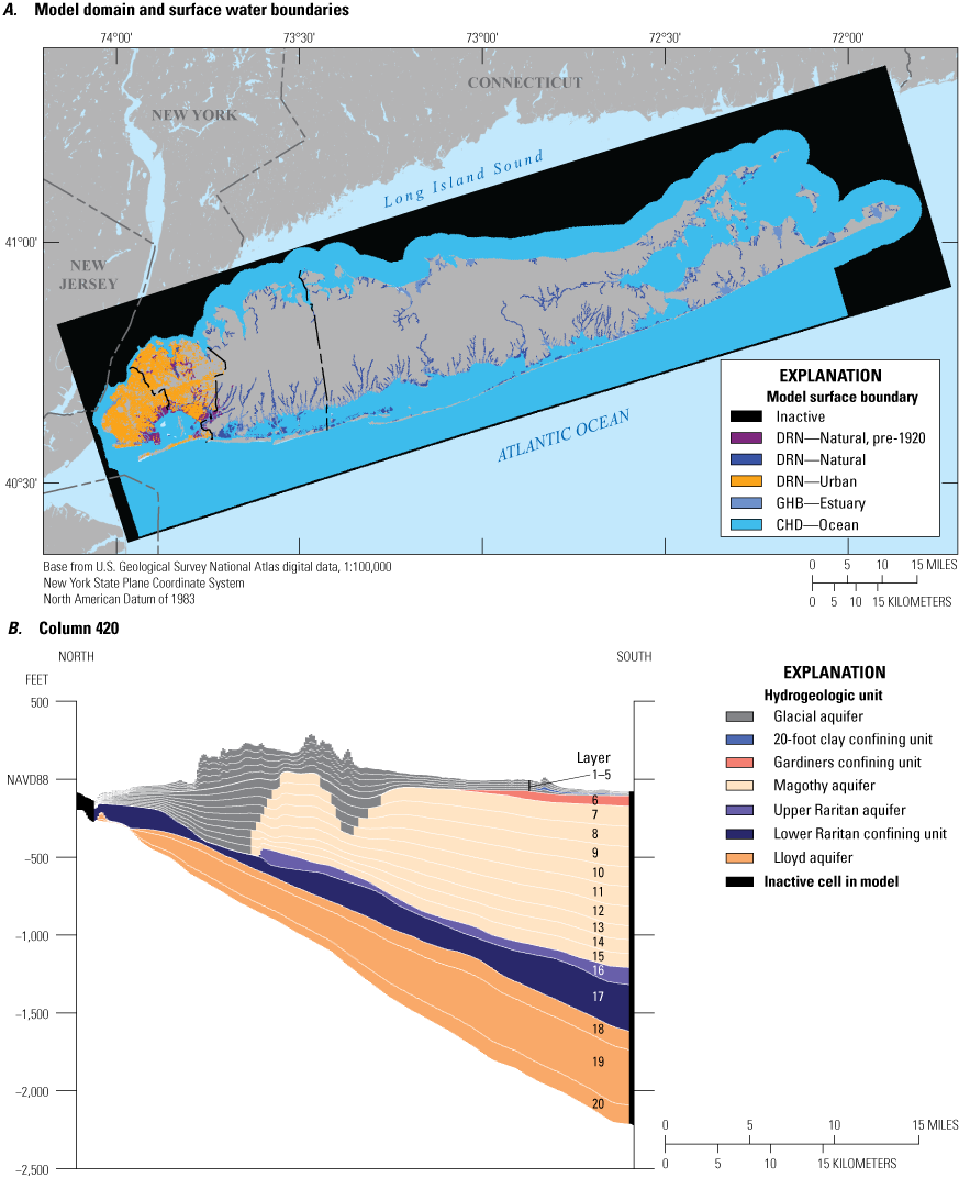
A, Map showing the areal extent of the model grid, active model areas, and surface-water boundary conditions of the transient groundwater-flow model of the aquifer system underlying Long Island, New York and B, cross section of model layering along column 420 of the groundwater-flow model. Location of column 420 shown on figure 10. DRN, Drain package; GHB, General Head Boundary package; CHD, Constant Head package (see McDonald and Harbaugh, 1988).
The model is three dimensional and consists of 20 layers, each of which has the same spatial discretization and active areas. Layer geometries were determined from the mapped surfaces from the hydrogeologic framework (Stumm and others, 2024), and the thickness of the model layers varies spatially to represent hydrostratigraphic units of variable thickness (fig. 12). The top and bottom model layers are referred to as model layers 1 and 20, respectively, with the model layer number increasing from 1 to 20 with depth in the model. The upper glacial aquifer is represented in the top five layers of the model, which are equally subdivided between the land surface and the top of the underlying Magothy and Jameco aquifers and Gardiners Clay unit (layers 1 to 5; fig. 21B).
The Magothy aquifer and contiguous Jameco aquifer are equally subdivided into nine layers between the merged top of the two aquifers and the top of the underlying upper Raritan aquifer (model layers 7 to 15; fig. 21B). These nine subdivided layers are extended into either the North Shore confining unit or glacial sediments where the Magothy and Jameco aquifers are absent due to erosion along the northern shore of the island (fig. 21B).
The upper Raritan aquifer is represented by a single layer between the top of the lower Raritan confining unit and the bottom of the Magothy aquifer (layer 16; fig. 21B); the layer represents the Magothy aquifer and has a uniform thickness of 2 ft where the upper Raritan is absent. The lower Raritan confining unit also is represented by a single model layer. The Lloyd aquifer and the contiguous North Shore aquifer are equally subdivided into three layers between the bottom of the Raritan confining unit and bedrock (layers 18 to 20). These layers include the upper glacial aquifer and the North Shore confining unit where the Lloyd and North Shore aquifers are absent. The Gardiners clay unit is represented in a single layer (layer 6), the top and bottom of which are determined from the mapped surfaces of the clay unit and the underlying Magothy aquifer. This layer includes the upper glacial aquifer with a thickness of 2 ft where the Gardeners clay is absent. Clays within the glacial sediments—Smithtown clay, the 20-foot clay, and the North Fork clay—are represented as single layers within the glacial sediments; the Smithtown clay is in layer 2, and the remaining two clay units are within layer 4. The tops and bottoms of the equally subdivided glacial layers are locally deformed to represent the mapped tops and bottoms of the clay units where present.
The numerical model is transient and simulates time-varying hydrologic conditions representing average annual conditions from 1900 to 2019. The total simulation time—43,380 days—is divided into 120, generally equal, stress periods, representing each calendar year. The length of each stress period is 365 days, except during leap years where there is an additional day. Hydraulic stresses are constant within each stress period and represent the annual averages of natural and anthropogenic recharge, and groundwater pumping estimated from compiled data. Each stress period is divided into three equal time steps to improve numerical precision of the simulation. The 120 annual stress periods are preceded by a conditioning stress period that approximates average predevelopment (pre-1900) conditions. This stress period has one time step that is 10,000 days in length; simulated conditions at the end of the initial stress period are the initial conditions for the simulation period from 1900 to 2019.
Boundaries
The conceptualization of how and where water enters, moves through, and leaves the aquifer system is critical for the development of an accurate flow model (Reilly, 2001). Boundary conditions are applied at appropriate model cells to simulate hydrologic features, including wells, streams, and coastal waters. A detailed discussion of grid discretization, boundary conditions, and the use of finite-difference equations to simulate groundwater flow is presented in McDonald and Harbaugh (1988); this general approach is implemented in MOFLOW 6 (Langevin and others, 2017). Surface boundaries were determined using the coastal geometry as determined from 1:24,000-scale digitized linework and digitized hydrography. These boundaries were modified by visual inspection of aerial photographs to ensure consistency between simulated boundaries and actual surface waters. Different types of surface waters, including open coastal waters, salt and brackish estuaries, salt marshes, fresh wetlands, and streams, were identified from aerial photographs using characteristics such as coastal morphology, water clarity and color, and vegetation.
Surface-water features are represented as head-dependent flux boundaries (fig. 21A). Salt marshes and freshwater streams and wetlands, which include streams, wetlands connected to streams, and pond outlets, are represented using the Drain (DRN) package for MODFLOW (McDonald and Harbaugh, 1988) as implemented in MODFLOW 6 (fig. 21A; Langevin and others, 2017). The DRN package is a passive boundary that does not allow streams influenced by pumping to serve as an infinite source of water to the underlying aquifer if hydraulic gradients are reversed; instead, streams represented with the DRN package can only receive groundwater discharge. Once the water level in the aquifer falls below the specified streambed altitude in the DRN cells, groundwater no longer discharges to the surface waters. Representing streams by using the DRN package was considered reasonable because streams on Long Island generally are gaining streams that accumulate groundwater baseflow downstream, and streamflow is depleted from a lowering of the water table and not induced infiltration.
This conceptualization is consistent with hydrologic processes typical of unconfined coastal systems like Long Island. Drain altitudes were specified as the mean light detection and ranging (lidar) altitude within each cell. Drain boundaries were assigned to the top layer of the model (layer 1). In addition to natural surface waters, drains also were assigned in areas with impervious surfaces in New York City. These drain boundaries implicitly represent subsurface infrastructure that can intercept the water table and passively collect groundwater in areas with shallow depths to water. The altitudes of the drains were specified as 10 ft below land surface, as determined from mean lidar altitude in the cell. Ponds and surface-water features were represented as areas with very high horizontal and vertical hydraulic conductivity values as compared to the surrounding aquifer: 50,000 and 5,000 ft/d, respectively.
Nearshore coastal water bodies, including tidal rivers and estuaries, were represented using the General Head Boundary (GHB) package, and open coastal waters, including the interior of large estuaries and offshore waters, were represented using the Constant Head (CHD) package for MODFLOW (McDonald and Harbaugh, 1988) as implemented in MODFLOW 6 (fig. 21A; Langevin and others, 2017). Coastal boundaries in saline surface waters were assigned to the top layer of the model (layer 1). The boundary altitude was specified as the mean bathymetric altitude within each cell (fig. 9; Danielson and Haines, 2017). Boundary altitudes in saline waters accounted for the density differences between fresh and saline water by using the freshwater-equivalent heads calculated from the height of the water column and seawater density.
The calculation of the freshwater equivalent boundary head was calculated within MODLFOW 6 from the specified sea level, the mean seabed altitude, and a salinity of 35 parts per thousand (ppt), which corresponds to a density of 1.025 kilograms per liter (kg/L). Sea level increased linearly during the simulation period (1900–2019), from −0.97 to 0.34 ft NAVD88. Constant head boundaries in the subsurface (layers 2 to 20) were assigned within the outermost cells of the active area (fig. 21A). These cells were assigned the altitude of the center of the model cells in each layer as well as the density of seawater, as estimated from salinity. The cells represent hydrostatic conditions along the edge of the model that accounts for density, allowing for the numerical model to calculate density and salinities within the aquifer system.
Hydraulic Properties
The discretized numerical model is assigned initial aquifer properties as determined from compiled data. These properties include horizontal hydraulic conductivity, anisotropy (the ratio of horizontal to vertical hydraulic conductivity), and confined and unconfined storage coefficients that are mapped to the model grid by geologic unit. The initial values of horizontal hydraulic conductivity for the upper glacial and Magothy aquifers were derived from the updated lithologic texture model described in the “Lithologic Texture Model” section of this report for the upper glacial, Jameco, and Magothy aquifers. The North Shore confining unit is a complex assemblage of lithologic units and properties (Stumm and others, 2024), and several wells used in development of the texture model are within the unit. Inspection of lithologic logs suggested sandy sediments are present in many areas so, unlike the Gardiners clay and lower Raritan confining units, the initial hydraulic conductivity values in the North Shore confining unit were derived from the texture model in shallow parts of the unit, contiguous with the Magothy and Jameco aquifers.
The numerical model uses the same grid dimensions and discretization as the texture model so that no spatial averaging was required to map the estimated hydraulic conductivity values for each texture-model layer to the two-dimensional model grid for each layer. The texture model has a vertical resolution of 10 ft, whereas numerical model layers can exceed 100 ft (fig. 21B). Horizontal hydraulic conductivity values derived from the lithologic texture model were vertically mapped to the numerical model layers in each cell by computing the thickness-weighted arithmetic mean of the values from the texture model for each coincident model layer. Values of vertical hydraulic conductivity used in the model were calculated from the horizontal hydraulic conductivity and anisotropy ratios.
Spatial patterns in the distribution of the initial hydraulic conductivity values are similar to those in the texture model, with generally lower initial hydraulic conductivity values present in northern and central parts of the island associated with moraines and ice-contact deposits and generally higher hydraulic conductivity values present in southern parts of the island associated with outwash deposits (fig. 22A). There are few broad spatial patterns in the hydraulic conductivity values of the Magothy aquifer, which has a complex depositional history (fig. 22B).
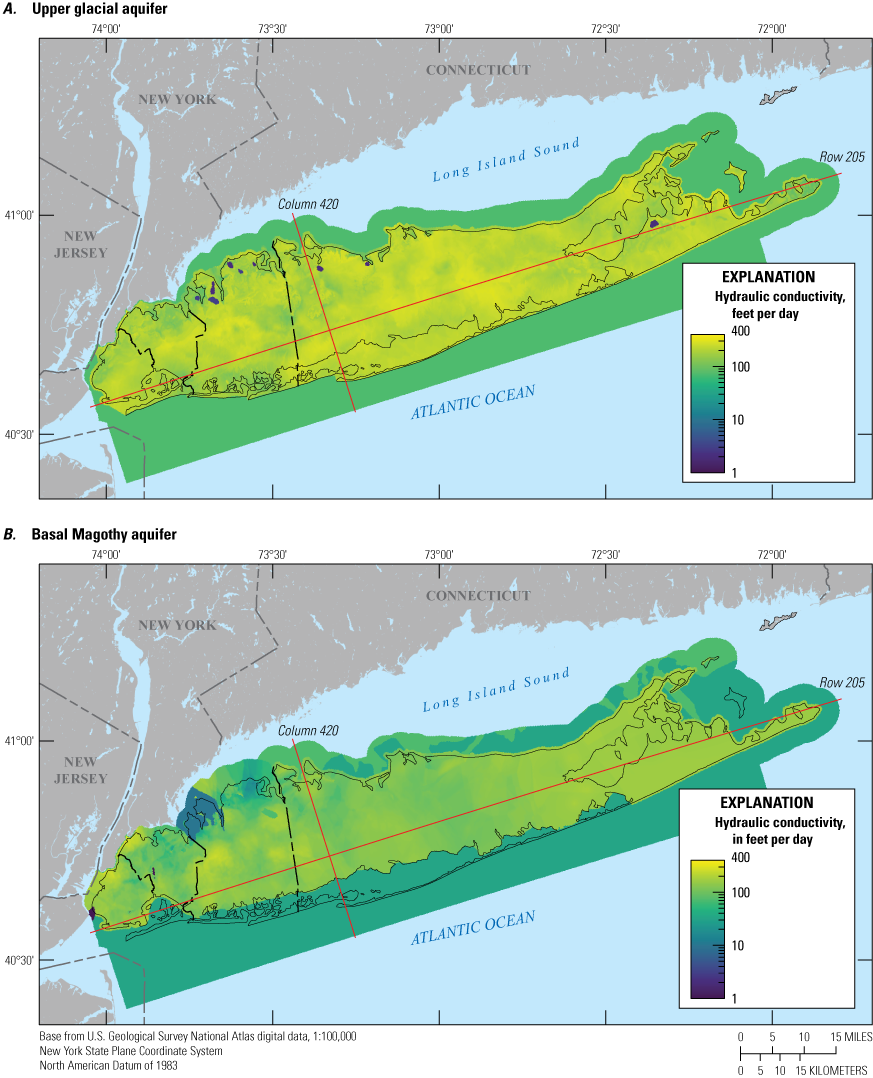
Maps showing initial horizontal hydraulic conductivity for A, the upper glacial aquifer (model layer 1) and B, the lower part of the Magothy aquifer (model layer 15) on Long Island, New York. Cross sections are shown on figure 23. Locations of column 420 and row 205 are shown in figure 10.
Vertical patterns in hydraulic conductivity generally reflect observed geologic trends in the upper glacial and Magothy aquifers (fig. 23). The largest hydraulic conductivity values within the upper glacial aquifer are within outwash deposits, and the lowest hydraulic conductivity values generally are within glacial moraines. The largest values of hydraulic conductivity in the Magothy aquifer are in the basal part of the unit, which was deposited in high-energy environments; the lowest values of hydraulic conductivity generally are in the middle part of the Magothy aquifer, which is a zone with large amounts of lignite, suggesting deposition in low-energy environments.
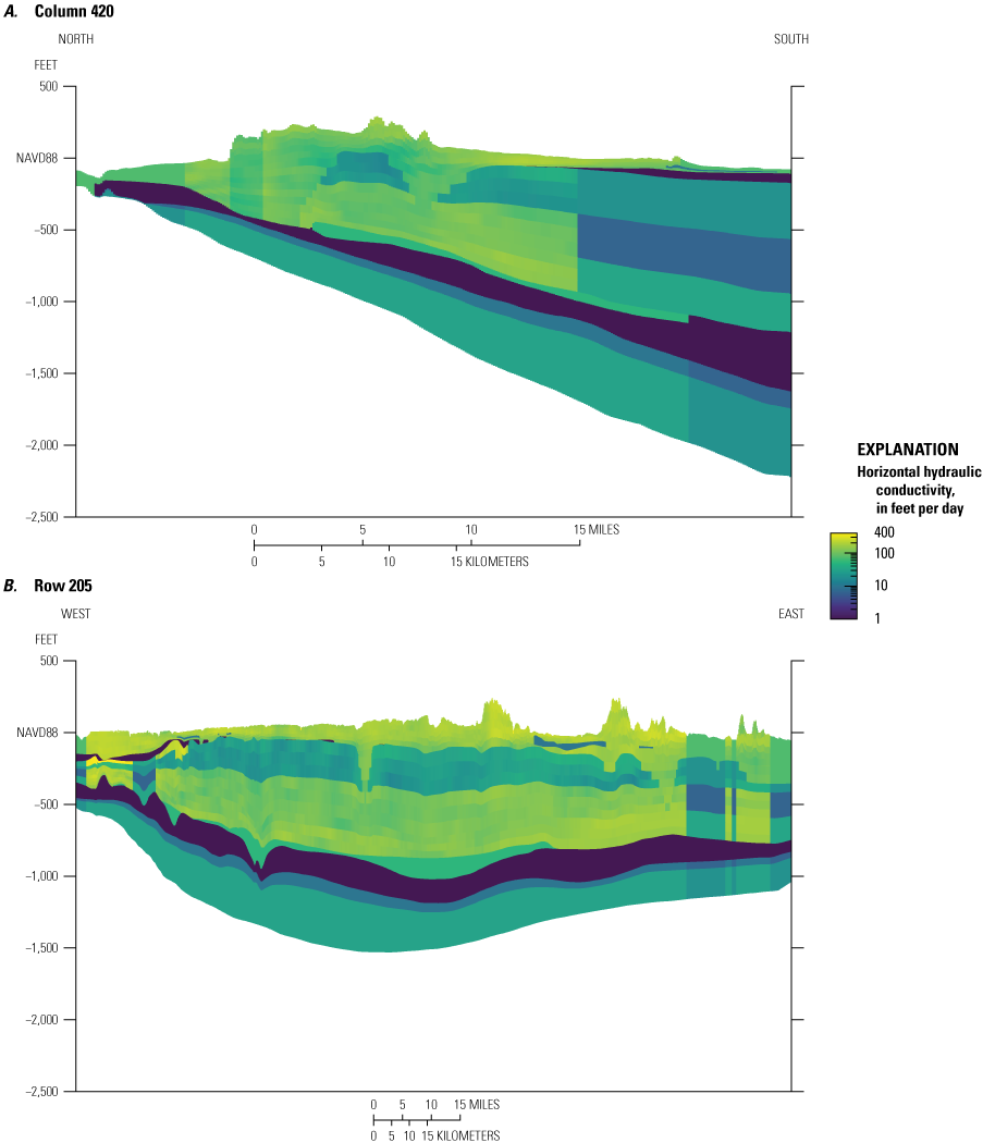
Cross sections showing vertical distribution of initial horizontal hydraulic conductivity A, along a north-south section (column 420) and B, along an east-west section (row 205), as mapped to the model grid representing Long Island, New York.
Sandy glacial sediments, including outwash, moraines, and ice-contact deposits, had a mean, initial texture-model-estimated horizontal hydraulic conductivity of about 167 ft/d. The initial horizontal hydraulic conductivity for glacial clays—the Smithtown clay, the 20-foot clay, and the North Fork clay—was specified as 10 ft/d. Shallow parts of the North Shore confining unit, contiguous with the Magothy and Jameco aquifers, had an initial texture-model-estimated horizontal hydraulic conductivity of about 79 ft/d; the initial horizontal hydraulic conductivity in deeper parts of the unit, contiguous with the Raritan and Lloyd aquifer, was specified as 10 ft/d. The North Shore aquifer had a specified initial horizontal hydraulic conductivity of 150 ft/d. The Jameco aquifer had a mean horizontal hydraulic conductivity of about 170 ft/d as estimated from the texture model. The Magothy aquifer had a mean hydraulic conductivity of 124 ft/d as estimated from the texture model. The underlying upper Raritan aquifer had a specified initial horizontal hydraulic conductivity of 50 ft/d. Most of the Lloyd aquifer had a specified initial horizontal hydraulic conductivity of 30 ft/d. Lithologic data suggested that the upper part of the Lloyd, underlying the lower Raritan confining unit, is fine grained with silt and clay, more similar to the overlying Raritan sediments (Stumm and others, 2024); the upper part of the Lloyd was assigned an initial horizontal hydraulic conductivity of 10 ft/d.
The initial horizontal hydraulic conductivities of the Gardiners clay and the lower Raritan confining units were specified as 1 ft/d for both units. Lithologic logs indicate clayey sediments in the upper part of the Magothy aquifer in parts of Queens County that may be part of the overlying Gardiners clay or a clayey heterogeneity within the upper part of the Magothy aquifer. The horizontal hydraulic conductivity in these sediments also was specified at an initial horizontal hydraulic conductivity of 1 ft/d.
The vertical hydraulic conductivity of fine-grained confining units generally is of more importance to groundwater flow than in sandy aquifer sediments. Anisotropy ratios were applied to confining units to yield values of initial vertical hydraulic conductivity that would be more typical of the confining units: 0.1 ft/d for glacial clays and 0.001 ft/d for the lower parts of the North Shore confining unit. Initial values and horizontal hydraulic conductivity as well as anisotropy ratios were adjusted during the calibration process.
Specific yield (unconfined storage) and specific storage (confined storage) affect the response of the hydrologic system to changing stresses. An initial specific yield (unconfined storage) of 0.23 and a specific storage (confined storage) of 1×10⁻⁶ was specified in each hydrogeologic unit. Specific yield and specific storage parameters were adjusted during model calibration.
The effective porosity of aquifer sediments does not affect simulated heads and flows but is an important control on groundwater velocity and travel times. The total porosity of unconsolidated sediments, defined as the fraction of open pore spaces, ranges from about 0.25 to about 0.7 (Freeze and Cherry, 1979). Stumm and others (2024) report porosity in sandy glacial sediments of 0.35 and 0.3 in the North Shore aquifer. Porosity in the Magothy aquifer ranged from 0.29 and 0.35 and from 0.28 to 0.29 in the Lloyd aquifer (Stumm and others, 2024). The effective porosity is a function of the interconnectedness of the pores and is less than total porosity. Specified porosities of sediments in the model range from 0.25 to 0.5 and vary by hydrogeologic unit. The porosity of Pleistocene aquifers, including the upper glacial, Jameco, and North Shore aquifers, was specified as 0.3, generally consistent with porosity values observed in glacial outwash sediments in nearby Cape Cod (Garabedian and others, 1988; Stumm and others, 2024). Cretaceous aquifer sediments, including the Magothy, upper Raritan, and Lloyd aquifers, generally have a lower hydraulic conductivity, are less sorted, and presumably, a lower porosity than glacial sediments. These aquifer sediments were assigned an effective porosity value of 0.25. Clayey sediments generally have higher porosities than sandy sediments. Glacial clays and the North Shore confining unit were assigned a porosity of 0.40. The porosity of both the Gardiners clay and the lower Raritan confining units was specified as 0.50.
Hydrologic Stresses
Natural recharge, as estimated from spatial and climate data, is combined with estimates of anthropogenic recharge components and mapped to the model grid. The location and depth of well screens used to withdraw groundwater are mapped to the model grid, and specified withdrawal rates were determined from compiled data. The hydrologic stresses simulated in the model are recharge (from both precipitation and anthropogenic return flow) and groundwater withdrawals. Anthropogenic return flow includes wastewater return flow from onsite domestic septic systems in unsewered areas and leaky sewers, recharge from leaky water-supply infrastructure, and rejected recharge from the rerouting of overland flow on impervious surfaces to retention or recharge basins. Groundwater withdrawals include those for commercial, domestic, industrial, and public supply uses. Both recharge and groundwater withdrawal stresses represent average annual conditions from 1900 to 2019.
Recharge into the model was simulated by use of the Recharge (RCH) package (McDonald and Harbaugh, 1988), as implemented in MODFLOW 6 (Langevin and others, 2017). Recharge was specified in the top model layer but was applied to the uppermost active layer if overlying layers become dry. Total recharge to the aquifer, which includes natural and anthropogenic recharge, was averaged and specified for stress periods representing the simulation period (1900–2019; fig. 24A).
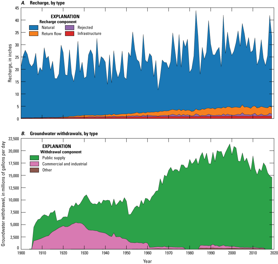
Graphs showing time series of A, estimated recharge and B, groundwater withdrawals from 1900 to 2019 on Long Island, New York. Recharge and groundwater withdrawals are from U.S. Geological Survey (2020b) and New York State Department of Environmental Conservation (2024).
The spatial variability of natural recharge arising from vegetation, soil type, and water capacity as computed by using the SWB model is represented as multipliers within the modeled area. Recharge in the model was determined by applying these multipliers to a scaling parameter that can facilitate a change in natural recharge into the model while preserving the spatial variability determined from the SWB model; this scaling parameter was adjusted during model calibration. Each of the three components of anthropogenic recharge were represented as multipliers and were independently estimated by combining the multipliers with scaling parameters to adjust anthropogenic recharge during model calibration. Natural recharge is the largest component of recharge to the aquifer system; anthropogenic recharge, which is the sum of recharge from leaky infrastructure, wastewater return flow, and stormwater, generally is small islandwide but has increased over time (fig. 24A). The adjusted recharge components—natural and anthropogenic—are combined to estimate total recharge to the aquifer system, which is mapped to the model grid as input using the RCH package. Additional spatial adjustment of the estimated total recharge was facilitated by use of a network of pilot points, which are parameters defined at specific points and used to define arrays of values by use of modeled interpolation. Pilot point parameters allow for spatially continuous adjustment to recharge and are adjusted during calibration.
A total of 2,942 wells withdrew groundwater from the Long Island aquifer system at different times between 1900 and 2019 for a variety of uses, including public supply, contaminant remediation, and industrial uses. Pumping data compiled from various sources were used to calculate annual average pumping rates for each well in operation; a total of 86,939 individual annual-average withdrawal stresses were estimated for this analysis. These individual pumping stresses were mapped to the model grid based on available information on the location and depth of each well. These pumping wells and stress points in time and space are represented in the model as a specified-flux boundary condition by use of the MODFLOW Well (WEL) package (McDonald and Harbaugh, 1988) as implemented in MODFLOW 6 (Langevin and others, 2017). The autoflow reduction option in the WEL package, which reduces pumping rates as model cells are dewatered, was set to 0.1 to avoid the numerical instability causes by pumping in dry model cells. Simulated pumping increased rapidly after 1950 and peaked in about 2000 (fig. 24B). Most pumping was for public supply, though pumping for commercial uses was the largest component of groundwater withdrawals in the early part of the 20th century (fig. 24B).
Simulation of Groundwater Flow
Variable-density groundwater flow is simulated by use of the MODFLOW 6 Buoyancy package, which solves the variable-density from of Darcy’s law (Langevin and others, 2020). The Buoyancy package is coupled with the MODFLOW 6 Groundwater Transport (GWT) model simulating salinity concentrations, which allows for fluid density to be dynamically updated with those concentrations (Langevin and others, 2022). The variable density flow equations are solved within each stress period, followed by the solution of the transport equations. The Buoyancy package (Langevin and others, 2008) updates the fluid densities, and the model solution advances to the next stress period.
A seawater salinity of 35 mg/L (as chloride) was assigned to constant-head boundary cells (as represented by use of the CHD package) by use of the Sources and Sink Mixing (SSM) package. Porosity values varied by unit: glacial sands were assigned porosity values of 0.35, sands in Cretaceous units were assigned values of 0.25, and clays were assigned porosity values between 0.40 and 0.50. The Advection (ADV) package was used to simulated advective transport, using a finite-difference method to solve the transport equation. The use of a mass-balance method, such as finite difference, in advection-dominated systems such as Long Island allows for conservation of mass but can result in numerical dispersion.
Dispersion is a measure of the spread of a solute within porous sediments that occurs in all aquifers. It is a function of natural heterogeneity and is scale dependent. Numerical dispersion is a function of spatial discretization, the length of a time step, and groundwater velocity and can be approximated from the following equation:
where α is numerical dispersion, X is cell length, V is velocity, and T is time-step length (Fletcher, 1991). No dispersion was explicitly simulated beyond the numerical dispersion arising from the finite-difference solution within the ADV package. The inherent assumption is that the numerical dispersion in the model is a reasonable approximation of that seen in the real system at the scale of the analysis. Given a spatial discretization of 500 ft and a time-step length of 121.75 days, and groundwater velocities calculated by the numerical model, equation 1 yields a mean numerical dispersion of about 250 ft. This estimated dispersion is consistent with literature values at the regional scale of this analysis (Gelhar and others, 1992; Schulze-Makuch, 2005)Estimation of Model Input Parameters
Model inputs were adjusted to produce an optimal fit to observed hydrologic conditions using inverse parameter-estimation techniques (Doherty and Hunt, 2010). Parameter estimation, as implemented in this effort, is a four-step process: (1) trial-and-error manual adjustments to initial parameter values, (2) an inverse algorithmic update of parameters resulting in an optimal fit to observed hydrologic conditions and associated data-quality weights, (3) manual adjustments, based on expert judgement, of inversely fit parameters to address local misfits between observations (measured values) and their model-simulated equivalents, and (4) conditioning of all model inputs to ensure all values are within ranges considered to be reasonable based on prior knowledge of the Long Island aquifer system.
Initial parameter values were assigned based on expert knowledge, literature values, and direct measurements of the groundwater system; these were updated using a trial-and-error approach. This involved using prior knowledge, known hydrogeologic conditions, and exploratory model runs to determine what adjustments were needed to improve general agreement between the model and the known system. These changes included adjustments to the hydrogeologic framework and aquifer property assignments and revisions to assumptions made for the various recharge components.
The simulated fit (or match) to select critical observations (measurements used for model calibration) was evaluated after each exploratory model simulation. The fit between observed and simulated conditions is quantified by an objective function that represents the weighted sum of squared residuals between each observation and its simulated equivalent multiplied by the weight of the observation, which is the inverse of the error associated with the observation. The objective function is referred to as PHI (Φ) and is defined by the following equation:
where Φ is the value of the objective function, wi is the weight assigned to the ith observation (the inverse of the associated error), yi,obs is the ith observed value, and yi,sim is the ith simulated equivalent. A lower objective function indicates an improvement in model fit. Model parameters were adjusted manually to improve fit, followed by another exploratory model simulation to assess improvement. This process of observation evaluation, manual parameter updating, and exploratory model testing was repeated. Once the trial-and-error adjustments were complete, parameter values were systematically adjusted to be consistent with historical observations using a methodology generally following Bayes’ theorem. The prior estimate of parameter values and their likely ranges (their uncertainty) that resulted from the trial-and-error process were updated through an inverse estimation step to be consistent with historical observations, resulting in a posterior set of parameter values and uncertainty.This parameter updating process was performed with an iterative ensemble smoother (iES) algorithm implemented in PEST++ version 5.0 (White and others, 2018, 2020b, 2021). Following implementation of iES, some model parameters were adjusted again manually to address local misfits between observations and their model-simulated equivalents. In a final manual conditioning step, some parameters were adjusted to ensure that resulting values were within acceptable ranges that reflect expert knowledge of the aquifer system. Generally, the conditioning had a minimal effect on model residuals.
Observations
The parameter estimation process requires hydrologic data (referred to as “observations” in modeling parlance) of suitable quality to reasonably represent conditions during the timescale of interest. Model input parameters are adjusted to best fit hydrologic conditions based on a comparison of model simulated equivalents to these observations. Field measurements of hydrologic conditions often have associated error (or noise), and large numbers of observations often are required to reasonably represent average hydrologic conditions during the model simulation period. Observations were selected for this process based on suitable data densities to reliably estimate annual averages consistent with the annual stress periods assigned in the transient model. Field measurements of water levels and streamflows are needed to calibrate the transient groundwater-flow model. In addition, observations of chloride concentrations are needed to verify the agreement between the position of the simulated saltwater interface as simulated by the model and that estimated from chloride data.
Water Levels and Streamflows
Historical groundwater-level and streamflow measurements were obtained from NWIS and reviewed to determine which of these observations were best suited for inclusion as model calibration targets. The dataset for 1900 to 2019 included 253,033 individual water-level measurements in 1,870 wells and 497,999 streamflow measurements at 111 streamgages. Annual averages were calculated from the measurements made at each observation location to match the temporal discretization of the model, and only average annual observations with a suitable number of measurements were selected for inclusion in the calibration. For instance, only wells with at least 5 consecutive years of 12 measurements in a calendar year were included in the final observation dataset where these observations were assigned weights based on the quality of the data. These weighted observations then are referred to as the model calibration targets used in the inverse calibration process. Yearly differences between annual water-level means also were calculated as a supplemental set of observations for model calibration.
Baseflow observations were calculated from NWIS streamflow measurements using a digital filter (Eckhardt, 2005). Only annual mean baseflow observations that consisted of at least 100 measurements in a calendar year were included in the final weighted observation dataset. In total, the final weighted observation dataset included the following calibration targets: (1) 5,623 annual average water levels from 369 wells, (2) 5,104 annual water-level differences from the same wells, and (3) 1,330 average annual baseflow observations from 25 streamgages (fig. 25).
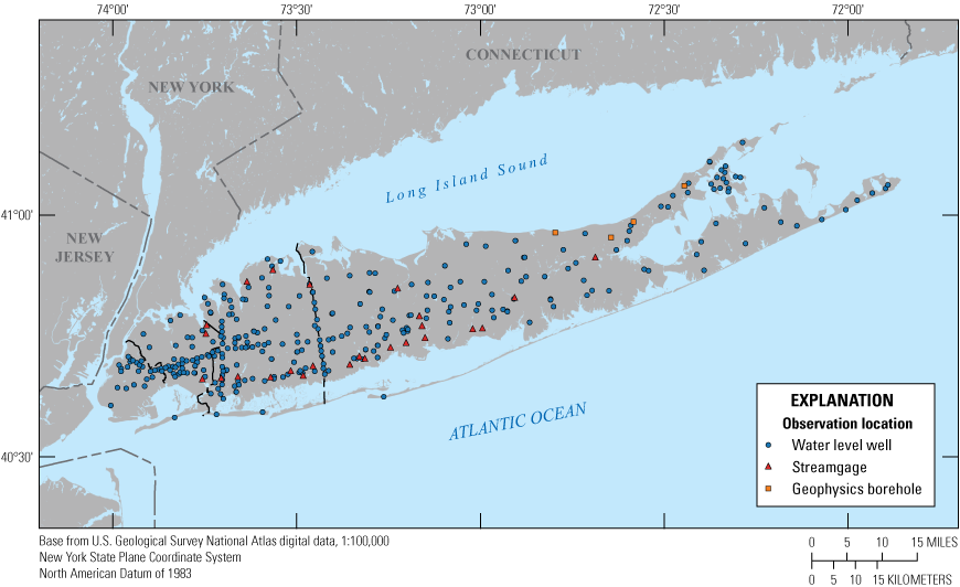
Map showing locations of water level and streamflow observations and borehole geophysical measurements to estimate chloride concentrations for use in calibration of the transient groundwater-flow model of the aquifer system underlying Long Island, New York. Data are from U.S. Geological Survey (2020b) and Stumm and others (2024).
The number of observations that meet the criteria for inclusion as model calibration targets varied with time (fig. 26A). Most water-level observations were from the upper glacial aquifer, which historically is where most groundwater was withdrawn; the largest number of those observations were between 1940 and the mid-1950s (fig. 26A). Streamflow observations began in the late 1940s and generally varied between 15 and 20 average annual observations after about 1950 (fig. 26B). Water-level and streamflow observations were sorted into six groups for inclusion in the inverse calibration process: (1) water levels in the unconfined aquifers, (2) water levels near the tops of groundwater mounds in the unconfined aquifers, (3) water levels in the confined portion of the Lloyd aquifer, (4) annual water-level differences, (5) major streamflows, (6) and minor streamflows (table 3).
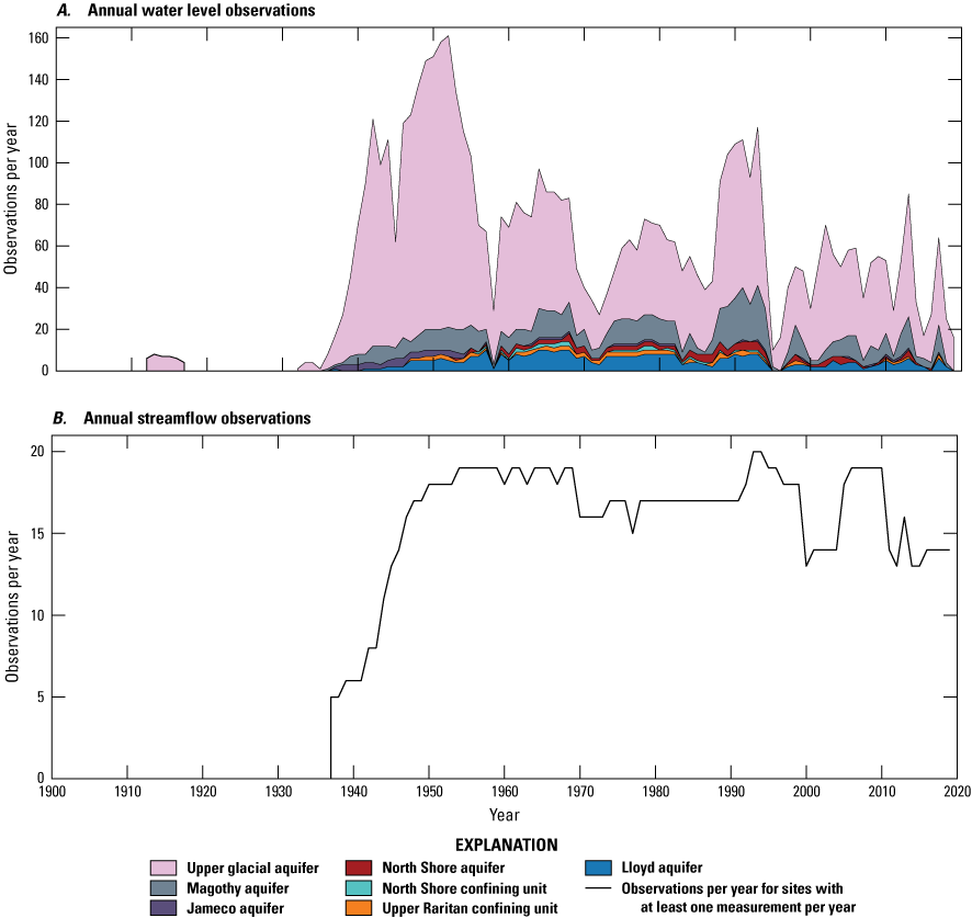
Graphs showing time series of the number of mean annual A, water-level observations, by geologic unit, and B, streamflow observations used for the inverse calibration of the transient groundwater-flow model of the aquifer system underlying Long Island, New York. Data are from U.S. Geological Survey (2020b) and New York State Department of Environmental Conservation (2024).
Table 3.
Summary of observation groups used for calibration of a transient, groundwater-flow model to simulate hydrologic conditions in the Long Island aquifer system on Long Island, New York.An additional synthetic observation group was added to limit the amount of automatic flow reduction that MODFLOW 6 performs on pumping wells to prevent those cells from going dry (Langevin and others, 2017). A target value of zero is desired for the automatic flow reduction observation group (representing no reduction in pumping) because the reported pumping values are actual withdrawal rates for wells pumping groundwater in saturated sediments, and those rates should not be reduced to prevent model cells from going dry.
Observation weights were assigned based on a general assumption of the observation quality. The weights corresponded to (1) a coefficient of variation of 10 and 30 percent for major and minor stream observations, respectively; (2) standard deviations of 2 and 0.5 ft for the groundwater levels pre-1990 and post-1990, respectively; and (3) a standard deviation of 1 and 0.5 ft for annual groundwater level differences pre-1990 and post-1990, respectively (table 3). Water-level and streamflow observations that did not meet the criteria for calculating reliable annual averages were assigned a weight of 0, meaning they did not influence estimation of the optimal parameters. An observation ensemble approach is implemented in iES to sample the observation error (or noise); each realization within the ensemble used observations stochastically sampled from normal distributions with means set by the reported observation value and standard deviations set as the inverse of the initial observation weight (table 3).
Chloride Concentrations
Observations of chloride concentrations include measurements from groundwater samples and estimates using electromagnetic conductivity measurements in PVC-cased wells. Chloride concentrations estimated from geophysical measurements were used as a qualitative assessment of the freshwater/saltwater interface location during trial-and-error testing and following iES calibration. Borehole electromagnetic conductivity is affected by water salinity (Stumm and others, 2021). A linear regression between concurrently collected electromagnetic conductivity data and chloride concentrations (Stumm and Como, 2017) was estimated following a log-log transformation (eq. 3; fig. 27):
whereCl−
is the chloride concentration, in milligrams per liter;
EM
is the electromagnetic conductivity, in microsiemens per meter; and
BC
is the mean of the regression residuals used as a bias correction factor (in this case 1.046).
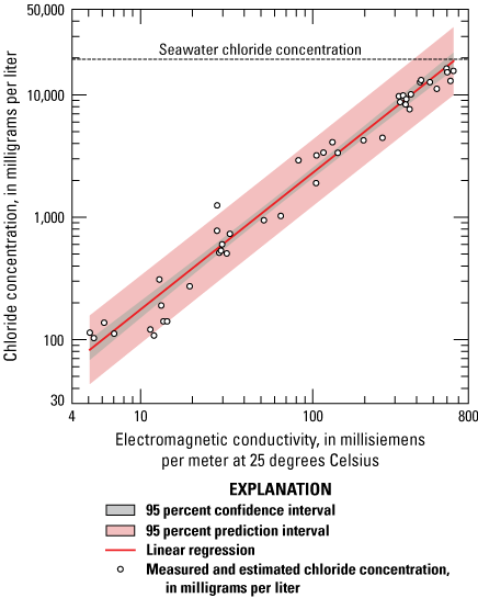
Graph showing relation between electromagnetic conductivity and measured chloride, including confidence and prediction intervals, for Long Island, New York. Data are from Stumm and others (2024).
Electromagnetic conductivity is also influenced by subsurface clay content, which can be semiquantitatively estimated from gamma radiation logs (Stumm and others, 2021). To reduce the effects of false positive chloride estimates in each profile, estimated chloride concentrations were set to zero at depths where concomitant gamma counts were greater than the 75th percentile for gamma in the whole well. Finally, vertical profiles of estimated chloride were discretized to align with the model layering and averaged by layer for direct comparison to simulated chloride in each layer. Uncertainty around the estimated chloride profiles was quantified for both profile sources. Uncertainty in the electromagnetic log estimated chloride profiles is derived from uncertainty in the linear regression, so upper and lower bounds were assigned the regression’s 95 percent prediction interval (fig. 27). Uncertainty for the simulated chloride profiles stems from a scale difference between the size of the model grid cells and the logged wells. To account for this spatial uncertainty, minimum and maximum chloride values were calculated for the model profiles from the eight model cells immediately adjacent to the model profile containing the logged well.
A database of 38,380 chloride concentrations in water samples from 3,747 wells was assembled to map spatial patterns of saltwater intrusion in the unconfined aquifer system—including the upper glacial, Magothy, and Jameco aquifers—and the underlying confined system, which includes the Lloyd and North Shore aquifers. The distribution of chloride in the aquifer system is documented in Stumm and others (2024). The estimated distribution of chloride and the mapped extent of saltwater intrusion is used as a qualitative metric to verify that simulated patterns of chloride concentrations generally are the same as those in the aquifer system.
Model Parameterization
The parameterization method employed in this effort used multipliers on initial values to allow for adjustment at multiple scales as discussed in White and others (2020a). As an example, hydraulic conductivity values were adjustable by both zonal multipliers assigned to specific hydrogeologic zones for broad-scale variability and pilot point multipliers (Doherty, 2003) within those zones for finer-scale variability (fig. 28). Parameter groups were developed and, with few exceptions, were adjustable during the parameter estimation (table 4). All parameters were given initial values and bounds constraining their variation during iES updates.
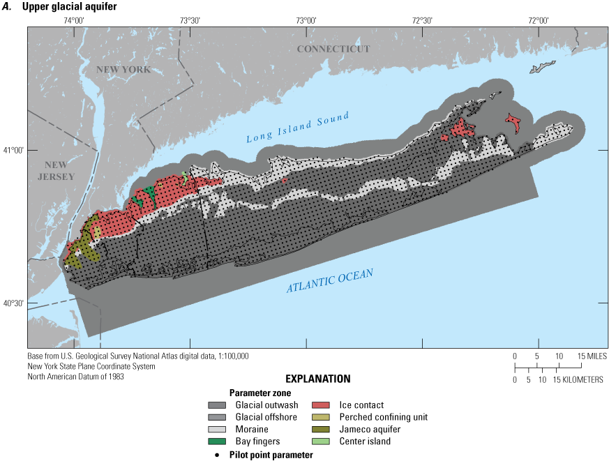
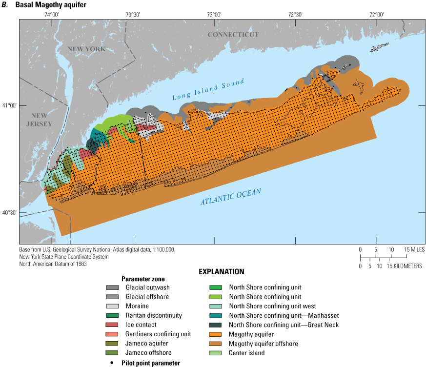
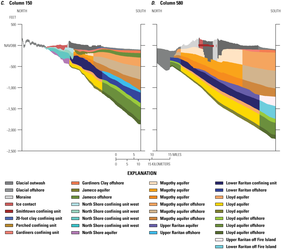
Maps showing parameter zones and pilot points in A, the upper glacial aquifer and B, the basal Magothy aquifer and cross sections showing vertical parameter zones along C, column 150 and D, column 580 in the transient groundwater-flow model of the aquifer system underlying Long Island, New York. Locations of cross sections (columns and rows) shown in figure 10.
Table 4.
Summary of parameter groups used to calibrate in the regional groundwater-flow model of Long Island, New York.[Model packages are from McDonald and Harbaugh (1988). E−X, ×10−X; GHB, General Head Boundary package; DRN, Drain package]
Aquifer Properties
Hydraulic conductivity was parametrized using geologic zones, as mapped to the three-dimensional model grid, and pilot points. A zonal multiplier was applied to each hydrogeologic zone, and pilot point multipliers were placed every 10 cells in all 20 model layers (fig. 28). The three-dimensional hydrogeologic framework mapped to the model grid was used to define a model zonation that represented the framework. Zones representing the major hydrogeologic units were subdivided to better represent heterogeneities known to exist from previous studies or to allow for a more adaptable approach to represent the local-scale heterogeneities not apparent in the broadly mapped hydrogeologic units (fig. 28C–D).
The upper glacial aquifer was subdivided by depositional unit (moraines, outwash, and ice-contact deposits; fig. 28C–D). The Magothy aquifer was subdivided into three vertical zones representing the fining upward depositional sequence observed in the hydrogeologic unit (Walter and Finkelstein, 2020). The Lloyd aquifer, likewise, was subdivided vertically into three zones; the uppermost zone represents fine-grained sediments that are transitional between the Lloyd and the lower Raritan confining unit (fig. 28C–D). The North Shore confining unit is a complex assemblage of preglacial fluvial, lacustrine, and marine sediments broadly mapped into a single hydrogeologic unit (Stumm and others, 2024). This hydrogeologic unit was subdivided spatially into four different zones, from west to east, to allow for more flexibility in estimating hydraulic properties and matching observed hydraulic conditions. The unit also was subdivided into four vertical zones. The upper two zones are contiguous with the Magothy and Jameco aquifers. An underlying zone is contiguous with lower Raritan confining unit, and the bottom zone is contiguous with the Lloyd and North Shore aquifers (fig. 28C).
Adjustment of the hydraulic conductivity values is a two-step process: (1) adjustment of the initial horizontal hydraulic conductivity values using an array of interpolated spatially variable multipliers, at the resolution of the model grid, derived from the pilot point network specific to each zone (fig. 28A–B); and (2) adjustment of the resultant horizontal hydraulic conductivity values by zonal parameters applied to each zone (fig. 28C–D). Separate pilot point networks were assigned within each horizontal hydraulic conductivity zone in each layer because these zones represent distinct depositional facies that should be interpolated independently from neighboring zones. Vertical hydraulic conductivity was calculated from horizontal hydraulic conductivity by using independently adjustable anisotropy ratio parameters that were categorially defined as a function of horizontal hydraulic conductivity. Resultant vertical hydraulic conductivity values were also adjusted by zonal parameters applied within each zone.
Specific storage and specific yield were parameterized by using initial values from prior knowledge of the system, as discussed in the “Model Parameterization” section of this report. Parameters representing specific storage (confined storage) were specified for each of the mapped hydrogeologic zones: an initial value of 1×10⁻⁶, with and lower and upper bounds of 1×10⁻⁷ and 1×10⁻⁴, respectively. A specific yield of 0.23, with lower and upper bounds of 0.05 and 0.35, was initially specified for each zone. Values of specific yield and specific storage were adjusted as independent parameters during the parameter estimation process such that final storage values varied among hydrogeologic zones.
Recharge
A multiscale approach was used for parameterizing recharge similar to the approach that was used for horizontal hydraulic conductivity. Estimating recharge consisted of several steps: (1) application of zonal parameters to each recharge component; (2) aggregation into total recharge; (3) application of annual multipliers; and (4) application of an array of interpolated spatially variable multipliers, at the resolution of the model grid, derived from a pilot point network. Zonal, annual, and spatial multipliers were adjusted during the parameter estimation process.
Zonal multipliers were applied to the natural recharge derived from SWB model and to the anthropogenic recharge components estimated from population and water-use data, as described in the “Natural and Anthropogenic Recharge” section of this report. A zonal multiplier was used for natural recharge for all the land area of Long Island. This initial zonal multiplier was based on the calibrated value of 1.2 in the steady state Long Island model (Walter and others, 2020) and was assigned lower and upper bounds of 0.8 and 1.5, respectively.
Rejected recharge was estimated from the SWB model (Finkelstein and others, 2022) and refers to potential recharge lost by runoff from impervious surfaces through stormwater infrastructure. Four separate countywide zonal multipliers were specified for rejected recharge across Long Island. Kings and Queens Counties generally had more impervious areas and storm and combined sewers that redirected road runoff into surrounding water bodies, whereas rejected recharge in Nassau and Suffolk Counties was more likely to be redirected to the groundwater system by extensive networks of recharge basins that capture road runoff.
The rejected recharge multipliers in Nassau and Suffolk Counties had an initial value of 1.0 because it was assumed that all runoff on impervious surfaces was accumulated in the extensive network of recharge basins throughout the counties. Conversely, in Kings and Queens Counties, the initial recharge multipliers were set to values of 0.1 and 0.3, respectively, because those counties have few recharge basins and a much more extensive sewer system to remove runoff. All four rejected recharge multipliers were adjusted during parameter estimation between lower and upper bounds of 0.001 and 1.0, respectively.
Five separate multipliers were applied to estimate wastewater return flow recharge with one multiplier applied to all unsewered areas across Long Island and four other multipliers applied separately by county for sewered areas. Wastewater recharge in unsewered areas represents septic system return flow and was assigned an initial parameter value of 0.9, representing a consumptive loss of 10 percent. The lower and upper bounds were specified to be 0.8 and 0.9, respectively. Wastewater recharge in sewered areas represents leakage from sewer lines and was assigned an initial parameter value, and lower and upper bounds (shown in paratheses, respectively) of 0.01 (0.001 and 0.1) in Kings County, 0.05 (0.001 and 0.1) in Queens County, 0.3 (0.001 and 0.4) in Nassau County, and 0.01 (0.001 and 0.1) in Suffolk County. Separate zonal multipliers, one for each of the four counites, also were used for estimating leaky infrastructure in areas serviced by public supply. The leaky infrastructure multipliers received an initial parameter value, and lower and upper bounds (shown in paratheses, respectively) of 0.05 (0.001 and 1.0) in Kings County, 0.1 (0.001 and 1.0) in Queens County, 0.3 (0.001 and 0.4) in Nassau County, and 0.01 (0.001 and 0.1) in Suffolk County.
The initial recharge values, and the adjusted zonal multipliers, are used to estimate new recharge values for each of the four recharge components—natural, rejected, wastewater, and leaky infrastructure—which were aggregated into the combined, total recharge value per model cell. This total recharge array was then adjusted by a single multiplier for each annual stress period with an initial value of 1.0 and upper and lower bounds of 0.5 and 2.0, respectively. Total recharge in each stress period was adjusted by a set of 321 pilot point multipliers on the total recharge, with a multiplier uniformly spaced every 40 cells (fig. 29). The pilot point multipliers generally received an initial value of 1.0 with upper and lower bounds of 0.1 and 10.0, respectively, but pilot points in central Nassau were updated with an initial value of 1.1 after trial-and-error exploratory simulations and following the approach discussed in Walter and others (2020; fig. 29). The pilot point network for each stress period produced an array of interpolated spatially variable multipliers, at the resolution of the model grid, which was multiplied by the total recharge array. Final annual total recharge arrays are the summation of the components derived from the SWB model, zonal multipliers, annual multipliers, and annual pilot point multiplier arrays.
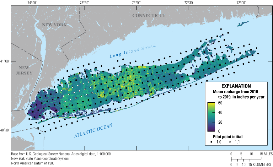
Map showing locations of pilot point multipliers and mean recharge rates for 2010 to 2019 for the transient groundwater-flow model of the aquifer system underlying Long Island, New York. Data are from U.S. Geological Survey (2020b) and New York State Department of Environmental Conservation (2024).
Model Boundaries and Stresses
Conductance at surface-water boundaries refers to the vertical resistance to flow within the sediments of the bottoms of the surface-water bodies between the aquifer and the surface-water body and is a function of vertical hydraulic conductivity (leakance), the assumed thickness of the bottom sediments, and the area of the model cell. Conductance at DRN and GHB boundaries is a lumped parameter, which means the parameter relies on more than one physical property or characteristic, in this case both vertical leakance and sediment thickness. Each GHB and DRN cell received a conductance multiplier with an initial value of 1.0 and upper and lower bounds of 0.1 and 10, respectively. The assumed thickness of the sediments and the area of the cell do not change, so that the estimates of the conductance are analogous to estimating the leakance.
The pumping rate of each well for each stress period was assigned a multiplier to account for both the uncertainty in historical pumping rate records and the structural uncertainty created by the application of the recorded pumping data to the relatively coarse model spatial and temporal discretization. The initial value for all pumping rate multipliers was 1.0, and the upper and lower bounds varied by year, reflecting perceived uncertainty in the historical records. Before 1951, when pumping records are most uncertain, the pumping rate multiplier upper and lower bounds were set to 0.5 and 1.5, respectively. Between 1951 and 1985, when pumping rate records are less uncertain, the multiplier upper and lower bounds were set to 0.8 and 1.2, respectively. After 1985, when pumping rate records are most certain, the multiplier upper and lower bounds were set to 0.9 and 1.1, respectively.
Prior Information and Specification of Initial Properties and Conditions
The conceptual model, hydrogeologic framework, and hydraulic properties values in the numerical model were determined from compilation and analysis of data and prior knowledge of the system from previous investigations. The numerical model combines the conceptual model and estimates of initial input values. Versions of the numerical model that represent differing conceptualizations of the hydrogeologic framework and initial hydraulic property values were iteratively tested within reasonable ranges to determine general agreement between simulated and observed hydrologic conditions. This process continued until there was a modified version of the initial numerical model that qualitatively agreed with observations of the real system and was considered a reasonable prior model for use in the iES parameter estimation. This model was tested further using a Monte Carlo approach to ensure that the model inputs and uncertainty ranges sufficiently captured hydrologic observations.
Trial and Error Adjustments
Based on the quantitative evaluation of water-level and streamflow observation residuals (measured versus simulated) and qualitative assessments of differences in observed versus simulated chloride profiles, the trial-and-error process resulted in data-driven adjustments to the hydrogeologic framework, initial hydraulic conductivity multiplier values, and initial recharge multiplier values. Exploratory model simulations showed that water-level observations could not be achieved in areas where groundwater flow was substantially affected by the North Shore confining unit. In the hydrogeologic framework, the North Shore confining unit was mapped as a homogenous unit (Stumm and others, 2024), but this homogeneity is not compatible with the spatial variability in observed water levels, even with the flexibility of pilot point multipliers. Therefore, the North Shore confining unit zone in the model was subdivided based on observation residuals, and each new subzone received an individual set of hydraulic conductivity zonal and pilot points multipliers (fig. 30).
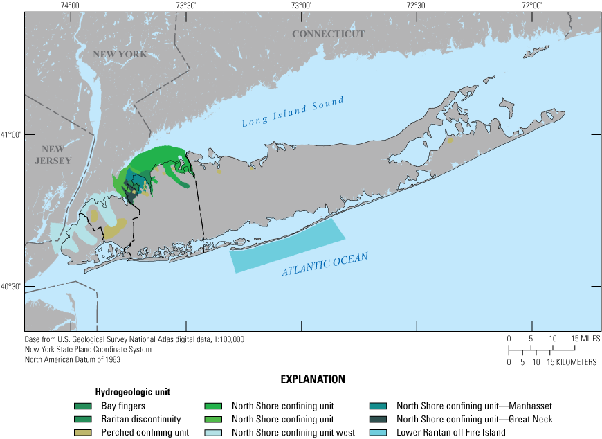
Map showing hydrogeologic unit zones that were added during trial-and-error forward runs of the transient groundwater-flow model of the aquifer system underlying Long Island, New York.
The lower Raritan offshore zone to the south of Fire Island was separated from the remaining lower Raritan offshore zone to create highly confined conditions to allow for offshore fresh groundwater to discharge upward from the Lloyd aquifer through the lower Raritan confining unit. The higher than expected water levels in the Lloyd aquifer arise from a state of the disequilibrium among pressures on either side of the freshwater/saltwater interface as the interface continues to move inland. These elevated water levels are the result of an ongoing adjustment of the aquifer system following the low stand of sea level during the last glacial maximum, about 19,000 years before present; this disequilibrium is most pronounced in the deep, confined parts of the Lloyd aquifer along the southern shore of central Suffolk County where the aquifer is the thickest and the bedrock surface is the deepest.
Discontinuities in confining units also were added as zones to improve fits to chloride observations and water levels in the Lloyd aquifer. A hydraulic connection between the Magothy and Lloyd aquifers was added in northeastern Nassau County to improve fits to water levels in that area. The location of this discontinuity was based upon localized water-level mounding in the Lloyd aquifer mapped by Monti and others (2013). Three discontinuities in the lower Raritan and North Shore confining units were added offshore of Great Neck and Manhasset Neck to improve fits to geophysics-derived chloride profiles and chloride concentrations reported by Stumm (2001) and Stumm and others (2002). These discontinuities provided hydraulic connections between the unconfined and confined units and were also implemented in a previous smaller scale variable density flow model centered on Great Neck and Manhasset Neck (Monti and others, 2009). Zonal parameters in offshore discontinuities near Great Neck and Manhasset Neck were changed from a value of 1.0 to a value 2.0.
Several adjustments were made to pilot point multipliers in addition to those made to the hydrogeologic framework described above. Horizontal hydraulic conductivity pilot points have an initial value 1.0, indicating no local change to the horizontal hydraulic conductivity field, and are adjusted during the trial-and-error parameter estimation process. Initial pilot point values were changed from 1.0 in several areas to improve fit to observed hydrologic conditions in several areas.
Several islandwide changes were made to horizontal hydraulic conductivity pilot point values. The horizontal hydraulic conductivity pilot points in glacial ice-contact deposits were decreased to 0.42, which is consistent with the poorly sorted nature of the sediments. The horizontal hydraulic conductivity pilot points in the Jameco aquifer, the most transmissive aquifer on Long Island (Williams and others, 2020; Stumm and others, 2024), were increased to 2.0. The horizontal hydraulic conductivity pilot points in the upper parts of the Magothy aquifer were decreased to 0.25, which reflects the upward-fining sequence in the Magothy aquifer where lower horizontal hydraulic conductivity values have been recorded in the upper parts of the unit (Walter and Finkelstein, 2020). In addition to these islandwide adjustments in pilot points, local-scale adjustments were made in several areas. The horizontal hydraulic conductivity pilot points in glacial moraines were decreased to 0.2 in parts of Kings, Queens, and Nassau Counties in western Long Island. The pilot points in glacial moraines in the western part of Suffolk County were decreased to 0.5, and the horizontal hydraulic conductivity pilot points in glacial outwash in the same parts of western Suffolk County also were decreased to 0.5.
Changes were made to vertical hydraulic conductivity parameters in addition to the changes to horizontal hydraulic conductivity parameters described above. Zonal parameters for vertical hydraulic conductivity were added and applied to parts of the upper glacial aquifer, the North Shore confining unit, and the lower Raritan confining unit to improve fit between the numerical model and the observed conditions. A zonal vertical hydraulic conductivity multiplier of 0.3 was applied to the upper glacial aquifer, and a zonal vertical hydraulic conductivity of 0.01 was applied to the lower Raritan confining unit. A zonal vertical hydraulic conductivity multiplier in the North Shore confining unit below Great Neck and Manhasset Neck was specified as 0.02, and a zonal vertical hydraulic conductivity multiplier of 0.01 was applied to parts of the North Shore confining unit to the east of Manhasset Neck.
Recharge pilot points were applied to total recharge and were assigned an initial value of 1.0. Pilot points encompassing north-central Nassau County were increased to a value of 1.1, which increased total recharge by 10 percent (fig. 29). Comparison of initial simulated water levels with observed water levels suggest a pattern of potentially higher natural recharge or a potential structural issue with unaccounted for anthropogenic recharge in this area. This change allowed for an improved fit between simulated and observed hydrologic conditions, specifically to better match unconfined water levels in that area.
Model simulation of the position and movement of the freshwater/saltwater interface requires an assignment of an initial condition of freshwater and saltwater concentrations throughout the model domain. The purpose of this initial condition is to provide a starting point with respect to salinity concentration for a warm start simulation that has enough elapsed time for the freshwater and saltwater flow systems to reach equilibrium for predevelopment conditions such that they generally are in balance and the freshwater/saltwater interface is static. Furthermore, assumptions of a static, initial freshwater/saltwater interface position are made more complicated because, in the Northern Atlantic Coastal Plain aquifer system, the freshwater and saltwater flow systems are not in equilibrium with present-day sea level conditions, and the freshwater/saltwater interface continues to move landward in response to the Holocene sea-level rise after the last glacial maximum, about 16,000 to 17,000 years before present (Meisler and others, 1984).
The initial position of the freshwater/saltwater interface is unknown before the onset of large-scale pumping in Kings and Queens Counties; however, it is assumed to be close to the shoreline given that public-supply wells in these areas were affected by elevated groundwater chloride concentrations by the early 1920s (Stumm and others, 2024). The final assignment of the initial salt concentration was derived through an iterative process of trial-and-error adjustments until this starting salinity concentration, when used in the simulation of annual changes in pumping and recharge from 1900 to 2019, provided the best match in both time and space to available chloride data in observation wells, pumping wells, and borehole and surficial geophysics logs and soundings. The resulting salt concentration distribution throughout the active model domain then is assumed to represent the predevelopment [1900] condition from which changes in pumping and recharge stresses are imposed for the 1900–2019 simulation period. A more detailed discussion of this match is presented in the “Model Calibration” section of this report.
Prior Monte Carlo Analysis
A prior Monte Carlo analysis was used to understand the uncertainty associated with the initial parameter values and bounds and to ensure that observations fell within the bounds of the prior parameter ensemble (fig. 31). The prior parameter ensemble was generated by stochastically sampling a normal distribution centered around the initial parameter values (table 4) and assuming that parameter bounds represent 95 percent confidence intervals. This ensemble of parameter values generates a set of model realizations, which were evaluated by comparing model outputs against observations. Figure 31 shows select water level and streamflow hydrographs generated during the prior Monte Carlo analysis, with a blue curve representing observations, gray curves representing all model realizations, and red curves representing a base realization that is considered a suitable choice when a single representative realization is desired (White and others, 2020b). The base realization differs from the other realizations that are obtained by taking a stochastic sample from a normal distribution built from initial parameter values and bounds. Instead, the base realization is initially made up of the specific starting values provided to PEST++, essentially the values that are considered most likely based on expert knowledge. This realization is then subjected to adjustment during each iteration of the iES algorithm, but the central tendency typically is unchanged. Therefore, the base realization typically is less variable than the other realizations. The large range of model outputs generated by the prior parameter ensemble represents the uncertainty inherent in the prior ensemble, which is constrained during the iES updates.
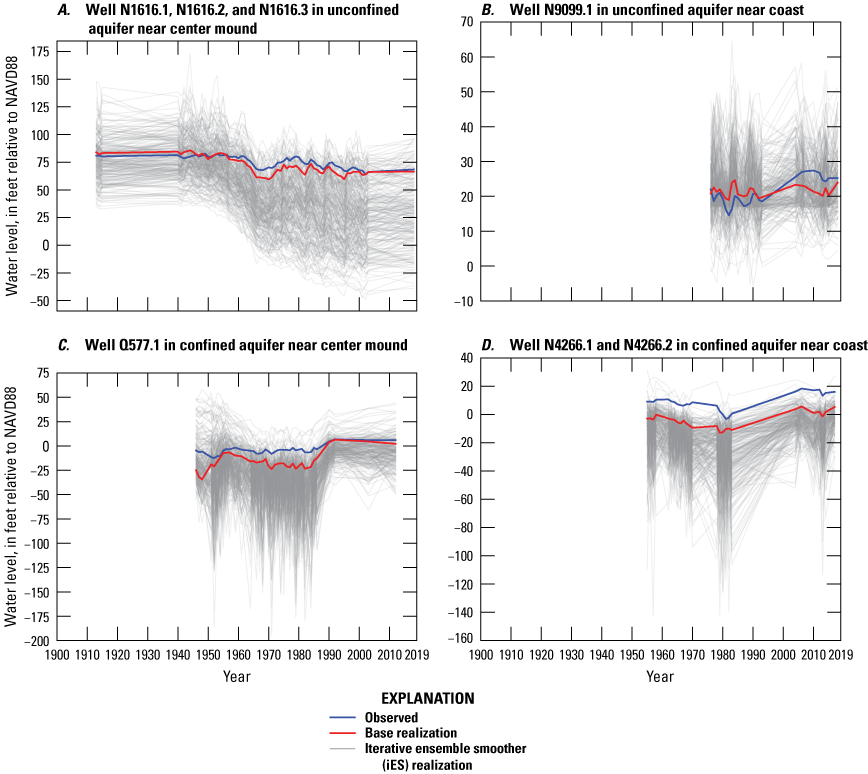
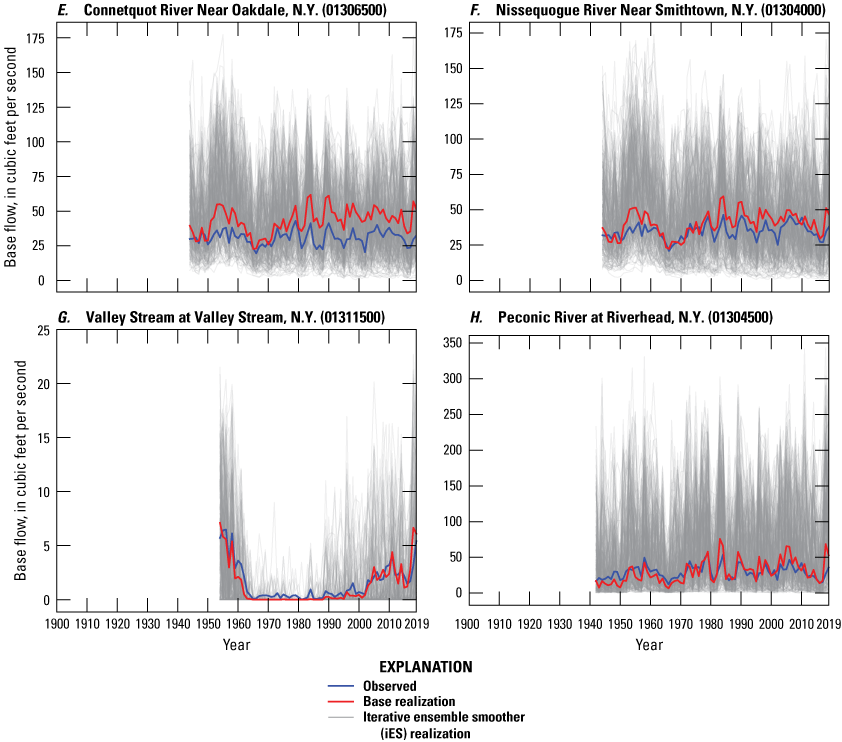
Graphs showing prior realizations for water-level observations at groundwater observation wells A, N1616 (in unconfined aquifer near center mound); B, N9099 (in unconfined aquifer near coast); C, Q577 (in confined aquifer near center mound); and D, N4266 (in confined aquifer near coast) and streamflow observations at E, Connetquot River near Oakdale, New York (station 01306500); F, Nissequogue River Near Smithtown, N.Y. (station 01304000); G, Valley Stream at Valley Stream, N.Y. (station 01311500); and H, Peconic River at Riverhead, N.Y. (station 01304500) U.S. Geological Survey streamgages for Long Island, New York. Data are from U.S. Geological Survey (2020b) and New York State Department of Environmental Conservation (2024). Locations shown on figure 39. NAVD88, North American Vertical Datum of 1988.
Estimation of Optimal Parameters Using Iterative Ensemble Smoother
The iES method of model calibration and history matching implemented in PEST++ for groundwater-flow models is documented in Corson-Dosch and others (2022) and Fienen and others (2022a, b). The initial observation weighting assumptions described in the “Observations” section of this report are qualitative and result in an imbalanced objective function (referred to as PHI), which is the squared sum of residuals between observations and simulated equivalents, each multiplied by their weight. An imbalanced PHI is the result of the disproportionate contribution of some observation, such as minor streamflow observations in this case to the objective function (fig. 32A). For iES, these initial weights were rebalanced using a relative-weighting scheme whereby the assigned weights reflected the identified importance of individual observation groups for estimating parameters. The weights were expressed as the fraction of the initial objective function contributed by residuals for that group of observations. The subjectively determined reasonable balance of the objective function was as follows: 30 percent for major streamflows, 22 percent for water levels in the unconfined aquifers, 19 percent to water level annual differences, 10 percent for the critical water levels near the unconfined groundwater mounds, 10 percent for minor streamflows, 8 percent for water levels in the Lloyd aquifer, and 1 percent for the automatic flow reduction synthetic observations (fig. 32B).
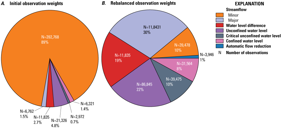
Graphs showing A, initial weights-based observation uncertainty and B, rebalanced weights used for calibration of the transient groundwater-flow model of the aquifer system underlying Long Island, New York. Data are from U.S. Geological Survey (2020b). The objective function (PHI) is defined in equation 2 of this report.
The iES technique builds on the Monte Carlo approach by evaluating an ensemble of parameter values, resulting in a residual vector and weighted objective function for each member of the parameter ensemble. From this information, the algorithm calculates an updated ensemble of parameter values to evaluate, and then, update iterations are performed, with each iteration yielding an ensemble of PHI values, further constraining the distribution sampled to generate the parameter ensemble (fig. 33). After enough iterations (different for each modeling application), both the PHI and parameter ensemble collapse into a small range of possible values, and the parameter ensemble no longer carries any meaningful information about model prediction uncertainty.
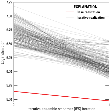
Graph showing changes in objective function (PHI) for successive parameter estimation iterations during calibration of the transient groundwater-flow model of the aquifer system underlying Long Island, New York. Data are from U.S. Geological Survey (2020b).
The base realization in this model calibration had the best (lowest) PHI value of all the realizations in both the prior (zeroth) and posterior (first) iES ensembles (fig. 33). The first iES iteration is considered to be optimal based on a subjective judgement that the objective function for the base realization had only lowered a small amount while retaining a substantially lower objective function than other realizations in the ensemble. The consistent superiority of the base over the whole ensemble and the relatively modest improvement of the objective function are expected given the substantial effort made to adjust the prior parameter ensemble during the trial-and-error process. The base realization residuals generally improved through the iES parameter update, as indicated by annual mean residuals (fig. 34). For water levels, posterior mean annual residuals were typically closer to 0 and had a narrower standard deviation than the prior mean annual residuals (fig. 34A). The most significant exception to this were water-level residuals between 1910 and 1920. Mean annual stream baseflow residuals moved much closer to 0 between the prior and posterior iES ensembles, especially after 1980, and with much narrower standard deviations (fig. 34B).
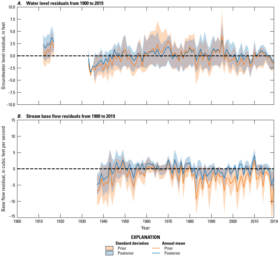
Graphs showing annual prior and posterior residuals for A, groundwater level and B, baseflows from 1900 to 2019 in the transient groundwater-flow model of the aquifer system underlying Long Island, New York. Data are from U.S. Geological Survey (2020b) and New York State Department of Environmental Conservation (2024).
Conditioned Model
The estimation of optimal parameters by use of inverse methods can result in model inputs that are outside of what is considered a reasonable range of values based on prior knowledge. Also, gaps in knowledge and structural error in the model can result in local fits that can be improved beyond that achieved through parameter estimation. The base realization from the iES was conditioned manually based on expert judgement to account for local misfits between observations and simulated equivalents and to ensure that final parameters were not outside acceptable ranges based on previous investigations and prior knowledge. A subset of horizontal hydraulic conductivity and recharge multipliers was adjusted to improve fit to the critical unconfined water-level observations group (table 4) that were not fully captured by iES. Vertical hydraulic conductivity multipliers in perched clay zones were decreased to 0.5 to increase simulated water levels to match high water-level observations in wells above or within the clays. Similar vertical hydraulic conductivity reductions for perched clay zones were necessary to match the 2005–15 mean water levels for these wells in the steady-state regional groundwater-flow model (Walter and others, 2020). Furthermore, multipliers in recharge pilot point locations in central Nassau County (fig. 29) were increased by 10 percent from 1950 to 2010 to account for underprediction of water levels during that period. Similar increases in recharge pilot point multipliers were necessary in the steady-state regional model to compensate for the underprediction of water levels in central and northern Nassau County following inverse calibration (Walter and others, 2020).
Scaling parameters applied to the natural and anthropogenic recharge arrays were truncated to an assumed maximum acceptable value to ensure that total recharge was considered reasonable in each cell of the model. Natural recharge was truncated in each cell using a maximum allowable recharge rate of 60 percent of precipitation to that cell. Rejected recharge was allowed to be as high as 100 percent of estimated potential rejected recharge from rerouting of overland runoff to retention and recharge basins. Recharge from wastewater in unsewered areas had a maximum allowable rate of 90 percent of the total potential wastewater in each cell; the maximum allowable wastewater recharge in sewered areas was 20 percent of the total available wastewater. Recharge from leaky infrastructure in each model cell was allowed to be as high as 20 percent of total estimated water use in the cell.
Truncation of natural recharge arrays resulted in reduced mean annual natural recharge rates throughout the period from 1900 to 2019, with slightly greater reductions on average after 1970 (fig. 35). Truncation of the anthropogenic recharge arrays also resulted in reduced mean annual recharge rates throughout the simulation period, with substantially larger reductions after 1960. These larger post-1960s reductions were predominantly due to truncation of return flow recharge, which scales with population and thus was more likely to be truncated later in the simulation period when the Long Island population was highest.
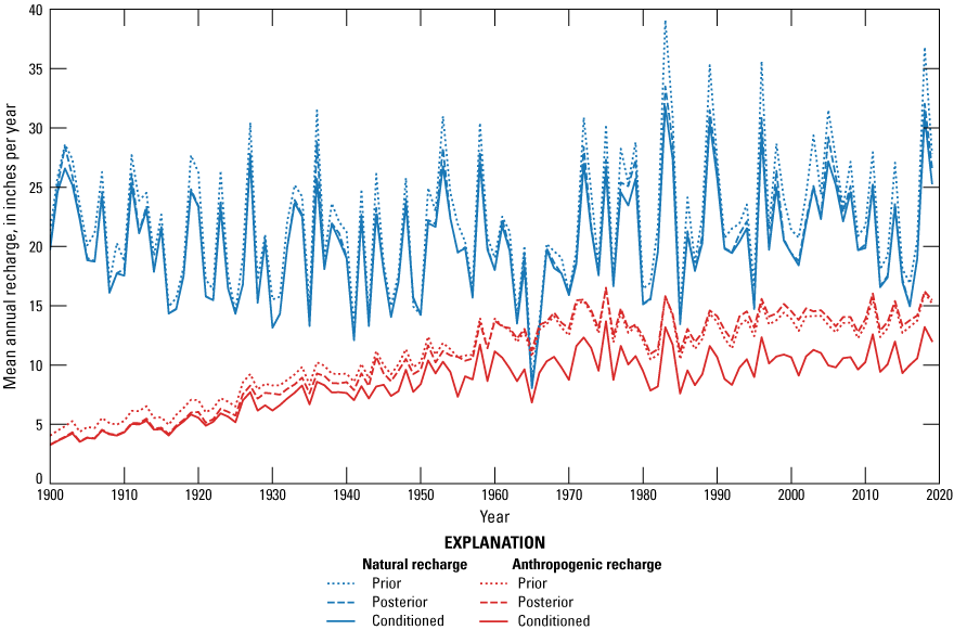
Graph showing prior, posterior, and conditioned natural and anthropogenic recharge from 1900 to 2019 simulated in the transient groundwater-flow model of the aquifer system underlying Long Island, New York. Data are from U.S. Geological Survey (2020b) and New York State Department of Environmental Conservation (2024).
Conditioning of the model parameters resulted in a PHI to 279,406, which was comparable to the posterior PHI of 297,919. The conditioning also yielded general spatial patterns, as shown by the difference between the posterior base realization model and the conditioned model. Conditioning resulted in generally higher water levels, up to 3 ft, in central Nassau County (fig. 36). Water levels generally were lower in western and central Suffolk County; the change in these areas generally was less than 2 ft. The changes in the water table that exceeded 5 ft were in areas with perched clays in several localized areas of the northern shore of Nassau County and northwestern parts of Suffolk County.
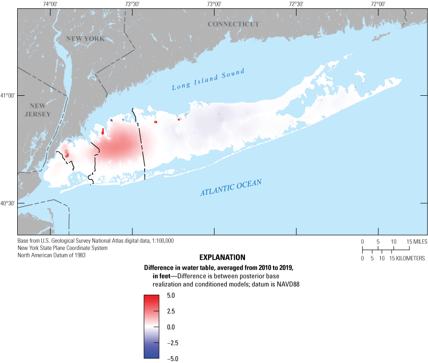
Map showing difference in mean water table, averaged from 2010 to 2019, between the posterior base realization model and conditioned model based on the transient groundwater-flow model of the aquifer system underlying Long Island, New York.
Conditioned Model Fit
The accuracy and precision of the model are indicators of the suitability of the model to represent historical conditions on Long Island and to predict future changes in hydrologic conditions in response to changes in hydrologic stresses, including natural and anthropogenic recharge, pumping, and sea-level rise. Observations of water levels and streamflows from 1900 to 2019 were compared to their simulated equivalents to evaluate if the model adequately represented historical hydrologic conditions. Vertical profiles of simulated chloride concentrations were compared to those estimated from electromagnetic measurements from available geophysical logs to determine the ability of the model to represent the current [2019] position of the freshwater/saltwater interface.
Water Levels and Streamflows
A comparison between observed water levels and streamflows and their simulated equivalents from the conditioned model indicated that the model reasonably matched observed hydrologic conditions (fig. 37). Water level differences generally plotted within ±5 ft of the 1:1 line, with only a few outliers having greater residuals (fig. 37A). Water level targets in the unconfined aquifers mostly plotted on or near the 1:1 line, with only a small group of outliers plotting well above the line (fig. 37B). Water level targets in the Lloyd aquifer mostly plotted on or near the 1:1 line, with some high measured values showing a strong underestimated bias (simulated equivalents are lower than observed values; fig. 37C). Water level targets in the unconfined aquifer near the central mound mostly plotted just below the 1:1 line, indicating a groupwide underestimated bias (fig. 37D). The minor stream targets generally plotted on or near the 1:1 line, with a slight overestimated bias as measured values increase (simulated equivalents are lower than observed values; fig. 37E). The minor stream targets generally plotted near the 1:1 line, with generally less bias than major streams (fig. 37F).
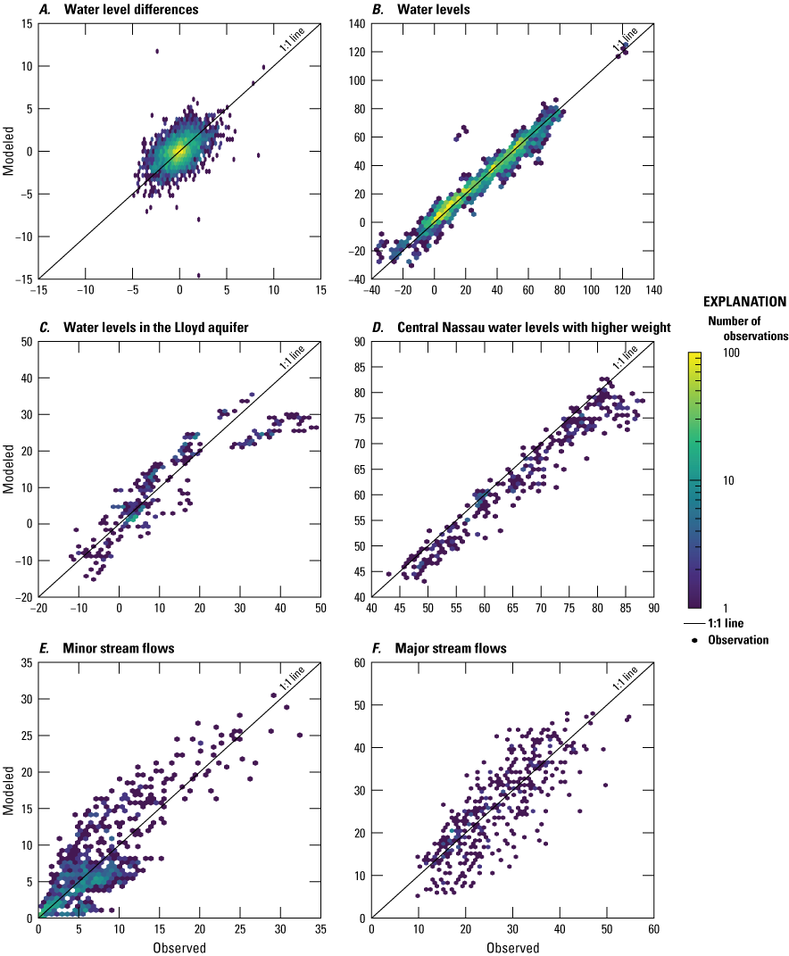
Graphs showing correspondence between observations and conditioned model simulated equivalents for A, water level differences, B, water levels, C, water levels in the Lloyd aquifer, D, water levels in central Nassau County, and flow in E, minor and F, major streams the transient groundwater-flow model of the aquifer system underlying Long Island, New York.
Generally, the mean residuals show a spatial mixture of both positive and negative values; a pattern that is the desired outcome from history matching and indicates that the results are generally unbiased (fig. 38). However, there are some consistent spatial patterns (clusters of observations are either greater or less than their simulated equivalents) that could indicate a small amount of structural error with the model (missing pumping or inaccurate pumping rates) or with the estimated hydraulic parameters in some areas. There are localized clusters of higher (overprediction) and lower (underprediction) simulated groundwater altitudes in the westernmost part of the island, in Kings County, than in the other parts of the island. This is likely caused by uncertainty in the simulated pre-1950 pumping rates from gaps in available historical water-use data. The model also overpredicted water levels in some locations where it is likely that local pumping was missing from the simulation. This can result in an anomalous overprediction of water levels at an individual observation that is surrounded by observations with substantially better fits, such as near well N6315 in central Nassau County (fig. 38B).
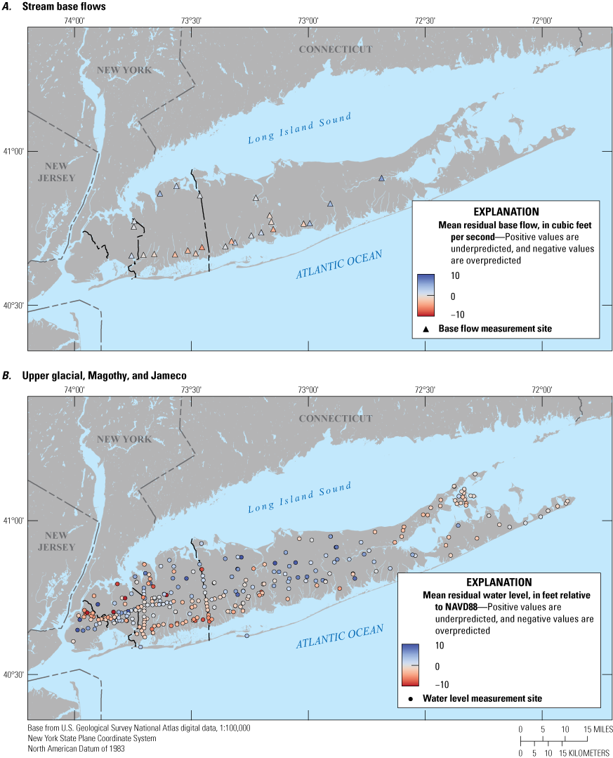
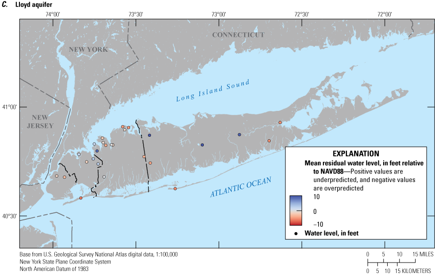
Maps showing absolute mean residuals for A, stream baseflows, B, water levels in the upper glacial, Magothy and Jameco aquifers, and C, water levels in the Lloyd aquifer in the transient groundwater-flow model of the aquifer system underlying Long Island, New York. NAVD88, North American Vertical Datum of 1988.
There is a consistent pattern of overprediction of water levels in unconfined aquifer wells and, to a lesser extent, streamflows along the southern shore in western and central parts of the island (fig. 38A–B). These wells and streams are strongly influenced by shoreline boundary conditions, and the regional representation of those boundaries in the model may not capture local shoreline complexity. This also is likely the case for the pattern of overprediction of unconfined water levels on the North and South Forks, which also are strongly influenced by the surrounding ocean boundary conditions.
Observation wells in the east-central part of the island show a pattern of underprediction in both unconfined and confined aquifers, indicating that a combination of higher recharge and higher vertical hydraulic conductivity values in the Raritan confining unit are necessary in this area to increase water levels above and below the Raritan confining unit (fig. 38B). This combination could be difficult to achieve given the assumptions on the upper acceptable constraints on total recharge, which resulted in truncated recharge rates in the conditioned model. Lower vertical hydraulic conductivity values in the Raritan confining unit would be needed to produce higher unconfined water levels, which directly conflicts with the higher vertical hydraulic conductivity values in the Raritan confining unit needed to produce higher confined heads in the Lloyd aquifer. This apparent contradiction suggests that observations in the confined and unconfined parts of the system are in conflict and that undefined heterogenies may be present in the lower Raritan confining unit in eastern Long Island.
Water-level and streamflow residuals generally vary randomly with little temporal bias (fig. 34). The exception is the consistently larger residuals seen in the early part of 20th century (before about 1950). This likely is due to the greater uncertainty in prior knowledge of pumping stresses and model inputs in the early part of the simulation period.
Chloride Concentrations
Chloride concentration profiles at monitoring wells and patterns in historical pumping well withdrawal rates indicative of a saltwater intrusion response were evaluated to confirm that the conditioned model adequately represented the dynamics of saltwater/freshwater interface movement from 1900 to 2019. The model simulation of the study period from 1900 to 2019 indicated extensive saltwater intrusion in the unconfined Magothy aquifer in Kings County where the unconfined aquifer system is fully intruded along the southern shore of the county and partially intruded well inland (fig. 39A). The Magothy aquifer also is fully intruded near Jamaica Bay in southern Queens County and partially intruded in southwestern Nassau County (fig. 39). This present-day inland presence of saline groundwater (Stumm and others, 2024) is a result of previous large-scale historical pumping, and subsequent intrusion (fig. 7; Buxton and Shernoff, 1999), and the low aquifer recharge rates in urbanized areas that have not yet flushed saltwater from the aquifer (fig. 15). There is also saltwater intrusion along parts of the northern shore of Nassau County. The simulated pattern of saltwater intrusion in western Long Island generally agrees with the mapped distribution of saltwater presented in Stumm and others (2024). Freshwater parts of the Magothy aquifer in eastern in Suffolk County are underlain by a natural saltwater interface that represents a density driven balance between freshwater from recharge and the surrounding saltwater (fig. 39A).
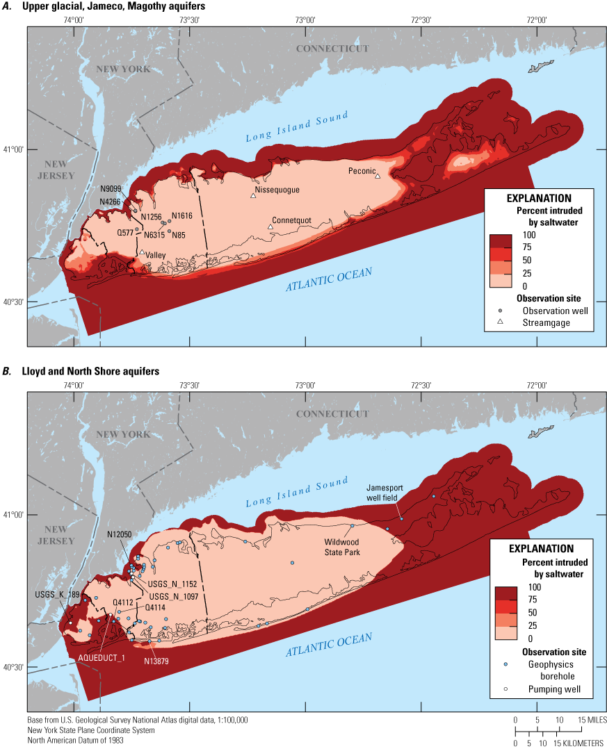
Maps showing simulated percent aquifer saltwater intrusion and location of electromagnetic conductivity logs in A, the upper glacial, Jameco, and Magothy aquifers and B, the Lloyd and North Shore aquifers in the transient groundwater-flow model of the aquifer system underlying Long Island, New York.
Model simulations also indicated saltwater intrusion in the confined Lloyd aquifer throughout most of Kings County, southern Queens County (near Jamaica Bay), and parts of the northern shore of Queens and Nassau Counties (fig. 39B). The Lloyd aquifer is fully intruded along Jamaica Bay and along the northwestern shore of Kings County. These areas are near inactive pumping centers that withdrew water from the Lloyd aquifer that later were abandoned in the early and middle 20th century due to increased chloride concentrations (fig. 7A–C). The Lloyd aquifer is naturally saline in eastern parts of Suffolk County beneath the North and South Forks (fig. 39B). The simulated patterns of saltwater intrusion in the Lloyd aquifer in Kings and Queens Counties are in general agreement with the observed current [2022] and historical chloride concentrations mapped for those areas (Stumm and others, 2024).
Vertical patterns of simulated chloride concentrations generally are in agreement with chloride concentrations estimated from electromagnetic borehole logging, as indicated by uncertainty bands and generally similar profile shapes (fig. 40). The uncertainty bounds on the geophysics-estimated chloride profiles (expressed as 95-percent prediction intervals) and the uncertainly bounds on the simulated chloride profiles (as expressed as the range of values in the model cell containing the well and the eight surrounding cells) generally overlap for nearly all model layers. The upper part of the profile for well N13879.1 is an exception to the general agreement between the model and the geophysics (fig. 40). This borehole was drilled approximately 500 ft from the shoreline in Long Beach (fig. 39), so the high chloride concentrations in the electromagnetic conductivity log in the upper Magothy aquifer are most likely due to localized saltwater overwash from coastal storms that is not accounted for in the groundwater model.
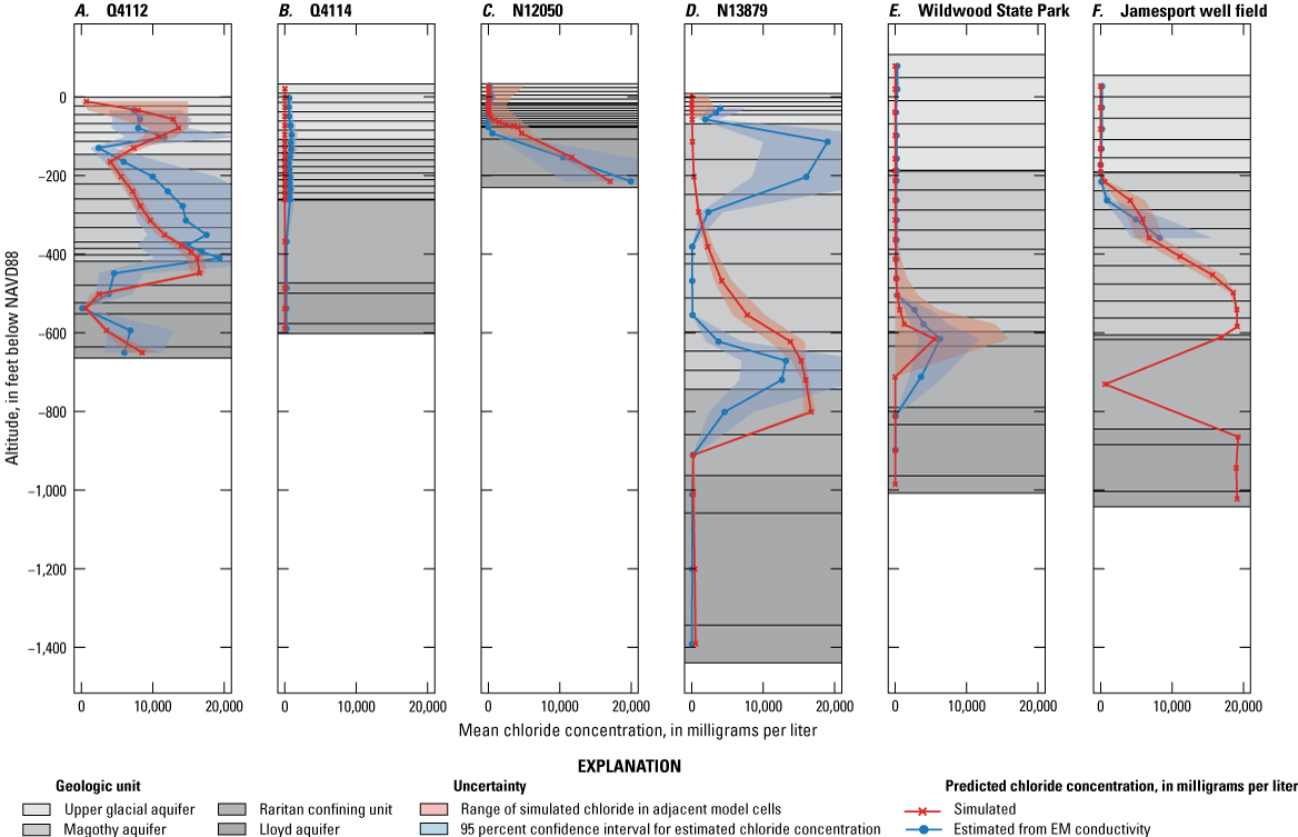
Graphs showing comparison of chloride concentration profiles estimated from electromagnetic conductivity logs and simulated chloride concentration profiles at six select sites in the regional groundwater-flow model of the Long Island aquifer system for Long Island, New York. A, Well Q4112 in Queens County; B, well Q4114 in Queens County; C, well N12050 in Nassau County; D, well N13879 in Nassau County; E, geophysics borehole at Wildwood State Park in Suffolk County; and F, geophysics borehole at Jamesport well field in Suffolk County. Data are from U.S. Geological Survey (2020b). NAVD88, North American Vertical Datum of 1988; EM, electromagnetic.
Saltwater intrusion into the aquifers from large-scale pumping resulted in the abandonment of many production wells in Kings, Queens, and Nassau Counties between the late-1940s and mid-1980s (Buxton and Shernoff, 1999). The pumping history of these wells can be used as qualitative indicators of changing chloride concentrations at the well location and serve as a qualitative verification of model-predicted chloride concentrations (fig. 41). Reported withdrawal rates in a set of abandoned wells indicated either decreases in withdrawals or a total cessation of pumping that coincided with increases in simulated chloride concentrations. For example, pumping in well USGS_K_189 from the Lloyd aquifer in Kings County decreased steadily starting in the late 1920s; simulated chloride steadily increased starting about 1920 to a maximum simulated chloride concentration of more than 17,000 mg/L in the early 1940s (fig. 41A). The simulated chloride concentration at a well withdrawing water from the upper Magothy aquifer in Queens County showed a similar pattern, with a cessation of pumping in about 1950 following an increase in simulated chloride concentrations (fig. 41B). Pumping in two abandoned wells in Nassau County decreased or ceased in the late 1990s following large increases in simulated chloride concentrations (fig. 41C–D)
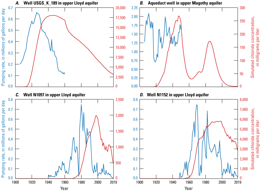
Graphs showing time series of historical pumping rates and simulated chloride concentrations at selected sites in the transient groundwater-flow model of the aquifer system underlying Long Island, New York. Data are from U.S. Geological Survey (2020b) and New York State Department of Environmental Conservation (2024).
The comparisons of pumping histories and changes in simulated chloride concentrations showed that concentrations decreased following the cessation of pumping, indicating that the model represented the effects of natural flushing of the aquifer from recharge. The confined Lloyd aquifer likely flushed slowly owing to the small amount of recharge to the aquifer. Chloride concentrations in well USGS_K_189 increased starting in the mid-1910s and exceeded 2,500 mg/L by 1920; the concentration still exceeded 2,500 mg/L in 2019 (fig. 41A). This is consistent with the presence of chloride in the Lloyd aquifer in New York City several decades after cessation of groundwater withdrawals from the Lloyd aquifer (Stumm and others, 2024). The response of chloride concentrations to time-varying pumping likely was more dynamic in the unconfined aquifers. Simulated concentrations decreased relatively quickly following cessation of pumping in the unconfined upper Magothy in Queens County by about 1950 (fig. 41B). There also was a later increase and subsequent decrease between about 1970 and 1990, likely because of a more regional response to pumping elsewhere in the aquifer.
Model Limitations and Uncertainty
The use of numerical models to simulate complex regional groundwater flow systems, such as the Long Island aquifer system, has inherent limitations; however, a proper model design to address scale-appropriate questions can help minimize these limitations. Some of the primary limitations of a numerical model include (1) the simplifying assumptions inherent in the conceptual model underlying the numerical model, (2) model discretization and the representation of hydrologic boundaries, (3) representation of hydraulic stresses and intrinsic aquifer properties, and (4) the accuracy of aquifer properties estimated from the data-driven model calibration.
The Long Island groundwater model is a simplification of a very complex natural system. The model integrates large amounts of spatially varying information about the groundwater system, including geologic framework and stream-network geometries, subsurface hydraulic properties, and measurements of water levels, streamflows, and chloride concentrations. Considerable efforts have been made into developing methods for quantifying model prediction uncertainty stemming from model parameters and observation data, but it is more difficult to quantify uncertainty related to structural error (Doherty and Welter, 2010). Structural error can be caused by unavoidable oversimplification of the natural system, such as consolidating complex hydrostratigraphic units into model layers or by insufficient information, such as missing pumping well data, both of which can limit the model’s ability to accurately represent real-world conditions. The effects of structural error caused by a complex hydrogeologic framework were mitigated by applying a highly parameterized approach to model construction and history matching, using zonal, pilot-point, and cell-specific multipliers to adjust model properties with as much flexibility as was determined appropriate. Despite the limitations inherent in numerical models, the Long Island regional model provides a useful and effective tool for investigating questions related to the regional flow system and resource management.
Discretization
The discretization of a model is determined to be the minimum cell size needed to reasonably represent the hydrologic system at a spatial scale appropriate for the analysis while maintaining a tractable model size given available computational resources. The model discretizes the groundwater-flow system into a grid consisting of cells that are 500 ft on a side and a thickness between 1 and 400 ft. Values in these model cells represent averages of the respective cell volumes. Similarly, simulated outputs from each cell represent average conditions within that cell. This averaging effect within the model cell can limit the ability to accurately represent local-scale stresses and observations at small scales.
Hydrologic features, including pumping wells and surface-waters, are often much smaller as compared to the discretization of the model. In the model, pumping wells are small features that are averaged over regional-scale model cells. Likewise, streams on Long Island generally are much narrower than the horizontal discretization of the model. The observations used to calibrate and verify the model also are averaged over the regional-scale model cells and variability at scales smaller than the discretization is not accounted for. Furthermore, temporal averaging of stresses into annual means further reduces the variability that can be accounted for by the model.
The broadly mapped zonation used to develop the hydrogeologic framework also limits the ability to represent local-scale heterogeneities that are likely present, but poorly understood, within geologic units. The use of highly parameterized, data-driven parameter estimation with pilot points allows for reasonable approximation of heterogeneities and gradational hydraulic conductivity fields.
Model discretization also affects the simulation of chloride concentrations. The use of the finite-difference methods in advection-dominated systems, such as is used in this model, can result in numerical dispersion (Fletcher, 1991), which tends to smear concentration fronts, limiting the ability to represent sharp concentration fronts near pumping centers. Numerical dispersion is a function of model discretization, velocity, and time-step length and is more substantial in regional-scale models; however, inspection of model results, including spatially mapped chloride and time-varying concentrations, indicates that the Long Island regional model can adequately represent thin zones of dispersion, and that numerical dispersion may reasonably approximate actual dispersion of the chloride front in this aquifer system.
Uncertainty in Model Parameters and Inputs
The iES updates are a function of the relative weights of the hydrologic observations, which are subjective and reflect the assumed relative importance of different types of observations to model predictions. Long-term streamflow observations were assumed to be better indicators of long-term hydrologic conditions and were given higher weights than observations of water levels. Changing the relative weights of the hydrologic observations would result in a different set of parameter ensembles and model inputs and could result in different model predictions. Even though the calibrated model has a degree of misfit (or error) that varies spatially, the model produced simulated water levels and streamflows that generally were in good agreement to observed values. The degree of misfit contributes to model-prediction uncertainty, which would be expected to be higher in areas of greater misfit or in areas with fewer weighted observations.
The most reliable initial aquifer properties and weighted water-level observations are within the upper glacial aquifer and within the Magothy and contiguous aquifers, which are the region’s principal aquifers and of particular concern to regulators and water purveyors. Fewer data are available in the underlying Raritan confining unit and Lloyd aquifers.
The Raritan confining unit is an important hydrogeologic control on deep groundwater flow and the position and movement of the freshwater/saltwater interface in the underlying Lloyd aquifer. However, few data are available on the surface altitude, thickness, and hydraulic characteristics of the Raritan confining unit, particularly in the central and eastern parts of Long Island. Representation of the Raritan confining unit in the model is generally based on available information regarding the hydraulic properties, geometry, and extent of the unit. The Raritan confining unit is assumed to be continuous across most of Long Island and absent only along the northern shore of the island, based on the data that are available. Although the model is in general agreement with water levels in the confined aquifer, discontinuities may exist in the unit that could affect water levels and the saltwater interface.
Wells Q577 and N4266 screened in the confining unit exhibit the greatest ensemble density well below the observed values, with the most extreme realizations simulating water-level altitudes several tens of feet below the central tendency (fig. 42). The main control on the simulated confined water-level altitudes is the hydraulic conductivity of the Raritan confining unit and the Lloyd aquifers, and yet the ranges and spatial distributions are poorly defined compared with the hydraulic conductivity in the unconfined aquifers. The posterior ensemble tendency toward substantially underpredicting the confined water levels indicates potential structural issues with the existing conceptual model and parameterization scheme for portions of the Raritan and Lloyd aquifers. Additional data are required to improve conceptualization of those aquifer units to improve this possible structural issue. Changing the representation (thickness, continuity, and hydraulic conductivity) of the Raritan confining unit could affect hydrologic predictions, including the degree of confinement and position of the freshwater/saltwater interface in the Lloyd aquifer along the southern shore of the island and the area contributing recharge to the Lloyd aquifer.
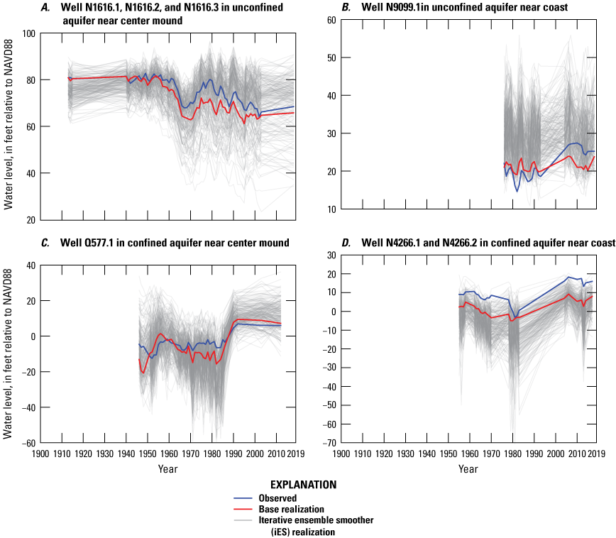
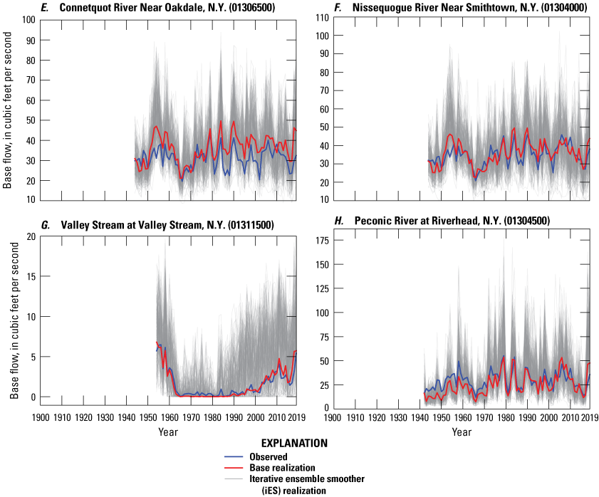
Graphs showing posterior ensemble of simulated water levels in wells A, N1616 (in unconfined aquifer near center mound); B, N9099 (in unconfined aquifer near coast); C, Q577 (in confined aquifer near center mound); and D, N4266 (in confined aquifer near coast), and base flows at E, Connetquot River near Oakdale, New York (station 01306500); F, Nissequogue River Near Smithtown, N.Y. (station 01304000); G, Valley Stream at Valley Stream, N.Y. (station 01311500); and H Peconic River at Riverhead, N.Y. (station 01304500) U.S. Geological Survey streamgages in the transient groundwater-flow model of the aquifer system underlying Long Island, New York.
The base realizations for flows in major streams generally are in good agreement, but there is a large range in the posterior ensembles (fig. 42E–H), particularly during periods of high flow. Streamflows broadly integrate hydrologic conditions and are highly sensitive to several model inputs. This results in the large uncertainty and the broad range of realizations seen in the posterior ensembles.
Distributions of the posterior ensemble results for select water levels show how model uncertainty varies depending on hydrologic setting (fig. 43). The spread of the distributions (summarized by the median and 5th and 95th percentiles) is representative of the relative uncertainty under each condition type. There is less uncertainty in confined (fig. 43C and D) than unconfined (fig. 43A and B) conditions, which points to the reduced effect that recharge variability has on the confined system relative to the unconfined. Additionally, there is less uncertainty in unconfined water levels near surface water boundaries (fig. 43B) where head-dependent boundary conditions constrain water levels in the adjacent aquifer than unconfined water levels near the center of the groundwater mound (fig. 43A). This is consistent with the inherent uncertainty in recharge estimates that is more pronounced at the mound and the stabilizing effect of the boundary conditions on uncertainty near the coast.
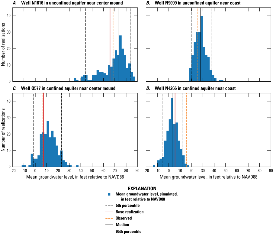
Histograms of ensemble mean simulated water levels from 2010 to 2019 for wells A, N1616, B, N9099, C, Q577, and D, N4266 in the transient groundwater-flow model of the aquifer system underlying Long Island, New York. NAVD88, North American Vertical Datum of 1988.
Data Gaps
The model incorporates pumping well withdrawal data from available records that extend from 2019 back to the early 1900s. The older records have an inherent uncertainty with regards to both withdrawal rates and the exact location and depth of pumping. The effects of this uncertainty are exhibited in certain observation wells with anomalously negative residuals, indicating that simulated water levels were overpredicted compared with nearby wells. Well N6315 in central Nassau (fig. 38) has simulated water levels that are similar to those at nearby wells (within 1 to 2 mi; fig. 44). These nearby wells have a relatively good fit to observed water levels, but the well N6315 observations in the 1960s are nearly 40 ft lower than the simulated levels (fig. 44). Such extreme negative residuals surrounded by relatively small residuals can potentially be accounted for by missing withdrawals in the historical pumping record. Withdrawal record uncertainties could be reduced by continued examination of historical archives, though this is ultimately limited by the quality of historical recordkeeping and archiving. Another solution for reducing withdrawal uncertainty would be to add synthetic pumping wells based on anomalously negative water-level residuals and giving those pumping well parameters large potential bounds that can be explored and constrained through iES.
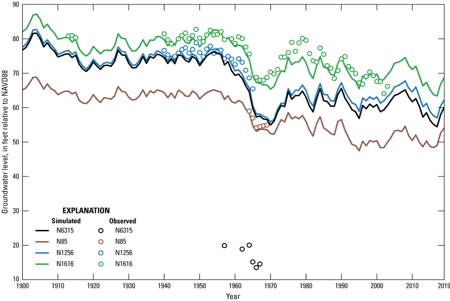
Graph showing groundwater level time series in well N6315, which has anomalous poor fit compared with nearby wells N85, N1256, and N1616 in the transient groundwater-flow model of the aquifer system underlying Long Island, New York. NAVD88, North American Vertical Datum of 1988.
Simulation of Hydrologic Conditions From 1900 To 2019
The Long Island aquifer system is hydrogeologically complex and is highly perturbed by land use changes, groundwater withdrawals, and anthropogenic recharge. Hydrologic conditions, including water levels, streamflows, and the distribution of saltwater in the aquifer, are dynamic and change in response to complex interactions between natural recharge and anthropogenic stresses on the system. The conditioned transient, regional groundwater model of Long Island was used to simulate hydrologic conditions from 1900 to 2019 to ensure that the model can adequately reproduce the aquifer system response to large changes in pumping and recharge during that time. These changes include the large-scale increase and subsequent decrease in pumping in Kings and Queens Counties in the early and mid-20th century, increases in pumping in Nassau and Suffolk Counites since the mid-20th century, and the islandwide response to the 1960s drought of record.
The simulation period from 1900 to 2019 was needed for the analysis of changes in the position and movement of the freshwater/saltwater interface and to ensure that the model will be suitable for representing hypothetical changes in future pumping and recharge conditions. Simulation of historical hydrologic conditions (hydrologic budgets, water levels, streamflows, and the position and movement of the freshwater/saltwater interface) provides the information needed to understand the dynamics of Long Island’s complex and highly perturbed aquifer system. Further, this understanding can assist water-resources managers in evaluating the response of the hydrologic system to hypothetical changes in natural and anthropogenic stresses.
Hydrologic Budgets
The hydrologic budget of an aquifer system refers to the balance between inflows into the aquifer system and outflows from the aquifer system. Recharge from precipitation is the only natural inflow of water into the Long Island aquifer system. Natural outflows from the system include groundwater discharge to freshwater streams and to coastal waters. An additional outflow from the system is groundwater withdrawn from pumped wells; much of this water is returned to the aquifer as anthropogenic recharge. Total recharge includes both natural and anthropogenic recharge. The only component of inflow to the aquifer system from off the island is anthropogenic recharge in Brooklyn and Queens Counties, which is from leaky infrastructure in areas that receive water imported from reservoirs in upstate New York. Storage is an additional component of the hydrologic budget and refers to the internal transfer of water into or out of the compressible aquifer matrix. Water moves into storage (from the aquifer) during wet periods, and storage is considered an outflow from the aquifer. Water moves out of storage and into the aquifer during dry periods and is considered an inflow to the aquifer.
The hydrologic budget of the Long Island aquifer system is dynamic and changes continually during time in response to natural and anthropogenic stresses (fig. 45). From 1900 to 2019, inflow from recharge varied annually with alternating wet and dry periods; 1965 and 1983 were the driest and wettest years, respectively. Recharge generally trended higher after about 1970. Groundwater discharge into coastal waters was the largest component of outflow, followed by discharge to freshwater streams. Outflow to wells increased steadily between 1900 and 2019. Storage was a small component of the budget during this period and alternated between outflow and inflow during wet and dry periods.
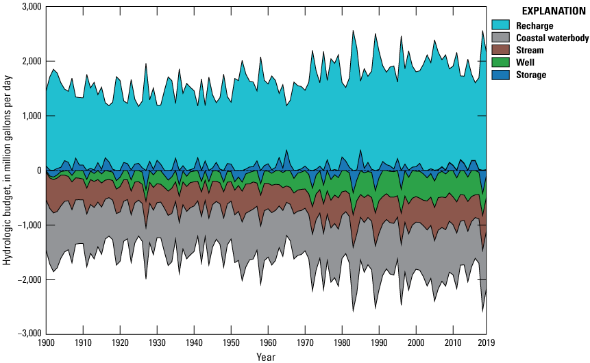
Graph showing changes in the hydrologic budget from 1900 to 2019 for Long Island, New York. Data are from U.S. Geological Survey (2020b).
Total inflow to the aquifer system in 1965, during a period of extended drought, was about 1,142 Mgal/d; about 71 percent from recharge and the remaining 29 percent was from water released from storage (table 5). In contrast, the total recharge to the aquifer system in 1983, one of the wettest years on record, was almost twice (1.9 times) the total recharge in 1965. The distribution of outflow to the receiving waters and pumping wells were similar during the 2 years, with the main difference being that, in 1983, about 14 percent of the total outflow was water going into aquifer storage, whereas in 1965 water was released from storage.
Table 5.
Summary of hydrologic budgets for 1900, 1965, 1983, 2019, and the 2010–19 average for Long Island, New York.[ft3/s, foot per second; —, no data; XX, not applicable]
Discharge to streams and urban drains as a percentage of total outflow was about 24 percent in both 1965 and 1983 (table 5) despite the fact that there was nearly twice the total outflow in 1983. Discharge to coastal waters was slightly higher as a percentage of the total outflow in 1965 (51 percent) compared with 1983 (46 percent). Groundwater withdrawals were a much higher percentage of the total outflow in 1965 (25 percent) compared with 1983 (16 percent) even though there was about 40 percent more pumping in 1983 compared with 1965.
Water Levels and Streamflows
The simulated water table for 2019 ranged from essentially 0 near the coast to more than 80 ft above NAVD88 in two water table mounds to the east and west of the major surface drainages in central Suffolk County (fig. 46A). Maximum water table altitudes in the eastern and western water table mounds on the mainland of Long Island were about 60 and 80 ft above NAVD88, respectively.
Locally, high water tables occur in the northern part of Nassau County and are associated with very low-transmissivity, possibly perched clays. The highest water table altitude of about 120 ft above NAVD88 occurs in the center of Manhasset Neck (fig. 46A). Nuclear magnetic resonance borehole logging in the area confirms that this local water table feature is in an area where the sediments are fully saturated.
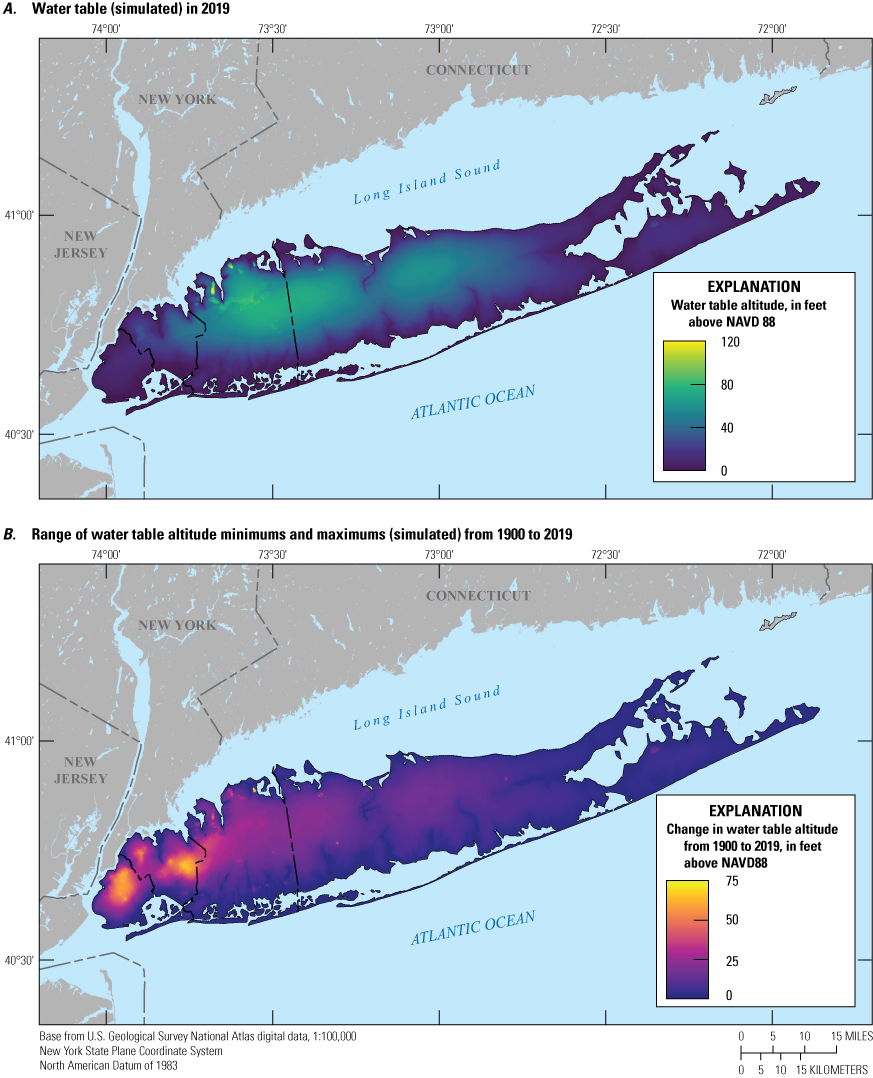
Map showing simulated A, water table in 2019 and B, range of minimum and maximum water table altitudes from 1900 to 2019 in the transient groundwater-flow model of the aquifer system underlying Long Island, New York.
The altitude of the water table changes in response to natural fluctuations in recharge and because of changes in groundwater withdrawals (fig. 46). The largest variability under natural conditions occurs near groundwater divides and areas of low hydraulic gradients, and the smallest variability is near the coast and streams and in high gradient areas where water levels are more constrained. Eastern parts of Suffolk County are the least perturbed areas on Long Island, and this pattern is evident there (fig. 46B). The range of water table altitudes in the center of the island is as high as 10 ft and is close to 0 ft along the coast.
The combination of changing natural and anthropogenic stresses has resulted in a large range of water table altitudes from 1900 to 2019 (fig. 46B). The largest range was in Kings and Queens Counties and is associated with areas with large historical groundwater withdrawals and cones of depression in the water table (fig. 7); water levels in this area have varied by more than 70 ft since 1900 (fig. 46B). The range of water table altitudes varied by more than 30 ft across large areas of central Nassau County. Locally, higher variability occurs near individual wells and in areas with low-transmissivity clays.
Water-level and streamflow variability differs between wells and stream sites (fig. 47). Water levels in well N1616 near the top of the western water table mound in the center of Nassau County varied by about 24 ft during the simulation period from 1900 to 2019; the drought of the mid-1960s is evident in the water levels (fig. 47A). By contrast, water levels in in well N9099 near the coast varied by about 7 ft (fig. 47B). The same pattern is seen in the confined Lloyd aquifer, though the variability of water levels may be large owing to the lower amount of storage in confined aquifers (fig. 47C and D), with larger variations in the center of the island and smaller variations near the coast.
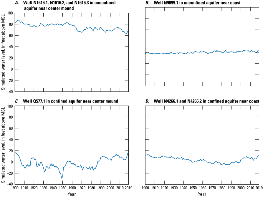
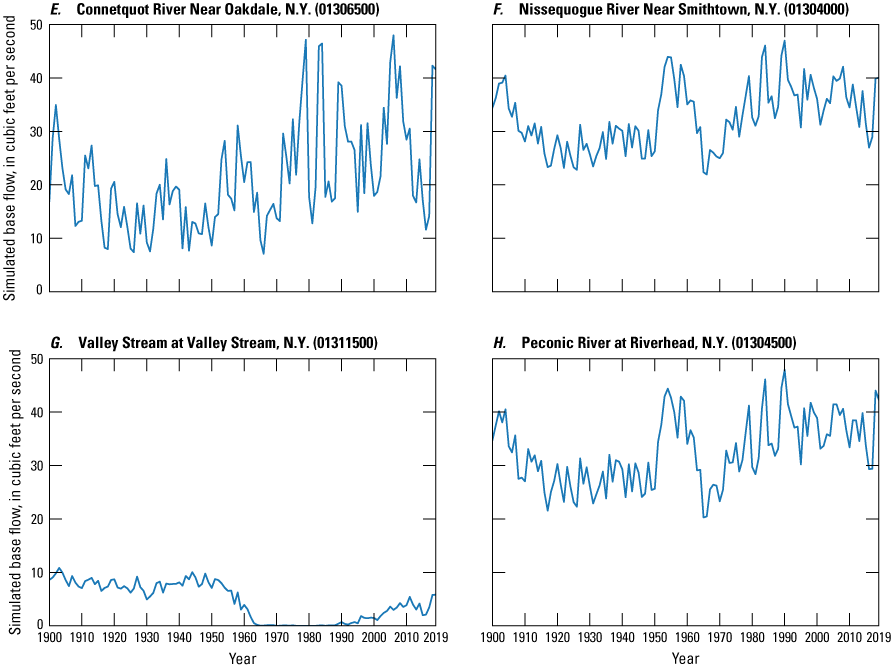
Graphs showing simulated time-varying, average annual A–D, water table altitudes in select hydrogeologic settings and E–H, baseflow at select stream sites from 1900 to 2019 in the transient groundwater-flow model of the aquifer system underlying Long Island, New York. NAVD88, North American Vertical Datum of 1988.
Water levels in the confined Lloyd aquifer in western Long Island also show large effects from groundwater withdrawals. Water levels in well Q577 varied by more than 45 ft (fig. 47C); water levels in the well were below sea level for most of the period before the early 1980s, which is likely attributed to pumping. The effects of natural stresses, such as the mid-1960s drought, are not readily apparent in this deep, confined aquifer; however, changes in pumping stress are much more pronounced, such as the more than 20-ft increase in water level following cessation of pumping in the early 1980s (fig. 47C). Water levels in the Lloyd aquifer near the coast (well N4266) show less variability than those inland near the groundwater mound; however, the variability exceeds 15 ft at well N4266 (fig. 47D), which is much larger than the variability seen in the unconfined Magothy aquifer at nearby well N9099 (fig. 47B). The water levels in well N4266 also are affected by pumping, as evidenced by the water levels below sea level between the mid-1960s and the late 1990s (fig. 47D).
Streams are surface features that are hydrologic expressions of the unconfined aquifer, and as a result, show more relative variability than do water levels in wells and are more closely correlated with recharge (fig. 47E–F); the amount of variation also is a function of hydrologic setting. Annual mean baseflow in the Peconic River in eastern Suffolk County varied by more than 40 ft3/s during the period, about twice the mean annual baseflow of 21 ft3/s, with large year-to-year variations (fig. 47E). Annual mean baseflow in the Nissequogue River in north-central Suffolk County varied by about 25 ft3/s during the same period, also with large year-to-year variations (fig. 47F). The Nissequogue River is between the regional east-west groundwater divide and the coast, in an area with generally steeper hydraulic gradients than the area near the Peconic River. As a result, there is more variability in baseflow in the Peconic River than the Nissequogue River; simulated flows in the Nissequogue and Peconic Rivers had coefficients of variation of 0.18 and 0.46, respectively. Temporal patterns in recharge are readily evident in streamflows, including the mid-1960s drought and periods of high recharge in the 1950s and early 1980s (fig. 47E–H).
Movement of the Freshwater/Saltwater Interface
The three-dimensional configuration of the freshwater/saltwater interface in the Long Island aquifer system has changed from 1900 to 2019, primarily from groundwater withdrawals in western Long Island. Since 1900, saltwater intrusion has occurred in both the unconfined and confined parts of the aquifer system in several areas on western Long Island because of groundwater withdrawals and the resulting depression of water levels. The transient regional model was used to simulate the movement of the freshwater/saltwater interface since 1900 and to define the current distribution of saltwater in the aquifer system in 2019. The current simulated interface was in generally good agreement with the interface as mapped from water quality and geophysical data (Stumm and others, 2024).
In 1900, saline groundwater with chloride concentrations exceeding 1,000 mg/L in the upper glacial aquifer generally was limited to a small area north of Jamaica Bay in Kings and Queens Counties (fig. 48A). In the early 20th century, the upper glacial aquifer was an important source of water in New York City, and large groundwater withdrawals caused saltwater intrusion and the abandonment of wells as early as the early 1930s (fig. 7). As of 2019, the upper glacial aquifer was intruded with saline groundwater well inland in Kings County (fig. 48B). The intrusion likely occurred in the early part of the 20th century but remained in the aquifer likely because of low recharge and groundwater flushing rates in this highly urbanized area.
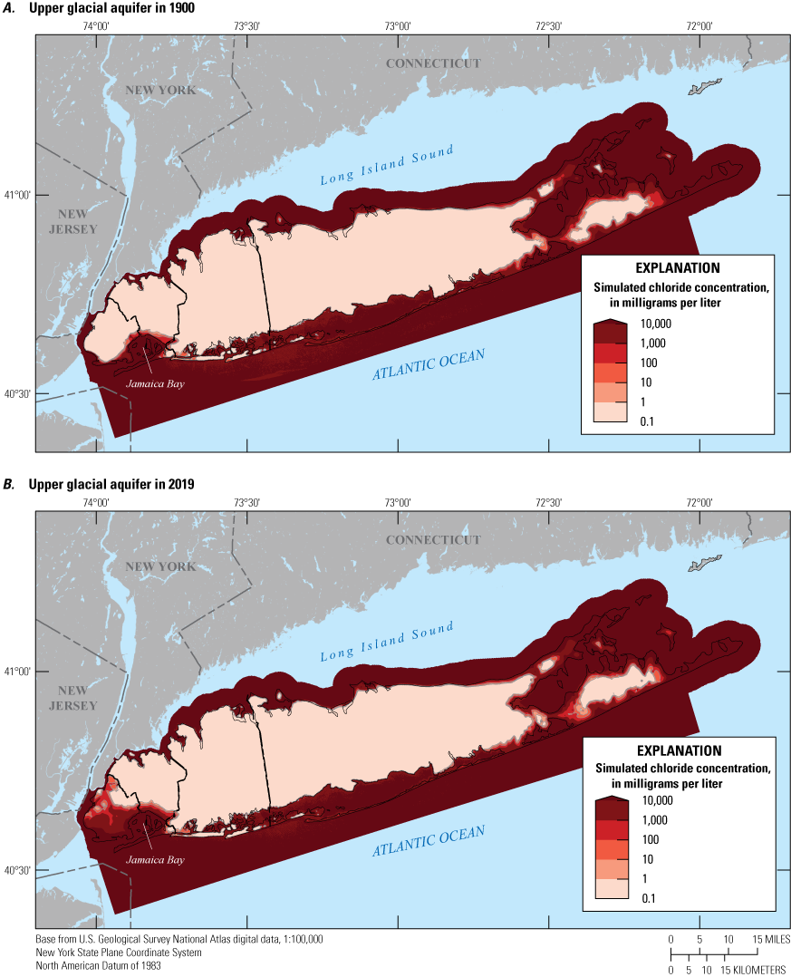
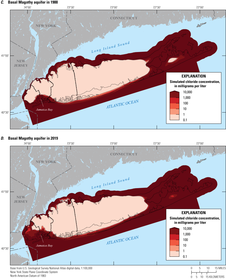
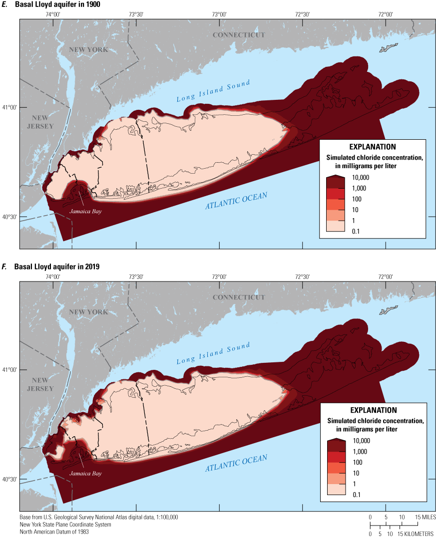
Maps showing chloride concentrations simulated in the transient groundwater-flow model of the aquifer system underlying Long Island, New York, for 1900 and 2019 in the A–B, upper glacial, C–D, basal Magothy, and E–F, Lloyd aquifers.
Groundwater in the Magothy aquifer is freshwater throughout much of the land area of western and central Long Island, and freshwater extends offshore along the southern shore of Nassau and Suffolk Counties where it is locally confined by the overlying Gardiners clay (fig. 48C–D). Saline groundwater with chloride concentrations exceeding 1,000 mg/L extended inland in the Magothy aquifer in a small area along the eastern shore of Jamaica Bay (fig. 48C). As of 2019, much the Magothy aquifer is intruded in most of Kings County and along Jamaica Bay in southern Queens County and southwestern Nassau County (fig. 48D). The Magothy aquifer was historically an important source of water in New York City and remains an important source of water in Nassau County. Pumping from the aquifer, particularly in the late 20th century, has led to saltwater intrusion in several areas in southern Queens and Nassau Counties (Terracciano, 1997).
Groundwater in the Lloyd aquifer also is freshwater throughout much of the land area of western and central Long Island. The Lloyd aquifer is confined by the overlying lower Raritan confining unit, and freshwater extends offshore along the southern shore of Nassau and Suffolk Counties (fig. 48E–F). In 1900, saltwater intrusion of the Lloyd aquifer was limited to a small area close to the shore of Jamaica Bay (fig. 48E). The Lloyd aquifer was an important source of water in New York City during most of the 20th century. Groundwater withdrawals from the aquifer resulted in cones of depression, saltwater intrusion, and abandonment of public supply wells by the mid-1980s. As of 2019, the Lloyd aquifer was intruded by saline groundwater with chloride concentrations exceeding 1,000 mg/L in most of Kings County and saline groundwater extended well inland in Queens County, north of Jamaica Bay (fig. 48F). The freshwater/saltwater interface was close to the shore in the Long Beach area in southwestern Nassau County. The Lloyd aquifer and the contiguous North Shore aquifer also were intruded in some areas along the northern shore of Nassau County, including Great Neck and Manhasset Neck.
The vertical position of the interface varies across Long Island (fig. 49). The interface underlying mainland Long Island is complex, with freshwater extending seaward beneath confining units, particularly along the southern shore. An inversion occurs in the Magothy aquifer, where it is confined by the Gardiners clay, and in the Lloyd aquifer, where it is confined by the lower Raritan confining unit (fig. 49A). The freshwater/saltwater interface underlying the North and South Forks approximates the bowl shape generally typical of sufficiently thick unconfined aquifers that results from density differences and the near-hydrostatic balance between fresh and saline groundwater (fig. 49B). The aquifer system along the southern shore of Long Island it is fully fresh to bedrock underneath the mainland of the island, but the Magothy and Lloyd aquifers are naturally saline underlying the eastern part of the island. The freshwater part of the upper glacial aquifer occurs in discontinuous lenses beneath the South Fork (fig. 49C). The upper glacial aquifer along the northern shore of Long Island shows is fully freshwater to bedrock underneath the western part of the island, but the Lloyd aquifer is locally intruded in several areas in Nassau and Queens Counties where the aquifer system is thin (fig. 49C–D).
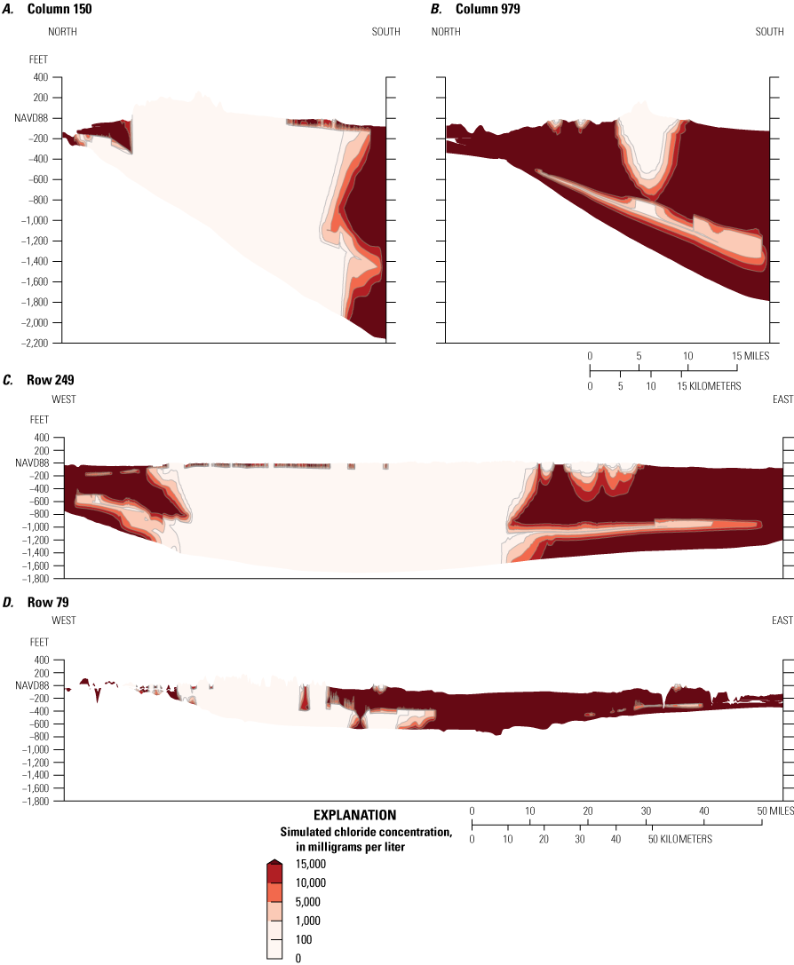
Cross sections showing chloride concentrations simulated in the transient groundwater-flow model of the aquifer system underlying Long Island, New York, for 2019 along A–B, north-south (down-dip sections) and C–D, east-west sections. Location of sections shown on figure 10.
Large-scale groundwater withdrawals since 1900 have caused intrusion of saline groundwater into both the unconfined and confined parts of the aquifer system, primarily in the densely populated western part of the island (fig. 48). Saltwater intrusion has been a societally important issue for several decades, and water-resources managers have had to make costly changes in infrastructure to ensure potable water for the region’s population. However, much of the regional aquifer system has been largely unaffected by saltwater intrusion.
The volume of freshwater, defined as containing chloride concentrations less than 1,000 mg/L, in the unconfined part of aquifer, which is the principal source of water for the region, has decreased only slightly since 1900, by about 15.7 cubic miles, or less than 5 percent (fig. 50A). The volume of freshwater in the confined part of the system, which is about half the volume of the unconfined system, has decreased by about 7 percent since 1900 (fig. 50A). The decadal change in the freshwater volume of the unconfined aquifer system varied slightly but was less than 1 percent for all decades (fig. 50B). The largest decadal decreases were in the early and mid-20th century, which corresponds to a period of large-scale groundwater withdrawals and documented saltwater intrusion in New York City and western Nassau County (figs. 4 and 7). The decadal change in the freshwater volume of the confined system was less variable and generally was constant between −0.4 and −0.6 percent per decade (fig. 50B). The model indicated that the effects of saltwater intrusion on the aquifer system, at an island wide scale, generally have been small. However, intrusion of saltwater into the aquifer can locally affect the sustainability of the aquifer system and the ability to utilize the aquifer as a source of potable water for individual communities. Areas that have been locally affected by saltwater intrusion include Kings County, southern Queens County, and southwestern and coastal areas of northern Nassau County (Stumm and others, 2024).
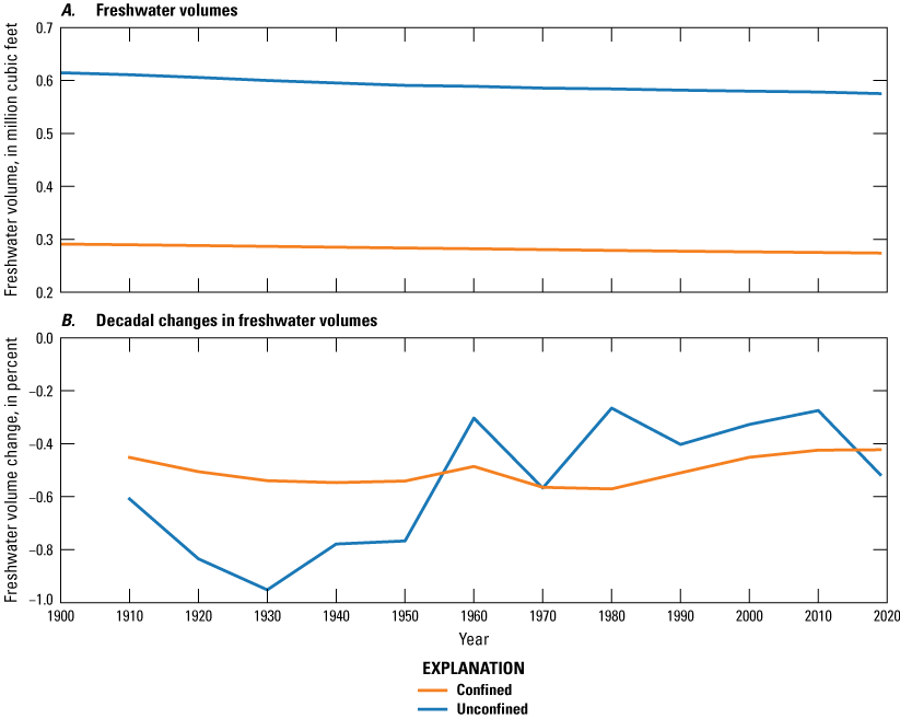
Graphs showing simulated A, freshwater volume (chloride concentration less than 1,000 milligrams per liter [mg/L]) and B, decadal changes in freshwater volumes in the transient groundwater-flow model of the aquifer system underlying Long Island, New York.
Models Developed for Prediction of Future Changes in Hydrologic Conditions
The conditioned model was determined to adequately represent historical conditions from 1900 to 2019; model inputs were also determined to reasonably represent the characteristics and properties of the real aquifer system. The simulated hydrologic conditions at the last year of the simulation period (2019) were an outlier compared with the average of the last decade of the simulation period (2010–19) in that recharge was about 16 percent higher in 2019 than the 10-year average, and pumping was about 10 percent lower than the 10-year average (table 5). Therefore, instead of extending the last year of the simulation period to serve as a baseline for comparison to predictive models of changing hydrologic stresses, two additional models were developed for average-annual and average-seasonal stresses for the 2010–19 period. These two models are representative of current [2019] average conditions that can be used as a baseline for comparison for predictive models of future hydrologic conditions.
Base Case Models of Average [2010–19] Conditions
Average pumping and recharge models were developed for both average-annual pumping and recharge stresses, and for average seasonal pumping and recharge for 2010–19 conditions. Natural recharge from 2010 to 2019 varied monthly from the annual equivalent of 0 in/yr in May 2015 to 93.3 in/yr in March 2010 (fig. 51A). Pumping varied from 208 Mgal/d in February 2017 to 824 Mgal/d in July 2010 (fig. 51A). Monthly pumping and recharge were used to calculate annual and seasonal averages for 2010–19 (fig. 51B); “in-season” refers to the five-month period from May through September and “off-season” refers to the period from October to April.
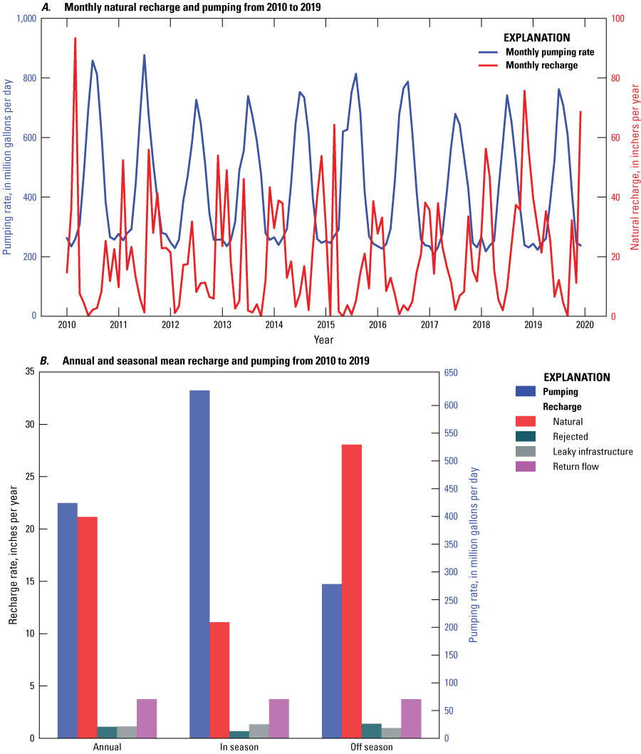
Graphs showing A, estimated monthly recharge from the soil-water balance model adjusted by PEST++ parameters and observed monthly pumping from 2010 to 2019 and B, annual and seasonal mean recharge for Long Island, New York. Data are from Finkelstein and others (2022).
The in-season and off-season averaged natural recharge rates for 2010–19, expressed as annual-equivalent rates, were about 10.5 and 27.7 in/yr, respectively. Pumping averaged 627 Mgal/d during the in-season months and 278 Mgal/d during the off-season months. The annual average natural recharge for 2010–19 was 20.5 in/yr; pumping averaged 414 Mgal/d during that period (fig. 51B). Anthropogenic recharge components were calculated for each month from 2010 to 2019 using monthly SWB estimates (Finkelstein and others, 2022) and pumping and annual population using the same approach as was used to calculate anthropogenic recharge for historical conditions. Recharge from leaky infrastructure is a function of pumping and varied seasonally; likewise, rejected recharge is a function of natural recharge and also varies seasonally (fig. 51B). Recharge from return flow is estimated from population, which was estimated from the 2010 census (U.S. Census Bureau, 2021b), and did not vary seasonally (fig. 51B).
The average annual and average seasonal recharge and pumping stresses were used to develop predictive models for the Long Island aquifer system at multidecadal time scales. The average annual model uses the recharge calculated from the monthly SWB recharge and the anthropogenic recharge components estimated from monthly pumping and population averaged during the 10-year period (2010–19); the simulation period is 30 annual stress periods. An additional annual-scale model, using the same simulated stresses, was developed that had a simulation time of 80 years. Seasonal recharge and pumping, as estimated from monthly values, also was used to develop an average seasonal baseline model of the system. In-season and off-season pumping and recharge were alternated within each simulated year, such that there was a total of 60 stress periods during the 30-year simulation period. The simulation multidecadal time scales were necessary to ensure that the transient model was at quasi-steady-state and that any evaluations of future hydrologic stresses were not affected by residual changes in storage from the initial conditions.
The initial conditions for both baseline models were heads and chloride concentrations computed after the final stress period of the historical-conditions model (the end of 2019). Natural recharge for 2019 was 23.9 in/yr, which was substantially higher than the average of 20.5 in/yr from 2010 to 2019. Groundwater withdrawals in 2019 were about 388 Mgal/d, which was about 7 percent lower than the average of 414 Mgal/d from 2010 to 2019. Both the annual and seasonal baseline models reached quasi-steady-state after a sufficient simulation time (fig. 52). Water levels reached quasi-steady-state within about 25 simulation years (fig. 52A) and streamflows reached a steady state within about 10 simulation years (fig. 52B). These stress periods represented model simulation time and were not used to predict a future conditions in any specific year.
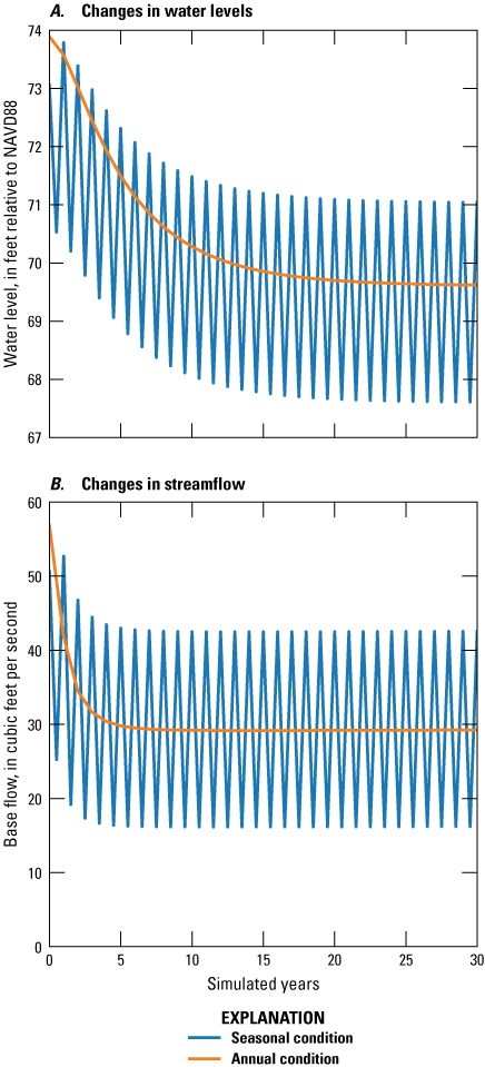
Graphs showing changes in A, water levels and B, streamflows during a 30-year simulation period in the transient groundwater-flow model of the aquifer system underlying Long Island, New York. NAVD88, North American Vertical Datum of 1988.
Seasonal changes in recharge and pumping substantially affect heads and streamflows (fig. 53A). The largest seasonal changes in water table altitudes exceed 10 ft in areas with fine-grained sediments, generally in moraines and low-permeability silt and clays and, possibly, areas of perched clays in northern Nassau County. The smallest changes are near surface waters, which constrain heads in the surrounding aquifer. The changes also are generally small in New York City due to the presence of urban drains, representing subsurface infrastructure, that also constrain water levels in some urbanized areas by intercepting water from rising water tables. Local occurrences of large seasonal changes in water table altitudes are near pumping wells and are the result of seasonal changes in groundwater withdrawals. Changes can be made to hydrologic stresses and the resultant heads and flows after a simulation period of 30 years can be compared to the final heads and flows from these baseline models to assess the effect of those changes on the hydrologic system, in the absence of other effects.
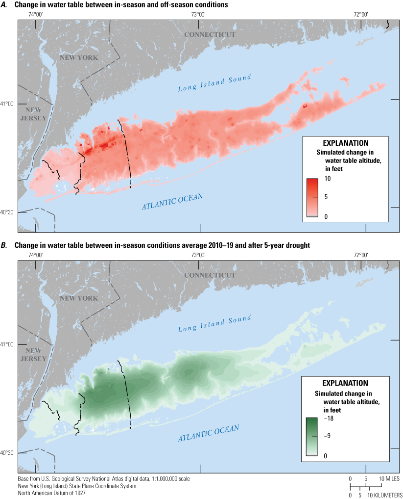
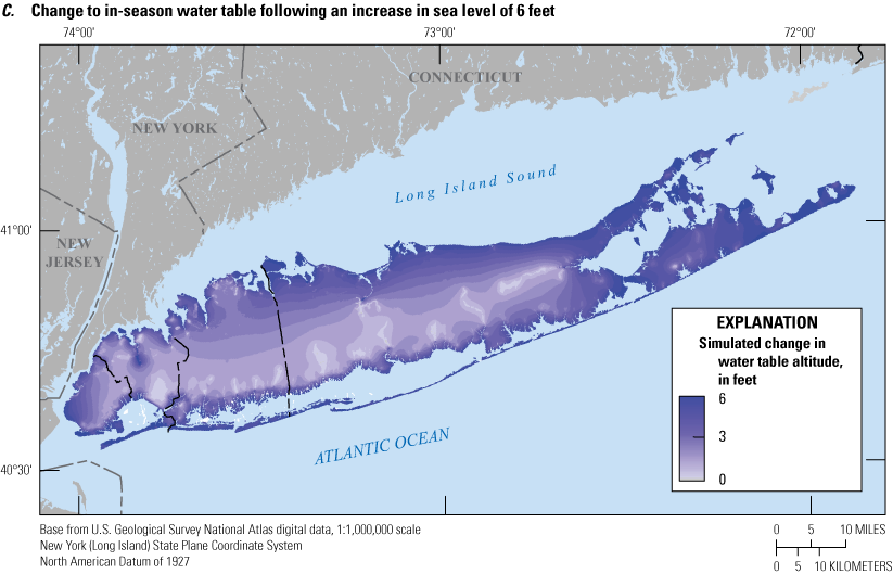
Maps showing changes in water table altitude for a comparison of A, in-season and off-season recharge and pumping (average for 2010–19), B, in-season recharge and pumping (average for 2010–19) and in-season after a 5-year drought, and C, sea level in 2019 and a sea level rise of 6 feet (average annual pumping and recharge for 2010–19) in the transient groundwater-flow model of the aquifer system underlying Long Island, New York.
Drought
The average seasonal baseline model was modified to represent the effects of a 5-year drought similar to the 1960s drought, often referred to as the “drought of record.” The drought is represented as starting in the 5th year of the simulation and has a duration of 5 years. The simulation of drought conditions was made by decreasing average seasonal recharge by 20 percent and increasing average public-supply and non-public-supply pumping by 20 and 10 percent, respectively. The comparison of water table changes for in-season conditions after the 5-year drought simulation, or the 10th year of the simulation, showed water-level declines ranging from 0 to 18 ft from the coast to the inland tops of the groundwater mounds (fig. 53B). Simulated water-level declines were small away from the coast, in the vicinity of the large streams that drain to the southern shore (fig. 53B). The in-season streamflows decreased by about 32 percent in response to the 5-year drought, while water-level changes in the vicinity of the streams were relatively small (fig. 53B).
The small change in water levels in these areas was because of the hydrologic control of the streams on nearby water levels. The streams on Long Island are groundwater fed; therefore, changes in pumping and recharge in the vicinity of these streams result in large changes in streamflows rather than in water levels. However, once the streams go dry during a drought or from nearby large-scale pumping, it is expected that water levels in these areas would continue to decline similar to those in areas away from streams.
Sea-Level Rise
The annual average baseline model was modified to represent a sea level position of 6 ft above NAVD88 as an alternative to the baseline sea level of 0.34 ft above NAVD88 in 2019. The altitude of the new sea level was used to identify model cells that are in emergent areas under current [2019] sea levels that would be submerged under the new sea level. Newly submerged land areas were assigned a head-dependent flux boundary, by use of the GHB package (McDonald and Harbaugh, 1988). Likewise, freshwater streams that are below the new sea level were converted from drain boundaries (using the DRN package) to GHB boundaries (fig. 54). Average annual recharge and pumping from 2010 to 2019 were simulated in the models. The simulations were discretized into 30 annual stress periods.
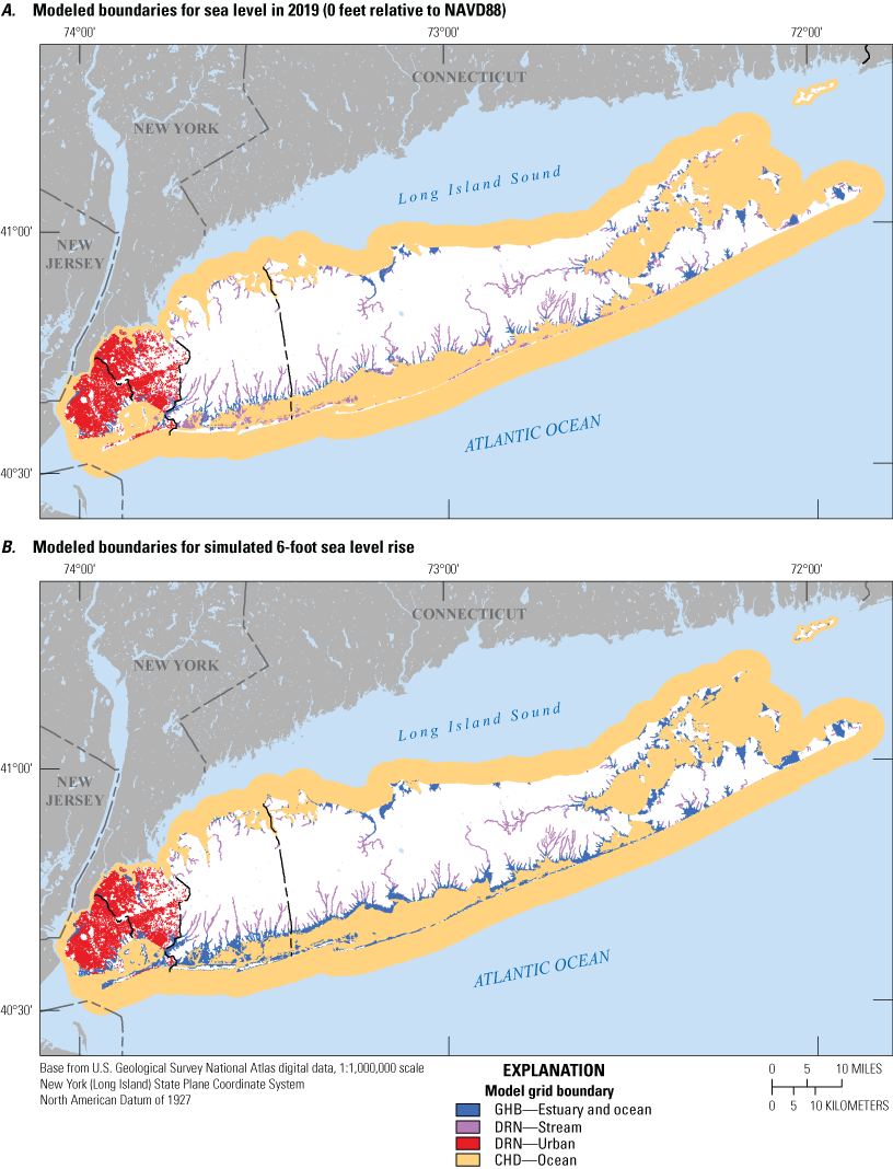
Maps showing hydrologic boundaries for A, sea level in 2019 and B, a sea level position 6 feet above the North American Vertical Datum of 1988 simulated in the transient groundwater-flow model of the aquifer system underlying Long Island, New York. DRN, Drain package; GHB, General Head Boundary package; CHD, Constant Head package (all from McDonald and Harbaugh, 1988); NAVD88, North American Vertical Datum of 1988.
Changes in sea level affect the base level of the aquifer and, therefore, water levels and streamflows (fig. 53C). The maximum change in water table altitudes, as determined by comparing the water table at the end of the 80-year simulation for current [2019] and future sea levels, generally is limited to the increase in sea level because only the base level is changed, and the recharge and pumping are unchanged. The maximum change in water table altitudes, assuming a 6-ft sea-level rise, generally is in areas adjacent to the coast in areas with no surface-water drainages. These areas are generally in the northeastern coast of Suffolk County and on the North and South Forks. The smallest changes in water table altitudes are along the southern shore of Nassau and Suffolk Countries (fig. 53C). These coastal areas are characterized by a dense network of streams. Streams are fixed boundaries that constrain heads by passively removing water from the system. This results in increased streamflows and the potential for local up coning of the shallow freshwater/saltwater interface beneath the streams, similar to what has been reported in analogous hydrologic settings on Cape Cod (Walter and others, 2016).
Summary
Long Island, New York, is underlain by a geologically complex aquifer system that is composed of Cretaceous and Pleistocene aquifers and confining units that are surrounded by saline groundwater. This aquifer system has been highly perturbed in the western part of the island by historical groundwater withdrawals and a conversion to urbanized land uses since the beginning of the 20th century. These anthropogenic stresses have led to large drawdowns in water levels in the both unconfined and confined aquifers, depletion of streamflows, saltwater intrusion, and the abandonment of public-water supplies. Though residents of New York City have utilized water imported from outside the island since the mid-1980s, the nearly 3 million residents of Nassau and Suffolk Counties relied solely on groundwater for potable water in 2019.
The U.S. Geological Survey developed a three-dimensional transient model of the Long Island aquifer system as part of an ongoing (since 2016) multiyear, cooperative investigation with the New York State Department of Environmental Conservation. The results of this analysis may be used to assist stakeholders and resource managers to evaluate the response of the groundwater-flow system to changes in future hydrologic stresses. Changes in anthropogenic stresses include future water-supply management and land use and infrastructure changes; and changes in natural stresses include recharge at seasonal and annual time scales, such as droughts, or decadal scales, such as sea-level rise. Hydrologic responses include changes in water-levels in all the hydrogeologic units; discharge to streams, coastal waters, and subsurface infrastructure; and the distribution of saline groundwater in the aquifer system.
The numerical model used the U.S. Geological Survey finite-difference modeling MODFLOW 6 software to represent changes in groundwater pumping and aquifer recharge from 1900 to 2019 at an annual time scale and forecast to future hydrologic conditions at both annual and seasonal scales, including water levels, streamflows, and the position of the freshwater/saltwater interface. The model used some of the hydrologic and geospatial data compiled and analyzed as part of the previous steady-state model of average 2005–15 conditions but required additional information to adequately represent historical conditions (1900–2005) and more recent and updated datasets developed after the previous modeling effort was completed (post-2015).
The regional, three-dimensional numerical model of Long Island is a synthesis of a comprehensive set of data on the physiography, geology, and hydrology of the island. These include data regarding the physiography of Long Island, the regional hydrogeologic framework, the hydraulic properties of aquifers and confining units, the extent of saline groundwater in the aquifer, natural and anthropogenic recharge, groundwater withdrawals, and current [2019] hydrologic conditions in the aquifer system. These datasets include an updated geologic framework of western Long Island derived from geologic and geophysical data collected as part of an ongoing drilling program, a compilation of historical chloride data, recharge estimates from a soil-water balance model from 1900 to 2019, and a compilation of historical pumping, water infrastructure, sewers and impervious surfaces, and observations of historical water levels and streamflows.
The distribution of recharge from precipitation was estimated from landscape characteristics and climate data. Anthropogenic recharge from wastewater, leaky infrastructure, and stormwater runoff were estimated from population, infrastructure, and pumping data. Water-use data, including well locations, depths, and pumping rates, were obtained from historical sources and records and used to estimate pumping stresses continuously in time and space throughout the simulation period.
The model was constructed using hydrogeologic and geospatial information to represent the geometry, boundaries, and hydraulic properties of the aquifer system. The finite-difference grid included 4,100 square miles and extended the length of Long Island from west to east, laterally to the boundary between the freshwater and saltwater groundwater system, and from the water table down to the top of the bedrock. This grid consisted of 348 rows, 1,308 columns, and 20 layers. Each model cell was 500 feet (ft) on a side in map view, with varying thickness by cell and by layer, based on existing and new information on the hydrogeologic unit altitudes and geometry of the regional aquifers and confining units.
Historical hydrologic conditions were estimated from a large number of hydrologic and water-quality measurements collected since the start of the 20th century and used to develop average annual observations of water levels, streamflows, and chloride concentrations from large networks of observation wells and stream sites from across Long Island. These observations were examined to determine those that reliably represent average annual conditions and, therefore, are suitable for calibration of the model. Initial estimates of model inputs and stresses, including aquifer properties, natural recharge, pumping, and recharge from anthropogenic sources were parametrized and adjusted to improve fit between observed hydrologic conditions and their simulated equivalents.
The calibration process involved trial and error adjustments using prior knowledge to improve general fit to observations, followed by an inverse calibration to update and optimize input parameters, using the iterative ensemble smoother algorithm implemented in the PEST++ version 5.0 software. The initial parameter values were adjusted to produce an optimal fit to observed hydrologic conditions using inverse parameter-estimation techniques. Parameter estimation, as implemented in this effort, was a four-step process: (1) trial-and-error manual adjustments to initial parameter values, (2) an inverse algorithmic update of parameters resulting in an optimal fit to observed hydrologic conditions and associated data-quality weights, (3) manual adjustments of inversely fit parameters from the optimal base realization to address local misfits between observations (measured values) and their model-simulated equivalents, and (4) conditioning of model inputs to ensure all values were within ranges considered to be reasonable based on prior knowledge of the Long Island aquifer system.
This calibration process resulted in a model that was generally in good agreement with observed hydrologic conditions, dynamically between 1900 and 2019. The calibrated model was used to develop two baseline models for comparison of simulated hypothetical future changes in hydrologic stresses. These baseline models included one representing average annual and one representing average seasonal conditions for the 2010–19 period. The model representing average annual conditions was used to develop a scenario representing an alternate sea level position of 6 ft above the North American Vertical Datum of 1988 (NAVD88), and the model representing average-seasonal conditions was modified to develop a scenario simulating the effects of a 5-year drought imposed upon current [2010–19] hydrologic conditions.
Recharge is the sole source of water to the aquifer system; groundwater discharges to coastal water and streams and is withdrawn by wells. Model-estimated annual recharge ranged from about 11 inches in 1965 to 41 inches in 1983. Under 2010–19 conditions, on average, about 23 percent of water was pumped from wells and about 47 and 27 percent discharged to coastal waters and streams, respectively; the remaining 4 percent was water that moved into storage in the aquifer matrix.
The highest water table altitudes are in west-central Long Island away from major surface water drainages. As of 2019, altitudes in the eastern and western water table mounds exceeded 60 and 80 ft above NAVD88, respectively. Water levels varied naturally in response to changes in recharge; the amount of variation was largest in the interior of the island in areas with high water table altitudes near groundwater divides and smallest near streams and coastal waters. The lowest water table altitudes generally were in the mid-1960s, during a period of extended drought. Water levels also varied in response to pumping stresses, and the total variability in water levels was the sum of natural and anthropogenic stresses.
The total range of water table altitudes on Long Island from 1900 to 2019 ranged from near 0 to more than 70 ft in western parts of Long Island. The largest range in water table altitude was in New York City and was associated with areas of large historical groundwater withdrawals between the 1920s and late 1980s. Water table altitude differences were generally less than 10 ft in eastern Suffolk County, where the aquifer system was under less influence from anthropogenic conditions.
The freshwater/saltwater interface generally extends to bedrock in most of western and central Long Island, where the island is wide, but occurs within the aquifer onshore beneath the North and South Forks where it approximates a bowl shape typical of unconfined aquifers. Freshwater extends offshore in the Magothy and Lloyd aquifers along the southern shore where the aquifers are confined by overlying confining units. There has been inland intrusion of saltwater into both the unconfined and confined parts of the aquifer in western Long Island in response to large-scale groundwater withdrawals, leading to the abandonment of some supply wells.
Saltwater intrusion has occurred in the upper glacial, Magothy, and Lloyd aquifers in most of Kings County, where large-scale withdrawals began near the start of the 20th century; pumping ceased in 1947 in response to the saltwater intrusion. Saltwater intrusion also has occurred in Queens County, where large groundwater withdrawals occurred throughout most of the 20th century. Saline groundwater has intruded all three aquifers but generally is limited to inland areas to the north of Jamaica Bay where the saltwater intrusion extends the furthest inland in the Lloyd aquifer. Saltwater also has intruded the Magothy aquifer in the southwestern part of Nasau County in response to continuing groundwater withdrawals in this urbanized area and in the Lloyd aquifer in some areas along the northern shore of Nassau County.
The aquifer system underlying Long Island is nearly 2,000 ft deep in some areas; recharge rates to the aquifer generally are high, and aquifers are extensive and transmissive, indicating that there generally are abundant water resources underlying the island. Much of western and central Long Island is densely populated, and large-scale groundwater withdrawals have occurred in the aquifer since the early 20th century, resulting in a change in freshwater volume in the aquifer system only by about 5 percent since the onset of large-scale pumping in 1900.
The decadal change in the freshwater volume was largest during the early and mid-20th century, corresponding to the largest historical pumping, but that change did not exceed 1 percent. This suggests that saltwater intrusion was of limited significance at an islandwide scale as of 2019. However, intrusion of saline groundwater likely continues to occur in some populated areas of Queens and Nassau Counties that could adversely affect water supplies or limit the potential for development of new water supplies. The benefits of the regional groundwater model are that it can serve as a tool to evaluate the viability of current and future water supplies at a regional scale and to support development of additional tools to model groundwater at a finer scale.
Selected References
Bakker, M., Post, V., Langevin, C.D., Hughes, J.D., White, J.T., Starn, J.J., and Fienen, M.N., 2016, Scripting MODFLOW model development using Python and FloPy: Groundwater, v. 54, no. 5, p. 733–739, accessed January 30, 2024, at https://doi.org/10.1111/gwat.12413.
Barlow, P.M., 1989, Determination of aquifer properties from a thermal tracer experiment, in Abstracts for the AGU spring meeting: Eos, American Geophysical Union, Transactions, v. 70, no. 15, p. 408, accessed February 13, 2024, at https://doi.org/10.1029/EO070i015p00271.
Barlow, P.M., and Hess, K.M., 1993, Simulated hydrologic responses of the Quashnet River stream-aquifer system to proposed ground-water withdrawals, Cape Cod, Massachusetts: U.S. Geological Survey Water-Resources Investigations Report 93–4064, 52 p., accessed January 29, 2024, at https://doi.org/10.3133/wri934064.
Bayraktar, B.N., Jahn, K.L., Walter, D.A., Masterson, J.P., Dressler, S.E., Finkelstein, J.S., and Monti, J., Jr., 2024, Simulations of the Long Island Aquifer System Response to Potential Changes in Future Hydrologic Conditions, Long Island, New York: U.S. Geological Survey data release, https://doi.org/10.5066/P13OHFKP.
Buxton, H.T., and Shernoff, P.K., 1999, Ground-water resources of Kings and Queens Counties, Long Island, New York: U.S. Geological Survey Water-Supply Paper 2498, 113 p., 7 pls. [Also available at https://doi.org/10.3133/wsp2498.]
Buxton, H.T., and Smolensky, D.A., 1999, Simulation of the effects of development of the ground-water flow system of Long Island, New York: U.S. Geological Survey Water-Resources Investigations Report 98–4069, 57 p., accessed January 24, 2024, at https://doi.org/10.3133/wri984069.
Cadwell, D.H., 1989, Surficial geologic map of New York—Lower Hudson sheet: New York State Museum Map and Chart Series 40, 1 sheet, scale 1:250,000. [Also available at https://www.nysm.nysed.gov/research-collections/geology/gis.]
Cadwell, D.H., and Muller, E.H., 1986, Surficial geologic map of New York: New York Museum data, accessed August 4, 2019, at https://www.nysm.nysed.gov/research-collections/geology/gis.
Chu, A., Monti, J., Jr., and Bellitto, A.J., 1997, Public-supply pumpage in Kings, Queens, and Nassau Counties: U.S. Geological Survey Open-File Report 81–499, 61 p. [Also available at https://doi.org/10.3133/ofr97567.]
Corson-Dosch, N., Fienen, M.N., Finkelstein, J.S., Leaf, A.T., White, J.T., Woda, J.C., and Williams, J.H., 2022, Areas contributing recharge to priority wells in valley-fill aquifers in the Neversink River and Rondout Creek drainage basins, New York: U.S. Geological Survey Scientific Investigations Report 2021–5112, 50 p., accessed October 16, 2023, at https://doi.org/10.3133/sir20215112.
Danielson, J.J., and Haines, J., 2017, Hurricane Sandy region—Topobathymetric elevation model of New England: U.S. Geological Survey web page, accessed October 5, 2019, at https://www.usgs.gov/special-topics/coastal-national-elevation-database-%28coned%29-applications-project/science/hurricane-0.
DeMott, L.M., Stumm, F., and Finkelstein, J., 2023, Bedrock-surface elevation and overburden thickness maps of the five boroughs, New York City, New York: U.S. Geological Survey Data Report 1176, 22 p., accessed December 12, 2023, at https://doi.org/10.3133/dr1176.
Doherty, J., 2003, Ground water model calibration using pilot points and regularization: Ground Water, v. 41, no. 2, p. 170–177, accessed October 2, 2023, at https://doi.org/10.1111/j.1745-6584.2003.tb02580.x.
Doherty, J., and Welter, D., 2010, A short exploration of structural noise: Water Resources Research, v. 46, no. 5, article W05525, 14 p., accessed December 23, 2023, at https://doi.org/10.1029/2009WR008377.
Doherty, J.E., and Hunt, R.J., 2010, Approaches to highly parameterized inversion—A guide to using PEST for groundwater-model calibration: U.S. Geological Survey Scientific Investigations Report 2010–5169, 59 p. [Also available at https://doi.org/10.3133/sir20105169.]
Doriski, T.P., and Wilde-Katz, F., 1982, Geology of the “20-foot” clay and Gardiners clay in southern Nassau and southwestern Suffolk counties, Long Island, New York: U.S. Geological Survey Water-Resources Investigations Report 82–4056, 21 p. [Also available at https://doi.org/10.3133/wri824056.]
Eckhardt, K., 2005, How to construct recursive digital filters for baseflow separation: Hydrological Processes, v. 19, no. 2, p. 507–515. [Also available at https://doi.org/10.1002/hyp.5675.]
Fienen, M.N., Corson-Dosch, N.T., White, J.T., Leaf, A.T., and Hunt, R.J., 2022a, Risk-based wellhead protection decision support—A repeatable workflow approach: Ground Water, v. 60, no. 1, p. 71–86. [Also available at https://doi.org/10.1111/gwat.13129.]
Fienen, M.N., Haserodt, M.J., Leaf, A.T., and Westenbroek, S.M., 2022b, Simulation of regional groundwater flow and groundwater/lake interactions in the Central Sands, Wisconsin: U.S. Geological Survey Scientific Investigations Report 2022–5046, 111 p., accessed October 16, 2023, at https://doi.org/10.3133/sir20225046.
Finkelstein, J.S., Monti, J., Jr., Masterson, J.P., and Walter, D.A., 2022, Application of a soil-water-balance model to estimate annual groundwater recharge for Long Island, New York, 1900–2019: U.S. Geological Survey Scientific Investigations Report 2021–5143, 25 p., accessed October 15, 2023, at https://doi.org/10.3133/sir20215143.
Franke, O.L., and Cohen, P., 1972, Regional rates of ground-water movement on Long Island, New York, chap. C of Geological survey research 1972: U.S. Geological Survey Professional Paper 800–C, p. C271–C277. [Also available at https://doi.org/10.3133/pp800C.]
Franke, O.L., and Getzen, R.T., 1976, Evaluation of hydrologic properties of the Long Island ground-water reservoir using cross-sectional analog models: U.S. Geological Survey Open-File Report 75–679, 80 p. [Also available at https://doi.org/10.3133/ofr75679.]
Garabedian, S.P., 1985, Effect of correlation between distribution coefficients and hydraulic conductivity on the macrodispersivity of non-conservative solutes: Eos, Transactions of the American Geophysical Union, v. 66, no. 46, p. 903, accessed February 13, 2024, at https://doi.org/10.1029/EO066i046p00813.
Garabedian, S.P., Gelhar, L.W., and Celia, M.A., 1988, Large-scale dispersive transport in aquifers—Field experiments and reactive transport theory: Massachusetts institute of Technology Ralph M. Parsons Laboratory Hydrology and Water Resources Systems Report 315, 291 p., accessed January 31, 2024, at https://www.nrc.gov/docs/ML0331/ML033160542.pdf.
Gelhar, L.W., Welty, C., and Rehfeldt, K.R., 1992, A critical review of data on field-scale dispersion in aquifers: Water Resources Research, v. 28, no. 7, p. 1955–1974, accessed October 15, 2023, at https://doi.org/10.1029/92WR00607.
Getzen, R.T., 1977, Analog-model analysis of regional three-dimensional flow in the ground-water reservoir of Long Island, New York: U.S. Geological Survey Professional Paper 982, 49 p., accessed January 25, 2024, at https://doi.org/10.3133/pp982.
Guswa, J.H, and LeBlanc, D.R., 1985, Digital models of ground-water flow in the Cape Cod aquifer system, Massachusetts: U.S. Geological Survey Water Supply Paper 2209, 112 p., accessed January 29, 2024, at https://doi.org/10.3133/wsp2209. [Supersedes USGS Open-File Report 80–67.]
Guswa, J.H., and Londquist, C.J., 1976, Potential for development of ground water at a test site near Truro, Massachusetts: U.S. Geological Survey Open-File Report 76–614, 38 p., 22 pls., accessed January 29, 2024, at https://doi.org/10.3133/ofr76614.
Harbaugh, A.W., 2005, MODFLOW–2005—The U.S. Geological Survey modular ground-water model—The ground-water flow process: U.S. Geological Survey Techniques and Methods, book 6, chap. A16, [variously paged]. [Also available at https://doi.org/10.3133/tm6A16.]
Jacob, C.E., 1941, Notes on the elasticity of the Lloyd sand on Long Island, New York: Eos, Transactions, American Geophysical Union, v. 22, no. 3, p. 783–787, accessed January 25, 2024, at https://doi.org/10.1029/TR022i003p00783.
Jahn, K.L., Walter, D.A., Masterson, J.P., Dressler, S.E., Finkelstein, J.S., and Monti, J., Jr., 2024, MODFLOW 6 model used to simulate groundwater flow in the Long Island, New York, regional aquifer system for 1900–2019 pumping and recharge conditions: U.S. Geological Survey data release, https://doi.org/10.5066/P14TRKUB.
Johnson, A.H., and Waterman, W.G., 1952, Withdrawal of ground water on Long Island: New York New York State Water, Power, and Control Commission Bulletin GW–28, 13 p., 1 pl. [Also available at https://archive.org/details/usgswaterresourcesnewyork-bull_gw_28/bull_gw_28/.]
Kilburn, C., 1981, Ground-water pumpage in Nassau County, Long Island, New York 1920–77—Introduction and user’s guide to the data compilation: U.S. Geological Survey Open-File Report 81–499, 67 p., 2 pls. [Also available at https://doi.org/10.3133/ofr81499.]
Kontis, A.L., 1999, Simulation of freshwater-saltwater interfaces in the Brooklyn-Queens aquifer system, Long Island, New York: U.S. Geological Survey Water-Resources Investigations Report 1998–4067, 26 p., accessed January 24, 2024, at https://doi.org/10.3133/wri984067.
Krulikas, R.K., and Koszalka, E.J., 1982, Geologic reconnaissance of an extensive clay unit in north-central Suffolk County, Long Island, New York: U.S. Geological Survey Water-Resources Investigations Report 82–4075, 9 p., 1 pl. [Also available at https://doi.org/10.3133/wri824075.]
Langevin, C.D., Hughes, J.D., Banta, E.R., and Niswonger, R.G., Panday, S., and Provost, A.M., 2017, Documentation for the MODFLOW 6 groundwater flow model: U.S. Geological Survey Techniques and Methods, book 6, chap. A55, 197 p., accessed October 23, 2023, at https://doi.org/10.3133/tm6A55.
Langevin, C.D., Panday, S., and Provost, A.M., 2020, Hydraulic-head formulation for density-dependent flow and transport: Ground Water, v. 58, no. 3, p. 349–362, accessed October 23, 2023, at https://doi.org/10.1111/gwat.12967.
Langevin, C.D., Provost, A.M., Panday, S., and Hughes, J.D., 2022, Documentation for the MODFLOW 6 groundwater transport (GWT) model: U.S. Geological Survey Techniques and Methods, book 6, chap. A61, 56 p., accessed October 12, 2023, at https://doi.org/10.3133/tm6A61.
Langevin, C.D., Thorne, D.T., Jr., Dausman, A.M., Sukop, M.C., and Guo, W., 2008, SEAWAT version 4—A computer program for simulation of multi-species solute and heat transport: U.S. Geological Survey Techniques and Methods, book 6, chap. A22, 30 p., accessed October 12, 2023, at https://doi.org/10.3133/tm6A22.
LeBlanc, D.R., Guswa, J.H., Frimpter, M.H., Londquist, C.J., 1986, Ground-water resources of Cape Cod, Massachusetts: U.S. Geological Survey Hydrologic Atlas 692, 4 sheets, accessed January 29, 2024, at https://doi.org/10.3133/ha692.
Lindner, J.B., and Reilly, T.E., 1983, Analysis of three tests of the unconfined aquifer in southern Nassau County, Long Island, New York: U.S. Geological Survey Water-Resources Investigations Report 82–4021, 52 p. [Also available at https://doi.org/10.3133/wri824021.]
Masterson, J.P., and Barlow, P.M., 1997, Effects of simulated ground-water pumping and recharge on ground-water flow in Cape Cod, Martha's Vineyard, and Nantucket Island basins, Massachusetts: U.S. Geological Survey Water Supply Paper 2447, 79 p., 1 pl., accessed January 29, 2024, at https://doi.org/10.3133/wsp2447. [Supersedes USGS Open-File Report 94–316.]
Masterson, J.P., Pope, J.P., Fienen, M.N., Monti, J., Jr., Nardi, M.R., and Finkelstein, J.S., 2016, Assessment of groundwater availability in the Northern Atlantic Coastal Plain aquifer system from Long Island, New York, to North Carolina: U.S. Geological Survey Professional Paper 1829, 76 p., accessed October 23, 2023, at https://doi.org/10.3133/pp1829.
Masterson, J.P., Walter, D.A., and LeBlanc, D.R., 1998, Delineation of contributing areas to selected public-supply wells, western Cape Cod, Massachusetts: U.S. Geological Survey Water-Resources Investigations Report 98-4237, 45 p., accessed January 29, 2024, at https://doi.org/10.3133/wri984237.
McClymonds, N.E., and Franke, O.L., 1972, Water-transmitting properties of aquifers on Long Island, N.Y.: U.S. Geological Survey Professional Paper 627–E, 24 p. [Also available at https://doi.org/10.3133/pp627E.]
McDonald, M.G., and Harbaugh, A.W., 1988, A modular three-dimensional finite-difference groundwater flow model: U.S. Geological Survey Techniques of Water-Resources Investigations, book 6, chap. A1, 586 p. [Also available at https://doi.org/10.3133/twri06A1.]
Meisler, H.P., Leahy, P., and Knobel, L.L., 1984, Effect of eustatic sea-level changes on saltwater-freshwater in the Northern Atlantic Coastal Plain: U.S. Geological Survey Water-Supply Paper 2255, 28 p. [Also available at https://doi.org/10.3133/wsp2255.]
Misut, P.E., and Monti, J., Jr., 1999, Simulation of ground-water flow and pumpage in Kings and Queens Counties, Long Island, New York: U.S. Geological Survey Water-Resources Investigations Report 98–4071, 50 p. [Also available at https://doi.org/10.3133/wri984071.]
Misut, P.E., Schubert, C.E., Bova, R.G., and Colabufo, S.R., 2004 Simulated effects of pumping and drought on ground-water levels and the freshwater-saltwater interface on the north fork of Long Island, New York: U.S. Geological Survey Water-Resources Investigations Report 2003–4184, 58 p., accessed January 24, 2024, at https://doi.org/10.3133/wri034184.
Moench, A.F., Garabedian, S.P., and LeBlanc, D.R., 2001, Estimation of hydraulic parameters from an unconfined aquifer test conducted in a glacial outwash deposit, Cape Cod, Massachusetts: U.S. Geological Survey Professional Paper 1629, 69 p., accessed January 25, 2024, at https://doi.org/10.3133/pp1629.
Moench, A.F., LeBlanc, D.R., and Garabedian, S.P., 1996, Preliminary type-curve analysis of an aquifer test in an unconfined sand and gravel aquifer, Cape Cod, Massachusetts, in Morganwalp, D.W., and Aronson, D.A., eds., U.S. Geological Survey Toxic Substances Hydrology Program—Proceedings of the Technical Meeting, Colorado Springs, Colorado, September 20–24, 1993: U.S. Geological Survey Water-Resources Investigations Report 94–4015, p. 273–281, accessed January 29, 2024, at https://doi.org/10.3133/wri944015.
Monti, J., Jr., Walter, D.A., Masterson, J.P., and Jahn, K.L., 2024, Unattenuated nitrogen load estimates from six nonpoint sources on Long Island, New York, from 1900 to 2019: U.S. Geological Survey Scientific Investigations Report 2024–5047, x p., https://doi.org/10.3133/sir20245047.
Monti, J., Jr., Como, M.D., and Busciolano, R.J., 2013, Water table and potentiometric surface altitudes in the upper glacial, Magothy, and Lloyd aquifers beneath Long Island, New York, April–May 2010: U.S. Geological Survey Scientific Investigations Map 3270, 5 pls. [Also available at https://doi.org/10.3133/sim3270.]
Monti, J., Jr., Misut, P.E., and Busciolano, R., 2009, Simulation of variable-density ground-water flow and saltwater intrusion beneath Manhasset Neck, Nassau County, New York, 1905–2005: U.S. Geological Survey Scientific Investigations Report 2008–5166, 71 p. [Also available at https://doi.org/10.3133/sir29985166.]
Niswonger, R.G., Panday, S., and Ibaraki, M., 2011, MODFLOW–NWT, a Newton formulation for MODFLOW–2005: U.S. Geological Survey Techniques and Methods, book 6, chap. A37, 44 p. [Also available at https://doi.org/10.3133/tm6A37.]
New York Department of Environmental Conservation, 2024, DEC info locator: New York State Department of Environmental Conservation database, accessed March 1, 2024, at https://gisservices.dec.ny.gov/gis/dil/.
Oliver, M.A., and Webster, R., 1990, Kriging—A method of interpolation for geographical information systems: International Journal of Geographical Information Systems, v. 4, no. 3, p. 313–332. [Also available at https://doi.org/10.1080/02693799008941549.]
Perlmutter, N.M., and Geraghty, J.J., 1963, Geology and ground-water conditions in southern Nassau and southeastern Queens Counties, Long Island, N.Y.: U.S. Geological Survey Water Supply Paper 1613–A, 205 p., 7 pls., accessed January 25, 2024, at https://doi.org/10.3133/wsp1613A. [Supersedes USGS Open-File Report 53–77 and USGS Open-File Report 54–98.]
Prince, K.R., and Schneider, B.J., 1989, Estimation of hydraulic characteristics of the upper glacial and Magothy aquifers at East Meadow, New York, by use of aquifer tests: U.S. Geological Survey Water-Resources Investigations Report 87–4211, 43 p. [Also available at https://doi.org/10.3133/wri874211.]
Reilly, T.E., 2001, System and boundary conceptualization in ground-water flow simulation: U.S. Geological Survey Techniques of Water-Resources Investigations, book 3, chap. B8, 29 p. [Also available at https://doi.org/10.3133/twri03B8.]
Reilly, T.E., and Buxton, H.T., 1985, Effects of sanitary sewers on ground-water levels and streams in Nassau and Suffolk Counties, New York; part 3—Development and application of southern Nassau County model: U.S. Geological Survey Water-Resources Investigations Report 83–4210, 41 p., accessed January 25, 2024, at https://doi.org/10.3133/wri834210.
Reilly, T.E., Buxton, H.T., Franke, O.L., and Wait, R.L., 1983, Effects of sanitary sewers on ground-water levels and streams in Nassau and Suffolk Counties, New York, Part 1; Geohydrology, modeling strategy, and regional evaluation: U.S. Geological Survey Water-Resources Investigations Report 82–4045, 45 p. [Also available at https://doi.org/10.3133/wri824045.]
Schubert, C.E., Bova, R.G., and Misut, P.E., 2004, Hydrogeologic framework of the North Fork and surrounding areas, Long Island, New York: U.S. Geological Survey Water-Resources Investigations Report 02–4284, 24 p., 4 pls., scale 1:120,000. [Also available at https://doi.org/10.3133/wri024284.]
Schulze-Makuch, D., 2005, Longitudinal dispersivity data and implications for scaling behavior: Ground Water, v. 43, no. 3, p. 443–456, accessed October 2, 2023, at https://doi.org/10.1111/j.1745-6584.2005.0051.x.
Shaffer, K.H., and Runkle, D.L., 2007, Consumptive water-use coefficients for the Great Lakes basin and climatically similar areas: U.S. Geological Survey Scientific Investigations Report 2007–5197, 191 p., accessed June 15, 2020, at https://doi.org/10.3133/sir20075197.
Smolensky, D.A., Buxton, H.T., and Shernoff, P.K., 1989, Hydrogeologic framework of Long Island, New York: U.S. Geological Survey Hydrologic Investigations Atlas HA–709, 3 sheets. [Also available at https://doi.org/10.3133/ha709.]
Sohl, T.L., Reker, R., Bouchard, M., Sayler, K., Dornbierer, J., Wika, S., Quenzer, R., and Friesz, A., 2018, Modeled historical land use and land cover for the conterminous United States—1938–1992: U.S. Geological Survey data release, accessed March 23, 2023, at https://doi.org/10.5066/F7KK99RR.
Sohl, T.L., Sayler, K.L., Bouchard, M.A., Reker, R.R., Friesz, A.M., Bennett, S.L., Sleeter, B.M., Sleeter, R.R., Wilson, T.S., Knuppe, M., and Van Hofwegen, T., 2014, Spatially explicit modeling of 1992 to 2100 land cover and forest stand age for the conterminous United States: Ecological Applications, v. 24, no. 5, p. 1015–1036. [Also available at https://doi.org/10.1890/13-1245.1.
Stumm, F., 2001, Hydrogeology and extent of saltwater intrusion of the Great Neck peninsula, Great Neck, Long Island, New York: U.S. Geological Survey Water Resources Investigations Report 99–4280, 41 p. [Also available at https://doi.org/10.3133/wri994280.]
Stumm, F., and Como, M., 2017, Delineation of saltwater intrusion through use of electromagnetic-induction logging—A case study in southern Manhattan Island, New York: Water (Basel), v. 9, no. 9, article 631, 17 p., accessed October 15, 2023, at https://doi.org/10.3390/w9090631.
Stumm, F., Como, M.D., and Zuck, M.A., 2021, Delineation of the freshwater-saltwater interface on southwestern Long Island, New York, through use of surface and borehole geophysical methods, in 28th Conference on Geology of Long Island and Metropolitan New York, Stony Brook, N.Y., April 10, 2021, proceedings: Stony Book University, 20 p., accessed February 5, 2024, at https://www.stonybrook.edu/commcms/geosciences/about/_LIG-Past-Conference-abstract-pdfs/2021-Abstracts/Stumm.pdfnybrook.edu.
Stumm, F., Finkelstein, J.S., and Williams, J.H., 2024, Hydrogeologic framework and extent of saltwater intrusion in Kings, Queens, and Nassau Counties, Long Island, NY: U.S. Geological Survey Scientific Investigations Report 2024–5048, xx p., https://doi.org/10.3133/sir20245048.
Stumm, F., Lange, A.D., and Candela, J.L., 2002, Hydrogeology and extent of saltwater intrusion on Manhasset Neck, Nassau County, New York: U.S. Geological Survey Water-Resources Investigations Report 00–4193, 42 p. [Also available at https://doi.org/10.3133/wri004193.]
Stumm, F., Lange, A.D., and Candela, J.L., 2004, Hydrogeology and extent of saltwater intrusion in the northern part of the town of Oyster Bay, Nassau County, New York: U.S. Geological Survey Water-Resources Investigations Report 03–4288, 55 p. [Also available at https://doi.org/10.3133/wri034288.]
Terracciano, S.A., 1997, Position of the freshwater/saltwater interface in southeastern Queens and southwestern Nassau Counties, Long Island, New York, 1987–88: U.S. Geological Survey Open-File Report 96–456, 17 p. [Also available at https://doi.org/10.3133/ofr96456.]
Thompson, D.G., and Leggette, R.M., 1936, Withdrawal of ground water on Long Island: New York New York State Water, Power, and Control Commission Bulletin GW–1, 28 p. [Also available at https://archive.org/details/usgswaterresourcesnewyork-bull_gw_1/bull_gw_1/.]
U.S. Census Bureau, 2021a, Census (P.L. 94-171) redistricting data summary file—2020: U.S. Census Bureau data, accessed October 1, 2021, at https://data.census.gov.
U.S. Census Bureau, 2021b, Population distribution and change—2010: U.S. Census Bureau data, accessed January 5, 2024, at https://www.census.gov/data/tables/time-series/dec/c2010br-01.html.
U.S. Geological Survey, 2004, User’s manual for the national water information system of the U.S. Geological Survey ground-water site inventory system: U.S. Geological Survey Open-File Report 2004–1238, 262 p., accessed January 23, 2018, at https://doi.org/10.3133/ofr20041238.
U.S. Geological Survey, 2020a, US topo—Maps for America: U.S. Geological Survey topographic maps, 1:24,000 scale digital maps, accessed February 1, 2024, at https://www.usgs.gov/programs/national-geospatial-program/us-topo-maps-america.
U.S. Geological Survey, 2020b, USGS water data for the nation: U.S. Geological Survey National Water Information System database, accessed September 9, 2023, at https://doi.org/10.5066/F7P55KJN.
U.S. Geological Survey, 2023, USGS GeoLog locator: U.S. Geological Survey web application, accessed February 1, 2024, at https://webapps.usgs.gov/GeoLogLocator/#!/.
U.S. Geological Survey, 2024a, Groundwater sustainability of the Long Island aquifer system: U.S. Geological Survey web page, accessed January 5, 2024, at https://www.usgs.gov/centers/new-york-water-science-center/science/groundwater-sustainability-long-island-aquifer-system.
U.S. Geological Survey, 2024b, National land cover database (NLCD): U.S. Geological Survey web page, accessed May 10, 2024, at https://www.usgs.gov/node/279743.
Veatch, A.C., Slichter, C.S., Bowman, I., Crosby, W.O., and Horton, R.E., 1906, Underground water resources of Long Island, New York: U.S. Geological Survey Professional Paper 44, 394 p. [Also available at https://doi.org/10.3133/pp44.]
Walter, D.A., and Finkelstein, J.S., 2020, Distribution of selected hydrogeologic characteristics of the upper glacial and Magothy aquifers, Long Island, New York: U.S. Geological Survey Scientific Investigations Report 2020–5023, 21 p., accessed September 9, 2021, at https://doi.org/10.3133/sir20205023.
Walter, D.A., and Whealan, A.T., 2005, Simulated water sources and effects of pumping on surface and ground water, Sagamore and Monomoy flow lenses, Cape Cod, Massachusetts: U.S. Geological Survey Scientific Investigations Report 2004–5181, 85 p. [Also available at https://doi.org/10.3133/sir20045181.]
Walter, D.A., Masterson, J.P., and Barlow, P.M., 1996, Hydrogeology and analysis of ground-water-flow system, Sagamore Marsh area, southeastern Massachusetts: U.S. Geological Survey Water-Resources Investigations Report 96–4200, 41 p., accessed January 29, 2024, at https://doi.org/10.3133/wri964200.
Walter, D.A., Masterson, J.P., Finkelstein, J.S., Monti, J., Jr., Misut, P.E., and Fienen, M.N., 2020, Simulation of groundwater flow in the regional aquifer system on Long Island, New York for pumping and recharge conditions in 2005–15: U.S. Geological Survey Scientific Investigations Report 2020–5091, 75 p., accessed September 9, 2021, at https://doi.org/10.3133/sir20205091.
Walter, D.A., McCobb, T.D., Masterson, J.P., and Fienen, M.N., 2016, Potential effects of sea-level rise on the depth to saturated sediments of the Sagamore and Monomoy flow lenses on Cape Cod, Massachusetts [ver. 1.1, October 2016]: U.S. Geological Survey Scientific Investigations Report 2016–5058, 55 p., accessed October 25, 2016, at https://doi.org/10.3133/sir20165058.
Warren, M.A., De Laguna, W., and Lusczynski, N.J., 1968, Hydrology of Brookhaven National Laboratory and vicinity, Suffolk County, New York: U.S. Geological Survey Bulletin 1156–C, 127 p., 10 pls., accessed January 25, 2024, at https://doi.org/10.3133/b1156C.
Westenbroek, S.M., Kelson, V.A., Dripps, W.R., Hunt, R.J., and Bradbury, K.R., 2010, SWB—A modified Thornthwaite-Mather soil-water-balance code for estimating groundwater recharge [ver. 1.1, March 14, 2012]: U.S. Geological Survey Techniques and Methods, book 6, chap. A31, 60 p., accessed March 11, 2013, at https://doi.org/10.3133/tm6A31.
White, J.T., 2018, A model-independent iterative ensemble smoother for efficient history-matching and uncertainty quantification in very high dimensions: Environmental Modelling & Software, v. 109, p. 191–201, accessed October 23, 2023. https://doi.org/10.1016/j.envsoft.2018.06.009.
White, J.T., Fienen, M.N., and Doherty, J.E., 2016, A python framework for environmental model uncertainty analysis: Environmental Modelling & Software, v. 85, p. 217–228, accessed October 23, 2023, at https://doi.org/10.1016/j.envsoft.2016.08.017.
White, J.T., Fienen, M.N., Barlow, P.M., and Welter, D.E., 2018, A tool for efficient, model-independent management optimization under uncertainty: Environmental Modelling & Software, v. 100, p. 213–221, accessed October 23, 2023, at https://doi.org/10.1016/j.envsoft.2017.11.019.
White, J.T., Foster, L.K., Fienen, M.N., Knowling, M.J., Hemmings, B., and Winterle, J.R., 2020a, Toward reproducible environmental modeling for decision support—A worked example: Frontiers in Earth Science, v. 8, article 50, 11 p., accessed October 23, 2023, at https://doi.org/10.3389/feart.2020.00050.
White, J.T., Hemmings, B., Fienen, M.N., and Knowling, M.J., 2021, Towards improved environmental modeling outcomes—Enabling low-cost access to high-dimensional, geostatistical-based decision-support analyses: Environmental Modelling and Software, v. 139, article 105022, 9 p., accessed October 23, 2023, at https://doi.org/10.1016/j.envsoft.2021.105022.
White, J.T., Hunt, R.J., Fienen, M.N., and Doherty, J.E., 2020b, Approaches to highly parameterized inversion—PEST++ version 5, a software suite for parameter estimation, uncertainty analysis, management optimization and sensitivity analysis: U.S. Geological Survey Techniques and Methods, book 7, chap. C26, 52 p., accessed October 23, 2023, at https://doi.org/10.3133/tm7C26.
Williams, J.H., Woodley, M., and Finkelstein, J.S., 2020, Aquifer transmissivity in Nassau, Queens, and Kings Counties, New York, estimated from specific-capacity tests at production wells: U.S. Geological Survey Open-File Report 2020–1108, 7 p., accessed October 23, 2023, at https://doi.org/10.3133/ofr20201108.
Yang, Q., Tian, H., Li, X., Tao, B., Ren, W., Chen, G., Lu, C., Yang, J., Pan, S., Banger, K., and Zhang, B., 2015, Spatiotemporal patters of evapotranspiration along the North American east coast as influenced by multiple environmental changes: Ecohydrology, v. 8, no. 4, p. 714–725, accessed January 23, 2019, at https://doi.org/10.1002/eco.1538.
Zhu, Z., and Reed, B., eds., 2014, Baseline and projected future carbon storage and greenhouse-gas fluxes in ecosystems of the eastern United States: U.S. Geological Survey Professional Paper 1804, 204 p., accessed June 20, 2020, at https://doi.org/10.3133/pp1804.
Conversion Factors
U.S. customary units to International System of Units
Temperature in degrees Fahrenheit (°F) may be converted to degrees Celsius (°C) as follows:
°C = (°F – 32) / 1.8.
Datums
Vertical coordinate information is referenced to the North American Vertical Datum of 1988 (NAVD88), National Geodetic Vertical Datum of 1929 (NGVD29).
Horizontal coordinate information is referenced to the North American Datum of 1927 (NAD 27).
Altitude, as used in this report, refers to distance above the vertical datum.
Supplemental Information
Specific conductance is given in microsiemens per centimeter at 25 degrees Celsius (µS/cm at 25 °C).
Concentrations of chemical constituents in water are given in either milligrams per liter (mg/L) or micrograms per liter (µg/L).
U.S. Geological Survey (USGS) local well number is a unique number and prefix assigned by county where K indicates Kings County, N indicates Nassau County, and Q indicates Queens County. Each county number is succeeded by a sequential number indicating if the borehole or well is the original completion at the site or a replacement. All boreholes or wells referenced in the report are original completions at the site and a suffix of .1 is implied but not shown.
Abbreviations
ADV
Advection package for MODFLOW
CHD
Constant Head package for MODFLOW
DRN
Drain package for MODFLOW
GHB
General Head Boundary package for MODFLOW
iES
iterative ensemble smoother
lidar
light detection and ranging
NYSDEC
New York State Department of Environmental Conservation
PEST
Parameter Estimation software
PHI
objective function for successive parameter estimation iterations
RCH
Recharge package for MODFLOW
SSM
Sources and Sink Mixing package for MODFLOW
SWB
soil-water balance
USGS
U.S. Geological Survey
WEL
Well package for MODFLOW
WWII
World War II
For more information, contact
Director, New York Water Science Center
U.S. Geological Survey
425 Jordan Road
Troy, NY 12180–8349
dc_ny@usgs.gov
or visit our website at
https://www.usgs.gov/centers/ny-water
Publishing support provided by the Pembroke Publishing Service Center
Disclaimers
Any use of trade, firm, or product names is for descriptive purposes only and does not imply endorsement by the U.S. Government.
Although this information product, for the most part, is in the public domain, it also may contain copyrighted materials as noted in the text. Permission to reproduce copyrighted items must be secured from the copyright owner.
Suggested Citation
Walter, D.A., Jahn, K.L., Masterson, J.P., Dressler, S.E., Finkelstein, J.S., and Monti, J., Jr., 2024, Simulation of groundwater flow in the Long Island, New York regional aquifer system for pumping and recharge conditions from 1900 to 2019: U.S. Geological Survey Scientific Investigations Report 2024–5044, 113 p., https://doi.org/10.3133/sir20245044.
ISSN: 2328-0328 (online)
Study Area
| Publication type | Report |
|---|---|
| Publication Subtype | USGS Numbered Series |
| Title | Simulation of groundwater flow in the Long Island, New York regional aquifer system for pumping and recharge conditions from 1900 to 2019 |
| Series title | Scientific Investigations Report |
| Series number | 2024-5044 |
| DOI | 10.3133/sir20245044 |
| Publication Date | August 20, 2024 |
| Year Published | 2024 |
| Language | English |
| Publisher | U.S. Geological Survey |
| Publisher location | Reston, VA |
| Contributing office(s) | New York Water Science Center |
| Description | Report: ix, 113 p.; 3 Data Releases; Interactive Geospatial Data Viewer |
| Country | United States |
| State | New York |
| County | Kings County, Nassau County, Queens County |
| Other Geospatial | Long Island |
| Online Only (Y/N) | Y |
| Additional Online Files (Y/N) | N |