

A Predictive Analysis of Water Use for Providence, Rhode Island
Links
- Document: Report (4.81 MB pdf) , HTML , XML
- Data Release: USGS data release - Model archive, input data, modeled estimates of water use 2005-2021, and forecasts of water use in 2030 and 2040 in Providence, Rhode Island
- NGMDB Index Page: National Geologic Map Database Index Page (html)
- Download citation as: RIS | Dublin Core
Acknowledgments
The author appreciates data and guidance from Peter LePage and Gregg Giasson of Providence Water, Kathleen Crawley and Timothy Stagnitta of the Rhode Island Water Resources Board, and from Laura Medalie of the U.S. Geological Survey (USGS). Assistance with data compilation was provided by Rachel Sheppard of the USGS. Initial project development was accomplished by Laura Medalie and Paul Barlow of the USGS. Methods development was improved through discussions with Jennifer Shourds, Melissa Lombard, Paul Barlow, Leslie DeSimone, and Robert Dudley of the USGS.
Abstract
To explain the drivers of historical water use in the public water systems (PWSs) that serve populations in Providence, Rhode Island, and surrounding areas, and to forecast future water use, a machine-learning model (cubist regression) was developed by the U.S. Geological Survey in cooperation with Providence Water to model daily per capita rates of domestic, commercial, and industrial water use. The PWSs in this area form a connected network that sources water from the Scituate Reservoir in Rhode Island. The cubist regression model was trained and tested on daily per capita rates for three categories of water use (domestic, commercial, and industrial) that were developed from quarterly water sales data and U.S. Census Bureau population estimates within each PWS service area from January 2005 through December 2021. The model was then used to make forecasts of future water use under varying scenarios of climate change, population growth, and economic growth for the years 2030 and 2040.
The resulting daily per capita rates, which were modeled from the historical data, had an r2 value of 0.94 and root mean square error of 6.7 gallons per capita daily. Results of the model were used to estimate total water use (the product of daily per capita rates and population) for all public water systems over the historical study period. Daily per capita rates in the study area decreased from 2005 to 2021, while population increased during that same period. “Category of water use” was the variable with the greatest explanatory power for modeling daily per capita rates. Overall, both daily per capita rates and total water use were projected to decrease in 2030 and 2040, in comparison to historical values from 2005 to 2021. Daily per capita rates and total water use were forecasted to decrease as economic growth rates increase. Daily per capita rates were expected to decrease as population growth rates increase; however, total water use was less sensitive to population growth rates than daily per capita rates. Effects of climate change were minimal over the 2030 and 2040 forecasting horizon for the scenarios tested.
Introduction
A machine-learning model (cubist regression) was developed by the U.S. Geological Survey in cooperation with Providence Water to understand historical and forecast future daily per capita rates of domestic, commercial, and industrial water use. Water-supply utility companies build infrastructure and create rate structures informed by expected water use. When actual use exceeds expected use, challenges in water availability and treatment capacity can emerge. When expected use exceeds actual use, residence time in pipes can increase leading to water quality challenges and reduced sales revenue can lead to financial challenges. Water utilities try to avoid these challenges by accurately anticipating future water use on timelines compatible with infrastructure development. For public water systems (PWSs) that provide water for more than one water use, such as domestic (for residences, indoor and outdoor), commercial (for commercial facilities, military, and non-military institutions), and industrial (for manufacturing and processing), the differences between each use add complexity to anticipating future use. To serve the budget and planning needs of public works managers, modeling current and forecasting future water use has been a focus of research in many communities (Lins and others, 2010; Lorente-Leyva and others, 2019; Robinson, 2019; Ahmed and others, 2020).
Providence Water is the largest PWS in the State of Rhode Island and currently supplies water directly to more than 300,000 people (Rhode Island Geographic Information System, 2022). Seven surrounding PWSs purchase water wholesale from Providence Water to distribute to their customers, bringing the total population served to greater than 600,000 people (fig. 1, table 1; Rhode Island Geographic Information System, 2022). The PWSs in this study, apart from Providence Water, are identified by their U.S. Environmental Protection Agency Safe Drinking Water Information System identifiers (U.S. Environmental Protection Agency, 2022). Two additional PWSs that purchased wholesale water from Providence Water in the past merged with Providence Water in 2017 and 2020, respectively, and are now included in the Providence Water service area. The sole source of water for Providence Water is the Scituate Reservoir, an impoundment of the North Branch Pawtuxet River in Scituate, Rhode Island. Of the seven PWSs that purchase wholesale water, six rely entirely on the Scituate Reservoir (through Providence Water). One PWS has additional sources of water, but these are not accounted for in this study.
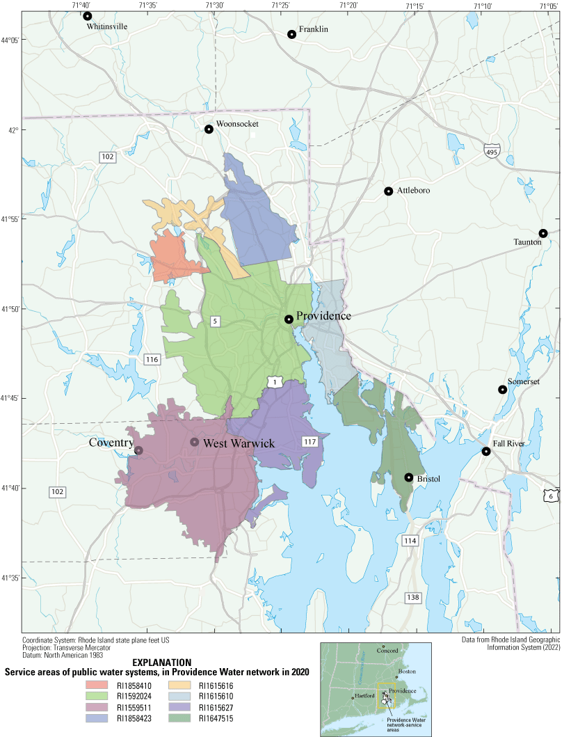
Map showing service area boundaries of all public water systems in the Providence Water network in 2020.
Table 1.
Size of service area and populations served by the public water systems included in the Providence Water network.[Data are from Rhode Island Geographic Information System (2022)]
Before this study, the most recent water-use study for Providence Water took place in 1992 and forecasted water use for the years of 1995, 2000, and 2010 (Roy F. Weston Inc., 1992). Total water withdrawals from the Scituate Reservoir in 2010, however, were below levels projected by Roy F. Weston Inc. (1992), despite more rapid than expected population growth in the serviced municipalities (Manson and others, 2023). Decreasing water withdrawals for public supply have been seen nationally between 2000 and 2015, and domestic daily per capita water-use rates fell nationally between 2005 and 2015 (Maupin and others, 2014; Dieter and others, 2018). The large declines in domestic water use are attributed to the increasing efficiency of home appliances since the 1990s (DeOreo and Mayer, 2012; DeOreo and others, 2016; U.S. Environmental Protection Agency, 2016).
Purpose and Scope
The purposes of this study are twofold: understand the drivers of historical water use in the Providence Water network (the service area of Providence Water and its wholesale customers) and forecast future water use in the same network. To meet these goals, a model was developed for quarterly water use, expressed as daily per capita rates of domestic, commercial, and industrial water use within each of the 8–10 PWSs connected to the Providence Water network. The model was developed for the span of January 2005–December 2021. This model was then used to make forecasts for each quarter in 2030 and 2040 under multiple simulated future scenarios. Quarters in this study run from January–March (Q1), April–June (Q2), July–September (Q3), and October–December (Q4). The scenarios simulated in this study included 12 combinations of 2 climate scenarios (low and high warming), 3 population scenarios (low, medium, and high growth rates), and 2 economic scenarios (low and high growth rates).
Methods
A cubist regression machine-learning model was created using historical data to model water use as daily per capita rates (Quinlan, 1992; RuleQuest Research, 2022). The model used a variety of predictor variables, and the structure of the model created through the machine learning process gave insight to the drivers of historical water use. Predictor variables included climate, demographic, and economic data. The cubist regression model was used to generate forecasts for 2030 and 2040. The predictor variables for those years were simulated to represent different possible future scenarios of climate change, population growth, and economic growth. The historical daily per capita rates used to train the model, the historical predictor variable data, the simulated future predictor variable values, the historical model estimates, the future model forecasts, and a file containing the cubist regression model for use in the R language are published separately in Chamberlin (2024). Reported and estimated daily per capita rates are converted to total water use by multiplying daily per capita rates with populations served.
PWS Service Area Boundaries
In the following methods, a Geographic Information System (GIS) analysis was used to aggregate data for each PWS. The service area boundaries of each PWS were obtained from the Rhode Island Geographic Information System (RIGIS; Rhode Island Geographic Information System, 2022). For the service area boundaries of the two PWSs that later merged with Providence Water, an older version of the service area boundaries shapefile was obtained from the Rhode Island Water Resources Board (RIWRB). The service area boundary of Providence Water prior to these two mergers was determined by spatially subtracting out the service areas of the two merged entities.
Calculating Daily Per Capita Water-Use Rates
Early modeling work during this study identified population as the most influential driver of water use, and therefore water use was modeled as daily per capita rates. Modeling water use as per capita rates instead of as total withdrawals confers several advantages, including improved robustness to statistical methods and easier outlier detection (National Research Council, 2002). Historical data of daily per capita water-use rates (in gallons per capita per day [gal/cap/d]) were calculated from water sale volumes (in gallons) to customers for the three categories of water use previously described, from population served estimates for each PWS in the Providence Water network (in persons), and from the length of each quarter (in days). Average daily per capita rates were calculated for each quarter, year, PWS, and category of water use for which data were available between 2005 and 2021.
Water Sales Volumes
The sources of the water-use data used in this study are water sales records from Providence Water, and annual reports submitted by all PWSs in Rhode Island to the RIWRB. Providence Water sales data were reported monthly, in gallons, by water-use category. Providence Water records split domestic water sales into two categories (“Residential,” representing single-family housing, and “Multi-Family”), which were summed to represent the domestic water-use category for this study. Some months were available as spreadsheets or workbooks, and others were available as Portable Document Format (PDF) files. The annual reports submitted by PWSs to the RIWRB were reported either in gallons or million gallons over a variety of time ranges. All reports were formatted as monthly; however, in many cases, months were left blank with no entries. These were interpreted to indicate that reported volumes represented periods longer than one month. Some reports provided monthly data, others provided quarterly or annual data, and some provided data at irregular time intervals. Reported categories used in this study included “Residential (Total),” which was designated as domestic water use for this study; “Industrial (Total),” which was designated as industrial water use; and “Commercial (Total)” and “Government (Total),” which were summed to represent commercial water use. There was also an “Other (Total)” category, which was not used in this study. The file formats of the annual reports were a mix of spreadsheets, spreadsheets exported as PDF files, PDF files of scanned handwritten reports, and R Data Format files.
Data from all file types except the R Data Format files were manually entered into a new spreadsheet. Once completed, the spreadsheet was loaded into R, where it was combined with data from the R Data Format files. Data then went through an extensive quality assurance and control process that involved plotting data, investigating outliers, referencing original data sources, and, when necessary, contacting the PWS through the assistance of the RIWRB. Adjustments made to the data using the original data sources differed for each report and were made with best professional judgement. Adjustments included correcting the entered year or month of data points by cross referencing annual reports and report sections that overlapped, standardizing the unique identifiers of the PWSs between annual report years, and correcting the units of entered data points on the basis of entered data from surrounding years, consistency between reports, and the feasible bounds of the physical system’s capacity (for example, data might be entered as gallons, but labelled as million gallons). In cases where a data point was reported on more than one annual report, and in cases where the values of the data point differed between reports, the most recent annual report was considered authoritative. Remaining outliers were flagged and the PWSs were contacted. When possible, data were corrected using information or updated reports provided by the PWSs. In one instance only, a PWS confirmed that a data point was physically impossible, but was unable to provide corrected data; therefore, this data point was omitted. When no additional information could be obtained from the PWSs, outliers were retained as entered.
Data reported at monthly timesteps were aggregated to a quarterly timescale. Data reported at quarterly timesteps were used as entered. Data reported at timesteps greater than quarterly were excluded from the historical data for this project. The two PWSs that were incorporated into Providence Water ceased to exist after 2017 and 2020, respectively. Data from these two incorporated entities prior to their incorporation into Providence Water were included in the historical data.
In addition to water sales data, the total volume withdrawn from the Scituate Reservoir is also reported on the annual reports from PW. These data were aggregated to quarterly withdrawals and were compared with the model estimates produced by the cubist regression model.
Population Served Estimates
The PWSs estimate their populations served and report them to the RIWRB and the Safe Drinking Water Information System; however, the methods used differ greatly among PWSs and estimates are not always updated year-to-year as populations grow. For this study, populations served for each PWS were re-estimated using a single method for each year and PWS in the Providence Water network. Population served estimates for each PWS were calculated using the block group level census data from the 2000 decennial count, and from the 5-year American Community Survey datasets for 2009–21, accessed through the Integrated Public Use Microdata Series (IPUMS; Manson and others, 2023). Any missing years of data (including the years 2001–08, which pre-dated the beginning of the American Community Survey 5-year dataset) for an individual block group were filled using linear interpolation between years. Missing data at the beginning or end of a series were given the same values as the closest data point. The population served for each PWS was calculated as the sum of the block group populations, weighted by the extent of spatial overlap between the PWS service boundaries and block groups. The smallest PWS extended across 8 block groups, whereas the largest extended across 283. This method assumes that the population within a given PWS’s service boundary was served by that PWS and no portion of that population was self-served.
The daily per capita rates were then calculated for each quarter as the quarterly volume sold for each category of water use divided by the number of days in the quarter and the population served for the PWS. The daily per capita rates used in the model included 1,268 data points from 9 PWSs, representing 3 different categories of water use and 72 quarters. The 3 categories of water use were evenly represented in the dataset: there were 423 daily per capita rates (ranging from 0 to 46.0 gal/cap/d) calculated for water used for commercial purposes, 417 daily per capita rates (0 to 19.1 gal/cap/d) calculated for water used for industrial purposes, and 428 daily per capita rates (112.3 to 139 gal/cap/d) calculated for water used for domestic purposes. Representation of daily per capita rates in the dataset varied over time, ranging from 48 data points in 2006 to 96 data points in 2008. Representation of the various PWSs also varied, with data points ranging from a minimum of 90 data points for RI1858423 to 204 data points each for RI1559511 and RI1592024.
Predictor Variable Data
The meteorological predictor variables included daily maximum temperatures and daily precipitation values; these were obtained from the Global Historical Climatology Network (GHCN-DAILY; Menne and others, 2012, 2023). Temperature and precipitation data for the years 2000–22 within 25 kilometers of the study area (fig. 1) were filtered to remove data points with data quality flags. For each PWS, daily timeseries of both metrics were generated as a distance-weighted average of all values for stations within 25 kilometers of the centroid of each PWS service boundary. Daily temperature and precipitation data were then aggregated to quarterly values of mean maximum temperatures (in degrees Celsius) and total precipitation (in millimeters) for the years 2005–21.
Demographic predictor variables included population density and median age. Population density of each PWS was calculated for each year between 2005 and 2021 using the population served estimates and the PWS service areas. Median age was obtained from IPUMS at block-group level for years 2000–21 (Manson and others, 2023). Data gaps for each block group were filled in the way previously described in the “Population Served Estimates” section. If no values were available for a census block group, gaps were filled with the mean value of the predictor variable. Block group median age values were aggregated to PWS service area by weighted averaging, using the population of each block group as the weights.
Housing-related predictor variables included in this study were housing unit age, housing unit size, the percentage of units with complete kitchen facilities, and the fraction of housing structures that were single-family homes. The number of housing units, the median build year of housing structures, the median number of rooms per housing unit, and the number of housing units with complete kitchen facilities (including a sink with a faucet, a stove or range, and a refrigerator) were obtained for each block group from IPUMS, and gaps were addressed as previously described (Manson and others, 2023). The percentage of housing units with complete kitchen facilities was calculated for all block groups, and then the median build year, median number of rooms, and percentage of housing units with complete kitchens were aggregated to PWS service areas using weighted averaging. The number of housing units in each block group was used as the weights. The ratio of single-family housing structures was calculated for each PWS using the “E-911 Sites” data layer from RIGIS (Rhode Island Geographic Information System, 2021). This dataset is an emergency response tool that contains locations, descriptions, and classifications of all structures in Rhode Island as of 2021. Structure locations were assigned to PWS service areas using spatial joins, and the ratio of single-family structures (E-911 codes R1 and R3) to all residential structures (E-911 codes R1–R4) were computed for all PWSs. These ratios were considered static throughout the timeframe of this study.
Economic and labor predictor variables in this study included median household income, gross domestic product (GDP), number of private establishments, the coincident economic activity index (CEAI), the unemployment rate, and the percentage of the labor force in nine different sectors of the economy. Median household income data came from IPUMS at block group resolution (Manson and others, 2023), gaps were filled as previously described, and values were aggregated to the PWSs by weighted averaging using the number of housing units per block group as weights. Income data were adjusted for inflation to 2020 U.S. dollars. Inflation data were obtained from the World Bank application programming interface (API) through the “priceR” R package (Condylios, 2022; World Bank, 2023). Monthly data of the size of the labor force and the number of people employed for each county in Rhode Island were obtained from Federal Reserve Economic Data (FRED; Federal Reserve Bank of St. Louis, 2023) using the API service, gap-filled in the same way as the data from IPUMS and averaged by quarter. Quarterly unemployment rates for each county were calculated from these values. Unemployment rates for PWS service areas were the weighted average of the county values, weighted by the spatial overlap of each PWS and each county. Monthly statewide data on the number of employees in total nonfarming industries, construction, education and health services, financial activities, government, information, leisure and hospitality, manufacturing, mining and logging, and professional and business services were also obtained from FRED API (Federal Reserve Bank of St. Louis, 2023). They were averaged by quarter and converted to quarterly percentages of the labor force using the ratio of employees in each sector to the total number of employees in nonfarming industries. Annual GDP data and quarterly data of the total number of private establishments for each county in Rhode Island were obtained from FRED API (Federal Reserve Bank of St. Louis, 2023), gaps were filled as previously described, and data were normalized by the number of people employed in each county. Gross domestic product values were adjusted for inflation to 2020 USD (Condylios, 2022; World Bank, 2023). The coincident economic activity index (CEAI) is a composite index that includes the number of nonfarm employees, the unemployment rate, the average hours worked in manufacturing, and wages and salaries (Federal Reserve Bank of St. Louis, 2023). Monthly statewide CEAI values were obtained from FRED API and averaged for each quarter.
Model Development
A cubist regression machine-learning model was developed using the derived daily per capita rates and the corresponding predictor variable data (Quinlan, 1992; Eng and Wolock, 2022; RuleQuest Research, 2022). The cubist regression model is a type of decision-tree-based model that creates a list of rules about when to apply various linear regression equations to make model estimates of the data. The use of linear regression models allows for more nuanced model estimates under scenarios for which predictor variable data are outside the bounds of training data. Because this study used a model trained on historical data to forecast future scenarios in which conditions differ from those seen historically, this was an important distinction of cubist regression. Other common decision-tree models were considered, including Boosted Regression Trees (Friedman, 2001, 2002) and Extreme Gradient Boosting (Chen and Guestrin, 2016), but these two popular model structures split data into average values instead of linear regressions. As a result, forecasts made for the different future scenarios by these models were similar despite the differences between the future scenarios.
To prevent the model from overfitting the data (meaning that the model describes random fluctuations in the data instead of real signals and therefore cannot be generalized), the model was trained on 80 percent of the data (the training data), then had its predictive ability tested using the remaining 20 percent (the testing data). The daily per capita rates and the associated predictor variable values for each data point were split randomly into training and testing subsets. The modeling steps of selecting predictor variables to include in the model and tuning the model hyperparameters were performed using the training data. Once the model is tuned, the final version of the model is trained with the training data and tested on the testing data.
Cubist regression models have two hyperparameters called “committees” and “neighbors” (Kuhn and Johnson, 2013). Hyperparameters are variable parameters that determine how the model is structured. A committee is a way of boosting the model by building multiple models in sequence. In other words, the input data for each model are adjusted based on the residuals of the previous model, and the final model estimates are made by averaging over the committees. Specifically, for any mth committee, the model uses a pseudo-response variable (in this case, an adjusted daily per capita rate) of the following form:
wherey
is the calculated daily per capita rate originally provided to the cubist regression model,
is the model estimate of y from the previous committee, and
is the pseudo daily per capita rate that is used in the new committee (Kuhn and Johnson, 2013).
When cubist regression models generate estimates, the estimates can be adjusted using the values of a certain number of neighbors, or similar data points from the training data (Kuhn and Johnson, 2013). This approach adjusts model estimates using the following formula:
whereK
is the number of neighbors used,
is a weighting factor based on the distance between new sample y and neighbor n,
is the daily per capita rate observed for neighbor n,
is the daily per capita rate estimated by the cubist regression model committees for a new sample y,
is the daily per capita rate estimated by the cubist regression model for neighbor n.
The exact number of each hyperparameter used is determined during a model tuning process that tests combinations of hyperparameters. The combination found to produce a model that optimizes a given loss function is selected as the final “best” model. In this study, root mean square error (RMSE) was used as the loss function. Model tuning was done using tenfold cross validations (Kuhn and Johnson, 2013). The final combination of hyperparameters from the tenfold cross validation was determined using the “oneSE” approach, which avoids overfitting by selecting the simplest model within one standard error of the model with the most minimized loss function (Breiman and others, 1984).
Predictor variable selection was included in the modeling process to produce the most concise model that excludes predictor variables with negligible effect on daily per capita rates. The Recursive Feature Elimination (RFE) process from the “caret” package (Kuhn, 2008, 2019) was used for predictor variable selection. The process sequentially removes variables in reverse order of their importance, retrains the model, and determines performance using the remaining variables (Kuhn, 2019). Initially, all predictor variables were introduced, and each sequential elimination decreased the number of included predictor variables by five. Model tuning of hyperparameters was nested within the RFE process, with each round of predictor variable selection retuning a new model for that subset of predictor variables. The RFE process was performed within a tenfold cross-validation framework, and the subset of predictor variables retained in the final model was the smallest subset within one standard error of the model with the lowest RMSE (Breiman and others, 1984).
After tuning and recursive feature elimination, a final model was trained using the selected hyperparameters and predictor variables. Specifically, the model was trained with two committees, and predictions were made with three neighbors. Twenty-four predictors were introduced into the recursive feature elimination, and fifteen predictor variables were retained for the final model. After modeling, model estimates were post-processed to correct for systematic bias using the empirical distribution matching method (Belitz and Stackelberg, 2021). This method adjusts the values of the model estimates so that the distribution of the model estimates matches the distribution of the observed data.
Tuning and training were done using the R packages “caret” (Kuhn, 2008), “Cubist” (Kuhn and Quinlan, 2023), “foreach” (Microsoft Corporation and Weston, 2022b) and “doParallel” (Microsoft Corporation and Weston, 2022a), with data organization facilitated using the packages “dplyr” (Wickham and others, 2023a), “tidyr” (Wickham and others, 2023b), and “purrr” (Wickham and Henry, 2023). Investigation of the tuned model was performed using the “iml” package (Molnar and others, 2018). The historical data used to train and test the model, a script that trains the cubist regression model and generates model estimates, and the historical model estimates are available in Chamberlin (2024).
Forecasts
The cubist regression model was used to forecast future water use from simulated predictor variable data. Forecasts were made for each quarter of years 2030 and 2040 (a total of eight time periods) under 12 unique combinations of two climate scenarios (low and high warming), three demographic scenarios (low, medium, and high rates of population growth), and two economic scenarios (low and high rates of economic growth). To approximate uncertainty in forecasts, a Monte Carlo approach was taken in which 100 iterations of each scenario for each quarter were simulated. What follows is a description of how each predictor variable used for the forecasts was simulated under the various scenarios.
The fraction of single-family housing out of total housing, the percentage of housing units with complete kitchen facilities, and the median number of rooms per housing unit were kept the same as they were in the historical data for all future scenarios. Values for these prediction variables were simulated by randomly sampling the historical values of the prediction variable in the appropriate PWS. Median age of the population was simulated to increase at a similar rate of approximately 0.2 years per year under all the climate, demographic, and economic scenarios. This level of growth was selected based on the average rate of increase in the Nation’s median age between 2021 and 2022, after viewing historical data from the U.S. Census Bureau to confirm that this rate was consistent with historical growth (Manson and others, 2023; U.S. Census Bureau, 202346). Values for this prediction variable were simulated using the value for each PWS in 2020, and by adding to that a value sampled from a normal distribution with a mean of 2 and standard deviation of 1 for each decade. Labor forecasts similarly did not vary by scenario, but did vary between 2030 and 2040, and were based on projections made by the Rhode Island Department of Labor (Rhode Island Department of Labor and Training, 2023).
Mean daily maximum temperature for each quarter was varied by climate scenario to assess the effect of climate change on water use but was not varied between 2030 and 2040. This decision was due to the great amount of overlap in climate models between 2030 and 2040 for the northeastern United States (Hayhoe and others, 2007; Sun and others, 2015; Runkle and others, 2022). Mean daily maximum temperature values were simulated by sampling a normal distribution described by the mean and standard deviation of the historical mean daily maximum temperature values for each PWS and quarter, then adjusted by increasing the mean and standard deviations of the distributions by the values given in table 2. Adjustments were chosen using the work of Hayhoe and others (2007). In general, simulated temperatures are warmer under the high warming scenario: however, the variations around the means are large, and there is considerable overlap between the two scenarios.
Table 2.
Summary of simulated average maximum daily temperatures in degrees Celsius used for forecasts in both 2030 and 2040 in the Providence Water network.[Data are from Chamberlin (2024). %, percent; ±, plus or minus]
Three population growth scenarios were simulated: high, medium, and low rates of growth. Populations served for each PWS were estimated for 2030 and 2040 using the 2020 population and simulated growth rates. Simulated growth rates were based on an analysis of historical growth rates in municipalities within the Providence Water network. Historical populations for 21 municipalities between 1970 and 2020 were obtained from IPUMS (Manson and others, 2023). For each of the 21 municipalities, five 10-year population change rates and four 20-year population change rates were calculated, producing a total of 105 historical 10-year population change rates, and 84 historical 20-year population change rates. The highest one-third of population change rates was randomly sampled to simulate population change in the high growth scenario, the middle one-third for the medium growth, and the lowest one-third for the low growth scenarios.1 The distributions used are summarized in tables 3 and 4.
Population could decrease in the future under low growth scenarios because of negative population change rates.
For each scenario, the population density of each PWS was calculated from the simulated population and the service area boundary. Service area boundaries were forecasted to remain constant. High rates of population growth were simulated to be accompanied by increased housing construction to accommodate larger populations, though the historical fraction of single housing out of total housing was kept constant. Median build year was increased from the 2020 value by a value sampled from a normal distribution with mean of 1 and standard deviation of 1 for each decade for the low growth scenario, a distribution with mean 3 and standard deviation of 1 for the medium growth scenario, and a distribution with mean 5 and standard deviation of 1 for the high growth scenario (tables 3, 4). These values were selected on the basis of a preliminary analysis of historical census data from IPUMS (Manson and others, 2023). Population growth scenarios were distinct from each other, with higher rates of population growth associated with higher total PWS populations served, greater average population densities, and newer average median build dates for housing structures (tables 3, 4).
Table 3.
Summary of population change scenarios for forecast year 2030 in the Providence Water network.[Data are from Chamberlin (2024). Negative percent growth indicates possible population decline. %, percent; —, not applicable; ±, plus or minus]
Table 4.
Summary of population change scenarios for forecast year 2040 in the Providence Water network.[Data are from Chamberlin (2024). Negative percent growth indicates possible population decline. %, percent; —, not applicable; ±, plus or minus; √, square root]
Two economic scenarios were considered: high and low rates of growth. To calculate the future values of the unemployment rate, median household income, GDP per employee, number of establishments per employee, and CEAI, base values for all PWSs were adjusted using simulated change rates derived from the 2005–21 data used for model development. Ten-year rates of change for each predictor variable were calculated for each PWS. This produced 63 estimates of each predictor variable. For all predictor variables except unemployment, the higher half of estimates were sampled to simulate the high growth scenario and the lower half of estimates were sampled to simulate the low growth scenario. To simulate rates of unemployment, the higher half of estimates was sampled to simulate the low growth scenario, and the lower half of estimates was sampled to simulate the high growth scenario. These distributions are summarized in table 5. To simulate 2030 predictor variable data, distributions were sampled and applied to the 2020 base values once. To simulate 2040 predictor variable data, distributions were sampled and applied to the 2020 base values twice. Of note, is that the low growth scenario allows for simulating a prolonged recession, where unemployment increases, and median household income, GDP, and the number of establishments all decrease. The simulated values of the five predictor variables varied in the economic scenarios are summarized in table 5.
Table 5.
Summary of the low and high economic growth scenarios in the Providence Water network.[Data are from Chamberlin (2024). Negative percent change values indicate decreases in the variable. GDP, gross domestic product. 2020 USD, United States dollar inflation adjusted to 2020; %, percent]
Results
Reported quarterly total water use from 2005 to 2021 varied greatly between water-use categories; the total reported Providence Water network use median was 0.54 million gallons per day (Mgal/d) for industrial water use, 9.2 Mgal/d for commercial water use, and 33 Mgal/d for domestic water use (Chamberlin, 2024). Reported total water use also varied by PWS, with a median quarterly total use of 26 Mgal/d for Providence Water, and medians that ranged between 0.53 and 6.8 Mgal/d for the other PWSs in the Providence Water network (Chamberlin, 2024).
Seasonality was present in the data, with a median total reported Providence Water network use of 38 Mgal/d in Q1, 38 Mgal/d in Q2, 51 Mgal/d in Q3, and 46 Mgal/d in Q4; there was a significant difference in water use between the four quarters (Kruskal-Wallis rank sum test with 3 degrees of freedom, p<0.001; Chamberlin, 2024). A Dunn’s multiple comparison test showed the most significant differences between Q1 and Q3 (p<0.001), and between Q2 and Q3 (p<0.001); there were no significant differences between Q1 and Q2 (p=0.80) or between Q3 and Q4 (p=0.07). Total reported Providence Water network use decreased between 2005 and 2021 (two-sided seasonal Mann Kendall with 3 degrees of freedom, p<0.001; Helsel and others, 2020), with a Sen’s seasonal slope of total Providence Water networkwide quarterly use of −0.54 Mgal/d per year (Chamberlin, 2024).
Calculated daily per capita rates showed similar seasonality and trends as total reported water use. Median daily per capita rates of water use for the Providence Water network were 57 gal/cap/d in Q1, 57 gal/cap/d in Q2, 77 gal/cap/d in Q3, and 68 gal/cap/d in Q4; a Kruskal-Wallis rank sum test with 3 degrees of freedom showed significant differences between quarters (p<0.001; Chamberlin, 2024). A Dunn’s multiple comparison test for daily per capita rates showed the most significant differences were between Q1 and Q3 (p<0.001) and between Q2 and Q3 (p<0.001); there were no significant differences between Q1 and Q2 (p=0.80) or between Q3 and Q4 (p=0.08). Daily per capita rates also decreased between 2005 and 2021 (two-sided seasonal Mann Kendall with 3 degrees of freedom, p<0.001; Helsel and others, 2020), with a Sen’s seasonal slope of −0.85 gal/cap/d per year (Chamberlin, 2024).
Model Structure and Performance
After model tuning and RFE, a cubist regression model with two committees was trained on the data. Model estimates were made using three neighbors. Of the 24 predictor variables introduced to the model, 15 were retained after the RFE process:
-
• category of water use (domestic, commercial, or industrial),
-
• the quarter of the calendar year,
-
• average daily maximum temperature,
-
• population density,
-
• median population age,
-
• the unemployment rate,
-
• the fraction of the labor force in manufacturing,
-
• the fraction of housing that are single-family homes,
-
• the median build year of housing,
-
• the median number of rooms per housing unit,
-
• the fraction of housing units with complete kitchens,
-
• median household income,
-
• GDP per employee,
-
• the number of establishments per employee, and
-
• the CEAI.
After bias correction, model estimates of daily per capita rates were correlated with an overall Pearson’s r2 of 0.99 for training data and 0.94 for testing data. Root mean square error for training data was 2.8 gal/cap/d and for testing data was 6.6 gal/cap/d. Modelled values of daily per capita rates for domestic, commercial, and industrial water-use fit the training data with Pearson’s r2 values of 0.96, 0.97, and 0.80, respectively, and Pearson’s r2 values of 0.77, 0.82, and 0.63, respectively, for the testing data. Root mean square error was 4.3, 1.9, and 1.1 gal/cap/d for training data for domestic, commercial, and industrial water use, respectively, and was 10.1, 4.6, and 1.3 gal/cap/d, respectively, for testing data. Model predictions are shown in figure 2.
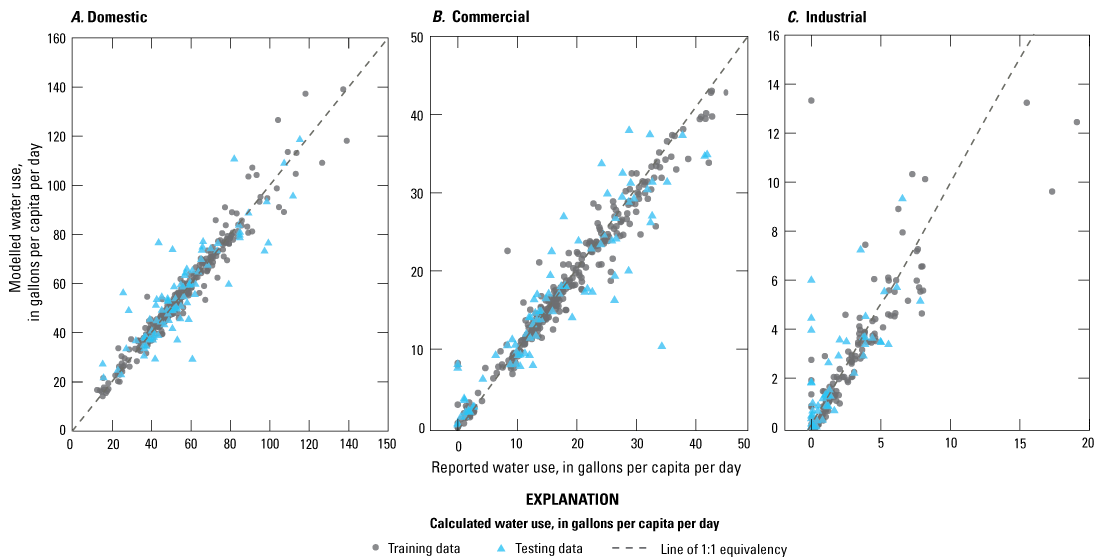
Graphs showing modeled predictions of water use compared with calculated total water use (in gallons per capita per day) in the Providence Water network for A, domestic, B, commercial, and C, industrial water-use categories.
Modeled total Providence Water network quarterly water use estimates from the cubist regression model included estimates of both reported and unreported water. Modeled total quarterly use between 2005 and 2021 had a significant negative trend of −0.96 Mgal/d per year (95-percent confidence interval of −0.79 to −1.15; seasonal Mann Kendall Trend test, p<0.001; fig. 3; Helsel and others, 2020). Estimated total Providence Water network use ranged from a minimum of 36 Mgal/d in Q1 2021 to a maximum of 73 Mgal/d in Q3 2005 (fig. 3). Estimated total Providence Water network water use should be higher than reported water use owing to the inclusion of unreported water use. It should also be less than total withdrawals from the Scituate Reservoir reported by Providence Water owing to water losses through leaks, water uses from the “Other (Total)” categories of the annual reports, water used to fight fires, and so on. Estimated total Providence Water network water use falls between these two values for 63 of the 68 quarters (or 93 percent of the period) examined in this study (fig. 3). Estimated water use fell below reported water use in Q4 2012, Q4 2015, and Q4 2020, and it rose above withdrawals from the Scituate Reservoir in Q4 2006 and Q1 2014. Modeled total Providence Water network quarterly use was significantly correlated with both reported use (p<0.001, Pearson’s r2=0.70) and Providence Water network withdrawals from the Scituate Reservoir (p<0.001, Pearson’s r2=0.46).
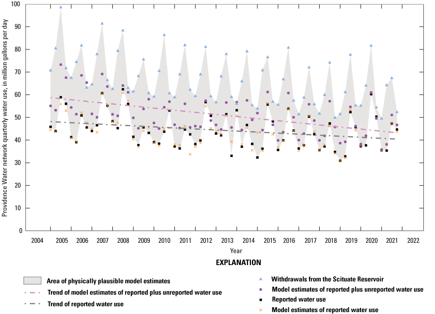
Graph showing model estimates of reported water use and model estimated of reported plus unreported water use for the Providence Water network. Also shown are Providence Water network reported water use, and withdrawals from the Scituate Reservoir.
Shapley Additive exPlanations (SHAP) values show the relative effect of predictor variables within the cubist regression model for each model estimate (Lundberg and Lee, 2017). SHAP values that are greater than zero increase the estimate, and values less than zero decrease the estimate. The predictor variable with the highest average absolute SHAP values was “category of water use” (fig. 4). The designation of “domestic” was associated with higher water-use estimates, whereas designations of “industrial” or “commercial” were associated with lower water-use estimates (fig. 5). Quarters 1 and 2 are generally associated with lower water use than quarters 3 and 4, and the difference is much greater for domestic water use than for commercial or industrial (fig. 5). Temperatures above 20 degrees Celsius were associated with greater domestic water use (fig. 6). Higher population densities were associated with higher commercial water use and lower domestic water use (fig. 7). Housing units with more rooms, and a greater median year structure built (in other words, more recently built housing) were associated with higher commercial water use and lower domestic water use (fig. 8). The portion of total housing that was single-family homes did not have a monotonic effect (fig. 8). The relative variation in SHAP values between water-use categories was generally less for economic predictor variables than it was for demographic or housing-related variables. An exception is that higher rates of employment in the manufacturing sector were associated with greater increases in domestic water use than in commercial or industrial water use (fig. 9).
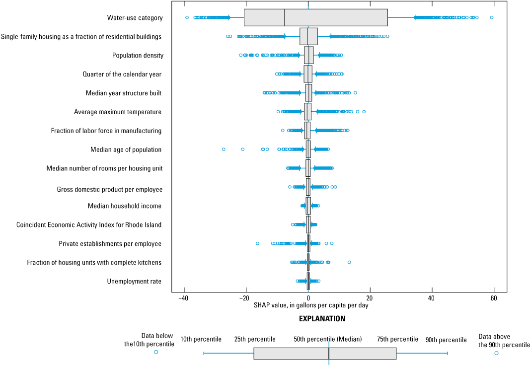
Graph showing Shapley Additive exPlanations (SHAP) values for all predictor variables used for predicting water use in the Providence Water network. Values are shown in descending order according to their mean absolute SHAP value. SHAP values are normalized to the mean training data prediction, with positive SHAP values indicating a positive effect on predictions, and negative values indicating negative effects.
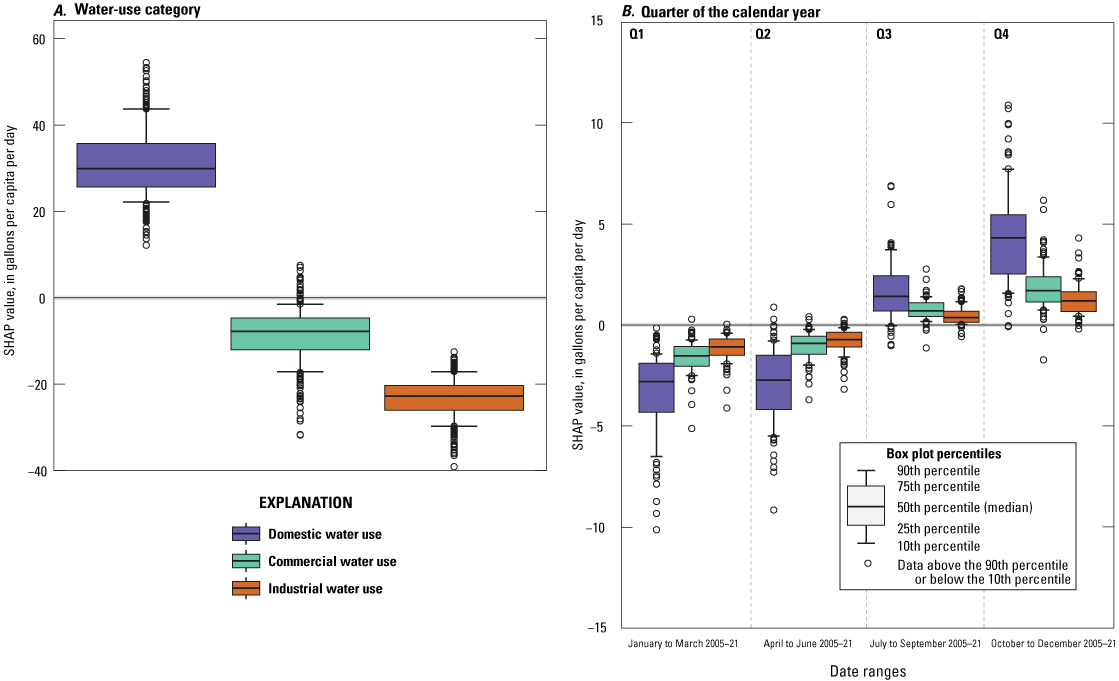
Graphs showing Shapley Additive exPlanations (SHAP) values for two of the predictor variables used for predicting water use in the Providence Water network. SHAP values represent the effects of A, water-use category and, B, quarter of the calendar year (shown for 2005–21). SHAP values are normalized to the mean training data prediction, with positive SHAP values indicating a positive effect on predictions, and negative values indicating negative effects.
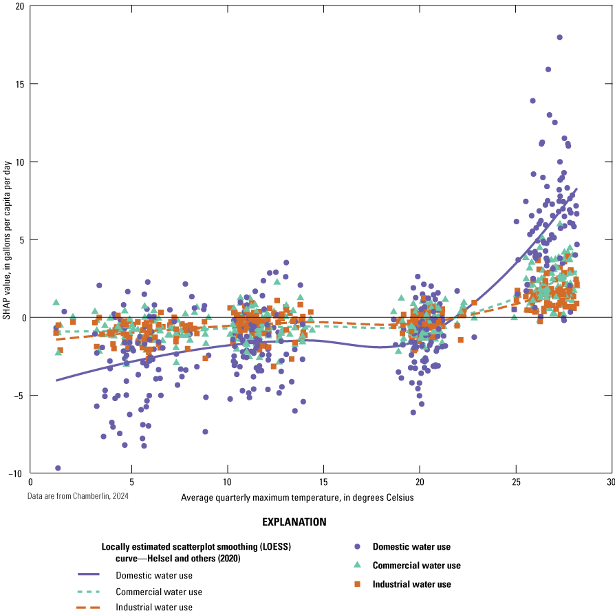
Graph showing Shapley Additive exPlanations (SHAP) values showing the effect of average quarterly maximum daily temperature in degrees Celsius on water use in the Providence Water network. SHAP values greater than 0 indicate the variable feature increased water use estimates, w values less than 0 indicate decreased water use estimates.
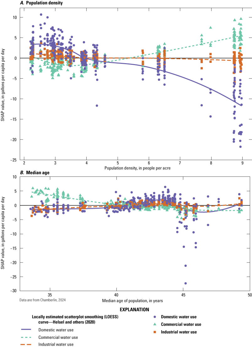
Graphs showing Shapley Additive exPlanations (SHAP) values showing the effects of demographic predictor variables on water use in the Providence Water network. Predictor variables include A, population density and, B, median age of population. SHAP values greater than 0 indicate the variable feature increased water-use estimates, while values less than 0 indicate decreased water-use estimates.
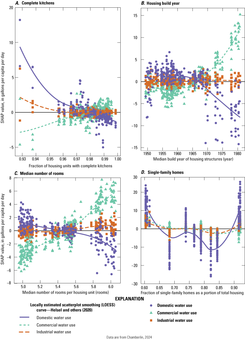
Graphs showing Shapley Additive exPlanations (SHAP) values showing the effect of housing predictor variables on water use in the Providence Water network. Predictor variables include A, housing units with complete kitchens, B, median build year of housing structures, C, median number of rooms per housing unit, and D, single-family homes as a portion of total housing. SHAP values greater than 0 indicate the variable feature increased water-use estimates, while values less than 0 indicate decreased water-use estimates.
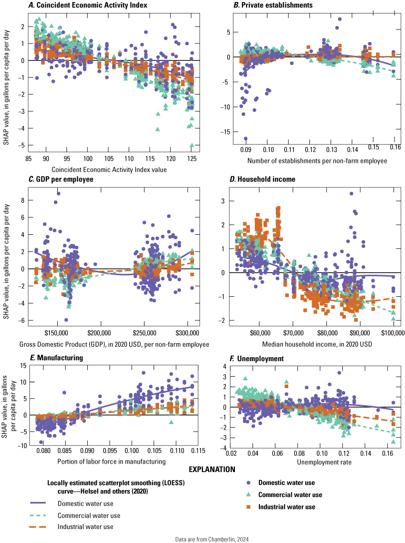
Graphs showing Shapley Additive exPlanations (SHAP) values showing the effects of economic predictor variables on water use in the Providence Water network. Economic predictor variables include A, coincident economic activity index, B, number of establishments per non-farm employee, C, gross domestic product (GDP) per non-farm employee, D, median household income in 2020 U.S. dollars (USD), E, portion of labor force in manufacturing, and F, unemployment rate. SHAP values greater than 0 indicate the variable feature increased water-use estimates, while values less than 0 indicate decreased water-use estimates.
Future Forecasts
Forecasts made by the cubist regression model indicated that daily per capita rates are expected to decrease more in the scenarios with high population growth (fig. 10). However, total Providence Water network water use in Mgal/d is forecasted to be less sensitive to population growth than daily per capita water-use rates. Both daily per capita rates of water use and total Providence Water network water use are forecasted to decrease under higher rates of economic growth (fig. 11). Effects of climate change were minimal over the 2030 and 2040 prediction horizon based on the scenarios tested (fig. 12). Though the median water use forecasted is estimated to be slightly higher under higher warming scenarios, the range of forecasted water use under each climate scenario overlap substantially.
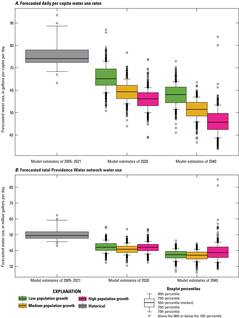
Graphs showing distributions of historical estimated annual water use and forecasted future water use in the Providence Water network under the three population growth scenarios considered in the study displayed as, A, daily per-capita water-use rates and, B, total Providence Water network average water use.
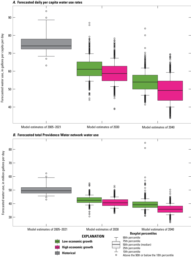
Graphs showing distributions of historical estimated annual water use and forecasted future water use in the Providence Water network under the two economic growth scenarios considered in the study displayed as, A, daily per-capita water-use rates, and B, total Providence Water network average water use.
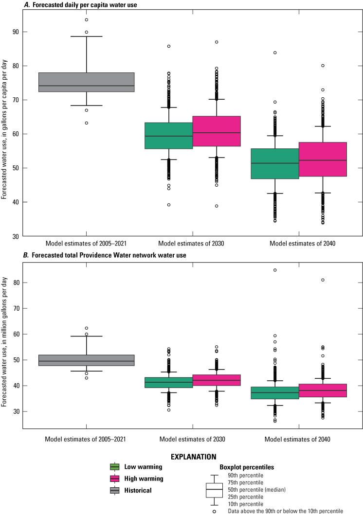
Graphs showing distributions of historical estimated annual water use and forecasted future water use in the Providence Water network under the two climate warming scenarios considered in the study displayed as, A, daily per-capita water-use rates and, B, total Providence Water network average water use.
Across all scenarios, annual average water use was forecast to decrease in 2030 and further decrease in 2040 (fig. 13). The annual forecasted daily per capita rates and Providence Water networkwide water use are forecasted to be significantly below the levels of water use seen in 2005–21 (Kruskal-Wallis test, p<0.001 for both groups). Of all the forecasts, only 17 percent of forecasted daily per capita rates and 21 percent of forecasted annual Providence Water networkwide uses were equal to, or greater than, those seen in 2005–21. Of all forecasts, 83 percent of daily per capita rates and 79 percent of Providence Water networkwide water-use forecasts were below values from 2005 to 2021.
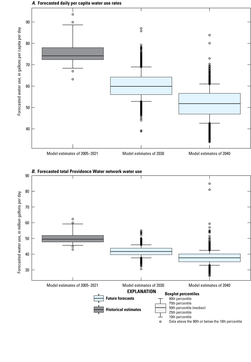
Graphs showing distributions of historical estimated annual water use and forecasted future water use under all scenarios considered in the study displayed as, A, daily per-capita water-use rates and, B, total Providence Water network average water use.
Annual median forecasts of daily per capita rates varied from a low of 42.4 gal/cap/d in 2040 under high population and economic growth scenarios and high climate warming to a high of 67.6 gal/cap/d in 2030 under low economic and population growth scenarios with high climate warming (table 6). The lowest median annual forecasted Providence Water networkwide use was 35.0 Mgal/d in 2040 under medium population growth, high economic growth, and low climate warming. The highest median annual forecasted Providence Water networkwide water use was 43.5 Mgal/d in 2030 under low population and economic growth, and high climate warming (table 6). Median forecasts for all scenarios were less than model estimates for 2005–21. The 95-percent confidence intervals of forecasted scenarios had some overlap with the historical 95-percent confidence intervals for all but the daily per capita water-use rate forecasts in the high population growth, high economic growth, and high climate change scenario in 2030. For the 2040 forecasts, however, only low population growth scenarios had overlapping 95-percent confidence intervals with the historical estimates for the daily per capita water-use rates (table 6). In 2040, all the high population growth rate scenarios had overlapping 95-percent confidence intervals for the total Providence Water network water use.
Table 6.
Annual average water-use forecasts for 2030 and 2040 in the Providence Water network compared with estimates for 2005–21.[gal/cap/d, gallons per capita per day; Mgal/d, million gallons per day; %, percent]
Similar patterns of forecasts were observed at the quarterly timescale, where forecasts fell below the historical ranges of quarterly water use (fig. 14). The differences between forecasted water-use rates and simulated water-use rates for the years 2005–21 were comparable in magnitude to the differences between quarters for each forecasted year. For example, daily per capita rates in Q3 2040 were predicted to be similar to the rates in Q1 each year from 2005 to 2021 (fig. 14). Forecasts for Q2 and Q4 were similar to each other in the forecasts for 2030 and 2040, whereas the Q3 forecasts were higher, and Q1 forecasts were lower. Quarterly forecasts are summarized in table 7.
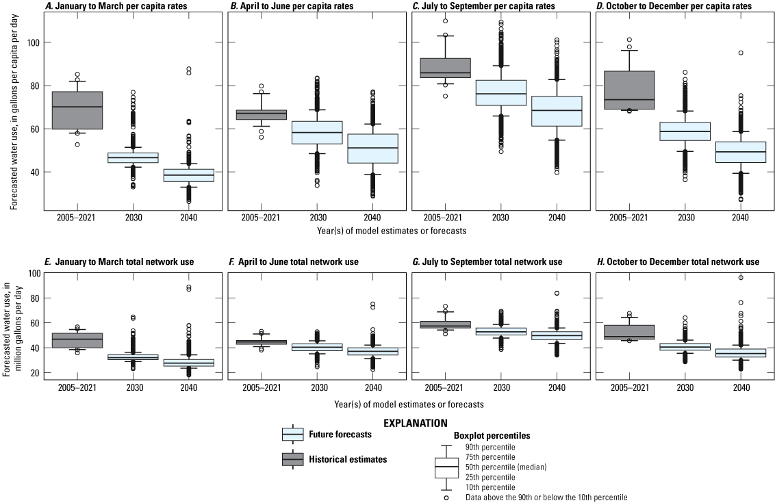
Graphs showing distributions of historical estimated water use and forecasted future water use in the Providence Water network under all scenarios considered in the study, per quarter (Q): A, Q1 daily per-capita water-use rates, B, Q2 daily per-capita water-use rates, C, Q3 daily per-capita water-use rates, D, Q4 daily per-capita water-use rates, E, Q1 Providence Water network total water use, F, Q2 Providence Water network total water use, G, Q3 Providence Water network total water use, and, H, Q4 Providence Water network total water use.
Table 7.
Quarterly average water-use forecasts for 2030 and 2040 in the Providence Water network compared with estimates for 2005–21.[gal/cap/d, gallons per capita per day; Mgal/d, million gallons per day; %, percent]
Discussion
The cubist regression model developed for historical water use had high accuracy, with an r2 of 0.94 for the testing data. The model estimated domestic, commercial, and industrial water use simultaneously, though the most influential variable in the model was the designation of the water-use category, indicating that the model estimated these different categories in different ways (Chamberlin, 2024). Within each category of water use, the r2 values of the testing data were lower than for the overall model, ranging from an r2 of 0.63 for industrial water use to 0.82 for commercial water use. A known strength of machine-learning models, such as cubist regression, is the flexibility with which they can accommodate non-linear interactions between different variables (Kuhn and Johnson, 2013). For example, in this study, many of the predictor variables displayed different patterns of significance on the basis of water-use category (figs. 6, 7, 8, 9). Different categories of water use are known to respond differently to different predictor variables, and, for that reason, water-use studies often model one category of water use at a time (for example, Lins and others, 2010; Huang and others, 2017; Harris and Diehl, 2019; Stagnitta and Medalie, 2023). The flexibility of the cubist regression model to accommodate the different interactions of predictor variables for different water-use categories allowed the use of one single model instead of separate models for each water-use category.
One PWS (RI2980183) reported annual volumes of water sold prior to 2015 but did not report quarterly volumes sold. For that reason, no data from this PWS were included in training the model. However, annual data by category of water use were available and were used to assess the performance of the model under conditions different from the conditions used to train the model. For this PWS, the correlation of model-estimated yearly water use to reported yearly water use for all categories of water use combined had a Pearson’s r2 value of 0.73, with a percent bias of 77 percent. However, correlation of model estimates to reported water use within water-use categories resulted in Pearson’s r2 values of 0.23 for domestic water use, 0.10 for commercial water use, and model estimates of a constant 0 for industrial water use, despite reported annual water use greater than zero. This indicates that the model can predict total water use more accurately than it can predict water use of a specific water-use category.
Drivers of Historical Water Use
The seasonality of water use, especially of domestic water use, is seen in many water-use studies, with more outdoor water use during the summer months (Mills and others, 2014; Ahmed and others, 2020). The SHAP values for the predictor variables average daily maximum temperature and calendar year quarter agree with this pattern: water use at temperatures greater than 20 degrees Celsius was greater than water use at lower temperatures, and the greatest increase was for domestic water use (fig. 6). The importance of calendar year quarter as a predictor variable in the model, with the highest water use in summer and fall, also supports greater seasonality for domestic water use than for commercial or industrial water use in this study (fig. 5).
Outdoor water use would reasonably be expected to be higher for single-family homes than multi-family homes, leading to greater overall daily per capita water-use rates in single-family homes (Stoker and Rothfeder, 2014; Villarin and Rodriguez-Galiano, 2019). In this study, areas with comparatively high proportions of single-family homes did have higher residential water use; however, so did areas with comparatively low proportions (fig. 8). The proportion of single-family homes was the only variable that was fixed for each PWS and did not vary across quarters or years; therefore, it is possible that the model used this predictor variable to account for differences between PWS not explicitly accounted for in this study (for example, differences in reporting procedures or differences in how service connections are categorized). The increase in water use at lower proportions of single-family housing may be due to some other factor not accounted for in this study. This study found a decrease in daily per capita domestic water use with increasing population density (fig. 7), which was consistent with the pattern of decreased per capita water use for larger cities seen in the United States (Mahjabin and others, 2018).
A previous study of water use in Providence, Rhode Island, done by Stagnitta and Medalie (2023), used linear regression to model water use at a monthly timescale between 2014 and 2021. The results of this study were generally consistent with Stagnitta and Medalie (2023). Their study also modeled daily per capita rates, and modeled single-family domestic, multi-family domestic, commercial (defined slightly differently than this study), and industrial water use separately with unique linear regression models for each category of water use. For both studies, temperature (as average daily maximum temperature in this study and as the square of minimum temperature in Stagnitta and Medalie [2023]) had a positive relation with domestic and industrial water use, though temperature was not retained in the commercial water-use model of Stagnitta and Medalie (2023). Similarly, Stagnitta and Medalie (2023) found binary indicators of low and high water-use seasons (defined as December–May for low water use and July–September for high water use) to be influential in their study. These findings may correspond to the influence of the calendar year quarter predictor variable in this model. Both Stagnitta and Medalie (2023) and this current study found CEAI to be inversely related to water use. The effects of the coronavirus disease 2019 (COVID-19) pandemic were explicitly included in Stagnitta and Medalie (2023) and were found to be significant for the commercial and industrial models. In the current study, the effects of the COVID-19 pandemic were not explicitly included, but the model estimated water use in 2020 (with an r2 of 0.98 on training data and an r2 of 0.88 on testing data) using the provided input predictor variable data. These model results may indicate that the provided input data sufficiently represented the effects of the pandemic without having to include the pandemic explicitly.
Forecasts of Future Water Use
The model estimates for many future scenarios showed water-use values that were less than reported or estimated water-use values over the past two decades. Median water-use forecasts were generally higher for 2030 than 2040, and 2030 projections were mostly lower than the water use estimated for 2021. The daily per capita rates are forecast to decrease with increasing population (due to increasing population density and newer housing) however, increasing populations increase total water use (in that more people consume more water), and, as such, the relative balance of these two effects led to a nearly negligible effect on total Providence Water network water use according to the population scenarios (fig. 10). Historically, the increase in population over the past two decades has been associated with an overall decrease in water use, which is likely caused by increased water efficiency of domestic use (DeOreo and Mayer, 2012; DeOreo and others, 2016). The model did not directly account for increases in efficiency of water-using appliances; however, other predictor variables, such as the median build age of housing units, may be capable of representing this trend. Other factors that can improve water efficiency, such as controlled leakage in pipes, more effective water auditing, and consumer education campaigns (U.S. Environmental Protection Agency, 2016), were likewise not included in this model, because of a lack of representative data.
The historical decrease of total Providence Water network water use between 2005 and 2021 indicates that the decreases in daily per capita rates have more than compensated for increases in population. The forecasts from this model indicate that this balance might be shifting in the future, in that decreases in daily per capita rates may no longer outweigh increases in population, and total network water use may not continue decreasing at the same rate or might stabilize at a lower level of water use. Though nearly all simulated scenarios were forecasted to have lower water use than historical water use, 17 percent of forecasted daily per capita rates were equal to historical rates. Therefore, the forecasts leave open the possibility for an increase in future water use, though the likelihood of a future increase in water use is small.
A limitation of this study is that the cubist regression model assumes that the current associations between the data will continue into the future. For example, if the association between changes in housing stock and changes in water use are different in the future (for example, if daily per capita rates no longer decrease with increases in median age of houses), the model will not account for these shifts. This study attempted to account for future unknowns such as this by modeling multiple future scenarios. We recommend using the forecasts based on demographic, economic, and climate scenarios together to bound the expectations for future water use projections rather than using them in isolation as precise estimates for individual scenarios.
Summary
Historical water use in the Providence Water network was accurately modeled by the U.S. Geological Survey in cooperation with Providence Water by using a cubist regression model. This study found that historical daily per capita rates in the Providence, Rhode Island, area have historically been affected by a combination of demographic, economic, and climate variables. In 2030 and 2040, mean annual water use is likely to continue to decrease with respect to historical (2005–21) total Providence Water network use, irrespective of changes in population, climate, or economic growth. Though varying rates of economic and population growth may change the magnitude of this decrease, the differences in estimated water use between the simulated future scenarios are generally smaller than the differences in estimated water use between 2005 and 2021, 2030, and 2040. Climate change is unlikely to have a substantial effect on water use in the next two decades. Water use across all seasons is forecast to decrease on average. However, under certain scenarios, several future forecasts of water use match or exceed historical water use. Therefore, although unlikely, the possibility of high water use (especially occasional or seasonal high water use) in the distribution system remains.
References Cited
Belitz, K., and Stackelberg, P.E., 2021, Evaluation of six methods for correcting bias in estimates from ensemble tree machine learning regression models: Environmental Modelling & Software, v. 139, 12 p., accessed May 04, 2023, at https://doi.org/10.1016/j.envsoft.2021.105006.
Breiman, L., Friedman, J.H., Olshen, R.A., and Stone, C.J., 1984, Classification and regression trees: New York, Chapman & Hall/CRC, 368 p. [Also available at https://doi.org/10.1201/9781315139470.]
Chamberlin, C.A., 2024, Model archive, input data, modeled estimates of water use 2005-2021, and forecasts of water use in 2030 and 2040 in Providence, Rhode Island: U.S. Geological Survey data release, https://doi.org/10.5066/P94XIQ7W.
Chen, T., and Guestrin, C., 2016, XGBoost: A scalable tree boosting system: Proceedings of the 22nd ACM SIGKDD International Conference on Knowledge Discovery and Data Mining, San Francisco, Calif., August 13–17, 2016: Association for Computing Machinery, p. 785–794, accessed September 6, 2023, at https://doi.org/10.1145/2939672.2939785.
Condylios, S., 2022, priceR—Economics and pricing tools (version 0.1.67): The Comprehensive R Archive Network webpage, accessed September 15, 2023, at https://doi.org/10.32614/CRAN.package.priceR.
DeOreo, W.B., Mayer, P., Dziegielewski, B., and Kiefer, J., 2016, Residential end uses of water, version 2—Executive report: Water Research Foundation, 15 p. [Also available at https://www.awwa.org/Portals/0/AWWA/ETS/Resources/WaterConservationResidential_End_Uses_of_Water.pdf.]
DeOreo, W.B., and Mayer, P.W., 2012, Insights into declining single-family residential water demands: Journal AWWA, v. 104, no. 6, p. E383–E394, accessed June 7, 2022, at https://doi.org/10.5942/jawwa.2012.104.0080.
Dieter, C.A., Maupin, M.A., Caldwell, R.R., Harris, M.A., Ivahnenko, T.I., Lovelace, J.K., Barber, N.L., and Linsey, K.S., 2018, Estimated use of water in the United States in 2015: U.S. Geological Survey Circular 1441, 65 p., accessed January 19, 2024, at https://doi.org/10.3133/cir1441. [Supersedes USGS Open-File Report 2017–1131.]
Eng, K., and Wolock, D.M., 2022, Evaluation of machine learning approaches for predicting streamflow metrics across the conterminous United States: U.S. Geological Survey Scientific Investigations Report 2022–5058, 27 p., accessed September 14, 2022, at https://doi.org/10.3133/sir20225058.
Federal Reserve Bank of St. Louis, 2023, FRED economic data: Federal Reserve Bank of St. Louis database, accessed December 5, 2023, at https://fred.stlouisfed.org/#.
Friedman, J.H., 2001, Greedy function approximation—A gradient boosting machine: Annals of Statistics, v. 29, no. 5, p. 1189–1232, accessed February 13, 2024, at https://doi.org/10.1214/aos/1013203451.
Friedman, J.H., 2002, Stochastic gradient boosting: Computational Statistics & Data Analysis, v. 38, no. 4, p. 367–378, accessed February 13, 2024, at https://doi.org/10.1016/S0167-9473(01)00065-2.
Harris, M.A., and Diehl, T.H., 2019, Withdrawal and consumption of water by thermoelectric power plants in the United States, 2015: U.S. Geological Survey Scientific Investigations Report 2019–5103, 15 p. [Also available at https://doi.org/10.3133/sir20195103.]
Hayhoe, K., Wake, C.P., Huntington, T.G., Luo, L., Schwartz, M.D., Sheffield, J., Wood, E., Anderson, B., Bradbury, J., DeGaetano, A., Troy, T.J., and Wolfe, D., 2007, Past and future changes in climate and hydrological indicators in the US Northeast: Climate Dynamics, v. 28, no. 4, p. 381–407, accessed January 15, 2023, at https://doi.org/10.1007/s00382-006-0187-8.
Helsel, D.R., Hirsch, R.M., Ryberg, K.R., Archfield, S.A., and Gilroy, E.J., 2020, Statistical methods in water resources: U.S. Geological Survey Techniques and Methods, book 4, chap. A3, 458 p., accessed January 15, 2023, at https://doi.org/10.3133/tm4A3. [Supersedes USGS Techniques of Water-Resources Investigations, book 4, chap. A3, version 1.1.]
Huang, A.-C., Lee, T.-Y., Lin, Y.-C., Huang, C.-F., and Shu, C.-M., 2017, Factor analysis and estimation model of water consumption of government institutions in Taiwan: Water, v. 9, no. 7, 10 p., accessed June 7, 2022, at https://doi.org/10.3390/w9070492.
Kuhn, M., 2008, Building predictive models in R using the caret package: Journal of Statistical Software, v. 28, no. 5, p. 1–26, accessed January 15, 2023, at https://doi.org/10.18637/jss.v028.i05.
Kuhn, M., 2019, The caret package: Github web page, accessed February 13, 2024, at https://topepo.github.io/caret/index.html.
Kuhn, M., and Johnson, K., 2013, Applied predictive modeling: New York, Springer, 600 p. [Also available at https://doi.org/10.1007/978-1-4614-6849-3.]
Kuhn, M., and Quinlan, R., 2023, Cubist—Rule- and instance-based regression modeling (version 0.4.2.1): The Comprehensive R Archive Network webpage, accessed November 13, 2023, at https://doi.org/10.32614/CRAN.package.Cubist.
Lins, G.M.L., Cruz, W.S., Vieira, Z.M.C.L., Neto, F.A.C., and Miranda, É.A.A., 2010, Determining indicators of urban household water consumption through multivariate statistical technique: Journal of Urban and Environmental Engineering, v. 4, no. 2, p. 74–80, accessed June 7, 2022, at https://doi.org/10.4090/juee.2010.v4n2.074080.
Lorente-Leyva, L.L., Pavón-Valencia, J.F., Montero-Santos, Y., Herrara-Granda, I.D., Herrara-Granda, E.P., and Peluffo-Ordóñez, D.H., 2019, Artificial neural networks for urban water demand forecasting—A case study: Journal of Physics—Conference Series 1284, 8 p., accessed June 7, 2022, at https://doi.org/10.1088/1742-6596/1284/1/012004.
Lundberg, S.M., and Lee, S.-I., 2017, A unified approach to interpreting model predictions, in Proceedings of the 31st International Conference on Neural Information Processing Systems (NIPS 2017), Long Beach, Calif., December 4–9, 2017: Red Hook, N.Y., Curran Associates, Inc., accessed September 11, 2023, at https://dl.acm.org/doi/10.5555/3295222.3295230.
Mahjabin, T., Garcia, S., Grady, C., and Mejia, A., 2018, Large cities get more for less—Water footprint efficiency across the US: PLoS ONE, v. 13, no. 8, 17 p., accessed February 21, 2024, at https://doi.org/10.1371/journal.pone.0202301.
Manson, S., Schroeder, J., Van Riper, D., Knowles, K., Kugler, T., Roberts, F., and Ruggles, S., 2023, IPUMS national historical geographic information system, version 18.0: Minneapolis, Minn., IPUMS NHGIS database, accessed June 13, 2023, at https://doi.org/10.18128/D050.V18.0.
Maupin, M.A., Kenny, J.F., Hutson, S.S., Lovelace, J.K., Barber, N.L., and Linsey, K.S., 2014, Estimated use of water in the United States in 2010: U.S. Geological Survey Circular 1405, 56 p. [Also available at https://doi.org/10.3133/cir1405.]
Menne, M.J., Durre, I., Korzeniewski, B., McNeill, S., Thomas, K., Yin, X., Anthony, S., Ray, R., Vose, R.S., Gleason, B.E., and Houston, T.G., 2023, Global historical climatology network–Daily (GHCN-Daily), version 3.29: National Oceanic and Atmospheric Administration, National Climatic Data Center dataset, accessed January 30, 2023, at https://doi.org/10.7289/V5D21VHZ.
Menne, M.J., Durre, I., Vose, R.S., Gleason, B.E., and Houston, T.G., 2012, An overview of the Global Historical Climatology Network-Daily database: Journal of Atmospheric and Oceanic Technology, v. 29, no. 7, p. 897–910, accessed January 15, 2023, at https://doi.org/10.1175/JTECH-D-11-00103.1.
Microsoft Corporation, and Weston, S., 2022a, doParallel—Foreach parallel adaptor for the 'parallel' package (version 1.0.17): The Comprehensive R Archive Network webpage, accessed March 14, 2024, at https://CRAN.R-project.org/package=doParallel.
Microsoft Corporation, and Weston, S., 2022b, Foreach—Foreach looping construct (version 1.5.2): The Comprehensive R Archive Network webpage, accessed March 14, 2024, at https://doi.org/10.32614/CRAN.package.foreach.
Mills, P.C., Duncker, J.D., Over, T.M., Domanski, M.M., and Engel, F.L., 2014, Evaluation of a mass-balance approach to determine consumptive water use in northeastern Illinois: U.S. Geological Survey Scientific Investigations Report 2014–5176, 90 p., accessed June 7, 2022, at https://doi.org/10.3133/sir20145176.
Molnar, C., Casalicchio, G., and Bischl, B., 2018, iml—An R package for interpretable machine learning: Journal of Open Source Software, v. 3, no. 26, 2 p., accessed January 15, 2023, at https://doi.org/10.21105/joss.00786.
National Research Council, 2002, Estimating water use in the United States—A new paradigm for the National Water-Use Information Program: Washington, D.C., The National Academies Press, 190 p. [Also available at https://doi.org/10.17226/10484.]
Rhode Island Department of Labor and Training, 2023, Major occupational group (Excel): State of Rhode Island Department of Labor and Training, accessed January 15, 2023, at https://dlt.ri.gov/labor-market-information/data-center/2030-industry-occupational-projections.
Rhode Island Geographic Information System, 2021, E-911 sites: State of Rhode Island Division of Planning and University of Rhode Island Environmental Data Center dataset, accessed May 18, 2022, at https://www.rigis.org/datasets/edc:e-911-sites/.
Rhode Island Geographic Information System, 2022, Water supply districts, 2022, State of Rhode Island Division of Planning and University of Rhode Island Environmental Data Center dataset, accessed November 8, 2022, at https://www.rigis.org/datasets/edc:water-supply-districts-2022/.
Robinson, J.A., 2019, Estimated use of water in the Cumberland River watershed in 2010 and projections of public-supply water use to 2040: U.S. Geological Survey Scientific Investigations Report 2018–5130, 62 p., accessed June 7, 2022, at https://doi.org/10.3133/sir20185130.
RuleQuest Research, 2022, Data mining with Cubist: RuleQuest Research webpage, accessed January 14, 2023, at https://www.rulequest.com/cubist-info.html.
Stagnitta, T.J., and Medalie, L., 2023, Assessment of factors that influence human water demand for Providence, Rhode Island: U.S. Geological Survey Scientific Investigations Report 2023–5057, 18 p., accessed September 5, 2023, at https://doi.org/10.3133/sir20235057.
Stoker, P., and Rothfeder, R., 2014, Drivers of urban water use: Sustainable Cities and Society, v. 12, p. 1–8, accessed February 21, 2024, at https://doi.org/10.1016/j.scs.2014.03.002.
Sun, L., Kunkel, K.E., Stevens, L.E., Buddenberg, A., Dobson, J.G., and Easterling, D.R., 2015, Regional surface climate conditions in CMIP3 and CMIP5 for the United States—Differences, similarities, and implications for the U.S. National Climate Assessment: National Oceanic and Atmospheric Administration Technical Report NESDIS 144, 111 p., accessed January 15, 2023, at https://doi.org/10.7289/V5RB72KG.
U.S. Census Bureau, 2023, America is getting older: U.S. Census Bureau press release, June 22, 2023, accessed February 13, 2024, at https://www.census.gov/newsroom/press-releases/2023/population-estimates-characteristics.html.
U.S. Environmental Protection Agency, 2016, Best practices to consider when evaluating water conservation and efficiency as an alternative for water supply expansion: U.S. Environmental Protection Agency report EPA-810-B-16-005, 60 p., accessed February 8, 2024, at https://www.epa.gov/sustainable-water-infrastructure/best-practices-water-conservation-and-efficiency-alternative-water.
U.S. Environmental Protection Agency, 2022, Safe drinking water information system (SDWIS): U.S. Environmental Protection Agency database, accessed November 16, 2023, at https://enviro.epa.gov/envirofacts/sdwis/search.
Villarin, M.C., and Rodriguez-Galiano, V.F., 2019, Machine learning for modeling water demand: Journal of Water Resources Planning and Management, v. 145, no. 5, accessed October 24, 2022, at https://doi.org/10.1061/(ASCE)WR.1943-5452.0001067.
Wickham, H., François, R., Henry, L., Müller, K., and Vaughan, D., 2023a, dplyr—A grammar of data manipulation (version 1.1.2): The Comprehensive R Archive Network webpage, accessed December 8, 2023, at https://CRAN.R-project.org/package=dplyr.
Wickham, H., and Henry, L., 2023, purrr—Functional programming tools (version 1.0.2): The Comprehensive R Archive Network webpage, accessed August 19, 2023, at https://CRAN.R-project.org/package=purrr.
Wickham, H., Vaughan, D., and Girlich, M., 2023b, tidyr—Tidy messy data (version 1.3.0): The Comprehensive R Archive Network webpage, accessed March 14, 2024, at https://doi.org/10.32614/CRAN.package.tidyr.
World Bank, 2023, World Bank documents & report API: World Bank webpage, accessed December 5, 2023, at https://documents.worldbank.org/en/publication/documents-reports/api.
Conversion Factors
Temperature in degrees Celsius (°C) may be converted to degrees Fahrenheit (°F) as follows:
°F = (1.8 × °C) + 32.
Temperature in degrees Fahrenheit (°F) may be converted to degrees Celsius (°C) as follows:
°C = (°F – 32) / 1.8.
Abbreviations
API
application programming interface
CEAI
coincident economic activity index
COVID-19
coronavirus disease 2019
FRED
Federal Reserve economic data
GDP
gross domestic product
IPUMS
Integrated Public Use Microdata Series
NHGIS
National Historical Geographic Information System
PDF
portable document format
PWS
public water system
RFE
recursive feature elimination
RI
Rhode Island
RIGIS
Rhode Island Geographic Information System
RIWRB
Rhode Island Water Resources Board
Q1
quarter 1 (January–March)
Q2
quarter 2 (April–June)
Q3
quarter 3 (July–September)
Q4
quarter 4 (October–December)
RMSE
root mean square error
SHAP
Shapley Additive exPlanation
USGS
U.S. Geological Survey
For more information about this report, contact:
Director, New England Water Science Center
U.S. Geological Survey
10 Bearfoot Road
Northborough, MA 01532
dc_nweng@usgs.gov
or visit our website at
https://www.usgs.gov/centers/new-england-water
Publishing support provided by the Pembroke, Baltimore, and Tacoma Publishing Service Centers
Disclaimers
Any use of trade, firm, or product names is for descriptive purposes only and does not imply endorsement by the U.S. Government.
Although this information product, for the most part, is in the public domain, it also may contain copyrighted materials as noted in the text. Permission to reproduce copyrighted items must be secured from the copyright owner.
Suggested Citation
Chamberlin, C.A., 2024, A predictive analysis of water use for Providence, Rhode Island: U.S. Geological Survey Scientific Investigations Report 2024–5052, 36 p., https://doi.org/10.3133/sir20245052.
ISSN: 2328-0328 (online)
Study Area
| Publication type | Report |
|---|---|
| Publication Subtype | USGS Numbered Series |
| Title | A predictive analysis of water use for Providence, Rhode Island |
| Series title | Scientific Investigations Report |
| Series number | 2024-5052 |
| DOI | 10.3133/sir20245052 |
| Publication Date | July 19, 2024 |
| Year Published | 2024 |
| Language | English |
| Publisher | U.S. Geological Survey |
| Publisher location | Reston, VA |
| Contributing office(s) | New England Water Science Center |
| Description | Report: viii, 36 p.; Data Release |
| Country | United States |
| State | Rhode Island |
| City | Providence |
| Online Only (Y/N) | Y |
| Additional Online Files (Y/N) | N |