

Estimating Daily Public Supply Water Use by Drinking Water Service Area in New Jersey
Links
- Document: Report (11.7 MB pdf) , HTML , XML
- Appendix: Appendix 1. (41.0 KB csv) - Drinking water service area systems characteristics for all 589 unique systems in New Jersey
- Download citation as: RIS | Dublin Core
Acknowledgments
The authors gratefully acknowledge Vince Monaco and his team from New Jersey American Water for their collaboration and providing daily public supply water-use data to the U.S. Geological Survey for this study. Thanks also go to Steve Domber, Ian Snook, and Kent Barr of the New Jersey Department of Environmental Protection, Geological and Water Survey for their many contributions and continued collaboration and cooperation over the years. The authors would also like to thank John Hammond for sharing R-script that he developed to retrieve daily climate data from gridMet. Gratitude also goes to Cheryl Dieter and Carol Luukkonen for their extensive colleague reviews—their comments and suggestions were very helpful in revising this document. The authors also appreciate the assistance and suggestions of Tom Suro with this report.
Preface
The U.S. Geological Survey (USGS) has been involved in a cooperative water-use related project, commonly referred to as NJWaTr, which is an abbreviation for the New Jersey Water Transfer Data Model, with the New Jersey Department of Environmental Protection since 2004. This particular research project resulted from a pilot proposed to the USGS Integrated Water Availability Assessments Program for the Delaware River Basin. As a result, this project is aligned with the Program’s mission and goals of examining the spatial and temporal distribution of water quantity and quality in both surface and groundwater, as related to human and ecosystem needs and as affected by human and natural influences (Miller and others, 2020, https://doi.org/10.3133/fs20203044).
The USGS has obtained relevant public supply water-use data from New Jersey American Water for use in this work. The data contained within this report are not available or have limited availability owing to a non-disclosure agreement because of proprietary interest or privacy concerns. Contact New Jersey American Water for more information.
Abstract
This report, prepared in cooperation with the New Jersey Department of Environmental Protection, presents a method for estimating daily public supply water use by drinking water service area systems for New Jersey. The ability to accurately estimate daily public supply water use could help water supply planners in New Jersey better understand and manage the state’s limited water resources and balance the competing needs for freshwater resources. Data sources for this work include daily public supply water-use data from 2016 through 2020 acquired from New Jersey American Water for 15 drinking water service areas and monthly data exported from the New Jersey Department of Environmental Protection’s online water transfer data model database (known as NJWaTr). The two datasets were compared by aggregating the daily data to a monthly timescale. Statistical regression analysis was applied to the daily data, along with climate data, to evaluate what factors are influential in estimating daily fluctuations and trends in daily public supply water use. Fifteen regression equations were developed, one for each of the 15 drinking water service area systems for which daily data were acquired. Regression equations for systems that had seasonal patterns performed better than equations for non-seasonal systems. For the test year (2020), the average adjusted coefficient of determination () for the linear regression with autoregressive errors model among systems with seasonality was 0.78; the average for the linear regression with autoregressive errors model among systems with little or no seasonality was 0.25. The effects of anomalous data in the regression analysis were examined by comparing values when the atypical data points were removed versus when they were retained in the analysis. Overall, including the anomalous data did not have a large effect on the results, and thus the data were retained for this study.
In addition to developing regression equations, all 589 unique drinking water service area systems in New Jersey were characterized based on socio-economic data and monthly water-use data from NJWaTr. Systems that are located near the New Jersey coast, serve populations larger than 1,970 people, or serve areas that have median property values over $256,250 tended to demonstrate seasonal water-use behaviors. Systems that have mostly urban residential land use tended to show little to no seasonal water-use behaviors. Finally, a method was developed to disaggregate monthly data to a daily timescale and was tested against systems for which daily data were not available. Two regression equation forms were developed to be applied to systems beyond the 15 systems from which the original equations were developed; one equation was developed for use when drinking water service area systems showed little to no seasonality, and the other equation was developed for use when systems displayed seasonal behavior.
To the extent possible, uncertainty and possible sources of error were identified and examined in relation to the regression model equations developed. Additional daily data from these 15 systems (over different years) and daily data from different systems could be used to further evaluate the results of the disaggregation through a comprehensive assessment of error. Further adjustments to the regression equations could be made, ultimately enhancing their accuracy.
Introduction
Public supply water use represents more than 75 percent of New Jersey’s annual average total water use and, in some regions of the state, it can be as high as 94 percent. In summer months, public supply withdrawals can increase 20–30 percent over winter averages (New Jersey Department of Environmental Protection [NJDEP], 2017). These seasonal increases show the importance of having accurate and reliable public supply water-use data. Furthermore, a better understanding of factors affecting public supply water use could help water resource managers in New Jersey manage the limited water resources and balance the competing needs for the state’s freshwater resources, especially during summer months when infrastructural, environmental, and ecologic limitations typically occur, and regional-specific demand increases (NJDEP, 2017).
The NJDEP has managed site-specific water-use data since 1990 through the collection and analysis of monthly withdrawal data (New Jersey Department of Environmental Protection Division of Water Supply and Geoscience, 2022). Monthly water-use data are difficult to compare to other datasets such as daily streamflow because of the difference in temporal resolution of the two data types. Prediction of daily water use could better support water-resources planning in comparison to other methods of water-use estimation, such as disaggregating monthly values to daily values by dividing the monthly total by the number of days in the month. Although this method of disaggregating monthly values is straightforward and simple, it does not capture the daily fluctuations observed in water use. Understanding factors that influence daily water use and utilizing tools to estimate or predict daily water use into the near future can enhance the decision making of water resource managers and suppliers (NJDEP, 2017). This is becoming particularly critical as water resources may become strained or more variable under changing climate conditions in the future (NJDEP, 2020).
A few studies on estimating public supply water use in the region have been previously conducted. Ahmed and others (2020) estimated daily public supply water-use demand and forecasted annual demand into the future for the District of Columbia (D.C.) metropolitan area between 2005 and 2020. This study found that daily temperature, daily precipitation, day of the week, and season or time of the year were all important, influential factors in forecasting or estimating daily water withdrawals and demands. Ahmed and others (2020) also found that demographic data (size of household), historical rates of water use, and utility billing (or cost of water) information were all important factors when examining long-term trends and multi-year forecasts of public supply water use. Another study by Van Abs and others (2018), which estimated water use by drinking water service area (DWSA) throughout New Jersey, found that residential land-use density, age of houses and residential buildings, topography, geographical region within the state, annual precipitation, and season were important factors in predicting water-use demand. Both locally based studies were influential on the approach taken in this study as the methods, particularly those from the D.C.-based study (Ahmed and others, 2020), were adapted and applied to New Jersey. The research presented in this report builds on the methods used in Ahmed and others (2020) for estimating daily public supply water use and determining if reasonable estimates could be derived for New Jersey.
Beyond the immediate state and region, there have been other studies that have looked at estimating daily water-use demand. Often, the time series signal of daily water-use data can be grouped into multiple temporal components. These components include long-term (multi-year) trends, seasonal and other cyclical affects, calendrical patterns (day of the week or holidays), and day-to-day patterns and fluctuations (Wong and others, 2010; Eslamian and others, 2016; Opalinski and others, 2019). From the studies mentioned above, it is clear that there are multiple, temporally varying factors that influence daily water-use demand, some of which were examined in this study.
Purpose and Scope
To assist water supply managers in making better informed decisions surrounding water use and availability for public supply purposes and to assist in developing a method to estimate daily public supply water use in New Jersey, daily water-use data for 15 DWSA systems were acquired from New Jersey American Water (NJAW). A DWSA is defined as the area to which a public water supplier delivers (Domber and others, 2006). The daily data were aggregated to a monthly timescale and compared to the reported monthly values from the New Jersey Water Transfer Data Model (NJWaTr) database (New Jersey Department of Environmental Protection Division of Water Supply and Geoscience, 2022) to verify if the datasets were comparable. Statistical regression analysis was applied to these daily data to produce estimates of public supply water use at the daily time step. Another goal of this work was to develop a way to use the NJWaTr database's monthly DWSA system dataset to estimate daily public water use and potentially be able to make predictions of daily water use in the future. Methods were developed to disaggregate the monthly dataset from NJWaTr into daily values. These monthly-to-daily disaggregation methods were tested, and the results are analyzed in the “Disaggregation of Monthly-to-Daily Water-Use Estimates” section. Limitations and potential sources of error and uncertainty as well as suggestions to improve estimations of daily public supply water use are discussed in the “Limitations of Generalized Regression Models” section.
The purpose of this report is to provide water resource managers with a method for estimating and predicting daily public supply water use by DWSA for New Jersey. This report describes the parameters and factors that influence public water supply, specifically on a daily timescale. The methods presented in this report incorporate those influential parameters and factors to estimate daily public supply water use. This report also discusses the robustness and degree of confidence of the methods described.
Public Supply Water-Use Data in New Jersey
Daily public supply delivery data reported by DWSA systems, hereafter referred to as “public supply water-use data” or “water-use data,” were acquired for 15 DWSA systems located in three regions of New Jersey (fig. 1; New Jersey Department of Environmental Protection Bureau of Geographic Information System [NJDEP Bureau of GIS], 2017b) from NJAW for the years 2016–20. The 15 DWSA systems were selected by NJAW and included a variety of systems based on size and geographic location. New Jersey American Water is the largest water utility in the state, serving nearly one-third of the 8.8 million people on public supply in New Jersey (U.S. Environmental Protection Agency, 2021; New Jersey American Water, 2022). The 15 DWSA systems examined in this study are located in three regions throughout the state with some systems along the Atlantic coast of New Jersey, some in north-central New Jersey, and some in south New Jersey (fig. 2). In this report, the names of these 15 NJAW DWSA systems are modified from the original source for conciseness. The prefix “NJ American” is excluded from the text of the report when referring to any one of the 15 systems.
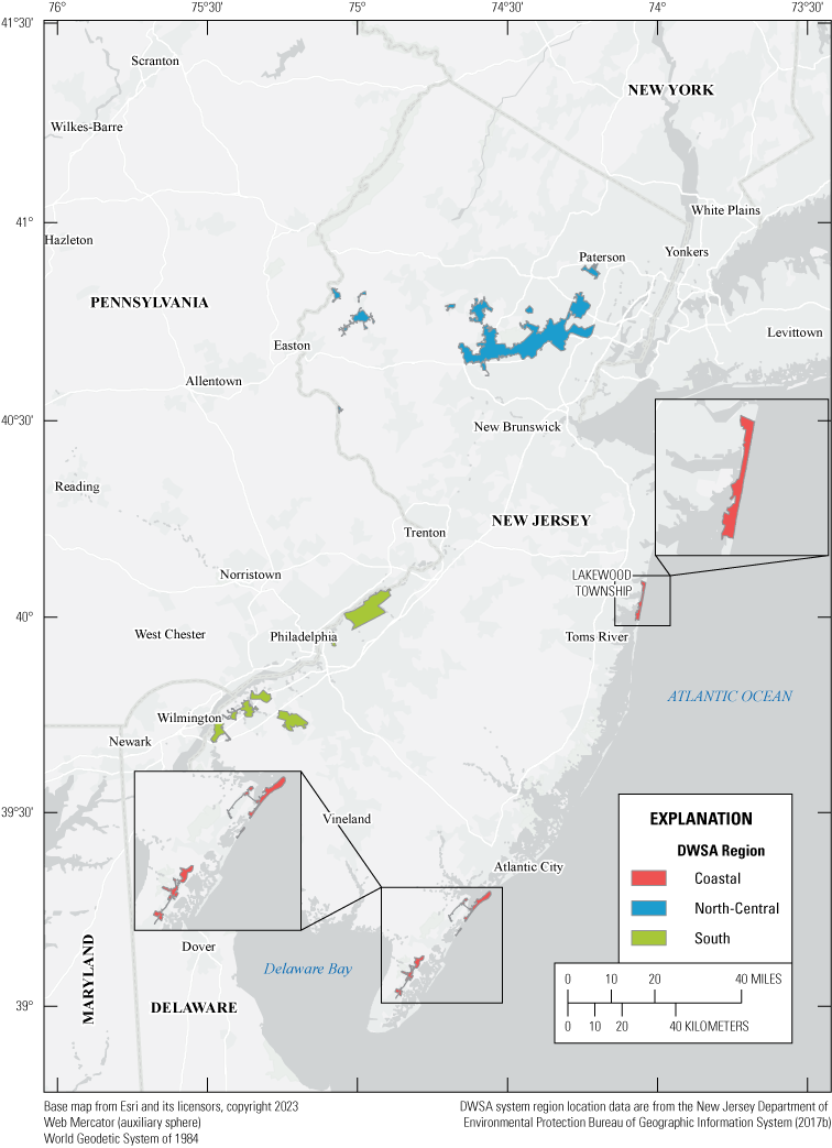
Map showing locations of three drinking water service area (DWSA) system regions in New Jersey.
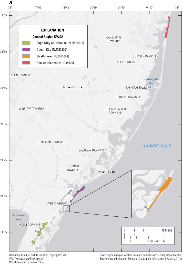
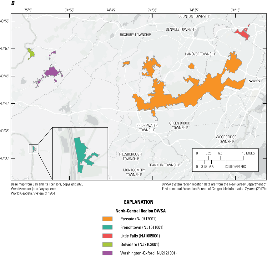
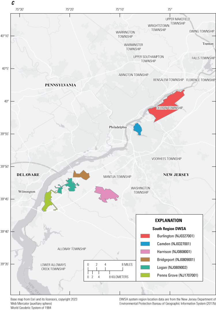
Maps showing locations of 15 New Jersey American Water drinking water service area (DWSA) systems by region: A, coastal, B, north central, and C, south.
Monthly-to-Daily Water-Use Data Comparison
Prior to using these data to build models and obtain predictions, NJAW’s daily public supply data were first compared to monthly public supply water-use data from the state-owned NJWaTr database (New Jersey Department of Environmental Protection Division of Water Supply and Geoscience, 2022). The purpose of this comparison was to help validate both datasets and identify any inconsistencies that may affect the analysis and models.
Daily system delivery data acquired from NJAW (in units of million gallons per day) were temporally aggregated to monthly values and then compared to monthly DWSA system data from the NJWaTr database for the 15 NJAW DWSA systems for the years 2016–20 (figs. 3, 4, and 5). Of the 15 DWSA systems, nine showed a close match to the monthly NJWaTr public supply data (table 1). In some cases, the water-use data from the two datasets matched almost perfectly, so that they were often indistinguishable when plotted, as is the case with Ocean City (fig. 3B), Strathmere (fig. 3C), Washington-Oxford (2016–19; fig. 4E), Harrison (fig. 5C), Bridgeport (fig. 5D), and Logan (fig. 5E) DWSA systems.
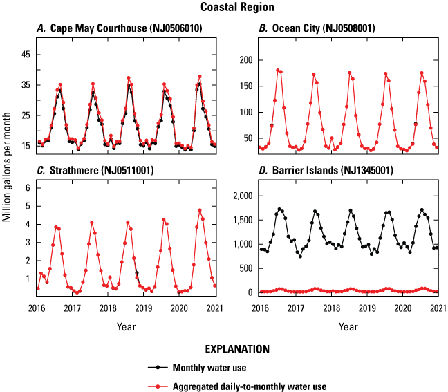
Plots comparing monthly water-use data to aggregated daily-to-monthly water-use data for drinking water service area systems in the New Jersey coastal region, 2016–20: A, Cape May Courthouse, B, Ocean City, C, Strathmere, and D, Barrier Islands. The Barrier Islands system represents a portion of the Coastal North system, for which complete daily water-use data were unavailable. These data therefore represent a portion of the Coastal North system’s total water use. Where only the aggregated data are visible, they are equal to the monthly values and are thus visually indistinguishable. Monthly water-use data are from the New Jersey Department of Environmental Protection Division of Water Supply and Geoscience (2022). Daily water-use data are from New Jersey American Water and are not available owing to a proprietary interest or sensitivity concern. Contact New Jersey American Water for more information.
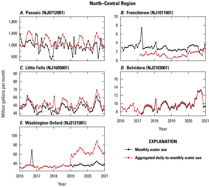
Plots comparing monthly water-use data to aggregated daily-to-monthly water-use data for drinking water service area systems in the New Jersey north-central region, 2016–20: A, Passaic, B, Frenchtown, C, Little Falls, D, Belvidere, and E, Washington-Oxford. Where only the aggregated data are visible, they are equal to the monthly values and are thus visually indistinguishable. Monthly water-use data are from the New Jersey Department of Environmental Protection Division of Water Supply and Geoscience (2022). Daily water-use data are from New Jersey American Water and are not available owing to a proprietary interest or sensitivity concern. Contact New Jersey American Water for more information.
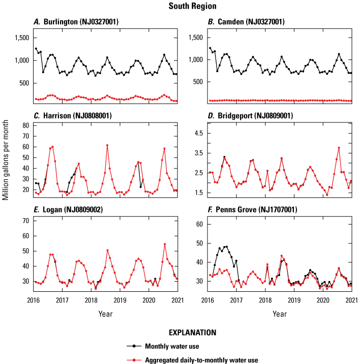
Plots comparing monthly water-use data to aggregated daily-to-monthly water-use data for drinking water service area systems in the New Jersey south region, 2016–20: A, Burlington, B, Camden, C, Harrison, D, Bridgeport, E, Logan, and F, Penns Grove. The Burlington and Camden systems represent portions of the Western Division system, for which complete daily water-use data were unavailable. These data therefore represent a portion of the Western Division system’s total water use. Where only the aggregated data are visible, they are equal to the monthly values and are thus visually indistinguishable. Monthly water-use data are from the New Jersey Department of Environmental Protection Division of Water Supply and Geoscience (2022). Daily water-use data are from New Jersey American Water and are not available owing to a proprietary interest or sensitivity concern. Contact New Jersey American Water for more information.
Table 1.
The mean monthly values, mean percent differences, and the root mean squared errors (RMSEs) for the 15 drinking water service area (DWSA) systems comparing aggregated daily data from New Jersey American Water (NJAW) and monthly data for the corresponding systems from the New Jersey Water Transfer Data Model (NJWaTr) database for the years 2016–20.[PWSID, public water system identification number; Mgal/month, million gallons per month; RMSE, root mean squared error; Mgal, million gallons]
Aggregated from daily data received from NJAW. These data are not available owing to a proprietary interest or sensitivity concern. Contact NJAW for more information.
Three of the 15 DWSA systems (referred to in this study as Barrier Islands [fig. 3D], Burlington [fig. 5A], and Camden [fig. 5B]) are portions of larger DWSA systems for which complete system data were not provided by NJAW: the Coastal North (part of the Coastal Region [NJ134500]) and Western Division (part of the South Region [NJ0327001]) systems. For this study, they were treated as individual systems. Because these three systems represent only partial system data, the aggregated daily data values from NJAW did not match well with, and were much lower than, the corresponding NJWaTr monthly values for the Coastal North and Western Division systems with a mean percent difference of at least −134% or smaller. For the remaining three systems, Passaic, Little Falls, and Frenchtown, the data from NJAW and NJWaTr do not match well even though they were complete system data and not partial system datasets. In these three systems, it is likely that the aggregated daily data and the monthly NJWaTr are different because of reporting inconsistencies, and (or) the complex nature of systems that exist in the northern part of the state (Vince Monaco, NJAW, oral commun., June 2020).
Daily Public Supply Water-Use Data
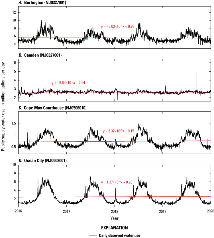
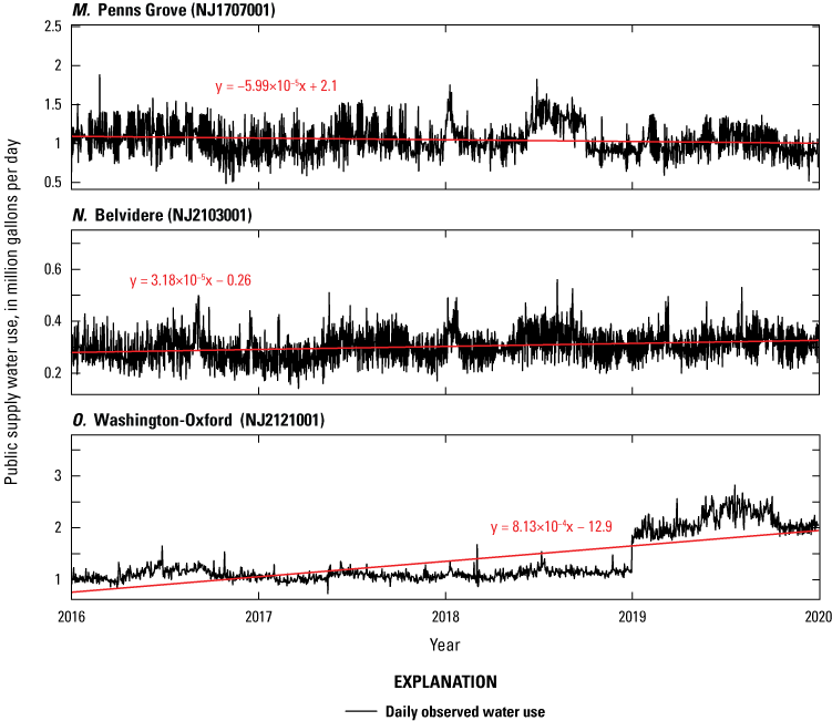
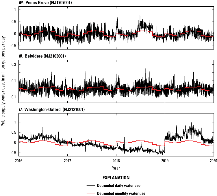
Daily public supply water use in New Jersey varies by time of year and location. Generally, publicly supplied water use is greater in the summer months than in the winter months (NJDEP, 2017), although this was not always the case for this study. Across all 15 systems, the average water use per day in the summer months (June–August) was 116 percent greater than the winter months (December–February). From visual examination of the plotted daily public supply water-use data, it appeared that a few data points were noticeably outside the typical range of values for the Strathmere, Frenchtown, Burlington, Camden, and Bridgeport systems (figs. 6C, 7B, 8A, 8B, and 8D). For these 10–20 data points, plant engineers from NJAW were consulted. Where possible, they provided explanations for what occurred at those plants on some of those days of interest. These explanations included hydrant flushing, water main breaks, using water to fight fires, or water-quality testing of newly replaced mains (NJAW, written commun., 2021). Some further analysis was conducted to estimate the effect of these data points by comparing the model results based on the datasets with and without the data points of interest. In addition to these short-term anomalous data points, the Washington-Oxford system had a noticeable shift in water use starting around the beginning of 2019 (fig. 7E). The average water use for this system from 2016 through 2019 was 1.10 million gallons per day (Mgal/d); thereafter, the average water use was 2.19 Mgal/d through 2020. This apparent shift in water use was possibly caused by changes in the DWSA system boundaries or changes in the buying and selling of water to other DWSA systems; however, the exact cause of the shift in water usage is unknown. Another noticeable long-term change in daily water use is observed in the Little Falls system about mid-way through 2018 (fig. 7C). The magnitude of volumes does not noticeably shift, rather the day-to-day variability appears to increase. This change may be due to differences in the way the data were reported. Finally, the daily dataset provided for the DWSA system of Frenchtown only included years from 2017 through 2020 and, as a result, the analyses for this system are based on 4 years of data. These noticeable shifts in data for the Washington-Oxford and Little Falls systems and missing data for the Frenchtown system occur over a longer timeframe in contrast to systems with anomalous data which occur over only 1 or 2 days. As a result, these longer-term shifts or data gaps would likely have a larger effect on any analysis and modeling performed as compared to those systems with shorter-term anomalous data because there are more anomalous data points to influence the model. However, for this study, the same analysis was carried out among all systems regardless of the apparent long-term shifts in datasets and missing data.
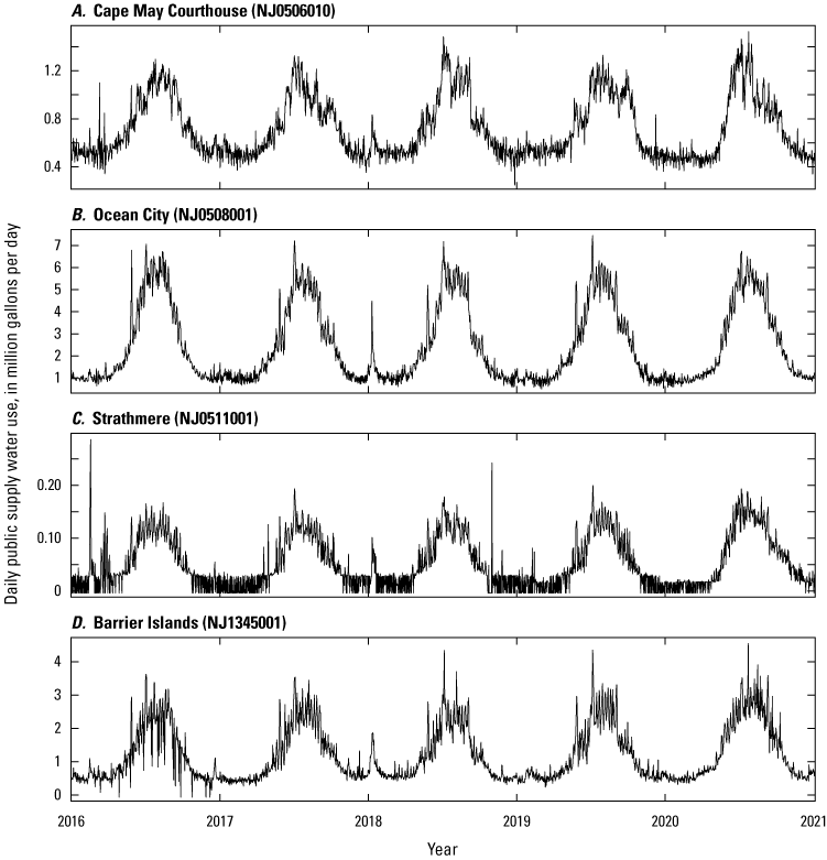
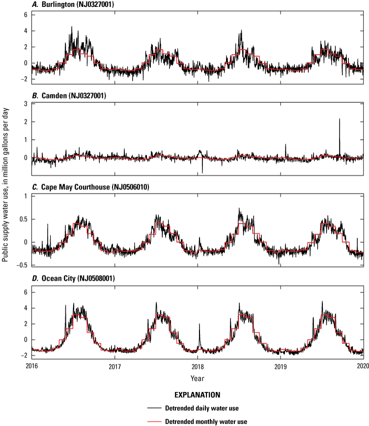
Time series plots showing daily public supply water-use data for the New Jersey American Water drinking water service area systems in the New Jersey coastal region, 2016–20: A, Cape May Courthouse, B, Ocean City, C, Strathmere, and D, Barrier Islands. The Barrier Islands system represents a portion of the Coastal North system, for which complete daily water-use data were unavailable. These data therefore represent a portion of the Coastal North system’s total water use. Daily water-use data are from New Jersey American Water and are not available owing to a proprietary interest or sensitivity concern. Contact New Jersey American Water for more information.

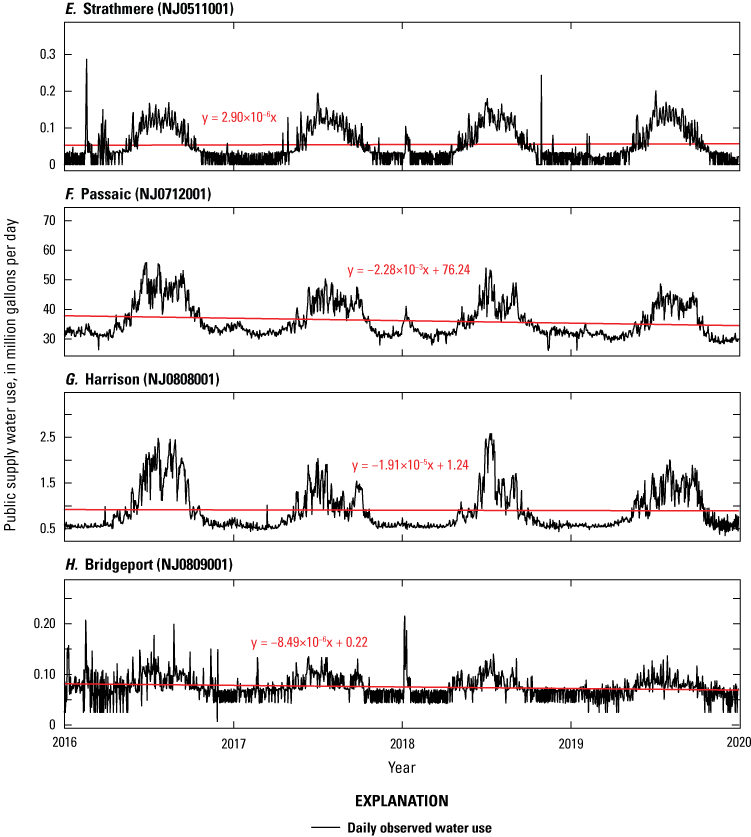
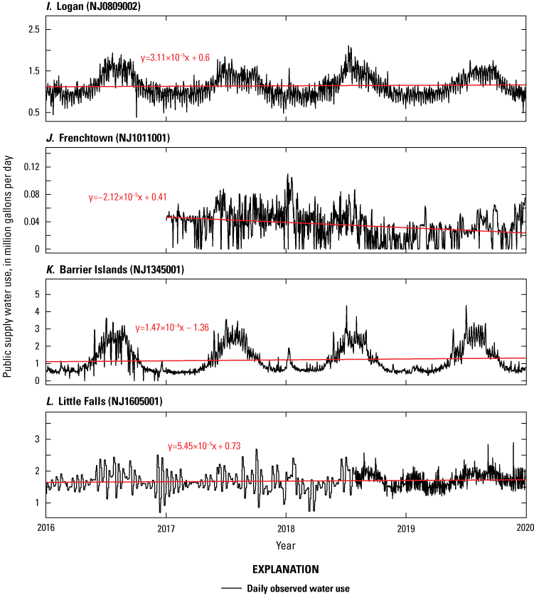
Time series plots showing daily public supply water-use data for the New Jersey American Water drinking water service area systems in the New Jersey north-central region, 2016–20: A, Passaic, B, Frenchtown, C, Little Falls, D, Belvidere, and E, Washington-Oxford. Daily water-use data are from New Jersey American Water and are not available owing to a proprietary interest or sensitivity concern. Contact New Jersey American Water for more information.
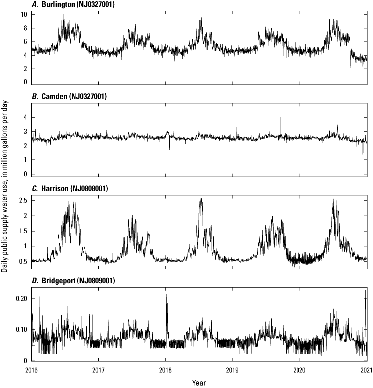
Time series plots showing daily public supply water-use data for the New Jersey American drinking water service area systems in the New Jersey south region, 2016–20: A, Burlington, B, Camden, C, Harrison, D, Bridgeport, E, Logan, and F, Penns Grove. The Burlington and Camden systems represent portions of the Western Division system, for which complete daily water-use data were unavailable. These data therefore represent a portion of the Western Division system’s total water use. Daily water use data are from New Jersey American Water and are not available owing to a proprietary interest or sensitivity concern. Contact New Jersey American Water for more information.
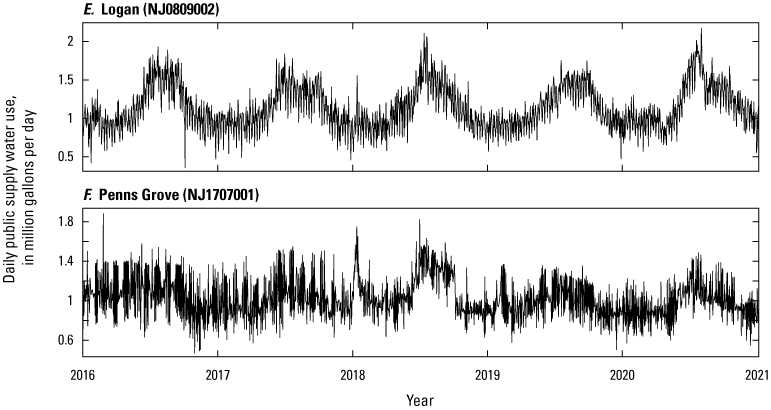
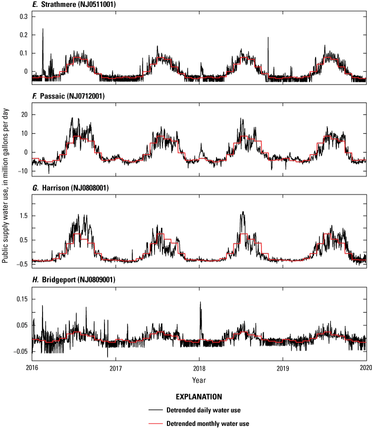
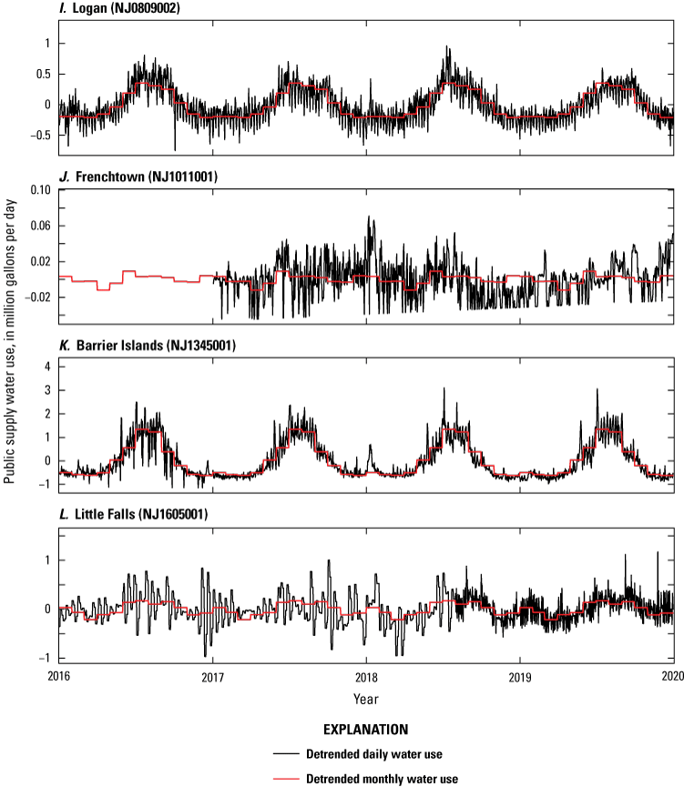
The 15 systems were grouped into two categories based on general, observable patterns in the daily data. Nine systems showed a strong seasonal signal throughout the 5 years of data, where water use was higher in summer months compared to winter months (figs. 6A, 6B, 6C, 6D, 7A, 8A, 8C, 8D, and 8E). The remaining six systems showed little to no seasonal pattern; instead, daily water use was mostly constant throughout each year (figs. 7B, 7C, 7D, 7E, 8B, and 8F). Among the nine DWSA systems with a seasonal signal, or seasonal systems, the average water use was 185-percent higher in summer months (June–August) compared to winter months (December–February), whereas the six DWSA systems with little to no seasonal signal, or non-seasonal systems, had an average increase in water use of 13 percent in summer months over winter months.
The initial groupings were confirmed by identifying the periodicity of each system’s data through periodograms. Periodograms quantify the relative importance of different frequencies in a dataset based on a scaled-Fourier transform of the time series data (Bloomfield, 2000). Peaks or local maxima in a periodogram indicate dominant frequencies in the data. Identifying the frequency at which the maximum spectral density occurs then allows for the corresponding period to be determined by computing the inverse of the frequency of interest, where the spectral density is the relative strength of the frequencies within the given time series signal (Kendall, 1946; Iyer and Chowdhury, 2009). Raw periodograms are rough estimates of the true spectral density (frequency domain representation of time series data) and are therefore subject to fluctuations and noise. Applying smoothing can improve the stability of (or the extent to which unimportant details are removed from) the raw periodogram (Bloomfield, 2000). The modified Daniell filter is one of the most common methods for smoothing, and in essence, constitutes a weighted moving average window where the endpoints receive less weight than the interior points. The modified Daniell filter can also be applied successively for more extensive smoothing (Bloomfield, 2000).
By generating a smoothed periodogram for each of the 15 systems, the seasonal and non-seasonal groupings were identified quantitatively (fig. 9). Systems with periodograms that had a maximum spectral density of approximately 365.2 days were categorized as seasonal systems (figs. 9A, 9C, 9D, 9E, 9F, 9G, 9I, and 9K), whereas systems with periodograms that had a maximum spectral density corresponding to a different number of days (less than or greater than 365.2) were categorized as non-seasonal (figs. 9B, 9H, 9J, 9L, 9M, 9N, and 9O). The groupings from the periodogram analysis confirmed the preliminary visual-based groupings, identifying the same nine systems as seasonal and the same six systems as non-seasonal. Burlington, Cape May Courthouse, Ocean City, Strathmere, Passaic, Harrison, Bridgeport, Logan, and Barrier Islands were confirmed as the nine seasonal systems. Camden, Frenchtown, Little Falls, Penns Grove, Belvidere, and Washington-Oxford were confirmed as the six non-seasonal systems. These seasonal and non-seasonal groupings were the basis for developing two regression equations to account for this key difference in the systems: one model equation form was developed for seasonal systems, and one model equation form was developed for non-seasonal systems.
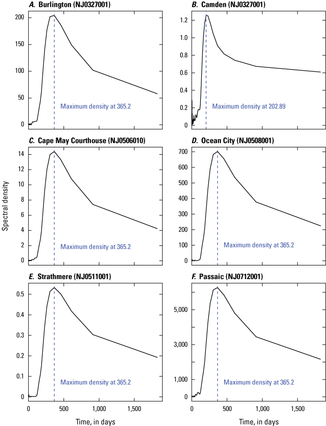
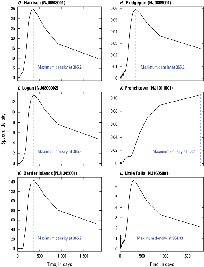
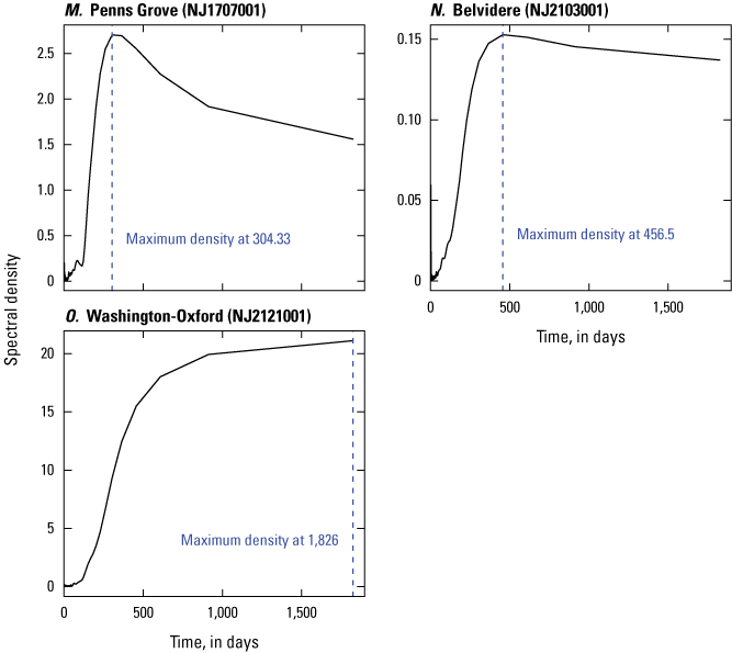
Smoothed periodograms showing the period at which the maximum spectral density occurs for the 15 New Jersey American Water drinking water service area systems, 2016–20: A, Burlington, B, Camden, C, Cape May Courthouse, D, Ocean City, E, Strathmere, F, Passaic, G, Harrison, H, Bridgeport, I, Logan, J, Frenchtown, K, Barrier Islands, L, Little Falls, M, Penns Grove, N, Belvidere, and O, Washington-Oxford.
Drinking Water Service Area System Characterizations
All DWSA systems throughout the state of New Jersey were also studied and characterized to provide additional insight on factors affecting daily public supply water use. Daily data were provided for only 15 DWSA systems, but monthly water-use data for all active systems (defined as those systems having monthly values from 2016 through 2020 in NJWaTr) were used for the characterization analysis (New Jersey Department of Environmental Protection Division of Water Supply and Geoscience, 2022). These DWSA systems were characterized based on geographic and socio-economic data (table 2; appendix 1). Categorizing the DWSA systems identified correlations between the characteristics of the systems and the monthly water-use data, namely whether there was an observable seasonality pattern or not.
Datasets and Methods
The datasets used in characterizing the DWSA systems in New Jersey included population served by DWSA for 2021 from the EPA’s Safe Drinking Water Information System (SDWIS; U.S. Environmental Protection Agency, 2021), the 2010 population estimates by census block group from the U.S. Census Bureau (U.S. Census Bureau, 2010), the 2017 New Jersey geographic boundaries for all DWSA systems (NJDEP Bureau of GIS, 2017b), the state of New Jersey’s 2019 tax parcel and property value data (New Jersey Office of Information Technology Office of Geographic Information System, 2019), the 2015 land-use and land cover data (NJDEP Bureau of GIS, 2015), the 2019 median household income estimates by census block group (U.S. Census Bureau, 2019), the landscape regions of New Jersey (NJDEP Bureau of GIS, 2017a), and NJWaTr monthly water-use data (New Jersey Department of Environmental Protection Division of Water Supply and Geoscience, 2022).
All datasets were clipped and summarized at the DWSA system level. The DWSA boundary coverage shapefile, obtained in 2020, represented the 2017 DWSA system boundaries and contained 589 unique systems (NJDEP Bureau of GIS, 2017b). The population-served data from SDWIS were available at the DWSA system level. Three of the DWSA systems from the NJAW daily datasets were provided as partial systems; to keep the analysis as consistent as possible, these partial systems were treated as individual systems. To help obtain population-served estimates for these partial systems, the 2010 Census Bureau population estimates were also used. The proportion of the total population in the partial DWSA system to the total population in the complete DWSA system was applied to scale SDWIS population-served data, resulting in estimated partial populations served for the three partial DWSA systems.
Median property values and median household incomes by DWSA system were calculated by aggregating land parcels and census block groups, respectively, to the DWSA system level. For these datasets, land parcels and census block groups were first intersected with the DWSA system boundaries. The property values dataset was filtered by property class, so only Class 2, or “residential property,” was considered for this analysis (New Jersey Register, 2018). Additionally, land parcels with a property value of zero were excluded. The median property values and household income were then calculated for each DWSA system. Because the data were filtered to include only residential properties, some of the 589 unique DWSA systems did not have appropriate tax data and thus did not have a median value. For these few systems, they were removed from the analysis as there were no data available. Median, rather than mean, values were used for the characterizations because the data were not normally distributed.
After obtaining a single summarized value for each socio-economic dataset (population served, household income, property value) per DWSA system, quartiles were calculated for each dataset based on all DWSA systems combined. Using quartiles allowed for the systems to be categorized into four groups based on the value of a given system. Subsequently, a given system was grouped into quartile 1 (Q1), quartile 2 (Q2), quartile 3 (Q3), or quartile 4 (Q4) according to the median property value for that particular DWSA system. This method of calculating quartiles to group the systems was used for the population-served values, median property values, and median household income values datasets (table 2).
Table 2.
Upper and lower limits for drinking water service area system characterization quartiles for each type of numerical dataset.[<, less than; ≥, greater than or equal to]
The residential land-use category was the only category from the 2015 land-use data used for this analysis, which accounts for about 12.5 percent of total land-use area in New Jersey (NJDEP Bureau of GIS, 2015). The residential land-use category is further separated into residential density subcategories. The rural residential density land-use subcategory comprises 13.8 percent, the low residential density land-use subcategory comprises 18.5 percent, the medium residential density land-use subcategory comprises 48.6 percent, and the high residential density land-use subcategory comprises 19.1 percent (NJDEP Bureau of GIS, 2015). These data were first intersected with the DWSA system boundaries, then residential density percentages were calculated at the DWSA system level. Initially, the percentage of land area for each of the four residential density categories (rural, low, medium, and high) was calculated for each system, where the total area of land for each density subcategory was divided by the total residential land-use area (in acres). To designate a single value for each DWSA system, the residential density with the largest percentage was used to categorize each system. Because there was little observable difference in water-use values with respect to seasonality between DWSA systems with rural, low, or medium residential densities as the largest percentage, these three residential densities were combined and classified as “non-urban.” Systems with high residential density as the largest percentage were classified as “urban.” The distinction between urban and non-urban systems was used in this study because there was a difference in seasonality between systems with rural, low, or medium residential densities and systems with high residential densities.
Another factor that was used to classify the DWSA systems was whether a given system was coastal or not. In New Jersey, many of the coastal towns and areas receive a large population influx in the summer from tourists (Stirling, 2018). Obtaining estimates on changes in these populations over the seasons was difficult, so identifying whether a DWSA was geographically close to the Atlantic coast was used as a proxy for the change in population caused by tourism. To determine a DWSA system’s status as coastal or not, the NJDEP landscape regions of New Jersey (NJDEP Bureau of GIS, 2017a) was used in conjunction with the DWSA system boundaries (NJDEP Bureau of GIS, 2017b). The “Atlantic coastal” region definition from the dataset provides a reasonable coverage of coastal, tourist-destination towns in the state (fig. 10). The DWSA systems that intersected with the Atlantic coastal landscape region were identified and categorized as coastal systems.
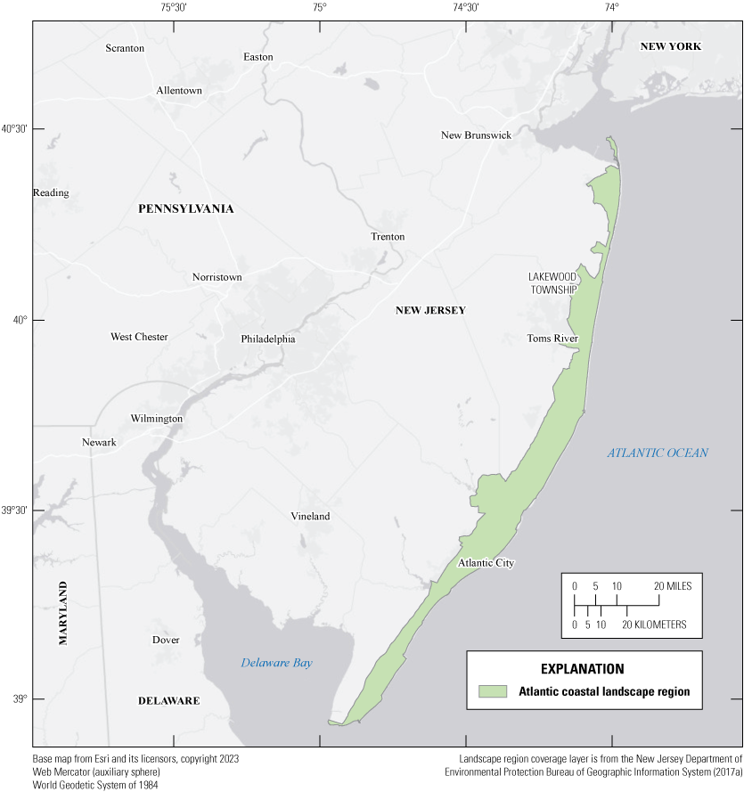
Map showing the coverage of the Atlantic coastal landscape region from the New Jersey Department of Environmental Protection’s landscape regions of New Jersey dataset.
Alternative methods to identify and categorize coastal systems were explored but not used because the categorizations of coastal systems included systems outside of the typical New Jersey summer tourist destinations, such as along the Delaware, Newark, and Raritan Bays. For example, the Coastal Area Facilities Review Act (CAFRA) boundaries for New Jersey dataset (NJDEP Bureau of GIS, 2005) created for planning and permitting purposes, represents coastal planning areas, but was not selected because it included DWSA systems along the Delaware Bay and along the Delaware River as well as some systems over 12 miles inland from any coastline. Another method considered was to apply a 5-mile buffer to the U.S. country boundary along the New Jersey coast. These alternative datasets were intersected with the DWSA boundaries to identify potential coastal systems. In both cases, there were DWSA systems included in regions not typically considered coastal towns or summer tourist destinations such as along the Raritan Bay (including Perth Amboy to Newark, New Jersey) and on the southern end, along the Delaware Bay to Salem County. The landscape regions of New Jersey dataset was used to assign coastal designations to the different systems so that systems that were not representative of the tourism effect in New Jersey and were not in the near vicinity of the Atlantic coast were not included. The landscape regions dataset best identified systems encompassing summer destinations in the state, that are affected by tourism and result in seasonal population changes, which impacts water-use patterns throughout the year.
Identifying Seasonality in Monthly Data
Once all DWSA systems were characterized into socio-economic (population served by DWSA, household income, property value) and geographical (coastal and non-coastal, urban and non-urban) groupings, monthly water-use data from NJWaTr were analyzed for seasonality (appendix 1). To identify whether a given system had a seasonal pattern, at least 24 consecutive months of water-use data from 2016 through 2020 were required. These years were the most recent 5 years of available data in NJWaTr at the time of analysis and most closely aligned with the daily data obtained from NJAW. Because of this requirement, 158 DWSA systems were excluded from this analysis, and 434 DWSA systems remained. Seasonality in monthly water use was determined using the same method described in the “Daily Public Supply Water-Use Data” section and is defined as higher usage during the summer months (May–September), as compared to lower usage during the cooler fall, winter, and spring months (October–April). The periodograms generated for Brigantine WD, Egg Harbor City WD, Norms Dale MHP, and Verona WD show how the strength of frequencies varied among the 434 systems (figs. 11 and 12). Systems with strong seasonality, like Brigantine WD and Egg Harbor City WD, show a peak frequency at 1/12, or a peak period of 12 months (figs. 11A, 11B, 12A, and 12B). It was determined that data could still visually appear seasonal with a dominant period of anywhere between 11 and 13 months, like that of Verona WD; therefore, any system with a peak in the periodogram corresponding to 11 through 13 months was classified as seasonal (figs. 11D and 12D).
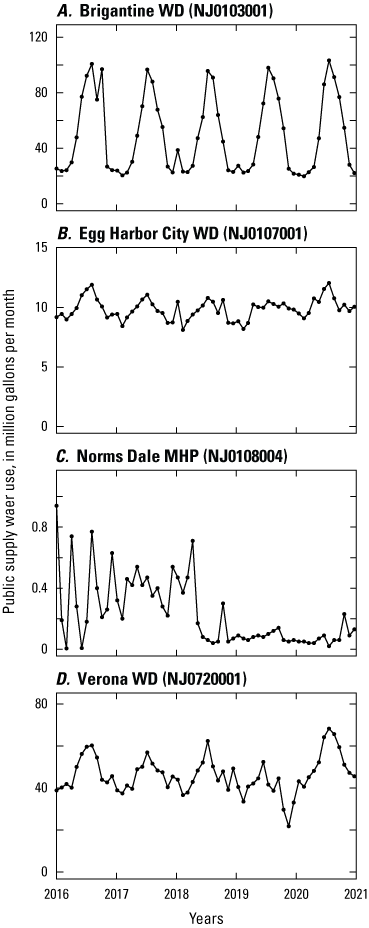
Plots showing monthly time series water-use data from the New Jersey Water Transfer Data Model (NJWaTr) database for four sample drinking water service area systems, 2016–20: A, Brigantine WD, B, Egg Harbor City WD, C, Norms Dale MHP, and D, Verona WD. Water-use data are from the New Jersey Department of Environmental Protection Division of Water Supply and Geoscience (2022).
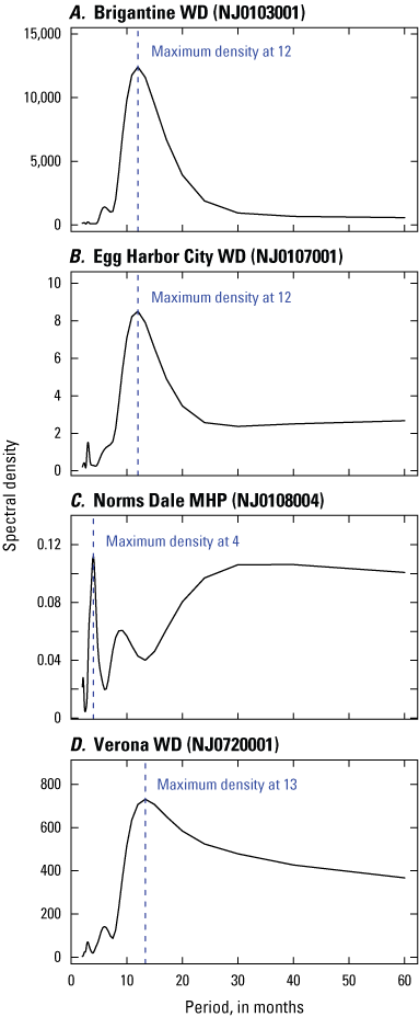
Smoothed periodograms showing data from the New Jersey Water Transfer Data Model (NJWaTr) database for four sample drinking water service area systems, 2016–20: A, Brigantine WD, B, Egg Harbor City WD, C, Norms Dale MHP, and D, Verona WD. Water-use data are from the New Jersey Department of Environmental Protection Division of Water Supply and Geoscience (2022).
In addition to using periodograms, the monthly water-use data for each of the DWSA systems were plotted and visually examined for a seasonal signal. There were 69 instances where the visual check was inconclusive so the periodogram results were used. There were 15 instances where the visual check and periodogram results disagreed. There were five cases where the visual inspection indicated that the systems were not seasonal, despite the periodogram results indicating they were seasonal. The same inspection found 10 systems were seasonal, despite the periodogram results indicating they were not seasonal. When the visual check was not immediately clear on whether a system was seasonal or not, the automated periodogram results were used. Only when a system’s water-use patterns were visually very clearly seasonal or not, was the visual check used in place of the periodogram as the periodogram can be sensitive to noise (one or two months with anomalous data) or large shifts in overall magnitudes in the data (a system’s usage noticeably decreases or increases over time). Another limitation of the periodogram is that it can only identify if there is any type of repeating, periodic pattern and does not distinguish between which type of periodic pattern. In this case, a specific seasonal pattern is the only repeating pattern of interest, where there is a substantial increase in water use in the summer months as compared to winter months. Occasionally, the results of the periodogram would indicate there is a yearly (or 12 month) repeating signal, but it would not follow the specific seasonal pattern described above. Because of these limitations, the visual inspection was used to verify or check the results.
Results and Patterns in DWSA Characterizations
One of the main purposes of the DWSA characterization was to identify any patterns in characteristics across all the systems, as they related to the degree of seasonality in water use. The motivation for focusing on seasonal water-use patterns came from the noticeable distinction in the daily data from the 15 NJAW systems highlighted in this study. Most of the 15 systems were placed into either a seasonal or non-seasonal group based on the daily water-use data provided. Therefore, the ability to determine if a system has a seasonal water-use pattern helps guide model development and water-use estimates for any DWSA system. All 15 NJAW DWSA systems were characterized based on the five datasets discussed above and were grouped into seasonal and non-seasonal categories based on the daily data provided from NJAW (table 3). The remaining 434 DWSA systems with water-use data in NJWaTr spanning the years 2016–20 were characterized in the same manner using monthly NJWaTr data to assess seasonality (appendix 1).
Table 3.
Characterization of 15 New Jersey American Water drinking water service area (DWSA) systems.[Quartiles are defined in table 2. PWSID, public water system identification number; DWSA, drinking water service area]
Residential density is based on data from the New Jersey Department of Environmental Protection Bureau of Geographic Information System (2015).
Coastal classification is based on data from the New Jersey Department of Environmental Protection Bureau of Geographic Information System (2017a).
Seasonality is based on monthly data from the New Jersey Department of Environmental Protection Division of Water Supply and Geoscience (2022).
The DWSA characterization results were graphed by the five datasets broken up into quartiles (figs. 13, 14, 15) or qualitative categories (fig. 16). Generally, there are more DWSA systems that display seasonal water-use patterns for those systems with larger populations served, higher median household income, and higher median property values as compared to smaller populations served, lower median household income, and lower median property-value systems. This can be observed by comparing the percentage of seasonal and non-seasonal systems between the highest quartiles (Q4) and lowest quartiles (Q1; figs. 13, 14, 15). This pattern is most distinct in the population-served dataset. In Q4 for population served, 80 percent of systems showed seasonality, whereas in Q1, only 20 percent of systems showed seasonality, a decrease of 60 percent (fig. 13). This pattern is least observable in the household income dataset where the corresponding difference between Q4 (64 percent) and Q1 (50 percent) is a decrease of only 14 percent (fig. 14). Overall, the percentage of seasonal DWSA systems varied the least when grouped by household income, which suggests this variable may not be as influential as others when it comes to predicting seasonality in monthly water use for New Jersey.
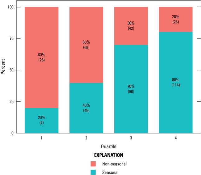
Graph showing the percentage of drinking water service area systems in the New Jersey Water Transfer Data Model database with seasonal and non-seasonal water-use patterns per population-served quartile. Quartiles are defined in table 2. The percentages were calculated based on available data for 430 systems. The water-use data are from 2016 through 2020 (New Jersey Department of Environmental Protection Division of Water Supply and Geoscience, 2022). The population-served data are from 2021 (U.S. Environmental Protection Agency, 2021).
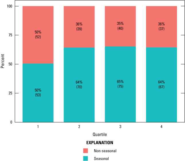
Graph showing the percentage of drinking water service area systems in the New Jersey Water Transfer Data Model database with seasonal and non-seasonal water-use patterns per median household income quartile. Quartiles are defined in table 2. The percentages were calculated based on available data for 433 systems. The water-use data are from 2016 through 2020 (New Jersey Department of Environmental Protection Division of Water Supply and Geoscience, 2022). The household income data are from 2019 (U.S. Census Bureau, 2019).
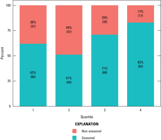
Graph showing the percentage of drinking water service area systems in the New Jersey Water Transfer Data Model database with seasonal and non-seasonal water-use patterns per median property value quartile. Quartiles are defined in table 2. The percentages were calculated based on available data for 388 systems. The water-use data are from 2016 through 2020 (New Jersey Department of Environmental Protection Division of Water Supply and Geoscience, 2022). The property value data are from 2019 (New Jersey Office of Information Technology Office of Geographic Information System, 2019).
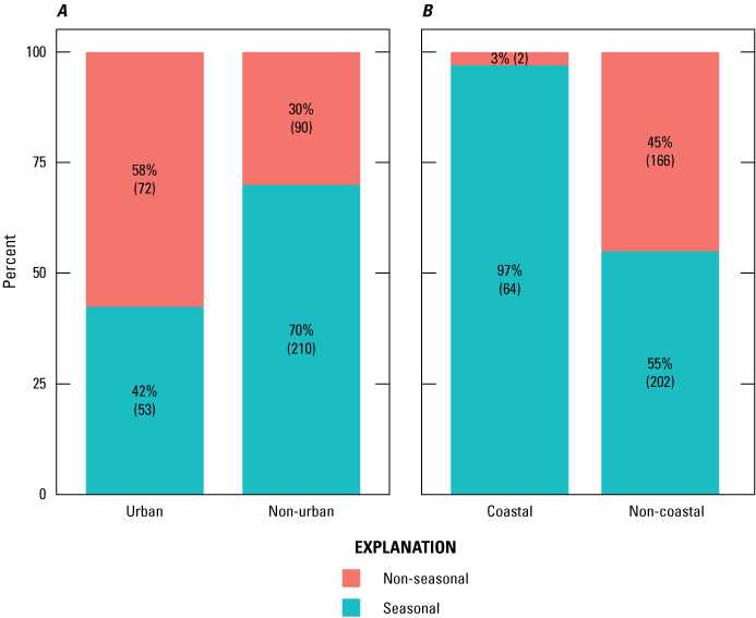
Graphs showing the percentage of drinking water service area systems in the New Jersey Water Transfer Data Model database with seasonal and non-seasonal water-use patterns per, A, residential density (urban and non-urban) and B, coastal classification (coastal and non-coastal). The percentages were calculated based on available data for 425 systems for figure 16A and 434 systems for figure 16B. The water-use data are from 2016 through 2020 (New Jersey Department of Environmental Protection Division of Water Supply and Geoscience, 2022). The residential density data are from 2015, and the coastal classification information is from 2017 (New Jersey Department of Environmental Protection Bureau of Geographic Information System, 2015, 2017a).
When systems are grouped by coastal and non-coastal categories, it is evident that more coastal systems show seasonality than non-coastal systems (fig. 16B). This finding supports what is known about increased summer populations in coastal areas, where increased populations during summer months are associated with increases in publicly supplied water use for those same months. When systems are grouped by urban and non-urban residential density, urban systems often show non-seasonal water-use patterns.
Ninety-seven percent of all DWSA systems that were classified as coastal showed a seasonal signal. Seventy percent of all systems classified as non-urban showed a seasonal signal. Additionally, 80 percent of all systems in Q4 for population served showed a seasonal signal (fig. 17). These results indicate that a DWSA system shows seasonal patterns of water use if it is classified as coastal, non-urban, and (or) it serves a large population (Q4).
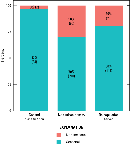
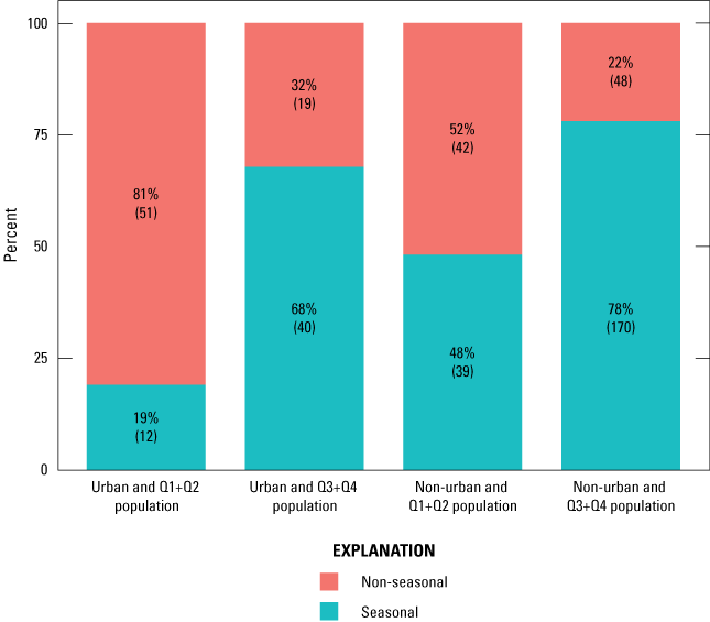
Graphs showing the percentage of drinking water service area systems with seasonal and non-seasonal water-use patterns that are classified as coastal or non-urban, and (or) serve the top 25 percent (Q4) population. Quartiles are defined in table 2. The values in parentheses indicate the number of DWSA systems used to calculate the percentages. The water-use data are from 2016 through 2020 (New Jersey Department of Environmental Protection Division of Water Supply and Geoscience, 2022). The residential density data are from 2015, the coastal classification information is from 2017, and the population-served data are from 2021 (New Jersey Department of Environmental Protection Bureau of Geographic Information System, 2015, 2017a; U.S. Environmental Protection Agency, 2021).
The systems were then grouped into more specific categories based on two characteristics rather than just one. Grouping the systems in two categories provided insight on whether certain DWSA characteristics had a stronger or weaker influence on seasonal water-use patterns. Combinations based on two of the three characteristics highlighted in figure 17 were used to create a total of nine distinct groups (figs. 18, 19, and 20). To align the population-served category with the qualitative categories (coastal or non-coastal, urban or non-urban), the population-served category was split into two groups: the top 50 percent (Q3 and Q4; denoted as Q3+Q4) and the bottom 50 percent (Q1 and Q2; denoted as Q1+Q2).
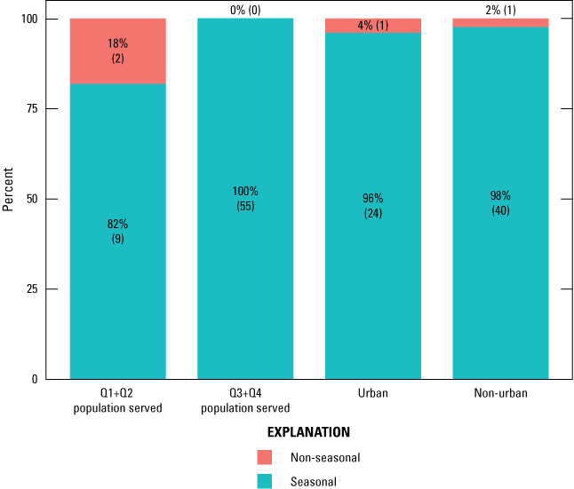
Graph showing the percentage of coastal drinking water service area systems with seasonal and non-seasonal water-use patterns that serve the bottom 50 percent (Q1+Q2) or the top 50 percent (Q3+Q4) populations or are classified as urban or non-urban. Quartiles are defined in table 2. The values in parentheses indicate the number of systems used to calculate the percentages. The water-use data are from 2016 through 2020 (New Jersey Department of Environmental Protection Division of Water Supply and Geoscience, 2022). The population-served data are from 2021 (U.S. Environmental Protection Agency, 2021). The residential density data are from 2015 (New Jersey Department of Environmental Protection Bureau of Geographic Information System, 2015).
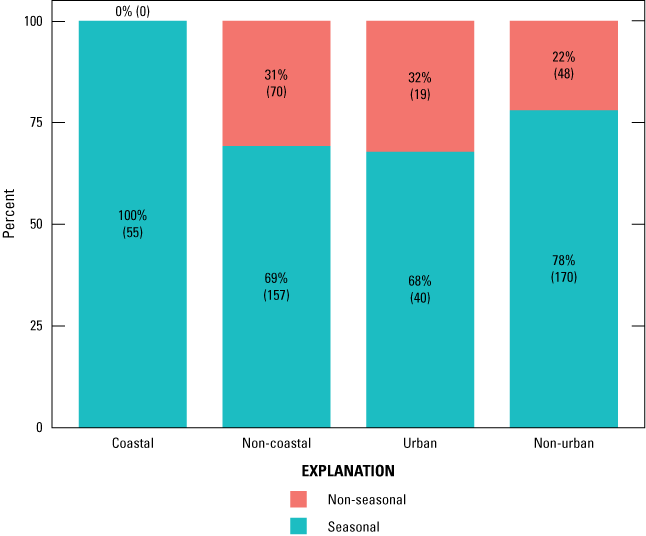
Graph showing the percentage of drinking water service area systems with seasonal and non-seasonal water-use patterns that serve the top 50 percent populations (Q3+Q4) and are classified as coastal, non-coastal, urban, or non-urban. Quartiles are defined in table 2. The values in parentheses indicate the number of systems used to calculate the percentages. The water-use data are from 2016 through 2020 (New Jersey Department of Environmental Protection Division of Water Supply and Geoscience, 2022). The coastal classification information is from 2017 (New Jersey Department of Environmental Protection Bureau of Geographic Information System, 2017a). The residential density data are from 2015 (New Jersey Department of Environmental Protection Bureau of Geographic Information System, 2015).
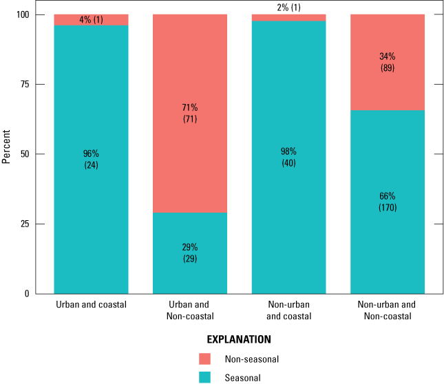
Graph showing the percentage of drinking water service area systems with seasonal and non-seasonal water-use patterns that are classified as urban and coastal, urban and non-coastal, non-urban and coastal, and non-urban and non-coastal. The values in parentheses indicate the number of systems used to calculate the percentages. The water-use data are from 2016 through 2020 (New Jersey Department of Environmental Protection Division of Water Supply and Geoscience, 2022). The residential density data are from 2015, and the coastal classification information is from 2017 (New Jersey Department of Environmental Protection Bureau of Geographic Information System, 2015, 2017a).
When the coastal systems are further grouped by residential density and by population served, they all show a high percentage of seasonality. When categorized in this manner, using these four categories (urban, non-urban, top 50 percent population [Q3+Q4], and bottom 50 percent [Q1+Q2] population), 82 percent or more systems displayed seasonal water-use behavior as seen in figure 18. This suggests that a system’s proximity to the coast is more influential in predicting its seasonality compared to the other factors considered here, namely residential land-use type and population size.
Systems that serve the top 50 percent populations and are categorized as coastal show the strength of the coastal factor as a determinant in seasonality (fig. 19). Seasonality was observed in 100 percent of coastal systems that serve top 50 percent populations, compared to 69 percent of non-coastal systems that serve top 50 percent populations (fig. 19). When separated by urban and non-urban residential densities, the percentage of seasonal systems that serve top 50 percent populations were 68 percent and 78 percent, respectively. The difference between these seasonal systems also indicates that the residential density is influential in predicting whether a system exhibits seasonality, where urban systems serving large (or top 50 percent) populations are less likely to exhibit seasonality than non-urban systems serving large (or top 50 percent) populations (fig. 19).
Separating urban systems by coastal classification shows that the coastal factor is likely a stronger determinant for a system’s seasonality than the residential density factor. Across all urban systems, 42 percent showed a seasonal signal (fig. 16A). But, when separated by coastal classification, 96 percent of urban, coastal systems showed a seasonal signal and 29 percent of urban, non-coastal systems showed a seasonal signal (fig. 20). The large difference in percentages when grouped further by coastal and non-coastal systems indicates a system’s proximity to the coast is likely a more influential determinant for its seasonality than its degree of urban residential density. If residential land use was more influential, the percentage of seasonal urban, coastal systems and seasonal urban, non-coastal systems may be more similar, or the percentage of seasonal urban, coastal systems may be much lower than the overall coastal system percentage (97-percent seasonal; fig. 17). The similarity in the percentages of seasonal urban, coastal systems and seasonal non-urban, coastal systems (98 percent; fig. 20) further indicates that a system’s coastal classification is more influential than a system’s residential density classification. Increased water use in summer months in systems along the coast, or in closer proximity to the coast, may be due to the increased number of people in those areas as a result of the influx of summer residents and tourists (Stirling, 2018). Additionally, higher water usage in summer months may be further explained by lawn irrigation and other outdoor activities such as car washing, flower and shrub watering, and use of sprinklers or pools (Dieter and others, 2018).
Similarly, there is an observable difference in seasonality percentages between urban systems that serve top 50 percent populations (68-percent seasonal) and urban systems that serve bottom 50 percent populations (19-percent seasonal; fig. 21). The percentage of systems that are seasonal between urban systems that serve top 50 percent populations (68 percent) and non-urban systems that serve top 50 percent populations (78 percent) is comparable and may indicate that the size of a population served may be more influential than the system’s residential density classification (fig. 21).
Graph showing the percentage of drinking water service areas with seasonal and non-seasonal water-use patterns that serve the bottom 50 percent (Q1+Q2) or top 50 percent (Q3+Q4) populations and are classified as urban or non-urban. Quartiles are defined in table 2. The values in parentheses indicate the number of systems used to calculate the percentages. The water-use data are from 2016 through 2020 (New Jersey Department of Environmental Protection Division of Water Supply and Geoscience, 2022). The population-served data are from 2021 (U.S. Environmental Protection Agency, 2021). The residential density data are from 2015 (New Jersey Department of Environmental Protection Bureau of Geographic Information System, 2015).
In summary, the degree to which a system’s water-use patterns show seasonality over a 12-month period, as defined as higher usage during the summer months (May–September), as compared to cooler fall, winter, and spring months (October–April), seems to be highly dependent on proximity to the coast and size of population served. If a system is classified as urban, it is more likely to display seasonality if the system serves a large population or is near the coast. Furthermore, if a system is classified as non-urban, it is likely to show seasonality, and even more so, if it serves a large population and (or) is near the coast.
Development of a Daily Water-Use Regression Model
After characterizing the DWSA systems of New Jersey, regression equations were developed using the daily data from NJAW to model daily public supply water-use estimates for different types of systems. The daily public supply water-use data from the 15 NJAW DWSA systems provide insight into day-to-day variability in water-use patterns that are not found in the monthly NJWaTr water-use data. The first step was to assess what factors were influential in daily public supply water-use patterns to include in the regression equations.
Datasets Incorporated
Daily water use varies day to day and is influenced by many factors. Weather variables, such as temperature, precipitation, and evapotranspiration, are often considered influential factors affecting daily changes in water use; numerous studies have evaluated their relation to daily and monthly water-use estimation (Maidment and Miaou, 1986; Zhou and others, 2000; Eslamian and others, 2016; Opalinski and others, 2019; Ahmed and others, 2020). In addition to weather-related variables, other temporal variables have often been included in daily water-use estimation studies, such as season, day of the week, or whether the day falls on a weekday or the weekend, and holidays (Wong and others, 2010; Eslamian and others, 2016). There are also factors that affect water use on longer time scales, such as year to year. Socio-economic variables such as household income, price of water, and population change, are often considered when studying annual, or other longer-term changes in water use (National Research Council, 2002; Eslamian and others, 2016). Variables affecting long-term water use were not considered in the model development because the primary purpose of this study was to estimate daily water use. However, some of the variables considered influential in long-term water-use trends were used to describe and categorize all the DWSA systems in New Jersey (see previous section titled “Drinking Water Service Area System Characterizations”).
To estimate daily public supply water use in New Jersey, multi-variable linear regression models, using ordinary least squares regression methods, were developed for each of the 15 DWSA systems. Daily maximum temperature, daily precipitation total, number of days since significant precipitation (defined as greater than 0.15 inches), reference evapotranspiration1 (ET), season, and day of the week were all considered in the model development. These initial variables were chosen based on review of previous studies and based on datasets that were readily accessible (Wong and others, 2010; Eslamian and others, 2016; Ahmed and others, 2020). Daily maximum temperature in degrees Celsius, daily precipitation in millimeters, and daily reference evapotranspiration in millimeters per day were obtained and downloaded from gridMET, a gridded dataset (with an approximate 4-kilometer spatial resolution) of meteorological data available through the Climatology Lab (Abatzoglou, undated), using climateR (version 0.1.0; Johnson, 2021). The dataset spans the contiguous United States from 1979 onwards, updated daily (Abatzoglou, 2011). The number of days since significant precipitation data was calculated from the daily precipitation totals to tally days since significant precipitation, using data downloaded from gridMet (Abatzoglou, 2011; undated). The season and day-of-the-week datasets were based on the time period of the daily public supply dataset (2016–20). The four seasons were defined as winter (January–March), spring (April–June), summer (July–September), and fall (October–December).
Reference ET is the ET rate based on a well-watered grass surface.
The DWSA boundary dataset for New Jersey (NJDEP Bureau of GIS, 2017b) was used to compute the mean daily maximum temperature and mean precipitation totals by DWSA in degrees Fahrenheit and inches, respectively. The volume threshold for the days since precipitation metric was set at 0.15 inches per day. Whether the day fell during the week or on the weekend was information used as a predictor variable, instead of the specific day of the week, because daily public supply data are known to be influenced by weekday or weekend (Eslamian and others, 2016). This factor is heretofore referred to as the weekday-weekend effect.
All analyses were performed using R statistical software (version 3.6.1; R Core Team, 2019). All potential predictor variables were first examined for multicollinearity, a statistical concept in which two or more predictor variables are highly correlated with one another (Helsel and others, 2020). Multicollinearity was estimated using the variance inflation factor (VIF) metric. Daily reference ET rates and daily maximum temperature showed high multicollinearity. For linear regression methods, it is assumed that all predictor variables are independent of each other and not highly correlated. As daily maximum temperature is more easily measured (and thus, likely more accurate) compared to ET, and because temperature is one of the most common predictor variables used in water-use estimation studies, ET was removed from consideration in building the regression models and only temperature was retained. This helped avoid the issue of ET and temperature being highly correlated to each other and not independent variables.
The data were also tested for normality using the Shapiro-Wilk test (Helsel and others, 2020) as well as visual examination of the distribution of the data. Because it was found that the data were not normally distributed, correlations between each predictor variable and the response variable (daily public supply water use) were estimated using the Spearman’s correlation coefficient where a p<0.05 indicates a 95-percent confidence level of correlation between the two variables (Helsel and others, 2020). Spearman’s correlation coefficient is nonparametric and therefore does not rely on any assumptions about the distribution of the data. The results of this correlation analysis indicated that season was not significantly correlated with daily public supply water use; thus, season was removed as a predictor variable and was not considered further in this study.
All nine NJAW DWSA systems categorized as displaying seasonal water-use patterns showed a significant correlation (p<0.001) between daily public supply volumes and daily maximum temperature (table 4). Within the same group, eight out of the nine seasonal systems showed significant correlation (p<0.05) between daily public supply volumes and the weekday-weekend effect, six systems showed significant correlation between daily public supply volumes and days since significant precipitation (p<0.01), and two systems showed significant correlation between daily public supply volumes and daily precipitation totals (p<0.05; table 4). Within the six NJAW DWSA systems categorized as non-seasonal, five systems showed significant correlation between daily public supply volumes and daily maximum temperature (p<0.001), three showed significant correlation for daily precipitation totals (p<0.05), three showed significant correlation for days since significant precipitation (p<0.05), and three showed significant correlation for the weekday-weekend effect (p<0.01; table 4).
Table 4.
Indication of significant correlation (p<0.05) between daily public supply volumes and various predictor variables.[Daily maximum temperature, precipitation, and days since significant precipitation data are from Abatzoglou (undated). PWSID, public water system identification number; DWSA, drinking water service area; X, significant correlation; —, no correlation]
The weekday-weekend effect is a predictor variable used in this study as daily public supply data are known to be influenced by weekday or weekend (Eslamian and others, 2016).
Data Transformations
Prior to fitting a linear regression model to the data, long-term base line trends were estimated and removed from the daily public supply water-use data. A line was fit to the data from 2016 through 2019 for each of the 15 DWSAs to remove any non-stationarity, or multi-year trends, observed in the data (fig. 22). These first 4 years of data were used to “train” the model and the last year of available data (2020) was used to “test” the model. As noted previously, the Washington-Oxford system data have a noticeable step increase between 2019 and 2020. Fitting a linear rate of change to the Washington-Oxford dataset may not have been the most appropriate choice for this system, but it was ultimately used in this study to keep consistency in the analysis across all DWSA systems. The equation used to remove any linear, multi-year trends was of the form
whereY(t)
is the untransformed daily public supply volume data in Mgal/d;
m
is the linear rate of change, or slope;
t
is the day between 2016 and year-end 2019; and
b
is a regression constant.
Plots comparing the linear multi-year water-use trends to the daily observed water-use data of 15 New Jersey American Water drinking water service area systems during the model training period (2016–19): A, Burlington, B, Camden, C, Cape May Courthouse, D, Ocean City, E, Strathmere, F, Passaic, G, Harrison, H, Bridgeport, I, Logan, J, Frenchtown, K, Barrier Islands, L, Little Falls, M, Penns Grove, N, Belvidere, and O, Washington-Oxford. The Burlington and Camden systems represent portions of the Western Division system, and the Barrier Islands system represents a portion of the Coastal North system; their data therefore represent a portion of their respective systems’ total water use. The data contained within this report are not available or have limited availability owing to a non-disclosure agreement because of proprietary interest or privacy concerns. Contact New Jersey American Water for more information.
Once the linear multi-year trends were removed from the daily public supply data, daily deviations from mean monthly values were calculated based on the detrended data. To obtain the deviations, mean monthly values were first determined for the detrended daily public supply data (fig. 23) and for daily maximum temperature and daily precipitation totals datasets during the model training period of 2016 through 2019. Mean monthly values were then subtracted from each daily public supply volume, daily maximum temperature, and daily precipitation datapoint to obtain each dataset’s daily deviation from its mean monthly value.
Plots comparing the detrended mean monthly values to the detrended daily water use of 15 New Jersey American Water drinking water service area systems during the model training period (2016–19): A, Burlington, B, Camden, C, Cape May Courthouse, D, Ocean City, E, Strathmere, F, Passaic, G, Harrison, H, Bridgeport, I, Logan, J, Frenchtown, K, Barrier Islands, L, Little Falls, M, Penns Grove, N, Belvidere, and O, Washington-Oxford. The Burlington and Camden systems represent portions of the Western Division system, and the Barrier Islands system represents a portion of the Coastal North system; their data therefore represent a portion of their respective systems’ total water use.
Daily deviations were used as model inputs for multiple reasons. First, the primary study objectives were centered around estimating daily public supply water use and identifying factors that drive daily demand. Therefore, daily fluctuations in public supply water use were isolated from seasonal and annual fluctuations, allowing the potential for influential factors to become more apparent. Second, after studying the variable correlations between the public supply data and predictor variable datasets and analyzing model diagnostics via a review of model residual distribution, using daily deviations from the mean as model inputs showed improved linear correlations and closer adherence to linear regression model assumptions. These transformed daily deviations from the mean data were then used to build a regression model of the form
whereYt
is the modeled, daily deviation of public supply water use at time-step t;
b0
is an empirically derived regression constant;
bi
is an empirically derived regression coefficient for predictor variable i;
xi,t
is the daily value of the predictor variable i at time-step t; and
Nt
is the model error term, or residual at time-step t.
In addition to the predictor variables discussed previously, daily temperature lagged 1, 2, and 3 days and daily precipitation lagged 1, 2, and 3 days were also included in the initial model development based on previous studies’ findings (Wong and others, 2010; Ahmed and others, 2020). Lagged temperature and precipitation data are defined here as data from either 1, 2, or 3 days prior to the modeled daily public supply water-use day of interest. For example, temperature lagged by 1 day would involve correlating daily public supply water-use data on a given day with temperature data from 1 day prior to that given day. All temperature and precipitation variables used in the model were incorporated as daily deviations from monthly averages, to correspond to the model response variable (daily deviations of public supply).
Selection of Predictor Variables
Backwards stepwise regression selection was used to identify which predictor variables were influential and should be retained in the regression equation for each of the 15 NJAW DWSA systems with daily public supply data. This model selection process involves starting with a regression model that includes all possible predictor variables, and then iteratively removes one predictor variable at a time, until the best fit model is found. The best fit model was determined based on the Akaike information criterion, a metric that is used to estimate the quality of a regression model (Akaike, 1974; R Core Team, 2019; Helsel and others, 2020). The regression variables that were identified as influential from the backwards stepwise regression selection process were then compared amongst the 15 systems, and between the seasonal and non-seasonal groups. The variables that were retained and considered as influential in at least half of the systems in a group (for example, in at least five of the nine systems in the seasonal group, and in at least three of the six systems in the non-seasonal group) were selected for the two regression model forms.
Among the seasonal group, the variables included in the model form were daily maximum temperature, daily maximum temperature lagged by 1 day and 2 days, precipitation lagged by 1 day, 2 days, and 3 days, number of days since significant precipitation, and the weekday-weekend effect. The linear regression equation for the seasonal group is written as
whereYt
is the modeled, daily deviation of public supply water use at time-step t;
b0
is an empirically derived regression constant or intercept;
bi
is an empirically derived regression coefficient for predictor variable i;
tmax
is the daily maximum temperature deviation from mean monthly value;
tlag1
is the deviation of daily maximum temperature from mean monthly value lagged by 1 day;
tlag2
is the deviation of daily maximum temperature from mean monthly value lagged by 2 days;
plag1
is the deviation of daily precipitation total from mean monthly value lagged by 1 day;
plag2
is the deviation of daily precipitation total from mean monthly value lagged by 2 days;
plag3
is the deviation of daily precipitation total from mean monthly value lagged by 3 days;
pp_ct
is the number of days since significant precipitation;
dow
is the weekday-weekend effect; and
Nt
is the model error term, or residual at time-step t.
For the non-seasonal group, the variables included in the model form were daily maximum temperature, number of days since significant precipitation, and the weekday-weekend effect. The linear regression equation for the non-seasonal group is written as
whereYt
is the modeled, daily deviation of public supply water use at time-step t;
b0
is an empirically derived regression constant or intercept;
bi
is an empirically derived regression coefficient for predictor variable i;
tmax
is the daily maximum temperature deviation from mean monthly value;
pp_ct
is the number of days since significant precipitation;
dow
is the weekday-weekend effect; and
Nt
is the model error term, or residual at time-step t.
The estimated regression coefficients are shown in table 5 for the seasonal group and in table 6 for the non-seasonal group. The regression coefficients represent the correlation factor between each particular predictor variable and the daily public supply water-use deviations. Positive values indicate a positive correlation between the two variables and negative values indicate a negative, or indirect, correlation. The intercept values are empirically derived regression constants.
Table 5.
Regression model coefficients for the seasonal New Jersey American Water drinking water service area (DWSA) systems for the model training period of 2016–19.[The intercept is an empirically derived regression constant. Values are significant to the 95-percent confidence level unless otherwise stated. PWSID, public water system identification number; tmax, daily maximum temperature; tlag1, daily maximum temperature lagged 1 day; tlag2, daily maximum temperature lagged 2 days; plag1, daily precipitation total lagged 1 day; plag2, daily precipitation total lagged 2 days; plag3, daily precipitation total lagged 3 days; pp_ct, days since significant precipitation; dow, weekday-weekend effect]
The dow is a predictor variable used in this study as daily public supply data are known to be influenced by weekday or weekend (Eslamian and others, 2016).
Table 6.
Regression model coefficients for the non-seasonal New Jersey American Water drinking water service area (DWSA) systems for the model training period of 2016–19.[The intercept is an empirically derived regression constant. Values are significant to the 95-percent confidence level unless otherwise stated. PWSID, public water system identification number; tmax, daily maximum temperature; pp_ct, days since significant precipitation; dow, weekday-weekend effect]
The dow is a predictor variable used in this study as daily public supply data are known to be influenced by weekday or weekend (Eslamian and others, 2016).
Autoregressive Integrated Moving Average (ARIMA) Model
One assumption of linear regression models is that the residuals, or errors, are random (Helsel and others, 2020). The residuals from the seasonal and non-seasonal regression model forms based on equations 3 and 4 contained some autocorrelation—when a variable is correlated with itself at different time steps—and were therefore, non-random. This is often the case with time series data as data from any given day are likely to be correlated with data from the previous days. To address this issue of autocorrelation, an autoregressive integrated moving average (ARIMA) model was fitted using the linear regression model residuals with the form
whereNt
is the total error term from the linear regression model at time-step t,
ARIMAt
is the portion of error explained by the ARIMA model at time-step t, and
εt
is the portion of error that remains and is random.
ARIMA models are comprised of an autoregressive component (AR), an integration component (I), and a moving average component (MA) (Hyndman and Athanasopoulos, 2018). These models require three parameters:
-
p the number of AR terms, which are those associated with past (or lagged) values of the variable of interest;
-
d the level or degree of differencing involved (I), which is a pre-processing transformation used to make a time series stationary; and
-
q the number of MA terms in the model, which are those associated with the lagged model residuals or errors.
For this application, because the data were previously detrended and any long-term trends (or non-stationarity) were removed, there was no differencing applied and, as a result, the d parameter was not relevant in the ARIMA model. The resulting form of the ARIMA model used here is written as

Nt
is the total error term from the linear regression model at time-step t;
c
is an empirically derived constant;
ARp
is the autoregressive model coefficient up to p terms;
Nt–p
is the linear regression model residual lagged by p time steps;
MAq
is the moving average model coefficient up to q terms;
εt-q
is the ARIMA model residual lagged by q time steps; and
εt
is the remaining, unexplained error at timestep t.
The parameters p and q were chosen based on examination of the partial autocorrelation function (PACF) plots and the autocorrelation function (ACF) plots, as well as use of the “auto.arima” function in the R package “forecast” (version 8.13; Hyndman and others, 2020) which automates the process of identifying the best fit parameters. The PACF and ACF plots help with estimating the values of p and q by showing the amount of autocorrelation in the regression model residuals over time (Hyndman and Athanasopoulos, 2018). Each of the 15 DWSA systems had some variations in the number of parameters but two general equation forms were ultimately chosen—one for the seasonal group and one for the non-seasonal group, to keep consistent with methods developed for this work. The two chosen equation forms were based on averages of the parameters p and q across each group of either seasonal or non-seasonal DWSA systems. Based on the analysis of the PACF and ACF plots in conjunction with the output from the ‘forecast’ R package, only the AR terms were found to be appropriate, and no MA terms were included for both groups. For the seasonal group, the ARIMA model of the form ARIMA(3,0,0) where p=3, d=0, and q=0, was used:
For the non-seasonal group, the model form ARIMA(6,0,0) where p=6, d=0, and q=0, was used:
The ARIMA model coefficient values and whether they were significant at a 95-percent confidence level are provided for the seasonal group (table 7) and non-seasonal group (table 8). The model forms were kept consistent across all systems within each group and therefore were not uniquely specific to each system. For example, all systems in the seasonal group had the same set of predictor variables and number of coefficients included in the model. However, the magnitudes of the model coefficients were unique to each individual system. Because the model forms were not uniquely specific to each system, 84 percent of all the model coefficients across all 15 systems were found to be significant.
Table 7.
Autoregressive integrated moving average (ARIMA) model coefficients for the drinking water service area (DWSA) systems in the seasonal group for the model training period of 2016–19.[Values are significant to the 95-percent confidence level unless otherwise stated. PWSID, public water supply identification number; AR1, autoregressive term lagged by 1 day; AR2, autoregressive term lagged by 2 days; AR3, autoregressive term lagged by 3 days]
Table 8.
Autoregressive integrated moving average (ARIMA) model coefficients for the New Jersey American Water drinking water service area (DWSA) systems in the non-seasonal group for the model training period of 2016–19.[Values are significant to the 95-percent confidence level unless otherwise stated. PWSID, public water supply identification number; AR1, autoregressive term lagged by 1 day; AR2, autoregressive term lagged by 2 days; AR3, autoregressive term lagged by 3 days; AR4, autoregressive term lagged by 4 days; AR5, autoregressive term lagged by 5 days; AR6, autoregressive term lagged by 6 days]
There were less terms, defined as the product of the model coefficient and predictor variable, retained in the linear regression models for the non-seasonal systems (3 terms) than for the seasonal systems (8 terms), and more terms retained in the ARIMA models for the non-seasonal systems (6 terms) than for the seasonal systems (3 terms). This indicates that climatic (weather) and weekly variables, generally, are better correlated with daily water use among seasonal systems than non-seasonal systems. Additionally, daily water-use volumes from days prior to the present are better correlated with daily water-use volumes at present, among the non-seasonal systems. In summary, based on the predictor variables examined in this study, daily public supply water use is better predicted by previous days’ water use more so than external variables, such as weather-related factors, for the non-seasonal systems.
Evaluating Regression Models
The primary measures of model error and accuracy used for this study were the root mean squared error (RMSE) and the adjusted coefficient of determination (). The RMSE can be described by
whereRMSE
is the root mean squared error;
n
is the sample size, in this case, the number of time steps;
t
is the time step;
Yt
is the actual or observed value at time-step t; and
Ŷt
is the predicted or fitted value at time-step t.
The RMSE is an absolute measure of model error, based on the difference between the observed and predicted values (Hyndman and Athanasopoulos, 2018). The can be described by
whereis the adjusted coefficient of determination;
R2
is the coefficient of determination;
n
is the sample size, in this case, the number of time steps; and
k
is the number of predictor variables used in the model.
The is different from the coefficient of determination (R2) in that it also accounts for the number of predictor variables included in the model (Helsel and others, 2020). Adding predictors to a model always increases the R2 value because there is an assumption that all predictors explain some of the dependent variable variance. The controls against this automatic increase and only increases if new predictor variables improve the model more than would be expected by chance. The provides a relative measure of model error and typically ranges from 0 to 1, with 0 indicating 0 percent of the variance in the observed data was explained by the model and 1 indicating 100 percent of the variance was explained by the model. Using a combination of RMSE and can provide a better evaluation of the models’ performances (Helsel and others, 2020).
The values of the models for each of the 15 DWSA systems are provided in table 9, where the values for the multi-year trends combined with the mean monthly values (column A); with the mean monthly values and modeled daily deviations (column B); and with the mean monthly values, modeled daily deviations, and the ARIMA models (column C) are all presented. The version of the model that included the combination of multi-year trends, mean monthly values, modeled daily deviations, and ARIMA models together showed improved performance and the highest values (table 9, column C). Subsequently, results and discussion presented hereafter use this version of the model that is referred to as the linear regression model with autoregressive errors, or LRA model.
Table 9.
Adjusted coefficient of determination () values for each of the 15 New Jersey American Water drinking water service area (DWSA) systems for the model training period of 2016–19.[PWSID, public water system identification number; +, addition of; ARIMA, autoregressive integrated moving average; LRA, linear regression model with autoregressive errors]
In addition to calculating values, the models were also visually assessed by plotting and comparing the observed values versus the LRA model values, which were comprised of the multi-year trends, mean monthly values, modeled daily deviations, and ARIMA models (figs. 24 and 25). Where the combination model does well, the points are more tightly aligned with the one-to-one (1:1) reference line, whereas the points are more spread out and scattered for DWSAs for which the model does not perform as well, showing distance from the 1:1 reference line. Generally, the seasonal systems fit closer to the 1:1 reference line than the non-seasonal systems (fig. 25). For some systems, the model underestimates very high values (figs. 24A, 24D, 24G, 24H, and 24I) and overestimates very low values (figs. 24A, 24D, 24G, and 24H), because there are generally fewer extreme high and low data points with which to train the model. A higher value indicates less error in the model.
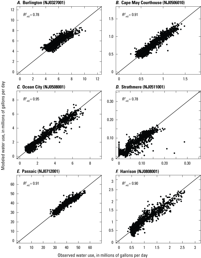
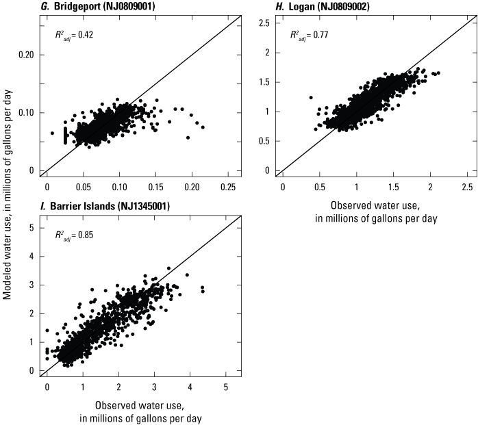
Scatterplots showing the observed versus modeled daily public supply water use (comprised of the multi-year trends, mean monthly values, modeled daily deviations, and autoregressive integrated moving average [ARIMA] models combined) for the nine seasonal New Jersey American Water drinking water service area systems during the model training period (2016–19): A, Burlington, B, Cape May Courthouse, C, Ocean City, D, Strathmere, E, Passaic, F, Harrison, G, Bridgeport, H, Logan, and I, Barrier Islands. The Barrier Islands system represents a portion of the Coastal North system, and the Burlington system represents a portion of the Western Division system; their data therefore represent a portion of their respective systems’ total water use. [, adjusted coefficient of determination]
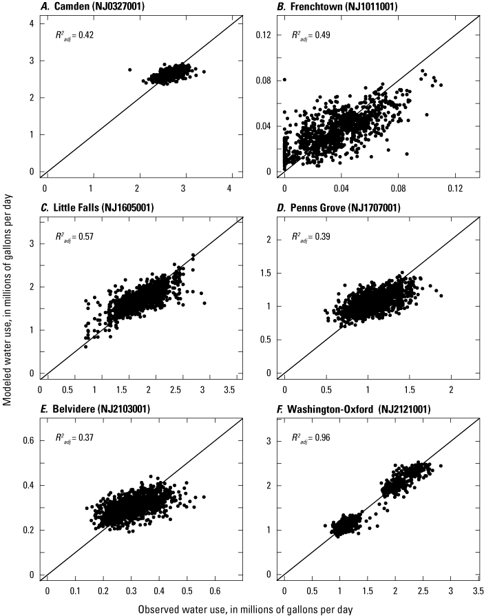
Scatterplots showing observed versus modeled daily public supply water use (comprised of the multi-year trends, mean monthly values, modeled daily deviations, and autoregressive integrated moving average models combined) for the six non-seasonal New Jersey American Water drinking water service area systems during the model training period (2016–19): A, Camden, B, Frenchtown, C, Little Falls, D, Penns Grove, E, Belvidere, and F, Washington-Oxford. The Camden system represents a portion of the Western Division system; its data therefore represent a portion of the Western Division system’s total water use. [, adjusted coefficient of determination]
Testing Regression Models on 2020 Data
With regards to using the 2020 data to test the models, because 2020 was the first year of the coronavirus disease 2019 (COVID-19) pandemic, one might expect to see different trends and patterns in water usage. Upon visual inspection, it was not obvious that data from 2020 were different than from previous years, either for daily data from NJAW or monthly data from NJWaTr. It is conceivable that the location and amount of water use changed with the release of certain recommendations from the health department. Stay-at-home guidelines could have shifted water use away from places of employment or recreation because people were advised to stay in their homes and, therefore, their home DWSA. Sanitation guidelines, such as increased hand washing, also potentially increased water use (Kim and others, 2021). For this study, there is insufficient information to determine if the COVID-19 pandemic impacted water usage and more years’ worth of data, in the years preceding and succeeding 2020, would be needed to confirm this theory.
The model performance for each of the 15 case-study systems is shown for the seasonal group (fig. 26) and non-seasonal group (fig. 27). Generally, the models for the seasonal DWSA systems performed better than those for the non-seasonal DWSA systems based on the values. The average value for the model test year among the seasonal group was 0.78; the average value for the same period among the non-seasonal group was 0.25. A possible explanation for why the seasonal DWSA system models perform better might be that the seasonal signal is fairly consistent and predictable from year to year, and the predictor variables used to build the model are mostly weather- or climate-related and thus better correlated with seasonality, which ultimately reduces unexplained variability. It is also possible that there might be additional variables which were not considered in this study that may help to better explain the day-to-day variability in the non-seasonal DWSA systems. However, it may also be that the day-to-day variability is simply random to some degree, and the random variability makes up a larger portion of the data in non-seasonally driven systems because of the lack of a dominant seasonal signal.
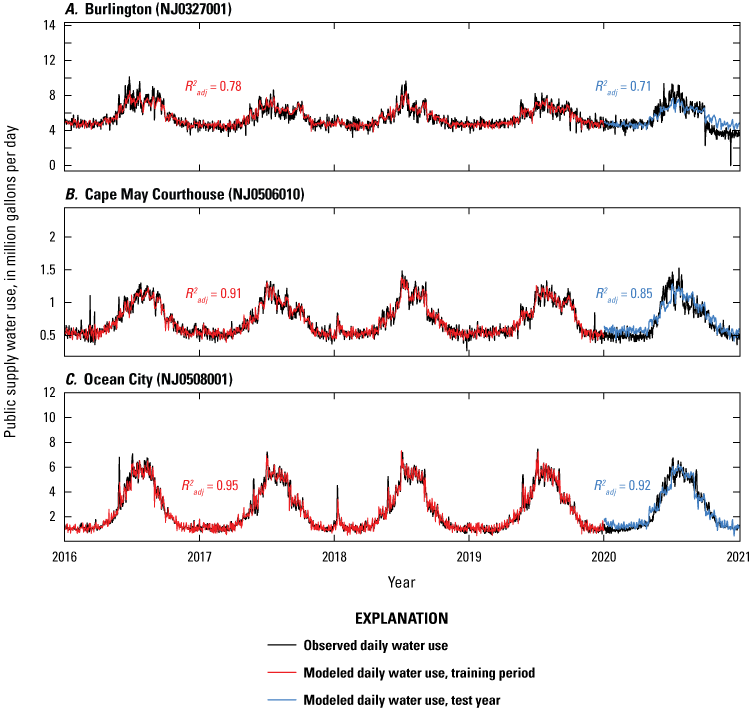
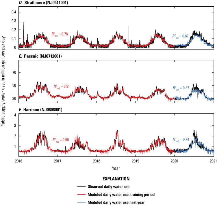
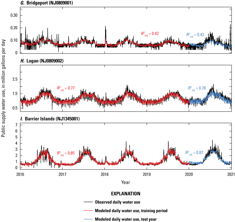
Plots comparing linear regressions with autoregressive errors model for the training period (2016–19) and the test year (2020) to observed daily public supply water use for the seasonal New Jersey American Water drinking water service area systems: A, Burlington, B, Cape May Courthouse, C, Ocean City, D, Strathmere, E, Passaic, F, Harrison, G, Bridgeport, H, Logan, and I, Barrier Islands. The Burlington system represents a portion of the Western Division system, and the Barrier Islands system represents a portion of the Coastal North system; their data therefore represent portions of their respective systems’ total water use. A higher adjusted coefficient of determination () values indicate better correlation and less error.
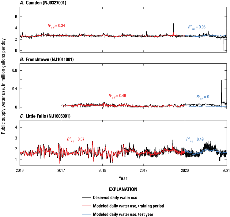
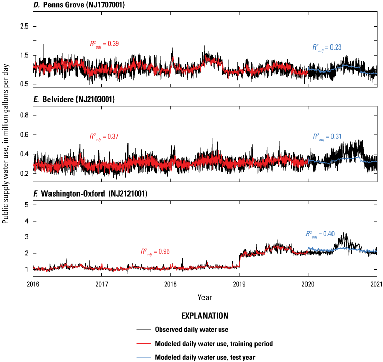
Plots comparing linear regressions with autoregressive errors model for the training period (2016–19) and the test year (2020) to observed daily public supply water use for the non-seasonal New Jersey American Water drinking water service area systems: A, Camden, B, Frenchtown, C, Little Falls, D, Penns Grove, E, Belvidere, and F, Washington-Oxford. The Camden system represents a portion of the Western Division system; its data therefore represent a portion of the Western Division system’s total water use. A higher adjusted coefficient of determination () values indicate better correlation and less error.
Visual comparison of the model training period and test year shows less day-to-day variability in the model estimates during the test year; this is particularly true of the non-seasonal systems during that time (figs. 27D and 27E). The difference in variability between the training period and the test year is due to the “forecasting” or “prediction” method for the ARIMA portion of the models. To estimate daily water use for the 2020 test year, multi-step (or dynamic) ARIMA forecasts were generated. For this estimation method, real or observed data were not used to adjust or correct the regression model estimates as it was assumed the time period of interest is in the future and observed data do not yet exist. In this case, estimating, or “predicting,” water use for 2020 was treated as if it was the future and therefore, no observed data were available to compare to and subsequently correct the model. In contrast to multi-step forecasting of the ARIMA portion of the models, the model predictions from the training period (2016–19) did incorporate the observed daily water-use volumes to correct and adjust the estimates for each day throughout the training period. As an example, when the model was used to estimate daily water use for June 10, 2018, data from 1 through 6 days before (June 4–9, 2018) were incorporated to compute the estimate. This is different from when the model was used to estimate daily water use for a given day in 2020 (test year). For June 10, 2020, for example, December 31, 2019, was the most recent observed data available to adjust the model—almost 6 months prior. The latter method of obtaining model estimates is considered forecasting because it assumes there are no available data for the time period of interest with which to compare and correct the model. With no new data to consider, the forecasted values from the ARIMA portion of the model will converge to zero because of the ARIMA model assumptions (Hyndman and Athanasopoulos, 2018). Ultimately, the predicted variability in daily water use for the 2020 test year is attributed only to external predictor variables (temperature, precipitation, day of the week), and not to autocorrelation, or the portion of variability explained by the ARIMA model, as is by design of the model.
The regression model for the Logan system performs well on the yearly and daily scale (fig. 26H). This system has a noticeable weekly signal where daily public supply water use drops over the weekend and is higher during the weekdays. Because of this regular and predictable pattern, along with an overall seasonal pattern, the regression model is able to capture and predict the day-to-day variations well based upon visual examination and mathematical calculation, with an R2 value of 0.76 for the test year (2020). In contrast, the regression model for the Belvidere system does not accurately predict daily public supply water use for 2020 (fig. 27E) based upon visual examination and mathematical calculation, with an R2 value of 0.31 for the test year. This result is likely because the Belvidere system does not have a prominent seasonal signal and the day-to-day variability in this system does not appear to be regular or predictable and is seemingly random based on the weather and climatic variables considered in this study. The results from the Washington-Oxford system appear acceptable with an R2 of 0.96 (fig. 27F), however it is important to note the exceptional situation for this system. As mentioned previously, there is a large step increase in daily water-use volumes between 2019 and 2020 for this system and explanations for this step increase are unknown (see “Daily Public Supply Water-Use Data” section). Although the same analysis as all other systems was applied here, there is less confidence in the accuracy and meaning in the results because of the large shift in the dataset for the Washington-Oxford system.
The RMSE was also calculated to help evaluate the performance of the models between the training period and the test year (table 10). Because RMSE is an absolute measure of error and the magnitudes of water use vary from system to system, RMSE is not as robust as for comparing performance between models (or DWSA systems). Instead, it can provide some insight toward the model error when comparing different time periods from the same model or within each DWSA system. In this case, the training period and the test year were compared.
Table 10.
The mean daily water-use volumes (2016–20) and root mean squared errors (RMSEs) in million gallons per day (Mgal/d) are shown for all 15 New Jersey American Water drinking water service area (DWSA) systems grouped by the training period (2016–19) and the test year (2020).[PWSID, public water system identification number; RMSE, root mean squared error]
Anomalous Data Points
As noted previously, in the section titled “Daily Public Supply Water-Use Data,” there were a few observed data points that were outside the typical range of values for a given DWSA system. The same regression analysis was performed on the datasets with these data points removed to evaluate the effect of these anomalous data on the regression models (fig. 28). There were five systems that had visually identifiable anomalous data points (Burlington, Strathmere, and Bridgeport in figure 26; Camden and Frenchtown in figure 27). When the regression analysis was applied with and without these anomalous data points, the differences in values ranged from 0.001 to 0.15 with a mean difference of 0.04 (table 11). The differences in RMSE ranged from 0.001 to 0.05 Mgal/d, with a mean difference of 0.01 Mgal/d (table 12). These findings indicate that including the few anomalous data points does not drastically affect the models and their performance (tables 11 and 12). Thus, retaining anomalous data points in any additional datasets that may be used to test the models may not have a sizable effect on the results.
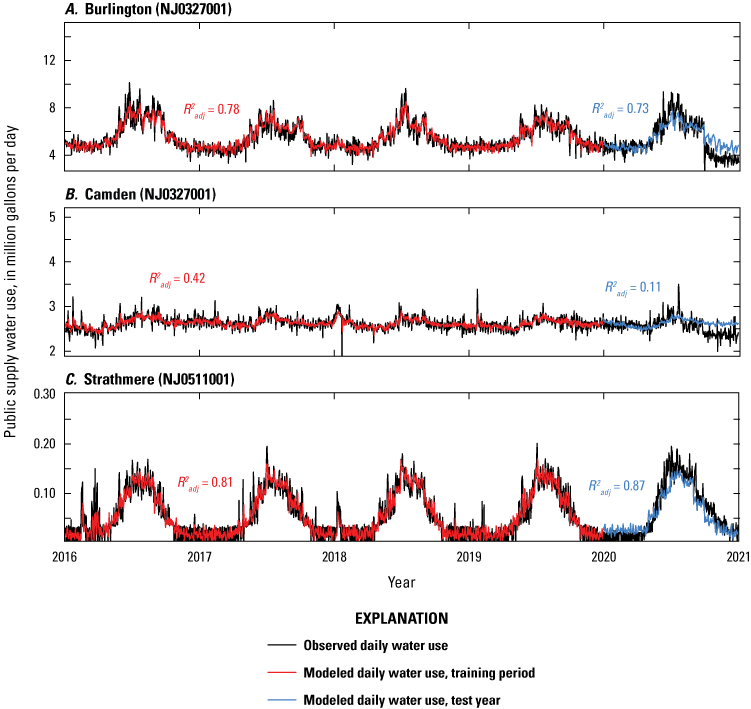
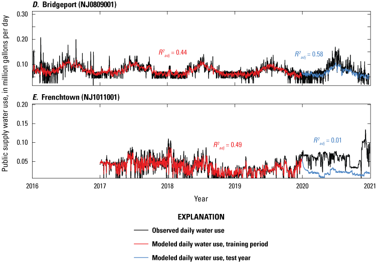
Plots showing linear regressions with autoregressive errors model for the training period (2016–19) and the test year (2020) for the subset of New Jersey American Water drinking water service area systems that had anomalous data points, which were removed in these figures: A, Burlington, B, Camden, C, Strathmere, D, Bridgeport, and E, Frenchtown. The Burlington and Camden systems represent portions of the Western Division system; their data therefore represent portions of the Western Division system’s total water use. [, adjusted coefficient of determination]
Table 11.
The adjusted coefficient of determination () values for the New Jersey American Water drinking water service area (DWSA) systems that had anomalous data, shown for the training period (2016–19) and the test year (2020) with the anomalous data removed and retained for comparison.[PWSID, public water system identification number]
Table 12.
The root mean squared errors for the New Jersey American Water drinking water service area (DWSA) systems that had anomalous data, shown for the training (2016–19) and test (2020) periods with the anomalous data removed and retained for comparison.[PWSID, public water system identification number; RMSE, root mean squared error]
Currently, the models do not estimate water use on the days with anomalous data well and may not elucidate anomalous data points found in additional datasets (for other time periods, beyond the training period and the test year, or for other DWSA systems). The reasons behind some of these data points, such as water main breaks (NJAW, written commun., 2021), are usually unpredictable. The goal of these regression models was to estimate typical daily public supply water use, so it is expected that the models may not accurately estimate these atypical days and events. Additionally, not all predictor variables and information that might be relevant in predicting these events, such as the age of the water supply system and its infrastructure, were included in this study. Even though the models do not predict these anomalous data points well, the model performance statistics are mostly unchanged even with these points removed owing to the small number of anomalous data points relative to the entire dataset. If a dataset were to have many more data points with uncharacteristic volumes of water use, the anomalous data points could have a larger impact on the overall model and its performance.
Accuracy and Limitations of Regression Equations
The primary measures of model error and accuracy used in this study were the RMSE and . Comparing each statistic between the training period and the test year, the models’ performance tends to drop slightly during the test year. The average increase in RMSE for the test year is 0.13 Mgal/d. The average decrease in for the test year is 0.18 Mgal/d. This is to be expected as the test data were treated as “new” data for the model and were not involved in training or developing the model. Instead, the model had to “predict” or extrapolate the data from the test year.
These models were created for the 15 DWSA systems in New Jersey for which daily public supply water-use data were provided and are therefore only appropriate for estimating water use within those 15 specific systems. There are likely commonalities in factors affecting daily public supply water use across DWSA systems in New Jersey. However, more daily data (from additional systems and additional years) are needed to better identify those commonalities and the extent to which these equations developed here are applicable to other systems. Additionally, there are likely influential factors beyond those studied here that could potentially improve the accuracy of daily public supply water-use estimates. The factors included in this study are commonly used factors in estimating water use, however there may be additional factors specific to New Jersey that could be suitable (Zhou and others, 2000; Eslamian and others, 2016; Opalinski and others, 2019; Ahmed and others, 2020). Finally, having more years’ worth of daily water-use data to train the models would likely improve the model performance, particularly for identifying any long-term trends that may be present in the data.
Disaggregation of Monthly-to-Daily Water-Use Estimates
In addition to establishing a method for modeling daily public supply water use in New Jersey for the 15 case-study DWSAs, a method of disaggregating monthly NJWaTr water-use data to daily time steps was tested. First, monthly water-use totals from NJWaTr from 2016 through 2020 were disaggregated to average daily water-use volumes by dividing the monthly volume total by the number of days in that month. This produced an average daily contribution of water use for each month and for each DWSA system in the NJWaTr database (fig. 29). For the three partial systems (Barrier Islands, Burlington, and Camden), scaling factors based on population were applied to the disaggregated water-use volumes. The ratio of the population in the partial DWSA system to the population in the complete DWSA system was applied to scale the disaggregated water-use volumes. The 2010 Census Bureau population estimates by census block group were used for this calculation, which includes total population in the area and not just publicly supplied populations. Even though the scaling factors adjusted the disaggregated NJWaTr data to magnitudes comparable to the partial NJAW systems, they did not adjust the patterns of water use because it was a simple multiplier. This can be observed in figure 29B and 29K.
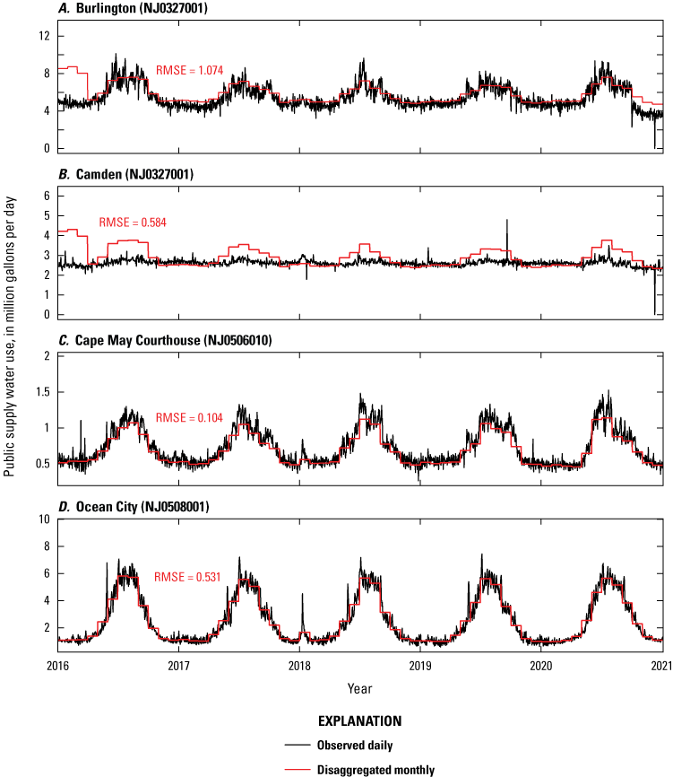
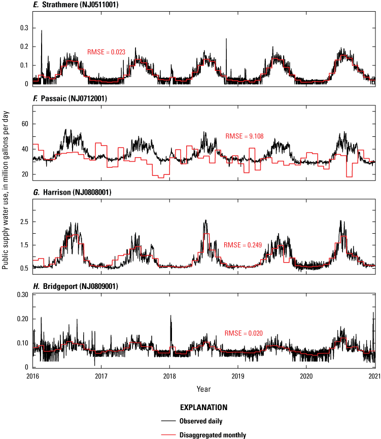
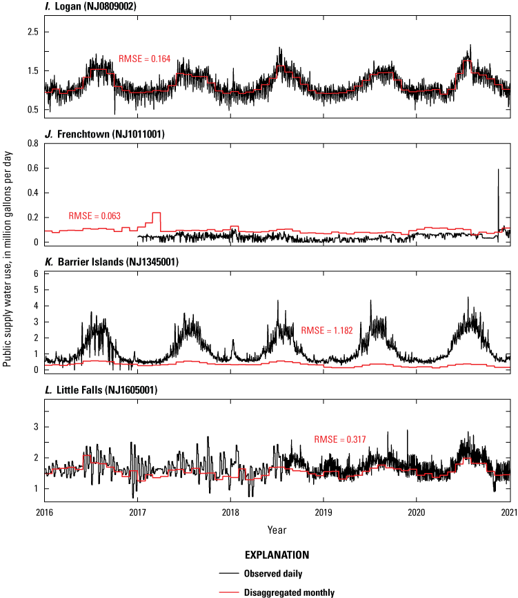
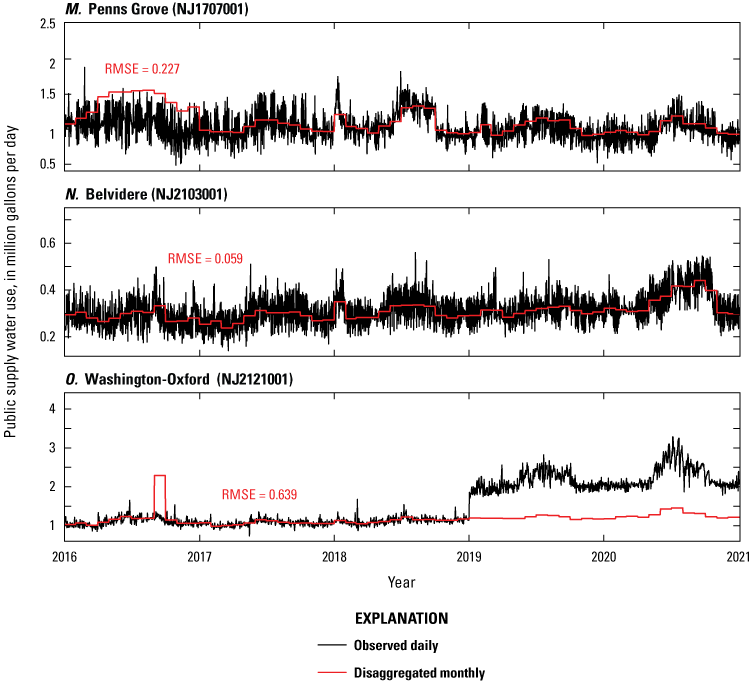
Plots comparing disaggregated water-use values from the New Jersey Water Transfer Data Model database to observed daily water-use data provided by New Jersey American Water (NJAW), 2016–20: A, Burlington, B, Camden, C, Cape May Courthouse, D, Ocean City, E, Strathmere, F, Passaic, G, Harrison, H, Bridgeport, I, Logan, J, Frenchtown, K, Barrier Islands, L, Little Falls, M, Penns Grove, N, Belvidere, and O, Washington-Oxford. The root mean squared error (RMSE) was calculated as a baseline error on the monthly-to-daily disaggregated data. The Burlington and Camden systems represent portions of the Western Division system, and the Barrier Islands system represents a portion of the Coastal North system; their data therefore represent portions of their respective systems’ total water use. Monthly water-use data are from the New Jersey Department of Environmental Protection Division of Water Supply and Geoscience (2022). Daily water-use data are from NJAW and are not available owing to a proprietary interest or sensitivity concern. Contact NJAW for more information.
The average daily water-use volumes from the simple disaggregation calculation provided a baseline for average daily water use per month for the 15 DWSA systems. Next, the modeled daily water-use deviation estimates produced from the 15 regression models were added to the NJWaTr average daily water-use volumes to obtain more realistic daily water-use estimates with day-to-day fluctuations incorporated, as shown in figures 30 and 31. Previously, when building the daily public supply regression models, as described in “Development of a Daily Water-Use Regression Model,” the mean monthly values had been subtracted out from the observed NJAW daily data to obtain daily deviations of water use. The deviations were used to train the model, and therefore the output of the models was estimates of daily deviations (from mean monthly values) of water use. To obtain actual daily water-use volumes, the mean monthly values that had been subtracted out prior to training the model were then added back to the model deviation estimates. Here, instead of using the mean monthly values calculated from the NJAW daily data (fig. 23), the disaggregated monthly NJWaTr volumes were used. By using the disaggregated monthly NJWaTr data as the baseline amount, future or historical daily water use could be forecasted or hindcasted for any of the 15 case-study systems provided there were temperature and precipitation data (or predicted data) available for the time period of interest.
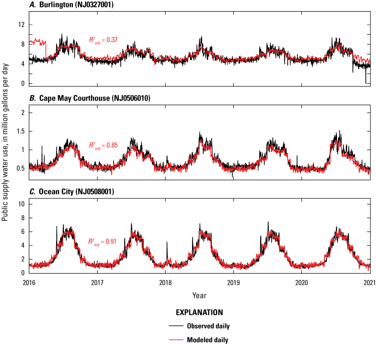
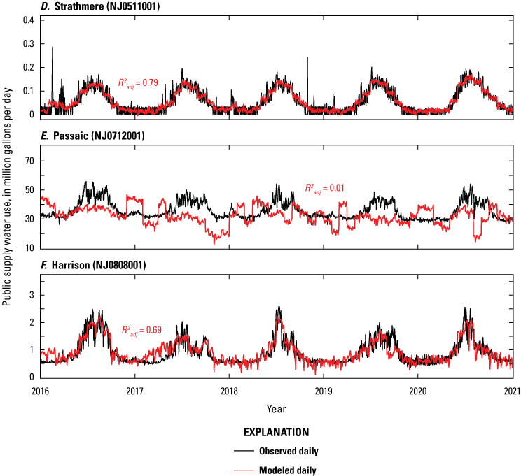
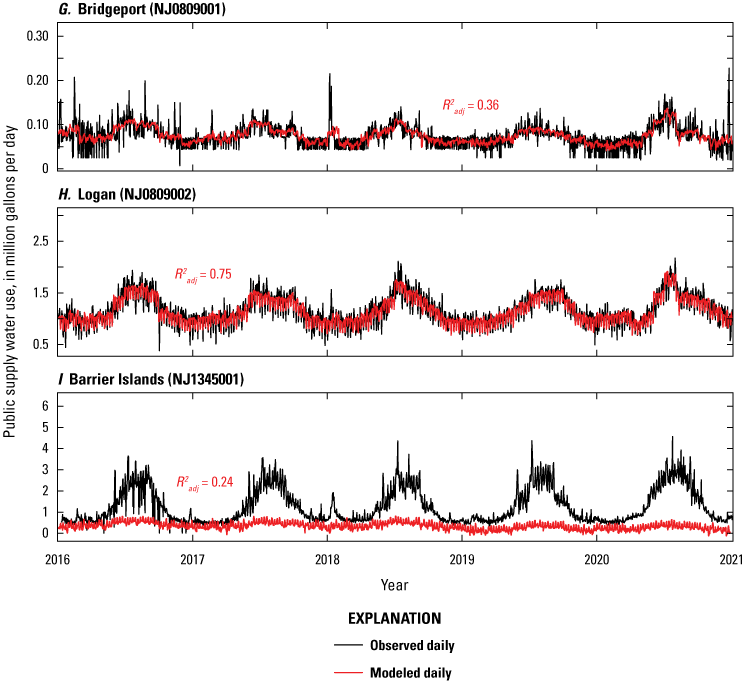
Plots comparing disaggregated New Jersey Water Transfer Data Model water use combined with the linear regression with autoregressive errors model estimates to observed daily water-use data provided by New Jersey American Water (NJAW) for the seasonal systems: A, Burlington, B, Cape May Courthouse, C, Ocean City, D, Strathmere, E, Passaic, F, Harrison, G, Bridgeport, H, Logan, and I, Barrier Islands. A higher adjusted coefficient of determination () values indicate better correlation. The Burlington system represents a portion of the Western Division system, and the Barrier Islands system represents a portion of the Coastal North system; their data therefore represent only portions of their respective systems’ total water use. Monthly water-use data are from the New Jersey Department of Environmental Protection Division of Water Supply and Geoscience (2022). Daily water-use data are from NJAW and are not available owing to a proprietary interest or sensitivity concern. Contact NJAW for more information.
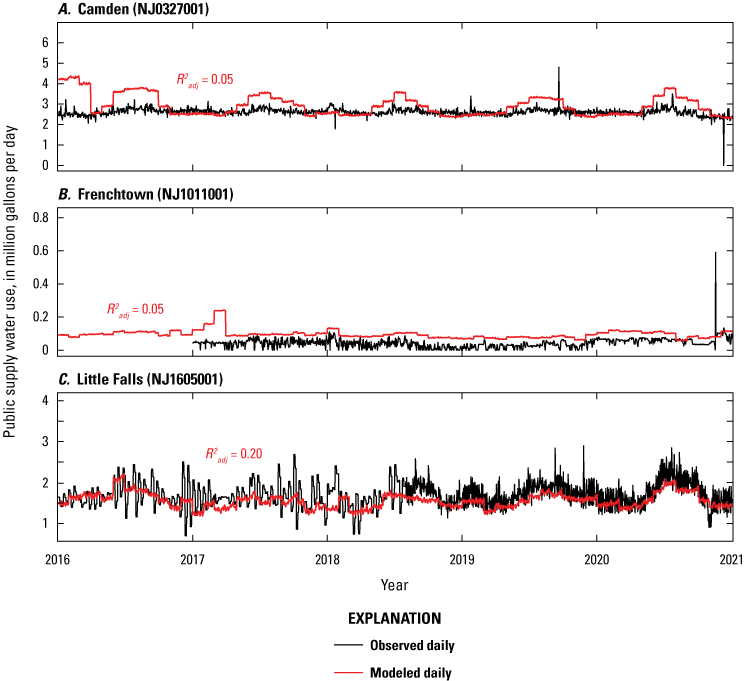
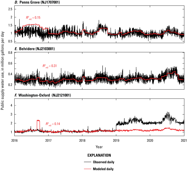
Plots comparing disaggregated New Jersey Water Transfer Data System water use combined with the linear regression with autoregressive errors model estimates to observed New Jersey American Water (NJAW) daily water use for the non-seasonal systems: A, Camden, B, Frenchtown, C, Little Falls, D, Penns Grove, E, Belvidere, and F, Washington-Oxford. A higher adjusted coefficient of determination () values indicate better correlation. The Camden system represents a portion of the Western Division system; its data therefore represent only a portion of the Western Division system’s total water use. Monthly water-use data are from New Jersey Department of Environmental Protection Division of Water Supply and Geoscience (2022). Daily water-use data are from NJAW and are not available owing to a proprietary interest or sensitivity concern. Contact NJAW for more information.
One limitation of using this method to disaggregate monthly values to daily values, is the inherent assumption that the NJWaTr monthly totals are representative of public supply water use in a given DWSA system for the total period of record. When the NJAW and NJWaTr data were compared previously, it was found that for some systems, the two datasets did not match and therefore, it would be expected that using this method would not produce accurate estimates for those systems whose aggregated daily totals did not align with the monthly values (figs. 3, 4, and 5).
The monthly-to-daily disaggregation method tested in this study indicates that a reasonable estimate of daily water use can be obtained for some of the 15 case-study DWSA systems (figs. 30 and 31). Because this method requires that the provided daily NJAW data agree closely with the monthly NJWaTr data, where the two datasets vary drastically, and subsequently this condition is not met, this method does not produce reasonable daily water-use estimates. More investigation into systems like these, where the two datasets do not agree, is warranted. Obtaining an understanding of buying and selling of water within and between DWSAs may provide insight into why these datasets do not agree.
For DWSA systems where the two datasets agree, the daily estimates produced are comparable to the daily estimates produced using solely the NJAW daily data. For example, the value for the Ocean City system from 2016 through 2019 based on the NJAW daily data was 0.95 (fig. 26C); the using the NJWaTr monthly data from the same period was 0.91 (fig. 30C). For the Logan system, the using the daily data was 0.77 (fig. 26H); the using the NJWaTr monthly data was 0.75 (fig. 30H). In contrast, for the Passaic system, where the two datasets did not agree, the values based on the daily data and NJWaTr monthly data were 0.91 (fig. 26E) and 0.01 (fig. 30E), respectively.
Another case where the datasets did not agree was for systems for which only partial DWSA daily public supply water-use data were provided. This was the case for the Barrier Islands, Burlington, and Camden systems, for which it was necessary to compare partial data to the total water use for the Coastal North and Western Division systems. Here, it was expected that the datasets would not agree as only a portion of the daily public supply data from the entire DWSA system was provided. To account for the fact that these systems had partial data, the fraction of the population within the partial DWSA of the total population in the entire DWSA was multiplied to the disaggregated monthly NJWaTr data. In essence, this scaled the NJWaTr data to be of similar magnitude to the partial DWSA system daily data. Although this allowed for the results to be of comparable magnitude, the patterns and variation in estimated public supply water use did not align with the observed daily data (figs. 30A, 30I, and 31A).
Developing and Using the Generalized Regression Models
This method for monthly-to-daily disaggregation would likely be more useful if it could be applied to systems beyond the 15 DWSA systems for which daily water-use data were acquired and for which the daily regression models were developed. To increase the applicability of this tested disaggregation method, a single averaged regression equation was developed to represent all seasonal systems, and a second averaged regression equation was developed to represent all non-seasonal systems. These averaged equations were developed based on the 15 case-study systems’ equations, but the intent was for them to be applicable for any system in the state, which assumes the 15 systems were representative of all DWSA systems in the state. However, having more daily data from more systems to further develop the averaged equations would likely improve their accuracy.
To compute the averaged regression equations, also referred to as the generalized regression equations, the daily public supply water-use data were first normalized by the populations served for each system. Then, the mean monthly values were calculated and subtracted from the data to obtain daily deviations. The normalized daily deviations public supply data were then averaged across each system grouping (seasonal and non-seasonal). For example, the normalized, daily deviations public supply data were averaged across all nine seasonal systems for each day in the period of interest (2016–20) resulting in one set of averaged (and normalized) daily deviations public supply data for systems demonstrating seasonal water-use patterns. This averaging was done for the climatic variables as well. For example, the daily maximum temperatures were averaged at each time step across all nine seasonal systems to obtain one averaged, daily maximum temperature.
Next, the same regression development method was applied as outlined above. Backward stepwise regression selection was used to select which predictor variables were best suited to predict the averaged, normalized daily public supply water-use deviations (eqs. 11 and 12). Once the best suited variables were identified, the regression model coefficients were estimated using R statistical software (R Core Team, 2019). This resulted in two sets of averaged (and normalized) model coefficients, one for seasonal systems and one for non-seasonal systems (table 13).
whereis the modeled, averaged daily deviation of public supply water use at time-step t;
bi
is an empirically derived regression coefficient for predictor variable i;
is the averaged daily maximum temperature deviation from mean monthly value;
is the averaged deviation of daily maximum temperature from mean monthly value lagged by 1 day;
is the averaged deviation of daily maximum temperature from mean monthly value lagged by 2 days;
is the averaged deviation of daily precipitation total from mean monthly value lagged by 1 day;
is the averaged deviation of daily precipitation total from mean monthly value lagged by 2 days;
is the averaged deviation of daily precipitation total from mean monthly value lagged by 3 days;
is the averaged number of days since significant precipitation;
dow
is the weekday-weekend effect; and
Nt
is the model error term, or residual at time-step t.
is the modeled, averaged daily deviation of public supply water use at time-step t;
bi
is an empirically derived regression coefficient for predictor variable i;
is the averaged daily maximum temperature deviation from mean monthly value;
is the averaged deviation of daily precipitation total from mean monthly value lagged by 1 day;
is the averaged deviation of daily precipitation total from mean monthly value lagged by 3 days;
is the averaged number of days since significant precipitation; and
Nt
is the model error term, or residual at time-step t.
ARIMA models for the generalized seasonal and non-seasonal groups were also developed using the same method from the individual daily ARIMA models (table 14). The seasonal system equation is of the form:
whereis the total error term from the averaged linear regression model at time-step t;
ARp
is the autoregressive model coefficient up to p terms;
is the averaged linear regression model residual lagged by p time steps; and
εt
is the remaining, unexplained error at timestep t.
The non-seasonal system equation is of the form:
whereis the total error term from the averaged linear regression model at time-step t;
ARp
is the autoregressive model coefficient up to p terms;
is the averaged linear regression model residual lagged by p time steps;
MAq
is the moving average model coefficient up to q terms;
is the averaged ARIMA model residual lagged by q time steps; and
εt
is the remaining, unexplained error at timestep t.
To test the accuracy of the generalized equations on a system for which there were monthly NJWaTr data but no daily data, the monthly data were first normalized by that system’s served population to scale the water-use volumes to the same magnitude.
Table 13.
Coefficient magnitudes of the averaged generalized regression models.[None of the coefficients show significance to the 95-percent confidence level. Negative values indicate an inverse relationship with the predictor variable. 3.48 E−07 means 3.48×10−7=0.000000348. , daily maximum temperature; , daily maximum temperature lagged 1 day; , daily maximum temperature lagged 2 days; , daily precipitation total lagged 1 day; , daily precipitation total lagged 2 days; , daily precipitation total lagged 3 days; , days since significant precipitation; dow, weekday-weekend effect; NA, not applicable]
| Regression coefficients | ||||||||
|---|---|---|---|---|---|---|---|---|
| Type | dow1 | |||||||
| Seasonal | 3.48 E−07 | 9.45 E−08 | 1.02 E−07 | −7.71 E−06 | −1.13 E−06 | −1.11 E−06 | 6.35 E−07 | −9.74 E−07 |
| Non-seasonal | 4.87 E−08 | NA | NA | −1.89 E−06 | NA | −1.48 E−06 | 3.08 E−07 | NA |
The dow (weekday-weekend effect) is a predictor variable used in this study as daily public supply data are known to be influenced by weekday or weekend (Eslamian and others, 2016).
Table 14.
Coefficient magnitudes of the averaged autoregressive integrated moving average (ARIMA) models.[Negative values indicate an inverse relationship with the predictor variable. ARIMA, autoregressive integrated moving average; AR1, autoregressive term lagged 1 day; MA1, moving average term lagged 1 day; MA2, moving average term lagged 2 days; MA3, moving average term lagged 3 days; NA, not applicable]
Next, the generalized regression equations were tested to determine if combining these equations with disaggregated monthly-to-daily NJWaTr data could produce reasonable daily water-use estimates for DWSA systems beyond the 15 highlighted in this study. The generalized equations were combined with the disaggregated monthly NJWaTr data using the same process discussed at the beginning of this section, but instead of using system-specific regression equations, the two generalized models (seasonal and non-seasonal) were used. The final step was to multiply the water-use volumes and their respective DWSA system populations served to rescale the data to the system’s original magnitudes. The estimated daily public supply water-use volumes were then compared to the NJAW daily public supply water-use data from 2016 through 2020 for the 15 systems with daily data (figs. 32 and 33). Overall, the estimates from the generalized models were similar to the system-specific models, with an overall average 6-percent increase in RMSE, which indicates this method is a reasonable way to estimate daily public supply given monthly data and accompanying climate information. In general, as observed previously with the system-specific regression equations the generalized seasonal equations performed better than the generalized non-seasonal equations and had higher adjusted R2 values (figs. 32 and 33), especially when the daily data align well with the monthly data from NJWaTr. There are limitations in using these generalized regression equations for systems where only partial data were provided, and therefore the data did not represent the whole system. Limitations also exist for systems where the aggregated daily data did not match the monthly totals in NJWaTr. These limitations are described in more detail in the “Limitations of Generalized Regression Models” section.
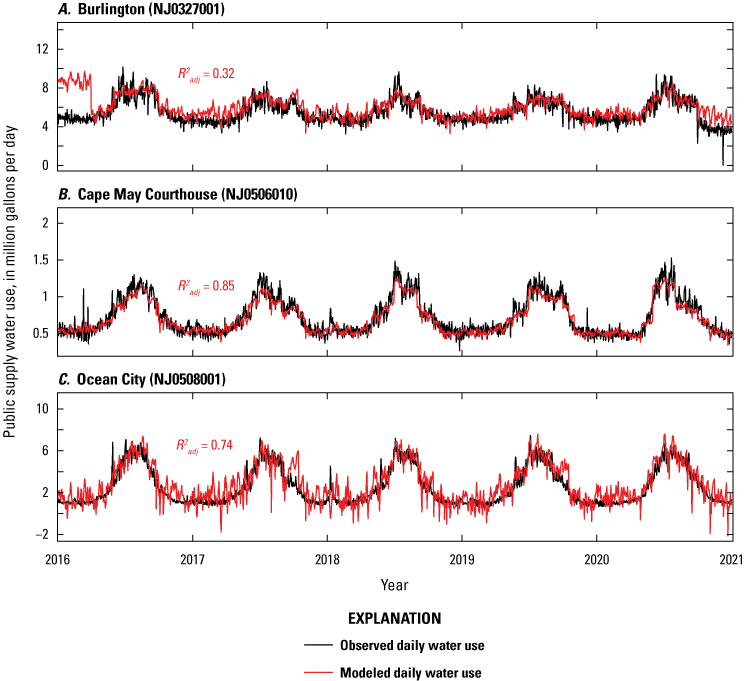
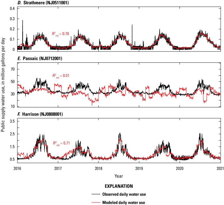
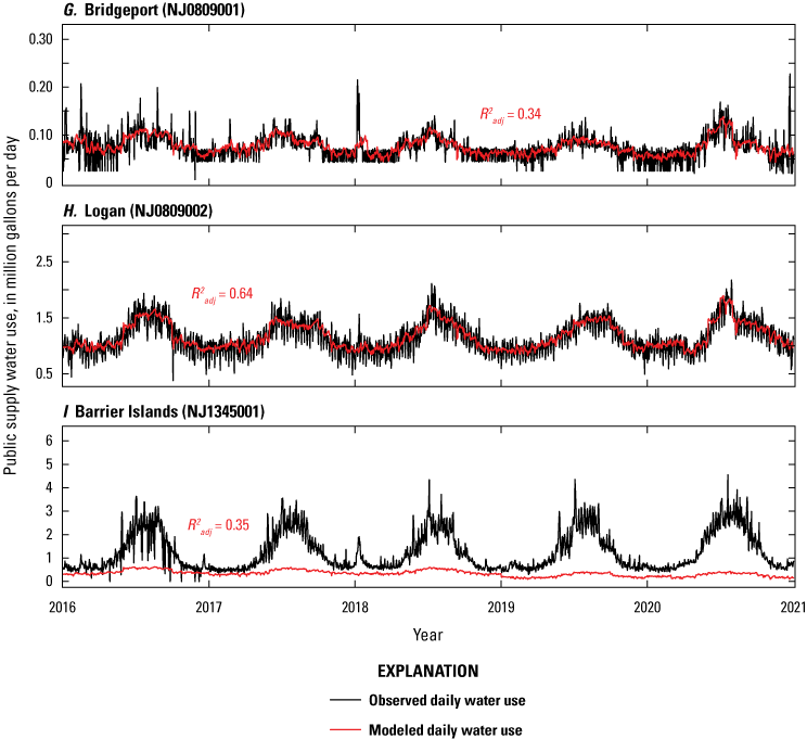
Plots comparing disaggregated New Jersey Water Transfer Data Model (NJWaTr) water use combined with the generalized linear regression with autoregressive errors model estimates to observed New Jersey American Water (NJAW) daily water use for the seasonal systems: A, Burlington, B, Cape May Courthouse, C, Ocean City, D, Strathmere, E, Passaic, F, Harrison, G, Bridgeport, H, Logan, and I, Barrier Islands. The Burlington system represents a portion of the Western Division system, and the Barrier Islands system represents a portion of the Coastal North system; their data therefore represent only portions of their respective systems’ total water use. Daily water-use data are from NJAW and are not available owing to a proprietary interest or sensitivity concern. Contact NJAW for more information. [, adjusted coefficient of determination]
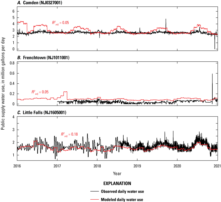
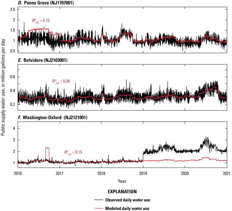
Plots comparing disaggregated New Jersey Water Transfer Data Model (NJWaTr) water use combined with the generalized linear regression with autoregressive errors model estimates to observed New Jersey American Water (NJAW) daily water use for the non-seasonal systems: A, Camden, B, Frenchtown, C, Little Falls, D, Penns Grove, E, Belvidere, and F, Washington-Oxford. The Camden system represents a portion of the Western Division system; its data therefore represent only a portion of the Western Division system’s total water use. Daily water-use data are from NJAW and are not available owing to a proprietary interest or sensitivity concern. Contact NJAW for more information. [, adjusted coefficient of determination]
Testing Generalized Regression Models on New DWSA Systems
As a final test of these generalized regression equations, three seasonal DWSA systems for which daily data were not available were selected from the NJWaTr database. The three systems were chosen based on their similarity to three seasonal NJAW systems. The first system was Long Beach–North Beach (NJ1517003; table 15, Comparison Group A), which was chosen because of its similarity to the Strathmere system: they both have smaller population-served (Q2) values, higher income and property values, non-urban residential density, and coastal geography. The second system chosen was Margate City (NJ0116001; table 15, Comparison Group B), which was similar to the Ocean City system: they both have larger population-served (Q4) values, higher property values, urban residential density, and coastal geography. The third system chosen was Ringwood (NJ1611002; table 15, Comparison Group C), because of its similarity to the Harrison system: they both have larger population-served (Q3) values, higher income and property values, non-urban residential density, and non-coastal geography.
Table 15.
Comparison of characteristics associated with three additional seasonal drinking water service area (DWSA) systems listed in the New Jersey Water Transfer Data Model database and the New Jersey American Water DWSA systems most similar to them.[Quartiles are defined in table 2. DWSA system names are from the New Jersey Department of Environmental Protection Bureau of Geographic Information System (2017b)]
Because the seasonal generalized regression models perform better than the non-seasonal generalized regression models discussed in this study, the focus was to test the generalized seasonal regression model, as there are likely additional influential factors to be explored with the non-seasonal model and modeled results of the non-seasonal systems showed more errors and less correlation. With these three test DWSA systems, the monthly NJWaTr data were disaggregated to an average daily total using the simple disaggregation method of dividing by number of days in the month and the generalized regression estimates (deviations from the mean monthly values) were added to include daily fluctuations. These final estimates were then compared to the disaggregated NJWaTr data, as there were no daily data to compare to for these three systems (fig. 34). The RMSEs were used to assess the modeled estimates in comparison to the disaggregated NJWaTr data and ranged from 0.006 to 0.17 Mgal/d (fig. 34). It is difficult to compare monthly and daily datasets; however, the primary purpose of this exercise was to determine if it is possible to obtain reasonable daily water-use volumes in the absence of daily data. The final estimates may be biased (high or low) because they are being assessed against data that were used to generate the estimates.
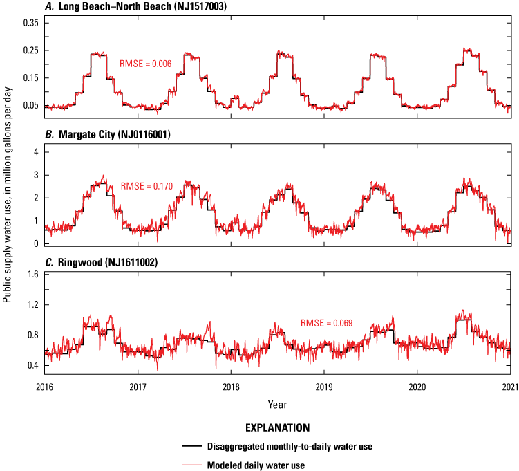
Plots showing disaggregated New Jersey Water Transfer Data System (NJWaTr) water use combined with the generalized linear regression with autoregressive errors model estimates as applied to three drinking water service area systems for which daily data were not available: A, Long Beach–North Beach, B, Margate City, and C, Ringwood. The root mean squared error (RMSEs) represents the error of the modeled estimates as compared to the disaggregated NJWaTr data.
Limitations of Generalized Regression Models
In addition to the limitations and extent of accuracy discussed in the section titled “Accuracy and Limitations of Regression Equations” with the 15 system-specific regression equations, there are additional constraints to consider that are introduced when using the generalized regression models and incorporating the NJWaTr dataset of monthly values. Combining the monthly NJWaTr datasets into the water-use estimates creates some additional uncertainty because the water-use data used in the estimations comes from two separate sources: one from NJAW’s daily dataset and one from NJWaTr’s monthly dataset. Both datasets may have some uncertainty and error that are likely not the same across, and potentially within, each dataset. Because these datasets may have different sources of uncertainty and types of errors, there is potential for the summed daily values not to match the monthly values, as was found in several systems. Having a better understanding of those systems whose daily values do not sum to monthly values could be valuable to improve model results and outcomes.
For the NJAW dataset, the level of quality assurance and quality control is unknown; for example, the specifics of meter calibration or other types of verification are unknown. Some examples of uncertainty and factors affecting accuracy were presented in the discussion on anomalous data points (in the section titled “Anomalous Data Points”) that were observed in several systems with daily data from NJAW. Data from NJWaTr were checked using a quality assurance and quality control procedure in which monthly data are checked against permitted allocation limits and checked against historical data for each site for its period of record (Shourds, 2020). Another source of uncertainty or errors inherent to the NJWaTr dataset may result from the fact that these public supply data come from many different purveyors. Furthermore, each system within a public supply purveyor could have its own individual sources of error or conditions specific to that system that may affect the quality and accuracy of the data.
Another source of uncertainty arises from averaging regression equation coefficients. Each model was initially developed for a specific DWSA system and therefore had unique coefficient values based on the correlation between a particular system’s daily water use and various predictor variables (like temperature and precipitation). By averaging the coefficients, any interpretation on the correlations between variables is not recommended. Rather, the primary purpose of averaging the coefficients was to determine if reasonable estimates of water use could be made on systems beyond the 15 systems for which daily data were acquired. This method of averaging regression coefficients and combining the outputs with NJWaTr data was tested for this study without any preconceived knowledge of what the results would be.
More data and further analysis would be needed to determine if this is a viable and accurate method for estimating daily public supply water use for any DWSA system in New Jersey. More daily data would allow for further model output verification. Additionally, exploring other factors or variables that may influence daily public supply water use, beyond those that were considered in this study, could also improve model outcomes.
Summary
Being able to better understand, and ultimately estimate, daily public supply water use supports water supply resource prediction and planning. In this study, public supply water use and various climatic and socio-economic factors were examined for significant correlation. It was found that drinking water service area (DWSA) systems that were considered coastal (and therefore may experience a large influx of tourist populations between May and September [Stirling, 2018]) nearly always showed strong seasonality in water use throughout the year (97 percent of coastal systems). Eighty percent of DWSA systems that served populations of 11,878 or more people showed strong seasonal water-use patterns and 70 percent of DWSA systems classified as non-urban (those with rural, low, or medium residential densities as the primary density) also showed seasonality in water-use patterns (fig. 17). Being able to determine whether a specific system shows seasonality or not was ultimately found to be relevant in the daily water-use estimation methods tested in this study.
Linear regression models combined with autoregressive integrated moving average (ARIMA) models were used to estimate daily public supply water use for 15 DWSA systems in New Jersey. Nine of the 15 systems showed strong seasonality and 6 systems showed little to no seasonality. The models developed for the seasonal systems generally performed better with an average adjusted coefficient of determination () of 0.78 for the test year, compared to the non-seasonal systems which had an average of 0.25 for the test year. Overall, it was found that daily water use among seasonal systems was better correlated with external variables (temperature, precipitation, day of the week) considered in this study compared to the non-seasonal systems. The external variables that showed the most consistent correlation to daily water use across the seasonal systems were daily maximum temperature, precipitation totals lagged by 1 day, and day of the week (also known as the weekday-weekend effect). Although the non-seasonal systems did not show as much correlation with the external predictor variables, water-use volumes from 1 to 6 days prior to the present was one of the better predictor variables for these systems. In other words, a given system’s water-use volumes on previous days heavily influenced estimates of the present day’s water use, more so than temperature, precipitation, or day of the week.
Finally, a method was tested to determine if daily public supply water use could be estimated for any DWSA system in New Jersey beyond the 15 New Jersey American Water systems highlighted in this study. This method was applied to and tested on the 15 systems for which there were daily data in order to identify the uncertainties. The 15 system-specific equations for estimating water use were averaged to obtain a more general and potentially more applicable equation of water-use estimation. Reasonable estimates of water use could be obtained depending on the system, with a range in values from 0.01 to 0.85. Because this method relied on agreement between the monthly NJWaTr data and daily NJAW data, this pilot method of estimating daily water use from monthly data did not perform well for some systems, as was expected. As this method was tested for the first time in this study, obtaining more data—for averaging the system-specific equations and for comparing estimates to observed volumes—would be beneficial in helping to determine the accuracy and reliability of the method.
References Cited
Abatzoglou, J.T., 2011, Development of gridded surface meteorological data for ecological applications and modelling: International Journal of Climatology, v. 33, no. 1, p. 121–131, accessed December 6, 2021, at https://doi.org/10.1002/joc.3413.
Abatzoglou, J.T., [undated], Download: Climatology Lab, accessed June 20, 2021, at https://www.climatologylab.org/gridmet.html.
Ahmed, S.N., Moltz, H.L.N., Schultz, C.L., and Seck, A., 2020, 2020 Washington metropolitan area water supply study—Demand and resource availability forecast for the year 2050: Interstate commission on the Potomac River Basin, ICPRB Report No. 20-3, prepared by authors under contract, variously paged. [Also available at https://www.potomacriver.org/publications/2020-washington-metropolitan-area-water-supply-reliability-study-demand-and-resource-availability-forecast-f or-the-year-2050/.]
Akaike, H., 1974, A new look at the statistical model identification: Institute of Electrical and Electronics Engineer Transactions on Automatic Control, v.19, no. 6, p.716-723, accessed October 2021 at https://doi.org/10.1007/978-1-4612-1694-0_16.
Bloomfield, P., 2000, Fourier analysis of time series—An introduction (2nd ed.): New York, John Wiley & Sons. [Also available at https://doi.org/10.1002/0471722235.]
Dieter, C.A., Maupin, M.A., Caldwell, R.R., Harris, M.A., Ivahnenko, T.I., Lovelace, J.K., Barber, N.L., and Linsey, K.S., 2018, Estimated use of water in the United States in 2015: U.S. Geological Survey Circular 1441, 65 p., https://doi.org/10.3133/cir1441. [Supersedes USGS Open-File Report 2017–1131].
Domber, S., Hoffman, J., and Grimes, A., 2006, New Jersey water withdrawals, uses, transfers, and discharges by HUC11, 1990 to 1999—User’s guide: New Jersey Department of Environmental Protection, 33 p. [Also available at https://www.nj.gov/dep/njgs/enviroed/HUC11/HUC11ug.pdf.]
Eslamian, S.A., Li, S.S., and Haghighat, F., 2016, A new multiple regression model for predictions of urban water use: Sustainable Cities and Society, v. 27, p. 419–429, accessed November 6, 2021, at https://doi.org/10.1016/j.scs.2016.08.003.
Helsel, D.R., Hirsch, R.M., Ryberg, K.R., Archfield, S.A., and Gilroy, E.J., 2020, Statistical methods in water resources: U.S. Geological Survey Techniques and Methods, book 4, chap. A3, 458 p., accessed July 10, 2021, at https://doi.org/10.3133/tm4A3. [Supersedes USGS Techniques of Water-Resources Investigations, book 4, chapter A3, version 1.1]
Hyndman, R.J., and Athanasopoulos, G., 2018, Forecasting—Principles and practice (2nd ed.): OTexts, accessed April 29, 2021, at https://otexts.com/fpp2.
Hyndman, R.J., Athanasopoulos, G., Bergmeir, C., Caceres, G., Chhay, L., O’Hara-Wild, M., Petropoulos, F., Razbash, S., Wan, E., and Yasmeen, F., 2020, forecast—Forecasting functions for time series and linear models (version 8.13): R package, accessed August 10, 2021, at https://pkg.robjhyndman.com/forecast/.
Iyer, V., and Chowdhury, K.R., 2009, Spectral Analysis—Time series analysis in frequency domain: The IUP Journal of Applied Econometrics, v. 8, no. 5 & 6, p. 83–101. [Also available at https://www.researchgate.net/publication/46563580_Spectral_Analysis_Time_Series_Analysis_in_Frequency_Domain.]
Johnson, M., 2021, climateR (version 0.1.0): GitHub website, accessed June 20, 2021, at https://github.com/mikejohnson51/climateR.
Kim, D., Yim, T., and Lee, J.Y., 2021, Analytical study on changes in domestic hot water use caused by COVID-19 pandemic, Energy, v. 231, no. 120915, accessed on September 9, 2023, at https://doi.org/10.1016/j.energy.2021.120915.
Maidment, D.R., and Miaou, S.-P., 1986, Daily water use in nine cities: Water Resources Research, v. 22, no. 6, p. 845–851, accessed December 10, 2021, at https://doi.org/10.1029/WR022i006p00845.
Miller, M.P., Clark, B.R., Eberts, S.M., Lambert, P.M., and Toccalino, P., 2020, Water priorities for the Nation—U.S. Geological Survey Integrated Water Availability Assessments: U.S. Geological Survey Fact Sheet 2020–3044, 2 p., accessed July 12, 2022, at https://doi.org/10.3133/fs20203044.
National Research Council, 2002, Regression models of water use, chap. 6 of Estimating water use in the United States—A new paradigm for the National Water-Use Information Program: Washington, D.C., The National Academies Press, p. 100–114, accessed September 18, 2021, at https://doi.org/10.17226/10484.
New Jersey American Water, 2022, About us: New Jersey American Water web page, accessed July 07, 2022, at https://www.amwater.com/njaw/About-Us/.
New Jersey Department of Environmental Protection [NJDEP], 2017, New Jersey water supply plan 2017–2022 (version 1.01): New Jersey Department of Environmental Protection, 484 p., accessed June 12, 2021, at https://www.nj.gov/dep/watersupply/wsp.html.
New Jersey Department of Environmental Protection [NJDEP], 2020, New Jersey scientific report on climate change (version 1.0): Trenton, NJ, New Jersey Department of Environmental Protection, 184 p., accessed August 16, 2024, at https://hdl.handle.net/10929/68415.
New Jersey Department of Environmental Protection Bureau of Geographic Information System [NJDEP Bureau of GIS], 2005, Coastal planning area for New Jersey version 20091215 (updated 2009): New Jersey Department of Environmental Protection Bureau of Geographic Information System, accessed March 1, 2021, at https://njogis-newjersey.opendata.arcgis.com/datasets/njdep:coastal-planning-area-2010-for-new-jersey/about. [Also available at https://www.nj.gov/dep/gis/digidownload/metadata/statewide/coast_pa.htm.]
New Jersey Department of Environmental Protection Bureau of Geographic Information System [NJDEP Bureau of GIS], 2015, Land use/land cover 2015 update, edition 20190128 (Land_lu_2015) (Web Mercator ArcGIS online service) (updated 2019): New Jersey Department of Environmental Protection Bureau of Geographic Information System, accessed March 2, 2021, at https://njogis-newjersey.opendata.arcgis.com/documents/njdep:land-use-land-cover-of-new-jersey-2015-download/about. [Superseded by Land use/land cover 2015 update, edition 20201225 (Land_lu_2015) (Web Mercator ArcGIS online service), available at https://www.arcgis.com/sharing/rest/content/items/6f76b90deda34cc98aec255e2defdb45/info/metadata/metadata.xml?format=default&output=html.]
New Jersey Department of Environmental Protection Bureau of Geographic Information System [NJDEP Bureau of GIS], 2017a, NJDEP species based habitat landscape regions, version 3.3, 20170509 (Envr_hab_ls_v3_3_regions) (Web Mercator ArcGIS Online Service): New Jersey Department of Environmental Protection Bureau of Geographic Information System, accessed August 17, 2022, at https://njogis-newjersey.opendata.arcgis.com/datasets/56cc839c150d4ad38dbbaec5f551ca58_83/about. [Superseded by Landscape project v. 3.4, available at https://njogis-newjersey.opendata.arcgis.com/documents/23737f11172e4ee7814c10ec3b396916/about.]
New Jersey Department of Environmental Protection Bureau of Geographic Information System [NJDEP Bureau of GIS], 2017b, Public Community Water Purveyor Service Areas, New Jersey, Edition 20190211 (Util_drinkingwater_PSA), accessed October 20, 2020, at https://njogis-newjersey.opendata.arcgis.com/datasets/00e7ff046ddb4302abe7b49b2ddee07e_13/about.
New Jersey Department of Environmental Protection Division of Water Supply and Geoscience, 2022, New Jersey water transfer model withdrawal, use, and return data summaries (updated October 27, 2022): New Jersey Geological Survey Digital Geodata Series DGS10-3, accessed September 4, 2024, at https://dep.nj.gov/njgws/digital-data/dgs-10-3/.
New Jersey Office of Information Technology Office of Geographic Information System, 2019, Parcels and MOD-IV Composite of New Jersey, accessed June 25, 2021, at https://njogis-newjersey.opendata.arcgis.com/documents/parcels-and-mod-iv-composite-of-nj-download/about.
New Jersey Register, 2018, Property classifications with definitions (amended January 16, 2018), section 2 of Preparation of local property tax list and duplicate, subchapter 2 of Local property tax—General, chapter 12 of Treasury—Taxation, title 18 of New Jersey Administrative Code: New Jersey Office of Administrative Law, accessed April 23, 2021, at https://libguides.njstatelib.org/legal-resources/administrative-law.
Opalinski, N.F., Bhaskar, A.S., and Manning, D.T., 2019, Spatial and seasonal response of municipal water use to weather across the Contiguous U.S: Journal of the American Water Resources Association, v. 56, no. 1, p. 68–81, accessed on January 21, 2021, at https://doi.org/10.1111/1752-1688.12801.
R Core Team, 2019, R—A language and environment for statistical computing, R Foundation for Statistical Computing: Vienna, Austria, accessed on July 5, 2019, at https://www.R-project.org/.
Shourds, J.L., 2020, Quality assurance/quality control procedure for New Jersey’s water-use data for the New Jersey Water Transfer Data System (NJWaTr): U.S. Geological Survey Open-File Report 2020–1085, 26 p., https://doi.org/10.3133/ofr20201085.
Stirling, S., 2018. These N.J. shore towns are about to see their populations explode: NJ.com, May 19, 2018, accessed February 8, 2023, at https://www.nj.com/data/2018/05/these_nj_shore_towns_are_about_to_see_their_populations_explode.html
U.S. Census Bureau, 2010, New Jersey 2010 Census block state-based shapefile with housing and population data, accessed March 10, 2022, at https://catalog.data.gov/dataset/tiger-line-shapefile-2010-2010-state-new-jersey-2010-census-block-state-based-shapefile-with-ho.
U.S. Census Bureau, 2019, Table B19013–Median household income in the past 12 months (in 2019 inflation-adjusted dollars), in the 2012–2019 American Community Survey: U.S. Census Bureau, accessed May 17, 2021, at https://data.census.gov/table?tid=ACSDT5Y2019.B19013.
U.S. Environmental Protection Agency, 2021, SDWIS Federal reports search: U.S. Environmental Protection Agency database, accessed June 11, 2021, at https://ordspub.epa.gov/ords/sfdw/sfdw/r/sdwis_fed_reports_public/200.
Van Abs, D.J., Ding, J., and Pierson, E., 2018, Water needs through 2040 for New Jersey public community water supply systems: New Brunswick, NJ, Rutgers University, 190 p. [Also available at https://dep.nj.gov/wp-content/uploads/water-supply-plan/van-abs-et-al-2018.01.19-water-needs-through-2040-for-nj-pcws_final-.pdf.]
Wong, J.S., Zhang, Q., and Chen, Y.D., 2010, Statistical modeling of daily urban water consumption in Hong Kong – trend, changing patterns, and forecast: Water Resources Research, v. 46, no. 3, W03506, accessed April 22, 2022, at https://doi.org/10.1029/2009WR008147.
Zhou, S.L., McMahon, T.A., Walton, A., and Lewis, J., 2000, Forecasting daily urban water demand—A case study of Melbourne: Journal of Hydrology, v. 236, no. 3–4, p. 153–164, accessed October 28, 2021, at https://doi.org/10.1016/S0022-1694(00)00287-0.
Appendix 1. Drinking water service area systems characteristics for all 589 unique systems in New Jersey
[Table is available for download as a comma separated values (CSV) file at http://doi.org/10.3133/sir20245061. Numeric data such as population served, household income, and property value are shown as quartile values (defined in table 2). PWSID, public water system identification number; mi2, square mile; DWSA, drinking water service area; —, insufficient data to perform characterizations]
References Cited
New Jersey Department of Environmental Protection Bureau of Geographic Information System [NJDEP Bureau of GIS], 2015, Land use/land cover 2015 update, edition 20190128 (Land_lu_2015) (Web Mercator ArcGIS online service) (updated 2019): New Jersey Department of Environmental Protection Bureau of Geographic Information System, accessed March 2, 2021, at https://njogis-newjersey.opendata.arcgis.com/documents/njdep:land-use-land-cover-of-new-jersey-2015-download/about. [Superseded by Land use/land cover 2015 update, edition 20201225 (Land_lu_2015) (Web Mercator ArcGIS online service), available at https://www.arcgis.com/sharing/rest/content/items/6f76b90deda34cc98aec255e2defdb45/info/metadata/metadata.xml?format=default&output=html.]
New Jersey Department of Environmental Protection Bureau of Geographic Information System [NJDEP Bureau of GIS], 2017a, NJDEP species-based habitat landscape regions, version 3.3, 20170509 (Envr_hab_ls_v3_3_regions) (Web Mercator ArcGIS Online Service): New Jersey Department of Environmental Protection Bureau of Geographic Information System, accessed August 17, 2022, at https://njogis-newjersey.opendata.arcgis.com/datasets/56cc839c150d4ad38dbbaec5f551ca58_83/about. [Superseded by Landscape project v. 3.4, available at https://njogis-newjersey.opendata.arcgis.com/documents/23737f11172e4ee7814c10ec3b396916/about.]
New Jersey Department of Environmental Protection Bureau of Geographic Information System [NJDEP Bureau of GIS], 2017b, Public Community Water Purveyor Service Areas, New Jersey, Edition 20190211 (Util_drinkingwater_PSA), accessed October 20, 2020, at https://njogis-newjersey.opendata.arcgis.com/datasets/00e7ff046ddb4302abe7b49b2ddee07e_13/about.
New Jersey Department of Environmental Protection Division of Water Supply and Geoscience, 2022, New Jersey water transfer model withdrawal, use, and return data summaries (updated October 27, 2022): New Jersey Geological Survey Digital Geodata Series DGS10-3, accessed September 4, 2024, at https://dep.nj.gov/njgws/digital-data/dgs-10-3/.
Conversion Factors
U.S. customary units to International System of Units
Temperature in degrees Celsius (°C) may be converted to degrees Fahrenheit (°F) as follows:
°F = (1.8 × °C) + 32.
Temperature in degrees Fahrenheit (°F) may be converted to degrees Celsius (°C) as follows:
°C = (°F – 32) / 1.8.
Datum
Horizontal coordinate information is referenced to the World Geodetic System 1984 (WGS84) datum.
Abbreviations
ACF
autocorrelation function
AR
autoregressive
ARIMA
autoregressive integrated moving average
COVID-19
coronavirus disease 2019
D.C.
District of Columbia
DWSA
drinking water service area
DWSG
Division of Water Supply and Geoscience
EPA
U.S. Environmental Protection Agency
ET
evapotranspiration
GIS
geographic information system
LRA
linear regression model with autoregressive errors
MA
moving average
NJAW
New Jersey American Water
NJDEP
New Jersey Department of Environmental Protection
NJWaTr
New Jersey Water Transfer Data Model
PACF
partial autocorrelation function
Q1
first quartile
Q2
second quartile
Q3
third quartile
Q4
fourth quartile
R2
coefficient of determination
adjusted coefficient of determination
RMSE
root mean squared error
SDWIS
Safe Drinking Water Information System
USGS
U.S. Geological Survey
VIF
variance inflation factor
For more information about this report, contact:
Director, New Jersey Water Science Center
U.S. Geological Survey
3450 Princeton Pike
Suite 110
Lawrenceville, NJ 08648
Or visit our website at
https://www.usgs.gov/centers/new-jersey-water-science-center
Publishing support provided by the Baltimore Publishing Service Center
Disclaimers
Any use of trade, firm, or product names is for descriptive purposes only and does not imply endorsement by the U.S. Government.
Although this information product, for the most part, is in the public domain, it also may contain copyrighted materials as noted in the text. Permission to reproduce copyrighted items must be secured from the copyright owner.
Suggested Citation
Shourds, J.L., and Scott, M.H., 2025, Estimating daily public supply water use by drinking water service area in New Jersey: U.S. Geological Survey Scientific Investigations Report 2024–5061, 90 p., https://doi.org/10.3133/sir20245061.
ISSN: 2328-0328 (online)
Study Area
| Publication type | Report |
|---|---|
| Publication Subtype | USGS Numbered Series |
| Title | Estimating daily public supply water use by drinking water service area in New Jersey |
| Series title | Scientific Investigations Report |
| Series number | 2024-5061 |
| DOI | 10.3133/sir20245061 |
| Publication Date | June 17, 2025 |
| Year Published | 2025 |
| Language | English |
| Publisher | U.S. Geological Survey |
| Publisher location | Reston, VA |
| Contributing office(s) | New Jersey Water Science Center |
| Description | Report: xi, 90 p.; Appendix |
| Country | United States |
| State | New Jersey |
| Online Only (Y/N) | Y |
| Additional Online Files (Y/N) | Y |