

Low-Flow Statistics Computed for Streamflow Gages and Methods for Estimating Selected Low-Flow Statistics for Ungaged Stream Locations in Ohio, Water Years 1975–2020
Links
- Document: Report (3.17 MB pdf) , HTML , XML
- Appendixes:
- Appendix 1 Table 1.1 (243 KB xlsx) - Table 1.1. Selected streamflow duration and low-frequency statistics for continuous-record streamflow gages in Ohio
- Appendix 1 Table 1.1 (115 KB csv) - CSV file
- Appendix 2 Table 2.1 (24.1 KB xlsx) - Table 2.1. Selected streamflow duration and low-frequency statistics for partial-record streamflow gages in Ohio
- Appendix 2 Table 2.1 (4.54 KB csv) - CSV file
- Data Release: USGS data release - Supporting data for low-flow statistics computed for streamflow gages and methods for estimating selected low-flow statistics for ungaged stream locations in Ohio, water years 1975–2020 (ver. 1.1, October 2024)
- Version History: Version History (2.07 KB txt)
- NGMDB Index Page: National Geologic Map Database Index Page (html)
- Download citation as: RIS | Dublin Core
Abstract
A study was conducted by the U.S. Geological Survey, in cooperation with the Ohio Water Development Authority and the Ohio Environmental Protection Agency, to compute low-flow frequency, flow-duration, and harmonic mean flow statistics for long-term streamflow gages and to develop regression equations to estimate those statistics at unregulated, ungaged stream locations in Ohio. The flow statistics were computed with data collected after the 1974 water year because upward trends and statistically significant step changes (occurring after the late 1960s but before 1975) in annual flow statistics were detected at many candidate gages in Ohio. A total of 180 continuous-record gages in Ohio and bordering States were identified as having at least 10 years of daily flow records during the analytical period (water years 1975–2020). Also identified were five low-flow partial-record gages in Ohio that had instantaneous low flows that correlated strongly with daily streamflows at one of the continuous-record gages (also referred to as index gages). For continuous-record gages, the following flow statistics were computed: annual and seasonal minimum 1-, 7-, 30-, and 90-day flows with 2-, 5-, 10-, 20-, and 50-year recurrence intervals; annual and seasonal 98-, 95-, 90-, 85-, 80-, 75-, 70-, 60-, 50-, 40-, 30-, 20-, and 10-percent duration flows; and the harmonic mean flow. For partial-record gages, estimates were made for annual and seasonal minimum 1-, 7-, 30-, and 90-day low flows with 2-, 10-, and 20-year recurrence intervals and annual and seasonal 98-, 95-, 90-, 85-, and 80-percent duration flows.
The drainage basin of each gage was inspected for anthropogenic or karst features that could appreciably affect or regulate low flows. That inspection resulted in data from 53 of the 180 continuous-record gages and the 5 low-flow partial-record gages being categorized as “unregulated” and subsequently used in regression analyses to develop equations for estimating low-flow statistics. Two hundred and sixty potential explanatory variables were tested for this study. In most cases, a streamflow-variability index (SVI) was chosen as the sole explanatory variable for the regression analyses to predict the harmonic mean and annual and seasonal low-flow yields. The exceptions were for one of the September–November low-flow yield statistics and all the December–February yield statistics. Drainage area, decimal longitude, and usually SVI were chosen as the explanatory variables for those exceptions and to predict the 80-percent duration flows. The SVI values used in the model were estimated from a geospatial grid of SVI values developed for this study by using an empirical Bayesian kriging regression prediction. Observations for continuous-record gages used in the regression analyses were weighted as a function of their record length. Weights for partial-record gages were estimated based on the weights determined for their index gages.
Equations for low-flow yields were developed by using censored regressions with a censoring level of 0.00001 cubic foot per second per square mile. Numerical constraints were placed on the yield equations if they could compute yields less than the yield censoring level or if the yields did not monotonically decrease with increasing SVI. Logistic-regression equations were developed, with SVI and drainage area as explanatory variables, to estimate the probability that the low-flow statistics were greater than the flow censoring level (0.01 cubic foot per second).
The regression equations presented in this report were developed for implementation in the Ohio StreamStats application. The equations are applicable to unregulated streams in Ohio and are not applicable to streams with karst drainage features, diversions, regulation, or other anthropogenic activities that can appreciably affect low flow. The equations were developed by using observations with a range of SVI values from 0.41 to 1.23 log10 cubic foot per second and a range of drainage areas from 0.21 to 540 square miles. The applicability of the equations outside these ranges is not known.
Introduction
The U.S. Geological Survey (USGS), in cooperation with the Ohio Water Development Authority and the Ohio Environmental Protection Agency, completed a study to compute low-flow frequency, flow-duration, and harmonic mean flow statistics for long-term streamflow gages (defined as gages with at least 10 years of streamflow record) in Ohio and to develop methods for estimating those statistics at unregulated, ungaged stream locations in Ohio. Low-flow and flow-duration statistics are useful for many purposes. For example, the statistics are often used to help make regulatory decisions about the appropriateness of a stream to be used as either a public or private water source, or to determine the amount of certain waste compounds that can be safely discharged into streams (U.S. Environmental Protection Agency, 2024). Despite the usefulness of low-flow statistics, the flow data required to compute the statistics have been collected at relatively few streams in Ohio. Because of the limited number of streams for which such statistics can be computed directly, there is a need to develop methods to estimate the flow statistics for ungaged stream locations. Note that “streamflow” and “flow” are used interchangeably in this report.
Purpose and Scope
The purpose of this report is to describe the methods and results of a study to (1) assess temporal trends in low flows; (2) compute low-flow frequency, flow-duration, and harmonic mean flow statistics for selected continuous- and partial-record streamflow gages; and (3) develop regression equations to facilitate estimation of the annual and seasonal minimum 1-, 7-, 30-, and 90-day mean flows with 10-year (0.1 annual nonexceedance probability) recurrence intervals, the 80-percent duration flow, and the harmonic mean flow at unregulated, ungaged stream locations in Ohio. The regression equations presented in this report were developed for implementation in the USGS StreamStats web application (https://streamstats.usgs.gov/ss/; Ries and others, 2017). This report also describes how streamflow gage records were selected for analysis, how potential explanatory variables were determined, and what limitations are associated with the analyses and the regression equations. Accompanying this report is a USGS data release (VonIns and Koltun, 2024) that includes files containing the statistics computed for the selected streamflow gages and the data used to develop the regression equations.
Previous Studies
Previous studies that determined low-flow frequency, flow-duration, and (or) harmonic mean flow characteristics for selected streamflow gages throughout Ohio include Johnson and Metzker (1981), Straub (2001), and Koltun and Kula (2013). Previous studies that included the development of equations to estimate one or more low-flow statistics for streams in Ohio include Johnson and Metzker (1981), Koltun and Schwartz (1987), Koltun and Whitehead (2002), and Koltun and Kula (2013). The low-flow statistics and equations published in those previous reports were representative of the time periods they analyzed; however, the results of this study are more current and representative of the post-1974 time period (for more on why the post-1974 period was selected, see the section “Temporal Trends in Low Flow”).
Selection of Streamflow Gages
In the context of this study, streamflow gages (hereafter referred to as “gages”) for which instantaneous flows are computed over periods of time long enough to permit the calculation of daily means are referred to as continuous-record gages. The other type of gages used in this study, referred to as low-flow partial-record gages, are gages where instantaneous flow is measured periodically—during low flows—so that they can be mathematically related to concurrent daily mean flows at a continuous-record gage, referred to as an “index gage.”
The first task required for selecting gages included in this study was to identify continuous-record gages in Ohio and in bordering States that had at least 10 years of flow data recorded during the analytical period (water years 1975–2020; for more on how the analytical period was selected, see the section “Temporal Trends in Low Flow”) and to identify low-flow partial-record gages in Ohio that had sufficient data and a strong enough correlation with their index gage to develop reliable estimates of low-flow statistics. A total of 180 continuous-record gages (118 in Ohio and 62 in adjacent States) and 5 low-flow partial-record gages (all in Ohio) met the stated criteria (fig. 1, tables 1 and 2).
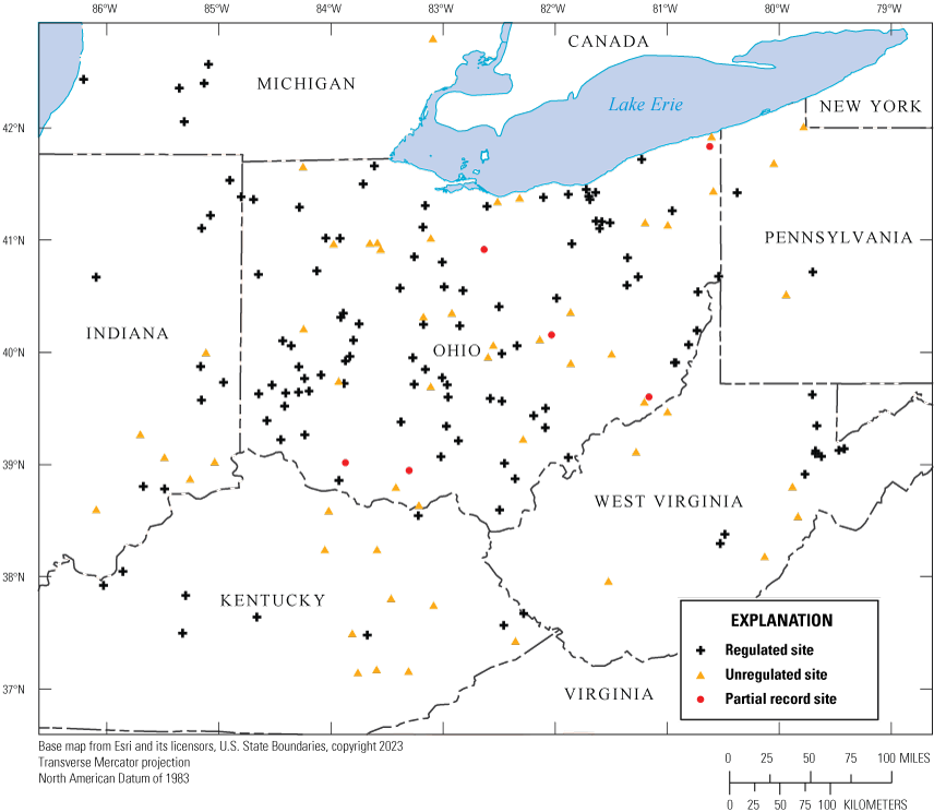
Generalized map of Ohio showing location of gages referenced in this study.
Table 1.
Streamflow gages in Ohio and border states for which low-flow statistics were computed (VonIns and Koltun, 2024).[USGS, U.S. Geological Survey; NAD 83, North American Datum of 1983; mi2, square mile; SVI, Streamflow-variability index; log10, logarithm base 10; ft3/s, cubic foot per second; tau, annual 7-day 10-year low-flow Kendall’s tau coefficient; p-value, 7-day 10-year Mann-Kendall probability value; OH, Ohio; partial, partial-record site; NA, not applicable; PA, Pennsylvania; continuous, continuous-record site; WV, West Virginia; KY, Kentucky; IN, Indiana; MI, Michigan]
Table 2.
Partial-record streamflow gages in Ohio for which low-flow statistics were computed.[Data from VonIns and Koltun (2024). USGS, U.S. Geological Survey; R2, coefficient of determination of the ordinary least square regression that defined the relation between the gage and its index site; OH, Ohio]
The second task was to check for upstream regulation, diversion, or other anthropogenic activity or features that could affect low flows. Gages that were substantially affected were not used to develop the regression equations. This review consisted of using the Geospatial Attributes of Gages for Evaluating Streamflow II dataset (Falcone, 2017), notes from USGS field personnel documented in the USGS National Water Information System (NWIS; USGS, 2022), satellite imagery from Google Earth (Google, 2022), the Ohio Dam Locator (Ohio Department of Natural Resources, 2023), and the National Inventory of Dams (U.S. Army Corps of Engineers, 2020) to look for indications that low flow at the streamflow gage was likely to be appreciably altered from its natural, unregulated state. Another review looked for the presence of karst drainage features in or near each gage’s drainage basin using maps and geospatial data on karst geology available through State agencies (Kentucky Geological Survey, 2023; West Virginia GIS Technical Center, 2024). Although karst drainage features are natural, their effect on low flows cannot be reliably accounted for by data that can be extracted from available geospatial datasets. Based on the results of the reviews, each gage was categorized as either “regulated” or “unregulated” (table 1), where unregulated is defined as low flows thought to be subject to no or minimal regulation and regulated is defined as low flows that are regulated by anthropogenic modifications (for example, withdrawals or diversions) or karst drainage features to the extent that these flows may differ appreciably from low flows in otherwise undeveloped settings without appreciable karst drainage.
Upstream features that resulted in a gage being categorized as regulated include urbanization, actively managed upstream dams, selected industry (such as mining), known diversions, wastewater treatment plant discharges, and water treatment plant intakes. Categorizing each gage was not a definitive process. Many streams at gaged locations in Ohio (especially those with large drainage basins) have some amount of upstream regulation or anthropogenic activity that could affect low flow, and it was frequently difficult to determine the magnitude of the effect. A total of 58 gages—53 continuous-record gages (27 in Ohio and 26 in adjacent States)—and 5 partial-record gages (all in Ohio)—were categorized as unregulated and therefore suitable for use in the low-flow regression analyses (table 1). Drainage areas of the gages that were deemed suitable for use in the low-flow regression analyses ranged from 0.21 to 540 square miles (mi2).
Methods for Computing Low-Flow Statistics
Selected low-flow statistics (frequently referred to as “design flows” in a regulatory context) have been chosen by agencies tasked with protecting the environment and the health of human and aquatic life to evaluate and regulate risks from contaminants that are transported in streams. Regulatory agencies use both hydrologically and biologically based design flows (U.S. Environmental Protection Agency, 2024). Hydrologically based design flows were computed by using the single lowest average N-day flow event (N being the number of days used to calculate the average) from each year of record, which were then examined by using extreme-value statistical methods. Biologically based design flow methods empirically examine all flows, but additional weight is placed on low-flow events within a period of record (even if several low-flow events occur in 1 year) to emphasize the actual frequency of low-flow periods when contaminants discharged from point sources are poorly diluted in streams (U.S. Environmental Protection Agency, 2024).
Throughout this document, annual and seasonal low-flow frequency statistics are designated by using the following convention: (averaging period in days)Q(recurrence interval in years). For example, the annual minimum 7-day flow with a 10-year recurrence interval is designated as 7Q10. Some of the analyses were based on yields, which are determined by dividing the statistic (for example 7Q10) by the drainage area at the gage, in square miles. Low-flow yield statistics are designated by appending an “m” to the flow statistic designation (for example, the 7Q10 yield is designated as 7Q10m). Flow-duration statistics are designated by prepending a “D” to the percent duration value. For example, the 80-percent duration value is designated as D80.
Temporal Trends in Low Flow
Mann-Kendall tests (Mann, 1945) were used to evaluate temporal trends in the annual minimum N-day flows and to test for stationarity, which is a requirement for the frequency analysis. The Mann-Kendall test statistic, tau, is a rank correlation coefficient between the annual minimum N-day low flow and time. It provides information on the strength of monotonic (unidirectional) temporal trend in the time series, with a Kendall’s tau of 0 indicating no trend, a tau of 1 indicating a perfect monotonically upward trend, and a tau of −1 indicating a perfect monotonically downward trend.
At the inception of this study, it was planned that all available period-of-record flow data would be used to compute the low-flow statistics; however, initial screening for temporal trends using the period-of-record annual minimum 7-day flows indicated an upward trend for many of the candidate gages in Ohio and many of those were statistically significant (all tests of statistical significance discussed in this report are based on an alpha of 0.05). In addition, time-series plots showed what appeared to be an abrupt increase (hereafter referred to as a “step change”) in the annual minimum 7-day flows at many of the gages, occurring between the late 1960s and early 1970s. Change-point detection tests (Pettitt, 1979) were subsequently used to test for the presence of step changes in the flow statistic and to identify the year when each step change occurred. The Pettitt tests indicated that many of the time series that had shown statistically significant trends had step changes occurring between the late 1960s and 1975. As an example, figure 2 shows the step change that occurred at USGS gage Mill Creek near Coshocton, Ohio (03140000), in 1972 (p=9.75×10⁻⁵). A subsequent literature search revealed that McCabe and Wolock (2002) had also identified noticeable increases in annual minimum and median daily flow in eastern U.S. streams for the period 1941–1999, and they stated that the changes in flow appeared to occur as a step change around 1970, rather than as a gradual trend. They attributed the changes to a hydroclimatic regime shift. Because of these findings, the USGS, in consultation with cooperating agencies, decided to restrict our analyses to data collected after the 1974 water year. That was done to produce a more stationary time series and to yield flow statistics that better reflect low-flow characteristics of more recent decades.
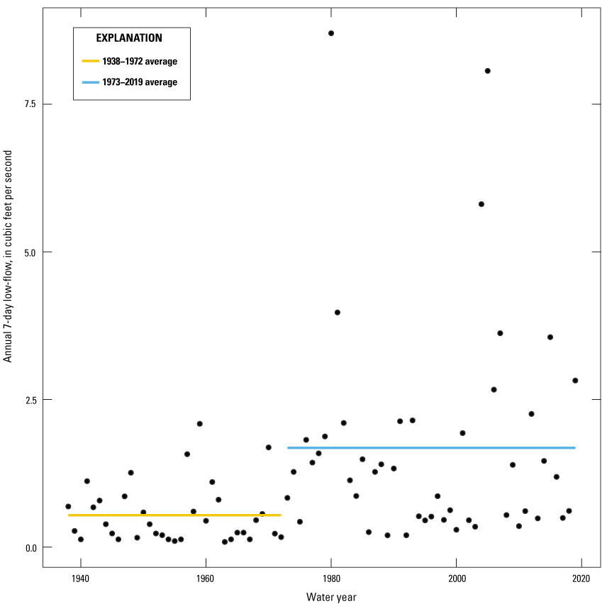
U.S. Geological Survey streamflow gage Mill Creek near Coshocton, Ohio (03140000), annual 7-day low flow (in cubic feet per second), with lines representing the average annual 7-day low flow before and after the probable change point (Pettitt’s test probable change point=1972, p=9.75×10⁻⁵; Pettitt, 1979).
After data were restricted to the post-1974 period (water years 1975–2020, hereafter referred to as the “analytical period”), Kendall’s tau values were again computed for annual minimum 1-, 7-, and 30-day flows. The computed tau values were approximately evenly mixed between positive and negative. Table 1 shows tau and p-value results (for the null hypothesis that tau is zero) for the annual minimum 7-day low flows. The 1- and 30-day low-flow tests had similar results: the same gages that had significant trends in the 7-day low-flow test had significant trends in the 1- and 30-day low-flow test results (not shown). In total, Mann-Kendall tests on data from gages ultimately classified as “unregulated” indicated that six gages (five in Ohio and one in Kentucky) had tau values that were significantly different from zero; two had negative trends and the others were positive (table 1).
Low-Flow Frequency
For continuous-record gages, annual and seasonal minimum 1-, 7-, 30-, and 90-day flows with 2-, 5-, 10-, 20-, and 50-year recurrence intervals were computed by using the USGS Hydrologic Toolbox software (Barlow and others, 2022). Daily mean flow data used in the computations were retrieved from NWIS (USGS, 2022) The toolbox was used to fit a log-Pearson Type III distribution to the annual minimum N-day mean flows, where N is 1, 7, 30, or 90 days. The log-Pearson Type III distribution is calculated by using the following equation (Riggs, 1972):
whereQt
is the N-day low flow,
X̅
is the mean of the base-10 logarithms of the nonzero annual or seasonal N-day low flows,
Kt
is a frequency factor that is a function of the recurrence interval and the coefficient of skewness, and
S
is the standard deviation of the base-10 logarithms of the nonzero annual or seasonal N-day low flows.
For partial-record gages, annual and seasonal minimum 1-, 7-, 30-, and 90-day low flows with 2-, 10-, and 20-year recurrence intervals were estimated by using a mathematical relation. For this study, that mathematical relation was developed by using Maintenance of Variance Extension, Type 1 (MOVE.1) regressions (Colarullo and others, 2018). The MOVE.1 regression equations were developed between low flows measured at the partial-record gages and concurrent daily mean flows at its index gages. Flow statistics computed for the partial-record gages are shown in appendix 2.
Flow Duration
The percentage of time that flow in a stream is likely to equal or exceed some specified value is referred to as flow duration. For example, a daily flow value that is equaled or exceeded 80 percent of the time is referred to as the 80-percent flow duration. For continuous-record gages, annual and seasonal 98-, 95-, 90-, 85-, 80-, 75-, 70-, 60-, 50-, 40-, 30-, 20-, and 10-percent duration flows were computed by using the Cunnane (1978) plotting position formula on the ranked daily flow data for complete climatic years during the analytical period. Annual and seasonal 98-, 95-, 90-, 85-, and 80-percent duration flows were estimated from the MOVE.1 regression developed between low flows measured at the partial-record gages and concurrent daily mean flows at their index gages. Flow-duration statistics are listed in appendixes 1 and 2.
Harmonic Mean Flow
The long-term harmonic mean flow is recommended by the U.S. Environmental Protection Agency as a design flow for assessing potential human health effects from contaminants in streams (Rossman, 1990). The harmonic mean minimizes the effect of large outliers while emphasizing small outliers, typically resulting in a harmonic mean flow that has a smaller magnitude than the arithmetic mean. The harmonic mean flow was computed from daily mean flows during the analytical period by the formula
whereQh
is the harmonic mean flow,
Nnz
is the number of nonzero daily mean flows,
Nt
is the total number of daily mean flows for the period of record, and
Qi
is the nonzero daily mean flow on day i.
Determination and Selection of Explanatory Variables
In order to develop regression equations for estimating low-flow statistics at ungaged stream locations, factors (hereafter referred to as “explanatory variables”) must be identified that can be used to mathematically explain all or part of the observed variation in the statistics. Explanatory variables in low-flow studies are typically measures of physical characteristics that vary in a systematic fashion with the low-flow statistics. Potential explanatory variables investigated in this study were selected in part because of their theoretical relation to low flows and in part because they can be or have been computed by using a geographic information system (GIS). The requirement that explanatory variables be determinable with a GIS comes from the desire to automate their determination within the StreamStats application.
Determining values of explanatory variables can be a time-consuming and expensive process. Some potential explanatory variables were determined from geospatial datasets that spanned the study area; however, others were determined from geospatial datasets with more limited geographic scope. Consequently, some potential explanatory variables were determined for all gages and others for just a subset of gages. For potential explanatory variables that were determined for a subset of the gages, it was necessary to ascertain whether the low-flow statistics of interest varied in a systematic fashion with those explanatory variables. As it turned out, none of the potential explanatory variables that were determined for only a subset of the gages showed sufficient potential as explanatory variables to warrant what would have been the next step: expanding the geographic scope of the geospatial dataset so that the explanatory variable could be determined for all the gages whose data were used to develop regression equations.
Approximately 260 potential explanatory variables were tested for this study (app. 3). Five primary sources of information were used to compute them: (1) the existing StreamStats application (https://streamstats.usgs.gov/ss/), (2) the USGS Hydro-Network Linked Data Index (NLDI; see https://labs.waterdata.usgs.gov/docs/nldi/about-nldi/index.html), (3) previously published geospatial datasets (for example, digital elevation models, watershed boundaries, and streamlines), (4) point data compiled for this study, and (5) grids of hydrogeologic information created for this study from standardized water-well drillers’ records.
The NLDI is a system that indexes previously published geospatial datasets to the National Hydrography Dataset Version 2 (https://nhdplus.com/NHDPlus/) catchments. The NLDI has a search service that permits retrieval of indexed information for points of interest through several retrieval mechanisms. A wide variety of local and catchment-level characteristics were retrieved from the NLDI for the gage locations (see app. 3). Among other categories, the NLDI data include information on (1) agricultural management and land conservation practices, (2) climate and water balance model characteristics, (3) climate characteristics, (4) geologic characteristics, (5) hydrology and hydrologic modifications, (6) landscape/landcover characteristics, (7) population and infrastructure, (8) ecoregions and physiography, (9) soil and topographic characteristics, and (10) water use. Not all the characteristics retrieved from NLDI had strong theoretical relations to the selected low-flow statistics, but they were readily available, so they were tested anyway. More information on the characteristics that can be retrieved from the NLDI can be found in Wieczorek and others (2018).
Grids of hydrogeologic characteristics were created for this study by using the methods described in Martin and others (2016) and Bayless and others (2017). Those methods used data from standardized water-well drillers’ records obtained from State-maintained databases to estimate the hydrogeologic characteristics. The grids of hydrogeologic characteristics created for this study have a 10- x 10-meter cell size and included
-
1. thickness of unconsolidated deposits,
-
2. total sand and gravel thickness within the unconsolidated deposits,
-
3. average horizontal hydraulic conductivity (K) for the first 30 feet (ft) and for the entire thickness of the unconsolidated deposits, and
-
4. average transmissivity (T) for the entire thickness of the unconsolidated deposits.
Potential explanatory variables computed from the hydrogeologic grids included catchment-area mean values and mean values for buffered areas extending 500 and 1,000 ft adjacent to streamlines upstream from the gages. Martin and others (2016) used the average horizontal hydraulic conductivity of the first 70 ft of unconsolidated deposits as an explanatory variable in regression equations that they developed for estimating 1Q10, 7Q10, and 30Q10 in Indiana. They used the average transmissivity of the full thickness of unconsolidated deposits within 1,000 ft of the stream channel as one of the explanatory variables in logistic-regression equations that they developed for estimating the annual probability of zero flow for those same statistics. For this study, the average horizontal hydraulic conductivity of first 30 ft of unconsolidated deposits was computed, rather than the 70 ft used in the Indiana study, because large areas of Ohio have unconsolidated deposit thicknesses considerably less than 70 ft.
A streamflow-variability index (SVI) was used as an explanatory variable in the most recent USGS publication that included equations for estimating low-flow statistics in Ohio (Koltun and Kula, 2013). SVI is a measure of the variability in streamflow at a gage resulting from variation in precipitation as it is mitigated by the physical characteristics of the basin. Typically, unregulated streams with relatively small SVIs have proportionally more flow contributed from groundwater discharge (or surface storage or both) than streams with larger SVIs (Lane and Lei, 1950). SVI is computed with the following equation:
whereSVI
is the streamflow-variability index,
Di
is the ith-percent duration flow (i=5, 10, 15, ... 95), and
is the mean of the base-10 logarithms of the 19 flow values at 5-percent class intervals from 5 to 95 percent on the flow-duration curve of daily mean flows.
A variety of methods were used to select explanatory variables included in the regression equations for estimating the low-flow statistics. The first (and potentially most informative) method was to create scatterplots of the low-flow statistics in relation to the potential explanatory variable. In general, if a potential explanatory variable is useful for estimating low-flow statistics, its scatterplot should show indication of a systematic relation between the variable and the statistic. If there is a random scatter of points in the plot, it is unlikely that the potential explanatory variable will be useful for estimation. Other methods, including bidirectional stepwise regression and forward stepwise regression, also were used to evaluate potential explanatory variables. Stepwise regressions can help in choosing good candidate explanatory variables when two or more explanatory variables are correlated.
After review of the scatterplots and the stepwise regression results, SVI was chosen as the explanatory variable for the regression equations to predict harmonic mean flow; the annual 1Q10m, 7Q10m, 30Q10m, and 90Q10m; the May–November 1Q10m, 7Q10m, 30Q10m, and 90Q10m; and the September–November 1Q10m, 7Q10m, 30Q10m. SVI alone, however, was not satisfactory as the only explanatory variable for the 80-percent duration flow, the September–November 90Q10m, and the December–February 1Q10m, 7Q10m, 30Q10m, and 90Q10m. For those statistics, one of two scenarios was selected to explain the flows more fully: (1) SVI, the drainage area, and the decimal longitude or (2) just the drainage area and the decimal longitude, when SVI was not a statistically significant explanatory variable.
Estimating the Streamflow-Variability Index at Ungaged Sites
To enable computation of low-flow statistics at ungaged sites in Ohio, it was necessary to develop statewide datasets for each of the explanatory variables. Drainage area, decimal longitude, and SVI are already computed within StreamStats; however, new estimates of SVI were needed to reflect streamflow variability during this study’s analytical period. In past studies (Koltun and Whitehead 2002; Koltun and Kula 2013), a grid of SVI estimates was created by using inverse-distance-weighted (IDW) interpolation on at-site values of SVI. The IDW interpolation effectively assumed that SVI varied in a distance-weighted linear fashion among the gages where SVI was known. However, if SVI does not vary linearly in space, as assumed, the accuracy of the resulting SVI grid is dependent on the number and spatial density of known SVI points. With spatially dense datasets, the accuracy of the assumption of linear variation in space is likely to be less important because interpolations are made over relatively short distances. Because the number of gages included in the regression analyses in this study was appreciably smaller than in the previous studies (due to the decision to include only data after the 1974 water year), other methods for developing the SVI grid were explored that were less dependent on the assumptions inherent in the IDW method.
The decision was made to develop the SVI grid using empirical Bayesian kriging (EBK) regression prediction (Esri, 2022b). EBK regression prediction is a geostatistical interpolation method that uses an explanatory raster (grid) known to systematically covary with the values of the data being interpolated (Krivoruchko, 2012). EBK regression prediction models simultaneously estimate both a regression model for the mean value and a semivariogram/covariance model for the error term. By operating on both components at the same time, they can make more accurate predictions than either regression or kriging can achieve on their own.
The SVI grid was created by using the EBK regression prediction routine implemented in the Esri ArcGIS Pro (version 3.2) Geostatistical Analyst software (Esri, 2022a). After reviewing scatterplots of SVIs computed from the analytical-period flow record of the gages in table 1 designated as “unregulated” and the potential explanatory variables described in the section “Determination and Selection of Explanatory Variables,” a previously published grid of estimated mean annual natural groundwater recharge (Wolock, 2003) was chosen as the explanatory grid. The recharge grid was chosen because it had a moderately strong negative correlation (R = −0.59), which was stronger than the other variables considered.
Residuals calculated from the SVI values computed from streamflow observations at unregulated gages and the SVI values from the EBK regression predictions ranged from −0.25 to 0.73 with a mean of 0.02 and a standard deviation of 0.15. Despite fewer gages being used in the current study, these results are similar to those reported by Koltun and Kula (2013), which used an IDW approach. In the analysis by Koltun and Kula (2013), residuals were computed by using a leave-one-out cross-validation technique and ranged from −0.51 to 0.63 with a mean of 0.01 and standard deviation 0.16. The grid of estimated SVI developed for Ohio by using EBK regression prediction is shown in figure 3, and at-gage EBK regression estimates from the grid are shown in table 1.
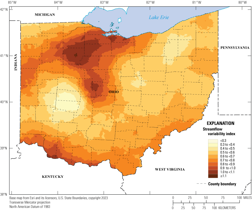
Generalized map of Ohio showing estimated spatial variation in streamflow-variability index.
Equations for Estimating Low-Flow Statistics
The relation between SVI and low-flow yields were not linear, so the options for developing low-flow yield equations were either to transform the model variables to fit a linear equation or to use a nonlinear or curvilinear equation. Log transformation and square root transformation were considered and rejected because of problems with zero-valued data or unwanted effects in the regression (Koltun and Kula, 2013). Because of these problems, and for consistency with previous studies, a cubic polynomial of SVI was used in the equations to predict the harmonic mean flow; annual yields; May–November 1Q10m, 7Q10m, 30Q10m, and 90Q10m; and the September–November 1Q10m, 7Q10m, 30Q10m. SVI alone was not a powerful enough predictor for September–November 90Q10m yield; the December–February 1Q10m, 7Q10m, 30Q10m, and 90Q10m yields; or the D80 flow, so a model with explanatory variables consisting of drainage area, decimal longitude, and, in most cases, SVI, was used to predict these statistics. In models that used drainage area as an explanatory variable, a square root transformation was applied to the low-flow yields and drainage area to improve linearity in the regression equations.
All linear regression equations were developed by using censored regression routines implemented in the censReg function of the USGS R package smwrQW (https://code.usgs.gov/water/analysis-tools/smwrQW). Zero values in the yield statistics were treated as left censored (meaning they were less than a specified value) because there is uncertainty in the measurement of the flow that makes it difficult in some cases to ascertain whether the flow (and associated yield) is truly zero. A censoring level of 0.00001 cubic feet per second per square mile ([ft3/s]/mi2) was used in the analyses when the yield statistics included zero-valued observations. Because weighted regression analyses were performed, the regressions were computed by the censReg function using maximum likelihood estimation, which accounts for the unequal sampling probability for each observation depending on whether the magnitude of the dependent variable is above or below the censoring level.
Observations used in the regressions were weighted as a function of the length of record of the associated gage. The weighted regression served to down-weight the importance of observations for gages with shorter records, which are more susceptible to time-sampling error. For continuous-record gages, the weight for a gage’s observations was computed by first computing a time fraction (the number of days with a computed daily mean flow in the gage record from 1975 through 2020 divided by the maximum number of days in that same period) and then dividing it by the average of time fractions for all gages included in the regression. For partial-record gages, the weight was estimated as the product of the weight computed for its index gage and the coefficient of determination (R2) from the MOVE.1 regression that defined the relation between the partial-record gage and its index site.
For polynomial models, first a regression model using orthogonalized (uncorrelated) polynomial terms was developed to assess the statistical significance of the explanatory variables. That was done because collinearity among the polynomial terms can inflate the variance in the coefficients, making it difficult to assess the statistical significance of the explanatory variables. The cubic polynomial matrix was orthogonalized by using the poly function in R (see https://www.rdocumentation.org/packages/stats/versions/3.6.2/topics/poly for more information). Once the statistical significance (or lack thereof) of the explanatory variables was established, a second regression model was developed by using the untransformed data to develop the equations presented in this report. Both models produce identical estimates and model metrics (such as pseudo R2); however, the magnitudes of the model parameter coefficients differ to account for the transformed explanatory variables.
Constraints were placed on equations if the equations could compute yields less than the censoring level (outside of the censReg function) or if the computed yields did not monotonically decrease with increasing SVI. In the first case, the constraint consisted of setting computed low-flow yields that were less than the censoring level to the censoring level. In the second case, the constraint consisted of setting the low-flow yield to the value at which the yield switched from decreasing to increasing with increasing SVI.
In the yield regressions that used the orthogonalized polynomial parameters, one of the SVI parameters (typically, SVI squared, but in one case SVI cubed) was not statistically significant in the 1-, 7-, and 90-day May–November equations and the 1- and 7-day equations for September–November. In each case, the statistically insignificant variable coefficient was small (always less than 0.04), making the equation result insensitive to that parameter relative to the other model parameters. Despite this, we chose to use a cubic polynomial model in each case to maintain consistency across the various equations that used a polynomial model form. Yield equations were plotted to confirm that the following three conditions were met: (1) yields monotonically decreased or were the same with increasing SVI, (2) yields did not decrease as the low-flow averaging period increased for the same seasonal period (for example, the annual [April–March] 1Q10m was less than or equal to the annual 7Q10m for a given SVI), and (3) annual low-flow yields were less than or equal to seasonal low-flow yields for the same frequency statistic (for example, the annual 7Q10m was less than or equal to the September–November 7Q10m for a given SVI). The first two conditions were met, but the third condition was not met in all cases. At SVI values greater than about 0.50, the May–November equations produced slightly lower yield estimates than the annual equations (the maximum difference was less than 0.00053 [ft3/s]/mi2). On further examination, we found that the annual and May–November 1Q10 and 7Q10 estimates for each gage in the calibration dataset were nearly equal (average absolute differences of 0.0186 and 0.0238 cubic foot per second [ft3/s], respectively) and the differences between the estimates were much smaller than the statistical uncertainty of the regression equations. Because of this and because the annual value must, by definition, be less than or equal to the seasonal values, we recommend (and intend to implement in StreamStats) that the April–March low-flow estimates be set to the lesser of the computed annual (April–March) and May–November low-flow estimates for a given averaging period. The final regression equations (table 3) have been formatted to provide estimates in units of cubic feet per second, which required that the yield equations be multiplied by the drainage areas. Fit statistics, including the root mean square error (RMSE) and the bounds for the interquartile range of residual errors (the range that contains 50 percent of the observations in the calibration dataset) are also reported in units of cubic feet per second. Censored estimates were set equal to the censoring level when computing the RMSE. As examples of the fit of the yield-based equations, figure 4 shows scatterplots of observed in relation to predicted 7Q10 and 30Q10 for the April–March season (table 3, eqs. 2 and 3), along with 1:1 lines.
Table 3.
Equations for estimating selected low-flow yield and flow-duration statistics for Ohio.[All computed statistics are in cubic feet per second; RMSE, root mean square error; pseudo R2, pseudo coefficient of determination; 1Q10, 1-day, 10-year low flow; DA, drainage area in square miles; SVI, streamflow-variability index in base-10 logarithms of cubic feet per second; ≤, less than or equal to; >, greater than; 7Q10, 7-day, 10-year low flow; 30Q10, 30-day, 10-year low flow; 90Q10, 90-day, 10-year low flow; Long, longitude in decimal degrees; HM, harmonic mean streamflow; D80, 80-percent duration streamflow]
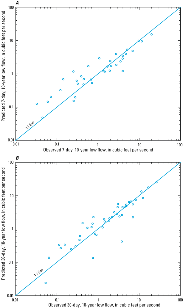
Scatterplots showing observed in relation to predicted A, 7-day, 10-year low flow and B, 30-day, 10-year low flow for unregulated streamgages in Ohio and bordering States for the April–March season.
Regression residuals were reviewed for spatial biases and homoscedasticity (nonconstant error variance). Residual plots sorted by region were reviewed to check for spatial biases, and standardized residuals were plotted against predicted yields and against explanatory variables to check for heteroscedasticity. The plots showed no obvious signs of spatial biases; however, some equations showed indications of potential heteroscedasticity. For example, there were more positive residuals than negative residuals with the 7Q10 equation when observed 7Q10 values exceeded about 3 ft3/s, indicating that the equations may tend to underestimate flows in that range more than would be expected if the errors were random. Because the calibration dataset was small (58 observations), it is uncertain whether the heteroscedasticity is real or a function of that particular sample set.
Logistic-Regression Equations for Identification of Low-Flow Yields Less Than the Censoring Level
Some of the constrained polynomial equations for yield predicted values less than or equal to the yield censoring level (0.00001 [ft3/s]/mi2). When those censored yields are multiplied by drainage area (as shown in table 3), the resulting flows are treated as censored as well, with a recommended censoring level for flow of 0.01 ft3/s (that is, all computed flows below this recommended censoring level are treated as <0.01 ft3/s rather than as their specific computed values). In some cases, the model predicted censored flows even though the observed flow was greater than the censoring level and, less frequently, it predicted uncensored flows when the observed flow was censored. To better distinguish between these two outcomes, logistic-regression equations (table 4) were developed to estimate the probability that the N-day, 10-year low flow was greater than the flow censoring level (see Helsel and others [2020] for more information on logistic regression). Explanatory variables in the logistic-regression equations include the SVI and the drainage area. If the computed probability is less than 0.50, it is suggested that the flow be assumed to be less than 0.01 ft3/s.
Table 4.
Logistic-regression equations for estimating the probability of uncensored flow for selected low-flow statistics for unregulated streams in Ohio.[Computation of specificity, sensitivity, and percent correct is based on of a probability of 0.50. All computed statistics are in cubic feet per second. p, probability; 1Q10, 1-day, 10-year low flow; e, base of natural logarithm; SVI, streamflow-variability index in base-10 logarithms of cubic feet per second; DA, drainage area in square miles; 7Q10, 7-day, 10-year low flow; 30Q10, 30-day, 10-year low flow]
Logistic-regression equations were developed for the annual, May–November, September–November 1Q10, 7Q10, and 30Q10 statistics (table 4). Table 4 shows each equation’s specificity (the percentage of censored statistics correctly identified), sensitivity (the percentage of uncensored statistics correctly identified), and the overall percentage of correct classifications when classifying is based on a probability of 0.50. Table 4 also shows the highest observed yield in the calibration dataset for an SVI larger than the equation’s constraint. No logistic-regression equations were developed for the other statistics because there were too few censored statistics in the calibration dataset to develop reliable equations.
The low-flow equations (table 3) and logistic-regression equations (table 4) are intended to be incorporated into the StreamStats application, which can be accessed at https://streamstats.usgs.gov/ss/. Upon the incorporation of these equations, the StreamStats application for Ohio will automatically compute the drainage areas and low-flow statistics listed in table 3. For equations that compute yields, StreamStats will convert the computed yields to flows, in cubic feet per second, by taking the product of the drainage area and yields.
Limitations of the Regression Equations
The regression equations are applicable to unregulated streams in Ohio. They are not applicable to streams with karst drainage features, diversion, regulation, or other conditions that can appreciably affect low flows. Ohio’s StreamStats application does not identify streams that are regulated; therefore, it is incumbent on the user to determine whether a stream is free from substantial low-flow regulation.
SVI was the primary explanatory variable in most of the regression equations. However, because SVI isn’t a physical basin characteristic, a new spatial grid was created by a spatial interpolation process (EBK regression prediction) that used at-site estimates of SVI and an explanatory variable raster dataset of estimated mean annual natural groundwater recharge. That grid can be used to estimate SVI at ungaged stream locations. Consequently, any errors in the SVI estimates will be reflected in the flow estimates computed by StreamStats (upon incorporation of the regression equations). For sites where the uncertainty of using regression equations to estimate low-flow statistics is unacceptable, installing and operating a streamflow gage for a minimum of 10 years allows for the computation of low-flow statistics with less uncertainty. The range of SVI values used to develop the equations was 0.41 to 1.23 log10 ft3/s, and the range of drainage areas was 0.21 to 540 mi2 (table 1). The applicability of these equations has not been determined for basins with SVIs or drainage areas outside of these ranges.
Summary
The U.S. Geological Survey, in cooperation with the Ohio Water Development Authority and the Ohio Environmental Protection Agency, completed a study to compute low-flow frequency, flow-duration, and harmonic mean flow statistics for long-term streamflow gages and to develop methods for estimating those statistics at unregulated, ungaged stream locations in Ohio. The study began by identifying continuous-record gages in Ohio and bordering States that had at least 10 years of flow data and low-flow partial-record gages in Ohio that had periodic instantaneous low-flow measurements that had strong mathematical relations to concurrent daily mean flows at a continuous-record gage. A total of 180 continuous-record gages and 5 low-flow partial-record gages met those criteria. For continuous-record gages, the following statistics were computed: annual and seasonal minimum 1-, 7-, 30-, and 90-day flows with 2-, 5-, 10-, 20-, and 50-year recurrence intervals; annual and seasonal 98-, 95-, 90-, 85-, 80-, 75-, 70-, 60-, 50-, 40-, 30-, 20-, and 10-percent duration flows, and the harmonic mean flow. For partial-record gages, a smaller set of statistics were estimated by using a Maintenance of Variance Extension, Type 1 regression developed from the low flows measured at the partial-record gages and the concurrent daily mean flows recorded at their index gages, generating annual and seasonal minimum 1-, 7-, 30-, and 90-day low flows with 2-, 10-, and 20-year recurrence intervals and annual and seasonal 98-, 95-, 90-, 85-, and 80-percent duration flows.
Initial screening for temporal trends in period-of-record time series of annual minimum 7-day flows computed for continuous-record gages indicated statistically significant upward trends for many of the candidate gages in Ohio. Change-point detection tests indicated that many of the time series that had shown statistically significant trends had step changes occurring after the late 1960s but before 1975. Because of these findings, the U.S. Geological Survey, in consultation with cooperating agencies, decided to restrict the analyses to data collected after the 1974 water year through the 2020 water year (referred to as the “analytical period”) to produce a more stationary time series and to compute flow statistics that better reflect low-flow characteristics of recent decades.
Gage drainage basins were inspected for upstream regulation, diversion, or other anthropogenic activity or features that could affect low flows. This was done to identify gages whose low flows are likely to be appreciably altered from a natural, unregulated state. Based on that review, each gage was categorized as either “regulated” or “unregulated.” A total of 53 continuous-record gages and 5 low-flow partial-record gages were categorized as unregulated, and their data were subsequently used in regression analyses to develop equations for estimating low-flow statistics.
Approximately 260 potential explanatory variables were tested for this study. With a few exceptions (for some statistics in the September–November, December–February seasons, and the 80-percent duration flows), a streamflow-variability index (SVI) was chosen as the sole explanatory variable for the regression equations to predict the harmonic mean and annual and seasonal low-flow yields. A model with explanatory variables consisting of drainage area, decimal longitude, and, in most cases, SVI, was used to predict those exceptions. The SVI values used in the regression analysis were obtained from a geospatial grid of SVI values developed for this study by means of empirical Bayesian kriging regression prediction.
Observations for continuous-record gages whose data were used in the regressions were weighted in the regression as a function of their length of record. Weights for partial-record gages were estimated based on the weights determined for their index gages. All linear regression equations for low-flow yields were developed by using censored regression, with a censoring level set to 0.00001 cubic foot per second per square mile. Numerical constraints were placed on equations if they could compute yields less than the censoring level or if the computed yields did not monotonically decrease with increasing SVI.
All regression equations in this report are presented in a form that permits computation of low-flow statistics in units of cubic feet per second. Logistic-regression equations were developed as a secondary check to estimate the probability that the N-day, 10-year low flow is greater than the censoring level (0.01 cubic foot per second). If the computed probability is less than 0.50, it is suggested that the flow be assumed to be less than 0.01 cubic foot per second.
The regression equations presented in this report were developed to be implemented in the Ohio StreamStats application. The equations are applicable to unregulated streams in Ohio. They are not applicable to streams with karst drainage features, diversion, regulation, or other conditions that can appreciably affect low flows. The range of SVI values used to develop the equations was 0.41 to 1.23 log10 cubic feet per second, and the range of drainage areas was 0.21 to 540 square miles (table 1). The applicability of these equations to stream locations with SVIs or drainage areas outside of these ranges has not been determined.
Acknowledgments
The authors would like to thank Leslie D. Arihood, scientist emeritus with the U.S. Geological Survey, for developing the geospatial grids of hydrogeologic characteristics.
References Cited
Barlow, P.M., McHugh, A.R., Kiang, J.E., Zhai, T., Hummel, P., Duda, P., and Hinz, S., 2022, U.S. Geological Survey Hydrologic Toolbox—A graphical and mapping interface for analysis of hydrologic data: U.S. Geological Survey Techniques and Methods, book 4, chap. D3, 23 p., accessed 2022 at https://doi.org/10.3133/tm4D3.
Bayless, E.R., Arihood, L.D., Reeves, H.W., Sperl, B.J.S., Qi, S.L., Stipe, V.E., and Bunch, A.R., 2017, Maps and grids of hydrogeologic information created from standardized water-well drillers’ records of the glaciated United States: U.S. Geological Survey Scientific Investigations Report 2015–5105, 34 p., accessed 2022 at https://doi.org/10.3133/sir20155105.
Colarullo, S.J., Sullivan, S.L., and McHugh, A.R., 2018, Implementation of MOVE.1, censored MOVE.1, and piecewise MOVE.1 low-flow regressions with applications at partial-record streamgaging stations in New Jersey: U.S. Geological Survey Open-File Report 2018–1089, 20 p., accessed 2022 at https://doi.org/10.3133/ofr20181089.
Cunnane, C., 1978, Unbiased plotting positions—A review: Journal of Hydrology, v. 37, no. 3–4, p. 205–222, accessed 2022 at https://doi.org/10.1016/0022-1694(78)90017-3.
Esri, 2022b, What is EBK regression prediction?: Esri web page, accessed August 31, 2023 at https://pro.arcgis.com/en/pro-app/latest/help/analysis/geostatistical-analyst/what-is-ebk-regression-prediction-.htm.
Falcone, J.A., 2017, U.S. Geological Survey GAGES–II time series data from consistent sources of land use, water use, agriculture, timber activities, dam removals, and other historical anthropogenic influences: U.S. Geological Survey data release, accessed 2022 at https://doi.org/10.5066/F7HQ3XS4.
Helsel, D.R., Hirsch, R.M., Ryberg, K.R., Archfield, S.A., and Gilroy, E.J., 2020, Statistical methods in water resources: U.S. Geological Survey Techniques and Methods, book 4, chap. A3, 458 p., and errata sheet, accessed 2022 at https://doi.org/10.3133/tm4A3. [Supersedes USGS Techniques of Water-Resources Investigations, book 4, chap. A3, version 1.1.]
Johnson, D.P., and Metzker, K.D., 1981, Low-flow characteristics of Ohio streams: U.S. Geological Survey Open-File Report 81–1195, 285 p., accessed 2021 at https://doi.org/10.3133/ofr811195.
Kentucky Geological Survey, 2023, Karst GIS, map, and publication resources: Lexington, Ky., University of Kentucky website, accessed 2023 at https://www.uky.edu/KGS/karst/karst_resources.php.
Koltun, G.F., and Kula, S.P., 2013, Methods for estimating selected low-flow statistics and development of annual flow-duration statistics for Ohio: U.S. Geological Survey Scientific Investigations Report 2012–5138, 195 p, accessed 2021 at https://doi.org/10.3133/sir20125138.
Koltun, G.F., and Schwartz, R.R., 1987, Multiple-regression equations for estimating low flows at ungaged stream sites in Ohio: U.S. Geological Survey Water-Resources Investigations Report 86–4354, 39 p., 6 pls. [Also available at https://doi.org/10.3133/wri864354.]
Koltun, G.F., and Whitehead, M.T., 2002, Techniques for estimating selected streamflow characteristics of rural unregulated streams in Ohio: U.S. Geological Survey Water Resources Investigations Report 2002–4068, 50 p. [Also available at https://doi.org/10.3133/wri024068.]
Krivoruchko, K., 2012, Empirical Bayesian kriging—Implemented in ArcGIS geostatistical analyst: ArcUser, v. 15, no. 4, p. 6–10, accessed 2023 at https://www.esri.com/news/arcuser/1012/empirical-byesian-kriging.html.
Lane, E.W., and Lei, K., 1950, Stream flow variability: Transactions of the American Society of Civil Engineers, v. 115, p. 1084–1098. [Also available at https://doi.org/10.1061/TACEAT.0006394.]
Mann, H.B., 1945, Nonparametric tests against trend: Econometrica, v. 13, no. 3, p. 245–259, accessed 2021 at https://doi.org/10.2307/1907187.
Martin, G.R., Fowler, K.K., and Arihood, L.D., 2016, Estimating selected low-flow frequency statistics and harmonic-mean flows for ungaged, unregulated streams in Indiana (ver. 1.1, October 2016): U.S. Geological Survey Scientific Investigations Report 2016–5102, 45 p., and data files, accessed 2022 at https://doi.org/10.3133/sir20165102.
McCabe, G.J., and Wolock, D.M., 2002, A step increase in streamflow in the conterminous United States: Geophysical Research Letters, v. 29, no. 24, article 2185, p. 38–1 to 38–4, accessed 2021 at https://doi.org/10.1029/2002GL015999.
Ohio Department of Natural Resources, 2023, Ohio Dam Locator: Ohio Department of Natural Resources database, accessed 2023 at https://gis.ohiodnr.gov/MapViewer/?config=ohiodams#.
Pettitt, A.N., 1979, A non-parametric approach to the change-point problem: Journal of the Royal Statistical Society Series C—Applied Statistics, v. 28, no. 2, p. 126–135. [Also available at https://doi.org/10.2307/2346729.]
Ries, K.G., III, Newson, J.K., Smith, M.J., Guthrie, J.D., Steeves, P.A., Haluska, T.L., Kolb, K.R., Thompson, R.F., Santoro, R.D., and Vraga, H.W., 2017, StreamStats, version 4: U.S. Geological Survey Fact Sheet 2017–3046, 4 p., accessed January 7, 2022, at https://doi.org/10.3133/fs20173046. [Supersedes USGS Fact Sheet 2008–3067.]
Riggs, H.C., 1972, Low-flow investigations: U.S. Geological Survey Techniques of Water-Resources Investigations, book 4, chap. B1, 18 p. [Also available at https://doi.org/10.3133/twri04B1.]
Rossman, L.J., 1990, Design stream flows based on harmonic means: Journal of Hydraulic Engineering, v. 116, no. 7, p. 946–950, accessed 2022 at https://doi.org/10.1061/(ASCE)0733-9429(1990)116:7(946).
Straub, D.E., 2001, Low-flow characteristics of streams in Ohio through water year 1997: U.S. Geological Survey Water-Resources Investigations Report 2001–4140, 423 p., accessed 2021 at https://doi.org/10.3133/wri014140.
U.S. Army Corps of Engineers, 2020, National inventory of dams: U.S. Army Corps of Engineers database, accessed 2023 at https://nid.sec.usace.army.mil/#/.
U.S. Environmental Protection Agency, 2024, Definition and characteristics of low flows: U.S. Environmental Protection Agency web page, accessed August 6, 2024, at https://www.epa.gov/hydrowq/definition-and-characteristics-low-flows.
U.S. Geological Survey [USGS], 2022, USGS water data for the Nation: U.S. Geological Survey National Water Information System database, accessed August 20, 2022, at https://doi.org/10.5066/F7P55KJN.
VonIns, B.L., and Koltun, G.F., 2024, Supporting data for low-flow statistics computed for streamflow gages and methods for estimating selected low-flow statistics for ungaged stream locations in Ohio, water years 1975–2020 (ver. 1.1, October 2024): U.S. Geological Survey data release, https://doi.org/10.5066/P92GD1WL.
West Virginia GIS Technical Center, 2024, West Virginia State GIS data clearinghouse: West Virginia GIS Technical Center website [search term—Karst], accessed 2024 at https://wvgis.wvu.edu/data/data.php.
Wieczorek, M.E., Jackson, S.E., and Schwarz, G.E., 2018, Select attributes for NHDPlus version 2.1 reach catchments and modified network routed upstream watersheds for the conterminous United States (ver. 4.0, August 2023): U.S. Geological Survey data release, accessed 2023 at https://doi.org/10.5066/F7765D7V.
Wolock, D.M., 2003, Estimated mean annual natural ground-water recharge in the conterminous United States: U.S. Geological Survey Open-File Report 03–311, accessed 2021 at https://doi.org/10.3133/ofr03311.
Appendix 1. Low-Flow, Flow Duration, and Harmonic Mean Flow Statistics for Continuous-Record Streamflow Gages in Ohio, 1975–2020
References Cited
VonIns, B.L., and Koltun, G.F., 2024, Supporting data for low-flow statistics computed for streamflow gages and methods for estimating selected low-flow statistics for ungaged stream locations in Ohio, water years 1975–2020 (ver. 1.1, October 2024): U.S. Geological Survey data release, https://doi.org/10.5066/P92GD1WL.
Appendix 2. Low-Flow, Flow Duration, and Harmonic Mean Flow Statistics for Partial-Record Streamflow Gages in Ohio, 1975–2020
References Cited
VonIns, B.L., and Koltun, G.F., 2024, Supporting data for low-flow statistics computed for streamflow gages and methods for estimating selected low-flow statistics for ungaged stream locations in Ohio, water years 1975–2020 (ver. 1.1, October 2024): U.S. Geological Survey data release, https://doi.org/10.5066/P92GD1WL.
Appendix 3. Basin Characteristics Tested for Use in Low-Flow Regression Analyses in Ohio
Location Variables
-
Latitude of basin centroid (Latc) Latitude of basin centroid, in decimal degrees (Koltun and others, 2006).
-
Longitude of basin centroid (Longc) Longitude of basin centroid, in decimal degrees (Koltun and others, 2006).
-
Maximum elevation Flowline catchment’s maximum elevation, in meters (Blodgett, 2020) as taken from National Hydrography Dataset Plus Version 2 (NHDPlusV2). Two variables were tested: local catchment maximum elevation and total catchment maximum elevation.
Hydrologic Variables
-
Artificial paths Percentage of NHDPlusV2 flowlines coded as artificial (Blodgett, 2020). Two variables were tested: percentage of local catchment and percentage of total catchment.
-
Average annual runoff Runoff, in millimeters, from McCabe and Wolock’s Runoff Model 1951–2000 for each NHDPlusV2 catchment (Blodgett, 2020). Tested variables include computation of local catchment and total catchment values.
-
Base-flow index Ratio of base flow to total streamflow, expressed as a percentage. Base flow is the sustained, slowly varying component of streamflow, usually attributed to groundwater discharge to a stream (Koltun and others, 2006). Two variables were tested: local catchment percentage and total catchment percentage.
-
Basin area Area, in square miles, that drains to the stream location (Koltun and others, 2006).
-
Basin length Flowline length, in kilometers. Values were taken directly from the NHDPlusV2’s NHDFlowline shapefile (Blodgett, 2020). Two variables were tested: local catchment length and total catchment length.
-
Canals or ditches Number of NHDPlusV2 flowlines coded as canals or ditches (Blodgett, 2020). Two variables were tested: number in the local catchment and number in the total catchment.
-
Connectors Percentage of NHDPlusV2 flowlines coded as connectors (Blodgett, 2020). Two variables were tested: percentage of the local catchment and percentage of the total catchment.
-
Depth to water Depth from the land to the top of the water table in unconfined conditions or to the top of the aquifer in confined conditions (Nelson and Valachovics, 2022). The same variable was also estimated by using data from Hydro Network-Linked Data Index (Blodgett, 2020). Tested variables include local catchment and total catchment averages.
-
Dunne overland flow Overland flow, in cubic feet per second, that occurs when the soil is saturated and cannot absorb any more water, or when the intensity of rainfall exceeds the soil’s infiltration capacity (Blodgett, 2020). Tested variables include local catchment and total catchment averages.
-
Flood region Ohio flood region, A or C (Koltun and others, 2006).
-
Horton overland flow Overland flow, in cubic feet per second, of water flowing horizontally across land surfaces when rainfall has exceeded infiltration capacity and depression storage capacity (Blodgett, 2020). Tested variables include local catchment and total catchment averages.
-
Longest flow path Flow path length, in miles. Values were computed by determining the longest flow path from the stream location to a topographic divide (which generally corresponded to the basin divide). StreamStats determined the longest flow path on the basis of a specially processed digital elevation model that includes the streams of the 1:100,000 National Hydrography Dataset (U.S. Geological Survey, 2020).
-
Low-flow region Low-flow regions used in some Koltun and Kula (2013) low-flow frequency regressions.
-
Pipeline Percentage of all flowline-reach lengths for each NHDPlus V2 catchment that are pipelines. Pipelines refer to human-made structures of steel, concrete, or polymers that direct surface water flows from one area to another (Blodgett, 2020).
-
Sinuosity Ratio of the curvilinear length (along the curve) and the Euclidean distance (straight line) between the end points of the curve (Blodgett, 2020).
-
Slope10-85 Channel slope, in feet per mile. Values were computed by (1) determining the longest flow path from the point of interest to a topographic divide (which generally corresponded to the basin divide), (2) determining the elevation at 10 percent of the distance along the longest flow path upstream from the point at which the flow statistic is desired (E10), (3) determining the elevation at 85 percent of the distance along the longest flow path upstream from the point at which the flow statistic is desired (E85), (4) determining the length of the stream segment between points 10 and 85 percent of the distance along the longest flow path upstream from the point at which the flow statistic is desired (L10–85), and then (5) dividing the change in elevation (E85−E10) by L10-85 (Koltun and others, 2006).
-
Stream density Stream density of catchment reach defined as length of flowlines divided by catchment area (Blodgett, 2020). Two variables were tested: local catchment density and total catchment density.
-
Streamflow-variability index (SVI) Streamflow-variability index at the stream location. Values were determined by using the Esri Spatial Analyst software’s Empirical Bayesian kriging geoprocessing function, with at-gage computed SVIs used as the dependent variable and a recharge raster (grid) of estimated mean annual natural groundwater recharge (Wolock, 2003) used as the explanatory variable.
-
Subsurface flow contact time index Estimated time, in number of days, that infiltrated water resides in the saturated subsurface zone of the basin before discharging into the stream (Blodgett, 2020). Tested variables include values for the local catchment and the total catchment.
-
Withdraws County-level estimates of freshwater withdrawals from 1995 to 2000 (Blodgett, 2020). Two variables were tested: local catchment withdrawals and total catchment withdrawals.
Soil and Geologic Variables
-
Bedrock permeability class Percentage of NHDPlus V2 flowline catchment categorized as one of five bedrock permeability classes: unconsolidated sand and gravel, sandstone, semiconsolidated sand, basalt and other volcanic rocks, sandstone and carbonate rocks, or carbonate rock (Blodgett, 2020). Two variables were tested for each class: percentage of local catchment and percentage of total catchment.
-
Estimated percent presence of soil restrictive layer in top 25 centimeters (cm) Estimated percentage of the soil restrictive layer present in the upper 25 cm of agricultural land (Blodgett, 2020). Two variables were tested: percentage of local catchment and percentage of total catchment.
-
Estimated percent presence of soil restrictive layer in top 35 cm Estimated percentage of the soil restrictive layer present in the upper 35 cm of agricultural land (Blodgett, 2020). Two variables were tested: percentage of local catchment and percentage of total catchment.
-
Estimated percent presence of soil restrictive layer in top 45 cm Estimated percentage of the soil restrictive layer present in the upper 45 cm of agricultural land (Blodgett, 2020). Two variables were tested: percentage of local catchment and percentage of total catchment.
-
Estimated percent presence of soil restrictive layer in top 55 cm Estimated percentage of the soil restrictive layer present in the upper 55 cm of agricultural land (Blodgett, 2020). Two variables were tested: percentage of local catchment and percentage of total catchment.
-
Glaciated Binary indicator of whether the stream location is in a glaciated area of Ohio. Estimates are based on water-well drillers’ records (Bayless and others, 2017).
-
Hydraulic conductivity for top 30 feet of deposits at gage Texture-based values for estimated equivalent horizontal and vertical hydraulic conductivity (in feet per day), of the top 30 ft of deposits at the gage. Estimates are based on water-well drillers’ records (Bayless and others, 2017).
-
Hydrologic soil group percentages Percentage of hydrologic soil group (A, B, C, D, CD, or BD) averaged over the basin (Blodgett, 2020). Two variables were tested for each group: percentage of local catchment and percentage of total catchment.
-
Mean bedrock transmissivity Specific-capacity-based transmissivity (in feet squared per day), of bedrock. Estimates are based on water-well drillers’ records (Bayless and others, 2017). Three variations of transmissivity were tested: (1) averaged across the basin, (2) within a 500-ft buffer of the stream, and (3) within a 1,000-ft buffer of the stream.
-
Mean hydraulic conductivity for top 30 ft of deposits Texture-based values for estimated equivalent horizontal and vertical hydraulic conductivity (in feet per day), of the top 30 ft of deposits. Estimates are based on water-well drillers’ records (Bayless and others, 2017). Three variations of conductivity were tested: (1) averaged across the basin, (2) within a 500-ft buffer of the stream, and (3) within a 1,000-ft buffer of the stream.
-
Mean hydraulic conductivity for unconsolidated deposits Texture-based values for estimated equivalent horizontal and vertical hydraulic conductivity (in feet per day), of unconsolidated deposits. Estimates are based on water-well drillers’ records (Bayless and others, 2017). Three variations of conductivity were tested: (1) averaged across the basin, (2) within a 500-fot buffer of the stream, and (3) within a 1,000-ft buffer of the stream.
-
Mean percent of clay in soil Percentage of clay in unconsolidated layers averaged across the basin. Estimates are based on well drillers’ records (Bayless and others, 2017). Two variables were tested: percentage of local catchment and percentage of total catchment.
-
Mean percent of sand in soil Percentage of sand in unconsolidated layers averaged across the basin. Estimates are based on well drillers’ records (Bayless and others, 2017). Two variables were tested: percentage of local catchment and percentage of total catchment.
-
Mean percent silt in soil Percentage of silt in unconsolidated layers. Estimates are based on well drillers’ records (Bayless and others, 2017). Two variables were tested: local catchment percent and total catchment percent.
-
Mean sand and gravel thickness within unconsolidated deposits Thickness of unconsolidated sand and gravel, in feet. Estimates are based on water-well drillers’ records (Bayless and others, 2017). Three variations of thickness were tested: (1) averaged across the basin, (2) within a 500-ft buffer of the stream, and (3) within a 1,000-ft buffer of the stream.
-
Mean sand and gravel transmissivity Specific-capacity-based transmissivity (in feet squared per day), of sand and gravel deposits. Estimates are based on water-well drillers’ records (Bayless and others, 2017). Three variations of transmissivity were tested: (1) averaged across the basin, (2) within a 500-ft buffer of the stream, and (3) within a 1,000-ft buffer of the stream.
-
Mean thickness of unconsolidated deposits Estimated thickness of unconsolidated glacial deposits, in feet, based on water-well drillers’ records (Bayless and others, 2017). Three variations of thickness were tested: (1) averaged across the basin, (2) within a 500-ft buffer of the stream, and (3) within a 1,000-ft buffer of the stream.
-
Mean transmissivity for unconsolidated deposits Specific-capacity-based transmissivity (in feet squared per day, of unconsolidated deposits. Estimates are based on water-well drillers’ records (Bayless and others, 2017). Three variations of transmissivity were tested: (1) averaged across the basin, (2) within a 500-ft buffer of the stream, and (3) within a 1,000-ft buffer of the stream.
-
Net recharge Total volume of water per unit area that effectively infiltrates to the aquifer from the surface averaged across the basin. Values include water from precipitation, rivers, lakes, irrigation, and artificial recharge sources. Two different estimates were tested, one based on well drillers’ records (Bayless and others, 2017) and another based on local topography, soil media, vadose zone media, vadose rating, and the infiltration capacity of the aquifer (Nelson and Valachovics, 2022).
-
Population density Density, in persons per square kilometer, for each NHDPlusV2 catchment (Blodgett, 2020). Two variables were tested: local catchment density and total catchment density.
-
Principal aquifer rock types Estimated percentage of catchment underlain by each of these principal aquifer rock types: unconsolidated sand and gravel, semiconsolidated sand, sandstone, carbonate-rock, sandstone and carbonate-rock, igneous and metamorphic-rock, or other rocks (Blodgett, 2020). Two variables were tested for each rock type: percentage of local catchment and percentage of total catchment.
-
Recharge at gage Same as “Net Recharge” but instead of an average over the basin, the value was calculated for the stream location (Bayless and others, 2017).
-
Unconsolidated deposits thickness at gage Estimated thickness of unconsolidated glacial deposits, in feet, at the gage, based on water-well drillers’ records (Bayless and others, 2017).
Land-Cover Variables
-
Dams built before 2013 Number of dams in the catchment built before or during 2013 (Blodgett, 2020). Two variables were tested: number of dams in the local catchment and number in the total catchment.
-
Density of roads Ratio defined as length of roadways in the catchment divided by catchment area (Blodgett, 2020). Two variables were tested: ratio of local catchment and ratio of total catchment.
-
Developed area Percentage of catchment area classified as developed (urban) land from NLCD 2011, classes 21–24 (Koltun and others, 2006). Two variables were tested: percentage of local catchment and percentage of total catchment.
-
Estuaries Percentage of catchment area covered by estuaries (Blodgett, 2020). Two variables were tested: percentage of local catchment and percentage of total catchment.
-
Forested area Percentage of catchment area covered by forest (Koltun and others, 2006). Two variables were tested: percentage of local catchment and percentage of total catchment.
-
Housing density Defined as number of houses in the catchment divided by catchment area (Blodgett, 2020).
-
Impervious Average percentage of impervious area as determined from the NLCD 2011 impervious dataset (Koltun and others, 2006). Two variables were tested: percentage of local catchment and percentage of total catchment.
-
Imperviousness in 100-m riparian buffer Average percentage of impervious area within a 100 m of riparian terrain (Blodgett, 2020). Two variables were tested: percentage of local catchment and percentage of total catchment.
-
Irrigated agriculture Percentage of watershed land area used for irrigated agriculture (Blodgett, 2020). Two variables were tested: percentage of local catchment and percentage of total catchment.
-
Lakes or ponds Percentage of catchment area covered by lakes or ponds (Blodgett, 2020). Two variables were tested: percentage of local catchment and percentage of total catchment.
-
Major dams built before 2013 Number of major dams in the catchment built before or during 2013. Major dams are defined as being at least 50 ft in height or having storage of at least 5,000 acre-feet (Blodgett, 2020). Two variables were tested: number of dams in the local catchment and number in the total catchment.
-
Maximum dam storage Total storage space, in acre-feet, of all reservoirs in a catchment below the maximum attainable water surface elevation, including any surcharge storage, of dams built on or before 2013 (Blodgett, 2020). Two variables were tested: local catchment storage space and total catchment storage space.
-
Normal dam storage Total storage space, in acre-ft, in all reservoirs in the catchment that is below the normal retention level, including dead and inactive storage, but excluding any flood control or surcharge storage for dams built before or during 2013 (Blodgett, 2020). Two variables were tested: local catchment storage space and total catchment storage space.
-
Playas Percentage of catchment area covered by playas (Blodgett, 2020). Two variables were tested: percentage of local catchment and percentage of catchment.
-
Reservoirs Percentage of catchment area covered by reservoirs (Blodgett, 2020). Two variables were tested: percentage of local catchment and percentage of total catchment.
-
Road and stream intersections Number of times a road intersects a stream (Blodgett, 2020). Two variables were tested: local catchment number and total catchment number.
-
Storage Percentage storage as determined from the National Land Cover Database (NLCD) 1992 (Koltun and others, 2006). Two variables were tested: percentage of local catchment and percentage of total catchment.
-
Swamps or marshes Percentage of catchment area covered by swamps or marshes (Blodgett, 2020). Two variables were tested: percentage of local catchment and percentage of total catchment.
-
Topographic wetness index Defined as ln(a/S); where ln is the natural log, a is the upslope area per unit contour length, and S is the slope at that point (Blodgett, 2020). See Juracek (1999) and Wolock and McCabe (1995) for more detail. Tested variables include values computed for local catchment and total catchment.
-
Tree canopy in 100-meter (m) riparian buffer Percentage of catchment within 100 m of riparian terrain dominated by trees generally taller than 5 m and with more than 20 percent total vegetation cover (Blodgett, 2020). Two variables were tested: percentage of local catchment and percentage of total catchment.
-
Wildfires Two variations were tested, (1) percentage of total catchment area affected by wildfire in 2011 and (2) percentage of local catchment area affected by wildfire in 2011 (Blodgett, 2020).
Climate Variables
-
Maximum average annual precipitation Maximum average annual precipitation, in millimeters. Tested variables include values for local catchment and total catchment.
-
Maximum monthly days of precipitation Watershed average of maximum number of days per month with measurable precipitation, derived from 30 years of record (1961–1990; Blodgett, 2020). Two variables were tested: local catchment and total catchment.
-
Mean-annual potential evapotranspiration Estimated, in millimeters, by using the Hamon (1961) equation (Blodgett, 2020). Two variables were tested: local catchment and total catchment.
-
Mean-annual precipitation at centroid Average annual precipitation, in millimeters, at centroid of basin, derived from 30 years of record (1961–1990; Blodgett, 2020).
-
Mean-annual precipitation at gage Average annual precipitation, in millimeters, at gage, derived from 30 years of record (1961–1990; Blodgett, 2020).
-
Mean day of first freeze Watershed average of the mean day of the year that the first freeze occurred, derived from 30 years of record (1961–1990). For example, a value of 300 represents the 300th day of the year, or October 27th (Blodgett, 2020). Tested variables include values derived for local catchment and total catchment.
-
Mean day of last freeze Watershed average of the mean day of the year that the last freeze occurred, derived from 30 years of record (1961–1990). For example, a value of 300 represents the 300th day of the year, or October 27th (Blodgett, 2020). Tested variables include values derived for local catchment and total catchment.
-
Mean maximum monthly air temperature Catchment average of the maximum monthly air temperatures (in degrees Celsius), derived from 30 years of record (1971–2000) (Blodgett, 2020). Two variables were tested: local catchment average and total catchment average.
-
Mean minimum monthly air temperature Catchment average of the minimum monthly air temperatures (in degrees Celsius) from 800-m PRISM data (https://www.prism.oregonstate.edu/), derived from 30 years of record (1971–2000) (Blodgett, 2020). Two variables were tested, local catchment and total catchment.
-
Mean monthly air temperature Watershed average of the monthly air temperatures (in degrees Celsius), derived from 30 years of record (1971–2000) (Blodgett, 2020). Two variables were tested: the local catchment average and total catchment average.
-
Mean monthly number of days of precipitation Watershed average number of days per month with measurable precipitation, derived from 30 years of record (1961–1990; Blodgett, 2020). Two variables were tested: local catchment days and total catchment days.
-
Mean number of consecutive days with precipitation Watershed average of the number of consecutive days with measurable precipitation, derived from 30 years of record (1961–1990; Blodgett, 2020). Two variables were tested: local catchment and total catchment.
-
Mean relative humidity Catchment average of relative percent humidity, derived from 30 years of record (1961–1990; Blodgett, 2020). Two variables were tested: local catchment relative humidity and total catchment relative humidity.
-
Minimum monthly days of precipitation Watershed average of minimum number of days per month with measurable precipitation, derived from 30 years of record (1961–1990; Blodgett, 2020). Two variables were tested: local catchment and total catchment.
-
Percent of total precipitation as snow Percentage of precipitation recorded as snow, derived from 30 years of record (1961–1990; Blodgett, 2020). Two variables were tested: local catchment and total catchment.
-
Watershed subjected to tile drains Percentage of watershed subjected to tile drains for the year 1992 (Blodgett, 2020). Two variables were tested: percentage of local catchment and percentage of total catchment.
Miscellaneous
-
Density of major NPDES permits Density of NPDES permits, in sites per 100 square kilometers (Blodgett, 2020). Two variables were tested: local catchment density and total catchment density.
-
Number of major National Pollution Discharge Elimination System (NPDES) permits Number of major NPDES permits in basin (Blodgett, 2020). Two variables were tested: local catchment number and total catchment number.
References Cited
Bayless, E.R., Arihood, L.D., Reeves, H.W., Sperl, B.J.S., Qi, S.L., Stipe, V.E., and Bunch, A.R., 2017, Maps and grids of hydrogeologic information created from standardized water-well drillers’ records of the glaciated United States: U.S. Geological Survey Scientific Investigations Report 2015–5105, 34 p., accessed 2022 at https://doi.org/10.3133/sir20155105.
Blodgett, D.L., 2020, The Hydro Network-Linked Data Index website: U.S. Geological Survey Water Data For The Nation Blog, accessed 2021 at https://waterdata.usgs.gov/blog/nldi-intro/.
Hamon, W.R., 1961, Estimating potential evapotranspiration: Journal of the Hydraulics Division, v. 87, no. 3, p. 107–120. [Also available at https://doi.org/10.1061/JYCEAJ.0000599.]
Juracek, K.E., 1999, Estimation of potential runoff-contributing areas in Kansas using topographic and soil information: U.S. Geological Survey Water-Resources Investigations Report 99–4242, 29 p., accessed 2023 at https://doi.org/10.3133/wri994242.
Koltun, G.F., and Kula, S.P., 2013, Methods for estimating selected low-flow statistics and development of annual flow-duration statistics for Ohio: U.S. Geological Survey Scientific Investigations Report 2012–5138, 195 p., accessed 2021 at https://doi.org/10.3133/sir20125138.
Koltun, G.F., Kula, S.P., and Puskas, B.M., 2006, A streamflow statistics (StreamStats) web application for Ohio: U.S. Geological Survey Scientific Investigations Report 2006–5312, 62 p., accessed 2021 at https://doi.org/10.3133/sir20065312.
Nelson, C.B., and Valachovics, T.R., 2022, Guide to the groundwater vulnerability map of Ohio: Ohio Department of Natural Resources Division of Geological Survey Open-File Report 2022–1, 25 p. [Also available at https://dam.assets.ohio.gov/image/upload/ohiodnr.gov/documents/geology/OFR2022_1_Nelson_2022.pdf.]
U.S. Geological Survey, 2020, National Hydrography Dataset Plus High Resolution (NDHPlus HR) website, accessed June 3, 2023, at https://www.usgs.gov/national-hydrography/nhdplus-high-resolution.
Wolock, D.M., 2003, Estimated mean annual natural ground-water recharge in the conterminous United States: U.S. Geological Survey data release, accessed 2021 at https://doi.org/10.5066/P9FSSVF3.
Wolock, D.M., and McCabe, G.J., Jr., 1995, Comparison of single and multiple flow direction algorithms for computing topographic parameters in TOPMODEL: Water Resources Research, v. 31, no. 5, p. 1315–1324, accessed 2021 at https://doi.org/10.1029/95WR00471.
Conversion Factors
U.S. customary units to International System of Units
Temperature in degrees Celsius (°C) may be converted to degrees Fahrenheit (°F) as follows:
°F = (1.8 × °C) + 32.
Datums
Vertical coordinate information is referenced to the North American Vertical Datum of 1988 (NAVD 88).
Horizontal coordinate information is referenced to the North American Datum of 1983 (NAD 83).
Supplemental Information
Annual and seasonal low-flow frequency statistics are designated by using the following convention: (averaging period in days)Q(recurrence interval in years). For example, the annual minimum 7-day flow with a 10-year recurrence interval is designated as 7Q10.
Low-flow yield statistics are designated by appending an “m” to the flow statistic designation. For example, the 7Q10 yield is designated as 7Q10m.
Flow-duration statistics are designated by prepending a “D” to the percent duration value. For example, the 80-percent duration value is designated as D80.
Abbreviations
EBK
empirical Bayesian kriging
GIS
geographic information system
IDW
inverse distance weighted
MOVE.1
Maintenance of Variance Extension, Type 1
N-day
the number of days used to calculate an average
NLDI
Hydro-Network Linked Data Index
NWIS
National Water Information System
RMSE
root mean square error
SVI
streamflow-variability index
USGS
U.S. Geological Survey
For more information about this report, contact:
Director, Ohio-Kentucky-Indiana Water Science Center
U.S. Geological Survey
6460 Busch Blvd, Suite 100
Columbus, OH 43229
or visit our website at
https://www.usgs.gov/centers/oki-water
Publishing support provided by the Pembroke Publishing Service Center
Disclaimers
Any use of trade, firm, or product names is for descriptive purposes only and does not imply endorsement by the U.S. Government.
Although this information product, for the most part, is in the public domain, it also may contain copyrighted materials as noted in the text. Permission to reproduce copyrighted items must be secured from the copyright owner.
Suggested Citation
VonIns, B.L., and Koltun, G.F., 2024, Low-flow statistics computed for streamflow gages and methods for estimating selected low-flow statistics for ungaged stream locations in Ohio, water years 1975–2020 (ver. 1.1, October 2024): U.S. Geological Survey Scientific Investigations Report 2024–5075, 37 p., https://doi.org/10.3133/sir20245075.
ISSN: 2328-0328 (online)
Study Area
| Publication type | Report |
|---|---|
| Publication Subtype | USGS Numbered Series |
| Title | Low-flow statistics computed for streamflow gages and methods for estimating selected low-flow statistics for ungaged stream locations in Ohio, water years 1975–2020 |
| Series title | Scientific Investigations Report |
| Series number | 2024-5075 |
| DOI | 10.3133/sir20245075 |
| Edition | Version 1.0: September 2024; Version 1.1: October 2024 |
| Publication Date | September 11, 2024 |
| Year Published | 2024 |
| Language | English |
| Publisher | U.S. Geological Survey |
| Publisher location | Reston, VA |
| Contributing office(s) | Ohio-Kentucky-Indiana Water Science Center |
| Description | Report: v, 37 p.; Data Release: 2 Tables |
| Country | United States |
| State | Ohio |
| Online Only (Y/N) | Y |
| Additional Online Files (Y/N) | Y |