

Use of a Numerical Groundwater-Flow Model and Projected Climate Scenarios To Simulate the Effects of Future Climate Conditions on Base Flow for Reach 1 of the Washita River Alluvial Aquifer and Foss Reservoir Storage, Western Oklahoma
Links
- Document: Report (1.86 MB pdf) , HTML , XML
- Datasets:
- USGS Water Data for the Nation - USGS NWIS database
- USGS Water Data for Oklahoma - USGS NWIS water data for Oklahoma
- Data Release: USGS Data Release - MODFLOW-NWT model data used to simulate base flow and groundwater availability under different future climatic conditions for reach 1 of the Washita River alluvial aquifer and Foss Reservoir, western Oklahoma
- NGMDB Index Page: National Geologic Map Database Index Page (html)
- Download citation as: RIS | Dublin Core
Acknowledgments
The authors thank Tom Pruitt (retired Bureau of Reclamation employee) for his help and guidance in supplying the downscaled climate-projection scaling factors that were used in this report. Examination of groundwater availability for reach 1 of the Washita River alluvial aquifer using Coupled Model Intercomparison Project (CMIP) downscaled climate scenarios was done in cooperation with the Bureau of Reclamation Oklahoma-Texas Area Office. We acknowledge the World Climate Research Programme’s Working Group on Coupled Modelling, which is responsible for CMIP, and we thank the climate modeling groups (listed in table 3 of this report) for producing and making available their model outputs. For CMIP, the U.S. Department of Energy's Program for Climate Model Diagnosis and Intercomparison provides coordinating support and led development of software infrastructure in partnership with the Global Organization for Earth System Science Portals. This study would not have been possible without the support of the Oklahoma Water Resources Board (OWRB); the calibrated model used in this study was developed in cooperation with the OWRB.
Abstract
To better understand the relation between climate variability and future groundwater resources in reach 1 of the Washita River alluvial aquifer and Foss Reservoir in western Oklahoma, the U.S. Geological Survey, in cooperation with the Bureau of Reclamation, used a previously published numerical groundwater-flow model and climate-model data to investigate changes in base flow and reservoir storage by evaluating three scenarios. The three projected climate scenarios were (1) a central-tendency scenario, (2) a warmer/drier scenario, and (3) a less-warm/wetter scenario. To estimate future base flow and groundwater availability in western Oklahoma, specifically in reach 1 of the Washita River alluvial aquifer, downscaled climate-model data from 231 Coupled Model Intercomparison Project phase 5 (CMIP5) projections coupled with a previously published numerical groundwater-flow model were used to compare the effects of different climate scenarios on the aquifer. Changes in base flow and groundwater-level elevations during a 30-year baseline scenario (1985–2014) and the three 30-year projected climate scenarios (2050–79) under central-tendency, warmer/drier, and less-warm/wetter climatic conditions were assessed by using the calibrated model. In the simulations, the amount of base flow and reservoir storage declined in the central-tendency and warmer/drier scenarios compared to the amount of base flow and reservoir storage under historical climatic conditions (baseline scenario). Mean annual change in reservoir storage decreased from the baseline scenario the most in the warmer/drier scenario, followed by the central-tendency scenario, but increased in the less-warm/wetter scenario compared to the baseline scenario. At the end of the simulation period (2079), the largest magnitude differences in groundwater-level elevations in all three projected climate scenarios relative to the baseline scenario occurred upstream from Foss Reservoir. Results from incorporating downscaled climate projections into localized numerical groundwater-flow models can highlight potential future changes in and implications for groundwater resources and availability.
Introduction
Surface water-groundwater systems and climate variables, such as temperature and precipitation, are intertwined (Green and others, 2011; Holman and others, 2012; Taylor and others, 2013), underscoring the value of considering climate projections for planning purposes regarding possible future water availability. Global climate projections from general circulation models (GCMs) have been used to project the possible effects of different climate scenarios on seasonal streamflow patterns (Miller and others, 2003), drought (Ryu and Hayhoe, 2017; Hoffmann and others, 2021), natural disasters (Van Aalst, 2006), and flash floods (Li and others, 2022), including for the south-central United States (Liu and others, 2012; Venkataraman and others, 2016). A range of future climatic conditions can be considered appropriate to analyze by using global climate projections from GCMs (Holman, 2006; Thrasher and others, 2013). The information obtained by incorporating downscaled climate projections into localized numerical groundwater-flow models (Swain and Davis, 2016; Labriola and others, 2020) is intended to help inform water managers as they plan for different future water conditions in their specific areas.
To better understand the relation between climate variability and future groundwater resources in reach 1 of the Washita River alluvial aquifer in western Oklahoma, the U.S. Geological Survey (USGS), in cooperation with the Bureau of Reclamation (hereinafter referred to as “Reclamation”), used a previously published numerical groundwater-flow model and climate-model data to investigate changes in base flow and reservoir storage by evaluating three scenarios. Reach 1 of the Washita River alluvial aquifer is an important source of water in western Oklahoma used primarily for agriculture, but other groundwater uses include public supply and mining (Oklahoma Water Resources Board [OWRB], 2017). The Washita River is the primary source of inflow to Foss Reservoir, a Reclamation reservoir used for flood control, recreation, and water supply (OWRB, 2020). Downscaled climate-model data were incorporated into a previously published MODFLOW numerical groundwater-flow model (Niswonger and others, 2011) for reach 1 of the Washita River alluvial aquifer (hereinafter referred to as the “groundwater model”) (Ellis and others, 2020) in order to evaluate different future climate scenarios. The three projected climate scenarios consist of (1) a central-tendency scenario, (2) a warmer/drier scenario, and (3) a less-warm/wetter scenario. The recharge and saturated-zone evapotranspiration results for different future climate scenarios were incorporated into the groundwater model to simulate how future climatic conditions may affect base flow in the Washita River and storage in Foss Reservoir. To assess the effects of different climate scenarios, downscaled climate-model data were used as inputs to the Soil-Water-Balance (SWB) model (Westenbroek and others, 2010). The resulting recharge and saturated-zone evapotranspiration estimates for three future scenarios were subsequently used as inputs to the groundwater model (Ellis and others, 2020).
Purpose and Scope
This report describes the simulated effects of changes in temperature and precipitation on base flow from reach 1 of the Washita River alluvial aquifer and storage in Foss Reservoir by using a modified previously published numerical groundwater-flow model and downscaled climate-model data to simulate three projected climate scenarios. Changes in temperature, precipitation, base flow, and reservoir storage were evaluated as part of the assessment of the simulated effects of climate variability on reach 1 of the Washita River alluvial aquifer and Foss Reservoir.
Description of Study Area
The study area focuses on reach 1 of the Washita River alluvial aquifer; the entire Washita River alluvial aquifer in Oklahoma consists of four administrative sections, or reaches, that are designated by the OWRB as “reaches 1–4” (OWRB, 2012). Reach 1 of the Washita River alluvial aquifer extends over an area of approximately 285 square kilometers (km2) along the Washita River and several tributaries in western Oklahoma (fig. 1). The Washita River provides the primary source of inflow to Foss Reservoir, which was constructed in 1961 by Reclamation for flood control, recreation, and water supply for surrounding municipalities (Reclamation, 2010). Base flow and streamflow from the Washita River (computed by using data from USGS streamgage 07324200 Washita River near Hammon, Okla. [USGS, 2022; table 1; fig. 1; hereinafter referred to as the “Hammon streamgage”], upstream from Foss Reservoir) constitute the primary inflow to Foss Reservoir (Ellis and others, 2020). Base flow is sustained by groundwater inflows to the Washita River from the hydraulically connected alluvial aquifer system (Ellis and others, 2020). In addition to the Hammon streamgage, other USGS streamgages in the study area include 07316500 Washita River near Cheyenne, Okla.; 07324400 Washita River near Foss, Okla.; and 07325000 Washita River near Clinton, Okla. (USGS, 2022) (table 1; fig. 1).
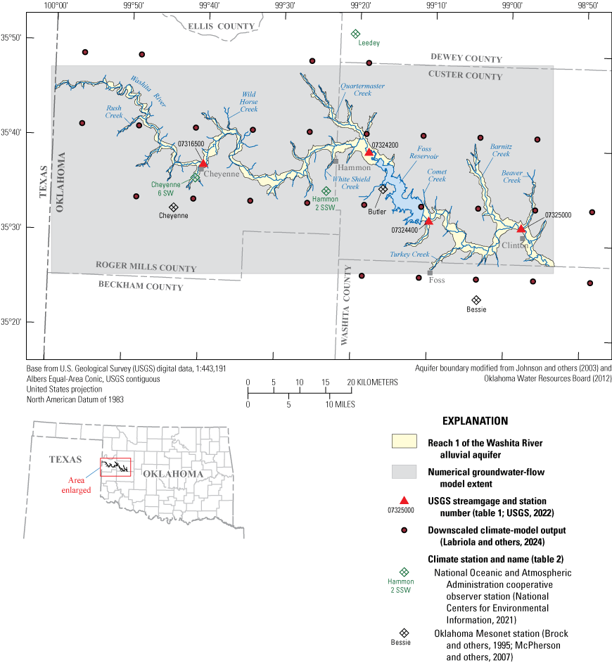
Reach 1 of the Washita River alluvial aquifer, model extent, climate-model output areas, climate stations, and U.S. Geological Survey streamgages in and near the study area, western Oklahoma.
Surveys of land use over the study area were obtained from the CropScape database (National Agricultural Statistics Service, 2019). CropScape data for the period 2008–18 depicted the area as undeveloped land and shrubland, along with a high percentage of irrigated land, specifically consisting of grass/pasture (18 percent) and cropland (56 percent), of which the two principal crops are winter wheat (70 percent) and alfalfa (19 percent) (National Agricultural Statistics Service, 2019). Mean annual precipitation during the 1920–2017 period of record for reach 1 of the Washita River (an average of the mean annual precipitation from six climate stations near reach 1) was about 625 millimeters (Ellis and others, 2020).
Table 1.
Information for selected U.S. Geological Survey streamgages in reach 1 of the Washita River alluvial aquifer, western Oklahoma.[Data from U.S. Geological Survey (2022); USGS, U.S. Geological Survey; Okla., Oklahoma; dates are in month/year format]
| USGS station number (fig. 1) | USGS station name | Latitude, in decimal degrees | Longitude, in decimal degrees | Period of record used in this analysis (may contain gaps) | |
|---|---|---|---|---|---|
| Begin | End | ||||
| 07316500 | Washita River near Cheyenne, Okla. | 35.62644 | −99.66840 | 10/1937 | 12/2015 |
| 07324200 | Washita River near Hammon, Okla. | 35.47310 | −100.12095 | 10/1969 | 12/2015 |
| 07324400 | Washita River near Foss, Okla. | 35.65644 | −99.30621 | 3/1956 | 12/2015 |
| 07325000 | Washita River near Clinton, Okla. | 35.42227 | −98.96928 | 10/1935 | 12/2015 |
Climate Projections and the Numerical Groundwater-Flow Model for Reach 1 of the Washita River Alluvial Aquifer
In this section, a description of how projected climate data were used in SWB model simulations is provided, along with a discussion of how the groundwater model was used to analyze base-flow and reservoir-storage changes. All of the USGS streamflow and groundwater data used in this analysis are stored in the USGS National Water Information System (USGS, 2022). The SWB model, in combination with downscaled climate and hydrology projections from the Coupled Model Intercomparison Project phase 5 (CMIP5) GCM, was used to simulate groundwater recharge and evapotranspiration for the 30-year baseline scenario (1985–2014) (hereinafter referred to as the “baseline scenario”) and three 30-year projected climate scenarios (2050–79) (hereinafter referred to as the “projected climate scenarios”) under warmer/drier, central tendency, and less-warm/wetter climatic conditions for the Washita River and the hydraulically connected Washita River alluvial aquifer. Groundwater recharge and evapotranspiration outputs from the SWB model were used in the groundwater model to simulate the effects of base-flow changes on surface water inflows to Foss Reservoir and estimate water-surface elevation and reservoir-storage changes by using techniques described in Labriola and others (2020). The following subsections provide a summary of the methods used to develop the climate datasets for input to the SWB model and a description of the groundwater model used for the analysis of the effects of climate projections on groundwater and Foss Reservoir in the study area.
Soil-Water-Balance Model for the 30-Year Baseline Scenario (1985–2014)
The SWB model (Westenbroek and others, 2010) was used to estimate groundwater recharge and evapotranspiration from climate and land-cover characteristic data inputs to the groundwater model (Ellis and others, 2020). Climate data, including precipitation (table 2) and minimum and maximum air temperatures, used in this simulation were retrieved from three Oklahoma Mesonet stations (Brock and others, 1995; McPherson and others, 2007) and three National Oceanic and Atmospheric Administration cooperative observer stations (National Centers for Environmental Information, 2021). The point data from these stations were interpolated into a two-dimensional grid that was used in the SWB model to estimate the climate of the study area. Data used in the SWB model, including land-cover characteristic data, soil-water storage capacity, and hydrologic soil group, were retrieved from the Digital General Soil Map database (Natural Resources Conservation Service [NRCS], 2018). Surface water flow directions were calculated by using a flow-direction grid derived from a digital elevation model (USGS, 2018) of the study area. The Thornthwaite-Mather method (Thornthwaite and Mather, 1957) is used in the SWB model to calculate recharge based on the mass-balance approach, which calculates the difference between water sources and water sinks for each grid cell. The following equation details the SWB mass-balance equation (modified from Westenbroek and others, 2010):
(1)
The mass-balance approach accounts for water sources in the form of precipitation, snowmelt, and surface runoff inflow. Precipitation was retrieved from the input climate data, snowmelt was accounted for from the combination of precipitation data and minimum and maximum air temperatures, and surface runoff inflow was calculated from a flow-direction grid of the study area and NRCS runoff-curve numbers (Cronshey and others, 1986). The water sinks of the mass-balance approach include plant interception, surface runoff outflow, and evapotranspiration. Plant interception was calculated from precipitation and land-cover type, surface runoff outflow was calculated by using NRCS runoff-curve numbers (Cronshey and others, 1986) based on the relation between rainfall and runoff, and evapotranspiration was calculated by using the methods from Hargreaves and Samani (1985) to calculate potential and actual evapotranspiration from daily climate minimum and maximum air temperature data. The National Centers for Environmental Information (2024) explain, “PE [potential evapotranspiration] is the demand or maximum amount of water that would be evapotranspired if enough water were available (from precipitation and soil moisture). AE [actual evapotranspiration] is how much water actually is evapotranspired and is limited by the amount of water that is available.” The change (Δ) in soil moisture accounts for the amount of water stored in soil and is calculated as the difference between potential evapotranspiration and daily precipitation.
Table 2.
Mean annual precipitation at selected Oklahoma Mesonet and National Oceanic and Atmospheric Administration cooperative observer (COOP) climate stations used in the analysis of the effects of climate projections on base flow and reservoir storage in reach 1 of the Washita River alluvial aquifer, western Oklahoma.[Oklahoma Mesonet data from Brock and others (1995) and McPherson and others (2007); COOP data from National Centers for Environmental Information (2021); all precipitation values are in inches per year; --, no data available]
| Station name (fig. 1) |
Period of record | Number of years | Mean annual precipitation | |||
|---|---|---|---|---|---|---|
| Period of record | 1930–88 | 1989–2008 | 2009–14 | |||
| Bessie (Oklahoma Mesonet) | 1994–2017 | 23 | 27.8 | -- | 29.8 | 21.0 |
| Butler (Oklahoma Mesonet) | 1994–2017 | 23 | 27.3 | -- | 28.7 | 20.3 |
| Cheyenne (Oklahoma Mesonet) | 1994–2017 | 23 | 27.0 | -- | 28.8 | 20.5 |
| Leedey (COOP) | 1941–2017 | 76 | 24.4 | 23.1 | 26.9 | 20.6 |
| Hammon 2 SSW (COOP) | 1920–2004 | 84 | 25.7 | 24.3 | 29.2 | -- |
| Cheyenne 6 SW (COOP) | 1923–93 | 70 | 23.2 | 22.9 | 21.7 | -- |
Soil-Water-Balance Model for the Projected Climate Scenarios (2050–79)
Climate projections can be used in the SWB model to calculate future recharge and evapotranspiration estimates for input to numerical groundwater-flow models. The climate projections used in this study are the monthly bias-corrected and spatially disaggregated projections of temperature and precipitation, statistically downscaled to an eighth degree latitude by an eighth degree longitude. The projections were obtained from an archive of climate and hydrology projections developed by Reclamation in partnership with the USGS, U.S. Army Corps of Engineers, Lawrence Livermore National Laboratory, Santa Clara University, Climate Central, and Scripps Institution of Oceanography (Reclamation, 2013). This archive of climate projections is based on GCM simulations compiled by the World Climate Research Programme’s Coupled Model Intercomparison Project for four future model emission scenarios known as representative concentration pathways (RCPs) (van Vuuren and others, 2011). For reach 1 of the Washita River alluvial aquifer, temperature and precipitation climate projections were derived from 231 climate projections from the bias-corrected and spatially disaggregated multimodel ensembles of the CMIP5 projections; each of the four RCPs represents a different forecasted radiative forcing level by the year 2100 depending on differences in climate policy (8.5, 6.0, 4.5, and 2.6 watts per square meter) (table 3). The RCP values increase as radiative forcing increases, indicating the extent of global atmospheric imbalance (U.S. Environmental Protection Agency, 2023). The four RCPs were developed by the global modeling community to incorporate a range of different radiative forcing outcomes depending on simulated different socioeconomic, energy, land-use, and emission (greenhouse gases and air pollutants) changes, enabling modelers to explore different possible climate outcomes through 2100 (van Vuuren and others, 2011).
Table 3.
Institutions providing climate-model output used in the analysis of the effects of climate projections on base flow and reservoir storage in reach 1 of the Washita River alluvial aquifer, western Oklahoma.[Data from Bureau of Reclamation (2010); W/m2, watt per square meter; Y, yes; --, no]
BCC = Beijing Climate Centre, China Meteorological Administration; CCCMA = Canadian Centre for Climate Modelling and Analysis; CMCC = Centro Euro-Mediterraneo per i Cambiamenti Climatici; CNRM-CERFACS = Centre National de Recherches Météorologiques/Centre Européen de Recherche et Formation Avancée en Calcul Scientifique; CSIRO-BOM = Commonwealth Scientific and Industrial Research Organisation (CSIRO) and Bureau of Meteorology (BOM), Australia; CSIRO-QCCCE = Commonwealth Scientific and Industrial Research Organisation in collaboration with Queensland Climate Change Centre of Excellence; EC-EARTH = EC-EARTH consortium; FIO = First Institute of Oceanography, State Oceanic Organization, China; INM = Institute for Numerical Mathematics; IPSL = Institut Pierre-Simon Laplace; LASG = LASG, Institute of Atmospheric Physics, Chinese Academy of Sciences; LASG-CESS = LASG, Institute of Atmospheric Physics, Chinese Academy of Sciences, and Centre for Earth System Science, Tsinghua University; MIROC = Atmosphere and Ocean Research Institute (The University of Tokyo), National Institute for Environmental Studies, and Japan Agency for Marine-Earth Science and Technology; MIROC(2) = Japan Agency for Marine-Earth Science and Technology, Atmosphere and Ocean Research Institute (The University of Tokyo), and National Institute for Environmental Studies; MOHC = Met Office Hadley Centre (additional HadGEM2-ES realizations contributed by Instituto Nacional de Pesquisas Espaciais); MPI-M = Max-Planck-Institut für Meteorologie (Max Planck Institute for Meteorology); MRI = Meteorological Research Institute; NASA GISS = National Aeronautics and Space Administration Goddard Institute for Space Studies; NCC = Norwegian Climate Centre; NIMR/KMA = National Institute of Meteorological Research/Korea Meteorological Administration; NOAA GFDL = National Oceanic and Atmospheric Administration Geophysical Fluid Dynamics Laboratory; NSF-DOE-NCAR = National Science Foundation-Department of Energy-National Center for Atmospheric Research Community Earth System Model Contributors; RSMAS = Rosenstiel School of Marine, Atmospheric & Earth Science, University of Miami.
The 231 climate projections were statistically grouped into climate scenarios by using the ensemble-informed hybrid delta (HDe) method (Reclamation, 2010). The HDe method uses the mean annual changes between a historical period and a future period to calculate percentile changes from both temperature and precipitation to inform projected climate scenarios. The HDe method yields five ensemble-informed projected climate scenarios—warmer/wetter (more warming, wetter), less-warm/wetter (less warming, wetter), less-warm/drier (less warming, drier), warmer/drier (more warming, drier), and central tendency—which are identified by the percentile changes in mean annual temperature and precipitation. The three projected climate scenarios used in this study that align with future climate outlooks in the study area (Liu and others, 2012; Bertrand and McPherson, 2018) were central tendency, warmer/drier, and less-warm/wetter scenarios (additional details regarding selection and use of climate-projection data are available in Reclamation [2010]). The central-tendency scenario is based on projections that intersect the 50 percent mean annual precipitation change and the 50 percent mean annual temperature change. The warmer/drier scenario represents projections that intersect the 10 percent mean annual precipitation change and the 10 percent mean annual temperature change. The less-warm/wetter scenario represents projections that intersect the 90 percent mean annual precipitation change and the 90 percent mean annual temperature change.
Monthly interpolated change factors were calculated to adjust SWB model inputs for each scenario in each of the grid cells following the methods described in Labriola and others (2020). Change factors were applied to the historical daily precipitation data as a scaling factor and to the historical daily temperature data as an offset. The daily scaling values associated with each month were the same as the offset factors needed for the SWB model during the month in question because the downscaled data were provided at a monthly interval. Once these factors were applied, representative climate data (temperature and precipitation) for each of the three scenarios were used as input in the SWB model for recharge and evapotranspiration estimation and subsequent modeling in a groundwater model (Ellis and others, 2020). Within the SWB simulation, the representative climate scenarios were the only inputs that changed between the projected climate scenarios and the groundwater model; land-use/land-cover, hydrologic soil group, surface water flow direction, and available soil-water capacity were unchanged from the baseline scenario in this study.
Numerical Groundwater-Flow Modeling
A groundwater model (Ellis and others, 2020) was used to simulate changes in base flows in the Washita River and water-surface elevations in Foss Reservoir between the baseline scenario and the three projected climate scenarios. MODFLOW-NWT (Niswonger and others, 2011), a Newton formulation for MODFLOW-2005 (Harbaugh, 2005), was used to accurately represent repeated cycles of drying and rewetting in model cells. The groundwater model features a cell size of about 100 meters (m) by 100 m; this spatial resolution was used to simulate groundwater flow in the alluvium and terrace deposits that contain the Washita River alluvial aquifer (layer 1) and in the underlying bedrock units (layer 2). The “Geologic Units and Hydrogeology of the Study Area” section of Ellis and others (2020, p. 12–18) provides a detailed description of the geologic framework of the Washita River alluvial aquifer. The groundwater model was temporally discretized into 433 stress periods, consisting of one initial steady-state period (representing inflows and outflows for all years from 1980 through 2015) and 432 monthly transient stress periods from January 1980 through December 2015. Specialized software packages have been incorporated into MODFLOW to simulate different hydrologic processes. The Recharge, General-Head Boundary, Streamflow Routing, Lake, Evapotranspiration, and Well packages of MODFLOW (Niswonger and others, 2011) were used in this assessment. The Recharge package (Harbaugh, 2005), which used the spatially distributed recharge values simulated from the SWB model, was applied to layer 1 in the groundwater model. The General-Head Boundary package (Harbaugh, 2005) was used to account for lateral groundwater flows into the model. The Streamflow-Routing package (Niswonger and Prudic, 2005) was used to simulate seepage between the aquifer and the major streams and tributaries within the study area. The Lake package (Merritt and Konikow, 2000; Niswonger and Prudic, 2005) was used to simulate the lakebed seepage between Foss Reservoir and groundwater in the surrounding aquifer. The Evapotranspiration package (Harbaugh, 2005) was used to simulate saturated-zone evapotranspiration (including transpiration by plants rooted in the saturated zone) in areas designated as wetlands in layer 1 of the groundwater model. Saturated-zone evapotranspiration values were calculated as the difference between potential evapotranspiration values and estimates of actual evapotranspiration values obtained from the SWB model (more information about saturated-zone evapotranspiration in reach 1 of the Washita River alluvial aquifer can be found in the “Saturated-Zone Evapotranspiration” section of Ellis and others [2020, p. 33–34]). The Well package (Harbaugh, 2005) was used to simulate groundwater use and well withdrawals during the model simulation. The groundwater model was calibrated using manual adjustment and automated calibration with the nonlinear regression code PEST++ (Welter and others, 2015). A sensitivity analysis indicated that the parameters that were most sensitive to changes were related to recharge and saturated-zone evapotranspiration; additional sensitivity-analysis information can be found in the “Sensitivity Analysis” section of Ellis and others (2020, p. 60–63).
Four scenarios were simulated: the baseline scenario (based on historical data) and the three projected climate scenarios (central tendency, warmer/drier, and less-warm/wetter). The baseline scenario represents the groundwater model for the historical period from 1985 to 2014 (Ellis and others, 2020), whereas the projected climate scenarios use recharge and evapotranspiration SWB model output files created from the climate projections to simulate a selected future period (2050–79). The Recharge package of the groundwater model contains monthly scaling factors that were adjusted to match historical groundwater and surface water observations that were used during the historical model calibration (Ellis and others, 2020); to be consistent for comparisons between the projected climate scenarios and the baseline scenario calculated from the groundwater model, the scaling factors were also applied to the Recharge packages of the climate simulations. For eight selected monthly stress periods between 1996 and 1998, the lake releases in the MODFLOW Lake package (Merritt and Konikow, 2000; Niswonger and Prudic, 2005) were manually reduced to account for reduced precipitation in the warmer/drier scenario; manually reducing selected lake releases improved the model stability. The runoff values from the last 12 stress periods representing 2015 were excluded to improve model stability (2015 is not in the 1985–2014 or 2050–79 time periods used in the study). The SWB outputs for groundwater recharge and evapotranspiration, as well as the groundwater model and new simulation results described herein, are published in a companion USGS data release (Labriola and others, 2024).
Simulated Effects of Future Climate Conditions on Base Flow and Reservoir Storage
The SWB model was used to calculate gridded recharge and evapotranspiration for the three projected climate scenarios based on GCM-simulated climate data. The recharge and evapotranspiration results for each of these future scenarios were incorporated into a groundwater model (Ellis and others, 2020) to simulate how potential future climatic conditions may change base flow in the Washita River and storage in Foss Reservoir within reach 1 of the Washita River alluvial aquifer relative to the baseline calibrated model conditions.
Soil-Water-Balance
Mean monthly precipitation and recharge were highest in May, and mean monthly temperature and potential evapotranspiration were highest in July (fig. 2). Mean monthly temperatures were higher in the projected climate scenarios compared to the baseline scenario (fig. 2A). Mean monthly precipitation in the central-tendency scenario was highest in January, February, June, and July compared to the other scenarios, whereas the less-warm/wetter scenario indicated a large increase in mean monthly precipitation in September compared to the baseline scenario (fig. 2B). Mean monthly recharge (fig. 2C) followed a pattern similar to that of mean monthly precipitation (fig. 2B) except for April, when recharge was lower and temperature and potential evapotranspiration were higher (fig. 2A, D). Mean monthly potential evapotranspiration increased steadily between January and July and then decreased steadily from August through December (fig. 2D).
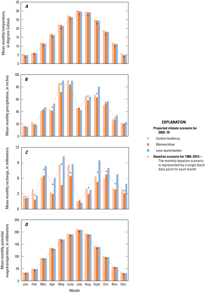
Mean monthly A, temperature and B, precipitation from historical (1985–2014) data and downscaled adjusted (2050–79) climate-model data and mean monthly C, recharge and D, potential evapotranspiration computed by using the Soil-Water-Balance model (Westenbroek and others, 2010) to compare the baseline scenario to three projected climate scenarios for reach 1 of the Washita River alluvial aquifer, western Oklahoma (data from Labriola and others, 2024).
The mean monthly temperature was highest in July for all three projected climate scenarios (fig. 2A). For the warmer/drier scenario, the mean monthly temperature was lowest in December, whereas for the central-tendency and less-warm/wetter scenarios, the mean monthly temperature was lowest in January. Higher monthly temperatures were estimated in all three projected climate scenarios compared to the baseline scenario. The July temperature for the three projected climate scenarios compared to the baseline scenario increased by 2.4 degrees Celsius (°C) for the central-tendency scenario, 1.9 °C for the warmer/drier scenario, and 1.7 °C for the less-warm/wetter scenario. The difference in mean monthly temperature was highest in October relative to the baseline scenario; the mean monthly temperature in October increased by 2.8 °C in the central-tendency scenario and by 1.9 °C in the warmer/drier and the less-warm/wetter scenarios. The higher temperatures in October for the three projected climate scenarios imply that warmer, summerlike Octobers are possible in the future, which could extend the growing season. The largest differences in temperature between the projected climate scenarios and the baseline scenario were increases in temperatures between April and October (that is, from the spring season to the fall season); higher temperatures during these months imply that the growing season may be warmer and longer, which could further increase groundwater-withdrawal demands for agriculture in the future.
Mean monthly precipitation was highest in May–June and August–September and lowest in January for all scenarios (fig. 2B), which corresponds with the typical rainy seasons in late spring and early fall shown in the historical data in baseline scenario. Historically (baseline scenario), May is the wettest month of the year and thus important for its contribution to water resources in the study area. Mean monthly May precipitation for the three projected climate scenarios compared to the baseline scenario increased 2.2 percent for the central-tendency, decreased 15.6 percent for the warmer/drier, and increased 6.0 percent for the less-warm/wetter scenarios; these differences are noteworthy, especially the projected large decrease in precipitation during the warmer/drier scenario. The months with the largest percentage changes in mean monthly precipitation between the baseline and central-tendency scenarios include January (+11.0 percent), February (+25.4 percent), April (−7.7 percent), and June (+9.9 percent). In the central-tendency scenario, winter and summer precipitation generally increased relative to the baseline scenario and decreased in spring and fall. Mean monthly precipitation in the warmer/drier scenario differed the most in April (−11.6 percent), May (−15.6 percent), and August (−11.0 percent) relative to the baseline scenario, and there was less precipitation in all months. Mean monthly precipitation in the less-warm/wetter scenario exceeded mean monthly precipitation for the baseline scenario by the largest amounts in September (16.0 percent), November (18.0 percent), and December (18.1 percent), whereas mean monthly precipitation for the less-warm/wetter scenario decreased in January (2.6 percent), July (6.6 percent), and August (2.3 percent). The large percentage increase in precipitation projected in September in the less-warm/wetter scenario is of note because the historical data in the baseline model indicates September as one of the three wettest months of the year. The projected increases in precipitation during November and December in the less-warm/wetter scenario compared to the baseline scenario will likely contribute meaningfully to recharge because the increase in precipitation during these months is during a time of year characterized by low groundwater withdrawals and low potential evapotranspiration losses.
Mean monthly recharge was generally highest in March, May–June, and September–October and lowest in July for all projected climate scenarios (fig. 2C); these peaks and troughs align with the baseline-scenario precipitation patterns (fig. 2B). The percentage changes for mean monthly recharge in July (the month with the lowest mean monthly recharge and precipitation) for the three projected climate scenarios compared to the baseline scenario were +0.7 percent for the central-tendency scenario, −4.3 percent for the warmer/drier scenario, and −22.7 percent for less-warm/wetter scenario (fig. 2C). The months with the largest percentage changes in mean monthly recharge between the baseline scenario and central-tendency scenario include February (+44.2 percent) and April (−31.2 percent). Mean monthly recharge was less in the warmer/drier scenario in every month relative to the baseline scenario, with the largest differences in April (−37.6 percent) and May (−46.8 percent). Mean monthly recharge in the less-warm/wetter scenario was higher relative to the baseline scenario during most months, with the largest percentage increases between the two scenarios observed in September (31.7 percent), November (37.6 percent), and December (36.9 percent), indicating an overall increase in recharge in all three projected climate scenarios during the latter part of the calendar year compared to the baseline scenario.
Mean monthly potential evapotranspiration was highest in July and lowest in December (fig. 2D) for the projected climate scenarios. Overall, higher potential evapotranspiration values were indicated in the projected climate scenarios compared to the baseline scenario, consistent with the overall pattern of higher temperatures in the three projected climate scenarios compared to the baseline scenario (fig. 2A). The percentage increases in mean monthly potential evapotranspiration in July (the month with highest overall evapotranspiration) for the three projected climate scenarios compared to the baseline scenario were 5.2 percent for the central-tendency, 4.0 percent for the warmer/drier, and 3.7 percent for less-warm/wetter scenarios (fig. 2D). The highest percentage changes in mean monthly potential evapotranspiration between the three projected climate scenarios and baseline scenario were in January, with increases of 25.5 percent in the central-tendency, 19.6 percent in the warmer/drier, and 19.4 percent in the less-warm/wetter scenarios.
Higher simulated annual recharge to the Washita River alluvial aquifer occurred during years with higher simulated annual precipitation (fig. 3B, C). Precipitation and recharge patterns contain similar temporal peaks and troughs, whereas temperature exhibits an inverse relation with recharge (fig. 3A, C), with smaller recharge amounts associated with higher temperatures. The less-warm/wetter scenario had the highest recharge and precipitation with mean annual values of 72.5 millimeters per year (mm/yr) and 615.5 mm/yr, respectively, which represented an increase from the baseline scenario of 16 percent for recharge and 7 percent for precipitation (table 4). Relative to the other projected climate scenarios, the warmer/drier scenario resulted in the lowest mean annual values for recharge (48.0 mm/yr) and precipitation (536.6 mm/yr), equating to percentage changes from the baseline scenario of −23 percent for recharge and −7 percent for precipitation. Compared to the other projected climate scenarios, the simulated values from the central-tendency scenario (6 percent less recharge and 1 percent more precipitation) aligned most closely with those from the baseline scenario. The highest mean annual temperature was simulated for the central-tendency scenario, followed by the warmer/drier, less-warm/wetter, and baseline scenarios.
Additional relations between mean annual temperature and precipitation with mean annual recharge and potential evapotranspiration were compared for the different climate scenarios. Higher mean annual temperature and precipitation in the less-warm/wetter scenario relative to the baseline scenario caused mean annual potential evapotranspiration to increase, but the increase in precipitation was sufficient to still drive mean annual recharge higher (fig. 3). Compared to the baseline scenario, the mean annual temperature and the mean annual precipitation were higher for the central-tendency scenario; despite slightly higher mean annual precipitation amounts, the higher temperatures caused a large increase in the mean annual potential evapotranspiration, resulting in a decrease in mean annual recharge for the central-tendency scenario compared to the baseline scenario. Mean annual temperature and precipitation were higher for the central-tendency scenario relative to the warmer/drier scenario, and higher mean annual recharge and similar mean annual potential evapotranspiration amounts were projected in the central-tendency scenario relative to the warmer/drier scenario. The annual precipitation values during the final 6 years of the simulation (2074–79) were less than the mean annual precipitation values during the 1985–2014 baseline scenario or during the entire 2050–79 future period for the three projected climate scenarios (fig. 3B) because the precipitation patterns during 1985–2014 are shifted forward into the simulation period: 2009–14 were relatively dry years; hence, 2074–79 were simulated as relatively dry years.
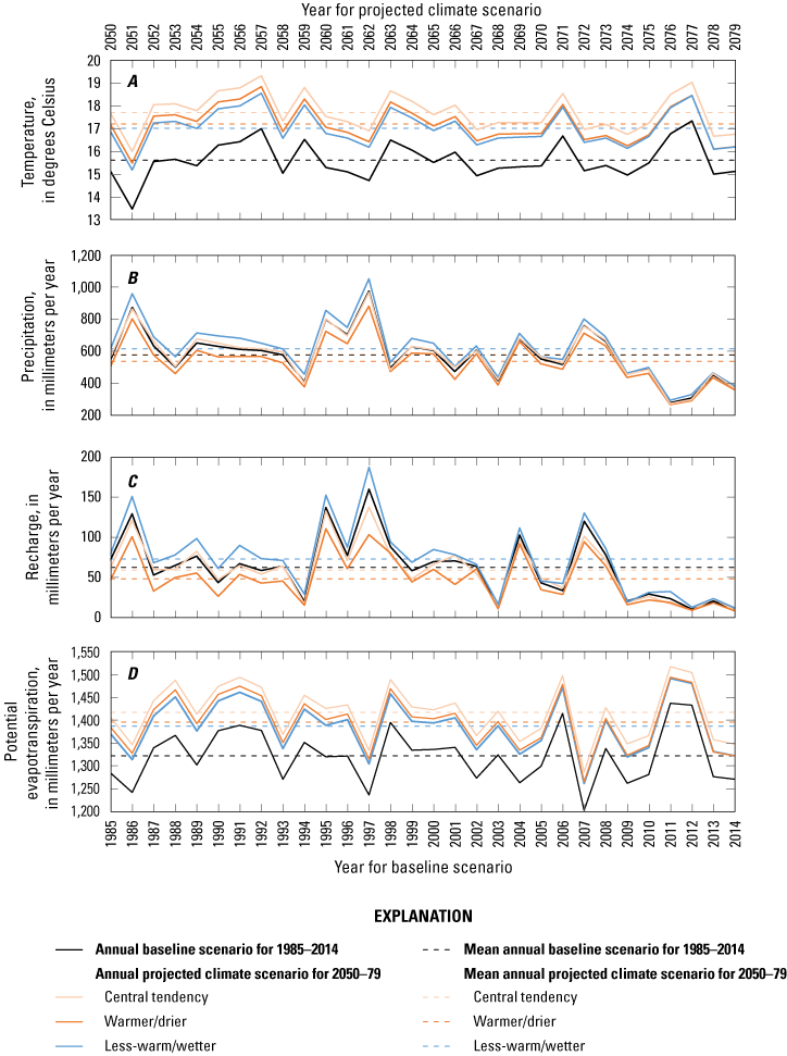
Annual and mean annual A, temperature and B, precipitation from the downscaled climate-model data and C, recharge and D, potential evapotranspiration computed by using the Soil-Water-Balance model (Westenbroek and others, 2010) to compare the baseline scenario to three projected climate scenarios for reach 1 of the Washita River alluvial aquifer, western Oklahoma. The baseline scenario was for 1985–2014, and the projected climate scenarios were for 2050–79 (Labriola and others, 2024).
Table 4.
Mean annual temperature and precipitation for the baseline scenario (1985–2014) and the three projected climate scenarios (2050–79: central tendency, warmer/drier, and less-warm/wetter) from the downscaled climate-model data and recharge and potential evapotranspiration computed by using the Soil-Water-Balance model (Westenbroek and others, 2010) to compare the baseline scenario to the projected scenarios for reach 1 of the Washita River alluvial aquifer, western Oklahoma.[Data from Labriola and others (2024); °C, degrees Celsius; mm/yr, millimeter per year; +, plus; −, minus; %, percentage change from the baseline scenario]
Numerical Groundwater-Flow Modeling
The climate-model outputs included simulated monthly base flow for the USGS streamgages in the study area and monthly storage in Foss Reservoir, which were collectively used to determine the effects of climate projections (temperature and precipitation) on recharge to and saturated-zone evapotranspiration from the groundwater system in reach 1 of the Washita River alluvial aquifer.
Base flows (groundwater discharge) upstream from Foss Reservoir were simulated for the Hammon streamgage (USGS station number 07324200, fig. 1). Simulated base flow from the projected climate scenarios can be compared to simulated base flow from the baseline scenario upstream from Foss Reservoir (fig. 4). The warmer/drier and central-tendency scenarios had the lowest amounts of mean monthly simulated base flows followed by the baseline scenario; the less-warm/wetter scenario had the highest amounts of mean monthly simulated base flows of the four scenarios. The mean monthly simulated base flow for the baseline scenario was 0.67 cubic meter per second (m3/s), whereas for the central-tendency, warmer/drier, and less-warm/wetter scenarios, the mean monthly simulated base flows were 0.62, 0.52, and 0.77 m3/s, respectively. A decrease in base flow into Foss Reservoir was projected in the central-tendency and the warmer/drier scenarios, whereas an increase in base flow was projected in the less-warm/wetter scenario. Mean monthly simulated base flows at the Hammon streamgage (fig. 4) were lowest in August and highest in March in all four scenarios. Low mean monthly simulated base-flow values in August corresponded with seasonally low recharge and precipitation values and high temperatures in July and August compared to May and June (fig. 2), whereas high mean monthly simulated base-flow values in March corresponded with seasonally high recharge and precipitation values during this month compared to January and February (fig. 2).
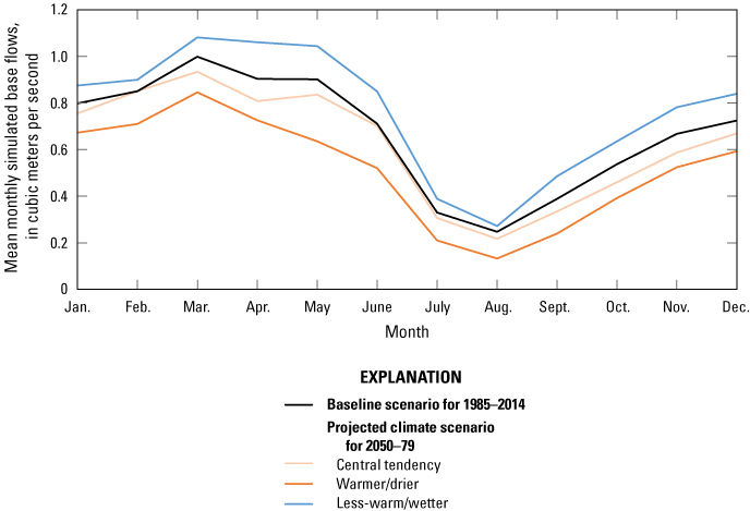
Mean monthly simulated base flow for the Washita River, western Oklahoma, upstream from Foss Reservoir at U.S. Geological Survey streamgage 07324200 Washita River near Hammon, Okla. (fig. 1), into Foss Reservoir for the baseline scenario (1985–2014) and the three projected climate scenarios (2050–79: central tendency, warmer/drier, and less-warm/wetter) (Labriola and others, 2024).
Reservoir storage for Foss Reservoir was largest in the less-warm/wetter scenario and smallest in the warmer/drier scenario (fig. 5). Reservoir storage in the baseline and central-tendency scenarios were nearly identical during the first few years of their respective simulated periods, but the central-tendency scenario gradually deviated from (decreased relative to) the baseline scenario over the remainder of the simulated periods. The percentage changes in mean annual reservoir storage between the projected climate scenarios and the baseline scenario were −6.2 percent for the central-tendency scenario, −20.0 percent for the warmer/drier scenario, and +19.7 percent for the less-warm/wetter scenario. The mean reservoir storage for 1985–2014 was 1.9×10⁸ cubic meters (m3) for the baseline scenario. The mean reservoir storage for 2050–79 was 1.7×10⁸ m3 for the central-tendency scenario, 1.5×10⁸ m3 for the warmer/drier scenario, and 2.3×10⁸ m3 for the less-warm/wetter scenario. At the end of the simulation, reservoir storage was −13 percent in the central-tendency scenario, −29 percent in the warmer/drier scenario, and +24 percent in the less-warm/wetter scenario compared to the baseline storage. Two storage elevation levels are referenced: dead pool, which is the elevation of the lowest water outlet from which water can be released, and conservation pool, which is the elevation at the top of the maximum normal operating level. Reservoir storage in the less-warm/wetter scenario exceeded the conservation-pool storage (2.0×10⁸ m3 [U.S. Army Corps of Engineers, 2023]) for most of the simulation period but often decreased to below the conservation-pool storage during years with relatively little precipitation (figs. 3 and 5). The warmer/drier scenario storage was often below the conservation-pool storage and approached the dead-pool storage (0.1×10⁸ m3 [U.S. Army Corps of Engineers, 2023]) during the final years of the simulation period (fig. 5).
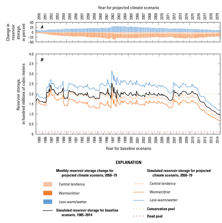
Comparison of A, changes in reservoir storage and B, reservoir storage for Foss Reservoir in reach 1 of the Washita River alluvial aquifer, western Oklahoma, for the baseline scenario (1985–2014) and the three projected climate scenarios (2050–79: central tendency, warmer/drier, and less-warm/wetter) (Labriola and others, 2024).
The water budget includes mean annual inflows and outflows upgradient and downgradient for the baseline scenario and projected climate scenarios (fig. 6). Areas upgradient and downgradient from Foss Reservoir were distinguished from one another by using the ZONEBUDGET utility of MODFLOW (Harbaugh, 1990). Recharge accounts for the largest component of groundwater inflows upgradient from Foss Reservoir, contributing 64, 61, 53, and 68 percent of the water budgets for the baseline, central tendency, warmer/drier, and less-warm/wetter scenarios, respectively (fig. 6A). Downgradient from Foss Reservoir, lateral groundwater inflow accounts for the largest component of groundwater inflows, contributing 40, 41, 45, and 36 percent of the water budgets for the baseline, central tendency, warmer/drier, and less-warm/wetter scenarios, respectively (fig. 6B). In the less-warm/wetter scenario, there is a higher amount of recharge compared to the other scenarios, resulting in less lateral groundwater inflow compared to the other scenarios. Saturated-zone evapotranspiration makes up the largest component of groundwater outflows upgradient from Foss Reservoir in the baseline, central-tendency, and warmer/drier scenarios (42, 45, and 45 percent, respectively), whereas seepage to streams was the largest upgradient groundwater outflow component in the less-warm/wetter scenario (48 percent) (fig. 6C). Seepage to streams accounts for the largest component of groundwater outflows downgradient from Foss Reservoir in all scenarios, accounting for 71, 69, 69, and 74 percent of the water budgets for the baseline, central-tendency, warmer/drier, and less-warm/wetter scenarios, respectively (fig. 6D).
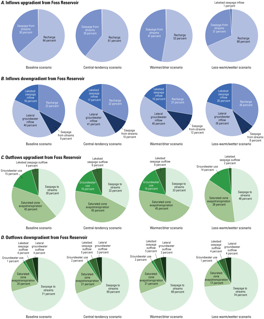
Groundwater inflows A, upgradient and B, downgradient and groundwater outflows C, upgradient and D, downgradient from Foss Reservoir in reach 1 of the Washita River alluvial aquifer, western Oklahoma, based on the mean annual water budgets simulated in the groundwater model for the baseline scenario (1985–2014) and the three projected climate scenarios (2050–79: central tendency, warmer/drier, and less-warm/wetter) (Labriola and others, 2024).
Total aquifer inflows and outflows for the groundwater model and percentage changes from the baseline scenario compared to the three projected climate scenarios were also calculated (Labriola and others, 2024). Total aquifer inflow consists of recharge, seepage from streams, lateral groundwater inflow, and lakebed seepage inflow. Upgradient from Foss Reservoir, total aquifer inflow increased by only 0.04 percent in the central-tendency scenario, decreased by 7 percent in the warmer/drier scenario, and increased by 11 percent in the less-warm/wetter scenario compared to the baseline scenario. Downgradient from Foss Reservoir, total aquifer inflow decreased by 2 percent in the central-tendency scenario, decreased by 9 percent in the warmer/drier scenario, and increased by 7 percent in the less-warm/wetter scenario compared to the baseline scenario. Total aquifer outflow consists of seepage to streams, saturated-zone evapotranspiration, groundwater use, lakebed seepage outflow, and lateral groundwater outflow. Total outflow upgradient from Foss Reservoir increased by 1 percent in the central-tendency scenario, decreased by 6 percent in the warmer/drier scenario, and increased by 11 percent in the less-warm/wetter scenario compared to the baseline scenario. Total outflow downgradient from Foss Reservoir decreased by 4 percent in the central-tendency scenario, decreased by 10 percent in the warmer/drier scenario, and increased by 6 percent in the less-warm/wetter scenario compared to the baseline scenario. Spatially, the largest magnitude changes in groundwater-level elevations at the end of the simulation period (2079) in all three projected climate scenarios relative to the baseline scenario were upstream from Foss Reservoir (fig. 7). Decreases in groundwater-level elevations were primarily observed in the central-tendency and warmer/drier scenarios (fig. 7A, B), whereas increases in groundwater-level elevations were primarily observed in the less-warm/wetter scenario (fig. 7C).
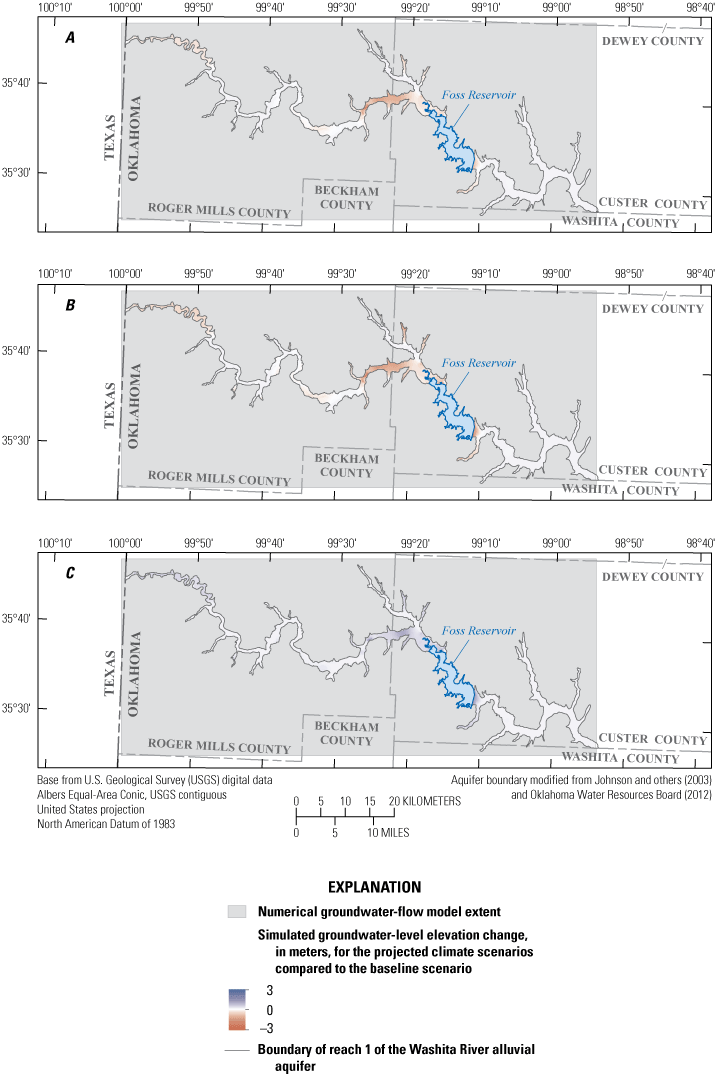
Simulated changes in groundwater-level elevations in reach 1 of the Washita River alluvial aquifer, western Oklahoma, for the A, central-tendency, B, warmer/drier, and C, less-warm/wetter scenarios at the end of the simulation period (2079) relative to groundwater-level elevations in the baseline scenario (1985–2014) (Labriola and others, 2024).
Model Assumptions and Limitations
A range of possible outcomes of future groundwater availability was assessed through the use of three projected climate scenarios; other projected climate scenarios could have been considered. The scenarios were computed by using a previously published groundwater model; all groundwater models have inherent limitations. Limitations of the groundwater model used in this assessment are described in the “Model Limitations” section of Ellis and others (2020, p. 74). Many of the model parameters used as inputs, such as groundwater withdrawals, land use, and land cover, remained static in the simulations associated with the projected climate scenarios because of insufficient data to generate model parameters that change over time and resulted in several limitations. For example, simulating groundwater withdrawals as being the same across all scenarios does not realistically portray how withdrawals are likely to change in response to different weather events, such as prolonged dry and wet periods. Incorporating future water-demand projections into the simulations (if possible) would also aid in representing realistic future conditions. Because land use and land cover are likely to change over time, it would be helpful to include projected land-use changes into simulations made by using groundwater models. Including these inputs in simulations may make it possible to determine a more comprehensive view of groundwater availability in future conditions. Including more data for variables that are likely to change over time may also improve predictions of water availability in the future. A particular limitation within the groundwater model used in this assessment, in cases where water-surface elevation was above the conservation pool (such as during the less-warm/wetter scenario), is that excess water was not released downstream and remains in the reservoir in the simulation. Similarly, anytime reservoir storage in the baseline scenario is above and the climate scenarios are below the conservation-pool storage, the model is releasing storage that would not be otherwise released (in respect to flood-control releases). Possible decreases over time in reservoir storage for Foss Reservoir caused by sediment deposition were not considered. Using a reservoir model to simulate water releases downstream when water-surface elevation was above the conservation pool would allow for more realistic water resource simulations.
Summary
To better understand the relation between climate variability and future groundwater resources in reach 1 of the Washita River alluvial aquifer in western Oklahoma, the U.S. Geological Survey, in cooperation with the Bureau of Reclamation, used a previously published numerical groundwater-flow model and climate-model data to investigate changes in base flow and reservoir storage by evaluating three scenarios. Three projected climate scenarios (central tendency, warmer/drier, and less-warm/wetter) representing 2050–79 were simulated with a previously published calibrated MODFLOW numerical groundwater-flow model to estimate base flow in the Washita River and storage in Foss Reservoir within reach 1 of the Washita River alluvial aquifer. Information regarding potential changes to storage in Foss Reservoir and availability of groundwater in the Washita River alluvial aquifer is intended to help inform water resource managers as they plan for different future water conditions in their specific areas.
The temperature and precipitation values from the three projected climate scenarios, based on 231 Coupled Model Intercomparison Project phase 5 (CMIP5) projections, were processed through the Soil-Water-Balance model to produce recharge and evapotranspiration estimates that were subsequently used in the groundwater-flow model. Recharge and saturated-zone evapotranspiration were the only parameters adjusted in the three projected climate scenarios; these adjustments show how temperature and precipitation may affect future groundwater availability within the aquifer and Foss Reservoir. Higher mean temperatures were projected in each of the climate scenarios compared to the baseline scenario. Precipitation during the warmer/drier scenario decreased compared to the baseline scenario, whereas precipitation during the central-tendency scenario slightly increased and during the less-warm/wetter scenario increased compared to the baseline scenario.
The months with the largest percentage changes in mean monthly recharge between the baseline scenario and central-tendency scenario included February (+44.2 percent) and April (−31.2 percent). The mean monthly recharge in the warmer/drier scenario was lower relative to the baseline scenario, with the largest differences in April (−37.6 percent) and May (−46.8 percent). The less-warm/wetter scenario had higher mean monthly recharge values relative to the baseline scenario during most months, with the largest percentage changes between the two scenarios observed in September (+31.7 percent), November (+37.6 percent), and December (+36.9 percent), indicating a higher than usual recharge at the end of the calendar year.
The warmer/drier and central-tendency scenarios had the lowest amounts of mean monthly simulated base flows followed by the baseline scenario; the less-warm/wetter scenario had the highest amounts of mean monthly simulated base flows of the four scenarios. A decrease in base flow into Foss Reservoir was projected in the central-tendency and the warmer/drier scenarios, whereas an increase in base flow was projected in the less-warm/wetter scenario. Mean monthly simulated base flows at a U.S. Geological Survey streamgage upstream from Foss Reservoir were lowest in August and highest in March in all four scenarios. Low mean monthly simulated base-flow values in August corresponded with seasonally low recharge and precipitation values and high temperatures in July and August compared to May and June, whereas high mean monthly simulated base-flow values in March corresponded with the seasonally high recharge and precipitation values during this month compared to January and February.
The largest annual storage in Foss Reservoir occurred in the less-warm/wetter scenario, and the smallest storage occurred in the warmer/drier scenario. Reservoir storage in the baseline and central-tendency scenarios were nearly identical during the first few years of their respective simulated periods, but the central-tendency scenario gradually deviated from (decreased relative to) the baseline scenario over the remainder of the simulated periods. At the end of the simulation period (2079), the largest magnitude differences in groundwater-level elevations in all three projected climate scenarios relative to the baseline scenario occurred upstream from Foss Reservoir. The mean annual percentage changes in reservoir storage between the projected climate scenarios and the baseline scenario were −6.2 percent for the central-tendency scenario, −20.0 percent for the warmer/drier scenario, and +19.7 percent for the less-warm/wetter scenario.
References Cited
Bertrand, D., and McPherson, R.A., 2018, Future hydrologic extremes of the Red River Basin: Journal of Applied Meteorology and Climatology, v. 57, no. 6, p. 1321–1336, accessed August 1, 2022, at https://doi.org/10.1175/JAMC-D-17-0346.1.
Brock, F.V., Crawford, K.C., Elliott, R.L., Cuperus, G.W., Stadler, S.J., Johnson, H.L., and Eilts, M.D., 1995, The Oklahoma Mesonet—A technical overview: Journal of Atmospheric and Oceanic Technology, v. 12, p. 5–19, accessed August 1, 2022, at https://doi.org/10.1175/1520-0426(1995)012%3C0005:TOMATO%3E2.0.CO;2.
Bureau of Reclamation [Reclamation], 2010, Climate change and hydrology scenarios for Oklahoma yield studies: Denver, Colo., U.S. Department of the Interior, Bureau of Reclamation, Technical Service Center, Technical Memorandum 86-68210-2010-01, 59 p., accessed September 28, 2024, at https://www.usbr.gov/gp/otao/research_climate_change_OTAO.pdf.
Bureau of Reclamation [Reclamation], 2013, Downscaled CMIP3 and CMIP5 climate projections—Release of downscaled CMIP5 climate projections, comparison with preceding information and summary of user needs: Denver, Colo., U.S. Department of the Interior, Bureau of Reclamation, Technical Service Center web page, accessed August 1, 2022, at https://gdo-dcp.ucllnl.org/downscaled_cmip_projections/dcpInterface.html.
Cronshey, R., McCuen, R., Miller, N., Rawls, W., Robbins, S., and Woodward, D., 1986, Urban hydrology for small watersheds (2d ed.): Washington, D.C., U.S. Department of Agriculture, Soil Conservation Service, Engineering Division, Technical Release 55, 164 p., accessed August 1, 2022, at https://www.nrc.gov/docs/ML1421/ML14219A437.pdf.
Ellis, J.H., Ryter, D.W., Fuhrig, L.T., Spears, K.W., Mashburn, S.L., and Rogers, I.M.J., 2020, Hydrogeology, numerical simulation of groundwater flow, and effects of future water use and drought for reach 1 of the Washita River alluvial aquifer, Roger Mills and Custer Counties, western Oklahoma, 1980–2015: U.S. Geological Survey Scientific Investigations Report 2020–5118, 81 p., accessed August 1, 2022, at https://doi.org/10.3133/sir20205118.
Green, T.R., Taniguchi, M., Kooi, H., Gurdak, J.J., Allen, D.M., Hiscock, H.M., Treidel, H., and Aureli, A., 2011, Beneath the surface of global changes—Impacts of climate change on groundwater: Journal of Hydrology, v. 405, nos. 3–4, p. 532–560, accessed August 1, 2022, at https://doi.org/10.1016/j.jhydrol.2011.05.002.
Harbaugh, A.W., 1990, A computer program for calculating subregional water budgets using results from the U.S. Geological Survey modular three-dimensional groundwater-flow model: U.S. Geological Survey Open-File Report 90–392, 46 p., accessed August 1, 2022, at https://doi.org/10.3133/ofr90392.
Harbaugh, A.W., 2005, MODFLOW-2005, the U.S. Geological Survey modular ground-water model—The ground-water flow process: U.S. Geological Survey Techniques and Methods, book 6, chap. A16, [variously paged], accessed August 1, 2022, at https://doi.org/10.3133/tm6A16.
Hargreaves, G.H., and Samani, Z.A., 1985, Reference crop evapotranspiration from temperature: Applied Engineering in Agriculture, v. 1, no. 2, p. 96–99, accessed August 1, 2022, at https://doi.org/10.13031/2013.26773.
Hoffmann, D., Gallant, A.J.E., and Hobbins, M., 2021, Flash drought in CMIP5 models: Journal of Hydrometeorology, v. 22, p. 1439–1454, accessed August 1, 2022, at https://doi.org/10.1175/JHM-D-20-0262.1.
Holman, I.P., 2006, Climate change impacts on groundwater recharge-uncertainty, shortcomings, and the way forward?: Hydrogeology Journal, v. 14, p. 637–647, accessed August 1, 2022, at https://doi.org/10.1007/s10040-005-0467-0.
Holman, I.P., Allen, D.M., Cuthbert, M.O., and Goderniaux, P., 2012, Towards best practice for assessing the impacts of climate change on groundwater: Hydrogeology Journal, v. 20, p. 1–4, accessed August 1, 2022, at https://doi.org/10.1007/s10040-011-0805-3.
Johnson, K.S., Stanley, T.M., and Miller, G.W., 2003, Geologic map of the Elk City 30' X 60' quadrangle, Beckham, Custer, Greer, Harmon, Kiowa, Roger Mills, and Washita Counties, Oklahoma: Oklahoma Geological Survey Geologic Quadrangle Map OGQ-44, 1 sheet, scale 1:100,000, accessed October 5, 2017, at http://ogs.ou.edu/docs/OGQ/OGQ-44-color.pdf.
Labriola, L.G., Ellis, J.H., and Gangopadhyay, S., 2024, MODFLOW-NWT model data used to simulate base flow and groundwater availability under different future climatic conditions for reach 1 of the Washita River alluvial aquifer and Foss Reservoir, western Oklahoma: U.S. Geological Survey data release, https://doi.org/10.5066/P9XFE87Q.
Labriola, L.G., Ellis, J.H., Gangopadhyay, S., Pruitt, T., Kirstetter, P., and Hong, Y., 2020, Evaluating the effects of downscaled climate projections on groundwater storage and simulated base-flow contribution to the North Fork Red River and Lake Altus, southwest Oklahoma, USA: Hydrogeology Journal, v. 28, p. 2903–2916, accessed August 1, 2022, at https://doi.org/10.1007/s10040-020-02230-x.
Li, Z., Gao, S., Chen, M., Gourley, J.J., Liu, C., Prein, A., and Hong, Y., 2022, The conterminous United States are projected to become more prone to flash floods in a high-end emissions scenario: Communications Earth & Environment, v. 3, article 86, 9 p., accessed August 1, 2022, at https://doi.org/10.1038/s43247-022-00409-6.
Liu, L., Hong, Y., Hocker, J.E., Shafer, M.A., Carter, L.M., Gourley, J.J., Bednarczyk, C.N., Yong, B., and Adhikari, P., 2012, Analyzing projected changes and trends of temperature and precipitation in the southern USA from 16 downscaled global climate models: Theoretical and Applied Climatology, v. 109, p. 345–360, accessed August 1, 2022, at https://doi.org/10.1007/s00704-011-0567-9.
McPherson, R.A., Fiebrich, C.A., Crawford, K.C., Kilby, J.R., Grimsley, D.L., Martinez, J.E., Basara, J.B., Illston, B.G., Morris, D.A., Kloesel, K.A., Melvin, A.D., Shrivastava, H., Wolfinbarger, J.M., Bostic, J.P., Demko, D.B., Elliott, R.L., Stadler, S.J., Carlson, J.D., and Sutherland, A.J., 2007, Statewide monitoring of the mesoscale environment—A technical update on the Oklahoma Mesonet: Journal of Atmospheric and Oceanic Technology, v. 24, no. 3, p. 301–321, accessed August 1, 2022, at https://doi.org/10.1175/JTECH1976.1.
Merritt, M.L., and Konikow, L.F., 2000, Documentation of a computer program to simulate lake-aquifer interaction using the MODFLOW ground-water flow model and the MOC3D solute-transport model: U.S. Geological Survey Water Resources Investigations Report 00–4167, 146 p., accessed August 1, 2022, at https://doi.org/10.3133/wri004167.
Miller, N.L., Bashford, K.E., and Strem, E., 2003, Potential impacts of climate change on California hydrology: Journal of the American Water Resources Association, v. 39, p. 771–784, accessed August 1, 2022, at https://doi.org/10.1111/j.1752-1688.2003.tb04404.x.
National Agricultural Statistics Service, 2019, CropScape—Cropland data layers, 2008–18: U.S. Department of Agriculture online database, accessed August 1, 2022, at https://nassgeodata.gmu.edu/CropScape/.
National Centers for Environmental Information, 2021, Climate at a glance: National Oceanic and Atmospheric Administration online database, accessed August 1, 2022, at https://www.ncei.noaa.gov/access/monitoring/climate-at-a-glance/divisional/time-series.
National Centers for Environmental Information, 2024, Climate monitoring—Potential evapotranspiration: National Oceanic and Atmospheric Administration online index, accessed August 14, 2024, at https://www.ncei.noaa.gov/access/monitoring/dyk/potential-evapotranspiration.
Natural Resources Conservation Service [NRCS], 2018, Geospatial Data Gateway: U.S. Department of Agriculture website, accessed August 1, 2022, at https://datagateway.nrcs.usda.gov/.
Niswonger, R.G., Panday, S., and Ibaraki, M., 2011, MODFLOW-NWT, a Newton formulation for MODFLOW-2005: U.S. Geological Survey Techniques and Methods, book 6, chap. A37, 44 p., accessed August 1, 2022, at https://doi.org/10.3133/tm6A37.
Niswonger, R.G., and Prudic, D.E., 2005, Documentation of the streamflow-routing (SFR2) package to include unsaturated flow beneath streams—A modification to SFR1: U.S. Geological Survey Techniques and Methods, book 6, chap. A13, 47 p., accessed August 1, 2022, at https://doi.org/10.3133/tm6A13.
Oklahoma Water Resources Board [OWRB], 2017, Taking and use of groundwater, chap. 30 in Title 785 of Oklahoma Administrative Code—Oklahoma Water Resources Board: Oklahoma Secretary of State, p. 124–176, accessed September 28, 2024, at https://rules.ok.gov/code.
Oklahoma Water Resources Board [OWRB], 2020, Lakes of Oklahoma: Oklahoma Water Resources Board web page, accessed August 1, 2022, at https://oklahoma.gov/owrb/data-and-maps/lakes-of-oklahoma.html.
Ryu, J.H., and Hayhoe, K., 2017, Observed and CMIP5 modeled influence of large-scale circulation on summer precipitation and drought in the south-central United States: Climate Dynamics, v. 49, p. 4293–4310, accessed August 1, 2022, at https://doi.org/10.1007/s00382-017-3534-z.
Swain, E., and Davis, J.H., 2016, Applying downscaled global climate model data to a groundwater model of the Suwannee River Basin, Florida, USA: American Journal of Climate Change, v. 5, no. 4, p. 526–557, accessed August 1, 2022, at https://doi.org/10.4236/ajcc.2016.54037.
Taylor, R.G., Scanlon, B., Döll, P., Rodell, M., van Beek, R., Wada, Y., Longuevergne, L., Leblanc, M., Famiglietti, J.S., Edmunds, M., Konikow, L., Green, T.R., Chen, J., Taniguchi, M., Bierkens, M.F.P., MacDonald, A., Fan, Y., Maxwell, R.M., Yechieli, Y., Gurdak, J.J., Allen, D.M., Shamsudduha, M., Hiscock, K., Yeh, P.J.-F., Holman, I., and Treidel, H., 2013, Ground water and climate change: Nature Climate Change, v. 3, p. 322–329, accessed August 1, 2022, at https://doi.org/10.1038/nclimate1744.
Thornthwaite, C.W., and Mather, J.R., 1957, Instructions and tables for computing potential evapotranspiration and the water balance: Centerton, N.J., Drexel Institute of Technology, Laboratory of Climatology, Publications in Climatology, v. 10, no. 3, p. 185–311, accessed August 1, 2022, at https://www.wrc.udel.edu/wp-content/publications/ThornthwaiteandMather1957Instructions_Tables_ComputingPotentialEvapotranspiration_Water%20Balance.pdf.
Thrasher, B., Xiong, J., Wang, W., Melton, F., Michaelis, A., and Nemani, R., 2013, Downscaled climate projections suitable for resource management: Eos, Transactions, American Geophysical Union, v. 94, no. 37, p. 321–323, accessed May 1, 2023, at https://doi.org/10.1002/2013EO370002.
U.S. Army Corps of Engineers, 2023, Foss Lake: U.S. Army Corps of Engineers web page, accessed May 1, 2023, at https://www.swt-wc.usace.army.mil/FOSS.lakepage.html.
U.S. Environmental Protection Agency, 2023, Climate change indicators—Climate forcing: U.S. Environmental Protection Agency web page, accessed May 16, 2023, at https://www.epa.gov/climate-indicators/climate-change-indicators-climate-forcing.
U.S. Geological Survey [USGS], 2018, National Elevation Dataset: U.S. Geological Survey web page, accessed August 1, 2022, at https://ned.usgs.gov/index.html.
U.S. Geological Survey [USGS], 2022, USGS water data for Oklahoma, in USGS water data for the Nation: U.S. Geological Survey National Water Information System database, accessed May 16, 2022, at https://doi.org/10.5066/F7P55KJN. [State water data directly accessible at https://waterdata.usgs.gov/ok/nwis/.]
Van Aalst, M.K., 2006, The impacts of climate change on the risk of natural disasters: Disasters, v. 30, p. 5–18, accessed May 16, 2023, at https://doi.org/10.1111/j.1467-9523.2006.00303.x.
van Vuuren, D.P., Edmonds, J., Kainuma, M., Riahi, K., Thomson, A., Hibbard, K., Hurtt, G.C., Kram, T., Krey, V., Lamarque, J.F., Masui, T., Meinshausen, M., Nakicenovic, N., Smith, S.J., and Rose, S.K., 2011, The representative concentration pathways—An overview: Climatic Change, v. 109, p. 5–31, accessed May 16, 2023, at https://doi.org/10.1007/s10584-011-0148-z.
Venkataraman, K., Tummuri, S., Medina, A., and Perry, J., 2016, 21st century drought outlook for major climate divisions of Texas based on CMIP5 multimodel ensemble—Implications for water resource management: Journal of Hydrology, v. 534, p. 300–316, accessed May 16, 2023, at https://doi.org/10.1016/j.jhydrol.2016.01.001.
Welter, D.E., White, J.T., Hunt, R.J., and Doherty, J.E., 2015, Approaches in highly parameterized inversion—PEST++ version 3, a Parameter ESTimation and uncertainty analysis software suite optimized for large environmental models: U.S. Geological Survey Techniques and Methods, book 7, chap. C12, 54 p., accessed August 1, 2022, at https://doi.org/10.3133/tm7C12.
Westenbroek, S.M., Kelson, V.A., Dripps, W.R., Hunt, R.J., and Bradbury, K.R., 2010, SWB—A modified Thornthwaite-Mather Soil-Water-Balance code for estimating groundwater recharge: U.S. Geological Survey Techniques and Methods, book 6, chap. A31, 59 p., accessed August 1, 2022, at https://doi.org/10.3133/tm6A31.
Conversion Factors
International System of Units to U.S. customary units
Temperature in degrees Celsius (°C) may be converted to degrees Fahrenheit (°F) as follows:
°F = (1.8 × °C) + 32.
Abbreviations
CMIP5
Coupled Model Intercomparison Project phase 5
GCM
general circulation model
HDe
ensemble-informed hybrid delta
NRCS
Natural Resources Conservation Service
OWRB
Oklahoma Water Resources Board
RCP
representative concentration pathway
Reclamation
Bureau of Reclamation
SWB
Soil-Water-Balance
USGS
U.S. Geological Survey
For more information about this publication, contact
Director, Oklahoma-Texas Water Science Center
U.S. Geological Survey
1505 Ferguson Lane
Austin, TX 78754–4501
For additional information, visit
https://www.usgs.gov/centers/ot-water
Publishing support provided by
Lafayette Publishing Service Center
Disclaimers
Any use of trade, firm, or product names is for descriptive purposes only and does not imply endorsement by the U.S. Government.
Although this information product, for the most part, is in the public domain, it also may contain copyrighted materials as noted in the text. Permission to reproduce copyrighted items must be secured from the copyright owner.
Suggested Citation
Labriola, L.G., Ellis, J.H., Gangopadhyay, S., Kirstetter, P.E., and Hong, Y., 2024, Use of a numerical groundwater-flow model and projected climate scenarios to simulate the effects of future climate conditions on base flow for reach 1 of the Washita River alluvial aquifer and Foss Reservoir storage, western Oklahoma: U.S. Geological Survey Scientific Investigations Report 2024–5082, 20 p., https://doi.org/10.3133/sir20245082.
ISSN: 2328-0328 (online)
Study Area
| Publication type | Report |
|---|---|
| Publication Subtype | USGS Numbered Series |
| Title | Use of a numerical groundwater-flow model and projected climate scenarios to simulate the effects of future climate conditions on base flow for reach 1 of the Washita River alluvial aquifer and Foss Reservoir storage, western Oklahoma |
| Series title | Scientific Investigations Report |
| Series number | 2024-5082 |
| DOI | 10.3133/sir20245082 |
| Publication Date | October 25, 2024 |
| Year Published | 2024 |
| Language | English |
| Publisher | U.S. Geological Survey |
| Publisher location | Reston, VA |
| Contributing office(s) | Oklahoma-Texas Water Science Center |
| Description | Report: viii, 20 p.; 2 Datasets, Data Release |
| Country | United States |
| State | Oklahoma |
| Other Geospatial | Washita River alluvial aquifer and Foss Reservoir storage |
| Online Only (Y/N) | Y |