

Analysis of Factors Affecting Plume Remediation in a Sole-Source Aquifer System, Southeastern Nassau County, New York
Links
- Document: Report (5.0 MB pdf) , HTML , XML
- Dataset: USGS National Water Information System database - USGS water data for the Nation
- Data Releases:
- USGS data release - MODFLOW 6 models for simulating groundwater flow and a proposed remediation system in the sole-source aquifer system in southeastern Nassau County, New York
- USGS data release - MODFLOW 6 model scenario used to simulate transient stresses, heads, and flows in the Regional Aquifer System of Long Island, New York, 2005–2019
- NGMDB Index Page: National Geologic Map Database Index Page (html)
- Download citation as: RIS | Dublin Core
Acknowledgments
The authors thank the New York State Department of Environmental Conservation (NYSDEC) for support and cooperation under the State Superfund Program. The assistance of many individuals is greatly appreciated. In particular, valuable coordination and assistance during the investigation were provided by Jason M. Pelton, Matthew Travis, and Kristin Granzen of NYSDEC; Shane McDonald of HDR Inc.; Daniel O'Rourke and Maryanne Taylor of CDM Smith; and Jeremy White of Intera Inc. Brian J. Schneider assisted with details on recharge basins. Helpful assistance with base-flow separation was provided by Robin L. Glas.
Thoughtful comments on this manuscript were provided by Eve Kuniansky and Kristina Masterson of the U.S. Geological Survey. John Masterson of the U.S. Geological Survey provided valuable assistance in scientific guidance and editing of this report.
Abstract
Several plumes of dissolved, chlorinated solvents, including trichloroethylene, have been identified in a sole-source aquifer near the former Northrop Grumman Bethpage Facility and Naval Weapons Industrial Reserve Plant sites in southeastern Nassau County, New York. Past investigations have documented that the groundwater contamination originated from this industrial area and now extends to the south, in the direction of groundwater flow. The intermixed plumes are commonly referred to as the “Navy Grumman groundwater plume.” Detailed groundwater-flow modeling was needed for the New York State Department of Environmental Conservation (NYSDEC) to evaluate design options necessary for the construction, operation, optimization, maintenance, and monitoring of a groundwater extraction and treatment cleanup plan selected in a December 2019 Amended Record of Decision by the NYSDEC to comprehensively address these plumes.
Consequently, the NYSDEC began a cooperative study with the U.S. Geological Survey in 2020 to better understand the local hydrogeologic framework using two independent approaches to characterize aquifer heterogeneity and update an existing regional groundwater-flow model to provide transient boundary conditions for new inset groundwater-flow models of the plume area. We developed these detailed inset models for the two independent aquifer characterizations using history-matching techniques coupled with a novel approach to risk-based management optimization of the remedial design. We also used the updated regional model to assess this optimized groundwater extraction and treatment design for potential saltwater intrusion.
The ensembles of parameters resulting from history matching provided a platform with which to evaluate capture by water-supply and remedial wells using particle-tracking techniques. Using the ensemble to select a risk stance, we performed multiobjective optimization to identify various configurations of remedial pumping that are consistent with external constraints and that favor potentially competing objectives. Multiple solutions provide tradeoffs that NYSDEC can consider. In general, pumping redistribution may help to prevent further contamination migration downgradient. These and other study results are intended to support decisions for the remedial design focused on the local area encompassing the full extent of the Navy Grumman groundwater plume.
Introduction
Several plumes of dissolved, chlorinated solvents, including trichloroethylene (TCE), have been identified in a sole-source aquifer near the former Northrop Grumman Bethpage Facility (NGBF) and Naval Weapons Industrial Reserve Plant (NWIRP) in southeastern Nassau County, New York (figs. 1 and 2). The NGBF and NWIRP are collectively labelled as “Industrial Facility” on figure 2. Chlorinated solvents are associated with acute and chronic human-health concerns. Some chlorinated solvents—including TCE—are classified as carcinogenic to humans by the U.S. Environmental Protection Agency (EPA). The EPA has set maximum contaminant levels (MCLs) for solvents in drinking water at low concentrations; the MCL for TCE is 5 micrograms per liter (µg/L) (EPA, 2024). Accordingly, the NGBF and NWIRP are listed as Class II sites (site numbers HW130003A and HW130003B, respectively) on the New York State registry of Inactive Hazardous Waste Disposal Sites (New York State Department of Environmental Conservation, 2023). Class II sites pose a significant threat to human health, and the environment and remedial actions are required under the New York State Superfund Program (New York State Department of Environmental Conservation, 2023).
Past investigations have documented that the groundwater contamination originated from the NGBF and NWIRP area and now extends nearly 4 miles to the south (fig. 2), the general direction of groundwater flow (HDR Inc., 2019). As such, the groundwater contamination is collectively referred to as the “Navy Grumman groundwater plume.” Some portions of the plume contain zones of more highly contaminated groundwater, where volatile organic compound (VOC) concentrations, including those for TCE, are one or more orders of magnitude greater than in the surrounding plume (Misut, 2014).
Knowledge of groundwater-flow patterns and rates is essential for effective management of groundwater resources and for mitigation of potential adverse effects of the plume on drinking-water supplies and nearby ecologically sensitive areas. Groundwater-flow models have been developed to simulate plume movement and effects on downgradient public-supply wells in the study area (Smolensky and Feldman, 1995; Arcadis G&M, Inc., 2003; Misut, 2014, 2018). More recently, a groundwater-flow model was developed by the U.S. Geological Survey (USGS), in cooperation with the New York State Department of Environmental Conservation (NYSDEC), to evaluate alternatives to hydraulically contain the plume as part of a feasibility study (Misut and others, 2020). Specifically, this study included simulation of contaminant transport, evaluation of potential effects of remedial scenarios on the environment (streamflows, wetlands, public-supply wells, and saltwater intrusion), and assessment of the feasibility of hydraulically containing and treating groundwater containing contaminants exceeding applicable standards (HDR Inc., 2019). This USGS modeling effort helped inform an Amended Record of Decision in which the NYSDEC selected a comprehensive plan to contain and expedite cleanup of the contaminant plume (New York State Department of Environmental Conservation, 2019).
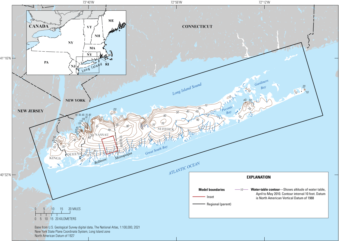
Location and hydrography of Long Island, regional (parent) and inset groundwater-flow model extents (Corson-Dosch and Fienen, 2023), and water-table altitudes in April–May 2010 on Long Island, New York. Modified from Walter and others (2020) and Monti and others (2013).
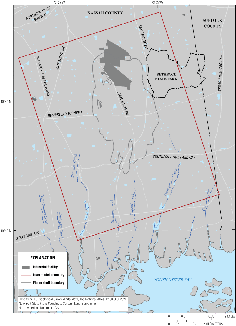
Inset groundwater-flow model extent (Corson-Dosch and Fienen, 2023), outline of plumes with concentrations of trichloroethylene (TCE) greater than the 5 micrograms per liter maximum contaminant level (U.S. Environmental Protection Agency, 2024), and other local features in southeastern Nassau County, New York. Plume shell outline from Daniel St. Germain (HDR Inc., written commun., 2022).
Further model development and refinement was needed for the NYSDEC to evaluate design options necessary for the construction, operation, optimization, maintenance, and monitoring of the remedy selected in the December 2019 Amended Record of Decision (New York State Department of Environmental Conservation, 2019). Consequently, the NYSDEC began a cooperative study with the USGS in 2020 to better understand the local hydrogeologic framework using two independent approaches to characterize aquifer heterogeneity and update an existing regional model to provide transient boundary conditions for new inset models (figs. 1 and 2) of the plume area. We developed these detailed inset models for the two independent aquifer-characterization approaches using history-matching techniques to inform prediction uncertainty coupled with a novel approach to risk-based optimization of the remedial design.
We also used the updated regional model to assess this optimized groundwater extraction and treatment design on the potential for landward encroachment of saline groundwater from south of the focus area. Study results are intended to be used to inform the design of the selected remedy and ultimately help the NYSDEC achieve several critical remedial goals including (1) halting further migration of VOC plumes from the NGBF and NWIRP sites, (2) preventing contamination from reaching unaffected drinking-water wells and reducing concentrations in currently impacted wells, (3) reducing the volume and contaminant concentrations within these VOC plumes, (4) protecting the Long Island sole-source aquifer and the region's water resources by returning treated water to the aquifer system, and (5) reducing the timeframe for cleaning up the VOC plumes (New York State Department of Environmental Conservation, 2019).
Purpose and Scope
The purpose of this report is to describe the results of a multipart study undertaken to further develop and refine models to evaluate design scenarios for groundwater extraction and treatment remediation of the Navy Grumman groundwater plume. Included in the report are an updated interpretation of the hydrogeologic framework with two independent characterizations of aquifer heterogeneity, an updated regional model providing transient boundary conditions for inset modeling of the plume area, new inset models for the two independent aquifer characterizations and risk-based optimization of the remedial design, and an updated regional model of freshwater/saltwater interface movement. This report also presents climatological, hydrological, and water-use data obtained between 2005 and 2019 to support development and application of the models (Corson-Dosch and Fienen, 2023).
We updated an existing regional groundwater-flow model of Long Island (Misut and others, 2024) and placed a finely discretized inset model of a portion of southeastern Nassau County within the more coarsely discretized regional model (fig. 1). This multiscale modeling approach allows the area near the plume to be simulated in finer detail than would be possible with the regional model but still establishes and maintains hydrologic connections to natural flow boundaries outside the inset area. A discussion of the limitations of the various modeling approaches used is included in this report. Representation of plume-source loading mechanisms, such as contaminant inflow from land surface, was beyond the scope of the study. Simulations described in this report do not characterize the historical development of any plume and represent only the conditions during the timeframe of the model history-matching period (2005–19).
Previous Investigations
Numerical models developed for the Long Island groundwater-flow system have been used by the USGS since the late 1960s to evaluate the availability and suitability of the island's groundwater resources (Schubert and others, 1997). A detailed timeline of the history of groundwater-flow model development in Nassau County through the 2010s is given in Misut (2011). Simulation of the groundwater-flow system of Nassau County began before the advent of digital computers through the experimental use of electric-analog models (Getzen, 1977). Smolensky and Feldman (1995) simulated groundwater-flow paths encompassing the NGBF and NWIRP area in cooperation with the Nassau County Health Department (NCHD) using the USGS model codes MODFLOW (McDonald and Harbaugh, 1988) and MODPATH (Pollock, 1994a, b).
At the time of the first MODFLOW analysis near the NGBF and NWIRP sites in 1995, groundwater flowed toward deep industrial pumping wells and away from surface-recharge basins where water captured by industrial wells was reintroduced. Use of an open-loop geothermal cooling system that included pumping wells and discharge to surface-recharge basins resulted in rearrangement and partial containment of a VOC plume, which was migrating in a generally southward direction at a rate of about 200 feet per year (ft/yr) as described by Smolensky and Feldman (1995).
Smolensky and Feldman (1995) also indicated that some groundwater upgradient from surface-recharge basins was drawn into the deep zones of industrial-well influence, but not captured, and ultimately discharged to the far-southern model boundary in the bottom part of the Magothy aquifer, near the contact with the underlying Raritan confining unit (refer to “Hydrogeologic Setting” section). From 1995 to the present (2023), consultants for the responsible parties developed a series of MODFLOW, MODPATH, and MT3D (Zheng, 1999) models that are generally consistent with the earlier USGS analyses but depict greater containment of VOCs upgradient from an onsite containment system and continued southward migration of VOCs downgradient from the onsite containment system (Arcadis G&M, Inc., 2009).
Particle-tracking analyses completed recently by USGS of partial (Misut, 2014, 2018) or complete (Misut and others, 2020) plume capture by pumping wells were in general agreement with previous studies. An analysis of total hydraulic-containment alternatives for the Navy Grumman groundwater plume began with the Naval Facilities Engineering Command (Tetra Tech, 2012) in 2011 and was continued by the NYSDEC (HDR Inc., 2019). The NYSDEC analysis was supported by USGS modeling of the effects of remedial scenarios on the movement of the Navy Grumman groundwater plume (Misut and others, 2020).
Misut and others (2020) also evaluated the effects of optimal plume-containment scenarios on streams and the location of the freshwater/saltwater interface along the south shore of Long Island. Further analyses were needed to comprehensively evaluate the effects of the hydraulic containment and post-treatment water-management system on the Navy Grumman groundwater plume and the potential hydraulic influences on surface waters, public-water supply wells, existing groundwater-recovery systems, and the potential for saltwater intrusion.
Description of the Study Area
Long Island is about 120 miles (mi) long, 25 mi across at its widest point, and 1,400 square miles (mi2) in total area. Long Island is bounded by Long Island Sound to the north, the Great Peconic Bay and Block Island Sound (not shown) to the east, the Atlantic Ocean to the south, and the East River (not shown) and the Upper New York Bay (not shown) to the west. The existing regional groundwater-flow model encompasses the entire four-county (Kings, Queens, Nassau, and Suffolk) area of Long Island (fig. 1). Inset models were developed for the local area encompassing the full extent of the Navy Grumman groundwater plume in southeastern Nassau County to represent two independent aquifer characterizations to help refine decision support for the remedial design. This inset area encompasses 36.2 mi2 and is bounded by South Oyster Bay to the south (fig. 2).
Hydrogeologic Setting
Land-surface altitudes on Long Island range from 0 feet (ft) above North American Vertical Datum of 1988 (NAVD 88) at the coast to more than 300 ft above NAVD 88 in some areas underlain by glacial moraines (fig. 3). The hummocky terrain associated with glacial moraines generally is bounded to the south by gently sloping outwash plains. Within the inset area, land-surface altitudes range from near sea level at the coast to more than 150 ft above mean sea level (MSL) in the northeastern part of the inset area.
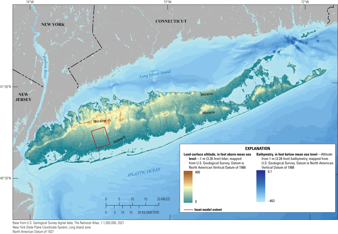
Inset model extent (Corson-Dosch and Fienen, 2023), and topography and bathymetry of Long Island, New York. Modified from Walter and others (2020). [m, meter; lidar, light detection and ranging]
The seven major hydrogeologic (and geologic) units on Long Island (fig. 4; Smolensky and others, 1990) are, in descending order, the upper glacial aquifer (Pleistocene deposits), Gardiners Clay (Gardiners Clay), Jameco aquifer (Jameco Gravel), Monmouth greensand (Monmouth Group, not shown in fig. 4), Magothy aquifer (Magothy Formation and Matawan Group, undifferentiated), Raritan confining unit (unnamed clay member of the Raritan Formation), and Lloyd aquifer (Lloyd Sand Member of the Raritan Formation). Within the inset area, the Jameco aquifer and Monmouth greensand are generally absent, and the Magothy aquifer is directly overlain by the upper glacial aquifer and (or) Gardiners Clay (in the southern-most portion). In addition to the major hydrogeologic units, other Pleistocene hydrogeologic units—the North Shore aquifer and North Shore confining unit (both of which are north of the study area)—underlie the upper glacial aquifer in some areas where Cretaceous hydrogeologic units are absent along the northern shore of the island (Stumm, 2001). Confining units occur locally within the upper glacial aquifer (Doriski and Wilde-Katz, 1982; Krulikas and Koszalka, 1982; Schubert and others, 2004).
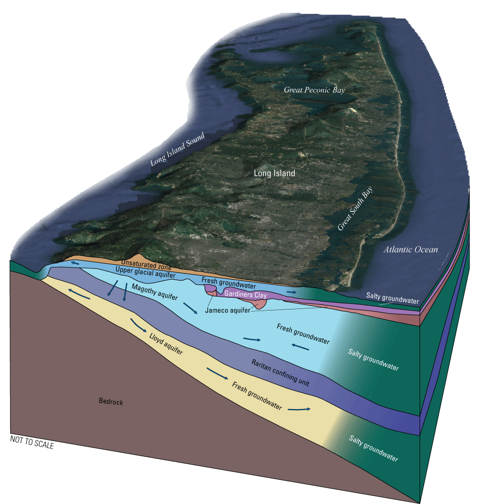
The major hydrogeologic units, generalized groundwater-flow directions, and general position of the freshwater/saltwater interface in the Long Island aquifer system, New York. From Walter and others (2020).
Recharge from precipitation is the sole source of natural water to the aquifer system. Long Island received an average of about 48 inches per year (in/yr) from 1900 to 2019; on average, about 48 percent (23 in/yr) recharges the aquifer at the water table (Finkelstein and others, 2022). Groundwater flows away from regional groundwater divides towards discharge at streams, coastal waters, and wells; some deep groundwater discharges upwards through confining units into salty groundwater (as subsea discharge) (fig. 4). Water-table altitudes exceed 60 ft in two areas—to the east and west of major surface-water drainages in the central part of Long Island (fig. 1). The western part of these two areas extends into the northern portion of the inset area. Water-table altitudes are also high locally in northern parts of Queens County, on necks and peninsulas in northern Nassau County, and in eastern Suffolk County (Walter and others, 2020).
The major aquifers are extensive, unconsolidated deposits that generally yield large quantities of water to wells. The most permeable units within this multilayered aquifer system consist predominantly of either sand or sand and gravel. The two regionally extensive clay units (the Gardiners Clay and Raritan confining units) have been estimated to have a vertical hydraulic conductivity (Kv) several orders of magnitude lower than that of the aquifers, and strongly restrict groundwater flow between the adjacent aquifers (Franke and Cohen, 1972). Where present, the two clay units separate the groundwater-flow system into three major aquifer assemblages: the upper glacial, Jameco, Magothy, and Lloyd aquifers (fig. 4). The Gardiners Clay impedes vertical flow between the upper glacial and Jameco and Magothy aquifers, predominately along the southern shore of the island including the inset area; the Raritan confining unit impedes vertical flow between the Jameco, Magothy and Lloyd aquifers in most areas of Long Island, including the inset area. The crystalline bedrock underlying the unconsolidated sediments is much less permeable, and the bedrock surface is considered the lower extent of the aquifer system.
This multilayered aquifer system is known for abundant water resources and groundwater-fed surface waters that harbor unique ecosystems. Surface runoff is negligible, and most precipitation recharges the aquifer at the water table in undeveloped areas. Recharge to the aquifer may be lower in developed areas owing to the interception of precipitation by impervious surfaces. The largest groundwater recharge deficits caused by impervious surfaces are in urbanized areas of New York City and southern Nassau County. However, much of the recharge potentially lost to impervious surfaces in Nassau County can recharge the aquifer through sumps, dry wells, and a network of more than 6,000 recharge basins (Walter and others, 2020).
Precipitation-derived groundwater is the sole source of drinking water for the residents of Nassau and Suffolk Counties and is the primary source of freshwater discharge to the numerous kettle-hole ponds, streams, and wetlands across Long Island and the inset area (fig. 1). Major streams in the inset area include Bellmore Creek and Massapequa Creek; minor streams include Carman Creek, Seaford Creek, Seamans Creek, Newbridge Creek, and Cedar Swamp Creek (fig. 2). These streams receive perennial (base) flow where their channels incise the water table, which only occurs in the southern part of the inset area. Because the channels are generally shallow, the low-lying areas surrounding these streams are vulnerable to flooding owing to the shallow depth to groundwater.
Population and Land Use
Long Island is densely populated and had an estimated population of about 8.1 million people in 2020 (U.S. Census Bureau, 2021). About 5 million people reside in Kings and Queens Counties, which constitute the New York City Boroughs of Brooklyn and Queens (not shown). The remaining population resides to the east, following a general west-to-east trend in land cover from highly developed areas in Nassau County to medium- and low-intensity developed areas in Suffolk County (Finkelstein and others, 2022).
Land use shows a similar pattern, generally transitioning from urban in the west to rural in the east, with densely urbanized landscapes in New York City and areas of undeveloped and agricultural land in eastern Suffolk County. Within the inset area, land use varies from urbanized in the southern and western parts to medium- and low-intensity developed areas in the northeastern part. More detailed information on population and land use across Long Island is presented in Finkelstein and others (2022).
Water Use
From 2005 to 2019, a total of about 424 million gallons per day (Mgal/d) of groundwater on average was withdrawn annually from the Long Island aquifer system for multiple uses, including public supply, agriculture, and industry (Walter and others, 2024). The public supply of drinking water accounted for nearly all (95 percent) of the total annual groundwater withdrawal on Long Island. About 34 Mgal/d of that total was withdrawn for public supply within the inset area. A total of about 8 Mgal/d of groundwater on average was withdrawn annually from the Long Island aquifer system for contaminant remediation during the same period (New York State Department of Environmental Conservation, 2020). This remedial pumping generally does not vary seasonally and has increased with time; all water is generally returned to the aquifer system after treatment. The vast majority (7.9 Mgal/d) of the total was withdrawn as part of Navy Grumman groundwater plume remediation within the inset area.
Hydrogeologic Framework
The Long Island aquifer system consists of unconsolidated Pleistocene and Cretaceous sediments that are underlain by somewhat impermeable crystalline bedrock. The altitude of the bedrock surface ranges from about 2,000 ft below NAVD 88 beneath Fire Island (not shown), a barrier island along the south-central part of Long Island (fig. 3), to near sea level along the East River (not shown) in northwestern Queens County, where there are small areas of bedrock outcrops (fig. 5) (Smolensky and others, 1990). The overlying Late Cretaceous sediments (older than about 66 million years before present) are part of the Northern Atlantic Coastal Plain regional aquifer system (Masterson and others, 2016) and are, in turn, generally overlain by Pleistocene sediments.
Pleistocene sediments were deposited largely during the Wisconsinan glaciation, when periods of ice advance and retreat formed morainal ridges that trend east to west along the spine of Long Island, and associated outwash plains generally to the south (Fuller, 1914; Cadwell and Muller, 1986). Locally extensive pre-Wisconsinan Pleistocene clay units lie within or beneath the glacial sediments and overlie Cretaceous sediments along the northern and southern shores of the island.

Inset area (Corson-Dosch and Fienen, 2023), extent of Cretaceous sediments, altitude of bedrock surface, and depth to water on Long Island, New York, in 2010. Modified from Walter and others (2020).
Long Island is bifurcated at the eastern end where two morainal ridges diverge to form the North and South Forks (fig. 3). The glacial moraines are bounded to the south by glacial outwash deposits and, generally, to the north by ice-contact deposits. The Pleistocene—glacial and nonglacial—sediments and the underlying Cretaceous units constitute a series of aquifers and confining units that is as thick as 2,000 ft on the southeastern-dipping bedrock surface. The Cretaceous units are absent in some areas near the northern shore of the island (fig. 5); Wisconsinan glacial sediments in these areas are either underlain by bedrock or by older (pre-Wisconsinan) Pleistocene glacial and nonglacial sediments. Pleistocene, coarse-grained (mainly sand and gravel) deposits on Long Island are commonly considered one hydrologic unit, which is referred to as the upper glacial aquifer (table 1).
Table 1.
Major hydrogeologic units of the Long Island aquifer system, New York.[From Stumm and others (2024). ft/d, foot per day; NMR, nuclear magnetic resonance]
Modification of Cretaceous Stratigraphy
Regional correlations between Long Island’s Cretaceous coastal plain sediments are based upon lithologic descriptions, core samples, pollen analyses, and gamma log patterns (Brown and others, 1972; Zapecza, 1989; Sirkin, 1986). The drill-core data and geophysical logs obtained by Stumm and others (2024) provide a basis for the naming of an additional Cretaceous hydrogeologic unit—the upper Raritan aquifer. More details about the information used to describe the upper Raritan aquifer and make this determination are provided in Stumm and others (2024). All other geologic and hydrologic unit names used in this report are those currently used by the USGS (Suter and others, 1949; Smolensky and others, 1990; Stumm, 2001; Stumm and others, 2002, 2004).
Upper Raritan Aquifer
The upper Raritan aquifer was introduced by Stumm and others (2024) to represent a unit of Cretaceous sediments that are part of the Raritan Formation present above the clay and silt of the Raritan confining unit and below the basal gravel of the Magothy aquifer in parts of western Long Island. The upper Raritan aquifer was initially identified by Stumm and others (2024) through analysis of high resolution (5-ft interval) core descriptions and gamma logs from a dense network of about 50 vertical profile borings drilled into the Raritan confining unit to help define the comingled plumes in southeastern Nassau County (fig. 6). The analysis indicated a substantial deviation of the top surface of the Raritan confining unit as compared to that in previously published maps (Suter and others, 1949; Smolensky and others, 1990). Dense clay beds clearly were absent in the upper part of the Raritan confining unit, indicating a possible facies or depositional change from fine- to coarse-grained lithologies in this part of the Raritan Formation.
The newly mapped upper part of the Raritan Formation is generally characterized by fine to coarse sand with silt and minor clay lenses below the Magothy aquifer’s basal gravel, whereas the Raritan confining unit has been previously described as consisting of dense clay and silt with small sand interbeds (Suter and others, 1949; Smolensky and others, 1990). Further analysis of hundreds of core descriptions and gamma logs in Kings, Queens, and Nassau Counties by Stumm and others (2024) indicated the upper Raritan aquifer extends throughout the southernmost parts of these counties. The aquifer also appears to extend throughout the central part of Nassau County (fig. 6) and may extend eastward into Suffolk County.
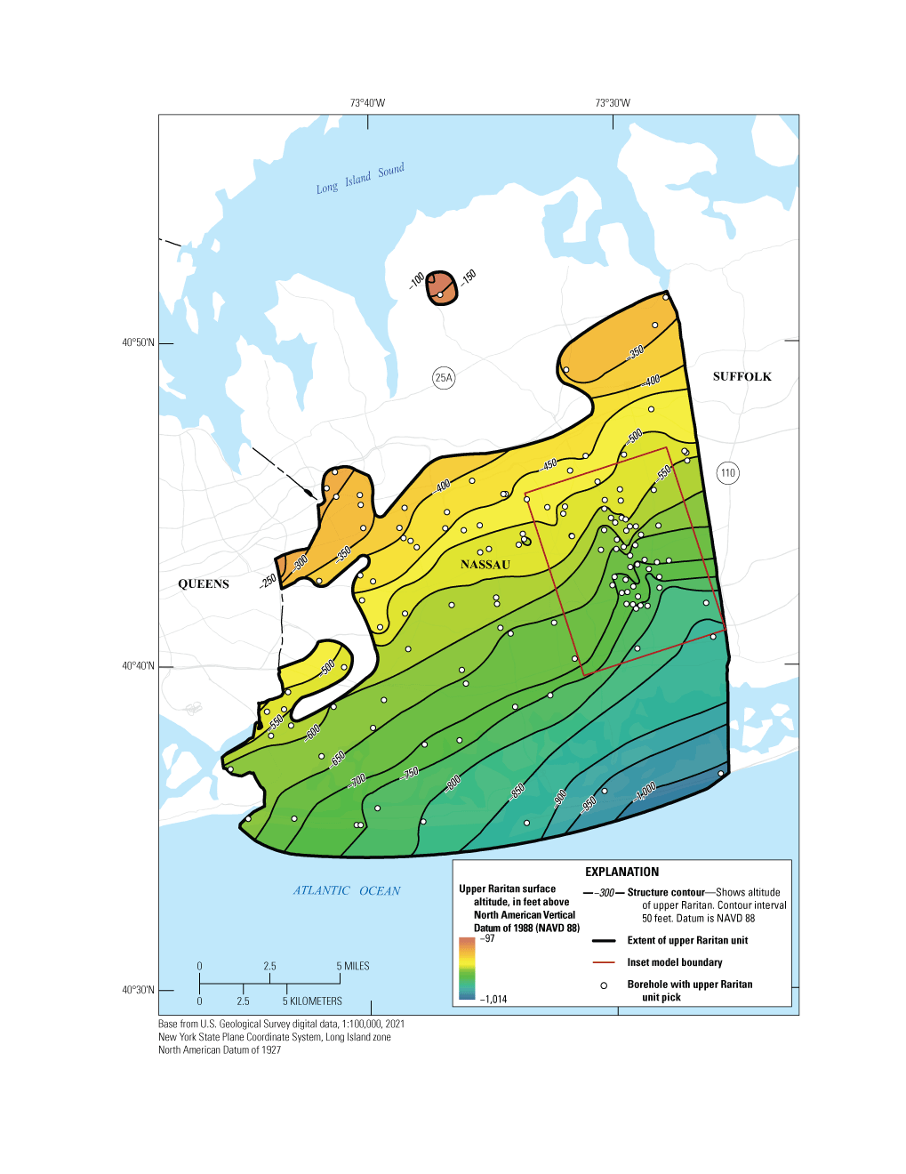
Inset area in relation to the surface altitude and extent of the upper Raritan aquifer underlying Nassau County, New York (Corson-Dosch and Fienen, 2023). Modified from Stumm and others (2024).
Raritan Confining Unit
The unnamed clay member of the Cretaceous Raritan Formation forms the Raritan confining unit (fig. 7), which underlies most of Nassau County (including the entire inset area) and dips to the southeast (Suter and others, 1949). The unit consists of dense clay and silt that are multicolored, including gray, white, red, and tan (Suter and others, 1949; Stumm, 2001; Stumm and others, 2002, 2004). The top of the Raritan confining unit was defined in Stumm and others (2024) and in this study by the presence of a dense clay and silt that is at least 20 ft in thickness based on core samples and gamma logs.
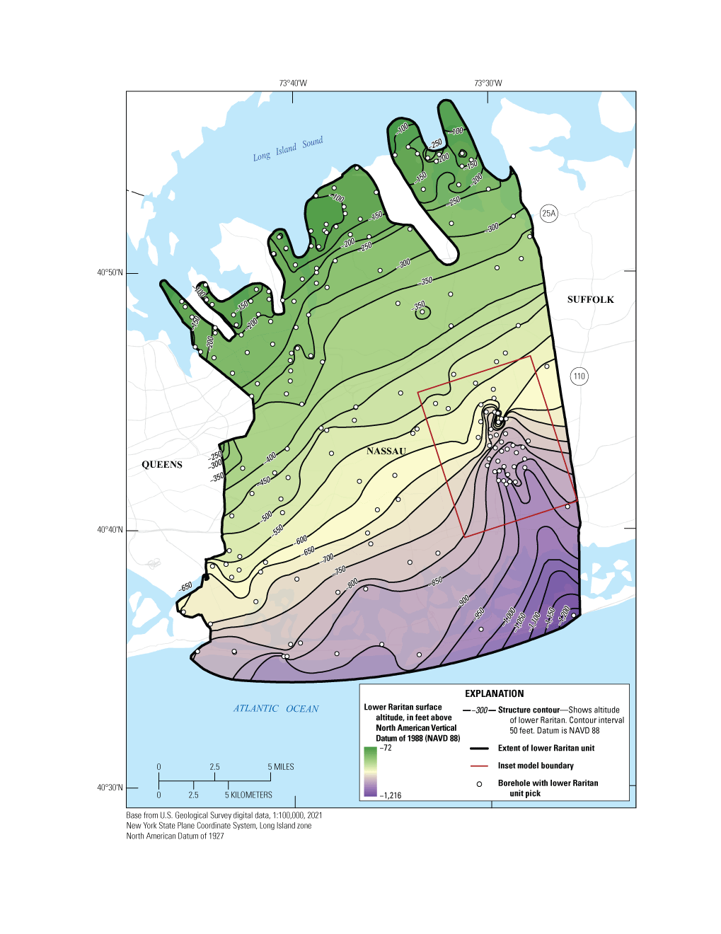
Inset model boundary, interpolation data, surface elevation, and extent of the Raritan confining unit underlying Nassau County, New York (Corson-Dosch and Fienen, 2023). Modified from Stumm and others (2024).
Distribution of Hydraulic Properties
Nuclear magnetic resonance (NMR) logs measure the induced magnetic moment of hydrogen protons contained within the fluid-filled pore space of porous media. Unlike other geophysical logs that respond to the rock matrix and fluid properties and are strongly dependent on mineralogy, NMR logs respond to the presence of hydrogen protons in the formation fluid to determine water content (equivalent to porosity in the saturated zone) and pore-size distribution (derived from bound versus mobile water) (Dlubac and others, 2013). NMR logs can be used to estimate vertically continuous porosity and hydraulic conductivity in the adjacent formation using equations and compilations of regressions determined from published collocated hydraulic tests of unconsolidated aquifers (Walsh and others, 2013; Knight and others, 2016; Kendrick and others, 2021).
NMR logs were collected from five deep groundwater monitoring wells in Nassau County (fig. 8) and were analyzed to determine clay-bound, capillary-bound, and mobile-water content or fraction and to estimate hydraulic conductivity of aquifers and confining units. More details about the collection and analysis of NMR logs from these wells, including the estimation of hydraulic properties using published co-located hydraulic tests, are provided in Stumm and others (2024).
Upper Glacial Aquifer
The upper glacial aquifer south of the glacial moraines consists predominantly of well-sorted outwash and is more hydraulically conductive than sediments north of the moraine where the aquifer consists of variably silty ice-contact deposits (fig. 9). The geometric mean horizontal hydraulic conductivity (Kh) estimated from 121 pumping tests in the glacial outwash was 200 feet per day (ft/d), whereas the geometric mean horizontal hydraulic conductivity estimated from 22 pumping tests north of the moraine was 120 ft/d (Stumm and others, 2024). The total porosity outwash (south of the moraine) ranged from 30 to 40 percent based on laboratory analysis of several hundred samples from southern Long Island reported by Veatch and others (1906).
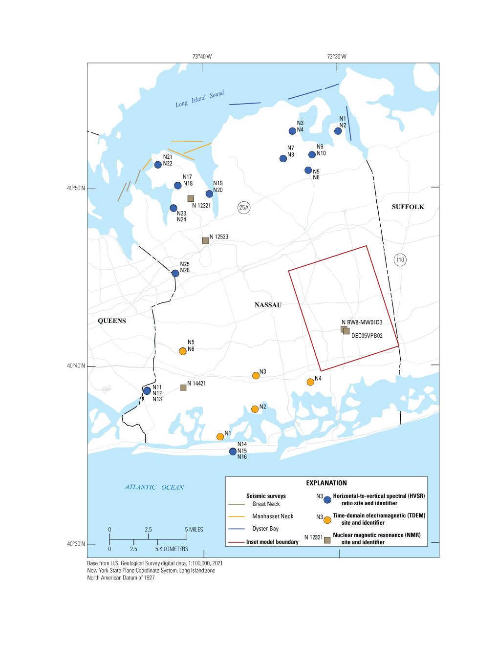
Inset area and location of nuclear magnetic resonance logging sites in Nassau County, New York (Corson-Dosch and Fienen, 2023). Modified from Stumm and others (2024).
Magothy Aquifer
The geometric mean Kh of the Magothy aquifer estimated from 35 pumping tests was 120 ft/d (Stumm and others, 2024). The geometric mean Kh estimated from the NMR logs of monitoring wells N 12523, N 14421, DEC-HC05-VPB02 (Pollen well), and N RW8-MW01D3 (fig. 8) was 140, 81, 88, and 110 ft/d, respectively (U.S. Geological Survey, 2022a, 2022b, 2022c). The geometric mean Kh ranged from a low of 0.33 ft/d for finer-grained intervals to a high of 590 ft/d for coarse-grained intervals. The mean total porosities of the Magothy aquifer estimated from the NMR logs of the four wells were 0.33, 0.38, 0.38, and 0.38, respectively (Stumm and others, 2024). The estimated mean mobile-water fractions of the Magothy aquifer in the four wells were 0.26, 0.24, 0.25, and 0.28, respectively. The mean mobile and bound water fractions for coarser-grained intervals were 0.34 and 0.03, whereas the mean mobile and bound water fractions for finer-grained intervals were 0.02 and 0.38, respectively.
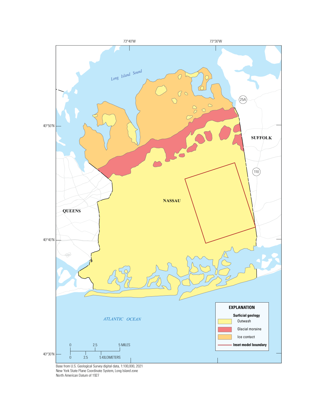
Inset area in relation to the surficial geology of Nassau County, New York (Corson-Dosch and Fienen, 2023). Modified from Stumm and others (2024).
Upper Raritan Aquifer
The geometric mean Kh estimated from the NMR logs of the upper Raritan aquifer penetrated by monitoring wells N 14421, DEC-HC05-VPB02 (Pollen well), and N RW8-MW01D3 (fig. 8) was 110, 100, and 40 ft/d, respectively, suggesting that the aquifer has similar Kh values to those of the upper parts of the Magothy aquifer (U.S. Geological Survey, 2022a, 2022b, 2022c; Stumm and others, 2024). In the upper Raritan aquifer, the geometric mean Kh values were as low as about 2 ft/d for finer-grained intervals and exceeded 350 ft/d in some coarser-grained intervals. The mean total porosities of the upper Raritan aquifer estimated from the NMR logs of monitoring wells N 14421, DEC-HC05-VPB02 (Pollen well), and N RW8-MW01D3 were 0.34, 0.33, and 0.28, respectively (Stumm and others, 2024). The estimated mean mobile-water fractions of the upper Raritan aquifer in the three wells were 0.26, 0.24, and 0.18, respectively. The mean mobile and bound water fractions for coarse-grained intervals were 0.34 and 0.03, whereas the mean mobile and bound water fractions for a fine-grained interval were 0.03 and 0.33.
Raritan Confining Unit
The geometric mean Kh of the clay and silt of the Raritan confining unit estimated from the NMR log of well N 12523 (fig. 8) was 0.30 ft/d (U.S. Geological Survey, 2022a, 2022b, 2022c; Stumm and others, 2024). The geometric mean Kh of a portion of the Raritan confining unit dominated by a silt and sand interval and a clay and silt interval estimated from the NMR log of well N 14421 (fig. 8) were 9.9 and 0.12 ft/d, respectively (Stumm and others, 2024). The total porosities of the Raritan confining unit clay and silt intervals estimated from the NMR logs of wells N 12523 and N 14421 averaged 0.28 and their bound water fractions averaged 0.26 and 0.27, respectively (Stumm and others, 2024). The silt and sand interval in N 14421 had a mean estimated total porosity of 0.32 and mean bound water fraction of 0.17.
Aquifer Characteristics
A large amount of lithologic data on the Long Island aquifer system has been collected as part of water-supply exploration and remedial investigations. The quality of these data varies, but when considered together, and in sufficient numbers, the data can be used to gain insight into the distribution of important aquifer characteristics such as hydraulic properties (Walter and Finkelstein, 2020).
Texture Model of the Upper Glacial and Magothy Aquifers
We completed a detailed characterization of lithologic descriptions and the conversion of these qualitative data to more quantitative measures of important hydrogeologic characteristics for the upper glacial and Magothy aquifers. This detailed analysis was centered on the inset area and included the development of a local-scale model of changes in sediment characteristics referred to herein as a “texture model.” This analytical approach generally followed the one used by Walter and Finkelstein (2020) to develop a model of changes in the sediment distribution correlated to changes in hydraulic conductivity for the entire Long Island aquifer system.
Lithologic Data Analysis
We generally followed the analytical approach of Walter and Finkelstein (2020) with 22,523 lithologic descriptions from 256 boreholes in the inset area (fig. 10) to define standard lithologic codes (table 1 in Walter and Finkelstein, 2020) for each vertical interval in each borehole. These coded intervals were assigned values of Kh and Kv from previous investigations (Walter and Finkelstein, 2020) and were assigned a binary variable representing the presence or absence of silt and clay. Each borehole was divided into 10-ft lengths, and mean hydraulic conductivity values were calculated for each interval; values in each 10-ft layer represented a thickness-weighted mean horizontal and geometric mean vertical calculated from all lithologic intervals coincident with the layer. These borehole descriptions were compiled into a geographic information system database containing borehole locations and mean hydraulic conductivity values.
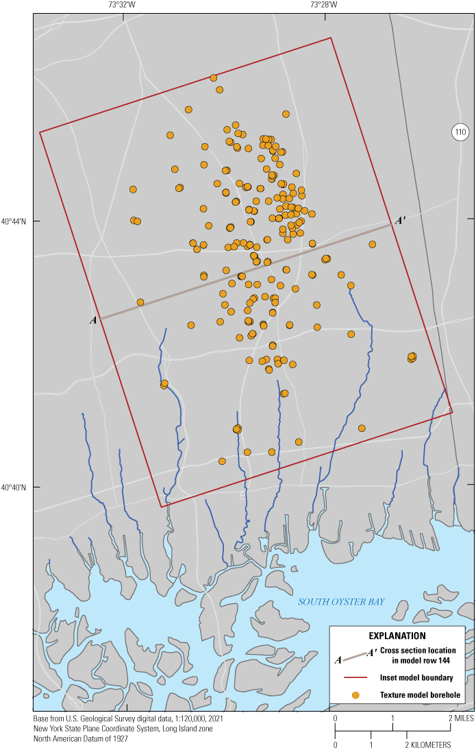
Location of boreholes used in the estimation of vertical and horizontal hydraulic conductivity for the inset area (Corson-Dosch and Fienen, 2023), southeastern Nassau County, New York.
Texture Model Development
Following the methods of Walter and Finkelstein (2020), stacked grids of Kh and Kv were created, each representing 10 ft of aquifer thickness spanning the upper glacial and Magothy aquifers in the inset area (fig. 11). Grids representing the upper glacial aquifer were horizontal, whereas those representing the Magothy aquifer were sloping and were draped onto a surface representing the bottom of the unit (fig. 11). A single grid represented the hydraulic conductivity over the full thickness of the upper Raritan aquifer (fig. 11).
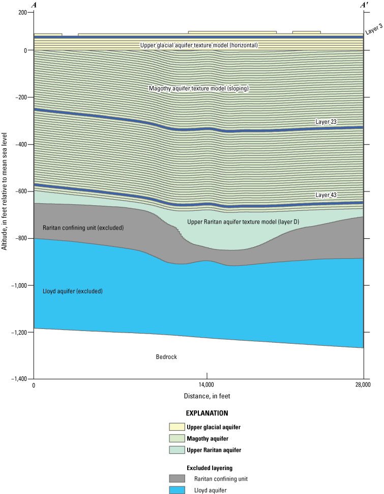
Vertical design of quasi-three-dimensional grids for the upper glacial (horizontal), Magothy (sloping), and upper Raritan aquifer texture models along an east–west section in the inset area (Corson-Dosch and Fienen, 2023), southeastern Nassau County, New York. Location of east–west section shown in figure 10.
We queried a geographic information system database (Walter and Finkelstein, 2020) to extract those boreholes that extended to or beyond each successive grid. These queried subsets of data points were used to interpolate values of Kh and Kv by use of ordinary, spherical kriging. The vertical stack of interpolated grids constitutes a quasi-three-dimensional texture model of each hydrogeologic unit (fig. 12) that, when combined, form a detailed representation of the principal aquifer system of the inset area (fig. 13).
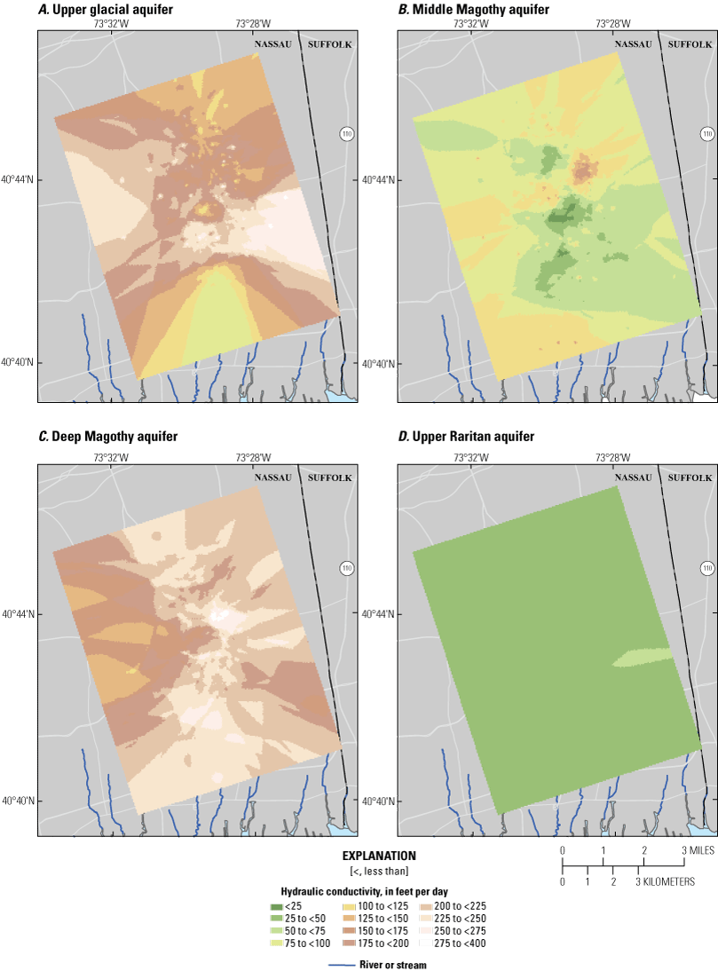
Interpolated horizontal hydraulic conductivity in the inset area (Corson-Dosch and Fienen, 2023), southeastern Nassau County, New York. A, Upper glacial aquifer. B, Middle Magothy aquifer. C, Deep Magothy aquifer. D, Upper Raritan aquifer. Vertical position of layers A–D shown in figure 11.
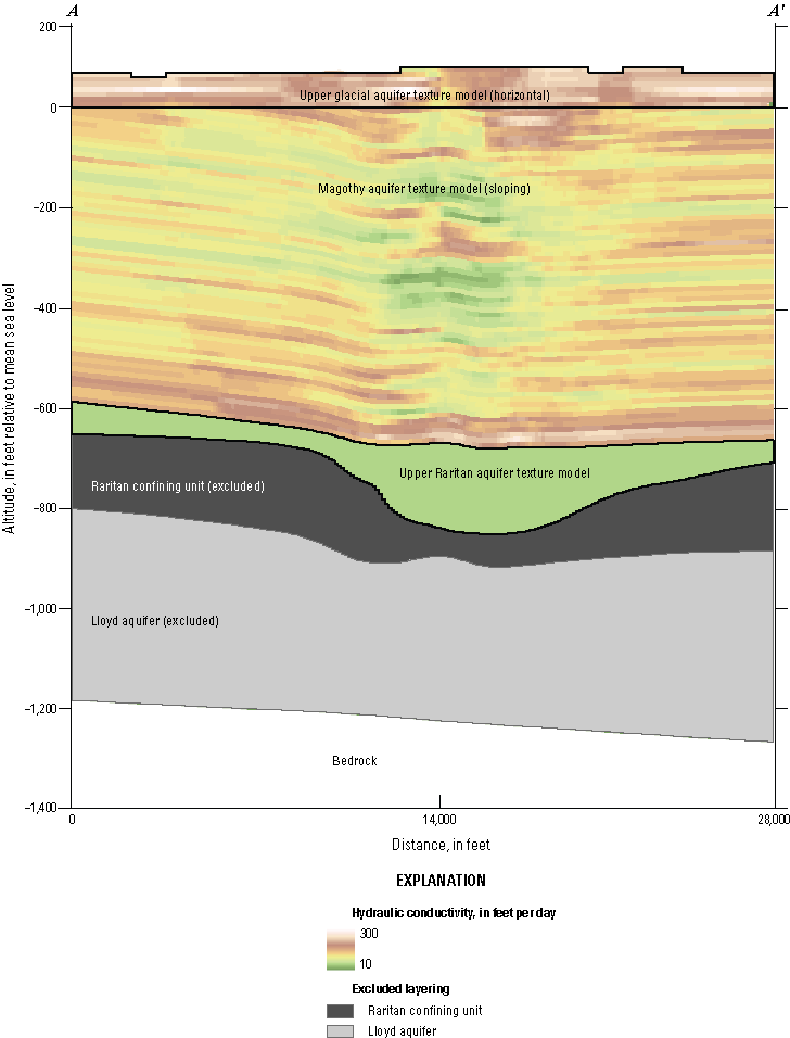
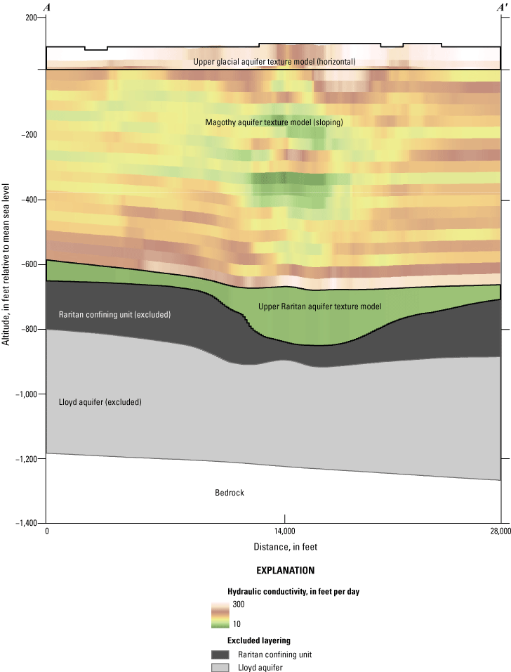
Vertical distribution of estimated horizontal hydraulic conductivity along an east–west section in the inset area (Corson-Dosch and Fienen, 2023), southeastern Nassau County, New York. Location of east–west section shown in figure 10.
Distribution of Hydraulic Conductivity
We modeled Kh and Kv, both important controls on groundwater flow, following the methods of Walter and Finkelstein (2020). The spatial and vertical patterns in Kh within the inset area (figs. 11–13) generally are consistent with the depositional history of the regional aquifer system.
Values of hydraulic conductivity in the upper glacial aquifer generally are lower in northern parts of the inset area and are associated with glacial moraines (fig. 12A). Hydraulic conductivity is highest in outwash sediments south of the moraine (fig. 12A). Outwash sediments consist largely of well-sorted sand; moraine sediments generally consist of fine-grained and poorly sorted sediments. In addition, the glacial sediments generally become finer with depth (figs. 13 and 14).
The Magothy aquifer within the inset area is more heterogenous than the upper glacial aquifer, with fewer broad spatial patterns, except in its basal portion. Hydraulic conductivity in the basal portion of the Magothy aquifer (fig. 12C), where sediments likely were deposited in fluvial depositional environments, generally is higher than in overlying portions of the unit (figs. 12B and C). Hydraulic conductivity values generally are lowest in the middle part of the Magothy aquifer (fig. 12B) where fine-grained sands and silts with interbedded clay lenses likely were deposited in overbank lake and wetland environments.
Vertical distribution of estimated horizontal hydraulic conductivity as mapped to the inset model grid along an east–west section, resampled to the model grid and layers (Corson-Dosch and Fienen, 2023), southeastern Nassau County, New York. Location of east–west section shown in figure 10.
Geostatistical Analysis of Aquifer Heterogeneity
Transition probability geostatistics (Carle, 1999) were used to generate multiple equally probable interpretations of aquifer heterogeneity conditioned to borehole data (New York State Department of Environmental Conservation, 2024a, 2024b51). We used the Transition Probability Geostatistical Software (T–PROGS) in Aquaveo’s Groundwater Modeling System (GMS), which is a pre- and post-processing software package for building models and simulating groundwater processes (Aquaveo, LLC, 2021). This geostatistical analysis resulted in 500 T–PROGS realizations of the hydrostratigraphy using the same input structure in a Monte Carlo-type analysis to explore aquifer heterogeneity as part of the groundwater modeling component of this investigation.
T–PROGS allows for the implementation of a Transition Probability and Markov Chain approach to geostatistical simulation of category-based variables (for example, geologic units, facies). This implementation involves three main steps (Carle, 1999):
-
1. calculation of transition probability,
-
2. modeling spatial variability with Markov chains, and
-
3. conditional simulation.
Each of these steps are accomplished by the following programs:
-
• GAMEAS: computes bivariate statistics (for example, transition probability, indicator cross-variogram, and so forth).
-
• MCMOD: develops one- and three-dimensional Markov chain models of spatial variability.
-
• TSIM: generates three-dimensional, cross-correlated conditional simulations (Carle, 1999).
In comparison to traditional variogram-based geostatistical methods, the Transition Probability and Markov Chain approach has the potential to improve spatial cross-correlations and can help with the integration of geologic interpretation of facies into the model development process (Carle, 1999).
Transition Probability Approach
The transition probability approach was developed to better describe the relation between observable features and model parameters. The transition probability measures the spatial variability (for example, given that a facies j is present at a location x, what is the probability that another [or the same] facies k occurs at location x+h). The approach can consider all cross-correlation information in three dimensions instead of just two dimensions (Carle, 1999).
Markov Chain Analysis
Markov chains are generated to represent the spatial variability seen from the observed transition probabilities and where the mean length and the proportions of the facies are identified. This assumes that the spatial occurrences depend only on the nearest data. The Markov chains are then used as a reference for the conditional simulation (Carle, 1999).
Conditional Simulation
The conditional simulation creates multiple equally probable spatial distributions of random geostatistical realizations that closely match the hard data at specified locations and exhibit a realistic pattern of spatial variability (Deutsch and Journel, 1992). There needs to be an understanding of the available data and the appropriate stratigraphic relations and spatial variability to produce a plausible representation in a geostatistical realization. These conditional simulations provide an example of geologic heterogeneity and (or) hydraulic properties distribution for flow and transport modeling and can be used to develop realistic aquifer system models to evaluate effects of heterogeneity on groundwater flow and contaminant transport (Carle, 1999).
Sediment Categories
A boring log is a description of the subsurface lithology and hydrogeologic conditions encountered during drilling, sampling, and coring. A total of 256 boring logs, the same as those used to develop the texture model, were described over a span of 20 years at and surrounding the NWIRP and NGBF sites. Variability in the description of encountered materials owing to the length of drilling history and the numerous geologists overseeing the coring had to be accounted for when compiling the boring logs into a database for the T–PROGS analyses. Each log was transcribed into a uniform format and nomenclature that included the following:
-
• Boring identification number
-
• Coordinates
-
• Start and end depth for each lithologic entry
-
• Material type (that is, clayey sand and poorly graded sand)
-
• Remark-1 (Material description)
-
• Remark-2 (Adjustments needed based on material description and gamma logs)
-
• Hydrogeologic unit
The sediment type, sediment description, and gamma log (if available) of each boring log entry were compared to verify the sediment type originally provided by the logger. If the material type entered was inconsistent with the sediment description or gamma log, it was adjusted and noted in Remark-2. This verification provided a framework to assess each log and reduce inconsistencies among loggers.
Input for the T–PROGS simulation used a master dictionary created from the boring log database of the boring log sediment types. For each log description, the entry was assigned to a lithologic category:
We assigned a value of 1, 2, 3, or 4 to these categories to represent their material identifier (table 2). Material identifiers were then brought into GMS and used as the input for the T–PROGS simulations.
Table 2.
Sediment type, horizontal hydraulic conductivity, and example descriptions used in Transition Probability Geostatistical Software (T–PROGS; Carle, 1999; Aquaveo, LLC, 2021) analysis of the aquifer system of southeastern Nassau County, New York.[ID, identifier; Kh, horizontal hydraulic conductivity (Bureau of Reclamation, 1977)]
Simulation Descriptions
T–PROGS was used to generate multiple equally probable models of aquifer heterogeneity all conditioned to the 256 boring logs. The goal was to create multiple material sets that support the stratigraphic framework of the groundwater model.
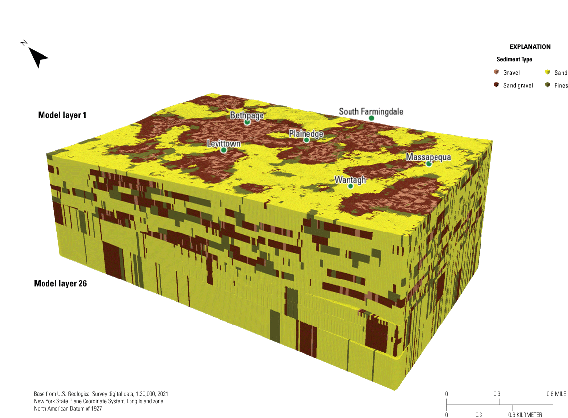
A three-dimensional grid was set up in GMS with 288 rows, 224 columns, and 26 layers to be coincident with the inset models (table 3, fig. 15). There are 256 boring logs with 22,838 individual intervals described that constitute the framework for the T–PROGS simulation. Each interval was assigned one of four categories (gravel, sand and gravel, sand, or fines; as described previously in the “Sediment Categories” section).
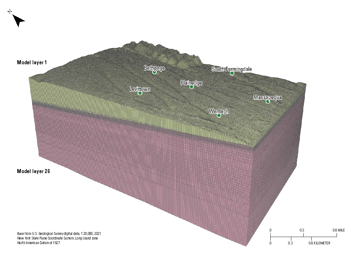
Grid used in Transition Probability Geostatistical Software (T–PROGS; Carle, 1999; Aquaveo, LLC, 2021) simulation of the aquifer system in the inset area (Corson-Dosch and Fienen, 2023), southeastern Nassau County, New York. Grid properties are presented in table 3.
Table 3.
Grid properties used in Transition Probability Geostatistical Software (T–PROGS; Carle, 1999; Aquaveo, LLC, 2021) analysis of the aquifer system of southeastern Nassau County, New York.The most important step when running T–PROGS is defining the transition probability data for each material in the three primary directions: vertical, strike, and dip. The vertical transition is developed first based on the borehole data. The data in the strike and dip directions are then derived from the vertical data (Carle, 1999). The distribution of the boring logs within the grid shell, the vertical extent of the boring logs, and the sediment types within each boring log are shown in figure 16. Sand is the most prevalent category with a distribution percentage of 60 percent (table 4, fig. 16). Sand and gravel (fig. 16) is the second most dominant sediment type with a distribution percentage of 24 percent. Sand and sand and gravel combined account for 84 percent of the total sediment types within the boring logs. Gravel and fines make up a distribution percentage of 5 and 11 percent, respectively. These sediment type distribution percentages were similar for each potential geostatistical realization computed by T–PROGS.
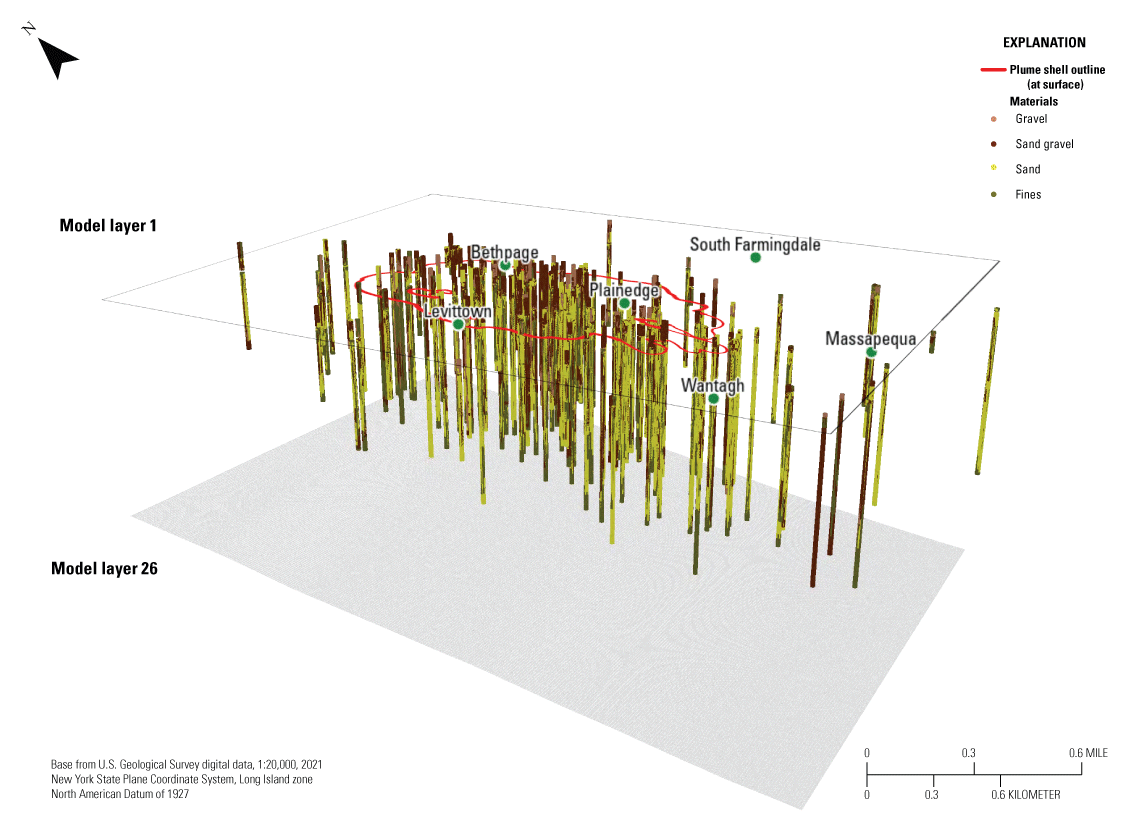
Grid shell with boring logs and material distributions used in Transition Probability Geostatistical Software (T–PROGS; Carle, 1999; Aquaveo, LLC, 2021) analysis of the aquifer system in the inset area (Corson-Dosch and Fienen, 2023), southeastern Nassau County, New York. Materials are described in table 2. Grid properties are presented in table 3.
Table 4.
Total percent material distribution for Transition Probability Geostatistical Software (T–PROGS; Carle, 1999; Aquaveo, LLC, 2021) analysis of the aquifer system of southeastern Nassau County, New York.[ID, identifier; materials are described in table 2]
Prior to creating a geostatistical realization, the GAMEAS utility was used to compute a set of transition probability curves as a function of lag distance for each material for a given sampling interval (Carle, 1999). Using a lag spacing of 0.3 ft, a maximum lag distance of 450 ft was computed, meaning the greatest distance a material correlates horizontally is 450 ft. In addition, the transition probability for each material with respect to each of the other materials is calculated and displayed graphically (fig. 17).
The probability is shown on each plot on the y-axis from 0 to 1, and the correlation distance on the x-axis (0 to 450; fig. 17). The top right graph indicates that there is very low probability to transition from gravel to fines throughout the 450-ft distance. The upper left plot indicates that there is a high probability of gravel adjacent to gravel at close distances and then the probability rapidly declines with distance. The goal of this portion of the analysis is to closely fit the Markov chain to the measured transition probability curve. The embedded transition probabilities derived from the calculated transition probability plots (fig. 17) are shown in table 5.
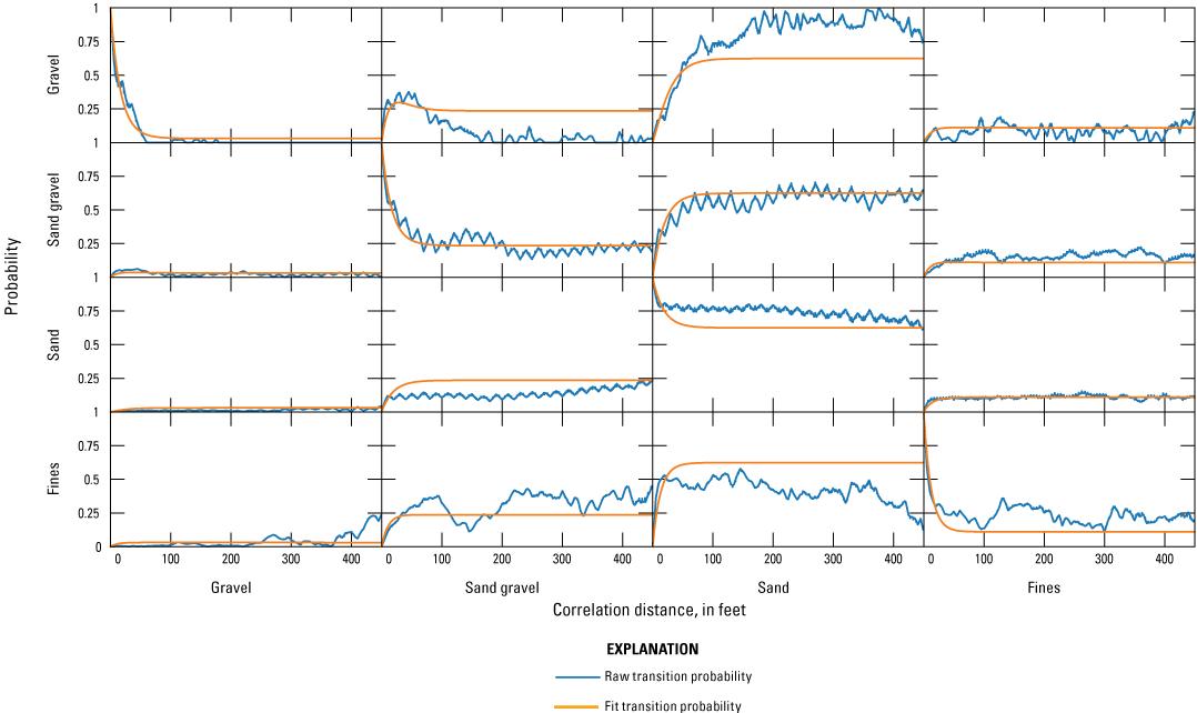
Transition probability plots for each material set in the Transition Probability Geostatistical Software (T–PROGS; Carle, 1999; Aquaveo, LLC, 2021) analysis of the aquifer system in the inset area (Corson-Dosch and Fienen, 2023), southeastern Nassau County, New York. Materials are described in table 2.
Table 5.
Embedded transition probability matrix calculated from Transition Probability Geostatistical Software (T–PROGS; Carle, 1999; Aquaveo, LLC, 2021) analysis of the aquifer system of southeastern Nassau County, New York, for the data used to generate the transition probability plots shown in figure 17 of this report (New York State Department of Environmental Conservation, 2024a, 2024b51).[Materials are described in table 2]
The next step in generating a realization is to define the Markov chains in the strike and dip directions. We applied Walther’s Law (Carle, 1999) to estimate the strike and dip Markov chains because borehole data in these directions are not sufficiently dense to calculate them in the same way as vertically. Walther’s Law states that vertical successions of deposited facies represent the lateral succession of environments of deposition. An assumption is made that the proportions are the same in all three directions. The lens length ratio is used to define the transition rate matrix with the diagonal transition rates defined from the lens lengths. These ratios calculate the lens length in the horizontal (strike and dip) directions based on the observed lens length in the vertical direction.
We used a trial-and-error method for determining the lens length ratios in the strike and dip directions to allow for appropriate connectivity between the borings (table 6). Different values were used for each sediment type in the lens length ratio and an example realization was created. This process was repeated until a realization was produced by T–PROGS that compared reasonably with the cross-sections interpreted by other methods, the borings, and knowledge of Long Island hydrogeology (Walter and Finkelstein, 2020). An orthogonal view of an example realization produced from the final lens length ratios used in the strike and dip directions is shown in figure 18.
Table 6.
Lens length ratios for strike and dip used in Transition Probability Geostatistical Software (T–PROGS; Carle, 1999; Aquaveo, LLC, 2021) analysis of the aquifer system of southeastern Nassau County, New York.[Materials are described in table 2]
Example realization for Transition Probability Geostatistical Software (T–PROGS; Carle, 1999; Aquaveo, LLC, 2021) analysis of the aquifer system of southeastern Nassau County, New York (Corson-Dosch and Fienen, 2023). Materials are described in table 2. Grid properties are presented in table 3.
Once the final lens length ratios were determined, T–PROGS was used to create 500 realizations based on the same input structure in a Monte Carlo type analysis. These 500 realizations were then used in the inset area groundwater-flow model to determine the potential range of, and most likely plume path based on, interpolated preferential flow paths.
Final Realizations
T–PROGS was run 500 times after a realization that compared reasonably to the data, cross-section, and knowledge of Long Island’s hydrogeology was created. These 500 realizations all held true to the boring logs at their locations and were interpolated in the vertical, strike, and dip between boring locations using the already determined transition probabilities and Markov chains. Six realization examples and the corresponding sediment type distributions for each example are shown in figures 19 and 20. Each realization varies slightly; however, the percent distributions remain consistent with the material distributions in the boring logs.
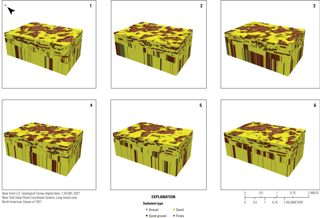
Example of six of the final realizations for Transition Probability Geostatistical Software (T–PROGS; Carle, 1999; Aquaveo, LLC, 2021) analysis of the aquifer system in the inset area (Corson-Dosch and Fienen, 2023), southeastern Nassau County, New York. Materials are described in table 2. Grid properties are presented in table 3.
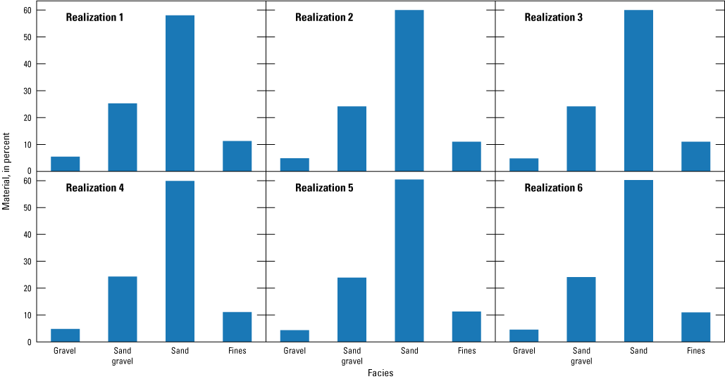
Material distributions from the corresponding realizations in figure 19 for Transition Probability Geostatistical Software (T–PROGS; Carle, 1999; Aquaveo, LLC, 2021) analysis of the aquifer system in the inset area (Corson-Dosch and Fienen, 2023), southeastern Nassau County, New York. Materials are described in table 2. The total may not equal the sum of values because of rounding to significant digits.
One of the 500 potential realizations shows channels of gravel and sand-gravel that stretch throughout the grid as would be expected in a deltaic deposit highlighting the preferential pathways that the plume at the NWIRP and NGBF sites could potentially follow (fig. 21). The areas between isosurfaces are areas of lower hydraulic conductivity and therefore are not considered preferential flow paths.
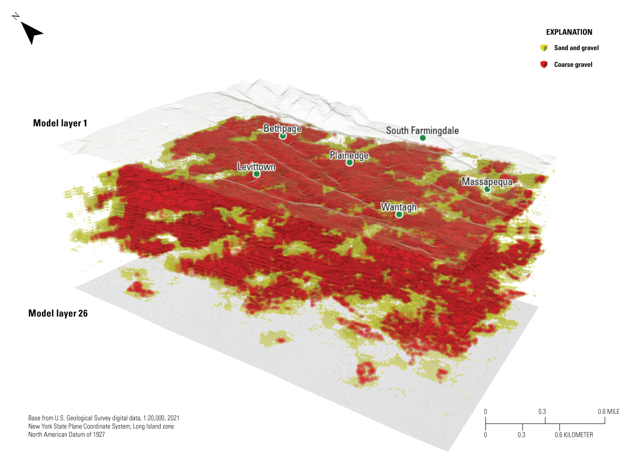
Preferential pathways (channels of higher hydraulic conductivity) a plume could potentially follow in 1 of the 500 final potential realizations for Transition Probability Geostatistical Software (T–PROGS; Carle, 1999; Aquaveo, LLC, 2021) analysis of the aquifer system in the inset area (Corson-Dosch and Fienen, 2023), southeastern Nassau County, New York. Grid properties are presented in table 3.
The T–PROGS realization is constrained by the location of the boring log information. Beyond the grid (fig. 16), the results are no longer as constrained because there are no borings for T–PROGS to use to guide the realization. The realization beyond the boundary of the existing borings is extrapolated from the boring information using the Markov chains and distribution percentages. Overall, the final compiled realizations match the boring logs closely and represent the known geology of the area.
Simulation of Monthly Changes in Regional Groundwater Pumping and Recharge
We updated the steady state Long Island Regional Model (LIRM; Walter and others, 2020) to run in the MODFLOW 6 code (Langevin and others, 2017) and converted it from a steady state to a transient model to simulate changes in monthly stresses from 2005 to 2019. Monthly hydrologic stresses from January 2005 through December 2019 were assembled for model inputs representing groundwater recharge and groundwater withdrawals, following the methods described in Walter and others (2020). Additionally, we incorporated existing remedial groundwater extraction and returned treated water at specific locations in southeastern Nassau County. Other than incorporating monthly hydrologic stresses (groundwater recharge and withdrawals) and aquifer storage properties, no modifications were made to the hydrologic boundaries, model layers, or hydraulic properties specified in the model described in Walter and others (2020). In this report, the term “transient LIRM” refers to the transient, updated version of the LIRM model.
Conversion from Steady State to Transient Simulations
The transient LIRM (Walter and others, 2020) simulates long-term steady-state conditions for the 2005–15 period and does not simulate transient changes in hydraulic head and groundwater flow. Monthly values for natural recharge from precipitation were calculated using a soil-water balance (SWB) model code to estimate spatially variable, natural recharge for Long Island (Finkelstein and others, 2022). Components of anthropogenic recharge—wastewater return flow, stormwater inflow, and inflow from leaky infrastructure—also were estimated for monthly stress periods for the simulation period 2005–19, which is consistent with the methods described in Walter and others (2020).
We compiled or estimated monthly groundwater withdrawals for various sources, including public-water supply, industrial, remediation, and agricultural uses, for the same period. No additional parameter estimation was completed for this scenario. Model properties and hydrologic boundaries were not adjusted to improve the match between simulated and observed heads; as such, model simulation results may not accurately represent the temporal responses to monthly hydrologic stresses in some locations. The input and output files used to run the updated transient LIRM are available in a USGS data release (Misut and others, 2024). The model archive is also available in a USGS data release (Corson-Dosch and Fienen, 2023).
Transient Recharge
We estimated recharge for each month from January 2005 through December 2019. Recharge components included natural and redirected recharge, return flow, and leakage from water-supply infrastructure. These recharge components were combined to estimate the total monthly recharge for the 2005–19 period.
Natural and Redirected Recharge
Finkelstein and others (2022) used the SWB model (Westenbroek and others, 2010) to estimate natural and redirected groundwater recharge for the Long Island aquifer system. Monthly recharge generally follows a seasonal cycle with most of the recharge occurring during the nongrowing season (fig. 22). Anomalies include Tropical Storm Tammy, which added significant recharge during October 2005; the wet summer of 2006; and a March 2010 Nor’easter (Finkelstein and others, 2022). Tropical Storm Tammy resulted in about a sixfold increase in the monthly mean recharge rate, and the March 2010 Nor’easter resulted in about a fourfold increase in this rate.
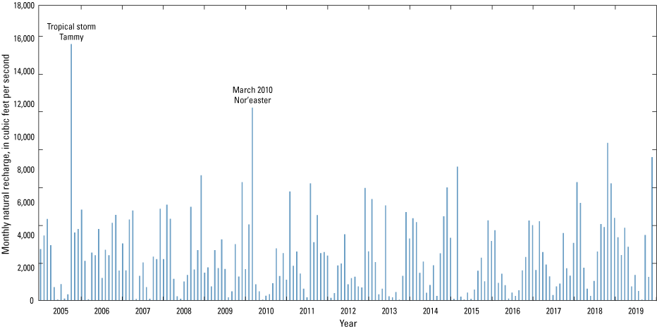
Monthly natural recharge applied to the model, 2005 to 2019, Long Island, New York (Corson-Dosch and Fienen, 2023).
In the more urbanized areas of Long Island, impervious surfaces intercept precipitation, resulting in less aquifer recharge as compared to predevelopment (prior to 1900 in Nassau County) conditions. The largest recharge deficits attributed to interception from impervious surfaces occur in the urbanized areas of New York City and southern Nassau County; however, much of the recharge potentially lost to impervious surfaces in Nassau County can recharge the aquifer through sumps, dry wells, and a network of more than 6,000 recharge basins (Walter and others, 2020).
Monthly estimates of redirected recharge from impervious surfaces were computed by subtracting SWB computations of the steady-state predevelopment condition from the 2005 to 2019 condition, resulting in a total redirected recharge of about 3 percent of natural recharge under present conditions (Finkelstein and others, 2022). The temporal pattern of redirected recharge (fig. 23) is like that of natural recharge (fig. 22) because of the correlation of predevelopment and 2005–19 conditions recharge with seasonal patterns of precipitation. In addition to Tropical Storm Tammy and the March 2010 Nor’easter, the Halloween Nor’easter of October 2011 also generated notable redirected recharge volume.
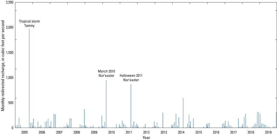
Monthly redirected recharge applied to model, 2005–19, Long Island, New York (Corson-Dosch and Fienen, 2023).
Wastewater Return Flow
We estimated wastewater return flow using population density derived from the 2010 census in conjunction with annual water use (Walter and others, 2020). About 85 percent of public-supply water use on Long Island is returned annually as wastewater return flow to the aquifer system by way of onsite domestic septic systems and constitutes a spatially and temporally distributed supplemental recharge. In areas served by public sewering, we assumed that 1 percent of wastewater recharged the aquifer from leaky sanitary sewer lines (Walter and others, 2020). Wastewater return flow was about 5 percent of total recharge to the water table during the 2005–19 period. The monthly wastewater return flow component of total recharge increased steadily from 130 to 140 cubic feet per second (ft3/s) during the 2005–19 period (fig. 24).
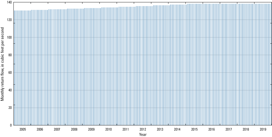
Monthly return flow applied to model, 2005 to 2019, Long Island, New York (Corson-Dosch and Fienen, 2023).
Water-Supply Infrastructure Leakage
An additional source of artificial recharge to the aquifer system is leakage from public-supply infrastructure. Most of Long Island is served by public supply; private water supplies do exist but are limited to small areas of eastern Suffolk County and the northern shore of Nassau County. The distribution of public-supply lines was estimated from the extent of roads within individual model cells (Walter and others, 2020). The potential for recharge from leaky infrastructure (as indicated by road length) generally reflects patterns of population and development and is largest in New York City and parts of Nassau County. In Kings and Queens Counties, about 700 Mgal/d of water is imported from a reservoir system in upstate New York, and assuming a 10-percent loss of water from the water distribution system, may result in about 70 Mgal/d of additional recharge on western Long Island (Misut and Monti, 1999).
Water-supply infrastructure leakage accounted for about 2 percent of natural recharge during the 2005 to 2019 period. The large seasonal range in this leakage term (fig. 25) is correlated with the seasonal variation in water use (fig. 26).
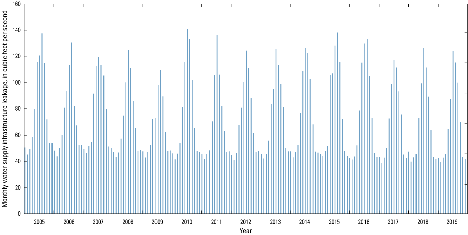
Monthly water-supply infrastructure leakage applied to model, 2005 to 2019, Long Island, New York (Corson-Dosch and Fienen, 2023).
Groundwater Withdrawals
An average of about 424 Mgal/d of groundwater was withdrawn annually from 2005 to 2015 from the Long Island aquifer system for multiple uses, including public supply, agriculture, and industry. The public supply of drinking water accounted for nearly all (95 percent) of the total annual groundwater withdrawal on Long Island. Agricultural withdrawals for crop irrigation generally were limited to eastern Suffolk County, with limited reporting (Walter and others, 2020). However, potential agricultural pumping was represented using the SWB model (Finkelstein and others, 2022) by estimating water demand by crop type and available precipitation, resulting in an estimated demand of about 2 Mgal/d. Seasonal cycles in pumping (fig. 26) relate to increased water demand during the summer caused by increased inhabitation, irrigation, and lawn irrigation demand.
During the 2005 to 2019 period, a total of about 8 Mgal/d of groundwater on average was withdrawn annually from the Long Island aquifer system for contaminant remediation (Corson-Dosch and Fienen, 2023). This remedial pumping generally does not vary seasonally and has increased with time; all water generally is returned to the aquifer system after treatment either by reinjection wells or discharge to recharge basins. The vast majority (7.9 Mgal/d) of the total was withdrawn as part of Navy Grumman groundwater plume remediation in southern Nassau County.
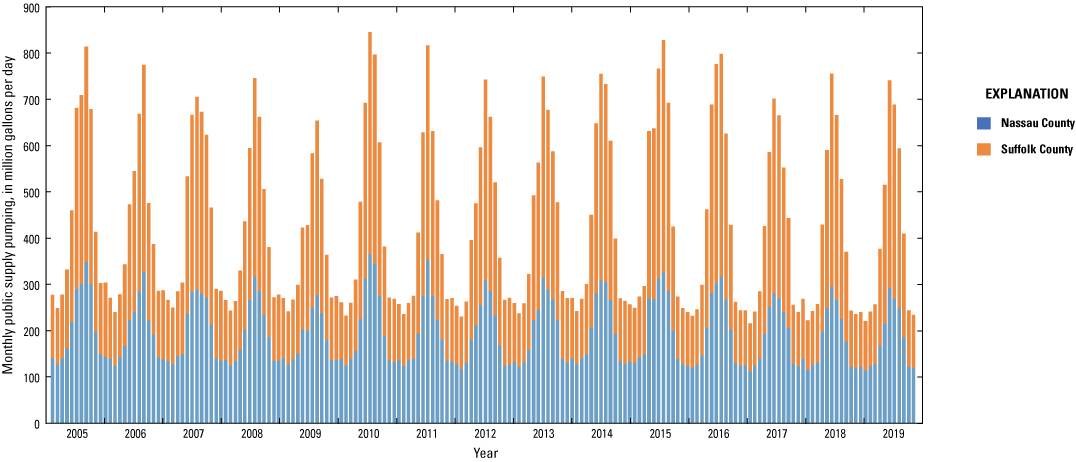
Monthly public supply pumping, 2005 to 2019, Long Island, New York (Corson-Dosch and Fienen, 2023).
Hydraulic Properties
The transient LIRM model requires specification of unconfined and confined storage. We assigned a uniform value of 0.25 to represent specific yield (Sy; unconfined storage) and a uniform value of 0.00001 to represent specific storage (Ss; confined storage), which are reported for Long Island sediments (Smolensky and others, 1990). All other hydraulic properties are unchanged from the values reported in the steady-state model of the LIRM (Walter and others, 2020).
Simulation of Heads and Flows
Hydraulic heads and groundwater flows were simulated using the MODFLOW 6 code (Langevin and others, 2017), for January 1, 2005, through December 31, 2019. Simulated hydraulic heads within the focus area ranged from about 10 to about 80 ft above NAVD 88, and water-table depressions and mounds formed in areas of remedial pumping and discharge to recharge basins, respectively. Hydraulic heads and groundwater flows at representative monitoring points (U.S. Geological Survey, 2023) within the inset area are shown on figure 27 and presented in tables 7 and 8.
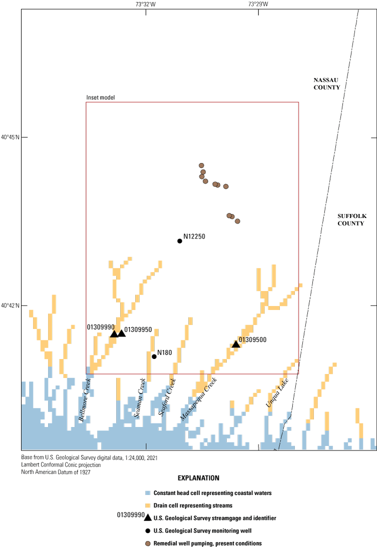
Locations of observation wells and streamgages (U.S. Geological Survey, 2023), southeastern Nassau County, New York (Corson-Dosch and Fienen, 2023).
Table 7.
Characteristics of hydraulic head observation wells, southeastern Nassau County, New York (U.S. Geological Survey, 2023).[Altitude, elevation, and screen midpoint in feet above North American Vertical Datum of 1988; ID, identification number; NWIS, National Water Information System (U.S. Geological Survey, 2023)]
Table 8.
Average base flow at U.S. Geological Survey streamgages, southeastern Nassau County, New York.[Observed data for 2005–19 (U.S. Geological Survey, 2023); base flows computed using the R package “hydrostats” (Bond, 2022) with an alpha filtering parameter value of 0.975 (Ladson and others, 2013); ft3/s, cubic feet per second; ft, feet; NAVD 88, North American Vertical Datum of 1988; NA, not applicable]
Hydrographs of simulated and observed hydraulic heads at selected observation wells are presented in figures 28 and 29. Hydraulic heads generally follow a seasonal cycle that peaks in the winter, with similarities to cycles of groundwater recharge (figs. 22 and 23) and the inverse of pumping cycles (figs. 25 and 26). The annual range of hydraulic heads is generally greater for deep wells screened in the Magothy aquifer than for shallow wells screened in the upper glacial aquifer, likely owing to the lesser water storage potential in the Cretaceous sediments as compared to glacial outwash sediments. However, during extreme precipitation events such as the March 2010 Nor’easter, the shallow upper glacial aquifer may be affected to a greater extent than the Magothy aquifer because the shallow upper glacial aquifer is closer to the recharge source.
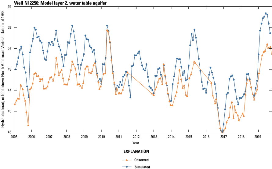
Simulated (Corson-Dosch and Fienen, 2023) and observed (U.S. Geological Survey, 2023) hydraulic heads at monitoring well N12250 screened in the upper glacial aquifer, 2005–19, southeastern Nassau County, New York.
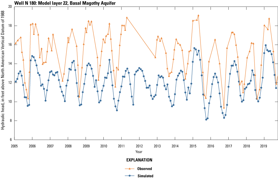
Simulated (Corson-Dosch and Fienen, 2023) and observed (U.S. Geological Survey, 2023) hydraulic heads in monitoring well N180, 2005–19, screened in the Magothy aquifer, southeastern Nassau County, New York.
We accessed daily mean streamflow using the R package dataRetrieval (De Cicco and others, 2018) from the U.S. Geological Survey National Water Information System (NWIS) database (U.S. Geological Survey, 2023) for the three streamgages in southeastern Nassau County: Massapequa Creek at Massapequa, New York (01309500); Bellmore Creek near Bellmore, New York (01309950); and Bellmore Creek Tributary at Bellmore, New York (01309990) (fig. 27, table 8). We performed base-flow separation of daily mean streamflow using the R package “hydrostats” (Bond, 2022), which uses a Lynne-Hollick filter to separate daily streamflow data into base-flow and quickflow components. An alpha filtering parameter value of 0.975 (Ladson and others, 2013) was used to provide the best match to observed base flows.
Hydrographs of simulated and observed base flows at Massapequa Creek (01309500) and Bellmore Creek (01309950) are presented in figures 30 and 31. The observed base flows for Bellmore Creek and Bellmore Creek Tributary streamgages (01309950 and 01309990) were summed to represent the total base flow for Bellmore Creek. Base flows generally followed a seasonal cycle that peaks in the winter, with similarities to cycles of groundwater recharge (figs. 22 and 23), simulated hydraulic heads (figs. 28 and 29), and the inverse of pumping cycles (figs. 25 and 26). The observed mean base flow for the available period of record at Massapequa Creek for 2005–19 was 2.71 cubic feet per second, which was comparable to the simulated base flow of 8.46 cubic feet per second. The observed mean base flow for the available period of record at Bellmore Creek for 2005–19 was 3.11 cubic feet per second, which was comparable to the simulated base flow for 2005–19 of 6.21 cubic feet per second.
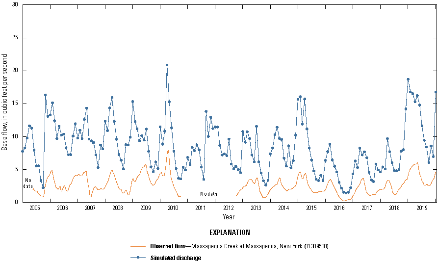
Simulated (Corson-Dosch and Fienen, 2023) and observed (U.S. Geological Survey, 2023) base flows at Massapequa Creek, 2005 to 2019, New York.
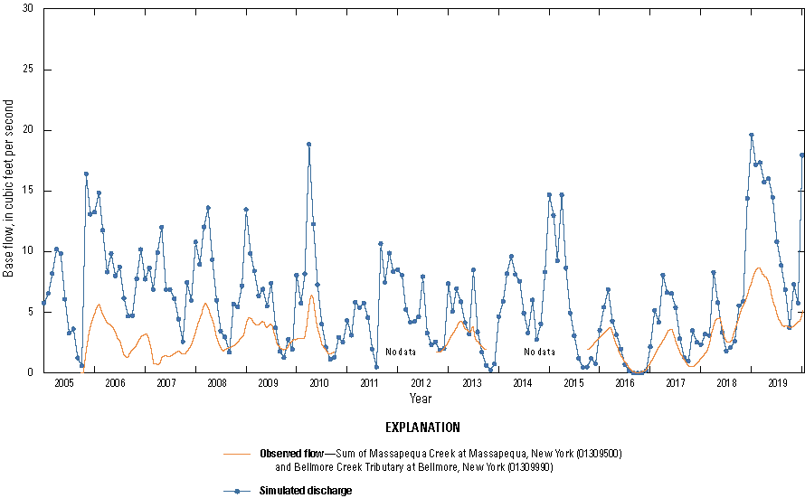
Simulated (Corson-Dosch and Fienen, 2023) and observed (U.S. Geological Survey, 2023) base flows at Bellmore Creek, 2005 to 2019, New York.
Plume-Focused Inset Model for Decision Support
We created a groundwater-flow model with particle-tracking and management optimization utilities as an inset from the transient LIRM. We developed this inset model to better understand the groundwater-flow system and the proposed remedial system designed to extract, treat, and return water to the aquifer system in the area of the Navy Grumman groundwater plume on Long Island, New York (refer to fig. 2). We used this inset model to simulate the currently proposed remedial pumping strategy for the plume, and a proof-of-concept management optimization modeling approach to refining the remedial design to explore tradeoffs among competing objectives related to plume containment.
Inset Model Development
We implemented the inset model using MODFLOW 6 (Langevin and others, 2017). The location of the inset model relative to the regional “parent” model is presented in figure 3. The inset model is connected to the regional hydrologic system using time-varying Constant Head (CHD) package (Langevin and others, 2017) boundary conditions set at the hydraulic head values in the transient LIRM for the same transient times simulated in both models. The inset model simulates 2005 to 2019 with monthly stress periods. The monthly water use and recharge, streambed conductance, and storage information were all inherited from the transient LIRM with layering, hydraulic conductivity, and a Streamflow Routing (SFR) package created using the MODFLOW-setup and SFR-maker codes (Leaf and others, 2021; Leaf and Fienen, 2022) using a similar insetting approach as Fienen and others (2022a). The remainder of this section describes the specific information as applied to the inset model.
Inset Model Domain
The inset model domain encompasses an area of about of 36 mi2 in southeastern Nassau County surrounding the plume. Surface elevations are highest in the northeastern part of the inset domain near the hamlet of Plainview and Bethpage State Park and generally decrease from north to south towards South Oyster Bay and the Atlantic Ocean. Streams drain the inset domain and typically flow parallel to the north-to-south slope. Larger streams in the inset domain include Bellmore Creek and Massapequa Creek, smaller streams include Seamans Creek, Seaford Creek, and Carman Creek. Although stream channels (expressed as a drainage pattern in the surface elevation model) extend into the northern part of the inset domain, stream reaches with perennial flow are only present in the southern part of the inset domain (fig. 32). There are wetlands adjacent to anastomosing sections of Bellmore Creek and Massapequa Creek near the coast in the southern part of the inset domain, which have shallow depth to groundwater.
Hydrogeologic units in the inset model domain include unconsolidated glacial and coastal-plain deposits and are described in detail in the “Hydrogeologic Framework” section. Permeable sand and gravel glacial deposits make up the surficial (upper glacial) aquifer. The glacial deposits are underlain by a thin, discontinuous marine clay layer in the southern-most portion of the domain (Gardiners Clay) that may act as a confining unit. Both units are underlain by a thick, regionally extensive coastal-plain deposit (Magothy aquifer) consisting of mostly sand and silt with a basal layer of gravel. This basal gravel is underlain by another unit of sand and silt (upper Raritan aquifer), which in turn is underlain by a fine-grained, clay-rich deposit (Raritan confining unit) that acts as a confining unit to the Lloyd aquifer below. Impermeable crystalline bedrock underlies the Lloyd aquifer and is considered to be the base of the aquifer system.
The area encompassed by the inset model domain is highly developed with extensive residential, commercial, and industrial land use. Aerial recharge is limited by impervious surfaces that generate excess stormwater runoff. Many large, human-constructed basins have been installed in developed areas throughout the model domain for stormwater retention and infiltration (Aronson and Seaborn, 1974). Numerous sole-source water-supply wells are active in the inset model domain, managed by distinct water utilities. An existing network of remedial pumping and reinjection wells are also active as part of a groundwater extraction, treatment, and return remedial system (New York State Department of Environmental Conservation, 2024a, 2024b).
Inset Model Discretization
The inset model extent adopted the bounds of the southeastern Nassau County inset area shown in figure 2. The layering adopted the same lithologic definitions as in the transient LIRM with the exception that layer 24 of the transient LIRM was subdivided into two layers in the inset model. The purpose of the two layers was to divide the Raritan confining unit into a clayey unit (inset model 25, the “lower Raritan”) and a sandy unit (inset model 24, the “upper Raritan”). Inset model layer 26 represents the Lloyd aquifer, which is consistent with layer 25 in the transient LIRM (table 9). All layers shallower than layer 24 are lithologically consistent with the transient LIRM (Walter and others, 2020).
We refined the horizontal discretization from the square 500 ft by 500 ft cells in the transient LIRM to square 125 ft by 125 ft cells. This is a 16-fold refinement of the transient LIRM geometry and is intended to facilitate higher resolution representation of the relation among remedial wells, the plume, surface waters, and boundary conditions.
The transient temporal discretization adopted the same 180 monthly stress periods as used in the transient LIRM, representing each month from January 1, 2005, through December 31, 2019. We implemented an initial steady-state stress period at the beginning of the simulation, which was constructed using the average stresses and boundary conditions of the entire 2005–19 period. More detailed information on the transient stress periods that were represented in the transient LIRM is presented in the “Conversion from Steady State to Transient Simulations” section.
Table 9.
Layers and corresponding lithology in the inset model (Corson-Dosch and Fienen, 2023).[--, no data]
Boundary Conditions
Boundary conditions that do not change from the transient LIRM model are mapped by MODFLOW-setup to the overlapping model cells in the inset model. These boundary conditions are presented on a map of the inset model area in figure 32.
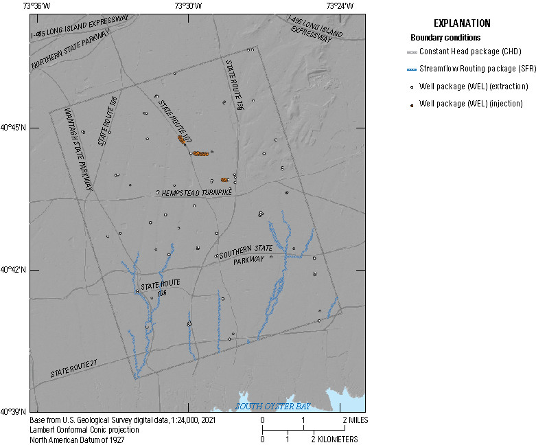
Boundary conditions for the inset model inherited from the transient Long Island Regional Model (Corson-Dosch and Fienen, 2023).
Recharge
Recharge was inherited from the transient LIRM at the 500 ft by 500 ft resolution represented by the transient LIRM. As a result, each 16-cell block of inset model cells contained within a single transient LIRM model cell used the same recharge value. Average annual recharge rates for the simulation period (2005–19) are shown in figure 33.
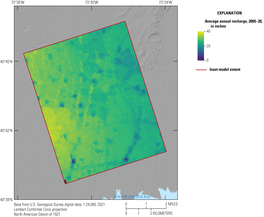
Average annual recharge conditions for 2005–19 for southern Nassau County, New York (Corson-Dosch and Fienen, 2023).
Stream-Aquifer Interactions
We simulated stream-aquifer interactions using the SFR package in MODFLOW 6 (Prudic and others, 2004; Niswonger and Prudic, 2005; Langevin and others, 2017). The SFR package simulates stream stage, surface-water exchange with the underlying aquifer, and streamflow routing. We developed the SFR network using SFR-maker (Leaf and others, 2021) based on the USGS National Hydrography Dataset Plus High Resolution (NHDPlus HR; U.S. Geological Survey, 2024). The NHDPlus HR provides geometry and routing information, which are both represented in the SFR package.
Streambed conductance was calculated by using the drain conductance represented in the transient LIRM using the Drain (DRN) package in MODFLOW 6. Streambed conductance is the product of hydraulic conductivity in the stream sediments and the area of the streambed, assuming a unit thickness. The finer resolution of the inset model grid meant that between 1 and 16 inset model cells could overlap an individual DRN cell in the transient LIRM. To account for this change in area, we calculated the streambed hydraulic conductivity in each cell of the inset model as
wherePumping Wells
Water-use data were inherited from the transient LIRM. Precise locations were provided to MODFLOW-setup to map x and y coordinates of hydrologic stresses such as pumping wells to the appropriate model cells. As a result, the location of pumping wells in the inset model is four times more accurate than in the transient LIRM; however, pumping rates are the same. In addition to improved location accuracy, the finer discretization further reduces the potential for wells in the inset model to act as weak sinks.
Focused Recharge
Several recharge basins (fig. 34) were simulated in the inset model to represent locations where treated water extracted in the remedial system was returned to the subsurface. We represented these in the inset model using the MODFLOW 6 Well (WEL) package with a return-flow (or reinjection) well implemented in each cell in the shallowest layer that overlaps with the outline of a recharge basin. We set hydraulic conductivity in these basins to an initial value that was high enough to accommodate the known return flows of treated water without simulating excessive mounding. This hydraulic conductivity parameter was allowed to vary in the history-matching process.
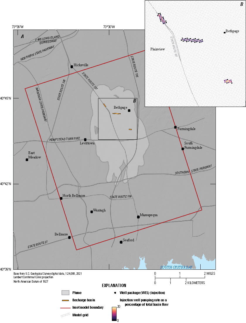
Representation of recharge basins and injection wells, both simulated using well boundary conditions in overlapping model cells (Corson-Dosch and Fienen, 2023). A, Location of the recharge basins relative to the inset model domain. B, Representation of basins as multiple wells and the corresponding distribution of basin recharge through those wells.
Static Constant Hydraulic Head Connection to the Long Island Regional Model
For each stress period (each month during 2005–19), the hydraulic head in the transient LIRM was mapped to the lateral bounding cells of the inset-model using MODFLOW-setup and assigned to the MODFLOW 6 CHD package. These groundwater heads represent the groundwater-flow dynamics of the regional system.
Hydraulic Properties
The hydraulic properties applied to the inset model include hydraulic conductivity, storage, and porosity. The initial values of these hydraulic properties were adjusted using history matching, as described in the “Parameter Estimation by Ensemble History Matching” section. Hydraulic conductivity was represented using two methods: a single realization generated using geostatistical interpolation referred to as the “texture model,” and an ensemble of 500 realizations generated using the transition probability geostatistical method (T–PROGS; Carle, 1999). Both conceptualizations are described in detail in the “Hydrogeologic Framework” section.
We specified specific yield as a constant value of 0.25 throughout the model and specific storage also was specified as a constant value of 1x10⁻⁵. Both uniform values were inherited from the transient LIRM. A single value for porosity of 0.35 was selected for the analysis in this report. Travel times were not reported in the particle-tracking simulations, and those model outputs are the only outputs that would be affected by changes in porosity.
Parameter Estimation by Ensemble History Matching
We adopted a Bayesian approach (Tarantola, 2005) to history matching for conditioning the prior estimates of model parameters on a systematic comparison of model outputs with field observations collocated in space and time. The resulting posterior estimate of model parameters reflects the prior knowledge of parameters and the information contained in the site-specific observations. This history-matching process was performed using the iterative ensemble smoother (iES) ensemble technique (White, 2018) implemented in the Parameter Estimation Software (PEST++; version 5.0.0; White, 2018; White and others, 2021). This process involves defining an objective function (phi) as the weighted sum of squared discrepancies between model outputs collocated in space and time with field observations. The iES algorithm systematically finds parameters that minimize phi. In this report, we use the terms “phi” and “objective function” interchangeably.
We performed separate iES history-matching processes for the texture model and T–PROGS representations of the hydraulic conductivity properties. The resulting posterior parameter ensembles were then available to characterize the variability (uncertainty) of model outputs and to form the basis for subsequent analysis including the management optimization as described below. Each process was represented by an initial ensemble of 500 realizations. The posterior ensemble was subjected to rejection sampling in which ensemble members with extremely poor correspondence to observation data, as quantified by the objective function, were removed.
Observation Data
Observations of groundwater heads and base flows were used for history matching for the 2005–19 period. The observation dataset consisted of three categories: (1) base flow in streams, (2) hydraulic heads in wells, and (3) temporal hydraulic head differences. Base-flow observations were derived from streamflow records at the streamgage on Massapequa Creek (01309500) and two streamgages on Bellmore Creek (01309950 and 01309990) shown in figure 27 and table 8 (U.S. Geological Survey, 2023).
Hydraulic head observations were collected from multiple sources, as outlined in Corson-Dosch and Fienen (2023). These observations were supplied at various temporal intervals ranging from occasional instantaneous values to some collected every 15 minutes for many months. To map these values to the monthly temporal discretization of the inset model, we selected the final (in time) measurement of groundwater head in each month as representative of that month in the model. Temporal differences were finally derived by subtracting sequential groundwater head observations in each well from each other where more than one monthly measurement was available. These temporal differences can be valuable in amplifying the effects of storage on the timing of aquifer dynamics (Doherty and Hunt, 2010; Anderson and others, 2015).
Observations are assigned weights to indicate how closely model outputs are expected to correspond to the observed values. We initially assigned these weights based on assumed standard deviations of 10-percent coefficient of variation for the base flow observations, 1.5 ft for groundwater head observations, and 0.5 ft for temporal groundwater head difference observations. These initial weights were calculated as the reciprocals of the assumed standard deviations and resulted in an imbalanced objective function. Information about observations and weights are summarized by group in table 10. Subjectively, weights were adjusted to rebalance the objective function for the texture model and T–PROGS models (fig. 35) so that base flow, hydraulic heads, and temporal hydraulic head differences make up 40, 40, and 20 percent of the initial objective function, respectively.
The ensemble approach of iES also allows for realizations of variability around the reported observation values, referred to below as “observation noise.” By default, the reciprocal of the weights is used as the standard deviation which, combined with the observation value as the mean, can be used by the PEST++ software to formulate a normal distribution about which a sample including observation noise for each observation is drawn for each ensemble realization.
Rebalancing the objective function and thus changing weights can result in standard deviation specifications that are inappropriate for the assumed variability around the observation values. Further, the default behavior in PEST++ does not include autocorrelation of the observation noise. To account for this, we calculated the covariance of the time series for all transient observations assuming an exponential variogram with unit variance and a correlation length of 140 days, and then scaled by the variance (the standard deviation values ascribed to each observation in table 10, squared). Examples of the observation noise realizations calculated in this way are shown in figure 36. In figure 36A, which includes temporal autocorrelation, the realizations are smoother, and more consistent with error on the time series that should vary smoothly, whereas in figure 36B the uncorrelated observation noise can suggest errors jumping above and below the reported values.
Table 10.
Summary of observation data and weights by group (Corson-Dosch and Fienen, 2023).[NA, not applicable]
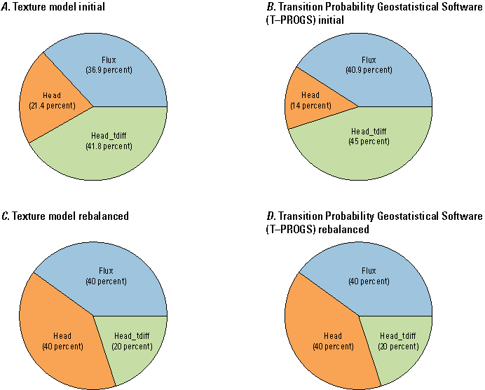
Rebalancing of the objective function based on prior Monte Carlo analysis (Corson-Dosch and Fienen, 2023). A, Pre-balanced objective function for the texture model inset. B, Pre-balanced objective function for the Transition Probability Geostatistical software model inset. C, Adjusted objective function after rebalancing for the texture model inset. D, Adjusted objective function after rebalancing for the Transition Probability Geostatistical (T—PROGS) software model inset.
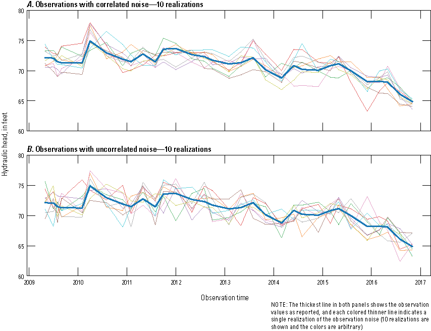
Noise realizations for a single representative, illustrative transient hydraulic head observation (Corson-Dosch and Fienen, 2023). A, Noise realization considering autocorrelation. B, Noise realization not considering autocorrelation.
Estimating Model Parameters
We adopted a multiscale approach to parameterizing inputs of properties in the inset model based on the methods described in White and others (2020) and Fienen and others (2022b). In this approach, most parameter values were defined as multipliers that are multiplied together against the initial reference property values. In the specific case of hydraulic conductivity, this allowed us to apply parameter adjustment at two scales: homogeneous zones and pilot points (Doherty, 2003). Different scales of parameters respond differently to information contained in observations so there is an advantage to designing the history-matching setup to accommodate this. The summary of initial parameter values, bounds, and numbers of parameters for the texture model and T–PROGS inset models are shown in tables 11 and 12, respectively.
Table 11.
Parameterization summary for the texture model version of the inset model (Corson-Dosch and Fienen, 2023).Table 12.
Parameterization summary for the Transition Probability Geostatistical Software (T–PROGS; Carle, 1999) version of the inset model (Corson-Dosch and Fienen, 2023).[T–PROGS, Transition Probability Geostatistical Software]
We developed separate inset models with the hydraulic conductivity distribution from the texture model and T–PROGS. The texture model was created using more and thinner layers than the layering in the inset model. As a result, the texture model was mapped to the inset model layers using a thickness-weighted arithmetic mean for Kh and a thickness-weighted geometric mean for Kv. The T–PROGS model was generated with the same layer configuration as the inset model, so the mapping was one-to-one in this case except for the Lloyd and Raritan units, which were omitted from T–PROGS calculations. We parameterized these two layers from a homogeneous starting point.
In both cases, the hydraulic conductivity values were adjusted such that their mean value was the same as the mean of the corresponding layer in the transient LIRM. This adjustment was done for all layers except for layer 4 (the Gardiners Clay, which was represented as a single value) and layer 24 (the representing the upper Raritan, which was not represented in the transient LIRM). As a result, each of the 500 initial realizations for the T–PROGS model has the same bulk mean hydraulic conductivity per layer, and because the relative proportions of each of the four zones in each layer are consistent among the realizations, the initial hydraulic conductivity values per zone per layer were nearly identical at the start.
For the texture model, we assigned a zonal multiplier to each layer and a network of pilot points in each layer for Kh and Kv. A subsequent analysis confirmed that Kv was less than Kh in all cells. For the T–PROGS model, each layer has four discrete values, and as a result, unique values were assigned to each of the four zones in each layer (for layers 1–23 except for layer 4, which was simulated as homogeneous) in addition to the same network of pilot points and layer-wise constant multipliers as for the texture model.
Each of the 500 realizations used for the texture model represented multipliers that expressed variability around an initial hydraulic conductivity distribution. An additional parameter was required in the T–PROGS inset model to indicate which of the initial 500 realizations of hydraulic conductivity was the starting point for multipliers to express variability around them. This parameter was set at an integer value and not allowed to change through the history-matching process.
The remaining parameterization was the same for the texture and T–PROGS models. We implemented a single multiplier, each, for 181 transient parameters for the boundary CHD, WEL, and recharge (RCH; Langevin and others, 2017) MODFLOW packages for each stress period. These multiplier parameters were restricted to the range of 1.0 to 1.2 for CHD, 0.9 to 1.1 for WEL, and 0.6 to 1.1 for RCH, respectively (table 11). Direct values (not multipliers) were assigned for hydraulic conductivity in the three recharge basins where the return of treated water to the aquifer was simulated, resulting in three Kh and three Kv parameters used in the history-matching process.
The same pilot-point network was used for all Ss, Sy, Kh, and Kv parameters. This pilot-point network included one pilot point assigned for every 15th row and column, resulting in a total of 6,650 parameters for each of the four properties spaced every 1,875 ft apart. Finally, vertical multipliers were assigned by model layer for Ss and Sy. The total number of adjustable parameters was 27,317 for the texture model and 27,501 for the T–PROGS model. The additional parameters in the T–PROGS formulation account for individual homogeneous Kh values we assigned to the four discrete zones per layer, which we allowed to vary independently from the pilot-point multipliers.
Prior Monte Carlo Analysis
The first step in the history-matching process is to evaluate a prior Monte Carlo analysis using the initial ensemble of 500 realizations to evaluate the overlap between model outputs and the noise realizations of observations. This “prior-data conflict” step provides an assessment of whether the model setup and initial ensemble of model parameters overlap sufficiently such that history matching is likely to improve their correspondence (Evans and Moshonov, 2006; Alfonzo and Oliver, 2019). A significant number of observations in prior-data conflict indicates either an error in the observation, an error in the model, or insufficient flexibility in adjusting the parameters (Fienen and others, 2022b). The prior Monte Carlo analysis of the texture model inset determined that 146 of the 14,124 observations were in prior-data conflict (1.03 percent of all the observations). Ninety percent of these 146 observations were determined to be in conflict owing to identifiable issues with the observation values (for example, possible well flooding, datum issues, and other factors; Corson-Dosch and Fienen, 2023). For these observations, the observation weight was set to 0.0 so they do not play a role in the parameter estimation process, but their values are still reported for qualitative inspection.
History Matching with the Iterative Ensemble Smoother
We selected the iES (White, 2018) as implemented in PEST++ (White and others, 2021) for history matching. This technique builds on the prior Monte Carlo analysis by evaluating an ensemble of parameter values, yielding a residual matrix, and calculating a weighted objective function for each member of the parameter ensemble. From this information, the algorithm calculates an updated ensemble of parameters to evaluate, and iterations are repeated until a posterior conditioned ensemble is obtained. This process results in an ensemble of objective function values from iteration to iteration.
The “Base” line on figure 37 represents a base realization ensemble member (discussed further in the “Base Realization” section) that is considered representative of the entire ensemble when a single realization is desired. This base ensemble member is calculated by iES by applying the approximate upgrade information to the initial parameter values and using observations unperturbed by noise to approximate a single minimum-error-variance solution. A base realization can be estimated for the texture model inset because it started with a single initial realization of hydraulic conductivity. However, a base realization of hydraulic conductivity cannot be estimated for the T–PROGS model inset because a single initial realization does not exist.
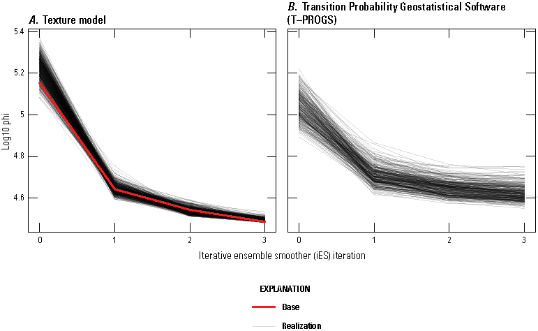
Change in the objective function (phi) for ensembles over iterative ensemble smoother iterations (Corson-Dosch and Fienen, 2023). A, Texture model inset. B, Transition Probability Geostatistical (T–PROGS) software model inset.
History-Matching Ensemble Results
The results of the first iES iteration were selected as optimal based on a subjective judgement that assumes the objective function had achieved an acceptable level of fit while still retaining enough variability in the ensemble to characterize the uncertainty in the system. Individual model runs may fail to converge during the history-matching process because of the randomized generation of parameter sets. When a model run fails to converge, iES drops that run from the ensemble. Most texture model inset realizations converged through the first iteration of the history-matching process, but many T–PROGS model inset realizations (209 out of 500) did not. These nonconverging runs likely were due to the large variability in the T–PROGS model inset hydraulic conductivity (Kh) zonations that produced unrealistic model properties when combined with randomized parameter sets.
Ensemble members with unacceptably high phi values were removed through the process of rejection sampling as a final step towards obtaining a posterior parameter ensemble. We selected a separate phi cutoff for each of the texture and T–PROGS model insets that removed anomalously high phi results and yielded an approximately normal distribution (fig. 38). This reduced the number of realizations retained in the posterior ensembles from the initial size of 500 realizations to 459 for the texture model inset and 268 for T–PROGS model inset.
Anomalously high phi values are common in the prior Monte Carlo analysis, and because high phi realizations are either eliminated or move toward the mean of the ensemble, more normally distributed phi values become apparent as the algorithm progresses through iterations. The T–PROGS model inset realizations are less constrained than the texture model inset, resulting in more realizations with phi values being dropped and fewer realizations remaining for the posterior ensemble than for the texture model inset.
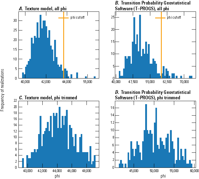
Histogram comparisons of phi for posterior parameter ensembles for texture model inset and Transition Probability Geostatistical (T–PROGS) software model inset (Corson-Dosch and Fienen, 2023). A, Texture model inset phi before trimming. B, T–PROGS inset model phi before trimming. C, Texture model inset phi after trimming. D, T–PROGS model inset phi after trimming.
The history matching discussion includes the full range of results from the entire posterior parameter ensemble and the results from the single representative base realization. The entire posterior parameter ensemble is used in the discussion of head and base-flow observations and for boundary condition parameters, where the visualization of the full range is possible. The base realization is preferrable for visualizing properties and water budget results. Results from both models are discussed in this section; however, only texture model inset results are shown for a base realization because the T–PROGS model inset had no base realization and, therefore, no single representative realization.
Base Realization
The base realization differs from the other realizations obtained by making a stochastic sample using the bounds of the initial parameter values. Instead, the base realization is initially made up of the specific starting values provided to PEST++. As a result, this base realization starts at values that are considered “most likely” by the users. This base realization then is subjected to adjustment during each iteration of the iES algorithm, but this single realization typically is less variable than the other realizations. The final values of the base realization represent the central tendency of the posterior parameter distribution (White and others, 2021).
Heads and Flows Residuals
Heads and flows residuals are calculated from the entire ensemble rather than focusing on a single realization; therefore, these residuals represent a range of outcomes consistent with prior knowledge of the parameters and the information from the observation data. The correspondence between model outputs and observations are grouped separately for the texture model and T–PROGS model insets. The base realization and the spread from all the realizations are shown on each plot as a dot and whiskers, respectively (figs. 39 and 40). The fit for the texture model inset base realization is shown in figure 39, whereas the fit for the T–PROGS model inset realizations closest to the median of the ensemble, based on weighted residuals, are shown in figure 40. There is more variance and bias in modeled outcomes with the T–PROGS model inset than with the texture model inset (figs. 39 and 40); however, these results are shown to have little bias and low variance relative to the uncertainty of the observations.
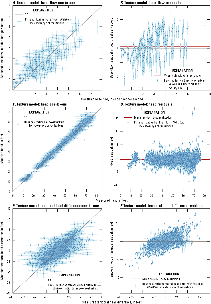
Observed versus modeled (one-to-one) and residuals (calculated as observed minus modeled for all texture models realizations) plots for the texture model inset (Corson-Dosch and Fienen, 2023). A, One-to-one plot for base-flow observations. B, Residuals plot for base-flow observations. C, One-to-one plot for hydraulic head observations. D, Residuals plot for hydraulic head observations. E, One-to-one plot for temporal hydraulic head difference observations. F, Residuals plot for temporal hydraulic head difference observations.
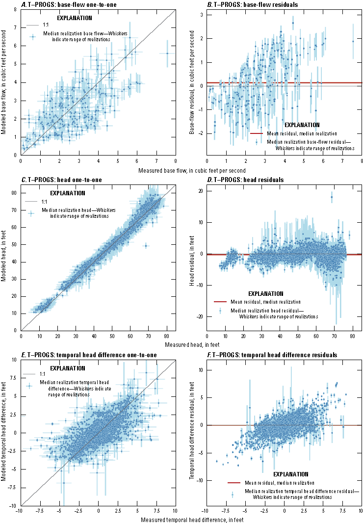
Observed versus modeled (one-to-one) and residuals (calculated as observed minus modeled for all texture models realizations) plots for the Transition Probability Geostatistical software (T–PROGS) model inset (Corson-Dosch and Fienen, 2023). A, One-to-one plot for base-flow observations. B, Residuals plot for base-flow observations. C, One-to-one plot for hydraulic head observations. D, Residuals plot for hydraulic head observations. E, One-to-one plot for temporal hydraulic head difference observations. F, Residuals plot for temporal hydraulic head difference observations. Transition Probability Geostatistical software (T–PROGS) model plots of observed versus modeled (one-to-one plot) and residuals (calculated as observed minus modeled for all T–PROGS realizations.
The correspondence between modeled flow in SFR cells at streamgage locations and observed base flow indicate that the ensemble of model outputs generally overlaps with the ensemble of observations (fig. 41). There is less scatter for all cases in the modeled results than in the observed data (for example, the two streamgages for the texture and T–PROGS model insets); overall, there is little bias, and the fit is considered reasonable.
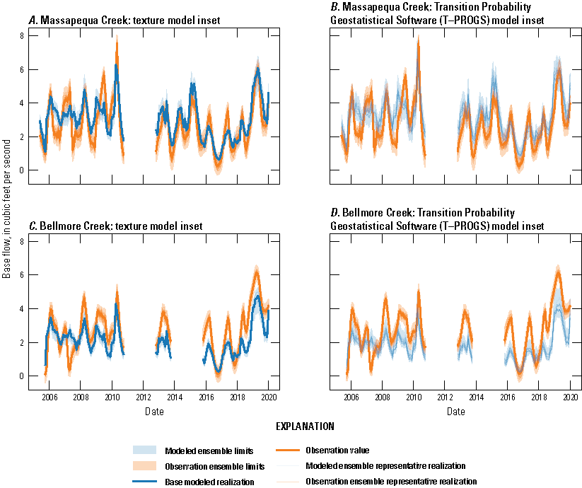
Simulated (Corson-Dosch and Fienen, 2023) and observed (U.S. Geological Survey, 2023) base flow. A, Texture model inset at Massapequa Creek. B, Transition Probability Geostatistical software (T–PROGS) model inset at Massapequa Creek. C, Texture model inset at Bellmore Creek. D, T–PROGS model inset at Bellmore Creek.
Transient hydraulic head and temporal hydraulic head-difference results (figs. 42 and 43) for selected locations shown in figures 44 and 45 were generated for the texture and T–PROGS model insets. Although there is some bias relative to the measured observation values, the modeled results are generally completely enveloped by the range of observation noise as shown by the modeled ensemble limits region being completely inside the observation ensemble limits region (fig. 42C, D, G, H).
A similar pattern is observed in the temporal hydraulic head-difference targets as seen with the transient hydraulic head targets; however, the temporal hydraulic head-difference results are less biased than those of the transient hydraulic head results (figs. 42A, B, E, F and 43A, B, E, F). Temporal hydraulic head-difference observations provide insight into the dynamics of the aquifer system over time, so even when there is some overall bias in transient hydraulic head observations, the dynamics can still be represented in meaningful ways to improve model prediction capabilities.
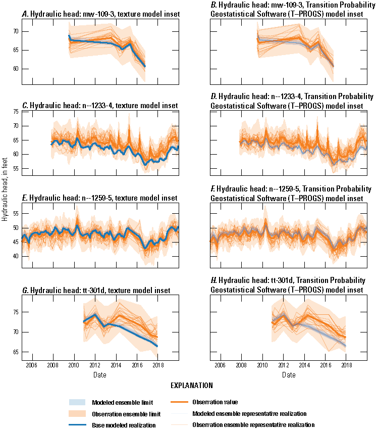
Simulated (Corson-Dosch and Fienen, 2023) and observed (U.S. Geological Survey, 2023) hydraulic head observations for selected observation locations, as identified in figure 44 and 45. A, Texture model inset at mw-109-3. B, Transition Probability Geostatistical software (T–PROGS) model inset at mw-109-3. C, Texture model inset at n—1233-4. D, T–PROGS model inset at n—1233-4. E, Texture model inset at n—1259-5. F, T–PROGS model inset at n—1259-5. G, Texture model inset at tt-301d. H, T–PROGS model inset at tt-301d.
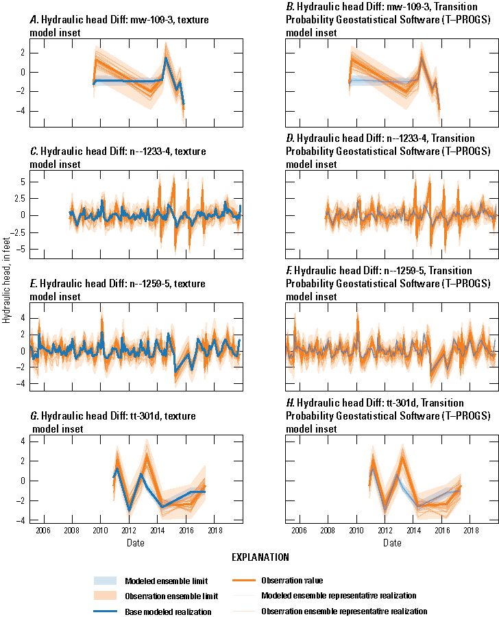
Simulated (Corson-Dosch and Fienen, 2023) and observed (U.S. Geological Survey, 2023) temporal hydraulic head-difference observations for selected observation locations, as identified in figures 44 and 45. A, Texture model inset at mw-109-3. B, Transition Probability Geostatistical software (T–PROGS) model inset at mw-109-3. C, Texture model inset at n—1233-4. D, T–PROGS model inset at n—1233-4. E, Texture model inset at n—1259-5. F, T–PROGS model inset at n—1259-5. G, Texture model inset at tt-301d. H, T–PROGS model inset at tt-301d.
The average residuals (modeled minus observed) of hydraulic heads and flux observations were computed over time and over the entire ensemble to display these results spatially. Maps of the spatial residuals grouped by hydrogeologic unit are shown on figures 44 and 45 for the texture and T–PROGS model insets, respectively. The residuals generally are low (close to zero) and randomly distributed for the texture and T–PROGS model insets, indicating low bias, which is a goal of the history-matching process.
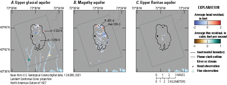
Spatial texture model average hydraulic head and base-flow residuals (Corson-Dosch and Fienen, 2023). Residuals are averages of each observation point for all stress periods and posterior ensemble members. Hydraulic head residuals are shown by aquifer. A, Upper glacial aquifer hydraulic head residuals and base-flow residuals. B, Magothy aquifer hydraulic head residuals. C, Upper Raritan residuals. The model layers corresponding to each lithology are presented in table 9.
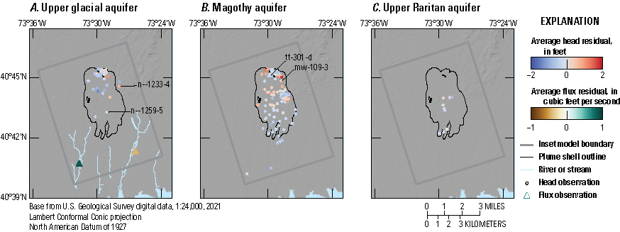
Spatial Transition Probability Geostatistical software (T–PROGS) model inset average hydraulic head and base-flow residuals (Corson-Dosch and Fienen, 2023). Residuals are averages of each observation point for all stress periods and posterior ensemble members. Hydraulic head residuals are shown by aquifer. A, Upper glacial aquifer hydraulic head residuals and base-flow residuals. B, Magothy aquifer hydraulic head residuals. C, Upper Raritan residuals. The model layers corresponding to each lithology are presented in table 9.
Hydraulic Properties
The post-history matching Kh and Kv from the base realization are shown in figures 46 and 47 for the texture model inset. Texture model inset Kh values agree favorably with literature values (Walter and Finkelstein, 2020) and values used in this area in the transient LIRM. The highest Kh values were typically in the upper glacial aquifer in represented in model layer 1, with a maximum value of 375 ft/d. The lowest values were in the layers representing fine-grained confining units including the Gardner’s Clay (layer 4, average Kh 0.009 ft/d) and the lower Raritan (layer 25, average Kh 0.01 ft/d). Kv is typically one to two orders of magnitude lower than Kh in the texture model inset. The average vertical anisotropy (the ratio of average Kh to average Kv) across all model layers was about 62 to 1 and ranged from 120 to 1 in model layer 1 to about 9 to 1 in model layer 9. These ranges are considered appropriate for the layered glacial- and marine-deposited sediments that make up the aquifers in the inset model domain. Kv was adjusted below recharge basins to reduce water-table flooding in these locations and to better represent measured infiltration rates by Seaburn and Aronson (1974). Kv was adjusted to 200 feet per day in layer 1 cells that contained recharge basins (in texture model and T–PROGS model insets). These adjusted cells exceed the upper bound of the color bar on this figure, which was intentionally limited to 40 feet per day to better illustrate Kv variably within and between other model layers.
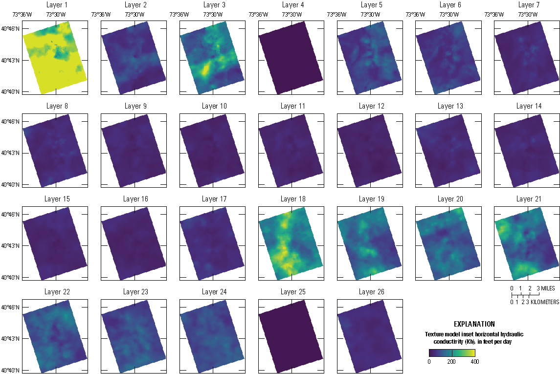
Texture model inset horizontal hydraulic conductivity (Kh) in all layers of the base realization (Corson-Dosch and Fienen, 2023). The lithology corresponding to each model layers is presented in table 9.
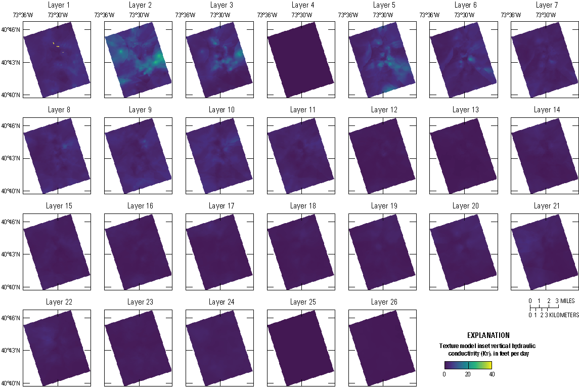
Texture model inset vertical hydraulic conductivity (Kv) in all layers of the optimal base realization (Corson-Dosch and Fienen, 2023). The lithology corresponding to each model layers is presented in table 9.
The Ss and Sy for the optimal base realization of the texture model are shown in figures 48 and 49, respectively. Literature values and the ranges used in the transient LIRM were used to set history-matching bounds for Ss and Sy because of the limited data available to constrain these storage properties (Walter and others, 2024). In MODFLOW 6, both storage properties (Ss and Sy) must be defined for each model cell. The Sy value then is used to calculate water exchange with storage when the water table is below the top of the cell; otherwise, Ss is used for this calculation. The water table is almost exclusively present within the top three layers in this model, so Sy values are summarized and visualized only in layers 1–3, whereas Ss values are summarized and visualized in layers 4–26. The average Ss was 9.7e-5 ft−1 across layers 4–26 and reached the lower and upper bounds of 1.0e-6 ft−1 and 1.0e-3 ft−1 in at least some places (fig. 49). Generally, Ss values are consistent with changes in lithology; however, close alignment of estimated Ss with lithology is not always achieved during the history-matching process. The average Sy was 0.276 in layers 1–3 and was highest in the top two model layers representing the upper portion of the upper glacial aquifer (fig. 48). Some Sy values reached the lower and upper bounds of 0.238 to 0.290, respectively; however, the Ss and Sy values resulting from the history-matching process generally are in good agreement with values reported for similar sediments in the literature (Batu, 1998).
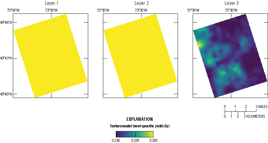
Texture model inset specific yield (Sy) in layers 1–3 of the optimal base realization (Corson-Dosch and Fienen, 2023). The lithology corresponding to each model layers is presented in table 9.
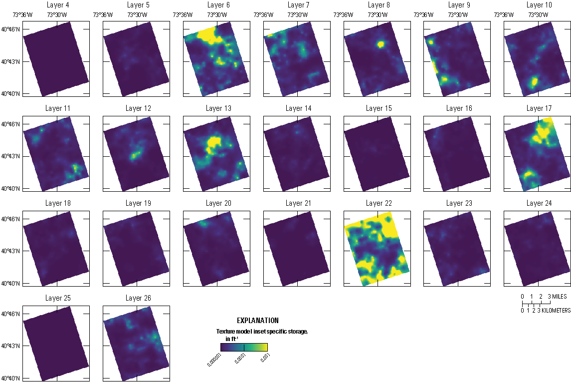
Texture model inset specific storage (Ss) in layers 4–26 of the optimal base realization (Corson-Dosch and Fienen, 2023). The lithology corresponding to each model layers is presented in table 9.
Boundary Conditions
We parameterized the principal model boundary conditions including specified flux (well pumping and recharge) and specified head (constant head), using multipliers that were constant for all stresses in a given stress period but varied with time between stress periods. These parameters were not constrained with autocorrelation because errors were not interpreted and uncertainty in their values would be associated from one time to another. For example, recharge might be adjusted in a stress period with a storm that occurs near the end of a stress period such that the effect of that storm is more appropriately applied to the model in the next stress period. In such a case, one stress period would be adjusted to decrease, whereas the next would be adjusted to increase recharge. The values of these multipliers across stress periods and across ensemble realizations for the texture and T–PROGS model insets are shown in figure 50. The limited range (20 percent) of flexibility is evident on these charts and, with a few exceptions, the multipliers did not reach their bounds.
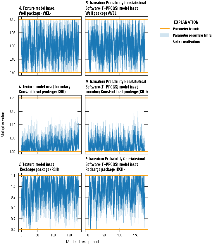
Ensemble parameter multipliers for temporal multipliers, displayed over model stress periods with upper and lower bounds. A, Well multipliers for the texture model inset (Corson-Dosch and Fienen, 2023). B, Well multipliers for Transition Probability Geostatistical software (T–PROGS) model inset. C, Boundary constant hydraulic head multipliers for the texture model inset. D, Boundary constant hydraulic head multipliers for T–PROGS model inset. E, Recharge multipliers for the texture model. F, Recharge multipliers for T–PROGS model inset.
Hydrologic Budget
The main components of the hydrologic budget for the texture model inset base realization are shown by model stress period in figure 51 and by calendar year in figure 52. The primary sources of groundwater inflow to the model include recharge (“RCHA In,” figs. 51–52), groundwater inflow across lateral boundary faces (“CHD In,” figs. 51–52), and through injection wells at recharge basins (“WEL In,” figs. 51–52). The primary outflows from the groundwater system were groundwater outflow across layer boundary faces (“CHD Out,” figs. 51–52), groundwater pumping at wells (“WEL Out,” figs. 51–52), and through discharge to gaining streams (“SRF Out,” figs. 51–52).
Storage terms are consistent with MODFLOW conventions where storage out is water entering storage and thus leaving the flowing groundwater system (STO–SS out and STO–SY out) and storage in (STO–SS In and STO–SY In) is water leaving storage and thus rejoining the flowing groundwater system (figs. 51 and 52; Langevin and others, 2017). Recharge was the largest source of groundwater inflow on an annual basis (fig. 52), though the volume of recharge inflow varied substantially by month (stress period), reflecting seasonal and event-driven dynamics in precipitation. Groundwater outflow across lateral boundaries was typically the largest annual groundwater sink. Well pumping was also a major outflow of groundwater and was often the largest outflow component during summer months (fig. 51).
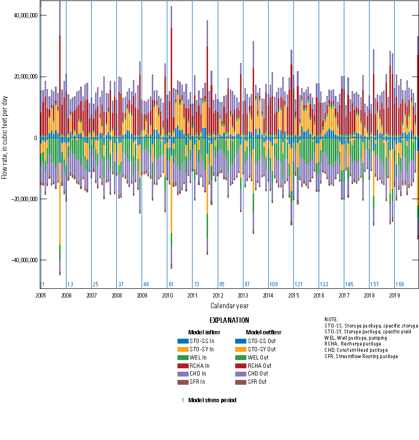
Texture model inset water balance, by stress period (Corson-Dosch and Fienen, 2023).
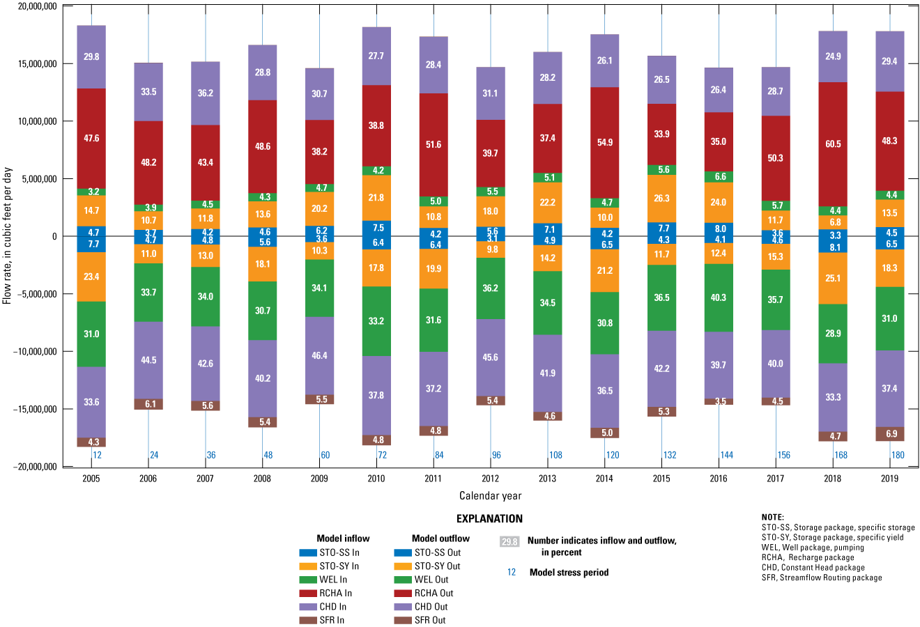
Texture model inset water balance, summed by year, with component percent of total inflows or outflows (Corson-Dosch and Fienen, 2023).
Proof-of-Concept Multiobjective Management Optimization
A key application of this inset model is use by the NYSDEC to inform evaluations of proposed and potential remedial strategies for the contamination plume in the Navy-Grumman area. The selected strategy for remediation is groundwater extraction and treatment in which contaminated water is pumped from the aquifer, treated in an aboveground facility, and then returned to the subsurface through infiltration basins or injection wells. A proof-of-concept evaluation of this remedial strategy was completed to provide information on the performance of different combinations of pumping rates and was subject to various environmental and operational constraints. Further discussion of the optimization techniques used in this report is provided in Fienen and others (2024).
The multiobjective aspect of this proof-of-concept approach stems from recognition that various objectives of the remediation plan may be in competition with one another, so a single scenario representing, in a sense, an “optimal” remediation strategy may not represent a fair tradeoff among the competing objectives. These objectives were based on both operational characteristics, such as the total amount of remediation pumping required, and the fate of plume contaminants as determined by the tracking of simulated water particles originating in the footprint of the plume defined as all model cells where the contaminant(s) of concern exceed their respective NYSDEC Standards, Criteria, and Guidance (Daniel St. Germain, HDR Inc., written commun., 2022). Selection of an “optimal” strategy requires subjective judgement and discussion of results in this report involve making such a subjective selection to illustrate characteristics of the algorithm and the solutions. This discussion does not indicate endorsement or recommendation of a specific outcome by the USGS.
A steady-state version of the inset model was used to perform this proof-of-concept multiobjective optimization analysis. This steady-state model represents pumping rates that are expected to be constant over long times but simplifies some of the aquifer system dynamics, such as seasonal recharge and pumping. This simplification was necessary at this proof-of-concept stage to keep model execution run times manageable so the optimization algorithm, introduced in the following section, could be executed multiple times with each execution requiring as much as tens of thousands of model runs.
Converting Model Stresses to Steady State
We calculated long-term average model stress and boundary values to create the steady-state inset model. Recharge and pumping rates, and constant head boundary heads that link the inset model to the transient LIRM, were averaged during 2005–19 to represent long-term average conditions. Water-supply pumping rates were adjusted to represent expected long-term average rates. Additionally, long-term average remedial well pumping rates (referred to by NYSDEC and hereafter in this report as the “commitments” pumping rates) represented the starting values for simulating the remedial system. With these changes in pumping, this steady-state inset model differs from the steady-state LIRM (Walter and others, 2020). Pumping rates for the commitments wells (the remediation wells for which commitments pumping rates have been assigned) were adjusted from these starting values to explore the tradeoffs of multiple objectives while maintaining constant pumping at the water-supply wells. The term “commitments” is used interchangeably with “baseline” in subsequent discussion to represent the initial assumed pumping regime from which optimization analysis starts.
Running Monte Carlo on Nontransient Estimated Parameters
The history-matching process described in the “Parameter Estimation by Ensemble History Matching” section resulted in two ensembles of model parameters—one each for the texture model inset and the T–PROGS model inset. These include constant parameter values for hydraulic conductivity and streambed conductance, and time-varying parameter values for recharge and constant head boundaries. The transient history-matching model runs include a steady-state initial stress period, so transient parameter multipliers for the constant head boundaries and recharge were adopted from that initial stress period. The storage parameters are not applicable to the steady-state model and thus are disregarded.
The performance of the ensemble as described above in the history-matching effort is based on correspondence between transient model outputs and the observation dataset. However, for evaluating remedial system performance, a different set of metrics are needed to explore the uncertainty of model outputs and to determine a risk with respect to optimization. The metrics of interest to the NYSDEC are metrics of capture by remedial wells and water-supply wells.
We added a particle-tracking algorithm, MODPATH 7 (Pollock, 2016) to the steady-state MODFLOW 6 model to evaluate plume capture. Forward trajectories of particles were simulated as starting in all model cells that intersect the plume shell (fig. 2). At the end of the simulation, the final destination (that is, endpoint) of the 113,328 particles was used to calculate the fraction of particles ending in various locations including the pumping wells or other model boundaries. The entire posterior Monte Carlo generated parameter ensemble was used for this particle-tracking analysis to provide an evaluation of the particle-capture uncertainty.
Selection of a Risk Level for Optimization
The posterior Monte Carlo analysis resulted in a range of values for metrics of capture by various classes of wells. The range of particles captured by commitment remedial wells (as a percentage of all particles released from the footprint of the plume shell) are shown on figure 53. The median of percent particles captured represents the risk-neutral stance. Only one realization from the ensemble of parameter sets is consistent with that median behavior. All realizations indicating percent capture less than the median can be considered risk-averse in the sense that the uncertainty of the results indicates a potential underestimate of capture. Conversely, realizations indicating percent capture greater than the median can be considered risk-tolerant in that they represent realizations that may overestimate capture. Evaluation of the uncertainty in this way is a form of correcting the model outputs considering uncertainty through “chance constraints” (Wagner and Gorelick, 1987). The risk-neutral stance selected for this analysis required the use of the realization that resulted in particle capture by the remedial wells closest to the median for each of the conceptual models (texture model and T–PROGS model insets).
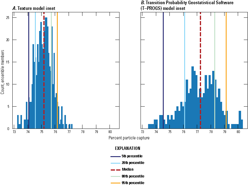
Histograms showing the percent of particles captured by remedial wells across all posterior Monte Carlo model runs (Corson-Dosch and Fienen, 2023). A, Texture model inset steady-state model. B, Transition Probability Geostatistical software (T–PROGS) model inset steady-state model.
Parameter Sweep
The initial optimization setup included adjusting remedial well pumping rates to maximize total plume capture. We initially started simulations with no remedial pumping and then adjusted pumping rates upward in increments of 5 percent of the total baseline or commitments remedial pumping, applied to all remedial wells equally, as much as 200 percent of the baseline remedial pumping. The increase in total capture is only from 80 percent to nearly 100 percent for the texture model inset and 95 percent to nearly 100 percent for T–PROGS model inset (fig. 54). However, as remedial pumping decreases from the baseline (100 percent of commitments) pumping, water-supply well capture increases owing to the location of several water-supply wells within the plume shell boundary as the remedial well capture decreases. In other words, adjusting remedial pumping substantially affects redistribution of capture between water-supply and remedial wells but only slightly affects total capture. Therefore, using total capture as an objective for optimization would likely result in an unacceptable level of water-supply well capture of the plume, which highlights the importance of evaluating system behavior prior to running through a sophisticated analysis.
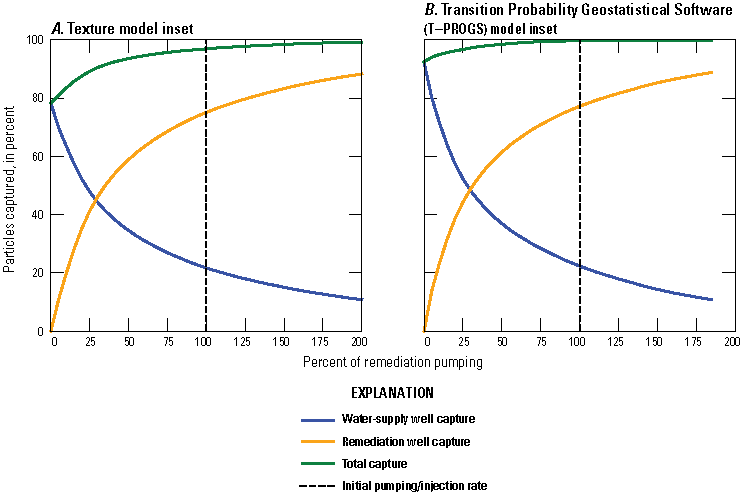
Tradeoffs of capture among total capture, remedial well capture, and water-supply well capture over a range of remedial pumping from 0 to 200 percent (Corson-Dosch and Fienen, 2023). A, Texture model inset. B, Transition Probability Geostatistical software (T–PROGS) model inset.
Formal Nonlinear Multiobjective Management Optimization
The tradeoffs between remedial and water-supply well pumping and plume capture necessitate a more complicated analysis than traditional single-objective optimization where a single objective is to be minimized or maximized, such as water-supply well and remedial well plume capture. Fienen and others (2024) provide a comparison between single and multiple objective optimization for this case. Instead, exploring the tradeoffs between these potentially competing objectives using a multiobjective approach may be more appropriate. In this analysis, the Non-Dominated Sorting Genetic Algorithm II (NSGA–II) (Deb and others, 2002) as implemented in PEST++ through the Multiple Objective Optimization under Uncertainty (MOU) version (White and others, 2022) was used.
The NSGA–II is a genetic algorithm requiring multiple generations of computations to converge on an optimal set of solutions that traverse the alternatives that are not dominated by any other alternative (a pareto frontier; Goodarzi and others, 2014). Solutions on this pareto frontier are defined ideally as points that are optimal for all objectives. However, exact pareto optimality with respect to all objectives is not achievable, so the frontier solutions are actually those for which only one objective can be improved.
Defining Decision Variables
“Decision variables” in management optimization are defined as the model inputs that are adjusted to explore optimal model solutions with respect to the multiple objectives and are subject to hard constraints. The only decision variables in this analysis were pumping extraction rates in remedial wells.
Simulating the Remedial System
The remedial system is defined by remedial pumping wells, treatment systems, injection wells, and infiltration basins at which treated water is returned to the subsurface. Extraction rates (decision variables) are selected by the algorithm to simulate each candidate solution. The amount of water extracted by each well then must be simulated as conveyed through the appropriate treatment system. The pumped water in each treatment system is then returned to the subsurface through the appropriate infiltration basin or injection well. The conveyance of extracted water to specific treatment systems is outlined in table 13 and shown schematically in figure 55.
Table 13.
Bounds on remedial pumping well rates, which treatment system each remedial well sends its water to, and limits on treatment capacity (Corson-Dosch and Fienen, 2023).[gal/min, gallon per minute; NA, not applicable; ft, feet; MSL, mean sea level; BWD, Bethpage Water District; ONCT, onsite containment system]
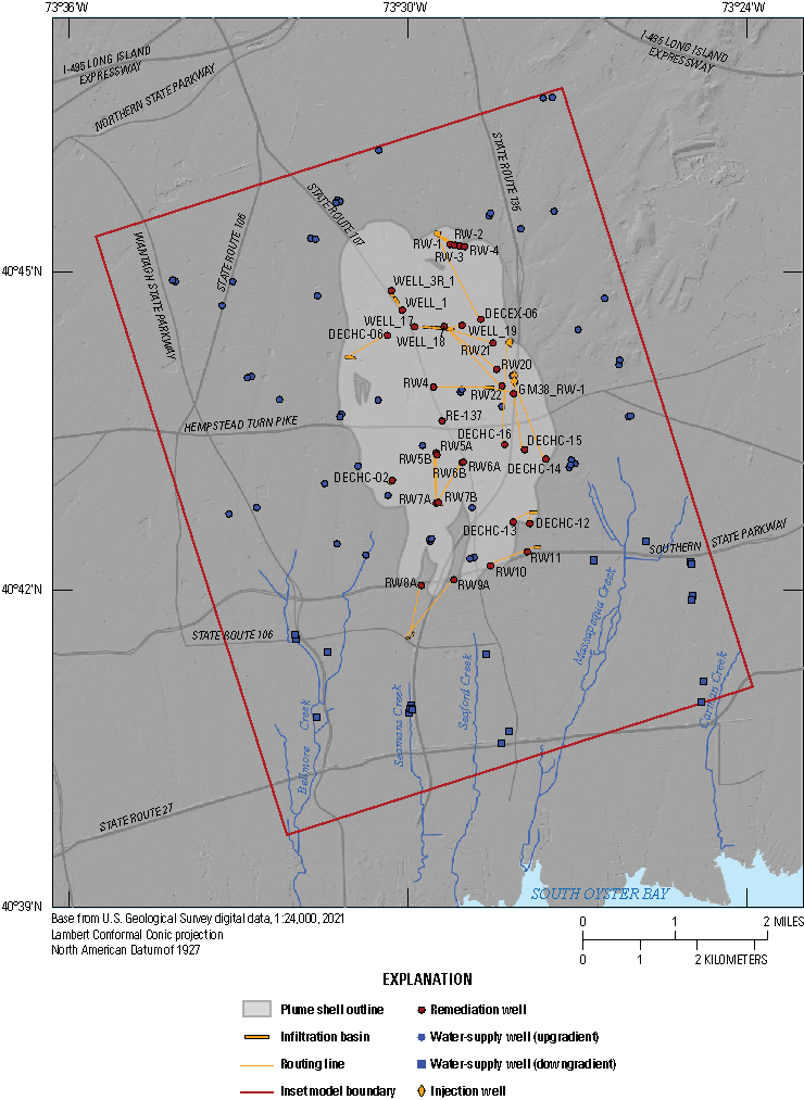
Remedial system schematically with locations of remedial wells, infiltration basins, and injection wells and the connections among them (Corson-Dosch and Fienen, 2023). The connections do not depict actual routing of pipelines.
Enforcing Constraints
Hard constraints are a combination of functions of model inputs and outputs and can restrict the search space for decision variables. For this analysis, the constraints enforced on model inputs included the following:
-
• specific ranges of pumping rates allowed for each remedial well (table 13)
-
• treatment system throughput limits (table 13)
-
• a minimum depth-to-water of 10 ft within a 1,500-ft buffer around infiltration basins to simulate the potential for flooding of residential infrastructure
-
• an upper limit on particle capture at downgradient wells
-
• an upper limit on particle capture by supply wells
These constraints can be operational (for example, limitations on treatment system capacity) or more subjective to set limits on the feasible search space of the algorithm (such as setting an upper limit on particle capture by supply wells, which was determined using early versions of the optimization).
Defining Objectives
Five potentially competing objectives that the algorithm was intended to optimize were defined. The objectives were the following:
-
1. maximize capture at remedial wells
-
2. maximize total particle capture (to avoid particles from leaving the area and making their way to the sea)
-
3. minimize capture at water-supply wells
-
4. minimize total remedial pumping (this is a proxy metric for cost of pumping and treating water)
-
5. minimize particles captured at downgradient wells
Analysis of Optimal Solutions for Plume Remediation
The MOU algorithm was started with 800 initial randomly selected sets of decision variable values (that is, individuals in a population). This population was allowed to progress for 70 generations in which various attributes of the individuals are combined and their fitness is evaluated. Fitness is defined as metrics in line with the objectives (for example, higher total particle capture and lower remedial pumping are both considered to have higher fitness).
The solutions that are chosen for management are “optimal” in the sense of having the greatest “fitness” as described above. However, particularly with multiple competing objectives, the determination of “optimal” is subjective. For the discussion here, we chose representative solutions as optimal for the purpose of discussion, but other analysts may judge the tradeoffs differently and choose different optimal solutions. The final set of optimal solutions, chosen for the purpose of discussion, for the texture model and T–PROGS model insets, are shown in figure 56A and B, respectively. The final set of optimal solutions for all the model simulations that were evaluated throughout the process are shown in figures 56C and D for the texture model and T–PROGS model insets, respectively. There is a nearly linear tradeoff between water supply and remedial capture, with the maximum capture by remedial wells corresponding with the lowest water-supply capture (fig. 54) in figure 56A and B; however, this selection does not consider the cost of remedial pumping or the costs of treatment that may be required at water-supply downgradient wells.
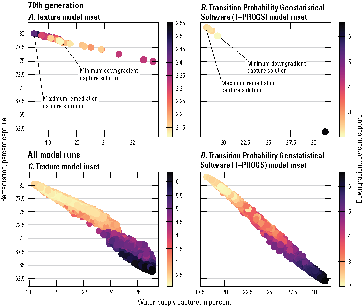
Tradeoffs among water-supply capture, remedial capture, and downgradient capture (Corson-Dosch and Fienen, 2023). A, Texture model inset, 70th generation. B, Transition Probability Geostatistical software (T–PROGS) model inset, 70th generation. C, Texture model inset, all model runs. D, T–PROGS model inset, all model runs.
A key advantage to using multiple objectives is that optimal solutions can be refined by incorporating additional information. For example, figure 57 shows the same information as figure 56, but the y-axes are changed from remediation capture to total remediation pumping. Remedial pumping is expressed as a percent of the baseline pumping rates where values less than 100 indicate a decrease in overall pumping and values greater than 100 indicate an increase in overall pumping. In contrast with the relation between water-supply and remedial capture, which is largely linear, the tradeoff is nonlinear when comparing water-supply capture with total remedial pumping.
The shape of the curves in figure 57 is less linear than in figure 56 and is characteristic of a pareto frontier. Near the origin of each graph, improving one objective degrades another objective—this is referred to as a pareto optimal point. For example, the decrease in water-supply plume capture from 21 to 18 percent results in an increase in remedial pumping of nearly 30 percent. From another perspective, increasing remedial pumping from 90 to 120 percent of the baseline only represents a 2-percent change in water-supply capture.
However, the straighter edges of the curve distant from the origin indicate locations where improvement can be made in one objective without incurring cost in the other. For example, there is a potential outcome where the water-supply capture can be decreased from 27 to 21 percent with only a small increase in total pumping (fig. 57A) because the MOU algorithm is able to redistribute pumping among the wells to optimize this outcome without significantly increasing the total pumping.
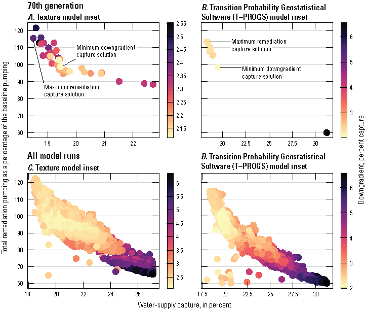
Tradeoffs among water-supply capture, total remedial pumping, and downgradient capture (Corson-Dosch and Fienen, 2023). A, Texture model inset, 70th generation. B, Transition Probability Geostatistical software (T–PROGS) model inset, 70th generation. C, Texture model inset, all model runs. D, T–PROGS model inset, all model runs.
The previous discussion presented the pareto optimal point example when only two competing objectives were considered. A third objective—downgradient capture—is also shown in figures 56 and 57. All three objectives (water-supply capture, remedial pumping, and downgradient capture) are observed at low values near the origin where a trough of downgradient capture is present when all the model runs are evaluated along the path to optimality (fig. 57C and D).
The pumping rates for two selected solutions from the optimization are shown in figures 58 and 59. The spatial distribution of pumping for the solutions were chosen (figs. 58B–C and 59B–C, respectively) based on the criterion of maximizing remedial capture without regard to total remedial pumping or downgradient capture (fig. 58), and the tradeoff point is identified in figure 56. A comparison of the optimal solutions with the baseline indicates slight increases in remedial well pumping along the outer edge of the plume. The subtlety of these changes largely is due to the strict constraints on pumping that allowed for limited redistribution of pumping among a subset of the remedial wells.
When total remedial pumping cost and downgradient plume capture were considered (fig. 59), the optimal solution was identified as closest to the pareto optimal point indicated in figure 57. The subtle changes from the baseline needed to achieve optimal pumping are similar to changes shown in figure 56 but with pumping generally redistributed to focus more on the center of the plume, which allows for more water-supply capture to the east in favor of preventing further downgradient migration. Baseline and optimal pumping rates for the two optimal solutions for each model are listed in table 14.
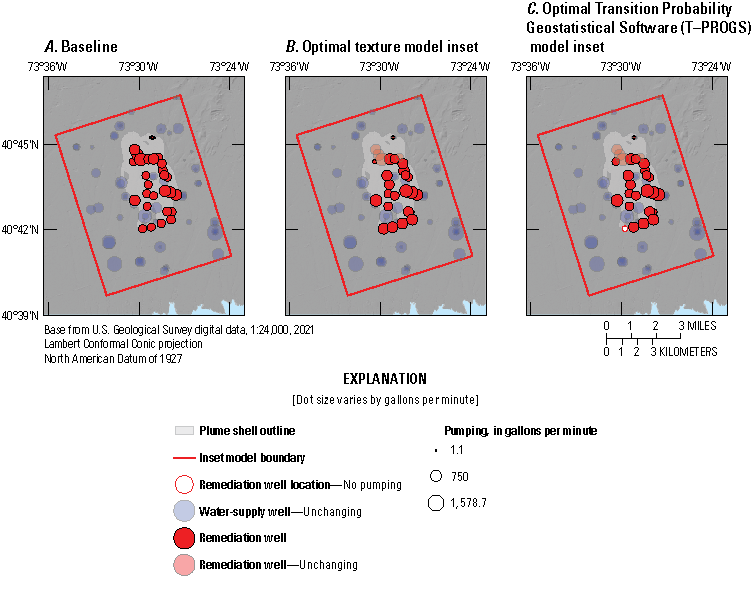
Pumping rates for water-supply wells and remedial wells (Corson-Dosch and Fienen, 2023). A, Baseline pumping rates. B, Optimal rates based on maximizing remedial capture for the texture model inset. C, Optimal rates based on maximizing remedial capture for Transition Probability Geostatistical software (T–PROGS) model inset. Baseline and optimal pumping rates are listed in table 14.
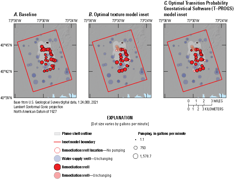
Pumping rates for water-supply wells and remedial wells (Corson-Dosch and Fienen, 2023). A, Baseline pumping rates. B, Optimal rates based on minimizing downgradient capture for the texture model inset. C, Optimal rates based on minimizing downgradient capture for Transition Probability Geostatistical software (T–PROGS) model inset. Baseline and optimal pumping rates are listed in table 14.
Table 14.
Baseline remediation pumping well rates, upper and lower bounds, and optimal rates from the maximum remediation capture and the minimum downgradient capture scenarios (Corson-Dosch and Fienen, 2023).[gal/min, gallon per minute; Min, minimum; Max, maximum; DGC, downgradient capture; T–PROGS, Transition Probability Geostatistical Software; ONCT, onsite containment system]
Simulation of the Effects of Remedial Pumping and Recharge on the Freshwater/Saltwater Interface
The potential effects of the proposed remedial pump and treatment plan on movement of the freshwater/saltwater interface were assessed when the recent (2024) model of Long Island was developed to simulate changes in the position and movement of the freshwater/saltwater interface in response to time-varying pumping and recharge stresses. This model simulates historical stresses for 1900–2019 to estimate the current (2019) position of the freshwater/saltwater interface, which then serves as the initial condition for simulation of future changes in stresses.
For this investigation, the simulated position of the interface, as represented in the simulation of hydrologic conditions for 1900–2019, was used as the starting condition in a simulation that includes the current and future remedial stresses discussed in this report. Changes in hydraulic heads and the position of the freshwater/saltwater interface were simulated for a 101-year period from 2020 to 2120. Two scenarios were evaluated: (1) a “no-change” scenario using public-supply and remedial stresses from 2019, and (2) a “commitments” scenario augmenting those 2019 stresses with additional remedial stresses representing commitments by responsible parties to fully remediate of the Navy Grumman groundwater plume (New York State Department of Environmental Conservation, 2019).
The simulated freshwater/saltwater interface, defined for the sake of evaluation of interface movement as the 5-percent isochlor between fresh and saltwater, continues to move landward under both future scenarios; however, the landward movement of the simulated interface position under the proposed “commitments” pumping scenario does not appreciably exceed that which results from the continued simulation of current condition pumping and recharge stress (figs. 60–61). The landward movement of the simulated interface position likely is due to the lagging response of the groundwater system to changes in pumping and recharge from 1900 to 2019, and the post-glacial sea-level rise as described in Walter and others (2024). There is no substantial difference in the rate of the movement of the interface position in the basal Magothy and Lloyd aquifers, although there is some water redistribution during future scenarios caused by the combination of deep remedial pumping and shallow recharge of treated water. This water redistribution likely is due to the large distance (about 10 mi) between remedial systems for the Navy Grumman groundwater plume and the current (2019) location of the coastline.
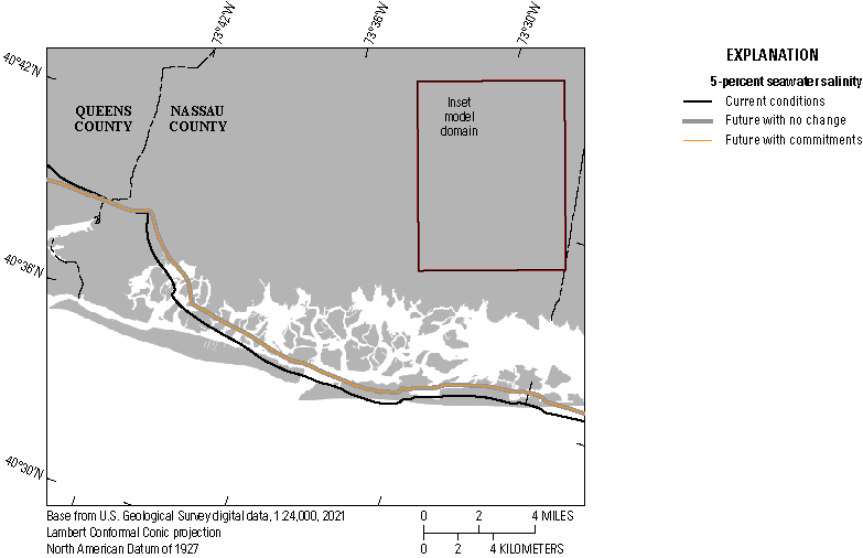
Simulated location of freshwater/saltwater interface (defined as the 5-percent isochlor between fresh and saltwater; Corson-Dosch and Fienen, 2023) in the Magothy aquifer for current (2019) and future (2100) conditions, southeastern Nassau County, New York.
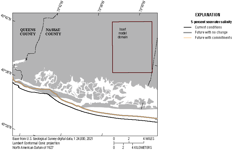
Simulated location of freshwater/saltwater interface (defined as the 5-percent isochlor between fresh and saltwater; Corson-Dosch and Fienen, 2023) in the Lloyd aquifer for current (2019) and future (2100) conditions, southeastern Nassau County, New York.
Summary and Conclusions
Several plumes of dissolved, chlorinated solvents, including trichloroethylene, have been identified in a sole-source aquifer near the former Northrop Grumman Bethpage facility (NGBF) and Naval Weapons Industrial Reserve Plant (NWIRP) in southeastern Nassau County, New York. Past investigations have documented that the groundwater contamination originated from the NGBF and NWIRP area and now extends nearly 4 miles to the south, in the direction of groundwater flow. As such, the comingled plumes are commonly referred to as the Navy Grumman groundwater plume. Knowledge of groundwater-flow patterns and rates is essential for effective management of groundwater resources and for mitigation of potential adverse effects of the plume on drinking-water supplies and ecosystems. A recent groundwater-flow model developed by the U.S. Geological Survey (USGS), in cooperation with the New York State Department of Environmental Conservation (NYSDEC), evaluated alternatives to hydraulically contain the plume as part of a feasibility study. The USGS modeling effort helped inform an Amended Record of Decision that identified a comprehensive plan to contain and clean up the contamination plume.
Further model development and refinement was needed for the NYSDEC to evaluate design options necessary for the construction, operation, optimization, maintenance, and monitoring of the comprehensive remedy selected in the December 2019 Amended Record of Decision to address these plumes. The purpose of this report is to describe the results of a multicomponent study undertaken to further develop and refine models to evaluate design scenarios for groundwater extraction and treatment remediation of the Navy Grumman groundwater plume. This report includes an updated interpretation of the hydrogeologic framework with two independent characterizations of aquifer heterogeneity; an updated regional model providing transient boundary conditions for inset modeling of the plume area; new inset models for the two independent aquifer characterizations and risk-based optimization of the remedial design; and an updated regional model of freshwater/saltwater interface movement. This multiscale modeling approach allows the area near the plume to be simulated in finer detail than would be possible with the regional model but still establishes and maintains hydrologic connections to natural flow boundaries outside the inset area.
The existing regional (parent) groundwater-flow model encompasses the entire four-county (Kings, Queens, Nassau, and Suffolk) area of Long Island, New York. New inset models to help refine decision support for the remedial design focused on the local area encompassing the full extent of the Navy Grumman groundwater plume in southeastern Nassau County. Major streams in the inset area include Bellmore Creek and Massapequa Creek; minor streams include Carman Creek, Seaford Creek, Seamans Creek, Newbridge Creek, and Cedar Swamp Creek. These streams receive perennial (base) flow in the southern part of the inset area where their channels incise the water table. Because the channels are generally shallow, the low-lying areas surrounding these streams are vulnerable to flooding caused by the shallow depth to groundwater. From 2005 to 2019, a total of about 424 million gallons per day (Mgal/d) of groundwater was withdrawn annually from the Long Island aquifer system for multiple uses, including public supply, agriculture, and industry. About 34 Mgal/d was withdrawn for public supply within the inset area. During the 2005 to 2019 period, a total of about 8 Mgal/d of groundwater on average was withdrawn annually from the Long Island aquifer system for contaminant remediation. The vast majority (7.9 Mgal/d) of the total was withdrawn as part of Navy Grumman groundwater plume remediation within the inset area.
A texture model inset was developed from the results of a detailed analysis of lithologic descriptions and the conversion of these qualitative data to more quantitative measures of important hydrogeologic characteristics of the upper glacial and Magothy aquifers. The detailed analysis was centered on the inset area and included the development of a local-scale texture model similar to the one previously developed for the entire Long Island aquifer system. The analytical approach was used with 22,523 lithologic descriptions from 256 boreholes in the inset area to define standard lithologic codes for each vertical interval in each borehole. A set of stacked three-dimensional grids was created, each 10 feet in thickness, that spanned the thicknesses of the upper glacial and Magothy aquifers in the inset area.
The spatial and vertical patterns in hydraulic conductivity within the inset area generally are consistent with the depositional history of the regional aquifer system. Lower values of hydraulic conductivity in the upper glacial aquifer generally occur in northern parts of the inset area and are associated with glacial moraines. Hydraulic conductivity is highest in outwash sediments south of the moraine. The Magothy aquifer is more heterogenous, with fewer broad spatial patterns, except in its basal portion. Hydraulic conductivity in the basal portion of the Magothy aquifer, where sediments likely were deposited in fluvial depositional environments, generally is higher than in overlying portions of the unit. The hydraulic conductivity generally is lowest in the middle part of the Magothy aquifer where sediments likely were deposited in overbank lake and wetland environments.
Transition Probability Geostatistical Software (T–PROGS) is a software package that performs transition probability geostatistics to generate multiple equally probable models of aquifer heterogeneity conditioned to borehole data. Five hundred T–PROGS realizations of the hydrostratigraphy were created using the same input structure in a Monte Carlo-type analysis to form the stratigraphic basis for the groundwater modeling. A total of 256 soil boring logs were described over a span of 20 years at and surrounding the NWIRP and NGBF sites. T–PROGS was used to generate multiple equally probable models of aquifer heterogeneity all conditioned to the 256 boring logs. The category sand is the most prevalent with a percentage distribution of approximately 60 percent. Sand and gravel is the second most dominant material with an approximate distribution percentage of 24 percent. Gravel and fines make up the last 16 percent at 5 percent and 11 percent, respectively. This material distribution holds true for each potential realization computed by T–PROGS when using these boring logs. Each realization varies slightly; however, the percent distributions remain consistent with the material distributions found in the borings.
A regional model was constructed generally following the Long Island regional groundwater-flow model (LIRM) to provide transient boundary conditions for inset modeling of the plume area. Enhancements to the existing regional model included updating of ongoing inset area remedial stresses (groundwater extraction and treatment systems), representation of transient stress periods, and updating the model code to MODFLOW 6. The transient LIRM simulates long-term steady-state conditions and does not simulate seasonal and other shorter-term, transient changes in hydraulic head and groundwater flow. To represent these transient changes in the groundwater system, monthly hydrologic stresses from January 2005 through December 2019 were assembled for seven stress components: natural recharge, redirected recharge, return flow, ponds, water-supply infrastructure leakage, public supply well pumping, and remedial pumping.
Using the MODFLOW 6 model code, hydraulic heads and groundwater flows were simulated for the period January 1, 2005, through December 31, 2019. Simulated heads within the inset area ranged from about 10 to about 80 feet above the North American Vertical Datum of 1988 and water-table mounds and depressions formed at points of remedial pumping and discharge, respectively. Hydraulic heads and base flows in streams at representative monitoring points within the inset area are similar to those of a model recently developed to simulate plume movement and effects on downgradient public-supply wells in the area. With regard to the inset area portion of the transient LIRM, average total inflow of about 105 cubic feet per second was divided as follows: water-table recharge (66 percent), lateral inflow (22 percent), and remedial system return flow from discharge of treated water to recharge basins (12 percent). Outflow that generally balanced inflow was divided as follows: groundwater pumping (57 percent), stream discharge (11 percent), and lateral outflow (32 percent).
An inset model was developed from the regional model for the evaluation of the efficacy of proposed remedial plans for the Navy Grumman groundwater plume area. This inset model was created using MODFLOW 6 and scripting tools to connect to the transient LIRM, which simulates all Long Island. This inset approach allows us to simulate the area near the plume in finer detail than would be possible with the regional model but still establishes and maintains the hydrologic connections to regional boundaries including Long Island Sound and the Atlantic Ocean. History matching was performed to tune model parameters for the inset such that two ensembles with different conceptual bases (the texture model and the T–PROGS model insets) were generated exploring the range of plausible aquifer hydraulic property conditions consistent with field observations.
The ensembles of parameters resulting from history matching provided a platform with which to evaluate capture by water-supply and remedial wells using particle tracking with MODPATH 7. Using the ensemble to select a risk stance, multiobjective optimization was completed to identify various configurations of remedial pumping that are consistent with external constraints and that balance potentially competing objectives. Multiple solutions from the multiobjective optimization simulations have tradeoffs that NYSDEC can consider. In general, if pumping is redistributed to focus more on the center of the plume, some water-supply well contaminant capture may increase to the east to prevent further migration downgradient. The choice of what constitutes an “optimal” solution from this analysis is subjective, requiring consideration of the competition among multiple objectives. For illustrative purposes, we selected candidate solutions for further analysis and discussion, but those selections do not constitute a recommendation of a solution for the decisionmakers to select.
A recently (2024) developed transient LIRM that simulates the response of the freshwater/saltwater interface to changes in hydrologic conditions from 1900 to 2019 was used to assess future response of the freshwater/saltwater interface to the proposed remedial pumping and return flow needed for plume containment.
Proposed plume containment remedial pumping and return flow stresses were simulated for two conditions—one simulating current stresses (“no change”) and one representing planned future remedial stresses (“commitments”) from 2020 to 2100. The simulations showed that there was progressive movement of salty groundwater towards the plume site regardless of the stress scenario used. The future rate of movement of the freshwater/saltwater interface was similar to historical rates and is attributed to the lagging response of the groundwater system to post-glacial sea-level rise. There was no substantial change in the rate of the movement of the Lloyd or basal Magothy freshwater/saltwater interfaces, although there is some redistribution of water owing to the combination of deep remedial pumping and shallow recharge of treated water, which likely is due to a sufficient distance between and the plume site and the current freshwater/saltwater interface.
References Cited
Alfonzo, M., and Oliver, D.S., 2019, Evaluating prior predictions of production and seismic data: Computational Geosciences, v. 23, no. 6, p. 1331–1347. [Also available at https://doi.org/10.1007/s10596-019-09889-6.]
Aquaveo, LLC, 2021, Groundwater Modeling System introduction: Aquaveo web page, accessed August 12, 2022, at https://www.aquaveo.com/software/gms-groundwater-modeling-system-introduction.
Arcadis G&M, Inc., 2003, Comprehensive groundwater model report—U.S. Naval Weapons Industrial Reserve Plant/Northrup Grumman, Bethpage New York: Melville, N.Y., Arcadis G&M, Inc., 140 p. [Also available at https://extapps.dec.ny.gov/data/DecDocs/130003B/Report.HW.130003B.2003-04-28.Comprehensive%20Groundwater%20Model%20.pdf.]
Aronson, D.A., and Seaborn, G.E., 1974, Appraisal of operating efficiency of recharge basins in Long Island, New York: U.S. Geological Survey Water-Supply Paper 2001–D, 22 p. [Also available at https://doi.org/10.3133/wsp01D.]
Bond, N., 2022, hydrostats—Hydrologic indices for daily time series data: The Comprehensive R Archive Network (CRAN), accessed July 9, 2024, at https://cran.r-project.org/web/packages/hydrostats/index.html.
Brown, P.M., Miller, J.A., and Swain, F.M., 1972, Structural and stratigraphic framework, and spatial distribution of permeability of the Atlantic Coastal Plain, North Carolina to New York: U.S. Geological Survey Professional Paper 796, 87 p., 59 pl. [Also available at https://doi.org/10.3133/pp796.]
Cadwell, D.H., and Muller, E.H., 1986, Surficial geologic map of New York: New York Museum data, accessed August 4, 2019, at https://www.nysm.nysed.gov/research-collections/geology/gis.
Carle, S.F., 1999, T-PROGS—Transition probability geostatistical software, Version 2.1: University of California, Davis, 84 p. [Also available at http://gmsdocs.aquaveo.com/t-progs.pdf.]
Corson-Dosch, N.T., and Fienen, M.N., 2023, MODFLOW 6 models for simulating groundwater flow and a proposed remediation system in the sole-source aquifer system in southeastern Nassau County, New York: U.S. Geological Survey data release, accessed month year at accessed July 9, 2024, at https://doi.org/10.5066/P92KSK8H.
Deb, K., Pratap, A., Agarwal, S., and Meyarivan, T.A.M.T., 2002, A fast and elitist multiobjective genetic algorithm—NSGA-II: IEEE Transactions on Evolutionary Computation, v. 6, no. 2, p. 182–197. [Also available at https://doi.org/10.1109/4235.996017.]
Deutsch, C.V., and Journel, A.J., 1992, Practical considerations in the application of simulated annealing in stochastic simulation: Mathematical Geology, v. 26, no. 1, p. 67–82. [Also available at https://doi.org/10.1007/BF02065876.]
De Cicco, L.D., Hirsch, R.M., and Watkins, W., 2018, Data retrieval—R packages for discovering and retrieving water data available from U.S. federal hydrologic web services: Reston, VA, U.S. Geological Survey, accessed July 9, 2024 at https://doi.org/10.5066/P9X4L3GE.
Dlubac, K., Knight, R., Song, Y.-Q., Bachman, N., Grau, B., Cannia, J., and Williams, J., 2013, Use of NMR logging to obtain estimates of hydraulic conductivity in the High Plains aquifer, Nebraska, USA: Water Resources Research, v. 49, no. 4, p. 1871–1886. [Also available at https://doi.org/10.1002/wrcr.20151.]
Doherty, J., 2003, Ground water model calibration using pilot points and regularization: Ground Water, v. 41, no. 2, p. 170–177. [Also available at https://doi.org/10.1111/j.1745-6584.2003.tb02580.x.]
Doherty, J., and Hunt, R.J., 2010, Approaches to highly parameterized inversion—A guide to using PEST for groundwater-model calibration: U.S. Geological Survey Scientific Investigations Report 2010–5169, 60 p. [Also available at https://doi.org/10.3133/sir20105169.]
Doriski, T.P., and Wilde-Katz, F., 1982, Geology of the “20-foot” clay and Gardiners Clay in southern Nassau and southwestern Suffolk counties, Long Island, New York: U.S. Geological Survey Water-Resources Investigations Report 82–4056, 21 p. [Also available at https://doi.org/10.3133/wri824056.]
Evans, M., and Moshonov, H., 2006, Checking for prior-data conflict: Bayesian Analysis, v. 1, no. 4, p. 893–914. [Also available at https://doi.org/10.1214/06-BA129
Fienen, M.N., Haserodt, M.J., Leaf, A.T., and Westenbroek, S.M., 2022a, Simulation of regional groundwater flow and groundwater/lake interactions in the Central Sands, Wisconsin: U.S. Geological Survey Scientific Investigations Report 2022–5046, 111 p. [Also available at https://doi.org/10.3133/sir20225046.]
Fienen, M.N., Corson‐Dosch, N.T., White, J.T., Leaf, A.T., and Hunt, R.J., 2022b, Risk‐based wellhead protection decision support—A repeatable workflow approach: Ground Water, v. 60, no. 1, p. 71–86. [Also available at https://doi.org/10.1111/gwat.13129.]
Fienen, M.N., Corson-Dosch, N.T., Jahn, K.L., and White, J.T., 2024, Comparing single and multiple objective constrained optimization algorithms for tuning a groundwater remediation system: Environmental Modelling & Software, v. 173, p. 105952. [Also available at https://doi.org/10.1016/j.envsoft.2024.105952.]
Finkelstein, J.S., Monti, J., Jr., Masterson, J.P., and Walter, D.A., 2022, Application of a soil-water-balance model to estimate annual groundwater recharge for Long Island, New York, 1900–2019: U.S. Geological Survey Scientific Investigations Report 2021–5143, 25 p. [Also available at https://doi.org/10.3133/sir20215143.]
Fuller, M.L., 1914, The geology of Long Island, New York: U.S. Geological Survey Professional Paper 82, 231 p. [Also available at https://doi.org/10.3133/pp82.
Franke, O.L., and Cohen, P., 1972, Regional rates of ground-water movement on Long Island, New York, in Geological survey research 1972: U.S. Geological Survey Professional Paper 800–C, p. C271–277. [Also available at https://doi.org/10.3133/pp800C.]
Getzen, R.T., 1977, Analog-model analysis of regional three-dimensional flow in the ground-water reservoir of Long Island, New York: U.S. Geological Survey Professional Paper 982, 49 p., accessed August 3, 2019, at https://doi.org/10.3133/pp982.
Goodarzi, E., Ziaei, M., and Hosseinipour, E., 2014, Introduction to optimization analysis in hydrosystem engineering, in Tatano, H., Zio, E., and Sousa-Poza, A., eds., Topics in safety, risk, reliability and quality: Springer International Publishing, accessed July 9, 2024 at https://doi.org/10.1007/978-3-319-04400-2.
HDR Inc., 2019, Feasibility study report—Northrup Grumman Bethpage facility (operable units 2 and 3) and Naval Weapons Industrial Reserve Plant (operable unit 2): Prepared for New York State Department of Environmental Conservation, work assignment D007625–32, 236 p. [Also available at https://extapps.dec.ny.gov/docs/remediation_hudson_pdf/ngnwirpfs.pdf.]
Kendrick, A.K., Knight, R., Johnson, C.D., Liu, G., Knobbe, S., Hunt, R.J., and Butler, J.J., Jr., 2021, Assessment of NMR logging for estimating hydraulic conductivity in glacial aquifers: Ground Water, v. 59, no. 1, p. 31–48. [Also available at https://doi.org/10.1111/gwat.13014.]
Knight, R., Walsh, D.O., Butler, J.J., Jr., Grunewald, E., Liu, G., Parsekian, A.D., Reboulet, E.C., Knobbe, S., and Barrows, M., 2016, NMR logging to estimate hydraulic conductivity in unconsolidated aquifers: Ground Water, v. 54, no. 1, p. 104–114. [Also available at https://doi.org/10.1111/gwat.12324.]
Krulikas, R.K., and Koszalka, E.J., 1982, Geologic reconnaissance of an extensive clay unit in north-central Suffolk County, Long Island, New York: U.S. Geological Survey Water-Resources Investigations Report 82–4075, 9 p., 1 pl. [Also available at https://doi.org/10.3133/wri824075.]
Ladson, A.R., Brown, R., Neal, B., and Nathan, R., 2013, A standard approach to baseflow separation using the Lyne and Hollick filter: Australian Journal of Water Resources, v. 17, no. 1, p. 25–34. [Also available at https://doi.org/10.7158/13241583.2013.11465417.]
Langevin, C.D., Hughes, J.D., Banta, E.R., Niswonger, R.G., Panday, S., and Provost, A.M., 2017, Documentation for the MODFLOW 6 Groundwater Flow Model: U.S. Geological Survey Techniques and Methods, book 6, chap. A55, 197 p., accessed July 9, 2024 at https://doi.org/10.3133/tm6A55.
Leaf, A.T., and Fienen, M.N., 2022, Modflow-setup—Robust automation of groundwater model construction: Frontiers in Earth Science (Lausanne), v. 10, p. 903965. [Also available at https://doi.org/10.3389/feart.2022.903965.]
Leaf, A.T., Fienen, M.N., and Reeves, H.W., 2021. SFRmaker and Linesink‐maker: Rapid construction of streamflow routing networks from hydrography data. Groundwater, v. 59, no. 5, p. 761–771. [Also available at https://doi.org/10.1111/gwat.13095.]
Masterson, J.P., Pope, J.P., and Fienen, M.N., Monti, J., Jr., Nardi, M.R., and Finkelstein, J.S., 2016, Assessment of groundwater availability in the Northern Atlantic Coastal Plain aquifer system from Long Island, New York, to North Carolina: U.S. Geological Survey Professional Paper 1829, 76 p. [Also available at https://doi.org/10.3133/pp1829.]
McDonald, M.G., and Harbaugh, A.W., 1988, A modular three-dimensional finite-difference ground-water flow model: U.S. Geological Survey Techniques of Water-Resources Investigations, book 6, chap. A1, 586 p. [Also available at https://doi.org/10.3133/twri06A1.]
Misut, P.E., 2011, Simulation of groundwater flow in a volatile organic compound-contaminated area near Bethpage, Nassau County, New York—A discussion of modeling considerations: U.S. Geological Survey Open-File Report 2011–1128, 19 p., accessed August 3, 2019, at https://doi.org/10.3133/ofr20111128.
Misut, P.E., 2014, Simulation of zones of contribution to wells at site GM–38, Naval Weapons Industrial Reserve Plant, Bethpage, New York: U.S. Geological Survey Scientific Investigations Report 2014–5036, 58 p., accessed August 3, 2019, at https://doi.org/10.3133/sir20145036.
Misut, P.E., 2018, Simulation of zones of contribution to wells south of the Naval Weapons Industrial Reserve Plant, Bethpage, New York: U.S. Geological Survey Scientific Investigations Report 2017–5161, 45 p., accessed August 3, 2019, at https://doi.org/10.3133/sir20175161.
Misut, P.E., and Monti, J., Jr., 1999, Simulation of ground-water flow and pumping in Kings and Queens Counties, Long Island, New York: U.S. Geological Survey Water-Resources Investigations Report 98-4071, 50 p. [Also available at https://doi.org/10.3133/wri984071.]
Misut, P.E., Walter, D., Schubert, C., and Dressler, S., 2020, Analysis of remedial scenarios affecting plume movement through a sole-source aquifer system, southeastern Nassau County, New York: U.S. Geological Survey Scientific Investigations Report 2020–5090, 83 p., accessed July 9, 2024 at https://doi.org/10.3133/sir20205090.
Misut, P.E., Walter, D.A., and Schubert, C.E., 2024, MODFLOW 6 model scenario used to simulate transient stresses, heads, and flows in the Regional Aquifer System of Long Island, New York, 2005–2019: U.S. Geological Survey data release, accessed July 9, 2024, at https://doi.org/10.5066/P907ORL5.
Monti, J., Jr., Como, M., and Busciolano, R., 2013, Water-table and Potentiometric-surface altitudes in the Upper Glacial, Magothy, and Lloyd aquifers beneath Long Island, New York, April-May 2010: U.S. Geological Survey, Scientific Investigations Map 3270, 4 sheets, scale 1:125,000, https://doi.org/10.3133/sim3270.
New York State Department of Environmental Conservation, 2020, Water withdrawals by facility—Beginning 2009: New York State Department of Environmental Conservation data, accessed June 15, 2020, at https://data.ny.gov/Energy-Environment/Water-Withdrawals-by-Facility-Beginning-2009/94ue-tysy.
New York State Department of Environmental Conservation, 2023, State superfund sites: New York State Department of Environmental Conservation web page, accessed April 28, 2023, at https://dec.ny.gov/environmental-protection/site-cleanup/brownfield-and-state-superfund-programs/state-superfund-sites.
New York State Department of Environmental Conservation, 2024a, Environmental Remediation Database: Northrop Grumman - Bethpage Facility Record, accessed September 2024, at https://extapps.dec.ny.gov/cfmx/extapps/derexternal/haz/details.cfm?ProgNo=130003A.
New York State Department of Environmental Conservation, 2024b, Environmental Remediation Database: Naval Weapons Ind. Reserve Plant Record, accessed September 2024, at https://extapps.dec.ny.gov/cfmx/extapps/derexternal/haz/details.cfm?ProgNo=130003B.
Niswonger, R.G., and Prudic, D.E., 2005, Documentation of the streamflow-routing (SFR2) package to include unsaturated flow beneath streams—A modification to SFR1: U.S. Geological Survey Techniques and Methods, book 6, chap. A13, 51 p., accessed February 2021 at https://doi.org/10.3133/tm6A13.
Pollock, D.W., 1994a, Source code and ancillary data files for the MODPATH particles tracking package of the ground-water flow model MODFLOW: U.S. Geological Survey Open-File Report 94–463, 2 CD–ROMs. [Also available at https://doi.org/10.3133/ofr94463.]
Pollock, D.W., 1994b, User’s guide for MODPATH/MODPATH–PLOT, version 3; a particle tracking post-processing package for MODFLOW, the U.S. Geological Survey finite-difference ground-water flow model: U.S. Geological Survey Open-File Report 94–464, 248 p. [Also available at https://doi.org/10.3133/ofr94464.]
Pollock, D.W., 2016, User guide for MODPATH Version 7—A particle-tracking model for MODFLOW: U.S. Geological Survey Open-File Report 2016–1086, 35 p., accessed July 9, 2024 at https://doi.org/10.3133/ofr20161086.
Prudic, D.E., Konikow, L.F., and Banta, E.R., 2004, A new Streamflow-Routing (SFR1) Package to simulate stream-aquifer interaction with MODFLOW-2000: U.S. Geological Survey Open-File Report 2004–1042, 104 p., accessed February 2021 at https://doi.org/10.3133/ofr20041042.
Schubert, C.E., Bova, R.G., and Misut, P.E., 2004, Hydrogeologic framework of the North Fork and surrounding areas, Long Island, New York: U.S. Geological Survey Water-Resources Investigations Report 02–4284, 24 p., 4 pls., scale 1:120,000. [Also available at https://doi.org/10.3133/wri024284.]
Schubert, C., and Buxton, H.T., Monti, J., Jr., 1997, Ground-water resource evaluation on Long Island, New York, using flow models and a geographic information system: U.S. Geological Survey Fact Sheet 239-96, 4 p. [Also available at https://doi.org/10.3133/fs23996.]
Seaburn, G.E., and Aronson, D.A., 1974, Influence of recharge basins on the hydrology of Nassau and Suffolk Counties, Long Island, New York: U.S. Geological Survey Water Supply Paper 2031, 66 p. [Also available at https://doi.org/10.3133/wsp2031.]
Sirkin, L.A., 1986, Palynology and Stratigraphy of Cretaceous and Pleistocene sediments on Long Island, New York—A basis for correlation with New Jersey coastal plain sediments: U.S. Geological Survey Bulletin 1559, 52 p. [Also available at https://doi.org/10.3133/b1559.]
Smolensky, D.A., Buxton, H.T., and Shernoff, P.K., 1990, Hydrogeologic framework of Long Island, New York: U.S. Geological Survey Hydrologic Atlas 709, 3 sheets. [Also available at https://doi.org/10.3133/ha709.]
Smolensky, D.A., and Feldman, S.M., 1995, Three-dimensional advective transport of volatile organic compounds in ground water beneath an industrial/residential area of Nassau County, New York: U.S. Geological Survey Water-Resources Investigations Report 92–4148, 53 p. [Also available at https://doi.org/10.3133/wri924148.]
Stumm, F., 2001, Hydrogeology and extent of saltwater intrusion of the Great Neck peninsula, Great Neck, Long Island, New York: U.S. Geological Survey Water-Resources Investigations Report 99–4280, 41 p. [Also available at https://doi.org/10.3133/wri994280.]
Stumm, F., Finkelstein, J.S., and Williams, J.H., 2024, Hydrogeologic framework and extent of saltwater intrusion in Kings, Queens, and Nassau Counties, Long Island, NY: U.S. Geological Survey Scientific Investigations Report 2024–5048, 75 p., accessed June 13, 2024, at https://doi.org/10.3133/sir20245048.
Stumm, F., Lange, A.D., and Candela, J.L., 2002, Hydrogeology and extent of saltwater intrusion on Manhasset Neck, Nassau County, New York: U.S. Geological Survey Water-Resources Investigations Report 00–4193, 42 p. [Also available at t https://doi.org/10.3133/wri004193.]
Stumm, F., Lange, A.D., and Candela, J.L., 2004, Hydrogeology and extent of saltwater intrusion in the northern part of the town of Oyster Bay, Nassau County, New York—1995–98: U.S. Geological Survey Water-Resources Investigations Report 2003–4288, 55 p. [Also available at https://doi.org/10.3133/wri034288.]
Tarantola, A., 2005, Inverse problem theory and methods for model parameter estimation: Philadelphia, Pennsylvania, Society for Industrial and Applied Mathematics, 342 p. [Also available at https://doi.org/10.1137/1.9780898717921.]
U.S. Census Bureau, 2021, Census (P.L. 94-171) redistricting data summary file—2020: U.S. Census Bureau data, accessed October 1, 2021, at https://data.census.gov.
U.S. Environmental Protection Agency (EPA), 2024, National Primary Drinking Water Regulations: Organic Chemicals except for PFAS, accessed September 1, 2024, at https://www.epa.gov/ground-water-and-drinking-water/national-primary-drinking-water-regulations#Organics.
U.S. Geological Survey, 2018, USGS water data for the Nation: U.S. Geological Survey National Water Information System database, accessed June 13, 2018, at https://doi.org/10.5066/F7P55KJN.
U.S. Geological Survey, 2022a, Aquifer test locator: U.S. Geological Survey web page, accessed August 15, 2022, at https://ny.water.usgs.gov/maps/aq-test/.
U.S. Geological Survey, 2022b, USGS GeoLog locator: U.S. Geological Survey web page, accessed August 15, 2022, at https://webapps.usgs.gov/GeoLogLocator/#!/.
U.S. Geological Survey, 2022c, USGS water data for the Nation: U.S. Geological Survey National Water Information System database, accessed August 15, 2022, at https://doi.org/10.5066/F7P55KJ.
U.S. Geological Survey, 2023, USGS water data for the Nation: U.S. Geological Survey National Water Information System database, accessed February 1, 2023, at https://doi.org/10.5066/F7P55KJN.
Veatch, A.C., Slichter, C.S., Bowman, I., Crosby, W.O., and Horton, R.E., 1906, Underground water resources of Long Island, New York: U.S. Geological Survey Professional Paper 44, 394 p. [Also available at https://doi.org/10.3133/pp44.]
Wagner, B.J., and Gorelick, S.M., 1987, Optimal groundwater quality management under parameter uncertainty: Water Resources Research, v. 23, no. 7, p. 1162–1174. [Also available at https://doi.org/10.1029/WR023i007p01162.]
Walsh, D., Turner, P., Grunewald, E., Zhang, H., Butler, J.J., Jr., Reboulet, E., Knobbe, S., Christy, T., Lane, J.W., Jr., Johnson, C.D., Munday, I., and Fitzpatrick, A., 2013, A small-diameter NMR logging tool for groundwater investigations: Ground Water, v. 51, no. 6, p. 914–926. [Also available at https://doi.org/10.1111/gwat.12024.]
Walter, D.A., and Finkelstein, J.S., 2020, Distribution of selected hydrogeologic characteristics of the upper glacial and Magothy aquifers, Long Island, New York: U.S. Geological Survey Scientific Investigations Report 2020–5023, 21 p., accessed July 9, 2024, at https://doi.org/10.3133/sir20205023.
Walter, D.A., Masterson, J.P., Finkelstein, J.S., Monti, J., Jr., Misut, P.E., and Fienen, M.N., 2020, Simulation of groundwater flow in the regional aquifer system on Long Island, New York, for pumping and recharge conditions in 2005–15: U.S. Geological Survey Scientific Investigations Report 2020–5091, 75 p., accessed July 9, 2024, at https://doi.org/10.3133/sir20205091.
Walter, D.A., Jahn, K.L., Masterson, J.P., Dressler, S.E., Finkelstein, J.S., and Monti, J., Jr., 2024, Simulation of groundwater flow in the Long Island, New York regional aquifer system for pumping and recharge conditions from 1900 to 2019: U.S. Geological Survey Scientific Investigations Report 2024–5044, 113 p., accessed September 2024 at https://doi.org/10.3133/sir20245044.
Westenbroek, S.M., Kelson, V.A., Dripps, W.R., Hunt, R.J., and Bradbury, K.R., 2010, SWB—A modified Thornthwaite-Mather Soil-Water-Balance code for estimating groundwater recharge: U.S. Geological Survey Techniques and Methods 6–A31, 60 p. [Also available at https://doi.org/10.3133/tm6A31.]
White, J.T., 2018, A model-independent iterative ensemble smoother for efficient history-matching and uncertainty quantification in very high dimensions: Environmental Modelling & Software, v. 109, p. 191–201. [Also available at https://doi.org/10.1016/j.envsoft.2018.06.009.]
White, J.T., Foster, L.K., Fienen, M.N., Knowling, M.J., Hemmings, B., and Winterle, J.R., 2020, Toward reproducible environmental modeling for decision support—A worked example: Frontiers in Earth Science, v. 8, article 50, 11 p., accessed September 2024 at https://doi.org/10.3389/feart.2020.00050.
White, J.T., Hunt, R.J., Fienen, M.N., and Doherty, J.E., 2021, Approaches to highly parameterized inversion: PEST++ version 5, a software suite for parameter estimation, uncertainty analysis, management optimization and sensitivity analysis: U.S. Geological Survey Techniques and Methods, book 7, chap. 26. [Also available at https://doi.org/10.3133/tm7C26.]
White, J.T., Knowling, M.J., Fienen, M.N., Siade, A., Rea, O., and Martinez, G., 2022, A model-independent tool for evolutionary constrained multi-objective optimization under uncertainty: Environmental Modelling & Software, v. 149, p. 105316. [Also available at https://doi.org/10.1016/j.envsoft.2022.105316.]
Zapecza, O.S., 1989 Hydrogeology framework of the New Jersey Coastal Plain: U.S. Geological Survey Professional Paper 1404 [Also available at https://doi.org/10.3133/pp1404B.]
Zheng, C., 1999, MT3D, a modular three-dimensional transport model for simulation of advection, dispersion, and chemical reactions of contaminants in groundwater systems: U.S. Environmental Protection Agency, 170 p., accessed July 9, 2024, at https://apps.dtic.mil/sti/tr/pdf/ADA373474.pdf.
Conversion Factors
U.S. customary units to International System of Units
Datum
Vertical coordinate information is referenced to the North American Vertical Datum of 1988 (NAVD 88).
Altitude, as used in this report, refers to distance above the vertical datum.
Supplemental Information
Concentrations of chemical constituents in water are given in either milligrams per liter (mg/L) or micrograms per liter (µg/L).
Abbreviations
CHD
MODFLOW Constant head package
DRN
MODFLOW Drain package
EPA
U.S. Environmental Protection Agency
GMS
Groundwater Modeling System
iES
iterative ensemble smoother
Kh
horizontal hydraulic conductivity
Kv
vertical hydraulic conductivity
LIRM
Long Island Regional Model
MCL
maximum contaminant level
MODFLOW
Modular Groundwater Modeling software
MODPATH
particle tracking software
MOU
Multiple Objective Optimization under Uncertainty
MSL
mean sea level
NAVD 88
North American Vertical Datum of 1988
NGBF
Northrop Grumman Bethpage Facility
NHDPlus HR
National Hydrography Dataset Plus High Resolution
NMR
nuclear magnetic resonance
NSGA–II
Non-Dominated Sorting Genetic Algorithm II
NWIRP
Naval Weapons Industrial Reserve Plant
NYSDEC
New York State Department of Environmental Conservation
PEST++
Parameter Estimation software
RCH
MODFLOW Recharge package
SFR
MODFLOW Streamflow Routing package
Ss
specific storage
SWB
soil-water-balance
Sy
specific yield
TCE
trichloroethylene
T–PROGS
Transition Probability Geostatistical software
USGS
U.S. Geological Survey
VOC
volatile organic compound
WEL
MODFLOW Well package
For more information about this publication, contact:
Director, USGS Upper Midwest Water Science Center
1 Gifford Pinchot Drive
Madison, Wisconsin 53726
608–828–9901
For additional information, visit: https://www.usgs.gov/centers/umid-water
Publishing support provided by the Rolla Publishing Service Center
Disclaimers
Any use of trade, firm, or product names is for descriptive purposes only and does not imply endorsement by the U.S. Government.
Although this information product, for the most part, is in the public domain, it also may contain copyrighted materials as noted in the text. Permission to reproduce copyrighted items must be secured from the copyright owner.
Suggested Citation
Fienen, M.N., Corson-Dosch, N., Stumm, F., Misut, P.E., Jahn, K., Troyer, J., Schubert, C.E., Walter, D.A., Finkelstein, J.S., Monti, J., Jr., St. Germain, D.J., Williams, J.H., and Woda, J.C., 2024, Analysis of factors affecting plume remediation in a sole-source aquifer system, southeastern Nassau County, New York: U.S. Geological Survey Scientific Investigations Report 2024–5086, 92 p., https://doi.org/10.3133/sir20245086.
ISSN: 2328-0328 (online)
Study Area
| Publication type | Report |
|---|---|
| Publication Subtype | USGS Numbered Series |
| Title | Analysis of factors affecting plume remediation in a sole-source aquifer system, southeastern Nassau County, New York |
| Series title | Scientific Investigations Report |
| Series number | 2024-5086 |
| DOI | 10.3133/sir20245086 |
| Publication Date | October 24, 2024 |
| Year Published | 2024 |
| Language | English |
| Publisher | U.S. Geological Survey |
| Publisher location | Reston, VA |
| Contributing office(s) | Upper Midwest Water Science Center |
| Description | Report: xii, 92 p.; 1 Dataset; 2 Data Releases |
| Country | United States |
| State | New York |
| County | Nassau County |
| Online Only (Y/N) | Y |
| Additional Online Files (Y/N) | N |