

Inset Groundwater-Flow Models for the Cache and Grand Prairie Critical Groundwater Areas, Northeastern Arkansas
Links
- Document: Report (22 MB pdf) , HTML , XML
- Figure: Layered figures (pdf)
- Dataset: USGS National Water Information System database - USGS water data for the Nation
- Data Release: USGS data release - Simulations of the groundwater-flow system in the Cache and Grand Prairie Critical Groundwater Areas, northeastern Arkansas
- NGMDB Index Page: National Geologic Map Database Index Page (html)
- Download citation as: RIS | Dublin Core
Acknowledgments
The authors thank the entire U.S. Geological Survey Mississippi Alluvial Plain study team for their support, cooperation, and feedback during this groundwater modeling aspect of the project. The authors also thank U.S. Geological Survey Lower Mississippi Gulf Water Science Center scientists Wesley Bolton, Renee Reichenbacher (formerly), Laura-Ruhl-Whittle, and Melissa Harris, and Nebraska Water Science Center scientist Mikaela Cherry for assistance on various tasks throughout the project.
Abstract
The water resources in the Mississippi alluvial plain, located in parts of Missouri, Kentucky, Tennessee, Mississippi, Louisiana, and Arkansas, supports a multibillion-dollar agricultural industry that relies heavily on pumping of groundwater for irrigation of crops and aquaculture. The primary source of groundwater for agricultural-related pumping is the Mississippi River Valley alluvial aquifer, which has declined in storage for decades; secondary groundwater sources include the middle Claiborne aquifer and Wilcox aquifer system. Two areas in northeastern Arkansas that lie within the Mississippi alluvial plain, part of the Cache and Grand Prairie regions, have been designated as Critical Groundwater Areas owing to decades of groundwater declines that resulted from past and current water use. The multidisciplinary Mississippi Alluvial Plain project, led by the U.S. Geological Survey, and funded by their Water Availability and Use Science Program, included objectives to develop numerical groundwater models in focus regions, including the part of the Cache and Grand Prairie regions of northeastern Arkansas. Two inset models were developed using the child model capabilities of MODFLOW 6, the U.S. Geological Survey’s Modular Hydrologic Model simulation software. Both models, called the Cache model and Grand Prairie model, simulated the groundwater system and surface-water/groundwater interactions for the Mississippi River Valley alluvial aquifer and underlying Tertiary-age aquifers and confining units to the Midway confining unit. Each model was spatially discretized into 500-meter x 500-meter orthogonal cells on a grid with 5-meter constant-thickness vertical layers that represented the Mississippi River Valley alluvial aquifer and increasing thickness layers for the aquifers and confining units below the alluvial aquifer. The Cache and Grand Prairie models were calibrated with the PEST++ iterative ensemble smoother Version 5 and employed high dimensional parameterization schemes of 13,740 and 30,436 parameters, respectively. The Cache mean absolute residual for groundwater-level observations within each model domain for the priority well was 1.58 meters. Grand Prairie mean absolute residuals for the alluvial aquifer and middle Claiborne aquifer groundwater-level observations were 2.71 and 10.78 meters, respectively. The groundwater budgets for the Cache and Grand Prairie models were characterized by substantial outflows to irrigation wells, which constituted about 52 and 54 percent of all outflows, with the primary source of water to those wells being releases from unconfined aquifer storage.
Introduction
The Mississippi alluvial plain (MAP) is one of the most important physiographic regions for agricultural production in the United States and is about 82,880 square kilometers (km2; 32,000 square miles [mi2]) in parts of Missouri, Kentucky, Tennessee, Mississippi, Louisiana, and Arkansas (fig. 1). The natural resources in the MAP support a 11.875-billion-dollar agricultural industry (Alhassan and others, 2019). Agricultural production, predominantly crops such as rice, soybeans, cotton, and aquaculture, relies heavily on groundwater for irrigation during the peak growing season (June, July, August) when crop water requirements exceed precipitation. The primary source of groundwater for agricultural-related pumping is the Mississippi River Valley alluvial aquifer (MRVA), which has declined in storage for decades (Clark and Hart, 2009).
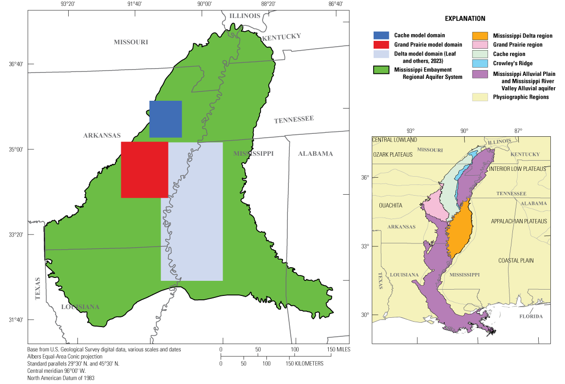
Mississippi Embayment Regional Aquifer System, Mississippi Alluvial Plain, and extents of the Cache model and Grand Prairie model (refer to the “Groundwater Flow Model Construction” section of this report for a definition of the Cache model and Grand Prairie model).
The Mississippi Alluvial Plain overlies part of the Mississippi Embayment Regional Aquifer System (MERAS). The water-bearing units that comprise the MERAS include the MRVA, which is the shallowest and primary groundwater source for irrigation and has experienced substantial declines in storage for decades (Clark and Hart, 2009). Deeper sources of groundwater in the MERAS, such as the Claiborne and Wilcox aquifer systems, supply water for municipal, industrial, and aquaculture use (Clark and Hart, 2009).The primary understanding of the groundwater systems and water use in this region comes from various hydrologic studies (refer to “Previous Studies” section of this report); however, the lack of historical water use reporting for irrigation (for example, metered pumping records) and detailed subsurface geologic and hydrostratigraphic framework studies that incorporate state-of-the-art techniques such as airborne electromagnetic (AEM) surveys indicated that an improved characterization of the subsurface geologic framework and updated estimates of water use would improve the current (2024) understanding of the MERAS hydrologic system from Hart and others (2008).
Mississippi Alluvial Plain Project
New methods and techniques for subsurface data collection and interpretation and advances in numerical hydrologic modeling tools led to the MAP project, which began in 2016 and is a multidisciplinary regional groundwater study with the overarching goal to better understand the hydrostratigraphy and water use in the MRVA. The MAP project was completed by the U.S. Geological Survey (USGS) and funded by their Water Availability and Use Science Program. The multidisciplinary aspect of the MAP project included focused studies on advanced characterization of the MRVA subsurface framework using (1) AEM geophysical techniques, (2) synthesis of field data including new groundwater monitoring well and water use meters, (3) soil zone modeling and water balance assessments, (4) water use modeling, (5) water quality assessments, and (6) numerical groundwater-flow modeling that integrated data and outputs from the other studies to assess the state of the hydrologic system and groundwater availability in the MRVA into the future. Focus areas for the numerical groundwater-flow modeling efforts include the Mississippi Delta region, described in Leaf and others (2023) and parts of the Cache and Grand Prairie regions in northeastern Arkansas described in this report (fig. 1; Ladd and Travers, 2019).
In northeastern Arkansas, the MRVA underlies the MAP west of the Mississippi River and ranges from 80 to 201 kilometers (km; 50–120 miles [mi]) wide and 402 km (250 mi) long (Ackerman, 1989a). In 1991, the State of Arkansas passed the Arkansas Groundwater Protection and Management Act to improve management of groundwater across the State (State of Arkansas, 1991; Arkansas Natural Resources Commission, 2014). The Arkansas Groundwater Protection and Management Act allows the Arkansas Natural Resources Commission to designate Critical Groundwater Areas. The purpose of this designation is to bring awareness to groundwater problems in areas that have experienced significant groundwater level declines and to “encourage Congress, the Arkansas Legislature, and state and federal agencies to place higher priority on commitment of resources to implement solutions” (Arkansas Department of Agriculture Natural Resources Division, 2023, p. 1). Two areas within the MAP’s Cache and Grand Prairie regions in northeastern Arkansas have been designated as Critical Groundwater Areas owing to decades of groundwater declines that resulted from past and current water use (Clark and others, 2011a; Arkansas Natural Resources Commission, 2014; Ladd and Travers, 2019).
Previous Studies
Groundwater resources in northeastern Arkansas were first described by Stephenson and others (1916). Later, studies began examining the effects of groundwater pumping on groundwater levels (Engler and others, 1945). A detailed description of the geology in the Mississippi Embayment was completed by Cushing and others (1964). Hosman and others (1968) and Boswell and others (1968) studied the hydrogeologic properties of the aquifers in the region. Brahana and Mesko (1988) assessed the hydrogeology and groundwater flow in the deeper Cretaceous aquifers in the northern Mississippi Embayment. Recently, Schrader (2008) mapped potentiometric surfaces for the Sparta-Memphis aquifer, and Kresse and others (2014) completed a comprehensive description of the hydrology and geochemical characteristics of aquifers in Arkansas. Regional scale numerical groundwater-flow models were developed for the MERAS by Clark and Hart (2009) and Clark and others (2011), and various scenarios were run for northeastern Arkansas (Clark and others, 2011a, 2013).
Northeastern Arkansas has been the subject of studies that developed numerical groundwater-flow models to better understand the effects of groundwater pumping and water use on the aquifer system since the 1980s (Broom and Lyford, 1981). The Mississippi Embayment was the subject of a USGS Regional Aquifer System Analysis Program study that developed groundwater-flow and water availability models (Ackerman, 1989a, 1989b, 1996). In the Grand Prairie region, groundwater availability models for future use were developed by Peralta and others (1985). Mahon and Poynter (1993) developed a digital groundwater-flow model of the alluvial aquifer in eastern Arkansas. Reed (2003) recalibrated the Mahon and Poynter model with updated aquifer and water use data. Gillip and Czarnecki (2009) validated and updated the northern Reed (2003) model, and Czarnecki (2010) looked at groundwater-flow assessment of the MRVA in northeastern Arkansas using the updated model from Gillip and Czarnecki (2009). McKee and Clark (2003) developed a numerical groundwater-flow model for the confined Sparta aquifer system. Hunt and others (2021) compared the performance of the latest automated parameter estimation tools for calibration to traditional automated parameter estimation tools using the MERAS model from Clark and Hart (2009). Several studies assessed the effect of irrigation projects and optimization of conjunctive water use in the Grand Prairie region using the Reed (2003) model (Czarnecki and others, 2003; Czarnecki, 2006 and 2007). In the Cache region, Czarnecki (2010) used the model from Reed (2003) to assess the effects of continued pumping on the cone of depression out to 2050 within the newly designated Cache River Critical Groundwater Area (hereafter referred to as the “Cache CGWA”; fig. 2A). A separate model was developed for the Cache region to assess the effects of pumping on groundwater levels into the future and to test pilot points for aquifer properties during calibration (Rashid and others, 2015).
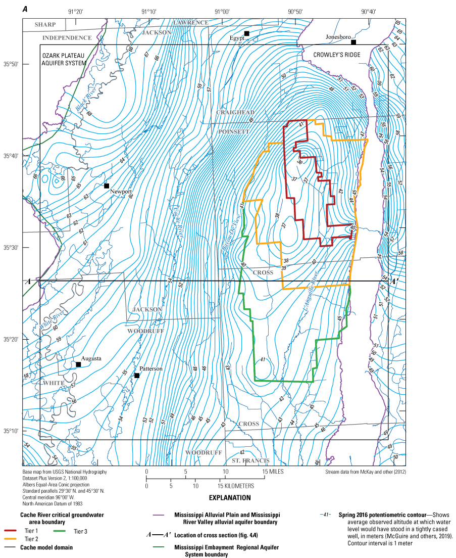

Maps of the regions, model domains, and Critical Groundwater Areas. A, Cache model. B, Grand Prairie model (refer to the “Groundwater Flow Model Construction” section of this report for a definition of the Cache model and Grand Prairie model).
Purpose and Scope
The purpose of this report is to document and describe the construction, calibration, and results of two inset groundwater-flow models developed for the Cache CGWA and Grand Prairie CGWA (fig. 2A, B). The scope of the study was to develop two numerical inset groundwater-flow models based on a newly developed regional groundwater-flow model of the MERAS, also developed for the MAP study and documented in Leaf and others (2023) as the Mississippi Embayment Regional Aquifer System version 3 (MERAS 3) model. The five numerical groundwater-flow models developed for the MAP study, including the Cache and Grand Prairie models, used MODFLOW 6, the latest core version of the USGS Modular Hydrologic Model code (Langevin and others, 2017). The latest version (version 5) of the Parameter ESTimation code ++ (PEST++) Iterative Ensemble Smoother (PESTPP–IES) was used to calibrate the models to historic observations from 1900 through 2018 (Welter and others, 2015; White, 2018). Model development and calibration for the Cache and Grand Prairie models, which are described in this report, were focused on the two CGWAs and build on previous modeling efforts to provide higher resolution groundwater-flow models that included updated recharge, water use, and AEM data to create robust groundwater models that can be used for water management decision support.
Study Area
The Cache and Grand Prairie study areas are subsets of the Cache River and Grand Prairie regions in the northeastern Arkansas section of the MAP and the western-central flank of the MERAS, which intersects the Ozark Plateau and Ozark Plateau aquifer system to the west (fig. 1). The Cache study area is about 5,180 km2 extending about 80 km south and about 64 km west from Jonesboro, Arkansas, including the region about 1.6 to 4.8 km east of Crowley’s Ridge to the fall line between the MERAS boundary and the Ozark Plateau aquifer system located west of the Black and White Rivers (fig. 2A). There is little surface relief and the greatest relief is at Crowley’s Ridge, which is an erosional remnant capped in many places by Quaternary-age alluvium and loess (Meissner, 1983). The Cache River (the region’s namesake) flows south through the study area from Egypt, Ark., and past Patterson, Ark. (fig. 2A).
The Grand Prairie study area is about 12,626 km2, extending about 121 km south and about 105 km west from Beebe, Ark., to Pendleton, Ark. (fig. 2B). The study area includes the Grand Prairie region (area between the Arkansas River and the White River) (fig. 2B; Reed, 2003). Within the MAP boundary, relief in the Cache River and Grand Prairie regions is low, with topography sloping downward from an altitude of about 322 meters (m) near the Missouri State line to an altitude of 45.72 m near the confluence of the White and Mississippi Rivers (fig. 2B).
Both study areas are predominantly natural treeless prairies that have been under rice cultivation since the early 1900s (Clark and others, 2011a). Today, the predominant land use in the Cache and Grand Prairie study areas and regions is agricultural (Clark and Hart, 2009; Gillip and Czarnecki, 2009). Agricultural land use is as much as 81 percent of total land use in the Cache study area and as much as 72 percent in the Grand Prairie study area (U.S. Department of Agriculture [USDA], 2014). Within this agricultural land, crop land ranges from 90 to 100 percent, whereas pasture for livestock ranges from 0 to 10 percent (USDA, 2014; Rashid and others, 2015). The total amount of land irrigated in the counties in the Cache study area ranges from 46 to 53 percent (USDA, 2014). Rice, soybeans, and cotton make up most crops grown, with lesser amounts of peanuts, wheat, and hay (USDA, 2014). The total amount of land irrigated in the counties in the Grand Prairie study area ranges from 39 to 47 percent (USDA, 2014). Rice, soybeans, and cotton make up most crops grown with lesser amounts of peanuts, wheat, and hay (USDA, 2014). Land use in the areas near streams has changed throughout the 20th century from hardwood forests, which flooded seasonally to agriculture, growing primarily rice and soybeans with some aquaculture.
The climate in northeastern Arkansas is humid subtropical with hot and humid summers and mild winters with little to no snowfall (Clark and others, 2011a). The 30-year normal annual precipitation in the area, based on a 120-year National Weather Service record at Jonesboro, Ark. (Craighead County), through 2020, is 1,245 millimeters (mm) (National Climatic Data Center, 2019). The 30-year normal monthly precipitation is fairly uniform throughout the years, ranging from a minimum of 80 mm during August to a maximum of 129 mm during March. Normal annual temperature for the area is about 15.6 °C. Normal monthly temperatures range from a low of 3.9 °C in January to a high of 26.7 °C in July.
Geology
Northeastern Arkansas is at the western edge of the syncline that plunges toward the Gulf of Mexico, with its axis parallel to the Mississippi River (Clark and Hart, 2009). Primary geologic units in northeastern Arkansas include the Quaternary-age alluvial and terrace deposits, the Tertiary-age Jackson Formation, Cockfield Formation, Cook Mountain Formation, Memphis Sand or Sparta Sand, and Wilcox Group (Clark and Hart, 2009; Kresse and others, 2014). Cushing and Others (1964), Ackerman (1996), and Kresse and others (2014) provide a more in-depth study of the geology of the MERAS in Arkansas. Alluvial and terrace deposits, the upper most unit in northeastern Arkansas, consist of unconsolidated sand, gravel, silt, and clay deposited by fluvial systems and environments (Kresse and others, 2014). The Jackson Group consists of unconsolidated clays and rare interbedded siltstone and sandstones (Kresse and others, 2014). The Cockfield Formation consists of fine- to medium-grained sand in the lower part and silt, clay, and lignite in the upper part (Kresse and others, 2014). The Cook Mountain Formation and Memphis Sand or Sparta Sand (also the Cane River Formation, and Carrizo Sand) in northeastern Arkansas, belong to the Claiborne Group, which consist of fine- to medium-grained well sorted sand with silt, clay, shale, and lignite (Kresse and others, 2014). The Wilcox Group consists of sands and clays in interbedded upper and lower units (Kresse and others, 2014) (appendix 1).
Hydrology
This section provides background on the important hydrology of the study area to provide context for the work completed in this study. It includes summaries of surface water features, groundwater and hydrogeologic units, geophysical data, and water use. The important hydrologic information summarized in this section can be used to understand the general hydrologic environment in the Cache River region and the Grand Prairie Region.
Surface Water
Primary surface-water features in the Cache region are the southerly flowing White River, Cache River, Bayou De View, and L’Anguille River (fig. 2A). The White River, with an average daily discharge of about 21,334,139 cubic meters per day (m3/d) (8,720 cubic feet per second [ft3/s]), is the largest stream in the region and flows along the western side of the regions, draining into the Mississippi River in southeast Arkansas (Schrader and others, 2005). The Cache River, located east of the White River, which has an average daily discharge of about 2,446,576 m3/d (1,000 ft3/s) and flows south from near Egypt, Ark., to its confluence with the White River in the Grand Prairie region (fig. 2A and 2B). Bayou De View flows through the central part of the region, discharging to the Cache River in the Grand Prairie region, and the L’Anguille River flows south through the eastern part of the region, just west of Crowley’s Ridge, which is the headwaters region for tributaries to the L’Anguille River (fig. 2A).
Primary surface-water features in the Grand Prairie region include the White River in the western region, Wattensaw Bayou, Bayou Two Prairie, and Bayou Meto in the central Grand Prairie region, and the Arkansas River that flows southeast from the Ozark Plateau to the Mississippi River in the southeastern corner of the region (fig. 2B). Peak flows in this area occur from March through April with low flows occurring October through November. Pumping of groundwater for irrigation has reduced base flows and increased the frequency of low flows for many rivers and streams in this area (Yasarer and others, 2020). The flow alteration is greatest in October owing to the cumulative withdrawal of groundwater (Yasarer and others, 2020). The drainage system in the MAP has changed in the last 80 years owing to changes in land use as well as drainage improvement projects, flood controls, the construction of levees and ditches, and the deepening and straightening of streams.
Groundwater and Hydrogeologic Units
Groundwater is present in several major hydrogeologic units in the northeastern Arkansas region of the MERAS (Hart and others, 2008). These major units, from shallowest to deepest, include the MRVA, Vicksburg-Jackson confining unit, the upper Claiborne aquifer, the middle Claiborne confining unit, the middle Claiborne aquifer, the lower Claiborne confining unit, the lower Claiborne aquifer, the middle Wilcox aquifer, the lower Wilcox aquifer, and the Midway confining unit (Hart and others, 2008). Detailed descriptions of each hydrogeologic unit for Arkansas is available in Kresse and others (2014). Hydraulic properties of primary aquifers and confining units in the Cache River and Grand Prairie regions from previous studies are summarized in table 1.
Table 1.
Summary of aquifer properties for primary aquifers and confining units and their source reference.[Kh, horizontal hydraulic conductivity; m/d, meter per day; Kv, vertical hydraulic conductivity; Kvani, vertical anisotropy of hydraulic conductivity, calculated as Kh/Kv; m−1, inverse meter; SY, specific yield; SS, specific storage; --, not applicable (specific yield is not a property of confined aquifers or confining units)]
| Aquifer/confining unit (shallowest to deepest) | Kh (m/d)a |
Kvani (Kh/Kv) |
SS (m−1)b |
SY (unitless) |
Aquifer recharge from precipitation (m/d) | Reference |
|---|---|---|---|---|---|---|
| Mississippi River Valley alluvial aquifer | 30.5–223 | 10–100 | 1.20E-6–6.0E-3 | 0.19–0.35 | 0.00009–0.0006 | Broom and Lyford (1981), Clark and Hart (2009), Rashid and others (2015), Reed (2003) |
| Vicksburg-Jackson confining unit | 0.3 | 500–1,475 | 1.10E-06 | -- | -- | Clark and Hart (2009) |
| Upper Claiborne aquifer | 8 | 612.8 | 8.50E-07 | -- | -- | Clark and Hart (2009) |
| Middle Claiborne confining unit | 0.047 | 564.6 | 9.40E-07 | -- | -- | Clark and Hart (2009) |
| Middle Claiborne aquifer (or Sparta-Memphis aquifer) | 1.1–44.5 | 243.4–798.8 | 1.00E-06–2.6E-5 | -- | -- | Clark and Hart (2009) |
| Lower Claiborne confining unit | 0.025 | 102 | 3.08E-07 | -- | -- | Clark and Hart (2009) |
| Lower Claiborne aquifer | 7.6 | 23 | 1.00E-06 | -- | -- | Clark and Hart (2009) |
| Middle Wilcox aquifer | 0.73 | 617.8 | 1.10E-06 | -- | -- | Clark and Hart (2009) |
| Lower Wilcox aquifer | 7.5 | 27.7 | 1.10E-06 | -- | -- | Clark and Hart (2009) |
| Midway confining unit | 3.05E-07 | 1 | -- | -- | -- | Brahana and Mesko (1988) |
The MRVA is the shallowest aquifer and primary source of fresh groundwater in the MAP (Kresse and others, 2014). Groundwater flow in the MRVA is generally from north to south but has changed in some regions owing to intensive pumping. In the Cache region, owing to decades of intensive groundwater pumping for irrigation and aquaculture, a cone of depression developed between Crowley’s Ridge and the Cache River (fig. 2A; Czarnecki, 2010; McGuire and others, 2019). Similarly, in the Grand Prairie region, groundwater declines have been recorded since the onset of irrigation pumping in the early 1900s with significant declines resulting in the depletion of the MRVA in the Grand Prairie CGWA by the late 20th century (fig. 2B; Clark and others, 2011a). Depletion of the MRVA primarily owing to irrigation pumping has caused increased water use in the deeper Sparta aquifer. Although not well quantified, low yields from wells screened in the MRVA in the Grand Prairie region have led farmers to install wells screened in the deeper Sparta aquifer so they can continue irrigating their crops (Kresse and others, 2014).
The thickness of the MRVA varies from 0 to 60 m throughout the Cache and Grand Prairie regions (Clark and Hart, 2009). The transmissivity of the MRVA in northeastern Arkansas ranges from 2,591 to 19,782 meters squared per day (m2/day) (Broom and Lyford, 1981). The MRVA horizontal hydraulic conductivity (Kh) ranges from 30.5 to 223 meters per day (m/d), specific yield (SY) values for unconfined conditions were about 0.19 to 0.3 (unitless), and specific storage (SS) values for confined conditions were 1.2x10⁻⁶ to 6x10⁻³ 1/m (Broom and Lyford, 1981; Czarnecki and others, 2003; Clark and Hart, 2009). Vertical anisotropy of hydraulic conductivity (Kvani), the ratio between Kh and vertical hydraulic conductivity (Kv) (Kh:Kv, unitless), ranged from 10 to 100 (table 1; Reed, 2003; Clark and Hart, 2009).
The Vicksburg-Jackson confining unit, where it exists in northeastern Arkansas in the Grand Prairie region, reduces the hydraulic connection between the MRVA and underlying middle Claiborne aquifer. The Kh, Kvani, and SS of the Vicksburg-Jackson confining unit is about 0.3 m/d; 1,475 m/d; and 1.1 x10⁻⁶ 1/m, respectively (Clark and Hart, 2009). The range of values from several sources is summarized in table 1.
The Tertiary-age aquifers below the MRVA include the Claiborne and Wilcox aquifers (Kresse and others, 2014). In northeastern Arkansas, the primary water use in the middle Claiborne aquifer occur in the undifferentiated Memphis Sand and Sparta Sand (Kresse and others, 2014). The Cache River Formation and Carrizo Sand are present in northeastern Arkansas (Clark and Hart, 2009). Locally and in various hydrologic studies, the middle Claiborne aquifer is referred to as the Memphis aquifer, the Sparta aquifer, or the Sparta-Memphis aquifer; these various names can add to the naming confusion, as described in Kresse and others (2014). Hereafter, in this report, the Sparta, Memphis, and Sparta-Memphis aquifers are referred to as the “middle Claiborne aquifer.” The middle Claiborne confining unit, above the middle Claiborne aquifer, had a Kh value of about 0.05 m/d and a Kvani of about 565 (same as table 1) (Clark and Hart, 2009). The middle Claiborne aquifer, in northeastern Arkansas, had Kh values from 1.1 to 44.5 m/d (Clark and Hart, 2009); middle Claiborne aquifer Kvani was about 207.2 and SS was about 1x10⁻⁶ to 2.6x10⁻⁵ 1/m. The lower Claiborne aquifer had a Kh value of about 7.6 m/d and Kvani was about 23 (Clark and Hart, 2009). The middle Wilcox aquifer Kh was about 0.7 m/d, the Kvani was about 617, and SS was 1.1x10⁻⁶ (Clark and Hart, 2009). The lower Wilcox aquifer Kh was about 7.5 m/d, the Kvani was about 28, and SS was 1.1x10⁻⁶ (Clark and Hart, 2009). The Midway confining unit, consisting of thick marine clays, underlies both regions, is assumed to contribute insignificant amounts of water to the overlying aquifer units, and is considered to be a no-flow boundary where it contacts the Wilcox aquifer system across the study area in northeastern Arkansas (Clark and Hart, 2009). Property values and their ranges from previous studies are also summarized in table 1.
Geophysical Data
Geophysical survey data were collected as a part of the MAP project to better characterize MRVA hydrostratigraphy (Minsley and others, 2021). Geophysical data primarily included 43,000 flight-line-kilometers (line-km) of AEM data with 3–6-km line spacing over the MAP region. Additionally, magnetic and radiometric data were collected to map shallow surficial geologic features and substructures (Minsley and others, 2021). AEM data use the changes in resistivity to differentiate between geologic layers in the near subsurface. Magnetic data inform geologic structure in the deep subsurface based on changes in magnetic properties. The geophysical data were processed into 5-meter-thick layers from the land surface to the depth of investigation, as much as 400 meters below the land surface (Minsley and others, 2021). The AEM data were inverted to resistivity values and classified into 10 groups (classes 1–10) based on a range of resistivity values. In group 1, the resistivities were less than 3.16 ohm-meters, and in group 10, the resistivities were greater than 1,000 ohm-meters (Minsley and others, 2021). These resistivity groups reflect the expected aquifer material whereby a low resistivity is correlated to low Kh values and vice versa (Minsley and others, 2021). More than 3,000 line-km of waterborne resistivity surveys were also completed to characterize subsurface structure beneath some major streams in the MAP region, including the Arkansas River and White River in northeastern Arkansas (Minsley and others, 2021). A full description of the geophysical survey completed for the MAP study is available in Minsley and others (2021).
Water Use
Primary groundwater use in the MAP and northeastern Arkansas region is for irrigation of crops and aquaculture (Kresse and others, 2014). As much as 93 percent of groundwater pumped for irrigation has come from the MRVA (Clark and others, 2011a). Other water uses include municipal, industrial, mining, thermoelectric power, domestic, and livestock (Kresse and others, 2014). Groundwater pumping for irrigation use began in the early 1900s and has increased by 665 percent since 1965 (Czarnecki and others, 2003; Clark and Hart, 2009). Groundwater use for irrigation in the Grand Prairie region is some of the highest in the State (Pugh and Holland, 2015). The primary source of groundwater for irrigation in northeastern Arkansas is the MRVA; however, owing to long term water-level declines in the MRVA around areas such as the Grand Prairie CGWA, water use for irrigation has increased in the middle Claiborne aquifer (Kresse and others, 2014). Historically, water use in the middle Claiborne aquifer was predominantly for municipal supply owing to better water quality than the MRVA; however, as of 2010 most of the water use from the Sparta aquifer is for irrigation (Kresse and others, 2014). Additionally, there are anecdotal accounts that wells screened in the MRVA and Middle Claiborne aquifer are present in the Grand Prairie region (Kresse and others, 2014). Surface water is primarily used for municipal, industrial, and thermoelectric power. Surface water use from streams and canals in the region ranges from 367 to 1,514 megaliters per day (97–400 million gallons per day [Mgal/d]) (Pugh and Holland, 2015).
In 2010, groundwater use in the Cache River and Grand Prairie regions ranged from 897 to 2,044 megaliters per day (237–540 Mgal/d) (Pugh and Holland, 2015). Water for irrigation ranges from 1,151 to 3,535 megaliters per day (304–934 Mgal/d), with 77 percent of total water use for irrigation and 95 percent for groundwater use (Pugh and Holland, 2015). The MRVA is the source for 90 percent of groundwater use in this area. Based on average precipitation, annual irrigation amounts for rice and soybeans are 787–990.6 mm and 508 mm, respectively (Pugh and Holland, 2015). Catfish ponds use approximately 2,184 mm of water per year and other fishponds use approximately 36 inches per year (in/yr) (Pugh and Holland, 2015).
Most of the irrigation water is applied using furrow or flood irrigation with minimal sprinkler or center pivot irrigation throughout the Cache River and Grand Prairie regions. Application efficiency for various irrigation methods, including continuous furrow and surge methods, ranges from 23 to 97 percent (Kandpal, 2018). Total water use for irrigation and municipal supply has increased since 1965 owing to population and agricultural growth; however, because most irrigation wells are not metered, precise pumping amounts remain uncertain (Pugh and Holland, 2015). Further, groundwater use in the MAP region is not well quantified because water use reporting and metered datasets are limited to recent times. In the Grand Prairie region, irrigation pumping in the middle Claiborne aquifer is highly uncertain because records of wells drilled in the Sparta aquifer (middle Claiborne aquifer is commonly referred to as the Sparta aquifer) may not be in the Arkansas well database, and voluntary reporting of pumping in the Grand Prairie may be uncertain (U.S. Geological Survey, 2021; Blake Forrest, Arkansas Dept. of Natural Resources, written commun., 2023). These inconsistencies are less of an issue in the Cache River region because there is less irrigation pumping from the middle Claiborne aquifer.
Currently (2024), there are no historical transient estimates of water use for irrigation and aquaculture in the MAP by crop type. Therefore, to improve these major water use estimates, a team within the MAP study developed a machine learning Aquaculture and Irrigation Water Use Model (AIWUM). This model estimated water use on a monthly timescale from May through September during 2000 through 2018 based on crop type, with a 1-mile spatial resolution for use in the groundwater-flow models developed for the MAP study (Wilson, 2021; Bristow and Wilson, 2023). The AIWUM estimated maximum monthly water use of about 25 million cubic meters for the Cache model domain and up to about 37 million cubic meters for the Grand Prairie model domain (fig. 3A, B). The AIWUM estimated less water use from 2013 through 2018 due to an increase in annual precipitation (fig. 3).
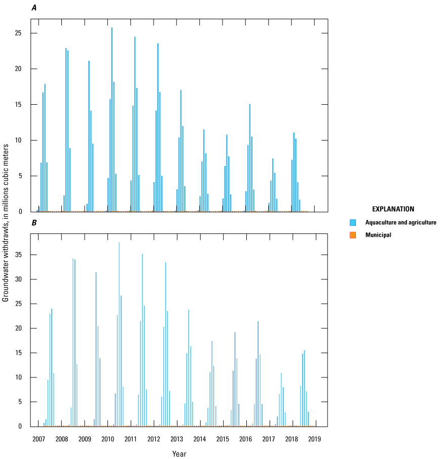
Plot of estimated monthly water use from the Aquaculture and Irrigation Water Use Model and the site-specific water use database from 2000 through 2018 (U.S. Geological Survey, 2020; Bristow and Wilson, 2023). A, Estimated water use in the Cache model domain. B, Estimated water use in the Grand Prairie model domain.
Groundwater-Flow Models
Conceptual Models of Groundwater Flow
A conceptual model of the region describes the hydrologic boundaries, aquifer physical properties, inflows, outflows, and changes in storage of the groundwater system using existing knowledge and data in the model domain. The conceptual model is then used as a guide to construct the numerical model. Owing to their spatial proximity, the conceptual models for the Cache and Grand Prairie regions were similar in their inflows, outflows, and physical properties.
Cache and Grand Prairie Model Domains
A combination of the 2016 MRVA potentiometric surface map from McGuire and others (2019) and major streams were used to delineate the Cache and Grand Prairie domains for the numerical models (hereafter referred to as the “Cache model domain” and the “Grand Prairie model domain”; fig. 2A, B). Each model domain was delineated to ensure focus areas of each numerical model were minimally affected by boundary conditions and to maximize natural no-flow boundaries where groundwater flow was parallel to the domain boundaries (Anderson and others, 2015). The focus areas for each model domain were the primary cones of depression (areas of largest water-level declines compared to the surrounding water table) underlying the Cache River and Grand Prairie CGWAs (fig. 2A, B).
The northern boundary of the Cache model domain extends from the Ozark Plateau and is just west of the MERAS fall line to just east of Crowley’s Ridge (fig. 2A). The groundwater-flow direction (perpendicular to equipotential lines in fig. 2A) along the northern Cache model domain boundary is more parallel to the boundary, flowing eastward until near Crowley’s Ridge where groundwater flow turns perpendicular and flows south along Crowley’s Ridge (fig. 2A). Flow parallel to the domain boundary indicates a no-flow boundary. Selection of the southern domain boundary applies the same principle as the northern boundary where groundwater flow is parallel to the domain boundary, approximating a no-flow regime. The eastern edge of the domain was chosen as the easternmost extent of Crowley’s Ridge, which acts as a barrier to groundwater flow as seen by the head gradient difference in the MRVA across the Crowley’s Ridge (fig. 2A; McGuire and others, 2019). The western edge of the domain was chosen where there was some parallel groundwater flow in the southwestern region (fig. 2A).
The northern boundary of the Grand Prairie model domain extends from the fall line between the MERAS and Ozark Plateau (fig. 2B) to St. Francis County (fig. 2B). The northern domain boundary is north of a cone of depression in northern Prairie County and about 20 km north of the primary cones of depression in the CGWA. The southern domain boundary, which extends from the forested lands in Cleveland County east such that the Arkansas River was inside the domain until near its confluence with the Mississippi River (fig. 2B). The eastern edge of the domain was chosen to include most of the White River through Monroe and Arkansas Counties (fig. 2B; McGuire and others, 2019). The western edge of the domain was chosen to encompass the Arkansas River where it flowed out of the Ozark Plateau and into the MERAS (fig. 2B).
Hydrostratigraphy from Geophysical Data
The resistivity data from AEM and waterborne geophysical surveys were used to further the understanding of the hydrostratigraphy of the Cache and Grand Prairie model domains to improve the conceptual hydrogeologic framework developed in Hart and others (2008). A brief description follows, but for more detail please refer to Minsley and others (2021). In the Cache model domain, the shallow alluvial system exhibited areas of low and high resistivity values horizontally and vertically throughout the MRVA, which indicated the MRVA was more heterogeneous than was represented in previous models that had specified single or uniform Kh, Kv, SS, and SY values. The middle Claiborne aquifer is a higher resistivity unit directly underlying the MRVA in the eastern region of the Cache extending under Crowley’s Ridge (fig. 4A). At a depth of about 40 to 70 m below the land surface, underlying Crowley’s Ridge in the central and southern area of the Cache model domain, the Cook Mountain Formation comprises the middle Claiborne confining unit and underlies the unconsolidated sediment cap of Crowley’s Ridge. The transition area between the prominent Midway confining unit and the middle Claiborne aquifer is the Wilcox aquifer system, which consists of the middle Wilcox and lower Wilcox aquifers; however, these are difficult to differentiate in the Cache model domain and can be considered a single aquifer system. The Midway confining unit was prominent in the resistivity data where it subcropped beneath the MRVA in the west and central MAP with an eastward dip (table 1.1).
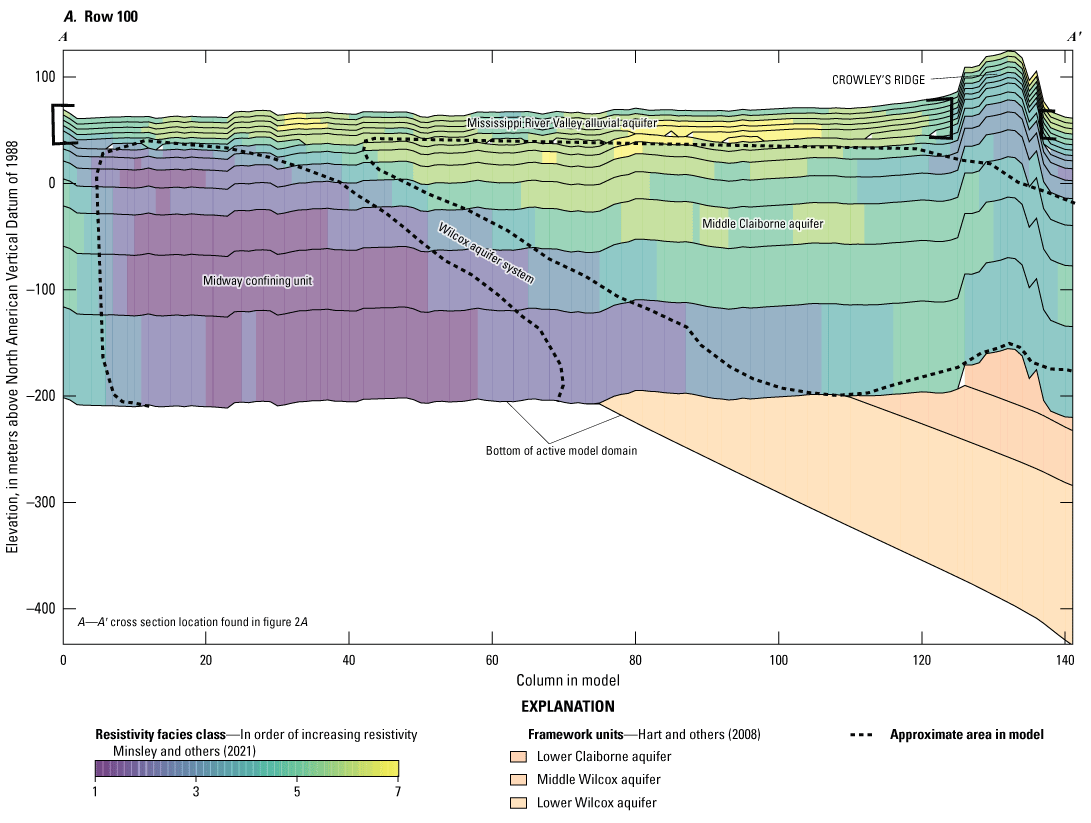

Generalized cross section of the airborne electromagnetic resistivity classes assimilated to the model vertical layers. A, Cache model. B, Grand Prairie model.
The Grand Prairie model domain, like the Cache model domain, exhibited a heterogeneous resistivity field in the MRVA that provided more detail on the potential Kh and Kv values throughout the aquifer. The middle Claiborne aquifer directly underlies the MRVA in the northern half of the region (Minsley and others, 2021). The Vicksburg-Jackson confining unit separates the MRVA and middle Claiborne aquifer in the southern half of the region; however, based on the resistivity classes, there are some small areas of higher resistivity within the Vicksburg Jackson confining unit that may allow for some hydraulic connection between the MRVA and middle Claiborne aquifer (fig. 4B). For the deepest areas resolved by the AEM data, parts of the middle Claiborne aquifer and lower Claiborne confining unit exhibit low resistivities, which represent less hydraulically conductive material.
Groundwater Inflows, Outflows, and Storage Changes
Inflows to both model domains included recharge from precipitation, recharge as seepage from streams, recharge return flows from irrigation, cross-boundary groundwater flow from upgradient adjacent areas, and releases from groundwater storage. Recharge from precipitation was estimated to be 0–5.73 in/yr with some small areas exceeding 20 in/yr (Reed, 2003; Clark and Hart, 2009; Reitz and others, 2017). Recharge as seepage from streams is affected by streambed properties such as Kv, can vary along a stream reach, and was estimated to be about 15–25 percent of recharge from precipitation, or as much as about 1.5 in. (Reed, 2003). Recharge as return flow from traditional gravity flood or furrow irrigation water has not been well quantified by previous studies but generally occurs where shallow clay layers in the MRVA are absent (Yaeger and others, 2018).
Outflows to both regions include irrigation and aquaculture pumping from wells, pumping from municipal wells, base flow discharge to streams, cross-boundary groundwater flow to downgradient adjacent areas, and replenishment of groundwater storage. The primary outflow is groundwater pumping for irrigation and to a lesser extent for aquaculture, and municipal from wells screened in the MRVA (Clark and others, 2011a). Evapotranspiration from groundwater by plant roots that reach the water table was negligible owing to widespread water-level declines in the 20th century, and it was not considered in past groundwater-flow models developed in the region (Reed, 2003; Clark and Hart 2009; Rashid and others, 2015).
Groundwater pumping is widespread in both model domains; however, to reduce the use of groundwater for crop irrigation and limit groundwater declines in areas with less saturated thickness in the MRVA, some surface-water irrigation exists in the Cache and Grand Prairie model domains (Yaeger and others, 2018). Surface-water irrigation occurs as diversions of streamflow to on-farm irrigation reservoirs that range in size from less than 10 acres to more than 300 acres (Yaeger and others, 2018). Diversions can occur from small bayous to large rivers. Construction and utilization of on-farm irrigation reservoirs has been ongoing since the mid-1970s with an increasing abundance of reservoirs through recent times (Yaeger and others, 2018). These on-farm storage reservoirs are shallow, typically have a depth of 2.4–3 m, and are filled to capacity in the wetter winter and early spring months (January through March). Farmers typically use the water stored in these reservoirs to furrow or flood irrigate their crops in the drier summer months (June through August) when evapotranspiration exceeds precipitation (Yaeger and others, 2018). Farms that have irrigation reservoirs typically also have irrigation wells that are assumed to only be used to irrigate their crops if the reservoirs do not have enough water stored because of a dry winter and spring when diverting streamflow was not possible.
Groundwater-Flow Model Construction
This section of the report describes the construction of the Cache and Grand Prairie inset numerical groundwater-flow models using the USGS MODFLOW 6 code (Langevin and others, 2017). Inset models are typically finer resolution models that fit inside (inset) and use boundary conditions of a larger model. The inset models for the Cache and Grand Prairie model domains were developed using the child model capabilities of MODFLOW 6 with the parent model as the regional MERAS 3 groundwater-flow model from Leaf and others (2023). Hereafter, the inset numerical groundwater-flow models of parts of the Cache and Grand Prairie regions will be referred to as the “Cache model” and “Grand Prairie model.”
The Cache and Grand Prairie models were constructed using the same workflow as the Delta inset model and MERAS 3 regional model, which were also developed for the MAP study (refer to “Modeling Goals and Approach” section in Leaf and others, 2023) with minor differences owing to conceptual differences between regions. The Cache and Grand Prairie models were constructed using Python packages developed by Leaf and Fienen (2022) and Leaf and others (2021). The Python tools were the core of a robust and automated workflow that allowed for the expeditious construction of inset models at a user-specified resolution whereby a model could be constructed, tested, and re-constructed with added complexity, and retested in a timeframe that was not previously achievable. Model files for the Cache model and Grand Prairie model are available as a USGS data release (Traylor and Weisser, 2024).
Hydrologic Boundaries
Hydrologic boundaries, with respect to the groundwater-flow system, exist where groundwater is exchanged with the landscape or surface-water system, or where groundwater flows in or out of the model domain. Hydrologic boundaries can be used to determine the extent of groundwater flow simulated in a numerical model. The hydrologic boundaries for the Cache and Grand Prairie models included aquifer boundaries and streams. The western extent of the MERAS was the main hydrologic boundary for northwestern and west-central part of the Cache model domain and for the northwestern and western part of the Grand Prairie model domains. The interface between the MRVA and the Ozark Plateau aquifer system was a boundary in the northwestern section of both model domains (fig. 5A, B). The Ozark Plateau aquifer system has a moderate hydraulic connection with the MRVA where groundwater generally flows from the higher elevation Ozark Plateau aquifer to the lower elevation MRVA; however, the contribution of the Ozark Plateau aquifer to the overall MERAS water budget is negligible (Clark and Hart, 2009; Clark and others, 2018).
Horizontal boundaries of groundwater flow exist along all four sides of each model domain except where the Ozark Plateau aquifer is absent. Specified fluxes, derived from MERAS 3 cell-by-cell fluxes, were assigned to the outermost model cells for all model layers using the Well (WEL) package (fig. 5; Harbaugh, 2005). Within model cells where the Ozark Plateau aquifer system intersected the MRVA, specified heads were assigned using the General Head Boundary (GHB) package (fig. 5A, B; Harbaugh, 2005). Hydraulic conductances assigned to the GHB cells were based on values in the Ozark model interface with the MRVA from Clark and others (2018).

Numerical groundwater-flow model boundary conditions. A, Cache model. B, Grand Prairie model.
The upper vertical boundary was the land surface, which was defined using a digital elevation model (U.S. Geological Survey, 2016). The lower vertical boundary was the top of the Midway confining unit represented as a vertical no-flow groundwater boundary in both models because the Midway confining unit is not hydrologically connected with the MERAS (Clark and Hart, 2009; Traylor and Weisser, 2024).
Spatial and Temporal Discretization
The Cache and Grand Prairie models were spatially discretized horizontally into 500-meter x 500-meter orthogonal cells on a grid with the following vertical layers, rows, and columns:
Vertical layering schemes used the same approach as described in Leaf and others (2023) whereby layers 1 through 8 in both models used the AEM data at 5-m constant thicknesses to represent the MRVA, layers 9 through 15 used increasing uniform thickness layers to represent the Vicksburg-Jackson confining unit and, if present, the Claiborne aquifers and confining units. Below layer 15, the MERAS framework layers from Hart and others (2008) were used to represent the bottom surfaces of Wilcox aquifers and confining units (fig. 4A, B).
The bottom of layer 8, a depth of 40 m (eight layers at 5-m thickness) was represented using the updated bottom of the MRVA, which was produced by James and Minsley (2021). Where the MRVA was less than a depth of 40 m, the remaining layers to the 40-m depth were assigned as pass-through cells of zero thickness (refer to “Regional and Inset Model Layering” section in appendix 1 of Leaf and others [2023] for a more detailed description). Layers 9 through 15 increased in thickness for both models at a multiplier of 1.5 where layer 15 was the lowest extent of the AEM data resistivity facies classes. The framework layers from Hart and others (2008) delineated the bottom elevations for layers 16 through 18 of the Cache model and layers 16 through 19 of the Grand Prairie model (fig. 4A, B).
Based on the resistivity facies classes from the AEM data, the MRVA thickness in both models varied from about 20 to 40 m (fig. 4A, B). Most cells were active in layers 1 through 4, because the MRVA was present almost everywhere at those depths. Pass-through cells, a new feature in MODFLOW 6, were assigned to cells where units did not exist; however, the overlying and underlying cells were active. The MRVA progressively thinned and became absent in layers 5–8 (fig. 6A, B). In layer 8, for both models, less than 50 percent of the cells were active (no pass-through) cells (fig. 6A, B).
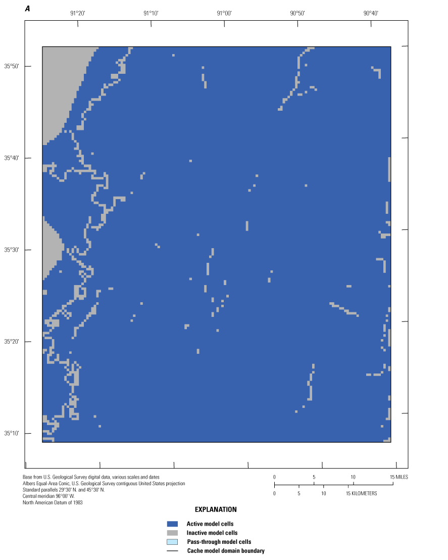

Map of the active, inactive, and pass-through model cells. A, Cache model. B, Grand Prairie model (these are layered .pdfs; download at https://doi.org/10.3133/sir20245088).
Temporal discretization for both models included 148 stress periods of varying lengths to simulate steady state and transient hydrologic conditions from January 1, 1900, through December 31, 2018. The first stress period simulated predevelopment steady-state conditions (without pumping), followed by six multiyear stress periods that simulated transient conditions from January 1, 1900, to April 1, 2007. The multiyear stress periods start and end dates aligned with the previous MERAS models, which had stress periods defined to account for major changes in pumping history (fig. 10 in Clark and Hart, 2009). Monthly stress periods simulated the transient hydrologic conditions from April 1, 2007, through December 31, 2018 (table 2.1; table 2.1 shows end date of January 1, 2019, because that is the stop time of the model, but that date is not simulated).
MODFLOW Inputs and Configuration
Recharge inputs to the Cache and Grand Prairie models were simulated using the Recharge (RCH; Harbaugh, 2005) package. Recharge was specified as transient array-based datasets using the values from a soil-water-balance (SWB; Westenbroek and others, 2018) model of the MERAS developed for the MAP project (Westenbroek and others, 2021). The recharge outputs from the SWB model, which had a cell resolution of 1,000 m to match the MERAS 3 resolution, were clipped and resampled to the size of the Cache and Grand Prairie model domains (Traylor and Weisser, 2024). The unsaturated zone was not simulated in the Cache model or Grand Prairie model because that functionality was not available in MODFLOW 6 at the time of model development, and it was not necessary to address the objective of the study.
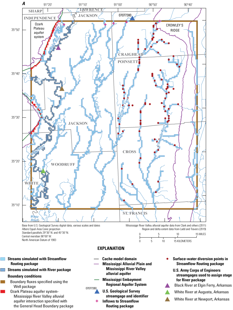
Streams were simulated in both models with the Streamflow Routing (SFR; Niswonger and Prudic, 2005) package except for the Black River, White River, and Little Red River (not shown) in the Cache model and the Arkansas River in the Grand Prairie model, which were simulated with the River (RIV; Harbaugh, 2005) package (fig. 5A). Stream reaches simulated in each model were delineated from the NHDPlus version 2 dataset (McKay and others, 2012) using python scripts with SFRmaker (Leaf and others, 2021) and MODFLOW setup (Leaf and Fienen, 2022) as described in the workflow from Leaf and others (2023). The SFR package simulated total stress period averaged streamflow in both models through the simulation of groundwater/surface-water exchange, accumulation of flow from upstream reaches and stream inflows from the edge of the model, and inflows of runoff generated by the SWB model from Westenbroek and others (2021) (fig. 5A, B). Daily runoff values from the SWB model were aggregated to stress period averaged values and assigned using the methods described in Leaf and others (2023).
Monthly stream inflow values were assigned using monthly average streamflow measured at streamgages where available. Inflow points where streamgages were absent or the measured streamflow datasets did not span the entire simulation period were filled with estimated streamflows from a random-forest regression surface-water model by Dietsch and others (2023). The Cache model included five inflow points where only one streamgage, the Cache River at Egypt, Ark. (USGS streamgage 07077380) was close enough to the model boundary and had available data to specify inflows to the SFR package network (fig. 5A). The other four inflow points used estimated monthly average streamflows from the random-forest regression surface-water model (Dietsch and others, 2023). The Grand Prairie model included 23 inflow points and, like the Cache model, only one inflow point used measured streamflows from a streamgage, the Cache River at Cotton Plant, Ark. (USGS streamgage 07077555); this streamgage did not have records prior to 2008, so estimated streamflows from the random-forest regression surface-water model were used to assign inflow values prior to 2008.
Diversions of streamflow from the SFR package were estimated in both models to simulate the removal of stream water to fill irrigation reservoirs (fig. 5A, B; Yaeger and others, 2017). Diversion data records on volumes or locations by each user were not available, so the diversion volumes, rates, and locations were estimated based on general reservoir filling practices and a remote sensing survey, which provided an inventory of irrigation reservoir locations (Yaeger and others, 2017; Michele Reba, U.S. Department of Agriculture-Agricultural Research Service, written commun., 2022). The SFR package diversion reaches were assigned based on proximity to the closest SFR reach to each reservoir. Diversion volumes for each irrigation reservoir were estimated based on the area of each irrigation reservoir from the inventory dataset in Yaeger and others (2017) with the assumption of an 8-ft filling depth. Diversion rates were estimated by equally dividing the diversion volume across typical filling months of February through May (Yaeger and others, 2017).
The SFR package physical properties, which were required in the package data file and were not generated from the NHDPlus version 2 dataset, included streambed thickness, Manning’s roughness coefficient, and streambed hydraulic conductivity (rhk) (Langevin and others, 2022; Traylor and Weisser, 2024). The rhk values were specified as leakance because streambed thicknesses were assigned a uniform value of 1 m for all reaches; streambed thickness is difficult to estimate on a large scale and a value of 1 is commonly used in models, with all the variability in leakance represented by rhk (Leaf and others, 2023). Initial values of streambed leakance were assigned using the values from a waterborne electrical resistivity survey of streams and lakes in the MAP by Adams and others (2019) or the geometric mean of the entire waterborne electrical resistivity survey dataset (Adams and others, 2019) where waterborne surveys were not completed. Streambed top elevations for each reach were assigned using a mean value from a digital elevation model dataset that was resampled to the model grid discretization (U.S. Geological Survey, 2019).
The RIV package was used for those major streams outside the focus CGWAs: the Black River, White River, and Little Red River (not shown) in the Cache model, and the Arkansas River in the Grand Prairie model (fig. 5A, B). The RIV package was used for these streams because they were far enough away from the cones of depression that the simulation of total routed streamflow by the SFR package was not necessary. The RIV package, a head-dependent boundary condition, simulated the groundwater/surface-water exchange based on the hydraulic head gradient among the RIV package stage and the head in underlying groundwater cell and a specified riverbed conductance term (Traylor and Weisser, 2024). The Cache model RIV package stages were interpolated from U.S. Army Corps of Engineers (USACE) stage records at one streamgage along the Black River in the model domain (fig. 5A; USACE streamgage Black River at Elgin Ferry, Ark.) and two USACE streamgages on the White River (fig. 5A; USACE streamgages White River at Augusta, Ark., and White River at Newport, Ark.) (U.S. Army Corps of Engineers, 2020). The Grand Prairie model RIV package stages were interpolated from USACE stage records at three streamgages along the Arkansas River in the model domain (fig. 5B; USACE streamgage Arkansas River at Pendleton, Ark.; Arkansas River at Pine Bluff, Ark.; Arkansas River at David D Terry L&D below Little Rock, Ark.) (U.S. Army Corps of Engineers, 2020).
Groundwater pumping was simulated with the WEL package (Harbaugh, 2005) in both models for irrigation, aquaculture, and municipal wells, and, only for the Grand Prairie model, thermoelectric wells using MODFLOW-setup methods described in Leaf and others (2023). For stress periods 2 through 6 (January 1, 1900, through April 1, 2007), the MERAS 2.2 model (Haugh and others, 2020) was used to specify the pumping rates and locations for all types of pumping. Irrigation and aquaculture, municipal, and thermoelectric pumping was simulated for the monthly stress periods 7 through 148 (April 1, 2007, through December 31, 2018) using MODFLOW-setup (Leaf and Fienen, 2022) and included in the WEL package input datasets. For the monthly stress periods, outputs from the AIWUM version 1.1 (Bristow and Wilson, 2023), which is summarized in the “Water Use” section of this report, were used to specify the locations and rates of irrigation and aquaculture pumping by crop type. When available, site-specific water use data (SWUDS) from 2000 through 2018 (U.S. Geological Survey, 2020) were used to simulate municipal pumping, and national estimates of thermoelectric pumping were provided by Diehl and Harris (2014) and Harris and Diehl (2019a,b). For monthly stress periods (April 1, 2007, through December 31, 2018), when SWUDS and thermoelectric pumping data were not available, the pumping rates were assigned in the WEL package based on pumping rates that were closest in time to the missing data gap.
Vertical layer assignments for irrigation and aquaculture pumping were determined using a geostatistical estimation dataset by Torak (2021), which estimated the irrigation production zone interval of the MRVA. The AEM survey associated with the MAP project was used to delineate a new bottom of the MRVA surface, included in the Cache and Grand Prairie models as the bottom of layer 8, so there is a difference between the two surfaces that may affect pumping placement vertically in the models. Most of the irrigation and aquaculture pumping were initially assigned to model layers 1–10 in both models. However, in the Grand Prairie region, owing to decades of groundwater declines in the MRVA, irrigation wells have gone dry and caused farmers to drill deeper past the MRVA and into the middle Claiborne aquifer (locally the Sparta aquifer) in search of a reliable source of groundwater (Kresse and others, 2014). This practice of installing wells screened in the middle Claiborne aquifer is not well quantified or documented, which precluded the accurate assignment of irrigation and aquaculture pumping in the middle Claiborne aquifer. To capture this practice in the Grand Prairie model, a fraction of irrigation and aquaculture pumping from wells in layers 5–8 was moved to the middle Claiborne aquifer model layer 15 if present and if resistivity facies classes were 3–7, indicating aquifer material. This was done to improve the simulation of the Sparta aquifer in the Grand Prairie model and capture a conceptual element of the system that has not been simulated in previous models. Vertical layer assignments for the nonagricultural pumping were specified using open intervals or estimated production zones from Knierim and others (2019).
Aquifer properties (Kh, Kv, SS, and SY) in both models were specified in the Node Properties File and the Storage (STO) package (Langevin and others, 2022) by way of zones that corresponded to the resistivity facies classes derived from the AEM survey data in Minsley and others (2021) and the original MERAS framework from Hart and others (2008) below the extent of the AEM data. Initial values for Kh, Kvani, SS, and SY were based on previous studies that included calibrated models discussed in the “Previous Studies” and “Groundwater and Hydrogeologic Units” sections of this report. Using the prior knowledge on aquifer properties and the resistivity classes that relate to fine-to coarse-grained material, the Kh values assigned in ascending order related to the resistivity facies class such that the lowest values of Kh corresponded to the lowest facies resistivity class (class 1) and the highest Kh values corresponded to the highest facies resistivity class (class 7). For non-AEM layers (layers 10 through 19), values from previous studies were used initially, then modified during calibration.
The Newton-Raphson formulation within MODFLOW 6 solved the groundwater-flow system of equations as specified in the integrated model solution (Langevin and others, 2022). The “moderate” option for the Cache and Grand Prairie models was employed owing to the simulation of at least one unconfined layer and minimal convergence issues with this setting (Langevin and others, 2022). Simulation run times on a modern laptop computer for the calibrated Cache and Grand Prairie models (refer to “Groundwater-Flow Model Calibration” section) were about 4 and 10 minutes, respectively. The Observations (OBS) package in MODLFOW 6 was also used to retrieve simulated groundwater altitudes for all layers at cells that intersected observation well locations (Langevin and others, 2022).
Groundwater-Flow Model Calibration
Calibration Approach
The Cache and Grand Prairie models were both calibrated using the PESTPP–IES version 5 code to automate the adjustment of parameters and improve the fit between measured observations or calibration targets and simulated equivalent model outputs. Manual trial-and-error adjustment of some parameters was done prior to automated calibration to improve the history matching and the understanding of the groundwater systems for each model. These initial values for the automated parameter estimation step are referred to as the “prior” parameter distribution. PESTPP–IES produces a “posterior” parameter distribution for a user-specified number of realizations for each iteration of the calibration (White, 2018). The “posterior” distribution of parameter values are different for each realization and each iteration of the calibration. At the conclusion of an automated PESTPP–IES calibration run, an individual realization from a specific iteration can be chosen to represent the best single combination of “calibrated” parameter values. Further, the ensemble from that chosen “calibrated” iteration can be used to represent the uncertainty or range of parameter values if a single realization is not adequate to address the needs of the study. In this study, the “base” realization was chosen as the single combination of “calibrated” parameter values because it is most similar to the traditional least squares parameter estimation algorithm used in the traditional Parameter Estimation software (Doherty, 2005).
The general calibration approach and workflow for the Cache and Grand Prairie models used the Delta inset model calibration approach from Leaf and others (2023); however, some changes were required in the Cache and Grand Prairie models to achieve acceptable calibration results. Similarities with the Delta inset model calibration approach include utilization of methods in the pyemu Python module to create the PEST++ framework around each model (White and others, 2016). This framework included set-up of template and instruction files and creation of a PEST control file. Some differences included parameter schemes, types of observation, and weighting of observation groups in automated calibration.
Automated calibration was performed using PESTPP–IES (White, 2018; White and others, 2020). The IES in PESTPP–IES is a tool that combines the Gauss-Levenberg-Marquardt (GLM) least-squares parameter estimation algorithm (used in PEST++–GLM; White and others, 2020) and Monte Carlo using the PEST++ interface to reduce an objective function (phi [Φ]), which is the sum of squared and weighted residual (measured minus simulated) values (Welter and others, 2015). PESTPP–IES is advantageous because it approximates the Jacobian (sensitivity) matrix by calculating correlations between an ensemble of parameters and observations, which allows for very high-dimensional parameterization without the computational burden associated with PEST++–GLM (White and others, 2020; Hunt and others, 2021) during an automated calibration run. The IES has been used to successfully calibrate groundwater-flow models in several recent studies (Corson-Dosch and others, 2022; Fienen and others, 2022; Ellis and others, 2023; Leaf and others, 2023) using thousands more parameters than traditional PEST from Doherty (2005). Therefore, the Cache and Grand Prairie models employed high dimensional parameterization schemes of 13,740 and 30,436 parameters, respectively.
Observations
Observations, used as calibration targets in the Cache and Grand Prairie model calibration process, inform PESTPP–IES during the parameter upgrade process. The fit between observations and their simulated equivalent values is an indication of a model’s ability to accurately simulate historic conditions and helps to illuminate bias in the results. In PEST++, similar observations can be assigned to groups where each group’s contribution to Φ can be assessed. The Cache and Grand Prairie models included 13 and 18 observation groups with nonzero weighted observations, respectively, and were grouped based on location and type of observation (tables 2 and 3). The observation groups (tables 2 and 3) for both models included the following:
-
• Measured groundwater levels for priority areas in each model as water levels for model spinup (head-spinup) and focus stress periods (head, priority_wells, prefix_disp, and prefix_priority_wells),
-
• measured and estimated streamflows (flux measured and flux-estimated), and
-
• secondary or derivative observations of spatial (prefix-sdiff) and temporal differences (prefix-tdiff) in groundwater levels and streamflows.
Most of the primary and derivative observation groups were based on those used in Leaf and others (2023).
Table 2.
Summary of observations used for calibration with the PEST++ Iterative Ensemble Smoother for the Cache model.| Observation group | Number of observations | Description | Source |
|---|---|---|---|
| flux_estimated | 171 | Estimated streamflows from the surface-water model | Dietsch and others (2023) |
| flux_estimated_sdiff | 401 | Estimated streamflow spatial differences between site locations on the same stream | Dietsch and others (2023) |
| flux_estimated_tdiff | 242 | Estimated streamflow temporal differences from stress period to stress period | Dietsch and others (2023) |
| flux_measured | 161 | Stress period average streamflows derived from measurements at streamgages | U.S. Geological Survey (2020) |
| flux_measured_tdiff | 197 | The difference between stress period average streamflows derived from measurements at streamgages from one stress period to the next | U.S. Geological Survey (2020) |
| head | 1,333 | Measured groundwater levels at observation wells | U.S. Geological Survey (2020) |
| head_disp | 639 | The change (or displacement) of measured groundwater levels at observation wells after 2010 | U.S. Geological Survey (2020) |
| head_sdiff | 68 | The difference in measured groundwater levels between two observations made during the same stress period | U.S. Geological Survey (2020) |
| head_spinup | 508 | Measured groundwater levels prior to April 2007 | U.S. Geological Survey (2020) |
| head_tdiff | 1,505 | The temporal difference in measured groundwater levels from one stress period to the next | U.S. Geological Survey (2020) |
| priority_wells | 693 | Measured groundwater levels at observation wells in priority areas | U.S. Geological Survey (2020) |
| priority_wells_disp | 427 | The change (or displacement) of measured groundwater levels at observation wells within priority areas after January 1, 2010 | U.S. Geological Survey (2020) |
| priority_wells_tdiff | 642 | The difference in measured groundwater levels between two observations in priority areas from one stress period to the next | U.S. Geological Survey (2020) |
Table 3.
Summary of observations used for calibration with the PEST++ Iterative Ensemble Smoother for the Grand Prairie model.[MRVA, Mississippi River Valley alluvial aquifer]
| Observation group | Number of observations | Description | Source |
|---|---|---|---|
| flux_estimated | 659 | Estimated streamflows from the surface-water model | Dietsch and others (2023) |
| flux_estimated_sdiff | 146 | Estimated streamflow spatial differences between site locations on the same stream | Dietsch and others (2023) |
| flux_estimated_tdiff | 659 | Estimated streamflow temporal differences from stress period to stress period | Dietsch and others (2023) |
| grandprairie_mrva_priority_wells | 799 | Measured groundwater levels located in priority areas of the MRVA | U.S. Geological Survey (2020) |
| grandprairie_mrva_priority_wells_disp | 465 | Measured groundwater levels located in priority areas of the MRVA after January 1, 2010 | U.S. Geological Survey (2020) |
| grandprairie_mrva_priority_wells_tdiff | 770 | The difference in measured groundwater levels located in priority areas of the MRVA from one stress period to the next available stress period with an observation | U.S. Geological Survey (2020) |
| grandprairie_mrva_spinup_wells | 451 | Measured groundwater levels from wells in the MRVA prior to April 2007 | U.S. Geological Survey (2020) |
| grandprairie_mrva_wells | 2,960 | Measured groundwater levels from wells in the MRVA, but outside of priority areas | U.S. Geological Survey (2020) |
| grandprairie_mrva_wells_disp | 1,291 | Measured groundwater levels from wells in the MRVA, but outside of priority areas, after January 1, 2010 | U.S. Geological Survey (2020) |
| grandprairie_mrva_wells_tdiff | 2,714 | The difference in measured groundwater levels located outside of priority areas of the MRVA from one stress period to the next available stress period with an observation | U.S. Geological Survey (2020) |
| grandprairie_sparta_priority_wells | 697 | Measured groundwater levels located in priority areas of the middle Claiborne (Sparta) aquifer | U.S. Geological Survey (2020) |
| grandprairie_sparta_priority_wells_disp | 309 | Measured groundwater levels located in priority areas of the middle Claiborne (Sparta) aquifer after January 1, 2010 | U.S. Geological Survey (2020) |
| grandprairie_sparta_priority_wells_tdiff | 650 | The difference in measured groundwater levels located in priority areas of the middle Claiborne (Sparta) aquifer from one stress period to the next available stress period with an observation | U.S. Geological Survey (2020) |
| grandprairie_sparta_wells | 285 | Measured groundwater levels from wells in the middle Claiborne (Sparta) aquifer, but outside of priority areas | U.S. Geological Survey (2020) |
| grandprairie_sparta_wells_disp | 95 | Measured groundwater levels from wells in the middle Claiborne (Sparta) aquifer, but outside of priority areas, after January 1, 2010 | U.S. Geological Survey (2020) |
| grandprairie_sparta_wells_tdiff | 251 | The difference in measured groundwater levels located in priority areas of the middle Claiborne (Sparta) aquifer from one stress period to the next available stress period with an observation | U.S. Geological Survey (2020) |
| head_spinup | 323 | Measured groundwater levels from wells in the middle Claiborne (Sparta) aquifer prior to April 2007 | U.S. Geological Survey (2020) |
| priority_wells | 263 | Measured groundwater levels located in priority areas of the MRVA or middle Claiborne (Sparta) aquifer that were not included in the other groups | U.S. Geological Survey (2020) |
Weights were assigned to each observation in both models based on each model’s goal so that PESTPP–IES prioritized the fit between certain observations and simulated equivalent values during the calibration process. Weights were initially set using the error-based weighting scheme from Hill and Tiedeman (2007) based on approximated measurement error and variance in observations. Then, weights were adjusted by observation group to represent their relative contribution to Φ; similar balancing approaches have been applied in other models (Leaf and others, 2023; Traylor and others, 2023). Each observation group’s contribution to Φ was based on the importance of the observation group to better simulate groundwater levels in and around the cones of depression within the CGWAs, particularly for the final 9 years of the simulation period (January 1, 2010, through December 31, 2018). The Grand Prairie observation group weights were balanced to improve the fit in the MRVA and middle Claiborne aquifers (Traylor and Weisser, 2024).
The Grand Prairie model observations were also assigned a standard deviation that was used to create the noise observations during the automated calibration with PESTPP–IES, which creates noise observation data to properly assess the effect of measurement error on parameter uncertainty (White and others, 2020; Traylor and Weisser, 2024). For preliminary automated calibration runs, PESTPP–IES generated noise observations that included some unrealistic values such as negative streamflows or very low groundwater-level altitudes. These unrealistic values interfered with the approximation of parameter-to-observation gradients and limited the ability of PESTPP–IES to improve the fit to the observations and provide a robust uncertainty assessment. Therefore, standard deviations of observations were specified, which enabled PESTPP–IES to create realistic noise observations and produce an acceptable calibration result.
Groundwater Levels
The Cache model was calibrated to 2,534 stress period length head observations from 195 wells located throughout the model domain (fig. 7A; table 2). Observation groups for primary groundwater levels included head and priority_wells. The secondary (or derivative) observation groups were head_disp, head_sdiff, head_spinup, head_tdiff, and priority_wells_disp (table 2). Detailed descriptions of each observation group and the number of observations for each group are included in table 2. Although the middle Claiborne aquifer exists or subcrops in the Cache model domain, separate observation groups were not necessary for the MRVA and middle Claiborne aquifer as the head observation group was reflective of conditions in the MRVA and middle Claiborne aquifer because they are hydrologically connected in this area.
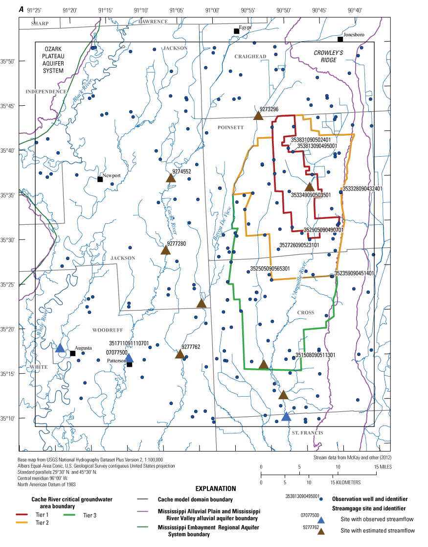

Map of observation wells and streamgage sites used during model calibration. A, Cache model. B, Grand Prairie model.
The Grand Prairie model was calibrated to 5,778 stress period length head observations from 340 wells located throughout the model domain (fig. 7B; table 3). The Grand Prairie model included more observation groups for primary groundwater levels than the Cache model. Additional groups of groundwater-level observations were needed to track the residuals in the MRVA and middle Claiborne aquifers separately because the middle Claiborne aquifer subcropped under much of the Grand Prairie model domain and had varying levels of hydrologic connection with the overlying MRVA. Also, a substantial number of observation wells were screened in the middle Claiborne aquifer owing to its importance as a municipal and agricultural water source (Kresse and others, 2014). Therefore, monthly measured groundwater-level observations were grouped by aquifer code (aqfr_cd; 110ALVM for MRVA and 124SPRT for middle Claiborne wells), provided in the National Water Information System database (U.S. Geological Survey, 2020), and by location in the priority Grand Prairie CGWA (fig. 1; table 3). These groups by aquifer and priority area also included the derivative observation groups with suffix “_disp” and “_tdiff.” Observation wells with other MRVA related aquifer codes such as 112TRRC and 112MRVAA were not included in the MRVA and middle Claiborne groups; however, they were included in the priority_wells group (table 3).
Streamflows
Streamflow observation groups were flux_measured, flux_estimated, flux_measured_tdiff, flux_estimated_sdiff, and flux_estimated_tdiff (tables 2 and 3). Monthly streamflow observations in both models were processed from daily measurements at streamgages in the model domain and (or) estimated streamflows from a random-forest surface-water model by Dietsch and others (2023). The Cache model was calibrated to 254 measured monthly streamflow observations from one streamgage and 352 estimated monthly streamflow observations from the eight locations in the random-forest model (table 2; fig. 7A). Streamgage measurements were processed from daily streamgage records into monthly averages to align with the monthly stress periods in the focus simulation period of the model. The Grand Prairie model did not have any measured streamflow observations within the focus simulation period; therefore, it was calibrated to 659 estimated monthly streamflow observations from the 13 locations in the random-forest model along coincident stream reaches (table 3; fig. 7B).
Calibration Parameters
Both models were parameterized using the same workflow as Leaf and others (2023), which included a combination of custom python scripts that utilized the pyEMU and Flopy python packages, following the methods in White and others (2020) (White and others, 2016; Bakker and others, 20239; Traylor and Weisser, 2024). A mix of fine- and coarse-scale spatial and temporal constants; pilot points; and zonal, gridded, and multiplier parameters were specified for inputs to provide PESTPP–IES adequate flexibility to adjust parameters and improve the spatial and transient simulation of the groundwater flow in each model during the calibration process. Many of the parameters in both models were the same; however, the Grand Prairie model included some additional parameters to aid in better simulating the groundwater system and stresses in the model domain.
Aquifer properties for both models were parameterized as “direct” values of Kh, Kvani, SY, and SS for zones corresponding to the resistivity facies classes from Minsley and others (2021), where the MRVA and non-MRVA facies were combined, and the hydrostratigraphic framework unit from Hart and others (2008). Further, Kh and Kvani properties were parameterized with pilot point multipliers by model layer (1–18 for Cache and 1–19 for Grand Prairie). SY pilot points were specified for model layers 1–10. Pilot points were placed every 10 cells for layers 1–15 and every 20 cells for layers 16–18 in both models. Initial values of “direct” parameters were assigned based on previous studies with groundwater-flow models in the regions (Broom and Lyford, 1981; Czarnecki and others, 2003; Clark and Hart, 2009) (fig. 8A, B). Pilot point multipliers of Kh, Kvani, and SY were assigned an initial value of 1.0 and adjusted during calibration.
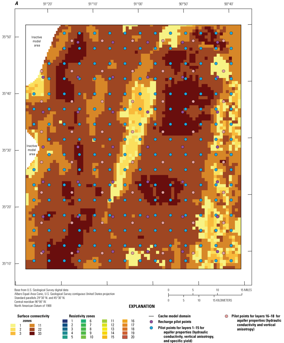

Pilot points for aquifer properties and recharge, surface conductivity, and resistivity zones by model layer used as calibration parameters (this is a layered .pdf; download at https://doi.org/10.3133/sir20245088). A, Cache model. B, Grand Prairie model.
Recharge from the SWB model was parameterized into spatial zone multipliers based on surface connectivity of the upper 15 m of AEM resistivity zones from Minsley and others (2021): pilot point multipliers with a spacing of 23 and 19 cells for the Cache and Grand Prairie models, respectively; and constant grid-scale multipliers for each stress period (fig. 8A, B). The Cache and Grand Prairie models included 18 and 48 surface connectivity zone multipliers, respectively; 41 and 116 pilot point multipliers, respectively; and 148 stress period multipliers each. The surface connectivity zones were used to parameterize recharge because it was assumed that the upper 15 m of the alluvial aquifer material affected the downward movement of water from the root zone to the water table. The surface connectivity dataset showed zones of lower and higher connection, where lower connection was indicated by the presence of more clay and higher connection was indicated by more sand (Minsley and others, 2021). The surface connectivity zones within the Cache model were further partitioned into zones that overlay MRVA and Crowley’s Ridge separately to avoid parameter compensation in two different physiographic regions (fig. 8A). Pilot points were specified to account for spatial heterogeneity in recharge that was not captured by the SWB model or the surface connectivity zones, which provided a finer-scale parameter to PESTPP–IES. Model grid-scale parameters for each stress period accounted for temporal trends in recharge not captured by the SWB model. Initial values for all recharge parameters were set to 1.0 for each multiplier; however, stress period multipliers were manually adjusted prior to automated calibration and discussed in the “Cache Model Calibration Process” and “Grand Prairie Model Calibration Process” sections. The lower and upper bounds for each group of recharge parameters were set to allow realistic flexibility during the automated calibration process so that recharge values would stay near or within the range of values from previous studies. Recharge parameter upper and lower bounds are listed in tables 4 and 5.
Table 4.
Summary of calibration parameters including their initial values and lower and upper bounds by parameter group for the Cache model.[--, unitless]
Table 5.
Summary of calibration parameters including their initial values and lower and upper bounds by parameter group for the Grand Prairie model.[--, unitless; MRVA, Missouri River Valley alluvial aquifer]
Cache and Grand Prairie model stream parameters included 601 and 1,496 SFR package rhk multipliers; 740 and 3,403 multipliers for SFR package inflows; 1,332 and 3,848 multipliers for runoff to the SFR package; and two and one conductance multipliers for RIV package cells, respectively. The rhk multipliers were specified for each NHDPlus version 2 stream segment unique identifier (Moore and Dewald, 2016) and surface connectivity zones from Minsley and others (2021). There is one stream segment unique identifier per hydrologic unit code level 12, which represented the fine-scale subwatershed parameterization. The surface connectivity zones (fig. 8A, B) were assumed to affect stream/aquifer interactions and acted as the coarse-scale parameters for the rhk (fig. 9A, B). Runoff generated by the SWB model and added to the SFR package network was parameterized as multipliers by surface connectivity zone and by stress period to account for coarse-scale uncertainty in runoff and temporal dynamics that may not have been entirely captured by the SWB model. The lower and upper bounds on the runoff multipliers were assigned values of 0.2 and 1.5 to allow for adjustment of parameters during automated calibration within reasonable limits. Inflows to the SFR package were parameterized with multipliers by stress period to account for the uncertainty in the estimated flows from the random-forest surface-water model and monthly average streamflows processed from daily measured values at streamgages near the model boundary. The Grand Prairie model stream parameters were specified like those from the Cache model, except that rhk values were also parameterized by the 11 coarse-scale hydrologic unit code level 8 watersheds to allow for more coarse-scale adjustment during automated calibration (fig. 9B). The conductance term for the Cache model RIV package was parameterized into two grid-scale multipliers for the cells representing the Black River and White River (fig. 9A). Similarly, the Grand Prairie model RIV package conductance was parameterized with a single grid-scale multiplier for the cells representing the Arkansas River (fig. 9B).
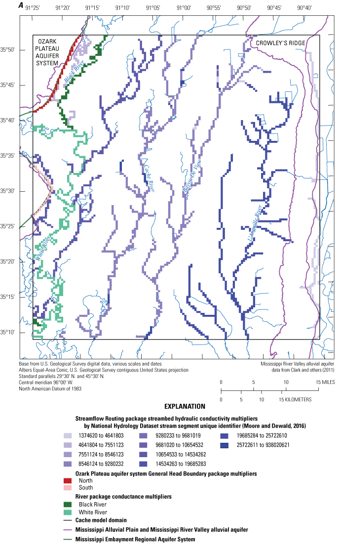

Streamflow Routing package, River package, and General Head Boundary package parameterization. A, Cache model. B, Grand Prairie model.
Conductance for the GHB package cells, where boundaries of the models intersected the Ozark Plateau aquifer system, were parameterized with grid-scale multipliers to account for uncertainty in the values obtained from Clark and others (2018). The Cache model included two GBH multipliers and a north and a south multiplier, and the Grand Prairie model included one GBH multiplier (fig. 9A, B). Lower and upper bounds for the conductance multipliers in both models were set to 0.01 and 100, respectively, to provide several orders of magnitude flexibility for PESTPP–IES during the automated calibration process.
Pumping rates in the WEL package were parameterized for both models by crop type, data source, possible reductions in pumping owing to surface-water access, and stress period. The Grand Prairie model included additional WEL package pumping rate parameters by combined model layer and AEM framework zone, and a separate parameter to adjust the fraction of MRVA pumping moved to the middle Claiborne aquifer to account for the uncertainty in agricultural pumping from the middle Claiborne aquifer in the Grand Prairie region, noted by McKee and Clark (2003). A python script moved a fraction of pumping from MRVA layers 5 through 8 to active cells designated with AEM framework zone two through seven in layer 15, which represented aquifer material in the middle Claiborne aquifer (Traylor and Weisser, 2024). Crop type pumping multipliers for both models included aquaculture, corn, cotton, nonagricultural, other, rice, and soybeans. The Cache model combined the unique stress periods with each crop type to create 889 crop types by stress period parameters, but the Grand Prairie model did not combine stress period multipliers with crop types. Grid scale pumping rate multipliers for both models were specified by SWUDS, Mississippi Embayment Regional Aquifer System version 2 (MERAS 2), and AIWUM data sources to provide flexibility and independence in parameters during the automated calibration process for pumping rates with different data sources. The Grand Prairie model combined data source with stress periods to create 412 “data source by stress period” multipliers; preliminary calibration runs indicated that the crop type by stress period multipliers scheme (used for the Cache model) was not adequate to capture the temporal trends in pumping rates.
Farms where irrigation reservoirs supplied stored surface water to irrigate crops during the summer were assumed to use less groundwater. Groundwater pumping cells in the WEL package that intersected potential irrigated cells supplied by surface water from irrigation reservoirs were assigned pumping rate multipliers to reduce pumping. The surface-water irrigated areas adjacent to irrigation reservoirs were unknown at the scale of both models; therefore, a dataset was constructed to approximate the crop area for which irrigation reservoirs supplied water. Using the irrigation reservoir dataset from Yaeger and others (2017), model cells that were within 200 m of a 10–30-acre reservoir, within 500 m of a 30–100-acre reservoir, and within 1,000 m of a reservoir greater than 100 acres were assigned a new variable boundname designation of “sw_irr” in the WEL package files, indicating they may potentially receive stored surface water; cells that did not intersect the irrigation reservoir area dataset were assigned the boundname “no_sw_irr.” These boundnames in each WEL package file were used to parameterize pumping in both models where “no_sw_irr” was assigned a multiplier of 1.0 and fixed during the calibration, and where “sw_irr” received a multiplier of 0.7 for the Cache model and 0.001 for the Grand Prairie model. The multipliers differed for both models owing to uncertainty in irrigation practices in both areas based on anecdotal evidence and the state of the MRVA in both areas. Reductions in groundwater pumping were assumed to preserve the aquifer and use surface water, if available, which was more common in the Grand Prairie area because the MRVA was more depleted in this region compared to the Cache area. Further, the climate was assumed to be a factor in using groundwater where surface water was available; groundwater was assumed to be used in drier than normal summer months.
Parameter-elevation Regressions on Independent Slopes Model (PRISM) data were used to define dry, average, and wet stress periods in the Grand Prairie model, where average was defined as the 40th to 60th percentile in monthly precipitation from 1999 through 2017 (PRISM Climate Group, 2022). The initial parameters were assigned using the monthly climate type from the PRISM data. For “sw_irr” pumping cells, if the June, July, or August stress periods were dry (less than 40th percentile of mean precipitation), they were assumed to use groundwater and their multipliers were set to 1.0; average and wet stress periods were assumed to use only surface water from the irrigation reservoirs and therefore were assigned a multiplier of 0.001, which effectively reduced pumping in the cell to near zero. Note that log normal parameters in PEST++ cannot be zero, but the difference between zero pumping and 0.001 of original pumping is effectively the same in the model. These multipliers were left as adjustable given the uncertainty in practices in the region but allowed for a more reasonable starting point for the automated calibration with PESTPP–IES (Traylor and Weisser, 2024).
Cache Model Calibration Process
Preliminary calibration runs for both models indicated that PESTPP–IES, which is a gradient-based algorithm like the traditional GLM, was substantially affected by the prior parameter ensemble of values that it generated (White, 2018; White and others, 2020). Therefore, some parameters were manually adjusted to improve the prior ensemble of parameter values for the automated PESTPP–IES calibration process. The Cache model calibration process included some manual adjustment of coarse parameters prior to automated calibration with PESTPP–IES. Manual adjustments were made to areal recharge and well pumping; specifically, Cache model recharge stress period multipliers were reduced from 1.0 to 0.2 to reduce recharge to within previously reported values (Reed, 2003; Clark and Hart, 2009; Reitz and others, 2017). Well pumping by crop-type stress period multipliers and well pumping by data source multipliers were increased from 1.0 to 1.2.
Grand Prairie Model Calibration Process
The Grand Prairie model calibration process underwent a series of preliminary calibration attempts focused on achieving an acceptable fit between groundwater-level observations and simulated equivalent values in the MRVA. Although these preliminary “MRVA-focused” automated calibration runs yield very good results within the MRVA, they yielded poor and unacceptable results in the middle Claiborne aquifer. The “MRVA-focused” calibration attempts weighted MRVA groundwater-level observations an order of magnitude higher than middle Claiborne aquifer observations and did not include the script that moved some fraction of MRVA groundwater pumping to the middle Claiborne aquifer. The implementation of the python script that moved some fraction of MRVA pumping to layer 15 of the model (middle Claiborne aquifer), coupled with balancing of the objective function such that middle Claiborne aquifer groundwater-level observation groups were weighted similar to MRVA observations, aimed to better align the numerical model with the conceptual model and reduce bias in simulated middle Claiborne aquifer groundwater levels while maintaining an acceptable fit to observations in the MRVA, which resulted in the “balanced” version of the Grand Prairie model. Additional preliminary calibration attempts with the “balanced” model did not yield acceptable fit to the observed groundwater levels in the MRVA when using the prior parameter values that were generated by PESTPP–IES for the “MRVA-focused” model. Finally, the best parameters of the base realization from iteration two for the “MRVA-focused” calibration that were coincident with “balanced” model parameters were used as the prior values for the final automated calibration with PESTPP–IES for the “balanced” model.
Groundwater-Flow Model Calibration Results
This section of the report presents calibration results for the Cache and Grand Prairie models that include ensemble (all realizations) and “base” realization results for each model’s fit to the measured or estimated observations and their final “posterior” parameter distributions and values. A model’s fit provides a metric for assessing a model’s ability to simulate past conditions; the objective function Φ is an indication of model fit. Model fit to observations, sometimes called history matching, can identify spatial and or temporal bias in the calibrated model based on the residuals (Leaf and others, 2023). Residuals are the difference between observations and their simulated equivalent values where a positive residual indicates a model’s undersimulation bias and a negative value indicates a model’s oversimulation bias (Traylor and others, 2023). Each model’s simulated groundwater levels were extracted using the OBS package and streamflows were extracted using the SFR observations option in the SFR package (Langevin and others, 2022).
The assessment of parameter fields is also an important aspect of calibration results, wherein the final parameter values obtained from the calibration process are compared to reasonable ranges of previously published values based on the current conceptual understanding of the hydrologic system. New insights gained from the calibration process about the conceptual model are discussed in subsequent sections of this report.
Ensemble Objective Function
The automated calibration step for the Cache model, using PESTPP–IES, was run through three iterations with a prior ensemble of 500 realizations. The automated calibration step for the Grand Prairie model, using PESTPP–IES, was run through four iterations with a prior ensemble of 800 realizations. Additional prior realizations were specified for the Grand Prairie model to facilitate exploration of parameter space based on a more uncertain conceptual model of prior parameters. The conceptual model focuses on uncertainty in agricultural pumping and anisotropy of Kv below the MRVA, particularly the Vicksburg-Jackson confining unit and middle Claiborne aquifer. The reduction in Φ across all iterations for the Cache and Grand Prairie models is shown in figure 10A an 10B. The Cache model reduction in Φ was about a 73-percent change between iteration zero and iteration two (table 6). The reduction in Φ was accompanied by a reduction in the standard deviation of Φ from values larger than the mean Φ to values more than 50 percent less than mean Φ, which was an indication of a reduction in model uncertainty (table 6). The Grand Prairie model reduction in Φ was 59.2 percent between iteration zero and iteration one (fig. 10B). The standard deviation in Φ between iteration zero and one decreased by from 79 percent of total Φ for iteration zero to about 24 percent of total Φ for iteration one (table 7). The ensemble of Φ for the Grand Prairie model excluded Φ values greater than 1x10⁵ for iteration one because values greater than that were determined to produce unacceptable fits to observations (fig. 10B).
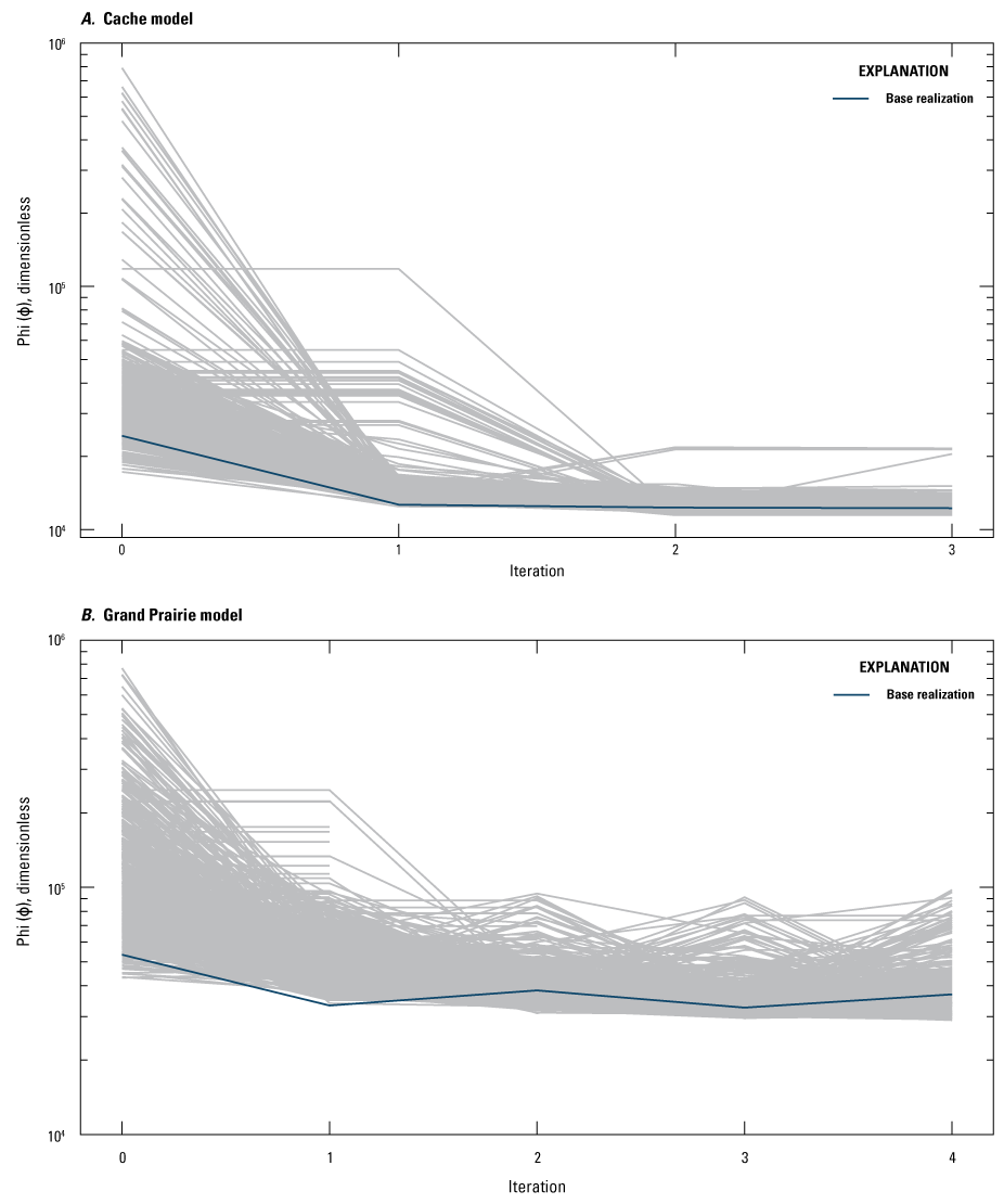
Plot of the PEST++ Iterative Ensemble Smoother objective functions through each iteration of the automated calibration process. A, Cache model. B, Grand Prairie model.
Table 6.
Summary statistics for the ensemble of objective functions from the PEST++ Iterative Ensemble Smoother calibration of the Cache model.[--, not applicable]
Table 7.
Summary statistics for the ensemble of objective functions from the PEST++ Iterative Ensemble Smoother calibration of the Grand Prairie model.[--, not applicable]
Calibrated Model Fit
The Cache model fit to observations was assessed using the base realization from iteration two of the PESTPP–IES calibration run. In the priority CGWA, absolute groundwater levels and spatial and temporal trends in groundwater levels were simulated with minimal bias and exhibited a good fit to measured observations (fig. 11A–F). The measured versus simulated one to one plots and histograms of residuals for each observation group are shown in figures 3.1–3.26, and the measured versus simulated changes in groundwater-level plots from the calibrated base realization of iteration two for the Cache model are shown in figures 4.1 and 4.2. The mean absolute residual for the priority_wells observation group was 1.58 m, which indicated a good fit to observed groundwater levels in the Cache CGWA (table 8). The fit to observed groundwater levels outside the Cache CGWA (head observation group) was also good, with a mean absolute residual of 2.41 m (table 8). Mean groundwater-level residuals for priority_wells and head observation groups were both positive, 0.33 and 1.12 m, respectively, which indicated a slight undersimulation bias (table 8). Spatial and temporal trends in simulated groundwater levels were minimal in the priority CGWA with some small over- and undersimulation, likely caused by uncertainty in agricultural water use from year to year. Most of the larger residuals in the head observation group were located outside of the CGWA, mainly in the north-central region of the model domain or east of Crowley’s Ridge (fig. 12A). Temporal trends in simulated groundwater levels during the primary calibration period from January 1, 2010, through December 1, 2018 (priority_wells_disp and head_disp observation groups) exhibited minimal bias with a mean residual of −0.01 m and 0.17 m, respectively (table 8; fig. 11A–F).
Table 8.
Calibration statistics summary of residuals for the base realization of iteration two for the Cache model. [Left][Residual, observed value minus simulated value; Absolute residual, absolute value of observed value minus simulated value; m3/d, cubic meter per day; m, meter]
Parameter groups summarized in table 2.
Table 9.
Calibration statistics summary of residuals for the base realization of iteration one of the Grand Prairie model. [Left][Residual, observed value minus simulated value; Absolute residual, absolute value of observed value minus simulated value]
Parameter groups summarized in table 3.
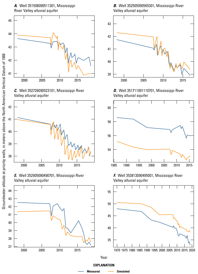
The measured versus simulated groundwater levels from observation wells in the Cache Critical Groundwater Area for the Cache model base realization of iteration two. A, Observation well 351508090511301. B, Observation well 352505090565301. C, Observation well 352726090523101. D, Observation well 351711091110701. E, Observation well 352905090490701. F, Observation well 353813090495001. Well locations are shown in figure 7A or 12A.
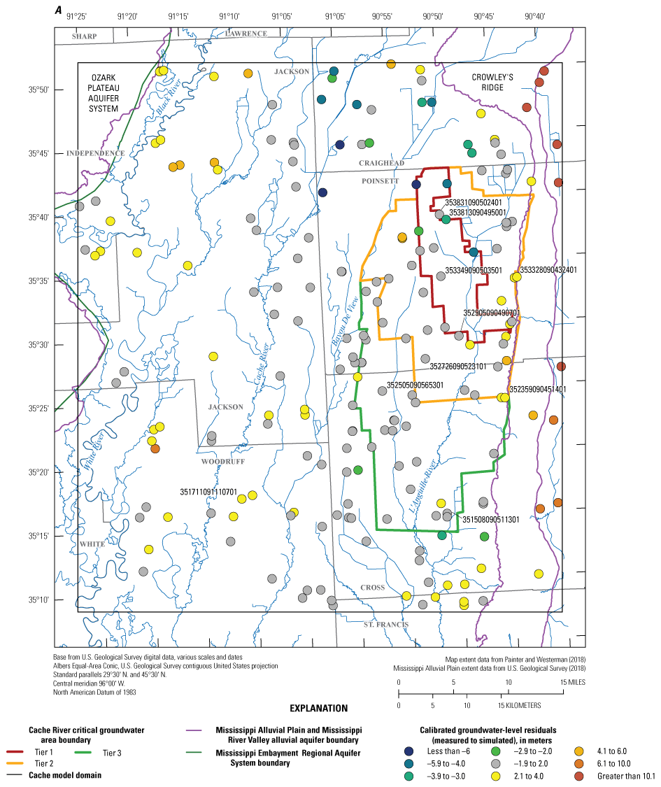

The spatial distribution of groundwater-level residuals from the calibrated base realization. A, Iteration two for the Cache model. B, Iteration one of the Grand Prairie model.
The primary streamflow observation groups of flux_measured and flux_estimated exhibited mean residuals of 31,246,319.02 cubic meters per day (m3/d) (12,771.45 ft3/s) and 98,889.08 m3/d (40.4 ft3/s) (table 8). Simulated streamflows at sites with estimated streamflow observations (flux_estimated observation group) exhibited a better fit compared to the measured data (fig. 13A–D). The large mean residual for the flux_measured was likely caused by the lack of measured streamflow data in the Cache model domain and the very low observation weights assigned based on the groundwater-level centric focus of the model. The only site with nonzero weighted and measured streamflows was the Cache River at Patterson, Ark. (USGS station 07077500) (fig. 7A), which meant that PESTPP–IES was not affected by the residuals for those observations and did not attempt to reduce it in the parameter upgrade process. Spatial differences in streamflow (flux_sdiff or flux_estimated_sdiff), an indication of the magnitude of gaining or losing flow along a stream reach, were oversimulated for the Cache River and Bayou De View, with a mean residual of −547,164.94 m3/d (223.65 ft3/s), which indicated the model allowed less leakage of stream water back into the aquifer (table 8). However, the mean residual was about 20 to 50 percent of mean streamflow and therefore the model is a reasonable representation of the natural system dynamics. The locations with estimated observations such as Bayou De View or the L’Anguille River tended to undersimulate streamflow particularly during low flow periods. This undersimulation indicated that stream inflows, estimated by the random forest surface-water model from Dietsch and others (2023), may have had a low bias during low flow periods or there were shallow processes, such as interflow or bank storage, not simulated by this groundwater-flow model that contributed water to streams during low flow periods (Leaf and others, 2023).
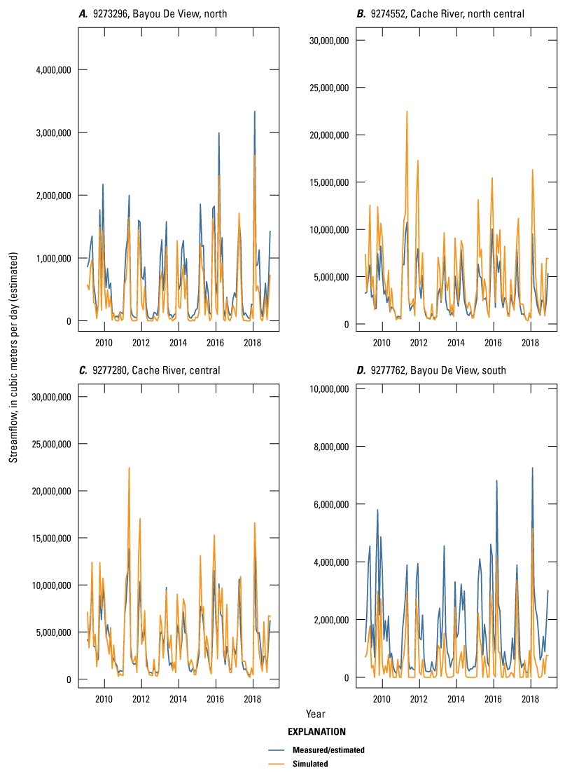
Measured/estimated compared with simulated streamflow for the Cache model base realization of iteration two. A, Bayou De View north site location. B, Cache River north central site location. C, Cache River central location. D, Bayou De View south location.
The “balanced” Grand Prairie model fit to observations was assessed using the base realization from iteration one of the PESTPP–IES calibration run. Iteration one was selected to avoid an overfit solution given that many of the prior parameter values for aquifer properties were derived from the “MRVA-focused” calibration run. Also, other studies have indicated that a realization chosen from iterations one through three is best for adequate history matching and reasonable parameter fields (White, 2018; Hunt and others, 2021; Leaf and others, 2023; Traylor and others, 2023). The measured/estimated compared with simulated one to one plots and histograms of residuals for each observation group from the calibrated base realization of iteration one for the “balanced” Grand Prairie model are shown in appendix figures 5.1–5.36.
The “balanced” Grand Prairie model adequately simulated streamflow across the model domain. The mean absolute residual for the flux_estimated observation group was −503,554.96 m3/d (−205.82 ft3/s), which is about 1 to 30 percent of estimated mean total flow for major streams including the White River, La Grue Bayou, Bayou Meto, and Wabbaseka Bayou (figs. 7B, 14A–F; table 9). Most streams exhibited a good fit between estimated and simulated streamflow during low flow periods. Spatially, streams with estimated observations in the southeastern region of the model in Arkansas County, such as La Grue Bayou (fig. 14A), exhibited some undersimulation of streamflow during low flow periods at multiple locations. The undersimulation of streamflow for La Grue Bayou and other streams in the southeastern region of the model may have been caused by uncertainty in diversions for irrigation reservoirs that led to more water being diverted in the model than what was actually diverted, or the streambed Kv values were not low enough to keep water from leaking through the streambed; however, this bias was not enough to affect the model’s ability to better understand La Grue Bayou’s stream-aquifer dynamics (fig. 14A).
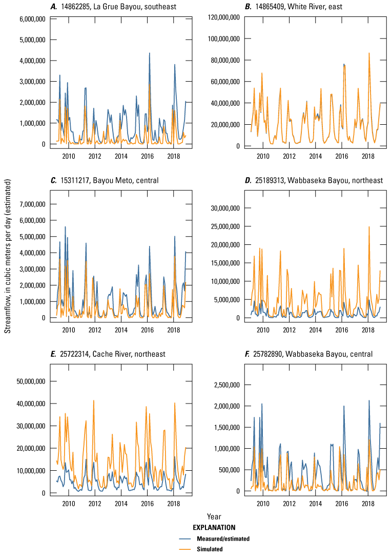
Measured/estimated versus simulated streamflow for the Grand Prairie model base realization of iteration one. A, La Grue Bayou at the southeast site location. B, White River east site location. C, Bayou Meto central location. D, Wabbaseka Bayou northeast site location. E, Cache River northeast site location. F, Wabbaseka Bayou central site location.
Overall, the “balanced” Grand Prairie model adequately simulated absolute groundwater levels and spatial and temporal trends in groundwater levels in the MRVA, and oversimulated absolute groundwater levels in the middle Claiborne aquifer; however, spatial and temporal trends simulated in the middle Claiborne aquifer were accurate (fig. 15A–F). The mean absolute residuals for the grandprairie_mrva_priority_wells and grandprairie_sparta_priority_wells observation groups were 2.71 and 10.78 m, respectively, which indicated that the “balanced” model simulated groundwater levels in the MRVA well, but there was substantial bias in the middle Claiborne aquifer (table 9). The mean residual for the grandprairie_mrva_priority_wells and grandprairie_sparta_priority_wells observation groups were −1.35 m and −9.95 m, respectively, which indicated a small oversimulation bias in the MRVA and a large oversimulation bias in the middle Claiborne aquifer (table 9). Spatial trends in simulated groundwater levels for the CGWA of the MRVA exhibited minor bias for the grandprairie_mrva_priority_wells, whereas groundwater levels outside of the CGWA (grandprairie_mrva_wells_residuals observation group) exhibited some undersimulation bias (mean residual of about 4 m) in the region between Bayou Meto and the Arkansas River and some oversimulation bias (mean residual of about −5 m) east of the White River (fig. 12B). Temporal trends in simulated groundwater levels, particularly for the focus calibration period from January 1, 2010, through December 31, 2018 (grandprairie_mrva_priority_wells_disp observation group), within the CGWA of the MRVA exhibited minor under simulation bias with a mean residual of 0.69 m, and adequately simulated pumping signals and overall changes in groundwater levels across the focus simulation period (fig. 12B). Spatial trends in groundwater levels outside the CGWA of the MRVA also exhibited minimal bias with a mean residual of −0.38 m for the grandprairie_mrva_wells_disp observation group (table 9, fig. 15B). Additional measured compared with simulated plots of groundwater levels for the calibrated base realization of iteration one for the Grand Prairie model are included in appendix figures 5.1–5.36 and 6.1–6.2.
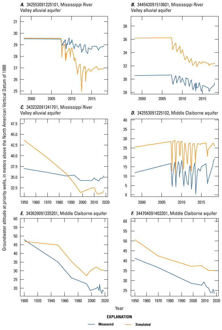
The measured compared with simulated groundwater levels from observation wells in the Grand Prairie Critical Groundwater Area for the Grand Prairie model base realization of iteration one. A, Mississippi River Valley Alluvial aquifer (MRVA) observation well 342553091225101. B, MRVA observation well 344543091510601. C, MRVA observation well 343232091241701. D, Middle Claiborne aquifer observation well 342553091225102. E, Middle Claiborne aquifer observation well 343639091335201. F, Middle Claiborne aquifer observation well 344704091403301. Well locations shown in figures 7B or 12B.
Spatial bias in the simulated middle Claiborne aquifer groundwater levels varied mostly from north to south across the Grand Prairie region. The “balanced” simulation exhibited the smallest oversimulation bias in Tier 1 and the central part of Tier 2 CGWAs with a mean residual in groundwater levels of about −4 m; the largest oversimulation bias was at the southern edges of Tier 2 and Tier 3 with mean residuals of about −11 m (fig. 15B). This increase in residuals farther south in the CGWA corresponded to the presence of the Vicksburg-Jackson confining unit, which subcrops between the MRVA and middle Claiborne aquifer. The spatial bias in simulated groundwater levels for the middle Claiborne aquifer indicated that the “balanced” Grand Prairie model better simulated the unconfined system where the MRVA and middle Claiborne aquifer are hydraulically well connected north of the Vicksburg-Jackson subcrop in southern Lonoke and Prairie counties compared to the confined middle Claiborne aquifer beneath the Vicksburg-Jackson confining unit in the central and southern region of the model domain in Jefferson and Arkansas counties (fig. 12B). Overall, the oversimulation and spatial bias in middle Claiborne aquifer groundwater levels can be attributed to uncertainty in agricultural pumping locations and volumes in the middle Claiborne aquifer across the Grand Prairie region.
Discussion of Calibrated Parameter Values
The Cache and Grand Prairie models were calibrated to produce reasonable parameter fields and values in addition to an acceptable fit to observations. Reasonable parameter fields should be relatively smooth with few extreme values except where conceptually appropriate (Hunt and others, 2019). The calibrated parameter fields for both models included aquifer properties of Kh, Kvani, SS, and SY; streambed Kv; areal recharge; pumping from wells; and general head and river conductance.
For the Cache model, the base realization of iteration two produced reasonable parameter fields and good fit to the observations (fit was discussed in the “Calibrated Model Fit” section of this report). Calibrated Kh for the MRVA model layers (1–8) ranged from 0.03 to 500 m/d (fig. 16). The largest MRVA Kh values (500 m/d) were in a region of higher resistivity in model layer 5. The smallest mean Kh for the MRVA was in a low resistivity region of layer 1 (18.86 m/d; fig. 16; table 10). The mean Kh for layers 1–4 and 5–8 was about 28 and 45 m/d, respectively, and similar to calibrated Kh values from previous studies (table 10; Reed, 2003; Clark and Hart, 2009; Rashid and others, 2015). The larger mean Kh values for deeper MRVA layers are consistent with the conceptual understanding that the coarser grained sediments are present deeper in the alluvial system (Reed, 2003). Model layers 9 through 15, which represent the Tertiary units, exhibited varying ranges of Kh. The Kh values for model layers 9–15 ranged from 0.13 to 500 m/d with mean Kh values from about 28 to 75 m/d (fig. 16). The largest Kh values were in the middle Claiborne aquifer and the smallest Kh values were in the Midway confining unit, which is consistent with the conceptual model of these units as a sand aquifer and clay dominated confining layer (fig. 16; Minsley and others, 2021). The Midway confining unit is most prominently visible in the AEM resistivity data from Minsley and others (2021; fig. 3A,D) and the Kh fields in figure 16 where it subcrops beneath the MRVA with an eastward dip for the entire Cache model. The shallowest subcrop of the Midway confining unit is in model layer 9 at the western end of the model (dips east) and is visible as the region of Kh less than 0.02 m/d (layer 9 in fig. 16). The middle Claiborne aquifer is the region of larger Kh to the east of the Midway confining unit and directly beneath the MRVA. The middle Claiborne aquifer Kh ranged from 1 to 500 m/d, similar to the MRVA; therefore, the MRVA and middle Claiborne aquifer are hydrologically connected in this region. The Kh values in the transition region between the Midway confining unit and the middle Claiborne aquifer represent the Wilcox aquifer system (lower and middle Wilcox aquifers); the transition between these two aquifers is difficult to distinguish in this region of the MERAS (Minsley and others, 2021). Model layers 16–18, which were defined using the framework layers from Hart and others (2008), represented the bottom of the lower Claiborne and Wilcox aquifers. The Kh ranges from about 0.02 to 100 m/d (fig. 16). Layer 16 was calibrated with the lowest mean Kh values of 0.2 m/d, which is consistent with interbedded clays in the lower Claiborne aquifer. Mean Kh for layers 17 and 18 was about 66 and 10 m/d for the Wilcox aquifer system, respectively. The pilot points multipliers for Kh by model layer increased by a mean of about 7 percent (mean multiplier of 1.068 for all model layers); locally, Kh pilot point values exhibited a range of 0.297–3.264. A summary of Kh pilot point multiplier values by model layer for the calibrated Cache model is provided in table 7.1. Precise values of Kh that cannot be distinguished from figure 16 are available in the model archive files associated with this report (Traylor and Weisser, 2024).
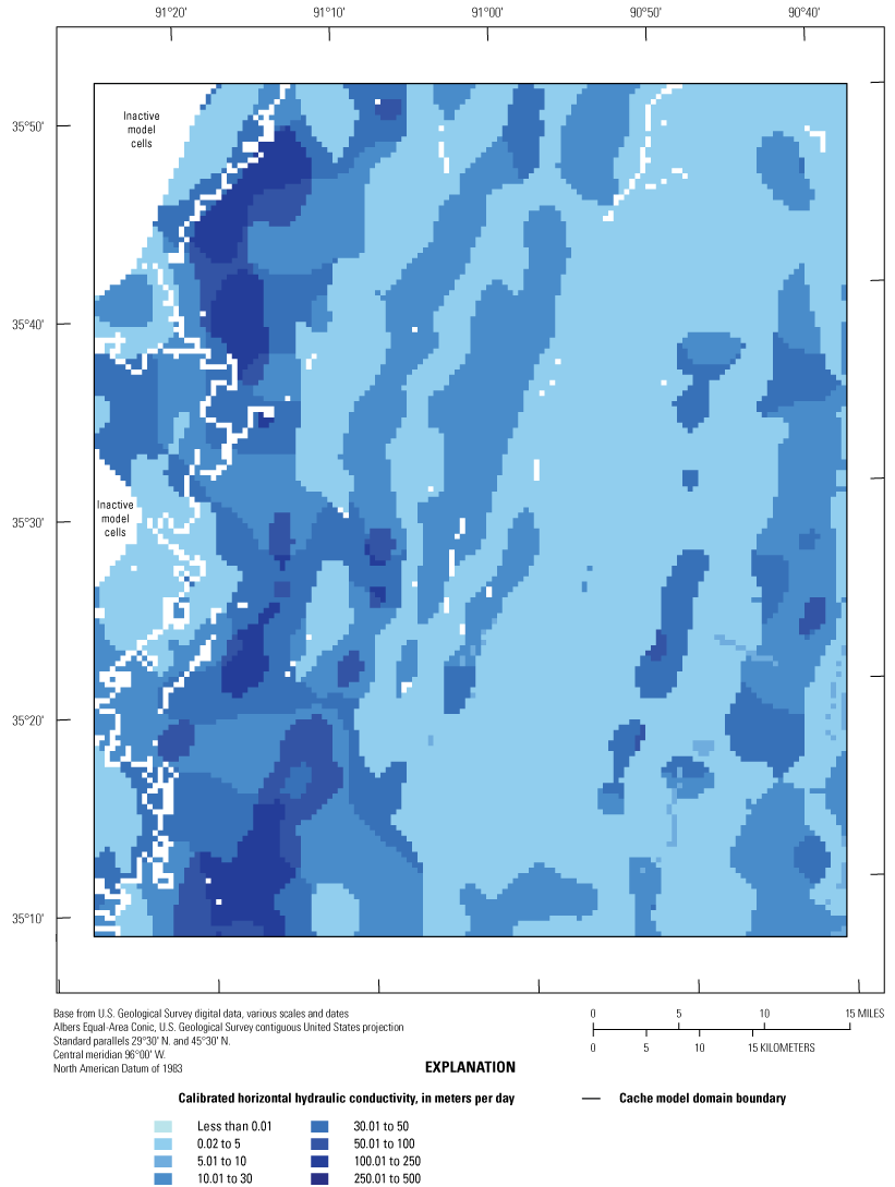
Calibrated horizontal hydraulic conductivity for the base realization of iteration two for the Cache model (this is a layered .pdf; download at https://doi.org/10.3133/sir20245088).
Table 10.
Summary of calibrated aquifer properties for the base realization of iteration two of the Cache model.[m/d, meter per day; Kh, horizontal hydraulic conductivity, Kvani; vertical anisotropy of hydraulic conductivity; Kv, vertical hydraulic conductivity; SY, specific yield]
Table 11.
Summary of calibrated Streamflow Routing package and River package properties for the base realization of iteration two of the Cache model.[rhk, streambed hydraulic conductivity used in Streamflow Routing package; SY, specific yield; SFR, Streamflow Routing package; RIV, River package]
Cache model Kvani ranged from about 1 to 33 (dimensionless) across all model layers. Mean Kvani for the MRVA and deeper Tertiary layers was about 6.59 and 7.28, respectively (table 10). Kvani ratios less than 10 indicated that vertical groundwater flow across model layers was not substantially impeded in the MRVA or the deeper Tertiary units (Fetter, 2001). The primary limiting factor in movement of water across all model layers was the Kh values. The largest Kvani value in the MRVA was about 32, located in model layer 4 (fig. 17). The MRVA Kvani values are consistent with coarse-grained alluvial sediments that facilitate vertical flow in a highly pumped system such as the MRVA in the Cache region. The largest Kvani value in the Tertiary layers 9–15 was about 33, located in one location in model layer 10 (fig. 17). Layer 17 exhibited a larger Kvani (about 17) than layers 16 or 18 but was still in the range where vertical flow between the layers was not substantially impeded. The Kvani values for the fine-grained Midway confining unit are smaller than previously published values in Clark and Hart (2009); however, the values in this study did not negatively affect the ability of the Cache model to accurately simulate past conditions, and parameter compensation was not evident in the other parameters based on reasonable parameter values and parameter fields for this model. The pilot point multipliers for Kvani by model layer increased by a mean of about 7 percent (mean multiplier of 1.066 for all model layers); locally, Kvani pilot point values exhibited a range of 0.275–3.725. A summary of Kvani pilot point multiplier values by model layer for the calibrated Cache model is available in table 7.1. Precise values of Kvani that cannot be distinguished from figure 17 are available in the model archive files associated with this report (Traylor and Weisser, 2024).
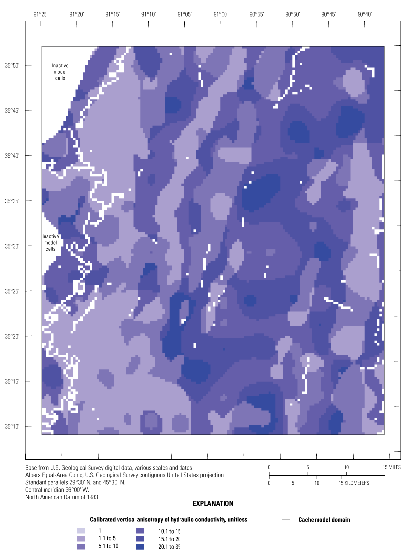
Calibrated vertical anisotropy for the base realization of iteration two for the Cache model (this is a layered .pdf; download at https://doi.org/10.3133/sir20245088).
Cache model SY ranged from 0.08 to 0.35 (dimensionless) and exhibited a mean SY of about 0.27 in the MRVA, which were consistent with previously published values (Reed, 2003; Clark and Hart, 2009; Rashid and others, 2015). The Cache model in this report provided a higher resolution of storage and aquifer properties than all previous models that simulated the Cache region whereby those previous studies specified single constant values or large zones for the MRVA. Calibrated SY fields in the heavily pumped layers of the MRVA (layers 4–7) exhibited multiple regions of larger SY values of 0.3 to 0.35 (fig. 18A; table 10). The Tertiary units (layers 9–18) exhibited a mean SY of 0.23. The SS values for all model layers ranged from 5.0x10⁻⁷ to 1x10⁻⁶ 1/m and were consistent with values from Reed (2003) (fig. 18B). The pilot point multipliers for SY by model layer increased from prior values by a mean of about 9 percent (mean multiplier of 1.079 for all model layers); locally, SY pilot point values exhibited a range of 0.337–4.152 (fig. 18). A summary of SY pilot point multiplier values by model layer for the calibrated Cache model is provided in table 7.1. Precise values of SY that cannot be distinguished from figure 18 are available in the model archive files associated with this report (Traylor and Weisser, 2024).
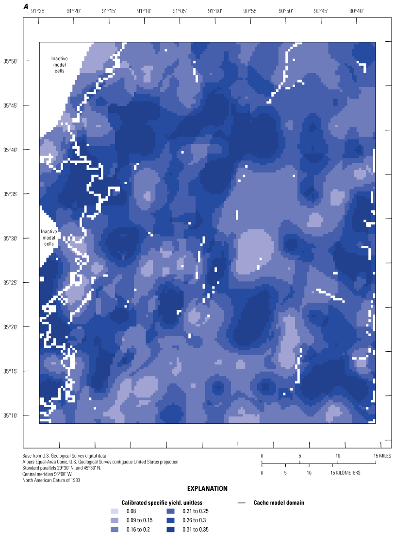

Calibrated specific yield and specific storage for the base realization of iteration two for the Cache model (these are layered .pdfs; download at https://doi.org/10.3133/sir20245088). A, Specific yield. B, Specific storage.
Areal recharge multipliers assigned by surface connectivity zone in the Cache model (fig. 8A) exhibited minimal to moderate deviations from their prior values of 1.0. The calibrated multipliers ranged from 0.57 to 1.49 and a mean of 1.08. The mean value by physiographic region (MRVA, Crowley’s Ridge, and Ozark Plateau) of the Cache model domain was 1.01 for the MRVA, 1.16 for Crowley’s Ridge, and 1.07 for the Ozark Plateau. The calibrated multiplier of 1.01 for the MRVA indicated that recharge from the SWB model deviated less from the spatial trends of the surface connectivity in the MRVA region than Crowley’s Ridge, likely because there were more observations and more focus on recharge in the MRVA, but the Crowley’s Ridge recharge also did not deviate substantially from the SWB model spatial trends (fig. 19A). Temporally, the stress period multipliers ranged from 0.07 to 0.87 (fig. 19B) with a mean of 0.22 and a standard deviation of 0.11; the prior value was 0.2. This 13- to 97-percent reduction in the SWB model estimated recharge (water leaving the root zone) indicated that the unsaturated zone substantially attenuated the downward movement of water toward the water table and multipliers of this magnitude were necessary in the absence of an unsaturated zone in the model simulation (fig. 19B).
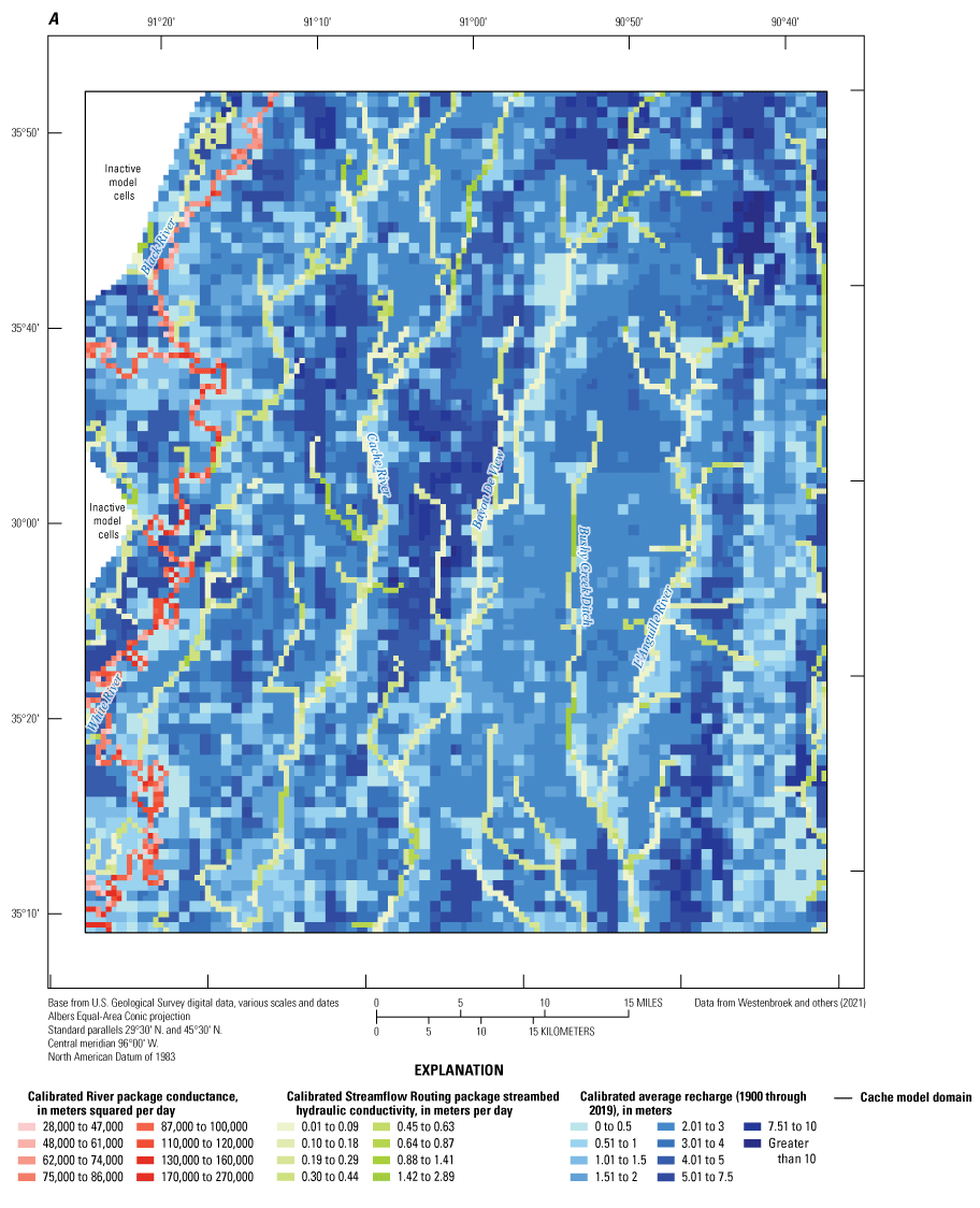

Calibrated recharge, streambed vertical hydraulic conductivity, and riverbed conductance for the base realization of iteration two for the Cache model. A, Map of calibrated average recharge from 1900 through 2019, Streamflow Routing package vertical hydraulic conductivity, and River package conductance. B, Plot of calibrated stress period multipliers for recharge.
Streambed Kv in the SFR package for the Cache model ranged from 0.01 to 2.89 m/d with a mean value of 0.25 m/d, similar to those in Reed (2003), and also varied substantially by reach (fig. 19A). Based on streambed Kv fields, streams in the Cache model were well connected to the MRVA in a few areas of short reaches, with most other reaches exhibiting small streambed Kv values that limited the stream’s connection with the MRVA. Mean streambed Kv was largest for the Cache River at 0.3 m/d in comparison among Bayou De View, the L’Anguille River, and Village Creek. The largest streambed Kv values (2.45 and 2.89 m/d) were on the northern reaches of the Cache River; Bushy Creek Ditch, a tributary to the L’Anguille River also had several reaches with streambed Kv of 2.16 m/d (fig. 19A). The smallest streambed Kv values were 0.01 m/d located on a northern reach of Bayou De View (fig. 19A). Riverbed conductance for the Black River and White River was 27,686 to 271,915 m2/d. The Black River was less connected to the MRVA with a mean conductance of 70,324 m2/d, and the White River exhibited a higher degree of connection to the MRVA with a mean conductance of 93,338 m2/d (fig. 19A, table 11). The upper reaches of the White River, below the confluence with the Black River and the White River near the outflow of the model domain, exhibited the largest riverbed conductance values. Like the streambed Kv in the SFR package, these riverbed conductances varied spatially from reach to reach, with large conductance reaches often adjacent to smaller conductance reaches (fig. 19A). The least conductive reaches were on the Black River in the northwest part of the model (fig. 19A).
Calibrated well pumping multipliers by crop type and stress period (wel_croptype_mult), and by data source (wel_datasource_mult) did not deviate substantially from their prior values of 1.2. These minimal grid scale adjustments to pumping stresses during the calibration process indicated that each data source provided pumping rates across the entire simulation period that were conceptually accurate after increasing the prior multipliers to 1.2. The calibrated combined crop type and stress period multipliers had a mean value of 1.21 to 1.25 for each of the crop types across all 148 stress periods (table 12). The multipliers by data source (SWUDS, MERAS 2, and Irrigation Water Use Model [IWUM]) exhibited a range from 1.0 to 1.33 (Traylor and Weisser, 2024). The largest deviation from the prior was in agricultural pumping (IWUM) multiplier, which was reduced by 0.2 to 1.0 (Traylor and Weisser, 2024). The multiplier for the spin-up stress periods (stress periods 2–7), which adjusted pumping from the MERAS 2 data source, increased by 0.13 to 1.33. The municipal pumping from the SWUDS data source decreased to 1.17. The calibrated water use multipliers by crop type for each stress period in the Cache model are shown in figure 8.1. Precise values of SY that cannot be distinguished from figure 18 are available in the model archive files associated with this report (Traylor and Weisser, 2024).
Table 12.
Summary of the calibrated parameters by parameter group for the base realization of iteration two for the Cache model.[--, unitless; posterior, post calibration]
For the Grand Prairie model, the base realization of iteration one produced acceptable parameter fields and fit to the observations (fit was discussed in the “Calibrated Model Fit” section of this report). Calibrated Kh for the MRVA model layers (1–8) ranged from 1.0 to 300 m/d (fig. 20). Each MRVA layer exhibited areas with Kh values of 300 m/d, with layer 3 exhibiting the most widespread areas with 300 m/d Kh values (fig. 20; Traylor and Weisser, 2024). For all MRVA layers, the areas with Kh values of 300 m/d were correlated to areas of higher resistivity from the AEM data (fig. 20). The mean Kh for layers 1–4 and 4–8 was about 78 and 48 m/d, respectively, and within the range of calibrated Kh values from previous studies (table 13; Reed, 2003; Clark and Hart, 2009). The larger mean Kh values for shallower MRVA layers are consistent with the AEM resistivity facies zones, which exhibited higher resistivity zones in the shallower layers but is not consistent with the overall concept that coarser grained sediments are present deeper in the alluvial system that was in the Cache model (Reed, 2003). Model layers 9 through 15, which represented the Tertiary-age units, including the Vicksburg-Jackson confining unit, middle Claiborne aquifer, and the lower Claiborne confining unit, exhibited varying ranges of Kh based on their representative geologic unit. The Kh values for model layers 9–15 ranged from 1.0 to 263 m/d with a mean value of 7.9 m/d (fig. 20; table 13). The largest Kh values were in small areas in layers 9 and 15 that corresponded to high resistivity areas (Minsley and others, 2021). The Vicksburg-Jackson confining unit was most prevalent in the southern half of the Grand Prairie model and was prominent in the Kh fields for layers 9–13 where it is represented by smaller Kh values (fig. 20). The middle Claiborne aquifer is unconfined and in hydraulic connection with the MRVA in the northern half of the model domain where the Vicksburg-Jackson confining unit is absent. In the southern half of the model domain, where the Vicksburg-Jackson confining unit is present, the middle Claiborne aquifer is confined and exhibited minimal connection with the overlaying MRVA. Model layers 16–18, which were defined using the framework layers from Hart and others (2008), represented the bottom surface of the lower Claiborne and Wilcox aquifers, like in the Cache model. In Grand Prairie model layers 16–19, Kh ranges from about 1.0 to 8.8 m/d and mean value of 2.1 m/d, which were like values from McKee and Clark (2003) and Clark and Hart (2009) (fig. 20). Layer 16 calibrated with the lowest mean Kh values of 0.2 m/d, which is consistent with interbedded clays in the lower Claiborne aquifer. On average, the pilot point multipliers for Kh by model layer increased by about 16 percent (mean multiplier of 1.16 for all model layers); locally, Kh pilot point values exhibited a range of 0.171–5.567 (table 7.2). A summary table of Kh pilot point multiplier values by model layer for the calibrated Grand Prairie model is in table 7.2. Precise values of SY that cannot be distinguished from figure 20 are available in the model archive files associated with this report (Traylor and Weisser, 2024).
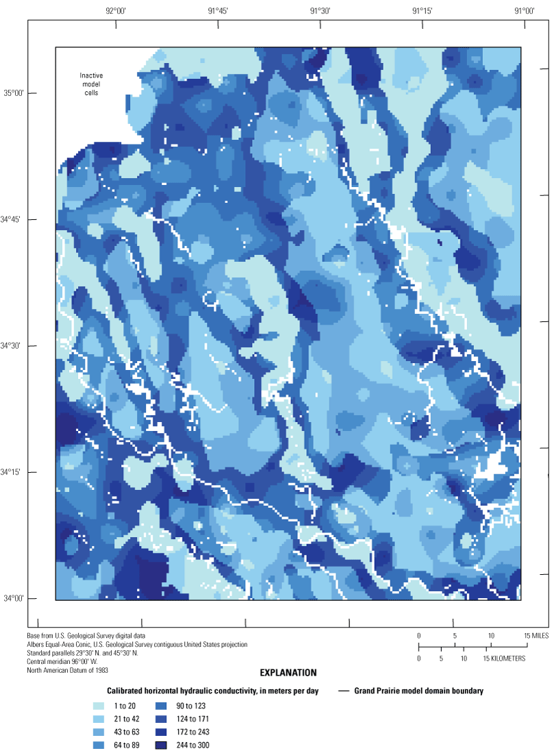
Calibrated horizontal hydraulic conductivity for the base realization of iteration one for the Grand Prairie model (this is a layered .pdf; download at https://doi.org/10.3133/sir20245088).
Table 13.
Summary of calibrated parameters by parameter group for the base realization of iteration one of the Grand Prairie model.[m/d, meter per day; Kh, horizontal hydraulic conductivity, Kvani, vertical anisotropy of hydraulic conductivity, calculated as Kh/Kv; Kv, vertical hydraulic conductivity]
Table 14.
Summary of calibrated Streamflow Routing and River package parameters for the base realization of iteration one of the Grand Prairie model.[rhk, streambed hydraulic conductivity used in Streamflow Routing package; SY, specific yield; SFR, Streamflow Routing package; RIV, River package]
Grand Prairie model Kvani (fig. 21) ranged from about 43 to 5,127 (dimensionless) across all model layers and overall was substantially higher than in the Cache model (fig. 17). Mean Kvani for the MRVA (layers 1–8) and deeper Tertiary layers (layers 9–19) was about 214 and 297, respectively (table 13). Kvani ratios greater than 100 indicated that vertical groundwater flow across model layers was substantially impeded (Fetter, 2001). The primary limiting factor in the vertical movement of water across all model layers was the aquifer characteristics indicated by the anisotropy ratios. The largest Kvani value in the MRVA was about 5,127, located in lower AEM resistivity zones of model layer 7 (figs. 4B, 8B, 21; Minsley and others, 2021). Large anisotropy values were also present in shallow MRVA layers, which is consistent with a shallow clay lens in the Grand Prairie model domain (figs. 4B, 20) that limits areal recharge. The largest Kvani value in the Tertiary layers 9–15 was about 4,654 and located in low resistivity zones of model layer 10 (Minsley and others, 2021) and spatially consistent with the Vicksburg-Jackson confining unit (approximately layers 9–12; figs. 4B, 21; table 15). Layers 16–19 exhibited a mean Kvani from 87 to 600 and exhibited some heterogeneity (fig. 21). The pilot point multipliers for Kvani by model layer increased by a mean of about 39 percent (mean multiplier of 1.39 for all model layers); locally, Kvani pilot point values exhibited a range of 0.140–9.365. A summary of Kvani pilot point multiplier values by model layer for the calibrated Grand Prairie model is provided in table 7.2.
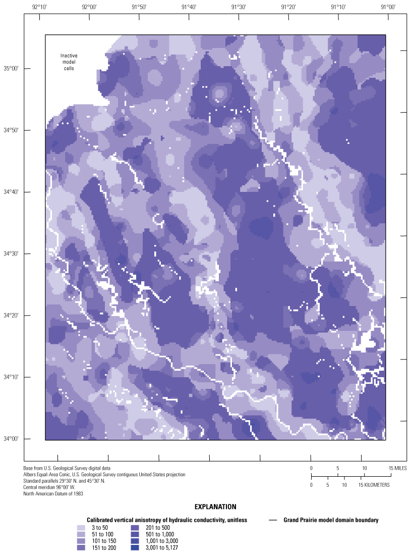
Calibrated vertical anisotropy for the base realization of iteration one for the Grand Prairie model.
Grand Prairie model SY ranged from 0.05 to 0.35 (dimensionless) and exhibited a mean SY of about 0.29 in the MRVA (layers 1–8), which were consistent with previously published values (fig. 22A; Reed, 2003; Clark and Hart, 2009). The Grand Prairie model, like the Cache model, provided a higher resolution of storage and aquifer properties for the MRVA than all previous models that simulated the Grand Prairie region with single constant values or large zones. Calibrated SY fields in all MRVA layers exhibited multiple regions of larger SY values of 0.05 to 0.35, which indicated the preference of the calibration toward higher storage values (fig. 22A). The Tertiary units (layers 9–18) exhibited a mean SY of 0.25, which is about 25 percent higher than in the middle Claiborne aquifer focused model from McKee and Clark (2003). The SS values for all model layers (fig. 22B) ranged from 5.6x10⁻⁷ to 3.9x10⁻⁶ 1/m and were consistent with values from Reed (2003) and McKee and Clark (2003) (table 13). The pilot point multipliers for SY by model layer increased by a mean of about 14 percent (mean multiplier of 1.138 for model layers 1–11); locally, SY pilot point multiplier values for the MRVA exhibited a range of 1.108–3.594. A summary of SY pilot point multiplier values by model layer for the calibrated Grand Prairie model is provided in table 7.2.
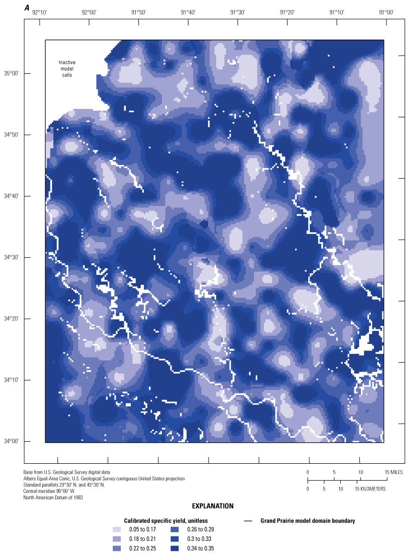

Calibrated specific yield and specific storage for the base realization of iteration one for the Grand Prairie model. A, Specific yield. B, Specific storage.
Areal recharge multipliers by surface connectivity zone exhibited minimal deviations from their prior values of 1.0. The calibrated multipliers by surface connectivity zone ranged from 0.78 to 1.17 and a mean of 1.02 (table 15). The calibrated multiplier of 1.02 for the MRVA indicated that recharge from the SWB model correlated well with the spatial trends of the surface connectivity (figs. 8B, 23A). Temporally, the stress period multipliers ranged from 0.10 to 1.19 with a mean of 0.39 and a standard deviation of 0.24 (fig. 23A). The mean deviation from prior values was −0.002, which indicated that overall, the calibration did not substantially alter the total amount of recharge to better match temporal trends across the simulation period. However, like the Cache model, the range in stress period multipliers (0.1 to 1.19) of the SWB model estimated recharge (water leaving the root zone) indicated that the unsaturated zone substantially attenuated the downward movement of water toward the water table for individual stress periods and locations (fig. 23A,B).
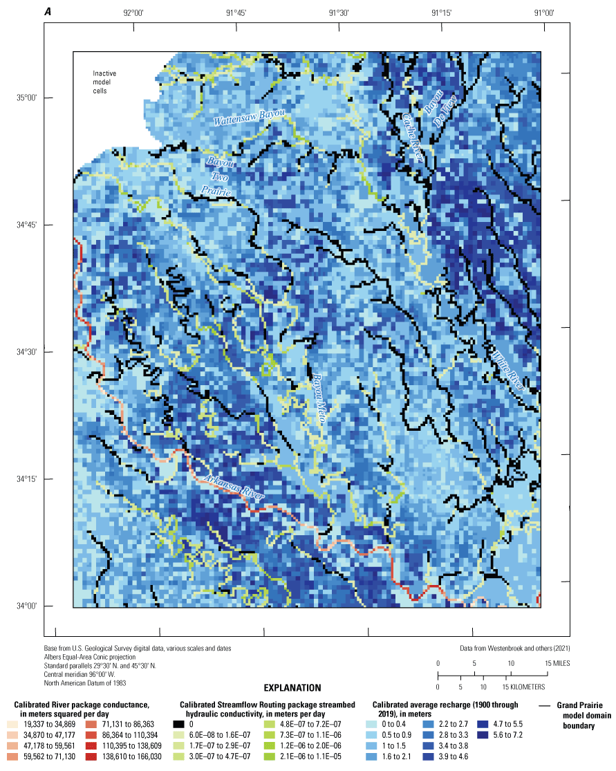

Calibrated recharge for the base realization of iteration one for the Grand Prairie model. A, Map of calibrated average recharge from 1900 through 2019, Streamflow Routing package hydraulic conductivity, and River package conductance. B, Plot of calibrated stress period multipliers for recharge.
The rhk values in the SFR package were very low and ranged from 0 to 3.9x10⁻⁶ m/d (fig. 23A) with a mean value of 1.2x10⁻⁶ m/d, which were substantially lower than the stream rhk values derived from conductances in Clark and Hart (2009). There was some variance in rhk by reach (fig. 23A). Based on streambed Kv fields, streams in the Grand Prairie model exhibited limited connection to the MRVA in most areas with a few reaches that exhibited larger rhk values and a greater connection to the MRVA. Mean rhk was largest for Bayou Meto at 0.0068 m/d compared to Bayou Two Prairie, the Cache River, White River, and Wattensaw Bayou (fig. 23B; table 14). The largest rhk values (3 m/d) were Bayou Meto (fig. 23B; table 14). Riverbed conductance for the Arkansas River was 64,890 to 557,150 m2/d with a mean value of 237,368 m2/d, which equates to an rhk of 0.95 m/d (3.11 ft/d) (Langevin and others, 2017); similar to the Arkansas River values from Clark and Hart (2009); however, the model from Clark and Hart (2009) simulated fewer streams than the Grand Prairie model in this study. Like the rhk in the SFR package, these riverbed conductances varied spatially from reach to reach, with large conductance reaches often adjacent to smaller conductance reaches (fig. 23A).
Well pumping multipliers by crop type, data source, and stress period did not deviate substantially from their prior values and base multipliers of 1.0 (fig. 8.1). The calibrated crop type multipliers exhibited a range from 0.73 to 1.42 with a mean of 1.03; all crop type multipliers decreased between 0 and 10 percent from their prior values. Like the Cache model data source multipliers, these small grid scale adjustments to pumping stresses during the calibration process indicated that each data source provided pumping rates across the entire simulation period that were conceptually accurate and only minor fine-tuning of the pumping multipliers was needed during the calibration process. The combined data source (agricultural, MERAS 2, SWUDS, and thermoelectric) and stress period multipliers had a mean value of 1.03 for all 148 stress periods (table 15). The largest variance (standard deviation) was for the MERAS 2 pumping values and was in accord with the greater uncertainty in pumping during the first seven stress periods where irrigation practices were less known. The mean of the multiplier for the municipal pumping from the SWUDS data source increased from 1.002 to 1.003.
Table 15.
Summary of the calibrated parameters by parameter group for the base realization of iteration one of the Grand Prairie model.[--, unitless; posterior, post calibration]
The parameter fraction_move_aiwum_mrva2sparta increased about 29 percent from 0.378 to 0.486, which indicated that PESTPP–IES preferred to increase the amount of pumping in the middle Claiborne aquifer to improve the calibration. As discussed in the “Calibration Parameters” section of this report, this parameter moved pumping from MRVA model layers 5 through 8 to layer 15. This parameter likely increased to compensate for the large oversimulation bias in groundwater-level residuals in the middle Claiborne aquifer throughout the simulation. Given the uncertainty in agricultural pumping from the middle Claiborne aquifer in the Grand Prairie region, this was an acceptable parameter adjustment that illuminates the need for better water use information in the middle Claiborne aquifer within the Grand Prairie region.
In the Grand Prairie model, well pumping multipliers by the coupled model layer and AEM framework zone (wel_layer_aemframework_mult) exhibited moderate deviations from their prior values, which illuminated PESTPP–IES’ preference for adjustments to pumping by layer in the Grand Prairie model (Traylor and Weisser, 2024). The mean multipliers ranged from about 0.455 to 5.125 and exhibited a mean value across all layers of 1.11 (table 15). PESTPP–IES increased or decreased multipliers for layers 1 through 15 from 9 to 63.8 percent. Pumping multipliers for layers 16 and 19 were increased by 346.2 and 412.5 percent, respectively, which indicated that pumping in the lower Claiborne aquifer and middle and lower Wilcox aquifers may have been underrepresented in the model prior to calibration. The calibrated well pumping multipliers by crop type for each stress period in the Cache model are shown in figure 8.2.
Posterior Parameter and Simulated Observation Distributions
The distribution of parameter values from the prior (or initial) PESTPP–IES ensemble compared with the posterior (or final) chosen iteration (iteration two for Cache and iteration one for Grand Prairie) ensemble provides an indication of parameter uncertainty and how it changed through calibration. Smaller posterior parameter distributions compared to their initial distributions indicated a reduction in the uncertainty. Conversely, a wider or similar distribution for posterior parameters indicates that the calibration did not reduce the uncertainty of that parameter or group of parameters; perhaps because its parameter identifiability was too low, it was not sensitive to the observation dataset or it already had an optimal distribution (Doherty and Hunt, 2009). The ensemble parameter distribution produces a range of simulated equivalent observations that can also be used to understand the uncertainty of outputs such as simulated groundwater levels. A summary of several salient parameter groups and simulated groundwater levels at priority wells for the calibration process for each model follows.
The Cache model’s posterior ensemble distribution was generally smaller and had reduced parameter uncertainty compared to the prior ensemble. Groups of parameters that exhibited the most reduction in their distribution included Kvani (Kvani_zone parameter group) for zone 9, several of the recharge zone multipliers (rzonemult parameter group), SFR package Kv multipliers by zone (sfr_mult_zone parameter group), and pumping multipliers by data source (wel_datasource parameter group) for all three pumping data sources, which are IWUM (analogous to AIWUM here), MERAS2, and SWUDS (fig. 24A–G). The agricultural pumping data source (IWUM) posterior parameter ensemble exhibited the largest reduction in its distribution, which indicated that the calibration gained the most information from the observations of that parameter and that the prior ensemble distribution was very wide and a reflection of how calibration can reduce uncertainty in important parameters. The calibration did not substantially change the distribution of most Kh and Kvani by zone and pumping by crop type parameters, which indicated that those parameters were likely less identifiable (figs. 9.1, 9.2; Doherty and Hunt, 2009).
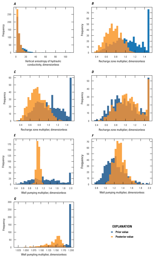
Prior and posterior parameter distributions for the Cache model parameter groups. A, Vertical anisotropy for zone 9 model. B, Recharge multiplier for zone 5. C, Recharge multiplier for zone 6. D, Streamflow Routing package multiplier for zone 3. E, Well package multiplier for the agricultural pumping data source. F, Well package multiplier for the Mississippi Embayment Regional Aquifer System model version 2 (MERAS 2) pumping data source. G, Well package multiplier for the municipal pumping data source.
The Grand Prairie model exhibited a marginal reduction in posterior ensemble parameter distributions for most parameters because the prior ensemble for many groups of parameters was based on a preliminary PESTPP–IES calibration ensemble from the “MRVA-focused” model instead of previously published values, as in the Cache model. The calibration did not substantially reduce the distribution of most Kh and Kvani by zone parameters, which indicated that those parameters were likely at reasonable values prior to the automated calibration (figs. 9.3, 9.4). Parameters that exhibited the largest reduction from prior to posterior parameter distributions were the well pumping multiplier parameters for the “other” crop type (parameter wel_croptype_mult) and for the fraction of pumping moved from the MRVA to model layer 15 of the middle Claiborne aquifer (parameter fraction_move_aiwum_mrva2sparta; fig. 25A, B). The uncertainty in pumping from the middle Claiborne aquifer within the Grand Prairie region was reflected in the model’s preference to increase pumping in the deeper aquifer whereby the posterior distribution of the fraction_move_aiwum_mrva2sparta parameter became more normally distributed rather than bimodal (fig. 25B).
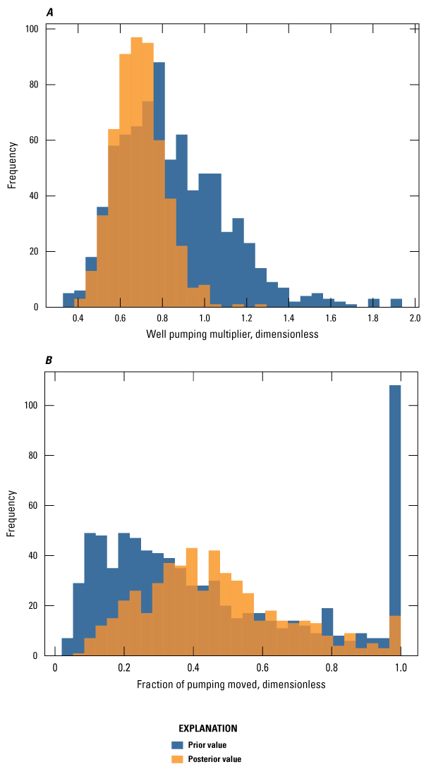
Prior and posterior parameter distributions for the Grand Prairie model parameter groups. A, Well package multiplier for the “other” crop type. B, Well package multiplier parameter that moves a fraction of Mississippi River alluvial aquifer pumping to model layer 15 (middle Claiborne aquifer).
The reduction in parameter uncertainty from the prior to posterior parameter ensembles for both models resulted in a reduction in the posterior distribution of simulated groundwater levels. In the Cache model, the calibration process reduced the 2007 through 2018 distribution of groundwater levels in observation well 352505090565301, located in the southern section of the Cache CGWA, from about 40 m to about 10 m (a 75 percent reduction) (figs. 26B, 7A). Cache model observation well 352726090523101, also located in the southern section of the Cache CGWA, exhibited a reduction from about 35 m to about 10 m (a 71 percent reduction) (figs. 26A, 7A). A similar reduction was present in the observation ensemble for groundwater levels in the Grand Prairie model within the northern section of the Grand Prairie CGWA where observation wells 344543091510601 and 345129091455801 exhibited a reduction from about 60 m to about 22 m (a 63 percent reduction) (figs. 26C, D, 7B).
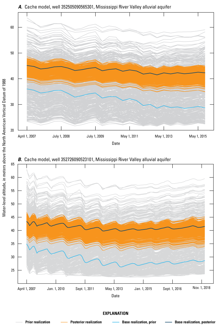

Prior and posterior ensemble distributions of simulated groundwater-level observations. A, Cache model observation well 352505090565301. B, Cache model observation well 352726090523101. C, Grand Prairie model observation well 344543091510601. D, Grand Prairie model observation well 345129091455801.
Groundwater Budget Results
Groundwater budgets for the Cache and Grand Prairie models were computed for the entire model domain and each CGWA Tier 3 for simulated years from 2007 through 2018. Groundwater budget results were calculated using the calibrated versions of each model, which included the base realization of iteration two for the Cache model and the base realization of iteration one for the Grand Prairie model. Total annual inflows and outflows and the percentage of total inflows and outflows for each budget term were computed to assess the relative magnitude of each groundwater budget component (tables 16–23).
Table 16.
The simulated (base realization of iteration two) annual groundwater budget total inflows for Cache model for each budget term from 2007 through 2018.[NA, not applicable; -, no value]
Table 17.
The simulated (base realization of iteration two) annual groundwater budget outflows for Cache model for each budget term from 2007 through 2018.[--, no value; NA, not applicable]
Table 18.
The simulated (base realization of iteration two) annual groundwater budget inflows for each budget term for Cache model Critical Groundwater Area Tier 3 from 2007 through 2018.[NA, not applicable]
Table 19.
The simulated (base realization of iteration two) annual groundwater budget outflows for each budget term for Cache model Critical Groundwater Area Tier 3 from 2007 through 2018.[NA, not applicable]
Table 20.
The simulated (base realization of iteration one) annual groundwater budget inflows for each budget term for Grand Prairie model from 2007 through 2018.[NA, not applicable]
Table 21.
The simulated (base realization of iteration one) annual groundwater budget outflows for each budget term for Grand Prairie model from 2007 through 2018.[NA, not applicable]
Table 22.
The simulated (base realization of iteration one) annual groundwater budget inflows for each budget term for Grand Prairie model Critical Groundwater Area Tier 3 from 2007 through 2018.[NA, not applicable]
Table 23.
The simulated (base realization of iteration one) annual groundwater budget outflows for each budget term for Grand Prairie model Critical Groundwater Area Tier 3 from 2007 through 2018.[NA, not applicable]
Cache Model Groundwater Budgets
The groundwater budgets for each area of the Cache model were characterized by irrigation and nonirrigation season trends in water use whereby the largest outflows were to pumping wells and occurred during the peak growing season (May through September). Across the entire model domain, the primary source of water to the wells was releases from unconfined groundwater storage (fig. 27A; tables 16 and 17). Mean 2007 through 2018 releases from unconfined aquifer storage were 50,886,613 m3, which was about 48 percent of all inflows (table 16). Stream leakage (from streams simulated with the SFR package) and areal recharge were other substantial inflows, constituting about 33 and 9 percent of total inflows, respectively (table 16). The large outflows to wells each irrigation season are due to pumping from agricultural wells for irrigation and aquaculture use; municipal water use did not contribute a substantial amount to total annual outflows. Mean 2007 through 2018 aquaculture, irrigation, and municipal pumping were 54,657,872 m3, constituting about 52 percent of all outflows (table 17).
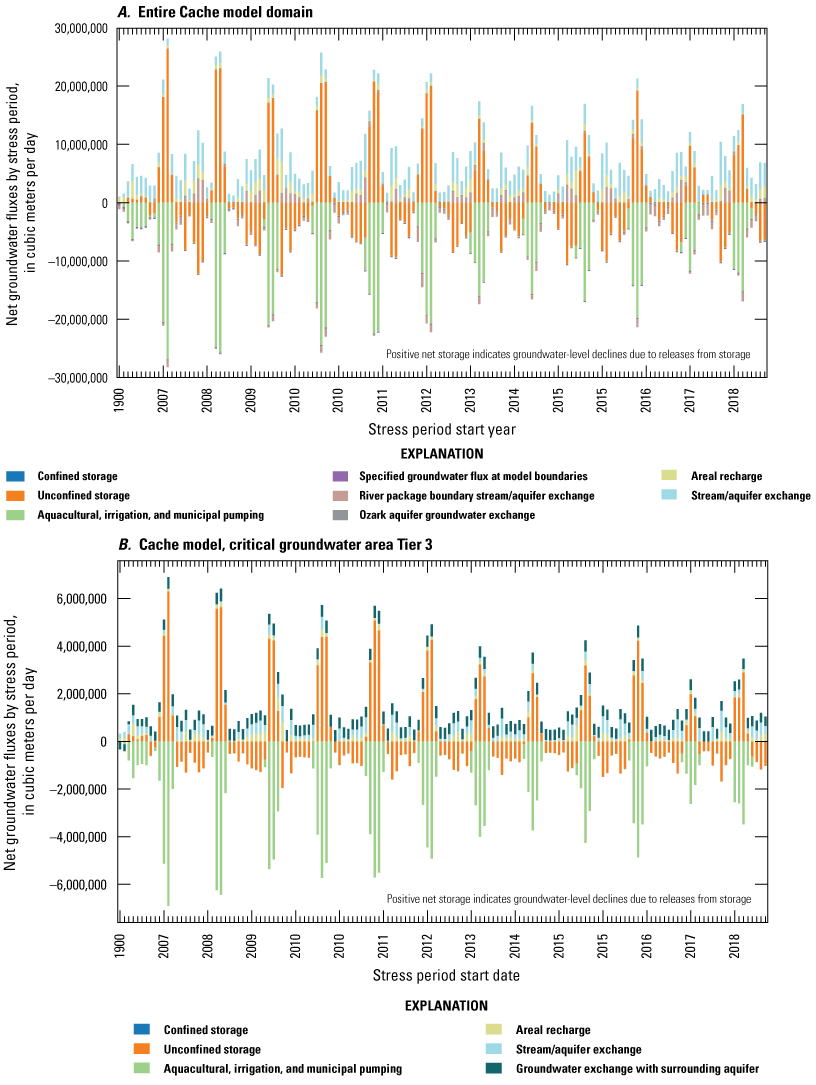
Plot of the groundwater budget for the Cache model. A, Entire Cache model domain. B, Tier 3 Critical Groundwater Area domain.
The groundwater budget for the Cache CGWA Tier 3 was characterized by large outflows to irrigation wells during the late spring and summer months and supported primarily by releases from groundwater storage, which was similar to the entire Cache model domain (fig. 27B; tables 18 and 9). From 2007 through 2018, mean annual outflows to aquaculture, irrigation, and municipal wells were about 64 percent of total outflows (table 19). Releases from unconfined storage were about 49 percent of total inflows. Other substantial inflows included leakage from streams simulated with the SFR package (about 15 percent), areal recharge (about 8 percent), and inflows from the surrounding aquifer (about 28 percent) (table 18). Other substantial outflows included replenishment to unconfined storage (about 34 percent). Outflows to the surrounding aquifer were minimal at about 1 percent (table 19).
The groundwater budgets for the entire Cache model domain and the CGWA Tier 3 indicated that there was more surface water and groundwater connection outside of the Tier 3 region than within (tables 16 and 18). This was evident visually whereby simulated water table altitudes for dry (September 1, 2014) and wet (May 1, 2009) conditions exhibit higher water table altitudes along the Cache River and Village Creek, which indicated losing stream conditions. Water table altitudes along the White River were lower than the surrounding aquifer during dry conditions, which indicated a gaining stream (fig. 28A,B). During wet conditions, the White River exhibited a losing stream owing to the higher water table altitudes than surrounding aquifer (fig. 28C,D). This behavior along the White River indicated that river stage was important in determining the level of connection with the underlying aquifer. Simulated stream leakage during dry conditions exhibited a number of stream reaches drying out primarily along the central and southern reaches of Bayou De View and tributaries of the L’Anguille River, whereas dry stream reaches during wet conditions were simulated mainly for small tributaries of Bayou De View and the L’Anguille River (fig. 28B,D).
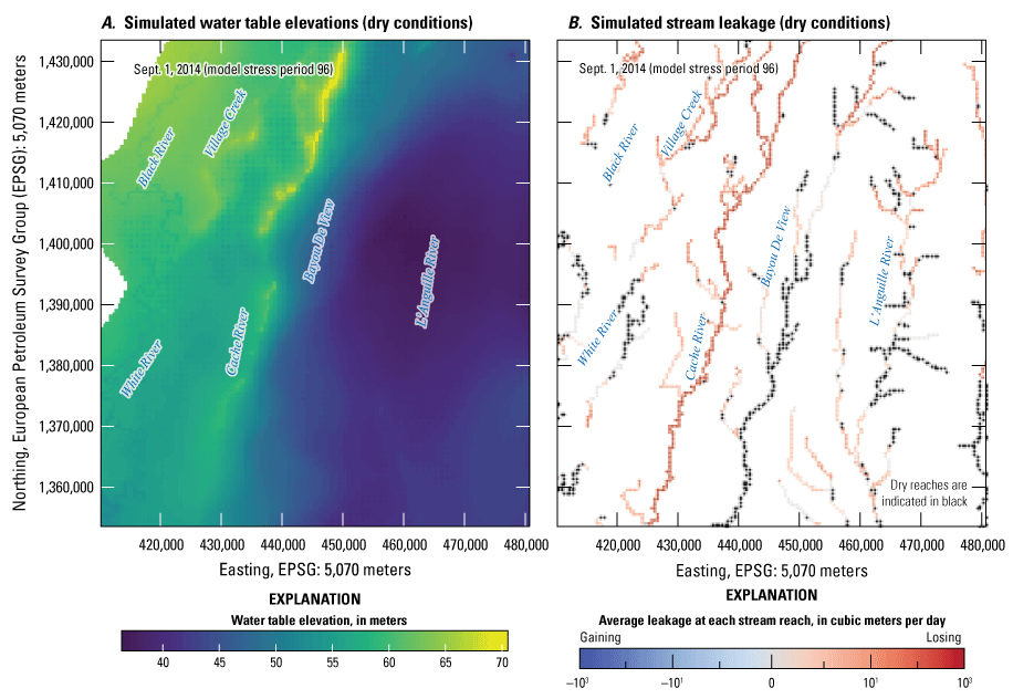

Simulated water table surface and calibrated stream leakage for the base realization of iteration two for the Cache model during dry and wet periods. A, Simulated water table altitudes in dry conditions (stress period 96). B, Simulated stream leakage in dry conditions (stress period 96). C, Simulated water table altitudes in wet conditions (stress period 32). D, Simulated stream leakage in wet conditions (stress period 32).
Grand Prairie Model Groundwater Budgets
The groundwater budgets for each area of the Grand Prairie model, including the MRVA and the Tertiary-age aquifers, are characterized by irrigation and nonirrigation seasonal trends in water use whereby the largest outflows were to pumping wells that operated during the peak growing season (May through September) to irrigate crops. Across the entire model domain, the primary source of water to the wells was the release of groundwater from unconfined storage (fig. 29A; tables 20 and 21). The total mean 2007 through 2018 release from unconfined aquifer storage was 46,704,367 m3, which was about 48 percent of all inflows (table 20). Connection with surface water was minimal in the Grand Prairie model throughout the entire domain. The mean annual stream leakage (from the SFR package) was about 218 m3, which is less than 1 percent of total inflows to the groundwater. Areal recharge was the primary source of water and accounted for about 35 percent of total inflows (table 20). The large outflows to wells during each irrigation season were due to pumping from agricultural wells for irrigation and aquaculture use, whereas municipal and thermoelectric water use did not contribute a substantial amount to total annual outflows. Mean outflow from 2007 through 2018 for aquaculture, irrigation, and municipal pumping was 52,053,330 m3, about 54 percent of all outflows (table 21).
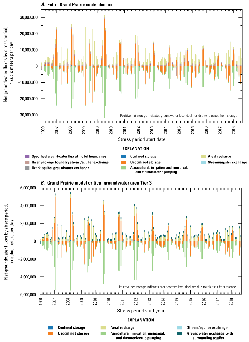
Groundwater-flow budget for the entire Grand Prairie model domain. A, Entire Grand Prairie model domain. B, Grand Prairie Critical Groundwater Area Tier 3.
The groundwater budget for the Grand Prairie CGWA Tier 3 was similar to the entire Grand Prairie model domain and was characterized by large outflows to irrigation wells during the late spring and summer months and supported primarily by releases from groundwater storage and limited connection to surface water (fig. 29B; tables 22 and 23). From 2007 through 2018, the mean annual outflow to aquaculture, irrigation, and municipal wells was about 56 percent of total outflows (table 23). Releases from unconfined storage were about 48 percent of total inflows (table 22). Other substantial inflows included areal recharge (about 28 percent) and inflows from the surrounding aquifer (about 24 percent) (table 22). Other substantial outflows included replenishment to unconfined storage (about 35 percent) and outflows to the surrounding aquifer (about 8 percent) (table 23).
Simulated groundwater budgets for the Grand Prairie model indicated minimal connection between surface water and groundwater for reaches simulated with the SFR package, particularly in the Grand Prairie region (between the Arkansas River and White River) (figs. 2B, 30A,B). There was more substantial connection simulated between the Arkansas River, which used the RIV package, and the groundwater system. This surface water and groundwater connection during dry (September 1, 2014) and wet (May 1, 2009) periods was evident in the higher simulated water table along the Arkansas River (fig. 30A,C). The primary cone of depression under the CGWA Tier 3 and between the Arkansas River and White River region was also similar for dry and wet periods. There were more dry stream reaches simulated during dry conditions than in wet conditions (fig. 30B,D); however, the dry conditions were in upper reaches of smaller streams with flows that generally originated within the model domain. During dry conditions, the simulated water table exhibited more drawdown across the model domain from pumping that was visible in the simulated water table altitudes (fig. 30A,C). Surface-water irrigation effects on the water table were also more prominent during wet conditions where water stored in irrigation reservoirs supplemented pumping in the region with the most drawdown (fig. 30A,B).
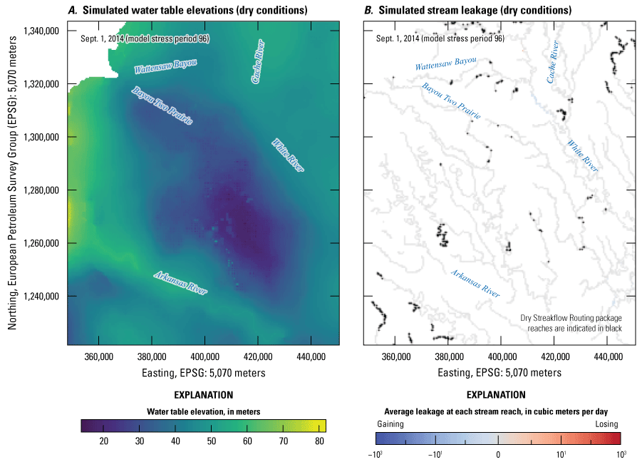

Simulated water table surface and calibrated stream leakage for the base realization of iteration one for the Grand Prairie model during dry and wet periods. A, Simulated water table altitudes in dry conditions (stress period 96). B, Simulated stream leakage in dry conditions (stress period 96). C, Simulated water table altitudes in wet conditions (stress period 32). D, Simulated stream leakage in wet conditions (stress period 32).
Pumping in the Tertiary-Age Aquifers
Both models simulated pumping in the Tertiary-age aquifers below the MRVA. For the Grand Prairie model, the magnitude of pumping was similar in the MRVA (model layers 1–8) and Tertiary-age aquifers (model layers 9–19), including the middle Claiborne aquifer (fig. 31A–C). This was a deviation from previous conceptual and numerical models of the Grand Prairie region in Clark and others (2011a,b), which stated that pumping in the middle Claiborne aquifer of northeastern Arkansas was one to two orders of magnitude less than the pumping from the MRVA. The total amount of pumping in the MRVA was about 5 percent less than the pumping from the Tertiary-age aquifers from April 2007 through December 2018. The mean monthly total pumping was about 2,162,345 m3 for the MRVA and about 2,267,726 m3 for the Tertiary-age aquifers. The monthly trend in pumping indicated that peak pumping from both aquifers generally occurred in July, which is in accord with the typical irrigation trends for crops. Mean monthly pumping volumes were largest for wells in the MRVA from June through September, whereas municipal pumping in the Tertiary-age aquifers accounted for larger mean monthly pumping volumes from October through May (fig. 31D). The conceptual change in pumping for the Tertiary-age aquifers, including the middle Claiborne aquifer was due to the movement of pumping from the MRVA to the middle Claiborne aquifer to improve the calibrated model’s fit to observed groundwater levels in the Tertiary-age layers of the model; this approach was deemed reasonable based on the uncertainty in Tertiary-age and middle Claiborne aquifer pumping in the Grand Prairie region, as described in the “Calibration approach” and “Groundwater-Flow Model Calibration Results” sections of this report.
Spatial distributions of calibrated pumping for the Cache model and Grand Prairie model MRVA and Tertiary-age aquifers are shown in figure 32A, B, respectively. In the Cache model, the MRVA (model layers 1–8) pumping primarily occurred in the central and western side of the model domain, and the deeper Tertiary-age aquifer (model layers 9–18) pumping occurred in the central and eastern side of the model domain (fig. 32A). In the Grand Prairie model, pumping from the MRVA and Tertiary-age aquifers was widespread across the model domain (fig. 32B).
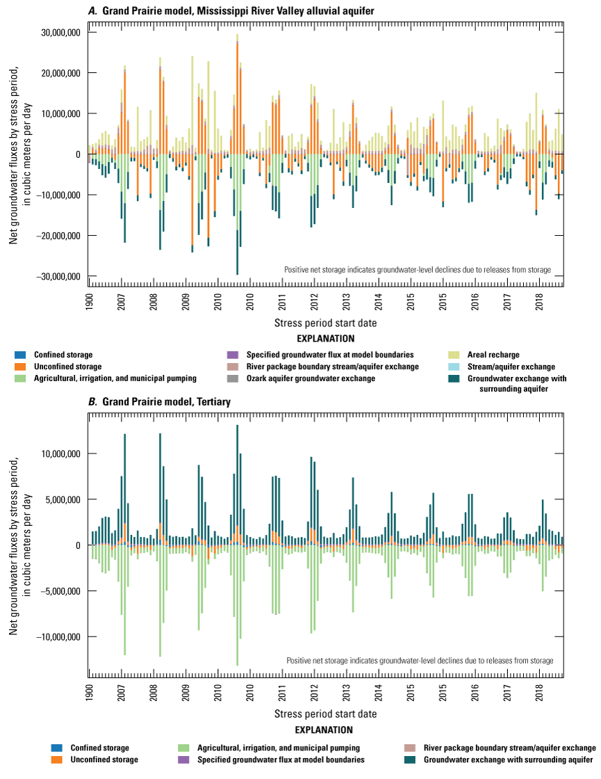

Groundwater-flow budget for Mississippi River Valley alluvial aquifer and the Tertiary-age aquifers in the Grand Prairie model. A, Mississippi River Valley alluvial aquifer. B, Tertiary-age aquifers (model layers 9–19). C, Total pumping by stress period for the Mississippi River Valley alluvial aquifer and the Tertiary-age aquifers. D, Monthly pumping from the Mississippi River Valley alluvial aquifer and Tertiary-age aquifers from April 2007 through December 2018.
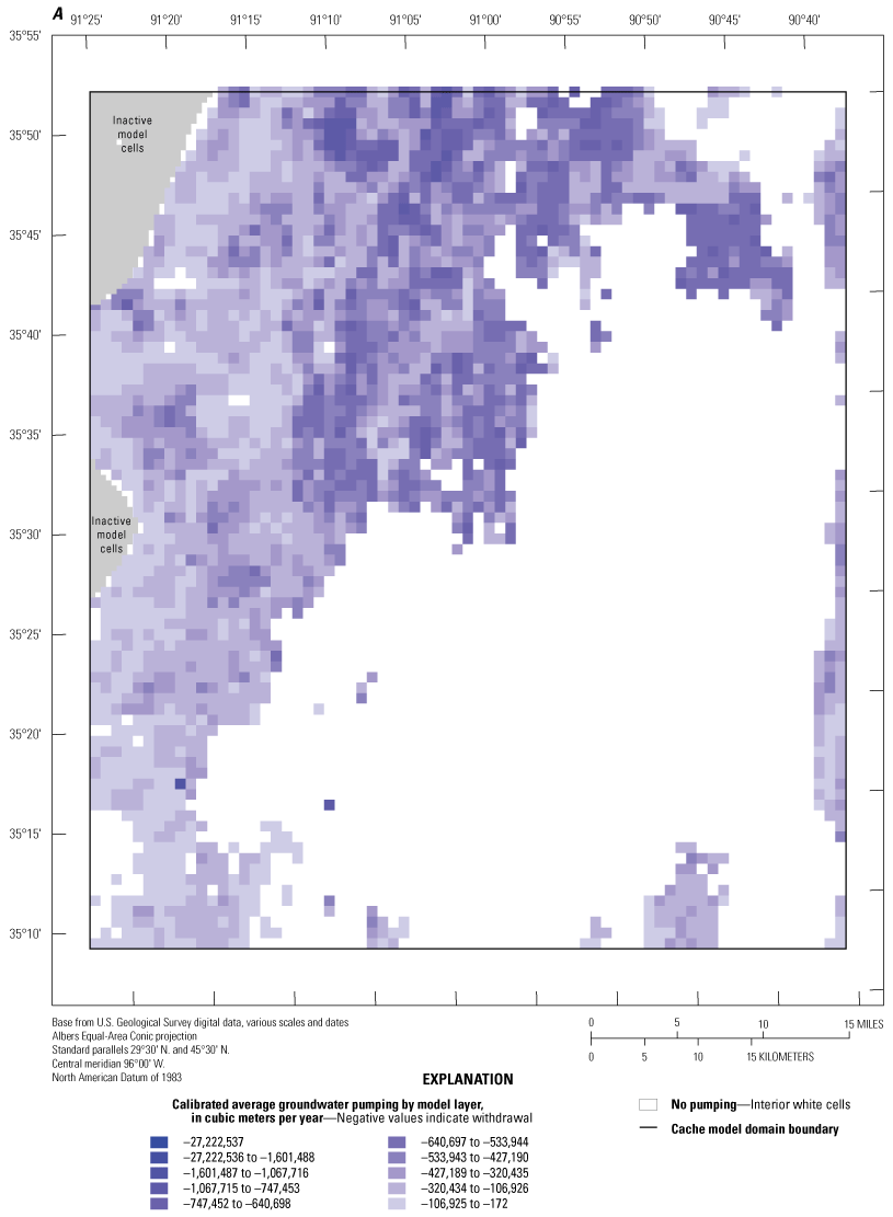

Total groundwater pumping for Mississippi River Valley alluvial aquifer (model layers 1–8) and the Tertiary-age aquifers (model layers 9 and greater). A, Cache model. B, Grand Prairie model (these are layered .pdfs; download at https://doi.org/10.3133/sir20245088).
Assumptions and Limitations
The Cache and Grand Prairie models were constructed to simulate the important groundwater processes in their respective domains. Calibration results indicated an acceptable match between the observed and simulated values for most areas; however, there are limitations in regard to the application of either model to address groundwater-related questions that are outside their intended purpose based on their design. This section describes many of these limitations and provides future potential users with guidelines for use of the Cache and Grand Prairie models in future studies.
Neither model directly simulated landscape or soil zone processes such as evapotranspiration, runoff, deep percolation passing through the root zone, or changes to soil moisture; however, these processes, including runoff and recharge to the water table, were simulated by a separate SWB model to provide inputs of recharge and runoff to each groundwater-flow model. Therefore, addressing landscape and soil zone questions with the Cache model and the Grand Prairie model would be inappropriate. Further, neither model directly simulated the hydrologic processes or movement of water in the unsaturated zone; therefore, use of either model to address questions pertaining to the unsaturated zone would be inappropriate.
The discretization of both models with 500-m cell sides, or cells with an area of 2,500 m2 (about 62 acres), was appropriate to simulate groundwater processes on an intermediate to semiregional scale. Neither model should be used to address questions on scales smaller than the size of a model cell. Temporally, the initial six spin-up stress periods were defined to provide reasonable groundwater conditions for the monthly stress periods from April 2007 through December 2018. Both models should only be used to address groundwater questions or better understand their respective groundwater systems for processes that can be resolved on timescales of 1 month or greater from 2010 through 2018. Given the coarse resolution of the initial six “spin up” stress periods, analyzing hydrologic phenomena that occur on less than a 1-month timescale, such as peak streamflow during intense precipitation events, would not be an appropriate use of either model.
The Cache model was constructed with a focus on the MRVA and secondarily the Tertiary-age aquifers underlying the MRVA between the Black River and White River on the western side of the model domain eastward to Crowley’s Ridge. The Cache model should not be used to address hydrologic questions for regions west of the Black River and White River or east of Crowley’s Ridge because boundary conditions specified at the edge of the model can affect the simulated groundwater conditions near those areas. The calibration focused on improving the simulation of the cone of depression within the CGWAs. The higher weights assigned to groundwater-level observations in the priority CGWAs for each model meant that both models were tuned to better represent groundwater levels in those areas. Further, the RIV package was used to simulate the Black River and White River system on the western side of the Cache model domain. This RIV package boundary condition did not simulate the routing of streamflow, which precludes the Cache model’s use to address streamflow routing questions for the Black River and White River. The Cache model did not simulate shallow subsurface processes such as interflow or bank storage that may be important in the simulation of streamflow for streams such as the L’Anguille River. Therefore, the observations for the L’Anguille River were zero-weighted during the calibration process, and the model should not be used to address total streamflow routing or discharge questions on that stream.
The Grand Prairie model was constructed with a focus on the MRVA and secondarily the Tertiary-age aquifers underlying the MRVA such as the middle Claiborne aquifer. Like the Cache model, the Grand Prairie model calibration was focused on improving the simulation of the cone of depression in the Grand Prairie region between the Arkansas River and White River based in the higher weights assigned to groundwater-level observations in that region. The RIV package was also used to simulate the Arkansas River system in the Grand Prairie model, which precludes the Grand Prairie model’s use to address streamflow routing questions on the Arkansas River. The Grand Prairie model should not be used to address groundwater-related questions south of the Arkansas River because this area was included in the simulation so that the boundary effects near the edges of the model did not affect conditions in the area of interest in and around the cone of depression.
The calibrated Grand Prairie model exhibited substantial positive bias in absolute groundwater levels simulated for the Tertiary-age hydrologic units below the MRVA, such as the middle Claiborne aquifer; however, simulated groundwater-level trends for this aquifer were in accord with observed values (discussed in the “Calibrated Model Fit” section of this report). Therefore, the Grand Prairie model should not be used to address groundwater-level questions that require use of absolute groundwater-level altitudes. However, analysis that requires the use of trends in simulated groundwater levels for the Tertiary-age hydrologic units below the MRVA, including the middle Claiborne aquifer, would be an appropriate use of those results.
The uncertainty in agricultural pumping that occurred in the Tertiary-age aquifers such as the middle Claiborne aquifer within the Grand Prairie model, coupled with the large positive bias in those model layers, required a fraction of pumping to be moved from the MRVA to the middle Claiborne aquifer, as described in the “Grand Prairie Model Calibration Process” section of this report. Many assumptions were made on locations and time periods that pumping should be moved from MRVA to Middle Claiborne because of minimal data or only anecdotal evidence about this practice, as described in the “Grand Prairie Model Calibration Process” section. Therefore, final pumping values for the MRVA and middle Claiborne aquifer reflect what was the best compromise to arrive at an acceptable calibration for both aquifers, but the pumping values could not be verified owing to a lack of measured data. Therefore, use of the Grand Prairie model to address water use or pumping rate and volume questions within the Tertiary-age aquifers such as the middle Claiborne aquifer would be an inappropriate use of the model.
Summary
The Mississippi alluvial plain (MAP), about 82,880 square kilometers of Missouri, Kentucky, Tennessee, Mississippi, Louisiana, and Arkansas, is one of the most important agricultural regions in the United States and supports a multibillion-dollar agricultural industry that relies heavily on groundwater for irrigation of crops such as rice, beans, cotton, and aquaculture during the peak growing season. The primary source of groundwater for agricultural-related pumping in the MAP is the Mississippi River Valley alluvial aquifer (MRVA), which has declined in storage for decades, and the secondary sources are the middle Claiborne aquifer and Wilcox aquifer.
In northeastern Arkansas, the MRVA underlies the region along the Mississippi River and in 1991, the State of Arkansas passed the Arkansas Groundwater Protection and Management Act to improve management of groundwater across the State and bring attention to areas that have experienced significant groundwater level declines. Two areas in northeastern Arkansas, within the MAP’s Cache and Grand Prairie regions, have been designated as Critical Groundwater Areas owing to decades of groundwater declines that resulted from past and current water use.
The multidisciplinary MAP project, led by the U.S. Geological Survey and funded by the U.S. Geological Survey’s Water Availability and Use Science Program, began in 2016 with the overarching goal to better understand the hydrostratigraphy and water use in the MRVA. Objectives of the numerical groundwater modeling aspect of the MAP project included studies to develop numerical groundwater-flow models in focus areas including part of the Cache and Grand Prairie regions of northeastern Arkansas. This report documents and describes the development, calibration, and results of the Cache and Grand Prairie inset groundwater-flow models.
The Cache and Grand Prairie regions are both in the northeastern Arkansas part of the MAP and the western-central flank of the Mississippi Embayment Regional Aquifer System. The Cache region is about 2,000 square miles, extending about 50 miles south and about 40 miles west from Jonesboro, Arkansas, including the region about 1 to 3 miles east of Crowley’s Ridge to the fall line between the Mississippi Embayment Regional Aquifer System boundary and the Ozark Plateau aquifer system located west of the Black and White Rivers. The Grand Prairie region is about 4,875 square miles, extending about 75 miles south and about 65 miles west from Beebe, Ark., to Pendleton, Ark. The region lies between the Arkansas River and the White River. Both regions are natural treeless prairies that have been under rice cultivation since the early 1900s. The predominant land use in the Cache and Grand Prairie regions is agricultural. Agricultural land use is as much as 81 percent of total land use in the Cache region and as much as 72 percent in the Grand Prairie region.
Northeastern Arkansas is at the western edge of the syncline that plunges toward the Gulf of Mexico, with its axis parallel to the Mississippi River. Primary geologic units in northeastern Arkansas include the Quaternary-age alluvium and terrace deposits, the Tertiary-age Jackson Formation, Cockfield Formation, Cook Mountain Formation, Memphis Sand or Sparta Sand, and Wilcox Group. Primary surface-water features in the Cache region are the south flowing White River, Cache River, Bayou De View, and the L’Anguille River. Primary surface-water features in the Grand Prairie include the White River and Cache River. Primary surface-water features in the Grand Prairie region include the White River in the western region, Wattensaw Bayou, Bayou Two Prairie, and Bayou Meto in the central Grand Prairie region, and the Arkansas River that flows southeast from the Ozark Plateau to the Mississippi River in the southeastern corner of the region.
Geophysical survey data were collected as a part of the MAP project to better characterize MRVA hydrostratigraphy. The geophysical data were processed into 5-meter-thick layers from the land surface to the depth of investigation, as much as 400 meters below the land surface with resistivities classified into 10 groups. These resistivity groups reflect the expected aquifer material whereby a low resistivity is correlated to low horizontal hydraulic conductivity values and vice versa.
The inset models were developed using the child model capabilities of the modular finite-difference flow model (MODFLOW) 6 with the parent model as the regional Mississippi Embayment Regional Aquifer System 3 groundwater-flow model, also developed as a part of the MAP project. The upper vertical boundary in both models was the land surface, which was defined using a digital elevation model. The top of the Midway confining unit represented a vertical no-flow groundwater boundary in both models because the Midway confining unit is not hydrologically connected with the Mississippi Embayment Regional Aquifer System. The Cache and Grand Prairie models were spatially discretized into 500-meter x 500-meter orthogonal cells on a grid with the following vertical layers, rows, and columns: Cache model—18, 161, 142; and Grand Prairie model—19, 245, 206. Vertical layering schemes for both models used the same approach where layers 1 through 8 were defined by the airborne electromagnetic data at 5-meter constant thicknesses to represent the MRVA; layers 9 through 15 used increasing uniform thickness layers to represent the Vicksburg-Jackson confining unit, Claiborne aquifers and confining units, and, below layer 15, the Mississippi Embayment Regional Aquifer System framework layers were used to represent the bottom surfaces of Wilcox aquifers and confining units. The bottom of layer 8, a depth of 40 meters (eight layers at 5-meter thickness) was represented using the updated bottom of the MRVA. Where the MRVA was less than a depth of 40 m, the remaining layers to the 40-meter depth were assigned as pass-through cells of zero thickness. Temporal discretization for both models included 148 stress periods with a simulation period from January 1, 1900, through December 31, 2018. The first stress period simulated predevelopment steady-state conditions (without pumping), followed by six multiyear transient stress periods from January 1, 1900, to April 1, 2007, and monthly stress periods thereafter through December 31, 2018.
Recharge inputs to the Cache and Grand Prairie models were simulated using the Recharge package. Recharge was specified as transient array-based datasets using the values from a soil-water-balance model of the Mississippi Embayment Regional Aquifer System developed for the MAP project. Streams were simulated in both models with the Streamflow Routing package except the Black River, White River, and Little Red River in the Cache model and the Arkansas River in the Grand Prairie model, which were simulated with the River package. The Streamflow Routing package simulated total streamflow in both models by simulating groundwater/surface-water exchange, accumulation of flow from upstream reaches and stream inflows from the edge of the model, and inflows of runoff generated by the soil-water-balance model. Diversions of streamflow from the Streamflow Routing package were specified in both models to simulate the removal of stream water to fill irrigation reservoirs. Groundwater pumping from wells related to irrigation and aquaculture, municipal, and, only for the Grand Prairie model, thermoelectric use was simulated in both models using the Well package. For stress periods 2 through 6 (January 1, 1900, through April 1, 2007), Mississippi Embayment Regional Aquifer System 2.2 was used to specify the pumping rates and location of pumping. For the monthly stress periods (April 1, 2007, through December 31, 2018), outputs from the Aquaculture Irrigation and Water Use Model version 1.1 were used to specify the locations and rates of irrigation and aquaculture pumping. The Newton-Raphson formulation within MODFLOW 6 solved the groundwater-flow system of equations as specified in the integrated model solution.
The Cache and Grand Prairie models were both calibrated using the Parameter Estimation code ++ Iterative Ensemble Smoother (PESTPP–IES) version 5 code to automate the adjustment of parameters and improve the fit between measured observations or calibration targets and simulated equivalent model outputs. Manual trial-and-error adjustment of some parameters was done prior to automated calibration to improve the history matching and improve the understanding of the groundwater systems for each model. The Cache and Grand Prairie models included 13 and 18 nonzero weighted observation groups, respectively, and were grouped based on location and type of observation, which included measured and estimated groundwater levels and streamflows, and derivative observations that include groundwater-level and streamflow differences in space and time.
Both models were parameterized with a mix of fine- and coarse-scale spatial and temporal constants; pilot points; and zonal, gridded, and multiplier parameters were specified for inputs. Recharge from the soil-water-balance model was parameterized into spatial zone multipliers based on surface connectivity of the upper 15 meters of airborne electromagnetic resistivity zones. Pumping rates in the Well package were parameterized for both models by crop type, data source, reductions owing to surface-water access, and stress period. The Grand Prairie model included additional Well package pumping rate parameters by combined model layer and airborne electromagnetic framework zone and a separate parameter to adjust the fraction of MRVA pumping moved to the middle Claiborne aquifer to account for the uncertainty in agricultural pumping from the middle Claiborne aquifer in the Grand Prairie region. The Grand Prairie model calibration process underwent a series of preliminary calibration attempts focused on achieving an acceptable fit between groundwater-level observations and simulated equivalent values in the MRVA. Although these preliminary “MRVA-focused” automated calibration runs yield very good results within the MRVA, they yielded poor and unacceptable results in the middle Claiborne aquifer. Therefore, a “balanced” Grand Prairie model was developed for calibration to reduce the bias in the middle Claiborne aquifer while maintaining acceptable results in the MRVA.
The automated calibration step for the Cache model, using PESTPP–IES, was run through three iterations with a prior ensemble of 500 realizations. The automated calibration step for the Grand Prairie model, using PESTPP–IES, was run through four iterations with a prior ensemble of 800 realizations. The Cache model fit to observations was assessed using the base realization from iteration two of the PESTPP–IES calibration run. The mean absolute residual for the priority_wells observation group was 1.58 meters, which indicated a good fit to observed groundwater levels in the Cache Critical Groundwater Area. The “balanced” Grand Prairie model fit to observations was assessed using the base realization from iteration one of the PESTPP–IES calibration run. The mean absolute residuals for the grandprairie_mrva_priority_wells and grandprairie_sparta_priority_wells observation groups were 2.71 and 10.78 meters, respectively, which indicated that the “balanced” model simulated groundwater levels in the MRVA well, but there was substantial bias in the middle Claiborne aquifer.
The Cache and the Grand Prairie models were both calibrated to produce reasonable parameter fields and values in addition to an acceptable fit to observations. For the Cache model, the base realization of iteration two produced reasonable parameter fields and a good fit to the observations. Calibrated horizontal hydraulic conductivity for the MRVA model layers (1–8) ranged from 0.03 to 500 meters per day. The mean horizontal hydraulic conductivity for layers 1–4 and 4–8 was about 28 and 45 meters per day, respectively, and similar to calibrated horizontal hydraulic conductivity values from previous studies. The larger mean horizontal hydraulic conductivity values for deeper MRVA layers are consistent with the conceptual understanding that the coarser grained sediments are present deeper in the alluvial system. Cache model specific yield ranged from 0.08 to 0.35 (dimensionless) and exhibited a mean specific yield of about 0.27 in the MRVA, which were consistent with previously published values. For the Grand Prairie model, the base realization of iteration one produced acceptable parameter fields and fit to the observations, and calibrated horizontal hydraulic conductivity for the MRVA model layers (1–8) ranged from 1.0 to 300 meters per day. The mean horizontal hydraulic conductivity for layers 1–4 and 4–8 was about 78 and 48 meters per day, respectively, and within the range of calibrated horizontal hydraulic conductivity values from previous studies. The larger mean horizontal hydraulic conductivity values for shallower MRVA layers are consistent with the airborne electromagnetic resistivity facies zones, which exhibited higher resistivity zones in the shallower layers, but are not consistent with the overall conceptual understanding that coarser grained sediments are present deeper in the alluvial system that was in the Cache model. Grand Prairie model specific yield ranged from 0.05 to 0.35 (dimensionless) and exhibited a mean specific yield of about 0.29 in the MRVA, which were consistent with previously published values. The parameter fraction_move_aiwum_mrva2sparta increased about 29 percent from 0.378 to 0.486, which indicated that PESTPP–IES preferred to increase the amount pumping in the middle Claiborne aquifer to improve the calibration.
The distribution of parameter values from the initial (or prior) PESTPP–IES ensemble compared with the final chosen iteration (iteration two for Cache and iteration one for Grand Prairie) ensemble provides an indication of parameter uncertainty and how it changed through calibration. The Cache model’s posterior ensemble distribution was generally smaller and reduced parameter uncertainty compared to the prior ensemble. The Grand Prairie model exhibited a marginal reduction in posterior ensemble parameter distributions for most parameters because the prior ensemble for many groups of parameters was based on a preliminary PESTPP–IES calibration ensemble from the “MRVA-focused” model. In the Cache and Grand Prairie models, the calibration process reduced the 2007 through 2018 distribution of groundwater levels in observation wells by about 75 and 63 percent, respectively.
The groundwater budgets for each area of the Cache model were characterized by irrigation and nonirrigation season trends in water use whereby the largest outflows were to pumping wells and occurred during the peak growing season. Mean 2007 through 2018 release from unconfined aquifer storage was 50,886,613 cubic meters (m3), which was about 48 percent of all inflows. Mean 2007 through 2018 aquaculture, irrigation, and municipal pumping was 54,657,872 m3, about 52 percent of all outflows. The groundwater budget for the Cache Tier 3 Critical Groundwater Area was similar to the entire Cache model domain. The groundwater budgets for the Grand Prairie model are characterized by irrigation and nonirrigation season trends in water use whereby the largest outflows were to pumping wells that occurred during the peak growing season (May through September) to irrigate crops. The total mean 2007 through 2018 release from unconfined aquifer storage was 46,704,367 m3, which was about 48 percent of all inflows. Mean 2007 through 2018 aquaculture, irrigation, and municipal pumping was 52,053,330 m3, about 54 percent of all outflows. Connection with surface water was minimal in the Grand Prairie model throughout the entire domain. The groundwater budget for the Grand Prairie CGWA Tier 3 was similar to the entire Grand Prairie model domain and was characterized by large outflows to irrigation wells during the late spring and summer months.
References Cited
Ackerman, D.J., 1989a, Hydrology of the Mississippi River valley alluvial aquifer, south-central United States – a preliminary assessment of the regional flow system: U.S. Geological Survey Water-Resources Investigations Report 88–4028, 80 p. [Also available at https://doi.org/10.3133/wri884028.]
Ackerman, D.J., 1989b, Potentiometric surfaces of the Mississippi River Valley alluvial aquifer in eastern Arkansas, spring 1972 and 1980: U.S. Geological Survey Water-Resources Investigations Report 88–4075, scale 1:500,000. [Also available at https://doi.org/10.3133/wri884075.]
Ackerman, D.J., 1996, Hydrology of the Mississippi River valley alluvial aquifer, south-central United States: U.S. Geological Survey Professional Paper 1416-D, 68 p. [Also available at https://doi.org/10.3133/pp1416D.]
Adams, R.F., Miller, B.V., and Kress, W.H., 2019, Waterborne resistivity inverted models, Mississippi Alluvial Plain, 2016–2018: U.S. Geological Survey data release, accessed December 2019at https://doi.org/10.5066/P9WQPRFB.]
Alhassan, M., Lawrence, C., Richardson, S., and Pindilli, E., 2019, The Mississippi Alluvial Plain aquifers—An engine for economic activity: U.S. Geological Survey Fact Sheet 2019–3003, 4 p. [Also available at https://doi.org/10.3133/fs20193003.]
Arkansas Department of Agriculture Natural Resources Division, 2023, Critical groundwater designation: Arkansas Department of Agriculture Natural Resources Division Fact Sheet, 2 p., accessed June 1, 2023, at https://www.agriculture.arkansas.gov/natural-resources/divisions/water-management/groundwater-protection-and-management-program/critical-groundwater-a reas/.
Arkansas Natural Resources Commission, 2014, Arkansas water plan update: Arkansas Natural Resources Commission, accessed August 11, 2023, at https://www.agriculture.arkansas.gov/wp-content/uploads/2020/05/AWP_Update_2014_Summary.pdf.
Bakker, M., Post, V., Hughes, J.D., Langevin, C.D., White, J.T., Leaf, A.T., Paulinski, S.R., Bellino, J.C., Morway, E.D., Toews, M.W., Larsen, J.D., Fienen, M.N., Starn, J.J., Brakenhoff, D.A., and Bonelli, W.P., 2023, FloPy v3.6.0.dev0 (preliminary): U.S. Geological Survey software release, accessed October 2020 at https://doi.org/10.5066/F7BK19FH.]
Boswell, E.H., Cushing, E.M., Hosman, R.L., and Jeffery, H.G., 1968, Quaternary aquifers in the Mississippi embayment, with a discussion of quality of the water: U.S. Geological Survey Professional Paper 448–E, 15 p., accessed October 1, 2021 at https://doi.org/10.3133/pp448E.
Brahana, J.V., and Mesko, T.O., 1988, Hydrogeology and preliminary assessment of regional flow in the upper Cretaceous and adjacent aquifers in the northern Mississippi embayment: U.S. Geological Survey Water-Resources Investigations Report 87–4000, 72 p. [Also available at https://doi.org/10.3133/wri874000.]
Bristow, E., and Wilson, J.L., 2023. Aquaculture and irrigation water-use model (AIWUM) version 1.1 estimates and related datasets for the Mississippi Alluvial Plain: U.S. Geological Survey data release, accessed April 2020 at https://doi.org/10.5066/P9RGZOBZ.
Broom, M.E., and Lyford, F.P., 1981, Alluvial aquifer of the Cache and St. Francis River basins, northeastern Arkansas: U.S. Geological Survey Open-File Report 81–476, 55 p. [Also available at https://doi.org/10.3133/ofr81476.]
Clark, B.R., and Hart, R.M., 2009, The Mississippi Embayment Regional Aquifer Study (MERAS)—Documentation of a groundwater-flow model constructed to assess water availability in the Mississippi Embayment: U.S. Geological Survey Scientific Investigations Report 2009–5172, 61 p. [Also available at https://doi.org/10.3133/sir20095172.]
Clark, B.R., Hart, R.M., and Gurdak, J.J., 2011, Groundwater availability of the Mississippi embayment: U.S. Geological Survey Professional Paper 1785, 62 p. [Also available at https://doi.org/10.3133/pp1785.]
Clark, B.R., Westerman, D.A., and Fugitt, D.T., 2011a, Simulation of the effects of groundwater withdrawals on water-level altitudes in the Sparta aquifer in the Bayou Meto-Grand Prairie area of eastern Arkansas, 2007–37: U.S. Geological Survey Scientific Investigations Report 2011–5215, 9 p. [Also available at https://doi.org/10.3133/sir20115215.]
Clark, B.R., Westerman, D.A., and Fugitt, D.T., 2011b, Simulation of the effects of groundwater withdrawals on water-level altitudes in the Sparta aquifer in the Bayou Meto-Grand Prairie area of eastern Arkansas, 2007–37: U.S. Geological Survey Scientific Investigations Report 2011–5215, 9 p. [Also available at https://doi.org/10.3133/sir20115215.]
Clark, B.R., Westerman, D.A., and Fugitt, D.T., 2013, Enhancements to the Mississippi Embayment Regional Aquifer Study (MERAS) groundwater-flow model and simulations of sustainable water-level scenarios: U.S. Geological Survey Scientific Investigations Report 2013–5161, 29 p. [Also available at https://doi.org/10.3133/sir20135161.]
Clark, B.R., Richards, J.M., and Knierim, K.J., 2018, The Ozark Plateaus Regional Aquifer Study—Documentation of a groundwater-flow model constructed to assess water availability in the Ozark Plateaus: U.S. Geological Survey Report 2018–5035, 33 p. [Also available at https://doi.org/10.3133/sir20185035.]
Corson-Dosch, N.T., Fienen, M.N., Finkelstein, J.S., Leaf, A.T., White, J.T., Woda, J., and Williams, J.H., 2022, Areas contributing recharge to priority wells in valley-fill aquifers in the Neversink River and Rondout Creek drainage basins, New York: U.S. Geological Survey Scientific Investigations Report 2021–5112, 50 p. [Also available at https://doi.org/10.3133/sir20215112.]
Cushing, E.M., Boswell, E.H., and Hosman, R.L., 1964, General geology of the Mississippi Embayment: U.S. Geological Survey Professional Paper 448–B, 32 p. [Also available at https://doi.org/10.3133/pp448B.]
Czarnecki, J.B., 2006, Simulation of various management scenarios of the Mississippi River valley alluvial aquifer in Arkansas: U.S. Geological Survey Scientific Investigations Report 2006–5052, 21 p. [Also available at https://doi.org/10.3133/sir20065052.]
Czarnecki, J.B., 2007, Simulated ground-water withdrawals by Cabot WaterWorks from the Mississippi River Valley alluvial aquifer, Lonoke County, Arkansas: U.S. Geological Survey Scientific Investigations Report 2007–5030, 39 p. [Also available at https://pubs.usgs.gov/sir/2007/5030/.]
Czarnecki, J.B., 2010, Groundwater-flow assessment of the Mississippi River Valley alluvial aquifer of northeastern Arkansas: U.S. Geological Survey Scientific Investigations Report 2010–5210, 33 p. [Also available at https://doi.org/10.3133/sir20105210.]
Czarnecki, J.B., Clark, B.R., and Reed, T.B., 2003, Conjuctive-use optimization model of the Mississippi River valley alluvial aquifer of northeastern Arkansas: U.S. Geological Survey Water-Resources Investigations Report 03–4233, 36 p. [Also available at https://doi.org/10.3133/wri034230.]
Diehl, T.H., and Harris, M.A., 2014, Withdrawal and consumption of water by thermoelectric power plants in the United States, 2010: U.S. Geological Survey Scientific Investigations Report 2014–5184, 28 p. [Also available at https://doi.org/10.3133/sir20145184.]
Dietsch, B.J., Asquith, W.H., Breaker, B.K., Westenbroek, S.M., and Kress, W.H., 2023, Simulation of monthly mean and monthly base flow of streamflow using random forests for the Mississippi River Alluvial Plain, 1901 to 2018: U.S. Geological Survey Scientific Investigations Report 2022–5079, 17 p. [Also available at https://doi.org/10.3133/sir20225079.]
Doherty, J.E., 2005, PEST, model independent parameter estimation—User manual (5th ed.): Brisbane, Australia, Watermark Numerical Computing, accessed July 26, 2011, at https://pesthomepage.org.
Doherty, J., and Hunt, R.J., 2009, Two statistics for evaluating parameter identifiability and error reduction: Journal of Hydrology, v. 366, no. 1-4, p. 119–127. [Also available at https://doi.org/10.1016/j.jhydrol.2008.12.018.]
Ellis, J.H., Knight, J.E., White, J.T., Sneed, M., Hughes, J.D., Ramage, J.K., Braun, C.L., Teeple, A., Foster, L.K., Rendon, S.H., and Brandt, J.T., 2023, Hydrogeology, land-surface subsidence, and documentation of the Gulf Coast Land Subsidence and Groundwater-Flow (GULF) model, southeast Texas, 1897–2018: U.S. Geological Survey Professional Paper 1877, 407 p. [Also available at https://doi.org/10.3133/pp1877.]
Engler, K., Thompson, D.G., and Kazmann, R.G., 1945, Groundwater supplies for rice irrigation in the Grand Prairie region, Arkansas: Arkansas University Agricultural Experiment Station Bulletin 457, 56 p., accessed June 1, 2023, at https://search.worldcat.org/title/Ground-Water-Supplies-For-Rice-Irrigation-in-the-Grand-Prairie-Region-Arkansas/oclc/631875489.
Fienen, M.N., Haserodt, M.J., Leaf, A.T., and Westenbroek, S.M., 2022, Simulation of regional groundwater flow and groundwater/lake interactions in the Central Sands, Wisconsin: U.S. Geological Survey Scientific Investigations Report 2022–5046, 111 p. [Also available at https://doi.org/10.3133/sir20225046.]
Gillip, J.A., and Czarnecki, J.B., 2009, Validation of a ground-water flow model of the Mississippi River Valley alluvial aquifer using water-level and water-use data for 1998–2005 and evaluation of water-use scenarios: U.S. Geological Survey Scientific Investigations Report 2009–5040, 22 p., accessed October 2020 at https://doi.org/10.3133/sir20095040.
Harbaugh, A.W., 2005, MODFLOW-2005—The U.S. Geological Survey modular ground-water model—The ground-water flow process: U.S. Geological Survey Techniques and Methods, book 6, chap. A16, p. 6–A16. [Also available at https://doi.org/10.3133/tm6A16.]
Hart, R.M., Clark, B.R., and Bolyard, S.E., 2008, Digital surfaces and thicknesses of selected hydrogeologic units within the Mississippi Embayment Regional Aquifer Study (MERAS): U.S. Geological Survey Scientific Investigations Report 2008–5098, 33 p. [Also available at https://doi.org/10.3133/sir20085098.]
Harris, M.A., and Diehl, T.H., 2019a, Withdrawal and consumption of water by thermoelectric power plants in the United States, 2015: U.S. Geological Survey Scientific Investigations Report 2019–5103, 15 p. [Also available at https://doi.org/10.3133/sir20195103.]
Harris, M.A., and Diehl, T.H., 2019b, Water withdrawal and consumption estimates for thermoelectric power plants in the United States, 2015: U.S. Geological Survey data release, accessed December 2019 at https://doi.org/10.5066/P9V0T04B.
Haugh, C.J., Killian, C.D., and Barlow, J.R.B., 2020, MODFLOW-2005 model used to evaluate water-management scenarios for the Mississippi Delta: U.S. Geological Survey data release, accessed October 2020 at https://doi.org/10.5066/P9906VM5.]
Hill, M.C., and Tiedeman, C.R., 2007, Effective groundwater model calibration—With analysis of data, sensitivities, predictions, and uncertainty: New York, Wiley and Sons, 455 p. [Also available at https://doi.org/10.1002/0470041080.]
Hosman, R.L., Long, A.T., Lambert, T.W., and others, 1968, Tertiary aquifers in the Mississippi embayment, with discussion of quality of the water: U.S. Geological Survey Professional Paper 448–D, 29 p., 8 plates [Also available at https://doi.org/10.3133/pp448D.]
Hunt, R.J., Fienen, M.N., and White, J.T., 2019, Revisiting “An Exercise in Groundwater Model Calibration and Prediction” after 30 years—Insights and new directions: Ground Water, v. 58, no. 2, p. 168–182. [Also available at https://doi.org/10.1111/gwat.12907.]
Hunt, R.J., White, J.T., Duncan, L.L., Haugh, C.J., and Doherty, J., 2021, Evaluating lower computational burden approaches for calibration of large environmental models: Ground Water, v. 59, no. 6, p. 788–798. [Also available at https://doi.org/10.1111/gwat.13106.]
James, S.R., and Minsley, B.J., 2021, Combined results and derivative products of hydrogeologic structure and properties from airborne electromagnetic surveys in the Mississippi Alluvial Plain: U.S. Geological Survey data release, accessed October 2021 at https://doi.org/10.5066/P9382RCI.
Kandpal, V., 2018, Evaluation of a solar powered variable flow tail water recovery system for furrow irrigation: University of Arkansas, Master’s Thesis, 153 p. [Also available at https://scholarworks.uark.edu/etd/2880.]
Knierim, K.J., Kingsbury, J.A., and Haugh, C.J., 2019, Groundwater withdrawal zones for drinking water from the Mississippi River Valley alluvial aquifer and Mississippi embayment aquifers: U.S. Geological Survey data release, accessed October 2020 at https://doi.org/10.5066/P9FZV4ED.
Kresse, T.M., Hays, P.D., Merriman, K.R., Gillip, J.A., Fugitt, D.T., Spellman, J.L., Nottmeier, A.M., Westerman, D.A., Blackstock, J.M., and Battreal, J.L., 2014, Aquifers of Arkansas—Protection, management, and hydrologic and geochemical characteristics of groundwater resources in Arkansas: U.S. Geological Survey Scientific Investigations Report 2014–5149, 334 p. [Also available at https://doi.org/10.3133/sir20145149.]
Ladd, D.E., and Travers, L.R., 2019, Generalized regions of the Mississippi Alluvial Plain: U.S. Geological Survey data release, accessed September 2022 at https://doi.org/10.5066/P915ZZQM.
Langevin, C.D., Hughes, J.D., Banta, E.R., and Niswonger, R.G., Panday, S., and Provost, A.M., 2017, Documentation for the MODFLOW 6 Groundwater Flow Model: U.S. Geological Survey Techniques and Methods, book 6, chap. A55, 197 p. [Also available at https://doi.org/10.3133/tm6A55.]
Langevin, C.D., Hughes, J.D., Provost, A.M., Russcher, M.J., Niswonger, R.G., Panday, S., Merrick, D., and Banta, E.R., 2022, MODFLOW 6 Modular Hydrologic Model version 6.3.0: U.S. Geological Survey software release, accessed October 2021 at https://doi.org/10.5066/P97FFF9M.
Leaf, A.T., Duncan, L.L, and Haugh, C.J., 2023, Modflow-6 models of the Mississippi embayment (MERAS 3) and Mississippi Delta: U.S. Geological Survey data release, accessed December 2023 at https://doi.org/10.3133/sir20235100.
Leaf, A.T., and Fienen, M.N., 2022, Modflow-setup—Robust automation of groundwater model construction: Frontiers of Earth Science, v. 10, 903965, 11 p. [Also available at https://doi.org/10.3389/feart.2022.903965.]
Leaf, A.T., Fienen, M.N., and Reeves, H.W., 2021, SFRmaker and Linesink-maker—Rapid construction of streamflow routing networks from hydrography data: Ground Water, v. 59, no. 5, p. 761–771. [Also available at https://doi.org/10.1111/gwat.13095.]
Mahon, G.L., and Poynter, D.T., 1993, Development, calibration, and testing of ground-water flow models for the Mississippi River Valley alluvial aquifer in eastern Arkansas using one-square-mile cells: U.S. Geological Survey Water-Resources Investigations Report 92–4106, 33 p. [Also available at https://doi.org/10.3133/wri924106.]
Meissner, C.R., 1983, Stratigraphic framework and distribution of lignite on Crowleys Ridge, Arkansas: U.S. Geological Survey Open-File Report 83–609, 33 p. 9 sheets. [Also available at https://doi.org/10.3133/ofr83609.]
McGuire, V.L., Seanor, R.C., Asquith, W.H., Kress, W.H., and Strauch, K.R., 2019, Potentiometric surface of the Mississippi River Valley alluvial aquifer, spring 2016: U.S. Geological Survey Scientific Investigations Map 3439, 14 p., 5 sheets, [Also available at https://doi.org/10.3133/sim3439.]
McKay, L., Bondelid, T., Dewald, T., Johnston, J., Moore, R., and Rea, A., 2012, NHDPlus Version 2—User guide (data model version 2.1): Horizon Systems Corp., accessed September 17, 2018, at http://nhdplus.com.
McKee, P.W., and Clark, B.R., 2003, Development and calibration of a ground-water flow model for the Sparta aquifer of southeastern Arkansas and north-central Louisiana and simulated response to withdrawals, 1998–2027: U.S. Geological Survey Water-Resources Investigations Report 03–4132, 80 p. [Also available at https://doi.org/10.3133/wri034132.]
Minsley, B.J., Rigby, J.R., James, S.R., Burton, B.L., Knierim, K.J., Pace, M.D.M., Bedrosian, P.A., and Kress, W.H., 2021, Airborne geophysical surveys of the lower Mississippi Valley demonstrate system-scale mapping of subsurface architecture: Communications Earth & Environment, v. 2, no. 131, p. 1–14, accessed October 1, 2022. https://doi.org/10.1038/s43247-021-00200-z.
Moore, R.B., and Dewald, T.G., 2016, The Road to NHDPlus—Advancements in digital stream networks and associated catchments: Journal of the American Water Resources Association, v. 52, no. 4, p. 890–900. [Also available at https://doi.org/10.1111/1752-1688.12389.]
National Climatic Data Center, 2019, Climate data online, weather observation station daily summaries: Asheville, N.C., National Climatic Data Center, digital data, accessed October 1, 2019, at https://www.ncei.noaa.gov/cdo-web/.
Niswonger, R.G., and Prudic, D.E., 2005, Documentation of the Streamflow-Routing (SFR2) Package to include unsaturated flow beneath streams—A modification to SFR1 (version 1.2): U.S. Geological Survey Techniques and Methods, book 6, chap. A13, 51 p., at https://doi.org/10.3133/tm6A13.
Painter, J.A., and Westerman, D.A., 2018, Mississippi Alluvial Plain extent, November 2017: U.S. Geological Survey data release, accessed October 2021, at https://doi.org/10.5066/F70R9NMJ.
Peralta, R.C., Yazdanian, A., Killian, P.J., and Shulstad, R.N., 1985, Future quaternary groundwater accessibility in the Grand Prairie—1993: Fayetteville, Arkansas Agricultural Experiment Station, University of Arkansas, Bulletin No. 877, 37 p. [Also available at https://digitalcommons.usu.edu/cee_facpub/886/.]
PRISM Climate Group, 2022, Prism climate data: Oregon State University, accessed September 1, 2022, at https://prism.oregonstate.edu.
Rashid, H.M., Clark, B.R., Mahdi, H.H., Rifai, H.S., and Al-Shukri, H.J., 2015, Simulations of potential future conditions in the Cache critical groundwater area, Arkansas: Environmental & Engineering Geoscience, v. 21, no. 1, p. 1–19, accessed October 1, 2021, at https://doi.org/10.2113/gseegeosci.21.1.1.
Reed, T.B., 2003, Recalibration of ground-water flow model of the Mississippi River valley alluvial aquifer of northeastern Arkansas, 1918–1998, with simulations of water levels caused by projected ground-water withdrawals through 2049: U.S. Geological Survey Water-Resources Investigations Report 03–4109, 63 p. [Also available at https://doi.org/10.3133/wri034109.]
Reitz, M., Sanford, W.E., Senay, G.B., and Cazenas, J., 2017, Annual estimates of recharge, quick-flow runoff, and evapotranspiration for the contiguous U.S. using empirical regression equations: Journal of the American Water Resources Association, 53, no. 4, p. 961–983. [Also available at https://onlinelibrary.wiley.com/doi/10.1111/1752-1688.12546.]
Schrader, T.P., Evans, D.A., and Brossett, T.H., 2005, Water resources data Arkansas water year 2005: U.S. Geological Survey Water-Data Report AR–05–01, 452 p., accessed September 2022 at https://pubs.usgs.gov/wdr/2005/wdr-ar-05/WDR-AR-05-1.pdf.
Schrader, T.P., 2008, Potentiometric surface in the Sparta-Memphis aquifer of the Mississippi Embayment, spring 2007: U.S. Geological Survey Scientific Investigations Map 3014, 1 sheet. [Also available at https://doi.org/10.3133/sim3014.]
State of Arkansas, 1991, An Act to enable the designation of critical groundwater use areas, 78th General Assembly, Regular Session 1991, House Bill 1528, Act 154, 10 p. [Also available at https://www.arkleg.state.ar.us/Home/FTPDocument?path=%2FACTS%2F1991%2FPublic%2F154.pdf.]
Stephenson, L.W., Crider, A.F., and Dole, R.B., 1916, Geology and ground waters of northeastern Arkansas: U.S. Geological Survey Water-Supply Paper 399, 315 p. [Also available at https://doi.org/10.3133/wsp399.]
Torak, L.J., 2021, Digital surfaces and site data of well-screen top and bottom altitudes defining the irrigation production zone of the Mississippi River Valley alluvial aquifer within the Mississippi Alluvial Plain project region: U.S. Geological Survey data release, accessed December 2021 at https://doi.org/10.5066/P9TSDEAC.
Traylor, J.P., and Weisser, A.R., 2024, Simulations of the groundwater-flow system in the Cache and Grand Prairie critical groundwater areas, northeastern Arkansas: U.S. Geological Survey data release, accessed October 2024 at https://doi.org/10.5066/P9HZWI8S.
Traylor, J.P., Guira, M., and Peterson, S.M., 2023, An integrated hydrologic model to support the Central Platte Natural Resources District Groundwater Management Plan, central Nebraska: U.S. Geological Survey Scientific Investigations Report 2023–5024, 143 p. [Also available at https://doi.org/10.3133/sir20235024.
U.S. Army Corps of Engineers, 2020, River gages: U.S. Army Corps of Engineers data, accessed December 2020 at https://rivergages.mvr.usace.army.mil/WaterControl/new/layout.cfm.
U.S. Department of Agriculture (USDA), 2014, Census of agriculture for 2012: Washington, National Agricultural Statistics Service, digital data, accessed November 1, 2019, at https://www.agcensus.usda.gov/.
U.S. Geological Survey, 2016, USGS National Elevation Dataset (NED) 1 arc-second downloadable data collection from The National Map 3D Elevation Program (3DEP)— National Geospatial Data Asset (NGDA) National Elevation Data Set (NED): U.S. Geological Survey digital data, accessed September 2021 at https://data.globalchange.gov/dataset/usgs-national-elevation-dataset-ned-1-arc-second.
U.S. Geological Survey, 2019, 3DEP products and services: U.S. Geological Survey, The National Map, accessed September 30, 2019, at https://nationalmap.gov/3dep_prodserv.html.
U.S. Geological Survey, 2020, USGS water data for the Nation: U.S. Geological Survey National Water Information System database, accessed December 2020 at https://doi.org/10.5066/F7P55KJN.
U.S. Geological Survey, 2021, Arkansas Waterwell 2.0 database: accessed January 2021 at https://wise.er.usgs.gov/wiseapp/ar_wateruse/waterwell/.
Welter, D.E., White, J.T., Hunt, R.J., and Doherty, J.E., 2015. Approaches in highly parameterized inversion—PEST++ Version 3, a Parameter ESTimation and uncertainty analysis software suite optimized for large environmental models: U.S. Geological Survey Techniques and Methods, book 7, chap. C12, 54 p. [Also available at https://doi.org/10.3133/tm7C12.]
Westenbroek, S.M., Engott, J.A., Kelson, V.A., and Hunt, R.J., 2018, SWB version 2.0—A soil-water-balance code for estimating net infiltration and other water-budget components: U.S. Geological Survey Techniques and Methods, book 6, chap. A59, 118 p., accessed October 2018, at https://doi.org/10.3133/tm6A59.
Westenbroek, S.M., Nielsen, M.G., and Ladd, D.E., 2021, Initial estimates of net infiltration and irrigation from a soil-water-balance model of the Mississippi Embayment Regional Aquifer Study area: U.S. Geological Survey Open-File Report 2021–1008, 29 p. [Also available at https://doi.org/10.3133/ofr20211008.]
White, J.T., Fienen, M.N., and Doherty, J.E., 2016, A python framework for environmental model uncertainty analysis: Environmental Modelling & Software, v. 85, p. 217–228. [Also available at https://doi.org/10.1016/j.envsoft.2016.08.017.]
White, J.T., 2018, A model-independent iterative ensemble smoother for efficient history- matching and uncertainty quantification in very high dimensions: Environmental Modelling & Software, v. 109, p. 191–201. [Also available at https://doi.org/10.1016/j.envsoft.2018.06.009.]
White, J.T., Hunt, R.J., and Fienen, M.N., and Doherty, J.E., 2020, Approaches to highly parameterized inversion—PEST++ Version 5, a software suite for parameter estimation, uncertainty analysis, management optimization and sensitivity analysis: U.S. Geological Survey Techniques and Methods, book 7, chap. C26. 52 p. [Also available at https://doi.org/10.3133/tm7C26.
Wilson, J.L., 2021, Aquaculture and Irrigation Water-Use Model (AIWUM) version 1.0—An agricultural water-use model developed for the Mississippi Alluvial Plain, 1999–2017: U.S. Geological Survey Scientific Investigations Report 2021–5011, 36 p. [Also available at https://doi.org/10.3133/sir20215011.]
Yaeger, M.A., Massey, J.H., Reba, M.L., and Adviento-Borbe, M.A.A., 2018, Trends in the construction of on-farm irrigation reservoirs in response to aquifer decline in eastern Arkansas—Implications for conjunctive water resource management: Agricultural Water Management, v. 208, p. 373–383, accessed October 1, 2021, at https://doi.org/10.1016/j.agwat.2018.06.040.
Yaeger, M.A., Reba, M.L., Massey, J.H., and Adviento-Borbe, M.A.A., 2017, On-farm irrigation reservoirs in two Arkansas critical groundwater regions—A comparative inventory: Applied Engineering in Agriculture, v. 33, no. 6, p. 869–878, accessed October 1, 2021, at https://doi.org/10.13031/aea.12352.
Yasarer, L.M.W., Taylor, J.M., Rigby, J.R., and Locke, M.A., 2020, Trends in land use, irrigation, and streamflow alteration in the Mississippi River Alluvial Plain: Frontiers in Environmental Science, v. 8, no. 66, 13 p. [Also available at https://doi.org/10.3389/fenvs.2020.00066.]
Appendix 1. Geologic and Hydrostratigraphic Units for Northeastern Arkansas
Table 1.1.
Geologic and hydrostratigraphic units in northeastern Arkansas (modified from Hart and others,2008).[--, Group name does not exist]
Appendix 2. Temporal Discretization for the Cache Model and Grand Prairie Model
Table 2.1.
Stress period number, length, and date range for the Cache model and Grand Prairie model.[Dates shown in month/day/year format]
Appendix 3. Measured Versus Simulated One to One Plots By Observation Group and Histograms of Residuals for the Cache Model
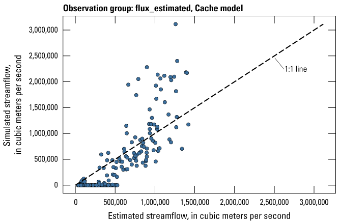
Plot of measured versus simulated values for the flux_estimated observation group.
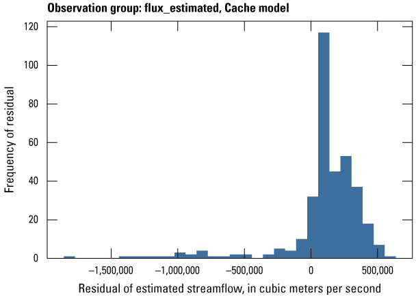
Histogram of the residuals from measured versus simulated values for the flux_estimated observation group.
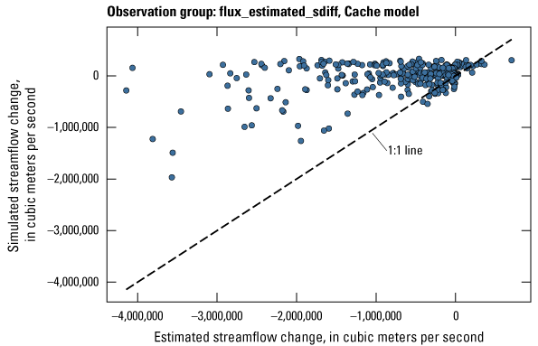
Plot of measured versus simulated values for the flux_estimated_sdiff observation group.
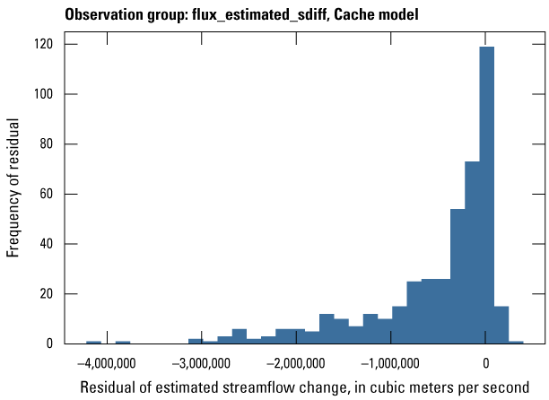
Histogram of the residuals from measured versus simulated values for the flux_estimated_sdiff observation group.
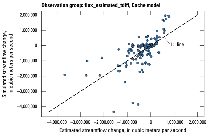
Plot of measured versus simulated values for the flux_estimated_tdiff observation group.
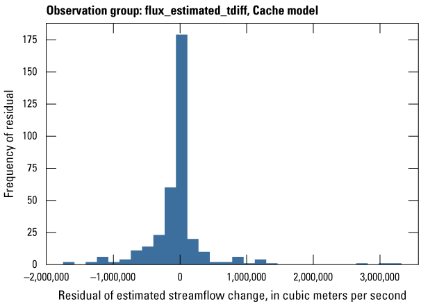
Histogram of the residuals from measured versus simulated values for the flux_estimated_tdiff observation group.
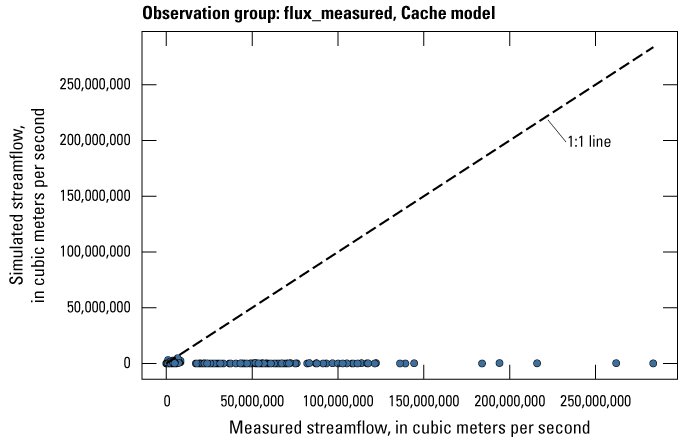
Plot of measured versus simulated values for the flux_measured observation group.
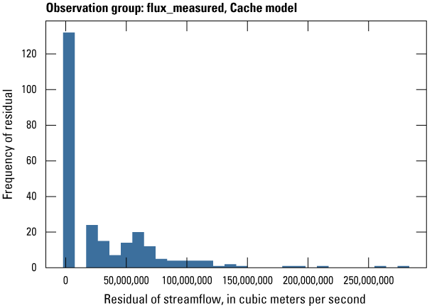
Histogram of the residuals from measured versus simulated values for the flux_measured observation group.
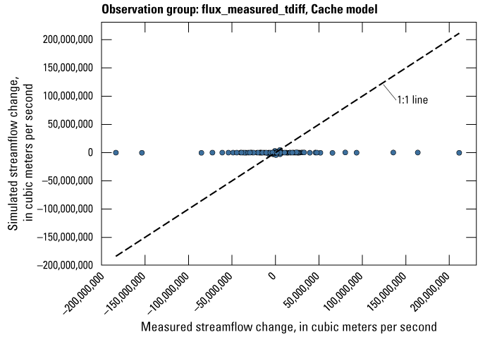
Plot of measured versus simulated values for the flux_measured_tdiff observation group.
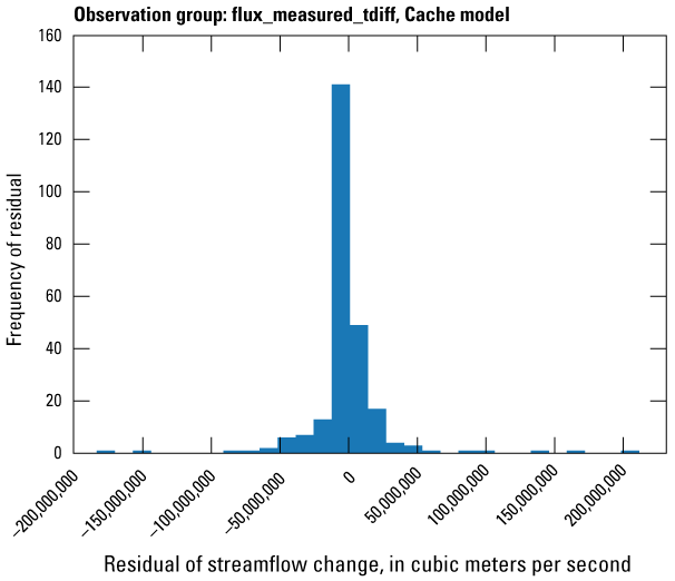
Histogram of the residuals from measured versus simulated values for the flux_measured_tdiff observation group.
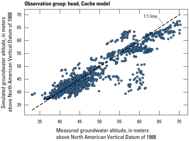
Plot of measured versus simulated values for the head observation group.
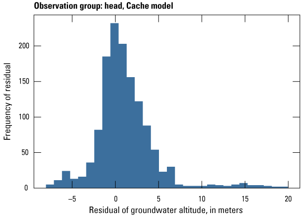
Histogram of the residuals from measured versus simulated values for the head observation group.
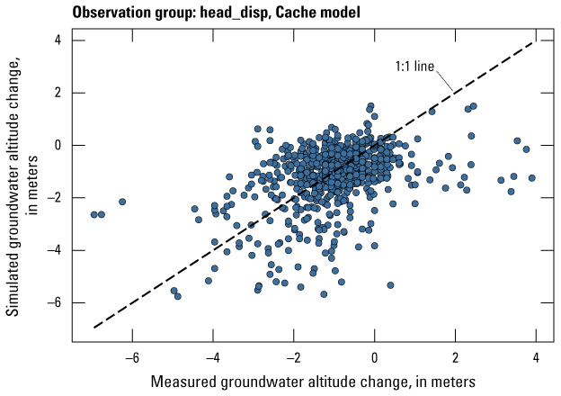
Plot of measured versus simulated values for the head_disp observation group.
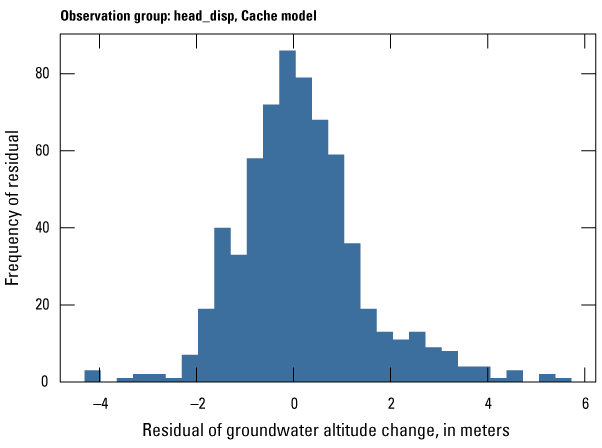
Histogram of the residuals from measured versus simulated values for the head_disp observation group.
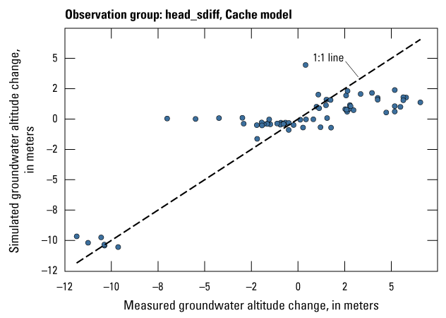
Plot of measured versus simulated values for the head_sdiff observation group.
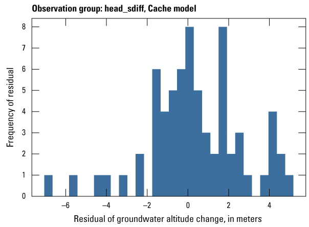
Histogram of the residuals from measured versus simulated values for the head_sdiff observation group.
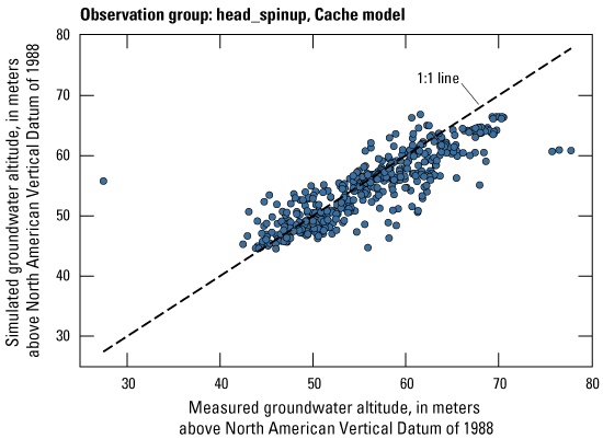
Plot of measured versus simulated values for the head_spinup observation group.
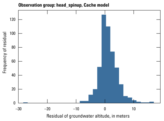
Histogram of the residuals from measured versus simulated values for the head_spinup observation group.
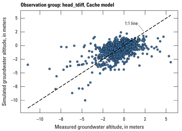
Plot of measured versus simulated values for the head_tdiff observation group.
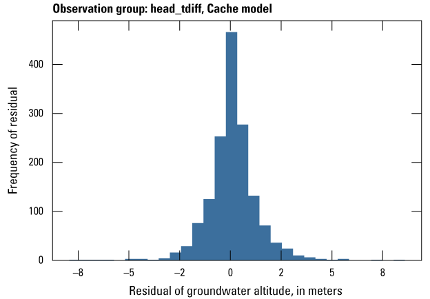
Histogram of the residuals from measured versus simulated values for the head_tdiff observation group.
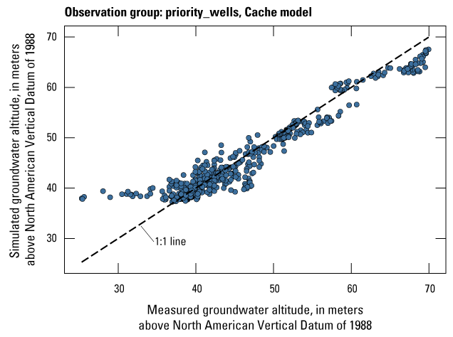
Plot of measured versus simulated values for the priority_wells observation group.
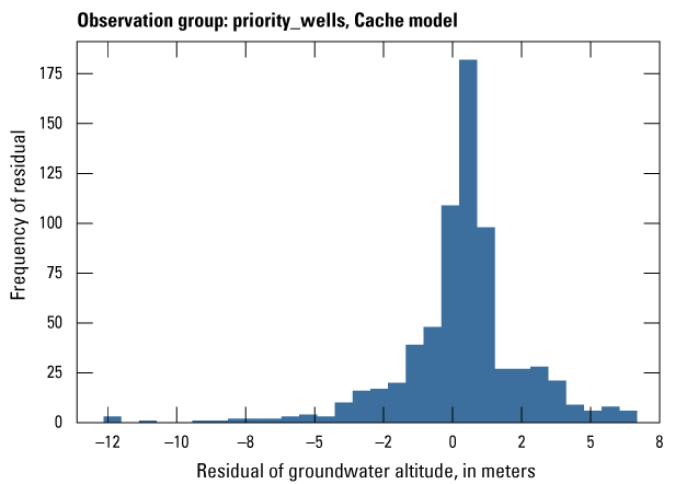
Histogram of the residuals from measured versus simulated values for the priority_wells observation group.
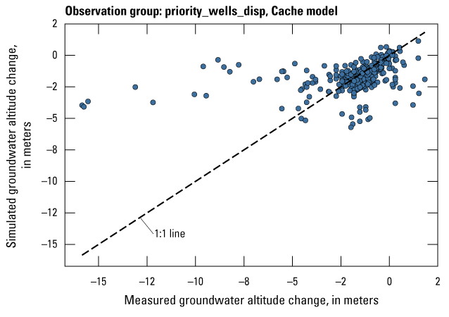
Plot of measured versus simulated values for the priority_wells_disp observation group.
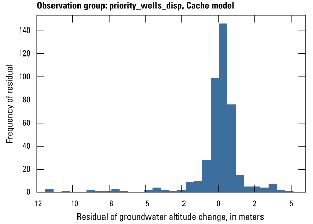
Histogram of the residuals from measured versus simulated values for the priority_wells_disp observation group.
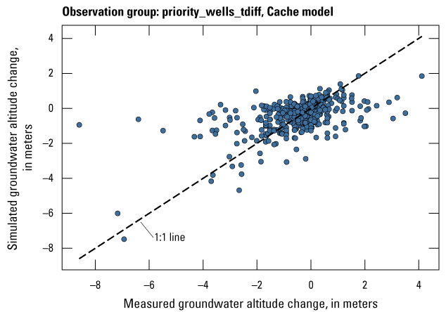
Plot of measured versus simulated values for the priority_wells_tdiff observation group.
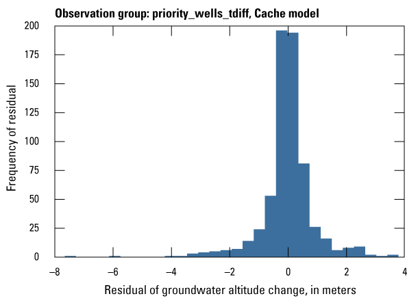
Histogram of the residuals from measured versus simulated values for the priority_wells_tdiff observation group.
Appendix 4. Measured Versus Simulated Plots of Water Levels at Select Observation Wells for the Calibrated Cache Model
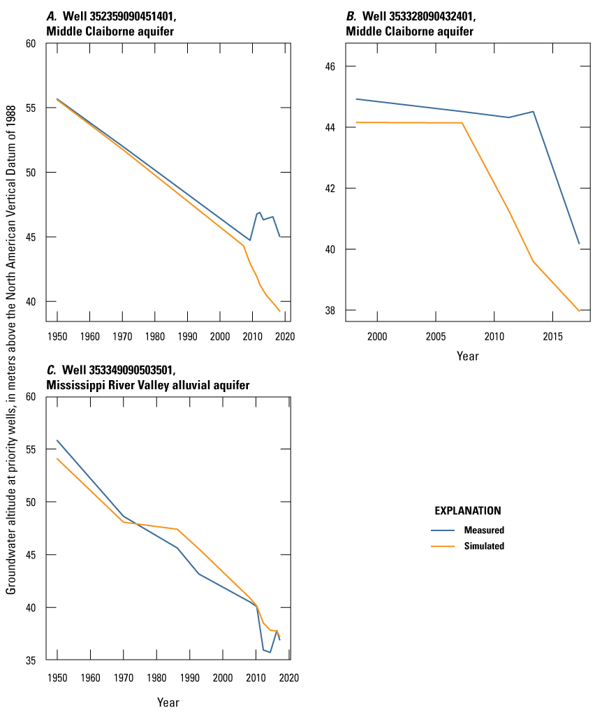
Plot of measured versus simulated values for observation wells for A, observation well 352359090451401; B, observation well 353328090432401; and C, observation well 353349090503501.
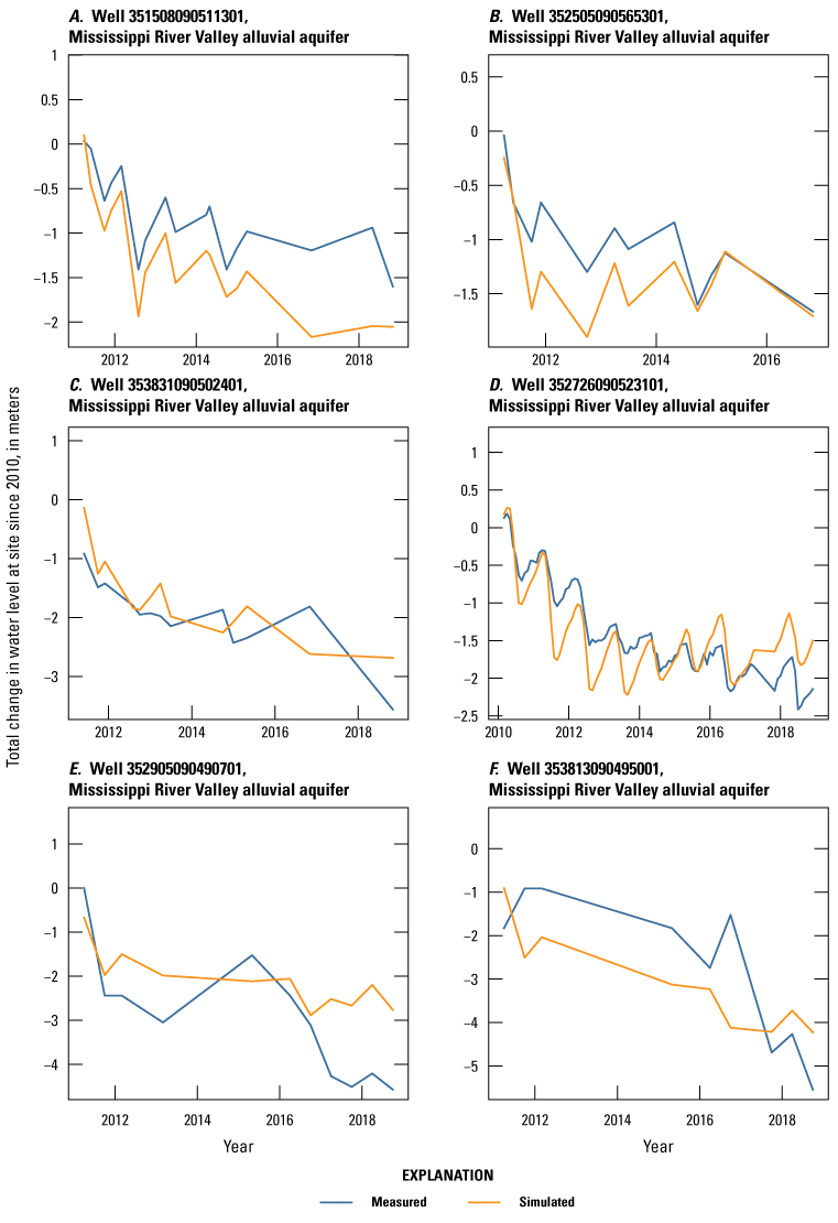
Plot of measured versus simulated values for observation wells for A, observation well 351508090511301; B, observation well 352505090565301; C, observation well 353831090502401; D, observation well 352726090523101; E, observation well 352905090490701; and F, observation well 353813090495001.
Appendix 5. Measured Versus Simulated One to One Plots by Observation Group and Histograms of Residuals for the Grand Prairie Model
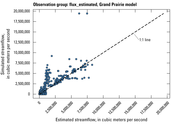
Plot of measured versus simulated values for the flux_estimated observation group.
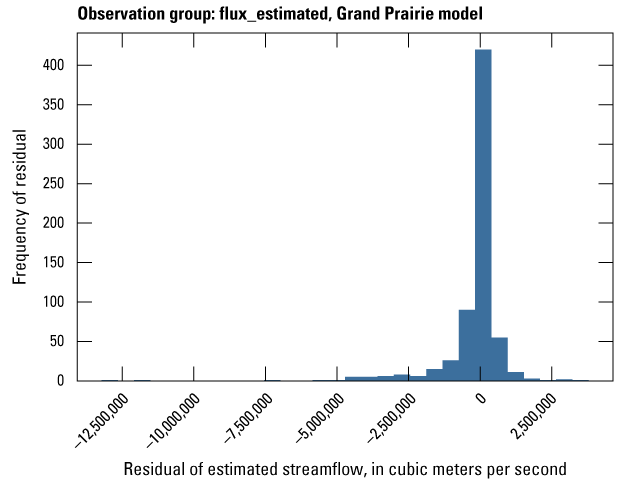
Histogram of the residuals from measured versus simulated values for the flux_estimated observation group
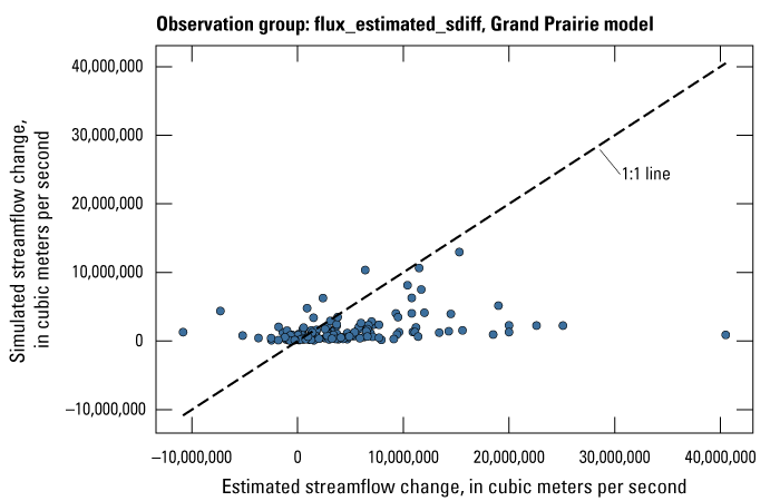
Plot of measured versus simulated values for the flux_estimated_sdiff observation group.
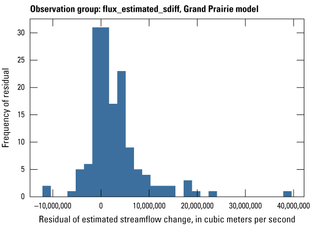
Histogram of the residuals from measured versus simulated values for the flux_estimated_sdiff observation group.
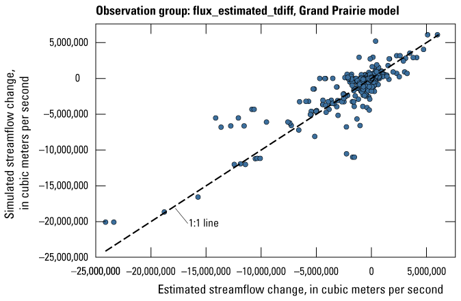
Plot of measured versus simulated values for the flux_estimated_tdiff observation group.
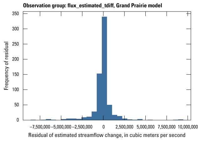
Histogram of the residuals from measured versus simulated values for the flux_estimated_tdiff observation group.
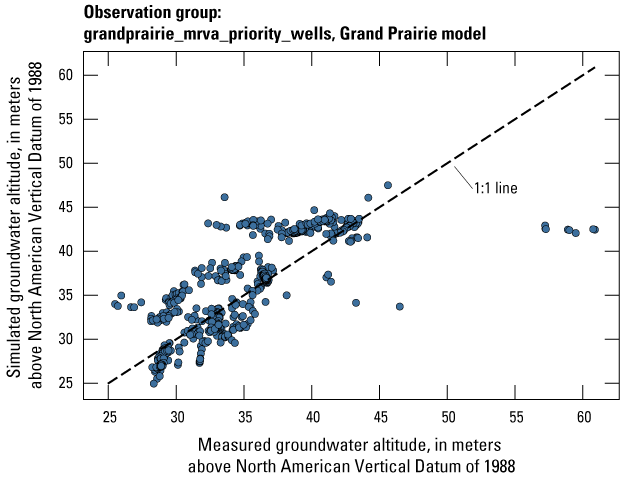
Plot of measured versus simulated values for the grandprairie_mrva_priority_wells observation group.
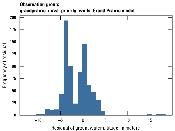
Histogram of the residuals from measured versus simulated values for the grandprairie_mrva_priority_wells observation group.
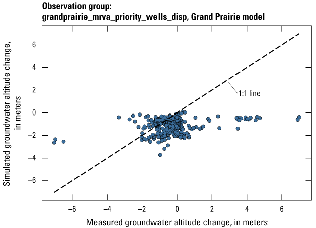
Plot of measured versus simulated values for the grandprairie_mrva_priority_wells_disp observation group.
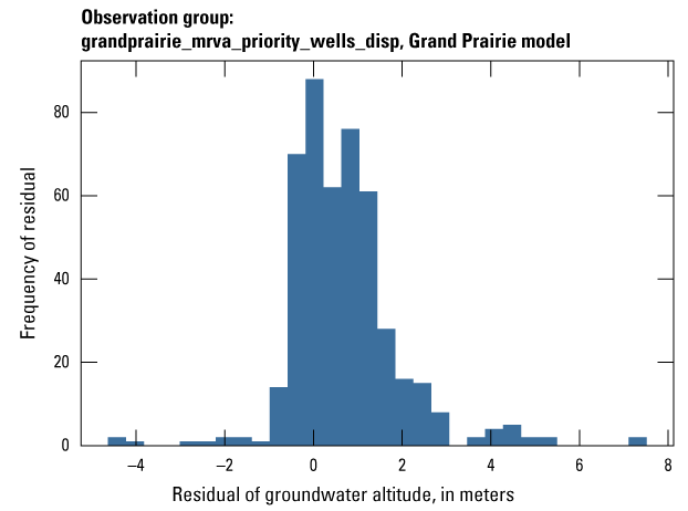
Histogram of the residuals from measured versus simulated values for the grandprairie_mrva_priority_wells_disp observation group.
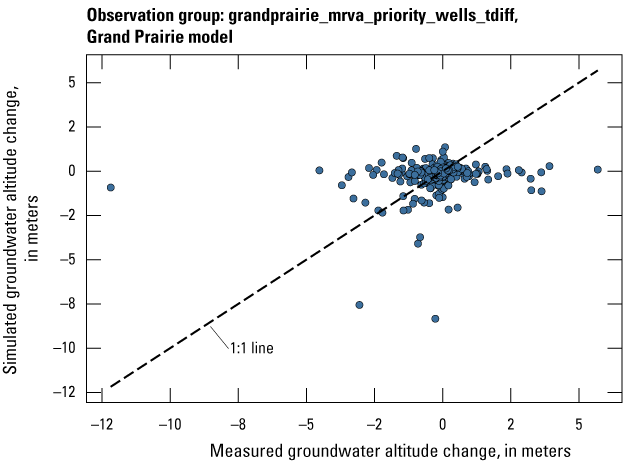
Plot of measured versus simulated values for the grandprairie_mrva_priority_wells_tdiff observation group.
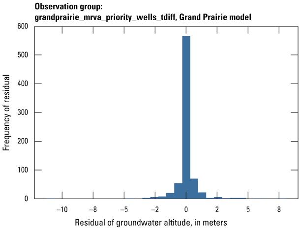
Histogram of the residuals from measured versus simulated values for the grandprairie_mrva_priority_wells_tdiff observation group.
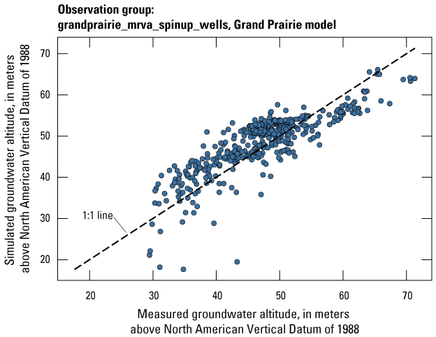
Plot of measured versus simulated values for the grandprairie_spinup_wells observation group.
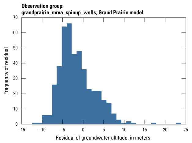
Histogram of the residuals from measured versus simulated values for the grandprairie_spinup_wells observation group.

Plot of measured versus simulated values for the grandprairie_mrva_wells observation group.
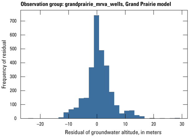
Histogram of the residuals from measured versus simulated values for the grandprairie_mrva_wells observation group.
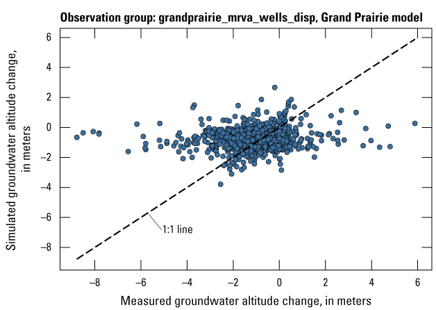
Plot of measured versus simulated values for the grandprairie_mrva_wells_disp observation group.
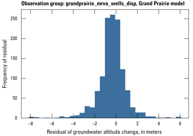
Histogram of the residuals from measured versus simulated values for the grandprairie_mrva_wells_disp observation group.
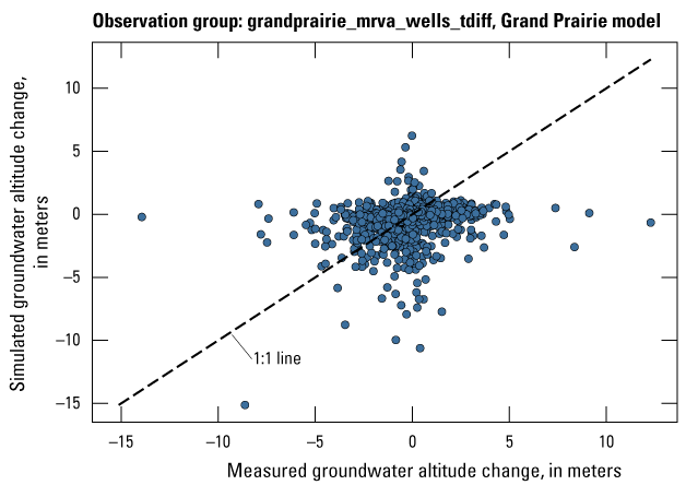
Plot of measured versus simulated values for the grandprairie_mrva_wells_tdiff observation group.
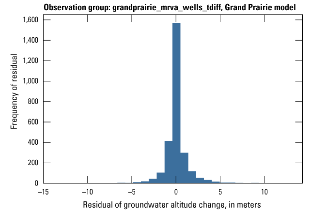
Histogram of the residuals from measured versus simulated values for the grandprairie_mrva_wells_tdiff observation group.
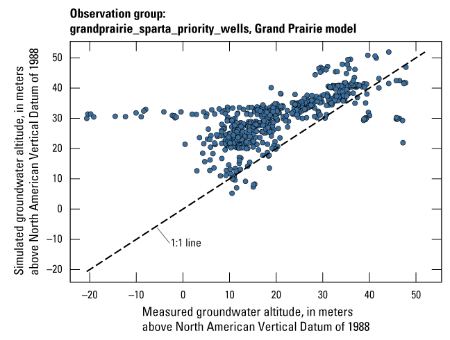
Plot of measured versus simulated values for the grandprairie_sparta_priority_wells observation group.
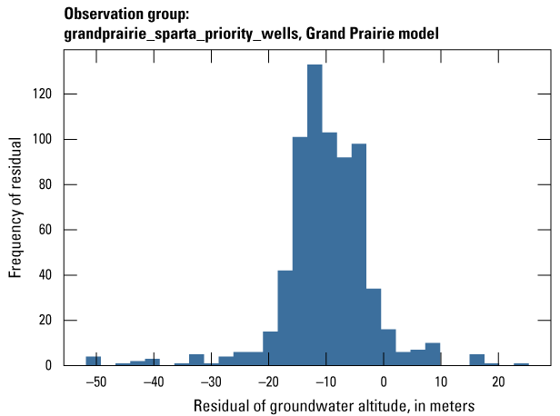
Histogram of the residuals from measured versus simulated values for the grandprairie_sparta_priority_wells observation group.
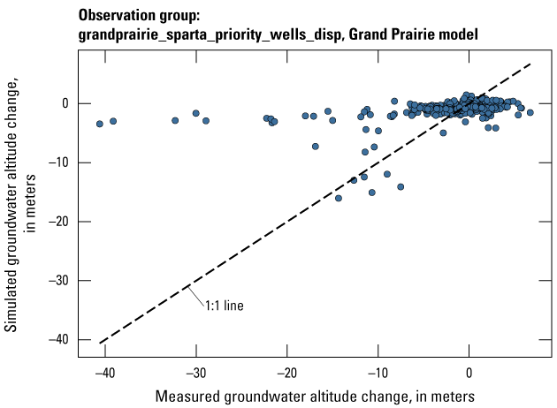
Plot of measured versus simulated values for the grandprairie_sparta_priority_wells_disp observation group.
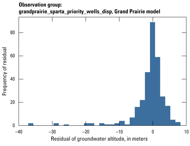
Histogram of the residuals from measured versus simulated values for the grandprairie_sparta_priority_wells_disp observation group.
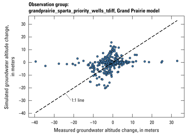
Plot of measured versus simulated values for the grandprairie_sparta_priority_wells_tdiff observation group.
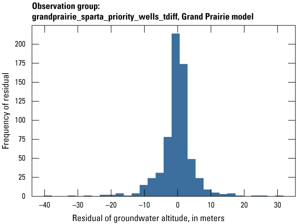
Histogram of the residuals from measured versus simulated values for the grandprairie_sparta_priority_wells_tdiff observation group.
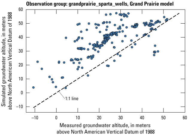
Plot of measured versus simulated values for the grandprairie_sparta_wells observation group.
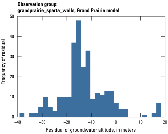
Histogram of the residuals from measured versus simulated values for the grandprairie_sparta_wells observation group.
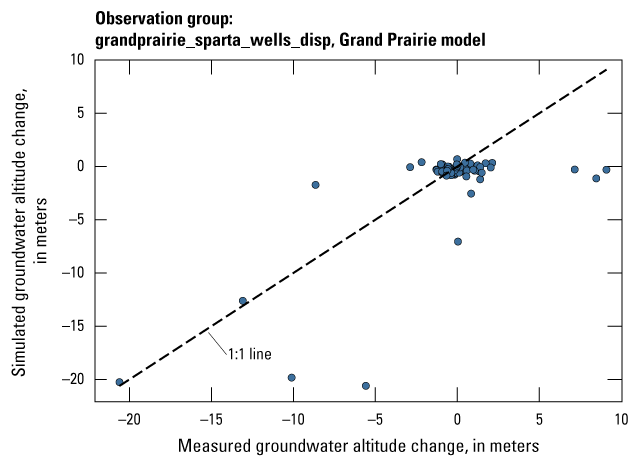
Plot of measured versus simulated values for the grandprairie_sparta_wells_disp observation group.
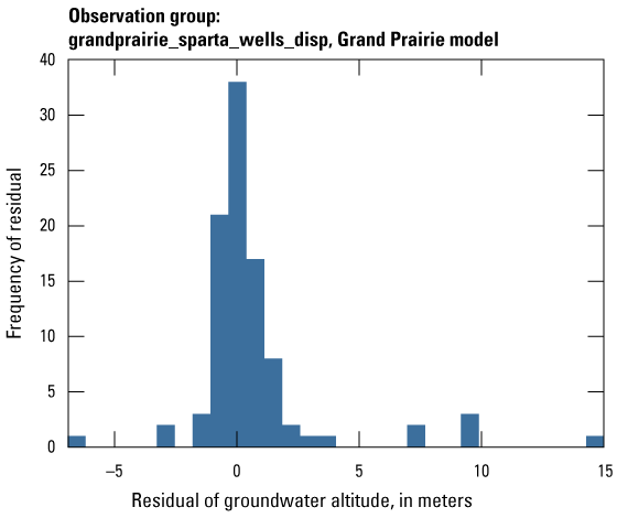
Histogram of the residuals from measured versus simulated values for the grandprairie_sparta_wells_disp observation group.
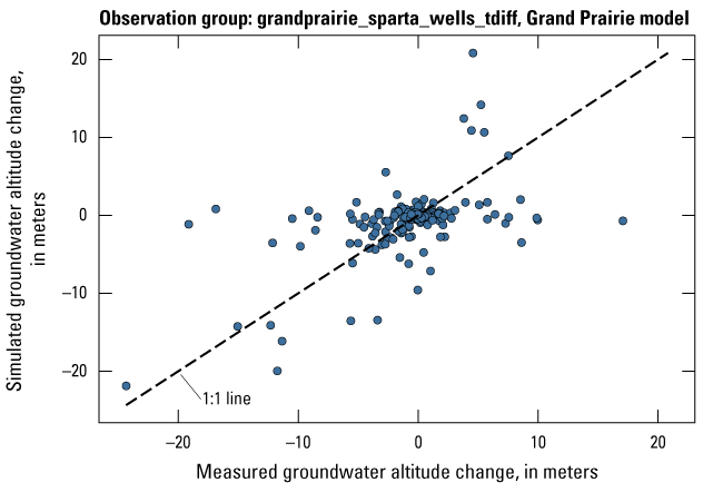
Plot of measured versus simulated values for the grandprairie_sparta_wells_tdiff observation group.
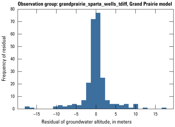
Histogram of the residuals from measured versus simulated values for the grandprairie_sparta_wells_tdiff observation group.
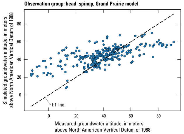
Plot of measured versus simulated values for the head_spinup observation group.
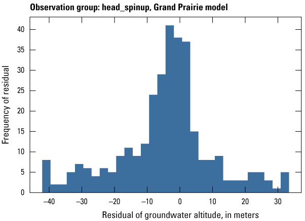
Histogram of the residuals from measured versus simulated values for the head_spinup observation group.
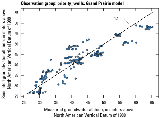
Plot of measured versus simulated values for the priority_wells observation group.
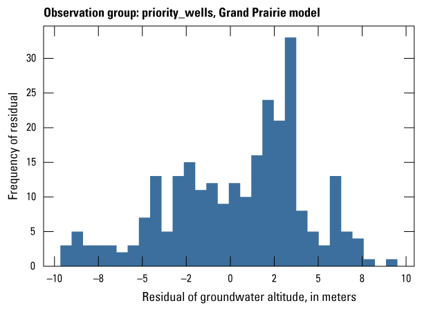
Histogram of the residuals from measured versus simulated values for the priority_wells observation group.
Appendix 6. Measured Versus Simulated Plots at Select Observation Wells for the Calibrated Grand Prairie Model
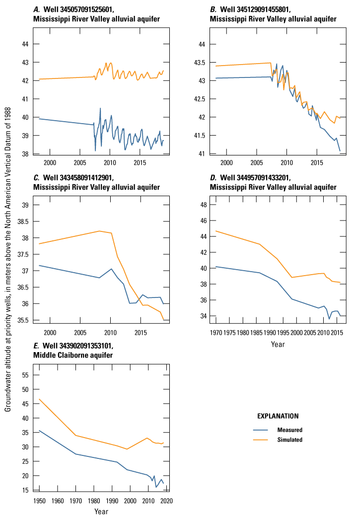
Plot of measured versus simulated groundwater levels for A) MRVA observation well 345057091525601, B) MRVA observation well 345129091455801, C) MRVA observation well 343458091412901, D) MRVA observation well 344957091433201, and E) middle Claiborne aquifer observation well 343902091353101.
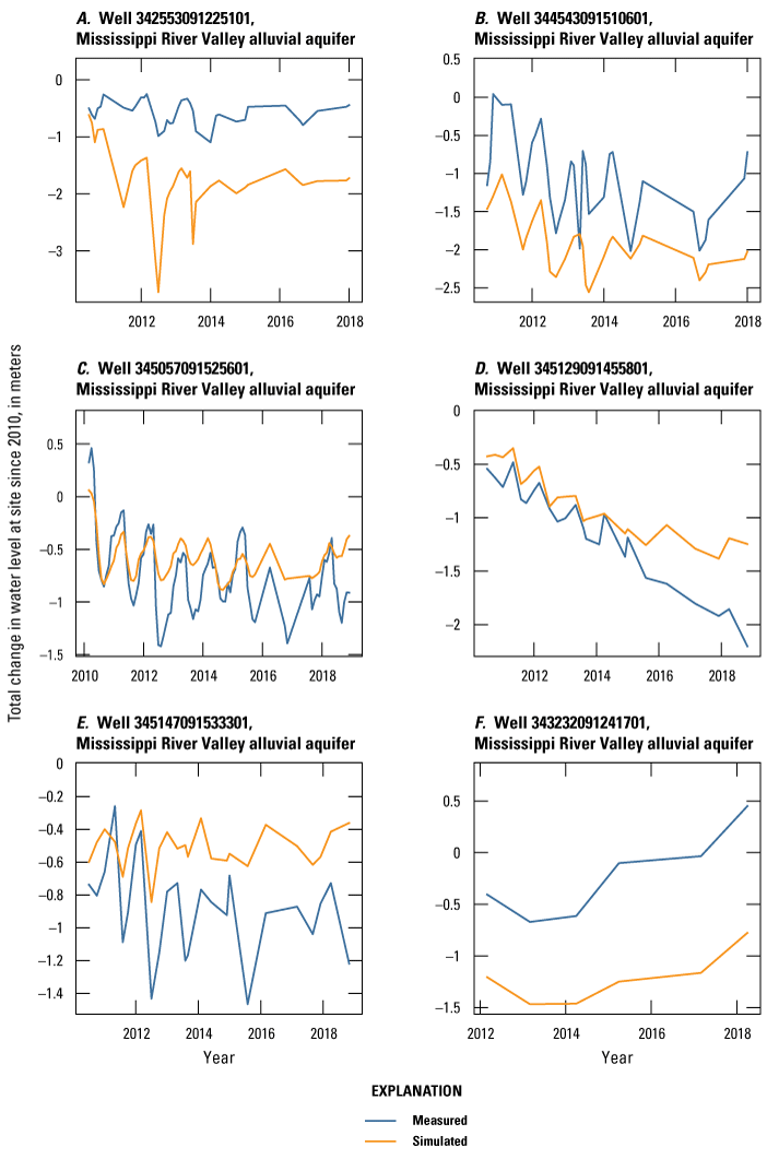
Plot of measured versus simulated groundwater levels for A) MRVA observation well 342553091225101, B) MRVA observation well 344543091510601, C) MRVA observation well 345057091525601, D) MRVA observation well 345129091455801, E) MRVA observation well 345147091533301, and F) MRVA observation well 343232091241701.
Appendix 7. Summary of Calibrated Aquifer Property Pilot Point Values for the Cache Model and Grand Prairie Model
Table 7.1.
The calibrated base realization of iteration two Cache model horizontal hydraulic conductivity, vertical anisotropy, and specific yield mean, minimum, and maximum pilot point values by model layer.[Kh, horizontal hydraulic conductivity; Kv, vertical hydraulic conductivity; Kvani, vertical anisotrophy of hydraulic conductivity, calculated as Kh/Kv; SY, specific yield; MRVA, Mississippi River Valley Alluvial aquifer; --, no data]
Table 7.2.
The calibrated base realization of iteration one Grand Prairie model horizontal hydraulic conductivity, vertical anisotropy, and specific yield mean, minimum, and maximum pilot point values by model layer.[Kh, horizontal hydraulic conductivity; Kv, vertical hydraulic conductivity; Kvani, vertical anisotrophy of hydraulic conductivity, calculated as Kh/Kv; SY, specific yield; MRVA, Mississippi River Valley Alluvial aquifer; --, no data]
Appendix 8. Calibrated Well Pumping Multiplier Parameters for Each Crop Type or Data Source by Stress Period for the Cache Model and Grand Prairie Model
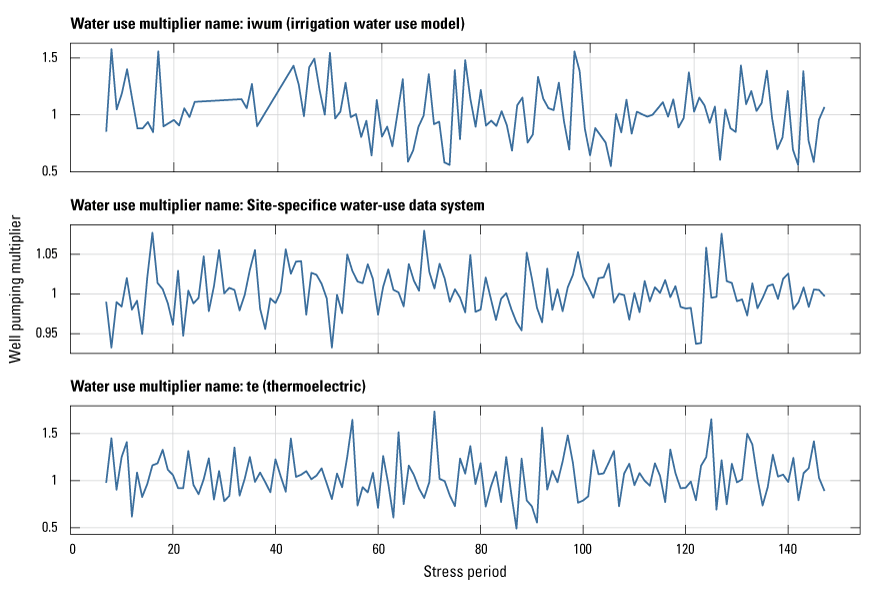
Plot of calibrated well pumping multipliers by crop type and stress period for the Cache model.
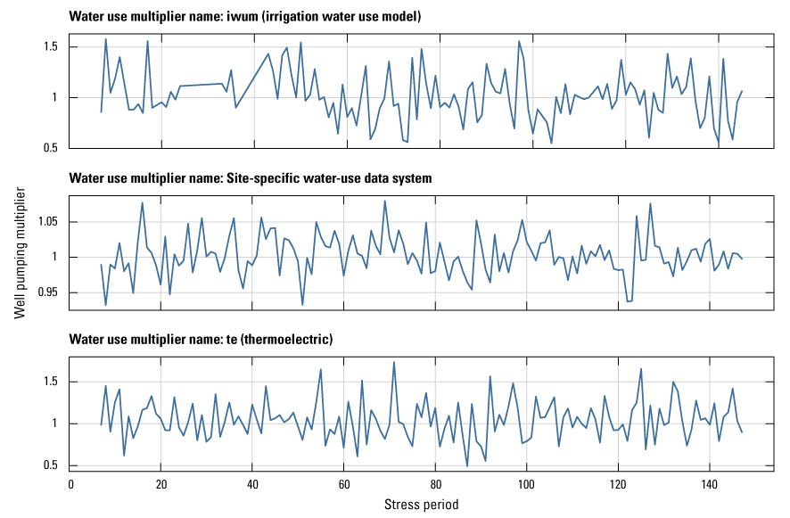
Plot of calibrated well pumping multipliers by data source and stress period for the Grand Prairie model.
Appendix 9. Prior and Posterior Ensemble Parameter Distributions for the Cache Model and Grand Prairie Model for Select Parameter Groups
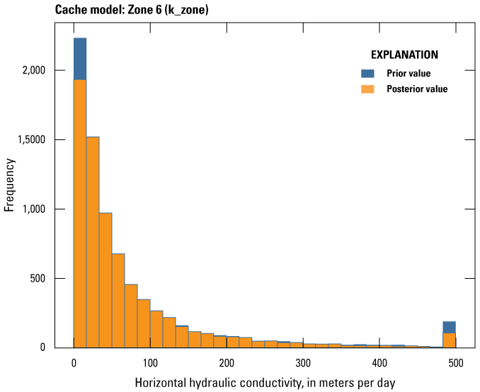
Cache model ensemble parameter distribution for the K_zone 6 parameter group.
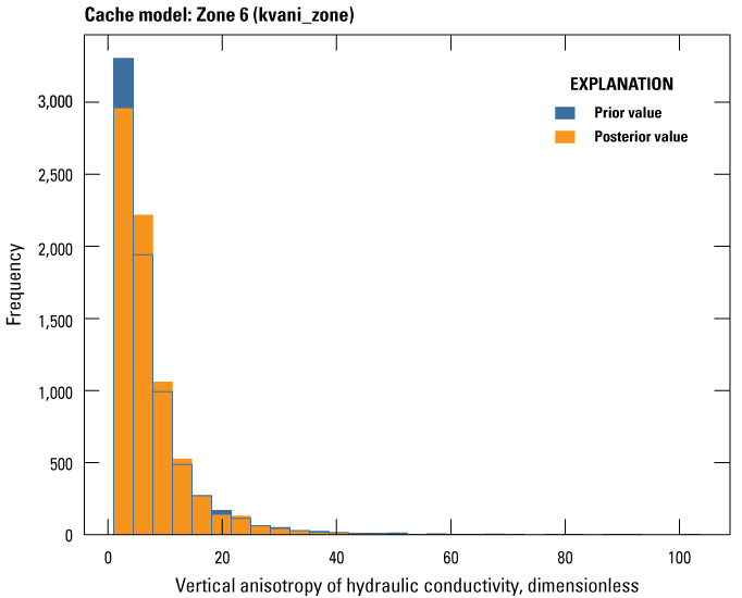
Cache model ensemble parameter distribution for the Kvani_zone 6 parameter group.
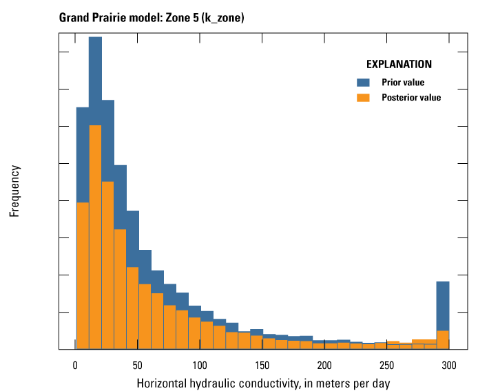
Grand Prairie model ensemble parameter distribution for the K_zone 5 parameter group.
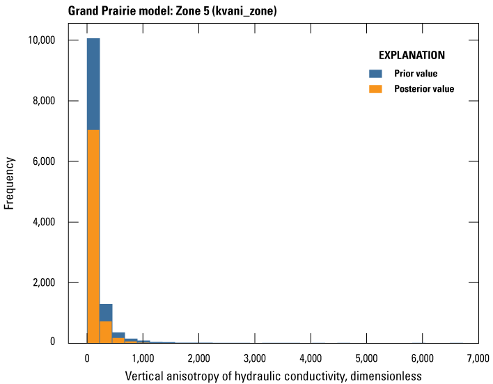
Grand Prairie model ensemble parameter distribution for the Kvani_zone 5 parameter group.
Conversion Factors
International System of Units to U.S. customary units
Temperature in degrees Celsius (°C) may be converted to degrees Fahrenheit (°F) as follows:
°F = (1.8 × °C) + 32.
Temperature in degrees Fahrenheit (°F) may be converted to degrees Celsius (°C) as follows:
°C = (°F – 32) / 1.8.
Datum
Vertical coordinate information is referenced to the North American Vertical Datum of 1988 (NAVD 88).
Horizontal coordinate information is referenced to the North American Datum of 1983 (NAD 83).
Altitude, as used in this report, refers to distance of the groundwater above the vertical datum.
Elevation, as used in this report, refers to distance of a physical land feature above the vertical datum.
Abbreviations
Φ
phi, objective function
AEM
airborne electromagnetic
AIWUM
Aquaculture and Irrigation Water Use Model
CGWA
Critical Groundwater Area
GHB
General Head Boundary package
GLM
Gauss-Levenberg-Marquardt
GP
Grand Prairie
IES
iterative ensemble smoother
IWUM
Irrigation Water Use Model
Kh
horizontal hydraulic conductivity
Kv
vertical hydraulic conductivity
Kvani
vertical anisotropy of hydraulic conductivity
line-km
flight-line-kilometers
MAP
Mississippi Alluvial Plain
MERAS
Mississippi Embayment Regional Aquifer System
MERAS 2
Mississippi Embayment Regional Aquifer System model version 2
MERAS 3
Mississippi Embayment Regional Aquifer System model version 3
MODFLOW
Modular Hydrologic Model
MRVA
Mississippi River Valley alluvial aquifer
NHDPlus
National Hydrography Dataset Plus
OBS
Observations package
PEST
Parameter ESTimation code
PEST++
Parameter ESTimation code ++, latest version
PESTPP–IES
PEST++ iterative ensemble smoother
PRISM
Parameter-elevation Regressions on Independent Slopes Model
RCH
Recharge package
rhk
streambed hydraulic conductivity
RIV
River package
SFR
Streamflow Routing package
SS
specific storage
STO
Storage package
SWB
soil-water-balance
SWUDS
site-specific water use data
SY
specific yield
USACE
U.S. Army Corps of Engineers
USDA
U.S. Department of Agriculture
USGS
U.S. Geological Survey
WEL
Well package
For more information about this publication, contact:
Director, USGS Nebraska Water Science Center
5231 South 19th Street
Lincoln, NE 68512
402–328–4100
For additional information, visit: https://www.usgs.gov/centers/ne-water
Publishing support provided by the
Rolla Publishing Service Center
Disclaimers
Any use of trade, firm, or product names is for descriptive purposes only and does not imply endorsement by the U.S. Government.
Although this information product, for the most part, is in the public domain, it also may contain copyrighted materials as noted in the text. Permission to reproduce copyrighted items must be secured from the copyright owner.
Suggested Citation
Traylor, J.P., Duncan, L.L., Leaf, A.T., Weisser, A.R., Dietsch, B.J., and Guira, M., 2024, Inset groundwater-flow models for the Cache and Grand Prairie Critical Groundwater Areas, northeastern Arkansas: U.S. Geological Survey Scientific Investigations Report 2024–5088, 152 p., https://doi.org/10.3133/sir20245088.
ISSN: 2328-0328 (online)
Study Area
| Publication type | Report |
|---|---|
| Publication Subtype | USGS Numbered Series |
| Title | Inset groundwater-flow models for the Cache and Grand Prairie Critical Groundwater Areas, northeastern Arkansas |
| Series title | Scientific Investigations Report |
| Series number | 2024-5088 |
| DOI | 10.3133/sir20245088 |
| Publication Date | November 08, 2024 |
| Year Published | 2024 |
| Language | English |
| Publisher | U.S. Geological Survey |
| Publisher location | Reston, VA |
| Contributing office(s) | Nebraska Water Science Center, Lower Mississippi-Gulf Water Science Center, Upper Midwest Water Science Center |
| Description | Report: xi, 152 p.; 13 Figures: 8.50 x 11.00 inches; Data Release; Dataset |
| Country | United States |
| State | Arkansas |
| Other Geospatial | Cache and Grand Prairie Critical Groundwater Areas |
| Online Only (Y/N) | Y |
| Additional Online Files (Y/N) | N |