

Conceptualization and Simulation of Groundwater Flow and Groundwater Availability in the Boone and Roubidoux Aquifers in Northeastern Oklahoma, 1980–2017
Links
- Document: Report (38.3 MB pdf) , HTML , XML
- Data Release: USGS Data Release - MODFLOW-NWT model used for the simulation of groundwater flow and analysis of groundwater availability in the Boone and Roubidoux aquifers in northeastern Oklahoma, 1980–2017
- NGMDB Index Page: National Geologic Map Database Index Page (html)
- Download citation as: RIS | Dublin Core
Acknowledgments
The project documented in this report was conducted in cooperation with the Oklahoma Water Resources Board (OWRB). The authors appreciate the contributions of many OWRB and USGS staff that led to the successful completion of the project. The authors thank the OWRB for support, especially Division Chief (Water Rights Administration Division) Christopher Neel who provided hydrogeologic data and helped with defining study objectives and deliverables.
The authors express gratitude to USGS employees who performed data-collection activities in the field. Billy Heard, Jordan Wentworth, and Justin White measured synoptic base flows during 2018. Shana Mashburn, Ian Rogers, Nicole Gammill, and Emily Moyer installed and maintained continuous groundwater-level recorders. In addition, Shana Mashburn, Nicole Gammill, and Waylon Marler facilitated data entry to the National Water Information System database. The authors also thank USGS employees Namjeong Choi, Evin Fetkovich, Chris Braun, Martha Watt, and S. Jerrod Smith, who performed detailed technical reviews on this report and the associated model archive data release. The authors acknowledge and appreciate these professional, experienced, and dedicated colleagues.
Abstract
Oklahoma Groundwater Law (Oklahoma Statute § 82-1020.5) requires that the Oklahoma Water Resources Board conduct hydrologic investigations to determine the maximum annual yield for the State’s groundwater basins. The Boone and Roubidoux aquifers (also known as the Springfield Plateau aquifer and Ozark aquifer, respectively) are bedrock aquifers that extend from northeastern Oklahoma into Kansas, Arkansas, and Missouri. At present (2024), the Oklahoma Water Resources Board has yet to legally issue orders for the final determination of maximum annual yields for the Boone and Roubidoux aquifers. To support determination of a maximum annual yield, the U.S. Geological Survey, in cooperation with the Oklahoma Water Resources Board, developed a hydrogeologic framework, a conceptual groundwater-flow model, and a calibrated numerical groundwater-flow model for the Boone and Roubidoux aquifers.
Three types of groundwater-availability scenarios were simulated by using the calibrated numerical model. These scenarios were used to (1) estimate equal-proportionate-share groundwater withdrawal rates (groundwater withdrawal applied equally over the aquifer), (2) quantify the potential effects of projected groundwater withdrawals on groundwater storage over a 50-year period, and (3) simulate the potential effects of a hypothetical 10-year drought. For the Boone aquifer, equal-proportionate-share groundwater withdrawal rates were 1.10, 0.98, and 0.96 acre-feet per acre per year for the 20-, 40-, and 50-year scenarios, respectively. For the Roubidoux aquifer, equal-proportionate-share groundwater withdrawal rates were 1.76, 1.34, and 1.25 acre-feet per acre per year for the 20-, 40-, and 50-year simulations, respectively. For the 50-year scenarios, stream seepage was minimally affected. Over the 10-year drought scenario, groundwater storage in the Boone and Roubidoux aquifers decreased by 660,451 acre-feet (6.7 percent) and 508,472 acre-feet (1.0 percent), respectively.
Introduction
The 1973 Oklahoma Water Law (Oklahoma Statute § 82-1020.5 [Oklahoma State Legislature, 2023b]) requires that the Oklahoma Water Resources Board (OWRB) conduct hydrologic investigations to support determination of the maximum annual yield (MAY) for each groundwater basin within the State; the OWRB (Oklahoma Secretary of State [OSS], 2023, chapter 30, subchapter 1, section 2) defines the MAY as “…the total amount of fresh groundwater that can be produced from each basin or subbasin allowing a minimum twenty (20) year life of such basin or subbasin.”
Oklahoma Groundwater Law (Oklahoma Statute § 82-1020.1 [Oklahoma State Legislature, 2023a]) defines freshwater (and thus fresh groundwater) as water with dissolved-solids concentrations of less than 5,000 parts per million (milligrams per liter [mg/L]). For bedrock aquifers, the 20-year life of the aquifer is achieved if at least 50 percent of the groundwater basin (hereinafter referred to as “aquifer”) retains 15 feet (ft) or more of saturated thickness after 20 years of groundwater withdrawals equally apportioned over the aquifer (OSS, 2023). An equal-proportionate-share (EPS) groundwater withdrawal rate (the maximum amount of groundwater that is permitted to be withdrawn annually for each acre of land owned or leased by the permit holder) is then determined from the MAY (OSS, 2023). The Springfield Plateau aquifer and the Ozark aquifer (known locally and hereinafter referred to as the “Boone aquifer” and “Roubidoux aquifer,” respectively) are bedrock aquifers in the Ozark Plateaus aquifer system that extends from northeastern Oklahoma into Kansas, Arkansas, and Missouri (fig. 1A). The OWRB categorizes the Roubidoux aquifer as a major aquifer (well yields are on average at least 50 gallons per minute) and the Boone aquifer as a minor aquifer (that which does not meet the criteria of a major aquifer; OWRB, 2012a). At present (2024), the OWRB has yet to establish MAYs for the Boone and Roubidoux aquifers (OWRB, 2023). To help support the OWRB’s determination of MAYs for the Boone and Roubidoux aquifers, the U.S. Geological Survey (USGS), in cooperation with the OWRB, conducted a hydrologic investigation and evaluated the effects of potential groundwater withdrawals and drought on groundwater availability for the Boone and Roubidoux aquifers in northeastern Oklahoma.
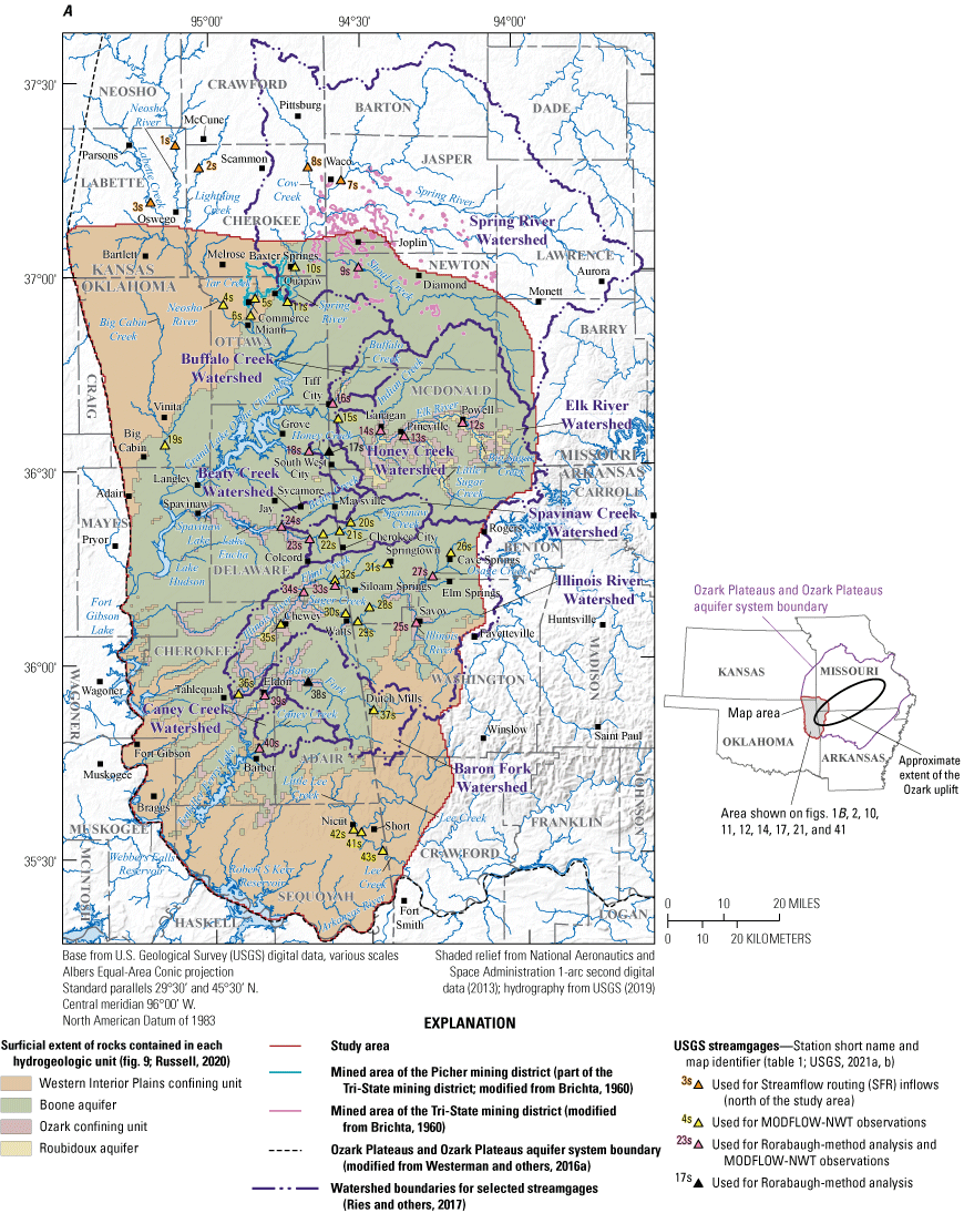
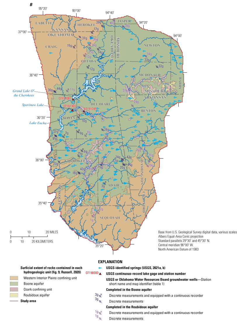
Study area in northeastern Oklahoma, southeastern Kansas, southwestern Missouri, and northwestern Arkansas and selected hydrogeologic units with A, selected U.S. Geological Survey (USGS) streamgages, and the watershed areas for selected streamgages from StreamStats (Ries and others, 2017) and B, discrete groundwater-level measurement locations, USGS continuous groundwater recorder deployment locations, USGS continuous-record lake gages, and USGS-identified springs for the Boone and Roubidoux aquifers.
Purpose and Scope
The purpose of this report is to describe the hydrogeology and results of the simulation of groundwater flow for the Boone and Roubidoux aquifers in northeastern Oklahoma. This report presents (1) a background on the hydrogeologic framework of the Boone and Roubidoux aquifers, (2) a conceptual groundwater-flow model that includes geochemical analyses of the groundwater and quantifies inflows and outflows for the aquifers, and (3) the results of groundwater-availability scenarios to determine how the aquifers respond to hydrologic stressors, such as drought and groundwater withdrawals. The calibrated, numerical groundwater-flow model and groundwater-availability scenarios were archived and released in a USGS data release (Trevisan and others, 2024).
The geographic scope of this report includes four hydrogeologic units in northeastern Oklahoma: (1) the Western Interior Plains confining unit (2) the Boone aquifer, (3) the Ozark confining unit, and (4) the Roubidoux aquifer. In addition to Oklahoma, the study area includes parts of Arkansas, Kansas, and Missouri to align more closely with aquifer hydrologic boundaries and facilitate construction of the conceptual groundwater-flow model and the numerical groundwater-flow model described in this report (fig. 1). Although the study area extends into Arkansas, Kansas, and Missouri, this hydrologic investigation is focused on the OWRB jurisdictional extent of these hydrogeologic units within Oklahoma.
Description of the Study Area
The Boone and Roubidoux aquifers are predominantly contained in Paleozoic-age carbonate rocks, and to a lesser extent in shales and siliciclastic rocks of similar age. The Boone and Roubidoux aquifers encompass approximately 34,000 and 68,000 square miles, respectively, in Arkansas, Kansas, Missouri, and Oklahoma (Russell and Stivers, 2020). To assess groundwater flow and availability in Oklahoma, the study area was confined primarily to the spatial extent of the Boone and Roubidoux aquifers in Oklahoma (including parts of southeastern Kansas, southwestern Missouri, and northwestern Arkansas as needed for modeling purposes). The study area encompasses approximately 7,600 square miles of which approximately 4,600 square miles are within Oklahoma (fig. 1A). The northern and eastern study area boundaries were delineated by watershed boundaries (EPA, 2020b) or along no-flow boundaries interpreted from published potentiometric surfaces (Imes and Emmett, 1994; Nottmeier, 2015). The western and southern study area boundaries represent the extents of the Boone and Roubidoux aquifers defined by Russell (2020) with some modifications based on the work of Westerman and others (2016a) and represent the saltwater-freshwater boundary where the rocks that contain the aquifers decrease in altitude and groundwater salinity increases (Imes and Emmett, 1994). The saltwater-freshwater boundary generally follows the topographic low of the Arkansas River but also is present along the western boundary of the study area (fig. 1A).
Uplift and subsequent erosion in the region created steep topography that spurred complex stream development, which is often characterized by deep, V-shaped valleys with dendritic drainage patterns (Huffman, 1958). The Boone aquifer is mostly unconfined but is confined by the Western Interior Plains confining unit in the northwest and southern parts of the study area (fig. 1A). The Roubidoux aquifer is almost entirely confined except where streams have eroded overlying rocks (mostly in the central part of the study area; fig. 1A).
The Boone and Roubidoux aquifers provide freshwater resources to 11 counties in northeastern Oklahoma (Adair, Cherokee, Craig, Delaware, Haskell, Mayes, Muscogee, Nowata, Ottawa, Sequoyah, and Wagoner Counties) that have a combined a population of approximately 332,000 (U.S. Census Bureau, 2023). Groundwater from the Boone aquifer is used primarily for domestic and minor agricultural, commercial, and public-supply purposes; groundwater from the Roubidoux aquifer is primarily used for industrial and public-supply purposes (OWRB, 2012a).
Land cover within the study area is predominantly forest (46.2 percent) and grassland and pasture (37.5 percent) followed by developed (6.8 percent), cropland (5.7 percent), and other (water, wetlands, barren, and shrubland; 3.7 percent) (fig. 2; National Agricultural Statistics Service, 2021). Most cropland is near the Arkansas River and north of the Neosho River near the Oklahoma-Kansas border. Cropland mostly consist of soybeans (34.2 percent of cropland), hay (29.5 percent of cropland), and corn (17.5 percent of cropland).
Irrigation groundwater use on land overlying the Boone and Roubidoux aquifers tends to be low because cropland is not a widespread land cover owing to poor soil development associated with surficial weathering of outcrops (land-surface exposures) of the karstic rock units that contain the aquifers in the area. Human development is relatively sparse; however, westward expansion in the 1800s spurred logging across the area, and the modern landscape is likely different from the landscape during pre-development (Jacobson and Primm, 1997).
The Tri-state mining district was one of the largest lead and zinc mining operations in the world, spanning parts Kansas, Missouri, and Oklahoma from the 1850s to the 1970s (fig. 1A; Aber and others, 2010; U.S. Environmental Protection Agency [EPA], 2023). In Oklahoma, lead and zinc were mostly mined in the Picher mining district (fig. 1A; Smith, 2013). Historical mining operations dewatered parts of the Boone aquifer and affected groundwater quality in the Boone aquifer (Aber and others, 2010).
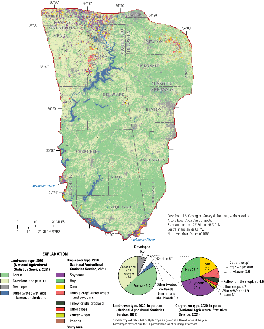
Land and crop cover over the study area in northeastern Oklahoma, southeastern Kansas, southwestern Missouri, and northwestern Arkansas, 2020.
Precipitation and Temperature
Long-term patterns in precipitation, temperature, and groundwater levels for the study area were analyzed by using data from 1895 to 2020. Monthly and annual precipitation and temperatures were averaged from the gridded climatic data from PRISM Climate Group (2022). To obtain monthly and annual precipitation and temperature values that more closely represented climatic conditions affecting the Boone and Roubidoux aquifers, gridded climate data were clipped to the study area extent and spatially averaged for each month and year. To evaluate long-term groundwater-level trends, groundwater-level data were obtained from the OWRB mass measurement program (OWRB, 2021) for the Boone aquifer and from the USGS National Water Information System (NWIS) database (USGS, 2021a, b) for the Roubidoux aquifer (table 1).
Table 1.
Description of continuous-record streamgages and lake gages, wells instrumented with continuous recorders, and wells at which only discrete groundwater-level data were collected within the study area in northeastern Oklahoma, southeastern Kansas, southwestern Missouri, and northwestern Arkansas.[Dates are in month/day/year format. “Present” is 2024. USGS, U.S. Geological Survey; Kans., Kansas; Okla., Oklahoma; Mo., Missouri; Ark., Arkansas; OWRB, Oklahoma Water Resources Board; NA, not applicable; --, not reported because the station was not used to collect continuous data]
| Station or identification number1 | Station short name and map identifier (fig. 1) | Station name | Latitude (decimal degrees) | Longitude (decimal degrees) | Aquifer | Period of record (may contain gaps) | |
|---|---|---|---|---|---|---|---|
| Begin date | End date2 | ||||||
| 07183500 | 1s | Neosho River near Parsons, Kans. | 37.3401 | −95.1100 | NA | 10/1/1921 | present |
| 07184000 | 2s | Lightning Creek near McCune, Kans. | 37.2812 | −95.0327 | NA | 10/1/1938 | present |
| 07184500 | 3s | Labette Creek near Oswego, Kans. | 37.1938 | −95.1925 | NA | 10/1/1938 | present |
| 07185000 | 4s | Neosho River near Commerce, Okla. | 36.9287 | −94.9575 | NA | 10/1/1939 | present |
| 07185090 | 5s | Tar Creek near Commerce, Okla. | 36.9437 | −94.8533 | NA | 7/21/2004 | present |
| 07185095 | 6s | Tar Creek at 22nd Street Bridge at Miami, Okla. | 36.9001 | −94.8683 | NA | 1/11/1984 | present |
| 07186000 | 7s | Spring River near Waco, Mo. | 37.2456 | −94.5664 | NA | 4/25/1924 | present |
| 07186055 | 8s | Cow Creek near Scammon, Kans. | 37.2806 | −94.6750 | NA | 2/19/2014 | 3/21/2019 |
| 07187000 | 9s | Shoal Creek above Joplin, Mo. | 37.0206 | −94.5138 | NA | 10/1/1941 | present |
| 07187600 | 10s | Spring River near Baxter Springs, Kans. | 37.0237 | −94.7211 | NA | 9/30/2008 | present |
| 07188000 | 11s | Spring River near Quapaw, Okla. | 36.9345 | −94.7472 | NA | 7/12/1939 | present |
| 07188653 | 12s | Big Sugar Creek near Powell, Mo. | 36.6159 | −94.1822 | NA | 5/25/2000 | present |
| 07188838 | 13s | Little Sugar Creek near Pineville, Mo. | 36.5840 | −94.3733 | NA | 10/1/2004 | present |
| 07188885 | 14s | Indian Creek near Lanagan, Mo. | 36.5993 | −94.4496 | NA | 5/24/2000 | present |
| 07189000 | 15s | Elk River near Tiff City, Mo. | 36.6315 | −94.5869 | NA | 10/1/1939 | present |
| 07189100 | 16s | Buffalo Creek at Tiff City, Mo. | 36.6709 | −94.6041 | NA | 5/24/2000 | present |
| 07189540 | 17s | Cave Springs Branch near South West City, Mo. | 36.5473 | −94.6180 | NA | 9/6/1997 | present |
| 07189542 | 18s | Honey Creek near South West City, Mo. | 36.5489 | −94.6836 | NA | 9/6/1997 | present |
| 07191000 | 19s | Big Cabin Creek near Big Cabin, Okla. | 36.5684 | −95.1522 | NA | 10/1/1947 | present |
| 07191160 | 20s | Spavinaw Creek near Maysville, Ark. | 36.3645 | −94.5513 | NA | 10/1/2001 | present |
| 07191179 | 21s | Spavinaw Creek near Cherokee City, Ark. | 36.3420 | −94.5877 | NA | 10/1/2001 | present |
| 07191220 | 22s | Spavinaw Creek near Sycamore, Okla. | 36.3347 | −94.6414 | NA | 10/1/1961 | present |
| 071912213 | 23s | Spavinaw Creek near Colcord, Okla. | 36.3226 | −94.6852 | NA | 10/1/2001 | present |
| 07191222 | 24s | Beaty Creek near Jay, Okla. | 36.3554 | −94.7763 | NA | 7/30/1998 | present |
| 07194800 | 25s | Illinois River at Savoy, Ark. | 36.1031 | −94.3444 | NA | 6/21/1979 | present |
| 07194880 | 26s | Osage Creek near Cave Springs, Ark. | 36.2815 | −94.2280 | NA | 10/1/1990 | present |
| 07195000 | 27s | Osage Creek near Elm Springs, Ark. | 36.2219 | −94.2883 | NA | 10/1/1950 | present |
| 07195400 | 28s | Illinois River at Highway 16 near Siloam Springs, Ark. | 36.1447 | −94.4947 | NA | 6/21/1979 | present |
| 07195430 | 29s | Illinois River South of Siloam Springs, Ark. | 36.1086 | −94.5333 | NA | 7/14/1995 | present |
| 07195500 | 30s | Illinois River near Watts, Okla. | 36.1301 | −94.5722 | NA | 10/1/1955 | present |
| 07195800 | 31s | Flint Creek at Springtown, Ark. | 36.2561 | −94.4336 | NA | 7/1/1961 | present |
| 07195855 | 32s | Flint Creek near West Siloam Springs, Okla. | 36.2161 | −94.6053 | NA | 10/1/1979 | present |
| 07195865 | 33s | Sager Creek near West Siloam Springs, Okla. | 36.2017 | −94.6052 | NA | 9/12/1996 | present |
| 07196000 | 34s | Flint Creek near Kansas, Okla. | 36.1865 | −94.7069 | NA | 10/1/1955 | present |
| 07196090 | 35s | Illinois River at Chewey, Okla. | 36.1043 | −94.7827 | NA | 10/1/2000 | present |
| 07196500 | 36s | Illinois River near Tahlequah, Okla. | 35.9255 | −94.9217 | NA | 10/1/1935 | present |
| 07196900 | 37s | Baron Fork at Dutch Mills, Ark. | 35.8800 | −94.4864 | NA | 4/1/1958 | present |
| 07196973 | 38s | Peacheater Creek at Christie, Okla. | 35.9548 | −94.6963 | NA | 9/1/1992 | 9/16/2004 |
| 07197000 | 39s | Baron Fork at Eldon, Okla. | 35.9216 | −94.8372 | NA | 10/1/1948 | present |
| 07197360 | 40s | Caney Creek near Barber, Okla. | 35.7851 | −94.8563 | NA | 10/1/1997 | present |
| 07249800 | 41s | Lee Creek at Short, Okla. | 35.5658 | −94.5319 | NA | 9/16/1999 | present |
| 07249920 | 42s | Little Lee Creek near Nicut, Okla. | 35.5731 | −94.5569 | NA | 10/1/2000 | present |
| 07249985 | 43s | Lee Creek near Short, Okla. | 35.5172 | −94.4642 | NA | 10/1/1930 | present |
| 07190000 | -- | Lake O' the Cherokees at Langley, OK | 36.4687 | −95.0414 | NA | 3/21/1940 | present |
| 07191285 | -- | Lake Eucha near Eucha, OK | 36.37508 | −94.9352 | NA | 10/1/2001 | present |
| 07191300 | -- | Spavinaw Lake at Spavinaw, OK | 36.38314 | −95.048 | NA | 10/1/2005 | present |
| 353341094513501 | 1g | 13N-23E-34 BCB 1 Roubidoux9 | 35.5615 | −94.8596 | Roubidoux | 12/2018 | 11/8/2020 |
| 353513094482401 | 2g | 13N-24E-10 CBB 1 Roubidoux5 | 35.5868 | −94.8067 | Roubidoux | 7/2017 | 11/8/2020 |
| 354852094442501 | 3g | 16N-24E-34 DDB 1 Boone10 | 35.8145 | −94.7402 | Boone | 7/2017 | 11/8/2020 |
| 355600094503501 | 4g | 17N-23E-22 CDA 1 Roubidoux4 | 35.9334 | −94.8431 | Roubidoux | 6/2017 | 11/8/2020 |
| 355741094461001 | 5g | 17N-24E-08 DCB 1 Boone9 | 35.9613 | −94.7696 | Boone | 6/2017 | 11/8/2020 |
| 360425094573101 | 6g | 18N-22E-04 AAD 1 Boone7 | 36.0736 | −94.9587 | Boone | 6/2017 | 11/9/2020 |
| 361104095081801 | 7g | 20N-20E-26 ADD 1 Boone11 | 36.1846 | −95.1384 | Boone | 12/2018 | 6/10/2019 |
| 361126094551801 | 8g | 20N-22E-24 CCC 1 Roubidoux6 | 36.1907 | −94.9217 | Roubidoux | 7/2017 | 11/9/2020 |
| 361317094594101 | 9g | 20N-22E-07 DDA 1 Boone5 | 36.2214 | −94.9947 | Boone | 6/2017 | 11/9/2020 |
| 362004094591601 | 10g | 21N-22E-05 BBC 1 Boone8 | 36.3343 | −94.9879 | Boone | 6/2017 | 11/9/2020 |
| 363230095054901 | 11g | 24N-21E-19 DDA 1 Roubidoux2 | 36.5415 | −95.0970 | Roubidoux | 6/2017 | 11/9/2020 |
| 364328094532701 | 12g | 26N-23E-19 BCB 1 Boone1 | 36.7244 | −94.8908 | Boone | 6/2017 | 11/15/2020 |
| 364859094552401 | 13g | 27N-22E-14 CCD 1 Roubidoux3 | 36.8165 | −94.9232 | Roubidoux | 6/2017 | 11/15/2020 |
| 365151094470801 | 14g | 28N-23E-36 BCD 1 Boone6 | 36.8641 | −94.7855 | Boone | 6/2017 | 11/15/2020 |
| 365258095013401 | 15g | 28N-21E-26 ACB 1 Boone3 | 36.8828 | −95.0262 | Boone | 6/2017 | 11/15/2020 |
| 365402094522201 | 16g | 28N-23E-18 CDC 1 Miami Well No 9 | 36.9001 | −94.8716 | Roubidoux | 4/2007 | 2/2/2013 |
| 365942094504203 | 17g | 29N-23E-17 BCA 1 Slim Jim Well | 36.9950 | −94.8450 | Boone | 10/2002 | present |
| 355407094593701 | 18g | 17N-22E-32 CDC 1 | 35.9020 | −94.9938 | Boone | -- | -- |
| 355654094185901 | 19g | 15N31W30CAD1 | 35.9479 | −94.3160 | Roubidoux | -- | -- |
| 355742094331201 | 20g | 17N-26E-09 CCA 1 | 35.9617 | −94.5536 | Boone | -- | -- |
| 355901094181401 | 21g | 15N31W17BBD1 | 35.9841 | −94.3020 | Roubidoux | -- | -- |
| 355914094340001 | 22g | 17N-26E-05 BAA 1 | 35.9873 | −94.5669 | Boone | -- | -- |
| 355920095111001 | 23g | 18N-20E-33 CDD 1 | 35.9890 | −95.1863 | Boone | -- | -- |
| 360006094340001 | 24g | 18N-26E-32 BAA 1 | 36.0017 | −94.5669 | Boone | -- | -- |
| 360151094594501 | 25g | 18N-22E-17 CCA 1 | 36.0324 | −94.9916 | Boone | -- | -- |
| 360509094224101 | 26g | 16N32W09ABD1 | 36.0859 | −94.3783 | Roubidoux | -- | -- |
| 361132095130901 | 27g | 20N-20E-19 CCD 1 | 36.1923 | −95.2194 | Boone | -- | -- |
| 361415094452501 | 28g | 20N-24E-04 DCA 1 Kansas GW Well | 36.2354 | −94.7538 | Boone | -- | -- |
| 362431094273601 | 29g | 20N33W14DBC1 | 36.4201 | −94.4555 | Roubidoux | -- | -- |
| 363220095132701 | 30g | 24N-20E-30 BCA 1 | 36.5390 | −95.2244 | Boone | -- | -- |
| 363236094290301 | 31g | Noel | 36.5427 | −94.4847 | Roubidoux | -- | -- |
| 364313094121101 | 32g | Longview | 36.7206 | −94.2052 | Boone | -- | -- |
| 364818094185301 | 33g | Neosho Springfield Plateau Aquifer | 36.8049 | −94.3148 | Boone | -- | -- |
| 364818094185302 | 34g | Neosho Ozark Aquifer | 36.8049 | −94.3148 | Roubidoux | -- | -- |
| 365229094520201 | 35g | 28N-23E-30 DBC 1 | 36.8751 | −94.8675 | Roubidoux | -- | -- |
| 365732094513201 | 36g | 29N-23E-30 CDD 1 Bluegoose Well | 36.9595 | −94.8577 | Roubidoux | -- | -- |
| 365745094580101 | 37g | 29N-22E-30 AAC 1 | 36.9626 | −94.9672 | Boone | -- | -- |
| 370224094320201 | 38g | Joplin | 37.0394 | −94.5335 | Roubidoux | -- | -- |
| 370244094443001 | 39g | 34S 24E 36BBA 01 | 37.0456 | −94.7419 | Boone | -- | -- |
| 370514094373901 | 40g | 34S 25E 13BAC 01 | 37.0873 | −94.6277 | Roubidoux | -- | -- |
| 9000 | 41g | NA | 35.9616 | −94.5466 | Boone | -- | -- |
| 9003 | 42g | NA | 36.0019 | −94.5588 | Boone | -- | -- |
| 9171 | 43g | NA | 35.9011 | −94.9864 | Boone | -- | -- |
| 9278 | 44g | NA | 36.5383 | −95.2194 | Boone | -- | -- |
| 9589 | 45g | NA | 36.1919 | −95.2131 | Boone | -- | -- |
The Köppen-Geiger climate classification system characterizes the climate of the study area as “warm, fully humid, with hot summers” (Kottek and others, 2006). Long-term (1895–2020) mean precipitation for the study area was approximately 44.2 inches per year (in/yr), and long-term (1895–2020) mean temperature was approximately 58.8 degrees Fahrenheit (fig. 3A, B). Mean annual precipitation was generally higher and mean annual temperature was generally cooler during the study period (1980–2017) compared to the period of record (1895–2020). However, recent temperatures (since about 2000) may be slightly above the 1895–2020 mean annual temperature according to other temperature sources (Menne and others, 2009; Thornton and others, 2020; National Oceanographic and Atmospheric Administration, 2023; Oklahoma Climatological Survey, 2024). Dry periods (defined in this report as periods of below normal precipitation) were generally sparse during the 1980–2017 study period. However, the study period began with a dry period that lasted from about 1976 to 1983. Other dry periods during the study period were relatively short-lived, lasting less than 5 years, and were mostly less severe than other dry periods throughout 1895–2020.
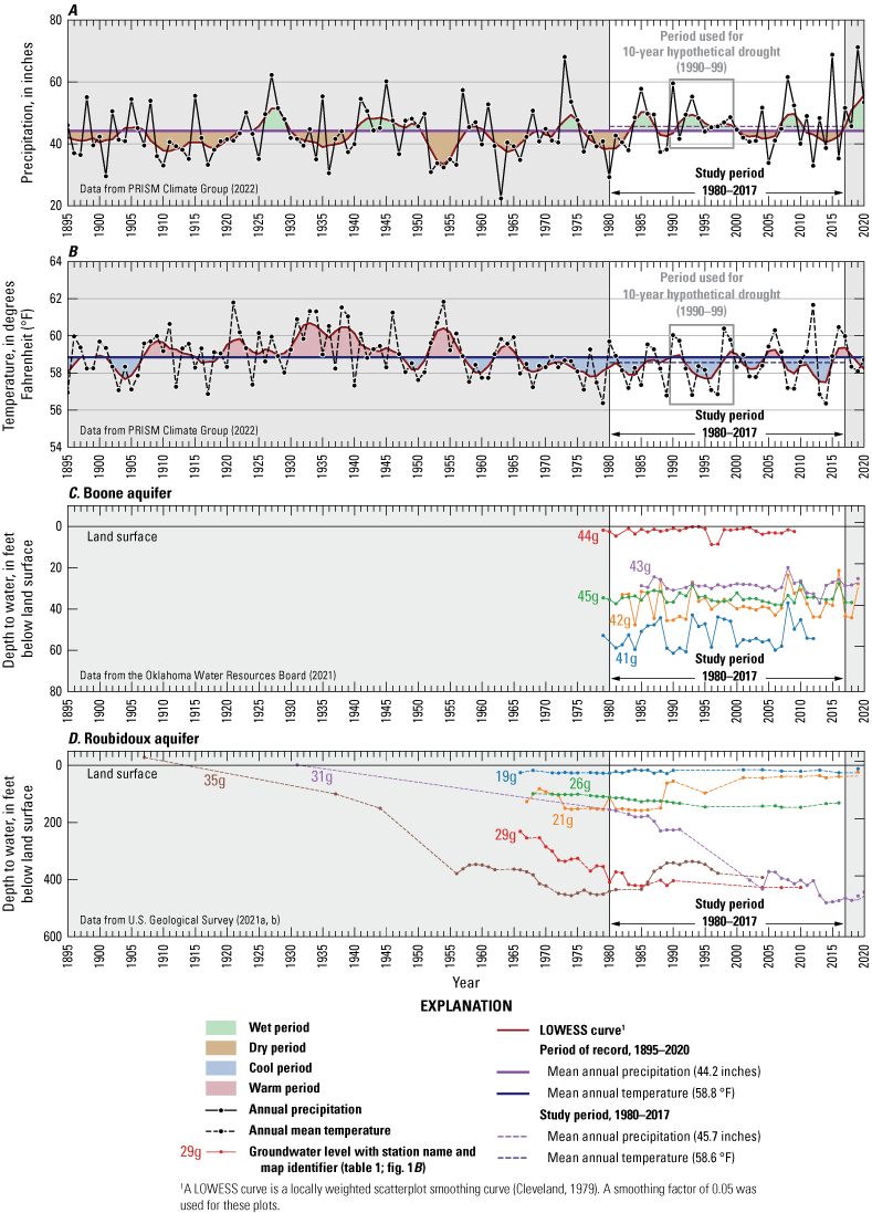
A, Long-term precipitation and B, long-term temperature data (1895–2020) from PRISM Climate Group (2022) for the study area and depth to water for selected groundwater wells for the C, Boone and D, Roubidoux aquifers.
Mean monthly precipitation was slightly higher for the study period (1980–2017) for most months compared to the period of record (1895–2020; fig. 4A). The largest differences were for November (about 0.5 inch [in.] more for the study period compared to the period of record) and December (about 0.25 in. more for the study period compared to the period of record). Mean monthly precipitation amounts during the study period for other months were approximately equal to mean monthly precipitation amounts for the period of record. The wettest month was May (mean precipitation was 5.90 in. for the study period and 5.69 in. for the period of record), and the driest months were January (2.22 in. for the study period and 2.29 in. for the period of record) and February (2.34 in. for the study period and 2.26 in. for the period of record; Trevisan and others, 2024).
Mean monthly temperatures were slightly cooler for the study period compared to those of the period of record (fig. 4B). July is typically the hottest month (mean temperature of about 80 degrees Fahrenheit), and January is typically the coolest month (mean temperature of about 36 degrees Fahrenheit).
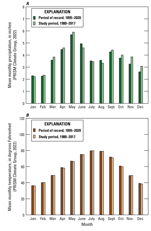
A, Mean monthly precipitation and B, mean monthly temperature for the long-term (1895–2020) period of record and the study period (1980–2017) for the study area in northeastern Oklahoma, southeastern Kansas, southwestern Missouri, and northwestern Arkansas.
Groundwater-Level Fluctuations in Response to Precipitation and Karst Development
Throughout the spatial extent of the Boone aquifer, groundwater levels often fluctuate between a relatively low or high level and remain approximately at or near those levels for periods of time even when precipitation varies (fig. 3C), which indicates that precipitation is not the only variable influencing groundwater-level fluctuations at these locations (Kresic, 2013; Murdoch and others, 2016). Groundwater levels in the Boone aquifer measured at relatively shallow depths below land surface were generally not as variable as those measured at greater depths below land surface (fig. 3C). Fractures and the conduits associated with karst development are common within the rocks that contain the Boone aquifer and can serve as pathways for enhancing the flow of water to the saturated zone of an aquifer (hereinafter referred to as “recharge”) (Imes and Emmett, 1994). If a well intersects multiple zones of the aquifer with high hydraulic property differences, then water levels could have multiple responses because one zone drains faster than the other, which is common in aquifers with karst development (Kresic, 2013). Alternatively, recharge could be restricted or delayed in areas of the aquifer with a larger amount of chert, which is composed of microcrystalline or cryptocrystalline quartz and is often characterized by low hydraulic conductivity unless it is sufficiently weathered or fractured (Minor, 2013; Murdoch and others, 2016). The manner in which chert, fractures, and conduits are distributed could have contributed to the short-term hydrograph patterns evident for groundwater levels in the Boone aquifer (at wells 41g and 42g for example [fig. 3C]), but it is difficult to ascertain patterns in groundwater levels related to karst development when using groundwater levels measured at an annual scale (Kresic, 2013).
For the Roubidoux aquifer, muted groundwater-level fluctuations in response to precipitation were likely caused by the relatively large (more than 5 miles) distances of the wells from the recharge zone where the aquifer was confined and by the relatively slow apparent groundwater velocities (as much as tens of thousands of years; Jurgens and others, 2022). Locations with large fluctuations in groundwater levels were often near groundwater wells with high withdrawal rates (more than 1,000 gallons per minute). In the Roubidoux aquifer, groundwater levels measured at well 365229094520201 (map identifier 35g) (table 1; fig. 3D) declined from artesian conditions (water flowed freely to the land surface without the need of a pump) in 1907 to more than 400 ft below land surface in 1974 as a result of prolonged large amounts of groundwater withdrawals in the area (Christenson and others, 1990).
Because some industrial wells in the area were taken offline, groundwater levels in well 35g rebounded by about 100 ft from 1985 to 1989 (fig. 3D; Christenson and others, 1990). Potentiometric-surface maps of the Roubidoux aquifer depicted large groundwater-level declines (more than 100 ft) around areas with high withdrawal rates (Gillip and others, 2008; Nottmeier, 2015), although groundwater use tends to be a small component of the conceptual water budget (Imes and Emmett, 1994; Hays and others, 2016) and the spatial extent of areas with large groundwater-level declines is relatively small (Gillip and others, 2008; Nottmeier, 2015). Large groundwater-level fluctuations (more than 100 ft per year in some instances) measured at well 355901094181401 (map identifier 21g) could also be influenced by the presence of chert, fracturing, and karst development, but the causes of the fluctuations were difficult to determine by using groundwater levels measured at an annual scale (fig. 3D).
Streamflow and Base-Flow Trends
Base flow and runoff are the major components of streamflow. Base flow is the amount of streamflow derived from groundwater discharge, and runoff is the component of streamflow contributed by direct precipitation, interflow, and overland flow (Freeze and Cherry, 1979). Estimation of base flow is important to determine the connection between an aquifer and a stream and is typically more important than runoff for sustaining streamflow throughout the year (Barlow and Leake, 2012). The fraction of base flow to streamflow is often referred to as the base-flow index (BFI) and is a useful statistic for analyzing the relation between streamflow and base flow over time (Wahl and Wahl, 1995).
For this report, USGS (2019) streamflow hydrograph data were separated into runoff and base-flow components by using the BFI method (Wahl and Wahl, 1995) implemented in the USGS Groundwater Toolbox (Barlow and others, 2015). Streamflow data used in the USGS Groundwater Toolbox are obtained from the NWIS (USGS, 2021a, b). The BFI method uses minimum daily streamflows at selected n-day bins (where n is the user-defined number of days and bins are n consecutive daily streamflow values). For the BFI method, the n-day bins are used to filter minimum daily streamflows to help estimate base flows, and “turning points” are selected from the minimum daily streamflows, that when scaled by 0.9, are less than those of temporally adjacent n-day bins. Base flows are then linearly interpolated between the selected turning points and aggregated to the desired monthly or annual temporal resolution. Multiple n-day bins were used to assess base flows computed with the BFI method. Mean base-flow index (percentage of streamflow that is base flow) was plotted against the n-day value; a 5-day bin was deemed appropriate for all streamgages because the slope was steeper when estimating base flow by using 4-day bins compared to 5-day or 6-day bins. Four streamgages with periods of record spanning the entire study period (1980–2017) and that were operated for a minimum 20 years prior to 1980 were selected for trend analysis (figs. 1A, 5A–D). Of the 43 selected streamgages present in the study area, data were collected for the entire study period at 15 streamgages (1980–2017; fig. 6A–D; table 1).
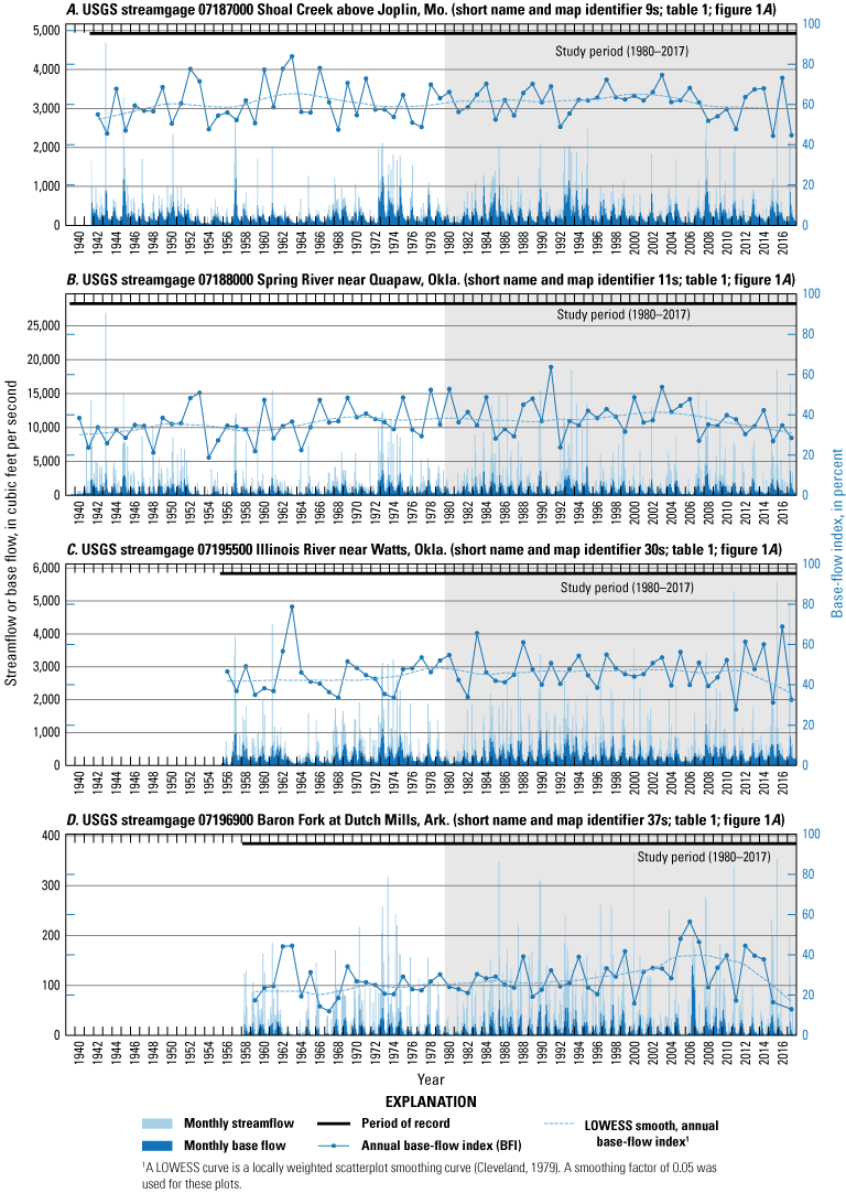
Monthly streamflow, monthly base flow, and annual base-flow index for selected U.S. Geological Survey (USGS) streamgages with at least 20 years of record prior to the study period (1980–2017): A, 07187000 Shoal Creek above Joplin, Mo. (streamgage 9s); B, 07188000 Spring River near Quapaw, Okla. (streamgage 11s); C, 07195500 Illinois River near Watts, Okla. (streamgage 30s), and D, 07196900 Baron Fork at Dutch Mills, Ark. (streamgage 37s).
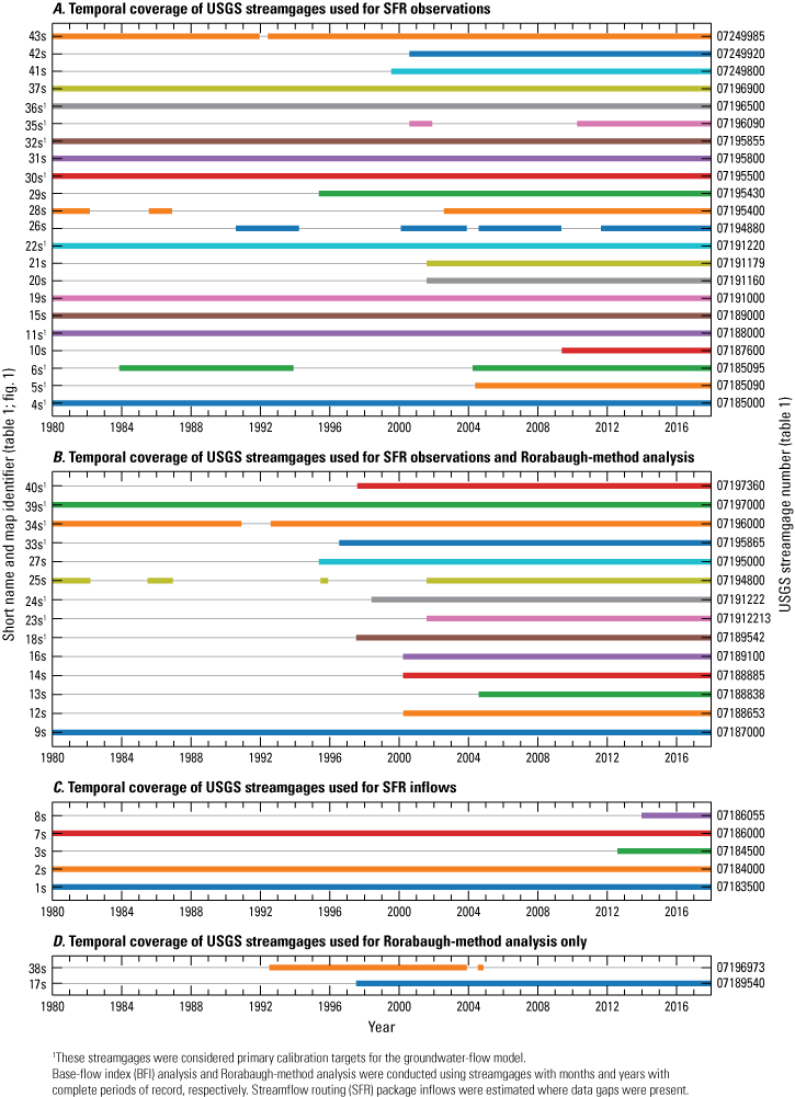
Temporal coverage during the 1980–2017 study period of U.S. Geological Survey (USGS) streamgages used for A, Streamflow Routing (SFR) observations, B, SFR observations and Rorabaugh-method analysis, C, SFR inflows, and D, Rorabaugh-method analysis.
Generally, the relation between streamflow and base flow followed similar patterns during the study period and prior to the study period (fig. 5A–D). Although locally weighted scatterplot smoothing (LOWESS) curves (Cleveland, 1979; Helsel and others, 2020) fitted to the base-flow index values varied somewhat over time, there were few statistically significant upward or downward trends, and the trends that were statistically significant were small (less than 0.22 cubic foot per second per year) (table 2; fig. 5A–D). From 2014 to 2017, a slight downward pattern in streamflow at some streamgages (fig. 5C, D) was present based on the LOWESS smoothing curve. This pattern could be caused by higher-than-normal precipitation after 2014 (fig. 3A), which would increase the runoff component of streamflow and the base-flow index (fig. 5A–D). Declining groundwater discharge to the streams could also reduce base flows; however, this would more likely occur during drier periods or in areas of high groundwater withdrawals.
Selected streamgages were analyzed for trends by using the Theil-Sen slope estimator and Kendall’s tau-b rank correlation statistic (table 2). The Theil-Sen slope estimator and Kendall’s tau-b rank correlation statistic (hereinafter referred to as “Kendall’s tau”) were calculated by using the SciPy (version 1.7.1; Virtanen and others, 2020) theilslopes and kendalltau functions, respectively. These statistics were also used to estimate trends and statistical significance of those trends for the periods of record at these streamgages (table 2; fig. 3). A 0.05 probability value (p-value) was used as the threshold to determine statistical significance. For these analyses, a p-value less than 0.05 indicates a greater than 95 percent likelihood that a trend exists in the data as represented by Kendall’s tau and the Theil-Sen slope (Helsel and others, 2020). Most long-term streamflows and base flows trends were upward but were not statistically significant at the 0.05 p-value for most of the selected streamgages (1940–2017; table 2; Helsel and others, 2020). Trends were statistically significant for base flow for USGS streamgages 0718800 Spring River near Quapaw, Okla. (streamgage 11s) and 07196900 Baron Fork at Dutch Mills, Ark. (streamgage 37s) and for base-flow index for streamgage 37s (tables 1–2; fig. 1A). The long-term streamflows and base flows may be increasing slightly over time at some streamgages, but upward trends (when present) were small, and Kendall’s tau was also small (about 0.20 or less). These upward trends could be caused by higher precipitation during the study period compared to the period of record (figs. 3A, 4A).
Table 2.
Theil-Sen slopes, Kendall’s tau, and p-values for the trends in annual streamflow, base flow, and base-flow index for selected streamgages for the period of record.[Streamgages were selected based on periods of record spanning at least 20 years prior to the 1980–2017 study period. Station information is provided in table 1; USGS, U.S. Geological Survey; ft3/s, cubic feet per second; p-value, probability value; Mo., Missouri; Okla., Oklahoma; Ark., Arkansas]
| USGS station number | Station short name and map identifier (fig. 1) | USGS station name | Annual streamflow | Annual base flow | Annual base-flow index | ||||||
|---|---|---|---|---|---|---|---|---|---|---|---|
| Theil-Sen slope, in ft3/s | Kendall's tau, dimensionless | p-value | Theil-Sen slope, in ft3/s | Kendall's tau, dimensionless | p-value | Theil-Sen slope, in percent per year | Kendall's tau, dimensionless | p-value1 | |||
| 07187000 | 9s | Shoal Creek above Joplin, Mo. | 1.59 | 0.12 | 0.13 | 0.91 | 0.13 | 0.10 | 0.05 | 0.08 | 0.33 |
| 07188000 | 11s | Spring River near Quapaw, Okla. | 10.09 | 0.12 | 0.11 | 4.63 | 0.19 | 0.01 | 0.06 | 0.14 | 0.06 |
| 07195500 | 30s | Illinois River near Watts, Okla. | 3.09 | 0.11 | 0.19 | 1.49 | 0.15 | 0.09 | 0.09 | 0.09 | 0.29 |
| 07196900 | 37s | Baron Fork at Dutch Mills, Ark. | 0.22 | 0.12 | 0.19 | 0.11 | 0.21 | 0.02 | 0.21 | 0.22 | 0.02 |
Groundwater Use Characteristics and Trends
The OWRB permits and regulates all groundwater use except for groundwater withdrawals of less than 5 acre-feet per year (acre-ft/yr that are used for domestic purposes for irrigating less than 3 acres of land for growing gardens, orchards, and lawns (82 OK Stat § 82-1020.1 [Oklahoma State Legislature, 2023b]). Permit holders self-report annual groundwater use to the OWRB; groundwater use for this study was acquired from the OWRB database of reported groundwater use from 1968 to 2018 (Christopher Neel, Water Rights Administration Division Chief, OWRB, written commun., 2020). Groundwater use reported to the OWRB was from prior right permits (landowners with wells established prior to regulation; OSS, 2023) and temporary permits (those given to landowners for wells completed in aquifers without a MAY designation by the OWRB; 82 OK Stat § 82-1020.1 [Oklahoma State Legislature, 2023a]). The OWRB also issues 90-day provisional temporary permits, but these permitted groundwater withdrawals were not included in the groundwater-use totals in this study because the 90-day provisional temporary permitted groundwater withdrawals were much less than the other types of permitted groundwater use.
Annual groundwater use from the OWRB was supplemented by groundwater-use estimates from other reports for groundwater use not collected (that is, not regulated) by the OWRB. These include groundwater use from the Western Interior Plains confining unit, domestic groundwater use in Oklahoma, and groundwater use in Kansas, Missouri, and Arkansas within the study area estimated through 2010 that were statistically modeled by using a combination of groundwater use reported by State agencies and USGS county-level groundwater-use estimates (Knierim and others, 2016, 2017).
Because reported groundwater use to the OWRB was relatively constant during 2010–18, the statistically modeled groundwater-use estimates for 2010 were assumed for 2011–18 (Knierim and others, 2016, 2017). Groundwater use was categorized as agricultural, domestic, public supply, and other. The “other” category includes groundwater use for fish and wildlife, recreation, livestock, irrigation, commercial, industrial, oil and gas, thermoelectric, and mining. The model archive associated with this report (Trevisan and others, 2024) contains (1) annual summaries of groundwater use by use type for all groundwater use in this report and (2) groundwater use by use type for domestic groundwater use and groundwater use in Kansas, Arkansas, and Missouri at the numerical groundwater-flow model grid-scale of this report. These data are provided without user-identifying information.
Groundwater-use permits in Oklahoma are primarily associated with wells in Delaware, Cherokee, and Adair Counties (fig. 7A) for the Boone aquifer, and with wells in Ottawa, Delaware, Craig, Cherokee, and Adair Counties for the Roubidoux aquifer (fig. 7B). Few groundwater-use permits were associated with wells in the southern part of the study area within Oklahoma (Muskogee and Sequoyah Counties; fig. 7A, B). There are fewer permits for groundwater withdrawals from the Boone aquifer (fig. 7A) than for withdrawals from the Roubidoux aquifer (fig. 7B). Agriculture and public-supply groundwater-use permits are the most commonly permitted use types (which excludes domestic use) for both aquifers. Permitted agriculture groundwater use and permitted public-supply groundwater use represent 15.6 and 79.9 percent of total permitted groundwater use, respectively, for the Boone aquifer (fig. 7A). In contrast, permitted agriculture groundwater use and permitted public-supply groundwater use represent 33.2 and 61.1 percent of total permitted groundwater use, respectively, for the Roubidoux aquifer (fig. 7B). Other permitted groundwater use represents approximately 5 percent of total permitted groundwater use for both aquifers.
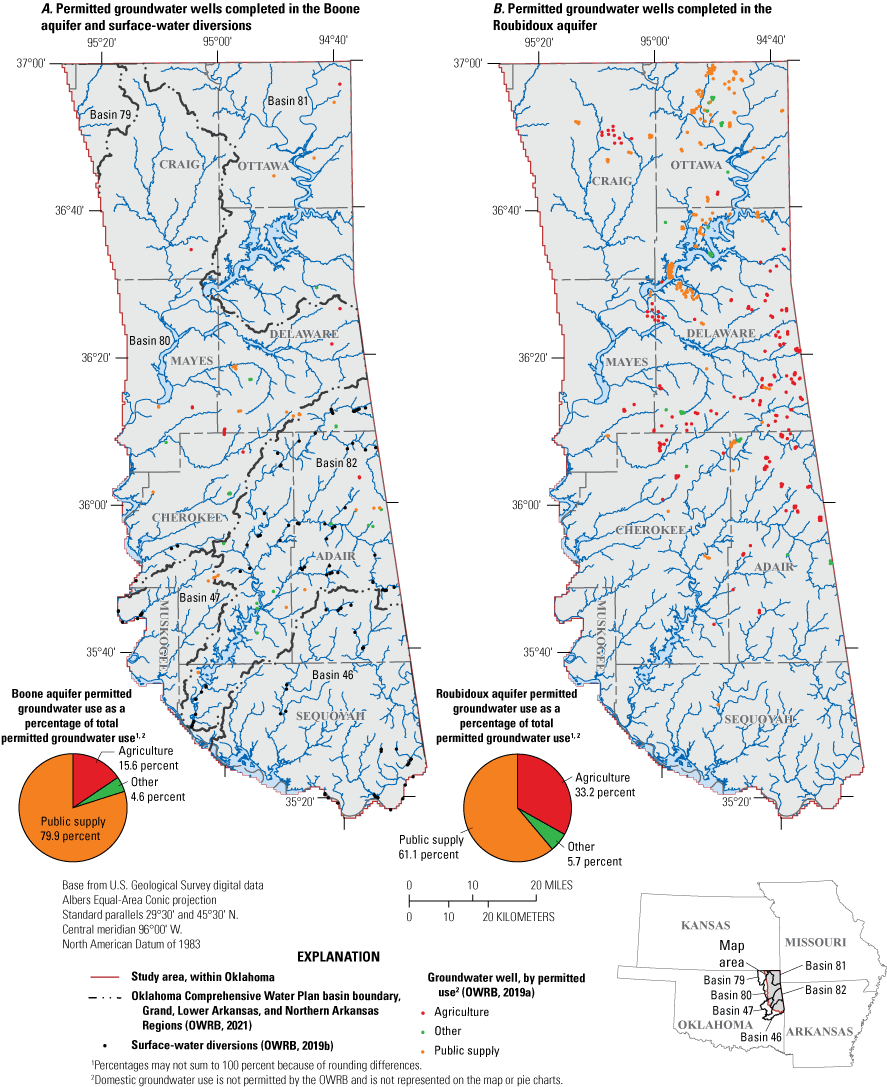
A, Permitted groundwater wells completed in the Boone aquifer (Oklahoma Water Resources Board [OWRB], 2019a), surface-water diversions (OWRB, 2019b), and Oklahoma Comprehensive Water Plan basin boundaries (OWRB, 2021), and B, permitted groundwater wells completed in the Roubidoux aquifer (OWRB, 2019a).
Groundwater use from the Boone and Roubidoux aquifers generally increased over time during 1968–2018 (fig. 8A, B, D; table 3), but groundwater use from the Boone aquifer within the study area declined after it peaked in the 1980s (fig. 8C). Within Oklahoma, groundwater use peaked in the late 1990s to early 2000s and then declined approximately 30 percent by 2018 for the Boone and Roubidoux aquifers (fig. 8A, B; table 3). Domestic groundwater use was the predominant use type for the Boone aquifer (fig. 8A, C; table 3). Public-supply groundwater use was the next highest use type but tended to be much less than domestic groundwater use for the Boone aquifer (fig. 8A, C; table 3). Public-supply groundwater use was typically the highest groundwater-use type for the Roubidoux aquifer (fig. 8B, D; table 3; Imes and Emmett, 1994). Domestic use was the next highest use after public supply for the Roubidoux aquifer (fig. 8B, D; table 3). Domestic use was not likely to affect groundwater levels as much as public-supply use because wells for domestic use typically withdraw less than 5 gallons per minute and are generally widely dispersed throughout the spatial extent of the aquifer. Because irrigation was not a major component of groundwater use, increased groundwater demand did not always correspond to drier periods when withdrawals would normally increase to sustain agricultural crops (fig. 8A–E; table 3).
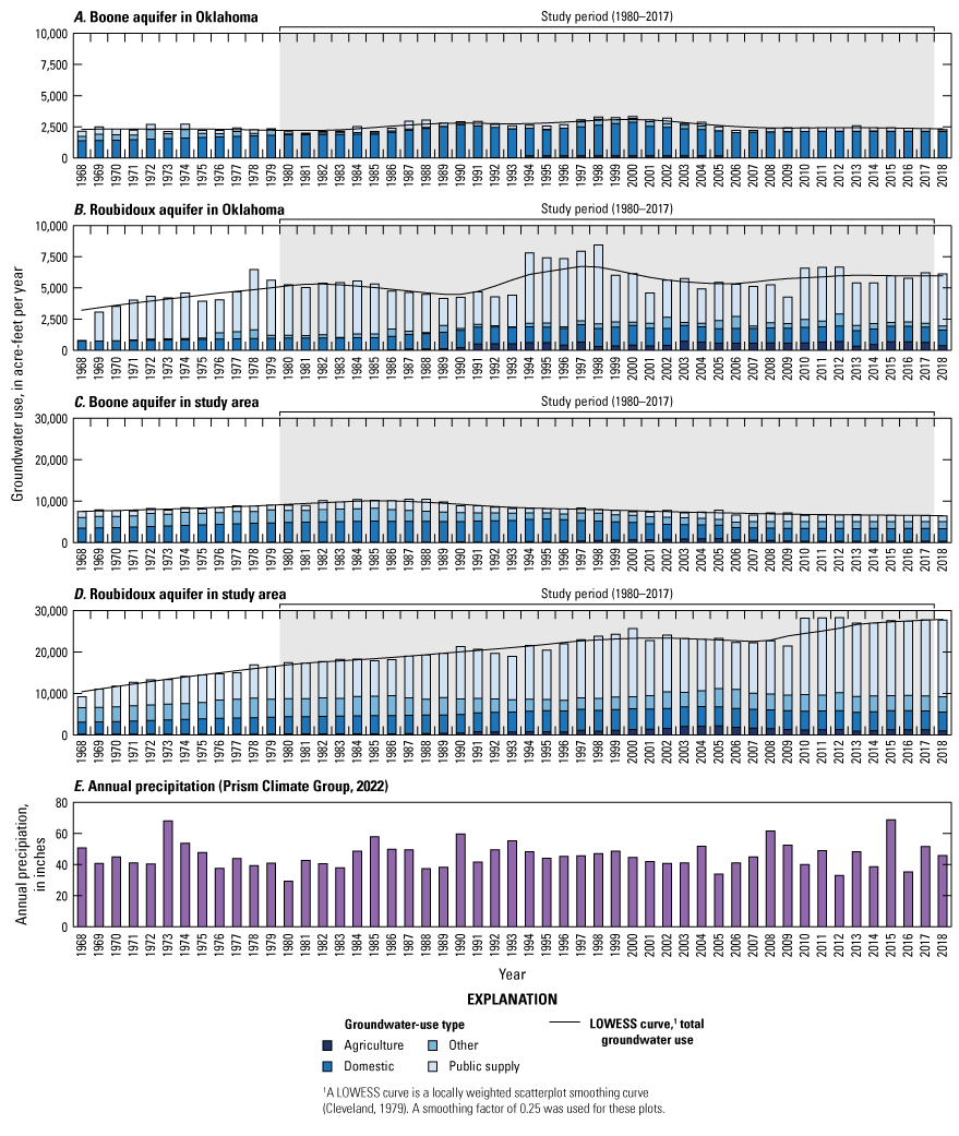
Historical (1968–2018) groundwater use by use type for the A, Boone aquifer in Oklahoma, B, the Roubidoux aquifer in Oklahoma, C, the Boone aquifer in the study area, and D, the Roubidoux aquifer in the study area and E, annual precipitation.
Table 3.
Annual reported groundwater use by use type from the Boone and Roubidoux aquifers, northeastern Oklahoma, 1968–2018.[acre-ft; acre feet]
Hydrogeologic Framework
A hydrogeologic framework characterizes the physical properties of aquifers and their confining units and the influence of those physical properties on groundwater chemistry and groundwater flow. A hydrogeologic framework was developed for the Boone and Roubidoux aquifers. The hydrogeologic framework includes (1) the hydrostratigraphy and lithology of the hydrogeologic units, (2) the spatial and vertical extents of the aquifers from Russell (2020), which were slightly modified based on information from Westerman and others (2016a), (3) potentiometric-surface maps for the Boone and Roubidoux aquifers, (4) descriptions of the hydraulic properties of aquifer materials, (5) an analysis of dissolved-solids concentrations in groundwater to assess potential saline-water migration within the aquifers, and (6) a geochemical analysis of dissolved ions to estimate the hydrologic connection between the Boone and Roubidoux aquifers.
Hydrogeologic Units
In order to simulate groundwater availability and groundwater flow, an important first step is to characterize the hydrogeologic units within the study area. The Western Interior Plains confining unit is the uppermost hydrogeologic unit in the study area. The Boone aquifer is mostly unconfined but is partially confined by the Western Interior Plains confining unit in the northwestern and southern parts of the study area. The Ozark confining unit underlies the Boone aquifer and confines the deeper parts of Roubidoux aquifer. The Roubidoux aquifer is mostly confined except in areas near streams where the overlying rocks have eroded away. The St. Francois confining unit underlies the Roubidoux aquifer, and the St. Francois aquifer underlies the St. Francois confining unit. The basement confining unit underlies the St. Francois aquifer (fig. 9). Within the study area, both the St. Francois aquifer and St. Francois confining unit are relatively thin compared to the other hydrogeologic units (Russell and Stivers, 2020), and flow between the Roubidoux aquifer and St. Francois aquifer is likely negligible (Imes and Emmett, 1994). The southern and southwestern boundaries of the Boone and Roubidoux aquifers are approximately delineated by the Arkansas River. In these areas, the Arkansas River acts as a sink and a regional flow boundary for the upper hydrogeologic units of the study area. Many of the hydrogeologic units composing the Western Interior Plains confining unit and Ozark confining unit or containing the Boone aquifer and Roubidoux aquifer are not considered part of the Ozark Plateaus aquifer system because groundwater becomes more saline as these rock units dip steeply southward and westward away from the study area southwest of the Arkansas River (Imes and Emmett, 1994). The extents of the hydrogeologic units used in this study were based on Russell (2020) with slight modifications to include the Arkansas River along the study area boundary by using the Ozark Plateaus aquifer system extents of Westerman and others (2016a).
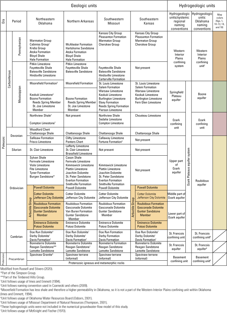
Geologic and hydrogeologic units of the study area in northeastern Oklahoma, northern Arkansas, southwestern Missouri, and southeastern Kansas (modified from Russell and Stivers, 2020, which was based on McKnight and Fischer, 1970; Imes and Emmett, 1994; Osborn, 2001; Thompson, 2001; Czarnecki and others, 2009; and Westerman and others, 2016b).
Hydrostratigraphy and Lithology
The major hydrogeologic units in the study area include the Western Interior Plains confining unit, the Boone aquifer, the Ozark confining unit, the Roubidoux aquifer, the St. Francois confining unit, and the St. Francois aquifer. The Western Interior Plains confining unit (Pennsylvanian and Mississippian age; fig. 9) overlies the Boone aquifer in parts of the study area. Below the Western Interior Plains confining unit is the Ozark Plateaus aquifer system. The Ozark Plateaus aquifer system is contained in Paleozoic-age sedimentary rocks and includes the Boone aquifer (contained in Mississippian-age rocks), the Ozark confining unit (Mississippian and Devonian age), the Roubidoux aquifer (contained in Cambrian- to Devonian-age rocks), and the St. Francois confining unit and St. Francois aquifer that both contain Cambrian-age rocks (fig. 9).
The uplifted part of the west-central Ozark Plateaus is commonly referred to as the Ozark Uplift (fig. 1) (Huffman, 1958; Jorgensen and others, 1993; Orndorff and others, 200198; Hudson and Murray, 2003; Weary and Schindler, 2004; Hudson and others, 2011). As a result of north-south compressional stresses during uplift events, the Ozark Uplift generally trends west along its major axis (Jorgensen and others, 1993; Orndorff and others, 2001; Hudson and Murray, 2003; Weary and Schindler, 2004; Hudson and others, 2011). Rocks within the study area generally dip away from the Ozark Uplift southward and westward toward the Arkansas River. In some locations within the study area, uplift and stream development spurred erosion of the rocks that contain the Boone aquifer and exposed the underlying rocks of the Ozark confining unit and Roubidoux aquifer. Naming conventions of geologic units vary among States (fig. 9). The Oklahoma geologic naming conventions are used in this report.
Western Interior Plains Confining Unit
The Western Interior Plains confining unit is present in the northwestern and southeastern parts of the study area (fig. 1A) and tends to thin from the study area boundary towards the interior of the study area (Russell and Stivers, 2020). The Western Interior Plains confining unit is mostly composed of Mississippian- to Pennsylvanian-age rocks (fig. 9). The available thickness data for Western Interior Plains confining unit in the study area were compiled and statistically summarized. The median thickness of the Western Interior Plains confining unit is 542 ft within the study area and 551 ft for Oklahoma (table 4). The Western Interior Plains confining unit mostly consists of shales but also of interbedded layers of sandstones and limestones in smaller quantities (Jorgensen and others, 1996; Westerman and others, 2016b). Although the Western Interior Plains confining unit is generally not considered water bearing, fracturing and the weathering of near-surface rocks (less than 300 ft below land surface) of the Western Interior Plains confining unit has increased the permeability of this confining unit in some areas, facilitating shallow groundwater flow in isolated locations (Imes and Emmett, 1994). In Oklahoma, the rocks of the Western Interior Plains confining unit tend to have less shale content and higher sandstone and limestone content compared to the rocks of the Western Interior Plains confining unit in Arkansas, Kansas, and Missouri. Therefore, groundwater yields from the Western Interior Plains confining unit within Oklahoma are often greater than groundwater yields from the Western Interior Plains confining unit outside of Oklahoma (Imes and Emmett, 1994; Hays and others, 2016).
Table 4.
Mean and median thicknesses of the Western Interior Plains confining unit, Boone aquifer, Ozark confining unit, and Roubidoux aquifer for the entire study area and for the part of the study area in Oklahoma.[Values are in feet. Values for Oklahoma are in parentheses. Based on data from Westerman and others (2016a)]
Boone Aquifer
The Boone aquifer (also known as the Springfield Plateau aquifer) is mostly unconfined within Oklahoma. From top to bottom, the rocks that contain the Boone aquifer predominantly consist of the Moorefield Formation, Keokuk Limestone, and Boone Formation (fig. 9). In Oklahoma, the Moorefield Formation consists of calcareous siltstones overlying black shale and oolitic limestone (Huffman, 1958) and is considered as one of the rock units that contain the Boone aquifer. In Arkansas, however, the shale content is greater and thus the Moorefield Formation is considered part of the Western Interior Plains confining unit (Hays and others, 2016). The Keokuk Limestone underlies the Moorefield Formation and is present in Oklahoma, Kansas, and Missouri (fig. 9). The Keokuk Limestone is usually blue-gray and is composed of tripolitic-chert-bearing limestone (Huffman, 1958; Bingham, 1969). The Keokuk Limestone is another important water-bearing unit for the Boone aquifer in northeastern Oklahoma. The Boone Formation (consisting of the Reeds Spring and St. Joe Limestone Members) underlies the Keokuk Limestone and contains various types of crinoidal, oolitic, and chert-rich limestones with occasional beds of chert-free limestone (McKnight and Fischer, 1970). The Boone Formation is the primary water-bearing unit of the Boone aquifer (fig. 10; Imes and Emmett, 1994). The St. Joe Limestone Member typically yields more groundwater than the Reed Springs Member or Keokuk Limestone because it contains much less chert than the Reed Springs Member or Keokuk Limestone (Hays and others, 2016). The Boone aquifer typically yields less than 50 gallons per minute of groundwater (OWRB, 2012a), but some wells have yielded as much as 1,000 gallons per minute of groundwater (Imes and Emmett, 1994).
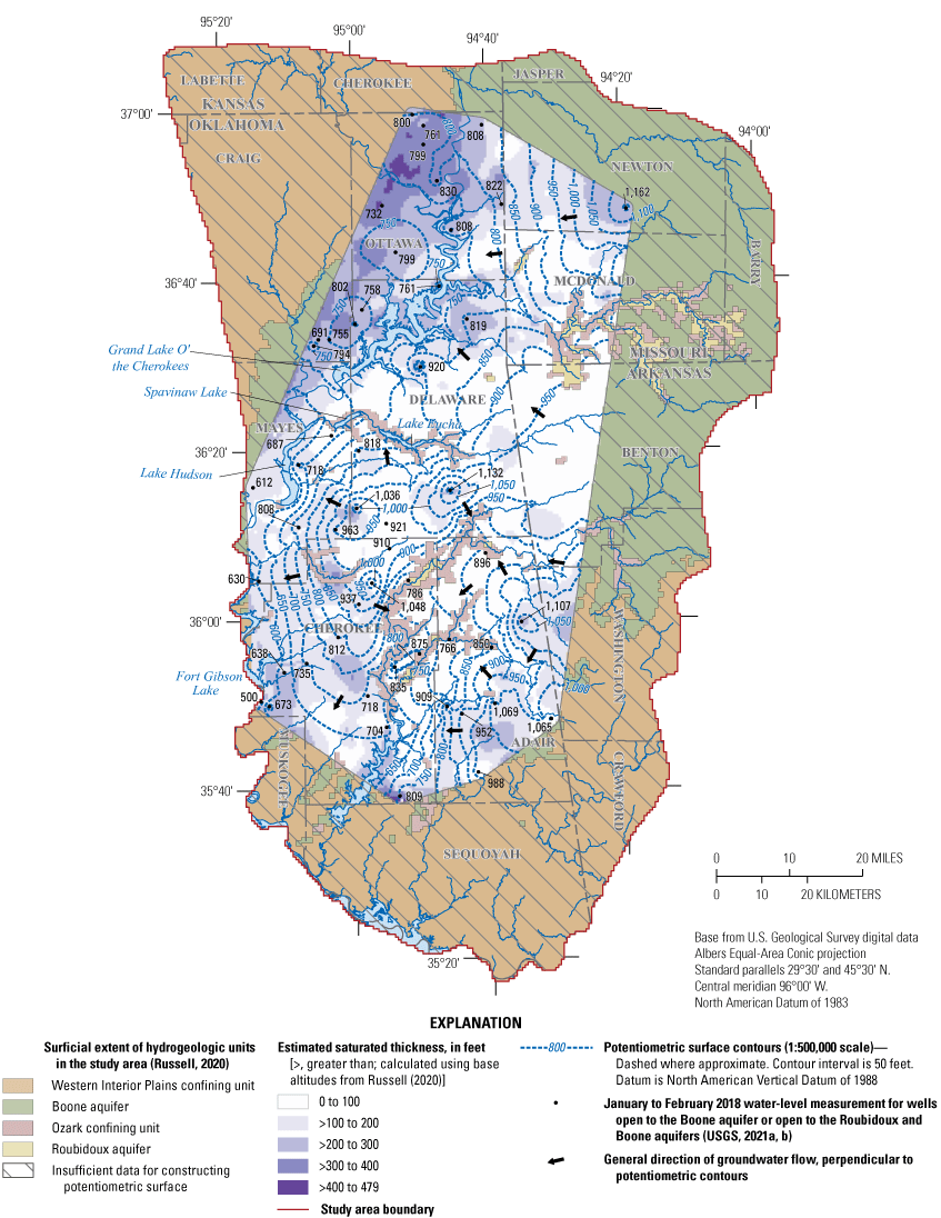
Potentiometric-surface contours and estimated saturated thickness of the Boone aquifer, January to February 2018, northeastern Oklahoma, northern Arkansas, southwestern Missouri, and southeastern Kansas.
The thickness of the Boone aquifer is relatively consistent throughout the study area except in areas where the unit has eroded away (Russell and Stivers, 2020). Median thickness of the Boone aquifer is 248 ft in the study area and 238 ft for Oklahoma (table 4). The tops of the rocks that contain the Boone aquifer are exposed at land surface except when the Western Interior Plains confining unit confines the aquifer from about the border between Cherokee County and Sequoyah County towards the Arkansas River and from a few miles northwest of Grand Lake O’ the Cherokees towards the western boundary of the aquifer and the northern extent of the study area (Russell and Stivers, 2020; fig. 1).
Secondary porosity, such as karst development and fracturing, controls the ability of the Boone aquifer to transmit water. The Boone aquifer has developed karst features such as caverns, enlarged fractures, and sinkholes owing to dissolution of soluble limestone along preferential-flow planes such as bedding planes and fracture traces. In some locations, as much as 70 percent of the thickness of the Boone aquifer is associated with chert (Brahana and others, 2009). The presence of chert in the Boone aquifer reduces its susceptibility to karst development and thus reduces yields relative to other aquifers within the Ozark Plateaus aquifer system. However, chert’s susceptibility to fracturing has enhanced permeability in some locations (Imes and Emmett, 1994).
Ozark Confining Unit
The Ozark confining unit limits groundwater flow between the overlying rocks of the Boone aquifer and underlying rocks of the Roubidoux aquifer. The Ozark confining unit mostly consists of Mississippian- and Devonian-age limestones and shales (fig. 9). In Oklahoma, the Ozark confining unit is composed, from top to bottom, of the Northview Shale, the Compton Limestone equivalent, the Woodford Chert, and the Chattanooga Shale. In the study area, the Ozark confining unit is mostly composed of Chattanooga Shale, and in some locations, this shale represents the entirety of the Ozark confining unit (Imes and Emmett, 1994). The Chattanooga Shale is a carbonaceous, pyritic, and fissile black shale that contains minor amounts of white sandstone at the base of the unit (McKnight and Fischer, 1970). Although the lithologic composition of the Ozark confining unit can be highly variable within the study area, leakance through the Ozark confining unit tends to be relatively low even in locations where shale content is low (Imes and Emmett, 1994).
The Ozark confining unit is present within most of the study area except for some small areas around streams where the rocks that compose the Ozark confining unit have eroded away, exposing the rocks that contain the Roubidoux aquifer (fig. 1B). The Ozark confining unit underlies the Boone aquifer and restricts groundwater flow between the Boone and Roubidoux aquifers. The Ozark confining unit is relatively thin compared to the rest of the hydrogeologic units in the study area, and median thickness is 43 ft within the study area and 47 ft within Oklahoma (table 4).
Roubidoux Aquifer
The Roubidoux aquifer is present throughout the entire study area and is mostly confined by the Ozark confining unit except near stream channels where rocks that compose the Ozark confining unit have eroded away. The Roubidoux aquifer is contained in Devonian- to Cambrian-age rocks (primarily limestones, dolomite, and sandstones; fig. 9). The Arbuckle Group is the thickest and highest-yielding unit of the Roubidoux aquifer (Christenson and others, 1990; Hays and others, 2016). The upper formations of the Arbuckle Group (from top to bottom, the Powell Dolomite, Cotter Dolomite, and Jefferson City Dolomite) are composed of dolomite with chert, sandstone, and occasionally shale lenses (Adamski and others, 1995). The Roubidoux Formation underlies the Jefferson City Dolomite (fig. 9) and is composed of sandstones, dolomite, and cherty dolomite (Thompson, 1991). The Gasconade Dolomite underlies the Roubidoux Formation; this unit occasionally contains sandy lenses, which typically yield large amounts of water (Imes and Emmett, 1994). At the base of the Gasconade Dolomite is the Gunter Sandstone Member, which is a fine- to coarse-grained sandstone with some dolomitic content (MacDonald and others, 1977). Underlying the Gunter Sandstone Member are the Eminence and Potosi Dolomites. The Eminence and Potosi Dolomites are similar in composition, consisting of fine- to coarse-grained dolomite with dense chert, drusy quartz, and occasionally glauconitic shale (Caplan, 1957, 1960). The Roubidoux aquifer is underlain by the St. Francois confining unit, which is composed of the Doe Run Dolomite, Derby Dolomite, and Davis Formation, all of Cambrian age. This confining unit restricts flow between the Roubidoux aquifer and the St. Francois aquifer. In the study area, the St. Francois confining unit and St. Francois aquifer are relatively thin (Russell and Stivers, 2020), and groundwater flow between the Roubidoux and St. Francois aquifers is likely negligible (Imes and Emmett, 1994).
The rocks that contain the Roubidoux aquifer dip toward the west from the Ozark uplift in southeastern Missouri towards Arkansas and Oklahoma; the Roubidoux aquifer is deepest in the southern part of the study area (Russell and Stivers, 2020). The aquifer is relatively thick, with a median thickness of 1,300 ft in the study area and 1,281 ft in Oklahoma (table 4). Secondary porosity (fracturing and karst development) is the main control on hydraulic properties (hydraulic conductivity, specific yield, and specific storage). Groundwater yields from the Roubidoux aquifer can be less than 10 gallons per minute and more than 1,000 gallons per minute (OWRB, 2012a).
Faulting
Most of the structural deformation of rocks associated with the Western Interior Plains confining unit, Boone aquifer, Ozark confining unit, and Roubidoux aquifer occurred during the Appalachian-Ouachita orogeny (Mississippian to Permian), when the rocks that contain the Ozark Plateaus aquifer system were compressed, resulting in normal and strike-slip faulting (Orndorff and others, 2001; Hudson and Murray, 2003; Weary and Schindler, 2004; Hudson and others, 2011; Hays and others, 2016). Russell and Stivers (2020) highlighted several regional, northeast-trending faults within the study area. However, offsets along the faults tend to be small relative to the overall thicknesses of the hydrogeologic units (McKnight and Fischer, 1970; Hudson and others, 2011) and do not strongly influence regional groundwater flows within the Ozark Plateaus aquifer system (Imes and Emmett, 1994).
Potentiometric Surface
The potentiometric surface is a representation of the groundwater altitude for an aquifer over a short period in time. Groundwater altitude is the height in feet above the North American Vertical Datum of 1988 to which the water level would rise under atmospheric pressure in a tightly cased well (Freeze and Cherry, 1979). According to Darcy’s law, groundwater flows from higher groundwater altitude to lower groundwater altitude or perpendicular to lines of equal groundwater altitude (Heath, 1983). The potentiometric surface provides insight into the general groundwater-flow direction and the groundwater-altitude features of an aquifer, such as depressions.
Potentiometric surfaces are not always sufficient to map groundwater altitude for karst systems; the heterogeneity in a karst system can produce discontinuities in groundwater altitude that cannot be represented as a spatially continuous, hypothetical surface (Kresic, 2013). That is, wells in close proximity can display large differences in groundwater altitude. Regardless, a potentiometric surface at a regional scale is likely appropriate because localized discontinuities in groundwater altitude do not likely affect regional groundwater flow as much as they affect local groundwater flow.
Water-level data collected between January 16, 2018, and February 23, 2018, were obtained from NWIS (USGS, 2021a, b) for the Boone and Roubidoux aquifers to construct potentiometric-surface maps for the Boone and Roubidoux aquifers. Methods described in Cunningham and Schalk (2011) were used to obtain water-level measurements. Groundwater levels were converted to groundwater altitudes by subtracting the depth to water from land-surface altitude sampled from the one-third arc-second digital elevation model (DEM; USGS, 2019). The one-third arc-second DEM was used because higher resolution digital elevation data were not available for the entire study area. Automated contouring was conducted in two steps: (1) interpolating a potentiometric surface from groundwater altitudes by using the ArcGIS Pro Topo to Raster tool (Esri, 2023a) and (2) contouring the resulting surface by using the ArcGIS Pro Contour tool (Esri, 2023b). Because the ArcGIS Pro Topo to Raster tool applies a spline that smooths the interpolation, a cell from the interpolated surface may have a different altitude than an input altitude within that cell (Esri, 2023c). Therefore, contours were manually adjusted to ensure that groundwater altitudes were appropriately represented by the contours. For the Boone aquifer, stream locations (as line features; EPA, 2020b; Esri, 2023a) and mean conservation pool altitudes for major lakes (OWRB, 2021; USACE, 2021) were used to include hydrography in the interpolation where the Boone aquifer was unconfined. For the Roubidoux aquifer, groundwater levels were not sufficiently dense to map certain depressions that were previously identified (Christenson and others, 1990; Gillip and others, 2008). Therefore, potentiometric-surface contours from Gillip and others (2008) were used to approximate the extent of the depressions. The annual precipitation in 2007 (44.8 in.) was similar to that of 2018 (45.8 in.); precipitation for both years approximated the mean annual precipitation of 44.2 in. during 1985–2020 (fig. 3A; Trevisan and others, 2024).
Typically, groundwater altitudes were highest in the eastern part of the study area and decreased westward (figs. 10, 11). In Delaware and Adair counties, groundwater from the Boone and Roubidoux aquifers generally flowed towards Spavinaw Lake, Eucha Lake, and Grand Lake O’ the Cherokees (figs. 10, 11). Regional groundwater-flow directions were similar to those of previous potentiometric-surface maps (Christenson and others, 1990; Jorgensen and others, 1993; Imes and Emmett, 1994; Gillip and others, 2008; Richards, 2010; Nottmeier, 2015), although some minor differences were present likely because of different time periods and spatial coverage of groundwater levels used (figs. 10, 11). Drawdown in parts of the Roubidoux aquifer in Ottawa and Craig Counties where there is extensive groundwater use has led to a persistent depression in the potentiometric surface (fig. 11; Christenson and others, 1990; Gillip and others, 2008). In Ottawa County, groundwater levels of the Roubidoux aquifer decreased by hundreds of feet but then rebounded by approximately 100 ft in the late 1980s (Christenson and others, 1990). This rebound was caused by the cessation of groundwater withdrawals from high-capacity well fields (Christenson and others, 1990). Because of similarities between previous potentiometric-surface maps and those from this report (figs. 10, 11), changes in groundwater storage were likely minimal in the long term (1993–2018).
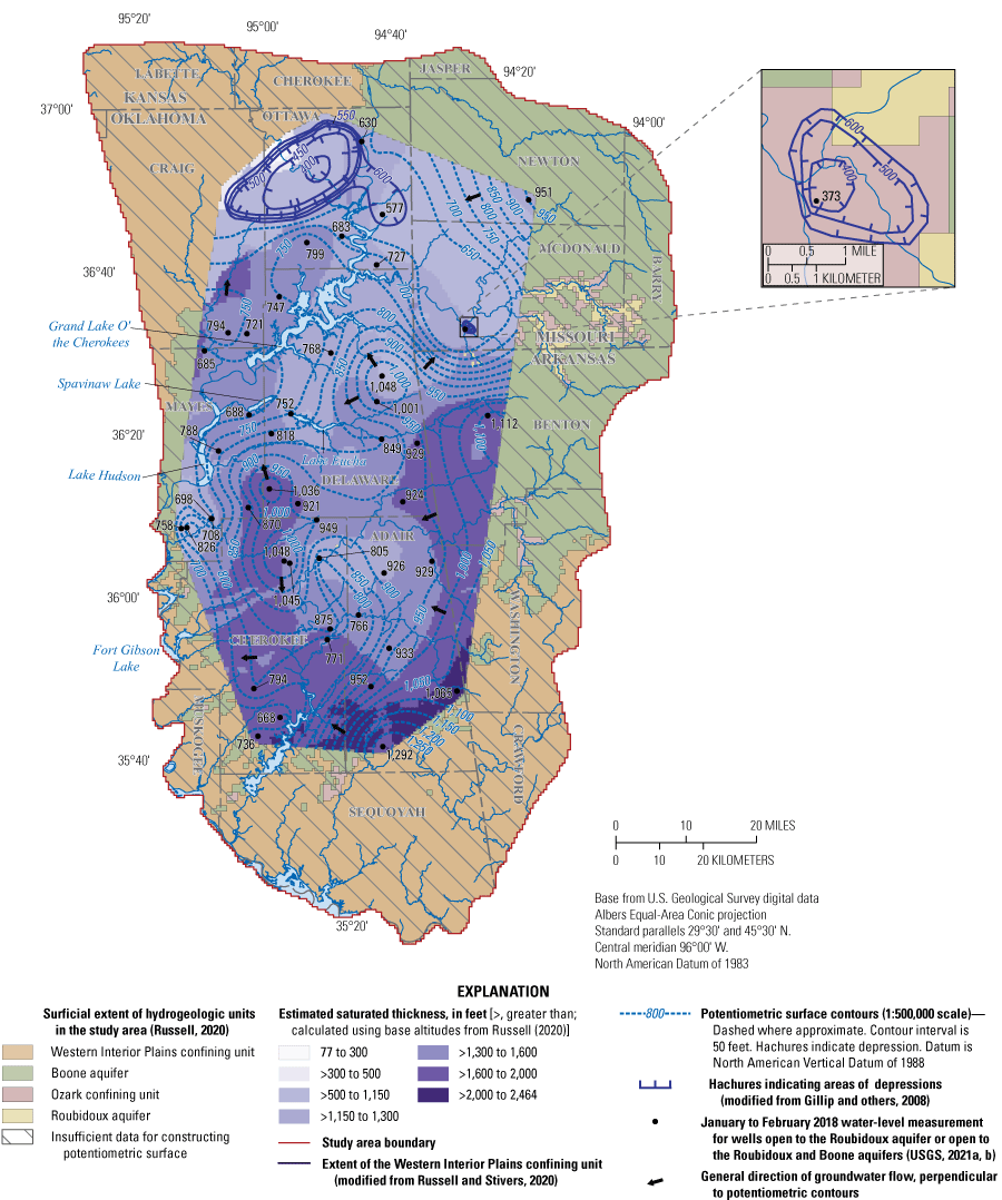
Potentiometric-surface contours and estimated saturated thickness of the Roubidoux aquifer, January to February 2018, northeastern Oklahoma, northern Arkansas, southwestern Missouri, and southeastern Kansas.
Hydraulic Properties
Hydraulic properties control how water flows through an aquifer and how much water is available for extraction from an aquifer. Hydraulic properties vary by the aquifer material, porosity, permeability, aquifer thickness, and saturation (Heath, 1983) and were assumed to be the primary control on groundwater flow for the Boone and Roubidoux aquifers. Hydraulic properties for the Boone and Roubidoux aquifers have been estimated through multi-well aquifer tests, specific-capacity tests, and numerical groundwater-flow modeling (hereinafter referred to as “groundwater-flow modeling”). The hydraulic properties for the Western Interior Plains confining unit, Boone aquifer, Ozark confining unit, and Roubidoux aquifer estimated in previous studies are summarized in table 5. Most hydraulic properties for the confining units (Western Interior Plains confining unit and Ozark confining unit) were estimated during previous groundwater-flow modeling studies (table 5)
Table 5.
Hydraulic properties for the Western Interior Plains confining unit, Boone aquifer, Ozark confining unit, and Roubidoux aquifer based on previous studies. (Modified from table 3 in Hays and others [2016]).[--, no data; ft/d, foot per day, ft−1, inverse feet; day−1, per day; approx., approximately; aquifer tests, multi-well-aquifer tests; groundwater modeling, numerical groundwater-flow modeling]
Boone Aquifer
Most of the hydraulic properties for the Boone aquifer have been estimated by using specific-capacity tests and from calibrated values obtained from previously published numerical groundwater-flow models (table 5); hydraulic-property data from previously published aquifer tests conducted by using multiple wells were not available. Horizonal hydraulic conductivity for the Boone aquifer generally ranged from 0.2 to 35.0 ft/d (table 5), but because of heterogeneity, horizontal hydraulic conductivity could be much higher locally in areas of extensive fracturing and karst development. Vertical hydraulic conductivity for the Boone aquifer is difficult to measure, and estimates obtained from groundwater-flow modeling were generally less than those for horizontal hydraulic conductivity. Estimates of vertical hydraulic conductivity ranged from 2.97×10⁻⁴ to 1.0 ft/d (table 5; Czarnecki and others, 2009). Estimates of specific yield (dimensionless) ranged from 0.003 to 0.20. Specific storage estimates ranged from 1×10⁻⁵ to 5×10⁻⁵ ft−1 and were based on values from previous groundwater-flow modeling studies (table 5). Hydraulic properties for the Boone aquifer were generally less variable than those for the Roubidoux aquifer.
Roubidoux Aquifer
Hydraulic properties for the entire Roubidoux aquifer were estimated from several multi-well aquifer tests, specific-capacity tests, and numerical groundwater-flow modeling (table 5). Horizontal hydraulic conductivity for the Roubidoux aquifer generally ranged from 8.64×10⁻⁴ to 86.4 feet per day (ft/d) (table 5; Imes and Emmett, 1994). Hydraulic conductivities in the study area likely represent a smaller range of values (about 0.1 to 31.9 ft/d; table 5; Macfarlane, 2007; Czarnecki and others, 2009). Vertical hydraulic conductivities for the Roubidoux aquifer are difficult to measure, and estimates from groundwater-flow modeling are generally less than estimates for horizontal hydraulic conductivities (table 5). Vertical hydraulic conductivity estimates ranged from 3.28×10⁻⁵ to 3.22 ft/d. Specific yield estimates from groundwater-flow modeling varied from 3×10⁻⁴ to 7.4995×10⁻², and specific storage estimates varied from 1×10⁻⁸ to 5×10⁻⁴ ft−1 (table 5).
Multi-well aquifer tests provide a robust methodology to estimate the hydraulic properties of an aquifer (Freeze and Cherry, 1979; Heath, 1983). For the Roubidoux aquifer, multi-well aquifer tests were conducted in Pittsburg, Kans. (Stramel, 1957; Macfarlane, 2007) and in Ottawa County, Okla. (Reed and others, 1955; Christenson and others, 1990).
Two multi-well aquifer tests were conducted in Pittsburg, Kans., for the Roubidoux aquifer (fig. 1; Macfarlane, 2007; Stramel, 1957). Estimated horizontal hydraulic conductivity from the first multi-well aquifer test ranged from 25.5 to 31.9 ft/d (table 5; Macfarlane, 2007). This estimate of hydraulic conductivity is typically higher than estimates of hydraulic conductivity from specific-capacity tests for the northern part of the study area (Macfarlane, 2007) and is likely higher than hydraulic conductivity within the study area (Imes and Emmett, 1994; Clark and others, 2018, 2019) or the Ozark Plateaus aquifer system (Pugh, 2008). Hydraulic conductivity was not calculated for the second study (Stramel, 1957), and estimated transmissivities were about two times greater than those of the first study (Macfarlane, 2007). A Theis solution (Heath, 1983) was used to estimate transmissivities for the multi-well aquifer test in the second study, and a Cooper-Jacob solution (Cooper and Jacob, 1946) was used to estimate transmissivities in the first study. A Cooper-Jacob solution is likely more appropriate for karst aquifers (Kresic, 2013).
Two studies analyzed multi-well aquifer tests for the Roubidoux aquifer in Ottawa County, Okla. The first study found that a Theis solution did not have strong agreement with data from the aquifer tests (Reed and others, 1955). Based on estimates of saturated thickness and transmissivities from this study, hydraulic conductivity ranged from about 9 to 13 ft/d (Reed and others, 1955). The second study re-analyzed these same multi-well aquifer tests assuming a leaky confining unit (Christenson and others, 1990). Estimates of transmissivities for the second study were about an order of magnitude less than those of the first study (Reed and others, 1955; Christenson and others, 1990; table 5). Estimates from the first study (Reed and others, 1955) were thought to be more representative of hydraulic conductivity for the Roubidoux aquifer near Ottawa County because these values are more similar to hydraulic conductivity estimated by using specific-capacity tests within the area (Macfarlane, 2007) and from previous groundwater modeling studies (Imes and Emmett, 1994; Czarnecki and others, 2009; Clark and others, 2018; table 5). Early-time groundwater levels were used to estimate hydraulic properties in the second study (Christenson and others, 1990). If karst features (such as conduits, vugs, or caves) were present in the aquifer, groundwater responses indicated by early-time groundwater levels would mostly represent water drained from the karst features and would be less representative of water drained from the aquifer matrix (Kresic, 2013). Using early-time groundwater levels with a Theis solution would result in lower estimates of hydraulic properties compared to using late-time groundwater levels for aquifers with karst development (p. 112 of Kresic, 2013). Thus, estimates for hydraulic properties from the first study (Reed and others, 1955) are likely more representative of the Roubidoux aquifer than estimates from the second study (Christenson and others, 1990).
Groundwater Quality
Dissolved-solids concentrations were the primary indicator of groundwater quality for this assessment. In addition to dissolved solids concentrations, groundwater quality was assessed for the Boone and Roubidoux aquifers by analyzing calcium carbonate, hardness, nitrate, radium-226, and radium-228.
Elevated dissolved-solids concentrations in groundwater can derive from a variety of sources such as dissolution of minerals, road salt or saline soils, connate seawater, and saltwater intrusion. Elevated dissolved-solids concentrations in the Ozark Plateaus aquifer system are derived from groundwater dissolution of salts from the Permian evaporites west of the study area; salty groundwater then flows eastward into the Paleozoic aquifers in eastern Oklahoma and Kansas (Nelson and others, 2015; Stanton and others, 2017). Salinity, as used in this report, is synonymous with dissolved-solids concentrations (Sharp, 2023). In some locations, the chloride-to-sulfate ratios of groundwater from the Ozark Plateaus aquifer system suggest that salinity is from connate seawater, but these locations are generally outside of the study area in Missouri (Miller, 1971; Baker and Leonard, 1995; Jorgensen and others, 1996). Chloride-to-sulfate ratios in groundwater from the Ozark Plateaus aquifer system are often greater than those in seawater, thus, Permian evaporites are the most likely source of salinity (Baker and Leonard, 1995; Nelson and others, 2015).
Precipitation is generally low in dissolved-solids concentrations, and dissolution of minerals in the rocks is often the main source of dissolved ions concentrations in groundwater (Hem, 1985). As precipitation recharges an aquifer, dissolved-solids concentrations in groundwater increase until equilibrium is achieved with the soluble minerals in the aquifer matrix (Hem, 1985).
Dissolved-solids concentrations in groundwater-quality samples were obtained from the USGS NWIS database (USGS, 2021a, b), the OWRB Groundwater Monitoring and Assessment Program (GMAP; OWRB, 2017), and the USGS National Produced Waters database (Blondes and others, 2018) for wells completed in the Boone aquifer, Roubidoux aquifer, and Western Interior Plains confining unit, or for wells completed in equivalent Paleozoic-age rocks outside of the study area. Dissolved-solids concentrations were used to assess spatial patterns in the concentration of groundwater salinity from the Boone and Roubidoux aquifers. Groundwater-quality samples collected outside of the study area were from wells completed in equivalent-age Paleozoic-age rocks but were not considered part of the same hydrogeologic units because of their extremely high salinity concentrations (more than 100,000 mg/L of dissolved solids). No concentrations for groundwater-quality samples listed in the GMAP database (OWRB, 2017) exceeded the OWRB freshwater regulatory limit of 5,000 mg/L. Groundwater samples from the GMAP database are only from Oklahoma (OWRB, 2017).
Groundwater-quality data from the GMAP were used to assess water quality of the Boone and Roubidoux aquifers with respect to EPA standards (OWRB, 2017; EPA, 2020a). Additionally, concentrations of various chemical constituents from the GMAP database were used to assess dominant anion and cation pairs to identify dominant hydrochemical facies throughout the aquifers and to assess the connectivity of the Boone and Roubidoux aquifers. Bumgarner and others (2012, p. 31) explain that hydrochemical facies “refers to a classification scheme used to describe water in terms of the major cation and anion milliequivalents composition.”
Dissolved-Solids Concentration Analysis
An analysis of dissolved-solids concentrations was done to assess potential salinity migration from evaporite-rich rock units in western Oklahoma and Kansas into the aquifers in the study area, and a geochemical analysis of dissolved ions was done to better understand the hydrologic connection between the Boone and Roubidoux aquifers. A saline transitional zone for the deep aquifers in the study area (which are typically contained in rocks of Paleozoic age) exists along the western boundary of the Ozark Plateaus aquifer system (fig. 12; Macfarlane and Hathaway, 1987; Jorgensen and others, 1993; Imes and Emmett, 1994; Macfarlane, 2010; Nelson and others, 2015). The identified saline transitional zone extended further eastward in Kansas and Missouri compared to Oklahoma (Macfarlane, 2010; Nelson and others, 2015). Groundwater within the saline transitional zone tends to be less saline than deeper groundwater residing in Paleozoic rocks west of the study area but slightly more saline than the groundwater residing in Paleozoic rocks in the study area (figs. 1A; Nelson and others, 2015). Dissolved-solids concentrations from groundwater in the Boone and Roubidoux aquifers within Oklahoma were mostly less than 5,000 mg/L (fig. 12).
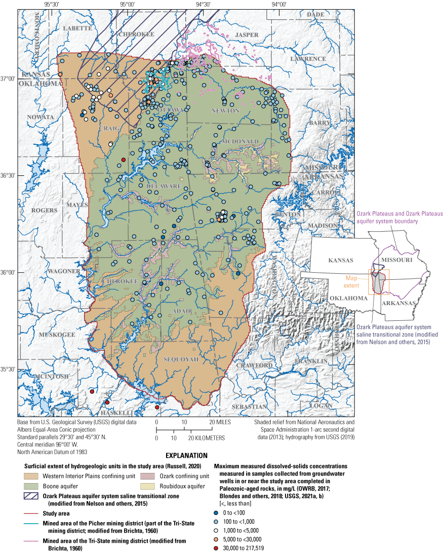
Maximum measured dissolved-solids concentrations in groundwater-quality samples from wells completed in Paleozoic-aged rocks, northeastern Oklahoma, northern Arkansas, southwestern Missouri, and southeastern Kansas.
Dissolved-solids concentrations in groundwater-quality samples collected from wells completed in the Roubidoux aquifer were usually higher than those in samples collected from wells completed in the Boone aquifer (fig. 13). Dissolved-solids concentrations listed in the GMAP database for groundwater-quality samples from wells completed in the Boone aquifer in Oklahoma ranged from 122 to 472 mg/L, with a mean concentration of 236 mg/L (OWRB, 2017). Dissolved-solids concentrations in groundwater-quality samples from wells completed in the Roubidoux aquifer ranged from 136 to 1,281 mg/L, and the mean and median concentrations were 474 and 330 mg/L, respectively. None of the dissolved-solids concentrations listed in the GMAP database were greater than the OWRB (2017) regulatory threshold of 5,000 mg/L for freshwater. Some concentrations for dissolved solids, however, did exceed the EPA’s secondary drinking water standard of 500 mg/L for dissolved-solids concentrations (EPA, 2020a).
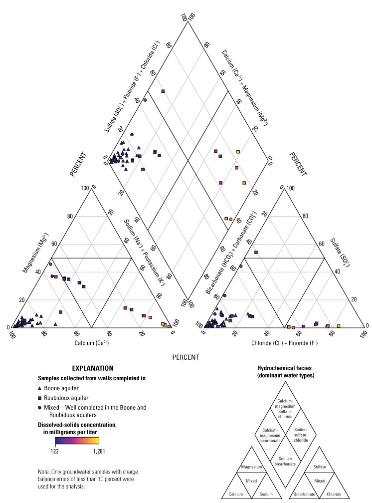
Piper diagram (Piper, 1944) showing major ions in groundwater-quality samples (Oklahoma Water Resources Board, 2017) considered in the major-ion analysis for wells in the Boone and Roubidoux aquifers, northeastern Oklahoma, 2017.
Within Oklahoma, hardness for groundwater-quality samples from wells completed in the Boone aquifer ranged from 100 to 326 mg/L of calcium carbonate, with a mean of 195 mg/L of calcium carbonate (OWRB, 2017). Hardness for groundwater-quality samples from wells completed in the Roubidoux aquifer ranged from 38 to 435 mg/L of calcium carbonate, with a mean of 141 mg/L of calcium carbonate.
The EPA sets primary drinking water standards for various contaminants (EPA, 2020a). The maximum contaminant level (MCL) is the permitted contaminant concentration limit for treated drinking water (EPA, 2020a). Although groundwater-quality samples collected from wells completed in the Boone or Roubidoux aquifer are not the same as treated drinking water, the EPA drinking water standards are still useful benchmarks for assessing groundwater quality. One groundwater-quality sample from the Boone aquifer exceeded the MCL for nitrate (10 mg/L; EPA, 2020a). Three groundwater-quality samples from the Roubidoux aquifer contained dissolved radium-226 and radium-228 concentrations exceeding the EPA’s MCL (5 picocuries per liter; OWRB, 2017). No other analyzed constituents exceeded the MCL standards (OWRB, 2017).
Dissolved Major-Ion Concentration Analysis
Dissolved major-ion concentration data from the GMAP program were plotted on a trilinear Piper diagram (Piper, 1944) to evaluate the hydrochemical facies, or dominant water types, for groundwater sampled from each aquifer by determining the relative abundance of major ions (fig. 13). Calcium, magnesium, sodium, potassium, sulfate, fluoride, chloride, bicarbonate, and carbonate were the major ions considered in the analysis. Groundwater-quality samples were excluded if the error for the milliequivalent ionic balance of the constituents was 10 percent or more. The hydrochemical facies were used to better understand the hydrogeologic connection between the Boone and Roubidoux aquifers and identify any groundwater-quality or groundwater-flow patterns.
The groundwater-quality samples were characterized as mostly calcium-bicarbonate dominant and sodium sulfate-chloride dominant (fig. 13). Groundwater-quality samples from wells completed in the Roubidoux aquifer generally had higher dissolved-solids concentrations compared to those from the Boone aquifer. When dissolved-solids concentrations were higher, groundwater-quality samples typically contained relatively large sodium and chloride ion concentrations. Groundwater-quality samples from wells completed in the Boone aquifer were mostly calcium-bicarbonate dominant; magnesium ions were present in lesser proportions than in the groundwater samples from the Roubidoux aquifer. Magnesium, calcium, and bicarbonate ions were likely from dissolution of the aquifer matrix by groundwater. The dissolved major-ion concentrations in groundwater-quality samples collected from wells completed in the Roubidoux aquifer were generally more dominated by magnesium and sodium ions compared to samples collected from wells completed in the Boone aquifer. Major-ion concentration differences indicate minimal groundwater flow between the Boone and Roubidoux aquifers in many areas. However, the hydrogeologic connection between the Boone and Roubidoux aquifers is difficult to conclusively determine from dissolved major-ion concentrations because both aquifers are contained in rocks composed of similar geology and geochemical characteristics.
Most of the samples for analysis of groundwater quality in the Roubidoux aquifer were collected in the northwestern part of the study area (fig. 12). Major-ion concentrations indicate that the water types of groundwater-quality samples in the northwest were generally sodium-sulfate dominant. These groundwater-quality samples were collected from wells that were close to the transitional saline zones identified by Macfarlane (2010) and Nelson and others (2015). The source of the sodium chloride ions was attributed to eastward flow of saline groundwater into the Roubidoux aquifer. A few samples collected from the Boone and Roubidoux aquifers in the southern part of the study area were sodium-chloride dominant. Salinity in these areas could potentially result from encroachment of saline groundwater from the west or the south (Macfarlane, 2010; Nelson and others, 2015). Groundwater salinity is high (more than 30,000 mg/L dissolved-solids concentration) for wells completed in Paleozoic-age rocks south and west of the Arkansas River (fig. 12; Nelson and others, 2015). Areas of groundwater containing elevated dissolved-solids concentrations (more than 5,000 mg/L) are isolated, and saline groundwater is not likely transported by groundwater flow, because regional groundwater-flow directions are generally towards the more saline groundwater in the west and the south (figs. 10, 11).
Dominant water types of samples collected from wells completed in different aquifers in the study area are depicted in figure 14 in relation to the spatial extent of the different hydrogeologic units in the study area. One groundwater-quality sample collected from a well completed in the Roubidoux aquifer was classified as calcium-magnesium sulfate-chloride water type. Eight groundwater-quality samples (seven from the wells completed in the Roubidoux aquifer and one completed in the Boone and Roubidoux aquifers) were classified as sodium sulfate-chloride water type. The remaining 44 groundwater-quality samples (from 31 wells completed in the Boone, 7 wells completed in the Roubidoux aquifer, and 6 wells completed in both the Boone and Roubidoux aquifers) were classified as calcium-magnesium bicarbonate water type. Typically, sulfate ions in groundwater in the Ozark Plateaus aquifer system in northern Oklahoma, eastern Kansas, and southwestern Missouri are derived from sulfate-bearing minerals within shales of the confining units of the Boone aquifer (Imes and Emmett, 1994; Adamski and others, 1995). Sulfate-bearing minerals are abundant in the Tri-state mining district (fig. 1; Spruill, 1987; Christenson, 1995; Petersen and others, 1998; DeHay, 2003; DeHay and others, 2004); sulfate ions in groundwater in the Tristate mining district derive mostly from sphalerite, galena, and chalcopyrites formed from hydrothermal fluids transported along fractures and fault planes (Wenz and others, 2012). High concentrations of sulfate ions in groundwater-quality samples from the Roubidoux aquifer likely indicated that the Boone and Roubidoux aquifers had a strong hydrogeologic connection where these samples were collected. Alternatively, many groundwater wells in the Picher mining district were completed in both the Boone and Roubidoux aquifers but have since been capped (IT Corporation, 1985). Abandoned wells open to both aquifers could also create a pathway for sulfate-rich groundwater to flow from the Boone aquifer into the Roubidoux aquifer.
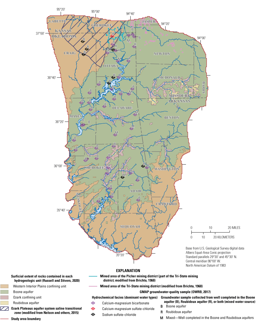
Location of wells with groundwater-quality samples analyzed for major ions, their dominant water type, and the aquifer from which the groundwater-quality sample was taken, northeastern Oklahoma, northern Arkansas, southwestern Missouri, and southeastern Kansas.
Overall, the water type of groundwater-quality samples collected from wells completed in the Boone aquifer tended to be calcium-bicarbonate dominant, and the water type of samples collected from wells completed in the Roubidoux aquifer tended to be calcium-bicarbonate or sodium sulfate-chloride dominant (fig. 14). In areas where the sampling results indicate that the Roubidoux aquifer contained groundwater that was sodium sulfate-chloride dominant, groundwater-quality samples collected from wells completed in the overlying Boone aquifer were not sodium-chloride dominant, indicating that mixing between the aquifers was likely minimal in these areas. Mixing is also likely minimal where the apparent groundwater age is on the order of only a few years. Apparent groundwater ages vary considerably in the study area, ranging from 3 to thousands of years (Jurgens and others, 2022). Groundwater-quality samples collected from wells completed in the Roubidoux aquifer contained higher ionic proportions of magnesium, likely because of the thicker dolomite-bearing formations in the rock units that contain the Roubidoux aquifer compared to those that contain the Boone aquifer (Imes and Emmett, 1994). Magnesium represented more than 20 percent of the ionic composition in some of the groundwater-quality samples collected from wells completed in the Boone aquifer (fig. 13). Dolomite is present in the Boone aquifer, and higher magnesium content could indicate a higher presence of dolomite in these areas. The different hydrochemical patterns for the waters of the Boone and Roubidoux aquifers indicate mixing of groundwater between the two aquifers is likely minimal at a regional scale but may be appreciable at a local scale.
Conceptualization of Groundwater-Flow System
A conceptual groundwater-flow model (hereinafter referred to as a “conceptual model”) is a representation or simplification of the groundwater-flow system created to describe groundwater flow across hydrologic boundaries. Hydrologic boundaries are locations where groundwater flows into or out of an aquifer, thus potentially affecting groundwater storage. The conceptual model in this report provides a simplified water budget for net groundwater flow across each identified hydrologic boundary based on the hydrogeologic framework, hydrologic controls, and climatic conditions.
This report presents two conceptual models: one conceptual model for the entire study area and one conceptual model for the part of the study area in Oklahoma (table 6). The conceptual models are subdivided to describe net flows (the difference between inflows and outflows for each water-budget category) for the Boone and Roubidoux aquifers. The conceptual models represent mean flows for the study period (1980–2017).
Table 6.
Inflows and outflows for the conceptual model for the Boone and Roubidoux aquifers within the study area in northeastern Oklahoma, southeastern Kansas, southwestern Missouri, and northwestern Arkansas and within the part of the study area in Oklahoma, 1980–2017.[Positive and negative values indicate flows into and out of the aquifer, respectively; RORA, a computer program within the USGS Groundwater Toolbox; WIPCS, Western Interior Plains confining system; OWRB, Oklahoma Water Resources Board; acre-ft/yr, acre-feet per year]
Recharge
Recharge for this report is defined as the amount of precipitation that percolates down to the saturated zone of the aquifer (sometimes referred to as diffuse recharge; Healy, 2010). Recharge is affected by precipitation rates, evapotranspiration rates, permeability, and moisture capacity of the unsaturated zone, and the topography of the land surface (Healy, 2010). Recharge varies spatially and temporally and is not easily measured directly but is often indirectly calculated from other groundwater-level measurements and climatological data (Healy, 2010). Recharge was estimated by using three methods: (1) the basin-scale recession-curve displacement method (Rorabaugh method; Rutledge, 1998); (2) the water-table fluctuation (WTF) method (Healy and Cook, 2002); and (3) the soil-water-balance (SWB) method (Westenbroek and others, 2010). Each method has different limitations. The Rorabaugh method is ideal for gaining streams with fast response times to precipitation events, but the Rorabaugh method generally overestimates recharge and is generally poor at estimating recharge at less than monthly intervals (Rutledge, 2000). The WTF method requires continuous collection of groundwater levels from groundwater wells that respond rapidly to precipitation events, but the WTF method requires knowledge of specific yield (which is often unknown) and likely can only reliably estimate recharge for a small area around the groundwater well (Healy and Cook, 2002). The SWB method is suited for regional recharge estimates at a coarser scale and at monthly or longer time periods, but the SWB method is a simulation that requires adjustment of model parameters to match estimates of spatially distributed recharge. Long-term recharge estimates for the conceptual model were made by using the Rorabaugh method because it was thought to be the most robust and appropriate method for the study area. The WTF method was used as a check of recharge from the Rorabaugh method. The SWB-method recharge was calibrated to the Rorabaugh-method recharge and was used to estimate temporally and spatially distributed recharge. Recharge estimates were likely more reasonable for the Boone aquifer compared to those of the Roubidoux aquifer because the rocks that contain the Roubidoux aquifer are exposed at land surface over a much smaller area compared to the relatively large surficial exposure of the rocks that contain the Boone aquifer (fig. 1).
Rorabaugh Method
The Rorabaugh method (Rorabaugh, 1964; Rutledge, 1998) is a hydrograph method for estimating basin-scale recharge. Rorabaugh-method-estimated recharge is proportional to the change in discharge between the pre-storm and post-storm recession curves at the critical time (the time after a peak where a linear recession is observed on a semi-log, daily discharge hydrograph) and is calculated by using the following equation:
whereR is the total volume of recharge, in cubic feet;
Q1 is the groundwater discharge at critical time (Tc) extrapolated from the pre-storm recession, in cubic feet per day;
Q2 is the groundwater discharge at Tc extrapolated from the post-storm recession, in cubic feet per day; and
K is the recession index (the time required for groundwater discharge to decrease by one log cycle after the recession curve becomes nearly linear on a daily, semi-log hydrograph).
For the Rorabaugh method, USGS streamgages were selected if the watershed drained mostly areas overlying the Boone and Roubidoux aquifers, and, for streamgages on the same stream, the farthest downstream streamgage that did not violate the assumptions or best practices of the Rorabaugh method (Rutledge, 2000). The Rorabaugh method is most appropriate for longer (annual) timeframes, basins with steeper relief, streams with watershed areas of 1–500 square miles, and streams that are gaining flow from the groundwater system (Rutledge, 2000). Some streamgages on smaller order streams were within the same watershed as larger order streams; however, long-term recharge was estimated by using a weighted mean based on the watershed area upstream from each streamgage. Compared to larger order streams, smaller order streams contribute a smaller component to the mean recharge because they drain smaller watershed areas, and any bias for the watershed-area-weighted mean annual recharge estimation is likely minimal where a greater number of streamgages were used within the selected watersheds.
RORA is a computer program within the USGS Groundwater Toolbox (Barlow and others, 2015) named after the developer of the Rorabaugh method (Rorabaugh, 1964) that allows the user to estimate recharge from streamflow by using a partially automated approach of the Rorabaugh method. For this program, streamflows and watershed areas from the USGS Groundwater Toolbox are downloaded from NWIS (USGS, 2021a, b). The RORA program was applied to selected streamgages (table 7) for continuous periods of record within the study period (1980–2017). To estimate long-term recharge, mean annual RORA-program estimated recharge values for each streamgage were averaged by computing a weighted mean; the weights consisted of the watershed area for a given streamgage divided by the sum of the watershed areas for all of the streamgages used for the RORA program. Watershed-area-weighted mean RORA-program estimated recharge (hereinafter referred to as “RORA-program estimated recharge”) was estimated to be 10.62 in/yr (tables 6, 7).
Table 7.
Watershed drainage area and mean annual RORA-program estimated recharge for selected USGS streamgages for the period from 1980 to 2017 where complete streamgage records were available.[--, not applicable; Mo., Missouri; Okla., Oklahoma; Ark., Arkansas; Recharge estimated by using the RORA program included in the U.S. Geological Survey (USGS) Groundwater Toolbox (Barlow and others, 2015)]
| USGS station number | USGS station name | Station short name and map identifier (table 1; fig. 1A) | Period analyzed | Mean annual RORA–program estimated recharge, in inches | Drainage area, in square miles |
|---|---|---|---|---|---|
| 07187000 | Shoal Creek above Joplin, Mo. | 9s | 1980–2017 | 12.47 | 427 |
| 07188653 | Big Sugar Creek near Powell, Mo. | 12s | 2002–17 | 8.48 | 141 |
| 07188838 | Little Sugar Creek near Pineville, Mo. | 13s | 2006–17 | 10.70 | 195 |
| 07188885 | Indian Creek near Lanagan, Mo. | 14s | 2002–17 | 10.03 | 239 |
| 07189100 | Buffalo Creek at Tiff City, Mo. | 16s | 2002–17 | 11.02 | 60.8 |
| 07189540 | Cave Springs Branch near South West City, Mo. | 17s | 1999–2017 | 7.16 | 8.00 |
| 07189542 | Honey Creek near South West City, Mo. | 18s | 1999–2017 | 9.65 | 48.7 |
| 071912213 | Spavinaw Creek near Colcord, Okla. | 23s | 2003–17 | 9.65 | 163 |
| 07191222 | Beaty Creek near Jay, Okla. | 24s | 2000–17 | 7.52 | 59.1 |
| 07194800 | Illinois River at Savoy, Ark. | 25s | 2003–15 | 8.13 | 167 |
| 07195000 | Osage Creek near Elm Springs, Ark. | 27s | 1997–2015 | 14.42 | 130 |
| 07195865 | Sager Creek near West Siloam Springs, Okla. | 33s | 1998–2017 | 12.74 | 19.1 |
| 07196000 | Flint Creek near Kansas, Okla. | 34s | 1994–2017 | 10.05 | 116 |
| 07196973 | Peacheater Creek at Christie, Okla. | 38s | 1994–2002 | 11.40 | 25.0 |
| 07197000 | Baron Fork at Eldon, Okla. | 39s | 1980–2017 | 10.46 | 312 |
| 07197360 | Caney Creek near Barber, Okla. | 40s | 1999–2017 | 10.81 | 90.2 |
| Mean | -- | -- | -- | 110.29 (10.38) | -- |
| Watershed-area-weighted mean | -- | -- | -- | 110.62 (10.14) | -- |
RORA-program estimated recharge was similar to recharge estimated by Hays and others (2016) by using the SWB method for the entire Ozark Plateaus aquifer system (mean annual recharge of 11 in/yr). Hays and others (2016) estimated recharge ranging from 0.4 to 15 in/yr (about 30 percent of precipitation) for the entire Ozark Plateaus aquifer system. Hydraulic properties within the study area tend to be slightly lower than other areas of the Ozark Plateaus aquifer system (Imes and Emmett, 1994), and thus recharge is likely less for the study area compared to the entire Ozark Plateaus aquifer system. For the study period (1980–2017), the RORA-program estimated recharge of 10.62 in/yr constituted about 23 percent of mean annual precipitation (45.7 in.; figs. 3A, 8E). RORA-program estimated recharge of 10.62 in/yr is similar to the 10.5 in/yr of recharge estimated for the Boone aquifer by the OWRB (OWRB, 2012a) and is in the range of 5 to 15 in/yr from Dugan and Peckenpaugh (1985) within the study area (fig. 1A).
RORA-program estimated recharge was used for conceptual model recharge estimates by applying the estimate to the land-surface areas where the rocks that contain the Boone and Roubidoux aquifers are exposed at land surface. Additionally, RORA-program estimated recharge was compared to recharge estimates from other methods used in this study.
Water-Table Fluctuation Method
The WTF method is a recharge estimation technique that assumes recharge is the main factor causing short-term, daily to weekly rises in water-table altitude following precipitation events (Healy and Cook, 2002). This method is best suited for groundwater wells instrumented with continuous recorders (hereinafter referred to as “groundwater gages”) with hydrographs that display rapid rises in response to precipitation (Healy and Cook, 2002). The WTF method estimates recharge at a groundwater well by using the following equation:
whereR
is recharge, in inches per year;
Sy
is the specific yield of the aquifer (dimensionless);
Δh
is the change in water-level altitude, in inches; and
Δt
is the change in time, in years.
Several groundwater gages were installed in the Boone and Roubidoux aquifers (fig. 1B). Two groundwater gages—well 5g (USGS well 355741094461001; table 1) in Adair County and well 9g (USGS well 361317094594101; table 1) in Delaware county (fig. 1B)—were completed in the Boone aquifer and were selected for the WTF method based on their suitability with respect to the assumptions inherent to the WTF method (fig. 15A, B). Other groundwater gages were excluded from the WTF method for various reasons. For example, if the groundwater gage was near a stream, it could be difficult to determine if rises were caused by precipitation or by groundwater inflows. Groundwater gages were also excluded if they were near karst development or chert, which could potentially affect vertical recharge (figs. 1B; for example, groundwater gages 6g, 12g, 15g; 15C) (p. 125 in Kresic, 2013; Murdoch and others, 2016). Other reasons to exclude gages were if the hydrographs displayed a subdued, delayed, or nonexistent response to precipitation (for example, groundwater gages 3g, 10g, and 14g; fig. 15D), or the well at the gage was completed under confined conditions (for example, groundwater gages 2g, 8g, 11g, and 13g; fig. 15E). In these instances, the WTF method would not be suitable for the groundwater gages because recharge was not rapidly reaching the water table or rises were not likely solely caused by recharge (if, after each precipitation event, groundwater levels rose to approximately the same level regardless of the quantity of precipitation). A dimensionless specific yield value of 0.01 was used for the WTF method based on specific yield estimates from previous studies of the Boone aquifer (table 5).
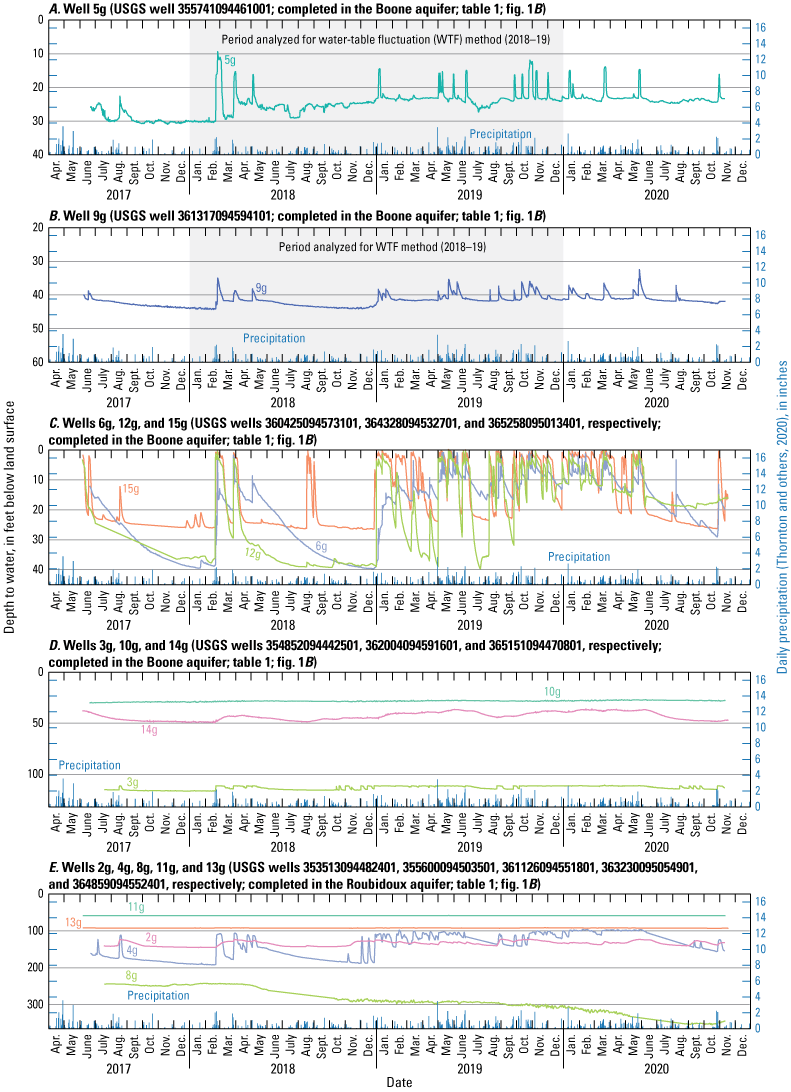
Groundwater levels (depth to water, in feet below land surface) measured from April 2017 to December 2020 at U.S. Geological Survey (USGS) wells A, USGS well 5g, B, USGS well 9g, C, USGS wells 6g, 12g, and 15g, and D, 3g, 10g, and 14g, and E, USGS wells 2g, 4g, 8g, 11g, and 13g, completed in the Boone and Roubidoux aquifers, and precipitation, northeastern Oklahoma, southeastern Kansas, southwestern Missouri, and northwestern Arkansas.
Mean WTF-estimated recharge for 2018–19 was 6.9 in/yr (10.6 percent of mean annual precipitation; table 8). This value was about two-thirds as much as the mean RORA-program estimated recharge (10.62 in/yr; table 7). Many factors, such as groundwater levels not responding to precipitation or an underestimation of specific yield, could contribute to low estimates of recharge. Also, the periods analyzed were not the same; data collected during 2018–19 were used for the WTF method, and data collected during 1980 to 2017 were used for the RORA method (periods of record for some streamgages did not span this entire period). Additionally, precipitation for the WTF analyzed period was typically higher than normal (fig. 3A).
Table 8.
Water-table fluctuation method (WTF) results for comparison of recharge for groundwater wells completed in the Boone aquifer with mean annual Daymet precipitation data (Thornton and others, 2020).[Specific yield of 0.01 was based on values from previous studies (table 5) for the Boone aquifer and was used to calculate recharge. Additionally, a specific yield was provided that would match RORA-program estimated recharge based on the sum of water-level rises]
| Short name and map identifier (table 1; fig. 1A) | Sum of rises during 2018–19 | Specific yield (table 5), dimensionless |
Recharge, in inches per year |
Mean annual Daymet precipitation data, 2018–19, in inches per year |
Recharge per mean annual precipitation, in percent |
Specific yield to match RORA-program estimated recharge, dimensionless |
|
|---|---|---|---|---|---|---|---|
| Feet | Inches | ||||||
| 5g | 160.5 | 1,925.4 | 0.01 | 9.6 | 62.9 | 14.8 | 0.011 |
| 9g | 70.9 | 850.2 | 0.01 | 4.3 | 62.9 | 6.5 | 0.025 |
| Mean | 115.7 | 1,387.8 | 0.01 | 6.9 | 62.9 | 10.6 | 0.015 |
WTF-estimated recharge was not used to develop estimates of long-term recharge for the conceptual model for several reasons. The WTF-estimated recharge was likely less reliable than the estimate obtained by using the RORA method because specific yield for the Boone aquifer is likely highly variable and the period of record of groundwater gages used in the WTF method was short (2 years).
Soil-Water-Balance Method
For the 1980–2017 study period, spatially distributed recharge within the study area was estimated by using the SWB method (Westenbroek and others, 2010). The computer code in the SWB method requires climatological (precipitation and temperature) and landscape (soil-water storage capacity, hydrologic soil group, land-surface gradient, and land-cover type) characteristics as input files in order to estimate recharge. Various sources were used to compile data for the input files to the SWB computer code; these input files and the output files are included in the associated data release (Trevisan and others, 2024). The SWB method uses a gridded data structure to determine the amount of infiltration resulting from precipitation that exceeds the storage capacity of the plant root zone (the depth below ground surface to which plant roots extend) and evapotranspiration demand.
The SWB method is used to simulate recharge by applying a modified version of the Thornthwaite-Mather method (Thornthwaite and Mather, 1957). The grid used for the SWB method consisted of 354 rows and 261 columns discretized into cells; each cell covered an area of 2,000 by 2,000 ft. The Hargreaves and Samani (1985) method for a reference latitude range of 34.5–35.5 degrees was used to estimate evapotranspiration for the SWB recharge simulation. Land-cover types were used to assign curve numbers (related to antecedent runoff potential) and plant root-zone depths for each cell. The default SWB plant root-zone depths ranged from 0 to 4.5 ft (Westenbroek and others, 2010). Because the root-zone depths are not well known and are highly sensitive to SWB recharge estimation, the root-zone depths were adjusted to calibrate to the conceptual model recharge (RORA-program estimated recharge). Root-zone depths from Westenbroek and others (2010) were for plants in Wisconsin; however, root-zone depths for Oklahoma are largely unknown, and root zones in the shales and limestones of the confining units and aquifers in the study area likely preclude deep root penetration (Schenk, 2008; Estrada-Medina and others, 2013). Root-zone depths were therefore reduced to better match conceptual model recharge (RORA-program estimated recharge). To match RORA-program estimated recharge, only the part of the study area where the Western Interior Plains confining unit was not present was used to calculate mean recharge for each array in the SWB simulation (1980–2017). The final root-zone depths were scaled to 27 percent of the original root-zone depths from Westenbroek and others (2010).
Daily precipitation, minimum temperature, and maximum temperature grids from 1980 to 2017 were obtained from the Daymet database (version 4; Thornton and others, 2020) and were used as inputs to the SWB code. Annual precipitation in the Daymet database (fig. 16C) was slightly higher than that from the PRISM Climate Group (2022) (fig. 3A); however, daily gridded climate data were not available from PRISM Climate Group (2022) for the entire 1980–2017 study period. Tabular summaries of the Daymet (Thornton and others, 2020) and PRISM Climate Group (2022) annual and monthly precipitation and annual and monthly SWB recharge can be found in Trevisan and others (2024). Soil-water storage capacity and hydrologic soil group data were obtained from the Gridded Soil Survey Geographic Database (U.S. Department of Agriculture, 2021) and sampled to the SWB model grid resolution. The land-surface gradient was obtained by using the D8 method (O’Callaghan and Mark, 1984) and was calculated from a one-third arc-second DEM (USGS, 2019) after resampling to the SWB model grid resolution using a mean land-surface altitude for each cell and filling sinks. Land-surface gradient is used by the SWB code to route runoff between cells. Land-cover types were obtained from the National Land Cover Database (Multi-Resolution Land Characteristics Consortium, 2021) and resampled to the SWB model grid resolution by using the most common land-cover type within each cell.
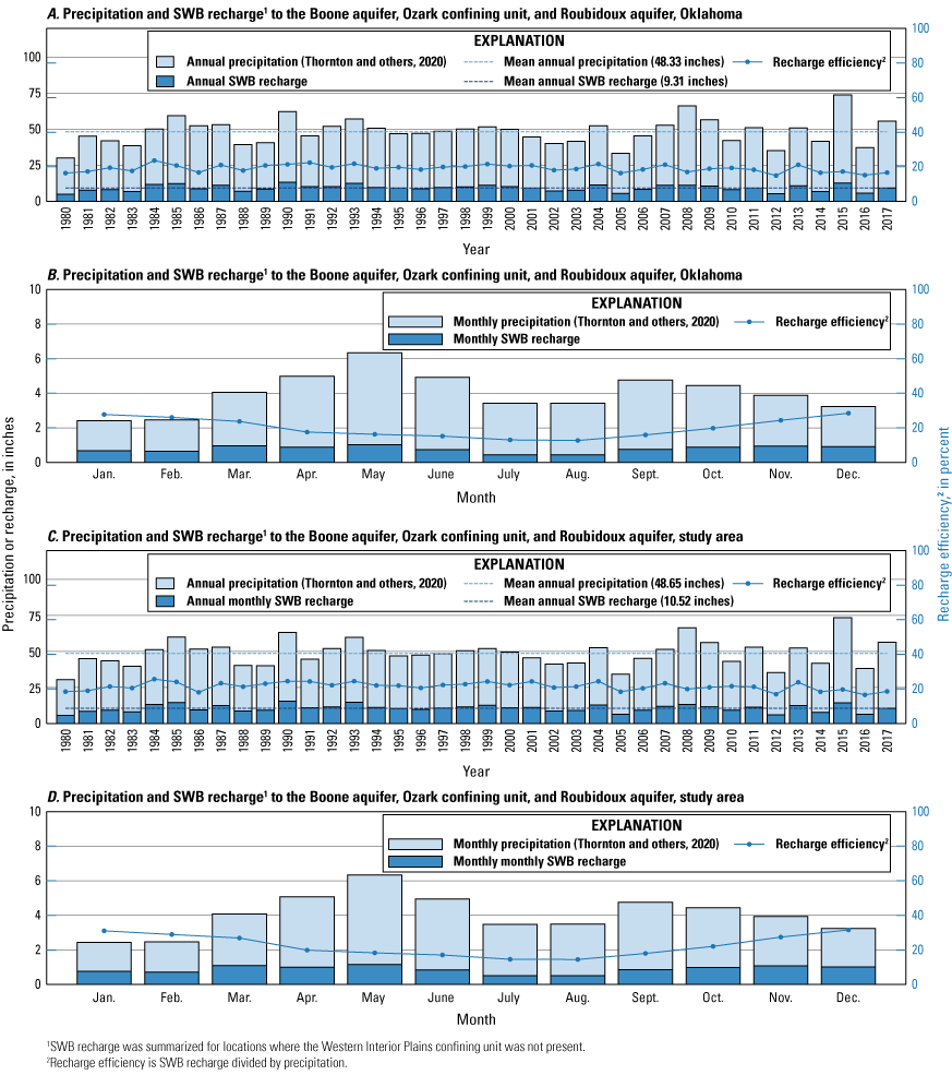
Annual precipitation and soil-water-balance (SWB) recharge and recharge efficiency for A, Oklahoma and C, the study area and monthly precipitation and SWB recharge for B, Oklahoma and D, the study area, 1980–2017.
Mean annual SWB recharge was 10.52 in. (fig. 16C) for parts of the study area where the Western Interior Plains confining unit was not present and was about 22 percent of Daymet mean annual precipitation (Thornton and others, 2020) over the 1980–2017 study period (48.65 in.; fig. 16C). Mean monthly and mean annual SWB recharge values were slightly lower in Oklahoma (0.78 and 9.31 in., respectively; Trevisan and others, 2024). Mean annual SWB recharge was typically less than 9 in. and ranged from 0 to 32.76 in. (fig. 17).
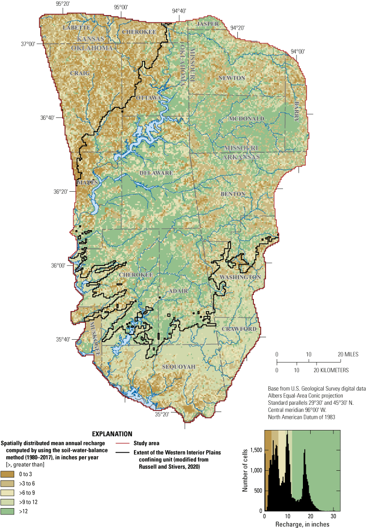
Spatially distributed mean annual recharge computed by using the soil-water-balance method (Westenbroek and others, 2010) for the study area in northeastern Oklahoma, southeastern Kansas, southwestern Missouri, and northwestern Arkansas, 1980–2017.
The locations with the highest mean annual SWB recharge were generally in the central and northeastern parts of the study area where rocks that contain the Boone and Roubidoux aquifers are exposed at land surface (fig. 17). SWB recharge tends to be lowest in the northwestern and southern parts of the study area. Where the Western Interior Plains confining unit is the uppermost hydrogeologic unit, mean annual SWB recharge was typically less than 9 in., and frequently less than 6 in. (fig. 17). All open-water features (lakes and ponds) identified in the study area did not receive any recharge because during the SWB simulation, recharge is set to zero over open water by the SWB code. Precipitation that falls on open water is intercepted and thus does not directly contribute to recharge (Westenbroek and others, 2010).
Saturated-Zone Evapotranspiration
Evapotranspiration is a process of water loss through evaporation and through plant-root uptake and subsequent transpiration. Much of this process occurs before water can recharge the aquifer; however, some evapotranspiration occurs after water reaches the saturated zone (Freeze and Cherry, 1979). Any evapotranspiration occurring above land surface or in the unsaturated zone would already be excluded from the recharge estimate—the only remaining type of evapotranspiration would be saturated-zone evapotranspiration. Saturated-zone evapotranspiration is typically highest where the water-table altitude is within the root zone; such locations are usually near streams and wetlands (Lubczynski, 2008). Wetlands covered less than 5 percent of the study area (U.S. Fish and Wildlife Service, 2021). Additionally, with the steep topography of the study area, groundwater levels are not likely to be near land surface, and saturated-zone evapotranspiration would be minimal. Many previous studies (Imes and Emmett, 1994; Czarnecki and others, 2009; Richards, 2010; Hays and others, 2016) did not consider saturated-zone evapotranspiration for conceptual water budgets of aquifers in the Ozark Plateaus aquifer system. Saturated-zone evapotranspiration was assumed to be negligible and was not included in the conceptual model.
Conceptual and Synoptic Stream Seepage Analysis
Quantifying the amounts of streamflow derived from base flow and runoff reveals the amount of flow that an underlying unconfined aquifer is either losing or gaining from a stream—movement of water referred to as “stream seepage.” Streamgages in or near the study area were selected for stream seepage analysis if at least 5 years of consecutive data were available and if the gaged streams were still present in the groundwater-flow model. Exceptions were made for streamgages that were used for aggregating inflows because few streamgages were available for estimating inflows to the study area for the simulated stream network.
Stream seepage analysis consisted of two components: (1) determination of seepage for the conceptual model by using a BFI-watershed analysis and (2) seepage analysis of synoptic streamflow measurements from January–February 2018. Details on the BFI method are provided in the “Streamflow and Base-Flow Trends” section of this report.
Many springs were near streams, so discharge from the springs was assumed to drain to streams (fig. 1B). Springs and streams were therefore combined as a single water-budget category.
Conceptual Model Seepage Estimation
Conceptual model seepage was determined by using several streamgages at the most downstream location within each watershed. Streamgages along dammed reaches (reaches downstream from dams where the stream is not free flowing) were not used in the analysis. Base flow estimated at streamgages was assumed to be equal to net seepage occurring upstream within the watershed of each streamgage.
Watersheds were delineated for each streamgage by using the USGS StreamStats tool (Ries and others, 2017). Small parts of some of the watersheds included areas where the Western Interior Plains confining unit was present, but seepage was assumed to be entirely from the Boone or Roubidoux aquifers for this analysis. Base flows were scaled by the percentage of watershed area within the study area to determine conceptual model seepage. Areas without streamgages were assumed to contribute base flows equal to the mean annual long-term (1980–2017) base flow per area of watershed for all the analyzed streamgages (table 9). Total estimated seepage was scaled to the areal extent of the surficial exposure of the rocks that contain each aquifer to estimate conceptual model seepage for the Boone and Roubidoux aquifers. These outcrop areas were then scaled to the part of the study area in Oklahoma in order to estimate the total seepage for Oklahoma.
Table 9.
Watershed area, base flow, and estimated seepage for selected U.S. Geological Survey streamgages used to estimate seepage for the conceptual model for the study area in northeastern Oklahoma, southeastern Kansas, southwestern Missouri, and northwestern Arkansas.[mi2, square mile; ft3/s, cubic foot per second; --, not applicable; [ft3/s]/mi2, cubic foot per second per square mile]
| Map name for watershed area (fig. 1A) | Short name and map identifier of streamgage associated with watershed (table 1; fig.1A) | Watershed area (Ries and others, 2017) | Long-term (1980–2017) flow | |||||
|---|---|---|---|---|---|---|---|---|
| Total area, in mi2 | Study area | |||||||
| Total contacting area,1 in mi2 | Total noncontacting area,1 in mi2 | Contacting area, in percent | Mean annual base flow, in ft3/s | Mean annual base flow per area of watershed, in [ft3/s]/mi2 | Estimated seepage, in acre-feet per year2 | |||
| Baron Fork watershed | 39s | 312 | 312 | 0 | 100 | 136 | 0.436 | 98,300 |
| Beaty Creek watershed | 24s | 59.1 | 59.1 | 0 | 100 | 15.3 | 0.259 | 11,100 |
| Buffalo Creek watershed | 16s | 90.2 | 90.2 | 0 | 100 | 23.7 | 0.262 | 17,100 |
| Caney Creek watershed | 40s | 91.7 | 91.7 | 0 | 100 | 35.1 | 0.383 | 25,400 |
| Elk River watershed | 15s | 853 | 835 | 17.4 | 98.0 | 362 | 0.424 | 257,000 |
| Honey Creek watershed | 18s | 48.6 | 48.6 | 0 | 100 | 18.6 | 0.382 | 13,400 |
| Illinois River watershed | 36s | 950 | 911 | 39.5 | 95.8 | 474 | 0.499 | 329,000 |
| Spavinaw Creek watershed | 23s | 162 | 162 | 0 | 100 | 68.8 | 0.424 | 49,800 |
| Spring River watershed | 11s | 2,520 | 541 | 1,970 | 21.5 | 787 | 0.313 | 123,000 |
| Ungaged watershed | -- | 2,200 | 2,200 | 0 | 100 | -- | -- | 628,000 |
| Total | -- | 7,290 | 5,260 | 2,030 | -- | -- | -- | 1,550,000 |
| Mean | -- | -- | -- | -- | -- | 223 | 0.376 | -- |
Seepage estimates for the Boone and Roubidoux aquifers represented 58.32 percent of recharge, which was near the middle of previously estimated percentages of stream seepage to recharge (20–90 percent; table 6; Imes and Emmett, 1994; Hays and others, 2016).
Synoptic Streamflow-Measurement Analysis
Synoptic streamflow measurements for streams that drain the Boone and Roubidoux aquifers were compiled for seepage analysis (fig. 18; USGS, 2021a, b). The data were from January 31 to February 1, 2018, a period when runoff was likely small and streamflows were likely supported by base flows. Additionally, continuously gaged streamflow data obtained from USGS streamgages within the study area were used to estimate seepage (water gained or lost by the stream from groundwater inflows or outflows, respectively) for several stream segments. Seepage was normalized to the length of the stream segment for which discharge was measured to compare seepage between stream segments of different lengths (Hays and others, 2016; Ellis, 2018; Ellis and others, 2020). Synoptic streamflow measurements and continuously gaged streamflow records are available in NWIS (USGS, 2021a, b).
When a synoptic streamflow measurement was made directly upstream or downstream from a streamgage, the nearest continuously gaged streamflow record from that streamgage was used in the stream seepage computation. If no streamflow measurement was made directly upstream or downstream of a streamgage, the nearest continuously gaged streamflow record corresponding to the mean synoptic streamflow measurement time was used in the stream seepage computation. By using this approach, streamflow was assumed constant between the time of each measurement such that travel times of water down a stream were assumed to be insignificant for determining seepage. For determining upstream streamflow, if multiple synoptic measurements or streamgages on multiple tributaries were upstream of a synoptic measurement, then the sum of streamflow from those streamgages or synoptic measurements was subtracted from the downstream streamflow value. Tributaries with no measurements or streamgages were assumed to contribute no seepage. Stream lengths were calculated by using the National Hydrography Dataset (NHD; EPA, 2020b). Seepage values were estimated by taking the change in streamflow divided by the stream lengths.
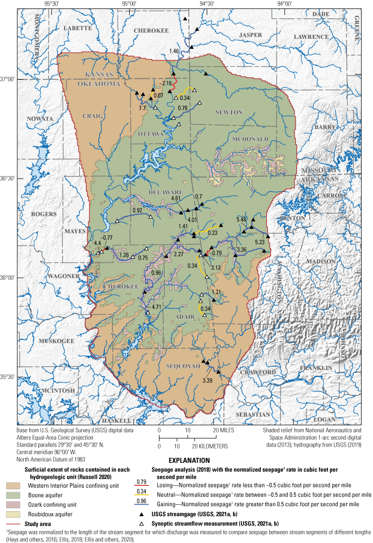
Seepage, selected synoptic streamflow measurements, and selected streamgages from January to February 2018 within the study area in northeastern Oklahoma, southeastern Kansas, southwestern Missouri, and northwestern Arkansas.
Seepage was normalized and classified into three categories: (1) gaining, (2) neutral, or (3) losing (fig. 18). Gaining stream segments were those for which normalized seepage was greater than 0.5 cubic foot per second per mile ([ft3/s]/mi), neutral stream segments were those for which normalized seepage was at or between 0.5 and −0.5 (ft3/s)/mi, and losing stream segments were those for which stream normalized seepage was less than −0.5 (ft3/s)/mi. Streams in the study area tend to be gaining; however, three segments in the study area were losing (fig. 18). Five stream segments were neutral. Losing stream segments tended to be shorter compared to the gaining stream segments. Seepage rates from the seepage analysis were not used for the conceptual model seepage estimates because they represent a short period of time and streamflows were measured following a year of above normal precipitation (2017). Therefore, the seepage values estimated by using the streamflows were not likely representative of long-term seepage for the study area.
Groundwater Use
Annual groundwater use for the Boone and Roubidoux aquifers was acquired from the OWRB reported groundwater-use database (Chris Neel, Water Rights and Administration Division Chief, OWRB, written commun., 2020), which does not include domestic groundwater use. To supplement groundwater use not reported to the OWRB, annual groundwater-use estimates for Kansas, Missouri, and Arkansas and domestic groundwater-use estimates were obtained from previously published estimates through 2010 (Knierim and others, 2017). To complete estimates through 2017, groundwater-use data from 2010 were assumed for each year following 2010 to supplement the data obtained by the OWRB. Long-term groundwater use for the conceptual model was estimated as the mean annual groundwater use over the 1980–2017 study period.
Leakage
Aquifer leakage for this study was defined as net groundwater flow between the Boone aquifer and the Roubidoux aquifer, and other types of leakage were assumed negligible. The hydraulic parameters of the Ozark confining unit indicate that a small amount of groundwater flows through this unit. The Ozark confining unit is mostly thin (less than 30 ft thick). Any groundwater flows into the Ozark confining unit were assumed to flow into either the Boone or Roubidoux aquifer and not remain in the Ozark confining unit, so groundwater losses to the Ozark confining unit were assumed to be negligible. Leakage from the Boone aquifer was assumed equal to leakage to the Roubidoux aquifer. Leakage between the Western Interior Plains confining unit and the Boone aquifer is likely small and often not considered a component of conceptual models for the Boone aquifer (Imes and Emmett, 1994; Hays and others, 2016). Therefore, leakage between the Western Interior Plains confining unit and the Boone aquifer was assumed to be negligible for the conceptual model in this report.
Aquifer leakage was assumed to be 8 percent of Boone aquifer recharge. This value is based on the estimated leakage by Imes and Emmett (1994) for the entire Ozark Plateaus aquifer system. Based on previous studies, leakage was determined to be a net outflow from the Boone aquifer and a net inflow to the Roubidoux aquifer (Imes and Emmett, 1994; Hays and others, 2016). Consideration was given to aquifers deeper than the Roubidoux aquifer; however, flows across boundaries of the Roubidoux aquifer to underlying aquifers were estimated to be about 1 percent or less of the conceptual water budget (Imes and Emmett, 1994; Hays and others, 2016).
Lateral Groundwater Flow
Lateral groundwater flow for this report consists of flow across the aquifer or study area boundaries. Attempts were made to estimate lateral groundwater flows based on regional groundwater-flow paths and hydraulic gradients; however, lateral groundwater flow is difficult to constrain given a lack of sufficient field measurements near the study area boundaries. Because long-term (decadal) groundwater-level measurements were relatively stable, change in storage was assumed to be negligible (fig. 3C, D). Based on this assumption, lateral groundwater flow was the last term estimated for the conceptual model water budget and was used to balance the conceptual model water budget.
Simulation of Groundwater Flow
A finite-difference numerical groundwater-flow model for the Boone and Roubidoux aquifers (hereinafter referred to as “groundwater-flow model”) was constructed by using MODFLOW-NWT (version 1.1.4), a version of MODFLOW considered ideal for simulating unconfined groundwater flow (Niswonger and others, 2011). MODFLOW-NWT is an extension of MODFLOW-2005 (Harbaugh, 2005) that uses a Newton formulation solver to solve for groundwater flow and the drying and rewetting of cells within the groundwater-flow model. Because of the modular nature of MODFLOW-NWT, many different types of packages can be added which simulate groundwater flows across various flow boundaries (for example, recharge, stream seepage, and groundwater use). Each package adds a new term to the groundwater-flow equation that is solved by the MODFLOW-NWT solver. Data inputs for each package are specified in text files or binary files (typically from previous MODFLOW-NWT simulations). The model was spatially and temporally discretized into cells and stress periods (with time steps composing stress periods), respectively. The cell size used in the model is the finest spatial resolution at which properties (such as land-surface altitude or hydraulic conductivity) may be represented given the availability of data. The stress-period length is the finest temporal resolution at which inflows and outflows may be represented, and the time step length is the finest (shortest) length of time for which model outputs may be written. Selected groundwater-flow model input values were adjusted to calibrate the model to available groundwater altitudes, base-flow observations, and the conceptual model. The calibrated groundwater-flow model inputs, outputs, metadata, directions for use, and ancillary data are available in a USGS data release (Trevisan and others, 2024).
Structural and Temporal Discretization
The groundwater-flow model was spatially discretized into 4 layers of 354 rows by 261 columns providing a 2,000-ft by 2,000-ft uniform cell size. Given the size of the study area, this relatively large cell size was chosen to reduce simulation times while suitably representing the features and groundwater-flow boundaries of the study area at a regional scale. The model was temporally discretized into 1 steady-state stress period followed by 456 monthly transient stress periods spanning January 1980 to December 2017. The steady-state stress period typically consisted of mean annual inputs from January 1980 to December 2017, but occasionally used inputs from 1979 as discussed in the following sections of this report. A steady-state stress period indicates that the groundwater-flow equation solved by MODFLOW-NWT provides inflows that equal outflows and that groundwater storage does not change. The steady-state simulation is used to create the initial conditions for groundwater altitude, groundwater flow, and groundwater storage to start the first transient stress period.
The active area of the groundwater-flow model was determined by using the previously published aquifer extents (Russell (2020). The western and southern edges of the active area of the model were set to no-flow boundaries; the setting of these no-flow boundaries is supported by the available hydrologic and geologic data (Christenson and others, 1990; Imes and Emmett, 1994). The eastern edge of the active area was delineated along a regional potentiometric surface at the point where any additional groundwater-flow contributions likely become minimal and was based on previous interpretations (Imes and Emmett, 1994; Nottmeier, 2015). The eastern edge of the active area also roughly corresponded to the watershed boundaries of major streams in the area (fig. 1A). The northern edge of the active area was delineated to avoid some areas with high groundwater withdrawals along this border of the model.
Altitudes of the base of each hydrogeologic unit represented in the groundwater-flow model were obtained from Russell (2020). Occasionally, the extent of the groundwater-flow model was extended by a few cells to include the Arkansas River where the river would cross an inactive cell and re-enter an active cell. Altitudes for the bases of the hydrogeologic units in these cells were estimated by taking the altitude from an adjacent cell or computing an average from multiple adjacent cells. The top of the groundwater-flow model was created by calculating the 95th percentile of the altitude of the one-third arc-second DEM for each 2,000-ft by 2,000-ft cell (USGS, 2019). This ensured that observed groundwater altitudes used for observations were below the simulated land surface.
Each hydrogeologic unit was represented in one or more layers of the model (figs. 19–21). The Western Interior Plains confining unit was represented in layer 1 (fig. 19). The Boone aquifer, Ozark confining unit, and Roubidoux aquifer were mostly represented in layers 2, 3, and 4, respectively (fig. 19). Although some studies have considered different parts of the Roubidoux aquifer (the lower, middle, and upper parts) separately for modeling purposes (Hays and others, 2016; Clark and others, 2018, 2019), this study considered the Roubidoux aquifer without dividing it into different parts, with constant hydraulic parameters over its thickness similar to the work of Czarnecki and others (2009) and Richards (2010). Horizontal groundwater flow between hydrogeologic layers was implemented by discretizing hydrogeologic units between several layers because MODFLOW-NWT does not simulate horizontal groundwater flow between different layers (Harbaugh, 2005). The Boone aquifer, Ozark confining unit, and Roubidoux aquifer were discretized across multiple layers where the rocks associated with each of these hydrogeologic units are exposed at land surface. For example, the deepest 80 percent of each of these hydrogeologic units was assigned to layers 2 for the Boone aquifer, layers 2–3 for the Ozark confining unit, and layers 2–4 for the Roubidoux aquifer (fig. 19). Next, the remaining 20 percent of the thickness of each hydrogeologic unit was assigned to layer 1 where the rocks that contained each hydrologic unit were exposed at ground surface (fig. 19). The altitudes of the bases in these locations were then adjusted to ensure at least 10 ft of thickness in layer 1 below the bottom altitude of the stream network. The representation of each layer of the groundwater-flow model and its corresponding hydrogeologic unit is depicted graphically (figs. 20, 21). Because the surficial exposures of the rocks of the Ozark confining unit and Roubidoux aquifer are small, the altitude of the base of layer 2 for the Ozark confining unit and layers 2 and 3 for the Roubidoux aquifer were interpolated by using a triangular-irregular-network interpolation (QGIS, 2022). The altitudes of the bases were further adjusted to remove hydrologic sinks.
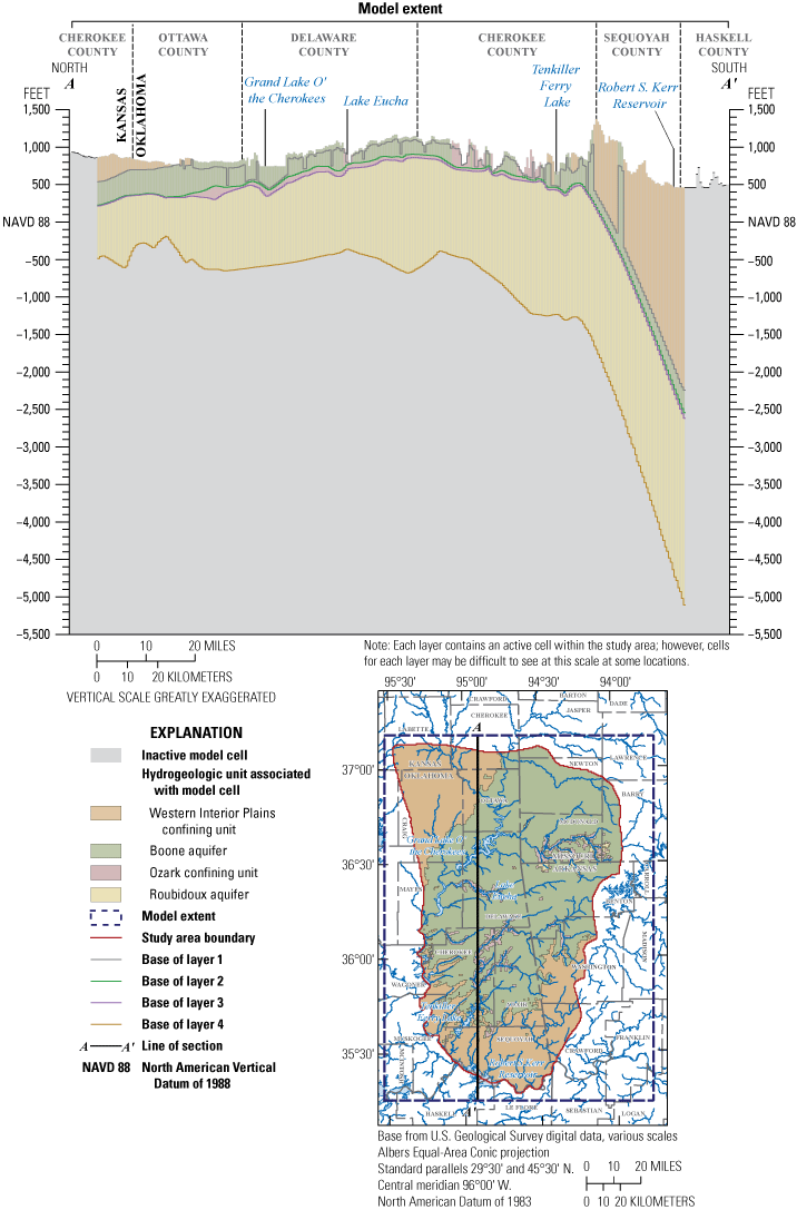
Example cross section of the groundwater-flow model showing how each model layer corresponds to each hydrogeologic unit along the A–A’ cross-section line (fig. 20) within the study area in northeastern Oklahoma, southeastern Kansas, southwestern Missouri, and northwestern Arkansas.
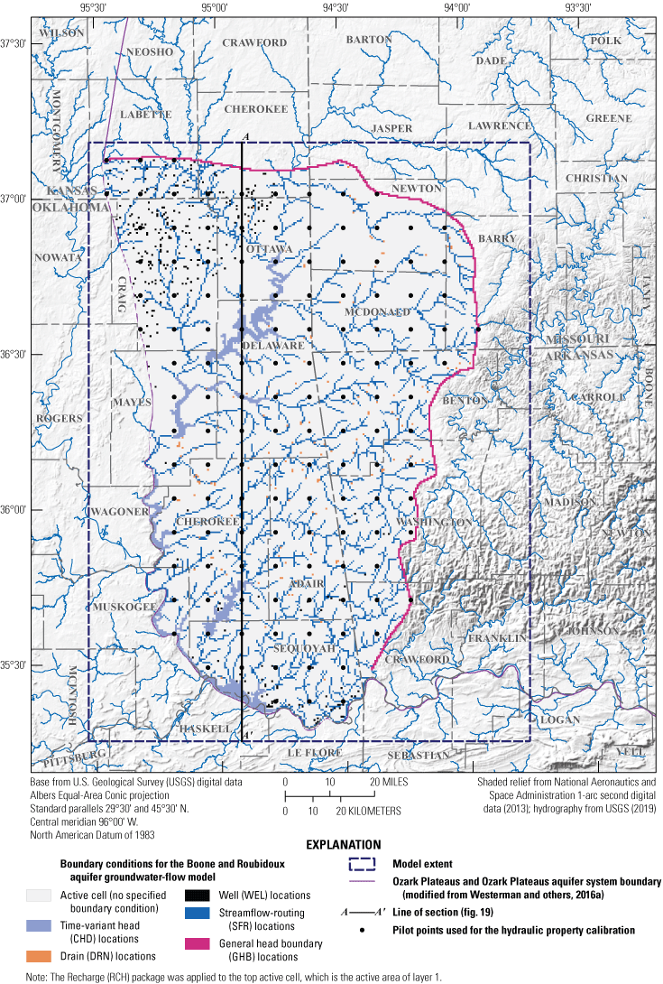
Boundary conditions for first layer of the groundwater-flow model, pilot points used for automated calibration for numerical groundwater-flow model hydraulic parameters, and the A–A’ cross-section line used for the cross section of the numerical groundwater-flow model (fig. 19) within the study area in northeastern Oklahoma, southeastern Kansas, southwestern Missouri, and northwestern Arkansas.
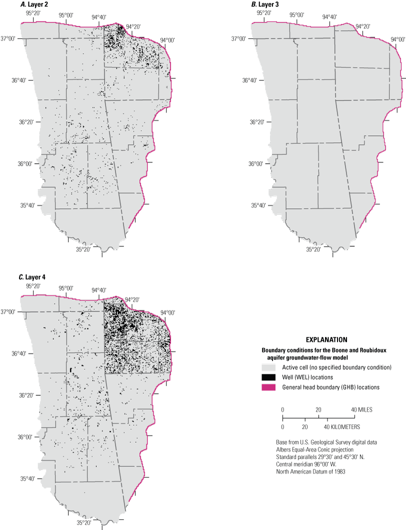
Boundary conditions for layers A, 2, B, 3, and C, 4 of the Boone and Roubidoux aquifer groundwater-flow model within the study area in northeastern Oklahoma, southeastern Kansas, southwestern Missouri, and northwestern Arkansas.
Hydraulic Properties
The Upstream Weighting package (UPW; Niswonger and others, 2011) was used to represent storage and hydraulic properties of the groundwater-flow model. The initial values for hydraulic conductivity, specific yield, and specific storage were initially set to values in the middle of the ranges of hydraulic properties listed in table 5. Initial horizontal hydraulic conductivity values were 0.1, 3, 0.005, and 5 ft/d in the Western Interior Plains confining unit, Boone aquifer, Ozark confining unit, and Roubidoux aquifer, respectively. Initial specific yield values ranged from 0.003 to 0.01 (dimensionless). Initial specific storage values ranged from 1.95×10⁻⁶ to 8.96×10⁻⁶ ft−1. Vertical anisotropy (ratio of horizontal to vertical hydraulic conductivity) was unknown and was arbitrarily set to an initial value of 1. Storage and hydraulic property values were further adjusted during manual and automated calibration to be within previously published ranges (table 5).
Testing of hydraulic parameters during manual calibration was done to help set the upper and lower bounds applied in automated parameter estimation for the Western Interior Plains confining unit and the Ozark confining unit. The bounds were created based on their effects on observation data and the feasibility of simulated groundwater altitudes (for example, an unfeasible simulated groundwater altitude would be hundreds of feet above the highest observed groundwater altitude).
Hydrologic Boundary Conditions
For a numerical groundwater-flow model, hydrologic boundaries are user-defined locations where groundwater can enter or leave the model. For this report, the hydrologic boundary conditions included recharge, lateral groundwater flow across the study area boundary, groundwater flow into and out of lakes and streams, groundwater issuing from springs, and groundwater withdrawals. These hydrologic boundary conditions were applied by using MODFLOW-NWT packages for each model layer where applicable (figs. 20, 21A–C).
Recharge
Recharge to the groundwater-flow model was simulated by using the Recharge (RCH) package (Harbaugh, 2005). The RCH package requires a user-specified recharge rate for each simulated cell and applies that rate over the specified time interval of each stress period. Monthly estimated aquifer recharge rates from the SWB code were used as inputs to the groundwater-flow model. Recharge was specified to occur in the top active cell, which is in the first layer of the model for every cell in layer 1. Recharge was initially set to a multiplier of 1.0 and varied within the range of 0.5 to 1.2 during calibration for each stress period. The multiplier is the value specified in the RCH package that is multiplied with each value in the recharge array to produce a new recharge array used by MODFLOW-NWT.
Lateral Groundwater Flow
Lateral groundwater flow across the study area boundary was simulated by using the General Head Boundary (GHB) package (Harbaugh, 2005). The GHB package is a groundwater-altitude-dependent boundary that requires the input of GHB altitude and conductance values for each GHB package cell. Conductance is computed by multiplying the hydraulic conductivity by the saturated cross-sectional area of a GHB package cell orthogonal to groundwater flow, and then dividing this sum by the distance between cell centroids. Groundwater flow between GHB cells and active cells in the model is calculated as the difference in groundwater-altitude values between the GHB cell and the individual cell in the model multiplied by the conductance of the GHB cell (Harbaugh, 2005).
GHBs were placed along the northern edge of the study area and along the eastern edges of the study area in each layer (figs. 20, 21A–C). Groundwater altitudes for each layer of the groundwater-flow model were estimated by using groundwater-altitude observations near the study area boundaries (USGS, 2021a, b) and by using potentiometric-surface maps (Imes and Emmett, 1994; Nottmeier, 2015). Groundwater altitudes for the GHB boundary were then calibrated by using bounds of 50 ft above and below the initial GHB altitude; groundwater altitudes were then adjusted to ensure the bounds were not more than model land-surface altitude or less than the altitude of the base of the layer. Initial GHB conductance values were estimated by using initial hydraulic conductivity estimates and the estimated saturated thickness for each GHB cell. GHB groundwater altitude and conductance were adjusted during calibration.
Lakes
The Time-Variant Specified-Head (CHD) package (Harbaugh, 2005) was used to simulate lake seepage to and from the major lakes and the hydrogeologic units in the study area (OWRB, 2021): Grand Lake O’ the Cherokees, Lake Eucha, Spavinaw Lake, Lake Hudson, Fort Gibson Lake, Webbers Falls Reservoir, Tenkiller Ferry Lake, and Robert S. Kerr Reservoir (fig. 1). Lake seepage for smaller lakes in the model area was assumed negligible.
The CHD package requires the input of beginning and ending lake-surface altitudes (hereinafter referred to as “lake stage”) for each stress period. For each model stress period, the beginning lake stage was set to the monthly lake stage from the stress period corresponding to the previous month, and the ending lake stage was set to the monthly lake stage from the month corresponding to a given stress period. For the steady-state stress period, beginning and ending lake stages were set to conservation pool altitude (USACE, 2021).
For most lakes, monthly lake stage was obtained from the USACE Water Control Data System (USACE, 2021) unless otherwise specified. Monthly lake stage was only available from November 1994 to the present. Lake stage before November 1994 was set to conservation pool altitude (USACE, 2021).
For Grand Lake O’ the Cherokees, lake-stage values inferred from the rating at USGS station 07190000 were used to estimate daily lake-storage values (USGS, 2021a, b). The rating depicts the relation between lake stage and lake storage and was computed in the 1940s; the full rating was published in Hunter and others (2020). The rating consists of 1-ft increments of lake stage and corresponding lake storage. The method used for estimating lake stage included calculating a linear equation for each 1-ft increment in lake stage consisting of a slope (change in lake stage, in feet, divided by the change in lake storage, in acre-feet) and an intercept (offset, in feet). Lake stage was estimated by finding the smallest storage value in the rating that was greater than the published lake storage. The slope and intercept at this section of the rating were then used to estimate a lake stage. There was some overlap between lake stage published in NWIS and the implementation of the rating used to publish lake storage. The overlapping data were used to determine a root mean square error of approximately 0.10 ft of lake stage. The statistics for the lake stage are included in the data release associated with this report (Trevisan and others, 2024). Daily lake-stage estimates were converted to monthly values by taking the mean of the daily lake-stage estimates for each month.
Available lake-stage values for Lake Eucha and Spavinaw Lake were also compiled for use in the CHD package. Historical lake-stage values prior to October 2007 were not available from the USACE for these lakes. Daily lake stages for these lakes were obtained from NWIS (USGS, 2021a, b) from October 2007 through December 2017. Daily lake stage was averaged for each month to obtain a monthly lake-stage value. Prior to October 2007, lake-stage values were set to conservation pool altitudes for Lake Eucha and Spavinaw Lake (USACE, 2021). When summarized in the simulated groundwater budget, the net groundwater flow between the lakes (CHD) and the aquifer was added to the seepage water-budget category.
Streams
The Streamflow Routing (SFR) package (version 2; Niswonger and Prudic, 2005) was used to simulate stream seepage between the stream and aquifer in accordance with Darcy’s law (Heath, 1983) and downstream routing of base flow in accordance with Manning’s equation (Chow, 1959). Stream components were separated into stream segments (portions of the stream that only contain inflows at one end and outflows at the other) and reaches (individual cells of the model along each segment).
Stream data representing the stream network in the study area were obtained from the NHD (EPA, 2020b). Streams with stream orders greater than one were used for the simulation to reduce the stream density. Minor adjustments were made to the representation of stream channels when a stream in an active cell crossed inactive cells to ensure that the stream network was continuous through the active model domain. Additionally, short stream segments (typically covering one to two cells of the model) and divergences (loops) in the NHD stream network were removed.
Streambed slopes and arbolate sums (the sum of the length of all upstream stream segments) from the NHD dataset were used for stream slopes and to estimate stream widths by using the arbolate-sum regression equation from appendix 2 on page 266 in Feinstein and others (2010). Stream widths for the Arkansas, Neosho, and Spring Rivers were reduced by 30 percent to more closely match the stream widths measured from aerial photography (Microsoft Corporation, 2021). Streambed widths were further adjusted during calibration within bounds of plus or minus 20 percent of initial estimates. Streambed altitudes were set to mean model-cell-resolution altitude based on the one-third arc-second DEM (USGS, 2019). The streambed altitudes derived from the one-third arc-second DEM altitudes (instead of the NHD streambed altitudes) were used to be consistent with the altitudes used for the rest of the groundwater-flow model.
The SFR package requires streambed altitudes to decrease in the downstream direction; streambed altitudes were adjusted where necessary by starting at stream segments with no inflows and moving reach-by-reach (cell-by-cell) downstream along the stream network to the outflow. When streambed altitudes increased downstream, they were removed and then linearly interpolated between the streambed altitudes of adjacent reaches. Additionally, some SFR streambed altitudes were manually adjusted by segment to better match calibration targets while maintaining an altitude of at least the minimum sampled altitude from the one-third arc-second DEM for each SFR cell.
Inflows to the SFR network were estimated by using estimated base flow at several USGS streamgages north of the study area (fig. 6C). Not all streamgage records spanned the entire study period (1980–2017). Streamgage records from streamgages north of the study area that did not span the entire study period were estimated by using the standardization by means method (Farmer and Vogel, 2013), where monthly flows are estimated by multiplying flows at a reference streamgage by the ratio of mean flow for the streamgage to be estimated divided by mean flow of the reference streamgage. Monthly inflows (as base flows) were estimated for USGS streamgage 07184500 Labette Creek near Oswego, Kans. (streamgage 3s) (table 1; fig. 1A) (using the sum of mean monthly base flows between USGS streamgage 07184000 Lightning Creek near McCune, Kans. [streamgage 2s] and USGS streamgage 07183500 Neosho River near Parsons, Kans. [streamgage 1s] as the reference base flow) and USGS streamgage 07186055 Cow Creek near Scammon, Kans. (streamgage 8s) (using mean monthly base flows for USGS streamgage 07186000 Spring River near Waco, Mo.[streamgage 7s] as the reference base flow). Estimated monthly base flows are shown in figure 22.
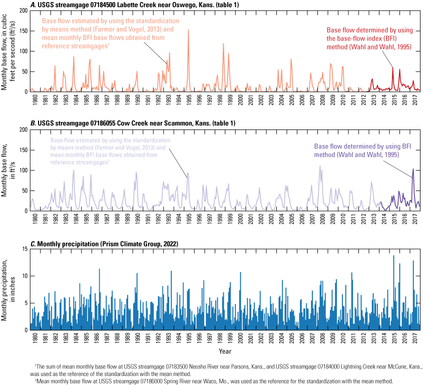
A, B, Base flow determined by using the base-flow index method and estimated by using the standardization with the mean method for selected streamgages in southeastern Kansas near the study area, and C, mean monthly precipitation for the study period (1980–2017).
Permitted surface-water diversion locations were obtained from the OWRB (2019b). The Grand River Dam Authority (GRDA) has the jurisdiction to regulate surface-water diversions in northeastern Oklahoma, which is an area that is about one-third of the part of the study area that is in Oklahoma (fig. 7A). The permits issued by the GRDA were not used for the groundwater-flow model because they were not publicly available. The OWRB-issued permits used in the SFR package were less than 1 percent of total base flows, and the permits issued by GRDA were likely only a small percentage of base flows. Annual surface-water diversions were scaled by OWRB (2012b–d) water-use monthly multipliers for each monthly stress period based on the use type associated with the permit and the basin where each surface-water diversion was located (figs. 7, 23). When summarized in the simulated groundwater budget, the net groundwater flow between the streams (SFR) and the aquifer was added to the seepage water-budget category.
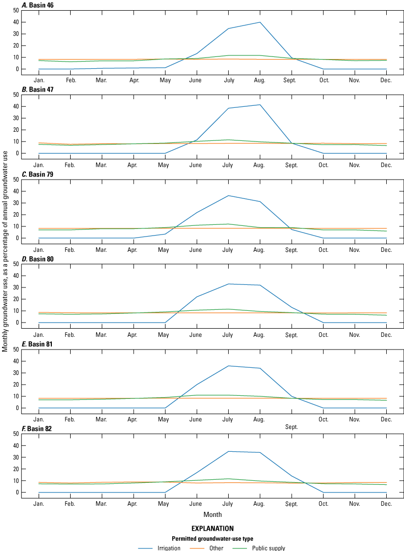
Monthly groundwater use by permitted type, for selected Oklahoma Comprehensive Water Plan water-management planning basins (Oklahoma Water Resources Board, 2012b–d) in the study area (figs. 1A, 7) in northeastern Oklahoma.
Seeps and Springs
For the groundwater-flow model, seeps and springs in the study area were the USGS-identified springs (USGS, 2019), which were represented by using the Drain (DRN) package (Harbaugh, 2005). The DRN package functions by removing groundwater when simulated groundwater altitudes exceed user-specified DRN altitudes; groundwater is removed at a rate proportional to the product of a user-specified DRN conductance and the difference between the simulated groundwater altitude and DRN groundwater altitude (eq. 6–10 in Harbaugh, 2005). Land-surface altitudes were point-sampled from the one-third arc-second DEM (USGS, 2019) at spring locations to use as altitudes for the DRN package. When multiple springs were located in the same cell, the mean of all sampled altitudes of all the springs in the cell was used for the DRN package altitudes for that cell. Initial DRN conductance values were set to 8,000 foot squared per day (ft2/d) and were further adjusted during calibration. When summarized in the simulated groundwater budget, the net groundwater flow between the springs (DRN) and the aquifer was added to the seepage water-budget category.
Groundwater Withdrawals
Groundwater withdrawals were simulated by using the Well (WEL) package (Niswonger and others, 2011). Groundwater withdrawals were distributed evenly among wells that shared the same groundwater permit. Annual groundwater withdrawals were discretized to monthly stress-period withdrawals based on monthly water use demand distributions for the six Oklahoma Comprehensive Water Plan water-management planning basins (basin numbers 46, 47, and 79–82) in the study area (OWRB, 2012a–d; figs. 7, 23). For wells outside of Oklahoma, but in the study area, the nearest surface-water basin in Oklahoma was used. Groundwater withdrawals were not simulated if they were located in cells used for the CHD or GHB packages; these packages could potentially simulate limitless amounts of water, and thus groundwater withdrawals would have minimal influence on simulated groundwater flow in the locations where GHB cells were used. Excluded groundwater withdrawals were a small component of total groundwater use and were mostly along GHBs outside of Oklahoma. For the first steady-state stress period, groundwater withdrawals were set to mean annual values for the 1980–2017 model period.
Model Calibration
The goal of model calibration for this study was to adjust uncertain model parameters to reduce the sum of squared weighted residuals (that is, more closely match simulated values to observations) and match the conceptual model with the simulated groundwater budget. Model calibration consisted of two steps: (1) manually adjusting model parameters and then (2) using automated calibration to iteratively adjust parameters to improve the objective function. Parameters from the GHB, DRN, RCH, SFR, and UPW packages were adjusted during the manual and automated calibration steps to better match calibration targets (measured data observations).
Automated Model Calibration
Automated model calibration was done by using parameter estimation software version 4 (PEST++ version 4; White and others, 2020a), which was modified from PEST++ version 3 (Welter and others, 2015). PEST++ version 4 contains a suite of tools including the PEST++ (PESTPP) iterative ensemble smoother (PESTPP-IES; White, 2018) software tool that was used to minimize the objective function. For minimizing the objective function, the PESTPP-IES software tool employs a Levenberg-Marquardt algorithm with an iterative ensemble smoother (Chen and Oliver, 2013). The objective function (Φ) is defined as:
wheren
is the number of observations;
ωi
is the observation weight at observation i;
si
is the simulated value at observation i;
oi
is the observed or estimated value at observation i.
PESTPP-IES minimizes the objective function by running multiple sets of ensembles where model parameters are iteratively adjusted within a user-defined range of values. In this manner, automated calibration can assess a broader combination of parameters faster than manually adjusting each parameter value. Additionally, PESTPP-IES uses singular value decomposition for regularizing solution subspace (Doherty, 2015; White and others, 2020b). Singular value decomposition improves the solution stability by identifying and adjusting the most sensitive parameters affecting observations and reduces the computation time required to complete automated calibration. Automated calibration was done by running ensembles in parallel on a high-performance computing (HPC) cluster using the parallel run manager built into the PEST++ suite (White and others, 2020b).
Calibration Parameters
During automated calibration, 10,552 parameters categorized into 29 parameter groups (table 10) were adjusted; the data associated with these parameters are published in the companion data release (Trevisan and others, 2024). These parameter groups include GHB conductance, GHB groundwater altitude, SFR parameters (streambed hydraulic conductivity, streambed thickness, and stream width), RCH monthly array multipliers, DRN conductance, and hydraulic parameters (hydraulic conductivity, horizontal-to-vertical hydraulic conductivity ratio, specific storage, and specific yield). Calibration parameters were adjusted to help reduce the objective function and more closely match calibration targets.
Table 10.
Groundwater-flow model calibrated parameter range for each parameter group and the parameter bounds used for the parameter estimation software PEST++ (PESTPP) automated calibration of the numerical groundwater-flow model of the Boone and Roubidoux aquifers for the study area in northeastern Oklahoma, southeastern Kansas, southwestern Missouri, and northwestern Arkansas.[ft, foot; ft2/d, foot squared per day; ft/d, foot per day]
Pilot points are gridded points used to distribute parameters more easily throughout the model extent and estimate parameter heterogeneity without prior knowledge about the spatial parameter distribution during automated calibration (Doherty, 2003) (fig. 20). During automated calibration, pilot-point parameters are adjusted. Then, an exponentially weighted kriging procedure is performed to interpolate parameters to the groundwater-flow model grid resolution. Pilot-point parameters were used for the four hydraulic parameters in each model layer: (1) horizontal hydraulic conductivity, (2) the vertical anisotropy, (3) specific storage, and (4) specific yield. For simplicity in the calibration process, each hydraulic parameter group and pilot points within that parameter group pertained to a specific hydrogeologic unit (for example, pilot points in group hk1, hk2, hk3, and hk4 pertained to hydraulic conductivities for the Western Interior Plains confining unit, Boone aquifer, Ozark confining unit, and Roubidoux aquifer, respectively; table 10). Parameter bounds for most hydraulic properties (table 5) were estimated by Imes and Emmett (1994) and Clark and others (2018, 2019); however, hydraulic conductivities for the Boone and Roubidoux aquifers were estimated by using information from other publications. For the Boone aquifer, horizontal hydraulic conductivity was estimated by Reed and Czarnecki (2006) and Czarnecki and others (2009) as indicated in table 5. For the Roubidoux aquifer, the upper bound of horizontal hydraulic conductivity was estimated from a multi-well aquifer test (Macfarlane, 2007); because multi-well aquifer tests are not typically performed in low-water-yielding areas of an aquifer, the lower bound was set to 0.001 ft/d based on iterative testing of different hydraulic parameters during manual calibration. Groundwater flow to streams was restricted to areas around streams where the Ozark confining unit was the uppermost hydrogeologic unit, and simulated groundwater altitudes were high within those areas (more than 500 ft above the top of the model [land surface]). Thus, in locations where the Ozark confining unit was the uppermost hydrogeologic unit in layer 1, the Roubidoux aquifer hydraulic parameters were used as an estimate for realistic near-surface hydraulic parameters. Near-surface hydraulic parameters for shallower rocks in the Ozark confining unit were likely greater than those for rocks at depth in the Ozark confining unit because near-surface rocks can be prone to fracturing (particularly for the more fissile rocks contained in the Ozark confining unit, which readily fracture along bedding planes) and are often more permeable compared to deeply buried rocks of this unit (Imes and Emmett, 1994).
Calibration Targets
Calibration targets consisted of three observation groups: groundwater-altitude observations, base-flow observations, and conceptual model recharge values for the Boone and Roubidoux aquifers. For automated calibration, calibration targets were weighted when determining the objective function (the sum of squared weighted residuals). That is, residuals are multiplied by weights, squared (multiplied by themselves), then summed. Weighting is necessary to control how much each observation contributes to the objective function. Observations often have different units of measure, and using unweighted values would cause the automated calibration process to favor observations with greater residuals.
For automated calibration, each observation group was weighted to contribute approximately equally to the objective function (sum of squared residuals), except for the conceptual model recharge components which were given a weight to scale the objective function two orders of magnitude less than the objective function contributions of the other observation groups. This decision was made because the conceptual model budget components were estimated by making simplifying assumptions and using mean estimates, and because the data were sparse for large parts of the study area. Also, initial starting values for recharge parameters closely matched the conceptual model targets, and, by weighting two orders of magnitude less than other observation groups, recharge could be adjusted without automated calibration favoring conceptual model recharge over the other observed calibration data.
After the initial weights were calculated for each group, the individual observation weights were further adjusted on the basis of several criteria. For groundwater-altitude observations, those that were within Oklahoma were weighted about double of those outside of Oklahoma. Additionally, groundwater-altitude observations were weighted proportionally to the inverse of the number of observations at each location to provide a more robust spatial calibration because a substantial number of observations (10 or more) were available for 47 wells, and few observations (less than 10) were available for 508 wells. Weighting each measurement equally would bias the objective function towards wells with more measurements. Groundwater-altitude observations were weighted equally for the Western Interior Plains confining unit and the Boone and Roubidoux aquifers. Manual calibration revealed that Western Interior Plains confining unit groundwater-altitude observations were sensitive to net leakage to or from the Boone aquifer. Western Interior Plains confining unit groundwater-altitude observations were important for constraining net leakage from the Boone aquifer and were often in locations with few Boone aquifer groundwater-altitude observations.
Base-flow observations were initially weighted such that each streamgage contributed approximately equally to the objective function. During the calibration process, the objective function weighting for base-flow observations were subsequently doubled for streamgages on streams that predominantly drained areas overlying the Boone and Roubidoux aquifers within Oklahoma to improve calibration results for those areas.
Groundwater-Altitude Observations
For the study area, 2,274 water-level observations for 1979 through 2017 are available in NWIS (USGS, 2021a, b). These water-level observations and their corresponding well depths were converted to groundwater-altitude observations and well-bottom altitudes, respectively, each measured from the land-surface altitude by using a one-third arc-second DEM (USGS, 2019). Observations were assigned to aquifers on the basis of well-bottom altitude and base-of-aquifer altitude (Russell, 2020). When conflicts arose between the aquifer assigned by using well-bottom altitude and the geologic unit coded for the measurement (based on the geologic unit associated with the aquifer from Russell and Stivers [2020]), publications using groundwater-altitude observations at those wells were used to identify the correct aquifer in which those wells were completed (Marcher and Kenny, 1983; Goemaat and others, 1984; Christenson, 1995; DeHay, 2003; DeHay and others, 2004). Discrepancies that resulted from using well-bottom altitudes likely arose from the relatively coarse (2,000-ft by 2,000-ft) resolution of the base-of-aquifer altitude and uncertainty in the DEM and base-of-aquifer altitudes.
Simulated groundwater altitudes were extracted from the groundwater-flow model by using the Head Observations (HOB) package for MODFLOW-NWT (Hill and others, 2000). The HOB package is used to assign a simulated groundwater-altitude observation to a cell and requires a user-specified row offset and column offset to place the observation in the cell. In addition to spatial interpolation, the HOB package also temporally interpolates between stress periods by using a simulated groundwater altitude that is based on a user-specified time offset.
Groundwater-altitude observations for 1979 were used for the steady-state simulation because precipitation during 1979 approximated the long-term (1885–2020) mean annual precipitation (fig. 3A) and did not overlap with any of the transient simulated periods. Because the steady-state simulation lacks a time component, steady-state groundwater-altitude observations were averaged when multiple observations were made in the same well in 1979. This reduced the total number of groundwater-altitude observations from 2,274 to 2,217, leaving 38 total observations in 1979 that were used for the steady-state simulation (fig. 24). Groundwater-altitude observations during 1980–2017 were used for the transient simulation. The number of groundwater-altitude observations for the transient stress periods totaled 2,179 (fig. 24). No groundwater altitudes were identified for the Ozark confining unit. For the period 1885–2020, groundwater-altitude measurements were most frequently made during January through April (fig. 25). March was the month with the most measurements (398), and November had the fewest (88) (fig. 25).
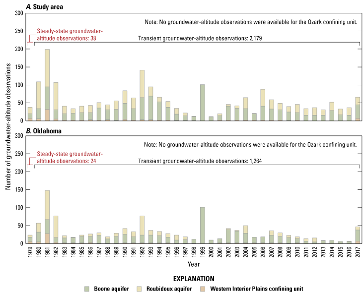
Number of groundwater-altitude observations used in the numerical groundwater-flow model by year for A, the study area in northeastern Oklahoma, southeastern Kansas, southwestern Missouri, and northwestern Arkansas, and B, the part of the study area in northeastern Oklahoma.
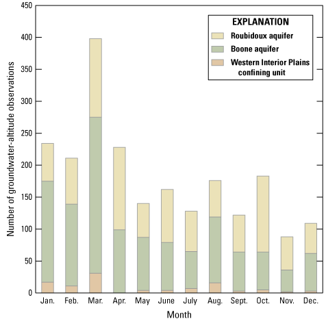
Number of groundwater-altitude observations used in the numerical groundwater-flow model by month for the study period (1980–2017).
Base-Flow Observations
For the steady-state simulation, mean annual base flow (1980–2017) was used as an observation for manual and automated calibration. Monthly base-flow observations were assigned to the stress period corresponding to the month and year of the observation and used for manual and automated calibration. All base-flow observations were compared with simulated base flows by using the Gage package for MODFLOW-NWT (Merritt and Konikow, 2000). The Gage package is used to extract simulated base flows at the outflow of every user-specified segment and reach number for a cell containing an SFR reach for each stress period. Base flows from 36 streamgages were used as observation targets in the calibration process, however not every streamgage recorded data for the entire 1980–2017 study period (figs. 1A, 6). Streamgages in Oklahoma that mostly drained watersheds overlying the Boone and Roubidoux aquifers were given preference during manual calibration and automated calibration.
Conceptual Model Budget Components
Components of the conceptual model were used to match simulated mean annual budget values (1980–2017). Each budget component was used for manual calibration, but for automated calibration, only long-term recharge for the Boone and Roubidoux aquifers was used. Recharge was the only parameter used for automated calibration because most other budget components were already calibrated to other calibration targets or were minor components of the conceptual model (table 6). Because MODFLOW-NWT reports groundwater flows for the entire simulation, subareas for each hydrogeologic unit were extracted by using the ZONEBUDGET utility (fig. 26A–D; Harbaugh, 1990).
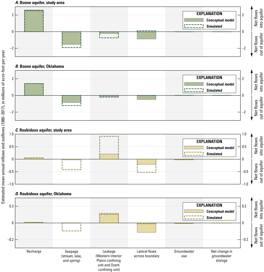
Conceptual model and simulated water-budget inflows and outflows for A, the Boone aquifer in the study area, B, the Boone aquifer in Oklahoma, C, the Roubidoux aquifer in the study area, and D, the Roubidoux aquifer in Oklahoma during the study period (1980–2017).
Calibration Results
Calibration results for this report were evaluated on the goodness-of-fit between the simulated and the observed calibration targets (table 11). The primary statistic for assessing the calibration results was the reduction in the total objective function. Automated calibration reduced the total objective function by about 96 percent from calibration inputs (from 1,340,001 to 65,145; table 11). The conceptual model recharge objective function component value was approximately double the precalibration objective function component value (from 6,667 to 12,851). Base-flow and groundwater-altitude objective function components were reduced by about 95 and 99 percent, respectively (from 666,667 to 24,953 and 666,667 to 27,340, respectively).
Table 11.
Components of the objective function for the automated calibration of the numerical groundwater-flow model of the Boone and Roubidoux aquifers for the study area in northeastern Oklahoma, southeastern Kansas, southwestern Missouri, and northwestern Arkansas.[RMSE, root mean square error; acre-ft/yr, acre-foot per year; ft3/s, cubic foot per second]
Totals for the objective function component may be different from the objective function component totals in the model archive (Trevisan and others, 2024) due to rounding.
Sensitivity Analysis
The Jacobian matrix represents a first-order relation between parameters and observations (White and others, 2020b). A groundwater-flow model sensitivity analysis was done by using the PEST++ Gauss-Levenburg-Marquardt (PESTPP-GLM) program (White and others, 2020b) to calculate a Jacobian matrix with dimensions of 1,163 parameters by 13,166 observations. The sensitivity analysis consisted of adjusting parameters by 1 percent and calculating a derivative (the change in the observation residual divided by the change in the parameter). Thus, higher derivatives within the Jacobian matrix indicate that a change in a given parameter affects an observation more than other parameters with smaller values in the Jacobian matrix (less sensitivity). The derivatives in the Jacobian matrix were with respect to the log of that parameter because adjustable parameters were log transformed using PESTPP-GLM (White and others, 2020b).
To complete the Jacobian matrix, the groundwater-flow model was simulated n times, where n is the total number of parameters, and another simulation was done without adjusting any parameters. Owing to the large number of adjusted parameters, the sensitivity analysis was done by parameter group, and the analysis was conducted in parallel on an HPC cluster and summarized based on parameter groups (fig. 27). Composite parameter sensitivities (eq. 5.3.1 on p. 73 of Doherty, 2015) were calculated to normalize observation sensitivities and parameter groups. For this report, sensitivity with respect to the groundwater-flow model refers to composite parameter sensitivity. A composite parameter sensitivity is the weighted, normalized column for each parameter from the Jacobian matrix with respect to the number of observations with nonzero weights. The composite parameter sensitivity is calculated by using the equation (all terms are considered dimensionless):
wherecps
is the composite parameter sensitivity;
JT
is the transpose of the Jacobian matrix;
Q
is the matrix of weights assigned to each observation;
J
is the Jacobian matrix; and
n
is the total number of observations with nonzero weights.
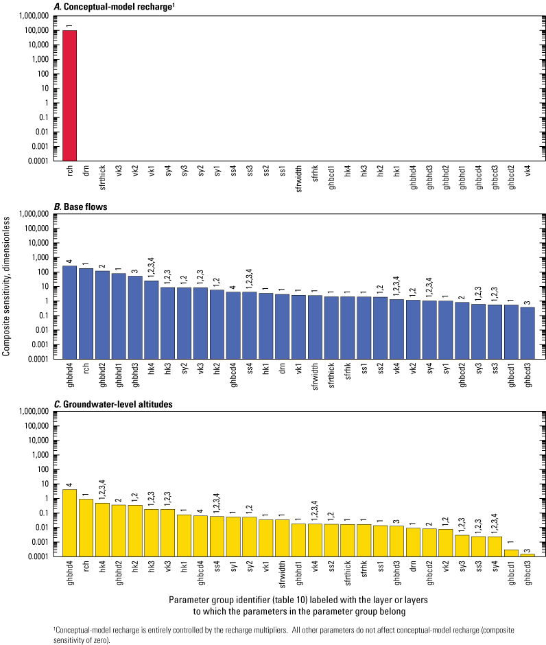
Parameter group composite sensitivities for A, conceptual-model recharge, B, base flows, and C, groundwater-level altitude parameter groups ordered by most sensitive to least sensitive and the layers for which parameters in each parameter group are located for the automated calibration of the numerical groundwater-flow model of the Boone and Roubidoux aquifers for the study area in northeastern Oklahoma, southeastern Kansas, southwestern Missouri, and northwestern Arkansas, 1980–2017.
Groundwater-altitude observations were consistently the least sensitive to parameter adjustment, the recharge multipliers were most sensitive, and base-flow observations were moderately sensitive during parameter adjustment (fig. 27A–C). Because recharge was only affected when adjusting the recharge multipliers (rch), all other parameter groups were insensitive (composite sensitivity of zero) for conceptual-model recharge observations (fig. 27A). Base-flow observations (fig. 27B) were generally more sensitive compared to groundwater-altitude observations (fig. 27C) during parameter adjustment. Generally, for parameters that corresponded to specific aquifers, observations were often more sensitive to parameter adjustment for the Boone and Roubidoux aquifers (parameter groups generally associated with layers 2 and 4, respectively) compared to adjusting the same parameters for the Western Interior Plains confining unit and Ozark confining unit (parameter groups generally associated with layers 1 and 3, respectively).
Observations were most sensitive to adjusting the recharge multipliers and the GHB altitudes for the Boone and Roubidoux aquifers (ghbhd2 and ghbhd4, respectively; fig. 27B, C), but hydraulic conductivity for the Roubidoux aquifer (hk4) was slightly more sensitive than the GHB altitudes for the Roubidoux aquifer with respect to groundwater altitudes (fig. 27C). Hydraulic conductivity pilot points for the Boone aquifer (hk2) were the next most sensitive parameters for the base-flow and groundwater-altitude observations. Base-flow and groundwater-altitude observations were generally less sensitive to parameter adjustment for the Ozark confining unit compared to other parameters. Thus, leakage from the Boone aquifer to the Roubidoux aquifer through the intervening Ozark confining unit may have high uncertainty. For the Ozark confining unit, observations were about as sensitive to the vertical anisotropy parameters as they were to hydraulic conductivity parameters.
Study Area Calibrated Parameters
The parameters for the groundwater-flow model (Trevisan and others, 2024) were calibrated manually and automatically by using various packages designed to work with MODFLOW-NWT as described in the “Simulation of Groundwater Flow” section of this report.
Calibrated SFR streambed hydraulic conductivity (sfrhk) and streambed thickness (sfrthick) ranged from 0.357 to 10 ft/d and 0.333 to 6 ft, respectively (table 10). The bounds for these values were not determined by field data collected as part of this study but were based on values from previous studies for other groundwater-flow models in Oklahoma (table 10; Smith and others, 2017, 2021; Ellis, 2018; Ellis and others, 2020). Because the Boone and Roubidoux aquifers that underlie the streams in the study area are bedrock aquifers, streambed thickness was assumed to be slightly less than the streambed thickness typical for streams overlying alluvial aquifers. GHB conductance values for the Boone aquifer (ghbhcd2 in table 10) ranged from 0.16 to 67,400 ft2/d, and conductance values for the Roubidoux aquifer (ghbcd4 in table 10) ranged from 3.22 to 130,000 ft2/d. DRN (representing springs) conductance values ranged from 984 to 10,000 ft2/d (drn in table 10). Conductance values for springs are difficult to determine, and springs for the groundwater-flow model lacked calibration data. Moderate conductance values were assumed for springs because they were considered minor outflows from the aquifers. RCH package array multipliers for SWB recharge grids ranged from 0.598 to 1.2 (rch in table 10).
For the Boone aquifer, horizontal hydraulic conductivity values ranged from 0.647 to 19.1 ft/d (hk2 in table 10), and for the Roubidoux aquifer, horizontal hydraulic conductivity values ranged from 0.054 to 31.9 ft/d (hk4 in table 10). The horizontal hydraulic conductivity values for both aquifers were within the range of horizontal hydraulic conductivity of 8.64×10⁻⁴ to 86.4 ft/d estimated in previous studies for the Ozark Plateaus aquifer system (Imes and Emmett, 1994; Hays and others, 2016; Clark and others, 2018, 2019).
Calibrated vertical hydraulic conductivity values for the Boone and Roubidoux aquifers were generally higher than those of previous studies (tables 5, 10); however, manual calibration revealed that using the vertical hydraulic conductivity values in table 5 would restrict drainage such that simulated base flows would be much greater than base-flow observations, groundwater altitudes would be hundreds of feet higher than the maximum measured groundwater altitude, and leakage between the Boone and Roubidoux aquifers would also be much less than the conceptual model leakage. Many groundwater-flow models were simulated during relatively drier periods when recharge was estimated to only be about 4 to 5 in/yr and as small as an order of magnitude less than the conceptual model recharge values (Reed and Czarnecki, 2006; Czarnecki and others, 2009; Clark and others, 2019). Differences among the parameters that were adjusted, the time periods analyzed, and the locations of the simulations between the groundwater-flow model of this report and the groundwater-flow models of previous reports (Reed and Czarnecki, 2006; Czarnecki and others, 2009; Clark and others, 2018, 2019) could also affect the differences in calibration of vertical conductivity. The spatial variability of vertical hydraulic conductivity (fig. 28C, D) was similar to that of horizontal hydraulic conductivity (fig. 28A, B).
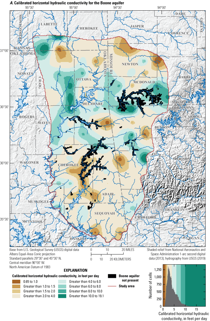
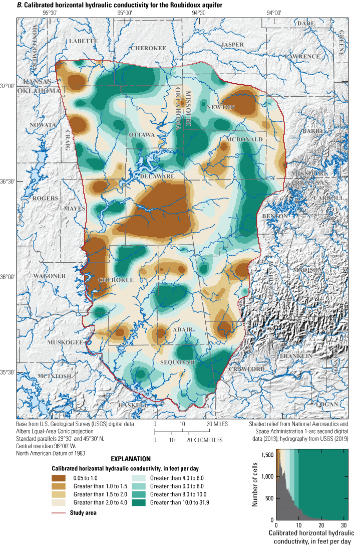
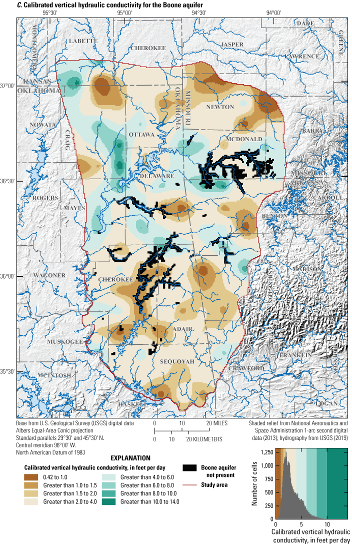
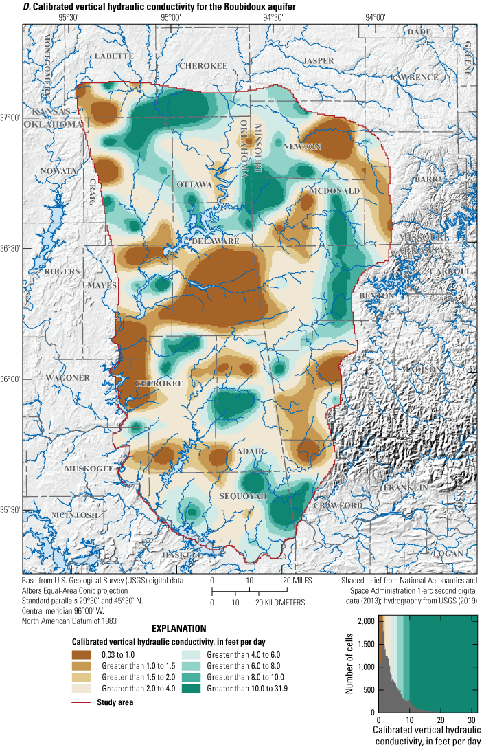
Calibrated horizontal hydraulic conductivity for the A, Boone aquifer and B, Roubidoux aquifer and calibrated vertical hydraulic conductivity for the C, Boone aquifer and D, Roubidoux aquifer in northeastern Oklahoma, southeastern Kansas, southwestern Missouri, and northwestern Arkansas.
Calibrated Parameters for the Study Area in Oklahoma
For the study area in Oklahoma, mean specific yield and mean specific storage (table 12) were similar to those estimated in previous studies (table 5). Mean specific yield for the Boone aquifer (table 12) was close the value of specific yield needed to match the WTF estimate of recharge to RORA-program estimated recharge (table 8; fig. 1A). Mean specific yield for the Boone aquifer was about three times the mean specific yield for the Roubidoux aquifer (table 12). Horizontal hydraulic conductivity for the Boone aquifer was relatively high in parts of Ottawa, Craig, Delaware, and Mayes Counties and relatively low in Adair, Cherokee, and Sequoyah Counties in Oklahoma (fig. 28A). For the Roubidoux aquifer, horizontal hydraulic conductivity was relatively high in parts of Ottawa, Craig, Delaware, Cherokee, and Adair Counties and relatively low in parts of Craig, Cherokee, and Sequoyah Counties (fig. 28B). Hydraulic conductivity for most cells in the model was less than 6 ft/d for the Boone and Roubidoux aquifers (fig. 28A, B). For the part of the study area in Oklahoma, mean horizonal hydraulic conductivity values were 4.03 ft/d and 5.11 ft/d for the Boone and Roubidoux aquifers, respectively (table 12).
Table 12.
Simulated groundwater-flow model properties and available groundwater storage at the end of the numerical-modeling period for the simulation of the Boone and Roubidoux aquifers, northeastern Oklahoma, 1980–2017.[Kh, horizontal hydraulic conductivity; Kv, vertical hydraulic conductivity; --, not determined; ft−1, per foot; Some values in this table represent summaries of cell-based calculations and, therefore, cannot be calculated from other values in this table]
Comparison of Simulated and Observed Calibration Targets
For this study, residuals were calculated as observed values minus simulated values. Thus, negative values indicate simulation overprediction, and positive values indicate simulation underprediction. The mean calibrated groundwater-altitude residual was −86.2 ft, indicating that, on average, simulated groundwater altitudes were greater than observed groundwater altitudes (table 11). Groundwater-altitude residuals for the Boone aquifer were not generally overpredicted or underpredicted spatially (figs. 29B, 30A), but simulated groundwater-altitude residuals for the Roubidoux aquifer were generally overpredicted spatially (figs. 29B, 30B). Structural features (such as fracturing, presence of chert, and karst development) were not represented in the model because of a lack of available field data, but these features may be contributing to overprediction in many of the simulations.
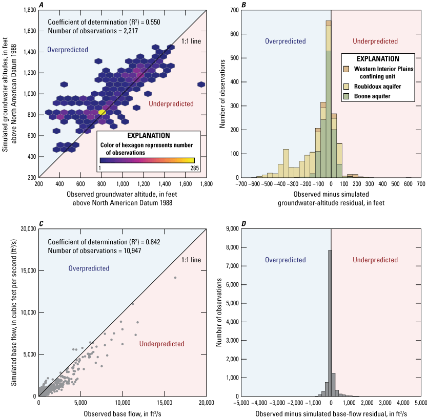
A, Observed and simulated groundwater altitudes, B, number of observed minus simulated groundwater-altitude observation residuals, C, observed and simulated base flows, and D, number of observed minus simulated base-flow residuals for the Boone and Roubidoux aquifers, northeastern Oklahoma, southeastern Kansas, southwestern Missouri, and northwestern Arkansas, 1980–2017.
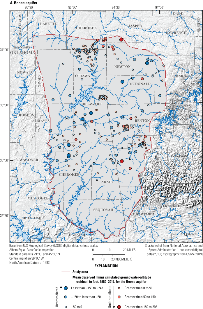
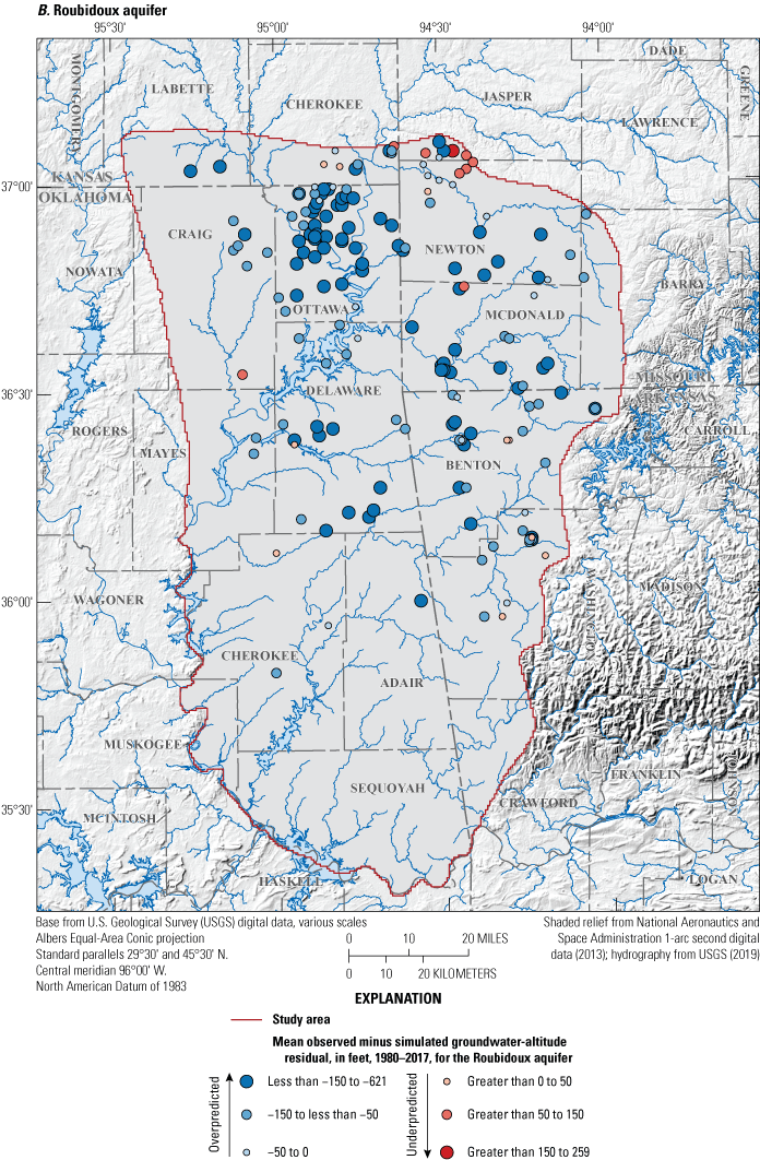
Spatial distribution of mean observed minus simulated groundwater-altitude residual for the calibrated numerical groundwater-flow model for the A, Boone and B, Roubidoux aquifers, northeastern Oklahoma, southeastern Kansas, southwestern Missouri, and northwestern Arkansas, 1980–2017.
Long-term (1980–2017) simulated and observed groundwater altitudes generally followed similar patterns. The calibrated groundwater-flow model generally overpredicted groundwater altitudes (fig. 31). For the Boone aquifer, simulated groundwater altitude was often more variable than observed groundwater altitudes, however the opposite was true for the Roubidoux aquifer (fig. 31). For the Roubidoux aquifer, simulated groundwater altitudes were overpredicted for lower groundwater-altitude observations (less than 600 ft; wells 16g, 31g, and 35g, fig. 31). Well 35g is one example where groundwater altitudes were influenced by nearby groundwater withdrawals in this location (figs. 3D, 31). Observed groundwater altitudes were frequently influenced by groundwater withdrawals in the study area.
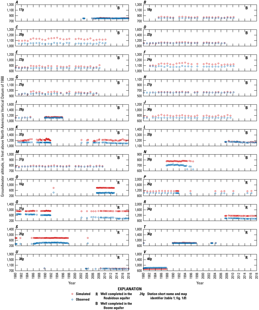
Simulated and observed groundwater altitudes at selected wells completed in the Boone and Roubidoux aquifers, northeastern Oklahoma, southeastern Kansas, southwestern Missouri, and northwestern Arkansas, 1980–2017.
The calibrated numerical groundwater-flow model slightly overpredicted base flows (fig. 29C, D). The mean base-flow residual was −1.95 ft3/s, indicating that, on average, base flows were overpredicted (table 11). Simulated base flows in the central and northern parts of the study area generally agreed closely with observed base flows (USGS streamgages 07187600 Spring River near Baxter Springs, Kans. [streamgage 10s], 07188000 Spring River near Quapaw, Okla. [streamgage 11s], 07195500 Illinois River near Watts, Okla. [streamgage 30s], and 07196000 Flint Creek near Kansas, Okla. [streamgage 34s]) (table 1; figs. 1A, 32). Peak base flows and base flows towards the southern part of the study area were likely difficult to match because of model discretization effects such as the absence of simulated alluvial aquifers at the coarse (2,000-ft by 2,000-ft) cell size used in the model.
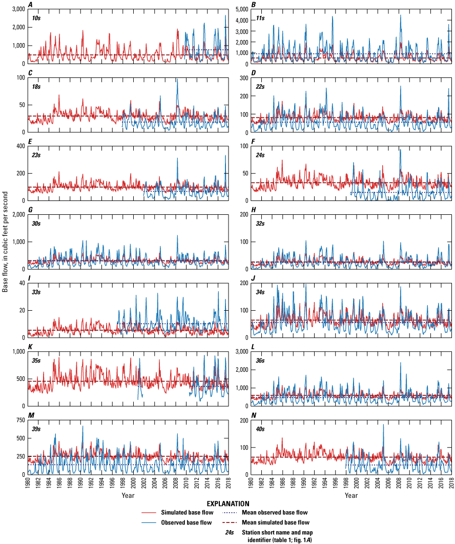
Simulated and observed base flow at selected USGS streamgages, northeastern Oklahoma, southeastern Kansas, southwestern Missouri, and northwestern Arkansas, 1980–2017.
Calibrated Groundwater-Flow Model Water Budget
The calibrated groundwater-flow model water budget (table 13; fig. 33) includes mean annual inflows and outflows for the model period 1980–2017. For the calibrated groundwater-flow model, simulated recharge (2,520,887 and 1,420,898 acre-ft/yr for the study area and for the part of the study area in Oklahoma, respectively) was the primary inflow for the Boone aquifer, and simulated leakage was the primary inflow for the Roubidoux aquifer (912,606 and 103,529 acre-ft/yr for the study area and for the part of the study area in Oklahoma, respectively). For both aquifers, seepage (to streams, springs, and lakes) was the largest outflow. Lateral flow across the study area boundary was a larger component of outflows than seepage for the Roubidoux aquifer. Otherwise, lateral flow across the study area and Oklahoma boundaries were relatively minor components of the water budget. Groundwater use accounted for less than 1 percent of total outflows for the Boone aquifer (in the study area and in the part of the study area in Oklahoma) and 2.27 percent (study area) and 5.02 percent (Oklahoma) of total outflows for the Roubidoux aquifer. Simulated groundwater use for the Boone aquifer in Oklahoma (−2,613 acre-ft/yr; table 13) was slightly higher than for the conceptual model (−2,608 acre-ft/yr; table 6). The borders that Oklahoma shares with Kansas, Missouri, and Arkansas cross some cells in the model; therefore, some small groundwater withdrawals in surrounding States were included when calculating the groundwater withdrawals for Oklahoma with the ZONEBUDGET utility. The difference accounted for about 0.19 percent of total groundwater use. Also, simulated groundwater use was less than the conceptual-model groundwater use for the study area because wells that were present along the GHB boundary were not included in the simulation.
Table 13.
Long-term simulated water budget for the Boone and Roubidoux aquifers for the entire study area in northeastern Oklahoma, southeastern Kansas, southwestern Missouri, and northwestern Arkansas and for the part of the study area in Oklahoma, 1980–2017.[Positive and negative values indicate flows into and out of the aquifer, respectively. Values not in parentheses are in acre-feet per year. Values in parentheses are percentages of total inflows or outflows. If water-budget category was an inflow (positive) then the percentage is referenced to total inflows, otherwise the percentage was referenced to outflows. Percentages may not sum to 100 percent due to rounding]
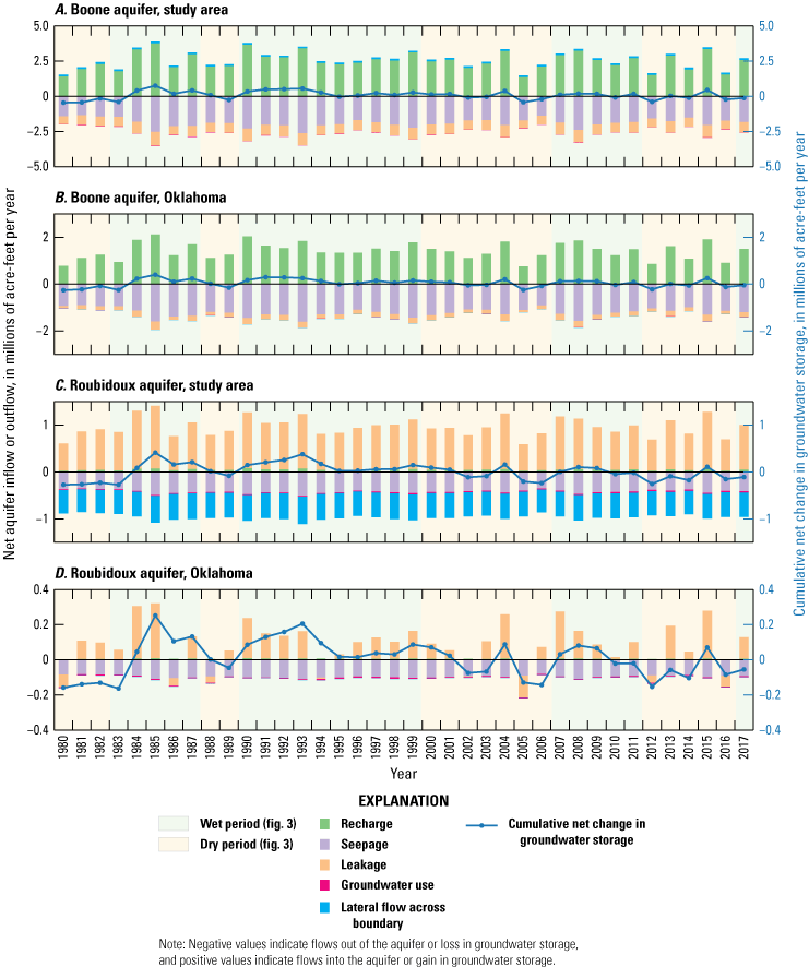
Annual inflows, outflows, and cumulative net changes in groundwater storage within the study area for the A, Boone and B, Roubidoux aquifers and Oklahoma for the C, Boone and D, Roubidoux aquifers for the numerical groundwater-flow model of the Boone and Roubidoux aquifers, 1980–2017.
For the Boone aquifer, most of the component flows of the conceptual model were similar to those of the simulated water budget (tables 6 and 13). Simulated recharge was about 3.5 percent (study area) and 1.3 percent (Oklahoma) less than conceptual model recharge (tables 6 and 13). Simulated seepage was about 20 percent (study area) and 56 percent (Oklahoma) greater than conceptual model seepage (tables 6 and 13). Simulated Boone aquifer leakage was about 251 percent greater for the simulation compared to the conceptual model for the study area (tables 6 and 13). Leakage was largely unknown and was specified as a mean leakage estimated for the entire Ozark Plateaus aquifer system. Simulated leakage from the Ozark confining unit, when normalized to each subarea, was still within the leakance bounds (multiplied by the volume of the Ozark confining unit) estimated by Christenson and others (1990) in Ottawa County, Okla. (table 5; Trevisan and others, 2024).
The components of the conceptual model did not match the simulated water budget as closely for the Roubidoux aquifer compared to the Boone aquifer (tables 6 and 13). Most of the components of the conceptual model for the Roubidoux aquifer were poorly represented by available field data. Simulated recharge, however, did match closely to that of the conceptual model. Seepage was estimated by using base-flow estimates from streamgages. Most streamgages drained either only the Boone aquifer or mostly the Boone aquifer; therefore, conceptual-model seepage estimates might be more representative of the Boone aquifer than the Roubidoux aquifer. Seeps also tend to occur in areas of the aquifer with more conduit development (Imes and Emmett, 1994), which would result in greater groundwater discharge.
Simulated leakage was about 251 percent and 336 percent greater than conceptual model leakage within the study area for the Boone and Roubidoux aquifers, respectively, but only about 73 percent greater and 10 percent less than conceptual model leakage within the Oklahoma part of the study area for the Boone and Roubidoux aquifers, respectively (tables 6 and 13). Leakage was largely unknown and specified as a mean leakage estimated for the entire Ozark Plateaus aquifer system. Simulated leakage from the Ozark confining unit, when normalized to each subarea, was still within the leakance bounds (multiplied by the volume of the Ozark confining unit) estimated by Christenson and others (1990) in Ottawa County, Okla. (table 5; Trevisan and others, 2024).
Simulated lateral groundwater flow was greater than conceptual model lateral groundwater flow by about 251 percent and 336 percent within the study area for the Boone and Roubidoux aquifers, respectively, and by about 99 and 90 percent within Oklahoma for the Boone and Roubidoux aquifers, respectively (tables 6 and 13). Lateral groundwater flow was not estimated by field data but was estimated by balancing groundwater flow in the conceptual model. For the study area, increased simulated leakage (compared to the conceptual model) accounts for the increased inflows, and thus, increased simulated seepage and lateral groundwater flow across the study area and Oklahoma boundaries. Changes in groundwater storage represent a larger component of the simulated groundwater budget for the Roubidoux aquifer than for the Boone aquifer (fig. 33A–D).
Simulated annual net groundwater storage changes reflect climatic variability during the transient-simulation model period 1980–2017 (fig. 33). Periods with loss in groundwater storage generally occur during years with below normal precipitation, and periods with gain in groundwater storage generally occur during years with above normal precipitation for both aquifers (fig. 33; fig. 8E). For both aquifers, the largest declines in storage occurred during 1980–83, 2005–07, and 2011–14, which were drier periods (fig. 3A). Cumulative net change in storage during the 10-year period 1990–99 was slightly positive for the Boone and Roubidoux aquifers (fig. 33).
Simulated Saturated Thickness and Groundwater Storage Availability
Simulated saturated thicknesses were calculated at the end of December 2017 for the Boone and Roubidoux aquifers. Patterns in simulated saturated thickness were generally similar to patterns in aquifer thickness. For example, the Boone and Roubidoux aquifers thicken towards the southern part of the study area where the saturated thicknesses were often greatest (fig. 34; Russell, 2020). The thinnest part of each aquifer with the smallest saturated thicknesses were generally in the northwestern part of the study area (fig. 34; Russell, 2020).
Boone aquifer saturated thickness ranged from 0 to 1,373 ft for the study area (fig. 34A). Areas of the Boone aquifer with the highest saturated thickness were mostly where the aquifer was confined (mostly 200 to 300 ft of saturated thickness; fig. 34A). In the unconfined part of the Boone aquifer, saturated thickness was often less than 200 ft (fig. 34A). Saturated thickness was generally less around streams and lakes except for streams and lakes in the northwestern part of the study area (fig. 34A). Saturated thickness greater than 650 ft was present where the Western Interior Plains confining unit has eroded and were also present in the thickest part of the Boone aquifer in the southeastern part of the study area. Saturated thickness was also less in an area within Craig County (where the aquifer is relatively thin in the northwestern part of the study area).
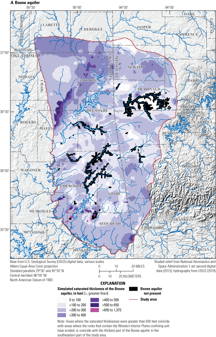
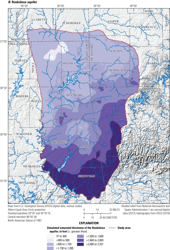
Simulated saturated thickness at the end of 2017 from the calibrated numerical groundwater-flow model for the A, Boone aquifer and B, Roubidoux aquifer, northeastern Oklahoma, southeastern Kansas, southwestern Missouri, and northwestern Arkansas.
For the Roubidoux aquifer, saturated thickness ranged from approximately 77 to 2,701 ft for the study area and the Oklahoma part of the study area (fig. 34B). Saturated thickness was relatively low in northeastern Cherokee County and northwestern Adair County. From about central Craig County to northwestern Ottawa County, saturated thickness was the lowest (500 ft or less).
Mean saturated thickness and transmissivity were calculated for the Boone and Roubidoux aquifers based on each active cell within Oklahoma (table 12). Mean transmissivity for the Roubidoux aquifer (7,591 ft2/d) was approximately an order of magnitude greater than transmissivity for the Boone aquifer (902 ft2/d), largely because the Roubidoux aquifer simulated saturated thickness (mean of 1,487 ft) was much thicker than that of the Boone aquifer (mean of 224 ft; table 12). The differences in saturated thickness between the Boone and Roubidoux aquifers resulted in greater simulated groundwater storage for the Roubidoux aquifer (50,226,846 acre-ft) than for the Boone aquifer (9,656,595 acre-ft) despite higher calibrated specific yield and specific storage for the Boone aquifer (table 12).
Groundwater-Availability Scenarios
Three types of groundwater-availability scenarios were simulated by using the calibrated groundwater-flow model. These scenarios were used to (1) estimate the equal-proportionate-share (EPS) groundwater withdrawal rate that ensures a minimum 20-, 40-, and 50-year life of the aquifer, (2) quantify the potential effects of projected well withdrawals on groundwater storage over a 50-year period, and (3) simulate the potential effects of a hypothetical 10-year drought on base flow and groundwater storage. The inputs and outputs for the groundwater-availability scenarios are available in Trevisan and others (2024).
Equal Proportionate Share
The Boone and Roubidoux aquifers are bedrock aquifers, and thus, the OWRB defines the life of a bedrock aquifer as a minimum 20-year period for which 50 percent of the aquifer maintains at least 15 ft of saturated thickness under groundwater withdrawals equally apportioned over the aquifer (hereinafter referred to as the “EPS target”; OSS, 2023). The OWRB considers, but is not required to use, the life of the aquifer when determining a maximum annual yield (MAY). Iterative EPS simulations for the Boone and Roubidoux aquifers were conducted for periods of 20, 40, and 50 years until the EPS target was reached. Utilities from the PESTPP software suite (White and others, 2020b) were used to incrementally adjust the uniform groundwater withdrawal rate, run the simulation, and record the percentage of cells with saturated thickness less than 15 ft. In each simulation, simulated wells from the calibrated model were discarded for the aquifers considered for the EPS determination, and a hypothetical well was placed in each active cell (where each active cell covers about 92 acres) for the aquifer being considered for each EPS simulation. For aquifers not considered for the simulation, historical groundwater withdrawals from 2017 were used. For example, historical groundwater withdrawals from 2017 were simulated in the Western Interior Plains confining unit and Roubidoux aquifer for the Boone aquifer EPS simulations. To restrict EPS simulations to Oklahoma, only cells with centroids in Oklahoma were used in calculating the EPS rate, although wells were simulated in the entire study area. The CHD package (representing lakes) and GHB package (representing lateral groundwater flows across the study area boundary) were deactivated during these simulations because these packages could supply limitless amounts of water (Harbaugh, 2005). The December 2017 simulated groundwater altitudes from the calibrated numerical model were used as the starting groundwater altitudes in each EPS simulation. Mean annual base flow (1980–2017) were used as inflows for the SFR package for each stress period.
For solver stability, the MODFLOW-NWT solver gradually reduced groundwater withdrawals when simulated groundwater altitudes were less than a specified threshold (5 percent of cell thickness for the simulations documented in this report) as cells become dry. Additionally, dry cells did not yield water. These factors indicated that the applied EPS rate in the WEL package was greater than the actual EPS rate. In this report, all EPS rates presented are actual EPS rates unless otherwise specified. The actual EPS rates were calculated as the total volume of groundwater withdrawn from each aquifer in Oklahoma divided by the number of years of the simulation and then divided by the modeled aquifer area for Oklahoma. To assess the sensitivity of recharge for the EPS rate, multiple EPS rates were determined by using mean annual recharge, 10 percent less than mean annual recharge, and 10 percent more than mean annual recharge.
Boone Aquifer
The EPS simulations for the Boone aquifer were conducted by using the PESTPP-GLM program (White and others, 2020b). The PESTPP-GLM program iteratively adjusted the groundwater withdrawal rate in the WEL package, conducted the simulation, and recorded the percentage of aquifer with saturated thickness less than 15 ft after solving for the EPS target after 20, 40, and 50 years. The 20-, 40-, and 50-year EPS rates for the Boone aquifer were 1.10, 0.98, and 0.96 acre-feet per acre per year ([acre-ft/acre]/yr), respectively, when simulating normal recharge conditions (that is, recharge equal to the long-term [1980–2017] mean annual SWB recharge for the study area; table 14). Given the 2,799,816 simulated acres for the Boone aquifer in Oklahoma, these rates correspond to annual yields of approximately 3,071,199; 2,749,343; and 2,674,636 acre-ft/yr for the 20-, 40-, and 50-year normal recharge scenarios, respectively. These rates exceed the reported 2018 groundwater use for the Boone aquifer (fig. 8A) by about three orders of magnitude. Decreasing and increasing recharge by 10 percent resulted in a change in the EPS rate of about 7–8 percent. At the end of the 20-year EPS simulation for the Boone aquifer (2037), simulated saturated thickness was lowest in the central to northern part of the study area (fig. 35). Streamflows were mostly depleted at the end of the 20-year EPS simulation for the Boone aquifer using normal recharge (fig. 35). Base flows at the end of the scenario were highest in streams with simulated inflows (Neosho and Spring Rivers) and the Elk River (in the northern part of the study area; fig. 1). Base flows were less than 50 ft3/s for other streams in the study area. Because the mean SWB recharge for 1980–2017 was used for the EPS simulation, the Boone aquifer was near equilibrium with EPS groundwater withdrawals and mean recharge because the change in groundwater storage was minimal between each of the final simulated years (fig. 36).
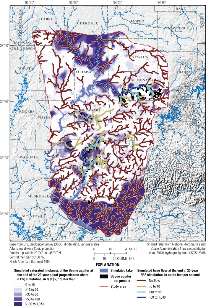
Saturated thickness of the Boone aquifer at the end of the 20-year equal-proportionate-share (EPS) groundwater-withdrawal simulation using the long-term (1980–2017) normal recharge, and simulated base flow at the end of the 20-year EPS simulation for the study area in northeastern Oklahoma, southeastern Kansas, southwestern Missouri, and northwestern Arkansas.
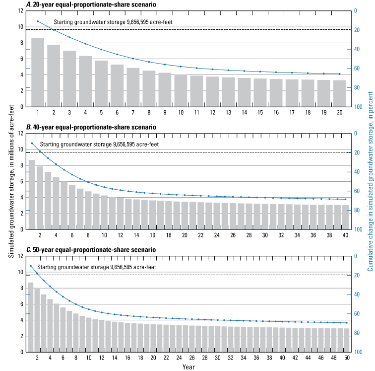
Groundwater storage simulated by using the 20-, 40-, and 50-year equal-proportionate-share scenarios for the Boone aquifer, northeastern Oklahoma, southeastern Kansas, southwestern Missouri, and northwestern Arkansas.
Table 14.
Estimated equal-proportionate-share (EPS) rates from each of the 20-, 40-, and 50-year simulations for the Boone aquifer, northeastern Oklahoma.[in/yr, inches per year]
An EPS rate is the maximum allowed annual groundwater-withdrawal rate for an aquifer per acre of land owned or leased by the permit holder (Oklahoma Secretary of State, 2023).
Roubidoux Aquifer
The EPS simulations for the Roubidoux aquifer required large groundwater withdrawal rates that rapidly dewatered many parts of the aquifer and caused simulation instability, resulting in the EPS target not being achieved. Instead, the EPS simulations for the Roubidoux aquifer were conducted by gradually increasing the EPS rates and graphing the percentage of the aquifer with less than 15 ft of saturated thickness for many simulations (fig. 37). These simulations were conducted by using the PEST++ parameter sweep program (PESTPP-SWP; White and others, 2020b) on an HPC cluster. The PESTPP-SWP program runs multiple simulations by adjusting parameters based on user-specified parameters. After each simulation, the simulated EPS rate and the percentage of the aquifer with less than 15 ft of saturated thickness (hereinafter referred to as the “PCT15”) were recorded as observations.
Another observation was an EPS rate (hereinafter referred to as the “leakage-adjusted EPS rate”) that was estimated by subtracting leakage from the Boone aquifer from the amount of simulated groundwater withdrawn from the Roubidoux aquifer. The leakage-adjusted EPS rate represents an EPS rate that assumes no leakage from the Boone aquifer and was determined by finding the maximum simulated (actual) EPS rate after correcting for leakage. Attempts were made to project the EPS rates to the EPS target by fitting exponential regressions. The actual EPS rates, which were calculated by dividing the total volume of groundwater withdrawn by the number of years and the area of the aquifer, plateaued (and declined slightly) even as the applied EPS rate (the rates applied in the WEL package) increased because of a reduction in groundwater availability and the smoothing conducted by the MODFLOW-NWT WEL package (fig. 37).
The Boone aquifer was mostly drained (PCT15 of about 99 percent for the maximum simulated EPS rate; Trevisan and others, 2024), resulting in small inflows to the Roubidoux aquifer. Depleting the Boone aquifer also caused most streams to transition to no flow for the 20-year EPS groundwater-withdrawal scenario for the Roubidoux aquifer (fig. 38); most streams also transitioned to no flow for the 20-year EPS groundwater-withdrawal scenario for the Boone aquifer (fig. 35). The EPS rate projected with exponential regressions was within 5 percent of this maximum simulated rate; however, the regressions were consistently overpredicting the EPS rate based on the observations for the simulations using higher simulated EPS rates. Because exponential regression equations poorly fit the data and the amount of groundwater withdrawn did not increase when the applied EPS rate was increased for larger applied EPS rates, the EPS rate was estimated from the maximum actual EPS rate (fig. 37A–I).
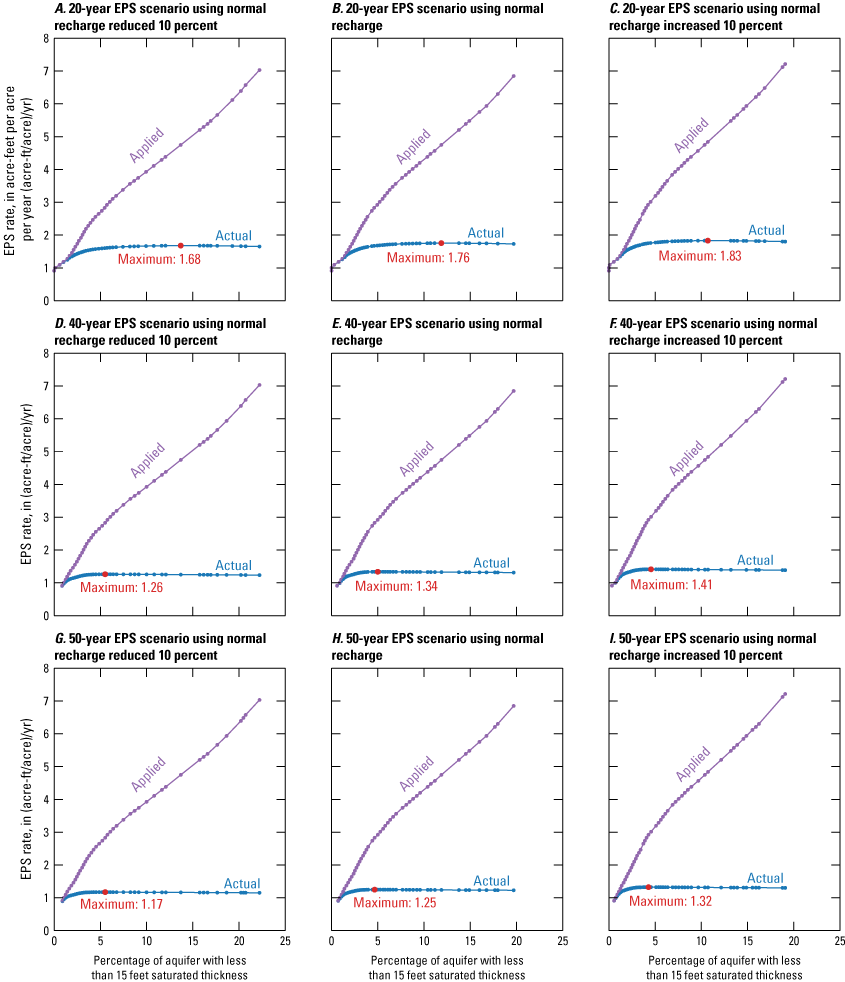
Applied and actual equal-proportionate-share (EPS) rates for the 20-year EPS groundwater-withdrawal scenario for the Roubidoux aquifer using A, normal recharge reduced 10 percent, B, normal recharge, and C, normal recharge increased 10 percent; for the 40-year EPS groundwater-withdrawal scenario for the Roubidoux aquifer using D, normal recharge reduced 10 percent, E, normal recharge, and F, normal recharge increased 10 percent; and for the 50-year EPS groundwater-withdrawal scenario for the Roubidoux aquifer using G, normal recharge reduced 10 percent, H, normal recharge, and I, normal recharge increased 10 percent.
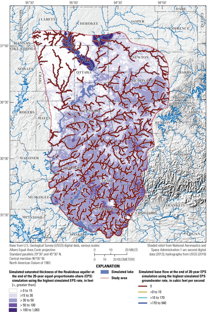
Saturated thickness and base flow for the Roubidoux aquifer from the highest applied 20-year equal-proportionate-share groundwater withdrawal rate using normal recharge conditions (recharge equal to the long-term [1980–2017] mean annual recharge).
The 20-, 40-, and 50-year EPS groundwater withdrawal rates for the Roubidoux aquifer were 1.76, 1.34, and 1.25 (acre-ft/acre)/yr, respectively, when simulating normal recharge (table 15). Given the 2,937,557 simulated acres for the Roubidoux aquifer in Oklahoma, these rates correspond to annual yields of about 5,155,653; 3,930,404; and 3,667,315 acre-ft/yr, for the 20-, 40-, and 50-year normal recharge scenarios, respectively. The 20-, 40-, and 50-year leakage-adjusted EPS rates were 0.60, 0.32, and 0.26 (acre-ft/acre)/yr, respectively, when simulating normal recharge (table 15). For the Roubidoux aquifer in Oklahoma, the leakage-adjusted EPS rates corresponded to annual yields of about 1,759,718; 932,514; and 750,852 acre-ft/yr, respectively. These rates were greater than 2018 groundwater use by about two to three orders of magnitude (fig. 8B). Decreasing and increasing recharge by 10 percent resulted in a change in the EPS rate of about 6–7 percent and almost no change in the leakage-adjusted EPS rate. The EPS rates for the Roubidoux aquifer are likely less sensitive to recharge than the EPS rates for the Boone aquifer because the Roubidoux aquifer is mostly confined and recharge is a smaller component of the water budget for the Roubidoux aquifer despite the generally greater Roubidoux aquifer thickness compared to that of the Boone aquifer (table 4).
Table 15.
Maximum actual equal-proportionate-share (EPS) groundwater withdrawal rates for the Roubidoux aquifer in Oklahoma for each 20-, 40-, and 50-year simulation.[in/yr, inches per year; (acre-ft/acre)/yr, acre-feet per acre per year]
An EPS rate is the maximum allowed annual groundwater-withdrawal rate for an aquifer per acre of land owned or leased by the permit holder (Oklahoma Secretary of State, 2023).
By using normal recharge and the highest applied 20-year EPS groundwater withdrawal rate for the Roubidoux aquifer, saturated thickness and base flow were mapped to visualize the conditions of the aquifer after the simulation (fig. 38). The highest applied 20-year EPS groundwater withdrawal rate simulation was used because the greatest reduction in groundwater altitudes would result from the simulation using this rate. Although the EPS groundwater withdrawal target rate was small, the aquifer was drained rapidly, a larger percentage (likely more than 50 percent) of the aquifer contained 50 ft of saturated thickness or less, and base flow was depleted from most of the streams (fig. 38). The EPS groundwater withdrawal rates which could produce the EPS groundwater withdrawal target would likely be close to the highest applied 20-year EPS groundwater withdrawal rate. Streams that were not dry were in the northern part of the model that contained SFR inflows; SFR inflows were likely sustaining base flows and saturated thickness in these locations. The highest actual EPS rates were selected as the EPS rate for each 20-, 40-, and 50-year EPS and simulated using normal recharge to illustrate changes in groundwater storage for the Roubidoux aquifer (fig. 39). Similar to the Boone aquifer (fig. 36), the Roubidoux aquifer was potentially in equilibrium with mean 1980–2017 recharge because decreases in groundwater storage were near zero at the ends of the EPS simulations (fig. 39). Cumulative percent changes in groundwater storage were slightly less than those for the Boone aquifer EPS simulations and could potentially be greater if the EPS simulations could be simulated to a PCT15 of 50 percent.
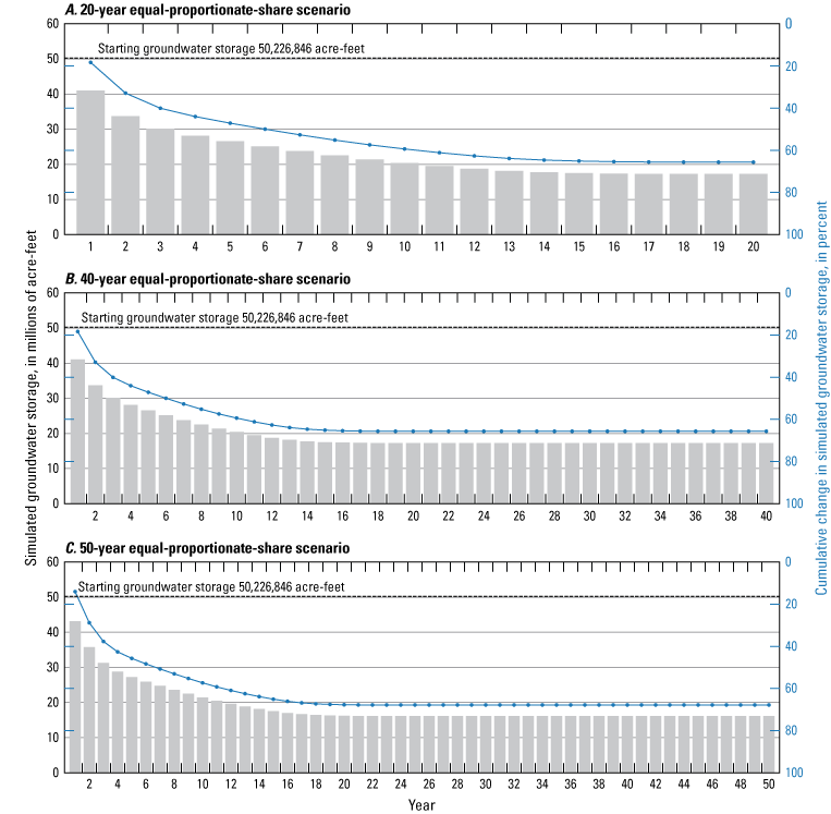
Groundwater storage simulated by using the highest applied equal-proportionate-share (EPS) groundwater-withdrawal rates for the 20-, 40-, and 50-year scenarios for the Roubidoux aquifer, northeastern Oklahoma, southeastern Kansas, southwestern Missouri, and northwestern Arkansas. (Because Roubidoux aquifer EPS rates could not be simulated, the highest applied EPS rate for the 20-year EPS groundwater-withdrawal scenario for this aquifer [fig. 37] was used instead.)
Comparison of Equal-Proportionate-Share and 2018 Groundwater-Withdrawal Rates
EPS simulations are a theoretical construct assuming the entire aquifer is fully developed with regularly spaced wells (one well per cell or one well per approximately 91.8 acres of simulated area), each withdrawing groundwater at rates often more than 100 times greater than 2018 reported groundwater use. Some parts of the aquifers may be more developed than others, but reported groundwater use for each aquifer was far less than groundwater use simulated in the EPS simulations. In Oklahoma, reported groundwater use for 2018 was approximately 2,279.87 acre-ft/yr and 6,136.16 acre-ft/yr for the Boone and Roubidoux aquifers, respectively (fig. 8A, B; Trevisan and others, 2024); 2018 reported groundwater use was equivalent to groundwater-withdrawal rates of approximately 0.0008 and 0.002 (acre-ft/acre)/yr for the Boone and Roubidoux aquifers, respectively, when equally distributed over the 2,799,816- and 2,937,557-acre spatial extents of the Boone and Roubidoux aquifers, respectively. Both rates are approximately 1 percent or less of the EPS rates estimated in this report.
Projected 50-Year Groundwater Withdrawals
Projected 50-year groundwater-withdrawal scenarios were constructed to simulate the effects of varying groundwater withdrawals on groundwater storage in the Boone and Roubidoux aquifers and stream seepage in Oklahoma. These scenarios were simulated by using monthly stress periods. Historical groundwater withdrawals were used for the scenarios, and mean monthly recharge, lake levels, and surface-water inflows were used for each scenario. Groundwater withdrawals for the four scenarios were (1) no groundwater withdrawals, (2) mean groundwater-withdrawal rates for the 1980–2017 study period, (3) groundwater-withdrawal rates for 2017, and (4) increased demand groundwater withdrawals at simulated wells. The increasing demand simulation used reported 2017 groundwater withdrawals increased by 58 percent evenly over the 50-year period, or a monthly increase of about 0.096 percent of the reported 2017 groundwater withdrawals. The 58-percent increase was the estimated increase in groundwater demand for northeastern Oklahoma from 2010 to 2060 (OWRB, 2012b).
Several years of data were required to achieve an approximate equilibrium between the projected 50-year groundwater withdrawals and mean recharge because the calibrated groundwater-flow model ended in 2017 with below mean annual recharge, and thus base flow initially increased for each simulation (fig. 40). Groundwater use represented a small component of the calibrated water budget (fig. 33); therefore, projected 50-year changes in groundwater withdrawals resulted in small changes in groundwater storage for the Boone and Roubidoux aquifers (table 16). Because stream seepage was a much larger component of the simulated water budget for the Boone aquifer compared to that of the Roubidoux aquifer, stream seepage for the Boone aquifer (fig. 40A) was much more affected by groundwater withdrawals compared to the Roubidoux aquifer (fig. 40B). Differences in stream seepage between the scenario using no groundwater withdrawals and the scenario using groundwater withdrawals increased 58 percent over a 50-year period were about 15 ft3/s for the Boone aquifer and 0.3 ft3/s for the Roubidoux aquifer (fig. 40A, B).
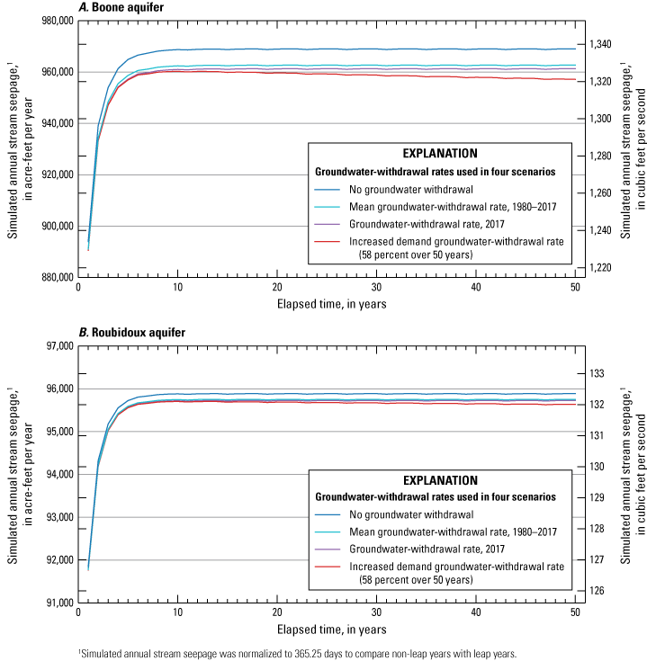
Simulated annual stream seepage for the 50-year groundwater-withdrawal scenarios for the A, Boone and B, Roubidoux aquifers for the study area in northeastern Oklahoma, southeastern Kansas, southwestern Missouri, and northwestern Arkansas.
Table 16.
Simulated changes in groundwater storage after 50 years of groundwater withdrawal at selected rates for the calibrated numerical model of the Boone and Roubidoux aquifers for the study area in northeastern Oklahoma, southeastern Kansas, southwestern Missouri, and northwestern Arkansas.[<, less than]
The increasing demand groundwater withdrawal rate assumed a cumulative 58-percent increase in groundwater withdrawal over 50 years based on 2010–60 demand projections for southern Oklahoma (Oklahoma Water Resources Board, 2012b).
Boone Aquifer
For the Boone aquifer, groundwater storage after 50 years with no groundwater withdrawals was 9,812,658 acre-ft, or 5,993 acre-ft (0.06 percent) greater than the groundwater storage at the end of the 2017-groundwater-withdrawal simulation (table 16). Groundwater storage at the end of the 50-year period with the increasing demand groundwater withdrawals was 9,803,276 acre-ft, or 3,389 acre-ft (0.03 percent) less than the storage at the end of the 2017-groundwater-withdrawal scenario. Groundwater storage after 50 years of groundwater withdrawals at the mean groundwater withdrawal for the 1980–2017 study period was 9,807,904 acre-ft, or 1,239 acre-ft (0.01 percent) greater than the groundwater storage at the end of the 2017-groundwater-withdrawal scenario.
Roubidoux Aquifer
For the Roubidoux aquifer, groundwater storage after 50 years with no groundwater withdrawals was 50,309,351 acre-ft, or 6,820 acre-ft (less than 0.01 percent) greater than the groundwater storage at the end of the 2017-groundwater-withdrawal scenario (table 16). Groundwater storage at the end of the 50-year period with the increasing demand groundwater withdrawals was 50,298,792 acre-ft, or 3,739 acre-ft (less than 0.01 percent) less than the storage at the end of the 2017-groundwater-withdrawal scenario. Groundwater storage after 50 years of groundwater withdrawals at the mean rate for the 1980–2017 study period was 50,303,211 acre-ft, or 680 acre-ft (less than 0.01 percent) greater than the groundwater storage at the end of the 2017-groundwater-withdrawal scenario.
Hypothetical 10-Year Drought
A hypothetical 10-year drought scenario was used to simulate the effects of a prolonged period of reduced recharge on groundwater storage. The generally wetter period 1990–99 was chosen as the simulated drought period (fig. 3A). Drought effects were quantified by comparing the results of the drought scenario to those of the calibrated numerical model (no drought) at the end of the simulated drought period (1999). To simulate the hypothetical drought, recharge in the calibrated groundwater-flow model was reduced by 50 percent and simulated inflows were reduced by 75 percent during the 1990–99 simulated drought period. These scaling factors were used to closely match values from 1980 (the middle of an 8-year dry period, fig. 3A), while still maintaining climate variability between each year.
Groundwater storage at the end of the drought scenario was 9,196,766 acre-ft for the Boone aquifer and 49,860,181 acre-ft for the Roubidoux aquifer (fig. 41; table 17). During the simulated drought, groundwater storage decreased by 660,451 acre-ft (6.7 percent) in the Boone aquifer and 508,472 acre-ft (1.0 percent) in the Roubidoux aquifer (fig. 41; table 17). The mean groundwater-level decline was 37.1 ft in the Boone aquifer (fig. 42A) and 37.1 ft in the Roubidoux aquifer (fig. 42B). Patterns in groundwater-level decline were similar between the Boone and Roubidoux aquifers. Groundwater altitudes generally declined the most in the central and southern parts of the study area (fig. 42). Groundwater levels declined by as much as 172 ft for the Boone aquifer (fig. 42A) and by as much as 165 ft for the Roubidoux aquifer (fig. 42B). For Oklahoma, the largest water-level declines occurred in the northeastern part of Oklahoma. Groundwater storage decreased to a maximum of about 800,000 acre-feet for the Boone aquifer and about 600,000 acre-feet for the Roubidoux aquifer (fig. 41). Stream seepage from the Boone aquifer declined by a greater percentage (about 50 percent) at the end of the hypothetical drought compared to the Roubidoux aquifer (decline of about 25 percent; fig. 43). More streams drain the Boone aquifer compared to the Roubidoux aquifer which is likely the primary factor influencing the differences in the change in stream seepage. About 5 years after the end of simulated drought, stream seepage returned to within 1 percent of the stream seepage amount in the calibrated groundwater-flow model. Because the Roubidoux aquifer is mostly confined in Oklahoma, climatic variability tends to affect the Roubidoux aquifer less than the Boone aquifer (which is mostly unconfined within the study area).
Table 17.
Change in simulated groundwater storage in the Boone and Roubidoux aquifers after a hypothetical 10-year period of drought, northeastern Oklahoma, 1990–99.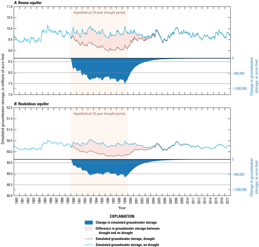
Simulated groundwater storage and changes in groundwater storage between the calibrated numerical groundwater-flow model and the hypothetical 10-year drought (1990–99) scenario for the A, Boone and B, Roubidoux aquifers in the study area in northeastern Oklahoma, southeastern Kansas, southwestern Missouri, and northwestern Arkansas, 1980–2017.
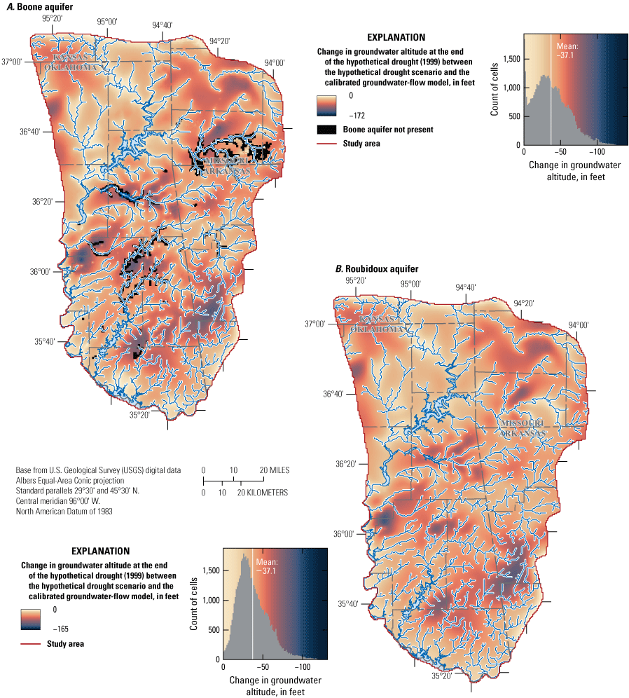
Change in groundwater altitude at the end of the hypothetical drought (1999) between the hypothetical drought scenario and the calibrated groundwater-flow model for the A, Boone and B, Roubidoux aquifers in the study area in northeastern Oklahoma, southeastern Kansas, southwestern Missouri, and northwestern Arkansas, 1980–2017.
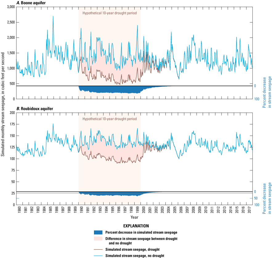
Stream seepage and changes in stream seepage between the calibrated numerical groundwater-flow model and the hypothetical 10-year drought (1990–99) scenario for the A, Boone and B, Roubidoux aquifers in the study area in northeastern Oklahoma, southeastern Kansas, southwestern Missouri, and northwestern Arkansas, 1980–2017.
Model Limitations
Some assumptions and simplifications were necessary in the simulation of groundwater flow. The use of the MODFLOW-NWT code requires the assumptions that (1) groundwater flows are governed by Darcy’s law (Heath, 1983), and (2) the aquifer hydrogeology can be simulated appropriately by the cell size and number of layers simulated. Darcy’s law is built on the assumptions that water is incompressible and of uniform density, and that groundwater flow is laminar through a porous media. Groundwater in the study area could deviate the inherent assumptions of Darcy’s law in some locations. Computing, time, and data-availability limitations prevented the use of cell sizes and calibration parameter discretization that could better represent the true variability of the hydrogeologic characteristics; therefore, results generated by the model may be more applicable to a regional, rather than local, area. Because of cell-size limitations, alluvial aquifers within the study area were not represented in the simulation. An uneven spatial and temporal distribution of groundwater-altitude observations resulted in data gaps in the calibration data.
The groundwater-flow model was created as an equivalent porous media groundwater-flow model, which means that although the aquifers are known to be karstic, with local-scale variability owing to fracturing and karst development, fractures and conduits were assumed to have minimal influence on groundwater flow at a regional scale such that hydraulic properties could be represented by their means over the thickness of the aquifer equivalently to an aquifer with porous media of equivalent mean hydraulic properties. Because MODFLOW-NWT follows Darcy’s law when calculating groundwater flows, the groundwater-flow model is most appropriate for assessing regional-scale groundwater flows because on a regional scale, local deviations from the inherent assumptions of Darcy’s law are minimized. Equivalent porous media MODFLOW-NWT simulations have been previously used to simulate groundwater flow in the Ozark Plateaus aquifer system (Imes and Emmett, 1994; Reed and Czarnecki, 2006; Czarnecki and others, 2009; Richards, 2010; Clark and others, 2018, 2019).
Apparent thicknesses (thicknesses derived from a vertical well log) were assumed for the groundwater-flow model and calculations within this report. The degree to which the rocks that contain each hydrologic unit dip was mostly small within the study area; therefore, stratigraphic thickness (the actual thickness of the hydrogeologic unit measured perpendicular to the dip) was estimated to be near apparent thickness for most of the study area. Any differences between actual and apparent thicknesses were likely less than 1 percent. The Boone and Roubidoux aquifers were mostly represented in a single layer and represented by uniform hydraulic properties in the groundwater-flow model at each cell, and thus, non-horizontal groundwater flow within each aquifer at the cell-scale was not simulated and was assumed negligible.
Saline groundwater in parts of the aquifers could potentially reduce water availability for model scenarios; however, salinity data were sparse in areas that are likely to be high in salinity. Based on the available salinity data, dissolved-solids concentrations were not sufficiently high to limit domestic or agricultural uses of water from large parts of the aquifer. The groundwater-flow simulations assumed a constant groundwater density.
The OWRB issues 90-day provisional temporary groundwater-use permits for short-term water-use needs (Oklahoma State Legislature, 2023a). The groundwater use for the 90-day provisional temporary groundwater permits was likely small and not included in the groundwater-flow model. For the EPS simulations, no maximum threshold was applied to groundwater withdrawals. The final EPS groundwater withdrawal rate may not be feasible for groundwater withdrawals from every location within the aquifer.
Summary
The 1973 Oklahoma Water Law requires that the Oklahoma Water Resources Board (OWRB) conduct hydrologic investigations to support determination of the maximum annual yield (MAY) for each groundwater basin within the State. The MAY is defined as the maximum amount of fresh groundwater that can be annually withdrawn while still allowing a minimum 20-year life of that groundwater basin.
Oklahoma Groundwater Law defines freshwater as water with dissolved-solids concentrations of less than 5,000 parts per million (milligrams per liter). For bedrock aquifers, the 20-year life of the aquifer is achieved if at least 50 percent of the groundwater basin (hereinafter referred to as “aquifer”) retains 15 feet (ft) or more of saturated thickness after 20 years of groundwater withdrawals equally apportioned over the aquifer. An equal-proportionate-share (EPS) groundwater withdrawal rate (the maximum amount of groundwater that is permitted to be withdrawn annually for each acre of land owned or leased by the permit holder) is then determined from the MAY. The Springfield Plateau aquifer and the Ozark aquifer (known locally and hereinafter referred to as the “Boone aquifer” and “Roubidoux aquifer,” respectively) are bedrock aquifers considered part of the Ozark Plateaus aquifer system that extends from northeastern Oklahoma into Kansas, Arkansas, and Missouri. At present (2024), the OWRB has yet to establish MAYs for the Boone and Roubidoux aquifers. To help determine MAYs for the Boone and Roubidoux aquifers, the U.S. Geological Survey (USGS), in cooperation with the OWRB, conducted a hydrologic investigation and evaluated the effects of potential groundwater withdrawals and drought on groundwater availability for the Boone and Roubidoux aquifers in northeastern Oklahoma.
The purpose of this report is to describe the hydrogeology and results of the simulation of groundwater flow for the Boone and Roubidoux aquifers in northeastern Oklahoma. This report presents (1) a background on the hydrogeologic framework of the Boone and Roubidoux aquifers, (2) a conceptual groundwater-flow model that includes geochemical analyses of the groundwater and quantifies inflows and outflows for the aquifers, and (3) the results of groundwater-availability scenarios to determine how the aquifers respond to hydrologic stressors, such as drought and groundwater withdrawals.
A hydrogeologic framework was developed for the Boone and Roubidoux aquifers which includes (1) the hydrostratigraphy and lithology of the hydrogeologic units, (2) the spatial and vertical extents of the hydrogeologic units, (3) potentiometric-surface maps for the Boone and Roubidoux aquifers, (4) descriptions of the hydraulic properties of aquifer materials, (5) an analysis of dissolved-solids concentrations in groundwater to assess potential saline-water migration within the aquifers, and (6) a geochemical analysis of dissolved ions to estimate the hydrologic connection between the Boone and Roubidoux aquifers. The hydrogeologic units that contain the Boone aquifer are composed mostly of limestones, and the hydrogeologic units that contain the Roubidoux aquifer are composed mostly of limestones, dolostones, and sandstones. The confining units in the area (Western Interior Plains confining system and the Ozark confining unit) are composed of mostly of shales, with some limestones and sandstones interbedded with the shales. The rocks of the hydrogeologic units generally dip southward and westward towards the study area boundaries. Regionally, groundwater flows westward in the northern part of the study area and southward towards the Arkansas River in the southern part of the study area. Saline groundwater is present west and south of the western and southern boundaries of the Boone and Roubidoux aquifers. Although these saline groundwater pockets exist, groundwater-quality samples rarely exceeded 5,000 milligrams per liter dissolved-solids concentrations. Migration of saline waters into the aquifer are likely minimal. Major-ion analysis indicated leakage from the Boone aquifer to the Roubidoux aquifer was likely occurring in the northern part of the study area but was overall limited to a small area of the aquifers.
A conceptual model was constructed to estimate regional, long-term (1980–2017) groundwater flow into and out of the Boone and Roubidoux aquifers for the study area and for the part of the study area in Oklahoma. The Roubidoux aquifer is mostly confined and received much less areal recharge compared to the Boone aquifer because the surficial exposure of the rocks that contain the Roubidoux aquifer is much smaller than the surficial exposure of the rocks that contain the Boone aquifer. Recharge was the largest inflow to the Boone aquifer, and leakage from the Boone aquifer was the largest inflow to the Roubidoux aquifer. Recharge was estimated by using the water-table fluctuation method (mean of 6.9 inches per year [in/yr] for 2018–19), Rorabaugh-method analysis (mean of 10.62 in/yr for 1980–2017), and a soil-water-balance simulation (mean of 10.52 in/yr for 1980–2017). A 1980–2017 conceptual model recharge estimate of 10.62 in/yr from Rorabaugh-method analysis was used to estimate recharge for both the Boone and Roubidoux aquifers. This recharge estimate was about 23 percent of mean annual precipitation (1980–2017). Recharge estimated from the soil-water-balance simulation was typically greatest in the central and northeastern parts of the study area. Recharge estimates were likely more reasonable for the Boone aquifer compared to those of the Roubidoux aquifer because the rocks that contain the Roubidoux aquifer crop out over a much smaller area compared to the rocks that contain the Boone aquifer.
A numerical groundwater-flow model of the Boone and Roubidoux aquifers and confining units was constructed by using the USGS MODFLOW-NWT modular groundwater-flow model (version 1.1.4) that includes a Newton formulation solver. The simulated area was discretized into 4 layers of 354 rows by 261 columns with a 2,000-ft by 2,000-ft uniform cell size. Temporal discretization consisted of 1 steady-state stress period followed by 456 monthly transient stress periods. Calibration targets included the conceptual model, groundwater-altitude observations, and base-flow observations from selected USGS streamgages. Numerical groundwater-flow model parameters were adjusted to better match calibration targets during manual and automated calibration. A sensitivity analysis revealed that changing recharge, the General Head Boundary package cells, and horizontal hydraulic conductivity had the greatest influence on matching observations.
Simulated saturated thickness at the end of the modeling period (2017) was more than 1,300 ft for some parts of the Boone aquifer, was more than 2,700 ft for parts of the Roubidoux aquifer, and was greatest in the southern part of the study area. For Oklahoma, simulated mean transmissivity was 902 feet squared per day for the Boone aquifer and 7,591 feet squared per day for the Roubidoux aquifer. Simulated mean horizontal hydraulic conductivities were 4.03 feet per day (ft/d) for the Boone aquifer and 5.11 ft/d for the Roubidoux aquifer. Simulated mean vertical conductivities were 3.18 ft/d for the Boone aquifer and 4.30 ft/d for the Roubidoux aquifer. Simulated specific yields were 0.010 and 0.0034 for the Boone and Roubidoux aquifers, respectively. Simulated groundwater storage at the end of the modeling period was 9,656,595 acre-feet (acre-ft) and 50,226,846 acre-ft for the Boone and Roubidoux aquifers, respectively.
Three types of groundwater-availability scenarios were simulated by using the calibrated groundwater-flow model. These scenarios were used to (1) estimate the equal-proportionate-share (EPS) groundwater withdrawal rate that ensures a minimum 20-, 40-, and 50-year life of the aquifer, (2) quantify the potential effects of projected well withdrawals on groundwater storage over a 50-year period, and (3) simulate the potential effects of a hypothetical 10-year drought on base flow and groundwater storage.
EPS rates for the 20-, 40-, and 50-year scenarios for the Boone aquifer were 1.10, 0.98, and 0.96 acre-feet per acre per year ([acre-ft/acre]/yr), respectively, when simulating normal recharge conditions. The Boone aquifer covered 2,799,816 simulated acres in Oklahoma, and the EPS rates correspond to annual yields of approximately 3,071,199; 2,749,343; and 2,674,636 acre-ft/yr for the 20-, 40-, and 50-year normal recharge scenarios, respectively. Decreasing and increasing recharge by 10 percent resulted in a change in the EPS rate of approximately 7 to 8 percent. Simulated saturated thickness was lowest in the central to northern part of the study area. The aquifer in the southern part of the study area maintained relatively greater saturated thickness than the rest of the aquifer, likely owing to leakage from the Western Interior Plains confining unit induced by additional groundwater withdrawals. Streamflows were mostly depleted at the end of the 20-year EPS simulation using normal recharge. Base flows at the end of the scenario were highest in streams with simulated inflows (Neosho and Spring Rivers) and the Elk River. Base flow was less than 50 cubic feet per second for other streams that were not dry.
Because applying EPS groundwater withdrawals for the Roubidoux aquifer was causing simulation instability, multiple EPS simulations were conducted, and the maximum EPS rate was determined. The maximum EPS rate was determined because the actual EPS rate did not increase when increasing the applied EPS rate owing to increasingly limited groundwater availability within the simulation. Roubidoux aquifer EPS rates for the 20-, 40-, and 50-year scenarios were 1.76, 1.34, and 1.25 (acre-ft/acre)/yr, respectively, when simulating normal recharge. Given the 2,937,557 simulated acres for the Roubidoux aquifer in Oklahoma, these rates correspond to annual yields of about 5,155,653; 3,930,404; and 3,667,315 acre-ft/yr for the 20-, 40-, and 50-year normal recharge scenarios, respectively. Leakage-adjusted EPS rates for the 20-, 40-, and 50-year scenarios were 0.60, 0.32, and 0.26 (acre-ft/acre)/yr, respectively, when simulating normal recharge. The leakage-adjusted EPS rates corresponded to annual yields of about 1,759,718; 932,514; and 750,852 acre-ft/yr for the 20-, 40-, and 50-year normal recharge scenarios, respectively. The EPS rates for the Roubidoux aquifer were generally less sensitive to changes in recharge than the EPS rates for the Boone aquifer. Decreasing and increasing recharge by 10 percent resulted in a change in the EPS rate of about 6 to 7 percent and almost no change in the leakage-adjusted EPS rate. Streams had mostly no flow after the 20-year simulation.
Projected 50-year groundwater-withdrawal scenarios were used to simulate the effects of varying groundwater withdrawal rates on groundwater storage and base flows in the Boone and Roubidoux aquifers. The effects of modified groundwater withdrawals were evaluated by quantifying differences in groundwater storage and base flow in four 50-year scenarios under mean annual conditions (1980–2017) that applied (1) no groundwater withdrawals, (2) mean groundwater-withdrawal rates for the study period (1980–2017), (3) groundwater-withdrawal rates for 2017, and (4) increased demand groundwater withdrawals at simulated wells. Because groundwater withdrawals were a small component (less than 1 percent and less than 5 percent for the Boone and Roubidoux aquifers, respectively) of the calibrated numerical-model budgets for the Boone and Roubidoux aquifers, changes to groundwater withdrawals affected stream seepage by less than 1 percent when adjusting groundwater withdrawals.
A hypothetical 10-year drought scenario was used to simulate the effects of a prolonged period of reduced recharge on groundwater storage. The monthly period 1990–99 was chosen as the simulated drought period. Drought effects were quantified by comparing the results of the drought scenario to those of the calibrated numerical model (no drought) at the end of the simulated drought period (1999). To simulate the hypothetical drought, recharge in the calibrated groundwater-flow model was reduced by 50 percent and simulated inflows were reduced by 75 percent during the 1990–99 simulated drought period. These scaling factors were used to closely match values from 1980 (the middle of an 8-year dry period), while still maintaining climate variability between each year. Groundwater storage at the end of the drought period was 9,196,766 acre-ft for the Boone aquifer and 49,860,181 acre-ft for the Roubidoux aquifer. Groundwater storage decreased by 660,451 acre-ft (6.7 percent) in the Boone aquifer and 508,472 acre-ft (1.0 percent) in the Roubidoux aquifer. Mean groundwater-level decline was 37.1 ft in the Boone aquifer and in the Roubidoux aquifer. Groundwater altitudes for the Boone and Roubidoux aquifers generally declined more for parts of the aquifer without lakes and streams. The largest groundwater-altitude declines for both aquifers were in southwestern Craig County, Oklahoma; levels declined by as much as 172 ft for the Boone aquifer and 165 ft for the Roubidoux aquifer. For Oklahoma, the largest water-altitude declines occurred in the northeastern part of Oklahoma. During the 10-year drought period, groundwater storage for the Boone aquifer declined more than groundwater storage for the Roubidoux aquifer, likely because recharge occurs over a much larger area over the Boone aquifer than the Roubidoux aquifer. Groundwater storage at the end of the 10-year drought period declined by 1.0 percent for the Roubidoux aquifer compared to 6.7 percent for the Boone aquifer despite the Boone aquifer losing only about 40 percent more groundwater storage than the Roubidoux aquifer. Stream seepage from the Boone aquifer declined by a greater percentage (about 50 percent) at the end of the hypothetical drought compared to the Roubidoux aquifer (decline of about 25 percent). More streams drain the Boone aquifer, which is likely the primary factor influencing the decline in stream seepage. About 5 years after the simulated drought, stream seepage returned to within 1 percent of the stream seepage amount in the calibrated groundwater-flow model. Because the Roubidoux aquifer is mostly confined in Oklahoma, climatic variability tends to affect the Roubidoux aquifer less than the Boone aquifer (which is mostly unconfined within the study area).
References Cited
Aber, J.S., Aber, S.W., Manders, G., and Nairn, R.W., 2010, Route 66—Geology and legacy of mining in the Tri-state district of Missouri, Kansas, and Oklahoma: The Geological Society of America Field Guide 17, 22 p., accessed February 16, 2024, at https://doi.org/10.1130/2010.0017(01).
Adamski, J.C., Petersen, J.C., Freiwald, D.A., and Davis, J.V., 1995, Environmental and hydrologic setting of the Ozark Plateaus study unit, Arkansas, Kansas, Missouri, and Oklahoma: U.S. Geological Survey Water-Resources Investigations Report 94–4022, 76 p., accessed November 26, 2021, at https://doi.org/10.3133/wri944022.
Baker, C.H., Jr., and Leonard, R.B., 1995, Hydrochemistry of aquifer systems and relation to regional flow patterns in Cretaceous and older rocks underlying Kansas, Nebraska, and parts of Arkansas, Colorado, Missouri, New Mexico, Oklahoma, South Dakota, Texas, and Wyoming: U.S. Geological Survey Water-Resources Investigations Report 94–4144, 53 p., accessed February 15, 2024, at https://doi.org/10.3133/wri944144.
Barlow, P.M., Cunningham, W.L., Zhai, T., and Gray, M., 2015, U.S. Geological Survey Groundwater Toolbox, a graphical and mapping interface for analysis of hydrologic data (version 1.0)—User guide for estimation of base flow, runoff, and groundwater recharge from streamflow data: U.S. Geological Survey Techniques and Methods book 3, chap. B10, 27 p., accessed June 5, 2020, at https://doi.org/10.3133/tm3B10.
Barlow, P.M., and Leake, S.A., 2012, Streamflow depletion by wells—Understanding and managing the effects of groundwater pumping on streamflow: U.S. Geological Survey Circular 1376, 84 p., accessed February 23, 2023, at https://doi.org/10.3133/cir1376.
Bingham, R.H., 1969, Springs in the Ozark Region, northeastern Oklahoma: Oklahoma Geology Notes, v. 29, no. 6, p. 135–145, accessed February 15, 2024, at http://ogs.ou.edu/docs/geologynotes/GN-V29N6.pdf.
Blondes, M.S., Gans, K.D., Engle, M.A., Kharaka, Y.K., Reidy, M.E., Saraswathula, V., Thordsen, J.J., Rowan, E.L., and Morrissey, E.A., 2018, U.S. Geological Survey National Produced Waters Geochemical Database (ver. 2.3, January 2018): U.S. Geological Survey data release, accessed February 15, 2024, at https://doi.org/10.5066/F7J964W8.
Brahana, J.V., Tennyson, R., Terry, J., Hays, P.D., and Pollock, E.D., 2009, Reactivated basement faulting as a hydrogeologic control of hypogene speleogenesis in the southern Ozarks of Arkansas, USA, in Stafford, K., ed., Advances in hypogene studies: National Cave and Karst Research Institute Symposium 1—National Cave and Karst Research Institute, p. 99–110, accessed July 29, 2024, at https://digitalcommons.usf.edu/cgi/viewcontent.cgi?article=1002&context=kip_monographs.
Brichta, L.C., 1960, Catalog of recorded exploration drilling and mine workings, Tri-State Zinc-Lead District—Missouri, Kansas, and Oklahoma: U.S. Bureau of Mines Information Circular 7993, 13 p. [Also available at https://digital.library.unt.edu/ark:/67531/metadc170724/m1/1/.]
Bumgarner, J.R., Stanton, G.P., Teeple, A.P., Thomas, J.V., Houston, N.A., Payne, J.D., and Musgrove, M., 2012, A conceptual model of the hydrogeologic framework, geochemistry, and groundwater-flow system of the Edwards-Trinity and related aquifers in the Pecos County region, Texas: U.S. Geological Survey Scientific Investigations Report 2012–5124 (revised July 10, 2012), 74 p., accessed March 20, 2024, at https://doi.org/10.3133/sir20125124.
Caplan, W.M., 1957, Subsurface geology of northwestern Arkansas: Little Rock, Arkansas Geological and Conservation Commission Information Circular 19, 14 p., accessed February 15, 2024, at https://www.geology.arkansas.gov/docs/pdf/publication/information-circulars/IC-19.pdf.
Caplan, W.M., 1960, Subsurface geology of Pre-Everton rocks in northern Arkansas: Little Rock, Arkansas Geological and Conservation Commission Information Circular 21, 17 p., accessed February 15, 2024, at https://www.geology.arkansas.gov/docs/pdf/publication/information-circulars/IC-21-Viewing.pdf.
Chen, Y., and Oliver, D.S., 2013, Levenberg–Marquardt forms of the iterative ensemble smoother for efficient history matching and uncertainty quantification: Computational Geosciences, v. 17, no. 4, p. 689–703, accessed February 15, 2024, at https://doi.org/10.1007/s10596-013-9351-5.
Christenson, S., 1995, Contamination of wells completed in the Roubidoux aquifer by abandoned zinc and lead mines, Ottawa County, Oklahoma: U.S. Geological Survey Water-Resources Investigations Report 95–4150, 110 p., accessed February 15, 2024, at https://doi.org/10.3133/wri954150.
Christenson, S.C., Parkhurst, D.L., and Fairchild, R.W., 1990, Geohydrology and water quality of the Roubidoux aquifer, northeastern Oklahoma: U.S. Geological Survey Open-File Report 90–570, 110 p., accessed February 15, 2024, at https://doi.org/10.3133/ofr90570.
Clark, B.R., Duncan, L.L., and Knierim, K.J., 2019, Groundwater availability in the Ozark Plateaus aquifer system: U.S. Geological Survey Professional Paper 1854, 82 p., accessed March 28, 2024, at https://doi.org/10.3133/pp1854.
Clark, B.R., Richards, J.M., and Knierim, K.J., 2018, The Ozark Plateaus Regional Aquifer Study—Documentation of a groundwater-flow model constructed to assess water availability in the Ozark Plateaus: U.S. Geological Survey Scientific Investigations Report 2018–5035, 33 p., accessed May 22, 2023, at https://doi.org/10.3133/sir20185035.
Cleveland, W.S., 1979, Robust locally weighted regression and smoothing scatterplots: Journal of the American Statistical Association, v. 74, no. 368, p. 829–836, accessed May 22, 2023, at https://doi.org/10.1080/01621459.1979.10481038.
Cooper, H.H., Jr., and Jacob, C.E., 1946, A generalized graphical method for evaluating formation constants and summarizing well-field history: Transactions, American Geophysical Union, v. 27, no. 4, p. 526–534, accessed February 15, 2024, at https://doi.org/10.1029/TR027i004p00526.
Cunningham, W.L., and Schalk, C.W., 2011, Groundwater technical procedures of the U.S. Geological Survey: U.S. Geological Survey Techniques and Methods, book 1, chap. A1, 151 p., accessed June 5, 2020, at https://doi.org/10.3133/tm1A1.
Czarnecki, J.B., Gillip, J.A., Jones, P.M., and Yeatts, D.S., 2009, Groundwater-flow model of the Ozark Plateaus aquifer system, northwestern Arkansas, southeastern Kansas, southwestern Missouri, and northeastern Oklahoma: U.S. Geological Survey Scientific Investigations Report 2009–5148 (revised March 2010), 62 p., accessed May 1, 2019, at https://doi.org/10.3133/sir20095148.
DeHay, K.L., 2003, Assessment and comparison of 1976–77 and 2002 water quality in mineshafts in the Picher mining district, northeastern Oklahoma and southeastern Kansas: U.S. Geological Survey Water-Resources Investigations Report 03–4248, p. 65, accessed February 15, 2024, at https://doi.org/10.3133/wri034248.
DeHay, K.L., Andrews, W.J., and Sughru, M.P., 2004, Hydrology and ground-water quality in the mine workings within the Picher mining district, northeastern Oklahoma, 2002–03: U.S. Geological Survey Scientific Investigations Report 2004–5043, 62 p., accessed February 15, 2024, at https://doi.org/10.3133/sir20045043.
Doherty, J., 2003, Ground water model calibration using pilot points and regularization: Ground Water, v. 41, no. 2, p. 170–177, accessed April 2, 2023, at https://doi.org/10.1111/j.1745-6584.2003.tb02580.x.
Doherty, J., 2015, Calibration and uncertainty analysis for complex environmental models: Brisbane, Australia, Watermark Numerical Computing, 227 p., accessed March, 6, 2021, at https://pesthomepage.org/pest-book.
Dugan, J.T., and Peckenpaugh, J.M., 1985, Effects of climate, vegetation, and soils on consumptive water use and ground-water recharge to the Central Midwest Regional aquifer system, mid-continent United States: U.S. Geological Survey Water-Resources Investigations Report 85–4236, 78 p., accessed February 15, 2024, at https://doi.org/10.3133/wri854236.
Ellis, J.H., 2018, Simulation of groundwater flow and analysis of projected water use for the Rush Springs aquifer, western Oklahoma: U.S. Geological Survey Scientific Investigations Report 2018–5136, 156 p. accessed February 15, 2024, at https://doi.org/10.3133/sir20185136.
Ellis, J.H., Ryter, D.W., Fuhrig, L.T., Spears, K.W., Mashburn, S.L., and Rogers, I.M.J., 2020, Hydrogeology, numerical simulation of groundwater flow, and effects of future water use and drought for reach 1 of the Washita River alluvial aquifer, Roger Mills and Custer Counties, western Oklahoma, 1980–2015: U.S. Geological Survey Scientific Investigations Report 2020–5118, 81 p., accessed February 15, 2024, at https://doi.org/10.3133/sir20205118.
Esri, 2023a, ArcGIS Pro—Topo to Raster tool: Esri web page, accessed January 11, 2024, at https://pro.arcgis.com/en/pro-app/latest/tool-reference/spatial-analyst/topo-to-raster.htm.
Esri, 2023b, ArcGIS Pro—Contour tool: Esri web page, accessed January 11, 2024, at https://pro.arcgis.com/en/pro-app/latest/tool-reference/spatial-analyst/contour.htm.
Esri, 2023c, ArcGIS Pro—How Topo to Raster works: Esri web page, accessed January 11, 2024, at https://pro.arcgis.com/en/pro-app/3.0/tool-reference/spatial-analyst/how-topo-to-raster-works.htm.
Estrada-Medina, H., Graham, R.C., Allen, M.F., Jiménez-Osornio, J.J., and Robles-Casolco, S., 2013, The importance of limestone bedrock and dissolution karst features on tree root distribution in northern Yucatán, México: Plant and Soil, v. 362, no. 1-2, p. 37–50, accessed February 15, 2024, at https://doi.org/10.1007/s11104-012-1175-x.
Farmer, W.H., and Vogel, R.M., 2013, Performance-weighted methods for estimating monthly streamflow at ungauged sites: Journal of Hydrology, v. 477, p. 240–250, accessed February 15, 2024, at https://doi.org/10.1016/j.jhydrol.2012.11.032.
Feinstein, D.T., Hunt, R.J., and Reeves, H.W., 2010, Regional groundwater-flow model of the Lake Michigan Basin in support of Great Lakes Basin water availability and use studies: U.S. Geological Survey Scientific Investigations Report 2010–5109, 379 p., accessed November 9, 2023, at https://doi.org/10.3133/sir20105109.
Freeze, R.A., and Cherry, J.A., 1979, Groundwater: Englewood Cliffs, N.J., Prentice Hall, 604 p., accessed March 21, 2024, at https://gw-project.org/books/groundwater/.
Gillip, J.A., Czarnecki, J.B., and Mugel, D.N., 2008, Potentiometric surfaces in the Springfield Plateau and Ozark aquifers of northwestern Arkansas, southeastern Kansas, southwestern Missouri, and northeastern Oklahoma, 2006: U.S. Geological Survey Scientific Investigations Report 2007–5253, 25 p., accessed February 15, 2024, at https://doi.org/10.3133/sir20075253.
Goemaat, R.L., Mize, L.D., and Spiser, D.E., 1984, Ground-water levels in observation wells in Oklahoma, 1982–83 climatic years: U.S. Geological Survey Open-File Report 84–472, 583 p., accessed February 15, 2024, at https://doi.org/10.3133/ofr84472.
Harbaugh, A.W., 1990, A computer program for calculating subregional water budgets using results from the U.S. Geological Survey modular three-dimensional finite-difference ground-water flow model: U.S. Geological Survey Open-File Report 90–392, 46 p., accessed February 15, 2024, at https://doi.org/10.3133/ofr90392.
Harbaugh, A.W., 2005, MODFLOW-2005—The U.S. Geological Survey modular ground-water model—The ground-water flow process: U.S. Geological Survey Techniques and Methods, book 6, chap. A16, [variously paged], accessed February, 15, 2024, at https://doi.org/10.3133/tm6A16.
Hargreaves, G.H., and Samani, Z.A., 1985, Reference crop evapotranspiration from temperature: Applied Engineering in Agriculture, v. 1, no. 2, p. 96–99, accessed February 15, 2024, at https://doi.org/10.13031/2013.26773.
Hays, P.D., Knierim, K.J., Breaker, B.K., Westerman, D.A., and Clark, B.R., 2016, Hydrogeology and hydrologic conditions of the Ozark Plateaus aquifer system: U.S. Geological Survey Scientific Investigations Report 2016–5137, 61 p., accessed February 15, 2024, at https://doi.org/10.3133/sir20165137.
Healy, R.W., 2010, Estimating groundwater recharge: Cambridge, U.K., Cambridge University Press, 245 p. [Also available at https://doi.org/10.1017/CBO9780511780745.]
Healy, R.W., and Cook, P.G., 2002, Using groundwater levels to estimate recharge: Hydrogeology Journal, v. 10, no. 1, p. 91–109, accessed August 3, 2022, at https://doi.org/10.1007/s10040-001-0178-0.
Heath, R.C., 1983, Basic ground-water hydrology: U.S. Geological Survey Water-Supply Paper 2220, 86 p., accessed October 5, 2023, at https://doi.org/10.3133/wsp2220.
Helsel, D.R., Hirsch, R.M., Ryberg, K.R., Archfield, S.A., and Gilroy, E.J., 2020, Statistical methods in water resources: U.S. Geological Survey Techniques and Methods, book 4, chap. A3, 458 p., accessed October 5, 2023, at https://doi.org/10.3133/tm4A3. [Supersedes USGS Techniques of Water-Resources Investigations, book 4, chap. A3, version 1.1.]
Hem, J.D., 1985, Study and interpretation of the chemical characteristics of natural water: U.S. Geological Survey Water-Supply Paper 2254, 263 p., accessed February 15, 2020, at https://doi.org/10.3133/wsp2254.
Hill, M.C., Banta, E.R., Harbaugh, A.W., and Anderman, E.R., 2000, MODFLOW-2000, the U.S. Geological Survey modular ground-water model—User guide to the observation, sensitivity, and parameter-estimation processes and three post-processing programs: U.S. Geological Survey Open-File Report 2000–184, 209 p., accessed August 3, 2020, at https://doi.org/10.3133/ofr00184.
Hudson, M.R., and Murray, K.E., 2003, Geologic map of the Ponca quadrangle, Newton, Boone, and Carroll Counties, Arkansas: U.S. Geological Survey Miscellaneous Field Studies Map 2412, accessed February 15, 2024, at https://doi.org/10.3133/mf2412.
Hudson, M.R., Turner, K.J., and Bitting, C.J., 2011, Geology and karst landscapes of the Buffalo National River area, northern Arkansas, in Kuniansky, E.L., ed., U.S. Geological Survey Karst Interest Group Proceedings, Fayetteville, Arkansas, April 26–29, 2011: U.S. Geological Survey Scientific Investigations Report 2011–5031, p. 191–212, accessed February 15, 2024, at https://doi.org/10.3133/sir20115031.
Huffman, G.G., 1958, Geology of the flanks of the Ozark Uplift, northeastern Oklahoma: Oklahoma Geological Survey Bulletin 77, 281 p., accessed October 28, 2019, at http://ogs.ou.edu/docs/bulletins/B77.pdf.
Hunter, S.L., Trevisan, A.R., and Villa, J., 2020, Data release of bathymetric map, surface area, and capacity of Grand Lake O′ the Cherokees, northeastern Oklahoma, 2019: U.S. Geological Survey data release, accessed February 2, 2024, at https://doi.org/10.5066/P9KA2T3Z.
Imes, J.L., and Emmett, L.F., 1994, Geohydrology of the Ozark Plateaus aquifer system in parts of Missouri, Arkansas, Oklahoma, and Kansas: U.S. Geological Survey Professional Paper 1414–D, 127 p., accessed April 5, 2019, at https://doi.org/10.3133/pp1414D.
IT Corporation, 1985, Engineering Supervision—Clearing and plugging sixty-six abandoned wells—Final report, volume 1: Oklahoma Water Resources Board, prepared by IT Corporation, accessed February 2, 2024, at https://semspub.epa.gov/work/06/1004289.pdf.
Jacobson, R.B., and Primm, A.T., 1997, Historical land-use changes and potential effects on stream disturbance in the Ozark Plateaus, Missouri: U.S. Geological Survey Water-Supply Paper 2484, accessed March 20, 2020, at https://doi.org/10.3133/wsp2484.
Jorgensen, D.G., Helgesen, J.O., and Imes, J.L., 1993, Regional aquifers in Kansas, Nebraska, and parts of Arkansas, Colorado, Missouri, New Mexico, Oklahoma, South Dakota, Texas, and Wyoming—Geohydrologic framework: U.S. Geological Survey Professional Paper 1414–B, 70 p., accessed February 2, 2024, at https://doi.org/10.3133/pp1414B.
Jorgensen, D.G., Helgesen, J.O., Signor, D.C., Leonard, R.B., Imes, J.L., and Christenson, S.C., 1996, Analysis of regional aquifers in the central Midwest of the United States in Kansas, Nebraska, and parts of Arkansas, Colorado, Missouri, New Mexico, Oklahoma, South Dakota, Texas, and Wyoming—Summary: U.S. Geological Survey Professional Paper 1414–A, 67 p., accessed February 2, 2024, at https://doi.org/10.3133/pp1414A.
Jurgens, B.C., Faulkner, K., McMahon, P.B., Hunt, A.G., Casile, G., Young, M.B., and Belitz, K., 2022, Over a third of groundwater in USA public-supply aquifers is Anthropocene-age and susceptible to surface contamination: Communications Earth & Environment, v. 3, article 153, accessed November 9, 2023, at https://doi.org/10.1038/s43247-022-00473-y.
Knierim, K.J., Nottmeier, A.M., Worland, S., Westerman, D.A., and Clark, B.R., 2016, Groundwater withdrawal rates from the Ozark Plateaus aquifer system, 1900 to 2010: U.S. Geological Survey data release, accessed February 2, 2024, at https://doi.org/10.5066/F7GQ6VV1.
Knierim, K.J., Nottmeier, A.M., Worland, S., Westerman, D.A., and Clark, B.R., 2017, Challenges for creating a site-specific groundwater-use record for the Ozark Plateaus aquifer system (central USA) from 1900 to 2010: Hydrogeology Journal, v. 25, no. 6, p. 1779–1793, accessed February 2, 2024, at https://doi.org/10.1007/s10040-017-1593-1.
Kottek, M., Grieser, J., Beck, C., Rudolf, B., and Rubel, F., 2006, World map of the Kӧppen-Geiger climate classification updated: Meteorologische Zeitschrift (Berlin), v. 15, no. 3, p. 259–263, accessed February 2, 2024, at https://doi.org/10.1127/0941-2948/2006/0130.
Lubczynski, M.W., 2008, The hydrogeological role of trees in water-limited environments: Hydrogeology Journal, v. 17, no. 1, p. 247–259, accessed June 5, 2020, at https://doi.org/10.1007/s10040-008-0357-3.
MacDonald, H., Zachry, D.L., and Jeffus, H., 1977, Northern Arkansas groundwater inventory: Arkansas Water Resources Center MSC–26, 187 p., accessed November 9, 2023, at https://scholarworks.uark.edu/cgi/viewcontent.cgi?article=1149&context=awrctr.
Macfarlane, P.A., 2007, The southeast Kansas Ozark aquifer water supply program—Phase 2 project results: Kansas Geological Survey Open File Report 2007–20, 117 p., accessed November 2020, at https://www.kgs.ku.edu/Hydro/Publications/2007/OFR07_20/of2007-20.pdf.
Macfarlane, P.A., 2010, Temporal variability in the quality of produced water from wells tapping the Ozark aquifer of southeast Kansas: Current Research in Earth Sciences, Kansas Geological Survey Bulletin 258, part 3, 35 p., accessed February 17, 2022, at https://www.kgs.ku.edu/Current/2010/Macfarlane/index.html.
Macfarlane, P.A., and Hathaway, L.R., 1987, The hydrogeology and chemical quality of ground waters from the lower Paleozoic aquifers in the Tri-State region of Kansas, Missouri, and Oklahoma: Kansas Geological Survey Groundwater Series 9, 37 p., accessed February 2, 2024, at https://semspub.epa.gov/work/07/30469741.pdf.
Marcher, M.V., and Kenny, J.F., 1983, Hydrology of Area 40, Western Region, Interior Coal Province, Kansas, Oklahoma and Missouri: U.S. Geological Survey Open-File Report 83–266, p. 97, accessed February 15, 2024, at https://doi.org/10.3133/ofr83266.
McKnight, E.T., and Fischer, R.P., 1970, Geology and ore deposits of the Picher field, Oklahoma and Kansas: U.S. Geological Survey Professional Paper 588, 165 p., accessed February 15, 2024, at https://doi.org/10.3133/pp588.
Menne, M.J., Williams, C.N., Jr., and Vose, R.S., 2009, The U.S. Historical Climatology Network monthly temperature data, version 2: Bulletin of the American Meteorological Society, v. 90, no. 7, p. 993–1008, accessed March 26, 2024, at https://doi.org/10.1175/2008BAMS2613.1.
Merritt, M.L., and Konikow, L.F., 2000, Documentation of a computer program to simulate lake-aquifer interaction using the MODFLOW ground-water flow model and the MOC3D solute-transport model: U.S. Geological Survey Water-Resources Investigations Report 00–4167, 146 p., accessed October 14, 2020, at https://doi.org/10.3133/wri004167.
Microsoft Corporation, 2021, Bing Maps imagery API: Microsoft web page, accessed November 12, 2023, at https://learn.microsoft.com/en-us/bingmaps/rest-services/imagery/.
Miller, J.C., 1971, Groundwater resources of Saline County, Missouri: Rolla, Mo., Missouri Geological Survey and Water Resources, Water Resources Report 26, 75 p., accessed February 15, 2024, at https://share.mo.gov/nr/mgs/MGSData/Books/Water%20Resources/Groundwater%20Resources%20of%20Saline%20County,%20Missouri/WR26.pdf.
Minor, P.M., 2013, Analysis of tripolitic chert in the Boone Formation (Lower Mississippian, Osagean), northwest Arkansas and southwestern Missouri: Fayetteville, Ark., University of Arkansas, Masters thesis, 85 p., accessed March 21, 2024, at https://scholarworks.uark.edu/etd/890/.
Multi-Resolution Land Characteristics Consortium, 2021, National Land Cover Database 2021: U.S. Geological Survey, accessed July 26, 2024, at https://www.mrlc.gov/data.
Murdoch, J., Bitting, C., and Van Brahana, J., 2016, Characterization of the karst hydrogeology of the Boone Formation in Big Creek Valley near Mt. Judea, Arkansas—Documenting the close relation of groundwater and surface water: Environmental Earth Sciences, v. 75, article 1160, accessed February 15, 2024, at https://doi.org/10.1007/s12665-016-5981-y.
National Aeronautics and Space Administration [NASA], 2013, NASA Shuttle Radar Topography Mission Global 1 arc second: NASA Land Processes Distributed Active Archive Center web page, accessed November 15, 2021, at https://doi.org/10.5067/MEaSUREs/SRTM/SRTMGL1.003.
National Agricultural Statistics Service, 2021, CropScape—Cropland data layers, 2020: National Agricultural Statistics Service web page, accessed January 18, 2022, at https://nassgeodata.gmu.edu/CropScape/.
National Oceanographic and Atmospheric Administration, 2023, U.S. Historical Climatology Network climate data version 2.5.5.20231108: National Oceanographic and Atmospheric Administration web page, accessed November 8, 2023, at https://www.ncei.noaa.gov/pub/data/ushcn/v2.5/.
Nelson, P.H., Gianoutsos, N.J., and Drake, R.M., II, 2015, Underpressure in Mesozoic and Paleozoic rock units in the midcontinent of the United States: AAPG Bulletin, v. 99, no. 10, p. 1861–1892, accessed February 15, 2024, at https://doi.org/10.1306/04171514169.
Niswonger, R.G., Panday, S., and Ibaraki, M., 2011, MODFLOW-NWT, A Newton formulation for MODFLOW-2005: U.S. Geological Survey Techniques and Methods, book 6, chap. A37, 44 p., accessed October 5, 2023, at https://doi.org/10.3133/tm6A37.
Niswonger, R.G., and Prudic, D.E., 2005, Documentation of the Streamflow-Routing (SFR2) package to include unsaturated flow beneath streams—A modification to SFR1 (ver. 1.30, April 2010): U.S. Geological Survey Techniques and Methods, book 6, chap. A13, 50 p., accessed October, 5, 2023, at https://doi.org/10.3133/tm6A13.
Nottmeier, A.M., 2015, Regional potentiometric surface of the Ozark aquifer in Arkansas, Kansas, Missouri, and Oklahoma, November 2014–January 2015: U.S. Geological Survey Scientific Investigations Map 3348, 1 sheet, accessed February 15, 2024, at https://doi.org/10.3133/sim3348.
O’Callaghan, J.F., and Mark, D.M., 1984, The extraction of drainage networks from digital elevation data: Computer Vision, Graphics, and Image Processing, v. 28, no. 3, p. 323–344, accessed March 22, 2024, at https://doi.org/10.1016/S0734-189X(84)80011-0.
Oklahoma Climatological Survey, 2024, Temperature history—Annual, northeast (CD3): Oklahoma Climatological Survey web page, accessed March 26, 2024, at https://climate.ok.gov/index.php/climate/climate_trends/temperature_history_annual_statewide/CD03/tavg/Annual.
Oklahoma Secretary of State [OSS], 2023, Oklahoma administrative code, title 785, chapter 30, subchapter 1, section 2, accessed May 16, 2023, at https://rules.ok.gov/code.
Oklahoma State Legislature, 2023a, Definitions, chap. 1020, section 1 of Waters and water rights: Oklahoma Statutes, title 82, accessed April 3, 2023, at https://oksenate.gov/sites/default/files/2019-12/os82.pdf.
Oklahoma State Legislature, 2023b, Determination of maximum annual yield, chap. 1020, section 5 of Waters and water rights: Oklahoma Statutes, title 82, accessed April 3, 2023, at https://oksenate.gov/sites/default/files/2019-12/os82.pdf.
Oklahoma Water Resources Board [OWRB], 2012a, Oklahoma Comprehensive Water Plan—Executive report (updated 2012): Oklahoma Water Resources Board, 159 p., accessed November 15, 2023, at https://www.owrb.ok.gov/supply/ocwp/pdf_ocwp/WaterPlanUpdate/draftreports/OCWP%20Executive%20Rpt%20FINAL.pdf.
Oklahoma Water Resources Board [OWRB], 2012b, Oklahoma Comprehensive Water Plan—Grand Watershed Planning Region report (ver. 1.1, updated 2012): Oklahoma Water Resources Board, 67 p., accessed November 15, 2023, at https://www.owrb.ok.gov/supply/ocwp/pdf_ocwp/WaterPlanUpdate/regionalreports/OCWP_Grand_Region_Report.pdf.
Oklahoma Water Resources Board [OWRB], 2012c, Oklahoma Comprehensive Water Plan—Lower Arkansas Watershed Planning Region report (ver. 1.1, updated 2012): Oklahoma Water Resources Board, 101 p., accessed November 15, 2023, at https://www.owrb.ok.gov/supply/ocwp/pdf_ocwp/WaterPlanUpdate/regionalreports/OCWP_LowerArkansas_Region_Report.pdf.
Oklahoma Water Resources Board [OWRB], 2012d, Oklahoma Comprehensive Water Plan Middle Arkansas Watershed Planning Region report (ver. 1.1, updated 2012): Oklahoma Water Resources Board, 133 p., accessed November 15, 2023, at https://www.owrb.ok.gov/supply/ocwp/pdf_ocwp/WaterPlanUpdate/regionalreports/OCWP_MiddleArkansas_Region_Report.pdf.
Oklahoma Water Resources Board [OWRB], 2017, Oklahoma groundwater report—Beneficial Use Monitoring Program, 172 p., accessed April 16, 2019, at https://www.owrb.ok.gov/quality/monitoring/bump/pdf_bump/Reports/GMAP2017.pdf.
Oklahoma Water Resources Board [OWRB], 2019a, GIS Data—Permitted Wells & Dedicated Lands: Oklahoma Water Resources Board online database, accessed July 29, 2024, at https://oklahoma.gov/owrb/data-and-maps/gis-data.html.
Oklahoma Water Resources Board [OWRB], 2019b, OWRB open data—Permitted surface water diversion points: Oklahoma Water Resources Board online database, accessed October 25, 2019, at https://home-owrb.opendata.arcgis.com/datasets/permitted-surface-waterdiversion-points.
Oklahoma Water Resources Board [OWRB], 2021, Interactive maps & GIS data: Oklahoma Water Resources Board online database, accessed December 2021 at https://www.owrb.ok.gov/maps/index.php.
Oklahoma Water Resources Board [OWRB], 2023, Maximum annual yield: Oklahoma Water Resources Board fact sheet, 2 p., accessed February 15, 2024, at https://www.owrb.ok.gov/about/about_pdf/Fact-MAY.pdf.
Orndorff, R.C., Weary, D.J., and Sebela, S., 2001, Geologic framework of the Ozarks of south-central Missouri—Contributions to a conceptual model of karst, in Kuniansky, E.L., ed., U.S. Geological Survey Karst Interest Group Proceedings, St. Petersburg, Florida, February 13–16, 2001: U.S. Geological Survey Water-Resources Investigations Report 2001–4011, p. 18–24, accessed September 24, 2024, at https://doi.org/10.3133/wri014011.
Osborn, N.I., 2001, Hydrogeologic investigation report of the Boone groundwater basin, northeastern Oklahoma: Oklahoma Water Resources Board Technical Report GW2001–2, 19 p., accessed May 1, 2019, at https://www.owrb.ok.gov/studies/reports/reports_pdf/boone.pdf.
Petersen, J.C., Adamski, J.C., Bell, R.W., Davis, J.V., Femmer, S.R., Freiwald, D.A., and Joseph, R.L., 1998, Water quality in the Ozark Plateaus, Arkansas, Kansas, Missouri, and Oklahoma, 1992–95: U.S. Geological Survey Circular 1158, 33 p., accessed February 15, 2024, at https://doi.org/10.3133/cir1158.
Piper, A.M., 1944, A graphic procedure in the geochemical interpretation of water-analyses: Transactions, American Geophysical Union, v. 25, no. 6, p. 914–928, accessed February 15, 2024, at https://doi.org/10.1029/TR025i006p00914.
PRISM Climate Group, 2022, Monthly 4-kilometer climate datasets: Oregon State University, accessed November 8, 2023, at https://ftp.prism.oregonstate.edu/monthly/.
Pugh, A.L., 2008, Summary of aquifer test data for Arkansas—1940–2006: U.S. Geological Survey Scientific Investigations Report 2008–5149, 33 p., accessed August 19, 2021, at https://doi.org/10.3133/sir20085149.
QGIS, 2022, QGIS—A free and open source geographic information system: QGIS Association website, accessed October 5, 2023, at https://www.qgis.org.
Reed, E.W., Schoff, S.L., and Branson, C.C., 1955, Ground-water resources of Ottawa County, Oklahoma: Oklahoma Geological Survey Bulletin 72, 203 p., accessed March 21, 2024, at http://www.ogs.ou.edu/pubsscanned/BULLETINS/bulletin72mm.pdf.
Reed, T.B., and Czarnecki, J.B., 2006, Ground-water flow model of the Boone Formation at the Tar Creek Superfund site, Oklahoma and Kansas: U.S. Geological Survey Scientific Investigations Report 2006–5097, 41 p., accessed March 21, 2024, at https://doi.org/10.3133/sir20065097.
Richards, J.M., 2010, Groundwater-flow model and effects of projected groundwater use in the Ozark Plateaus aquifer system in the vicinity of Greene County, Missouri—1907–2030: U.S. Geological Survey Scientific Investigations Report 2010–5227, 106 p., accessed February 15, 2024, at https://doi.org/10.3133/sir20105227.
Ries, K.G., III, Newson, J.K., Smith, M.J., Guthrie, J.D., Steeves, P.A., Haluska, T.L., Kolb, K.R., Thompson, R.F., Santoro, R.D., and Vraga, H.W., 2017, StreamStats, version 4: U.S. Geological Survey Fact Sheet 2017–3046, 4 p., accessed January 2022 at https://doi.org/10.3133/fs20173046.
Russell, C.A., 2020, Data used to describe hydrogeologic units and create contour maps and cross sections of the Boone and Roubidoux aquifers, northeastern Oklahoma: U.S. Geological Survey data release, accessed February 15, 2024, at https://doi.org/10.5066/P967BVQL.
Russell, C.A., and Stivers, J.W., 2020, Hydrogeologic units, contour maps, and cross sections of the Boone and Roubidoux aquifers, northeastern Oklahoma, 2020: U.S. Geological Survey Scientific Investigations Map 3452, 2 sheets, accessed February 15, 2024, at http://doi.org/10.3133/sim3452.
Rutledge, A.T., 1998, Computer programs for describing the recession of ground-water discharge and for estimating mean ground-water recharge and discharge from streamflow records—Update: U.S. Geological Survey Water-Resources Investigations Report 98–4148, 43 p., accessed February 15, 2024, at https://doi.org/10.3133/wri984148.
Rutledge, A.T., 2000, Considerations for use of the RORA program to estimate ground-water recharge from streamflow records: U.S. Geological Survey Open-File Report 00–156, accessed February 15, 2024, at https://doi.org/10.3133/ofr00156.
Schenk, H.J., 2008, Soil depth, plant rooting strategies and species’ niches: The New Phytologist, v. 178, no. 2, p. 223–225, accessed February 15, 2024, at https://doi.org/10.1111/j.1469-8137.2008.02427.x.
Sharp, J.M., Jr., 2023, A glossary of hydrogeology: The Groundwater Project, 196 p., accessed February 6, 2024, at https://doi.org/10.21083/978-1-77470-079-2.
Smith, S.J., 2013, Estimation of volume and mass and of changes in volume and mass of selected chat piles in the Picher mining district, Ottawa County, Oklahoma, 2005–10: U.S. Geological Survey Scientific Investigations Report 2013–5011, 20 p., accessed July 26, 2024, at https://doi.org/10.3133/sir20135011.
Smith, S.J., Ellis, J.H., Paizis, N.C., Becker, C.J., Wagner, D.L., Correll, J.S., and Hernandez, R.J., 2021, Hydrogeology and model-simulated groundwater availability in the Salt Fork Red River aquifer, southwestern Oklahoma, 1980–2015: U.S. Geological Survey Scientific Investigations Report 2021–5003, 85 p., accessed February 15, 2024, at https://doi.org/10.3133/sir20215003.
Smith, S.J., Ellis, J.H., Wagner, D.L., and Peterson, S.M., 2017, Hydrogeology and simulated groundwater flow and availability in the North Fork Red River aquifer, southwest Oklahoma, 1980–2013: U.S. Geological Survey Scientific Investigations Report 2017–5098, 107 p., accessed February 15, 2024, at https://doi.org/10.3133/sir20175098.
Spruill, T.B., 1987, Assessment of water resources in lead-zinc mined areas in Cherokee County, Kansas: U.S. Geological Survey Open-File Report 84–439, 102 p., accessed February 15, 2024, at https://doi.org/10.3133/wsp2268.
Stanton, J.S., Anning, D.W., Brown, C.J., Moore, R.B., McGuire, V.L., Qi, S.L., Harris, A.C., Dennehy, K.F., McMahon, P.B., Degnan, J.R., and Böhlke, J.K., 2017, Brackish groundwater in the United States: U.S. Geological Survey Professional Paper 1833, 185 p., accessed February 15, 2024, at https://doi.org/10.3133/pp1833.
Stramel, G.J., 1957, The hydraulic properties of the Ordovician rocks at Pittsburg, Kansas: Kansas Geological Survey, Bulletin 127, part 5, accessed November 9, 2023, at https://www.kgs.ku.edu/Publications/Bulletins/127_5/.
Thompson, T.L., 1991, Paleozoic succession in Missouri—Part 2, Ordovician System: Rolla, Mo., Missouri Department of Natural Resources, Division of Geology and Land Survey, Report of Investigations 70, 282 p., accessed February 15, 2024, at https://ia902501.us.archive.org/5/items/1991MOPaleozoicSuccessionPart2/1991MOPaleozoicSuccessionPart2.pdf.
Thompson, T.L., 2001, Lexicon of stratigraphic nomenclature in Missouri: Rolla, Mo., Missouri Department of Natural Resources, Division of Geology and Land Survey, Report of Investigation Number 73, 371 p., accessed July 26, 2024, at https://share.mo.gov/nr/mgs/MGSData/Books/Reports%20of%20Investigations/Lexicon%20of%20Stratigraphic%20Nomenclature%20in%20Missouri/RI-073.pdf.
Thornthwaite, C.W., and Mather, J.R., 1957, Instructions and tables for computing potential evapotranspiration and the water balance: Centerton, N.J., Drexel Institute of Technology, Laboratory of Climatology, Publications in Climatology, v. 10, no. 3, p. 185–311, accessed February 15, 2024, at https://www.wrc.udel.edu/wp-content/publications/ThornthwaiteandMather1957Instructions_Tables_ComputingPotentialEvapotranspiration_Water%20Balance.pdf.
Thornton, M.M., Shrestha, R., Wei, Y., Thornton, P.E., Kao, S.-C., and Wilson, B.E., 2020, Daymet—Daily surface weather data on a 1-km grid for North America, version 4: Oak Ridge, Tenn., ORNL DAAC web page, accessed February 15, 2024, at https://doi.org/10.3334/ORNLDAAC/1840.
Trevisan, A.R., Correll, J.S., and Knierim, K.J., 2024, MODFLOW-NWT model used for the simulation of groundwater flow and analysis of groundwater availability in the Boone and Roubidoux aquifers in northeastern Oklahoma, 1980–2017: U.S. Geological Survey data release, https://doi.org/10.5066/P9KWWUAV.
U.S. Army Corps of Engineers [USACE], 2021, Reservoir release, storage, evaporation, and precipitation data for lakes: U.S. Army Corps of Engineers database, accessed April 1, 2021, at https://www.swt-wc.usace.army.mil/stations.htm.
U.S. Census Bureau, 2023, Annual estimates of the resident population for counties in Oklahoma—April 1, 2020 to July 1, 2022 (CO-EST2022-POP-40): U.S. Census Bureau database, accessed May 26, 2023, at https://www.census.gov/data/tables/time-series/demo/popest/2020s-counties-total.html.
U.S. Department of Agriculture, 2021, Gridded Soil Survey Geographic (GSSURGO) Database for the Conterminous United States: Natural Resources Conservation Service, accessed February 15, 2024, at https://gdg.sc.egov.usda.gov/.
U.S. Environmental Protection Agency [EPA], 2020a, Drinking water regulations and contaminants: EPA web page, accessed March 24, 2020, at https://www.epa.gov/sdwa/drinking-water-regulations-and-contaminants.
U.S. Environmental Protection Agency [EPA], 2020b, National Hydrography Dataset Plus version 2: EPA web page, accessed April 11, 2020, at https://www.epa.gov/waterdata/get-nhdplus-national-hydrography-dataset-plus-data.
U.S. Environmental Protection Agency [EPA], 2023, EPA in Kansas—EPA Region 7 cleans up contaminated tributary in southeast Kansas: EPA web page, accessed March 5, 2024, at https://www.epa.gov/ks/epa-region-7-cleans-contaminated-tributary-southeast-kansas#:~:text=Spanning%20nearly%202%2C500%20square%20miles,between%20abou t%201850%20and%201970.
U.S. Fish and Wildlife Service, 2021, National Wetlands Inventory—Download seamless wetlands data by State: U.S. Fish and Wildlife Service database, accessed August 5, 2021, at https://www.fws.gov/wetlands/Data/State-Downloads.html.
U.S. Geological Survey [USGS], 2019, The National Map—TNM download: U.S. Geological Survey, accessed April 15, 2019, at https://viewer.nationalmap.gov/basic/.
U.S. Geological Survey [USGS], 2021a, USGS water data for the Nation: U.S. Geological Survey National Water Information System database, accessed May 1, 2021, at https://doi.org/10.5066/F7P55KJN.
U.S. Geological Survey [USGS], 2021b, U.S. Geological Survey water data for Oklahoma: U.S. Geological Survey National Water Information System database, accessed May 1, 2021, at https://waterdata.usgs.gov/ok/nwis/.
Virtanen, P., Gommers, R., Oliphant, T.E., Haberland, M., Reddy, T., Cournapeau, D., Burovski, E., Peterson, P., Weckesser, W., Bright, J., van der Walt, S.J., Brett, M., Wilson, J., Millman, K.J., Mayorov, N., Nelson, A.R.J., Jones, E., Kern, R., Larson, E., Carey, C.J., Polat, I., Feng, Y., Moore, E.W., VanderPlas, J., Laxalde, D., Perktold, J., Cimrman, R., Henriksen, I., Quintero, E.A., Harris, C.R., Archibald, A.M., Ribeiro, A.H., Pedregosa, F., van Mulbregt, P., Vijaykumar, A., Bardelli, A.P., Rothberg, A., Hilboll, A., Kloeckner, A., Scopatz, A., Lee, A., Rokem, A., Woods, C.N., Fulton, C., Masson, C., Häggström, C., Fitzgerald, C., Nicholson, D.A., Hagen, D.R., Pasechnik, D.V., Olivetti, E., Martin, E., Wieser, E., Silva, F., Lenders, F., Wilhelm, F., Young, G., Price, G.A., Ingold, G.-L., Allen, G.E., Lee, G.R., Audren, H., Probst, I., Dietrich, J.P., Silterra, J., Webber, J.T., Slavič, J., Nothman, J., Buchner, J., Kulick, J., Schönberger, J.L., de Miranda Cardoso, J.V., Reimer, J., Harrington, J., Rodríguez, J.L.C., Nunez-Iglesias, J., Kuczynski, J., Tritz, K., Thoma, M., Newville, M., Kümmerer, M., Bolingbroke, M., Tartre, M., Pak, M., Smith, N.J., Nowaczyk, N., Shebanov, N., Pavlyk, O., Brodtkorb, P.A., Lee, P., McGibbon, R.T., Feldbauer, R., Lewis, S., Tygier, S., Sievert, S., Vigna, S., Peterson, S., More, S., Pudlik, T., Oshima, T., Pingel, T.J., Robitaille, T.P., Spura, T., Jones, T.R., Cera, T., Leslie, T., Zito, T., Krauss, T., Upadhyay, U., Halchenko, Y.O., and Vázquez-Baeza, Y., 2020, SciPy 1.0—Fundamental algorithms for scientific computing in Python: Nature Methods, v. 17, no. 3, p. 261–272, accessed October 5, 2023, at https://doi.org/10.1038/s41592-019-0686-2.
Wahl, K.L., and Wahl, T.L., 1995, Determining the flow of Comal Springs at New Braunfels, Texas, in Texas Water ‘95—A Component Conference of the First International Conference on Water Resources Engineering, San Antonio, Texas, August 16–17, 1995, [Proceedings]: American Society of Civil Engineers, p. 77–86, accessed October 19, 2023, at https://www.usbr.gov/tsc/techreferences/hydraulics_lab/pubs/PAP/PAP-0708.pdf.
Weary, D.J., and Schindler, J.S., 2004, Geologic map of the Van Buren South quadrangle, Carter County, Missouri: U.S. Geological Survey Geologic Investigations Series Map I–2803, 1 sheet, accessed February 15, 2024, at https://doi.org/10.3133/i2803.
Welter, D.E., White, J.T., Hunt, R.J., and Doherty, J.E., 2015, Approaches in highly parameterized inversion—PEST++ Version 3, a Parameter ESTimation and uncertainty analysis software suite optimized for large environmental models: U.S. Geological Survey Techniques and Methods, book 7, chap. C12, 54 p., accessed October 18, 2023, at https://doi.org/10.3133/tm7C12.
Wenz, Z.J., Appold, M.S., Shelton, K.L., and Tesfaye, S., 2012, Geochemistry of Mississippi Valley–type mineralizing fluids of the Ozark Plateau—A regional synthesis: American Journal of Science, v. 312, no. 1, p. 22–80, accessed February 15, 2024, at https://doi.org/10.2475/01.2012.02.
Westenbroek, S.M., Kelson, V.A., Dripps, W.R., Hunt, R.J., and Bradbury, K.R., 2010, SWB—A modified Thornthwaite-Mather Soil-Water-Balance code for estimating groundwater recharge: U.S. Geological Survey Techniques and Methods book 6, chap. A31, 59 p., accessed February 15, 2024, at https://doi.org/10.3133/tm6A31.
Westerman, D.A., Gillip, J.A., Richards, J.M., Hays, P.D., and Clark, B.R., 2016a, Altitudes and thicknesses of hydrogeologic units of the Ozark Plateaus aquifer system in Arkansas, Kansas, Missouri, and Oklahoma: U.S. Geological Survey data release, accessed May 1, 2019, at https://doi.org/10.5066/F7HQ3X0T.
Westerman, D.A., Gillip, J.A., Richards, J.M., Hays, P.D., and Clark, B.R., 2016b, Altitudes and thicknesses of hydrogeologic units of the Ozark Plateaus aquifer system in Arkansas, Kansas, Missouri, and Oklahoma: U.S. Geological Survey Scientific Investigations Report 2016–5130, 32 p., accessed May 1, 2019, at https://doi.org/10.3133/sir20165130.
White, J.T., 2018, A model-independent iterative ensemble smoother for efficient history-matching and uncertainty quantification in very high dimensions: Environmental Modelling & Software, v. 109, p. 191–201, accessed June 5, 2020, at https://doi.org/10.1016/j.envsoft.2018.06.009.
White, J.T., Hunt, R.J., Fienen, M.N., and Doherty, J.E., 2020a, PEST++—A software suite for parameter estimation, uncertainty analysis, management optimization and sensitivity analysis: U.S. Geological Survey GitHub web page, accessed June 28, 2022, at https://github.com/usgs/pestpp/releases/tag/4.3.17.
White, J.T., Hunt, R.J., Fienen, M.N., and Doherty, J.E., 2020b, Approaches to highly parameterized inversion—PEST++ Version 5, a software suite for parameter estimation, uncertainty analysis, management optimization and sensitivity analysis: U.S. Geological Survey Techniques and Methods book 7, chap. C26, 51 p., accessed February 15, 2024, at https://doi.org/10.3133/tm7C26.
Conversion Factors
U.S. customary units to International System of Units
*Leakance: The standard unit for leakance is foot per day per foot [(ft/d)/ft]. In this report, the mathematically reduced form, per day (/d), is used for convenience.
Temperature in degrees Celsius (°C) may be converted to degrees Fahrenheit (°F) as follows:
°F = (1.8 × °C) + 32.
Temperature in degrees Fahrenheit (°F) may be converted to degrees Celsius (°C) as follows:
°C = (°F – 32) / 1.8.
Datums
Vertical coordinate information is referenced to the North American Vertical Datum of 1988 (NAVD 88).
Horizontal coordinate information is referenced to the North American Datum of 1983 (NAD 83).
Altitude, as used in this report, refers to distance above the vertical datum.
Supplemental Information
Concentrations of chemical constituents in water are in milligrams per liter (mg/L).
Abbreviations
BFI
base-flow index
CHD
Time-variant head package for MODFLOW-NWT
DEM
digital elevation model
DRN
Drain package for MODFLOW-NWT
EPA
U.S. Environmental Protection Agency
EPS
equal proportionate share
GHB
General Head Boundary package for MODFLOW-NWT
GMAP
Groundwater Monitoring and Assessment Program (OWRB)
GRDA
Grand River Dam Authority
HOB
Head Observations package for MODFLOW-NWT
HPC
high-performance computing
MAY
maximum annual yield
MCL
maximum contaminant level
MODFLOW-2005
A modular finite-difference numerical groundwater-flow modeling software
MODFLOW-NWT
Newton-Raphson formulation for MODFLOW-2005
NHD
National Hydrography Dataset
NWIS
National Water Information System (USGS database)
OSS
Oklahoma Secretary of State
OWRB
Oklahoma Water Resources Board
Phi
the objective function or sum of squared residuals
PCT15
percentage of the aquifer with less than 15 feet of saturated thickness
PEST++
parameter estimation software version 4
PESTPP-IES
PEST++ iterative ensemble smoother utility
PESTPP-GLM
PEST++ Gauss-Levenburg-Marquardt parameter inversion utility
PESTPP-SWP
PEST++ parameter sweep utility
RCH
Recharge package for MODFLOW-NWT
RORA
a computer program within the USGS Groundwater Toolbox that implements Rorabaugh’s method
SFR
Streamflow Routing package for MODFLOW-NWT
SWB
soil-water-balance
UPW
Upstream Weighting package for MODFLOW-NWT
USGS
U.S. Geological Survey
WEL
Well package for MODFLOW-NWT
WTF
water-table fluctuation
For more information about this publication, contact
Director, Oklahoma-Texas Water Science Center
U.S. Geological Survey
1505 Ferguson Lane
Austin, TX 78754-4501
For additional information, visit
https://www.usgs.gov/centers/ot-water
Publishing support provided by
Lafayette Publishing Service Center
Disclaimers
Any use of trade, firm, or product names is for descriptive purposes only and does not imply endorsement by the U.S. Government.
Although this information product, for the most part, is in the public domain, it also may contain copyrighted materials as noted in the text. Permission to reproduce copyrighted items must be secured from the copyright owner.
Suggested Citation
Trevisan, A.R., Russell, C.A., Lockmiller, H.A., Wagner, D.L., Correll, J.S., and Knierim, K.J., 2024, Conceptualization and simulation of groundwater flow and groundwater availability in the Boone and Roubidoux aquifers in northeastern Oklahoma, 1980–2017: U.S. Geological Survey Scientific Investigations Report 2024–5093, 105 p., https://doi.org/10.3133/sir20245093.
ISSN: 2328-0328 (online)
Study Area
| Publication type | Report |
|---|---|
| Publication Subtype | USGS Numbered Series |
| Title | Conceptualization and simulation of groundwater flow and groundwater availability in the Boone and Roubidoux aquifers in northeastern Oklahoma, 1980–2017 |
| Series title | Scientific Investigations Report |
| Series number | 2024-5093 |
| DOI | 10.3133/sir20245093 |
| Publication Date | October 16, 2024 |
| Year Published | 2024 |
| Language | English |
| Publisher | U.S. Geological Survey |
| Publisher location | Reston, VA |
| Contributing office(s) | Oklahoma-Texas Water Science Center |
| Description | Report: xiv, 105 p.; Data Release |
| Country | United States |
| State | Oklahoma |
| Other Geospatial | Boone and Roubidoux aquifers |
| Online Only (Y/N) | Y |