

Streamflow Characteristics and Trends in New Jersey, Water Years 1903–2017
Links
- Document: Report (17.6 MB pdf) , HTML , XML
- Data Release: USGS data release - Streamflow characteristics and trends at continuous-record and partial-record streamflow-gaging stations in New Jersey, water years 1903–2017
- NGMDB Index Page: National Geologic Map Database Index Page (html)
- Download citation as: RIS | Dublin Core
Abstract
As New Jersey’s population density remains high, so does its requirements for water management. Understanding the streamflow conditions throughout the state and how they may have changed over time is an important part of managing the water resources within the state. The New Jersey Department of Environmental Protection has many responsibilities related to protecting the environment and natural resources and among them is protecting the waters in the lakes, rivers, and streams of New Jersey for current and future use. To support this mission, the U.S. Geological Survey updated high- and low-streamflow statistics for 97 continuous-record streamgages and low-streamflow statistics for 719 partial-record streamgages throughout the state. The continuous-record streamgages included in the study had a minimum of 20 years of record, spanning from 1903 to 2017.
This study is an update to previous studies that documented the high- and low-streamflow statistics for New Jersey streams in the 1970s and in 2005. The 1982 report by Gillespie and Schopp documented low-flow characteristics and flow duration for about 400 continuous and partial-record streamgages. The U.S. Geological Survey computed streamflow statistics including, but not limited to, maximum, minimum, and means for period of record, flow durations, nonexceedance high- and low-flow frequencies, base flow, runoff, peak-to-mean flow ratios, and September median streamflow.
Overall, both high and low flows are generally increasing in New Jersey, though the results are not uniform across the State. Streamflow trends and changes to duration and frequency statistics can be influenced by local water use, in addition to climate variables. The resulting computations at some streamgages indicated considerable positive change while others showed considerable negative change. Water managers and regulators can use the data provided here and in the companion data release to assess individual stream reaches and watershed management areas to evaluate the available resources and changes, which may have developed during the periods for which streamflow statistics are available.
Introduction
As the population continues to increase and New Jersey maintains its status as one of the most densely populated states in the country, the demand for water also increases. The New Jersey Department of Environmental Protection (NJDEP)’s responsibilities include protecting the environment and natural resources of the state for current and future use, which includes protecting the waters in the lakes, rivers, and streams. Streamflow statistics, utilized by water managers and planners to help them understand flow conditions in the rivers and streams, are computed from published streamflow data at continuous- and partial-record streamgages. Streamflow statistics are also used by planners and regulatory agencies, like NJDEP, to make decisions about minimum passing flows, surface-water withdrawals, and establishing limits for waste load discharges for municipal and industrial facilities.
Increases in population and development in New Jersey over the past 120 years has not only increased demands for water but also the need for wastewater discharges to streams. Improvements in water-use efficiency have helped influence decreases in total water use in some areas according to USGS county-level estimates (Falcone, 2017). These human activities, in addition to influences from climatic changes over time, have contributed to alterations of natural streamflow conditions. The U.S. Geological Survey (USGS), in cooperation with other Federal, State, and local agencies, has collected and published daily mean streamflow data for hundreds of streamgages across the state of New Jersey since the late 1890s (U.S. Geological Survey, 2023).
This report updates statistics previously published in “Streamflow Characteristics and Trends in New Jersey, Water Years 1897–2003” (Watson and others, 2005) and can be considered the fourth in a series of streamflow statistic reports for New Jersey. Earlier reports published are “Low-flow Characteristics and Flow Duration of New Jersey Streams” (Gillespie and Schopp, 1982) and “Statistical Summaries of New Jersey Streamflow Records—Water Resources Circular 23” (Laskowski, 1970). Daily mean streamflow for 97 continuous-record streamgages and 719 partial-record streamgages in New Jersey were used to compute the statistics presented in this report (fig. 1). The entire period of record available for continuous- and partial-record streamgages was used in this analysis, unless otherwise noted. The range of records span from 1903 to 2017.
Detailed tables with statistics for all the continuous- and partial-record streamgages are provided as a separate data release (Williams and others, 2024). This study also produced an interactive mapper to allow users to explore the computed statistics for each streamgage graphically (https://geonarrative.usgs.gov/njstreamflowcharacteristics/). Computation of updated statistics provides information to help evaluate if streamflow has statistically changed at these continuous-record and partial-record streamgages. Water managers and regulators, like NJDEP, can use these statistics, along with other detailed information about water demand, to make decisions to protect the State’s water supply and the ecological health of the waters of New Jersey.
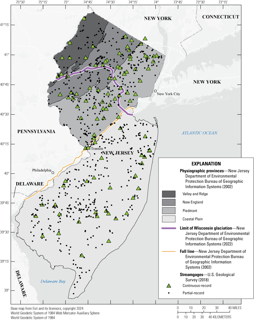
Map showing the physiographic provinces and selected U.S. Geological Survey continuous- and partial-record streamgages in and near New Jersey.
Purpose and Scope
The purpose of this report is to update and build upon the three previous studies to help assess the quantity of surface water in New Jersey (Laskowski, 1970; Gillespie and Schopp, 1982; Watson and others, 2005). This study computed updated surface-water statistics at USGS streamgages through the 2017 water year; the Watson and others (2005) report used data from continuous-record streamgages through the 2001 water year and from partial-record streamgages through the 2003 water year. This report serves as a single reference for water managers, policy makers, engineers, and consultants to cite the status of New Jersey surface water resources. This update also expands on the previous streamflow characteristics report by adding base flow, runoff, and several measures of annual variability, as well as a trend assessment at partial-record streamgages.
Continuous-record streamgages with additional approved data since 2001 and a minimum of 20 years of record through 2017 and partial-record streamgages with a minimum of 10 measurements through 2017 were included in this analysis. For the purposes of this report, the term “partial-record streamgage” describes a stream monitoring location that collected data either as discrete streamflow measurements, or on a continuous basis, for less than 20 years. High, low, and flow-duration statistics were computed using the entire period of record available at each continuous-record streamgage, except those defined as having a known change in the streamflow characteristics that would define a different data population, such as the construction of a reservoir. Low-flow statistics were computed at partial-record streamgages with sufficient data for regression analysis, even if new data were not available beyond the data used in the previous report. The final low-flow statistics estimated for these streamgages were based on a weighted average of regressions with multiple index sites.
A total of 97 continuous-record streamgages and 719 partial-record streamgages were included in this study. An assessment of trends and variability in streamflow was also conducted to quantify changes in water resources for the available periods of record at continuous-record streamgages. Trend tests on the residuals of the regressions were computed using the Mann- Kendall trend (MK) test (Hamed and Ramachandra Rao, 1998) to identify possible changes in the statistical relation between continuous- and partial-record streamgages.
Description of Study Area
Familiarity with the basic geology and geography of New Jersey is key to understanding its hydrology. New Jersey includes four primary physiographic provinces. The noncoastal provinces—Valley and Ridge, New England, and Piedmont—comprise the northern part of the state and are located above the Fall Line, a regional geomorphological boundary between Piedmont metamorphic rock and Coastal Plain sedimentary rock (fig. 1). The Coastal Plain covers the southern part of the state and is located below the Fall Line (fig. 1). The Fall Line is a low, east-facing largely buried cliff extending nearly parallel to the Atlantic coastline from New Jersey to the Carolinas (Newell and others, 1998). The Fall Line is the western limit of the coastal sediments separating the hard Paleozoic metamorphic rocks of the Piedmont Physiographic Province to the west from softer, more gently dipping Mesozoic and Tertiary sedimentary rocks of the Coastal Plain to the east. This erosional scarp, in many ways, affects the behavior of streamflow owing to the nature of the underlying geology; for example, whether a stream channel is steeply sloped with swift-moving waters or is more gently sloped with typically lower stream velocities is, to varying degrees, dependent on the underlying geology and streambed material (Watson and McHugh, 2014). The northernmost province, Valley and Ridge is known for long, parallel, northeast to southwest facing ridges and valleys. This region includes the Wallkill River Basin and is composed of faulted and folded sedimentary layers of sandstone, shale, and limestone. The New England Province is generally composed of hilly uplands, divided by steep-sided stream beds. This province includes the Passaic River Basin, as well as several glaciated lakes, and is underlain by erosion resistant rock, including granite, gneiss, and some Precambrian marble. The Piedmont Province is a broad lowland but possesses some ridges. It includes the Raritan River Basin, the largest drainage basin entirely within New Jersey and is underlain by interbedded sandstone, shale, conglomerate, basalt, and diabase. The Coastal Plain Province is a flatland that includes the New Jersey Pine Barrens, a largely uninhabited wilderness. This province includes the Lower Delaware River Basin, comprised of unconsolidated layers of sand, silt, and clay.
As the most densely populated state in the country, New Jersey is influenced by urbanization, agriculture, and ongoing land development (U.S. Census Bureau, 2023). The population of New Jersey is variable by region, yet always growing. Population centers include communities that serve as suburbs of New York City and Philadelphia as well as smaller cities such as Newark, Elizabeth, Trenton, and New Brunswick. Seasonally, large populations are drawn to the Jersey Shore. Other regions include large expanses of wilderness, such as the Delaware Water Gap and the New Jersey Pine Barrens. The rest of the state, especially the northern tip and southwest end of the state, are largely agricultural. This diversity of land and population centers plays an important role in water use and streamflow statistics statewide. The streamflow in many New Jersey rivers and streams can be regulated by storage and releases from reservoirs, some of which may be used to store drinking water. Another activity affecting streamflow statistics is diversions for a variety of purposes, including wastewater treatment, crop irrigation, and recreation. For example, cranberry bogs in southern New Jersey require large diversions of water at specific times of the year. Accounting for such human-driven influences is crucial for gaining a full understanding of streamflow characteristics statewide.
Previous Studies
The USGS has regularly provided statewide, detailed, statistical assessments of all available streamflow records, with each report building and expanding upon previous work. Laskowski (1970) authored “Statistical Summaries of New Jersey Streamflow Records—Water Resources Circular 23” in 1970 to expand on the earlier publication of “New Jersey streamflow records analyzed with electronic computer—Water Resources Circular 6” (Miller and McCall, 1961) with the computation of statistical moments for more than 80 streamflow records and daily low-flow and high-flow frequency statistics to help Federal and State agencies as well as municipalities and local professionals concerned with water availability and conservation. As the population increased, the demand for water to meet the needs of homes, industries, and irrigation was anticipated to increase. Understanding the magnitude and frequency of available streamflow became necessary for water supply planning purposes. In response to this need for better information about streamflow availability, a streamflow statistics report completed in 1981 was published as an update and expansion of the 1970 report (Gillespie and Schopp, 1982). This report analyzed low-flow frequency and flow-duration data for 400 continuous- and partial-record streamgages, some of which had been in operation for over 50 years. Most recently, Watson and others (2005) not only summarized both high- and low-flow data from 1897 to 2003, but also began to assess trends in streamflow in relation to urbanization and increased average precipitation. These updated statistics were instrumental for allocating surface-water withdrawals, setting waste load allocation limits, investigating total maximum daily loads (TMDLs), and studying the effects of contamination sources on the chemical and biological qualities of streams.
Other reports have further contributed to the understanding and management of surface water resources in New Jersey. A report by Esralew and Baker (2008) established set time frames for periods of record—baseline and current—which has become important for assessing future changes in streamflow resulting from increased development. Additionally, Watson and McHugh (2014) presented regionalized regression equations for estimation of monthly flow duration and monthly low-flow frequency statistics in ungaged New Jersey streams. Including both baseline and current conditions, these equations estimate 87 different streamflow statistics, including monthly 99th, 90th, 85th, 75th, 50th, and 25th percentile flow durations of the minimum 1-day daily flow, August–September 99th, 90th, and 75th percentile minimum 1-day daily flow, and monthly 7-day, 10-year low-flow frequencies. More recently, a report by Hammond and Fleming (2021) included trend analysis for a few low-flow statistics for 1950–2018 and 1980–2018 for some streamgages in the Delaware River basin, including New Jersey.
Methods
A comprehensive collection of statistics was computed for streamflow records to aid in the evaluation of water resources in New Jersey. Flow frequency and duration were computed for continuous-record streamgages using the same methods as the previous report (Watson and others, 2005). The calculation of base flow and runoff were added to the current study to aid in the assessment of these two basic components of surface-water flow. Trend tests in high and low n-day series, base flow and runoff, peak to 3-day mean flow ratio, as well as annual skew and kurtosis (a description of skew and kurtosis is presented in the “Streamflow Variability” section), were computed to explore possible changes in streamflow and its variability over time. A subset of low-flow frequency, duration statistics, and base flow were computed at partial-record streamgages using regression with continuous-record daily mean flows. Trends in the residuals of those regressions were also determined to explore possible changes in flow over time. The various types of statistics, record types, and trend analysis are listed in table 1. Details on the types and methods of computed statistics and trend analyses are described throughout this report.
Table 1.
List of statistics computed for continuous- and partial-record streamgages in New Jersey for the period 1903–2017.[Winter period is defined as November 1 through April 30]
Continuous-Record Streamgages
Streamgages with a total of at least 20 years of daily streamflow record through 2017, and daily streamflow data since 2001, were used in this analysis. A total of 97 streamgages operated by the USGS fits this criterion (fig. 1). A table of the streamgages used in this study along with additional streamgage information is available in the associated data release (Williams and others, 2024). Most of the streamgages (63) are in the northern half of the State, above the geologic fall line, with varying Valley and Ridge, New England, and Piedmont geology (fig. 1); only 34 of the streamgages are in the southern half of the State, draining Coastal Plain geology (fig. 1). Analyses utilized the entire period of record available at each continuous-record streamgage, except those which were defined in the previous reports as having a known change in the basin which would define a different data population, such as the construction of a reservoir. The previous report included statistics for both pre- and post-event periods. In this study’s analysis, statistics and trends were computed at those streamgages using data only in the latter period of record. Further details about the total 97 streamgages are given in the following list:
-
• 80 streamgages were included in the previous report. (17 streamgages did not previously have 20 years of record.)
-
• 16 streamgages have a break in the record because of a substantial hydrologic change upstream.
-
• 4 streamgages were discontinued after 2001; therefore, they do not have data completely through 2017.
-
• 20 streamgages are denoted as “regulated” due to controlled releases from upstream reservoirs. The designation does not indicate the presence of general water withdrawals and municipal discharges in the streamgage basin.
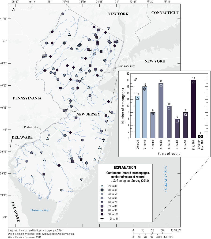
Map and bar graph showing distribution of period of record among continuous-record streamgages in New Jersey, 1903–2017.
Although most of the statistics included in this study were previously computed in Watson and others (2005), several new statistics were added for a more comprehensive assessment of streamflow. The first four groups of statistics listed below were computed in the previous report, but a percent change in value was determined for the current analysis. The winter season for statistics computed in these groups is defined as November 1 to April 30:
-
• Maximum, minimum, mean for period of record
-
• Duration of flow (annual and winter)
-
• 50-, 20-, 10-, 5-, and 4-percent annual nonexceedance (or 2-, 5-, 10-, 20-, and 25-year recurrence interval) frequencies of (annual and winter) minimum 1-,7-, and 30-consecutive day average flow (hereafter, referred to as 1-,7-, and 30-day low flows).
-
• 50-, 20-, 10-, 5-, and 4-percent annual exceedance (or 2-, 5-, 10-, 20-, and 25-year recurrence interval) frequencies of (annual and winter) maximum 1-,7-, and 30-consecutive day average flow (hereafter, referred to as 1-,7-, and 30-day high flows).
The ratio of peak flow was only computed for a selected subset of streamgages in the previous report; it was computed for all streamgages in this study.
The statistics listed below were not included in Watson and others (2005) and were added to this study’s analysis to provide a more comprehensive assessment of streamflow in New Jersey:
-
• Drought-of-record base flow (1962–70)
-
• Median September flow
-
• Annual variability measured as annual skew and kurtosis
The MK test was computed on several of the annual time series of streamflow statistics using different assumptions of serial correlation to determine if trends were present. The MK test assesses the data to determine if there is a statistical monotonic trend upwards or downwards, that is, if the values are consistently increasing or decreasing over time. Serial correlation is related to how consecutive values or values in a series influence each other or how they are correlated. Sen’s slope, often referred to as part of the Theil-Sen estimator, was also computed to determine the magnitude of change over time for the various statistics. The Theil-Sen regression relies on the median of the slopes between points, and not the mean, making it more robust and less sensitive to outliers (Sen, 1968). Evaluating changes in Sen’s slope was assumed to be a good method to look for changes over time that were less sensitive to outliers or extreme events. Details on the approach and methods is described in the “Trend Analysis” section. The trend tests were applied to the following annual time series:
-
• 1-,7-, and 30-day minimum average low flow (annual and winter)
-
• 1-,7-, and 30-day maximum average high flow (annual and winter)
-
• Ratio of peak flow to 3-day mean
-
• Base flow and runoff
-
• Skew and kurtosis
Flow Durations
Flow-duration curves define the percentage of time flows were equaled or exceeded for a given period (Searcy, 1959). Specific intervals of the curve (1-, 2-, 5-, 10-, 20-, 25-, 30-, 40-, 50-, 60-, 70-, 75-, 80-, 85-, 90-, 95-, 99-percent) were computed for both annual and winter seasons using the R-program EGRET (Hirsch and DeCicco, 2015) for all 97 continuous-record streamgages for the entire periods of record, when applicable. The percent change in the flow-duration intervals for the 80 streamgages included in Watson and others (2005) were also computed. Flow-duration curves help provide information about streamflow behavior in the basin. A steeper sloped flow-duration curve may represent a basin that is more reactive to events or is generally more variable than a basin with a flatter flow-duration curve (fig. 3). The added level of analysis focusing on the computation of flow-duration curves for just the winter season attempts to provide finer information about the basin response to winter conditions. Understanding the winter component of the composite annual flow-duration curve provides an opportunity to assess the influence of the winter season on the annual statistics. Changes in computed flow durations are presented in the subsection titled “Percent Change in Streamflow” in the “Results” section of this report.
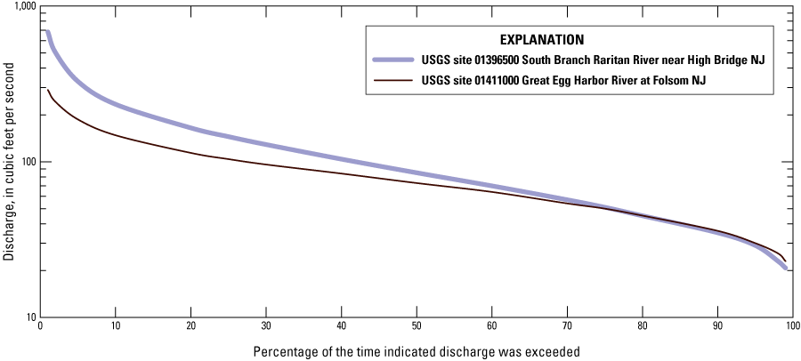
Line graph showing flow-duration curves for South Branch Raritan River near High Bridge, New Jersey, USGS site 01396500 and Great Egg Harbor River at Folsom, N.J., USGS site 01411000. N.J., New Jersey; USGS, U.S. Geological Survey.
Base Flow and Runoff
Streamflow can be separated into the following two basic components: base flow and runoff. Runoff is the portion of streamflow resulting directly from precipitation; base flow is the portion of streamflow sustained by groundwater discharge. Separation of these flow components was achieved using the PART base flow separation program (Rutledge, 1998) within the USGS software Groundwater Toolbox (Barlow and others, 2014). The PART program determines base-flow days according to the number of preceding days with continuous recession. The program then linearly interpolates between base-flow days to determine the portion of base flow during runoff events (Rutledge, 1998, p. 34–36; Rutledge, 2007). The mean base flow and runoff was computed for each year of available record, as well as for the entire periods of record for 96 continuous streamgages. The flow components are not able to be separated for canal flow, as measured at Delaware and Raritan Canal at Port Mercer, N.J. (01460440). Analyzing the amounts of each of these pieces of streamflow records aids in the understanding of water availability and variability.
Streamflow Variability
Skew and kurtosis are measures of extremes within a data distribution. Skewness can be considered as the extent of the tails (extreme events) or degree symmetry of the distribution, whereas kurtosis can be thought of as the heaviness of the tails or peakedness of the distribution. Annual values of skew and kurtosis were computed for all 97 continuous-record streamgages for the given periods of record included in the study using R statistical software (R Core Team, 2019).
The analysis originally followed the previous report in evaluating the variability of streamflow by examining the ratios of flow durations, 10/90 and 25/75. However, this approach was determined to be insufficient because some continuous-record streamgage 90th and 75th percentile flow durations were zero, and, therefore, a ratio could not be calculated. The flow-duration ratios are effective at describing the behavior of the central tendencies of the distribution of flows; however, in the interest of flow variability, the shape and extremes of the distribution were of greater utility. Instead, examination of skew and kurtosis were implemented to supplement trend analysis of high and low flows with changes in streamflow variability.
Streamflow variability can be affected by such factors as increased impervious surface, changes in water use, and changes in climate. High and low flows may not change in magnitude alone, but also could have changes in frequency. Understanding both frequency and magnitude of critical or extreme streamflow aids in water management and planning.
Peak-Flow Ratio
The peak-flow ratio is the annual maximum instantaneous flow divided by the 3-day mean flow for the day before, day of, and day after the peak (Watson and others, 2005). To examine the high-flow event variability, the peak-flow ratio for each year of record was computed for all continuous-record streamgages in the study. A watershed’s ability to store and attenuate runoff is measured by the peak-flow ratio (Watson and others, 2005). The higher the ratio, the flashier the stream with quickly rising and receding peaks. A change in the ratio over time can be an indication of changes in land use or vegetation cover in the basin, as well as changes in the intensity and duration of storms.
Frequency Analysis
A frequency curve relates the magnitude of a variable to its frequency of occurrence (Riggs, 1968). The USGS software Surface Water Toolbox (SWToolbox; Kiang and others, 2018) was used to compute mean high and low flows for a given number of consecutive days (n-day) for each year year of record. For this study, the annual highest and lowest 1-, 7-, and 30-day mean-flow time series were determined for both full-year and winter seasons. The annual period used was based on the climatic year (April 1 to March 31) for low-flow frequency analysis (U.S. Interagency Advisory Committee on Water Data, 1982), and the water year (October 1 to September 30) for high-flow frequency analysis. Under natural conditions, the lowest annual flows typically occur in late summer when evapotranspiration is high and groundwater levels are low. Annual low-flow frequency statistics are, therefore, assumed to represent summer conditions. This assumption does not hold true for streamgages below regulated reservoirs where the lowest flow of the year may occur during winter months, depending on operations of the reservoir. Periods were not truncated to determine strictly summer flow frequencies.
The frequency calculation within SWToolbox determines the plotting positions of the annual n-day series and fits a probability curve to the data using a Log-Pearson type III (LPIII) statistical distribution. Flow exceedance and nonexceedances are then estimated using that curve. A conditional probability adjustment is applied to records with zero flows, in which the probabilities are first determined without including the zero flows, then adjusted according to occurrence of zero flows. Details on the approach are described in the published SWToolbox Techniques and Methods (Kiang and others, 2018).
For high-flow frequency analyses, the probability that a streamflow is exceeded for a given period of time is referred to as the exceedance probability; for low-flow frequency analysis, the probability that streamflow is not exceeded is the nonexceedance probability. The specific high- and low-flow probabilities computed from the curves were the 50-, 20-, 10-, 5-, and 4-percent annual exceedance and nonexceedance probabilities, which correspond to the 2-, 5-, 10-, 20- and 25-year recurrence intervals. The percent change in the high- and low-flow frequency flows for the 80 streamgages included in Watson and others (2005) were also computed and the periods through 2001 were compared against the periods through 2017.
Low-flow frequency statistics such as the annual 7-day low flow with a 10-percent annual nonexceedance probability (7Q10) are often used for permitting and regulation of water resources. New Jersey is among the states that utilize the 7Q10 statistic in several regulatory processes including water allocations permitting (Hoffman and others, 2012) High-flow frequency statistics (as opposed to peak-flow frequency statistics) are not typically used in regulation or structural design but could be considered useful for comparing to peak-flow frequencies and changes to storm variability and water availability.
Fit of Frequency-Distribution Curve and Outliers
The LPIII distribution is the recommended statistical distribution for use in hydrologic frequency analysis (Riggs, 1972). The shape of the LPIII curve is determined using the first three moments of the log transformed data: mean (µ), standard deviation (σ), and skew (ɣ). The skew is then used in determining the frequency factor (K) for given probabilities (p) to produce the following equation to build the LPIII curve:
Though recommended, the fit of the data to the LPIII curve must still be examined to ensure a reasonable estimate of probability of flow. Using the SWToolbox program, the Kolmogorov-Smirnov (KS) test was applied to evaluate the fit of the annual n-day time series to the LPIII distribution to assess the estimated frequency statistics. The test is applied to nonzero values and determines the probability that the data fit the defined distribution. The LPIII curves that do not have a 95-percent probability of fitting the data are flagged as failing the test.
The KS test evaluates the entirety of the curve, but this study focuses on frequencies 4–50-percent probabilities, or the right side of the plotted curve. At times, the KS test may indicate that the data fit the distribution within 95 percent, but visually the data do not appear to fit well at the probabilities of interest in this study. Visual assessments were also used to evaluate the fit of the data points to the LPIII curves at these lower probabilities. Often a less-than-ideal fit is visually noted with shorter periods of record, which reinforces the need for using a statistical distribution—so that information on frequency of events can be produced from a relatively smaller sample of the data population. However, when a sufficient period of record is collected, arbitrarily assumed as more than 50 years, it might also be assumed the fit of the data to the frequency curve would visually improve. When the data do not fit well, it may indicate that the data do not represent a single population, perhaps because of a climate shift or effects from local water use, or that LPIII is not the best distribution to be used. Unexpectedly, when this discrepancy with long-term records was observed in this study, the data seemed to not fit around the 10th percent nonexceedance, the most used return period in low-flow management.
The SWToolbox program also identifies outliers based on the K-Ratio. If the ratio is greater than one, then the value is flagged as an outlier. The identification and removal of outliers is common in frequency calculations of flood flows. Peak-flow data populations are considerably different, as they are instantaneous flow values whereas this study is using daily mean flow values. The daily mean flows have less noise and error than do instantaneous peak flows. Regardless, in pursuit of a better fit, outliers identified by the K-ratio test were removed from the annual n-day series at three long-term streamgages. These outliers and bias-driven values were removed at these streamgages, 01399500, 01396500, and 01377500, to see if a better curve fit could be accomplished at the 10th percent exceedance value. No appreciable difference was made to the curve, as the overall data skew was not greatly affected by only a few values, but rather by the dataset as a whole. The 01377500 streamgage was the only streamgage to fail the KS test.
High- and low-flow frequencies were determined for all 97 continuous-record streamgages in the study. If the data had a 95-percent probability of fitting the given distribution, meaning it passed the KS test, then the frequencies were determined using the LPIII curve, even if the data had a visually poor fit. The flow frequencies were computed as simple percentage exceedances when LPIII curves failed the fit test or when the streamgages were noted as having considerable upstream regulation. The method used to compute the flow frequency value is designated in the output as LPIII or percentage exceedances. This differs from methods used in the previous study (Watson and others, 2005), which only used visual assessment and fitted a hand-drawn graphical estimate for curves with a poor fit. This change in methodology between studies for estimating poor or nonfitting data could contribute to misrepresentation of changes in flow when comparing the percentage differences between the two studies.
Trend Analysis
The calculation of frequency statistics and various flow components is helpful for permitting and design, as well as documenting the current state of water resources. Determining if and how water resources are changing over time is critical for water resource management planning, especially in a heavily populated state with a changing climate. Trend analysis was used to further evaluate streamflow records; evidence for trends were computed for: base flow, runoff, all n-day series, skew, kurtosis, and peak-flow ratios. The MK test was used for this study as it is appropriate for hydrologic data. It is a nonparametric test which does not require that the data be normally distributed. A trend was considered to be statistically significant when p<0.05.
The MK test uses the ranks of values in the dataset to detect the presence of a trend. In using the ranks of values, the test is not subject to influence from outliers or rare events, which are common in hydrologic data in the form of floods and droughts. However, it also assumes that the data are independent (have no serial correlation). Statistical evidence of a trend can be influenced by the presence of serial correlation, which can be present in hydrologic data series in the form of persistent wet and dry climate cycles.
The presence of serial correlation can be alleviated one of two ways. It can either be removed from the data before applying the trend test, known as “pre-whitening” (Hamed, 2008). The second option is to modify the test to account for the serial correlation. To account for the possibility of serial correlation in the data for this study, the variance of the MK test statistic was adjusted to compensate for an assumed condition of serial correlation.
The MK test was used for three different assumptions of serial correlation: independence (meaning no serial correlation), short-term persistence (STP), and long-term persistence (LTP) using variance correction methods from Hamed and Ramachandra Rao, 1998; Hamed, 2008; and Hodgkins and others, 2017. Short term persistence assumes a significant correlation of data lagged by 1 year with itself. Long term-persistence assumes significant correlations of data lagged at intervals greater than 1 year. Measures of serial correlation were computed using the lag-1 correlation coefficient for STP and the Hurst coefficient for LTP (Hamed and Ramachandra Rao, 1998; and Hamed, 2008).
Partial-Record Streamgages
A subset of low-flow statistics was estimated at 719 partial-record streamgages for this study. Partial-record streamgages can be either continuous-record streamgages with less than 20 years of record or streamgages that have at least 10 discrete measurements of flow. The low-flow statistics determined at long-term continuous-record streamgages (index sites) were transferred to partial-record streamgages using the Maintenance of Variance Extension Type 1 (MOVE1) method of record extension (Hirsch, 1982) using discrete flow measurements made during base-flow conditions at the partial-record streamgage and concurrent daily mean flows at the index sites. The MOVE1 method derived by Hirsch takes a different regression approach and attempts to preserve the mean and the variance of low-flow estimates rather than minimize the mean and variance, as is typically done with least-squares regression. An example of how the MOVE1 method was applied for this study and the previous study can be found in the report “Streamflow Characteristics and Trends in New Jersey, Water Years 1897–2003” by Watson and others (2005). The estimated low-flow statistics at partial-record streamgages were:
-
• Annual 1-, 7-, and 30-day low flow with a 10-percent annual nonexceedance probability
-
• Winter 7- and 30-day low flow with a 10-percent annual nonexceedance probability
-
• 50th and 75th percent duration flow
-
• September median flow
-
• Mean annual base flow
-
• Drought base flow (1962–70)
The regressions were executed using the R-script documented in “Implementation of MOVE.1, censored MOVE.1, and piecewise MOVE.1 low-flow regressions with applications at partial-record streamgaging stations in New Jersey” by Colarullo and others (2018). The script screened the data for base-flow conditions, which are defined in the program as a change in streamgage height of 0.02 foot (ft) or less at the partial-record streamgage and a change in the daily mean flow at the index site between +10 and −30 percent from the previous day. The script also allowed for the use of multiple continuous-record streamgages (index sites). The use of more than one index site provided more robust estimates rather than over-relying on a single continuous-record streamgage to estimate the low-flow statistics. To incorporate the strength of the multiple individual regressions into a final estimate for the partial-record streamgage, a weighted average flow was determined using the time-sampling error of the streamgage records combined with the error associated with each regression. An average of at least 10 data points among the regressions was required to qualify the partial-record flow estimates for inclusion in this study. For streamgages with measurements of zero flow, the censored MOVE1 regression within the R-script was applied. Colarullo and others (2018) documents details on the script, including base-flow screening, weighting scheme, and associated methodologies.
An MK test for trends was also applied to each set of residuals of the individual regressions to determine if the relation between the partial-record streamgage and each index site was changing through time. Each partial-record streamgage, therefore, had multiple tests of trends in residuals, concurrent with the number of associated index sites. If the trend in regression residuals, considered statistically significant when p <0.05, was consistent across all index sites used with a particular partial-record streamgage, greater confidence was given to conclude that a trend in flow exists at the partial-record streamgage. For example, when residuals were increasingly positive relative to the determined regression line over time and the particular index site did not have an identified trend in base flow, the trend indicated that the streamflow was increasing at the partial-record streamgage over time. When this same result was observed at all index sites used for a particular partial-record streamgage, then greater confidence was given to the presumption that a trend in flow was present at the partial-record streamgage. When residuals were repeatedly shown as increasingly negative through time, with no base-flow trend at the index sites, then the trends showed that the flow was decreasing at that partial-record streamgage.
Index Site Selection
Although the MOVE1 program incorporates regression error and the use of multiple index sites, the selection of index sites used has a direct influence on the estimated flow trends in residuals at the partial-record streamgages. Knowledge of the local hydrology and index site conditions are important factors that can influence streamgage selection beyond the criteria of little to no known regulation. Other criteria considered in the index site selection process include:
-
• Length of record greater than 25 years
-
• Identified trend (IND) for 1 or fewer annual low-flow time series
-
• Pass KS test and visual test for fit of LPIII curve
Streamgages were then grouped according to physiographic province (table 2 and fig. 4). Partial-record streamgage basins falling within the same physiographic province all used the same list of index sites.
Table 2.
List of USGS streamgages used as index sites in low-flow regression analysis in New Jersey, drainage area, record length, and the associated physiographic province.[USGS, U.S. Geological Survey; NA, not applicable]
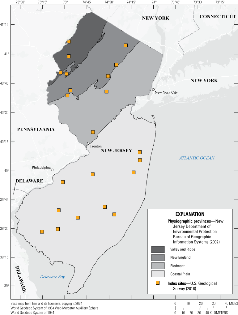
Map showing index site locations for partial-record streamgages across New Jersey physiographic provinces.
An exception was made to the 25-year requirement for the unglaciated New England Province, as there are not many index sites in this physiographic province. Three index sites were used for more than one physiographic province because of their proximity and mixed basin characteristics.
Another exception was made with the Neshanic River at Reaville, N.J., USGS site 01398000 streamgage. Although relied upon in the previous study, it failed the KS test for the 30-day low, and the annual 1-day low flow with a 10-percent annual nonexceedance probability (1Q10) is now zero. Having a 1Q10 frequency magnitude of zero means this streamgage can no longer be used in the MOVE1 regression analysis because an input variable value of zero would always result in an estimate of zero at the partial-record streamgage.
Results
The duration, frequency, and summary statistics (table 1) for 97 continuous-record streamgages and 719 partial-record streamgages in New Jersey were computed for each period of record through 2017. Trends for various magnitudes of high flow, low flow, and flow variability were determined for continuous-record streamgages. The magnitude and statistical significance of those trends are presented in this report. For partial-record streamgages, trends in regression residuals were computed and reported by the proportion of streamgages with a statistically significant trend. The percent change in flow at streamgages for which statistics were computed by Watson and others (2005) was also determined to assess changes in streamflow versus trend test results. The computed flow statistics, trends, and percent change in flow are available for download from the associated data release published in Williams and others (2024) as well as through a web map (https://geonarrative.usgs.gov/njstreamflowcharacteristics/).
Trends in Streamflow at Continuous-record Streamgages
Seventeen streamflow characteristics were assessed using the MK test under three different assumptions of serial correlation to determine the prevalence and direction of trends within streamflow data in New Jersey. These characteristics included base flow, runoff, skew, kurtosis, and peak-flow ratio, as well as the 1-, 7-, and 30-day high and low flows for both annual and winter-only periods. A total of 1,647 time series of flow characteristics among 97 streamgages were tested. Trends for time series, base flow, and runoff characteristics were not determined for one canal streamgage. Three levels of serial correlation (persistence) were assumed, and adjustments were accordingly applied to the variance of each characteristic’s MK test statistic: an independent test (no adjustment, IND), short-term persistence (STP), and long-term persistence (LTP). The adjusted variance was applied to all data characteristics and all streamgages regardless of whether there was evidence of serial correlation. This was primarily because serial correlation is often present in hydrologic data in the form of persistent wet and dry climate cycles, but records may not be long enough to provide evidence. It was also done to show the range of effect for all three types of assumed serial correlation.
Tests assuming no serial correlation (IND) yielded 314 streamflow characteristics with statistically significant trends, which was the largest group—accounting for about 19 percent of the total. When variance was adjusted for STP, the tests indicated only 241 statistically significant trends, about 15 percent of the total number of characteristics. When the variance was adjusted for LTP, even fewer statistically significant trends (111, or 7 percent) were identified. However, evidence for serial correlation does not appear to be substantial for STP or necessarily clear for LTP and may not justify the variance adjustment for all streamgages.
Measures of serial correlation were determined using the lag-1 correlation coefficient for STP and the Hurst coefficient for LTP (Hamed and Ramachandra Rao, 1998; and Hamed, 2008).
-
• For STP, lag-1 correlation values close to 1 indicate strong positive serial correlation; values close to −1 indicate strong negative serial correlation.
-
• For LTP, a Hurst exponent between 0.5 and 1 indicates positive serial correlation, meaning a change (increase or decrease) between observations will probably be followed by another change. A value between 0 and 0.5 indicates a time series with long-term switching between high and low values in adjacent pairs, meaning that a single high value will probably be followed by a low value and that the value after that will tend to be high, with this tendency to switch between high and low values lasting a long time into the future.
When examining lag-1 correlation, few streamgage characteristics indicated strong evidence of STP. In all, no time series had a lag-1 correlation coefficient less than –0.6, and only 28 individual times series among 12 streamgages had a lag-1 correlation coefficient greater than +0.6 (table 3). Twenty-seven of the 28 time series were representative of low-flow conditions. None of the high flow n-day series, runoff, winter 30-day low, skew, nor kurtosis indicated evidence of short-term persistence. The annual 1-day low-flow time series had the largest number, with 11 streamgages having a lag-1 correlation coefficient (STP) greater than 0.6. The winter 1-day and annual and winter 7-day time series had a small subset of those 11 streamgages that showed at least some evidence of STP. One of the 11 streamgages also had minor evidence for STP for base flow. One streamgage had minor evidence of STP for peak-flow ratio. All streamgages that indicated some evidence of STP were either below a reservoir with heavy regulation or influenced by water use. In the case of the streamgage at Cedar Creek at Western Blvd near Lanoka Harbor, N.J., USGS site 01408900, the tide likely influences the 1- and 7-day lows, providing attributes of STP. Of the total 28 time series indicating some STP, 22 exhibited a statistically significant trend. After the variance was adjusted to account for STP, 7 of the trends indicated were no longer statistically significant, but 15 of the time series still had p-values <0.05. Assuming lag-1 serial correlation for all sites appears to have been unjustified.
Table 3.
Trend results after adjustment for lag-1 serial correlation in select streamflow characteristics in New Jersey, periods of record spanning 1903–2017.[Where indicated, a lag-1 correlation coefficient less than 0.6 (meaning weak evidence for short-term persistence) is shown for the indicated time series and is shaded gray to help visualize computed trend patterns. Trend persists indicates a statistically significant trend was indicated for an assumption of serial independence, and that the trend remained statistically significant after adjusting the variance for short-term persistence. Trend resolved indicates a statistically significant trend was indicated for an assumption of serial independence, and that the trend was resolved after adjusting the variance for short-term persistence. No trend indicates that no statistically significant trend was indicated for an assumption of serial independence. Winter period is November 1 through April 30]
Determining the existence of long-term persistence is not straightforward, as there is a high degree of uncertainty in the Hurst coefficient for records with less than 100 years of data (Khaliq and others, 2009). Only one streamgage in this study had more than 100 years of record. Overall, 398 time series among 79 of the streamgages indicated some evidence of LTP, considerably more than the 28 time series among 12 streamgages which indicated STP. Length of record did not appear to have a considerable influence on the value of the Hurst coefficient (fig. 5). The streamgage with the largest average Hurst coefficient for high flows was the one at East Branch Paulins Kill near Lafayette, N.J., USGS site 01443280, which has 25 years of record. The streamgage with the largest average Hurst coefficient for low flows was at Rockaway River below Reservoir at Boonton, N.J., USGS site 01381000, which does have the longest record of 111 years; however, the streamgage is heavily regulated, and the persistence pattern is likely a reflection of reservoir operations.
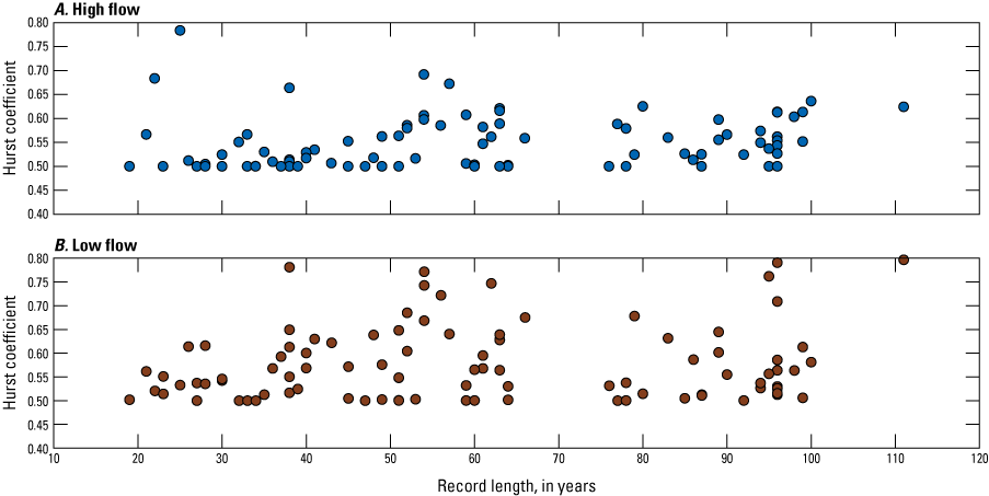
Scatterplot of the average computed Hurst coefficient compared to record length of continuous-record streamgages in New Jersey, 1903–2017. A, high flows and B, low flows.
It was expected that longer-duration low flows (30-day) might exhibit more persistence than short-duration low flows (1-day), as the longer durations were assumed to better reflect long-term basin storage which was assumed to better represent climate patterns. Although this appears to be true for high flows, there appears to be greater difference according to flow magnitude, with low flows indicating greater evidence of LTP than high flows (fig. 6). The 1-day annual low flows indicated the largest number of streamgages (42) with Hurst coefficients greater than 0.6 indicating a relatively strong indication of LTP (table 4). All other n-day time series had, on average, 23 streamgages with evidence for LTP. Base flow and runoff had 40 streamgages indicating evidence of LTP, again supporting the idea that the more generalized or robust flow characteristics would best display long-term patterns. Peak-flow ratio, skew, and kurtosis had the fewest streamgages with indicated evidence for long-term persistence (9, 5, and 4, respectively), which supports the idea that measures of the extremes or tails of the dataset might be expected to have minimal serial dependence.
Table 4.
Range of computed Hurst coefficients for selected flow characteristics at 97 streamgages in New Jersey, period of record spanning 1903–2017.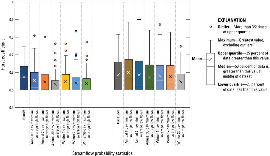
Boxplots of the Hurst coefficients for various flow statistics at continuous-record streamgages in New Jersey, 1903–2017.
The number of time series with statistically significant trends decreases considerably as the variance is adjusted with each assumption of serial correlation, from 314 (IND) to 241 (STP) to 111 (LTP), by design. When evidence for serial correlation is considered, rather than simply assuming it exists, the decrease in the number of statistically significant trends is not as large, with 307 after adjustment for STP and 218 after adjustment for LTP. Of the total 398 time series with some evidence of LTP, only 124 indicated a statistically significant trend using the IND assumption. After adjusting the variance for LTP, 28 of the time series still indicated a statistically significant trend.
Including adjustments for serial correlation is necessary in terms of recognizing the likelihood of cyclical patterns in hydrologic data and putting trends into context of long-term climate variability, especially when considering that interpreting the evidence for serial correlation is not straightforward. However, most statistics used in permitting use available record, regardless of when it was collected or how long it is—unless there is a known major change in the basin. Knowing if the available stream record used for planning or permitting is changing can inform water managers of what might be expected in the near term for permit renewals and changes in allocation. In general, for all assumptions of serial correlation, most of the statistically significant trends indicated increasing rather than decreasing flows among the 17 streamflow characteristic time series (table 1). The percentage of continuous-record streamgages indicating statistically significant trends under the basic assumption of no serial correlation for high flow, low flow, and the measures of variability are shown in fig. 7 A, B, C, D, and E. For a broader view, the percentage of trend results at continuous-record streamgages for all flow characteristics are shown in figure 7F. The resulting number, direction, and magnitude of trend tests for the various streamflow characteristics are discussed in more detail in the following sections, focused only on the assumption of serial independence, with the knowledge that the results considering STP and LTP have fewer statistically significant trends.
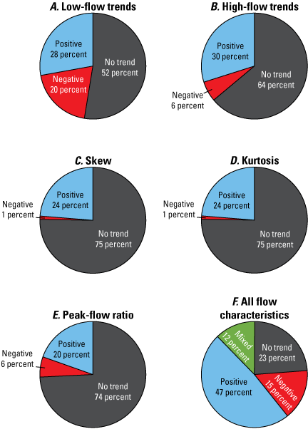
Pie charts showing the percentage of continuous-record streamgages with statistically significant trends (p<0.05) under an assumption of no serial correlation in New Jersey, 1903–2017. A, low-flow trends, B, high-flow trends, C, skew, D, kurtosis, E, annual peak-flow ratio, and F, all flow characteristics.
Variability—Skew and Kurtosis
Examining the annual distribution of streamflow provided a general assessment of possible changes to stream variability without choosing specific streamflow characteristics, such as the annual 1-day high flow. In using skew and kurtosis, the extremes of the distribution are characterized and assessed for changes. Twenty-four streamgages indicated statistically significant trends in the annual skew of the distribution of daily mean streamflow, all of which were increasing except for one (Saddle River at Lodi, N.J., USGS site 01391500). Of the 24 streamgages, 23 also indicated statistically significant trends for kurtosis; all the kurtosis trends were also increasing except for 01391500. One additional streamgage (Crosswicks Creek at Extonville, N.J., USGS site 01464500) indicated an increase in kurtosis but not skew.
The distribution of streamflow within a given year is generally skewed to the right, or positively, with high-flow events causing the shape to be “right-tailed.” Increasing skew over time suggests that the shape of the distribution is changing, possibly because of larger flow events (the tail) becoming greater in relation to the bulk of the streamflow record. Increasing kurtosis indicates that the data within the distribution are occurring more often in the tail or that extreme events are occurring more often as time progresses. The Saddle River at Lodi, N.J., 01391500 streamgage is the only exception to this trend, where the data indicate that the highest flow events are not as large and are occurring less often.
Record length appears to be a factor in whether skew and kurtosis are significantly changing. Of the 25 streamgages indicating a trend in either skew or kurtosis, 18 (>70 percent) had records longer than 80 years. Meanwhile, streamgages with more than 80 years of record account for 28 percent of the number of streamgages included in this study (fig. 2). Even though more streamgages with longer records had significant positive trends, the magnitude of the trend, as computed by Sen’s slope was less (fig. 8) for those longer record streamgages.
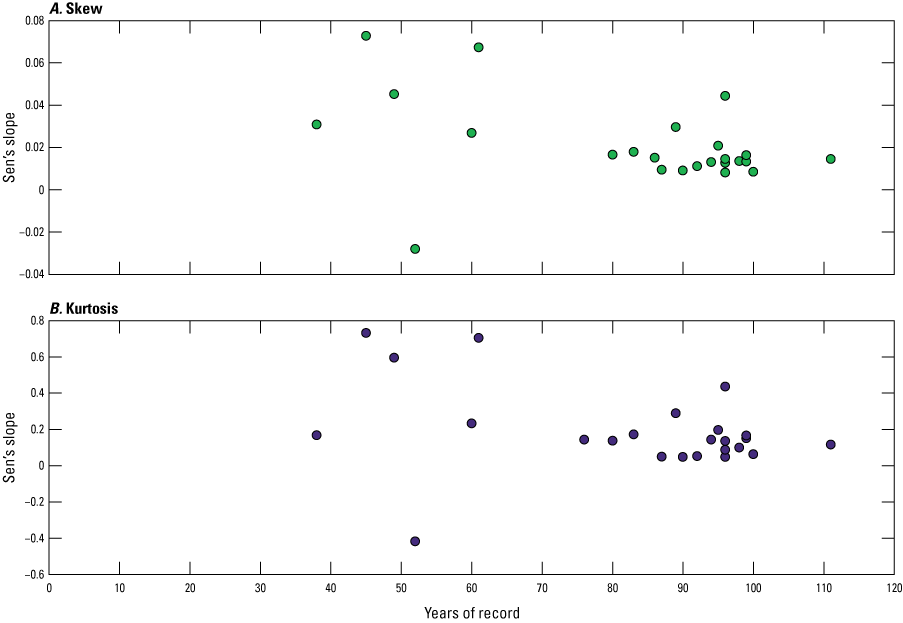
Scatterplots of the magnitude of statistically significant trends (p<0.05) in computed continuous-record streamgages in New Jersey, 1903–2017, compared to years of record. A, skew and B, kurtosis
Base Flow and Low n-day Flows
The range or magnitude of the low-flow characteristics tested for trends speaks to possible changes in variability of streamflow. The characteristics tested include annual base flow and n-day series of the lowest 1-, 7-, and 30-day flows during annual and winter seasons. Base flow is the largest or most coarse measure of what is considered “low flow” in this study. The n-day series captures finer scale measurements of low flow, with the lowest 1-day flow representing an extreme event for a given year. Though annual lowest n-day flows series are determined using the full climatic year (April 1–March 31) it is assumed these lowest events occur in the summer, following the typical hydrologic cycle of the northern hemisphere. This assumption does not hold true for streamgages that have controlled or regulated flow. Examining trends and their occurrence of either annual (summer) and winter can inform shifts in climate or seasonal weather patterns.
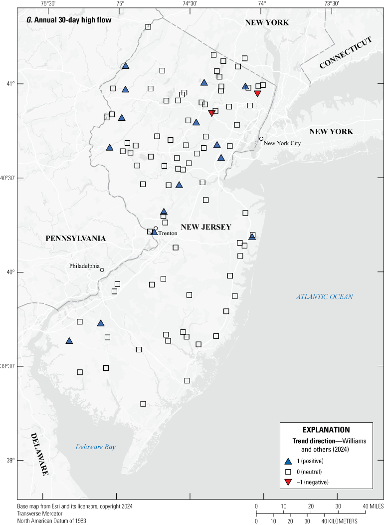
In all, 46 continuous-record streamgages indicated a statistically significant trend for at least 1 or more of the low-flow characteristics computed in this study and are summarized in table 5 and figure 9; more detailed information for the continuous-record streamgages can be found in the associated date release (Williams and others, 2024). Decreasing flows trends were identified at 19 streamgages, and flow is controlled or regulated at 2 of those streamgages. Increasing flow trends were identified at 27 streamgages, 10 of those streamgages are regulated. Recall from the “Methods, Continuous Records Streamgages” section that for regulated streamgages, periods of record used in the calculations do not include earlier unregulated periods. The same proportion of negative trends were observed in the north and south (about 17 percent of streamgages in each region); positive trends appear to be concentrated in northern New Jersey (fig. 10).
Table 5.
Number of New Jersey continuous-record streamgages indicating a statistically significant trend for various low-flow characteristics, 1903–2017.[Winter period is defined as November 1 through April 30]
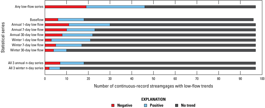
Bar graph showing the number of continuous-record streamgages in New Jersey with statistically significant trends (p<0.05) for various low-flow characteristics and combinations thereof, 1903–2017.
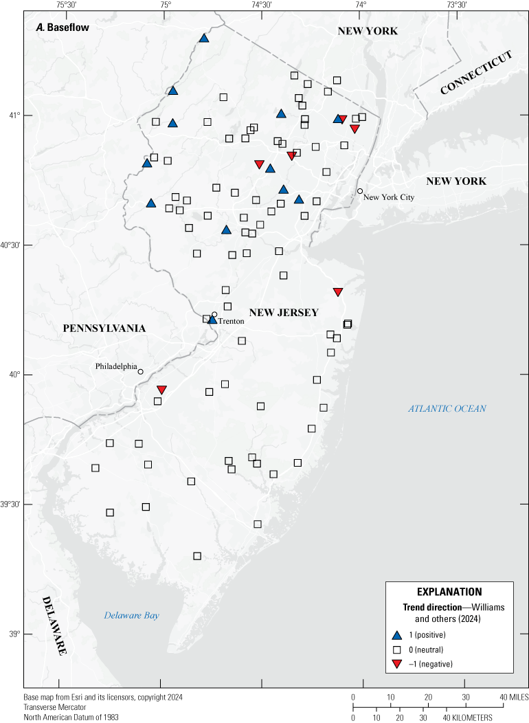
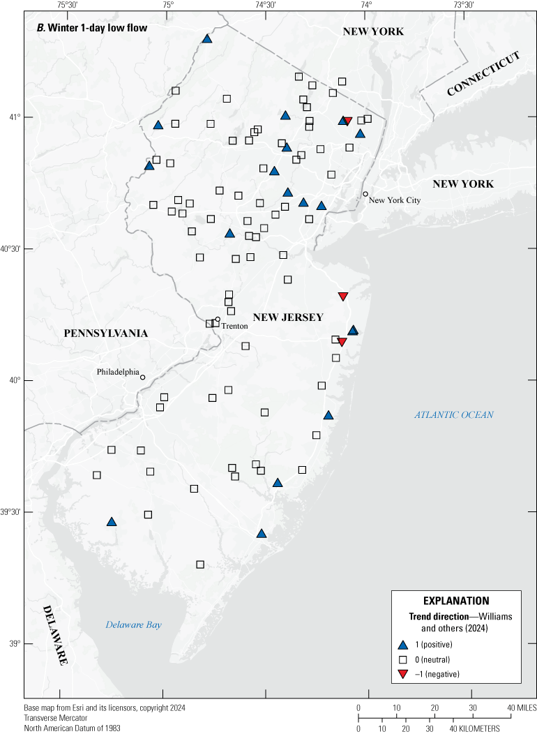
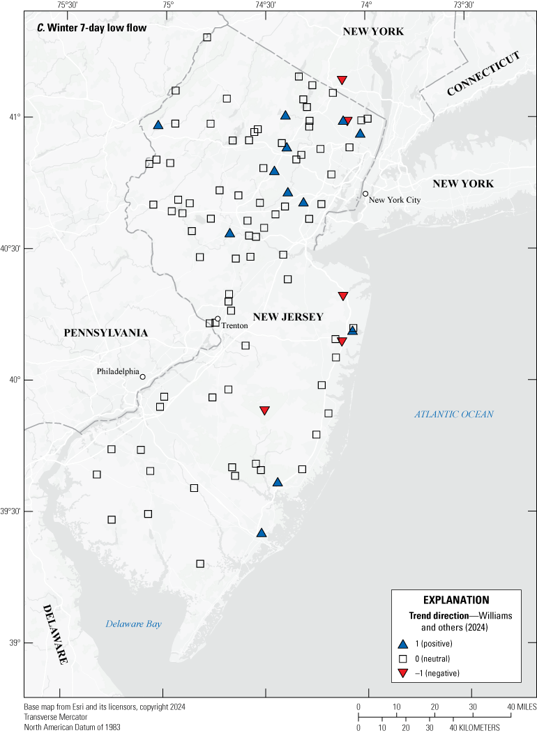
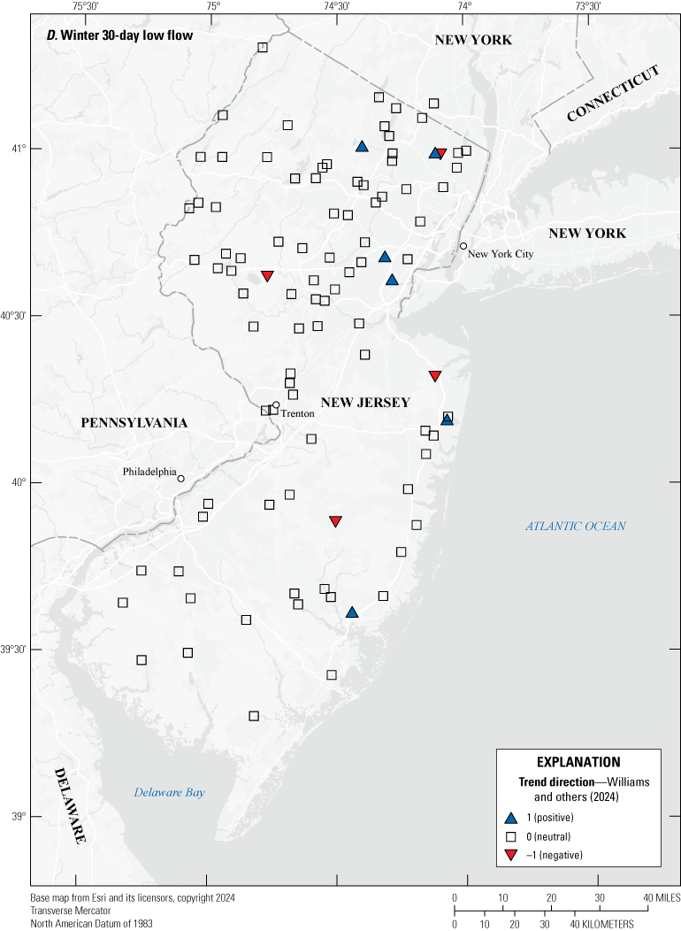
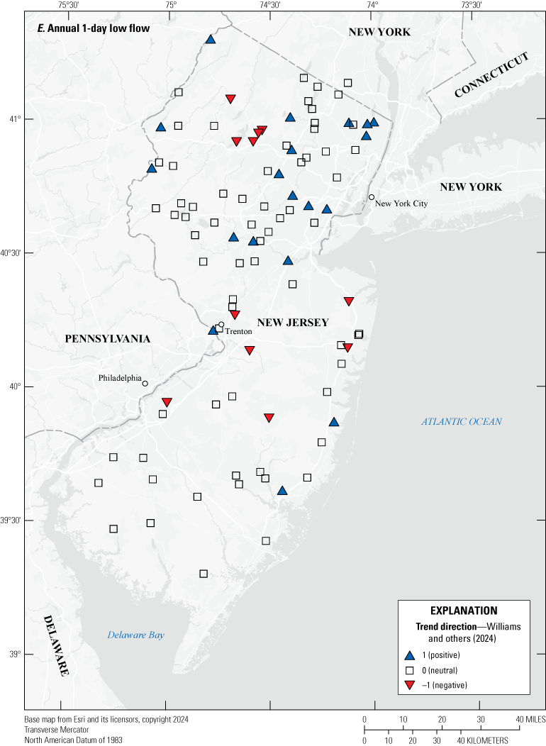
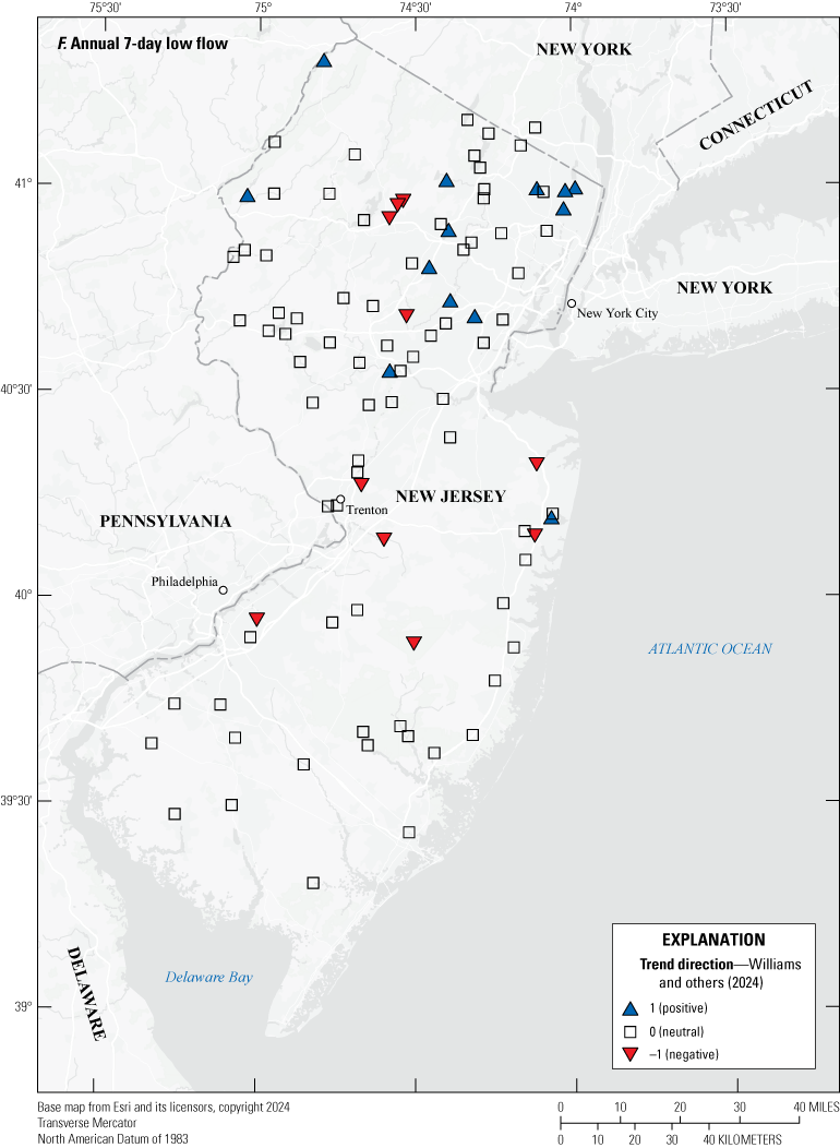
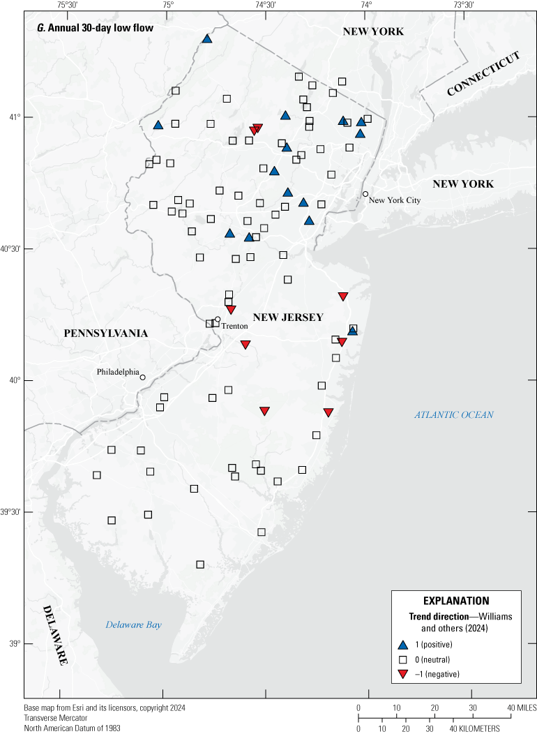
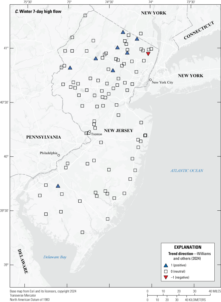
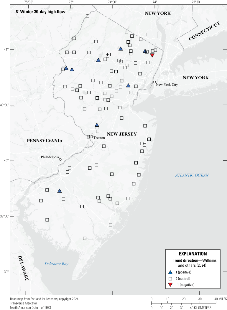
Maps showing continuous-record streamgages with statistically significant trends (p<0.05) in low flow in New Jersey, 1903–2017. A, base flow, B, winter 1-day low flow, C, winter 7-day low flow, D, winter 30-day low flow, E, annual 1-day low flow, F, annual 7-day low flow, and G, annual 30-day low flow.
Whereas table 5 and figure 10 illustrate the number of trends for each individual low-flow characteristic, as well as the totals for each season, the trends can also be explored in various alternate groupings. At the coarsest measure of low flow considered—base flow—statistically significant trends were identified at 18 streamgages (6 negative, 12 positive). At 6 of those streamgages, base flow was the only low-flow characteristic with evidence of a trend (2 negative, 4 positive). A larger number of streamgages (39) were identified as having a statistically significant trend for at least one of the finer scale 1-, 7-, or 30-day low-flow series for either annual, winter, or both periods. Only 18 of those 39 streamgages indicated trends during both annual (summer) and winter low flow (3 negative, 15 positive).
For any annual (summer) n-day low-flow series, a total of 32 streamgages indicated statistically significant changes in flow (12 negative, 20 positive). Of the total 32 streamgages, more than half (18) indicated a trend for all 3 n-day series (7 negative, 11 positive). For any winter n-day low-flows, 25 streamgages indicated statistically significant changes in flow (6 negative, 19 positive). Of the 25 total streamgages, only 7 indicated a trend for all 3 n-day series (2 negative, 5 positive).
Sen’s slope was then divided by the streamgage drainage area so that the degree of indicated change could be compared among the streamgages for each statistic. Note, however, that this comparison does not necessarily infer that the trend is the result of basin-wide changes but could also be the result of a point-source discharge or withdrawal at any point in the basin, including immediately upstream of the given streamgage.
The largest statistically significant negative trend in cubic feet per second per square mile per year (ft3/s/mi2/yr) in base flow was −0.0429 ft3/s/mi2/yr at Whippany River near Pine Brook, N.J., USGS site 01381800. However, none of the n-day flow series showed evidence of a statistically significant trend at this location. This streamgage has a relatively short period of record of 21 years. Another streamgage located further upstream on the Whippany River (Whippany River near Morristown, N.J., USGS site 01381400) had the second largest statistically significant negative trend in base flow at −0.0358 ft3/s/mi2/yr. The data at this streamgage also did not show evidence for statistically significant trends in any of the n-day low-flow series. The period of record at Morristown is similar at 22 years. The streamgage Whippany River at Morristown (01381500) is located between the streamgage in Pine Brook (01381800) and the streamgage near Morristown (01381400) and has 96 years of record. At this streamgage, all low-flow characteristics except for the winter 30-day low flow indicated statistically significant positive trends. The different trends indicated at each streamgage are likely influenced not only by length of record, but also by local water use upstream of each streamgage.
The largest positive trend in base flow was 0.0136 ft3/s/mi2/yr at the streamgage at Hohokus Brook at Ho-Ho-Kus, N.J., USGS site 01391000. At this location, the n-day series for both annual and winter flows indicated statistically significant positive trends and account for the largest positive trends in the n-day flows, with the highest at 0.0191 for the 30-day low-flow series (table 6). Streamflow at Hohokus Brook at Ho-Ho-Kus, N.J., 01391000 receives contribution from several point-source dischargers upstream of the streamgage.
The largest statistically significant negative trend in ft3/s/mi2/yr for the n-day low-flows was −0.0142 at East Branch Paulins Kill near Lafayette, N.J., 01443280, for the 1-day annual low-flow (table 6). The period of record for this streamgage is relatively short at 25 years, beginning only in 1993. This streamgage did not have any other flow characteristics that showed a statistically significant trend. In examining the daily flow record at this streamgage, the statistically significant decrease in 1-day low flows appears to be attributable to a few extreme occurrences which appear to be outliers and likely anthropogenic in nature. A quarry on an upstream tributary may be contributing to the change in flow.
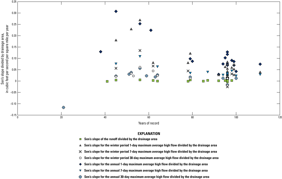
Examining the magnitude and direction of trends versus record length can inform the influence of cyclical wet and dry periods on the statistics, as opposed to assuming the existence of and adjusting for serial correlation (fig. 11). Generally, streamgages with less than 60 years of data (record beginning after 1956) were associated with the greatest range of low-flow Sen’s slope. The overall range of Sen’s slope per drainage area is listed in table 6 (−0.0429 to 0.0191 ft3/s/mi2/yr). For records between 20 and 40 years in length (beginning after 1976), most trends were negative (10 of 13 streamgages); for records between 40 and 60 years in length (beginning between 1957 and 1976), most trends were positive (8 of 11). Streamgages with greater than 60 years of record (beginning prior to 1956) have smaller ranges of low-flow Sen’s Slopes (−0.0095 to 0.0048), and most trends were positive (17 of 22).
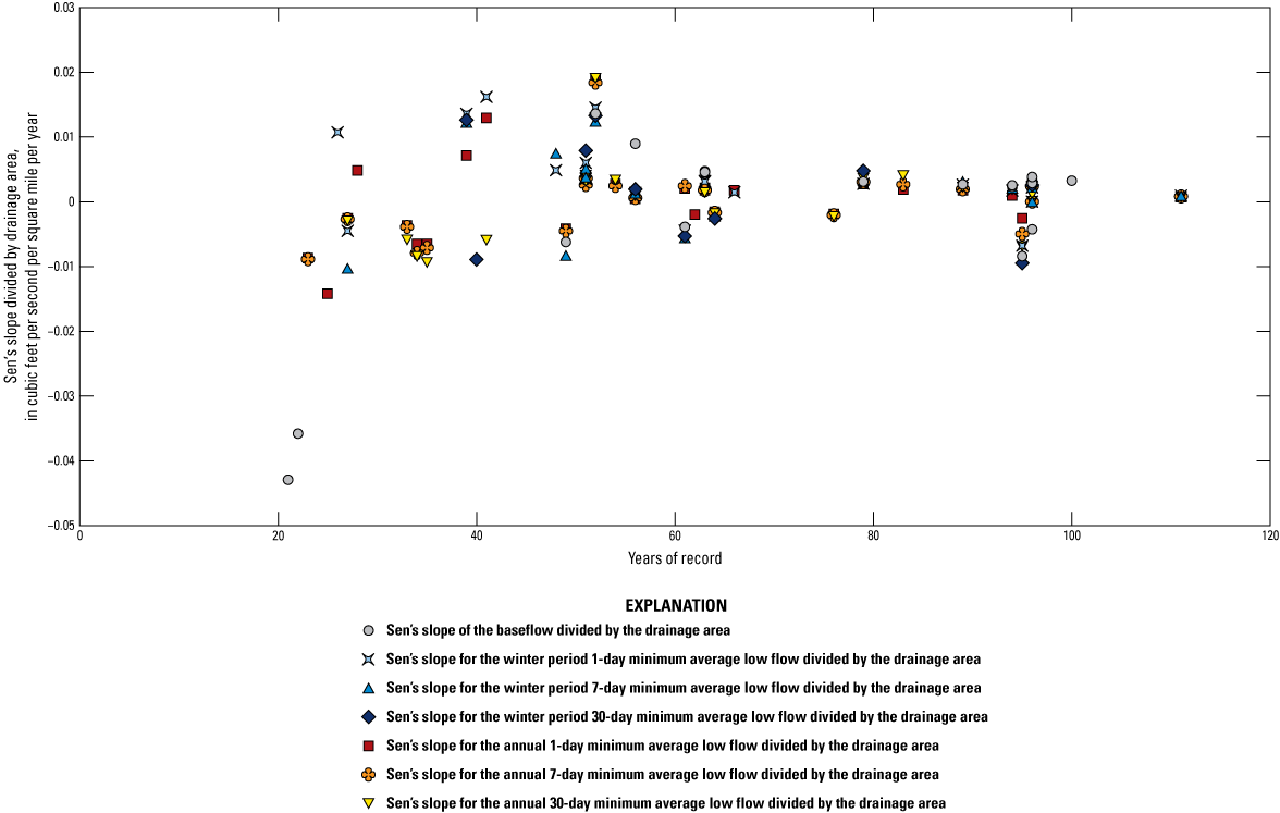
Scatterplot showing the magnitude of statistically significant trends (p<0.05) in low flow at continuous-record streamgages in New Jersey, 1903–2017, compared to years of record.
Table 6.
Magnitude of statistically significant trends in low flow at continuous-record streamgages in New Jersey, 1903–2017.[Winter season is November 1 through April 30. Measurements are given in cubic feet per second per square mile per year]
Runoff and High n-day Flows
The high-flow characteristics examined for trends in this report mirror the range and magnitude of low-flow statistics, with runoff (the counterpart to base flow) as the coarsest measure of the upper half of the hydrograph and the highest 1-, 7-, and 30-day high flows informing possible changes in duration and magnitude of large rainfall events. Examination of n-day high flows can inform water managers of more common flooding conditions as well as extreme events without the large uncertainty and variation that can be associated with frequency analysis of annual peak flows. Highest n-day flows typically occur during the winter. Although it may seem redundant, differences in trends of annual compared to winter high flows can still inform shifts in seasonal climate if differing numbers of trends are observed in each season, though not ideal. The use of annual and winter high values in this study were implemented, in part, to replicate Watson and others (2005).
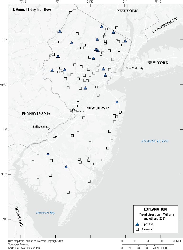
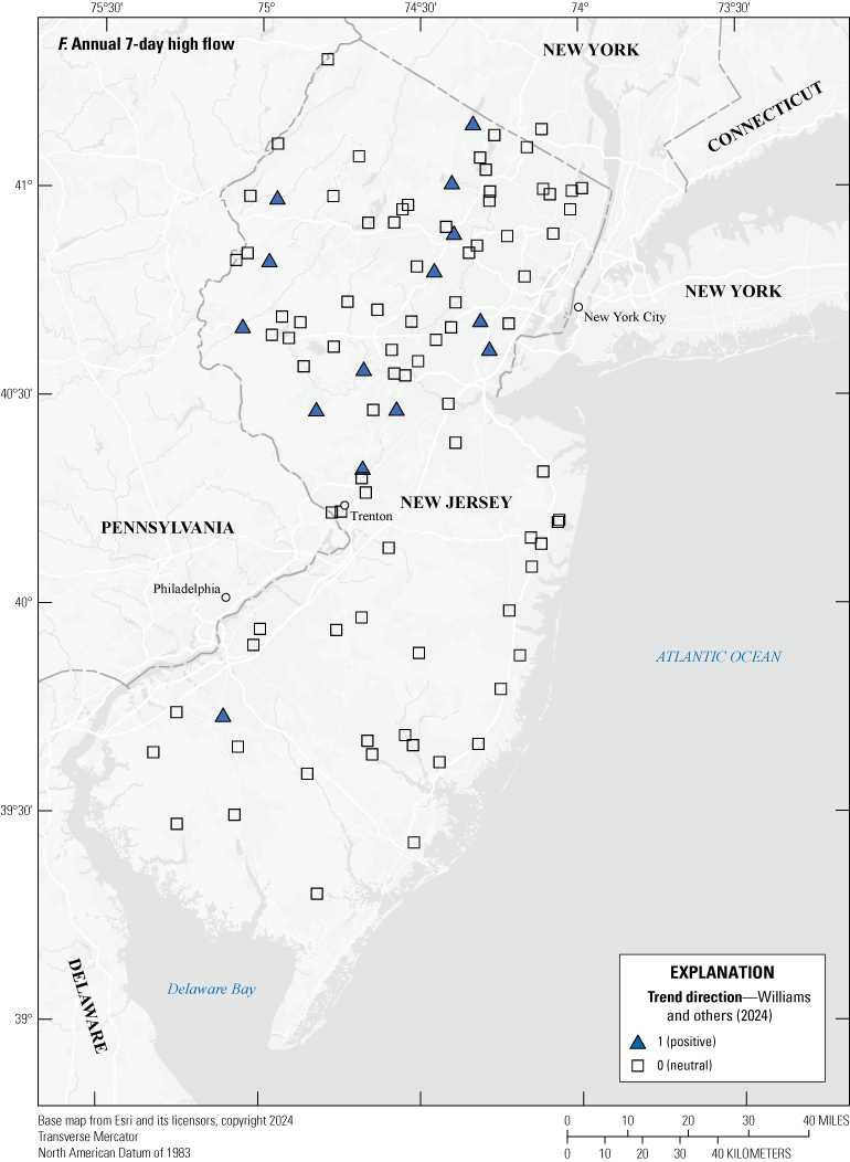
A total of 35 continuous-record streamgages indicated a statistically significant trend for at least 1 or more of the high-flow characteristics computed in this study (table 7 and fig. 12). Most of the trends indicated increasing flows (6 negative, 29 positive). Of the negative trends, flow is regulated or controlled at 1 streamgage; of the positive trends, 6 streamgages are regulated (fig. 13). All but a few of the positive high-flow trends were in northern New Jersey.
Table 7.
Number of New Jersey continuous-record streamgages indicating a statistically significant trend for various high-flow characteristics, 1903–2017.[Winter period is defined as November 1 through April 30].
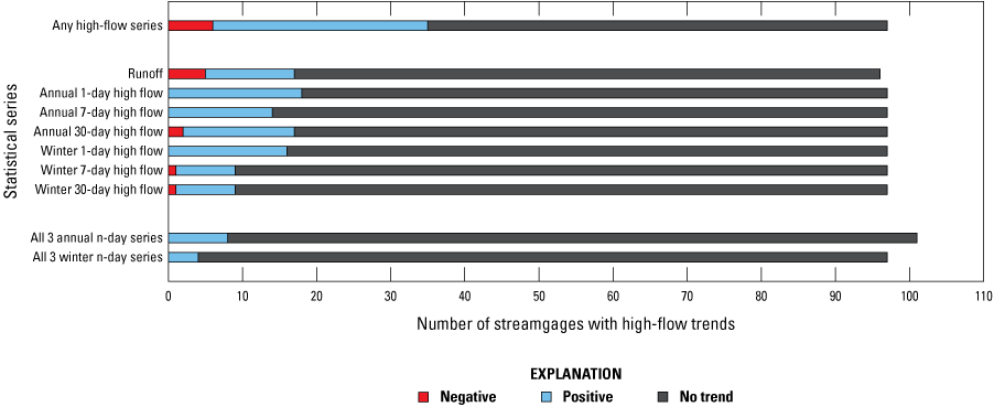
Bar graph showing the number of continuous-record streamgages in New Jersey with statistically significant trends (p<0.05) for various high-flow characteristics and combinations thereof, 1903–2017.
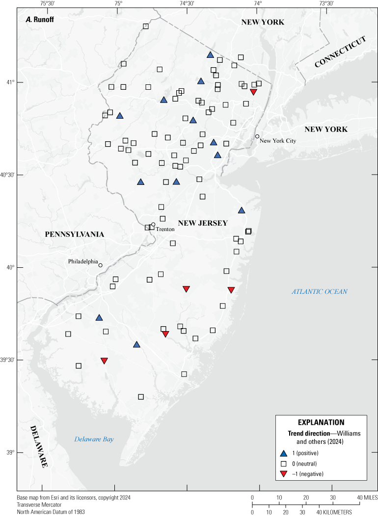
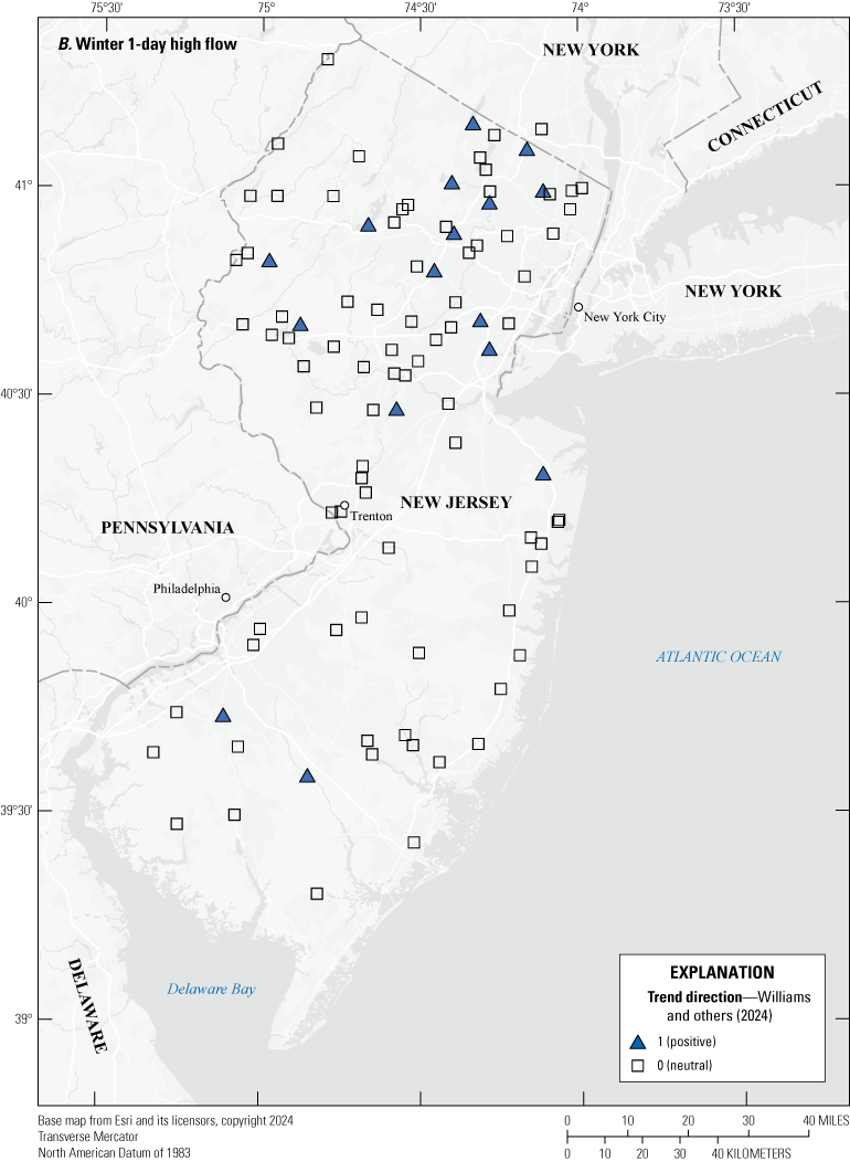
Maps showing continuous-record streamgages with statistically significant trends (p<0.05) in high flow in New Jersey, 1903–2017. A, runoff, B, winter 1-day low flow, C, winter 7-day low flow, D, winter 30-day low flow, E, annual 1-day low flow, G, annual 30-day low flow.
At the coarsest measure of high flow—runoff—statistically significant trends were identified at 17 streamgages (5 negative, 12 positive). Four southern New Jersey streamgages indicated a trend only for runoff (all negative). As was the case for low flow, a larger number of streamgages (31) indicated statistically significant trends at the finer-scale 1-, 7-, or 30-day high flow series for either annual, winter, or both seasons. In the case of high-flow characteristics, approximately half of those streamgages (16) indicated changing flow for both annual and winter n-day values. Only one of the streamgages which had both annual and winter n-day high-flow trends indicated decreasing flow.
For any annual n-day high-flow series, a total of 28 streamgages indicated statistically significant changes in flow (2 decreasing, 26 increasing). Of the 28, only 8 indicated a trend for all 3 n-day series (all positive). For any winter n-day high-flow series, fewer (19) streamgages indicated statistically significant changes in flow (1 decreasing, 14 increasing). Of the 19 streamgages, only 4 indicated a trend for all 3 n-day high flow series (all positive). With a greater number of streamgages having evidence for trends in the annual versus winter series, it suggests that highest flows may be shifting to later in the spring (after April 30).
As with the magnitudes of low-flow trends, Sen’s slope was divided by drainage area so comparisons could be made among streamgages. Unlike the low-flow characteristics, high-flow trends are not likely attributable to point-source discharges and withdrawals, which typically account for a much smaller proportion of the highest n-day flow or base flow values. In addition to shifts in climate, regulation and changes in land cover may contribute to changes in n-day high flows.
The largest statistically significant negative trend in runoff was −0.0129 ft3/s/mi2/yr at the Hackensack River at New Milford, N.J., USGS site 01378500 (table 8), a heavily regulated streamgage located immediately downstream from Oradell Reservoir, with 96 years of record. In addition to runoff, the annual 30-day, winter 7-day, and winter 30-day high-flows also indicated negative trends. The largest statistically significant positive trend in runoff was 0.0051 ft3/s/mi2/yr at the Pequannock River at Macopin Intake Dam, N.J., USGS site 01382500 (table 8), also a heavily regulated streamgage with 56 years of record. All n-day high-flow series also indicated positive trends.
The largest statistically significant negative trend for the n-day high-flow series was −0.1167 ft3/s/mi2/yr at the Whippany River near Pine Brook, N.J., 01381800, the annual 30-day high-flow (table 8). No other n-day high-flow statistics, either annual or winter, showed evidence of a trend. Recall however, that base flow at this streamgage also had the largest negative trend in base flow and it only has 21 years of record.
The largest statistically significant positive trend for the n-day high-flow series was 0.3071 ft3/s/mi2/yr at Mantua Creek at East Holly Avenue at Pitman, N.J., USGS site 01475001, for the annual 1-day high-flow (table 8). All the n-day high-flows, as well as runoff, indicated statistically significant increases. The period of record at 01475001 stretches back to 1940; however, there are two gaps in the record, 1976–2003 and 2006–09, for a total of 45 years of record. This streamgage is occasionally regulated from gates at Kressey Lake.
As was observed in the low-flow trends, the largest range of Sen’s slopes for statistically significant high-flow characteristics were associated with streamgages having less than 60 years of record (−0.1167 to 0.3071; fig. 14). Only two streamgages with record length between 20 and 40 years indicated a statistically significant high-flow trend. The Whippany River near Pine Brook, N.J., 01381800 streamgage showed a negative trend in the 30-day high, whereas Pequest River at Huntsville, N.J., USGS site 01445000, showed a positive trend in 1-day high-flows. For streamgages with records greater than 60 years, the range in Sen’s slope for high-flow trends was −0.0197 to 0.1281 ft3/s/mi2/yr, with decreasing runoff only accounting for negative trends at 4 of the 6 streamgages with negative trends.
Plot of the magnitude of statistically significant trends (p<0.05) in high flow at continuous-record streamgages in New Jersey, 1903–2017, compared to years of record.
Table 8.
Magnitude of statistically significant trends in high flow at continuous-record streamgages in New Jersey, 1903–2017.[Winter season is November 1 through April 30. Measurements are given in cubic feet per second per square mile per year]
Peak-Flow Ratio
As a way to assess both a high-flow characteristic and flow variability, the annual peak-flow ratio was examined. An increasing peak-flow ratio over time would indicate that the annual instantaneous peak is becoming larger in relation to the mean daily flow one day prior, the day of, and one day after the peak. This circumstance suggests that more intense rainfall events are occurring, or that the streamflow is becoming “flashier,” or occurring during times of relatively low base flow in the summer. A decreasing peak-flow ratio over time would indicate that the peak is becoming smaller in relation to associated 3-day mean flow. This circumstance suggests that peaks may be prolonged or increasing in duration, or perhaps occurring on already saturated soils with higher prepeak mean daily flow or possibly smaller peaks happening more frequently on saturated soils.
Twenty-five streamgages indicated a statistically significant trend in peak-flow ratio (Williams and others, 2024). More than 75 percent of the trends indicated an increase in the peak-flow ratio over time. These results coincide with the premise that 1-day high flows may be occurring more often in the annual (summer) series than in the winter season.
The magnitude or the number of statistically significant trends does not appear to be influenced by length of record (fig. 15). Streamgage West Branch Middle Brook near Martinsville, N.J., USGS site 01403150, has an exceptionally high increasing Sen’s slope. This streamgage has the smallest drainage area of all those included in this study, 1.99 square miles.
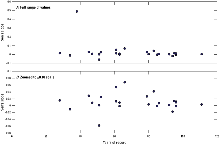
Scatterplot of the magnitude of statistically significant trends (p<0.05) in peak-flow ratio to years of record at continuous-record streamgages in New Jersey, 1903–2017. A, full range of values, and B, zoomed to plus or minus 0.10 scale.
Trends in Regression Residuals at Partial-Record Streamgages
The residuals of the MOVE1 regressions used to estimate low-flow statistics at partial-record streamgages were assessed for trends using the MK test. Because the test is applied to the regression residuals and not a continuous time series of data, a statistically significant (p<0.05) trend indicates a change in the relation between the partial-record streamgage and the continuous-record index site over time. The assumption was made that changes in the relation are likely due to changing flows at the partial-record streamgage, as streamgages with little or no trends in the computed low-flow characteristics were one of the criteria for use of an index site.
A different number of index sites were used per partial-record streamgage, depending on 1) physiographic province as noted in the methods section, and 2) available data. To summarize identified trends in the residuals, a ratio or percentage of the number of index sites indicating a statistically significant trend was determined for each partial-record streamgage. Only the direction of the trend was determined, not the magnitude. It is assumed that as a greater proportion of index sites per partial-record streamgage are identified, the likelihood that flows are changing at the partial-record streamgage increases.
Among the 719 partial-record streamgages, 321 indicated a trend in residuals with at least 1 index site (Williams and others, 2024). The single index site trends were split close to even, with 145 negative and 176 positive. Additionally, of the 321 streamgages with a trend in residuals, 53 had more than 50 percent of index sites indicating a statistically significant (p<0.05) trend in the residuals (26 negative, 27 positive). Having more than 50 percent of the index sites showing a trend in residuals increases the likelihood that the partial-record streamgage has a similar trend. Table 9 lists the index sites used in the regressions and accompanying information on the number of partial-record streamgages that used each index site and the proportion of trends in residuals indicated for each index site. The table is sorted by which index site indicated the greatest number of trends, to determine if any particular index site(s) may have had undue influence in designating a trend. It appears that the proportion (percentage) of trends identified increased with the number of partial-record streamgages which used each index site; in other words, the more often an index site was used, the greater the likelihood it would indicate change at a partial-record streamgage (fig. 16). The span of the partial-record streamgage data (end year minus begin year of discrete flow measurements) also did not seem to influence the number of index site regression residuals that indicated a trend (fig. 17). Trends at partial-record streamgages are most likely due to localized effects of water use. A map showing the direction and spatial distribution of low-flow trends at partial-record streamgages, based on the proportion of statistically significant trends in regression residuals, is presented in figure 18.
Table 9.
Continuous-record streamgages used as index sites in regression analysis with partial-record streamgages and the results of trend tests in New Jersey, 1903–2017.[USGS, U.S. Geological Survey]
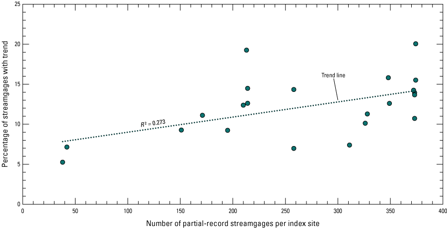
Percentage of partial-record streamgages in New Jersey with a statistically significant trend (p<0.05) in regression residuals for the period 1903–2017, versus the total number of partial-record streamgages regressed against each continuous-record streamgage.
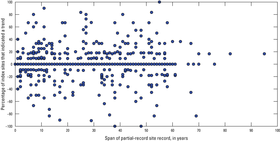
Percentage of continuous-record streamgages indicating a statistically significant trend in regression residuals per partial-record streamgage versus the span of the record, in years, of the partial-record streamgage in New Jersey, 1903–2017.
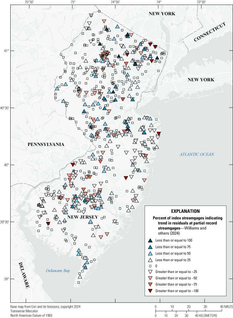
Map showing the percentage of index sites indicating a statistically significant trend (p<0.05) in regression residuals per partial-record streamgage versus the span of the record, in years, of the partial-record streamgage in New Jersey, 1903–2017.
Trends in Low Flow in Over-Allocated Basins
The New Jersey Geological and Water Survey Technical Memorandum 13-3 (Domber and others, 2013) established an approach for determining water availability in the State using a low-flow margin, defined as the difference between the 7-day 10-year low flow, herein referred to as the 7Q10, and the September median flow. The low-flow margin was determined for subwatersheds at the 11-digit hydrologic unit code (HUC11) scale (Domber and others, 2013). The NJDEP then identified HUC11s for which allocated water exceeded the low-flow margin.
Both positive and negative trends in low-flow characteristics at continuous-record streamgages were identified in over-allocated basins, as defined by NJDEP (table 10). Negative trends were identified for at least one of the computed low-flow characteristics at eight continuous-record streamgages among seven of those identified HUC11s. Positive trends in low-flow characteristics were identified at 11 streamgages among 9 HUC11s.
Table 10.
Number and direction of trends of computed low-flow characteristics at continuous-record streamgages in New Jersey, for which the associated HUC11 allocated water exceeds the low-flow margin.[USGS, U.S. Geological Survey; regulated flow, a reservoir or flow control structure upstream of the streamgage; HUC11, 11-digit hydrologic unit code; NJ, New Jersey]
Trends in flow at partial-records sites were defined by the percentage of index sites which had statistically significant trends in the residuals of the regressions with each partial-record site. Just as with the continuous-record streamgages, partial-record streamgages indicate both increasing and negative trends in HUC11s where allocation exceeded the low-flow margin. Sites where the percentage of index sites with residual trends greater than ±50 percent are listed in table 11.
Table 11.
Partial-record streamgages in New Jersey with more than half of the index sites used in low-flow regression analysis that had statistically significant trends in residuals among HUC11 where allocated water exceeds the low-flow margin.[USGS, U.S. Geological Survey; HUC11, 11-digit hydrologic unit code]
Recall that the trend tests were applied to the full periods of record for both continuous and partial-record streamgage analysis. Current or changing water use may not be reflected in the trend test results or the allocated amounts from the NJDEP assessment.
Comparison of Results—2001 and 2017
This study used 97 continuous-record streamgages and 719 partial-record streamgages with data through 2017. A subset of 80 continuous-record streamgages and 462 partial-record streamgages were included as part of the previous report (Watson and others, 2005), which used data through 2001. Trends were assessed for the same n-day flows (high and low, annual, and winter) for continuous-record streamgages in both studies; however, Watson and others (2005) did not assess regression residuals at partial-record streamgages. The same streamflow characteristics for flow durations and n-day high and low, annual, and winter flow were computed in both studies. The statistics for streamgages included in both studies were compared to help users develop a better understanding of changes in high- and low-streamflow trends, as well as how much the computed streamflow characteristics may have changed. This type of comparison may help to inform possible effects on water resource management.
Changes in Trends at Continuous-Record Streamgages
Among the 80 continuous-record streamgages that were included in both the current and previous (Watson and others, 2005) studies, trends in the annual 1-, 7-, and 30-day high and low, annual, and winter flow series were computed using the MK trend test under the assumption of serial independence. Trend test results indicated a considerable increase in the number of statistically significant positive trends, in both high and low flows, for both seasons (fig. 19).
The total number of positive n-day high-flow trends more than doubled from 37, using data through 2001, to 82, using data through 2017. The largest increase in number of positive trends was observed for the annual 30-day high flow. The total number of negative or decreasing n-day high-flow trends dropped from 5 to 3 for the same datasets. A similar change in the number of trends in n-day low flow was observed, but to a lesser degree, with positive trends ranging from 61 to 82 between the two datasets. The total number of negative trends in n-day low flows declined from 37 to 25 (fig. 19).
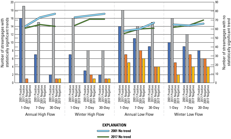
Bar graph showing the number of statistically significant trends (p<0.05) in n-day flow at continuous-records streamgages in New Jersey using data through 2001 versus 2017.
Percent Change in Streamflow
The determination of trends in streamflow noted in the previous sections evaluates the full periods of record for statistically significant changes. To quantify changes in streamflow since the previously computed statistics through 2001 (Watson and others, 2005), the percent change in individual streamflow statistics were computed. This determination can provide information of possible impacts of the updated statistics on streamflow permits and prior management strategies, regardless of whether the data show a statistically significant trend. Comparisons in continuous-record streamgage-flow statistics include changes in computed durations (1-, 2-, 5-, 10-, 20-, 25-, 30-, 40-, 50-, 60-, 70-, 75-, 80-, 85-, 90-, 95-, 99-percent) and all high and low flow frequencies (1-, 7-, and 30-day high and low flows at 50-, 20-, 10-, 5-, and 4-percent exceedance and nonexceedances, for annual and winter periods). For partial-record streamgage statistics, percent change in the 1-, 7-, 30-day annual, and 7- and 30-day winter low flows at 10-percent annual nonexceedance probability, the 75th and 50th percentile flow, and the annual mean flow were computed.
Continuous-Record Percent Change in Streamflow
Most changes to computed streamflow characteristics for both flow durations and frequencies were generally within ±10 percent using the additional data collected among the 80 continuous-record streamgages that were included in both this and the previous report. The lower flow characteristics typically accounted for changes greater than ±10 percent from the previous report, with a full range of change from −100 to +500 percent.
A greater number of both annual and winter flow duration values indicated decreases in flow durations, though the change was mostly minimal—between 0 and −5 percent. Histograms demonstrating the distribution of the annual and winter flow percent change among the 1,360 individual computed durations (17 durations among the 80 sites) are shown in figure 20. Of those computed annual flow durations, 61 percent (830) indicated decreases and 38 percent (514) indicated increases in flow from 2001 to 2017; 1 percent (16) indicated zero change. For winter flow durations, 57 percent (778) indicated decreases and 39 percent (525) indicated increases; 4 percent (57) indicated zero change. Only 13 and 9 percent of computed annual and winter durations indicated a change in flow greater than 10 percent. The histograms do not include values of zero change because the zeroes would fall into the −5 to 0 percentage bin, making it appear there were more negative changes than were actually computed.
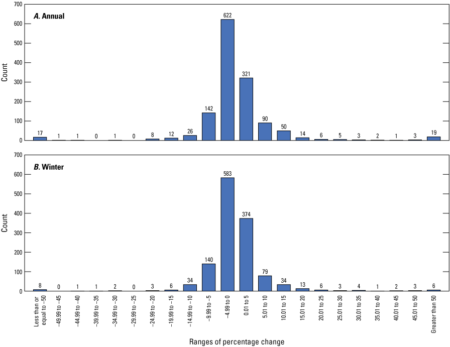
Histogram of percent change from 2001 to 2017 for 80 continuous-record streamgages in New Jersey. A, annual streamflow duration values, and B, winter streamflow duration values. Durations computed were the 1-, 2-, 5-, 10-, 20-, 25-, 30-, 40-, 50-, 60-, 70-, 75-, 80-, 85-, 90-, 95-, and 99-percent flows. Winter period is November 1 through April 30. A total of 16 annual and 57 winter zero values for duration flow percent change are not included in the graphs.
Percent change was not consistent in either the positive or negative direction for all 17 computed durations for a given site, indicating some changes to the distribution of flow in the duration curves. The 50th through 5th percentile flows indicated mostly negative changes. Lowest flows (99th to 95th percentiles) indicated greatest percent change with most outliers greater than ±50 percent, but, overall, leaned more positive. Boxplots of the distribution of percent change of each of the 17 annual and winter flow durations are shown in figure 21 and figure 22.
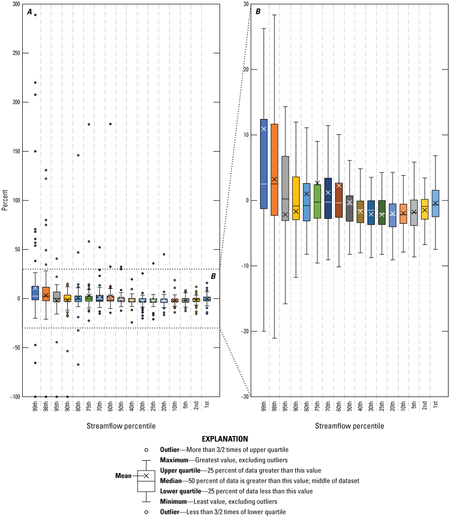
Boxplots showing range of percent change in annual flow durations at continuous-record streamgages in New Jersey from 2001 to 2017. A, with statistical outliers and B, without statistical outliers.
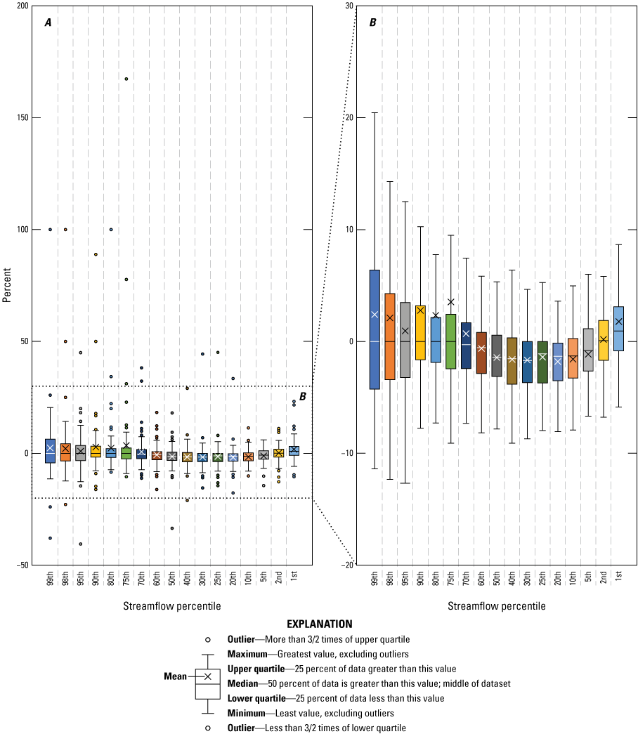
Boxplots showing the range of percent change in winter flow durations at continuous-record streamgages in New Jersey from 2001 to 2017. A, with statistical outliers and B, without statistical outliers. Winter period is from November 1 through April 30.
The greatest decreases in the lower flow durations (99th to 90th) were observed at both regulated and unregulated sites (USGS sites 01378500, 01407500, 01382500, 01401650, 01381000, and 01396800). The outliers of percent change ranged from −47 to −100 percent. The greatest increases in the lower flow durations were at mostly unregulated sites (USGS sites 01396800, 01401000, 01455500, 01403150, 01466500, 01443900, and 01403540). The outlier changes ranged from +22 to +289 percent.
The computed frequency statistics, which are generally associated with the rarest occurring flow conditions, indicated more increases than decreases for both low and high flows from 2001 to 2017. Histograms demonstrating the distribution of the low and high flow computed percent changes among the 1,920 individual computed frequency statistics (12 n-day frequencies for both annual and winter flows among the 80 sites) are shown in figure 23. The histograms do not include values of zero change. Of the low-flow frequency statistics, 7 percent (125) indicated zero change; for high flow, 1 percent (11) indicated zero change. Generally, most changes in low and high frequency statistics were slightly greater than the changes in durations statistics, ranging mostly from −10 to +15 percent. A greater proportion indicated positive changes in both low and high flow frequencies, at 58 and 75 percent, respectively.
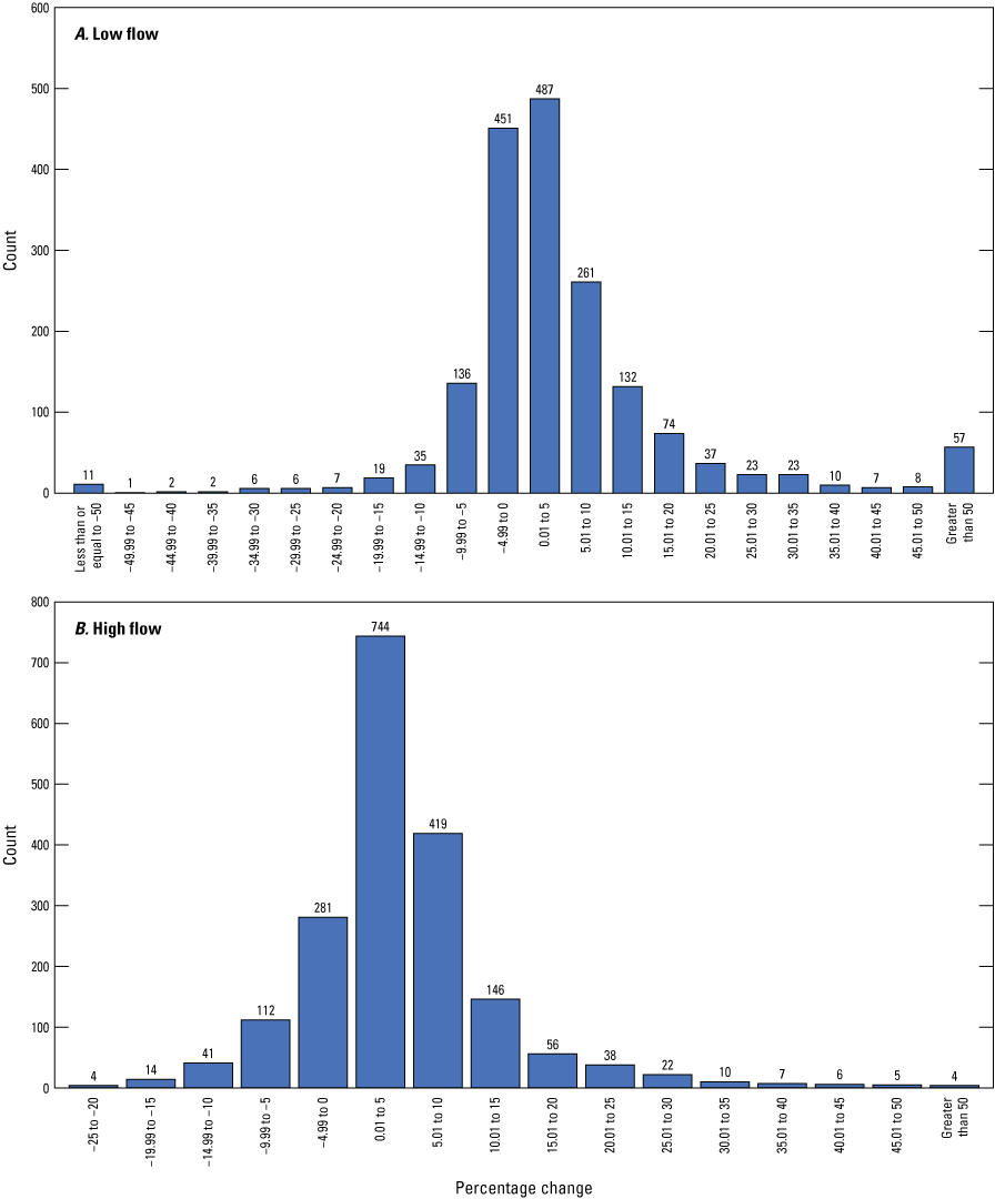
Histogram of the frequency statistics percentage of change from 2001 to 2017. A, low flow, and B, high flow. Frequencies computed were the 1-, 7- and 30- day high and low flows at 50-, 20-, 10-, 5-, and 4-percent exceedance and nonexceedance for annual and winter periods. Winter period is from November 1 through April 30. A total of 125 and 11 zero values for low- and high-flow frequency percent change are not included in the graphs.
A histogram plot showing the percent change in low-flow statistics was generally between −10 to +15 percent, and high-flow percent change was generally between -5 and +15 percent change for the majority of streamgages. The outliers and ranges of percent change do not indicate a clear pattern or bias for a particular n-day or recurrence interval, as shown in the boxplots in fig. 24 and fig. 25. As mentioned in the “Methods” and “Frequency Analysis” sections, some of the changes in frequency flow statistics at regulated streamgages in this study may be a result of the different approaches used in analysis of data that did not fit the LPIII distribution; that is, using a graphical or visual fit compared to computing a percentage of the flows.
The largest increases in low-flow frequency statistics were at the streamgage below Musconetcong River at outlet of Lake Hopatcong, N.J., USGS site 01455500. The site is heavily regulated with a minimum passing flow. The second largest overall increase was observed at Rockaway River below Reservoir at Boonton, N.J., 01381000, which is also heavily regulated with a minimum passing flow. Increases were between 0 and +500 percent.
The streamgage with the largest decreases in low-flow frequency statistics was Absecon Creek at Absecon, N.J., USGS site 01410500. Flow at this site is unregulated but is affected by tidal fluctuations. The site with the second most decreases in flow frequencies was at Neshanic River at Reaville, N.J., 01398000. This site is not regulated (has no controlled flow upstream). Decreases were between 0 and −100 percent.
For high-flow frequencies, the two streamgages with the highest increase were Pequest River at Huntsville, N.J., 01445000, and Mantua Creek at East Holly Avenue at Pitman, N.J., 01475001. Neither streamgage is regulated. Changes were between 2 and 50 percent for the two streamgages.
The streamgages with the greatest decrease in high-flow frequencies were West Branch Middle Brook near Martinsville, N.J., 01403150, and Cedar Creek at Western Blvd near Lanoka Harbor, N.J., 01408900. The Martinsville streamgage has a very small drainage area (1.99 square miles), and the Lanoka Harbor streamgage is affected by tide. Neither site is regulated. The decreases were relatively minimal, ranging from −2 to −19 percent.
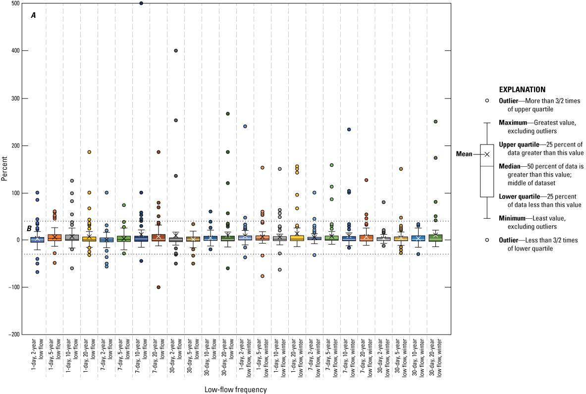
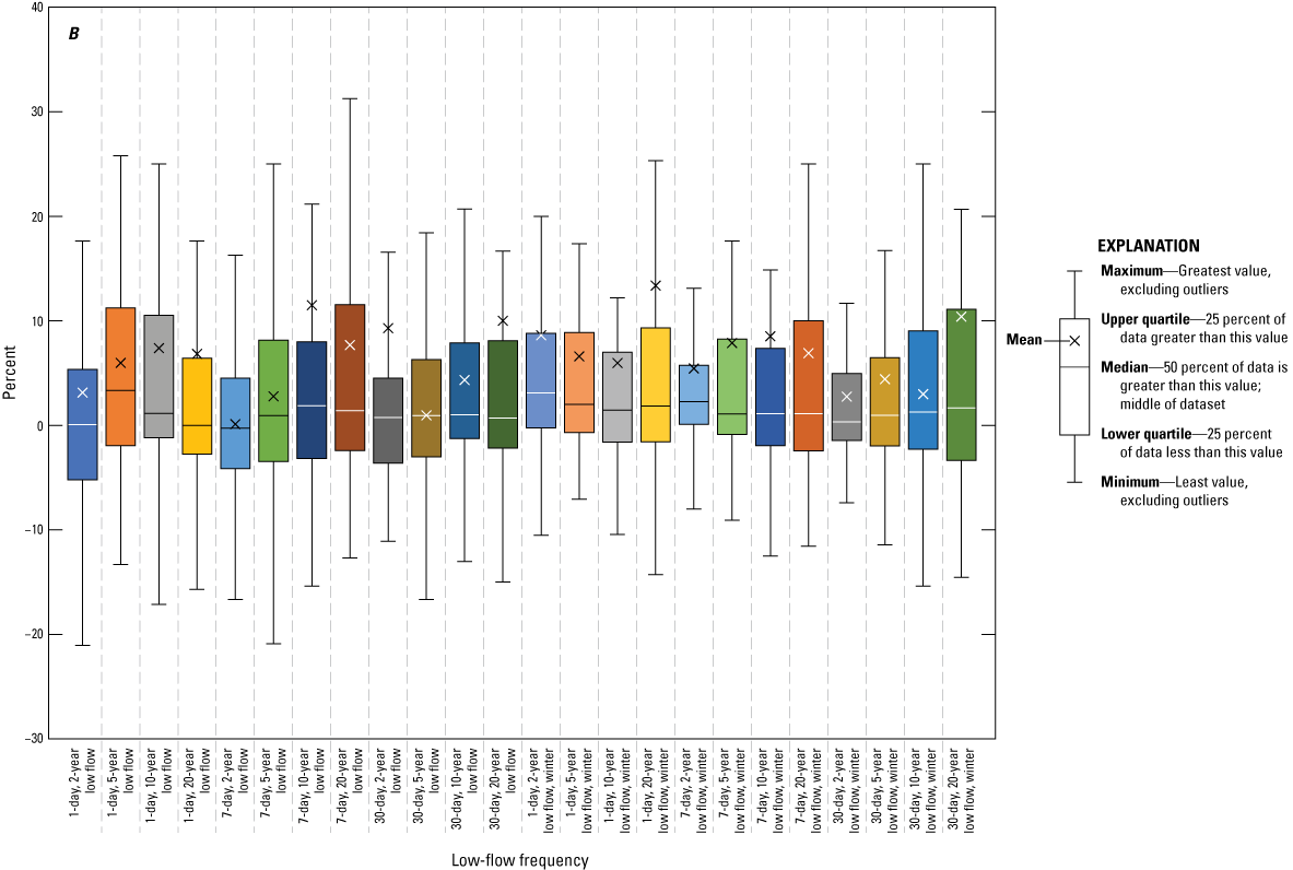
Boxplots showing range of percent change in annual and winter low-flow frequency statistics at continuous-record streamgages in New Jersey from 2001 to 2017. A, with statistical outliers and B, without statistical outliers. Winter period is from November 1 to April 30.
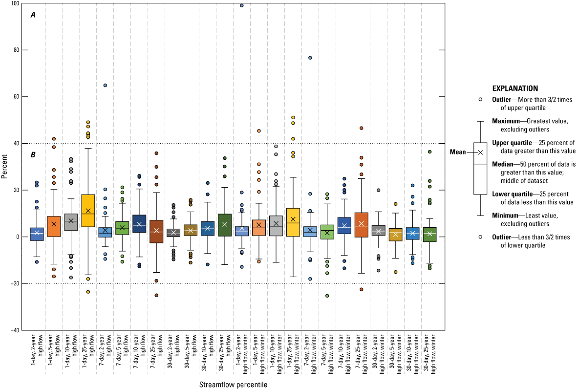
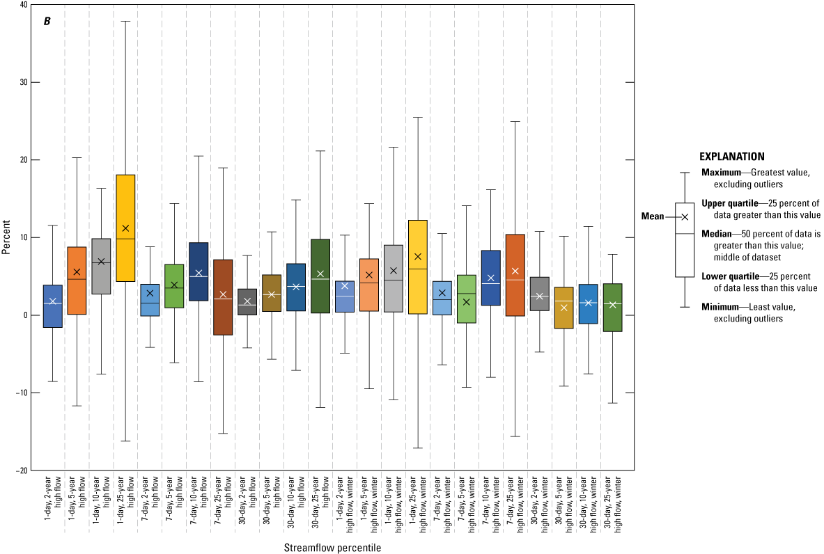
Boxplots showing range of percent change in annual and winter high-flow frequency statistics at continuous-record streamgages in New Jersey from 2001 to 2017. A, with statistical outliers and B, without statistical outliers. Winter period is from November 1 to April 30.
Partial-Record Streamgage Percent Change in Low Flow
Of the 719 partial-record streamgages in the current analysis using data through 2017, 462 of the streamgages were also computed in the 2005 report, which used data through 2001, and were available for comparison. As indicated earlier, partial-record streamgage statistics were computed using a MOVE1 relation with 22 continuous-record streamgages (index sites), 19 of which were also included in the previous report. The percent change in the computed statistics at the index sites from 2001 to 2017 ranged from −15 to +25 percent, but only about 9 percent of those changes were greater than 10 percent (table 12).
Table 12.
Percent change in computed low-flow statistics at continuous-record streamgages in New Jersey, from 2001 to 2017. The streamgages were used to estimate low-flow statistics at partial-record streamgages in New Jersey, through 2017.[Data are given in percentages. USGS, U.S. Geological Survey. Blue shading indicates changes greater than 10 percent, red shading indicates changes less than -10 percent]
Overall, the changes in the low-flow statistics at the partial-record streamgages were greater than those observed at the continuous-record streamgages. Like the continuous-record low-flow frequency statistics, the change skewed slightly toward more increases in flow. Most percent changes in partial-record streamgages low-flow statistics ranged from −15 to +20 percent (fig. 26). Of the possible 3,696 values of change (8 computed statistics for 462 streamgages), about 17 percent (634) of values indicated zero change and are excluded from the histogram. Percentage change could not be computed for 6 percent (217) of values, as the 2001 computed value was a zero.
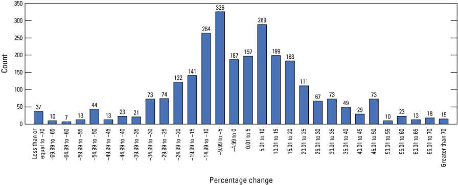
Histogram of percent change in low-flow statistics at 462 partial-record streamgages in New Jersey from 2001 to 2017. Computed statistics were the 1-, 7-, 30-day annual, and 7- and 30-day winter low flows at 10 percent annual nonexceedance probability, the 75th and 50th percentile flow, and the annual mean flow. The data in the graph do not include values of zero or those percent changes that could not be computed because of a zero value in 2001.
A histogram plot of percent change in low-flow statistics at 462 partial-record streamgages in New Jersey shows a broad distribution of streamgages between -30 and +50 percent change. The range of percent change among the individual low-flow statistics is consistent, as seen in the boxplots in figure 27. The greatest changes were observed as outliers at the lower flows, the 1-day annual and 1- and 7-day winter, 10-year statistics. The annual median flow indicated the least amount of change among the partial-record streamgage statistics.
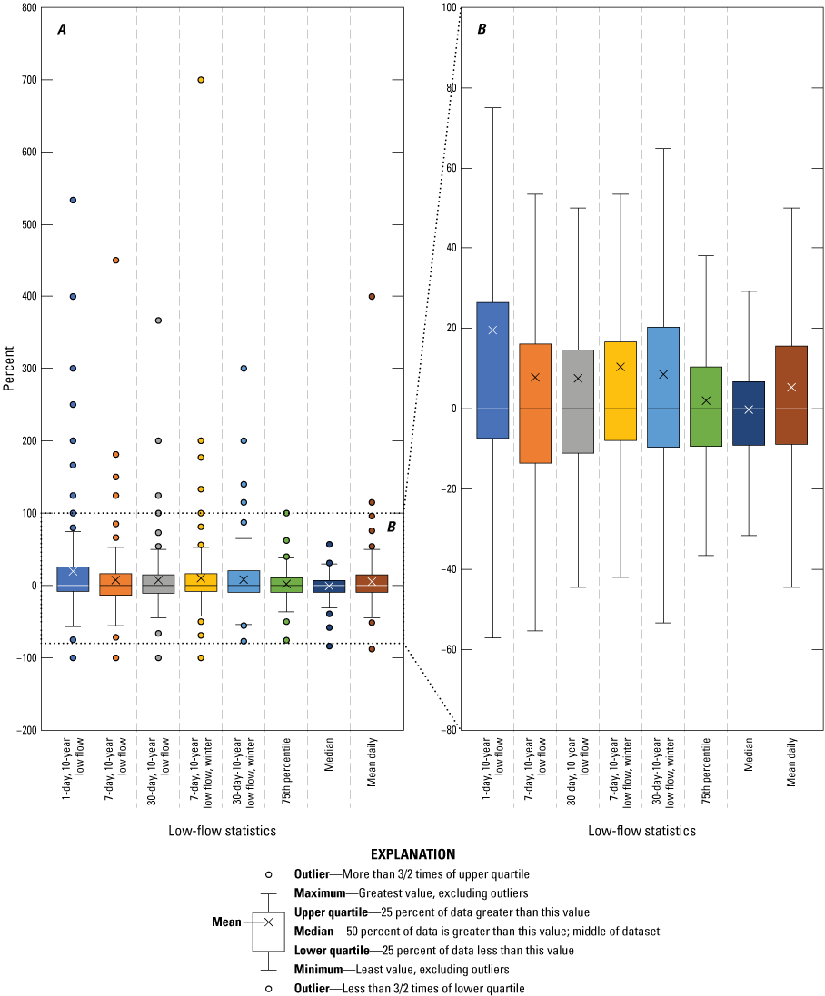
Boxplots showing the range of percent change in low-flow statistics at partial-record streamgages in New Jersey, from 2001 to 2017. A, with statistical outliers and B, without statistical outliers.
Summary and Conclusion
Streamflow data collected in New Jersey from 1903 to 2017 were compiled and analyzed to produce a collection of statistical characteristics to describe the frequency, duration, variability, and trends in streamflow. The information generated from this study serves as a repository and reference to enhance the understanding and support management of water resources in the State.
Overall, the direction of statistical trends in low-flow characteristics were somewhat balanced, with 28 percent of the continuous-record streamgages tested indicating a positive trend, and 20 percent indicating a negative trend. The same was not true for high-flow characteristics, with 30 percent of the continuous-record streamgages tested indicating a positive trend, but only 6 percent indicating a negative trend. Decreasing flow trends were more often observed in southern New Jersey. Fewer streamgages indicated increased variability. About 25 percent of the continuous-record streamgages tested indicated increased variability by analyzing results of annual skew, kurtosis, and peak flow ratio. The partial-record streamgages showed slightly different results, with about 45 percent showing a trend in at least 1 index site, but only about 7 percent had more than 50 percent of the reference index sites that showed a trend.
A total of 97 continuous-record streamgages and 719 partial-record streamgages were included in the analysis. Computed continuous-record streamflow characteristics included the following:
-
• Maximum, minimum, mean for period of record
-
• Duration of flow (annual and winter)
-
• 50-, 20-, 10-, 5-, and 4-percent annual nonexceedance (or 2-, 5-, 10-, 20-, and 25-year recurrence interval) frequencies of 1-,7-, and 30-consecutive day minimum average low flow (annual and winter)
-
• 50-, 20-, 10-, 5-, and 4-percent annual exceedance (or 2-, 5-, 10-, 20-, and 25-year recurrence interval) frequencies of 1-,7-, and 30-consecutive day maximum average high flow (annual and winter)
-
• Ratio of peak to 3-day mean flow
-
• Mean annual base flow and runoff
-
• Drought-of-record base flow (1962–70)
-
• Median September flow
-
• Annual variability measured as annual skew and kurtosis
Low-flow characteristics were computed at partial-record streamgages using MOVE1 regressions of flow with continuous-record streamgages. The computed low-flow characteristics included the following:
-
• Annual 1-, 7-, and 30-day low flow with a 10 percent annual nonexceedance probability
-
• Winter 7- and 30-day low flow with a 10 percent annual nonexceedance probability
-
• 50th and 75th percent duration flow
-
• September median flow
-
• Mean annual base flow
-
• Drought-of-record base flow (1962–70)
Mann-Kendall trend tests were applied to n-day low and high flows, base flow, runoff, peak-flow ratio, skew, and kurtosis annual time series using independent, lag-1, and long-term persistence assumptions of serial correlation for all streamgages. A Sen-Thiel slope was computed to determine the magnitude of change over time for the various statistics. An MK test for trends was also applied to the residuals of the individual regressions of partial-record streamgages to determine if the relation between index site and the partial-record streamgages was changing through time. For both continuous- and partial-record streamgages, the percent change in streamflow characteristics from those reported in Watson and others (2005) was also determined.
The number of statistically significant trends decreased for all flow characteristics when variance was adjusted to account for assumptions of short term (lag-1) and long-term persistence. However, evidence for serial correlation does not appear to be substantial for STP or necessarily clear for LTP and may not justify the variance adjustment for all streamgages. Most statistics used in water use permitting use all available record, regardless of when it was collected or how long it is—unless there is a known major change in the basin. Knowing if the available stream record used for planning or permitting is changing or has an identified trend can inform water managers of what might be expected in the near term for permit renewals and changes in allocation. Although the trend tests of all three assumptions of serial correlation were computed for this study and are available in the data release (Williams and others, 2024), the discussion focused on the results of the independent assumption, with the knowledge that the other results have fewer statistically significant trends.
About a quarter of streamgages indicated increasing variability as measured by annual skew, kurtosis, and peak-flow ratio. This finding is supported by both the annual 1-day low- and high-flow time series indicating the greatest number of trends among all flow characteristics. The Saddle River at Lodi, N.J., 01391500 streamgage is the only exception to this trend, where the data indicate that the highest flow events are not as large and are occurring less often. Lodi is the only streamgage with decreasing skew and kurtosis. There was also a greater number of streamgages having evidence for trends in the annual versus winter high-flow series, suggesting that the highest flows may be shifting to later in the spring (after April 30).
Examining the magnitude and direction of trends versus record length can inform the influence of cyclical wet and dry periods on the statistics, as opposed to assuming the existence of and adjusting for serial correlation. The magnitude of statistically significant trends in this study was influenced by length of record; the largest trends occurring between 40 and 60 years of record for both high and low flows, as well as variability. Though less in magnitude, a greater number of trends were identified in skew and kurtosis at streamgages with records longer than 80 years. These results reflect that the longer the record is collected, the more likely it is to have captured a comparatively rare drought or flood event.
The magnitude or number of trends in peak-flow ratio does not appear to be influenced by record length. Twenty-five streamgages indicated a statistically significant trend in peak-flow ratio. More than 75 percent of the trends indicated an increase in the peak-flow ratio over time. These results coincide with the premise that 1-day high flows are occurring more often in the annual (summer) series than in the winter season, which would also indicate an increased peak-flow ratio.
Trends at partial-record streamgages are most likely due to localized effects of water use. Of the 719 partial-record streamgages, 321 indicated a trend in residuals with at least 1 index site (145 decreasing, 176 increasing). Of the 321 partial-record streamgages, 53 had more than 50 percent of index sites indicating a statistically significant (p<0.05) trend in the residuals (26 decreasing, 27 increasing). The span of the partial-record streamgage data (end year minus begin year of discrete flow measurements) did not seem to influence the number of index site regression residuals that indicated a trend.
Both positive and negative trends in low-flow characteristics at continuous-record streamgages were identified in over-allocated basins, as defined by New Jersey Department of Environmental Protection (NJDEP). The same was true for trends in residuals of partial-record streamgage regressions. Recall that the trend tests were applied to the full periods of record for both continuous- and partial-record streamgage analysis. Current or changing water use may not be reflected in the trend test results or the allocated amounts from the NJDEP assessment.
When compared to the previous assessment of New Jersey streamflow characteristics and trends (Watson and others, 2005), which used data through 2001, the number of statistically significant positive trends is growing among the 80 long-term continuous streamgages that were included in both studies. A greater number of positive trends in both annual and winter, low and high n-days flows are in this study as compared to the previous analysis. The number of negative trends appears to be declining for both high and low flows at these older streamgages.
When assessing the percent change in the computed streamflow characteristics from the previous report, most differences for both flow durations and frequencies were generally within ±10 percent using the additional data collected. Percent change was not consistent in either the positive or negative direction for all 17 computed durations for a given streamgage, indicating some changes to the distribution of flow in the duration curves. Generally, most changes in low- and high-flow frequency statistics were slightly greater as compared with the changes in durations statistics, ranging from −10 to +15 percent. Some of the changes in frequency flow statistics at regulated streamgages in this study may be a result of the different approaches used for data that did not fit the LPIII distribution; that is, using a graphical or visual fit compared to computing a percentage of the flows. Most percent changes in partial-record streamgage low-flow statistics ranged from −15 to +20 percent. Less than 5 percent of all computed changes in flow were greater than ±50 percent.
Streamflow trends and changes to duration and frequency statistics can be influenced by water use, in addition to climate variables. This study did not attempt to parse out the distinction of those influences, but rather focused on reporting updates and potential changes at selected streamgages. Despite trends in streamflow appearing to be mostly increasing in New Jersey, the magnitude of changes in streamflow appears somewhat stable or increasing, but only slightly. However, the results are not necessarily consistent or uniform, with some individual stream locations indicating considerable change in either direction. Water managers and regulators can use the data provided here to more effectively assess individual reaches and watershed management areas and to better understand the resources available and the potential streamflow changes from water years 1903 to 2017.
Acknowledgments
The authors would like to extend their sincere appreciation to several USGS colleagues, without whom this report would not have been completed. Robert G. Reiser (retired) contributed to the initial planning and development of the project. Glenn Hodgkins of the New England Water Science Center provided guidance and R code to help assess trends in the context of serial correlation. Dean Riddle and Robert Palumbo completed the initial delineation for over 800 drainage basins for the associated web mapper. Steve Cauller assisted with mapping of the data results. Lucas Pick (former employee) contributed to data summarization. Jessica Hopple (retired) assembled, organized, and prepared the very large dataset that was produced from this study. Toby Feaster and John Hammond peer-reviewed the report.
References Cited
Barlow, P.M., Cunningham, W.L., Zhai, T., and Gray, M., 2014, U.S. Geological Survey groundwater toolbox, a graphical and mapping interface for analysis of hydrologic data (version 1.0)—User guide for estimation of base flow, runoff, and groundwater recharge from streamflow data: U.S. Geological Survey Techniques and Methods, book 3, chap. B10, 27 p., accessed February 22, 2023, at https://doi.org/10.3133/tm3B10.
Colarullo, S.J., Sullivan, S.L., and McHugh, A.R., 2018, Implementation of MOVE.1, censored MOVE.1, and piecewise MOVE.1 low-flow regressions with applications at partial-record streamgaging stations in New Jersey: U.S. Geological Survey Open-File Report 2018–1089, 20 p., accessed February 15, 2023, at https://doi.org/10.3133/ofr20181089.
Domber, S., Snook, I., and Hoffman, J.L., 2013, Using the stream low flow margin method to assess water availability in New Jersey’s water-table-aquifer systems: New Jersey Geological Survey Technical Memorandum 13–3, 70 p., accessed February 15, 2023, at https://www.nj.gov/dep/njgs/pricelst/tmemo/tm13-3.pdf.
Esralew, R.A., and Baker, R.J., 2008, Determination of baseline periods of record for selected streamflow-gaging stations in New Jersey for determining ecologically relevant hydrologic indices (ERHI): U.S. Geological Survey Scientific Investigations Report 2008–5077, 70 p., accessed February 22, 2023, at https://pubs.usgs.gov/sir/2008/5077/.
Falcone, J.A., 2017, U.S. Geological Survey GAGES-II time series data from consistent sources of land use, water use, agriculture, timber activities, dam removals, and other historical anthropogenic influences: U.S. Geological Survey data release, accessed February 22, 2023, at https://doi.org/10.5066/F7HQ3XS4.
Gillespie, B.D., and Schopp, R.D., 1982, Low-flow characteristics and flow duration of New Jersey streams: U.S Geological Survey Open-File Report 81–1110, 164 p., accessed February 23, 2023, at https://pubs.usgs.gov/of/1981/1110/report.pdf.
Hamed, K.H., 2008, Trend detection in hydrologic data—The Mann-Kendall trend test under the scaling hypothesis: Journal of Hydrology, v. 349, no. 3–4, p. 350–363, accessed February 23, 2023, at https://doi.org/10.1016/j.jhydrol.2007.11.009.
Hamed, K.H., and Ramachandra Rao, A., 1998, A modified Mann-Kendall trend test for autocorrelated data: Journal of Hydrology, v. 204, no. 1–4, p. 182–196, accessed February 22, 2023, at https://doi.org/10.1016/S0022-1694(97)00125-X.
Hammond, J.C., and Fleming, B.J., 2021, Evaluating low flow patterns, drivers and trends in the Delaware River Basin: Journal of Hydrology, v. 598, article 126246, 13p., accessed February 22, 2023, at https://doi.org/10.1016/j.jhydrol.2021.126246.
Hirsch, R.M., 1982, A comparison of four streamflow record extension techniques: U.S. Geological Survey Water Resources Research, v.18, no. 4, p. 1081–1088, accessed February 15, 2023, at https://doi.org/10.1029/WR018i004p01081.
Hirsch, R.M., and De Cicco, L.A., 2015, User guide to exploration and graphics for RivEr Trends (EGRET) and dataRetrieval—R packages for hydrologic data (version 2.0, February 2015): U.S. Geological Survey Techniques and Methods, book 4, chap. A10, 93 p., accessed February 22, 2023, at https://pubs.usgs.gov/tm/04/a10/.
Hodgkins, G.A., Dudley, R.W., Nielsen, M.G., Renard, B., and Qi, S.L., 2017, Groundwater-level trends in the U.S. glacial aquifer system, 1964–2013: Journal of Hydrology, v. 553, p. 289–303, accessed February 22, 2023, at https://doi.org/10.1016/j.jhydrol.2017.07.055.
Hoffman, J.L., Petriman, O., Bleicher, M., Boyle, J., Domber, S., French, M., Gheen, J., Johnson, S., Mennel, B., Myers, J., Nicholson, L., Rancan, H., Roman, E., Shin-Chim, R., 2012, Hydrogeologic testing and reporting procedures in support of New Jersey water allocation permit applications: New Jersey Department of Environmental Protection, Water Resources Management, Division of Water Supply and Geoscience, New Jersey Geological and Water Survey Technical Memorandum 12-2, 109 p., accessed February 23, 2023, at https://www.nj.gov/dep/njgs/pricelst/tmemo/tm12-2.pdf.
Kiang, J.E., Flynn, K.M., Zhai, T., Hummel, P., and Granato, G., 2018, SWToolbox—A surface-water tool-box for statistical analysis of streamflow time series: U.S. Geological Survey Techniques and Methods, book 4, chap. A–11, 33 p., accessed February 22, 2023, at https://doi.org/10.3133/tm4A11.
Khaliq, M.N., Ouarda, T.B.M.J., and Gachon, P., 2009, Identification of temporal trends in annual and seasonal low flows occurring in Canadian rivers—The effect of short and long-term persistence: Journal of Hydrology, v. 369, nos. 1–2, p. 183–197, accessed February 23, 2023, at https://doi.org/10.1016/j.jhydrol.2009.02.045.
Laskowski, S.L., 1970, Statistical summaries of New Jersey streamflow records: New Jersey Department of Environmental Protection Water Resources Circular 23, 264 p., accessed February 23, 2023, at https://pubs.usgs.gov/publication/70047882.
Newell, W.L., Powars, D.S., Owens, J.P., Stanford, S.D., and Stone, B.D., 1998, Surficial geological map of central and southern New Jersey: U.S. Geological Survey Miscellaneous Investigations Series Map I-2540-D, 21 p. https://doi.org/10.3133/i2540D.
R Core Team (2019) R: A Language and Environment for Statistical Computing. R Foundation for Statistical Computing, Vienna, accessed on May 21, 2019, at https://www.R-project.org.
Rutledge, A.T., 2007, Update on the use of the RORA program for recharge estimation: Ground Water, v. 45, no. 3, p. 374–382, accessed February 22, 2023, at https://doi.org/10.1111/j.1745-6584.2006.00294.x.
Rutledge, A.T., 1998, Computer programs for describing the recession of ground-water discharge and for estimating mean ground-water recharge and discharge from streamflow records—Update: U.S. Geological Survey Water-Resources Investigations Report 98–4148, 43 p., accessed February 22, 2023, at https://pubs.usgs.gov/wri/wri984148.
Sen, P. K., 1968, Estimates of the regression coefficient based on Kendall’s tau. Journal of the American Statistical Association, v. 63, no. 324, p.1379–1389, accessed February 23, 2023, at https://doi.org/10.1080/01621459.1968.10480934.
U.S. Census Bureau, 2023, Census 2020 State and county quick facts, accessed on February 22, 2023, at https://www.census.gov/quickfacts/fact/table/NJ,US/PST045223.
U.S. Geological Survey, 2023, USGS water data for the nation: U.S. Geological Survey National Water Information System database, accessed February 23, 2023, at https://doi.org/10.5066/F7P55KJN.
Watson, K.M., Reiser, R.G., Nieswand, S.P., and Schopp, R.D., 2005, Streamflow characteristics and trends in New Jersey, water years 1897–2003: U. S. Geological Survey Scientific Investigations Report 2005–5105, 131 p., accessed February 22, 2023, at https://pubs.usgs.gov/sir/2005/5105/.
Watson, K.M., and McHugh, A.R., 2014, Regional regression equations for the estimation of selected monthly low-flow duration and frequency statistics at ungaged sites on streams in New Jersey: U.S. Geological Survey Scientific Investigations Report 2014–5004, 59 p., accessed February 15, 2023, at https://pubs.usgs.gov/sir/2014/5004/.
Williams, B.M., McHugh, A.R., Sullivan, S.L., and Hopple, J.A., 2024, Streamflow characteristics and trends at continuous-record and partial-record streamflow-gaging stations in New Jersey, water years 1903–2017: U.S. Geological Survey data release, https://doi.org/10.5066/P9IGMJGU.
Supplemental Information
A water year is the 12-month period from October 1 through September 30 of the following year and is designated by the calendar year in which it ends.
MOVE1 is dominantly used as an acronym in this report to describe the Maintenance of Variance Type 1 method used in the calculations of low-flow frequencies, except for when referring to the publication of Colarullo and others, 2018, where MOVE.1 is used to align with the report title. Both terms refer to the same method.
Abbreviations
1Q10
Annual 1-day low flow with a 10-percent annual nonexceedance probability
7Q10
Annual 7-day low flow with a 10-percent annual nonexceedance probability
ft3/s/mi2/yr
cubic feet per second per square mile per year
HUC11
11-digit hydrologic unit code
IND
identified trend
KS
Kolmogorov-Smirnov test
LPIII
Log-Pearson type III distribution
LTP
long term persistence
MK
Mann-Kendall trend test
MOVE1
Maintenance of Variance method Type 1
NJDEP
New Jersey Department of Environmental Protection
STP
short term persistence
SWToolbox
Surface Water Toolbox
USGS
U.S. Geological Survey
For more information about this report, contact:
Director, New Jersey Water Science Center
U.S. Geological Survey
3450 Princeton Pike, Suite 110
Lawrenceville, NJ 08648
Or visit our website at
https://www.usgs.gov/centers/new-jersey-water-science-center.
Publishing support provided by the Baltimore Publishing Service Center.
Disclaimers
Any use of trade, firm, or product names is for descriptive purposes only and does not imply endorsement by the U.S. Government.
Although this information product, for the most part, is in the public domain, it also may contain copyrighted materials as noted in the text. Permission to reproduce copyrighted items must be secured from the copyright owner.
Suggested Citation
McHugh, A.R., Suro, T.P., Sullivan, S.L., and Williams, B.M., 2024, Streamflow characteristics and trends in New Jersey, water years 1903–2017: U.S. Geological Survey Scientific Investigations Report 2024–5099, 59 p., https://doi.org/10.3133/sir20245099.
ISSN: 2328-0328 (online)
Study Area
| Publication type | Report |
|---|---|
| Publication Subtype | USGS Numbered Series |
| Title | Streamflow characteristics and trends in New Jersey, water years 1903–2017 |
| Series title | Scientific Investigations Report |
| Series number | 2024-5099 |
| DOI | 10.3133/sir20245099 |
| Publication Date | December 11, 2024 |
| Year Published | 2024 |
| Language | English |
| Publisher | U.S. Geological Survey |
| Publisher location | Reston, VA |
| Contributing office(s) | New Jersey Water Science Center |
| Description | Report: vi, 59 p.; Data Release |
| Country | United States |
| State | New Jersey |
| Online Only (Y/N) | Y |
| Additional Online Files (Y/N) | N |