

Groundwater Hydrology, Groundwater and Surface-Water Interactions, Water Quality, and Groundwater-Flow Simulations for the Wet Mountain Valley Alluvial Aquifer, Custer and Fremont Counties, Colorado, 2017–19
Links
- Document: Report (12.1 MB pdf) , HTML , XML
- Data Releases:
- USGS data release - Environmental tracer model for the Wet Mountain Valley alluvial aquifer, Custer and Fremont Counties, Colorado, 2019
- USGS data release - Groundwater-flow model of the Wet Mountain Valley alluvial aquifer, Custer and Fremont Counties, Colorado
- Download citation as: RIS | Dublin Core
Abstract
In 2017, the U.S. Geological Survey, in cooperation with the Upper Arkansas Water Conservancy District, began a study to provide a comprehensive analysis of the Wet Mountain Valley alluvial aquifer, Custer and Fremont Counties, Colorado. The study included collection of data pertaining to groundwater hydrology, groundwater and surface-water interactions, and water quality in the alluvial aquifer. In addition to providing foundational information on the hydrology of the alluvial aquifer, a numerical groundwater-flow model was developed to estimate the potential effects of additional storage of groundwater in the alluvial aquifer.
Groundwater-level elevation data from 30 wells were used to estimate groundwater-flow directions in the alluvial aquifer, which were generally from the southwest to northeast, away from the Sangre de Cristo Mountains and towards perennial streams in the center of the valley. Although some seasonal variation was apparent in groundwater-level elevation records, no statistically significant seasonal trends were indicated. Statistically significant long-term trends were indicated in groundwater-level elevation records for 8 of the 30 wells, and of these wells with statistically significant trends, all but 1 indicated a negative trend of groundwater-level elevations. Spatial evaluation of wells with statistically significant negative groundwater-level elevation trends showed many are in areas of denser well drilling for domestic or other uses, indicating increasing groundwater use could potentially be causing groundwater-level elevation declines. There were instances of wells with no statistically significant groundwater-level elevation trends also located in areas of greater density of well completions. Additional investigations may be necessary to more fully characterize the processes responsible for negative groundwater-level elevation trends.
Streamflow gain or loss calculations were completed for low flow in 2017–19 and for high flow in 2018 in nine reaches of streams within the study area. Stream reaches of the upper Texas Creek, upper Grape Creek, upper-middle Grape Creek, and Taylor Creek displayed consistent streamflow loss in each period from 2017 to 2019. These stream reaches represent long-term sources of recharge to the alluvial aquifer. Streamflow gain or loss varies through time in other stream reaches (lower Texas Creek, lower-middle Grape Creek, lower Grape Creek below Westcliffe, and lower Grape Creek above DeWeese Reservoir). The temporally variable behavior indicates these stream reaches may be sources of groundwater recharge or areas of groundwater discharge, likely depending on temporal dynamics between the elevation of the water table and the stream.
Water-quality samples were collected from 10 groundwater wells and 10 stream sites during September through November 2019. All groundwater and stream samples were analyzed for major and trace elements and stable isotopes of water. A subset of groundwater samples was also analyzed for the environmental tracers sulfur hexafluoride, tritium, and noble gases. Comparison of water-quality results to U.S. Environmental Protection Agency drinking water-quality standards indicated no constituents exceeded primary standards for human health. Spatial evaluation of water quality indicated the concentrations of various constituents are likely controlled by groundwater and surface-water interactions and by spatial variability in bedrock geology underlying the alluvial aquifer. Specifically, streams shown to gain from groundwater had water chemistry constituent compositions similar to groundwater, whereas streams exiting the Sangre de Cristo Mountains tended to have compositions consistent with snowmelt. Groundwater geochemistry appeared to be partially controlled by oxidation-reduction processes and by proximity to igneous rocks in the Wet Mountains. Environmental tracers used to estimate groundwater age indicated all sampled groundwater contained tracers representing modern recharge (approximately less than 65 years old) but mixing of premodern recharge (approximately more than 65 years old) also occurs. Spatial evaluation of environmental tracers indicated large faults may be conduits for upwelling of older groundwater. No trends were observed in groundwater age with well depth, indicating all sampled wells are located within the zone of active groundwater flow. The presence of modern groundwater in wells with statistically significant negative groundwater-level elevation trends indicates groundwater storage depletions may be partially offset by capture of modern recharge. Repeated sampling of groundwater age would be necessary, however, to determine if any trends in groundwater age exist, which may indicate changing groundwater recharge, storage, or discharge. Additional investigations could also consider quantifying groundwater age in deeper wells to more fully define the depth of active groundwater flow.
A numerical groundwater-flow model was developed to estimate components of the water budget, simulate groundwater and surface-water interactions, and evaluate the potential effects of aquifer storage and recovery. Simulated groundwater-level elevations from the calibrated groundwater-flow model are similar to the observed pattern of groundwater-level elevations with higher elevations in the western part of the study area along the Sangre de Cristo Mountains. Simulated water-budget components indicate most of the recharge to the alluvial aquifer is derived from streamflow losses, which is consistent with observations of losing streams along the mountain front. The largest groundwater discharge component of the alluvial aquifer was to streams in the center of the valley, where observations of stream gain or loss indicated the predominance of gaining conditions. Comparison of groundwater and surface-water interactions between the calibrated groundwater-flow model for 2000-19 (the base-case model) and a simulation including additional recharge, representing potential aquifer storage and recovery operations, indicated the additional recharge distributed throughout the area had minimal effects on streamflow in the nearby Grape Creek. An analysis of subregional groundwater budgets showed approximately 54 percent of the additional recharge flowed back to nearby Grape Creek, and the other 46 percent was distributed laterally into adjacent cells in the alluvial aquifer. The comparison of simulations and subregional water budget show the additional recharge did not substantially alter groundwater-level elevations or basin wide groundwater storage. Although the analysis of additional recharge provided in the numerical groundwater-flow model considers only one of many possible recharge scenarios, the model provides a useful tool that could be modified for various scenarios to understand potential effects of managed aquifer recharge.
Introduction
Groundwater resources in Colorado are found in both bedrock and alluvial settings, with alluvial aquifers being the primary source of water produced for irrigation, domestic, and industrial purposes (Topper and others, 2003). Alluvial aquifers are commonly located along former or present river and stream channels, or in intermontane valleys with thick accumulations of sediment. Management of water resources in Colorado includes consideration of the connection between groundwater and surface water in these alluvial settings (Topper and others, 2003), and as a result, water-resources investigations are increasingly focusing on integrated assessments using diverse observations and groundwater-flow models.
The upper Arkansas River Basin, located in south-central Colorado (fig. 1), is a primary water-supply source in Colorado and has an expected population growth of 2 percent per year, with a projected population of more than 100,000 people by 2030 (Colorado Office of Economic Development and International Trade, 2012; Colorado Water Conservation Board, 2007). Water supplies for the increasing population will be supplied by domestic wells in much of the upper Arkansas River Basin (Watts, 2005). As the population increases in the upper Arkansas River Basin, local planning and zoning officials will continue decision making about water supplies for subdivisions and individual sewage disposal systems, and those decisions could benefit from a better understanding of local groundwater conditions and availability of water.

Map showing location of the Wet Mountain Valley study area in Custer and Fremont Counties, Colorado.
A groundwater storage study in the Arkansas River and South Platte River Basins (South Platte River Basin is to the north, not shown in fig. 1) identified the Buena Vista-Salida area and the Wet Mountain Valley as two areas within the larger upper Arkansas River Basin with the potential for increased groundwater storage capacity (Colorado Water Conservation Board, 2007). The Buena Vista-Salida area was studied in detail and results published in Watts (2005) and Watts and others (2014). These investigations included spatial and temporal evaluation of groundwater occurrence, hydrologic properties of the aquifers, and groundwater and surface-water interactions. Although the Buena Vista-Salida area has been the subject of previous hydrologic investigations, until now (2024) no integrated water-resource assessment has been completed for the Wet Mountain Valley.
The Colorado Water Plan (Colorado Water Conservation Board, 2007) provided a comprehensive evaluation of possible water-management projects leading to more sustainable groundwater and surface-water use. One water-management approach highlighted in the Colorado Water Plan is aquifer storage and recovery, a process by which groundwater recharge is induced into the aquifer and return flow from gaining streams or other groundwater discharge areas are used to maximize the beneficial use of combined groundwater and surface-water resources (Dillon and others, 2019). Aquifer storage and recovery has been assessed in northern Colorado (Chinnasamy and others, 2018) and is also being considered for other areas. The Buena Vista-Salida area and the Wet Mountain Valley both could have potential for use as aquifer storage and recovery areas based on their hydrogeologic framework and proximity to surface-water bodies.
The Upper Arkansas Water Conservancy District is researching options to store surface water in the subsurface within the Wet Mountain Valley to supplement growing water usage in the area. Preliminary investigations indicated groundwater is present at shallow depths (less than 10 feet below land surface) in the central region of the valley. However, there are areas in the remainder of the valley where depth to the water table is greater than 100 feet (Londquist and Livingston, 1978). Variations in depth to water may provide conditions suitable for aquifer storage and recovery, depending on groundwater-flow rates and the relation of groundwater to streams.
To evaluate the potential for aquifer storage and recovery in the Wet Mountain Valley, basic information is needed on the geometry (depth and extent) of the basin-fill alluvial aquifer, aquifer properties, and the water budget of the basin. Previous hydrogeologic investigations of the Wet Mountain Valley provide some of the information (McLaughlin, 1966; Londquist and Livingston, 1978; Scott and Taylor, 1975); however, there is no published information on aquifer properties, and current data are needed on groundwater pumping, recharge rates, land use, depth to the water table, and streamflow.
In 2017, the U.S. Geological Survey (USGS), in cooperation with the Upper Arkansas Water Conservancy District, began a study to provide a comprehensive analysis of the alluvial aquifer in the Wet Mountain Valley. The study included groundwater hydrology, groundwater and surface-water interactions, and water-quality data collection for the alluvial aquifer. Using data collected during the study and long-term monitoring by the USGS, a groundwater-flow model was developed to evaluate the potential for aquifer storage and recovery in the alluvial aquifer. The bedrock within the mountains on either side of the thick alluvial aquifer likely contains appreciable groundwater and may be connected to the alluvial aquifer; however, the focus of this study was groundwater and surface-water interaction between the alluvial aquifer and streams in the valley.
Purpose and Scope
The purpose of this report is to provide an analysis of the groundwater hydrology, groundwater and surface-water interactions, and water-quality of an alluvial aquifer in the Wet Mountain Valley, Colo., and to evaluate the potential for aquifer storage and recovery using new and historical data to develop a groundwater-flow model. To provide for conceptual and quantitative information used to develop the groundwater-flow model, several types of data were collected. Groundwater-level elevation data were collected from wells located throughout the aquifer to identify groundwater-flow directions. Streamflow was measured seasonally at streams throughout the valley to identify locations of possible interaction between surface water and the alluvial aquifer. Aquifer testing was completed to estimate hydraulic properties to be used in the groundwater-flow model. Finally, water-quality samples were collected from a subset of wells and streams to further identify locations of groundwater discharge.
This report does not quantitatively assess groundwater resources in the bedrock, as potential aquifer storage and recovery were not anticipated to occur in the bedrock. This report contains the qualitative assessment of possible connections with the bedrock aquifer, and suggestions were included for potential additional investigations to incorporate quantitative evaluation of both alluvial and bedrock aquifers and assess their connectivity. Qualitative assessment of alluvial and bedrock aquifer connectivity was made using water-quality data.
Study Area
The Wet Mountain Valley is an intermountain graben basin, about 50 miles west of Pueblo, Colorado, in Custer and Fremont Counties, Colo. (fig. 1). The valley is aligned northwest–southeast and is bounded on the west by the Sangre de Cristo Mountains, on the east by the Wet Mountains, and on the south by the Promontory Divide. The geologic framework of the valley is complex (fig. 2) with the mountains on either side of the valley composed of bedrock, and the flat valley floor is underlain primarily by alluvial valley-fill material. The Sangre de Cristo Mountains are primarily composed of early and middle Proterozoic igneous rocks and late Paleozoic (Pennsylvanian and Permian) sedimentary and metasedimentary rocks (Lindsey, 2010). The Wet Mountains are primarily composed of Tertiary igneous rocks (Cappa, 1998). The Tertiary Santa Fe Formation, a lacustrine to fluvial sandstone (Brister and Gries, 1994), is exposed at the base of both the Sangre de Cristo and Wet Mountains, near the center of the Wet Mountain Valley, and near the Promontory Divide. The central region of the valley is composed of Quaternary gravels and alluvium, which thicken to the west (Crouch and others, 1984; Zohdy and others, 1971). The convergence of the Alvarado Fault and the Westcliffe Fault at the northern end of the valley marks the northern extent of the valley-fill materials (Robson, 1985).
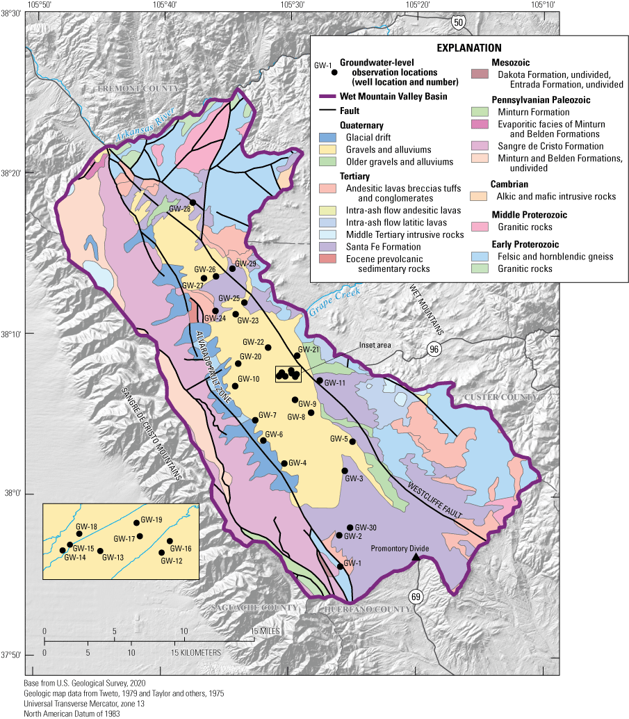
Map showing geology and well locations from the National Water Information System database (U.S. Geological Survey, 2021) of the Wet Mountain Valley alluvial aquifer, Custer and Fremont Counties, Colorado (Tweto, 1979; Taylor and others, 1975).
The Wet Mountain Valley contains thick alluvial and valley-fill deposits that are the principal sources of groundwater in the study area (Londquist and Livingston, 1978; Robson, 1985). The aquifer is composed of older alluvium from glacial deposits, younger post-glacial alluvium from stream deposits, and recent alluvial fans along the range front of the Sangre de Cristo Mountains (Londquist and Livingston, 1978). The Wet Mountain Valley alluvial aquifer is the primary source for domestic and household-use wells (Colorado Division of Water Resources, 2022), and, as the population increases, the groundwater use from the alluvial aquifer likely will increase to meet increasing demand. Groundwater wells are also completed in bedrock aquifers adjacent to the alluvial aquifer, and there may be hydrologic connections between the bedrock and alluvial aquifers. Newman and others (2021) completed aquifer testing in the alluvial aquifer and cataloged well pumping and drawdown data in the bedrock aquifers in order to estimate hydraulic properties. The analysis results indicated the ratio of well pumping rate to drawdown (quantified using the parameter specific capacity) was greater in alluvial wells than bedrock wells. The greater specific capacity in the alluvium than the bedrock may indicate the alluvial aquifer is likely to be more productive for water supply, consistent with previous investigations (Londquist and Livingston, 1978; Robson, 1985) and the distribution of wells in the valley.
Climate in the study area varies spatially but is generally semiarid. Climate data were extracted from the Climate Engine online tool (Huntington and others, 2017) for three locations in the study area—the Wet Mountains, Westcliffe, and the Sangre de Cristo Mountains. Mean annual precipitation for 1979 through 2019 at these three locations was, respectively, 24 inches (in.), 14 in., and 39 in., reflecting orographic precipitation effects. In each of the three locations, most of the annual precipitation accumulated in April and August (Huntington and others, 2017). Winter snowstorms also provide substantial snow accumulation. June had the least precipitation at all locations (Huntington and others, 2017). Evapotranspiration estimates for the three locations also exhibited spatial and temporal variability. Mean annual evapotranspiration for the Wet Mountains, Westcliffe, and the Sangre de Cristo Mountains was respectively 35, 49, and 48 in., with each location having maximum evapotranspiration in June (Huntington and others, 2017).
The primary streams draining the Wet Mountain Valley are Grape Creek and Texas Creek, which flow north and east across the valley toward their confluences with the Arkansas River north and east of the Wet Mountain Valley (fig. 1). In addition to Grape Creek and Texas Creek, many smaller streams drain the Sangre de Cristo Mountains. These streams may interact with groundwater within the bedrock or within the alluvium. Streamflow varies seasonally in the Wet Mountain Valley because of the effect of snowmelt. Streamflow is generally greatest in June as snow is melted in the surrounding mountain ranges. Streamflow then decreases throughout the remainder of the summer to reach a minimum during the months of October through January (Londquist and Livingston, 1978; Watts and others, 2014).
Land-cover and land-use data for the Wet Mountain Valley (Multi-Resolution Land Characteristics Consortium, 2021) indicate the primary land-cover classifications in the study area are evergreen forest, shrubland, herbaceous vegetation, hay and pasture, mixed forest, and emergent herbaceous wetland. Only a small part of the study area is classified as developed, with both medium- and low-density developments being present around Westcliffe. Agriculture and grazing on the hay and pastureland are primary economic drivers within the study area (U.S. Department of Agriculture, 2017a; 2017b). Both Custer and Fremont Counties experienced an increase in the number of farms (cropland and pastureland) and total area of cropland since 2012 (U.S. Department of Agriculture, 2017a; 2017b).
Populations in both Custer and Fremont Counties have increased steadily since the 1950s (fig. 3), and in 2020, the estimated populations were 4,755 and 47,801, respectively (Colorado Department of Local Affairs, 2020). Of the Custer County population, between 12 and 25 percent reside in adjacent Westcliffe and Silver Cliff (fig. 1). Of the Fremont County population, between 33 and 45 percent reside in Cañon City. Westcliffe and Cañon City (fig. 1) are the most populous cities in Custer and Fremont Counties, respectively, and the remainder of the population, in both counties, is primarily dispersed in rural areas.

Graph showing number of wells drilled per year in the Wet Mountain Valley (Colorado Division of Water Resources, 2019) and actual and estimated population for Custer and Fremont Counties, Colorado, 1940–2030 (Colorado Department of Local Affairs, 2020).
Data for groundwater well completions in the Wet Mountain Valley are available through the Colorado Decision Support System (CDSS; Colorado Division of Water Resources, 2019), and well completions through time indicate the greatest number of wells drilled per year occurred in 1994 and 2008 (fig. 3). Increases in well completions, however, do not coincide exactly with growing populations. Of the completed wells, 38 percent are less than 100 feet (ft) deep, 30 percent are 100 to 200 ft deep, 14 percent are 200 to 300 ft deep, and 18 percent are greater than 300 ft deep.
Study Methods
This section describes the integrated methods applied to conceptualize and quantify the hydrologic system in the Wet Mountain Valley alluvial aquifer, Custer and Fremont Counties, Colo. Although several previous investigations estimated the alluvium thickness (Zohdy and others, 1971) and provided initial groundwater budget estimates (Londquist and Livingston, 1978), no previous investigations incorporated groundwater and surface-water synoptic evaluations. Recent investigations in the Buena Vista-Salida area (fig. 1 this report; Watts and others, 2014) found connections between groundwater and surface water, which necessitates an integrated approach using multiple lines of evidence including physical and geochemical datasets to evaluate hydrologic conditions.
Monitoring locations for groundwater-level elevations, streamflow, and water quality were established throughout the study area to evaluate spatial and temporal variations. Monitoring data were collected between December 2017 and November 2019. All data collected as part of this study are available through the U.S. Geological Survey (USGS) National Water Information System (NWIS; USGS, 2021) database using USGS site numbers provided in tables 1 and 2.
Table 1.
Groundwater-level observation well site information in the Wet Mountain Valley, Colorado, locations shown in figures 2 and 4.[U.S. Geological Survey (USGS) site numbers are linked to the National Water Information System database (USGS, 2021). X, sites equipped with pressure transducers; A, sites where the full suite of water-quality data, including environmental tracers, were collected; O, sites where water-quality data with the exception of environmental tracers were collected; U, an unknown screen depth; -, not applicable]
Table 2.
Streamflow observation site information in the Wet Mountain Valley, locations shown in figure 5.[U.S. Geological Survey (USGS) site identifiers and site names are linked to the National Water Information System database (USGS, 2021). SW, surface water; CO, Colorado; nr, near; Tr, trail; A, sites where all water-quality constituents were collected; I, sites where samples of stable isotopes only were collected; Ln, lane; -, not applicable]
Groundwater Hydrology
Spatial and temporal evaluation of groundwater-level elevation data were useful for understanding the groundwater-flow directions and rates within the study area. The USGS has operated a network of groundwater-level wells in the Wet Mountain Valley since the 1970s, and 29 of these sites were selected for groundwater-level observations during this study (fig. 4 and table 1). One additional groundwater site in the study area was not measured during this study but had recent data from 2011 (GW-30) and was included in the analysis. Groundwater wells were screened within the upper 450 ft of the aquifer, and most were screened in the upper 200 ft (table 1). All sites had discrete groundwater-level depth measurements, which were then converted to groundwater-level elevations above the North American Vertical Datum of 1988 (NAVD88) using the groundwater-level depth below land surface and the well measuring-point elevation in NAVD88 as determined by extraction from the USGS 5-meter digital elevation model (USGS, 2020), assuming an approximate 2.7-ft accuracy. Groundwater-level depth below land surface was measured 15 to 21 times at the various wells from December 2017 to November 2019. Groundwater-level depth below land surface was measured using either an electric or a steel tape (Cunningham and Schalk, 2011).

Map showing groundwater-level observation wells from the National Water Information System database (USGS, 2021) and line of hydrologic cross section (A–A') illustrated in figure 6, in the Wet Mountain Valley, Colorado, 2017–19. Irrigated land from Multi-Resolution Land Characteristics Consortium (2021).
Nine wells were additionally equipped with pressure transducers to collect continuous groundwater-level data between March 2018 and November 2019 to evaluate short-term groundwater-level elevation fluctuations in locations dispersed throughout the study area. Pressure transducers were set to record groundwater-level depth below ground surface at 15-minute intervals, and during each site visit, the continuous data were manually downloaded for input to NWIS. The effect of pumping conditions was observed in some discrete and continuous datasets. When pumping or recent pumping was identified, the affected groundwater level(s) were flagged and were not used in subsequent statistical analysis. Both discrete and continuous groundwater-level elevation data were used to assess the groundwater distribution and flow directions within the study area.
In addition to spatial evaluation of groundwater-level data, statistical methods were used to evaluate trends in groundwater-level elevations through time. Such trend tests may indicate areas where groundwater recharge sources were changing or where groundwater storage is decreasing (Helsel and others, 2020). The Mann-Kendall trend test with the Theil-Sen slope estimator were used to evaluate temporal trends in each dataset, as these methods are robust and applicable to non-normally distributed datasets (Helsel and others, 2020). These tests were completed using the available groundwater wells dataset in the study area. Some wells in the study area have records extending back decades and use of these data strengthens the analysis by evaluating trends during long periods of time. Long-term records generally had fewer measurements per year, whereas records collected during this study have more frequent measurements. Measurements were filtered to only include data from the winter months, November–March, when pumping for agricultural uses were less likely to affect groundwater levels (Malenda and Penn, 2020). Data records flagged for pumping, recent pumping, or as dry wells were removed from the trend analysis. Trend tests were conducted using the R programming language (R Core Team, 2020) and methods described in Malenda and Penn (2020). The Mann-Kendall trend test null hypothesis was no monotonic relation between groundwater-level elevations through time, whereas the alternative hypothesis is a monotonic, but not necessarily linear, relation between groundwater-level elevations and through time. Where a p-value less than (<) 0.05 resulted from the test, the null hypothesis was rejected, and a statistically significant trend was indicated. The Theil-Sen slope estimator was used to quantify linear changes in groundwater-level elevations in feet per year (Helsel and others, 2020). In addition to the long-term Mann-Kendall test to evaluate groundwater-level elevation trends, a seasonal Mann-Kendall test was applied to continuous groundwater-level elevation data using the approach described by Malenda and Penn (2020).
Groundwater and Surface-Water Interactions
Evaluation of the interaction between groundwater and surface water is of primary interest to the regional water-resource analysis in the Wet Mountain Valley because streams can be a source of groundwater recharge or discharge depending on the relative stream-surface position to the local groundwater-level elevations. When groundwater-level elevations near the streambed are higher than the stream-surface elevation, groundwater may discharge into the stream and is a condition known as a gaining stream. Conversely, if the groundwater-level elevations are lower than the stream-surface elevation, stream water may infiltrate into the groundwater and is a condition known as a losing stream. Gaining streams are groundwater discharge locations, and losing streams are groundwater recharge locations (Winter and others, 1999). In headwaters areas of the Rocky Mountains, streams can exhibit variable spatial and transient patterns of groundwater and surface-water interaction (Paschke and others, 1995). Spatially, streams that originate in steep mountainous terrains can gain groundwater discharge in a downstream direction and then lose water to alluvial-valley groundwater systems where they exit the mountainous terrain and topographic gradients flatten (Paschke and others, 1995). On an annual cycle, streams may change from gaining to losing as spring snowmelt runoff recedes and the water table is lowered during fall base-flow conditions. Groundwater and surface-water interactions also can be affected by spatial variations in aquifer saturated thickness and hydraulic conductivity (Winter and others, 1999).
To evaluate if streams in the study area were gaining or losing, and where those interactions occur, synoptic streamflow measurements were collected at 33 stream sites (fig. 5 and table 2) on four separate occasions. Streamflow measurement sites were selected to represent the margin of the alluvial aquifer along the Sangre de Cristo Mountains where numerous perennial streams exit the mountains and enter the Wet Mountain Valley. Streamflow measurement locations in the center of the valley were selected based on existing USGS sites and where stream access was possible. Streamflow during low-flow conditions is expected to be unaffected by irrigation or diversions as these measurements occurred after the end of irrigation season (generally May through October). Streamflow was measured during low flow in the fall 2017, 2018, and 2019, and during high-flow conditions from snow melt in the summer 2018. Low-flow 2017 measurements were made between September 20 and October 7, high-flow 2018 measurements were made between June 18 and 29, low-flow 2018 measurements were made between October 1 and 12, and low-flow 2019 measurements were made between September 30 and October 17. Streamflow was measured using an acoustic Doppler velocimeter according to methods described in Rehmel (2007) and Turnipseed and Sauer (2010).

Map showing streamflow measurement locations from the National Water Information System database (USGS, 2021) and stream network grouping for streamflow gain or loss calculations in the Wet Mountain Valley, Custer and Fremont Counties, Colorado, 2017–19.
Streamflow measurement locations were evaluated using geographic information systems to create a network of connected reaches from the upslope locations in the mountains to the outlet of Grape Creek and Texas Creek in the Wet Mountain Valley (fig. 5). This network analysis allows streamflow gain or loss to be accounted for along the entire stream network and incorporates the irrigation diversions effect using the geospatial distribution of diversion locations obtained from the CDSS (Colorado Division of Water Resources, 2019). Using streamflow measured at upstream and downstream locations, net streamflow gain or loss from each reach was calculated according to equation 1 (modified from Simonds and Sinclair, 2002):
whereΔQ is the net streamflow gain or loss in cubic feet per second (ft3/s),
Qd is the downstream streamflow in ft3/s,
ΣQu is the sum of upstream streamflow locations in ft3/s,
Values of ΔQ less than zero indicate the stream reach is losing (a source of groundwater recharge), and values of ΔQ greater than zero indicate the stream reach is gaining (a point of groundwater discharge).
The net seepage gain or loss along each reach is subject to errors in streamflow measurement, which are accumulated (Rosenberry and LaBaugh, 2008). Total error for each net seepage calculation was calculated according to the error propagation formula in equation 2 (Harmel and others, 2006):
where andError in individual measurements was quantified using the interpolated variance estimator as described by Cohn and others (2013) and recorded by the acoustic doppler velocimeter. Discrete measurement errors from each location were used to calculate the total measurement error within a given group of paired upstream and downstream Streamflow measurement locations. The total error measured in ft3/s is compared to the calculated streamflow gain or loss to quantify the net error in percent of the gain or loss within the reach.
Upstream and downstream sites for calculation were identified based on the stream network from the National Hydrography Dataset (NHD; USGS, 2019). The stream network and streamflow measurement site distribution were such that some sites had only one upstream measurement, whereas other sites had multiple upstream measurement sites. These physiographic streamflow site groupings (fig. 5) allow for net streamflow gain or loss along a given reach to be quantified.
Diversion information was obtained from the CDSS (Colorado Division of Water Resources, 2019). Diversions were only applicable to the high-flow (June) 2018 measurements because records show diversions during September and October (the period of data collection for the low-flow measurements) make up less than 3 and 1 percent, respectively, of annual diversion quantities. Diversions were therefore not included in the calculations for the low-flow periods because the amount of water diverted is generally less than the streamflow measurement error. The most recent detailed monthly diversion data with spatially referenced diversion points were from 2015, prior to this study. As such, no spatially referenced diversion data were available for the study data-collection period of 2017–19. To estimate diversions during the study period, monthly data from 2015 were used to calculate mean daily diversions and were scaled according to total annual precipitation in the study area in 2015 compared to 2018 because differences in diversion availability were generally related to annual climate based on analysis of the available dataset. To set the precipitation scaling factor, the total annual precipitation in 2018 (a dry year) was divided by the total annual precipitation in 2015 (a more normal year). The scaled diversions were then estimated using the scaling factor and were used for net streamflow gain or loss calculation for the high-flow 2018 measurements. A 10 percent error was assumed for diversion data. Based on records from the CDSS (Colorado Division of Water Resources, 2019), all diversions were routed to agricultural fields and were not returned to streams; therefore, no diversion quantities were routed back to streams in the calculations. To provide relevant quantitative diversion information for understanding streamflow gain or loss high flow, 2018 calculations were also completed without diversions. Although this analysis contains uncertainty because of the precipitation scaling, the results assist in quantifying the diversions relevancy to groundwater and surface-water interactions. The total reported diversions in 2015 of approximately 33,000 acre-feet per year (acre-ft/yr) from the CDSS (Colorado Division of Water Resources, 2019) are also compared with the budgets of the numerical groundwater-flow model as described in the section “Groundwater-Flow Simulations” of this report.
Water-Quality Sample Collection and Analysis
Water-quality samples were collected from groundwater wells and streams to assist with conceptualization of the groundwater system (Glynn and Plummer, 2005). This section provides details on sample collection and analysis, quality control, and methods used to conduct evaluation.
Sample Collection and Analytical Methods
Groundwater samples were collected from domestic water supply wells screened in the upper 210 ft of the alluvial aquifer using equipment thoroughly cleaned between wells following standard USGS methods (USGS, variously dated). All samples were collected according to procedures described in the USGS National Field Manual for the Collection of Water-Quality Data (USGS, variously dated). Briefly, groundwater wells were pumped at a consistent rate until water temperature, specific conductance, pH, dissolved oxygen, and turbidity had stabilized to within ±0.2 degrees Celsius, ±3 percent, ±2 standard units (SU), ±0.3 milligrams per liter (mg/L), and ±0.5 turbidity units, respectively, or until three casing volumes were removed, whichever took longer. This ensured water being sampled was representative of groundwater within the aquifer. Stream samples were collected using grab sampling methods, and water temperature and specific conductance data were measured in the field.
Water-quality samples were analyzed for major elements (alkalinity, calcium, chloride, fluoride, magnesium, potassium, silica, sodium, and sulfate), trace elements (bromide, iron, manganese, selenium, and uranium), and stable isotopes of water. A subset of samples distributed spatially throughout the study area were additionally analyzed for environmental tracers (sulfur hexafluoride [SF6], tritium [3H], and noble gases [helium, neon, argon, krypton, and xenon]). Samples for major and trace elements analyses were collected in polyethylene bottles and filtered to 0.45 micrometers. Samples for cations analyses were preserved in the field with nitric acid and refrigerated, and samples for anions were unpreserved and refrigerated. Samples for stable isotopes of water were collected, unfiltered, in glass bottles. Samples of SF6 were collected, unfiltered, in duplicate, in glass bottles with no headspace by bottom filling after flushing with three volumes of sample water. Tritium samples were collected, unfiltered, in polyethylene bottles with no headspace by bottom filling after flushing with three volumes of sample water. Samples of noble gases (helium, neon, argon, krypton, xenon) were collected, unfiltered, in duplicate, in copper tubes (Aeschbach-Hertig and Solomon, 2013) and flushed of all air bubbles before being sealed under positive pressure.
Anions were analyzed by ion-exchange chromatography, and cations were analyzed by inductively coupled plasma-atomic emission spectrometry at the National Water Quality Laboratory, Lakewood, Colo. (Fishman and Friedman, 1989; Fishman, 1993). Trace elements were analyzed by inductively coupled plasma-optical emission spectrometry and inductively coupled plasma-mass spectrometry at the USGS National Water Quality Laboratory (Garbarino and others, 2005). Stable isotopes of water (ratio of hydrogen-2 to hydrogen-1 in a sample relative to a standard, δ2H; and ratio of oxygen-18 to oxygen-16 in a sample relative to a standard, δ18O) were analyzed by dual-inlet isotope-ratio mass spectrometry (Révész and Coplen, 2008a, 2008b) at the USGS Reston Stable Isotope Laboratory, Reston, Va., and are reported in standard stable-isotopic units of per mil (Kendall and others, 2015) with uncertainties of ±2 per mil and ±0.2 per mil, respectively. Concentrations of SF6 were analyzed using purge and trap gas chromatography followed by an electron capture detector according to the method of Busenberg and Plummer (2000) at the USGS Groundwater Dating Laboratory, Reston, Va., and results are reported in units of femtomoles per kilogram (fm/kg) with uncertainty ranging from 20 percent at the minimum reporting limit to 3 percent at the maximum reporting limit. Tritium analysis was conducted using distillation and electrolytic enrichment followed by liquid scintillation at the USGS Menlo Park Tritium Laboratory, Menlo Park, Calif., and results are reported in tritium units (TU) with analytical uncertainty ranging from 0.14 to 0.27 TU. Concentrations and isotopes of noble gases were analyzed using a magnetic-sector mass spectrometer and ultralow vacuum extraction line (Hunt, 2015) at the USGS Noble Gas Laboratory, Lakewood, Colo., and are reported in units of cubic centimeters at standard temperature and pressure per gram of water and as isotopic ratios, respectively, with analytical uncertainties of 1 percent (helium), 2 percent (neon), 2 percent (argon), 3 percent (krypton), and 3 percent (xenon).
Quality Assurance
Quality-control samples (field blanks and duplicates) were collected for major and trace elements to evaluate sampling and (or) analytical bias. Results of quality-control samples are summarized in table 3 and table 4.
Table 3.
Results of quality-control field blank samples.[Site identifiers are listed in table 1 and table 2. Sample date in month/day/year format. Mean environmental concentrations were calculated using environmental samples in groundwater and surface water for comparison with blank samples collected on the same day at groundwater and surface water sites, respectively. GW, groundwater; CaCO3 calcium carbonate; <, less than; SiO2, silicon dioxide; SW, surface water; — indicates quantity cannot be calculated where constituent was not reported in blank sample]
Table 4.
Results of quality-control field replicate samples.[Site identifiers are listed in table 1 and table 2. Sample date in month/day/year format. Relative percent difference calculated according to Mueller and others (2015). Positive relative percent difference indicates replicate results greater than environmental sample results. Negative relative percent difference indicates replicate results less than environmental sample results. GW, groundwater; CaCO3 calcium carbonate; <, less than; SiO2, silicon dioxide; SW, surface water]
Data quality was assessed by collection of field blank and replicate samples and using charge-balance calculations. Two blank and two replicate samples were collected, one each from groundwater wells and from surface water. The 2 replicate and 2 blank samples each represent 15 percent of the total 13 environmental samples collected. Results of blank samples are summarized in table 3, and results of replicate samples are summarized in table 4. Charge balance, which is the process of determining whether water contains an electrical charge, was assessed in all samples (Mueller and others, 2015). Evaluation of blank samples indicates four constituents (calcium, manganese, silica, and sulfate) were above the method reporting limit. Detections of calcium, manganese, and sulfate occurred at groundwater site GW-23 whereas the detection of silica occurred at surface-water site SW-8. The concentrations detected in the blanks may be compared to the mean environmental concentrations in the media of interest (groundwater or surface water) to evaluate possible bias in the results. For groundwater, the concentration in blanks was 0.16, 26, and 0.15 percent of the mean environmental concentration for calcium, manganese, and sulfate, respectively (table 3). Low concentrations in blanks compared to mean environmental concentrations indicates bias in environmental groundwater samples is negligible for calcium or sulfate, but possibly substantial for manganese. For surface-water samples, the silica concentration detected in the blank was 0.90 percent of the mean environmental surface-water concentration, indicating little potential bias (table 3).
Variability was evaluated using the relative percent difference (RPD), calculated according to equation 3 (Mueller and others, 2015):
Evaluation of replicate samples indicates all analytes had RPD values less than 10 percent, except for bromide, iron, and manganese. Manganese displayed an RPD of 14 percent in the replicate groundwater sample at site GW-3 whereas bromide and iron displayed RPDs of 27 and 13 percent, respectively at site SW-10 (table 4). Charge balance for all samples was within plus or minus 10 percent, indicating completeness of individual water-quality results. Altogether the results of the quality-assurance analysis indicate water-quality data for manganese in groundwater display both bias and variability, whereas water-quality data for bromide and iron in surface water display potential variability (Mueller and others, 2015). These conclusions affect the interpretation of groundwater manganese and surface-water bromide and iron data but indicate the remainder of the dataset adequately represents environmental conditions. One sample bottle, for well GW-28, was broken in transit to the laboratory, so no concentrations of calcium, iron, magnesium, manganese, potassium, or silica were reported for this well, and charge-balance calculations could not be completed.
Data Analysis
Major and trace elements were compared to drinking-water standards of the U.S. Environmental Protection Agency (2020a; 2020b) to provide context on possible groundwater use for drinking-water supplies and were used to evaluate geochemical processes occurring in groundwater and surface water. Environmental tracers were used to investigate travel times and conceptual models of groundwater flow and were examined using a variety of methods. First, noble gases were used to estimate groundwater recharge temperature and models of excess air (which conceptually indicate conditions during recharge) using software DGMETA (Jurgens and others, 2020) and according to the approach described by Aeschbach-Hertig and Solomon (2013). Second, measured 3H and SF6 concentrations were used to assign groundwater samples to modern (recharged within approximately the past 65 years), premodern (recharged before approximately the past 65 years), or mixed groundwater age categories according to the methodology described in Lindsey and others (2019) and Busenberg and Plummer (2000). Third, isotopes of noble gases were used to estimate tritiogenic helium-3 concentrations using DGMETA (Jurgens and others, 2020), which were subsequently used in combination with 3H concentrations to estimate groundwater age of the modern fraction of groundwater according to the tritium-helium method described by Suckow (2014). Fourth, noble gases were used to estimate terrigenic helium-4 concentrations, which were further used to estimate groundwater age of the premodern fraction of groundwater according to methods described by Kulongoski and others (2008). Finally, the results of all previously described environmental tracers were used in combination to evaluate mixed groundwater ages and physical models of groundwater flow using software TracerLPM (Jurgens and others, 2012). All environmental tracer analysis and modeling are available in Newman, 2024.
The combined use of environmental tracers allows for conceptualization of groundwater residence times, recharge sources, and mixing (Gardner and Heilweil, 2014; Manning, 2009; 2011). These approaches were helpful in further constraining processes that may be ambiguous using tools such as groundwater-flow models, which were calibrated to hydraulic heads and fluxes but may not be able to differentiate between processes such as mountain block recharge and streamflow loss recharge (Markovich and others, 2019). Environmental tracers were also ideal for indicating steady-state or transient-hydrologic conditions (Massoudieh, 2013), a pertinent consideration in semiarid regions such as the study area. These environmental tracer results provide a baseline for additional sampling and interpretation.
Development of Groundwater-Flow Models
A groundwater-flow model is a tool used to gain understanding of physical processes governing water availability in an aquifer and may be used to predict future conditions. Groundwater-flow models vary in complexity, from analytical models of single hydrologic features to numerical models that simulate multiple interacting processes through time. Groundwater-flow model development for the Wet Mountain Valley was done in a stepwise manner from a simplified two-dimensional, steady-state analytical model to a more complex three-dimensional, transient numerical MODFLOW-NWT (Niswonger and others, 2011) model of the alluvial aquifer consistent with recommendations for robust model development (National Groundwater Association, 2017).
Two-Dimensional Groundwater Model
The stepwise approach initially included creating a two-dimensional cross-sectional model of the Wet Mountain Valley from the median observed position of the water table and assumptions of hydraulic properties using the software TopoDrive (Hsieh, 2001), a two-dimensional steady state groundwater-flow model. TopoDrive is an analytical model that computes a distribution of hydraulic heads given hydraulic properties and orientations of the water table (Hsieh, 2001). A hydrologic cross section through the study area created using TopoDrive is shown in figure 6. This generalized model of the hydrologic system was created using the median of available observed groundwater-level elevations along the approximate cross-section line A–A' displayed in figure 4, the approximate alluvial aquifer depth (Zohdy and others, 1971), and hydraulic conductivity (K) estimates for the alluvial aquifer from Newman and others (2021). The resulting groundwater-flow paths approximation represents a steady-state condition, assumes isotropic conditions, and supports a generalized conceptual model of groundwater hydrology for the Wet Mountain Valley. Near the western boundary of the alluvial aquifer along the Sangre de Cristo Mountains, where the alluvial aquifer is thickest, groundwater gradients and flow were generally downwards indicating groundwater recharge (fig. 6). Lateral flow likely dominates in the central region of the valley. Finally, in the eastern part of the valley where the alluvial aquifer is thinnest, the groundwater gradients were upwards, consistent with gaining streams and shallow water-table conditions observed by Londquist and Livingston, (1978). Although this model is simplified, it provides a general understanding of the general groundwater- flow paths in the alluvial aquifer.

Simulated hydrologic cross section (location shown in fig. 4) with TopoDrive (Hsieh, 2001) through the Wet Mountain Valley, Custer and Fremont Counties, Colorado, from west (A) to east (A') showing different hydrogeologic units and depth (Zohdy and others, 1971).
Three-Dimensional Groundwater Model
Following simple conceptual model development using TopoDrive (Hsieh, 2001), a three-dimensional numerical groundwater-flow model was built using the code MODFLOW-NWT (Niswonger and others, 2011). The numerical groundwater-flow model was used to simulate three-dimensional steady-state and transient-groundwater flow and groundwater and surface-water interactions. Spatial discretization and simulated boundary conditions of the numerical groundwater-flow model are shown in figure 7, and the incorporation of hydrologic boundaries using MODFLOW-NWT (Niswonger and others, 2011) packages is described in the following paragraphs. Input files, output files, and model code for the numerical groundwater-flow model are provided in (Russell and Newman, 2025).
The active model domain was specified based on the study area geologic map in geographic information system format (Green, 1992) to include the Quaternary alluvium and the Tertiary Santa Fe Formation, consistent with preliminary investigations of the alluvial aquifer, which grouped the Santa Fe Formation with more recently deposited alluvial material (Londquist and Livingston, 1978). The model domain was discretized into 261 rows and 133 columns of square cells at 820 ft (250 meters [m]) on each side, for a total of 20,007 active cells. The model grid was rotated by 36 degrees to the northwest to align with the orientation of the valley and the assumed groundwater-flow directions to maximize flow orthogonal to cell faces (fig. 8). The model grid was projected and aligned relative to the Universal Transverse Mercator coordinate system (North American Datum of 1983, units: meters, zone: 13N). The model is discretized into two layers in the vertical direction. The first (upper) layer has a uniform thickness of 328 ft (100 m), and the thickness of the second layer ranges from 196 ft (60 m) to 328 ft (100 m), with most of the layer being 328 ft thick. The alluvial aquifer is substantially thicker than the maximum depth of 656 ft simulated in the model (Zohdy and others, 1971). However, the primary purpose of the model was to understand groundwater and surface-water interactions within the alluvial aquifer, which were likely minimally affected by deeper flow paths. Simulation of additional layers to a greater depth would add complexity to the model and increase model run times.
Temporally, the numerical groundwater-flow model was initially discretized into 241 stress periods. The first stress period simulates a mean steady-state period, and the subsequent 240 stress periods were transient and simulate each month from 2000 to 2019. For the initial (steady state) stress period of the numerical model, hydrologic stressors, and groundwater flow rates were assumed to be constant with the stress period representing mean annual data for the transient model stress periods. The outputs from the steady-state model stress period were used as inputs to the subsequent beginning transient stress period.
Water-budget components included in the model were recharge, interaction with streams (including groundwater recharge or discharge), groundwater pumping, evapotranspiration, and physical model boundaries. The Wet Mountain Valley numerical groundwater-flow model is made up of multiple hydrologic boundaries representing areas of inflow or outflow, and these hydrologic boundaries were simulated using MODFLOW-NWT (Niswonger and others, 2011) packages (fig. 7). The hydrologic boundaries simulated in the numerical model were separated into three different types, head-dependent, specified-flux, and no flow boundaries. No flow boundaries do not allow groundwater flow to cross, and these boundaries are used to represent the exterior of the model domain and the bottom of the model domain where groundwater flow is conceptualized to be inactive. Groundwater flow is allowed to occur between layers 1 and 2 of the model domain. Head-dependent boundaries compute flow into or out of the model based on differences between user-specified groundwater levels. Specified-flux boundaries allow flow into or out of model based on user-specified rates. Evapotranspiration, streams, and basal-flux out of the alluvial aquifer (conceptualized as exchanges between layers 1 and 2 of the model) were simulated using head-dependent boundaries, and recharge and well withdrawals were simulated in the model using specified-flux boundaries.
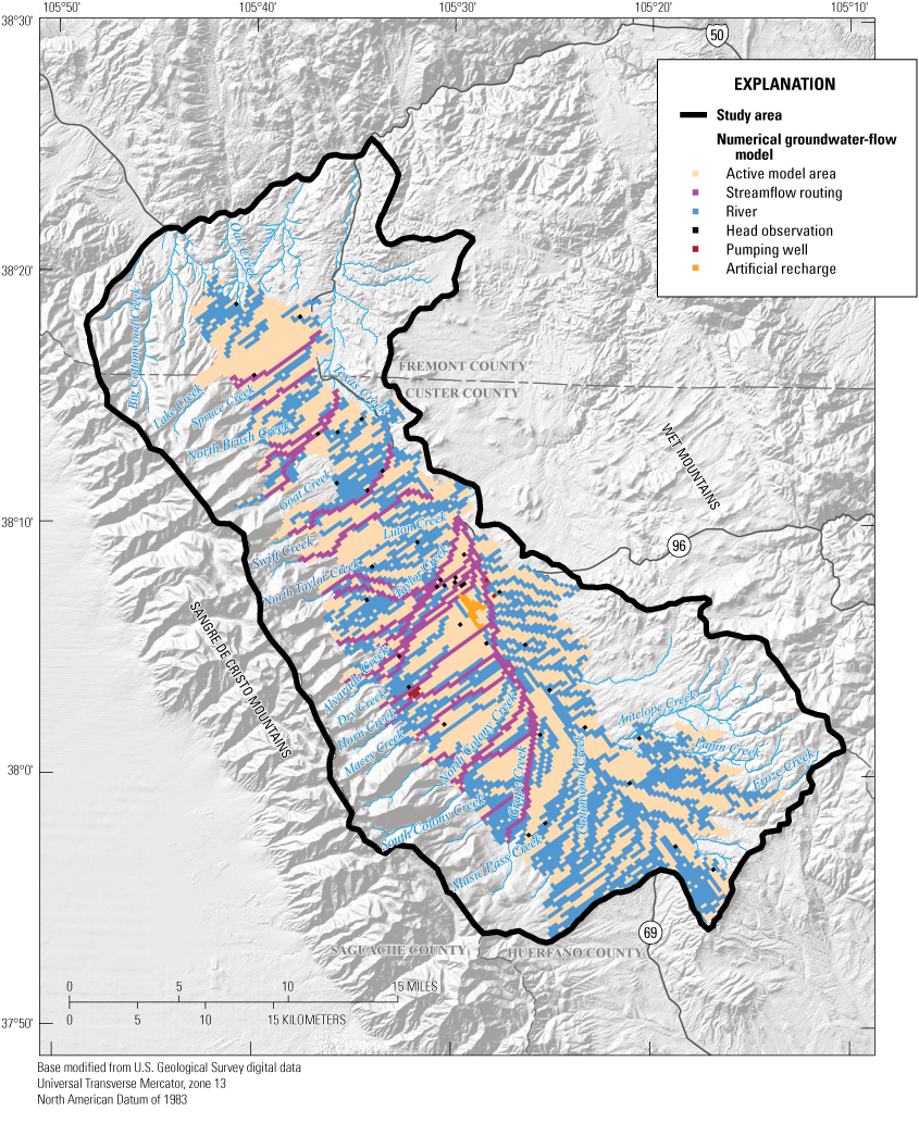
Map showing boundary conditions of the numerical groundwater-flow model for the Wet Mountain Valley alluvial aquifer, Custer and Fremont Counties, Colorado, 2000–19 (Russell and Newman, 2025).
Groundwater recharge and evapotranspiration were simulated using the recharge (RCH) and evapotranspiration (EVT) packages in MODFLOW (Harbaugh and others, 2000). The spatial and temporal variations of recharge and evapotranspiration applied to the simulated aquifers across the active model domain were calculated using the Soil-Water-Balance (SWB) computer code (Westenbroek and others, 2010). The SWB code is based on a modified Thornthwaite-Mather soil-water-balance approach using available gridded climate, soil, and hydrologic data to estimate the amount of recharge infiltrating the simulated aquifers and the amount of evapotranspiration occurring throughout the model domain. To estimate the amount of evapotranspiration occurring, the Hargreaves-Samani approach was used because this method does not require an advanced climate data network and is the most suitable approach for use with gridded precipitation data (Westenbroek and others, 2010). Observed daily precipitation data used in the SWB model were extracted from a single climate station located in Westcliffe, Colo. (site WCF01; Colorado State University, 2021). Land-cover data within the model area were derived from the National Land Cover Database (Multi-Resolution Land Characteristics Consortium, 2021) and were used to assign runoff curve numbers and plant root-zone depths (fig. 4). The plant root-zone depths used in the SWB code varied depending on plant type and soil textures, and for the Wet Mountain Valley area, the root zone depths ranged from 0.49 to 2.20 ft below land surface. Gridded soil properties, such as available water capacity and soil groups, were derived from the Soil Survey Geographic database (Natural Resources Conservation Service, 2020). Hydrologic data, such as runoff flow direction and runoff downslope routing, were calculated using depression filled USGS digital elevation models (USGS, 2020).
Outputs from SWB were used to calculate recharge in the RCH package by taking the difference between infiltration of precipitation and other water applied to the ground surface and potential evapotranspiration. In this manner, the RCH package accounts for the net infiltration recharge by incorporating much of the evapotranspiration. Additional possible evapotranspiration was accounted for in the EVT package by calculating the difference between actual evapotranspiration and potential evapotranspiration (both values extracted by SWB model). This additional evapotranspiration was included in the EVT package to ensure that evapotranspiration was not under-represented in the model. Both RCH and EVT were varied on a monthly basis.
The SWB code is a numerical model and was calibrated to the conceptual groundwater recharge values calculated using the water-table fluctuation method (Healy and Cook, 2002) and data from sites GW-7, GW-10, GW-11, and GW-26 (table 1). The water-table fluctuation method quantifies groundwater recharge based on observed temporal variation in groundwater-level elevation from a specific period corresponding to starting and ending dates of groundwater-level elevation oscillations and assumption of the aquifer specific yield (Sy). Applicable groundwater-level elevation data records were available for four periods at sites GW-7 and GW-26, two periods at site GW-10, and one period at site GW-11. There were no available Sy estimates for the study area, but well logs obtained from the CDSS (Colorado Division of Water Resources, 2019) indicate much of the alluvial aquifer is poorly sorted. Consistent with this type of material, an Sy ranging from 0.01 to 0.10 was used for calculations (Freeze and Cherry, 1979). Calculated aerial diffuse recharge rates based on the water-table fluctuation method for the study area ranged from 0.015 to 0.699 feet per year (ft/yr) using Sy=0.01 and from 0.15 to 6.9 ft/yr using Sy=0.10. Comparison of these calculated recharge rates to meteoric precipitation at each site extracted from the Parameter-elevation Regressions on Independent Slopes Model (Daly and others, 1994) indicates these recharge estimates range from 1 to 42 percent of annual precipitation using Sy=0.01 and 9 to 423 percent of annual precipitation using Sy=0.10. These results indicate the high range of Sy values were not physically possible, and thus, the lower range of diffuse recharge estimates were more reliable. The broad range in estimates is caused by the short length of some oscillatory groundwater-level elevation records (shorter records tended to have greater calculated recharge values). As such, the calculated median and the mean were better suited to the long-term analysis applied in the numerical groundwater-flow model. The mean groundwater recharge as a proportion of site-specific precipitation was 12 percent, whereas the median was 5 percent. Based on these results of the water-table fluctuation method, aerial diffuse groundwater recharge was applied throughout the active model domain at a constant rate of 0.215 ft/yr, which is between 7 and 18 percent of the mean annual precipitation ranges for the valley bottom and the Sangre de Cristo Mountains, respectively, as estimated from the Climate Engine online tool (Huntington and others, 2017).
To evaluate the groundwater and surface-water interactions that occur in the Wet Mountain Valley alluvial aquifer, streams were simulated using the MODFLOW Streamflow-Routing (SFR2) stream package (fig. 7; Niswonger and Prudic, 2005). This package simulates stream-aquifer interactions and allows for comparison between simulated and observed stream gain and loss. The SFR2 package computes exchanges between groundwater and discretized stream reaches based on streambed hydraulic properties, the stream reach dimensions, and the simulated groundwater-level elevations in the aquifer near the stream. To create stream reaches for the SFR2 package, all streams in the study area were extracted from the NHD (USGS, 2019). The stream network was then simplified to include only perennial streams included with synoptic streamflow measurements made during the study period. In this manner, the streamflow network simulated by the numerical groundwater-flow model is directly relatable to the streamflow gain or loss calculations during the study period, as described in detail in the “Groundwater and Surface-Water Interactions” section of this report. All SFR2 stream segments had a thickness of 1.00 ft (0.3048 m) and a Manning’s roughness coefficient of 0.025. Streambed conductance for each stream segment ranged from 0.98 feet per day (ft/d; 0.30 meters per day [m/d]) to 9.84 ft/d (3.0 m/d), values typical for incorporation of the SFR2 package in large-scale models (Anderson and others, 2015). A single simulated stream width of 10 ft (3.048 m) was used in the SFR2 package. Streambed elevations were modified using USGS 5-meter digital elevation model (USGS, 2020) values to allow for accurate simulated base flows. To provide a complete evaluation of the groundwater and surface-water interactions throughout the Wet Mountain Valley, the RIV package (Harbaugh and others, 2000) was used to account for ephemeral streams where streamflow was not measured. The RIV package simulates flow between the aquifer and surface-water features in the RIV package depending on stage of the surface-water feature, hydraulic conductance of the feature-aquifer interconnection, and the hydraulic head at the node in the cell underlying the surface-water feature. Because streams simulated with the RIV package (fig. 7) are typically shallow (less than 2 ft), a stage level of 1.0 ft above streambed was set for all simulated streams. This stage is generally consistent with stages observed during streamflow measurements (U.S. Geological Survey, 2021). There was spatial variation of the hydraulic conductance values in the streams simulated in the RIV package, and the values ranged from 706 ft/d (215.44 m/d) to 13,123 ft/d (4,000 m/d) based on typical values for large-scale models (Anderson and others, 2015).
Groundwater pumping from wells was simulated using the WEL package of MODFLOW (Harbaugh and others, 2000). Based on the CDSS (Colorado Division of Water Resources, 2019), there were two primary pumping wells located in the valley permitted for groundwater withdrawals and seven recreation and irrigation wells located along the western edge of the active model area (fig. 8A). Mean monthly withdrawal rates during the transient stress period 2000–19 were extracted from the CDSS database (Colorado Division of Water Resources, 2019). The well withdrawal rates provided by the CDSS database were simulated as hydrologic stressors on the alluvial aquifer. The mean simulated monthly well withdrawals (fig. 8B) show well withdrawals were greatest in June, July, and August.

Map showing the Wet Mountain Valley alluvial aquifer, Custer and Fremont Counties, Colorado, A, spatial distribution of simulated pumping; and a graph presenting B, monthly mean well withdrawals simulated, 2000–19 (Russell and Newman, 2025).
In some investigations, domestic well pumping is included in groundwater-flow models. For example, in a regional groundwater-flow model of the Denver Basin aquifer system, Paschke (2011) simulated household-use only wells having withdrawals of 0.3 acre-ft/yr. Household-only use wells were also assumed to have partial return flow to the aquifer; however, so the net pumping rate was 0.15 acre-ft/yr. Extraction of well logs from the CDSS database (Colorado Division of Water Resources, 2019) indicated 2,073 possible wells within the boundary of the Wet Mountain Valley alluvial aquifer. This dataset was further filtered to exclude well uses other than domestic or household-use only, resulting in 1,587 wells being classified as domestic or household-use only. However, of these well applications, many wells may never have been completed. The dataset was further filtered to those wells for which the permit has been issued, resulting in 171 domestic wells with issued permits. If these wells have the same net groundwater withdrawal of 0.15 acre-ft/yr, the total groundwater discharge from domestic and household-use only wells would be 25.7 acre-ft/year. This groundwater withdrawal is minor compared to other components of the groundwater budget. If all 1,587 wells (including unpermitted wells) pumped from the aquifer at 0.15 acre-ft/yr, then the total groundwater discharge from domestic and household-use only wells would be 238 acre-ft/year. Although this second potential estimate of groundwater withdrawals from domestic wells is larger than assuming only permitted wells, the distributed nature of domestic and household-use only wells would limit the effect of any single well. Pumping withdrawals from domestic and household-use only wells were excluded from the study to simplify the implementation of the numerical model. If additional concerns arise related to domestic well pumping, pumping from domestic and household only wells could be added to the numerical groundwater-flow model archived in Russell and Newman (2025).
Following initial model setup, the numerical model was calibrated by adjusting hydrologic parameter values to achieve better agreement between simulated and observed groundwater levels. Model calibration includes manual and computer-aided calibration steps. Manual calibration was performed by changing input parameter values until a user-specified and subjective reasonable fit was achieved for groundwater-level elevations. After manual calibration was completed, the computer-aided calibration step was done using the computer program PEST++IES (White and others, 2020) to complete the calibration process based on quantitative criteria. The parameter estimation code PEST++IES applies an iterative ensemble smoother algorithm to adjust model parameters and minimize a user-defined objective function describing discrepancies between the model simulations and observations (White and others, 2020). The computer program used in the computer-aided calibration step continuously changes user-specified parameters to minimize the differences between simulated and observed groundwater-level elevations and base flows. These user-specified parameters were set within a predetermined range that conceptually match the properties of the alluvial aquifer. Initial hydraulic property values were derived from aquifer testing described by Newman and others (2021), which was used to indicate spatial variability in K within the alluvial aquifer. Calibrated K values were then compared to the range of K and spatial patterns in K described by Newman and others (2021).
The computer-aided calibration process used input parameter and observation groups. Input parameters were split into 6 groups of 552 total parameters, and observations were split into 2 groups of 1,292 total observations. Of the 552 parameters, there were 241 parameters for recharge, 144 parameters for horizontal hydraulic conductivity (Kh), 144 parameters for the vertical to horizontal hydraulic conductivity ratio (Kv/h), 2 parameters for SFR2 streambed conductance, 14 parameters for evapotranspiration, 3 parameters for RIV streambed conductance, 2 parameters for specific storage, and 1 parameter each for Sy and SFR2 streambed thickness. The recharge parameters were multipliers applied to each recharge array for every stress period within the numerical model, and the range of the recharge multipliers was limited to only allow realistic recharge rates to the simulated groundwater system. The 144 parameters for Kh and Kv/h were evenly spaced points throughout the active model domain using a pilot points approach (Doherty, 2003), and the parameters can be divided into two groups of 72 parameters for Kh and Kv/h in each model layer. Initial K values were derived from Newman and others (2021), which provided information on Kh, whereas Kv values were assumed to be represented by downscaling Kh as is common in most layered aquifers because of increasing compaction with depth (Anderson and others, 2015). Most evapotranspiration parameters were multipliers (13 of 14) used similarly to recharge array multipliers, with 12 representing monthly evapotranspiration rates and the other multiplier representing the evapotranspiration rate for the steady-state stress period of the numerical model. The last evapotranspiration parameter adjusted the root-zone depth in the EVT package. All boundary conductance parameters were limited to conductance values consistent with the aquifer testing that was completed by Newman and others (2021).
Of the 1,292 observations used in the computer-aided calibration process, there were 1,052 groundwater-level elevation observations from 35 wells and 240 base-flow observations from 1 streamflow measurement location (Grape Creek near Westcliffe, CO, SW-10; USGS site identifier 07095000). All groundwater-level elevation data were retrieved from the USGS NWIS database (USGS, 2021). Base-flow observations from the streamflow measurement location Grape Creek near Westcliffe, CO, were obtained from the Colorado Department of Water Resources (Colorado Division of Water Resources, 2022) for the fall and winter months (October through March) when snowmelt runoff in the valley is generally at a minimum. This streamflow measurement site was operated by USGS until 1995 and is now (2024) operated by the Colorado Department of Water Resources. This streamflow measurement location is outside the active model area. Streamflow data from the Grape Creek streamflow measurement location were compared to seasonal trends in base flow at the model domain edge. However, because the Grape Creek streamflow measurement location is located outside of the model domain, streamflow data were not weighted as heavily as the groundwater-level elevation observations during the calibration process. In other words, during the computer-aided calibration process, parameters were adjusted to match the groundwater-level elevation observations more closely than the base-flow observations.
One goal of this study was to evaluate the potential for additional groundwater storage in the alluvial aquifer by the diversion of streamflow and subsequent artificial recharge during high streamflow periods, such as during snowmelt runoff. The diversion and streamflow storage process is known as managed aquifer recharge or aquifer storage and recovery (ASR; Dillon and others, 2019). Using streamflow diversions for ASR has the potential to change streamflow timing (Ronayne and others, 2017). The calibrated model was used to simulate ASR, as described in this report section, and to evaluate potential resulting changes to the budget of streams and base-flow timing for the Wet Mountain Valley.
Several spatial criteria were considered to determine the simulated ASR location in the model. First, it was assumed the points of diversion and recharge would be in proximity to one another so that diverted stream water would not be pumped substantial distances. This necessitated simulating the artificial recharge area at a location near a stream in the model and at a location with available groundwater storage capacity above the water table. The analysis also assumed surface infrastructure such as roads would be available, so streams near the base of the mountain front where road access is limited were not considered. These criteria resulted in the selection of a simulated artificial recharge area near Grape Creek in the central area of the model (fig. 7).
Streamflow records from Grape Creek were analyzed and used to determine the potential simulated artificial recharge volume. Daily discharge data for 2000 to 2021 from Grape Creek near Westcliffe (SW-10) (Colorado Division of Water Resources, 2022),were used to calculate the median and maximum monthly streamflows for 2000–2021 to determine the month with the greatest streamflow. These calculations indicate June has the greatest streamflow with a median value of 23.5 ft3/s. Next, the mean base flow simulated by the numerical model (17.66 ft3/s) was subtracted from the median June streamflow value, equaling 5.84 ft3/s. This value of 5.84 ft3/s was the amount assumed available for ASR because it is the amount that could be diverted from the stream without decreasing streamflow to below the base-flow value. During the ASR simulation, the streamflow within Grape Creek was not reduced because the water that could be diverted is conceptualized as snowmelt runoff, which is not directly simulated by the groundwater model. The artificial recharge simulation results from the computer program ZONEBUDGET (Harbaugh, 1990) were used to evaluate the difference in groundwater and surface-water dynamics between the two models (model without artificial recharge and with artificial recharge) through the entire model period. The additional recharge simulation was completed for the entire simulated period using the calibrated model and adding recharge using the RCH package that conceptually represents ASR operations. This analysis does not incorporate concerns related to water rights, the mechanism of artificial recharge, or other logistical aspects of ASR. Input files, output files, and model code for the numerical groundwater-flow model are provided in Russell and Newman (2025).
Groundwater Hydrology
Groundwater levels from 30 wells were used to evaluate groundwater flow directions and aquifer recharge. During the study period, 29 groundwater wells were monitored for groundwater-level elevations, and 1 additional well (GW-30) was included, which had sufficient long-term data from before the study period to be included in the analysis. Groundwater-level elevation data are available from the NWIS database (USGS, 2021) using the site numbers in table 1, and well locations are shown in figure 4.
The median values of measured groundwater-level elevations in each well throughout the study period were used to estimate the water-table elevation throughout the alluvial aquifer, displayed with a 100-ft contour interval (fig. 9). The estimated water-table elevation contours indicate much of the flow in the alluvial aquifer originates in the west, along the boundary of the alluvium with the Sangre de Cristo Mountains. Steep groundwater gradients are observed near the western mountain front where groundwater-level elevation contours are closely spaced indicating groundwater inflow from the Sangre de Cristo Mountains and tributary valleys. Near the center of the alluvial aquifer, potentiometric-surface contours were more widely spaced, indicating larger areas of similar groundwater-level elevations. The estimated potentiometric-surface map is similar to the conceptual cross-sectional hydrologic model illustrated in figure 6 with respect to the indicated gradients and directions of groundwater flow, indicating the simple and steady-state assumptions used in creating the TopoDrive (Hsieh, 2001) generalized hydrologic model were generally applicable to much of the study area.
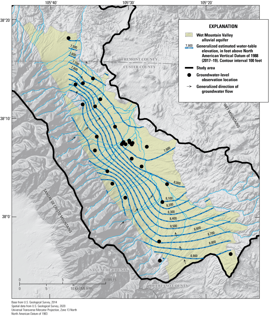
Map showing estimated water-table elevation based on median groundwater-level elevations collected for the Wet Mountain Valley alluvial aquifer, Custer and Fremont Counties, Colorado, 2017–19. Contours were graphically estimated and created using discrete data from groundwater-level elevation observation wells from the National Water Information System database (USGS, 2021).
Discrete groundwater-level elevations showed variations on seasonal and interannual timescales. Seasonal differences in groundwater-level elevations varied across the study area with most wells having annual or interannual groundwater-level elevation variation of 1 to 10 ft. In some wells, the groundwater-level elevation tended to be highest in the spring (GW-14 and GW-28), whereas others tended to be highest in summer (GW-6 and GW-27). Differences in seasonal groundwater-level elevation trends (fig. 10) were likely linked to groundwater recharge and discharge in the vicinity of the wells and affected by land use, geology, precipitation distribution, and proximity to streams. Wells with high groundwater-level elevations in the spring were likely affected by recharge from streamflow loss during the spring snowmelt period, whereas wells with high groundwater-level elevations in the summer were likely affected by irrigation losses contributing to groundwater recharge. In late summer and fall, wells in irrigated areas would tend to show decreasing groundwater-level elevations as evapotranspiration increases. Statistical evaluation of seasonal trends in continuous groundwater-level elevation data using the seasonal Mann-Kendall test (Helsel and others, 2020; Malenda and Penn, 2020) indicated there were no statistically significant seasonal trends at a p-value of 0.05. Although continuous records did not indicate statistically significant seasonal groundwater-level elevation trends, these datasets were useful in constraining groundwater recharge using the water-table fluctuation method and warrants consideration for other investigations in similar hydrogeologic settings.
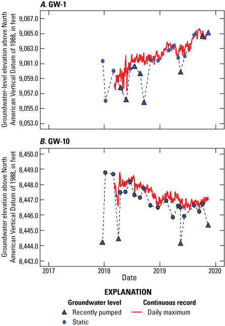
Hydrographs from 2017 to 2019 from the National Water Information System database (USGS, 2021) for two example observation wells in the Wet Mountain Valley alluvial aquifer, Custer and Fremont Counties, Colorado, with statistically significant groundwater-level elevation trends. A, GW-1 has a positive Theil-Sen slope, and B, GW-10 has a negative Theil-Sen slope.
Interannual variations in groundwater-level elevations were evident in many of the wells with records longer than 10 years. These wells generally showed groundwater-level elevation declines during regional droughts in 2012 and 2018 based on data from the Climate Engine online tool (Huntington and others, 2017), and this pattern is evident in the records for wells GW-14, GW-22, GW-23, GW-27, and GW-29. Effects of drought on groundwater-level elevations have been previously indicated in the upper Arkansas River Basin (Watts, 2005), and data from wells in the Wet Mountain Valley also indicate drought was correlated with decreasing groundwater-level elevations. Some wells showed recovery of groundwater-level elevations following the drought periods (U.S. Geological Survey, 2021).
Statistical evaluation of long-term trends in groundwater-level elevation using the Mann-Kendall test and Thiel-Sen slope estimator (Helsel and others, 2020) indicates 8 of the 30 wells with discrete groundwater-level data, display statistically significant trends at the p-value <0.05 level (table 5). Of the 30 wells, 3 do not have enough winter (November through March) groundwater-level elevation observations to complete the statistical evaluation. Of the eight wells with statistically significant trends, seven have negative Theil-Sen slopes, and one has a positive Theil-Sen slope (GW-1; fig. 10A). Examples of sites with statistically significant groundwater-level elevation trends and both negative and positive Theil-Sen slope estimates are illustrated in figure 10. Some wells in the analysis have different periods of available data, although the Mann-Kendall test and Theil-Sen slope estimator may be used in datasets such as these with differing record lengths (Helsel and other, 2020).
Table 5.
Results of Mann-Kendall trend tests for groundwater-level observation wells not including data that were affected by pumping, recent pumping, or dry wells as identified in National Water Information System database (USGS, 2021).[Discrete data were analyzed for November–March each year in the dataset. The Mann-Kendall trend test was used to evaluate the significance of a monotonic trend (Helsel and others, 2020), and the Theil-Sen slope estimator calculates the direction of the groundwater-level elevation change through time. Statistically significant trends were determined to exist where the Mann-Kendall trend test p-value was less than 0.05. n-winter, number of winter observations included in the analysis for a given well; p-value, probability value indicating level of significance; tau, rank correlation coefficient indicating strength of correlation between groundwater-level elevations and time; trend, direction and magnitude of groundwater-level elevation change through time; —, not calculated]
The spatial distribution of groundwater-level observation wells with statistically significant groundwater-level elevation trends is illustrated in figure 11. Wells with negative Theil-Sen trends were generally interspersed throughout the study area and were near wells having no statistically significant groundwater-level elevation trend. Also shown in figure 11 is the spatial density of all wells in the study area based on well-permits from the CDSS (Colorado Division of Water Resources, 2019). Comparing well density in wells per square mile with the spatial distribution of wells with statistically significant negative trends, Theil-Sen slopes indicate several wells with negative trends occur in areas of dense well completions. There were several wells with statistically significant negative groundwater-level elevation trends outside of areas with dense wells; however, there also were areas with high well density without statistically significant negative trends. This partial overlap of high well density with statistically significant negative groundwater-level elevation trends indicates other factors in addition to well density likely affect groundwater-level elevation trends. These other factors could include proximity to streams, climatic effects, or spatially variable hydraulic characteristics of the aquifer. A single well with a statistically significant positive Theil-Sen slope is just outside the mapped boundary of the alluvial aquifer (fig. 11). Based on the surficial geologic map (fig. 2), this well is located in an area classified as felsic gneiss, though based on well logs, it is completed in the Santa Fe Formation indicating that the regional scale geologic map may not accurately reflect the site-specific geologic boundaries in this location. This well has variable water-quality characteristics as discussed in the “Water-Quality” section of this report. Those variable water-quality characteristics combined with the difference in statistically significant groundwater-level elevation trend slope indicate the bedrock aquifer, or the margin of the bedrock aquifer, may be functioning separately from the alluvial aquifer.
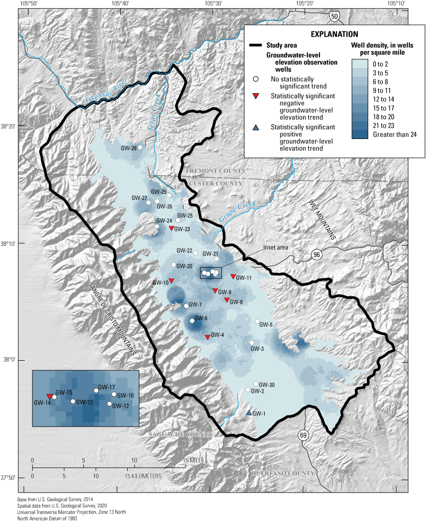
Map showing spatial distribution of groundwater-level observation wells from the National Water Information System database (USGS, 2021) with groundwater-level elevation trend-test results and interpolated well density in wells per square mile based on well permits from the Colorado Decision Support System for the Wet Mountain Valley alluvial aquifer, Custer and Fremont Counties, Colorado, 2017–19 (Colorado Division of Water Resources, 2019).
Groundwater and Surface-Water Interactions
Groundwater and surface-water interaction assessment relied on synoptic streamflow measurements at 33 locations throughout the Wet Mountain Valley (table 2; fig. 5). Synoptic streamflow measurements were collected during four time periods (low-flow 2017, 2018, and 2019 and high-flow 2018). Streamflow measurement data are available through the NWIS database (USGS, 2021) using the site numbers in table 2.
Calculations of streamflow gain or loss were completed for the high-flow period in 2018 and low-flow periods in 2017, 2018, and 2019 in nine identified stream reaches (fig. 5). Results of streamflow gain or loss calculations are summarized in table 6. Stream reaches in the analysis displayed variable spatial patterns with respect to transient streamflow gain or loss. Streamflow gain or loss calculations for the high-flow period of 2018, including estimated diversions, indicates each reach, with the exception of lower-middle Grape Creek (which has no diversions), was gaining flow from groundwater (table 6). This result is somewhat unexpected as it is common in mountain block-alluvial settings, such as the Wet Mountain Valley, for streams to lose flow to groundwater during the spring runoff period, a phenomenon termed surface mountain-front recharge (Markovich and others, 2019). When diversion data were excluded from streamflow gain or loss calculations for the high flow in 2018, almost all studied reaches indicated streamflow loss. The only gaining reach when diversions were excluded was lower Grape Creek below Westcliffe. The inconsistency in calculation results between datasets with or without diversions indicates data on diversions are key for understanding surface-water dynamics during the spring snowmelt runoff period. Because the diversion data were scaled from 2015 and were not directly collected during the current study period, and because the preceding winter experienced low snowfall (Natural Resources Conservation Service, 2020), these results are interpreted with some uncertainty. These results also highlight the value of collecting simultaneous data on diversions for any additional work in the Wet Mountain Valley. Despite the uncertainty associated with these calculations, transient groundwater and surface-water interactions during the high-flow period were not the central focus of the current investigation. Because the focus is characterizing base flow and the long-term hydrologic processes and budget components, streamflow gain or loss calculations from low-flow periods, discussed next, were more representative of base-flow conditions, because these components reflect the relations between groundwater and surface water without transient snowmelt-runoff effects.
Table 6.
Results of streamflow gain or loss calculations for the Wet Mountain Valley from 2017 through 2019. Data from the National Water Information System database (USGS, 2021).[Positive net streamflow gain or loss values indicate gaining conditions from groundwater. Negative net streamflow gain or loss calculations indicate losing conditions to groundwater. Low-flow 2017 measurements were made between September 20 and October 7. High-flow 2018 measurements were made between June 18 and June 29. Low-flow 2018 measurements were made between October 1 and October 12, and low-flow 2019 measurements were made between September 30 and October 17. USGS, U.S. Geological Survey; —, no calculations completed because streamflow measurement locations were dry; CO, Colorado; SW, surface water; Tr, trail; nr, near; Ln, lane]
Streamflow gain or loss calculations for the low-flow periods of 2017, 2018, and 2019 were more consistent than calculations for the high-flow period of 2018 (table 6). Several stream reaches displayed consistent streamflow loss in each period (upper Texas Creek, upper Grape Creek, upper-middle Grape Creek, and Taylor Creek). These stream reaches represent long-term sources of recharge to the alluvial aquifer. Other stream reaches displayed time-variant patterns in low-flow streamflow gain or loss (lower Texas Creek, lower-middle Grape Creek, lower Grape Creek below Westcliffe, and lower Grape Creek above DeWeese Reservoir). Only one area displayed streamflow gains in every period of the analysis, middle Texas Creek. This reach is near the center of the alluvial aquifer (fig. 5) where groundwater would be expected to be discharging to surface water based on the conceptual model of the study area (fig. 6). The primary difference between streams displaying consistent losing reaches and stream reaches with temporally variant patterns is their spatial association with the range front of the Sangre de Cristo Mountains (the transition from bedrock to valley-fill alluvium). Stream reaches showing consistent streamflow loss (upper Texas Creek, upper Grape Creek, upper-middle Grape Creek, and Taylor Creek) were all located relatively close to the mountain front, whereas stream reaches that display more transient patterns (lower Texas Creek, lower-middle Grape Creek, lower Grape Creek below Westcliffe, and lower Grape Creek above DeWeese Reservoir) were all located more centrally in the valley-fill alluvium and farther from the Sangre de Cristo mountain front (fig. 5). The temporally variant patterns in these latter stream reaches during low-flow periods indicate reaches may be sources of groundwater recharge or areas of groundwater discharge, likely depending on local dynamics between the elevation of the water table and the streamflow varying through time.
In some instances, there were substantial accumulated errors in the streamflow gain or loss calculations. Examples include lower Texas Creek in low flow 2017 and low-flow 2019, lower-middle Grape Creek during nearly all periods, and lower Grape Creek above DeWeese Reservoir during low-flow 2018 (table 6). Large errors were generally the result of streamflow measurement sections deviating from ideal conditions because of variable streambeds, high angles between streamflow measurement, and primary downstream velocity (when the measurement cross section was not setup perpendicular to the primary direction of streamflow), and the presence of eddies in the stream (Turnipseed and Sauer, 2010). Although some errors were large, there were only two instances where the errors are substantial enough to change the direction of the calculated streamflow gain or loss. These errors were in lower-middle Grape Creek during high-flow 2018 (table 6). Therefore, although some other errors were substantial, they do not indicate uncertainty as to the direction of exchange between streams and groundwater.
In summary, low-flow streamflow measurements made during this study appear to consistently represent the long-term patterns of groundwater and surface-water interactions in the study area. These low-flow measurements were not affected by the potential for surface-water diversions, which complicated the analysis of streamflow gain or loss during 2018 high-flow conditions. In general, the results indicate streams exiting the Sangre de Cristo Mountains were sources of groundwater recharge, whereas streams in the center of the valley and the alluvial aquifer were locations of groundwater discharge. These streamflow gain or loss relations assist with conceptualizing the groundwater-flow model, as described further in the “Groundwater-Flow Simulations” section of this report.
Water Quality
Water-quality samples were collected from 10 groundwater wells and 10 streams during September through November 2019. All groundwater samples were analyzed for major and trace elements and stable isotopes of water. A subset of groundwater samples was also analyzed for the environmental tracers, SF6, 3H, and noble gases. All stream samples were analyzed for stable isotopes of water, and a subset were analyzed for major and trace elements. All water-quality constituent results are available in the NWIS database (USGS, 2021) using the site numbers in tables 1 and 2. Water-quality sampling results are summarized in table 7.
Table 7.
Water-quality sampling results for groundwater and surface water within the Wet Mountain Valley alluvial aquifer, 2019 from the National Water Information System database (USGS, 2021).[Site common names and identifiers are listed in tables 1 and 2. —, result not available for specific water-quality parameter at given site; <, result less than laboratory reporting limit; CaCO3, calcium carbonate; SiO2, silicon dioxide]
Major-Ion and Trace Element Chemistry
Comparison of water-quality results to U.S. Environmental Protection Agency drinking water-quality standards (U.S. Environmental Protection Agency, 2020a; 2020b) indicates no constituents exceeded primary standards based on human health. Manganese and iron exceeded secondary standards based on aesthetic considerations in several locations: in GW-1, GW-4, GW-11, and SW-10 for manganese and in GW-1 for iron. Exceedances of secondary water-quality standards do not pose a risk to human health. These results were similar to those of Londquist and Livingston (1978), which indicated some areas of elevated concentrations of manganese and iron.
A Piper diagram (Piper, 1944) of water-quality results shown in figure 12 illustrates groundwater and surface water have similar major-ion compositions, with all water sampled being calcium-bicarbonate type water. Surface water generally had greater total dissolved solids concentrations than groundwater, as indicated by the relative size of the symbol in figure 12. The calcium-bicarbonate water type is likely derived from the dissolution of carbonaceous minerals in the adjacent mountain blocks and alluvial aquifer. The pH of sampled water also reflects interaction with carbonaceous minerals, as pH ranged from 6.9 to 7.7 in groundwater and 8.1 to 8.7 in surface water (table 7). The major-ion composition of samples collected in this study is consistent with results presented in Londquist and Livingston (1978).

Piper diagram (Piper, 1944) showing major-ion chemistry of groundwater and surface water collected during sampling of the Wet Mountain Valley alluvial aquifer, Custer and Fremont Counties, Colorado, 2019 from the National Water Information System database (USGS, 2021). Relative symbol sizes are scaled to the total dissolved solids concentration of the samples, with larger symbols indicating greater total dissolved solids.
Spatial evaluation of water-quality results illustrated in figure 13 indicates the concentrations of select constituents can be used to evaluate groundwater and surface-water interactions. Specifically, concentrations of chloride were generally greater in groundwater wells than in streams (fig. 13A). The greatest chloride concentration occurs in Grape Creek near Westcliffe (site SW-10), where Grape Creek was shown to be gaining flow from groundwater by streamflow gain or loss calculations during low-flow 2018 and low-flow 2019 (table 6). Bromide shows a similar pattern (not shown in figures; USGS, 2021). Site SW-10 is downstream from the Round Mountain Water and Sanitation District wastewater treatment plant (U.S. Environmental Protection Agency, 2022), and solute concentrations at this location may be affected by wastewater discharge or leakage to surface water or groundwater. Manganese concentrations appear to be affected by other geochemical processes, likely oxidation-reduction reactions in the shallow subsurface (Appelo and Postma, 2005). Sites SW-10 and GW-1 have substantially greater manganese concentrations (24.6 and 26.7 micrograms per liter, respectively) than any other locations (fig. 13B), and these relative concentrations of manganese mimic relative iron concentrations throughout the study area (table 7). High concentrations of iron and manganese generally represent reducing conditions in the environment (Appelo and Postma, 2005). The high manganese concentration occurrence in site SW-10 were likely because of locally reducing conditions in the streambed, where groundwater with low oxygen content discharges to the stream. These manganese geochemistry interpretations are viewed with some caution; however, as manganese showed some propensity for high bias in quality-assurance samples. Lastly, uranium concentrations in figure 13C show a distinctive pattern of greater concentrations in the eastern half of the study area and in surface water gained from groundwater at site SW-10. The eastern part of the study area is underlain by Tertiary intrusive igneous rocks (fig. 2) associated with ore deposits (Cappa, 1998). The occurrence of uranium in the groundwater may indicate groundwater is flowing through the underlying igneous rocks where it could be acquiring some trace elements. This potential uranium source is also supported by noble-gas data, which is discussed in the “Noble Gases and Environmental Tracers” section of this report. All uranium concentrations were less than the U.S. Environmental Protection Agency maximum contaminant level of 30 micrograms per liter for drinking water (U.S. Environmental Protection Agency, 2020a).
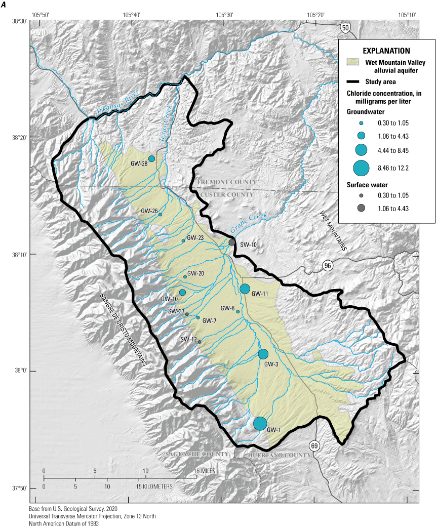

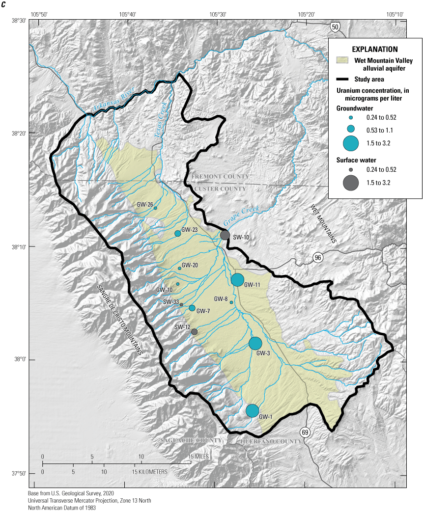
Maps showing sampled groundwater wells and stream sites with concentrations for the Wet Mountain Valley alluvial aquifer, Custer and Fremont Counties, Colorado, 2019, from the National Water Information System database (USGS, 2021), for A, chloride; B, manganese; and C, uranium.
Stable Isotopes of Water
Stable isotopes of water are plotted in figure 14 and indicate both groundwater and surface water were sourced from snowmelt given the clustering of data points near the Rocky Mountain Meteoric Water Line derived from Anderson and others (2016). However, the linear best-fit regressions to the datasets have slopes less than either the Rocky Mountain Meteoric Water Line of Anderson and others (2016) or the Global Meteoric Water Line of Craig (1961), indicating evaporation has occurred. The groundwater linear best-fit line shows a lesser slope than the surface-water line indicating greater evaporation (Kendall and others, 2015). The lesser slope of the groundwater line is generally driven by the isotopic composition of the sample from site GW-1. This site is located just outside of the boundary of the alluvial aquifer (fig. 4) and likely receives groundwater recharge from partially evaporated stream loss.
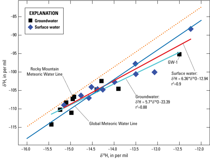
Graph showing stable isotopes of water (deuterium, δ2H; and oxygen-18, δ18O) in groundwater and surface water of the Wet Mountain Valley, Custer and Fremont Counties, Colorado, collected in 2019 (USGS, 2021), with best-fit linear regression lines, the Rocky Mountain meteoric water line of Anderson and others (2016) and the global meteoric water line of Craig (1961).
Using the approach of Jasechko and others (2014), the seasonality of groundwater recharge was assessed from the stable isotope data. This approach uses the isotopic composition of groundwater and precipitation throughout the year. Recharge is assigned as either winter or summer dominated based on the comparison of each sample to the volume-weighted precipitation composition. Isotopes in precipitation data were extracted from the Online Isotopes in Precipitation Calculator (Bowen, 2020), which uses the approach described in Bowen and Revenaugh (2003). Results of these calculations are presented in table 8. Values represent the winter recharge to summer recharge ratio, with a value of 1 indicating recharge is equally distributed between summer and winter, values less than 1 indicating recharge is biased towards summer months, and values greater than 1 indicating recharge is biased towards winter months (Jasechko and others, 2014). Calculation results indicate winter recharge dominates throughout the study area. Sites GW-7 and GW-26 indicate equally distributed summer and winter recharge, and site GW-1 result indicates substantial summer recharge. Site GW-1 was noted previously as having an evaporated isotopic composition likely affected by streamflow loss during summer months (fig. 14).
Table 8.
Results of groundwater recharge seasonality calculations using stable isotopes of water according to the method of Jasechko and others (2014). Site common names for groundwater wells are listed in table 1.[δ2H, stable isotopic composition of hydrogen]
Noble Gases and Environmental Tracers
Noble gases and environmental tracers may be used to investigate characteristics of groundwater recharge (temperature and excess air), groundwater-residence time (the time since the water recharged), and groundwater flow and mixing conceptual models (Aeschbach-Hertig and Solomon 2013; Gardner and Heilweil, 2014; Kulongoski and Hilton, 2012; Manning, 2009). Environmental tracer sampling results from six wells dispersed throughout the aquifer are presented. First, estimated groundwater-recharge temperatures are assessed. Second, apparent ages of the modern component of groundwater recharge are assessed using 3H and SF6. Third, noble gases and noble-gas isotopes were used to indicate the mixing of modern and premodern groundwater and to provide initial estimates of the age of the premodern fraction. Finally, all results were combined in a framework using software TracerLPM (Jurgens and others, 2012) to quantitatively investigate mixing and physical models of groundwater flow. All results are summarized in table 9 and available in Newman (2024).
Modeling of noble gases indicates the groundwater-recharge temperature for most wells is approximately 1 to 6 degrees Celsius colder than the observed groundwater temperature during sampling (table 9), and approximately 1 to 4 degrees Celsius warmer than the median air temperature of 6 degrees Celsius as measured at the Colorado State University weather station at Westcliffe for 2011 through 2020 (site WCF01; Colorado State University, 2021). Noble gas groundwater recharge temperatures are commonly used to evaluate the presence of mountain-block recharge (subsurface inflow to alluvial aquifers from consolidated bedrock aquifers), which is different from mountain-front recharge derived from streamflow loss at the mountain front (Markovich and others, 2019). There were relatively few data points by which to quantitatively evaluate the presence of mountain-block compared to mountain-front recharge in the study area because of the lack of groundwater wells completed in the mountain block, which would provide in-situ mountain groundwater temperatures and could be used to create elevation-temperature relations by which to rigorously assess mountain-block recharge (for example, Manning, 2009, 2011).
Table 9.
Environmental tracer concentrations and model results for samples collected from a subset of observation wells in the Wet Mountain Valley, Colorado, 2019. Environmental tracer modeling results are from Newman (2024).[Groundwater recharge temperatures were calculated using software DGMETA (Jurgens and others, 2020). Tritium-based age categories calculated per Lindsey and others (2019). Tritium-helium-3 ages calculated per Suckow (2014). Apparent helium-4 ages of premodern groundwater fraction calculated per Kulongoski and others (2008) when terrigenic helium-4 concentrations were greater than 1x10⁻⁹ cubic centimeters per gram of water at standard temperature and pressure. Sulfur hexafluoride piston-flow ages calculated per Busenberg and Plummer (2000). Best-fit lumped parameter models, ages of modern components in mixtures, and best-fit fractions on modern components were all calculated using TracerLPM (Jurgens and others, 2012). Best-fit mixtures between modern and premodern groundwater were only calculated where apparent helium-4 ages were calculated and where graphical analysis indicated the sample was fit by a binary mixing model. R/Ra, ratio of helium-3 (3He) to helium-4 (4He) in groundwater samples (R) compared to helium-3 (3He) to helium-4 (4He) in the atmosphere (Ra) MF, model failure for sample; —, not applicable for sample]
The groundwater-recharge temperature distribution in the alluvial aquifer (5.7–10.6 degrees Celsius) indicates recharge could be derived from mountain-block recharge, mountain-front recharge (streamflow loss), or irrigation losses (table 9). As summarized in table 6, streamflow loss contributes to groundwater recharge in the study area. Measured mountain stream temperatures during discrete streamflow measurements ranged from approximately 1 to 8 degrees Celsius (USGS, 2021) similar to the calculated groundwater-recharge temperatures for sites GW-1, GW-7, GW-8, and GW-23 (table 9). Each of these wells were located near stream channels and could be recharged by streamflow losses (fig. 4). Sites GW-1 and GW-7 were also located near the alluvial aquifer boundary, and groundwater recharge temperatures could be attributed to either mountain-front recharge (streamflow loss) or from mountain-block recharge (subsurface groundwater flow from the mountain block to the alluvial aquifer) in these locations. A more complete characterization of the interconnected bedrock-alluvial system warrants consideration for additional investigations in the study area, as the mountain-block recharge quantity is one of the primary unknowns relating to long-term groundwater budgets (Markovich and others, 2019). Groundwater-recharge temperatures in GW-11 and GW-28 were approximately 4 degrees Celsius warmer than the median annual air temperature and indicate recharge from irrigation losses, as irrigation losses tend to occur during warmer months (Thoma and others, 2011). These wells were located near irrigated fields (fig. 4) and help clarify irrigation losses were a potentially important water-budget component for the alluvial aquifer.
Calculated apparent groundwater ages using the tritium-helium method (Solomon and Cook, 2000) and the SF6 piston-flow method (Busenberg and Plummer, 2000) are summarized in table 9, as are tritium-based age categories (Lindsey and others, 2019). All sampled groundwater wells had detectable 3H, although 3H concentrations in wells GW-1 and GW-28 were only slightly greater than the method reporting limit. The presence of 3H in all wells indicates all sampled groundwater consists of at least some modern water (has been partially recharged since the 1960s; Lindsey and others, 2019). The apparent tritium-helium-3 ages for the samples range from about 25 to 64 years (table 9). Sulfur hexafluoride concentrations were greater than that explainable by atmospheric equilibrium in five of the six wells (model failure indicated in table 9), likely because of SF6 derived from the aquifer material (Friedrich and others, 2013). Well GW-28 was the only well with a SF6 concentration consistent with groundwater-age dating (Busenberg and Plummer, 2000) and had a calculated piston-flow age of 38 years (table 9). This piston-flow age represents only the modern fraction of groundwater in the well. Tritium-based age categories summarized in table 9 and calculated using the approach of Lindsey and others (2019) indicate samples from four groundwater wells were modern, and two were mixtures of modern and premodern water. Despite the tritium-helium ages and tritium-based age categories indicating all groundwater have been partially recharged within the past 70 years, the presence of modern groundwater containing 3H or SF6 may create a modern bias in the overall interpreted age of the groundwater (McCallum and others, 2015; Suckow, 2014). The method of Lindsey and others (2019) does not account for this possible mixing if the observed 3H is more than the cutoff value of 0.5 tritium units selected to represent modern water in the study area. Because of this possible modern bias, it is crucial to also evaluate possible mixing of older groundwater in each sample. Using noble-gas modeling results, the apparent age of the groundwater premodern fraction was calculated using terrigenic helium-4 concentrations according to the terrigenic-helium accumulation method described in Kulongoski and others (2008). These premodern groundwater-component ages were included in TracerLPM modeling, where tracer data visual inspection was used to determine the most applicable lumped parameter model (table 9). Error minimization functionality in TracerLPM (Jurgens and others, 2012) was then used to calculate mixing fractions of modern and premodern components. Noble gases and TracerLPM modeling are described in the following paragraphs.
Ratios of helium-3 (3He) to helium-4 (4He) in groundwater samples (R) compared to 3He to 4He in the atmosphere (Ra) ranged from 0.11 to 4.56 (table 9). Values of R/Ra greater than one indicate addition of 3He either from 3H decay or from the mantle, which is enriched in 3He (Kulongoski and Hilton, 2012). The presence of excess 4He, which causes R/Ra values of less than 1, may indicate long residence times in the crust and addition of He derived from uranium-thorium decay (Gardner and Heilweil, 2014; Manning, 2009; Solomon, 2000). In addition to the R/Ra values, comparison of R/Ra with ratios of 4He to neon-20 (20Ne) (fig. 15A) were useful for qualitatively evaluating groundwater-residence times and sources of noble gases, because this comparison separates helium components (between tritiogenic with R/Ra values greater than 1 and crustal with R/Ra values less than 1) and allows comparison to a gas derived primarily from the atmosphere (20Ne). Values of R/Ra and 4He/20Ne in the Wet Mountain Valley indicate groundwater likely has a wide range of residence times and mixing relations. Several groundwater samples have R/Ra values greater than one, specifically wells GW-7 (R/Ra = 1.74) and GW-8 (R/Ra = 4.56) (fig. 15). These high R/Ra values could be the result of mantle helium input or of 3H decay to tritiogenic helium-3 (3Hetrit; Kulongoski and Hilton, 2012). Given all groundwater samples have detectable 3H (table 9) and based on calculated 3Hetrit concentrations, it is likely the excess 3He in these groundwater samples is from 3H decay, and not a mantle helium signature. Addition of helium from terrigenic sources is evident, however, for wells GW-11, GW-23, and GW-28 based on terrigenic 4He concentrations several orders of magnitude greater than the background crustal value of approximately 2 x 10⁻⁸ cubic centimeters per gram of water at standard temperature and pressure, as summarized in table 9 and illustrated in figure 15. Wells GW-11 and GW-28 were aligned with major faults in the valley (fig. 15B), and the faults may be conduits for mixing of older deeply sourced groundwater with modern recharge. Both Gardner and Heilweil (2014) and Manning (2009) used noble-gas modeling in similar manners to indicate groundwater evolution in fault-block valleys. Noble-gas model inputs and results are available in Newman (2024).


A, Graph showing ratios of helium-3 (3He) to helium-4 (4He) in groundwater samples (R) compared to 3He to 4He in the atmosphere (Ra) compared to the ratio of 4He to neon-20 (20Ne). Air-saturated water saturated water with a composition were calculated according to methods described in Kipfer and others (2002), and B, map showing R/Ra values for a subset of observation wells sampled in 2019 for environmental tracers and faults in Wet Mountain Valley, Custer and Fremont Counties, Colorado. Site numbers are listed in table 1.
Results of TracerLPM modeling are summarized in table 9 and illustrated in figure 16, which includes results from samples as well as idealized lumped parameter models. The piston-flow model generally represents groundwater flow in a simple aquifer system or near the recharge zone in a more complex system. The exponential piston-flow model may represent spatial changes in recharge or confining conditions, and the dispersion model can be used to represent many aquifer geometries when flow paths may be longer or when multiple flow paths converge (Jurgens and others, 2012). Binary mixtures of the piston flow and dispersion models is also shown. Environmental tracer modeling results are from Newman (2024).
Plots of tritiogenic helium-3 (3Hetrit) compared to 3H in figure 16A conceptualize the physical flow system governing the modern groundwater component, and 4He compared to 3H in figure 16B conceptualizes potential mixing between premodern and modern groundwater. Based on 3Hetrit compared to 3H (fig. 16A), either the piston-flow or exponential piston-flow models provide the best fit to groundwater from wells GW-8, GW-23, and GW-28 fit whereas groundwater from well GW-7 is best represented by the dispersion model. Groundwater from GW-1 and GW-11 are not well represented by any models based on 3Hetrit compared to 3H alone, and GW-11 does not plot in the field of view illustrated in figure 16A. When considering 4He compared to 3H (fig. 16B), groundwater from well GW-1 plots near the dispersion model, groundwater from wells GW-7, GW-8, GW-11, and GW-23 plot near a binary mixture between the piston-flow model and dispersion model, and groundwater from well GW-28 is not represented by any of the considered models and has greater 4He concentrations than those explained by the models. Although GW-8 plots near the binary mixing line, it has terrigenic helium-4 (4Heterr) concentrations too low to indicate substantially premodern groundwater. Considering multiple tracers, such as illustrated in figure 16A, B, assists in evaluating potential mixtures and nonuniqueness associated with lumped-parameter modeling (Suckow, 2014).
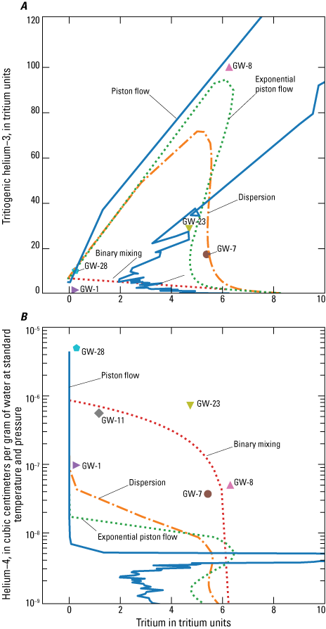
Graphs showing TracerLPM (Jurgens and others, 2012) modeling for groundwater collected from a subset of observation wells in the Wet Mountain Valley, Custer and Fremont Counties, Colorado, 2019, for A, tritiogenic helium-3 compared to tritium and B, helium-4 compared to tritium. Lines correspond to the composition of a groundwater sample for the given idealized lumped-parameter model with a range of residence times and data points corresponding to compositions of sampled groundwater. Site numbers are given in table 1. Environmental tracer modeling results are from Newman (2024).
The modern groundwater component from several wells are well represented by either the piston-flow or exponential piston-flow models in terms of 3Hetrit compared to 3H (fig. 16A, GW-8, GW-23, and GW-28) and likely results from modern distributed recharge from precipitation. In comparison, the dispersion model best fits the data for well GW-7, when considering 3Hetrit compared to 3H (fig. 16A), and the modern recharge in this well may be a mixture of several sources, such as precipitation infiltration, streamflow loss, or irrigation loss. None of the considered models fit the data from wells GW-1 and GW-11 when considering their 3Hetrit compared to 3H compositions, indicating more complex sources of modern recharge.
Binary mixing between the piston-flow model and dispersion model may be used to evaluate mixing relations between older and modern groundwater components. The binary mixing is possible because 4He is primarily derived from longer residence times in the aquifer, and 3H is derived from modern recharge. As illustrated in figure 16B, groundwater from wells GW-7, GW-11, and GW-23 were consistent with binary mixing, and TracerLPM modeling allows for calculation of the fractions of each model in the mixture (table 9). Well GW-7 was simulated as mostly modern groundwater and displayed a calculated age of the modern component in the mixture equal to the calculated apparent tritium-helium age of 25 years. Conversely, groundwater from wells GW-11 and GW-23 was dominated by the older groundwater component in the binary mixtures (table 9). These binary mixing models were subject to some uncertainty because the accumulation rate of 4Heterr is difficult to estimate (Jurgens and others, 2020) and introduces complexity into these calculations. Additional investigations could use other a groundwater-age tracers to more quantitatively estimate mixed water ages, such as carbon-14 (Suckow, 2014), and this tracer has been successful in similar hydrologic settings (Manning, 2009).
The groundwater from well GW-1 has unique chemistry. In addition to the mixed character between modern and premodern groundwater (figs. 16A, B), the groundwater from this well displayed a variety of elevated concentrations (bromide, chloride, fluoride, iron, magnesium, manganese, selenium, and uranium) and displayed summer-dominated groundwater recharge (table 8). This well is screened in the Santa Fe Formation, a sedimentary rock unit generally included in the alluvial sequence in both geologic (Cappa, 1998) and hydrologic (Londquist and Livingston, 1978) investigations. Additionally, this well is unique in displaying a statistically significant positive groundwater-level elevation trend (table 5). The differences in groundwater chemistry and groundwater-level trends indicate the Santa Fe Formation may be hydrologically distinct from the alluvial aquifer, and this bedrock system may have different characteristics that could be assessed by additional investigations.
Groundwater age has commonly been used as a proxy for sustainability, though this approach is a simplification of the relations between groundwater recharge, storage, and discharge (Ferguson and others, 2020). Nevertheless, groundwater age and mixing in the Wet Mountain Valley alluvial aquifer may be useful for understanding potential interactions between groundwater pumping and groundwater resources availability. One groundwater sustainability conceptualization is based on the determination of active and inactive regions of groundwater flow within an aquifer. Vertical stratification in groundwater age may also be used to indicate active and inactive zones of groundwater flow (Condon and others, 2020), where increasing groundwater age with depth may indicate a transition to more inactive conditions where groundwater would require longer periods to be recharged. All sampled groundwater in the Wet Mountain Valley alluvial aquifer contained a proportion of modern recharge, and there was no trend in groundwater age with well depth. Together, these findings indicate all sampled groundwater wells were within the active region of groundwater flow within the aquifer. Sampling of deeper wells could help further define the vertical extent of the active groundwater region. The deepest well sampled for environmental tracers in this study was 210 ft deep consistent with the majority of wells in the study area (table 1). There were wells up to approximately 700 ft deep, however, according to the CDSS (Colorado Division of Water Resources, 2019). Additional investigations could consider sampling deeper wells to define potential vertical gradients in groundwater age.
Groundwater age may also be compared to trends in groundwater-level elevations to determine if any covariance exists and if the cause of declining groundwater-level elevations could be depletion of premodern groundwater. Of wells sampled for groundwater age, four have statistically significant groundwater-level elevation trends and two have no statistically significant trend (table 5). Wells GW-8, GW-11, and GW-23 have statistically significant negative groundwater-level elevation trends, and GW-1 has a positive groundwater-level elevation trend. Wells with negative groundwater-level elevation trends have the greatest tritium concentrations in the study (table 9) indicating groundwater depletions (recognized by decreasing groundwater-level elevations) may be offset by modern recharge, although repeated sampling for groundwater-age tracers could help determine if groundwater ages change through time. Temporal variability in groundwater age is a primary indicator of changing groundwater recharge, storage, and discharge characteristics (Massoudieh, 2013); therefore, repeated sampling of groundwater-age tracers could warrant additional investigation. Well GW-1, with a positive trend, is classified as a mixture between modern and premodern groundwater and is unlikely groundwater age alone can explain this positive groundwater-level elevation trend.
Groundwater-Flow Simulations
The numerical groundwater-flow model for the Wet Mountain Valley alluvial aquifer was constructed using the finite-difference groundwater modeling code MODFLOW-NWT (Niswonger and others, 2011). The model was manually and computer-aided calibrated for the period 2000–19, the computer-aided calibration method used PEST++IES (White and others, 2020). The goal of these calibration processes was to maximize the fit between observed and simulated streamflow and groundwater-level elevations. The calibrated model was used to quantify components of the groundwater budget of the alluvial aquifer in the Wet Mountain Valley, including groundwater-recharge, groundwater and surface-water interactions, and groundwater withdrawal by wells. The calibrated numerical model was then used for a simulation where additional recharge was supplied near Grape Creek (fig. 7). Model input and output files are available in Russell and Newman (2025).
Following manual and computer-aided model calibration, the mean difference between the observed and simulated groundwater-level elevation observations was 4.78 ft, indicating the mean of the simulated groundwater-level elevations was within 5 ft of the observed values. A graph of simulated compared to observed groundwater-level elevations (fig. 17) indicates the model was able to simulate the full observed range of groundwater-level elevations with reasonable accuracy. Spatial evaluation of calibration head residuals indicates larger residuals were mostly distributed near the boundaries of the active model area (fig. 18).
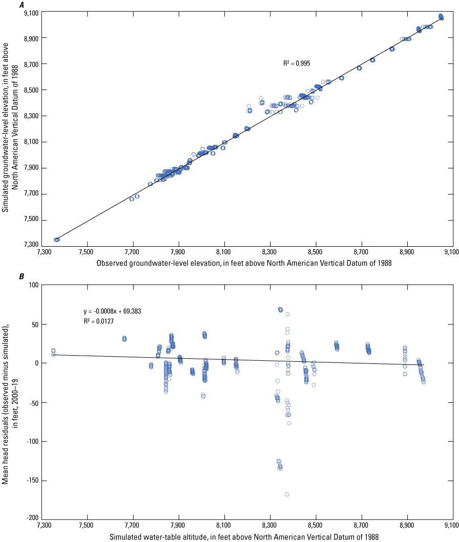
Graph showing simulated compared to observed groundwater-level elevations for the Wet Mountain Valley alluvial aquifer, Custer and Fremont Counties, Colorado, 2000–19. R2 = coefficient of determination. Model results are from Russell and Newman (2025).
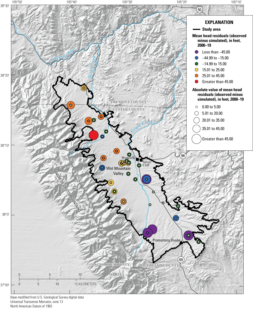
Map showing spatial distribution of mean hydraulic-head residuals from the calibrated model of the Wet Mountain Valley alluvial aquifer, Custer and Fremont Counties, Colorado, 2000–19. Symbol sizes vary according to the absolute value of the residual, with larger symbols representing larger residuals. Model results are from Russell and Newman (2025).
Model sensitivity analysis used PEST++IES (White and others, 2020) results to determine the sensitivity of observation groups to parameter values that were modified during computer-aided calibration. The more sensitive the observation groups are to a parameter, the more changes in the parameter will affect model results. The sensitivity analysis used the combined base flows and groundwater-level elevation observations in the top model layer and showed that the observations were most sensitive to horizontal hydraulic conductivity and applied recharge. The areas where the model is most sensitive to changes in horizontal hydraulic conductivity were towards the central and western parts of the active model area in layer one, shown in figure 19A. The final calibrated K distribution in layer one is shown in figure 19B which illustrates that K values tend to be greatest along the eastern and southern parts of the alluvial aquifer. Higher K values in the eastern part of the model domain near Grape Creek are consistent with aquifer testing described by Newman and others (2021). There are also apparent linear features in the final calibrated K distribution that may be related to model discretization. These linear features are not expected to substantially change the model performance. The locations of the increased conductivity zones tend to correspond with north–south trending faults in the study area (fig. 2), indicating faulting may play a role in governing groundwater flow. This evaluation is consistent with groundwater-age dating results, which indicated possible premodern groundwater inflow along faults.


Maps of the Wet Mountain Valley alluvial aquifer, Custer and Fremont Counties, Colorado, 2000–19, showing A, sensitivity to changes in horizontal hydraulic conductivity; and B, final calibrated horizontal hydraulic conductivity in layer one of the numerical groundwater-flow model, in feet per day. Model results are from Russell and Newman (2025).
The water budget for the Wet Mountain Valley calibrated numerical model during the transient stress period 2000–19, shows the simulated inflows and outflows for the aquifer (table 10). On mean, the two largest inflows into the alluvial aquifer came from leakage from all streams simulated in the active model area and recharge applied to the active model area. These two inflows accounted for approximately 52 and 33 percent of mean annual inflow, respectively (fig. 20). The mean annual inflow to the alluvial aquifer from streams was approximately 291,991 acre-feet per year (acre-ft/yr), and the mean annual inflow to the alluvial aquifer from applied recharge was approximately 459,407 acre-ft/yr. Vertical flow from the deeper alluvial aquifer (represented by layer two) accounted for less than 20 percent of the mean annual inflow and supplied approximately 135,190 acre-ft/yr of water to the shallow alluvial aquifer (represented by layer one) (table 10). Seepage from the aquifer to streams (groundwater discharge) was the largest outflow from the aquifer and accounted for a mean annual outflow of 724,593 acre-ft/yr, or about 83 percent of mean annual outflows from the aquifer. Vertical flow to the deeper alluvial aquifer (layer 2) was the second largest outflow with a mean annual outflow of 143,947 acre-ft/yr, or about 16 percent of mean annual outflows from the alluvial aquifer. Well withdrawals and EVT were also outflows from the alluvial aquifer; however, they accounted for a combined rate of only 526 acre-ft/yr, or less than 1 percent of the mean annual outflows from the aquifer (table 10).
Table 10.
Simulated water budget for the calibrated numerical model for Wet Mountain Valley alluvial aquifer, 2000–19. Model results are from Russell and Newman (2025).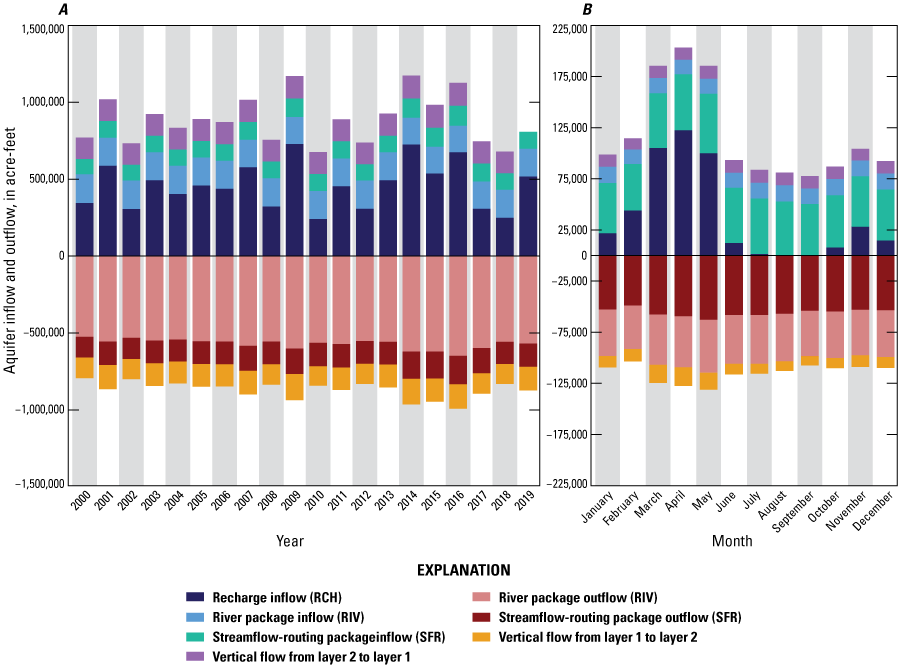
Graphs showing the Wet Mountain Valley alluvial aquifer, Custer and Fremont Counties, Colorado, A, yearly totals of inflows and outflow from the model packages simulated, and B, the mean monthly inflows and outflows simulated during the transient period, 2000–19. Model results are from Russell and Newman (2025).
Overall, these water-budget estimates were similar in magnitude to those presented in Londquist and Livingston (1978). Londquist and Livingston (1978) estimated a groundwater budget for the southern part of the study area, an area of 167 square miles. This study considered the entire alluvial aquifer, an area of 242 square miles or 1.44 times the area studied by Londquist and Livingston (1978). Londquist and Livingston (1978) estimated a net inflow of 205,000 acre-ft/yr for the alluvial aquifer. This study estimates 886,589 acre-ft/yr of total inflow. However, 135,190 acre-ft/yr of this inflow is derived from exchanges between the shallow and deep layers of the alluvial aquifer (layers 1 and 2), a process not considered by Londquist and Livingston (1978). Additionally, this study accounts for inflows that enter the alluvial aquifer from numerous streams, which were not accounted for by Londquist and Livingston (1978). The estimates provided in this study were believed to be representative of conditions between 2000 and 2019 and were based on more diverse datasets, such as site-specific estimates of hydraulic properties provided by Newman and others (2021), whereas Londquist and Livingston (1978) relied on assumptions of steady state and less distributed datasets.
The mean annual inflows and outflows from each model package (fig. 20A) provides a detailed water-budget components summary. The SFR2 package (Niswonger and Prudic, 2005; primarily representing the perennial streams) is the largest inflow and is followed by the RCH and RIV packages (Harbaugh and others, 2000; primarily representing smaller ephemeral tributaries). The SFR2 package is also the largest outflow, and the RIV package had the second largest outflow. The mean annual inflow and outflow simulated by each package in the numerical model does not change substantially through time. The mean monthly inflows and outflows from each model package show the seasonal trends within each package (fig. 20B). This mean monthly trend analysis shows the effect of recharge on the aquifer. April had the most inflow into the aquifer because of the increase of recharge from snowmelt applied to the aquifer, and September had the lowest amount of inflow because of the lack of recharge being applied during that month based on results of the SWB model.
The simulated groundwater-level elevations from the final model period (December 2019) ranged from 7,184 to 11,313 ft, with the highest groundwater-level elevations along the western edge of the active model area and decreasing in the northeastern direction (fig. 21). Simulated groundwater-level elevation contours did not change substantially through time, thus the final model period illustrated in figure 21 is representative of other time periods in the model. The simulated groundwater-flow direction was typically away from the mountain front of the Sangre de Cristo Mountains (fig. 9; similar to conceptual model water-table orientations), and groundwater flow in this direction supplied base flow to many streams in the model domain.
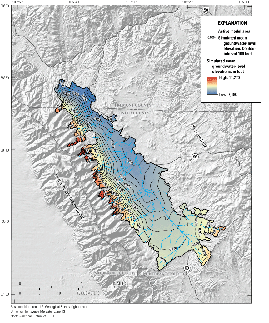
Map showing simulated mean groundwater-level elevations for the model, Wet Mountain Valley alluvial aquifer, Custer and Fremont Counties, Colorado, 2000–19. Model results are from Russell and Newman (2025).
To assess proposed water-management actions, such as ASR, an additional simulation using the calibrated Wet Mountain Valley alluvial aquifer model was created to evaluate the effects of diverting available base flow from Grape Creek to a nearby location for hypothetical artificial recharge. To simulate these proposed water-management actions, an area near Grape Creek with more available groundwater storage was identified (fig. 7), and additional recharge was applied to this area within the RCH package for the entirety of the simulated period. The mean depth to groundwater simulated by the model in the area of additional recharge was 43 ft below land surface. Additional recharge was applied during June, because this month has the highest median base flow values recorded at the Grape Creek streamflow measurement location (Colorado Division of Water Resources, 2022). The resulting simulated groundwater-level elevations showed the additional recharge applied to this area had a minimal effect on simulated groundwater-level elevations at less than 1 foot, a difference less than the mean residual of the model of 1.99 ft, meaning any predicted differences in groundwater-level elevations were less than the model accuracy.
Comparison of simulated groundwater and surface-water interactions between the calibrated base-case model (the model without additional recharge) and the model with simulated aquifer storage and recovery indicates the additional recharge distributed throughout the area had minimal effects on the nearby Grape Creek, with a median additional base flow of 0.13 ft3/s because of the additional recharge (fig. 22A). To determine how the additional recharge was distributed throughout the numerical model area, a user-specified subregional water budget was computed using the ZONEBUDGET computer program (Harbaugh, 1990). The ZONEBUDGET analysis showed approximately 54 percent of the additional recharge went to nearby streams, and about 46 percent flowed laterally into adjacent model cells, showing most of the water eventually fed into the additional simulated base flow described previously (fig. 22B). The comparison of simulations and subregional water budget show the additional recharge did not substantially modify the groundwater budget of the alluvial aquifer or groundwater-flow directions.
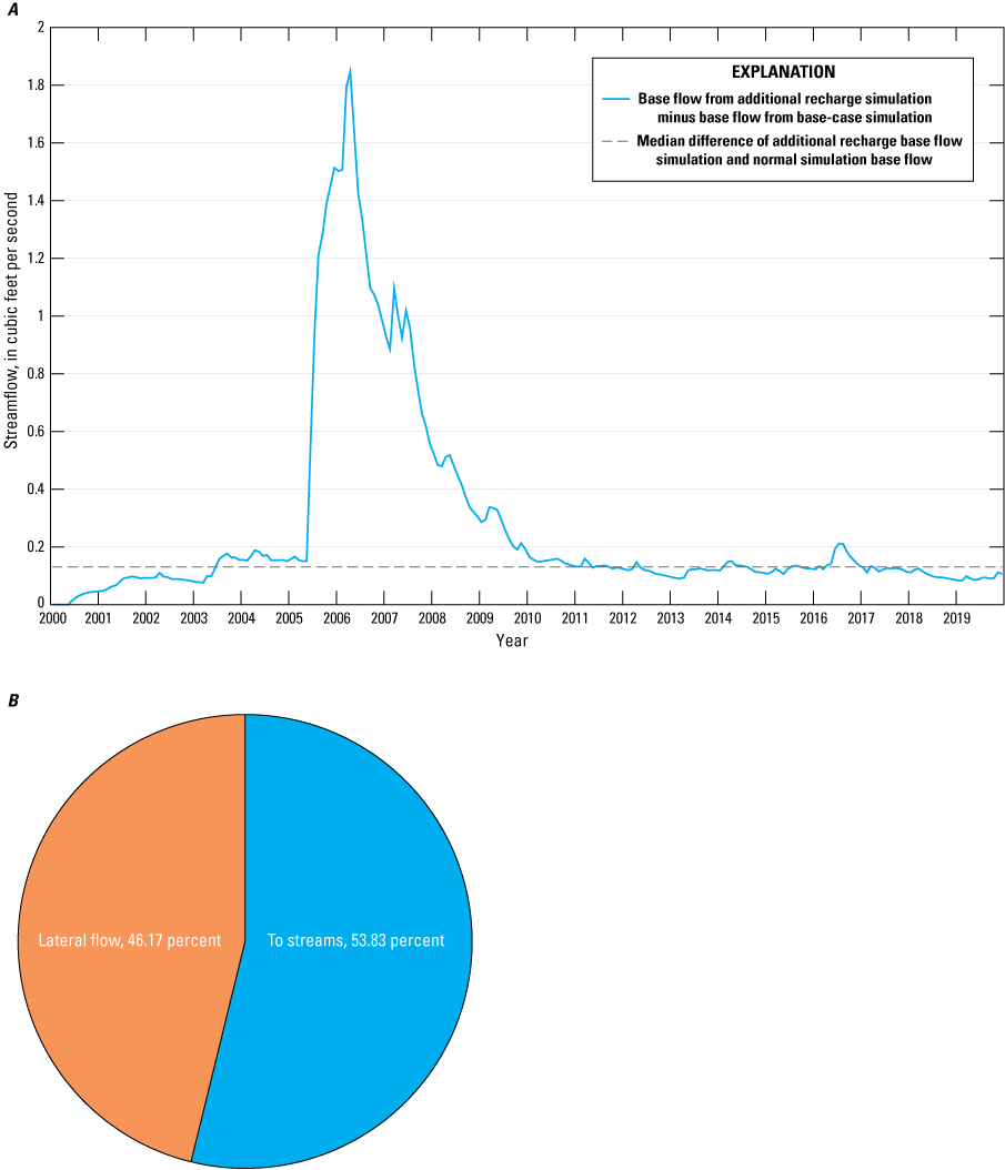
Graphs showing A, comparison of base flow from additional recharge simulation and base flow from normal simulation run, 2000–19, of the Wet Mountain Valley alluvial aquifer numerical model; and B, percentages of the additional recharge distribution to outflows in the additional recharge zone, computed using the computer program ZONEBUDGET (Harbaugh, 1990). Model results are from Russell and Newman (2025).
Model Limitations
The numerical groundwater-flow model of the Wet Mountain Valley is useful for understanding large-scale hydrologic processes occurring in the alluvial aquifer, but the model is limited in some instances by the numerical framework and discretization, and in the boundary conditions representation. Limitations related to framework and discretization include the simulated alluvial aquifer thickness compared to the actual alluvial aquifer thickness. Limitations in available data related to the boundary conditions representation include how groundwater and surface-water interactions are simulated in the model and the assignment of a single MODFLOW (Harbaugh and others, 2000) package to model cells where in the physical system multiple processes may occur simultaneously.
Geophysical alluvial aquifer investigations indicate the alluvium may be several thousand feet thick along the western extent of the aquifer where it meets the Sangre de Cristo Mountains (Zohdy and others, 1971). The numerical groundwater-flow model ranges in thickness from 524 to 656 ft, which is substantially less than the total possible alluvial thickness. This simplification was necessary as almost all groundwater-level observation wells were less than 600 ft deep, meaning the model would be unconstrained by observations if it were deepened. Because one focus of this study was to evaluate the effects of artificial recharge derived from streamflow, the model was focused on the upper parts of the aquifer. If water-resource questions arise pertinent to the lower layers of the aquifer, then the numerical groundwater-flow model used in this analysis could be modified to predict conditions deeper in the aquifer.
The primary limitation related to representation of model boundary conditions is the manner in which streams were simulated. There were limitations on the data available to accurately represent these streams, such as data on channel elevation, roughness estimates, and streambed thickness. Because of the study area steep topography and the abundance of streams without available streamflow measurements (fig. 5), it was necessary to simplify the network of SFR2 package (Niswonger and Prudic, 2005) cells. Streams simulated using the SFR2 package allow aquifer bidirectional flow, whereas streams simulated using the RIV package (Harbaugh and others, 2000) were less well constrained by the model in the ability to have bidirectional flow. Substantial additional streamflow measurements would need to be made within the model area to incorporate all streams into the SFR2 package.
The large water-budget components made up by leakage to and from the SFR2 and RIV packages, compared with the small water-budget component made up by evapotranspiration in the EVT package (Harbaugh and others, 2000), illustrates one model limitation by simulating only one hydrologic stressor in each grid cell. In package assignment to grid cells, it is possible to assign only one package to a given cell. This study was focused on groundwater and surface-water interactions; therefore, streams were the model package assignment focus. In some instances, the SFR2 or RIV package was used where there may also be irrigated fields, which could represent a component of groundwater discharge from the system to evapotranspiration. The streams located in areas that may be groundwater discharge locations via evapotranspiration may mean some of the discharge simulated in the SFR2 or RIV packages is discharging to evapotranspiration in the physical system. This simplification is necessary to simulate the stream network with high resolution and is not expected to result in a bias in the net groundwater budget or in simulated groundwater-flow directions.
Despite these limitations, the numerical groundwater-flow model was able to produce simulated groundwater-level elevations that closely matched observations. The model also simulated both the groundwater discharge to streams (gaining streams) and streamflow groundwater recharge (losing streams). Gaining and losing conditions were corroborated throughout the model domain by physical streamflow gain or loss measurements. Overall, the groundwater-flow model is suitable for large-scale evaluation of hydrologic budgets within the study area and for assessing potential effects of ASR.
Summary
In 2017, the U.S. Geological Survey, in cooperation with the Upper Arkansas Water Conservancy District, began a study to provide a comprehensive analysis of the Wet Mountain Valley alluvial aquifer, Custer and Fremont Counties, Colorado. The study included collection of data pertaining to groundwater hydrology, groundwater and surface-water interactions, and water quality in the alluvial aquifer. In addition to providing foundational information on the alluvial aquifer hydrology, a numerical groundwater-flow model was developed to evaluate the regional groundwater-flow system and estimate the potential effects of additional groundwater storage in the alluvial aquifer. The diverse datasets collected as part of this study allow for an integrated understanding of the alluvial aquifer.
Groundwater-level elevations in 30 wells were used to estimate groundwater-flow directions, which were generally from the southwest to northeast, away from the Sangre de Cristo Mountains and towards perennial streams in the center of the valley. Although some seasonal variation was apparent in groundwater-level elevation records, no statistically significant seasonal trends were indicated. Statistically significant long-term trends were indicated in groundwater-level elevation records for 8 of the 30 wells evaluated in this study, and of these wells with statistically significant trends, all but 1 indicated a negative trend of groundwater-level elevations. Theil-Sen slopes of groundwater-level elevation change in wells with statistically significant groundwater-level elevation decreases ranged from –0.126 to –1.06 feet per year. Spatial evaluation of wells with statistically significant negative groundwater-level elevation trends showed many were in areas of denser well drilling for domestic or other uses, potentially indicating increasing groundwater use could be causing groundwater-level elevation declines. However, there were instances of wells with no statistically significant groundwater-level elevation trends also in areas of denser well completions. Additional investigations could more fully characterize processes responsible for negative groundwater-level elevation trends by monitoring groundwater wells at a larger range of depths and for a longer period of time to evaluate how groundwater-level elevation trends may differ vertically through the aquifer and the effect of climate.
Measurements of streamflow gain or loss were completed for the low-flow periods of 2017, 2019, and 2018 and the high-flow period of 2018 (spring) in nine stream reaches within the study area. Several stream reaches displayed consistent streamflow loss in each period (upper Texas Creek, upper Grape Creek, upper-middle Grape Creek, and Taylor Creek). These stream reaches represent long-term sources of recharge to the alluvial aquifer. Other stream reaches display time-variant patterns in low streamflow gain or loss (lower Texas Creek, lower-middle Grape Creek, lower Grape Creek below Westcliffe, and lower Grape Creek above DeWeese Reservoir). The temporally variable patterns indicate these stream reaches may be sources of groundwater recharge or areas of groundwater discharge, likely depending on local time varying dynamics between the elevation of the water table and the stream.
Water-quality samples were collected from 10 groundwater wells and 10 stream sites during September through November 2019. All groundwater and stream samples were analyzed for major and trace elements and stable isotopes of water. A subset of groundwater samples was also analyzed for environmental tracers sulfur hexafluoride, tritium, and noble gases. Comparison of water-quality results to U.S. Environmental Protection Agency drinking water-quality standards indicates no constituents exceeded primary standards based on human health. Spatial water quality evaluation indicated the concentrations of various constituents were likely controlled by groundwater and surface-water interactions and potentially by spatial variability in bedrock geology underlying the alluvial aquifer. Specifically, streams shown to gain from groundwater had compositions similar to groundwater, whereas streams exiting the Sangre de Cristo Mountains tended to have dilute compositions indicating a snowmelt source. Groundwater geochemistry appears to be partially controlled by oxidation-reduction processes and by proximity to igneous rocks in the Wet Mountains. Environmental tracers, used to estimate groundwater age, indicated all sampled groundwater contained a portion of modern recharge (approximately less than 65 years old), but mixing of premodern recharge (approximately more than 65 years old) also occurs. No trends were observed in groundwater age with well depth, indicating all sampled wells were located within the active groundwater flow zone. Spatial evaluation of environmental tracers indicated large faults may be conduits for older groundwater inflow. The presence of modern groundwater in wells with statistically significant negative groundwater-level elevation trends indicates groundwater storage depletions may be partially offset by modern recharge capture. Repeated groundwater- age sampling could help determine if any trends in groundwater age exist, which may indicate changing groundwater recharge, storage, or discharge. Additional investigations could also consider quantifying groundwater age in deeper wells to more fully explore the depth of active groundwater flow.
A transient, three-dimensional numerical groundwater-flow model was developed and used to estimate water-budget components, simulate groundwater and surface-water interactions, and evaluate the potential effects of a hypothetical scenario of aquifer storage and recovery. Groundwater-level elevations from the calibrated groundwater-flow model were similar to the conceptual understanding of groundwater-level elevations with the highest elevations in the western part of the study area along the Sangre de Cristo Mountains and flow toward the northeast. Simulated water-budget components indicate the primary source of recharge to the alluvial aquifer is from streamflow losses, consistent with observations of losing streams along the mountain front. The largest alluvial aquifer groundwater-discharge component was to streams in the center of the valley, where stream gain or loss observations indicated the predominance of gaining conditions. Comparison of groundwater and surface-water interactions between the calibrated groundwater-flow model for current conditions (the base-case model, 2000–19) and a simulation including additional recharge, representing potential aquifer storage and recovery operations, indicated the additional recharge distributed throughout the area had minimal effects on the nearby Grape Creek. A groundwater budget analysis showed approximately 54 percent of the additional recharge went to nearby streams, and about 46 percent flowed laterally into adjacent alluvial aquifer areas. The 54 percent additional recharge that returned to Grape Creek resulted in a median streamflow increase of 0.13 cubic feet per second compared to the simulation without additional recharge. The comparison of simulations and subregional water budget show the additional recharge did not substantially modify the groundwater budget of the alluvial aquifer or groundwater-flow directions. The published calibrated numerical groundwater-flow model is a useful tool to understand the potential effect of variable hydrologic changes within the study area.
The study described in this report outlines several areas of potential additional investigations within the Wet Mountain Valley that may more fully characterize the groundwater system. Additional areas of potential study include (1) an integrated characterization of the bedrock aquifer, and if connectivity exists between the bedrock aquifer and the alluvial aquifer; (2) more detailed evaluation of the effect of surface-water diversions on streamflow gain or loss, which could benefit from additional records on diversions within the area; and, (3) further evaluation of groundwater age structure in the valley to understand if human interactions with the hydrologic system may cause storage changes within the aquifers. These additional potential investigations could build upon the hydrologic framework and budgets described within this report.
Acknowledgments
Field assistance that benefitted this project was provided by Michael Holmberg, Will McDermott, and Emily Baker.
References Cited
Anderson, L., Berkelhammer, M., and Mast, M.A., 2016, Isotopes in North American Rocky Mountain snowpack 1993–2014: Quaternary Science Reviews, v. 131, p. 262–273, accessed September 12, 2020, at https://doi.org/10.1016/j.quascirev.2015.03.023.
Bowen, G.J., 2020, Online isotopes in precipitation calculator, version 3.1, accessed January 15, 2020, at https://wateriso.utah.edu/waterisotopes/pages/data_access/oipc.html.
Bowen, G.J., and Revenaugh, J., 2003, Interpolating the isotopic composition of modern meteoric precipitation: Water Resources Research, v. 39, no. 10, accessed August 8, 2019, at https://doi.org/10.1029/2003WR002086.
Busenberg, E., and Plummer, L.N., 2000, Dating young groundwater with sulfur hexafluoride—Natural and anthropogenic sources of sulfur hexafluoride: Water Resources Research, v. 36, no. 10, p. 3011–3030. [Also available at https://doi.org/10.1029/2000WR900151.]
Chinnasamy, C.V., McIntyre, W.C., and Mays, D.C., 2018, Technical and administrative feasibility of alluvial aquifer storage and recovery on the South Platte River of northeastern Colorado: Water Policy, v. 20, no. 4, p. 841–854, accessed April 4, 2019, at https://doi.org/10.2166/wp.2018.174.
Cohn, T.A., Kiang, J.E., and Mason, R.R., 2013, Estimating discharge measurement uncertainty using the interpolated variance estimator: Journal of Hydraulic Engineering, v. 139, no. 5, p. 502–510, accessed March 22, 2019, at https://doi.org/10.1061/(ASCE)HY.1943-7900.0000695.
Colorado Department of Local Affairs, 2020, Population projections in Colorado: Colorado Information Marketplace, accessed December 29, 2020, at https://data.colorado.gov/Demographics/Population-Projections-in-Colorado/q5vp-adf3.
Colorado Division of Water Resources, 2019, Colorado decision support system: Colorado Division of Water Resources, accessed June 19, 2019, at https://dnrweb.state.co.us/cdss/.
Colorado Division of Water Resources, 2022, Discharge data for Grape Creek near Westcliffe: Colorado Division of Water Resources, accessed January 28, 2022, at https://dwr.state.co.us/Tools/Stations/GRAWESCO?params=DISCHRG.
Colorado Office of Economic Development and International Trade, 2012, Annual report 2012—Region 13: Colorado Office of Economic Development and International Trade 9 p., accessed December 28, 2020, at https://choosecolorado.com/wp-content/uploads/2016/07/2012-OEDITAnnualReport.pdf.
Colorado State University, 2021, CoAgMET climate station pages: Colorado State University, accessed June 28, 2021, at http://www.coagmet.colostate.edu/station/stn_select.html.
Colorado Water Conservation Board, 2007, Colorado’s water supply future statewide water supply Initiative—Phase 2: Colorado Water Conservation Board, 350 p., accessed December 28, 2020, at http://cwcb.state.co.us/public-information/publications/Documents/ReportsInvestigations/TechnicalRoundtableReportFinalDraft.pdf.
Condon, L.E., Markovich, K.H., Kelleher, C.A., McDonnell, J.J., Ferguson, G., and McIntosh, J.C., 2020, Where is the bottom of a watershed?: Water Resources Research, v. 56, accessed August 19, 2021 at https://doi.org/10.1029/2019WR026010.
Craig, H., 1961, Isotopic variations in meteoric waters: Science, v. 133, no. 3465, p. 1702–1703, accessed April 9, 2019, at https://doi.org/10.1126/science.133.3465.1702.
Crouch, T.M., Cain, D., Abbott, P.O., Penley, R.D., and Hurr, R.T., 1984, Water-resources appraisal of the upper Arkansas River Basin from Leadville to Pueblo, Colorado: U.S. Geological Survey Water-Resources Investigations Report 82–4114, 130 p. [Also available at https://doi.org/10.3133/wri824114.]
Daly, C., Neilson, R.P., and Phillips, D.L., 1994, A statistical-topographic model for mapping climatological precipitation over mountainous terrain: Journal of Applied Meteorology, v. 33, p. 140–158. [Also available at https://doi.org/10.1175/1520-0450(1994)033<0140:ASTMFM>2.0.CO;2.]
Dillon, P., Stuyfzand, P., Grischek, T., Lluria, M., Pyne, R.D.G., Jain, R.C., Bear, J., Schwarz, J., Wang, W., Fernandez, E., Stefan, C., Pettenati, M., van der Gun, J., Sprenger, C., Massmann, G., Scanlon, B.R., Xanke, J., Jokela, P., Zheng, Y., Rossetto, R., Shamrukh, M., Pavelic, P., Murray, E., Ross, A., Bonilla Valverde, J.P., Palma Nava, A., Ansems, N., Posavec, K., Ha, K., Martin, R., Sapiano, M., 2019, Sixty years of global progress in managed aquifer recharge: Hydrogeology Journal, v. 27, p. 1–30, accessed July 12, 2020, at https://doi.org/10.1007/s10040-018-1841-z.
Doherty, J., 2003, Ground water model calibration using pilot points and regularization: Groundwater, v. 41, no. 2, p. 170–177. [Also available at https://doi.org/10.1111/j.1745-6584.2003.tb02580.x.]
Ferguson, G., Cuthbert, M.O., Befus, K., Gleeson, T., and McIntosh, J.C., 2020, Rethinking groundwater age: Nature Geoscience, v. 13, p. 592–594, accessed January 12, 2021, at https://doi.org/10.1038/s41561-020-0629-7.
Fishman, M.J., and Friedman, L.C., eds., 1989, Methods for determination of inorganic substances in water and fluvial sediments: U.S. Geological Survey Techniques of Water-Resources Investigations, book 5, chap. A1, 545 p., accessed February 27, 2014, at https://doi.org/10.3133/twri05A1.
Fishman, M.J., ed., 1993, Methods of analysis by the U.S. Geological Survey National Water Quality Laboratory—Determination of inorganic and organic constituents in water and fluvial sediments: U.S. Geological Survey Open-File Report 93–125, 217 p., accessed February 27, 2014, at https://doi.org/10.3133/ofr93125.
Friedrich, R., Vero, G., von Rohden, C., Lessmann, B., Kipfer, R., and Aeschbach-Hertig, W., 2013, Factors controlling terrigenic SF6 in young groundwater of the Odenwald region (Germany): Applied Geochemistry, v. 33, p. 318–329, accessed October 12, 2019, at https://doi.org/10.1016/j.apgeochem.2013.03.002.
Gardner, P.M. and Heilweil, V.M., 2014, A multiple-tracer approach to understanding regional groundwater flow in the Snake Valley area of the eastern Great Basin, USA: Applied Geochemistry, v. 45, p. 33–49, accessed December 2, 2019, at https://doi.org/10.1016/j.apgeochem.2014.02.010.
Glynn, P.D., and Plummer, L.N., 2005, Geochemistry and the understanding of ground-water systems: Hydrogeology Journal, v. 13, p. 263–287. [Also available at https://doi.org/10.1007/s10040-004-0429-y.]
Green, G.N., 1992, The digital geologic map of Colorado in ARC/INFO format: U.S. Geological Survey Open-File Report 92–0507, 9 p. accessed April 7, 2019, at https://doi.org/10.3133/ofr92507DO.
Harbaugh, A.W., 1990, A computer program for calculating subregional water budgets using results from the U.S. Geological Survey modular three-dimensional ground-water flow model: U.S. Geological Survey Open-File Report 90–392, 46 p. [Also available at https://doi.org/10.3133/ofr90392.]
Harbaugh, A.W., Banta, E.R., Hill, M.C., and McDonald, M.G., 2000, MODFLOW-2000, the U.S. Geological Survey modular ground-water model—User guide to modularization concepts and the ground-water flow process: U.S. Geological Survey Open-File Report 00–92, 121 p. [Also available at https://doi.org/10.3133/ofr200092.]
Harmel, R.D., Cooper, R.J., Slade, R.M., Haney, R.L., and Arnold, J.G., 2006, Cumulative uncertainty in measured streamflow and water quality data for small watersheds: Transactions of the ASABE, v. 49, no. 3, p. 689–701. [Also available at https://doi.org/10.13031/2013.20488.]
Healy, R.W., and Cook, P.G., 2002, Using groundwater levels to estimate recharge: Hydrogeology Journal, v. 10, p. 91–109, accessed January 12, 2019, at https://doi.org/10.1007/s10040-001-0178-0.
Helsel, D.R., Hirsch, R.M., Ryberg, K.R., Archfield, S.A., and Gilroy, E.J., 2020, Statistical methods in water resources: U.S. Geological Survey Techniques and Methods, book 4, chapter A3, 458 p., accessed December 2, 2020, at https://doi.org/10.3133/tm4A3. [Supersedes USGS Techniques of Water-Resources Investigations, book 4, chapter A3, version 1.1.]
Hunt, A.G., 2015, Noble Gas Laboratory’s standard operating procedures for the measurement of dissolved gas in water samples: U.S. Geological Survey Techniques and Methods, book 5, chap. A11, 22 p., accessed April 6, 2019, at https://doi.org/10.3133/tm5A11.
Huntington, J., Hegewisch, K., Daudert, B., Morton, C., Abatzoglou, J., McEvoy, D., and Erickson, T., 2017, Climate engine—Cloud computing of climate and remote sensing data for advanced natural resource monitoring and process understanding: Bulletin of the American Meteorological Society, accessed June 18, 2019, at https://doi.org/10.1175/BAMS-D-15-00324.1.
Hsieh, P.A., 2001, TopoDrive and ParticleFlow—Two computer models for simulation and visualization of ground-water flow and transport of fluid particles in two dimensions: U.S. Geological Survey Open-File Report 01–286, 35 p. [Also available at https://doi.org/10.3133/ofr01286.]
Jasechko, S., Birks, S.J., Gleeson, T., Wada, Y., Fawcett, P.J., Sharp, Z.D., McDonnell, J.J., and Welker, J.M., 2014, The pronounced seasonality of global groundwater recharge: Water Resources Research, v. 50, no. 11, p. 8845–8867, accessed March 20, 2020, at https://doi.org/10.1002/2014WR015809.
Jurgens, B.C., Böhlke, J., Haase, K., Busenberg, E., Hunt, A.G., and Hansen, J.A., 2020, DGMETA (Version 1)—Dissolved gas modeling and environmental tracer analysis computer program: U.S. Geological Survey Techniques and Methods 4–F5, 50 p., https://doi.org/10.3133/tm4F5.
Kipfer, R., Aeschbach-Hertig, W., Peeters, F., and Stute, M., 2002, Noble gases in lakes and groundwaters, in Porcelli, D., Ballentine, C.J., and Wieler, R., eds., Noble gases in geochemistry and cosmochemistry: Quebec, Mineralogical Association of Canada, p. 615–700, accessed November 19, 2019, at https://doi.org/10.1515/9781501509056-016.
Kulongoski, J.T., Hilton, D.R., Cresswell, R.G., Hostetler, S., and Jacobson, G., 2008, Helium-4 characteristics of groundwaters from central Australia—Comparative chronology with chlorine-36 and carbon-14 dating techniques: Journal of Hydrology, v. 348, p. 176–194, accessed May 7, 2020, at https://doi.org/10.1016/j.jhydrol.2007.09.048.
Kulongoski, J.T. and Hilton, D.R., 2012, Applications of groundwater helium, in Baskaran, M. ed., Handbook of Environmental Isotope Geochemistry: Berlin, Springer-Verlag, p. 285–304, accessed May 7, 2020, at https://doi.org/10.1007/978-3-642-10637-8_15.
Lindsey, B.D., Jurgens, B.C., and Belitz, K., 2019, Tritium as an indicator of modern, mixed, and premodern groundwater age: U.S. Geological Survey Scientific Investigations Report 2019–5090, 18 p., accessed June 18, 2020, at https://doi.org/10.3133/sir20195090.
Malenda, H.F., and Penn, C.A., 2020, Groundwater levels in the Denver Basin bedrock aquifers of Douglas County, Colorado, 2011–19: U.S. Geological Survey Scientific Investigations Report 2020–5076, 44 p., accessed October 18, 2020, at https://doi.org/10.3133/sir20205076.
Manning, A.H., 2009, Ground-water temperature, noble gas, and carbon isotope data from the Española Basin, New Mexico: U.S. Geological Survey Scientific Investigations Report 2008–5200, 69 p. [Also available at https://doi.org/10.3133/sir20085200.]
Manning, A.H., 2011, Mountain-block recharge, present and past, in the eastern Española Basin, New Mexico, USA: Hydrogeology Journal, v. 19, p. 379–397. [Also available at https://doi.org/10.1007/s10040-010-0696-8.]
Markovich, K., Manning, A.H., Condon, L., and McIntosh, J., 2019, Mountain-block recharge—A review of current understanding: Water Resources Research, v. 55, no. 11, p. 8278–8304, accessed November 2, 2020, at https://doi.org/10.1029/2019WR025676.
Massoudieh, A., 2013, Inference of long-term groundwater flow transience using environmental tracers—A theoretical approach, Water Resources Research, v. 49, p. 8039–8052, accessed September 8, 2019, at https://doi.org/10.1002/2013WR014548.
McCallum, J.L., Cook, P.G., and Simmons, J.T., 2015, Limitations of the use of environmental tracers to infer groundwater age: Groundwater, v. 53, p. 56–70, accessed October 19, 2019, at https://doi.org/10.1111/gwat.12237.
Mueller, D.K., Schertz, T.L., Martin, J.D., and Sandstrom, M.W., 2015, Design, analysis, and interpretation of field quality-control data for water-sampling projects: U.S. Geological Survey Techniques and Methods, book 4, chap. C4, 54 p., accessed June 2, 2020, at https://doi.org/10.3133/tm4C4.
Multi-Resolution Land Characteristics Consortium, 2021, National land cover dataset–2016 CONUS: Multi-Resolution Land Characteristics Consortium, accessed March 2, 2021, at https://www.mrlc.gov/data/nlcd-2016-land-cover-conus.
Natural Resource Conservation Service, 2020, Soil survey geographic database, accessed September 10, 2020, at https://www.nrcs.usda.gov/wps/portal/nrcs/detail/soils/survey/?cid=nrcs142p2_053627/.
Newman, C.P., Kisfalusi, Z.D., and Holmberg, M.J., 2021, Assessing specific-capacity data and short-term aquifer testing to estimate hydraulic properties in alluvial aquifers of the Rocky Mountains, Colorado, USA: Journal of Hydrology: Regional Investigations, v. 38., no. 100949, 20. p., accessed November 2, 2021, at https://doi.org/10.1016/j.ejrh.2021.100949.
Newman, C.P., 2024, Environmental tracer model for the Wet Mountain Valley alluvial aquifer, Custer and Fremont Counties, Colorado, 2019: U.S. Geological Survey data release, https://doi.org/10.5066/P9342SSP.
Niswonger, R.G., and Prudic, D.E., 2005, Documentation of the Streamflow-Routing (SFR2) Package to include unsaturated flow beneath streams—A modification to SFR1: U.S. Geological Survey Techniques and Methods 6–A13, 50 p. [Also available at https://doi.org/10.3133/tm6A13.]
Paschke, S.S., Harrison, W.J., and Walton-Day, K., 1995, Effects of acidic recharge on groundwater at the St. Kevin Gulch site, Leadville, Colorado: Geochemistry: Exploration, Environment, Analysis, v. 1, p. 3–14, accessed April 25, 2024 at https://doi.org/10.1144/geochem.1.1.3.
Paschke, S.S. ed., 2011, Groundwater availability of the Denver Basin aquifer system, Colorado: U.S. Geological Survey Professional Paper 1770, 274 p. Also available at https://doi.org/10.3133/pp1770.]
Piper, A.M., 1944, A graphic procedure in the geochemical interpretation of water-analyses: EOS Transactions American Geophysical Union, v. 25, no. 6, p. 914–928, accessed June 4, 2020, at https://doi.org/10.1029/TR025i006p00914.
R Core Team, 2020, R—A language and environment for statistical computing: Vienna, Austria, R Foundation for Statistical Computing, accessed October 2, 2019, at https://www.R-project.org/.
Rehmel, M., 2007, Application of acoustic doppler velocimeters for streamflow measurements: Journal of Hydraulic Engineering, v. 113, no. 12, p. 1433–1438, accessed August 5, 2019, at https://doi.org/10.1061/(ASCE)0733-9429(2007)133:12(1433).
Révész, Kinga, and Coplen, T.B., 2008a, Determination of the δ(2H/1H) of water—RSIL lab code 1574, chap. C1 of Révész, Kinga, and Coplen, T.B., eds., Methods of the Reston Stable Isotope Laboratory: U.S. Geological Survey Techniques and Methods 10–C1, 27 p. [Also available at https://doi.org/10.3133/tm10C1.]
Révész, Kinga, and Coplen, T.B., 2008b, Determination of the δ(18O/16O) of water: RSIL lab code 489, chap. C2 of Révész, Kinga, and Coplen, Tyler B., eds., Methods of the Reston Stable Isotope Laboratory: U.S. Geological Survey Techniques and Methods 10–C2, 28 p. [Also available at https://doi.org/10.3133/tm10C2.]
Robson, S.G., 1985, Proposed work plan for the study of hydrologic effects of ground-water development in the Wet Mountain Valley, Colorado: U.S. Geological Survey Open-File Report 84–866, 13 p., accessed May 20, 2019, at https://doi.org/10.3133/ofr84866.
Ronayne, M.J., Roudebush, J.A., and Stednick, J.D., 2017, Analysis of managed aquifer recharge for retiming streamflow in an alluvial river: Journal of Hydrology, v. 544, p. 373–382, accessed June 22, 2020, at https://doi.org/10.1016/j.jhydrol.2016.11.054.
Rosenberry, D.O., and LaBaugh, J.W., 2008, Field techniques for estimating water fluxes between surface water and ground water: U.S. Geological Survey Techniques and Methods 4–D2, 128 p. [Also available at https://doi.org/10.3133/tm4D2.]
Russell, C.A., and Newman, C.P., 2025, Groundwater-flow model of the Wet Mountain Valley alluvial aquifer, Custer and Fremont Counties, Colorado: U.S. Geological Survey data release, https://doi.org/10.5066/P9AAUGNY.
Scott, G.R., and Taylor, R.B., 1975, Post-Paleocene Tertiary rocks and Quaternary volcanic ash of the Wet Mountain Valley, Colorado: U.S. Geological Survey Professional Paper 868, 15 p. [Also available at https://doi.org/10.3133/pp868.]
Simonds, F.W., and Sinclair, K.A., 2002, Surface water-ground water interactions along the Lower Dungeness River and vertical hydraulic conductivity of streambed sediments, Clallam County, Washington, September 1999–July 2001: U.S. Geological Survey Water-Resources Investigations Report 2002–4161, 69 p. [Also available at https://doi.org/10.3133/wri024161.]
Solomon, D.K., and Cook, P.G., 2000, 3H and 3He, in Cook, P.G., and Herczeg, A.L., eds., Environmental tracers in subsurface hydrology: New York, Springer Science, p. 397–424. [Also available at https://doi.org/10.1007/978-1-4615-4557-6_13.]
Solomon, D.K., 2000, 4He in groundwater, in Cook, P.G. and Herczeg, A.L., eds., Environmental tracers in subsurface hydrology: New York, Springer Science, p. 425–439. [Also available at https://doi.org/10.1007/978-1-4615-4557-6_14.]
Suckow, A., 2014, The age of groundwater—Definitions, models and why we do not need this term: Applied Geochemistry, v. 50, p. 222–230, accessed July 10, 2019, at https://doi.org/10.1016/j.apgeochem.2014.04.016.
Thoma, M.J., McNamara, J.P., Gribb, M.M., and Benner, S.G, 2011, Seasonal recharge components in an urban/agricultural mountain front aquifer system using noble gas thermometry: Journal of Hydrology, v. 409, p. 118–127, accessed June 20, 2020, at https://doi.org/10.1016/j.jhydrol.2011.08.003.
U.S. Department of Agriculture Natural Resources Conservation Service, 2017a, Census of agriculture 2017 county profile, Custer County, Colorado: U.S. Department of Agriculture, accessed February 24, 2021, at https://www.nass.usda.gov/Publications/AgCensus/2017/Online_Resources/County_Profiles/Colorado/cp08027.pdf.
U.S. Department of Agriculture Natural Resources Conservation Service, 2017b, Census of agriculture 2017 county profile, Fremont County, Colorado U.S. Department of Agriculture, accessed February 24, 2021, at https://www.nass.usda.gov/Publications/AgCensus/2017/Online_Resources/County_Profiles/Colorado/cp08043.pdf.
U.S. Department of Agriculture National Resource Conservation Service, 2021, Snow telemetry data, station South Colony–773, accessed March 3, 2021, at https://wcc.sc.egov.usda.gov/nwcc/site?sitenum=773.
U.S. Environmental Protection Agency, 2020a, National primary drinking water regulations: U.S. Environmental Protection Agency, accessed December 21, 2020, at https://www.epa.gov/ground-water-and-drinking-water/national-primary-drinking-water-regulations.
U.S. Environmental Protection Agency, 2020b, Secondary drinking water standards—Guidance for nuisance chemicals: U.S. Environmental Protection Agency, accessed December 21, 2020, at https://www.epa.gov/sdwa/secondary-drinking-water-standards-guidance-nuisance-chemicals.
U.S. Environmental Protection Agency, 2022, Detailed facility report for facility 110006781385, accessed March 17, 2022, at https://echo.epa.gov/detailed-facility-report?fid=110006781385.
U.S. Geological Survey [USGS], variously dated, National field manual for the collection of water-quality data: U.S. Geological Survey Techniques of Water-Resources Investigations, book 9, chaps. A1–A10, variously paginated, accessed November 1, 2019, at https://pubs.water.usgs.gov/twri9A.
U.S. Geological Survey [USGS], 2019, National hydrography dataset (NHD), accessed March 4, 2019, at https://hydro.nationalmap.gov/arcgis/rest/services/nhd/MapServer.
U.S. Geological Survey [USGS], 2020, National elevation dataset: accessed February 2020, at https://apps.nationalmap.gov/downloader/.
U.S. Geological Survey [USGS], 2021, USGS water data for the Nation: U.S. Geological Survey National Water Information System database, accessed July 30, 2021, at https://doi.org/10.5066/F7P55KJN.
Watts, K.R., 2005, Hydrogeology and quality of ground water in the upper Arkansas River Basin from Buena Vista to Salida, Colorado, 2000–2003: U.S. Geological Survey Scientific Investigations Report 2005–5179, 61 p. [Also available at https://doi.org/10.3133/sir20055179.]
Watts, K.R., Ivahnenko, Tamara, Stogner, R.W., and Bruce, J.F., 2014, Groundwater and surface-water interaction and potential for underground water storage in the Buena Vista-Salida Basin, Chaffee County, Colorado, 2011: U.S. Geological Survey Scientific Investigations Report 2014–5095, 63 p., accessed August 29, 2019, at https://doi.org/10.3133/sir20145095.
Westenbroek, S.M., Kelson, V.A., Dripps, W.R., Hunt, R.J., and Bradbury, K.R., 2010, SWB-A modified Thornthwaite-Mather Soil-Water-Balance code for estimating groundwater recharge: U.S. Geological Survey Techniques and Methods 6–A31, 60 p. [Also available at https://doi.org/10.3133/tm6A31.]
White, J.T., Foster, L.K., Fienen, M.N., Knowling, M.J., Hemming, B., and Winterle, J.R., 2020, Toward reproducible environmental modeling for decision support—A worked example: Frontiers in Earth Science, v. 8, no. 50, accessed February 12, 2021, at https://doi.org/10.3389/feart.2020.00050.
Winter, T.C., Harvey, J.W., Franke, O.L., and Alley, W.M., 1999, Ground water and surface water—A single resource: U.S. Geological Survey Circular 1139, 79 p., accessed August 20, 2019, at https://doi.org/10.3133/cir1139.
Conversion Factors
Temperature in degrees Celsius (°C) may be converted to degrees Fahrenheit (°F) as follows:
°F = (1.8 × °C) + 32.
Temperature in degrees Fahrenheit (°F) may be converted to degrees Celsius (°C) as follows:
°C = (°F – 32) / 1.8.
Datum
Vertical coordinate information is referenced to the North American Vertical Datum of 1988 (NAVD 88).
Horizontal coordinate information is referenced to North American Datum of 1983 (NAD 83).
Elevation, as used in this report, refers to distance above the vertical datum.
Supplemental Information
Specific conductance is given in microsiemens per centimeter at 25 degrees Celsius (µS/cm at 25 °C).
Concentrations of chemical constituents in water are given in either milligrams per liter (mg/L) or micrograms per liter (µg/L).
Results for measurements of stable isotopes of an element (with symbol E) in water, solids, and dissolved constituents commonly are expressed as the relative difference in the ratio of the number of the less abundant isotope (iE) to the number of the more abundant isotope of a sample with respect to a measurement standard.
Abbreviations
acre-ft/yr
acre-feet per year
ASR
aquifer storage and recovery
CDSS
Colorado Decision Support System
K
hydraulic conductivity
Kh
horizontal hydraulic conductivity
Ky/h
ratio of vertical to horizontal hydraulic conductivity
MODFLOW
modular three-dimensional finite-difference groundwater flow model
NAD 83
North American Datum of 1983
NAVD 88
North American Vertical Datum of 1988
NHD
National Hydrography Dataset
NWIS
National Water Information System
R
ratio of helium-3 to helium-4 in sample
Ra
ratio of helium-3 to helium-4 in air
RCH
recharge package of MODFLOW
RIV
river package of MODFLOW
EVT
evapotranspiration package of MODFLOW
SWB
surface water balance model
SFR2
streamflow routing two package of MODFLOW
RPD
relative percent difference
SU
standard units
Sy
specific yield
TU
tritium units
USGS
U.S. Geological Survey
WEL
well package of MODFLOW
3H
tritium
3He
helium-3
4He
helium-4
20Ne
neon-20
3Hetrit
tritiogenic helium-3
4Heterr
terrigenic helium-4
δ2H
deuterium
δ18O
oxygen-18
Publishing support provided by the Science Publishing Network,
Denver Publishing Service Center
For more information concerning the research in this report, contact the
Director, USGS Colorado Water Science Center
Box 25046, Mail Stop 415
Denver, CO 80225
(303) 236-4882
Or visit the Colorado Water Science Center website at
Disclaimers
Any use of trade, firm, or product names is for descriptive purposes only and does not imply endorsement by the U.S. Government.
Although this information product, for the most part, is in the public domain, it also may contain copyrighted materials as noted in the text. Permission to reproduce copyrighted items must be secured from the copyright owner.
Suggested Citation
Newman, C.P., Russell, C.A., Kisfalusi, Z.D., and Paschke, S.S., 2025, Groundwater hydrology, groundwater and surface-water interactions, water quality, and groundwater-flow simulations for the Wet Mountain Valley alluvial aquifer, Custer and Fremont Counties, Colorado, 2017–19: U.S. Geological Survey Scientific Investigations Report 2024–5105, 62 p., https://doi.org/10.3133/sir20245105.
ISSN: 2328-0328 (online)
Study Area
| Publication type | Report |
|---|---|
| Publication Subtype | USGS Numbered Series |
| Title | Groundwater hydrology, groundwater and surface-water interactions, water quality, and groundwater-flow simulations for the Wet Mountain Valley alluvial aquifer, Custer and Fremont Counties, Colorado, 2017–19 |
| Series title | Scientific Investigations Report |
| Series number | 2024-5105 |
| DOI | 10.3133/sir20245105 |
| Publication Date | January 28, 2025 |
| Year Published | 2025 |
| Language | English |
| Publisher | U.S. Geological Survey |
| Publisher location | Reston VA |
| Contributing office(s) | Colorado Water Science Center |
| Description | Report: vii, 62 p.; 2 Data Releases |
| Country | United States |
| State | Colorado |
| County | Custer County, Fremont County |
| Other Geospatial | Upper Arkansas River |
| Online Only (Y/N) | Y |