

A Trend Analysis and Model Comparison of Total Phosphorus Concentrations and Loads in the Boise River near Parma, Southwestern Idaho, Water Years 2003–21
Links
- Document: Report (6.7 MB pdf) , HTML , XML
- Data Release: USGS data release - Water quality modeling results of total phosphorus for the lower Boise River near Parma, Idaho 2002 - 2021
- NGMDB Index Page: National Geologic Map Database Index Page (html)
- Download citation as: RIS | Dublin Core
Acknowledgments
This work was conducted with the financial support of the City of Boise, the Idaho Department of Environmental Quality, and the Lower Boise Watershed Council. We would like to express our gratitude to U.S. Geological Survey personnel Lauren Zinsser, Bob Hirsch (emeritus), and Natalie Day for their indispensable assistance in preparing this report, and to Daniel Murray and William Knuckles for their field and water-quality sample preparation efforts.
Abstract
Total phosphorus (TP) concentrations and loads in the Boise River near Parma, Idaho, were examined to identify changes by month over a 19-year period from water year 2003 through water year 2021 and to evaluate the performance of three common water-quality models. Mean annual TP concentrations and loads were estimated to have reduced by approximately 60 percent over the study period. Mean annual TP concentrations were reduced from 0.42 milligrams per liter in 2003 to 0.18 milligrams per liter in 2021. Mean annual TP loads were reduced from 816 kilograms per day in 2003 to 302 kilograms per day in 2021. Mean annual concentrations and loads reduced by approximately 3 percent per year with the largest changes occurring in the non-irrigation season of October through April. The TP load remained highest in May across the model period while peak concentration shifted from January to March.
High-frequency TP data collected with an automated sampler every 49 hours enabled detailed model performance evaluation of the Load Estimator (LOADEST), Weighted Regressions on Time, Discharge, and Season (WRTDS), and WRTDS method with Kalman filtering (WRTDS_K) water-quality models generated with near-monthly data. All three models were generally able to reproduce the observed concentrations, with the largest errors occurring in the spring when observed concentrations were most variable. Annual TP loads varied by up to 27 percent, or approximately 128,000 kilograms, between the three models calibrated on monthly data. In this system with highly variable concentrations, we note that performance metrics for WRTDS_K based on monthly calibration data masked serious errors that were only revealed by comparing results against higher frequency (49-hour) autosampler data. This emphasizes the value of high frequency validation data to quantify uncertainty in water-quality models when applied to systems where concentrations change rapidly. Lastly, we identify that hydraulic routing may be a valuable addition to discharge, season, and time in water-quality modeling for systems with significant human intervention in natural hydro-biogeochemical processes.
Introduction
The Boise River, a tributary to the Snake River (fig. 1), was listed in the 2004 Hells Canyon total maximum daily load (TMDL) report as a source of total phosphorus (TP) and given a target TP load of 242 kilograms per day (kg/d; Idaho Department of Environmental Quality and Oregon Department of Environmental Quality, 2004). This load equates to 0.07 milligrams per liter (mg/L) of TP. In 2008, Boise River water quality downstream of Middleton, Idaho (fig. 1) was identified as impaired for TP, sediment, and Escherichia coli (E. coli) based on the criteria for its designated beneficial uses: cold-water fisheries, primary contact recreation, and secondary contact recreation (Idaho Department of Environmental Quality, 2008). Excess periphyton, attributed to excess TP, was identified as the primary concern for meeting the criteria for designated recreational beneficial uses. Through modeling efforts (Idaho Department of Environmental Quality, 2015), it was determined that achieving the 0.07 mg/L TP target set forth for the Snake River in the 2004 Hells Canyon TMDL would address the excess periphyton growth. Thus, a target concentration of 0.07 mg/L TP at the Boise River near Parma, Idaho (U.S. Geological Survey [USGS] site 13213000; U.S. Geological Survey, 2023, hereafter referred to as the “Boise River near Parma” site) was set in the 2015 Total Phosphorus addendum to the Boise River TMDL (Idaho Department of Environmental Quality, 2015). Total phosphorus load allocations were developed for point sources and non-point sources within the watershed contributing to the Boise River downstream of Lucky Peak Dam, hereafter referred to as the lower Boise River.
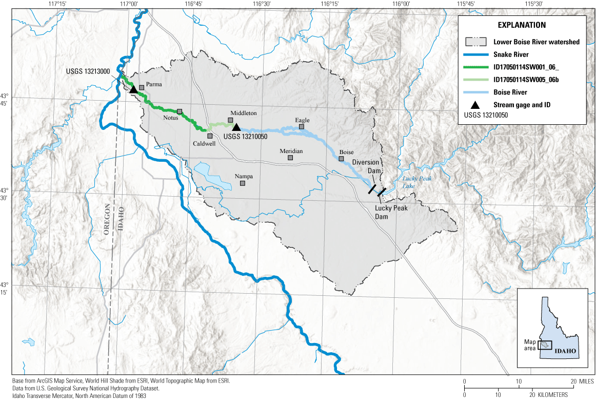
The Boise River watershed, Idaho. The lower Boise River, defined as the Boise River downstream of Lucky Peak Dam, is shown in varying shades to specify impaired units referenced in the 2015 Total Maximum Daily Load (Idaho Department of Environmental Quality, 2015). ID17050114SW001_06_ and ID17050114SW005_06b are assessment unit codes for impaired river reaches and are included for comparison with the in the Idaho Department of Environmental Quality Integrated Assessment (Idaho Department of Environmental Quality, 2022).
Several TP sources within the lower Boise River Basin have been identified. These include municipal sources such as water treatment facilities, industrial sources such as permitted discharges, stormwater sources such as storm drains, and agricultural non-point sources (Mullins, 1998). TP contributions from each source likely have unique annual patterns. Municipal sources likely contribute a relatively constant TP load year-round. Stormwater sources contribute TP load in short-duration events following precipitation and snowmelt events. Agricultural sources likely contribute TP load during the summer via surface runoff and for more extended periods via shallow subsurface return flows of irrigation water to the Boise River (Idaho Department of Environmental Quality, 2015).
In the years since the 2004 Hells Canyon TMDL and the 2015 Boise River TP TMDL were implemented for the Boise River, substantial investments have been made in upgrading wastewater treatment facilities, improving stormwater management, and implementing agricultural best management practices in the lower Boise River watershed (City of Boise, 2019) with the objective of reducing TP concentrations in the Boise River. Additionally, there have been extensive water-quality monitoring efforts in the Boise River dating back more than 40 years (Bureau of Reclamation, 1977; Thomas and Dion, 1974; Mullins 1998; MacCoy, 2004; Etheridge, 2013; Etheridge and others, 2014). In 2015, an intensive water-quality monitoring program began to collect water samples from the Boise River near Parma every 49 hours to produce a temporally dense dataset of TP concentration. These data were collected to (1) track the progress toward meeting the 0.07 mg/L TP target, (2) evaluate common water-quality modeling approaches to extract similar information from less frequent observations in the future, and (3) characterize variability in a highly managed system.
Discharge in the Boise River below Lucky Peak Dam is highly controlled. Discharge in the winter is typically low and stable with a minimum instream flow of 260 cubic feet per second (7.36 cubic meters per second). In the spring, discharge from the reservoir is increased to make room in the reservoir for snowmelt. The timing and magnitude of increased discharge varies from year to year and depends on the snowpack. Nearly all the water that flows from Lucky Peak Reservoir in the winter and spring arrives at the Boise River near Parma site. In contrast, in the summer, a substantial portion of water released from the reservoir is diverted into an extensive network of irrigation canals to irrigate cropland and for other consumptive uses (fig. 1). In some years more water is released from Lucky Peak Reservoir than is needed for instream and diversion flow requirements, typically to mitigate flooding risks in the spring and early summer. In these years, a larger portion of the water released from Lucky Peak Reservoir stays in the Boise River all the way to the Boise River near Parma site. This practice results in elevated discharge in the summer at the Boise River near Parma site in some years. Due to the highly managed and dynamic nature of this system (Thomas and Dion, 1974), high-frequency sampling was required to capture water-quality variability and to track progress toward the target of 0.07 mg/L TP.
The high-frequency TP dataset was also essential to evaluate three common water-quality models: the Weighted Regressions on Time, Discharge, and Season (WRTDS; Hirsch and others, 2010), the WRTDS method with Kalman Filtering (WRTDS_K; Lee and others, 2019), and the Load Estimator (LOADEST; Runkel and others, 2004) models. These models are commonly used to interpolate water-quality conditions between discrete samples based on observed relationships between the modeled parameter and discharge, season, and time of year. Despite their wide-spread use, there is limited evaluation of the uncertainty associated with these models when calibrated with less frequent observations (Lee and others, 2019), especially in systems where discharge is strongly controlled by anthropogenic actions and is mostly decoupled from natural hydrologic forcings. The high-frequency TP dataset from the Boise River near Parma is well suited to quantify the magnitude and timing of uncertainty associated with these models by allowing some observations to be withheld from model calibration and compared against model results.
Purpose and Scope
There are two overarching purposes to this report: (1) quantify trends in TP concentrations and loads in the Boise River near Parma, Idaho from water year 2003 through water year 2021 and (2) compare the performance of three common water-quality models for TP at this site over the study period.
The trends in TP concentrations and loads are reported to document changes over the 19-year study period. During this period, investments have been made in the lower Boise River watershed to reduce TP loading, in part in response to the implementation of a TP TMDL (Idaho Department of Environmental Quality, 2015). This report focuses on quantifying the magnitude and timing of changes in TP concentration and loading. A WRTDS_K water-quality model generated with all the observation data was used to approximate TP loads on dates without TP concentration observations.
Water-quality model performance was evaluated to identify conditions that challenge the underlying assumptions of WRTDS_K and two other common water-quality models, LOADEST and WRTDS. The temporal richness of TP data collected at the Boise River near Parma provides a unique opportunity to evaluate the accuracy of these water-quality models in a highly managed system.
Previous Investigations
Previous studies provide a baseline against which to compare current estimates of TP loading in the Boise River, explain the annual temporal dynamics of phosphorus loading in this system, and illustrate the need for inter-model comparisons.
In 1974, Thomas and Dion (1974) documented a sevenfold increase in TP concentrations from 0.07 mg/L just downstream of Lucky Peak Reservoir to 0.45 mg/L in the Boise River at the confluence with the Snake River. In 1977, the Bureau of Reclamation identified municipal water treatment as the primary source of TP in the lower Boise River watershed (Bureau of Reclamation, 1977). In their study, the Bureau of Reclamation (1977) also found that water quality on the Boise River worsens in the downstream direction. Similar findings of water-quality degradation in the downstream direction were reported in 1989 by the Idaho Department of Environmental Quality (Idaho Department of Health and Welfare, 1989). Mullins (1998) later documented TP loading of up to 3,618 kg/d at the Boise River near Parma from 1994 to 1997 and identified municipal water treatment facilities as the main contributor of TP loading during the non-irrigation season. Mullins (1998) reported a median TP concentration of 0.27 mg/L. In data collected from 1994 to 2002, MacCoy (2004) reported a sevenfold increase in TP concentration from Diversion Dam (fig. 1) to the Boise River near Parma site, which is very similar to the results reported by Thomas and Dion (1974). The median concentration of TP at Parma reported by MacCoy (2004) was 0.30 mg/L and total phosphorus concentrations were found to be negatively correlated with discharge. It was concluded that under high-flow conditions (like those that occurred in 1997), TP concentrations could be comprised largely of particulate phosphorus because of sediment mobilization, indicating that the source of phosphorus could be impacted by hydrologic conditions. In contrast, they found that the orthophosphate percentage was highest in the non-irrigation season and attributed this to groundwater seepage. Further evidence of seasonal impacts on TP sources was seen in the percentage of TP entering the river upstream of Middleton during the irrigation season (24 percent) and non-irrigation season (45 percent). MacCoy (2004) further documented that wastewater treatment plant contributions were 83 percent that of tributaries (486 versus 586 kg/d) during a non-irrigation synoptic, and 69 percent (555 versus 809 kg/d) during the irrigation season. Despite the variations in TP sources and concentrations by season, the median TP load at Parma (909 kg/d) was not significantly influenced by season. Further, MacCoy (2004) found no discernible temporal trends over time in nutrient concentrations from 1994 to 2002.
Multiple previous studies have focused on water-quality modeling for the Boise River (Donato and MacCoy, 2005; Wood and Etheridge, 2011; Etheridge, 2013). Using LOADEST, Donato and MacCoy (2005) identified an annual decrease in TP load in the Boise River near Parma of 2 percent per year from 1994 to 2002. This decreasing trend, which was not evident from the synoptic data alone (MacCoy, 2004), illustrated the utility of incorporating water-quality modeling in trend analysis, as it goes beyond the discrete sampling schedule to estimate conditions throughout the year. Model results indicated that the mean irrigation season TP load ranged from 336 to 1,159 kg/d. They identified the inability to model hysteresis as a potential limitation in model accuracy, indicating the potential utility of a more complex model that allows for the influence of discharge on concentration to vary over time.
Wood and Etheridge (2011) reported on water-quality conditions in the Boise River for water years 2009 and 2010. Their study was the first to identify high-frequency variation in TP concentrations at the Boise River near Parma site using water samples collected every 49 hours that were analyzed for TP. Median TP concentrations of 0.28 and 0.30 mg/L were reported for water years 2009 and 2010, similar to those reported by Mullins (1998) for 1994–1997 (0.27 mg/L), and MacCoy (2004) for 1994–2002 (0.30 mg/L). Wood and Etheridge (2011) reported an average daily TP load of 818 kg/d and 755 kg/d for water years 2009 and 2010, respectively, which are similar to loads estimated from observations (909 kg/d; MacCoy, 2004) and modeling of data in the 1990s (340–1,159 kg/d; Donato and MacCoy, 2005). Wood and Etheridge (2011) also calibrated a seasonally adjusted surrogate model to compute TP concentration from daily mean specific conductance and turbidity data. Specific conductance was assumed to respond to dissolved phosphorus, and turbidity was assumed to respond to particulate phosphorus. The surrogate model was operationally produced for a number of years and was eventually discontinued due to deterioration in model performance attributed to reductions in TP and a shift in the ratio of dissolved to total phosphorus in the absence of corresponding changes in surrogates.
Etheridge (2013) conducted a series of water-quality synoptics and constructed mass balance models for TP loads within the Boise River. In that study, wastewater treatment plants (WWTPs) were identified as the dominant source of TP loading within the watershed. Lander, West Boise, and Nampa WWTPs constituted from 88 to 90 percent of the total point-source TP loads measured from six municipal WWTP permittees during the sampling efforts in 2010 to 2012. Etheridge (2013) further indicated that within-system nutrient cycling may modulate point-source loading signals through biological uptake.
Our comparison of water-quality models builds on previous work conducted outside the Boise River basin. For example, Lee and others (2019) provided a comprehensive review of multiple approaches for estimating annual TP loads. Their analysis included a comparison between LOADEST, WRTDS, and WRTDS_K in computing annual TP load and found WRTDS_K to perform the best over a range of sampling strategies, with 58 to 85 percent of modeled annual TP loads being within 20 percent of the observed annual loads. We build on this analysis here to look at the sub-annual performance of water-quality modeling in a highly managed watershed.
Datasets
Water-Quality Data
Discrete water-quality samples were collected at Boise River near Parma and analyzed for TP (fig. 2; U.S. Geological Survey, 2023). Discrete water-quality samples were collected approximately monthly (average sampling interval of 33 days, ranging from 1 to 143 days) from October 16, 2002 to October 1, 2008, and again from December 31, 2010 to October 1, 2015. These data were collected by USGS Idaho Water Science Center staff using the Equal Width Increment (EWI) method. In the EWI method, the stream cross section is divided into 10 equal-width increments, and samples are collected by lowering and raising a sampler through the water column at each increment at a constant transit rate. These samples are composited in a plastic churn for distribution into bottles during processing (U.S. Geological Survey, variously dated). From water years 2016 through 2021, discrete samples were collected six times per year at the Boise River near Parma site using the EWI method.
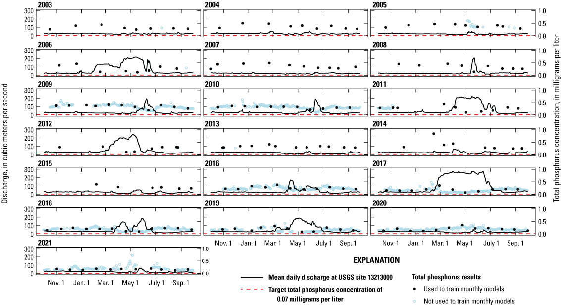
Total phosphorus concentration and discharge, measured at Boise River near Parma, Idaho, October 1, 2002, through September 30, 2021 (U.S. Geological Survey [USGS] site 13213000; U.S. Geological Survey, 2023). Each sub-plot shows 1 water year. Note the periods of prolonged elevated discharge in 2006, 2011, 2012, 2016, 2017, 2018, and 2019.
In addition to discrete sampling, a Teledyne ISCO autosampler was deployed at the monitoring location to increase sampling frequency. From October 1, 2008 to December 31, 2010, samples were collected approximately every 2 days, with one interruption from December 11, 2008 to January 13, 2009. After this period of 2-day sampling, the monthly sampling regime resumed until October 1, 2015. In 2015 the USGS began collection of TP samples with an automated sample collection system once every 49 hours. The 49-hour time interval was selected to collect samples from every hour of the day while collecting a sample approximately every 2 days. This sampling interval was maintained through the end of the study period. The autosampler was configured to sample from a location verified to represent the entire channel’s water-quality conditions for TP (fig. 3). Discrete samples collected coincidently with autosampler samples between 2008 and 2021 were used in this evaluation. Data from discrete samples and samples collected with the autosampler were combined to make a complete dataset that was used to generate the water-quality models for determining trends in TP.
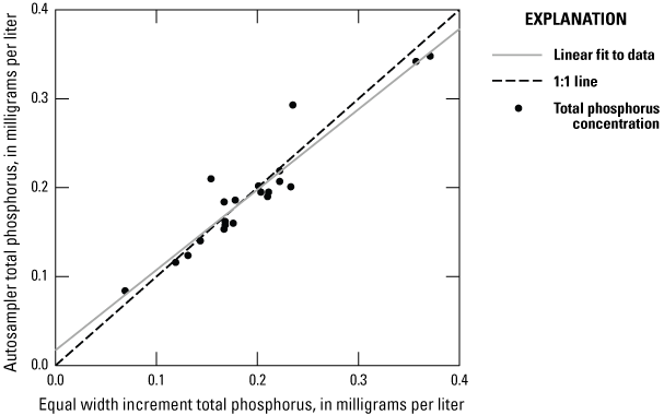
Total phosphorus (TP) concentrations sampled from the left bank by the autosampler are in close agreement with the TP concentrations collected by compositing samples collected across the entire channel using the Equal Width Increment (EWI) method (U.S. Geological Survey, variously dated) at Boise River near Parma, Idaho (U.S. Geological Survey site 13213000; U.S. Geological Survey, 2023).
Samples were analyzed at the USGS National Water Quality Laboratory for TP in mg/L as phosphorus using method I-4650-03 (Patton and Kryskalla, 2003). Samples were transferred to glass culture tubes, alkaline persulfate reagent was added, samples were tightly capped, then digested at 121 degrees Celsius (°C) and 117 kilopascals in an autoclave for 1 hour. Using the alkaline persulfate digestion procedure, all forms of inorganic and organic phosphorus were hydrolyzed to orthophosphate and quantified via photometry in a continuous flow analyzer (Patton and Kryskalla, 2003). Results of this procedure were reported with the USGS parameter code 00665, defined as “phosphorus, water, unfiltered, milligrams per liter as phosphorus.” The unit for this parameter is referred to in the text and figures hereafter as mg/L.
Autosampler-collected samples were compared against EWI-collected samples to verify that they represented the entire channel’s conditions (fig. 3). EWI sampling trips targeted hydrologically distinct times, for example winter storm runoff, near-peak flows, and lowest flows. Twenty-five pairs of samples were collected using the EWI and autosampler methods between 2008 and 2021. The average relative percent difference in TP concentration between autosampler- and EWI-collected samples was 2.6 percent. The median relative percent difference was 1.7 percent and ranged from 0.1 to 8.6 percent. These relative percent differences are considered minimal and confirm that the autosampler-collected samples were representative of whole-channel conditions through time and in various hydrologic conditions.
To verify data integrity, blank and replicate samples were collected throughout the sampling period. Throughout the study period (October 1, 2002 to September 30, 2021), 46 blanks, 139 replicates, and 1,392 regular samples were collected and used for this analysis. Blanks were collected to test field sample collection, sample processing, and laboratory analysis methods for potential sources of contamination. Equipment blanks were collected by passing inorganic blank water through the sampling and processing equipment and were analyzed for TP using the same methods as the environmental samples. These methods are described in detail in the USGS National Field Manual (U.S. Geological Survey, variously dated). Blank collection began in November 2008. Between 2008 through September 2010, the TP reporting level was 0.020 mg/L. No blanks were measured above this level during this time period. The reporting level throughout the rest of the study period was 0.010 mg/L due to improvements in analytical techniques. Three blank samples with concentrations of 0.01, 0.11, and 0.46 mg/L equaled or exceeded the reporting level of 0.010 mg/L TP. Given the three blank results at or above the reporting level, other evidence (for example, temporally correlated seasonal anomalies) of data quality issues was pursued, and none was found. The highest blank result prompted an investigation into data collected one month before and after its collection date of October 30, 2015. The data surrounding this blank did not seem unusual for the time of year they were collected and did not exhibit unusual variability. It was determined that this unusually high blank result does not necessitate deletion of data collected soon before or after its collection time. Despite the aforementioned blank results, we interpret the mostly non-detect blank results (93 percent of blank results) as an indication that the sampling method does not introduce TP.
Split replicates were collected to evaluate laboratory sample analysis methods and sample processing methods. The split replicates were collected with typical sample collection protocol, except two bottles were filled from the churn, rather than one. Split replicates were generated from EWI and autosampler samples. On average, replicates were collected about every 47 days, and one regular sample was collected about every 4.5 days. Split replicate pairs had a maximum relative percent difference of 4.1 percent, a minimum of 0.0 percent, a median of 0.7 percent and a mean of 0.8 percent. Close agreement between the split replicates indicates that sample processing (for example, aliquoting) and laboratory analyses were not significant sources of error.
During 2018, 2019, and 2020, there were 59 cases where the laboratory was not able to analyze samples within their hold times. These delays resulted in several data points being flagged as estimated. Potential effects of these hold time violations were investigated and were determined to be minimal in part because of the lack of a gas phase for phosphorus and its near total digestion in the alkaline persulfate TP analysis method. Even if phosphorus was degraded or transformed before analysis, it is expected to have remained in liquid or solid form in the bottle and therefore would have been digested and measured accurately. Thus, samples that were not analyzed within the recommended 30-day hold times were included in this study.
Discharge Data
The discharge data used for this project were collected by the USGS at the Boise River near Parma (fig. 1). This continuous discharge dataset ranges from 1975 through the present day (2023; U.S. Geological Survey, 2023). While there are some gaps in the discharge record prior to 2002, the data are continuous for the 19-year period of this study (water years 2003 through 2021). Water-quality samples were collected for nearly the full range of observed discharge values at this site, as is illustrated in the discharge duration curve for the study period in figure 4.
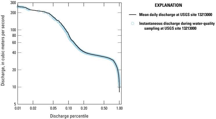
Discharge duration curve showing mean daily discharge at Boise River near Parma, Idaho, October 1, 2002–September 30, 2021 (U.S. Geological Survey [USGS] site 13213000; U.S. Geological Survey, 2023). The instantaneous discharge values at the times that water-quality samples were collected illustrate that all observed discharge conditions are represented in the water-quality observations. Both axes have been logarithmically (base 10) transformed.
Trend Analysis of Discharge and Total Phosphorus
Weighted Regressions on Time, Discharge, and Season Model
To analyze trends in discharge and TP concentration at the Boise River at Parma site, we used the Weighted Regressions on Time, Discharge, and Season (WRTDS) model. The WRTDS model is a statistical water-quality modeling method developed to adapt to changing environmental conditions (Hirsch and others, 2010). The R programming language (R Core Team, 2020) and the EGRET R package (Hirsch and De Cicco, 2015) were used to develop and run the WRTDS model for the Boise River near Parma site.
As a multivariate linear regression model (eq. 1), WRTDS models the natural log of concentration as a function of discharge and time. The discharge component accounts for the relationship between hydrologic processes and water quality, and the time component accounts for seasonality and temporal trends. This relationship is described by:
whereln(ci)
is the natural log of concentration (TP in this case) on day i, in milligrams per liter;
βi0–4
are regression coefficients, in various units;
Qi
is the mean daily discharge on day i, in cubic meters per second;
Ti
is the time since the beginning of the modeling period, in decimal years; and
εi
is the model residual, in milligrams per liter.
The parameter regression coefficients (βi0 – βi4) are date-specific and are computed from a subset of observations that are the most similar to observations on date i in terms of time, discharge, and season. As explained in Hirsch and others (2010), relative weights are assigned to data points based on similarity in discharge, time, and season for every discharge-time combination. Readers are referred to Hirsch and others (2010) for a complete explanation of regression weighting.
Daily flux in kilograms per day is computed from the daily estimates of concentration as:
whereFi
is the daily flux, in kilograms per day;
ci
is the daily estimate of concentration, in milligrams per liter;
Qi
is the daily mean discharge, in cubic meters per second; and
86.4
is a unit conversion factor that converts concentration units from milligrams per liter to kilograms per cubic meter, and discharge units from cubic meters per second to cubic meters per day.
A process known as “flow normalization” was used to detect water-quality trends independent of changes in discharge over the study period. This is done by computing constituent concentrations that would have occurred if every year in the modeling period were an “average” hydrologic year. Flow-normalized concentrations were computed from the WRTDS modeled concentrations and observed discharge as:
whereE[Cfn(T)]
is the flow-normalized concentration for time T (a specific day of a specific year);
w(Q,T)
is the Weighted Regressions on Time, Discharge, and Season (WRTDS) estimate of concentration; and
fTs(Q)
is the probability density function of discharge (Q), specific to a particular time of year, designated as Ts.
For more information on flow normalization, see Hirsch and De Cicco (2015).
After WRTDS was calibrated, the EGRET package was also used to apply the WRTDS_Kalman (WRTDS_K) method. WRTDS_K amends the results from WRTDS by reducing model residuals to zero. Modeled values between observations are adjusted based on the preceding and following observations, based on the assumption that serial correlation exists between observations. For further details on the WRTDS_K formulation, see Lee and others (2019).
Model performance was evaluated with root mean square error (RMSE), bias, and Pearson correlation coefficient (R2) computed from observed and modeled values. RMSE was computed as the square root of the mean squared difference between observed and modeled values. Bias was computed as the mean difference between modeled and observed values. Pearson correlation coefficient was computed as the covariance of modeled and observed values divided by the product of the standard deviation in modeled and observed values.
Trend Analysis Approach—Discharge
Trends in discharge at the Boise River near Parma were evaluated to identify changes in hydrologic conditions and to determine if WRTDS modeling should be run with or without discharge stationarity. Daily discharge values were used to compute annual and monthly mean, 7-day minimum, and 7-day maximum statistics for every water year and every month from October 2002 through September 2021. Mann-Kendall trend tests were used to identify the direction (that is, increase or decrease) in discharge and the statistical significance of changes in discharge. Theil-Sen regression (Sen, 1968; Theil, 1992) was used to compute the average rate of change in discharge over the analysis period. Trends in minimum, mean, and maximum discharge were analyzed at annual and monthly timescales.
Trend Analysis Approach—Total Phosphorus
Trend analyses for TP concentrations and loads were conducted using a WRTDS_K model (Lee and others, 2019) generated with all TP observations available from water year 2003 through water year 2021 (number of samples [n]=1,392) using the default parameter values. Flow-normalized trends were extracted from the underlying model and the rates of change were estimated using bootstrapping in EGRETci (Hirsch and others, 2015).
Flow-normalized trend analysis was used to remove the influence of discharge variability by estimating the concentrations and loads that would have occurred under “normal” discharge conditions. This eliminates the influence of hydrologic variability on water quality and allows for underlying trends to be detected. Annual, seasonal, and monthly summaries were then computed from the daily flow-normalized concentration and load estimates and used to determine temporal trends. Trends in flow-normalized concentrations and loads were summarized as annualized rates of change (for example, milligrams per liter per year and kilograms per day per year) and as percent rates of change. The statistical significance of the trends was determined using a bootstrapping approach available in the R package EGRETci (Hirsch and others, 2015).
Trend Analysis Results
Discharge Trends
WRTDS model configuration requires determination of discharge stationarity over time. Trends in annual discharge show relative stationarity in mean discharge (fig. 5B) and 7-day maximum discharge (fig. 5C) and a decrease in 7-day minimum discharge (fig. 5A) values over the model period. The annual 7-day minimum discharge decrease of 2.3 percent per year was the only statistically significant (p-value less than [<] 0.1) change in discharge at the annual timescale.
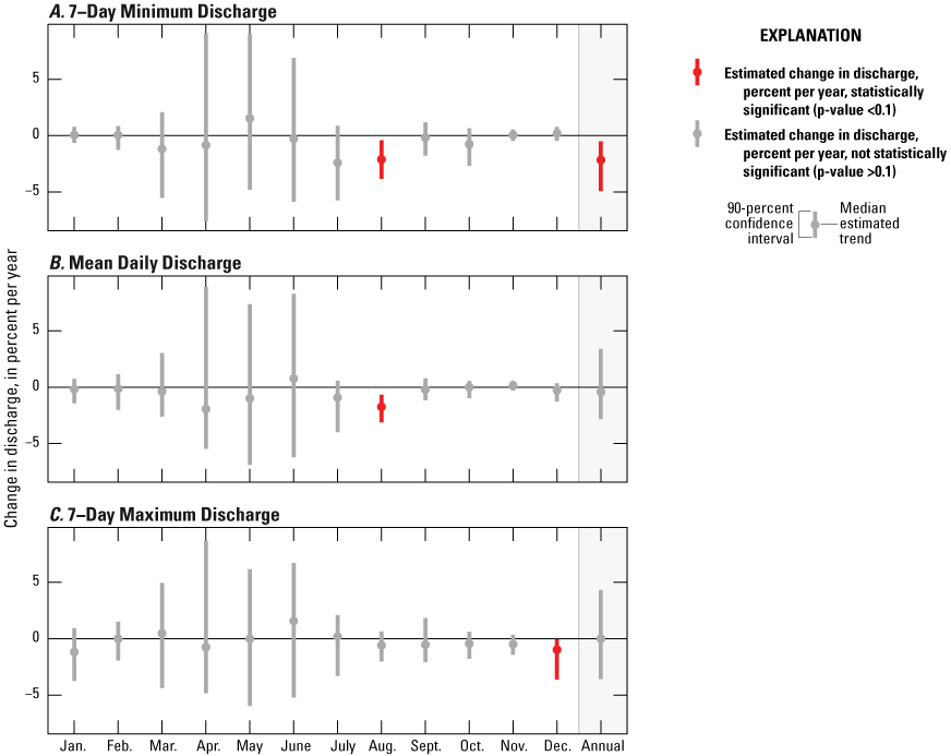
Monthly and annual trends in 7-day minimum discharge (A), mean daily discharge (B), and 7-day maximum discharge (C) at Boise River near Parma, Idaho, water years 2003 to 2021 (U.S. Geological Survey site 13213000; U.S. Geological Survey, 2023). Discharge was relatively stable in annual mean and 7-day maximum discharge and there was a decrease in 7-day minimum discharge. [<, less than; >, greater than.]
At the monthly scale, changes in discharge were statistically significant (p-value <0.1) for August and December, only (fig. 5). There was a 2 percent per year decrease in August for both 7-day minimum (fig. 5A) and mean (fig. 5B) discharge values. Seven-day maximum discharge decreased at a rate of 1 percent per year for December (fig. 5C). The relative stability in discharge for most months and at the annual time scale supports the use of WRTDS modeling which requires stationarity of discharge over time.
Total Phosphorus Trends
WRTDS “half-window” model tuning parameters are typically selected a priori and the model regression coefficients, βi0–4, are computed from observed discharge and concentration records. The a priori selection of “half-window” parameters means that WRTDS models are rarely calibrated in the traditional sense, because no model parameters are tuned to improve performance. Rather, a WRTDS model is fit to observed data. Hereafter we use the term “generate” to identify when a WRTDS model is fit to data in order to distinguish from calibration, where parameters are adjusted to improve model fit. The WRTDS model generated with all observations (n=1,392) had a near-zero bias, low RMSE, and high Pearson correlation coefficient (R2; table 1). Because the majority (67 percent) of observations used to generate this model were collected with the autosampler that was installed in 2015, the prevailing conditions from water years 2016 through 2021 had larger influence on model generation than the conditions from water years 2002 through 2015 (fig. 2).
Table 1.
Model performance metrics for the Weighted Regressions on Time, Discharge, and Season model (WRTDS; Hirsch and others, 2010) calibrated on all total phosphorus concentration observations at Boise River near Parma, Idaho (U.S. Geological Survey site 13213000; U.S. Geological Survey, 2023).[Unit: mg/L, milligram per liter]
Mean total phosphorus concentrations (fig. 6) and loads (fig. 7) decreased during the irrigation and non-irrigation seasons over the modeling period. This is seen for the observed hydrologic conditions (points in figs. 6 and 7), and the flow normalized results (lines in figs. 6 and 7). Non-irrigation season mean concentrations were higher than mean concentrations in the irrigation season early in the modeling period (for example, before about 2012), and became more similar from 2012 through 2021 (fig. 6). From water year 2003 through water year 2021, the annualized rates of decrease in flow-normalized TP concentration and load were 3.3 and 3.4 percent per year, respectively (table 2).
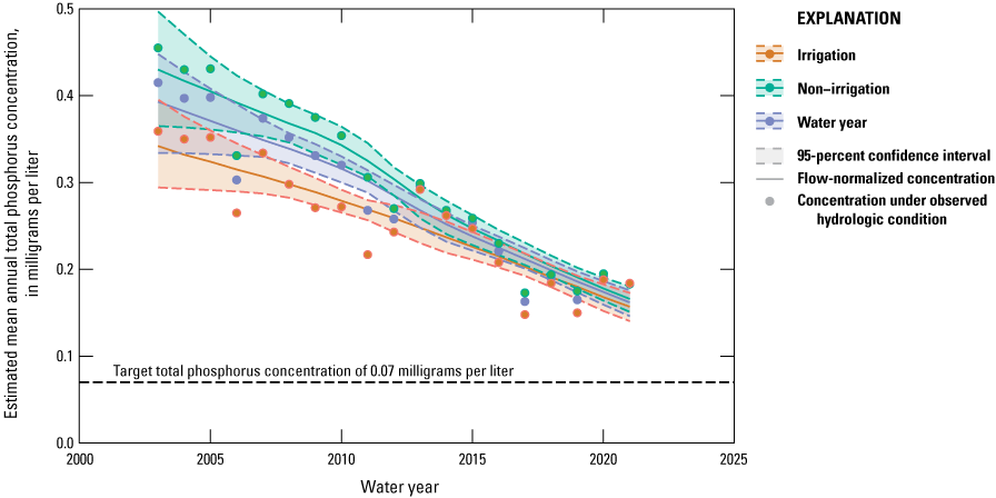
Annual total phosphorus concentrations modeled with the Weighted Regressions on Time, Discharge, and Season model (Hirsch and others, 2010) using observed hydrologic conditions (points) and average (that is, flow-normalized) hydrologic conditions (lines) at Boise River near Parma, Idaho, water years 2003 through 2021 (U.S. Geological Survey site 13213000; U.S. Geological Survey, 2023). Data are presented as average concentrations by water year, the irrigation season (May through September), and non-irrigation season (October through April).
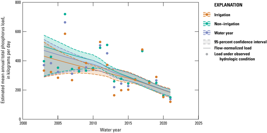
Average daily total phosphorus loads modeled with the Weighted Regressions on Time, Discharge, and Season model (Hirsch and others, 2010) using observed hydrologic conditions (points) and average (that is, flow-normalized) hydrologic conditions (lines) at Boise River near Parma, Idaho, water years 2003 through 2021 (U.S. Geological Survey site 13213000; U.S. Geological Survey, 2023). Data are presented as average daily loads by water year, irrigation season (May through September), and non-irrigation season (October through April).
Table 2.
Annualized trend analysis of flow-normalized Weighted Regressions on Time, Discharge, and Season model (Hirsch and others, 2010) results.[Lower and upper limits are from the 95th percentile of the bootstrapping regression. Non-irrigation, October 1 through April 30; Irrigation, May 1 through September 30. Shading is present for visual grouping. Units: mg/L per year: milligram per liter per year; % per year, percent per year; kg/d per year, kilogram per day per year]
The greatest reductions in total phosphorus concentrations and loads occurred in the non-irrigation period (table 2) of October through April. Results of model bootstrapping, running the model many times to approximate uncertainty, indicate that the downward trends in concentrations and loads are statistically significantly different from zero as the 95th percentile in rates of change (lower and upper limit in table 2) are all negative, indicating that a downward trend is highly likely (Hirsch and others, 2015).
The rate of decline in concentrations, seen in the spacing between water year profiles of monthly mean modeled flow-normalized concentrations in figure 8, illustrates the rapid decrease in modeled flow-normalized concentration in January from 2010 through 2014, coincident with improvements in water treatment facilities within the watershed (City of Boise, 2019). In contrast, the rate of change in the summer months of May and June show a steadier rate of change over the model period (fig. 8). The timing of peak flow-normalized concentrations for an average hydrologic year is modeled to have shifted from January in 2003 to March by water year 2021. Additionally, the modeled annual flow-normalized concentration signal shifted from having a dominant peak in the winter to having a bimodal distribution with nearly equal maximum concentrations in March and July for an average hydrologic year (fig. 8).
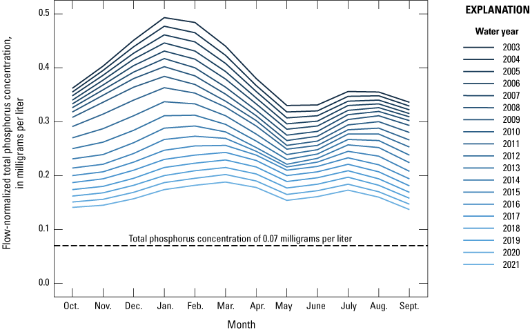
Water-year profiles of monthly mean flow-normalized total phosphorus (TP) concentration modeled with the Weighted Regressions on Time, Discharge, and Season method with Kalman filtering (WRTDS_K; Lee and others, 2019) from water year 2003 through water year 2021. The graph illustrates the pronounced decrease in TP concentrations in January and February.
The monthly mean modeled flow-normalized load signal has been dominated by a single peak in May for the entire modeling period, driven by the frequent high discharge in May (fig. 9). Decreases in monthly mean modeled flow-normalized load were most pronounced for the months of April and May, and least for July and August (fig. 9).
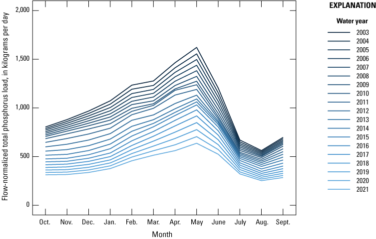
Water-year profiles of monthly mean flow-normalized total phosphorus load modeled with the Weighted Regressions on Time, Discharge, and Season method with Kalman filtering (WRTDS_K; Lee and others, 2019) from water year 2003 through water year 2021. The graph illustrates the pronounced decrease in total phosphorus load in May.
While flow-normalized data are useful for identifying and quantifying trends, actual modeled concentrations and loads are useful for identifying what happened in the system with all the complications of high and low water years. To this end, modeled mean monthly TP concentrations show a steady decrease, with the largest decreases occurring in January and February and an overall reduction in mean annual TP concentration of 0.24 mg/L (table 3). Mean annual TP loads, computed from WRTDS_K and expressed in kilograms of phosphorus per day, reduced from 816 kg/d in water year 2003 to 302 kg/d in water year 2021. Mean monthly loads were modeled to decrease from water years 2003 to 2021 the most for the months of January and February (table 4).
Table 3.
Mean monthly and mean annual total phosphorus concentration, in milligrams per liter, modeled using the Weighted Regressions on Time, Discharge, and Season method with Kalman filtering (Lee and others, 2019) with all total phosphorus observations.[Abbreviations: Oct., October; Nov., November; Dec., December; Jan., January; Feb., February; Mar., March; Apr., April; Aug., August; Sept., September]
Table 4.
Mean monthly and mean annual total phosphorus load, in kilograms per day, modeled using the Weighted Regressions on Time, Discharge, and Season method with Kalman filtering (Lee and others, 2019) generated with all total phosphorus observations.[Abbreviations: Oct., October; Nov., November; Dec., December; Jan., January; Feb., February; Mar., March; Apr., April; Aug., August; Sept., September]
Trends Discussion
Trends in the discharge record show that low flows generally became lower over the modeling period while the mean and high flows were unchanged (fig. 5A–C). At the monthly scale, reductions in low flows were only significant in August. Some potential drivers of the reduction of 7-day minimum and mean August discharge could include an increase in water withdrawal from the river, reduced discharge from drains returning to the river, a reduction in shallow groundwater recharge to the river through increased irrigation efficiency practices and canal lining, increased water re-use and pump-backs within canal systems, and reduced discharge of wastewater to canals in favor of land application and agricultural re-use. Further investigation into trends in each tributary and point sources would be needed to conclusively determine the cause of the reduction in August low flows. The relatively stable discharge records over the modeling period indicate that concentration reductions, as opposed to discharge reductions, are responsible for load reductions and supports the use of WRTDS modeling with stationary flows.
The water-quality trend analysis documents for the first time the significant decrease in TP in the Boise River near Parma and agrees well with previous studies for periods where they overlap. Donato and MacCoy, (2005) reported TP loads between 341 and 1,159 kg/d for the period between 1994 and 2002. The WRTDS_K model generated with all the data suggests a mean annual load of 816 kg/d for water year 2003 (table 4). Wood and Etheridge (2011) reported a TP load of 818 kg/d water year 2009, which is within 5 percent of the modeled annual load in this work for the same year (781 kg/d, table 4). Previous work can be combined to identify a general downward trend in loads from Mullins (1998) who estimated a median daily load of 1,027 kg/d in 1994 through 1997 to Wood and Etheridge (2011) estimating median daily load of 818 kg/d in 2009. That trend is further seen in the results here with mean annual TP loads of approximately 309 kg/d in 2021 (King and Yoder, 2023).
Modeled mean annual TP concentrations were reduced by nearly 60 percent over the 19-year model period (table 3). These reductions are likely from a combination of reductions in loading from a variety of sources. Changes in wastewater treatment systems to increase nutrient removal are expected to reduce nutrient loading year-round. In contrast, the impacts of improvements to stormwater are limited to times of overland flow and runoff. Reductions in stormwater loading can come from improvements in municipal stormwater management (for example, settling basins, retention ponds, and street sweeping programs) as well as reductions in runoff from agricultural lands in response to precipitation events (from, for example, changes in riparian buffers and the use of cover crops). Improvements in irrigated soil stability (for example, conversion from flood irrigation to more targeted irrigation systems and the use of no-till-drills to minimize soil disturbance when planting) are expected to follow a seasonal pattern in response to seasonal irrigation practices. The TP concentrations reduced the most in the months of January and February (table 3) when system loading is expected to be dominated by shallow groundwater, municipal point sources, and stormwater. While there are known investments in each of these potential sources (City of Boise, oral commun., 2023; City of Nampa, oral commun., 2023; City of Meridian, oral commun., 2023; City of Middleton, oral commun., 2023; Ada Country Highway District, oral commun., 2023; Lower Boise Watershed Council, oral commun., 2023; Idaho Power Company, oral commun., 2023) further investigation of loads from various sources within the lower Boise River watershed is needed to attribute the reductions in concentration and load to specific sources and sectors. Analyzing water-quality data collected for permit compliance monitoring and from individual tributaries would assist in attributing system-wide reductions in TP loading.
To place the rate of change by month into context, the year that the mean modeled TP concentration is projected to reach the TMDL target of 0.07 mg/L was computed. Assuming the rates of change observed from water year 2016 through 2021 continue, the mean monthly TP concentration in the Boise River is projected to reach the TMDL target concentration of 0.07 mg/L between water years 2027 and 2040, depending on the month, with February projected to reach this milestone first, and April projected to reach it last (table 5).
Table 5.
Rate of change in modeled total phosphorus concentrations from water years 2016 through 2021 and the year when mean monthly total phosphorus concentrations are projected to equal 0.07 milligrams per liter.[Rate of change: Computed as linear rate of change over water years 2016–21. Water year: Water year when the mean monthly total phosphorus concentration is projected to equal 0.07 milligrams per liter. Shading is present for visual grouping. Unit: mg/L, milligram per liter]
Water-Quality Model Comparison
The second objective of this analysis was to compare the performance of multiple models in reproducing observed total phosphorus (TP) in this system where discharge is highly regulated and manipulated and sources of TP vary. Performance was evaluated by generating water-quality models using observations selected at roughly monthly intervals and assessing the resulting models’ performances using the remaining observations. Model performance was evaluated by month, season, and year to identify conditions that may impact model accuracy.
Models Used in Comparison
WRTDS (Hirsch and others, 2010), WRTDS_K (Lee and others, 2019), and the Load Estimator (LOADEST; Runkel and others, 2004) models were evaluated in the inter-model comparison. The WRTDS and WRTDS_K models are described in the “Trend Analysis of Discharge and Total Phosphorus” section. LOADEST is a common water-quality model that is often applied to interpolate water-quality conditions in systems where discharge and season have a strong relationship with water quality. The LOADEST model can take on multiple forms as given below:
whereL
is the modeled daily load;
a0 and a1
are tuned model parameters;
ln(Q)
is the natural log of discharge;
L
is the modeled daily load;
a0–2
are tuned model parameters;
Q
is mean daily discharge;
dtime
is decimal time;
L
is the modeled daily load;
a0–3
are tuned model parameters;
Q
is mean daily discharge;
dtime
is decimal time;
L
is the modeled daily load;
a0–3
are tuned model parameters;
Q
is mean daily discharge;
dtime
is decimal time;
L
is the modeled daily load;
a0–4
are tuned model parameters;
Q
is mean daily discharge;
dtime
is decimal time;
L
is the modeled daily load;
a0–4
are tuned model parameters;
Q
is mean daily discharge;
dtime
is decimal time;
L
is the modeled daily load;
a0–5
are tuned model parameters;
Q
is mean daily discharge;
dtime
is decimal time; and
L
is the modeled daily load;
a0–6
are tuned model parameters;
Q
is mean daily discharge; and
dtime
is decimal time.
Decimal time, which is included in the description of the variable dtime, is the time and date of interest divided by the full time period of the model. The equation used in modeling water quality is selected in an automated fashion by starting with the simplest model and adding more explanatory variables until the model performance no longer improves. The model that produces the lowest Akaike Information Criterion (Akaike, 1974) statistic is then used to model concentration and load.
Datasets Used in Comparison
To evaluate the performance of the water-quality models, discharge and water-quality data from water years 2003 through 2021 were split into two datasets: “monthly” and “validation.” The monthly dataset was created by resampling the original complete dataset with an average interval between data points of 33-days (fig. 2). This was done by creating a list of targeted dates on a 33-day interval and selecting the discrete water-quality observation that was closest in time to each date in the list (King and Yoder, 2023). Each observation was only included once in the monthly dataset. This dataset was used to generate water-quality models using LOADEST, WRTDS, and WRTDS_K.
The validation dataset was used to test and validate water-quality model results. This dataset was created by selecting all remaining data points that were not included in the monthly dataset. Summary statistics for each dataset are available in table 6 and the monthly and validation datasets are shown in figure 2 (King and Yoder, 2023). The majority (72 percent) of validation samples were collected in the second half of the study period, meaning that model results from water years 2011 through 2021 have greater influence on the performance metrics.
Table 6.
Summary statistics for each dataset used to compare water-quality models.[Total phosphorus (TP) concentration is given in milligrams per liter; Full, Monthly and Validation datasets refer to the models generated with all TP observations, with TP observations collected approximately every month, and with all of the data not in the monthly dataset, respectively]
Model Selection and Generation
The LOADEST model was selected and the WRTDS model was calibrated using the monthly dataset. Each model’s performance was evaluated using both the “monthly” and “validation” datasets. The model performance evaluation with the monthly data (used for model generation) was implemented to reflect what a user would produce in a typical situation where only monthly data are available. The model performance evaluation with the validation dataset was implemented to test each model's ability to estimate concentrations of samples not included in the monthly dataset which was used to generate the model results. Model performance statistics were computed from residuals, defined here as modeled minus observed values (fig.10), for both the monthly and the validation data.
Model performance was evaluated by calculating the following model diagnostics (with both monthly and validation data) for both concentration and load: RMSE, bias (calculated by taking the sum of all the residuals and dividing it by the number of residuals), and Pearson correlation coefficient (R2). RMSE was calculated to provide an estimate of the magnitude of model error, bias was calculated to determine the average direction of error (that is, over or under prediction), and R2 was calculated for comparison between model outputs. Ultimately, the most suitable model of each model type (WRTDS and LOADEST) was chosen by selecting the model equation (LOADEST) and model input parameters (WRTDS) that produced the lowest RMSE of concentration generated with monthly data. The RMSE was chosen as the primary metric over other performance metrics because of its sensitivity to large errors. The WRTDS model selected in this section was used to generate the WRTDS_K model used in the model comparison below. The potential model choices for LOADEST were LOADEST models 1–9. LOADEST-8 was selected with an RMSE of 0.072 mg/L for concentration, and 436 kg/d for load. There were no adjusted model parameters for the LOADEST-8 model. Hereafter, the LOADEST model used in the comparison will be referred to as the LOADEST-8 model.
Three WRTDS weighting parameters, windowY, windowS, windowQ, were calibrated prior to model comparison. The three terms control how similar a data point must be in time (windowY, units of years) season (windowS, units of years), and discharge (windowQ, units of natural logarithm of cubic meters per second) to be included in the weighted regression for a given time-discharge combination. These terms define half of the width of the search space within which observations will be included and are referred to in the WRTDS documentation as “half-windows.” For example, for windowY = 1, all values within one year of an observation (in other words, a 2-year window) are used in the temporal term of the WRTDS regression. In the calibration process, a range of values was set for each parameter from the WRTDS documentation (Hirsch and others, 2010), and 1,089 combinations of parameter values were tested (table 7). The parameter set that produced the lowest RMSE of concentration was selected as the optimal parameter combination (table 7). The RMSE in the calibration process ranged from 0.069 to 0.072 mg/L. The default values were used for the other modifiable parameters, minNumObs, minNumUncen, and edgeAdjust. These parameters are described in detail in (Hirsch and others, 2010).
Table 7.
Default Weighted Regressions on Time, Discharge, and Season (WRTDS; Hirsch and others, 2010) model parameters, minimum and maximum parameter values used for calibration, and parameter values selected for generation of the WRTDS and WRTDS with Kalman filtering (Lee and others, 2019) models with monthly data.[windowY, the half-width window for time weighting, in years; windowS, half-width window for seasonal weighting, in years; windowQ, half-width window for weighting based on ln(Q); WRTDS, Weighted Regressions on Time, Discharge, and Season model (Hirsch and others, 2010); WRTDS_K, Weighted Regressions on Time, Discharge, and Season method with Kalman filtering (Lee and others, 2019)]
A summary of model results using the selected and calibrated models are provided in table 8 and table 9 for concentration and load, respectively.
Table 8.
Summary statistics of model results and validation data, shown as total phosphorus concentration in milligrams per liter.[The validation dataset is observed data, not model results, and is shown here for comparison purposes. Concentration units are milligrams per liter. Abbreviations: WRTDS, Weighted Regressions on Time, Discharge, and Season model (Hirsch and others, 2010); WRTDS_K, Weighted Regressions on Time, Discharge, and Season method with Kalman filtering (Lee and others, 2019); LOADEST-8, Load Estimator model 8 (Runkel and others, 2004)]
Table 9.
Summary statistics of model results and validation data, shown as total phosphorus load in kilograms per day.[The validation dataset is observed data, not model results, and is shown here for comparison purposes. Load units are kilograms per day. Abbreviations: WRTDS, Weighted Regressions on Time, Discharge, and Season model (Hirsch and others, 2010); WRTDS_K, Weighted Regressions on Time, Discharge, and Season method with Kalman filtering (Lee and others, 2019); LOADEST-8, Load Estimator model 8 (Runkel and others, 2004)]
Model Comparison Results
For comparison purposes, we report model performance based on RMSE of reproducing the observed TP concentration reported in the validation dataset. These observation data were withheld from model generation to represent an independent evaluation dataset. Most of the validation data (72 percent) were observed during the second half of the model period and are therefore mostly representative of model performance from water years 2011 through 2021.
Load Estimator Model—Concentration
LOADEST-8 had an RMSE of 0.071 mg/L and an overprediction bias of 0.0073 mg/L (table 10) relative to the validation data. The overprediction bias increased throughout the study period, with a median concentration residual of 0.00 mg/L during water years 2003–2010, and a median residual of 0.02 mg/L during water years 2011–2021 (table 11). This is expected because the validation data are skewed towards more recent observations that tend to have lower concentrations. LOADEST-8 had smaller biases during the irrigation season (May 1–September 30) than the rest of the year throughout the study period with the lowest monthly bias in August (–0.0034 mg/L) and highest in January (0.031 mg/L; fig. 11). LOADEST-8 produced the largest monthly RMSE values in April and the lowest monthly RMSE values in September (fig. 12). Seasonality in performance coincides with the seasonality in observed TP concentrations (fig. 13), with smaller model error associated with periods of lower variance in TP concentrations.
Table 10.
Overall model performance metrics computed with total phosphorus concentration residuals (observed minus predicted) for each model type for models generated with monthly data.[Statistics in the Monthly data and Validation data columns represent model output as compared with the monthly and validation datasets, respectively. Abbreviations: LOADEST-8, Load Estimator 8 model (Runkel and others, 2004); WRTDS, Weighted Regressions on Time, Discharge, and Season model (Hirsch and others, 2010); WRTDS_K, Weighted Regressions on Time, Discharge, and Season method with Kalman filtering (Lee and others, 2019); RMSE, root mean square error; R2, Pearson correlation coefficient. Unit: mg/L, milligram per liter]
Table 11.
Summary statistics of model performance relative to validation data and mean daily total phosphorus load estimates from each model.[Data in bottom two rows represent mean metrics for a given range of water years. Abbreviations: Conc., concentration; LOADEST-8, Load Estimator model 8 (Runkel and others, 2004); WRTDS, Weighted Regressions on Time, Discharge, and Season model (Hirsch and others, 2010); WRTDS_K, Weighted Regressions on Time, Discharge, and Season method with Kalman filtering (Lee and others, 2019); WRTDS_K full, WRTDS_K model generated with all observed concentration data and used for the trend analysis; —, no validation data with which to compute model performance. Units: kg/d, kilogram per day; mg/L, milligram per liter]
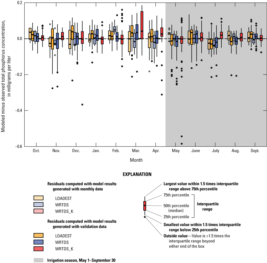
Monthly distribution of concentration residuals, defined as modeled minus observed. One outlier at –1.4 milligrams per liter from the April Weighted Regressions on Time, Discharge, and Season method with Kalman filtering (WRTDS_K; Lee and others, 2019) validation data residuals series is not shown because it is outside of the plot range. Lighter colors represent residuals computed with model results generated with monthly data, while darker colors represent residuals computed with model results generated with validation data. [>, greater than.]
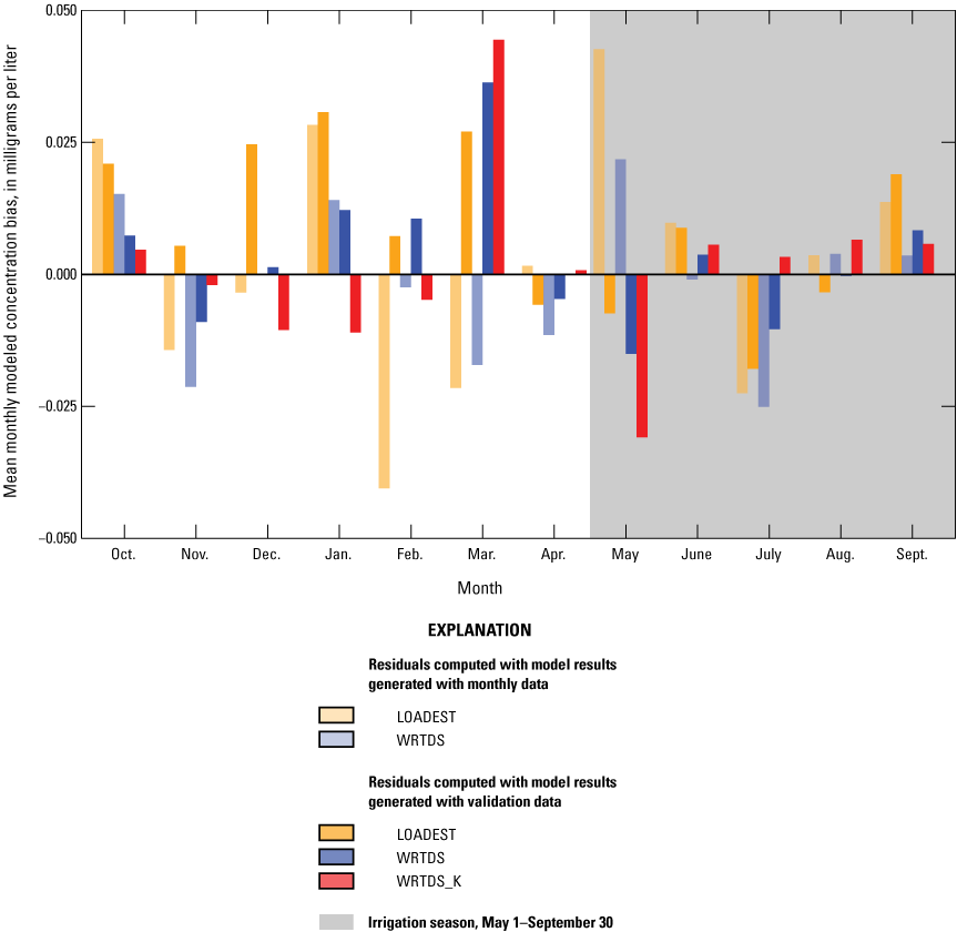
Mean monthly bias of modeled daily average concentrations and observed concentrations of total phosphorus. Lighter columns are the bias calculated with monthly data. Darker columns are the bias calculated with validation data. Weighted Regressions on Time, Discharge, and Season method with Kalman filtering (WRTDS_K, Lee and others, 2019) monthly data bias columns do not show up because they are all equal to zero, as expected from the WRTDS_K method.
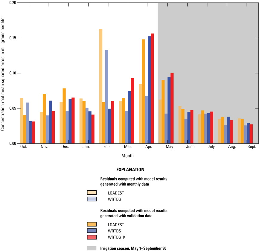
Mean monthly root mean squared error (RMSE) of modeled daily total phosphorus concentration. Lighter columns are the RMSE calculated with monthly data, darker columns are the RMSE calculated with validation data. Weighted Regressions on Time, Discharge, and Season method with Kalman filtering (WRTDS_K; Lee and others, 2019) monthly data RMSE columns do not show up because they are all equal to zero, as expected from the WRTDS_K method.
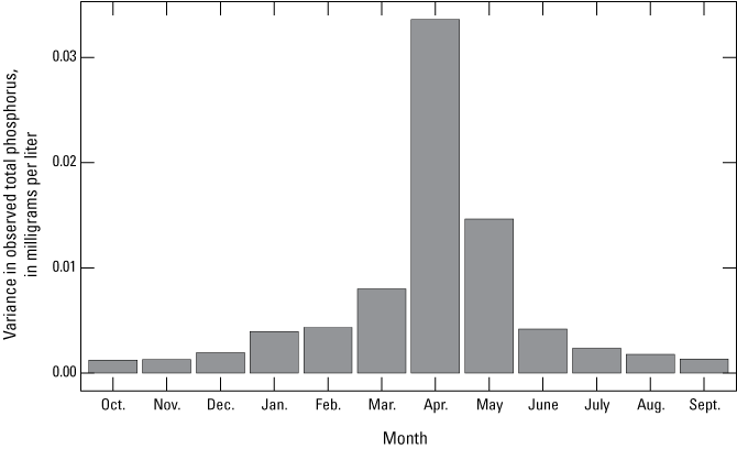
Variance in observed concentrations for water years 2016–2021. The increased variance in April coincides with poor model performance, while the decreased variance in July through November corresponds to increased model performance.
Load Estimator Model—Load
Overprediction in concentration resulted in an overprediction in load as well, as seen in the median residual and bias in load computed by LOADEST-8 relative to the validation data (table 12). Throughout the 19-year study period, residuals show that the model trended from slightly underpredicting during the beginning of the study period to overpredicting at the end of the study period (table 11). Seasonally, the model performed best during irrigation season based on all three performance metrics (fig. 14; table 13). On a monthly basis according to RMSE, model performance was best during August and worst during April (fig. 15). On a monthly basis, model bias was smallest during August and largest during March (fig. 16).
Table 12.
Overall model performance metrics computed with total phosphorus load residuals (observed minus predicted) for each model type generated with monthly data.[Statistics in the Monthly data and Validation data columns represent model output as compared with the monthly and validation datasets, respectively. Abbreviations: LOADEST-8, Load Estimator 8 model (Runkel and others, 2004); WRTDS, Weighted Regressions on Time, Discharge, and Season model (Hirsch and others, 2010); WRTDS_K, Weighted Regressions on Time, Discharge, and Season method with Kalman filtering (Lee and others, 2019); RMSE, root mean square error; R2, Pearson correlation coefficient. Unit: kg/d, kilogram per day]
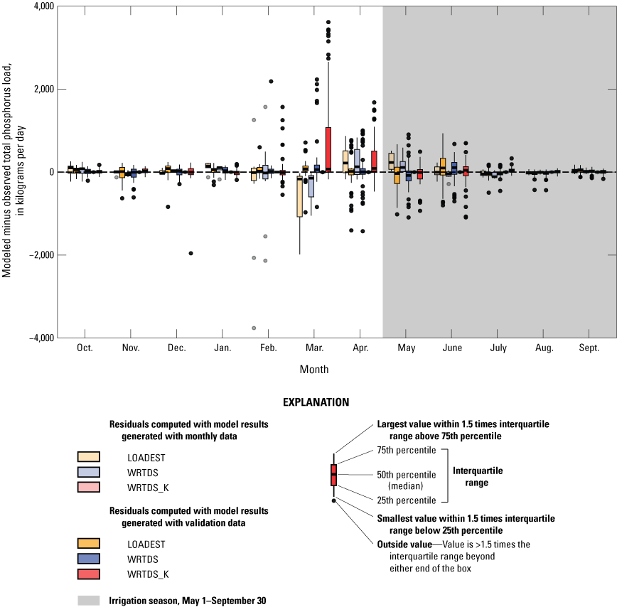
Monthly distribution of load residuals, defined as modeled minus observed. Lighter colors represent residuals computed with monthly data, while darker colors represent residuals computed with validation data. [>, greater than.]
Table 13.
Seasonal model performance metrics computed with total phosphorus load residuals from each model for the irrigation and non-irrigation seasons.[Irrigation season is defined as May 1–September 30; non-irrigation season is October 1–April 30. Abbreviations: RMSE, root mean square error; LOADEST-8, Load Estimator model 8 (Runkel and others, 2004); WRTDS, Weighted Regressions on Time, Discharge, and Season model (Hirsch and others, 2010); WRTDS_K, Weighted Regressions on Time, Discharge, and Season method with Kalman filtering (Lee and others, 2019); Non-irr, non-irrigation. Unit: kg/d, kilogram per day]
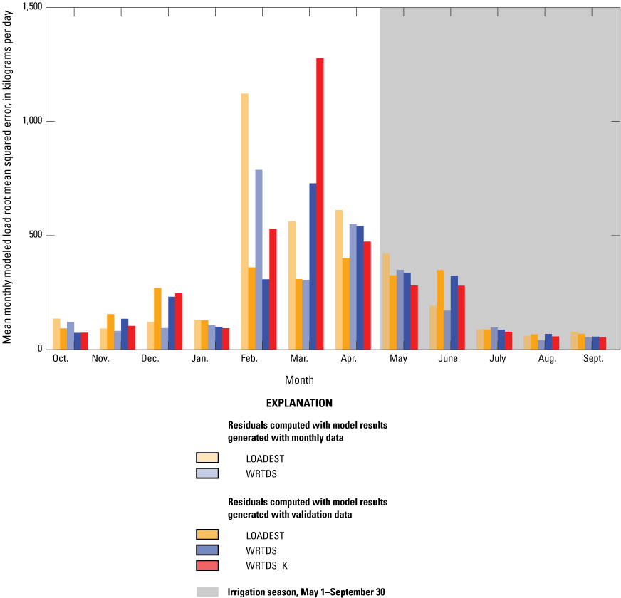
Mean monthly root mean squared error (RMSE) of modeled daily average load and observed load of total phosphorus. Lighter columns are the RMSE calculated with monthly data, and darker columns are the RMSE calculated with validation data Weighted Regressions on Time, Discharge, and Season method with Kalman filtering (WRTDS_K; Lee and others, 2019) monthly data RMSE columns do not show up because they are all equal to zero, as expected from the WRTDS_K method.
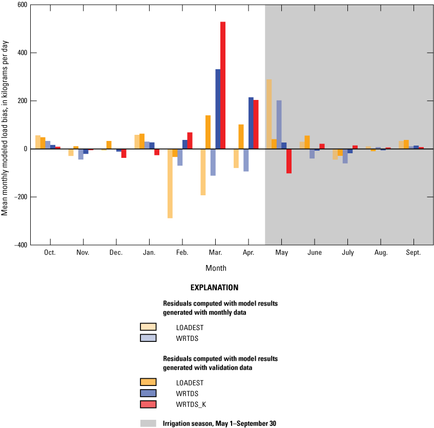
Monthly bias of modeled daily average total phosphorus load. Lighter columns represent model results generated with monthly data, while the darker columns represent validation data. Weighted Regressions on Time, Discharge, and Season method with Kalman filtering (WRTDS_K; Lee and others, 2019) monthly bias columns do not show up because they are all equal to zero, as expected from the WRTDS_K method.
Weighted Regressions on Time, Discharge, and Season Model—Concentration
The WRTDS model had a median residual of 0.0074 mg/L and a bias of 0.0024 mg/L (table 10) compared with the validation data. There was a shift from overprediction, or positive bias, for the water years 2003–10 to underprediction, or negative bias, during water years 2011–21 (table 11). Model fit was better during water years 2003–10 than during the second half of the study period (table 11). This difference in performance during the first and second halves of the study period was likely due to samples being collected more frequently during the second half of the study period.
Model residuals were smallest during irrigation season (table 14). The median residual shows that the model overpredicted during both irrigation and non-irrigation season, while the bias shows that the model overpredicted during non-irrigation season and slightly underpredicted during irrigation season (table 14). The WRTDS model’s RMSE was lowest in September and highest in April (fig. 12), which coincides with variation in observed TP concentrations (fig. 13).
Table 14.
Seasonal model performance metrics computed with total phosphorus concentration residuals from each model for the irrigation and non-irrigation seasons.[Irrigation season is defined as May 1–September 30; non-irrigation season is October 1–April 30. Residual computed as observed minus modeled. Abbreviations: RMSE, root mean squared error; LOADEST-8, Load Estimator model 8 (Runkel and others, 2004); WRTDS, Weighted Regressions on Time, Discharge, and Season model (Hirsch and others, 2010); WRTDS_K, Weighted Regressions on Time, Discharge, and Season method with Kalman filtering (Lee and others, 2019); Non-irr., non-irrigation. Unit: mg/L, milligram per liter]
Weighted Regressions on Time, Discharge, and Season Model—Load
On average, WRTDS performed well relative to validation data-calculated load. The slight overprediction in modeled concentration produced slight overprediction in load as seen in the positive median residual and bias in load in table 12. WRTDS overpredicted loads during water years 2003–2010 and underpredicted in 2011–2021, with poorer relative model performance in the second half of the modeling period (table 11). Note that 74 percent of validation data observations were collected during the second half of the study period, covering a wider range of conditions and skewing toward lower concentrations which could impact the model performance metrics. Seasonally, the WRTDS model produced smaller residuals in the irrigation season compared with the non-irrigation season (fig. 14; table 13). Both the residual median and bias indicate that the model overpredicted during both seasons (table 13). The WRTDS model’s RMSE of load was smallest in September and largest in March (fig. 15).
Weighted Regressions on Time, Discharge, and Season Method with Kalman Filtering—Concentration
When compared to validation data, WRTDS_K performed well and slightly overpredicted TP concentrations (table 10). WRTDS_K shifted from slightly underpredicting concentration from 2003 through 2010 to slightly overpredicting in the period from 2011 through 2021 (table 11). Seasonally, model performance was better during irrigation season than non-irrigation season and the residual median indicated a consistent overpredicting in concentration (table 14; fig. 11). On a monthly basis, WRTDS_K performed best during September and worst during April according to RMSE (fig. 12). As with the other models, seasonality in performance coincided with the seasonality in observed TP concentrations (fig. 13), with better model performance associated with periods of lower variance in TP concentrations (for example, late summer).
Weighted Regressions on Time, Discharge, and Season Method with Kalman Filtering—Load
Throughout the study period, the WRTDS_K model overestimated loads relative to validation data (table 12). Over time, model performance decreased and went from slightly underpredicting during water years 2003–2010 to overpredicting during water years 2011–2021 (table 11). Seasonally, residuals in WRTDS_K modeled loads were smaller during the irrigation season than in the non-irrigation season (table 13). Residual median values in load for the WRTDS_K model were positive during both the irrigation and non-irrigation seasons (table 13). On a monthly basis, WRTDS_K modeled loads produced the smallest RMSE in September and largest RMSE in March (fig. 15). According to bias, model performance was best during November and worst during March (fig. 16).
Model Comparison Discussion
Differences between models were subtle, and no single model performed notably better than the others when generated using monthly data and compared with the validation dataset. All the models overpredicted concentration, resulting in an overprediction in load, especially during spring high flows. None of the models were able to reproduce the observed range of concentrations, which is expected from these models that regress to the mean and do not replicate the extremes in data. Additionally, the model produced mean daily estimates while the observations are instantaneous, which can lead to an underestimation in the range of model predictions.
When interpreting our results, it is important to acknowledge that the modeled TP values represent mean daily concentrations while the monthly and validation data are instantaneous measurements collected during a very short (less than 5 minute) period of time within a day. As such, there is an implicit assumption that instantaneous observations represent mean daily values which may not be accurate on days with large variability in discharge. It is also important to acknowledge that 72 percent of the validation data were collected in the second half of the study period, meaning that the performance metrics are weighted towards the 2011 through 2021 water years. Given that observed concentrations were lower in more recent observations, this may contribute to the overprediction in model output for recent times that was observed in all three models (table 11).
Evaluation of Model Results Generated with Monthly Data
Of the three water-quality models, WRTDS_K produced the smallest residuals in both concentration (table 10) and load (table 12) compared with the monthly data used to train the models. This is inherent in its formulation, which reduces residuals to zero. In the absence of a validation dataset, we would conclude that the WRTDS_K model outperformed the other models in this system because it produced the smallest residuals. However, when evaluated against the validation data, we see that WRTDS_K produced higher RMSE values in both concentration (table 10), and loads (table 12) than were produced by WRTDS and LOADEST-8. This illustrates the importance of dedicated validation data (separate from the data used to build the model) for evaluating model performance.
To put model performance into context, figures 17–20 illustrate times when the models generated with monthly data did or did not reproduce the observed TP concentrations. The WRTDS_K model generated with all the observations from the first section of this report is included in the figures 17–20 to represent an approximation of the actual concentrations over time. Figure 17 highlights that the concentration-to-discharge relationship is modeled to vary by time and season in WRTDS, as seen by the reversal in modeled TP concentration because of a peak in discharge from December 2009 to January 2010 while LOADEST produced a dilution effect for both discharge peaks. Also note that a second, smaller peak in observed TP concentration in mid-January 2010 was not accompanied by a significant change in discharge, and that none of the models reproduced this feature (fig. 17).
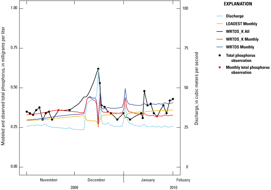
Observed and modeled total phosphorus concentrations and observed discharge at Boise River near Parma, Idaho, November 2009 to February 2010 (U.S. Geological Survey site 13213000; U.S. Geological Survey, 2023). This example illustrates a period when all monthly models failed to identify a peak in total phosphorus during a high flow event in December 2009. [LOADEST Monthly, Load estimation model 8 (Runkel and others, 2004) trained with approximately monthly observations of total phosphorus; WRTDS_K All, Weighted Regression on Time Discharge and Season with Kalman Filtering model (Lee and others, 2019) trained with all available total phosphorus observations; WRTDS_K Monthly, Weighted Regression on Time Discharge and Season with Kalman Filtering (Lee and others, 2019) model trained with approximately monthly total phosphorus observations; WRTDS Monthly, Weighted Regression on Time Discharge and Season model (Hirsch and others, 2010) trained with approximately monthly total phosphorus observations.]
In early 2014, there was a winter storm that produced a high TP concentration of approximately 0.8 mg/L (fig. 18). The WRTDS_K model recreates this peak because the observation is included in the monthly dataset which was used for model generation. Note that other, larger discharge peaks including one just a few weeks later did not produce the same TP concentration, highlighting the complexity of TP dynamics in this system.
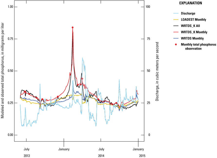
Observed and modeled total phosphorus concentrations and observed discharge at Boise River near Parma, Idaho, July 2013 through January 2015 (U.S. Geological Survey site 13213000; U.S. Geological Survey, 2023). This period illustrates a period when the Weighted Regressions on Time, Discharge, and Season model (WRTDS) and Load Estimator model (LOADEST) missed a peak in total phosphorus concentrations that WRTDS_K and WRTDS_K All models recreated because the observation happened to fall within the “monthly” dataset. WRTDS and LOADEST models generated with monthly data did not identify this as a time of elevated concentration. Note that all observations in this period were used in calibration, so no total phosphorus observation data (black dots shown in figs. 17, 19, and 20) are visible. [LOADEST Monthly, Load estimation model 8 (Runkel and others, 2004) trained with approximately monthly observations of total phosphorus; WRTDS_K All, Weighted Regression on Time Discharge and Season with Kalman Filtering (Lee and others, 2019) model trained with all available total phosphorus observations; WRTDS_K Monthly, Weighted Regression on Time Discharge and Season with Kalman Filtering model (Lee and others, 2019) trained with approximately monthly total phosphorus observations; WRTDS Monthly, Weighted Regression on Time Discharge and Season model (Hirsch and others, 2010) trained with approximately monthly total phosphorus observations.]
In April 2017, WRTDS_K overestimated TP concentrations because concentrations in the monthly dataset were higher than the adjacent points (fig. 19). WRTDS and LOADEST were closer to the observed concentrations during this period because they were not forced through the monthly observation data points. All the models performed well from about May 2017 to October 2017 as the concentration ranges were limited and followed a predictable pattern (fig. 19).
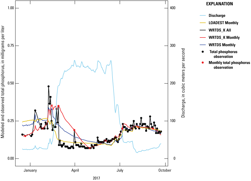
Observed and modeled total phosphorus concentrations and observed discharge at Boise River near Parma, Idaho, December 2016 to October 2017, (U.S. Geological Survey site 13213000; U.S. Geological Survey, 2023). The graph shows a period when the Weighted Regressions on Time, Discharge, and Season method with Kalman filtering model trained with monthly data (WRTDS_K Monthly) overestimated total phosphorus concentrations because two calibration points were higher that the adjacent validation points. The Weighted Regressions on Time, Discharge, and Season model (WRTDS) and Load Estimator model (LOADEST) were closer to the observed concentrations during this period because they were not forced through the elevated calibration data points. The Weighted Regressions on Time, Discharge, and Season model with Kalman filtering trained with all the data (WRTDS_K All) is included as an approximation of actual total phosphorus concentrations. [LOADEST Monthly, Load estimation model 8 (Runkel and others, 2004) trained with approximately monthly observations of total phosphorus; WRTDS_K All, Weighted Regression on Time Discharge and Season with Kalman Filtering (Lee and others, 2019) model trained with all available total phosphorus observations; WRTDS_K Monthly, Weighted Regression on Time Discharge and Season with Kalman Filtering model (Lee and others, 2019) trained with approximately monthly total phosphorus observations; WRTDS Monthly, Weighted Regression on Time Discharge and Season model (Hirsch and others, 2010) trained with approximately monthly total phosphorus observations.]
The pattern at the end of summer 2017 (fig. 19) was repeated in 2019 (fig. 20), and all three models correctly identified the increase in TP concentration that coincides with the decrease in discharge at the end of the spring release.
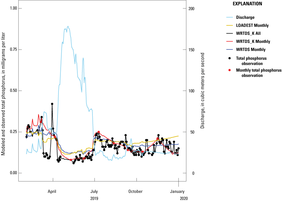
Observed and modeled total phosphorus concentrations and observed discharge at Boise River near Parma, Idaho, February 2019 to January 2020 (U.S. Geological Survey site 13213000; U.S. Geological Survey, 2023). This example period illustrates an increase in observed total phosphorus concentrations coincident with the end of the spring/summer high discharge. This event in 2019 was successfully identified by all three monthly models indicating a consistent relationship between the end of elevated discharge in the early summer and an increase in total phosphorus concentrations. The Weighted Regressions on Time, Discharge, and Season model with Kalman filtering trained with all the data (WRTDS_K All) is included as an approximation of actual total phosphorus concentrations. [LOADEST Monthly, Load estimation model 8 (Runkel and others, 2004) trained with approximately monthly observations of total phosphorus; WRTDS_K All, Weighted Regression on Time Discharge and Season with Kalman Filtering (Lee and others, 2019) model trained with all available total phosphorus observations; WRTDS_K Monthly, Weighted Regression on Time Discharge and Season with Kalman Filtering model (Lee and others, 2019) trained with approximately monthly total phosphorus observations; WRTDS Monthly, Weighted Regression on Time Discharge and Season model (Hirsch and others, 2010) trained with approximately monthly total phosphorus observations.]
Model Performance Through Time
Concentration estimates from every model produced small summary statistics on residuals, indicating that they were able to capture some components of the watershed system’s relationships between explanatory variables and concentration (table 10). Visible as a cluster in the lower parts of figs. 21C and 21F, the WRTDS_K model overpredicted concentrations for a certain group of observations. The data comprising these clusters fall within the first quarter of 2017 and 2019 and correspond with higher-than-usual flows. This cluster isn’t visible for LOADEST or WRTDS, indicating that WRTDS_K overpredicted more and differently than the other models in these instances of high flows.
Underprediction of the highest loads by LOADEST-8 and WRTDS is also shown in figure 21D and 21E. These periods may represent instances when discharge was high and brought higher concentrations than the models’ defined relationship between concentration and discharge estimated. Additionally, overprediction or underprediction can occur when a monthly calibration data point does not accurately reflect the mean condition of the concentration in the period it represents. This is a factor with all the models but can be exaggerated in the WRTDS_K model results because the approach forces model results through the calibration data (fig. 19). In the case of loads, WRTDS also has a group of overpredictions (fig. 21E). However, these overestimates are smaller than those of WRTDS_K, some by almost half. Unlike the concentration observations and predictions, the load estimates from WRTDS and WRTDS_K overpredicted enough to flatten the slope of the linear fit to 0.71, and 0.55, respectively (fig. 21E and 21F).
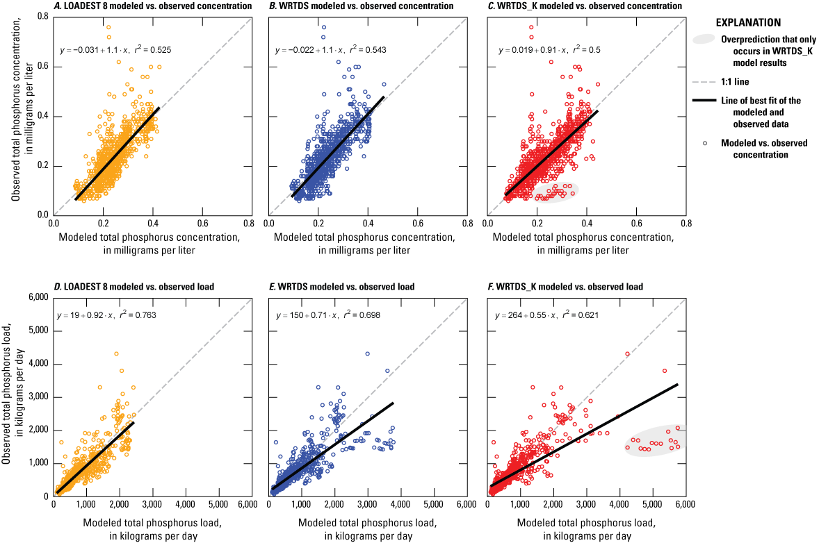
Modeled versus observed total phosphorus concentration and load for the validation dataset (King and Yoder, 2023). The top row shows concentration in milligrams per liter (A–C) and bottom row shows load in kilograms per day (D–F). The equation for the linear line of best fit of the modeled (x) and observed (y) total phosphorus concentration and the Spearman correlation coefficient (r2) is shown in the top left area of each plot.
Seasonality of Model Performance
All models produced the lowest RMSE in September and the highest RMSE in April, (fig. 12). Model performance was similar in these months across all models, with RMSEs within 0.008 mg/L in April. The poor model performance in April corresponds with increased variance in observed concentrations and discharge, giving rise to an increased chance for monthly observations to misrepresent prevailing conditions (fig. 13).
All three models produced smaller residuals in concentration during irrigation season than the non-irrigation season (table 14). LOADEST-8 showed the most variability by season, with non-irrigation bias and residual median values 10 and 4.7 times larger than in the irrigation season, respectively (table 14). The models also tended to overpredict concentrations in the non-irrigation season (fig. 10). In contrast, non-irrigation season validation data residuals are distributed with medians slightly below zero and outliers that are unevenly distributed around zero, especially in the case of WRTDS and WRTDS_K (fig. 10).
Error in the non-irrigation season is largest in April (fig.16), which is also the month with the highest variability in observed TP concentration (fig.13). The high variability in observed TP concentrations in the Boise River near Parma in April could reflect a variation in how much water is routed through the canal system prior to reaching the Boise River near Parma. In high snow-years a significant amount of water is routed down the main channel of the Boise River, producing a dilution effect in TP relative to discharge. In normal or low-snow years no such pulse of low TP water is released. These two different scenarios result in non-stationarity in the springtime discharge-TP relationships on a multi-year timescale (fig. 22). Future modeling efforts could focus on incorporating additional information on water sources in addition to account for variation in how water is routed through the system.
Model Performance Relative to Discharge
Discharge and time are explanatory variables of TP concentration in the LOADEST-8, WRTDS, and WRTDS_K models. As such, recreating the relationship between discharge and TP is important for accurate model performance. To better understand this relationship, TP concentrations are plotted as a function of discharge by month in figure 22A–L. Data were categorized by years with and without discharge augmentation. Discharge augmentation, a method to mitigate flood risks in the spring and to meet in-stream discharge targets during the irrigation season, is defined in this work as: Releases of water from Lucky Peak Reservoir beyond the irrigation demand that results in elevated discharge along the main stem of the Boise River in the spring. The difference between discharge augmentation years, identified visually from the hydrograph (fig. 2), and years without discharge augmentation, is most pronounced for the months of February, March, and April (fig. 22B–D). In discharge augmentation years, there was a dilution effect with higher flows resulting in lower concentrations, indicating that the source of elevated discharge was low in TP. This is consistent with a conceptual model in which some amount of water that is low in TP flows from Lucky Peak to the Boise River near Parma without being diverted from the river for irrigation. Conversely, in years without discharge augmentation, the range of discharge was much smaller, concentrations were higher, and higher discharges were associated with higher TP concentrations, indicating that the source of elevated discharge was also high in TP. This is consistent with a conceptual model of stormwater and first-flush irrigation water delivering nutrients to the river. The varying relationship between TP and discharge indicates that models based only on discharge would struggle to characterize springtime TP concentrations and that models that account for the differing sources of water are more likely to capture dynamics in the spring when there is the most variability. Notably, the water-quality models produced the smallest RMSE values in the months of August and September (figs. 12, 15) when ranges of TP and discharge were both relatively small (figs. 13, 22).
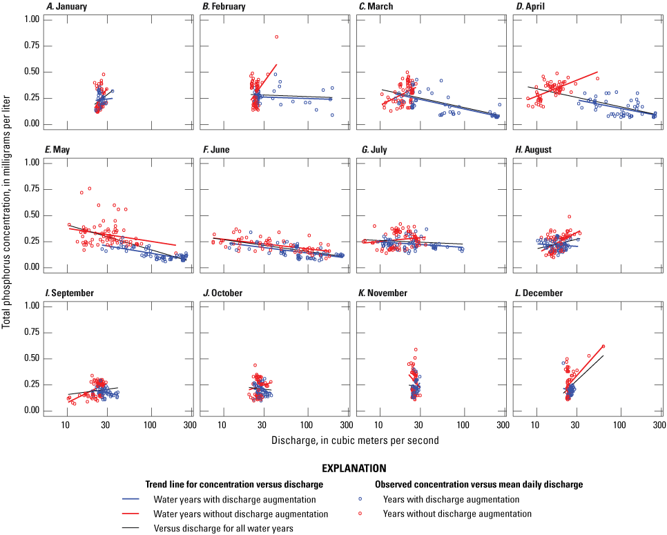
Relationship between observed total phosphorus concentrations and discharge, grouped by month, in the Boise River near Parma, Idaho, water year 2003 through 2021 (U.S. Geological Survey site 13213000; U.S. Geological Survey, 2023). The discharge-total phosphorus relationships are the most distinct between years with and without discharge augmentation in the months of February, March, and April, illustrating the challenge of predicting total phosphorus concentrations from discharge in these months.
Implications of Model Selection
This dataset allowed a unique opportunity to calibrate on near-monthly data, and test on higher frequency validation data. This allowed us to evaluate how the various models perform, and to contrast that with performance of models generated with higher frequency data. Results from the models calibrated on monthly data are compared with the results from the WRTDS_K model calibrated on all observations from the first part of this report (WRTDS_K all; table 11, figs. 17–20).
Performance of the models calibrated with monthly data is driven, in part, by the observations selected for model generation (monthly dataset). As shown in Lee and others (2019), the degree to which the model generation samples represent conditions is important. Spring 2017 provides an example of how model generation sample selection can result in model errors, especially for WRTDS_K where model results are adjusted to observations. As seen in figure 19, in cases where consecutive monthly samples happen to fall on elevated concentrations, WRTDS_K modeled values between these samples are biased high. In contrast, WRTDS and LOADEST-8 are more responsive to changes in discharge, time, and season, and were closer to the observed concentrations. This illustrates how WRTDS_K may appear to outperform other models when its performance is evaluated with monthly data and how additional testing may be needed to determine if it is actually more accurate than alternatives like LOADEST.
Concentration Exceedance Probabilities
Model selection can have impacts on computed TP distributions, and therefore on exceedance probabilities. While the median modeled concentration did not vary significantly between models (table 8), the exceedance rate for higher concentrations was noticeably different between models. The model results from WRTDS_K calibrated on all the data, used here to represent the best approximation of TP concentrations, exceeded an example threshold of 0.25 mg/L 6 percent of the time. In contrast, model results from LOADEST-8, WRTDS, and WRTDS_K calibrated on monthly observations exceeded this same threshold 10, 8, and 15 percent of the time, respectively (table 15). These differences in exceedance probability illustrate the importance of model selection.
Table 15.
Modeled median total phosphorus concentration, number of days that total phosphorus concentration exceeded 0.25 milligrams per liter, and percent of days total phosphorus concentration exceeded 0.25 milligrams per liter, water years 2016 through 2021.[Abbreviations: LOADEST-8, Load Estimator model 8 (Runkel and others, 2004); WRTDS, Weighted Regressions on Time, Discharge, and Season model (Hirsch and others, 2010); WRTDS_K, Weighted Regressions on Time, Discharge, and Season model with Kalman filtering (Lee and others, 2019); TP, total phosphorus; >, greater than. Unit: mg/L, milligram per liter]
Annual Load Estimates
Annual load estimates for water years computed from LOADEST, WRTDS, and WRTDS_K calibrated at the monthly scales were compared against those computed from WRTDS_K calibrated on the full observation dataset. Differences in annual load were found to be within 20 percent in 18 of the 19 years for LOADEST-8, 17 of 19 years for WRTDS, and 15 of the 19 years in WRTDS_K (table 16). Lee and others (2019) found annual TP loads to fall within 20 percent of observations 61, 66, and 69 percent of the time for LOADEST, WRTDS, and WRTDS_K, respectively. Lee and others (2019) noted a decrease in accuracy of annual load estimates generated with LOADEST and WRTDS_K as the coefficient of variation in observed loads increased. This could explain the reduced model performance in the Boise River in the springtime when variation in discharge (fig. 13), and therefore load, was highest. Annual load estimates, computed from models in this report calibrated at the monthly timescale, varied by up to 27 percent or approximately 128,000 kg per year of TP.
Table 16.
Number and percentage of years, out of 19 total years modeled, that annual total phosphorus load is within 20 percent of the estimate from Weighted Regressions on Time, Discharge, and Season method with Kalman filtering (WRTDS_K; Lee and others, 2019) calibrated on all observations.[Abbreviations: LOADEST-8, Load Estimator model 8 (Runkel and others, 2004); WRTDS, Weighted Regressions on Time, Discharge, and Season model (Hirsch and others, 2010); WRTDS_K, Weighted Regressions on Time, Discharge, and Season method with Kalman filtering (Lee and others, 2019)]
From water year 2016 through water year 2021, when there is a continuous set of high-frequency data for comparison, WRTDS and WRTDS_K models calibrated on near-monthly data showed greatest divergence from load estimates from the fully calibrated model in February, March, and April (fig. 23). In contrast, LOADEST-8 calibrated on monthly data had the worst performance in September, October, November, and December. The difference in load between water-quality models for the summer months was less significant, and all three models produced the lowest errors in June, July, and August. TP load in the irrigation season of May through September from 2015 through 2021 averaged 570 kg/d from the WRTDS_K model generated with all observations. Results from the three monthly-calibrated models were all within 8 percent of this value and were within 4 percent of each other.
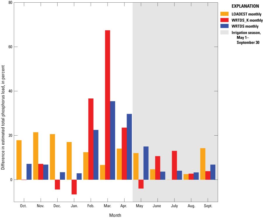
Mean monthly percent differences for water years 2016–2021 in estimated loads for models generated on monthly data relative to the Weighted Regressions on Time, Discharge, and Season method with Kalman filtering model (Lee and others, 2019) generated with all data. Positive values indicate monthly model estimates were higher than the estimates from the model generated with all available data.
Summary
This report is the first to document reductions in total phosphorus (TP) concentrations and loads in the Boise River. From water year 2003 through 2021, there was a 60 percent reduction in mean annual TP concentrations and loads in the Boise River near Parma with mean annual concentration decreasing from 0.42 to 0.18 milligrams per liter and mean annual load decreasing from 816 to 302 kilograms per day.
Reductions were greatest in the non-irrigation season of October through April, consistent with the known reduction in point-source loading from municipal wastewater treatment facilities (City of Boise, 2019). The seasonality of reductions suggests that reductions were not uniform over all sources of TP in the system. Future work could focus on identifying the rates of reductions from specific sources to identify the areas where additional reduction efforts could be focused.
The performance of three common water-quality models were compared and none of the models presented significantly outperformed the others. The water-quality models, calibrated on near-monthly data struggled to reproduce a validation dataset, despite producing low residuals in the calibration process. This highlights the value of looking beyond the calibration metrics and testing water-quality models on validation data that are withheld from model generation. It was identified that monthly data are insufficient to capture the dynamics of this system, especially in the spring months, driven in part by rapid changes in concentration in this system where discharge is highly managed.
Furthermore, stark differences in the discharge-TP relationship between water years, especially in the spring, illustrate the potential utility of including information on water routing and water resource management decisions in future water-quality monitoring and modeling efforts. This is especially important in systems with highly controlled discharge regimes where the discharge-nutrient relationship is impacted by management decisions.
References Cited
Akaike, H., 1974, A new look at the statistical model identification: IEEE Transactions on Automatic Control, v. 19, no. 6, p. 716–723, accessed August 2, 2024 at https://doi.org/10.1109/TAC.1974.1100705.
Donato, M.M., and MacCoy, D.E., 2005, Phosphorus and suspended sediment load estimates for the lower Boise River, Idaho, 1994–2002 (ver. 2.0): U.S. Geological Survey Scientific Investigations Report 2004–5235, 30 p., accessed August 2, 2024, at https://doi.org/10.3133/sir20045235.
Etheridge, A.B., 2013, Evaluation of total phosphorus mass balance in the lower Boise River and selected tributaries, southwestern Idaho: U.S. Geological Survey Scientific Investigations Report 2013–5220, 70 p., accessed August 2, 2024, at https://doi.org/10.3133/sir20135220.
Etheridge, A.B., MacCoy, D.E., and Weakland, R.J., 2014, Water-quality and biological conditions in selected tributaries of the Lower Boise River, southwestern Idaho, water years 2009–12: U.S. Geological Survey Scientific Investigations Report 2014–5132, 58 p., accessed November 17, 2024, at https://doi.org/10.3133/sir20145132.
Hirsch, R.M., Archfield, S.A., and De Cicco, L.A., 2015, A bootstrap method for estimating uncertainty of water quality trends: Environmental Modelling & Software, v. 73, p. 148–166, accessed August 2, 2024, at https://doi.org/10.1016/j.envsoft.2015.07.017.
Hirsch, R.M., and De Cicco, L.A., 2015, User guide to exploration and graphics for RivEr Trends (EGRET) and dataRetrieval—R packages for hydrologic data: U.S. Geological Survey Techniques and Methods, book 4, chap. A10, 93 p., accessed August 2, 2024, at https://doi.org/10.3133/tm4A10.
Hirsch, R.M., Moyer, D.L., and Archfield, S.A., 2010, Weighted regressions on time, discharge, and season (WRTDS), with an application to Chesapeake Bay river inputs: Journal of the American Water Resources Association, v. 46, no. 5, p. 857–880, accessed August 2, 2024, at https://doi.org/10.1111/j.1752-1688.2010.00482.x.
Idaho Department of Environmental Quality, 2008, Sediment and bacteria allocations addendum to the lower Boise River TMDL: Idaho Department of Environmental Quality, 14 p., accessed August 2, 2024, at https://www2.deq.idaho.gov/admin/LEIA/api/document/download/11728.
Idaho Department of Environmental Quality, 2015, Lower Boise River TMDL total phosphorus addendum-0815: Idaho Department of Environmental Quality, 148 p., accessed August 2, 2024, at https://www2.deq.idaho.gov/admin/LEIA/api/document/download/11737.
Idaho Department of Environmental Quality, 2022, Idaho’s 2022 integrated report: State of Idaho Department of Environmental Quality, 129 p., accessed November 17, 2024, at https://www2.deq.idaho.gov/admin/LEIA/api/document/download/16619.
Idaho Department of Environmental Quality and Oregon Department of Environmental Quality, 2004, Snake River-Hells Canyon total maximum daily load (TMDL): Idaho Department of Environmental Quality, 638 p., accessed August 2, 2024, at https://www.oregon.gov/deq/FilterDocs/tmdlrev.pdf.
King, T.V., and Yoder, A.M., 2023, Water quality modeling results of total phosphorus for the lower Boise River near Parma, Idaho 2002 - 2021: U.S. Geological Survey data release, https://doi.org/10.5066/P98DMTAN.
Lee, C.J., Hirsch, R.M., and Crawford, C.G., 2019, An evaluation of methods for computing annual water-quality loads: U.S. Geological Survey Scientific Investigations Report 2019–5084, accessed August 2, 2024, at https://doi.org/10.3133/sir20195084.
MacCoy, D.E., 2004, Water-quality and biological conditions in the lower Boise River, Ada and Canyon Counties, Idaho, 1994–2002: U.S. Geological Survey Scientific Investigations Report 2004–5128, accessed August 2, 2024, at https://doi.org/10.3133/sir20045128.
Mullins, W.H., 1998, Water-quality conditions of the lower Boise River, Ada and Canyon Counties, Idaho, May 1994 through February 1997 (revised May 2000): U.S. Geological Survey Water-Resources Investigations Report 98–4111, 32 p., accessed August 2, 2024, at https://doi.org/10.3133/wri984111.
Patton, C.J., and Kryskalla, J.R., 2003, Methods of analysis by the U.S. Geological Survey National Water Quality Laboratory-Evaluation of alkaline persulfate digestion as an alternative to Kjeldahl digestion for determination of total and dissolved nitrogen and phosphorus in water: U.S. Geological Survey Water-Resources Investigations Report 2003–4174, 33 p., accessed August 2, 2024, at https://doi.org/10.3133/wri034174.
R Core Team, 2020, R—A language and environment for statistical computing: R Foundation for Statistical Computing software release, accessed August 2, 2024, at https://www.R-project.org/.
Runkel, R. L., Crawford, C.G., and Cohn, T.A., 2004, Load Estimator (LOADEST)—A FORTRAN program for estimating constituent loads in streams and rivers: U.S. Geological Survey Techniques and Methods, book 4, chap. A5, 75 p., accessed August 2, 2024, at https://doi.org/10.3133/tm4A5.
Sen, P.K., 1968, Estimates of the regression coefficient based on Kendall’s tau: Journal of the American Statistical Association, v. 63, no. 324, p. 1379–1389, accessed November 4, 2024, at https://doi.org/10.1080/01621459.1968.10480934.
Theil, H., 1992, A rank-invariant method of linear and polynomial regression analysis, chap. 20 of Raj, B., and Koerts, J., eds., Henri Theil’s contributions to economics and econometrics—Advanced studies in theoretical and applied econometrics, vol. 23: Dordrecht, Springer, p. 345–381, accessed November 4, 2024, at https://doi.org/10.1007/978-94-011-2546-8_20.
Thomas, C.A., and Dion, N.P., 1974, Characteristics of streamflow and ground-water conditions in the Boise River Valley, Idaho: U.S. Geological Survey Water-Resources Investigations Report 74–38, 56 p., 3 pls. in pocket, accessed August 2, 2024, at https://doi.org/10.3133/wri7438.
U.S. Geological Survey, [variously dated], Collection of water samples (ver. 2.0): U.S. Geological Survey Techniques of Water-Resources Investigations, book 9, chap. A4, 166 p., accessed August 2, 2024, at https://pubs.er.usgs.gov/publication/twri09A4. [Also available at https://doi.org/10.3133/twri09A4.]
U.S. Geological Survey, 2023, USGS water data for the Nation: U.S. Geological Survey National Water Information System database, accessed July 31, 2024, at https://doi.org/10.5066/F7P55KJN.
Wood, M.S., and Etheridge, A., 2011, Water-quality conditions near the confluence of the Snake and Boise Rivers, Canyon County, Idaho: U.S. Geological Survey Scientific Investigations Report 2011–5217, 64 p., accessed August 2, 2024, at https://doi.org/10.3133/sir20115217.
Conversion Factors
Supplemental Information
Concentrations of chemical constituents in water are given in milligrams per liter (mg/L).
For more information about the research in this report,
contact the
Director, Idaho Water Science Center
U.S. Geological Survey
230 Collins Road
Boise, Idaho 83702-4250
https://www.usgs.gov/centers/id-water
Manuscript approved on November 4, 2024
Publishing support provided by the U.S. Geological Survey
Science Publishing Network, Tacoma Publishing Service Center
Disclaimers
Any use of trade, firm, or product names is for descriptive purposes only and does not imply endorsement by the U.S. Government.
Although this information product, for the most part, is in the public domain, it also may contain copyrighted materials as noted in the text. Permission to reproduce copyrighted items must be secured from the copyright owner.
Suggested Citation
King, T.V., and Yoder, A.M., 2025, A trend analysis and model comparison of total phosphorus concentrations and loads in the Boise River near Parma, southwestern Idaho, water years 2003–21: U.S. Geological Survey Scientific Investigations Report 2024–5110, 41 p., https://doi.org/10.3133/sir20245110.
ISSN: 2328-0328 (online)
Study Area
| Publication type | Report |
|---|---|
| Publication Subtype | USGS Numbered Series |
| Title | A trend analysis and model comparison of total phosphorus concentrations and loads in the Boise River near Parma, southwestern Idaho, water years 2003–21 |
| Series title | Scientific Investigations Report |
| Series number | 2024-5110 |
| DOI | 10.3133/sir20245110 |
| Publication Date | March 27, 2025 |
| Year Published | 2025 |
| Language | English |
| Publisher | U.S. Geological Survey |
| Publisher location | Reston, VA |
| Contributing office(s) | Idaho Water Science Center |
| Description | Report: vi, 41p.; Data Release |
| Country | United States |
| State | Idaho |
| City | Parma |
| Other Geospatial | Boise River |
| Online Only (Y/N) | Y |