

Updating and Recalibrating the Integrated Santa Rosa Plain Hydrologic Model to Assess Stream Depletion and to Simulate Future Climate and Management Scenarios in Santa Rosa, Sonoma County, California
Links
- Document: Report (37 MB pdf) , HTML , XML
- Data Release: USGS Data Release - Santa Rosa Plain integrated hydrological model—Simulating the hydrological system of the Santa Rosa Plain, California, with analysis of future climate scenarios
- NGMDB Index Page: National Geologic Map Database Index Page (html)
- Download citation as: RIS | Dublin Core
Acknowledgments
The authors thank Sonoma Water and the California State Water Resources Control Board for their cooperation on this project, including providing funding, expertise, and logistical support for data compilation and analysis. The work by Linda Woolfenden was done while serving as a volunteer with the U.S. Geological Survey. The authors thank U.S. Geological Survey colleagues, including Claudia Faunt, Whitney Seymour, and John Engott, for assistance in data compilation, analysis, and support.
Abstract
The Santa Rosa Plain Hydrologic Model (SRPHM) was developed and published in 2014 through a collaboration between the U.S. Geological Survey (USGS) and Sonoma Water to analyze the hydrologic system in the Santa Rosa Plain watershed, help meet the increasing demand for fresh water, and prepare for future uncertainties in water resources. The original model simulated hydrological conditions and water use from water years 1975 to 2010. Recently (2023), the USGS, in cooperation with the California State Water Resources Control Board and Sonoma Water, updated the SRPHM model to extend its simulation period to the end of the 2018 calendar year, incorporate new estimates of rural and agricultural water use, and use an efficient input format for climate variables. The updated model was recalibrated, and evaluation of the new model calibration is included in this report. This report presents the results of comparing the hydraulic heads, streamflow, and groundwater budget simulated by the updated model with those generated by the original model and observed data. The main difference in the simulated budget between the original and updated SRPHM is the estimates of agricultural pumping, rural domestic pumping, and return flow generated from rural water use that was not simulated in the original model. The revised agricultural pumping is simulated using the Agricultural Water Use package in GSFLOW, which constrains pumping to available groundwater. The use of the agricultural package leads to a more realistic estimation of agricultural water use, with revised agricultural pumping being one-third less than that in the original model. The revised rural pumping is about half of the pumping in the original model because of using detailed parcel data to estimate population density in rural areas instead of coarse census tracts. Overall, average total inflows for water years 2006–10 simulated by the updated model were about 2 percent less than the original model, and the average total updated outflows were nearly 5 percent less than the original model. The updated model was then used to generate stream depletion maps, simulate climate change scenarios during 2019–99, and simulate water rights allocation using the Model for Decision Support in Integrated River Basin Management (MODSIM). The results from simulating eight future climate scenarios indicated either an increase in groundwater storage or no significant change in the next 80 years, along with an increase in recharge, an increase in actual evapotranspiration in six out of eight climate projections, and an increase in surface runoff. The increases in the simulated future groundwater storage, recharge, evapotranspiration, and runoff in most climate projections are mainly driven by the projected increase in precipitation in most of the future climate scenarios. The updated model also was used to test a pilot case study demonstrating water-resource allocation among different users with different water rights using the integrated MODSIM-Groundwater and Surface-Water Flow Model (GSFLOW) platform. The updated SRPHM serves as a valuable tool for analyzing historical and future hydrologic conditions in the Santa Rosa Plain watershed and preparing for future uncertainties.
Introduction
The Santa Rosa Plain watershed covers about 262 square miles (mi2) and contains the Santa Rosa Plain (SRP) and Rincon Valley groundwater subbasins, parts of the Kenwood Valley, Wilson Grove Formation Highlands, Healdsburg area, Alexander Valley groundwater subbasins, and parts of the Sonoma and Mayacmas Mountains (figs. 1–3 in chapter A of Woolfenden and Nishikawa, 2014). Water resource managers in the Santa Rosa Plain watershed rely on a combination of Russian River water, local groundwater resources, and recycled and other water conservation programs to meet the water demands of urban, agricultural, and rural users (Woolfenden and Nishikawa, 2014). In 2006, the U.S. Geological Survey (USGS) began a study in cooperation with Sonoma Water, the cities of Cotati, Rohnert Park, Santa Rosa, and Sebastopol, the town of Windsor, the California American Water Company, and the County of Sonoma to assess the water resources of the Santa Rosa Plain watershed and develop models to better understand the groundwater and surface-water systems in the watershed. An integrated groundwater and surface-water model, the Santa Rosa Plain Hydrologic Model (herein referred to as the “SRPHM 1.0”) (Woolfenden and Nishikawa, 2014), was developed as part of the 2006 study. Recently (2023), the USGS, in cooperation with the California State Water Resources Control Board (SWRCB) and Sonoma Water, updated the model to extend the simulation period, revise estimates of selected model inputs, and use the updated model to (1) simulate stream depletion by groundwater pumping, (2) develop a pilot case study that uses the coupled water allocation model (Model for Decision Support in Integrated River Basin Management [MODSIM]) and Groundwater and Surface-Water Flow Model (GSFLOW), and (3) simulate future climate scenarios. The updated model (herein referred to as the “SRPHM 2.0”; Ryter and Alzraiee, 2025) described in this report will be used in the development of a groundwater sustainability plan for the Santa Rosa Plain groundwater subbasin as part of the Sustainable Groundwater Management Act (California Department of Water Resources, 2023).
Purpose and Scope
This report describes important updates made to the SRPHM 1.0 and outlines the methodologies used to complete the updates. Additionally, this report documents steps taken to recalibrate the model and presents the updated groundwater budget, streamflows, and hydraulic heads simulated by the SRPHM 2.0. Finally, the report also documents the application of the SRPHM 2.0 for mapping stream depletion factors, simulating the effects of future climate scenarios on water budget components, and demonstrating the benefits of applying the coupled MODSIM-GSFLOW system to allocate water among different users in the Santa Rosa Plain watershed.
Model updates include (1) extending the original simulation period from water years 1975–2010 to also include calendar years 2011–18 and adding the climate and anthropogenic stresses for the extended period; (2) converting the representation of climate inputs from daily gridded arrays for precipitation and minimum and maximum air temperature to a more efficient weather station-driven approach that reduces data storage requirements; (3) estimating rural domestic pumping using more detailed information than was used in the SRPHM 1.0 and to simulate return flow from rural septic tanks; (4) replacing the agricultural pumping estimates calculated by the Crop Water Demand Model (CWDM; Hevesi, 2014a) with the recently (2020) developed Agricultural Water Use (AG) package in GSFLOW (Niswonger, 2020); and (5) using the dynamic water transfer module in the Precipitation-Runoff Modeling System (PRMS; Regan and LaFontaine, 2017) to simulate the application of reclaimed water as recharge.
The SRPHM 2.0 was recalibrated to minimize the differences between simulated hydraulic heads and streamflow and both the measured and simulated data by the SRPHM 1.0 for water years 1975–2010. Comparisons of the long-term average and annual groundwater budgets simulated by the SRPHM 1.0 and SRPHM 2.0 for water years 2006–10 are presented in the “Simulated Groundwater Budgets” section of this report. The SRPHM 2.0 was used to (1) map stream depletion factors, (2) simulate multiple climate scenarios for 2019–99 using the updated model, and (3) develop a pilot modeling platform where the GSFLOW is fully coupled with the MODSIM to allocate water with user-defined water-use priorities.
Previous Investigations
Previous hydrologic investigations in the Santa Rosa Plain span several decades before the development of the SRPHM 1.0, with incremental improvement in the understanding of surface and subsurface hydrologic processes (Cardwell, 1958; California Department of Water Resources, 1975; Herbst and others, 1982; Kadir and McGuire, 1987). Studies completed by the USGS, in cooperation with Sonoma Water and other stakeholders, include detailed geologic and hydrologic investigations. Sweetkind and others (2010) developed a geologic conceptualization of the Santa Rosa Plain. Nishikawa (2013a) described the hydrology, hydrogeology, and water quality, which led to the development of a conceptual model of the Santa Rosa Plain watershed; the conceptual model was the basis for the SRPHM 1.0 (Woolfenden and Nishikawa, 2014). The SRPHM 1.0 was developed using GSFLOW (Markstrom and others, 2008) to simulate integrated groundwater and surface-water conditions for water years 1975–2010. The model was used to assess the effect of groundwater pumping on streamflow and groundwater-budget components during the historical simulation period and to evaluate the hydrologic effects of possible future climate variability without pumping for water years 2011–99 and with projected pumping for water years 2011–40. For additional details, the reader is referred to Woolfenden and Nishikawa (2014).
Study-Area Description
The following description of the study area provides a general overview of the Santa Rosa Plain watershed. A detailed discussion of the subsurface geology, hydrology, and hydrogeology of the study area is provided by Sweetkind and others (2013) and Nishikawa (2013a). The Santa Rosa Plain watershed lies within the Coast Ranges geomorphic province on the northwestern edge of California (fig. 1). The Santa Rosa Plain watershed includes all of the Mark West Creek watershed, with areas added to include most of the Santa Rosa Plain (SRP) groundwater subbasin (fig. 3 in Nishikawa 2013a). The Santa Rosa Plain is relatively flat compared with the surrounding mountains and includes some internal topographic features. The Mark West Creek, Santa Rosa Creek, and the Laguna de Santa Rosa are the major streams that drain the Santa Rosa Plain watershed (fig. 3 in Nishikawa, 2013a).
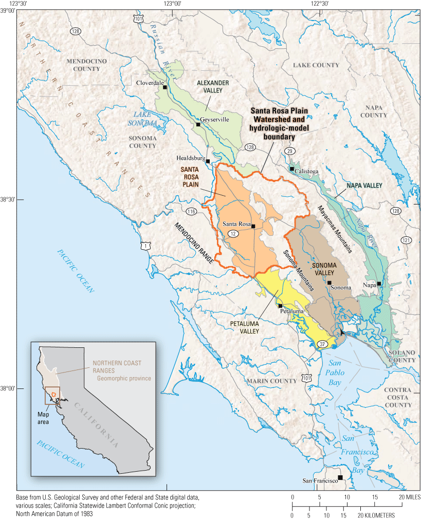
Location of the Santa Rosa Plain watershed study area, Sonoma County, California (modified from Woolfenden and Nishikawa, 2014).
The Santa Rosa Plain watershed has a Mediterranean climate with cool, wet winters and warm, dry summers, with considerable spatial and temporal variability that is affected by topography, season, and interannual variability. The mean annual precipitation was about 30 inches (in.) in the Santa Rosa Plain and about 50 in. in the Sonoma and Mayacmas Mountains during 1971–2000 (Nishikawa, 2013a). The mean air temperature near the City of Santa Rosa in 1990–2005 ranged from a minimum of 47 degrees Fahrenheit (°F) during January to a maximum of 70 °F during July, with a mean temperature of 59 °F (Brown and Caldwell, 2006).
A detailed discussion of the spatial and temporal land-use changes and their effect on the hydrology of the watershed is provided by Nishikawa (2013a). The major population centers in the Santa Rosa Plain watershed are the cities of Santa Rosa, Rohnert Park, Cotati, Sebastopol, and the town of Windsor (fig. 2 and fig. 2 in Nishikawa, 2013a). The long-term changes in land use from native vegetation to grassland and agriculture that started in the mid-1800s and rapid urbanization that started in the 1940s have generally resulted in increased runoff and flashiness of streamflow (Nishikawa, 2013a).
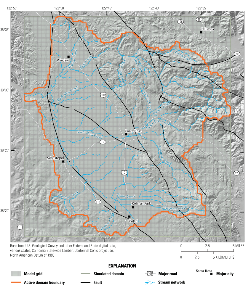
Santa Rosa Plain watershed boundary with major cities, major roads, stream network, simulated domain, faults, and model grid, Sonoma County, California.
Description of the Santa Rosa Plain Hydrologic Model (SRPHM) 1.0
The following description provides a summary of the SRPHM 1.0; a detailed discussion is provided in Woolfenden and Nishikawa (2014). The SRPHM 1.0 simulates surface and soil-zone processes, streams, and groundwater-flow systems within the Santa Rosa Plain watershed using the USGS GSFLOW (Markstrom and others, 2008). The horizontal simulated domain of the SRPHM 1.0 was discretized into 660 by 660 feet (ft) cells, or hydrologic response units (HRUs), in PRMS, with a total of 168 rows and 157 columns (fig. 2). The vertical groundwater model domain was discretized into eight layers with varying thicknesses and hydraulic properties based on the geological framework model developed by Sweetkind and others (2010). The simulation period spanned from water years 1975 to 2010, using 432 monthly stress periods with daily time steps.
Inflows to the integrated hydrologic system included natural and anthropogenic sources. Natural sources include precipitation and subsurface flow from neighboring groundwater basins along the western boundaries (see fig. 1 in Woolfenden, 2014). Anthropogenic inflow included recharge of treated wastewater (reclaimed water). Diffuse or areal recharge to the groundwater system and focused recharge from streams were simulated by the GSFLOW. Outflows from the integrated hydrologic system included groundwater pumping, evapotranspiration (ET), and streamflow. ET and streamflow were simulated by the GSFLOW. Groundwater pumping for public-supply, rural domestic, and agricultural uses was specified. Groundwater pumping for public supply was based on reported or estimated annual pumping data (Woolfenden and Nishikawa, 2014). Rural domestic pumping was estimated for residents outside city limits, using population data from the U.S. Census Bureau. Agricultural pumping was estimated using a loosely coupled PRMS watershed-component model and the CWDM (Hevesi, 2014a, in Woolfenden and Nishikawa, 2014).
Model Updates
The following updates were applied to the SRPHM 1.0: (1) the simulation period was extended from water years 1975 to 2010 to also include calendar years 2011–18; (2) the climate representation in the PRMS was converted from daily gridded arrays (climate-hru approach) for precipitation and minimum and maximum air temperature to a data storage efficient, weather station-driven approach (Markstrom and others, 2015); (3) the rural domestic pumping estimates were revised by using a more detailed approach compared to what was used in the SRPHM 1.0, and the resulting return flow was simulated; (4) the agricultural pumping calculated by the CWDM (Hevesi, 2014a, in Woolfenden and Nishikawa, 2014) was replaced with the AG package (Niswonger, 2020), which efficiently calculates irrigation demand while accounting for groundwater availability and physical constraints; and (5) the dynamic water-transfer module in PRMS (Regan and LaFontaine, 2017) was used to better simulate the application of reclaimed water as recharge.
Extending Simulation Period
The SRPHM 1.0 simulated water years 1975 through 2010. The updated model (discussed in an accompanying data release by Ryter and Alzraiee, 2025) now extends through calendar year 2018. Model inputs for the extended periods included precipitation, minimum and maximum air temperature, pumping, and recharge from reclaimed water. Reported pumping data for public supply were compiled by Sonoma Water from local water suppliers and the California Department of Water Resources. Where pumping data were missing, estimates were derived using data from previous years.
Climate Stresses
The climate_hru module in the SRPHM 1.0 used daily gridded data for prescribing precipitation and minimum and maximum air temperature. The daily climate grids were developed by interpolating available daily precipitation and maximum and minimum air temperature data for climate stations in or near the Santa Rosa Plain watershed and distributing the values to each HRU (Hevesi, 2014b, in Woolfenden and Nishikawa, 2014). The climate data files needed a large amount of storage space (three 2.5-gigabyte files), which made it challenging to transfer, share, and archive the model. In addition, reading large datasets from the physical disk during simulation can slow down the simulation as the processor waits for large data files to be read.
In the SRPHM 2.0, the distribution of climate stresses to HRUs was revised by multiplying the climate stress at two weather stations (Santa Rosa [CIMIS 83] and Windsor [CIMIS 103]; fig. 3) by a distribution factor (California Department of Water Resources, 2019). For precipitation, the measured value at the weather stations is multiplied by the rain adjustment factor (rain_adj) in PRMS. The hru_psta parameter is used to assign the identification number of the weather station to each HRU within the climate zone associated with the station (fig. 3). The rain_adj was computed for each month by dividing the average daily precipitation grided values in the SRPHM 1.0 by the average precipitation at the associated weather station. The precip_1st module (Markstrom and others, 2015) was used to distribute computed precipitation values to each HRU for each time step. This approach reduced the size of datasets used to represent climate substantially while producing similar accuracy as the gridded approach used in the SRPHM 1.0.
The temp_1sta module (Markstrom and others, 2015) was used to distribute the minimum and maximum air temperature to each HRU based on monthly lapse-rate parameters (tmax_lapse and tmin_lapse, parameters representing the change in air temperature per 1,000 units of elevation change) and temperature-adjustment parameters (tmax_adj and tmin_adj parameters to adjust air temperature for each HRU based on slope and aspect). The daily minimum and maximum temperature grids in the SRPHM 1.0 were used in the calculation of monthly averages for temperature adjustment parameters and lapse rates.
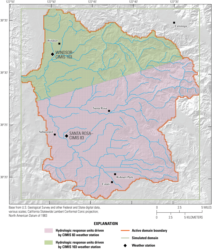
Weather stations Santa Rosa (CIMIS 83) and Windsor (CIMIS 103), with precipitations, minimum and maximum temperature measurements (California Department of Water Resources, 2019), and climate zones used in the watershed model, Santa Rosa Plain watershed, Sonoma County, California.
Rural Domestic Pumping
Rural domestic pumping was estimated in the SRPHM 1.0 for residents outside city limits using population data from the U.S. Census Bureau and average per capita water use (Woolfenden and Nishikawa, 2014). The estimated population density for rural areas within census tracts likely was overestimated because tracts may include both urban and rural areas, resulting in an overestimation of rural pumping. The per capita rural pumping was assumed to be 0.19 acre-feet per year (acre-ft/yr; California Department of Water Resources, 1994).
The updated rural domestic pumping is based on parcel data (Raftelis, 2019; Sonoma Water, 2021) and parcel zoning codes. Parcel data, typically generated by counties and used for property management and taxation, may include information about whether a house or structure exists on the property, as well as the parcel boundaries, area, land use, and zoning. There are 11,943 domestic wells associated with the parcels (Sonoma Water, 2021). Indoor and outdoor, indoor-only, and outdoor-only groundwater uses were identified using zoning codes for each parcel. Parcels with indoor and outdoor groundwater use typically represent residential zoning. Parcels identified as indoor-only groundwater use are those with mixed residential and agricultural zone codes; agricultural demands for these parcels were estimated using the AG package (Niswonger, 2020; see the “Simulation of Agricultural Water Use” section). Parcels with outdoor groundwater use were identified where groundwater pumping was used only for outdoor areas based on information provided by water service providers (Sonoma Water, 2021).
The per parcel pumping rate was aggregated for each model cell and each stress period (fig. 4). The model layers from which the domestic wells pump were determined based on the reported domestic well depths (California Department of Water Resources, 2020; Well Completion Report map). The annual groundwater pumping rate for each model cell with rural pumping was estimated like shown in equation (eq.) 1:
whereQrural
is the total rural domestic pumping at a cell i,
nparcel
is the number of parcels,
Qindoor
is indoor water use (0.24 acre-ft/yr),
Airr
is parcels area,
Pirr
is the percentage of the parcel area irrigated (assumed to be a constant value of 2.8 percent for all parcels), and
Iirr
is the turf irrigation depth (2.9 feet per year [ft/year]; Sonoma Water, 2021).
The start time for pumping was estimated using the year a parcel was developed. The seasonal distribution of pumping for rural residential wells was determined by a local water provider and allows for greater pumping in the summer months compared to the winter. In the SRPHM 2.0, the estimated rural domestic groundwater pumping is notably lower compared with the estimated rural domestic pumping in the SRPHM 1.0 (fig. 5). The change in estimates over time for the SRPHM 2.0 is gradual and reflects the transitional development dates of parcels from the parcel database, in contrast to the use of periodic census surveys in the SRPHM 1.0.
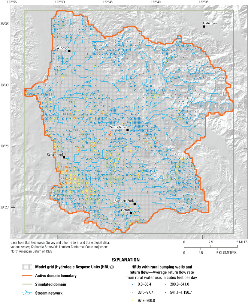
Hydrologic response units (HRU) with rural pumping wells and average return flow rate from rural water use estimated as 80 percent of indoor water use (modified from Sonoma Water, 2021), Santa Rosa Plain watershed, Sonoma County, California.
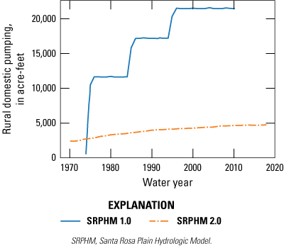
Estimated historical annual rural domestic pumping in the original Santa Rosa Plain Hydrologic Model (SRPHM 1.0; Woolfenden and Nishikawa, 2014) and updated model (SRPHM 2.0; Ryter and Alzraiee, 2025), modified from Sonoma Water, (2021), Santa Rosa Plain watershed, Sonoma County, California. Historical pumping estimates prior to water year 1975 are not included in the model.
Reclaimed Wastewater and Septic Return Flows
Reclaimed municipal wastewater used for irrigation within the Santa Rosa Plain watershed was simulated in the SRPHM 1.0 by adding the value of daily reclaimed water for the HRU to the value of daily precipitation that was simulated using the PRMS climate-hru module. The recently (2017) developed dynamic water-use module in PRMS allows for reclaimed water to be simulated separately from precipitation (Regan and LaFontaine, 2017). Separating the two sources of inflow into different modules allows for independent updates or extensions. The input of reclaimed water is a time series of water transfers to locations inside the model domain. Monthly time series for reclaimed wastewater, starting in water year 1990, were extracted from the SRPHM 1.0 and distributed to irrigated HRUs (approximately 200 land-use parcels near the town of Windsor and throughout areas of Laguna de Santa Rosa [Woolfenden and Nishikawa, 2014]).
The SRPHM 1.0 did not account for return flow from septic tanks. The model was updated to incorporate septic return flow by assuming that 80 percent of the rural indoor water use is applied as recharge onto the upper active layer (O’Conner Environmental, Inc., 2018; Sonoma Water, 2021). The Flow and Head Boundary package was used in SRPHM 2.0 to simulate the recharge rates from the septic return flow shown on figure 4. The recharge is applied directly to the saturated zone and thus the travel time through the unsaturated zone is not simulated.
Simulation of Agricultural Water Use
Agricultural water use was simulated in the SRPHM 1.0 using a PRMS model independent of the U.S. Geological Survey modular finite-difference flow model (MODFLOW; Harbaugh, 2005; Niswonger and others, 2011). This stand-alone application of PRMS is referred to as the “Crop Water Demand Model (CWDM)” because it was used in an iterative procedure to estimate irrigation amounts in each HRU (hereafter referred to as the “PRMS-CWDM”; Hevesi, 2014a, in Woolfenden and Nishikawa, 2014). The PRMS-CWDM was used to simulate crop irrigation demand by first estimating the daily unmet crop water demand, assuming irrigated fields covered the complete area of HRUs that were used to represent agriculture. Estimates of the unmet crop water demand were used to specify pumping rates from agricultural wells that are linked to the irrigated HRUs shown in Woolfenden and Nishikawa (2014). The estimated pumping requirements calculated by the PRMS-CWDM were then used to specify pumping rates in the MODFLOW well (WEL) package of the GSFLOW. Because the PRMS-CWDM was not coupled with the GSFLOW, groundwater availability was not considered in the water demand calculations, which is an important limitation of the agricultural water-use estimate in the SRPHM 1.0.
The updated irrigation demand in the SRPHM 2.0 was estimated using the recently (2020) developed AG package (Niswonger, 2020) that dynamically computes crop water demand, irrigation pumping, and irrigation return flow. This approach helps overcome the limitations associated with the usage of the PRMS-CWDM in the SRPHM 1.0. The AG package estimates crop demand by iteratively using the ET deficit (difference between PRMS variables, potential ET, and actual ET [AET]) and includes soil moisture provided by natural precipitation and applied irrigation water. The use of the AG package allows for the estimation of irrigation pumping while considering all surface and subsurface hydrologic processes, including groundwater availability. If irrigation demand exceeds the amount of available groundwater, the pumping is reduced to the available amount. Moreover, the AG package allows for future model updates to use diverted surface water for irrigation and a more accurate representation of irrigated areas as a fraction of the total HRU area. The update in the SRPHM 2.0 includes extending the irrigation water use to the calendar year 2018.
The AG package inputs include irrigated fields, shown for 2012 on figure 6, that were determined from land-use datasets for 1974, 1986, 1999, and 2008 (Nishikawa and others, 2013b) and newly released Department of Water Resources land use datasets for 2012, 2014, 2016, and 2018. Crop types in the SRPHM 1.0, including field crops, grains, orchards, pasture, truck crops, turf grass, and vineyard, were retained in the updated model. Crop type changes with time were assigned to the corresponding HRU using the nearest in-time crop for that cell. The crop type assigned to an HRU is based on which crop type covers most of the HRU area. Crops that are not irrigated were not simulated by the AG package. The temporal change of the total irrigated area for each crop type is shown on figure 7.
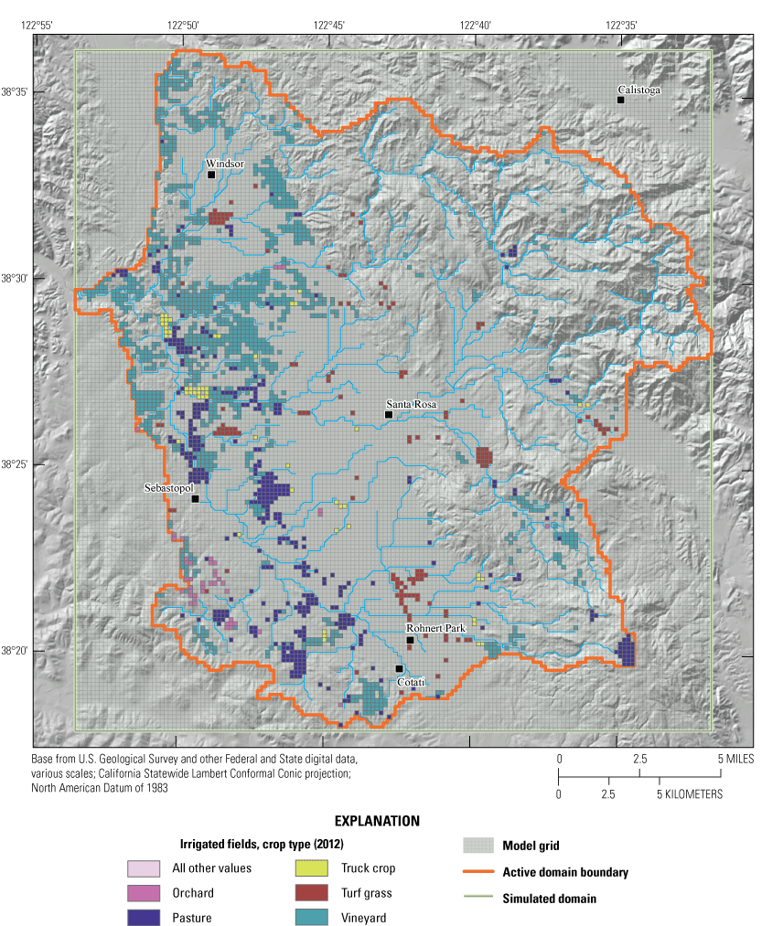
Crop types (2012) and hydrologic response units (HRUs) that contain irrigated areas used as input for the Agricultural Water Use package in the Groundwater and Surface-Water Flow Model (modified from Sonoma Water, 2021), Santa Rosa Plain watershed, Sonoma County, California.
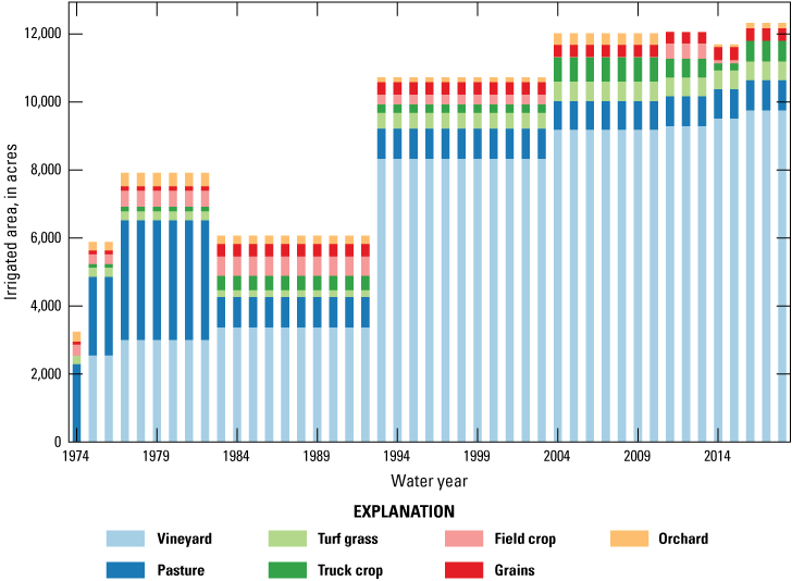
Total annual irrigated area (acres) of active crop fields within the Santa Rosa Plain groundwater subbasin, calendar years 1974–2018. Years without recorded data were assigned by the nearest year with available data, Santa Rosa Plain watershed, Sonoma County, California, based on land-use maps for 2012.
In the AG package, crop coefficients, which represent the ratio of actual evapotranspiration to reference evapotranspiration for a specific crop at a given growth stage, are not directly used. However, they are indirectly incorporated by adjusting the monthly Jensen-Haise coefficients for irrigated HRUs. The model was updated to use crop coefficient values from various sources, including Snyder and others (1987a, 1987b), Gibeault and others (1989), Allen and others (1998), Brush and others (2004), and Davids Engineering (2013). Monthly crop coefficients for each crop type are shown on figure 8A, and the irrigation schedule for each crop is presented on figure 8B. To realistically simulate irrigation rates, some adjustments were made to the PRMS soil parameters for irrigated HRUs to better reproduce external estimates of irrigation (Sonoma Water, 2021), and table 1 lists these changes in the SRPHM 2.0 and explains their rationale.
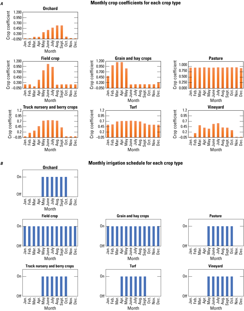
A, Monthly crop coefficients, and B, monthly irrigation schedules for each crop type (modified from Sonoma Water, 2021), Santa Rosa Plain watershed, Sonoma County, California.
Table 1.
Precipitation-Runoff Modeling System (PRMS) soil parameters adjusted at irrigated hydrologic response units (HRUs).[ET, evapotranspiration; NA, not available]
Calibration of the Santa Rosa Plain Hydrologic Model
The SRPHM 2.0 model (Ryter and Alzraiee, 2025) updates altered the simulated streamflow and groundwater heads relative to SPRHM 1.0. As a result, additional calibration was required to compensate for the discrepancies that arose in the simulated output. The goal of SRPHM 2.0 calibration was to minimize deviations from the observed calibration targets used in the SRPHM 1.0 calibration. Those calibration targets include measured hydraulic heads and dry-season streamflow (baseflow; fig. 9) because these values were most affected by the model updates. As with the calibration of the SRPHM 1.0 (Woolfenden and Nishikawa, 2014), the calibration of SRPHM 2.0 used a trial-and-error approach. Automated calibration tools, such as PEST (Doherty, 1994) or UCODE (Poeter and Hill, 1999), are usually used for this purpose; however, because of the long execution time of the SRPHM 1.0 (more than 36 hours in 2014 and about 30 hours in 2022), automated calibration of SRPHM 1.0 was considered impractical (Woolfenden and Nishikawa, 2014).
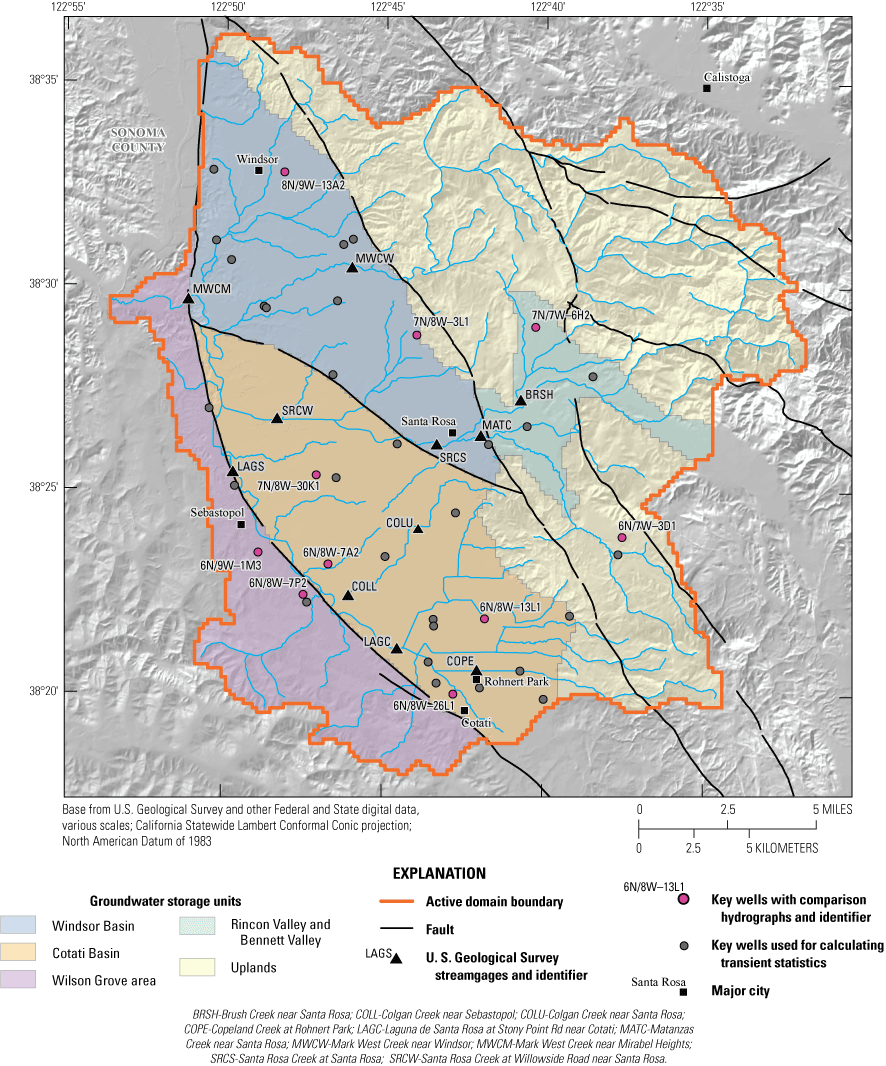
Locations of groundwater storage units, active domain boundaries, faults, key wells, and streamgages used in the recalibration and evaluation of the updated Santa Rosa Plain Hydrologic Model (SRPHM 2.0; Ryter and Alzraiee, 2025), Santa Rosa Plain watershed, Sonoma County, California.
Because of the minor changes to parameters that affect streamflow and groundwater heads, most of the parameters in the SRPHM 2.0 were unchanged from the SRPHM 1.0 (Woolfenden and Nishikawa, 2014). Parameters that were adjusted during calibration of the SRPHM 2.0 were horizontal conductivity, general-head-boundary conductance, hydraulic conductivity of the stream bed, saturated hydraulic conductivity of the unsaturated zone beneath streams, ssr2gw_rate parameter in PRMS that controls recharge flow rate from the gravity storage to the groundwater system, and the Jensen-Haise coefficient (jh_coef) in PRMS that is used in estimating the magnitude of monthly potential ET (Regan and LaFontaine, 2017).
Calibration Results
The recalibration outcomes for SRPHM 2.0 encompass a discussion of the adjusted values of input parameters and an evaluation of the model’s fit. Additionally, the results provide a comparative analysis between SRPHM 2.0 and SRPHM 1.0, which includes simulated heads, streamflows, and the groundwater budget. Much of the recalibration effort for the SRPHM 2.0 model focused on reducing high simulated groundwater heads resulting from the decreased groundwater pumping for the updated rural and agricultural water use. The updated groundwater budget, including the decrease in rural and agricultural pumping, is examined in detail in the “Simulated Groundwater Budgets” section of this report.
Parameter Adjustments
Model recalibration involved adjusting model parameters, including the horizontal hydraulic conductivity (HK) for different layers, the conductance of general head boundary conditions, streambed conductance, the conductivity of the unsaturated zone beneath the streams, and some PRMS parameters that affect groundwater recharge. The HK for the SRPHM 2.0 was 5 percent greater than HK in the SRPHM 1.0 to offset increased simulated groundwater levels caused by decreased groundwater pumping added to the updated model. The change in HK was implemented using the Parameter Value file (PVAL) in MODFLOW. Figure 10 shows the HK field simulated by the SRPHM 2.0. The range of the final values of HK is 0.0001–124.36 feet per day (ft/d). The mean HK values are 7.92, 1.75, 2.99, 2.81, 1.83, 1.14, 0.43, and 0.32 ft/d for layers 1–8, respectively, reflecting a general decreasing trend in HK with depth.
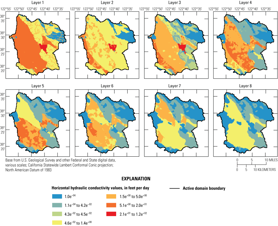
Spatial distribution of updated horizontal hydraulic conductivity values (feet per day) in each layer (layers 1–8) of the Santa Rosa Plain Hydrologic Model (SRPHM 2.0; Ryter and Alzraiee, 2025), Santa Rosa Plain watershed, Sonoma County, California.
The general-head boundary conductance on the western margin of the active model area (fig. 1 in Woolfenden, 2014) was increased by a factor of 10 to increase the rate of groundwater outflow; however, this had only a local effect on the simulated heads near the general head boundary cells.
Adjusted parameters in the streamflow routing (SFR) package (Niswonger and Prudic, 2005) include the HK of the streambed and the vertical saturated HK of the unsaturated zone beneath the streams. The streambed HK and the unsaturated zone HK were decreased for streams gaining flow from the groundwater system in the SRPHM 1.0. For streams losing flow, both SFR parameters were increased. The adjusted streambed HK values ranged from about 0.007 to 9.8 ft/d (fig. 11), with higher values predominantly assigned in the upland streams and creeks near the eastern margins of the Santa Rosa Plain (fig. 11).
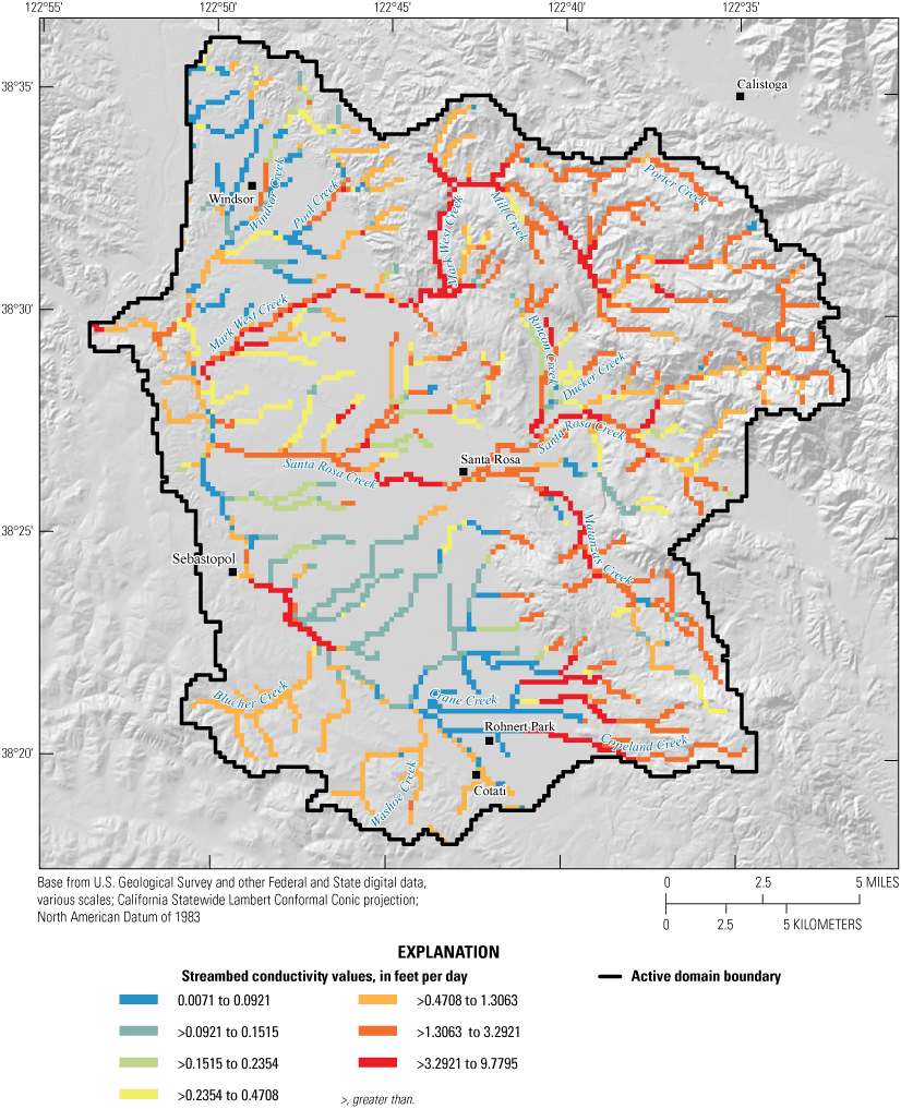
Spatial distribution of updated streambed conductivity values (feet per day) in the Santa Rosa Plain Hydrologic Model (SRPHM 2.0; Ryter and Alzraiee, 2025), Santa Rosa Plain watershed, Sonoma County, California.
Reducing aquifer recharge was another calibration measure implemented to lower simulated groundwater levels. Because parameters affecting recharge also can affect simulated soil moisture content that in turn affects the agricultural water demand, the recharge was reduced in a manner that also accommodated crop demands estimated by Sonoma Water (2021). A strategy to reduce deep percolation through the unsaturated zone to the aquifer was devised that would reduce the PRMS parameter ssr2gw, which reduced vertical flow from the soil zone. To keep the soil water from increasing, the PRMS parameter jh_coef was increased, which increased plant uptake. Reasonable adjustments were at a 25-percent increase in jh_coef and a 25-percent decrease in ssr2gw. These adjustments helped lower the simulated groundwater head in the SRPHM 2.0 without increasing the irrigation pumping estimated by Sonoma Water (2021).
Assessment of Model Fit
Comparison of simulated and measured streamflow and hydraulic heads provides an assessment of how accurately the SRPHM 2.0 replicates the measured data and how well the simulated streamflow and hydraulic heads match the simulated equivalents in the SRPHM 1.0 that was thoroughly calibrated. Streamflow simulated by the SRPHM 2.0 was compared with streamflow records and simulated values from the SRPHM 1.0 at 11 USGS streamgages (fig. 9) for model-fit statistics and streamflow hydrographs for the period of record for each streamgage. Although the SRPHM 2.0 was calibrated only to dry-season streamflow (baseflow), the assessment of simulated and measured streamflow was made for all flow conditions.
Hydraulic heads simulated by the SRPHM 2.0 were compared with 6,361 measured heads in 83 wells and hydraulic heads simulated by the SRPHM 1.0 for water years 1975–2010 for model-fit statistics. A subset of 38 wells (see well locations on fig. 9), identified as key wells in Woolfenden and Nishikawa (2014), was selected for hydrograph comparison during model calibration; measured and simulated heads for 10 of these wells (fig. 9) are discussed in this report.
Streamflow Comparison
Streamflow statistics used to assess model fit were the weighted-average statistics percent-average-estimation error (PAEE; Hevesi and others, 1992), absolute-average-estimate error (AAEE; defined as the absolute value of PAEE), and Nash-Sutcliffe model efficiency (NSME; Krause and others, 2005) for monthly streamflow at the 11 streamgages used to calibrate the model. The PAEE and AAEE statistics are measures of model bias. The NSME is a standardized measure of the mean-square error. An NSME value greater than 0 indicates an improved fit relative to the sample mean (Woolfenden and Nishikawa, 2014). The streamflow statistics given in table 2 show that the streamflow simulated by the SRPHM 2.0 worsened the fit to the measured data compared with the SRPHM 1.0 for most streamgages. However, the differences are relatively small, and the SRPHM 2.0 matches observed values well, except for the Matanzas Creek (MATC) streamgage. The SRPHM 2.0 provides an improvement in simulated streamflow for the Brush Creek near Santa Rosa (BRSH) and Colgan Creek near Sebastopol (COLL) streamgages (fig. 9), where the statistics indicate a better fit to the measured data relative to SRPHM 1.0. The NSME for streamflow simulated by the SRPHM 2.0 was −1.3 for the MATC streamgage, indicating that the mean is a better predictor of streamflow at this streamgage than the model.
Table 2.
Summary of model calibration results for the original and updated Santa Rosa Plain Hydrologic Models (SRPHM 1.0; Woolfenden and Nishikawa, 2014) and SRPHM 2.0 (Ryter and Alzraiee, 2025) for daily mean and monthly mean streamflows at selected streamgages, Santa Rosa Plain watershed, Sonoma County, California.[Max, maximum; ft3/s, cubic feet per second; min, minimum; PAEE, percent-average-estimation error; %, percent; AAEE, absolute-average-estimate error; NSME, Nash-Sutcliffe model efficiency]
Figures 12A–12K show the simulated streamflow for the SRPHM 1.0 and SRPHM 2.0 and the measured data. The timing of the high and low flows simulated by the SRPHM 2.0 compared well with the measured data and the SRPHM 1.0 at all streamgages; however, the streamflows generally were higher for the SRPHM 2.0.
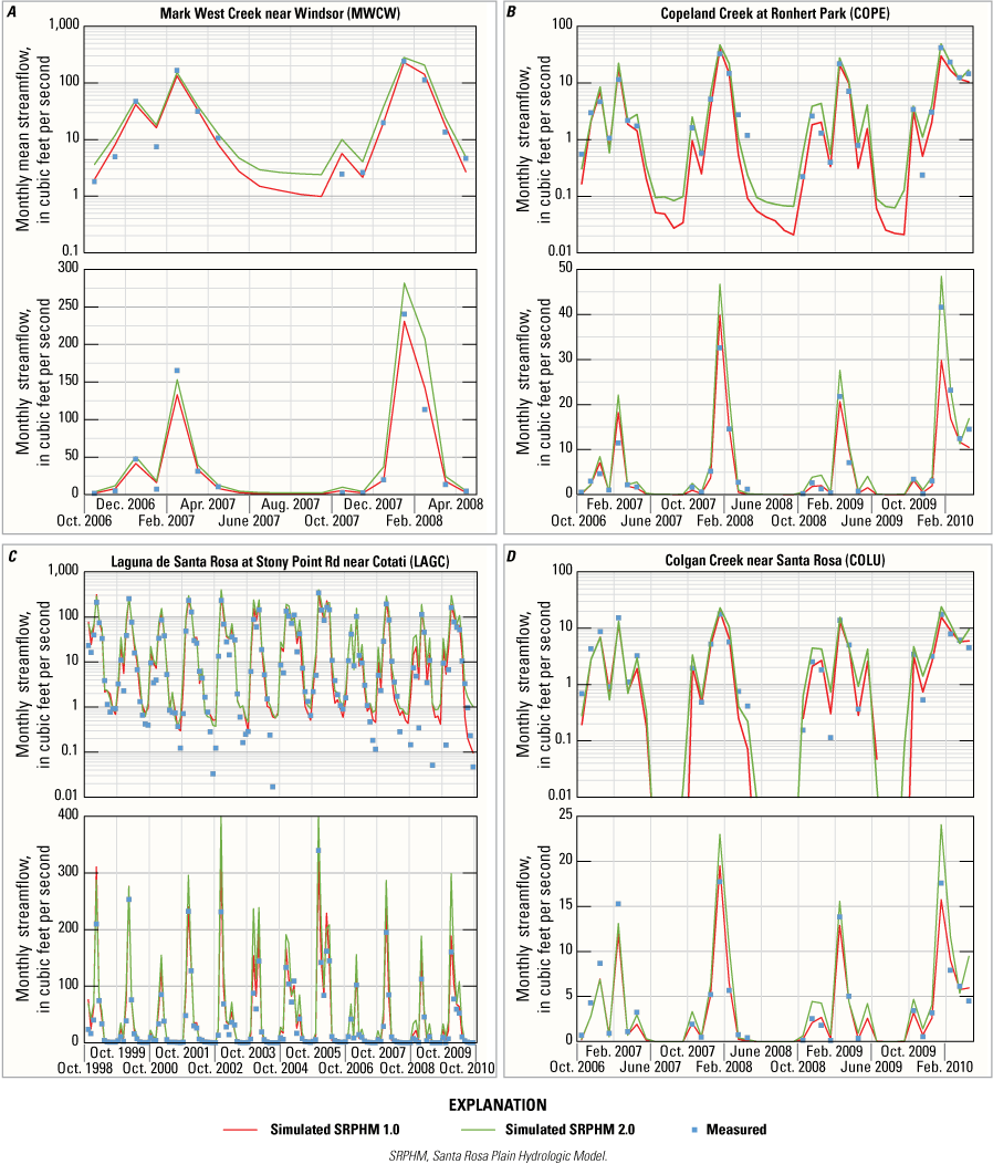
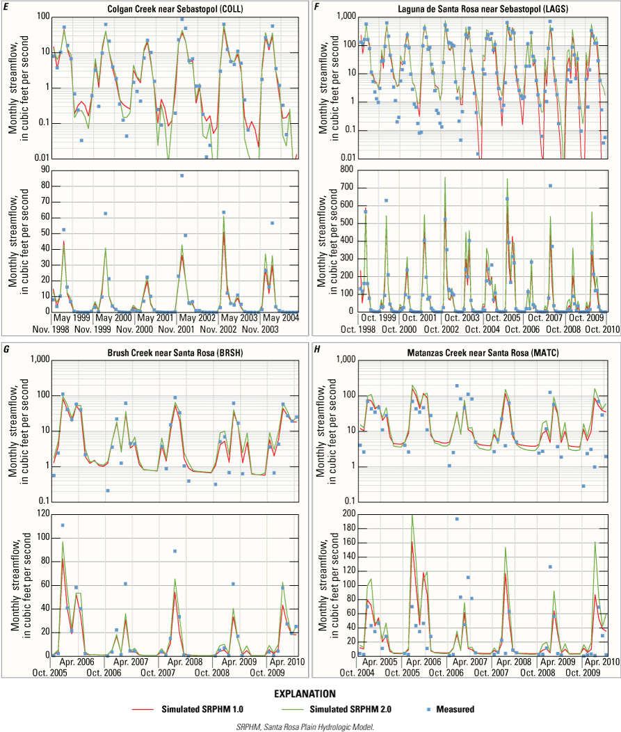
Comparison of simulated and measured monthly mean streamflow (linear [lower plot] and logarithmic scales [upper plot]) for the calibrated model at streamgages A, Mark West Creek near Windsor; B, Copeland Creek at Rohnert Park; C, Laguna de Santa Rosa at Stony Point Road near Cotati; D, Colgan Creek near Santa Rosa; E, Colgan Creek near Sebastopol; F, Laguna de Santa Rosa near Sebastopol; G, Brush Creek near Santa Rosa; H, Matanzas Creek near Santa Rosa; I, Santa Rosa Creek at Santa Rosa; J, Santa Rosa Creek at Willowside Road near Santa Rosa; and K, Mark West Creek near Mirabel Heights, Santa Rosa Plain Hydrologic Model (SRPHM 2.0; Ryter and Alzraiee, 2025), Santa Rosa Plain watershed, Sonoma County, California.
Hydraulic-Head Comparison
Model-fit statistics for residuals (measured head minus simulated hydraulic heads) for water years 1975–2010 include the average, median, minimum, maximum, root mean square error (RMSE), and normalized root mean square error (NRMSE). The statistics for the SRPHM 2.0 are compared with the statistics for the SRPHM 1.0 (table 3). The NRMSE is calculated by dividing the RMSE by the total range of measured groundwater levels in the groundwater system (628 ft; Anderson and Woessner, 1992). The value is expressed as a percentage, and previous studies (Drost and others, 1999; Ely and Kahle, 2012; Woolfenden and Nishikawa, 2014) indicated that this value should be less than 10 percent to be acceptable. The NRMSE for the SRPHM 1.0, using all 6,361 head measurements used for calibration, was 4.4 percent; the NRMSE for the SRPHM 2.0 was 4.5 percent. The average and median residuals for the SRPHM 2.0 were lower (more negative) than the SRPHM 1.0 because of the greater number of negative residuals (simulated heads higher than the measured data) for the SRPHM 2.0 (table 3).
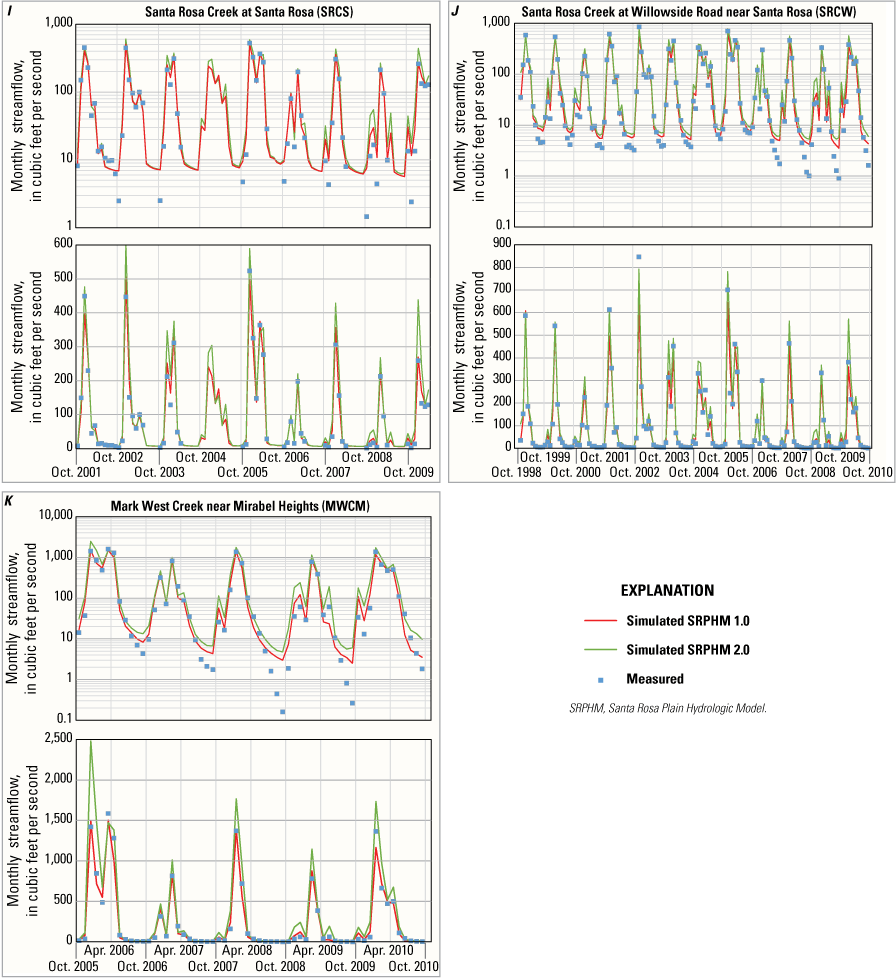
The simulated hydraulic heads for SRPHM 1.0 and SRPHM 2.0 are plotted against observed heads in figure 13. In general, measured groundwater levels and simulated hydraulic heads follow the correlation line (1:1). The heads simulated by the SRPHM 2.0 generally agree with the SRPHM 1.0. The SRPHM 2.0 overestimates 62 percent of measured heads in comparison with 58 percent for the SRPHM 1.0. The SRPHM 1.0 and SRPHM 2.0 residuals are plotted against the simulated hydraulic heads on figure 13B. In general, the plots show the residuals for both models were similarly distributed about zero, with a greater number of negative residuals (simulated heads higher than measured heads). Residuals randomly distributed at about zero indicated no bias in the simulated values (Hill, 1998).
Simulated hydraulic heads from the original Santa Rosa Plain Hydrologic Model (SRPHM 1.0; Woolfenden and Nishikawa, 2014) and the updated Santa Rosa Plain Hydrologic Model (SRPHM 2.0; Ryter and Alzraiee, 2025), Santa Rosa Plain watershed, Sonoma County, California, for A, simulated heads compared with observed heads; and B, the difference between measured and simulated hydraulic heads (residuals) plotted against observed heads.
Table 3.
Summary of hydraulic head calibration results for the original Santa Rosa Plain Hydrologic Model (SRPHM 1.0; Woolfenden and Nishikawa, 2014) and the updated Santa Rosa Plain Hydrologic Model (SRPHM 2.0; Ryter and Alzraiee, 2025), Santa Rosa Plain watershed, Sonoma County, California.[ft, feet; RMSE, root mean square error; NRMSE, normalized root mean square error; %, percent]
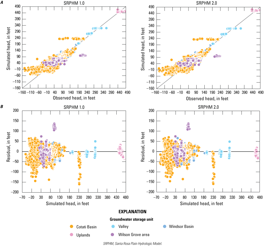
Simulated and measured hydraulic heads from the SRPHM 1.0 and SRPHM 2.0 for selected wells are shown on figure 14. The hydraulic heads simulated by the SRPHM 2.0 generally tracked the measured data similar to the SRPHM 1.0. The hydrographs shown on figure 14 are representative of the groundwater conditions in the Windsor and Cotati Basins (fig. 4 in Woolfenden and others, 2014), the Wilson Grove area in the SRP, and Rincon Valley and Bennett Valley in the uplands (fig. 9). The heads simulated by the SRPHM 2.0 were an improved fit to the measured data compared with the SRPHM 1.0 for wells 7N/8W-3L1, 6N/8W-7A2, 7N/8W-30K1, and 6N/7W-3D1 (figs. 14B, C, D, and J, respectively). The heads simulated by the SRPHM 2.0 were similar to those simulated by the SRPHM 1.0 for the other wells shown on figure 14. A detailed discussion of variation in measured and simulated hydraulic heads can be found in Woolfenden and Nishikawa (2014).
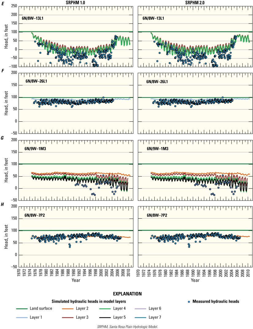
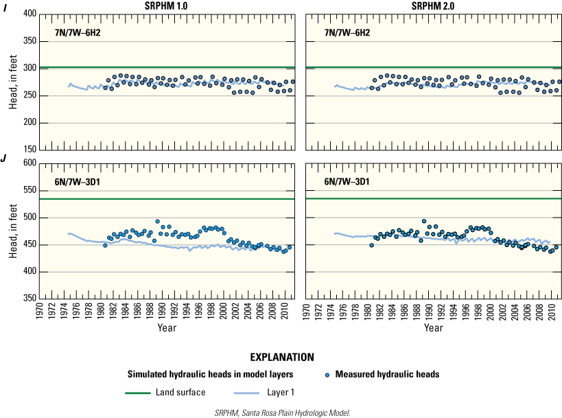
Measured and simulated hydraulic heads for wells in the original Santa Rosa Plain Hydrologic Model (SRPHM 1.0; Woolfenden and Nishikawa, 2014) and the updated Santa Rosa Plain Hydrologic Model (SRPHM 2.0; Ryter and Alzraiee, 2025), Santa Rosa Plain watershed, Sonoma County, California: A, 8N/9W-13A2; B, 7N/8W-3L1; C, 6N/8W-7A2; D, 7N/8W-30K1; E, 6N/8W-13L1; F, 6N/8W-26L1; G, 6N/9W-1M3; H, 6N/8W-7P2; I, 7N/7W-6H2; and J, 6N/7W-3D1.
Simulated Groundwater Budgets
Comparisons of groundwater budget components for the SRPHM 1.0 and SRPHM 2.0 for water years 2006–10 are shown on figures 15, 16, and 17. Figure 15 shows the average component values for the 5-year period as a percentage of total inflows (fig. 15A) and outflows (fig. 15B). Average values for the areal recharge and the subsurface inflow as a percent of average total inflows for the SRPHM 2.0 were similar to the SRPHM 1.0. Recharge from streams was 4 percent higher for the SRPHM 1.0 than for the SRPHM 2.0, due, in part, to the higher amount of pumping in the SRPHM 1.0, which resulted in lower groundwater heads beneath streams. Septic return flow accounted for 3 percent of total inflows in the SRPHM 2.0 (fig. 15A). As a percentage of total outflows, only subsurface outflow and surface leakage were generally similar for the two models. Groundwater ET and agricultural pumping simulated by the SRPHM 2.0 were 5 percent higher and 5 percent lower, respectively, than the SRPHM 1.0. The largest differences in budget percentages were for discharge to streams and total pumping for rural and public supply, which were 8 percent higher and 12 percent lower, respectively, for the SRPHM 2.0 (fig. 15B). Lower rates of pumping in the SRPHM 2.0 resulted in higher water levels, more discharge to streams, and higher groundwater ET.
The temporal variability for inflows and outflows for water years 2006–10 is similar for the SRPHM 1.0 and SRPHM 2.0 (fig. 16). The variation in inflows is affected primarily by variations in annual precipitation. The SRPHM 1.0 simulates greater amounts of recharge from streams than the SRPHM 2.0, primarily because of higher amounts of pumping in the SRPHM 1.0, which can result in lower water levels (fig. 16A). Conversely, the SRPHM 2.0 simulated greater amounts of discharge to streams than the SRPHM 1.0 (fig. 16B); the lower agricultural and rural pumping rates likely resulted in higher water levels simulated by the SRPHM 2.0. The SRPHM 2.0 also simulated greater amounts of groundwater ET and surface leakage (fig. 16B) than the SRPHM 1.0 because of higher groundwater heads associated with lower pumping rates. Subsurface inflow and outflow are similar for the two models (figs. 16A and 16B).
Average total inflows for water years 2006–10 simulated by the SRPHM 2.0 were about 2 percent less than the SRPHM 1.0, even with the inclusion of septic return flow in the SRPHM 2.0 (fig. 16A). Average total outflows simulated by the SRPHM 2.0 were nearly 5 percent less than the SRPHM 1.0 (fig. 16B). A main contributor to the difference in inflows and outflows between the SRPHM 1.0 and SRPHM 2.0 is the revised estimates of agricultural and rural domestic pumping. The revised rural domestic pumping, combined with municipal and industrial pumping, for the SRPHM 2.0 is about half the amount simulated in the SRPHM 1.0. The reduction in rural pumping is on account of SRPHM 1.0 being based on overestimated population densities that were based on coarse census tracks encompassing urban and rural zones. This pumping estimation approach likely resulted in an overestimated rural pumping because of the inflated population densities. The updated rural domestic pumping, on the other hand, is based on parcel data and parcel zoning codes (Raftelis, 2019; Sonoma Water, 2021). This approach has led to a more accurate representation of the spatial variability of rural pumping.
The simulated agricultural pumping for the SRPHM 2.0 is about one-third less than the amount specified in the SRPHM 1.0 (fig. 17A). The reduction in agricultural pumping is explained by noticing that SRPHM 1.0 used irrigation estimates derived from the PRMS-CWDM, which was not strongly integrated with GSFLOW, and therefore did not consider groundwater availability in its calculations, likely leading to an overestimation of agricultural pumping. In contrast, the SRPHM 2.0 uses the AG package, which is strongly coupled with the GSFLOW, to simulate irrigation demand while considering water availability, leading to a more realistic estimation of agricultural pumping. The cumulative change in groundwater storage for the SRPHM 2.0 tracks the pattern of the cumulative storage change for the SRPHM 1.0 during water years 2006–10; however, storage change for the SRPHM 2.0 is substantially lower than for the SRPHM 1.0 (fig. 17B).
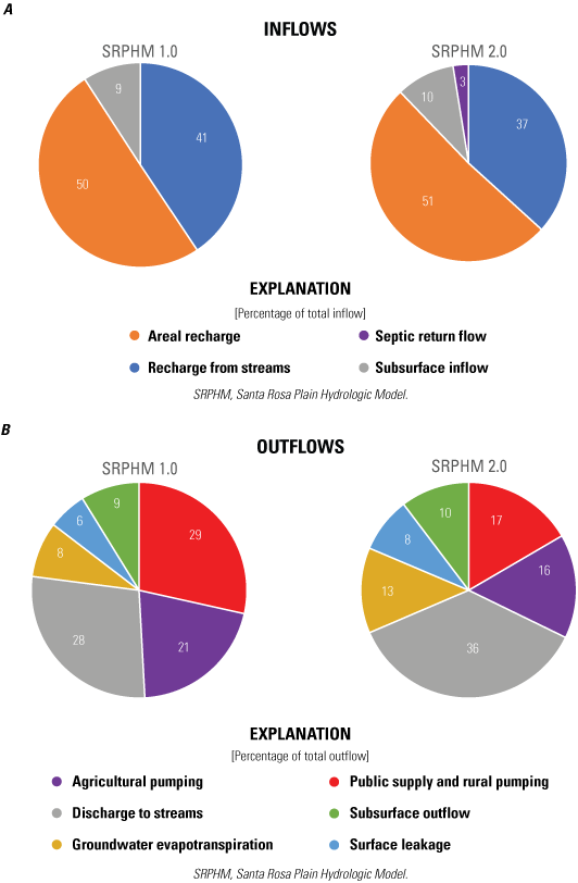
Annual average simulated groundwater budget components as A, a percentage of total inflows; and B, a percentage of total outflows for the original Santa Rosa Plain Hydrologic Model (SRPHM 1.0; Woolfenden and Nishikawa, 2014) and the updated Santa Rosa Plain Hydrologic Model (SRPHM 2.0; Ryter and Alzraiee, 2025) for water years 2006–10, Santa Rosa Plain watershed, Sonoma County, California.
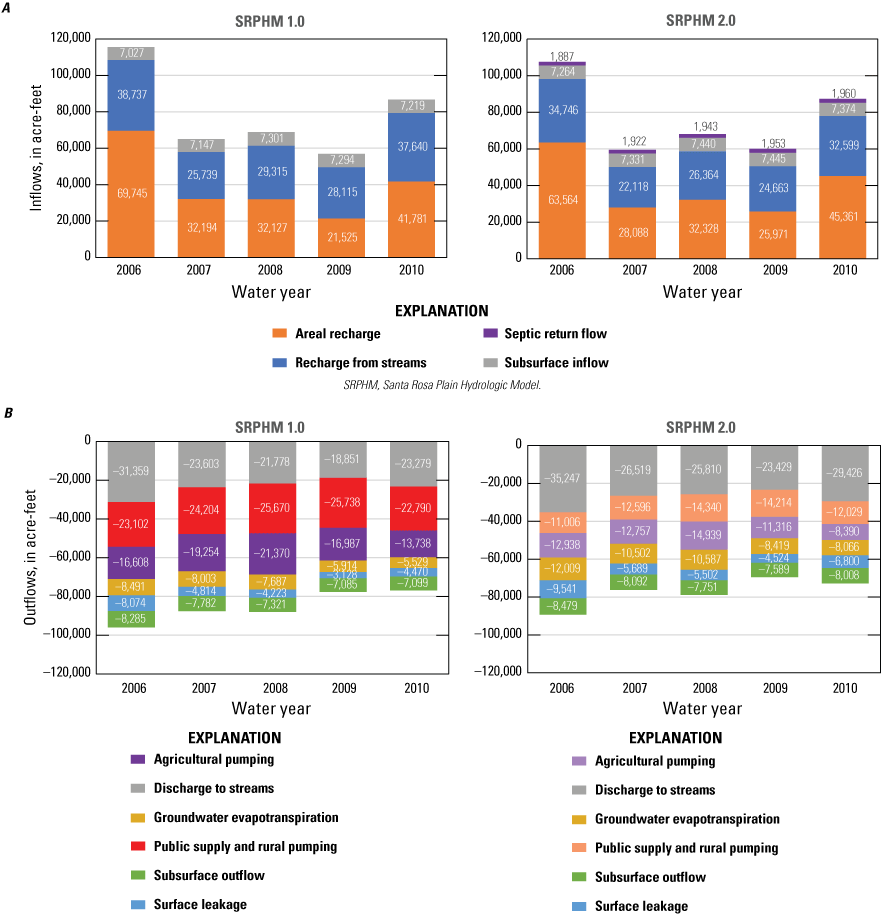
Annual groundwater A, inflows; and B, outflows simulated by the original Santa Rosa Plain Hydrologic Model (SRPHM 1.0; Woolfenden and Nishikawa, 2014) and the updated Santa Rosa Plain Hydrologic Model (SRPHM 2.0; Ryter and Alzraiee, 2025) for water years 2006–10, Santa Rosa Plain watershed, Sonoma County, California.
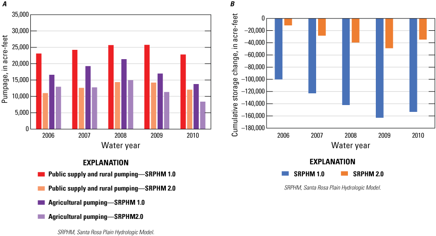
Groundwater pumping and cumulative storage simulated by the original Santa Rosa Plain Hydrologic Model (SRPHM 1.0; Woolfenden and Nishikawa, 2014) and the updated Santa Rosa Plain Hydrologic Model (SRPHM 2.0; Ryter and Alzraiee, 2025) for water years 2006–10: A, annual groundwater pumping; and B, cumulative groundwater storage, Santa Rosa Plain watershed, Sonoma County, California.
Mapping Simulated Stream Depletion
Understanding the effect of groundwater withdrawals on streamflow is essential for water managers to assess groundwater availability in alluvial aquifers, manage water rights, and protect water quality and aquatic ecosystems (Barlow and Leake, 2012). Interactions between groundwater systems and surface streams are controlled by (1) the hydraulic gradient between a stream and the groundwater level in an adjacent aquifer; (2) the conductance of the streambed; and (3) the proximity of withdrawal to groundwater discharge areas, including streams, phreatophyte forests, and springs (Barlow and Leake, 2012). The direction of the hydraulic gradient controls if a stream loses water to, or gains water from, the aquifer, and the streambed conductance controls the rate of water exchange. Withdrawal of groundwater or a stream diversion can alter the hydraulic gradient direction and the magnitude of water exchange. Groundwater withdrawal will be balanced by a corresponding decrease in groundwater storage, discharge to springs, lateral groundwater flow, and ET (Theis, 1940). The SRPHM 2.0 described in this report was used to simulate the effects of groundwater pumping on stream-aquifer interactions in the Santa Rosa Plain watershed.
Methods
The approach adopted for the development of stream depletion maps is based on the method described by Leake and others (2010). This method uses a numerical model to determine the proportion of water pumped from an aquifer that comes from streams or a reduction in groundwater that would have discharged to the stream. This proportion is referred to as the stream depletion factor (SDF). Depletion refers to an increase in stream loss, which can result from a decrease in groundwater flow to streams or an increase in flow from streams to groundwater or the unsaturated zone beneath a stream. The SDF varies depending on location, pumping rates, and other stresses. To determine the average SDF, the sum of simulated transient stream losses is divided by the total change in pumping (eq. 2).
where
ΔQs,t
is the increase in stream loss at time t resulting from an increase in groundwater pumping,
ΔQwell,t
is the change in groundwater pumping, and
T
is the total simulated period.
When an integrated hydrologic model is used for SDF calculations, simulating groundwater pumping can affect water flow and storage in different compartments of the hydrologic system, such as the saturated zone, unsaturated zone, and soil zone. For example, groundwater pumping can reduce water in storage and lower the groundwater level, potentially decreasing the water available to plants and reducing ET. Additionally, the model simulates infiltration through the land surface, flow through the unsaturated zone, plant uptake through the soil root zone, and deep percolation. Pumping can cause a decrease in the simulated head, resulting in a thicker unsaturated zone, with increased storage capacity and a potential decrease in recharge. Additionally, streams may become disconnected from groundwater due to pumping, delaying water infiltration from streams to groundwater, further reducing the water available to the groundwater system.
To produce a map of SDF, the model must be run once for each new well location and compare stream depletion with the baseline model without the additional pumping. Equipped with the simulated depletion values, eq. 2 is solved for SFD. Note that this approach assumes superposition of the effects of additional groundwater pumping onto preexisting historical groundwater pumping (Leake and others, 2010). The assumption of superposition generally requires that relations between pumping and the capture of groundwater discharge and storage be linear or mildly nonlinear (Nadler and others, 2018). The simulated area in SRPHM 2.0 is large, containing more than 16,700 active cells. Performing SDF analysis for every cell in the domain is computationally infeasible, and restricting pumping to cells near simulated streams would still require several thousand model runs. Moreover, many hypothetical wells may not represent future groundwater well construction and may exist in zones where groundwater yields are small. Thus, it was determined that, for this analysis, the best way to capture the variability in wells, hydrogeology, and the hydrologic system of the Santa Rosa Plain watershed was to increase the pumping rate in existing wells by a fixed amount each stress period and then calculate the SDF resulting from the increased pumping. Existing wells are distributed across the model area and in areas where future groundwater development is likely to take place. There were 4,304 municipal, industrial, and rural wells simulated in the SRPHM 2.0 (all of which were used in the SDF analysis).
Wells in the model have a wide range of pumping rates that vary over time. To determine a reasonable increase in pumping for SDF, the average pumping rate of municipal and industrial wells in the model was used for the simulation period. This rate, large enough to affect streams without depleting the aquifer storage or causing mathematical instabilities in the model, was estimated to be 208 gallons per minute.
Another consideration for calculating the SDF is the computational time required for running the model 4,304 times. Because a full model run takes more than 2 days to simulate the period 1975–2018, the SDF analysis was run only during 2000–15. The restart option in the GSFLOW (Regan and others, 2015) was used to save hydrologic conditions at the end of the 1975–99 water year period, which were subsequently used as initial conditions for the SDF analysis period. Using the restart option reduced the model run time to about 1 day and provided enough time for the system to respond to the increased pumping with measurable effects on stream-aquifer interaction.
To reduce the effect of model error on the SDF calculations, stream depletion was analyzed locally on SFR stream cells within about a 1.5-mile diameter of the cell containing the sampled well. An area of this size was large enough to contain the well cone of depression and the lateral effects of water captured by the well, such as decreased base flow for downgradient streams.
Results
Figure 18A shows the mean interpolated SDF across all layers for wells in the SRPHM 2.0, and figures 18B–18D show SDF values interpolated for three model layers. High SDF values were simulated near and to the east of the City of Santa Rosa and along parts of Mark West Creek. Streamflow depletion factors were lower along Windsor Creek and Laguna de Santa Rosa (fig. 18). The mean SDF values ranged from 0 to 0.99, with an overall mean of 0.11 and a standard deviation of 0.16. The depth of well screens can affect how pumping affects surface water. Figures 18B–18D show the interpolated SDF using wells with the top of the screen interval in layers 1–3. The number of wells with screening in layers 1, 2, and 3 are 1,862, 1,052, and 1,275, respectively; their locations are shown on figures 18B–18D. The spatial mean SDF values decrease with depth as follows.
-
• Layer 1 range: 0–0.99, mean: 0.13
-
• Layer 2 range: 0–0.87, mean: 0.11
-
• Layer 3 range: 0–0.75, mean: 0.10
In the eastern part of the model domain, wells screened in layer 3 can cause substantial stream depletion; however, the accuracy of the spatial interpolation deteriorates for locations far from wells in layers 2 and 3.
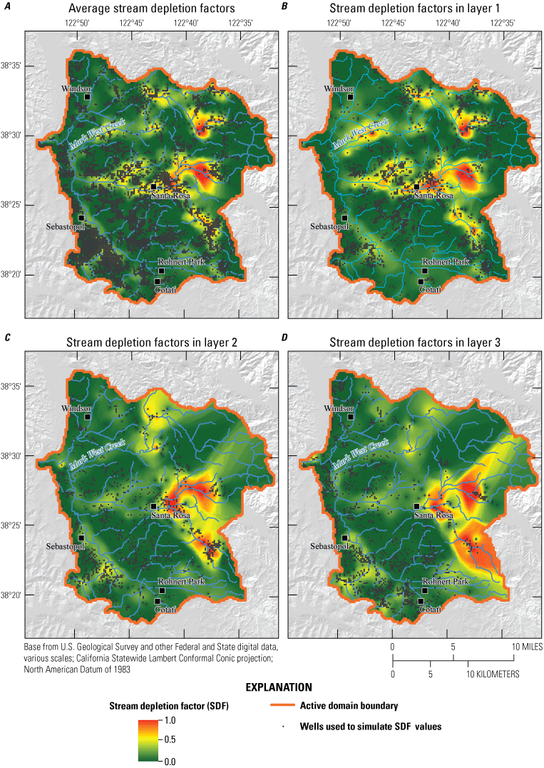
Computed stream depletion factors corresponding to an increase in pumping of 208 gallons per minute across 4,304 wells during 2000–15 for A, all layers; B, layer 1; C, layer 2; and D, layer 3, Santa Rosa Plain watershed, Sonoma County, California (Ryter and Alzraiee, 2025).
Depletion-dominated wells are characterized in this report by depletion exceeding half of the pumping rate. Depletion-dominated zones occupy parts of the areas within and east of the City of Santa Rosa and near part of Mark West Creek (fig. 18). The depletion near the City of Santa Rosa may be large because drawdown at a well can intersect several perennial streams, including Rincon Creek, Santa Rosa Creek, and Matanzas Creek. In contrast, the SDF values along Laguna de Santa Rosa are below 0.5. The depletion-dominated areas for layer 1 are the largest among all the layers in the model (fig. 18B). The depletion-dominated area in layer 2 is more localized in the upper reaches of Santa Rosa Creek and its eastern tributaries (fig. 18C). Depletion-dominated zones in layer 3 (fig. 18D) show similarities to layer 2; however, the accuracy of interpolated SDF values is relatively low in the eastern part of the model because of the small number of wells screened within layer 3.
To gain insight into the overall relation between anthropogenic water use and stream-aquifer interaction, an unimpaired conditions simulation was conducted by deactivating all groundwater pumping. A comparison between the impaired conditions (when baseline pumping is active) and unimpaired conditions is shown on figure 19. The results indicated that the streams in the Santa Rosa Plain watershed, under unimpaired conditions, generally are gaining streams (as indicated by negative values of flow from streams to the aquifer). Additionally, it is observed that groundwater pumping has the potential to capture more than 10,000 acre-feet of unimpaired streamflow per year.
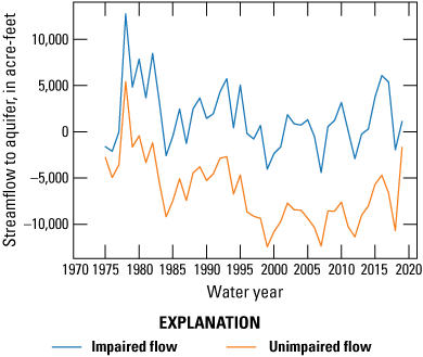
Comparison between simulated annual stream leakage to the aquifer under impaired and unimpaired conditions during the period between water year 1975 and calendar year 2018 in the Santa Rosa Plain watershed, Sonoma County, California. The simulated impaired conditions represent scenarios when pumping is active, whereas the simulated unimpaired conditions represent stream leakage when pumping is inactive (Ryter and Alzraiee, 2025).
Simulation of Climate Change Scenarios
Global climate models (GCMs) indicate that global temperature is expected to rise between 2 and 7 degrees Celsius (°C) within the next century (Christensen and others, 2007; Pierce and others, 2018). Projected changes to precipitation are highly variable among different models; however, in general, it is expected that the climate in California will shift toward a climate with a higher frequency of extreme wet and dry multi-year periods (Swain and others, 2018; DeFlorio and others, 2024). In particular, Swain and others (2018) indicated that the frequency of extreme dry-to-wet precipitation will increase by 25–100 percent in California, which is similar to the recently recorded rapid change from the multi-year drought between 2012 and 2016 to the extreme wet period during 2016–17. Understanding the response of the integrated hydrologic system in the Santa Rosa Plain watershed to these possible climate change scenarios is necessary for continuing to meet water demands in the Santa Rosa area. To address this need, the SRPIM 2.0 model was used to simulate the projected climate changes in the Santa Rosa Plain watershed during 2018–99.
Future Climate Projections
Although all GCM projections indicate ongoing warming will continue in the future as a result of persistent greenhouse gas emissions, the rate of warming varies across different models. Furthermore, GCMs project an overall increase in precipitation variability, with a higher likelihood of intense storms and prolonged dry periods. However, the magnitude and duration of these changes remain uncertain. To address this uncertainty, four GCM projections are used to account for a broader spectrum of potential future climate conditions.
The climate projections include daily temperature and precipitation time series extending from 2018 to 2099. Each of the GCMs considers two greenhouse gas emission scenarios: RCP-4.5 (RCP45) and RCP-8.5 (RCP85). The RCP45 scenario simulates increasing greenhouse gas emissions until 2040, after which emissions start to decline. In contrast, the RCP85 scenario assumes greenhouse gas emissions will continue to rise through 2099. The selected GCMs, which include the Canadian Earth System Model (CanESM2), Centre National de Recherches Météorologiques Climate Model version 5 (CNRM-CM5), Hadley Centre Global Environment Model version 2—Earth System (HadGEM2-ES), and Model for Interdisciplinary Research on Climate version 5 (MIROC5), include a range of potential future climate conditions that are suitable for California and were used in the Fourth California Climate Assessment (Pierce and others, 2014). The daily temperature and precipitation datasets were downscaled for the State of California by Cal-Adapt (2022) using the localized constructed analog method (Pierce and others, 2014).
Time series of climate data from the GCMs were extracted from the corresponding GCM grid cells associated with the Santa Rosa and Windsor weather stations, which served as input to the SRPHM 2.0 model for representing climate stresses. Although the GCM climate data had already undergone initial downscaling and correcting processes using multiple stations across California, further bias correction was applied to refine the GCM data. This additional correction involved using historical climate observations from the Santa Rosa and Windsor weather stations and applying the empirical quantile-mapping method described in Panofsky and Brier (1968) and outlined in Luo and others (2018). The empirical cumulative distribution function was computed for the historical temperature and precipitation data, which was then used to adjust the future GCM data to align with a similar distribution. The bias correction procedure was implemented using the statsmodel module for Python (version 0.13.5; Seabold and Perktold, 2010).
Figure 20A shows the average deviation of future temperature and precipitation from the mean historical climate conditions, and figure 20B shows the projected cumulative precipitation for each climate scenario. It is important to note that although the average of climate conditions (fig. 20A) provides a concise summary of future projections, it does not fully represent the range and variability of future conditions. Comparisons in figure 20A show that all GCMs project an increase in temperature ranging from 2.8 to 5.6 °F above the historical mean by the year 2100, with the RCP85 scenario consistently predicting a warmer climate compared with RCP45. The CanESM2-RCP85 scenario has the highest projected temperature increase, followed by HadGEM2-ES-RCP85, whereas CNRM-CM5-RCP45 shows the smallest deviation from historical temperatures, at approximately 2.8 °F.
Precipitation projections show greater variability, ranging from −0.3 to 13 in. from the historical average. The CanESM2 and CNRM-CM5 scenarios generally project substantial precipitation increases, whereas MIROC5 and HadGEM2-ES show minor increases or even a slight decrease compared with the historical levels. The MIROC5-RCP85 and HadGEM2-ES-RCP85 projections represent extreme water scarcity scenarios, characterized by substantial temperature increases and few or negligible changes in average precipitation. By the end of the project period, cumulative precipitation projections (fig. 20B) for the CNRM-CM5 and CanESM2 scenarios are anticipated to be around 20 and 40 percent higher, respectively, compared to MIROC5 and HadGEM2 projections.
Projection of Future Water Use
To simulate future hydrologic conditions in the SRP, it was necessary to estimate future water use across three water-use categories: (1) municipal, (2) rural domestic, and (3) agricultural. The municipal and rural water uses are affected by the size of the population served; thus, future municipal and rural water use was assumed to be proportional to population growth. County-level estimates of future population growth, based on Hauer (2019), were used to scale groundwater pumping. These estimates were made at 5-year intervals from 2020 to 2100 for all counties in the United States and considered different Shared Socioeconomic Pathways (SSPs) that include diverse combinations of demographic, economic, social, and technological factors (Hauer, 2019). The analysis herein includes an average of five SSP scenarios for estimating groundwater pumping.
Estimates of future pumping involved the following steps: (1) projected population data for Sonoma County during 2020–99 was gathered (Hauer, 2019); (2) the historical Sonoma County population in 2015 was set as the reference population to compute the population change ratio; (3) the population change ratio was calculated for each future 5-year interval (for example, the population change ratio for the year 2050 was computed by dividing population in 2050 by population in 2015); and (4) future pumping rates were determined by scaling the 2015 reference pumping by the population change ratio for each 5-year interval. Municipal and rural pumping were scaled using the same population change ratio. Based on Hauer (2019), the population growth ratio was estimated to range between 1.0 and 1.12 during 2018–99.
Information about future agricultural practices is limited; therefore, it is assumed that there will be no changes in land use, irrigated fields, or crop types after 2018 in the next 82 years. It is important to interpret and use the projections presented herein in this context. The effect of climate change on agriculture is simulated using the AG package in the GSFLOW, which estimates irrigation demand as a function of simulated soil moisture content, reference, and actual ET. Reference ET is calculated by PRMS using temperature time series derived from the climate change scenarios. Soil moisture is simulated by PRMS and triggers irrigation water applications (in other words, water use). Because crop water demands are dynamically calculated for each climate scenario, groundwater pumping for irrigation represents the effects of climate change and changes in crop-water requirements caused by climate change.
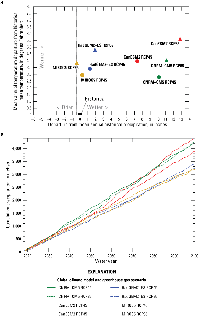
Projected climate conditions for eight global climate model scenarios generated by four global climate models; each model simulates two greenhouse gas emission scenarios: A, displays the deviation of projected average precipitation and temperature from historical averages for the eight global climate model scenarios; B, shows the cumulative change in the volume of precipitation for the same global climate model scenarios, Santa Rosa Plain watershed, Sonoma County, California.
Simulated Changes to Hydrologic Processes
Projections of future climate, including daily time series of precipitation and minimum and maximum temperature, were processed and used to drive climate changes in the GSFLOW at the Santa Rosa (CIMIS 83) and Windsor (CIMIS 103) weather stations. The effects of climate change are evaluated by comparing historical (1975–2019 water years) and projected (2020–99 water years) groundwater storage, groundwater recharge, ET, stream outflow, stream leakage, and simulated agricultural pumping.
Changes to Groundwater Storage
Figure 21 shows the simulated changes in groundwater storage over time, using a 15-year-moving average window for each year from 2023 to 2093 (covering 7 years before and after), for the eight climate projections. Overall, the results indicated either increasing groundwater storage or no substantial change relative to the historical mean. The CanESM2 and CNRM-CM5 models have the highest increase in precipitation, leading to the greatest increase in groundwater storage. The groundwater storage for the CNRM-CM5 scenarios increased the most, with a maximum increase of about 0.6 percent in 2093 compared with the historical mean. Conversely, simulated groundwater storage values for the MIROC5 and HadGEM-ES models generally fluctuate near the historical average. Simulating projections from HadGEM2-ES-RCP85 produced the greatest reduction in groundwater storage, approximately 0.3 percent less than that of the historical mean by 2093. This reduction places it 0.1 percent below the minimum historical groundwater storage simulated in water years 1975 and 1992. In general, the effect of climate change on groundwater storage seems to be minor, with the driest conditions potentially occurring under the HadGEM2-ES-RCP85 projection.
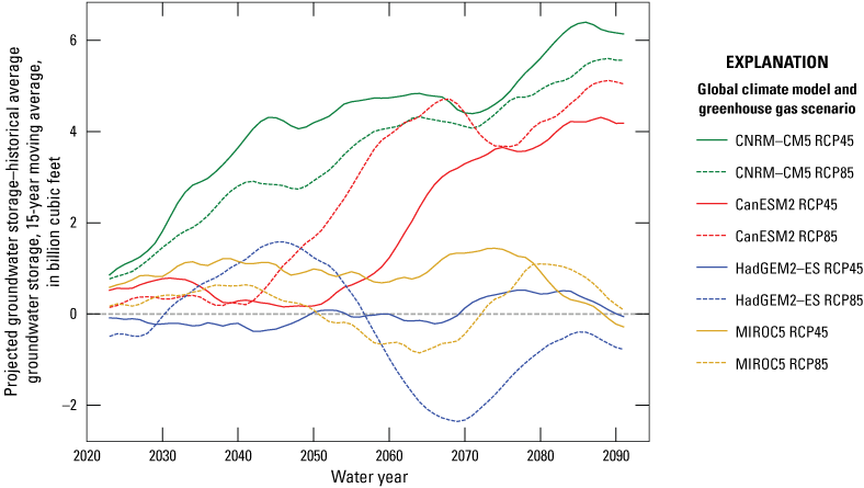
Simulated groundwater storage for eight global climate models and greenhouse gas scenarios compared to the historical average groundwater storage in the Santa Rosa Plain watershed, Sonoma County, California. A 15-year moving average window was used for each year from 2023 to 2093 (covering 7 years before and after).
Increased precipitation does not always correspond to an increase in groundwater storage. For example, a comparison of results from the CanESM2-RCP85 projection (largest increases in temperature and precipitation) with the CNRM-CM5 projection (milder increases in temperature and precipitation) shows the CanESM2-RCP85 having a smaller increase in simulated groundwater storage than the CNRM-CM5 scenario for both GCMs. This comparison indicates that the increase in precipitation may be offset by the increase in potential ET resulting from the higher atmospheric temperatures.
Changes to Recharge, Evapotranspiration, and Streamflow
Changes in groundwater storage presented in the previous section result from changes in water use and other hydrologic processes that affect recharge, ET, and runoff. Although most of the climate scenarios in this report show an increase in average precipitation, the increase in groundwater storage is not proportional to the increase in precipitation. To explain how climate change can affect future groundwater availability, this analysis focuses on how the different climate scenarios affect simulated recharge, ET, and streamflow. The results of this analysis are summarized on figure 22.
Climate change can affect the rate and spatiotemporal distribution of recharge by changing patterns of precipitation and increasing ET as a result of the projected increase in temperature. Figure 22 illustrates the partition of precipitation into recharge, ET, and stream outflow from the watershed. In addition, figure 22D shows a comparison of historical and future precipitation volume per unit area. The boxplots of the average rate of each of these hydrologic components per unit area of the watershed (in inches) are computed annually based on the water year. The boxplot summarizes the probability distribution functions (PDF) of these rates, including mean, 5th, 50th, and 95th quantiles (fig. 22).
Figure 22A shows that the PDFs of recharge rates have shifted to higher values in all scenarios compared with the historical PDF. The mean and median of historical recharge rates are smaller than any future mean and median (50th quantile), with mean values consistently exceeding the median. The range of variability of annual recharge is wider for CNRM-CM5 and CanESM2. Moreover, it can be shown that the 95th quantile, representing high recharge events, increased in climate projections CNRM-CM5 and CanESM2 and stayed approximately the same in HadGEM2 and MIROC5. The highest increase in recharge mean of about 3.5 in. per unit area was in the CNRM-CM5 scenario compared to the historical rate of about 2.6 in. per unit area (an increase of 34 percent). The CanESM2-RCP85 scenario, which has the highest increase of the precipitation mean (fig. 22D), simulated a slightly smaller increase in recharge over the mean than the CNRM-CM5 scenarios. This slight increase in recharge can be explained by the higher ET and stream outflow simulated by the CanESM2-RCP85 scenario. The AET (fig. 22B) rates increased in all models except for the MIROC5 model, which produced slightly smaller AET means (about 0.5 in. below the historical mean).
The stream outflow (fig. 22C) increased for all future projections compared to the historical stream outflow, with the highest increase in the mean of about 70 percent occurring with CanESM2-RCP85, which has the highest increase in precipitation and temperature. Moreover, the 95th percentile of projected stream outflow increased in most of the models and scenarios (except for MIROC5-RCP45) compared to the historical stream outflow. The simulated historical 95th quantile of stream outflow was about 22 in. per unit area compared to a maximum 95th quantile of about 41 in. per unit area in CanESM2-RCP85 projections, indicating a higher risk of floods in the Santa Rosa Plain watershed with the CanESM2-RCP85 scenario.
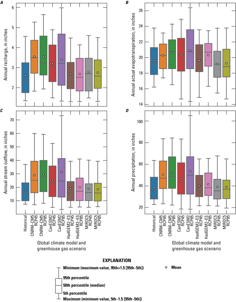
A, Simulated recharge; B, simulated actual evapotranspiration; C, simulated stream outflow; and D, projected precipitation for eight global climate model scenarios (2023–99) compared to historical conditions in the Santa Rosa Plain watershed, Sonoma County, California (Ryter and Alzraiee, 2025).
Changes to Stream Leakage
Increases in surface water runoff, illustrated by the increase in stream outflow shown on figure 22C, affect the average net stream leakage to the aquifer. Figure 23 shows the average annual net stream leakage to the aquifer increased for most future climate projections compared to the historical net steam leakage, except for the CNRM-CM5-RCP45 scenario. Moreover, the mean of the net stream leakage to groundwater simulated under the RCP-85 gas emission scenarios is consistently greater than the mean of the net stream leakage for the RCP-45 scenarios. The CNRM-CM5-RCP45 simulation resulted in a decrease in net stream-to-aquifer leakage despite the overall increase in precipitation and surface runoff. One possible explanation for this is that the CNRM-CM5-RCP45 scenario resulted in the largest increase in groundwater storage, leading to a higher water table. Increases in groundwater levels beneath streams reduced the hydraulic gradient between the stream and the aquifer and may even reverse the gradient, resulting in gaining instead of losing streams. This explanation also is illustrated by the 5th quantile, which represents the probability of streams gaining large volumes of groundwater, which is highest (more negative) for CNRM-CM5-RCP45.
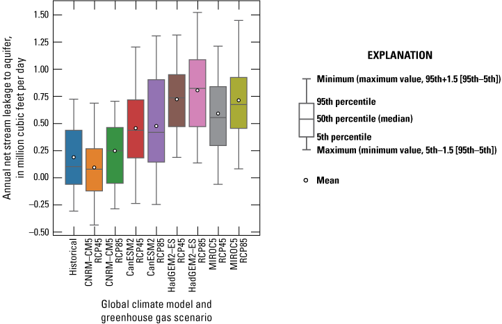
Simulated net stream leakage to the aquifer for eight global climate model scenarios (2023–99) compared to historical conditions in the Santa Rosa Plain watershed, Sonoma County, California (Ryter and Alzraiee, 2025).
Changes to Agricultural Water Use
As mentioned previously, this analysis does not represent future changes in land use or crop types. Simulated agricultural water use is affected by several factors, including changes in soil-water storage caused by changes in precipitation patterns, alterations in potential ET because of rising atmospheric temperatures, and variations in groundwater availability for irrigation purposes. Figure 24A shows the mean and range of simulated agricultural pumping values across the considered climate projections, represented as mean value enveloped by one standard deviation above and below the mean. Figure 24B shows the cumulative deviation from the mean historical agricultural water use for each climate scenario. The increased agricultural pumping corresponds to an increase in agricultural water demand because of the rise in potential ET for the considered climate scenarios. The average projected agricultural water use for all scenarios at the end of 2099 is about 17,000 acre-ft/yr, compared to the historical (1975–2019 water years) average of about 11,000 acre-ft/yr. The cumulative deviation from the historical mean indicated that CanESM2-RCP85 and HadGEM2-ES-RCP85 had the largest increases in agricultural water use (fig. 24B). This increase can be attributed to the higher temperature increases from the historical mean shown on figure 20A for these climate models. In contrast, the CNRM-CM5-RCP45 scenario simulated the smallest increase in agricultural water use (and the smallest increase in average temperature) from the historical mean.
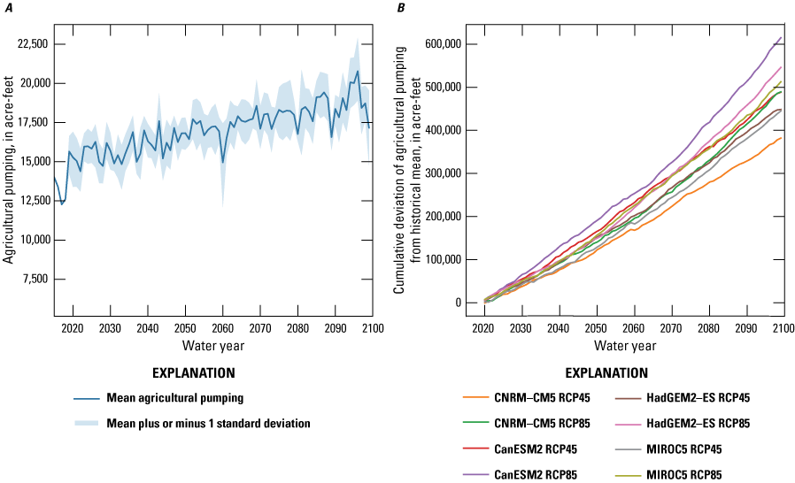
Simulated agricultural water use for eight global climate model scenarios in the Santa Rosa Plain watershed, Sonoma County, California: A, shows the mean and the mean plus and minus one standard deviation of agricultural pumping across the climate scenarios; and B, shows the cumulative deviation of agricultural pumping for each climate model scenario (Ryter and Alzraiee, 2025).
Simulating Water Rights Using Coupled Models
Water-resource management often involves simulating hydrologic processes and river operations independently, without fully considering the interactions between groundwater and surface water. As a result, water allocation decisions during extreme drought episodes may not adequately account for the complexities of physical, operational, and legal constraints crucial for effective decision-making. To address this limitation, Morway and others (2016) started the development of an advanced modeling tool that couples two models: MODFLOW (Harbaugh, 2005; Niswonger and others, 2011), which simulates flow in connected surface water and groundwater systems, and MODSIM (Labadie, 2006), a generalized river basin decision support system for simulating surface-water network flows subject to water right allocations and reservoir operations. This coupled approach enables a more comprehensive simulation and understanding of the integrated water system. Building on this advancement, the modeling approach developed by Morway and others (2016) has been extended to incorporate the GSFLOW and MODSIM. The integrated platform MODSIM-GSFLOW facilitates sharing of agricultural demands calculated by GSFLOW with MODSIM. Once provided with the calculated agricultural demands, MODSIM calculates the actual allocation (Niswonger, 2020; Kitlasten and others, 2021), subject to the legal constraints governing the basin (in other words, prior appropriations and reservoir releases). By enabling dynamic calculations of water demands and related allocations (for example, diversions), the MODSIM-GSFLOW more accurately assesses future water resources under a changing climate, allowing for a better representation of water allocation decisions during extreme climate events that are of particular interest for water-resource planners and managers. The integrated approach offered in MODSIM-GSFLOW uniquely accounts for the interaction between surface water and groundwater and river operations, leading to more informed water-resource management decisions.
Figure 25 shows a schematic of the coupled MODSIM-GSFLOW framework. The MODSIM simulates river and reservoir operations and water allocation; for example, diversions subject to physical and administrative constraints (for example, prior appropriations or if-then-else type operations). The GSFLOW simulates flows and storage, incorporating physical hydrologic constraints. The integration of GSFLOW and MODSIM enables the representation of stream-aquifer interactions and changes in agricultural demands, simulated by GSFLOW, that are then included in the calculations of surface-water diversions and allocations by MODSIM. Water-use rights are represented by cost (or weight) values assigned in MODSIM based on the relative priority of competing water rights or user-defined management preferences. The cost assigned to a water right is expressed as a negative value, with a higher absolute value indicating a higher water-use priority. To determine the total cost associated with a single water right holder, the assigned cost is multiplied by the volume of diverted water in MODSIM. The optimization process involves allocating water among multiple water right holders in a manner that minimizes the summation of the total cost, thus promoting more realistic water allocation in the model that is consistent with how water is allocated according to priorities and other policies that affect water use in the appropriated Santa Rosa Plain watershed.
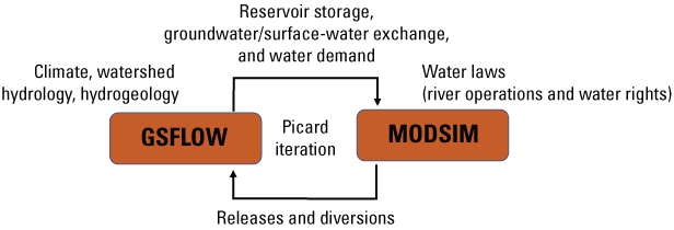
Schematic representation of the coupled Model for Decision Support in Integrated River Basin Management (MODSIM) and Groundwater and Surface-Water Flow Model (GSFLOW).
In the coupled framework, a single time-step simulation begins with MODSIM, and it estimates allocated diversions for all surface water without considering runoff and stream-aquifer interaction. Subsequently, GSFLOW simulates runoff to the stream system while accounting for the diversions estimated by MODSIM as withdrawals from the stream network. Within GSFLOW, the AG package calculates water requirements and the SFR package (Niswonger and Prudic, 2005) simulates the exchange of groundwater and surface water (in other words, stream-aquifer interactions), representing gains and losses in each segment. Next, the simulated agricultural water demand and groundwater-surface water exchange data are passed to MODSIM for calculating physically and legally available diversions. The iterative process continues for this time step until the MODSIM-GSFLOW achieves convergence, ensuring that the coupled system optimizes water allocation among users.
The coupled MODSIM-GSFLOW was used to do a pilot study in the Mark West Creek, a subbasin within the Santa Rosa Plain watershed (fig. 26). The objective of the pilot study was to assess the potential of MODSIM-GSFLOW framework for analyzing hypothetical management scenarios that honor the governing framework within the Mark West Creek subbasin. In this pilot study, the model focused on simulating water rights allocation and storage operations to meet demands in the Mark West Creek subbasin. To process the demand data, the California State Water Board used the Electronic Water Rights Information Management System (eWRIMS; California State Water Resources Control Board, 2021), which separated water demand by specific use types, such as domestic, agriculture, and other uses. Each water-use type was assigned a different relative supply priority (“pseudo priority”), allowing for analysis of the effects of different policies on fulfilling environmental flow requirements. Although the MODSIM network was developed for the stream network in the active domain of the SRPHM 2.0, the detailed representation of water rights, storage ponds, and water demands by water-use type was applied to the Mark West Creek subbasin. Data for points of diversion (POD; fig. 26), places of use (POU; fig. 26), and water rights in Mark West Creek were compiled by the SWRCB using the eWRIMS.
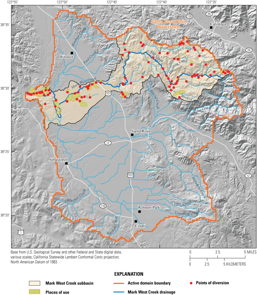
Boundary of Mark West Creek subbasin, points of diversion, and places of use in the Santa Rosa Plain watershed, Sonoma County, California.
Simulated Water Rights
Water demands associated with four beneficial water use types are simulated in the model. These types are domestic indoor, domestic outdoor, irrigation, and economic water use, which includes all other beneficial uses. The model uses existing water rights for the PODs to supply water to the designated demands. Water rights simulated by MODSIM can be classified as “riparian” or “appropriative water rights.” A riparian water right adopts a correlative share for using the surface water flowing through a property (Mooney and Burch, 2003; California State Water Resources Control Board, 2023). A riparian water right is tied to the property through which it flows, and the owner cannot store water to be used during a later dry season nor can the owner transfer the water to other users.
A new custom allocation algorithm for sharing water by riparian water rights holders was implemented in MODSIM. This approach allocates the water shortages (the difference between the required volume of water and the available volume of water) proportionally to the respective user so that each user gets a fair share of the water regardless of their location in the basin. This sharing approach follows the drought water right curtailment methods described in Lord and others (2018).
Appropriative water rights (Mooney and Burch, 2003; California State Water Resources Control Board, 2023) allow diverting an appropriated volume of water based on the prior appropriation doctrine (in other words, first in time, first in right). These water rights allow diversions from a location at the water source and beneficially using it at another location that might not be adjacent to the water source. Unlike riparian water rights, appropriative water rights can be sold or transferred to a different owner and appropriated water can be stored. Appropriative water rights after 1914 fall within the jurisdiction of the SWRCB (Mooney and Burch, 2003). Pre-1914 and post-1914 water rights are handled differently by SWRCB. Although groundwater is regulated by common law, the subterranean stream (underground watercourse that is connected to surface water) is treated as surface water. Riparian rights have priority over appropriative rights, which give the highest priority to the most senior water user. The Mark West Creek watershed has 98 water rights (table 4): 34 riparian water rights, 2 pre-1914 appropriative water rights, and 62 post-1914 appropriative water rights. About half of the water rights have permitted pond storage.
Table 4.
Summary of types of water rights, counts, and associated storage ponds in the Mark West Creek subbasin in Santa Rosa Plain watershed, Sonoma County, California.Two options to represent the agricultural water demand are simulated in MODSIM: (1) user-specified water use that is estimated using eWRIMS data processed by the eWRIMS analyzer and (2) dynamically simulated agricultural water requirement by the AG package in GSFLOW. For the first option, monthly estimates of domestic, agricultural, and economically beneficial water uses are derived from single-year data extracted from the eWRIMS. The estimated water uses are assumed to be annually invariant for the simulation period. For the second option, agricultural water use is dynamically simulated using the GSFLOW AG package, while the other water use types used the eWRIMS calculated demands. In the coupled model simulation, accretion and depletions calculated by the GSFLOW for each stream segment are passed to MODSIM to calculate diversion amounts while considering surface water availability and crop water demands. As a result, the effects of pumping are reflected in the surface-water deliveries and in the supplemental pumping. The maximum flow rate for water rights is set to the water right face value in the eWRIMS, which is defined as the amount of water that a water right holder is allowed to divert, store, or use under their right.
Model for Decision Support in Integrated River Basin Management Network
The MODSIM stream network (fig. 27) was created to coincide with the segments and confluences of the SFR package. Each diversion in the SFR package was represented with a single SFR segment with only one reach. The MODSIM routes water through the network with nodes representing gains and losses to the system (available water and water rights at the PODs). The MODSIM determines how much surface water to divert at each POD (fig. 26) along Mark West Creek based on the water rights associated with each POD. Each POD can provide water to one or more POU, which may include different water-use types, such as indoor domestic, outdoor domestic, agricultural, and economic water use. Additional components to the MODSIM network are (1) logical constructs (node arrangements) that define different water rights, pseudo priorities for each water-use type, water distribution to storage ponds, and the water-use types at each place of use (fig. 28) and (2) synthetic links and nodes used to represent the stream accretions and depletions for each segment as water routed in MODSIM, which must be from a node to a node (not shown on fig. 28).
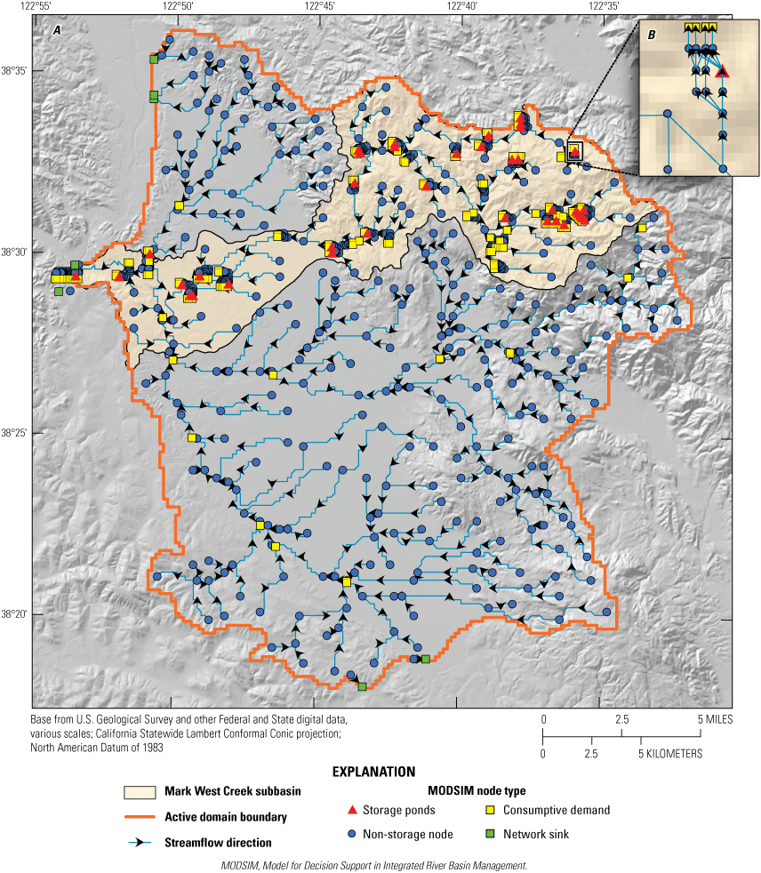
Components of the Model for Decision Support in Integrated River Basin Management (MODSIM; Labadie, 2006) network: A, MODSIM network and node types that provide a visual representation of the system's structure and the various nodes involved; and B, a zoomed-in view of one of the logical water allocation constructs, demonstrating how water is allocated among different water-use types, Santa Rosa Plain watershed, Sonoma County, California (Ryter and Alzraiee, 2025).
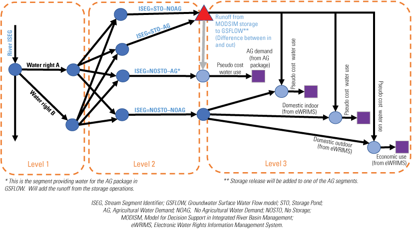
The logical construct used to represent the allocation of diverted water among different water rights (level 1), different storage options (level 2), and different water-use types (level 3).
The logical construct (fig. 28) shows how MODSIM-computed diverted water from each POD is allocated for use or storage by different water-use types. This calculation considers the legal availability of water and the water rights associated with each POU. To account for the multiple water-use types within a single POU, MODSIM combines the water demands from all water-use types into a single POD referred to as “pseudo-demands.” Each logical construct consists of three levels of logical branching, each representing a finer level of water allocation logic. Level 1 (fig. 28) represents water diversion from a POD to different water rights holders. In level 2 (fig. 28), water is allocated among multiple water-use types (for example, agricultural and non-agricultural) with and without a storage pond. Diversions to storage nodes within MODSIM can fulfill demands across various water-use types and are controlled by MODSIM using parameters such as total storage volume and maximum monthly inflows to store. In level 3, each user type is handled differently in MODSIM (shown on fig. 28), where links are branched to convey water to its final POU destination, represented with demand nodes.
The MODSIM initially allocates water among riparian rights holders because they have higher priority. Because all riparian water rights share the same level of priority, MODSIM minimizes the total shortage for all users while maintaining proportional curtailments. Any remaining water is then allocated among appropriative water rights holders, whose priority is determined by their respective priority dates (decree date).
Demonstration of Alternative Management Scenarios
The coupled MODSIM-GSFLOW platform was used to analyze the integrated hydrologic system response to hypothetical management scenarios and water right cost values. This analysis serves to demonstrate the capabilities of the MODSIM-GSFLOW. It is important to note that the management scenarios were solely intended for illustrative purposes. The management scenarios were developed in collaboration with the SWRCB and were based on demand estimates from a single year (2005) for the simulation that used the eWRIMS to estimate demands. In addition, these scenarios were limited to the Mark West Creek watershed as a pilot case study. Consequently, modifications were not made to water usage in other areas of the Santa Rosa Plain watershed region. The framework developed can be expanded to simulate realistic demands and water-rights priorities, providing valuable support to decision-makers.
In the illustrative scenarios presented herein, MODSIM applies logical constructs to simulate minimum instream flow (ISF) requirements with different pseudo priorities. Ensuring a minimum ISF rate can be essential for protecting wildlife habitats and instream water quality. Two locations within the subbasin were selected by the SWRCB to perform the analysis of minimum ISF for juvenile rearing of steelhead and coho salmon in Mark West Creek (California Department of Fish and Wildlife, 2022; Carlin and others, 2022). The two locations selected were (1) Mark West Creek 1 (fig. 29), which corresponds to ISF requirements in lower Mark West Creek, where moderate water year type (not dry nor wet) flow requirements were used (table 12 in California Department of Fish and Wildlife [2022]) and (2) Mark West Creek 2 (fig. 29), which corresponds to the optimum minimum ISF value of 34 cubic feet per second (ft3/s) for juvenile rearing of steelhead (table 9 in California Department of Fish and Wildlife, 2022).
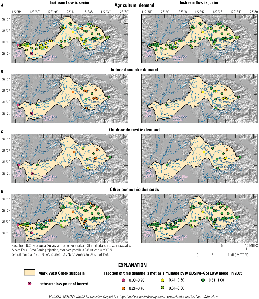
Curtailment options of surface-water diversion for four water use types when instream flow has senior water priority (left) versus junior water priority (right) in Mark West Creek, in the Santa Rosa Plain watershed, Sonoma County, California. A, Agricultural demand; B, indoor domestic demand; C, outdoor domestic demand; and D, other economic demands.
The model is set up to compare two alternative scenario constraints by different levels of ISF priorities. The two scenario constraints are (1) setting the ISF priority to the most junior priorities in the system and (2) setting the ISF with the most senior priority that would cause curtailments for all water rights to meet the flow requirements.
The effects of changing the ISF priority on all water-use categories and rights are summarized on figures 29, 30, and 31. Figure 29 shows the fraction of times the water demand is fulfilled for the individual water right for the four water-use categories. As expected, the results indicated that increasing the priority of ISF leads to a decrease in the percentage of times the water demand is met. For example, this percentage ranged from 0.21 to 1.00 for the indoor category when the ISF had a senior priority. However, when the ISF is assigned a junior priority, the values increase to a range from 0.40 to 1.00. Similar patterns are observed for all water-use types. Furthermore, the effect of designating a senior water right for ISF is more pronounced during the dry season (April–October), like shown on figures 30 and 31. This effect is particularly noticeable in the curtailment of surface-water diversion (reduction of the fraction of time demand is met) for the agricultural and economic water use category (fig. 29). These results, although illustrative, highlight the value of the coupled MODSIM-GSFLOW framework in assessing alternative management scenarios while also enforcing physical and legal constraints. By using this framework, decision-makers can gain valuable insights into the implications of different prioritization strategies and better understand the trade-offs involved in water allocation during critical periods.
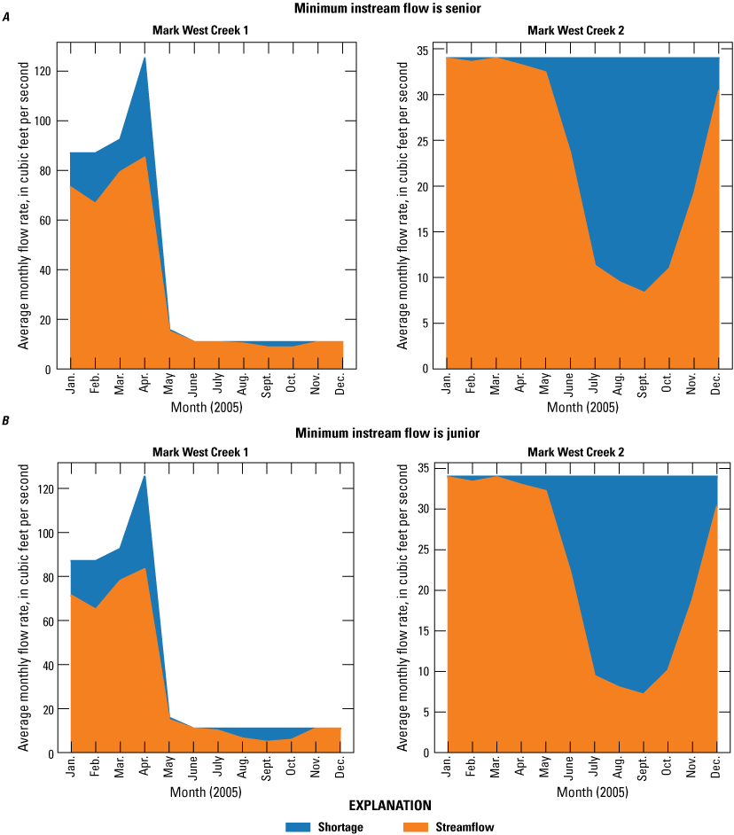
Simulated available shortages and streamflow (difference between available and required streamflow) at two points of interest. The figure shows the available and shortage streamflow for two management targets. A, Minimum instream flow requirements are senior; and B, minimum instream flow requirements are junior, Mark West Creek 1 and 2, in the Santa Rosa Plain watershed, Sonoma County, California (Ryter and Alzraiee, 2025).
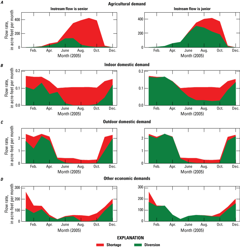
Effect of the curtailment of surface-water diversion for four water-use types and the comparison of the scenarios where instream flows have senior water priority (left) versus junior water priority (right) in Mark West Creek, Santa Rosa Plain watershed, Sonoma County, California. A, Agricultural demand; B, indoor domestic demand; C, outdoor domestic demand; and D, other economic demands (Ryter and Alzraiee, 2025).
Summary and Conclusions
Effective management of the limited water resources in the 262-square-mile Santa Rosa Plain watershed is crucial to meet the challenges posed by increasing water demand and uncertainties surrounding future water availability. Numerical models are essential tools to simulate historical and future conditions, assess the responses of the hydrologic system to natural and anthropogenic stresses, and aid in decision-making processes. In pursuit of this objective, the Santa Rosa Plain Hydrologic Model (SRPHM, version 1.0) was developed in 2014 and subsequently updated in 2023 (SRPHM, version 2.0) through a collaboration with the U.S. Geological Survey, Sonoma Water (formerly known as Sonoma County Water Agency), and the California State Water Resources Control Board. The original model (SRPHM 1.0) was developed using the fully coupled Groundwater and Surface-Water Flow Model (GSFLOW) to simulate the integrated hydrologic system, including surface and subsurface water processes. The model served as a tool for analyzing the hydrologic system in the Santa Rosa Plain watershed and to help develop a basin-wide water management plan that meets the increasing demand for fresh water and to simulate the effect of future climate conditions and alternative management scenarios. The original model focused on simulating hydrological conditions and water use, including municipal, rural, and agricultural water consumption, from water years 1975 to 2010. However, the need to enhance the predictive capabilities of the model led to its update, therefore, helping to meet stakeholder needs.
The model update documented in this report involved (1) extending the model to simulate historical conditions up to calendar year 2018, (2) incorporating new estimates of rural water use and agricultural demand using the Agricultural Water Use package in GSFLOW and simulating return flow from septic tanks, and (3) updating the representation of climate in the model by transitioning from daily gridded data to an efficient data storage approach that greatly simplifies updating the model to future periods and running climate and water management scenarios under different climate conditions. To address the previous model calibration bias, the model was recalibrated, and the model fits of simulated streamflow and hydraulic heads were assessed using statistical assessments to observed values. Most of the original model input parameters were kept the same; however, some minor changes were made to the horizontal hydraulic conductivity, general head boundary conductance, streambed hydraulic conductivity, vertical saturated hydraulic conductivity of the unsaturated zone beneath the streams, and some of the Precipitation-Runoff Modeling System parameters. Evaluation of the updated model included comparisons with observed data and the original model.
Model results indicated that the streamflow and hydraulic heads simulated by the updated model generally were in agreement with observed values and the original model, though there were some relatively small increases in error compared to the observed streamflow. Simulated streamflow values generally were higher for the updated model (SRPHM 2.0). An analysis of the simulated groundwater budget reveals some changes in various inflow and outflow components. The average recharge from streams (as a percentage of total inflow) decreased by 4 percent. The average areal recharge and subsurface inflow remained relatively unchanged. The newly added septic-tank inflow contributed about 3 percent of the average inflows. For outflow components, public supply and rural domestic pumping decreased from about 29 to 17 percent of the total outflow in the SRPHM 2.0. Simulated agricultural water use (as a percentage of total outflow) decreased by about 5 percent, evapotranspiration (ET) increased by 5 percent, and subsurface outflow and surface leakage were similar between the updated and original models.
The SRPHM 2.0 was used to create stream depletion maps by simulating the effects of increased pumping at municipal and industrial wells in the model. The resulting simulated depletion factors presented a wide range of spatial variability, with a spatial average of 0.11 and a standard deviation of 0.16. Additionally, the depletion factors were observed to decrease with depth. The areas with the highest stream depletion factors were identified near the City of Santa Rosa, particularly along Santa Rosa Creek and along upper Mark West Creek. In contrast, smaller depletion values were simulated along Winsor Creek and Laguna de Santa Rosa.
The effect of climate change on the integrated hydrologic system was investigated through simulations of eight climate projections, representing four global circulation models (CanESM2, CNRM-CM5, HadGEM2-ES, and MIROC5). Each model was run with two greenhouse gas emission scenarios (RCP-45 and RCP85), covering the period from 2018 to 2099. The projected average temperature is expected to increase within a range from 2.8 to 5.6 degrees Fahrenheit above historical averages. Precipitation patterns indicate a wider range of variability, spanning from −0.3 to 13 inches (in.) from the historical mean. The results for all simulations indicated either an increase in groundwater storage or no significant change, along with an increase in recharge, an increase in actual ET in six out of eight climate projections, and an increase in surface runoff. It is worth noting that these changes may include a wide range of variability because of the unpredictability of precipitation patterns and intensity, leading to alternating periods of extreme dryness and excessive rainfall. During wet periods, high streamflow, such as the 95th quantile, may increase substantially, reaching as much as 41 inches per year (in/yr) compared to the historical value of 22 in/year. This possibility emphasizes the potential for more intense and extreme wet periods and a higher risk of flood because of climate change.
Finally, the updated model was used to assess a newly developed modeling platform that couples GSFLOW and MODSIM. The tightly coupled MODSIM-GSFLOW system aims to allocate surface water among various places of use with different water-right priorities, including indoor and outdoor domestic, agricultural, and economic water use. The modeling platform accounts for the physical constraints of the hydrologic system while also ensuring compliance with environmental and legal flow requirements. To demonstrate the effectiveness of this modeling system, a pilot case study was done to allocate water resources among different users in the Mark West Creek area. The study specifically evaluated the effect of maintaining minimum instream flow requirements to protect wildlife habitats and preserve instream water quality. Although the MODSIM-GSFLOW pilot study used hypothetical alterations in existing water rights, the results demonstrated the potential value of the modeling platform to quantitatively evaluate water allocation spatially and temporally under alternative management scenarios. This integrated approach offers valuable insights into sustainable water-resource management, helping decision-makers optimize water allocation and balance the needs of different stakeholders while protecting ecological and environmental resources.
References Cited
Allen, R.G., Pereira, L.S., Raes, D., and Smith, M., 1998, Crop evapotranspiration—Guidelines for computing crop water requirements: Food and Agriculture Organization of the United Nations, Irrigation and Drainage Paper 56, 300 p., accessed June 19, 2024, at https://www.fao.org/docrep/x0490e/x0490e00.htm.
Barlow, P.M., and Leake, S.A., 2012, Streamflow depletion by wells—Understanding and managing the effects of groundwater pumping on streamflow: U.S. Geological Survey Circular 1376, 84 p. [Available at https://doi.org/10.3133/cir1376.]
Brown and Caldwell, 2006, 2005 Urban water management plan: Santa Rosa, Calif., Sonoma County Water Agency, prepared by Brown and Caldwell, Rancho Cordova, Calif., [variously paged], accessed June 18, 2024, at https://evogov.s3.amazonaws.com/media/185/media/164718.pdf.
Brush, C.F., Belitz, K., and Phillips, S.P., 2004, Estimation of a water budget for 1972–2000 for the Grasslands Area, central part of the western San Joaquin Valley, California: U.S. Geological Survey Scientific Investigations Report 2004–5180, 59 p., accessed June 19, 2024, at https://doi.org/10.3133/sir20045180.
Cal-Adapt, 2022, LOCA derived data [GeoTIFF]: Data from LOCA downscaled CMIP5 climate projections, Cal-Adapt website, University of California, Berkeley’s Geospatial Innovation Facility, The California Energy Commission, accessed March 15, 2022, at https://cal-adapt.org/.
California Department of Fish and Wildlife, 2022, Watershed-wide instream flow criteria for Mark West Creek: California Department of Fish and Wildlife, Watershed Criteria Report no. 2022-01, 51 p. [Available at https://nrm.dfg.ca.gov/FileHandler.ashx?DocumentID=203270&inline.]
California Department of Water Resources, 1994, California water plan update: California Department of Water Resources Bulletin 160–93, 397 p. [Available at https://www.waterboards.ca.gov/waterrights/water_issues/programs/bay_delta/wq_control_plans/1995wqcp/admin_records/part05/328.pdf.]
California Department of Water Resources, 2019, California Irrigation Management System (CIMIS) overview: California Department of Water Resources website, accessed January 26, 2019, at https://cimis.water.ca.gov.
California Department of Water Resources, 2020, Well Completion Reports: California Department of Water Resources web page, accessed August 20, 2020, at https://water.ca.gov/Programs/Groundwater-Management/Wells/Well-Completion-Reports.
California Department of Water Resources, 2023, Sustainable Groundwater Management Act (SGMA): California Department of Water Resources web page, accessed March 8, 2023, at https://water.ca.gov/Programs/Groundwater-Management/SGMA-Groundwater-Management.
California State Water Resources Control Board, 2021, eWRIMS—Electronic Water Rights Information Management System: California State Water Resources Control Board web page, accessed October 14, 2021, at https://www.waterboards.ca.gov/waterrights/water_issues/programs/ewrims/.
California State Water Resources Control Board, 2023, The water rights process: California State Water Resources Control Board web page, accessed July 26, 2023, at https://www.waterboards.ca.gov/waterrights/board_info/water_rights_process.html.
Cardwell, G.T., 1958, Geology and ground water in the Santa Rosa and Petaluma areas, Sonoma County, California: U.S. Geological Survey Water-Supply Paper 1427, 273 p., 5 pls. [Available at https://doi.org/10.3133/wsp1427.]
Christensen, J.H., Hewitson, B., Busuioc, A., Chen, A., Gao, X., Held, I., Jones, R., Kolli, R.K., Kwon, W.-T., Laprise, R., Rueda, V.M., Mearns, L., Menéndez, C.G., Räisänen, J., Rinke, A., Sarr, A., and Whetton, P., 2007, Regional climate projections, chap. 11 in Solomon, S., Qin, D., Manning, M., Chen, Z., Marquis, M., Averyt, K.B., Tignor, M., and Miller, H.L., Jr., eds., Climate change 2007—The physical science basis. Contribution of Working Group I to the Fourth Assessment Report of the Intergovernmental Panel on Climate Change: Cambridge, United Kingdom, Cambridge University Press, p. 849–940. [Available at https://www.ipcc.ch/site/assets/uploads/2018/02/ar4-wg1-chapter11-1.pdf.]
DeFlorio, M.J., Sengupta, A., Castellano, C.M., Wang, J., Zhang, Z., Gershunov, A., Guirguis, K., Niño, R.L., Clemesha, R.E.S., Pan, M., Xiao, M., Kawzenuk, B., Gibson, P.B., Scheftic, W., Broxton, P.D., Switanek, M.B., Yuan, J., Dettinger, M.D., Hecht, C.W., Cayan, D.R., Cornuelle, B.D., Miller, A.J., Kalansky, J., Monache, L.D., Ralph, F.M., Waliser, D.E., Robertson, A.W., Zeng, X., DeWitt, D.G., Jones, J., and Anderson, M.L., 2024, From California’s extreme drought to major flooding—Evaluating and synthesizing experimental seasonal and subseasonal forecasts of landfalling atmospheric rivers and extreme precipitation during winter 2022/23: Bulletin of the American Meteorological Society, v. 105, no. 1, p. E84–E104. [Available at https://doi.org/10.1175/BAMS-D-22-0208.1.]
Doherty, J., 1994, PEST—A unique computer program for model-independent parameter optimization, in Institution of Engineers Australia and International Association of Hydrogeologists, Water down under 94—Preprints of papers: Australia, Institution of Engineers, National Conference Publication, p. 551–554. [Available at https://search.informit.org/doi/10.3316/informit.752715546665009.]
Drost, B.W., Ely, D.M., and Lum, W.E., II, 1999, Conceptual model and numerical simulation of the ground-water-flow system in the unconsolidated sediments of Thurston County, Washington: U.S. Geological Survey Water-Resources Investigations Report 99–4165, 106 p. [Available at https://doi.org/10.3133/wri994165.]
Ely, D.M., and Kahle, S.C., 2012, Simulation of groundwater and surface-water resources and evaluation of water-management alternatives for the Chamokane Creek basin, Stevens County, Washington: U.S. Geological Survey Scientific Investigations Report 2012–5224, 74 p. [Available at https://doi.org/10.3133/sir20125224.]
Gibeault, V.A., Cocker-ham, S., Henry, J.M., and Meyer, J., 1989, California turfgrass—It’s use, water requirement and irrigation: California Turfgrass Culture, v. 39, nos. 3–4, 14 p., accessed June 19, 2024, at https://turfgrass.ucr.edu/sites/default/files/2023-08/ctc39_34.pdf.
Harbaugh, A.W., 2005, MODFLOW-2005—The U.S. Geological Survey modular ground-water model—The ground-water flow process: U.S. Geological Survey Techniques and Methods, book 6, chap. A16, 253 p. [Available at https://doi.org/10.3133/tm6A16.]
Hauer, M.E., 2019, Population projections for U.S. counties by age, sex, and race controlled to shared socioeconomic pathway: Scientific Data, v. 6, no. 1, article 190005, 15 p., accessed June 19, 2024, at https://doi.org/10.1038/sdata.2019.5.
Hevesi, J.A., 2014a, Supplemental information—Documentation of the crop water demand model used to estimate agricultural irrigation, app. 1 of Woolfenden, L.R., and Nishikawa, T., eds., Simulation of groundwater and surface-water resources of the Santa Rosa Plain watershed, Sonoma County, California: U.S. Geological Survey Scientific Investigations Report 2014–5052, p. 235–258. [Available at https://doi.org/10.3133/sir20145052.]
Hevesi, J.A., 2014b, Watershed-component model, chap. B of Woolfenden, L.R., and Nishikawa, T., eds., Simulation of groundwater and surface-water resources of the Santa Rosa Plain watershed, Sonoma County, California: U.S. Geological Survey Scientific Investigations Report 2014–5052, p. 21–54. [Available at https://doi.org/10.3133/sir20145052.]
Hevesi, J.A., Istok, J.D., and Flint, A.L., 1992, Precipitation estimation in mountainous terrain using multivariate geostatistics—Part 1—Structural analysis: Journal of Applied Meteorology and Climatology, v. 31, no. 7, p. 661–676. [Available at https://doi.org/10.1175/1520-0450(1992)031<0661:PEIMTU>2.0.CO;2.]
Hill, M.C., 1998, Methods and guidelines for effective model calibration; with application to UCODE, a computer code for universal inverse modeling, and MODFLOWP, a computer code for inverse modeling with MODFLOW: U.S. Geological Survey Water-Resources Investigations Report 98–4005, 90 p. [Available at https://doi.org/10.3133/wri984005.]
Kitlasten, W., Morway, E.D., Niswonger, R.G., Gardner, M., White, J.T., Triana, E., and Selkowitz, D., 2021, Integrated hydrology and operations modeling to evaluate climate change impacts in an agricultural valley irrigated with snowmelt runoff: Water Resources Research, v. 57, no. 6, 30 p. [Available at https://doi.org/10.1029/2020WR027924.]
Krause, P., Boyle, D.P., and Bäse, F., 2005, Comparison of different efficiency criteria for hydrological model assessment: Advances in Geosciences, v. 5, no. 5, p. 89–97. [Available at https://doi.org/10.5194/adgeo-5-89-2005.]
Labadie, J.W., 2006, MODSIM—Decision support system for integrated river basin management—3rd International Congress on Environmental Modelling and Software: Burlington, Vt., [July 9–13, 2006]: Brigham Young University, 11 p., accessed July 24, 2023, at https://scholarsarchive.byu.edu/cgi/viewcontent.cgi?article=3254&context=iemssconference.
Leake, S.A., Reeves, H.W., and Dickinson, J.E., 2010, A new capture fraction method to map how pumpage affects surface water flow: Groundwater, v. 48, no. 5, p. 690–700. [Available at https://doi.org/10.1111/j.1745-6584.2010.00701.x.]
Lord, B., Magnuson-Skeels, B., Tweet, A., Whittington, C., Adams, L., Thayer, R., and Lund, J., 2018, Drought water right curtailment analysis for California’s Eel River: Journal of Water Resources Planning and Management, v. 144, no. 2, 11 p. [Available at https://doi.org/10.1061/(ASCE)WR.1943-5452.0000820.]
Luo, M., Liu, T., Meng, F., Duan, Y., Frankl, A., Bao, A., and De Maeyer, P., 2018, Comparing bias correction methods used in downscaling precipitation and temperature from regional climate models—A case study from the Kaidu River Basin in western China: Water, v. 10, no. 8, 21 p. [Available at https://doi.org/10.3390/w10081046.]
Markstrom, S.L., Niswonger, R.G., Regan, R.S., Prudic, D.E., and Barlow, P.M., 2008, GSFLOW—Coupled ground-water surface-water flow model based on the integration of the precipitation-runoff modeling system (PRMS) and the modular ground-water flow model (MODFLOW-2005): U.S. Geological Survey Techniques and Methods, book 6, chap. D1, 240 p. [Available at https://doi.org/10.3133/tm6D1.]
Markstrom, S.L., Regan, R.S., Hay, L.E., Viger, R.J., Webb, R.M.T., Payn, R.A., and LaFontaine, J.H., 2015, PRMS-IV, the precipitation-runoff modeling system, version 4: U.S. Geological Survey Techniques and Methods, book 6, chap. B7, 158 p. [Available at https://doi.org/10.3133/tm6B7.]
Mooney, D.B., and Burch, M.A., 2003, The water acquisition handbook—How to acquire water for the environment in California: Trust for Public Land, 114 p., accessed July 26, 2023, at https://www.tpl.org/resource/california-water-acquisition-handbook.
Morway, E.D., Niswonger, R.G., and Triana, E., 2016, Toward improved simulation of river operations through integration with a hydrologic model: Environmental Modelling & Software, v. 82, p. 255–274. [Available at https://doi.org/10.1016/j.envsoft.2016.04.018.]
Nadler, C., Allander, K., Pohll, G., Morway, E., Naranjo, R., and Huntington, J., 2018, Evaluation of bias associated with capture maps derived from nonlinear groundwater flow models: Groundwater, v. 56, no. 3, p. 458–469. [Available at https://doi.org/10.1111/gwat.12597.]
Nishikawa, T., ed., 2013a, Hydrologic and geochemical characterization of the Santa Rosa Plain watershed, Sonoma County, California: U.S. Geological Survey Scientific Investigations Report 2013–5118, 178 p. [Available at https://doi.org/10.3133/sir20135118.]
Nishikawa, T., Hevesi, J.A., Sweetkind, D.S., and Woolfenden, L.R., 2013b, Introduction to the study area, chap. A, in Nishikawa, T., ed., Hydrologic and geochemical characterization of the Santa Rosa Plain watershed, Sonoma County, California: U.S. Geological Survey Scientific Investigations Report 2013–5118, p. 7–25. [Available at https://doi.org/10.3133/sir20135118.]
Niswonger, R.G., 2020, An agricultural water use package for MODFLOW and GSFLOW: Environmental Modelling & Software, v. 125, 16 p. [Available at https://doi.org/10.1016/j.envsoft.2019.104617.]
Niswonger, R.G., and Prudic, D.E., 2005, Documentation of the streamflow-routing (SFR2) package to include unsaturated flow beneath streams—A modification to SFR1: U.S. Geological Survey Techniques and Methods, book 6, chap. A13, 50 p. [Available at https://doi.org/10.3133/tm6A13.]
Niswonger, R.G., Panday, S., and Ibaraki, M., 2011, MODFLOW-NWT—A Newton formulation for MODFLOW-2005: U.S. Geological Survey Techniques and Methods, book 6, chap. A37, 44 p. [Available at https://doi.org/10.3133/tm6A37.]
Pierce, D.W., Cayan, D.R., and Thrasher, B.L., 2014, Statistical downscaling using localized constructed analogs (LOCA): Journal of Hydrometeorology, v. 15, no. 6, p. 2558–2585. [Available at https://doi.org/10.1175/JHM-D-14-0082.1.]
Pierce, D.W., Kalansky, J.F., and Cayan, D.R., 2018, Climate, drought, and sea level rise scenarios for California’s fourth climate change assessment: State of California Energy Commission report, 78 p. [Available at https://www.energy.ca.gov/sites/default/files/2019-11/Projections_CCCA4-CEC-2018-006_ADA.pdf.]
Poeter, E.P., and Hill, M.C., 1999, UCODE, a computer code for universal inverse modeling: Computers & Geosciences, v. 25, no. 4, p. 457–462. [Available at https://doi.org/10.1016/S0098-3004(98)00149-6.]
Raftelis, 2019, Santa Rosa Plain Groundwater Sustainability Agency, rate study report: Santa Rosa, Calif., Santa Rosa Plain Groundwater Sustainability Agency, prepared by Raftelis Financial Consultants, Inc. (Raftelis), Los Angeles, 105 p. [Available at http://santarosaplaingroundwater.org/wp-content/uploads/06.13.2019_Santa-Rosa-Plain-GSA-Rate-Study-Report-June-11-2019.2_ada-2.pdf.]
Regan, R.S., and LaFontaine, J.H., 2017, Documentation of the dynamic parameter, water-use, stream and lake flow routing, and two summary output modules and updates to surface-depression storage simulation and initial conditions specification options with the Precipitation-Runoff Modeling System (PRMS): U.S. Geological Survey Techniques and Methods, book 6, chap. B8, 60 p. [Available at https://doi.org/10.3133/tm6B8.]
Regan, R.S., Niswonger, R.G., Markstrom, S.L., and Barlow, P.M., 2015, Documentation of a restart option for the U.S. Geological Survey coupled groundwater and surface-water flow (GSFLOW) model: U.S. Geological Survey Techniques and Methods, book 6, chap. D3, 19 p. [Available at https://doi.org/10.3133/tm6D3.]
Ryter, D.W., and Alzraiee, A.H., 2025, Santa Rosa Plain integrated hydrological model–Simulating the hydrological system of the Santa Rosa Plain, California, with analysis of future climate scenarios: U.S. Geological Survey data release, available at https://doi.org/10.5066/P1MCCAOM.
Seabold, S., and Perktold, J., 2010, Statsmodels—Econometric and statistical modeling with Python in van der Walt, S., and Millman, J., eds., Proceedings of the 9th Python in Science Conference (SciPy 2010), Austin, Tex., June 28–July 3, 2010: Austin, Tex., SciPy, p. 92–96. [Available at https://doi.org/10.25080/Majora-92bf1922-011.]
Snyder, R.L., Lanini, B.J., Shaw, D.A., and Pruitt, W.O., 1987a, Using reference evapotranspiration (ETo) and crop coefficients to estimate crop evapotranspiration (ETc) for agronomic crops, grasses, and vegetable crops: Berkeley, California, Cooperative Extension of the University of California Division of Agriculture and Natural Resources, Leaflet 21427, 12 p. [Available at https://cimis.water.ca.gov/Content/PDF/21427-KcAgronomicGrassandVeg.pdf.]
Snyder, R.L., Lanini, B.J., Shaw, D.A., and Pruitt, W.O., 1987b, Using reference evapotranspiration (ETo) and crop coefficients to estimate crop evapotranspiration (ETc) for trees and vines: Berkeley, Calif., Cooperative Extension of the University of California, Division of Agriculture and Natural Resources, Leaflet 21428, 8 p. [Available at https://cimis.water.ca.gov/Content/PDF/21428-KcTreesandVines.pdf.]
Sonoma Water, 2021, Groundwater sustainability plan Santa Rosa plain groundwater subbasin: Santa Rosa Groundwater Sustainability Agency, accessed December 8, 2023, at https://santarosaplaingroundwater.org/wp-content/uploads/000_Santa_Rosa_GSP_508.pdf.
Swain, D.L., Langenbrunner, B., Neelin, J.D., and Hall, A., 2018, Increasing precipitation volatility in twenty-first-century California: Nature Climate Change, v. 8, p. 427–433. [Available at https://doi.org/10.1038/s41558-018-0140-y.]
Sweetkind, D.S., Hevesi, J.A., Nishikawa, T., Martin, P., and Farrar, C.D., 2013, Hydrology of the Santa Rosa Plain watershed, Sonoma County, California, chap. B of Nishikawa, T., ed., Hydrologic and geochemical characterization of the Santa Rosa Plain watershed, Sonoma County, California: U.S. Geological Survey Scientific Investigations Report 2013–5118, p. 27–112. [Available at https://doi.org/10.3133/sir20135118.]
Sweetkind, D.S., Taylor, E.M., McCabe, C.A., Langenheim, V.E., and McLaughlin, R.J., 2010, Three-dimensional geologic modeling of the Santa Rosa Plain, California: Geosphere, v. 6, no. 3, p. 237–274. [Available at https://doi.org/10.1130/GES00513.1.]
Theis, C.V., 1940, The source of water derived from wells—Essential factors controlling the response of an aquifer to development: American Society of Civil Engineers, v. 10, p. 277–280. [Available at https://water.usgs.gov/ogw/pubs/Theis-1940.pdf.]
Woolfenden, L.R., 2014, Groundwater-component model, chap. C of Woolfenden, L.R., and Nishikawa, T., eds., Simulation of groundwater and surface-water resources of the Santa Rosa Plain watershed, Sonoma County, California: U.S. Geological Survey Scientific Investigations Report 2014–5052, p. 55–74. [Available at https://doi.org/10.3133/sir20145052.]
Woolfenden, L.R., and Nishikawa, T., eds., 2014, Simulation of groundwater and surface-water resources of the Santa Rosa Plain watershed, Sonoma County, California: U.S. Geological Survey Scientific Investigations Report 2014–5052, 258 p. [Available at https://doi.org/10.3133/sir20145052.]
Woolfenden, L.R., Nishikawa, T., and Hevesi, J.A., 2014, Introduction, chap. A of Woolfenden, L.R., and Nishikawa, T., eds., Simulation of groundwater and surface-water resources of the Santa Rosa Plain watershed, Sonoma County, California: U.S. Geological Survey Scientific Investigations Report 2014–5052, p. 21–54. [Available at https://doi.org/10.3133/sir20145052.]
Conversion Factors
U.S. customary units to International System of Units
Temperature in degrees Celsius (°C) may be converted to degrees Fahrenheit (°F) as follows:
°F = (1.8 × °C) + 32.
Temperature in degrees Fahrenheit (°F) may be converted to degrees Celsius (°C) as follows:
°C = (°F − 32) / 1.8.
Supplemental Information
Specific conductance is given in microsiemens per centimeter at 25 degrees Celsius (µS/cm at 25 °C).
Concentrations of chemical constituents in water are given in either milligrams per liter (mg/L) or micrograms per liter (µg/L).
Note to USGS users: Use of hectare (ha) as an alternative name for square hectometer (hm2) is restricted to the measurement of small land or water areas. Use of liter (L) as a special name for cubic decimeter (dm3) is restricted to the measurement of liquids and gases. No prefix other than milli should be used with liter.
A water year is the period from October 1 to September 30 and is designated by the year in which it ends; for example, water year 2015 was from October 1, 2014, to September 30, 2015.
Abbreviations
AG
Agricultural Water Use
CWDM
Crop Water Demand Model
ET
evapotranspiration
eWRIMS
Electronic Water Rights Information Management System
GCM
global climate models
GSFLOW
Groundwater and Surface-Water Flow Model
HRU
hydrologic response unit
HK
horizontal hydraulic conductivity
ISF
instream flow
MODSIM
Model for Decision Support in Integrated River Basin Management
NSME
Nash-Sutcliffe model efficiency
NRMSE
normalized root mean square error
PAEE
percent-average-estimation error
PDF
probability distribution functions
POD
points of diversion
POU
places of use
PRMS
Precipitation-Runoff Modeling System
SDF
stream depletion factor
SFR
streamflow routing
SRPHM
Santa Rosa Plain Hydrologic Model
SWRCB
California State Water Resources Control Board
USGS
U.S. Geological Survey
For more information concerning the research in this report, contact the
Director, California Water Science Center
U.S. Geological Survey
6000 J Street, Placer Hall
Sacramento, California 95819
https://www.usgs.gov/centers/california-water-science-center
Publishing support provided by the Science Publishing Network,
Sacramento Publishing Service Center
Disclaimers
Any use of trade, firm, or product names is for descriptive purposes only and does not imply endorsement by the U.S. Government.
Although this information product, for the most part, is in the public domain, it also may contain copyrighted materials as noted in the text. Permission to reproduce copyrighted items must be secured from the copyright owner.
Suggested Citation
Alzraiee, A., Rich, A., Woolfenden, L., Ryter, D., Triana, E., and Niswonger, R., 2025, Updating and recalibrating the integrated Santa Rosa Plain Hydrologic Model to assess stream depletion and to simulate future climate and management scenarios in Santa Rosa, Sonoma County, California: U.S. Geological Survey Scientific Investigations Report 2024–5121, 57 p., https://doi.org/10.3133/sir20245121.
ISSN: 2328-0328 (online)
Study Area
| Publication type | Report |
|---|---|
| Publication Subtype | USGS Numbered Series |
| Title | Updating and recalibrating the integrated Santa Rosa Plain Hydrologic Model to assess stream depletion and to simulate future climate and management scenarios in Santa Rosa, Sonoma County, California |
| Series title | Scientific Investigations Report |
| Series number | 2024-5121 |
| DOI | 10.3133/sir20245121 |
| Publication Date | March 10, 2025 |
| Year Published | 2025 |
| Language | English |
| Publisher | U.S. Geological Survey |
| Publisher location | Reston, VA |
| Contributing office(s) | California Water Science Center |
| Description | Report: x, 57 p.; Data Release |
| Country | United States |
| State | California |
| County | Sonoma County |
| City | Santa Rosa |
| Online Only (Y/N) | Y |