

Dynamic Rating Method for Computing Discharge and Stage from Time-Series Data
Links
- Document: Report (3.64 MB pdf) , HTML , XML
- Data Releases:
- USGS data release - Dynamic rating method for computing discharge from time series stage data-site datasets
- USGS data release - Dynamic stage to discharge rating model archive
- USGS data release - Dynamic rating model archive
- Software Release: USGS software release - DynRat
- Download citation as: RIS | Dublin Core
Abstract
Ratings are used for several reasons in water-resources investigations. The simplest rating relates discharge to the stage of a river (the stage-discharge relation). From a pure hydrodynamics perspective, all rivers and streams have some form of hysteresis in the relation between stage and discharge because flow becomes unsteady as a flood wave passes. The stage-discharge relation is unable to represent hysteresis. However, a dynamic rating method can capture hysteresis, which is driven by the variable energy slope of a flood wave.
A dynamic rating method called DYNPOUND, which accommodates compact and compound channel geometry, was developed by simplifying the one-dimensional Saint-Venant equations. The DYNPOUND method was developed in the Python programming language and computes discharge from stage and stage from discharge. Stage and discharge time series computed with this dynamic rating method were compared to the U.S. Geological Survey (USGS) published stage and discharge time series. The results from the DYNPOUND method were also compared to in-person field measurements of stage and discharge made at 10 USGS streamgages.
DYNPOUND was calibrated for 10 USGS streamgages using published discharge time-series data computed with a simple rating method. The calibration objective was to minimize the mean squared logarithmic error (MSLE) of the DYNPOUND-computed discharge with respect to the discharge time series computed by a simple rating method. For each site, the calibration process also included comparing all field measurements within a selected water year to the corresponding DYNPOUND-computed discharge data points. The MSLE of the DYNPOUND-computed discharge time series for the 10 sites ranged from 8.51×10⁻⁴ to 1.36×10⁻¹. For each site, an event-based period was selected to compare the discharge time series computed with the dynamic rating method to discharge field measurements made at the streamgages; the range of MSLE for the 10 DYNPOUND-computed discharge sites was from 4.79×10⁻⁴ to 2.30×10⁻².
Introduction
A relation using a continuous surrogate measure to estimate discharge is termed a “rating.” Ratings are used for a variety of reasons in water-resources investigations, but they are predominantly used at streamgages, where autonomously measured stage is used to compute discharge by use of a rating (Kennedy, 1984). No widely accepted method for direct discrete continuous measurement of discharge in natural channels is available. Commonly then, the rating is developed and calibrated using discharge measurements made onsite by field staff. When direct discrete continuous discharge measurements are not available, discharge is typically determined by continuous surrogate measures of one or more variables such as stage, water-surface slope, rate of change in stage, or index velocity; all measurements of these surrogate variables are collected at a streamgage. The derivation of discharge through these surrogate variables uses various models to create and implement the rating (Rantz and others, 1982).
The simplest rating relates discharge to stage of the river (simple rating). Hydrologists and engineers have long recognized hysteresis (loop effect) in relations between stage and discharge (Jones, 1915; Corbett, 1943; Fread, 1973; Faye and Cherry, 1980; Rantz and others, 1982; Kennedy, 1984). From a hydrodynamics perspective, disregarding channel-bed mobility, all rivers and streams have some form of hysteresis (loop effect) in the relation between stage and discharge. This also applies to prismatic channels without floodplains because flow is unsteady as the flood wave passes (fig. 1). The hysteresis is sometimes small enough to be hidden within the error of the measurements. Likewise, when the discharge event period is long enough, the hysteresis averages out. For example, a mean daily discharge value will often mitigate the effects of hysteresis, which are more evident in instantaneous hourly or 15-minute discharge values as explained in Faye and Cherry (1980, p. 19):
The hysteretic relation of stage to discharge indicates that estimates of instantaneous dynamic discharge based on rating curves can be [substantially] in error. On the other hand, estimates of mean dynamic discharge based on rating curves may not be so severely affected by hysteresis because integration of the underestimated flow during the rising stages is frequently compensated for by a corresponding overestimate during falling stages.
For both reasons, simple ratings are often adequate to compute discharge for most streamgages.

Graph showing the theoretical determination of the relation between stage and discharge for a 100-foot-wide rectangular prismatic channel using a one-dimensional unsteady fully dynamic open-channel hydraulic model with varying bed slopes and rates of unsteadiness (rate of change in local velocity with respect to time) for the inflow hydrograph at the upstream end.
Simple ratings do not work when a unique relation between stage and discharge is lacking, such as for streamgages on low-gradient streams, streams with variable backwater, streams with large amounts of channel or overbank storage, streams with highly unsteady flow (rapid rises via flood wave movement), or streams with highly mobile beds (Holmes, 2017). In these situations, a complex rating is often required. A complex rating relates discharge to stage and other variables because of the lack of a unique, univariate relation between stage and discharge. Complex rating methods vary from simply adding a second independent variable in the process of computing discharge to sophisticated computer models solving the Saint-Venant equations, which are conservation-of-momentum and conservation-of-mass partial differential equations (French, 1985). For the governing differential assumptions, Fread (1973) developed what was termed a “dynamic loop” rating method for channels with compact geometry (no floodplain); this method computes discharge from a time series of stage measurements at a single streamgage. This rating method accounts for the variable energy slope defined by Fread (1975, p. 214) as being “associated with the dynamic inertia and pressure forces of the unsteady flood discharge” as opposed to rating loops imposed by alluvial bedform dynamics or scour and fill processes.
This report documents the development and testing of an expansion of Fread’s (1973) original dynamic loop method that includes channels with noncompact channel geometry (channels with floodplains). Testing the expanded method consists of comparing DYNPOUND-computed discharge and stage to simulated and U.S. Geological Survey (USGS) Water Science Center (WSC)-computed discharge and WSC-measured stage. Simulated discharge and stage time series were generated using the modeling software, Hydrologic Engineering Center River Analysis System (HEC–RAS; U.S. Army Corps of Engineers, 2016), that computes results using the one-dimensional Saint-Venant equations. Discrete discharge measurements and the associated stage value provide the observed (field measurement) discharge at streamgage sites.
Dynamic Rating Method Theory
By making simplifying assumptions, Fread (1973) used the conservation of mass and momentum equations to develop a method to estimate the friction slope from a single streamgage’s time series of stage and knowledge of how the flood wave moved through a short section of channel at the streamgage location. The simplifying assumptions made are as follows:
-
1. lateral inflow and outflow are negligible;
-
2. the channel width is assumed constant in the streamwise direction (direction of flow);
-
3. energy losses from channel friction and turbulence are described by Manning’s equation;
-
4. the geometry of the section is assumed permanent (scour and fill and bedform effects are negligible);
-
5. the bulk of the flood wave moves approximately as a kinematic wave, which implies the friction slope is approximately equal to the bed slope, and the wave propagates only in the downstream direction; and
-
6. the flow at the section is controlled by the channel geometry, the friction slope, the bed slope, and the shape of the flood wave.
The development of Fread’s original method and a discussion of that method (DYNMOD) are in two publications by Fread (1973, 197516). The same assumptions made by Fread are used to develop the method described in this report (DYNPOUND). The development of the method follows.
The one-dimensional flow in a stream can be described by the Saint-Venant equations (Cunge and others, 1980), which consist of an equation that represents the one-dimensional streamwise form of the conservation of mass as
and an equation that represents the one-dimensional streamwise form of the conservation of momentum as whereA
is the wetted cross-section area of the channel, in square feet;
t
is the time, in seconds;
Q
is the discharge, in cubic feet per second;
x
is the streamwise distance along the channel, in feet;
β
is the non-uniform velocity distribution coefficient;
g
is the acceleration of gravity, in feet per second squared;
h
is the water-surface elevation above a datum plane, in feet; and
Sf
is the friction slope, in feet per feet (dimensionless).
If the channel geometry, water-surface elevation, and Manning’s roughness coefficient (n) are known, then β and K are known. The roughness coefficient hereinafter within the narrative is termed the “n-value.”
Because the method uses data from a single streamgage, the above assumptions are used to adjust equations 1 and 2 so that differential terms with respect to the downstream distance, x in (, ), are replaced with approximations that eliminate the need for these terms. The process starts by taking the partial derivative with respect to x in the second term in equation 2, which yields equation 6.
Using the chain rule, the partial derivative of β with respect to x yields . If , the change in nonuniform velocity distribution coefficient with respect to depth and , the change in depth with respect to streamwise distance are both assumed to be much less than one, then the product of the two is considered to be negligible with respect to the rest of the terms, so the term is dropped and equation 6 reduces to equation 7. Moving the partial derivative of cross-sectional area with respect to time to the right-hand side of equation 1 yields equation 8. Using the chain rule in taking the partial derivative of A with respect to x and using the assumption of B (Henderson, 1966) yields equation 9. Substituting equations 8 and 9 into equation 7 yields equation 10. The water-surface elevation slope, , which is in the third term of equation 2, is equivalent to the slope of the water depth minus bed slope, S0, as shown in equation 11. Discharge is related to K and Sf by , where is the sum of the conveyance of each sub-section. Solving this equation for gives equation 12 Sf in terms of Q and . Substituting equations 10, 11, and 12 into equation 2, dividing through by the product gA, and rearranging the result yields equation 13. The pressure term, , is the remaining partial derivative with respect to x. Henderson (1966) shows that for a flood wave moving approximately as a kinematic wave (assumption 5), the pressure term can be represented as wherec
is the flood wave velocity, in feet per second; and
r
is defined as the dimensionless ratio of S0 to the average wave slope (SW)
hp
is the stage at the peak of a typical flood, in feet;
h0
is the stage before the beginning of the typical flood, in feet;
Vk
is the velocity of the flood wave, in feet per second; and
τ
is the elapsed time between the beginning of the typical flood to the peak of the flood, in seconds.
Qp
is the peak discharge for a typical flood, in cubic feet per second;
Q0
is the discharge before the beginning of the typical flood, in cubic feet per second; and
is the wetted cross-section area associated with the average stage,
Solution Method
To compute an unknown stage or discharge for a time tj, which is sometime after a time tj-1, the method requires the following:
-
• known constants, which are S0, r, and g;
-
• a known discharge value Qj-1 observed at a time tj-1;
-
• a known stage value hj-1 observed at a time tj-1;
-
• A, B, β, and K as known functions of stage.
An additional known value is required depending on the unknown value to be computed. If an unknown discharge Qj at time tj is to be computed, then a known stage hj is required. If an unknown stage hj at time tj is to be computed, then a known discharge Qj is required.
Equation 13 contains continuous derivatives that need to be discretized to compute time-series values. Beginning with the derivative in the first term, can be discretized as
The derivative in the second term, , becomes where The pressure term in equation 13 is computed from equation 14, which requires c and the derivative to be computed. Equation 16 is used to compute c and contains the derivative , which becomes where For the implementation of this method, Δh=0.01 foot. After the derivative of K with respect to A is computed, equation 16 is used to compute the c. The partial derivative of stage with respect to time is computed as The discrete form of equation 14 becomes Substituting all discrete approximations of derivatives into equation 13 yields equation 28.Equation 28 is a nonlinear function of the unknown variable (Qj or hj) because all other values of r are known. The root of equation 28, and thus the value of the unknown variable, is determined using the secant method (Dahlquist and Björck, 1974).
The solution method to equation 28 was implemented (Domanski and others, 2025) in the Python programming language (Python Software Foundation, 2023). The results shown in this report were computed using the Python implementation (Domanski and others, 2025), and the software for its maintenance track is available through Knight and others (2025).
Evaluation Using Model-Generated Test Scenarios
Simulated scenario test datasets were created from one-dimensional unsteady Hydrologic Engineering Center River Analysis System (HEC–RAS; U.S. Army Corps of Engineers, 2016) simulation results. The purpose of creating the simulated test datasets was to compare the results computed with the dynamic rating method (DYNPOUND) described in this report to results computed using the HEC–RAS model one-dimensional unsteady shallow water equations, of which the dynamic rating method is a simplification. The simulated test datasets were obtained from Domanski and others (2022a; 2025). The source code and calibration parameters for the stage-to-discharge DYNMOD and original DYNPOUND rating methods, along with the HEC–RAS project files, are available in Domanski and others (2022b). The source code and calibration parameters for the newly improved DYNPOUND rating method and updated HEC–RAS project files are available from Domanski and others (2025). The dynamic rating software, DynRat, was developed using the original source code and is available in Knight and others (2025). The improved DYNPOUND method has the functionality to specify stage and n-value pairs for a cross section or subsection, with noteworthy shifts in flow patterns at specific stages but no obvious change in geometry. Additionally, the method computes both stage-to-discharge and discharge-to-stage time series.
A prismatic channel geometry (fig. 2), with floodplains on each side and a main channel with a total length of 80 miles, was used for four different scenarios with different combinations of S0 and r (table 1). An n-value of 0.035 was used for all cross sections. The cross sections in the channels were split into three subsections to compute for β and to smooth out the stage-conveyance relation (fig. 3c). The subsection stationing includes the two bank stations so that two subsections contain the left and right overbank areas and one subsection contains the main channel.
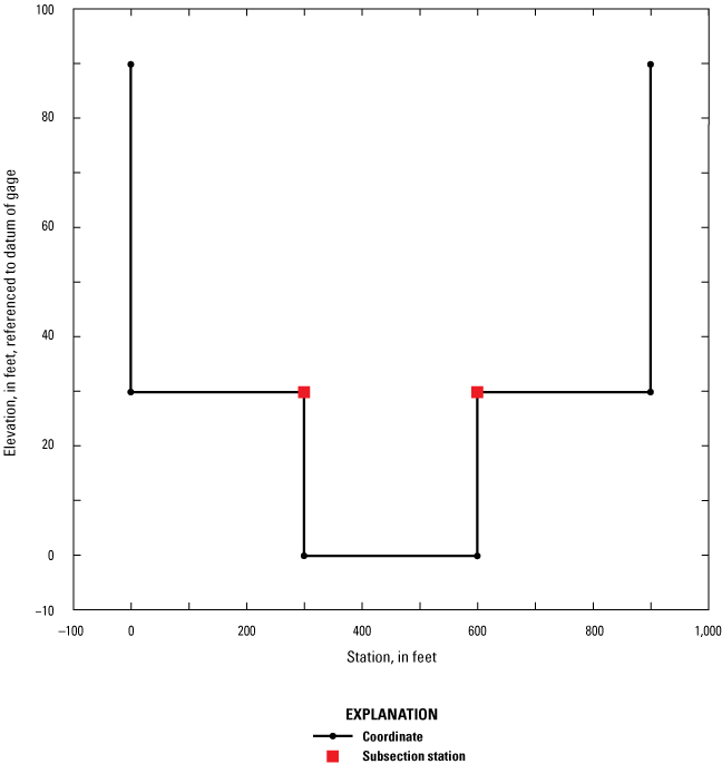
Graph showing a representative cross section for simulated test datasets.

Graphs showing stage plotted against four variables. A, top width and wetted perimeter; B, area; and C, conveyance.
Different inflow hydrographs were developed for the evaluation to test the range of unsteadiness in the simulated responses from the three computation methods: HEC–RAS, DYNMOD, and DYNPOUND. A normal depth boundary condition was used at the downstream end of each scenario with the appropriate S0 assigned to the normal depth relation.
All scenarios were simulated in HEC–RAS. The HEC–RAS computed stage and discharge time series at the cross-section (40 miles downstream from the inflow point, midway between the most upstream and most downstream cross sections of the 80-mile reach) were extracted and used to compute and compare the discharge with the dynamic rating methods. The midpoint of the cross section was selected to reduce the effects of the boundary conditions on the simulation results. The Manning’s n-value, S0, and r values used in the development of the HEC–RAS scenarios were assigned to the parameters in the dynamic rating discharge computations.
Dataset Development
The width of the main channel of the simulated cross section was 300 feet (ft), the floodplains have a total width of 600 ft, and the total width of the cross section was 900 ft. The bankfull depth of the main channel was 30 ft. The subsection stations coincide with the bank stations at 300 and 600 ft (fig. 2). An n-value of 0.035 was used for all scenarios in the cross section.
Table 1.
Bed slope and ratio of bed slope to average wave slope of simulated test data scenarios.[r, ratio of bed slope to average wave slope]
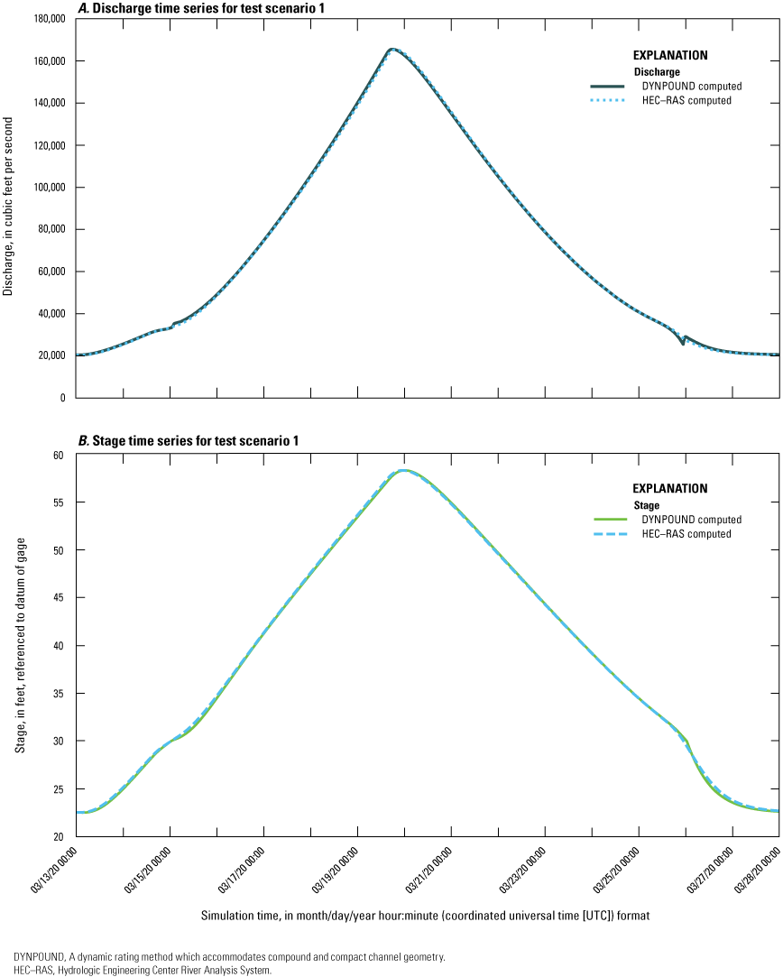
Four sets of hydrographs, which were used as upstream boundary conditions for each scenario, were developed to simulate stage and discharge time series under varied channel slope and unsteadiness conditions in the test scenarios (figs. 4–7; Domanski and others, 2022b; Domanski and others, 2025). The value of unsteadiness can be characterized by r, which is the ratio of S0 to Sw (eq. 17). The larger the value of r for a particular S0, the lower the unsteadiness of the hydrograph; that is, the time from the onset of the flooding to the flood peak increases with increasing value of r. To determine the actual inflow hydrographs used for the scenarios, a flood wave slope was computed from a S0 and an assumed value of r (table 1). The rising and falling limbs of the stage hydrograph were computed using the constant value of the slope of the flood wave between the end points of 75 percent of the bankfull main channel depth (22.5 ft) to the peak stage (60 ft). The peak stage was chosen such that the total wetted area in the floodplain equaled the wetted area in the upstream channel location. Manning’s equation from the stage hydrograph was used to compute the discharge hydrographs for the upstream boundary condition.

Graphs showing time series for simulated test scenario 1 (Domanski and others, 2025). A, discharge and B, stage.
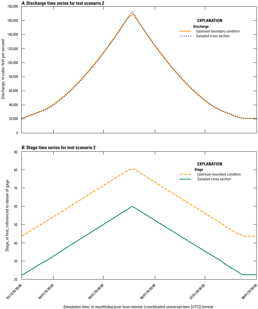
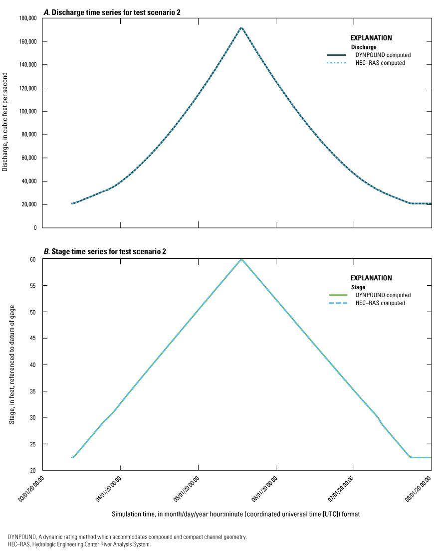
Graphs showing time series for simulated test scenario 2 (Domanski and others, 2025). A, discharge and B, stage.
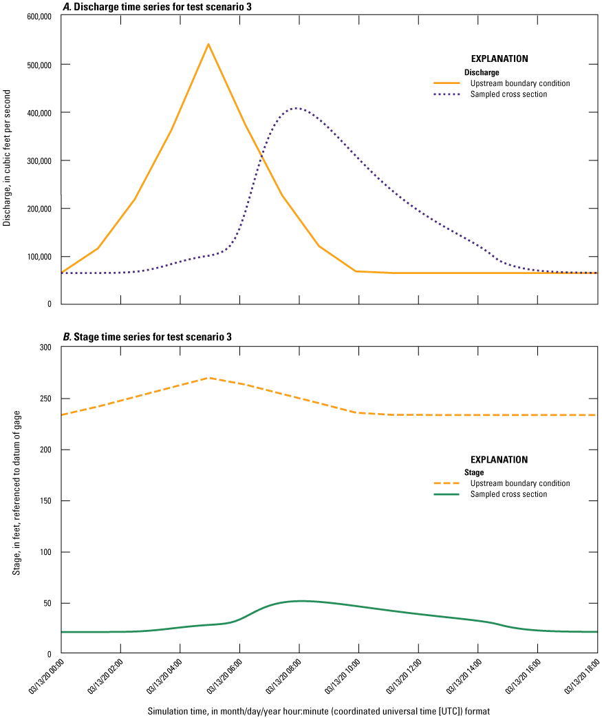
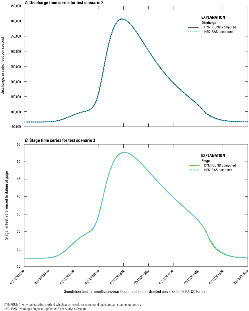
Graphs showing time series for simulated test scenario 3 (Domanski and others, 2025). A, discharge and B, stage.
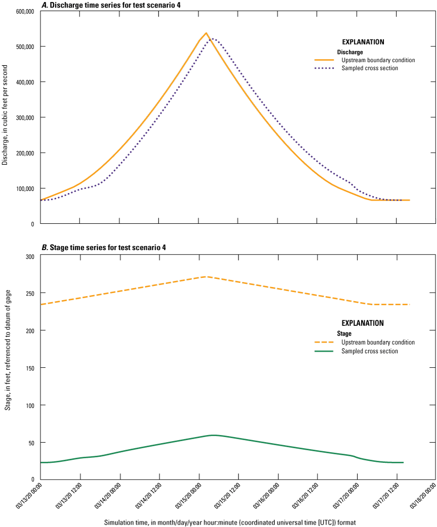
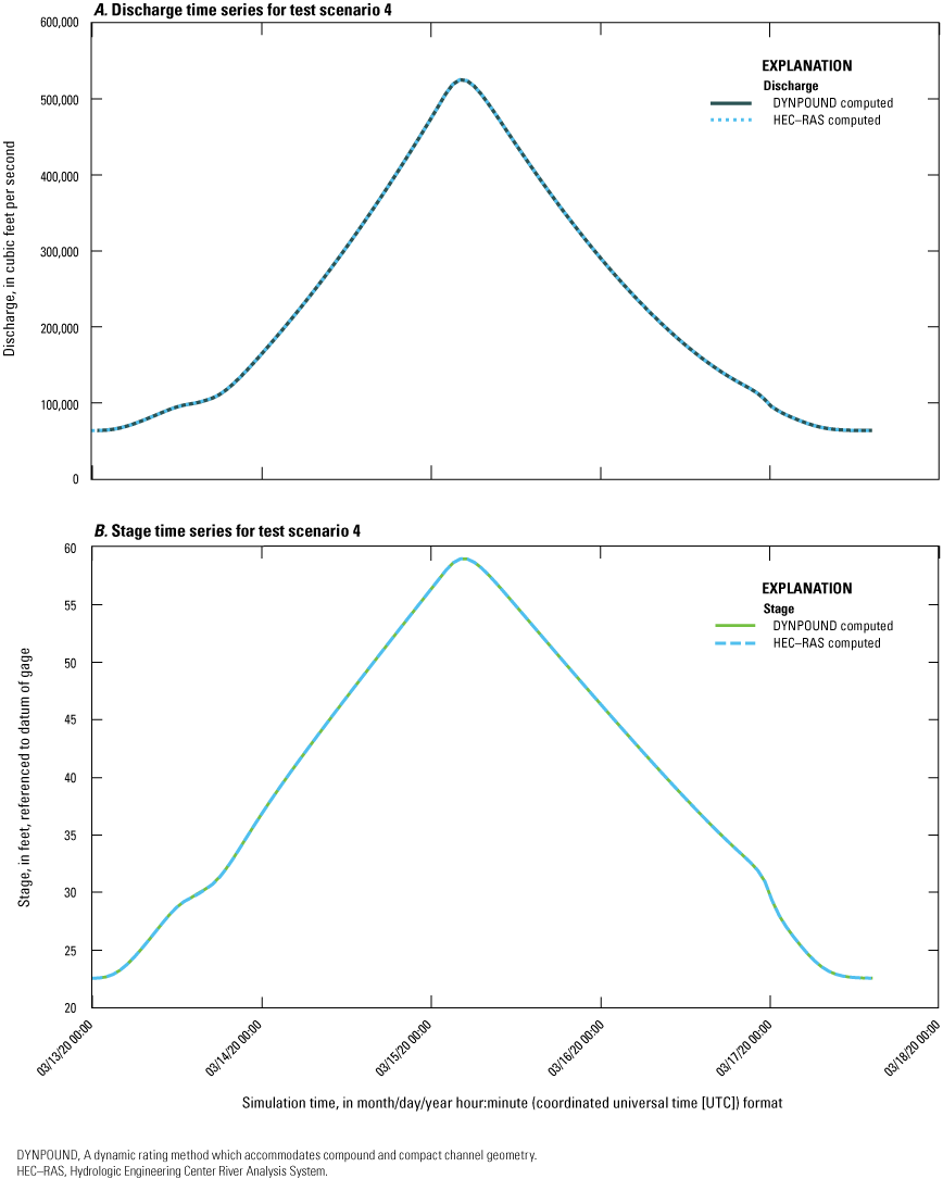
Graphs showing time series for simulated test scenario 4 (Domanski and others, 2025). A, discharge and B, stage.
Evaluation
A preliminary analysis of the four test scenarios was performed using the DYNMOD method, in which jumps in discharge were observed in the time series (Domanski and others, 2022b). The first jump, from a higher to a lower discharge, took place when the stage rose from below to above the channel bank elevation, and the second jump, from a lower to higher discharge, took place once the elevation fell below the bank elevation. These jumps happened because of abrupt changes in the relations of top width, wetted perimeter, and area with stage (fig. 3). For more information about these test scenarios and the DYNMOD method, refer to Domanski and others (2022b).
Overall, the magnitude of the mean percent error was much greater in the results computed with the DYNMOD method (Domanski and others, 2022b). The error is smaller in the time series computed with the DYNPOUND method because this method relies on the conveyance, as well as area and top width (refer to eq. 13). The function of conveyance with stage can be developed so that changes are less abrupt by creating subsections in the cross section, as was done for the simulated test scenarios.
The DYNPOUND method performed well compared to the full one-dimensional unsteady flow equations within HEC–RAS for all four scenarios. The mean percent error for the DYNPOUND-computed discharge was approximately 2.01×10⁻¹ percent. The mean percent error for the DYNPOUND-computed stage was −1.05×10⁻¹ percent. (table 2).
Table 2.
Performance statistics for the DYNPOUND computation method.[DYNPOUND is the newly developed method that solves for stage and discharge in compact and compound channels. MSLE, mean squared logarithmic error]
Scenarios 1 (fig. 4) and 3 (fig. 6) have values of r equaling 10 (table 1) and, therefore, are highly unsteady and show pronounced hysteresis in the stage versus discharge curves. Scenarios 2 (fig. 5) and 4 (fig. 7), which have values of r equaling 100 (table 1), do not show hysteresis. Furthermore, the DYNPOUND method performs better for discharge and stage in scenarios 2 and 4 than it does in scenarios 1 and 3 (table 2). Scenarios 2 and 4 effectively have one-to-one stage-discharge relations.
Scenario 1
At approximately 30 ft, where flow begins to exceed the main channel, DYNPOUND-computed discharge and stage time series show a “jog” in the relation (fig. 8). This is likely due to the abrupt change in channel geometry and the application of a single n-value for the entire channel. The scenario 1 stage-discharge relation indicates hysteresis in the HEC–RAS results because of unsteady flow effects captured by the dynamic ratings simulations (fig. 9).
Graphs showing time series for simulated scenario 1 (Domanski and others, 2025). A, Discharge computed with the DYNPOUND method; B, stage computed with the DYNPOUND method.
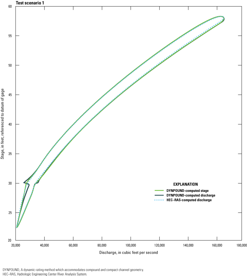
Graph showing the relation between stage and computed discharge and discharge and computed stage for simulated scenario 1 (Domanski and others, 2025).
Scenario 2
Scenario 2’s computed hydrographs indicate a lack of hysteresis (figs. 10 and 11). The stage-discharge relation of the HEC–RAS results for scenario 2 is effectively one-to-one because the distance between the discharge values computed at a given stage is small (fig. 11).
Graphs showing time series for simulated scenario 2 (Domanski and others, 2025). A, Discharge computed with the DYNPOUND method; B, Stage computed with the DYNPOUND method.
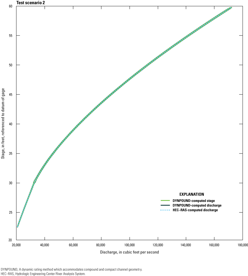
Graph showing the relation between stage and computed discharge and discharge and computed stage for simulated scenario 2 (Domanski and others, 2025).
Scenario 3
Scenario 3’s stage discharge relation computed by HEC–RAS shows hysteresis with a similar “jog” to scenario 1, at 30 ft, when the channel geometry changes (fig. 12 and fig. 13).
Graphs showing time series for simulated scenario 3 (Domanski and others, 2025). A, Discharge computed with the DYNPOUND method; B, Stage computed with the DYNPOUND method.
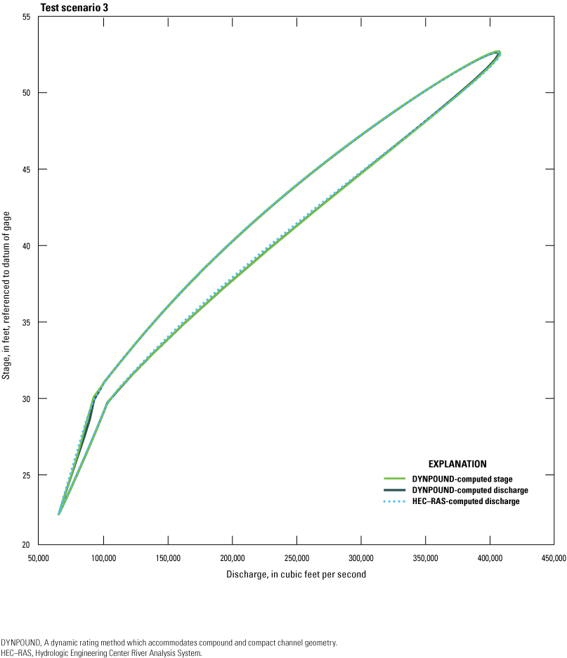
Graph showing the relation between stage and computed discharge and discharge and computed stage for simulated scenario 3 (Domanski and others, 2025).
Scenario 4
The stage-discharge relation of the scenario 4 time series (fig. 14) as computed using HEC–RAS does not show hysteresis and can effectively be considered a one-to-one relation (fig. 15).
Graphs showing time series for simulated scenario 4 (Domanski and others, 2025). A, Discharge computed with the DYNPOUND method; B, stage computed with the DYNPOUND method.
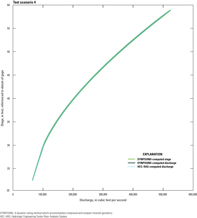
Graph showing the relation between stage and computed discharge and discharge and computed stage for simulated scenario 4 (Domanski and others, 2025).
Evaluation Using Field Data
Field measurements of discharge and stage and WSC-computed discharge and WSC-measured stage from 10 USGS streamgages were used to evaluate the DYNPOUND method (U.S. Geological Survey, 2020). These streamgages represent a variety of geographic locations and geomorphic conditions. The 10 streamgage sites chosen for evaluation were Meherrin River near Bryants Corner, Virginia (USGS streamgage 02052090); Tug Fork at Kermit, West Virginia (USGS streamgage 03214500); Tittabawassee River at Midland, Michigan (USGS streamgage 04156000); Red River of the North at Fargo, North Dakota (USGS streamgage 05054000); Papillion Creek at Fort Crook, Nebraska (USGS streamgage 06610795); Gasconade River at Jerome, Missouri (USGS streamgage 06933500); Mississippi River at St. Louis, Missouri (USGS streamgage 07010000); Calcasieu River near Kinder, Louisiana (USGS streamgage 08015500); Rio Grande near Cerro, New Mexico (USGS streamgage 08263500); and San Joaquin River near Mendota, California (USGS streamgage 11254000) (fig. 16 and table 3).
Dataset Development
Site datasets consisted of WSC-computed discharge and WSC-measured stage time series, field measurements of discharge and stage, cross-section geometry, and bed slope. Time series and field measurements were obtained from the National Water Information System (NWIS; U.S. Geological Survey, 2020). Cross-section geometry and bed slope were computed for each site using a combination of acoustic Doppler profiler (ADCP) software, AreaComp2 USGS utility (U.S. Geological Survey, 2015), ArcGIS Pro (Esri, 2021), and HEC–RAS (U.S. Army Corps of Engineers, 2016).
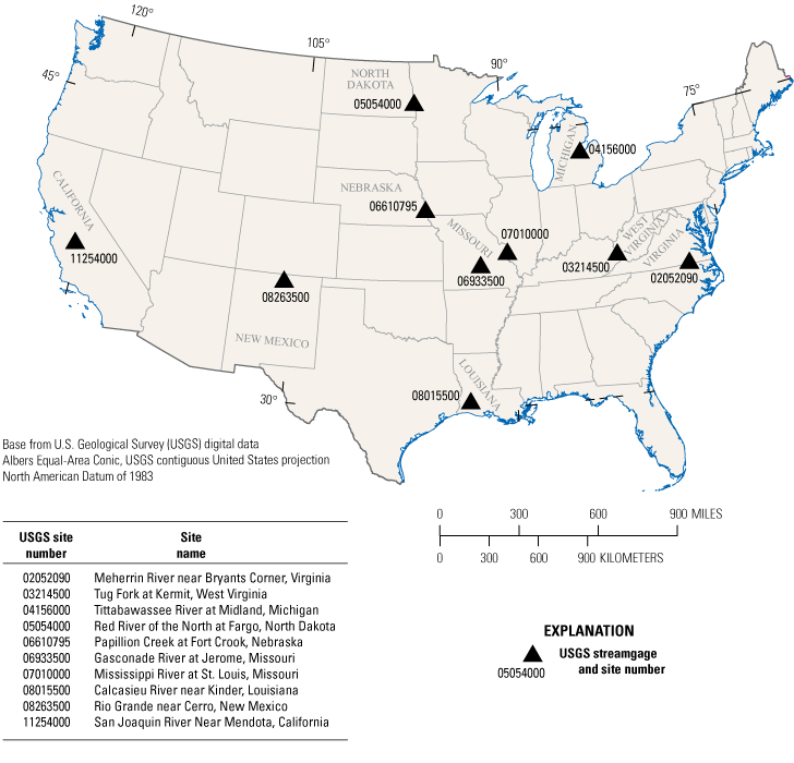
Map of U.S. Geological Survey streamgage sites used to evaluate discharge computed with the dynamic rating methods (U.S. Geological Survey, 2020). USGS, U.S. Geological Survey.
Table 3.
Streamgage number and name, drainage area, and slope of the field sites used to evaluate the DYNPOUND dynamic rating method.[Data from U.S. Geological Survey, 2020. DYNPOUND is the newly developed method that solves for stage and discharge in compact and compound channels. mi2, square mile]
Bed slope was calculated using elevation contour, topographical maps, and the National Hydrography Dataset (U.S. Geological Survey, 2017; Domanski and others, 2022a).
Cross-Section Geometry
To obtain cross-section geometry, an ADCP discharge measurement was selected for each site that generally corresponded to a high-flow event. The ADCP measurement was then converted into a “station, depth” coordinate format and imported into AreaComp2. AreaComp2 was used to convert the “station, depth” coordinates to “station, elevation” (in stage datum) coordinates. Next, a digital elevation model (DEM; U.S. Geological Survey, 2017; Michigan State University, 2020; U.S. Department of Agriculture, 2021) was imported into RAS Mapper within HEC–RAS, which was used to generate a “station, elevation” (in stage datum) cross section (fig. 17). This cross section created from the DEM was combined with the cross section created from the ADCP transect to create a cross section that contained the main channel and overbank sections (fig. 18).
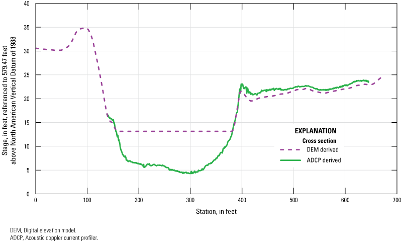
Graph showing cross sections derived from an acoustic doppler profiler (ADCP) and a digital elevation model (DEM) at Tittabawassee River at Midland, Michigan (U.S. Geological Survey streamgage 04156000).
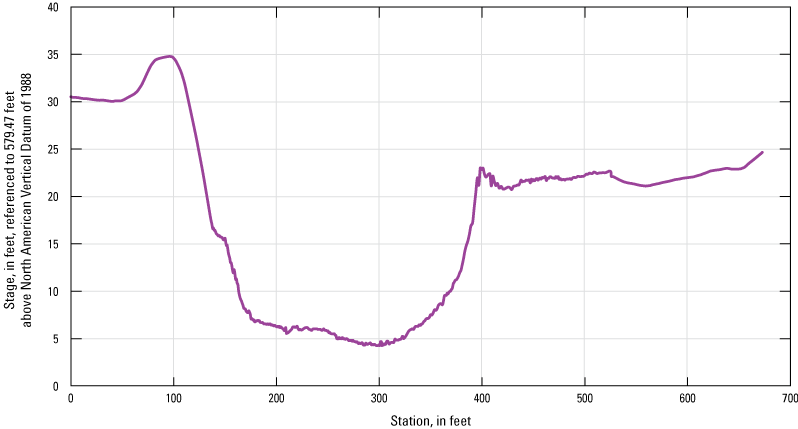
Graph showing combined cross section at Tittabawassee River at Midland, Michigan (U.S. Geological Survey streamgage 04156000). ft, foot.
The cross section created from the ADCP measurement most accurately represented the channel, and the cross section created from the DEM was used to represent the larger floodplain. In some cases, a stage measurement was made during a peak-flow event that was high enough to capture some of the floodplain. If that happened, then “station, elevation” (in stage datum) coordinates from the ADCP measurement superseded the overlapping coordinates from the DEM. Geospatially locating ADCP transects at sites without geolocation data associated with ADCP measurements was difficult. If a cross section created from the DEM was used exclusively, it generally lacked accurate channel geometry. If a cross section created from the ADCP was used, it generally lacked floodplain geometry. Sometimes cross sections with these limitations did not produce accurate results in either of the dynamic rating computation methods. When associated geolocation data for an ADCP measurement was lacking and the location of the cross section was otherwise unable to be located, the cross-section geometry was taken from the DEM exclusively, and properties of the channel geometry were estimated.
Bed Slope
Bed slope (S0) was calculated using elevation contours, historical topographical maps, and the National Hydrography Dataset flowline geospatial files (U.S. Geological Survey, 2017; Domanski and others, 2022a). Points were chosen upstream and downstream from each streamgage where an elevation contour line crossed the channel; reach lengths varied depending on available map contours, ranging from approximately 4,582 to 781,450 ft (Domanski and others, 2022a). To compute S0, the following equation was used:
whereEvaluation
Discharge and stage time series were computed with the DYNPOUND method for streamgages where cross-section geometry was created and real-time stage and discharge data were being collected. These time series were computed at 10 streamgages in California, Louisiana, Michigan, Missouri, Nebraska, New Mexico, North Dakota, Virginia, and West Virginia.
For all sites, an event was chosen to compute the value of r (ratio of S0 to SW); the event was typically an isolated flood wave with a moderate peak stage and discharge. The stage at the time immediately before the onset of the flood was inserted into equation 20 as h0. The peak stage of the flood is hp in equation 20. The time of peak stage minus the time of occurrence of h0 is τ in equation 20.
Subsections were added to the cross section of each site based on the need to (1) develop a smooth conveyance and stage relation, (2) add regions where transitions in roughness occur in the floodplain, (3) remove those areas of the cross section that do not contribute to the momentum of the flow (in other words, sections of the floodplain that were not inundated or sections of the channel higher in elevation than the peak stage during a high flow event), and (4) allow for computation of the non-uniform velocity distribution coefficient. To determine the smoothness of the stage-conveyance relation, conveyance was plotted against stage and visually analyzed. If an abrupt change in the slope of the relation was observed, the cross section was analyzed for sudden changes in geometry. Existing subsections that contained sudden changes in geometry were split into two subsections by inserting a split where the changes take place.
If there was a sudden change in the slope of the relation with no obvious change in channel geometry, the n-values of the cross section were modified according to the stage value at which the flow pattern shifted. The change was assumed to be because of unknown phenomena such as varying bed material or vegetation, obstruction, or channel meandering (Davidian, 1984; Arcement and Schneider, 1989).
A full water year of stage and discharge time series was used to calibrate the method at each site. A water year is defined as the 12-month period, October 1 through September 30, and is designated by the calendar year in which it ends. Typically, at least 5 field measurements were used to calibrate each of the 10 streamgages for which results are discussed. Cross sections were also subsectioned so the DYNPOUND-computed measurement would match the field measurement. The S0, value of r, and cross-section geometry were considered fixed values for the calibration.
After the site was calibrated, a different period in the record was selected to evaluate the method. For each site, the evaluation period typically follows the calibration period and contains at least five field measurements, and a wide range of WSC-computed discharge and WSC-measured stage time-series values. Discharge field measurements were then compared to DYNPOUND-computed discharge at the same times and vice versa for stage field measurements. Sometimes, WSC-computed discharge or WSC-measured stage data were missing from the time series, in which case the missing discharge or stage values of the DYNPOUND-computed time series were estimated through linear interpolation (Domanski and others, 2022b). If the period of missing data was longer than a few hours, a different period was chosen for calibration.
Meherrin River near Bryants Corner, Virginia
The USGS streamgage at Meherrin River near Bryants Corner, Virginia (USGS streamgage 02052090), encompasses 870 square miles (mi2). The computed S0 for the site is 0.00037809 (table 3). The value of r computed for the event with a peak stage of 16.82 ft at 6:15 (coordinated universal time [UTC]) on December 28, 2015 (U.S. Geological Survey, 2020), is 80.63. The cross section used to compute the time series for this streamgage is shown in figure 19. The n-values chosen for the DYNPOUND computations vary from 0.045 to 0.45 (table 4). The cross section was split into five subsections; subsection stations are 250, 265, 350, and 375 ft from left bank.
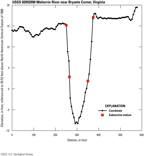
Graph showing the cross section used to compute the stage and discharge time series at Meherrin River near Bryants Corner, Virginia (U.S. Geological Survey streamgage 02052090; U.S. Geological Survey, 2020).
Twenty field measurements of stage and discharge from the 2017 water year were used for calibration (table 5 and table 6). The WSC-measured stage time series for the 2017 water year was used to compute discharge, and the WSC-computed discharge time series for the same water year was used to compute stage using the DYNPOUND method. (U.S. Geological Survey, 2020). The MSLE for the DYNPOUND discharge calibration was 1.30×10⁻², and the mean percent error was 2.36 percent (table 5). The MSLE for the DYNPOUND stage calibration was 9.97×10⁻³, and the mean percent error was 0.37 (table 6).
Table 4.
Stage and roughness coefficient values used to calibrate the DYNPOUND method at Meherrin River near Bryants Corner, Virginia (U.S. Geological Survey streamgage 02052090).[Data from Domanski and others, 2025. ft, foot]
Table 5.
Discharge calibration results for the DYNPOUND ratings at Meherrin River near Bryants Corner, Virginia (U.S. Geological Survey streamgage 02052090).[Field measurement discharge data from U.S. Geological Survey, 2020. DYNPOUND is the newly developed method that solves for stage and discharge in compact and compound channels. MM, month; DD, day; YYYY, year; UTC, coordinated universal time; FM, field measurement; ft3/s, cubic foot per second; SLE, squared logarithmic error; NA, not applicable]
Table 6.
Stage calibration results for the DYNPOUND ratings at Meherrin River near Bryants Corner, Virginia (U.S. Geological Survey streamgage 02052090).[Field measurement stage data from U.S. Geological Survey, 2020. DYNPOUND is the newly developed method that solves for stage and discharge in compact and compound channels. MM, month; DD, day; YYYY, year; UTC, coordinated universal time; FM, field measurement; ft, foot; SLE, squared logarithmic error; NA, not applicable]
To evaluate the stage-discharge relation for the USGS streamgage at Meherrin River near Bryants Corner, Virginia, time series of stage and discharge were computed for the period between May 17 and 31, 2018, which included four field measurements used for error assessment (fig. 20 and fig. 21). A comparison of field measurement discharge and DYNPOUND-computed discharge for the period indicates the DYNPOUND values were biased high when compared to the field measurements and had a mean error of 6.25 percent (fig. 20). The MSLE was 6.40×10⁻³ (table 7). The mean error for the DYNPOUND-computed stage was −0.84 percent, and the MSLE was 2.48×10⁻³ (table 8). DYNPOUND captured hysteresis in the stage-discharge relation for the computed event, whereas the USGS-computed discharge is monotonic and did not capture hysteresis (fig. 22).
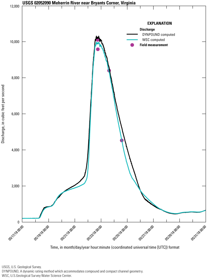
Graph showing the discharge time series computed with the DYNPOUND method shown with the time series of WSC-computed discharge and field measurements made at Meherrin River near Bryants Corner, Virginia (U.S. Geological Survey streamgage 02052090; U.S. Geological Survey, 2020).
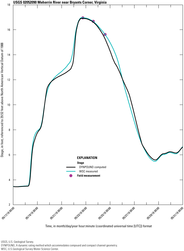
Graph showing the stage time series computed with the DYNPOUND method shown with the time series of WSC-measured stage and field measurements made at Meherrin River near Bryants Corner, Virginia (U.S. Geological Survey streamgage 02052090; U.S. Geological Survey, 2020).
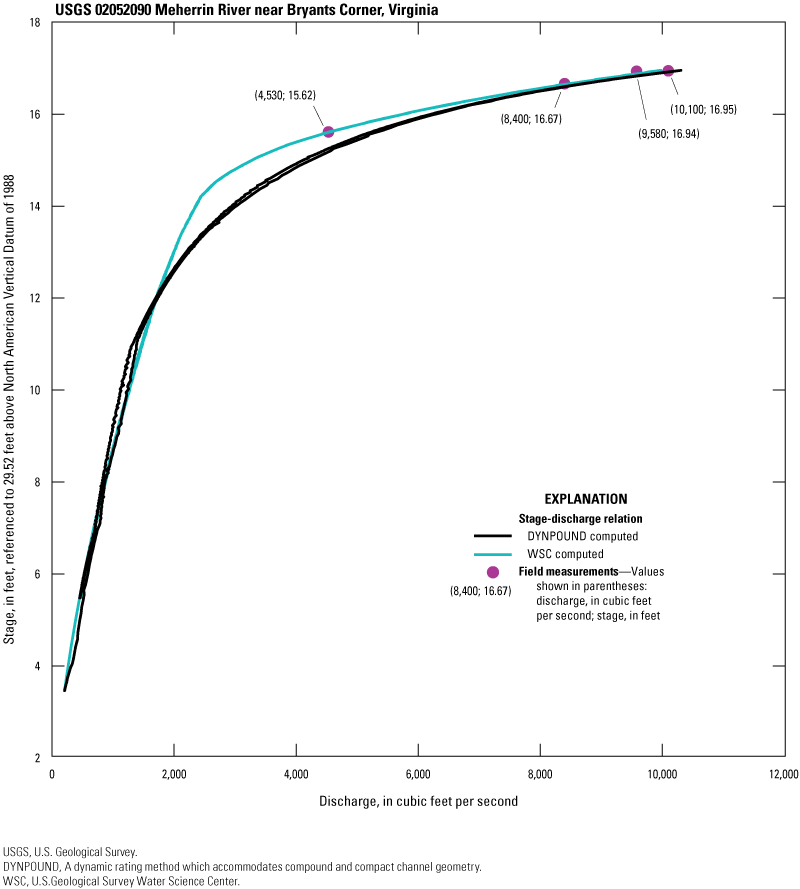
Graph showing the stage-discharge relation at Meherrin River near Bryants Corner, Virginia (U.S. Geological Survey streamgage 02052090; U.S. Geological Survey, 2020), using discharge computed with the DYNPOUND method, WSC-computed discharge, and field measurements.
Table 7.
Discharge computed for an event-based time series at Meherrin River near Bryants Corner, Virginia (U.S. Geological Survey streamgage 02052090), with the DYNPOUND methods and the associated error.[Field measurement discharge data from U.S. Geological Survey, 2020. DYNPOUND is the newly developed method that solves for stage and discharge in compact and compound channels. MM, month; DD, day; YYYY, year; UTC, coordinated universal time; FM, field measurement; ft3/s, cubic foot per second; SLE, squared logarithmic error; NA, not applicable]
Table 8.
Stage computed for an event-based time series at Meherrin River near Bryants Corner, Virginia (U.S. Geological Survey streamgage 02052090), with the DYNPOUND methods and the associated error.[Field measurement stage data from U.S. Geological Survey, 2020. DYNPOUND is the newly developed method that solves for stage and discharge in compact and compound channels. MM, month; DD, day; YYYY, year; UTC, coordinated universal time; FM, field measurement; ft, foot; SLE, squared logarithmic error; NA, not applicable]
Tug Fork at Kermit, West Virginia
The USGS streamgage Tug Fork at Kermit, West Virginia (USGS streamgage 03214500), encompasses 1,277 mi2. The computed S0 for the site is 0.000352 (table 3). The r value, computed from the event with the peak stage of 24.35 ft at 01:15 (coordinated universal time [UTC]) on April 25, 2017 (U.S. Geological Survey, 2020), is 37.19. The cross section used to compute the time series is shown in figure 23. However, it does not meet the criteria for subdivision (Dalrymple and Benson, 1967; Davidian, 1984). The n-values were chosen for the full cross section based on a plot of n-values, calculated with Manning’s equation and field measurements, versus stage (table 9). To review software functionality and documentation regarding these plots, refer to the software release by Knight and others (2025).
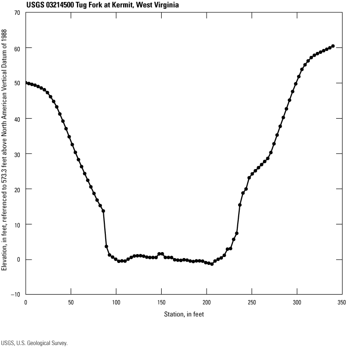
Graph showing the cross section used to compute the stage and discharge time series at Tug Fork at Kermit, West Virginia (U.S. Geological Survey streamgage 03214500; U.S. Geological Survey, 2020).
Six field measurements of stage and discharge from the 2016 water year were used to calibrate the method at this site. (table 10 and table 11). The WSC-measured stage time series for the 2016 water year was used to compute discharge, and the WSC-computed discharge time series for the same water year was used to compute stage using the DYNPOUND method (U.S. Geological Survey, 2020). The MSLE for the DYNPOUND discharge calibration was 7.84×10⁻³, and the mean percent error was −6.69 percent (table 10). The MSLE for the DYNPOUND stage calibration was 3.17×10⁻², and the mean percent error was 3.27 percent (table 11).
Table 9.
Stage and roughness coefficient values used to calibrate the DYNPOUND method at Tug Fork at Kermit, West Virginia (U.S. Geological Survey streamgage 03214500).[Data from Domanski and others, 2025. ft, foot]
Table 10.
Calibration results for the DYNPOUND discharge ratings at Tug Fork at Kermit, West Virginia (U.S. Geological Survey streamgage 03214500).[Field measurement discharge data from U.S. Geological Survey, 2020. DYNPOUND is the newly developed method that solves for stage and discharge in compact and compound channels. MM, month; DD, day; YYYY, year; UTC, coordinated universal time; FM, field measurement; ft3/s, cubic foot per second; SLE, squared logarithmic error; NA, not applicable]
Table 11.
Calibration results for the DYNPOUND stage ratings at Tug Fork at Kermit, West Virginia (U.S. Geological Survey streamgage 03214500).[Field measurement stage data from U.S. Geological Survey, 2020. DYNPOUND is the newly developed method that solves for stage and discharge in compact and compound channels. MM, month; DD, day; YYYY, year; UTC, coordinated universal time; FM, field measurement; ft, foot; SLE, squared logarithmic error; NA, not applicable]
To evaluate the stage-discharge relation for the USGS streamgage Tug Fork at Kermit, West Virginia, time series of stage and discharge were computed for the period between February 5 and March 1, 2018, which included five field measurements used for error assessment (fig. 24 and fig. 25). The DYNPOUND-computed discharge values had a mean percent error of 3.47 percent, and the MSLE was 1.38×10⁻² (table 12). The mean percent error for the DYNPOUND-computed stage was −4.71 percent, and the MSLE was 1.05×10⁻² (table 13). DYNPOUND captured hysteresis in the stage-discharge relation for the computed event, whereas the USGS-computed discharge is monotonic (fig. 26). The DYNPOUND computation has some inaccuracy because two of the field measurements are outside the loop: one was collected during the rising limb, and one was collected during the falling limb (fig. 26). Natural conditions, such as varying vegetation, debris, obstructions, or meandering of the channel, may be the cause of this inaccuracy, but are unknown to the authors. Tug Fork forms a section of the boundary between Kentucky and West Virginia, a mountainous region where torrential flows are common (McClellan, 2018), therefore requiring further calibration by those familiar with its hydrologic characteristics.

Graph showing the discharge time series computed with the DYNPOUND method shown with the time series of WSC-computed discharge and field measurements made at Tug Fork at Kermit, West Virginia (U.S. Geological Survey streamgage 03214500; U.S. Geological Survey, 2020).
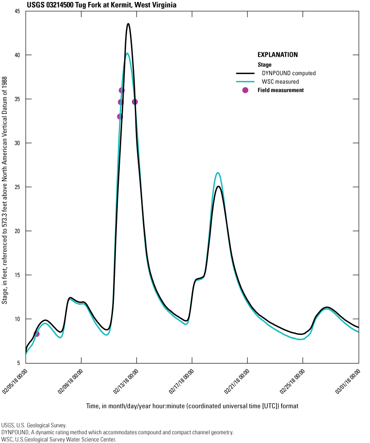
Graph showing the stage time series computed with the DYNPOUND method shown with the time series of WSC-measured stage and field measurements made at Tug Fork at Kermit, West Virginia (U.S. Geological Survey streamgage 03214500; U.S. Geological Survey, 2020).
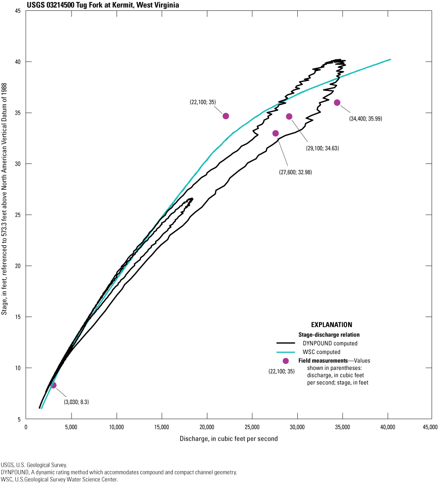
Graph showing the stage-discharge relation at Tug Fork at Kermit, West Virginia (U.S. Geological Survey streamgage 03214500; U.S. Geological Survey, 2020), using discharge computed with the DYNPOUND method, WSC-computed discharge, and field measurements.
Table 12.
Discharge computed for an event-based time series at Tug Fork at Kermit, West Virginia (U.S. Geological Survey streamgage 03214500), with the DYNPOUND methods and the associated error.[Field measurement discharge data from U.S. Geological Survey, 2020. DYNPOUND, the newly developed method that solves for discharge in compact and compound channels. MM, month; DD, day; YYYY, year; UTC, coordinated universal time; FM, field measurement; ft3/s, cubic foot per second; SLE, squared logarithmic error; NA, not applicable]
Table 13.
Stage computed for an event-based time at the streamgage at Tug Fork at Kermit, West Virginia (U.S. Geological Survey streamgage 03214500), with the DYNPOUND methods and the associated error.[Field measurement stage data from U.S. Geological Survey, 2020. DYNPOUND, the newly developed method that solves for stage and discharge in compact and compound channels. MM, month; DD, day; YYYY, year; UTC, coordinated universal time; FM, field measurement; ft, foot; SLE, squared logarithmic error; NA, not applicable]
Tittabawassee River at Midland, Michigan
The USGS streamgage Tittabawassee River at Midland, Michigan (USGS streamgage 04156000) encompasses 2,400 mi2. The computed S0 for the site is 0.000139 (table 3). The value of r was computed as 18.08 by using the event with a peak stage of 22.16 ft at 12:30 UTC on April 11, 2015 (U.S. Geological Survey, 2020). The cross section used to compute the time series is shown in figure 27. Subsection stations are at 90 and 401 ft. The leftmost subsection of the cross section becomes inundated at stages above 35 ft. Based on the channel geometry and corresponding stage, an n-value of 0.0285 was chosen. An n-value of 0.0315 was used when stages rose above 22 ft on the flood-plain area of the right bank (fig. 27 and table 14). The middle subsection, which contains the same geometry as the main channel and assigned an n-value of 0.033, is always used when computing hydraulic properties (fig. 27 and table 14).
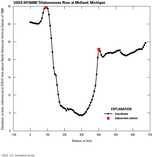
Graph showing the cross section used to compute the stage and discharge time series for the Tittabawassee River at Midland, Michigan (U.S. Geological Survey streamgage 04156000; U.S. Geological Survey, 2020).
Nine field measurements of stage and discharge collected during the 2017 water year were used for calibration (table 15 and table 16). The WSC-measured stage time series from the 2017 water year was used to compute discharge, and the WSC-computed discharge time series for the same water year was used to compute stage using the DYNPOUND method (U.S. Geological Survey, 2020). The calibration results for the DYNPOUND discharge computation indicate the MSLE was 2.88×10⁻², and the mean percent error was 1.93 percent (table 15). The MSLE for the DYNPOUND stage calibration was 0.24, and the mean error was 4.22×10⁻³ percent (table 16).
Table 14.
Stage and roughness coefficient values used to calibrate the DYNPOUND method at Tittabawassee River at Midland, Michigan (U.S. Geological Survey streamgage 04156000).[Data from Domanski and others, 2025. ft, foot]
Table 15.
Discharge calibration results for the DYNPOUND ratings at Tittabawassee River at Midland, Michigan (U.S. Geological Survey streamgage 04156000).[Field measurement discharge data from U.S. Geological Survey, 2020. DYNPOUND, the newly developed method that solves for stage and discharge in compact and compound channels. MM, month; DD, day; YYYY, year; UTC, coordinated universal time; FM, field measurement; ft3/s, cubic foot per second; SLE, squared logarithmic error; NA, not applicable]
Table 16.
Stage calibration results for the DYNPOUND ratings at Tittabawassee River at Midland, Michigan (U.S. Geological Survey streamgage 04156000).[Field measurement discharge data from U.S. Geological Survey, 2020. DYNPOUND, the newly developed method that solves for stage and discharge in compact and compound channels. MM, month; DD, day; YYYY, year; UTC, coordinated universal time; FM, field measurement; ft, feet; SLE, squared logarithmic error; NA, not applicable]
Field measurements of stage and discharge, DYNPOUND-computed stage and discharge time series, and WSC-computed stage and discharge time series were evaluated for the period between May 1 and June 30, 2020 (fig. 28 and fig. 29). The peak of the period is an extreme event for the site due to a dam break upstream. The stage hydrograph reached 35.13 ft (fig. 29), which was above the stage values defined by the cross-section geometry on the right overbank (fig. 27).
The DYNPOUND-computed stage and discharge values were compared to three field measurements (table 17 and table 18). The DYNPOUND discharge time series had a mean percent error of −0.57 percent and a MSLE of 1.71×10⁻³ (table 17). The DYNPOUND stage time series had a mean percent error of 0.40 percent and a MSLE of 6.19×10⁻⁴ (table 18). The DYNPOUND method captured hysteresis in the stage-discharge relation, whereas the USGS-computed method was not capable of representing hysteresis (fig. 30). The stage-discharge relation computed with DYNPOUND shows fluctuating discharges near the peak stage of the time series, which may be because of the poor definition of the cross-section geometry under the extreme flow conditions. Discharge might be better computed for this site by including a more precise definition of the channel geometry at high stages.
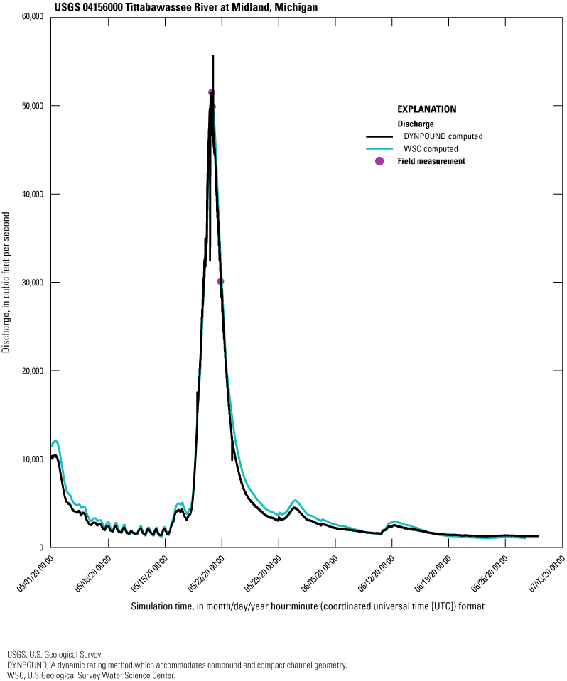
Graph showing the discharge time series computed with the DYNPOUND method shown with the time series of WSC-computed discharge and field measurements made at Tittabawassee River at Midland, Michigan (U.S. Geological Survey streamgage 04156000; U.S. Geological Survey, 2020).
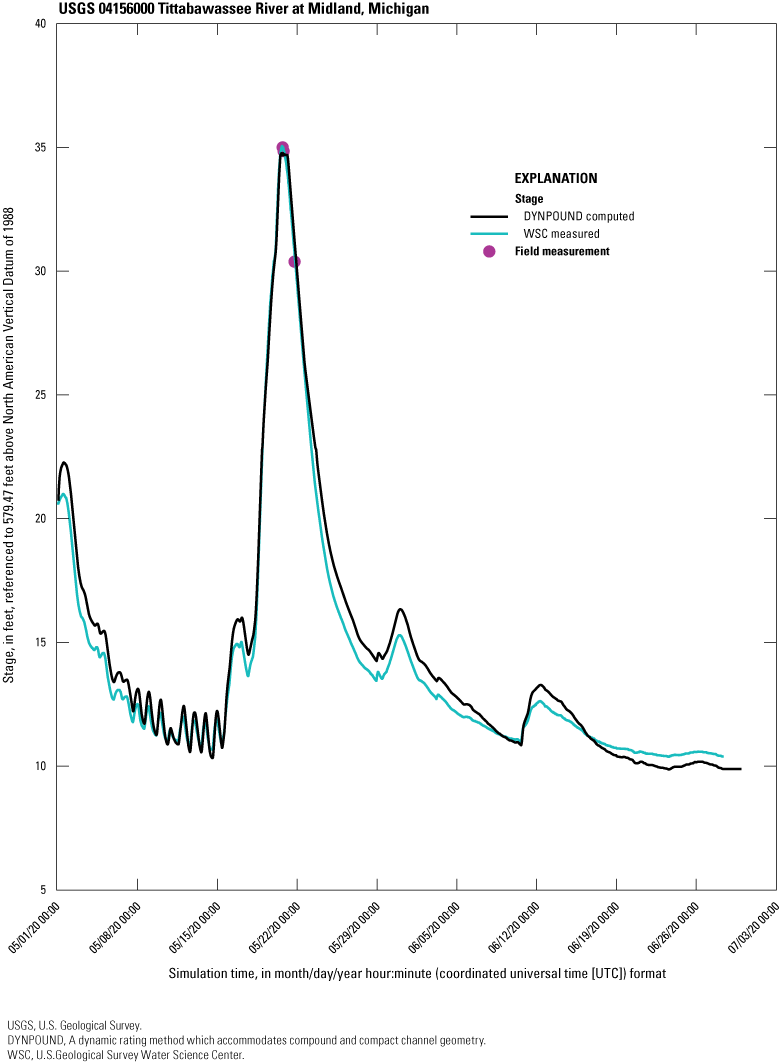
Graph showing the stage time series computed with the DYNPOUND method shown with the time series of WSC-measured and field measurements made at Tittabawassee River at Midland, Michigan (U.S. Geological Survey streamgage 04156000; U.S. Geological Survey, 2020).
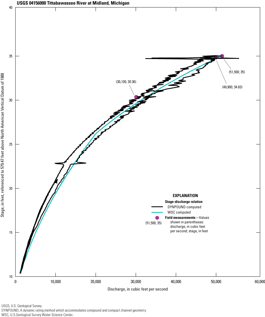
Graph showing the stage-discharge relation at Tittabawassee River at Midland, Michigan (U.S. Geological Survey streamgage 04156000; U.S. Geological Survey, 2020), using discharge computed with the DYNPOUND method, WSC-computed discharge, and field measurements.
Table 17.
Discharge computed with the DYNPOUND method and associated error for an event-based time series at Tittabawassee River at Midland, Michigan (U.S. Geological Survey streamgage 04156000).[Field measurement discharge data from U.S. Geological Survey, 2020. DYNPOUND, the newly developed method that solves for discharge in compact and compound channels. MM, month; DD, day; YYYY, year; UTC, coordinated universal time; FM, field measurement; ft3/s, cubic foot per second; SLE, squared logarithmic error; NA, not applicable]
Table 18.
Stage computed with the DYNPOUND method and associated error for an event-based time series at Tittabawassee River at Midland, Michigan (U.S. Geological Survey streamgage 04156000).[Field measurement discharge data from U.S. Geological Survey, 2020. DYNPOUND, the newly developed method that solves for stage and discharge in compact and compound channels. MM, month; DD, day; YYYY, year; UTC, coordinated universal time; FM, field measurement; ft, feet; SLE, squared logarithmic error; NA, not applicable]
Red River of the North at Fargo, North Dakota
The USGS streamgage Red River of the North at Fargo, North Dakota (U.S. Geological Survey streamgage 05054000) encompasses 6,800 mi2. The Red River of the North flows north through South Dakota, North Dakota, and Minnesota before entering Canada. Discharge at this site is affected by climactic variability and human alteration of the surrounding landscape, such as dam construction and agriculture (Nustad and Vecchia, 2020). The computed S0 for the site is 0.000145 (table 3). The r value, computed from the event with a peak stage of 27.85 ft at 23:30 UTC on June 23, 2014 (U.S. Geological Survey, 2020), is 27.4. The cross section used to compute the time series was split into four subsections for the DYNPOUND computation (fig. 31). Subsection stations are 625, 875, and 1,060 ft. The n-values used to calibrate the DYNPOUND computations vary from 0.067 to 0.224 (table 19).
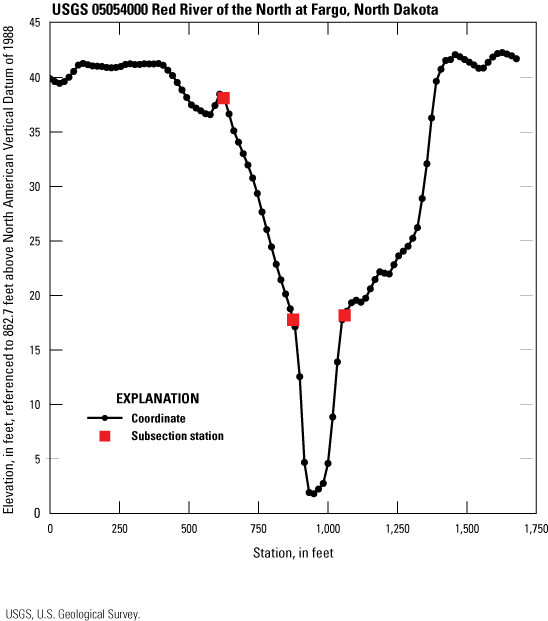
Graph showing the cross section used to compute the discharge time series at Red River of the North at Fargo, North Dakota (U.S. Geological Survey streamgage 05054000; U.S. Geological Survey, 2020).
Twelve field measurements of stage and discharge collected during the 2019 water year were used for calibration (table 20 and table 21). The WSC-measured stage time series from the 2019 water year was used to compute discharge, and the WSC-computed discharge time series for the same water year was used to compute stage using the DYNPOUND method (U.S. Geological Survey, 2020). The MSLE for the DYNPOUND discharge calibration was 9.62×10⁻³, and the mean percent error was 3.48 percent (table 20). The MSLE for the DYNPOUND stage calibration was 1.30×10⁻³, and the mean percent error was 1.53 percent (table 21).
Table 19.
Stage and roughness coefficient values used to calibrate the DYNPOUND method at Red River of the North at Fargo, North Dakota (U.S. Geological Survey streamgage 05054000).[Data from Domanski and others, 2025. ft, foot]
Table 20.
Discharge calibration results for the DYNPOUND ratings at Red River of the North at Fargo, North Dakota (U.S. Geological Survey streamgage 05054000).[Field measurement discharge data from U.S. Geological Survey, 2020. DYNPOUND, the newly developed method that solves for stage and discharge in compact and compound channels. MM, month; DD, day; YYYY, year; UTC, coordinated universal time; FM, field measurement; ft3/s, cubic foot per second; SLE, squared logarithmic error; NA, not applicable]
Table 21.
Stage calibration results for the DYNPOUND ratings at Red River of the North at Fargo, North Dakota (U.S. Geological Survey streamgage 05054000).[Field measurement stage data from U.S. Geological Survey, 2020. DYNPOUND, the newly developed method that solves for stage and discharge in compact and compound channels. MM, month; DD, day; YYYY, year; UTC, coordinated universal time; FM, field measurement; ft, feet; SLE, squared logarithmic error; NA, not applicable]
A discharge time series was computed with DYNPOUND for the period between March 16 and May 5, 2020, and was used to evaluate the generated rating in comparison to six field measurements collected during this period (fig. 32). The stage-discharge relation for the computed event is shown in figure 33. DYNPOUND shows that there is hysteresis with significant oscillation at stages of 19 ft and above. The channel begins to widen considerably at 19 ft, which may account for some of the oscillation. Other possible causes of the oscillation may be attributed to the hydroclimatic variability of the site, such as rising groundwater, surface-water runoff, increased soil moisture, and surface-water storage of the surrounding basin (Nustad and Vecchia, 2020). The WSC-computed discharge failed to capture hysteresis. The mean percent error of the DYNPOUND computed discharge was 0.21 percent and the MSLE was 6.37×10⁻³ (table 22). The DYNPOUND method was unable to compute stage for this event, which may relate to errors in the channel geometry.
Table 22.
Discharge computed with the DYNPOUND method and associated error for an event-based time series at Red River of the North at Fargo, North Dakota (U.S. Geological Survey streamgage 05054000).[Field measurement discharge data from U.S. Geological Survey, 2020. DYNPOUND, the newly developed method that solves for stage and discharge in compact and compound channels. MM, month; DD, day; YYYY, year; UTC, coordinated universal time; FM, field measurement; ft3/s, cubic foot per second; SLE, squared logarithmic error; NA, not applicable]
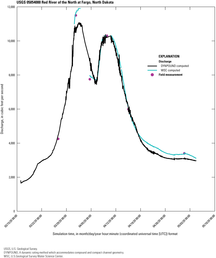
Graph showing the discharge time series computed with the DYNPOUND method shown with the time series of WSC-computed discharge and field measurements made at Red River of the North at Fargo, North Dakota (U.S. Geological Survey streamgage 05054000; U.S. Geological Survey, 2020).
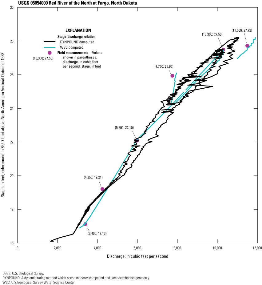
Graph showing the stage-discharge relation at Red River of the North at Fargo, North Dakota (U.S. Geological Survey streamgage 05054000; U.S. Geological Survey, 2020), using discharge computed with the DYNPOUND method, WSC-computed discharge, and field measurements.
Papillion Creek at Fort Crook, Nebraska
The USGS streamgage Papillion Creek at Fort Crook, Nebraska (USGS streamgage 06610795) encompasses 946 mi2. The computed S0 for the site is 0.00025438 (table 3). The value of r, computed from the event with a peak stage of 21.76 ft at 5:15 (coordinated universal time [UTC]) on June 17, 2017 (U.S. Geological Survey, 2020), is 2.7. The cross section used to compute the time series was split into four subsections for the DYNPOUND computation, with subsection stations at 105, 245, and 325 ft (fig. 34). Manning’s n-values selected to calibrate the DYNPOUND computations varied from 0.022 to 0.015 (table 23).
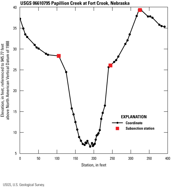
Graph showing the cross section used to compute the stage and discharge time series at Papillion Creek at Fort Crook, Nebraska (U.S. Geological Survey streamgage 06610795; U.S. Geological Survey, 2020).
Eight field measurements of stage and discharge from the 2016 water year were used for calibration (table 24 and table 25). The WSC-measured stage time series for the 2016 water year was used to compute discharge, and the WSC-computed discharge time series for the same water year was used to compute stage using the DYNPOUND method. (U.S. Geological Survey, 2020). The MSLE for the DYNPOUND discharge calibration was 3.04×10⁻², and the mean percent error was 13.40 percent (table 24). The MSLE for the DYNPOUND stage calibration was 6.62×10⁻³, and the mean percent error was −1.90 percent (table 25).
Table 23.
Stage and roughness coefficient values used to calibrate the DYNPOUND method at Papillion Creek at Fort Crook, Nebraska (U.S. Geological Survey streamgage 06610795).[Data from Domanski and others, 2025. ft, foot]
Table 24.
Discharge calibration results for the DYNPOUND ratings at Papillion Creek at Fort Crook, Nebraska (U.S. Geological Survey streamgage 06610795).[Field measurement discharge data from U.S. Geological Survey, 2020. DYNPOUND, the newly developed method that solves for stage and discharge in compact and compound channels; MM, month; DD, day; YYYY, year; UTC, coordinated universal time; FM, field measurement; ft3/s, cubic foot per second; SLE, squared logarithmic error; NA, not applicable]
Table 25.
Stage calibration results for the DYNPOUND ratings at Papillion Creek at Fort Crook, Nebraska (U.S. Geological Survey streamgage 06610795).[Field measurement stage data from U.S. Geological Survey, 2020. DYNPOUND, the newly developed method that solves for stage and discharge in compact and compound channels; MM, month; DD, day; YYYY, year; UTC, coordinated universal time; FM, field measurement; ft3/s, cubic foot per second; SLE, squared logarithmic error; NA, not applicable]
To evaluate the stage-discharge relation for the USGS streamgage Papillion Creek at Fort Crook, Nebraska, time series of stage and discharge were computed for the period between August 22 and 24, 2014, which included three field measurements used for error assessment (fig. 35 and fig. 36). DYNPOUND captured hysteresis for two peaks in the stage-discharge relation for the computed event (fig. 37). A comparison between the WSC-computed and DYNPOUND-computed discharge for the period resulted in a mean percent error of 14.26 percent and a MSLE of 2.30×10⁻² (table 26). Results of the comparison between WSC-measured and DYNPOUND-computed stage for this event showed a mean percent error of −3.01 percent and a MSLE of 6.72×10⁻³ (table 27).
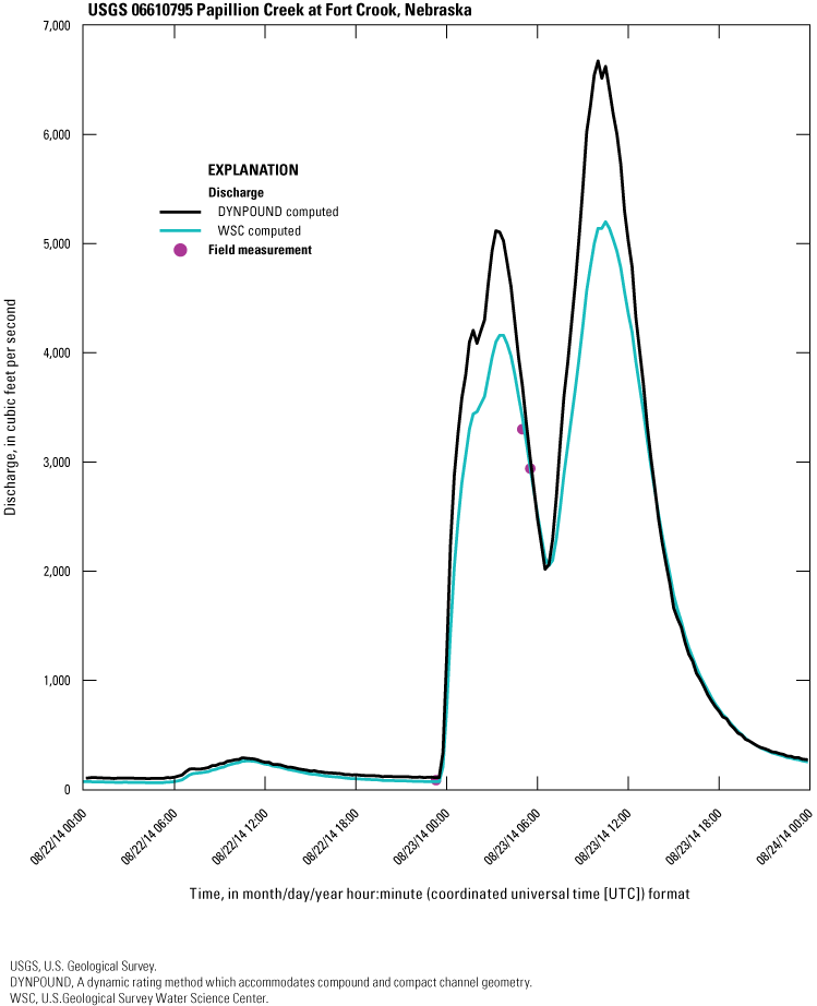
Graph showing the discharge time series computed with the DYNPOUND method shown with the time series of WSC-computed discharge and field measurements made at Papillion Creek at Fort Crook, Nebraska (U.S. Geological Survey streamgage 06610795; U.S. Geological Survey, 2020).
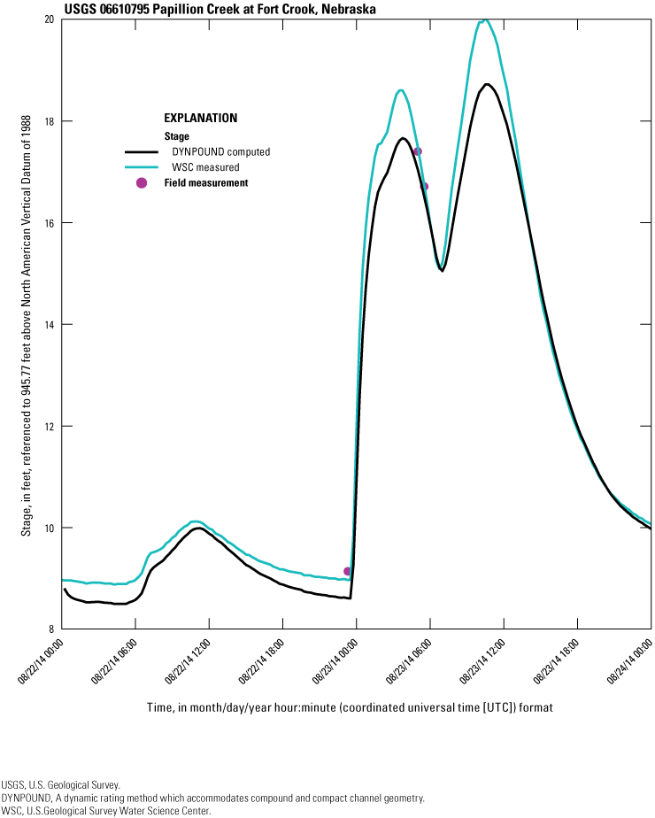
Graph showing the stage time series computed with the DYNPOUND method shown with the time series of WSC-measured stage and field measurements made at Papillion Creek at Fort Crook, Nebraska (U.S. Geological Survey streamgage 06610795; U.S. Geological Survey, 2020).
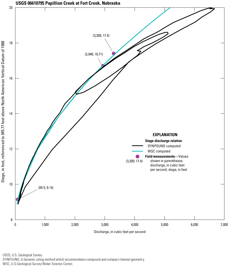
Graph showing the stage-discharge relation at Papillion Creek at Fort Crook, Nebraska (U.S. Geological Survey streamgage 06610795; U.S. Geological Survey, 2020), using discharge computed with the DYNPOUND method, WSC-computed discharge, and field measurements.
Table 26.
Discharge computed for an event-based time series at Papillion Creek at Fort Crook, Nebraska (U.S. Geological Survey streamgage 06610795), with the DYNPOUND methods and the associated error.[Field measurement discharge data from U.S. Geological Survey, 2020. DYNPOUND, the newly developed method that solves for stage and discharge in compact and compound channels. MM, month; DD, day; YYYY, year; UTC, coordinated universal time; FM, field measurement; ft3/s, cubic foot per second; SLE, squared logarithmic error; NA, not applicable]
Table 27.
Stage computed for an event-based time series at Papillion Creek at Fort Crook, Nebraska (U.S. Geological Survey streamgage 06610795), with the DYNPOUND methods and the associated error.[Field measurement stage data from U.S. Geological Survey, 2020; DYNPOUND, the newly developed method that solves for stage and discharge in compact and compound channels; MM, month; DD, day; YYYY, year; UTC, coordinated universal time; FM, field measurement; ft3/s, cubic foot per second; SLE, squared logarithmic error; NA, not applicable]
Gasconade River at Jerome, Missouri
The USGS streamgage at Gasconade River at Jerome, Missouri (USGS streamgage 06933500) encompasses 2,840 mi2. The computed S0 for the site is 0.00040953 (table 3). The value of r, computed from the event with a peak stage of 20 ft at 9:00 (coordinated universal time [UTC]) on February 26, 2018 (U.S. Geological Survey, 2020), is 30.02. The cross section used to compute the time series was split into four subsections for the DYNPOUND computation, with subsection stations at 525, 725, and 1,275 ft (fig. 38). The n-values used to calibrate the DYNPOUND computations varied from 0.026 to 0.19 (table 28).
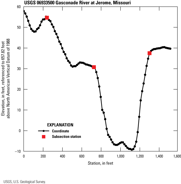
Graph showing the cross section used to compute the discharge time series at Gasconade River at Jerome, Missouri (U.S. Geological Survey streamgage 06933500; U.S. Geological Survey, 2020).
Seven stage and discharge field measurements from the 2016 water year were used for calibration (table 29 and table 30). The WSC-measured stage time series for the 2016 water year was used to compute discharge, and the WSC-computed discharge time series for the same water year was used to compute stage using the DYNPOUND method (U.S. Geological Survey, 2020). The MSLE for the DYNPOUND discharge calibration was 1.36×10⁻¹, and the mean percent error was 33.79 percent (table 29). The MSLE for the DYNPOUND stage calibration was 9.12×10⁻², and the mean percent error was −44.26 percent (table 30).
Table 28.
Stage and roughness coefficient values used to calibrate the DYNPOUND method at Gasconade River at Jerome, Missouri (U.S. Geological Survey streamgage 06933500).[Data from Domanski and others, 2025. ft, foot]
Table 29.
Discharge calibration results for the DYNPOUND ratings at Gasconade River at Jerome, Missouri (U.S. Geological Survey streamgage 06933500).[Field measurement discharge data from U.S. Geological Survey, 2020. DYNPOUND, the newly developed method that solves for stage and discharge in compact and compound channels. MM, month; DD, day; YYYY, year; UTC, coordinated universal time; FM, field measurement; ft3/s, cubic foot per second; SLE, squared logarithmic error; NA, not applicable]
Table 30.
Stage calibration results for the DYNPOUND ratings at Gasconade River at Jerome, Missouri (U.S. Geological Survey streamgage 06933500).[Field measurement stage data from U.S. Geological Survey, 2020. DYNPOUND, the newly developed method that solves for stage and discharge in compact and compound channels. MM, month; DD, day; YYYY, year; UTC, coordinated universal time; FM, field measurement; ft, feet; SLE, squared logarithmic error; NA, not applicable]
To evaluate the stage-discharge relation for the USGS streamgage Gasconade River at Jerome, Missouri, time series of stage and discharge were computed for the period between March 15 and June 23, 2017, which included four field measurements used for error assessment (fig. 39 and fig. 40). DYNPOUND captured minor hysteresis in the stage-discharge relation for the computed event, whereas the USGS-computed discharge is monotonic (fig. 41). A comparison between the observed and computed discharge for the period resulted in a mean percent error of 4.73 percent for DYNPOUND. The MSLE was 9.43×10⁻³ (table 31). Results of the stage computation in comparison to field measurements for this event showed a mean percent error of −2.30 percent and a MSLE of 1.23×10⁻² (table 32).
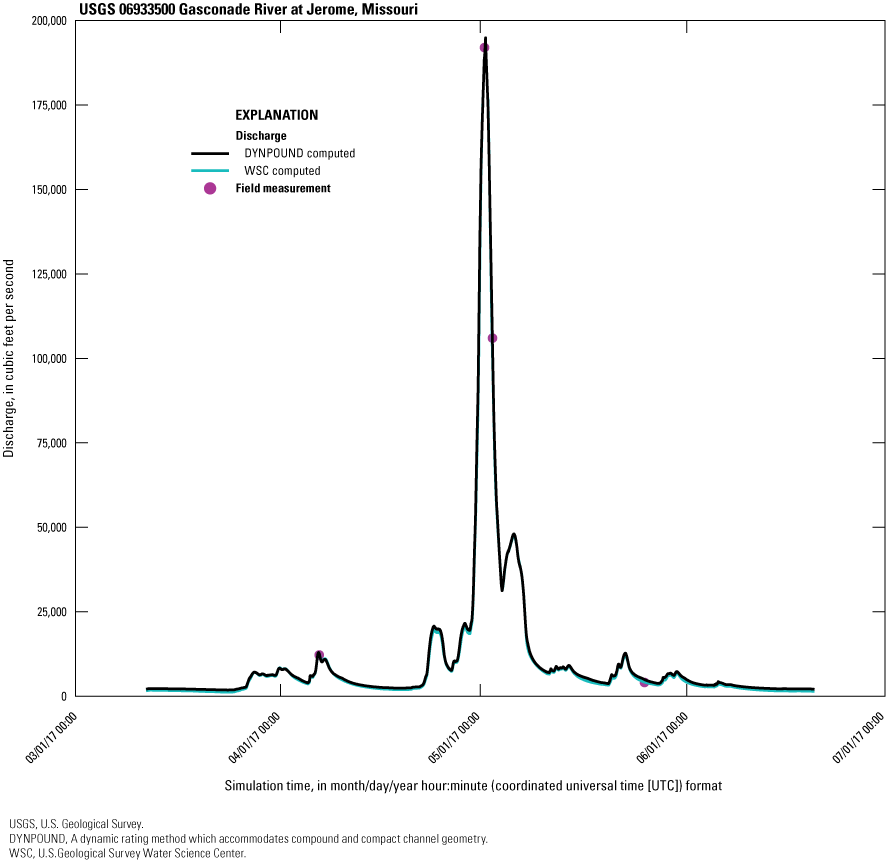
Graph showing the discharge time series computed with the DYNPOUND method shown with the time series of WSC-computed discharge and field measurements made at Gasconade River at Jerome, Missouri (U.S. Geological Survey streamgage 06933500; U.S. Geological Survey, 2020).
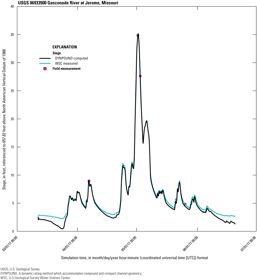
Graph showing the stage time series computed with the DYNPOUND method shown with the time series of WSC-measured stage and field measurements made at Gasconade River at Jerome, Missouri (U.S. Geological Survey streamgage 06933500; U.S. Geological Survey, 2020).
Graph showing stage-discharge relation at Gasconade River at Jerome, Missouri (U.S. Geological Survey streamgage 06933500; U.S. Geological Survey, 2020), using discharge computed with the DYNPOUND method, WSC-computed discharge, and field measurements.
Table 31.
Discharge computed for an event-based time series at Gasconade River at Jerome, Missouri (U.S. Geological Survey streamgage 06933500), with the DYNPOUND methods and the associated error.[Field measurement discharge data from U.S. Geological Survey, 2020. DYNPOUND, the newly developed method that solves for stage and discharge in compact and compound channels. MM, month; DD, day; YYYY, year; UTC, coordinated universal time; FM, field measurement; ft3/s, cubic foot per second; SLE, squared logarithmic error; NA, not applicable]
Table 32.
Stage computed for an event-based time series at Gasconade River at Jerome, Missouri (U.S. Geological Survey streamgage 06933500), with the DYNPOUND methods and the associated error.[Field measurement stage data from U.S. Geological Survey, 2020. DYNPOUND, the newly developed method that solves for stage and discharge in compact and compound channels. MM, month; DD, day; YYYY, year; UTC, coordinated universal time; FM, field measurement; ft, feet; SLE, squared logarithmic error; NA, not applicable]
Mississippi River at St. Louis, Missouri
The USGS streamgage on the Mississippi River at St. Louis, Missouri (USGS streamgage 07010000), encompasses 697,000 mi2. The S0 for the site is 0.000110 (table 3). A value of 13.5 for r was computed using the event with a peak stage of 24.8 ft at 14:00 (UTC) on March 13, 2013 (U.S. Geological Survey, 2020). The cross section used to compute the discharge time series is shown in figure 42. No subdivision of the cross section for this site was made to compute stage and discharge with the DYNPOUND method. The n-values chosen to calibrate the DYNPOUND computations varied from 0.029 to 0.058 (table 33).
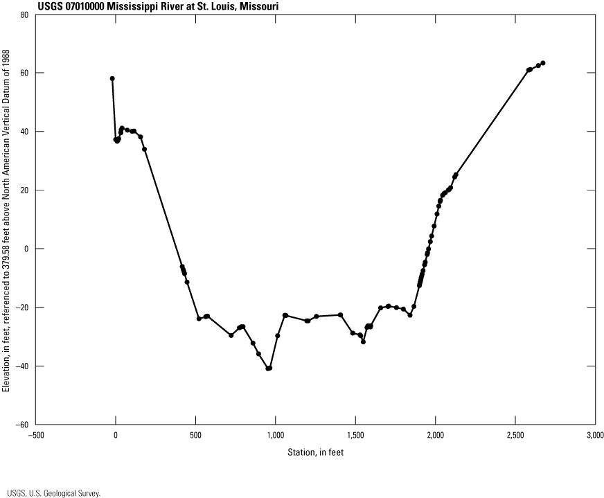
Graph showing the cross section used to compute the discharge time series at Mississippi River at St. Louis, Missouri (U.S. Geological Survey streamgage 07010000; U.S. Geological Survey, 2020).
Eleven field measurements of stage and discharge collected during the 2014 water year were used to calibrate the dynamic ratings for the Mississippi River at St. Louis, Missouri, streamgage (table 34 and table 35). The WSC-measured stage time series from the 2014 water year was used to compute discharge, and the WSC-computed discharge time series for the same water year was used to compute stage using the DYNPOUND method (U.S. Geological Survey, 2020). For the DYNPOUND discharge calibration, the MSLE was 2.30×10⁻³, and the mean percent error was −2.75 percent (table 34). The DYNPOUND stage calibration resulted in a MSLE of 1.17×10⁻¹ and a mean percent error of 20.64 percent (table 35).
Table 33.
Stage and roughness coefficient values used to calibrate the DYNPOUND method at Mississippi River at St. Louis, Missouri (U.S. Geological Survey streamgage 07010000).[Data from Domanski and others, 2025. ft, foot]
Table 34.
Discharge calibration results for the DYNPOUND ratings at Mississippi River at St. Louis, Missouri (U.S. Geological Survey streamgage 07010000).[Field measurement discharge data from U.S. Geological Survey, 2020. DYNPOUND, the newly developed method that solves for stage and discharge in compact and compound channels. MM, month; DD, day; YYYY, year; UTC, coordinated universal time; FM, field measurement; ft3/s, cubic foot per second; SLE, squared logarithmic error; NA, not applicable]
Table 35.
Stage calibration results for the DYNPOUND ratings at Mississippi River at St. Louis, Missouri (U.S. Geological Survey streamgage 07010000).[Field measurement stage data from U.S. Geological Survey, 2020; DYNPOUND, the newly developed method that solves for stage and discharge in compact and compound channels. MM, month; DD, day; YYYY, year; UTC, coordinated universal time; FM, field measurement; ft3/s, cubic foot per second; SLE, squared logarithmic error; NA, not applicable]
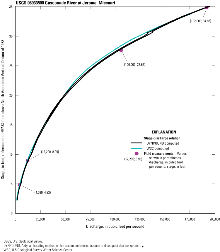
To evaluate the dynamic rating methods for this site, stage and discharge for the period between June 1 and August 15, 2015, were computed and compared to the 68 field stage and discharge measurements made at this site (fig. 43 and fig. 44). The mean percent error for the DYNPOUND-computed discharge was 0.37 percent, and the MSLE was 1.75×10⁻³ (table 36). For the DYNPOUND-computed stage, the mean percent error was −0.90 percent, and the MSLE was 7.08×10⁻⁴ (table 37). DYNPOUND captured hysteresis in the stage-discharge relation for the computed event, whereas the USGS-computed discharge is single-valued. The WSC- and DYNPOUND-computed stage-discharge relations were biased to the right compared to the field measurements. Further adjustment of the n-values, based on first-hand knowledge of channel conditions, may improve the DYNPOUND-computed relation (fig. 45).
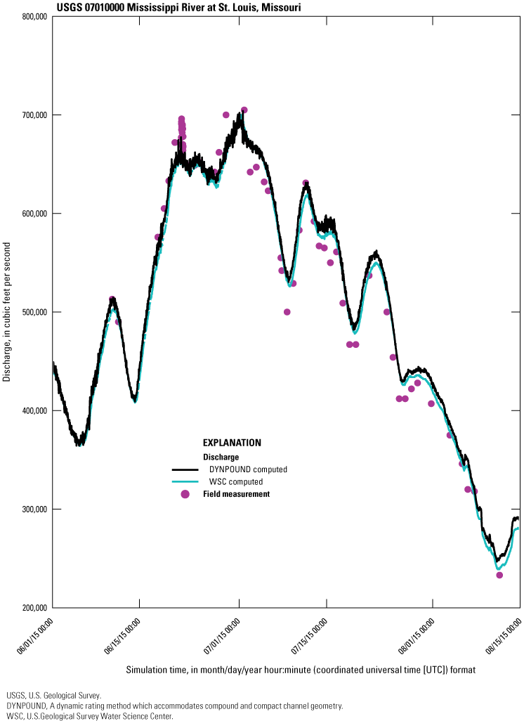
Graph showing the discharge time series computed with the DYNPOUND method shown with the WSC-computed discharge time series and field measurements made at Mississippi River at St. Louis, Missouri (U.S. Geological Survey streamgage 07010000; U.S. Geological Survey, 2020).
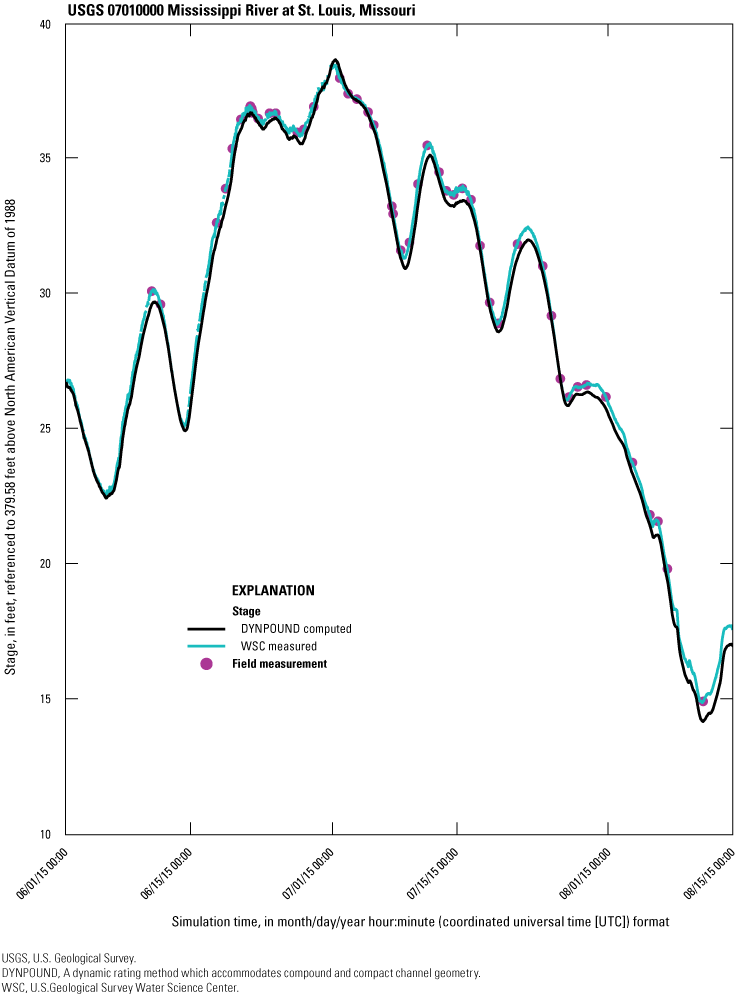
Graph showing the stage time series computed with the DYNPOUND method shown with the time series of WSC-measured stage and field measurements made at Mississippi River at St. Louis, Missouri (U.S. Geological Survey streamgage 07010000; U.S. Geological Survey, 2020).
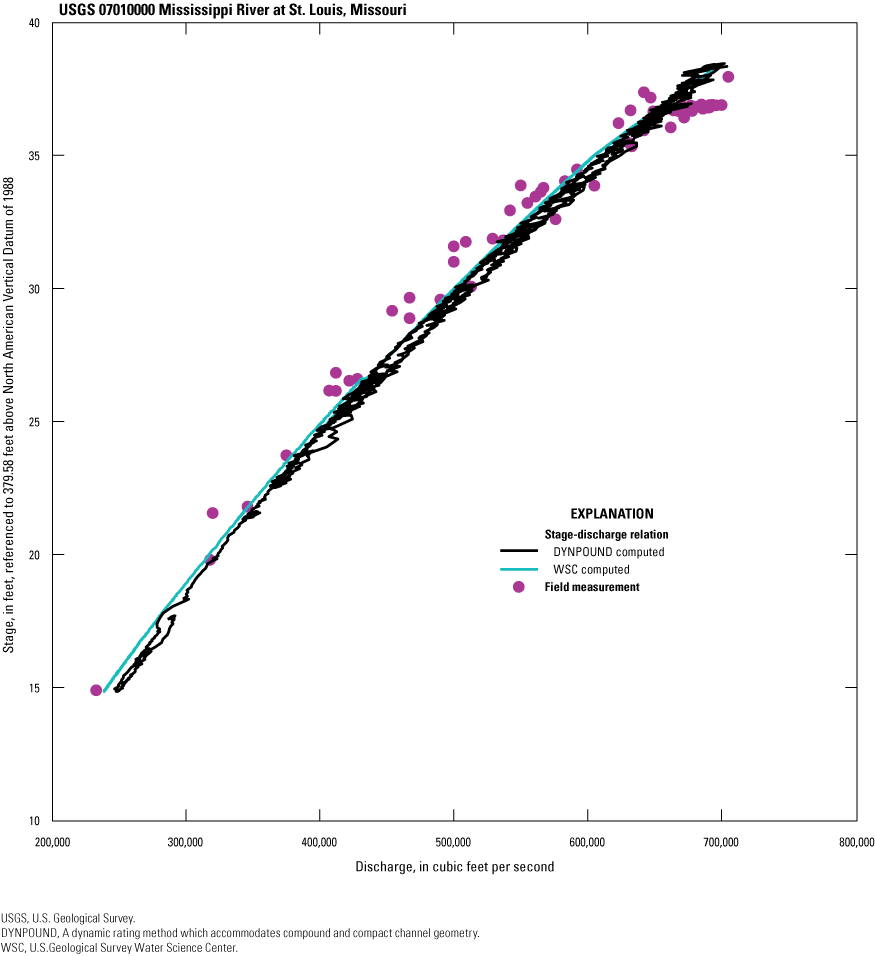
Graph showing the stage-discharge relation at Mississippi River at St. Louis, Missouri (U.S. Geological Survey streamgage 07010000; U.S. Geological Survey, 2020), using discharge computed with the DYNPOUND method, WSC-computed discharge, and field measurements.
Table 36.
Discharge computed for an event-based time series at Mississippi River at St. Louis, Missouri (U.S. Geological Survey streamgage 07010000), with the DYNPOUND method and the associated error.[Field measurement discharge data from U.S. Geological Survey, 2020. DYNPOUND, the newly developed method that solves for stage and discharge in compact and compound channels. MM, month; DD, day; YYYY, year; UTC, coordinated universal time; FM, field measurement; ft3/s, cubic foot per second; SLE, squared logarithmic error; NA, not applicable]
Table 37.
Stage computed for an event-based time series at Mississippi River at St. Louis, Missouri (U.S. Geological Survey streamgage 07010000), with the DYNPOUND method and the associated error.[Field measurement stage data from U.S. Geological Survey, 2020. DYNPOUND, the newly developed method that solves for stage and discharge in compact and compound channels. MM, month; DD, day; YYYY, year; UTC, coordinated universal time; FM, field measurement; ft, feet; SLE, squared logarithmic error; NA, not applicable]
Calcasieu River near Kinder, Louisiana
The USGS streamgage Calcasieu River near Kinder, Louisiana (USGS streamgage 08015500), represents an area of 1,700 mi2. At this location, the river is surrounded by a coastal plain consisting of pine forests, agriculture, and urban areas (Forbes, 1988). The computed S0 for the site is 0.00018992 (table 3). The value of r is 9.79 and was computed from the event with a peak stage of 19.44 ft at 23:30 (coordinated universal time [UTC]) on July 16, 2019 (U.S. Geological Survey, 2020). The cross section used to compute the time series is shown in figure 46. The channel cross section was split into three subsections for the DYNPOUND computation; subsection stations were at 2,051.52 and 2,366 ft (fig. 46). Manning’s n−values, used to calibrate the DYNPOUND computations, varied from 0.064 to 0.15 (table 38).
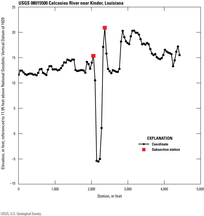
Graph showing the cross section used to compute the stage and discharge time series at Calcasieu River near Kinder, Louisiana (U.S. Geological Survey streamgage 08015500; U.S. Geological Survey, 2020).
Five discharge and four stage field measurements from the 2019 water year were used for calibration (table 39 and table 40). The WSC−measured stage time series for the 2019 water year was used to compute discharge, and the WSC−computed discharge time series for the same water year was used to compute stage using the DYNPOUND method (U.S. Geological Survey, 2020). The MSLE for the DYNPOUND discharge calibration was 1.15×10⁻¹, and the mean percent error was 37.80 percent (table 39). The MSLE for the DYNPOUND stage calibration was 6.08×10⁻², and the mean percent error was −12.18 percent (table 40).
Table 38.
Stage and roughness coefficient values used to calibrate the DYNPOUND method at Calcasieu River near Kinder, Louisiana (U.S. Geological Survey streamgage 08015500).[Data from Domanski and others, 2025. ft, foot]
Table 39.
Discharge calibration results for the DYNPOUND ratings at Calcasieu River near Kinder, Louisiana (U.S. Geological Survey streamgage 08015500).[Field measurement discharge data from U.S. Geological Survey, 2020. DYNPOUND, the newly developed method that solves for stage and discharge in compact and compound channels. MM, month; DD, day; YYYY, year; UTC, coordinated universal time; FM, field measurement; ft3/s, cubic foot per second; SLE, squared logarithmic error; NA, not applicable]
Table 40.
Stage calibration results for the DYNPOUND ratings at Calcasieu River near Kinder, Louisiana (U.S. Geological Survey streamgage 08015500).[Field measurement stage data from U.S. Geological Survey, 2020. DYNPOUND, the newly developed method that solves for stage and discharge in compact and compound channels. MM, month; DD, day; YYYY, year; UTC, coordinated universal time; FM, field measurement; ft, feet; SLE, squared logarithmic error; NA, not applicable]
To evaluate the ratings for the USGS streamgage 08015500 Calcasieu River near Kinder, Louisiana, time series of stage and discharge were computed for the period between January 30 and April 16, 2018, which included one field measurement used for error assessment (fig. 47 and fig. 48). DYNPOUND captured hysteresis for each of the three peaks in the stage-discharge relation for the computed period, whereas the WSC-computed discharge is monotonic (fig. 49). A comparison of the field measurement and DYNPOUND-computed discharge for the period resulted in a percent error of 2.21 percent (table 41). For the DYNPOUND-computed stage, the percent error was −1.89 percent (table 42).
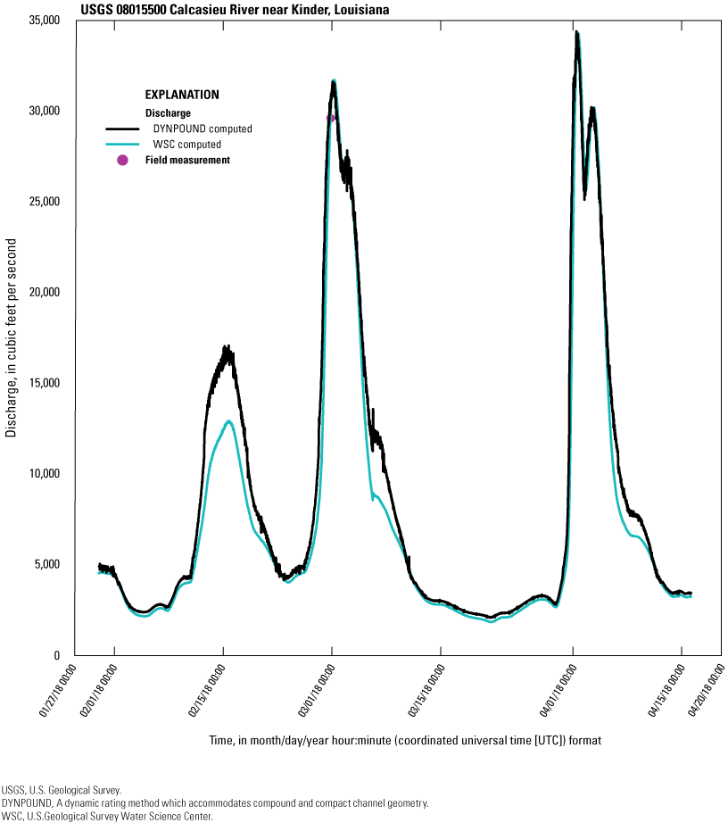
Graph showing the discharge time series computed with the DYNPOUND method shown with the time series of WSC-computed discharge and field measurements made at Calcasieu River near Kinder, Louisiana (U.S. Geological Survey streamgage 08015500; U.S. Geological Survey, 2020).
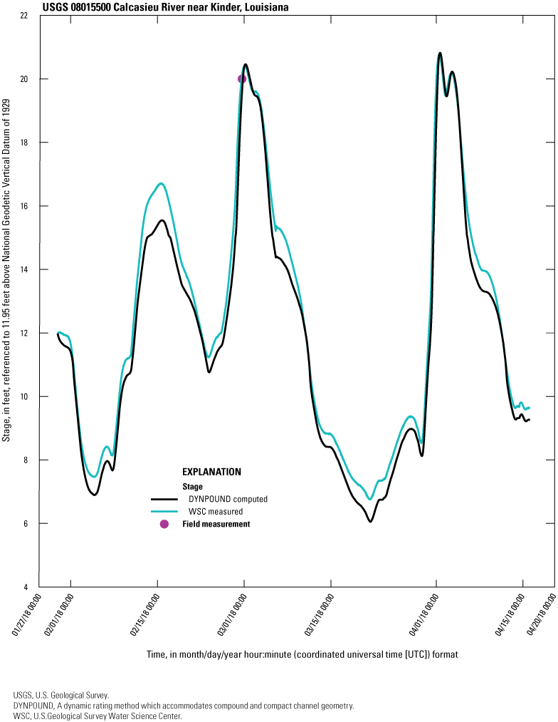
Graph showing the stage time series computed with the DYNPOUND method shown with the time series of WSC-measured stage and field measurements made at Calcasieu River near Kinder, Louisiana (U.S. Geological Survey streamgage 08015500; U.S. Geological Survey, 2020).
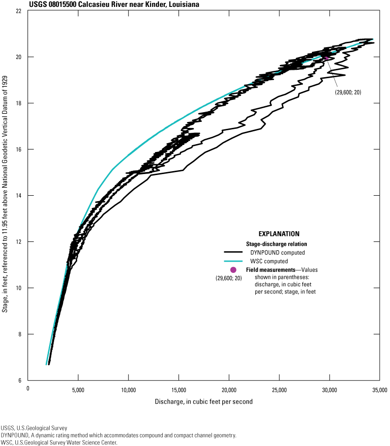
Graph showing the stage-discharge relation at Calcasieu River near Kinder, Louisiana (U.S. Geological Survey streamgage 08015500; U.S. Geological Survey, 2020), using discharge computed with the DYNPOUND method, WCS-computed discharge, and field measurements.
Table 41.
Discharge computed for an event-based time series at Calcasieu River near Kinder, Louisiana (U.S. Geological Survey streamgage 08015500), with the DYNPOUND methods and the associated error.[Field measurement discharge data from U.S. Geological Survey, 2020. DYNPOUND, the newly developed method that solves for stage and discharge in compact and compound channels. MM, month; DD, day; YYYY, year; UTC, coordinated universal time; FM, field measurement; ft3/s, cubic foot per second; SLE, squared logarithmic error]
Table 42.
Stage computed for an event-based time series at Calcasieu River near Kinder, Louisiana (U.S. Geological Survey streamgage 08015500), with the DYNPOUND methods and the associated error.[Field measurement stage data from U.S. Geological Survey, 2020. DYNPOUND, the newly developed method that solves for stage and discharge in compact and compound channels. MM, month; DD, day; YYYY, year; UTC, coordinated universal time; FM, field measurement; ft, foot; SLE, squared logarithmic error]
Rio Grande Near Cerro, New Mexico
The USGS streamgage Rio Grande near Cerro, New Mexico (USGS streamgage 08263500) encompasses 8,440 mi2. The Rio Grande meanders through an 800-ft-deep canyon (Bureau of Land Management, 2024), in which 50–75 percent of peak flows are the result of snowmelt runoff in late spring to early summer (Elias and others, 2015). The S0 for the site is computed as 0.00360 (table 3). A value for r of 697 was computed using the event with a peak stage of 5.57 ft at 03:00 (UTC) on June 3, 2021 (U.S. Geological Survey, 2020). Values of r are anticipated to fall within a range of approximately 10 to 100 (Fread, 1973). The computed value of r for this site is substantially larger than the largest expected value. Further investigation could help determine the cause of the high value of r for this site.
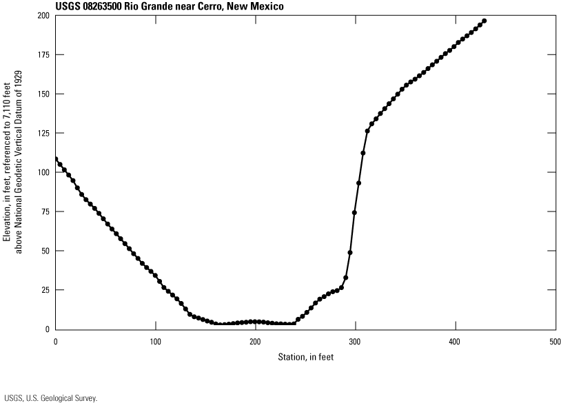
Graph showing the cross section used to compute the stage and discharge time series at Rio Grande near Cerro, New Mexico (U.S. Geological Survey streamgage 08263500; U.S. Geological Survey, 2020).
Seven field measurements of stage and discharge collected during the 2015 water year were used for calibration. The WSC-measured stage time series from the 2015 water year was used to compute discharge, and the WSC-computed discharge time series for the same water year was used to compute stage using the DYNPOUND method (U.S. Geological Survey, 2020). No subdivision of the cross section (fig. 50) was warranted based upon subdivision criteria in the computation of the hydraulic properties for the DYNPOUND method. The n-value used to calibrate the DYNPOUND computations varied from 0.064 to 0.128 (table 43). The calibrated Manning’s n values were much larger than anticipated, and the large n-values may be mitigating for phenomena not adequately captured in the rating. The MSLE and mean percent error for the DYNPOUND discharge calibration were 8.51×10⁻⁴ and 0.35 percent, respectively (table 44). The MSLE and mean percent error for the DYNPOUND stage calibration were 2.02×10⁻² and −0.40 percent, respectively (table 45).
Table 43.
Stage and roughness coefficient values used to calibrate the DYNPOUND method at Rio Grande near Cerro, New Mexico (U.S. Geological Survey streamgage 08263500).[Data from Domanski and others, 2025. ft, foot]
Table 44.
Discharge calibration results for the DYNPOUND ratings at Rio Grande near Cerro, New Mexico (U.S. Geological Survey streamgage 08263500).[Field measurement discharge data from U.S. Geological Survey, 2020. DYNPOUND, the newly developed method that solves for stage and discharge in compact and compound channels. MM, month; DD, day; YYYY, year; UTC, coordinated universal time; FM, field measurement; ft3/s, cubic foot per second; SLE, squared logarithmic error; NA, not applicable]
Table 45.
Stage calibration results for the DYNPOUND ratings at Rio Grande near Cerro, New Mexico (U.S. Geological Survey streamgage 08263500).[Field measurement stage data from U.S. Geological Survey, 2020. DYNPOUND, the newly developed method that solves for stage and discharge in compact and compound channels. MM, month; DD, day; YYYY, year; UTC, coordinated universal time; FM, field measurement; ft, foot; SLE, squared logarithmic error; NA, not applicable]
The stage and discharge values computed during the period between April 1 and August 5, 2019, were used to evaluate the DYNPOUND method for this site; the two field measurements made during this period were used for comparison. The DYNPOUND-computed discharge was lower at the peaks above 2,000 ft3/s, and the DYNPOUND-computed stage was higher at the peaks over 9 ft (fig. 51, fig. 52, and fig. 53). The mean percent error of the DYNPOUND-computed discharge is 3.84 percent, and the MSLE is 1.39×10⁻³ (table 46). The mean percent error of the DYNPOUND-computed stage is −2.32 percent, and the MSLE is 1.82×10⁻² (table 47).
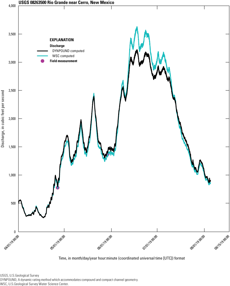
Graph showing the discharge time series computed with the DYNPOUND method shown with the time series of WSC-computed discharge and field measurements made at Rio Grande near Cerro, New Mexico (U.S. Geological Survey streamgage 08263500; U.S. Geological Survey, 2020).
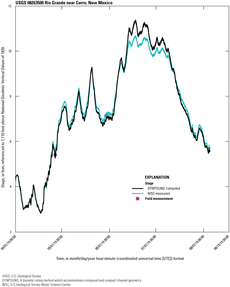
Graph showing stage time series computed with the DYNPOUND method shown with the time series of WSC-measured stage and field measurements made at Rio Grande near Cerro, New Mexico (U.S. Geological Survey streamgage 08263500; U.S. Geological Survey, 2020).
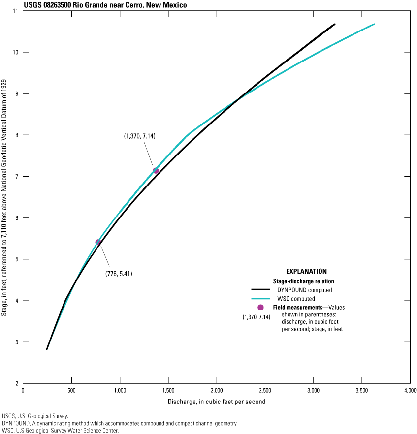
Graph showing the stage-discharge relation at Rio Grande near Cerro, New Mexico (U.S. Geological Survey streamgage 08263500; U.S. Geological Survey, 2020), using discharge computed with the DYNPOUND method, WSC-computed discharge, and field measurements.
Table 46.
Discharge computed with the DYNPOUND method and associated error for an event-based time series at Rio Grande near Cerro, New Mexico (U.S. Geological Survey streamgage 08263500).[Field measurement discharge data from U.S. Geological Survey, 2020. DYNPOUND, the newly developed method that solves for stage and discharge in compact and compound channels. MM, month; DD, day; YYYY, year; UTC, coordinated universal time; FM, field measurement; ft3/s, cubic foot per second; SLE, squared logarithmic error; NA, not applicable]
Table 47.
Stage computed with the DYNPOUND method and associated error for an event-based time series at Rio Grande near Cerro, New Mexico (U.S. Geological Survey streamgage 08263500).[Field measurement stage data from U.S. Geological Survey, 2020. DYNPOUND, the newly developed method that solves for stage and discharge in compact and compound channels. MM, month; DD, day; YYYY, year; UTC, coordinated universal time; FM, field measurement; ft, foot; SLE, squared logarithmic error; NA, not applicable]
San Joaquin River Near Mendota, California
The USGS streamgage San Joaquin River near Mendota, California (U.S. Geological Survey streamgage 11254000) encompasses 3,940 mi2. The meandering San Joaquin River is characterized by low-gradient flows and a sandy bottom (Marineau and others, 2017). The computed S0 for the site is 0.000248 (table 3). A high value of 159.5 for r was computed from the event with a peak stage of 5.46 ft at 12:30 (UTC) on February 22, 2015 (U.S. Geological Survey, 2020). The cross section used to compute the time series is shown in figure 54.
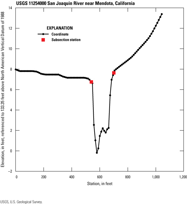
Graph showing the cross section used to compute the stage and discharge time series at San Joaquin River Near Mendota, California (U.S. Geological Survey streamgage 11254000; U.S. Geological Survey, 2020).
Nine field measurements of stage and discharge collected during the 2015 water year were used for calibration. The WSC-measured stage time series from the 2015 water year was used to compute discharge, and the WSC-computed discharge time series for the same water year was used to compute stage using the DYNPOUND method (U.S. Geological Survey, 2020). The cross section for the DYNPOUND analyses was subdivided into three subsections for the DYNPOUND computations; subsection stations were at 540 and 700 ft (fig. 54). The n-values used to calibrate the DYNPOUND computations varied from 0.031 to 0.08 (table 48). The MSLE for the DYNPOUND discharge calibration was 7.88×10⁻³, and the mean percent error was −4.89 percent (table 49). The MSLE for the DYNPOUND stage calibration was 3.89×10⁻², and the mean percent error was 2.03 percent (table 50).
Table 48.
Stage and roughness coefficient values used to calibrate the DYNPOUND method at San Joaquin River near Mendota, California (U.S. Geological Survey streamgage 11254000).[Data from Domanski and others, 2025. ft, foot]
Table 49.
Discharge calibration results for the DYNPOUND ratings at San Joaquin River near Mendota, California (U.S. Geological Survey streamgage 11254000).[Field measurement discharge data from U.S. Geological Survey, 2020. DYNPOUND, the newly developed method that solves for stage and discharge in compact and compound channels. MM, month; DD, day; YYYY, year; UTC, coordinated universal time; FM, field measurement; ft3/s, cubic foot per second; SLE, squared logarithmic error; NA, not applicable]
Table 50.
Stage calibration results for the DYNPOUND ratings at San Joaquin River near Mendota, California (U.S. Geological Survey streamgage 11254000).[Field measurement stage data from U.S. Geological Survey, 2020. DYNPOUND, the newly developed method that solves for stage and discharge in compact and compound channels. MM, month; DD, day; YYYY, year; UTC, coordinated universal time; FM, field measurement; ft, foot; SLE, squared logarithmic error; NA, not applicable]
Time series of stage and discharge were computed for the period between May 20 and July 10, 2019, to evaluate the DYNPOUND method at San Joaquin River near Mendota, California (fig. 55 and fig. 56). Two field measurements are available for comparison during this period. The MSLE for the DYNPOUND computed discharge is 1.72×10⁻² with a mean percent error of −4.27 percent (table 51). Stage computed with the DYNPOUND method resulted in a MSLE of 9.11×10⁻³ and a mean percent error of 3.91 percent (table 52). DYNPOUND captures hysteresis in the stage-discharge relation for the computed event and shows intensifying oscillation as stage rises above 8 ft. This intensifying oscillation might be attributed to flow inundating the floodplain on the left channel bank. By comparison, the WSC-computed discharge is singled-valued (fig. 57). Compared to the discharge observed on June 9, 2019, at 18:32 UTC, the DYNPOUND computed discharge is 7.26 percent higher.
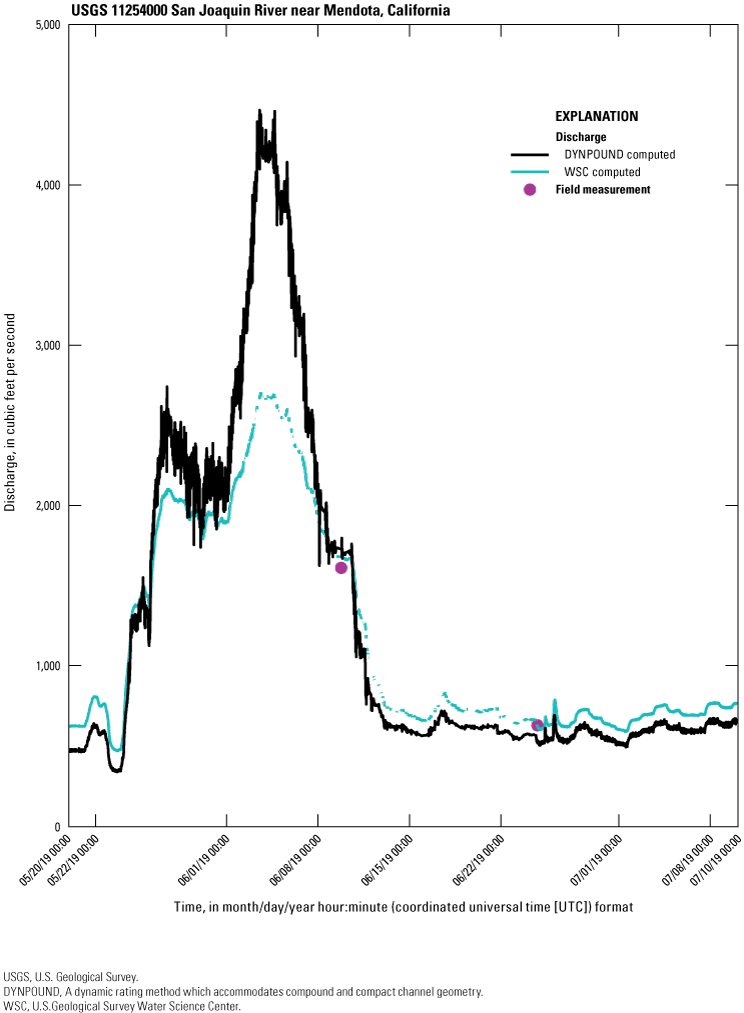
Graph showing the discharge time series computed with the DYNPOUND method shown with the time series of WSC-computed discharge and field measurements made at San Joaquin River near Mendota, California (U.S. Geological Survey streamgage 11254000; U.S. Geological Survey, 2020).
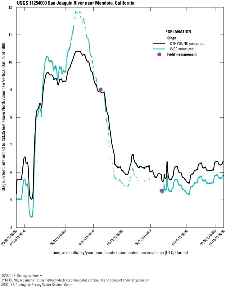
Graph showing the stage time series computed with the DYNPOUND method shown with the time series of WSC-measured stage and field measurements made at San Joaquin River near Mendota, California (U.S. Geological Survey streamgage 11254000; U.S. Geological Survey, 2020).
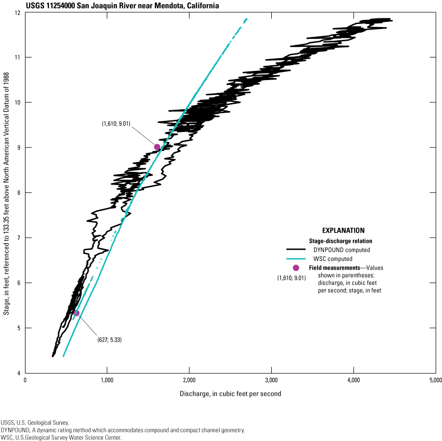
Graph showing the stage-discharge relation at San Joaquin River near Mendota, California (U.S. Geological Survey streamgage 11254000; U.S. Geological Survey, 2020), using discharge computed with the DYNPOUND method, WSC-computed discharge, and field measurements.
Table 51.
Discharge computed with the DYNPOUND method and associated error for an event-based time series at San Joaquin River near Mendota, California (U.S. Geological Survey streamgage 11254000).[Field measurement discharge data from U.S. Geological Survey, 2020. DYNPOUND, the newly developed method that solves for stage and discharge in compact and compound channels. MM, month; DD, day; YYYY, year; UTC, coordinated universal time; FM, field measurement; ft3/s, cubic foot per second; SLE, squared logarithmic error; NA, not applicable]
Table 52.
Stage computed with the DYNPOUND method and associated error for an event-based time series at San Joaquin River near Mendota, California (U.S. Geological Survey streamgage 11254000).[Field measurement stage data from U.S. Geological Survey, 2020. DYNPOUND, the newly developed method that solves for stage and discharge in compact and compound channels. MM, month; DD, day; YYYY, year; UTC, coordinated universal time; FM, field measurement; ft, foot; SLE, squared logarithmic error; NA, not applicable]
Dynamic Rating Application Guidelines
The DYNPOUND method may be improved by verifying the accuracy of and correcting the representation of the cross-section geometry and discharge conditions that affect rating development. The goal of developing this method is to provide a viable and cost-effective alternative for rating complex sites, therefore lowering usage of less accurate surrogate methods and the need for expensive index velocity equipment. Through the course of developing and testing the dynamic rating method, the following are suggested best practices for using this method.
-
• Select an appropriate cross section to characterize the channel geometry described as follows:
-
o Select a reach where the flow is approximately one-dimensional (flow is orthogonal to the banks);
-
o The flow direction should be well established in a one-dimensional nature. An ideal cross section would be one that is straight at least 100 times the bankfull depth upstream and 100 times the bankfull depth downstream; and
-
o Within a river reach, avoid cross sections with abrupt changes in cross-sectional geometry.
-
-
• If possible, select multiple flood events to compute and assess the value of r in equation 20;
-
• Create the channel’s cross-section geometry properties and ensure that the stage/conveyance curve is smooth by subdividing the cross section;
-
• Choose a series of high-flow events to calibrate the values of Manning’s stage and roughness coefficients by the DYNPOUND method. Evaluate the method using a different set of high-flow events; and
-
• Although DYNPOUND was written for complex channels (those with floodplains), the method may perform well for compact channels (those without floodplains).
Summary
Ratings are used for a variety of reasons in water-resources investigations, but a predominant use of ratings is at streamgages, where autonomously measured stage is converted to discharge by use of a stage-discharge rating. Measuring discharge continuously is challenging and expensive and, therefore, discharge is typically determined through surrogate measures of one or more variables such as stage, water-surface slope, rate of change in stage, or index velocity collected at a streamgage. The discharge rating is developed and calibrated using discharge measurements made by field personnel. The simplest and most common rating relates discharge to stage of the river (simple rating).
For some sites, simple ratings work well. Simple ratings do not work for streamgages on low-gradient streams, streams with variable backwater, streams with large amounts of channel or overbank storage, streams with highly unsteady flow, or streams with highly mobile beds. Hydrologists and engineers have long recognized that hysteresis (loops) is in relations between stage and discharge. The hysteresis is sometimes small enough to be hidden within the error of the measurements. Likewise, when the discharge event period is large enough, the hysteresis averages out. In these cases, a dynamic rating is often needed. A dynamic rating relates discharge to stage and other variables because of the lack of a unique, univariate relation between stage and discharge at these sites. This type of rating accounts for a variable energy slope caused by unsteady flow accelerations. The newly improved dynamic rating method (DYNPOUND), which was developed for compact and compound channel geometry, is described in this report. This report explains the derivation of DYNPOUND’s mathematical formulation and how its numerical solution method was developed. The improved DYNPOUND method includes the functionality to set pairs of stage and Manning’s roughness coefficients (n-values) in cases where flow shifts dramatically, within cross sections or subsections, without notable changes in channel geometry.
Stage and discharge time series computed with the DYNPOUND rating method were compared to the simulated stage and discharge time series computed from the one-dimensional unsteady shallow water equations. These simulated time series were generated using one-dimensional hydraulic modeling software (HEC-RAS) and a prismatic channel created from a compound cross section. Four scenarios were designed for analysis using two different bed slopes and four different hydrographs that serve as the upstream boundary conditions. The hydrographs were created to capture the range of unsteadiness in the flow conditions. The mean squared logarithmic error (MSLE) between the DYNPOUND-computed discharge and HEC-RAS-computed discharge ranged from 2.747×10⁻⁷ to 2.02×10⁻⁴. The MSLE between the DYNPOUND-computed stage and HEC-RAS-computed stage ranged from 7.24×10⁻⁸ to 2.60×10⁻⁵.
Results computed with the DYNPOUND method were then compared to time series of WSC-computed discharge, WSC-measured stage, and field data previously collected at 10 USGS streamgage sites. A cross-section geometry for each streamgage site was created by combining “station, elevation” coordinates from ADCP discharge measurements with digital elevation data. Coordinate data were extracted from previously collected discharge measurements. Bed slopes for the sites were estimated from topographic maps due to a lack of existing data. The DYNPOUND computation is quite sensitive to bed slope input values, so more accurate values may improve results. WSC-measured stage and WSC-computed discharge time series, required for method computation, were obtained from the U.S. Geological Survey National Water Information System database (NWIS). Field measurements, which were used to calibrate and evaluate the performance of the DYNPOUND method, were also obtained from NWIS.
Dynamic ratings were developed and calibrated for each site. Calibration was done by adjusting n-values and adding subsections to the cross section to minimize the MSLE with respect to field measurements for the respective site. DYNPOUND successfully computed discharge and stage for each site. The DYNPOUND discharge calibration had a MSLE range of 8.51×10⁻⁴ to 1.36×10⁻¹, and the stage calibration had a MSLE range of 1.30×10⁻³ to 1.17×10⁻¹.
One event-based period was chosen for each site to evaluate the calibration of DYNPOUND; the calibrated rating was used, along with the stage time series from the period, to compute a discharge time series and vice versa. DYNPOUND successfully computed discharge and stage for the entire event at nine of the sites; it did not successfully compute a stage time series at one site. The range of MSLE for the DYNPOUND-computed event discharge was from 4.79×10⁻⁴ to 2.30×10⁻². For the DYNPOUND-computed event stage, the MSLE was from 6.19×10⁻⁴ to 1.82×10⁻².
Acknowledgments
The U.S. Geological Survey field offices of the California Water Science Center, Caribbean-Florida Water Science Center, Central Midwest Water Science Center, Dakota Water Science Center, Lower Mississippi-Gulf Water Science Center, Nebraska Water Science Center, New England Water Science Center, New Mexico Water Science Center, Ohio-Kentucky-Indiana Water Science Center, Oregon Water Science Center, Upper Midwest Water Science Center, Utah Water Science Center, Virginia and West Virginia Water Science Center, and Washington Water Science Center were instrumental in providing site data for this project.
References Cited
Arcement, G.J., and Schneider, V., 1989, Guide for selecting Manning’s roughness coefficients for natural channels and flood plains: U.S. Geological Survey Water-supply paper 2339, 38 p. [Also available at https://doi.org/10.3133/wsp2339.]
Bureau of Land Management, 2024, Rio Grande del Norte National Monument: U.S. Department of the Interior, Bureau of Land Management, accessed April 29, 2024, at https://www.blm.gov/visit/rgdnnm.
Corbett, D.M., 1943, Stream-gaging procedure: U.S. Geological Survey Water-Supply Paper 888, 153 p. [Also available at https://doi.org/10.3133/wsp888.]
Dalrymple, T., and Benson, M.A., 1967, Measurement of peak discharge by the slope-area method: U.S. Geological Survey Techniques of Water-Resources Investigations, book 3, chap. A2, 12 p. [Also available at https://pubs.usgs.gov/twri/twri3-a2/.]
Davidian, J., 1984, Computation of water-surface profiles in open channels: U.S. Geological Survey Techniques of Water-Resources Investigations, book 3, chap. A15, 48 p. [Also available at https://doi.org/10.3133/twri03A15.]
Domanski, M.M., Holmes, R.R., Jr., and Heal, E.N., 2022a, Dynamic rating method for computing discharge from time series stage data-Site datasets: U.S. Geological Survey data release, accessed January 2023, at https://doi.org/10.5066/P955QRPQ.
Domanski, M.M., Holmes, R.R., Jr., and Heal, E.N., 2022b, Dynamic stage to discharge rating model archive: U.S. Geological Survey data release, accessed January 2023, at https://doi.org/10.5066/P9YUV9DG.
Domanski, M.M., Holmes, R.R., Jr., and Heal, E.N., 2025, Dynamic rating model archive: U.S. Geological Survey data release, https://doi.org/10.5066/P9X7QZFG.
Elias, E.H., Rango, A., Steele, C.M., Mejia, J.F., and Smith, R., 2015, Assessing climate change impacts on water availability of snowmelt-dominated basins of the Upper Rio Grande basin: Journal of Hydrology. Regional Studies, v. 3, p. 525–546. [Also available at https://doi.org/10.1016/j.ejrh.2015.04.004.]
Esri, 2021, ArcGIS Pro: Esri website, accessed March 2020 at https://www.esri.com/en-us/arcgis/products/arcgis-pro/overview.
Faye, R.E., and Cherry, R.N., 1980, Channel and dynamic flow characteristics of the Chattahoochee River, Buford Dam to Georgia Highway 141: U.S. Geological Survey Water-Supply Paper 2063, 66 p. [Also available at https://doi.org/10.3133/wsp2063.]
Forbes, M.J., 1988, Hydrologic investigations of the lower Calcasieu River, Louisiana: U.S. Geological Survey Water-Resources Investigations Report 87–4173, 61 p. [Also available at https://doi.org/10.3133/wri874173.]
Fread, D.L., 1975, Computation of stage-discharge relationships affected by unsteady flow: Journal of the American Water Resources Association, v. 11, no. 2, p. 213–228. [Also available at https://doi.org/10.1111/j.1752-1688.1975.tb00674.x.]
Jones, B.E., 1915, A method of correcting river discharge for a changing stage: U.S. Geological Survey Water-Supply Paper 375–E, 130 p. [Also available at https://doi.org/10.3133/wsp375E.]
Kennedy, E.J., 1984, Discharge ratings at gaging stations: U.S. Geological Survey Techniques of Water-Resources Investigations, book 3, chap. A10, 59 p. [Also available at https://pubs.usgs.gov/twri/twri3-a10/.]
Knight, T.M., Domanski, M.M., and Heal, E.N., 2025, DynRat: U.S. Geological Survey software release, https://doi.org/10.5066/P13FOADX.
Marineau, M.D., Wright, S.A., Whealdon-Haught, D.R., and Kinzel, P.J., 2017, Physical characteristics of the lower San Joaquin River, California, in relation to white sturgeon spawning habitat, 2011–14: U.S. Geological Survey Scientific Investigation Report 2017–5069, 47 p., https://doi.org/10.3133/sir20175069.
McClellan, L., 2018, Paddling the eastern borderlands in search of big fish and rich history—Blue Water Trails, the Tug Fork of the Big Sandy River: Kentucky Afield, p. 23–27. [Also available at https://fw.ky.gov/Fish/Documents/Tug%20Fork.pdf.]
Michigan State University, 2020, Michigan State University map library: Michigan State University database, accessed March 2020 at https://msugis.maps.arcgis.com/home/index.html.
Nustad, R.A., and Vecchia, A.V., 2020, Water-quality trends for selected sites and constituents in the international Red River of the North Basin, Minnesota and North Dakota, United States, and Manitoba, Canada, 1970–2017: U.S. Geological Survey Scientific Investigations Report 2020–5079, 75 p., accessed August 2024, at https://doi.org/10.3133/sir20205079.
Python Software Foundation, 2023, Python: Python Software Foundation website, accessed May 30, 2023, at https://www.python.org/downloads/.
Rantz, S.E., and others, 1982, Measurement and computation of streamflow—Volume 2. Computation of discharge: U.S. Geological Survey Water-Supply Paper 2175, 631 p. [Also available at https://pubs.usgs.gov/wsp/wsp2175/wsp2175_vol2.pdf.]
U.S. Army Corps of Engineers, 2016, Hydrologic engineering center river analysis system HEC-RAS 5.0 user’s manual: Davis, Calif., Hydrologic Engineering Center, 960 p. [Also available at https://www.hec.usace.army.mil/software/hec-ras/documentation/HEC-RAS%205.0%20Users%20Manual.pdf.]
U.S. Department of Agriculture, 2021, Geospatial Data Gateway: U.S. Department of Agriculture database, accessed March 2020 at https://datagateway.nrcs.usda.gov/GDGHome.aspx.
U.S. Geological Survey, 2015, AreaComp2, version 2-1.04: U.S. Geological Survey website, accessed March 2020 at https://hydroacoustics.usgs.gov/indexvelocity/AreaComp.shtml.
U.S. Geological Survey, 2017, U.S. Geological Survey TNM Hydrography (National Hydrography Dataset): U.S. Geological Survey database, accessed March 2021 at https://apps.nationalmap.gov/downloader/.
U.S. Geological Survey, 2020, USGS water data for the Nation: U.S. Geological Survey National Water Information System database, accessed March 2020 at https://doi.org/10.5066/F7P55KJN.
Conversion Factors
U.S. customary units to International System of Units
Datum
Vertical coordinate information is referenced to the North American Vertical Datum of 1988 (NAVD 88), National Geodetic Vertical Datum of 1929 (NGVD 1929), and World Geodetic System (WGS 1984).
Supplemental Information
A water year is the 12-month period from October 1 through September 30 of the following year and is designated by the calendar year in which it ends.
Abbreviations
ADCP
acoustic Doppler current profiler
DEM
digital elevation model
DYNMOD
Fread’s original method
DYNPOUND
dynamic rating method
HEC–RAS
Hydrologic Engineering Center River Analysis System
MSLE
mean squared logarithmic error
USGS
U.S. Geological Survey
UTC
coordinated universal time
WSC
U.S. Geological Survey Water Science Center
For more information about this publication, contact
Director, Lower Mississippi-Gulf Water Science Center
U.S. Geological Survey
640 Grassmere Park, Suite 100
Nashville, TN 37211
For additional information, visit https://www.usgs.gov/centers/lmg-water/
Publishing support provided by Lafayette Publishing Service Center
Disclaimers
Any use of trade, firm, or product names is for descriptive purposes only and does not imply endorsement by the U.S. Government.
Although this information product, for the most part, is in the public domain, it also may contain copyrighted materials as noted in the text. Permission to reproduce copyrighted items must be secured from the copyright owner.
Suggested Citation
Domanski, M.M., Holmes, R.R., Jr., Heal, E.N., and Knight, T.M., 2025, Dynamic rating method for computing discharge and stage from time-series data: U.S. Geological Survey Scientific Investigations Report 2024–5129, 92 p., https://doi.org/10.3133/sir20245129.
ISSN: 2328-0328 (online)
Study Area
| Publication type | Report |
|---|---|
| Publication Subtype | USGS Numbered Series |
| Title | Dynamic rating method for computing discharge and stage from time-series data |
| Series title | Scientific Investigations Report |
| Series number | 2024-5129 |
| DOI | 10.3133/sir20245129 |
| Publication Date | March 11, 2025 |
| Year Published | 2025 |
| Language | English |
| Publisher | U.S. Geological Survey |
| Publisher location | Reston, VA |
| Contributing office(s) | Lower Mississippi-Gulf Water Science Center |
| Description | Report: ix, 92 p.; 3 Data Releases; 1 Software Release |
| Country | United States |
| Other Geospatial | continental United States |
| Online Only (Y/N) | Y |
| Additional Online Files (Y/N) | N |