

Estimating the Magnitude and Frequency of Floods at Ungaged Locations on Streams in Tennessee Through the 2013 Water Year
Links
- Document: Report (3.44 MB pdf) , HTML , XML
- Data Release: USGS Data Release - Tabular and geospatial data for the magnitude and frequency of floods at ungaged locations on streams in Tennessee, through the 2013 water year
- Download citation as: RIS | Dublin Core
Abstract
To improve estimates of the frequency of annual peak flows for ungaged locations on non-urban, unregulated streams in Tennessee, generalized least-squares multiple linear-regression techniques were used to relate annual peak flows from streamgages operated by the U.S. Geological Survey to physical, climatic, and land-use characteristics of their drainage basins. Geospatial data acquired since the previous study in 2003, annual peak-streamflow data through the 2013 water year, and Bulletin 17C methods for frequency analysis of annual peak-streamflow data were used in the study. Generalized least-squares regression equations were developed for four hydrologic areas with distinct hydrologic, geologic, and topographic characteristics. Drainage area was used as an explanatory variable in equations developed for each hydrologic area. In addition to drainage area, a 2-year recurrence-interval climate factor was used for hydrologic area 1, a 10–85 channel slope was used for hydrologic area 2, and percent imperviousness was used for hydrologic area 4. The regression equations can be used to estimate annual exceedance probability streamflows for ungaged locations on non-urban, unregulated streams in Tennessee. The term “unregulated” indicates that streamflow is not appreciably influenced by regulation from reservoirs or other impoundments. Average standard errors of prediction for the regression equations ranged from 44.4 to 51.4 percent for hydrologic area 1; 30.4 to 42.9 percent for hydrologic area 2; 35.7 to 42.6 percent for hydrologic area 3; and 32.5 to 47.4 percent for hydrologic area 4.
Introduction
Transportation engineers require reliable estimates of the magnitude and frequency of peak streamflows to design bridges, culverts, and other structures near streams and rivers. Methods used to estimate the magnitude and frequency of peak streamflows at ungaged locations are commonly updated at the request of stakeholders to include recent streamflow data, incorporate statistical improvements in frequency analysis, and implement technological improvements that increase the accuracy of basin and climatic characteristics that affect hydrologic response in streams. The U.S. Geological Survey (USGS) last published methods for estimating the magnitude and frequency of annual peak streamflow at ungaged locations on streams in Tennessee (Law and Tasker, 2003) using streamgages operated by the USGS having at least 10 years of observed annual peak streamflows through the 2000 water year. For this study, more than 10 additional years of streamflow record were available for many of the streamgages used to develop the predictive equations. During this period, previously known maximum flood peaks were exceeded at many USGS streamgages throughout middle and west Tennessee.
Since the USGS last published methods for estimating magnitude and frequency of annual peak streamflow at ungaged locations on streams in Tennessee, updated guidelines for frequency analysis of annual peak streamflow by Federal agencies, referred to as “Bulletin 17C,” have been published (England and others, 2019). Bulletin 17C guidance incorporated in this analysis includes an updated regional skew coefficient for the study area; use of the expected moments algorithm (EMA) for fitting the log-Pearson type III (LP3) distribution to the annual peaks; and the application of the Multiple Grubbs-Beck test (MGBT) for identifying potentially influential low floods (PILFs) in the distribution of annual peak streamflows.
In 2020, the USGS, in cooperation with the Tennessee Department of Transportation, updated the methods for predicting the magnitude and frequency of floods at ungaged locations for streams in Tennessee. Regression equations were developed to predict streamflows corresponding to the 50-, 20-, 10-, 4-, 2-, 1-, 0.5-, and 0.2-percent annual exceedance probabilities (AEPs). The new regression equations will be incorporated into the StreamStats web application (https://streamstats.usgs.gov/ss/) (U.S. Geological Survey, 2019) to automate the process of predicting streamflows for selected AEPs for ungaged locations on streams in Tennessee. Geospatial data associated with the study, including drainage basins and basin characteristics, and the tabular data referenced in this report are available in Heal and others (2025).
Purpose and Scope
The purposes of this report are to provide (1) updated estimates of streamflows corresponding to 50-, 20-, 10-, 4-, 2-, 1-, 0.5-, and 0.2-percent AEPs for 454 streamgages operated by the USGS in the study area (figs. 1–5); and (2) updated regional regression equations (RREs) for estimating streamflows corresponding to AEPs at ungaged locations on streams within each of four hydrologic areas (HAs) (figs. 1–5).
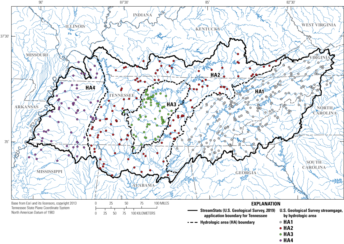
Streamgages, hydrologic areas, and the Tennessee StreamStats application boundary, Tennessee and parts of Alabama, Georgia, Kentucky, Mississippi, North Carolina, and Virginia.
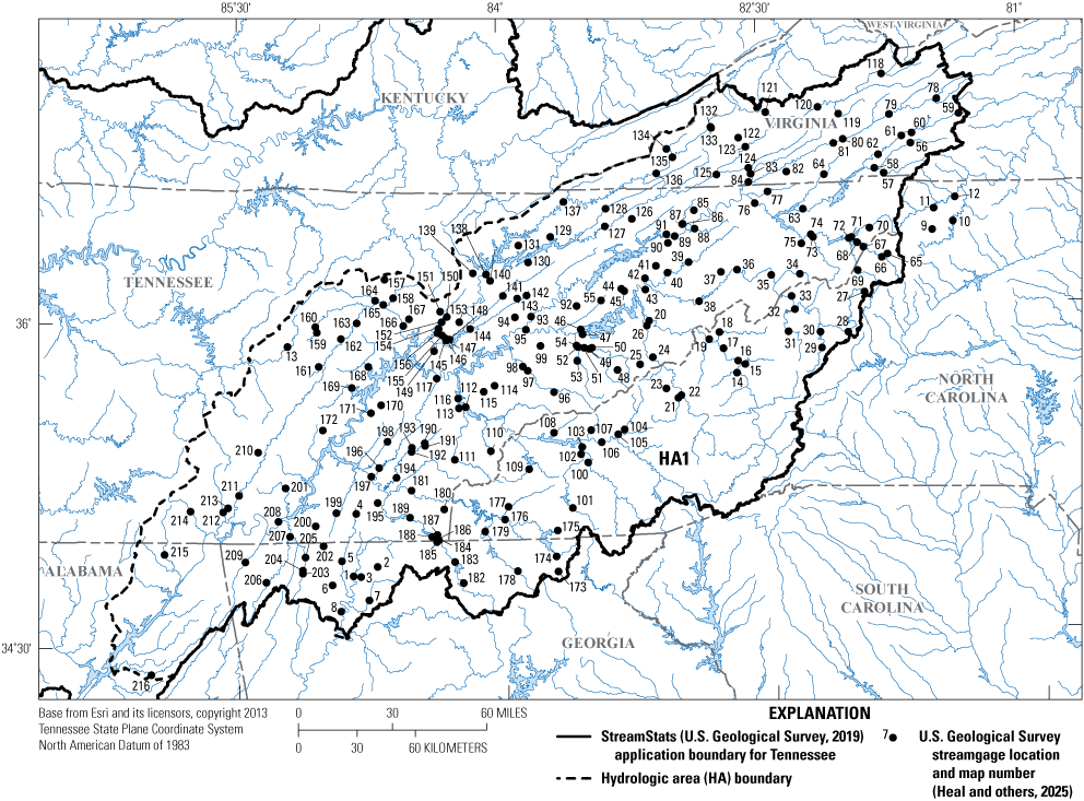
Streamgages in hydrologic area 1, east Tennessee and parts of Alabama, Georgia, North Carolina, and Virginia.
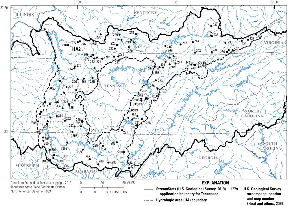
Streamgages in hydrologic area 2, middle Tennessee and parts of Alabama, Kentucky, and Mississippi.
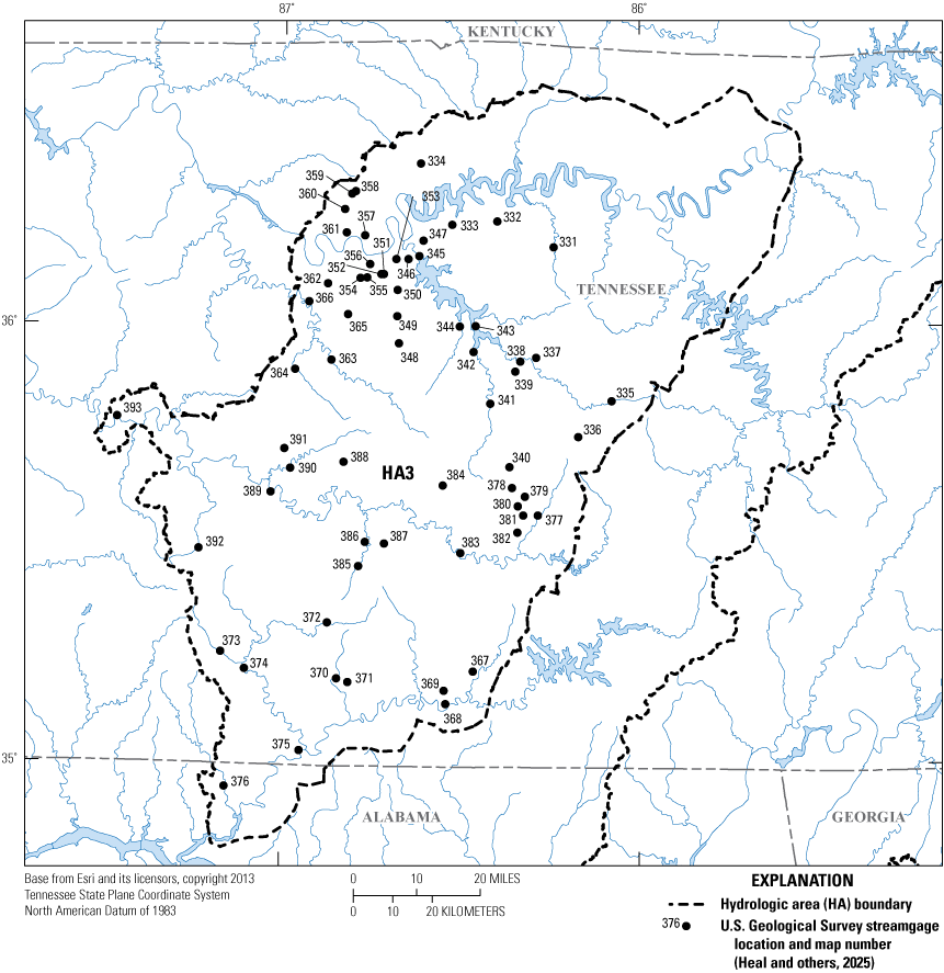
Streamgages in hydrologic area 3, middle Tennessee and part of Alabama.
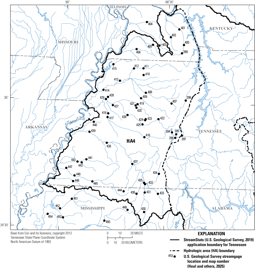
Streamgages in hydrologic area 4, west Tennessee and parts of Kentucky and Mississippi.
Basin characteristics derived from geographic information systems (GIS) and annual peak-streamflow records for 454 streamgages located in generally rural areas of Tennessee and in the adjacent States of Georgia, North Carolina, Virginia, Alabama, Kentucky, and Mississippi (fig. 1) were used to develop the RREs. Streamgages used to develop the RREs were required to have at least 10 years of observed annual peaks through water year 2013 (a water year is defined as the period October 1 through September 30, named for the year in which it ends), and those peak streamflows needed to not have been appreciably affected by urbanization. Of the 454 streamgages used for this study, 443 streamgages were used in the previous study and drained basins with 1 percent to about 30 percent total impervious area (Law and Tasker, 2003). Whereas most of the streamgages used in the current study have drainage basins with a relatively low percentage of urbanization, seven basins for streamgages in middle and east Tennessee (where the percentage of impervious area was not found to be useful in estimating annual peak streamflows) were determined to have greater than 20 percent impervious area. In west Tennessee, where percent imperviousness was found to be useful in estimating annual peak streamflows, only one streamgage used in the current study had a basin with greater than 10 percent impervious area. Of the 454 streamgages used in the current study, 430 streamgages had basins with less than 10 percent impervious area.
Description of the Study Area
The description of this study area was originally presented in Law and Tasker (2003), and it is summarized herein. The diverse physiography and topography of Tennessee ranges from the lowlands of the Mississippi River Valley and Coastal Plain physiographic provinces to the hills of the Western Valley physiographic province and the Central Basin and Highland Rim physiographic sections, across the elevated and incised Cumberland Plateau physiographic section, to the mountains of the Valley and Ridge and Blue Ridge physiographic provinces (Fenneman and Johnson, 1946; Miller, 1974). Other than areas of anthropogenic disturbance such as quarries, land-surface elevations generally range from about 250 feet (ft) above the North American Vertical Datum of 1988 (NAVD 88) along the Mississippi River in west Tennessee to over 6,600 ft above NAVD 88 in the mountains of east Tennessee.
Geology in Tennessee is variable. West Tennessee is characterized by horizontal beds of unconsolidated sand, silt, clay, and gravel. Middle Tennessee is dominated by horizontal beds of karstic limestone. East Tennessee is characterized by folded beds of limestone and dolomite, and the mountains of east Tennessee are underlain by folded beds of complex metamorphic and igneous rock.
The average annual precipitation in Tennessee varies from about 36 to 82 inches (in.), generally increasing from west to east (PRISM Climate Group, Oregon State University, 2014). Generally low average precipitation of 45 in. or less occurs in west Tennessee near the Mississippi River in the Coastal Plain physiographic province and in northern middle Tennessee in the Highland Rim and Nashville Basin sections of the Interior Low Plateaus physiographic province. Other areas of relatively low precipitation are in the northeastern part of the State in the Valley and Ridge physiographic province and the Blue Ridge physiographic province, where precipitation is variable. The highest average precipitation occurs in the eastern part of the State along the eastern boundary of the Appalachian Plateaus physiographic province and in the southeast part of the State along the Great Smoky Mountains in the Blue Ridge physiographic province (Fenneman and Johnson, 1946; Miller 1974). Annual peak streamflows typically occur during the winter and early spring (December through March) when frequent frontal storms yield widespread rains of high intensity on often already saturated ground. Localized peak-streamflow response of small watersheds occurs during the summer when thunderstorms produce intense downpours over relatively small geographic areas. In the fall, the remnants of hurricanes sometimes result in large rain events that can produce annual peak streamflows.
Previous Investigations
Jenkins (1960), Patterson (1964), Speer and Gamble (1964), Randolph and Gamble (1976), Weaver and Gamble (1993), and Law and Tasker (2003) previously reported methods for estimating the magnitude and frequency of annual peak streamflows for rural streams in Tennessee. Randolph and Gamble (1976) delineated and statistically validated four HAs (fig. 1) similar to those used in subsequent studies. Weaver and Gamble (1993) used methods from Bulletin 17B (Interagency Advisory Committee on Water Data, 1982) and conducted the first study to use generalized least-squares (GLS) techniques for developing regional regression equations (Stedinger and Tasker, 1985). Law and Tasker (2003) presented regional regression equations and a region of influence method for predicting the magnitude and frequency of annual peak streamflows, in which a subset of streamgages is used to develop unique regression equations for estimating peak streamflows for AEPs at ungaged locations.
Data Compilation
A first step in conducting a flood-frequency analysis is the selection of candidate streamgages within the study area. The chosen streamgages must be reviewed for quality assurance and quality control prior to the computation of peak streamflows for selected AEPs. After the streamgages are selected and reviewed, basin characteristics for each streamgage must be calculated or acquired from other sources. For streamgages within a particular HA, the peak streamflows for AEPs are the dependent variables in the regional regression equations; the basin characteristics are the independent variables.
Streamgage Selection
Streamgages within Tennessee and parts of Mississippi, Alabama, Georgia, North Carolina, Virginia, and Kentucky were considered for use in the study. USGS peak-streamflow data were acquired from the USGS National Water Information System (NWIS; USGS, 2016). Streamgages used in the study had at least 10 years of observed annual peaks through water year 2013 and were free from regulation by large dams and reservoirs. Annual peak-streamflow data from a final dataset of 454 streamgages (302 in Tennessee, 18 in Alabama, 19 in Georgia, 36 in Kentucky, 14 in Mississippi, 37 in North Carolina, and 28 in Virginia) were used in the flood-frequency analysis and to develop the RREs; of these 454 streamgages, 443 were used in the previous study (Law and Tasker, 2003).
Basin Delineation and Characteristics
Of the 454 candidate streamgages used in the study, 441 are within the StreamStats application boundary for Tennessee (fig. 1). GIS-based methods similar to those incorporated in the StreamStats application (USGS, 2019) for Tennessee were used to delineate drainage basins and determine drainage area (DRNAREA), main-channel slope (CSL10_85), and 2-year recurrence-interval climate factor (CLIMFAC2YR) (table 1) for streamgages within the StreamStats application boundary for Tennessee. Calculated DRNAREA values for the streamgages were compared to published values available from NWIS (USGS, 2016) for validation. Geospatial- and StreamStats-based delineations for streamgages 07030240 and 02348600 produced basins that were inaccurate and required manual correction before basin characteristics could be computed. For 13 streamgages located outside of the StreamStats application boundary for Tennessee (fig. 1), delineation of drainage basins and calculation of DRNAREA were accomplished by using StreamStats (USGS, 2019), and CSL10_85 and CLIMFAC2YR values were obtained from Law and Tasker (2003). For 450 of the 454 streamgages in the study area, percent imperviousness (LC11IMP) (table 1) was calculated by using National Land Cover Database Percent Developed Imperviousness data, 2011 edition (USGS, 2014). For the four streamgages in North Carolina that are outside the StreamStats application boundary for Tennessee (fig. 1), LC11IMP was obtained from StreamStats.
Table 1.
Physical and climatic basin characteristics used as explanatory variables in the generalized least-squares regression equations.Drainage Area
Drainage area (DRNAREA) is the surface area of the drainage basin of a streamgage, in square miles. For the 441 streamgages within the Tennessee StreamStats application boundary (fig. 1), drainage basins were delineated by using flow-direction grids derived from the 1/3 arc-second (approximately 10-meter [m]) National Elevation Dataset (USGS, variously dated). For the remaining 13 streamgages which lie outside of the Tennessee StreamStats application boundary (fig. 1), delineations of drainage basins and computations of DRNAREA were accomplished by using StreamStats.
10–85 Channel Slope
The 10–85 channel slope (CSL10_85), in feet per mile, is the change in elevation between points along the main channel at 10 and 85 percent of the stream length upstream from the streamgage, divided by the stream-wise distance between the points. Ideally, the stream length used for determining points at 10 and 85 percent upstream from the streamgage is measured from the outlet to the basin divide. The further the headwaters of the main channel are from the watershed divide, the more subjective the manual computation of stream length can become. A GIS method was used to determine the stream length by identifying the longest flow path upstream from the site of interest; the longest flow path does not always conform to the main-channel path from the streamgage to the basin divide.
Percent Imperviousness
Percent imperviousness is the percentage of surface area of a drainage basin through which precipitation is unable to infiltrate into the soil. Impervious surface can increase storm runoff to streams. LC11IMP was calculated for the basins of 450 streamgages in this study by using the National Land Cover Database 2011 Percent Developed Imperviousness dataset (USGS, 2014). For the remaining four streamgages located in North Carolina, LC11IMP was obtained from StreamStats (USGS, 2019).
Conceptually, LC11IMP is relatively high in drainage basins of urban streams, where much of the surface area is paved. Even though most of the basins for streamgages used in this study had relatively low values of LC11IMP, seven of the basins had LC11IMP values greater than 20 percent. These basins with LC11IMP values greater than 20 percent are in HAs 1–3, where LC11IMP was not determined to be a statistically useful explanatory variable in prediction of streamflows for AEPs. Within HA4, only streamgage 07032200 had an LC11IMP value (13.7 percent) greater than 10 percent.
2-Year Climate Factor
Lichty and Karlinger (1990) describe a method for integrating long-term rainfall and pan evaporation data into a climate factor to help describe the spatial variability in the frequency of annual peak streamflow of small basins. Climate factors for 2-, 25-, and 100-year recurrence-interval floods (streamflows for 0.5, 0.04, and 0.01 AEPs, respectively) were developed using data from 71 long-term rainfall stations and regression analysis relating peak-streamflow estimates from 50 rainfall-runoff models to basin characteristics. The climate factors, which describe the effects of climate variability on peak streamflows, were developed and regionalized by kriging within a large part of the United States. Law and Tasker (2003) used only the 2-year recurrence interval climate factor (CLIMFAC2YR) for predicting peak-streamflow-frequency magnitudes within the study area, and CLIMFAC2YR is the only climate variable used in this study.
Annual Exceedance Probability Analysis
An AEP is the probability that a streamflow of a given magnitude will be met or exceeded in a given year. For this study, streamflows corresponding to the 50-, 20-, 10-, 4-, 2-, 1-, 0.5-, and 0.2-percent AEPs were computed. The previous study of the magnitude and frequency of flooding in Tennessee (Law and Tasker, 2003) reported flood recurrence intervals, such as the 100-year flood. An annual recurrence interval is the reciprocal of an AEP for a given flood magnitude; for example, a flood having an AEP of 1 percent (0.01, or 1/100) is equivalent to the 100-year recurrence interval (table 2).
AEPs corresponding to annual peak streamflows for the 454 streamgages in the study area were computed by using the USGS program PeakFQ, version 7.0.29368 (Flynn and others, 2006; Feaster and others, 2014; Veilleux and others, 2014). The PeakFQ program was used to fit a log-Pearson type III distribution to base-10 logarithms of annual peak streamflows per Bulletin 17C guidelines (England and others, 2019), which include the use of EMA (Cohn and others, 1997) and MGBT (Cohn and others, 2013) for identifying PILFs during the fitting process. The LP3 distribution is a three-moment distribution that requires estimating the population mean, standard deviation, and skew coefficient.
Expected Moments Algorithm
The EMA method (Cohn and others, 1997) for estimating streamflows corresponding to AEPs incorporates streamflow intervals and perception thresholds that describe peak-streamflow knowledge for every year in the period of record for a streamgage, including the systematic peak streamflows, historical peak streamflows, and gaps in the peak-streamflow record (Southard and Veilleux, 2014). Using streamflow intervals and perception thresholds, the EMA can accommodate censored peak-streamflow data (streamflows that are known only to be greater than or less than some value) and interval peak-streamflow data (streamflows that are known only to be greater than some value and less than another value).
Multiple Grubbs-Beck Test for Detecting Potentially Influential Low Floods
The distribution of annual peak streamflows for a streamgage can contain one or more low outliers, which are small observations that deleteriously affect the upper-tail results (decreasing AEP) (Interagency Advisory Committee on Water Data, 1982; Cohn and others, 2013). For example, during drier years, some small annual peak streamflows may not represent floods or whole basin response to precipitation inputs. These small annual peak streamflows, or PILFs, are small observations that could potentially exert a large influence on the fitted flood-frequency curve (Cohn and others, 2013; England and others, 2019). PILFs can result from physical processes different from those associated with large floods and should not affect the part of the flood-frequency curve representing large floods (Cohn and others, 2013). The MGBT used with EMA provides a standard approach for detecting multiple PILFs. The use of the MGBT can improve the fit of the flood-frequency curve for large floods (Cohn and others, 2013; Southard and Veilleux, 2014).
Regional Skew
The skew coefficient is a measure of asymmetry of the distribution of a set of annual peak streamflows about the median. If the mean of a distribution of annual peak streamflows is equal to the median, the distribution has zero skew. One or more extremely high annual peak streamflows in a distribution can result in a positive skew, when the mean of the distribution exceeds the median. One or more extremely low annual peak streamflows in a distribution can result in a negative skew, when the mean of the distribution is less than the median. The skew coefficient estimated from a series of annual peak streamflows at a given streamgage (the station skew) may not provide an accurate estimate of the population skew. England and others (2019) suggested that the station skew be weighted with a regional skew determined by analysis of skew of annual peak-streamflow data from selected long-term streamgages in the study area. For this study, a regional skew was determined for input to the weighted skew computation.
Station skew coefficients and their associated mean square errors for 214 streamgages in the study area with at least 30 years of record were used to compute a weighted mean skew. The inverses of the mean square errors of the station skews were used as the weights. The weighted mean regional skew for the study area was estimated to be a constant value of 0.10 with a mean square error of 0.132.
Development of Regional Regression Equations
Streamflows corresponding to the 50-, 20-, 10-, 4-, 2-, 1-, 0.5-, and 0.2-percent AEPs were related to basin characteristics by using multiple linear regression techniques. Ordinary least-squares (OLS) regression techniques were used to validate previously defined HAs (Randolph and Gamble, 1976; Law and Tasker, 2003) and to determine the most useful significant values for basin characteristics for use in predicting streamflows corresponding to AEPs within each HA. Once the most useful basin characteristics were determined, final regression equations were developed by using GLS regression techniques (Tasker and Stedinger, 1989).
Validation of Hydrologic Areas
Parts of eight physiographic divisions defined by Fenneman and Johnson (1946) and Miller (1974) were combined to create four HAs (HAs 1–4), which had been previously defined by Randolph and Gamble (1976). The boundaries of these HAs were modified slightly for use in the most recent low-flow and flow duration study for Tennessee (Law and others, 2009), and those modifications were adopted for the current peak-streamflow study. Each HA has distinct hydrologic, geologic, and topographic characteristics (Law and Tasker, 2003). HA1 covers most of east Tennessee (fig. 1), including most of the Cumberland Plateau physiographic section and the entirety of the parts of the Valley and Ridge and Blue Ridge physiographic provinces that are in Tennessee. HA2 includes almost all the Highland Rim and parts of the Cumberland Plateau physiographic sections and the Western Valley physiographic province. HA3 is predominantly in the Central Basin physiographic section. HA4 includes the Coastal Plain physiographic province and the western part of the Western Valley physiographic province (Fenneman and Johnson, 1946; Miller, 1974). Of the 454 streamgages used in this study, HA1 contains 216, HA2 contains 114, HA3 contains 63, and HA4 contains 61 streamgages (table 3).
Table 3.
Numbers of streamgages by State and hydrologic area used to estimate the magnitude and frequency of floods at ungaged location on streams in Tennessee through the 2013 water year.| State | Number of streamgages by hydrologic area (fig. 1) | Total streamgages by State | |||
|---|---|---|---|---|---|
| 1 | 2 | 3 | 4 | ||
| Alabama | 2 | 15 | 1 | 0 | 18 |
| Georgia | 19 | 0 | 0 | 0 | 19 |
| Kentucky | 0 | 28 | 0 | 8 | 36 |
| Mississippi | 0 | 3 | 0 | 11 | 14 |
| North Carolina | 37 | 0 | 0 | 0 | 37 |
| Tennessee | 130 | 68 | 62 | 42 | 302 |
| Virginia | 28 | 0 | 0 | 0 | 28 |
| Total streamgages by hydrologic area | 216 | 114 | 63 | 61 | 454 |
To determine the validity of the previously defined HAs for use in this study, a Wilcoxon signed-rank test (Tasker, 1982) was performed on the residuals of a single-variable OLS regression equation developed using all 454 streamgages in the study, with the base-10 logarithm of DRNAREA as the explanatory variable and the base-10 logarithm of the streamflow corresponding to the 0.01 AEP as the dependent variable. At a significance level of 0.05 (p≤0.05), the residuals from HAs 1–3 were determined to be a statistically different population than the residuals from all the streamgages. The residuals from HA4 were not found to be significantly different from the residuals of all the streamgages, but the residuals from HA4 were determined to be a statistically different population than the residuals from each of the other regions (HAs 1–3) when tested separately at a significance level of 0.05.
Evaluation of Basin Characteristics
Exploratory regression techniques can be used to iterate through all unique combinations of explanatory variables (basin characteristics) to determine the optimal combination that explains the independent variables (streamflows corresponding to the AEPs). Exploratory OLS regression was used to determine which basin characteristics were statistically significant in explaining streamflows corresponding to the selected AEPs, and therefore would be used in the development of the final GLS regression equations for each HA. For a subset of AEPs, unique combinations of DRNAREA, CSL10_85, CLIMFAC2YR, and LC11IMP were evaluated. All basin characteristics and AEPs were logarithmically transformed using base-10 logarithms, and 1 was added to LC11IMP prior to the transformation. Within each HA, the combination of explanatory variables with the highest adjusted R-squared value and for which all variables were significant at the 95-percent confidence level (p≤0.05) was selected from the suite of possible combinations. The selected basin characteristics were then used to develop the final GLS regression equations for this study.
Generalized Least-Squares Regression
GLS regression techniques, which can account for differences in streamflow record length, variability of the streamflow record, and cross correlation of concurrent streamflow at different streamgages, were used to generate the final regression equations and measures of accuracy. Particularly when these issues affect streamflow data used in the analysis, GLS regression techniques produce more accurate predictions and better estimates of accuracy than OLS techniques (Stedinger and Tasker, 1985). Using GLS regression, streamflows corresponding to selected AEPs were estimated using Bulletin 17C (England and others, 2019) methods. The GLS RREs were determined by using the weighted-multiple-linear regression (WREG) computer program (Eng and others, 2009; U.S. Geological Survey, 2013).
GLS RREs predicting streamflows corresponding to the 50-, 20-, 10-, 4-, 2-, 1-, 0.5-, and 0.2-percent AEPs were developed for HAs 1–4 (fig. 1; table 4). Explanatory variables used in the final equations were DRNAREA and CLIMFAC2YR for HA1; DRNAREA and CSL10_85 for HA2; DRNAREA for HA3; and DRNAREA and LC11IMP for HA4 (table 4). Because LC11IMP is expressed as a percentage of basin area and is zero at many locations, 1 was added to the values of LC11IMP before the logarithmic transformation.
Table 4.
Final generalized least-squares regression equations for estimating streamflows corresponding to selected annual exceedance probabilities on rural streams in Tennessee and associated performance metrics.[AEP, annual exceedance probability; RI, recurrence interval; GLS, generalized least squares; ft3/s, cubic foot per second; Pseudo-R2, pseudo coefficient of determination; AVP, average variance of prediction; log10(ft3/s), base-10 logarithm of cubic feet per second; %, percent; Q, annual exceedance probability streamflow; DRNAREA, drainage area, in square miles; CLIMFAC2YR, 2-year recurrence-interval climate factor; CSL10_85, 10 and 85 percent channel slope, in feet per mile; LC11IMP, impervious area, in percent]
Other than the explanatory variable CSL10_85 used in equations predicting streamflows corresponding to the 0.005 and 0.002 (0.5- and 0.2-percent) AEPs for HA2, all basin characteristics used in the final GLS regression equations (table 4) were statistically significant (p≤0.05). For HA2, DRNAREA and CSL10_85 were statistically significant in predicting streamflows corresponding to the 0.5, 0.2, 0.1, 0.04, 0.02, and 0.01 (50-, 20-, 10-, 4-, 2-, and 1-percent) AEPs. For the 0.005 and 0.002 AEPs, CSL10_85 was not statistically significant when DRNAREA and CSL10_85 were used as the only explanatory variables. To avoid the potential for predictions of streamflows corresponding to greater AEPs to exceed the predictions for the 0.005 and 0.002 AEPs, DRNAREA and CSL10_85 were used as explanatory variables in all equations for HA2. Average standard errors of prediction for the regression equations ranged from 44.4 to 51.4 percent for HA1, 30.4 to 42.9 percent for HA2, 35.7 to 42.6 percent for HA3, and 32.5 to 47.4 percent for HA4 (table 4). The relation between residuals and predicted streamflow corresponding to the 0.01 (or 1-percent) AEP using the GLS equations is shown in figure 6.
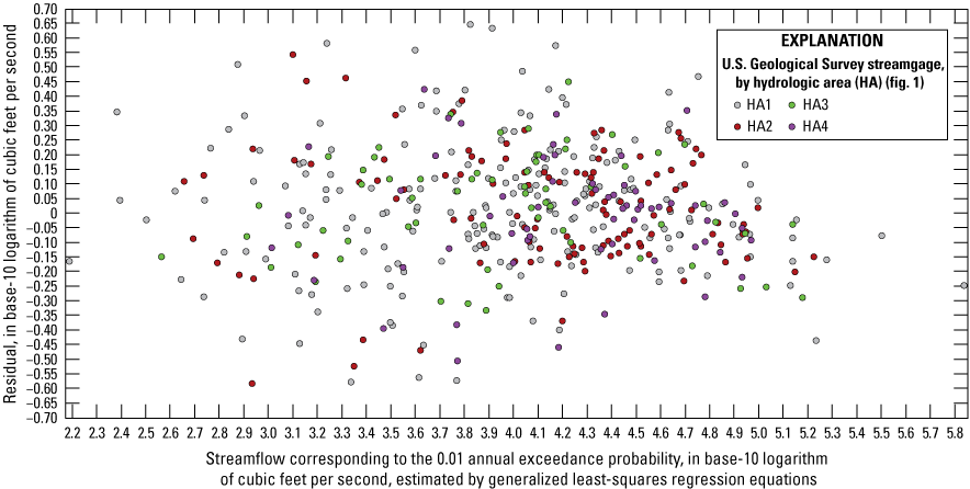
Relation between residuals and predicted streamflows corresponding to the 0.01 annual exceedance probability using the generalized least-squares equations.
Applications of Methods
RREs are statistical models that must be interpreted and applied within the limits of the data used to develop them and with the understanding that the results are best-fit estimates with an associated variance. The RREs are not valid at locations where dams, flood-control structures, channelization, diversion, or backwater have an appreciable effect on annual peak streamflow. Applications of the equations for estimating streamflows corresponding to selected AEPs differ for gaged locations on streams, ungaged locations on gaged streams, and locations on ungaged streams. EMA estimates for gaged locations and GLS estimates for ungaged locations can be used to determine weighted estimates for gaged locations and ungaged locations near streamgages. EMA, GLS, and weighted estimates for streamgages used in the study are available in tables A and B of Heal and others (2025).
Streamgage Locations
Accuracy of at-site estimates of streamflows corresponding to AEPs computed for a streamgage can be increased by weighting the at-site estimates with estimates computed by using the GLS equations. If the at-site and GLS estimates of a given AEP are weighted inversely proportional to their associated variances, the variance of the weighted estimate will be less than the variances of either the at-site or the GLS estimate. The weighted estimate is computed by using the following equation (England and others, 2019):
whereQp(g)w
is the weighted estimate of streamflow corresponding to the selected p-percent AEP at streamgage (g), in cubic feet per second;
VPp(g)r
is the variance of prediction of streamflow corresponding to the p-percent AEP at streamgage (g) from the GLS regression model, in log base-10 units;
Qp(g)s
is the estimate of streamflow corresponding to the p-percent AEP at streamgage (g) from the EMA analysis, in cubic feet per second;
VPp(g)s
is the variance of prediction of streamflow corresponding to the p-percent AEP at streamgage (g) from the EMA analysis, in log base-10 units; and
Qp(g)r
is the estimate of streamflow corresponding to the p-percent AEP at streamgage (g) from the GLS regression model, in cubic feet per second.
The variance of prediction of the weighted estimate for streamgage (g) (in log base-10 units) can be computed as:
whereVPp(g)w
is the variance of prediction of the weighted estimate of streamflow corresponding to the p-percent AEP at streamgage (g), in log base-10 units.
A 95-percent confidence interval for the weighted estimate (in cubic feet per second) can be computed as:
whereUngaged Locations on Gaged Streams
For ungaged locations, streamflows corresponding to selected AEPs are estimated by using the appropriate GLS equation (table 4). Streamflows at ungaged locations on gaged streams can be improved by applying a drainage area ratio. The following procedure is recommended if the drainage area at the ungaged location is within 50 percent of the drainage area at the gaged location (drainage area ratio is more than 0.5 or less than 1.5) (Ries and Dillow, 2006):
whereQp(u)
is the estimate of streamflow corresponding to the p-percent AEP at the ungaged location after transferring the weighted estimate from the gaged location, u, in cubic feet per second;
DRNAREA(u)
is the drainage area at the ungaged location, in square miles;
DRNAREA(g)
is the drainage area at the streamgage location, in square miles;
b
is the exponent of drainage area from the appropriate GLS equation (table 5); and
Qp(g)w
is the weighted estimate of streamflow corresponding to the p-percent AEP at the streamgage location, in cubic feet per second.
Table 5.
Drainage area generalized least-squares regression equations for estimating exponent b for equation 5 (Ries and Dillow, 2006).[AEP, annual exceedance probability; RI, recurrence interval; GLS, generalized least squares; ft3/s, cubic foot per second; Pseudo-R2, pseudo coefficient of determination; AVP, average variance of prediction; log10(ft3/s), base-10 logarithm of cubic feet per second; %, percent; Q, annual exceedance probability streamflow; DRNAREA, drainage area, in square miles]
The weighted flood estimate at the ungaged location can be computed by using the following equation:
whereQp(u)w
is the weighted estimate of streamflow at the ungaged location for the p-percent AEP, in cubic feet per second;
│ΔA│
is the absolute difference in drainage areas between the ungaged location (DRNAREA(u)) and the streamgage (DRNAREA(g)) location, in square miles;
DRNAREA(g)
is the drainage area at the streamgage location, in square miles;
Qp(u)r
is the GLS estimate of streamflow at the ungaged location corresponding to the p-percent AEP, in cubic feet per second; and
Qp(u)
is the estimate of streamflow corresponding to the p-percent AEP at the ungaged location after transferring the weighted estimate from the gaged location, u, in cubic feet per second.
If the drainage area of an ungaged location differs by more than 50 percent from that of the streamgage location, the GLS estimate becomes considerably more uncertain. If an ungaged location is between two streamgages on the same stream, the streamgage with the closest drainage area ratio and longest period of record is suggested for use (Sauer, 1964).
Accuracy and Limitations of GLS Equations
Accuracy and limitations of the GLS equations are affected by several factors. The equations are applicable at locations on streams in Tennessee where annual peak streamflows are not substantially affected by regulation, diversion, channelization, urbanization, or backwater. The equations are most applicable when estimating streamflow for basins having characteristics (explanatory variables) within the ranges of those used to develop the GLS equations (table 6); using explanatory variables outside of these ranges may result in prediction errors greater than expected (table 4).
Table 6.
Ranges of physical and climatic basin characteristics for use in generalized least-squares regression equations, by hydrologic area.[DRNAREA, drainage area; mi2, square miles; CSL10_85, 10 and 85 percent channel slope; ft/mi, feet per mile; LC11IMP, imperviousness; CLIMFAC2YR, 2-year recurrence-interval climate factor; N/A, not applicable]
| Hydrologic area (fig. 1) |
Number of streamgages used | Range of basin characteristic | |||
|---|---|---|---|---|---|
| DRNAREA, in mi2 | CSL10_85, in ft/mi | LC11IMP, in percent | CLIMFAC2YR, dimensionless | ||
| 1 | 216 | 0.20–21,400 | N/A | N/A | 2.05–2.42 |
| 2 | 114 | 0.42–2,560 | 1.74–356 | N/A | N/A |
| 3 | 63 | 0.17–2,050 | N/A | N/A | N/A |
| 4 | 61 | 0.95–2,310 | N/A | 0.26–13.7 | N/A |
The GLS equations are intended for use with basin characteristics computed using the methods described in this report. The StreamStats application (USGS, 2019) for Tennessee contains the same GIS layers and measurement methods used to calculate basin characteristics and estimates streamflows corresponding to various AEPs by using the GLS equations developed for this study.
Summary
Methods for estimating the magnitude and frequency of flooding at ungaged locations on rural streams in Tennessee were last updated in 2003. Since then, many years of additional annual peak-streamflow data have been collected, more geospatial data for calculation of explanatory variables have become available, and improved statistical methods have been developed for flood-frequency analysis. Thus, the U.S. Geological Survey (USGS), in cooperation with the Tennessee Department of Transportation, developed multiple linear regression equations to estimate streamflows corresponding to selected annual exceedance probabilities (AEPs) at ungaged locations on streams in Tennessee. Version 7.0.29368 of USGS PeakFQ software was used to conduct frequency analyses of annual peak streamflows for 454 streamgages operated by the USGS in Tennessee and surrounding States. Streamflows corresponding to the 50-, 20-, 10-, 4-, 2-, 1-, 0.5-, and 0.2-percent AEPs (the 2-, 5-, 10-, 25-, 50-, 100-, 200-, and 500-year floods, respectively) were estimated by using the expected moments algorithm in PeakFQ.
Four hydrologic areas used in previous flood-frequency studies in Tennessee were validated for statistical independence. For each hydrologic area, generalized least squares (GLS) regression equations were developed, incorporating combinations of drainage area (DRNAREA), 10–85 channel slope (CSL10_85), 2-year recurrence-interval climate factor (CLIMFAC2YR), and percent imperviousness (LC11IMP) as explanatory variables. Statistically significant (p≤0.05) explanatory variables used in the equations were DRNAREA and CLIMFAC2YR for HA1; DRNAREA and CSL10_85 for HA2; DRNAREA for HA3; and DRNAREA and LC11IMP for HA4.
The final GLS regression models were generated using the USGS weighted-multiple-linear regression (WREG) program, resulting in standard errors of prediction ranging from 30.4 to 51.4 percent. The GLS regression equations are applicable at locations on streams in Tennessee where annual peak streamflows are not substantially affected by regulation, diversion, channelization, backwater, or urbanization. The applicability and accuracy of the GLS regression models depend on the basin characteristics measured for an ungaged location on a stream being within range of those used to develop the equations. Methods are presented for using the GLS regression equations to estimate streamflows corresponding to selected AEPs at ungaged locations on both gaged and ungaged streams and to calculate weighted at-site estimates of streamflows corresponding to AEPs at streamgage locations. The final GLS regression equations and methods for estimating streamflows corresponding to selected AEPs have been incorporated in the USGS StreamStats application for Tennessee.
References Cited
Cohn, T.A., England, J.F., Berenbrock, C.E., Mason, R.R., Stedinger, J.R., and Lamontagne, J.R., 2013, A generalized Grubbs-Beck test statistic for detecting multiple potentially influential low outliers in flood series: Water Resources Research, v. 49, no. 8, p. 5047–5058, accessed October 22, 2015, at https://doi.org/10.1002/wrcr.20392.
Eng, K., Chen, Y.-Y., and Kiang, J.E., 2009, User’s guide to the weighted-multiple-linear regression program (WREG ver. 1.0): U.S. Geological Survey Techniques and Methods, book 4, chap. A8, 21 p., accessed July 31, 2024, at https://doi.org/10.3133/tm4A8.
England, J.F., Jr., Cohn, T.A., Faber, B.A., Stedinger, J.R., Thomas, W.O., Jr., Veilleux, A.G., Kiang, J.E., and Mason, R.R., Jr., 2019, Guidelines for determining flood flow frequency—Bulletin 17C (ver. 1.1, May 2019): U.S. Geological Survey Techniques and Methods, book 4, chap. B5, 148 p., accessed July 31, 2024, at https://doi.org/10.3133/tm4B5.
Feaster, T.D., Gotvald, A.J., and Weaver, J.C., 2014, Methods for estimating the magnitude and frequency of floods for urban and small, rural streams in Georgia, South Carolina, and North Carolina, 2011 (ver. 1.1, March 2014): U.S. Geological Survey Scientific Investigations Report 2014–5030, 104 p., accessed February 18, 2025, at http://dx.doi.org/10.3133/sir20145030.
Fenneman, N.M., and Johnson, D.W., 1946, Physical divisions of the United States: U.S. Geological Survey, 1 sheet, scale 1:7,000,000, accessed July 31, 2024, at https://doi.org/10.3133/70207506.
Flynn, K.M., Kirby, W.H., and Hummel, P.R., 2006, User’s manual for program PeakFQ annual flood-frequency analysis using Bulletin 17B guidelines: U.S. Geological Survey Techniques and Methods, book 4, chap. B4, 42 p., accessed July 31, 2024, at https://doi.org/10.3133/tm4B4.
Heal, E.N., Ladd, D.E., and Ensminger, P.A., 2025, Tabular and geospatial data for the magnitude and frequency of floods at ungaged locations on streams in Tennessee, through the 2013 water year: U.S. Geological Survey data release, https://doi.org/10.5066/P9IEJQB7.
Interagency Advisory Committee on Water Data, 1982, Guidelines for determining flood flow frequency—Bulletin 17B of the Hydrology Subcommittee: U.S. Geological Survey, Office of Water Data Coordination, 183 p., accessed November 11, 2021, at https://water.usgs.gov/osw/bulletin17b/dl_flow.pdf.
Law, G.S., and Tasker, G.D., 2003, Flood-frequency prediction methods for unregulated streams of Tennessee, 2000: U.S. Geological Survey Water-Resources Investigations Report 03–4176, 79 p., accessed June 6, 2018, at https://pubs.usgs.gov/wri/wri034176/.
Law, G.S., Tasker, G.D., and Ladd, D.E., 2009, Streamflow-characteristic estimation methods for unregulated streams of Tennessee: U.S. Geological Survey Scientific Investigations Report 2009–5159, 212 p., 1 pl., accessed March 27, 2019, at https://pubs.usgs.gov/sir/2009/5159/.
Patterson, J.L., 1964, Magnitude and frequency of floods in the United States—Part 7, Lower Mississippi River Basin: U.S. Geological Survey Water Supply Paper 1681, 636 p., accessed February 22, 2023, at https://doi.org/10.3133/wsp1681.
PRISM Climate Group, Oregon State University, 2014, United States average annual total precipitation, 1991–2020 (4-kilometer ASCII digital file), accessed December 23, 2024, at https://prism.oregonstate.edu.
Ries, K.G., III, and Dillow, J.A., 2006, Magnitude and frequency of floods on nontidal streams in Delaware: U.S. Geological Survey Scientific Investigations Report 2006–5146, 57 p., accessed February 22, 2023, at https://pubs.usgs.gov/sir/2006/5146/.
Southard, R.E., and Veilleux, A.G., 2014, Methods for estimating annual exceedance-probability flows and largest recorded floods for unregulated streams in rural Missouri: U.S. Geological Survey Scientific Investigations Report 2014–5165, 39 p., accessed November 11, 2021, at https://doi.org/10.3133/sir20145165.
Stedinger, J.R., and Tasker, G.D., 1985, Regional hydrologic analysis 1—Ordinary, weighted, and generalized least squares compared: Water Resources Research, v. 21, no. 9, p. 1421–1432, accessed October 26, 2015, at https://www.agu.org/journals/wr/v021/i009/WR021i009p01421/WR021i009p01421.pdf.
U.S. Geological Survey, 2013, WREG—Weighted-multiple linear regression program: U.S. Geological Survey web page, accessed June 1, 2014, at https://water.usgs.gov/software/WREG/.
U.S. Geological Survey, 2014, NLCD 2011 percent developed imperviousness (2011 edition, amended 2014)—National Geospatial Data Asset (NGDA) Land Use Land Cover: U.S. Geological Survey, accessed July 25, 2017, at https://www.mrlc.gov/nlcd11_data.php.
U.S. Geological Survey, 2016, USGS water data for the Nation: U.S. Geological Survey National Water Information System database, accessed 2015 at https://doi.org/10.5066/F7P55KJN.
U.S. Geological Survey, 2019, The StreamStats program: U.S. Geological Survey website, accessed February 16, 2023, at http://streamstats.usgs.gov/ss.
U.S. Geological Survey, [variously dated], 1/3 arc-second National Elevation Dataset: U.S. Geological Survey database, accessed 2006 at https://nationalmap.gov.
Veilleux, A.G., Cohn, T.A., Flynn, K.M., Mason, R.R., Jr., and Hummel, P.R., 2014, Estimating magnitude and frequency of floods using the PeakFQ 7.0 program: U.S. Geological Survey Fact Sheet 2013–3108, 2 p., accessed July 31, 2024, at https://doi.org/10.3133/fs20133108.
Weaver, J.D., and Gamble, C.R., 1993, Flood frequency of streams in rural basins of Tennessee: U.S. Geological Survey Water-Resources Investigations Report 92–4165, 38 p., accessed July 9, 2016, at https://pubs.usgs.gov/wri/1992/4165/report.pdf.
Conversion Factors
U.S. customary units to International System of Units
Datums
Vertical coordinate information is referenced to the North American Vertical Datum of 1988 (NAVD 88).
Horizontal coordinate information is referenced to the North American Datum of 1983 (NAD 83).
Supplemental Information
Water year A 1-year period from October 1 to September 30, defined by the year in which it ends; for example, the 2013 water year is the period October 1, 2012–September 30, 2013.
Abbreviations
AEP
annual exceedance probability
CLIMFAC2YR
2-year recurrence-interval climate factor
CSL10_85
main-channel slope
DRNAREA
drainage area
EMA
expected moments algorithm
GIS
geographic information system
GLS
generalized least squares
HA
hydrologic area
LC11IMP
percent imperviousness
LP3
log-Pearson type III
MGBT
Multiple Grubbs-Beck test
OLS
ordinary least squares
PILF
potentially influential low flood
RRE
regional regression equation
USGS
U.S. Geological Survey
WREG
weighted-multiple-linear regression computer program
For more information about this publication, contact
Director, Lower Mississippi-Gulf Water Science Center
U.S. Geological Survey
640 Grassmere Park, Suite 100
Nashville, TN 37211
For additional information, visit
https://www.usgs.gov/centers/lmg-water/
Publishing support provided by
Lafayette Publishing Service Center
Disclaimers
Any use of trade, firm, or product names is for descriptive purposes only and does not imply endorsement by the U.S. Government.
Although this information product, for the most part, is in the public domain, it also may contain copyrighted materials as noted in the text. Permission to reproduce copyrighted items must be secured from the copyright owner.
Suggested Citation
Ladd, D.E., and Ensminger, P.A., 2025, Estimating the magnitude and frequency of floods at ungaged locations on streams in Tennessee through the 2013 water year: U.S. Geological Survey Scientific Investigations Report 2024–5130, 19 p., https://doi.org/10.3133/sir20245130.
ISSN: 2328-0328 (online)
Study Area
| Publication type | Report |
|---|---|
| Publication Subtype | USGS Numbered Series |
| Title | Estimating the magnitude and frequency of floods at ungaged locations on streams in Tennessee through the 2013 water year |
| Series title | Scientific Investigations Report |
| Series number | 2024-5130 |
| DOI | 10.3133/sir20245130 |
| Publication Date | May 29, 2025 |
| Year Published | 2025 |
| Language | English |
| Publisher | U.S. Geological Survey |
| Publisher location | Reston, VA |
| Contributing office(s) | Lower Mississippi-Gulf Water Science Center |
| Description | Report: vi, 19 p.; Data Release |
| Country | United States |
| State | Tennessee |
| Online Only (Y/N) | Y |