

Using the D-Claw Software Package to Model Lahars in the Middle Fork Nooksack River Drainage and Beyond, Mount Baker, Washington
Links
- Document: Report (12 MB pdf) , HTML , XML
- Appendixes:
- Appendix 4 - Scenario A1 (35.4 MB) - Scenario A1
- Appendix 4 - Scenario A2 (41.7 MB) - Scenario A2
- Appendix 4 - Scenario A3 (50.4 MB) - Scenario A3
- Appendix 4 - Scenario B1 (25.6 MB) - Scenario B1
- Appendix 4 - Scenario B2 (37.6 MB) - Scenario B2
- Appendix 4 - Scenario B3 (47 MB) - Scenario B3
- Appendix 4 - Scenario C2 (35.9 MB) - Scenario C2
- Appendix 4 - Scenario D2 (26.5 MB) - Scenario D2
- Appendix 4 - Scenario E2 (22.1 MB) - Scenario E2
- Data Release: USGS data release - Simulated lahar extents and dynamics in the Middle Fork Nooksack River drainage, resulting from hypothetical landslide sources on the western summit of Mount Baker, Washington
- NGMDB Index Page: National Geologic Map Database Index Page (html)
- Download citation as: RIS | Dublin Core
Acknowledgments
The authors thank Jessica Ball and Katy Barnhardt of the U.S. Geological Survey (USGS) for their constructive reviews that greatly improved the manuscript. We also thank Larry Mastin (USGS) for his nuanced edits prior to manuscript submission and James Vallance (USGS) for discussions about LAHARZ uncertainty. A special thanks to Jon Major who helped clarify several conceptional issues and provided helpful editorial comments that were greatly appreciated. Joe Beaulaurier, of Whatcom News, kindly and quickly responded to our request for a photograph showing flooding in the City of Sumas, Washington, during the November 2021 floods.
Abstract
Lahars, or volcanic mudflows, are the most hazardous eruption-related phenomena that will affect communities living along rivers that originate on Mount Baker. In the past 15,000 years, the largest lahars from Mount Baker have affected the Middle Fork Nooksack River drainage and beyond. Here we use the physics-based D-Claw software package to model nine lahar scenarios that are initiated as water-saturated landslides between Sherman Crater and the Roman Wall on the Mount Baker edifice and flow down the Middle Fork Nooksack River. The scenarios range in volume from 1 to 260 million cubic meters and have an initial hydraulic permeability from 10−12 to 10−10 meters squared. Model output includes data such as flow depth, velocity, runout distance, area inundated, arrival time, and sediment concentration as well as information that allows scientists to calculate other important hydrologic characteristics such as lahar discharge. These data are important to officials who have the responsibility to plan for, or take mitigation measures against, future Mount Baker lahars. To check the validity of the D-Claw results, we compare the scenarios to known geologic information. We also compare D-Claw results with empirical models that have been used in the past to determine potential inundation areas, runout distances, and arrival times. These comparisons highlight similarities and differences between empirical and physics-based models. We also present D-Claw scenario-based animations to help scientists, officials, and lay people alike to visualize how future lahars could affect communities.
Introduction
Lahar is an Indonesian word that describes highly mobile and destructive mixtures of water and sediment that start on volcanoes and flow down valley. They are the primary volcano hazard for communities along river valleys that originate on Mount Baker in northwest Washington State. In this report, we use the term debris flow, instead of lahar, for mixed flowage events (generally 10 million cubic meters [Mm3] or less) that are triggered by non-volcanic process such as intense rain on loose material or failure of ice-cored glacial material (Vallance and others, 2002). We use the term lahar for mixed flowage events that are volcanically triggered. Lahars can range in volume from less than one to hundreds of million cubic meters.
Geologic field studies have established that in the past 15,000 years, lahars with volumes up to hundreds of millions of cubic meters have inundated valleys on the east and south flanks of Mount Baker (Hyde and Crandell, 1978; Easterbrook and Kovanen, 1996; Kovanen and others, 2001; Tucker and others 2014; Scott and others, 2020). The largest of these, the Middle Fork lahar (approximately 240 Mm3, Scott and others, 2020), originated as a landslide between the Roman Wall and Sherman Crater about 6.7 thousand years ago (ka) and quickly transformed into a lahar that flowed down the Middle Fork Nooksack River valley and toward the Sumas River valley (fig. 1). Other post-glacial lahars traveled down drainages on the east flank that today would flow into the Baker Lake reservoir, but in this report, we focus solely on the Nooksack River system.
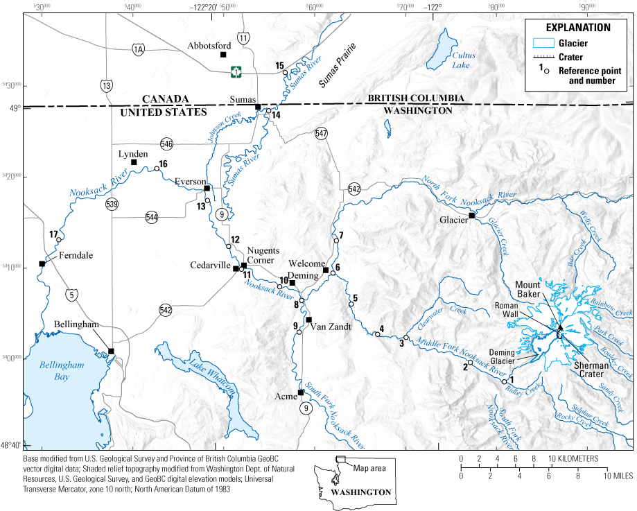
Location map of study area showing reference points, population centers, major transportation corridors, and major geographic features in northwestern Washington.
Although we can generally trace the pathway of past lahars from geologic deposits, details regarding their inundation area, flow depth, and discharge are often difficult or impossible to determine centuries to millennia after an event has occurred due to post-event erosion or burial by younger sediments. Furthermore, lahar travel speeds—critical information for emergency responders and planners—cannot be determined directly from deposits. The empirical model, LAHARZ (Iverson and others, 1998; Schilling, 1998), based on a correlation between lahar volume and valley topography, has been widely employed in the Cascade Range and worldwide to forecast lahar inundation area and runout distance. However, LAHARZ has several limitations: it provides no information about lahar travel times or other flow dynamics; it is poorly constrained in flat, unconfined areas; it does not allow a lahar to bifurcate (split) due to topography; and it cannot consider the subtle dependence of lahar behavior on source-area location, downstream terrain features, or physical properties of the lahar material. Therefore, we employ a new, high-resolution physics-based model, D-Claw, which overcomes some of the limitations of LAHARZ and other empirical models. Specifically, D-Claw provides information such as flow depth, velocity, arrival time, and discharge of potential future lahars, it allows lahars to bifurcate, and it provides important information on lahar dynamics for a given volume, sediment attribute, and topography.
In this report, we summarize D-Claw modeling results of nine hypothetical lahars (table 1) between 1 and 260 Mm3 that originate as water-saturated landslides high on the southwest flank of Mount Baker near Sherman Crater. Within seconds of landslide initiation, increased pore pressure fluidizes the material and transforms the landslide into a lahar. In these scenarios, the lahars flow down the Middle Fork Nooksack River valley and beyond. Such events have occurred in the past and will likely occur again in the future. As there are multiple ways that lahars can be initiated at snow-and-ice-clad volcanoes like Mount Baker—for example, eruption column collapse, lava-flow front collapse, glacial outbursts, and meteorological events—it is important to recognize that these simulations portray lahars initiated by landslides and not by other phenomena. The nine scenarios vary principally by initial landslide volume (which here is equivalent to lahar volume) and material properties (notably, hydraulic permeability) that affect lahar mobility. See methods section on the D-Claw numerical model for consideration of other variables.
Table 1.
List of scenarios as they relate to volume and initial hydraulic permeability.[The letter denotes the scenario volume in million cubic meters (Mm3) and the subscripted scenario number refers to the initial hydraulic permeability (k0, in square meters [m2]). A represents 260 Mm3; B represents 108 Mm3; C represents 37 Mm3; D represents 10 Mm3; and E represents 1 Mm3; (1) k0=10−10 m2; (2) k0=10−11 m2; and (3) k0=10−12 m2]
Our five lahar volumes (1, 10, 37, 108, and 260 Mm3) simulate estimated volumes of events that have happened in the past or could occur in the future. The three smallest volumes (scenarios C2, D2, and E2) are volumetrically similar to past volcanically triggered small-volume lahars and non-volcanically triggered debris flows at Mount Baker (Scott and others, 2020). Like lahars, debris flows can begin as landslides. However, unlike most volcanically triggered lahars, where the change of state of the volcano may give some warning that an event could occur, many debris flows often occur without geophysical or observational warning. Debris flows commonly occur in areas of steep terrain and favorable geologic conditions such as weak, altered rock or weak substrates (for example, the 2010 Mount Meager landslide [Guthrie and others, 2012], the May 2013 debris flow in the Middle Fork Nooksack River [Mount Baker Volcano Research Center, 2013], and the 2014 Oso, Wash. (State Road [SR] 530) landslide [Keaton and others, 2014]). The largest known non-volcanically induced event at Mount Baker in the past 15,000 years was a debris avalanche (landslide) that transformed into a debris flow in the Rainbow Creek valley on the east flank of the volcano during the late 19th century. The debris avalanche had an estimated volume of 20 Mm3 (Scott and others, 2020).
The two largest volumes, 206 and 108 Mm3 (scenarios A and B, respectively), approximate the volume of the largest lahar that has occurred at Mount Baker in the past 15,000 years (Scott and others, 2020) and the volume of altered rock around Sherman Crater (Finn and others, 2018), respectively. These volumes are an order of magnitude larger than the aforementioned Rainbow Creek debris avalanche and debris flow. Such large volumes are most likely to occur during volcanic unrest (a period of time when subsurface magma movement is detected either observationally or instrumentally) or eruption (when magma reaches the surface). During unrest, as magma moves toward the surface, it can deform the upper edifice causing a landslide of weak, hydrothermally altered rock. Such a failure may or may not coincide with the beginning of eruptive activity. The Electron mudflow at Mount Rainier is a rare instance in which a large-volume lahar appears to have occurred without any associated volcanic activity (Vallance and Sisson, 2022)—no such similar event is known to have occurred at Mount Baker.
This report does not attempt to forecast future lahar events at Mount Baker, but rather focusses on potential downstream consequences of lahars of given volumes and properties. The scenarios discussed in this study, although informed by geological data and Mount Baker’s topography, are approximations of what could, but not necessarily what will, happen in the future. Thus, no scenario is deemed imminent or most likely and, because of the low number of known lahar events at Mount Baker, the likelihood of one scenario over another cannot be assessed probabilistically. Any probabilistic forecasts based on potential landslide source geometries would be highly questionable given the large number of uncertainties involved. Nonetheless, these scenarios can help inform communities living within the Nooksack River system how to prepare for, and respond to, future lahar events.
The purpose of this report is to publish the output data from the nine D-Claw scenarios and to provide the basic geologic context with which to assess that data. For those readers who may like to use the data for community planning purposes but do not have a technical background, we provide a narrative that helps explain the data and their limitations.
Lahars and Major Debris Flows in the Middle Fork Nooksack River Valley During the Past 15,000 Years
We use the geologic history of Mount Baker to inform the range of volumes used in our scenarios. Mount Baker is the only volcano in the United States’ part of the Cascade Range to have experienced both alpine and continental glaciation. Glacial erosion has been so extensive that fragmental deposits older than 15,000 years—such as from pyroclastic flows and lahars—have been removed (Hildreth and others, 2003; Scott and others, 2020). Thus, we restrict our discussion to lahars and major debris flows that have affected the Middle Fork Nooksack River valley (fig. 1; table 2) in the past 15,000 years. Throughout this report, all ages, except that from Cameron (1989), are given as calibrated radiocarbon ages (see Scott and others [2020] for age details). The calibrated ages are each combined ages of several radiocarbon ages using the OxCal program (Bronk Ramsey, 2001, 2009), whereas the Cameron age is from a single radiocarbon age with a large uncertainty. The Cameron (1989) age is given as in the original report as an uncalibrated radiocarbon age in years before present (yr B.P., where present is considered 1950 C.E.).
Pratt Creek Sequence (Latest Pleistocene)
A 30-meter-thick sequence of lava flows and deposits of pyroclastic flows, lahars, and fluvially reworked material in lower Pratt Creek, a tributary of Ridley Creek and the Middle Fork Nooksack River, rests on continental glacial deposits from the last ice age (Scott and others, 2020). The sequence contains several coarse-grained (sand to boulder) deposits dominated by clasts that show signs of being emplaced hot, as well as cooler, sandier deposits. Scott and others (2020) interpreted the hot deposits as being from pyroclastic flows formed by collapses of lava flow fronts near the summit of the volcano and the cooler, sandier deposits from lahars that were triggered by hot rocks mixing with snow and ice. The sequence occurred between about 16.3 and 9.8 ka, as it overlies glacial till 16.3 ka in age and is overlain by a soil that contains a tephra fall dated to about 9.8 ka. Scott and others (2020) argued a more likely age is between 14.2 and 11.8 ka based on sediment stratigraphy in Baker Lake. Deposits have not been traced beyond their exposure in Pratt Creek and volumes of individual units are unknown but are likely less than a few million cubic meters.
Schriebers Meadow Lahar (Early Holocene)
The Schriebers Meadow lahar (9.5 ka) is the oldest known Holocene (past 11,700 years; Walker and others, 2009) lahar of consequence at Mount Baker. Based on the high clay content (9 percent by weight matrix clay) of the deposit, the lahar is thought to have been triggered by a landslide in hydrothermally altered rock upslope from Schriebers Meadow on the Mount Baker edifice (Scott and others, 2020). The exact location and cause of the failure are unknown. This event is not directly related to known volcanic activity, although it may be related to a thin tephra deposit, tephra layer MY of Scott and others (2020). The lahar deposit is distributed from Ridley Creek (a tributary of the Middle Fork Nooksack River) to Sulphur Creek. The bulk of the deposit is preserved in Sulphur and Rock Creeks, where it forms the meadow surface surrounding the Schriebers Meadow cinder cone (Hyde and Crandell, 1978; Thomas, 1997; Hildreth and others, 2003; Scott and others, 2020). The lahar deposit overlies the Pratt Creek assemblage and underlies the Ridley Creek lahar deposit. Little is known about its original extent or its effects on the Middle Fork Nooksack River valley other than its presence in Ridley Creek (fig. 1). Scott and others (2020) estimated the deposit volume as 25–30 Mm3.
Middle Fork Lahar (Middle Holocene)
The Middle Fork lahar, the largest known post-glacial lahar from Mount Baker, originated as a landslide above the Deming Glacier in the region between Sherman Crater and the Roman Wall (Tucker and others, 2014; Scott and others, 2020) about 6.7 ka. Scott and others (2020) described its deposit as only the basal part of a long-recognized lahar deposit in the Middle Fork Nooksack River valley (Hyde and Crandell, 1978; Easterbrook and Kovanen, 1996). Deposits of this lahar are found in upper Rocky Creek and along the length of the Middle Fork Nooksack River. Along the Middle Fork Nooksack River, flow depths were as much as 65 meters (m) in the 350-m-wide channel downstream from Ridley Creek, and more than 85 m in the approximately 200-m-wide gorge downstream from Clearwater Creek (fig. 1). Entrainment of sediment along the valley caused a gradual change in deposit matrix color and composition as the flow incorporated non-Mount Baker gravel-sized clasts (more than 25 percent of the deposit; Scott and others, 2020).
The lahar traveled down the Middle Fork Nooksack River into the North Fork Nooksack River, past the confluence with the South Fork Nooksack River, and then into the main channel of the Nooksack River. It flowed at least as far as Nugents Corner, Wash. (fig. 1), about 50 kilometers (km) downstream from the source area. Well logs in the Nugents Corner area show a maximum deposit thickness of 14 m (Scott and others, 2020). However, an unknown proportion of that deposit thickness may consist of the overlying Ridley Creek lahar deposit.
A study of Sumas River valley well-log data (Cameron, 1989) showed that in post-glacial time and into the middle-late Holocene, the Nooksack River flowed northward into the Sumas River valley (fig. 1). Cameron (1989) noted that volcanic gravels from Mount Baker are limited to the shallowest Nooksack River floodplain deposits but are extensive in the Sumas River valley subsurface (for example, sand and gravel unit 3 of Cameron [1989]). Subsequent investigations by Pittman and others (2003) suggested that the change in the Nooksack River from northward flow to the current westward flow may be relatively recent, perhaps only in the past 1,000 years or so.
About 7 to 8 km southeast of Sumas, Wash. (fig. 1), there is a concentration of buried logs within unit 3 over an eight-square kilometer area. Cameron (1989) suggested the logs are within a debris-flow or lahar deposit whose flow originated in the Nooksack River valley. A tephra in Pangborn Bog was tentatively identified as Mazama ash (7.6 ka; Bacon, 1983; Zdanowicz and others, 1999) with an age of 7.14±0.6 ka B.P. from peat directly below the tephra (Cameron, 1989). This appears to correlate to a tephra deposit beneath unit 3. Scott and others (2020) suggested that based on the stratigraphy, these logs could be part of the Middle Fork lahar deposit but could not conclude if the deposit was primary or reworked, or whether unit 3 may include some thickness of the Ridley Creek lahar deposit. If unit 3 deposits are primary and only from the Middle Fork lahar, then the estimated lahar volume is about 240 Mm3 with a travel distance of greater than 63 km (Scott and others, 2020).
Like the Schriebers Meadow lahar deposit, the Middle Fork lahar deposit contains a high proportion of matrix clay (as much as 11 percent by weight), which indicates highly altered material in the source area. The Middle Fork lahar may have occurred during a period of unrest that preceded eruptive activity at Mount Baker (Scott and others, 2020).
Ridley Creek Lahar (Middle Holocene)
Hyde and Crandell (1978) considered the Ridley Creek lahar deposit to be the finer-grained top of the Middle Fork lahar deposit, but Scott and others (2020) defined it as the product of a separate lahar that likely occurred soon after the Middle Fork lahar and was coincident with the start of magmatic activity. Like the Middle Fork lahar, Scott and others (2020) surmised that the Ridley Creek lahar originated as a landslide of altered rock from the east portion of the Roman Wall, the area just west of Sherman Crater, and perhaps parts of Sherman Crater itself. Most of the lahar descended the upper Easton Glacier and entered the Middle Fork Nooksack River by way of Ridley Creek (fig. 1). Smaller portions of the flow spilled into Rocky and Sulphur Creeks. Radiocarbon and wiggle-match ages show that the age of the Ridley Creek lahar deposit is indistinguishable from that of the Middle Fork lahar deposit (Scott and others, 2020).
The Ridley Creek lahar deposit is distinguishable from that of the Middle Fork lahar deposit at multiple locations. Downstream from the confluence of Ridley Creek and the Middle Fork Nooksack River (fig. 1), the Ridley Creek lahar deposit forms local terraces below the peak-flow deposits of the Middle Fork lahar. Farther downstream, it overlies the Middle Fork lahar deposit and is between 3 and 7 m thick with a sharp or, less commonly, transitional contact. Near its source (less than 25 km from source), the Ridley Creek lahar deposit is distinguished from the Middle Fork lahar deposit by matrix color (tan versus blue), texture (generally finer grained), and the absence of wood. Farther downstream (greater than 30 km), distinctions in color and texture are less pronounced owing to the incorporation of sediment along the river valley. The thickness of the Ridley Creek lahar deposit 35 km from source suggests the lahar likely flowed at least as far as Nugents Corner (50 km from source). Scott and others (2020) estimated the deposit volume to be about 150 Mm3. Like the Middle Fork and Schriebers Meadow lahar deposits, the Ridley Creek lahar deposit is matrix-rich (as much as 70 percent by weight) and has high amounts of matrix-clay (as much as 10 percent by weight).
The Ridley Creek lahar is the last known lahar to flow down the Middle Fork Nooksack River valley. Since that time, however, there have been several notable debris-flow events that were triggered either by mass wasting of alpine glaciers or meteorological events. We discuss a few of the more notable ones below.
Debris Flow at Elbow Lake Trailhead (1.6 ka)
A debris-flow deposit, exhumed by a 2003 flood event, mantles a 7-m tall terrace on the north bank of the Middle Fork Nooksack River at the Elbow Lake Trailhead (Tucker and others, 2014; Scott and others, 2020). This site is about 6.4 km downstream from the 2013 Deming Glacier terminus. The deposit is 1 to 1.5 m thick and has a clay-poor, gray matrix. Outer rings of a log buried by the deposit yield a date of about 1.6 ka.
No juvenile clasts are found in the deposit, which suggests a non-eruptive origin. As the date corresponds to a time of alpine glacial advance, the most likely origin is either an extreme rain event or a glacial outburst flood. The deposit has not been traced farther downstream, but an estimated volume based on its thicknesses at the trailhead and at a site upstream is about 10 Mm3 (Scott and others, 2020).
Deming Glacier Debris Flow (1927 C.E.)
In June 1927, the distal kilometer or more of the Deming Glacier collapsed (C.F. Easton, written commun., 1911–1931). The initial flow of water and ice transformed rapidly into a debris flow containing both Mount Baker and non-Mount Baker lithologies. The debris-flow deposit forms a continuous, well-defined terrace 10–15 m above the present channel of the Middle Fork Nooksack River, 1.5 km downstream from the 2013 glacial terminus. About 1.5 km downstream from the confluence with Ridley Creek, the debris flow transformed into a more water-rich hyperconcentrated flow (60 percent sediment by volume; Pierson and Scott, 1985) that traveled to just beyond the confluence with Clearwater Creek (fig. 1). Scott and others (2020) estimated the volume of the debris flow at around 10 Mm3.
Debris Flow of May 31, 2013
A seismic event at Mount Baker was recorded at 2:53 a.m. Pacific daylight time on May 31, 2013. Between 5:00 and 5:30 a.m., a large spike in turbidity and discharge (25 cubic meters per second [m3/s] [865 cubic feet per second (ft3/s)] at 5 a.m.; 28 m3/s [976 ft3/s] at 5:15 a.m.; and 25 m3/s [874 ft3/s] at 5:30 a.m.) was noted at the U.S. Geological Survey (USGS) MF Nooksack River near Deming WA streamgage no. 12208000 (near reference point [RP] 4 in the Middle Fork Nooksack River [fig. 1]; USGS, 2016), 20 km downstream from the Deming Glacier terminus. Near the confluence of Ridley Creek and the Middle Fork Nooksack River, mud-covered boulders were thrown 4.6 m (15 feet) above the river channel (Mount Baker Volcano Research Center, 2013). Spikes in flow discharge were also noted on USGS streamgages near Nugents Corner (USGS streamgage no. 12210700; USGS, 2016) and Lynden, Wash. (USGS streamgage no. 12211500; USGS, 2016), and there were reports of sediment-laden water at the mouth of the Nooksack River (C. Driedger, USGS, oral commun., 2013). The origin of this event was hypothesized as failure of part of a glacial moraine above the terminus of the Deming Glacier (Mount Baker Volcano Research Center, 2013).
What is important about this event, and other non-eruptive events discussed previously, is that debris flows can result in brief periods of high discharge and heavy sediment loads downstream. Although such events are rarely life threatening to communities downstream, they can be life threatening to anyone who is unlucky enough to be in the valley bottoms close to the volcano when such random events occur.
Table 2.
Summary of major lahars and debris flows in the Middle Fork Nooksack River drainage during the Holocene.[Data for all lahars and debris flows, except for the debris flow of May 31, 2013, come from Scott and others (2020). Data for the May 31, 2013, debris flow is from the Mount Baker Volcano Research Center’s website post on June 5, 2013 (Mount Baker Volcano Research Center, 2013) and from Tucker and others (2014). Mm3, million cubic meters; <, less than; km, kilometer; Nd, no data; ka, thousands of years; ~, about; >, greater than]
Methods
The D-Claw numerical model
We simulated nine lahars using D-Claw (Debris Conservation laws), a numerical modeling software package built within the open-source Clawpack project (www.clawpack.org; Mandli and others, 2016) and utilizing extensions of GeoClaw algorithms for free-surface flows over variable topography (George, 2008, 2011; Berger and others, 2011; LeVeque and others, 2011). D-Claw was developed at the USGS to simulate the dynamics of debris flows, landslides, and lahars that are comprised of evolving mixtures of sediment and water (Iverson and George, 2014; George and Iverson, 2014). D-Claw has been applied to simulate hazardous geologic events such as the 2014 Oso (SR 530), Wash., landslide disaster (Iverson and others, 2015; Iverson and George, 2016) and potential future lahars at Mount Rainier, Wash. (George and others, 2022). Here we provide a short overview of the D-Claw model. The program and data release for these nine simulations are found in George and others (2025a, b). For an in-depth explanation of the foundational physics and mathematics, see Iverson and George (2014) and George and Iverson (2014), and for an in-depth qualitative model explanation see George and others (2022).
D-Claw is a depth-averaged model based on conservation of mass and momentum for a gravity-driven granular-fluid mixture. There is an established precedent for using depth-averaged models for relatively shallow large-scale flows ranging from water waves and floods (for example, Stoker, 1957; Vreugdenhil, 1994) to dry rock avalanches (Savage and Hutter, 1989). In more complex multi-component flows composed of granular-fluid mixtures the interactions of particles and fluid heavily influence the pore-fluid pressure and frictional resistance, and hence the mechanics and mobility of a saturated landslide, debris flow, or lahar (Iverson, 1997). Early depth-averaged models for these complex mixtures commonly represented the material as single-component fluids with complex rheologies (for example, McDougall and Hungr, 2004; Christen and others, 2010). More recently, two-phase models, such as D-Claw, have been developed that account directly for solid-fluid interactions (see also, Kowalski and McElwaine [2013], Bouchut and others [2016], and Mergili and others [2017]).
In D-Claw, the spatially and temporally varying solid-volume fraction, m, and basal pore-fluid pressure, p, coevolve in a tightly coupled manner. The model is based in part on the phenomenon of granular dilatancy (Reynolds, 1886), which implies that as granular materials shear under force, granular rearrangement drives the surrounding solid-volume fraction toward a dynamic equilibrium, meq. Thus, dilatancy, which is the propensity for granular contraction or expansion, regulates the pore-pressure response to motion. In D-Claw, the difference between the ambient or instantaneous solid volume fraction m of the shearing mass and equilibrium solid volume fraction meq determines whether the water-sediment mixture is in a contractive or dilative state (see Iverson and George [2014]). Where m−meq<0, shearing promotes granular contraction and elevated pore-fluid pressure, which reduces the effective Coulomb frictional resistance and thus enhances mobility. Where m−meq>0, shearing leads to granular expansion, lower pore-fluid pressure, and higher frictional resistance, which reduces mobility. The equilibrium solid fraction meq is not a fixed parameter in D-Claw simulations, but rather evolves as a function of flow variables and material parameters. However, the critical state or quasi-static value for meq, referred to as mcrit, provides a baseline initial value for meq and is assumed to be dependent only on the granular composition of the sediment. Therefore, mcrit is a fixed parameter in D-Claw simulations, which influences the evolving mobility of the material. The timescale of pore-pressure elevation (or reduction) and thus enhanced (or diminished) mobility also depends on locally varying properties of the water-sediment mixture. Therefore, initial conditions and material parameters that characterize the water-sediment mixture heavily influence downslope flow dynamics and have a profound effect on landslide mobility, internal frictional resistance, and lahar runout distance.
Because detailed subsurface heterogeneities of initial landslide masses are unknown, we assume that the initial sediment material properties are uniform, although they can evolve as functions of the flow variables based on physical model assumptions (Iverson and George, 2014). Thus, in this report, all simulations have saturated landslide source material with a uniform initial porosity of (1−m0, where m0 is the initial solid-volume fraction; table 3), and material parameters that characterize relatively porous granular mixtures upon failure (m0−mcrit<0). Thus, after failure, the landslide is more prone to liquefaction and mobility. Landslides with relatively more compact material (less porous mixtures where m0−mcrit>0), tend to exhibit little or no liquefaction, resulting in a slow-moving landslide. Although such landslides could occur at Mount Baker, they pose little down-valley hazard and are not addressed in this report. See Iverson and others (2015), Iverson and George (2016), and George and others (2022) for more details regarding model assumptions.
A material property of flowing debris that greatly influences D-Claw results is the dynamic hydraulic diffusivity, which affects the timescale for which elevated (or diminished) pore-fluid pressure can persist. The rate at which elevated pore pressure, which accompanies liquification, relaxes toward equilibrium (hydrostatic pressure, the point at which liquification ceases) affects how mobile a lahar is. The dynamic hydraulic diffusivity is inversely proportional to the effective viscosity, μ, of the inter-granular fluid (a mixture of water and suspended fine material such as clays), and proportional to the local dynamic hydraulic permeability, k, which characterizes the ease of fluid flow through a granular mixture (table 3). The hydraulic permeability, k, is assumed to be a dynamic function of the solid-volume fraction m. In D-Claw, the initial value of k (k0) and μ are fixed parameters that together provide a baseline characterization of the intrinsic composition of the fluid- and sediment mixture. The sediment composition is characterized by additional parameters that are not varied or discussed herein (see Iverson and George [2014]).
Table 3.
List of initial values and modeling parameters used in the D-Claw scenarios for landslides that originate on the edifice of Mount Baker, northwestern Washington.[m3, cubic meter; m2, square meter; N·s/m2, Newton-second per square meter; kg/m3, kilogram per cubic meter]
The values for μ, and k0 are subject to uncertainty and subsurface heterogeneities but are generally constrained by geologic data, laboratory tests, and flume experiments (Iverson and others 2010; Iverson and George, 2014). Because the hydraulic diffusivity is proportional to the ratio k/μ in our simulations, we vary only the initial hydraulic permeability parameter, k0, and explore how it affects lahar mobility and runout distance. In general, smaller initial hydraulic permeabilities (for example, k0=10−12 m2) support longer periods of sustained elevated pore pressure (which means less friction), and therefore farther lahar runout distances, than larger initial hydraulic permeabilities (for example, k0=10−10 m2).
In our simulations, there is no water in the river channel; thus, we do not account for how river flow affects lahar dynamics. Instead, we assume that lahar volume and hydraulic permeability dominate any influence of interaction between the lahar and river flow that might occur. Whether this assumption is correct, especially for large rivers at flood stage, is a complex problem and currently a topic of investigation.
Mount Baker Base Topography and Landslide Source Areas
In these simulations, we use a 5-meter resolution digital elevation model (DEM) for our base topography. The DEM was derived mostly from airborne light detection and ranging (lidar) surveys flown from 2013 to 2017 (a small area near Sumas, Wash., is from a 2006 lidar survey). Individual DEMs are from the Washington Department of Natural Resources and Province of British Columbia GeoBC. The DEMs were converted to uniform datums, projected to the Universal Transverse Mercator zone 10 coordinate system, and mosaicked to form a single DEM of the study area. Elevations of most rivers and other waterbodies are represented as the water surface at the time of lidar collection, except in the main-stem Nooksack River downstream from Welcome, Wash., where the topography of the riverbed (Anderson and Grossman, 2017) has been incorporated into the DEM.
In our D-Claw simulations, each lahar is initiated by a hypothetical landslide originating on the southwest flank of Mount Baker, between Sherman Crater and the Roman Wall (fig. 1). The landslide volume is equivalent to the volume of the lahar. Landslide source areas were outlined based on estimated bulked lahar volumes (in other words, the initial landslide volume and material entrained into the lahar during flow) of past events, the amount of altered rock near Sherman Crater (Hildreth and others, 2003; Warren, 2008; Finn and others, 2018; Scott and others, 2020), and interpretation of topography. Although D-Claw can incorporate bulking into a scenario, the amount of bulking is poorly constrained, so we simplified our approach and used the estimated bulked volumes of the lahars as our initial landslide volumes instead of trying to factor bulking into the simulations. Several longitudinal transects were drawn for each source area. For each transect, we made slip-surface profiles that had the form of logarithmic spirals—a commonly assumed profile for failure surfaces in homogenous material (Jaboyedoff and others, 2020, and references therein). The profiles and elevations of the source-area margins were used to interpolate a continuous slip surface within the source area resulting in scenario volumes of 1, 10, 37, 108, and 260 Mm3.
Lahar Volumes, Initial Hydraulic Permeability, and Simulation Durations
We explore nine lahar scenarios (table 1) that hopefully encompasses the range of likely future lahars at Mount Baker in the Middle Fork Nooksack River valley. All the lahar scenarios start as landslides sourced between Sherman Crater and the Roman Wall (fig. 1). In all scenarios, pore pressure within the water-saturated landslides quickly increases to fluidize the material that then moves down the Middle Fork Nooksack River and beyond as a lahar. We use the same material properties (table 3) in all scenarios, varying only the landslide failure volume (1, 10, 37, 108, and 260 Mm3) and, for the two largest volumes (108 and 260 Mm3), the initial hydraulic permeability (k0=10−10, 10−11, 10−12 m2). For the 1, 10, and 37 Mm3 scenarios, we use only an initial hydraulic permeability of 10−11 m2. A value of k0=10-11 m2 provided the best comparative match of D-Claw model runs to sparse geological constraints and to the broad brush statistical LAHARZ model (see “Discussion” section).
Our initial landslide volumes reflect estimated lahar and debris-flow volumes from the geologic record (Scott and others, 2020) and the estimated volume of hydrothermally altered rock near Sherman Crater (Finn and others, 2018). Using airborne geophysics, Finn and others (2018) estimated about 100 Mm3 of altered rock around Sherman Crater, which is similar to the smaller (108 Mm3) our two largest volumes. Our largest volume, 260 Mm3, is slightly larger than the estimated bulked volume of 240 Mm3 for the Middle Fork lahar (6.7 ka; Scott and others, 2020). A volume, of 37 Mm3 is of the same order of magnitude as largest known non-eruption induced flank failure at Mount Baker—Rainbow Creek debris avalanche during the late 19th century—and of some of the smaller eruption-induced lahars (for example, an estimated volume of 35 Mm3 for the Park Creek lahar; Scott and others, 2020). We also include 1 and 10 Mm3 volumes in our scenarios as these smaller-volume events can occur during unrest and eruption but also can, and more often do, happen during periods of quiescence.
For the initial hydraulic permeability, we use a range from k0=10−12 to 10−10 m2. These values come from permeabilities measured in static laboratory tests (Iverson and others, 2010) and from large-scale debris-flow experiments (see fig. 5 in Iverson and George [2014]) as in-progress lahar hydraulic permeabilities are unknown. Lahars with low clay content (less than 5 percent by weight; Vallance and Scott, 1997; Vallance and Iverson, 2015) tend to have larger hydraulic permeability values, whereas clay-rich (greater than 5 percent by weight) lahars tend to have smaller values.
The D-Claw model uses adaptive mesh refinement (AMR), which allows it to solve for fine-scale resolution in areas of interest when needed (for example, the landslide or lahar flow path) and coarse-scale resolution in areas of little interest (see George and others [2022]). The AMR approach greatly minimizes computational time, which would be much greater if uniformly spaced grids or even variably spaced static topographically fit meshes were used for the entire domain and duration of a simulation.
Even using AMR, our D-Claw simulations, which utilized 5-m resolutions for the finest mesh, are computationally intensive due to the large area of our computational domain. Thus, it can take many weeks to a few months to run a single simulation. For scenarios using initial hydraulic permeabilities of 10−10 and 10−11 m2, flows reached their final runout distances within 1 to 12 hours (of simulated real time) after landslide initiation. However, in the most mobile scenarios (those with an initial hydraulic permeability of 10−12 m2) final runout distances were not reached until 15 to 24 hours after landslide initiation. When using fine-scale resolutions, D-Claw is a tool for research and advanced community preparedness, but it is not nimble enough for crisis response or probability modeling.
Reference Points
We selected 17 locations (fig. 1) as reference points (RP) for comparing spatially and temporally varying flow properties. Chosen reference points correspond to significant changes in channel configuration, topography, and (or) to population centers (table 4; appendix 1). Reference points are located in current river channels, which may or may not have been the channel during past events nor will necessarily be the channel during future ones. The upper Middle Fork Nooksack River valley (RP-1 and RP-2) is steep and narrow, but the channel becomes even more constricted mid-valley, where it enters a bedrock gorge (RP-3 and RP-4) before widening in the lower reaches (RP-5 and RP-6). Reference point 6 marks the confluence of the Middle Fork Nooksack and North Fork Nooksack Rivers near the town of Welcome, Wash. The confluence is essentially a T-intersection where in some scenarios a portion of the lahar flows upstream (toward RP-7). At the confluence with the South Fork Nooksack River (RP-8), the Nooksack River valley narrows and turns sharply northward, which causes flow to back up into the South Fork Nooksack River drainage. Upriver flow in the South Fork Nooksack River drainage is captured by RP-9 between the towns of Van Zandt and Acme, Wash. Beyond the confluence of the North Fork Nooksack and South Fork Nooksack Rivers, the river is called the Nooksack River. Reference point 10 is near Deming, Wash., the largest population center (approximately 330 people) within 50 km of Mount Baker. The river leaves the mountain front near RP-11 (near Nugents Corner) and widens into the unconfined floodplain of the main channel of the Nooksack River (RP-12). Near Everson, Wash. (RP-13), there is a low divide (about 2 m) between the Nooksack and the Sumas River valleys. During major storms (for example, 1990, 2009, and 2021), some Nooksack River flood waters spill into the Sumas River valley through Johnson Creek (fig. 1), inundating communities as far north as Sumas, Wash. (near RP-14; fig. 2), and Abbotsford, British Columbia, Canada (near RP-15). The Nooksack River flows westward from Everson past the communities of Lynden (RP-16) and Ferndale (near RP-17) and into Bellingham Bay.
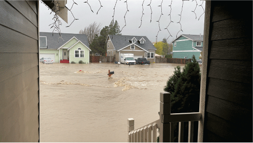
Photograph showing flooding in a neighborhood in Sumas, Washington, shortly after noon on November 15, 2021. Photograph by Desiree Daniels, used with permission.
Table 4.
Reference points used in the text.[Distance in river kilometers (km) and miles (mi) from the landslide source area (between Sherman Peak and Roman Wall; fig. 1) and the reference point (RP). Distance was estimated using Google Earth mapping tools with measurements rounded up. General topography describes the reach between reference points or confluences pertinent to this report. Locations are the precise reference point in Universal Transverse Mercator (UTM), zone 10, coordinates to correspond with map designations (see appendix 1 for locations in latitude and longitude). All communities are in the State of Washington, United States, except Abbotsford, which is in British Columbia, Canada. —, no nearby community; B.C., British Columbia]
Discharge Calculations
We calculated discharge at RP-4 and RP-11 (fig. 1) as they are near USGS gaging stations. Reference point 4 is at a constriction in the Middle Fork Nooksack River about 2 river kilometers upstream from the MF Nooksack River near Deming, WA, gaging station (USGS streamgage station no. 12208000; USGS, 2016), and RP-11 is about 300 m upstream from the Nooksack River at North Cedarville gaging station (USGS streamgage station no. 12210700; USGS, 2016). The gage at North Cedarville replaced one that was at Deming from about 1908 to 2005.
Discharges from D-Claw simulations were calculated by integrating the flow depth (m) and velocity (in meters per second [m/s]) through transects that span the channel at RP-4 and RP-11 yielding the total discharge (m3/s). In all cases, the initial discharge or volume flux is zero because the model does not account for existing river flow. At RP-4, we used the river surface for the base because we did not have actual topography to use, whereas at RP-11, actual river topography was used.
We did not calculate discharge for the two smallest-volume scenarios (1 and 10 Mm3) because the smallest volume did not reach RP-4, and neither reached RP-11.
Arrival Times Using an Empirical Methodology
Arrival times can be directly pulled from the D-Claw simulations, but not all volcanoes or drainages on volcanoes that have lahar hazards have D-Claw simulations. Thus, we use this opportunity to compare D-Claw simulation arrival times for the three largest lahars with those calculated using an empirical methodology (Pierson, 1998). Pierson (1998) gathered worldwide data for historical volcanic debris avalanches, debris flows, and lahars where there was either a direct or indirect measurement of peak flow rates or total flow volume. He concluded that travel times could be estimated as a function of distance from source when the approximate peak discharge near source could be estimated. Based on peak discharge, the data were binned into four categories—extremely large (greater than 1,000,000 m3/s), very large (10,000–1,000,000 m3/s), large (1,000–10,000 m3/s), and moderate (100–1,000 m3/s)—with each category defining distinct regression curves for estimating travel time at a given distance from source.
If only the total volume of a mass flow is known, Pierson (1998) used a method by Mizuyama and others (1992) to relate peak discharge to the fully bulked flow volume. Mizuyama and others (1992) noted that clay-poor (which they termed granular flows) and clay-rich flows have parallel but slightly different regression lines. For a similar volume, peak discharges from clay-poor flows are slightly to moderately greater than for clay-rich flows. Because we wanted to compare D-Claw arrival times with the empirical arrival times, we followed the empirical methodology throughout our calculations. As we have no data (other than from the D-Claw simulations) for approximate peak discharges near source, we used the relationship of Mizuyama and others (1992) to calculate peak discharge values for our scenarios. We used the clay-rich flow regression line because Scott and others (2020) showed that the Schriebers Meadow, Middle Fork, and Ridley Creek lahars all had matrix clay contents of about 10 percent by weight.
Using Pierson’s (1998) empirical methodology, the three largest volumes fall within the very large mass flow category and therefore use the same regression curve to calculate arrival times. We also calculated arrival times using the regression curve for the next smaller category (large mass flows) and the regression curve for the next larger category (extremely large mass flows) (table 5). We did not attempt to estimate an arrival time for that portion of the lahars that move upriver in the North Fork Nooksack (RP-7) and South Fork Nooksack (RP-9) Rivers because the flow dynamics of moving upriver may be quite different than those for moving downriver. However, we did use the empirical model to estimate arrival times for RP-14, RP-15, RP-16, and RP-17, even though in the D-Claw scenarios, the lahar bifurcates once flow is deep enough to top the levee at Everson (RP-13). How bifurcation may affect arrival times using the empirical model is unknown.
Uncertainty
Models are simplifications of complex processes. In D-Claw, we estimate a few initial material parameters (table 3) and analyze how flow properties—inundation area, runout, flow depth, speed, and discharge—change as a lahar moves down valley. An advantage of D-Claw is that most of those properties can be extracted directly from the output results, although discharge has to be calculated. The accuracy of the data output, however, is difficult to quantify.
D-Claw scenario results have been tested against recent landslide events that have transformed into debris flows (for example, the 2010 Mount Meager landslide, in British Columbia, Canada [Guthrie and others, 2012], and the 2014 Oso [SR 530] landslide in Washington State [Iverson and others, 2015; Iverson and George, 2016]) with comparable results. D-Claw simulations also compare reasonably well with the empirical runout and inundation area model LAHARZ (Iverson and others, 1998; Schilling, 1998) and with empirical arrival times (Pierson, 1998) as we will discuss below. Large lahars, however, are relatively rare, so there has been no comparison of D-Claw results with recent volcanic events. At Mount Rainier, where there is good geologic information on prehistoric lahar deposits and runout distances, D-Claw simulations using estimated lahar volumes compared favorably with known geologic deposits (George and others, 2022). However, even with reasonable comparisons, the uncertainties involved are such that D-Claw results are most appropriate for broad decision-making purposes and are not suitable for extrapolation to street-level boundaries or fine-scale (minutes to tens of minutes) travel times.
General Results
Officials responsible for planning for, or responding to, a lahar event need answers to several questions: What communities and infrastructure will be affected? When will the lahar arrive? How deep will it be? When will it end? Although we do not know how big the next lahar will be, the range in D-Claw scenario volumes can provide important information for considering these questions. We will discuss these questions in general terms first before looking more thoroughly at specific scenarios.
Lahar Runout Distance and Inundation Area
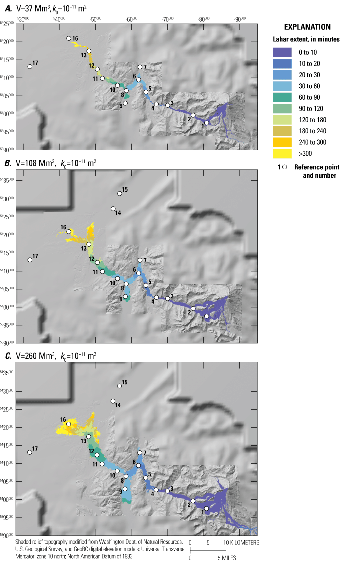
We first compare lahar runout and inundation results (fig. 3) for the three largest lahar volumes (260, 108, and 37 Mm3) at an initial hydraulic permeability of 10−11 m2 (scenarios A2, B2, and C2; table 1). Not surprisingly, inundation area, and to a lesser degree runout distance, scale with volume (in other words, the larger the volume the more area inundated and the farther the lahar travels). Comparison of just the two largest-volume events at initial hydraulic permeabilities of 10−10 m2 (scenarios A1 and B1) and 10−12 m2 (scenarios A3 and B3) show inundation area and, to a lesser degree, run out distance again scaling with volume (fig. 4).
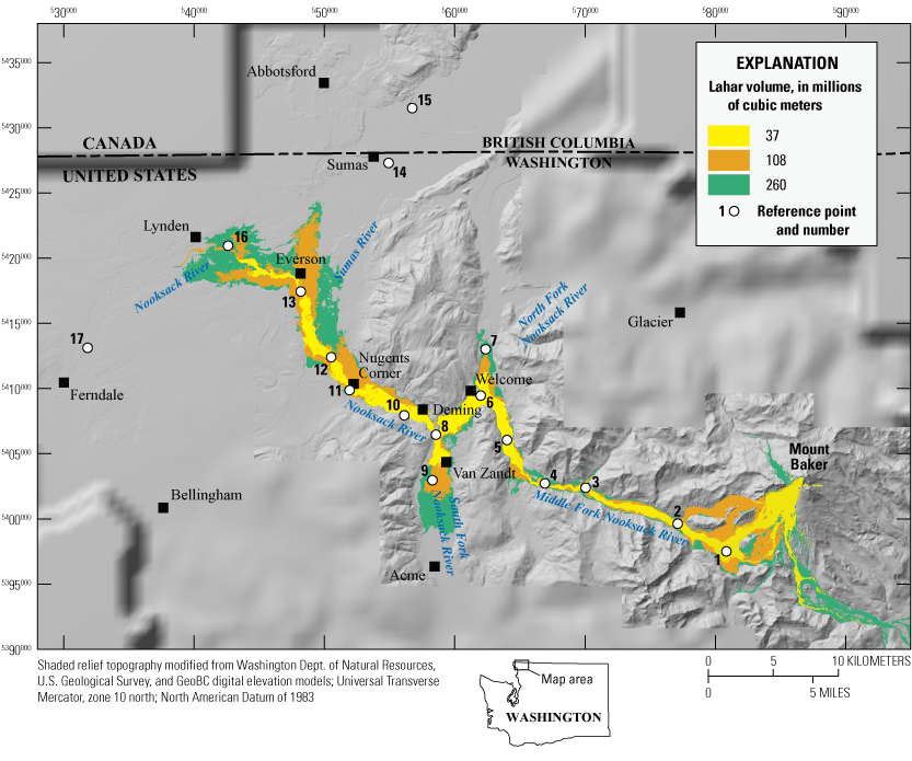
Map showing the comparison of D-Claw model runout distances and inundation areas for the three largest volume events with initial hydraulic permeability (k0) of 10−11 square meters (m2).
![Maps showing comparisons of D-Claw model runout distances and inundation areas for
the two largest-volume events, 108 and 260 million cubic meters, at differing initial
hydraulic permeabilities (k0, in square meters [m2]). A, Model of lahar runout distances with k0=10−10 m2 (scenarios A1, B1). B, Model of lahar runout distances with k0=10−12 m2 (scenarios A3, B3).](https://pubs.usgs.gov/sir/2024/5133/images/sir20245133_fig04.png)
Maps showing comparisons of D-Claw model runout distances and inundation areas for the two largest-volume events, 108 and 260 million cubic meters, at differing initial hydraulic permeabilities (k0, in square meters [m2]). A, Model of lahar runout distances with k0=10−10 m2 (scenarios A1, B1). B, Model of lahar runout distances with k0=10−12 m2 (scenarios A3, B3).
Although volume does not have a profound effect on runout distance (fig. 3), initial hydraulic permeability (k0) does (figs. 4, 5). For example, a lahar with a volume of 260 Mm3 and k0=10−10 m2 (largest hydraulic permeability; scenario A1) barely reaches Deming (near RP-10; figs. 4A, 5B), whereas a lahar of the same volume but k0=10−12 m2 (smallest hydraulic permeability; scenario A3) reaches well into Canada (beyond RP-14 and RP-15; figs. 4B, 5B). In scenarios A3 and B3 (figs. 4B, 5; table 1), the lahar bifurcates at Everson (RP-13) with some of the lahar flowing northward into the Sumas River valley toward Sumas, Wash., and Abbotsford, British Columbia, Canada (RP-14, RP-15), and some of the lahar flowing westward down the Nooksack River valley past the City of Lynden, Wash. (RP-16).
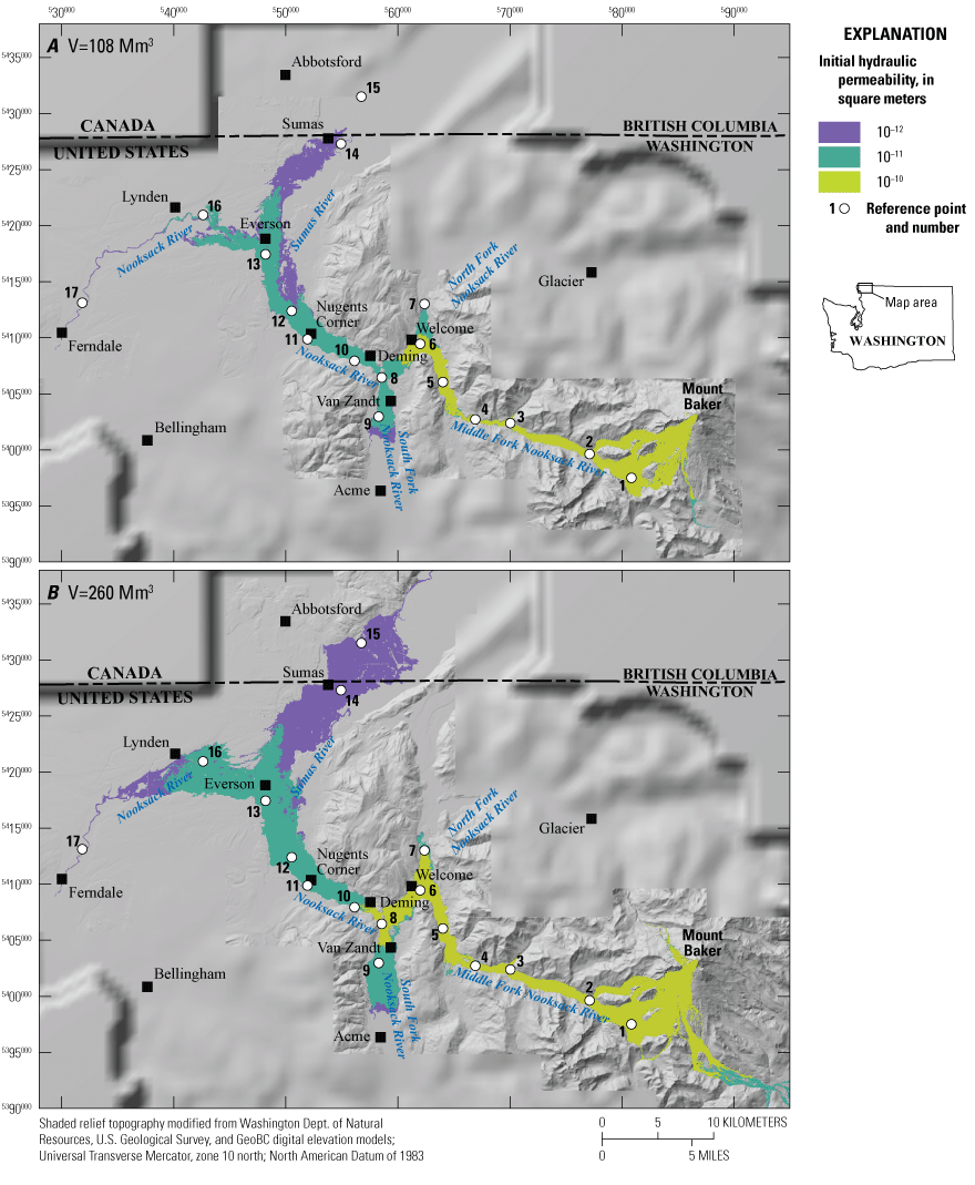
Maps showing how initial hydraulic permeability affects runout distance and inundation area. A, D-Claw model results using a volume of 108 million cubic meters (Mm3) and three different initial hydraulic permeabilities (k0=10−10, 10−11, 10−12 m2; scenarios B1, B2, B3). B, D-Claw model results using a volume of 260 Mm3 and three different initial hydraulic permeabilities (k0=10−10, 10−11, 10−12 m2; scenarios A1, A2, A3).
Lahar Speed and Arrival Times
Velocity varies throughout a moving lahar. Because not all the mass of a lahar is at a single point, a lahar has a flow front and some length of material behind it, which we will call the flow tail (fig. 6). As a lahar encounters an object or ceases to move, the velocity at the flow front may decrease while the tail continues to move down valley. This will cause the lahar depth to increase at the flow front and for some distance upstream (fig. 6A). In some cases, the lahar may reach a depth that causes the stalled front to overtop an object or resume forward movement resulting in a decrease of flow depth at the flow front and thinning upstream (fig. 6B).
Speed determines how quickly a lahar will reach a certain point (lahar arrival time) and to a degree its destructive potential. With all else being equal, faster-moving lahars will exert more force on objects and are more erosive than slower-moving ones. In most scenarios (tables 6, 7, 8 appendix 2), lahar flow speed is generally greatest when the flow first passes by a reference point, with two general exceptions. At RP-2 and RP-5, maximum lahar speeds coincide with maximum lahar depths, rather than with arrival time. At RP-2, this delay in timing is likely caused by material sloshing up the south canyon wall at RP-1 (appendix 4). At RP-5, it is likely due to the lahar exiting the narrow bedrock canyon (RP-4).
Within 25 km of the source (RP-1 to RP-4; fig. 1), arrival times for the two largest-volume lahars vary little with either volume or initial hydraulic permeability (fig. 7), whereas the arrival time for the 37 Mm3 volume lags moderately behind them (table 5). Arrival times for the two largest volumes begin to diverge from each other at intermediate distances of greater than 25 to 50 km (RP-5 to RP-11), and then more substantially at distances greater than 50 km (RP-12 to RP-17). Arrival times for flows of similar volume but differing hydraulic permeability (fig. 8; table 5) are similar at proximal and intermediate distance (scenarios with an initial hydraulic permeability of 10−10 begin to lag just before they stall) and only diverge considerably at the most distal reaches (greater than 60 km; table 5). These comparisons indicate that all other factors being equal, the larger the volume the faster the flow and therefore the earlier the arrival times.
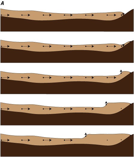
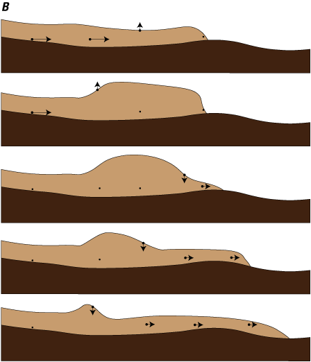
Diagrams showing flow vectors as a lahar stalls, which often occurs behind obstacles or uphill slopes. The lahar (light brown) is moving from left to right over the topography (dark brown). Arrows depict direction of flow, and the length corresponds to speed. Dots without arrows indicate when movement stops, and the speed is zero. A, The lahar encounters a topographic barrier that it cannot overtop. The flow front stalls and incoming material from upstream (the tail) accumulates behind the stalled front, causing a deepening of lahar material that progressively moves upriver (to the left). B, The flow front stalls behind a topographic barrier. As incoming material accumulates behind the flow front, the flow front deepens, which contributes additional driving forces on the front, allowing it to overtop the barrier. As the flow front moves forward there is a shallowing of material that moves upstream. These flow phenomena can generate observable waves of changing lahar depth moving upriver, even though the flow material itself does not reverse direction or travel upriver.
Lahar arrival times for three different volumes (V) but the same initial hydraulic permeability (k0) of 10−11 square meters (m2). A, Scenario C2, 37 million cubic meters (Mm3). B, Scenario B2, 108 Mm3. C, Scenario A2, 260 Mm3. Note that the lahar extent-interval scale changes as the lahar gets farther from source and the river gradient decreases. The change qualitatively reflects our confidence in the arrival times (shorter intervals reflect higher confidence, longer intervals reflect lower confidence).
![Lahar arrival times for a volume (V) of 260 million cubic meters (Mm3) at varying initial hydraulic permeabilities (k0; in square meters [m2]). A, Scenario A1, k0=10−10 m2. B, Scenario A2, k0=10−11 m2. C, Scenario A3, k0=10−12 m2. Note that the lahar extent-interval scale changes as the lahar gets farther from
source and the river gradient decreases. The change qualitatively reflects our confidence
in the arrival times (shorter intervals reflect higher confidence, longer intervals
reflect lower confidence).](https://pubs.usgs.gov/sir/2024/5133/images/sir20245133_fig08.png)
Lahar arrival times for a volume (V) of 260 million cubic meters (Mm3) at varying initial hydraulic permeabilities (k0; in square meters [m2]). A, Scenario A1, k0=10−10 m2. B, Scenario A2, k0=10−11 m2. C, Scenario A3, k0=10−12 m2. Note that the lahar extent-interval scale changes as the lahar gets farther from source and the river gradient decreases. The change qualitatively reflects our confidence in the arrival times (shorter intervals reflect higher confidence, longer intervals reflect lower confidence).
Table 5.
Comparison of D-Claw model arrival times with the empirical model of Pierson (1998).[D-Claw arrival times at reference points (RP) are pulled directly from scenario model outputs. The appropriate regression curve for the three largest volumes regardless of initial hydraulic permeability is that for the very large mass flow bin of Pierson (1998). However, we also calculated arrival times using the regression curves for extremely large (next larger bin) and large (next smaller bin) mass flows. hh:mm, hours, minutes; km, kilometer; mi, mile; Mm3, million cubic meters; —, indicates no data because the lahar did not reach this reference point]
Lahar Flow Depth
Flow depth determines who and what may be at risk during passage of a lahar. It is important to note that flow depth (depth of the flowing water and sediment mixture) and deposit thickness (thickness of the remaining sediment layer covering the landscape after the event is over) are different concepts. A photograph taken after the May 18, 1980, eruption of Mount St. Helens of a man standing on the North Fork lahar deposit below mudlines on trees illustrates this difference well (fig. 9). Another difference between these two concepts is that flow depth is essentially instantaneous, whereas deposit thickness results from progressive accumulation of material as the flow passes by an area.
In the D-Claw simulations, the flow depth for a given reference point at the end of a simulation is a proxy for lahar deposit thickness.
![Photograph of mud lines from the May 18, 1980, Mount St. Helens North Fork Toutle
River lahar. A man (about 2 m [6 feet] tall) is standing on lahar deposit looking
at the mudline on trees indicative of the peak flow depth when the lahar passed by
the area. Photograph by Lyn Topinka, U.S. Geological Survey.](https://pubs.usgs.gov/sir/2024/5133/images/sir20245133_fig09.png)
Photograph of mud lines from the May 18, 1980, Mount St. Helens North Fork Toutle River lahar. A man (about 2 m [6 feet] tall) is standing on lahar deposit looking at the mudline on trees indicative of the peak flow depth when the lahar passed by the area. Photograph by Lyn Topinka, U.S. Geological Survey.
At a given location, lahar flow depths vary through time, as can readily be seen on hydrographs (fig. 10, appendix 3). For example, the hydrograph (fig. 10E) for scenario A2 (260 Mm3, k0=10−11 m2) at RP-4 shows the lahar arriving about 9 minutes (tables 5 and 6) after landslide initiation with a flow depth of about 64 m. The depth increases rapidly until it reaches its maximum depth of about 125 m, 5 minutes after arrival. As the lahar moves downstream, lahar flow depth at RP-4 diminishes quickly to about 5 meters at 60 minutes after landslide initiation, and to less than 2 meters at 80 minutes after initiation. By 155 minutes after landslide initiation, all flow past RP-4 effectively has ceased (fig. 10E; table 6). For the same lahar, the flow front reaches RP-16 (near Lynden, Wash.; figs. 1, 10E) about 6 hours (352 minutes) after landslide initiation. By this time, the flow front speed has slowed down substantially compared to previous values (table 6). Flow depth at RP-16 increases over the next hour until it reaches its maximum depth of slightly over 5 m and remains at that depth for the remainder of the simulation. The animation for this scenario (appendix 4, scenario A2) shows the lahar flow front beginning to stall as it reaches RP-16. As the flow front ceases to move forward, material from the tail keeps moving forward increasing the depth (see fig. 6A) until all flow movement ceases after about 12 hours.
In proximal and more confined areas (RP-1 to RP-12), lahar arrival times and maximum flow depths often occur within minutes or tens of minutes of each other (see tables 6, 7, 8; appendixes 2, 4). In more distal and broader valley areas (RP-13 to RP-17), however, the time interval between lahar arrival time and maximum flow depth is often longer, sometimes lagging by more than an hour. As the lahar moves into broad valley reaches, it becomes shallower and wider and therefore encounters more frictional resistance. The frictional resistance contributes to slowing and eventually stalling the flow front, allowing time for the lahar tail to contribute to the overall flow front depth (fig. 6A).
![Plots showing D-Claw model hydrographs of the two largest lahar volumes (V) and each
initial hydraulic permeability (k0) for the reference points (RP) in this study. A, Scenario B1, 108 million cubic meters (Mm3) and k0=10−10 m2. B, Scenario B2, 108 Mm3 and k0=10−11 m2. C, Scenario B3, 108 Mm3 and k0=10−12 m2. D, Scenario A1, 260 Mm3 and k0=10−10 m2. E, Scenario A2, 260 Mm3 and k0=10−11 m2. F, Scenario A3, 260 Mm3 and k0=10−12 m2. Note that in the left panels with reference points 1–4, the time scales from 0 to
240 minutes, whereas for reference points 5–17, the time scales 0 to 880 minutes.
Some lines, however, end before 880 minutes depending on total simulation time (only
the simulations with initial hydraulic permeabilities of 10−12 ran for more than 12 hours [880 minutes] as most other simulations had stopped before
that time). The flow depth at the end of a simulation indicates deposit thickness
(for example in A, reference point 5 shows a peak flow depth of 20 meters, the simulations stopping
at 480 minutes, and the deposit thickness at 480 minutes of a little more than 5 meters).
Time listed with each reference point indicates the arrival time in minutes at that
reference point.](https://pubs.usgs.gov/sir/2024/5133/images/sir20245133_fig10ac.png)
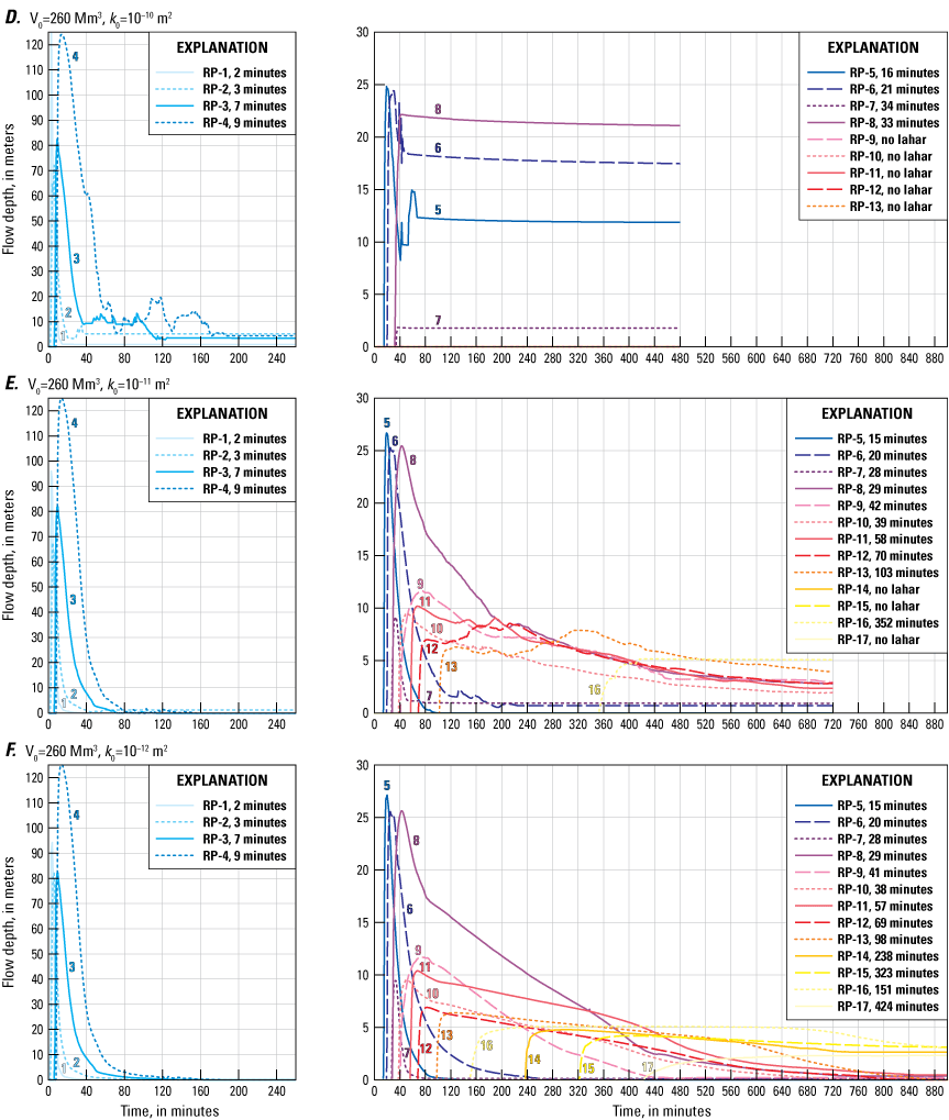
Plots showing D-Claw model hydrographs of the two largest lahar volumes (V) and each initial hydraulic permeability (k0) for the reference points (RP) in this study. A, Scenario B1, 108 million cubic meters (Mm3) and k0=10−10 m2. B, Scenario B2, 108 Mm3 and k0=10−11 m2. C, Scenario B3, 108 Mm3 and k0=10−12 m2. D, Scenario A1, 260 Mm3 and k0=10−10 m2. E, Scenario A2, 260 Mm3 and k0=10−11 m2. F, Scenario A3, 260 Mm3 and k0=10−12 m2. Note that in the left panels with reference points 1–4, the time scales from 0 to 240 minutes, whereas for reference points 5–17, the time scales 0 to 880 minutes. Some lines, however, end before 880 minutes depending on total simulation time (only the simulations with initial hydraulic permeabilities of 10−12 ran for more than 12 hours [880 minutes] as most other simulations had stopped before that time). The flow depth at the end of a simulation indicates deposit thickness (for example in A, reference point 5 shows a peak flow depth of 20 meters, the simulations stopping at 480 minutes, and the deposit thickness at 480 minutes of a little more than 5 meters). Time listed with each reference point indicates the arrival time in minutes at that reference point.
Table 6.
Lahar arrival, maximum flow depth, and lahar cessation for scenario A2 (260 million cubic meters and initial hydraulic permeability [k0] of 10−11 m2).[Lahar arrival is the arrival time, depth, speed, and percent solid fraction of the lahar when it first reaches a given reference point (RP). Maximum lahar depth shows the time, depth, speed, and percent solid fraction of the lahar at time of maximum lahar depth. Lahar stops (or end of simulation) shows the time and depth when the lahar ceases to move any more material past a given reference point. The simulation time for this scenario was 12 hours. Note that maximum depths may have 0 speed indicating that the lahar had stalled (ceased moving forward) at that time. Also, lahar depth at arrival may be 0 because of the depth is too small to round up to a significant figure. hh:mm, hours:minutes; m, meters; m/s, meters per second; —, indicates no data because the lahar did not reach this reference point]
Regardless of volume or hydraulic permeability (tables 6, 7, 8; fig. 10; appendixes 2, 3), the greatest flow depth in all simulations occurs at RP-4, where the Middle Fork Nooksack River is narrowly constricted in a bedrock canyon. The maximum flow depth for the two largest volume events—about 125 m for 260 Mm3 and 100 m for 108 Mm3—is similar regardless of hydraulic permeability (fig. 10), which reflects the narrowness of the canyon and proximity to source.
In the steep upper reaches of the Middle Fork Nooksack River (RP-1 to RP-4), flow depths for the largest three volumes diminish quickly, usually within an hour after passing a given reference point (fig. 10; tables 6, 7, 8; appendixes 2, 3). In the more mobile scenarios, k0=10−11 m2 and 10−12 m2 (fig. 10B, C, E, F), the entire lahar passes these upper reaches and deposits little to no sediment (scenario flow depths return to zero). In the less mobile scenarios, k0=10−10 m2 (fig. 10A, D), decrease in pore pressure increases frictional resistance leading to cessation of flow and deposition of material (scenario flow depths remain above zero).
Where topography is less steep (RP-5 to RP-17; fig. 10), lahar flow depths often do not return to zero, but are generally maintained at a meter or more hours after the lahar has passed. In some cases, this may reflect that the scenario run time was not long enough, but in most cases, it reflects deposition of sediment. Many scenarios show little deposition in the steeper reaches close to the volcano and greater deposition in low-gradient areas farther down river (see RP-13 to RP-17; fig. 10B, C, E, and F).
Lahar Discharge Measurements
Discharge data at RP-4 and RP-11 were calculated for the three largest lahar volumes (37, 108, and 260 Mm3) and for the two largest volumes at varying initial hydraulic permeabilities (figs. 11, 12). In general, discharge scales with volume (the greater the volume, the higher the discharge) and less so with initial hydraulic permeability (although, in general, the greater the initial hydraulic permeability, the lower the discharge). Discharge climbs rapidly as the lahar reaches a given reference point and falls more slowly (due to deposition of material) after peak discharge is reached. For a given volume, peak discharges are an order of magnitude greater at transect 4 (near RP-4) than at transect 11 (near RP-11) (figs. 11, 12). For flows with an initial hydraulic permeability of 10-−10, the discharge decay curves at both RP-4 and RP-11 do not decay smoothly, reflecting feedback mechanisms as the flow front begins to stall.
![Discharge (volume flux, in cubic meters per second) at transect 4 (near RP-4) through
time. Graph is shown in 0.2-hour increments up to 1 hour after landslide failure for
select volumes (V, in millions of cubic meters [Mm3]) and initial hydraulic permeabilities (k0, in square meters [m2]). Each dot is a data point.](https://pubs.usgs.gov/sir/2024/5133/images/sir20245133_fig11.png)
Discharge (volume flux, in cubic meters per second) at transect 4 (near RP-4) through time. Graph is shown in 0.2-hour increments up to 1 hour after landslide failure for select volumes (V, in millions of cubic meters [Mm3]) and initial hydraulic permeabilities (k0, in square meters [m2]). Each dot is a data point.
![Discharge (volume flux, in cubic meters per second) at transect 11 (near RP-11) through
time. Graph is shown in hour increments up to 12 hours after landslide failure for
select volumes (V, in millions of cubic meters [Mm3]) and initial hydraulic permeabilities (k0, in square meters [m2]). Each dot is a data point.](https://pubs.usgs.gov/sir/2024/5133/images/sir20245133_fig12.png)
Discharge (volume flux, in cubic meters per second) at transect 11 (near RP-11) through time. Graph is shown in hour increments up to 12 hours after landslide failure for select volumes (V, in millions of cubic meters [Mm3]) and initial hydraulic permeabilities (k0, in square meters [m2]). Each dot is a data point.
Specific Scenarios
We focus here on end member simulations of the two largest-volume lahars, scenario B1 (108 Mm3, k0=10−10 m2), the smallest and least mobile of the two, and scenario A3 (260 Mm3, k0=10−12 m2), the largest and most mobile lahar modeled. Understanding these end members helps one to better interpret scenarios that lie between them.
Scenario B1. Landslide Volume of 108 Mm3 and Initial Hydraulic Permeability (k0) of 10−10 m2
We first consider scenario B1 (table 7), whose volume approximates the current amount of altered rock around Sherman Crater (Finn and others, 2018) and is slightly smaller than the estimated volume of the Ridley Creek lahar (6.7 ka; 150 Mm3; Scott and others, 2020). The initial hydraulic permeability of 10−10 m2 is the largest we considered and results in lower mobility flows; under this initial hydraulic permeability, pore pressure decreases rapidly, increasing friction that ultimately stops movement.
As in all our scenarios, within seconds of failure, the saturated landslide mass becomes fluidized and moves downslope as a lahar (appendix 4, scenario B1). A small portion of the lahar overtops ridges to the north and south of the canyon below Deming Glacier (figs. 1, 13A). It takes less than two minutes for the lahar to reach RP-1 at the base of the volcano (table 7). When the flow reaches RP-1, it slams into the opposing valley wall (south valley wall of the Middle Fork Nooksack River) in several pulses, some that briefly reach depths of more than 50 m, before moving down valley (appendix 4, scenario B1). The lahar arrives at RP-1 traveling approximately 50 m/s (about 180 kilometers per hour [km/h]) and is 17 meters deep (table 7). Depth quickly increases to 56 m as material from several pulses coalesce. Three minutes after landslide initiation, the lahar reaches RP-2, by which time it has slowed considerably to 29 m/s (104 km/h) with an initial depth of about 4 meters. Two minutes later (5 minutes after initiation), the maximum flow depth at RP-2 is 60 m, and flow speed has increased to 34 m/s (122 km/h). After about 100 minutes, lahar material is no longer moving past RP-2 (fig. 10A; table 7).
Table 7.
Lahar arrival, maximum flow depth and lahar cessation for scenario B1 (108 million cubic meters, initial hydraulic permeability [k0] of 10−10 m2).[Lahar arrival is the arrival time, depth, speed, and percent solid fraction of the lahar when it first reaches a given reference point (RP). Maximum lahar depth shows the time, depth, speed, and percent solid fraction of the lahar at time of maximum lahar depth. Lahar stops (or end of simulation) shows the time and depth when the lahar ceases to move any more material past a given reference point. The simulation time for this scenario was 8 hours. Note that maximum depths may have 0 speed indicating that the lahar had stalled (ceased moving forward) at that time. hh:mm, hours:minutes; m, meters; m/s, meters per second]
Panels showing D-Claw lahar extent, inundation, and flow depths for scenario B1 at select time intervals. Volume is 108 million cubic meters (Mm3) with an initial hydraulic permeability (k0) of 10−10 square meters (m2). Simulation time (t) is in hh:mm:ss. A, 2 minutes. B, 18 minutes. C, 30 minutes. D, 1 hour. E, 3 hours. F, 8 hours.
Between RP-2 and RP-3, the valley broadens with a corresponding decrease in lahar speed (table 7). It speeds up again as the lahar reaches RP-4 where the river valley is entrenched in a narrow bedrock canyon. At RP-4, the lahar reaches a maximum depth of almost 95 m (figs. 10A, 13B), about 18 minutes after landslide initiation (figs. 10A, 13B).
As the lahar leaves the bedrock canyon, the valley broadens and becomes less steep, which allows the lahar to spread out, diminishing both flow-front depth and speed (table 7). The lahar flow front, which had traversed the first 25 km in slightly more than 10 minutes, takes 18 minutes to traverse the remaining10 km between RP-4 and RP-6. Twenty-nine minutes after initiation, the lahar reaches RP-6 (figs. 10A, 13C; table 7), and the flow front stalls seven minutes later.
As the lahar flow front stalls, material from the tail increases lahar depth at the flow front as well as upstream (figs. 6, 10A, and 13C, D; appendix 4, scenario B1). At RP-5 (30 km from source), initial flow depth is 10 m, but the maximum flow depth of about 20 m occurs about 25 minutes later (45 minutes after landslide initiation; table 7). Between one and three hours after initiation, pore pressure at the flow front increases enough for the flow to advance slightly (fig. 6B) over the next several hours (figs. 13D, E; appendix 4, scenario B1). Movement ceases by eight hours after initiation with resultant deposit thicknesses between RP-4 and RP-6 of 5 to 12 meters. Upstream from RP-5, deposit thicknesses are between 1 and 5 meters (figs. 10A, 13F).
Scenario A3: Landslide Volume of 260 Mm3 and Initial Hydraulic Permeability of 10−12 m2
Scenario A3 (260 Mm3, k0=10−12) simulates the largest and most mobile lahar; thus, it is the most extreme scenario that we modeled. Initial landslide volume is based on the estimated bulked volume of the Middle Fork lahar, the largest known lahar in Mount Baker’s post-glacial history.
There are many similarities in flow dynamics between scenarios A3 and B1 for the first 35 km of travel as well as some important differences. Although generally similar overall, scenario A3 speeds are slightly higher (tables 7, 8), the flow inundates more area between RP-4 and RP-5 (figs. 13D 14A), and flow depth decays more quickly and regularly (figs. 10A, F). In scenario A3, the lahar reaches RP-6 at the mouth of the Middle Fork Nooksack River twenty minutes after landslide initiation (table 8; figs. 10F, 14A) with a depth of 4.4 m—a little more than half the initial depth in scenario B1, but its arrival speed of 13.2 m/s (47.5 km/h; tables 5, 8) is almost five times greater than that of scenario B1 (2.9 m/s; 10.4 km/h; table 7). The maximum lahar depth of 25.6 m at RP-6 is slightly more than double that in scenario B1 (12.2 m), but depth decays more quickly (figs. 10A, F) as the flow front moves both down and up the North Fork Nooksack River. In scenario A3, the lahar at RP-6 is less than 3-m deep two hours after landslide initiation, whereas in scenario B1 it is still over 10-m deep two hours after initiation.
The distinctions noted above reflect both the differences in volume and initial hydraulic permeability. In scenario B1, having the larger initial hydraulic permeability, the lahar loses pore pressure more quickly, which increases friction and causes the lahar to stall soon after arrival at RP-6. In scenario A3, having the smaller initial hydraulic permeability, the lahar maintains sufficient pore pressure by RP-6 to keep it highly fluidized and moving down valley.
Table 8.
Lahar arrival, maximum flow depth, and lahar cessation for scenario A3 (260 million cubic meters and initial hydraulic permeability [k0] of 10−12 square meters).[Lahar arrival is the arrival time, depth, speed, and percent solid fraction of the lahar when it first reaches a given reference point (RP). Maximum lahar depth shows the time, depth, speed, and percent solid fraction of the lahar at time of maximum lahar depth. Lahar stops (or end of simulation) shows the time and depth when the lahar ceases to move any more material past a given reference point. The simulation time for this scenario was 15 hours. Note that maximum depths may have 0 speed indicating that the lahar had stalled (ceased moving forward) at that time. hh:mm, hours:minutes; m, meters; m/s, meters per second]
Panels showing D-Claw lahar extent, inundation, and flow depths for scenario A3 at select time intervals. Volume is 260 million cubic meters (Mm3) with an initial hydraulic permeability of 10−12 square meters (m2). Simulation time (t) is in hh:mm:ss. A, 20 minutes. B, 30 minutes. C, 1 hour. D, 2 hours.; E, 4 hours. F, 15 hours. White circles with numbers are reference points mentioned in text.
As the lahar enters the North Fork Nooksack River (RP-6), the flow hits the north valley wall (fig. 14B; appendix 4, scenario A3) and bifurcates with some flow moving upriver toward RP-7 and some down river toward RP-8 (fig. 14B). The upriver portion reaches RP-7—the farthest upriver reference point in the North Fork Nooksack River—and RP-8 at the confluence of the South Fork Nooksack and North Fork Nooksack Rivers about the same time (28 and 29 minutes, respectively; fig. 14B; table 8). At RP-7, the lahar reaches a maximum depth of 9.5 m about 33 minutes after landslide initiation. Flow depth at RP-7 decreases over the next 1.5 hours as the flow drains downriver leaving behind a deposit less than a meter thick (table 8; figs. 10F, 14C; appendix 4, scenario A3).
Although some of the flow moves up the North Fork Nooksack River, most of it moves downriver (southwestward). The lahar reaches the confluence with the South Fork Nooksack River (RP-8) 29 minutes after landslide initiation (table 8). Beyond this confluence, the river swings northwestward into a constricted bedrock reach and the name changes to the Nooksack River. This change in flow direction, coupled with narrowing of the river valley, causes the lahar to back up into the South Fork Nooksack River valley, which previously had been unaffected because no lahar material had spilled into the river’s headwaters. In the South Fork Nooksack River valley, the lahar moves upstream past RP-9 within an hour after landslide initiation and reaches a peak depth of nearly 12 m shortly thereafter (figs. 10F, 14C; table 8). As the lahar reaches R-9, 43 minutes after landslide initiation, flow depth at RP-8 has risen to more than 25 m and the flow front has passed Deming (RP-10) (fig. 10F).
The flow front reaches Deming, near RP-10, about 40 minutes after landslide initiation (fig. 10F) with an initial flow depth of only 0.3 m and speed of 3.9 m/s (14 km/h; table 8). These depths and speeds are considerably slower than the initial flow depth and speed at RP-8. However, flow depth at RP-10 builds quickly and reaches a maximum depth of 9.5 m less than 15 minutes later (fig. 10F). The flow reaches the mountain front near Nugents Corner (RP-11), within an hour after landslide initiation (fig. 14C; table 8). Both the initial and maximum flow depth are greater at RP-11 than at RP-10 because the river channel is narrower at RP-11. Between RP-10 and RP-11, the lahar fills the valley wall-to-wall with depths between 2 and 10 m (fig. 14C). As the lahar exits the mountain front onto the broad floodplain of the Nooksack River (RP-12), its speed slows substantially, and flow depth diminishes as well (fig. 10F; table 8).
Although the lahar slows considerably, it reaches Everson (RP-13) less than 2 hours after landslide initiation (table 8; figs. 10F, 14D). At 2 hours, flow depth near the mouth of the South Fork Nooksack River (RP-8) is about 12 m (figs. 10F, 14D). When the lahar initially reaches Everson, it is not deep enough to overtop the 2-m-high levee (appendix 4, scenario A3). Within 30 minutes, however, the flow is deep enough to overtop the levee, and the flow bifurcates with some material flowing northward into the Sumas River valley and the rest moving down the Nooksack River.
The northward flow reaches Sumas (RP-14) near the Canadian border about 4 hours after landslide initiation (figs. 10F, 14E; table 8). It takes another 90 minutes to reach RP-15 across the Canadian border as decreasing pore pressure and increasing friction slow the lahar considerably. Nonetheless, maximum flow depths at RP-14 and RP-15 range from 4- to 5-m deep (fig. 10F; table 8). After twelve hours, the flow is barely moving in the Sumas River valley, and after 15 hours flow ceases moving at RP-14 (fig. 14F; table 8).
The distances from source area to RP-14 in the Sumas River valley and to RP-16 along the Nooksack River valley are similar (table 4), but due to river gradients, the lahar reaches RP-16, near Lynden (figs. 10F, 14F; appendix 4, scenario A3), after 2.5 hours, almost 90 minutes before it reaches RP-14 (table 8). The lahar is initially confined to the Nooksack River channel, but within an hour after reaching RP-16, it broadens out and covers much of the floodplain (appendix 4, scenario A3). A shallow, mostly channel-confined lahar continues down valley and reaches RP-17, northeast of the City of Ferndale, Wash., a little over seven hours after landslide initiation (fig. 10F; table 8).
While the flow front moves downstream, the tail of the lahar also moves downstream (scenario A3, appendix 4). Lahar movement does not cease at RP-9 in the South Fork Nooksack River until more than 8 hours after lahar initiation (table 8). Very sluggish lahar movement continues at RP-8 and throughout the Nooksack and Sumas River valleys for more than 12 hours after event onset. Equally important is that when flow stops after 15 hours, deposits at RP-15, RP-16, and RP-17 are more than 2 meters deep (table 8; fig. 14F; appendix 4, scenario A3).
Discussion
Mount Baker has a rich history of lahars and debris flows affecting the Middle Fork Nooksack River drainage and beyond during the past 15,000 years. To help visualize potential future hazards, we use the physics-based D-Claw model to simulate lahars that start as water-saturated landslides and quickly transform to lahars. These simulations help understand flow dynamics through time as flows encounter changing topography and respond to changes in the granular-fluid mixtures. To check the veracity of our results, we compare D-Claw inundation, runout distances, and flow depths with geologic constraints. We also compare D-Claw inundation and runout distances with those from the empirical LAHARZ model (Iverson and others, 1998), and we compare D-Claw arrival times with those from an empirical methodology proposed by Pierson (1998). Lastly, we discuss how scenarios help address volcano hazard questions asked by responders tasked with community preparedness and protection.
How Well Do the D-Claw Scenarios Fit Geologic Constraints?
There are limited subaerial deposits of the Middle Fork and Ridley Creek lahars (the two largest post-glacial lahars) from which we can estimate flow depths (the deposits reflect a minimum flow depth), and they are largely restricted to the Middle Fork Nooksack River drainage. Subaerial deposits of the Middle Fork lahar show: 1) a minimum flow depth of about 65 m in the 350-m-wide channel upstream from Ridley Creek (near RP-1;Tucker and others, 2014); 2) a minimum flow depth of about 40 m in Clearwater Creek (near RP-3; Kovanen and others, 2001); 3) a minimum flow depth of more than 85 m in the less-than-200-m-wide canyon downstream from Clearwater Creek (RP-4; Hyde and Crandell, 1978); and 4) a minimum flow of depth of more than 5 m along the North Fork Nooksack River about 125 m downstream from the confluence with the Middle Fork Nooksack River (Tucker and others, 2014; Scott and others, 2020). Subaerial deposits of the Ridley Creek lahar show: 1) a minimum flow depth of 3 to 7 m along the Middle Fork Nooksack River between Ridley Creek (RP-1) and the confluence with Clearwater Creek (RP-3); and 2) a minimum flow depth of a little more than 2 m along the North Fork Nooksack River location noted in (4) of the previous list (Scott and others, 2020). Just downstream from the North Fork Nooksack and Middle Fork Nooksack River confluence (RP-6), mid-Holocene lahar deposits are buried beneath younger sediment and found only in well logs. Based on well-log data, Scott and others (2020) estimated that the mid-Holocene Middle Fork lahar deposit has a thickness of about 14 m near Nugents Corner (RP-11). And Cameron (1989) identified a several-meter-thick mid-Holocene log-rich unit (unit 3) in well logs in the Sumas River valley between RP-13 and RP-14, which she suggested could be a deposit from a lahar or debris flow from the Nooksack River valley and that Scott and others (2020) suggested may be from the Middle Fork lahar.
D-Claw simulations of the two largest volume lahars, 108 and 260 Mm3, show maximum flow depths at all initial hydraulic permeabilities are similar to, and in some cases exceed, depths based on deposit constraints along the Middle Fork Nooksack River. None of the smaller-volume (37, 10, and 1 Mm3) lahar scenarios, however, approach those constrained flow depths (see appendixes 2, 3).
None of the simulations have flow depths of 14 m near Nugents Corner (RP-11), which is the lahar-deposit thickness reported in well-log data (Scott and others, 2020). But deposit thickness represents sediment accumulation through time, whereas flow depth is an instantaneous parameter. Furthermore, the two largest-volume scenarios with k0=10−11 m2 and 10−12 m2 (scenarios A2, A3, B2, and B3) have maximum flow depths between 8.5 and 10.4 m at RP-11, which are consistent with the geologic observations at there. This is especially true if the buried deposits at Nugents Corner represent both the Ridley Creek and Middle Fork lahars or if that thickness includes both primary and secondary (post-initial lahar) deposits.
Only scenarios A3 (figs. 4B, 14E) and B3 (fig. 4A), which have the smallest initial hydraulic permeability (k0=10−12 m2), show extensive primary lahar flow in the Sumas River valley. As will be discussed in the next section, only the largest LAHARZ volume of 1,000 Mm3, which is an order of magnitude greater than the D-Claw scenario A and B volumes, replicates the flow path of the most mobile D-Claw scenario, scenario A3 (fig. 15). This difference in volumes raises alternative possibilities regarding the interpretation of unit C, the log-rich unit that lies above the purported Mount Mazama ash (7.6 ka), in the Sumas River valley (Cameron, 1989). If this unit represents the Middle Fork lahar deposit, then:1) is Scott and others’ (2020) estimated lahar volume too low; 2) did the Middle Fork lahar have an unusually low initial hydraulic permeability due to high clay content or some other material property; or, 3) did some other factor, such as high river flow, play a role in making the flow highly mobile? If unit C represents secondary remobilization (erosion and redeposition) of part of the Middle Fork lahar deposit, then is the flow volume estimated by Scott and others (2020) too high? We are currently unable to answer these questions.
Comparison of D-Claw and LAHARZ Runout Extent and Inundation Areas
Our D-Claw simulation volumes of 1, 10, 37, 108, and 260 Mm3 are similar to volumes commonly used in the empirical LAHARZ model (1, 3, 10, 30, 100, 300, and 1000 Mm3; Iverson and other 1998). Because the LAHARZ model does not allow flows to bifurcate, two LAHARZ simulations were constructed—one that forced flow westward down the Nooksack River valley (fig. 15A), and another that forced flow northward down the Sumas River valley (fig. 15B).
LAHARZ models showing runout distance and area inundated for lahar volumes of 1 to 1,000 million cubic meters. A, Flow forced westward down the Nooksack River. B, Flow forced northward down the Sumas River valley. Proximal hazard zone delineated by a height over length energy cone of 0.3.
We first compare D-Claw and LAHARZ runout distances and inundation areas for the three smaller-volume lahar scenarios (C2, D2, and E2; fig. 16). All three D-Claw scenarios have an initial hydraulic permeability of 10−11 m2 (fig. 16B). LAHARZ model results (fig. 16A) indicate that a 1 Mm3 lahar would stop about a kilometer downstream from RP-3, a 10 Mm3 lahar would stop just upstream from RP-6 and a 30 Mm3 lahar would flow slightly upstream on the South Fork Nooksack River and barely past Deming near RP-10. D-Claw model results show a lahar volume of 1 Mm3 (scenario E2) would not even reach RP-3, whereas the two larger-volume lahars 10 and 37 Mm3 (scenarios D2 and C2) would flow considerably beyond runout distances in the LAHARZ models (figs. 16B, 17). The LAHARZ inundation area is essentially valley wall to valley wall, whereas in the D-Claw simulations, distal inundation areas are more confined to the channel.
Comparisons of areas inundated and runout distances from LAHARZ and D-Claw models. A, LAHARZ model results. Height over length energy cone is 0.3 (delineates the proximal hazard zone) and volumes are 1, 10, and 30 million cubic meters. B, D-Claw model results for the three smallest volumes of 1, 10, and 37 million cubic meters using an initial hydraulic permeability (k0) of 10−11 square meters (scenarios E2, D2, and C2, respectively). The D-Claw model shows the total area inundated during the entirety of the simulations.
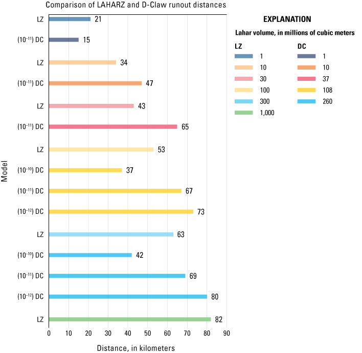
Graph comparing lahar runout distances of LAHARZ (LZ) and D-Claw (DC) models. Because lahar flow cannot bifurcate in the LAHARZ model, at 1,000 million cubic meters we show only the distance for the LAHARZ model in which most of the flow goes northward into the Sumas River valley (see fig. 15). The numbers next to the histogram lines are runout distances in kilometers. The numbers in parenthesis associated with the DC volumes indicate the initial hydraulic permeability (in square meters) used in those scenarios.
LAHARZ and D-Claw runout distances (fig. 17) and inundation areas for the three largest-volume D-Claw scenarios at initial hydraulic permeability of 10−11 m2 (scenarios A2, B2, and C2; fig. 18) are reasonably similar, although D-Claw scenarios show slightly greater runout distances (especially for scenario C1, which is volumetrically 20 percent greater than the LAHARZ volume) than the LAHARZ model. How much of the differences falls within uncertainty for the two models is unknown. However, when comparing LAHARZ and D-Claw model results for the two largest-volume lahars with initial hydraulic permeabilities of 10−10 m2 (scenarios A1 [260 Mm3] and B1 [108 Mm3]) and 10−12 m2 (scenarios A3 and B3) the results do not compare well (figs.17, 19). In scenarios A1 and B1, D-Claw runout distances are much less than LAHARZ runout distances and in scenarios A3 and B3, D-Claw runout distances and inundation areas are much greater (fig. 19).
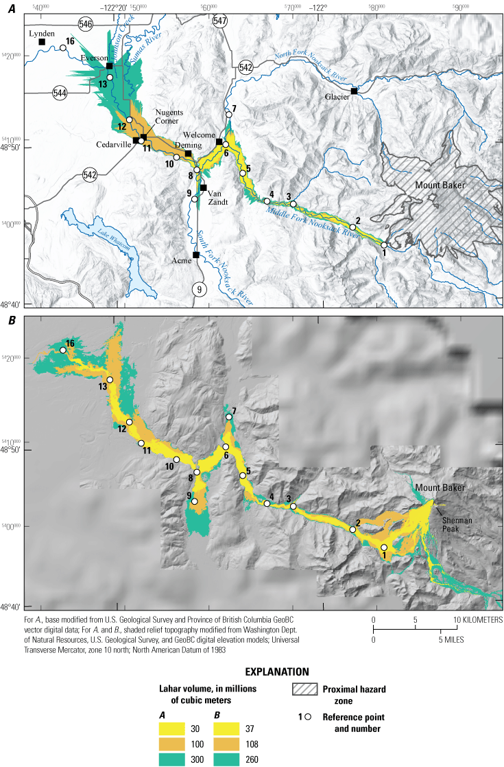
Comparisons of areas inundated and runout distances from LAHARZ and D-Claw models. A, LAHARZ model with height over length energy cone of 0.3 (delineates the proximal hazard zone) and lahar volumes 30, 100, and 300 million cubic meters. B, D-Claw model results for the three largest volumes, 37, 108, and 260 Mm3, using an initial hydraulic permeability (k0) of 10−11 square meters (scenarios C2, B2, and A2, respectively). The D-Claw model shows the total area inundated during the entirety of the simulations.
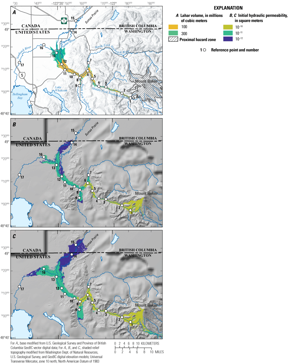
Comparisons of areas inundated and runout distances from LAHARZ and D-Claw models. A, LAHARZ model with most flow forced down the Sumas River valley. Height over length energy cone is 0.3 (delineates the proximal hazard zone), volumes are 100 and 300 Mm3. B, D-Claw model results for 108 Mm3, using initial hydraulic permeabilities (k0) of 10−10 square meters (m2), 10−11 m2, and 10−12 m2 (scenarios B1, B2, and B3, respectively). C, D-Claw model results for volume 260 Mm3 using k0=10−10 m2, k0=10−11 m2, and k0=10−12 m2 (scenarios A1, A2, and A3, respectively). The D-Claw model shows the total area inundated during the entirety of the simulations.
There are several reasons for the differences between the empirical LAHARZ and physics-based D-Claw scenario results. Primary among them is that the LAHARZ database is both relatively small and includes debris flows and lahars of various origins and material properties; thus, it averages diverse flow behaviors. Because D-Claw is a physics-based model, each simulation is unique to the model parameters of that simulation. Another is that in the LAHARZ model, the flow fills the cross-sectional and planimetric areas of the valley, then subtracts that volume until there is no more material left (Iverson and others, 1998). In the D-Claw simulations, the lahar flow front keeps moving (as does the flow tail) until frictional forces dissipate the momentum, and the flow front stops. Thus, material keeps moving throughout the simulation (see animations in appendix 4). Thus, in the D-Claw simulations, the flow dynamics and local topography determine the area inundated rather than just cross-sectional and planimetric areas. Also, in the LAHARZ scenarios, the source area for the lahar is assumed to be within the proximal hazard zone defined by where the energy cone (ratio of the vertical descent from the summit (H) divided by the horizontal runout (L) of events such as pyroclastic flows) intersect the topography (Iverson and others, 1998). For our LAHARZ construction we use a value of 0.3, which is at the upper end of the range (0.1 to 0.3) of values commonly used to specify proximal hazard zones (Hayashi and Self, 1992; Iverson and others, 1998) because that value encompasses most known pyroclastic-flow deposits from Mount Baker. Thus, in LAHARZ models the lahar starts at the base of the proximal zone, whereas in the D-Claw scenarios, the lahar starts at the source area and allows the model parameters and topography from source to determine flow length and area inundated. Lastly, the LAHARZ and D-Claw model volumes are slightly different.
The best fit between LAHARZ and D-Claw results is when D-Claw scenarios have an initial hydraulic permeability of k0=10−11 m2, which is also the best fit with the geologic data. In other words, the average of real-world examples fit better with simulations that use an initial hydraulic permeability of 10−11 m2 than those that use hydraulic permeabilities larger or smaller. In none of the D-Claw scenarios with k0=10−11 m2 did the lahar extensively inundate the Sumas River valley, although there is minor flow on the west side of the valley. Thus, a fundamental question remains as to how much the Sumas River valley is at risk during a future large lahar from Mount Baker.
Comparison of D-Claw Arrival Times with Empirical Methodology
Arrival times are important for those tasked with determining if, and when, people and livestock need to evacuate a given area. In the D-Claw scenarios, arrival times (tables 5, 6, 7, and 8; appendix 2) are extracted directly from model output. Due to the uncertainties regarding initial assumptions and the long computational times to run each scenario, we did not try to bracket the range of arrival times by changing material model parameters (other than hydraulic permeability) or to calculate error. However, we do bracket the arrival times of the empirical method (Pierson, 1998) as discussed in the methods section.
Because not every drainage on a volcano has or will have D-Claw simulation information, we use this opportunity to compare D-Claw arrival times with arrival times from the empirical model of Pierson (1998). Public officials have used the empirical arrival times from Pierson (1998) in communities around Mount Baker before the D-Claw simulations existed. D-Claw arrival times (table 5) for the three largest volumes (scenarios A1-3, B1-3, and C2) are generally faster than the very large mass flow empirical model times. From RP-2 to RP-8 (confluence of the North Fork and South Fork Nooksack Rivers, 40 km from source), D-Claw arrival times for the two largest volumes at all initial hydraulic permeabilities are much closer to the extremely large mass flow arrival times (table 5) than the very large mass flow arrival times and for the smaller volume, scenario C2, D-Claw arrival times are between those calculated for extremely large and very large mass flows (table 5). Thus, at these distances D-Claw arrival times may be faster than those calculated for very large mass flows by 30 minutes to more than an hour. Between RP-10 (Deming, 43 km from source) and RP-13 (Everson, 60 km from source), D-Claw arrival times for scenario C2 are similar to the very large mass flow arrival times; for scenarios B2 and B3, D-claw arrival times are between the extremely large and very large mass flow arrival times, and for the most voluminous and mobile scenarios, A2 and A3, D-claw arrival times also fall between the extremely large and very large mass flow arrival times but are closer to the extremely large mass flows. Beyond RP-13, however, D-Claw arrival times are similar to or slower than those of the very large mass flows (table 5). The slowing of the D-Claw lahar arrival times at far distances likely reflects the profound effect of lower gradient topography and broadening of the river valley on lahar dynamics, which may not be reflected as well in the database of the empirical model.
Overall, within 50 km from the source, D-Claw arrival times for the three-largest volumes (tables 5) are faster than the very large mass flow arrival times calculated from the empirical model (Pierson, 1998) and are more like those for extremely large mass flows. Extremely large mass flows of Pierson (1998) have peak discharges that are one to two orders of magnitude greater than those from the D-Claw simulations. Although we do not know the uncertainties associated with either model, the differences suggest that for clay rich, highly mobile lahars, the arrival times calculated using the empirical method may be too slow. Reasons for the discrepancy may be because—as was the case between the empirical model LAHARZ and the D-Claw model—the empirical travel-time model averages many types of flow behavior over many different landscape types whereas the D-Claw simulations are changing dynamically while flowing over actual topography. Other reasons may include that the empirical model database is small, and therefore does not adequately reflect average flow behavior, and that the initial D-C-Claw parameters may be a bit biased toward more mobile flows.
Comparison of D-Claw Discharge Measurements with River Flow Discharge Measurements
Peak discharge values for the three largest volumes at RP-4 and RP-11 range from 2,000 to 310,000 m3/s (70,600 to 10,950,000 ft3/s). Peak discharges at RP-4 near the MF Nooksack River near Deming, WA, streamgage (USGS streamgage station no. 12208000; USGS, 2016) for volumes of 260, 108, and 37 Mm3 with k0=10−11, are 310,000 m3/s (10,950,000 ft3/s), 125,000 m3/sec (4,415,000 ft3/s), and 40,000 m3/s (1,413,000 ft3/s), respectively. By RP-11 near the Nooksack River at North Cedarville streamgage (USGS streamgage station no. 12210700; USGS, 2016), peak discharges drop by an order of magnitude to 29,000 m3/s (1,025,000 ft3/s), 12,500 m3/s (441,000 ft3/s), and 2,000 m3/s (70,600 ft3/s), respectively. To put these numbers in perspective, the largest flood on record (since 1909) of the Nooksack River occurred on November 15, 2021, with a peak discharge at the Nooksack River at North Cedarville streamgage station (USGS streamgage station no. 12210700; near RP-11; USGS, 2016) of about 2,000 m3/s (70,600 ft3/s). The Middle Fork Nooksack River peak discharge for that day was 487 m3/s (17,200 ft3/s). Thus, even the relatively small-volume 37 Mm3 lahar has a peak discharge similar to that of the largest recorded historical flood on the Nooksack River.
At RP-4, peak discharges of the two largest volumes are the same order of magnitude as the average annual discharge of the Amazon River in South America (about 209,000 m3/s; 7,381,000 ft3/s; Latrubesse, 2008). And peak discharges of all three volumes dwarf the average annual discharge of Mississippi River, United States (about 18,400 m3/s; 651,000 ft3/s; Kammerer, 1990), the largest river in North America. Even by RP-11, the two largest volume lahar peak discharges are more than or slightly less than the average annual discharge of the Mississippi River. It must be noted, however, that we are comparing peak discharges, which are short lived events, with average annual discharges, which include a range of discharges smoothed over an annual timeframe.
Although these calculated D-Claw peak discharges are large, they are similar to peak discharges estimated for historical lahars worldwide (see tables 2 and 5 in Pierson, 1998, where the term debris flow is used for lahar). For example, the 1985 Azufrado lahar from Nevado del Ruiz volcano (Colombia) had an estimated peak discharge of 48,000 m3/s (1,695,100 ft3) 10 km from source; the 1980 South Fork Toutle River lahar from Mount St. Helens (United States) had an estimated peak discharge of 68,000 m3/s (2,400,000 ft3/s) 4 km from source; and the 1887 Rio Esmeraldas lahar from Cotapaxi Volcano (Ecuador) had an estimated peak discharge of about 200,000 m3/s (7,063,000 ft3/s) near the volcano (Pierson, 1998). All these values and those from Mount Baker, however, are dwarfed by estimated peak discharges of about 1,000,000 m3/s (35,300,000 ft3/s) for the 1980 Mount St. Helens debris avalanche at 18 km from source (Voight and others, 1983) and 12,400,000 m3/s (438,000,000 ft3/s) for the Osceola mudflow (Mount Rainier) 4 km from source (Vallance and Scott, 1997). The Osceola mudflow occurred about 5,600 years ago and was triggered by a massive debris avalanche (3.8 cubic kilometers [km3]; Vallance and Scott, 1997) approximately 1.5 times larger than that at Mount St. Helens in 1980 (Glicken, 1990, 199618).
Discharge values attest to the power of even moderate lahars. However, lahar and river discharges are not exactly comparable. Because lahars are a sediment-rich, fluid-granular mixture, their power and erosional capabilities are more intense than river flows. Lahars, however, lose pore pressure as they move downstream. With the loss of pore pressure, frictional resistance increases, slowing the lahar and decreasing the discharge. Thus, while lahar discharge is still very high at RP-11, it will continue to decrease as the lahar moves downstream. River flow has less frictional resistance and therefore can maintain an elevated discharge value for longer distances downstream even in the absence of tributary streams entering the main river.
Future Considerations Regarding Hazards
When considering future hazardous lahars on the Middle Fork Nooksack River system and beyond, it is important to consider flow size, mobility, runout distance, depth, and velocity. For a given flow volume, we can use D-Claw simulations to provide insight into all these issues. This can help communities visualize how lahars across a range of volumes can affect populations at risk and the time they might have to respond to a particular event.
The size (volume) of the next Middle Fork Nooksack River lahar or debris flow will be influenced by whether Mount Baker is quiescent or in a state of unrest or eruption, the mechanism(s) that initiates the lahar, and how much material the flow incorporates as it moves down valley. As previously noted, the two larger-volume simulations of 108 and 260 Mm3 (scenarios B and A) are most likely to occur during volcanic unrest or eruption. Thus, there will likely be some warning that the state of the volcano has changed and that lahars of all sizes have an increased potential of occurring.
Just as we cannot forecast the initial onset or volume of an eruption-related lahar, neither can we know in advance its mobility. By using a range of potential initial hydraulic permeabilities, we show how mobility affects runout distances and inundation areas (figs. 4, 5). Whether a community plans for an extreme-case scenario (A3; fig. 14) or something less, it is important to understand how different initial conditions affect a scenario.
The size and mobility of lahars not only affect runout distances and inundation areas, but they also affect flow speed. In general, the larger and more mobile the lahar, the faster and farther it will flow. The D-Claw simulations show that populations between the Middle Fork Nooksack River canyon (RP-4) and Welcome (RP-6) could be affected by lahars within 10 to 30 minutes after lahar initiation. Van Zandt (near RP-9) and Deming (RP-10) could be inundated within 30 to 40 minutes of lahar initiation. Everson (RP-13) could be reached in as little as two hours with overtopping of the levee occurring tens of minutes later. Because many factors affect flow behavior during an actual event, these arrival times may be close to minimum estimates (table 5; appendixes 2, 4).
Lahars flow faster than river water, and because of their higher sediment concentrations (similar to flowing concrete) they are more destructive. Lahars can move large boulders, trees, and other debris (such as buildings, vehicles, bridges, and other human-made objects) more readily and for farther distances than river flow. The higher sediment concentrations also mean that lahars can scour and undercut riverbanks more readily, especially in steeper terrain. Thus, bridges and roads that might only be inundated by river water during a flood may be damaged or destroyed by a lahar. Within about 50 km from the volcano, maximum flow depths generally lag arrival flow depths by only minutes to tens of minutes; thus, most damage to infrastructure will likely occur soon after lahar arrival. Calculated discharge values at RP-4 and RP-11 also attest to the potential destructive power of moderate- to large-volume lahars. The discharge values at these localities for the two largest lahars simulated are tens to hundreds of times greater than the discharge of the largest recorded flood since 1909.
Although we cannot currently model lahar interaction with river flow, we know from experience that as lahars move down river valleys, they push river water ahead, causing an increase in depth of river flow prior to lahar arrival. They also can mix with river flow and evolve in character with distance downstream. The D-Claw scenarios simulate lahar behavior only and do not consider interactions between lahars and river flow.
Additionally, D-Claw does not address post-lahar sediment erosion and transport issues that can affect downstream communities. Lahar deposits can affect the landscape long after an eruptive event is over. Deposited sediment raises the level of the riverbed, thereby increasing flood frequency because there is less depth in the river channel. Rivers will try to reestablish their former gradient after a large influx of sediment (Pierson and others, 2011). Thus, they will move easily erodible sediment and deposit that sediment farther downstream in areas that may not have originally been affected by a lahar. This downriver effect is well-illustrated by landscape responses to both the 1980 eruption of Mount St. Helens and the 1991 eruption of Mount Pinatubo (Philippines), the site of the second largest volcanic eruption of the 20th century. At Mount Pinatubo, many communities living along rivers draining the volcano, which were not heavily affected by lahars during the eruption, experienced tremendous sediment deposition and flooding after the eruption (fig. 20). The devastating post-eruption activity occurred because of the enormous amount of erodible material that was deposited on the volcano and in the river valleys by the eruption. During heavy rainfalls, the sediment was eroded as the river tried to reestablish itself and then was transported and deposited farther downstream (for example, see Rodolfo and others, 1996).
Another potential use of the D-Claw data is in recovery efforts. The D-Claw simulations give an indication as to how much sediment may be deposited in an area during a given event. This can help communities and companies consider what they may need to do once the lahar event is over.
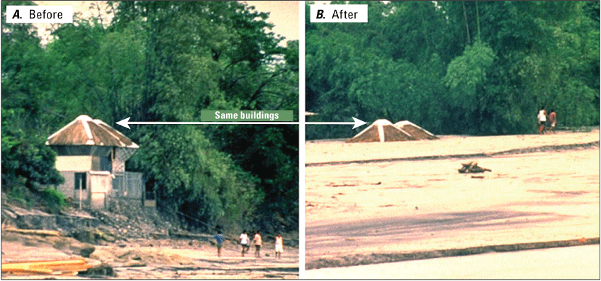
Photographs showing post-eruption sedimentation after the cataclysmic eruption of Mount Pinatubo, Philippines, on June 15, 1991. A, A house by the Sacobia-Bamban River on July 23, 1991. B, Only the roof of the house remained unburied on August 16, 1991, after nearly 9 meters of sediment were deposited during a single rain-induced lahar on August 15, 1991. Modified from Punongbayan and others (1996). Photographs by R.S. Punongbayan, Philippine Institute of Volcanology and Seismology.
Large volume eruption-triggered lahars (several tens to hundreds of millions of cubic meters) have low yearly probabilities compared to generally smaller-volume, non-eruptive related debris flows. Over the past 15,000 years, eruptive events at Mount Baker have occurred on average every couple of thousands of years, although the spacing between events is not equal. Whereas there were many eruptive events between 15,000 and 10,000 years ago, there have been only a few in the past 10,000 years (Scott and others, 2020). However, once an eruption begins, it can continue intermittently over the course of weeks to years. Non-eruption related, small-volume debris flows associated with intense rainstorms, glacial outbursts, or collapses of ice-cored sediment high on the flanks of the volcano during prolonged warm weather, can occur in any year without warning and are usually short-lived events. Although these smaller events have fewer devastating consequences for infrastructure and human life, they can still affect water quality and be especially devastating for aquatic ecosystems.
Limitations of the D-Claw Model
Although lahar models are great aids for understanding and visualizing rare events, they are only simplifications of complex processes and are not necessarily depictions of what will happen in the future. There may be similarities, but there may also be substantial differences, especially if river channels become choked with debris causing flows to develop new pathways. Thus, understanding the limitations of the D-Claw scenarios is important. First, all simulations were constructed as if there was no water in the river valleys. Exactly how a lahar interacts with river water is unknown but is a topic of current investigation. Second, the D-Claw scenarios were constructed for landslide-initiated lahars only. There are many other triggering mechanisms for lahars, such as hot rock and snow and (or) ice interactions during explosive events, lava flow-front and lava dome collapses, and so forth. How these different triggering mechanisms affect lahar behavior was not examined in this report. Third, because we use a landslide-triggering mechanism in our simulations, the scenarios assume that the source material is a mobile, clay-rich mixture of rock and sediment. Lahars with low clay contents commonly transform to sandier hyperconcentrated flows (less than 60 percent sediment by volume; Pierson and Scott, 1985) as they move downstream. Fourth, it is difficult to show the uncertainty in D-Claw model results. Many model parameters have a range in values, but we can only use a single value for each model. Because of the uncertainties involved, the D-Claw results are most appropriate for broad decision-making purposes and should not be extrapolated to street-level boundaries or fine-scale travel times. Lastly, D-Claw simulations that have a large area extent and fine-scale resolution (like those used in this report) are computationally demanding and can take a long time to run (often a few to several weeks). Thus, during a crisis there may not be enough time to run D-Claw simulations using such fine-scale resolution for large areas. Nonetheless, D-Claw is a unique and valuable tool to help communities plan for potential hazards from a future eruption during quiescence and may be a useful tool at a coarser resolution during prolonged periods of volcanic unrest.
Conclusion
Volcanic eruptions at Mount Baker are rare. On average they occur every several thousand years, although the spacing between eruptions is not equal. Lahars are the primary volcano hazard for communities along river valleys that originate on Mount Baker, and depending on the size, can have minor to devastating effects. The physics-based D-Claw model provides unique information regarding how lahars of specific volumes and physical properties interact with the landscape. In the nine scenarios presented herein, landslides originating between Sherman Crater and the Roman Wall, on southwest flank of Mount Baker, transform quickly into lahars that flow down the Middle Fork Nooksack River and beyond. These simulations show how lahars of different sizes and physical characteristics, like those that have happened in the past, could affect downstream communities. The scenarios indicate that lahars ranging in volume from 37 to 260 million cubic meters (Mm3) could reach the confluence of the Middle Fork Nooksack and North Fork Nooksack Rivers within 30 minutes of initiation and be as deep as 20 meters. Even smaller-volume lahars can affect the Middle Fork Nooksack River. The two largest-volume lahars simulated (108 and 260 Mm3), at initial hydraulic permeabilities of 10−11 and 10−12 m2, could reach Deming, Washington, within 50 minutes of lahar initiation with discharge values substantially greater than the largest flood on record and maximum flow depths between about 7 and 9.5 m. The simulations show that these larger-volume lahars could reach Everson, Wash., within 2 hours, followed by overtopping of the levee within tens of minutes. Communities along the Nooksack and Sumas Rivers, including those not immediately affected by a lahar, could experience increased sedimentation and flooding years to decades after the lahar ended. The results from these scenarios can help communities prepare for the next eruption-related lahar that affects the Middle Fork Nooksack River, thereby helping to keep natural processes, like volcanic eruptions, from becoming natural disasters.
References Cited
Anderson, S.W., and Grossman, E.E., 2017, Topographic and bathymetric elevation data for the Nooksack River, Fall 2015: U.S. Geological Survey data release, https://doi.org/10.5066/F72B8W7M.
Bacon, C.R., 1983, Eruptive history of Mount Mazama and Crater Lake caldera, Cascade Range, U.S.A: Journal of Volcanology and Geothermal Research, v. 18, no. 1–4, p. 57–115, https://doi.org/10.1016/0377-0273(83)90004-5.
Berger, M.J., George, D.L., LeVeque, R.J., and Mandli, K.T., 2011, The GeoClaw software for depth-averaged flows with adaptive refinement: Advances in Water Resources, v. 34, no. 9, p. 1195–1206, https://doi.org/10.1016/j.advwatres.2011.02.016.
Bouchut, F., Fernandez-Nieto, E.D., Mangeney, A., and Narbona-Reina, G., 2016, A two-phase two-layer model for fluidized granular flows with dilatancy effects: Journal of Fluid Mechanics, v. 801, p. 166–221, https://doi.org/10.1017/jfm.2016.417.
Bronk Ramsey, C., 2001, Development of the radiocarbon calibration program: Radiocarbon, v. 43, no. 2A, p. 355–363, https://doi.org/10.1017/S0033822200038212.
Bronk Ramsey, C., 2009, Bayesian analysis of radiocarbon dates: Radiocarbon, v. 51, no. 1, p. 337–360, https://doi.org/10.1017/S0033822200033865.
Christen, M., Kowalski, J., and Bartelt, P., 2010, RAMMS—Numerical simulation of dense snow avalanches in three-dimensional terrain: Cold Regions Science and Technology, v. 63, no. 1–2, p. 1–14, https://doi.org/10.1016/j.coldregions.2010.04.005.
Finn, C.A., Deszcz-Pan, M., Ball, J.L., Bloss, B.J., and Minsley, B.J., 2018, Three-dimensional geophysical mapping of shallow water saturated altered rocks at Mount Baker, Washington—Implications for slope stability: Journal of Volcanology and Geothermal Research, v. 357, p. 261–275, https://doi.org/10.1016/j.jvolgeores.2018.04.013.
George, D.L., 2008, Augmented Riemann solvers for the shallow water equations over variable topography with steady states and inundation: Journal of Computational Physics, v. 227, no. 6, p. 3089–3113, https://doi.org/10.1016/j.jcp.2007.10.027.
George, D.L., 2011, Adaptive finite volume methods with well-balanced Riemann solvers for modeling floods in rugged terrain—Application to the Malpasset dam-break flood (France, 1959): International Journal for Numerical Methods in Fluids, v. 66, no. 8, p. 1000–1018, https://doi.org/10.1002/fld.2298.
George, D.L., Barnhart, K.R., and Iverson, R.M., 2025a, D-Claw—A library for simulation of granular-fluid flows, version 1.0.0: U.S. Geological Survey software release, https://doi.org/10.5066/P13GUXUT. [Also available at https://code.usgs.gov/claw/dclaw]
George, D.L., Cannon, C.M., Benage, M.C, and Gardner, C.A., 2025b, Simulated lahar extents and dynamics in the Middle Fork Nooksack River drainage, resulting from hypothetical landslide sources on the western summit of Mount Baker, Washington: U.S. Geological Survey data release, https://doi.org/10.5066/P1PEX7FS.
George, D.L., and Iverson, R.M., 2014, A depth-averaged debris-flow model that includes the effects of evolving dilatancy—II. Numerical predictions and experimental tests: Proceedings of the Royal Society A, v. 470, no. 2170, 31 p., https://doi.org/10.1098/rspa.2013.0820.
George, D.L., Iverson, R.M., and Cannon, C.M., 2022, Modeling the dynamics of lahars that originate as landslides on the west side of Mount Rainier, Washington: U.S. Geological Survey Open-File Report 2021–1118, 54 p., https://doi.org/10.3133/ofr20211118.
Glicken, H., 1996, Rockslide-debris avalanche of May 18, 1980, Mount St. Helens volcano, Washington: U.S. Geological Survey Open-File Report, 96–677, 90 p. https://doi.org/10.3133/ofr96677
Guthrie, R.H., Friele, P., Allstadt, K., Roberts, N., Evans, S.G., Delaney, K.B., Roche, D., Clague, J. J. and Jakob, M., 2012, The 6 August 2010 Mount Meager rockslide-debris flow, Coast Mountains, British Columbia—Characteristics, dynamics, and implications for hazard and risk assessment: Natural Hazards and Earth System Sciences, v. 12, p. 1277–1294, https://doi.org/10.5194/nhess-12-1277-2012.
Hildreth, W., Fierstein, J., and Lanphere, M., 2003, Eruptive history and geochronology of the Mount Baker volcanic fields, Washington: Geological Society of America Bulletin, v. 115, p. 729–764, https://doi.org/10.1130/0016-7606(2003)115<0729:EHAGOT>2.0.CO;2.
Hayashi, J.N., and Self, S., 1992, A comparison of pyroclastic flow and debris avalanche mobility: Journal of Geophysical Research, v. 97, no. B6, p. 9063–9071, https://doi.org/10.1029/92JB00173.
Hyde, J.H., and Crandell, D.R., 1978, Postglacial volcanic deposits at Mount Baker, Washington, and potential hazards from future eruptions: U.S. Geological Survey Professional Paper 1022–C, 17 p., https://doi.org/10.3133/pp1022C.
Iverson, N.R., Mann, J.E., and Iverson, R.M., 2010, Effects of soil aggregates on debris-flow mobilization—Results from ring-shear experiments: Engineering Geology, v. 114, no. 1–2, p. 84–92, https://doi.org/10.1016/j.enggeo.2010.04.006.
Iverson, R.M., 1997, The physics of debris flows: Reviews of Geophysics, v. 35, no. 3, p. 245–296, https://doi.org/10.1029/97RG00426.
Iverson, R.M., and George, D.L., 2014, A depth-averaged debris-flow model that includes the effects of evolving dilatancy—I. Physical basis: Proceedings of the Royal Society A, v. 470, no. 2170, 31 p., https://doi.org/10.1098/rspa.2013.0819.
Iverson, R.M., and George, D.L., 2016, Modelling landslide liquefaction, mobility bifurcation and the dynamics of the 2014 Oso disaster: Geotechnique, v. 66, no. 3, p. 175–187, https://doi.org/10.1680/jgeot.15.LM.004.
Iverson, R.M., George, D.L., Allstadt, K., Reid, M.E., Collins, B.D., Vallance, J.W., Schilling, S.P., Godt, J.W., Cannon, C.M., Magirl, C.S., Baum, R.L., Coe, J.A., Schulz, W.H., and Bower, J.B., 2015, Landslide mobility and hazards—Implications of the 2014 Oso disaster: Earth and Planetary Science Letters, v. 412, p. 197–208, https://doi.org/10.1016/j.epsl.2014.12.020.
Iverson, R.M., Schilling, S.P., and Vallance, J.W., 1998, Objective delineation of lahar-inundation hazard zones: Geological Society of America Bulletin, v. 110, no. 8, p. 972–984, https://doi.org/10.1130/0016-7606(1998)110<0972:ODOLIH>2.3.CO;2.
Jaboyedoff, M., Carrea, D., Derron, M.H., Oppikofer, T., Penna, I.M., and Rudaz, B., 2020, A review of methods used to estimate initial landslide failure surface depths and volumes: Engineering Geology, v. 267, 18 p., https://doi.org/10.1016/j.enggeo.2020.105478.
Kovanen, D.J., Easterbrook, D.J., and Thomas, P.A., 2001, Holocene eruptive history of Mount Baker, Washington: Canadian Journal of Earth Sciences, v. 38, no. 9, p. 1355–1366, https://doi.org/10.1139/e01-025.
Kowalski, J., and McElwaine, J.N., 2013, Shallow two-component gravity-driven flows with vertical variation: Journal of Fluid Mechanics, v. 714, p. 434–462, https://doi.org/10.1017/jfm.2012.489.
Latrubesse, Edgardo M., 2008, Patterns of anabranching channels: The ultimate end-member adjustment of mega rivers: Geomorphology, v. 101, p 130–145, https://doi.org/10.1016/j.geomorph.2008.05.035.
LeVeque, R.J., George, D.L., and Berger, M.J., 2011, Tsunami modeling with adaptively refined finite volume methods: Acta Numerica, v. 20, p. 211–289, https://doi.org/10.1017/S0962492911000043.
Mandli, K.T., Ahmadia, A.J., Berger, M.J., Calhoun, D., George, D.L., Hadjimichael, Y., Ketcheson, D.I., Lemoine, G.I., and LeVeque, R.J., 2016, Clawpack—Building an open-source ecosystem for solving hyperbolic PDEs: PeerJ Computer Science, v. 2, 27 p., https://doi.org/10.7717/peerj-cs.68.
McDougall, S., and Hungr, O., 2004, A model for the analysis of rapid landslide motion across three-dimensional terrain: Canadian Geotechnical Journal, v. 41, no. 6, p. 1084–1097, https://doi.org/10.1139/t04-052.
Mergili, M., Fischer, J.-T., Krenn, J., and Pudasaini, S.P., 2017, r.avaflow v1, an advanced open-source computational framework for the propagation and interaction of two-phase mass flows: Geoscientific Model Development, v. 10, no. 2, p. 553–569, https://doi.org/10.5194/gmd-10-553-2017.
Mount Baker Volcano Research Center, 2013, Large debris flow in the Middle Fork Nooksack River—May 31, 2013: Mount Baker Volcano Research Center web page, accessed November 10, 2021, at https://mbvrc.wordpress.com/2013/06/05/large-debris-flow-in-middle-fork-nooksack-river-may-31-2013/.
Pierson, T.C., 1998, An empirical method for estimating travel times for wet volcanic mass flows: Bulletin of Volcanology, v. 60, no. 2, p. 98–109, https://doi.org/10.1007/s004450050219.
Pierson, T.C., Scott, K.M., 1985, Downstream dilution of a lahar—Transition from debris flow to hyperconcentrated streamflow: Water Resources Research, v. 21, no. 10, https://doi.org/10.1029/WR021i010p01511.
Pierson, T.C., Pringle, P.T., and Cameron, K.A., 2011, Magnitude and timing of downstream channel aggradation and degradation in response to a dome-building eruption at Mount, Oregon: Geological Society of America Bulletin, v. 123, no. 1–2, p. 3–20, https://doi.org/10.1130/B30127.1.
Punongbayan, R.S., Newhall, C.G., and Hobblitt, R.P., 1996, Photographic Record of Rapid Geomorphic Change at Mount Pinatubo, 1991–94, in Newhall, C.G., and Punongbayan, R.S., eds., Fire and mud—Eruptions and lahars of Mount Pinatubo, Philippines: University of Washington Press and U.S. Geological Survey, p. 21–66.
Reynolds, O., 1886, Dilatancy: Nature, v. 33, no. 853, p. 429–430, https://doi.org/10.1038/033429b0.
Rodolfo, K.S., Umbal, J.V., Alonso, R.A., Remotique, C.T., Paladio-Melosantos, M.L., Salvador, J.H.G., Evangelista, D., and Miller, Y., 1996, Two years of lahars on the western flank of Mount Pinatubo—Initiation, flow processes, deposits and attendant geomorphic and hydraulic changes, in Newhall, C.G., and Punongbayan, R.S. eds., Fire and mud—Eruptions and lahars of Mount Pinatubo, Philippines: University of Washington Press and U.S. Geological Survey, p. 989–1013.
Savage, S.B., and Hutter, K., 1989, The motion of a finite mass of granular material down a rouch incline: Journal of Fluid Mechanics, v. 199, p. 177–215, https://doi.org/10.1017/S0022112089000340.
Schilling, S.P., 1998, LAHARZ—GIS programs for automated mapping of lahar-inundation hazard zones: U.S. Geological Survey Open-File Report 98–683, 80 p., https://doi.org/10.3133/ofr98638.
Scott, K.M., Tucker, D.S., Riedel, J.L., Gardner, C.A., and McGeehin, J.P., 2020, Latest Pleistocene to present geology of Mount Baker Volcano, northern Cascade Range, Washington: U.S. Geological Survey Professional Paper 1865, 170 p., https://doi.org/10.3133/pp1865.
Tucker, D.S., Scott, K.M., Grossman, E.E., and Linneman, S., 2014, Mount Baker lahars and debris flows, ancient, modern and future, in Dashtgard, S., and Ward, B., eds., Trials and tribulations of life on an active subduction zone—Field trips in and around Vancouver, Canada: Geological Society of America Field Guide 38, p. 33–52, https://doi.org/10.1130/2014.0038(03).
U.S. Geological Survey [USGS], 2016, USGS water data for the Nation: U.S. Geological Survey National Water Information System database, accessed May 2024, at https://doi.org/10.5066/F7P55KJN.
Vallance, J.W., and Scott, K.M., 1997, The Osceola Mudflow from Mount Rainier—Sedimentology and hazard implications of a huge clay-rich debris flow: Geological Society of America Bulletin, v. 109, no. 2, p. 143–163, https://doi.org/10.1130/0016-7606(1997)109<0143:TOMFMR>2.3.CO;2.
Vallance, J.W., and Sisson, T.W., 2022, Geologic field-trip guide to volcanism and its interaction with snow and ice at Mount Rainier, Washington: U.S. Geological Survey Scientific Investigations Report 2017–5022–A, 76 p., https://doi.org/10.3133/sir20175022A.
Voight, B., Janda, R.J., Glicken, H., and Douglass, P.M., 1983, Nature and mechanics of the Mount St. Helens rockslide–avalanche of 18 May 1980: Geotechnique, v. 33, no. 3, p. 243–273. https://doi.org/10.1680/geot.1983.33.3.243.
Vreugdenhil, C.B., 1994, Numerical methods for shallow-water flow: Dordrecht, The Netherlands, Kluwer Academic Publishers, 272 p., https://doi.org/10.1007/978-94-015-8354-1.
Walker, M., Johnsen, S., Rasmussen, S.O., Popp, T., Steffensen, J.-P., Gibbard, P., Hoek, W., Lowe, J., Andrews, J., Björck, S., Cwynar, L.C., Hughen, K., Kershaw, P., Kromer, B., Litt, T., Lowe, D.J., Nakagawa, T., Newnham, R., and Schwander, J., 2009, Formal definition and dating of the GSSP (Global Stratotype Section and Point) for the base of the Holocene using the Greenland NGRIP ice core and selected auxiliary records: Journal of Quaternary Science, v. 24, p. 3–17., https://doi.org/10.1002/jqs.1227.
Zdanowicz, C.M., Zielinski, G.A., and Germani, M.S., 1999, Mount Mazama eruption—Calendrical age verified, and atmospheric impact assessed: Geology, v. 27, no. 7, p. 621–624, https://doi.org/10.1130/0091-7613(1999)027<0621:MMECAV>2.3.CO;2.
Appendix 1. Reference Point Locations in Latitude and Longitude
Table 1.1.
Latitude and longitude for reference points used in the text.[Universal Trans Mercator coordinates converted to latitude and longitude (see table 1 in “Introduction”)]
Appendix 2. Timing, Depth, Speed, Solid Volume Fraction, and Cessation of Movement for the Nine D-Claw Scenarios
Table 2.1.
Scenario A1—Lahar arrival times at reference points from a landslide failure where the volume is 260 million cubic meters and the initial hydraulic permeability is 10−10 square meters.[The simulation time for this scenario is 8 hours. Lahar arrival is the arrival time, depth, speed, and percent solid fraction of the lahar when it first reaches a given reference point (RP). Maximum lahar depth shows the time, depth, speed, and percent solid fraction of the lahar at time of maximum lahar depth. Lahar stops (or end of simulation) shows the time and depth when the lahar ceases to move any more material past a given reference point. Note that maximum depths may have 0 speed indicating that the lahar had stalled (ceased moving forward) at that time. Also, lahar depth at arrival may be 0 because of the depth is too small to round up to a significant figure. hh:mm, hours:minutes; m, meters; m/s, meters per second]
Table 2.2.
Scenario A2—Lahar arrival times at reference points from a landslide failure where the volume is 260 million cubic meters and the initial hydraulic permeability is 10−11 square meters.[The simulation time for this scenario is 12 hours. Lahar arrival is the arrival time, depth, speed, and percent solid fraction of the lahar when it first reaches a given reference point (RP). Maximum lahar depth shows the time, depth, speed, and percent solid fraction of the lahar at time of maximum lahar depth. Lahar stops (or end of simulation) shows the time and depth when the lahar ceases to move any more material past a given reference point. Note that maximum depths may have 0 speed indicating that the lahar had stalled (ceased moving forward) at that time. Also, lahar depth at arrival may be 0 because of the depth is too small to round up to a significant figure. hh:mm, hours:minutes; m, meters; m/s, meters per second; —, indicates no data because the lahar did not reach this reference point]
Table 2.3.
Scenario A3—Lahar arrival times at reference points from a landslide failure where the volume is 260 million cubic meters and the initial hydraulic permeability is 10−12 square meters.[The simulation time for this scenario is 15 hours. Lahar arrival is the arrival time, depth, speed, and percent solid fraction of the lahar when it first reaches a given reference point (RP). Maximum lahar depth shows the time, depth, speed, and percent solid fraction of the lahar at time of maximum lahar depth. Lahar stops (or end of simulation) shows the time and depth when the lahar ceases to move any more material past a given reference point. Note that maximum depths may have 0 speed indicating that the lahar had stalled (ceased moving forward) at that time. hh:mm, hours:minutes; m, meters; m/s, meters per second]
Table 2.4.
Scenario B1—Lahar arrival times at reference points from a landslide failure where the volume is 108 million cubic meters and the initial hydraulic permeability is 10−10 square meters.[The simulation time for this scenario is 8 hours. Lahar arrival is the arrival time, depth, speed, and percent solid fraction of the lahar when it first reaches a given reference point (RP). Maximum lahar depth shows the time, depth, speed, and percent solid fraction of the lahar at time of maximum lahar depth. Lahar stops (or end of simulation) shows the time and depth when the lahar ceases to move any more material past a given reference point. Note that maximum depths may have 0 speed indicating that the lahar had stalled (ceased moving forward) at that time. hh:mm, hours:minutes; m, meters; m/s, meters per second]
Table 2.5.
Scenario B2—Lahar arrival times at reference points from a landslide failure where the volume is 108 million cubic meters and the initial hydraulic permeability is 10−11 square meters.[The simulation time for this scenario is 12 hours. Lahar arrival is the arrival time, depth, speed, and percent solid fraction of the lahar when it first reaches a given reference point (RP). Maximum lahar depth shows the time, depth, speed, and percent solid fraction of the lahar at time of maximum lahar depth. Lahar stops (or end of simulation) shows the time and depth when the lahar ceases to move any more material past a given reference point. N/A denotes that the lahar did not reach this reference point. NaN is not a number and indicates a spurious value. hh:mm, hours:minutes; m, meters; m/s, meters per second; —, indicates no data because the flow did not reach this reference point.]
Table 2.6.
Scenario B3—Lahar arrival times at reference points from a landslide failure where the volume is 108 million cubic meters and the initial hydraulic permeability is 10−12 square meters.[The simulation time for this scenario is 15 hours. Lahar arrival is the arrival time, depth, speed, and percent solid fraction of the lahar when it first reaches a given reference point (RP). Maximum lahar depth shows the time, depth, speed, and percent solid fraction of the lahar at time of maximum lahar depth. Lahar stops (or end of simulation) shows the time and depth when the lahar ceases to move any more material past a given reference point. NaN is not a number and indicates a spurious value. hh:mm, hours:minutes; m, meters; m/s, meters per second; —, indicates no data because the lahar did not reach this reference point.]
Table 2.7.
Scenario C2—Lahar arrival times at reference points from a landslide failure where the volume is 37 million cubic meters and the initial hydraulic permeability is 10−11 square meters.[The flow does not reach beyond RP-13. The simulation time for this scenario is 12 hours. Lahar arrival is the arrival time, depth, speed, and percent solid fraction of the lahar when it first reaches a given reference point (RP). Maximum lahar depth shows the time, depth, speed, and percent solid fraction of the lahar at time of maximum lahar depth. Lahar stops (or end of simulation) shows the time and depth when the lahar ceases to move any more material past a given reference point. Note that lahar speed at arrival may be 0 because of the speed is too low to round up to a significant figure. NaN is not a number and indicates a spurious value. hh:mm, hours:minutes; m, meters; m/s, meters per second; —, indicates no data because the lahar did not reach this reference point]
Table 2.8.
Scenario D2—Lahar arrival times at reference points from a landslide failure where the volume is 10 million cubic meters and the initial hydraulic permeability is 10−11 square meters.[The simulation time for this scenario is 8 hours. Lahar arrival is the arrival time, depth, speed, and percent solid fraction of the lahar when it first reaches a given reference point (RP). Maximum lahar depth shows the time, depth, speed, and percent solid fraction of the lahar at time of maximum lahar depth. Lahar stops (or end of simulation) shows the time and depth when the lahar ceases to move any more material past a given reference point. Note that maximum depths may have 0 speed indicating that the lahar had stalled (ceased moving forward) at that time. Also, lahar depth or speed at arrival may be 0 because of the depth (or speed) is too small (too low) to round up to a significant figure. NaN is not a number and indicates a spurious value. hh:mm, hours:minutes; m, meters; m/s, meters per second; —, indicates no data because the lahar did not reach this reference point]
Table 2.9.
Scenario E2—Lahar arrival times at reference points from a landslide failure where the volume is 1 million cubic meters and the initial hydraulic permeability is 10−11 square meters.[The flow does not reach RP-3. The simulation time for this scenario is 8 hours, but most movement stopped before 2 hours. Lahar arrival is the arrival time, depth, speed, and percent solid fraction of the lahar when it first reaches a given reference point (RP). Maximum lahar depth shows the time, depth, speed, and percent solid fraction of the lahar at time of maximum lahar depth. Lahar stops (or end of simulation) shows the time and depth when the lahar ceases to move any more material past a given reference point. Note that maximum depths may have 0 speed indicating that the lahar had stalled (ceased moving forward) at that time. hh:mm, hours:minutes; m, meters; m/s, meters per second]
Appendix 3. D-Claw simulation hydrographs for scenarios C2, D2, and E2
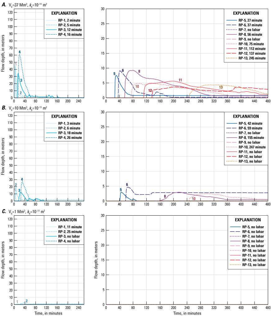
D-Claw model hydrographs for the three smallest lahar volumes, all with an initial hydraulic permeability of k0=10−11 square meters (m2). A, 37 million cubic meters (Mm3; scenario C2). B, 10 Mm3 (scenario D2). C, 1 Mm3 (scenario E2). Note that the left panels only have reference points (RP) 1–4 and the time is from 0 to 240 minutes, whereas the right panels have reference points 5–13, and time is 0 to 480 minutes. If a given hydrograph line ends before the end of the time on the graph, it indicates that in the simulation, the lahar ceased moving by that time. Colors depict the hydrograph for a given reference point. Time listed with each reference point indicates the arrival time at that reference point. Note in scenario E2 (C), the lahar does not flow as far as RP-3.
Appendix 4. Animated Simulations
Conversion Factors
U.S. customary units to International System of Units
International System of Units to U.S. customary units
Temperature in degrees Celsius (°C) may be converted to degrees Fahrenheit (°F) as follows:
°F = (1.8 × °C) + 32.
Temperature in degrees Fahrenheit (°F) may be converted to degrees Celsius (°C) as follows:
°C = (°F – 32) / 1.8.
Moffett Field Publishing Service Center, California
Manuscript approved for publication December 27, 2024
Edited by Kathryn Pauls
Layout and design by Cory Hurd
Cartography support by Katie Sullivan
Disclaimers
Any use of trade, firm, or product names is for descriptive purposes only and does not imply endorsement by the U.S. Government.
Although this information product, for the most part, is in the public domain, it also may contain copyrighted materials as noted in the text. Permission to reproduce copyrighted items must be secured from the copyright owner.
Suggested Citation
Gardner, C.A., Benage, M.C., Cannon, C., and George, D.L., 2025, Using the D-Claw software package to model lahars in the Middle Fork Nooksack River drainage and beyond, Mount Baker, Washington: U.S. Geological Survey Scientific Investigations Report 2024–5133, 47 p., https://doi.org/10.3133/sir20245133.
ISSN: 2328-0328 (online)
Study Area
| Publication type | Report |
|---|---|
| Publication Subtype | USGS Numbered Series |
| Title | Using the D-Claw software package to model lahars in the Middle Fork Nooksack River drainage and beyond, Mount Baker, Washington |
| Series title | Scientific Investigations Report |
| Series number | 2024-5133 |
| DOI | 10.3133/sir20245133 |
| Publication Date | May 12, 2025 |
| Year Published | 2025 |
| Language | English |
| Publisher | U.S. Geological Survey |
| Publisher location | Reston, VA |
| Contributing office(s) | Geology, Minerals, Energy, and Geophysics Science Center, Volcano Science Center |
| Description | Report: vii, 47 p.; 9 Animation Videos; Data Release |
| Country | United States |
| State | Washington |
| Other Geospatial | Middle Fork Nooksack River, Mount Baker |