

Assessment and Validation of Depressions in Digital Elevation Models From Multiple Elevation Data Sources and Delineation of Depressions, Sinking Streams, and Their Watersheds in Tennessee and Parts of Kentucky, Virginia, North Carolina, Georgia, Alabama, and Mississippi
Links
- Document: Report (4.51 MB pdf) , HTML , XML
- Data Release: USGS Data Release - Geospatial dataset of depressions, sinking streams, and associated watersheds in karst areas of Tennessee and parts of surrounding States
- NGMDB Index Page: National Geologic Map Database Index Page (html)
- Download citation as: RIS | Dublin Core
Acknowledgments
The authors would like to thank U.S. Geological Survey retirees Tim Diehl and Gregg Hileman for their contributions in determining the methods applied in this study.
Abstract
Closed depressions and sinking streams in karst landscapes pose difficulties for water-resources management, in the construction of roads and other public works, and in hydrologic and hydrogeomorphic analyses. Digital elevation models (DEMs) can be used to identify the location and determine the size and shape of closed depressions, but separating artificial depressions due to error from real depressions in DEMs can be difficult. Artificial depressions in the DEMs can result from errors that were inherited from limitations in the source data, the interpolation of the elevation data into a grid of values, or horizontal and vertical accuracy of the elevation data. Because the source dataset used to derive DEMs is only a model of the true landscape, field verification is necessary to separate artificial depressions from real ones in DEMs. DEM analysis alone can only be used to determine whether a depression is likely or unlikely to exist in the landscape.
The U.S. Geological Survey has applied methods to delineate depressions, sinking streams, and their watersheds by using DEMs derived from two sources of elevation data within karst areas of Tennessee and parts of surrounding States. Preliminary depressions, which include all depressions before separating the likely depressions from the unlikely depressions, were delineated from the DEMs with 30- by 30-foot cells derived from each elevation data source. The characteristics of these preliminary depressions were compared to occurrence probabilities for depressions derived from numerical error propagation tests in 10 test areas across the study area and to topographic-contour source data within a 17,739-square-mile test area in middle Tennessee and northern Alabama. The comparison was conducted to determine depression characteristics that, when combined with depression-proximity filters, could be used to separate unlikely from likely depressions. Preliminary depressions were examined in the field at 91 sites in Tennessee, and field observations were compared to digital determinations of unlikely and likely depressions.
The density and size of depressions derived from each elevation dataset were compared within eight karst regions in the study area. Depressions and their watersheds were compiled from each elevation dataset. Sinking streams derived from the National Hydrography Dataset and their watersheds also were compiled for the study area.
Introduction
Digital elevation models (DEMs) contain numerous topographic depressions, also referred to as sinks or pits, represented by an area of one or more contiguous grid cells with elevations lower than neighboring cells (Zandbergen, 2010). Depressions in DEMs interrupt the connectivity of flow networks derived from DEM analysis (Tribe, 1992), and it is common practice to remove all depressions from DEMs used in hydrologic or hydrogeomorphic applications to derive a fully connected drainage network (Lindsay and Creed, 2006; Poppenga and others, 2010; Zandbergen, 2010). This practice is typically justified because artificial depressions due to error in DEMs are common and closed depressions in certain natural landscapes are rare (Lindsay and Creed, 2006; Zandbergen, 2010).
Although many of the depressions in DEMs are artificial, some are real, such as those in karst landscapes. The term “karst” can be defined as a terrain with distinctive hydrology and surface features, such as closed depressions, sinkholes, and sinking streams, resulting from high rock solubility and well-developed fracture porosity (Ford and Williams, 2007; Weary and Doctor, 2014). In addition to posing problems for hydrologic analysis, karst features present several challenges to natural resources management and the construction of roads and other public works. These features can adversely affect the construction and maintenance of roadways and the hydraulic structures needed along roadways. Planning, permitting, designing, and building these structures depend on reliable maps showing karst features. Roadway spills and other types of contamination that enter karst depressions have the potential to rapidly enter groundwater, making karst depression and catchment delineation crucial to water-resources protection in karst areas. Therefore, the common practice of removing all depressions from DEMs used in hydrologic or hydrogeomorphic applications is not necessarily justified in karst areas.
DEMs are discretized representations of their source elevation data, which are in turn modeled representations of the landscape derived from elevation surveys. In this sense, DEMs can contain errors that are inherited from limitations in the source elevation data, and they can contain errors that are products of interpolating the source elevation data into a grid of elevation values. The source data, such as topographic contours or mass points with elevation values, contain errors in their representation of the landscape which can lead to errors of omission (false negatives) and commission (false positives) of depressions. For example, contour maps omit many depressions that are shallower than the contour interval. The source data may also misrepresent surface-water flow through culverts and drains and under small bridges, resulting in what are often large artificial depressions (Poppenga and others, 2010; Zandbergen, 2010; Wall and others, 2015). All these errors inherent in the DEM are derived from the source data; interpolation of the source data onto a grid can also introduce errors because of the limited horizontal and vertical accuracy of the grid (Tribe, 1992; Lindsay and Creed, 2006; Zandbergen, 2010). Because DEMs include the error inherent in the source data and the error associated with DEM creation, field verification is required to separate artificial depressions from real ones in a DEM; DEM analysis can only help determine whether a depression from a DEM is unlikely or likely to exist in the true landscape. To determine the effects of depressions on DEM-based hydrologic or hydrogeomorphic analysis, unlikely depressions must be separated from likely depressions.
Several approaches can be used to distinguish artificial and real depressions (Lindsay and Creed, 2006; Zandbergen, 2010; Wall and others, 2015), but the process of separating depressions that are due to error in DEMs from those that likely exist on the landscape is not straightforward. Certain types of DEM source data, such as topographic contours, can be used to identify DEM-derived depression errors of commission (false positives) and omission (false negatives) (Lindsay and Creed, 2006). In the case of DEMs derived from topographic contours, depressions that do not contain at least one closed-depression contour at the source-data interval are considered errors of commission; areas where a closed-depression contour exists in the source data, but no DEM-derived depression exists, are considered errors of omission. In the case of closely spaced mass-point-derived DEMs, such as those derived from light detection and ranging (lidar) and photogrammetric techniques, examination of the source data is less useful than examination of the source contours in determining errors in DEM-derived depressions because mass-point data alone do not define a surface from which depressions can be visibly detected (Lindsay and Creed, 2006).
Additionally, DEMs derived from closely spaced mass-point source data can possess greater surface roughness and contain many more depressions than DEMs generated from contours (MacMillan and others, 2003; Lindsay and Creed, 2005), causing even greater difficulty in separating unlikely from likely depressions in DEMs derived from highly accurate, closely spaced source data. In cases where examination of source data is not sufficient, numerical error propagation tests can be effective in distinguishing unlikely from likely depressions (Lindsay and Creed, 2006; Zandbergen, 2010), but propagation tests are not feasible for large study areas because they are time consuming and computer intensive. Additionally, numerical error propagation tests will often indicate that artificial depressions caused by topographic barriers such as roads, bridges, and culverts are likely real (Zandbergen, 2010). Methods exist to identify and remove depressions caused by topographic barriers, but these methods may not remove all such artificial depressions (Poppenga and others, 2010; Wall and others, 2015). Due to errors and misrepresentations of the landscape inherent in DEM source data, examination of source data and numerical error propagation tests will only help to establish justification for calling a depression artificial or real (Lindsay and Creed, 2006). Field investigations offer the most reliable method of determining whether a depression exists in the landscape, but visiting all DEM-derived depressions is not feasible for large study areas. DEM analysis alone, without field verification, can only help classify DEM-derived depressions as unlikely or likely to exist in the true landscape.
The U.S. Geological Survey (USGS), in cooperation with the Tennessee Department of Transportation, investigated the karst areas of Tennessee and parts of surrounding States to identify karst features such as depressions, sinking streams, and their watersheds by using DEMs created from multiple sources of elevation data and digital hydrographic data. The USGS and the Tennessee Department of Transportation developed methods for delineating preliminary depressions from the DEMs to classify them as likely or unlikely to exist in the true landscape. The geospatial datasets for depressions derived from the DEMs, sinking streams derived from digital hydrographic data, and watersheds of the depressions and sinking streams are available in Ladd (2025).
Purpose and Scope
The purposes of this report are to document the methods and assessment techniques used to classify depressions in DEMs as likely or unlikely to exist; to delineate depressions, sinking streams, and their associated watersheds from multiple elevation data sources and digital hydrographic data within the karst areas of Tennessee and parts of surrounding States; to characterize the spatial distribution of these features within the area; and to present geospatial datasets of these features and their watersheds (Ladd, 2025). DEM analysis was used to delineate preliminary depressions derived from elevation source data such as topographic maps, lidar data, and photogrammetrically derived data. Depressions, sinking streams, and their watersheds were compiled into geospatial datasets, and the spatial distribution of depressions within each karst region in the study area was characterized.
Although subjective distinctions between depressions and karst features were made at field visit locations, the DEM analysis methods used for this study provide no distinction between sinkholes, man-made depressions, or natural depressions; such distinctions are beyond the scope of the study and this report. Many of the depressions in the geospatial datasets are considered compound or nested depressions, in which the boundary representing the area of internal drainage contains additional internal closed depressions; in these cases, only the outer boundary of the internally drained area is represented. In this regard, the geospatial datasets of depressions are not intended to represent every depression or sinkhole on the landscape. Depressions in the geospatial datasets represent areas of internal drainage that have the potential to store surface runoff. Some sinking streams that do not terminate in depressions, and therefore store no surface runoff, are included in the geospatial datasets, and watersheds for these sinking streams are included in the watershed datasets.
Study Area
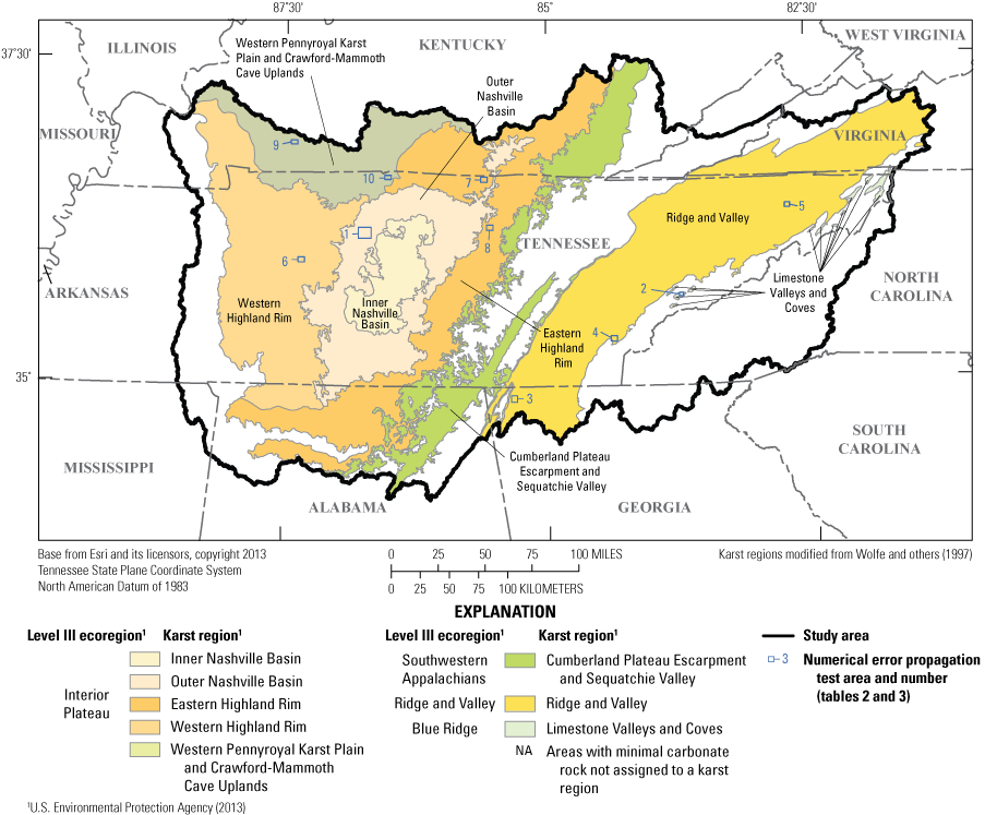
The study area comprises approximately 61,800 square miles (mi2) in the eastern two-thirds of Tennessee and parts of Kentucky, Virginia, North Carolina, Georgia, Alabama, and Mississippi, and encompasses the Cumberland, Tennessee, Barren, and Conasauga River watersheds (fig. 1). Soluble carbonate rocks underlie most of middle Tennessee, large areas of east Tennessee, and parts of surrounding States (fig. 2). Wolfe and others (1997) divided the carbonate areas of Tennessee into eight karst regions based on geologic structure, stratigraphy, relief, regolith thickness, and karst landforms. The boundaries and names of these regions were modified to create eight karst regions for this report: (1) the Inner Nashville Basin, corresponding to the Inner Central Basin region from Wolfe and others (1997), (2) the Outer Nashville Basin, corresponding to the Outer Central Basin region from Wolfe and others (1997), (3) the Eastern Highland Rim, corresponding to the Eastern Highland Rim subregion of the Highland Rim region from Wolfe and others (1997), (4) the Western Highland Rim, corresponding to the Western Highland Rim subregion of the Highland Rim region from Wolfe and others (1997), (5) the Western Pennyroyal Karst Plain and Crawford-Mammoth Cave Uplands, corresponding to the Pennyroyal Plateau subregion of the Highland Rim region from Wolfe and others (1997), (6) the Cumberland Plateau Escarpment and Sequatchie Valley, corresponding to the Coves and Escarpments of the Cumberland Plateau region from Wolfe and others (1997), (7) the Ridge and Valley, corresponding to the Valley and Ridge region from Wolfe and others (1997), and (8) the Limestone Valleys and Coves, corresponding roughly to the Western Toe of the Blue Ridge region from Wolfe and others (1997) (fig. 2). The boundaries and names for the Inner Nashville Basin, Outer Nashville Basin, Eastern Highland Rim, Western Highland Rim, and Limestone Valleys and Coves were compiled from Level IV ecoregion data (U.S. Environmental Protection Agency, 2013). The Western Pennyroyal Karst Plain and Crawford-Mammoth Cave Uplands karst region and Cumberland Plateau and Sequatchie Valley region boundaries and names were compiled from combined Level IV ecoregions (U.S. Environmental Protection Agency, 2013). The Ridge and Valley region boundary and name were taken from the Ridge and Valley Level III ecoregion (U.S. Environmental Protection Agency, 2013).
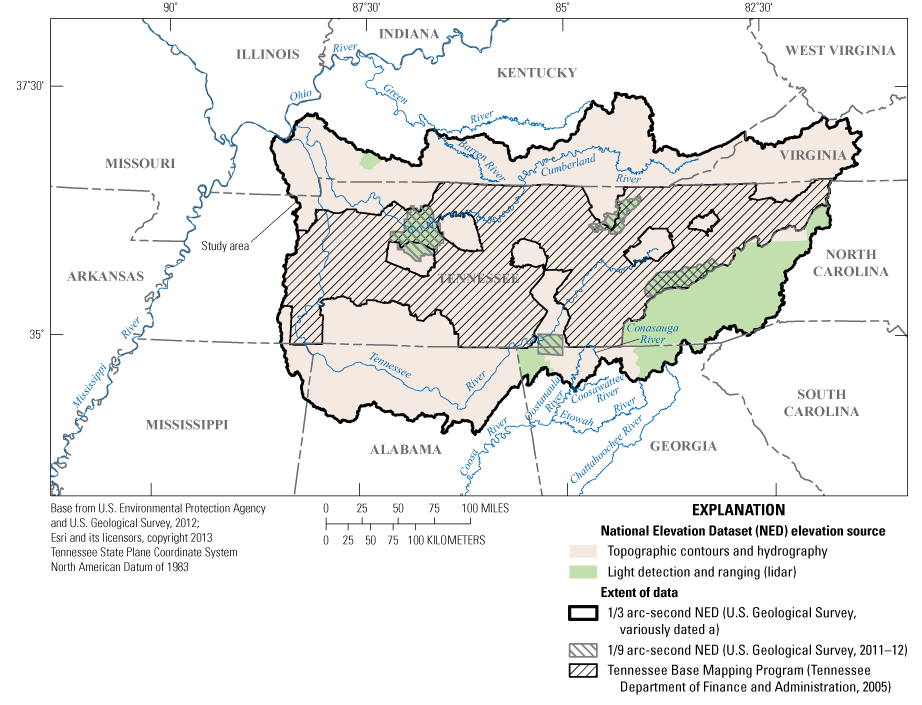
Location of the study area in Tennessee and parts of Kentucky, Virginia, North Carolina, Georgia, Alabama, and Mississippi; extent of elevation data; and National Elevation Dataset (NED) elevation sources.
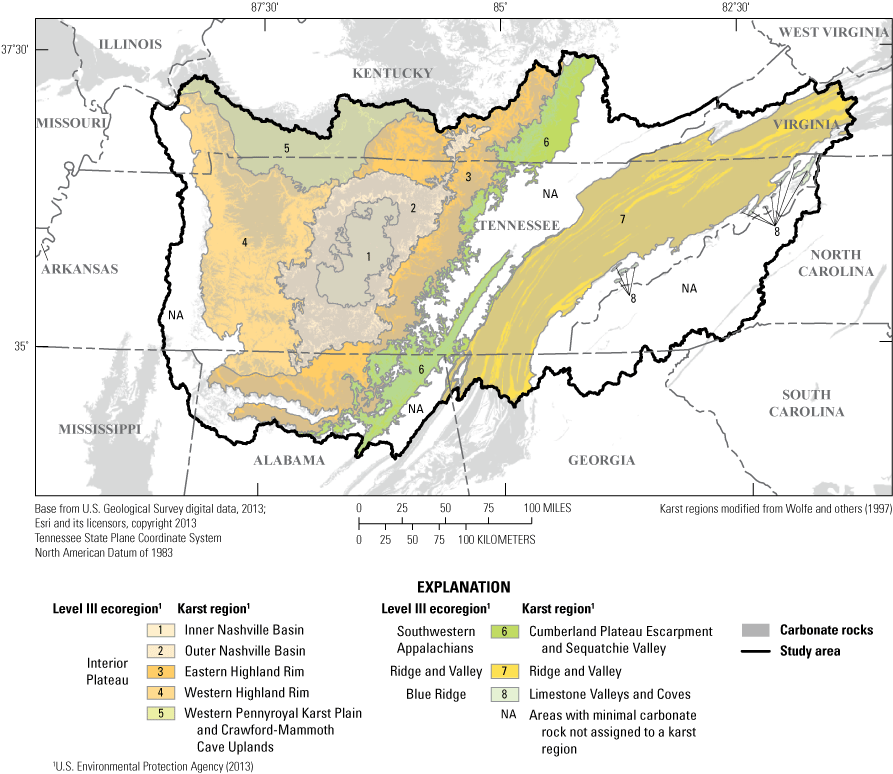
Karst regions and carbonate rocks within and near the study area in Tennessee and parts of Kentucky, Virginia, North Carolina, Georgia, Alabama, and Mississippi corresponding to karst regions defined from Wolfe and others (1997) and ecoregions from U.S. Environmental Protection Agency, (2013).
Methods of Study
DEM analysis and depression assessment methods were used to identify and separate unlikely from likely depressions and to delineate depressions and sinking streams by using DEMs and hydrography vector data. Two sources of digital elevation data, described further in the “Acquisition of Digital Elevation and Hydrography Data” section, were used in the study: (1) the National Elevation Dataset (NED; Gesch and others, 2002; Gesch, 2007; USGS, 2011–12, variously dated a), which was derived from topographic-contour source data for some areas and lidar source data for other areas (fig. 1), and (2) photogrammetrically derived data collected by the State of Tennessee as part of the Tennessee Base Mapping Program (TNBMP; Tennessee Department of Finance and Administration, 2005, 2007; fig. 1). These elevation data, along with flowlines from the National Hydrography Dataset (NHD; USGS, variously dated b), were prepared for DEM analysis by using methods similar to those described by Djokic (2008).
A collection of preliminary depressions was delineated from each prepared elevation dataset. Differences in accuracy and resolution of source data, described further in the “Elevation Accuracy Assessment and Numerical Error Propagation” section, exist among the topographic-contour-based NED, the lidar-based NED, and the photogrammetry-based TNBMP elevation data. Additionally, the contour source data used for the topographic-contour-based NED allow for visual detection of depressions, which is not possible with the mass points and break lines used as sources for the lidar-based NED and the photogrammetry-based TNBMP data. For these reasons, different criteria were used to distinguish unlikely from likely depressions derived from the topographic-contour-based NED than were used to distinguish unlikely from likely depressions derived from the lidar-based NED and the photogrammetry-based TNBMP data. However, the same methods and tests used for depression assessment were applied for comparison to preliminary depressions from all sources.
Proximity filters, such as the proximity of depressions to developed areas and certain man-made features, and depression-characteristic thresholds based on the assessments were used to distinguish unlikely from likely depressions. To eliminate some of the artificial depressions caused by roads, bridges, and other topographic barriers represented in the DEMs, a culvert and small bridge location approximation and enforcement method similar to the one proposed by Wall and others (2015) was used to cut flow pathways through transportation routes in the previously processed DEMs. The DEMs were processed a final time to delineate depressions, sinking streams, and associated watersheds for the depressions and sinking streams. The resulting geospatial datasets derived from each elevation source and the NHD were examined to characterize the spatial variability of depression characteristics within the study area.
Acquisition of Digital Elevation and Hydrography Data
The NED used in this study included USGS 1/3 and 1/9 arc-second DEMs. The contour-derived NED came from 1/3 arc-second (approximately 10 meters) DEMs (USGS, variously dated a), and the lidar-derived NED came from 1/3 arc-second and 1/9 arc-second (approximately 3 meters) DEMs (USGS, 2011–12, 2014a, b; fig. 1), which were in raster format when acquired. The 1/3 arc-second NED was updated with more current and higher resolution source data as they have become available (USGS, 2014a), often by incorporating data from the 1/9 arc-second NED (Evans, 2014; USGS, 2014b). The most current release of the 1/3 arc-second NED included more 1/9 arc-second lidar-derived NED source data than the version downloaded in June 2011 for this study (USGS, 2011, 2014b). To incorporate more current high-resolution elevation source data, 1/9 arc-second NED source data were downloaded in June 2013 and merged with the original NED used for this study (fig. 1). The photogrammetrically derived TNBMP elevation data, provided by the State of Tennessee in Triangular Irregular Network format, were derived from a combination of 1:1,200- and 1:4,800-scale mass points and accompanying break lines.
A hydrography dataset was compiled for the study area from 1:24,000-scale high-resolution NHD flowlines (USGS, variously dated b). Extensive checking and editing were conducted to ensure proper stream connectivity within the study area. After editing, the flowlines were separated into a connected stream network and disconnected streams, henceforth referred to as “sinking streams” (Ladd, 2025).
Elevation Data Preprocessing
In preparation for DEM analysis, a common raster format, coordinate system, cell size, and elevation unit were chosen for each elevation dataset. The 1/3 and 1/9 arc-second DEMs from the NED were in raster format when acquired. TNBMP elevation data were converted from Triangular Irregular Network format to raster format by using a natural-neighbor interpolation technique to meet the formatting requirements for this study. Each raster was projected to a Lambert Conformal Conic projection and resampled to a 30-foot (ft) cell size. Elevation values for the NED were converted to feet above the North American Vertical Datum of 1988.
Each formatted DEM was prepared by using methods similar to those described by Djokic (2008) to ensure that flow directions represent known drainage patterns and to reduce the occurrence of preliminary depressions near and within stream channels. The connected stream network derived from NHD flowlines was imposed onto each DEM using the AGREE method (Hellweger, 1997) with a 60-ft stream buffer, a 10-ft smooth drop from the buffer edge to the flowline, and a 1,000-ft flowline drop. After imposing the connected stream network, cells in connected stream locations were removed from DEMs, leaving only the stream buffer imposed onto the elevation data. The AGREE method (Hellweger, 1997) forces flow within the 60-ft stream buffer toward known stream locations from the NHD. Although practically all depressions within the 60-ft stream buffer are eliminated through this enforcement, the buffered area represents a relatively small part of the 61,800-mi2 study area and was deemed appropriate for the spatial and technical scope of the project. DEMs with imposed streams from the connected NHD flowlines will be referred to as “hydroimposed DEMs” in the remainder of this report.
Delineation and Characterization of Preliminary Depressions
The NED and TNBMP hydroimposed DEMs were processed by using the ArcGIS Fill tool (Esri, 2017) to raise all depression elevations enough to remove all internal drainage from the rasters. The filled areas were converted to rasters representing preliminary depressions, with areas defined by the extent of contiguous cells with the same filled elevation. These preliminary depressions include all unlikely and likely depressions derived from each DEM.
Depression size and shape characteristics were determined for each preliminary depression by comparing filled-cell characteristics to the hydroimposed DEMs and through determining the general density of contiguous filled cells for depressions derived from each elevation data source. Size and shape characteristics were examined during the preliminary depression assessments to determine characteristic thresholds for separating unlikely and likely depressions. Depression-proximity characteristics were also determined for each preliminary depression, including depression proximity to closed 10-ft contours, which was examined as a potential indicator of likely depressions. Other proximity characteristics, such as proximity to transportation pathways, proximity to developed areas, and proximity to inundated areas or boundaries of man-made hydrologic structures, were also determined and used as filters to indicate that a preliminary depression is unlikely.
Size and Shape Characteristics of Depressions
Zandbergen (2010) determined that small and shallow depressions derived from digital elevation data are more likely to be artificial than large and deep depressions. Depression size characteristics such as area, maximum depth, and volume were determined for preliminary depressions from the NED and the TNBMP data by comparing the respective hydroimposed DEM elevations to the filled elevations for the preliminary depressions. A depression shape and size metric, termed “mean enclosure,” also was calculated for each preliminary depression. Mean enclosure was determined by calculating the number of depression cells within the immediate 3 x 3 cell neighborhood of each cell in a depression with the ArcGIS Focal Statistics tool (Esri, 2017), subtracting 1 from the sum of cells in the neighborhood (because the total sum includes the cell of interest), and then calculating the average value for all cells within a given depression (fig. 3). In general, small mean enclosure values for relatively large depressions can indicate oddly shaped or thin features (for example, a drainage ditch), providing evidence that such a depression is possibly artificial.
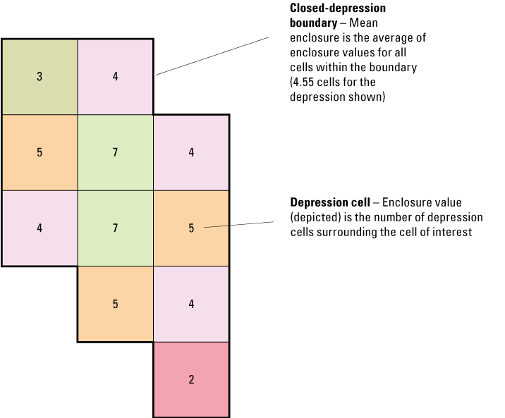
Conceptual figure showing depression cells within a closed-depression boundary and calculation of mean enclosure.
Proximity Characteristics of Depressions and Filters
If depressions can be identified in the source data for a DEM, then comparison of the source depressions to depressions derived from DEMs can provide a means to distinguish unlikely from likely depressions in DEMs (Lindsay and Creed, 2006). In topographic-contour maps, closed contours that are lower than neighboring contours can be identified as depressions. Digital contours derived from topographic-contour-based DEMs can be used as a surrogate for the source contours if they are unavailable. Closed 10-ft contours were delineated from each elevation dataset, and 30-ft buffers were created around each of the delineated preliminary depressions. Preliminary depressions whose buffers contained at least one closed 10-ft contour with an area of at least 900 square feet (ft2) that was delineated from the same preliminary depression source data were flagged and examined during assessments as an indicator of likely depressions. When contours are derived from digital elevation data such as rasters or Triangular Irregular Networks, small, closed contours with an area of less than 900 ft2 (the size of one grid cell) can be spurious artifacts of the contouring process.
DEMs can include artificial depressions caused by objects elevated above the surrounding terrain such as transportation pathways, where routing of water through culverts, into drains, or beneath small bridges is not represented (Lindsay and Creed, 2005; Poppenga and others, 2010; Zandbergen, 2010; Wall and others, 2015; fig. 4). Artificial depressions can be particularly pronounced in lidar-derived data, where more detail is captured than in coarser elevation data (Poppenga and others, 2010), such as data derived from topographic contours. Without field inspection, determining which depressions are caused by “topographic barriers,” where water is routed beneath a road or bridge, can be difficult. In artificial depressions caused by topographic barriers, the lowest elevation within the depression, or depression bottom, would often be close to the barrier (Poppenga and others, 2010). Locations of preliminary depression bottoms were delineated based on the minimum elevations and were compared to locations of detailed street (TomTom North America, Inc., and Esri, 2013b), major road (TomTom North America, Inc., and Esri, 2013c), railroad (TomTom North America, Inc., and Esri, 2013d), and airport runway (TomTom North America, Inc., and Esri, 2013a) vector digital data. Preliminary depressions with bottoms within 200 ft of these features were flagged as unlikely.
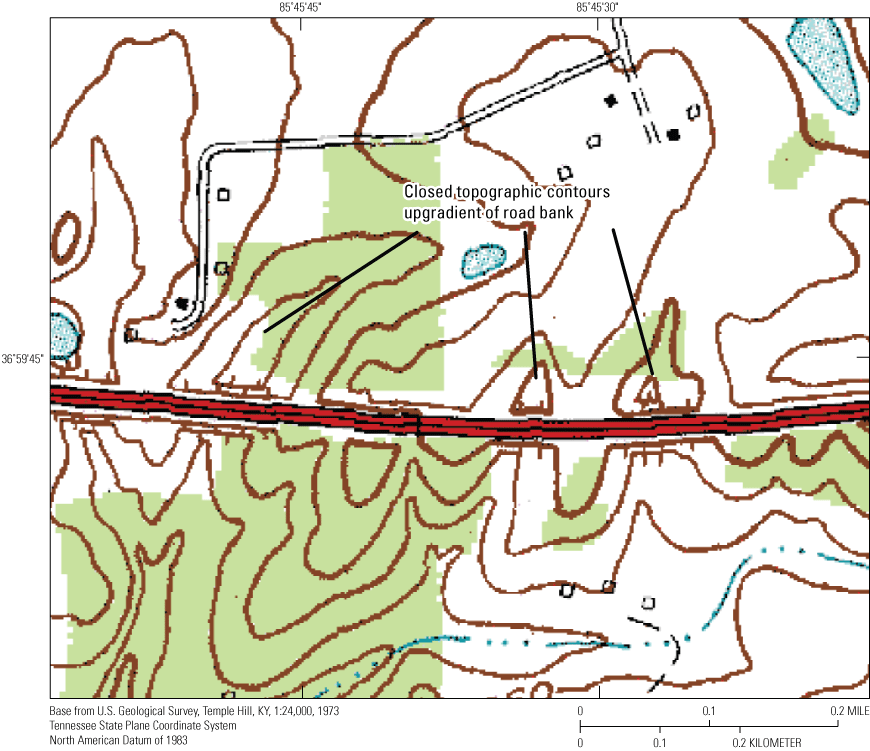
Example of a topographic map showing closed-depression contours upgradient of a road bank, creating artificial depressions.
Other off-terrain objects causing depressions include developed or impervious areas, where real depressions exist in the elevation data but are man-made or caused by development. Partly because of increased development and urbanization over time, this is a problem that is more pronounced in lidar-derived data than in data derived from topographic contours delineated decades ago. Raster cells designated as being in low-, medium-, or high-intensity developed areas from the 2011 National Land Cover Database (USGS, 2014c; Homer and others, 2015) were converted to polygon vectors. Preliminary depressions derived from the contour-based NED with bottoms that fall within polygons representing low- to high-intensity developed areas were flagged as unlikely. Preliminary depressions derived from the lidar-based NED and the TNBMP data with bottoms that fall within polygons representing low- to high-intensity developed areas were flagged as artificial.
Some preliminary depressions derived from the NED and TNBMP elevation data were located within inundated areas or boundaries of man-made hydrologic structures. Certain waterbody features and hydrographic landmarks from the NHD (USGS, variously dated b) were used to determine specific areas where preliminary depressions should be considered unlikely. These areas include (1) NHD lakes, ponds, or reservoirs intersecting connected streams derived from the NHD, (2) NHD hydrologic landmarks, such as dams or locks, and (3) sinking streams from the NHD upstream of their termination point. These features were extracted from the NHDWaterbody, NHDArea, and NHDFlowline feature classes (USGS, variously dated b), respectively. Preliminary depressions from all elevation data sources intersecting these features were flagged as artificial.
Assessment Methods for Preliminary Depressions
An assessment of preliminary depressions based on elevation accuracy and comparisons to topographic-contour source data was performed to determine proper depression-characteristic thresholds for distinguishing unlikely from likely depressions. This assessment included estimating the vertical accuracy of each elevation dataset, a numerical error propagation technique based on the estimated vertical accuracy of the elevation data in 10 test areas (fig. 5), and a comparison of preliminary depression locations to topographic-contour source data. Although all of the assessments were applied to depressions derived from each elevation dataset, different assessment methods were used to distinguish unlikely from likely depressions derived from the topographic-contour-derived NED than were used to distinguish unlikely from likely depressions derived from the lidar-derived NED and the photogrammetrically derived TNBMP data. Depressions delineated from the topographic-contour-derived NED could be assessed by using topographic-contour source data, which was in turn part of the process used to separate unlikely from likely digital depressions in the topographic-contour-based NED. The lidar-based NED and photogrammetrically based TNBMP data were derived from mass points with elevation data and break lines, which do not lend themselves to a visual or proximity-based detection of depressions.
Locations of numerical propagation test areas within the study area in Tennessee, Kentucky, and Georgia.
Elevation Accuracy Assessment and Numerical Error Propagation
Zandbergen (2010) determined that the occurrence of depressions in a DEM is strongly influenced by the DEM’s estimated vertical error. Gesch and others (2014) determined a vertical root mean square error (RMSE) of 5.08 ft for the April 2013 release of the 1/3 arc-second NED for the conterminous United States (table 1) by comparing the NED’s elevations to those from over 25,000 geodetic control points used by the National Geodetic Survey to develop the GEOID12A (National Geodetic Survey, 2012) geoid model of global mean sea level used to measure precise surface elevations at the time of this study. To verify this assessment of the NED at a local scale and to estimate the vertical accuracy of the TNBMP data, elevations from the NED and TNBMP data were compared to a subset of these geodetic control points within the study area. A vertical RMSE of 4.99 ft (table 1) was determined for the NED within the study area from a comparison with 383 geodetic control points, and a vertical RMSE of 3.31 ft was determined for the TNBMP data from a comparison with 86 geodetic control points within the study area (table 1). Although the lidar-based NED would likely have lower vertical error than the contour-based NED, not enough geodetic controls points were present in lidar-based areas to make an accurate assessment solely for the lidar-based NED; therefore, the lidar-based NED and the contour-based NED were assigned one value of vertical error. Although the geodetic control points used to assess vertical accuracy are located broadly across the extent of each elevation dataset, the distribution of elevations and general terrain conditions captured by the geodetic control points are not entirely representative of the topography within the study area. Therefore, vertical accuracy values determined in this fashion may not represent the true error associated with every grid cell in each respective DEM. Regardless, this method still represents a logical and feasible approach for estimating vertical accuracy over such a large area.
Table 1.
Absolute vertical accuracy estimates for the National Elevation Dataset and Tennessee Base Mapping Program elevation data as compared to 86 reference geodetic control points in the study area in Tennessee, Kentucky, Virginia, North Carolina, Georgia, Alabama, and Mississippi.[Accuracy assessment was done with benchmarks associated with GEOID12A from the National Geodetic Survey (2012). ft, foot; RMSE, root mean square error; NED, National Elevation Dataset (U.S. Geological Survey, 2011–12, variously dated a); TNBMP, Tennessee Base Mapping Program (Tennessee Department of Finance and Administration, 2005, 2007)]
Error statistics for April 2013 1/3 arc-second NED for the conterminous United States are from Gesch and others (2014).
Lindsay and Creed (2006) and Zandbergen (2010) describe a numerical error propagation technique to determine the probability of depression cell occurrence in a DEM based on estimated vertical accuracy and resolution of the raster representing elevation data. A similar method was applied in 10 test areas (fig. 5) within the study area to help determine depression-characteristic thresholds which might be used to distinguish unlikely from likely depressions. Of the 10 test areas, 6 were in areas where the NED was derived from 1:24,000-scale topographic contours, 4 were in areas where the NED was derived from lidar data, and TNBMP data were available for 8 of the test areas (tables 2 and 3). To apply this technique, an error raster of random, normally distributed values with a mean of zero and standard deviation roughly equal to the determined elevation RMSE was created. For the test areas composed of NED-derived DEMs, a standard deviation of 5 ft was used; for the test areas composed of TNBMP data, a standard deviation of 3 ft was used. Typically, the error raster would be smoothed and rescaled to account for spatial autocorrelation in DEM error (Lindsay and Creed, 2006; Zandbergen, 2010); however, in absence of information pertaining to the spatial autocorrelation of error in the elevation datasets, no smoothing or rescaling was performed for this study. The error raster was added to the DEM, and depressions were delineated using the previously described methods. For this study, the error raster was added to the hydroimposed DEMs instead of the raw DEMs to reduce the occurrence of depressions in and near stream channels. This process was repeated 600 times in a Monte Carlo simulation to derive a map of depression occurrence probability for each raster cell within each test area, where each raster cell was assigned a probability value between zero and one. For this study, the methods for determining depression cell occurrence probabilities described by Lindsay and Creed (2006) and Zandbergen (2010) were extended to all the cells within a preliminary depression and used to determine the probability that the depression is likely. Equation 1 was used to determine the depression probability, or the probability that at least one of the cells within each preliminary depression was part of an actual depression according to the Monte Carlo simulations. Depression probabilities determined from the Monte Carlo simulations performed with the NED and TMBMP elevation data were compared to depression metrics such as area, volume, and mean enclosure to determine if a relation exists between depression characteristics and probability, and how that relation might differ between different sources of elevation data.
wherePdep
is the depression probability, or the probability that at least one cell within a preliminary depression is truly part of a depression based on the Monte Carlo simulations, and
ρ
is the Monte-Carlo-derived occurrence probability for a cell within a preliminary depression.
A summary of preliminary depression data within each test area, including the number of preliminary depressions, number of high-probability depressions according to the Monte Carlo simulations, and high-probability depression metrics is shown in tables 2 (NED) and 3 (TNBMP data).
Table 2.
Selected statistics for preliminary depressions derived from the National Elevation Dataset within 10 numerical error propagation test areas in Tennessee, Kentucky, and Georgia.[mi2, square mile; %, percent; ft2, square foot; ft3, cubic foot; NED, National Elevation Dataset; N/A, not applicable]
| Test area (fig. 5) | Size of test area (mi2) | Karst region | Source of elevation data | Original source | Total number of preliminary depressions | Total number of preliminary depressions per square mile | Preliminary depressions with occurrence probability of at least 99% | |||
|---|---|---|---|---|---|---|---|---|---|---|
| Number (percentage of total) | Number per square mile | Average area (ft2) |
Average volume (ft3) |
|||||||
| 1 | 39.3 | Outer Nashville Basin | Lidar-based NED | Lidar1 | 9,956 | 253.33 | 914 (9.18%) | 23.26 | 64,385 | 189,613.60 |
| 2 | 3.81 | Limestone Valleys and Coves | Lidar-based NED | Lidar1 | 531 | 139.37 | 110 (20.7%) | 28.87 | 31,925 | 204,522.75 |
| 3 | 11.4 | Ridge and Valley | Lidar-based NED | Lidar1 | 438 | 38.42 | 114 (26.0%) | 10.00 | 95,132 | 496,481.96 |
| 4 | 9.61 | Ridge and Valley | Topographic- contour-based NED | 1:24,000-scale contours and hydrography1 | 331 | 34.44 | 159 (48.0%) | 16.55 | 82,868 | 565,987.19 |
| 5 | 6.74 | Ridge and Valley | Topographic-contour-based NED | 1:24,000-scale contours and hydrography1 | 197 | 29.23 | 58 (29.4%) | 8.61 | 47,964 | 437,522.71 |
| 6 | 9.67 | Western Highland Rim | Topographic-contour-based NED | 1:24,000-scale contours and hydrography1 | 258 | 26.68 | 50 (19.4%) | 5.17 | 42,372 | 125,152.32 |
| 7 | 9.58 | Eastern Highland Rim | Topographic-contour-based NED | 1:24,000-scale contours and hydrography1 | 176 | 18.37 | 46 (26.1%) | 4.80 | 177,789 | 2,280,769.10 |
| 8 | 9.58 | Eastern Highland Rim | Topographic-contour-based NED | 1:24,000-scale contours and hydrography1 | 399 | 41.65 | 51 (12.8%) | 5.32 | 18,335 | 54,703.53 |
| 9 | 7.59 | Western Pennyroyal Karst Plain and Crawford-Mammoth Cave Uplands | Lidar-based NED | Lidar1 | 987 | 130.04 | 249 (25.2%) | 32.81 | 85,171 | 337,117.84 |
| 10 | 7.59 | Western Pennyroyal Karst Plain and Crawford-Mammoth Cave Uplands | Topographic-contour-based NED | 1:24,000-scale contours and hydrography1 | 300 | 39.53 | 37 (12.3%) | 4.87 | 266,522 | 547,175.51 |
| Total | 114.87 | N/A | N/A | N/A | 13,573 | 118.16 | 1,788 (13.2%) | 15.57 | 73,526 | 327,697.02 |
Table 3.
Selected statistics for preliminary depressions derived from the Tennessee Base Mapping Program elevation data within eight numerical error propagation test areas in Tennessee.[mi2, square mile; %, percent; ft2, square foot; ft3, cubic foot; TNBMP, Tennessee Base Mapping Program; N/A, not applicable]
| Test area (fig. 5) | Size of test area (mi2) | Karst region | Source of elevation data | Original source | Total number of preliminary depressions | Total number of preliminary depressions per square mile | Preliminary depressions with occurrence probability of at least 99% | |||
|---|---|---|---|---|---|---|---|---|---|---|
| Number (percentage of total) | Number per square mile | Average area (ft2) |
Average volume (ft3) |
|||||||
| 1 | 39.3 | Outer Nashville Basin | TNBMP | 1:1,200- and 1:4,800-scale mass points and break lines1 | 2,302 | 58.6 | 607 (26.4%) | 15.44 | 95,621 | 293,527.74 |
| 2 | 3.81 | Limestone Valleys and Coves | TNBMP | 1:1,200- and 1:4,800-scale mass points and break lines1 | 341 | 89.5 | 58 (17.0%) | 15.22 | 40,795 | 253,330.28 |
| 4 | 9.61 | Ridge and Valley | TNBMP | 1:1,200- and 1:4,800-scale mass points and break lines1 | 639 | 66.5 | 141 (22.1%) | 14.67 | 80,866 | 635,659.76 |
| 5 | 6.74 | Ridge and Valley | TNBMP | 1:1,200- and 1:4,800-scale mass points and break lines1 | 260 | 38.6 | 89 (34.2%) | 13.20 | 41,208 | 289,998.41 |
| 6 | 9.67 | Western Highland Rim | TNBMP | 1:1,200- and 1:4,800-scale mass points and break lines1 | 339 | 35.1 | 68 (20.1%) | 7.03 | 49,063 | 154,472.82 |
| 7 | 9.58 | Eastern Highland Rim | TNBMP | 1:1,200- and 1:4,800-scale mass points and break lines1 | 460 | 48 | 71 (15.4%) | 7.41 | 129,321 | 1,392,867.43 |
| 8 | 9.58 | Eastern Highland Rim | TNBMP | 1:1,200- and 1:4,800-scale mass points and break lines1 | 789 | 82.4 | 95 (12.0%) | 9.92 | 32,694 | 128,154.56 |
| 10 | 7.59 | Western Pennyroyal Karst Plain and Crawford-Mammoth Cave Uplands | TNBMP | 1:1,200- and 1:4,800-scale mass points and break lines1 | 1,081 | 142.4 | 152 (14.1%) | 20.02 | 61,455 | 159,306.69 |
| Total | 95.9 | N/A | N/A | N/A | 6,211 | 64.77 | 1,281 (20.6%) | 13.36 | 78,410 | 354,480.42 |
For each elevation dataset, various combinations of thresholds for depression area, volume, and mean enclosure were compared to depression probabilities within the numerical error propagation test areas to determine thresholds that would produce low false positive (depressions that meet threshold requirements but have probabilities below 0.99) rates while producing false negative (depressions that have probabilities of at least 0.99 but did not meet the threshold requirements) rates of less than 12 percent for depressions from each dataset. The appropriate depression-characteristic thresholds were determined by iterating through various combinations of depression-characteristic values and examining the resulting false positive and false negative rates. Proper mean enclosure thresholds that could potentially eliminate some of the thin or oddly shaped large depressions were determined by visual inspection of digital depressions. The lidar-derived NED and photogrammetrically derived TNBMP elevation data that produced low false positive rates and false negative rates below 12 percent were selected as indicators of likely depressions for preliminary depressions across the entire study area. Numerical error propagation tests were not used to determine depression-characteristic thresholds for distinguishing unlikely from likely depressions in the topographic-contour-derived NED because topographic contours derived from the NED can be used to help determine whether a depression is likely in those areas; however, numerical error propagation tests used to determine depression-characteristic thresholds that produced low false positives and false negatives for depressions derived from the topographic-contour-derived NED were determined for comparison only.
Comparison of Preliminary Depressions to Topographic-Contour Source Data
Taylor and Nelson (2008) compiled karst geospatial data for the Interior Low Plateaus physiographic region (Fenneman, 1938) in the central United States, the extent of which is roughly equivalent to that of the Interior Plateau Level III ecoregion (U.S. Environmental Protection Agency, 2013) within the study area. The compilation of karst data includes points placed in apparent centroids of closed-depression contours from 1:24,000-scale topographic maps in parts of middle Tennessee and northern Alabama (Taylor and Nelson, 2008). A subset of these point locations (fig. 6) within a 17,739-mi2 test area were compared to locations of topographic-contour-based preliminary depressions derived from the NED to determine depression proximity and size characteristics that might be used to distinguish unlikely from likely depressions. The centroid locations from Taylor and Nelson (2008) were compared to locations of depressions derived from the lidar-based NED and the photogrammetry-based TNBMP data to quantify how well the topographic-contour source data matched depressions derived from other sources used in the current investigation. Depressions derived from 1:24,000-scale topographic contours are more comparable to the closed-contour centroid locations from the karst compilation than are the depressions derived from other sources; depressions derived from the lidar-based NED and the TNBMP are not based on 1:24,000-scale topographic contours and would be expected to produce a different spatial distribution of depressions than the topographic-contour-based NED.
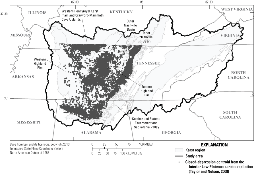
Locations of closed-depression centroids that were compared to preliminary depressions delineated from digital elevation data in middle Tennessee and northern Alabama.
Field Validation
During May through July 2014, field validations of a subset of preliminary depression features in the study area were conducted at 91 sites (fig. 7) to apply a level of quantitative accuracy to depressions derived from each dataset. The subset of preliminary depression features examined during the field visits contained unlikely depressions and those deemed likely based on characteristic criteria determined during assessments and through proximity filters. Many sites contained clusters of depressions, and the number of depressions at each site varied among elevation data sources. Field visits were conducted in each karst region within the study area except the Limestone Valleys and Coves in the Blue Ridge Level III ecoregion (figs. 2 and 7). Field validations consisted primarily of “road observations” because most sites were on private property. To help ensure visibility from the vehicle, only selected sites within a 600-ft buffer of interstates, State highways, and U.S. highways (Tele Atlas North America, Inc., and Esri, 2008) were visited initially. The buffer was later altered to cover the area from 1,000 to 2,000 ft away from the interstates, State highways, and U.S. highways (Tele Atlas North America, Inc., and Esri, 2008). The altered buffer generally minimized the number of structure-related artificial depressions encountered during the field validations but also affected site access and visibility.
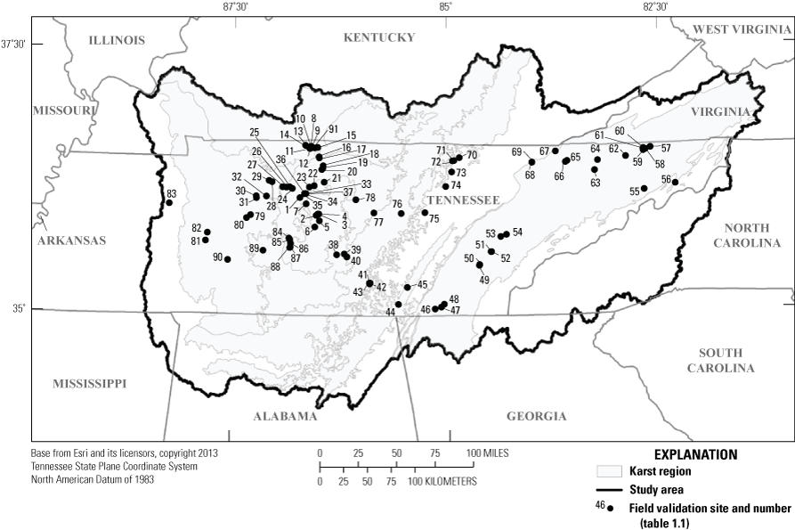
Locations of 91 field validation sites within the study area in Tennessee.
During the field visits, locations of preliminary depressions derived from all elevation sources were examined. At many sites, preliminary depressions from multiple data sources were available. In parts of the study area where the lidar-derived NED was merged into the topographic-contour-derived NED (fig. 1), elevation data derived from contours and from lidar covered the same area. At field visit locations where data were from both sources, preliminary depressions were derived from both sources to compare the preliminary depressions derived from the different elevation data sources for the NED. In all, 168 total preliminary depressions were visited at 91 sites: 66 were derived from the contour-based NED, 21 were derived from the lidar-based NED, and 81 were derived from the TNBMP data. Attempts were made in the field to determine whether each preliminary depression existed in the field and whether those existing in the field were karst depressions.
Reduction of Artificial Depressions Caused by Topographic Barriers
Prior to the delineation of the depressions that are included in Ladd (2025), methods similar to those described by Wall and others (2015) were used to approximate locations of flow pathways under topographic barriers to flow, such as roads and bridges, and enforce the pathways into the hydroimposed DEMs for each elevation dataset. In contrast to using preliminary depression proximity to topographic barriers as a filter for the identification of unlikely depressions, the methods described by Wall and others (2015) help reduce the number of artificial depressions caused by topographic barriers to flow in the DEMs by eliminating the barriers where flow is likely to cross.
Artificial depressions caused by topographic barriers are particularly prominent in DEMs derived from lidar, where more detail of the land surface is captured than in coarser elevation data (Poppenga and others, 2010), such as elevation data derived from topographic contours. Vector datasets of detailed streets (TomTom North America, Inc., and Esri, 2013b), major roads (TomTom North America, Inc., and Esri, 2013c), railroads (TomTom North America, Inc., and Esri, 2013d), and airport runways (TomTom North America, Inc., and Esri, 2013a) were acquired for the study area and were assumed to coincide with the transportation pathways that act as topographic barriers in the DEMs. In the parts of the NED derived from lidar data and in the TNBMP elevation data, where more detail of the land surface is captured than in parts of the NED derived from topographic contours, the detailed streets were used with the railroad and airport runway data to approximate locations of topographic barriers in the DEMs. The relatively less dense major road data were used with the railroad and airport runway data in the parts of the NED derived from topographic contours, where a visual inspection of the source topographic maps indicated that major roads more accurately represented topographic barriers to flow than did detailed streets. Because the set of connected streams derived from the NHD was enforced onto the hydroimposed DEMs, followed by removal of the DEM cells underlying the connected streams, connected streams already breached transportation pathways in the hydroimposed DEMs used for this analysis.
Sinking-stream features derived from the NHD were intersected with the transportation pathways. Intersections between the sinking streams and the airport runways created lines because the runways are represented by polygons; otherwise, points were created at the intersections for the remainder of the transportation pathway lines. A 100-ft buffer was created around the intersections, and the sinking-stream features were clipped to the buffers. The clipped sinking-stream features were converted to a grid, and the ArcGIS Zonal Fill tool (Esri, 2017) was used to find the minimum elevation from the hydroimposed DEMs along the boundary of the clipped sinking-stream grid within each buffered area. This minimum elevation value was assigned to the clipped stream grid segments, which acted as approximate culvert locations enforced onto the hydroimposed DEMs. The ArcGIS Fill tool (Esri, 2017) was used on the hydroimposed DEMs with enforced culvert locations to eliminate any depressions caused by transportation corridors. The ArcGIS Flow Direction tool (Esri, 2017) was used on the filled DEMs to assign a flow direction to each cell in the culvert-enforced hydroimposed DEMs, and the ArcGIS Flow Accumulation tool (Esri, 2017) was used to determine the number of cells that contribute flow to each cell in the culvert-enforced hydroimposed DEMs. From the flow accumulation grid, a synthetic stream grid of flow accumulation values of at least 5,000 cells (approximately 0.16 mi2) was generated, and the synthetic stream grid was converted to vector lines. The entire intersection, buffer, and culvert-enforcement process was repeated on the previously culvert-enforced and hydroimposed DEMs using the streamlines representing flow accumulation greater than 5,000 cells. The process was repeated a third time using streamlines representing flow accumulation greater than 120 cells (approximately 0.004 mi2) to create final culvert-enforced hydroimposed DEMs, termed “culvert-enforced DEMs” in the remainder of this report.
Delineation of Depressions, Sinking Streams, and Watersheds
Depressions were delineated by using the culvert-enforced DEMs for each elevation dataset. Depression characteristics were calculated by using the same methods used to delineate preliminary depressions. The final depressions derived from the culvert-enforced DEMs were depressions that (1) passed depression-characteristic thresholds to be deemed likely, and (2) passed the proximity filters required to remain in the depression dataset.
To delineate watersheds from each elevation dataset for depressions and sinking streams that were obtained by editing the NHD (USGS, variously dated b), custom flow direction grids were created from the culvert-enforced DEMs from each elevation dataset. The custom flow direction grids created for delineating watersheds of closed depressions from the NED and the TNBMP data were created using a different method than the one used for delineating watersheds of sinking streams. To create the custom flow direction grids for the delineation of depression watersheds, the sinking streams from the NHD were separated into two subsets composed of sinking streams that intersect depressions and those that do not. Grid cells in the culvert-enforced DEMs derived from the NED and TNBMP data were then removed from within the boundaries of depressions and from the locations of sinking streams that do not terminate within a depression, and elevation values at grid cells at the locations of sinking streams that intersect depressions were decreased by 1,000 ft. A fill process was run on the resulting grid, and a flow direction grid was created from the filled grid. To create a custom flow direction grid for delineating sinking-stream watersheds, grid cells were removed from the culvert-enforced grid derived from the NED at all sinking-stream locations. A fill process was run on the resulting grid, and a flow direction grid was created from the filled grid. The ArcGIS Watershed tool (Esri, 2017) was used to create watersheds for depressions and sinking streams from their respective custom flow direction grids. The geospatial datasets of depressions derived from the culvert-enforced DEMs, sinking streams derived from digital hydrographic data, and watersheds for the depressions and sinking streams are available in Ladd (2025).
Results and Discussion
Proximity filters and characteristic thresholds determined during preliminary depression assessments were used for separating unlikely from likely depressions. The elevation data source influences the types of characteristics and thresholds used to justify the separation. Source data that can be examined, such as contour-derived elevation data, can be used to identify false negatives (when the depression exists in the source data but is not delineated) and false positives (when the depression does not exist in the source data but is delineated). In the DEMs derived from lidar data or photogrammetry, which use mass points with elevations as a data source, topographic contours only represent a sample of the data used to create the surface and are not reliable for distinguishing unlikely from likely depressions (Lindsay and Creed, 2006). Because of the differences in the types of source data used for the DEMs in this study, different methods were used to separate unlikely from likely depressions derived from the lidar-based NED and the photogrammetrically based TNBMP data than were used to separate unlikely from likely depressions derived from the topographic-contour-based NED. In the lidar- and photogrammetry-based DEMs, numerical error propagation tests were used to assign a probability to whether a given depression was unlikely or likely. Ideally, these tests would be performed across the entire study area, but the number of simulations required to determine depression probabilities make study-area-wide application unfeasible in large areas.
For this study, depression probabilities were compared to depression size and shape characteristics, and depression-characteristic thresholds were used to help make the distinction between likely and unlikely depressions in the entire study area. For the topographic-contour-based DEMs, the depression-characteristic thresholds were used in combination with contour data to separate unlikely from likely depressions. For the lidar- and photogrammetry-based DEMs, results of numerical error propagation tests were used to determine depression-characteristic thresholds to separate unlikely from likely depressions. The contour data and characteristic thresholds were used to minimize false positives and false negatives in the delineated depressions.
For the depressions derived from the topographic-contour-based NED, false positives were defined as delineated depressions that contained a 10-ft contour derived from the contour-based NED and met depression-characteristic thresholds but did not contain a closed-depression centroid placed within contours on 1:24,000-scale topographic maps (Taylor and Nelson, 2008). False negatives were defined as closed-depression centroids that were outside of depressions delineated from the topographic-contour-derived NED that contained a 10-ft contour and met depression-characteristic thresholds. For the lidar- and photogrammetry-based DEMs, the use of depression-characteristic thresholds resulted in some false positives (depressions that meet the threshold criteria but do not have probabilities of at least 0.99) and false negatives (depressions that have a probability of at least 0.99, but do not meet the threshold criteria).
Error rates derived from numerical error propagation tests are not directly comparable to those derived from comparisons to topographic-contour source data because the primary criterion for what is considered a likely depression is different between the two assessment methods. Even if a depression contains a closed contour or is considered a likely depression based on numerical error propagation tests, the depression may still not exist on the landscape. Errors in source data, such as misrepresentations of surface flow through culverts or beneath bridges (fig. 4), or errors in the DEM interpolation process, can cause disagreement between depressions derived from DEMs and depressions in the natural landscape (Lindsay and Creed, 2006; Wall and others, 2015). Field visits are the most reliable method for determining whether a depression derived from DEM analysis actually exists in the natural landscape (Lindsay and Creed, 2006).
Numerical Error Propagation Tests
Numerical error propagation tests were used to assign likelihoods to each preliminary depression within the 10 test areas (fig. 5). The likelihoods derived from the numerical error propagation tests were used to determine depression-characteristic thresholds for separating unlikely from likely depressions delineated from the lidar- and photogrammetry-based DEMs. Ideally, tests like numerical error propagation would be used across the entire study area, allowing depression probability to be the primary distinguishing factor for unlikely and likely depressions when elevation source data cannot be used to make such a distinction; however, the number of simulations required to calculate depression probabilities makes an application unfeasible for large areas. For this study, depression probabilities were compared to selected depression characteristics to determine combined characteristic thresholds that can be applied to make the distinction between unlikely and likely depressions in the remainder of the study area.
Determining a probability threshold for likely depressions is a subjective process (Lindsay and Creed, 2006). Previous applications of numerical error propagation to determine likely depressions have been done in several ways, including assigning the maximum cell probability within a depression to the entire depression delineated from elevation data (Lindsay and Creed, 2006) and using a cell probability threshold to define the extent of likely depressions (Zandbergen, 2010). Calculating the depression probability (Pdep) as the probability that at least one cell within a depression is likely, based on the Monte Carlo simulations as was done in this study, produces a depression probability value that is heavily influenced by cell depths and the area of each depression. A comparison of volume (a function of cell depth and depression area) to Pdep indicated that all elevation data generally produced depressions with a wide range of probabilities when depression volumes were less than approximately 17,000 cubic feet (ft3). When depression volumes were greater than 17,000 ft3, all depressions had probabilities of at least 0.99 (fig. 8A). Similarly, all preliminary depressions with areas greater than approximately 12,000 ft2 had probabilities of at least 0.99 (fig. 8B), and all preliminary depressions with mean enclosure of five or more cells had probabilities of at least 0.99 (fig. 8C). The convergence of Pdep values above multiple depression-characteristic values lends credence to the choice of 0.99 as a proper threshold for high-likelihood depressions.


Scatterplots showing A, volume B, area, and C, mean enclosure compared to depression probabilities for preliminary depressions derived from the National Elevation Dataset (NED; U.S. Geological Survey, 2011–12, variously dated a) and Tennessee Base Mapping Program (Tennessee Department of Finance and Administration, 2005, 2007) elevation data within numerical error propagation test areas (fig. 5) in the study area in Tennessee, Kentucky, and Georgia.
Because the numerical error propagation tests could not be conducted across the entire study area, depression-characteristic thresholds were determined for distinguishing unlikely from likely lidar-based NED and photogrammetrically derived TNBMP depressions. Zandbergen (2010) found that using a single depression characteristic, such as depth or area, would likely lead to many incorrect classifications of unlikely and likely depressions. For depressions derived from the lidar-based NED and the TNBMP data, multiple criteria were required to consider a depression likely. For the lidar-based NED, these criteria were (1) a minimum area, volume, and mean enclosure of 2,700 ft2 (approximately 251 square meters [m2]), 31 ft3 (approximately 0.88 cubic meter [m3]), and 1.33 cells, respectively, (2) an area of at least 8,100 ft2 (approximately 753 m2) or a volume of at least 12,000 ft3 (approximately 340 m3), and (3) a mean enclosure of at least 3 cells for depressions with an area of at least 8,100 ft2 (approximately 753 m2; table 4). For depressions derived from the TNBMP elevation data, likely depressions required (1) a minimum area, volume, and mean enclosure of 2,700 ft2 (approximately 251 m2), 161 ft3 (approximately 4.56 m3), and 1.33 cells, respectively, (2) an area of at least 7,200 ft2 (approximately 204 m2) or a volume of at least 8,000 ft3 (approximately 227 m3), and (3) a mean enclosure of at least 3 cells for depressions with an area of at least 9,000 ft2 (approximately 836 m2).
Depression-characteristic thresholds determined from the numerical error propagation tests were not used to distinguish unlikely from likely depressions in the topographic-contour-derived NED, but the depression-characteristic thresholds for depressions delineated from the topographic-contour-derived NED were used for comparison of numerical error propagation results across the various elevation data. For depressions delineated from the topographic-contour-based NED, thresholds determined from the numerical error propagation tests were (1) a minimum area, volume, and mean enclosure of 3,600 ft2 (approximately 334 m2), 3 ft3 (approximately 0.08 m3), and 1.5 cells, respectively, and (2) an area of at least 6,300 ft2 (approximately 585 m2) or a volume of at least 10,000 ft3 (approximately 283 m3; table 4).
The area, volume, and mean enclosure thresholds for the depressions derived from the lidar-based NED produced a false positive rate of 3.97 percent and a false negative rate of 11.9 percent within the four numerical error propagation test areas that contained lidar data (table 4). The thresholds for depressions derived from the TNBMP data produced a false positive rate of 4.68 percent and a false negative rate of 11.9 percent within the eight numerical error propagation test areas that contained TNBMP data. The thresholds for depressions derived from the topographic-contour-based NED produced a false positive rate of 5.99 percent and a false negative rate of 8.48 percent within the six numerical propagation test areas that contained contour-derived data.
Table 4.
Preliminary depression-characteristic thresholds and error statistics within 10 numerical error propagation test sites in Tennessee, Kentucky, and Georgia.[mi2, square mile; ft2, square foot; ft3, cubic foot; NED, National Elevation Dataset (data from U.S. Geological Survey, 2011–12, variously dated a); TNBMP, Tennessee Base Mapping Program (data from Tennessee Department of Finance and Administration, 2005, 2007); N/A, not applicable; %, percent]
Although the primary aim of threshold selection is the reduction of false positives and negatives, error reduction is not the only concern. The mean enclosure characteristic calculated for this study is a measure of how surrounded each depression cell is, on average, by other depression cells. Hence, the magnitude of mean enclosure is related to both the size and shape of a depression. An increase in depression area generally relates to an increase in mean enclosure up to a logical upper limit for mean enclosure of eight cells. Depressions with relatively large areas and relatively small mean enclosure values tend to be either long and thin or oddly shaped features and can often be characteristic of man-made features and drainage ditches truncated by off-terrain objects. The application of numerical error propagation tests can result in high probabilities for these and other artificial depressions caused by off-terrain objects, providing validation for the use of higher mean enclosure thresholds for depressions with large areas; however, removal of features with relatively low mean enclosure values and large areas can lead to an increase in false negative rates as determined here.
Differences in the depression density within the numerical error propagation test areas, the characteristic threshold values, and the error rates between depressions derived from the different elevation data sources are due in part to differences in the estimated elevation error term introduced into the numerical error propagation tests and differences in source-data resolution. The error term used in the numerical error propagation tests for the TNBMP data was 3 ft, as opposed to the 5-ft error term used in the lidar- and contour-based NED. Zandbergen (2010) reported that an increase in the error term in tests performed on the same elevation data generally leads to a decrease in the number of depressions and an increase in the size of the depressions, meeting a given probability threshold. In this study, this relation was not seen when comparing different elevation data sources. The TNBMP data produced fewer preliminary depressions, fewer high-likelihood depressions, and larger (generally in terms of area and volume) high-likelihood depressions on average than the lidar-derived NED in two shared test areas (tables 2 and 3). The TNBMP data produced more preliminary depressions than the contour-based NED in six shared areas and produced more high-likelihood depressions in five of the six shared areas, although neither dataset produced clearly larger high-likelihood depressions in the shared areas (tables 2 and 3). These comparisons indicate that source-data resolution and accuracy as well as the error term used in the numerical error propagation tests influence high-likelihood depression density and size, and the differences in depression density and size influence the chosen threshold values and error rates. Further study could help verify and quantify these effects.
Error Assessment of Depressions From Topographic-Contour Source Data
For depressions derived from topographic-contour-based DEMs, a comparison to the topographic-contour source data can be helpful in distinguishing unlikely from likely depressions in DEMs. If elevation data are derived from contours, a derived depression containing at least one closed contour of the same interval as the source data can be considered a likely feature. If a depression occurs in contour-based elevation data but there is no source contour to justify it, then the depression must have resulted from the interpolation process and can safely be considered artificial (Lindsay and Creed, 2006).
In large study areas where the source topographic contours are unavailable in a digital format, digital contours derived directly from the DEM can be used to help make the distinction between unlikely and likely depressions. In the comparison of closed-contour centroids identified by Taylor and Nelson (2008) to preliminary depressions, a false positive rate of depression delineation from a DEM could be estimated by determining the number of likely depressions not containing an identified closed-depression centroid. A false negative rate could be estimated by determining the number of closed-depression centroids that do not fall within a depression derived from the DEM, although a false negative rate calculated by using this method would likely be overestimated because many DEM-derived depressions contain more than one closed-contour centroid.
Approximately 93 percent of closed-depression centroid locations identified by Taylor and Nelson (2008) were within preliminary depressions derived from the topographic-contour-based NED. Only about 78 percent of the closed-depression centroids were within preliminary depressions derived from the contour-based NED that contained a closed 10-ft contour within a 30-ft buffer of the depression, indicating that the use of 10-ft contours as a qualifier introduced up to 15 percent of additional false negatives on top of the original 6.88 percent (table 5). When including only depressions that contained a closed 10-ft contour within a 30-ft buffer around the depression, preliminary depressions delineated from the contour-based NED produced false positive rates of 95.1 percent when no filtering was used and 1.43 percent when filters were applied. Adding a minimum depression volume threshold of 5,000 ft3, a minimum mean enclosure threshold of 4.5 cells, and the contour-containing requirement for depressions delineated from the contour-based NED reduced the false positive rate by 0.8 percent (from 1.43 to 0.63 percent). These additions only increased the false negative rate by 2.5 percent (from 22.5 to 25 percent), adding justification for volume and mean enclosure thresholds for likely depressions derived from the contour-based NED.
As expected, false positive and negative rates in preliminary depressions derived from the lidar-based NED and the photogrammetry-based TNBMP data were higher than those for the depressions derived from the contour-based NED. For depressions derived from the lidar-based NED, false positive rates were 99.7 percent when no filters were used, 2.90 percent when the 10-ft contour requirement was added, and 1.29 percent when the 5,000-ft3 volume and the 4.5-cell mean enclosure thresholds were added to the contour requirement (table 5). False negative rates for depressions derived from the lidar-based NED were 38.5 percent when no filters were used, 60.1 percent when the contour requirement was applied, and 62.6 percent when the volume and mean enclosure thresholds were added.
Error rates for preliminary depressions derived from the TNBMP data were lower than those derived from the lidar-based NED, with false positive rates of 98.5 percent when no filters were applied, 3.52 percent when the contour requirement was applied, and 2.21 percent when the volume and mean enclosure thresholds were applied (table 5). False negative rates for preliminary depressions derived from the TNBMP data were 40.1 percent when no filters were applied, 55.8 percent with the contour requirement, and 56.2 percent with the volume and mean enclosure thresholds.
Table 5.
Selected error statistics from the comparison of closed-contour centroids (Taylor and Nelson, 2008) to preliminary depressions derived from all elevation data sources for the study area in Tennessee, Kentucky, Virginia, North Carolina, Georgia, Alabama, and Mississippi.[mi2, square mile; ft, foot; ft3, cubic foot; NED, National Elevation Dataset (data from U.S. Geological Survey, 2011–12, variously dated a); %, percent; TNBMP, Tennessee Base Mapping Program (data from Tennessee Department of Finance and Administration, 2005, 2007)]
When using a contour filter in depressions derived from the contour-based NED data, high error rates can occur. False positives can be caused by several factors. Some closed contours were omitted due to human error when constructing the closed-depression centroid dataset. Generally, in the 2008 study (Taylor and Nelson, 2008), closed-depression centroids were not placed in unlikely depressions caused by off-terrain objects, such as transportation pathways; however, these features often contain closed contours (fig. 4). Additionally, a 10-ft contour interval was chosen for the contour filter, but the contour interval of the source data in which the centroids were placed generally was 10 ft or greater within the test area. The inability of the DEM to accurately represent the contour source data would affect false positive and false negative rates. A DEM that does not accurately represent the source data could lead to (1) missing depressions, additional depressions, or inaccurately located depressions when compared to the source contours, and (2) missing contours, additional contours, or inaccurately located contours when compared to the source contours. Errors due to deriving contours from the DEM could be eliminated if digital source contours are available, but those related to human error, an inability to distinguish false depressions caused by off-terrain objects from likely depressions, and DEM inaccuracies in relation to the source data would remain.
Field Validation
Although numerical error propagation tests and comparisons to DEM source data can provide justification for whether a DEM-derived depression is unlikely or likely, field visits are the most reliable method for determining whether a depression actually exists in the natural landscape. Even if a DEM-derived depression is examined in the field, making determinations about whether the feature exists in the landscape and whether it is a karst feature is still a subjective and imperfect process (Lindsay and Creed, 2006). Determining the presence of depressions and karst features is particularly difficult in developed areas where the natural landscape has been modified. Recent development makes comparisons to depressions derived from topographic-contour-based DEMs especially difficult if the topographic-contour source data were mapped prior to development. Even in rural areas with mature karst, wooded areas can obscure easy viewing of depressions and limit the ability to verify the presence of depressions and karst features. Because of these difficulties, determinations could not be made at some of the field visit locations.
For preliminary depressions derived from each elevation source, comparisons were made between field determinations (including whether a depression exists in the field and whether existing depressions are karst features) and digital determinations for preliminary depressions (including whether a preliminary depression is likely based on depression-characteristic thresholds, and whether those depressions deemed likely based on thresholds are considered artificial and were removed from the dataset based on proximity filters; appendix 1). Agreement rates between field and digital determinations were calculated only for sites where a definitive field determination could be made.
For the preliminary depressions derived from the topographic-contour-based NED, the agreement between field determinations of whether a depression exists in the field and the digital determination of whether the depression is likely based on characteristic thresholds is 72.9 percent, and the agreement between field determinations of whether a depression is a karst feature and whether a depression is likely based on characteristic thresholds is 70.0 percent. After adding the proximity filters to the likely depressions derived from the contour-based NED, the agreements between the field determinations of a depression existing in the field and a depression being a karst feature also were 72.9 and 70.0 percent, respectively.
For the TNBMP-based preliminary depressions, the agreement between field determinations of whether a depression exists and the digital determination of whether the depression is likely based on characteristic thresholds is 98.6 percent, and the agreement between field determinations of whether a depression is a karst feature and whether a depression is likely based on thresholds is 79.7 percent. After adding the proximity filters to the TNBMP-based preliminary depressions, the agreements between the field determinations of a depression existing in the field and a depression being a karst feature were 82.6 and 71.9 percent, respectively.
The lidar-based preliminary depressions had the highest rate of agreement (100 percent) of all preliminary depressions between those that exist in the field and those that are deemed likely based on characteristic threshold requirements. However, the rate of agreement for whether a depression exists in the field and whether a depression is deemed likely after proximity filters are applied (63.2 percent), and the rates of agreement for whether a depression is a karst feature and whether a depression is deemed likely after characteristic thresholds (66.7 percent) and after proximity filters (53.3 percent) were applied, are all lower than rates for depressions from other sources. A few reasons could cause this discrepancy. All (100 percent) of the lidar-based preliminary depressions that were visited in the field met the characteristic thresholds to be deemed likely, which is the highest rate of visited depressions from all sources. Additionally, the visited lidar-based preliminary depressions had the highest rates of preliminary depressions deemed unlikely due to proximity to developed areas (38.1 percent) and proximity to likely depression-excluding objects in general (also 38.1 percent) compared to the visited depressions from other sources. The relatively high rate of lidar-based preliminary depressions that are influenced by development, combined with the inherent difficulty in making an accurate field determination of whether a depression is a karst feature in developed areas, likely led to a low agreement rate between whether a lidar-based preliminary depression was deemed likely after characteristic thresholds were applied and whether a depression was considered a karst feature, as well as low agreement rates between whether a lidar-based preliminary depression was deemed likely after proximity filters were applied and field determinations were made.
Reduction of Unlikely Depressions Caused by Topographic Barriers
To quantify the effect of the application of the flow pathway enforcement methods (Wall and others, 2015) in this study, the number of preliminary depressions deemed likely after passing characteristic thresholds and proximity filters and that have a bottom within 200 ft of detailed streets (TomTom North America, Inc., and Esri, 2013b), major roads (TomTom North America, Inc., and Esri, 2013c), railroads (TomTom North America, Inc., and Esri, 2013d), and airport runways (TomTom North America, Inc., and Esri, 2013a) were compared before and after the application of flow pathway enforcement. The flow pathway enforcement methods used to create the culvert-enforced DEMs used for this study led to the removal of 2,052 (10.2 percent) unlikely depressions that were caused by topographic barriers derived from the contour-based NED; 3,428 (36.7 percent) unlikely depressions derived from the lidar-based NED; and 14,330 (26.2 percent) unlikely depressions derived from the TNBMP data. The flow pathway enforcement methods will not remove all artificial depressions caused by topographic barriers from elevation data prior to the delineation of depressions (Wall and others, 2015). Quantification of the number of artificial depressions remaining in each dataset after the application of the flow pathway enforcement methods would require further study.
Depression Statistics Within Karst Regions
The depressions documented in Ladd (2025) were used to calculate statistics within each karst region in the study area. For each karst region, the density metrics and characteristics of depressions delineated from the contour-based NED, the lidar-based NED, and the TNBMP data were compared (table 6). Depressions delineated from the contour-based NED had lower densities, higher average areas, higher average volumes, and higher average mean enclosure values than the lidar-based depressions and the TNBMP-based depressions within all karst regions (table 6; fig. 9A, C–E). In general, average values of density and area within each karst region for depressions from the lidar-derived NED and the TNBMP data were more similar to one another than to the average values of density and area for depressions from the topographic-contour-based NED. DEMs derived from finely spaced mass-point data produce more depressions in general than DEMs derived from contours (MacMillan and others, 2003; Lindsay and Creed, 2005), so higher densities in depressions from the lidar-derived NED and the photogrammetrically derived TNBMP data compared to depressions from the contour-derived NED are expected. Additionally, increased surface roughness would generally lead to an increase in relatively small depressions, bringing the average depression size down in a given area.
Although average areas and volumes were smaller for depressions from the lidar-derived NED and the TNBMP data than for depressions from the contour-based NED, depressions from the lidar-based NED were generally smaller than those derived from the TNBMP data in most areas, including the Cumberland Plateau Escarpment and Sequatchie Valley, Inner Nashville Basin, Limestone Valleys and Coves, Ridge and Valley, and Western Highland Rim karst regions, as well as the parts of the study area that lie outside of a designated karst region (table 6; fig. 9C). The areal extent of depressions delineated from the contour-based NED composed a higher percentage of the Cumberland Plateau Escarpment and Sequatchie Valley, Inner Nashville Basin, and Western Pennyroyal Karst Plain and Crawford-Mammoth Cave Uplands karst regions than the lidar-based depressions, but the lidar-based NED covered less than 10 percent of these regions within the study area (table 6; fig. 9B), making density metrics for depressions derived from the lidar-based NED suspect in these areas. The areal extent of depressions delineated from the contour-based NED also composed a higher percentage of the Western Pennyroyal Karst Plain and Crawford-Mammoth Cave Uplands karst region than depressions delineated from the TNBMP elevation data, but the TNBMP elevation data also covered less than 10 percent of the Western Pennyroyal Karst Plain and Crawford-Mammoth Cave Uplands karst region (table 6; fig. 9B). Depressions from the lidar-derived NED were generally larger than those derived from the TNBMP data in the Outer Nashville Basin and Western Pennyroyal Karst Plain and Crawford-Mammoth Cave Uplands karst regions, but the lidar-derived NED and the TNBMP data composed less than 10 percent of the Western Pennyroyal Karst Plain and Crawford-Mammoth Cave Uplands karst region (table 6; fig. 9C, D).
Table 6.
Selected statistics for depressions in karst regions in the study area in Tennessee, Kentucky, Virginia, North Carolina, Georgia, Alabama, and Mississippi.[mi2, square mile; ft2, square foot; ft3, cubic foot; NED, National Elevation Dataset (data from U.S. Geological Survey, 2011–12, variously dated a); TNBMP, Tennessee Base Mapping Program (data from Tennessee Department of Finance and Administration, 2005, 2007); --, no data]
| Karst region (fig. 2) |
Total area (mi2) | Elevation data | Area within karst region with elevation data (mi2) | Number of depressions | Depression density (depressions per mi2) | Average depression area (ft2) | Average depression volume (ft3) | Average depression mean enclosure (number of cells) |
|---|---|---|---|---|---|---|---|---|
| Cumberland Plateau Escarpment and Sequatchie Valley | 4,589 | Topographic-contour-based NED | 4,501 | 2,466 | 0.55 | 362,653 | 9,379,705 | 6.32 |
| Lidar-based NED | 88.1 | 137 | 1.56 | 67,684 | 708,546 | 4.76 | ||
| TNBMP | 1,327 | 4,794 | 3.61 | 96,040 | 2,625,638 | 4.99 | ||
| Eastern Highland Rim | 7,509 | Topographic-contour-based NED | 7,509 | 11,458 | 1.53 | 378,276 | 3,092,356 | 6.63 |
| Lidar-based NED | -- | -- | -- | -- | -- | -- | ||
| TNBMP | 2,517 | 22,507 | 8.94 | 98,283 | 655,850 | 5.30 | ||
| Inner Nashville Basin | 1,670 | Topographic-contour-based NED | 1,567 | 5,151 | 3.29 | 183,703 | 721,396 | 6.40 |
| Lidar-based NED | 103 | 883 | 8.57 | 35,838 | 135,485 | 4.97 | ||
| TNBMP | 1,216 | 21,122 | 17.4 | 64,829 | 183,367 | 5.27 | ||
| Limestone Valleys and Coves | 140 | Topographic-contour-based NED | 111 | 39 | 0.35 | 135,600 | 1,557,426 | 6.47 |
| Lidar-based NED | 28.6 | 372 | 13.0 | 28,587 | 167,292 | 4.86 | ||
| TNBMP | 139 | 574 | 4.12 | 32,605 | 189,116 | 4.85 | ||
| Outer Nashville Basin | 4,751 | Topographic-contour-based NED | 4,215 | 1,814 | 0.43 | 119,816 | 800,144 | 6.25 |
| Lidar-based NED | 535 | 3,708 | 6.93 | 51,286 | 402,573 | 4.78 | ||
| TNBMP | 3,031 | 11,139 | 3.67 | 44,954 | 216,344 | 4.90 | ||
| Ridge and Valley | 10,907 | Topographic-contour-based NED | 10,465 | 24,759 | 2.37 | 130,639 | 1,619,876 | 6.25 |
| Lidar-based NED | 443 | 3,732 | 8.42 | 48,466 | 154,212 | 4.91 | ||
| TNBMP | 6,146 | 44,933 | 7.31 | 51,729 | 382,930 | 5.09 | ||
| Western Highland Rim | 7,263 | Topographic-contour-based NED | 7,044 | 1,774 | 0.25 | 142,176 | 892,200 | 6.22 |
| Lidar-based NED | 219 | 838 | 3.83 | 31,810 | 111,579 | 4.48 | ||
| TNBMP | 3,485 | 9,222 | 2.65 | 45,421 | 135,103 | 4.90 | ||
| Western Pennyroyal Karst Plain and Crawford-Mammoth Cave Uplands | 3,304 | Topographic-contour-based NED | 3,176 | 23,459 | 7.39 | 371,521 | 3,032,254 | 6.62 |
| Lidar-based NED | 129 | 1,983 | 15.4 | 80,439 | 289,459 | 5.42 | ||
| TNBMP | 113 | 1,425 | 12.6 | 59,492 | 189,769 | 5.10 | ||
| Unassigned within study area | 21,683 | Topographic-contour-based NED | 15,128 | 2,447 | 0.16 | 189,480 | 5,819,364 | 6.09 |
| Lidar-based NED | 6,554 | 6,097 | 0.93 | 29,721 | 217,898 | 4.62 | ||
| TNBMP | 6,989 | 21,101 | 3.02 | 41,506 | 586,149 | 4.62 |
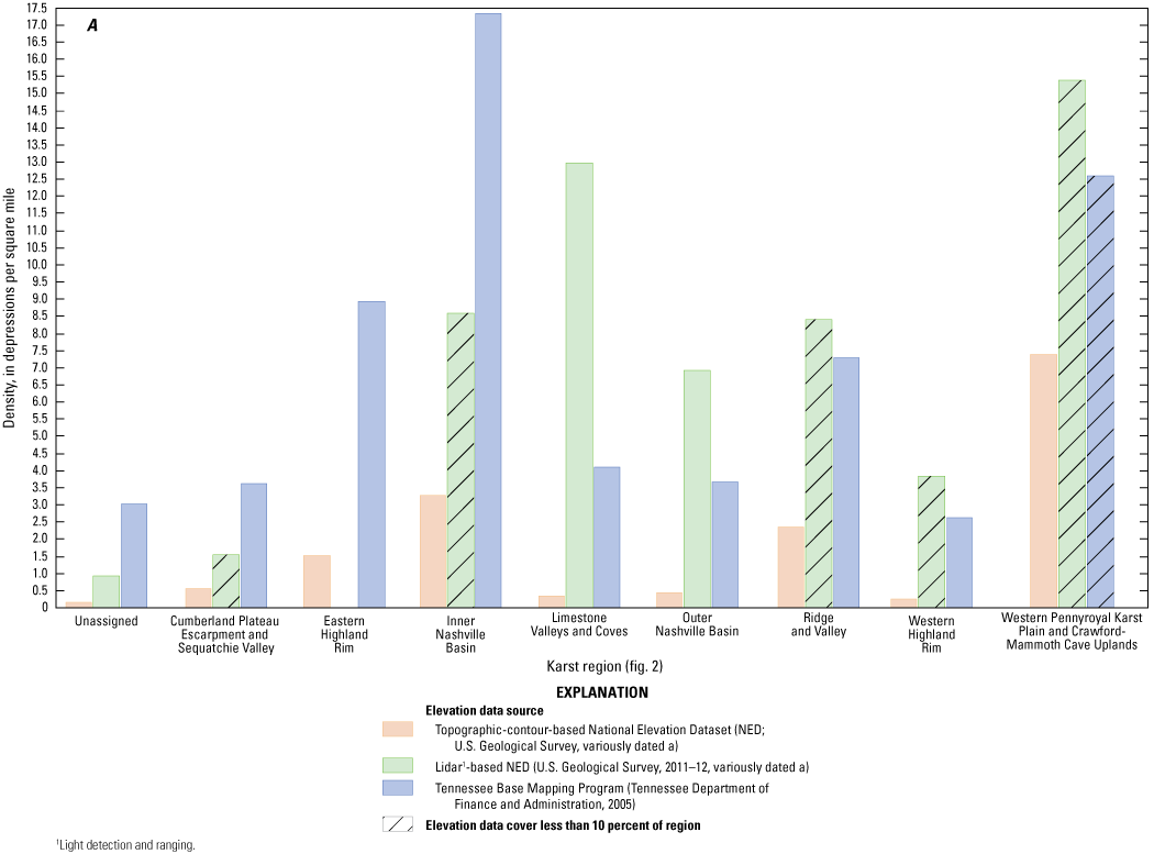


A, Density in depressions per square mile, B, depression area as percentage of karst region, C, average depression area in square feet, D, average depression volume in cubic feet, and E, average depression mean enclosure in cells within each karst region in the study area in Tennessee, Kentucky, Virginia, North Carolina, Georgia, Alabama, and Mississippi.
The differences in criteria used to separate unlikely from likely depressions complicate the direct comparison of depression density and size among elevation data sources. However, apparent density and average size trends within depressions from multiple elevation sources across karst regions can provide more evidence for the existence of those trends. The Western Pennyroyal Karst Plain and Crawford-Mammoth Cave Uplands karst region has generally high densities, high percentages of depression area, and high average areas of likely depressions from all elevation data sources (table 6; fig. 9A–C). The Cumberland Plateau Escarpment and Sequatchie Valley karst region has relatively low densities of likely depressions and low percentages of depression area from all sources but also contains relatively high average areas and the highest average volumes of depressions from all sources (table 6; fig. 9A–D). The Eastern Highland Rim, where the lidar-derived NED is absent, has the highest average area values for depressions from the contour-derived NED and the TNBMP (table 6; fig. 9C). The lowest average volumes for likely depressions from the lidar-derived NED and the TNBMP data occurred in the Western Highland Rim karst region, where the average volume for depressions from the contour-derived NED were generally low (table 6; fig. 9D). The highest average mean enclosure values for likely depressions from the contour-based NED and the TNBMP data occurred in the Eastern Highland Rim, where depressions derived from lidar are absent (table 6; fig. 9E). The highest average mean enclosure value for likely depressions from the lidar-derived NED was in the Western Pennyroyal Karst Plain and Crawford-Mammoth Cave Uplands karst region, which also had the second and third highest average mean enclosure values for depressions from the contour-based NED and the TNBMP data, respectively.
Some general discrepancies in depression density and percentage of depression area exist when different elevation data sources are used. The highest density of depressions and percentage of depression area from the contour-derived NED and the lidar-based NED occurred in the Western Pennyroyal Karst Plain and Crawford-Mammoth Cave Uplands karst region, while the highest density of depressions and percentage of depression area from the TNBMP data occurred in the Inner Nashville Basin karst region (table 6; fig. 9A, B). The lowest densities of depressions and percentages of depression area from the contour-based NED and the lidar-based NED occurred outside of designated karst regions within the study area; the density of depressions and percentage of depression area from the TNBMP data were slightly lower in the Western Highland Rim karst region than outside of designated karst regions. Within the Limestone Valleys and Coves, the density of depressions and percentage of depression area from the lidar-based NED were relatively high compared to the density values for depressions and percentages of depression area from the contour-based NED and the TNBMP data.
Summary
Closed depressions and sinking streams in karst landscapes pose difficulties in water-resources management, the construction of roads and other public works, and hydrologic and hydrogeomorphic analyses. Digital elevation models (DEMs) contain numerous depressions, including real depressions that exist in the natural landscape and artificial depressions caused by errors in the source data or in the DEM interpolation process. Unlikely depressions in the digital elevation data must be separated from likely depressions to understand the effects of likely depressions on a DEM-based hydrologic or hydrogeomorphic analysis and to obtain accurate locations of these features for water-resources protection and road construction.
The U.S. Geological Survey, in cooperation with the Tennessee Department of Transportation, conducted a study in middle Tennessee, east Tennessee, and parts of surrounding States to separate unlikely from likely depressions in DEMs and to delineate depressions, sinking streams, and watersheds of closed depressions and sinking streams by using digital hydrographic data from the National Hydrography Dataset (NHD) and two sources of elevation data: (1) the National Elevation Dataset (NED), derived from topographic-contour source data in some areas and light detection and ranging (lidar) source data in other areas and (2) photogrammetrically derived data collected by the State of Tennessee as part of the Tennessee Base Mapping Program (TNBMP). Each elevation dataset was preprocessed, a fill operation was performed on each preprocessed DEM, and filled cells were identified as locations of preliminary depressions, including all the potentially artificial and real depressions delineated from each DEM. Depression characteristics, such as area, volume, and mean enclosure, and proximity to closed 10-foot contours, certain flowline and man-made features from the NHD, transportation pathways, and developed areas were determined for each preliminary depression.
Assessments were performed to determine depression-characteristic thresholds that were used in combination with proximity filters to separate artificial from real depressions derived from each DEM. Regardless of the resolution and type of elevation source data, DEMs representing karst areas contained a large percentage of depressions that are artificial based on the results of numerical error propagation tests and comparisons to topographic-contour source data. Several approaches were used to separate unlikely from likely depressions, and the appropriate method for determining the separation depended in part on the availability and format of the elevation source data. Numerical error propagation tests were performed in 10 test areas to determine depression occurrence probabilities, which were compared to depression characteristics to determine thresholds that could be used to separate unlikely from likely depressions derived from the lidar-based NED and the TNBMP data in the study area. Depression size and shape characteristic thresholds were calculated separately for the depressions derived from the lidar-based NED and the TNBMP elevation data. Thresholds were chosen primarily to minimize false positives and false negatives in the delineated depressions based on the results of the numerical error propagation tests. Comparisons of depression characteristics to the results of numerical error propagation tests generally indicated that large depressions were more likely to be real than small depressions, providing justification for the use of size thresholds in separating unlikely from likely depressions. Once appropriate thresholds were chosen and applied, the false positive rate was 3.97 percent, and the false negative rate was 11.9 percent for the depressions derived from the lidar-based NED when compared to results of the numerical error propagation tests. The false positive rate was 4.68 percent, and the false negative rate was 11.9 percent for the depressions derived from the TNBMP elevation data when compared to the results of the numerical error propagation tests.
Because the source data for the contour-based NED could be examined and compared to locations of delineated depressions, the depression-characteristic thresholds used to separate unlikely from likely depressions delineated from the contour-based NED were determined differently than the thresholds determined for depressions derived from the lidar-based NED and the TNBMP elevation data. Locations of depressions derived from the contour-based NED were compared to topographic locations of closed-contour centroids, primarily within middle Tennessee and northern Alabama, to determine depression characteristics that could be used to separate unlikely from likely depressions derived from the contour-based NED. In this scenario, the false positive rate was 0.63 percent (the delineated depression did not contain a depression centroid), and the false negative rate was 25 percent (the depression centroid was not contained within a delineated depression). It should be noted that the error rates determined for depressions derived from the contour-based NED were calculated differently from, and are not directly comparable to, those calculated for depressions from the lidar-based NED and the TNBMP data.
Field validation is the most reliable way to determine whether a depression exists in the natural landscape, and verification methods other than field examination can only provide justification for deeming a depression artificial or real. A subset of preliminary depressions from each elevation data source, including some that were unlikely and some that met the criteria to be deemed likely, were visited at 91 sites in Tennessee to determine whether the features actually existed in the field and whether they were karst features. Field determinations of depression existence and karst-feature existence were compared to digital determinations of whether a depression qualified based on characteristic thresholds and after applying proximity filters. Examination of the depressions at field sites indicated that agreement rates between field determinations and digital determinations of depression existence decreased as the agreement criteria became more stringent. The highest rates of agreement occurred when comparing whether depressions existed in the field to whether digital depressions were deemed likely after characteristic thresholds were applied. Agreement rates decreased when field-verified karst features were compared to the digital determinations of whether depressions are likely based on characteristic thresholds. After proximity filters, such as depression proximity to certain man-made features from the NHD, were applied to the digital depressions to deem some digital depressions unlikely, agreement rates between field-verified depressions and karst features and delineated depressions from the lidar-based NED and the TNBMP elevation data decreased even more. Agreement rates between field-verified depressions and karst features and depressions delineated from the contour-based NED did not decrease after the addition of proximity filters, likely because the proximity filters for depressions derived from the contour-based NED were less stringent than those used for the depressions derived from the lidar-based NED and the TNBMP data. Depressions derived from the lidar-based NED had the highest rate of agreement (100 percent) between field-verified depressions and digital depressions deemed likely after characteristic thresholds were applied. Agreement rates between digital depressions derived from the lidar-based NED and field-verified karst features, however, were lower than digital depressions from the other sources, both before and after proximity thresholds were applied. The reduction in agreement rates was likely because most of the lidar-based depressions are in developed areas, and making a field determination of whether or not a feature is karst related is difficult in developed areas.
Prior to the final delineation of depressions, sinking streams, and watersheds of depressions and sinking streams, a flow pathway enforcement technique was used to help eliminate unlikely depressions caused by topographic barriers, such as roads, bridges, and overpasses, to flow in the DEMs. Depressions were delineated, and depression characteristics were calculated from the culvert-enforced DEMs for each elevation data source using the same methods that were used for preliminary depression delineation and characterization, and artificial depressions were separated from actual depressions based on proximity filters and characteristic thresholds determined during assessments. Watersheds for sinking streams derived by editing the NHD and for depressions were delineated using custom flow direction grids created from the culvert-enforced DEMs, depressions, and sinking streams.
For each karst region in the study area, the density and characteristics of depressions delineated from the contour-derived NED, the lidar-derived NED, and the TNBMP data were compared. Depressions delineated from the contour-based NED had lower densities, higher average areas, higher average volumes, and higher average mean enclosure values than the lidar-based depressions and the TNBMP-based depressions within all karst regions. The overall trends of depression density and size within karst regions were similar among elevation data sources in some areas. The Western Pennyroyal Karst Plain and Crawford-Mammoth Cave Uplands karst region has generally high densities, high percentages of depression area, and high average areas of depressions from all elevation data sources. The Cumberland Plateau Escarpment and Sequatchie Valley karst region has relatively low densities of likely depressions and low percentages of depression area from all sources but also contains relatively high average areas and the highest average volumes of depressions from all data sources. The Eastern Highland Rim, where the lidar-derived NED is absent, has the highest average area values for depressions from the contour-derived NED and the TNBMP. The lowest average volumes for likely depressions from the lidar-derived NED and the TNBMP data were in the Western Highland Rim karst region. The highest average mean enclosure values for likely depressions from the contour-derived NED and the TNBMP data were in the Eastern Highland Rim, where depressions derived from lidar are absent. The highest average mean enclosure value for depressions from the lidar-derived NED was in the Western Pennyroyal Karst Plain and Crawford-Mammoth Cave Uplands karst region, which had the second and third highest average mean enclosure values for depressions from the contour-derived NED and the TNBMP data, respectively.
In contrast to the similarities between depressions from the different elevation data sources, some general discrepancies in density exist. The highest density of depressions and highest percentage of depression area from the contour-derived NED and the lidar-derived NED occurred in the Western Pennyroyal Karst Plain and Crawford-Mammoth Cave Uplands karst region, and the highest density of depressions and highest percentage of depression area from the TNBMP data occurred in the Inner Nashville Basin karst region. The lowest densities of depressions and lowest percentages of depression area from the contour-derived NED and the lidar-derived NED occurred outside of designated karst regions within the study area; the density of depressions and percentage of depression area from the TNBMP data were slightly lower in the Western Highland Rim karst region than outside of designated karst regions. Within the Limestone Valleys and Coves, the density of depressions and percentage of depression area from the lidar-derived NED were relatively high compared to the density values for depressions and percentages of depression area from the contour-derived NED and the TNBMP data.
References Cited
Djokic, D., 2008, Comprehensive terrain preprocessing using Arc Hydro Tools: Esri ArcGIS web page, accessed September 22, 2014, at https://www.arcgis.com/home/item.html?id=41c96fadd2bf49ff8851002042c0495f.
Evans, G., 2014, National Elevation Dataset—February 2014 release notes: U.S. Geological Survey web page, accessed October 2, 2014, at https://ned.usgs.gov/processingNotes.html.
Gesch, D.B., Oimoen, M.J., and Evans, G.A., 2014, Accuracy assessment of the U.S. Geological Survey National Elevation Dataset, and comparison with other large-area elevation datasets—SRTM and ASTER: U.S. Geological Survey Open-File Report 2014–1008, 10 p., accessed July 24, 2024, at https://doi.org/10.3133/ofr20141008.
Hellweger, F., 1997, AGREE—DEM surface reconditioning system: Austin, Tex., University of Texas, Cockrell School of Engineering web page, accessed September 23, 2014, at https://www.ce.utexas.edu/prof/maidment/GISHYDRO/ferdi/research/agree/agree.html.
Homer, C.G., Dewitz, J.A., Yang, L., Jin, S., Danielson, P., Xian, G., Coulston, J., Herold, N.D., Wickham, J.D., and Megown, K., 2015, Completion of the 2011 National Land Cover Database for the conterminous United States—Representing a decade of land cover change information: Photogrammetric Engineering and Remote Sensing, v. 81, no. 5, p. 345–354.
Ladd, D.E., 2025, Geospatial dataset of depressions, sinking streams, and associated watersheds in karst areas of Tennessee and parts of surrounding States: U.S. Geological Survey data release, https://doi.org/10.5066/F74F1PZJ.
Lindsay, J.B., and Creed, I.F., 2005, Sensitivity of digital landscapes to artifact depressions in remotely-sensed DEMs: Photogrammetric Engineering and Remote Sensing, v. 71, no. 9, p. 1029–1036, accessed September 7, 2017, at https://www.ingentaconnect.com/content/asprs/pers/2005/00000071/00000009/art00001.
Lindsay, J.B., and Creed, I.F., 2006, Distinguishing actual and artefact depressions in digital elevation data: Computers & Geosciences, v. 32, no. 8, p. 1192–1204, accessed September 28, 2017, at https://www.sciencedirect.com/science/article/pii/S0098300405002578.
MacMillan, R.A., Martin, T.C., Earle, T.J., and McNabb, D.H., 2003, Automated analysis and classification of landforms using high-resolution digital elevation data—Applications and issues: Canadian Journal of Remote Sensing, v. 29, no. 5, p. 592–606, accessed October 1, 2017, at https://doi.org/10.5589/m03-031.
National Geodetic Survey, 2012, GPS on bench marks (GPSBM) used to make GEOID12A: National Oceanic and Atmospheric Administration, National Geodetic Survey web page, accessed September 16, 2014, at https://www.ngs.noaa.gov/GEOID/GEOID12A/GPSonBM12A.shtml.
Poppenga, S.K., Worstell, B.B., Stoker, J.M., and Greenlee, S.K., 2010, Using selective drainage methods to extract continuous surface flow from 1-meter lidar-derived digital elevation data: U.S. Geological Survey Scientific Investigations Report 2010–5059, 12 p., accessed September 7, 2017, at https://pubs.usgs.gov/sir/2010/5059/.
Tennessee Department of Finance and Administration, 2007, Tennessee Base Mapping Program—Technical specifications: Tennessee Department of Finance and Administration, Office for Information Resources, GIS Services digital data, accessed June 4, 2014, at https://gis.tn.gov/TNBMP.shtml.
U.S. Environmental Protection Agency, 2013, Shapefile of Level IV ecoregions of the conterminous United States: Corvallis, Oreg., U.S. Environmental Protection Agency, National Health and Environmental Effects Laboratory web page, accessed October 20, 2014, at https://www.epa.gov/wed/pages/ecoregions/level_iii_iv.htm.
U.S. Environmental Protection Agency and U.S. Geological Survey, 2012, National Hydrography Dataset Plus—NHDPlus: Horizon Systems Corporation database, accessed May 2014 at http://www.horizon-systems.com/NHDPlus/NHDPlusV2_data.php.
U.S. Geological Survey [USGS], 2011, National Elevation Dataset—April 2011 release notes: U.S. Geological Survey web page, accessed October 14, 2014, at https://ned.usgs.gov/processingNotes.html.
U.S. Geological Survey [USGS], 2011–12, 1/9 arc-second National Elevation Dataset: U.S. Geological Survey data release, accessed June 2013 at http://nationalmap.gov.
U.S. Geological Survey [USGS], 2014a, National Elevation Dataset—Frequently asked questions: U.S. Geological Survey web page, accessed September 25, 2014, at https://ned.usgs.gov/faq.html.
U.S. Geological Survey [USGS], 2014b, National Elevation Dataset—Spatial metadata: U.S. Geological Survey web page, accessed September 24, 2014, at https://ned.usgs.gov/downloads.html.
U.S. Geological Survey [USGS], 2014c, National Land Cover Database 2011 (NLCD 2011)—Land Cover National Geospatial Data Asset (NGDA) land use land cover (2011 ed., amended 2014): Sioux Falls, S. Dak., U.S. Geological Survey database, accessed August 23, 2017, at https://www.mrlc.gov/nlcd11_data.php.
U.S. Geological Survey [USGS], [variously dated] a, 1/3 arc-second National Elevation Dataset: U.S. Geological Survey raster data, accessed June 2011 at https://nationalmap.gov.
U.S. Geological Survey [USGS], [variously dated] b, National Hydrography Dataset: U.S. Geological Survey dataset, accessed December 2011 at https://nhd.usgs.gov/data.html.
Wall, J., Doctor, D.H., and Terziotti, S., 2015, A semi-automated tool for reducing the creation of false closed depressions from a filled lidar-derived digital elevation model, in Multidisciplinary Conference on Sinkholes and the Engineering and Environmental Impacts of Karst (14th), Rochester, Minn., October 5–9, 2015, [Proceedings]: National Cave and Karst Research Institute, p. 255–262, accessed September 7, 2017, at http://scholarcommons.usf.edu/sinkhole_2015/ProceedingswithProgram/GIS_Databases_and_Maps/5/.
Appendix 1
Table 1.1.
Field observations from 91 site visits and digital determinations of depressions derived from the National Elevation Dataset and Tennessee Base Mapping Program elevation data for the study area in Tennessee, Kentucky, Virginia, North Carolina, Georgia, Alabama, and Mississippi.[NED, National Elevation Dataset (data from U.S. Geological Survey, 2011–12, variously dated a); TNBMP, Tennessee Base Mapping Program (data from Tennessee Department of Finance and Administration, 2005, 2007); N/A, not applicable]
| Site (fig. 7) |
Elevation data | Karst region (fig. 2) | Field determinations | Digital determinations | ||
|---|---|---|---|---|---|---|
| Depression exists in field | Depression is a karst feature | Deemed likely after applying characteristic thresholds | Remains in dataset after application of proximity filters | |||
| 1 | Topographic-contour-based NED | Outer Nashville Basin | unsure | no | yes | yes |
| 1 | Lidar-based NED | Outer Nashville Basin | unsure | no | yes | no |
| 1 | TNBMP | Outer Nashville Basin | unsure | no | yes | no |
| 2 | Topographic-contour-based NED | Inner Nashville Basin | unsure | no | no | no |
| 2 | TNBMP | Inner Nashville Basin | yes | no | yes | yes |
| 3 | Topographic-contour-based NED | Inner Nashville Basin | unsure | no | no | no |
| 3 | TNBMP | Inner Nashville Basin | unsure | no | no | no |
| 3 | TNBMP | Inner Nashville Basin | yes | no | yes | no |
| 3 | TNBMP | Inner Nashville Basin | unsure | no | no | no |
| 4 | Topographic-contour-based NED | Inner Nashville Basin | yes | no | yes | yes |
| 4 | Topographic-contour-based NED | Inner Nashville Basin | yes | no | yes | yes |
| 4 | TNBMP | Inner Nashville Basin | yes | yes | yes | no |
| 5 | Topographic-contour-based NED | Inner Nashville Basin | yes | yes | yes | yes |
| 5 | TNBMP | Inner Nashville Basin | yes | yes | yes | yes |
| 6 | Topographic-contour-based NED | Inner Nashville Basin | yes | yes | yes | yes |
| 6 | TNBMP | Inner Nashville Basin | yes | yes | yes | yes |
| 7 | Topographic-contour-based NED | Outer Nashville Basin | yes | yes | yes | yes |
| 7 | Lidar-based NED | Outer Nashville Basin | yes | yes | yes | no |
| 7 | TNBMP | Outer Nashville Basin | yes | yes | yes | no |
| 8 | TNBMP | Western Pennyroyal Karst Plain and Crawford-Mammoth Cave Uplands | unsure | unsure | yes | yes |
| 9 | Topographic-contour-based NED | Western Pennyroyal Karst Plain and Crawford-Mammoth Cave Uplands | unsure | unsure | no | no |
| 9 | TNBMP | Western Pennyroyal Karst Plain and Crawford-Mammoth Cave Uplands | unsure | unsure | yes | yes |
| 10 | Topographic-contour-based NED | Western Pennyroyal Karst Plain and Crawford-Mammoth Cave Uplands | yes | no | yes | yes |
| 11 | Topographic-contour-based NED | Western Pennyroyal Karst Plain and Crawford-Mammoth Cave Uplands | yes | yes | yes | yes |
| 12 | TNBMP | Western Pennyroyal Karst Plain and Crawford-Mammoth Cave Uplands | unsure | unsure | yes | yes |
| 13 | Topographic-contour-based NED | Western Pennyroyal Karst Plain and Crawford-Mammoth Cave Uplands | yes | yes | no | no |
| 14 | Topographic-contour-based NED | Western Pennyroyal Karst Plain and Crawford-Mammoth Cave Uplands | yes | yes | yes | yes |
| 15 | Topographic-contour-based NED | Western Pennyroyal Karst Plain and Crawford-Mammoth Cave Uplands | yes | yes | yes | yes |
| 15 | TNBMP | Western Pennyroyal Karst Plain and Crawford-Mammoth Cave Uplands | yes | yes | yes | yes |
| 16 | Topographic-contour-based NED | Eastern Highland Rim | yes | no | no | no |
| 17 | TNBMP | Eastern Highland Rim | yes | no | yes | yes |
| 18 | TNBMP | Outer Nashville Basin | yes | no | yes | yes |
| 19 | TNBMP | Outer Nashville Basin | yes | unsure | yes | no |
| 20 | Topographic-contour-based NED | Outer Nashville Basin | yes | unsure | no | no |
| 20 | TNBMP | Outer Nashville Basin | yes | unsure | yes | yes |
| 21 | Topographic-contour-based NED | Inner Nashville Basin | yes | no | no | no |
| 22 | Topographic-contour-based NED | Outer Nashville Basin | yes | no | no | no |
| 22 | lidar-based NED | Outer Nashville Basin | yes | no | yes | yes |
| 23 | Topographic-contour-based NED | Outer Nashville Basin | yes | yes | yes | yes |
| 23 | Topographic-contour-based NED | Outer Nashville Basin | yes | yes | no | no |
| 23 | Lidar-based NED | Outer Nashville Basin | yes | yes | yes | yes |
| 23 | TNBMP | Outer Nashville Basin | yes | yes | yes | no |
| 24 | Topographic-contour-based NED | Outer Nashville Basin | yes | yes | no | no |
| 24 | Lidar-based NED | Outer Nashville Basin | yes | yes | yes | no |
| 24 | TNBMP | Outer Nashville Basin | yes | yes | yes | no |
| 25 | Lidar-based NED | Outer Nashville Basin | yes | no | yes | no |
| 26 | Lidar-based NED | Outer Nashville Basin | yes | no | yes | yes |
| 26 | TNBMP | Outer Nashville Basin | yes | no | yes | yes |
| 27 | Lidar-based NED | Outer Nashville Basin | yes | yes | yes | yes |
| 27 | TNBMP | Outer Nashville Basin | yes | yes | yes | yes |
| 28 | TNBMP | Western Highland Rim | unsure | no | yes | yes |
| 29 | TNBMP | Western Highland Rim | yes | unsure | yes | yes |
| 30 | TNBMP | Western Highland Rim | yes | no | yes | yes |
| 31 | Topographic-contour-based NED | Western Highland Rim | yes | no | yes | yes |
| 31 | TNBMP | Western Highland Rim | yes | no | yes | yes |
| 32 | Topographic-contour-based NED | Western Highland Rim | yes | no | yes | yes |
| 32 | Lidar-based NED | Western Highland Rim | yes | no | yes | yes |
| 32 | TNBMP | Western Highland Rim | yes | no | yes | yes |
| 33 | Topographic-contour-based NED | Outer Nashville Basin | yes | yes | yes | yes |
| 33 | Lidar-based NED | Outer Nashville Basin | yes | yes | yes | no |
| 33 | TNBMP | Outer Nashville Basin | yes | yes | yes | no |
| 34 | Topographic-contour-based NED | Outer Nashville Basin | yes | yes | yes | yes |
| 34 | Lidar-based NED | Outer Nashville Basin | yes | yes | yes | yes |
| 34 | TNBMP | Outer Nashville Basin | yes | yes | yes | yes |
| 35 | Lidar-based NED | Outer Nashville Basin | yes | yes | yes | no |
| 36 | Topographic-contour-based NED | Outer Nashville Basin | no | no | yes | yes |
| 37 | Topographic-contour-based NED | Outer Nashville Basin | unsure | unsure | yes | yes |
| 37 | Lidar-based NED | Outer Nashville Basin | unsure | unsure | yes | yes |
| 37 | TNBMP | Outer Nashville Basin | unsure | unsure | yes | yes |
| 38 | Topographic-contour-based NED | Outer Nashville Basin | yes | yes | no | no |
| 38 | Topographic-contour-based NED | Outer Nashville Basin | yes | yes | no | no |
| 38 | TNBMP | Outer Nashville Basin | yes | yes | yes | yes |
| 39 | Topographic-contour-based NED | Outer Nashville Basin | yes | yes | yes | yes |
| 39 | TNBMP | Outer Nashville Basin | yes | yes | yes | yes |
| 40 | Topographic-contour-based NED | Eastern Highland Rim | yes | unsure | yes | yes |
| 40 | TNBMP | Eastern Highland Rim | yes | unsure | yes | yes |
| 40 | TNBMP | Eastern Highland Rim | yes | unsure | yes | yes |
| 41 | Topographic-contour-based NED | Eastern Highland Rim | yes | yes | yes | yes |
| 41 | Topographic-contour-based NED | Eastern Highland Rim | yes | yes | yes | yes |
| 41 | TNBMP | Eastern Highland Rim | yes | yes | yes | yes |
| 41 | TNBMP | Eastern Highland Rim | yes | yes | yes | yes |
| 42 | Topographic-contour-based NED | Eastern Highland Rim | yes | yes | yes | yes |
| 42 | TNBMP | Eastern Highland Rim | yes | yes | yes | yes |
| 43 | TNBMP | Eastern Highland Rim | unsure | unsure | yes | yes |
| 43 | TNBMP | Eastern Highland Rim | unsure | unsure | yes | yes |
| 44 | Topographic-contour-based NED | Cumberland Plateau Escarpment and Sequatchie Valley | unsure | unsure | no | no |
| 45 | Topographic-contour-based NED | Cumberland Plateau Escarpment and Sequatchie Valley | yes | unsure | yes | yes |
| 45 | TNBMP | Cumberland Plateau Escarpment and Sequatchie Valley | yes | unsure | yes | yes |
| 46 | Lidar-based NED | Ridge and Valley | yes | unsure | yes | no |
| 46 | Lidar-based NED | Ridge and Valley | yes | unsure | yes | no |
| 46 | Lidar-based NED | Ridge and Valley | yes | unsure | yes | yes |
| 46 | Lidar-based NED | Ridge and Valley | yes | unsure | yes | yes |
| 46 | Lidar-based NED | Ridge and Valley | yes | unsure | yes | yes |
| 47 | Topographic-contour-based NED | Ridge and Valley | yes | yes | no | no |
| 47 | Lidar-based NED | Ridge and Valley | yes | yes | yes | yes |
| 48 | Lidar-based NED | Ridge and Valley | yes | yes | yes | yes |
| 48 | Lidar-based NED | Ridge and Valley | yes | yes | yes | yes |
| 49 | TNBMP | Ridge and Valley | yes | yes | yes | yes |
| 50 | Topographic-contour-based NED | Ridge and Valley | yes | no | yes | yes |
| 50 | TNBMP | Ridge and Valley | yes | no | yes | no |
| 51 | Topographic-contour-based NED | Ridge and Valley | yes | yes | no | no |
| 51 | TNBMP | Ridge and Valley | yes | yes | yes | yes |
| 51 | TNBMP | Ridge and Valley | yes | yes | yes | yes |
| 52 | Topographic-contour-based NED | Ridge and Valley | yes | yes | yes | yes |
| 52 | TNBMP | Ridge and Valley | yes | yes | yes | yes |
| 53 | TNBMP | Ridge and Valley | yes | yes | yes | yes |
| 54 | Topographic-contour-based NED | Ridge and Valley | yes | yes | yes | yes |
| 54 | TNBMP | Ridge and Valley | yes | yes | yes | yes |
| 55 | Topographic-contour-based NED | Ridge and Valley | yes | yes | yes | yes |
| 55 | TNBMP | Ridge and Valley | yes | yes | yes | yes |
| 56 | TNBMP | Ridge and Valley | yes | yes | yes | yes |
| 57 | Topographic-contour-based NED | Ridge and Valley | yes | yes | yes | yes |
| 57 | TNBMP | Ridge and Valley | yes | yes | yes | yes |
| 58 | Topographic-contour-based NED | Ridge and Valley | yes | yes | yes | yes |
| 58 | TNBMP | Ridge and Valley | yes | yes | yes | no |
| 59 | Topographic-contour-based NED | Ridge and Valley | yes | yes | yes | yes |
| 59 | TNBMP | Ridge and Valley | yes | yes | yes | yes |
| 60 | Topographic-contour-based NED | Ridge and Valley | yes | yes | yes | yes |
| 60 | TNBMP | Ridge and Valley | yes | yes | yes | yes |
| 60 | TNBMP | Ridge and Valley | yes | yes | yes | yes |
| 61 | Topographic-contour-based NED | Ridge and Valley | yes | yes | yes | yes |
| 61 | TNBMP | Ridge and Valley | yes | yes | yes | yes |
| 62 | Topographic-contour-based NED | Ridge and Valley | yes | yes | yes | yes |
| 62 | TNBMP | Ridge and Valley | yes | yes | yes | yes |
| 63 | Topographic-contour-based NED | Ridge and Valley | yes | yes | yes | yes |
| 63 | TNBMP | Ridge and Valley | yes | yes | yes | yes |
| 64 | Topographic-contour-based NED | Ridge and Valley | yes | yes | yes | yes |
| 64 | TNBMP | Ridge and Valley | yes | yes | yes | yes |
| 65 | Topographic-contour-based NED | Ridge and Valley | yes | yes | yes | yes |
| 65 | TNBMP | Ridge and Valley | yes | yes | yes | yes |
| 66 | Topographic-contour-based NED | Ridge and Valley | yes | yes | no | no |
| 67 | Topographic-contour-based NED | Ridge and Valley | yes | yes | yes | yes |
| 67 | TNBMP | Ridge and Valley | yes | yes | yes | yes |
| 68 | TNBMP | Ridge and Valley | yes | yes | yes | yes |
| 68 | TNBMP | Ridge and Valley | yes | yes | yes | yes |
| 68 | TNBMP | Ridge and Valley | yes | yes | yes | yes |
| 69 | TNBMP | Ridge and Valley | unsure | unsure | yes | yes |
| 70 | TNBMP | N/A | yes | unsure | yes | yes |
| 71 | TNBMP | N/A | yes | yes | yes | yes |
| 72 | TNBMP | N/A | yes | yes | yes | yes |
| 73 | Topographic-contour-based NED | N/A | yes | yes | no | no |
| 73 | TNBMP | N/A | yes | yes | yes | yes |
| 74 | TNBMP | N/A | yes | unsure | yes | yes |
| 75 | TNBMP | N/A | yes | yes | yes | no |
| 76 | Topographic-contour-based NED | Eastern Highland Rim | yes | yes | yes | yes |
| 76 | Topographic-contour-based NED | Eastern Highland Rim | yes | yes | yes | yes |
| 77 | TNBMP | Eastern Highland Rim | yes | yes | yes | yes |
| 78 | Topographic-contour-based NED | Outer Nashville Basin | yes | yes | yes | yes |
| 79 | Topographic-contour-based NED | Western Highland Rim | yes | yes | yes | yes |
| 79 | TNBMP | Western Highland Rim | yes | yes | yes | no |
| 80 | Topographic-contour-based NED | Western Highland Rim | unsure | unsure | no | no |
| 80 | TNBMP | Western Highland Rim | unsure | unsure | yes | yes |
| 81 | TNBMP | Western Highland Rim | yes | yes | yes | yes |
| 82 | Topographic-contour-based NED | Western Highland Rim | yes | unsure | no | no |
| 82 | TNBMP | Western Highland Rim | yes | unsure | yes | yes |
| 83 | Topographic-contour-based NED | N/A | yes | yes | yes | yes |
| 83 | TNBMP | N/A | yes | yes | yes | yes |
| 84 | Topographic-contour-based NED | Inner Nashville Basin | yes | yes | yes | yes |
| 84 | TNBMP | Inner Nashville Basin | yes | yes | no | no |
| 85 | TNBMP | Inner Nashville Basin | yes | yes | yes | yes |
| 86 | Topographic-contour-based NED | Inner Nashville Basin | yes | yes | yes | yes |
| 87 | Topographic-contour-based NED | Inner Nashville Basin | yes | yes | yes | yes |
| 88 | TNBMP | Inner Nashville Basin | yes | yes | yes | yes |
| 89 | Topographic-contour-based NED | Outer Nashville Basin | yes | yes | yes | yes |
| 89 | TNBMP | Outer Nashville Basin | yes | yes | yes | yes |
| 90 | Topographic-contour-based NED | Western Highland Rim | yes | yes | no | no |
| 90 | TNBMP | Western Highland Rim | yes | yes | yes | yes |
| 91 | TNBMP | Western Pennyroyal Karst Plain and Crawford-Mammoth Cave Uplands | yes | no | yes | yes |
Conversion Factors
U.S. customary units to International System of Units
Datums
Vertical coordinate information is referenced to the North American Vertical Datum of 1988 (NAVD 88).
Horizontal coordinate information is referenced to the North American Datum of 1983 (NAD 83).
Elevation, as used in this report, refers to distance above the vertical datum.
For more information about this publication, contact
Director, Lower Mississippi-Gulf Water Science Center
U.S. Geological Survey
640 Grassmere Park, Suite 100
Nashville, TN 37211
For additional information, visit
https://www.usgs.gov/centers/lmg-water/
Publishing support provided by
Lafayette Publishing Service Center
Disclaimers
Any use of trade, firm, or product names is for descriptive purposes only and does not imply endorsement by the U.S. Government.
Although this information product, for the most part, is in the public domain, it also may contain copyrighted materials as noted in the text. Permission to reproduce copyrighted items must be secured from the copyright owner.
Suggested Citation
Ladd, D.E., and Carmichael, J.K., 2025, Assessment and validation of depressions in digital elevation models from multiple elevation data sources and delineation of depressions, sinking streams, and their watersheds in Tennessee and parts of Kentucky, Virginia, North Carolina, Georgia, Alabama, and Mississippi: U.S. Geological Survey Scientific Investigations Report 2024–5134, 44 p., https://doi.org/10.3133/sir20245134.
ISSN: 2328-0328 (online)
Study Area
| Publication type | Report |
|---|---|
| Publication Subtype | USGS Numbered Series |
| Title | Assessment and validation of depressions in digital elevation models from multiple elevation data sources and delineation of depressions, sinking streams, and their watersheds in Tennessee and parts of Kentucky, Virginia, North Carolina, Georgia, Alabama, and Mississippi |
| Series title | Scientific Investigations Report |
| Series number | 2024-5134 |
| DOI | 10.3133/sir20245134 |
| Publication Date | June 26, 2025 |
| Year Published | 2025 |
| Language | English |
| Publisher | U.S. Geological Survey |
| Publisher location | Reston, VA |
| Contributing office(s) | Lower Mississippi-Gulf Water Science Center |
| Description | Report: viii, 44 p.; Data Release |
| Country | United States |
| State | Alabama, Georgia, Kentucky, Mississippi, North Carolina, Tennessee, Virginia |
| Online Only (Y/N) | Y |