Evaluating drought risk of the Red River of the North Basin using historical and stochastic streamflow upstream from Emerson, Manitoba

Fleford S. Redoloza; Robin L. Glas; Rochelle A. Nustad; Karen R. Ryberg

doi:10.3133/sir20255002

Evaluating Drought Risk of the Red River of the North Basin Using Historical and Stochastic Streamflow Upstream from Emerson, Manitoba

Scientific Investigations Report 2025-5002

Prepared in cooperation with the International Joint Commission, North Dakota Department of Water Resources, Red River Joint Water Resource District, and Red River Watershed Management Board

By: Fleford S. Redoloza, Robin L. Glas, Rochelle A. Nustad, and Karen R. Ryberg

https://doi.org/10.3133/sir20255002

Metrics

Web analytics dashboard Metrics definitions

Links

Document: Report (9.8 MB pdf) , HTML , XML
Dataset: USGS National Water Information System database - USGS water data for the Nation
Data Release: USGS data release - Red River of the North low flow water-balance model and supporting data
Download citation as: RIS | Dublin Core

Acknowledgments

We gratefully acknowledge the International Joint Commission, North Dakota Department of Water Resources, Red River Joint Water Resource District, Red River Watershed Management Board, and International Red River Watershed Board for their support in furthering the understanding of drought conditions in the Red River of the North Basin.

We gratefully acknowledge the assistance of Angela Gregory, formerly of the U.S. Geological Survey, for her initial efforts in this work to gather streamflow, soil characteristics, and weather data, and to develop the water-balance model grid and the block-bootstrap method for stochastic weather. We also wish to acknowledge U.S. Geological Survey colleagues Tara Williams-Sether and Ryan McShane for their helpful reviews and Todd Anderson for providing technical support.

Abstract

Drought and its effect on streamflow are important to understand because of the potential to adversely affect water supply, agricultural production, and ecological conditions. The Red River of the North Basin in north-central United States and central Canada is susceptible to dry conditions. During an extended drought, streamflow conditions in the Red River of the North may become inadequate to support existing water supply needs in the basin for agriculture, industry, human use, and aquatic life. To understand potential future low-streamflow conditions in the Red River of the North Basin, the U.S. Geological Survey, in cooperation with the International Joint Commission, North Dakota Department of Water Resources, Red River Joint Water Resource District, and Red River Watershed Management Board, developed a water-balance model of the Red River of the North Basin upstream from Emerson, Manitoba, Canada, and coupled the model with stochastic weather inputs to simulate possible future low-streamflow conditions.

Historical changes in low-streamflow conditions were characterized across the Red River of the North Basin using multiple change-point analysis for 12 streamgages. Across these stations, significant change-point years in 1943 and 1994 marked increases in the magnitude of low-streamflow conditions. During 1920–2015, conversion of primary land (not affected by human use) to agricultural and secondary land was followed by a conversion from smalls grains to corn and soybeans as the dominant crop type. From land-use analysis, 1940–2000 was determined to have relatively stable land use and therefore was used as the calibration period for the water-balance model.

A deterministic water-balance model was developed for the Red River of the North Basin upstream from Emerson, Manitoba. The water-balance model was calibrated with data from 37 U.S. Geological Survey streamgages for 1940–2000 and verified using data for 2001–15. The calibrated water-balance model simulated streamflow distributions that mirrored the seasonal patterns of the observed mean monthly streamflow and the standard deviation of the monthly streamflow data, especially during the fall and winter months when streamflow was lowest. For the verification period, during the low-streamflow months of December through January, the difference between simulated and observed data was similar to the calibration comparison and successfully reproduced seasonal trends in the distribution of streamflow, even when using weather data that were outside the calibration period.

To determine the future risk of low-streamflow conditions in the Red River of the North Basin, a block-bootstrap method was used to generate multiple possible future climates. These stochastically generated weather time series were then input to a water-balance model to simulate a distribution of possible streamflows. Three sets of experiments were performed, with each experiment containing a set of scenarios. The first set of experiments from the stochastic streamflow model were designed to investigate how changes in reservoir management would affect the distribution of low streamflow. Relative to scenario 1 (present-day [2023] reservoir operation), scenario 2 (no reservoir operation) shifted the low-streamflow frequency curves downward, reducing the annual minimum monthly streamflow for the Emerson subbasin. Subbasins were defined by the contributing area upstream from a selected streamgage station. Relative to scenario 1, scenario 3 (regulated streamflow with an increased reservoir capacity of 10 percent) shifted the low-streamflow frequency curves upward for the Emerson subbasin. The magnitude of this upward shift, caused by increased reservoir capacity, was lower than the magnitude of the shift caused by the absence of the reservoirs, which indicates that the streamflow was most affected when the reservoirs were first constructed.

The second set of experiments from the stochastic streamflow model included two scenarios that were performed to better understand how the Red River of the North Basin responds to long periods of low or high precipitation. The results indicate that the model consistently overestimated streamflow, but the relative change between a wet and dry climate state of simulated streamflow distribution reasonably matched the relative change of historical streamflow. Across the subbasins, the model was most accurate for low-streamflow conditions associated with nonexceedance probabilities between 20 and 40 percent.

The third set of experiments from the stochastic streamflow model were done to investigate low-streamflow response across the basin to several drought events. Low-end streamflow was reduced when the basin was exposed to a drought, and the magnitude of the reduction increased with longer or more intense droughts. Compared to the low-intensity drought scenarios, the range of percent reductions (as indicated by the interquartile range) was larger for the high-intensity drought scenarios for all subbasins, and the subbasins of Grand Forks and Emerson had a smaller range of reductions compared to the other three subbasins. The larger drainage area—combined with the large contribution of the Red Lake River and several other Minnesota tributaries that generally experience wetter climate conditions—upstream from the Emerson and Grand Forks subbasins may contribute to the smaller range in reductions under the high intensity scenarios. Comparison of the percent reduction in low-end streamflow among subbasins also indicated that the effects of drought duration and intensity could be cumulative. Combining factors of time and intensity produced a larger reduction in streamflow than when each effect was isolated. The array of drought scenarios can be used to determine how a subbasin would respond to multiple possible future conditions. Based on climate predictions, the drought scenario that best matches a future anticipated drought scenario can be used to estimate a low streamflow response for a given subbasin.

Introduction

Drought and its effect on streamflow is important to understand because of the potential to adversely affect water supply, agricultural production, and ecological conditions. The Red River of the North Basin (hereafter referred to as the “basin”) is susceptible to dry conditions. Low streamflows in the Red River of the North (hereafter referred to as the “Red River”) are particularly sensitive to basin-wide changes in surface and groundwater storage conditions, which in turn depend on the multidecadal balance among precipitation, evapotranspiration, runoff, and other variables; thus, historical and potential future changes in the probability distribution of low streamflow in the basin may be related to gradual climate variability; multidecadal climatic persistence (the tendency for wet or dry conditions to persist for long periods, perhaps decades, before reversing); landscape changes (such as crop types, tillage practices, surface drainage, tile drainage, and urbanization); or any combination of these factors. During an extended drought, streamflow conditions in the Red River may become inadequate to support existing water supply needs in the basin for agriculture, industry, human use, and aquatic life. The fertile soils in the basin have given rise to an economy that is dominated by agricultural production (U.S. Department of Agriculture, 2019), where drought events that cause low streamflow and soil moisture deficits can cause substantial crop and income loss. For the developed communities along the Red River corridor, such as Fargo, North Dakota, municipal water supplies would also be threatened under drought conditions (Hearne, 2007). Concern about future water supplies has led to the development of the Red River Valley Water Supply Project (RRVWSP; anticipated completion in 2027), which is an interbasin transfer of water from the Missouri River (RRVWSP, 2023). The health of fisheries, migratory bird habitats, and wetlands are also sensitive to periodic droughts in the basin, and species that are adapted to live under historically wet conditions may struggle to survive if dry conditions were to persist (U.S. Army Corps of Engineers, 2017).

The Red River starts at the confluence of the Bois de Sioux and Otter Tail Rivers at Wahpeton, N. Dak., and Breckenridge, Minnesota (fig. 1; Stoner and others, 1993). From that confluence, the Red River forms the natural border of North Dakota and Minnesota and meanders northward through the plain formed by Glacial Lake Agassiz (not shown), crossing the United States–Canada international boundary and continuing to its outlet at Lake Winnipeg, Manitoba (fig. 1). The basin comprises substantial parts of eastern North Dakota, northwestern Minnesota, and southern Manitoba, and a small portion of northeastern South Dakota (Stoner and others, 1993). The basin has a drainage area of 116,500 square kilometers (km²; International Joint Commission, 2022); this area excludes the Assiniboine River Basin, which is commonly excluded when studies are focused on areas upstream from Winnipeg, Manitoba. The Red River at the international boundary (U.S. Geological Survey [USGS] streamgage 05102500, Red River of the North at Emerson, Manitoba, operated by Environment and Climate Change Canada [ECCC] as streamgage MA05OC0001 [ECCC, 2021]), and hereafter referred to as “station 39”; fig. 1, table 1) has a drainage area 103,700 km² (USGS, 2020a).

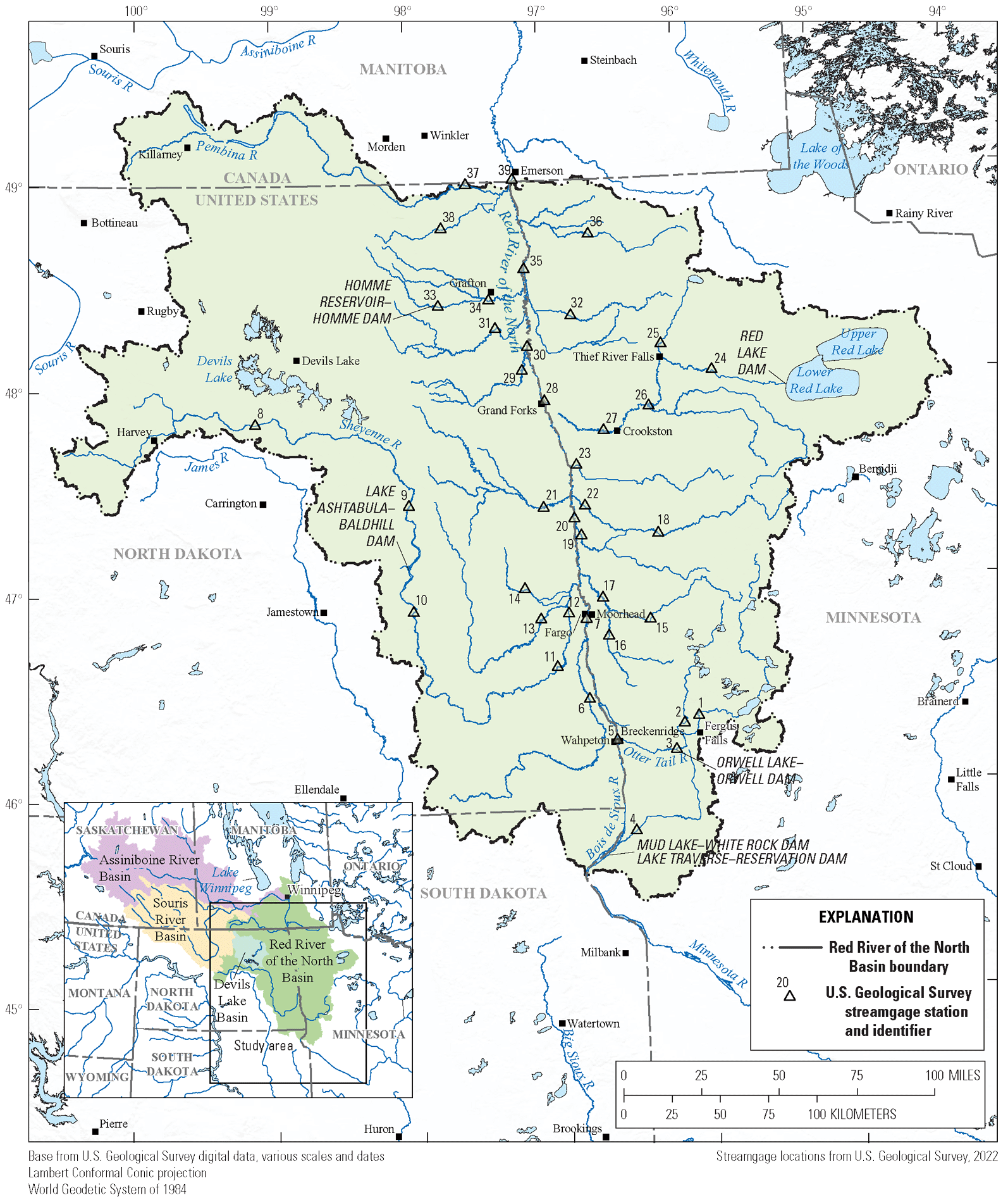
Study area with 39 streamgage stations and Red River of the North Basin boundary. — Figure 1.
Locations of selected reservoirs and streamgages in the Red River of the North Basin.

Table 1.

Selected streamgages in the Red River of the North Basin used for multiple change-point analysis and calibration of the water-balance model. Data for these streamgages are available from U.S. Geological Survey (2020a) using the U.S. Geological Survey station number.

^{[ID, identification; USGS, U.S. Geological Survey; Minn., Minnesota; WBM, water-balance
model; N. Dak., North Dakota; MCPA, multiple change-point analysis; --, not applicable;
ECCC, Environment and Climate Change Canada]}

Table 1. Selected streamgages in the Red River of the North Basin used for multiple change-point analysis and calibration of the water-balance model. Data for these streamgages are available from U.S. Geological Survey (2020a) using the U.S. Geological Survey station number.
Map ID (fig. 1)	USGS station number	Station name	Subbasin name	Analysis performed	Period of record
1	05030500	Otter Tail River near Elizabeth, Minn.	Upper Otter Tail	WBM	1904–2022
2	05040500	Pelican River near Fergus Falls, Minn.	Pelican River	WBM	1909–80
3	05046000	Otter Tail River below Orwell Dam near Fergus Fall, Minn.	Lower Otter Tail	WBM	1930–2022
4	05049000	Mustinka River above Wheaton, Minn.	Mustinka	WBM	1915–58
5	05051500	Red River of the North at Wahpeton, N. Dak.	Wahpeton	MCPA, WBM	1942–2022
6	05053000	Wild Rice River near Abercrombie, N. Dak.	South Wild Rice	WBM	1932–2022
7	05054000	Red River of the North at Fargo, N. Dak.	Fargo	MCPA, WBM	1901–2022
8	05055500	Sheyenne River at Sheyenne, N. Dak.	Upper Sheyenne	WBM	1929–51
9	05057000	Sheyenne River near Cooperstown, N. Dak.	Sheyenne to Cooperstown	WBM	1944–2022
10	05058500	Sheyenne River at Valley City, N. Dak.	Cooperstown Ashtabula	MCPA, WBM	1919–2022
11	05059000	Sheyenne River near Kindred, N. Dak.	Middle Sheyenne	WBM	1949–2022
12	05059500	Sheyenne River at West Fargo, N. Dak.	--	MCPA	1903–2022
13	05060000	Maple River near Mapleton, N. Dak.	Maple River	WBM	1958–2022
14	05060500	Rush River at Amenia, N. Dak.	Rush River	WBM	1946–2022
15	05061000	Buffalo River near Hawley, Minn.	North Buffalo	WBM	1945–2022
16	05061500	South Branch Buffalo River at Sabin, Minn.	South Buffalo	WBM	1945–2022
17	05062000	Buffalo River near Dilworth, Minn.	Lower Buffalo	WBM	1931–2022
18	05062500	Wild Rice River at Twin Valley, Minn.	--	MCPA	1909–2022
19	05064000	Wild Rice River at Hendrum, Minn.	North Wild Rice	WBM	1944–2022
20	05064500	Red River of the North at Halstad, Minn.	Halstad	WBM	1961–2022
21	05066500	Goose River at Hillsboro, N. Dak.	Goose	WBM	1931–2022
22	05067500	Marsh River near Shelly, Minn.	Marsh	WBM	1944–2022
23	05069000	SandHill River at Climax, Minn.	Sand Hill	WBM	1943–2022
24	05075000	Red Lake River at High Landing near Goodridge, Minn.	Upper Red Lake	MCPA, WBM	1929–2022
25	05076000	Thief River near Thief River Falls, Minn.	Thief	WBM	1909–2022
26	05078500	Clearwater River at Red Lake Falls, Minn.	Clearwater	MCPA, WBM	1909–2022
27	05079000	Red Lake River at Crookston, Minn.	Lower Red Lake	MCPA, WBM	1901–2022
28	05082500	Red River of the North at Grand Forks, N. Dak.	Grand Forks	MCPA, WBM	1900–2022
29	05083000	Turtle River at Manvel, N. Dak.	Turtle	WBM	1945–70
30	05083500	Red River of the North at Oslo, Minn.	Oslo	WBM	1936–76
31	05085000	Forest River at Minto, N. Dak.	Forest	WBM	1944–2022
32	05087500	Middle River at Argyle, Minn.	Middle	WBM	1945–2022
33	05089000	South Branch Park River below Homme Dam, N. Dak.	South Park	WBM	1949–94
34	05090000	Park River at Grafton, N. Dak.	Park	WBM	1931–2022
35	05092000	Red River of the North at Drayton, N. Dak.	Drayton	WBM	1936–2022
36	05094000	South Branch Two Rivers at Lake Bronson, Minn.	Two Rivers	MCPA, WBM	1928–2022
37	05100000	Pembina River at Neche, N. Dak.	Pembina	MCPA, WBM	1903–2022
38	05101000	Tongue River at Akra, N. Dak.	Tongue	WBM	1950–2022
39	05102500¹	Red River of the North at Emerson, Manitoba	Emerson	MCPA, WBM	1912–2020

¹

This site is operated by ECCC with an ECCC station number of MA05OC0001 (ECCC, 2021), but streamflow data from ECCC are stored in the National Water Information System with USGS station number 05102500 (USGS, 2020a).

The basin stands out in national flood trend studies as an area of increasing flood magnitude (Hirsch and Ryberg, 2012; Peterson and others, 2013; Hodgkins and others, 2019; Ryberg and others, 2020; Norton and others, 2022; Sando and others, 2022); however, the trend in flood magnitude may represent multidecadal persistence of the wet period that likely started in the 1970s (Kolars and others, 2016). Because of the upward trend, flood monitoring and flood protection have been a primary focus in the basin since 1997 (Ryberg and others, 2007a, 2007b 47; U.S. Army Corps of Engineers, 2011a, 2011b, 2011c, 2022b 57 58 62; Gunderson, 2021).

A switch to a multidecadal persistence of a dry period in the basin would shift the focus to drought and measures to combat drought. Relatively few studies have explicitly characterized low-streamflow conditions in the basin, and they have not included data from the past 20 years (for example, Wiche and Williams-Sether, 1997; Williams-Sether and Gross, 2016). Low-streamflow and drought conditions have happened periodically throughout the basin during the past few centuries, including a severe drought in the mid-1800s as evidenced by tree-ring analysis and historical accounts (Severson and Sieg, 2006; Lapp and others, 2013). The 1930s had several of the lowest streamflow years on record for station 39, with subsequent low-streamflow periods in 1960, 1977, and 1990 (USGS, 2020a). A 10-year drought like the Dust Bowl in the 1930s has been projected to have a detrimental $33 billion economic impact in North Dakota (RRVWSP, 2023). Historical changes in climate and runoff in the north-central United States appear to be more consistent with complex transient shifts in seasonal climatic conditions than with gradual climate change, with precipitation the primary driver as opposed to temperature, evapotranspiration, or land-use change (Ryberg and others, 2014); however, as temperature increases, climate change may become a crucial factor, with increases in evapotranspiration and summer droughts becoming more probable than spring droughts (Knapp and others, 2023). Climate change could reinforce the low-streamflow concern, with low-streamflow conditions potentially becoming the most severe in the fall and winter (de Loë, 2009).

Wet and Dry Climate States

The basin is susceptible to persistent periods of wet and dry climate states that can adversely affect ecological conditions and water supply (Vecchia, 2008; Ryberg and others, 2014; Ryberg, 2015). Research has documented that these distinct periods of hydroclimatic persistence, which lack an intermediate state, are a feature of a broader region containing the north-central United States and southern Manitoba and Saskatchewan, Canada (Burn and Goel, 2001; St. George and Nielsen, 2002; Vecchia, 2008; Ryberg and others, 2014; Razavi and others, 2015; Kolars and others, 2016; Ryberg and others, 2016b). These wet and dry climate states are visible in the sediments of Devils Lake, N. Dak., from the past 4,000 years (Bluemle, 1996), in tree-rings in the region from the past 300 years (Ryberg and others, 2016b), and in tree-rings and sediment cores in a 1,000-year reconstruction at the Waubay Lakes complex (not shown) in northeastern South Dakota just south of the basin (Shapley and others, 2005). Several historical accounts also describe persistent wet and dry states and sudden shifts between them (Rannie, 1998; Severson and Sieg, 2006; Ryberg, 2015).

In the 1990s, many USGS streamgages in the basin recorded an abrupt increase in median annual peak streamflows (Ryberg and others, 2020; Sando and others, 2022). Beginning in 1994, mean annual streamflow, 7-day low streamflow in winter, 7-day low streamflow in summer, peak streamflow because of snowmelt runoff, peak streamflow because of rainfall, and counts of high streamflow (streamflow above the mean plus one standard deviation) and extreme streamflow (streamflow above the mean plus two standard deviations) days increased in the five major river basins of Minnesota, including the Red River of the North Basin, in response to an increase in total annual precipitation during the past half century (Novotny and Stefan, 2007). This timing is consistent with Williams-Sether (1999), who documented a sudden change from dry to wet conditions in North Dakota around 1992–93. Sando and others (2022) analyzed annual peak streamflow at streamgages in the region of this basin and determined that abrupt upward trends in peak streamflow corresponded with predominantly upward trends in annual precipitation and variable (upward and downward) trends in annual air temperature. Vecchia (2008, p. 1) determined that “although future precipitation is impossible to predict, paleoclimatic evidence and recent research on climate dynamics indicate the current wet conditions are not likely to end anytime soon. For example, there is about a 72-percent likelihood wet conditions will last at least 10 more years and about a 37-percent likelihood wet conditions will last at least 30 more years.”

Climate

The basin in the United States is in a climate zone identified by the Köppen-Geiger classification system as Dfb, where D indicates that the primary climate is snow, f indicates that the precipitation conditions are fully humid, and b indicates that the temperature conditions result in warm summers (Peel and others, 2007; Ryberg and others, 2016a). This classification means that historically floods have been dominated by snowmelt runoff and low-streamflow conditions were in late summer to fall. The basin also lies in a transition zone from the humid, continental climate of the east to the semiarid climate of the Great Plains and is sensitive to relatively small changes in precipitation, temperature, and evapotranspiration (Ryberg and others, 2014, 2016a; Runkle and others, 2022). Further information about precipitation, temperature, and evapotranspiration—main water budget components—as well as their future predictions are provided in the following three sections.

Precipitation

Seasonal and annual precipitation in the basin differ spatially, where eastern parts of the basin receive higher amounts of precipitation compared to the western part (Stoner and others, 1993; Ryberg and others, 2014). Precipitation has changed temporally in the basin; it has increased in the past several decades (Williams-Sether, 1999; Wiche and others, 2000; Vecchia, 2008; Sando and others, 2022) but may still be within the range of natural climate variability (Ryberg and others, 2016b). In future climate scenarios, variability in precipitation is expected to increase (Knapp and others, 2023). Although projections are not available specifically for the basin, projections in North Dakota and Minnesota provide a general idea of future precipitation in the basin. In North Dakota, projections indicate that winter precipitation will increase, which in turn could increase soil moisture (Frankson and others, 2022). Precipitation is projected to increase in Minnesota, with increases likely in winter and spring (Runkle and others, 2022). Extreme precipitation events are also projected to increase in frequency and intensity in North Dakota, potentially leading to increased runoff and flooding (Frankson and others, 2022); however, the intensity of droughts also is projected to increase in North Dakota and Minnesota (Frankson and others, 2022; Runkle and others, 2022, Knapp and others, 2023).

Temperature

Located in the interior of North America, far from the moderating effects of the oceans, the basin experiences a wide range of temperatures (Frankson and others, 2022; Runkle and others, 2022). Like precipitation, temperature projections for North Dakota and Minnesota are expected to be indicative of the basin’s future temperature. Since the beginning of the 20th century, temperatures have increased in all four seasons in North Dakota and Minnesota, with the largest temperature increases in the winter (Frankson and others, 2022; Runkle and others, 2022). The frequency of hot summer temperatures has not increased in North Dakota, but overall warming is expected to continue and intensify heat waves (Frankson and others, 2022). In Minnesota an increase in the number of extremely hot days accompanying overall warming is expected (Runkle and others, 2022).

Evapotranspiration

Evaporation increases from east to west across the basin. Evaporation computed in energy-budget studies at Cottonwood Lake, N. Dak. (not shown; Winter and Carr, 1980), Devils Lake, N. Dak. (Wiche, 1992), and Williams Lake, Minn. (not shown; Sturrock and others, 1992), indicate that mean annual net evaporation ranges from 10.2 centimeters (cm) in the eastern part of the basin to 55.9 cm in the western part. Potential evapotranspiration (PET) is greater in the western part of the basin than in the eastern part, but actual evapotranspiration depends on the moisture available during the year (Stoner and others, 1993). Increases in evaporation rates because of rising temperatures may increase the rate of soil moisture loss and the intensity of naturally occurring droughts (Frankson and others, 2022; Runkle and others, 2022).

Reservoir Construction

Low-streamflow conditions and a history of flooding prompted reservoir construction in the basin beginning in the 1930s (Robert Halliday & Associates, 2010). Red Lake Dam (on the outlet of the Lower Red Lake to the Red Lake River; fig. 1) was completed in 1931 and was designed with a dual purpose for the U.S. Army Corps of Engineers: to impound flood water in the natural reservoir formed by Upper and Lower Red Lake and to release stored water to augment low streamflows (U.S. Army Corps of Engineers, 2020; Forum News Service and Perry, 2021). Construction of the Lake Traverse-Reservation Dam on the Bois de Sioux River began in 1936 and was completed in 1941 and was designed for flood control and water conservation during drought (U.S. Army Corps of Engineers, 2023b). Lake Ashtabula-Baldhill Dam on the Sheyenne River was authorized in 1944, put into emergency service in 1950, and completed in 1951 (U.S. Army Corps of Engineers, 2023a). The water control plan for Lake Traverse-Reservation Dam and Mud Lake-White Rock Dam is currently (2023) being updated to ensure it meets the needs of the communities and minimizes flood threats (U.S. Army Corps of Engineers, 2023b). Orwell Lake-Orwell Dam on the Otter Tail River was begun in 1951 and completed in 1953 (U.S. Army Corps of Engineers, 2023c). Construction for Homme Reservoir-Homme Dam (on the south branch of the Park River) began in 1948 and was completed in 1950 (U.S. Army Corps of Engineers, 2024). Other smaller reservoirs and dams are in the basin, but the major ones described here are operated by the U.S. Army Corps of Engineers to support emergency response to flooding in the entire basin; under low-streamflow conditions, the reservoirs and dams are managed for fish and wildlife purposes and for water supply for communities (U.S. Army Corps of Engineers, 2022a).

International Concerns about Low-Streamflow Conditions

Given the transboundary nature of the Red River, low-streamflow conditions are of concern particularly at the transboundary station, station 39. The International Joint Commission (IJC) established the International Red River Board in 2000 in response to the 1997 flood and in 2021 promoted the Board to a full watershed board named the International Red River Watershed Board (IRRWB). The IRRWB was established to help resolve transboundary disputes regarding the waters and ecosystems of the Red River, its tributaries, and aquifers (IJC, 2022). The IRRWB is tasked with establishing streamflow apportionment and future instream flow criteria for maintaining fish and fish habitat at the transboundary station. In future decades, the IRRWB could recommend steps to mitigate potential adverse effects of extreme low-streamflow conditions on fish habitat and aquatic biota in the Red River. Estimating the probability of extreme low streamflows happening during future decades would inform this effort.

Low-streamflow probabilities need to be considered in relation to land-use changes and reservoir operation. The extremely low winter streamflows of the 1930s are considered unlikely to reoccur because of the dams and reservoirs (Robert Halliday & Associates, 2010); however, reoccurrence of extremely low streamflows is dependent on the duration, intensity, and extent of drought conditions. To address concerns about potential future low-streamflow conditions in the basin, the USGS, in cooperation with the IJC, North Dakota Department of Water Resources, Red River Joint Water Resource District, and Red River Watershed Management Board developed a water-balance model (WBM) of the basin upstream from Emerson, Manitoba, and coupled the model with stochastic weather inputs to simulate possible future low-streamflow conditions. The model and associated data are available in Redoloza and others (2025).

Purpose and Scope

The purpose of this report is to describe a WBM of the basin upstream from Emerson, Manitoba, coupled with stochastic weather inputs to simulate possible future low-streamflow conditions and to present model simulation results for evaluating drought risk in the basin upstream from station 39. The stochastic streamflow model was developed in three stages that are described in subsequent sections:

1. analysis of historical changes in annual low streamflow related to changes in land use and climatic persistence;
2. development of a WBM for simulating monthly streamflow in response to climatic inputs; and
3. evaluating future drought risk by coupling stochastic climate inputs with the WBM (referred to as the stochastic streamflow model).

Analysis of Historical Changes in Low-Streamflow Conditions Related to Climatic Persistence and Land Use

Historical changes in low-streamflow conditions and land use in the basin were analyzed to guide WBM development and to aid in interpreting WBM results. Changes in low-streamflow conditions between dry and wet periods were summarized, and a period of relative land-use stability was identified and used as the calibration period for the WBM.

Data and Methods

Historical changes in low streamflow and land use across the basin were summarized using publicly available data. Sources of data and methods of aggregation are described in the following two sections.

Low Streamflow

To characterize historical changes in low streamflow, multiple change-point analysis was performed on daily mean streamflow data for USGS streamgages along the Red River and its tributaries that were downloaded from the National Water Information System (USGS, 2020a) using the R package dataRetrieval (DeCicco and others, 2023). To identify multidecadal patterns in low streamflow, streamflow data were retained for analysis if the period of record started in 1945 or earlier and if the period of record ended in 2015 or later. This date range maximized the number of stations within the basin and years of record available for analysis. Twelve streamgages met the criteria for multiple change-point analysis (table 1). To capture the months of lowest streamflows and avoid splitting the low-streamflow season (late summer to late winter) into 2 years, daily streamflow data were subdivided into climate years, which begin on April 1 and ends on March 31 of the following year.

Historical low streamflow was summarized as annual minimum monthly streamflow, defined as the minimum monthly streamflow for each climate year. This low-streamflow metric was chosen because it can be compared with the WBM, which outputs streamflow in monthly time steps. For months with at least 20 days of daily streamflow data, a mean was computed for that month. For months with fewer than 20 days of streamflow data, that month was considered missing. If a month was noted as missing during the spring runoff months (March–July), an annual minimum was still computed for that climate year. Conversely, if a month was noted as missing during August through February, when low streamflow is most likely, that climate year’s minimum was considered missing. Using the same criterion for missingness, the more common low flow metric of annual mean consecutive 30-day minimum streamflow was calculated for all streamgages to compare with the monthly timesteps of the WBM.

Climate years that were missing from the record were candidates for missing value imputation using the Maintenance of Variance Extension Type 3 (MOVE 3) methodology originally developed by Vogel and Stedinger (1985) and using the R package PFFREX (Siefken and McCarthy, 2021). Four USGS streamgages had complete daily streamflow records for 1902–2022, and eight streamgages had incomplete records but were successfully imputed using MOVE 3 for 1900–2020 (table 1). Incomplete low-streamflow records were imputed if at least 10 years of nonmissing values were overlapping, and the Pearson’s correlation coefficient was at least 0.7.

For the complete and imputed low-streamflow records of selected stations, years of abrupt change in the annual minimum monthly streamflow were identified by a multiple change-point analysis using the R package ecp (James and others, 2019). The divisive hierarchical estimation algorithm (E-divisive) was used to find change points in the mean of each streamgage low-streamflow time series; the algorithm uses a permutation test and binary bisection with a minimum of 30 years between each change point (Matteson and James, 2014). The E-divisive iterative methodology requires fewer assumptions of the data than other widely used change-point methods and does not require the user to specify the penalty type or number of change points. For each low-streamflow time series, change-point years were identified and compared to land-use changes, reservoir storage, and changes in climate states.

Land Use

To accompany the historical analysis of low streamflow, as well as to guide the calibration of the WBM, land-use and crop-cover data were compiled and aggregated for the United States part of the basin. The longest possible period was used for land use analysis and needed for WBM calibration. The period of 1920–2015 was identified. For 1920–2015, gridded annual land-use data from the Land-Use Harmonization dataset (Hurtt and others, 2020) were aggregated over the United States part of the basin to summarize large-scale land-use conversions from primary land to agricultural cropland and secondary land. In this context, primary land is defined as natural vegetation that is forested or unforested and has not been affected by human activities, such as deforestation or agriculture. Secondary land is defined as land recovering from human disturbances during the Land-Use Harmonization dataset simulation period (850–2100). To summarize changes in crop cover across the basin, county-level data from the U.S. Census of Agriculture were retrieved from the Inter-University Consortium for Political and Social Research for 1930–97 (Haines and others, 2018). Additionally, county-level crop-cover data for 1997–2017 were retrieved from the National Agricultural Statistics Service (U.S. Department of Agriculture, 2024) using the rnassqs R package (Potter, 2019). Spatially aggregated crop-cover data were plotted in time series and visually inspected to identify periods of relative land-use stability to inform the WBM calibration period.

Low-Streamflow Conditions Related to Climatic Persistence and Land Use

The time series of annual minimum monthly streamflow closely resemble the time series of the annual mean consecutive 30-day minimum streamflow for two main-stem streamgages along the Red River; the streamgages were in the headwaters at the Red River of the North at Wahpeton, N. Dak. (USGS streamgage 05051500; hereafter referred to as “station 5”; fig. 1, table 1), and downstream at station 39 (fig. 2). Change points in the annual minimum monthly streamflow that were considered statistically significant (α=0.05) for stations 39 and 5 were identified as increasing toward higher magnitudes in the early 1940s (marking the end of the Dust Bowl drought and beginning of the construction of reservoirs) and in the mid- and late-1990s (marking an increase in low streamflow with a shift toward wetter climate conditions). Notably, the annual minimum monthly streamflow has increased by nearly four times the pre-1943 mean for station 39, with increased variability in streamflow apparent in the most recent decades for stations 39 and 5 (fig. 2).

A, annual minimum monthly streamflow ranges from about 0 to 100 and mean annual minimum
monthly streamflow steps up from about 10 to 50 cubic meters per second from the beginning
to the end of the period. B, annual minimum monthly streamflow ranges from about 0
to 40 and mean annual minimum monthly streamflow steps up from about 5 to 12 cubic
meters per second. — Figure 2.
Annual minimum monthly and 30-day minimum streamflow time series with mean annual minimum monthly streamflow calculated between significant changepoints. A, Red River of the North at Emerson, Manitoba (U.S. Geological Survey streamgage 05102500; U.S. Geological Survey, 2020a). B, Red River of the North at Wahpeton, North Dakota (U.S. Geological Survey streamgage 05051500; U.S. Geological Survey, 2020a).

When considering annual minimum monthly streamflow from 1900 to 2020 for all 12 streamgages, low streamflow decreased in the early 1920s (9 stations had a significant decreasing change point between 1920 and 1924), leading into the dry period of the Dust Bowl in the 1930s (fig. 3). Most stations experienced a subsequent increase in low streamflows in 1943 (7 of 12 stations had a significant increasing change point in 1943 or 1944), consistent with reservoir construction and the end of the 1930s drought. A period of moderately increasing or steady streamflow followed across the basin for 1943–94, after which most stations experienced another significant increasing change point (11 of 12 stations had an increasing change point between 1993 and 1999) toward higher annual low streamflows that continued through climate year 2020.

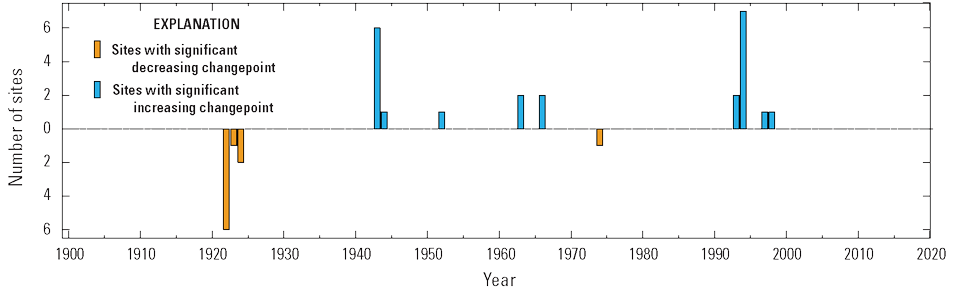
The number of sites with significant changepoints were clustered with most sites decreasing
from 1920-25 and most sites increasing in 1943-44 and 1993-94. — Figure 3.
Significant change points in the annual minimum monthly streamflow for selected streamgages in the Red River of the North Basin from 1900 to 2020.

Using the results from the multiple change-point analysis (fig. 2), the low-streamflow time series were subdivided into an extremely dry (1900–43) period and an extremely wet (1994–2020) period, marked by the most predominant change-point years, 1943 and 1994. For all 12 stations in the change-point analysis, the median percent increase in annual minimum monthly streamflow was 233 percent (table 2) from extremely dry to extremely wet periods. A previous flood risk study of the nearby Souris River Basin (Kolars and others, 2016) identified periods of dry and wet climate states for the region as 1945–69 and 1970–2011, respectively. Using a similarly subdivided record of the 12 streamgages in this analysis, climate periods were defined as dry (1940–69) and wet (1970–2015). The median percent increase from the dry to the wet climate state was 65 percent for annual minimum monthly streamflow across the basin.

Table 2.

Percent change in annual minimum monthly streamflow between wet and dry conditions at selected streamgages in the Red River of the North Basin.

^{[ID, identification; USGS, U.S. Geological Survey; MOVE 3, maintenance of variance
extension Type 3; N. Dak., North Dakota; --, not applicable; Minn., Minnesota]}

Table 2. Percent change in annual minimum monthly streamflow between wet and dry conditions at selected streamgages in the Red River of the North Basin.
Map ID (fig. 1)	USGS station number	Station name	Index station used in MOVE 3 extension	Percent change in annual¹ minimum monthly streamflow between wet and dry state
Map ID (fig. 1)	USGS station number	Station name	Index station used in MOVE 3 extension	Extremely dry state (1900–43) and extremely wet state (1994–2020)²	Dry climate state (1940–69) and wet climate state (1970–2015)³
5	05051500	Red River of the North at Wahpeton, N. Dak.	05059500	145	59
7	05054000	Red River of the North at Fargo, N. Dak.	--	364	89
10	05058500	Sheyenne River at Valley City, N. Dak.	05059500	1,634	1,523
12	05059500	Sheyenne River at West Fargo, N. Dak.	05054000	259	159
18	05062500	Wild Rice River at Twin Valley, Minn.	05054000	207	87
24	05075000	Red Lake River at High Landing near Goodridge, Minn.	05079000	168	52
26	05078500	Clearwater River at Red Lake Falls, Minn.	05062500	108	66
27	05079000	Red Lake River at Crookston, Minn.	--	118	30
28	05082500	Red River of the North at Grand Forks, N. Dak.	--	270	60
26	05094000	South Branch at Two Rivers at Lake Bronson, Minn.	05100000	158	19
37	05100000	Pembina River at Neche, N. Dak.	05059500	440	140
39	05102500	Red River of the North at Emerson, Manitoba	--	394	64
Median of percent change		All stations	--	233	65

¹

As determined from multiple change-point analysis.

²

As presented in Kolars and others (2016).

Throughout the basin, the transition from primary land to either agricultural or secondary land took place largely between 1920 and 1970 (fig. 4A). Across the basin, cropland is by far the dominant land use, covering about 80 percent of the basin. Crop types have undergone a major shift during the last century, switching from small grains to corn and soybeans as the dominant crop type around 2010 (fig. 4B). This shift is consistent with other reports citing several drivers of this crop conversion, from biofuel incentives to longer growing seasons and warmer temperatures (Johnston, 2014; Lin and Henry, 2016; O’Brien and others, 2020). After the recent wet climate state and crop type conversion from small grains to corn and soybeans, subsurface tile drainage has become more common across the basin, which lowers soil moisture and salinity concentrations (Almen and others, 2021). Given these changes in land use during the past century, 1940–2000 was identified as a period of relatively stable land use and therefore was used as the calibration period for the WBM.

About 60 to 75 percent of the basin was cropland and secondary land from 1940-2000.
Around 50 percent of the basin was hay and small grains, and 10 percent of the basin
was corn and soy from 1940-2000. After 2000, hay and small grains steadily decreased
and corn and soy steadily increased crossing over each other around 2005. — Figure 4.
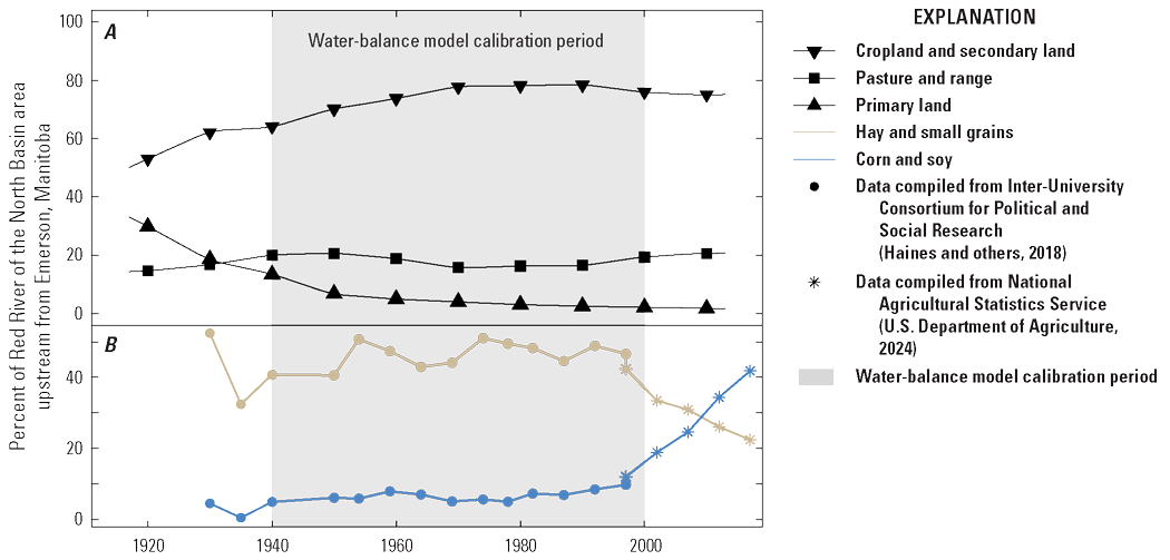
Land-use change in the Red River of the North Basin from 1920 to 2015. A, Land-use change as percentage of land area from 1920 to 2015. B, crop-cover change as percentage of land area from 1930 to 2017.

Water-Balance Model for Estimating Streamflow

A deterministic WBM—developed by Gray and McCabe (2010) and adapted by Kolars and others (2016) for the Souris River Basin—was developed for the basin (Redoloza and others, 2025). Climatic inputs of precipitation, temperature, and PET, in conjunction with basin soil properties of available water storage (AWS) and permeability, were used to simulate monthly streamflow at selected streamgages. Climatic inputs are routed through the model using equations intended to estimate the amount of water added, retained, or lost at each monthly time step. The same equations in the appendix of Kolars and others (2016) were used for the model herein, with some modifications that are explained in the “Water-Balance Model Description and Calibration” section of this report. The precipitation is partitioned into snow, rain, or a mixture of rain and snow depending on the air temperature. A 10- by 10-kilometer (km) grid was used to divide the basin into 1,515 cells. The WBM was used for this study because its explicit calculations of water processes help improve the interpretability of the model results. It also ensures that regardless of how the parameter values may change, key physical properties and hydraulic relations within the model are not violated.

Input Data for Water-Balance Model

Streamflow data were gathered from the USGS and subbasins were delineated to define streamgages as pour points. Two static inputs (soil permeability and AWS capacity) and three dynamic inputs (monthly precipitation, temperature, and PET) were used for each subbasin where streamflow was simulated.

Streamflow

Daily streamflow data were retrieved for USGS streamgages (USGS, 2020a). Any station within the basin that had streamflow records during any period from 1940 to 2015 was used, resulting in 37 streamgages (table 1) used in developing the WBM.

Watershed Delineation

Subbasins within the basin were defined by first identifying streamgages that met the streamflow record requirements. The selected streamgages were defined as pour points, identifying the outlet of each subbasin (fig. 5). Each pour point was analyzed using StreamStats (USGS, 2020b) to define the watershed boundaries upstream from the pour point. Of 38 subbasins delineated, the 37 subbasins corresponding to the streamgages were used (fig. 5). Devils Lake subbasin was not included in the model. It is a closed lake basin, and, coincident with increased streamflow in the 1990s, lake elevations rose about 10 meters (m; North Dakota Department of Water Resources, 2024). Since 2007, water has been artificially pumped from the lake to the Sheyenne River. Because pumping is unlikely under the drought conditions that are the focus of this report, the Devils Lake subbasin was excluded.

Study area with 37 subbasins. — Figure 5.
Streamgages and corresponding subbasins, designated by station identifier (table 1), used for developing the water-balance model for the Red River of the North Basin.

Soil Characteristics

Data were needed to describe soil permeability and AWS capacity in the WBM. Soil permeability and AWS capacity data for subbasins in the United States (fig. 6) were obtained from the Gridded Soil Survey Geographic Database (gSSURGO), version 2.2 (U.S. Department of Agriculture, 2020), with a map resolution of 1:24,000. Soil permeability data for the Canadian half of the Pembina subbasin (fig. 6; subbasin 37 in fig. 5) were obtained from Detailed Soil Survey (DSS) of Canada (Agriculture and Agri-Food Canada, 2020), with a map resolution of 1:100,000. Soil permeability and AWS capacity for the United States were available for the depth range of 0–100 cm from gSSURGO. Soil permeability for Canada was available from the DSS for the depth range of 0–90 cm. Soil products from gSSURGO and DSS were combined by calculating weighted means of each soil parameter to match the spatial resolution of the WBM 10- by 10-km grid (fig. 6). For the Pembina subbasin, a single constant value of 21.5 millimeters (mm) for AWS capacity was provided by Manitoba Agriculture and Resource Development, differing from the variable values provided in the gSSURGO product (fig. 6; Sung Joon Kim, Manitoba Agriculture and Resource Development, written commun., 2021). Although there is a considerable difference between AWS capacity values for the United States and Canada, there is consistency between units, and the Canadian part is a small area compared to the total area of the whole basin.

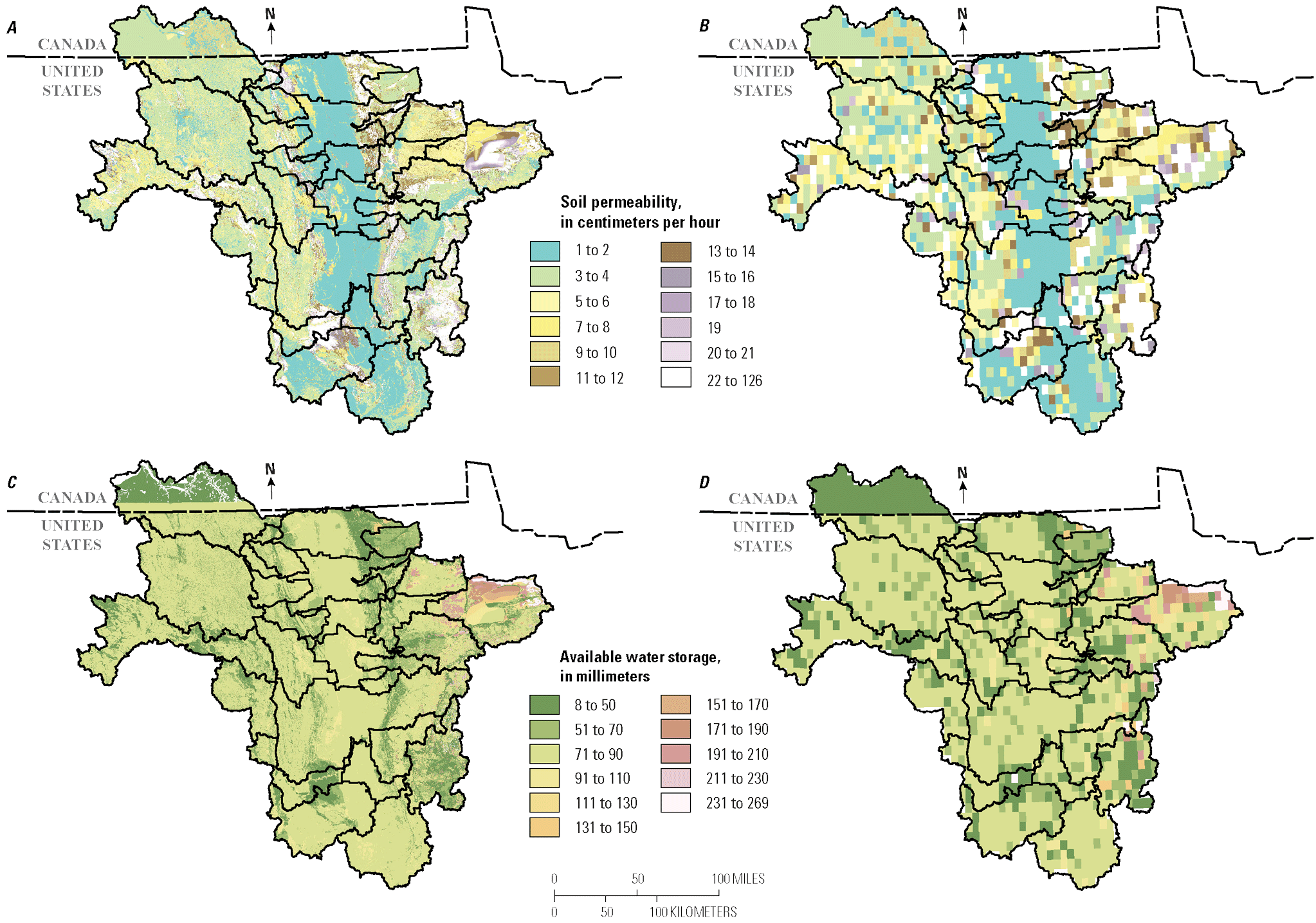
Soil permeability ranging from 1 to 126 centimeters per hour and available water storage
ranging from 8 to 269 millimeters. — Figure 6.
Soil permeability and available water storage (AWS) capacity. A, Soil permeability before data were averaged to the 10- by 10-kilometer (km) grid. B, Soil permeability after data were averaged to the 10- by 10-km grid. C, AWS before data were averaged to the 10- by 10-km grid. D, AWS after data were averaged to the 10- by 10-km grid.

Weather Data

Monthly temperature and precipitation data were retrieved from the U.S. Historical Climatology Network (National Centers for Environmental Information, 2024) and the adjusted and homogenized Canadian climate data (ECCC, 2024) for 1912–2015. Forty-three weather stations within the basin and a 1-degree buffer surrounding the basin were evaluated for completeness of data records for precipitation and temperature: 36 stations had data from 1912 to 2015, and 7 stations had differing record lengths (fig. 7). For records to be considered complete, each weather station was required to have more than 85 percent of their data between 1912 and 2015 (table 3). All seven Canadian stations were missing parts of their records, particularly from 1912 to 1920 and from 2001 to 2015. Missing data were estimated by locating the nearest weather stations with data covering the missing data period and meeting the 85-percent completeness criterion. Precipitation and temperature data were not normally distributed and were corrected by applying a cubic root to transform the data to be closer to being normally distributed. A cubic root transformation produced the closest to normally distributed data. Linear regression was used to calculate the relation between the weather station missing data from 1920 to 1959 and one or two of the closest weather stations. The weather data for 1920–59 were used because the record for this period had enough data to support a regression equation used for imputing missing data. The linear regression relation was then used to estimate periods of missing data. Once the precipitation and temperature data were adjusted with estimates for missing data, they were distributed to the model grid using the locally estimated scatterplot smoothing method (Venables and Ripley, 2002) for 1912–2015 (Redoloza and others, 2025). Lastly, PET was calculated using the Hamon method (Lu and others, 2005), with the precipitation and temperature data and solar angles calculated using latitude.

Table 3.

Selected United States and Canadian weather stations used for calibration of the water-balance model for the Red River of the North Basin.

^{[USHCN, U.S. Historical Climatology Network (National Centers for Environmental Information, 2024); --, not applicable; AHCCD, Adjusted and homogenized Canadian climate data (Environment
and Climate Change Canada, 2024)]}

Table 3. Selected United States and Canadian weather stations used for calibration of the water-balance model for the Red River of the North Basin.
Station identifier	Station name	Source	Latitude	Longitude	Period of record	Precipitation		Temperature
Station identifier	Station name	Source	Latitude	Longitude	Period of record	Missing period	Station(s) used to estimate missing period of record	Missing period	Station(s) used to estimate missing period of record
USH00210018	Ada	USHCN	47.2992	−96.5161	1912–2015	None¹	--	None¹	--
USH00210252	Argyle	USHCN	48.3311	−96.8253	1912–2015	None¹	--	None¹	--
USH00210515	Baudette	USHCN	48.7094	−94.5869	1912–2015	None¹	--	None¹	--
USH00212142	Detroit Lakes 1 North-northeast	USHCN	46.8372	−95.8372	1912–2015	None¹	--	None¹	--
USH00212916	Fosston 1 East	USHCN	47.5636	−95.7244	1912–2015	None¹	--	None¹	--
USH00213303	Grand Rapids Forest Lab	USHCN	47.2436	−93.4975	1912–2015	None¹	--	None¹	--
USH00214106	Itasca University of Minnesota	USHCN	47.2256	−95.1919	1912–2015	None¹	--	None¹	--
USH00214652	Leech Lake	USHCN	47.2467	−94.2228	1912–2015	None¹	--	None¹	--
USH00215175	Marcell 5 Northeast	USHCN	47.6308	−93.6522	1912–2015	None¹	--	None¹	--
USH00215400	Milan 1 Northwest	USHCN	45.1219	−95.9269	1912–2015	None¹	--	None¹	--
USH00215563	Montevideo 1 Southwest	USHCN	44.9364	−95.7536	1912–2015	None¹	--	None¹	--
USH00215638	Morris West Central Experiment Station	USHCN	45.5903	−95.8747	1912–2015	None¹	--	None¹	--
USH00216360	Park Rapids 2 South	USHCN	46.9006	−95.0678	1912–2015	None¹	--	None¹	--
USH00217087	Roseau	USHCN	48.8486	−95.7675	1912–2015	None¹	--	None¹	--
USH00218618	Walker Ah Gwah Ching	USHCN	47.0744	−94.57	1912–2015	None¹	--	None¹	--
USH00320941	Bottineau	USHCN	48.8214	−100.445	1912–2015	None¹	--	None¹	--
USH00321408	Casselton Agronomy Fargo-Moorhead	USHCN	46.8769	−97.2328	1912–2015	None¹	--	None¹	--
USH00323287	Fullerton 1 East-southeast	USHCN	46.1581	−98.4	1912–2015	None¹	--	None¹	--
USH00323594	Grafton	USHCN	48.4181	−97.4247	1912–2015	None¹	--	None¹	--
USH00323621	Grand Forks University National Weather Service	USHCN	47.9217	−97.0981	1912–2015	None¹	--	None¹	--
USH00324203	Hillsboro 3 North	USHCN	47.4389	−97.0664	1912–2015	None¹	--	None¹	--
USH00324418	Jamestown State Hospital	USHCN	46.8844	−98.685	1912–2015	None¹	--	None¹	--
USH00324958	Langdon Experiment Farm	USHCN	48.7622	−98.3447	1912–2015	None¹	--	None¹	--
USH00325220	Lisbon	USHCN	46.4522	−97.6822	1912–2015	None¹	--	None¹	--
USH00325479	Mandan Experiment Station	USHCN	46.8128	−100.91	1912–2015	None¹	--	None¹	--
USH00326015	Moffit 3 Southeast	USHCN	46.6706	−100.229	1912–2015	None¹	--	None¹	--
USH00326255	Napoleon	USHCN	46.5067	−99.7692	1912–2015	None¹	--	None¹	--
USH00326947	Pembina	USHCN	48.9711	−97.2417	1912–2015	None¹	--	None¹	--
USH00328792	Towner 2 Northeast	USHCN	48.3706	−100.391	1912–2015	None¹	--	None¹	--
USH00329100	Wahpeton 3 North	USHCN	46.3233	−96.6108	1912–2015	None¹	--	None¹	--
USH00329445	Willow City	USHCN	48.6061	−100.291	1912–2015	None¹	--	None¹	--
USH00390020	Aberdeen Regional Airport	USHCN	45.4433	−98.4131	1912–2015	None¹	--	None¹	--
USH00391739	Clark	USHCN	44.8817	−97.7325	1912–2015	None¹	--	None¹	--
USH00395456	Mellette 4 West	USHCN	45.155	−98.5825	1912–2015	None¹	--	None¹	--
USH00395536	Milbank 4 Northwest	USHCN	45.2836	−96.6689	1912–2015	None¹	--	None¹	--
USH00398932	Watertown Regional Airport	USHCN	44.9047	−97.1494	1912–2015	None¹	--	None¹	--
5010481	Brandon	AHCCD	49.87	−99.98	1890–2012	2012–15	Bottineau, Langdon	2008–2012	Bottineau, Langdon
5031320	Indian Bay	AHCCD	49.62	−95.2	1915–2015	1912–15 and 2007–15	Langdon, Pembina	1912–15 and 2007–15	Langdon, Pembina
5021849	Morden Experiment Farm	AHCCD	49.18	−98.08	1888–2007	2007–2015	Langdon, Pembina	Small gaps, 1999	Langdon, Pembina
5032162	Pinawa	AHCCD	50.18	−96.07	1915–2015	1912–15 and 2011–15	Roseau, Pembina	1912–15 and 2014–15	Roseau, Pembina
5022759	Sprague	AHCCD	49.02	−95.6	1916–2007	1912–16 and 2007–15	Roseau, Baudette	1912–15	Roseau, Baudette
5023222	Winnipeg	AHCCD	49.92	−97.23	1872–2007	2007–2015	Pembina	2007–2015	Pembina
6022476	Fort Frances	AHCCD	48.65	−93.43	1912–2011	2011–2015	Baudette	1912–1915	Baudette

¹

Some small gaps, but more than 85 percent of the values were available.

15 weather stations are in the basin and 28 weather stations are in the 1-degree buffer
around the basin. — Figure 7.
Locations of meteorological stations in and near the Red River of the North Basin used for calibrating the water-balance model.

Water-Balance Model Description and Calibration

The WBM requires a monthly time series of weather data as input. The WBM iterates over each cell in the model domain and each month in the model period, using precipitation, temperature, and several other parameters to calculate the monthly water volume that a given cell contributes to its corresponding subbasin outlet (fig. 8). The result is an estimate of monthly streamflow for each subbasin. After the monthly streamflow for each subbasin is calculated, all water contributions from each subbasin are directed through streamflow routing that corresponds to the appropriate hydrologic connections. The outflow of a subbasin is equal to the sum of the contributions of the local cells and the contributions of all the subbasins that are upstream from the given subbasin. Some of the streamflow is directed to reservoirs. At the reservoirs, reservoir outflow was determined by calculating the output volume necessary to meet a target water volume change for the current month, which is the mean total volume change in the reservoir for that month. The target volume change was first determined by calculating the difference between the observed inflows and outflows of the reservoirs. Once the mean volume changes for the reservoirs were calculated, reservoir outflows were adjusted so that the mean reservoir changes for each month matched the historical changes. The result was a WBM for the basin that could estimate the monthly streamflow at 37 streamgages for the given weather conditions.

Precipitation represented as an arrow falls as rain or snow and either goes into the
soil box or the snow-pack box. From each of the boxes, arrows and lines representing
different processes show how the water eventually becomes runoff into the stream. — Figure 8.
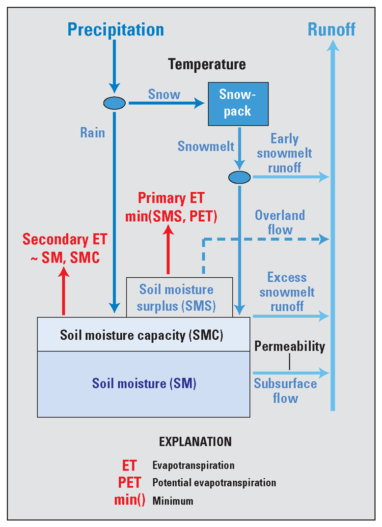
Schematic of water-balance model for a generic grid cell (from Kolars and others, 2016).

The WBM was calibrated to simulate monthly streamflow and to align the statistical distributions of the simulated streamflow with those of the observed streamflow. Note that the WBM was not intended to forecast the streamflow for a specific month as closely as possible. A forecast model would require input data with higher spatial and temporal resolution of precipitation, temperature, evapotranspiration, and soil parameters. Such a model was considered outside the scope of this study. Instead, the goal was to develop a WBM that simulates monthly streamflow with the same statistical distributions as observed streamflow. More specifically, if a change in climate causes a change in the streamflow statistical distribution, then the calibrated WBM would also simulate the same change in the streamflow statistical distribution when exposed to the same change in climate. Because the focus was on the statistical distribution of streamflow, the WBM was calibrated by adjusting the model parameters so that the mean and standard deviation of the simulated streamflow closely matched that of the observed streamflow. Also, water use and RRVWSP operation were not explicitly included in the model. Historical water use is implicitly included in the model because the historical streamflow used in calibration includes the effects of water use. Although specific details on the RRVWSP operation have not been finalized, streamflow at the Red River of the North at Fargo, N. Dak. (USGS streamgage 05054000; hereafter referred to as “station 7”; fig. 1, table 1), is one consideration that can be used to determine when the RRVWSP would operate. In support of providing information for determining frequency of future use of the RRVWSP under different drought conditions, results are provided for station 7.

Subbasin Dynamics

The WBM consisted of a series of subbasins that were delineated to simulate the monthly streamflow observed at their respective streamgages. After precipitation falls inside the cells of the subbasin, a set of equations determine how much of the precipitation is directed to soil moisture, snow, evapotranspiration, or outflow from the subbasin. Calculations for how water moves through the different processes are all in units of water depth. Once the amount of runoff for the subbasin is calculated, the depth is multiplied by the drainage area of the subbasin to produce the volume of water generated by the subbasin for the given month. Note that these calculations only produce the volume of water generated for each subbasin. To calculate the streamflows that correspond to the streamgages observations, streamflow routing calculations described in the “Streamflow Routing” section must be performed.

The WBM has 28 parameters that were adjusted during the calibration process (described in detail in appendix 1). These WBM parameters were defined for all 37 subbasins. For a few WBM parameters, there are multiple versions of the same parameter to compensate for the different conditions that can exist in different months. Water first enters the model through precipitation. To adjust the amount of precipitation that a cell receives, parameter A_prc is used. Two temperature thresholds, T_s and T_r, are defined and used to determine whether precipitation falls as snow or rain, respectively. These temperature thresholds are used in other functions in the WBM that rely on monthly temperatures for their calculations. When precipitation falls, these threshold temperatures are used to calculate how precipitation is allocated between rain and snow.

Once mean temperatures become warm enough, C_{mf_JanFeb} and C_{mf_MarDec} are used to determine how much snowmelt is generated as a function of ambient temperatures. When snowmelt is generated, a small part is immediately directed to runoff. This early snowmelt runoff is controlled by three parameters (F_{SM_JanFeb}, F_{SM_Mar}, and F_{SM_Apr}) because this fraction of runoff can vary depending on the current month. Any remaining snowmelt is then sent to soil moisture. The parameter A_SC is used to adjust the AWS capacity of the soil. Any water already in soil moisture can exit the system as runoff through subsurface flows. These subsurface flows are a function of the soil permeability, which can be adjusted using the $A_{K s}$ parameter. The parameters A_GW, K_{s_mx}, and A_pwr are then used to calculate how much soil moisture becomes runoff. The amount of runoff generated from soil moisture is a function of soil permeability, soil moisture, and temperature. During freezing conditions, the parameters A_GWf and C_fGWm are used to calculate how much runoff is generated from frozen ground.

If soil moisture is already at capacity, then any excess water added to soil moisture is considered surplus. After calculation of the subsurface flows, the amount of surplus generated is adjusted using the A_Sur parameter. A fraction of this surplus water is assigned as direct runoff, with the parameters F_{DR_JanMar}, F_{DR_Apr}, F_{DR_May}, F_{DR_Jun}, and F_{DR_JulDec} determining this fraction for different months. After considering direct runoff, the remaining surplus water and water in soil storage are then exposed to evapotranspiration. The parameter C_SFT is used to calculate how much soil storage is exposed to evapotranspiration as a function of mean temperature. The imported PET values are also adjusted using the parameters A_{PET_ini}, A_{PET_May}, and A_{PET_Jun}, which define adjustments depending on the current month. If there is still excess water after evapotranspiration is considered, then this excess overland flow is first adjusted by parameters EO_{mx_ini} and EO_{mx_MarApr}, which define the maximum limit for this flow depending on the current month. Afterward, a fraction of this excess overland flow is added to the runoff for the current month, which is determined using the F_EOi parameter, whereas the remaining amount of excess overland flow is added to the next month’s runoff.

The adjustment factors A_prc, A_SC, A_Sur, A_{PET_ini}, A_{PET_May}, and A_{PET_Jun} can have values greater than one, which allows the WBM to have flexibility to fit the distribution of observed data. Adjusting these values enables the WBM calibration to account for additional water in the system or to compensate for excess water, thereby aligning the generated streamflows more closely with observed data; however, increasing the number of parameters and the range of their values increases the risk of the model overfitting the data. The calibration and verification process therefore were designed to mitigate this risk. The WBM was calibrated using data from 1940 to 2000 and verified using weather conditions from 2001 to 2015. Because the verification process uses weather data not included in the calibration period, it allows for the evaluation of the WBM performance under untested conditions, which ensures that the WBM output remains consistent with expectations based on physical principles, even when subjected to new sets of weather data. The WBM also includes flow limits that ensure no negative streamflows are generated. Additional experiments with stochastic weather generation described in the “Evaluating Future Drought Risk Using a Stochastic Streamflow Model” section further reinforce this consistency check.

Streamflow Routing

After calculating the monthly water volume output for each subbasin, all subbasins are routed together to generate the streamflow that can be compared against observed streamflow. The structure of the streamflow routing network ensured that the streamflow generated for every streamgage was equal to the streamflow generated by the local subbasin plus the contributions of water generated from all subbasins upstream from the local subbasin. These hydrologic connections were determined using StreamStats (USGS, 2020b).

Initially, the streamflow routing system was built with parameters for simulating streamflow lag; however, the calibration process demonstrated enough flexibility in the model parameters that the streamflow lag could be implicitly simulated using only subbasin parameters. During the calibration process, the WBM was calibrated to compensate for the effects of streamflow lag.

Along with subbasins, the streamflow routing network also includes connections with reservoirs. The reservoirs in the WBM can only have a single inlet and a single outlet; therefore, if multiple subbasins flow into a reservoir, all incoming flows are combined into a single inflow to the reservoir. The outflow from the reservoir is then routed to the next downstream subbasin. With this streamflow routing network, the reservoir units simulate solely the dynamics of reservoir outflows.

Reservoir Data

To simplify WBM construction, reservoir headwater subbasins (reservoirs without an upstream subbasin) were not considered in the model. Rather, the dynamics of reservoir headwater subbasins were represented in the dynamics of the downstream subbasin. Under these constraints, only four reservoirs were considered: Lake Ashtabula, Orwell Lake, Lake Traverse, and Mud Lake. Reservoir stage and outflow were available for all reservoirs from U.S. Army Corps of Engineers (2022a). Lake Traverse and Mud Lake are two connected reservoirs, with water from Lake Traverse feeding into Mud Lake. To simplify model construction, the WBM treats the two reservoirs as a single reservoir unit, referred to as Lake Traverse-Mud Lake; therefore, the WBM simulates only three reservoir units.

To calculate the outflows of the reservoirs, a change of the reservoir water volume for each month was estimated. After the change of the water volume of the reservoir was estimated for each month, these values were then set as constants for the model. The outflow from a reservoir can then be calculated by taking the volume of the water inflow and subtracting the volume change of the reservoir for that month. To derive the change of water volume for each month, observations of streamflow and reservoir water elevation were used to calculate the volume of water entering and leaving the reservoir for each month. The difference between the inflow and outflow volumes were then calculated for each month. This time series of monthly changes of volume were aggregated to yield a new time series with values proportional to reservoir water elevation. The mean of the aggregated values was then calculated for each month, which means a single set of values describe the reservoir dynamics for each of the 12 months of the year (table 4). The monthly values were then used to calculate the reservoir outflows for all years. Note that the monthly values were determined separately from the construction of the model, meaning the values did not change during the calibration process for the WBM. Also, note that the cumulative volume change values are expressed as flow rates, in cubic meters per second. This expression of the values, which is possible because the values describe a change of water volume over a month, allows the reservoir outflows to be calculated solely in terms of flow rates. During model simulations, the table of cumulative volume changes and the input flow rate was used to calculate the reservoir outflow using equation 1:

Q_{i}^{O u t} = Q_{i}^{I n} - (Q_{i}^{V o l} - Q_{i - 1}^{V o l})

(1)

where

i: is the current month;
$Q_{i}^{O u t}$: is the mean outflow of the reservoir for the current month, in cubic meters per second;
$Q_{i}^{I n}$: is the mean inflow to the reservoir for the current month, in cubic meters per second;
$Q_{i}^{V o l}$: is the cumulative volume change of the reservoir over the current month, expressed as a flowrate in cubic meters per second (table 4); and
$Q_{i - 1}^{V o l}$: is the cumulative volume change of the reservoir over the previous month, expressed as a flowrate in cubic meters per second (table 4).

Table 4.

Mean cumulative monthly change in reservoir volume expressed as a flowrate in cubic meters per second.

Table 4. Mean cumulative monthly change in reservoir volume expressed as a flowrate in cubic meters per second.
Month	Mean cumulative monthly change in reservoir volume expressed as a flow rate (cubic meters per second)
Month	Lake Ashtabula	Orwell Lake	Lake Traverse-Mud Lake
January	−8.17	1.93	0.82
February	−10.98	1.85	0.27
March	−8.69	1.51	7.21
April	−0.85	2.32	13.1
May	0.10	2.71	6.55
June	0.07	2.38	4.50
July	−0.07	1.90	1.87
August	0.01	1.99	1.26
September	0.24	1.99	-0.38
October	−0.95	2.01	0.91
November	−3.46	2.01	0.05
December	−5.69	2.05	0.57

For each month, after a reservoir receives an input volume of water, $Q_{i}^{I n}$ , a fraction of the water $(Q_{i}^{V o l} - Q_{i - 1}^{V o l})$ is subtracted from the inflow and directed to reservoir storage. This method of using the difference of cumulative change values $(Q_{i}^{V o l} - Q_{i - 1}^{V o l})$ ensures that the volume of water in the reservoirs does not drift with time to volumes greater or less than what was observed in the data. Values in table 4 were adjusted to simulate different scenarios of reservoir operation.

Model Calibration and Verification

The WBM was calibrated using historical streamflow data from 1940 to 2000. This period was selected for calibration for two reasons: (1) from land-use change analysis described previously, land use and crop cover were relatively stable during this period; and (2) the length of the period was sufficient to accurately represent the streamflow distribution for all subbasins. By selecting a period of relatively stable land use and crop cover, simulations using stochastic weather are assumed to be affected only by changes in climatic inputs, not changes in land use and crop cover.

To guide the WBM calibration process, an objective function was developed. This objective function represents the overall error of the WBM in relation to differences between the simulated and the observed streamflows. During the calibration process, the parameters of the WBM were adjusted to minimize the value of this objective function. Because the WBM was used to generate statistical distributions of streamflow, this objective function was designed to evaluate how well the distributions simulated by the WBM matched the distributions observed in the historical streamflow record. The objective function construction was based on the calibration methods presented by Kolars and others (2016) for their modeling work on the Souris River Basin. Kolars and others (2016) adjusted the model parameters in a way that reproduces, as closely as possible, the monthly means and standard deviations of the natural flows. This study formalizes this goal with an objective function and extends the objective function for all flows. The objective function is composed of a set of root-mean-square errors (RMSE) calculated and combined using equations 2–5:

{\bar{M}}_{i} = (M_{i}^{A} + M_{i}^{F} + M_{i}^{M} + M_{i}^{L}) \frac{1}{4}

(2)

{\bar{S}}_{i} = (S_{i}^{A} + S_{i}^{F} + S_{i}^{M} + S_{i}^{L}) \frac{1}{4}

(3)

T E_{i} = {\bar{M}}_{i} + {\bar{S}}_{i}

(4)

T E_{t o t} = \sum_{i = 1}^{37} T E_{i}

(5)

where

i: is the index for one of the 37 subbasins;
$M_{i}^{A}$: is the RMSE of the mean of the monthly streamflows using the entire record for subbasin i, in cubic meters per second;
$M_{i}^{F}$: is the RMSE of the mean of the monthly streamflows using only the first 15 years of the record for subbasin i, in cubic meters per second;
$M_{i}^{M}$: is the RMSE of the mean of the monthly streamflows using only the middle 15 years of the record for subbasin i, in cubic meters per second;
$M_{i}^{L}$: is the RMSE of the mean of the monthly streamflows using only the last 15 years of the record for subbasin i, in cubic meters per second;
${\bar{M}}_{i}$: is the mean RMSE score for the mean of the monthly streamflows for the four periods of record for subbasin i, in cubic meters per second;
$S_{i}^{A}$: is the RMSE of the standard deviation of the monthly streamflows using the entire record for subbasin i, in cubic meters per second;
$S_{i}^{F}$: is the RMSE of the standard deviation of the monthly streamflows using only the first 15 years of the record for subbasin i, in cubic meters per second;
$S_{i}^{M}$: is the RMSE of the standard deviation of the monthly streamflows using only the middle 15 years of the record for subbasin i, in cubic meters per second;
$S_{i}^{L}$: is the RMSE of the standard deviation of the monthly streamflows using only the last 15 years of the record for subbasin i, in cubic meters per second;
${\bar{S}}_{i}$: is the mean RMSE score for the standard deviation of the monthly streamflows for the four periods of record for subbasin i, in cubic meters per second;
TE_i: is the fitness score for the overall error for the subbasin i; and
TE_tot: is the fitness score for the overall error for the entire basin.

The RMSE terms are calculated based on the aggregation metric (mean or standard deviation) and the period of interest (full record, first 15 years, middle 15 years, or last 15 years). Subsetting the record into 15-year periods allows the calibration process to accurately simulate variations in streamflow distribution as climatic conditions change through decades instead of merely reproducing the distribution observed throughout the entire period of record. During the calibration process, the parameters of the WBM are adjusted to minimize the value of TE_i for each subbasin, which in turn minimizes the value of TE_tot for the entire basin.

The calibration of the WBM began with the headwater subbasins (reservoirs or streamgages without an upstream subbasin). Many versions of the WBM were generated, with all the parameter values for the subbasins varying in each version. The parameter values were generated by randomly sampling from a uniform distribution bounded by the domain range for each parameter. The domain ranges for the parameters were wide enough to allow the WBM to fit the calibration data. After a WBM was generated, it was evaluated against the objective function to produce a fitness score, TE_i. For computational efficiency, only headwater subbasins were evaluated. As subbasin models were generated and evaluated, the best performing model parameters were recorded for each subbasin. This process was repeated until the TE_i scores of the subbasins no longer decreased with further modifications to model parameters. The best model parameters identified through the calibration process were then applied to the headwater subbasins. The model parameters for these subbasins were then held constant for the rest of the calibration process.

The calibration process for the WBM next moved to the subbasins directly downstream from the headwater basins. Once again, multiple versions of the model were generated, each with different randomly generated model parameters. During this process, all subbasins upstream from a given subbasin were left untouched. Once optimal model parameters were adopted for a given subbasin, it was left untouched for the rest of the calibration process. The process then shifted to the next subbasin downstream and was repeated until all subbasins were calibrated (tables 1.1–1.4).

To evaluate how well the model performed across multiple subbasins, the final RMSE scores for each subbasin were collected and compared after the calibration process (table 5). Across the subbasins, those with a higher RMSE score for the mean of the monthly streamflow also had a higher RMSE score for the standard deviation of the monthly streamflows. The positive correlation between RMSE of the mean of the monthly streamflow and the standard deviation of the monthly streamflow indicates that the overall performance for each subbasin can be summarized by taking the sum of the mean RMSE of monthly flows of the basin for both the mean and the standard deviation, referred to as the total RMSE. The total RMSE score correlates with the size of the drainage area for each subbasin, so the larger the total streamflow for the subbasin, the larger its corresponding total mean RMSE score. To correct for the effects of drainage area on the total RMSE score, the total mean RMSE score was normalized against the total streamflow for each subbasin (table 5). This normalization allows for comparison between the subbasins, independent of subbasin size. Based on the flow-normalized total mean RMSE score, the subbasins have similar model performance, and the score does not correlate with the size of the drainage areas.

Table 5.

Root-mean-square error of the mean and standard deviation for the monthly flows for each subbasin in the Red River of the North Basin in the calibrated water-balance model.

^{[ID, identification; USGS, U.S. Geological Survey; RMSE, root-mean-square error]}

Table 5. Root-mean-square error of the mean and standard deviation for the monthly flows for each subbasin in the Red River of the North Basin in the calibrated water-balance model.
Map ID (fig. 5)	USGS station number and subbasin identifier	Subbasin name	Mean RMSE for mean of monthly streamflow¹ (cubic meters per second)	Mean RMSE for standard deviation of monthly streamflow² (cubic meters per second)	Total mean RMSE score³ (cubic meters per second)	Total mean RMSE score (normalized by total streamflow)⁴
1	05030500	Upper Otter Tail	4.42	1.21	5.62	0.04
2	05040500	Pelican River	0.60	0.36	0.96	0.04
3	05046000	Lower Otter Tail	3.27	2.20	5.47	0.04
4	05049000	Mustinka	0.97	1.68	2.65	0.17
5	05051500	Wahpeton	6.11	7.10	13.21	0.05
6	05053000	South Wild Rice	3.82	5.95	9.78	0.18
7	05054000	Fargo	12.10	13.43	25.53	0.09
8	05055500	Upper Sheyenne	0.68	1.53	2.21	0.16
9	05057000	Sheyenne to Cooperstown	2.46	3.89	6.35	0.10
10	05058500	Cooperstown Ashtabula	1.59	2.33	3.92	0.07
11	05059000	Middle Sheyenne	4.29	4.78	9.07	0.07
13	05060000	Maple River	2.75	5.40	8.14	0.15
14	05060500	Rush River	0.26	0.56	0.82	0.15
15	05061000	North Buffalo	0.82	1.05	1.87	0.06
16	05061500	South Buffalo	1.02	2.09	3.12	0.11
17	05062000	Lower Buffalo	2.09	4.02	6.12	0.09
19	05064000	North Wild Rice	4.75	5.16	9.91	0.08
20	05064500	Halstad	27.78	41.40	69.19	0.07
21	05066500	Goose	3.31	2.88	6.20	0.14
22	05067500	Marsh	1.01	2.20	3.21	0.14
23	05069000	Sand Hill	1.17	1.46	2.63	0.08
24	05075000	Upper Red Lake	5.25	4.76	10.01	0.05
25	05076000	Thief	3.15	4.40	7.55	0.11
26	05078500	Clearwater	3.73	4.92	8.65	0.07
27	05079000	Lower Red Lake	5.98	12.12	18.10	0.04
28	05082500	Grand Forks	43.09	47.46	90.55	0.08
29	05083000	Turtle	0.45	2.14	2.60	0.15
30	05083500	Oslo	56.02	44.58	100.60	0.09
31	05085000	Forest	0.92	1.64	2.57	0.11
32	05087500	Middle	0.92	1.20	2.12	0.12
33	05089000	South Park	0.28	0.76	1.04	0.12
34	05090000	Park	1.14	2.10	3.24	0.13
35	05092000	Drayton	58.04	55.91	113.95	0.07
36	05094000	Two Rivers	1.92	2.65	4.57	0.11
37	05100000	Pembina	6.20	7.50	13.70	0.15
38	05101000	Tongue	0.27	0.63	0.90	0.10
39	05102500	Emerson	67.28	69.04	136.32	0.09

¹

The mean of the RSME of the mean of the monthly streamflows for four periods of interest, M_i in equation 2.

²

The mean of the RMSE of the standard deviation of the monthly streamflows for four periods of interest, S_i in equation 3.

³

The fitness score for the overall error for the subbasin, TE_i in equation 5.

⁴

The total mean RMSE was normalized against the total sum of the monthly mean of the observed streamflows. This normalization was done to allow comparison between subbasins.

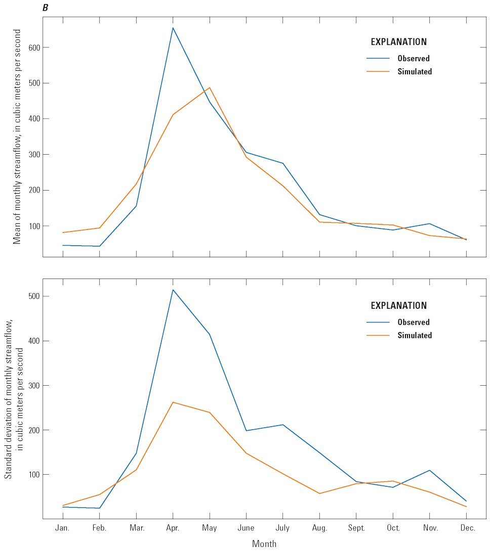
Wahpeton and Emerson subbasins were used to visually compare simulated and observed mean monthly streamflow and standard deviation of the monthly streamflow for the calibration period (fig. 9). The simulated streamflow distributions mirrored the seasonal patterns of the observed mean monthly streamflow data (fig. 9). Like the observed data, the simulated monthly streamflows also increased toward a peak during the spring months of March through April and reached their minimum values in the fall and winter months of November through January. The model was also able to reproduce the seasonal cycles for the standard deviation of the monthly streamflows, where the standard deviation peaked in the spring and summer months of March through May and was at its minimum in the fall and winter months of November through January. The standard deviation of the simulated streamflow generally was lower than the observed streamflow with the largest difference during peak streamflows in March through May. This underestimation of streamflow variance was because the model was unable to accurately simulate the peak streamflows generated from the high runoff in the spring. Peak streamflow events are on the order of days to weeks, whereas the WBM uses a monthly time step. Although high-flow months can have streamflow droughts, the focus of this model was on the lowest streamflow conditions, which typically are during months other than the spring and as such the underestimation of the variance of spring peak streamflow events was considered unimportant to the scope of this report. Within the low-streamflow months of September through January, the model accurately simulates the variance of these lower streamflows. Based on the flow-normalized total RMSE scores, a reasonably good fit was achieved (table 5). Overall, the mean flow-normalized total RMSE score for all subbasins was small at 0.10. Several subbasins had a flow-normalized total RMSE score of 0.04 or much lower than the mean of 0.10. Some of the smaller subbasins had higher flow-normalized total RMSE score, such as South Wild Rice, which was 0.18. For main-stem subbasins, Emerson, Grand Forks, Halstad, and Fargo, the flow-normalized total RMSE scores of 0.09, 0.08, 0.07, and 0.09, respectively, were slightly better than the mean flow-normalized total RMSE score.

A, The largest differences between the observed and simulated data generally were
in April when monthly streamflow was the largest. For the mean of monthly streamflow,
the maximum observed value was 50 compared to 40 cubic meters per second for simulated.
For the standard deviation of monthly streamflow, the maximum observed value was 50
compared to 25 cubic meters per second for simulated. B, The largest differences between
the observed and simulated data generally were in April when monthly streamflow was
the largest. For the mean of monthly streamflow, the maximum observed value was 525
compared to 475 cubic meters per second for simulated. For the standard deviation
of monthly streamflow, the maximum observed value was 400 compared to 250 cubic meters
per second for simulated. — Figure 9.
Simulated and observed streamflow for the calibrated water-balance model during the calibration period (1940–2000). A, Red River of the North at Wahpeton, North Dakota, subbasin (U.S. Geological Survey streamgage 05051500). B, Red River of the North at Emerson, Manitoba, subbasin (U.S. Geological Survey streamgage 05102500). Observed streamflow data are from U.S. Geological Survey (2020a).

Figure 9.
Simulated and observed streamflow for the calibrated water-balance model during the calibration period (1940–2000). A, Red River of the North at Wahpeton, North Dakota, subbasin (U.S. Geological Survey streamgage 05051500). B, Red River of the North at Emerson, Manitoba, subbasin (U.S. Geological Survey streamgage 05102500). Observed streamflow data are from U.S. Geological Survey (2020a).

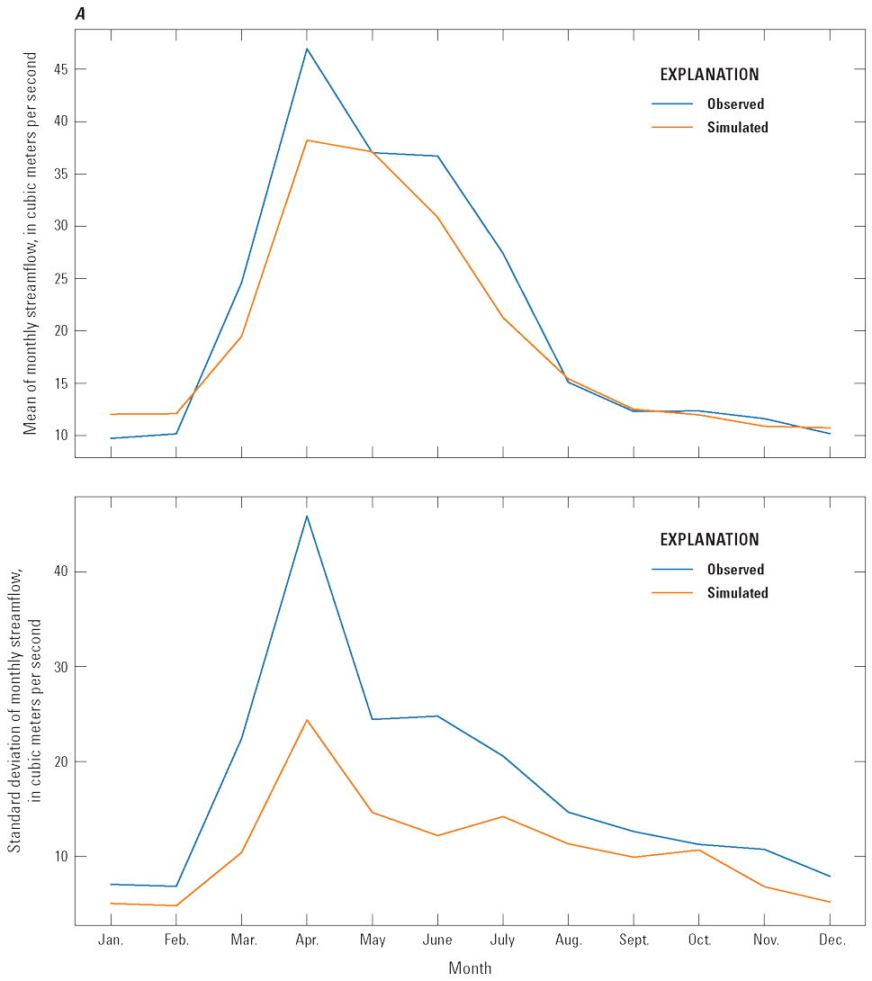
After calibration, it was important to verify the model. The verification process is crucial to assess if the calibrated model can accurately simulate underlying physical processes that extend to different climatic scenarios. To verify the model, streamflows were simulated using the calibrated model with weather data from 2001 to 2015. For the verification period, the seasonal changes in mean and standard deviation of monthly streamflow were simulated reasonably well (fig. 10); mean and standard deviation of streamflow increased during the spring and summer months (from March through June) and then decreased to their lowest levels during the fall and winter months (from October through January). Like the calibration period, for the verification period, the simulated mean and standard deviation of monthly streamflow distribution generally underestimated the observed data, especially during the spring months. This underestimation was likely for the same reason as was observed with the calibration data. For the low-streamflow months of December through January, the difference between simulated and observed data was like the calibration comparison and successfully reproduced seasonal trends in the streamflow distribution, even when using weather data that were outside the calibration period. The WBM’s capability of converting weather data into estimations of streamflow distributions was then combined with several stochastically generated climates to generate low-streamflow frequency curves for multiple possible future climate scenarios. A more thorough examination of the WBM’s performance is presented in the “Wet and Dry Climate States” section.

Figure 10.
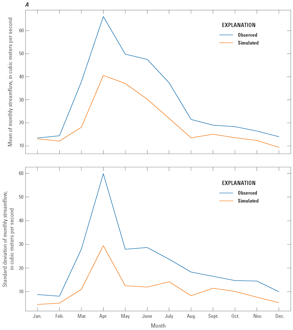
Simulated and observed streamflow for the calibrated water-balance model during the verification period (2001–15). A, Red River of the North at Wahpeton, North Dakota, subbasin (U.S. Geological Survey streamgage 05051500). B, Red River of the North at Emerson, Manitoba, subbasin (U.S. Geological Survey streamgage 05102500). Observed streamflow data from U.S. Geological Survey (2020a).

Evaluating Future Drought Risk Using a Stochastic Streamflow Model

The future risk of low-streamflow conditions and droughts in the basin was evaluated for multiple possible future climates using a stochastic approach to predict future streamflow conditions. This approach involved generating multiple possible future weather conditions using historical weather data. These generated weather series were then combined with the WBM to generate multiple possible future streamflows (hereafter referred to as the stochastic streamflow model). The stochastic streamflow model produced low-streamflow frequency curves at different subbasins, along with uncertainty bounds to help describe the influence of future climate variability on future streamflows.

To verify the accuracy of the WBM under simulated climates, two 50-year climate series that replicate the wet and dry climate states of the historical record were generated. Using the two climate periods, a low-streamflow frequency curve representing the difference between the streamflow distributions was calculated for simulated and historical streamflow and compared. Multiple weather drought conditions were also generated to assess how the basin would respond to several drought intensities and durations. The result was a range of possible changes to future low streamflows when the basin is subjected to a range of possible future climates.

Methods

The stochastic streamflow model consists of the calibrated WBM combined with stochastically generated weather inputs to simulate stochastic streamflow. The WBM requires a time series of PET, temperature, and precipitation data as input. For the stochastic generation of these inputs, a block-bootstrap method (Davison and Hinkley, 1997) was used to sample the historical period to create new time series. To generate a potential future time series for weather, an initial starting year and period length is selected, then the historical period of weather record is randomly sampled and each sample of weather data is appended to the previous sample to generate a new time series of data; for example, for a 50-year time series of weather generated from the WBM calibration period of 1940–2015, if the starting year was 1950 and the period length was 8 years, the first 8 years of the generated time series would contain weather data from 1950 to 1958. Then another period of the weather record is randomly sampled and appended to the first 8 years of the generated time series. This process is repeated until a new 50-year time-series of weather record is generated. The block-bootstrap method allows flexibility for how the starting years and period length are randomly selected. These parameters for the block-bootstrap method varied across the different stochastic simulation experiments performed to meet the goals for each experiment.

The first set of experiments were designed to investigate how changes to reservoir management would affect the distribution of low streamflow, which was done by adjusting the volume changes in table 4 that the WBM references when performing reservoir calculations. Three types of reservoir operation were tested. The first type was present-day (2023) operation, where the reservoirs were operated as they were during the calibration period (regulated streamflow), meaning no adjustments were made in the model for the reservoir volume change values. For the second type of operation, the reservoirs were disabled so that any water entering the reservoir was immediately released (unregulated streamflow); therefore, in the model, the reservoir volume change values (table 4) were not used during calculation of reservoir outflows. The third type of reservoir operation combined present-day (2023) reservoir operation with a reservoir capacity increase of 10 percent (regulated streamflow with an increased reservoir capacity of 10 percent), which was implemented in the model by raising the volume change values in table 4 by 10 percent. Across all three reservoir operation types, the stochastic weather used by the model was generated in the same way. The block bootstrap method was selected to generate the time series for the weather because this method of generation preserves many of the correlations that may exist among the PET, temperature, and precipitation data. If a parametric method had been used, the statistical models would have had to explicitly define a lot of these correlations as was done by Kolars and others (2016). Because the focus of this study is on the statistical distribution for streamflows and not necessarily on the climate trends that drive these patterns, the block bootstrap method was determined to be suitable. Work by Vogel and Shallcross (1996) demonstrates how the block bootstrap method has advantages compared to parametric methods for time series models. When using the block-bootstrap method to generate the potential future time series for weather, the starting year was sampled within the available record of 1912–2015. The length of the sampled period was randomly determined by sampling from the geometric distribution using equation 6:

P r (x) = \frac{1}{l} {(1 - \frac{1}{l})}^{x - 1}

(6)

where

x: is the length of the sampled period, in years, $x \in \{1, 2, 3 \dots\}$ ;
Pr(x): is the probability a period length of x will be used; and
l: is the mean period length, set to l=4.

By setting l=4, the sampled period length varies with lengths shorter or longer than the mean length of 4 years. Sampling by period blocks preserves the assumption that adjacent years are correlated to each other. The weather was generated until a time series of 50 years was reached.

To calculate a range of possible streamflows, 100 realizations of 50-year time series of weather were generated for each experiment. Each 50-year time series of weather was input to the WBM to produce 100 50-year time series of monthly streamflow. Each monthly streamflow time series was then converted into a low-streamflow frequency curve by plotting the annual minimum monthly streamflow against the corresponding nonexceedance probability. The nonexceedance probability for a given annual minimum monthly streamflow was calculated by dividing the rank of the flow by the total number of samples; for example, if a given year had an annual minimum monthly streamflow that was second lowest across all 50 simulated years, then that streamflow was given a nonexceedance probability of 4 percent. The 100 low-streamflow frequency curves were then compiled to produce a distribution of low-streamflow frequency curves for a given experiment. The effects of different reservoir operation were investigated by observing how they shifted the distribution of these low-streamflow frequency curves.

The second set of experiments were designed to investigate how streamflows would change under multidecadal climate changes, which was done by running a WBM in the two climate states defined by Kolars and others (2016): the dry climate state during 1940–69 and the wet climate state during 1970–2015. For both climate states, the block-bootstrap method was used to generate 100 realizations of 50-year time series of weather, with sampling periods also having a mean length of 4 years; however, the first two sets of climate experiments differed in the years from which they were allowed to sample. When generating the dry climate state, the block-bootstrap method only sampled from years within 1940–69, whereas for the wet climate state only years within 1970–2015 were sampled. The two sets of generated weather were then input to the WBM to create two sets of monthly streamflows, which were then converted into low-streamflow frequency curves as in the experiments with reservoir operation. These low-streamflow frequency curves were then aggregated to produce two distributions of low-streamflow frequency curves, with one distribution for the dry climate state and the other for the wet climate state. The two low-streamflow frequency curve distributions were compared to investigate how the basin responds to multidecadal climate changes in precipitation.

The third set of experiments were designed to investigate how the basin would respond to a substantive drought event. These experiments investigated how the low-streamflow distribution varies with changes to the severity and duration of these drought events. The experiments involved applying the model to a 50-year weather time series that contained two climate states. The time series began with 10 years of weather that simulated the weather from all of 1912–2015, meaning that the block-bootstrap method sampled from years within 1912–2015. This initial decade was designed to allow the model to begin with a consistent starting condition. The weather then switched to a drought state where the precipitation received by the basin was substantially reduced. This was done by sorting the weather data by annual precipitation, and then using the block-bootstrap method to sample only from a percentage of the driest years. Depending on the experiment, the droughts could vary by the severity of the drought, defined by the percentage of driest years sampled, and by the duration of the drought. Drought severity varied by sampling from the 10, 20, and 40 percent of driest years and drought duration varied by 5 years, 10 years, and 20 years, which produced a set of 9 stochastic experiments that were performed. After the drought state was constructed, the weather returned to the same weather type as the initial decade until the 50-year limit was reached. For each experiment with different types of drought events, 100 realizations of 50-year weather time series were generated. These weather time series were then converted into distributions of low-streamflow frequency curves as in the previous sets of experiments.

Additional experiments were attempted to explore how streamflow distributions may shift with future expectations of rising temperatures; for example, rising mean temperatures during the winter could accelerate the production of snowmelt, thereby causing shifts in the timing of spring runoffs. A simple approach to studying the effect of temperature on streamflow would be to sort weather data by mean winter temperatures and then use the block-bootstrap method to sample the upper percentile of warmest winters and generate a synthetic climate with elevated winter temperatures. Then, weather data could be sampled from years with lower mean winter temperatures to generate another synthetic climate for comparison. After evaluating both climate states using the WBM, the distribution of streamflow could then be compared, with any differences attributed to the changes in winter temperatures; however, this analysis relies on the assumption that the effects on the streamflow distributions could only be attributed to temperature. This assumption requires no correlation between mean winter temperatures and other weather factors that could also affect streamflow distributions, such as winter precipitation; however, the mean winter temperature against the total winter precipitation for all of 1912–2015 (fig. 11) indicates that these factors are negatively correlated. This negative correlation means that if a change in streamflow distribution was observed, the streamflow change could be attributed to an increase in the mean winter temperature or a decrease in the total winter precipitation. A better sampling method or an alternative technique for generating the weather based on temperature must be used to correct for the influence of precipitation. The calibrated WBM alone was not sufficient to decouple the effects of precipitation and temperature, so further work on this experiment was not completed.

Total winter precipitation ranged from about 20,000 to 140,000 millimeters and mean
winter temperature ranged from -20 to -6 degrees Celsius. — Figure 11.
Total winter precipitation plotted against mean winter temperature during 1912–2015. Precipitation and temperature data are computed from the weather inputs to the water-balance model (Redoloza and others, 2025).

Future Drought Risk Evaluation

Three sets of experiments from the stochastic streamflow model were used to investigate changes in streamflow related to changes in reservoir management, the effect of wet and dry climate states, and nine different drought conditions. Results from these simulations are described in the following three sections.

Reservoir Management

The first set of experiments from the stochastic streamflow model were designed to investigate how changes in reservoir management would affect the distribution of low streamflow. Three reservoir management scenarios were considered: (1) regulated streamflow (present-day (2023) reservoir operation), (2) unregulated streamflow (no reservoir operation), and (3) regulated streamflow with an increased reservoir capacity of 10 percent. Under scenario 1, there was a 10 percent probability that, for any given future year, the month with the lowest monthly streamflow had a streamflow of 12.6 cubic meters per second (m³/s) or lower (fig. 12). Under scenario 2, the streamflow curve shifted so that there was a 10-percent probability that, for any given future year, the month with the lowest monthly streamflow had a streamflow of 9.9 m³/s or lower (fig. 12). The extent of overlap of the confidence intervals for the scenarios changes for different probabilities. The overall overlap is smallest at the nonexceedance probability of 17 percent (fig. 12). At this percentage, the median streamflow curve for scenario 2 (no reservoir operation) intersects with the lower bound of the 90-percent confidence interval for scenario 1. The overlap of the confidence intervals is the greatest at the nonexceedance probability of 76 percent (fig. 12). Relative to scenario 1, scenario 2 (no reservoir operation), reduced the 10-percent nonexceedance probability by 21.7 percent for the Emerson subbasin (table 6).

The median of the unregulated scenario is lower than the median of the regulated scenario
and the 90-percent confidence intervals of the two scenarios have some overlap. — Figure 12.
Comparison of the low-streamflow frequency curve between the unregulated and regulated scenario at the Emerson subbasin.

Table 6.

Shift in median value of mean monthly streamflow for selected subbasins in the Red River of the North Basin for reservoir management experiment scenarios.

^{[±, plus or minus]}

Table 6. Shift in median value of mean monthly streamflow for selected subbasins in the Red River of the North Basin for reservoir management experiment scenarios.
Subbasin name	Nonexceedance probability in percent	Comparison of scenario 2 (unregulated streamflow) to scenario 1 (regulated streamflow)¹		Comparison of scenario 3 (10-percent reservoir capacity increase) to scenario 1 (regulated streamflow)¹
Subbasin name	Nonexceedance probability in percent	Shift in median value of mean monthly streamflow, in percent	Uncertainty²	Shift in median value of mean monthly streamflow, in percent	Uncertainty²
Emerson	5	−23.2	±22.0	2.6	±21.9
Emerson	10	−21.7	±21.6	2.7	±21.3
Emerson	20	−11.9	±15.4	1.2	±13.9
Emerson	40	−10.3	±15.1	0.2	±14.8
Grand Forks	5	−30.1	±17.7	3.0	±19.8
Grand Forks	10	−20.9	±15.8	3.1	±14.5
Grand Forks	20	−18.4	±16.4	1.7	±15.5
Grand Forks	40	−11.5	±18.7	0.7	±17.6
Halstad	5	−28.4	±20.7	1.6	±25.6
Halstad	10	−34.8	±15.8	2.8	±19.6
Halstad	20	−29.3	±13.6	3.5	±11.8
Halstad	40	−16.2	±15.2	1.7	±14.0
Fargo	5	−19.5	±23.5	−0.2	±25.8
Fargo	10	−9.8	±16.7	2.0	±17.5
Fargo	20	−13.5	±13.7	2.4	±15.3
Fargo	40	−11.5	±11.8	1.0	±13.6
Wahpeton	5	−13.8	±22.1	0.6	±24.9
Wahpeton	10	−15.5	±15.4	−0.1	±17.5
Wahpeton	20	−23.2	±14.6	2.2	±14.2
Wahpeton	40	−12.1	±11.4	1.4	±12.9

¹

Scenario 1 is regulated streamflow (present-day [2023] reservoir operation); scenario 2 is unregulated streamflow (no reservoir operation); scenario 3 is regulated streamflow with an increased reservoir capacity of 10 percent.

²

Defined as the 68.3-percent confidence interval.

The shift of the median of the low-streamflow frequency curves compared to scenario 1 was calculated for scenarios 2 and 3 for the subbasins of Emerson, Grand Forks, Halstad, Fargo, and Wahpeton (table 6). Relative to scenario 1, scenario 2 (no reservoir operation) shifted the low-streamflow frequency curves downward, reducing the annual minimum monthly streamflow for the Emerson subbasin by 21.7, 11.9, and 10.3 percent for nonexceedance probabilities of 10, 20, and 40 percent, respectively (fig. 12; table 6). The curves shifted because, without the reservoirs, no stored water is available to supplement the low streamflow, thereby reducing the magnitude of the streamflow on the low end of the frequency curve. This shift in the low-streamflow frequency curve under scenario 2 was expected because volume was conserved in the WBM by reducing the streamflow output when the additional water supplemented by the reservoirs was removed. Relative to scenario 1, scenario 3 (regulated streamflow with an increased reservoir capacity of 10 percent) shifted the low-streamflow frequency curves upward for the Emerson subbasin, with a shift of 2.7, 1.2, and 0.2 percent for annual minimum monthly streamflow with nonexceedance probabilities of 10, 20, and 40 percent, respectively (table 6). This shift upwards was expected because the increased capacity allows more stored reservoir water to be added to the streams during low streamflow, thereby increasing the streamflow at the lower end of the streamflow frequency curve. The magnitude of this upward shift was lower than the magnitude of the shift caused by the absence of the reservoirs, which indicates that the streamflow was most affected when the reservoirs were first constructed.

Hypothetical revisions to reservoir capacity can increase the amount of control the reservoirs have on streamflow, but it is important to note that the magnitude of the shift in the simulated streamflow was an underestimate of what is possible. Recall that the reservoir outflows were calculated by taking the volume of the inflow of water and subtracting out that month’s change of volume of the reservoir. The change of volume of the reservoirs are a table of constants defined for each month. These constants were derived by calculating the mean difference of the observed inflow and outflow volumes of the reservoirs. When calculating the outflows of these reservoirs, there was no consideration for the future predicted inflow of these reservoirs. This behavior of reservoir management is unlike what is performed by reservoir operators who do change reservoir outflows based on anticipated future inflows. Taking the mean of the reservoir operation effectively reduced the simulated effect reservoirs have on streamflow.

Uncertainty associated with these shifts of streamflow distributions was calculated from the stochastic simulations for the three scenarios (table 6). The uncertainty associated with the shift of the medians was calculated as bounds encompassing the 68.3-percent confidence interval, corresponding approximately to one standard deviation from the mean; for example, for the Emerson subbasin at a nonexceedance probability of 10 percent, disabling the reservoirs caused the median of the streamflow to reduce 21.7 percent with a corresponding uncertainty of plus or minus (±) 21.6 percent (table 6). Note that this measure of uncertainty assumes that the shifts of the medians for the streamflow curves can be approximated with a normal distribution. Small-scale numerical experiments were performed to validate this assumption and ensure that interpretations derived from these values do not change. Note that the uncertainty of these simulations is caused solely by the variability from the stochastically generated weather. Given a specific state of the distribution of water in the model, and given a specific time series of weather, the model will always produce the same distribution of streamflow. Across the three scenarios, the only thing that was changed was the reservoir operations. The shifts of the median are solely due to differences in reservoir operations. The results of these scenarios indicate the magnitude of streamflow change induced by different reservoir operation compared against the uncertainty generated from weather variability.

Wet and Dry Climate States

The second set of experiments from the stochastic streamflow model were performed to better understand how the basin responds to long periods of low or high precipitation. The first scenario was a dry climate state with generated weather representing relatively low precipitation from 1940 to 1969. The second scenario was a wet climate state with generated weather representing relatively high precipitation from 1970 to 2015. Both scenarios used the same WBM with the current (2023) operations for the reservoirs and differed primarily in the range of years sampled to generate the 50-year climate period. These long climate periods allowed for comparisons between the low-streamflow frequency curves generated from stochastic climate data simulations and historical observations.

Comparison of the low-streamflow frequency curves of the simulated streamflow (generated from stochastic climate data) with the historical streamflow during 1940–69 for the Emerson subbasin indicates that the simulated streamflow was consistently overestimated (fig. 13). This behavior of overestimating streamflow was consistent for multiple subbasins, indicating that the WBM does not produce highly accurate predictions of the historical low-streamflow values. This inaccuracy is partly because of mechanisms in the model that ensure no negative streamflow can exist, which caused the model to always have at least a small amount of streamflow during all simulations. Although the simulated low-streamflow values were overestimated, the relative change of simulated streamflow distributions reasonably matched the relative change of historical streamflow distributions.

The historical streamflow ranges from about 3 to 45 cubic meters per second and the
median of the simulated streamflow ranges from about 3 to 65 cubic meters per second. — Figure 13.
Comparison of low-streamflow frequency curve between simulated streamflow from generated climate data and historical streamflow (U.S. Geological Survey streamgage 05102500, U.S. Geological Survey, 2020a) during 1940–69 for the Emerson subbasin.

As a measure of how well the model was able to reproduce the relative change in streamflow distribution between the dry climate state and the wet climate state, a new low-streamflow frequency curve was calculated and will be referred to as the wet-to-dry streamflow frequency curve. The wet-to-dry streamflow frequency curve, calculated by subtracting the dry climate low-streamflow frequency curve (1940–69) from the wet climate (1970–2015) low-streamflow frequency curve and normalized by subbasin drainage area, was calculated for the simulated and historical streamflow, and compared (fig. 14). The wet-to-dry streamflow frequency curve was normalized by subbasin drainage area to allow for comparison among subbasins. For simulated and historical streamflow, the wet-to-dry streamflow frequency curve was positive for most nonexceedance probabilities indicating that the wetter climate has introduced more water into the system, causing streamflow to increase (fig. 14). For a given site, areas of the overlap between the simulated and historical wet-to-dry streamflow frequency curve indicate that the model is accurately reproducing relative change of streamflow distribution between the dry climate state and the wet climate state. Subbasins with stations along the main stem of the basin were investigated to monitor how the performance of the model varies across different flow magnitudes from the headwaters at Wahpeton to the outlet of the entire basin at Emerson. Halstad and Grand Forks subbasins were considered because of the major tributaries upstream from them. Results from Halstad reflect the influence of the Sheyenne River, a major tributary on the western side of the basin, and Grand Forks reflects the influence of the Red Lake River, the largest tributary by volume on the eastern side of the basin (USGS, 2020b). For the Emerson, Grand Forks, Halstad, Fargo, and Wahpeton subbasins, the model was able to successfully predict the wet-to-dry streamflow frequency curve for lower-end nonexceedance probabilities (fig. 14).

For all 5 sites, the historical streamflow and simulated streamflow are generally
close to one another between about 0 and 50 percent nonexceedance probability, but
above 50 percent the historical streamflow is much higher than the simulated streamflow. — Figure 14.
The wet-to-dry streamflow frequency curve (calculated as the difference in streamflow between a wet [1970–2015] and dry [1940–69] climate state and normalized by drainage area of the subbasin) for simulated and historical annual minimum monthly streamflow. A, Emerson subbasin (U.S. Geological Survey [USGS] streamgage 05102500). B, Grand Forks subbasin (USGS streamgage 05082500). C, Halstad subbasin (USGS streamgage 05064500). D, Fargo subbasin (USGS streamgage 05054000). E, Wahpeton subbasin (USGS streamgage 05051500). Historical streamflow data are from U.S. Geological Survey (2020a).

Across the subbasins, the model was most accurate for streamflows associated with nonexceedance probabilities between 20 and 40 percent, as indicated by the overlapping wet-to-dry streamflow frequency curves of simulated and historical streamflow (fig. 14). For higher nonexceedance probabilities, the simulated wet-to-dry streamflow frequency curve is below the historical curve indicating that the model underestimates the change in the streamflow distribution between the wet and dry climate states (fig. 14); however, these probabilities are beyond the low-streamflow regime of interest. The model most accurately predicts the historical wet-to-dry streamflow frequency curve for the Emerson subbasin as indicated by the largest range of overlapping nonexceedance probabilities from 0 to 5 percent and 20 to 60 percent (fig. 14A). The Wahpeton subbasin is the second-best performing subbasin where the historical wet-to-dry streamflow frequency curve was within the 90-percent confidence intervals of the simulated wet-to-dry streamflow frequency curve from 0 to 55 percent nonexceedance probabilities. Wahpeton is a headwater subbasin, and Emerson subbasin is the outlet for the entire basin. Despite different streamflow magnitudes with different hydrological structures, both subbasins exhibit similar model performance, which demonstrates how the model performance is independent of the mean streamflow of the subbasin. For low values of nonexceedance probabilities (0 to 5 percent), the Fargo subbasin performs second-best, where the historical wet-to-dry streamflow frequency curve was contained within the 90-percent confidence interval and the two curves were closer together than for the Wahpeton subbasin (fig. 14D). The Halstad subbasin had the poorest prediction for nonexceedance probabilities from 0 to 5 percent, but still performs well within nonexceedance probabilities from 20 to 40 percent (fig. 14C). Overall, the model accurately predicts the wet-to-dry streamflow frequency curve within the 20 to 40 nonexceedance probabilities.

Drought Events

The third set of experiments from the stochastic streamflow model were done to investigate low-end streamflow response across the basin to several drought events. Nine scenarios were considered, each involving a 50-year weather simulation with 10 years of normal weather followed by a drought event of varying intensity and duration and then a return to normal weather for the remaining years of the 50-year time series. The single drought event varied in intensity (sampling from the 40-, 20-, and 10-percent driest years on record) and duration (5, 10, and 20 years). Drought event intensity will be referred to as low intensity (40-percent driest years sampled), moderate intensity (20-percent driest years sampled), and high intensity (10-percent driest years sampled).

Low-end streamflow was reduced when the basin was exposed to a drought, and the magnitude of the reduction increased with longer or more intense droughts (fig. 15). To compare the overall results across the drought scenarios, the percent reduction of low-end streamflow—defined here as all low-streamflow frequency curve values below the 40-percent nonexceedance probability—between the nine drought scenarios and scenario 1 (regulated streamflow with present-day [2023] reservoir operation) was calculated and presented as a statistical distribution for the outlets of the Emerson, Fargo, Grand Forks, Halstad, and Wahpeton subbasins (fig. 15). For the Emerson subbasin (fig. 15A), a 5-year low-intensity drought produced a median low-end streamflow reduction of 0.2 percent. A 20-year low-intensity drought further reduced the median low-end streamflow by 3.1 percent, whereas increasing the 5-year low-intensity drought to a 5-year high-intensity drought reduced the median low-end streamflow by 2.8 percent (fig. 15A). Among the five subbasins, for the low-intensity drought, the Wahpeton subbasin had the largest difference in median low-end streamflow between 5-year and 20-year drought durations with reductions of 1.3 percent and 4.6 percent, respectively (fig. 15E). In comparison, the smallest difference between the 5-year and 20-year drought durations for low-intensity droughts was the Halstad subbasin, with reductions of 1.3 percent, and 2.4 percent, respectively (fig. 15D). For all subbasins, with a high-intensity drought, there was a larger effect between a drought duration of 5 years and 20 years; for example, under a high-intensity drought, for the Wahpeton subbasin the median low-end streamflow was reduced by 3.3 percent for a 5-year duration compared to 17 percent for a 20-year duration (fig. 15E). Compared to the low-intensity drought scenarios, the range of percent reductions (as indicated by the interquartile range) was larger for the high-intensity drought scenarios for all subbasins, and the subbasins of Grand Forks and Emerson had a smaller range of reductions compared to the other three subbasins. The larger drainage area—combined with the large contribution of the Red Lake River and several other Minnesota tributaries that generally experience wetter climate conditions—upstream from the Emerson and Grand Forks subbasins may contribute to the smaller range in reductions under the high intensity scenarios.

A, The median percent reductions range from 0.5 to about -15. B, The median percent
reductions range from 1 to about -15. C, The median percent reductions range from
2 to about -13. D: The median percent reductions range from 2 to about -12. The median
percent reductions range from 2 to about -18. — Figure 15.
The distribution of percent reduction of low-end streamflows (nonexceedance probability of 40 percent or less) for nine drought scenarios. A, Emerson subbasin. B, Fargo subbasin. C, Grand Forks subbasin. D, Halstad subbasin. E, Wahpeton subbasin.

Comparison of the percent reduction in low-end streamflow among subbasins also indicated that the effects of drought duration and intensity could be cumulative. In the Grand Forks subbasin, a 5-year, low-intensity drought yielded a median low-end streamflow reduction of 0.8 percent, and a 20-year high-intensity drought yielded a reduction of 12.9 percent (fig. 15C). For the Fargo subbasin, a 5-year low-intensity drought yielded a median low-end streamflow reduction of 0.8 percent, but a 20-year high-intensity drought yielded a reduction of 14.7 percent (fig. 15B). Combining factors of time and intensity produced a larger reduction in streamflow than when each effect was isolated.

The combination of drought intensity and duration scenarios also allowed for comparison of equivalent effects on streamflow; for example, the Emerson and Wahpeton subbasins had similar distributions of streamflow reduction between the scenario with a low-intensity 20-year drought and the scenario with a moderate-intensity (sampling from the 20-percent driest years) 10-year drought (fig. 15). This similarity indicates an equivalence between doubling the drought duration from 10 to 20 years and increasing the drought intensity from low to moderate.

To assess a percent reduction at four specific nonexceedance probabilities for the five subbasins, the entire low-streamflow frequency curve for each drought scenario was used to calculate a shift in the median value of streamflow relative to scenario 1, along with corresponding uncertainty (68.3-percent confidence interval around the median; tables 7–9). Among the five subbasins, for each drought scenario, the 5-percent nonexceedance probability generally had the largest shift in the median value of mean monthly streamflow as well as the largest uncertainty (tables 7–9); for example, for a low-intensity drought for the Fargo subbasin, at the 5-percent nonexceedance probability the median streamflow was reduced by 6.1 percent compared to 1 percent for a 10-percent nonexceedance probability (table 7). Additionally, the shift in median streamflow at a specific nonexceedance probability was larger with increasing drought intensity. For the Fargo subbasin, at a nonexceedance probability of 5 percent, the median streamflow was reduced by 6.1 percent for the 5-year low-intensity drought (table 7), compared to 26.0 percent for a 5-year moderate-intensity drought (table 8). For the Fargo subbasin, at a nonexceedance probability of 5 percent, a 10-year moderate-intensity drought reduced the median streamflow by 29.8 percent (table 8). The largest reduction in median streamflow of 54.4 percent was observed for the Emerson subbasin at a nonexceedance probability of 5 percent for a 20-year high-intensity drought (table 9). The array of drought scenarios can be used to determine how a subbasin would respond to multiple possible future conditions. Based on climate predictions, the drought scenario that best matches a future anticipated drought scenario could be used to produce an estimate of the low streamflow response for a given subbasin.

Table 7.

Shift in median value of mean monthly streamflow for selected subbasins in the Red River of the North Basin for low-intensity drought events.

^{[±, plus or minus]}

Table 7. Shift in median value of mean monthly streamflow for selected subbasins in the Red River of the North Basin for low-intensity drought events.
Subbasin name	Nonexceedance probability, in percent	5-year low-intensity drought¹		10-year low-intensity drought¹		20-year low-intensity drought¹
Subbasin name	Nonexceedance probability, in percent	Shift in median value of mean monthly streamflow, in percent²	Uncertainty³	Shift in median value of mean monthly streamflow, in percent²	Uncertainty³	²Shift in median value of mean monthly streamflow, in percent	Uncertainty³
Emerson	5	−3.1	±28.2	−3.6	±28.9	−10.3	±27.0
Emerson	10	0.7	±21.4	−3.7	±22.4	−4.7	±21.4
Emerson	20	−0.2	±13.9	−0.8	±14.5	−4.5	±16.0
Emerson	40	−2.0	±14.5	−3.5	±14.0	−6.1	±12.9
Grand Forks	5	−5.4	±23.5	−6.9	±25.9	−11.7	±22.4
Grand Forks	10	−1.0	±15.9	−2.0	±16.6	−9.8	±17.5
Grand Forks	20	−0.1	±16.1	−2.1	±14.9	−3.5	±15.1
Grand Forks	40	−2.5	±16.8	−2.8	±16.9	−6.5	±16.6
Halstad	5	−7.8	±28.5	−8.2	±29.1	−9.7	±27.6
Halstad	10	−0.6	±20.2	−3.4	±20.3	−3.4	±19.0
Halstad	20	−0.5	±12.8	−0.6	±12.7	−3.4	±11.1
Halstad	40	−0.5	±14.1	−4.1	±12.9	−8.7	±13.9
Fargo	5	−6.1	±29.2	−23.2	±28.7	−27.0	±27.9
Fargo	10	−1.0	±19.0	−1.2	±18.9	−7.9	±19.8
Fargo	20	−1.8	±15.1	−2.1	±14.9	−2.6	±13.8
Fargo	40	−1.6	±12.7	−4.8	±12.7	−7.7	±12.1
Wahpeton	5	−2.5	±26.9	−19.6	±26.8	−20.7	±24.3
Wahpeton	10	−4.3	±21.0	−5.3	±21.2	−9.7	±21.9
Wahpeton	20	−0.6	±16.2	−9.4	±16.3	−9.4	±16.1
Wahpeton	40	−2.8	±12.3	−4.4	±12.0	−4.4	±11.8

¹

The 40-percent driest years were sampled for low-intensity droughts and drought duration was varied by 5, 10 and 20 years.

²

Calculated as the difference in median value of monthly streamflow between drought scenario and scenario 1 (regulated streamflow with present-day [2023] reservoir operation).

³

Defined as the 68.3-percent confidence interval.

Table 8.

Shift in median value of mean monthly streamflow for selected subbasins in the Red River of the North Basin for moderate-intensity drought events.

^{[±, plus or minus]}

Table 8. Shift in median value of mean monthly streamflow for selected subbasins in the Red River of the North Basin for moderate-intensity drought events.
Subbasin name	Nonexceedance probability, in percent	5-year moderate-intensity drought¹		10-year moderate-intensity drought¹		20-year moderate-intensity drought¹
Subbasin name	Nonexceedance probability, in percent	Shift in median value of mean monthly streamflow, in percent²	Uncertainty³	Shift in median value of mean monthly streamflow, in percent²	Uncertainty³	Shift in median value of mean monthly streamflow, in percent²	Uncertainty³
Emerson	5	−3.9	±32.5	−8.5	±31.9	−14.4	±27.8
Emerson	10	−2.6	±21.9	−6.6	±20.4	−13.8	±19.1
Emerson	20	−2.1	±14.9	−4.6	±14.9	−13.7	±13.7
Emerson	40	−1.8	±14.3	−4.1	±14.2	−10.3	±14.8
Grand Forks	5	−8.6	±26.7	−14.2	±23.9	−26.1	±23.3
Grand Forks	10	−5.5	±16.7	−9.9	±18.1	−14.6	±17.0
Grand Forks	20	−1.5	±14.4	−3.4	±15.1	−7.4	±15.7
Grand Forks	40	−3.2	±17.3	−9.9	±17.1	−20.3	±16.8
Halstad	5	−9.5	±30.8	−20.1	±28.6	−27.8	±25.4
Halstad	10	−3.4	±20.3	−9.1	±21.7	−22.4	±21.5
Halstad	20	−1.2	±12.9	−5.0	±11.9	−11.6	±13.1
Halstad	40	−4.4	±14.0	−7.4	±13.4	−10.2	±12.6
Fargo	5	−26.0	±29.2	−29.8	±28.2	−45.5	±31.3
Fargo	10	−4.6	±20.0	−8.5	±26.9	−24.5	±25.8
Fargo	20	−2.1	±15.4	−6.0	±15.8	−16.3	±15.8
Fargo	40	−4.6	±13.0	−7.7	±13.2	−8.1	±12.6
Wahpeton	5	−19.6	±27.8	−21.9	±25.4	−39.9	±28.0
Wahpeton	10	−5.3	±21.2	−15.3	±23.9	−17.6	±21.8
Wahpeton	20	−11.2	±15.8	−15.4	±16.1	−18.6	±17.3
Wahpeton	40	−4.0	±13.2	−5.3	±13.2	−7.5	±11.3

¹

The 20-percent driest years were sampled for moderate-intensity droughts and drought duration was varied by 5, 10 and 20 years.

²

Shift in median is calculated as the difference between drought scenario and scenario 1 (regulated streamflow with present-day [2023] reservoir operation).

³

Defined as the 68.3-percent confidence interval.

Table 9.

Shift in median value of mean monthly streamflow for selected subbasins in the Red River of the North Basin for high-intensity drought events.

^{[±, plus or minus]}

Table 9. Shift in median value of mean monthly streamflow for selected subbasins in the Red River of the North Basin for high-intensity drought events.
Subbasin name	Nonexceedance probability, in percent	5-year high-intensity drought¹		10-year high-intensity drought¹		20-year high-intensity drought¹
Subbasin name	Nonexceedance probability, in percent	Shift in median value of mean monthly streamflow, in percent²	Uncertainty³	Shift in median value of mean monthly streamflow, in percent²	Uncertainty³	Shift in median value of mean monthly streamflow, in percent²	Uncertainty³
Emerson	5	−9.6	±30.7	−35.2	±27.6	−54.4	±22.1
Emerson	10	−4.8	±21.1	−21.9	±19.9	−28.8	±24.2
Emerson	20	−5.7	±16.0	−13.7	±14.6	−23.6	±14.8
Emerson	40	−1.8	±15.2	−6.1	±15.5	−17.0	±15.9
Grand Forks	5	−14.7	±24.7	−37	±21.5	−54.7	±18.2
Grand Forks	10	−8.7	±18.1	−22.3	±16.8	−27.9	±17.4
Grand Forks	20	−2.2	±17.7	−10.9	±16.5	−25.0	±16.7
Grand Forks	40	−3.1	±17.0	−11.1	±17.1	−20.9	±17.4
Halstad	5	−23.3	±27.9	−40.9	±23.4	−49.0	±18.3
Halstad	10	−12.9	±21.5	−26.1	±21.5	−46.0	±18.3
Halstad	20	−0.6	±12.7	−11.6	±13.6	−21.8	±16.2
Halstad	40	−4.4	±13.9	−5.5	±14.0	−9.6	±13.4
Fargo	5	−29.9	±26.3	−50.1	±25.4	−53.9	±20.1
Fargo	10	−8.3	±27.8	−24.5	±23.1	−53.4	±17.7
Fargo	20	−3.2	±15.9	−14.7	±16.2	−28.9	±19.0
Fargo	40	−3.8	±13.0	−7.7	±12.9	−10.8	±13.7
Wahpeton	5	−22.0	±27.1	−45.2	±25.2	−49.5	±19.7
Wahpeton	10	−5.3	±23.9	−17.6	±21.7	−50.5	±17.5
Wahpeton	20	−12.8	±16.1	−17.0	±16.0	−30.9	±17.4
Wahpeton	40	−4.4	±12.1	−8.2	±12.3	−8.9	±12.2

¹

The 10-percent driest years were sampled for high-intensity droughts and drought duration was varied by 5, 10 and 20 years.

²

Shift in median is calculated as the difference between drought scenario and scenario 1 (regulated streamflow with present-day [2023] reservoir operation).

³

Defined as the 68.3-percent confidence interval.

The percent shifts in the low-streamflow frequency curve from this array of experiments (tables 7–9) can be converted into estimates of future low-streamflow values and how they may shift with possible future droughts. Because the shifts in the median value were reported in percent changes (tables 7–9), to convert these percent shifts into streamflow values, a low-streamflow frequency curve must be assumed; for example, a low-streamflow frequency curve for station 7, which corresponds to the outlet of the Fargo subbasin, was constructed using historical streamflow data from 1912 to 2015 (fig. 16A). Based on the low-streamflow frequency curve for station 7, there is a 20-percent probability that, for any given future year, the month with the lowest mean streamflow will have a streamflow of 1.1 m³/s or lower (fig. 16A). This value assumes the future climate will be like the climate from 1912 to 2015. Suppose that, for the next 50 years, a severe drought lasting 10 years is anticipated. Based on the results of the high-intensity drought scenarios (table 9), the streamflow value corresponding to the nonexceedance probability of 20 percent will most likely be reduced by 14.7 percent for station 7. Applying the 14.7-percent reduction to the 1.1-m³/s streamflow derived from the historical low-streamflow frequency curve (fig. 16A) results in a streamflow of 0.94 m³/s; therefore, if the basin experienced a 10-year high-intensity drought within the next 50 years, there is a 20-percent probability that, for any given future year, the month with the lowest mean streamflow for station 7 will have a streamflow of 0.94 m³/s or lower. This streamflow value is a reduction of 0.16 m³/s compared to the streamflow estimate derived from assuming no future drought event. Similarly, performing the same calculations for station 39, which corresponds to the outlet for the Emerson subbasin, based on the historical streamflow curve for station 39 (fig. 16B) and the results of the high-intensity drought scenarios (table 9) there is a 5 percent chance that, for any given future year, the month with the lowest mean streamflow will have a streamflow of 0.84 m³/s or lower, assuming a 10-year high-intensity drought arrives within the next 50 years.

A, The annual minimum monthly streamflow ranges from 0 to about 30 cubic meters per
second. B, The annual minimum monthly streamflow ranges from 0 to about 80 cubic meters
per second. — Figure 16.
Low-streamflow frequency curve using observed streamflow data from 1912 to 2015. A, Red River of the North at Fargo, North Dakota (U.S. Geological Survey streamgage 05054000) B, Red River of the North at Emerson, Manitoba (U.S. Geological Survey streamgage 05102500). Data are from U.S. Geological Survey (2020a).

Summary

Drought and its effect on streamflow is important to understand because of the potential to adversely affect water supply, agricultural production, and ecological conditions. The Red River of the North Basin is susceptible to dry conditions. Low streamflows in the Red River of the North are particularly sensitive to basin-wide changes in surface and groundwater storage conditions, which in turn depend on the multidecadal balance among precipitation, evapotranspiration, runoff, and other variables; thus, historical, and potential future changes in the probability distribution of low streamflow in the basin may be related to gradual climate variability; multidecadal climatic persistence, which is the tendency for wet or dry conditions to persist for long periods, perhaps decades before reversing; landscape changes such as crop types, tillage practices, surface drainage, tile drainage, and urbanization; or any combination of these factors. During an extended drought, streamflow conditions in the Red River of the North may become inadequate to support existing water supply needs in the Red River of the North Basin for agriculture, industry, human use, and aquatic life. The Red River of the North Basin comprises substantial parts of North Dakota, northwestern Minnesota, and southern Manitoba, and a small part of northeastern South Dakota. To understand potential future low-streamflow conditions in the Red River of the North Basin, the U.S. Geological Survey, in cooperation with the International Joint Commission, North Dakota Department of Water Resources, Red River Joint Water Resource District, and Red River Watershed Management Board, developed a water-balance model of the Red River of the North Basin upstream from Emerson, Manitoba, Canada, and coupled the model with stochastic weather inputs to simulate possible future low-streamflow conditions.

Historical changes in low-streamflow conditions were characterized across the Red River of the North Basin using multiple change-point analysis for 12 streamgages. Across these stations, the predominant change-point years, 1943 and 1994, marked significant increases in the magnitude of low-streamflow conditions that coincide with the end of the 1930s drought, the construction of reservoirs, and wetter climate conditions. Analysis of land-use and crop-cover data was done using publicly available datasets that were aggregated over the Red River of the North Basin from 1920 to 2020. During this time, primary land was converted to agricultural and secondary land and the crop type on the agricultural land shifted from predominantly small grains to corn and soybeans. In the early 2000s corn and soybeans became the dominant crop type and subsurface tile drainage was widely implemented to compensate for the wetter climate conditions. From land-use analysis, it was determined that the period of 1940–2000 represented relatively stable land use and was used as the calibration period for the water-balance model.

A deterministic water-balance model was developed for the Red River of the North Basin upstream from Emerson, Manitoba. Climatic inputs of precipitation, temperature, and PET, in conjunction with Red River of the North Basin soil properties of available water storage and permeability, were used to simulate monthly streamflow at selected streamgages. Each streamgage was represented as a subbasin within the water-balance model. Each subbasin was composed of a set of 10- by 10-kilometer grid cells that receive precipitation. After precipitation falls inside the cells of the subbasin, a set of equations determine how much of the precipitation is directed to soil moisture, snow, evapotranspiration, or outflow from the subbasin. Outflow from each of the subbasins are then connected to each other through a streamflow routing network. The streamflow network also includes reservoirs: Lake Ashtabula, Orwell Lake, Lake Traverse, and Mud Lake, with the last two reservoirs treated as a single unit. Reservoir outflow was modeled by calculating outflows needed to maintain the mean monthly storage-level changes for each reservoir. The water-balance model was calibrated against U.S. Geological Survey streamgage data from 1940 to 2000 and verified using data from 2001 to 2015. The water-balance model was calibrated to simulate monthly streamflow and to align the statistical distributions of the simulated streamflow with those of the observed streamflow. Note that the water-balance model was not intended to forecast the streamflow for a specific month as closely as possible. The calibrated water-balance model simulated streamflow distributions that mirrored the seasonal patterns of the observed mean monthly streamflow and the standard deviation of the monthly streamflow data, especially during the fall and winter months when streamflow was lowest. The standard deviation of the simulated streamflow was generally lower than the observed streamflow with the largest difference during peak streamflows in March through May. For the verification period, during the low-streamflow months of December through January, the difference between simulated and observed data were like the calibration comparison and successfully reproduced seasonal trends in the streamflow distribution, even when using weather data that was outside the calibration period.

The future risk of low-streamflow conditions and droughts in the basin was evaluated for multiple possible future climates using a stochastic approach to predict future streamflow conditions. The stochastic streamflow model consisted of the calibrated water-balance model combined with stochastically generated weather inputs to simulate stochastic streamflow. For the stochastic generation of potential evapotranspiration, temperature, and precipitation data, a block-bootstrap method was used to sample the historical period of 1912–2015 to create new time series. The block-bootstrap method allows flexibility for how the starting years and period length are randomly selected. These parameters for the block-bootstrap method varied across the different stochastic simulation experiments performed to meet the goals for each experiment. To calculate a range of possible streamflows, 100 realizations of 50-year time series of weather were generated for each experiment. Each 50-year time series of weather was input to the water-balance model to produce 100 50-year time series of monthly streamflow. Each monthly streamflow time series was then converted into a low-streamflow frequency curve by plotting the annual minimum monthly streamflow against the corresponding nonexceedance probability.

The first set of experiments from the stochastic streamflow model were designed to investigate how changes in reservoir management would affect the distribution of low streamflow. Three reservoir management scenarios were considered: (1) regulated streamflow (present-day [2023] reservoir operation), (2) unregulated streamflow (no reservoir operation), and (3) regulated streamflow with an increased reservoir capacity of 10 percent. Relative to scenario 1, scenario 2 (no reservoir operation) shifted the low-streamflow frequency curves downward, reducing the annual minimum monthly streamflow for the Emerson subbasin by 21.7, 11.9, and 10.3 percent for nonexceedance probabilities of 10, 20, and 40 percent, respectively. Relative to scenario 1, scenario 3 (regulated streamflow with an increased reservoir capacity of 10 percent) shifted the low-streamflow frequency curves upward for the Emerson subbasin, with a shift of 2.7, 1.2, and 0.2 percent for annual minimum monthly streamflow with nonexceedance probabilities of 10, 20, and 40 percent, respectively. This shift upwards was expected because the increased capacity allows more stored reservoir water to be added to the streams during low streamflow, thereby increasing the streamflow at the lower end of the streamflow frequency curve. The magnitude of this upward shift was lower than the magnitude of the shift caused by the absence of the reservoirs. This indicates that the streamflow was most affected when the reservoirs were first constructed.

The second set of experiments from the stochastic streamflow model included two scenarios that were performed to better understand how the Red River of the North Basin responds to long periods of low or high precipitation. The first scenario was a dry climate state, in which the generated weather represented a climate with relatively low precipitation from 1940 to 1969. The second scenario was a wet climate state, in which the generated weather represented a long period of relatively high precipitation from 1970 to 2015. After generating the distribution of low-streamflow frequency curves for both scenarios, low-streamflow frequency curves were created using the streamflow record for each of the time periods. The model consistently overestimated streamflow. This inaccuracy is partly because of mechanisms in the model that ensure no negative streamflows can exist, which caused the model to always have at least a small amount of streamflow during all simulations. Small streamflows across all the subbasins produced low-streamflow frequency curves that consistently overestimated the streamflow. Nonetheless, the relative change between a wet and dry climate state of simulated streamflow distribution reasonably matched the relative change of historical streamflow. Across the subbasins, the model was most accurate for streamflows associated with nonexceedance probabilities between 20 and 40 percent.

The third set of experiments from the stochastic streamflow model were done to investigate low-streamflow response across the basin to several drought events. Nine scenarios were considered, each involving a 50-year weather simulation with 10 years of normal weather followed by a drought period and then a return to normal weather for the remaining years of the 50-year time series. The single drought event varied in intensity (sampling from the 40-, 20-, and 10-percent driest years on record) and duration (5, 10, and 20 years). Drought event intensity will be referred to as low intensity (40-percent driest years sampled), moderate intensity (20-percent driest years sampled), and high intensity (10-percent driest years sampled). The nine drought scenarios were compared to scenario 1 (regulated streamflow with present-day [2023] reservoir operation) to calculate the distribution of percent reduction of low streamflow for the outlets of the Emerson, Grand Forks, Halstad, Fargo, and Wahpeton subbasins. Low-end streamflow was reduced when the basin was exposed to a drought, and the magnitude of the reduction increased with longer or more intense droughts. Compared to the low-intensity drought scenarios, the range of percent reductions (as indicated by the interquartile range) was larger for the high-intensity drought scenarios for all subbasins, and the subbasins of Grand Forks and Emerson had a smaller range of reductions compared to the other three subbasins. The larger drainage area—combined with the large contribution of the Red Lake River and several other Minnesota tributaries that generally experience wetter climate conditions—upstream from the Emerson and Grand Forks subbasin may contribute to the smaller range in reductions under the high intensity scenarios. Comparison of the percent reduction in low-end streamflow among subbasins also indicated that the effects of drought duration and intensity could be cumulative. Combining factors of time and intensity produced a larger reduction in streamflow than when each effect was isolated. Similar distributions of streamflow reduction for Emerson and Wahpeton subbasins between the scenario with a low-intensity 20-year drought and the scenario with a moderate-intensity 10-year drought indicates an equivalence between doubling the drought duration from 10 to 20 years and increasing the drought intensity from low to moderate. Among the five subbasins, for each drought scenario, the 5-percent nonexceedance probability generally had the largest shift in the median value of mean monthly streamflow as well as the largest uncertainty. Additionally, the shift in median streamflow at a specific nonexceedance probability was larger with increasing drought intensity. The largest reduction in median streamflow of 54.4 percent was observed for the Emerson subbasin at a nonexceedance probability of 5 percent for a 20-year high-intensity drought. The array of drought scenarios can be used to determine how a subbasin would respond to multiple possible future conditions. Based on climate predictions, the drought scenario that best matches a future anticipated drought scenario can be used to produce an estimate of the low streamflow response for a given subbasin; for example, if the basin experienced a 10-year high-intensity drought within the next 50 years, there is a 20-percent probability that, for any given future year, the month with the lowest mean streamflow for U.S. Geological Survey streamgage 05054000 (station 7) will have a streamflow of 0.94 cubic meter per second or lower, or a reduction of 0.16 cubic meter per second. This method of deriving streamflow values also can be used to estimate low streamflows for other streamgages and future anticipated climates.

References Cited

Agriculture and Agri-Food Canada, 2020, Detailed Soil Survey (DSS) compilations: Government of Canada webpage, accessed July 7, 2020, at https://www.gov.mb.ca/agriculture/soil/soil-survey/index.html.

Almen, K., Jia, X., DeSutter, T., Scherer, T., and Lin, M., 2021, Impact of controlled drainage and subirrigation on water quality in the Red River Valley: Water (Basel), v. 13, no. 3, p. 308. [Also available at https://doi.org/10.3390/w13030308.]

Bluemle, J.P., 1996, From the State Geologist: North Dakota Geological Survey Newsletter, v. 23, no. 1, p. 1–2.

Burn, D.H., and Goel, N.K., 2001, Flood frequency analysis for the Red River at Winnipeg: Canadian Journal of Civil Engineering, v. 28, no. 3, p. 355–362. [Also available at https://doi.org/10.1139/l00-122.]

Davison, A.C., and Hinkley, D.V., 1997, Bootstrap methods and their application: Cambridge University Press, 598 p., accessed May 2024 at https://doi.org/10.1017/CBO9780511802843.

DeCicco, L., Hirsch, R., Lorenz, D., Watkins, D., and Johnson, M., 2023, dataRetrieval: U.S. Geological Survey webpage, accessed May 2024 at https://code.usgs.gov/water/dataRetrieval.

de Loë, R., 2009, Sharing the waters of the Red River Basin—A review of options for transboundary water governance: Rob de Loë Consulting Services Prepared for International Red Rivers Board, International Joint Commission, 78 p., accessed March 10, 2023, at https://www.ijc.org/sites/default/files/de%20Loe%20Final%20Report.pdf.

Environment and Climate Change Canada [ECCC], 2024, Adjusted and homogenized Canadian climate data: Government of Canada, accessed November 18, 2020, at https://www.canada.ca/en/environment-climate-change/services/climate-change/science-research-data/climate-trends-variability/adjusted-homogenized-cana dian-data.html.

Environment and Climate Change Canada [ECCC], 2021, Water level and flow data: ECCC webpage, accessed March 6, 2021, at https://wateroffice.ec.gc.ca/index_e.html.

Forum News Service, and Perry, J.J., 2021, Army Corps of Engineers take action to maintain Minnesota lake levels during drought: INFORUM, accessed May 2024 at https://www.inforum.com/sports/northland-outdoors/army-corps-of-engineers-take-action-to-maintain-minnesota-lake-levels-during-drought#:~:text=Because %20of%20the%20conditions%2C%20the%20Corps%20announced%20in,of%20precipitation%20have%20resulted%20in%20lower%20water%20levels.

Frankson, R., Kunkel, K.E., Stevens, L.E., Easterling, D.R., Shulski, M., Akyüz, A., Umphlett, N.A., and Stiles, C.J., 2022, North Dakota state climate summary 2022: National Oceanic and Atmospheric Administration Technical Report 150-ND, 5 p., accessed March 6, 2023, at https://statesummaries.ncics.org/chapter/nd/.

Gray, S.T., and McCabe, G.J., 2010, A combined water balance and tree ring approach to understanding the potential hydrologic effects of climate change in the central Rocky Mountain region: Water Resources Research, v. 46, no. 5, accessed October 3, 2023, at https://doi.org/10.1029/2008WR007650.

Gunderson, D., 2021, Fargo-Moorhead diversion project construction picks up pace: MPR News, accessed June 15, 2021, at https://www.mprnews.org/story/2021/05/20/fargomoorhead-diversion-project-construction-picks-up-pace.

Haines, M., Fishback, P., and Rhode, P., 2018, United States agriculture data, 1840–2012 (version 4): Inter-university Consortium for Political and Social Research webpage, accessed May 2024 at https://doi.org/10.3886/ICPSR35206.v4.

Hearne, R.R., 2007, Evolving water management institutions in the Red River Basin: Environmental Management, v. 40, no. 6, p. 842–852. [Also available at https://doi.org/10.1007/s00267-007-9026-x.]

Hirsch, R.M., and Ryberg, K.R., 2012, Has the magnitude of floods across the USA changed with global CO2 levels?: Hydrological Sciences Journal, v. 57, no. 1, p. 1–9. [Also available at https://doi.org/10.1080/02626667.2011.621895.]

Hodgkins, G.A., Dudley, R.W., Archfield, S.A., and Renard, B., 2019, Effects of climate, regulation, and urbanization on historical flood trends in the United States: Journal of Hydrology, v. 573, p. 697–709. [Also available at https://doi.org/10.1016/j.jhydrol.2019.03.102.]

Hurtt, G.C., Chini, L., Sahajpal, R., Frolking, S., Bodirsky, B.L., Calvin, K., Doelman, J.C., Fisk, J., Fujimori, S., Klein Goldewijk, K., Hasegawa, T., Havlik, P., Heinimann, A., Humpenöder, F., Jungclaus, J., Kaplan, J.O., Kennedy, J., Krisztin, T., Lawrence, D., Lawrence, P., Ma, L., Mertz, O., Pongratz, J., Popp, A., Poulter, B., Riahi, K., Shevliakova, E., Stehfest, E., Thornton, P., Tubiello, F.N., van Vuuren, D.P., and Zhang, X., 2020, Harmonization of global land-use change and management for the period 850–2100 (LUH2) for CMIP6: Geoscientific Model Development, v. 13, no. 11, p. 5425–5464, accessed May 2024 at https://doi.org/10.5194/gmd-13-5425-2020.

International Joint Commission [IJC], 2022, The International Red River Watershed Board: International Joint Commission, accessed March 6, 2023, at https://www.ijc.org/sites/default/files/IRRB-FoldedBrochure-v12-Print.pdf.

James, N.A., Zhang, W., and Matteson, D.S., 2019, ecp—An R package for nonparametric multiple change point analysis of multivariate data: Comprehensive R Archive Network webpage, R package version 3.1.4, accessed May 2024 at https://cran.r-project.org/web/packages/ecp/index.htmlhttps://cran.r-project.org/package=ecp.

Johnston, C.A., 2014, Agricultural expansion—Land use shell game in the US Northern Plains: Landscape Ecology, v. 29, no. 1, p. 81–95. [Also available at https://doi.org/10.1007/s10980-013-9947-0.]

Knapp, C.N., Kluck, D.R., Guntenspergen, G., Ahlering, M.A., Aimone, N.M., Bamzai-Dodson, A., Basche, A., Byron, R.G., Conroy-Ben, O., Haggerty, M.N., Haigh, T.R., Johnson, C., Mayes Boustead, B., Mueller, N.D., Ott, J.P., Paige, G.B., Ryberg, K.R., Schuurman, G.W., and Tangen, S.G., 2023, Northern Great Plains, chap. 25 of Crimmins, A.R., Avery, C.W., Easterling, D.R., Kunkel, K.E., Stewart, B.C., and Maycock, T.K., eds., Fifth National Climate Assessment: Washington D.C., U.S. Global Change Research Program, accessed December 15, 2023, at https://doi.org/10.7930/NCA5.2023.CH25.

Kolars, K.A., Vecchia, A.V., and Ryberg, K.R., 2016, Stochastic model for simulating Souris River Basin precipitation, evapotranspiration, and natural streamflow: U.S. Geological Survey Scientific Investigations Report 2015–5185, 55 p., accessed June 29, 2017, at https://doi.org/10.3133/sir20155185.

Lapp, S.L., Jaques, J.-M.S., Sauchyn, D.J., and Vanstone, J.R., 2013, Forcing of hydroclimatic variability in the northwestern Great Plains since AD 1406: Quaternary Research, v. 310, p. 47–61.

Lin, M., and Henry, M.C., 2016, Grassland and wheat loss affected by corn and soybean expansion in the Midwest corn belt region, 2006–2013: Sustainability (Basel), v. 8, no. 11, p. 1177. [Also available at https://doi.org/10.3390/su8111177.]

Lu, J., Sun, G., McNulty, S.G., and Amatya, D.M., 2005, A comparison of six potential evapotranspiration methods for regional use in the southeastern United States: Journal of the American Water Resources Association, v. 41, no. 3, p. 621–633, accessed May 2024 at https://doi.org/10.1111/j.1752-1688.2005.tb03759.x.

Matteson, D.S., and James, N.A., 2014, A nonparametric approach for multiple change point analysis of multivariate data: Journal of the American Statistical Association, v. 109, no. 505, p. 334–345. [Also available at https://doi.org/10.1080/01621459.2013.849605.]

National Centers for Environmental Information, 2024, U.S. Historical Climatology Network: National Oceanic and Atmospheric Administration, accessed November 18, 2020, at https://www.ncei.noaa.gov/products/land-based-station/us-historical-climatology-network.

North Dakota Department of Water Resources, 2024, Flood history and response Devils Lake: North Dakota Department of Water Resources Factsheet, 4 p., accessed March 15, 2024, at https://www.swc.nd.gov/pdfs/dl_fact_sheet.pdf.

Norton, P.A., Delzer, G.C., Valder, J.F., Tatge, W.S., and Ryberg, K.R., 2022, Assessment of streamflow trends in the eastern Dakotas, water years 1960–2019: U.S. Geological Survey Scientific Investigations Report 2022–5055, 20 p., accessed May 2024 at https://doi.org/10.3133/sir20225055.

Novotny, E.V., and Stefan, H.G., 2007, Streamflow in Minnesota—Indicator of climate change: Journal of Hydrology, v. 334, no. 3–4, p. 319–333. [Also available at https://doi.org/10.1016/j.jhydrol.2006.10.011.]

O’Brien, P.L., Hatfield, J.L., Dold, C., Kistner‐Thomas, E.J., and Wacha, K.M., 2020, Cropping pattern changes diminish agroecosystem services in North and South Dakota, USA: Agronomy Journal, v. 112, no. 1, p. 1–24. [Also available at https://doi.org/10.1002/agj2.20001.]

Peel, M.C., Finlayson, B.L., and McMahon, T.A., 2007, Updated world map of the Köppen-Geiger climate classification: Hydrology and Earth System Sciences, v. 11, no. 5, p. 1633–1644. [Also available at https://doi.org/10.5194/hess-11-1633-2007.]

Peterson, T.C., Jr., Heim, R.R., Hirsch, R., Kaiser, D.P., Brooks, H., Diffenbaugh, N.S., Dole, R.M., Giovannettone, J.P., Guirguis, K., Karl, T.R., Katz, R.W., Kunkel, K., Lettenmaier, D., McCabe, G.J., Paciorek, C.J., Ryberg, K.R., Schubert, S., Silva, V.B.S., Stewart, B.C., Vecchia, A.V., Villarini, G., Vose, R.S., Walsh, J., Wehner, M., Wolock, D., Wolter, K., Woodhouse, C.A., and Wuebbles, D., 2013, Monitoring and understanding changes in heat waves, cold waves, floods, and droughts in the United States—State of knowledge: Bulletin of the American Meteorological Society, v. 94, no. 6, p. 821–834. [Also available at https://doi.org/10.1175/BAMS-D-12-00066.1.]

Potter, N.A., 2019, rnassqs—An R package to access agricultural data via the USDA National Agricultural Statistics Service (USDA-NASS) ‘Quick Stats’: API: Journal of Open Source Software, v. 4, no. 43, 1880 p.

Rannie, W.F., 1998, A survey of hydroclimate, flooding, and runoff in the Red River Basin prior to 1870: Geological Survey of Canada Open-File Report 3705, 189 p.

Razavi, S., Elshorbagy, A., Wheater, H., and Sauchyn, D., 2015, Toward understanding nonstationarity in climate and hydrology through tree ring proxy records: Water Resources Research, v. 51, no. 3, p. 1813–1830. [Also available at https://doi.org/10.1002/2014WR015696.]

Red River Valley Water Supply Project [RRVWSP], 2023, FAQ: Red River Valley Water Supply Project webpage, accessed March 6, 2023, at https://rrvwsp.com/faq/.

Redoloza, F.S., Nustad, R.A., and Glas, R.L., 2025, Red River of the North low flow water-balance model and supporting data: U.S. Geological Survey data release, accessed February 2025 at https://doi.org/10.5066/P13XEN8U.

Robert Halliday & Associates, 2010, Determination of natural flow for apportionment of the Red River, May 2010: Robert Halliday & Associates Report, 54 p., accessed March 7, 2023, at https://www.ijc.org/sites/default/files/Red%20River%20ApportionmentFinalRev1%20with%20Appendix-may2010.pdf.

Runkle, J., Kunkel, K.E., Frankson, R., Easterling, D., and Champion, S., 2022, Minnesota state climate summary: National Oceanic and Atmospheric Administration Report 150-MN, 4 p., accessed March 6, 2023, at https://statesummaries.ncics.org/chapter/mn/.

Ryberg, K.R., 2015, The impact of climate variability on streamflow and water quality in the North Central United States: Fargo, North Dakota, North Dakota State University, Ph.D. dissertation, 277 p.

Ryberg, K.R., Akyüz, F.A., Wiche, G.J., and Lin, W., 2016a, Changes in seasonality and timing of peak streamflow in snow and semi-arid climates of the north-central United States, 1910-2012: Hydrological Processes, v. 30, no. 8, p. 1208–1218. [Also available at https://doi.org/10.1002/hyp.10693.]

Ryberg, K.R., Hodgkins, G.A., and Dudley, R.W., 2020, Change points in annual peak streamflows—Method comparisons and historical change points in the United States: Journal of Hydrology, v. 583, 124307. [Also available at https://doi.org/10.1016/j.jhydrol.2019.124307.]

Ryberg, K., Lin, W., and Vecchia, A., 2014, Impact of climate variability on runoff in the north-central United States: Journal of Hydrologic Engineering, v. 19, no. 1, p. 148–158. [Also available at https://doi.org/10.1061/(ASCE)HE.1943-5584.0000775.]

Ryberg, K.R., Macek-Rowland, K.M., Banse, T.A., and Wiche, G.J., 2007a, A history of flooding in the Red River Basin: U.S. Geological Survey General Information Product 55, 1 p., accessed June 15, 2022, at https://doi.org/10.3133/gip55.

Ryberg, K.R., Macek-Rowland, K.M., Wiche, G.J., and Klapprodt, L.A., 2007b, 10th anniversary of the 1997 Red River flood: U.S. Geological Survey General Information Product 49, 1 sheet, accessed June 15, 2022, at https://doi.org/10.3133/gip49.

Ryberg, K.R., Vecchia, A.V., Akyüz, F.A., and Lin, W., 2016b, Tree-ring-based estimates of long-term seasonal precipitation in the Souris River Region of Saskatchewan, North Dakota, and Manitoba: Canadian Water Resources Journal, v. 41, no. 3, p. 412–428.

Sando, R., Sando, S.K., Ryberg, K.R., and Chase, K.J., 2022, Attribution of monotonic trends and change points in peak streamflow in the Upper Plains region of the United States, 1941–2015 and 1966–2015, chap. C of Ryberg, K.R., ed., Attribution of monotonic trends and change points in peak streamflow across the conterminous United States using a multiple working hypotheses framework, 1941–2015 and 1966–2015: U.S. Geological Survey Professional Paper 1869, p. C1–C36, accessed October 4, 2022, at https://doi.org/10.3133/pp1869.

Severson, K.E., and Sieg, C.H., 2006, The nature of eastern North Dakota—Pre-1880 historical ecology: Fargo, North Dakota, North Dakota Institute for Regional Studies, 308 p.

Shapley, M.D., Johnson, W.C., Engstrom, D.R., and Osterkamp, W.R., 2005, Late Holocene flooding and drought in the northern Great Plains, reconstructed from tree rings, lake sediments and ancient shorelines: The Holocene, v. 15, no. 1, p. 29–41. [Also available at https://doi.org/10.1191/0959683605hl781rp.]

Siefken, S.A., and McCarthy, P.M., 2021, Peak flow frequency R extensions: U.S. Geological Survey software release, accessed May 2024 at https://doi.org/10.5066/P99ETAVR.

St. George, S., and Nielsen, E., 2002, Hydroclimatic change in southern Manitoba since AD 1409 inferred from tree rings: Quaternary Research, v. 58, no. 2, p. 103–111. [Also available at https://doi.org/10.1006/qres.2002.2343.]

Stoner, J.D., Lorenz, D.L., Wiche, G.J., and Goldstein, R.M., 1993, Red River of the North Basin, Minnesota, North Dakota, and South Dakota: Journal of the American Water Resources Association, v. 29, no. 4, p. 575–615. [Also available at https://doi.org/10.1111/j.1752-1688.1993.tb03229.x.]

Sturrock, A.M., Winter, T.C., and Rosenberry, D.O., 1992, Energy budget evaporation from Williams Lake—A closed lake in north central Minnesota: Water Resources Research, v. 28, no. 6, p. 1605–1617. [Also available at https://doi.org/10.1029/92WR00553.]

U.S. Army Corps of Engineers, 2011a, Final feasibility report and environmental impact statement—Fargo-Moorhead Metropolitan Area Flood Risk Management: U.S. Army Corps of Engineers Report, 585 p.

U.S. Army Corps of Engineers, 2011b, Fargo-Moorhead metropolitan area flood risk management—Appendix A-1b, Hydrology: U.S. Army Corps of Engineers Supplemental Draft Feasibility Report and Environmental Impact Statement, 123 p., accessed April 7, 2020, at http://fmdam.org/wp-content/uploads/2017/09/3_Appendix_A1b_EOE.pdf.

U.S. Army Corps of Engineers, 2011c, Fargo-Moorhead metropolitan area flood risk management—Appendix A-1c, Hydrology: U.S. Army Corps of Engineers Supplemental Draft Feasibility Report and Environmental Impact Statement, 39 p., accessed November 20, 2024, at https://fmdiversion.gov/wp-content/uploads/2022/11/4_Appendix_A1c_HEC.pdfhttps://fmdiversion.gov/pdf/CorpsReports2/Vol II_AppendixA/4_Appendix_A1c_HEC.pdf.

U.S. Army Corps of Engineers, 2017, Red River of the North comprehensive watershed management plan: U.S. Army Corps of Engineers webpage, accessed March 10, 2023, at https://www.mvp.usace.army.mil/Home/Projects/Article/571164/red-river-of-the-north-comprehensive-watershed-management-plan/.

U.S. Army Corps of Engineers, 2020, National inventory of dams: U.S. Army Corps of Engineers webpage, accessed March 10, 2023, at https://nid.sec.usace.army.mil/.

U.S. Army Corps of Engineers, 2022a, Flood control sites (MN)—Lake Traverse, Orwell Lake, Red Lake, Big Stone-Highway 75 Dam, Lac qui Parle: U.S. Army Corps of Engineers webpage, accessed March 7, 2023, at https://www.mvp.usace.army.mil/Home/Projects/Article/571128/flood-control-sites-mn-lake-traverse-orwell-lake-red-lake-big-stone-highway-75.

U.S. Army Corps of Engineers, 2022b, Fargo-Moorhead diversion project receives $437 million in Infrastructure Investment and Jobs Act plan: U.S. Army Corps of Engineers webpage, accessed March 10, 2023, at https://www.mvp.usace.army.mil/Media/News-Releases/Article/2903857/fargo-moorhead-diversion-project-receives-437-million-in-infrastructure-investm/.

U.S. Army Corps of Engineers, 2023a, Lake Ashtabula–Baldhill Dam—Valley City, North Dakota: U.S. Army Corps of Engineers Report, 3 p., accessed March 7, 2023, at https://www.mvp.usace.army.mil/Portals/57/docs/Public%20Affairs/Brochure/Recreation/150408-A-FW121-003_Ashtabula.pdf?ver=2017-06-28-163157-700.

U.S. Army Corps of Engineers, 2023b, Lake Traverse: U.S. Army Corps of Engineers webpage, accessed March 7, 2023, at https://www.mvp.usace.army.mil/Missions/Recreation/Lake-Traverse/.

U.S. Army Corps of Engineers, 2023c, Orwell Lake Recreation Area—Fergus Falls, Minnesota: U.S. Army Corps of Engineers Report, 3 p., accessed March 7, 2023, at https://www.mvp.usace.army.mil/Portals/57/docs/Public%20Affairs/Brochure/Recreation/2020_Orwell_Lake_Brochure_Web.pdf.

U.S. Army Corps of Engineers, 2024, Homme Lake: U.S. Army Corps of Engineers webpage, accessed March 15, 2024, at https://www.mvp.usace.army.mil/Missions/Recreation/Homme-Lake/.

U.S. Department of Agriculture, 2019, North Dakota at a glance: U.S. Department of Agriculture Report, 4 p., accessed March 7, 2023, at https://www.nass.usda.gov/Statistics_by_State/North_Dakota/Publications/Cooperative_Projects/ND%20at%20a%20Glance/At%20a%20Glance%202019.pdf.

U.S. Department of Agriculture, 2024, National Agricultural Statistics Service Quick Stats, U.S. Department of Agriculture database, accessed May 2024 at https://quickstats.nass.usda.gov/.

U.S. Department of Agriculture, 2020, Gridded Soil Survey Geographic (gSSURGO) database: U.S. Department of Agriculture webpage, accessed on July 7, 2020, at https://datagateway.nrcs.usda.gov/.

U.S. Geological Survey [USGS], 2020a, USGS water data for the Nation: U.S. Geological Survey National Water Information System database, accessed October 30, 2020, at https://doi.org/10.5066/F7P55KJN.

U.S. Geological Survey [USGS], 2020b, StreamStats Version 4.4.0: U.S. Geological Survey webpage, accessed October 8, 2020, at https://streamstats.usgs.gov/ss/.

Vecchia, A.V., 2008, Climate simulation and flood risk analysis for 2008-40 for Devils Lake, North Dakota: U.S. Geological Survey Scientific Investigations Report 2008–5011, 28 p., accessed March 6, 2023, at https://pubs.usgs.gov/sir/2008/5011/.

Venables, W.N., and Ripley, B.D., 2002, Modern applied statistics with S—Statistics and computing: Springer Publishing Company, Inc., 495 p., accessed May 2024 at https://doi.org/10.1007/978-0-387-21706-2.

Vogel, R.M., and Stedinger, J.R., 1985, Minimum variance streamflow record augmentation procedures: Water Resources Research, v. 21, no. 5, p. 715–726. [Also available at https://doi.org/10.1029/WR021i005p00715.]

Vogel, R.M., and Shallcross, A.L., 1996, The moving blocks bootstrap versus parametric time series models: Water Resources Research, v. 32, no. 6, p. 1875–1882. [Also available at https://doi.org/10.1029/96WR00928.]

Wiche, G.J., 1992, Evaporation computed by energy-budget and mass-transfer methods and water-balance estimates for Devils Lake, North Dakota, 1986–88: North Dakota State Water Commission Water Resources Investigation 11, 52 p., accessed March 6, 2023, at https://www.dwr.nd.gov/info_edu/reports_and_publications/pdfs/wr_investigations/wr11_report.pdf.

Wiche, G.J., and Williams-Sether, T., 1997, Streamflow characteristics of streams in the upper Red River of the North Basin, North Dakota, Minnesota, and South Dakota: U.S. Geological Survey Open File Report 97–416, 374 p., accessed March 6, 2023, at https://doi.org/10.3133/ofr97416

Wiche, G.J., Vecchia, A.V., Osborne, L., Wood, C.M., and Fay, J.T., 2000, Climatology, hydrology, and simulation of an emergency outlet, Devils Lake Basin, North Dakota: U.S. Geological Survey Water-Resources Investigations Report 00–4174, 16 p., accessed March 6, 2023, at https://doi.org/10.3133/wri004174.

Williams-Sether, T., 1999, From dry to wet, 1988–97, North Dakota: U.S. Geological Survey Fact Sheet 075–99, 4 p., accessed March 6, 2023, at https://doi.org/10.3133/fs07599.

Williams-Sether, T., and Gross, T.A., 2016, Regression equations to estimate seasonal flow duration, n-day high-flow frequency, and n-day low-flow frequency at sites in North Dakota using data through water year 2009: U.S. Geological Survey Scientific Investigations Report 2015–5184, 12 p., accessed March 6, 2023, at https://doi.org/10.3133/sir20155184.

Winter, T.C., and Carr, M.R., 1980, Hydrologic setting of wetlands in the Cottonwood Lake area, Stutsman County, North Dakota: Water-Resources Investigations Report 80–99, accessed March 6, 2023, 42 p., at https://doi.org/10.3133/wri8099.

Appendix 1. Water-Balance Model Equations

The water-balance model contains a set of equations that, when calculated in sequence, estimates the total water generated by a subbasin each month. For each monthly time step of the model, inputs are the monthly precipitation in terms of millimeters of depth equivalent, the mean temperature for the month in degrees Celsius, and the potential evapotranspiration in terms of millimeters of depth equivalent. As the model runs, the model uses static variables such as the available water storage capacity and soil permeability. After calculating how much water is allocated to each process, the model outputs an estimate for the local contribution of subbasin streamflow in terms of cubic meters per second.

Model calculations begin by first allocating precipitation that falls within a grid cell. Using the mean monthly temperature, precipitation that falls into a grid cell is allocated as either rain or snow:

P

=

P_rawA_prc

(7)

P_{s} = \{\begin{matrix} P, T_{a v g} \leq T_{s} \\ P (\frac{T_{r} - T_{a v g}}{T_{r} - T_{s}}), T_{s} < T_{a v g} \leq T_{r} \\ 0, T_{a v g} > T_{s} \end{matrix}

(8)

P_r

=

P

–

P_s

(9)

where

P_raw: is the precipitation the grid cell receives, in millimeters;
A_prc: is an adjustment factor for precipitation, unitless;
P: is precipitation after adjustment, in millimeters;
T_avg: is the mean monthly temperature, in degrees Celsius;
T_s: is the temperature where only snow exists, in degrees Celsius;
T_r: is the temperature where only rain exists, in degrees Celsius;
P_s: is the precipitation received as snow, in millimeters; and
P_r: is the precipitation received as rain, in millimeters.

The initially imported precipitation P_raw is first adjusted by parameter A_prc and then allocated as either as snow P_s or rain P_r based on the mean temperature T_avg. All received precipitation is converted to all snow if temperatures are below freezing T_s or all rain if temperatures are above a threshold temperature T_r. The parameters A_prc, T_s, and T_r are adjusted for each subbasin during the calibration process.

As snow is generated in the model, elevated temperatures can convert part of the snowpack into snowmelt:

C_{m f} = \{\begin{matrix} C_{m f_J a n F e b}, January through February \\ C_{m f_M a r D e c}, March through December \end{matrix}

(10)

S M_{1} = \{\begin{matrix} 0, (S P_{i - 1} + P_{s} = 0) A N D (T_{a v g} \leq T_{s}) \\ S P_{i - 1} + P_{s}, (S P_{i - 1} + P_{s}) < C_{m f} (T_{a v g} - T_{s}) \\ C_{m f} (T_{a v g} - T_{s}), (S P_{i - 1} + P_{s}) \geq C_{m f} (T_{a v g} - T_{s}) \end{matrix}

(11)

SP_i

=max(

SP_i_–1

+

P_s

–

SM₁

, 0)

(12)

where

C_mf: is a linear coefficient that converts mean temperature into snowmelt, in millimeters per degree Celsius;
SP_i_–1: is the snowpack the grid cell has from the previous month, in millimeters;
SM₁: is the snowmelt first generated, in millimeters; and
SP_i: is the snowpack the grid cell has for the current month, in millimeters.

Snowmelt is calculated using a linear model with parameter C_mf, which converts the difference between the ambient and freezing temperatures (T_avg−T_s) into an amount of snowmelt generated SM₁. The parameter C_mf becomes C_{mf_JanFeb} during January through February and C_{mf_MarDec} during March through December. The amount of snowpack SP_i for the current month is then updated based on the addition of snow precipitation P and loss from snowmelt SM₁. The parameters C_{mf_JanFeb} and C_{mf_MarDec} are adjusted for each subbasin during the calibration process.

After snowmelt is generated, a small fraction of the snowmelt is released as runoff:

F_{S M} = \{\begin{matrix} F_{S M_J a n F e b}, January through February \\ F_{S M_M a r}, March \\ F_{S M_A p r}, April \\ 0, May through December \end{matrix}

(13)

RO_SM

=

F_SMSM₁

(14)

SM₂

=max(

SM₁

–

RO_SM

, 0)

(15)

where

F_SM: is the fraction of snowmelt released as runoff, unitless;
RO_SM: is the snowmelt released as runoff, millimeters; and
SM₂: is the snowmelt remaining after releasing runoff, in millimeters.

F_SM is the parameter used to define what fraction of the snowmelt is released as runoff. The parameter F_SM becomes F_{SM_JanFeb} during January through February, F_{SM_Mar} during March, F_{SM_Apr} during April, and zero during the remaining months. The parameters F_{SM_JanFeb}, F_{SM_Mar}, and F_{SM_Apr} are adjusted for each subbasin during the calibration process. The remaining snowmelt SM₂ is calculated to account for water lost to runoff.

Any remaining snowmelt and rain are then routed to the soil moisture storage. Water in soil moisture storage can then be released as runoff through subsurface flows:

K_s

=

K_{s_raw}A_Ks

(16)

SC

=

SC_rawA_SC

(17)

A_{T} = max (\frac{\min (T_{a v g}, T_{r}) - T_{s}}{T_{r} - T_{s}}, 0)

(18)

A_{e x p} = e^{(A_{p w r} (\frac{\min (K_{s}, K_{s_m x})}{K_{s_m x}} - 1))}

(19)

G W_{m x} = \{\begin{matrix} A_{G W} A_{e x p} A_{T} S C, T_{a v g} > T_{s} \\ A_{G W f} S C, T_{a v g} \leq T_{s} \end{matrix}

(20)

F_{G W} = \{\begin{matrix} \frac{G W_{m x}}{S C} {(\frac{W S_{i - 1}}{S C})}^{2}, T_{a v g} > T_{s} \\ C_{f G W m} G W_{m x}, T_{a v g} \leq T_{s} \end{matrix}

(21)

RO_GW₁

=

F_GWWS_i_–1

(22)

WS_GW

=max(

WS_i_–1

–

RO_GW₁

, 0)

(23)

where

K_s_{_}_raw: is the soil permeability, in centimeters per hour;
A_Ks: is an adjustment factor for the soil permeability, unitless;
K_s: is the soil permeability after adjustment, in centimeters per hour;
SC_raw: is the available water storage capacity, in millimeters;
A_SC: is an adjustment factor for the available water storage capacity, unitless;
SC: is the available water storage capacity after adjustment, in millimeters;
F_T: is the normalized mean temperature, unitless;
K_s_{_}_mx: is the maximum soil permeability, in centimeters per hour;
A_pwr: is an adjustment factor for the power of A_exp, unitless;
A_exp: is an exponential factor that varies based on soil permeability, unitless;
A_T: is an adjustment factor that varies based on temperature, unitless;
A_GW: is an adjustment factor for GW_mx during nonfreezing conditions, unitless;
A_GWf: is an adjustment factor for GW_mx during freezing conditions, unitless;
GW_mx: is the maximum amount of water the soil can release, in millimeters;
WS_i_–1: is the amount of water in soil storage from the previous month, in millimeters;
C_fGWm: is a linear coefficient converting GW_mx into a fraction of WS_i_–1, unitless;
F_GW: is a fraction of the stored water released as runoff, unitless;
RO_GW₁: is soil moisture released as runoff, in millimeters; and
WS_GW: is the amount of water in storage after considering subsurface flows, in millimeters.

The groundwater runoff RO_GW₁ is calculated as a fraction F_GW of the water already stored in the soil as soil moisture WS_i_–1 from the previous month. The fraction F_GW is based on the maximum water the soil can release GW_mx and the water already in soil storage WS_i_–1, both normalized against the total storage capacity of the soil SC. The maximum water the soil can release GW_mx is itself a function of the soil SC, mean temperatures T_avg, and soil permeability K_s. Temperature modifies GW_mx through adjustment factor A_T, which reduces the amount of water that can be released as mean temperatures approach freezing. Soil permeability K_s modifies GW_mx through adjustment factor A_T, which normalizes the soil permeability K_s to a maximum value K_s_{_}_mx before mapping the value onto an exponential curve parameterized by factor A_pwr. The effect these factors have on GW_mx can also be modified using the A_GW factor. Note that during a freezing condition where T_avg≤T_s, GW_mx becomes just a fraction of SC, with the fraction defined by the parameter A_GWf. Also, during a freezing condition, F_GW is calculated using a linear model parametrized by C_fGWm, which then converts GW_mx into a fraction of soil moisture that is released as runoff. Before calculations of groundwater runoff, imported values for soil permeability K_s_{_}_raw and soil SC_raw are first modified by their respective adjustment factors A_Ks and A_SC to produce an adjusted soil permeability K_s and an adjusted soil SC. The parameters A_Ks, A_SC, K_s_{_}_mx, A_pwr, A_GW, A_GWf, and C_fGWm are adjusted for each subbasin during the calibration process.

During April or May, when there is both ground thaw and snowmelt, the runoff from groundwater reaches its maximum value by receiving the snowmelt:

S M_{3} = \{\begin{matrix} S M_{2} - (G W_{m x} - R O_{G W 1}), (S M_{2} > G W_{m x} - R O_{G W 1}) A N D (During April or May) \\ 0, (S M_{2} \leq G W_{m x} - R O_{G W 1}) A N D (During April or May) \\ S M_{2}, During remaining months \end{matrix}

(24)

R O_{G W 2} = \{\begin{matrix} G W_{m x}, (S M_{2} > G W_{m x} - R O_{G W 1}) A N D (During April or May) \\ R O_{G W 1} + S M_{2}, (S M_{2} \leq G W_{m x} - R O_{G W 1}) A N D (During April or May) \\ R O_{G W 1}, During remaining months \end{matrix}

(25)

WS_prc

=max(

WS_GW

+

SM₃

+

P_r

, 0)

(26)

where

SM₃: is the snowmelt remaining after considering April–May runoff, in millimeters;
RO_GW₂: is soil moisture runoff after considering April–May snowmelt, in millimeters; and
WS_prc: is the amount of water in storage after considering precipitation, in millimeters.

SM₃ is the remaining snowmelt after removing the amount from the extra runoff. RO_GW₂ is total amount of groundwater runoff released after considering additional snowmelt runoff during April or May. WS_prc contains the amount of water stored in the soil after adding contributions from snowmelt SM₃ and rain P_r.

After calculations with subsurface runoff, the total surplus of water is calculated. A part of the surplus water is then released as runoff:

S u r = \{\begin{matrix} A_{S u r} (W S_{p r c} - S C), W S_{p r c} > S C \\ 0, W S_{p r c} \leq S C \end{matrix}

(27)

WS_i

=min(

WS_prc

,

SC

)

(28)

F_{D R} = \{\begin{matrix} F_{D R_J a n M a r}, January to March \\ F_{D R_A p r}, April \\ F_{D R_M a y}, May \\ F_{D R_J u n}, June \\ F_{D R_J u l D e c}, July through December \end{matrix}

(29)

RO_DIR

=

F_DRSur

(30)

Sur_DR

=

Sur

–

RO_DIR

(31)

where

A_Sur: is an adjustment factor for the surplus water, unitless;
Sur: is the surplus amount of water, in millimeters;
WS_i: is the amount of water in soil storage for the current month, in millimeters;
F_DR: is a fraction of the surplus water released as direct runoff, unitless;
RO_DIR: is surplus water released as direct runoff, in millimeters; and
Sur_DR: is the remaining surplus water after considering direct runoff, in millimeters.

The surplus of water Sur is defined as the difference between the amount of water in the soil and the storage capacity of the soil (WS_prc–SC), with this difference modified with an adjustment factor A_Sur. A part of this surplus water Sur is then released as direct runoff RO_DIR using the fraction F_DR, which becomes F_{DR_JanMar} during January to March, F_{DR_Apr} during April, F_{DR_May} during May, F_{DR_Jun} during June, and F_{DR_JulDec} during July through December. The parameters A_Sur, F_{DR_JanMar}, F_{DR_Apr}, F_{DR_May}, F_{DR_Jun}, and F_{DR_JulDec} are adjusted for each subbasin during the calibration process.

Once a part of the surplus water is released as direct runoff, the remaining surplus water and water in the soil storage are then exposed to evapotranspiration:

A_{P E T} = \{\begin{matrix} A_{P E T_M a y}, May \\ A_{P E T_J u n}, June \\ A_{P E T_i n i}, remaining months \end{matrix}

(32)

PET

=

A_PETPET_rw

(33)

F_{S C E} = \{\begin{matrix} \frac{T_{a v g} + 1}{C_{S F T}} A_{T}, T_{a v g} \geq - 1 \\ 0, T_{a v g} < - 1 \end{matrix}

(34)

A E T = \{\begin{matrix} P E T, S u r_{D R} \geq P E T \\ S u r_{D R} + F_{S C E} S C, (0 < S u r_{D R} < P E T) A N D (S u r_{D R} + F_{S C E} S C \leq P E T) \\ P E T, (0 < S u r_{D R} < P E T) A N D (S u r_{D R} + F_{S C E} S C > P E T) \\ F_{S C E} S C, (S u r_{D R} = 0) A N D (F_{S C E} S C \leq P E T) \\ P E T, (S u r_{D R} = 0) A N D (F_{S C E} S C > P E T) \end{matrix}

(35)

E O_{m x} = \{\begin{matrix} E O_{m x_M a r A p r}, March through April \\ E O_{m x_i n i}, remaining months \end{matrix}

(36)

E O_{i} = \{\begin{matrix} min (S u r_{D R} - A E T, E O_{m x}), S u r_{D R} > A E T \\ 0, S u r_{D R} \leq A E T \end{matrix}

(37)

RO_Tot

=

EO_iF_EOi

+

RO_GW₂

+

RO_SM

+

RO_DIR

+

EO_i_–1

(1–

F_EOi

)

(38)

where

AET: is the actual evapotranspiration, in millimeters;
A_PET: is an adjustment factor for the potential evapotranspiration, unitless;
PET_rw: is the potential evapotranspiration, in millimeters;
PET: is the potential evapotranspiration after adjustment, in millimeters;
C_SFT: is a linear coefficient to convert temperature into a fraction, in degrees Celsius;
F_SCE: is the fraction of soil storage exposed to evapotranspiration, unitless;
PET: is the potential evapotranspiration after adjustment, in millimeters;
EO_mx: is the maximum excess overland flow, in millimeters;
EO_i: is surplus water set as excess overland flow for the current month, in millimeters;
EO_i–₁: is surplus water set as excess overland flow for the previous month, in millimeters;
F_EOi: is the fraction of EO_i set as runoff for the current month, unitless; and
RO_Tot: is the total runoff generated by the grid cell for the current month in, millimeters.

Imported values of potential evapotranspiration PET_rw are first multiplied by an adjustment factor A_PET that becomes A_{PET_May} during May, A_{PET_Jun} during June, and A_{PET_ini} during the remaining months. The actual evapotranspiration AET is then calculated based on the surplus water that remains after considering direct runoff Sur_DR and the fraction of soil storage exposed to evapotranspiration F_SCESC. The fraction of exposed soil F_SCE is calculated using a linear model parameterized by C_SFT, which converts the ambient temperature into a fraction. The fraction of soil exposed reduces as ambient temperatures approach freezing. The conditional statements for calculating the AET ensure only water that is available in surplus water and soil storage is lost to evapotranspiration. Any surplus water that remains after considering evapotranspiration is considered excess overland flow. The excess overland flow is first limited to a maximum value EO_mx, with EO_mx becoming EO_{mx_MarApr} during March and April and EO_{mx_ini} during the remaining months. When the excess overland flow has been adjusted (EO_i), the flow is then partitioned into two parts. A fraction of the excess overland flow F_EOi is added to the total runoff for the basin. The remaining fraction for the overland flow is then added to the total runoff for the next month. The runoff contributions from groundwater, snowmelt, and other processes are then summed to produce the total runoff generated by the grid cell for the current month RO_Tot. The parameters A_{PET_May}, A_{PET_Jun}, A_{PET_ini}, C_SFT, EO_{mx_MarApr}, EO_{mx_ini}, and F_EOi are adjusted for each subbasin during the calibration process.

Once the total runoff of each grid cell is calculated, the mean total runoff for all the grid cells in the subbasin is calculated. This mean runoff is combined with the area of the subbasin to calculate the monthly mean streamflow generated by the subbasin:

Q = (\frac{1, 000}{86, 400}) \frac{\bar{R O_{T o t}} A r_{S B}}{d}

(39)

where

$\bar{R O_{T o t}}$: is the mean total runoff generated by all cells in the subbasin, in millimeters;
Ar_SB: is the potential evapotranspiration, in square kilometers;
d: is the number of days in the month, in days; and
Q: is the monthly mean streamflow generated by the subbasin, in cubic meters per second.

The equation contains a unit correction factor of 1,000 to convert the product of square kilometer area of the subbasin with millimeters of depth equivalent of total runoff into cubic meters. The unit correction factor of 84,600 then converts the number of days in the month into seconds. The result is the monthly mean streamflow generated by the subbasin reported in terms of cubic meters per second. The calibrated model parameters are available in tables 1.1–1.4.

Table 1.1.

Final calibrated precipitation and temperature parameters for Red River of the North water-balance model.

^{[USGS, U.S. Geological Survey; A_prc, unitless adjustment factor for precipitation; T_s, temperature in degrees Celsius where only snow exists; T_r, temperature in degrees Celsius where only rain exists; C_{mf_JanFeb}, linear coefficient in millimeters per degree Celsius that converts average temperature
into snowmelt for months from January through February; C_{mf_MarDec}, linear coefficient in millimeters per degree Celsius that converts average temperature
into snowmelt for months from March through December; NA, not applicable]}

Table 1.1. Final calibrated precipitation and temperature parameters for Red River of the North water-balance model.
Subbasin name	USGS station	A_prc	T_s	T_r	C_{mf_JanFeb}	C_{mf_MarDec}
Upper Otter Tail	05030500	0.36	−19.20	1.12	26.24	10.40
Pelican River	05040500	0.21	−18.22	8.07	20.06	27.36
Lower Otter Tail	05046000	0.07	−5.37	1.44	16.15	27.02
Mustinka	05049000	0.15	−14.58	13.22	22.36	17.22
Wahpeton	05051500	0.18	−7.28	15.90	26.55	31.38
South Wild Rice	05053000	0.14	−19.84	2.08	5.85	7.58
Fargo	05054000	0.50	−14.23	15.52	27.96	36.49
Upper Sheyenne	05055500	0.07	−7.21	3.93	20.46	18.42
Sheyenne to Cooperstown	05057000	0.07	−6.75	1.81	37.24	20.38
Cooperstown Ashtabula	05058500	0.07	−7.58	4.04	21.45	17.93
Middle Sheyenne	05059000	0.22	−5.83	3.12	18.16	22.28
Maple River	05060000	0.21	−16.14	2.65	26.28	23.91
Rush River	05060500	0.24	−8.79	2.26	18.50	20.37
North Buffalo	05061000	0.27	−5.00	0.34	20.71	35.32
South Buffalo	05061500	0.36	−5.36	1.51	31.64	10.04
Lower Buffalo	05062000	0.39	−18.49	16.43	8.49	15.80
North Wild Rice	05064000	0.21	−5.90	19.17	6.72	9.29
Halstad	05064500	0.57	−18.85	11.17	33.55	31.34
Goose	05066500	0.22	−15.45	15.85	23.36	31.68
Marsh	05067500	0.97	−9.57	17.97	21.81	20.93
Sand Hill	05069000	0.20	−5.76	12.77	26.37	37.56
Upper Red Lake	05075000	0.22	−18.64	19.58	26.57	14.45
Thief	05076000	0.22	−18.98	1.01	28.75	22.80
Clearwater	05078500	0.41	−7.18	4.23	18.65	18.60
Lower Red Lake	05079000	0.92	−5.90	8.64	25.58	16.58
Grand Forks	05082500	0.20	−15.01	13.11	28.53	17.88
Turtle	05083000	0.36	−6.58	7.78	31.64	22.75
Oslo	05083500	0.84	−12.29	2.15	30.60	20.72
Forest	05085000	0.20	−6.32	13.82	20.33	20.81
Middle	05087500	0.17	−6.15	13.20	31.72	33.10
South Park	05089000	0.45	−8.05	8.51	18.38	23.89
Park	05090000	0.36	−5.85	10.26	18.80	9.83
Drayton	05092000	0.46	−19.12	10.85	22.09	12.26
Two Rivers	05094000	0.32	−7.09	7.62	28.65	10.42
Pembina	05100000	0.15	−5.16	17.74	39.57	29.09
Tongue	05101000	0.31	−5.33	16.98	8.69	24.51
Emerson	05102500	0.05	−15.06	9.38	32.16	24.92
Maximum possible value	NA	4.00	−5.00	20.00	40.00	40.00
Minimum possible value	NA	0.00	−20.00	0.00	5.00	5.00

Table 1.2.

Final calibrated soil moisture parameters for Red River of the North water-balance model.

^{[USGS, U.S. Geological Survey; F_{SM_JanFeb}, unitless fraction of snowmelt released as runoff for months from January through
February; F_{SM_Mar}, unitless fraction of snowmelt released as runoff for March; F_{SM_Apr}, unitless fraction of snowmelt released as runoff for April; A_SC, unitless adjustment factor for available water storage capacity; A_Ks, unitless adjustment factor for soil permeability; A_GW, unitless adjustment factor for the maximum amount of water the soil can release;
K_{s_mx}, maximum soil permeability in centimeters per hour; A_pwr, unitless adjustment factor for an exponential factor that varies based on soil permeability;
A_GWf, unitless adjustment factor for the maximum amount of water the soil can release
during freezing conditions; C_fGWm, unitless linear coefficient converting the maximum amount of water the soil can
release into a fraction of water in soil storage from the previous month; NA, not
applicable]}

Table 1.2. Final calibrated soil moisture parameters for Red River of the North water-balance model.
Subbasin name	USGS station	F_{SM_JanFeb}	F_{SM_Mar}	F_{SM_Apr}	A_SC	A_Ks	A_GW	K_{s_mx}	A_pwr	A_GWf	C_fGWm
Upper Otter Tail	05030500	0.48	0.99	0.87	2.00	2.08	0.816	19.29	0.80	0.20	0.04
Pelican River	05040500	0.69	0.54	0.51	0.29	1.01	0.013	33.49	0.29	0.73	0.48
Lower Otter Tail	05046000	0.28	0.11	0.56	2.69	1.23	0.825	10.28	1.28	0.98	0.97
Mustinka	05049000	0.51	0.62	0.46	2.57	2.28	0.209	16.66	1.87	0.72	0.67
Wahpeton	05051500	0.36	0.08	0.53	0.47	2.59	0.313	11.48	0.58	0.11	0.90
South Wild Rice	05053000	0.47	0.09	0.49	2.35	3.99	0.334	18.39	2.17	0.34	0.14
Fargo	05054000	0.44	0.41	0.13	2.91	0.85	0.123	19.68	0.77	0.21	0.11
Upper Sheyenne	05055500	0.24	0.43	0.16	0.96	2.09	0.004	26.82	0.86	0.69	0.34
Sheyenne to Cooperstown	05057000	0.29	0.04	0.25	3.70	0.14	0.747	33.29	0.52	0.00	0.67
Cooperstown Ashtabula	05058500	0.01	0.02	0.14	0.09	2.03	0.081	23.36	1.75	0.17	0.01
Middle Sheyenne	05059000	0.59	0.78	0.74	3.79	0.07	0.448	16.80	1.72	0.52	0.74
Maple River	05060000	0.90	0.81	0.18	3.09	2.21	0.895	15.19	1.92	0.18	0.40
Rush River	05060500	0.34	0.78	0.47	3.53	2.13	0.117	20.33	1.91	0.39	0.67
North Buffalo	05061000	0.39	0.66	0.11	3.01	2.38	0.138	29.07	1.92	0.95	0.11
South Buffalo	05061500	0.25	0.00	0.13	0.80	2.57	0.553	16.23	0.40	0.35	0.13
Lower Buffalo	05062000	0.09	0.25	0.88	1.54	2.35	0.090	17.60	1.14	0.06	0.05
North Wild Rice	05064000	0.17	0.58	0.26	1.58	1.91	0.738	33.57	1.67	0.72	0.12
Halstad	05064500	0.33	0.18	0.39	2.06	3.84	0.801	23.89	1.02	0.73	0.92
Goose	05066500	0.36	0.01	0.15	2.44	0.73	0.588	23.23	2.51	0.31	0.07
Marsh	05067500	0.98	0.30	0.89	3.10	0.07	0.282	22.01	2.72	0.00	0.36
Sand Hill	05069000	0.30	0.48	0.04	3.83	0.69	0.220	35.72	2.78	0.27	0.10
Upper Red Lake	05075000	0.24	0.29	0.01	2.24	3.34	0.595	33.03	2.00	0.68	0.01
Thief	05076000	0.39	0.03	0.24	3.26	2.53	0.051	38.85	0.57	0.29	0.13
Clearwater	05078500	0.05	0.05	0.94	1.00	2.11	0.533	10.40	2.98	0.09	0.02
Lower Red Lake	05079000	0.21	0.12	0.48	3.27	1.82	0.141	28.42	0.99	0.92	0.07
Grand Forks	05082500	0.85	0.54	0.83	2.61	3.90	0.427	12.60	0.36	0.53	0.62
Turtle	05083000	0.31	0.16	0.78	2.56	1.97	0.129	29.63	0.95	0.84	0.23
Oslo	05083500	0.65	0.41	0.93	2.12	0.41	0.356	32.20	2.96	0.42	0.62
Forest	05085000	0.99	0.30	0.99	1.58	0.74	0.512	12.46	1.30	0.05	0.74
Middle	05087500	0.04	0.46	0.14	2.56	2.83	0.199	17.13	1.30	0.03	0.11
South Park	05089000	0.27	0.18	0.71	1.22	3.03	0.300	20.54	1.37	0.74	0.53
Park	05090000	0.28	0.28	0.84	0.93	1.45	0.204	27.29	1.52	0.74	0.13
Drayton	05092000	0.50	0.62	0.49	3.40	0.95	0.390	27.77	1.40	0.04	0.43
Two Rivers	05094000	0.71	0.34	0.01	0.27	3.87	0.033	19.98	2.12	0.28	0.12
Pembina	05100000	0.37	0.52	0.46	3.38	3.14	0.191	34.11	1.15	0.49	0.01
Tongue	05101000	0.28	0.42	0.81	0.73	2.48	0.604	15.78	2.02	0.79	0.87
Emerson	05102500	0.62	0.13	0.06	0.04	0.96	0.675	30.65	1.13	0.31	0.34
Maximum possible value	NA	1.00	1.00	1.00	4.00	4.00	0.900	40.00	3.00	1.00	1.00
Minimum possible value	NA	0.00	0.00	0.00	0.00	0.00	0.001	10.00	0.07	0.00	0.00

Table 1.3.

Final calibrated direct runoff parameters for Red River of the North water-balance model.

^{[USGS, U.S. Geological Survey; A_Sur, unitless adjustment factor for the surplus water ; F_{DR_JanMar}, unitless fraction of the surplus water released as direct runoff during January
through March; F_{DR_Apr}, unitless fraction of the surplus water released as direct runoff during April; F_{DR_May}, unitless fraction of the surplus water released as direct runoff during May; F_{DR_Jun}, unitless fraction of the surplus water released as direct runoff during June; F_{DR_JulDec}, unitless fraction of the surplus water released as direct runoff during July through
December; NA, not applicable]}

Table 1.3. Final calibrated direct runoff parameters for Red River of the North water-balance model.
Subbasin name	USGS station	A_Sur	F_{DR_JanMar}	F_{DR_Apr}	F_{DR_May}	F_{DR_Jun}	F_{DR_JulDec}
Upper Otter Tail	05030500	0.66	0.56	0.25	0.86	0.53	0.79
Pelican River	05040500	1.47	0.60	0.46	0.36	0.28	0.24
Lower Otter Tail	05046000	1.43	0.05	0.68	0.12	0.89	0.83
Mustinka	05049000	3.45	0.48	0.83	0.22	0.14	0.04
Wahpeton	05051500	2.69	0.43	0.99	0.08	0.15	0.21
South Wild Rice	05053000	3.77	0.03	0.70	0.34	0.14	0.09
Fargo	05054000	2.54	0.56	0.83	0.01	0.09	0.01
Upper Sheyenne	05055500	2.44	0.15	0.71	0.15	0.05	0.11
Sheyenne to Cooperstown	05057000	1.05	0.38	0.15	0.81	0.67	0.47
Cooperstown Ashtabula	05058500	2.48	0.90	0.24	0.57	0.27	0.07
Middle Sheyenne	05059000	3.34	0.32	0.38	0.30	0.05	0.19
Maple River	05060000	2.30	0.18	0.64	0.25	0.15	0.09
Rush River	05060500	2.42	0.74	0.96	0.05	0.16	0.04
North Buffalo	05061000	1.73	0.90	0.77	0.55	0.37	0.30
South Buffalo	05061500	1.16	0.52	0.61	0.27	0.25	0.12
Lower Buffalo	05062000	3.79	0.17	0.52	0.44	0.20	0.97
North Wild Rice	05064000	3.59	0.73	0.96	0.24	0.38	0.23
Halstad	05064500	1.09	0.79	0.58	0.59	0.05	0.06
Goose	05066500	3.80	0.33	0.81	0.27	0.14	0.07
Marsh	05067500	3.35	0.21	0.38	0.17	0.21	0.09
Sand Hill	05069000	3.16	0.81	0.74	0.42	0.27	0.31
Upper Red Lake	05075000	1.98	0.38	0.81	0.45	0.26	0.08
Thief	05076000	3.23	0.98	0.92	0.80	0.44	0.30
Clearwater	05078500	3.29	0.08	0.24	0.43	0.08	0.07
Lower Red Lake	05079000	0.75	0.09	0.60	0.50	0.18	0.04
Grand Forks	05082500	0.88	0.87	0.90	0.96	0.60	0.20
Turtle	05083000	1.00	0.43	0.17	0.39	0.12	0.05
Oslo	05083500	3.67	0.99	0.82	0.69	0.22	0.33
Forest	05085000	0.91	0.09	0.90	0.69	0.16	0.03
Middle	05087500	3.66	0.15	0.98	0.06	0.88	0.34
South Park	05089000	1.02	0.26	0.66	0.30	0.16	0.07
Park	05090000	0.75	0.23	0.03	0.12	0.23	0.09
Drayton	05092000	0.54	0.05	0.81	0.97	0.64	0.09
Two Rivers	05094000	2.34	0.10	0.73	0.95	0.28	0.31
Pembina	05100000	1.82	0.86	0.71	0.99	0.49	0.71
Tongue	05101000	1.26	0.41	0.47	0.56	0.05	0.13
Emerson	05102500	1.53	0.19	0.86	0.93	0.72	0.45
Maximum possible value	NA	4.00	1.00	1.00	1.00	1.00	1.00
Minimum possible value	NA	0.50	0.00	0.00	0.00	0.00	0.00

Table 1.4.

Final calibrated overland flow parameters for Red River of the North water-balance model.

^{[USGS, U.S. Geological Survey; C_SFT, linear coefficient to convert temperature in degrees Celsius into a fraction; A_{PET_ini}, unitless adjustment factor for the potential evapotranspiration for all months except
May and June; A_{PET_May}, unitless adjustment factor for the potential evapotranspiration for May; A_{PET_Jun}, unitless adjustment factor for the potential evapotranspiration for June; EO_{mx_ini}, maximum excess overland flow in millimeters for all months except May and June;
EO_{mx_MarApr}, maximum excess overland flow millimeters for all months except May and June ; F_EOi, fraction of excess overland flow millimeters for the current month set as runoff]}

Table 1.4. Final calibrated overland flow parameters for Red River of the North water-balance model.
Subbasin name	USGS station	C_SFT	A_{PET_ini}	A_{PET_May}	A_{PET_Jun}	EO_{mx_ini}	EO_{mx_MarApr}	F_EOi
Upper Otter Tail	05030500	41.31	3.21	1.15	1.65	1,031.04	3,579.39	0.84
Pelican River	05040500	12.56	0.58	1.10	1.72	2,093.07	1,236.84	0.43
Lower Otter Tail	05046000	40.79	3.18	3.56	3.38	1,941.67	3,120.04	0.21
Mustinka	05049000	26.97	3.50	3.22	1.88	4,208.77	4,213.32	0.75
Wahpeton	05051500	15.43	2.47	3.28	1.21	3,572.98	2,097.50	0.73
South Wild Rice	05053000	31.26	1.42	1.08	0.50	98.54	1,185.20	0.12
Fargo	05054000	10.96	2.53	1.83	0.55	2,232.44	2,897.78	0.14
Upper Sheyenne	05055500	40.99	1.67	1.69	1.27	115.53	2,014.57	0.61
Sheyenne to Cooperstown	05057000	22.87	3.76	0.27	3.36	2,669.45	3,788.18	0.67
Cooperstown Ashtabula	05058500	35.46	2.90	3.88	2.38	4,124.53	3,458.83	0.83
Middle Sheyenne	05059000	36.20	1.93	0.50	2.01	1,059.52	4,445.32	0.88
Maple River	05060000	45.57	2.13	2.35	0.29	1,052.75	824.44	0.09
Rush River	05060500	30.83	2.70	2.17	2.33	4,072.90	4,075.27	0.71
North Buffalo	05061000	23.80	2.25	3.42	3.06	4,502.82	3,954.29	0.21
South Buffalo	05061500	33.98	1.69	2.33	0.40	4,883.56	386.24	0.86
Lower Buffalo	05062000	35.70	1.85	0.49	0.96	3,905.67	1,486.39	0.35
North Wild Rice	05064000	46.75	3.32	3.36	3.55	4,285.99	3,180.87	0.50
Halstad	05064500	24.94	3.79	1.87	1.24	3,784.98	3,087.25	1.00
Goose	05066500	42.58	2.85	1.60	1.99	2,755.60	1,842.66	0.75
Marsh	05067500	12.47	3.00	3.85	3.28	716.09	3,648.44	0.56
Sand Hill	05069000	15.79	0.93	1.35	2.32	4,197.82	407.59	0.26
Upper Red Lake	05075000	13.71	0.33	3.64	0.43	2,350.65	1,559.07	0.72
Thief	05076000	20.97	3.01	3.83	3.88	3,553.09	4,537.05	0.35
Clearwater	05078500	42.24	2.37	3.66	1.38	2,161.21	2,143.65	0.23
Lower Red Lake	05079000	32.52	3.09	1.20	0.03	3,366.44	3,722.90	0.26
Grand Forks	05082500	39.11	0.12	0.48	2.57	1,081.26	1,832.41	0.41
Turtle	05083000	12.58	2.25	2.71	3.14	1,289.41	1,737.26	0.40
Oslo	05083500	48.60	3.03	2.34	3.86	4,522.48	1,157.82	0.76
Forest	05085000	15.63	1.73	2.44	0.06	74.78	272.51	0.56
Middle	05087500	19.81	3.75	2.81	0.51	3,264.43	2,614.72	0.71
South Park	05089000	15.01	2.83	1.27	1.94	2,534.17	2,603.14	0.37
Park	05090000	13.85	2.95	0.06	0.40	238.46	4,521.83	0.95
Drayton	05092000	29.78	0.74	0.72	0.68	3,039.26	3,474.33	0.56
Two Rivers	05094000	12.10	1.59	1.41	1.31	4,697.54	43.61	0.43
Pembina	05100000	15.57	2.94	2.10	1.97	4,993.88	1,453.21	0.61
Tongue	05101000	17.31	2.32	3.85	0.46	1,728.79	3,724.54	0.39
Emerson	05102500	18.33	0.24	3.42	2.38	589.54	4,787.78	0.06
Maximum possible value	NA	50.00	4.00	4.00	4.00	5,000.00	5,000.00	1.00
Minimum possible value	NA	10.00	0.00	0.00	0.00	0.00	0.00	0.00

Conversion Factors

International System of Units to U.S. customary units


Multiply	By	To obtain
Length
centimeter (cm)	0.3937	inch (in.)
millimeter (mm)	0.03937	inch (in.)
kilometer (km)	0.6214	mile (mi)
meter (m)	1.094	yard (yd)
Area
square kilometer (km²)	0.3861	square mile (mi²)
Volume
cubic meter (m³)	35.31	cubic foot (ft³)
Flow rate
cubic meter per second (m³/s)	35.31	cubic foot per second (ft³/s)
centimeter per hour (cm/h)	0.3937	inch per hour (in/h)

Temperature in degrees Celsius (°C) may be converted to degrees Fahrenheit (°F) as follows:

°F = (1.8 × °C) + 32.

Supplemental Information

A climate year is the period from April 1 to March 31 and is designated by the year in which it ends; for example, climate year 2021 was from April 1, 2020, to March 31, 2021.

Abbreviations

AWS: available water storage
DSS: Detailed Soil Survey of Canada
ECCC: Environment and Climate Change Canada
gSSURGO: Gridded Soil Survey Geographic Database
IJC: International Joint Commission
IRRWB: International Red River Watershed Board
PET: potential evapotranspiration
RMSE: root-mean-square error
RRVWSP: Red River Valley Water Supply Project
USGS: U.S. Geological Survey
WBM: water-balance model

For more information about this publication, contact:

Director, USGS Dakota Water Science Center

821 East Interstate Avenue, Bismarck, ND 58503

1608 Mountain View Road, Rapid City, SD 57702

605–394–3200

For additional information, visit: https://www.usgs.gov/centers/dakota-water

Publishing support provided by the

Rolla Publishing Service Center

Disclaimers

Any use of trade, firm, or product names is for descriptive purposes only and does not imply endorsement by the U.S. Government.

Although this information product, for the most part, is in the public domain, it also may contain copyrighted materials as noted in the text. Permission to reproduce copyrighted items must be secured from the copyright owner.

Suggested Citation

Redoloza, F.S., Glas, R.L., Nustad, R.A., and Ryberg, K.R., 2025, Evaluating drought risk of the Red River of the North Basin using historical and stochastic streamflow upstream from Emerson, Manitoba: U.S. Geological Survey Scientific Investigations Report 2025–5002, 58 p., https://doi.org/10.3133/sir20255002.

ISSN: 2328-0328 (online)

Study Area

Additional publication details
Publication type	Report
Publication Subtype	USGS Numbered Series
Title	Evaluating drought risk of the Red River of the North Basin using historical and stochastic streamflow upstream from Emerson, Manitoba
Series title	Scientific Investigations Report
Series number	2025-5002
DOI	10.3133/sir20255002
Publication Date	March 12, 2025
Year Published	2025
Language	English
Publisher	U.S. Geological Survey
Publisher location	Reston, VA
Contributing office(s)	New York Water Science Center, Dakota Water Science Center
Description	Report: viii, 58 p.; Data Release; Dataset
Country	Canada, United States
State	Manitoba, Minnesota, North Dakota
Other Geospatial	Red River of the North Basin
Online Only (Y/N)	Y
Additional Online Files (Y/N)	N

Evaluating Drought Risk of the Red River of the North Basin Using Historical and Stochastic Streamflow Upstream from Emerson, Manitoba

Table of Contents

Links

Acknowledgments

Abstract

Introduction

Table 1.

Wet and Dry Climate States

Climate

Precipitation

Temperature

Evapotranspiration

Reservoir Construction

International Concerns about Low-Streamflow Conditions

Purpose and Scope

Analysis of Historical Changes in Low-Streamflow Conditions Related to Climatic Persistence and Land Use

Data and Methods

Low Streamflow

Land Use

Low-Streamflow Conditions Related to Climatic Persistence and Land Use

Table 2.

Water-Balance Model for Estimating Streamflow

Input Data for Water-Balance Model

Streamflow

Watershed Delineation

Soil Characteristics

Weather Data

Table 3.

Water-Balance Model Description and Calibration

Subbasin Dynamics

Streamflow Routing

Reservoir Data

(1)

Table 4.

Model Calibration and Verification

(2)

(3)

(4)

(5)

Table 5.

Evaluating Future Drought Risk Using a Stochastic Streamflow Model

Methods

(6)

Future Drought Risk Evaluation

Reservoir Management

Table 6.

Wet and Dry Climate States

Drought Events

Table 7.

Table 8.

Table 9.

Summary

References Cited

Appendix 1. Water-Balance Model Equations

(7)

(8)

(9)

(10)

(11)

(12)

(13)

(14)

(15)

(16)

(17)

(18)

(19)

(20)

(21)

(22)

(23)

(24)

(25)

(26)

(27)

(28)

(29)

(30)

(31)

(32)