

Hydrogeology and Groundwater Quality in the Snake River Alluvial Aquifer at Jackson Hole Airport, Wyoming, 2011–20
Links
- Document: Report (6.7 MB pdf) , HTML , XML
- Appendix: Appendix 1—Tables 1.1 to 1.10
- Dataset: USGS National Water Information System database - USGS water data for the Nation
- NGMDB Index Page: National Geologic Map Database Index Page (html)
- Download citation as: RIS | Dublin Core
Acknowledgments
The authors gratefully acknowledge the assistance of the operations staff at the Jackson Hole Airport. The authors are grateful to all the people who supported this study, assisted with data collection, and helped prepare this report.
Rod Caldwell and Pete McMahon, U.S. Geological Survey, are acknowledged for their technical reviews of report drafts. Robert M. Hirsch (U.S. Geological Survey, emeritus) is thanked for his guidance regarding application of the seasonal Kendall test to this study’s water-quality datasets. Rebekah Davis and Lisa Delcour, U.S. Geological Survey, are thanked for technical edit of this report. Suzanne Roberts (U.S. Geological Survey, retired) is thanked for creating illustrations. Rebecca Inman, U.S. Geological Survey, is thanked for revising illustrations. Scott Edmiston, Jerrod Wheeler, Sarah Davis, Dennis Elliott, Seth Davidson, Brittany Brasfield, Meryl Storb, Megan Moss, and Shaun Moran, U.S. Geological Survey, are thanked for their assistance collecting all the data that made production of this report possible.
Abstract
The Snake River alluvial aquifer underlying the Jackson Hole Airport (JHA) in northwest Wyoming is an important source of water used for domestic, commercial, and irrigation purposes by the airport and nearby residents. The U.S. Geological Survey, in response to previously identified water-quality concerns in the area, monitored and evaluated changes in hydrogeologic characteristics and groundwater-quality conditions of the alluvial aquifer during 2011–20. During that period, the Jackson Hole Airport made several changes that potentially improved water quality at and downgradient from the airport. Well, water level, and hydrogeologic data were collected from the alluvial aquifer to identify hydrogeologic characteristic and groundwater quality changes. Additionally, results of statistical tests were applied to water-quality results to evaluate trends in selected physical properties and constituent concentrations with time. The trends of those data show that water quality did improve overall during the study period compared to previously collected data. Presumably, these trends are in response to the changes in the aircraft deicing/anti-icing fluid (ADAF) formulation used by the JHA, the many JHA infrastructure improvements made during 2011–20, the degradation of existing ADAFs in subsurface soils and groundwater, or some combination of these possibilities.
Introduction
The Snake River alluvial aquifer underlies much of the Snake River valley in northwest Wyoming, including Grand Teton National Park, in an area known as Jackson Hole. This alluvial aquifer is used for domestic, public supply, commercial, livestock, and irrigation purposes (Nolan and Miller, 1995). In 2015, the U.S. Geological Survey (USGS) estimated that about 98 percent of the water used for domestic and public supply in Teton County was groundwater (Dieter and others, 2018). Water from the alluvial aquifer is used for domestic and commercial purposes by the Jackson Hole Airport (JHA) and nearby residents. Airport activities and facilities (“airport operations” hereafter) potentially affect water quality in the aquifer. Because of the shallow water table, coarse soils, and high rates of aquifer hydraulic conductivity, the JHA is in an area of high vulnerability to groundwater contamination (Hamerlinck and Arneson, 1998).
This study is a followup to two previous USGS studies characterizing the hydrogeology and groundwater quality of the Snake River alluvial aquifer underlying the JHA (Wright, 2010, 2013). These two studies identified three water-quality concerns in wells downgradient from airport operations: (1) highly reduced (oxygen depleted) geochemical (groundwater) conditions, (2) dissolved iron and manganese concentrations greater than secondary maximum contaminant levels (SMCLs) set by U.S. Environmental Protection Agency (EPA) Secondary Drinking Water Regulations (SDWRs; EPA, 2018), and (3) detection of anthropogenic (human-made) compounds known as benzotriazoles that are components of aircraft deicing/anti-icing fluids (ADAFs).
Studies of water quality near other airports in the United States and Norway have documented components of ADAF in airport snowbanks (Corsi and others, 2006b), surface-water runoff (Corsi and others, 2001; Olds and others, 2021), and shallow groundwater (Cancilla and others, 1998, 2003a; Breedveld and others, 2002, 2003). When released into the environment, these ADAFs can harm aquatic ecosystems, including decreased dissolved-oxygen conditions and aquatic toxicity (Cancilla and others, 1998, 2003b; Corsi and others, 2001, 2006a18, 2006b, 201221; Olds and others, 2021). Studies have determined that glycols, a freezing point depressant and the primary ingredient in ADAFs, have high biochemical oxygen demand, creating the potential for oxygen depletion in receiving waters (Corsi and others, 2001, 2012). If compounds with high biochemical oxygen demand are added to groundwater, the redox state of groundwater can change from naturally oxic (oxidized or oxygen rich) to anoxic (reduced or oxygen limited) conditions. Furthermore, ADAFs contain various performance-enhancement additives, including corrosion inhibitors (benzotriazole compounds) and surfactants, which have been implicated as components of ADAF that contribute to aquatic toxicity (Pillard and others, 2001; Corsi and others, 2006a).
The initial USGS study (Wright, 2010) detected geochemical conditions (highly reduced groundwater) that indicated the presence and degradation of organic compounds, such as ADAFs or their breakdown products, in groundwater downgradient from historical JHA deicing application areas; however, glycols were not detected in any of the groundwater samples. The study concluded the absence of deicer-derived glycols in groundwater at the airport was likely because of one or a combination of the following: (1) glycols break down rapidly in water and soil (Klecka and others, 1993); (2) glycol concentrations from the downgradient side of the airport may be diluted; (3) analytical methods used had relatively high laboratory reporting levels (LRLs); and (4) glycols were not present in the aquifer. Because glycols were not detected in the first study, groundwater samples collected during the second study were not analyzed for glycols but were analyzed for three benzotriazole compounds, which have lower laboratory reporting levels than glycols (Wright, 2013). The three benzotriazole compounds (1H-benzotriazole [1H-BT], 4-methyl-1H-benzotriazole [4-MeBT], and 5-methyl-1H-benzotriazole [5-MeBT]) are collectively referred to as “benzotriazoles” in this report. The benzotriazoles 4-MeBT and 5-MeBT, once common ADAF additives, were detected in each of the wells in the zone of highly reduced groundwater observed downgradient from the historical airport deicing areas. The detection of benzotriazoles in groundwater downgradient from airport operations provided conclusive evidence that ADAFs had seeped into groundwater at the JHA, and that breakdown of these ADAFs created highly reduced conditions that resulted in the high concentrations of dissolved iron and manganese in part of the alluvial aquifer (Wright, 2013).
As a result of environmental concerns, the JHA began modifying its deicer management practices. During 2008, the airport began using a specialized truck to vacuum excess ADAF from the airport apron. Recovered ADAF was stored onsite until it could be transported to a facility in Salt Lake City, Utah, for proper disposal (Hatch, 2007). Additionally, the JHA changed to a more “environmentally friendly” ADAF formulation in 2009 (Dustin Havel, Jackson Hole Airport, written commun., 2020). During October 2012, a new aircraft deicing pad and deicer recovery system at the northeast end of the taxiway became operational. Before installation of this facility, aircraft were deiced at the gate near the terminal; since completion of this project, aircraft now taxi to the deicing pad for deicing. This pad allows for the recovery of excess ADAF, which collects in an underground 30,000-gallon tank before being hauled away for disposal offsite (Dustin Havel, Jackson Hole Airport, written commun., 2020).
The aircraft deicing pad and deicer recovery system project was the first of many infrastructure improvements the airport has completed since 2011 to reduce the potential effects of airport operations on water quality. During 2015–17, the commercial apron was reconstructed. The commercial apron is where commercial aircraft were deiced before completion of the deicing pad. Old concrete and underlying soils were removed before replacing the ramps, which now drain runoff through a series of oil and water separators to a stormwater detention and filtration system that was completed in 2019 (Dustin Havel, Jackson Hole Airport, written commun., 2020). During 2017, a pipeline was constructed that now conveys all airport wastewater to the town of Jackson wastewater treatment facility. This allowed for removal of the onsite wastewater treatment facility and discontinued use of the septic leach fields. During 2018, infrastructure improvements included removal of the old underground tank fuel farm and replacement with a new above-ground system with leak and spill protections, and replacement of aging rental car wash and service facilities with a new facility that recycles and reuses wash water with as much as 80-percent efficiency (Dustin Havel, Jackson Hole Airport, written commun., 2020). Improvements to the stormwater detention and filtration system were completed in 2019. This system replaced a dry-well system, and it now collects stormwater from the aircraft apron (described previously) and the landside car parking areas, directing it to a detention system that filters out hydrocarbons and solids before the water is metered out to a stilling basin on the southern end of the airport (Dustin Havel, Jackson Hole Airport, written commun., 2020).
The primary goal of this followup study was to monitor and evaluate changes in hydrogeologic characteristics and groundwater-quality conditions of the alluvial aquifer during 2011–20. As described, this period coincided with changes to airport deicer use and management practices and numerous improvements to airport infrastructure that potentially improved water quality at the JHA. A secondary goal of the study was to establish a baseline characterization of local hydrogeologic and water-quality characteristics at a new monitor well (JH–DI1) installed in 2012 downgradient from the current (2023) aircraft deicing pad and deicer recapture system to monitor for changes in groundwater quality before and after using the system.
Purpose and Scope
The purpose of this report is to describe the hydrogeologic characteristics of the alluvial aquifer underlying the JHA during August 2012–August 2020 and the water quality within the aquifer during 2011–20. Water-quality samples were collected twice annually to characterize groundwater quality when the water table was lowest (typically before or at beginning of spring) and highest (typically mid-to-late summer). This report describes hydrogeologic characteristics upgradient and downgradient from airport facilities that include the direction of groundwater flow, horizontal and vertical hydraulic gradients, and estimated groundwater-flow rates. In addition, water-quality conditions for major-ion chemistry, nutrients, trace elements, and anthropogenic compounds such as benzotriazoles are described. Reduction and oxidation (redox) processes are characterized and examined in relation to selected constituents. Conclusions drawn from study results also are described. Much of the hydrogeologic and water-quality data presented in the two previous studies (Wright, 2010, 2013) are referenced in this report. Those data and all data collected for this report are available in the USGS National Water Information System (USGS, 2021a; appendix tables 1.1–1.5, 1.7–1.8).
Description of Study Area
JHA is approximately 8 miles (mi) north of the town of Jackson in the southern part of Jackson Hole, a semiarid, high-altitude valley in northwestern Wyoming (fig. 1). The airport also is within Grand Teton National Park, near the park’s southwestern boundary. JHA is at an altitude of about 6,400 feet (ft) above the North American Vertical Datum of 1988 (NAVD 88), covers an area of 533 acres, and has one runway and one taxiway (Jackson Hole Airport, 2020), even though it is the busiest commercial airport in Wyoming (Jackson Hole Airport, 2025).
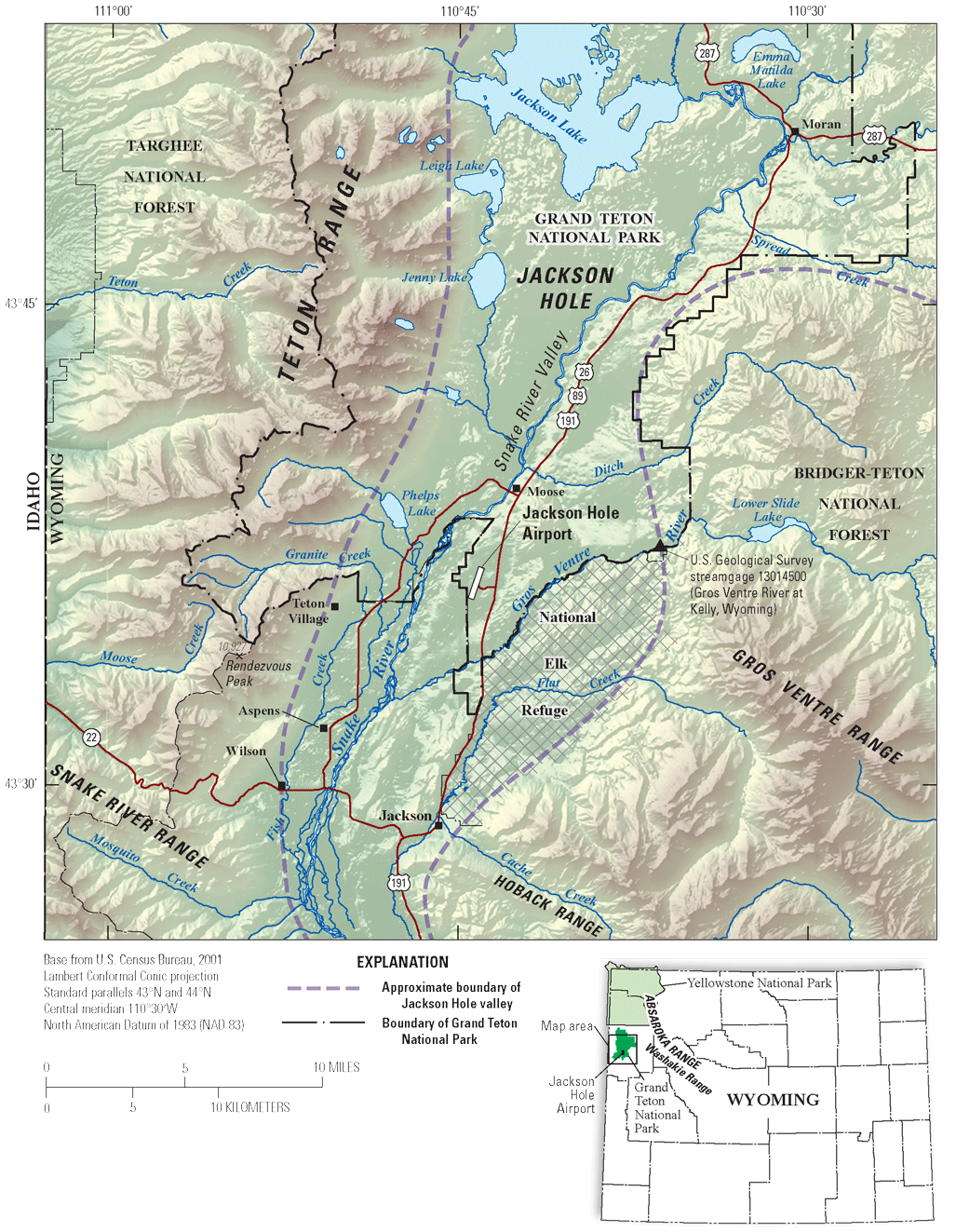
Location of Jackson Hole Airport in the Jackson Hole valley, Wyoming.
The study area lies within Jackson Hole, a geological depression, or “structural basin,” formed by a large block of the Earth’s crust that dropped down along a fault at the base of the Teton Range with its hinge point in the highlands to the east (Love and Reed, 1971). Jackson Hole is bounded on the west by the Teton Range, to the south by the Snake River and Hoback Ranges, to the east by the Gros Ventre Range, and to the north-northeast by the Washakie and Absaroka Ranges, which extend north along the eastern boundary of both Grand Teton and Yellowstone National Park (fig. 1). The geology around the study area is complex with strata ranging from Precambrian basement rocks to Quaternary unconsolidated surficial deposits (fig. 2).
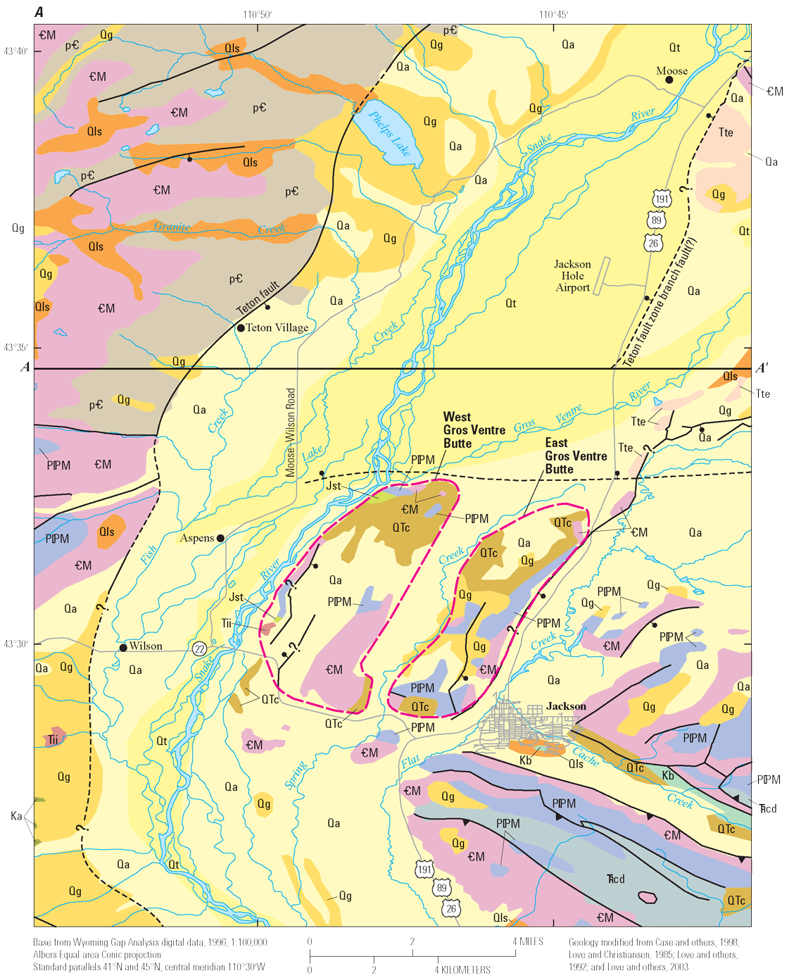
A, Generalized geology and B, geologic section in the vicinity of the Jackson Hole Airport, Jackson, Wyoming (modified from fig. 7 of Eddy-Miller and others, 2009).
JHA is east of the Snake River on Snake River terrace deposits underlain by siltstone deposits of the Chugwater and Dinwoody Formations (fig. 2) (Pierce and Good, 1992; Love and others, 2003). These terrace deposits consist of Quaternary-age unconsolidated gravel, pediment, and fan deposits that are saturated and collectively constitute a large water-table aquifer throughout the eastern part of Grand Teton National Park and the Jackson Hole area (Nolan and Miller, 1995; Nolan and others, 1998). The aquifer informally is named the “Jackson aquifer” (Nolan and Miller, 1995) and is referred to as the “Snake River alluvial aquifer” in this report. The thickness of the Snake River alluvial aquifer near the airport is estimated to be 200 to 250 ft (Nolan and others, 1998) and is the primary water source for the JHA and nearby residents. Lithologic logs of monitoring wells installed at JHA indicate the Quaternary deposits range in size from sand to cobble with most deposits primarily consisting of coarse gravel (Wright, 2010, 2013).
The Snake River alluvial aquifer is unconfined, and depth to water measured in July 1993 ranged from less than (<) 1 to 233.91 ft (median=10.78 ft) below land surface (Nolan and Miller, 1995). Depth to water changes with topography and is shallowest near bodies of surface water. Depth to water at the JHA as measured by the USGS during 2011–20 ranged from 31.93 to 61.51 ft below land surface (Wright, 2013; this report). Recharge of the alluvial aquifer generally is by infiltration of precipitation, streamflow leakage, irrigation water, and movement of deep groundwater near fault zones (Nolan and Miller, 1995). Groundwater in the Snake River alluvial aquifer generally follows the topography, moving from high altitudes toward the Snake River and to the southwest through the Snake River valley (Nolan and Miller, 1995). Groundwater in the Snake River alluvial aquifer at the JHA generally flows from the northeast to the southwest (Kumar and Associates, written commun., 1993; Nolan and Miller, 1995; Wright, 2010, 2013).
Climatically, the study area is in the Middle Rockies ecoregion, which is a temperate, semiarid steppe regime (Chapman and others, 2004). Climate conditions in the Jackson Hole area change with the season and altitude. Mean monthly temperatures for 1991–2020 at the climate station in Moose, Wyoming, approximately 4 mi north of JHA, ranged from 14.3 degrees Fahrenheit (°F) in January to 62.7 °F in July (annual average=38.4 °F; National Oceanic and Atmospheric Administration, 2023). At the same climate station, mean monthly precipitation for 1991–2020 ranged from 1.15 inches (in.) in July to 2.78 in. in December (annual average=23.01 in.; National Oceanic and Atmospheric Administration, 2023). Much of the precipitation in the Jackson Hole area is snowfall. Snow falls about 9 months of the year, and annual average snowfall was 165.9 in. for the period 1991–2020 at Moose, Wyo. (National Oceanic and Atmospheric Administration, 2023).
Study Design
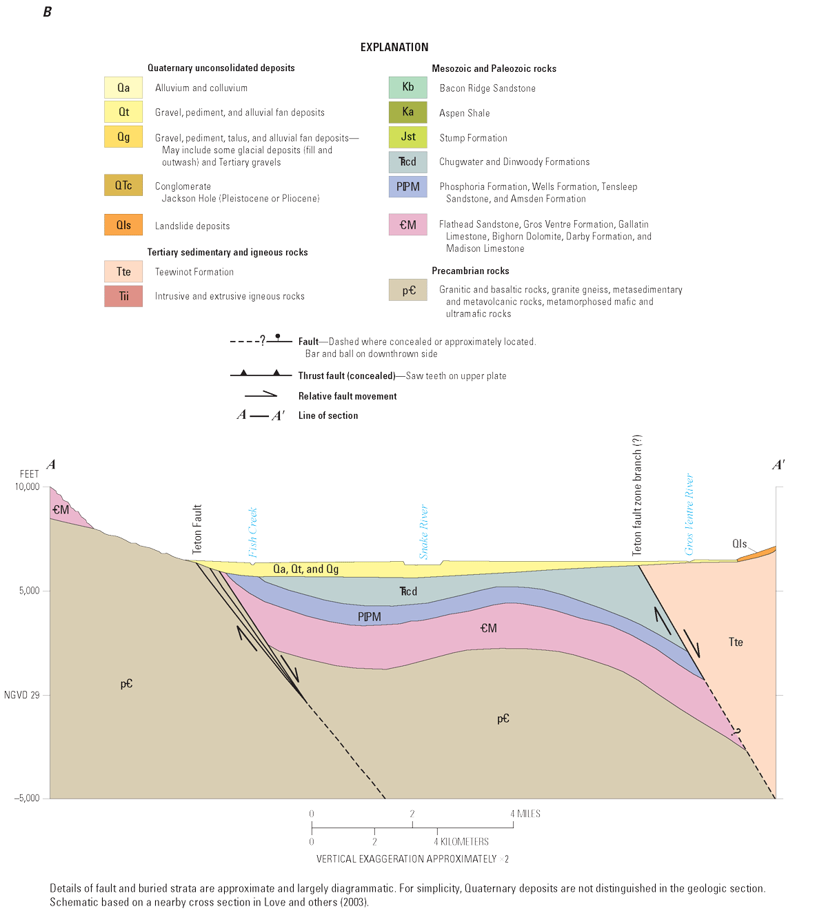
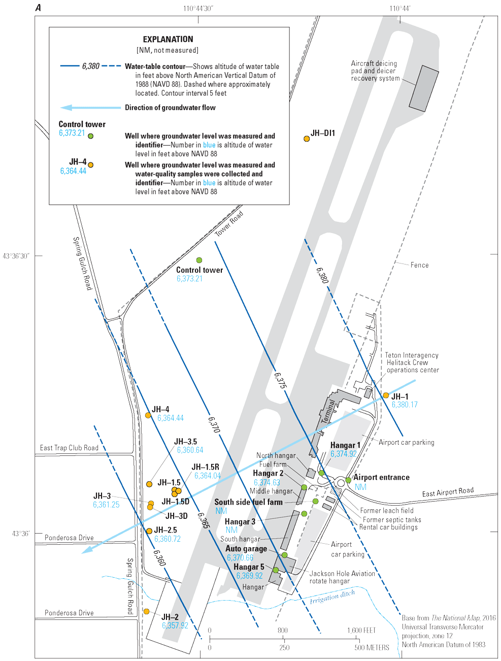
Water-level monitoring and water-quality sampling was done at 10 monitor wells at JHA between 2011 and 2020, including 9 monitor wells installed for previous studies (Wright, 2010, 2013) and 1 new monitor well (JH–DI1) installed in 2012 during this study to establish a baseline understanding of local hydrogeologic and water-quality characteristics downgradient from the new aircraft deicing pad and deicer recovery system (“deicing pad” hereafter; fig. 3) installed in 2011. In addition to these 10 monitor wells, 8 existing production wells and 1 monitor well (JH–1.5) were selected for additional water-level monitoring (fig. 3). The hydrogeology of the Snake River alluvial aquifer underlying the JHA was characterized, in part, using water levels collected from these 19 wells.
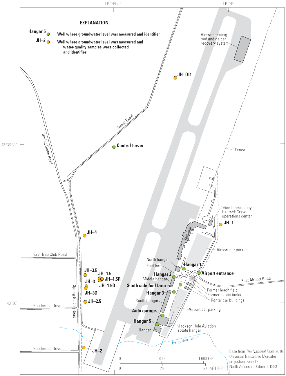
Location of wells used in the study area for data collection, Jackson Hole Airport, Jackson, Wyoming.
The 10 monitor wells used for this study were installed along the direction of groundwater flow based on published water-table contour maps (Kumar and Associates, written commun., 1993; Nolan and Miller, 1995; Wright, 2010, 2013). Eight of the 10 monitor wells sampled during this study are screened across the water table, and two monitor wells (JH–1.5D and JH–3D) are completed in a deeper part of the aquifer (appendix table 1.1). Well JH–1.5D is screened from 85 to 95 ft below land surface. Well JH–3D is not screened, is bottom fed, is open at 102.58 ft below land surface, and acts as a piezometer/monitor well. Well JH–1 is upgradient from and northeast of airport operations and east of the Teton Interagency Helitack Crew operations center (fig. 3). A paired set of monitor wells (referred to as a “monitor-well cluster” hereafter), including a water-table well (JH–1.5R) and a deeper well (JH–1.5D), compose monitor-well cluster 1.5 installed west of the runway and downgradient from airport operations, as well as upgradient from monitor-well cluster 3. Well JH–1.5R was installed in October 2011 as a replacement for well JH–1.5. Well JH–1.5 is no longer sampled for water quality, but water-level measurements are still collected from it. Monitor-well cluster 3 consists of water-table well JH–3 and deeper well JH–3D (fig. 3). Five water-table wells (JH–2, JH–2.5, JH–3, JH–3.5, and JH–4) are downgradient from airport operations along the southwest airport boundary (fig. 3).
Groundwater samples were collected biannually from all 10 water-quality monitor wells with the following exceptions. Samples were not collected when the water table was below the bottom of well screens at well JH–3.5 during the April 2015 sampling event and at wells JH–2.5, JH–3.5, and JH–4 during the April 2016 sampling event. Samples were not collected at well JH–4 during the 2017 sampling season because the site was covered with a storage container that was part of a temporary concrete plant operating on the west side of the airport.
Water-quality results in this report include all samples collected during August 2012–August 2020. In addition, water-quality data collected during June 2011–April 2012 as part of the previous study (Wright, 2013) are included in the “Water Quality” section of this report to help evaluate water-quality changes and trends during the 10-year period (2011–20) when samples were collected and analyzed for benzotriazoles. Field and laboratory analyses mostly were the same as described in Wright (2013), except for wells JH–DI1 and JH–4 that had some differences in laboratory analyses as described later in this report section.
The number and type of analyses collected from each well during August 2012–August 2020 are provided in table 1, and all inorganic analytical results for the same period are tabulated in appendix table 1.8. Physical properties measured in the field for each sample (field analyses) are listed in table 2, and all measurements are tabulated in appendix table 1.7. Field and laboratory results from 2011 are published in Wright (2013) and generally are not included herein except for physical properties and selected constituents. In addition, wells with low dissolved-oxygen (DO) concentrations (<0.5 milligram per liter [mg/L]) were analyzed for sulfide to better understand redox processes in anoxic wells.
Table 1.
Number of field and laboratory analyses for groundwater samples collected from monitor wells at the Jackson Hole Airport, Jackson, Wyoming, 2012–20.[Data are summarized from table 7 and appendix tables 1.3, 1.7, and 1.8. USGS, U.S. Geological Survey; VOC, volatile organic compound; GRO, gasoline-range organics; DRO, diesel-range organics; BTEX, benzene, toluene, ethylbenzene, and xylenes; --, not applicable]
| USGS site number (USGS, 2021a) | Well identifier (fig. 3) | Field analyses | Laboratory analyses | |||||||||
|---|---|---|---|---|---|---|---|---|---|---|---|---|
| USGS National Water Quality Laboratory | USGS-contracted laboratory1 | Wisconsin State Laboratory of Hygiene | ||||||||||
| Physical properties | Major ions | Nutrients | Trace elements | Dissolved organic carbon | VOCs | GRO | DRO | BTEX | Glycols | Benzotriazole compounds2 | ||
| 433615110440001 | JH–1 | 15 | 15 | 15 | 9 | 15 | -- | -- | -- | -- | -- | 15 |
| 433604110443403 | JH–1.5R | 15 | 15 | 15 | 9 | 15 | -- | -- | -- | -- | -- | 15 |
| 433604110443402 | JH–1.5D | 15 | 15 | 15 | 9 | 15 | -- | -- | -- | -- | -- | 15 |
| 433551110443501 | JH–2 | 15 | 15 | 15 | 9 | 15 | -- | -- | -- | -- | -- | 15 |
| 433600110443701 | JH–2.5 | 14 | 14 | 14 | 8 | 14 | -- | -- | -- | -- | -- | 14 |
| 433603110443501 | JH–3 | 15 | 13 | 15 | 9 | 15 | -- | -- | -- | -- | -- | 15 |
| 433603110443502 | JH–3D | 15 | 15 | 15 | 9 | 15 | -- | -- | -- | -- | -- | 15 |
| 433605110443801 | JH–3.5 | 13 | 13 | 13 | 7 | 13 | -- | -- | -- | -- | -- | 13 |
| 433613110443501 | JH–4 | 12 | 12 | 12 | 6 | 12 | 2 | 2 | 2 | -- | -- | 12 |
| 433641110441501 | JH–DI1 | 17 | 17 | 13 | 8 | 16 | 1 | 2 | 1 | 1 | 15 | 16 |
TestAmerica Laboratories, Inc., in Denver, Colorado, analyzed water samples for VOCs, GRO, and DRO from well JH–DI1 during 2012 and for glycols during 2012 and 2013. RTI Laboratories, Inc., in Livonia, Michigan, analyzed samples for glycols from well JH–DI1 from 2014 to 2017, and for GRO and DRO from well JH–4 during 2019. Samples were analyzed for glycols (ethylene and propylene glycol) by Microbac Laboratories in Marietta, Ohio, during April 2018, SGS North America, Inc., in Dayton, New Jersey, during August 2018, and SGS North America, Inc., in Houston, Texas, during 2019 and 2020. VOCs collected during 2019 were analyzed by SGS North America, Inc., in Orlando, Florida, in May and SGS North America, Inc., in Wheat Ridge, Colorado, in August.
Table 2.
Summary of physical properties, inorganic constituents, reporting levels, and reporting level types for groundwater samples collected at Jackson Hole Airport, Jackson, Wyoming, 2012–20, and analyzed in the field or at the U.S. Geological Survey National Water Quality Laboratory.[IDL, instrument detection level; --, not applicable; DLDQC, detection limit by DQCALC procedure (U.S. Geological Survey, 2015); SiO2, silicon dioxide; MRL, minimum reporting level; DLBLK, detection limit determined with blank data (U.S. Geological Survey, 2015)]
Laboratory analyses and associated LRLs and reporting level types for inorganic constituents, including major ions, nutrients, trace elements, and dissolved organic carbon (DOC), are listed in table 2. Laboratory analyses and associated laboratory reporting levels, and Chemical Abstracts Service Registry Numbers for organic constituents typically of anthropogenic origin, including volatile organic compounds (VOCs), diesel-range organics (DRO), gasoline-range organics (GRO), glycols, and benzotriazole compounds are listed in table 3. Benzotriazoles are a class of chemicals historically used in ADAFs as corrosion inhibitors and have increased the toxicity of ADAF to aquatic organisms (Pillard, 1995; Cancilla and others, 1997; Cornell and others, 2000). Benzotriazoles can be detected at relatively lower LRLs than glycols, were detected at low concentrations during the previous study (Wright, 2013), and are used in this study as a surrogate for identifying ADAFs in JHA groundwater because of the much lower LRLs.
Table 3.
Summary of volatile organic compounds, gasoline-range organics, diesel-range organics, glycols, and benzotriazole compounds analyzed in groundwater samples collected at Jackson Hole Airport, Jackson, Wyoming, 2012–20.[Compounds detected during study are shown in bold type and noted with footnote 13. µg/L, microgram per liter; EPA, U.S. Environmental Protection Agency; --, not applicable; C6–C10, C10–C32, and C10–C36, ranges of carbon compounds included in the analysis]
This report contains Chemical Abstracts Service Registry Numbers, which are registered trademarks of the American Chemical Society. The Chemical Abstracts Service recommends verifying these numbers through their Client Services.
This compound was analyzed as part of the volatile organic compound analysis, but it is an ether used as a fuel oxygenate.
The EPA drinking-water advisory ranges from a 20-µg/L odor threshold to a 40-µg/L taste threshold (EPA, 2018).
Water-quality results of the wells sampled through 2011 for previous studies (fig. 3) (Wright, 2010, 2013) did not indicate the widespread occurrence of anthropogenic compounds such as VOCs, GRO, or DRO in the alluvial aquifer at the JHA; therefore, subsequent samples from most of these wells were not reanalyzed for these constituents. However, the first sample collected from well JH–DI1 (installed summer 2012 and first sample collected August 22, 2012) was analyzed for all these constituents to define baseline conditions in the alluvial aquifer downgradient from the deicing pad (fig. 3). One additional sample also was collected from well JH–DI1 on April 3, 2013, and analyzed for GRO and four VOCs (benzene, toluene, ethylbenzene, and xylenes, collectively referred to as BTEX) to confirm these constituents were not present in the aquifer at this location. Samples for VOCs, GRO, and DRO were collected from well JH–4 during the spring and fall of 2019 to assess if these organic compounds were contributing to changes in redox conditions identified at this well. Additionally, although glycol compounds were not detected during the first study (Wright, 2010) and were not included in the second study (Wright, 2013), samples were collected once in 2012 and biannually during 2013–20 from well JH–DI1 and analyzed for glycols to monitor for potential changes in groundwater quality downgradient from deicing activities at the deicing pad at the northeast end of the taxiway (fig. 3).
Methods of Data Collection and Analysis
This section describes methods used to construct monitor wells, measure water levels, analyze hydrogeologic data, and collect and analyze groundwater and quality-control samples. Standardized USGS technical guidance describing these methods are documented in the USGS “National Field Manual for the Collection of Water-Quality Data” (NFM; USGS, variously dated) and “Groundwater Technical Procedures of the U.S. Geological Survey” (Cunningham and Schalk, 2011).
Well Construction and Ancillary Information
The techniques used to install most of the monitor wells used to study the hydrogeology and water quality of the alluvial aquifer underlying the JHA are described in Wright (2010, 2013). Well construction and related ancillary information for wells used during this study are presented in appendix table 1.1. As noted previously, one of these monitor wells (JH–DI1) was installed downgradient from the deicing pad during the summer of 2012. This shallow (water-table) well was constructed with a 2-in. diameter, flush-jointed polyvinyl chloride (PVC) well casing and well screen (appendix table 1.1). The well screen for well JH–DI1 is 20 ft long (well screen installed from 50 to 70 ft below land surface; appendix table 1.1) and was installed from about 5–10 ft above the water table to a depth about 10–15 ft below the water table at the time of installation, allowing the well to “straddle” the water table during seasonal changes and to facilitate detection of low-density contaminants such as petroleum-based fuels that can float on or near the water-table surface. Before sampling, well JH–DI1 was pumped or “developed” using methods described in Lapham and others (1995) to remove artifacts associated with drilling, such as drilling fluids, to provide water representative of the aquifer being sampled and to improve movement of water into the well.
Well locations and altitudes were determined by the USGS or from surveys contracted by the airport. Well locations were determined by the USGS using a global positioning system that reported latitude and longitude using the North American Datum of 1983 (NAD 83) with horizontal accuracy of less than plus or minus (±) 49 ft (Garmin Ltd, 2004). Altitudes for the monitor wells installed for this study were determined using conventional surveying methods.
Water-Level Measurement
Discrete water levels were measured in wells during each site visit to the airport (appendix table 1.2), and hourly water levels were collected using continuous water-level recorders at selected wells during and after other field activities were completed. Discrete water levels were typically measured with a calibrated electric tape (e-tape) when possible or less frequently with a calibrated steel tape. A detailed description of the methods used to measure water levels by use of e-tape or steel tape are described in Cunningham and Schalk (2011). Water levels were measured to one-hundredth of a foot (0.01 ft), and replicate measurements were made during each site visit to ensure the water level measured was correct. Discrete groundwater-level measurements were processed, reviewed, approved, and published in accordance with USGS policy (USGS, 2017a). Discrete groundwater-level measurements are available through the USGS National Water Information System (NWIS) database (USGS, 2021a) using the 15-digit site-identification numbers in appendix table 1.1.
Continuous water-level recorders were installed in monitor wells JH–1, JH–2, JH–3, and JH–4 during 2008 and in monitor wells JH–1.5R, JH–1.5D, JH–3D, and JH–DI1 during 2014. These instruments were installed by the Teton Conservation District and the USGS, respectively, and have been maintained and operated by the USGS since 2012. These self-contained pressure transducer/data logging units are vented, allowing for changes in barometric pressure, and are accurate to ±0.012 ft (In-Situ, Inc., 2013, p. 23). Discrete water-level measurements were collected each time that data were downloaded and during each site visit (appendix table 1.2) to verify proper reading of each instrument. Continuous time-series water-level data collected through water year 2020 were analyzed, reviewed, approved, and published in accordance with USGS policy (USGS, 2017b). Time-series data for wells with continuous water-level recorders can be retrieved from the USGS NWIS database (USGS, 2021a) using the 15-digit site numbers in appendix table 1.1.
Water-Table Contours, Hydraulic Gradient, and Groundwater Velocity
This section describes constructed water-table contours and calculated hydraulic gradients and groundwater velocities. A spreadsheet tool (3PE) was used to determine groundwater-flow directions and calculate hydraulic gradients and groundwater velocities (Beljin and others, 2014). Water-table contours were constructed using methods described in Heath (1983) and presented in Wright (2010). The spreadsheet tool uses Darcy’s Law to calculate groundwater velocities (Wright, 2010).
The spreadsheet tool (3PE) was developed in Microsoft Excel, and the software package uses a mathematical approach to calculate hydraulic gradients and determine groundwater-flow directions and magnitudes using the three-point solution method (Beljin and others, 2014). Data necessary for these calculations included well coordinates for three wells in a triangle (appendix table 1.1), groundwater-level altitudes for each of the three wells (appendix table 1.2), and estimates of the hydraulic conductivity and effective porosity of aquifer materials. Assuming that groundwater flow at the JHA is perpendicular to the water-table contours and the aquifer is homogeneous and isotropic, groundwater velocity was estimated using horizontal hydraulic conductivities of 2,900 and 1,200 feet per day (Nelson Engineering, 1992) and an estimated effective porosity for the sand and gravel aquifer (Wright, 2010, 2013) of 30 percent (appendix table 4.2 of Fetter, 1988).
Groundwater Sampling and Analysis
Most groundwater samples were collected biannually between 2012 and 2020, with each sampling event representing different hydrogeologic conditions, and were collected at or close to the water-table low in the spring and at or close to the water-table high in the summer. Samples were analyzed in the field and laboratory for selected constituents. This section briefly describes the analytical laboratories, constituents analyzed by each laboratory, and LRLs. In this report, the term “reporting level” is used in a general sense to represent any type of LRL.
Groundwater samples were collected and processed in a mobile water-quality laboratory in accordance with standard USGS methods described in the USGS NFM (USGS, variously dated). A clean, portable and submersible sampling pump was used to collect groundwater-quality samples. Water was pumped from each well through a sampling manifold and a flow-through chamber in the mobile laboratory until at least three well-casing volumes had been removed and measurements of physical properties of DO, pH, specific conductance, temperature, and turbidity had stabilized. These physical properties (table 2) were measured in the field as part of sample collection using methods described in the USGS NFM (USGS, variously dated). Alkalinity was determined using incremental titration of a filtered water sample with sulfuric acid as described in the USGS NFM (USGS, variously dated). Samples collected for analyses of major ions, selected nutrients, selected trace elements, and dissolved organic carbon were filtered by passing sample water through a pre-conditioned (purged with deionized water) 0.45-micrometer, nominal-pore-size, disposable capsule filter. In this report, constituents in filtered and unfiltered water samples are referred to as dissolved and total, respectively.
Water samples were analyzed for dissolved major ions, trace elements, nutrients, and organic carbon (DOC) at the USGS National Water Quality Laboratory (NWQL) in Denver, Colorado. Major ions and trace elements (table 2) were analyzed using ion-exchange chromatography or inductively coupled plasma-atomic-emission spectroscopy (Fishman and Friedman, 1989; Fishman, 1993). Nutrients (table 2) were analyzed using colorimetry (Fishman, 1993), and DOC was analyzed using ultraviolet light-promoted persulfate oxidation and infrared spectrometry (Brenton and Arnett, 1993).
TestAmerica Laboratories, Inc., in Denver, Colo., was contracted to analyze water samples for VOCs, GRO, and DRO from well JH–DI1 during 2012 (table 3) and glycols during 2012 and 2013 using EPA methods. Samples were analyzed for VOCs using EPA method 524.2 (Munch, 1995) and for GRO, DRO (C10–C32 and C10–C36 ranges), and glycols using EPA SW846 method 8015B (EPA, 1996a; table 3).
RTI Laboratories, Inc., in Livonia, Michigan, was contracted to analyze samples for glycols from well JH–DI1 from 2014 to 2020 and two sets of samples for VOCs, GRO, and DRO from well JH–4 during 2019. From 2014 to 2017, RTI Laboratories, Inc., analyzed samples for glycols (diethylene glycol, ethylene glycol, propylene glycol, and triethylene glycol) using EPA SW846 method 8015B (EPA, 1996a). Beginning in 2018, RTI Laboratories, Inc., subcontracted the glycol analyses (ethylene and propylene glycol) to Microbac Laboratories in Marietta, Ohio, in April 2018, and to SGS North America, Inc., in Dayton, New Jersey, in August 2018, and in Houston, Texas, during 2019 and 2020. During 2019, two sets of samples collected from well JH–4 were analyzed for GRO using EPA SW846 method 8021/8015B (EPA, 1996a, 1996b) and for DRO using EPA SW846 method 8015B (EPA, 1996a) by RTI Laboratories, Inc., in Livonia, Mich. Samples from well JH–4 analyzed for VOCs (by EPA method 524.2) during 2019 were subcontracted to SGS North America, Inc., in Orlando, Florida, in May and in Wheat Ridge, Colo., in August.
The Wisconsin State Laboratory of Hygiene (WSLH) was contracted to analyze water samples for benzotriazoles (1H-BT, 4-MeBT, and 5-MeBT). All groundwater samples collected from each of the 10 water-quality monitor wells during 2012–20 were analyzed for benzotriazoles (table 3). The WSLH has developed a high performance/liquid chromatography/triple quadruple mass spectrometry method to determine the benzotriazole compounds in water (Wisconsin State Laboratory of Hygiene, 2007).
Low-concentration range DO, sulfide, and ferrous iron (Fe2+) were analyzed in the field laboratory using a HACH DR 2800 spectrophotometer (HACH, 2007). Methods of analyses included HACH method 8316, which is the indigo carmine method using AccuVac ampoules for low-range DO; HACH method 8146, which is the 1,10-phenanthroline method using AccuVac ampoules for Fe2+; and HACH method 8131, which is a methylene blue method for sulfide (HACH, 2007).
Each of the laboratories described previously reported analytical results in accordance with their protocols. The remainder of this section briefly describes how data are reported. Reporting levels for constituents analyzed as part of this study are presented in tables 2–3. The less than symbol (<) indicates that the chemical was not detected and was therefore censored. For data reported by the NWQL, TestAmerica Laboratories, RTI Laboratories, Inc., Microbac Laboratories, and SGS North America, Inc., the value after the less than (<) symbol is the detection limit determined using the procedure in DQCALC software (DLDQC), the detection limit determined using blank data procedures (DLBLK; U.S. Geological Survey, 2015), or the minimum reporting level (MRL) associated with that analysis. The MRL, as defined by the NWQL, is the smallest measured concentration of a substance that can be measured reliably by using a given analytical method (Timme, 1995). For benzotriazole data reported by the WSLH (table 3), the value after the less than (<) symbol is the level of detection (LOD) or detection limit, defined as the lowest concentration level that can be determined to be statistically different from a blank sample with 99-percent confidence (Wisconsin Department of Natural Resources, 1996). The LOD approximately is equal to the method detection limit (MDL) for those analyses for which the MDL can be calculated. Some water-quality results, especially those for organic compounds in this study, are qualified with an “E” or are reported as a less than (<) value. The “E” remark code indicates greater uncertainty in the associated result, and the value should be considered estimated. Values generally are estimated when the value is greater than the MDL but less than the established reporting level. Three additional data qualifiers were used by the NWQL: (1) “n,” value below the LRL and above the long-term method detection level; (2) “d,” sample was diluted and method “high range” was exceeded; and (3) “b,” value was extrapolated below the lowest calibration standard, method range, or instrument linear range. The WSLH data also have been reported with an “E” remark code. In this case, the “E” remark code indicates the value is estimated and less than the level of quantitation (LOQ), but equal to or greater than the LOD. The LOQ is the level above which quantitative results may be obtained with a specified degree of confidence. The LOQ is defined mathematically as equal to 10 times the standard deviation of a series of replicate results used to determine the LOD (Wisconsin Department of Natural Resources, 1996).
Determining Redox Conditions
Concentrations of redox-sensitive species, including nitrate (NO3–), manganese (manganous manganese [or Mn2+]), iron (ferrous iron, or Fe2+), and sulfate (SO42–), along with DO (O2), and sulfide (sum of dihydrogen sulfide [aqueous H2S], hydrogen sulfide [HS–], and sulfide [S2–]) were used to assess the biological redox status of groundwater using the classification framework of McMahon and Chapelle (2008). Because redox processes in groundwater tend to segregate into zones dominated by one electron-accepting process, the redox framework uses the concentrations of the redox-sensitive species to assign the predominant redox process to groundwater samples. An automated spreadsheet program was used to assign the redox classification to each sample (Jurgens and others, 2009). Redox class and process assignments are presented in the “Redox Conditions” section. If a redox assignment was not determined for a sample, it likely was due to missing data for one or more of the redox-sensitive species. Total dissolved manganese and iron concentrations as determined by the USGS NWQL were used in the spreadsheet in place of Mn2+ and Fe2+ because these are the most common forms of manganese and iron in groundwater (Hem, 1985). A detailed description of the redox classification framework is presented in McMahon and Chapelle (2008) and Chapelle and others (2009). Spreadsheet instructions and details of redox assignments are presented in Jurgens and others (2009). A brief description of redox assignments using the spreadsheet follows.
When all four redox-sensitive species and DO are entered, the general redox class (oxic, suboxic, anoxic, or mixed) is determined from the redox process. For samples that have sulfide measurements in addition to DO and the four redox-sensitive species, Fe2+ and SO42– reduction is differentiated in the redox process column using the calculated iron-to-sulfide ratio. For samples missing one or more of the redox-sensitive species, the general redox class was determined using the DO concentration: “oxic” for DO concentrations greater than or equal to 0.5 mg/L, “suboxic” for low DO conditions which cannot be defined further without additional data, “anoxic” for DO concentrations <0.5 mg/L, or “mixed” when conditions mix available electron acceptors or final products.
Quality Assurance and Quality-Control Sample Collection
Quality assurance (QA) throughout this study included collection and evaluation of quality-control (QC) samples and strict adherence to sample collection, processing, and analysis guidelines in the USGS NFM (USGS, variously dated). QC samples were collected and used to assess the quality of the data reported for environmental groundwater-quality samples collected from wells. QC samples included several different types of blank samples and replicate environmental samples. The QC samples were collected using the same collection, preservation, and laboratory analytical methods as the environmental samples.
Blank Samples
A variety of blank samples were collected to determine the extent environmental analytical results were affected by bias (contamination of environmental samples) introduced during field equipment cleaning, field sample collection, field sample processing, and laboratory analytical procedures. Blank samples, including field-equipment, source-solution, and trip blanks, were prepared with water that was certified to be free of analytes of interest (blank water) before submission to analytical laboratories for analysis. A brief description of each type of blank sample follows:
-
• Field-equipment blanks consisted of certified organic- or inorganic-blank water (depending on the type of analysis) that has been processed through the sampling system after field cleaning and was subjected to all aspects of sample collection, field processing, preservation, transportation, cleaning, and laboratory handling as the environmental sample. Field-equipment blanks are used to evaluate the adequacy of field-equipment cleaning, and the cleanliness of sample collection, processing, storage, and transport protocols (Mueller and others, 1997). For this study, field-equipment blanks generally were collected after sampling equipment had been used to collect a water sample from a well that previously had detections of 4-MeBT. Field equipment was cleaned, and field-equipment blanks were collected, by passing water through all the sample tubing, from the sampling pump, through the sampling chamber, and the capsule filter (for filtered samples), before lowering the sampling pump into the well to collect environmental samples.
-
• Source-solution blanks were collected by pouring certified blank water directly into the sample bottle in a clean area on the day of sampling. These blanks are used to determine if the blank water, sample container, or preservation chemicals are contaminated. One source-solution blank was collected during this study (appendix table 1.4) to determine if certified inorganic-blank water was free of benzotriazoles and could be used for collection of field-equipment blanks.
-
• Trip blanks are VOC samples prepared in the laboratory using analyte-free water. Trip blanks were supplied by the laboratory providing VOC analyses and were transported with VOC sample bottles to the field, kept with these sample bottles throughout sampling, and then returned to the laboratory for analysis with associated environmental samples. Trip blanks are used to identify contamination introduced during sample transport and storage. Three trip blanks were collected during this study (appendix table 1.4). One trip blank was collected for each round of sampling that included collection of VOC samples. Analytical results for only two trip blanks are presented in appendix table 1.4 because the third trip blank (collected August 13, 2019) was sent to the laboratory but not analyzed because no VOCs were detected in the associated environmental sample.
A quantified result in any blank sample was considered evidence that contamination could have biased groundwater sample results. Analytical results for groundwater samples were compared to the maximum quantified concentration in each blank sample collected during the same sampling event. EPA guidance (EPA, 1989, p. 5–17) recommends a reported concentration in an environmental sample that is less than five times the concentration in a related blank sample be qualified. In this report, water-quality results are presented as they were received from the laboratory. Constituents that meet EPA guidance criteria have been qualified using a footnote in the water-quality data tables presented in this report. For data analysis purposes, these values were considered nondetections. All qualifications were based on quantified results in field-equipment blank or trip-blank samples. Constituents were not detected in the source-solution blank.
Twenty-four field-equipment blank samples were collected during this study (appendix table 1.4). One-third (8) of these field-equipment blank samples were from well JH–DI1 because it was the only well where samples were collected and analyzed for glycol compounds. The remaining field-equipment blank samples (16) were collected before environmental sample collection from 7 other monitor wells. Sixteen constituents were detected at low but measurable concentrations in field-equipment blank samples: 1 major ion (calcium), 1 uncharged species (silica), 2 nutrients (ammonia and total nitrogen), DOC, 6 trace elements (antimony, chromium, cobalt, copper, manganese, and strontium), and 5 organic compounds (dichloromethane, vinyl chloride, diethylene glycol, ethylene glycol, and propylene glycol; appendix table 1.4). Importantly, benzotriazoles were not detected in any blank samples. A brief description of these detections and resultant effects on environmental concentrations follows.
Concentrations of calcium and silica measured in field-equipment blank samples (four detections; two each) were low; two of the detections were below the LRL but above the long-term MDL. Both constituents were detected in environmental samples, but environmental sample results were not qualified because these constituents generally were detected at concentrations several orders of magnitude larger than the concentrations measured in the field-equipment blank samples.
Concentrations of nutrients (ammonia and total nitrogen) measured in field-equipment blank samples (7 detections) were low (appendix table 1.4); 6 of the 7 detections were below the LRL, but above the long-term MDL. Ammonia and total nitrogen results for environmental samples with detections less than five times the maximum concentration detected in the field-equipment blank sample for that sampling event were qualified using a footnote (appendix table 1.8).
Concentrations of DOC measured in field-equipment blank samples (two detections) were low; one of two detections was at the LRL but above the long-term MDL. DOC results for environmental samples with detections less than five times the maximum concentration detected in the field-equipment blank sample for that sampling event were qualified using a footnote (appendix table 1.8).
Concentrations of trace elements detected in field-equipment blank samples (antimony, chromium, cobalt, copper, manganese, and strontium; 11 detections total) were low; 6 of the 11 detections were below the LRL but above the long-term MDL. When detected in environmental samples, concentrations of antimony, chromium, cobalt, and copper were generally low (appendix table 1.8); consequently, concentrations for many environmental samples were qualified due to being less than five times the maximum detected concentration in the field-equipment blank for each associated sampling event. Environmental sample concentrations of manganese ranged from nondetections (below LRL) to greater than 1,000 mg/L, resulting in only one manganese concentration being qualified (appendix table 1.8). Environmental sample concentrations of strontium were high in relation to field-equipment blank sample concentrations, so no strontium concentrations were qualified.
Two field-equipment and two trip-blank samples were collected and analyzed for VOCs; both types of blank samples were collected before environmental sample collection at well JH–DI1 on August 22, 2012, and at well JH–4 on May 7, 2019. One VOC (dichloromethane) was detected in the field-blank sample and two VOCs (dichloromethane and vinyl chloride) were detected in the trip-blank sample collected at well JH-4 during May 2019 (appendix table 1.4), but not in the associated environmental sample (appendix table 1.8). In addition to VOCs, two field-equipment blank samples were analyzed for GRO and DRO; neither organic constituent was detected in the samples (appendix table 1.4).
Eight field-equipment blank samples were collected and analyzed for glycols during sampling at well JH–DI1 (types of glycol compounds analyzed varied during study; appendix table 1.4). Well JH–DI1 was the only well from which samples were collected and analyzed for glycol compounds during August 2012–20. Three different glycol compounds (total of five glycol detections) were detected in four of the eight field-equipment blank samples (appendix table 1.8). Of the five field-equipment blank detections, only one sample (collected August 13, 2019) had detections of a glycol compound (ethylene glycol) in both the field-equipment blank sample and the associated environmental sample; consequently, the environmental sample concentration was qualified (appendix table 1.3).
Replicate Samples
Replicate samples are two or more samples collected and processed sequentially, so that the samples are considered essentially identical in composition. By analyzing these samples for the same constituents, replicate sampling results can be used to evaluate the cumulative effects of field and laboratory procedures on the reproducibility (precision) of analyte concentration values reported by the laboratory. Although two replicate samples are not adequate to assess precision, they can be used to evaluate whether variability of results for the samples is within the range of expected precision based on the larger available dataset. Potential variability was estimated by comparing replicate groundwater samples. Twenty-two replicate samples were collected from eight monitor wells during 2012–20 and analyzed for many constituents (appendix table 1.5). Variability for each analyte was estimated as the relative percent difference (RPD) between constituent concentrations measured in the primary environmental sample and the replicate environmental sample using equation 1:
whereCenv
is the concentration of the analyte in the environmental sample;
Crep
is the concentration of the analyte in the replicate environmental sample;
|Cenv–Crep|
is the absolute value of the difference between concentrations of the analyte in the primary environmental sample and the replicate environmental sample; and
(Cenv+Crep)/2
is the mean concentration of the analyte in the primary environmental sample and replicate environmental sample.
RPDs were calculated only for constituents with detections in both the environmental sample and associated replicate environmental sample. The RPD could not be calculated if a concentration was censored in either or both samples. For this study, RPD values greater than 20 percent indicated that analytical results might be affected by high variability. Calculated RPDs are presented in appendix table 1.5. Overall, analytical results for 16 constituents were qualified due to high variability. These results have been identified using a footnote in table 7 and appendix table 1.8. RPDs for environmental samples with associated replicate environmental samples (“replicate pairs”) generally were acceptable. Many of the replicate pairs with high variability were a result of low constituent concentrations in both the environmental and replicate samples. Small differences in low concentrations can result in large RPDs. Of all the replicate pairs collected during this study, only two were identified as having RPDs of concern. One replicate pair (well JH–DI1, August 22, 2012) indicated high variability for iron (RPD=88 percent), and the second replicate pair (well JH–DI1, April 30, 2013) indicated high variability for iron (RPD=163 percent) and manganese (145 percent; appendix table 1.5). These sample results with high RPDs were not rejected because these samples were reanalyzed by the NWQL, and the resulting concentrations were similar. During initial review of the sampling results, there was concern sediment might have broken through the 0.45-micron filter used for sampling; however, major ions analyzed with these constituents in the same samples had RPDs less than 10 percent. The only samples collected during August 2012 and April 2013 and associated with these higher RPDs were from well JH–DI1.
Major-Ion Balance
Major-ion data were quality-assured by calculating a cation-anion balance (“ionic charge balance”). The sum of concentrations of dissolved cations in milliequivalents per liter should equal the sum of concentrations of dissolved anions in milliequivalents per liter (Hem, 1985). The percent difference between the sum of concentrations of cations and anions in milliequivalents per liter was calculated using equation 2:
Ionic charge balances were calculated for groundwater samples with major-ion analyses. The ionic charge balances ranged from −3.08 to 6.61 percent. An ionic charge balance within ±5 percent is preferable (Friedman and Erdmann, 1982; Clesceri and others, 1998). Four ionic charge balances during this study slightly exceeded 5 percent and ranged from about 5.1 to 6.6 percent; these balances were considered acceptable for this study.
Statistical Analysis
All statistical analyses and tests were done using the R statistical environment (R Core Team, 2021), including various statistical packages developed for R. Nonparametric (rank-based and “distribution-free”) statistical methods were used almost exclusively for data analysis and interpretation. Water-quality datasets typically are nonnormal, so nonparametric methods generally are preferable over parametric methods to evaluate water-quality data (Helsel, 2012; Helsel and others, 2020). Nonparametric methods also are resistant to outliers and are more appropriate for small sample sizes where nonnormality can be more difficult to detect.
For this report, a significance level (α value, or attained level of significance) of 0.05 was used for statistical tests. The significance level is the probability (p-value) of incorrectly rejecting the null hypothesis when true. The null hypothesis of a statistical test was rejected if the p-value was less than or equal to an α level of 0.05, and the test results were considered statistically significant. A p-value less than or equal to 0.05 indicates there is only a 5 percent or less chance of getting the observed results if the null hypothesis is true.
Summary statistics determined for constituents with uncensored data values were computed using standard methods (Helsel and others, 2020). Methods used to calculate summary statistics for constituents with censored (“less than”) data values were selected using guidance provided by Helsel (2012). Two methods generally were used to compute summary statistics for large datasets (more than 50 data values for a given constituent) with less than 50 percent of the data values censored—the nonparametric flipped Kaplan-Meier method for constituents with only 1 reporting level and the maximum likelihood estimation method for constituents with more than 1 reporting level. The maximum likelihood estimation method also was used for large datasets with 50 to 80 percent of the data values censored, regardless of the number of reporting levels. For some datasets, these methods imputed (statistically estimated) median values that were less than reporting levels; these values should be considered as estimates based on probability distributions inherent to each method (Helsel, 2012). Both methods were implemented using the Non-Detects and Data Analysis for Environmental Data (NADA) package (Lee, 2020) for R. Summary statistics were not determined for constituents with greater than 80 percent of data values censored (Helsel, 2012).
The nonparametric rank-sum test, also known as the Mann-Whitney U test or Wilcoxon rank-sum test (Helsel, 2012), was used to determine if two independent datasets consisting of uncensored data values were from the same population. The nonparametric generalized Wilcoxon rank-sum test (a “survival analysis” or “score-test” version of the Wilcoxon rank-sum test) available in the NADA2 package for R (Julian and Helsel, 2021), known as the Peto-Peto test (Helsel, 2012), was used to determine if two independent datasets consisting of uncensored and censored data values were from the same distribution by comparing empirical cumulative distribution functions. The null hypotheses for the test (rejected when p-value<0.05) is that the datasets were from the same population (rank-sum test) or distribution (Peto-Peto test), and the alternative hypotheses is that the datasets were from different populations or distributions, respectively.
Tukey-style boxplots (Helsel and others, 2020) were constructed for selected water-quality properties or constituents to statistically summarize data and to qualitatively compare physical-property values or constituent concentrations among different wells. Results from quantitative comparisons (rank-sum or Peto-Peto tests) of properties or constituents between wells with detections of 4-MeBT and wells without detections are presented on the boxplots. Boxplots for constituents consisting of uncensored and censored data values were constructed using the censored boxplot function in the NADA package for R (Lee, 2020). This function computes percentiles using robust regression-on-order statistics (Helsel and others, 2020); therefore, median concentration values in the boxplots for these constituents may differ slightly from the median concentration values computed using the Kaplan-Meier or maximum likelihood estimate methods that are listed in a later report summary table. Boxplots constructed for constituents with censored values were truncated at the highest LRL (Helsel, 2012).
The nonparametric Kendall’s tau (τ) correlation test was used to determine the direction and strength of the monotonic relation (linear or nonlinear relation in one direction) between two continuous water-quality properties or constituents (Helsel, 2012). Test results consist of a test statistic, Kendall’s τ correlation coefficient, and a p-value. The null hypothesis for the test (rejected when p-value<0.05) is that the variables are uncorrelated, and the alternative hypothesis is that the variables are correlated. Kendall’s τ values range from −1 to 1, and a value of 0 indicates no correlation. Increased strength of correlation is indicated as τ values approach −1 or 1. τ coefficient values generally are lower than linear correlation coefficients with the same strength; for example, a linear correlation of 0.9 or above is approximately equivalent to a τ value of about 0.7 or above (Helsel and others, 2020). A version of the test available in the NADA package for R (Lee, 2020) was used for datasets consisting of uncensored and censored data values. In this report, p-values greater than or equal to 0.05 but less than or equal to 0.09, although not significant with an α level of 0.05, indicated “weak,” “nonsignificant” correlation between two continuous variables of interest.
The nonparametric seasonal Kendall test (Helsel and others, 2020), as implemented in the rkt package for R (Marchetto, 2021), was used to test for trends in selected physical-property values and constituent concentrations in samples from individual wells with time (2011–20). The seasonal Kendall test computes a Mann-Kendall test for each season of a year, and a year can consist of two or more seasons. The Mann-Kendall test calculates a Kendall’s τ correlation coefficient and associated significance test for any data pair, and the test is essentially the same as the Kendall test described in the previous paragraph except that one of the variables is time. The null hypothesis for the Mann-Kendall test is that the variable did not change (increase or decrease) with time, and the alternative hypothesis is that the variable did change with time. The seasonal Kendall test combines the results of individual Mann-Kendall tests into one overall test to determine whether the tested variable changed in a consistent direction with time (monotonic trend). The test can be used to determine trends for datasets with censored data values, but primarily for datasets with one censoring level and minimal censoring (Helsel, 2012). However, an alternative version of the test (seasonal Kendall permutation test on censored data) has been developed for datasets with more than one censoring level (multiply censored), more substantial censoring, or with both characteristics and is available in the NADA2 package for R (Julian and Helsel, 2021). This version of the test was used for datasets where one or both seasons contained multiply censored data values, substantial censoring, or both characteristics. Two seasons were defined for all seasonal Kendall tests. As described in the “Groundwater Sampling and Analysis” report section, groundwater-quality samples were collected as close as possible to the times of year when the water table was at its shallowest and deepest. Consequently, these two times of year were used to define the two “seasons” for the seasonal Kendall tests. In some cases, individual seasons contained more than one analysis for a given property or constituent; when this occurred, a median value was computed and used for the test (Helsel and others, 2020).
In addition to determining the statistical significance of trends, trend magnitudes were determined by calculating the Theil-Sen line or Akritas-Theil-Sen line and associated slopes (Helsel, 2012; Helsel and others, 2020). Both lines are nonparametric slope estimates and are calculated as the median of all slopes determined by using all the possible pairs of data values and years. The Theil-Sen line is a slope estimate for datasets with uncensored or minimally censored values, whereas the Akritas-Theil-Sen line is a slope estimate for datasets with censored values, including datasets where both variables are censored (Helsel, 2012). Because both methods are nonparametric tests, no assumption about the distribution of the residuals of the data are made. Both methods determine a slope, so ideally data should be transformed if nonlinear (Helsel, 2012). Consequently, datasets were evaluated visually using bivariate plots, and some datasets were log-transformed (by taking the natural logarithms) to make the data “more linear” before analysis. For log-transformed datasets, a straight Theil-Sen or Akritas-Theil-Sen line indicates a constant rate of change, and a curved line indicates a non-constant rate of change.
Trend-analysis results were categorized into several groups based on significance—p-values <0.05 were considered evidence of an upward or downward trend, p-values greater than or equal to 0.05 and <0.1 were considered evidence of a probable upward or probable downward trend, and p-values greater than or equal to 0.1 indicated no trend. This approach does not rely upon use of a single alpha value to indicate a trend, especially cases where there is fairly strong evidence of an upward or downward trend (in the case of this study, p-values greater than or equal to 0.05 and <0.1 and strong visual evidence of a trend), but it fell short of qualifying as a significant trend because of use of the single α value (Helsel and others, 2020, chap. 12).
Hydrogeology Results and Discussion
Water levels in unconfined aquifers like the Snake River alluvial aquifer commonly vary seasonally. Graphical representations (hydrographs) of groundwater levels measured during 2008–09 and 2011–12 were constructed for the two previous studies (fig. 6 of Wright, 2010, and fig. 4 of Wright, 2013, respectively). Hydrographs of continuous groundwater-level altitudes for wells JH–1, JH–1.5R, JH–2, JH–3, and JH–4 and daily mean streamflow for the Gros Ventre River at Kelly, Wyo. (USGS streamgage 13014500; fig. 1) for 2012–20 are shown in figure 4. Discrete water-level measurements for 2008–09 and 2011–12 were tabulated in the two previous studies (table 2 of Wright, 2010, and app. 2 of Wright, 2013, respectively), and measurements for 2012–20 are tabulated in appendix table 1.2 of this report. Hydrographs constructed for previous studies (Wright, 2010, 2013) and for this study (fig. 4) show the Snake River alluvial aquifer water table varied seasonally in response to precipitation-driven recharge (primarily mountain snowmelt) during April–June and possibly irrigation-induced recharge (see irrigation ditch in fig. 3) during June–October, with minimal aquifer recharge during November–March (fig. 4). Groundwater-level altitude increases in the spring generally followed increases in streamflow in nearby streams such as the Gros Ventre River (USGS streamgage 13014500 [Gros Ventre River at Kelly, Wyo.; USGS, 2021b], fig. 4). Although the timing of the lowest and highest water-table altitudes varied from year to year, the water table typically was at its lowest level in mid-March to early April, at the beginning of spring, and at its highest level in July, at the end of the peak of snowmelt. During some years, the water table declined below the well screen for wells JH–2 (2013–14, 2016–17, and 2020) and JH–4 (2013–14 and 2020), resulting in small gaps in the water-level record for those wells (fig. 4). During 2012–20, the smallest water-level change during a single year was 7.51 ft (well JH–1, increase between March and July 2015), and the largest change was 13.51 ft (well JH–3, increase between March and July 2014; fig. 4). Well JH–1 consistently had the highest water-table altitudes, and well JH–2 consistently had the lowest water-table altitudes (fig. 4; appendix table 1.2). On average, the water-table altitude between wells JH–1 and JH–2 (a horizontal distance of about 3,540 ft) decreased a little more than 22 ft.
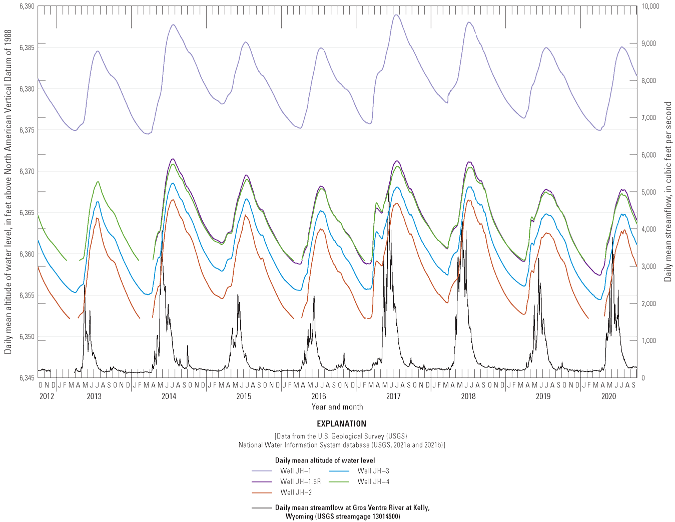
Water levels for selected wells sampled at the Jackson Hole Airport, Jackson, Wyoming, and daily mean streamflow at Gros Ventre River at Kelly, Wyoming (U.S. Geological Survey streamgage 13014500), 2012–20.
Using discrete water-level measurements, water-table contours were constructed (fig. 5A–B) using multiple three-point calculations to assist with “fitting” of contours. A water-table contour map was constructed for two water-level measurement events during a single year (2019), representing the approximate lowest (fig. 5A, May 2019) and highest (fig. 5B, August 2019) water-level conditions of 2019. Assuming groundwater flow is perpendicular to water-table contours, the direction of groundwater flow generally was from the northeast to the southwest for both measurement events as shown in figures 5A and 5B, indicating seasonal variation in the direction of horizontal groundwater flow is minimal. The general direction of groundwater flow seems to not have changed substantially since 2012 (Wright, 2013).
Horizontal hydraulic gradients were calculated for several combinations of monitor wells for the period of April 2013 to August 2020; these calculated values are summarized in table 4, and all values are tabulated in appendix table 1.6. Horizontal hydraulic gradients ranged from 0.006 to 0.008 foot per foot (ft/ft; average=0.007 ft/ft) (table 4), which is the same average determined during previous studies (Wright, 2010, 2013). The spatial uniformity of calculated hydraulic gradients across the airport indicates that the hydraulic gradient of the aquifer at the JHA continues to be relatively uniform, despite regular pumping of production wells in the study area (fig. 3).

Water-table contours and estimated direction of groundwater flow for A, low water table in May 2019, and B, high water table in August 2019, Jackson Hole Airport, Jackson, Wyoming.
Table 4.
Summary of horizontal hydraulic gradients and groundwater velocities calculated for selected monitor wells and water-level measurement events at the Jackson Hole Airport, Jackson, Wyoming, 2013–20.[Data are summarized from appendix table 1.6. K, hydraulic conductivity]
Value of K determined at the Aspens (Nelson Engineering, 1992).
Value of K determined at Teton Village (Nelson Engineering, 1992).
Monitor wells JH–1.5R and JH–1.5D of well cluster 1.5 and monitor wells JH–3 and JH–3D of well cluster 3 were near each other and completed at different depths in part to evaluate the hydraulic potential (differences in hydraulic head or groundwater level) for vertical groundwater flow at the well cluster locations. Negative vertical hydraulic gradients indicate the potential for downward flow, and positive vertical hydraulic gradients indicate the potential for upward flow. The vertical hydraulic gradient in the Snake River alluvial aquifer at both well clusters was small. Calculated vertical hydraulic gradients at well cluster 1.5 varied during 2013–20, ranging from 0.006 ft/ft in August 2013 to 0.016 ft/ft in February 2018 (average=0.012 ft/ft). Calculated vertical hydraulic gradients at well cluster 3 varied during 2013–20, ranging from −0.001 ft/ft in August 2017 to 0.009 ft/ft in April 2013 (average=0.005 ft/ft). Although the ranges of gradients are somewhat different than previously described (Wright, 2013), the average vertical hydraulic gradients were still very similar. However, the calculated vertical hydraulic gradients indicated vertical groundwater-flow directions at these two monitor well clusters were somewhat different than in the previous study (Wright, 2013). During 2013–20, vertical hydraulic gradients at monitor well cluster 1.5 consistently indicated the potential for downward vertical groundwater flow in the Snake River alluvial aquifer at this location. At monitor well cluster 3, vertical hydraulic gradients during 2013–20 indicated the potential for upward and downward vertical groundwater flow. The ratios of the average horizontal hydraulic gradient to the average vertical hydraulic gradient at monitor well clusters 1.5 and 3 were 0.58 and 1.4 ft, respectively. These ratios mean that for every 0.58 or 1.4 ft that water moves horizontally, groundwater is likely to move 1 ft vertically (downward), assuming horizontal and vertical conductivities of aquifer materials are the same.
Horizontal groundwater velocities were calculated for each airport visit using hydraulic conductivity values from Teton Village and the Aspens and using an estimated porosity of 30 percent as described previously in the “Methods of Data Collection and Analysis” section. Calculated groundwater velocities are summarized in table 4, and all velocities are tabulated in appendix table 1.6. Groundwater velocity was estimated to be as high as 76 feet per day (ft/d) using the horizontal hydraulic gradient calculated for March 2020 using water-level data for wells JH–1, JH–2, and JH–3 and the hydraulic conductivity for Teton Village. The groundwater velocity was estimated to be as low as 26 ft/d using the hydraulic gradients calculated for July 2013 and April 2014 using water-level data from wells JH–1, JH–2, and JH–4 and the hydraulic conductivity for the Aspens (appendix table 1.6). The range of hydraulic gradients determined for the period from April 2013 to August 2020 is slightly higher than the range of hydraulic gradients determined for previous periods (Wright, 2010, 2013). Using an estimated linear distance of 3,540 ft from well JH–1 to well JH–2 and the minimum and maximum groundwater-velocity estimates for July 2013 and 2014, respectively, it would take approximately 47 to 136 days for water in the aquifer to travel from well JH–1 (upgradient from airport operations) to well JH–2 along the southwest boundary of the airport (fig. 5).
The calculated rates of horizontal groundwater velocity (table 4) are estimates and could vary at different locations at the JHA. Although lithologic data for monitor wells JH–1 to JH–4 and the narrow range of horizontal hydraulic gradients for these wells indicate the Snake River alluvial aquifer at the airport is relatively homogeneous, horizontal hydraulic conductivity differs from point to point and along a flow path because lithology typically is heterogeneous and anisotropic. The actual groundwater velocity may be different between two points depending on the heterogeneity of the aquifer. The direction of flow also might not be perpendicular to water-table contours as shown in figures 5A–B (due to anisotropy) and likely is not in a straight line. Variability in well depths and well screen lengths are sources of additional uncertainty. These factors, and the estimated porosity value chosen, could substantially affect the groundwater velocity estimates.
Groundwater-velocity estimates (table 4) only describe movement of groundwater in the Snake River alluvial aquifer and are not applicable to solute movement. Solute movement through saturated media, such as an aquifer, is affected by advection as well as other physical processes such as diffusion and dispersion, and chemical processes such as sorption, precipitation, oxidation and reduction, and biodegradation (Fetter, 1993). Consequently, many solutes (including soluble contaminants) may move at a rate much slower than groundwater flow through the aquifer.
Water-Quality Results and Discussion
Groundwater quality in the Snake River alluvial aquifer at the JHA during 2011–20 is described in this report section. All physical-property measurements and analytical results for groundwater samples collected during June 2011–April 2012 were provided in the report for the previous study (Wright, 2013), and results for samples collected during August 2012–August 2020 for this study are provided in this report. However, some physical-property measurements and analytical results for groundwater samples collected during June 2011–April 2012 are reproduced in this report to facilitate discussion and analysis of water-quality changes and trends over a longer period (2011–20). All water-quality data can be retrieved from the USGS NWIS database (USGS, 2021a) using the 15-digit USGS site numbers listed in table 1.
Physical-property values and constituent concentrations measured in groundwater samples collected for this study are compared to EPA drinking-water standards and health advisories for physical properties and chemical constituents in drinking water (EPA, 2018). Although none of the monitor wells sampled for this study are used to supply drinking water, EPA drinking-water standards and health advisories provide a basis for assessing groundwater quality at the JHA. The EPA maximum contaminant level (MCL) is a legally enforceable, health-based standard and is the maximum allowable concentration of a constituent in drinking water from a public water-supply system that provides water to at least 15 connections and to at least 25 people (EPA, 2018). An EPA Lifetime Health Advisory Level (HAL) is a nonenforceable, health-based standard and is the concentration of a constituent in drinking water at or below which there are no adverse, noncarcinogenic effects over a lifetime of exposure (EPA, 2018). EPA SDWRs, also known as SMCLs, are nonenforceable standards recommended to public water-supply systems (EPA, 2018). An SDWR is a concentration in drinking water above which cosmetic effects (such as skin or tooth discoloration) or aesthetic effects (such as taste, odor, or color) may occur. An EPA action level (AL) is the concentration of a constituent in drinking water at or above which additional treatment is required to decrease the constituent concentration (EPA, 2018). An EPA drinking water advisory level (DWA) is the concentration of a constituent in drinking water at or below which there are no adverse health or aesthetic effects (EPA, 2018). An EPA maximum contaminant level goal (MCLG) is a concentration in drinking water below which there is no known health risk. EPA DWAs and MCLGs are nonenforceable standards.
Physical Properties
Physical properties (DO, pH, specific conductance, temperature, and turbidity) were measured each time a well was sampled. Physical-property measurements for the 10 monitor wells sampled during 2011–20 are tabulated in appendix table 1.7 and summarized in relation to applicable EPA drinking-water standards and health advisories for drinking water (EPA, 2018) in table 5.
Table 5.
Summary of physical properties, inorganic constituents, and dissolved organic carbon results for groundwater samples collected from monitor wells at the Jackson Hole Airport, Jackson, Wyoming, 2011–20.[Data from the U.S. Geological Survey (USGS) National Water Information System database (USGS, 2021a) and summarized from appendix tables 1.7 and 1.8. EPA, U.S. Environmental Protection Agency; mg/L, milligram per liter; <, less than; --, not applicable; SDWR, Secondary Drinking Water Regulation; µS/cm, microsiemen per centimeter at 25 degrees Celsius; °C, degree Celsius; NTRU, nephelometric turbidity ratio unit; MCL, maximum contaminant level; CaCO3, calcium carbonate; HCO3, bicarbonate; DWA, drinking water advisory level; SiO2, silica; HAL, Lifetime Health Advisory Level; n, value was below the laboratory reporting level and above the long-term method detection level; NC, median value not calculated because constituent was highly censored (80 percent or more values less than laboratory reporting level); N, nitrogen; MCLG, maximum contaminant level goal]
Median values were determined using detections and nondetections. For some constituents, imputed median concentration values are less than the laboratory reporting levels (refer to the “Statistical Analysis” section).
Two of the five physical properties (pH and turbidity) measured during this study have EPA drinking-water standards or health advisories. Only one physical property (turbidity) was measured in a monitor well (JH-DI1) at a value greater than an EPA drinking-water standard or health advisory during 2011–20 (table 5). The MCL for turbidity was exceeded in one sample collected from monitor well JH–DI1 on April 30, 2013; this well was installed in 2012 and was only sampled once before this event. Consequently, well JH-DI1 was redeveloped, and subsequent turbidity values measured in this well did not exceed the MCL (appendix table 1.7). Three of the five physical properties (DO, pH, and specific conductance) measured during this study are discussed in greater detail in this report section, including evaluation of trends during 2011–20 using the seasonal Kendall test (refer to the “Statistical Analysis” section and three physical property report subsections that follow). Results of trend analyses using the seasonal Kendall test (including p-values, Kendall’s τ values, and Theil-Sen and Akritas-Theil-Sen slopes) are tabulated in appendix table 1.9.
Dissolved Oxygen
DO concentrations measured each time a well was sampled were used as the first indication of the redox condition of water in each well (refer to “Determining Redox Conditions” section). Concentrations less than 0.5 mg/L indicated anoxic/reducing conditions, and greater concentrations indicated oxic conditions. Measured DO concentrations during 2011–20 ranged from <0.1 to 9.75 mg/L (median=1.65 mg/L; table 5; fig. 6A). DO concentrations indicative of anoxic/reducing conditions (DO<0.5 mg/L) were measured in 1 or more water samples from 7 of 10 sampled monitor wells, including all 6 monitor wells with benzotriazole detections (JH–1.5R, JH–1.5D, JH–2.5, JH–3, JH–3D, and JH–3.5) and 1 well without benzotriazole detections (well JH–4; fig. 6A; appendix table 1.7). DO concentrations in the 4 wells without detections of 4-MeBT (JH–1, JH–2, JH–4, and JH–DI1) were significantly higher (p-values<0.001, Peto-Peto test) than in the 6 wells with detections (median DO concentrations=6.6 and 0.4 mg/L, respectively; fig. 6A). DO concentrations in 3 of 4 wells without detections of 4-MeBT (JH–1, JH–2, and JH–DI1) were consistently oxic (DO>0.5 mg/L) during 2011–20 (fig. 6A).
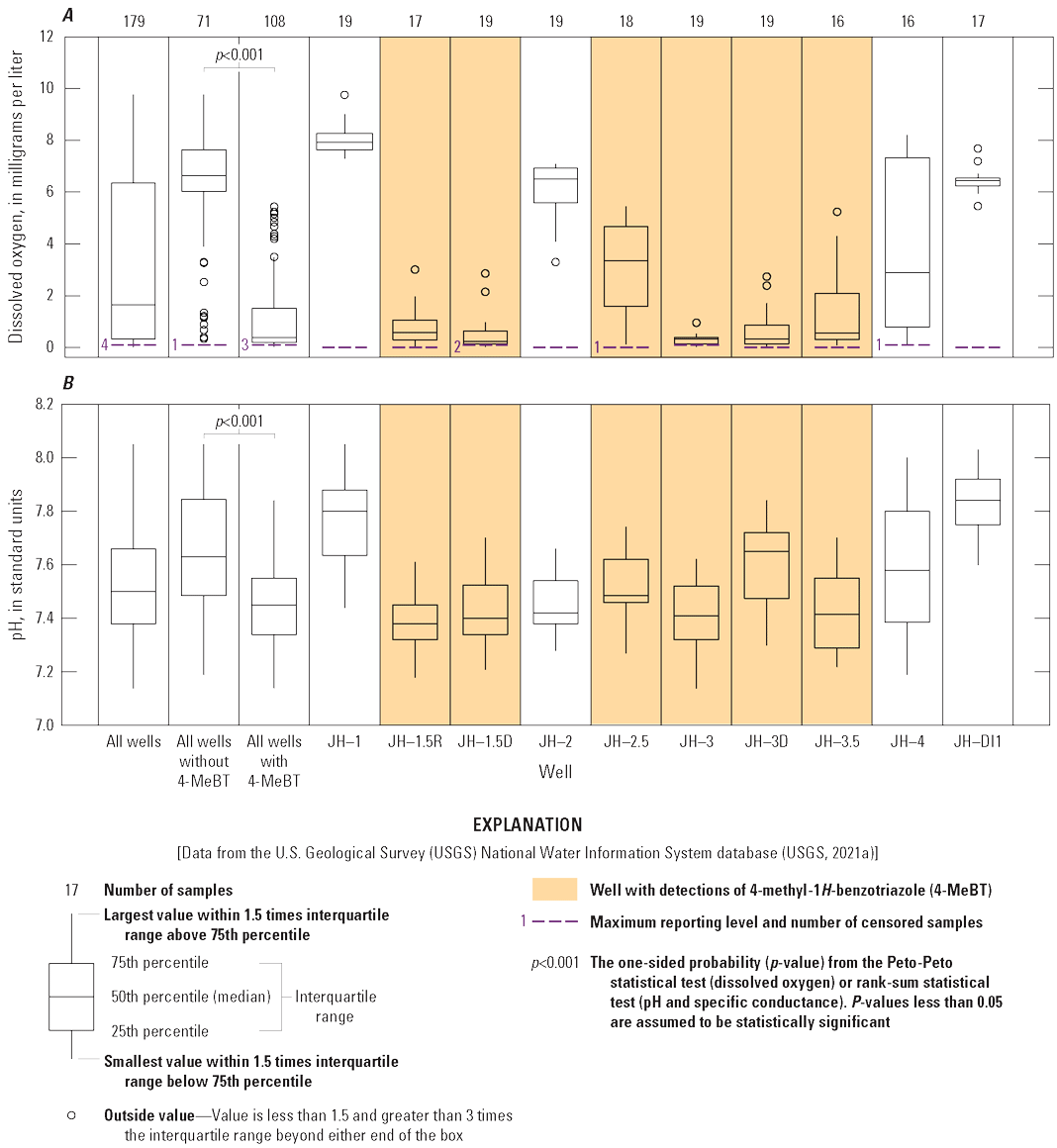
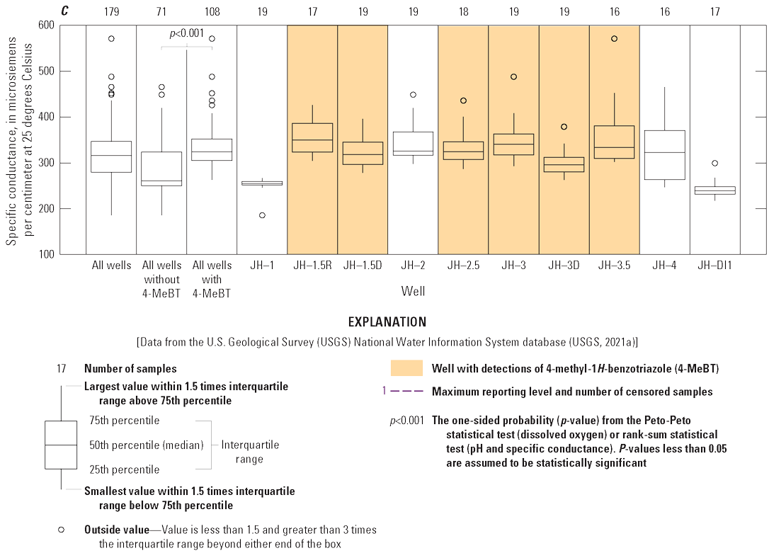
Statistical summary of A, dissolved-oxygen concentrations, B, pH values, and C, specific-conductance values in groundwater samples collected from monitor wells at the Jackson Hole Airport, Jackson, Wyoming, 2011–20.
Median DO concentrations in the four wells without detections of 4-MeBT ranged from 2.9 to 7.9 mg/L (wells JH–4 and JH–1, respectively; figs. 6A, 7). Median DO concentrations in the 6 wells with detections of 4-MeBT were mostly lower than in the 4 wells without detections and ranged from 0.2 to 3.4 mg/L (wells JH–1.5D and JH–2.5, respectively; figs. 6A, 7). Of these six wells, only well JH–2.5 had a median DO concentration greater than 1 mg/L (figs. 6A, 7). Wells with detections of 4-MeBT also had significantly lower median pH values, significantly higher median specific-conductance values, and significantly higher dissolved iron and manganese concentrations than wells without detections (p-values<0.05; figs. 6B–C, 7; also refer to the next two report subsections that follow, “pH” and “Specific Conductance,” and the “Dissolved Iron and Dissolved Manganese” section).
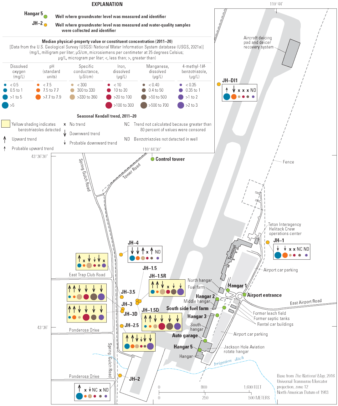
Distribution ranges of median values and concentrations, and seasonal Kendall trend test results, for selected physical properties or constituents measured in groundwater samples from monitor wells at the Jackson Hole Airport, Jackson, Wyoming, 2011–20.
DO concentrations in the alluvial aquifer varied substantially (anoxic to oxic), both spatially and with time (figs. 6–8). Although anoxic conditions were present in seven wells, these conditions were not persistent during 2011–20 (fig. 8). For example, samples collected during 2011 from well JH–2.5 were all anoxic, whereas samples collected during 2012–20 were all oxic (fig. 8E). Conversely, samples collected during 2011–16 from well JH–4 were oxic, whereas samples collected during 2018 were suboxic or mixed (oxic-anoxic), mixed (anoxic and oxic-anoxic) during 2019, and both oxic and anoxic during 2020 (fig. 8I; no samples were collected from well JH–4 during 2017; also refer to the “Redox Conditions” section).
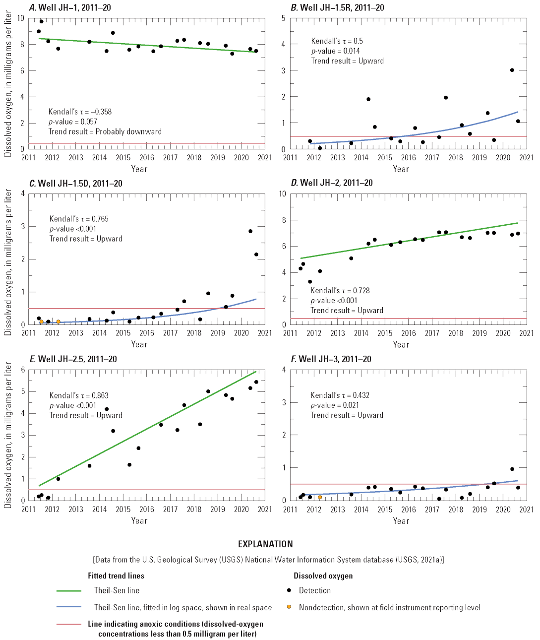
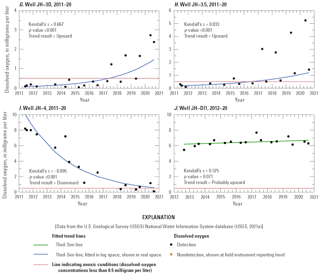
Trends in dissolved-oxygen concentrations in groundwater samples from monitor wells, Jackson Hole Airport, Jackson, Wyoming, 2011–20. A, Well JH–1. B, Well JH–1.5R. C, Well JH–1.5D. D, Well JH–2. E, Well JH–2.5. F, Well JH–3. G, Well JH–3D, H, Well JH–3.5. I, Well JH–4. J, Well JH–DI1.
Although consistently oxic, DO concentrations varied in wells JH–1, JH–2, and JH–DI1 during 2011–20. For example, an upward trend in DO concentrations (p-value<0.001) was determined at well JH–2, and concentrations ranged from a low of 3.3 mg/L in November 2011 to a high of 7.1 mg/L in April and August 2017 (figs. 7, 8D; appendix table 1.9). Similarly, an upward trend in DO concentrations was determined at well JH–DI1, and a probable downward trend was determined at well JH–1 (figs. 7, 8A, J; appendix table 1.9).
Wright (2013) reported anoxic/reducing conditions for an area southwest of JHA operations that included six wells, all of which also had detections of 4-MeBT (JH–1.5R, JH–1.5D, JH–2.5, JH–3, JH–3D, and JH–3.5; fig. 7). Upward trends in DO concentrations during 2011–20 were determined at all six of these wells (p-values ranging from <0.001–0.021; figs. 7, 8B–C, E–H; appendix table 1.9). By 2020, DO in five of these wells (JH–1.5R, JH–1.5D, JH–2.5, JH–3D, and JH–3.5) had increased to concentrations greater than the 0.5-mg/L threshold for anoxic water, substantially decreasing the areal extent of groundwater with reducing conditions (fig. 8B–C, E–H). Although DO in well JH–3 was measured only once at a concentration greater than 0.5 mg/L (1.0 mg/L; May 21, 2020), an upward trend in DO concentrations during 2011–20 and change in the redox class from exclusively anoxic to also suboxic, mixed (oxic-anoxic), or oxic during 2018–20 indicated groundwater conditions were returning to conditions similar to background conditions measured in the alluvial aquifer upgradient from airport operations towards the end of the study period (fig. 8F; also refer to the “Redox Conditions” section). A downward trend in DO concentrations during 2011–20 was determined at well JH–4 (p-value=<0.001; fig. 8I), which is outside of the area with reducing conditions and detections of 4-MeBT (fig. 7). DO concentrations in 3 of 6 samples collected from well JH–4 during 2018–20 were less than the 0.5-mg/L threshold for anoxic water (fig. 8I).
pH
Values of pH measured during 2011–20 ranged from 7.1 to 8.1 (median=7.5; table 5). All measured pH values were within the EPA SDWR range of 6.5–8.5. Median pH for the 4 wells without detections of 4-MeBT (about 7.6) was significantly higher (p-values<0.001, rank-sum test) than median pH for the 6 wells with detections (about 7.4; fig. 6B). The lower pH in wells with detections of 4-MeBT may be indirectly attributable to 4-MeBT degradation. Biological degradation of organic compounds typically results in increases in microbial activity and alkalinity (Chapelle, 2001). Increases in alkalinity are due to the production of carbon dioxide as a byproduct of the increased microbial activity (respiration). Alkalinity helps maintain groundwater pH by buffering groundwater from acids (Hem, 1985). Consequently, groundwater in contaminated wells where anaerobic biological degradation of organic compounds such as 4-MeBT is occurring would be expected to have higher alkalinity (and correspondingly lower pH) than in uncontaminated wells. Median alkalinity for the 4 wells with detections of 4-MeBT (about 153 mg/L as calcium carbonate [CaCO3]) was significantly higher (p-value<0.001, rank-sum test) than median alkalinity for the 6 wells without detections (about 122 mg/L as CaCO3). This indicates increased microbial activity and associated carbon dioxide production may be responsible for the lower pH in wells with 4-MeBT.
An upward trend in pH was determined at 5 of 6 wells with detections of 4-MeBT (JH–1.5R, JH–1.5D, JH–2.5, JH–3, and JH–3D; figs. 7, 9B–C, E–G); no trend was determined at the sixth well (JH–3.5; figs. 7, 9H; appendix table 1.9). For the 4 wells without 4-MeBT, a probable downward trend in pH was determined at 1 well (JH–1), a downward trend was determined at 2 wells (JH–4 and JH–DI1), and no trend was determined at 1 well (JH–2; figs. 7, 9A, D, I–J; appendix table 1.9).
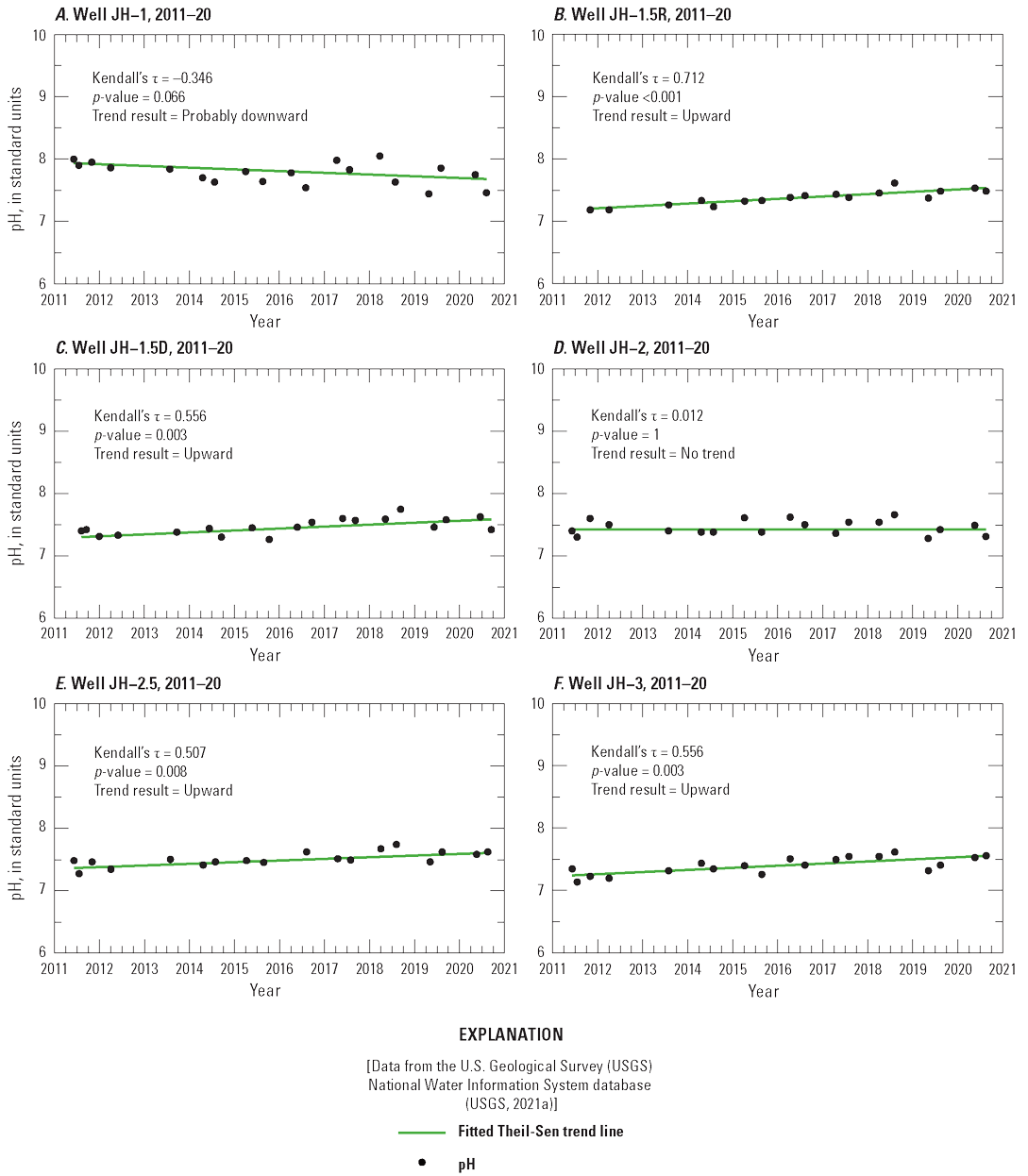
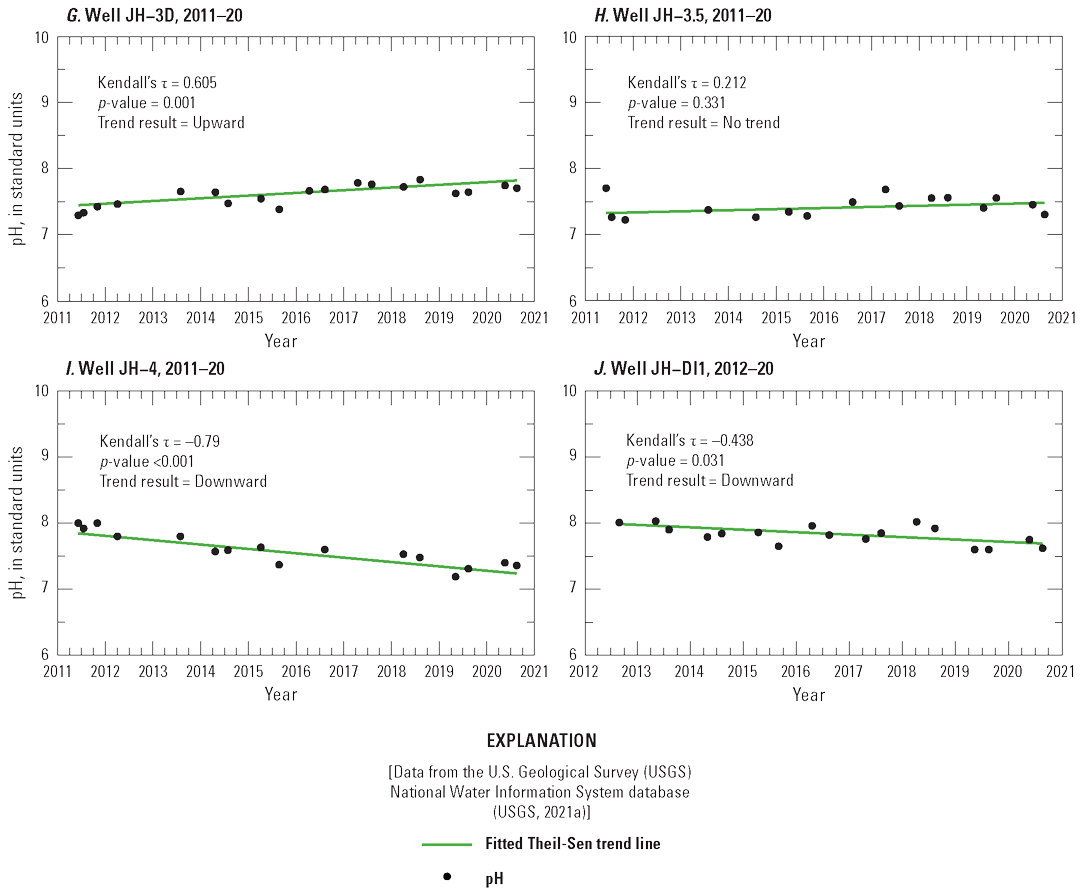
Trends in pH values in groundwater samples from monitor wells, Jackson Hole Airport, Jackson, Wyoming, 2011–20. A, Well JH–1. B, Well JH–1.5R. C, Well JH–1.5D. D, Well JH–2. E, Well JH–2.5. F, Well JH–3. G, Well JH–3D, H, Well JH–3.5. I, Well JH–4. J, Well JH–DI1.
Specific Conductance
Specific-conductance values measured during 2011–20 ranged from 186 to 571 microsiemens per centimeter at 25 degrees Celsius (µS/cm; median=316 µS/cm; table 5; fig. 6). These values are within the range of values for specific conductance (112 to 863 µS/cm) reported by Nolan and Miller (1995) for water from 34 wells completed in Quaternary alluvium, colluvium, and gravel, and pediment, fan, and glacial deposits in Teton County, Wyo. Specific-conductance values generally were lower in wells without detections of 4-MeBT than in wells with 4-MeBT detections (fig. 6C). Median specific conductance for the 6 wells with detections of 4-MeBT (325 µS/cm) was significantly higher (p-values<0.001, rank-sum test) than median specific conductance for the 4 wells without detections (261 µS/cm; fig. 6C).
A downward trend in specific conductance was determined at all 6 wells with detections of 4-MeBT (JH–1.5R, JH–1.5D, JH–2.5, JH–3, JH–3D, and JH–3.5; figs. 7, 10B–C, E–H; appendix table 1.9). For the 4 wells without 4-MeBT, an upward trend in specific conductance was determined at 1 well (JH–4), a probable downward trend was determined at 1 well (JH–2), and no trends were determined at 2 wells (JH–1 and JH–DI1; figs. 7, 10A, D, I–J; appendix table 1.9).
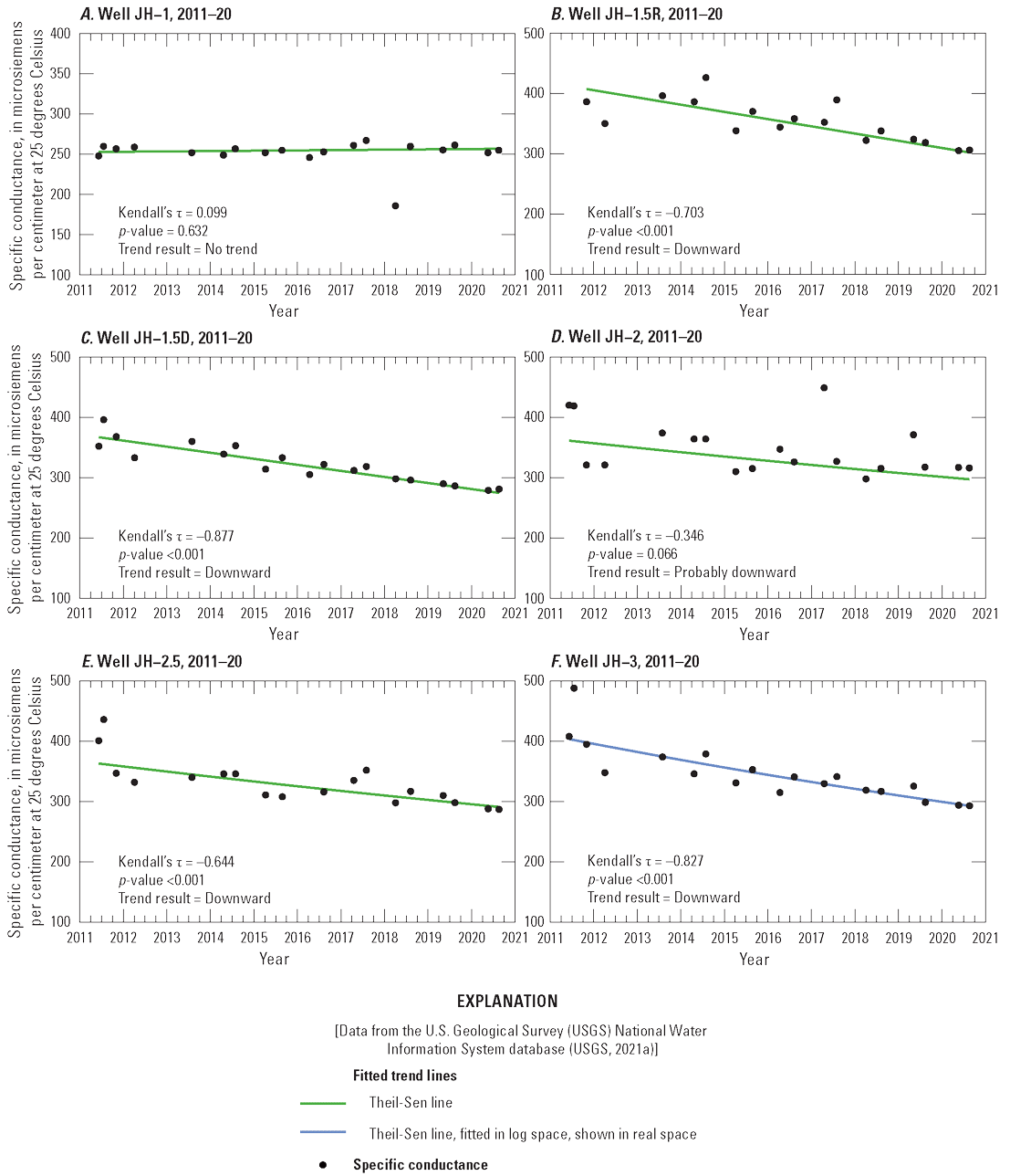
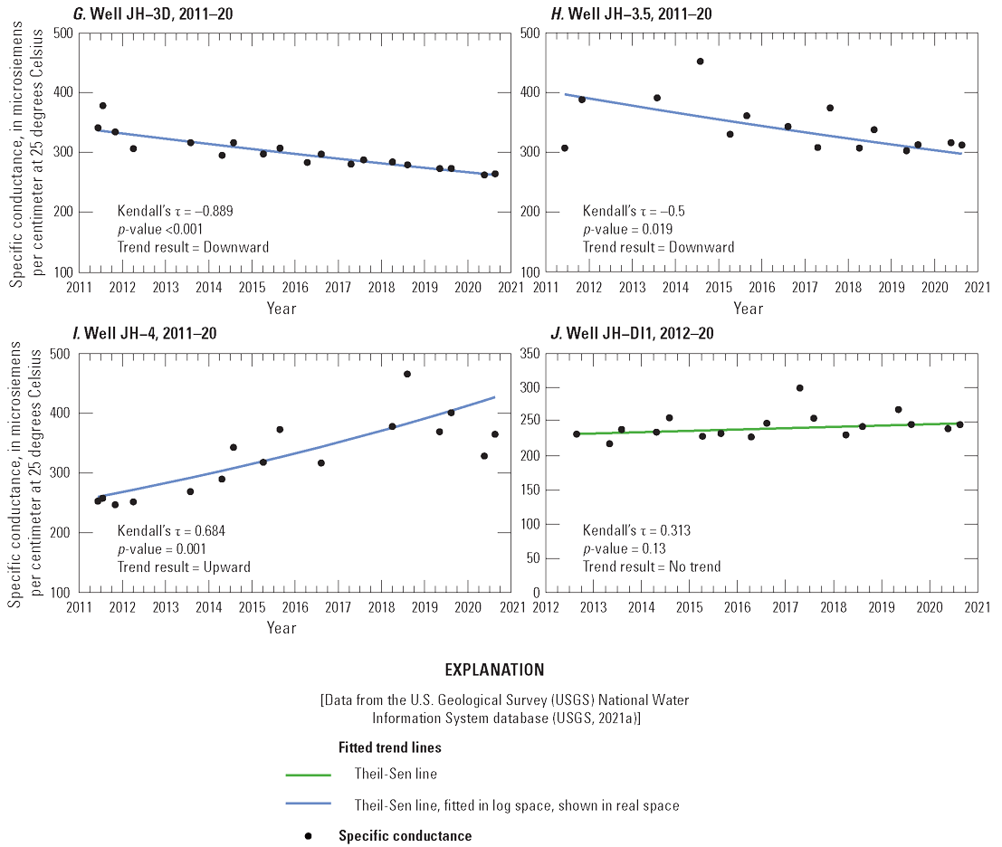
Trends in specific-conductance values in groundwater samples from monitor wells, Jackson Hole Airport, Jackson, Wyoming, 2011–20. A, Well JH–1. B, Well JH–1.5R. C, Well JH–1.5D. D, Well JH–2. E, Well JH–2.5. F, Well JH–3. G, Well JH–3D, H, Well JH–3.5. I, Well JH–4. J, Well JH–DI1.
Redox Conditions
This section of the report provides a brief definition of redox, identifies the redox processes that can occur provided the right conditions exist, and describes redox conditions in JHA monitor wells during 2011–20. The chemical quality of groundwater commonly is affected by redox processes (Chapelle, 2001; Chapelle and others, 2009).
Redox is a natural chemical process often facilitated by microorganisms by which chemical species donate or accept electrons; the donating chemical species is considered “oxidized,” whereas the accepting chemical species is considered “reduced.” Dissolved and particulate carbon are the most common electron donors, and there are several common electron acceptors (McMahon and Chapelle, 2008). Electron acceptors are used by microorganisms in a sequence that progresses in specific order based on the amount of energy provided, beginning with oxygen and followed by nitrate, manganese, iron, sulfate, and carbon compounds such as carbon dioxide (Appelo and Postma, 2005; McMahon and Chapelle, 2008). Reduction reactions also occur sequentially and in a specific order dependent on reactant availability, often generating undesirable byproducts such as dissolved manganese (manganous manganese, or Mn2+) or dissolved iron (ferrous iron, or Fe2+), as was the case in many monitor wells at the JHA during 2011–20 (refer to the “Dissolved Iron and Dissolved Manganese” section). These two trace elements can cause drinking water to taste metallic or cause black or brown staining when the water becomes oxidized (oxygenated) (Hem, 1985).
The redox state of groundwater in the Snake River alluvial aquifer, as determined using measurements of DO and redox-sensitive chemical constituents (nitrate, iron, manganese, and sulfate), was the first indicator of contamination at the JHA (Wright, 2010). Wright (2010) reported that groundwater upgradient from the JHA operations (towards the northeast boundary of the JHA, “background” well JH–1) naturally was oxic (oxygenated), whereas groundwater in parts of the alluvial aquifer downgradient from the JHA operations (towards southwest boundary of the JHA) was anoxic/reducing (oxygen-poor), as initially identified in samples from monitor wells JH–3 and JH–3D collected during 2008–09. This difference in the redox state of groundwater in the alluvial aquifer upgradient and downgradient from the JHA (Wright, 2010), indicated in part by low DO concentrations and high dissolved iron and manganese concentrations, led to further investigation during 2011–12, including installation of additional monitor wells (Wright, 2013). Continued study of the aquifer’s redox state by sampling an expanded well network, and the consistent identification of anthropogenic compounds (benzotriazoles) in six downgradient wells, led Wright (2013) to conclude microbial oxidation of compounds in ADAFs likely was responsible for the reduced groundwater conditions in the alluvial aquifer at the JHA.
Concentrations of DO and several dissolved redox-sensitive constituents determined onsite (sulfide) and offsite at a laboratory (nitrate, iron, manganese, and sulfate) were used to further assess the redox status of anoxic/reduced waters using the classification scheme of McMahon and Chapelle (2008) and Chapelle and others (2009). The classification scheme uses threshold concentrations of these redox-sensitive species to assign the predominant redox process to groundwater samples. A spreadsheet program that automates the classification scheme was used to assign a general redox class and predominant redox process to each sample (Jurgens and others, 2009). Identified redox classes and processes determined for each groundwater sample collected from the 10 monitor wells during 2011–20 are listed in table 6.
Table 6.
Assignment of redox classes and processes for groundwater samples collected from monitor wells at the Jackson Hole Airport, Jackson, Wyoming, 2011–20.[Data are from the U.S. Geological Survey (USGS) National Water Information System database (USGS, 2021a) and summarized from table 7 and appendix tables 1.7 and 1.8. Dates are given in month/day/year. Values of constituents detected at or above the U.S. Environmental Protection Agency Secondary Drinking Water Regulation are shown in bold and noted with footnote 4. mg/L, milligram per liter; NO3−, nitrate as nitrogen (calculated as difference between nitrate plus nitrite as nitrogen and nitrite as nitrogen); Mn, total dissolved manganese used as an estimate of manganous manganese (Mn2+); µg/L, microgram per liter; Fe, total dissolved iron used as an estimate of ferrous iron (Fe2+); SO42–, dissolved sulfate; H2S, dihydrogen sulfide; HS−, hydrogen sulfide; S2−, sulfide; --, not applicable; <, less than; NC, median value not calculated; 4-MeBT, 4-Methyl-1-H-benzotriazole; 5-MeBT, 5-Methyl-1-H-benzotriazole. General redox class abbreviations: Oxic, dissolved oxygen (O2) greater than or equal to 0.5 mg/L; Anoxic, O2<0.5 mg/L; Suboxic, low dissolved-oxygen conditions that cannot be defined further without additional data. Redox process abbreviations: O2, oxygen reduction; Fe(III), iron reduction; Mn(IV), manganese reduction; SO4, sulfate reduction; CH4gen, methanogenesis; NO3, nitrate reduction]
Median values were determined using detections and nondetections. For some constituents, imputed median concentration values are less than the laboratory reporting levels (refer to the “Statistical Methods” section).
Median value not calculated because constituent was highly censored (80 percent or more values less than reporting level).
Value of constituent detected at or above the U.S. Environmental Protection Agency Secondary Drinking Water Regulation (EPA, 2018).
Data are not sufficient to determine the redox process (Jurgens and others, 2009).
These detections were considered suspect and were treated as nondetections for data summary and analysis purposes (refer to the “Benzotriazole Compounds” section).
DO concentrations were significantly higher in wells without benzotriazole detections than in wells with detections (refer to the “Physical Properties” section). Three of four wells without benzotriazole detections (JH–1, JH–2, and JH–DI1) were oxic throughout 2011–20 (table 6; fig. 8A, D, J). The fourth well without benzotriazole detections (well JH–4) was oxic during 2011–16, although DO concentrations decreased throughout the period (fig. 8I; table 6). DO concentrations continued to decrease after 2016, and groundwater conditions at well JH–4 became suboxic, mixed (oxic-anoxic and anoxic), and finally anoxic by the end of the study (fig. 8I; table 6). Oxygen, nitrate, and manganese reduction were the redox processes identified in well JH–4 during 2018–20, including more than one process (mixed) identified in the 2018–19 samples (table 6).
All six wells with benzotriazole detections had anoxic/reducing (including suboxic and mixed) conditions for at least some period during 2011–20 (fig. 8; table 6). Iron and manganese reduction were the predominant redox processes identified in most anoxic water samples from wells with triazole detections (table 6). Less common redox processes identified in anoxic water samples (including wells without benzotriazole detections) included, in order of increasingly reduced conditions, nitrate reduction, sulfate reduction, and methanogenesis (table 6). The predominant redox process identified at well JH–3 varied seasonally during part of the study period. Well JH–3 was anoxic throughout most of 2011–20; the predominant redox process alternated seasonally between iron and manganese reduction until 2018, after which groundwater in the vicinity of the well became less reducing, as indicated by anoxic, mixed (oxic-anoxic), suboxic, or oxic conditions during 2018–20 (table 6; fig. 8F).
Although variable spatially and with time, the general redox classes and processes identified in table 6 indicate that groundwater in the six wells with anoxic/reducing conditions at the beginning of the study in 2011 (all of which had benzotriazole detections) became less reducing and more oxic with time. Groundwater conditions at 4 of 6 monitor wells with benzotriazole detections (JH–1.5D, JH–2.5, JH–3D, and JH–3.5) changed from anoxic/reducing to oxic during the study period; conditions at some of these wells transitioned from anoxic to mixed (oxic-anoxic) or suboxic before becoming oxic near the end of the study period (table 6; fig. 8C, E, G–H). The remaining two wells (JH–1.5R, JH–3) with benzotriazole detections transitioned from anoxic to mixed (oxic-anoxic) or suboxic by the end of the study period (table 6; fig. 8B, F). The effect these changes towards less reducing or oxic conditions have had on the occurrence and distribution of selected inorganic and organic constituents in groundwater at the JHA are discussed in the “Major Ions, Nutrients, and Trace Elements,” “Dissolved Iron and Dissolved Manganese,” and “Anthropogenic Compounds” sections that follow.
DOC, a potential carbon source for microorganisms, was detected in at least one sample from each well during 2011–20 (app. 5 and app. 8 of Wright, 2013). Concentrations of DOC generally were low in samples from all 10 wells, ranging from <0.23 to 3.85 mg/L (median=0.45 mg/L; table 5). The DOC concentrations in samples collected during 2011–20 from all 10 wells were mostly within the estimated range of 0 to about 3 mg/L considered natural in groundwater (fig. 6–1 of Drever, 1997), except for one slightly higher concentration (3.85 mg/L) in a sample collected from well JH–1 during April 2018 (appendix table 1.8). DOC concentrations in samples from the 6 wells with detections of 4-MeBT were significantly higher (p-value<0.05, Peto-Peto test) than in samples from the 4 wells without detections (JH–1, JH–2, JH–4, and JH–DI1) (median DOC concentrations=0.46 and 0.41 mg/L, respectively), although this concentration difference is likely of little environmental consequence.
Major Ions, Nutrients, and Trace Elements
Inorganic constituent concentrations for all samples collected during 2011–20, including major ions, nutrients, and trace elements, are summarized in relation to applicable EPA drinking-water standards and health advisories (collectively, “benchmarks”) for drinking water in table 5 (EPA, 2018). Of the 43 inorganic constituents measured, 22 have enforceable or nonenforceable health-based benchmarks, 5 have nonenforceable, aesthetic-based benchmarks, and 17 have no established benchmarks (table 5). No inorganic constituents were detected at concentrations greater than EPA health-based standards (MCL or health advisory); however, two trace elements (iron and manganese) were detected at concentrations greater than their respective EPA aesthetic standards (SDWRs). Both iron and manganese have SDWRs due to several potential aesthetic/cosmetic (taste, odor, color, and staining) and technical (corrosion and scale) effects to drinking water (EPA, 2018). Constituent exceedances of SDWRs are described in parts of the report that follow.
The major-ion composition of groundwater in the study area largely results from chemical reactions between water and sediments in the soil and aquifer and, to a lesser extent, from ions in precipitation. Groundwater at the airport was fresh (dissolved-solids concentration <1,000 mg/L; Heath, 1983), and dissolved-solids concentrations ranged from 126 to 330 mg/L (median=190 mg/L; table 5). Calculated hardness values ranged from 88 to 273 mg/L as CaCO3 (median=154 mg/L as CaCO3; table 5), indicating groundwater generally was moderately hard (61 to 120 mg/L as CaCO3) to very hard (greater than 180 mg/L as CaCO3; Hem, 1985).
The relative proportions of the major cations (calcium, magnesium, potassium, and sodium) and the major anions (bicarbonate plus carbonate [based on field titration], chloride, fluoride, and sulfate) were used to determine water type. Although concentrations of major cations and anions in water samples from individual wells have varied since reported by Wright (2010, 2013), the relative proportions of these ions have not changed—calcium was the predominant cation and bicarbonate was the predominant anion in all water samples collected during 2011–20. Therefore, groundwater samples from all sites continue to be classified as calcium-bicarbonate type waters (appendix table 1.8; app. 5 of Wright, 2013).
Nutrients were detected at low concentrations in all groundwater samples, and all concentrations were much smaller than applicable EPA MCLs and health advisories (table 5). Dissolved nitrite plus nitrate as nitrogen (identified as “nitrate” hereafter) concentrations ranged from <0.02 to 3.77 mg/L (median=0.07 mg/L; table 5). Nitrate was detected almost always in water samples with oxic conditions (DO greater than 0.5 mg/L), indicating nitrate was the primary nitrogen species in the alluvial aquifer that typically is naturally oxic (refer to the “Redox Conditions” section). Ammonia as nitrogen was detected in at least one sample from each sampled monitor well (including qualified concentrations), mostly when groundwater conditions in a well were anoxic (appendix table 1.8; table 8 and apps. 4–5 of Wright, 2013). Nitrate can be reduced by bacteria to nitrous oxide, ammonia, and nitrogen gas when exposed to anoxic/anaerobic conditions (Hem, 1985; McMahon and Chapelle, 2008). Ammonium also can be produced by the mineralization of organic nitrogen, most commonly in anoxic waters. Although ammonia can be produced by either process, the presence of ammonia instead of nitrate is an indicator of reducing conditions at and near many JHA monitor wells sampled during 2011–20.
The highest nitrate concentrations measured during 2011–20 typically were in water samples from well JH–2. Both previous studies (Wright, 2010, 2013) noted concentrations of nitrate at well JH–2 commonly were higher than other sampled wells and speculated the higher concentrations could be because this well was directly downgradient from the former septic leach field (fig. 3). However, the median nitrate concentration (0.61 mg/L) at well JH–2 (2011–20) is less than the median concentration (0.69 mg/L as nitrogen) reported for nitrite plus nitrate in groundwater samples from Quaternary deposits within Teton County, Wyo. (Nolan and Miller, 1995), and 14 of 18 samples are within the range of concentrations (0 to 1 mg/L) that are commonly expected in groundwater in the absence of human effects (Dubrovsky and others, 2010). Only one sample (3.77 mg/L, April 18, 2017) collected from well JH–2 during 2011–20 was substantially higher than this 1-mg/L threshold (apps. 5 and 8 of Wright, 2013).
Total nitrogen and dissolved orthophosphate (as phosphorus) were detected in at least one sample from all 10 monitor wells (appendix table 1.8; app. 5 of Wright, 2013). Total nitrogen concentrations ranged from <0.05 to 4.74 mg/L (median=0.12 mg/L; table 5). Dissolved orthophosphate concentrations ranged from 0.006 to 0.055 mg/L (median=0.011 mg/L; table 5).
Samples were analyzed for as many as 23 trace elements during 2011–20. Two trace elements (iron and manganese) were analyzed in all samples collected between 2011 and 2020, and an additional 21 trace elements were analyzed in samples collected once in 2013 (July–August) and twice each year during 2015–18. Trace-element analyses for 2011–12 and 2013–20 are tabulated in appendix 5 of Wright (2013) and appendix table 1.8 of this report, respectively (except 2012 analyses for well JH–DI1 also are included in appendix table 1.8). A summary of trace-element concentrations in relation to applicable EPA health-based and aesthetic drinking-water standards and advisories (EPA, 2018) is presented in table 5. Trace-element concentrations were low relative to EPA standards except for dissolved iron and dissolved manganese, which were detected at concentrations exceeding their respective EPA SDWRs (aesthetic standards). Both constituents can cause cosmetic or aesthetic effects when present in drinking water at high concentrations, potentially requiring treatment. Dissolved iron and manganese in JHA groundwater are discussed in greater detail in the next report section, “Dissolved Iron and Dissolved Manganese.”
Dissolved Iron and Dissolved Manganese
Dissolved iron and manganese in JHA groundwater during 2011–20 are described in this report section. The frequency of detection and measured concentrations of both constituents are described and related to geochemical conditions, and then concentration trends in the sampled monitor wells are evaluated.
Summary of Detections and Concentrations
Dissolved iron and manganese were detected in at least one sample collected from all 10 monitor wells during 2011–20, including 52 percent (93 of 179) of samples analyzed for iron and 64 percent (114 of 179) of samples analyzed for manganese (table 6; fig. 11). Concentrations of dissolved iron and dissolved manganese ranged from <3.2 (lowest reporting level) to 1,052 micrograms per liter (µg/L; median=5.72 µg/L), and from <0.15 (lowest reporting level) to 1,730 µg/L (median=1 µg/L), respectively (table 6; fig. 11).
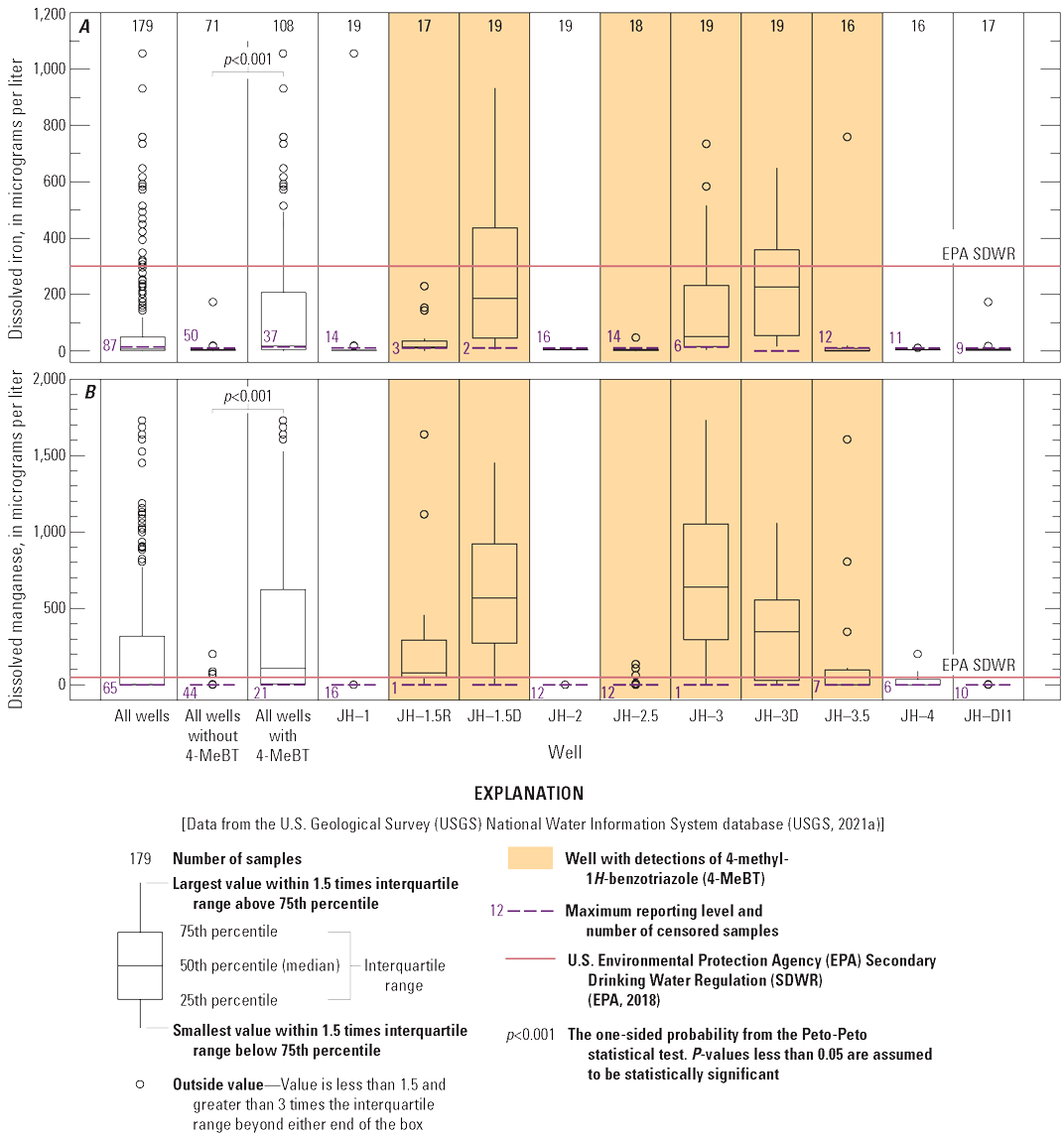
Statistical summary of A, dissolved iron and B, dissolved manganese concentrations in groundwater samples collected from monitor wells at the Jackson Hole Airport, Jackson, Wyoming, 2011–20.
Redox conditions, specifically low DO concentrations, were a strong indicator of high iron and manganese concentrations in the alluvial aquifer at the JHA during 2011–20. With few exceptions, dissolved iron and manganese concentrations were substantially higher when groundwater conditions near a well were anoxic, suboxic, or mixed, than when conditions were oxic (table 6). In fact, concentrations of dissolved iron and manganese typically were near or below LRLs in samples with oxic waters (DO greater than 0.5 mg/L, unless samples had mixed redox conditions), which were mostly from wells without detections of benzotriazoles (figs. 11–12; table 6). Except for 4 samples collected during 2018–20 from 1 well (JH–4), anoxic, suboxic, or mixed conditions were present at least once only in the 6 wells with detections of benzotriazoles, especially 4-MeBT (refer to the “Dissolved Oxygen” and “Redox Conditions” sections). Dissolved iron and manganese concentrations in samples from the 6 wells with detections of 4-MeBT were significantly higher (p-values<0.001, Peto-Peto test) than from the 4 wells without detections (fig. 11). These results mostly reflect the significantly lower DO concentrations (and associated anoxic conditions) in wells with detections of 4-MeBT than in wells without detections (refer to the previous “Physical Properties” and “Redox Conditions” sections and the next report subsection, “Relation to Geochemical Conditions;” fig. 6A; table 6).
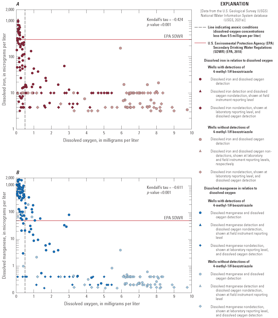
Relations between A, dissolved iron and dissolved oxygen, and B, dissolved manganese and dissolved oxygen in groundwater samples collected from monitor wells at the Jackson Hole Airport, Jackson, Wyoming, 2011–20.
Median dissolved iron concentrations for the six wells with detections of 4-MeBT ranged from 0.48 to 228 µg/L (wells JH–3.5 and JH–3D, respectively; table 6; figs. 7, 11). Median dissolved iron concentrations for three of four wells without detections (JH–1, JH–4, and JH–DI1) were low and ranged from 1.5 to 4.0 µg/L (wells JH–1 and JH–DI1, respectively; table 6; figs. 7, 11). Median dissolved iron concentrations for three wells (JH–1, JH–2.5, and JH–3.5) in table 6 are smaller than the lowest reporting level (<3.2 µg/L) and were imputed (statistically estimated; refer to the “Statistical Analysis” section). Median dissolved manganese concentrations for the 6 wells with detections of 4-MeBT ranged from 0.02 to 641 µg/L (wells JH–2.5 and JH–3, respectively), and median dissolved manganese concentrations for 3 of 4 wells without detections (JH–2, JH–4, and JH–DI1) were very low and ranged from 0.18 to 0.23 µg/L (wells JH–2 and JH–DI1, respectively; table 6; figs. 7, 11). The median dissolved iron concentration for well JH–2 and median dissolved manganese concentration for well JH–1 was not computed because greater than 80 percent of the values were censored (table 6; Helsel, 2012).
Dissolved iron concentrations exceeded the EPA SDWR of 300 µg/L (EPA, 2018) in about 11 percent (19 of 179) of samples collected during 2011–20 (table 6). Concentrations of dissolved iron greater than the EPA SDWR were identified only when groundwater conditions near a well were anoxic (DO<0.5 mg/L) and 4-MeBT was detected in the sample (table 6; fig. 11). Four of six wells with detections of 4-MeBT (JH–1.5D, JH–3, JH–3D, and JH–3.5) had one or more samples with dissolved iron concentrations greater than the EPA SDWR (table 6; fig. 11). For these four wells, the percentage of samples with dissolved iron concentrations greater than the EPA SDWR, from largest to smallest, was about 42 percent for well JH–1.5D (8 of 19 samples), 32 percent for well JH–3D (6 of 19 samples), 21 percent for well JH–3 (4 of 19 samples), and 6 percent for well JH–3.5 (1 of 16 samples; table 6).
Dissolved manganese was detected in more wells at concentrations above its respective EPA SDWR (7 wells) than dissolved iron (4 wells; table 6). Dissolved manganese concentrations exceeded the EPA SDWR of 50 µg/L (EPA, 2018) in 39 percent (70 of 179) of samples collected during 2011–20 (tables 5, 6). Concentrations of dissolved manganese greater than the EPA SDWR were identified when groundwater conditions in the vicinity of a well were anoxic, suboxic, or mixed and when 4-MeBT was detected in the sample except for four samples with anoxic or mixed conditions collected during 2018–20 from well JH–4, which never had a detection of 4-MeBT (table 6). Twenty-five percent (4 of 16) of samples from well JH–4 had dissolved manganese concentrations greater than the EPA SDWR (table 6). All six wells with detections of 4-MeBT had at least three samples with dissolved manganese concentrations greater than the EPA SDWR. For these six wells, the percentage of samples with dissolved manganese concentrations greater than the EPA SDWR, from largest to smallest, was about 90 percent for well JH–1.5D (17 of 19 samples), 79 percent for well JH–3 (15 of 19 samples), 77 percent for well JH–1.5R (13 of 17 samples), 68 percent for well JH–3D (13 of 19 samples), 31 percent for well JH–3.5 (5 of 16 samples), and 17 percent for well JH–2.5 (3 of 18 samples; table 6). Of note, well JH–1.5D had the highest percentage of samples with dissolved iron and manganese concentrations greater than their respective EPA SDWRs (42 and 90 percent, respectively).
Relation to Geochemical Conditions
Iron and manganese are naturally present in most aquifers, mostly because of dissolution and weathering of minerals in soils, sediments, and rocks (Hem, 1985). Geochemical conditions (redox conditions and pH) affect the solubility and mobility of iron and manganese in groundwater, and reduced species are much more soluble than the oxidized species (Hem, 1985; Chapelle, 2001; McMahon and Chapelle, 2008; Ayotte and others, 2011; DeSimone and others, 2014; McMahon and others, 2019).
During 2011–20, the frequency of detection and concentration of dissolved iron and dissolved manganese in individual wells (figs. 11, 13) varied in response to changing geochemical conditions of groundwater near a well, although much more so for redox than for pH, and more commonly in the 6 wells with detections of benzotriazoles than in the 4 wells without detections. Using data collected from all 10 monitor wells during 2011–20, this relation between redox conditions and concentrations of both constituents was reflected by significant negative correlations between concentrations of DO and dissolved iron and manganese (Kendall’s τ=−0.424 and −0.611, respectively; both p-values<0.001; fig. 12). When the sample data were subdivided by wells, DO concentrations were negatively correlated (p-values<0.05) with dissolved iron concentrations in 3 wells (JH–1.5D, JH–3, JH–3D; Kendall’s τ=−0.40 to −0.71) and negatively correlated (p-values<0.05) with dissolved manganese concentrations in 5 wells (JH–1.5R, JH–1.5D, JH–3D, JH–3.5, JH–4; Kendall’s τ=−0.50 to −0.69; appendix table 1.10). A nonsignificant (0.05≤p-value≤0.09) negative correlation between DO and dissolved iron concentrations was noted for 1 well (JH–1.5R; Kendall’s τ=−0.50; appendix table 1.10), and weak, significant negative correlations between DO and dissolved manganese concentrations were noted for 3 wells (JH–2.5, JH–3, and JH–DI1; Kendall’s τ=−0.32 to −0.33; appendix table 1.10).
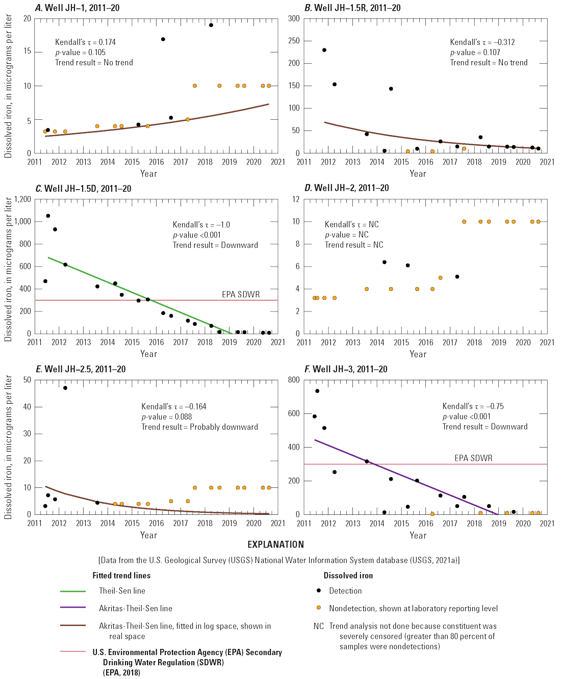
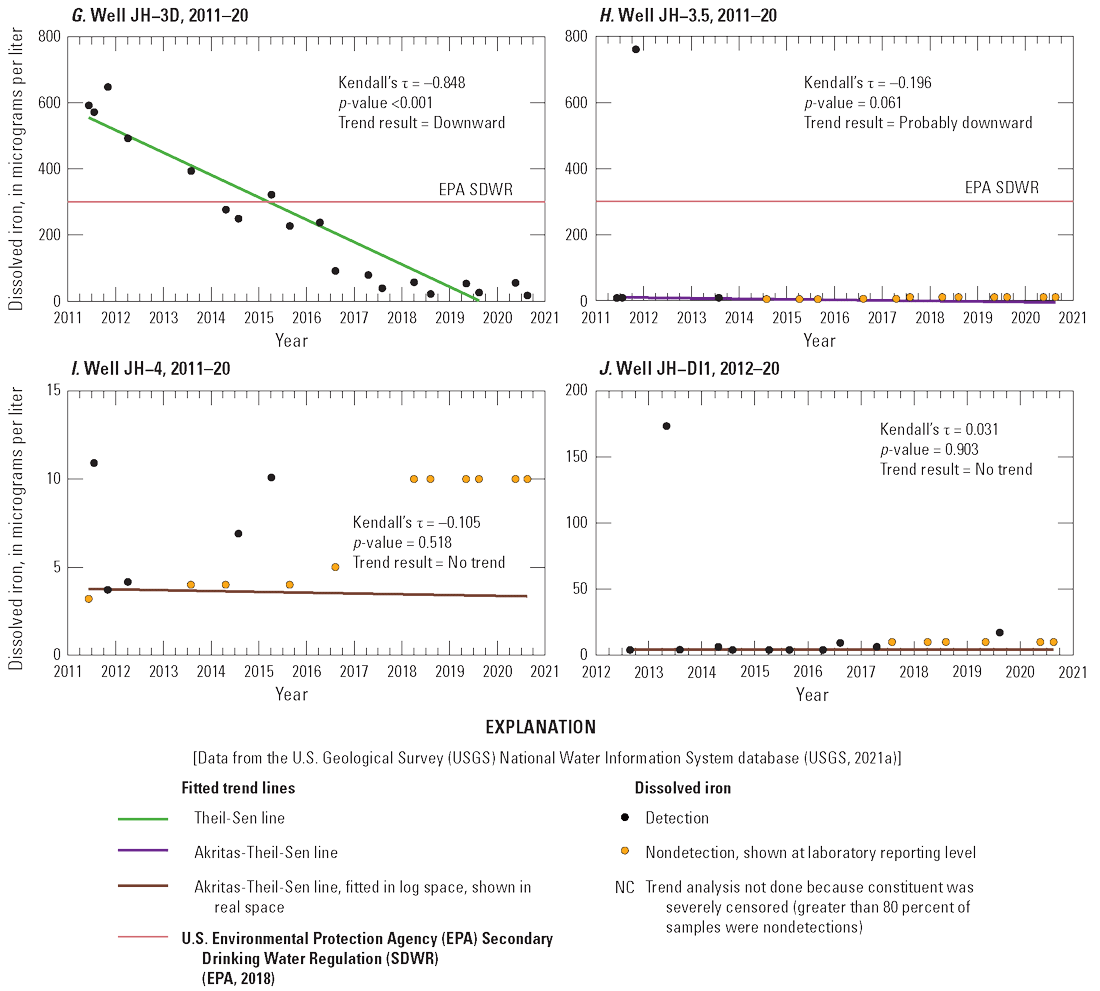
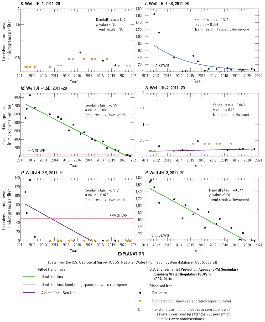
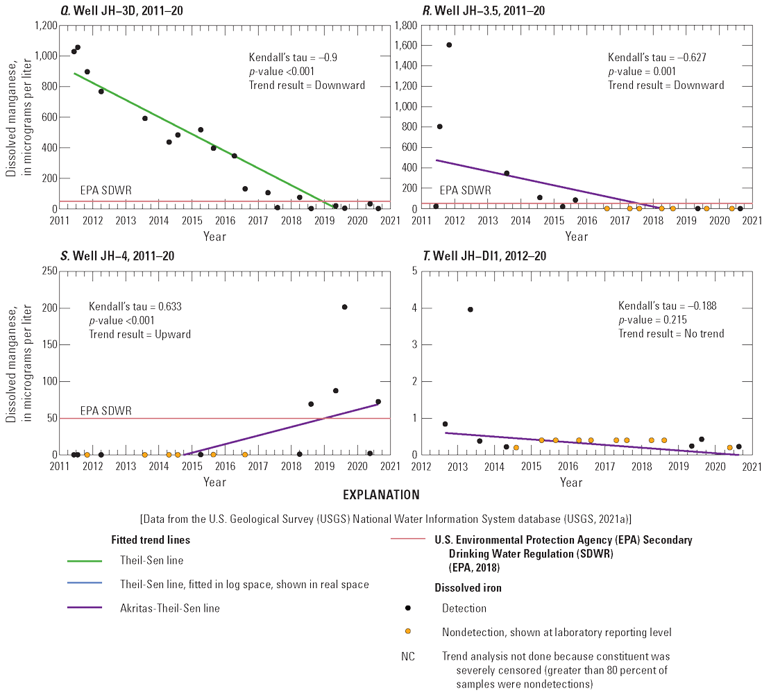
Trends in dissolved iron (A–J) and manganese (K–T) concentrations in groundwater samples from monitor wells, Jackson Hole Airport, Jackson, Wyoming, 2011–20.
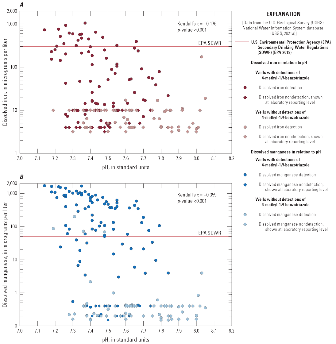
Relations between A, dissolved iron and pH, and B, dissolved manganese and pH in groundwater samples collected from monitor wells at the Jackson Hole Airport, Jackson, Wyoming, 2011–20.
Using data collected from all wells during 2011–20, pH values were weakly negatively correlated with dissolved iron concentrations (Kendall’s τ=−0.176, p-value<0.001) and negatively correlated with dissolved manganese concentrations (all sample data; Kendall’s τ=−0.359, respectively; p-value<0.001; fig. 14). When the sample data were subdivided by wells, pH values were negatively correlated (p-values<0.05) with dissolved iron concentrations in 3 wells (JH–1.5D, JH–3, JH–3D, Kendall’s τ=−0.51 to −0.58) and negatively correlated (p-values<0.05) with dissolved manganese concentrations in 5 wells (JH–1.5D, JH–3, JH–3D, JH–3.5, JH–4; Kendall’s τ=−0.51 to −0.61; appendix table 1.10).
As expected, given their redox-sensitive nature, dissolved iron and manganese were measured at higher concentrations when anoxic conditions in each well were strongly reducing, which most commonly was when manganese or iron reduction was identified as the predominant redox processes during 2011–20 (table 6). High dissolved iron concentrations greater than the EPA SDWR for iron typically indicated the presence of high dissolved manganese concentrations greater than the EPA SDWR for manganese, but the opposite did not occur as often (table 6). This observation is consistent with typical redox sequence progression after oxygen and nitrate have been reduced, in which manganese is reduced before iron (refer to the “Redox Conditions” section).
Redox conditions progressed beyond iron reduction near some wells during 2011–20, as indicated by the following characteristics of some samples:
-
• Detection of sulfides, which are generated by sulfate reduction, in at least three samples from each of the 7 wells during 2011–20, and identification of sulfate reduction as one of two predominant redox processes at well JH–1.5R during April 2012 (mixed anoxic conditions) and July 2014 (mixed oxic-anoxic conditions; table 6);
-
• Detection of dissolved methane gas, which is generated by methanogenesis, in samples from wells JH–1.5 (predecessor of well JH–1.5R), JH–1.5D, JH–2.5, JH–3, JH–3D, and JH–3.5 in June 2011 (app. 6 of Wright, 2013; samples collected from 10 monitor wells during 2011–20 were analyzed once for methane in June 2011); and
-
• Identification of methanogenesis (carbon dioxide reduction) as the predominant redox process in samples from wells JH–1.5 (predecessor of well JH–1.5R) and JH–3 during June 2011 (Wright, 2013; table 6; also refer to the “Redox Conditions” section).
High dissolved iron and manganese concentrations were common in samples with these characteristics (table 6). Except for the few samples where the predominant redox processes were identified as sulfate reduction or methanogenesis, the predominant redox processes identified for most samples with high dissolved iron and manganese concentrations were manganese or iron reduction (and infrequently, mixed redox conditions and processes), despite evidence of more reduced conditions in some samples (table 6). This indicates that parts of the aquifer screened by the wells may have contained waters that were very strongly reduced and, thus, “more reduced” than the redox process (manganese or iron reduction) indicated in table 6. Evidence of more than one redox process in water samples (including samples classified as mixed) could be explained by the mixing of waters from different redox zones upgradient from the well, a well screen open to more than one redox zone, or spatial variability in microbial activity/redox processes in the aquifer (Chapelle, 2001).
Wright (2013) observed that all wells with benzotriazole detections were downgradient from airport operations, including the airport terminal where most plane deicing was done before construction of the deicing pad during 2011. Reducing conditions present in an otherwise oxic aquifer indicate an upgradient or natural, in-place source of organic carbon or oxidizable minerals (Chapelle, 2001). No substantial anthropogenic sources of dissolved organic carbon were detected in the alluvial aquifer during 2011–20. DOC concentrations in the alluvial aquifer were low (typically <1 mg/L), despite significantly higher concentrations in wells with benzotriazoles (refer to the “Redox Conditions” section). Other potential sources of organic carbon such as human-made organic compounds (for example, VOCs, GRO, DRO, and glycols) were rarely detected (refer to the “Anthropogenic Compounds” section). Additionally, unconsolidated sand and gravel aquifers such as the Snake River alluvial aquifer tend to have very low amounts of sedimentary organic carbon (app. A of Interstate Technology & Regulatory Council, 2015). Consequently, the absence of substantial sources of organic carbon and the consistent detection of benzotriazoles in wells downgradient from airport operations during 2011–20 strengthens the conclusion of the previous study (Wright, 2013) that microbial oxidation of ADAFs produced anoxic conditions that lead to reductive dissolution of naturally occurring iron and manganese from aquifer sediments. However, microbial oxidation of ADAFs was not likely the cause of suboxic, mixed, and anoxic conditions and resultant high manganese concentrations in well JH–4 during 2018–20 because no benzotriazole compounds (or any other anthropogenic compounds) were detected in the well (table 6). Well JH–4 is a flush-mounted well next to a staging area that has been used to support JHA construction activities. The staging area included a concrete plant during 2015–17. In 2017, a temporary building associated with the concrete plant was placed over well JH–4, preventing access for data collection. These and other construction activities since the well was installed have increased the surrounding grade and land surface, causing the well to be in a low point in this area. Thus, it is possible that surface water may have collected and entered the well, potentially transporting surficial organic matter into the aquifer that subsequently was oxidized and created the reducing conditions (and resultant high manganese concentrations) observed at this well.
Positive correlations between dissolved iron and manganese concentrations indicate a common source of both trace elements in the alluvial aquifer sediments underlying the airport. Using all data collected during 2011–20, a significant positive correlation was found between dissolved iron and manganese concentrations (Kendall’s τ=0.522, p-value<0.001). When the sample data were subdivided by wells, dissolved iron concentrations were positively correlated (p-values<0.05) with dissolved manganese concentrations in four wells: JH–1.5R (Kendall’s τ=0.42), JH–1.5D (Kendall’s τ=0.92), JH–3 (Kendall’s τ=0.82), and JH–3D (Kendall’s τ=0.94; appendix table 1.10). These four wells had varying anoxic, suboxic, or mixed redox conditions during most of 2011–20 and the only exceedances of the EPA SDWR for iron and most of the exceedances of the EPA SDWR for manganese of all sites sampled (83 percent; table 6). Oxidized forms of iron and manganese commonly co-occur together in aquifer sediments, most commonly as oxyhydroxide coatings on sediment grains, but also as minerals composing aquifer sediments (Chapelle, 2001). Thus, the positive correlations between dissolved iron and manganese concentrations indicate aquifer sediment mineralogy, in combination with reducing conditions induced by microbial degradation of ADAFs, may have largely controlled concentrations of both trace elements in parts of the alluvial aquifer at the JHA during 2011–20. However, as described previously, there was no evidence indicating degradation of ADAFs was the cause of suboxic, mixed, and anoxic conditions and resultant high manganese concentrations in the aquifer in the vicinity of well JH–4 during 2018–20.
Trends in Dissolved Iron and Dissolved Manganese Concentrations
Trends in dissolved iron and manganese concentrations during 2011–20 were evaluated with the nonparametric seasonal Kendall test (refer to the “Statistical Analysis” section). The trend test was applied to dissolved iron and manganese concentrations at nine wells. Because of severe censoring (greater than 80 percent of samples censored), trend tests for dissolved iron and manganese were not done for wells JH–2 and JH–1, respectively. Trends in dissolved iron and manganese concentrations for 2011–20, including results of seasonal Kendall tests, are shown in a series of graphs for individual wells in figure 13 and spatially for all wells in figure 7. Results of seasonal Kendall tests for dissolved iron and manganese (including p-values, Kendall’s τ values, and Theil-Sen and Akritas-Theil-Sen slopes) are tabulated in appendix table 1.9.
Downward and probable downward trends in dissolved iron and manganese concentrations during 2011–20 were determined at six of the monitor wells at the JHA (figs. 7, 13; appendix table 1.9). The results of the seasonal Kendall tests for the 6 wells with benzotriazole detections indicated downward trends in iron concentrations at 3 wells (JH–1.5D, JH–3, and JH–3D), probable downward trends at 2 wells (JH–2.5 and JH–3.5), and no trend at 1 well (JH–1.5R; figs. 7, 13B–C, E–H; appendix table 1.9). No trends in dissolved iron concentrations were determined at the four wells without benzotriazole detections (JH–1, JH–2, JH–4 and JH–DI1; figs. 7, 13A, D, I–J; appendix table 1.9). The results of the seasonal Kendall tests for the 6 wells with benzotriazole detections indicated downward trends in dissolved manganese concentrations at 5 wells (JH–1.5D, JH–2.5, JH–3, JH–3D, and JH–3.5) and a probable downward trend at 1 well (JH–1.5R; fig. 13B–C, E–H; appendix table 1.9). No trends in dissolved manganese concentrations were determined at 3 of 4 wells without benzotriazole detections (JH–1, JH–2, and JH–DI1), but an upward trend was determined at 1 well (JH–4; figs. 7, 13A, D, I–J; appendix table 1.9). The upward trend in dissolved manganese concentrations in well JH–4 corresponded with downward trends in DO and pH, and an upward trend in specific conductance (refer to the “Physical Properties” section; fig. 7; appendix table 1.9).
The downward and probable downward trends in dissolved iron and manganese concentrations at individual wells with benzotriazole detections mostly corresponded with upward and probable upward trends in DO concentrations and pH values (refer to the “Physical Properties” section), downward and probable downward trends in specific-conductance values (refer to the “Physical Properties” section), and 4-MeBT concentrations (and nondetections of 5-MeBT by 2018; refer to the “Anthropogenic Compounds” section) for the same wells (fig. 7). Collectively, these trends indicated groundwater-quality conditions near all wells with benzotriazole detections were returning to water-quality conditions similar to background water-quality conditions measured in the alluvial aquifer upgradient from airport operations, potentially in response to the changes in the ADAF formulation used by the JHA, many JHA infrastructure improvements made during 2011–20, and degradation of existing ADAFs in subsurface soils and groundwater, or some combination of these possibilities.
Out of the 6 wells with detections of benzotriazoles, all of which had 1 or more detections of dissolved iron or manganese at concentrations greater than respective EPA SDWRs during 2011–20, only 1 well (JH–1.5R) had detections of either constituent at concentrations greater than these standards by 2020 (fig. 13; table 6). In 2020, dissolved manganese concentrations in well JH–1.5R (83.2 µg/L in May and 51.2 µg/L in July) were higher than the EPA SDWR of 50 µg/L but were substantially lower than the highest concentration (1,639 µg/L, November 2011) measured in that well during 2011–20 (table 6). Of the remaining 5 wells with benzotriazole detections during 2011–20, dissolved iron and manganese typically were detected at low concentrations or were no longer detected above reporting levels by 2020 (table 6); all but 1 of these wells (well JH–3.5) had downward trends in 4-MeBT concentrations (refer to the “Anthropogenic Compounds” section).
Anthropogenic Compounds
As a commercial airport, the JHA uses many different anthropogenic compounds as part of daily operations. It is for this reason that the two previous studies analyzed groundwater samples for organic compounds commonly associated with anthropogenic activities, including VOCs, GRO, DRO, glycols, and benzotriazoles, to determine if any of these compounds were present and affecting redox conditions in the alluvial aquifer. Of these compounds, only benzotriazoles, specifically 4-MeBT and 5-MeBT, were consistently detected in groundwater samples collected at the JHA (Wright, 2010, 2013); therefore, groundwater samples collected from most wells during August 2012–August 2020 were not routinely analyzed for the other anthropogenic compounds (VOCs, GRO, DRO, and glycols).
Volatile Organic Compounds, Gasoline-Range Organics, and Diesel-Range Organics
As part of the previous study (Wright, 2013), groundwater samples from 10 monitor wells collected during June and July 2011 and April 2012 were analyzed for VOCs, GRO, and DRO. Three VOCs (benzene, ethylbenzene, and total xylene) and GRO were detected infrequently at low, estimated concentrations in at least one sampled well. DRO was not detected in any of the wells. Benzene was detected at a low estimated concentration of 0.09 µg/L in the sample from well JH–1.5D collected during April 2012; however, this value was less than five times the concentration measured in the associated trip blank, so the detection was qualified and considered questionable (Wright, 2013). Ethylbenzene was detected at an estimated concentration of 0.11 µg/L in the June 2011 sample collected from well JH–2.5, and total xylene was detected at estimated concentrations of 0.26 and 0.20 in the June and July 2011 samples collected from well JH–2.5, respectively. GRO was detected at an estimated concentration of 11 µg/L in the July 2011 sample collected from well JH–1.5D.
Groundwater samples from two monitor wells (JH–DI1 and JH–4) collected during August 2012–August 2020 were analyzed for VOCs, GRO, and DRO (table 1). Samples from well JH–DI1 were initially analyzed for these and other constituents to determine the “baseline” groundwater-quality conditions downgradient from and before use of the airport deicing pad, and subsequently to monitor for their presence after deicing activities began at the facility. Unlike well JH–DI1, these organic compounds were added to the analyte list for well JH–4 to determine if their presence was responsible for the increasingly reduced conditions observed in this well during the study period (refer to the “Redox Conditions” section). DO concentrations in well JH–4 significantly decreased, whereas dissolved manganese concentrations significantly increased during 2011–20 (refer to the “Physical Properties” and “Dissolved Iron and Dissolved Manganese” sections), despite no detections of benzotriazoles in samples from the well (table 7).
The groundwater sample collected from well JH–DI1 on August 22, 2012, was analyzed for VOCs, GRO, and DRO. GRO was detected at a low, estimated concentration (16 µg/L) in the environmental sample, but not in the corresponding replicate sample (appendix tables 1.3, 1.5). Because GRO was detected in the environmental sample, but not in the corresponding replicate sample, an additional (confirmatory) sample from well JH–DI1 was subsequently collected on April 30, 2013. GRO and BTEX compounds were not detected in the sample, indicating they were likely not present in the aquifer at this location (appendix table 1.3).
Samples for VOCs, GRO, and DRO were collected twice from well JH–4 during 2019. GRO was detected at low, estimated concentrations in the environmental sample (30 µg/L) and corresponding replicate sample (19 µg/L) collected on August 13, 2019 (appendix tables 1.3, 1.5). Because the environmental sample and replicate sample values were estimated concentrations, and the RPD (about 45 percent; appendix table 1.5) between the samples was large (greater than 20 percent; refer to the “Quality Assurance and Quality-Control Sample Collection” section), there is considerable uncertainty associated with both concentration values reported by the analyzing laboratory.
Glycols
Although glycols were not detected during the two previous studies (Wright, 2010, 2013), samples collected from well JH–DI1 were analyzed for glycol compounds during August 2012–20 to document water-quality conditions near the well and to facilitate comparison with future water samples collected to monitor for potential groundwater-quality changes due to deicing activities at the upgradient deicing pad installed during 2011 (fig. 5). Glycol compounds were detected in five samples collected from well JH–DI1 during August 2012–August 2020 (appendix table 1.3), but evaluation of the field and laboratory quality-control sample data associated with the environmental samples indicated these five detections may be due to contamination introduced during sampling or laboratory analysis, or due to other laboratory-related issues. However, the available information is not sufficient to conclusively determine the presence or absence of glycols in the alluvial aquifer near well JH–DI1.
Two glycol compounds (diethylene glycol and triethylene glycol) that are not components of deicers were detected at the JHA. Diethylene glycol was detected at a concentration of 9.8 µg/L in 1 of 11 environmental samples from well JH–DI1 (August 1, 2017) analyzed for the constituent, but it was not detected in the corresponding replicate sample (appendix tables 1.3, 1.5). Triethylene glycol was detected in 1 of 11 environmental samples from well JH–DI1 analyzed for the constituent at an estimated concentration of 2.7 µg/L (July 13, 2013; appendix table 1.3). The compound also was detected in an associated laboratory blank sample (appendix table 1.3), indicating the detection likely was attributable to laboratory contamination.
Ethylene glycol, a component in deicers, was detected in 3 of 17 samples from well JH–DI1 that were analyzed for the constituent at estimated concentrations of 0.53 µg/L (April 22, 2014), 2.9 µg/L (August 13, 2019), and 2.7 µg/L (May 19, 2020; appendix table 1.3). Two of three ethylene glycol detections (estimated concentrations: 0.53 µg/L, April 22, 2014, and 2.7 µg/L, May 19, 2020) were in the environmental samples but not in the corresponding replicate samples (appendix tables 1.3, 1.5). The remaining ethylene glycol detection (estimated concentration: 2.9 µg/L, August 13, 2019) was at a concentration less than five times the maximum concentration measured in an associated laboratory blank sample (appendix table 1.3; also refer to the “Quality Assurance and Quality-Control Sample Collection” section).
Benzotriazole Compounds
Samples for analysis of benzotriazoles (1H-BT, 4-MeBT, and 5-MeBT) were collected each time a monitor well was sampled during 2011–20. One set of benzotriazole analyses for well JH–DI1 (sample from July 31, 2013) is missing because the sample bottle broke during transit to the analyzing laboratory.
Only two of the three benzotriazole compounds measured (4-MeBT and 5-MeBT) were detected in wells sampled during 2011–20 (table 7). Both benzotriazoles were detected in 7 of 10 monitor wells sampled during 2011–20 (table 7). Benzotriazoles were detected twice from well JH–2 at low concentrations at or slightly greater than the LOD (4-MeBT, July 9, 2016, and 5-MeBT, July 29, 2014). However, both well JH–2 benzotriazole detections are considered suspect for the following reasons: (1) 4-MeBT and 5-MeBT were detected only once each, unlike all other wells with detections where both compounds were detected more frequently; (2) water from well JH–2 was consistently oxic with nondetectable to low iron and manganese concentrations during 2011–20, unlike all other wells with detections, which had anoxic waters and high iron and manganese concentrations for at least some period; (3) 4-MeBT was not detected in the sample with 5-MeBT, unlike all other samples when 5-MeBT was detected; and (4) the 4-MeBT concentration is at the LOD (table 7). For these reasons, both detections were treated as nondetections in this report for summary and analysis purposes because the available information was insufficient to conclusively determine if the detections represented rare occurrence in the alluvial aquifer near well JH–2 or were due to contamination introduced during sampling or laboratory analysis. Therefore, all summary and analysis of data in this report was done assuming benzotriazoles were detected in only six wells. The six remaining wells with benzotriazole detections included wells JH–1.5R (and its predecessor well JH–1.5), JH–1.5D, JH–2.5, JH–3, JH–3D, and JH–3.5 (table 7).
Table 7.
Analytical results for benzotriazole compounds in groundwater samples collected from monitor wells at the Jackson Hole Airport, Jackson, Wyoming, 2011–20.[Data are from the U.S. Geological Survey (USGS) National Water Information System database (USGS, 2021a). Sample date is shown in mm/dd/yyyy, month/day/year, and sample time is shown in hh:mm, hour:minute (24 hour). Value of constituents detected at or above the limit of quantitation are show in bold and noted with footnote 2. µg/L, microgram per liter; <, less than symbol indicates the chemical was not detected and the value after the less than is the limit of detection; E, value was measured above the level of detection and below the level of quantitation and is considered estimated; --, not applicable]
| USGS site number | Well identifier (fig. 3) | Sample date | Sample time | 1H-benzotriazole (µg/L) |
4-Methyl-1-H-benzotriazole (µg/L) | 5-Methyl-1-H-benzotriazole (µg/L) |
|---|---|---|---|---|---|---|
| 433615110440001 | JH–1 | 106/08/2011 | 12:00 | <0.25 | <0.35 | <0.25 |
| 433615110440001 | JH–1 | 107/19/2011 | 10:30 | <0.25 | <0.35 | <0.25 |
| 433615110440001 | JH–1 | 111/01/2011 | 11:00 | <0.25 | <0.35 | <0.25 |
| 433615110440001 | JH–1 | 104/03/2012 | 10:30 | <0.25 | <0.35 | <0.25 |
| 433615110440001 | JH–1 | 07/29/2013 | 16:20 | <0.25 | <0.35 | <0.25 |
| 433615110440001 | JH–1 | 04/21/2014 | 18:30 | <0.25 | <0.35 | <0.25 |
| 433615110440001 | JH–1 | 07/28/2014 | 19:00 | <0.25 | <0.35 | <0.25 |
| 433615110440001 | JH–1 | 04/06/2015 | 18:40 | <0.25 | <0.35 | <0.25 |
| 433615110440001 | JH–1 | 08/24/2015 | 18:00 | <0.25 | <0.35 | <0.25 |
| 433615110440001 | JH–1 | 04/11/2016 | 18:45 | <0.25 | <0.35 | <0.25 |
| 433615110440001 | JH–1 | 08/08/2016 | 18:00 | <0.25 | <0.35 | <0.25 |
| 433615110440001 | JH–1 | 04/17/2017 | 17:50 | <0.25 | <0.35 | <0.25 |
| 433615110440001 | JH–1 | 07/31/2017 | 18:20 | <0.25 | <0.35 | <0.25 |
| 433615110440001 | JH–1 | 04/03/2018 | 10:20 | <0.25 | <0.35 | <0.25 |
| 433615110440001 | JH–1 | 08/06/2018 | 18:40 | <0.25 | <0.35 | <0.25 |
| 433615110440001 | JH–1 | 05/06/2019 | 18:10 | <0.25 | <0.35 | <0.25 |
| 433615110440001 | JH–1 | 08/13/2019 | 14:20 | <0.25 | <0.35 | <0.25 |
| 433615110440001 | JH–1 | 05/18/2020 | 17:50 | <0.25 | <0.35 | <0.25 |
| 433615110440001 | JH–1 | 08/17/2020 | 17:30 | <0.25 | <0.35 | <0.25 |
| 433604110443401 | JH–1.5 | 106/10/2011 | 10:30 | <0.25 | 22.1 | E0.33 |
| 433604110443401 | JH–1.5 | 107/20/2011 | 18:00 | <0.25 | 21.6 | E0.27 |
| 433604110443403 | JH–1.5R | 111/02/2011 | 17:30 | <0.25 | 213 | E0.68 |
| 433604110443403 | JH–1.5R | 104/04/2012 | 18:20 | <0.25 | 28.5 | E0.33 |
| 433604110443403 | JH–1.5R | 08/01/2013 | 16:40 | <0.25 | 2,32.3 | <0.25 |
| 433604110443403 | JH–1.5R | 04/24/2014 | 10:00 | <0.25 | 23.0 | 22.6 |
| 433604110443403 | JH–1.5R | 07/31/2014 | 18:00 | <0.25 | 22.0 | 20.27 |
| 433604110443403 | JH–1.5R | 04/09/2015 | 12:30 | <0.25 | 24.6 | <1.3 |
| 433604110443403 | JH–1.5R | 08/27/2015 | 14:50 | <0.25 | 23.8 | 2,40.49 |
| 433604110443403 | JH–1.5R | 04/13/2016 | 12:30 | <0.25 | 24.5 | <0.25 |
| 433604110443403 | JH–1.5R | 08/11/2016 | 09:15 | <0.25 | 23.0 | 20.38 |
| 433604110443403 | JH–1.5R | 04/20/2017 | 10:00 | <0.25 | 21.6 | <0.25 |
| 433604110443403 | JH–1.5R | 08/02/2017 | 12:00 | <0.25 | 22.4 | 20.39 |
| 433604110443403 | JH–1.5R | 04/05/2018 | 09:30 | <0.25 | 23.7 | <0.25 |
| 433604110443403 | JH–1.5R | 08/08/2018 | 13:50 | <0.25 | 23.9 | <0.25 |
| 433604110443403 | JH–1.5R | 05/09/2019 | 14:50 | <0.25 | 22.9 | <0.25 |
| 433604110443403 | JH–1.5R | 08/15/2019 | 15:00 | <0.25 | 23.1 | <0.25 |
| 433604110443403 | JH–1.5R | 05/21/2020 | 18:30 | <0.25 | 20.82 | <0.25 |
| 433604110443403 | JH–1.5R | 08/20/2020 | 15:10 | <0.25 | 21.4 | <0.25 |
| 433604110443402 | JH–1.5D | 16/10/2011 | 11:50 | <0.25 | 22.2 | E0.33 |
| 433604110443402 | JH–1.5D | 17/20/2011 | 19:30 | <0.25 | 22.4 | E0.33 |
| 433604110443402 | JH–1.5D | 111/3/2011 | 13:00 | <0.25 | 29.8 | E0.77 |
| 433604110443402 | JH–1.5D | 14/5/2012 | 10:20 | <0.25 | 28.1 | E0.40 |
| 433604110443402 | JH–1.5D | 07/31/2013 | 13:30 | <0.25 | 2,32.8 | <0.25 |
| 433604110443402 | JH–1.5D | 04/23/2014 | 17:00 | <0.25 | 21.1 | 20.8 |
| 433604110443402 | JH–1.5D | 07/31/2014 | 14:50 | <0.25 | 22.3 | 20.31 |
| 433604110443402 | JH–1.5D | 04/09/2015 | 14:30 | <0.25 | 23.3 | <1.1 |
| 433604110443402 | JH–1.5D | 08/27/2015 | 12:20 | <0.25 | 23.4 | 2,40.38 |
| 433604110443402 | JH–1.5D | 04/13/2016 | 09:30 | <0.25 | 22.0 | <0.25 |
| 433604110443402 | JH–1.5D | 08/11/2016 | 12:10 | <0.25 | 22.1 | 20.27 |
| 433604110443402 | JH–1.5D | 04/20/2017 | 13:00 | <0.25 | 21.1 | <0.25 |
| 433604110443402 | JH–1.5D | 08/02/2017 | 16:10 | <0.25 | 21.4 | 20.35 |
| 433604110443402 | JH–1.5D | 04/05/2018 | 11:40 | <0.25 | 22.6 | <0.25 |
| 433604110443402 | JH–1.5D | 08/08/2018 | 17:30 | <0.25 | 22.2 | <0.25 |
| 433604110443402 | JH–1.5D | 05/09/2019 | 12:10 | <0.25 | 22.0 | <0.25 |
| 433604110443402 | JH–1.5D | 08/15/2019 | 13:00 | <0.25 | 22.0 | <0.25 |
| 433604110443402 | JH–1.5D | 05/21/2020 | 15:40 | <0.25 | 20.76 | <0.25 |
| 433604110443402 | JH–1.5D | 08/20/2020 | 13:10 | <0.25 | 21.0 | <0.25 |
| 433551110443501 | JH–2 | 16/8/2011 | 17:10 | <0.25 | <0.35 | <0.25 |
| 433551110443501 | JH–2 | 17/19/2011 | 15:30 | <0.25 | <0.35 | <0.25 |
| 433551110443501 | JH–2 | 111/1/2011 | 15:10 | <0.25 | <0.35 | <0.25 |
| 433551110443501 | JH–2 | 14/3/2012 | 15:30 | <0.25 | <0.35 | <0.25 |
| 433551110443501 | JH–2 | 07/30/2013 | 13:10 | <0.25 | <0.35 | <0.25 |
| 433551110443501 | JH–2 | 04/22/2014 | 16:30 | <0.25 | <0.35 | <0.25 |
| 433551110443501 | JH–2 | 07/29/2014 | 15:10 | <0.25 | <0.35 | 40.26 |
| 433551110443501 | JH–2 | 04/07/2015 | 15:30 | <0.25 | <0.35 | <0.25 |
| 433551110443501 | JH–2 | 08/25/2015 | 15:00 | <0.25 | <0.35 | <0.25 |
| 433551110443501 | JH–2 | 04/12/2016 | 13:15 | <0.25 | <0.35 | <0.25 |
| 433551110443501 | JH–2 | 08/09/2016 | 14:00 | <0.25 | 50.35 | <0.25 |
| 433551110443501 | JH–2 | 04/18/2017 | 13:30 | <0.25 | <0.35 | <0.25 |
| 433551110443501 | JH–2 | 08/01/2017 | 13:00 | <0.25 | <0.35 | <0.25 |
| 433551110443501 | JH–2 | 04/04/2018 | 10:40 | <0.25 | <0.35 | <0.25 |
| 433551110443501 | JH–2 | 08/07/2018 | 16:45 | <0.25 | <0.35 | <0.25 |
| 433551110443501 | JH–2 | 05/07/2019 | 16:50 | <0.25 | <0.35 | <0.25 |
| 433551110443501 | JH–2 | 08/12/2019 | 18:40 | <0.25 | <0.35 | <0.25 |
| 433551110443501 | JH–2 | 05/19/2020 | 13:10 | <0.25 | <0.35 | <0.25 |
| 433551110443501 | JH–2 | 08/18/2020 | 13:30 | <0.25 | <0.35 | <0.25 |
| 433600110443701 | JH–2.5 | 16/9/2011 | 15:00 | <0.25 | 24.3 | E0.43 |
| 433600110443701 | JH–2.5 | 17/21/2011 | 11:00 | <0.25 | 23.7 | E0.32 |
| 433600110443701 | JH–2.5 | 111/3/2011 | 14:30 | <0.25 | 27.8 | E0.72 |
| 433600110443701 | JH–2.5 | 14/4/2012 | 09:50 | <0.25 | 28.5 | E0.26 |
| 433600110443701 | JH–2.5 | 07/31/2013 | 10:10 | <0.25 | 2,33.3 | <0.25 |
| 433600110443701 | JH–2.5 | 04/23/2014 | 09:40 | <0.25 | 23.3 | 22.6 |
| 433600110443701 | JH–2.5 | 07/31/2014 | 09:50 | <0.25 | 22.7 | 20.28 |
| 433600110443701 | JH–2.5 | 04/09/2015 | 10:50 | <0.25 | 23.8 | <1.4 |
| 433600110443701 | JH–2.5 | 08/27/2015 | 09:30 | <0.25 | 23.4 | 2,40.38 |
| 433600110443701 | JH–2.5 | 08/10/2016 | 09:20 | <0.25 | 22.5 | <0.25 |
| 433600110443701 | JH–2.5 | 04/19/2017 | 09:20 | <0.25 | 22.0 | <0.25 |
| 433600110443701 | JH–2.5 | 08/02/2017 | 09:00 | <0.25 | 21.9 | 20.28 |
| 433600110443701 | JH–2.5 | 04/04/2018 | 13:00 | <0.25 | 23.7 | <0.25 |
| 433600110443701 | JH–2.5 | 08/08/2018 | 11:30 | <0.25 | 22.3 | <0.25 |
| 433600110443701 | JH–2.5 | 05/08/2019 | 12:40 | <0.25 | 22.7 | <0.25 |
| 433600110443701 | JH–2.5 | 08/14/2019 | 13:30 | <0.25 | 22.7 | <0.25 |
| 433600110443701 | JH–2.5 | 05/20/2020 | 10:30 | <0.25 | 21.0 | <0.25 |
| 433600110443701 | JH–2.5 | 08/19/2020 | 12:10 | <0.25 | 21.3 | <0.25 |
| 433603110443501 | JH–3 | 16/9/2011 | 18:30 | <0.25 | 22.0 | E0.39 |
| 433603110443501 | JH–3 | 17/20/2011 | 11:00 | <0.25 | 21.8 | E0.41 |
| 433603110443501 | JH–3 | 111/2/2011 | 13:50 | <0.25 | 28.1 | E0.61 |
| 433603110443501 | JH–3 | 14/4/2012 | 12:50 | <0.25 | 28.7 | E0.52 |
| 433603110443501 | JH–3 | 08/01/2013 | 11:00 | <0.25 | 1,22.1 | <0.25 |
| 433603110443501 | JH–3 | 04/23/2014 | 13:30 | <0.25 | 23.2 | 22.3 |
| 433603110443501 | JH–3 | 07/30/2014 | 11:10 | <0.25 | 21.5 | 20.34 |
| 433603110443501 | JH–3 | 04/08/2015 | 12:45 | <0.25 | 24.0 | <1.2 |
| 433603110443501 | JH–3 | 08/26/2015 | 12:10 | <0.25 | 23.3 | 2,40.41 |
| 433603110443501 | JH–3 | 04/12/2016 | 16:30 | <0.25 | 23.1 | <0.25 |
| 433603110443501 | JH–3 | 08/10/2016 | 12:40 | <0.25 | 22.1 | <0.25 |
| 433603110443501 | JH–3 | 04/19/2017 | 17:00 | <0.25 | 21.2 | <0.25 |
| 433603110443501 | JH–3 | 08/03/2017 | 09:30 | <0.25 | 21.2 | 20.32 |
| 433603110443501 | JH–3 | 04/04/2018 | 15:50 | <0.25 | 23.4 | <0.25 |
| 433603110443501 | JH–3 | 08/09/2018 | 09:45 | <0.25 | 22.1 | <0.25 |
| 433603110443501 | JH–3 | 05/09/2019 | 09:10 | <0.25 | 22.8 | <0.25 |
| 433603110443501 | JH–3 | 08/15/2019 | 09:20 | <0.25 | 21.8 | <0.25 |
| 433603110443501 | JH–3 | 05/21/2020 | 09:30 | <0.25 | 21.1 | <0.25 |
| 433603110443501 | JH–3 | 08/20/2020 | 10:00 | <0.25 | 20.86 | <0.25 |
| 433603110443502 | JH–3D | 16/9/2011 | 20:30 | <0.25 | 21.1 | E0.28 |
| 433603110443502 | JH–3D | 17/20/2011 | 13:00 | <0.25 | 21.1 | E0.26 |
| 433603110443502 | JH–3D | 111/2/2011 | 15:10 | <0.25 | 22.1 | E0.27 |
| 433603110443502 | JH–3D | 14/4/2012 | 14:50 | <0.25 | 23.0 | E0.31 |
| 433603110443502 | JH–3D | 08/01/2013 | 13:40 | <0.25 | 2,31.4 | <0.25 |
| 433603110443502 | JH–3D | 04/24/2014 | 15:00 | <0.25 | 20.94 | 20.81 |
| 433603110443502 | JH–3D | 07/30/2014 | 15:50 | <0.25 | 20.84 | 20.29 |
| 433603110443502 | JH–3D | 04/08/2015 | 16:30 | <0.25 | 21.8 | <0.61 |
| 433603110443502 | JH–3D | 08/26/2015 | 17:30 | <0.25 | 21.8 | <0.25 |
| 433603110443502 | JH–3D | 04/13/2016 | 15:30 | <0.25 | 21.2 | <0.25 |
| 433603110443502 | JH–3D | 08/10/2016 | 16:30 | <0.25 | 21.1 | <0.25 |
| 433603110443502 | JH–3D | 04/19/2017 | 14:20 | <0.25 | 20.59 | <0.25 |
| 433603110443502 | JH–3D | 08/03/2017 | 15:20 | <0.25 | 20.62 | 20.27 |
| 433603110443502 | JH–3D | 04/04/2018 | 17:50 | <0.25 | 21.3 | <0.25 |
| 433603110443502 | JH–3D | 08/09/2018 | 13:00 | <0.25 | 20.92 | <0.25 |
| 433603110443502 | JH–3D | 05/08/2019 | 17:20 | <0.25 | 20.78 | <0.25 |
| 433603110443502 | JH–3D | 08/14/2019 | 18:00 | <0.25 | 21.3 | <0.25 |
| 433603110443502 | JH–3D | 05/20/2020 | 16:30 | <0.25 | <0.35 | <0.25 |
| 433603110443502 | JH–3D | 08/19/2020 | 16:40 | <0.25 | 20.51 | <0.25 |
| 433605110443801 | JH–3.5 | 16/9/2011 | 10:00 | <0.25 | <0.35 | <0.25 |
| 433605110443801 | JH–3.5 | 17/21/2011 | 14:30 | <0.25 | E0.37 | <0.25 |
| 433605110443801 | JH–3.5 | 111/2/2011 | 11:10 | <0.25 | 21.2 | E0.28 |
| 433605110443801 | JH–3.5 | 14/1/2012 | No sample | No sample | No sample | No sample |
| 433605110443801 | JH–3.5 | 07/30/2013 | 15:00 | <0.25 | 2,3E0.67 | <0.25 |
| 433605110443801 | JH–3.5 | 07/30/2014 | 18:20 | <0.25 | 20.55 | 20.27 |
| 433605110443801 | JH–3.5 | 04/08/2015 | 09:30 | <0.25 | 20.66 | <0.38 |
| 433605110443801 | JH–3.5 | 08/26/2015 | 09:30 | <0.25 | 21.1 | <0.25 |
| 433605110443801 | JH–3.5 | 08/09/2016 | 15:50 | <0.25 | 20.67 | <0.25 |
| 433605110443801 | JH–3.5 | 04/18/2017 | 15:50 | <0.25 | <0.35 | <0.25 |
| 433605110443801 | JH–3.5 | 08/01/2017 | 15:30 | <0.25 | 20.58 | 20.28 |
| 433605110443801 | JH–3.5 | 04/05/2018 | 14:30 | <0.25 | 20.59 | <0.25 |
| 433605110443801 | JH–3.5 | 08/08/2018 | 09:00 | <0.25 | 20.79 | <0.25 |
| 433605110443801 | JH–3.5 | 05/08/2019 | 09:10 | <0.25 | 20.40 | <0.25 |
| 433605110443801 | JH–3.5 | 08/14/2019 | 10:30 | <0.25 | 20.88 | <0.25 |
| 433605110443801 | JH–3.5 | 05/19/2020 | 18:10 | <0.25 | <0.35 | <0.25 |
| 433605110443801 | JH–3.5 | 08/19/2020 | 09:40 | <0.25 | <0.35 | <0.25 |
| 433613110443501 | JH–4 | 16/8/2011 | 15:00 | <0.25 | <0.35 | <0.25 |
| 433613110443501 | JH–4 | 17/19/2011 | 13:00 | <0.25 | <0.35 | <0.25 |
| 433613110443501 | JH–4 | 111/1/2011 | 13:30 | <0.25 | <0.35 | <0.25 |
| 433613110443501 | JH–4 | 14/3/2012 | 13:00 | <0.25 | <0.35 | <0.25 |
| 433613110443501 | JH–4 | 07/30/2013 | 10:40 | <0.25 | <0.35 | <0.25 |
| 433613110443501 | JH–4 | 04/22/2014 | 14:00 | <0.25 | <0.35 | <0.25 |
| 433613110443501 | JH–4 | 07/29/2014 | 13:00 | <0.25 | <0.35 | <0.25 |
| 433613110443501 | JH–4 | 04/07/2015 | 13:15 | <0.25 | <0.35 | <0.25 |
| 433613110443501 | JH–4 | 08/25/2015 | 12:30 | <0.25 | <0.35 | <0.25 |
| 433613110443501 | JH–4 | 08/09/2016 | 12:10 | <0.25 | <0.35 | <0.25 |
| 433613110443501 | JH–4 | 04/03/2018 | 17:30 | <0.25 | <0.35 | <0.25 |
| 433613110443501 | JH–4 | 08/07/2018 | 14:30 | <0.25 | <0.35 | <0.25 |
| 433613110443501 | JH–4 | 05/07/2019 | 13:30 | <0.25 | <0.35 | <0.25 |
| 433613110443501 | JH–4 | 08/13/2019 | 18:00 | <0.25 | <0.35 | <0.25 |
| 433613110443501 | JH–4 | 05/19/2020 | 15:40 | <0.25 | <0.35 | <0.25 |
| 433613110443501 | JH–4 | 08/18/2020 | 16:40 | <0.25 | <0.35 | <0.25 |
| 433641110441501 | JH–DI1 | 08/22/2012 | 13:00 | <0.25 | <0.35 | <0.25 |
| 433641110441501 | JH–DI1 | 04/30/2013 | 11:30 | <0.25 | <0.35 | <0.25 |
| 433641110441501 | JH–DI1 | 07/31/2013 | 16:20 | -- | -- | -- |
| 433641110441501 | JH–DI1 | 04/22/2014 | 10:30 | <0.25 | <0.35 | <0.25 |
| 433641110441501 | JH–DI1 | 07/29/2014 | 10:30 | <0.25 | <0.35 | <0.25 |
| 433641110441501 | JH–DI1 | 04/07/2015 | 10:30 | <0.25 | <0.35 | <0.25 |
| 433641110441501 | JH–DI1 | 08/25/2015 | 10:00 | <0.25 | <0.35 | <0.25 |
| 433641110441501 | JH–DI1 | 04/12/2016 | 09:30 | <0.25 | <0.35 | <0.25 |
| 433641110441501 | JH–DI1 | 08/09/2016 | 10:00 | <0.25 | <0.35 | <0.25 |
| 433641110441501 | JH–DI1 | 04/18/2017 | 10:30 | <0.25 | <0.35 | <0.25 |
| 433641110441501 | JH–DI1 | 08/01/2017 | 09:30 | <0.25 | <0.35 | <0.25 |
| 433641110441501 | JH–DI1 | 04/03/2018 | 14:10 | <0.25 | <0.35 | <0.25 |
| 433641110441501 | JH–DI1 | 08/07/2018 | 11:30 | <0.25 | <0.35 | <0.25 |
| 433641110441501 | JH–DI1 | 05/07/2019 | 09:30 | <0.25 | <0.35 | <0.25 |
| 433641110441501 | JH–DI1 | 08/13/2019 | 10:00 | <0.25 | <0.35 | <0.25 |
| 433641110441501 | JH–DI1 | 05/19/2020 | 09:40 | <0.25 | <0.35 | <0.25 |
| 433641110441501 | JH–DI1 | 08/18/2020 | 10:30 | <0.25 | <0.35 | <0.25 |
Analytical results for samples collected during 2011–12 are reproduced in this report to facilitate discussion and analysis of water-quality changes/trends over a longer period (2011–20).
Relative percent difference (RPD) between the groundwater sample and the replicate sample is greater than 20 percent.
Quantified concentration in the environmental sample is less than five times the maximum concentration in a blank sample.
Both detections were treated as nondetections for summary and analysis purposes in this report for the following reasons: (1) geochemical characteristics measured at this well (oxic waters with nondetectable to low concentrations of iron and manganese) were unlike all other wells with detections of these compounds; (2) 4-methyl-1-H-benzotriazole was not detected with 5-methyl-1-H-benzotriazole, as was the case with every other well with a detection of 5-methyl-1-H-benzotriazole during this study; and (3) available information was insufficient to conclusively determine if the detections represented rare occurrence in the alluvial aquifer near well JH–2 or were due to contamination introduced during sampling or laboratory analysis.
Concentrations of 4-MeBT ranged from less than the LOD (0.35 µg/L) to 13 µg/L (well JH–1.5R, November 2, 2011), and many detections were an order of magnitude greater than the LOD (table 7; fig. 15). Median 4-MeBT concentrations ranged from 0.55 to 3 µg/L (wells JH–3.5 and JH–1.5R, respectively; figs. 7, 15). Concentrations of 5-MeBT ranged from less than the LOD (range=<0.25 to <1.4 µg/L, but mostly <0.25 µg/L) to 2.6 µg/L (well JH–1.5R, April 24, 2014, and well JH–2.5, April 23, 2014; table 7). The benzotriazole 4-MeBT was detected more frequently and consistently at higher concentrations than 5-MeBT (table 7). In fact, many detections of 5-MeBT were reported as estimated concentrations by the analyzing laboratory, and 5-MeBT was not detected in any well after 2017 (table 7). This pattern of more frequent 4-MeBT detections and 4-MeBT concentrations higher than 5-MeBT concentrations is consistent with other benzotriazole research, which determined 5-MeBT is more biodegradable than 4-MeBT (Cornell, 2002; Weiss and Reemtsma, 2005).
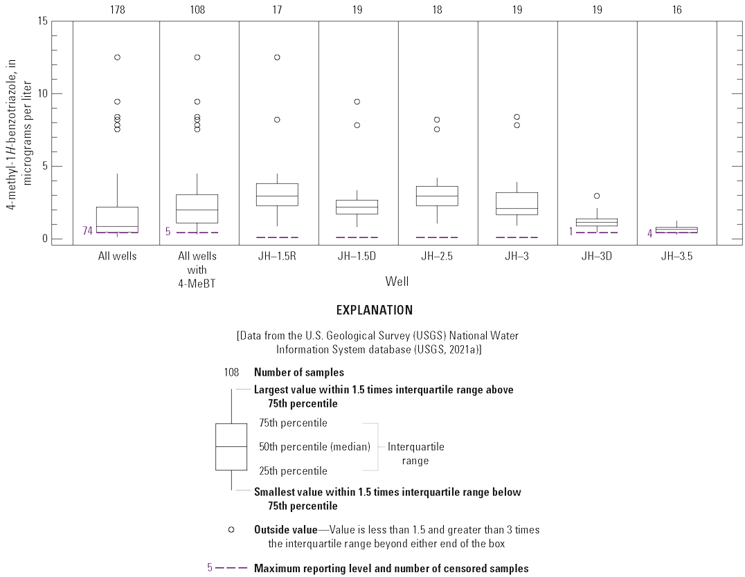
Statistical summary of 4-methyl-1H-benzotriazole (4-MeBT) concentrations in groundwater samples collected from monitor wells at the Jackson Hole Airport, Jackson, Wyoming, 2011–20.
Based on samples from monitor well clusters 1.5 and 3, benzotriazole concentrations generally decreased with depth during 2011–20. At well cluster 1.5, 4-MeBT concentrations in the deeper well (JH–1.5D) were lower than in the shallower well (JH–1.5 [2011] and JH–1.5R [2012–20]) for 15 of 19 (about 79 percent) sampling events (table 7). Concentrations of 4-MeBT in the deeper well at well cluster 3 (JH–3D) were lower than in the shallower well (JH–3) for all 19 sampling events (table 7).
Benzotriazoles were detected only in wells that experienced anoxic/reducing (including suboxic and mixed) conditions for at least some period during 2011–20 (table 6; also refer to the “Redox Conditions” section). Using data collected from all six wells with benzotriazole detections during 2011–20, 4-MeBT concentrations were negatively correlated with DO concentrations (Kendall’s τ= −0.467, p-value<0.001; fig. 16A). When the sample data were subdivided by wells, 4-MeBT concentrations in 4 of 6 wells (JH–1.5R, JH–1.5D, JH–2.5, and JH–3D) were negatively correlated (p-values<0.05) with DO concentrations (Kendall’s τ= −0.36 to −0.66; appendix table 1.10).
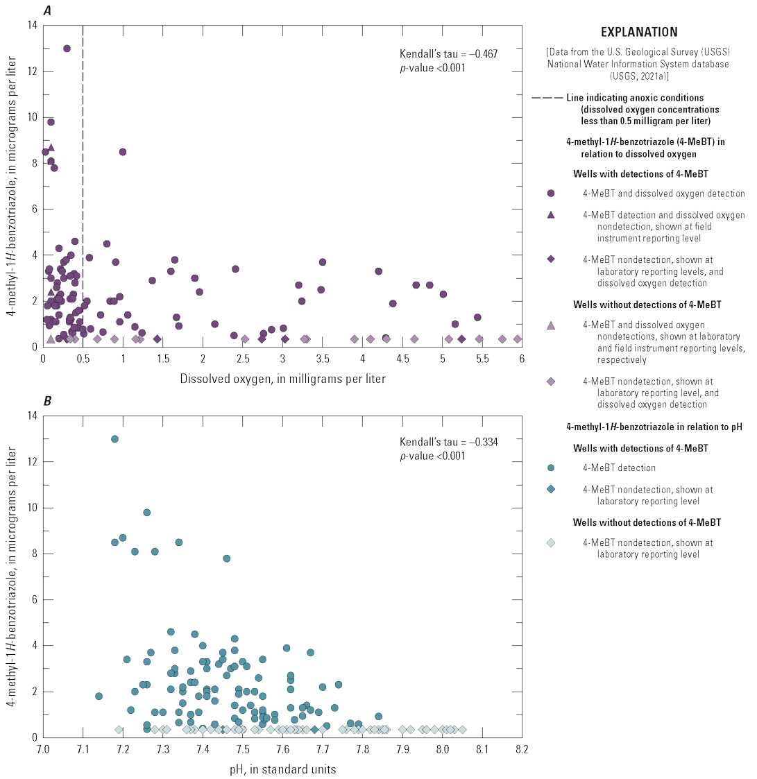
Relations between 4-methyl-1H-benzotriazole (4-MeBT) concentrations and A, dissolved-oxygen concentrations, and B, pH values in groundwater samples collected from monitor wells at the Jackson Hole Airport, Jackson, Wyoming, 2011–20.
Concentrations of 4-MeBT were evaluated in relation to pH values. Using data collected from all six wells with benzotriazole detections during 2011–20, 4-MeBT concentrations were negatively correlated with pH values (Kendall’s τ= −0.334, p-value<0.001; fig. 16B). When the sample data were subdivided by wells, 4-MeBT concentrations in 4 of 6 wells (JH–1.5D, JH–2.5, JH–3, and JH–3D) were negatively correlated (p-values<0.05) with pH values (Kendall’s τ= −0.35 to −0.42; appendix table 1.10).
Trends in 4-MeBT concentrations for the six wells with benzotriazole detections during 2011–20 were evaluated with the seasonal Kendall test (refer to the “Statistical Analysis” section). Results of seasonal Kendall tests (including p-values, Kendall’s τ values, and Theil-Sen and Akritas-Theil-Sen slopes) are tabulated in appendix table 1.9. Trends in 4-MeBT concentrations for 2011–20, including results of seasonal Kendall tests, are shown in a series of graphs for individual wells in figure 17 and spatially for all wells in figure 7. The results of the seasonal Kendall tests indicated downward trends in 4-MeBT concentrations at 4 wells (JH–1.5D, JH–2.5, JH–3, and JH–3D), a probable downward trend at 1 well (JH–1.5R), and no trend at 1 well (JH–3.5; figs. 7, 17; appendix table 1.9). No benzotriazoles were detected in well JH–3.5 in 2020. The downward and probable downward trends in 4-MeBT concentrations at wells JH–1.5D, JH–2.5, JH–3, and JH–3D (and nondetections of 5-MeBT after 2017; fig. 17; table 7) corresponded with numerous other trends indicating water quality was returning to conditions similar to background water-quality conditions in these wells during 2011–20, including upward trends for DO and pH, and downward trends for specific conductance, dissolved iron, and dissolved manganese (refer to the “Physical Properties” and “Dissolved Iron and Dissolved Manganese” sections; appendix table 1.9).
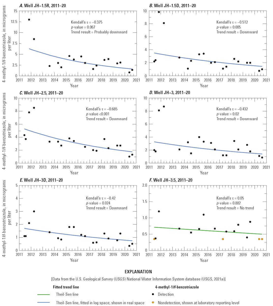
Trends in 4-methyl-1H-benzotriazole (4-MeBT) concentrations in monitor wells at the Jackson Hole Airport, Jackson, Wyoming, 2011–20. A, Well JH–1.5R. B, Well JH–1.5D. C, Well JH–2.5. D, Well JH–3. E, Well JH–3D. F, Well JH–3.5.
Summary
The Snake River alluvial aquifer underlying the Jackson Hole Airport (JHA) in northwest Wyoming is an important source of water used for domestic, commercial, and irrigation purposes by the airport and nearby residents. Two previous U.S. Geological Survey (USGS) studies of water quality at the JHA, done in cooperation with the Jackson Hole Airport Board, identified highly reduced (oxygen depleted) groundwater conditions, dissolved iron and manganese at concentrations greater than U.S. Environmental Protection Agency (EPA) Secondary Drinking Water Regulations (SDWRs), and anthropogenic (human-made) compounds known as benzotriazoles (components of aircraft deicing/anti-icing fluids [ADAFs]) in the alluvial aquifer downgradient from airport operations. Because of these water-quality concerns, a followup study was done to monitor and evaluate changes in hydrogeologic characteristics and groundwater-quality conditions of the alluvial aquifer during 2012–20, a period several years after the airport began changing deicer use and management practices and during which the airport made numerous infrastructure improvements that potentially improved water quality at the JHA. A secondary goal of the study was to establish a baseline characterization of local hydrogeologic and water-quality characteristics at a new monitor well (JH–DI1) installed downgradient from a new aircraft deicing pad and deicer recapture system and to monitor for potential changes in groundwater quality before and after use of the system.
Groundwater-level measurements were collected from 19 wells, and groundwater-quality samples were collected and analyzed from a subset of 10 of these wells. Data collected throughout this study, including groundwater levels; field measurements of physical properties of water, major ions, nutrients, anthropogenic compounds; and miscellaneous field and laboratory analytical results, are presented in this report. The direction of groundwater flow, hydraulic gradients, and estimated groundwater velocity rates of the Snake River alluvial aquifer underlying the JHA are presented in this report. Redox conditions and processes for sampled wells are described. Dissolved iron, dissolved manganese, and benzotriazole concentrations in JHA groundwater are summarized and examined in relation to geochemical conditions. Statistical analyses were used to summarize water-quality data, evaluate relations between water-quality properties and constituents, and test for trends in selected water-quality properties and constituent concentrations with time.
Groundwater levels measured during August 2012–August 2020 indicated that although there were annual variations in water-table elevation and timing of elevation changes, the primary aquifer characteristics (groundwater-flow direction, hydraulic gradients, and groundwater velocities) changed little in comparison to the two previous studies. The alluvial aquifer water table varied seasonally in response to precipitation-driven recharge (primarily mountain snowmelt) during April–June and irrigation-induced recharge during June–October, with minimal aquifer recharge during November–March. Although the timing of the lowest and highest water-table altitudes varied from year to year, the water table typically was at its lowest level in mid-March to early April, at the beginning of spring, and at its highest level in July, at the end of the peak of snowmelt. During August 2012–August 2020, the smallest water-level change within a single year was 7.51 feet and the largest change was 13.51 feet within individual wells. Constructed water-table contour maps show that the water table in 2019 was consistently highest in the northeast part of the airport and lowest in the southwest, indicating groundwater flow generally was from the northeast to the southwest. On average, the water table decreased about 22 feet across the airport with an average horizontal hydraulic gradient of 0.007 foot per foot (ft/ft), which is the same average as the previous study. Calculated hydraulic gradients across the airport continued to be relatively uniform, despite regular pumping of production wells in the study area. The average vertical hydraulic gradient was 0.009 ft/ft, which is slightly larger than the average of 0.005 ft/ft determined in the previous study. The horizontal groundwater velocity in the alluvial aquifer was estimated to be 26 to 76 feet per day, which is similar to the previous study. The travel time from the farthest upgradient well to the farthest downgradient well (a distance of about 3,540 feet) was approximately 47 to 136 days. This estimate of groundwater velocity only describes the movement of water through the aquifer because soluble contaminants may move at a rate slower than groundwater flowing through the aquifer.
Water in the Snake River alluvial aquifer sampled during 2011–20 was determined to be of good quality, with a few exceptions. No inorganic constituents (major ions, nutrients, and trace elements) were detected at concentrations greater than EPA health-based standards such as maximum contaminant levels (MCLs) or health advisory levels. Redox conditions in as many as seven wells were anoxic/reducing, although conditions in most of these wells became less reduced and more oxic with time. Dissolved iron and dissolved manganese were detected at concentrations exceeding EPA SDWRs in as many as 7 of 10 sampled wells. Several anthropogenic compounds (volatile organic compounds, gasoline-range organics, and glycols) were detected infrequently at low concentrations. Detection of the volatile organic compounds and gasoline-range organics likely was due to contamination introduced during sampling or laboratory analysis or due to other laboratory-related issues. Available information was insufficient to conclusively determine the presence or absence of glycols in the alluvial aquifer. The benzotriazoles 4-methyl-1H-benzotriazole (4-MeBT) and 5-methyl-1H-benzotriazole (5-MeBT) were detected at low concentrations in 7 of 10 sampled wells. Because infrequent detections in 1 of these wells were considered suspect, only 6 wells were considered to have benzotriazole detections for data summary and analysis purposes.
Dissolved-oxygen (DO) concentrations and redox-sensitive constituents were used to assess the redox status (oxic, suboxic, anoxic, or mixed) of groundwater sampled from wells. DO concentrations in the 6 wells with detections of 4-MeBT were significantly lower than in the 4 wells without detections (statistical probability level [p-value] less than [<] 0.001). Wells with detections of 4-MeBT also had significantly lower median pH values, higher median specific-conductance values, and higher dissolved iron and manganese concentrations than wells without detections (p-values<0.05, rank-sum and Peto-Peto tests). DO concentrations in 3 of 4 wells without detections of 4-MeBT were consistently oxic (DO>0.5 milligrams per liter) during 2011–20. The fourth well without benzotriazole detections (JH–4) was oxic during 2011–16, but became suboxic, mixed (oxic-anoxic and anoxic), and finally anoxic by the end of the study. Oxygen, nitrate, and manganese reduction were the redox processes identified in well JH–4 during 2018–20. All six wells with benzotriazole detections had anoxic/reducing (including suboxic and mixed) conditions for at least some period during 2011–20. Iron and manganese reduction were the predominant redox processes identified in most anoxic water samples from wells with benzotriazole detections. Although variable spatially and with time, identified general redox classes and processes indicate that groundwater in wells with anoxic/reducing conditions at the beginning of the study became less reducing and more oxic with time.
Dissolved iron and manganese were detected in at least 1 sample collected from all 10 monitor wells during 2011–20, including 52 percent of samples analyzed for iron and 64 percent of samples analyzed for manganese. Concentrations ranged from <3.2 (lowest reporting level) to 1,052 micrograms per liter (µg/L; median=5.72 µg/L) for dissolved iron and from <0.15 (lowest reporting level) to 1,730 µg/L (median=1 µg/L) for dissolved manganese. Dissolved iron and manganese concentrations in the 6 wells with detections of 4-MeBT were significantly higher (p-values<0.001, Peto-Peto test) than in the 4 wells without detections. For both constituents, detection frequencies and concentrations increased when DO concentrations decreased and groundwater conditions became increasingly reduced and anoxic, and decreased when DO concentrations increased and conditions became less reduced or oxic.
The EPA SDWR of 300 µg/L for iron was exceeded in about 11 percent of samples, and the EPA SDWR of 50 µg/L for manganese was exceeded in 39 percent of samples. Concentrations of dissolved iron greater than the EPA SDWR were identified only when groundwater conditions near a well were anoxic and 4-MeBT was detected in the sample. Dissolved manganese was detected in more wells at concentrations above its respective EPA SDWR (7 wells) than dissolved iron (4 wells). Concentrations of dissolved manganese greater than the EPA SDWR were identified when groundwater conditions near a well were anoxic, suboxic, or mixed and mostly when 4-MeBT was detected in the sample (exceptions were four samples with anoxic or mixed conditions collected during 2018–20 from well JH–4, which never had a detection of 4-MeBT). High dissolved iron concentrations typically indicated the presence of high dissolved manganese concentrations, but the converse did not occur as often. This observation is consistent with typical redox sequence progression after oxygen and nitrate have been reduced, in which manganese is reduced before iron.
Only two of the three benzotriazole compounds measured (4-MeBT and 5-MeBT) were detected in sampled wells. Both compounds were consistently detected in 6 of 10 sampled wells. Concentrations of 4-MeBT ranged from less than the limit of detection (LOD; 0.35 µg/L) to 13 µg/L, with many detections an order of magnitude greater than the LOD. Concentrations of 5-MeBT ranged from less than the LOD (range=<0.25 to <1.4 µg/L) to 2.6 µg/L. The benzotriazole 4-MeBT was detected more frequently and consistently at higher concentrations than 5-MeBT, and 5-MeBT was not detected in any well after 2017. This pattern of more frequent 4-MeBT detections and 4-MeBT concentrations higher than 5-MeBT concentrations is consistent with other benzotriazole research, which determined 5-MeBT is more biodegradable than 4-MeBT. Benzotriazoles were detected only in wells with anoxic/reducing (including suboxic and mixed) conditions for at least some period during 2011–20. Using data collected from all six wells with benzotriazole detections during 2011–20, 4-MeBT concentrations were negatively correlated (a relation where one variable increases as the other decreases, and vice versa) with DO concentrations (p-value<0.001) and pH values (p-value<0.001). When the sample data were subdivided by wells, 4-MeBT concentrations in 4 of 6 wells were negatively correlated (p-value<0.05) with DO concentration and pH values.
All wells with benzotriazole detections were downgradient from airport operations, including the airport terminal where most plane deicing was done before construction of the deicing pad in 2011. Reducing conditions present in an otherwise oxic aquifer indicate an upgradient or natural, in-place source of organic carbon or oxidizable minerals. No substantial sources of organic carbon were found in the alluvial aquifer during 2011–20. Dissolved organic carbon concentrations in the alluvial aquifer were low, including in wells with benzotriazole detections, and other potential sources of organic carbon such as anthropogenic organic compounds (for example, volatile organic compounds, gasoline-range organics, diesel-range organics, and glycols) were rarely detected. Consequently, the absence of substantial sources of organic carbon and the consistent detection of benzotriazoles in wells downgradient from airport operations during 2011–20 strengthens the conclusion of the previous study that microbial oxidation of ADAFs likely produced anoxic conditions that lead to reductive dissolution of naturally occurring iron and manganese from aquifer sediments. Statistically significant positive correlations (a relation where two variables tend to move in the same direction) between dissolved iron and manganese concentrations indicate aquifer sediment mineralogy, in combination with reducing conditions induced by microbial degradation of ADAFs, may have largely controlled concentrations of both trace elements in parts of the alluvial aquifer at the JHA during 2011–20. However, microbial oxidation of ADAFs was not likely the cause of suboxic, mixed, and anoxic conditions and resultant high manganese concentrations in well JH–4 during 2018–20 because no benzotriazole compounds (or any other anthropogenic compounds) were detected in the well.
Statistical tests indicated downward and probable downward trends in dissolved iron and manganese concentrations at many wells during 2011–20. The results of the seasonal Kendall tests for the 6 wells with benzotriazole detections indicated downward trends in iron concentrations at 3 wells, probable downward trends at 2 wells, and no trend at 1 well. No trends in dissolved iron concentrations were determined at the four wells without benzotriazole detections. The results of the seasonal Kendall tests for the 6 wells with benzotriazole detections indicated downward trends in dissolved manganese concentrations at 5 wells and a probable downward trend at 1 well. No trends in dissolved manganese concentrations were determined at 3 of 4 wells without benzotriazole detections, but an upward trend was determined at 1 well (JH–4). The upward trend in dissolved manganese concentrations at well JH–4 corresponded with downward trends in DO and pH, and an upward trend in specific conductance. The downward and probable downward trends in dissolved iron and manganese concentrations at individual wells with benzotriazole detections mostly corresponded with upward and probable upward trends in DO concentrations and pH values, and downward and probable downward trends in specific-conductance values and 4-MeBT concentrations (and nondetections of 5-MeBT by 2018 for the same wells). Out of the six wells with detections of benzotriazoles, all of which had one or more detections of dissolved iron or manganese at concentrations greater than respective EPA SDWRs during 2011–20, only one well had detections of either constituent at concentrations greater than these standards by 2020. Dissolved manganese concentrations in this well were above the EPA SDWR of 50 µg/L in 2020, but substantially lower than the highest concentration measured during 2011–20. Of the remaining five wells with benzotriazole detections during 2011–20, dissolved iron and manganese typically were detected at low concentrations or were no longer detected above laboratory reporting levels by 2020; all but one of these wells had downward trends in 4-MeBT concentrations.
The results of seasonal Kendall tests indicated downward trends in 4-MeBT concentrations at 4 wells, a probable downward trend at 1 well, and no trend at 1 well. No benzotriazoles were detected in 2020 in one well with previous detections. The downward and probable downward trends in 4-MeBT concentrations at four wells (and nondetections of 5-MeBT after 2017) corresponded with numerous other trends, including upward trends for DO and pH, and downward trends for specific conductance. Collectively, these trends indicated groundwater-quality conditions near all wells with benzotriazole detections were returning to water-quality conditions similar to background water-quality conditions measured in the alluvial aquifer upgradient from airport operations. Presumably, these trends are in response to the changes in the ADAF formulation used by the JHA, many JHA infrastructure improvements made during 2011–20, degradation of existing ADAFs in subsurface soils and groundwater, or some combination of these possibilities.
References Cited
Ayotte, J.D., Gronberg, J.M., and Apodaca, L.E., 2011, Trace elements and radon in groundwater across the United States, 1992–2003: U.S. Geological Survey Scientific Investigations Report 2011–5059, 115 p., accessed March 21, 2022, at https://doi.org/10.3133/sir20115059.
Beljin, M., Ross, R., and Acree, S., 2014, 3PE— A tool for estimating groundwater flow vectors: Washington, D.C., U.S. Environmental Protection Agency, EPA 600/R-14/273, 60 p. [Also available at https://cfpub.epa.gov/si/si_public_record_report.cfm?Lab=NRMRL&direntryid=287064.]
Breedveld, G.D., Roseth, R., Sparrevik, M., Hartnik, T., and Hem, L.J., 2003, Persistence of the de-icing additive benzotriazole at an abandoned airport: Water Air and Soil Pollution Focus, v. 3, p. 91–101, accessed March 19, 2024, at https://doi.org/10.1023/A:1023961213839.
Brenton, R.W., and Arnett, T.L., 1993, Methods of analysis by the U.S. Geological Survey National Water Quality Laboratory—Determination of dissolved organic carbon by UV-promoted persulfate oxidation and infrared spectrometry: U.S. Geological Survey Open-File Report 92–480, 12 p. [Also available at https://doi.org/10.3133/ofr92480.]
Cancilla, D.A., Baird, J.C., and Rosa, R., 2003a, Detection of aircraft deicing additives in groundwater and soil samples from Fairchild Air Force Base, a small to moderate user of deicing fluids: Bulletin of Environmental Contamination and Toxicology, v. 70, p. 868–875. [Also available at https://doi.org/10.1007/s00128-003-0063-8.]
Cancilla, D.A., Baird, J.C., Geis, S.W., and Corsi, S.R., 2003b, Studies of the environmental fate and effect of aircraft deicing fluids—Detection of 5-methyl-1H-benzotriazole in the fathead minnow (Pimephales promelas): Environmental Toxicology and Chemistry, v. 22, no. 1, p. 134–140. [Also available at https://doi.org/10.1002/etc.5620220117.]
Cancilla, D.A., Holtkamp, A., Matassa, L., and Fang, X., 1997, Isolation and characterization of Microtox-active components from aircraft de-icing/anti-icing fluids: Environmental Toxicology and Chemistry, v. 16, no. 3, p. 430–434. [Also available at https://doi.org/10.1002/etc.5620160306.]
Cancilla, D.A., Martinez, J., and Van Aggelen, G.C., 1998, Detection of aircraft deicing/antiicing fluid additives in a perched water monitoring well at an international airport: Environmental Science & Technology, v. 32, no. 23, p. 3834–3835. [Also available at https://doi.org/10.1021/es980489k.]
Chapelle, F.H., Bradley, P.M., Thomas, M.A., and McMahon, P.B., 2009, Distinguishing iron-reducing from sulfate-reducing conditions: Ground Water, v. 47, no. 2, p. 300–305. [Also available at https://doi.org/10.1111/j.1745-6584.2008.00536.x.]
Chapman, S.S., Bryce, S.A., Omernik, J.M., Despain, D.G., ZumBerge, J.R., and Conrad, M., 2004, Ecoregions of Wyoming (color poster with map, descriptive text, summary tables, and photographs): Reston, Va., U.S. Geological Survey, scale 1:1,400,000. [Also available at http://www.ecologicalregions.info/htm/wy_eco.htm.]
Cornell, J.S., Pillard, D.A., and Hernandez, M.T., 2000, Comparative measures of the toxicity of component chemicals in aircraft deicing fluid: Environmental Toxicology and Chemistry, v. 19, no. 6, p. 1465–1472. [Also available at https://doi.org/10.1002/etc.5620190601.]
Corsi, S.R., Geis, S.W., Loyo-Rosales, J.E., and Rice, C.P., 2006a, Aquatic toxicity of nine aircraft deicer and anti-icer formulations and relative toxicity of additive package ingredients alkylphenol ethoxylates and 4,5-methyl-1H-benzotriazoles: Environmental Science & Technology, v. 40, no. 23, p. 7409–7415. [Also available at https://doi.org/10.1021/es0603608.]
Corsi, S.R., Geis, S.W., Loyo-Rosales, J.E., Rice, C.P., Sheesley, R.J., Failey, G.G., and Cancilla, D.A., 2006b, Characterization of aircraft deicer and anti-icer components and toxicity in airport snowbanks and snowmelt runoff: Environmental Science & Technology, v. 40, no. 10, p. 3195–3202. [Also available at https://doi.org/10.1021/es052028m.]
Corsi, S.R., Hall, D.W., and Geis, S.W., 2001, Aircraft and runway deicers at General Mitchell International Airport, Milwaukee, Wisconsin, USA, 2. Toxicity of aircraft and runway deicers: Environmental Toxicology and Chemistry, v. 20, no. 7, p. 1483–1490. [Also available at https://doi.org/10.1002/etc.5620200710.]
Corsi, S.R., Mericas, D., and Bowman, G.T., 2012, Oxygen demand of aircraft and airfield pavement deicers and alternative freezing point depressants: Water, Air, & Soil Pollution, v. 223, p. 2447–2461. [Also available at https://doi.org/10.1007/s11270-011-1036-x.]
Cunningham, W.L., and Schalk, C.W., comps., 2011, Groundwater technical procedures of the U.S. Geological Survey: U.S. Geological Survey Techniques and Methods, book 1, chap. A1, 151 p. [Also available at https://doi.org/10.3133/tm1A1.]
DeSimone, L.A., McMahon, P.B., and Rosen, M.R., 2014, The quality of our Nation’s waters—Water quality in principal aquifers of the United States, 1991–2010: U.S. Geological Survey Circular 1360, 151 p. [Also available at https://doi.org/10.3133/cir1360.]
Dieter, C.A., Linsey, K.S., Caldwell, R.R., Harris, M.A., Ivahnenko, T.I., Lovelace, J.K., Maupin, M.A., and Barber, N.L., 2018, Estimated use of water in the United States county-level data for 2015 (ver. 2.0, June 2018): U.S. Geological Survey data release, accessed March 22, 2022, at https://doi.org/10.5066/F7TB15V5.
Dubrovsky, N.M., Burow, K.R., Clark, G.M., Gronberg, J.M., Hamilton, P.A., Hitt, K.J., Mueller, D.K., Munn, M.D., Nolan, B.T., Puckett, L.J., Rupert, M.G., Short, T.M., Spahr, N.E., Sprague, L.A., and Wilber, W.G., 2010, The quality of our Nation’s waters—Nutrients in the Nation’s streams and groundwater, 1992–2004: U.S. Geological Survey Circular 1350, 174 p. [Also available at https://doi.org/10.3133/cir1350.]
Eddy-Miller, C.A., Wheeler, J.D., and Essaid, H.I., 2009, Characterization of interactions between surface water and near-stream groundwater along Fish Creek, Teton County, Wyoming, by using heat as a tracer: U.S. Geological Survey Scientific Investigations Report 2009–5160, 53 p., accessed September 4, 2024, at https://doi.org/10.3133/sir20095160.
Fishman, M.J., ed., 1993, Methods of analysis by the U.S. Geological Survey National Water Quality Laboratory—Determination of inorganic and organic constituents in water and fluvial sediments: U.S. Geological Survey Open-File Report 93–125, 217 p. [Also available at https://doi.org/10.3133/ofr93125.]
Fishman, M.J., and Friedman, L.C., 1989, Methods for determination of inorganic substances in water and fluvial sediments (3d ed.): U.S. Geological Survey Techniques of Water-Resources Investigations, book 5, chap. A1, 545 p. [Also available at https://doi.org/10.3133/twri05A1.]
Friedman, L.C., and Erdmann, D.E., 1982, Quality assurance practices for the chemical and biological analyses of water and fluvial sediments: U.S. Geological Survey Techniques of Water-Resources Investigations, book 5, chap. A6, 181 p. [Also available at https://doi.org/10.3133/twri05A6.]
Garmin Ltd, 2004, eTrex® Legend C color map navigator owner’s manual: Garmin Ltd, accessed December 9, 2023, at https://static.garmincdn.com/pumac//eTrexLegendC_OwnersManual.pdf.
Hatch, C., 2007, Truck to suck deicer from airport tarmac: Jackson Hole News & Guide, December 20, 2007, accessed April 16, 2022, at https://www.jhnewsandguide.com/news/top_stories/truck-to-suck-deicer-from-airport-tarmac/article_923063ef-877c-5784-826b-32044bafc4b2.html.
Helsel, D.R., Hirsch, R.M., Ryberg, K.R., Archfield, S.A., and Gilroy, E.J., 2020, Statistical methods in water resources: U.S. Geological Survey Techniques and Methods, book 4, chap. A3, 458 p. [Also available at https://doi.org/10.3133/tm4a3.] [Supersedes USGS Techniques of Water-Resources Investigations, book 4, chap. A3, ver. 1.1.]
Hem, J.D., 1985, Study and interpretation of chemical characteristics of natural water (3d ed.): U.S. Geological Survey Water-Supply Paper 2254, 263 p. [Also available at https://doi.org/10.3133/wsp2254.]
In-Situ, Inc., 2013, Operator's manual Level Troll® 300, 500, 700, 700H instruments: In-Situ, Inc., 84 p., accessed March 5, 2025, at https://in-situ.com/pub/media/support/documents/Level-TROLL-300-Manual.pdf.
Interstate Technology & Regulatory Council, 2015, Integrated DNAPL site characterization and tools selection ISC-1: Washington, D.C., Interstate Technology & Regulatory Council, DNAPL Site Characterization Team, accessed April 30, 2023, at https://projects.itrcweb.org/DNAPL-ISC_tools-selection/Content/Resources/DNAPLPDF.pdf.
Jackson Hole Airport, 2020, Airport history: Jackson Hole Airport website, accessed June 26, 2020, at https://www.jacksonholeairport.com/about-jac/history/.
Julian, P., and Helsel, D.R., 2021, NADA2—Data analysis for censored environmental data (ver. 1.0.0): R package, accessed March 9, 2021, at https://cran.r-project.org/web/packages/NADA2/.
Jurgens, B.C., McMahon, P.B., Chapelle, F.H., and Eberts, S.M., 2009, An Excel® workbook for identifying redox processes in ground water: U.S. Geological Survey Open-File Report 2009–1004, 8 p., accessed October 27, 2021, at https://doi.org/10.3133/ofr20091004.]
Klecka, G.M., Carpenter, C.L., and Landenberger, B.D., 1993, Biodegradation of aircraft deicing fluids in soil at low temperatures: Ecotoxicology and Environmental Safety, v. 25, no. 3, p. 280–295. [Also available at https://doi.org/10.1006/eesa.1993.1026.]
Lapham, W.W., Wilde, F.D., and Koterba, M.T., 1995, Ground-water data collection protocols and procedures for the National Water-Quality Assessment Program—Selection, installation, and documentation of wells and collection of related data: U.S. Geological Survey Open-File Report 95–398, 69 p. [Also available at https://doi.org/10.3133/ofr95398.]
Lee, L., 2020, NADA—Nondetects and data analysis for environmental data (ver. 1.6-1.1): R package, accessed January 2021 at https://cran.r-project.org/web/packages/NADA/index.html.
Love, J.D., and Christiansen, A.C., 1985, Geologic map of Wyoming: U.S. Geological Survey Geologic Map, 3 sheets, scale 1:500,000. [Also available at https://doi.org/10.3133/70046739.]
Love, J.D., and Reed, J.C., Jr., 1971, Creation of the Teton landscape—The geologic story of Grand Teton National Park: Moose, Wyo., Grand Teton Natural History Association, 120 p., accessed December 10, 2022, at https://www.nps.gov/parkhistory/online_books/grte/grte_geology/sec1.htm.
Love, J.D., Reed, J.C., Jr., and Christiansen, A.C., 1992, Geologic map of Grand Teton National Park, Teton County, Wyoming: U.S. Geological Survey Miscellaneous Investigations Series Map I–2031, scale 1:62,500. [Also available at https://doi.org/10.3133/i2031.]
Marchetto, A., 2021, Package ‘rkt’—Mann-Kendall test, seasonal and regional Kendall tests: R package, ver. 1.6, accessed March 31, 2021, at https://cran.r-project.org/web/packages/rkt/rkt.pdf.
McMahon, P.B., Belitz, K., Reddy, J.E., and Johnson, T.D., 2019, Elevated manganese concentrations in United States groundwater, role of land surface-soil-aquifer connections: Environmental Science & Technology, v. 53, no. 1, p. 29–38. [Also available at https://doi.org/10.1021/acs.est.8b04055.]
McMahon, P.B., and Chapelle, F.H., 2008, Redox processes and water quality of selected principal aquifer systems: Groundwater, v. 46, no. 2, p. 259–271. [Also available at https://doi.org/10.1111/j.1745-6584.2007.00385.x.]
Mueller, D.K., Martin, J.D., and Lopes, T.J., 1997, Quality-control design for surface-water sampling in the National Water-Quality Assessment Program: U.S. Geological Survey Open-File Report 97–223, 17 p. [Also available at https://doi.org/10.3133/ofr97223.]
National Oceanic and Atmospheric Administration, 2023, 1991–2020 Climate normals for Moose, Wyoming: National Ocean and Atmospheric Administration web page, accessed February 9, 2023, at https://www.ncei.noaa.gov/access/us-climate-normals/#dataset=normals-annualseasonal&timeframe=30&location=MT&station=USW00094017.
Nolan, B.T., Campbell, D.L., and Senterfit, R.M., 1998, Depth of the base of the Jackson aquifer, based on geophysical exploration, southern Jackson Hole, Wyoming, USA: Hydrogeology Journal, v. 6, p. 374–382. [Also available at https://doi.org/10.1007/s100400050160.]
Nolan, B.T., and Miller, K.A., 1995, Water resources of Teton County, Wyoming, exclusive of Yellowstone National Park: U.S. Geological Survey Water-Resources Investigations Report 95–4204, 76 p. [Also available at https://doi.org/10.3133/wri954204.]
Olds, H.T., Corsi, S.R., and Rutter, T.D., 2021, Benzotriazole concentrations in airport runoff are reduced following changes in airport deicer formulations: Integrated Environmental Assessment and Management, v. 18, no. 1, p. 245–257. [Also available at https://doi.org/10.1002/ieam.4468.]
Pierce, K.L., and Good, J.D., 1992, Field guide to the Quaternary geology of Jackson Hole, Wyoming: U.S. Geological Survey Open-File Report 92–504, 54 p. [Also available at https://doi.org/10.3133/ofr92504.]
Pillard, D.A., 1995, Comparative toxicity of formulated glycol deicers and pure ethylene and propylene glycol to Ceriodaphnia dubia and Pimephales promelas: Environmental Toxicology and Chemistry, v. 14, no. 2, p. 311–315. [Also available at https://doi.org/10.1002/etc.5620140217.]
Pillard, D.A., Cornell, J.S., DuFresne, D.L., and Hernandez, M.T., 2001, Toxicity of benzotriazole and benzotriazole derivatives to three aquatic species: Water Research, v. 35, no. 2, p. 557–560. [Also available at https://doi.org/10.1016/S0043-1354(00)00268-2.]
Timme, P.J., 1995, National Water Quality Laboratory 1995 services catalog: U.S. Geological Survey Open-File-Report 95–352, 120 p. [Also available at https://doi.org/10.3133/ofr95352.]
U.S. Environmental Protection Agency [EPA], 1989, Data evaluation, chap. 5 of Risk assessment guidance for Superfund—Volume I, Human health evaluation manual (part A): Washington, D.C., Office of Emergency and Remedial Response, U.S. Environmental Protection Agency Report EPA/540/1–89/002, 30 p., accessed July 31, 2021, at https://www.epa.gov/sites/default/files/2015-09/documents/rags_a.pdf.
U.S. Environmental Protection Agency [EPA], 1996a, Test methods for evaluating solid waste, physical/chemical methods, SW-846, 3d ed., update IV—Method 8015B nonhalogenated organics using GC/FID, rev. 2: Washington, D.C., U.S. Environmental Protection Agency, [variously paged]. [Also available at archive.epa.gov/epawaste/hazard/testmethods/web/pdf/method%208015b,%20revision%202%20-%201996.pdf.]
U.S. Environmental Protection Agency [EPA], 1996b, Test methods for evaluating solid waste, physical/chemical methods, SW-846, 3d ed., update IV—Method 8021B aromatic and halogenated volatiles by gas chromatography using photoionization and/or electrolytic conductivity detectors, rev. 2: Washington, D.C., U.S. Environmental Protection Agency, [variously paged].
U.S. Environmental Protection Agency [EPA], 2018, 2018 Edition of the drinking water standards and health advisories: Washington, D.C., U.S. Environmental Protection Agency, Office of Water, EPA 822–F–18–001, March 2018, 12 p., accessed March 7, 2022, at https://www.epa.gov/system/files/documents/2022-01/dwtable2018.pdf.
U.S. Geological Survey [USGS], [variously dated], National field manual for the collection of water-quality data, section A of Handbooks for water-resources investigations: U.S. Geological Survey Techniques of Water-Resources Investigations, book 9, 10 chap. (A0–A8, A10). [Also available at https://doi.org/10.3133/twri09.]
U.S. Geological Survey [USGS], 2015, Changes to National Water Quality Laboratory (NWQL) procedures used to establish and verify laboratory detection and reporting limits: U.S. Geological Survey National Water Quality Laboratory Technical Memorandum 15.02, accessed April 5, 2021, at https://nwql.usgs.gov/tech_memos/nwql.2015-02.pdf.
U.S. Geological Survey [USGS], 2017a, Policy and procedures for processing and publishing discrete groundwater-level records: U.S. Geological Survey Office of Groundwater Technical Memorandum 2017.04, accessed December 12, 2020, at https://water.usgs.gov/admin/memo/GW/gw2017.04.pdf.
U.S. Geological Survey [USGS], 2017b, Procedures for processing, approving, publishing, and auditing time-series records for water data: U.S. Geological Survey Office of Groundwater Technical Memorandum 2017.03, accessed December 12, 2020, at https://water.usgs.gov/admin/memo/GW/gw2017.03.pdf.
U.S. Geological Survey [USGS], 2021a, USGS groundwater data for Wyoming, in USGS water data for the Nation: U.S. Geological Survey National Water Information System database, accessed May 15, 2021, at https://doi.org/10.5066/F7P55KJN. [Wyoming groundwater data are directly accessible at https://waterdata.usgs.gov/wy/nwis/gw/.]
U.S. Geological Survey [USGS], 2021b, USGS 13014500 Gros Ventre River at Kelly WY, in USGS water data for the Nation: U.S. Geological Survey National Water Information System database, accessed May 15, 2021, at https://doi.org/10.5066/F7P55KJN. [Site data are directly accessible at https://waterdata.usgs.gov/monitoring-location/13014500/#parameterCode=00065&period=P7D&showMedian=true.]
Weiss, S., and Reemtsma, T., 2005, Determination of benzotriazole corrosion inhibitors from aqueous environmental samples by liquid chromatography-electrospray ionization-tandem mass spectrometry: Analytical Chemistry, v. 77, no. 22, p. 7415–7420. [Also available at https://doi.org/10.1021/ac051203e.]
Wright, P.R., 2010, Hydrogeology and water quality in the Snake River alluvial aquifer at Jackson Hole Airport, Jackson, Wyoming, September 2008–June 2009: U.S. Geological Survey Scientific Investigations Report 2010–5172, 54 p. [Also available at https://doi.org/10.3133/sir20105172.]
Wright, P.R., 2013, Hydrogeology and water quality in the Snake River alluvial aquifer at Jackson Hole Airport, Jackson, Wyoming, water years 2011 and 2012: U.S. Geological Survey Scientific Investigation Report 2013–5184, 65 p. [Also available at https://doi.org/10.3133/sir20135184.]
Appendix 1. Supplemental Data Tables
References Cited
Helsel, D.R., Hirsch, R.M., Ryberg, K.R., Archfield, S.A., and Gilroy, E.J., 2020, Statistical methods in water resources: U.S. Geological Survey Techniques and Methods, book 4, chap. A3, 458 p. [Also available at https://doi.org/10.3133/tm4a3.] [Supersedes USGS Techniques of Water-Resources Investigations, book 4, chap. A3, ver. 1.1.]
U.S. Environmental Protection Agency [EPA], 2018, 2018 Edition of the drinking water standards and health advisories: Washington, D.C., U.S. Environmental Protection Agency, Office of Water, EPA 822–F–18–001, March 2018, 12 p., accessed March 7, 2022, at https://www.epa.gov/system/files/documents/2022-01/dwtable2018.pdf.
U.S. Geological Survey [USGS], 2015, Changes to National Water Quality Laboratory (NWQL) procedures used to establish and verify laboratory detection and reporting limits: U.S. Geological Survey National Water Quality Laboratory Technical Memorandum 15.02, accessed April 5, 2021, at https://nwql.usgs.gov/tech_memos/nwql.2015-02.pdf.
U.S. Geological Survey [USGS], 2021, USGS water data for the Nation: U.S. Geological Survey National Water Information System database, accessed May 15, 2021, at https://doi.org/10.5066/F7P55KJN.
Conversion Factors
U.S. customary units to International System of Units
Temperature in degrees Celsius (°C) may be converted to degrees Fahrenheit (°F) as follows: °F = (1.8 × °C) + 32.
Temperature in degrees Fahrenheit (°F) may be converted to degrees Celsius (°C) as follows: °C = (°F – 32) / 1.8.
Datum
Vertical coordinate information is referenced to the North American Vertical Datum of 1988 (NAVD 88).
Horizontal coordinate information is referenced to the North American Datum of 1983 (NAD 83).
Altitude, as used in this report, refers to distance above the vertical datum.
Supplemental Information
Specific conductance is given in microsiemens per centimeter at 25 degrees Celsius (µS/cm at 25 °C).
Concentrations of chemical constituents in water are given in either milligrams per liter (mg/L) or micrograms per liter (µg/L).
Abbreviations
<
less than
±
plus or minus
1H-BT
1H-benzotriazole
4-MeBT
4-methyl-1H-benzotriazole
5-MeBT
5-methyl-1H-benzotriazole
ADAF
aircraft deicing/anti-icing fluid
AL
action level
BTEX
benzene, toluene, ethylbenzene, and xylenes
C
carbon
CaCO3
calcium carbonate
CH4
methane
DLBLK
detection limit using blank data procedure
DLDQC
detection limit using DQCALC procedure in DQCALC software
DO
dissolved oxygen
DOC
dissolved organic carbon
DQCALC
a procedure in the DQCALC software package
DRO
diesel-range organics
DWA
drinking water advisory level
E
estimated value
EPA
U.S. Environmental Protection Agency
e-tape
electric tape
Fe2+
ferrous iron
GRO
gasoline-range organics
HAL
Lifetime Health Advisory Level
HS–
hydrogen sulfide
H2S
dihydrogen sulfide
JHA
Jackson Hole Airport
LOD
level of detection
LOQ
level of quantitation
LRL
laboratory reporting level
MCL
maximum contaminant level
MCLG
maximum contaminant level goal
MDL
method detection limit
Mn2+
manganous manganese
MRL
minimum reporting level
NADA
Non-Detects and Data Analysis for Environmental Data (statistical package for R)
NAD 83
North American Datum of 1983
NAVD 88
North American Vertical Datum of 1988
NFM
National Field Manual for the Collection of Water-Quality Data
NO3−
nitrate
NWQL
National Water Quality Laboratory
O2
oxygen
p-value
statistical probability level
PVC
polyvinyl chloride
QA
quality assurance
QC
quality control
R
programming language for statistical computing and graphics
RPD
relative percent difference
redox
reduction and oxidation processes
S2−
sulfide
SDWR
Secondary Drinking Water Regulation
SO42−
sulfate
τ
tau
USGS
U.S. Geological Survey
VOC
volatile organic compound
WSLH
Wisconsin State Laboratory of Hygiene
For more information about this publication, contact:
Director, USGS Wyoming-Montana Water Science Center
3162 Bozeman Avenue
Helena, MT 59601
406–457–5900
For additional information, visit: https://www.usgs.gov/centers/wy-mtwater/
Publishing support provided by the
Rolla Publishing Service Center
Disclaimers
Any use of trade, firm, or product names is for descriptive purposes only and does not imply endorsement by the U.S. Government.
Although this information product, for the most part, is in the public domain, it also may contain copyrighted materials as noted in the text. Permission to reproduce copyrighted items must be secured from the copyright owner.
Suggested Citation
Wright, P.R., and Bartos, T.T., 2025, Hydrogeology and groundwater quality in the Snake River alluvial aquifer at Jackson Hole Airport, Wyoming, 2011–20: U.S. Geological Survey Scientific Investigations Report 2025–5006, 80 p., https://doi.org/10.3133/sir20255006.
ISSN: 2328-0328 (online)
Study Area
| Publication type | Report |
|---|---|
| Publication Subtype | USGS Numbered Series |
| Title | Hydrogeology and groundwater quality in the Snake River alluvial aquifer at Jackson Hole Airport, Wyoming, 2011–20 |
| Series title | Scientific Investigations Report |
| Series number | 2025-5006 |
| DOI | 10.3133/sir20255006 |
| Publication Date | June 05, 2025 |
| Year Published | 2025 |
| Language | English |
| Publisher | U.S. Geological Survey |
| Publisher location | Reston, VA |
| Contributing office(s) | Wyoming-Montana Water Science Center |
| Description | Report: x, 80 p.; Appendix; Dataset |
| Country | United States |
| State | Wyoming |
| Other Geospatial | Jackson Hole Airport |
| Online Only (Y/N) | Y |
| Additional Online Files (Y/N) | Y |