

Hydrogeologic Mapping and Three-Dimensional Geologic Modeling of Glacial Deposits in a Multicounty Area of Southeastern Michigan, Northeastern Indiana, and Northwestern Ohio
Links
- Document: Report (13.4 MB pdf) , HTML , XML
- Data Release: USGS data release - Hydrogeologic framework of the glacial deposits in a multicounty area of southeastern Michigan, northeastern Indiana, and northwestern Ohio
- NGMDB Index Page: National Geologic Map Database Index Page (html)
- Download citation as: RIS | Dublin Core
Acknowledgments
Thanks are extended to the Michigan Department of Environmental Quality, the Indiana Department of Natural Resources, and the Ohio Department of Natural Resources for providing expertise and data used for this project. Barrett Hamilton, Robert Darner, Charles Hart, and Harvie Pollard of the U.S. Geological Survey provided assistance collecting groundwater-level data. Neal Mathes (Eidgenössische Technische Hochschule [ETH] Zürich) provided geographic information system support.
Abstract
The glacial deposits underlying southeastern Michigan, northeastern Indiana, and northwestern Ohio are a substantial source of water to communities, agriculture, and industry in the region. Previous efforts to characterize aquifer materials in the area cited a need for additional information about the underlying hydrogeologic characteristics and related groundwater availability as well as improved mapping of the extent and properties of the glacial deposits.
Recent U.S. Geological Survey multi-State compilations of water-well drilling records have greatly increased access to high-resolution geologic data, particularly in glacial depositional environments. This study by the U.S. Geological Survey, in cooperation with the Ohio Environmental Protection Agency, uses processed data from the State-managed collections of well records to characterize the glacial deposits in the study area using two methods. The first method creates two-dimensional maps of basic hydrogeologic information commonly required for assessments of groundwater availability, including (1) total thickness of glacial deposits, (2) total thickness of coarse-grained deposits, (3) specific-capacity-based transmissivity and hydraulic conductivity, and (4) texture-based estimated equivalent horizontal and vertical hydraulic conductivity and transmissivity. The second method builds a hydrogeologic framework of the complex glacial aquifer through construction of a volumetric geologic model by using three-dimensional kriging.
Results of the volumetric model indicate that aquifer materials are primarily concentrated in the western parts of the study area near the Indiana-Ohio border. Coarse-grained sediments are also present as surficial deposits in the north of the study area where intermixing glacial advances created complex distributions of unconsolidated deposits. Two-dimensional maps of hydrogeologic properties support the volumetric model, showing thicknesses of coarse-grained deposits that reach up to 250 feet in the western sections of the study area and progressively thin to near absence in the east. Visualization of the aquifer materials with a volumetric model generally shows a highly discontinuous distribution of coarse- and fine-grained materials, with no clearly defined boundaries to delineate the extent of the aquifer. Comparisons of cross sections derived from the volumetric model with existing published maps support previous near-surface hydrogeologic interpretations while filling gaps where data are sparse, particularly in deeper parts of the aquifer. Both the two-dimensional maps and the volumetric model provide data that can directly inform assessments of groundwater availability, in addition to having future applications to studies of groundwater flow and transport.
Introduction
Groundwater resources in southeastern Michigan, northeastern Indiana, and northwestern Ohio have been a recurring subject of interest as it relates to sources of public, irrigation, and industrial water supplies. The glacial deposits composing the aquifer are a substantial source of water to the communities in the area. Understanding of the long-term water budget of the glacial aquifer is critical because the aquifer is the only source of drinking water for some communities in the area.
Improved mapping of the thickness and extent of aquifer and nonaquifer materials in the glacial deposits is required to accurately assess the groundwater resources (John Esch, Great Lakes Geologic Mapping Coalition, written commun., 2011). There have been previous attempts to map and characterize the glacial deposits in the aquifer, most notably through the unapproved 2007 sole source aquifer petition to the U.S. Environmental Protection Agency (Tritium, Inc., 2007). Initiated by the City of Bryan, Ohio, the purpose of the petition for the “Michindoh Glacial Aquifer” was “protection and management of a vulnerable aquifer system that represents the sole source of drinking water within the designated area” (Tritium, Inc., 2007). Upon review of the petition, resource managers and stakeholders determined that the gaps in subsurface data and the methods used to define the boundaries of the glacial deposits led to an inadequate representation of the aquifer. Initial methods used in that study to delineate glacial deposits in the aquifer incorporated surface drainage basins, surface-water features, groundwater divides, and economic boundaries. Resource managers cited a need for improved technical information about the underlying hydrogeologic characteristics and related groundwater availability (U.S. Environmental Protection Agency, 2013; Great Lakes Geologic Mapping Coalition, 2014). Though the focus of this report was initially on the 11 counties that are intersected by or are immediately adjacent to the proposed sole source aquifer boundary (Allen, DeKalb, and Steuben Counties in Indiana; Branch, Hillsdale, and Lenawee Counties in Michigan; Defiance, Fulton, Henry, Paulding, and Williams Counties in Ohio), the study area was expanded to include surrounding counties (fig. 1) to ensure adequate representation of the aquifer.
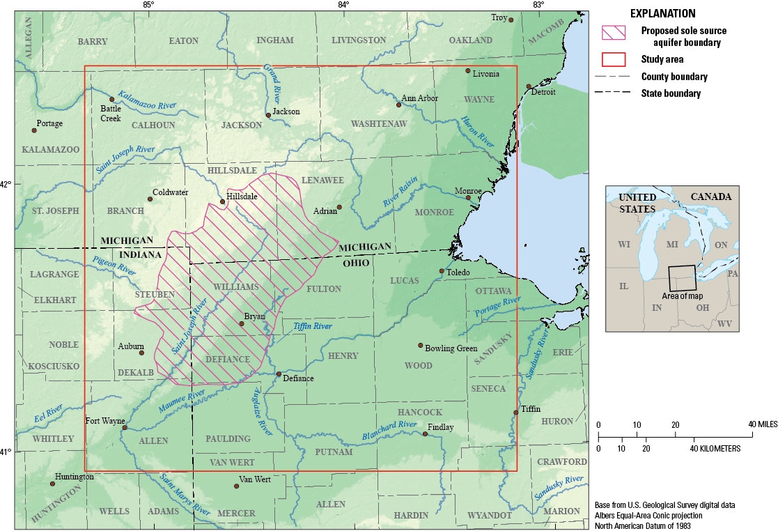
Map showing the study area and boundary of the proposed sole source aquifer of the glacial aquifer system underlying southeastern Michigan, northeastern Indiana, and northwestern Ohio.
In 2022, the U.S. Geological Survey, in cooperation with the Ohio Environmental Protection Agency, completed a study that used new techniques to characterize the glacial deposits that make up the aquifer. Multi-State compilations of well-drilling records provided lithologic data used to map the extent of the glacial deposits and identify data gaps where glacial deposits have not been characterized in existing water-well drilling records (Lampe, 2009; Bayless and others, 20173). These data were then used to create a volumetric geologic model of the distribution and hydrogeologic characteristics of the glacial aquifer.
Purpose and Scope
This report describes the sources of data and the methods used to develop a hydrogeologic framework of glacial deposits in the study area. Processed data from State-managed collections of well records were used in two methods of characterizing the deposits of the glacial aquifer. The first method created two-dimensional maps of hydrogeologic information commonly required for assessments of groundwater availability. The second method created a volumetric geologic model through the use of three-dimensional statistical methods. An analysis of groundwater levels and flow directions provides additional context for interpretation of the mapping products. This report is intended to provide an updated conceptual model for groundwater resources and a three-dimensional, data-derived hydrogeologic framework model for use as a tool to visualize the spatial distribution of glacial deposits in the study area, with a particular focus on the coarse-grained aquifer materials. The hydrogeologic framework represents overall regional features and is not intended to be a substitute for site-specific studies. Insights gained from this updated hydrogeologic framework can inform water-resource management in the study area and guide development of future groundwater-flow models. The three-dimensional hydrogeologic framework data are available in a companion data release to this report (Riddle, 2025).
Previous Investigations
A process of analyzing well records to provide spatially distributed grids of hydrogeologic parameters was originally developed by Arihood (2009) and used to produce statewide maps of horizontal and vertical conductivity in the Lake Michigan Basin. The methodology was applied widely by Bayless and others (2017), who assessed approximately 14 million wells from State-managed collections of water-well drillers’ records to create a database of hydrogeologic properties for the entire glaciated United States.
At a regional scale, Lampe (2009) and Arihood (2009) created a digital geologic framework of bedrock units and unconsolidated deposits for a groundwater-flow model of the Lake Michigan Basin; the glacial aquifer characterized in this study is partly represented in Arihood (2009). Groundwater-flow models of Elkhart County, Indiana, near the study area show a similar geology and indicate that rendering of the glacial geology precisely is critical when delineating capture zones of wells within groundwater-flow models (Arihood and others, 2019).
Coen (1989) conducted a comprehensive assessment of groundwater resources in Williams County, Ohio. Groundwater availability, flow, and quality were appraised through examination of well-drillers’ logs, by measurements of water levels in a network of wells, and by sampling selected wells and streams for water quality analysis. The study noted the incomplete characterization of the bedrock surface due to the limited number of wells that penetrate the bedrock in parts of the county.
In Indiana, Fenelon and others (1994) identified aquifers and constructed potentiometric maps throughout the State through generation of 3,500 miles of section lines in 104 cross sections. Cross sections were generated from water-well records, oil- and gas-well completion reports, and observation-well records. In northeastern Indiana, extensive surficial and buried sand and gravel aquifers were identified in the four cross sections that intersected the study area.
Arihood and others (2019) used well-record processing to determine the effects of increased geologic detail in hydrostratigraphic frameworks on groundwater-flow models. Results from two groundwater-flow models were compared: one constructed by the more traditional approach of manually selecting a limited number of representative well logs to build a groundwater-flow model framework, and one constructed by a semiautomated, geostatistical approach using all available lithologic data to develop a more heterogeneous framework. The geostatistical approach resulted in a small improvement in calibration statistics relative to the manual approach. This was partly attributed to the increased detail in how the geostatistical approach represented the distribution of fine- and coarse-grained deposits.
Hydrogeologic Setting
Though the focus of this study was primarily on the unconsolidated deposits, an understanding of the bedrock formations in the study area was required. Bedrock defines the lower confining boundary of the volumetric model and, where unconsolidated deposits are thin, bedrock aquifers are an important source of groundwater.
Bedrock Aquifers
Bedrock underlying glacial deposits is predominantly shale lithology in the study area and is generally low permeability (fig. 2). Sediments that formed bedrock geologic units in the 11-county region were deposited in the Michigan Basin from the Silurian Period (444 to 423 million years before present [Ma]) to the Mississippian Subperiod (360 to 325 Ma). The older, Silurian-aged geologic units are at the bedrock surface in the southern part of the study area, and the younger, Mississippian-aged geologic units are at the bedrock surface in the northern part of the study area (fig. 2), closer to the center of the Michigan Basin (not shown). Statewide bedrock aquifer maps were previously compiled in Ohio with expected aquifer pumping yields assigned to bedrock aquifers that correspond with individual bedrock geologic units (Ohio Department of Natural Resources, 2001). These estimated yields can be extrapolated to correlative geologic units in Indiana and Michigan.
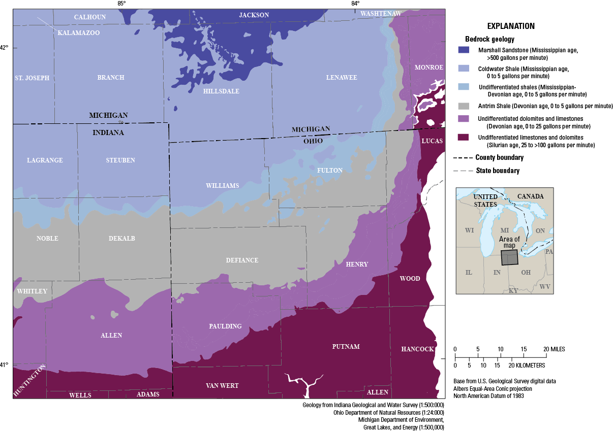
Map showing bedrock geologic units and corresponding groundwater availability (expressed as expected pumping yields in gallons per minute) in southeastern Michigan, northeastern Indiana, and northwestern Ohio. Expected pumping yields for the Marshall Sandstone are based on Grannemann and Twenter (1985), and well yields for other rock units are based on Ohio Department of Natural Resources aquifer maps (Ohio Department of Natural Resources, 2001).
The Coldwater Shale of Mississippian age is exposed in southern Michigan (Milstein, 1987), the northeastern tip of Indiana (Gray and others, 1987), and the northwestern tip of Ohio (Slucher and others, 2006). Multiple geologic units with predominantly shale lithologies are also mapped to the south and east of the Coldwater Shale in the study area, such as the Ellsworth Shale in Indiana (Gray and others, 1987) and the Bedford Shale in Michigan (Milstein, 1987). These geologic units of Devonian age (419 to 372 Ma) correspond with bedrock aquifers in Ohio of Mississippian age that produce 0 to 5 gallons per minute (gal/min), and the older Antrim Shale of Devonian age that is mapped in all three States to the south also produces minimal amounts of water (Ohio Department of Natural Resources, 2001). Higher potential pumping yields (10–100 gal/min) in the southwestern part of the study area are observed in Allen County, Indiana (Fleming and others, 1994), for wells pumping near the Antrim Shale, but much of the groundwater storage for wells used in these estimates is likely from overlying glacial aquifers. Fleming and others (1994) also note that groundwater from wells associated with the Antrim Shale is commonly high in hydrogen sulfide.
Limestone (calcium carbonate) and dolomite (calcium-magnesium carbonate) rocks are collectively referred to as “carbonates,” and their associated aquifers in the tri-State area have much higher potential well yields than shale lithologies in Ohio (Ohio Department of Natural Resources, 2001) and Indiana (Fleming and others, 1994). In Ohio, carbonate aquifers are primarily used as groundwater sources in Paulding, Defiance, and Henry Counties and have potential pumping yields in the 0–100 gal/min range (Ohio Department of Natural Resources, 2001). In Indiana, carbonate bedrock wells are reported to produce between 75 and 1,000 gal/min, but localized areas near the Indiana-Ohio State line have limited groundwater availability (Fleming and others, 1994). The highest pumping potentials are in western Allen County, Indiana, where relatively high relief on the buried bedrock surface is inferred to have promoted more preglacial karst development in the area and therefore more extensive bedrock conduit networks (Fleming and others, 1994). The thickness of overlying glacial sequences also is greater to the west, suggesting that groundwater storage in overlying glacial sequences contributes to these higher pumping estimates for carbonate aquifers in western Allen County, Indiana.
The Marshall Sandstone is primarily exposed in Hillsdale County, Michigan (fig. 2), and two distinct lithologies make up the formation: a lower member that consists of fine-grained sandstone that is present in the central parts of the county and an upper member composed of fine- to coarse-grained sandstone that is isolated to northern Hillsdale County (Monnett, 1948). The hydraulic characteristics of the Marshall Sandstone are described by Grannemann and Twenter (1985) and Lynch and Grannemann (1997) for a site in Calhoun County, Michigan, to the northwest and are based on pumping data from wells that intercept both the lower and upper members of the Marshall Sandstone. The Marshall Sandstone wells in Calhoun County are capable of producing 300 to 1,000 gal/min, but groundwater model simulations indicate that pumping in excess of 3,000 gal/min can produce significant aquifer drawdown (Grannemann and Twenter, 1985). Groundwater recharge is estimated at 30 percent of annual precipitation, and this estimate, coupled with the occurrence of organic chemicals in the aquifer at Battle Creek, Michigan (Lynch and Grannemann, 1997), suggests that aquifer susceptibility to contamination is a concern for the Marshall Sandstone aquifer.
Glacial Aquifers
Groundwater availability in the original 11-county study area coincides closely with the composition of glacial deposits that overly bedrock. Aquifers associated with unconsolidated deposits in glaciated terrains are commonly referred to as “glacial aquifers,” although the water-bearing units can consist of glaciofluvial (associated with glacial meltwater), glaciolacustrine (associated with glacial lakes), and postglacial valley-fill deposits in addition to glacial deposits originating from subglacial environments. Glacial deposits exposed at the land surface in the tri-State region are predominantly associated with the Huron-Erie ice lobe that entered the area during the Last Glacial Maximum and ancestral phases of Lake Erie (Fisher and others, 2015). These deposits are generally grouped by sequences based on landforms such as the arcuate moraine landforms that mark multiple positions of the Huron-Erie ice lobe (figs. 3 and 4).
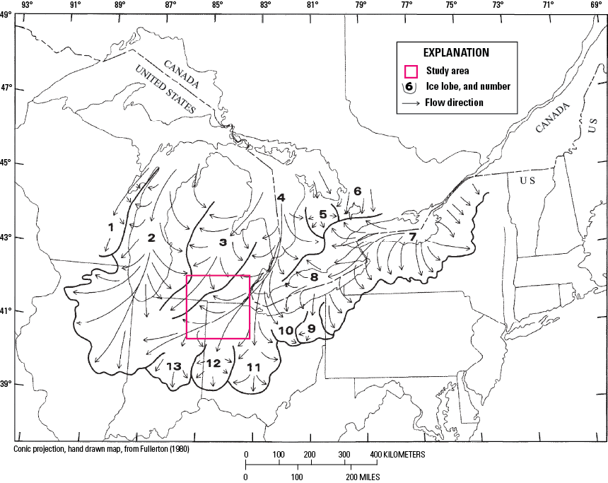
Map showing ice flow patterns in the central and eastern Great Lakes region from Fullerton (1980). The Saginaw ice lobe (3) and Huron-Erie ice lobe (4 and 8) positions shown are from the Last Glacial Maximum, when the continental glacier was near its southernmost extent. The interlobate region is indicated by converging arrows that represent ice flow paths.
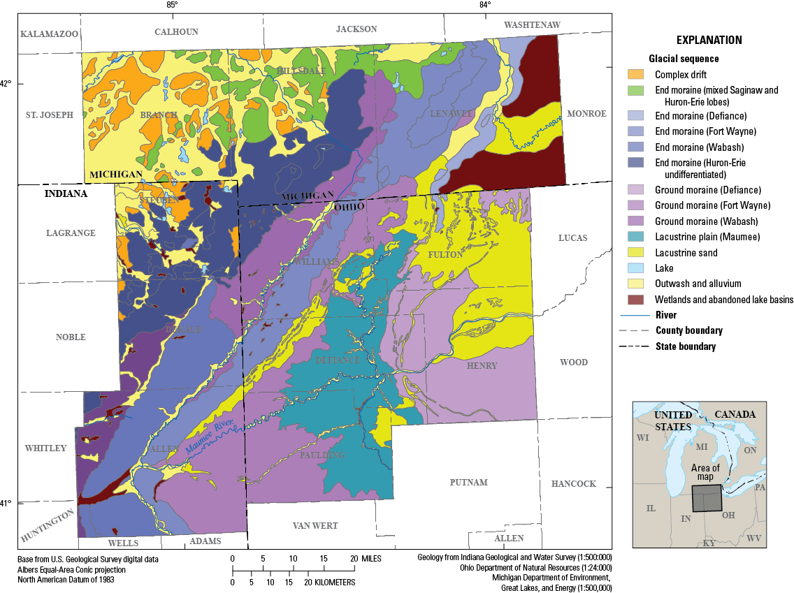
Map showing glacial deposits in southeastern Michigan, northeastern Indiana, and northwestern Ohio. Glacial sequences were generalized from glacial geologic maps showing surficial deposits in Michigan (Farrand, 1982), Indiana (Gray, 1989), and Ohio (Pavey and others, 1999).
Lacustrine deposits dominate the low-relief plain that hosts the modern Maumee River (fig. 4), and the ubiquitous fine-grained deposits affect both groundwater and surface-water processes. Groundwater availability in the Maumee Lake Plain is limited in Ohio, especially south of the Maumee River, with well yields typically ranging between 0 and 25 gal/min (Ohio Department of Natural Resources, 2001). This is consistent with the southern part of the lake plain in Indiana that is bounded on the west by the Fort Wayne moraine (fig. 4), but wells in the lake plain north of the Maumee River commonly produce 50–100 gal/min (Fleming and others, 1994). The impermeable nature of fine-grained lacustrine deposits in the Maumee Lake Plain generally results in limited groundwater recharge except where relatively thin lacustrine sequences overlie shallow bedrock aquifers in Indiana (Fleming and others, 1994). Conversely, highly permeable beach and dune sand deposits (lacustrine sand, fig. 4) along the perimeter of the ancestral Lake Erie Basin form aquifers and provide direct pathways for groundwater recharge (Fleming and others, 1994).
The Huron-Erie ice lobe entered the ancestral Lake Erie Basin from the northeast (fig. 3) and transported lacustrine deposits westward, incorporating the fine-grained deposits into glacial tills that form the framework of multiple end moraines (landforms generated at the edge of a glacier with high topography relative to surrounding terrain) and ground moraines (planar landforms composed of till deposited at the base of a glacier). The fine-grained tills are characteristic of Huron-Erie lobe moraines, which generally contain progressively more sand to the west (Gooding, 1973). The Defiance moraine (described by Fisher and others, 2015) is the easternmost moraine sequence, followed by the Fort Wayne and then Wabash moraines moving westward.
Groundwater availability for each of the moraine sequences can generally be divided into north and south regions separated by the Maumee River. Wells associated with the Defiance moraine sequences south of the Maumee River typically produce less than 25 gal/min, and regions with limited groundwater availability (less than 5 gal/min well yields) are common (Ohio Department of Natural Resources, 2001). North of the Maumee River, wells in lacustrine sand sequences covering a large section of the lacustrine plain (fig. 4) can produce up to 100 gal/min, and lacustrine sand aquifers beneath and adjacent to the Defiance moraine, which extends into Lenawee County, Michigan, can produce between 100 and 500 gal/min (Ohio Department of Natural Resources, 2001). Water availability from unconsolidated aquifers is similar for the southern limbs of both the Fort Wayne and Wabash moraines, where many wells bypass the generally unproductive glacial tills and draw from deeper bedrock aquifers (Fleming and others, 1994). North of the Maumee River, groundwater availability is erratic from deposits beneath the Fort Wayne moraine, with lacustrine fine sand aquifers providing sufficient supplies for many residential wells and isolated deeper sand and gravel sequences capable of supporting pumping rates greater than 100 gal/min (Fleming and others, 1994). North of the City of Fort Wayne, Ind. (near the southwest corner of the study area), the Wabash moraine sequences transition into an interlobate area where buried deposits of the Saginaw ice lobe (fig. 3) intermix with Huron-Erie sequences. Fleming and others (1994) refer to this complex aquifer as the “Huntertown aquifer” in Allen County, Indiana, and expected pumping rates are commonly between 10 and 100 gal/min (potential well yields increase to 300–500 gal/min near the DeKalb County, Indiana, border to the north).
Aquifer recharge potential for water-bearing sand and gravel units associated with the Fort Wayne and Wabash moraine sequences is dependent on the spatial extent and thickness of the Lagro Formation, a glacial till that typically contains between 35 and 60 percent clay, owing to its lacustrine mud origin, that was glacially transported to the morainal regions (Fleming and others, 1994). The Lagro Formation is an aquitard with thickness varying from 10 feet (ft) in some areas of Allen County to more than 100 ft along end moraine crests, but vertical fractures are common, with some reaching 20 ft into the glacial till (Fleming and others, 1994), creating secondary permeability. Similar fractures are observed in glacial tills of northern Ohio (Brockman and Szabo, 2000).
Glacial outwash and alluvial deposits are common at the boundaries of moraine sequences, which typically coincide with river valleys, and the associated aquifers are some of the most productive in the tri-State region. According to Ohio Department of Natural Resources (2001) aquifer maps, alluvium within the Saint Joseph River valley hosts an aquifer that typically produces 100–500 gal/min in Williams County, Ohio. Further downstream and to the southwest, Fleming and others (1994) report more modest expected pumping rates (less than 200 gal/min) from outwash beneath the Saint Joseph River alluvial deposits and only isolated locations where 500 gal/min pumping rates are achievable. In Michigan, mixed outwash and more recent alluvial deposits are mapped throughout Branch County, Michigan, and in the northwest half of Hillsdale County (Farrand, 1982). Large areas of surficial outwash deposits are also mapped in northern Steuben County, Indiana (Gray, 1989), but sparse work has been done to characterize the hydrogeologic properties of associated aquifers in this three-county area spanning Michigan and Indiana.
Fleming and others (1994) and Fisher and others (2020) document the interplay of surface and subsurface glacial sequences in the interlobate region of northeastern Indiana and southern Michigan, where the Saginaw and Huron-Erie ice lobes merged during the Last Glacial Maximum (fig. 3). The Huntertown aquifer is composed primarily of northern-sourced Saginaw outwash sequences and underlies a laterally extensive Lagro Formation aquitard deposited by the westward flowing Huron-Erie ice lobe (Fleming and others, 1994). It is unclear how this general relationship between surface and subsurface glacial deposits extends north of Allen County, Indiana, and broad-scale (1:500,000) maps of surficial glacial deposits suggest that surficial till sequences become increasingly discontinuous to the north with more intermixed sand and gravel outwash deposits (fig. 4). In southern Michigan, glacial tunnel channels identified in Branch and Hillsdale Counties trend northwest to southeast, and some extend south into Indiana (Fisher and others, 2005). These glaciofluvial features likely coincide with prolific aquifers, but their dimensions and hydrogeologic properties have not been described. The existing aquifer maps in the tri-State area are derived from maps of surficial geology (Ohio Department of Natural Resources, 2001) or through manual analysis of well-log data (Fleming and others, 1994), highlighting the importance of building a three-dimensional model to facilitate a better understanding of the subsurface geologic architecture and hydrogeologic properties.
Data Compilation and Preparation for the Hydrogeologic Framework
Well records for the study area were originally extracted from the national dataset compiled by Bayless and others (2017). Water-well drillers’ records in the study area were reassessed in April 2020 in each respective State’s database, but it was determined that the additional available wells did not provide sufficient data on the deepest parts of the aquifer or where bedrock surface information was most needed.
The well-record dataset was processed by using a modification of the methods described by Arihood (2009). Well drillers’ descriptions of lithology in each log were renamed to a set of standardized textural descriptions as specified in the U.S. Geological Survey Ground-Water Site-Inventory (GWSI) System (U.S. Geological Survey, 2005). Well drillers’ descriptions of geologic deposits and the corresponding GWSI lithologic codes are listed in table 1. Error-checking programs were used to scan the database and eliminate records that were found to be incomplete, duplicated, or containing obvious logical mistakes such as nonsequential depths or geological impossibilities (Arihood and others, 2019).
Table 1.
Well-log descriptions, Ground-Water Site-Inventory System codes, and textural groups of geologic deposits used to define aquifer and nonaquifer units in the study area in southeastern Michigan, northeastern Indiana, and northwestern Ohio.[Modified from Arihood and others (2019). USGS, U.S. Geological Survey; N/A, not applicable]
| Description of geologic deposit | General classification of geologic deposits | USGS Ground-Water Site- Inventory (GWSI) System lithology code assigned from well drillers’ records | Material type in objective model (modified from Fetter, 1994) |
|---|---|---|---|
| Boulders | Aquifer | BLDR | Gravel |
| Boulders and sand | Aquifer | BLSD | Gravel |
| Cobbles | Aquifer | COBB | Gravel |
| Gravel | Aquifer | GRVL | Gravel |
| Rubble | Aquifer | RBBL | Gravel |
| Sand and gravel | Aquifer | SDGL | Gravel |
| Cobbles and sand | Aquifer | COSD | Sand/outwash |
| Outwash | Aquifer | OTSH | Sand/outwash |
| Sand | Aquifer | SAND | Sand/outwash |
| Loam | Nonaquifer | LOAM | Silty sands |
| Loess | Nonaquifer | LOSS | Silty sands |
| Overburden | Nonaquifer | OBDN | Silty sands |
| Sand and silt | Nonaquifer | SDST | Silty sands |
| Silt | Nonaquifer | SILT | Silty sands |
| Soil | Nonaquifer | SOIL | Silty sands |
| Gravel, sand, and silt | Nonaquifer | GRDS | Silty sands |
| Boulders, silt, and clay | Nonaquifer | BLSC | Silt, sandy silts, clayey sands |
| Clay, some sand | Nonaquifer | CLSD | Silt, sandy silts, clayey sands |
| Cobbles, silt, and clay | Nonaquifer | COSC | Silt, sandy silts, clayey sands |
| Gravel and clay | Nonaquifer | GRCL | Silt, sandy silts, clayey sands |
| Gravel, cemented | Nonaquifer | GRCM | Silt, sandy silts, clayey sands |
| Gravel, silt, and clay | Nonaquifer | GRSC | Silt, sandy silts, clayey sands |
| Marl | Nonaquifer | MARL | Silt, sandy silts, clayey sands |
| Muck | Nonaquifer | MUCK | Silt, sandy silts, clayey sands |
| Mud | Nonaquifer | MUD | Silt, sandy silts, clayey sands |
| Peat | Nonaquifer | PEAT | Silt, sandy silts, clayey sands |
| Sand and clay | Nonaquifer | SDCL | Silt, sandy silts, clayey sands |
| Sand, gravel, and clay | Nonaquifer | SGVC | Silt, sandy silts, clayey sands |
| Sand, some clay | Nonaquifer | SNCL | Silt, sandy silts, clayey sands |
| Silt and clay | Nonaquifer | STCL | Silt, sandy silts, clayey sands |
| Clay | Nonaquifer | CLAY | Clay, till |
| Hard pan | Nonaquifer | HRDP | Clay, till |
| Till | Nonaquifer | TILL | Clay, till |
| Basalt | Bedrock | BSLT | N/A |
| Chert | Bedrock | CHRT | N/A |
| Coal | Bedrock | COAL | N/A |
| Conglomerate | Bedrock | CGLM | N/A |
| Dolomite | Bedrock | DLMT | N/A |
| Evaporite | Bedrock | EVPR | N/A |
| Granite | Bedrock | GRNT | N/A |
| Gypsum | Bedrock | GPSM | N/A |
| Igneous (undifferentiated) | Bedrock | IGNS | N/A |
| Limestone | Bedrock | LMSN | N/A |
| Limestone and dolomite | Bedrock | LMDM | N/A |
| Quartzite | Bedrock | QRTZ | N/A |
| Rock | Bedrock | ROCK | N/A |
| Sandstone | Bedrock | SNDS | N/A |
| Sandstone and shale | Bedrock | SDSL | N/A |
| Schist | Bedrock | SCST | N/A |
| Shale | Bedrock | SHLE | N/A |
| Siltstone | Bedrock | SLSN | N/A |
| Slate | Bedrock | SLTE | N/A |
The resulting dataset containing the standardized descriptions of geologic deposits was combined with another dataset containing location information for each well, a geographic projection definition, the well depth, the land-surface altitude, and well-construction information (depth to top and bottom of screen, casing length, casing diameter, construction date, well-development information [pumping rate, pumping duration, pump drawdown], and water use) to produce a georeferenced dataset of all the well-record information. Only well logs with field-verified coordinates were included in the dataset. Well logs located by address geocoding, or coordinates based on township, range, and section, were not included in the dataset.
Development of Mapping Products
Although there have been multiple studies that infer the subsurface geology from depositional environment, glacial landforms, and surficial geology in the study area (Farrand, 1982; Gray, 1989; and Pavey and others, 1999), the mapping products from this study were developed by using an objective geostatistical approach. Previous interpretations of surficial and subsurface geology were used for comparison and validation of the geostatistical model.
Development of the Two-Dimensional Grids of Hydrogeologic Information
A detailed description of the process to convert well-record data into grids of hydrogeologic information and lithologic segment files is described in Arihood (2009) and Bayless and others (2017), and a flowchart outlining this process is presented in figure 5. Two-dimensional grids were produced for specified thicknesses of the glacial deposits and represent an average value for the deposits in that layer. Grid cell size in the horizontal plane was approximately 450 by 450 meters (m).
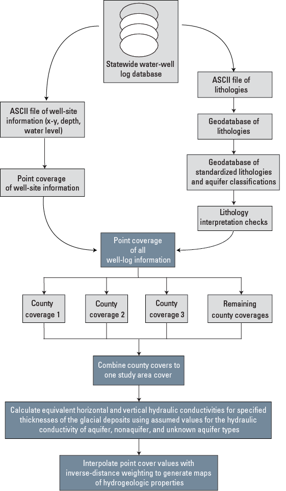
Flowchart for processing well logs into grids of hydrogeologic information and lithologic segments. Figure modified from Arihood (2009). ASCII, American Standard Code for Information Interchange.
To allow variation of hydraulic conductivity with depth, the glacial deposits are represented in the model by up to three layers, from top to bottom: layer 1, which includes the topmost glacial thickness and is as much as 50 ft thick; layer 2, which includes as much as the next 50 ft of glacial thickness below layer 1 where present; and layer 3, which accounts for any remaining glacial thickness where present. This layering scheme allowed for increased detail near the land surface, where most of the groundwater wells in the study area are completed.
The upper bounding surface used for determining the layers represents the land-surface altitude as interpolated from the top elevation of each well in the dataset by using an inverse-distance weighting method. This method of interpolation estimates point values by averaging the values of sample data points in the vicinity of each target location. The closer a point is to the location being estimated, the more weight it has in the calculation of target location values. If land-surface altitude was not recorded in the well log, then a value interpolated from a 30-m digital elevation model (DEM) (U.S. Geological Survey, 2020) was substituted for the missing altitude data. Land-surface altitude from the DEM was also substituted if the land-surface altitude in the well record differed by more than 10 ft from the DEM.
The lower bounding surface was initially interpolated from the bedrock lithologies in the well dataset. In parts of the study area where wells encountering bedrock lithologies were limited, the interpolated lower bounding surface was adjusted to a depth below any unconsolidated wells it intersected. The total unconsolidated thickness was computed by subtracting the lower bounding surface from the upper bounding surface.
Maps of hydrogeologic information were generated on the basis of the percentage of aquifer (coarse-textured) and nonaquifer (fine-textured) material (table 1) described in a well log in each specified layer. The texture-based values of hydraulic conductivity were computed by assuming a horizontal hydraulic conductivity of 100 feet per day (ft/d) for aquifer material and 1 ft/d for nonaquifer material, and a vertical hydraulic conductivity of 10 ft/d for aquifer material and 0.001 ft/d for nonaquifer material. These values of hydraulic conductivity were selected because they represent most values for glacial deposits and would be easily scalable to future applications.
Through incorporation of the specific layer thickness, grids of transmissivity were computed. The percentage of aquifer material throughout the full unconsolidated thickness was used to compute the total thickness of coarse-grained deposits at each well log. The point values of these parameters (texture-based estimated equivalent horizontal hydraulic conductivity, vertical hydraulic conductivity, transmissivity, and total thickness of coarse-grained deposits) were interpolated across the study area by application of an inverse-distance weighting algorithm available within ArcGIS. Details of these methods are described in Arihood (2009).
Where available, well discharge, duration of pumping, and water-level drawdown for wells in Indiana and Ohio (water-well drillers’ records for Michigan did not include well-development data at the time of data collection) were input to a modified form of the Theis equation (Prudic, 1991) to determine the specific-capacity-based conductivity. An iterative process was used to calculate transmissivity by use of an initial value of 500 feet squared per day (ft2/d). The process stops after several iterations when the difference between the old estimate and new estimate for transmissivity becomes less than 5 ft2/d, and the last new estimate is used. The value of transmissivity was adjusted for the effect of partial penetration by the well screen into the aquifer by use of a method described by Butler (1957, p. 160). Values of conductivity were calculated by dividing transmissivity by the thickness of saturated aquifer material penetrated by the well, which provides a conservative estimate for conductivity (Arihood, 2009).
Development of the Three-Dimensional Hydrogeologic Framework Model
A three-dimensional hydrogeologic framework model was developed to assist in visualizing the distribution of aquifer materials in the study area. The commercial software Earth Volumetric Studio (EVS) was used to create a continuous distribution of lithologies of the study area. EVS is an environmental data-visualization system with a module-based graphical user interface designed to fit many applications. EVS uses an internal expert system to characterize the input dataset and build multidimensional variograms (C Tech Development Corporation, 2022). The expert system evaluates the frequency and distribution of the input data and creates a variogram that minimizes differences between known data points and values estimated by the kriging.
As with the two-dimensional maps, the upper bounding surface of the volumetric model represents the land-surface altitude interpolated from the top elevation of each well in the well-record dataset. Rather than using the inverse-distance weighting interpolation to define the bottom boundary, as was done with the two-dimensional maps, the bottom boundary of the volumetric model was defined as the contact between unconsolidated deposits and bedrock. During preliminary kriging attempts, the limited number of wells that reach bedrock in large expanses of the study area did not allow for a realistic representation of this contact. Where bedrock altitudes were sparse and the kriged contact between unconsolidated deposits and bedrock was poorly defined, a small number of synthetic wells were generated and included in the final kriging routine to constrain the bottom model boundary. Bedrock altitude was extracted for synthetic wells from the interpolated bedrock surfaces of Soller and others (2012).
Model grid cell size in the horizontal plane was 500 by 500 m. Grid cell size varies in the vertical plane; the thickness of the volumetric model is divided evenly into 30 model layers over the entire thickness of the modeled deposits. The thickest unconsolidated sections of the model contain grid cells up to 15 ft thick.
Although the geostatistical processing, or kriging, of the hydrogeologic framework was automated within EVS, the program requires parameters that can be derived from the well-record data by a hydrologist familiar with the hydrogeologic setting and the datasets available. Hydrogeologic experience is required to make decisions that will allow the program to produce a framework that meets the purpose of the study. Some kriging geostatistical parameters (including the sill, minimum and maximum range, and nugget) can be specified by the user and directly affect the sharpness of boundaries between aquifer units. The variogram nugget represents variability of data at very small distances from each point (Matzke and others, 2010) and was set at zero for this study. The sill can be understood as the largest variability of a property between pairs of wells (data points), and the range is the approximate distance between data points at which the largest variability of a property is reached (Matzke and others, 2010). Parameters, which included the horizontal-to-vertical bias and the variogram sill and range, were varied on a trial-and-error basis, and the distribution was recalculated until several working distributions were developed. The working distributions were reviewed, and the distribution of deposits that best matched prior surficial geologic mapping of the study area was selected (Soller and others, 2012).
Whereas the two-dimensional grids assigned numerical values to each lithology prior to kriging, the three-dimensional-model kriging process used individual lithology codes to estimate the areas of the framework between well logs. Of the 52 standardized lithologies represented in the well logs in the study area, 33 lithologies represented the unconsolidated sediments. These were further categorized into five general textural classes, with two representing aquifer materials and three representing nonaquifer materials (table 1). Grouping lithologies by texture allows for a simplified understanding of the distribution of aquifer units and establishes an easier approach to parameterize groundwater-flow models that may use this hydrogeologic framework in the future. The methods for creating a three-dimensional volumetric representation of glacial lithologic materials are described in detail in Arihood and others (2019).
Synoptic Water-Level Measurements
In addition to examining the distribution of aquifer materials, two synoptic groundwater-level surveys were conducted to add another component to the conceptual understanding of the aquifer. Synoptic surveys were conducted during the nongrowing (January–March 2022) and growing seasons (August 2022) to allow for assessment of water levels under different hydrologic conditions. Groundwater-level data from 70 wells were used to simulate potentiometric surfaces for the unconsolidated sediments in parts of the study area by interpolation in ArcGIS. Synoptic sites were located within the 11 counties that are intersected by the boundary of the previously proposed sole source aquifer. Measurements were collected by using standard techniques and methods outlined by Cunningham and Schalk (2011).
Estimated Distributions of Hydrogeologic Properties and Hydrogeologic Framework Model
The distributions of wells completed in glacial deposits and wells completed in the bedrock are shown in figures 6A and 6B, respectively. Figure 6A shows that relatively shallow glacial wells (less than 90 ft deep) are well distributed throughout the study area, but deeper wells are concentrated in a southwest-to-northeast-trending section of the study area from Indiana through northwestern Ohio and into the central-northeastern section of the study area in Michigan. Figure 6B shows that very few wells reach bedrock in that same southwest-to-northeast-trending section. In total, approximately 60,500 wells were used in the development of the two-dimensional grids of hydrogeologic information and volumetric model after processing. Well-record density for the study area was approximately 5.3 wells per square mile.
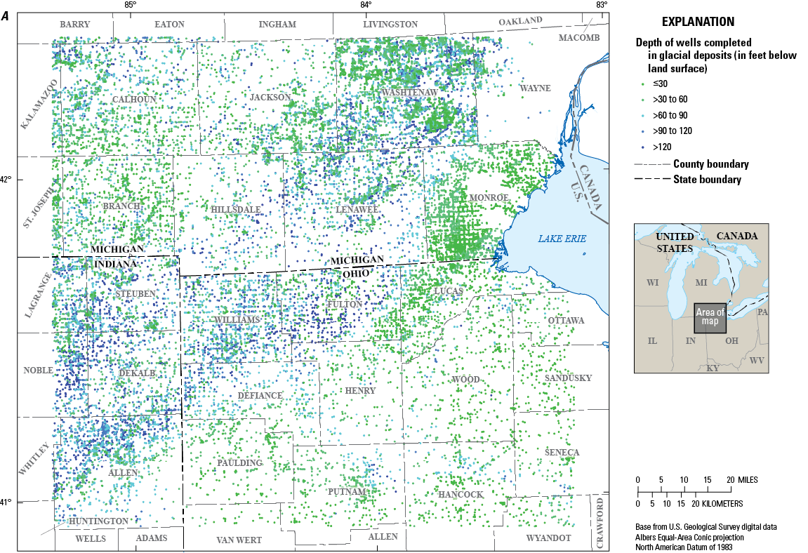
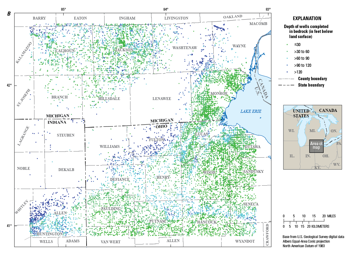
Maps showing the distribution of A, wells completed in glacial deposits and B, wells completed in bedrock, used to create maps of hydrogeologic information and a three-dimensional volumetric model for the glacial deposits in a multicounty area of southeastern Michigan, northeastern Indiana, and northwestern Ohio.
Maps of Two-Dimensional Hydrogeologic Information
The total thickness of unconsolidated deposits (fig. 7) was discretized into layers of specific thickness to calculate hydrogeologic properties. Each layer does not cover the entire study area; layers 2 and 3 are not present in areas where the unconsolidated thickness is less than 50 ft and 100 ft, respectively. This resulted in an average layer thickness that ranged from 10 to 40 ft. Maps of texture-based estimated equivalent hydraulic conductivity and transmissivity are presented in figures 8–10.
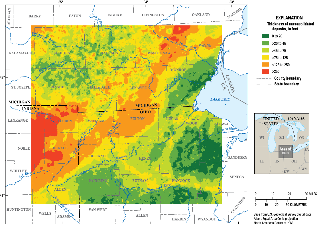
Map showing total thickness of unconsolidated deposits in southeastern Michigan, northeastern Indiana, and northwestern Ohio.
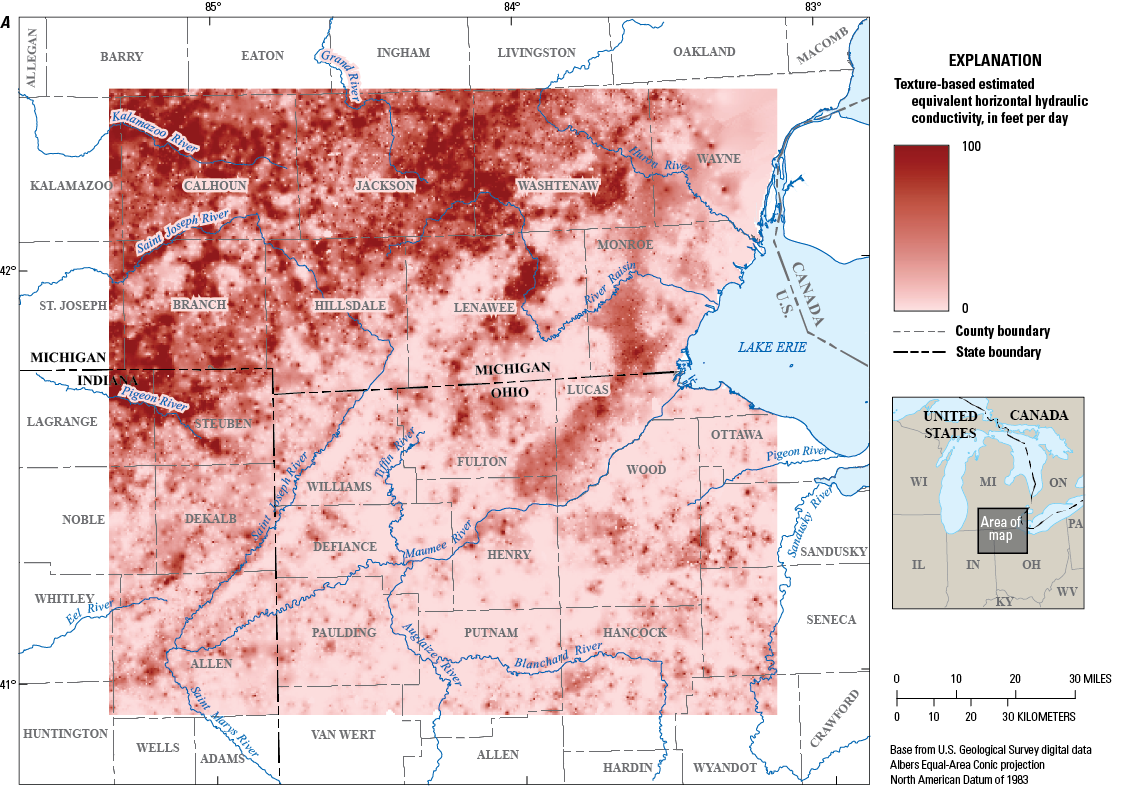
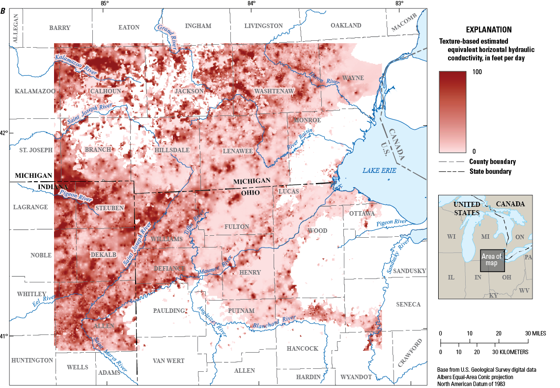
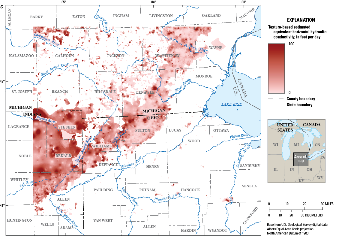
Maps showing texture-based estimated equivalent horizontal hydraulic conductivity for A, layer 1, B, layer 2, and C, layer 3 in southeastern Michigan, northeastern Indiana, and northwestern Ohio.
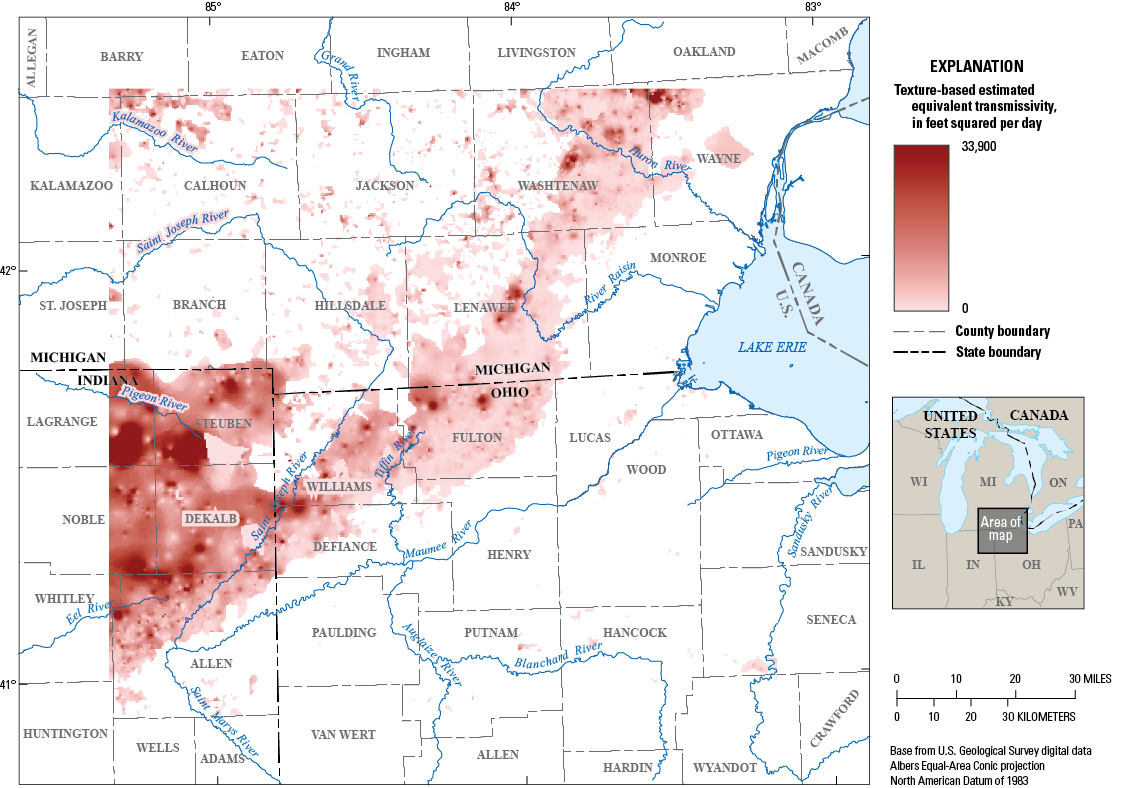
Map showing texture-based estimated equivalent transmissivity for layer 3 in southeastern Michigan, northeastern Indiana, and northwestern Ohio. Transmissivities for layers 1 and 2 range from 0 to 5,000 feet squared per day and exactly mirror their corresponding horizontal conductivity distributions in figure 8 because of their uniform layer thicknesses of 50 feet.
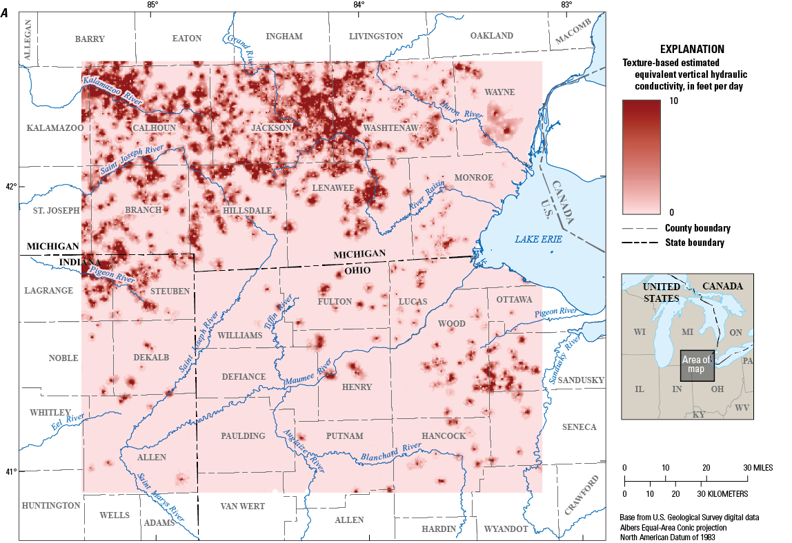
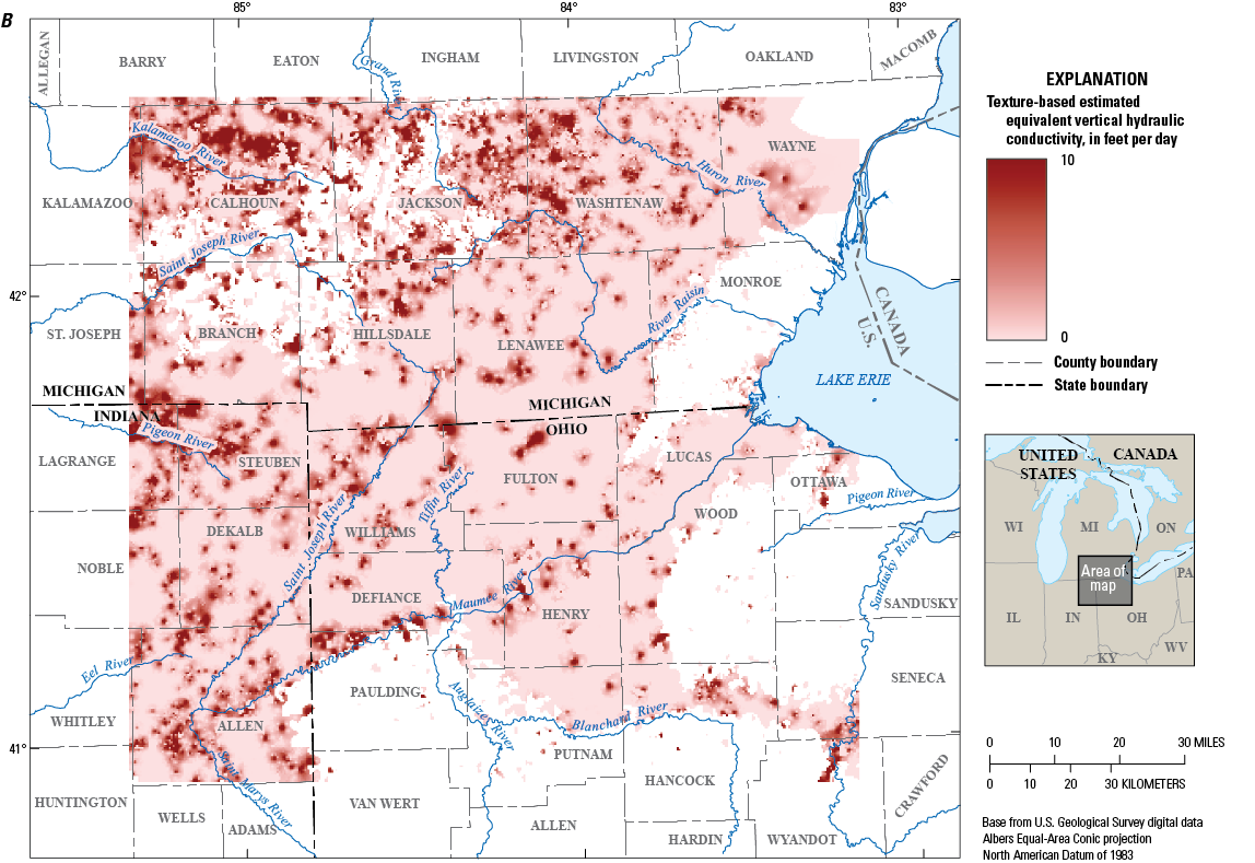
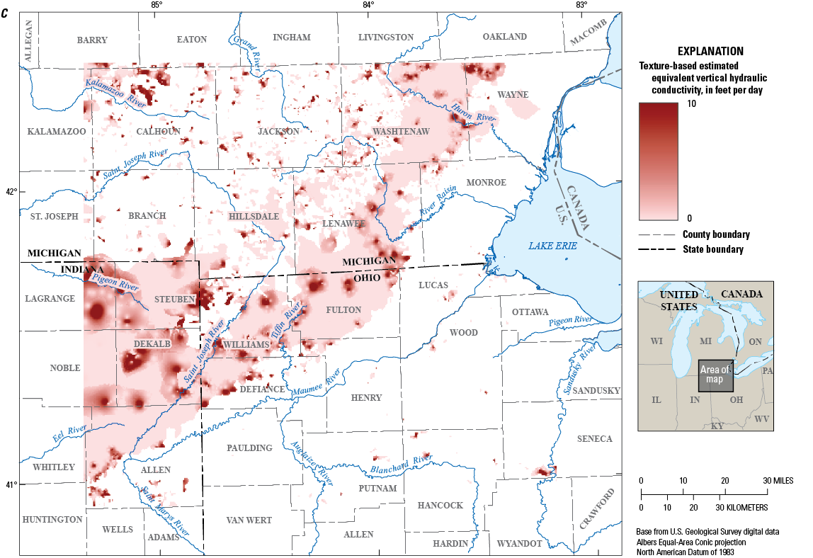
Maps showing texture-based equivalent vertical hydraulic conductivity for A, layer 1, B, layer 2, and C, layer 3 in southeastern Michigan, northeastern Indiana, and northwestern Ohio.
The maps of conductivity and transmissivity show that, in general, higher conductivity deposits are most prevalent near the surface in the north and northwestern sections of the study area near Steuben, Branch, Calhoun, and Jackson Counties (figs. 8A and 8B). But as the unconsolidated thickness increases toward DeKalb and Allen Counties (and in some central-to-northeast-trending areas near Defiance and Williams Counties), higher conductivity deposits are concentrated deeper in the subsurface (fig. 8C). As hydraulic conductivity represents a material’s capacity to transmit water, the higher conductivity deposits have the potential for greater groundwater availability. The three-layer discretization for the conductivity maps allows for thinner layers near the land surface, which help to visualize the expansive layer of fine-grained deposits that cover the surface of much of the study area.
Cumulative thickness of coarse-grained (aquifer) deposits shows correlation with mapped conductivities while providing new insights into coarse-grained distributions (fig. 11). The presence of coarse-grained deposits correlates well with the high-conductivity areas in figs. 8 and 9, which especially highlight where coarse-grained deposits are limited. Coarse-grained deposits greater than 20 ft thick in Ohio are sparse outside of Williams County and are often less than 5 ft thick.
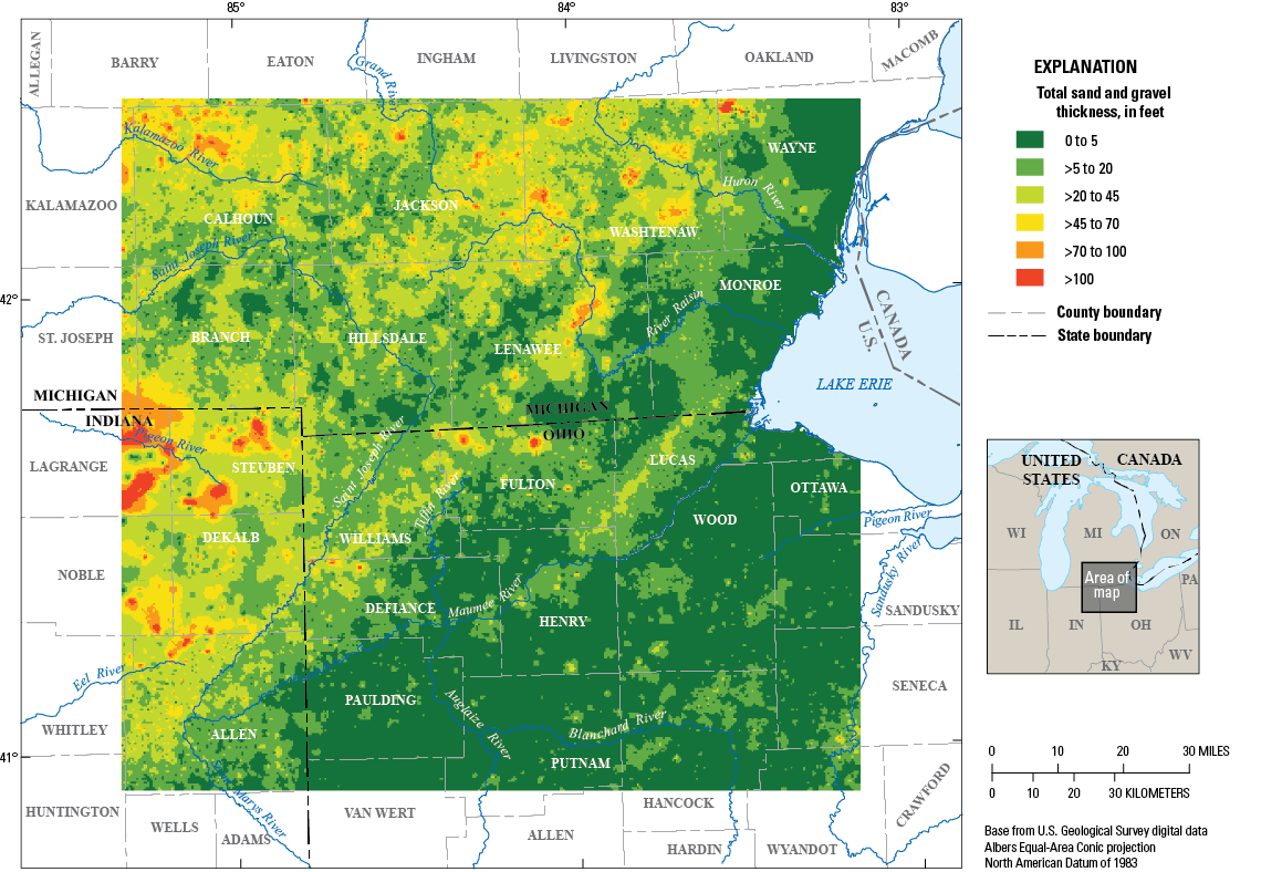
Map showing thickness of coarse-grained deposits in southeastern Michigan, northeastern Indiana, and northwestern Ohio.
Specific-capacity-based maps show similar distributions of high-conductivity deposits throughout the study areas. The map of specific-capacity-based horizontal hydraulic conductivity of coarse-grained sediments within the glacial deposits (fig. 12) shows that the highest conductivity deposits are concentrated near Steuben County, Indiana, and Williams County, Ohio. Throughout most of the remaining study area in Ohio, high-conductivity areas are sparse. Combining the specific-capacity-based horizontal hydraulic conductivity grid with the coarse-grained deposits grid allows for calculation of the specific-capacity-based transmissivity of coarse-grained deposits within the glacial deposits (fig. 13). Specific-capacity-based maps were created only for Indiana and Ohio because water-well drillers’ records for Michigan did not include well-development data at the time of data compilation.
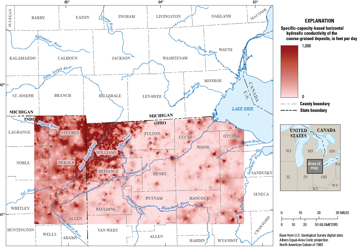
Map showing specific-capacity-based horizontal hydraulic conductivity of the glacial deposits in southeastern Michigan, northeastern Indiana, and northwestern Ohio.
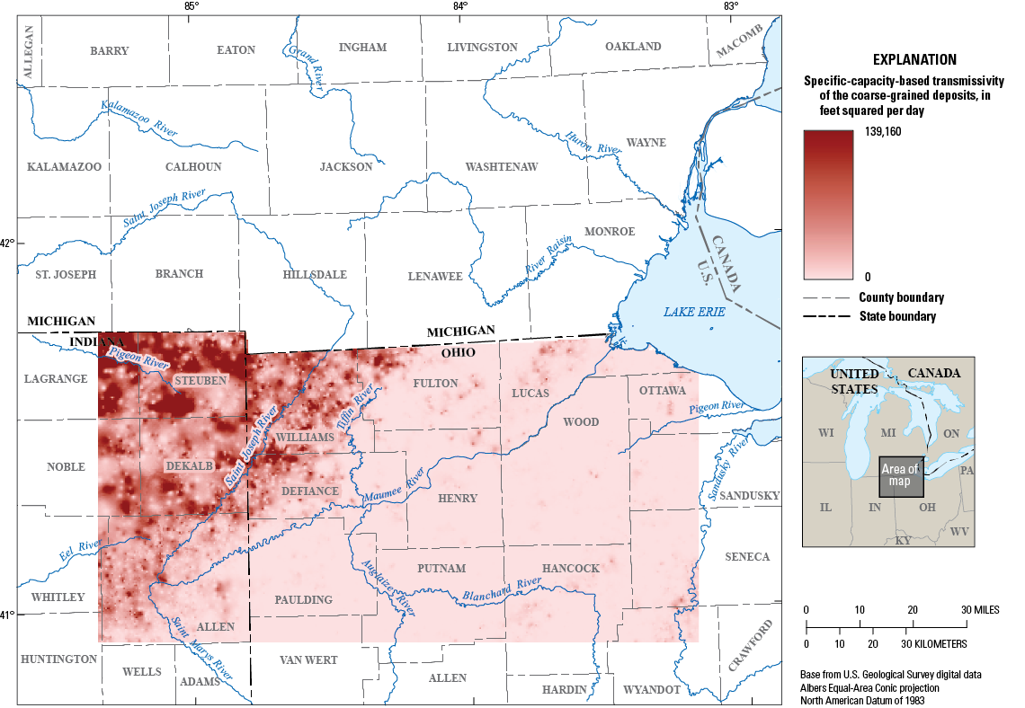
Map showing specific-capacity-based transmissivity of the glacial deposits in southeastern Michigan, northeastern Indiana, and northwestern Ohio.
Volumetric Geologic Model
The volumetric geologic model is used to describe the spatial distribution of aquifer and nonaquifer materials in the subsurface of the study area. The three-dimensional distribution of coarse- and fine-grained deposits affects many aquifer characteristics that determine the availability of groundwater (figs. 14 and 15). Coarse-grained deposits such as outwash (predominantly composed of sand and gravel deposited by proglacial meltwater), lacustrine sands (former well-sorted beach sands), and alluvial deposits (deposited by postglacial streams in valleys) commonly make up unconfined aquifers in the region with high groundwater yields and readily transmit water downward (recharge aquifers) when exposed at the ground surface. In contrast, fine-grained silt and clay particles deposited as moraines or within the ancestral lake basin make up modern soils and subsurface deposits that generally have very low permeability and limit recharge to underlying intertill and basal aquifers.
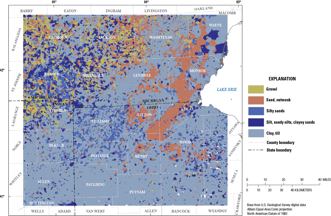
Map showing the textural classes of lithologies at land surface in the study area in southeastern Michigan, northeastern Indiana, and northwestern Ohio.
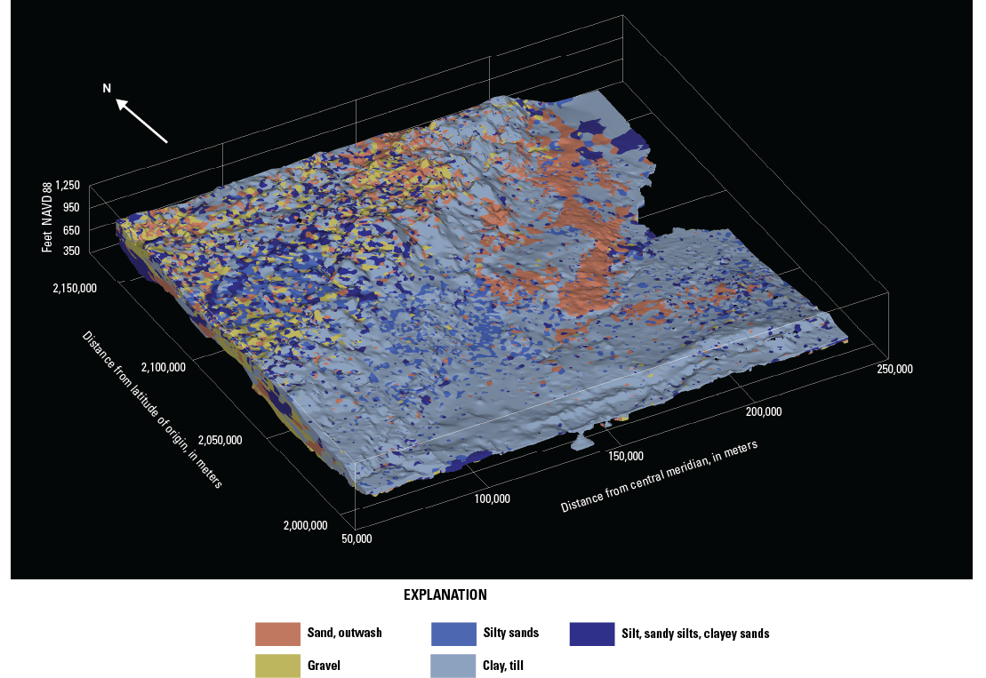
Block diagram showing the textural classes of lithologies in the study area in southeastern Michigan, northeastern Indiana, and northwestern Ohio. Horizontal coordinates are based on the Albers Equal-Area Conic projection, standard parallels 29°30′ and 45°30′ N., latitude of origin 23° N, central meridian 86° W.; North American Datum of 1983. Vertical coordinates are relative to the North American Vertical Datum of 1988 (NAVD 88).
Throughout most of the study area, a layer of fine-grained deposits covers the land surface. In the areas of higher topography near the middle of the study area, these deposits likely represent glacial tills composing the moraines that dominate the landscape. The surficial fine-grained deposits in the southeastern section of the study area represent the thin (less than 50 ft thick) lacustrine deposits that overlie shallow bedrock. Coarse-grained deposits are also represented in the lacustrine deposits as sand in southwest-to-northeast-trending deposits.
The distribution of coarse-grained deposits (composed of textural classes “sand” and “sand and gravel”) is shown in figure 16. Although aquifer materials are concentrated in the western and northwestern parts of the study area, no clear boundary that defines the extent of the aquifer can be interpreted. The complex depositional environment (as detailed in the “Hydrogeologic Setting” section) has resulted in a highly heterogeneous mix of glacial deposits that make identification of a clear boundary not possible with current tools and technology.
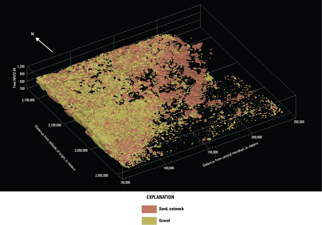
Three-dimensional distribution of coarse-grained deposits in the glacial aquifer underlying southeastern Michigan, northeastern Indiana, and northwestern Ohio. Horizontal coordinates are based on the Albers Equal-Area Conic projection, standard parallels 29°30′ and 45°30′ N., latitude of origin 23° N., central meridian 86° W.; North American Datum of 1983. Vertical coordinates are relative to the North American Vertical Datum of 1988 (NAVD 88).
Coarse-grained deposits are concentrated in the western sections of the study area, and in these sections aquifer materials can be present at multiple depths. In the southwestern areas, the sands and gravels are present beneath the fine-grained surficial tills and made vertically discontinuous by intervening deposits of silty clay-textured materials. In the northwest, coarse-grained deposits interbed with clay- and silt-textured deposits throughout the entire unconsolidated thickness. These vertically heterogenous deposits are common in interlobate glaciated settings that are present in this area where former ice lobes of the Laurentide Ice Sheet joined one another.
Potentiometric Surface Mapping
Groundwater levels in 70 groundwater wells were used to create the potentiometric surfaces in figures 17 and 18; wells exhibited a wide range of depths, diameters, and uses. Because of the heterogeneous nature of the glacial deposits and the existence of discontinuous confining layers throughout the study area, wells used to create the potentiometric surfaces were completed in aquifers at various depths under locally confined conditions. Groundwater levels ranged from approximately 650 to 1,050 ft above the North American Vertical Datum of 1988 during the first synoptic survey, varying by ±4 ft when compared with the measurements taken during the second synoptic survey. The potentiometric surface generally mirrors the surface topography, with regional groundwater flow from the highest measured hydraulic heads in Hillsdale County, Michigan, east towards Lake Erie and south towards northeastern Indiana and northwestern Ohio. No specific pattern was detected to describe where water levels were higher or lower during the growing and nongrowing season. Synoptic site data and water levels are recorded in table 2 and are available in the U.S. Geological Survey National Water Information System database (U.S. Geological Survey, 2022).
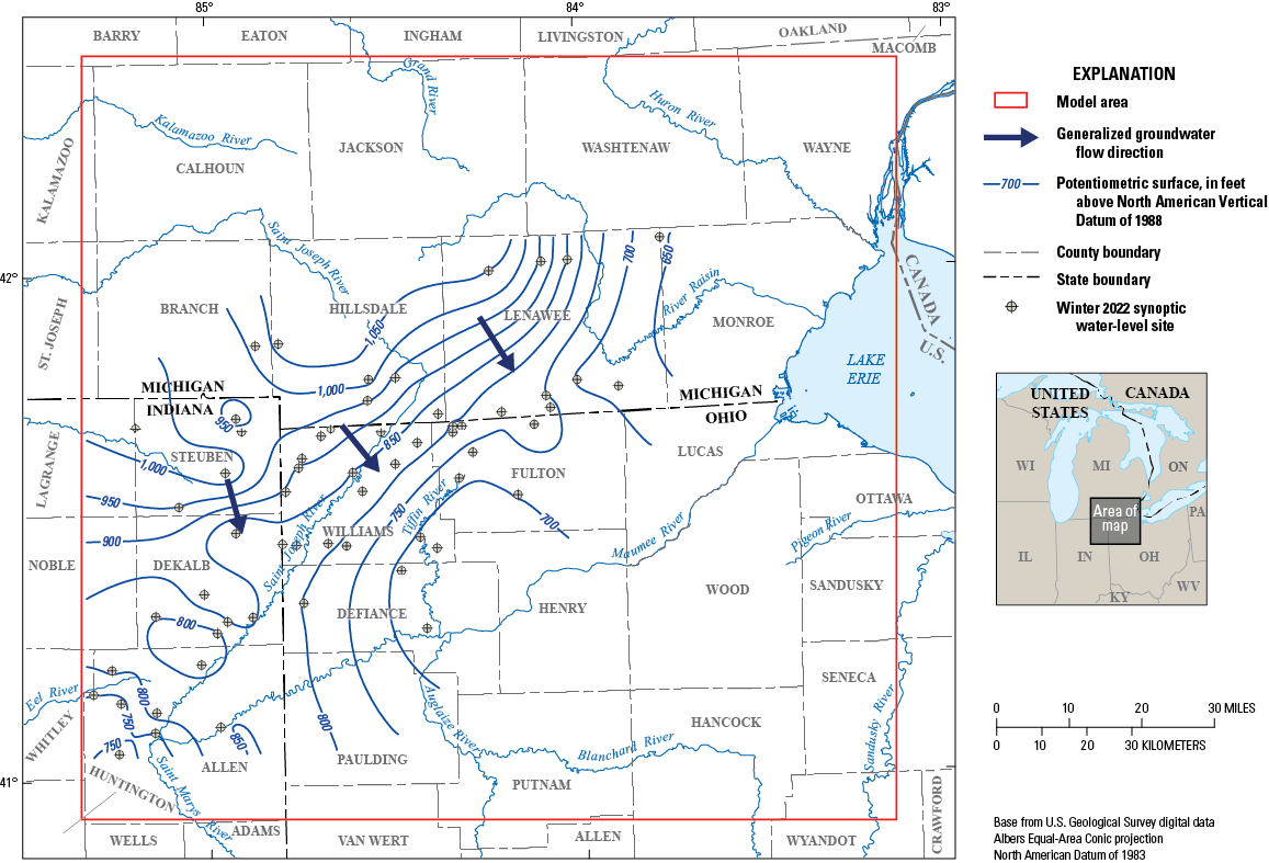
Map showing wells completed in glacial deposits measured during the first groundwater-level synoptic survey (January–March 2022; table 2) and the interpolated potentiometric surface in southeastern Michigan, northeastern Indiana, and northwestern Ohio.
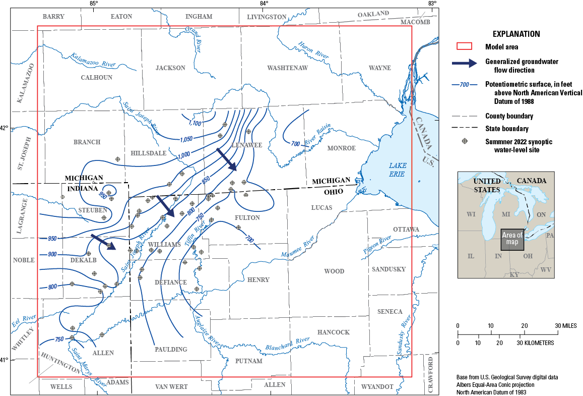
Map showing wells completed in glacial deposits measured during the second groundwater-level synoptic survey (August 2022; table 2) and the interpolated potentiometric surface in southeastern Michigan, northeastern Indiana, and northwestern Ohio.
Table 2.
Synoptic groundwater-level measurements collected from January to March 2022 and August 2022 in southeastern Michigan, northeastern Indiana, and northwestern Ohio.[USGS, U.S. Geological Survey; NAVD 88, North American Vertical Datum of 1988; --, no data]
Comparing Maps of Hydrogeologic Information With Maps From Other Studies
The maps of hydrogeologic information created during this study were compared with existing maps of similar information to (1) qualitatively evaluate the similarity of the results to previously published work, (2) discover areas where the well-record processing uncovers geologic detail not discernable from surface features, (3) discover areas requiring additional evaluation of the well-record data for potential errors, and (4) discover inaccuracies in the well-record interpretation process. The volumetric model allowed for the construction of cross sections between any two points in the study area. This allows for direct comparisons of cross sections constructed from the volumetric model with those created in previous studies. The geologic sections illustrate slices of the three-dimensional hydrogeologic framework model, with intercepted wells shown to illustrate how precisely the model represented well lithology. Synoptic water-level survey sites can be used to add another component to the conceptual understanding of the aquifer. Well-record data and water levels can be projected onto proximate cross sections selected for comparison with previous studies. Synoptic sites can also be used as anchors to create new cross sections. Cross-section traces are depicted in figure 19.
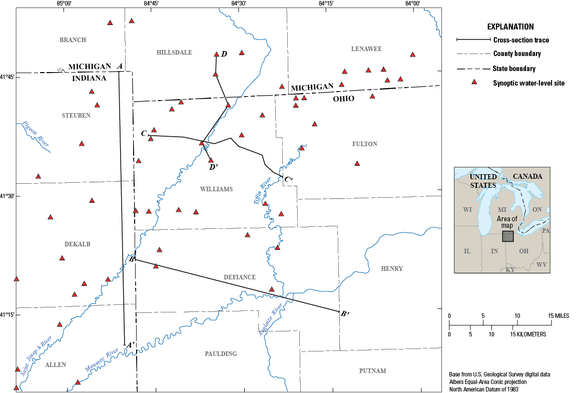
Map showing volumetric model cross-section traces and synoptic water-level survey sites in southeastern Michigan, northeastern Indiana, and northwestern Ohio. (Synoptic sites listed in table 2.)
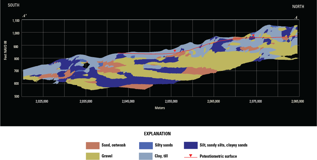
Volumetric cross section A–A′ generated with Earth Volumetric Studio (C Tech Development Corporation, 2022) along the trace of a cross section in Fenelon and others (1994; fig. 21 of this report). (See figure 19 for the location of the cross section.) Horizontal coordinates are based on the Albers Equal-Area Conic projection, standard parallels 29°30′ and 45°30′ N., latitude of origin 23° N., central meridian 86° W.; North American Datum of 1983. Vertical coordinates are relative to the North American Vertical Datum of 1988 (NAVD 88).
A cross section from this study showing the distribution of unconsolidated deposits was compared with a cross section from the “Hydrogeologic Atlas of Aquifers in Indiana” (Fenelon and others, 1994) (figs. 20 and 21). The south-to-north-trending cross sections in the glacial aquifer generally agreed with respect to the near-surface glacial deposit distribution, with both cross sections showing thinner unconsolidated deposits to the south that become thicker with increased coarse-grained deposits moving to the north. The atlas displays considerable uncertainty greater than 100 ft below the surface, but the volumetric model provides some estimate of the deposits at depth because it incorporates more recent well-record data that may not have been previously available.
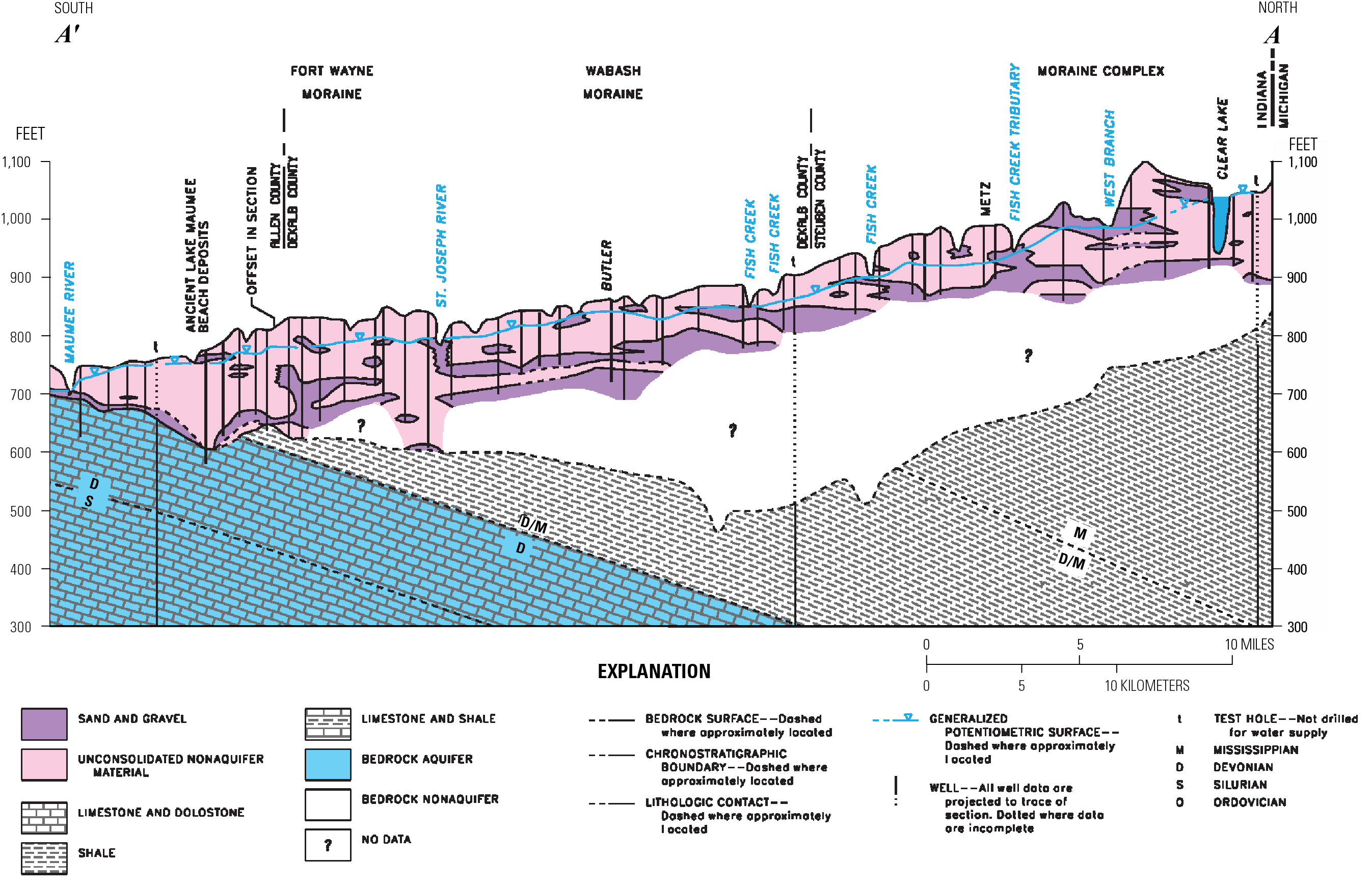
Cross-section segment from Fenelon and others (1994) that coincides with volumetric cross section A–A′ (fig. 20). (See fig. 19 for the location of the cross section.)
Cross sections constructed from the volumetric model can also be correlated with larger scale, county-specific maps of groundwater resources to confirm previous assessments of subsurface hydrogeology or fill in data gaps. When compared with Ohio Department of Natural Resources published maps of the “Ground-Water Resources of Defiance County” (Schmidt, 1982), cross sections generally agreed, with both displaying increasing concentrations of discontinuous, coarse-grained deposits to the west (figs. 22 and 23). The synoptic site in figure 18 located in western Defiance County and intersected by cross section B–B′ is an example of a well screened in the isolated basal aquifer units that are prevalent throughout the study area. Construction of cross sections that match selected traces of those in Coen’s (1989) assessment of groundwater resources in Williams County allows for enhanced visualization of the subsurface geology by filling in the unconsolidated materials between mapped well logs (figs. 24 and 25). The model-derived cross section (fig. 24) more clearly displays the discontinuous nature of the conductive sediments that make up much of the glacial aquifer. Interpolated water levels along the cross section show a steadily decreasing potentiometric surface from west to east.
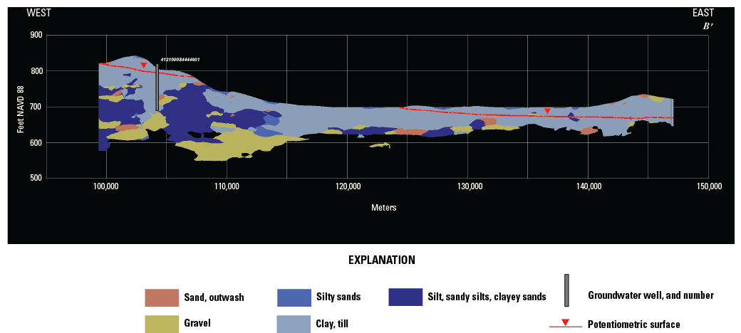
Volumetric cross section B–B′ generated with Earth Volumetric Studio (C Tech Development Corporation, 2022) along the trace of a cross section in Schmidt (1982; fig. 23 of this report). (See fig. 19 for the location of the cross section and table 2 for synoptic water levels of adjacent groundwater wells.) Horizontal coordinates are based on the Albers Equal-Area Conic projection, standard parallels 29°30′ and 45°30′ N., latitude of origin 23° N., central meridian 86° W.; North American Datum of 1983. Vertical coordinates are relative to the North American Vertical Datum of 1988 (NAVD 88).
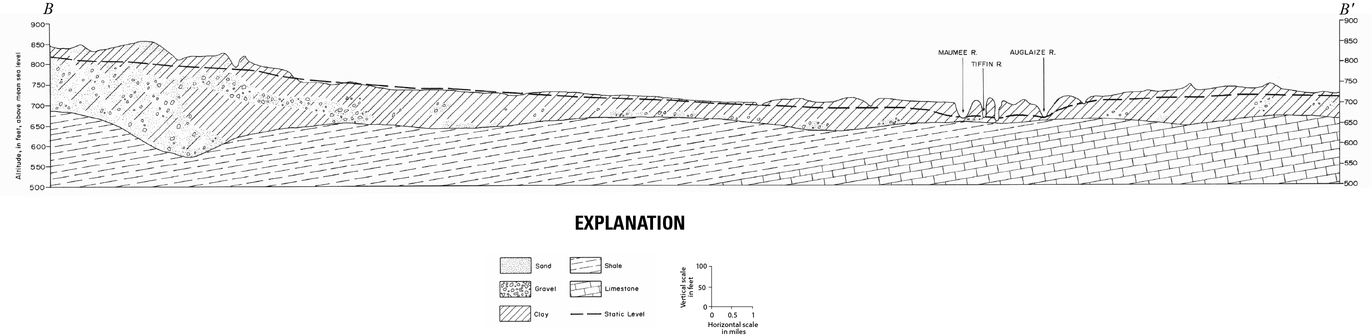
Cross section from Schmidt (1982) that coincides with volumetric cross section B–B′ (fig. 22). (See fig. 19 for the location of the cross section.)
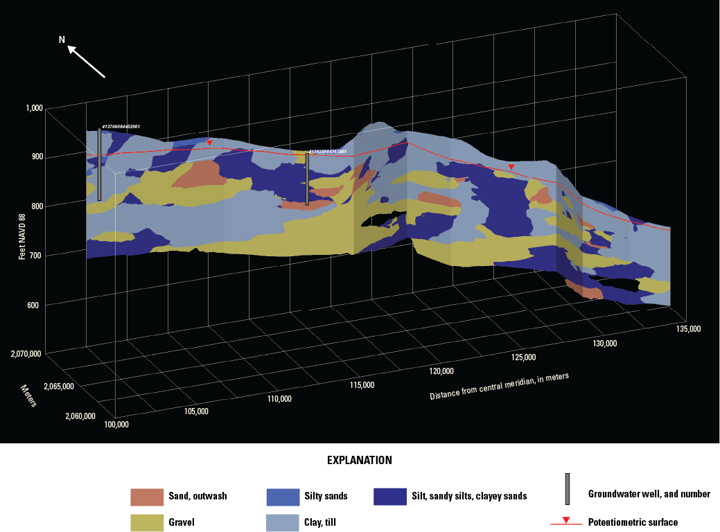
Volumetric cross section C–C′ generated with Earth Volumetric Studio (C Tech Development Corporation, 2022) along the trace of a cross section in Coen (1989; fig. 25 of this report). (See fig. 19 for the location of the cross section and table 2 for synoptic water levels of adjacent groundwater wells.) Horizontal coordinates are based on the Albers Equal-Area Conic projection, standard parallels 29°30′ and 45°30′ N., latitude of origin 23° N., central meridian 86° W.; North American Datum of 1983. Vertical coordinates are relative to the North American Vertical Datum of 1988 (NAVD 88).
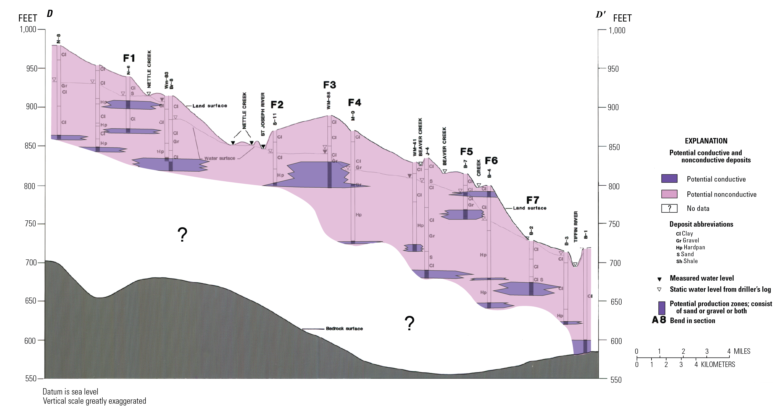
Cross section from Coen (1989) that coincides with volumetric cross section C–C′ (fig. 24). (See fig. 19 for the location of the cross section.)
As previously noted, the mapped potentiometric surface generally mirrors the surface topography, sloping from north to south as exhibited in cross section D–D′ (fig. 26). This mirroring is observed in the glacial deposits in Williams County as well as in the less extensive and less connected glacial aquifer units in Hillsdale County where there is greater reliance on bedrock aquifers to meet groundwater demands.
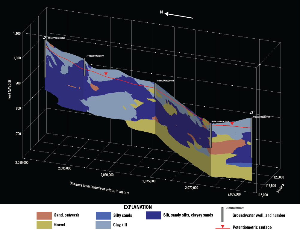
Volumetric cross section D–D′ generated with Earth Volumetric Studio (C Tech Development Corporation, 2022). (See fig. 19 for the location of the cross section and table 2 for synoptic water levels of adjacent groundwater wells.) Horizontal coordinates are based on the Albers Equal-Area Conic projection, standard parallels 29°30′ and 45°30′ N., latitude of origin 23° N., central meridian 86° W.; North American Datum of 1983. Vertical coordinates are relative to the North American Vertical Datum of 1988 (NAVD 88).
The comparisons indicate that the trends in major geologic features were generally captured by the maps created during this study; however, the density of drillers’ records was an important factor in determining the resolution of minor geologic features in these maps.
Model Limitations and Uncertainties
The geostatistical approaches used to generate the products in this study are limited by the quality of the underlying well log, as well-driller reports introduce multiple types of uncertainty into the model. Although the well-record dataset provides extensive hydrogeologic information, errors in location of the well logs can result in misplaced lithologies and incorrect altitudes for those lithologies. The validity of output from kriging routines used to interpolate stratigraphic boundaries may be decreased by inaccurate lithologic descriptions or inconsistent notation of stratigraphic breaks.
The potential for sampling bias in the well-record dataset is present because wells are drilled only until they reach aquifer material that can yield sufficient water. As a result, wells screened in aquifers at relatively low altitudes or intercepting bedrock are limited in number, and representation of lithology in the deepest parts of the aquifer could be negatively affected. Interpolation between points where aquifers yield sufficient water could result in the impression that all aquifers in an area are transmissive, although because of the high degree of heterogeneity of glacial deposits in the study area, low-yielding aquifers may be present. In addition, the low-yielding aquifers, if encountered, are not reported. Where wells reaching bedrock were sparse and synthetic wells were added to help define the bedrock surface, unconsolidated thickness calculations could be negatively affected.
The generated potentiometric surfaces show some uncertainty due to potential sources of error associated with (1) the accuracy of the measuring-point altitude at the top of each well, (2) well plumbness and alignment, (3) human error, and (4) changing conditions during the survey period.
The two-dimensional maps and volumetric model are both subject to the limitations of the underlying modeling algorithm and the decisions of the modeler. Though the mapping products were generated by an objective geostatistical approach, kriging parameters set by the modeler using a trial-and-error approach directly affected the final distribution of lithologic materials. Variations in these parameters (guided primarily by the scale of the analysis and the modeling objectives) can result in alternative, realistic distributions of lithology with different interpretations.
Summary
Recent U.S. Geological Survey multi-State compilations of water-well drilling records have greatly increased access to high-resolution geologic data, leading to improved mapping of the extent and properties of glacial deposits in groundwater availability studies. In this study, the U.S. Geological Survey, in cooperation with the Ohio Environmental Protection Agency, used processed data from State-managed collections of well records to characterize the glacial deposits in an area of southeastern Michigan, northeastern Indiana, and northwestern Ohio.
A geologic framework for the glacial deposits was built by using approximately 60,500 well records from State-managed well-record databases to construct the hydrogeologic properties maps and volumetric model. The well-record dataset was processed by using methods modified from those described by Arihood (2009). Mapping products from this study were developed by using an objective geostatistical approach. Point values of texture-based equivalent transmissivity, horizontal hydraulic conductivity, and vertical hydraulic conductivity were computed for each well on the basis of the percentages of aquifer and nonaquifer materials in specified thicknesses of the glacial deposits. Well discharge, duration of pumping, and water-level drawdown for each well, where available, were input to a modified form of the Theis equation to determine specific-capacity-based aquifer transmissivity and conductivity. Point values of hydrogeologic properties were then interpolated throughout the study area by using an inverse-distance weighting method. The resulting two-dimensional maps of conductivity and transmissivity show that, in general, coarse-grained deposits (higher transmissivity) are most prevalent near the surface in the northern and northwestern sections of the study area, primarily in Michigan. Maps of unconsolidated thickness show the thickest deposits near Indiana (and in some central-to-northeast-trending areas), and coarse-grained deposits are concentrated deeper in the subsurface.
A three-dimensional volumetric geologic model was developed to visualize the spatial distribution of glacial deposits in the subsurface of the study area. The three-dimensional model kriging process used individual lithology codes to estimate the areas of the volumetric model between well logs. The 33 standardized lithologies representing the unconsolidated sediments in the geologic model were divided into five general textural classes. Cross sections derived from the three-dimensional volumetric model were compared with existing maps of similar information. The south-to-north-trending cross sections in the study area generally agreed with respect to the near-surface glacial deposit distributions exhibited in the “Hydrogeologic Atlas of Aquifers in Indiana” (Fenelon and others, 1994), showing limited unconsolidated deposits to the south that become thicker with increased coarse-grained deposits to the north. Cross sections in the geologic framework generally agreed with those from published maps of the “Ground-Water Resources of Defiance County,” Ohio (Schmidt, 1982); both displayed increasing concentrations of discontinuous, coarse-grained deposits to the west. Interpolated water levels along a cross section in Williams County, Ohio, exhibit a steadily decreasing potentiometric surface from west to east.
Two- and three-dimensional map products show that although the distribution of coarse-grained deposits that would likely compose aquifer materials are concentrated in the western and northwestern parts of the study area, no clear boundary that defines the extent of the aquifer can be interpreted, and aquifer materials can be present at multiple depths. The complex depositional environment produces a highly heterogeneous mix of glacial deposits that makes identification of a clear boundary impossible.
Two synoptic groundwater-level surveys were conducted during the nongrowing (January–March) and growing seasons (August) to allow for assessment of water levels under different hydrologic conditions and to add additional components to the characterization of the aquifer. Measurements from 70 wells were used to create potentiometric surfaces for the unconsolidated sediments in parts of the study area. The potentiometric surface generally mirrors the surface topography; regional groundwater flows from the highest measured hydraulic heads in Hillsdale County, Michigan, east towards Lake Erie and south towards northeastern Indiana and northwestern Ohio. Insights gained from the groundwater-level survey and the hydrogeologic framework can inform water-resource management in the study area and guide development of future groundwater-flow models.
References Cited
Arihood, L.D., 2009, Processing, analysis, and general evaluation of well-driller records for estimating hydrogeologic parameters of the glacial deposits in a ground-water flow model of the Lake Michigan Basin: U.S. Geological Survey Scientific Investigations Report 2008–5184, 26 p. [Also available at https://doi.org/10.3133/sir20085184.]
Arihood, L.D., Lampe, D.C., Bayless, E.R., and Brown, S.E., 2019, Comparison of groundwater-model construction methods, representations of glacial geology, model designs, and groundwater-model flow simulations within Elkhart County, Indiana: U.S. Geological Survey Scientific Investigations Report 2019–5088, 44 p., accessed May 2020 at https://doi.org/10.3133/sir20195088.
Bayless, E.R., Arihood, L.D., Reeves, H.W., Sperl, B.J.S., Qi, S.L., Stipe, V.E., and Bunch, A.R., 2017, Maps and grids of hydrogeologic information created from standardized water-well drillers’ records of the glaciated United States: U.S. Geological Survey Scientific Investigations Report 2015–5105, 34 p., accessed May 2020 at https://doi.org/10.3133/sir20155105.
C Tech Development Corporation, 2022, Earth science software tutorials and documentation: C Tech Development Corporation web page, accessed October 2020 at http://www.ctech.com/.
Coen, A.W., III, 1989, Ground-water resources of Williams County, Ohio, 1984–86: U.S. Geological Survey Water-Resources Investigations Report 89–4020, 95 p., 5 pls. [Also available at https://doi.org/10.3133/wri894020.]
Cunningham, W.L., and Schalk, C.W., comps., 2011, Groundwater technical procedures of the U.S. Geological Survey: U.S. Geological Survey Techniques and Methods, book 1, chap. A1, 151 p., accessed May 2020 at https://doi.org/10.3133/tm1A1.
Farrand, W.R., 1982, Quaternary geology of southern Michigan: Michigan Department of Natural Resources, Geologic Publication QG–01, 1 sheet, scale 1:500,000, accessed February 7, 2021, at https://ngmdb.usgs.gov/Prodesc/proddesc_71889.htm.
Fenelon, J.M., Bobay, K.E., Greeman, T.K., Hoover, M.E., Cohen, D.A., Fowler, K.K., Woodfield, M.C., and Durbin, J.M., 1994, Hydrogeologic atlas of aquifers in Indiana: U.S. Geological Survey Water-Resources Investigations Report 1992–4142, 197 p. [Also available at https://doi.org/10.3133/wri924142.]
Fisher, T.G., Blockland, J.D., Anderson, B., Krantz, D.E., Stierman, D.J., and Goble, R., 2015, Evidence of sequence and age of ancestral Lake Erie lake-levels, northwest Ohio: The Ohio Journal of Science, v. 115, no. 2, p. 62–78. [Also available at https://doi.org/10.18061/ojs.v115i2.4614.]
Fisher, T.G., Dziekan, M.R., McDonald, J., Lepper, K., Loope, H.M., McCarthy, F.M., and Curry, B.B., 2020, Minimum limiting deglacial ages for the out-of-phase Saginaw Lobe of the Laurentide Ice Sheet using optically stimulated luminescence (OSL) and radiocarbon methods: Quaternary Research, v. 97, p. 71–87. [Also available at https://doi.org/10.1017/qua.2020.12.
Fisher, T.G., Jol, H.M., and Boudreau, A.M., 2005, Saginaw Lobe tunnel channels (Laurentide Ice Sheet) and their significance in south-central Michigan, USA: Quaternary Science Reviews, v. 24, no. 22, p. 2375–2391. [Also available at https://doi.org/10.1016/j.quascirev.2004.11.019.]
Fullerton, D.S., 1980, Preliminary correlation of post-Erie interstadial events (16,000–10,000 radiocarbon years before present), central and eastern Great Lakes region, and Hudson, Champlain, and St. Lawrence Lowlands, United States and Canada: U.S. Geological Survey Professional Paper 1089, 52 p., 1 pl. [2 sheets], accessed February 5, 2021, at https://doi.org/10.3133/pp1089.
Gooding, A.M., 1973, Characteristics of late Wisconsinan tills in eastern Indiana: Indiana Geological Survey Bulletin 49, 28 p., accessed February 3, 2021, at https://legacy.igws.indiana.edu/bookstore/details.cfm?Pub_Num=B49.
Grannemann, N.G. and Twenter, F.R., 1985, Geohydrology and ground-water flow at Verona well field, Battle Creek, Michigan: U.S. Geological Survey Water-Resources Investigations Report 85–4056, 54 p., accessed February 3, 2021, at https://doi.org/10.3133/wri854056.
Gray, H.H., 1989, Quaternary geologic map of Indiana: Indiana Geological Survey Miscellaneous Map 49, 1 sheet, scale 1:500,000, accessed March 15, 2021, at https://legacy.igws.indiana.edu/bookstore/details.cfm?Pub_Num=MM49.
Gray, H.H., Ault, C.H., and Keller, S.J., 1987, Bedrock Geologic Map of Indiana: Indiana Geological Survey Miscellaneous Map 48, 1 sheet, scale 1:500,000, accessed March 15, 2021, at https://legacy.igws.indiana.edu/bookstore/details.cfm?Pub_Num=MM48.
Great Lakes Geologic Mapping Coalition, 2014, 10-year plan—Prioritized mapping areas: Great Lakes Geologic Mapping Coalition website, accessed September 6, 2018, at https://legacy.igws.indiana.edu/GreatLakesGeology/10YearPlan.cfm.
Lampe, D.C., 2009, Hydrogeologic framework of bedrock units and initial salinity distribution for a simulation of groundwater flow for the Lake Michigan Basin: U.S. Geological Survey Scientific Investigations Report 2009–5060, 49 p. [Also available at https://doi.org/10.3133/sir20095060.]
Lynch, E.A., and Grannemann, N.G., 1997, Geohydrology and simulations of ground-water flow at Verona well field, Battle Creek, Michigan, 1988: U.S. Geological Survey Scientific Investigations Report 97–4068, 45 p., accessed February 3, 2021, at https://doi.org/10.3133/wri974068.
Matzke, B.D., Wilson, J.E., Nuffer, L.L., Dowson, S.T., Hathaway, J.E., Hassig, N.L., Sego, L.H., Murray, C.J., Pulsipher, B.A., Roberts, B., and McKenna, S., 2010, Visual Sample Plan Version 6.0 user’s guide: Richland, Wash., Pacific Northwest National Laboratory, PNNL–19915, prepared for the U.S. Department of Energy, 255 p., accessed April 22, 2019, at https://vsp.pnnl.gov/ docs/PNNL%2019915.pdf.
Milstein, R.L., comp., 1987, Bedrock geology of southern Michigan: Michigan Department of Natural Resources, Geological Survey Division, 1 sheet, scale 1:500,000, accessed March 15, 2021, at https://ngmdb.usgs.gov/Prodesc/proddesc_71887.htm.
Ohio Department of Natural Resources, 2001, Ohio geology interactive map: Ohio Department of Natural Resources web application, accessed January 29, 2021, at https://gis.ohiodnr.gov/website/dgs/geologyviewer/.
Pavey, R.R., Goldthwait, R.P., Brockman, C.S., Hull, D.N., Swinford, E.M., and Van Horn, R.G., 1999, Quaternary geology of Ohio: Ohio Department of Natural Resources, Ohio Division of Geological Survey Map 2, 1 sheet, scale 1:500,000, accessed February 7, 2021, at https://ngmdb.usgs.gov/Prodesc/proddesc_16629.htm.
Prudic, D.E., 1991, Estimates of hydraulic conductivity from aquifer-test analysis and specific-capacity data, Gulf Coast Regional Aquifer Systems, south-central United States: U.S. Geological Survey Water-Resources Investigations Report 90–4121, 38 p. [Also available at https://doi.org/10.3133/wri904121.]
Riddle, A.D., 2025, Hydrogeologic framework of the glacial deposits in a multicounty area of southeastern Michigan, northeastern Indiana, and northwestern Ohio: U.S. Geological Survey data release, https://doi.org/10.5066/P13BO3GJ.
Schmidt, J.J., 1982, Ground-water resources of Defiance County: Ohio Department of Natural Resources, Ground Water Resource Map 31, 1 sheet, scale 1:62,500, accessed October 1, 2021, at https://dam.assets.ohio.gov/image/upload/ohiodnr.gov/documents/geology/Defiance_GWR_36x29_EOGS04726.pdf.
Soller, D.R., Packard, P.H., and Garrity, C.P., 2012, Database for USGS Map I–1970—Map showing the thickness and character of Quaternary deposits in the glaciated United States east of the Rocky Mountains: U.S. Geological Survey Data Series 656, accessed May 2020 at https://doi.org/10.3133/ds656.
Tritium, Inc., 2007, Sole source aquifer petition—Michindoh Glacial Aquifer: Prepared for the City of Bryan, Ohio, 57 p., accessed December 30, 2022, at https://www.epa.gov/sites/default/files/2016-02/documents/michindoh-sole-source-aquifer-petition-2007-69pp.pdf.
U.S. Environmental Protection Agency, 2013, EPA in Ohio—Michindoh Aquifer: U.S. Environmental Protection Agency web page, accessed September 6, 2018, at https://www.epa.gov/oh/michindoh-aquifer.
U.S. Geological Survey, 2005, User's Manual for the National Water Information System of the U.S. Geological Survey—Ground-water site-inventory system (ver. 4.4): U.S. Geological Survey Open-File Report 2005–1251, 274 p., accessed May 2020 at https://doi.org/10.3133/ofr20051251.
U.S. Geological Survey, 2020, The national map, 3DEP elevation index, DEM products: U.S. Geological Survey web application, accessed August 12, 2020, at https://apps.nationalmap.gov/viewer/.
U.S. Geological Survey, 2022, USGS water data for the Nation: U.S. Geological Survey National Water Information System database, accessed September 1, 2022, at https://doi.org/10.5066/F7P55KJN.
Datum
Vertical coordinate information is referenced to the North American Vertical Datum of 1988 (NAVD 88).
Horizontal coordinate information is referenced to the North American Datum of 1983 (NAD 83).
Altitude, as used in this report, refers to distance above the vertical datum.
Supplemental Information
The standard unit for transmissivity is cubic foot per day per square foot times foot of aquifer thickness [(ft3/d)/ft2]ft. In this report, the mathematically reduced form, foot squared per day (ft2/d), is used for convenience.
Geologic ages are given in mega-annum (Ma), or million years before present.
For more information about this report, contact:
Director, Ohio-Kentucky-Indiana Water Science Center
U.S. Geological Survey
6460 Busch Blvd, Suite 100
Columbus, OH 43229
or visit our website at
https://www.usgs.gov/centers/oki-water
Publishing support provided by the Pembroke, Moffett Field, and Reston Publishing Service Centers
Disclaimers
Any use of trade, firm, or product names is for descriptive purposes only and does not imply endorsement by the U.S. Government.
Although this information product, for the most part, is in the public domain, it also may contain copyrighted materials as noted in the text. Permission to reproduce copyrighted items must be secured from the copyright owner.
Suggested Citation
Riddle, A.D., Arihood, L.D., Naylor, S., and Lampe, D.C., 2025, Hydrogeologic mapping and three-dimensional geologic modeling of glacial deposits in a multicounty area of southeastern Michigan, northeastern Indiana, and northwestern Ohio: U.S. Geological Survey Scientific Investigations Report 2025–5008, 47 p., https://doi.org/10.3133/sir20255008.
ISSN: 2328-0328 (online)
Study Area
| Publication type | Report |
|---|---|
| Publication Subtype | USGS Numbered Series |
| Title | Hydrogeologic mapping and three-dimensional geologic modeling of glacial deposits in a multicounty area of southeastern Michigan, northeastern Indiana, and northwestern Ohio |
| Series title | Scientific Investigations Report |
| Series number | 2025-5008 |
| DOI | 10.3133/sir20255008 |
| Publication Date | May 29, 2025 |
| Year Published | 2025 |
| Language | English |
| Publisher | U.S. Geological Survey |
| Publisher location | Reston, VA |
| Contributing office(s) | Ohio-Kentucky-Indiana Water Science Center |
| Description | Report: viii, 47 p.; Data Release |
| Country | United States |
| State | Indiana, Michigan, Ohio |
| Online Only (Y/N) | Y |
| Additional Online Files (Y/N) | N |