

Application of Hydrologic Simulation Program—FORTRAN (HSPF) as Part of an Integrated Hydrologic Model for the Salinas Valley, California
Links
- Document: Report (38.5 MB pdf) , HTML , XML
- Data Release: USGS data release - Salinas Valley watershed model—Application of Hydrologic Simulation Program—FORTRAN (HSPF)
- NGMDB Index Page: National Geologic Map Database Index Page (html)
- Download citation as: RIS | Dublin Core
Acknowledgments
This report documents a cooperative project between the Monterey County Water Resources Agency (MCWRA) and the U.S. Geological Survey (USGS). The project was funded by MCWRA and USGS cooperative matching funds.
Abstract
The U.S. Geological Survey (USGS), in cooperation with the Monterey County Water Resources Agency, completed studies to help evaluate the surface-water and groundwater resources of the Salinas Valley study area, consisting of the entire Salinas River watershed and several smaller, adjacent coastal watersheds draining into Monterey Bay. The Salinas Valley study area is a highly productive agricultural region that depends on the coordinated use of surface water and groundwater to meet demand for irrigation and public water supply. To continue to meet these demands, a better understanding of the historical water balance and the effects of water-resource development on the long-term sustainability of water resources in the Salinas Valley study area is needed.
This report documents the development and application of the Salinas Valley Watershed Model (SVWM) to simulate the daily historical water balance and hydrologic conditions of the Salinas Valley study area for water years 1949–2018, including the many ungaged tributary subdrainages in the rugged and mountainous upland areas that surround flat-lying valley lowlands, which coincide with developed areas and croplands irrigated with groundwater. The SVWM simulates the natural hydrologic system for the entire Salinas Valley watershed and adjacent coastal basins, excluding anthropogenic components such as pumping, diversions, irrigation, and reservoir operations, for the 70-year period beginning October 1, 1948, and ending September 30, 2018.
The SVWM uses two modeling applications: the Hydrologic Simulation Program—Fortran (HSPF) to simulate the natural hydrologic system and the Basin Characterization Model (BCM) to develop spatially distributed, historical climate inputs for HSPF. The HSPF application simulates the daily surface-water and shallow subsurface-water storage and flow processes, including interception storage and evaporation on vegetation, surface retention storage and evaporation, pervious land soil water storage and evapotranspiration, runoff from impervious and pervious land areas, streamflow, recharge from pervious land areas, and recharge from streamflow seepage. Climate inputs developed using the BCM are daily precipitation, daily maximum and minimum air temperature, and daily potential evapotranspiration (PET).
Salinas Valley Watershed Model parameters were estimated using geospatial data and then adjusted by trial-and-error fitting of simulated daily streamflow to long-term records of observed streamflow at 29 USGS streamgages and to estimated daily surface-water inflows to two reservoirs in the Salinas Valley study area, Lakes Nacimiento and San Antonio. The trial-and-error calibration provided a good match between simulated and observed daily, monthly, mean-monthly, and annual streamflow. The overall goodness-of-fit statistics for the calibrated model included a weighted mean percent-average estimation error of 2.0 percent for daily and monthly streamflow; 2.1 percent for annual streamflow; and Nash–Sutcliffe model efficiency values of 0.64 for daily mean streamflow, 0.84 for monthly streamflow, and 0.88 for annual streamflow.
Spatially averaged, 70-year mean simulation results for the Salinas Valley study area included precipitation of 18.5 inches per year (in/yr), evapotranspiration of 14.9 in/yr, net recharge of 2.7 in/yr, and surface-water outflow to Monterey Bay of about 0.96 in/yr. Net recharge consisted of two components, about 2.6 in/yr stream seepage recharge and 0.08 in/yr inter-channel net land-area recharge. Total recharge for the Salinas Valley study area was 4.4 in/yr, about 24 percent of precipitation, with about 1.7 in/yr becoming groundwater discharge from pervious land areas. The 70-year mean runoff was 3.5 in/yr, about 19 percent of precipitation; however, most of the runoff, about 74 percent, became stream seepage recharge rather than surface-water outflow to Monterey Bay. About 48 percent of the runoff was from groundwater discharge, with overland runoff contributing 28 percent and interflow runoff contributing 24 percent.
Evapotranspiration varied spatially in response to variability in precipitation, PET, land cover, and the root zone’s water-holding capacity. The relative contributions to runoff from overland runoff, interflow runoff, and groundwater discharge also varied spatially, with the highest percentages of overland and interflow runoff occurring for the more rugged and wetter, high-elevation locations along the western crest of the valley.
Results indicated mostly ephemeral streamflow with a lack of sustained baseflow during summer months for most locations and a high degree of spatial and temporal variability in streamflow characterized by the rapid onset of peak flows in response to precipitation. The lack of sustained groundwater discharge to streams (baseflow) caused streamflow to be highly sensitive to the temporal variability in precipitation, especially in response to drier-than-average winters, resulting in no-flow conditions along the main channel of the Salinas River.
The Nacimiento River subdrainage was the largest source of surface-water inflow to the lower Salinas River valley, with a 70-year mean discharge of 259 cubic feet per second (ft3/s), and the Arroyo Seco subdrainage was the second largest inflow with a mean discharge of 163 ft3/s. Compared to tributary drainages in the hotter and drier eastern and southern parts of the Salinas Valley with lower mean discharge rates, the Nacimiento River and Arroyo Seco subdrainages are located closer to the Pacific Ocean moisture source on the west side of the valley and include higher elevation, steeper terrain with thinner soil cover, higher precipitation, and lower PET, all characteristics that are conducive to runoff generation. The total 70-year mean surface-water inflow from all tributaries to the lower Salinas Valley was 558,000 acre-feet per year (acre-ft/yr), or about 770 ft3/s. The mean surface-water outflow to Monterey Bay from the Salinas Valley study area was only 232,000 acre-ft/yr (320 ft3/s), including 201,000 acre-ft/yr (278 ft3/s) outflow from the Salinas River, indicating that 67 percent of the tributary inflows, 374,000 acre-ft/yr, became stream seepage recharge.
The final 20 years of the simulation period (water years 1999–2018) was the driest 20-year period within the 70-year simulation period. The mean recharge for water years 1999–2018 was about 2.1 in/yr, or 20 percent less than the 70-year mean. The mean surface-water outflow to Monterey Bay for water years 1999–2018 was about 0.65 in/yr, or 32 percent less than the 70-year mean. Water years 1999–2018 also included the driest 10-year period, water years 2007–16, with a mean recharge of 1.5 in/yr (44 percent less than the 70-year mean) and a mean surface-water outflow of 0.59 in/yr (39 percent less than the 70-year mean).
Introduction
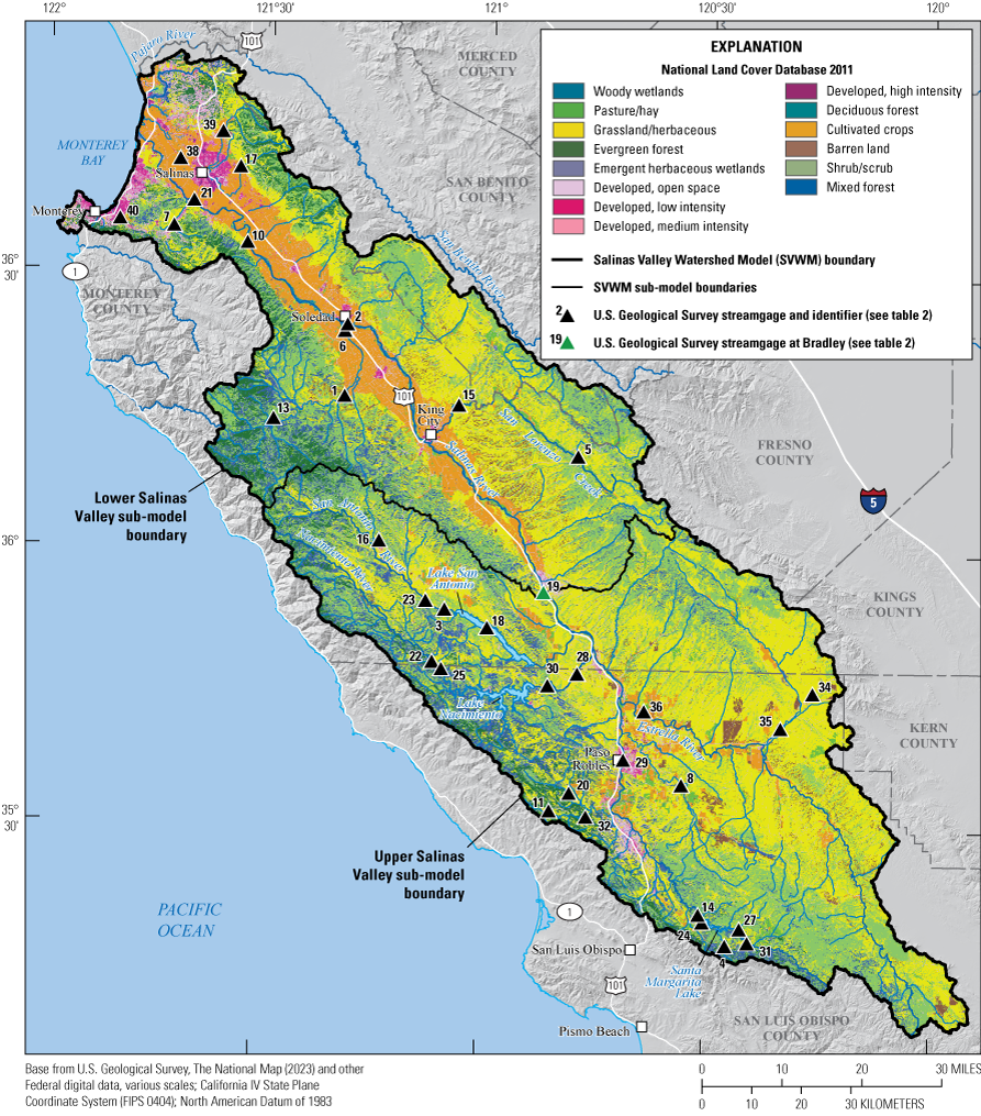
California’s Salinas Valley is one of the most productive agricultural basins in the world (California Department of Food and Agriculture, 2022) due to the fertile valley soil, temperate climate, and availability of water for irrigation (Lapham and Heileman, 1901; Cook, 1978). The groundwater resources of the basin are used heavily to meet water supply needs, including crop irrigation and municipal water supply. To better understand impacts on groundwater resources, the lower Salinas Valley study area was defined as an area of interest for the development and application of a groundwater flow model, referred to as the Salinas Valley Integrated Hydrologic Flow Model (SVIHM; fig. 1; Henson and Jachens, 2022). The lower Salinas Valley study area includes several smaller watersheds draining the coastal region adjacent to the mouth of the Salinas River. Most of the area within the lower Salinas Valley study area consists of extensively farmed alluvial lowlands at elevations approximately less than 500 feet (ft), surrounded by mountainous tributary drainages ranging in elevation from 500 to 5,872 ft (fig. 1).
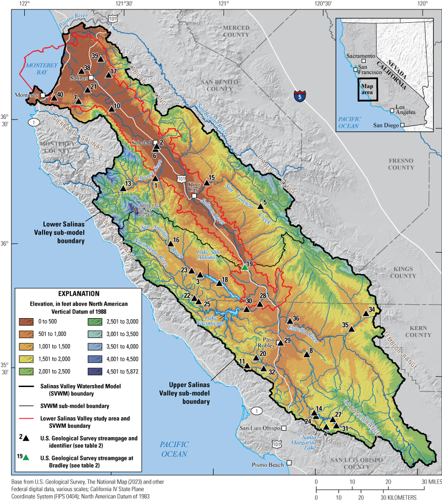
Salinas Valley study area, with land-surface elevation, major rivers and streams, reservoirs, and U.S. Geological Survey streamgages (Henson and others, 2022; U.S. Geological Survey, 2023; Hevesi and others, 2025).
The Salinas River watershed (SRW) and adjacent coastal drainages including the areas of agricultural and groundwater development comprise a total area of 4,529 square miles (mi2), herein referred to as the Salinas Valley study area (fig. 1). The Salinas Valley study area has been experiencing insufficient water supplies, and stakeholders are facing legal and regulatory restrictions on water use. The historical imbalances between supply and demand have resulted in declining groundwater levels (California Department of Public Works, 1946; Monterey County Water Resources Agency, 1995; Baillie and others, 2015), seawater intrusion (California Department of Public Works, 1946; Leedshill-Herkenhoff, Inc., 1985; Monterey County Water Resources Agency, 1995, 1996), impaired water supplies (California Department of Water Resources, 1971; Kulongoski and Belitz, 2007; Moran and others, 2011; Harter and others, 2012), regulatory actions on pumping, adjudication (Monterey County Water Resources Agency, 1995; Baillie and others, 2015), and requirements for minimum in-stream fish flows (Monterey County Water Resources Agency, 2018). Water imbalances are likely to be further exacerbated by potential future climate change and variability, such as longer and more severe drought periods followed by periods with extreme precipitation events (Brown and Caldwell, 2014). Finding replacement water supplies and improving watershed management could help stakeholders comply with legal mandates, adapt to future climate variability and changing land use, and improve environmental and ecohydrological conditions.
The Salinas Valley Watershed Model (SVWM), developed in cooperation with the Monterey County Water Resources Agency, includes an area coincident with the Salinas Valley study area and was developed to simulate the natural hydrologic system of the Salinas Valley study area, with a focus on precipitation-runoff processes and the need to estimate surface-water inflows from mountainous upland areas draining into the area of the SVIHM. Application of the SVWM is intended to improve the understanding of the land-surface and shallow subsurface (soil zone) hydrology of the upland drainages that are tributaries to the main branch of the Salinas River and adjacent developed areas, including groundwater basins and surface-water reservoirs. Results obtained using the SVWM could be used to help develop a broader, more comprehensive analysis of the natural hydrologic system for the entire Salinas Valley study area.
The SVWM was applied to simulate the natural hydrology of the Salinas Valley study area for a 70-year historical climate period from water years 1949 to 2018 (October 1, 1948, to September 30, 2018); a water year is the 12-month period from October 1 through September 30 designated by the calendar year in which it ends. The SVWM uses an integrated modeling approach consisting of the Basin Characterization Model (BCM; Flint and others, 2021) and the Hydrologic Simulation Program—Fortran (HSPF; Bicknell and others, 2005) computer codes to simulate the natural hydrologic system in response to daily climate inputs and the physical characteristics of the surface-water drainages within the Salinas Valley study area. The SVWM simulations account for climate, surface, and shallow subsurface components of the natural hydrologic system, including surface water and shallow groundwater, with an emphasis on natural hydrologic processes at the land surface and in the shallow subsurface, including the upper soil layer and the root zone.
The BCM component of the SVWM was used to develop the historical daily climate inputs for the HSPF component, consisting of daily values of precipitation, air temperature, and potential evapotranspiration (PET). The climate inputs are required to run HSPF for a continuous simulation of the hydrologic system for the 70-year target period. The BCM used a 270-meter (m) gridded representation of the watershed to account for localized orographic effects on precipitation and air temperature and topographic controls on PET.
The HSPF component of the SVWM was discretized as a connected network of 690 hydrologic response units (HRUs) defined by surface hydrography and was run using an hourly time step, with daily and monthly model outputs used for model calibration and for the analysis of simulated water balance components. The HSPF outputs included surface-water outflows from ungaged tributary drainages upstream of the SVIHM and Salinas Valley lowlands that include areas of productive groundwater development. The simulated outflows can be used as inflow boundary conditions for the SVIHM. The results generated by the SVWM are intended to help water managers evaluate and adjust to projected effects on water supplies and demands in the Salinas Valley watershed caused by changes in land use, population, and climate.
Purpose and Scope
The purpose of this study was to develop a precipitation-runoff model, the SVWM, to simulate the surface-water inflows and shallow subsurface components of the natural hydrologic system of the Salinas Valley study area, including all tributary upland areas that provide surface-water inflows to lower elevation areas overlying groundwater basins in the Salinas Valley study area. The SVWM was used to simulate the natural hydrologic system of the Salinas Valley study area from water years 1949 to 2018 with the goal of developing a better understanding of the long-term historical water balance.
This report describes the development, calibration, and application of the SVWM (consisting of the BCM and HSPF model components) to quantify precipitation-runoff processes, including climate, surface-water flow, evapotranspiration (ET), and recharge in the Salinas Valley study area. The specific objectives of this study were to (1) apply the SVWM to quantify the historical distribution of precipitation falling on the land surface, infiltrating the root zone, returning to the atmosphere by ET, contributing to streamflow as overland runoff, percolating through the root zone to become recharge or contributing to streamflow as shallow subsurface interflow or deeper base flow, and flowing through the stream channel network; (2) provide a characterization and historical context of the spatial and temporal variability and distribution of the simulated water balance components; and (3) simulate the water inflows from the tributary drainage basins in the upland areas for potential use as boundary conditions for integrated surface water–groundwater modeling in the Salinas Valley study area.
Study Area
The Salinas River valley is bounded by the Diablo, Temblor, and Gabilan Ranges to the east and the Santa Lucia and Sierra de Salinas Ranges to the west (fig. 1). The SVWM includes the entire Salinas River watershed and several smaller drainages along the Monterey Bay coast that drain into Monterey Bay. The Salinas River is the third longest river in the State of California and is the largest river in California’s Central Coast region, draining an area of 4,160 mi2. The Salinas River originates in the La Panza Range of central San Luis Obispo County and flows 170 miles (mi) north and northwest through Monterey County before discharging into Monterey Bay, about 80 mi south of San Francisco (fig. 1). Major tributaries to the Salinas River include Arroyo Seco, San Lorenzo Creek, and the San Antonio, Nacimiento, and Estrella Rivers (fig. 1).
Land-surface elevations in the SVWM average 1,426 ft and range from 0 ft along the coast to a maximum of 5,872 ft at the summit of Junipero Serra Peak in the Santa Lucia Range and the headwaters of the Arroyo Seco drainage (fig. 1). The general area of the groundwater basin in the SVIHM is approximately defined by the extent of the Salinas Valley alluvial basin and the transition from the valley floor to the steeper terrain of the surrounding uplands (fig. 1). Land-surface elevations within the SVIHM range from 0 to about 2,000 ft at various locations along the SVIHM boundary (fig. 1). Land-surface elevations within the area of the upper Salinas River watershed, upstream of the SVIHM boundary, range from about 100 to about 4,000 ft (fig. 1).
Water Use and Management
The Salinas River watershed contains three reservoirs: Lake Nacimiento and Lake San Antonio, each with an area of about 22 mi2, and Santa Margarita Lake, with an area of about 1.1 mi2 (fig. 1). The reservoirs are used primarily to provide flood protection and are operated for a variety of uses that include municipal water supplies, agricultural irrigation, recreation, groundwater recharge, and protection of fish habitat. The dams impounding Lakes Nacimiento and San Antonio were constructed to control floodwaters and provide water for summer recharge of the Salinas Valley groundwater basin for urban and agricultural use (Brown and Caldwell, 2014). The dam impounding Lake Nacimiento, located in northern San Luis Obispo County approximately 20 mi from the coast, was completed in 1957 (fig. 1) and provides a maximum storage capacity of 377,900 acre-feet (acre-ft). The dam impounding Lake San Antonio, located in southern Monterey County about 16 mi northwest of Paso Robles, was completed in 1967 and provides a maximum storage capacity of 477,000 acre-ft. The management of Lakes Nacimiento and San Antonio, including operation of the dams, is under the jurisdiction of the California Department of Water Resources, Division of Safety of Dams (Brown and Caldwell, 2014).
Climate
The climate in the Salinas Valley study area is characterized by warm, dry summers and cool, moist winters (Baillie and others, 2015). Based on an 80-year average of climate records from 1931 to 2015, from the National Climatic Data Center station at the Salinas airport (station USW00023233 at https://www.ncdc.noaa.gov/cdo-web/datatools/findstation) located on the valley floor, the average annual temperature is 57 degrees Fahrenheit (°F), and the average annual precipitation is 13 inches (in.) falling as rain primarily during the winter and early spring. The distribution of precipitation across the study area is dependent on the topography, prevailing winds, and proximity to the coastline (Daly and others, 2004). Precipitation generally increases with increasing altitude due to orographic lifting and adiabatic cooling of moist air, but also decreases with increasing distance from the coastline, such that the higher land elevations for summit locations on the east side of the Salinas Valley receive less precipitation compared to equivalent land elevations on the west side of the valley (Tinsley, 1975; Montgomery–Watson Consulting Engineers, 1994; Daly and others, 2004).
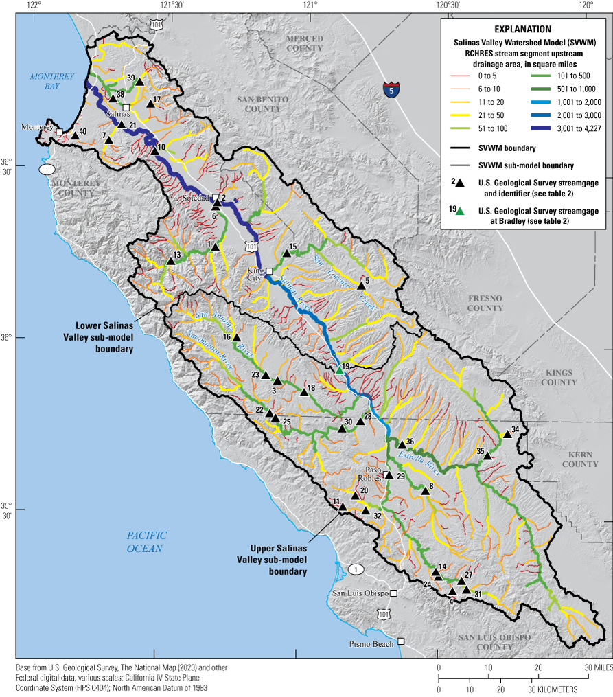
Hydrography
For reasons discussed in the “Model Layout and Discretization” section, the SVWM was divided into two sub-model areas south and north of the U.S. Geological Survey (USGS) streamgage 11150500 (gage 19, Salinas River at Bradley; in this report, streamgage is synonymous with gage; the streamgage numbering sequence does not include numbers 9, 12, 26, 33, and 37; fig. 2); the upper Salinas Valley sub-model (USVS), south of the streamgage and the lower Salinas Valley sub-model (LSVS), north of the streamgage (fig. 2; tables 1, 2). In addition to the two sub-model areas, the Salinas Valley study area was further subdivided into 10 surface-water subbasins and 28 surface-water subdrainages (figs. 2, 3; tables 1, 3). The subbasins and subdrainages were used in this study to analyze and compare characteristics and model results for different parts and tributaries of the study area. The subbasin and subdrainage areas were defined based on hydrography, including the location of tributary junctions, drainage areas, streamgages, and reservoirs. The USVS and LSVS each include 5 subbasins and 14 subdrainages.
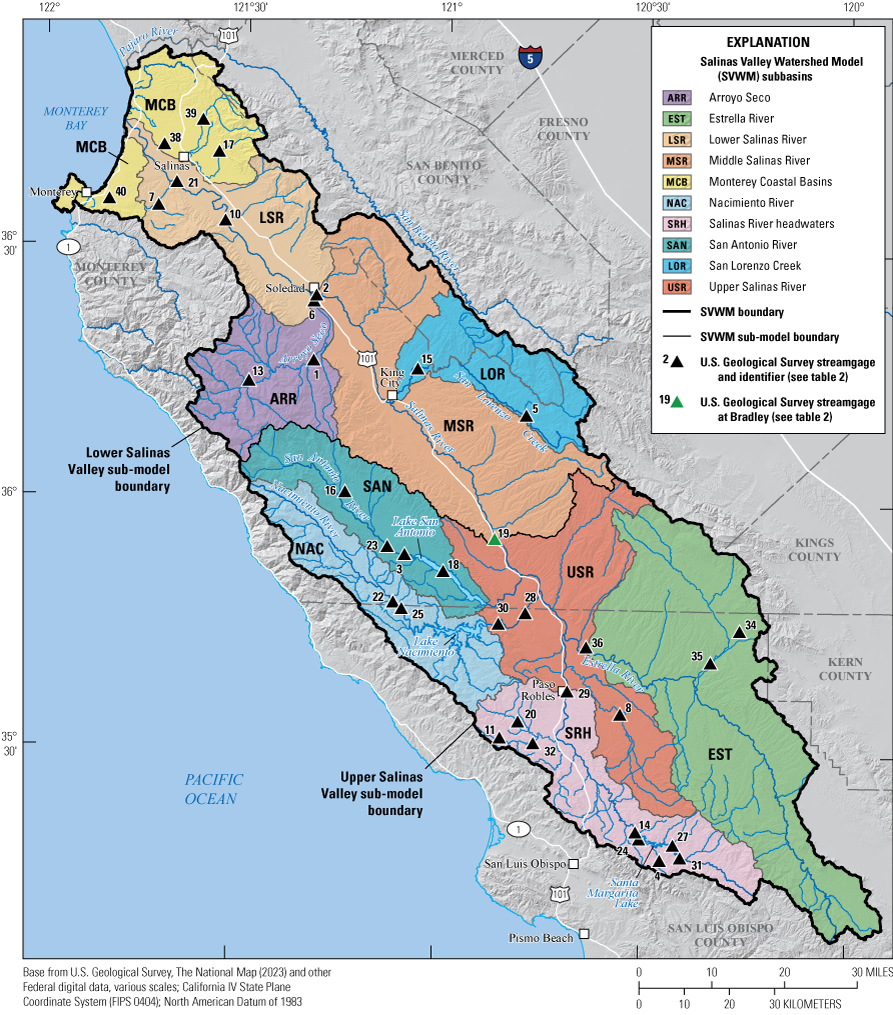
Surface-water subbasins in the Salinas Valley study area (Hevesi and others, 2025).
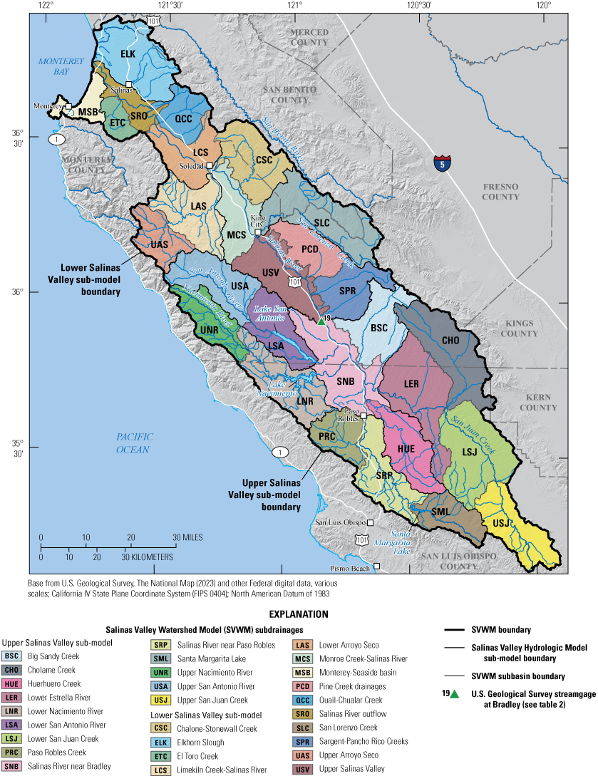
Surface-water subdrainages in the Salinas Valley study area (Hevesi and others, 2025).
Table 1.
Subbasin areas and topographic characteristics of subbasins in the Salinas Valley study area.[Subbasins and sub-models are listing in order of upstream to downstream tributary connections. Abbreviations: mi2, square mile; Min, minimum; Max, maximum; —, not applicable]
Table 2.
U.S. Geological Survey (USGS) streamgages in the Salinas Valley study area with daily streamflow records between water years 1948 and 2018.[ID, identification; mi2, square mile; mm/dd/yyyy, month/day/year; SVWM, Salinas Valley Watershed Model]
Table 3.
Subdrainage areas and topographic characteristics of subdrainages in the Salinas Valley study area.[Subdrainages are listing in order of upstream to downstream tributary connections. Abbreviations: mi2, square mile; Min, minimum; Max, maximum]
The Estella River (EST) subbasin drains the southeastern part of the SVWM and includes four subdrainages: the Cholame Creek (CHO), the upper and lower San Juan Creek (USJ and LSJ) subdrainages, and the lower Estrella River (LER) subdrainage. The Salinas River headwaters (SRH) subbasin drains the southwestern part of the SVWM and includes the Santa Margarita Lake (SML), Salinas River near Paso Robles (SRP), and Paso Robles Creek (PRC) subdrainages. The upper Salinas River (USR) subbasin drains the south-central part of the SVWM, upstream of gage 19 and downstream of the city of Paso Robles, and includes the Huerhuero Creek (HUE), Big Sandy Creek (BSC), and Salinas River near Bradley (SNB) subdrainages. The Arroyo Seco (ARR), San Antonio River (SAN), and Nacimiento River (NAC) subbasins drain the western part of the SVWM with each subbasin including upper and lower subdrainages; the upper and lower Arroyo Seco (UAS and LAS) in the ARR, the upper and lower San Antonio River (USA and LSA) in the SAN, and upper and lower Nacimiento River (UNR and LNR) in the NAC. The middle Salinas River (MSR) subbasin includes five subdrainages in the west-central part of the SVWM downstream of gage 19 and upstream of USGS streamgage 11151700 (gage 6, Salinas River at Soledad): the Sargent–Pancho Rico Creeks (SPR), Pine Creek drainage (PCD), upper Salinas Valley (USV), Chalone–Stonewall Creek (CSC), and Monroe Creek–Salinas River (MCS) subdrainages. The San Lorenzo Creek (SLC) subdrainage is coincident with the San Lorenzo Creek (LOR) subbasin and is a major tributary to the MSR subbasin, draining the eastern side of the Salinas River valley. The lower Salinas River (LSR) subbasin includes four subdrainages in the lower Salinas Valley between gage 6 and the mouth of the Salinas River: the Limekiln Creek–Salinas River (LCS), Quail–Chualar Creek (QCC), El Toro Creek (ETC), and Salinas River outflow (SRO) subdrainages. The Monterey Coastal Basin (MCB) subbasin includes two separate areas consisting of several small drainages emptying into Monterey Bay: the Elkhorn Slough (ELK) subdrainage adjacent to the northeastern side of the SRO subdrainage and the Monterey–Seaside basin (MSB) subdrainage adjacent to the southwestern side of the SRO.
Physiography
An important characteristic of the Salinas Valley study area is the substantial amount (more than 3,000 ft) of topographic relief on both sides of the valley, particularly the central valley, and between the headwaters and mouth of the Salinas River (fig. 1; table 1). Based on the National Elevation Dataset (U.S. Geological Survey, 2023), the mean land-surface elevation of the Salinas Valley study area is 1,425 ft above the North American Vertical Datum of 1988 (NAVD 88) and ranges from a minimum of 0 ft at the mouth of the Salinas River to a maximum of 5,872 ft at the summit of Junipero Serra Peak in the headwaters of the Arroyo Seco drainage along the western boundary of the SRW (fig. 1). Relief in the UAS and LAS subdrainages and the USA subdrainage on the west side of Salinas Valley is about 5,000 ft. The relief in the LCS and SLC subdrainages on the east side of the valley is more than 4,000 ft (figs. 1, 3; table 3).
The land-surface slope is generally greatest in the headwater drainages along the western and eastern boundaries of the SRW. Calculated as rise over run, land-surface slope is less than 0.l for most of the valley floor and locations along the coastal plain, and it increases to more than 0.3 for most of the more rugged terrain in the upland areas, reaching values as high as 1.0–2.37 for steeper slopes and canyons in the uplands on both sides of the valley (fig. 4; table 1). The high relief and comparatively steep slopes for many of the tributary drainages to the Salinas River result in rapid runoff response times and accumulation of channelized streamflow during storms, often referred to as flashiness in the characteristics of streamflow.
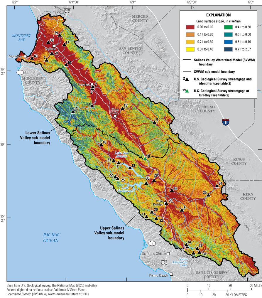
Land-surface slope, calculated as rise over run, in the Salinas Valley study area (U.S. Geological Survey, 2023; Hevesi and others, 2025)
Streamflow
The characteristics of high relief and mountainous terrain combined with a focused distribution of annual precipitation from a limited number of winter (December–March) storms result in large variations in streamflow, seasonally and between peak and mean streamflow conditions (fig. 5). Mean monthly streamflow in February ranges from about 1,200 to 1,450 cubic feet per second (ft3/s) at three streamgages along the main branch of the Salinas River (USGS streamgages 11150500 [gage 19], 11152300 [gage 10], and 11151700 [gage 6]), in the middle and LSR subbasins, compared to mean monthly flows of about 220 ft3/s and less from October to December at these locations (fig. 5A). Controlled reservoir releases from May to September cause increased mean monthly streamflow of as much as about 500 ft3/s at USGS streamgage 11150500 (gage 19); however, mean monthly streamflow is less than 200 ft3/s at USGS streamgages 11152300 (gage 10) and 11151700 (gage 6), downstream from USGS streamgage 11150500 (gage 19). Maximum monthly streamflows are approximately an order of magnitude greater than mean monthly flows along the Salinas River and minor tributaries (figs. 5B, F) and about five times greater for major tributaries (fig. 5D). Mean monthly July–October streamflow of about 15 ft3/s and less for major tributaries and 2 ft3/s and less for minor tributaries are very low compared to January–March flows of more than 200 ft3/s for major tributaries and more than 35 ft3/s for minor tributaries (fig. 5A).
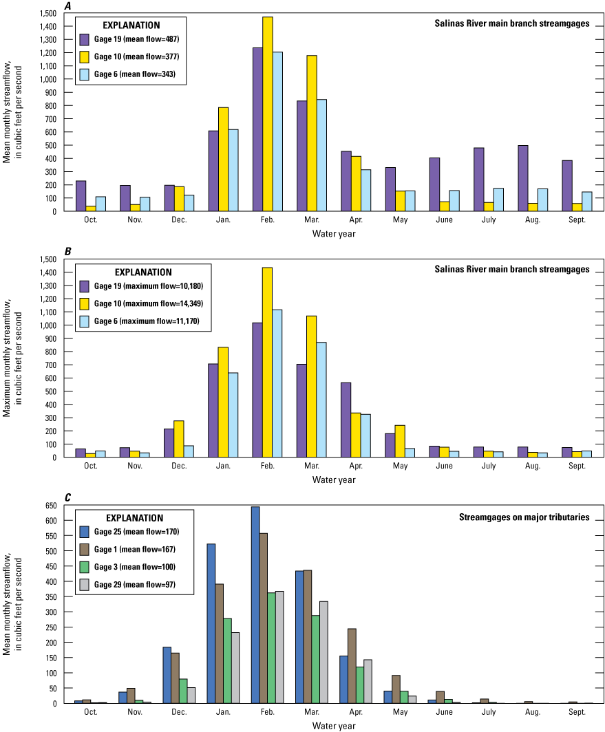
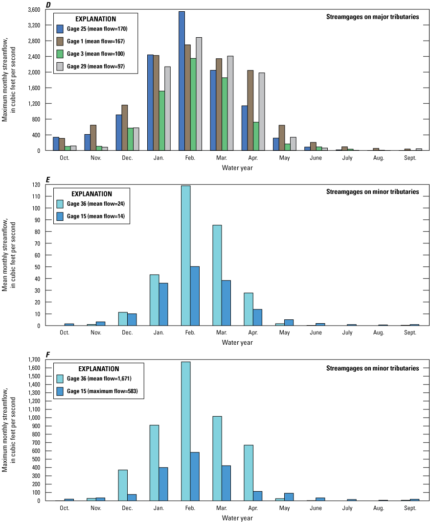
Monthly streamflow at selected streamgages in the Salinas Valley study area; A, mean monthly streamflow at three streamgages on the Salinas River; B, maximum monthly streamflow at three streamgages on the Salinas River; C, mean monthly streamflow at major tributaries to the Salinas River and the Salinas River headwater subbasin; D, maximum monthly streamflow at major tributaries to the Salinas River and the Salinas River headwater subbasin; E, mean monthly streamflow at two minor tributaries to the Salinas River; and F, maximum monthly streamflow at two minor tributaries to the Salinas River (U.S. Geological Survey, 2016; Hevesi and others, 2022, 2025).
An important characteristic of streamflow in the Salinas River is that mean flows are not the highest at the mouth of the river. The long-term average streamflow close to the mouth of the Salinas River to Monterey Bay, as measured at the USGS streamgage 11152500 (gage 21, fig. 1), is approximately 333 ft3/s or about 241,000 acre-feet per year (acre-ft/yr). In comparison, the average flow at USGS streamgage 11152300 (gage 10) is 377 ft3/s, the average flow at USGS streamgage 11151700 (gage 6) is 343 ft3/s, and the average flow at USGS streamgage 11150500 (gage 19) is 487 ft3/s. The differences in streamflow between the streamgages on the main branch of the Salinas River indicate a loss of streamflow likely caused by seepage through the streambed and into the underlying unsaturated zone along a section of the channel where the water table is lower than the streambed elevation.
Characteristics of streamflow in the SRW also include managed streamflow conditions downstream from the reservoirs, particularly Lake Nacimiento. In addition to controlled releases from Lake Nacimiento and Lake San Antonio to augment crop irrigation during the dry summer months, a portion of the Salinas River outflow to Monterey Bay occurs in response to controlled releases for environmental purposes to promote the threatened anadromous steelhead run in the Central Coast (Brown and Caldwell, 2014). Controlled reservoir releases are indicated by mean monthly streamflows greater than 400 ft3/s for the months of July and August at USGS streamgage 11150500 (gage 19; Salinas River near Bradley, downstream from the NAC junction; figs. 1, 5A) and to a lesser degree at USGS streamgage 11151700 (gage 6; Salinas River at Soledad; fig. 1), with mean monthly streamflows of more than 150 ft3/s during July and August (fig. 5A).
Groundwater
Groundwater flow generally follows the topography of the Salinas Valley study area, going from the mountain ranges, down to the Salinas Valley floor and then flowing toward Monterey Bay (Hamlin, 1904; Jenkins, 1943; Simpson and others, 1946; Kennedy Jenks L.L.C., 2004). Sources of groundwater recharge include percolation of precipitation, streamflow infiltration, and return flows from agricultural irrigation. The primary source of groundwater discharge in the Salinas Valley is through the pumping of wells (Hamlin, 1904; Simpson and others, 1946; Monterey County Water Resources Agency, 2006; Burton and Wright, 2018). A significant portion of runoff that originates in the uplands and contributes to streamflow in the middle and lower reaches of the Salinas River channel does not reach Monterey Bay, but rather infiltrates the riverbed and recharges the valley-fill aquifers that are subsequently pumped for irrigation or municipal use (Montgomery–Watson Consulting Engineers, 1994; Fugro West, Inc., 1995; Harding ESE, 2001; Kennedy Jenks L.L.C., 2004). Some of the infiltrated streamflow also may contribute to riparian ET.
Natural groundwater recharge to the Salinas Valley occurs during the wet winter months (December–March) as infiltrated streamflow from the Salinas River; with major inflows from the Arroyo Seco, Nacimiento, and San Antonio Rivers; as infiltrated streamflow from smaller tributaries, and as direct percolation from precipitation (Brown and Caldwell, 2014). Evidence of infiltrated streamflow is indicated by the streamflow records along the main branch of the Salinas River, with decreasing streamflow occurring at downstream streamgages. The natural groundwater recharge in the Salinas Valley occurring in response to winter precipitation is augmented during the late spring and summer months by controlled releases from Lakes Nacimiento and San Antonio.
Land Cover
Land cover can have an important effect on surface hydrology in terms of interception and retention storage and surface roughness affecting infiltration and overland flow. In addition, differences in vegetation type can result in substantial differences in ET. As defined by the 30-m resolution National Land Cover Database (NLCD) in 2011 (U.S. Geological Survey, 2014), natural vegetation constituted about 82 percent of the total land cover in the Salinas Valley study area, consisting mostly of grasslands and shrublands for most subdrainages, especially the mid to lower elevation subdrainages in the eastern and southeastern parts of the Salinas Valley watershed (figs. 3, 6; table 4). In contrast, forestlands have the highest percentage of land cover for several subdrainages along the wetter western side of the Salinas Valley watershed, including the UAS, PRC, and LNR subdrainages. The percentage of shrubland is about the same for the USVS and LSVS sub-model areas, whereas the USVS area includes a higher percentage of grassland and a lower percentage of cultivated crop areas compared to the LSVS. The coastal subdrainages, including the LSV, ELK, and MSB, contain the highest percentages of combined low, medium, and high-density developed lands (about 11–33 percent). The lowest elevation subdrainages generally contain the highest percentage of developed open space (about 17 percent). Open water comprises only about 0.5 percent of the land cover in the Salinas Valley study area.
National Land Cover Data (NLCD) 2011 land cover types in the Salinas Valley study area (U.S. Geological Survey, 2014).
Table 4.
National Land Cover Data (NLCD) 2011 land cover types, as a percentage of subdrainage and sub-model areas, for the Salinas Valley study area.[Subdrainages are listed in order of upstream to downstream tributary connections. Abbreviation: Cult., cultivated; —, not applicable]
The 2011 NLCD 30-m resolution, percentage of forest canopy cover supplements the NLCD land cover types and provides an additional measure of the density of tree cover. As with land cover type, forest canopy cover is an important characteristic affecting interception storage and ET. The percentage of canopy cover based on NLCD averages about 11 percent in the Salinas Valley study area and ranges from 0 percent throughout the study area to a maximum of 93 percent in the Monterey Coastal subdrainage (fig. 7; table 5). In general, the wetter and cooler western side of the Salinas Valley has a higher percentage of canopy cover, with greater than 20 percent average canopy cover for many subdrainages, compared with the eastern side of the valley, with less than 10 percent average canopy cover for many subdrainages. Several subdrainages in the coastal region also have comparatively higher average canopy cover resulting from higher precipitation and lower PET demand compared to inland areas.
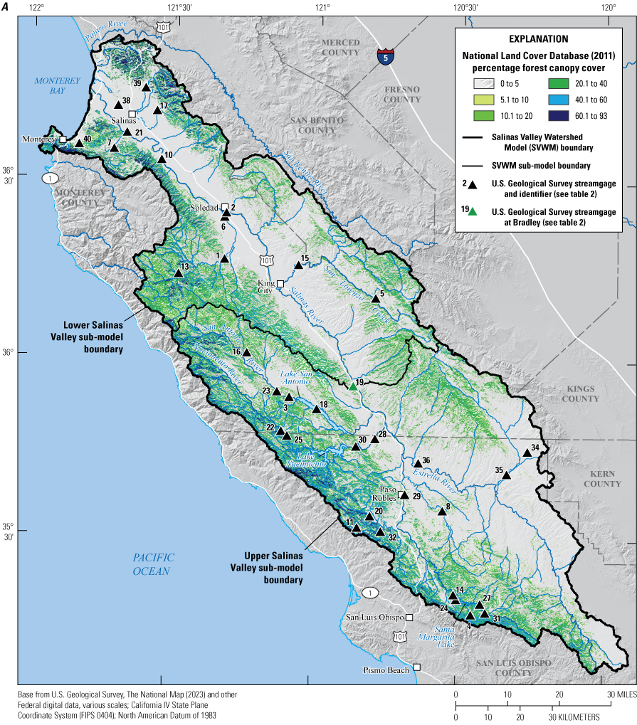
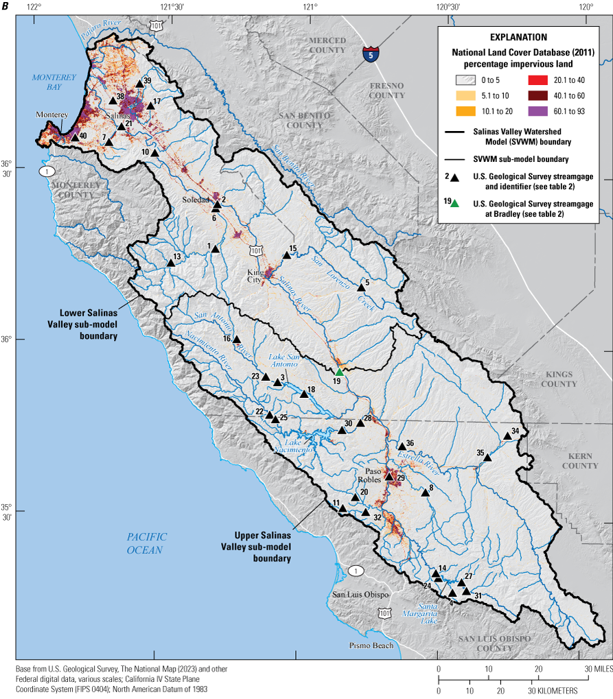
National Land Cover Database (NLCD) 2011 percentage of A, forest canopy cover and B, impervious land cover in the Salinas Valley study area (U.S. Geological Survey, 2014).
Table 5.
National Land Cover Database (NLCD) 2011, percentage of forest canopy and percentage of impervious area for subdrainage and sub-model areas, Salinas Valley study.[Subdrainages are listed in order of upstream to downstream tributary connections. Abbreviations: ARR, Arroyo Seco; EST, Estrella River; LOR, San Lorenzo Creek; LSR, lower Salinas River; MSR, middle Salinas River; NAC, Nacimiento River; SAN, San Antonio River; SD, standard deviation; SRH, Salinas River headwaters; USR, upper Salinas River; —, not applicable]
The 2011 NLCD 30-m resolution impervious land cover dataset indicates the percentage coverage of impervious developed lands such as parking lots, roads, and rooftops. Impervious land cover can have a significant localized effect on runoff generation and streamflow in terms of increased peak flows, increased flow volumes, and an overall increase in the flashiness of runoff. Impervious land cover, based on the 2011 data, averages only 1.2 percent of the total land area within the Salinas Valley study area (fig. 7; table 5). However, in subdrainages with population centers such as the cities of Salinas, Seaside, and Paso Robles, the percentage of impervious land cover can be as high as 100 percent locally. The average percentage of impervious cover is higher for the subdrainages in the coastal region, ranging from about 6 to 18 percent impervious land, compared to most of the more remote inland subdrainages with an average impervious cover of 0.2 percent and less.
Soils
Soils properties affecting hydrologic processes include the soil storage capacity and soil hydraulic conductivity, both of which can be highly variable because of differences in soil thickness, texture, and structure. Soil texture, including grain-size distribution and structure, are important properties affecting water infiltration and percolation. The available water capacity of soils is an indicator of the potential amount of water available for plant transpiration when precipitation (or irrigation) is not limited and is dependent on soil texture and thickness. Soils with high permeability and storage capacities tend to favor recharge over runoff, depending on climate and the hydraulic conductivity of the underlying bedrock or alluvium.
Soil texture classes, defined according to particle size distribution based on the Soil Survey Geographic database (SSURGO; U.S. Department of Agriculture [USDA], 2017), range from clayey to fine soils to coarse-loamy and sandy-skeletal soils in the Salinas Valley study area (fig. 8; table 6). Fine-loamy soils are the most prevalent basinwide soil texture for the USVS and LSVS areas. On the scale of subdrainages, however, soil texture is variable, with clayey-skeletal soils being the most prevalent in 4 of the 28 subdrainages, and loamy soils being most prevalent in 4 different subdrainages. Clayey to fine soils are most prevalent in the LNR and ELK subdrainages, whereas sandy soil is the most prevalent in the MSB subdrainage, and loamy-skeletal soil is the most prevalent in the UAS subdrainage.
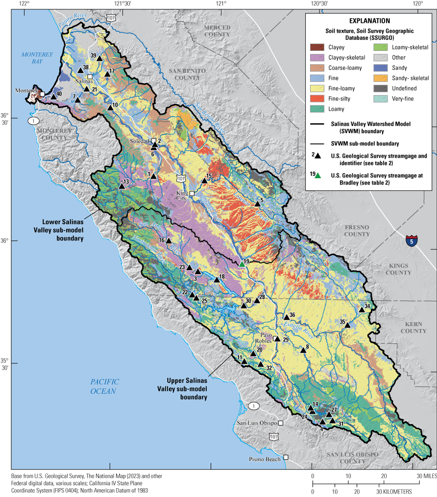
Soil Survey Geographic database information on soil texture classes in the Salinas Valley study area (U.S. Department of Agriculture, 2017).
Table 6.
Soil Survey Geographic database (SSURGO) soil texture classes for subdrainage areas in the Salinas Valley study area.[Subdrainages are listed in order of upstream to downstream tributary connections. Abbreviations: ARR, Arroyo Seco; EST, Estrella River; LOR, San Lorenzo Creek; LSR, lower Salinas River; MCB, Monterey Coastal Basins; MSR, middle Salinas River; NAC, Nacimiento River; SAN, San Antonio River; SRH, Salinas River headwaters; USR, upper Salinas River; —, not applicable]
The available water capacity for soils in the study area, based on SSURGO data for a maximum soil thickness of 150 centimeters (cm; about 5 ft), averages 4.5 in. and varies from 0 to 16.5 in. (fig. 9). High soil storage capacities of 8.5 in. and more are generally located in the larger valley bottoms where medium to fine-grained (clayey and loamy) soils overlay unconsolidated valley-fill sediments and tend to be the thickest compared to locations on hillsides. In comparison, low available water capacities of 2.5 in. and less are dominantly located at the higher elevations of headwater areas with steep slopes and relatively thinner coarser-grained soils. Locations with very low soil storage capacities of 0.5 in. and less occur throughout the upper parts of the ARR, SAN, and NAC subdrainages, coinciding with locations having the steepest terrain within the study area and locations having clayey-skeletal, loamy-skeletal, and undefined soils. Locations with intermediate available water capacities from 4.5 to 8.5 in. include the uplands on the eastern side of the valley and the central region of the upper Salinas Valley and tend to be coincident with more intermediate slopes and finer, well-structured soils underlain by sedimentary rocks.
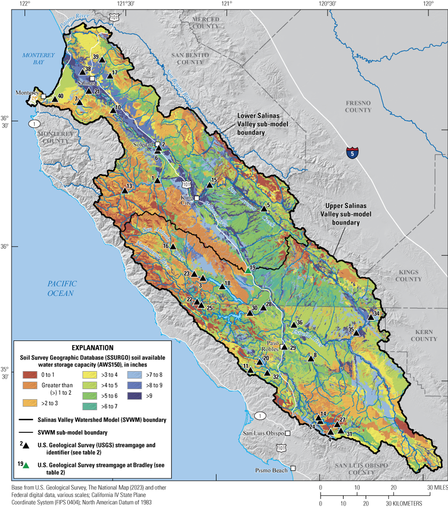
Soil Survey Geographic database (SSURGO) soil available water storage capacity up to 150 centimeters soil depth, Salinas Valley study area (U.S. Department of Agriculture, 2017).
Generalized Surface Geology
In addition to topography, land cover, and soils, surficial geology consisting of unconsolidated deposits and consolidated rock forming the land surface is an important characteristic affecting the hydrologic system of the Salinas Valley study area. Alluvium and porous sedimentary rocks with high permeability are more conducive to recharge rather than runoff generation, whereas shales, siltstones, and igneous and metamorphic rocks with low permeability are more conducive to runoff generation.
The Salinas Valley study area includes a wide variety of different rock types, from unconsolidated alluvium to consolidated sediments and igneous, metamorphic, and volcanic rock types (fig. 10; table 7). The dominant consolidated rock type outcropping in the Salinas Valley study area is conglomerate, mostly throughout the USR watershed, followed by unconsolidated alluvium consisting of valley-fill sediments and river wash deposits. Sandstone and siltstone are present throughout the western side and east–central side of the valley, respectively. Shale and siltstone are present throughout most of the Nacimiento subdrainage, and igneous and metamorphic rocks crop out in the upland areas of the LSVS, the UAS subdrainage, and the upper parts of the SRH subbasin. Volcanic rocks are the least common consolidated rock type outcropping in the SVWM, located mostly in the uplands adjacent to the northeastern boundary of the SVWM.
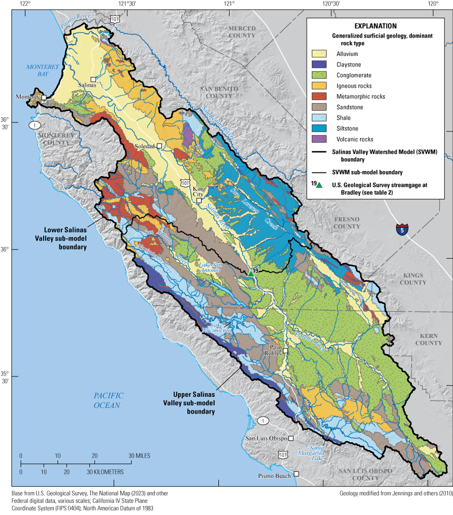
Generalized California surficial geology for the Salinas Valley Watershed Model (SVWM) study area (Jennings, 1977).
Table 7.
Generalized surficial geology for subdrainage areas in the Salinas Valley study area.[Subdrainages are listed in order of upstream to downstream tributary connections. Abbreviations: ARR, Arroyo Seco; EST, Estrella River; LOR, San Lorenzo Creek; LSR, lower Salinas River; MCB, Monterey Coastal Basins; MSR, middle Salinas River; NAC, Nacimiento River; SRH, Salinas River headwaters; USR, upper Salinas River; —, not applicable]
Model Development
Development of the SVWM required nine generalized steps: (1) defining the model domain; (2) defining a conceptual model and simplifying assumptions appropriate for the intended model application; (3) selecting an appropriate model code to simulate selected processes of the natural hydrologic system; (4) selecting the simulation period; (5) estimating the initial conditions; (6) defining the model boundary, layout, and spatial discretization; (7) developing climate inputs consisting of spatially interpolated daily precipitation, maximum and minimum daily air temperature, and simulated daily PET; (8) estimating initial values for model parameters representing the physical characteristics of the Salinas Valley study area; and (9) performing model calibration to refine and finalize parameter values. These nine steps are described in more detail in the subsections below.
Model Domain
The SVWM model domain was defined mostly by surface-water drainage divides based on hydrologic unit code 12 boundaries (HUC-12, https://water.usgs.gov/GIS/huc.html; Seaber and others, 1987), with minor modifications using National Hydrography Dataset (NHD) flowlines and flow directions based on calculated land-surface slope using 10-m (98.4-ft) resolution digital elevation data. The 4,530 mi2 SVWM area includes 35 complete or partial HUC-12 areas.
The SVWM domain encompasses the entire SRW and smaller coastal drainages along the Monterey Bay coastline adjacent to the Salinas River outflow (figs. 2, 3). The SVWM consists of two connected HSPF sub-model components: the 2,540 mi2 USVS and the 1,990 mi2 LSVS (fig. 2) that are connected in the upper Salinas Valley at the Salinas River USGS streamgage 11150500 (gage 19, near Bradley; fig. 2; table 2). All surface-water outflows from the USVS enter the LSVS at this streamgage location.
Conceptual Model
The components of the natural hydrologic system represented by the SVWM include climate (precipitation and maximum and minimum air temperature), PET, ET, soil moisture, runoff, interflow, baseflow, recharge, and streamflow for the Salinas Valley study area. The SVWM was developed using the BCM (Flint and others, 2021) and the HSPF (version 12.4; Bicknell and others, 1997, 2005). The daily climate inputs required by HSPF are provided by the BCM (precipitation maximum and minimum air temperature and PET).
The HSPF application is a widely used and well documented modeling program originally developed and supported by the U.S. Environmental Protection Agency and USGS in 1984 and based on the Stanford Watershed Model (Bicknell and others, 2001, 2005). The HSPF application has been used extensively for hydrologic studies covering a broad range of areas and for a variety of objectives (Atkins and others, 2005; Amirhossien and others, 2015; Stern and others, 2016). Documentation of HSPF version history and the use and theory that led to the development of HSPF is widely available (Donigian and Imhoff, 2009). The conceptual model of the natural hydrologic system represented by the SVWM is based on the HSPF algorithm.
The HSPF computer program is a semi-distributed, process-based, mostly deterministic, and continuous-simulation algorithm for simulating water flow and storage processes with options for simulating water quality and transport processes (Donigian and others, 1984; Bicknell and others, 2001). Applications of HSPF can be used to simulate basin response to normal and extreme precipitation (or lack of precipitation) and to simulate spatial and temporal variability and trends in climate; to evaluate water budgets and water quality; and to evaluate changes in the hydrologic system, such as flow regimes, flood peaks and volumes, soil-water relationships, and groundwater recharge. Through parameter optimization and sensitivity analysis, models developed using HSPF can be calibrated to multiple streamgages to reflect a variety of physiographic characteristics.
Hydrologic processes simulated by HSPF include pervious and impervious surface storage (including interception and retention storage), pervious and impervious surface runoff (overland flow), pervious land infiltration, soil water storage, percolation, ET, interflow, recharge, streamflow, stream losses to evaporation and seepage, and shallow (active) groundwater reservoir storage and discharge (baseflow) contributions to streamflow and riparian ET (fig. 11; Bicknell and others, 2005). The HSPF model provides a comprehensive simulation of rainfall-runoff and streamflow processes, allowing for analysis of surface and shallow subsurface-water budget components and processes such as soil moisture, ET, and recharge for inter-channel areas and components of streamflow (overland runoff, interflow, baseflow, and streamflow seepage) for intra-channel areas.
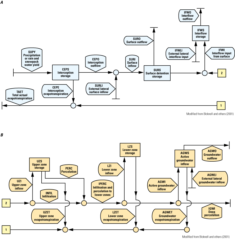
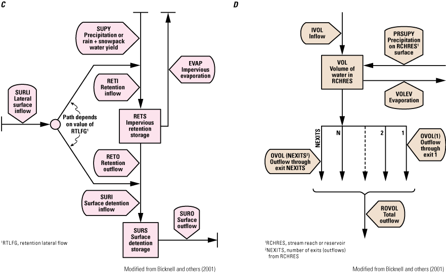
Diagram of water flow and storages simulated by the Hydrologic Simulation Program—Fortran (HSPF): A, surface storage and flow processes simulated on pervious land areas; B, subsurface storage and flow processes simulated in the subsurface underlying pervious land areas; C, surface storage and flow processes simulated on impervious surfaces; and D, streamflow simulated in channels (Bicknell and others, 2005) Abbreviations: NEXITS, number of outflow exits from a RCHRES; RCHRES, stream reach or reservoir in HSPF.
The dominant components of the HSPF conceptual model are the surface and shallow-subsurface (primarily the root zone), stream channels, and larger water bodies (lakes and reservoirs). The surface and shallow-subsurface systems include the plant canopy, land surface, soil zone, and groundwater reservoir supplying groundwater discharge to the stream channels. The plant canopy includes natural vegetation, crops, and landscaped urbanized areas. Two types of land surfaces are represented by HSPF: (1) pervious land areas (PERLNDs) and (2) impervious land areas (IMPLNDs), which are further broken down according to soil type, land cover type, vegetation density, geology, and topography. Pervious land areas represent natural and developed land areas with soil cover, and IMPLNDs represent impervious developed land surfaces, such as rooftops, roads, and parking lots.
Each PERLND is partitioned into several storage zones, including interception storage, surface detention (upper zone) storage, interflow storage, root-zone (lower-zone) storage representing soils and the upper subsurface of consolidated or unconsolidated rock underlying PERLNDs (for example, fractured or weathered bedrock), and active groundwater storage (Bicknell and others, 2005). The lower zone storage is conceptually defined as extending from the ground surface to the base of the root zone. Pervious land areas are used to simulate the storage and transfer of water to the atmosphere as ET, shallow subsurface flow through the soil to stream channels as interflow, and deeper percolation to groundwater reservoirs as recharge.
The HSPF layout for the SVWM was configured such that all runoff generated by the PERLND and IMPLND model components (including overland runoff, interflow runoff, and groundwater discharge) is routed to a single stream reach or reservoir (RCHRES) model component. In addition to receiving inflows from upstream PERLNDs and IMPLNDs, RCHRESs along the downstream sections of flow paths receive inflows from one or more tributary RCHRESs. Streamflow through the connected stream network is simulated using the kinematic wave approximation of the Saint-Venant equations of one-dimensional channel flow, where water accumulated in each RCHRES from contributing land areas and upstream RCHRESs is routed to the downstream RCHRES.
The Hydrologic Simulation Program—Fortran uses a simplified representation of the deeper subsurface below the root zone that includes the groundwater-flow system. Recharge to the groundwater system is partitioned between active and inactive groundwater reservoirs. Water that is stored in the active groundwater reservoir is available for ET and groundwater discharge to streams, whereas recharge to the inactive groundwater reservoir is an outflow from the hydrologic system simulated by HSPF. The simplified representation accounts for the component of total streamflow that originates as groundwater discharge to stream channels (also referred to as the baseflow component of streamflow), which is important for model calibration and the simulation of water budgets. The inactive groundwater reservoir is used to represent outflows from the hydrologic system that are not explicitly defined by the HSPF model, such as pumping, groundwater underflows across basin boundaries, or increases to deep aquifer storage (deep recharge).
In the conceptual model applied for the SVWM, irrigation and flow diversions were assumed to be minor compared to precipitation, especially in the upland areas of the Salinas Valley study area where the percentage of irrigated agricultural land is small. Furthermore, it was assumed in the conceptual model that most of the irrigation water is returned to the atmosphere by ET. Reservoir operations were not simulated by the SVWM. However, the daily water budgets in the subdrainages contributing water inflows to the reservoir areas in response to precipitation were simulated. Modules in HSPF used to simulate snowfall, snow storage, and snowmelt were not activated in the SVWM; all precipitation was simulated as rain. Although snowfall can occur at higher elevations in the SVWM study area, the accumulation and subsequent melting of snow was not considered to be a significant factor affecting the natural hydrologic system of the Salinas Valley study area.
Simulation Period and Initial Conditions
The SVWM was run using an hourly time step to simulate a continuous daily water balance for each HRU and RCHRES. Daily climate inputs developed by the BCM were partitioned into hourly increments for the HSPF simulation. The target simulation period used for the SVWM started with water year 1949 (October 1, 1948) and ended with water year 2018 (September 30, 2018). The target simulation period was intended to provide an estimate of the historical natural water balance and to allow for a sufficiently long period of time to analyze the spatial and temporal variability of water-balance components, including ET, surface- and subsurface-water storage, recharge, and streamflow.
Precipitation-runoff models generally require an initialization period to help minimize uncertainties associated with the assumed or estimated initial conditions (Markstrom and others, 2008; Hevesi and others, 2019). The SVWM simulations were run starting on October 1, 1947, to provide for a 1-year initialization period (water year 1948) before the target simulation period (water years 1949–2018) to reduce the effect of transients associated with initial conditions specified at start-up. The initial conditions include water contents for interception storage, retention storage, soil moisture (upper and lower zones), interflow storage, and active groundwater storage that were either set to zero or based on values defined in the HSPF manual (Bicknell and others, 2005).
Model Layout and Discretization
The SVWM discretization is used to account for the spatially varying physical characteristics of the Salinas Valley study area, including spatial heterogeneity in topography, vegetation and land cover, soils, geology, water bodies, and climate. The discretization also is used to define the various tributary surface-water drainages connected to the main channel of the Salinas River, the smaller drainages along the Monterey Bay coast, and drainages supplying boundary inflows from upland areas to the lower elevation developed land areas of the Salinas Valley.
The HRU is the basic homogeneous model segment used to spatially partition and discretize the SVWM domain. The SVWM was discretized such that each HRU contains a single PERLND connected to a single RCHRES, with the network of connected RCHRESs representing the natural surface-water drainage system of the Salinas Valley study area as a one-dimensional flow routing network.
Outflows from each HRU are ET, surface-water discharges to RCHREs, and inflows to the inactive groundwater reservoir. Surface-water discharges from HRUs to RCHRESs are overland runoff, interflow, and groundwater discharge from the active groundwater reservoir. Water storage, inflows, and outflows are simulated as a water-equivalent depth for the area of each HRU and groundwater reservoir associated with each HRU. Inflows to each RCHRES are hourly rainfall, outflows from the connected HRU, and surface-water inflows from upstream RCHRESs.
The SVWM discretization includes 690 HRUs, ranging in area from 65 to 25,376 acres (0.1–39.6 mi2), with mean HRU land-surface elevations ranging from 12 to 4,252 ft (fig. 12). The HRU delineation was developed using irregular-polygon areas representing surface-water sub-drainages that were defined using a combination of 10-m (98-ft) digital elevation models (DEMs), the NHD streamlines and sub-drainage boundaries (U.S. Geological Survey, 2019), and Calwater version 2.2.1 watershed areas (California Department of Forestry and Fire Protection, 2004).
Mean land-surface elevation for 690 hydrologic response units (HRUs) used in the Salinas Valley Watershed Model (SVWM; U.S. Geological Survey, 2023; Hevesi and others, 2025).
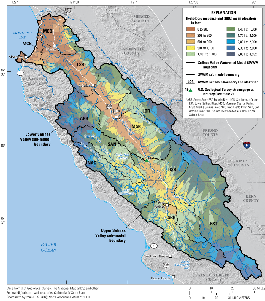
The percentage of impervious developed land cover averaged over the area of each HRU ranged from 0 to 55 percent (fig. 13). Hydrologic response units with a substantial percentage of impervious cover include one IMPLND element as a fraction of the total HRU area, with a corresponding reduction in the PERLND area such that the combined IMPLND and PERLND area equals the total area for that HRU. A total of 181 HRUs include IMPLND elements, with impervious areas ranging from 11 to 2,216 acres.
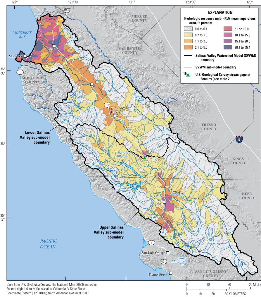
Mean percentage of impervious land cover for 690 hydrologic response units (HRUs) used in the Salinas Valley Watershed Model, calculated using the 2011 National Land Cover Database 30-meter (98 foot) percentage of impervious developed land cover (U.S. Department of Agriculture, 2017).
The SVWM discretization was defined such that each HRU is connected to one RCHRES, resulting in a stream channel network of 690 linked RCHRESs, with a given RCHRES having zero to many tributary connections to upstream RCHRESs, depending on the position of the RCHRES in the routing network. All RCHRESs in the stream channel network discharge to a single downstream RCHRES, with exceptions for a small number of RCHRESs discharging to Monterey Bay from the SRO, ELK, and MSB subdrainages. First-order RCHRESs in the headwater drainages do not have a tributary connection to upstream RCHRESs and only receive inflows from the single connected HRU. The headwater RCHRESs represented by the RCHRES network have drainage areas ranging from 0.1 to 50 mi2 with 46 headwater RCHRESs having drainage areas less than 1 mi2 and 179 RCHRESs having drainage areas of 1–5 mi2 (fig. 14). There are 231 RCHRESs that have contributing drainage areas between 5 and 20 mi2, and there are 150 RCHRESs that have drainage areas greater than 50 mi2.
Location and size of total contributing drainage areas for 690 stream reaches or reservoirs (RCHRES) used to discretize the Salinas Valley Watershed Model (Hevesi and others, 2025)
The HSPF code version used to develop the SVWM is limited to a maximum number of 1,000 model elements, with each PERLND, IMPLND, and RCHRES defining separate model elements. The SVWM model discretization includes a total of 1,561 elements (the sum of 690 PERLNDs, 181 IMPLNDs, and 690 RCHRESs), exceeding the capacity of the HSPF code version used. To preserve the degree of spatial detail provided by the 1,561 model elements, the SVWM was divided into the 2 HSPF sub-model domains, the USVS and the LSVS (fig. 2). The USVS has an area of 2,536 mi2 containing 387 HRUs with 36 HRUs including IMPLNDs. The LSVS has an area of 1,992 mi2 containing 303 HRUs with 69 HRUs including IMPLNDs. The LSVS is connected to the USVS by the outflow of the Salinas River at USGS streamgage 11150500 (gage 19, Salinas River near Bradley).
The more detailed discretization provided by the two connected sub-models allowed for an improved representation of variability in climate and watershed characteristics such as slope, land cover, soil properties, and surficial geology, compared to a single model representing the entire study area. In addition, the higher level of discretization using two sub-models with 1,561 elements compared to a single model with 1,000 elements, resulted in a more precise delineation of all tributary drainages to the lower Salinas Valley study area (defined by the SVIHM boundary as mentioned earlier; fig. 15). The SVWM simulated surface-water tributary inflows at 148 locations along the SVIHM boundary from the tributary drainages. The simulated inflows can be used to define boundary conditions for integrated hydrologic modeling of the lower Salinas Valley study area. The drainage areas for the 148 inflow locations were grouped into 25 tributary drainages with areas ranging from 11 mi2 for the Quail Creek (QUAI) tributary drainage in the northwest part of the SVWM (southeast of the city of Salinas) to 1,574 mi2 for the Salinas River (SALI) tributary drainage supplying surface-water inflow from the upper Salinas Valley watershed (fig. 15; table 8). Average elevations for the tributary drainages range from 997 ft for the Cherry Canyon (CHER) tributary drainage to 3,393 ft for the Arroyo Seco (SECO) tributary drainage (table 8). The total 3,625 mi2 area comprising all tributary drainages, referred to as the Salinas Valley upland area (SVU), has an average elevation of 1,671 ft and elevations ranging from −1 to 5,872 ft. In contrast, the 904 mi2 land area of the SVIHM has an average elevation of 441 ft with elevations ranging from −1 to 3,003 ft (table 8).
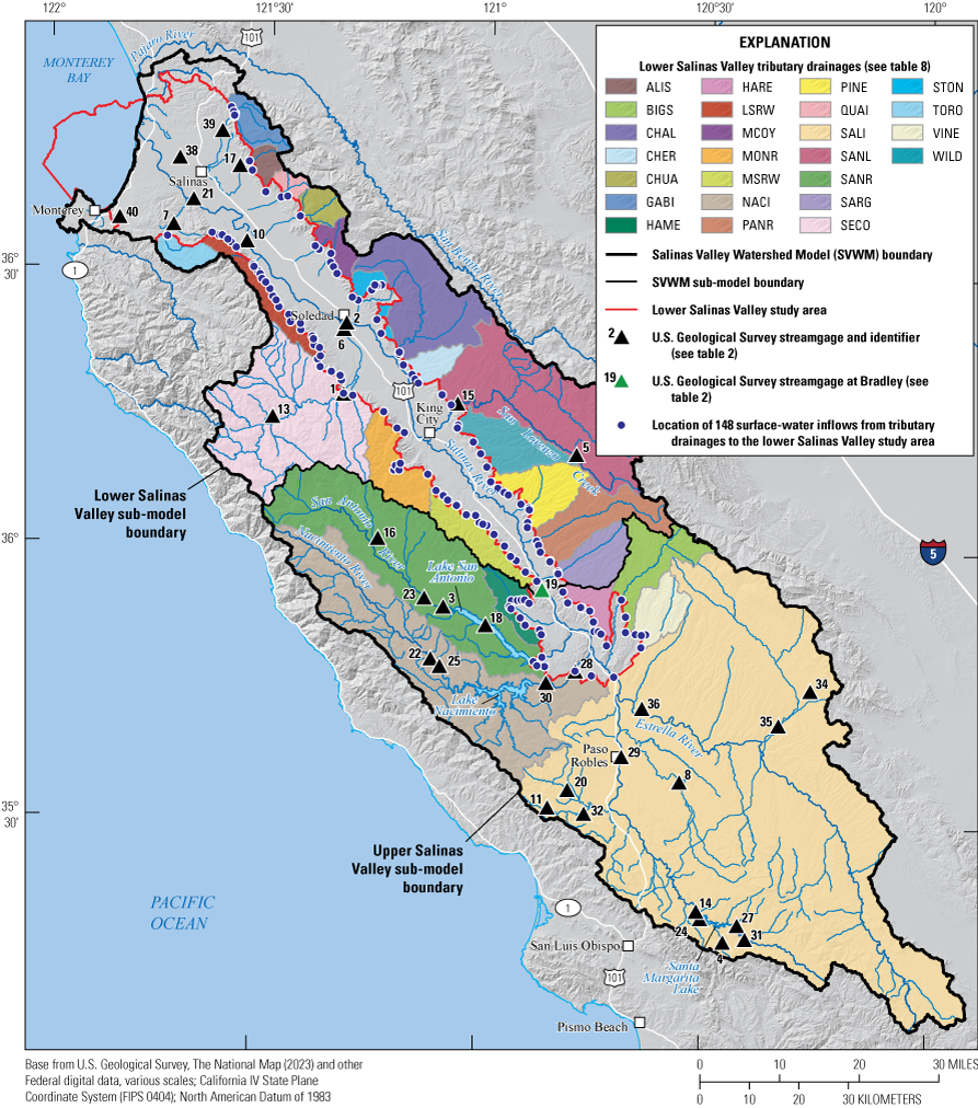
Lower Salinas Valley study area tributary drainages and locations of 148 surface-water inflows (Henson and others, 2022; Hevesi and others, 2025) Abbreviations: ALIS, Alisal Creek; BIGS, Big Sandy Creek; CHAL, Chalone Creek; CHER, Cherry Canyon; CHUA, Chualar Creek; GABI, Gabilan Creek; HAME, Hames Creek; HARE, Hare Canyon; LSRW, lower Salinas River West; MCOY, McCoy Creek; MONR, Monroe Creek; MSRW, middle Salinas River West; NACI, Nacimiento River; PANR, Pancho Rico Creek; PINE, Pine Creek; QUAI, Quail Creek; SALI, Salinas River; SANL, San Lorenzo Creek; SANR, San Antonio River; SARG, Sargent Creek; SECO, Arroyo Seco; STON, Stonewall Creek; TORO, El Toro Creek; VINE, Vineyard Canyon; WILD, Wildhorse Canyon.
Table 8.
Drainage basin areas and topographic characteristics of tributary drainages to the lower Salinas Valley study area.[mi2, square mile; Min, minimum; Max, maximum]
Basin Characterization Model Climate Inputs
The BCM was used to develop climate inputs for the SVWM. The BCM consists of a set of computer codes for grid-based water balance simulations and includes preprocessing applications for spatially distributing and downscaling climate variables and for simulating PET for historical climate and future climate scenarios and projections (Flint and Flint, 2007, 2012; Flint and others, 2013, 2021; Stern and others, 2016). The BCM applications use monthly climate data from the Parameter-elevation Regression on Independent Slopes Model (PRISM; Daly and others, 1994, 2004), available daily climate records, and the Gradient-Inverse-Distance-Squared method (Nalder and Wein, 1998) to downscale and spatially interpolate climate data to a 270-m (886-ft) grid covering the SVWM study area. Inputs used by the BCM to develop the HSPF climate inputs consisted of daily precipitation records from 155 climate stations (fig. 16), daily maximum and minimum air temperature records from 113 climate stations (fig. 17), gridded PRISM maps of monthly precipitation, monthly maximum and minimum air temperature, and land-surface elevations for the 270-m grid of the SVWM. The precipitation and air temperature climate grids developed by the BCM were applied to simulate daily PET using the Priestley–Taylor method (Flint and others, 2021).
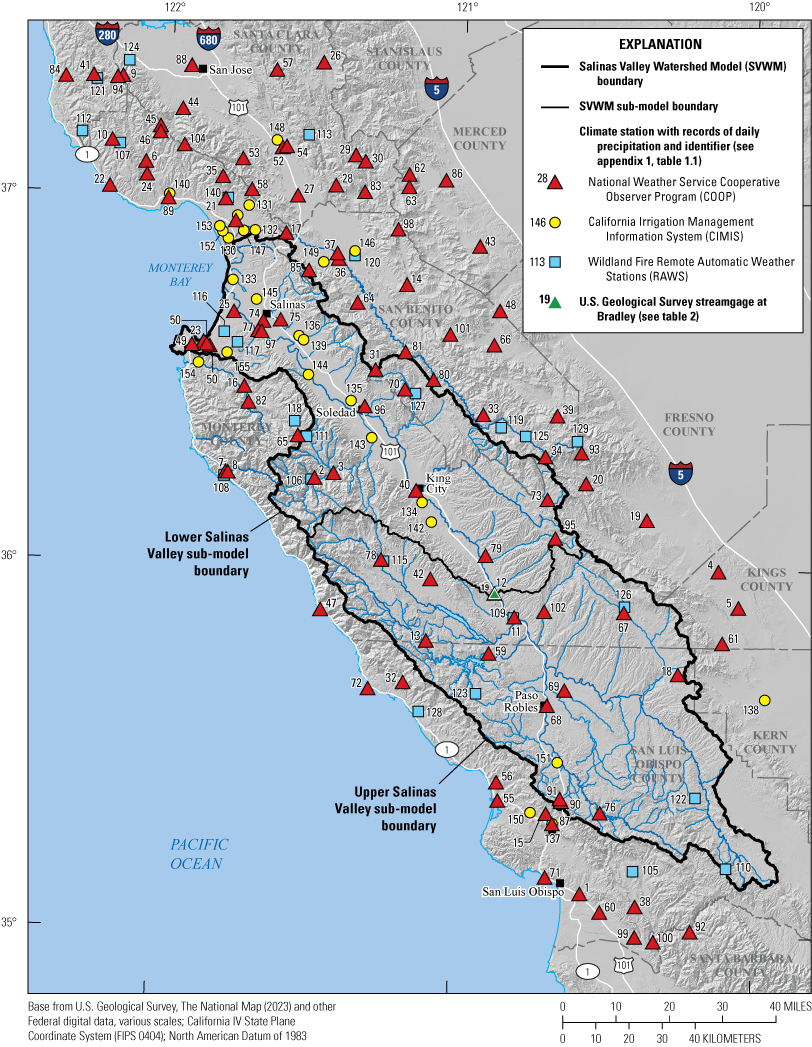
Locations of climate stations having records of the daily precipitation used in the Basin Characterization Model (BCM) to develop daily climate input for the Salinas Valley Watershed Model (Hevesi and others, 2022).
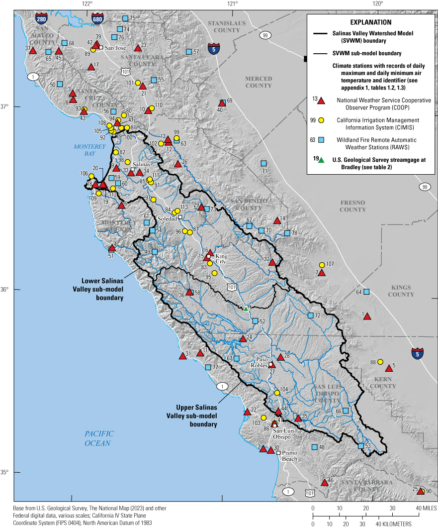
Locations of climate stations having records of daily maximum and minimum air temperature used in the Basin Characterization Model (BCM) to simulate daily potential evapotranspiration (PET) for the Salinas Valley Watershed Model (Hevesi and others, 2022).
A listing of the 155 climate stations shown on figure 16 with daily precipitation records used to develop climate inputs is provided in appendix 1, table 1.1. A listing of the 113 climate stations shown on figure 17 with daily minimum and maximum air temperature records used to develop climate inputs is provided in appendix 1, tables 1.2 and 1.3, respectively. The number of years of data for daily precipitation ranged from 1.8 years for Salinas 6 SSW (station 77, app. 1, table 1) to 70.8 years for Paso Robles (station 68, app. 1, table 1). The number of years of data for daily minimum and maximum air temperature ranged from 1.9 years for King City Airport (station 16, app. 1, tables 1.2, 1.3) to 70.4 years for Santa Cruz (station 43, app. 1, tables 1.2, 1.3). Mean annual precipitation ranged from 5.7 in. for Orchard Sunflower Valley (station 61, app. 1, table 1.1) to 54.2 in. for Ben Lomond (station 107, app. 1, table 1.1). Mean minimum daily air temperature ranged from 37.7 °F for station Priest Valley (station 32, app. 1, table 1.2) to 57.0 °F for station Kettleman Hills (station 64, app. 1, table 1.2) and mean maximum daily air temperature ranged from 60.4 °F for San Simeon Point Piedras Blancas (station 31, app. 1, table 1.3) to 80.1 °F for Avenal 9 SSE (station 1, app. 1, table 1.3).
The four BCM-simulated 270-m gridded climate inputs (precipitation, maximum and minimum air temperature, and PET) were averaged over the area of each HRU. Using a uniform hourly distribution, the four daily climate time series developed for each HRU were disaggregated into hourly time series, starting 1 second after midnight on October 1, 1947, and ending at midnight on September 30, 2018. The 690 unique sets of hourly climate time-series inputs were compiled and stored in a single binary Watershed Data Management (WDM) file used by the HSPF code.
The annual (water year) basinwide mean precipitation estimated for the Salinas Valley study area using the BCM indicates high interannual variability, with annual precipitation greater than 32 in. for 6 water years and less than 12 in. for 10 water years, compared to a 70-year mean precipitation of 18.5 inches per year (in/yr; fig. 18A). The ARR subbasin had the highest annual precipitation for all water years, with a maximum annual precipitation of about 61 in. for water year 1998 (fig. 18B). In comparison, water year 1983 was the wettest year for the SRH and NAC subbasins, with about 51 in. of annual precipitation for both subbasins (fig. 18B). Water year 2014 was the driest year in the 70-year period with about 7 in. of precipitation basinwide for the SVWM (fig. 18A), varying from about 13 in. for the ARR subbasin to about 6 in. for the LOR and MSR subbasins (fig. 18B).
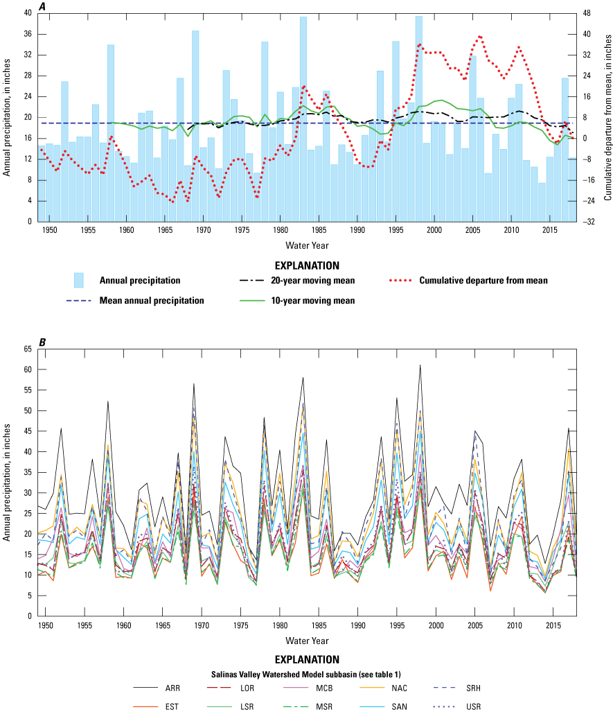
Precipitation for water years 1948–2018 estimated using the Basin Characterization Model (BCM): A, annual precipitation averaged for the area of the Salinas Valley Watershed Model (SVWM) and B, annual precipitation averaged over 10 subbasin areas in the Salinas Valley study area. Abbreviations: ARR, Arroyo Seco; EST, Estrella River; LOR, San Lorenzo Creek; LSR, lower Salinas River; MCB, Monterey Coastal Basins; MSR, middle Salinas River; NAC, Nacimiento River; SAN, San Antonio River; SRH, Salinas River headwaters; USR, upper Salinas River (Hevesi and others, 2022).
The 70-year (water years 1949–2018) mean precipitation simulated by the BCM and averaged over the 690 HRU areas indicates a high degree of spatial variability, with about 36–60 in/yr for the high-elevation HRUs along the western boundary to less than 12 in/yr for low-lying HRUs in the central part of the valley and the southeastern part of the study area, and values less than 10 in/yr along the southeastern boundary (fig. 19). Precipitation was less variable in the Salinas Valley lowlands and coastal basins, ranging from about 12 to 15 in/yr for most locations, with higher values of 15–21 in/yr for the coastal basins in the northwest part of the lower Salinas Valley.
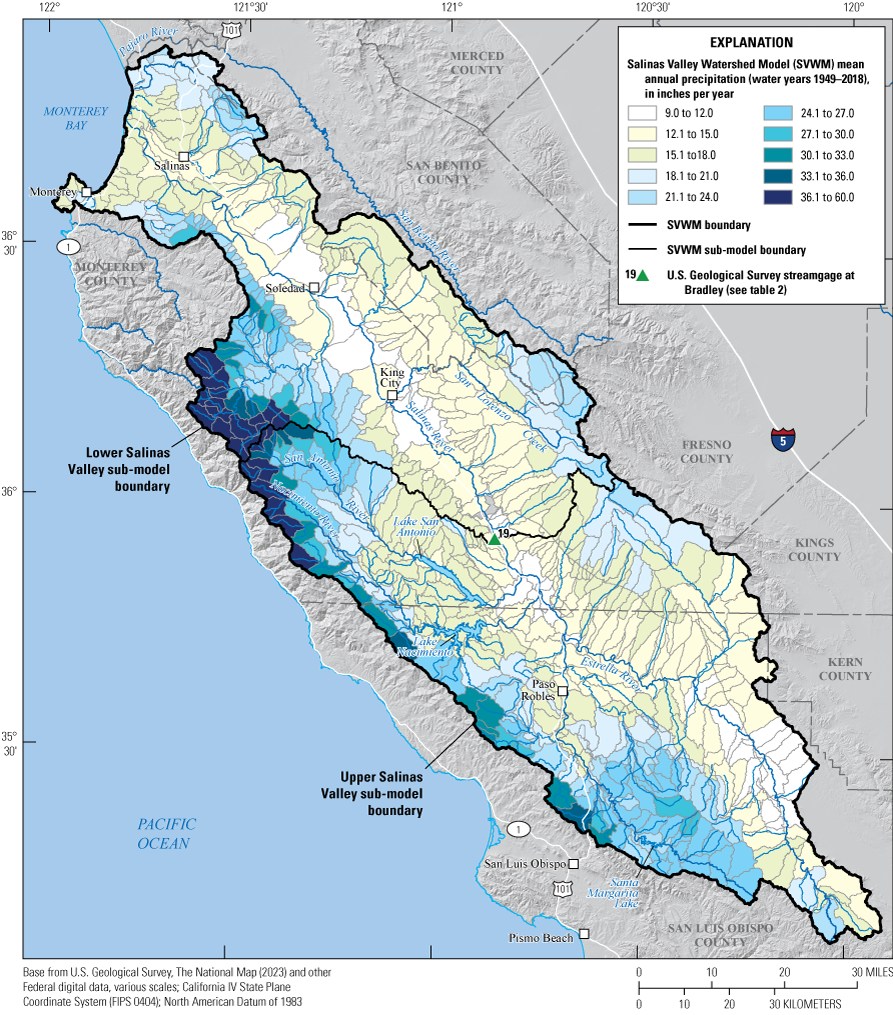
Mean annual precipitation estimated using the Basin Characterization Model (BCM) for 690 hydrologic response units (HRUs) used in the Salinas Valley Watershed Model (Hevesi and others, 2025).
Annual (water year) 70-year mean PET simulated by the BCM and averaged over the 690 HRU areas also indicates substantial spatial variability in climate (fig. 20). The mean PET for the SVWM was 58.1 in. and varied from a minimum of about 55.3 in. for water year 1998 to high values of more than 59.5 in. for several water years including 1959, 1984, and 2014 (fig. 20A). Water year 2014, the driest year, also had the highest PET of 60 in. The MCB subbasin had the lowest PET for all water years, ranging from about 48 in. for water years 1999 and 2011 to 54 in. for water year 1997 (fig. 20B). The EST and USR subbasins had the highest annual PET values of about 62 in. or higher for water years 1959, 1960, 1984, 1996–97, and 2014–15 (fig. 21).
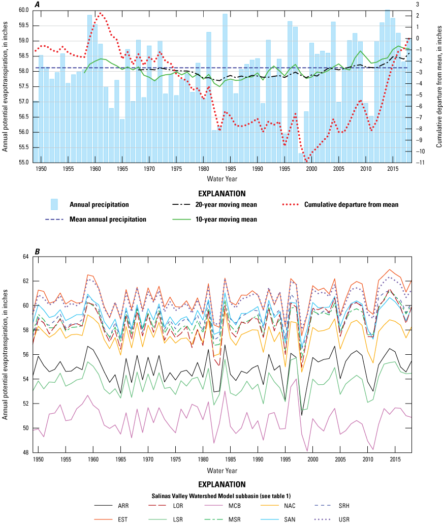
Potential evapotranspiration (PET) simulated using the Basin Characterization Model (BCM): A, annual PET averaged for the Salinas Valley Watershed Model (SVWM) and B, annual PET averaged for subbasins in the SVWM. Abbreviations: ARR, Arroyo Seco; EST, Estrella River; LOR, San Lorenzo Creek; LSR, lower Salinas River; MCB, Monterey Coastal Basins; MSR, middle Salinas River; NAC, Nacimiento River; SAN, San Antonio River; SRH, Salinas River headwaters; USR, upper Salinas River (Hevesi and others, 2022).
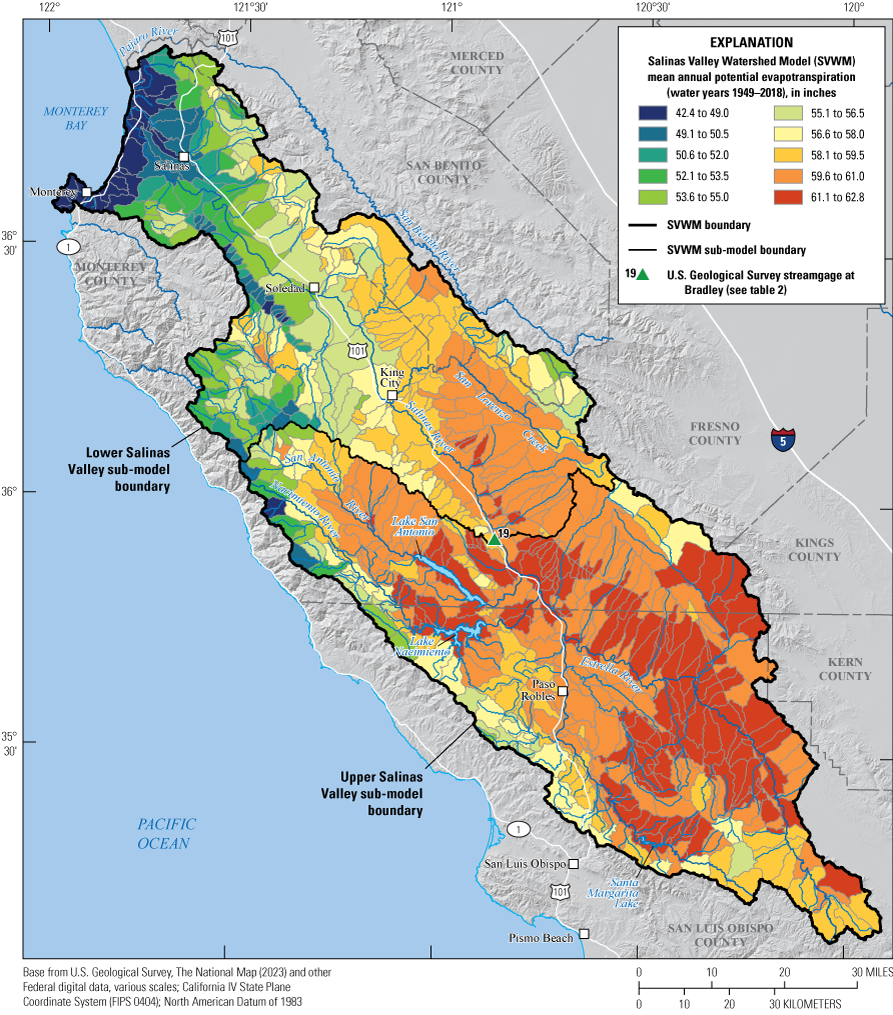
Mean annual potential evapotranspiration (PET) for water years 1949–2018 simulated using the Basin Characterization Model (BCM) and averaged for 690 hydrologic response units (HRUs) used in the Salinas Valley Watershed Model (Hevesi and others, 2022).
The BCM-simulated 70-year mean PET varied from high values of about 61–63 in/yr for HRUs in the more inland, southeast part of the SVWM to low values of about 42–46 in/yr for HRUs closer to the coastline (fig. 21). North- to northeast-facing slopes on the west side of the Salinas Valley (particularly in northwestern part of the SVWM) also had lower mean annual PET values of about 49–52 in/yr compared to the basinwide mean of 58.1 in/yr. Mean annual PET within the lower elevation of the upper Salinas Valley varied from about 60 to 63 in/yr and overall had higher values compared to most locations in the Salinas Valley study area.
Seasonal variability in precipitation and PET is an important characteristic of the Salinas Valley study area. The basinwide mean monthly precipitation is the highest for January for the SVWM and all subbasins, ranging from about 3 in. for the EST and MSR subbasins to 6.4 in. for the ARR subbasin (fig. 22A). February is the second wettest month for the SVWM and all subbasins, varying from about 2.8 in. for the LSR, EST, and MSR subbasins to 5.8 in. for the ARR subbasin. For the dry-season months, June through August, mean monthly precipitation is approximately zero for all subbasins. In contrast to precipitation, mean monthly PET is highest during the dry season months of May through August (fig. 22B). Although the basinwide 70-year mean PET of 58.1 in/yr is more than three times the basinwide 70-year mean precipitation of 18.4 in/yr, the mean monthly precipitation for December through February exceeds mean monthly PET.
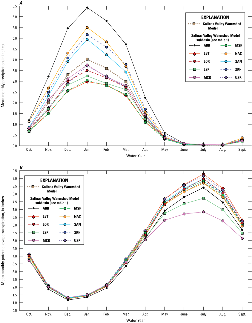
Climate inputs developed using the Basin Characterization Model (BCM) for the Salinas Valley Watershed Model (SVWM) and subbasins; A, mean monthly precipitation and B, mean monthly potential evapotranspiration. Abbreviations: ARR, Arroyo Seco; EST, Estrella River; LSR, lower Salinas River; MSR, middle Salinas River; MCB, Monterey Coastal Basins; NAC, Nacimiento River; SRH, Salinas River headwaters; SAN, San Antonio River; LOR, San Lorenzo Creek; USR, upper Salinas River (Hevesi and others, 2022)
Model Parameters
The HSPF code requires a User Control Input (UCI) file to specify model control options, the simulation period, model parameters, and input and output filenames needed to run a simulation. The UCI file is an American Standard Code for Information Interchange text file with a formatted, column-specified input structure. The model parameters are organized according to the modular structure of HSPF, with separate input groups used for simulating water flow and storage within PERLND areas, IMPLND areas, and the connected RCHRES network. In addition to the UCI file, simulations require the WDM file containing the time series inputs and outputs, including hourly climate (precipitation, air temperature, and PET) and hourly and daily streamflow.
Parameters used to simulate water flow and storage in PERLNDs define spatially varying catchment properties throughout the SVWM and were the most important for representing the physical characteristics of the Salinas Valley study area (table 9). Initially, model parameters were defined using a combination of geospatial data and representative values from previous studies, including suggested values provided in the HSPF user’s manual (U.S. Environmental Protection Agency, 2000; Bicknell and others, 2001). During the model-calibration procedure, 15 of the 17 parameters listed in table 9 were then adjusted and refined, as discussed in more detail in the “Model Calibration” section. Parameters (defined in table 9) LZSN, INFILT, LSUR, KVARY, AGWRC, INFEXP, DEEPFR, BASETP, and AGWETP were scaled using geospatial data and calibrated as a set of unique values for each HRU. Monthly parameters INTERCEP, UZSN, MANNING, INTERFLW, IRC, and LZETPARM were scaled using geospatial data and calibrated for each HRU as a unique set of 12 monthly values.
Table 9.
Hydrologic Simulation Program—Fortran (HSPF) pervious land-area (PERLND) parameters used in the Salinas Valley Watershed Model (SVWM) to represent basin characteristics for the Salinas Valley study area (modified from U.S. Environmental Protection Agency, 2000).[Modified from U.S. Environmental Protection Agency (2000); Abbreviations: ET, evapotranspiration; ft, foot; ft/ft, foot per foot; GW, groundwater; in., inch; in/hr, inch per hour; Max, maximum; Min, minimum]
Initial estimates of LZSN, the lower zone storage capacity, were varied as a function of the mean AWS150 value from SSURGO (fig. 9), the mean 30-m DEM slope (fig. 4), and the weighted average of DEM slope classes for each HRU. The model parameter INFILT affects the infiltration capacity of the soil and was varied for each HRU as the weighted average of the 13 SSURGO soil texture classes within the SVWM, where the weighting factors were defined by the area-fraction of each soil texture class for each HRU (fig. 8). The model parameter LSUR, the length of the overland flow plane used to simulate re-infiltration of surface runoff, was estimated based on the inverse of DEM-derived slope, with steeper slopes resulting in lower LSUR values, and then adjusted during calibration.
The model parameters KVARY and AGWRC were varied for each HRU using the surficial geologic map (fig. 10; Jennings, 1977). The KVARY parameter affects the simulation of groundwater recession flow, enabling the recession flow to be non-exponential in its decay with time, and was calculated as the weighted average of KVARY values defined for each of the 9 surficial geologic rock types (for this study all metamorphic rock types from Jennings [1977] were grouped as metamorphic rocks and all volcanic rock types from Jennings [1977] were grouped as volcanic rocks), with the weighting factors calculated as the area-fraction of the surficial geologic rock type within each HRU (fig. 10). The AGWRC parameter is the basic groundwater recession rate and also was calculated for each HRU as the area-fraction weighted average of values defined for each of 9 surficial geologic rock types. The INFEXP parameter controls the infiltration rate into the root zone and was estimated as a function of the mean DEM slope for each HRU. The DEEPFR parameter controls the rate of inflow to the inactive groundwater reservoir (groundwater that does not contribute to groundwater discharge in the HSPF simulation). As with KVARY and AGWRC, DEEPFR was varied for each HRU based on the surficial geologic map and the area fraction of the different surficial geologic rock types within each HRU (fig. 10). The AGWETP parameter controls groundwater ET losses and was estimated based on the area-fraction of cropland in each HRU.
Six parameters, INTERCEP, UZSN, MANNING, INTERFLW, IRC, and LZETPARM (table 9), were defined using the HSPF option of having a set of 12 monthly values for each HRU to represent seasonal variability. The INTERCEP parameter defines the interception storage capacity for vegetation and was varied for each HRU as the area-fraction weighted average of values defined for each NLCD land cover type (fig. 6). In addition to land cover type, the NLCD 30-m resolution, percentage of forest canopy cover data (fig. 7A) was used to increase the interception storage capacity based on increasing canopy cover. The INTERFLW parameter controls the interflow inflow rate and was varied using monthly scaling factors and the calculated mean 30-m DEM slope for each HRU. The IRC parameter is the interflow recession coefficient and was also varied monthly as a function of the 30-m DEM slope for each HRU.
The model parameters LZETPARM, MANNING, and UZSN were varied by month and by the area-weighted average of the different NLCD land cover types within each HRU. The LZETPARM parameter is used for simulating plant transpiration as a function of PET, vegetation type, and growing season. The MANNING parameter is the surface roughness coefficient used for simulating overland flow. The UZSN parameter is the upper zone storage capacity used to account for surface retention storage. In addition to NLCD land cover type, the NLCD percentage of canopy cover was used to scale the parameters LZETPARM and UZSN by increasing parameter values with increasing canopy cover percentage. Mean land-surface slope also was used to scale the MANNING and UZSN parameters, with an increase in slope resulting in a decrease in values for both parameters.
Several parameters were defined directly using the Geographic Information System (GIS) applications or by the suggested default values and were held constant during model calibration. The SLSUR parameter, the slope of the overland flow plane used by HSPF to simulate overland runoff and infiltration of overland flow, was defined directly as the mean calculated rise-over-run slope of all 30-m DEM grid cells within each HRU. The INFILD parameter was set to a constant value of 2.0, as recommended in the HSPF user’s manual and supporting documentation (U.S. Environmental Protection Agency, 2000; Bicknell and others, 2001), and was not adjusted during model calibration. Impervious land-area parameters also were defined based on suggested values in HSPF documentation and were not adjusted during model calibration. Impervious land-area parameters LSUR, SLSUR, and NSUR (NSUR is equivalent to the MANNING roughness coefficient used for pervious land areas) were set to 200, 0.117, and 0.05 ft, respectively. The impervious land-area parameter RETSC, the retention storage capacity, was set to 0.1 in.
Parameters for simulating surface-water flow through the 690 RCHRES elements comprising the SVWM drainage network include stream reach length, the change in elevation over the length of the stream reach, and a table defining the stage-area-volume-discharge relation for each stream reach, referred to as the Flow-table (Ftable). The Ftables used in the SVWM included two outlets, one for streamflow and a second outlet used to simulate seepage losses from the infiltration of surface water through the streambed. Discharge for the second outlet representing seepage loss was set to zero or near-zero outflow for stream reaches assumed to have none to negligible stream seepage.
The Ftables were estimated using rating curves, field data, and peak discharge data measured at the USGS streamgages in the Salinas Valley study area (table 2). The data were used to define the Ftables in the RCHRES segments where the streamgages were located. The Ftables for segments without a streamgage were estimated based on the proximity to the nearest streamgage and scaled according to the length and slope of the channel represented by the RCHRES, the channel width, the upstream drainage area, and the estimated permeability of the streambed based on the surficial geology and soil texture. Additionally, Ftables for many stream reaches were adjusted during calibration, particularly with respect to the seepage outflow rate.
Model Calibration
Model calibration is done by comparing simulated and measured variables. Measured values, often referred to as observations of the variable of interest, are determined directly from field data or from values calculated from field data. Ideally, the observed variable of interest has continuous records at the desired temporal resolution spanning multi-year periods that capture a full range of conditions and variability, with at least one drier-than-average period and one wetter-than-average period.
The SVWM was calibrated by comparing simulated and observed streamflow, where observed streamflow is calculated using measurements of stream stage, velocity, or both. Streamflow accounts for the integrated effects of the hydrologic processes in the drainage area upstream from the streamgage used for calibration and is generally the variable used for calibrating hydrologic models such as the SVWM. Observed streamflow in the Salinas Valley is characterized by rapid surface runoff response to precipitation in upland drainages, with ephemeral streamflow in most channels and seasonally distributed baseflow after winter storms with very low to no-flow conditions during the dry summer months. In addition to seasonal variability, there is substantial annual variability in streamflow in response to variability in annual precipitation. To achieve a good calibration for the SVWM, simulated streamflow needed to represent a wide range of flow conditions for a variety of catchment areas, from flashy peak flows having short durations of several days or less to long periods of several months with very low flows (less than 10 ft3/s) and extended no-flow conditions at most streamgages.
Calibration Procedure
Streamflow records for 29 USGS streamgages within the SVWM (fig. 1; table 10) with observed streamflow between October 1, 1948, and October 1, 2015, (water years 1949–2015) were used for calibration. In addition to the USGS streamflow data, estimates of surface-water inflows to Lake Nacimiento from October 1, 1958, to September 30, 2013, and to Lake San Antonio from October 1, 1966, to September 30, 2013, were provided by Monterey County Water Resources Agency (MCWRA) and included as observations. All calibration runs were started on October 1, 1947, to allow for a minimum of a 1-year model initialization period before the target period used for calibration at each streamgage.
Table 10.
U.S. Geological Survey (USGS) streamgages and reservoirs with estimated inflows along with calibration periods used for calibrating the Salinas Valley Watershed Model (SVWM).[ID, identification; HSPF, Hydrologic Simulation Program–Fortran; mi2, square mile; mm/dd/yyyy, month/day/year; NWIS, National Water Information System; RCHRES, stream reach or reservoir; —, not applicable]
Calibration was done using an iterative trial-and-error approach of adjusting PERLND parameters identified in table 9 to improve the match between simulated and observed streamflow. Trial-and-error adjustments for spatially distributed parameters were done primarily by changing scaling factors that were defined using geospatial data, which included topography, soils, land cover, and geology. In the case of discrete geospatial data such as land cover type, soil texture, and geology, the scaling factors were calculated as the weighted mean value based on the area-fraction of discrete data within each HRU. In the case of continuous 30-m (98-ft) gridded data such as land elevation, slope, percentage of forest canopy, and percentage of imperviousness, parameter values were calculated as the average of the gridded data values within each HRU area. This method of parameter estimation and calibration used in the SVWM resulted in a unique set of pervious land parameters for each HRU.
Calibration Statistics
The calibration procedure used a quantitative analysis of the goodness-of-fit between simulated and observed time series based on the available period of record at each streamgage from October 1, 1948, to September 30, 2015, (table 10) and was done using the percent-average estimation error (PAE) and the Nash–Sutcliffe model efficiency (NSME) statistics (Nash and Sutcliffe, 1970; Donigian and Imhoff, 2009; Duda and others, 2012; Hevesi and Johnson, 2016; Hevesi and others, 2019). Calibration periods varied from a minimum of 5.2 years for USGS streamgage 11147040 (gage 11) to a maximum of 67 years at USGS streamgage 11152000 (gage 1), with a mean calibration period of 28 years for all streamgages (table 10). The PAE statistic provides a measure of model bias, where a value of 0.0 percent indicates an unbiased model fit. Values of PAE in the range of plus or minus 10 percent indicate an acceptable calibration (Donigian and Imhoff, 2009). The NSME statistic is a standardized mean squared-error statistic, similar to the coefficient of determination (R2) used in regression analysis, that is often used to compare goodness-of-fit results between different models (Nash and Sutcliffe, 1970; Markstrom and others, 2008; Hevesi and others, 2019). An NSME value greater than 0.0 indicates the model provides a better match to the observed values than the mean of the observed values (the mean has an NSME equal to 0.0). The closer the NSME is to 1.0, the better the match is between simulated and observed values, with a value of 1.0 indicating a perfect match to observed values.
The PAE and NSME goodness-of-fit statistics between simulated and observed streamflow were evaluated using daily mean, monthly mean, annual (water year) mean, and mean monthly streamflow at each streamgage for varying values of parameters selected for calibration (table 9). To summarize the calibration results for the 31 streamflow comparisons, weighted mean PAE, percent estimation error (PE), and NSME statistics were calculated for each parameter set tested. The weighting factors were defined for each streamgage using the average of two products consisting of (1) the length of the calibration period at each streamgage divided by the total length of record for all streamgages and (2) the square root of the contributing drainage area for each streamgage divided by the sum of the square root of the total drainage area for all streamgages. The weighted mean PAE was calculated using the absolute value of PAE calculated at each individual streamgage. Calibration criteria used for the SVWM are provided in table 11. To achieve a minimum level of calibration for the SVWM, the weighted mean goodness-of-fit statistics needed to meet the satisfactory criteria or better for daily, monthly, and annual streamflow, with the goal of having results meet the good to very good criteria.
Parameter Sensitivity
Before the process of trial-and-error model calibration, an initial set of parameter values was defined using the recommended range of values provided by the HSPF user’s manual and supporting documentation (U.S. Environmental Protection Agency, 2000; Bicknell and others, 2001, 2005). Six baseline models were defined using the range of typical and possible parameter values listed in BASINS Technical Note 6, Estimating Hydrology and Hydraulic Parameters for HSPF (U.S. Environmental Protection Agency, 2000). Typical and possible mean parameter values were calculated using the minimum and maximum values for the typical and possible ranges. The six baseline parameter sets consisted of (1) typical minimum values, (2) typical maximum values, (3) typical mean values, (4) possible minimum values, (5) possible maximum values, and (6) possible mean values, with all HRUs having uniform parameter values as listed in table 9.
Goodness-of-fit statistics were calculated for the 31 simulated daily streamflow comparisons using the six baseline models as a means of evaluating initial estimates for pervious land parameters. The weighted mean PAE, PE, and NSME results indicated that the possible mean and typical maximum baseline models provided better initial parameter values compared to the typical minimum, typical mean, possible minimum, and possible maximum baseline values (table 12). The possible mean baseline model with PAE of 39.2, PE of −15.2, and NSME of 0.355 provided the best overall goodness-of-fit results compared to the four other baseline models; however, all six baseline models failed to provide a satisfactory calibration result. The typical and possible minimum baseline models greatly overestimated the amount of streamflow, and the typical minimum, possible minimum, and mean baseline models provided a very poor fit to observed streamflow based on the negative NSME results. The possible mean, typical maximum, and possible maximum baseline models provided an improved model fit compared to the other three baseline models but underestimated the weighted average mean, maximum, and minimum streamflows. All six baseline models underestimated the weighted average median streamflow.
Table 12.
Goodness-of-fit results comparing observed streamflow with six baseline models developed using documented ranges in the Hydrologic Simulation Program—Fortran (HSPF) parameter values.[ft3/s, cubic foot per second; Max, maximum; Min, minimum; NSME, Nash-Sutcliffe model efficiency; PAE, percent-average estimation error; PE, percent estimation error; %, percent]
As part of parameter estimation, the sensitivity of the SVWM to pervious land parameters was evaluated using a simple approach of varying selected parameters across a range of possible values and comparing the weighted mean goodness-of-fit statistics for simulated daily streamflow. The analysis was used to help indicate which parameters would likely have the greatest effect on streamflow and therefore have the greatest effect on calibration results. To perform the sensitivity analysis, pervious land parameters were set to uniform values across all HRUs for each simulation. Minimum and maximum values in table 9 provided an approximate guide for defining the range of parameter values tested. Each test simulation was done using parameter values defined by the typical mean baseline model (table 9), whereas a single parameter was varied across a range of minimum to maximum values. Parameters having the option for monthly values (table 9) were set to a constant value for all months. For each parameter tested, all other parameters were set to constant uniform values for all HRUs as defined by the typical mean baseline model (table 9). The procedure was repeated for each parameter in table 9.
Results indicated a high degree of model sensitivity in terms of simulated daily streamflow to parameters LZSN, INFILT, and LZETPARM (table 13). The best goodness-of-fit results using the typical mean baseline model were obtained with values from 8.0 to 15.0 in. for LZSN, 0.05 in/hr for INFILT, and 0.99 for LZETPARM. The LZSN values less than 5.5 in. resulted in a substantial overestimation of streamflow because of insufficient water storage capacity in the root zone causing a reduction in ET. The LZETPARM values of 0.3 and less also resulted in a reduction in ET and a corresponding overestimation of streamflow. The LZSN values greater than 8 in. resulted in an underestimation of streamflow because of the high root zone storage capacity causing a high percentage of precipitation being lost to ET.
Table 13.
Goodness-of-fit results used to evaluate model sensitivity to adjustments in values of pervious land parameters used in the Salinas Valley Watershed Model (SVWM).[ft, foot; ft/ft, foot per foot; ft3/s, cubic foot per second; in., inch; in/hr, inch per hour; Max, maximum; Min, minimum; NSME, Nash-Sutcliffe model efficiency; PAE, percent-average estimation error; PE, percent estimation error; *, asterisks designate parameter value for typical mean baseline model; %, percent]
Model sensitivity was shown as being intermediate to variations in parameters affecting baseflow recession (KVARY and AGWRC), the parameter controlling deep recharge to groundwater not contributing to baseflow (DEEPFR), parameters defining the interception storage capacity of vegetation and the retention storage capacity of the land surface (INTERCEP and UZSN), and the parameter controlling interflow recession (IRC; table 13). Model sensitivity was shown to be low for parameters controlling the re-infiltration of overland flow (LSUR and SLSUR), the exponent in the infiltration equation (INFEXP), the parameters controlling groundwater ET (BASETP and AGWETP), the roughness coefficient for overland flow (MANNING), and the coefficient controlling interflow (INTERFLW).
Calibrated Parameters
Summarized parameter values calculated as the mean, median, maximum, minimum, and variance for the 690 calibrated HRU values for the SVWM are listed in tables 14 and 15. Summarized values for parameters with constant monthly values (values are the same for each month) are in table 14. Summarized values for parameters with monthly varying values are in table 15. The goodness-of-fit statistics for the set of parameters in tables 14 and 15 are provided in the “Calibration Results” section.
Table 14.
Summary statistics for parameters with constant monthly values calibrated to 690 hydrologic response units (HRUs) used in the Salinas Valley Watershed Model (SVWM).[See table 9 for all Hydrologic Simulation Program—Fortran (HSPF) parameter descriptions. Abbreviations: ft, foot; ft/ft, foot per foot; in., inch; in/hr, inch per hour]
Table 15.
Summary statistics for monthly varying parameters calibrated to 690 hydrologic response units (HRUs) used in the Salinas Valley Watershed Model (SVWM).[See table 9 for all Hydrologic Simulation Program—Fortran (HSPF) parameter descriptions. Abbreviation: in., inch]
Calibrated values for the length of the overland flow plane, LSUR, were defined by using the equation 0.7 minus HRU slope times 600 ft, resulting in a range of values from 49.2 to 418.5, with a mean value of 275.5 for the SVWM. The soil zone water storage capacity, LZSN, was the most critical parameter adjusted during calibration, with values for the calibrated model ranging from 0.10 to 29.74 in. and a mean value of 8.69 in. for the SVWM. The mean calibrated value for INFILT is 0.24, ranging from 0.0005 to 13.3, with high values of 0.81 and greater mostly in the lowlands of Salinas Valley and locations with loamy soils. The KVARY parameter, adjusted for each geologic rock type, includes a minimum value of 0.2 for metamorphic rock types and a maximum value of 2.0 for alluvium and conglomerate surficial geology.
Calibrated values for AGWETP, used to empirically represent groundwater pumped for crop irrigation, include high values of 0.2 and greater in areas with substantial cropland in the middle and lower Salinas Valley, and intermediate values between 0.06 and 0.2 are in the upper Salinas Valley for HRUs containing vineyards. Calibrated values for AGWRC, scaled according to surficial geologic rock type, range from low values of 0.91 for alluvium and 0.937 for conglomerate to high values of 0.97 for rock types in upland areas, including a maximum of 0.999 for igneous and metamorphic rock types.
Calibrated values for INTERCEP are highest in May and lowest in October (table 15). Higher values for INTERCEP are assigned to HRUs having mostly forested land cover and a high percentage of canopy cover, compared to HRUs with mostly grassland. The INTERFLW parameter, controlling the rate of interflow to streams, is highest for February and March and lowest for July through October (table 15). The highest INTERFLW values for March and October are for HRUs in the UAS and along the western boundary of the LSR subbasins. Calibrated values for the IRC parameter have a similar spatial pattern as INTERFLW, with high values in the Arroyo Seco subdrainage (table 15).
Calibrated values for LZETPARM are highest in April and lowest in October (table 15). Calibrated values for MANNING are highest in March and April and lowest in September and October (table 15). Calibrated values for UZSN include maximum values for March through May and a minimum mean for the SVWM for October (table 15). Locations with the highest values in April include the lower Salinas Valley floor and the SRH.
Calibration Results
The overall goodness-of-fit statistics for the calibrated model included weighted mean PAE and NSME values of 2.0 and 0.64 percent for daily mean streamflow, 2.0 and 0.84 percent for monthly streamflow, and 2.1 and 0.88 percent for annual streamflow, respectively (table 16). The results were considered satisfactory for daily streamflow, very good for monthly streamflow, and good for annual streamflow.
Table 16.
Salinas Valley Watershed Model calibration results showing goodness-of-fit statistics using daily, monthly, and annual streamflow.[ft3/s, cubic foot per second; ID, identification; Max, maximum; Min, minimum; NSME, Nash-Sutcliffe model efficiency; USGS, U.S. Geological Survey; —, not applicable; %, percent]
The NSME statistic for daily streamflow ranged from 0.09 to 0.85 (table 16). Sixteen of the USGS streamgages and both reservoir inflows had very good NSME results of 0.7 or higher for daily streamflow, with 10 of the 29 locations having NSME values of 0.75 or higher, including the two reservoir inflows. Comparisons of simulated and observed daily streamflow for 15 selected streamgages using the calibrated model are provided on figure 23. The model performed well in terms of matching the timing and magnitude of most storms. The simulated daily streamflow at USGS streamgages 11150500 (gage 19) and 11152500 (gage 21) were well matched to the large runoff event during water year 1951, resulting in more than 20,000 ft3/s daily mean streamflow for the Salinas River (figs. 23N, 24O). The 8-year calibration period used for USGS streamgages 11150500 (gage 19) and 11152500 (gage 21), water years 1949–1957, was before the completion of Lake Nacimiento and was considered representative of natural streamflow conditions in the main branch of the Salinas River.
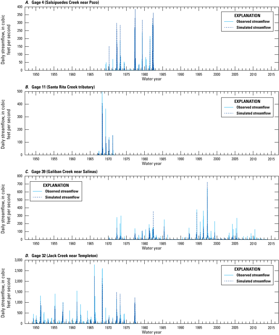
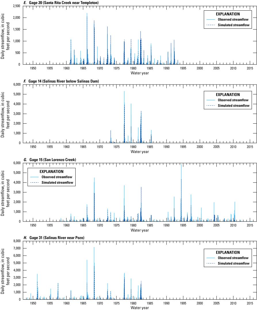

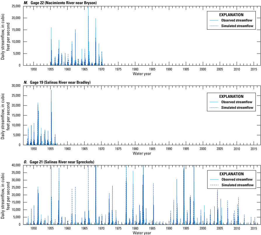
Comparison of observed (light blue) versus simulated (dashed dark blue) daily streamflow at selected U.S. Geological Survey streamgages: A, gage 4; B, gage 11; C, gage 39; D, gage 32; E, gage 20; F, gage 14; G, gage 15; H, gage 31; I, gage 24; J, gage 13; K, gage 18; L, gage 1; M, gage 22; N, gage 19; and O, gage 21 (U.S. Geological Survey, 2016; Hevesi and others, 2025).
As expected, calibration results for monthly streamflow showed improved NSME results compared to daily streamflow for all locations, with values ranging from 0.47 to 0.97 (table 16). There were 26 locations that had very good NSME values of 0.80 or higher for monthly streamflow, and 6 locations that had excellent values of 0.9 or higher. The monthly hydrographs indicate a good visual fit to wetter-than-average periods at most streamgages during water years 1969, 1978, and 1998 (fig. 24). Considering the bias of the calibration statistics to high flows, visual comparison of log-transformed streamflow was used qualitatively as part of calibration (figs. 24A, C, E, J).
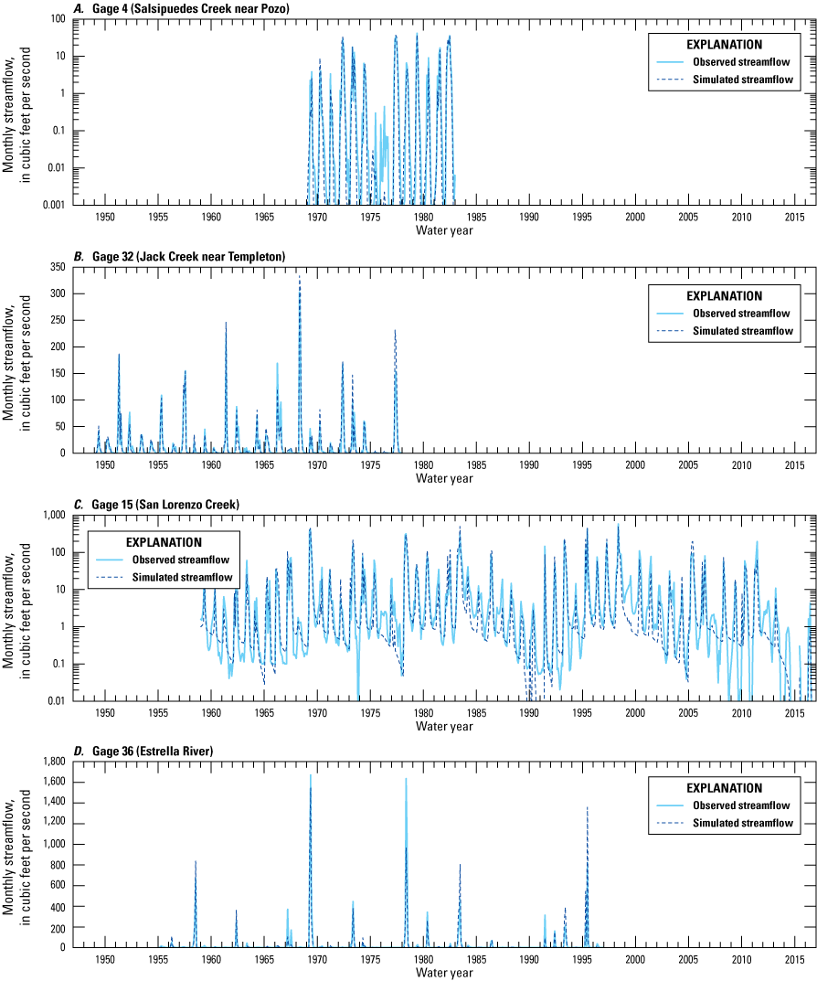
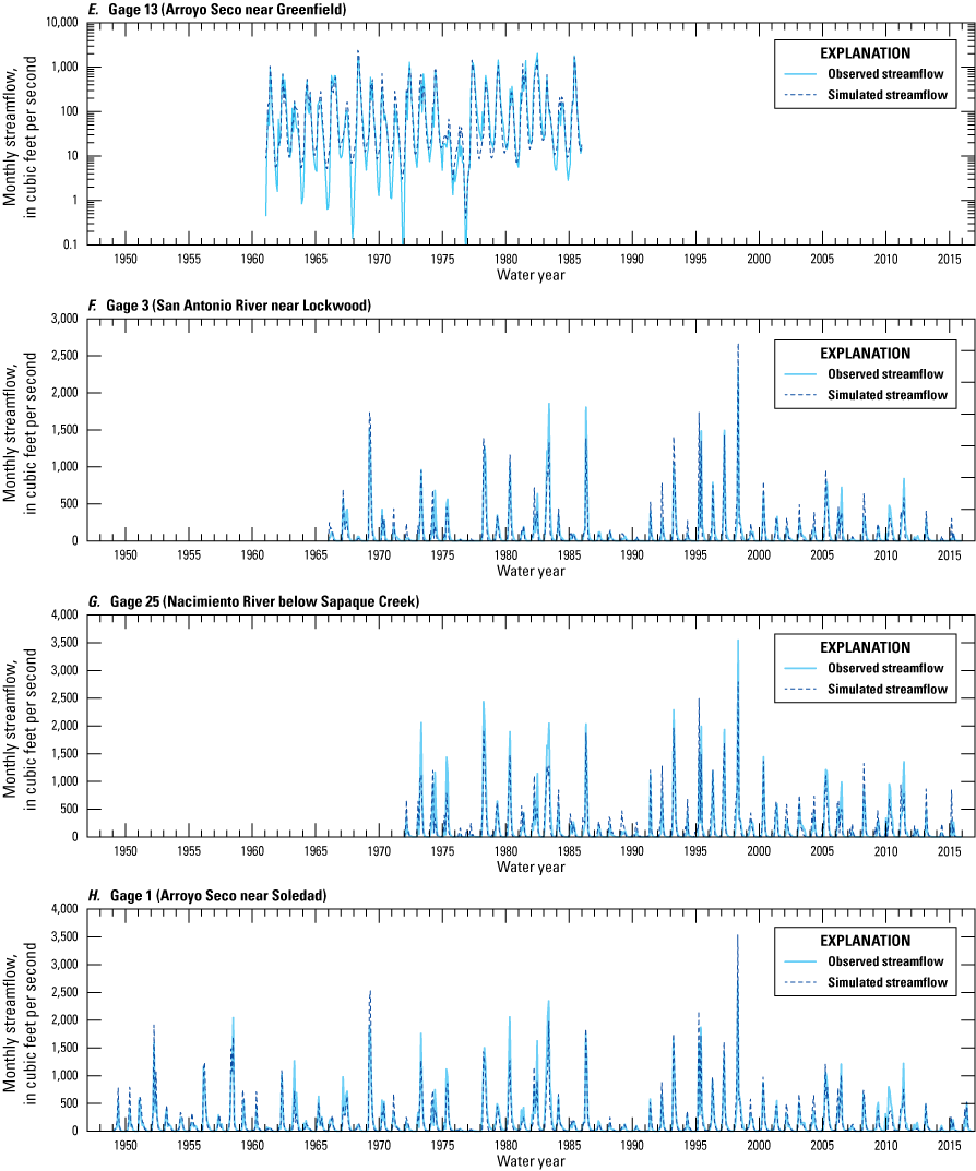
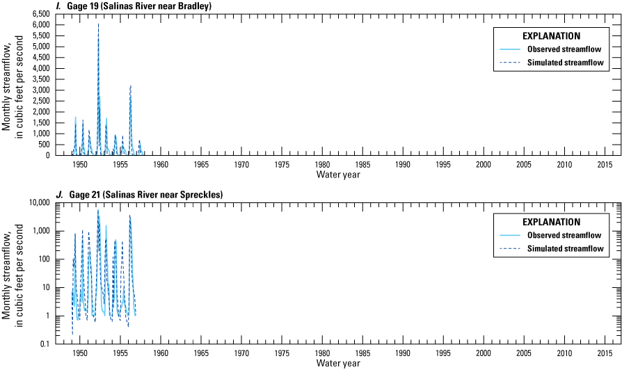
Comparison of observed (light blue) versus simulated (dashed dark blue) monthly streamflow at selected U.S. Geological Survey streamgages: A, gage 4; B, gage 32; C, gage 15; D, gage 36; E, gage 13; F, gage 3; G, gage 25; H, gage 1; I, gage 19; and J, gage 21.
The calibration results for annual streamflow were similar to results for monthly streamflow, with NSME ranging from 0.47 to 0.99 (table 16). Only 4 locations had NSME results less than 0.8 for annual streamflow, and 13 locations had results of 0.9 or higher. The annual (water year) hydrographs at 10 selected streamgages indicate a good to very good fit between simulated and observed flows at most streamgages for the wetter-than-average years of 1969 and 1998, and a fair to good fit for water year 1983 (fig. 25). Results also indicated a good general match to drier-than-average periods, such as water years 1988–1990, at most streamgages.
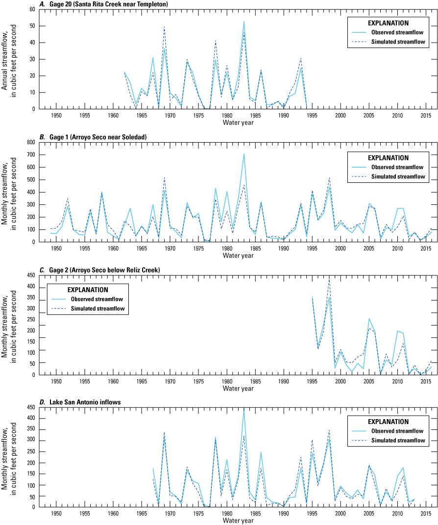
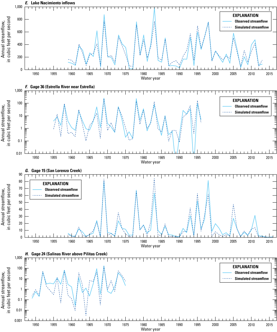
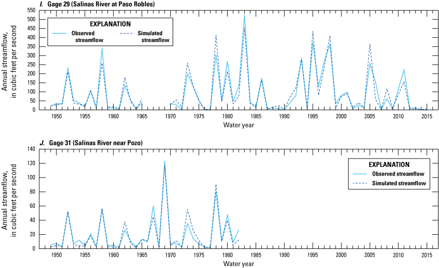
Comparison of observed (light blue) versus simulated (dashed dark blue) annual and monthly streamflow at selected U.S. Geological Survey streamgages: A, gage 20; B, gage 1; C, gage 2; D, Lake San Antonio inflows; E, Lake Nacimiento inflows; F, gage 36; G, gage 15; H, gage 24; I, gage 29; and J, gage 31 (U.S. Geological Survey, 2016; Hevesi and others, 2025).
The combined calibration result, based on the comparison of simulated versus observed long-term (period of record) mean streamflow and maximum daily, monthly, and annual streamflow for all 31 streamflow records (29 USGS streamgages and 2 reservoir inflows), indicated a good calibration in terms of low overall estimation bias and R2 values of 0.798–0.999 (figs. 26A, B, C, D). Mean monthly streamflow as a percentage of total annual streamflow, calculated as the average result for all 31 records, indicated a satisfactory comparison of the seasonal distribution of simulated versus observed streamflow (figs. 26E, F), with February having the highest mean monthly percentage of annual streamflow and August having the lowest mean monthly percentage of annual streamflow.
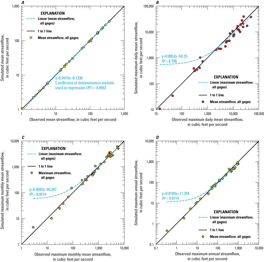
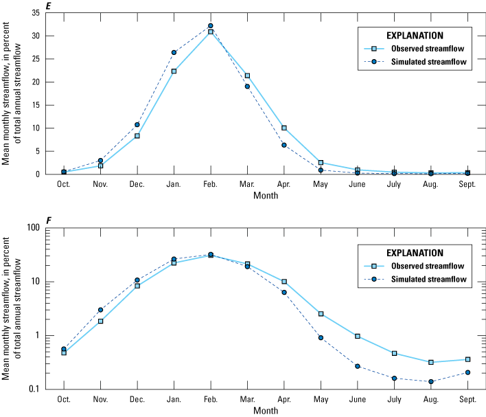
Summarized comparison of observed versus simulated streamflow for 29 U.S. Geological Survey streamgages and 2 reservoir inflows: A, mean streamflow; B, maximum daily mean streamflow; C, maximum monthly mean streamflow; D, maximum annual streamflow; E, mean monthly streamflow; and F, mean monthly streamflow, shown on a log scale (U.S. Geological Survey, 2016; Hevesi and others, 2025).
Comparisons between simulated and observed mean monthly streamflow were used as an indication of the goodness-of-fit to the seasonal distribution of streamflow for all streamgages. Monthly streamflow was calculated as a mean monthly percentage of total annual flow to standardized results for all streamgages and provided an equal weight to each streamgage (table 17). The R2 statistic was used as a measure of the goodness-of-fit and ranged from a minimum of 0.67 for USGS streamgage 11143300 (gage 40), to a maximum of 0.99 for several streamgages, including USGS streamgage 11152000 (gage 1), 11151300 (gage 15), and 11143500 (gage 31). An R2 of 0.97 was calculated for the average of the mean monthly streamflow, as a percentage of total annual streamflow, for the 29 USGS streamgages and the 2 reservoir inflows.
Table 17.
Salinas Valley Watershed Model calibration results showing goodness-of-fit statistics using mean monthly streamflow.[—Left][ID, identification; R2, coefficient of determination]
The percentage departure of annual streamflow from the long-term (period of record) mean streamflow was compared for all simulated and observed annual flows (fig. 27A). The comparison was used to help evaluate the combined goodness-of-fit for all annual flows based on a standardized measure of flow. The R2 value of 0.88 indicated a good fit between simulated and observed annual flows for the combined set of annual streamflows. In addition, the residuals of the difference between simulated and observed percentage departure of annual flow from mean streamflow did not indicate estimation bias relative to the annual time series (fig. 27B).
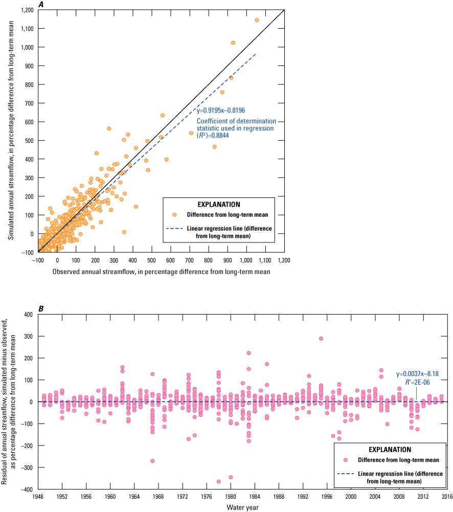
Summarized comparison of simulated versus observed streamflow for all U.S. Geological Survey streamgages and reservoir inflows: A, annual streamflow as a percentage of long-term mean streamflow and B, residual of annual streamflow, simulated minus observed, as percentage difference from mean streamflow (U.S. Geological Survey, 2016; Henson and others, 2022; Hevesi and others, 2025).
Model Validation
Model validation provides an indication of model uncertainty and forecasting accuracy by comparing simulated and observed streamflow using records that were not included as part of the calibration procedure. The SVWM was validated using streamflow records for five streamgages having streamflow records that were not included in the calibration procedure: USGS streamgages 11152650 (gage 38), 11150500 (gage 19), 11151700 (gage 6), 11152300 (gage 10), and 11152500 (gage 21). The validation period for USGS streamgage 11152650 (gage 38) included the later part of the record, from 2002 to 2016, whereas the calibration period included the earlier record, from 1971 to 1986. Records from USGS streamgages 11152300 (gage 10) and 11151700 (gage 6) were not used in model calibration because of the effect of reservoir releases on daily and monthly streamflow. U.S. Geological Survey streamgages 11152500 (gage 21) and 11150500 (gage 19) were included in model calibration using records before the completion of Lake Nacimiento (water years 1949–56), whereas the validation period for these streamgages included records from 1957 to 2016. The validation periods using the four streamgages on the Salinas River post-dated the completion of the dam impounding Lake Nacimiento, and therefore, the observed streamflow included managed flow conditions. The comparison between simulated and observed streamflow at the four streamgages on the Salinas River was done to evaluate changes in flow conditions relative to unimpaired streamflow conditions represented by the SVWM, in addition to model validation.
The validations results were considered good for USGS streamgages 11152500 (gage 21), 11150500 (gage 19), and 11152650 (gage 38), in terms of low estimation bias, as indicated by PAE values from −0.1 to 2.1 percent (table 18). The monthly and annual NSME results for USGS streamgages 11152500 (gage 21) and 11152650 (gage 38) were good (0.70 and 0.87, respectively). In contrast, the monthly NSME result for USGS streamgage 11150500 (gage 19) was poor and the annual result was fair, most likely because of the direct effect of flow releases from Lakes Nacimiento and San Antonio. The annual hydrograph comparing simulated and observed streamflow at USGS streamgage 11150500 (gage 19) indicates an overestimation of high annual flows and an underestimation of low annual flows, which is an expected result in terms of comparing simulated unimpaired streamflow to the managed observed flows (fig. 28D). The PAE results of 1.6–2.1 for USGS streamgage 11150500 (gage 19), however, indicate a good result in terms of the USVS accurately representing the long-term mean streamflow conditions at this location. In general, the model validation result was considered satisfactory to good based on the visual comparison of the annual hydrographs at all five streamgages (fig. 28).
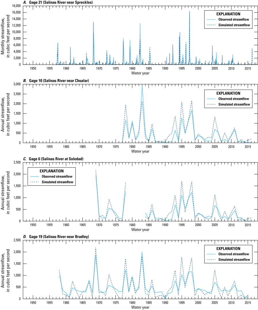
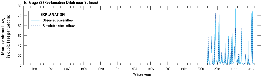
Model validation using comparisons of observed and simulated streamflow at A, gage 21; B, gage 10; C, gage 6; D, gage 19; and E, gage 38 (U.S. Geological Survey, 2016; Hevesi and others, 2025).
Table 18.
Model validation results for five selected U.S. Geological Survey streamgages.[ft3/s, cubic foot per second; ID, identification; NSME, Nash-Sutcliffe model efficiency; Obs., observed; Sim., simulated; SVWM, Salinas Valley Watershed Model; USGS, U.S. Geological Survey; %, percent; —, not applicable]
Results for USGS streamgages 11152300 (gage 10) and 11151700 (gage 6) indicated overestimation of the long-term mean streamflow by 22 and 32 percent, respectively. These two streamgages were not included in model calibration and the overestimation could be indicative of the effect of groundwater pumping along this section of the Salinas Valley, between gages 6 and 10 (with pumping decreasing baseflow), and the high degree of uncertainty associated with simulating streamflow losses caused by seepage through the streambed. In addition, local flow diversions and return flows from irrigation may have an effect on the Salinas River streamflow in this part of the valley, and these processes are not simulated by the SVWM.
Model Limitations
The SVWM is considered successful for its intended purpose; however, understanding the model limitations is important for determining appropriate applications, evaluating results, and qualitatively assessing model uncertainty. The timing, magnitude, frequency, and spatial distribution of daily precipitation are the most important factors affecting simulated streamflow by the SVWM. Although a total of 194 climate stations with records of daily precipitation and air temperature were used to develop the climate inputs for the SVWM, many of these stations had gaps in the record or short records (10 years or less) compared to the entire simulation period of 70 years. For many periods in the 71-year simulation period that included water year 1948 as the model initialization period, only a fraction of the 194 stations were active, and a greater degree of uncertainty was associated with the spatially interpolated climate inputs for HRUs that were far from the nearest climate station. Additionally, some areas of the SVWM have a lower density of stations throughout the simulation period, and therefore, the simulation results for these areas may be associated with a higher degree of uncertainty relative to results in areas with a higher density of climate stations.
The daily climate inputs developed by the BCM are adequate for estimating daily, monthly, and annual water budgets. However, a daily time step with uniformly distributed hourly precipitation might not adequately represent high hourly precipitation rates that may occur during severe storms. High hourly precipitation rates can result in a greater proportion of precipitation contributing to Hortonian surface-water runoff as compared to the proportion of precipitation contributing to pervious land infiltration. Hortonian surface-water runoff can be a substantial component of streamflow during storms. Inadequate representation of the high precipitation rates might cause the SVWM to potentially underestimate surface runoff and the magnitude of peak flows during some storm periods.
Many of the critical HSPF parameters used in the SVWM, such as the parameters controlling ET and recharge from the soil zone; the partitioning of overland runoff, interflow, and recharge; and the rates of interflow and groundwater discharge to streams, were not measured, but rather were estimated and then adjusted during the model calibration process. The final calibrated values are considered reasonable estimates of HSPF parameters based on values used in previous studies; however, the values might not be representative of actual field conditions and might not agree with the measured values if such values become available. In addition, many of the parameters were estimated using available geospatial datasets representing average historical field conditions at specific times, such as the NLCD 2011 land-cover type, percentage of impervious land cover, and percentage of forest canopy cover. At some locations, these estimated values might not be representative of conditions in the early or final parts of the simulation period. All parameters representing the physical characteristics of the Salinas Valley study area, such as land cover, topography, hydrography, soil properties, and surficial geology, were set to constant, time-invariant values for the simulation period.
Anthropogenic effects on the hydrologic system, such as the construction of reservoirs and the implementation of managed river flows at different times in the simulation period, are not represented by the SVWM. Other changes through time not represented by the model include increased diversions of surface water and changes in pumping and irrigation practices. The inclusion of crop and landscape irrigation in the SVWM would likely cause an increase in mean soil moisture simulated for the central and lower valley areas of the SVWM where agricultural land cover is prevalent and developed lands are associated with urbanized areas. The increased soil moisture would result in increased ET and might also result in increased recharge and runoff.
The SVWM uses a simplified, empirical representation of the groundwater system that does not account for the three-dimensional heterogeneity of aquifer systems and the physics of groundwater storage and flow. The groundwater reservoirs simulated by the SVWM represented only the active part of the groundwater system contributing to streamflow and ET and were assumed to be coincident with the boundaries of the associated HRUs that were defined mostly by surface-water drainage divides rather than groundwater-flow divides. The AGWRC coefficient controlling the time-varying rate of groundwater discharge to streams was estimated and calibrated based on surficial characteristics of drainage basins such as topography, land cover, soils, and surficial geology; the underlying geologic structure is not represented by the SVWM. The SVWM-simulated groundwater reservoirs do not represent the total groundwater-flow system in underlying aquifers, and therefore, the SVWM cannot be used to quantify the groundwater system such as changes in aquifer storage. Groundwater travel times and flow paths through the unsaturated zone are not explicitly simulated by the SVWM, and therefore, rejected recharge for locations with a high water table is not simulated; this could cause an overestimation of recharge for these locations.
Simulation Results, Water Years 1949–2018
Simulation results for the 70-year target period, water years 1949–2018, were used to evaluate and quantify water balance components of the natural hydrologic system for the Salinas Valley study area, including the Salinas River watershed and several smaller, adjacent drainages along the Monterey Bay coast. Simulated components include ET, recharge, surface runoff (overland flow), interflow, and groundwater discharge (baseflow) for the 690 HRUs, and streamflow and stream seepage losses for the 690 stream reaches connecting the HRUs. The results were used to analyze the spatial and temporal variability of the natural hydrologic system for the 70-year historical simulation period. Results were compared between the 10 subbasin areas, 28 subdrainage areas, and 25 upland tributary drainages having outflows to the lower Salinas Valley study area, an area generally coincident with developed lands and agricultural land irrigated with groundwater.
Precipitation is the only inflow to the natural hydrologic system of the Salinas Valley study area simulated by the SVWM. The three outflows simulated by the SVWM are ET, surface-water outflow (streamflow) to Monterey Bay from the Salinas River and smaller adjacent basins along the Monterey Bay coastal region, and recharge to the inactive groundwater reservoir. Recharge to the inactive groundwater reservoir accounts for water that does not contribute to groundwater discharge either as baseflow to streams or transpiration from the saturated zone and is an outflow of water from the hydrologic system represented by the SVWM. As simulated by the SVWM, recharge to the inactive groundwater reservoir consists of two components: (1) streamflow seepage losses in stream reaches and (2) inter-channel recharge from PERLNDs, also referred to in this study as net land-area recharge.
In addition to precipitation and the three outflows, components of the water balance that were analyzed included total recharge, surface runoff (overland flow), interflow runoff, and groundwater discharge to stream reaches (baseflow) from the active groundwater reservoir. Total recharge was calculated as the sum of recharge to the active and inactive groundwater reservoirs. Results for selected inflows and outflows are provided in tables 19 and 20 for subbasin areas, subdrainage areas, and upland drainage areas tributary to the central and lower Salinas Valley lowlands (fig. 15). Table 19 shows the 1948–2018 70-year mean annual inflows and outflows as an average water equivalent depth, in units of in/yr, for the area of each subbasin, subdrainage, and upland tributary drainage. Table 20 shows the 70-year mean inflows and outflows in terms of water volumes, in units of thousands of acre-ft/yr, for subbasins, subdrainages, and upland tributary drainages. Results in terms of area-averaged water equivalent depths provided in table 19 provide a more direct comparison of the differences in the hydrologic character between the various subbasins and subdrainages because the effect of drainage area size is excluded, whereas the water volumes shown in table 20 provide a more direct comparison of the absolute magnitude of water balance components between subbasins and subdrainages.
Table 19.
Simulation results for selected water balance components calculated as mean annual inches of water inflows and outflows, water years 1949–2018, for subbasins, subdrainages, and tributary drainages in the Salinas Valley study area.[AET, actual evapotranspiration; in/yr, inch per year]
Table 20.
Simulation results for selected water balance components calculated as mean annual inflow and outflow volumes, in thousands of acre-feet per year (acre-ft/yr), water years 1949–2018, for subbasins, subdrainages, and tributary drainages in the Salinas Valley study area.[acre-ft/yr, acre-foot per year; AET, actual evapotranspiration; ft3/s, cubic feet per second]
Evapotranspiration
The simulated 70-year mean ET of 14.9 in/yr for the Salinas Valley study area was the largest outflow of water from the SVWM, about 3.6 million acre-ft/yr, accounting for about 80 percent of the 70-year mean precipitation inflow of 18.5 in/yr, about 4.5 million acre-ft/yr (tables 19, 20). Results for HRUs ranged from mean values of 17–26 in/yr for higher elevations with substantial forest cover and thick soils along the western and eastern sides of the SVWM, to less than 11 in/yr throughout the valley floor and in some parts of the western and eastern sides, and less than 9.5 in. in the southeastern part of the Salinas River watershed (fig. 29). The spatial distribution of ET is partly consistent with the spatial distribution of precipitation (fig. 19) because the magnitude of ET is dependent on water availability; however, the spatial distribution also is affected by spatial variations in PET (fig. 21), soil water storage capacity (fig. 9), land-surface slope (fig. 4) and other factors controlling runoff, and vegetation. The highest mean ET of more than 19 in/yr was simulated for the ARR subbasin and the UAS, LAS, and SRH subdrainages, which also has the highest mean precipitation of 30.1 in/yr (table 19). The lowest ET of 12.9 in/yr was simulated for the NAC and MSR subbasins in part because of coarse soils on steep slopes limiting the storage capacity of the root zone.
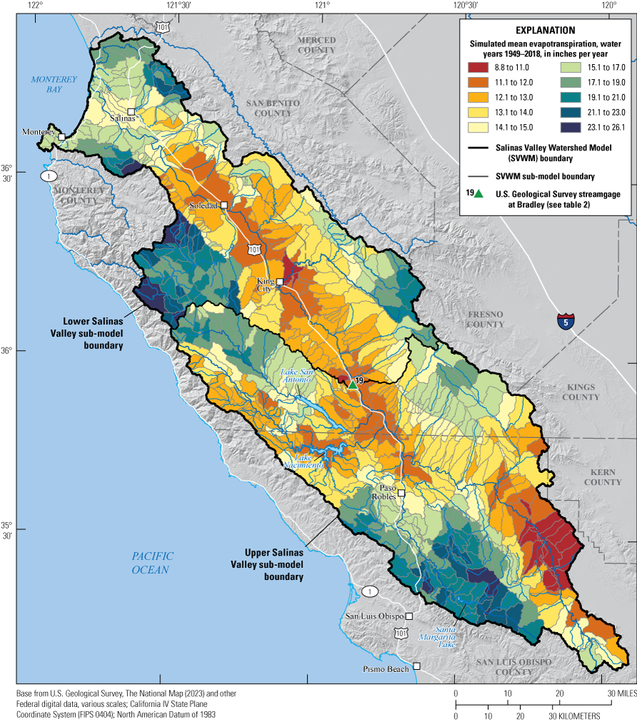
Salinas Valley Watershed Model simulation results for mean evapotranspiration (total actual evapotranspiration [AET]), water years 1949–2018 (Hevesi and others, 2025).
Runoff
Total runoff simulated by the SVWM from each HRU to the connected RCHRES stream segment includes three separate flow components: overland runoff, interflow runoff, and groundwater discharge to streams (baseflow). Total HRU runoff is the unrouted surface-water outflow from HRUs to the stream network. The accumulated total runoff is routed through the connected RCHRES network using the kinematic wave algorithm in HSPF to simulate streamflow.
The 70-year mean total runoff simulated by the SVWM for the Salinas Valley study area was of 3.52 in/yr for the SVWM, or 19 percent of precipitation (table 19). The NAC subbasin had the highest mean total runoff of 11.82 in/yr, about 48 percent of precipitation. In comparison, the LOR had the lowest mean total runoff of only 1.2 in/yr, about 7 percent of precipitation. Mean total runoff of more than 10 in/yr and higher was simulated for HRUs along the western boundary of the SVWM in response to the high precipitation, low PET, steep terrain, and thin soil cover (fig. 30). Low runoff of 1.0 in/yr and less was simulated for the hotter and drier areas of the SVWM, such as the central valley of the Salinas River and along the southeast part of the SVWM domain. The low runoff simulated for the Salinas River valley does not include irrigation return flows because irrigation is not accounted for by the SVWM.
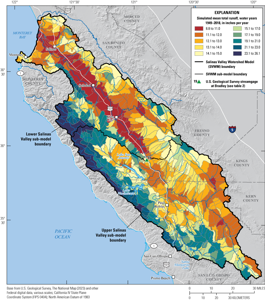
Simulated mean total runoff to stream channels using the Salinas Valley Watershed Model, water years 1949–2018 (Hevesi and others, 2025).
Overland runoff is simulated by the SVWM when precipitation exceeds the storage capacity of the land surface and soil zone or when the precipitation rate exceeds the infiltration capacity of PERLNDs. Overland runoff can reinfiltrate the ground surface depending on the slope, length, and roughness of the overland flow plane (defined by parameters SSLUR, LSUR, and MANNING). Simulation results for overland runoff included a 70-year basinwide mean of 0.97 in/yr for the Salinas Valley study area, or about 5.2 percent of precipitation and 28 percent of total runoff (table 19). A maximum subbasin mean overland runoff of 5.5 in/yr was simulated for the NAC subbasin, which was about 22 percent of precipitation and 46 percent of total runoff (table 19). In contrast, a mean overland runoff of only 0.03 in/yr was simulated for the EST subbasin. High overland runoff was generally limited to the high-elevation HRUs along the western boundary of the Salinas Valley study area, coinciding with the locations of the highest precipitation and the steepest terrain (fig. 31).
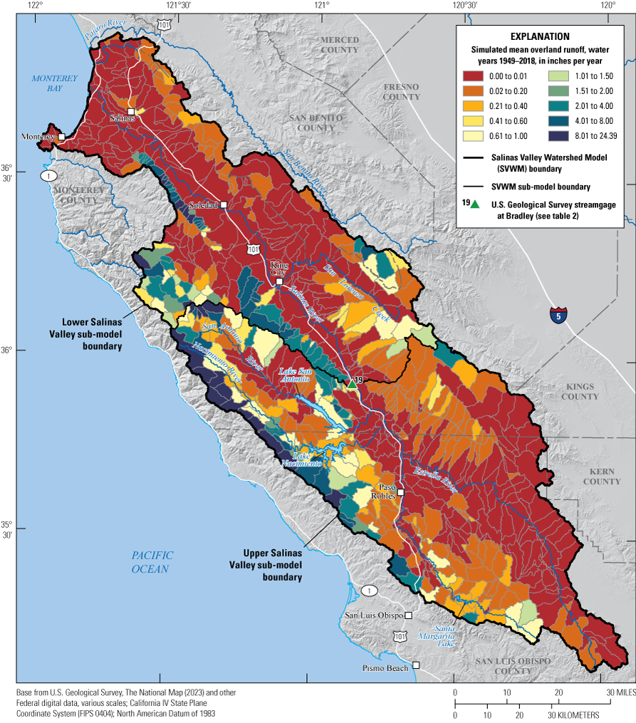
Salinas Valley Watershed Model simulation results for mean overland runoff to stream channels, water years 1949–2018 (Hevesi and others, 2025).
The simulated 70-year mean basinwide interflow runoff to stream channels of 0.84 in/yr was similar in magnitude to overland runoff (table 19). The highest interflow runoff of 3.36 in/yr, about 13.6 percent of precipitation, was simulated for the NAC subbasin. The ARR subbasin also had a high mean interflow runoff of 3.08 in/yr compared to the other 8 subbasins having mean values of 1.45 in/yr and less. As with overland runoff, the highest mean interflow runoff of 4 in/yr and more was simulated along the western boundary of the Salinas Valley study area in response to the high precipitation and steep terrain (fig. 32). Low mean interflow values of 0.5 in/yr and less were simulated for the areas that are drier, more inland, less rugged, and more flat-lying, which comprise much of the Salinas Valley study area.
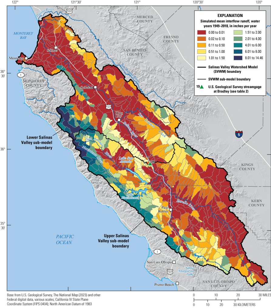
Salinas Valley Watershed Model simulation results for mean interflow runoff to stream channels, water years 1949–2018 (Hevesi and others, 2025).
Groundwater discharge to streams from the active groundwater reservoir, referred to as baseflow, is simulated by the SVWM as a function of the groundwater recession parameters AGWRC and KVARY and the amount of water recharging and stored in the active groundwater reservoir, minus groundwater losses to transpiration. The 70-year mean groundwater discharge to streams simulated for the Salinas Valley study area was 1.71 in/yr, which was 48 percent of the total outflow to stream channels and about 9.2 percent of precipitation (table 19). The ARR subbasin had the highest mean groundwater discharge to streams of 6.1 in/yr, about 20 percent of precipitation, and 60 percent of the total outflow from HRUs. In contrast, the mean groundwater discharge to streams for the NAC subbasin was only 3.0 in/yr, about 12 percent of precipitation and 25 percent of total outflow.
Mean values of groundwater discharge to streams of 3.0 in/yr and higher were simulated for HRUs in the SRH, NAC, SAN, and ARR subbasins, with very high values of 8–28 in/yr simulated for HRUs in the headwaters of the ARR and SAN subbasins (fig. 33). Mean groundwater discharge to streams of at least 0.1 in/yr was simulated for most HRUs in the SVWM. The lowest mean values of less than 0.1 in/yr were simulated for low-elevation, flat-lying HRUs in the valley bottom of the middle and lower Salinas Valley, generally coincident with the location of unconsolidated alluvium.
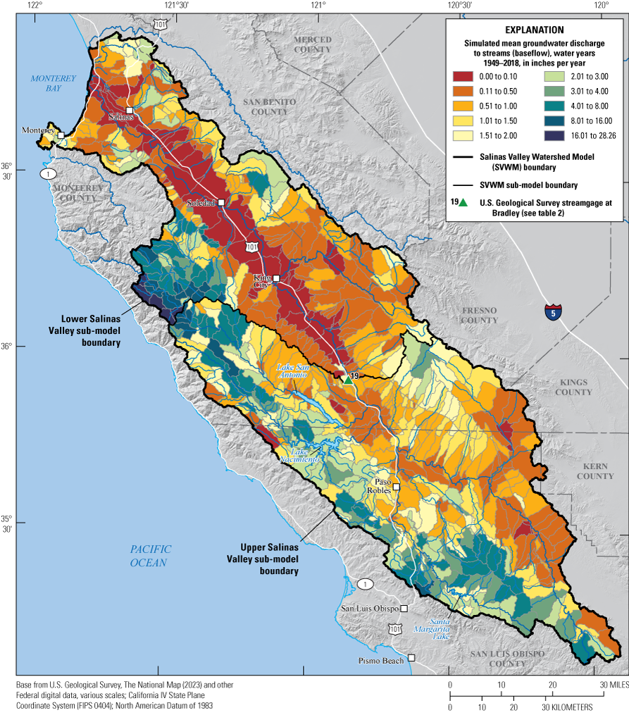
Salinas Valley Watershed Model simulation results for mean groundwater discharge to streams, water years 1949–2018 (Hevesi and others, 2025).
Recharge
Groundwater recharge simulated by the SVWM includes inflows to the active and inactive groundwater reservoirs. Unlike recharge supplying the active groundwater reservoir used to simulate groundwater discharge to streams and transpiration from the saturated zone, recharge to the inactive groundwater reservoir is an outflow from the hydrologic system represented by the SVWM. Recharge to the inactive groundwater reservoir is referred to in this study as net recharge. Net recharge does not contribute groundwater discharge to streams or transpiration from the saturated zone. As simulated by the SVWM, net recharge consists of two components: (1) stream seepage recharge, or the infiltration of streamflow through the streambed and (2) deep recharge from PERLNDs. Conceptually, net recharge simulated by the SVWM may represent increases in groundwater storage, recharge to groundwater reservoirs having flow paths with long travel times or flow paths contributing to basin underflows, riparian ET, or outflows from wells.
The 70-year mean inter-channel recharge (net land-area recharge) was the smallest component of the water balance simulated by the SVWM, with a 70-year mean value of 0.08 in/yr, or about 20,000 acre-ft/yr and 0.5 percent of precipitation for the Salinas Valley study area (tables 19, 20). The MCB subbasin had the highest net land-area recharge of 0.28 in/yr, or about 1.5 percent of precipitation, with HRUs along the northern boundary of the SVWM having the highest rates of more than 0.5 in/yr (fig. 34). All other subbasins had net land-area recharge rates of 0.13 in/yr and less, with the NAC, ARR, and LOR subbasins having rates of approximately zero. The lowest net land-area recharge rates were mostly coincident with consolidated bedrock types having low permeability, such as igneous and metamorphic rocks, shales, and claystones. Overall, the upper Salinas Valley had a greater mean annual net land-area recharge volume compared to the lower Salinas Valley (table 20), mostly because of a high percentage of permeable conglomerate bedrock underlying soils (fig. 10).
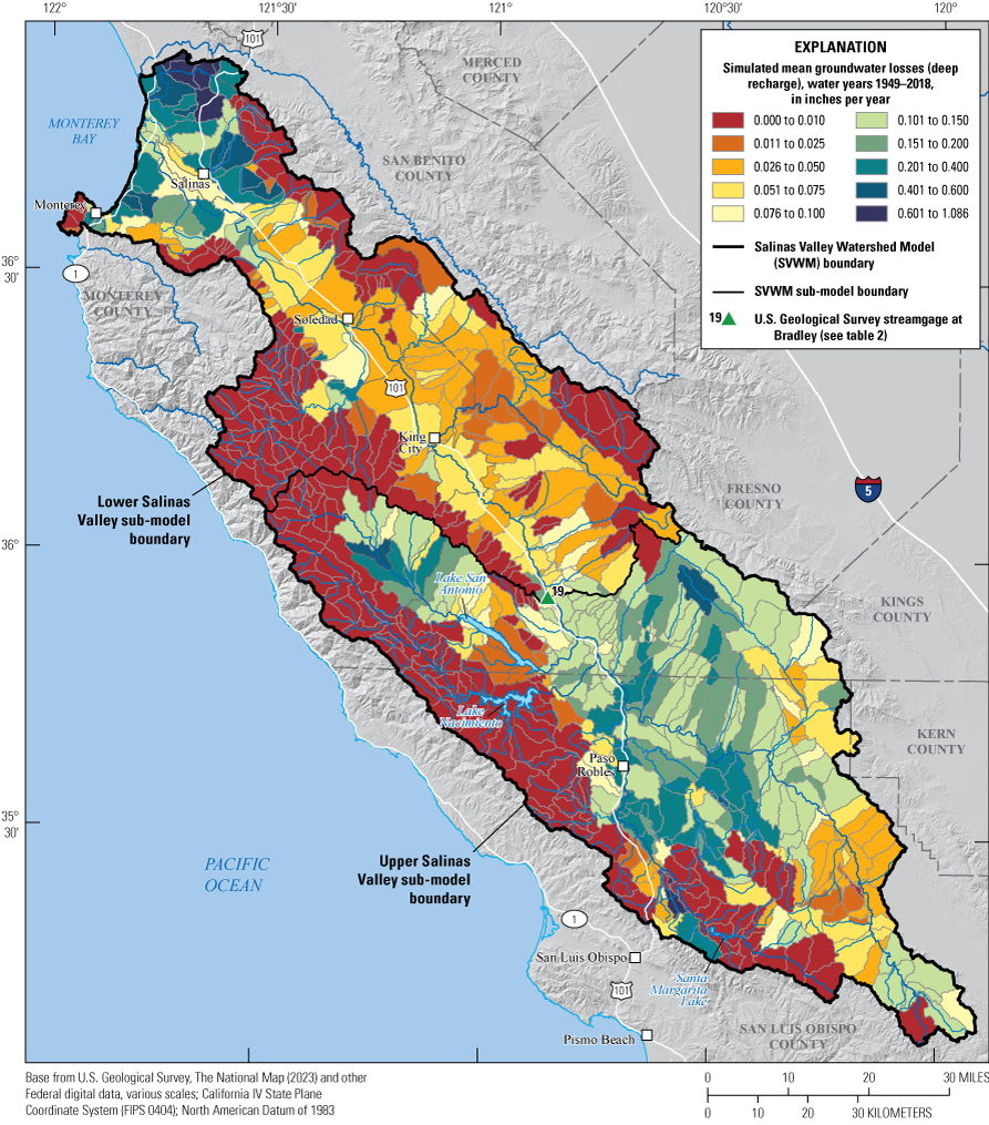
Salinas Valley Watershed Model simulation results for mean groundwater losses (deep recharge), water years 1949–2018 (Hevesi and others, 2025).
Stream losses resulting from the downward seepage of streamflow through the streambed are an important component of the water balance simulated by the SVWM. Simulating the streamflow losses, or stream seepage recharge, was needed to achieve a satisfactory calibration of many of the streamgages in the Salinas Valley study area. As indicated by the streamflow records in the Salinas Valley study area, a substantial portion of the runoff generated in the upland areas of the Salinas River watershed is not discharged to Monterey Bay as streamflow, but rather is reinfiltrated into the main channel of the Salinas River and becomes recharge to aquifers that are potential sources of groundwater pumped for crop irrigation and other uses. For example, the observed mean streamflow at USGS streamgage 11151700 (gage 6; table 2) on the Salinas River is less than the sum of observed streamflow at upstream USGS streamgages 11150500 (gage 19) and 11151300 (gage 15) for water years 1984–2014, with a cumulative decrease in annual streamflow of about 3.2 million acre-ft, or a mean annual decrease in streamflow of 128 ft3/s (fig. 35A).
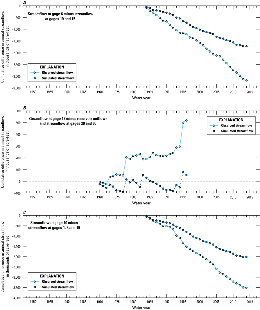
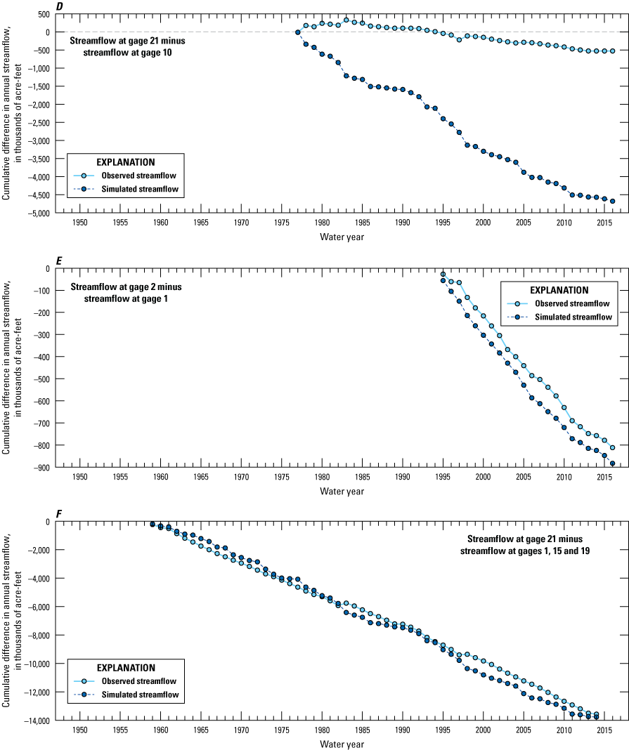
Comparison of observed and simulated differences in annual streamflow at selected U.S. Geological Survey streamgages: A, streamflow at gage 6 minus streamflow at gages 19 and 15; B, streamflow at gage 19 minus reservoir outflows and streamflow at gages 29 and 36; C, streamflow at gage 10 minus streamflow at gages 1, 6, and 15; D, streamflow at gage 21 minus streamflow at gage 10; E, streamflow at gage 2 minus streamflow at gage 1; and F, streamflow at gage 21 minus streamflow at gages 1, 15, and 19 (U.S. Geological Survey, 2016; Hevesi and others, 2025).
Differences in observed streamflow at other locations also indicate stream losses. There was a cumulative decrease of 3.6 million acre-ft from water years 1984 to 2014 at USGS streamgage 11152300 (gage 10; table 2) on the Salinas River compared to the sum of observed streamflow at upstream USGS streamgages 11152000 (gage 1), 11151700 (gage 6), and 11151300 (gage 15; fig. 35C); a cumulative decrease of 0.8 million acre-ft from water years 1995 to 2016 between downstream USGS streamgage 11152050 (gage 2) and upstream USGS streamgage 11152000 (gage 1) on the Arroyo Seco (fig. 35E); and a cumulative decrease of 13 million acre-ft (a long-term mean streamflow loss of 310 ft3/s) from water years 1959 to 2014 at USGS streamgage 11152500 (gage 21) on the Salinas River compared to the sum of streamflow at upstream USGS streamgages 11152000 (gage 1), 11151300 (gage 15), and 11150500 (gage 19; fig. 35F).
Stream seepage recharge is simulated by the SVWM using a second outflow node for each stream reach (the first outflow node is used for simulating streamflow) and was conceptualized as a component of deep recharge to the inactive groundwater reservoir as opposed to recharge to the active groundwater reservoir used for simulating baseflow. Total deep recharge to the inactive groundwater reservoir, calculated as the sum of net land-area recharge and stream seepage recharge, is an outflow from the SVWM because this water does not contribute to simulated baseflow or simulated ET from shallow groundwater. Rather, deep recharge is conceptualized as contributing to groundwater reservoirs that may supply water for crop irrigation or consumptive use, contributing to deep groundwater storage, or contributing to groundwater underflow.
The simulated decreases between streamgages indicated a good match to the observed differences in streamflow between USGS streamgages 11152050 (gage 2) and 11152000 (gage 1) on the Arroyo Seco and between USGS streamgage 11152500 (gage 21) on the Salinas River and the sum of streamflow at upstream USGS streamgages 11152000 (gage 1), 11151300 (gage 15), and 11150500 (gage 19; figs. 35E, F). Simulated decreases in streamflow were about half the observed decreases between USGS streamgages 11151700 (gage 6) and the sum of streamflow at upstream USGS streamgages 11151300 (gage 15) and 11150500 (gage 19; fig. 35A). The simulated decreases in streamflow also were about half the observed decreases between USGS streamgage 11152300 (gage 10) and upstream USGS streamgages 11152000 (gage 1), 11151700 (gage 6), and 11151300 (gage 15; fig. 35C). Although the results indicated discrepancy between simulated and observed decreases in streamflow at several locations that were analyzed, the simulation results provided a good overall match to the combined decrease in streamflow in the MSR and LSR subbasins, as indicated by the observed differences in streamflow between USGS streamgage 11152500 (gage 21) and upstream USGS streamgages 11152000 (gage 1), 11151300 (gage 15), and 11150500 (gage 19; fig. 35F).
The LSR subbasin had the highest mean simulated stream seepage recharge, as a water equivalent depth for the subbasin area, of 10.74 in/yr (table 19). The ARR subbasin had the second highest mean stream seepage recharge, expressed as a water equivalent depth, of 5.27 in/yr. The MCB subbasin had the smallest stream seepage of 0.18 in/yr, followed by the NAC subbasin with the next smallest stream seepage of 0.23 in/yr (table 19). Simulated streamflow losses were highest along the middle and lower reaches of the Salinas River, and along the lowermost reaches of the ARR, varied from 16 to 32 ft3/s in the middle Salinas Valley and LAS, and varied from 16 to 70 ft3/s in the lower Salinas Valley (figs. 1, 36). Mean stream losses in the main channels of tributary drainages ranged from 1 to 16 ft3/s, and stream losses in the headwater drainages ranged from 0 to 0.5 ft3/s for most RCHRESs in the drainage network.
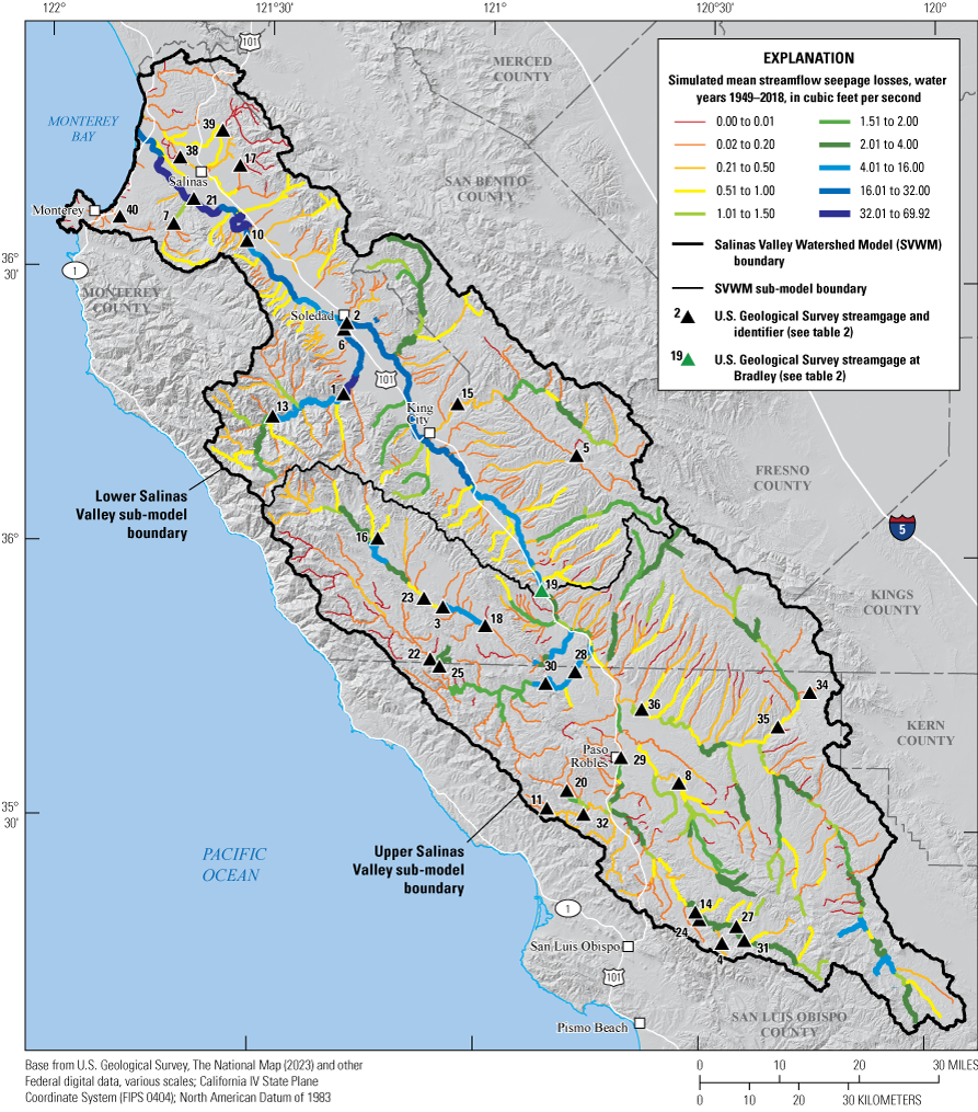
Salinas Valley Watershed Model simulation results for mean streamflow seepage losses, in cubic feet per second, water years 1949–2018 (Hevesi and others, 2025).
Overall, deep recharge to the inactive groundwater reservoir from stream seepage was substantially greater than net land-area recharge to the inactive groundwater reservoir for all subbasins and subdrainages except for the MCB subbasin and the ELK and MSB subdrainages (tables 19, 20). Total stream seepage for the Salinas Valley study area was 627,000 acre-ft/yr for the 70-year simulation period and was substantially greater than the total net land-area recharge of only 20,000 acre-ft/yr (table 20). The total recharge volume to the inactive groundwater reservoir of 446,000 acre-ft/yr for the LSVS was more than double the total recharge volume for the USVS and also was greater than the surface-water outflow of 232,000 acre-ft/yr for the Salinas Valley study area. In contrast, total recharge to the inactive groundwater reservoir was only 201,000 acre-ft/yr for the USVS, substantially less than the surface-water outflow of 346,000 acre-ft/yr.
Streamflow
Simulated 70-year mean streamflow ranged from a maximum of 505 ft3/s for the Salinas River directly downstream from the juncture of the Arroyo Seco tributary to less than 1 ft3/s for most of the small tributary drainages in drier sections of the SVWM (figs. 1, 37). The simulated 70-year mean streamflow at the mouth of the Salinas River was only 278 ft3/s, substantially less than the mean streamflow of 478 ft3/s simulated at USGS streamgage 11150500 (gage 19), because of the large number of streamflow losses caused by streambed seepage (table 20). The simulated 70-year mean streamflow for most sections of the Salinas River in the LSVS, downstream of gage 19, was between 200 and 500 ft3/s (fig. 37). The highest mean tributary inflow of 278 ft3/s was simulated for the NAC subbasin (figs. 1, 37; table 20). High tributary inflows to the Salinas River also were simulated for the ARR (106 ft3/s) and SAN (87 ft3/s) subbasins (table 20). The simulated total mean surface-water inflow from all tributary drainages to the lower Salinas Valley study area was 770 ft3/s (table 20).
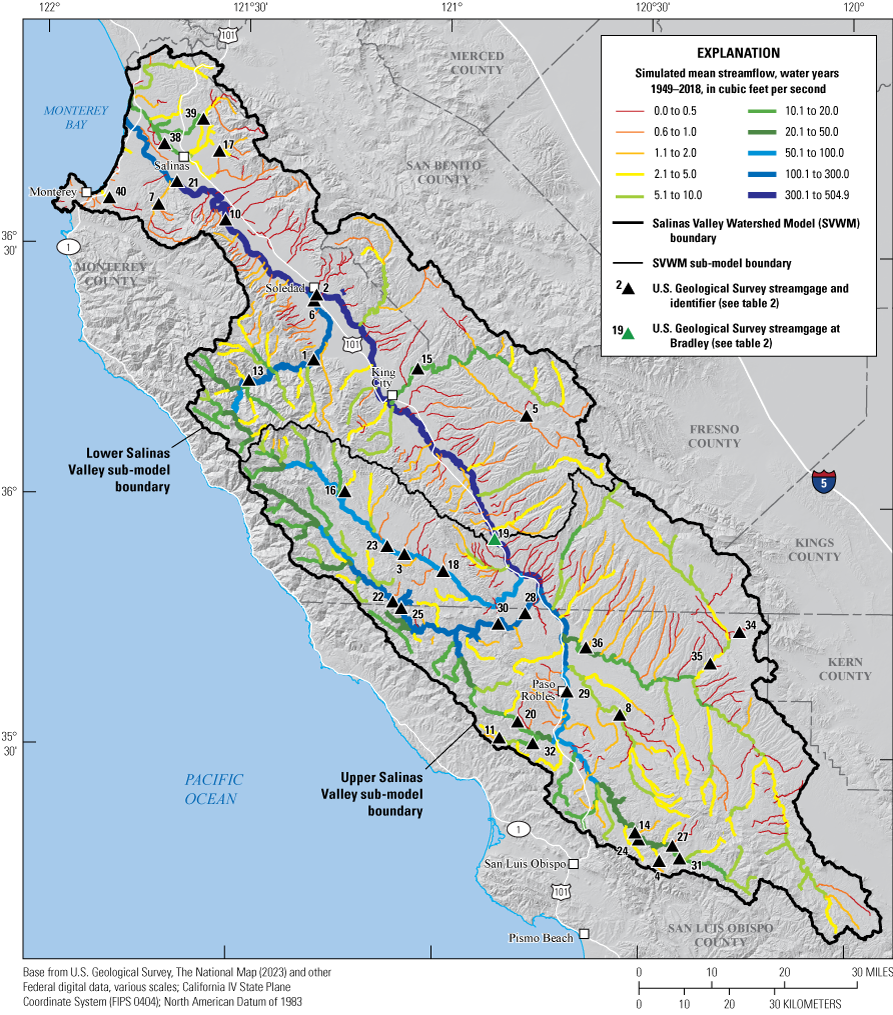
Salinas Valley Watershed Model simulation results for mean streamflow, in cubic feet per second (ft3/s), water years 1949–2018 (Hevesi and others, 2025).
Expressed as an equivalent runoff depth of the total upstream contributing area for each RCHRES stream segment, the highest 70-year mean runoff depth of 20 to more than 30 in/yr were simulated for the rugged uplands along the western side of the valley (fig. 38). In contrast, simulated runoff depths were only 2 in/yr and less for most stream segments on the east side of the Salinas Valley. Along the section of the Salinas River within the LSVS, downstream of gage 19, runoff depths varied from 1 to 4 in/yr above USGS streamgage 11152500 (gage 21) but decreased to less than 1 in/yr downstream from USGS streamgage 11152500 (gage 21). Simulated runoff depths for many of the lower elevation drainages on the drier, eastern side of the Salinas Valley were less than 0.5 in/yr.
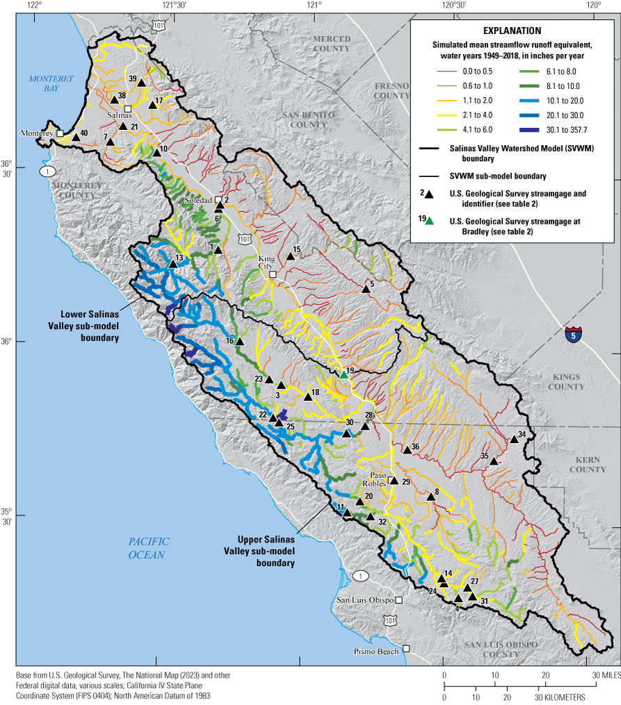
Salinas Valley Watershed Model simulation results for mean streamflow runoff equivalent in inches per year, water years 1949–2018 (Hevesi and others, 2025).
Simulated maximum daily streamflow for water years 1949–2018 varied from less than 200 ft3/s for headwater drainages to 80,000–92,000 ft3/s along the main channel of the Salinas River in the MSR and LSR subbasins (figs. 1, 2, 39). Total daily inflow from all tributary drainages to the lower Salinas Valley study area reached a maximum of 124,000 ft3/s during water year 1995 and exceeded 80,000 ft3/s during water years 1969 and 1966 (fig. 40A). Maximum daily streamflow was 10,000–20,000 ft3/s in the ARR, SAN, EST, and SRH subbasins, and 20,000–40,000 ft3/s in the NAC subbasin (figs. 2, 39). Maximum daily inflows from the SECO tributary drainage into the lower Salinas Valley study area were 10,000 ft3/s during water years 1969 and 1998 and 12,000 ft3/s during water year 1995 (fig. 40B). In contrast, maximum daily inflows were higher from the Nacimiento River (NACI) and SALI tributary drainages, with maximum daily inflows of about 37,000 ft3/s during water year 1967 for NACI and during water year 1995 for SALI (figs. 40C, D).
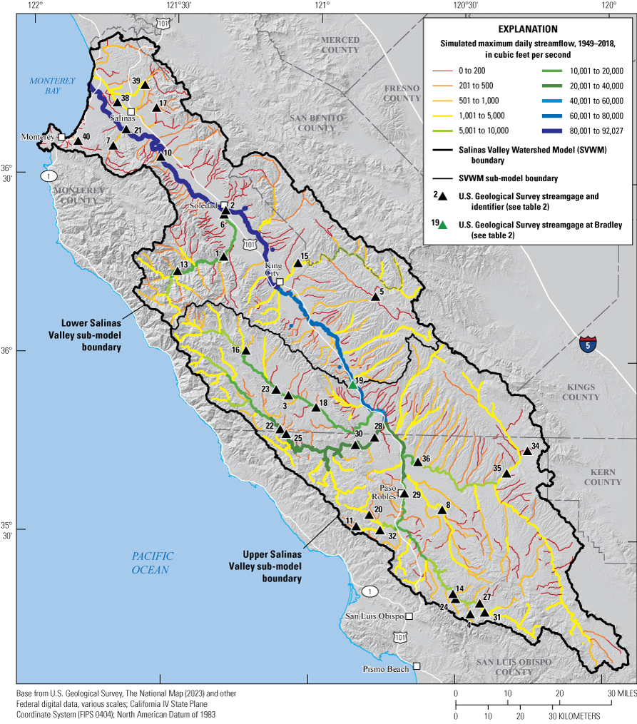
Salinas Valley Watershed Model simulation results for maximum daily streamflow seepage losses, in cubic feet per second, water years 1949–2018 (Hevesi and others, 2025).
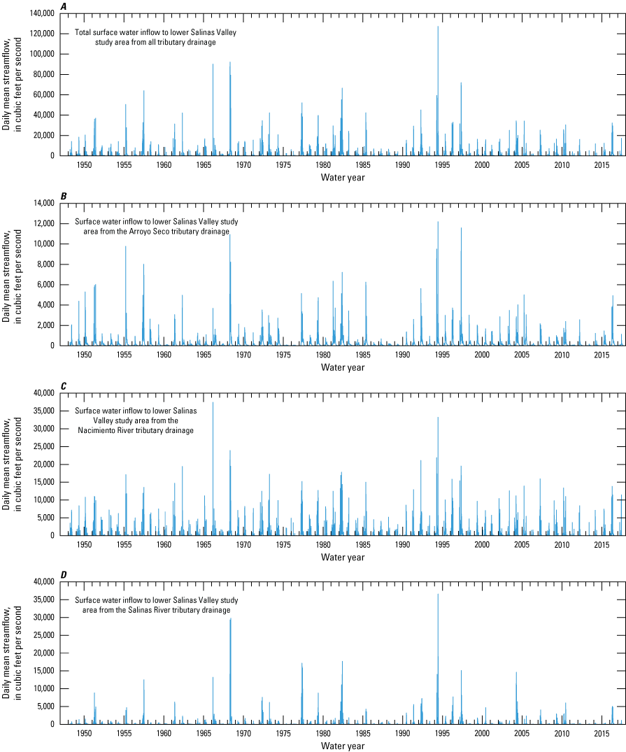
Simulated total daily surface-water inflows to the lower Salinas Valley study area from A, all tributary drainages; B, the Arroyo Seco tributary drainage (SECO); C, the Nacimiento River tributary drainage (NACI); and D, from the Salinas River tributary drainage (SALI; Hevesi and others, 2025).
Differences in simulated water balance components between the 10 subbasins were strongly dependent on differences in precipitation, with the ARR subbasin having the highest precipitation of about 30.1 in/yr, and the middle Salinas Valley subbasin having the lowest precipitation of about 14.7 in/yr. The NAC subbasin had the highest total flow (total runoff) to streams of about 11.8 in/yr, the highest percentage of total runoff relative to precipitation, and the highest percentage of overland runoff relative to total runoff to streams. In contrast, the ARR subbasin had the highest percentage of groundwater discharge to streams relative to the total runoff to streams. A large percentage of the 10.1 in/yr total outflow to streams in the ARR subbasin, about 5.3 in/yr, was lost to stream seepage. Only 4.9 in/yr (about 77,000 acre-ft/yr) of the total runoff simulated in the ARR subbasin reached the Salinas River channel. Total inflow from upland tributaries to the Salinas Valley lowlands was about 2.9 in/yr (558,000 acre-ft/yr) or about 15 percent of the 19.6 in/yr precipitation falling over the tributary subbasins.
Annual Results
The time series of annual ET for the Salinas Valley study area indicated a high degree of year-to-year variability, coinciding with the annual variability in precipitation, with high annual totals of more than 22 in. for water years 1958, 1983, 1995, and 1998 (fig. 41A). Comparison of annual results for the subbasins (fig. 42) indicated that ET was the largest water outflow for all years and all subbasins except NAC, where streamflow exceeded ET for water years with more than about 40 in. total precipitation, including 1958, 1969, 1978, 1983, 1996, 1998, and 2017 (the wettest water years for all subbasins). Water year 2014, the driest year, with less than 8 in. of precipitation for the Salinas Valley study area, had the lowest simulated annual ET of about 7 in. (fig. 41A). Comparison of annual ET between the 10 subbasin areas indicated differences of more than 6 in. between subbasins for some years, such as between the EST and ARR subbasins (fig. 43A). Relative differences between the subbasins were not consistent year to year, with the highest annual ET alternating between the SRH and ARR subbasins, mostly in response to spatial variations in annual precipitation. Water year 2014, the driest water year, had the lowest ET for all subbasins, and water years 1983 and 1998, the two wettest water years, had higher than average ET for all subbasins.
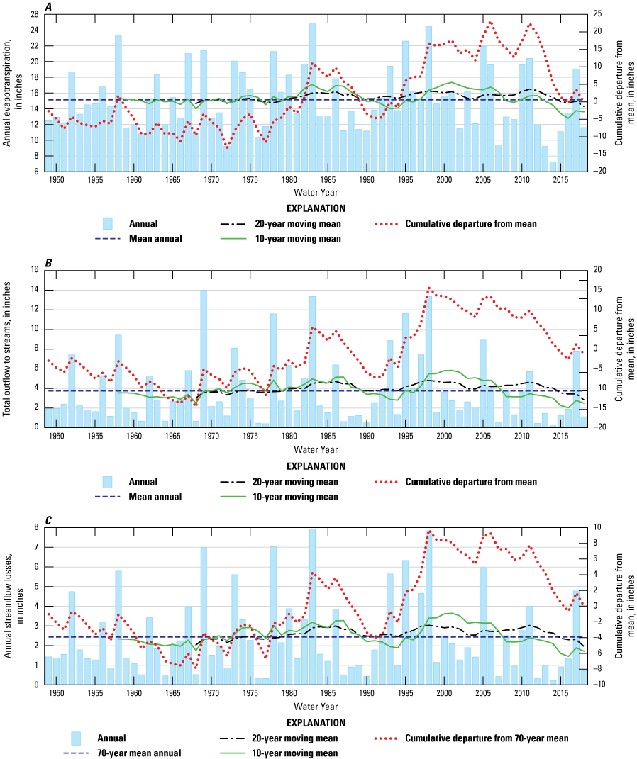
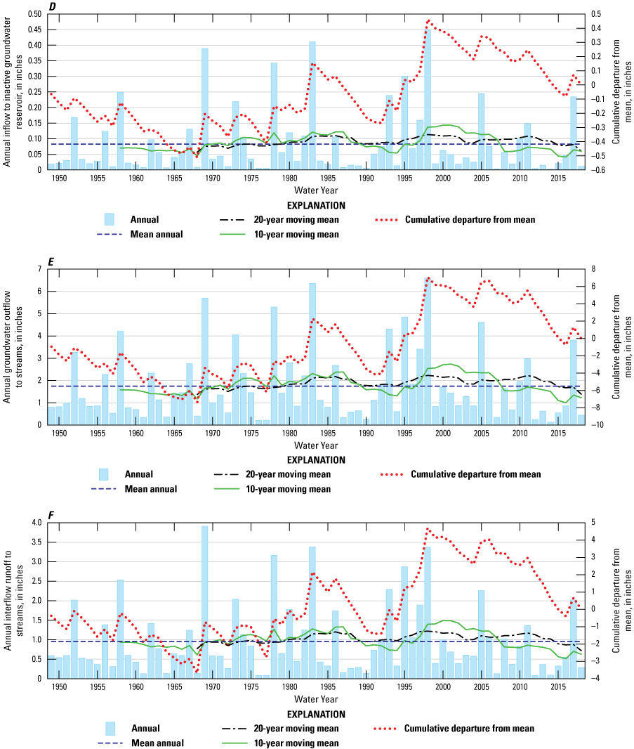
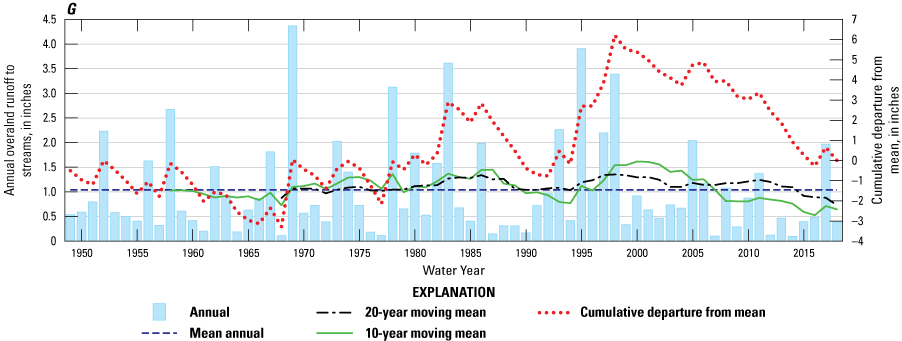
Annual simulation results for the Salinas Valley study area using the Salinas Valley Watershed Model (SVWM): A, actual evapotranspiration; B, total outflow to streams; C, streamflow losses; D, inflow to inactive groundwater reservoirs; E, groundwater outflow to streams; F, interflow runoff to streams; and G, overland runoff to streams (Hevesi and others, 2025).
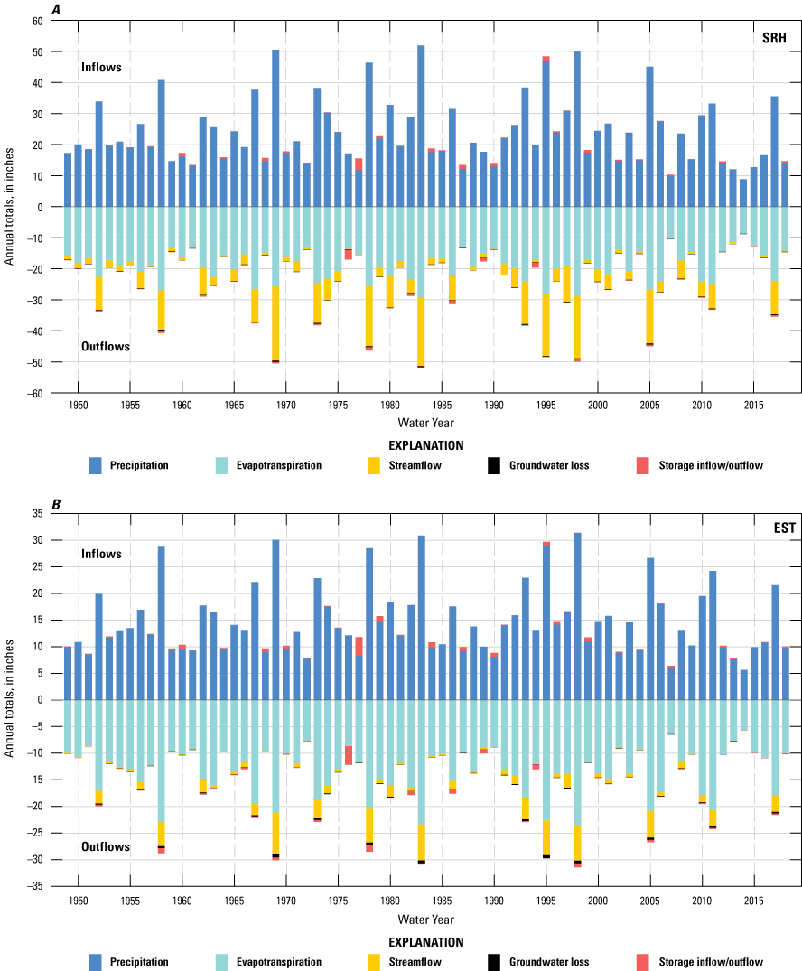
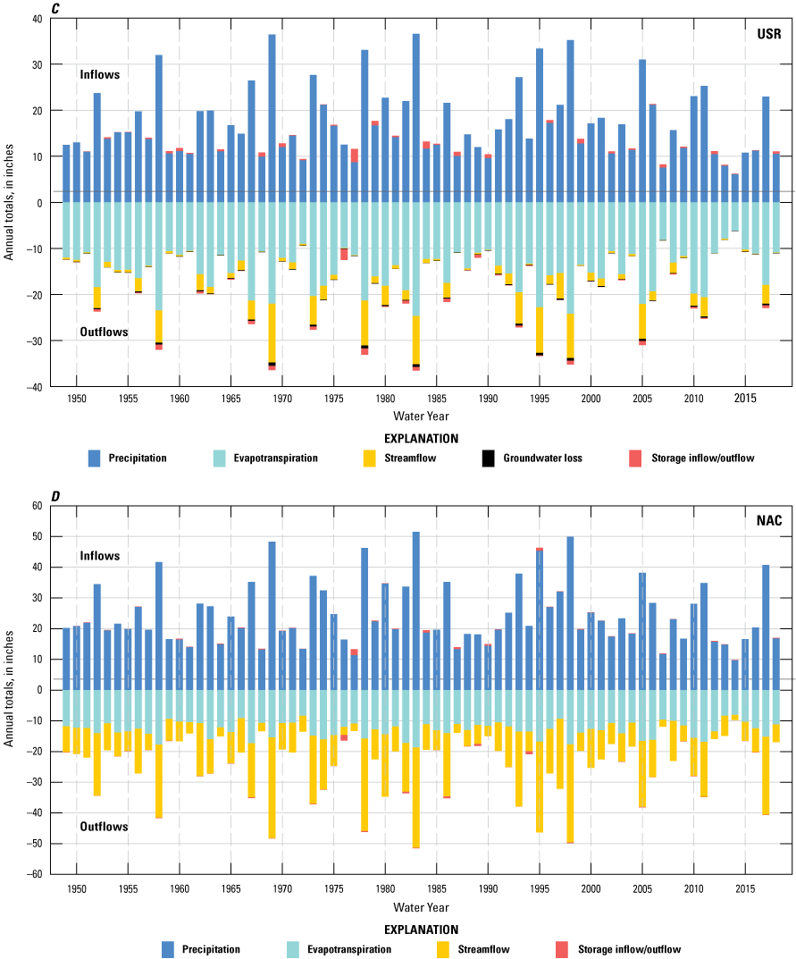
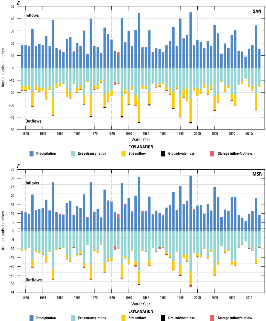
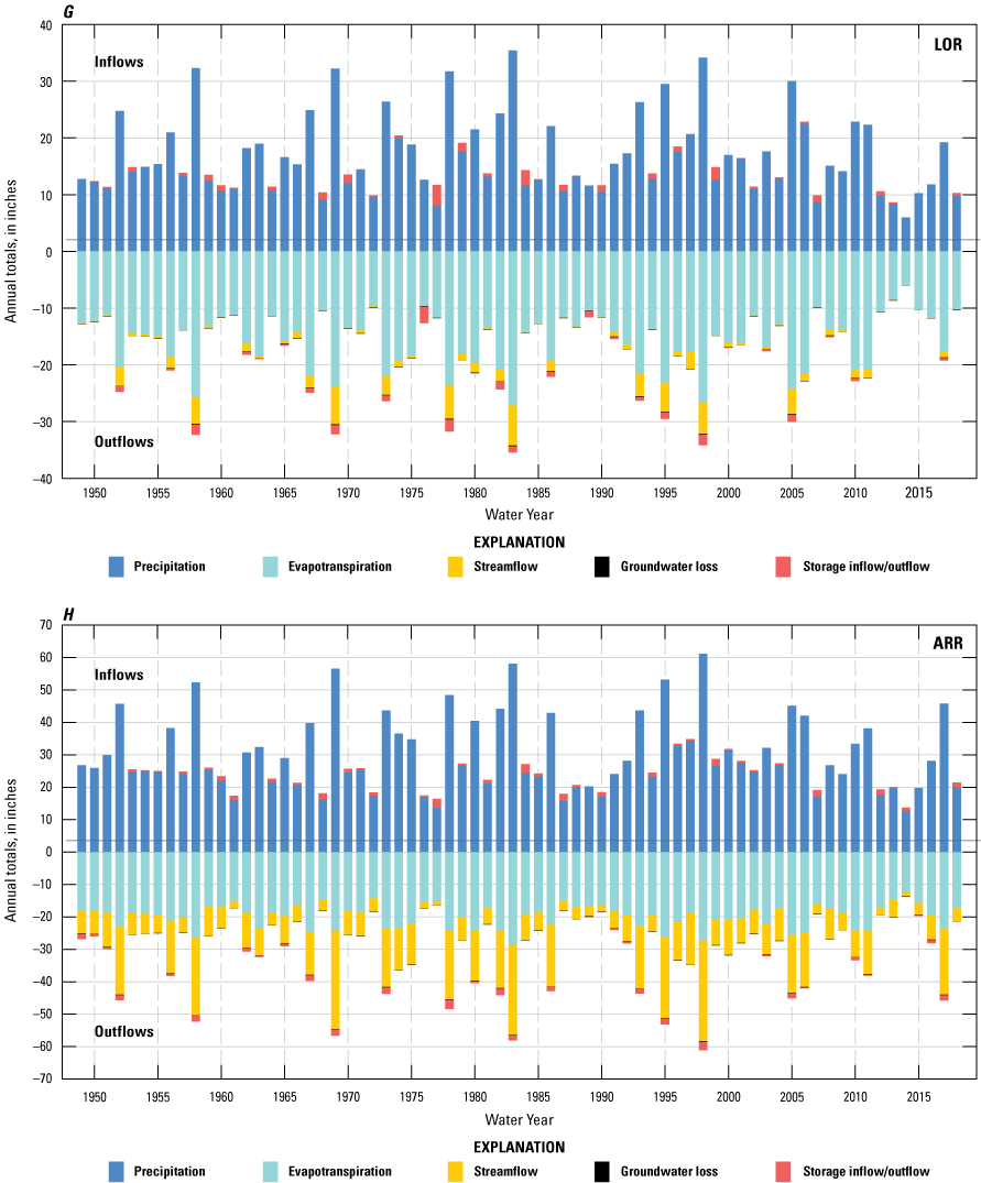
Simulated annual (water year) inflows and outflows for subbasins A, SRH, Salinas River headwaters; B, EST, Estrella River; C, USR, upper Salinas River; D, NAC, Nacimiento River; E, SAN, San Antonio River; F, MSR, middle Salinas River; G, LOR, San Lorenzo Creek; H, ARR, Arroyo Seco; I, LSR, lower Salinas River; and J, MCB, Monterey Coastal Basins (Hevesi and others, 2025).
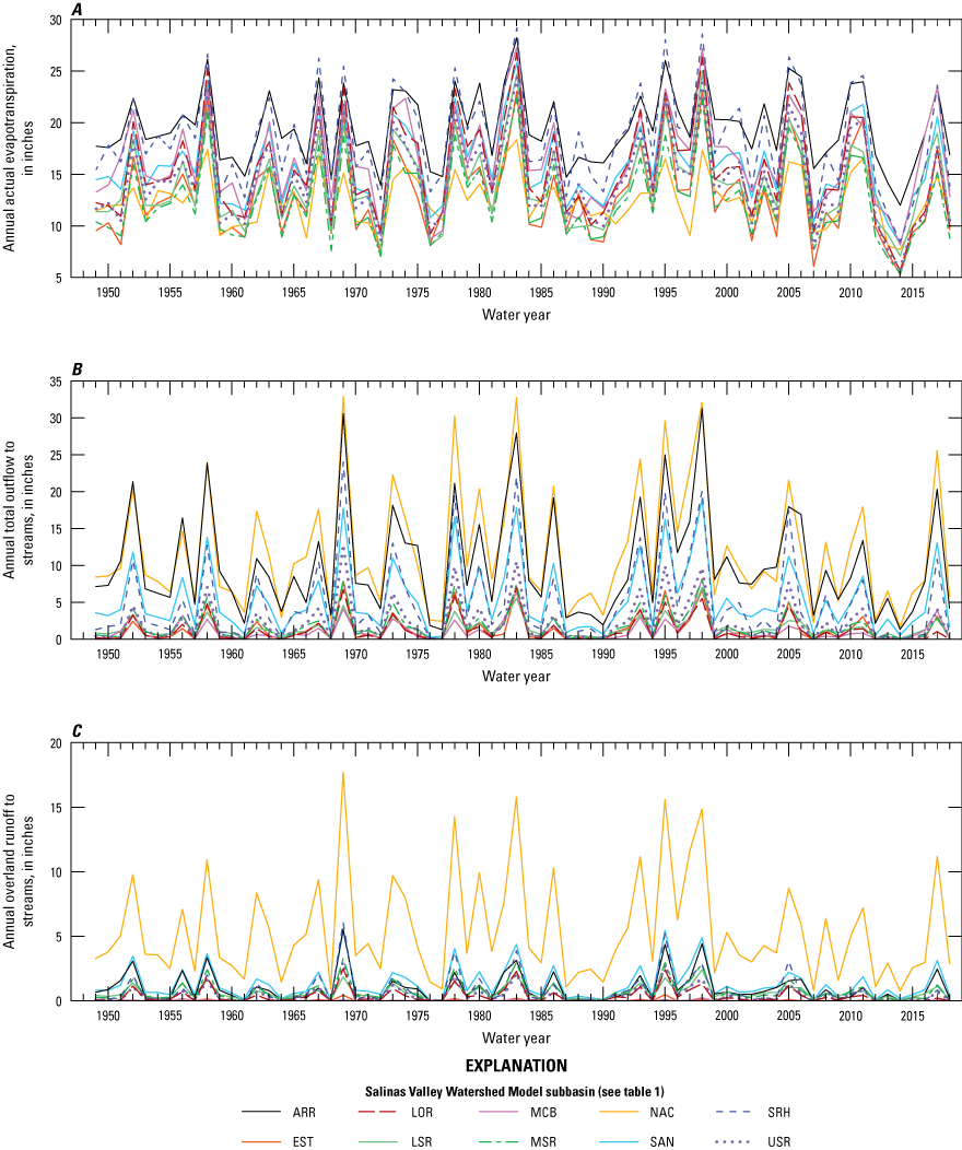
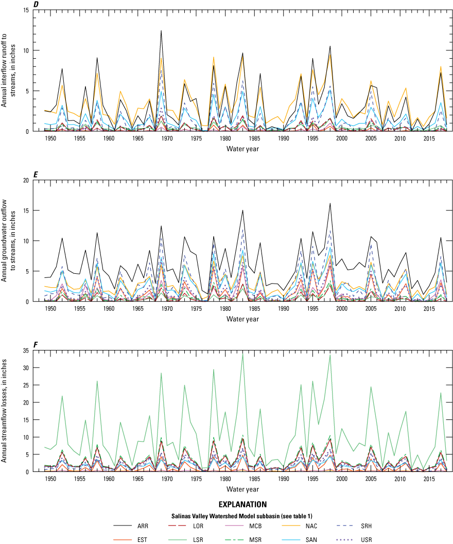
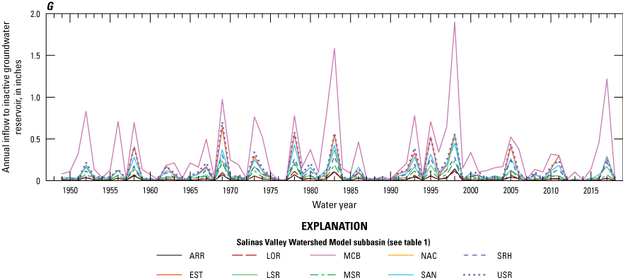
Comparison of annual simulation results for 10 subbasins in the Salinas Valley study area using the Salinas Valley Watershed Model, water years 1949–2018: A, actual evapotranspiration; B, land-area total outflow to streams; C, overland runoff to streams; D, interflow runoff to streams; E, groundwater outflow to streams; F, streamflow losses; and G, inflow to inactive groundwater reservoir. Abbreviations: ARR, Arroyo Seco; EST, Estrella River; LOR, San Lorenzo Creek; LSR, lower Salinas River; MCB, Monterey Coastal Basins; MSR, middle Salinas River; NAC, Nacimiento River; SAN, San Antonio River; SRH, Salinas River headwaters; and USR, upper Salinas River (Hevesi and others, 2025).
Water year 1969 had the highest annual runoff (total outflow to streams) of about 14 in. for the Salinas Valley study area (fig. 41B). In contrast, many dry years (such as 2014) had low runoff values of less than 1.0 in. The cumulative departure from mean runoff for the Salinas Valley study area indicated a drier-than-normal period, relative to the 70-year mean, starting after water year 1998. The ARR and NAC subbasins had the highest total runoff outflow to streams for all water years, with both subbasins exceeding 25 in. during the three wet years 1969, 1983, and 1998 (fig. 43B). As with total runoff to streams, annual variability in overland runoff, interflow runoff, and groundwater outflow to streams was high for most subbasins (figs. 43C, D, E). Water year 1969 had the highest overland and interflow runoff for most subbasins, whereas water year 1998 had the highest groundwater outflow to streams for most subbasins.
Basinwide annual streamflow seepage (streamflow losses) simulated for the Salinas Valley study area was highest for water year 1983 (about 7.9 in. equivalent basinwide water depth) and water year 1998 (about 7.8 in. basinwide water depth; fig. 41C). A minimum mean basinwide streamflow loss of about 0.2 in. was simulated for water year 2014. The cumulative departure from the 70-year mean-annual stream seepage recharge indicates a period of below-average stream seepage after water year 2006 (fig. 41C). Annual results for subbasins indicated that the simulated streamflow losses were much higher for the LSR subbasin compared to all other subbasins, with 12 water years exceeding 20 in. (fig. 43F).
Mean Monthly Results
Comparison of the mean monthly simulation results for the SVWM and the 10 subbasins indicated large variations in components of the water balance across different areas of the Salinas Valley study area (fig. 44). Mean monthly actual evapotranspiration (AET), the largest outflow of water from the SVWM, reached a maximum of about 4.2 in. during April for the ARR subbasin, whereas the NAC subbasin reached a maximum of 2.7 in. during March (fig. 44A).
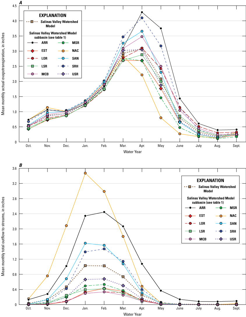
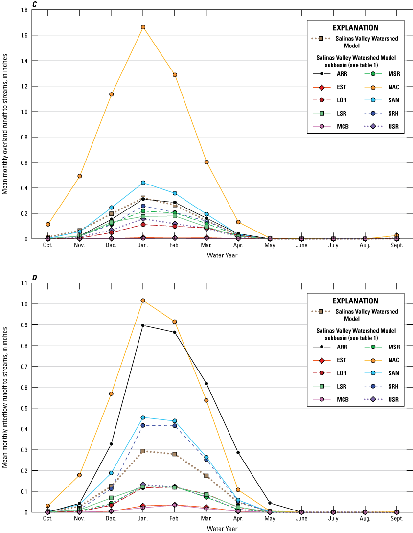
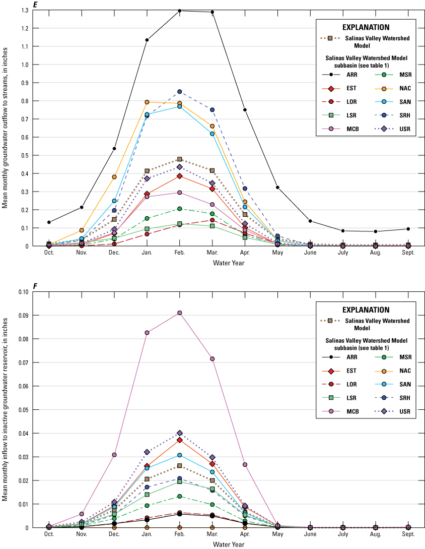
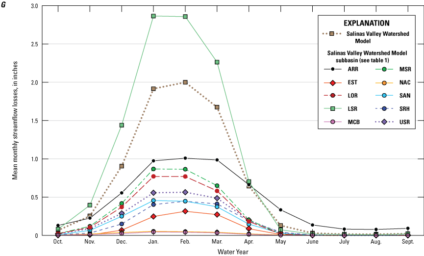
Salinas Valley Watershed Model (SVWM) mean monthly simulation results for subbasins during water years 1949–2018: A, total actual evapotranspiration; B, total outflow to streams; C, overland runoff to streams; D, interflow runoff to streams; E, groundwater outflow to streams; F, inflow to inactive groundwater reservoir; and G, streamflow losses. Abbreviations: ARR, Arroyo Seco; EST, Estrella River; LOR, San Lorenzo Creek; LSR, lower Salinas River; MCB, Monterey Coastal Basins; MSR, middle Salinas River; NAC, Nacimiento River; SAN, San Antonio River; SRH, Salinas River headwaters; USR, upper Salinas River (Hevesi and others, 2025).
The NAC subbasin has a maximum mean monthly total runoff outflow (land-area runoff) of 3.5 in. to streams during January, compared to the ARR subbasin where the maximum mean monthly total runoff outflow of 2.4 in. to streams occurs during February (fig. 44B). Mean monthly overland runoff to streams is much greater for the NAC subbasin compared to all other subbasins, with a maximum mean monthly overland runoff of about 1.65 in. occurring during January (fig. 44C).
The NAC and ARR subbasins have similar results for mean monthly interflow runoff to streams (fig. 44D), whereas the ARR subbasin has a much higher mean monthly groundwater outflow (baseflow) to streams compared to other subbasins, with the highest values of about 1.3 in. occurring during February and March (fig. 44E). The MCB subbasin had a much higher mean monthly inflow to inactive groundwater (deep recharge) compared to other subbasins, with a maximum of 0.09 in. occurring during February (fig. 44F). The LSR subbasin had a much higher mean monthly streamflow loss compared to other subbasins, with the highest values of about 2.8 in. occurring during January and February (fig. 44G).
Multi-Year Variability
Analysis of annual, basinwide results for the Salinas Valley study area was used to identify and compare multi-year wet and dry periods within the 70-year simulation period (water years 1949–2018). Wet and dry periods were identified using the moving 20-year mean and the cumulative departure from the 70-year annual mean, both calculated as a percentage departure from the 70-year mean. The analysis was done using annual (water year) results for precipitation, ET, recharge, and surface-water outflow (fig. 45), with recharge defined as the sum of stream seepage recharge and inter-channel net land-area recharge to the inactive groundwater reservoir (recharge that does not contribute to groundwater discharge) and surface-water outflow defined as streamflow to Monterey Bay from the Salinas Valley study area.
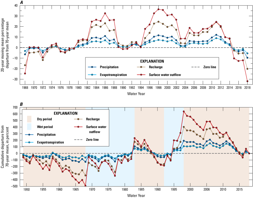
Salinas Valley Watershed Model (SVWM) multi-year variability in basinwide annual precipitation, evapotranspiration, recharge, and surface-water outflow: A, 20-year moving mean percentage departure from the 70-year mean and B, cumulative percentage departure from the 70-year mean (Hevesi and others, 2025).
The percentage of cumulative departure from the 70-year mean was used for a direct comparison of annual variability for the four water balance components (fig. 45B). The cumulative departure for surface-water outflow indicated the highest degree of annual variability in terms of percentage of departures from the mean, with recharge indicating the next highest degree of annual variability, and ET indicating the lowest degree of annual variability relative to the 70-year mean. Three drier-than-average and two wetter-than-average periods were identified based on consistent trends of decreasing values (negative slope) for drier-than-average periods and consistent trends of increasing values (positive slope) for wetter-than-average periods.
The three drier-than-average periods were water years 1949–68, 1984–92, and 1999–2018, and the two wetter-than-average periods were water years 1969–83 and 1993–98 (fig. 46). The 9-year period of 1984–92 was the driest with 3.7 million acre-ft/yr precipitation, 0.38 million acre-ft/yr recharge, and 0.17 million acre-ft/yr surface-water outflow (fig. 46). The 6-year period of 1993–98 was the wettest with 6.5 million acre-ft/yr precipitation resulting in about 310 percent greater recharge (1.18 million acre-ft/yr) and about 430 percent greater surface-water outflow (0.74 million acre-ft/yr) compared to the 1984–92 dry period.
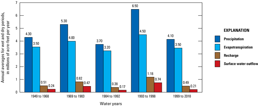
Salinas Valley Watershed Model (SVWM) variability in basinwide average annual precipitation, evapotranspiration, recharge, and surface-water outflow for multi-year wet and dry periods, in millions of acre-feet per year (Hevesi and others, 2025).
The last 20 years of the simulation period (water years 1999–2018) was the driest 20-year period in the 70-year simulation (fig. 45A), and the second driest of the three drier-than-average periods identified using the cumulative departure from mean curves, with 0.49 million acre-ft/yr recharge about 20 percent less than the 70-year mean and 0.21 million acre-ft/yr surface-water outflow about 32 percent less than the 70-year mean. In addition to the lowest mean recharge and surface-water outflow for any 20-year period, the last 20 years (water years 1999–2018) also included the driest 10-year period, ending with water year 2016, with a mean recharge of 1.5 in/yr (0.36 million acre-ft/yr) and a mean surface-water outflow of 0.59 in/yr (0.14 million acre-ft/yr). The last 20-year and 10-year periods included water year 2014, the driest year in the simulation, with 7.5 in. precipitation, 0.24 in. recharge (0.06 million acre-ft/yr), and 0.08 in. surface-water outflow (0.02 million acre-ft/yr).
Summary and Conclusions
The U.S. Geological Survey (USGS), in cooperation with the Monterey County Water Resources Agency (MCWRA), has been conducting studies to help evaluate the surface-water and groundwater resources of the 4,529 square mile Salinas Valley study area. The study area comprises the entire Salinas River watershed and several smaller, adjacent coastal basins draining into Monterey Bay. The study area includes a highly productive agricultural region that depends on the coordinated use of surface water and groundwater to meet the demands for irrigation and public water supply.
To help the MCWRA meet the demands for irrigation and public water supply, the Salinas Valley Watershed Model (SVWM) was developed for the purpose of improving the understanding of the natural hydrologic system and quantifying components of the water balance, including precipitation, evapotranspiration (ET), recharge, and streamflow. The SVWM combines two hydrologic modeling applications: the Basin Characterization Model (BCM) and the Hydrologic Simulation Program–Fortran (HSPF). The SVWM was calibrated and applied to simulate the historical natural water balance for the Salinas Valley study area for water years 1949–2018. Simulation results for the 70-year period were used to provide estimates of daily, monthly, and annual surface-water inflows from mountainous, upland tributary drainages surrounding the more flat-lying lowlands in the central, lower Salinas Valley that include developed lands and irrigated croplands dependent on groundwater.
The BCM was applied using a 270-meter (886-foot) grid covering the Salinas Valley study area to develop spatially distributed daily climate inputs for the SVWM consisting of precipitation, maximum and minimum air temperature, and potential evapotranspiration (PET). The daily climate inputs were disaggregated to hourly time steps used by HSPF to provide a continuous simulation of the natural hydrologic system, with an emphasis on hydrologic processes of the land cover, pervious and impervious land surfaces, and the shallow subsurface including the root zone.
The SVWM was discretized into 690 irregular polygon areas referred to as hydrologic response units (HRUs). The HRUs are used to account for spatially varying climate and watershed characteristics and were defined hydrographically and topographically by the stream drainage network, subdrainage areas, and boundaries separating valley lowlands from the surrounding, more rugged upland areas. Geospatial data defining topography, land cover, soil properties, and surficial geology were used to estimate hydrologic parameters for pervious and impervious land areas comprising the HRUs. The 690 HRUs were linked to 690 stream reaches used to simulate the natural surface-water drainage network of the Salinas Valley study area.
The SVWM model domain was divided into the upper and lower Salinas Valley sub-model domains (USVS; LSVS), with 387 HRUs in the USVS and 303 HRUs in the LSVS. The use of two separate model domains allowed for a more detailed model discretization representing spatial heterogeneity in climate and watershed characteristics and to better represent the many small tributary subdrainages providing inflows to the Salinas Valley lowlands.
Initial estimates of model parameters were refined by trial-and-error calibration based on the fitting of simulated daily, monthly, and annual (water year) streamflow to available streamflow records at 29 USGS streamgages. Records of estimated daily, monthly, and annual inflows for two reservoirs in the Salinas Valley study area, Lakes Nacimiento and San Antonio, also were used in model calibration. The trial-and-error calibration resulted in a good overall fit between simulated and observed streamflow, as defined by the calibration criteria of plus or minus 10 percent average estimation error and a Nash–Sutcliffe Model Efficiency (NSME) statistic of 0.5 or higher for daily streamflow, 0.6 or higher for monthly streamflow, and 0.7 or higher for annual streamflow. Calibration results indicated the greatest sensitivity to parameters controlling root zone water content, ET, groundwater discharge to streams (baseflow), interflow runoff, and overland runoff. The model archive for the calibrated model is available in Hevesi and others (2025) for citing the data release with the model archive.
The SVWM was used to simulate the daily hydrologic water budget for a 70-year period beginning October 1, 1948, and ending September 30, 2018 (water years 1949–2018). The simulations were started on October 1, 1947, to allow a 1-year model initialization period. The simulation results were used to develop and analyze the long-term, 70-year mean water budget and transient annual, monthly, and daily water budgets for 10 subbasins, 28 subdrainages, 25 upland tributary drainages to the Salinas Valley lowlands, and the 690 HRUs and connected stream reaches.
During the 70-year mean precipitation for the Salinas Valley study area, the only inflow to the natural hydrologic system represented by the SVWM, was 18.5 inches per year (in/yr) or about 4.47 million acre-feet per year (acre-ft/yr), varying from 9 in/yr for low elevations along the valley floor to as much as 60 in/yr for the highest elevation drainages in the Arroyo Seco subbasin. The simulated 70-year mean ET was 14.9 in/yr, equal to about 3.6 million acre-ft/yr and about 81 percent of the total water outflow from the Salinas Valley study area. Evapotranspiration varied from 8.8 to 26 in/yr in response to spatial variability in precipitation, PET, land cover, and the water-holding capacity of the root zone.
Recharge simulated by the SVWM included recharge to the active and inactive reservoirs. The SVWM uses the active groundwater reservoir as the water source, contributing groundwater discharge to streams and ET from groundwater, and is replenished by recharge from water percolating beneath the root zone of pervious land areas. Recharge from the root zone, also referred to as net land-area recharge, is partitioned into recharge to the active and inactive reservoirs, with all or most of the land-area recharge contributing to the active groundwater reservoir, then subsequently to groundwater discharge. The 70-year mean recharge for the Salinas Valley study area, calculated as the sum of recharge contributing to baseflow, net land area recharge (also referred to as deep recharge in this report), and stream seepage was about 4.4 in/yr (about 1.06 million acre-ft/yr) and 23.7 percent of precipitation, with 1.71 in/yr (about 412,000 acre-ft/yr) contributing to the baseflow component of streamflow. Net land-area recharge to the inactive groundwater reservoir (deep recharge) was only 0.08 in/yr or about 0.5 percent of the total outflow.
Recharge to the inactive groundwater reservoir, simulated by the SVWM as recharge that does not contribute groundwater discharge to streams or ET, included intra-channel stream seepage recharge resulting from the infiltration of streamflow through the streambed. The 70-year mean recharge to the inactive groundwater reservoir, including stream seepage recharge and net land-area recharge, was 2.7 in/yr or about 647,000 acre-ft/yr and about 14.5 percent of the total water outflow, which is the second largest outflow of water from the SVWM. The 70-year mean stream seepage recharge for the Salinas Valley study area was about 2.6 in/yr (equal to about 627,000 acre-ft/yr) and accounted for 14 percent of the water outflow from the SVWM hydrologic system.
The simulated 70-year mean land-area runoff from HRUs consisted of overland runoff, interflow runoff, and groundwater discharge to streams, and was 3.5 in/yr or about 850,000 acre-ft/yr and 19 percent of precipitation. Most of the runoff was simulated as groundwater discharge; the 70-year mean groundwater discharge to streams accounted for about 48 percent of the total runoff for the Salinas Valley study area. In comparison, the 70-year mean overland runoff was 0.97 in/yr (about 28 percent of total runoff), and the mean interflow runoff was about 0.84 in/yr (about 24 percent of total runoff). Most of the land-area runoff subsequently became stream seepage recharge. The simulated surface-water outflow to the ocean was only 0.96 in/yr (232,000 acre-ft/yr) about 5.2 percent of precipitation and 27 percent of the runoff generated from land areas. This result was found to be generally consistent with streamflow records in the Salinas Valley study area. The simulated 70-year mean surface-water inflow into the lower Salinas Valley from all surrounding upland tributary areas was about 770 cubic feet per second (ft3/s), equal to about 558,000 acre-ft/yr and about 15 percent of precipitation over the upland areas. In contrast, the 70-year mean streamflow at the mouth of the Salinas River was only about 278 ft3/s (about 201,000 acre-ft/yr) and 4.8 percent of precipitation over the entire Salinas River watershed.
The Nacimiento River (NAC) subbasin was the primary source of streamflow to the main channel of the Salinas River, with a simulated 70-year mean streamflow of about 277 ft3/s. In comparison, the Estrella River (EST) subbasin, with an area of 924 square miles (mi2), almost 3 times the 325 mi2 area of the NAC subbasin, had a 70-year mean streamflow of only 21 ft3/s. The large difference in runoff between the two subbasins is caused primarily by differences in climate between the west and east sides of the Salinas Valley study area: the proximity of the NAC subbasin drainage area close to the Pacific Ocean moisture source results in higher precipitation and lower PET compared to the more inland EST subbasin. In addition to climate, differences in topography, soils, and surface geology cause differences in runoff and streamflow as a percentage of precipitation and the portion of streamflow lost to stream seepage recharge.
Simulated groundwater discharge to streams (baseflow) was the main source of streamflow for many locations in the Salinas Valley study area, varying from less than 0.1 in/yr for drier, lower elevation HRUs to about 28 in/yr for high-elevation HRUs along the southwestern boundary of the Arroyo Seco subbasin. Simulated baseflow was seasonal for most locations because winter season recharge was not sufficient to maintain baseflow throughout the dry summer months for most stream reaches. Most of the groundwater discharge occurred over a time span of days to weeks rather than months after winter storms. The lack of sustained baseflow caused streamflow to be mostly ephemeral and highly sensitive to the temporal variability in precipitation, with extended dry periods resulting in no-flow conditions along the main channel of the Salinas River. Simulated streamflow was consistent with streamflow records throughout the Salinas Valley study area in terms of flashy peak flows in response to storms followed by low-flow and no-flow conditions during the dry summer months and extended dry periods.
The simulated overland and interflow components of runoff from inter-channel land areas also had a high degree of variability between HRUs and subdrainages. The 70-year mean overland runoff was less than 0.4 in/yr for most locations in the Salinas Valley study area; however, mean values of 4 in/yr and higher were simulated for HRUs with high precipitation, steep slopes, low soil storage capacity, and low-permeability bedrock underlying the soil zone. The simulated 70-year mean interflow runoff also varied spatially with low values of 0.5 in/yr and less for most locations and high values of 4 in/yr and greater for HRUs with high precipitation and steep slopes. The relative magnitude of interflow runoff compared to overland runoff varied considerably between subbasins and subdrainages. Interflow runoff tended to be higher than overland runoff for HRUs with thicker soils and forested land cover, whereas overland runoff was higher than interflow runoff for HRUs with a high percentage of grasslands and impervious land cover.
Analysis of annual, basinwide results for the Salinas Valley study area was used to identify and compare multi-year wet and dry periods within the 70-year simulation period (water years 1949–2018). The percentage of cumulative departures from the 70-year mean for precipitation, ET, net recharge to the inactive groundwater reservoir, and surface-water outflow to Monterey Bay were used to identify three drier-than-average periods (water years 1949–68, 1984–92, and 1999–2018) and two wetter-than-average periods (water years 1969–83 and 1993–98). Surface-water outflow indicated the highest degree of variability between wet and dry periods in terms of percentage of departures from the 70-year mean, with relative differences between multi-year means as high as 430 percent. Relative differences between mean values for wet and dry periods were about 310 percent for recharge, 176 percent for precipitation, and 136 percent for ET.
The final 20 years of the simulation period (water years 1999–2018) were the driest 20-year period within the 70-year simulation period. Mean precipitation for water years 1999–2018 was about 10 percent less than the 70-year mean. The 20-year mean PET was the highest for water years 1999–2018 (58.6 in/yr) compared to all other 20-year periods, further decreasing the amount of water available for recharge and streamflow. Mean recharge for water years 1999–2018 was about 2.1 in/yr or 20 percent less than the 70-year mean. The mean surface-water outflow to the ocean for water years 1999–2018 was about 0.65 in/yr or 32 percent less than the 70-year mean. Water years 1999–2018 also included the driest 10-year period, water years 2007–16, with a mean recharge of 1.5 in/yr (44 percent less than the 70-year mean) and a mean surface-water outflow of 0.59 in/yr (39 percent less than the 70-year mean). The last 20-year and 10-year periods included water year 2014, the driest year in the simulation, with 7.5 inches of precipitation, 0.24 inches of recharge, and 0.08 inches of surface-water outflow.
References Cited
Amirhossien, F., Alireza, F., Kazem, J., and Mohammadbagher, S., 2015, A comparison of ANN and HSPF models for runoff simulation in Balkhichai River Watershed, Iran: American Journal of Climate Change, v. 4, no. 3, p. 203–216. [Available at https://doi.org/10.4236/ajcc.2015.43016.]
Atkins, J.T., Jr., Wiley, J.B., and Paybins, K.S., 2005, Calibration parameters used to simulate streamflow from application of the Hydrologic Simulation Program-FORTRAN Model (HSPF) to mountainous basins containing coal mines in West Virginia: U.S. Geological Survey Scientific Investigations Report 2005–5099, 79 p. [Available at https://doi.org/10.3133/sir20055099.]
Baillie, M., Chau, L., and Turner, J., 2015, State of the Salinas River groundwater basin: Salinas, Calif., Monterey County Resource Management Agency, prepared by Brown and Caldwell, Walnut Creek, Calif., 241 p. [Available at https://digitalcommons.csumb.edu/cgi/viewcontent.cgi?article=1020&context=hornbeck_cgb_6_a.]
Brown and Caldwell, 2014, State of the Salinas River Groundwater Basin: Salinas, Calif., Brown and Caldwell, prepared for Monterey County Water Resources Agency, 240 p. [Available at https://digitalcommons.csumb.edu/hornbeck_cgb_5/47/.]
Burton, C.A., and Wright, M.T., 2018, Status and understanding of groundwater quality in the Monterey-Salinas Shallow Aquifer study unit, 2012–13—California GAMA Priority Basin Project: U.S. Geological Survey Scientific Investigations Report 2018–5057, 116 p. [Available at https://doi.org/10.3133/sir20185057.]
California Department of Food and Agriculture, 2022, California Agricultural Statistics Review, 2021–2022: California Department of Food and Agriculture report, 159 p. [Available at https://www.cdfa.ca.gov/Statistics/PDFs/2022_Ag_Stats_Review.pdf.]
California Department of Forestry and Fire Protection, 2004, California interagency watershed map of 1999 (Calwater 2.2.1): U.S. Department of Agriculture, Soil Conservation Service, California Interagency Watershed Mapping Committee, 435 p., accessed September 4, 2017, at https://map.dfg.ca.gov/metadata/calw221_polygon_20131205_wm.html.
Daly, C., Gibson, W.P., Doggett, M., Smith, J., and Taylor, G., 2004, Up-to-date monthly climate maps for the conterminous United States—Proceedings of the 14th AMS Conference on Applied Climatology, 84th AMS Annual Meeting Combined Preprints, Seattle, Wash., January 13–16, 2004: American Meteorological Society, 8 p.
Daly, C., Neilson, R.P., and Phillips, D.L., 1994, A statistical-topographic model for mapping climatological precipitation over mountainous terrain: Journal of Applied Meteorology, v. 33, no. 2, p. 140–158. [Available at https://doi.org/10.1175/1520-0450(1994)033%3C0140:ASTMFM%3E2.0.CO;2.]
Donigian, A.S., Jr., and Imhoff, J.C., 2009, Evaluation and performance assessment of watershed models—Proceedings of the Water Environment Federation TMDLS Conference, Minneapolis, Minn., August 9–12, 2009: WEF Specialty Conference, p. 12–45. [Available at https://www.researchgate.net/publication/233669770_Evaluation_and_Performance_Assessment_of_Watershed_Models.]
Donigian, A.S., Jr., Imhoff, J.C., Bicknell, B.R., and Kittle, J.L., Jr., 1984, Application guide for Hydrological Simulation Program—FORTRAN (HSPF): Athens, Ga., U.S. Environmental Protection Agency, Office of Research and Development, Environmental Research Laboratory report EPA-600/3-84-065, 177 p. [Available at https://nepis.epa.gov/Exe/ZyPURL.cgi?Dockey=2000HMKI.txt.]
Flint, A.L., and Flint, L.E., 2007, Application of the basin characterization model to estimate in-place recharge and runoff potential in the Basin and Range carbonate-rock aquifer system, White Pine County, Nevada, and adjacent areas in Nevada and Utah: U.S. Geological Survey Scientific Investigations Report 2007–5099, 20 p. [Available at https://pubs.usgs.gov/sir/2007/5099/pdf/sir20075099.pdf.]
Flint, L.E., and Flint, A.L., 2012, Downscaling future climate scenarios to fine scales for hydrologic and ecological modeling and analysis: Ecological Processes, v. 1, no. 2, 15 p. [Available at https://doi.org/10.1186/2192-1709-1-2.]
Flint, L.E., Flint, A.L., and Stern, M.A., 2021, The basin characterization model—A regional water balance software package.: U.S. Geological Survey Techniques and Methods, book 6, chap. H1, 85 p. [Available at https://doi.org/10.3133/tm6H1.]
Fugro West, Inc., 1995, North Monterey County hydrogeologic study: Salinas, Calif., Monterey County Water Resources Agency, prepared by Fugro West, Inc., Monterey Calif., v. 1, 423 p. [Available at http://www.elkhornsloughctp.org/uploads/files/1421885098Fugro%20Water%20Study%20October%201995%20Vol%201.pdf.]
Harding ESE, 2001, Final report—Hydrogeologic investigation of the Salinas Valley basin in the vicinity of Fort Ord and Marina Salinas Valley, California: Salinas, Calif., Monterey County Water Resources Agency, prepared by Harding ESE, Novato, Calif., 165 p. [Available at https://svbgsa.org/wp-content/uploads/2020/08/2001-Final-Report-Hydrog.pdf.]
Harter, T., Lund, J.R., Darby, J.L., Fogg, G.E., Howitt, R., Jessoe, K.K., Pettygrove, G.S., Quinn, J.F., Viers, J.H., Boyle, D.B., Canada, H.E., DeLaMora, N., Dzurella, K.N., Fryjoff-Hung, A., Hollander, A.D., Honeycutt, K.L., Jenkins, M.W., Jensen, V.B., King, A.M., Kourakos, G., Liptzin, D., Lopez, E.M., Mayzelle, M.M., McNally, A., Medellin-Azuara, J., and Rosenstock, T.S., 2012, Addressing nitrate in California’s drinking water—With a focus on Tulare Lake Basin and Salinas Valley Groundwater: Davis, Calif., University of California, Davis, Center for Watershed Sciences, Report for the State Water Resources Control Board Report to the Legislature, 78 p. [Available at https://ucanr.edu/sites/groundwaternitrate/files/138956.pdf.]
Henson, W.R., and Jachens, E.R., 2022, Lower Salinas Valley hydrologic models—Discretization data (ver. 1.1, July 2023): U.S. Geological Survey data release, https://doi.org/10.5066/P9850MAK.]
Henson, W.R., Hevesi, J.A., Hanson, R.T., Bittner, D., Herbert, D.M., and Jachens, E.R., 2022, Salinas Valley hydrologic models—Surface water data: U.S. Geological Survey data release. [Available at https://doi.org/10.5066/P93COXL6.]
Hevesi, J.A., and Johnson, T.D., 2016, Estimating spatially and temporally varying recharge and runoff from precipitation and urban irrigation in the Los Angeles Basin, California: U.S. Geological Survey Scientific Investigations Report 2016–5068, 192 p. [Available at https://doi.org/10.3133/sir20165068.]
Hevesi, J.A., Hanson, R.T., and Masoner, J.R., 2019, Precipitation runoff modeling system (PRMS) as part of an integrated hydrologic model for the Osage Nation, northeastern Oklahoma, 1915–2014: U.S. Geological Survey Scientific Investigations Report 2019–5030, 142 p. [Available at https://pubs.er.usgs.gov/publication/sir20195030.]
Hevesi, J., Henson, W.R., Hanson, R.T., Earll, M.M., Herbert, D.M., and Jachens, E.R., 2025, Salinas Valley watershed model—Application of Hydrologic Simulation Program—FORTRAN (HSPF): U.S. Geological Survey data release, https://doi.org/10.5066/P9FJAWC4.]
Hevesi, J.A., Henson, W.R., Hanson, R.T., Stern, M.A., and Jachens, E.R., 2022, Salinas valley hydrologic system—Regional climate data: U.S. Geological Survey data release, https://doi.org/10.5066/P942J2BC.
Kennedy Jenks L.L.C., 2004, Final report—Hydrostratigraphic analysis of the northern Salinas Valley: Salinas, Calif., Monterey County Water Resources Agency, prepared by Kennedy Jenks, L.L.C., San Francisco, Calif., project no. 035901.00, 113 p. [Available at https://www.countyofmonterey.gov/home/showpublisheddocument/19582/636232667568400000.]
Kulongoski, J.T., and Belitz, K., 2007, Ground-water quality data in the Monterey Bay and Salinas Valley Basins, California, 2005—Results from the California GAMA Program: U.S. Geological Survey Data Series 258, 84 p. [Available at https://doi.org/10.3133/ds258.]
Lapham, M.H., and Heileman, W.H., 1901, Soil survey of the lower Salinas Valley, California: U.S. Department of Agriculture, Bureau of Soils report, p. 481–519. [Available at https://digitalcommons.csumb.edu/cgi/viewcontent.cgi?article=1091&context=hornbeck_usa_3_d.]
Markstrom, S.L., Niswonger, R.G., Regan, R.S., Prudic, D.E., and Barlow, P.M., 2008, GSFLOW—Coupled ground-water and surface-water flow model based on the integration of the Precipitation-Runoff Modeling System (PRMS) and the Modular Ground-Water Flow Model (MODFLOW-2005): U.S Geological Survey Techniques and Methods, book 6, chap. D1, 240 p. [Available at https://pubs.er.usgs.gov/publication/tm6D1.]
Monterey County Water Resources Agency, 1995, 1995—Hydrogeology and water supply of Salinas Valley, White paper by Salinas Valley Ground Water Basin Hydrology Conference: Monterey County Water Resources Agency Water Reports. 21 p. [Available at https://digitalcommons.csumb.edu/hornbeck_cgb_6_a/25.]
Monterey County Water Resources Agency, 2006, Monterey County groundwater management plan: Monterey County Water Resources Agency, 77 p. [Available at https://digitalcommons.csumb.edu/hornbeck_cgb_5/27.]
Monterey County Water Resources Agency, 2018, Nacimiento Dam Operation Policy: Monterey County Water Resources Agency, 186 p. [Available at https://www.countyofmonterey.gov/home/showpublisheddocument/63151/636628427976500000.]
Moran, J.E., Esser, B.K., Hillegonds, D., Holtz, M., Roberts, S.K., Singleton, M.J., and Visser, A., 2011, California GAMA special study—Nitrate fate and transport in the Salinas Valley: Lawrence Livermore National Laboratory, Report No. LLNL-TR-484186, 52 p. [Available at https://doi.org/10.2172/1122241.]
Nalder, I.A., and Wein, R.W., 1998, Spatial interpolation of climatic normals—Test of a new method in the Canadian boreal forest: Agricultural and Forest Meteorology, v. 92, no. 4, p. 211–225. [Available at https://doi.org/10.1016/S0168-1923(98)00102-6.]
Nash, J.E., and Sutcliffe, J.V., 1970, River flow forecasting through conceptual models part I—A discussion of principles: Journal of Hydrology, v. 10, no. 3, p. 282–290. [Available at https://doi.org/10.1016/0022-1694(70)90255-6.]
Seaber, P.R., Kapinos, F.P., and Knapp, G.L., 1987, Hydrologic unit maps: U.S. Geological Survey Water Supply Paper 2294, 63 p. [Available at https://doi.org/10.3133/wsp2294.]
Simpson, T.R., McPartland, J.W., Nilsson, W.I., Vickroy, G.M., and Farrington, T.K., 1946, Salinas Basin investigation—Summary report: State of California, Department of Public Works, Division of Water Resources Bulletin no. 52-B. [Available at https://digitalcommons.csumb.edu/hornbeck_cgb_1/6/.]
Stern, M.A., Flint, L.E., Minear, J.T., Flint, A.L., and Wright, S.A., 2016, Characterizing changes in streamflow and sediment supply in the Sacramento River Basin, California, using hydrological simulation program—FORTRAN (HSPF): Water, v. 8, no. 10, 21 p. [Available at https://doi.org/10.3390/w8100432.]
U.S. Department of Agriculture [USDA], 2017, Soil data access: U.S. Department of Agriculture web page, accessed January 4, 2017, at https://sdmdataaccess.sc.egov.usda.gov.
U.S. Environmental Protection Agency, 2000, BASINS technical note 6—Estimating hydrology and hydraulic parameters for HSPF: U.S. Environmental Protection Agency, Office of Water, EPA-823-R00-012, 34 p. [Available at https://www.epa.gov/sites/default/files/2015-08/documents/2000_08_14_basins_tecnote6.pdf.]
U.S. Geological Survey, 2014, National Land Cover Database (NLCD) 2011 land cover conterminous United States: U.S. Geological Survey data release, https://doi.org/10.5066/P97S2IID.]
U.S. Geological Survey, 2016, USGS water data for the Nation: U.S. Geological Survey, National Water Information System Database, accessed December 27, 2018, at http://waterdata.usgs.gov/nwis/.
U.S. Geological Survey, 2019, National hydrography dataset: U.S. Geological Survey web page, accessed January 3, 2018, at https://www.usgs.gov/national-hydrography/national-hydrography-dataset.
U.S. Geological Survey, 2023, 1/3rd arc-second digital elevation models (DEMs)—USGS national map 3DEP downloadable data collection: U.S. Geological Survey data. [Available at https://www.sciencebase.gov/catalog/item/4f70aa9fe4b058caae3f8de5.]
Appendix 1. Climate Stations with Records of Daily Climate Used to Develop Climate Inputs for the Salinas Valley Watershed Model
Table 1.1.
Climate stations with records of daily precipitation used to develop daily precipitation input for the Salinas Valley Watershed Model.[COOP, Cooperative Weather Station; CIMIS, California Irrigation Management and Information System; ID, identification; RAWS; Remote Automated Weather Station]
Table 1.2.
Climate stations with records of daily minimum air temperature used to develop daily minimum air temperature input for the Salinas Valley Watershed Model.[COOP, Cooperative Weather Station; CIMIS, California Irrigation Management and Information System; ID, identification; RAWS; Remote Automated Weather Station; °F, degrees Fahrenheit]
Table 1.3.
Climate stations with records of daily maximum air temperature used to develop daily maximum air temperature input for the Salinas Valley Watershed Model.[COOP, Cooperative Weather Station; CIMIS, California Irrigation Management and Information System; ID, identification; RAWS; Remote Automated Weather Station; °F, degrees Fahrenheit]
Conversion Factors
U.S. customary units to International System of Units
Temperature in degrees Fahrenheit (°F) may be converted to degrees Celsius (°C) as follows:
°C = (°F – 32) / 1.8.
Datums
Horizontal coordinate information is referenced to the North American Datum of 1983 (NAD 83).
Vertical coordinate information is referenced to the North American Vertical Datum of 1988 (NAVD 88).
Supplemental Information
A water year is the 12-month period from October 1 through September 30 and is designated by the calendar year in which it ends.
Abbreviations
AET
actual evapotranspiration
BCM
Basin Characterization Model
D-8
eight-direction routing
DEM
digital elevation model
ET
evapotranspiration
Ftable
Flow-table
GIS
Geographic Information System
HRU
hydrologic response unit
HSPF
Hydrologic Simulation Program—FORTRAN
HUC
hydrologic unit code
IMPLND
impervious land area
LSVS
lower Salinas Valley sub-model
MCWRA
Monterey County Water Resources Agency
NHD
National Hydrography Dataset
NLCD
National Land Cover Data
NSME
Nash–Sutcliffe model efficiency
PAE
percent-average estimation error
PE
percent estimation error
PERLND
pervious land area
PET
potential evapotranspiration
PRISM
Parameter-elevation Regression on Independent Slopes Model
R2
coefficient of determination
RCHRES
stream reach or reservoir in HSPF
RETSC
retention storage capacity
SRW
Salinas River watershed
SSURGO
Soil Survey Geographic database
SVIHM
Salinas Valley Integrated Hydrologic Flow Model
SVU
Salinas Valley upland area
SVWM
Salinas Valley Watershed Model
UCI
user control input
USGS
U.S. Geological Survey
USVS
upper Salinas Valley sub-model
WDM
Watershed Data Management
Subdrainages
BSC
Big Sandy Creek
CHO
Cholame Creek
CSC
Chalone–Stonewall Creek
ELK
Elkhorn Slough
ETC
El Toro Creek
HUE
Huerhuero Creek
LAS
lower Arroyo Seco
LCS
Limekiln Creek–Salinas River
LER
lower Estrella River
LNR
lower Nacimiento River
LSA
lower San Antonio River
LSJ
lower San Juan Creek
MCS
Monroe Creek–Salinas River
MSB
Monterey–Seaside basin
PCD
Pine Creek drainages
PRC
Paso Robles Creek
QCC
Quail–Chualar Creek
SLC
San Lorenzo Creek
SML
Santa Margarita Lake
SNB
Salinas River near Bradley
SPR
Sargent–Pancho Rico Creeks
SRO
Salinas River outflow
SRP
Salinas River near Paso Robles
UAS
upper Arroyo Seco
USA
upper San Antonio River
UNR
upper Nacimiento River
USJ
upper San Juan Creek
USV
upper Salinas Valley
Tributary Drainages
ALIS
Alisal Creek
BIGS
Big Sandy Creek
CHAL
Chalone Creek
CHER
Cherry Canyon
CHUA
Chualar Creek
GABI
Gabilan Creek
HAME
Hames Creek
HARE
Hare Canyon
LSRW
lower Salinas River West
MCOY
McCoy Creek
MONR
Monroe Creek
MSRW
middle Salinas River West
NACI
Nacimiento River
PANR
Pancho Rico Creek
PINE
Pine Creek
QUAI
Quail Creek
SALI
Salinas River
SANL
San Lorenzo Creek
SANR
San Antonio River
SARG
Sargent Creek
SECO
Arroyo Seco
STON
Stonewall Creek
TORO
El Toro Creek
VINE
Vineyard Canyon
WILD
Wildhorse Canyon
For more information concerning the research in this report, contact the
Director, California Water Science Center
U.S. Geological Survey
6000 J Street, Placer Hall
Sacramento, California 95819
https://www.usgs.gov/centers/california-water-science-center
Publishing support provided by the U.S. Geological Survey
Science Publishing Network, Sacramento Publishing Service Center
Disclaimers
Any use of trade, firm, or product names is for descriptive purposes only and does not imply endorsement by the U.S. Government.
Although this information product, for the most part, is in the public domain, it also may contain copyrighted materials as noted in the text. Permission to reproduce copyrighted items must be secured from the copyright owner.
Suggested Citation
Hevesi, J.A., Henson, W., Hanson, R.T., Jachens, E.R., Bond, S., Earll, M.M., and Herbert, D., 2025, Application of Hydrologic Simulation Program—FORTRAN (HSPF) as part of an integrated hydrologic model for the Salinas Valley, California: U.S. Geological Survey Scientific Investigations Report 2025–5009, 148 p., https://doi.org/10.3133/sir20255009.
ISSN: 2328-0328 (online)
Study Area
| Publication type | Report |
|---|---|
| Publication Subtype | USGS Numbered Series |
| Title | Application of Hydrologic Simulation Program—FORTRAN (HSPF) as part of an integrated hydrologic model for the Salinas Valley, California |
| Series title | Scientific Investigations Report |
| Series number | 2025-5009 |
| DOI | 10.3133/sir20255009 |
| Publication Date | April 08, 2025 |
| Year Published | 2025 |
| Language | English |
| Publisher | U.S. Geological Survey |
| Publisher location | Reston, VA |
| Contributing office(s) | California Water Science Center |
| Description | Report: xii, 148 p.; Data Release |
| Country | United States |
| State | California |
| Other Geospatial | Salinas Valley |
| Online Only (Y/N) | Y |