

Spatial and Seasonal Water-Quality Patterns and Temporal Water-Quality Trends in Lake Conroe on the West Fork San Jacinto River Near Conroe, Texas, 1974–2021
Links
- Document: Report (5.81 MB pdf) , HTML , XML
- Dataset: USGS National Water Information System database - USGS water data for the Nation
- Download citation as: RIS | Dublin Core
Abstract
The impoundment of Lake Conroe in 1973 created an important water resource for greater Houston, Texas. The U.S. Geological Survey, in cooperation with the San Jacinto River Authority, analyzed water-quality data collected from 1974 to 2021 at upreservoir, mid-reservoir, and downreservoir sites in Lake Conroe. Water-column and seasonal variability of selected water-quality constituents (physiochemical properties, major ions, nutrients, and trace metals) were assessed, as well as thermal stratification. Water-quality trends were evaluated for 1974–2021 and 1993–2021.
Near-surface water (1–3 feet below the water surface) was warmer and contained higher dissolved-oxygen concentrations compared to near-bottom water (2–3 feet above the reservoir bottom). Dissolved-oxygen concentrations were lowest in summer and highest in winter. Specific conductance was higher near the bottom and varied seasonally, being lowest in winter and highest in summer. Values of pH were generally higher at the surface, with some variability between sites and seasons. Water transparency was higher downreservoir and seasonally lowest in summer.
Major-ion concentrations varied minimally within the water column and seasonally, except for sulfate, which was higher in winter and lower in summer. Most nutrient and trace metal concentrations were highest near the bottom during summer, notably at deeper sites. Thermal stratification in Lake Conroe begins in spring and peaks in summer and was limited to the deeper parts of the reservoir. The seasonal variability observed in dissolved constituent concentrations was driven by thermal stratification. Trend analyses for 1974–2021 indicated positive trends in water temperature, dissolved oxygen, pH, potassium, sodium, and silica. Negative trends were detected for calcium and magnesium near the reservoir bottom. During 1993–2021, positive trends were detected for near-surface dissolved-oxygen concentration, specific conductance, pH, all major ions excluding sulfate, and near-surface ammonia plus organic nitrogen concentration. Negative trends were determined for ammonia, iron, and manganese concentrations. Water transparency generally decreased over time.
Introduction
Lake Conroe is a reservoir on the West Fork San Jacinto River in Montgomery and Walker Counties near Conroe, Texas, and is an important resource for municipal and industrial water supply in the greater Houston area (fig. 1). The reservoir was constructed in 1973 through collaboration between the City of Houston, the Texas Water Development Board (TWDB), and the San Jacinto River Authority (SJRA) to help meet the growing municipal water-supply needs of the greater Houston area amid rapid population growth in the mid-20th century (Leber and others, 2021). In recent years, the rapidly growing population in the Lake Conroe watershed and the surrounding Montgomery County has increased concern among water-quality managers about the effects of urbanization on the water quality and water supply of Lake Conroe (Bodkin and Oden, 2010). In addition to being a water-supply source for Montgomery County, Lake Conroe serves as an alternative water-supply source for the City of Houston (TWDB, 2020). The reservoir is as an important water resource for aquatic habitat and is a popular recreation destination for the greater Houston area (SJRA, 2015). Lake Conroe is an essential part of the regional water plan (TWDB, 2020) and an integral part of the surrounding community.
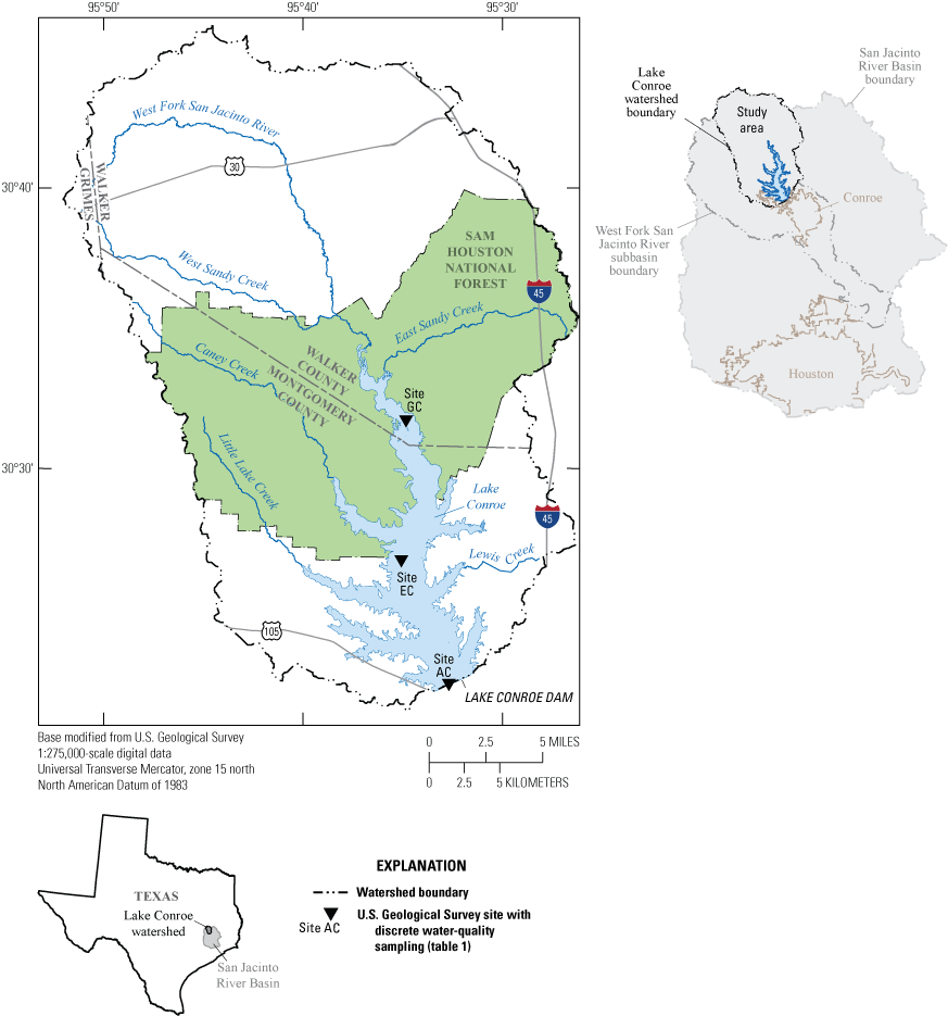
U.S. Geological Survey water-quality monitoring sites on Lake Conroe, Texas.
The U.S. Geological Survey (USGS), in cooperation with the SJRA, has collected discrete water-quality data from Lake Conroe since 1974. The monitoring program was designed to better understand the newly formed reservoir and its limnological processes, and because samples continue to be collected on an annual basis, it provides ongoing monitoring of general water-quality conditions in the reservoir. Because the types of data that are collected and sampling sites have remained consistent over time, the water-quality data lend themselves to long-term water-quality characterizations and trend analyses. In all but 2 years since 1974, water-quality surveys have been completed three times each year and include depth profiles of dissolved-oxygen concentration, pH, specific conductance, and water temperature; in 2013 and 2018, two water-quality surveys were completed instead of three. Surveys also include the collection of water samples at two depth intervals from three sites for analyses of major ions, nutrients, and trace metal concentrations. Water-quality monitoring sites were chosen to represent the main body of the reservoir and include (1) site USGS-302127095335501 Lake Conroe Site AC near Conroe, Tex. (hereinafter referred to as “site AC”), which is in the downstream part of the reservoir at the Lake Conroe dam (hereinafter referred to as “downreservoir”); (2) site USGS-302607095360901 Lake Conroe Site EC near Conroe, Tex., (hereinafter referred to as “site EC”), which is mid-reservoir; and (3) site USGS-303129095360501 Lake Conroe Site GC near Conroe, Tex. (hereinafter referred to as “site GC”), which is in the upstream part of Lake Conroe (hereinafter referred to as “upreservoir”) (table 1). A summary and trend analysis of selected physicochemical properties (water-quality properties measured in situ in the water column) and water-quality constituents for the first 9 years of data collection at Lake Conroe was completed in 1985 (Flugrath and others, 1985). Additional data have since been collected, and rapid land development at Lake Conroe, the surrounding area, and the upstream watershed has occurred since 1985. Urban development, population growth, and growing water needs in the greater Houston area (Montgomery and Harris Counties) have placed greater demands on Lake Conroe as a water supply (TWDB, 2020). Between 1974, when water-quality monitoring in Lake Conroe began, and 2020, the population of the greater Houston area increased from 2,098,000 to 6,246,000 (Pacific Northwest Regional Economic Analysis Project, 2024). Population in the greater Houston area is projected to increase an additional 20 percent, or by 1,060,000 people, from 2020 to 2040. This expected population growth will further increase the water demands and the potential for water shortages in the area (TWDB, 2022). Rapid land development and population growth can contribute to water-quality degradation over time, especially when watershed-protection practices are lacking or insufficient (Foster and others, 2000; Foley and others, 2005; Adhikari and others, 2016).
Table 1.
U.S. Geological Survey water-quality monitoring sites on Lake Conroe, Texas.[Horizontal coordinate information is referenced to the North American Vertical Datum of 1983. USGS, U.S. Geological Survey; ft, foot; Tex., Texas]
| USGS site number | USGS site name | Short name for site (fig. 1) | Mean water depth (ft) | Location in Lake Conroe | Latitude (decimal degrees) | Longitude (decimal degrees) |
|---|---|---|---|---|---|---|
| 302127095335501 | Lake Conroe Site AC near Conroe, Tex. | Site AC | 53 | Lake Conroe dam (downreservoir) | 30.3575 | −95.5654 |
| 302607095360901 | Lake Conroe Site EC near Conroe, Tex. | Site EC | 39 | Mid-reservoir | 30.4353 | −95.6025 |
| 303129095360501 | Lake Conroe Site GC near Conroe, Tex. | Site GC | 28 | Headwaters (upreservoir) | 30.5247 | −95.6014 |
Changes in water quality over time and within the water column of a reservoir such as Lake Conroe are affected by both anthropogenically driven and natural changes within the watershed that drains into the reservoir. Anthropogenic influences that affect water quality include changes in land use (Foley and others, 2005), such as urbanization (Colston, 1974; Carle and others, 2007), deforestation, untreated or inadequately treated wastewater discharges from wastewater treatment plants (WWTPs) (Steele and Aitkenhead-Peterson, 2011), sanitary sewer overflows, inadequate onsite sewage facilities, pet and livestock waste, agricultural runoff (U.S. Environmental Protection Agency [EPA], 2023a), litter and waste from recreational activities, and silt and debris from construction sites in high-growth areas (SJRA, 2015). Natural changes in water quality are affected by the composition and weathering of the surrounding geology and soil (Hem, 1985); climate (Nielsen-Gammon, 2011); topography (Dillon and Kirchner, 1975); hydrological processes, such as precipitation runoff and infiltration (Varis and Somlyody, 1996); aquatic vegetation; and natural disturbances, such as floods and droughts (Mosley, 2015). To gain a better understanding of how water quality has changed temporally and spatially in Lake Conroe, a reservoir-wide water-quality characterization and temporal trend analysis was completed by the USGS in cooperation with the SJRA. The approach includes using water-quality statistics to describe variability within the water column and between seasons; a characterization of thermal stratification; and a statistical trend analysis using the Seasonal Kendall test (SKT) and Mann-Kendall test adjusted for censored data, both of which are trend-analysis methods that incorporate seasonal variability.
Purpose and Scope
The purpose of the report is to (1) describe the vertical, spatial, and seasonal variability of selected physicochemical properties and constituents in Lake Conroe during 1974–2021; (2) characterize the relation between thermal stratification and selected physicochemical properties and constituents; and (3) expand on the trend analysis performed by Flugrath and others (1985) by evaluating water-quality trends for physicochemical properties, major ions, nutrients, and trace metals in Lake Conroe for two periods, 1974–2021 and 1993–2021. Water-quality data presented in this report were collected during 1974–2021 at three sites in Lake Conroe. Data used for the statistical summaries and analyses were obtained from the USGS National Water Information System (NWIS) database (USGS, 2024).
Description of Study Area
Lake Conroe is about 7 miles (mi) northwest of Conroe, Tex. (fig. 1) and drains an area of 445 square miles (mi2). The total reservoir capacity of Lake Conroe was computed in 2020 to be 417,605 acre-feet (acre-ft) at the conservation pool elevation of 201.0 feet (ft) above the National Geodetic Vertical Datum 1929 (Leber and others, 2021). Lake Conroe is 21 mi long and has a width that ranges from about 1 to 6 mi. When full, the mean depth of the reservoir is about 20 ft, with a maximum depth of about 70 ft. Depths are greatest in the drowned channel of the West Fork San Jacinto River nearest to the Lake Conroe dam. The depths outside of the drowned channel are less than or equal to 25 ft (SJRA, 2023). The Lake Conroe dam is an earthfilled embarkment 82 ft high and 11,300 ft long and features a controlled emergency spillway. Discharges are managed by means of a 10-ft concrete conduit through the dam (Leber and others, 2021).
The Lake Conroe watershed includes northern Montgomery and southern Walker Counties and covers roughly 25 percent, or 450 mi2, of the West Fork San Jacinto subbasin (Texas Commission on Environmental Quality, 2002; SJRA, 2023). The West Fork San Jacinto River is the largest inflow into Lake Conroe. Major tributaries, such as West Sandy, East Sandy, Caney, Lewis, and Little Lake Creeks, also contribute inflow to Lake Conroe (fig. 1).
The climate in the Lake Conroe watershed is humid subtropical (Larkin and Bomar, 1983) with a mean annual temperature of 20.2 degrees Celsius (°C) during 1974–2021 (National Climatic Data Center, 2023). Precipitation in the watershed varied annually and seasonally during 1974–2021. The mean annual precipitation during 1974–2021 was 49.3 inches (in.). Annual precipitation amounts ranged from 26.9 in. for 1999 to 72.7 in. for 2017 (fig. 2A). During the first half of the study period (1974–97), the mean annual precipitation was 48.5 in., compared to 50.1 in. for the second half of the study period (1998–2021). Precipitation totals were generally highest in May and lowest in February (National Climatic Data Center, 2023).
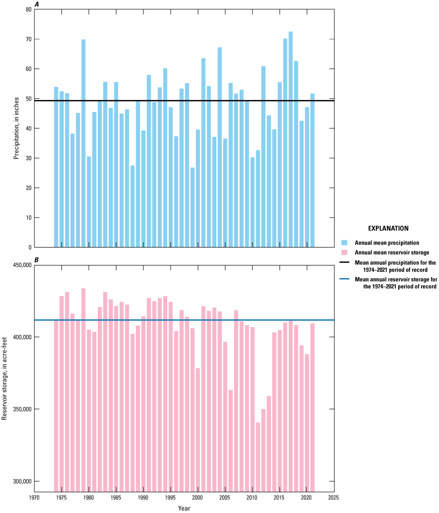
Annual mean and mean annual totals of A, precipitation for Lake Conroe watershed; and B, reservoir storage for Lake Conroe, Texas, during 1974–2021.
Variations in Lake Conroe reservoir storage during the study period generally reflected precipitation patterns in the watershed (fig. 2). The long-term (1974–2021) mean annual reservoir storage was 409,000 acre-ft. Annual mean storage values ranged from 341,000 acre-ft in 2011 to 434,000 acre-ft in 1979 (TWDB, 2023). The three lowest values for annual mean reservoir storage occurred in consecutive years: 2011, 2012, and 2013. Annual mean reservoir storage was typically greater in the first half of the study period than in the second half. The top 13 annual mean reservoir storage values were for years within the first half of the study period. The four largest annual mean reservoir storage values were during the first 10 years after reservoir impoundment.
Land cover in the Lake Conroe watershed includes developed, forested, pastured, and wetland areas (fig. 3). The northernmost section of the watershed, north of where the West Fork San Jacinto River enters Lake Conroe (fig. 3), contains mostly cultivated lands, pastures, forests, and cleared land resulting from timber harvesting (SJRA, 2015), as well as dense urban development surrounding Huntsville, Tex. (fig. 3). The middle section of the watershed, approximately 3 mi north of site EC, south of West Sandy Creek and East Sandy Creek, and west of Interstate 45, includes gently rolling, heavy forested terrain (fig. 3) that lies primarily within the Sam Houston National Forest. The southernmost section of the watershed is more densely developed than the northern and middle sections and has considerable residential and commercial development near the reservoir shores. Lake Conroe occupies a large part of the southernmost section of the watershed (Bodkin and Oden, 2010; SJRA, 2015). Forested land cover in Montgomery County decreased from 43 percent in 2001 (463 mi2) to 38 percent in 2021 (409 mi2) and developed land cover, such as apartment complexes and commercial businesses, increased from 21 percent from 2001 (226 mi2) to 29 percent in 2021 (312 mi2) (Multi-Resolution of Land Characteristics Consortium [MRLC], 2023). In 2021, impervious surfaces, such as concrete, asphalt streets, parking lots, and roofs, covered approximately 10 percent (108 mi2) of the total land cover in Montgomery County (MRLC, 2023). Approximately 220 storm drain outfalls and 40 WWTPs are located within the Lake Conroe watershed and discharge into a stream or directly into the reservoir (SJRA, 2015).
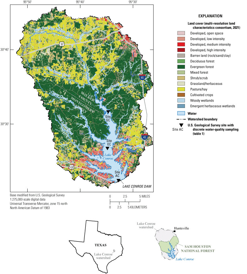
Land use in the Lake Conroe watershed, Texas, 2021.
The population of Montgomery County increased by roughly 540,000 people, or 700 percent, from 1974 to 2020 (U.S. Census Bureau, 2020; fig. 4). In 1974, the population density of Montgomery County was 75 people per mi2 and had increased to 595 people per mi2 by 2020. From 2010 to 2020, the population increased by 165,000 people, or about 36 percent. The growth in population is reflected by changes in land use in the watershed, such as areas of increased urban development and decreased forested land. In 2015, SJRA began treating water from Lake Conroe to produce drinking water for the residents of Montgomery County. In addition, the reservoir serves as the City of Houston’s reserve drinking-water supply and is also used for recreational purposes (SJRA, 2023).
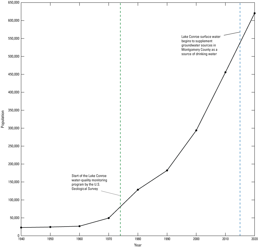
Population of Montgomery County, Texas, 1940–2020.
Previous Studies
In 1985, the USGS published findings on water quality at Lake Conroe from water-quality data collected from the reservoir’s impoundment in 1973 through 1982 (Flugrath and others, 1985). During this 9-year span, the USGS conducted 27 water-quality surveys on Lake Conroe coinciding with winter, spring, and summer. Discrete water-quality sampling sites were chosen to represent different locations and depths on Lake Conroe (table 1). The three sites chosen to represent the main body of the reservoir were (1) downreservoir site AC at the Lake Conroe dam, where the mean depth was 53 ft; (2) midreservoir site EC, where the mean depth was 39 ft; and (3) upreservoir site GC, where the mean depth was 28 ft. During each survey, dissolved-oxygen concentration, pH, specific conductance, and water temperature were measured near the top of the water column (1–3 ft below the water surface), near the bottom of the water column (2–3 ft above the reservoir bottom), and at intervening depth intervals of about 10 ft. Water samples were collected near the reservoir surface and bottom to define spatial variations and thermal-stratification patterns of major ions, nutrients, and trace metals. The depth at which the samples were collected near the reservoir bottom varied between sites because of differences in reservoir depth. The near-bottom samples at a given site over the period of record were collected at different depths because of fluctuations in reservoir stage, as well as slight variations in the distance from the reservoir bottom at which samples were collected because of choices made by the individual collecting the samples. Near-bottom samples collected at site AC ranged from 39 to 69 ft below the water surface, whereas near-bottom samples collected at site EC ranged from 20 to 44 ft below the water surface, and near-bottom samples collected at site GC ranged from 9 to 35 ft below the water surface.
The report by Flugrath and others (1985) discussed seasonal and spatial trends in dissolved-oxygen, major-ion, trace metal, and nutrient concentrations. The study indicated that the highest dissolved-oxygen concentrations were measured in summer and were higher near the dam than in the upstream part of the reservoir. Dissolved-oxygen concentrations of less than 0.5 milligram per liter (mg/L) were measured at water depths greater than 30 ft in summer, representing anoxic conditions. Major-ion concentrations peaked in summer at all sites. The highest concentrations of trace metals (iron and manganese) were near the reservoir bottom at the deepest site (site AC) during summer. Nutrient concentrations were highest during summer near the reservoir bottom. Nutrient concentrations remained consistent seasonally from one year to the next, which Flugrath and others (1985) suspected was indicative of a recycling process that prevents nutrient accumulation. Flugrath and others (1985) also suggested that thermal stratification in Lake Conroe began in March and persisted until October, with the most pronounced thermal stratification from June through September. Dissolved-oxygen, major-ion, trace metal, and nutrient concentrations correlated with thermal-stratification patterns. The lowest dissolved-oxygen concentrations and highest major-ion, trace metal, and nutrient concentrations were detected during summer in the hypolimnion (the relatively cold [less than approximately 25 °C], anoxic lowest depth-layer thermodynamically isolated from the rest of the reservoir [Boehrer and Schultze, 2008]). In winter, the concentrations of these chemical constituents tended to remain uniform across the reservoir and at all depths (Flugrath and others, 1985).
Methods
This section of the report outlines how water-quality data were collected from Lake Conroe. The methods used to analyze the data are also described. The data collected were analyzed to (1) characterize water-quality conditions, (2) describe water-column and seasonal variability, (3) characterize thermal stratification, and (4) test for long-term and recent trends.
Discrete Data Collection
Discrete water-quality data were collected from Lake Conroe to determine physicochemical properties, including water temperature, dissolved oxygen, specific conductance, and pH, and laboratory analyzed constituents, including major ions, nutrients, and trace metals. Discrete water-quality data were collected approximately three times per year (in winter, spring, and summer) during 1974–2021. Vertical profiles of water temperature, dissolved-oxygen concentration, specific conductance, and pH were collected by using a portable water-quality single parameter or multiparameter meter at sites AC, EC, and GC over the study period (fig. 1; table 1) following methods consistent with those in the National Field Manual for the Collection of Water Quality Data (USGS, variously dated). Water-quality meter readings were collected along vertical profiles from 1–3 ft below the water surface to 2–3 ft above the reservoir bottom in increments of approximately 5–10 ft. Water transparency was measured by using a Secchi disk and a measuring tape (Harrison, 2016).
Discrete samples for laboratory analysis of major ions (calcium, magnesium, potassium, sodium, chloride, sulfate, silica, and fluoride), hardness, nutrients (ammonia, ammonia plus organic nitrogen, phosphorous, orthophosphate as phosphorous, nitrite, and nitrate plus nitrite), and trace metals (iron and manganese) were collected 1–3 ft below the water surface and 2–3 ft above the reservoir bottom at sites AC, EC, and GC (table 1) during 1974–2021. Samples collected during 1974–2001 for the analysis of major ions and trace metals were filtered in the field through a 0.45-micron pore size capsule filter. The samples analyzed for nutrients from 1974 through 1992 were unfiltered and are not described in this study, except for the discussion of nitrate plus nitrite concentrations. Beginning in 1993, all samples collected for nutrient analysis were filtered through a 0.45-micron pore size capsule filter. Previous studies (Fishman and Friedman, 1989) have indicated there are minimal differences between unfiltered and filtered nitrate plus nitrite concentration analysis methods; thus, results from both methods were considered equivalent and were used for the general characterization of nitrate plus nitrite concentrations in Lake Conroe. In addition to the discrete samples collected either 1–3 ft below the water surface or 2–3 ft above the reservoir bottom, discrete samples for laboratory analysis of nutrients and trace metals were also collected at a mid-depth interval; however, these samples are not described in this report because of the highly variable range of depths at which the mid-depth sample was collected. Water-quality samples were collected from a boat by using the discrete-depth point sample method (Graham and others, 2008). Discrete samples were collected by using a peristaltic pump and polyethylene tubing. Dedicated polyethylene tubing (tubing used at one site only) was attached to the water-quality meter cable and lowered to the depth of the planned sample. The sample was then pumped directly from the reservoir into the sample bottle. Three sampling-tubing volumes were pumped prior to the collection of samples at different depths to fill the tubing with water representative of that depth interval. Water samples collected by the USGS were filtered and preserved adhering to USGS protocols and guidelines described in the National Field Manual for the Collection of Water Quality Data (USGS, variously dated). Samples for major ion, hardness, nutrient, and trace metal analyses were chilled and shipped overnight to the USGS National Water Quality Laboratory (NWQL) in Denver, Colorado. Methods for major-ion analysis are documented in Fishman and Friedman (1989) and Fishman (1993). Methods for nutrient analysis are documented in Fishman and Friedman (1989), Patton and Truitt (1992), Fishman (1993), Patton and Truitt (2000), and Patton and Kryskalla (2011). Methods for trace metal analysis are documented in Hoffman and others (1996). Nutrient (excluding nitrate plus nitrite and nitrite) and trace-metal data collected and analyzed before 1993 are not discussed in this report because of changes in the analytical methods at the USGS NWQL in 1992 (Fishman, 1993; Hoffman and others, 1996). All water-quality data collected during 1974–2021 are available from the NWIS database (USGS, 2024).
Water-Quality Data Considerations
Several changes in laboratory analysis methods occurred over the course of the 47 years from 1974 to 2021 from which water-quality data were compiled. Notable changes in data collection methods that could present challenges when assessing water-quality characteristics and evaluating trends include variations in data collection methods (for example, substitution of the fraction [filtered or unfiltered] being measured in the sample for some water-quality analyte groups), and changes in laboratory analysis methods and laboratory reporting levels (LRLs). One of the objectives of this study was to describe water quality by site and sampling depth to describe the variability within the water column and across the reservoir; water quality in reservoirs varies spatially and with depth (Dawson and others, 2015). Because sampling depths varied among sites and among sampling events for a given site, the data were standardized to two sets of depth interval classifications: a “near-surface” interval that included the sample or measurement collected near the top of the water column (1–3 ft below the water surface) and a “near-bottom” interval that included the sample or measurement collected near the bottom of the water column (2–3 ft above the reservoir bottom).
Quality-Assurance Procedures
Several quality-assurance procedures were applied to the water-quality data prior to characterization and analysis. The ionic-charge balance of individual samples was evaluated, and samples with charge balances differences exceeding 5 percent were reviewed to determine if any water-quality results warranted removal from the dataset because of potential sampling or analytical errors. Results labeled with an “estimated” qualifier were considered to be a detection and included in the dataset.
Computation of summary statistics and temporal trends for water-quality data was complicated by the occurrence of constituents not detected during laboratory analysis, herein described as left-censored “less-than” values, or nondetections. Left-censored values are denoted with a less than symbol (“<”) and are assigned to a result when the concentration of a constituent is less than its LRL. The LRL is the concentration at which the rate of reporting false negative values is minimized such that the probability of falsely reporting a nondetection for a sample that contained a property at a concentration equal to or greater than the LRL is no more than 1 percent (Childress and others, 1999; Foreman and others, 2021). Because of the number of censored values reported for nutrients and trace metals, excluding nitrate plus nitrite, summary statistics were only computed from data collected after 1992. From 1993 onward, changes in sample collection methods and laboratory analytical methods reduced the number of censored values for these constituents.
Quality Control
USGS protocols for the use and interpretation of quality-control data are described in Mueller and others (2015). Replicate samples are a type of quality-control sample collected to evaluate the variability of sample processing and analysis in water quality (Mueller and others, 2015). Sequential-replicate sampling, which is a method of quality-control sampling in which multiple samples are collected consecutively (over a short period of time), was used to collect second (or duplicate) sets of major ion, nutrient, and trace metal samples. The dataset for this report includes a total of 25 sequential-replicate samples consisting of 11 samples collected at site AC from 1999 to 2021, 9 samples collected at site EC from 2000 to 2021, and 5 samples collected at site GC from 2003 to 2020 (tables 2–3).
Table 2.
Major ion data from quality-control replicate samples collected at U.S. Geological Survey water-quality monitoring sites AC, EC, and GC, near Conroe, Texas, 1999–2021.[Dates are in month/day/year format; h, hour; CST, central standard time; mg/L, milligram per liter; S, sample collected from near-surface interval; Env., environmental sample; Rep., replicate sample; NA, not applicable; RPD, relative percent difference; B, sample collected from near-bottom interval; E, estimated; <, less than; —, not available]
Because sampling depths varied among sites and among sampling events for a given site, the data were standardized to two sets of depth interval classifications: a near-surface interval that included the sample or measurement collected 1–3 ft below the water surface and a near-bottom interval that included the sample or measurement collected 2–3 ft above the reservoir bottom.
Table 3.
Nutrient and trace-metal data from quality-control replicate samples collected at U.S. Geological Survey water-quality monitoring sites AC, EC, and GC, near Conroe, Texas, 1999–2021.[Dates are in month/day/year format; h, hour; CST, central standard time; mg/L, milligram per liter; N, nitrogen; P, phosphorous; µg/L, microgram per liter; S, sample collected from near-surface interval; Env., environmental sample; Rep., replicate sample; NA, not applicable; RPD, relative percent difference; B, sample collected from near-bottom interval; E, estimated; <, less than; —, not available]
Because sampling depths varied among sites and among sampling events for a given site, the data were standardized to two sets of depth interval classifications: a near-surface interval that included the sample or measurement collected 1–3 ft below the water surface and a near-bottom interval that included the sample or measurement collected 2–3 ft above the reservoir bottom.
To determine variability in environmental samples, the relative percent difference (RPD) between each pair of samples was calculated by using the following equation:
whereC1
is the contaminant concentration in the environmental sample, and
C2
is the contaminant concentration in the sequential-replicate sample.
RPDs were not calculated for (1) replicate pairs where both values in the replicate pair were censored, (2) replicate pairs where one value in the replicate pair was censored, or (3) replicate pairs where one or both values were qualified as estimated (Mueller and others, 2015). The RPDs of sequential-replicate sample pairs are included in tables 2–3. An RPD of 20 percent or less between sequential-replicate pairs was considered to indicate acceptable reproducibility for this study and relatively low variability in the samples (Mueller and others, 2015). Among the 384 possible comparisons between different constituent pairs produced from analyzing the 25 quality-control samples for 16 constituents, nondetections (indicated by a less than (“<”) symbol in tables 2–3) were observed in one or both samples in 115 of the constituent pairs. In the 269 comparisons with a detection in both samples, the RPDs ranged from 0 to 126.6 percent, with a mean RPD of 8.0 percent. Mean RPDs were less than 15 percent for nutrients collectively and individually were 14.9 percent for ammonia, 11.1 percent for nitrite, 10 percent for ammonia plus organic nitrogen, 11.1 percent for nitrate plus nitrite, 10.4 percent for phosphorous, and 10.6 percent for orthophosphate. Mean RPDs collectively were less than 10 percent for major ions and individually were 1.8 percent for calcium, 1.9 percent for magnesium, 2.8 percent for sodium, 3.8 percent for potassium, 1.6 percent for chloride, 9.6 percent for sulfate, 5.6 percent for fluoride, and 6.7 percent for silica. Mean RPDs for the trace metals iron and manganese were 15.1 and 26.0 percent, respectively. The RPD was within acceptable limits (<20 percent) for 241 replicate pairs or 89.6 percent of the pairs. RPDs greater than 20 percent indicate higher variability in the analytical results. High variability may be due to environmental and replicate samples being collected sequentially in different bottles, with any changes in the environment being reflected in a sequential replicate more so than other replicate types, such as split or concurrent replicates (Mueller and others, 2015). Additionally, high variability in the analytical results could be due to some replicate pairs having high RPD values with a small absolute difference in concentration. For example, the RPD for the replicate pair for orthophosphate measured in samples collected near the bottom at site AC on June 29, 1999, was 32.4 percent (table 3), whereas the absolute difference in concentration was only 0.102 mg/L.
Field-blank samples were collected to measure the bias that may have been introduced to the samples because of sampling, processing, or analytical procedures (USGS, 2006). Field-blank samples were prepared at the monitoring site before the collection and processing of an environmental sample (Mueller and others, 1997). The field-blank samples were analyzed for major ions, nutrients, and trace metals. From 1974 to 2021, three field-blank samples were collected at site AC, three field-blank samples were collected at site EC, and one field-blank sample was collected at site GC. Ammonia was detected in one of the field-blank samples collected from site AC at a concentration of 0.01 mg/L and was qualified as “below the reporting level (0.01 mg/L) but at or above the detection level” by the NWQL. Manganese was detected in one of the field-blank samples collected from site EC at a concentration of 0.20 microgram per liter (µg/L) and was qualified as “below the reporting level (0.20 µg/L) but at or above the detection level” by the NWQL. No constituents were detected in the field-blank sample collected at site GC.
Summary Statistics
Summary statistics, including the minimum, 50th percentile (median), mean, maximum, and standard deviation values, were calculated using methods described in Bolks and others (2014) and Helsel and others (2020) and are included in tables 4–6. Summary statistics by season were also calculated and are included in tables 7–15. Procedures for computing summary statistics were based on the number of samples and the percentage of censored data for each water-quality constituent measured or collected at each site and depth interval (and season in tables 7–15) combination. Summary statistics were calculated by using robust regression on order statistics for physicochemical property or constituent for each site and depth (and season in tables 7–15) with a sample size consisting of less than 50 reported values of which no more than 80 percent were censored values (that is, a minimum of 10 uncensored values) or a sample size greater than or equal to 50 reported values of which no more than 50 percent were censored values (that is, a minimum of 25 uncensored values). Such statistics require at least three uncensored observations and an assumption that the censored data represent an approximately normal or lognormal distribution (Helsel and others, 2020). Using this method, the detected values are plotted on a probability plot and a linear regression line is calculated to approximate the assumed distribution. Censored observations were imputed on the basis of this regression and then combined with the detected values to compute estimates of summary statistics (Interstate Technology Regulatory Council, 2013; Bolks and others, 2014). If the sample size was greater than 50 and contained 50–80 percent censored values, the summary statistics were calculated by using a maximum likelihood estimation (MLE) procedure that requires a sample size of at least 50 data points and can handle multiple LRLs. The MLE procedure is used to estimate the mean and variance by maximizing the likelihood of the uncensored values while simultaneously treating each censored value as an inequality. Once mean and variance statistics are determined, other summary statistics can be estimated. In the MLE procured, it is assumed that the censored values are distributed in a manner similar to the uncensored values (Interstate Technology Regulatory Council, 2013). Summary statistics were not calculated for constituents having greater than 80 percent censored data at any given site and depth combination. In some instances, summary statistics for a physicochemical property or constituent for an entire depth interval were calculated, which involved applying the appropriate statistical method to the entire dataset (sites AC, EC, and GC) for a given physicochemical property or constituent and depth interval.
Table 4.
Summary statistics for physicochemical properties measured at U.S. Geological Survey water-quality monitoring sites, AC, EC, and GC, for the period 1974–2021.[°C, degree Celsius; mg/L, milligram per liter; µS/cm at 25 °C; microsiemens per centimeter at 25 °C; ft, foot; --, not applicable]
| Site short name (fig. 1) | Depth intervala | Number of observations | Number of censored observations | Percent censored data | Period of record (years) | Statistic | ||||
|---|---|---|---|---|---|---|---|---|---|---|
| Minimum | Maximum | Mean | Median | Standard deviation | ||||||
| AC | Surface | 142 | 0 | 0 | 47 | 8.00 | 32.2 | 23.2 | 26.8 | 7.57 |
| AC | Bottom | 142 | 0 | 0 | 47 | 7.50 | 28.7 | 18.9 | 20.0 | 5.45 |
| EC | Surface | 142 | 0 | 0 | 47 | 7.00 | 32.6 | 24.0 | 27.7 | 7.67 |
| EC | Bottom | 142 | 0 | 0 | 47 | 7.00 | 30.3 | 21.2 | 23.5 | 6.61 |
| GC | Surface | 143 | 0 | 0 | 47 | 7.50 | 34.9 | 24.8 | 28.0 | 7.88 |
| GC | Bottom | 141 | 0 | 0 | 47 | 6.50 | 32.1 | 23.1 | 25.5 | 7.53 |
| AC | Surface | 142 | 0 | 0 | 47 | 1.9 | 13.4 | 8.2 | 8.2 | 2.2 |
| AC | Bottom | 140 | 0 | 0 | 47 | 0.1 | 11.8 | 3.4 | 1.1 | 3.9 |
| EC | Surface | 142 | 0 | 0 | 47 | 4.6 | 12.7 | 8.8 | 8.7 | 1.8 |
| EC | Bottom | 141 | 0 | 0 | 47 | 0.1 | 14.0 | 4.1 | 2.5 | 4.1 |
| GC | Surface | 141 | 0 | 0 | 47 | 4.0 | 13.2 | 8.4 | 8.4 | 2.0 |
| GC | Bottom | 132 | 0 | 0 | 47 | 0.1 | 12.7 | 4.9 | 4.5 | 3.3 |
| AC | Surface | 142 | 0 | 0 | 47 | 126 | 349 | 218 | 210 | 42.4 |
| AC | Bottom | 142 | 0 | 0 | 47 | 128 | 390 | 249 | 241 | 55.5 |
| EC | Surface | 142 | 0 | 0 | 47 | 123 | 345 | 214 | 207 | 42.5 |
| EC | Bottom | 142 | 0 | 0 | 47 | 123 | 359 | 231 | 222 | 48.7 |
| GC | Surface | 142 | 0 | 0 | 47 | 96.0 | 346 | 203 | 205 | 51.2 |
| GC | Bottom | 133 | 0 | 0 | 47 | 80.0 | 381 | 210 | 210 | 60.3 |
| AC | Surface | 142 | 0 | 0 | 47 | 6.8 | 9.2 | 8.1 | 8.1 | 0.50 |
| AC | Bottom | 142 | 0 | 0 | 47 | 6.3 | 8.5 | 7.3 | 7.2 | 0.41 |
| EC | Surface | 142 | 0 | 0 | 47 | 7.2 | 9.3 | 8.3 | 8.4 | 0.48 |
| EC | Bottom | 142 | 0 | 0 | 47 | 6.3 | 8.9 | 7.4 | 7.4 | 0.48 |
| GC | Surface | 142 | 0 | 0 | 47 | 6.5 | 9.4 | 8.1 | 8.1 | 0.70 |
| GC | Bottom | 141 | 0 | 0 | 47 | 6.2 | 9.0 | 7.4 | 7.4 | 0.55 |
| AC | Surface | 136 | 0 | 0 | 47 | 1.3 | 7.9 | 3.4 | 3.2 | 1.4 |
| AC | Bottom | -- | -- | -- | -- | -- | -- | -- | -- | -- |
| EC | Surface | 134 | 0 | 0 | 47 | 1.3 | 8.2 | 3.0 | 2.7 | 1.3 |
| EC | Bottom | -- | -- | -- | -- | -- | -- | -- | -- | -- |
| GC | Surface | 136 | 0 | 0 | 47 | 0.33 | 5.9 | 1.8 | 1.6 | 0.84 |
| GC | Bottom | -- | -- | -- | -- | -- | -- | -- | -- | -- |
Because sampling depths varied among sites and sampling events for the same site, the data were standardized to two sets of depth interval classifications: a “near-surface” interval that included the sample or measurement collected 1–3 ft below the water surface and a “near-bottom” interval that included the sample or measurement collected 2–3 ft above the reservoir bottom.
Table 5.
Summary statistics for major ions and water hardness measured at U.S. Geological Survey water-quality monitoring sites, AC, EC, and GC, for either the period 1974–2021 or 1993–2021, depending on the period of record of available data.[mg/L, milligram per liter; CaCO3, calcium carbonate; <, less than]
| Site short name (fig. 1) | Depth intervala | Number of observations | Number of censored observations | Percent censored data | Sampling date range | Period of record (years) | Statistic | ||||
|---|---|---|---|---|---|---|---|---|---|---|---|
| Minimum | Maximum | Mean | Median | Standard deviation | |||||||
| AC | Surface | 142 | 0 | 0 | 1974–2021 | 47 | 15.2 | 39.0 | 26.0 | 25.0 | 4.88 |
| AC | Bottom | 140 | 0 | 0 | 1974–2021 | 47 | 15.5 | 46.0 | 28.7 | 27.7 | 6.19 |
| EC | Surface | 142 | 0 | 0 | 1974–2021 | 47 | 14.8 | 38.7 | 25.4 | 24.2 | 4.90 |
| EC | Bottom | 142 | 0 | 0 | 1974–2021 | 47 | 14.0 | 44.0 | 26.9 | 25.9 | 5.86 |
| GC | Surface | 141 | 0 | 0 | 1974–2021 | 47 | 11.0 | 37.6 | 22.7 | 22.6 | 5.60 |
| GC | Bottom | 140 | 0 | 0 | 1974–2021 | 47 | 9.00 | 41.0 | 23.2 | 22.5 | 6.36 |
| AC | Surface | 142 | 0 | 0 | 1974–2021 | 47 | 1.32 | 3.17 | 2.15 | 2.10 | 0.393 |
| AC | Bottom | 140 | 0 | 0 | 1974–2021 | 47 | 1.34 | 3.43 | 2.29 | 2.29 | 0.442 |
| EC | Surface | 142 | 0 | 0 | 1974–2021 | 47 | 1.32 | 3.22 | 2.14 | 2.10 | 0.397 |
| EC | Bottom | 142 | 0 | 0 | 1974–2021 | 47 | 1.30 | 3.40 | 2.21 | 2.15 | 0.440 |
| GC | Surface | 141 | 0 | 0 | 1974–2021 | 47 | 1.20 | 3.27 | 2.08 | 2.04 | 0.455 |
| GC | Bottom | 140 | 0 | 0 | 1974–2021 | 47 | 1.00 | 3.40 | 2.14 | 2.09 | 0.512 |
| AC | Surface | 141 | 0 | 0 | 1974–2021 | 47 | 2.30 | 5.48 | 3.28 | 3.11 | 0.631 |
| AC | Bottom | 139 | 0 | 0 | 1974–2021 | 47 | 2.40 | 5.45 | 3.40 | 3.22 | 0.650 |
| EC | Surface | 141 | 0 | 0 | 1974–2021 | 47 | 2.20 | 5.48 | 3.25 | 3.10 | 0.650 |
| EC | Bottom | 141 | 0 | 0 | 1974–2021 | 47 | 2.40 | 5.38 | 3.30 | 3.20 | 0.648 |
| GC | Surface | 140 | 0 | 0 | 1974–2021 | 47 | 2.26 | 5.41 | 3.37 | 3.22 | 0.691 |
| GC | Bottom | 138 | 0 | 0 | 1974–2021 | 47 | 2.17 | 5.90 | 3.44 | 3.29 | 0.768 |
| AC | Surface | 142 | 0 | 0 | 1974–2021 | 47 | 6.79 | 27.6 | 13.1 | 12.0 | 4.09 |
| AC | Bottom | 140 | 0 | 0 | 1974–2021 | 47 | 6.49 | 26.7 | 13.0 | 12.2 | 4.08 |
| EC | Surface | 142 | 0 | 0 | 1974–2021 | 47 | 6.64 | 27.3 | 12.9 | 12.0 | 4.09 |
| EC | Bottom | 142 | 0 | 0 | 1974–2021 | 47 | 5.90 | 27.4 | 12.9 | 12.0 | 4.13 |
| GC | Surface | 141 | 0 | 0 | 1974–2021 | 47 | 4.45 | 27.2 | 13.1 | 12.6 | 4.54 |
| GC | Bottom | 140 | 0 | 0 | 1974–2021 | 47 | 3.30 | 28.3 | 13.6 | 13.0 | 5.15 |
| AC | Surface | 142 | 0 | 0 | 1974–2021 | 47 | 11.2 | 38.2 | 20.6 | 19.7 | 5.75 |
| AC | Bottom | 141 | 0 | 0 | 1974–2021 | 47 | 8.83 | 38.0 | 20.6 | 19.5 | 6.02 |
| EC | Surface | 142 | 0 | 0 | 1974–2021 | 47 | 8.48 | 37.7 | 20.5 | 19.4 | 5.69 |
| EC | Bottom | 142 | 0 | 0 | 1974–2021 | 47 | 8.47 | 37.7 | 20.4 | 20.0 | 5.99 |
| GC | Surface | 141 | 0 | 0 | 1974–2021 | 47 | 5.99 | 42.0 | 21.1 | 20.6 | 7.02 |
| GC | Bottom | 140 | 0 | 0 | 1974–2021 | 47 | 5.20 | 58.0 | 22.2 | 21.0 | 9.09 |
| AC | Surface | 140 | 1 | 1 | 1974–2021 | 47 | 1.00 | 15.0 | 6.57 | 6.35 | 2.12 |
| AC | Bottom | 139 | 5 | 4 | 1974–2021 | 47 | 0.24 | 12.0 | 5.03 | 5.10 | 3.11 |
| EC | Surface | 140 | 3 | 2 | 1974–2021 | 47 | <1.00 | 13.0 | 6.48 | 6.10 | 2.10 |
| EC | Bottom | 140 | 2 | 1 | 1974–2021 | 47 | 0.36 | 15.0 | 5.72 | 5.70 | 2.93 |
| GC | Surface | 139 | 1 | 1 | 1974–2021 | 47 | 1.00 | 18.2 | 7.25 | 6.76 | 3.07 |
| GC | Bottom | 138 | 0 | 0 | 1974–2021 | 47 | 1.97 | 21.0 | 7.57 | 6.78 | 3.57 |
| AC | Surface | 142 | 1 | 1 | 1974–2021 | 47 | <0.01 | 13.5 | 6.35 | 6.38 | 3.31 |
| AC | Bottom | 141 | 0 | 0 | 1974–2021 | 47 | 1.10 | 21.0 | 9.80 | 9.70 | 4.28 |
| EC | Surface | 142 | 0 | 0 | 1974–2021 | 47 | 0.59 | 13.3 | 6.60 | 6.84 | 3.22 |
| EC | Bottom | 141 | 0 | 0 | 1974–2021 | 47 | 1.10 | 14.0 | 7.96 | 7.90 | 3.03 |
| GC | Surface | 141 | 0 | 0 | 1974–2021 | 47 | 0.30 | 15.2 | 9.04 | 9.30 | 3.10 |
| GC | Bottom | 140 | 0 | 0 | 1974–2021 | 47 | 0.50 | 19.0 | 10.2 | 10.5 | 3.40 |
| AC | Surface | 83 | 17 | 20 | 1993–2021 | 28 | 0.07 | 0.22 | 0.12 | 0.11 | 0.04 |
| AC | Bottom | 82 | 16 | 19 | 1993–2021 | 28 | 0.08 | 0.23 | 0.12 | 0.12 | 0.04 |
| EC | Surface | 83 | 12 | 14 | 1993–2021 | 28 | 0.07 | 0.22 | 0.12 | 0.11 | 0.04 |
| EC | Bottom | 83 | 14 | 17 | 1993–2021 | 28 | 0.07 | 0.22 | 0.12 | 0.11 | 0.04 |
| GC | Surface | 82 | 17 | 21 | 1993–2021 | 28 | 0.06 | 0.23 | 0.12 | 0.12 | 0.04 |
| GC | Bottom | 81 | 17 | 21 | 1993–2021 | 28 | 0.06 | 0.23 | 0.12 | 0.11 | 0.04 |
| AC | Surface | 142 | 0 | 0 | 1974–2021 | 47 | 47.5 | 109 | 73.8 | 71.1 | 14.5 |
| AC | Bottom | 140 | 0 | 0 | 1974–2021 | 47 | 45.8 | 128 | 81.2 | 78.4 | 17.1 |
| EC | Surface | 142 | 0 | 0 | 1974–2021 | 47 | 45.7 | 109 | 72.3 | 69.1 | 13.6 |
| EC | Bottom | 142 | 0 | 0 | 1974–2021 | 47 | 40.3 | 120 | 76.5 | 73.2 | 16.2 |
| GC | Surface | 141 | 0 | 0 | 1974–2021 | 47 | 32.4 | 106 | 65.3 | 64.8 | 15.5 |
| GC | Bottom | 140 | 0 | 0 | 1974–2021 | 47 | 26.6 | 120 | 66.6 | 64.9 | 17.8 |
Because sampling depths varied among sites and sampling events for the same site, the data were standardized to two sets of depth interval classifications: a “near-surface” interval that included the sample or measurement collected 1–3 ft below the water surface and a “near-bottom” interval that included the sample or measurement collected 2–3 ft above the reservoir bottom.
Table 6.
Summary statistics for nutrients and trace metals measured at U.S. Geological Survey water-quality monitoring sites, AC, EC, and GC, for either the period 1974–2021 or 1993–2021, depending on the period of record of available data.[Mean, median, and standard deviation were not computed for water-quality records with greater than 80 percent left-censored data. mg/L, milligram per liter; N, nitrogen; P, phosphorous; µg/L, microgram per liter; <, less than; --, not applicable]
| Site short name (fig. 1) | Depth intervala | Number of observations | Number of censored observations | Percent censored data | Sampling date range | Period of record (years) | Statistic | ||||
|---|---|---|---|---|---|---|---|---|---|---|---|
| Minimum | Maximum | Mean | Median | Standard deviation | |||||||
| AC | Surface | 83 | 45 | 54 | 1993–2021 | 28 | <0.01 | 0.20 | 0.02 | <0.01 | 0.04 |
| AC | Bottom | 82 | 7 | 9 | 1993–2021 | 28 | <0.01 | 5.1 | 1.2 | 0.39 | 1.5 |
| EC | Surface | 83 | 58 | 70 | 1993–2021 | 28 | <0.01 | 0.27 | 0.02 | <0.01 | 0.03 |
| EC | Bottom | 83 | 14 | 17 | 1993–2021 | 28 | <0.01 | 3.2 | 0.36 | 0.08 | 0.62 |
| GC | Surface | 82 | 45 | 55 | 1993–2021 | 28 | <0.01 | 0.14 | 0.02 | <0.01 | 0.02 |
| GC | Bottom | 81 | 25 | 31 | 1993–2021 | 28 | <0.01 | 0.28 | 0.06 | 0.03 | 0.06 |
| AC | Surface | 77 | 0 | 0 | 1993–2021 | 28 | 0.30 | 0.57 | 0.41 | 0.40 | 0.06 |
| AC | Bottom | 76 | 0 | 0 | 1993–2021 | 28 | 0.30 | 5.9 | 1.5 | 0.62 | 1.6 |
| EC | Surface | 77 | 0 | 0 | 1993–2021 | 28 | 0.30 | 0.69 | 0.42 | 0.42 | 0.07 |
| EC | Bottom | 77 | 0 | 0 | 1993–2021 | 28 | 0.29 | 4.2 | 0.77 | 0.48 | 0.67 |
| GC | Surface | 76 | 0 | 0 | 1993–2021 | 28 | 0.30 | 1.1 | 0.50 | 0.49 | 0.13 |
| GC | Bottom | 76 | 0 | 0 | 1993–2021 | 28 | 0.35 | 1.1 | 0.55 | 0.51 | 0.14 |
| AC | Surface | 85 | 71 | 84 | 1993–2021 | 28 | <0.01 | 0.06 | -- | -- | -- |
| AC | Bottom | 82 | 28 | 34 | 1993–2021 | 28 | <0.01 | 1.3 | 0.25 | 0.08 | 0.30 |
| EC | Surface | 85 | 72 | 85 | 1993–2021 | 28 | <0.01 | 0.06 | -- | -- | -- |
| EC | Bottom | 83 | 54 | 65 | 1993–2021 | 28 | <0.01 | 0.50 | 0.10 | 0.01 | 0.74 |
| GC | Surface | 82 | 45 | 55 | 1993–2021 | 28 | <0.01 | 0.15 | 0.03 | 0.02 | 0.03 |
| GC | Bottom | 81 | 29 | 36 | 1993–2021 | 28 | <0.01 | 0.20 | 0.04 | 0.03 | 0.04 |
| AC | Surface | 83 | 51 | 61 | 1993–2021 | 28 | <0.004 | 0.020 | 0.006 | 0.005 | 0.003 |
| AC | Bottom | 82 | 20 | 24 | 1993–2021 | 28 | <0.004 | 1.27 | 0.236 | 0.085 | 0.037 |
| EC | Surface | 83 | 57 | 69 | 1993–2021 | 28 | <0.004 | 0.040 | 0.005 | <0.004 | 0.005 |
| EC | Bottom | 85 | 38 | 45 | 1993–2021 | 28 | <0.004 | 0.450 | 0.054 | 0.009 | 0.098 |
| GC | Surface | 83 | 37 | 45 | 1993–2021 | 28 | <0.004 | 0.100 | 0.015 | 0.008 | 0.020 |
| GC | Bottom | 81 | 22 | 27 | 1993–2021 | 28 | <0.004 | 0.190 | 0.028 | 0.015 | 0.037 |
| AC | Surface | 83 | 58 | 70 | 1993–2021 | 28 | <0.001 | 0.134 | 0.006 | <0.001 | 0.034 |
| AC | Bottom | 82 | 46 | 56 | 1993–2021 | 28 | <0.001 | 0.170 | 0.006 | 0.002 | 0.018 |
| EC | Surface | 83 | 65 | 78 | 1993–2021 | 28 | <0.001 | 0.030 | 0.003 | <0.001 | 0.013 |
| EC | Bottom | 83 | 56 | 67 | 1993–2021 | 28 | <0.001 | 0.049 | 0.006 | <0.001 | 0.022 |
| GC | Surface | 82 | 63 | 77 | 1993–2021 | 28 | <0.001 | 0.030 | 0.002 | <0.001 | 0.007 |
| GC | Bottom | 81 | 53 | 65 | 1993–2021 | 28 | <0.001 | 0.030 | 0.003 | <0.001 | 0.006 |
| AC | Surface | 139 | 86 | 62 | 1974–2021 | 47 | <0.02 | 0.30 | 0.06 | 0.03 | 0.12 |
| AC | Bottom | 137 | 78 | 57 | 1974–2021 | 47 | <0.02 | 0.30 | 0.07 | 0.04 | 0.12 |
| EC | Surface | 139 | 99 | 71 | 1974–2021 | 47 | <0.02 | 0.30 | 0.05 | 0.02 | 0.10 |
| EC | Bottom | 139 | 83 | 60 | 1974–2021 | 47 | <0.02 | 0.30 | 0.07 | 0.03 | 0.12 |
| GC | Surface | 138 | 95 | 69 | 1974–2021 | 47 | <0.02 | 0.69 | 0.05 | 0.02 | 0.07 |
| GC | Bottom | 137 | 90 | 65 | 1974–2021 | 47 | <0.02 | 0.64 | 0.06 | 0.03 | 0.10 |
| AC | Surface | 81 | 47 | 58 | 1993–2021 | 28 | <3.00 | 73.1 | 6.82 | 4.41 | 8.12 |
| AC | Bottom | 79 | 15 | 19 | 1993–2021 | 28 | 2.20 | 5,650 | 871 | 78.6 | 1,236 |
| EC | Surface | 80 | 41 | 51 | 1993–2021 | 28 | <3.00 | 96.5 | 9.01 | 5.00 | 13.2 |
| EC | Bottom | 80 | 20 | 25 | 1993–2021 | 28 | <3.20 | 2,400 | 268 | 11.2 | 508 |
| GC | Surface | 78 | 24 | 30 | 1993–2021 | 28 | <3.00 | 345 | 43.7 | 10.0 | 66.2 |
| GC | Bottom | 78 | 15 | 19 | 1993–2021 | 28 | <3.00 | 609 | 72.9 | 16.0 | 119 |
| AC | Surface | 81 | 8 | 10 | 1993–2021 | 28 | <0.200 | 395 | 19.0 | 1.56 | 59.2 |
| AC | Bottom | 79 | 2 | 3 | 1993–2021 | 28 | 0.590 | 8,400 | 2,080 | 736 | 2,344 |
| EC | Surface | 80 | 7 | 9 | 1993–2021 | 28 | 0.270 | 119 | 8.32 | 1.55 | 19.2 |
| EC | Bottom | 80 | 3 | 4 | 1993–2021 | 28 | 0.320 | 5,950 | 722 | 97.4 | 1,157 |
| GC | Surface | 78 | 4 | 5 | 1993–2021 | 28 | 0.360 | 82.4 | 8.77 | 3.40 | 13.5 |
| GC | Bottom | 78 | 1 | 1 | 1993–2021 | 28 | 0.430 | 749 | 89.7 | 16.3 | 149 |
Because sampling depths varied among sites and sampling events for the same site, the data were standardized to two sets of depth interval classifications: a “near-surface” interval that included the sample or measurement collected 1–3 ft below the water surface and a “near-bottom” interval that included the sample or measurement collected 2–3 ft above the reservoir bottom.
Table 7.
Seasonal summary statistics for physicochemical properties at U.S. Geological Survey water-quality monitoring site AC, for the period 1974–2021.[°C, degree Celsius; mg/L, milligram per liter; µS/cm at 25 °C, microsiemens per centimeter at 25 °C; ft, foot; --, not applicable]
Because sampling depths varied among sites and sampling events for the same site, the data were standardized to two sets of depth interval classifications: a “near-surface” interval that included the sample or measurement collected 1–3 ft below the water surface and a “near-bottom” interval that included the sample or measurement collected 2–3 ft above the reservoir bottom.
Table 8.
Seasonal summary statistics for major ions and water hardness measured at U.S. Geological Survey water-quality monitoring site AC, for either the period 1974–2021 or 1993–2021, depending on the period of record of available data.[mg/L, milligram per liter; CaCO3, calcium carbonate; <, less than]
Because sampling depths varied among sites and sampling events for the same site, the data were standardized to two sets of depth interval classifications: a “near-surface” interval that included the sample or measurement collected 1–3 ft below the water surface and a “near-bottom” interval that included the sample or measurement collected 2–3 ft above the reservoir bottom.
Table 9.
Seasonal summary statistics for nutrients and trace metals measured at U.S. Geological Survey water-quality monitoring site AC, for either the period 1974–2021 or 1993–2021, depending on the period of record of available data.[Mean, median, and standard deviation were not computed for water-quality records with greater than 80 percent left-censored data. mg/L, milligram per liter; N, nitrogen; P, phosphorous; µg/L, microgram per liter; <, less than; --, not applicable]
Because sampling depths varied among sites and sampling events for the same site, the data were standardized to two sets of depth interval classifications: a “near-surface” interval that included the sample or measurement collected 1–3 ft below the water surface and a “near-bottom” interval that included the sample or measurement collected 2–3 ft above the reservoir bottom.
Table 10.
Seasonal summary statistics for physicochemical properties measured at U.S. Geological Survey water-quality monitoring site EC, for the period 1974–2021.[°C, degree Celsius; mg/L, milligram per liter; µS/cm at 25 °C, microsiemens per centimeter at 25 °C; ft, foot; --, not applicable]
Because sampling depths varied among sites and sampling events for the same site, the data were standardized to two sets of depth interval classifications: a “near-surface” interval that included the sample or measurement collected 1–3 ft below the water surface and a “near-bottom” interval that included the sample or measurement collected 2–3 ft above the reservoir bottom.
Table 11.
Seasonal summary statistics for major ions and water hardness measured at U.S. Geological Survey water-quality monitoring site EC, for either the period 1974–2021 or 1993–2021, depending on the period of record of available data.[mg/L, milligrams per liter; CaCO3, calcium carbonate; <, less than]
Because sampling depths varied among sites and sampling events for the same site, the data were standardized to two sets of depth interval classifications: a “near-surface” interval that included the sample or measurement collected 1–3 ft below the water surface and a “near-bottom” interval that included the sample or measurement collected 2–3 ft above the reservoir bottom.
Table 12.
Seasonal summary statistics for nutrients and trace metals measured at U.S. Geological Survey water-quality monitoring site EC, for either the period 1974–2021 or 1993–2021, depending on the period of record of available data.[Mean, median, and standard deviation were not computed for water-quality records with greater than 80 percent left-censored data. mg/L, milligram per liter; N, nitrogen; P, phosphorous; µg/L, microgram per liter; <, less than; --, not applicable]
Because sampling depths varied among sites and sampling events for the same site, the data were standardized to two sets of depth interval classifications: a “near-surface” interval that included the sample or measurement collected 1–3 ft below the water surface and a “near-bottom” interval that included the sample or measurement collected 2–3 ft above the reservoir bottom.
Table 13.
Seasonal summary statistics for physicochemical properties measured at U.S. Geological Survey water-quality monitoring site GC, for the period 1974–2021.[°C, degree Celsius; µS/cm at 25 °C, microsiemens per centimeter at 25 °C; mg/L, milligram per liter; ft, foot; --, not applicable]
Because sampling depths varied among sites and sampling events for the same site, the data were standardized to two sets of depth interval classifications: a “near-surface” interval that included the sample or measurement collected 1–3 ft below the water surface and a “near-bottom” interval that included the sample or measurement collected 2–3 ft above the reservoir bottom.
Table 14.
Seasonal summary statistics for major ions and water hardness measured at U.S. Geological Survey water-quality monitoring site GC, for either the period 1974–2021 or 1993–2021, depending on the period of record of available data.[mg/L, milligram per liter; CaCO3, calcium carbonate]
Because sampling depths varied among sites and sampling events for the same site, the data were standardized to two sets of depth interval classifications: a “near-surface” interval that included the sample or measurement collected 1–3 ft below the water surface and a “near-bottom” interval that included the sample or measurement collected 2–3 ft above the reservoir bottom.
Table 15.
Seasonal summary statistics for nutrients and trace metals measured at U.S. Geological Survey water-quality monitoring site GC, for either the period 1974–2021 or 1993–2001, depending on the period of record of available data.[Mean, median and standard deviation were not computed for water-quality records with greater than 80 percent left-censored data. mg/L, milligram per liter, N, nitrogen; P, phosphorous; µg/L, micrograms per liter; <, less than; --, not applicable]
Because sampling depths varied among sites and sampling events for the same site, the data were standardized to two sets of depth interval classifications: a “near-surface” interval that included the sample or measurement collected 1–3 ft below the water surface and a “near-bottom” interval that included the sample or measurement collected 2–3 ft above the reservoir bottom.
Water-Quality Temporal Trend Analysis
Trend analyses were conducted on the water-quality data collected from Lake Conroe; no adjustments were made for variations in the streamflow entering the reservoir because historical streamflow inflow data were sparse. Water-quality data consisting of fewer than 20 physicochemical properties or fewer than 20 laboratory-measured water-quality constituent concentrations were excluded from the trend analysis. Temporal trends were determined for a long-term trend analysis period (1974–2021), a recent trend analysis period (1993–2021), or both, depending on the length of record of available data. These two trend analysis periods were selected to acknowledge modifications in sample collection and laboratory analyses methods. Additionally, including a recent trend analysis period in the analysis can provide insights on more recent changes that may be obscured in the long-term trend test results (Buchanan and Mandel, 2015). Site and depth-interval combinations were assigned a specific data type to determine the most suitable trend analysis method for each physicochemical property or constituent (table 16; Buchanan and Mandel, 2015). The data type was based on the length of the record available and the extent of data censoring. Data classified as Type I were tested for long-term (1974–2021) and recent (1993–2021) trends. Data classified as Type II were used exclusively for computing trends in the recent period. Data censoring types “a” and “b” were assigned on the basis of the percentage of censored values: less than 5 percent and 5–80 percent, respectively. Datasets where more than 80 percent of the data were reported as nondetections were classified as censoring type “c”; trend analysis was not performed for these data, because when more than 80 percent of the data are censored, the sensitivity of the trend test decreases and the trend test results are unreliable (EPA, 2009; Interstate Technology Regulatory Council, 2013).
Table 16.
Trend methods applied by data type determined for each period of record of available data and degree of censoring.[A long-term data availability type consists of data from 1974–2021 and a recent data availability type consists of data from 1993–2021. <, less than; >, greater than; %, percent]
Nonparametric statistical methods were used to determine temporal trends for selected physicochemical properties and constituents. Two trend methods were used to characterize temporal changes in water quality in Lake Conroe: the Seasonal Kendall test (SKT) and the Mann-Kendall test, adapted for censored data. The SKT is a statistical test that measures for a monotonic relation between water-quality concentration data over time (Helsel and others, 2020). This method is widely used for evaluating temporal changes in water-quality datasets because the results of the SKT are not strongly influenced by outliers, minimal assumptions are made about the distribution shape of the datasets, and the test requires only water-quality concentration data (Hirsch and others, 1982; Helsel and others, 2020). The SKT can be used when there is an expected effect of seasonality in water-quality concentrations. Seasonal effects are accounted for through the separation and comparisons of data by each season (Hirsch and Slack, 1984). The SKT was paired with the Theil-Sen slope to estimate a rate of change over the period of record (Helsel and others, 2020). The SKT uses Kendall’s tau, a measure of the strength of monotonic correlation ranging from −1 to 1, which indicates a stronger negative trend as Kendall’s tau approaches −1 and a stronger positive trend as Kendall’s tau approaches 1 (Hirsch and others, 1982).
The Mann-Kendall test, adapted for censored data, is a nonparametric statistical test used to assess trends in a time-series dataset where some observations are censored and contain multiple LRLs (EPA, 2000a; Helsel and others, 2020). The Mann-Kendall test is similar to the SKT in that it does not assume a specific distribution shape for the data, and it assesses the presence of a monotonic relation between concentration and time. The Mann-Kendall test was performed after censoring the data to the highest reporting level for a given physicochemical property or constituent. The SKT was used to determine both long-term trends in water-quality data with few (less than 5 percent) censored values (Type Ia) and recent trends with no censored values (Type IIa). The Mann-Kendall test adapted for censored data was applied to censoring type b (5–80 percent censored values) for both Type I and Type II datasets (table 16). Near-surface and near-bottom physicochemical properties and constituents were tested separately.
Temporal trends for select physicochemical properties and constituents were determined on the basis of statistical significance and were considered significant when the probability value (p-value) was computed to be less than or equal to (≤) 0.05. A p-value ≤0.05 indicates a significant association between the two variables at a 95-percent confidence level (Helsel and others, 2020). In this report, a p-value greater than (>) 0.05 was interpreted to indicate the absence of a statistically significant trend. For all trend test results with data types a and b, the p-value and Kendall’s tau value are reported herein. In this report, a statistically significant strong positive trend is defined by a p-value ≤0.05 and a Kendall’s tau value greater than or equal to (≥) 0.25. A statistically significant strong negative trend is defined by a p-value ≤0.05 and a Kendall’s tau ≤−0.25. If a significant trend was determined and less than 40 percent of the water-quality data were left censored, the slope of the trend is reported (Helsel and others, 2020). If more than 40 percent of water-quality data were censored, the slope is not reported because of the unreliability of slope estimates in datasets with substantial censoring (Shoda and Murphy, 2022). The Theil-Sen estimator, the median of all possible slopes between pairs of data, was calculated and used in conjunction with the trend tests to determine the magnitude of the annual change and direction of the trend (Akritas and others, 1995; EPA, 2000a).
Three seasons were defined for trend analysis on the basis of data availability: winter (January, February, and March), spring (April, May, and June), and summer (July, August, and September). Water-quality data were collected in October during only 2 years, and no water-quality data were collected in November or December; thus, a fall season was not included. Discussions of seasonality in the datasets refer exclusively to the three seasons during which measurements were made and samples were collected. As a result of varying sampling frequencies, two samples were collected in one season during some years. Helsel and others (2020) recommend culling the data to create a thinned dataset with one sample in each season within the same calendar year before applying the SKT or Mann-Kendall test. The culled dataset was produced by selecting the observation nearest the midpoint of each season to represent the value for that season and year. The lack of four-season data collection may result in the underestimation of some annual water-quality change and variability at the sites. The trend results described herein are applicable for winter, spring, and summer.
Spatial and Seasonal Water-Quality Patterns in Lake Conroe
The following sections describe the general conditions of physicochemical properties and constituent concentrations in samples collected from the three active water-quality monitoring sites for two qualitative depth intervals in Lake Conroe. Water-column variability (comparison of near-surface and near-bottom measurements), spatial variability (comparison among sites in the upstream part of the reservoir, mid-reservoir, and near the dam), seasonal variability, and thermal stratification are described and presented in the context of four groups of water-quality properties or analytes:
-
• physicochemical properties (water temperature, dissolved-oxygen concentration, specific conductance, pH, and Secchi-disk depth);
-
• major ions (calcium, magnesium, potassium, sodium, chloride, sulfate, silica, and fluoride) and water hardness;
-
• nutrients (ammonia, ammonia plus organic nitrogen, phosphorous, orthophosphate, nitrite, and nitrate plus nitrite); and
-
• trace metals (iron and manganese).
Physicochemical Properties
Water temperature can affect water chemistry, biological activity, and oxygen solubility within a waterbody (USGS, 2018a) and is dependent on factors such as season, wind (Magee and Wu, 2017), and elevation (Livingstone and others, 2005). The rate of chemical reactions typically increases with increasing water temperature, which can affect biological activity (Soler-López and others, 2022). Water temperature summary statistics are reported in table 4 and depicted in figure 5A. Water temperature in Lake Conroe varied within the water column and ranged from 7.50 to 32.2 °C at site AC, 7.00 to 32.6 °C at site EC, and 6.50 to 34.9 °C at site GC. Water temperatures near the reservoir bottom were generally lower and less variable compared to water temperatures measured near the surface. Additionally, the variability between near-surface and near-bottom water temperatures increased with site depth. The median surface temperature of the reservoir was 27.5 °C. The median water temperature near the bottom was 22.5 °C. Water temperatures were slightly lower downreservoir toward the dam, although values were generally similar among sites. The variability between near-surface and near-bottom temperatures was directly proportional to water-column depth at the sites.
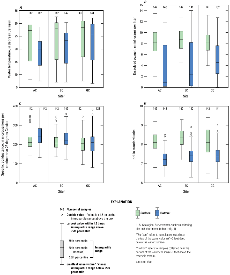
Water-column variability of physicochemical properties in near-surface and near-bottom samples of A, water temperature; B, dissolved oxygen; C, specific conductance; and D, pH measured in samples collected at Lake Conroe sites AC, EC, and GC, near Conroe, Texas, 1974–2021.
Water temperature seasonal summary statistics are reported in tables 7, 10, and 13, and seasonal water temperature variability is depicted in figure 6A–C. Monthly depth profiles of water temperature are depicted in figure 7. Water temperatures were warmest in July and August and coldest in January in both depth intervals at all three sites. During winter, water was nearly isothermal at all sites, indicating that the water was well-mixed throughout the reservoir at that time. The variability between near-surface and near-bottom water temperatures during spring and summer at sites AC and EC was greater than the variability in temperature with depth at site GC. Small differences in the water temperature measured near the surface and reservoir bottom were observed during winter, spring, and summer at the shallow site (site GC). Surface-water warming began in spring, which created density differences within the water column that resulted in the development of a gradual vertical temperature gradient at sites AC and EC (fig. 7A–B). The temperature gradient steepened in summer, and water temperatures decreased abruptly at approximately 30 ft below the water surface, where a well-defined thermocline developed at site AC and sometimes at site EC. The water temperature data available indicate that thermal stratification begins in Lake Conroe during spring, becomes established in summer, and is fully developed through at least the end of summer. Thermal stratification was limited to deeper parts (sites AC and EC) of the reservoir and typically originated downreservoir from site GC. Site GC did not exhibit patterns of thermal stratification because the water-column depths at this site are shallow enough and the wind forces strong enough to collectively allow water to mix from top to bottom. The water temperature (and consequently, density) therefore remained consistent throughout the water column.
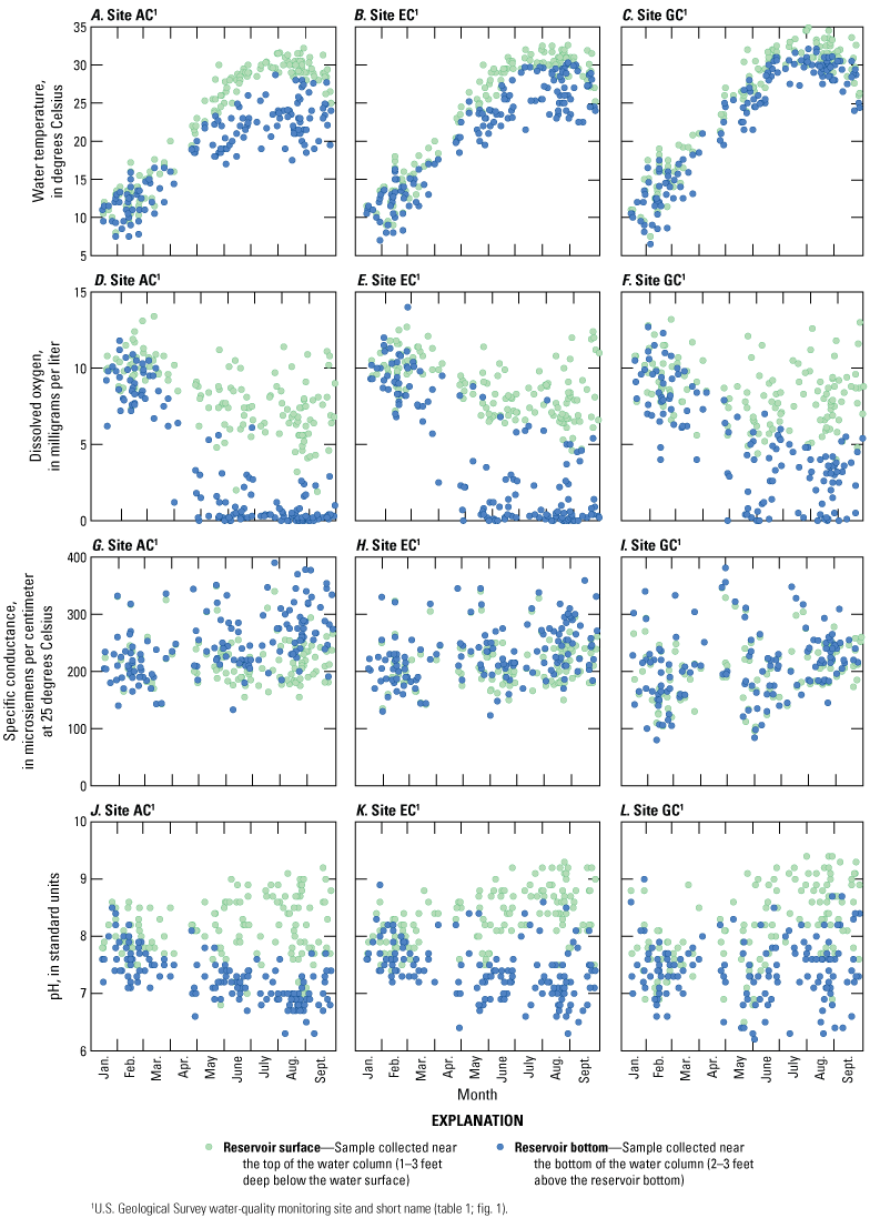
Seasonal variability of physicochemical properties in near-surface and near-bottom samples collected at Lake Conroe sites AC, EC, and GC near Conroe, Texas, 1993–2021. A–C, water temperature; D–F, dissolved oxygen; G–I, specific conductance; and J–L, pH.
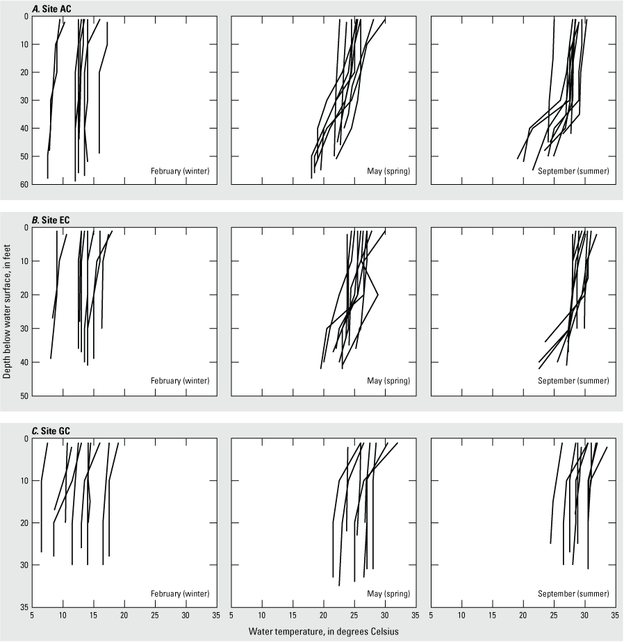
Selected depth profiles of water temperatures measured during February, May, and September at Lake Conroe sites A, AC; B, EC; and C, GC, near Conroe, Texas, 1974–2021.
The concentration of dissolved oxygen in a reservoir is affected by atmospheric pressure, ion activity, and temperature. Dissolved oxygen is produced by atmospheric aeration and algal photosynthesis and is consumed by chemical and biological reactions, like respiration, ammonia nitrification, and the decomposition of organic matter in the sediments and water column (Lewis, 2020). Dissolved oxygen is essential for the survival and growth of many aquatic organisms (Hem, 1985).
Summary statistics for dissolved-oxygen concentration are reported in table 4 and depicted in figure 5B. The dissolved-oxygen concentration of the reservoir water varied with depth and location. Dissolved-oxygen concentrations ranged from 0.1 to 13.4 mg/L at site AC, 0.1 to 14.0 mg/L at site EC, and 0.1 to 13.2 mg/L at site GC. Near the water surface, dissolved-oxygen concentrations ranged from 1.9 to 13.4 mg/L. Concentrations near the reservoir bottom ranged from 0.1 to 14.0 mg/L. The median dissolved-oxygen concentration was greater near the surface (8.4 mg/L) than near the bottom (3.0 mg/L). Sites AC and EC showed greater variability between near-surface and near-bottom dissolved-oxygen concentrations compared to site GC. Near the surface, dissolved-oxygen concentrations were consistent among sites, with median concentrations ranging from 8.2 to 8.7 mg/L. Near the bottom, concentrations were lowest at site AC and highest at site GC, with median concentrations equaling 1.1 and 4.5 mg/L, respectively.
Seasonal summary statistics for dissolved-oxygen concentration are reported in tables 7, 10, and 13, and seasonal variability of dissolved oxygen is depicted in figure 6D–F. Monthly depth profiles of dissolved-oxygen concentrations are depicted in figure 8. Concentrations of dissolved oxygen followed a general seasonal pattern of lower concentrations in summer and higher concentrations in winter. Concentrations were lowest near the reservoir bottom, particularly during thermal stratification. The median concentration for all sites was 3.7 mg/L in summer and 9.9 mg/L in winter. Dissolved-oxygen concentration tended to decrease as water temperature increased. Seasonal variability was lower at site GC than at sites AC and EC, especially in spring and summer. During summer, the median dissolved-oxygen concentration at site AC was 2.9 mg/L, whereas during winter, when circulation tends to increase in the reservoir, the median dissolved-oxygen concentration was 9.7 mg/L. The median concentration at site EC was 5.9 mg/L in summer and 10 mg/L in winter, and the median concentration at site GC was 5.2 mg/L in summer and 9.1 mg/L in winter.
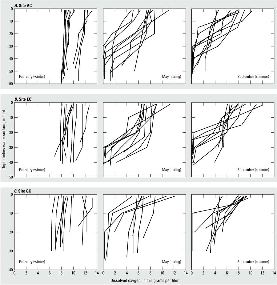
Selected depth profiles of dissolved-oxygen concentrations measured in February, May, and September at Lake Conroe sites A, AC; B, EC; and C, GC, near Conroe, Texas, 1974–2021.
Sites that exhibited seasonal thermal stratification also exhibited decreasing dissolved-oxygen concentrations with depth (fig. 8). Dissolved oxygen primarily originates from air-water contact and photosynthesis, but the hypolimnion in Lake Conroe is isolated from the surface during thermal stratification, resulting in little reaeration from the atmosphere. The release of oxygen from photosynthesis in the relatively cold and dark hypolimnion is also minimal (Bolke, 1979). During winter, dissolved-oxygen concentrations remained fairly uniform with depth because of vertical water-column mixing and isothermal conditions (fig. 6). The onset of thermal stratification in spring reduced vertical mixing in the water column and resulted in the development of a gradual oxygen gradient, primarily at the two deepest sites, sites AC and EC. The lack of oxygen replenishment to the reservoir bottom resulted in decreased dissolved-oxygen concentrations below approximately 10 ft at sites AC and EC during spring and summer (fig. 8). When thermal stratification conditions existed, water became anoxic, with dissolved-oxygen concentrations less than 0.5 mg/L at depths greater than 30 ft (fig. 8), which coincides with depths at which pronounced temperature decreases also occurred (fig. 7). At site GC or during winter, the season when thermal stratification was not established, anoxia was rare because of vertical mixing, a process that facilitates continuous oxygen distribution in the water column.
Specific conductance is a measure of the ability of a substance to conduct an electric current and is proportional to the total concentration of dissolved solids within a waterbody (Hem, 1985). The weathering of minerals in near-surface soil or bedrock within the watershed typically acts as a source of dissolved ions. Periods of substantial drought or heavy precipitation can affect specific conductance values. Without inputs from precipitation and runoff during periods of drought in conjunction with losses of water by the process of evaporation, less water is available for dilution and ions remain and tend to accumulate in the reservoir, thereby increasing specific conductance. Specific conductance decreases in response to heavy precipitation because ion concentrations tend to be diluted by inflow contributions from storm runoff with low ion concentrations (Bouvy and others, 2003).
Specific conductance summary statistics are reported in table 4 and depicted in figure 5C. Specific conductance ranged from 126 to 390 microsiemens per centimeter at 25 °C (µS/cm at 25 °C) at site AC, 123 to 359 µS/cm at site EC, and 80 to 381 µS/cm at site GC. Specific conductance was generally higher near the bottom than near the water surface at all sites. Variability between near-surface and near-bottom median specific conductance values was greater at site AC than at sites EC and GC. Specific conductance generally increased downreservoir.
Seasonal summary statistics for specific conductance are reported in tables 7, 10, and 13, and seasonal variability of specific conductance is depicted in figure 6G–I. Monthly depth profiles of specific conductance are depicted in figure 9. During spring and summer, specific conductance generally increases with depth at sites AC and EC, whereas specific conductance remains fairly consistent throughout the water column at site GC. During winter, variability in specific conductance is minimal throughout the water column at all sites. Specific conductance did not exhibit the strong thermal-stratification patterns observed in the water temperature or dissolved-oxygen profiles. During summer, changes in specific conductance values associated with thermal stratification were the most well-defined at site AC, with a pronounced increase at about the same depth where there was a pronounced decrease in temperature. The higher specific conductance values measured near the bottom during periods of thermal stratification may be attributed to the release of carbon dioxide (a result of decomposed organic matter), which dissolves in water to form carbonate ions, increasing the ion concentration and specific conductance (Elçi, 2008). At site GC, specific conductance remained relatively uniform with depth during winter, spring, and summer, because thermal-stratification development was minimal at that site.
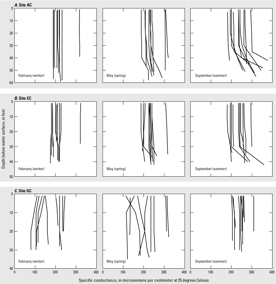
Selected depth profiles of specific conductance measured in February, May, and September at Lake Conroe sites A, AC; B, EC; and C, GC, near Conroe, Texas, 1974–2021.
The pH is a measure of how acidic or basic water is; acids are classified with a pH value between 0 and 7, bases are classified with a pH value between 7 and 14, and a pH value of 7 is considered neutral (Hem, 1985). Precipitation, geology, biological processes, land use, and human activities can affect the pH of water in a reservoir (EPA, 2023b). The pH of a waterbody is widely used as an indicator of water quality because it affects the solubility of metal hydroxides, oxidation-reduction reactions, and nutrient availability (Stumm and Morgan, 1996; Saalidong and others, 2022).
Summary statistics for pH are reported in table 4 and depicted in figure 5D. Values for pH ranged from 6.3 to 9.2 at site AC, 6.3 to 9.3 at site EC, and 6.2 to 9.4 at site GC. The median pH value near the surface was 8.2 and ranged from 6.5 to 9.4. The median pH near the reservoir bottom was 7.3 and ranged from 6.2 to 9.0. The pH measured near the surface was always higher than pH measured near the bottom. Higher pH values measured near the surface, compared to near the reservoir bottom, are expected as a result of variations in light penetration throughout the water column. Increased light penetration near the surface promotes photosynthetic activity, which removes carbon dioxide and increases pH levels (Soler-López and others, 2022).
Seasonal summary statistics for pH values are reported in tables 7, 10, and 13, and seasonal variability of pH is depicted in figure 6J–L. Monthly depth profiles of pH values are depicted in figure 10. Seasonal variability of pH depended on the site and depth interval of the measurement. At the two deepest sites, AC and EC, values of pH measured near the reservoir bottom were slightly higher in winter than in summer. Values of pH at site GC were generally more variable than at sites AC and EC throughout the three seasons when water-quality data were collected. Overall, pH values measured near the surface were higher during summer than winter, which may be a result of increased algal productivity during summer. During winter, pH values were nearly uniform with depth at all sites. During summer, pH values decreased consistently with depth at all three sites (fig. 10).
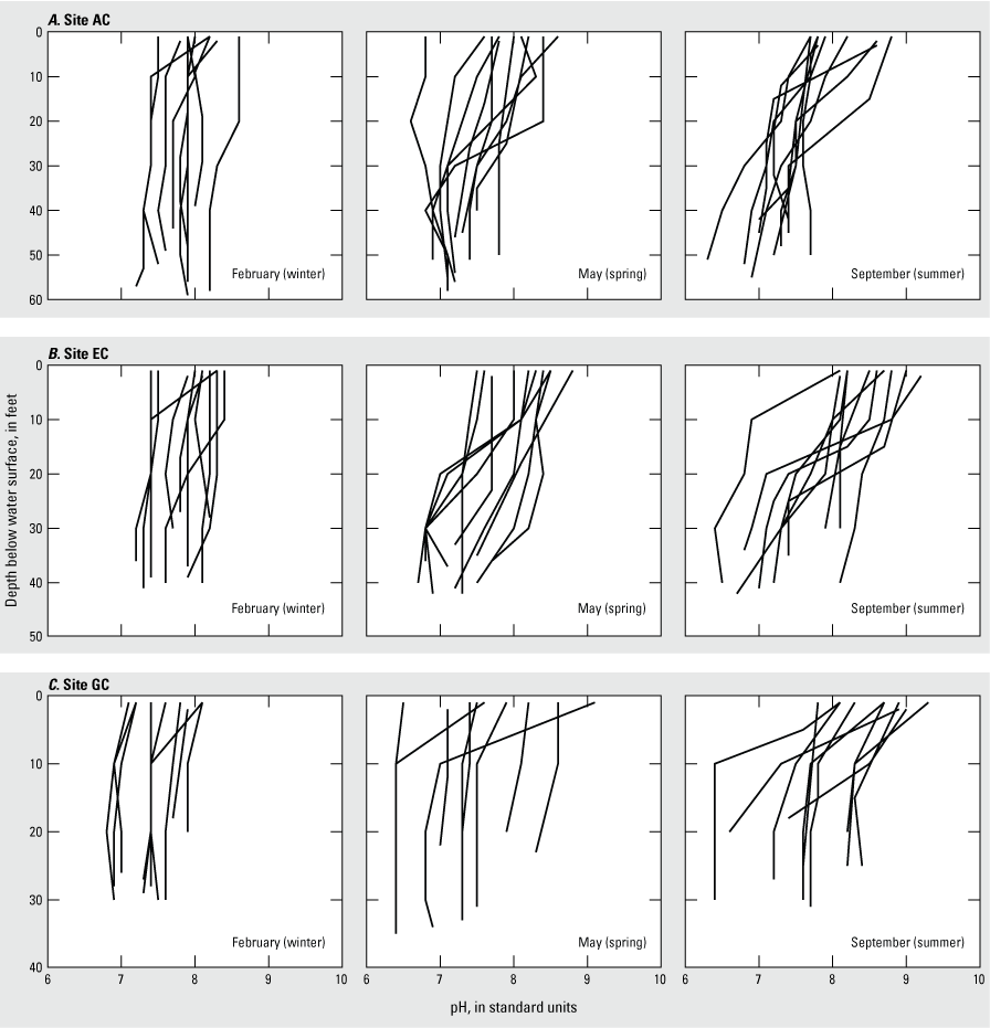
Selected depth profiles of measured pH in February, May, and September at Lake Conroe sites A, AC; B, EC; and C, GC, near Conroe, Texas, 1974–2021.
Water transparency and approximate sunlight penetration in bodies of water are measured by using a circular disk marked with black and white quadrants, called a Secchi disk. The measure used, Secchi-disk depth, is determined by lowering a Secchi disk into the water column and noting the depth at which the black and white quadrants are no longer visible (Preisendorfer, 1986). Secchi-disk depth is used to estimate the euphotic zone, which is the vertical portion of the water column where sufficient sunlight penetration is available to support the growth of aquatic vegetation such as algae. The relation between Secchi-disk depth and the depth of the euphotic zone varies considerably depending on the optical and chemical properties of the water. Summarizing the findings from several researchers that compiled data from numerous lakes, Golubkov and Golubkov (2024) reported the depth of the euphotic zone typically ranged from 1.7 times the Secchi-disk depth in colored lakes with high concentrations of dissolved organic matter to 2.4 times the Secchi-disk depth in clear lakes and 4.8 times the Secchi-disk depth in turbid lakes.
Water transparency decreases when concentrations of suspended particles and algae increase. Natural and anthropogenic sources, such as particle resuspension of bottom sediments from wind and waves as well as agricultural and urban stormwater runoff can increase suspended-particle concentrations. Secchi-disk depth measurements are a useful indicator of reservoir productivity. Eutrophic reservoirs are highly productive and nutrient-rich and typically are characterized by shallower Secchi-disk depths and thus decreased water transparency, compared to less productive oligotrophic reservoirs that are nutrient-poor (Green and others, 1996). The high nutrient concentrations in eutrophic lakes can lead to an overabundance of organic matter that subsequently dies and decays, causing dissolved-oxygen levels to decline to levels that will not support aquatic life (Chislock and others, 2013).
Summary statistics for Secchi-disk depth (and thus water transparency) are reported in table 4 and depicted in figure 11A. Secchi-disk depths measured in Lake Conroe ranged from 0.33 to 8.2 ft. Median Secchi-disk depths ranged from 1.6 ft at site GC to 3.2 ft at site AC. Water transparency was generally highest near the dam at site AC and the lowest upreservoir at site GC. The shallower Secchi-disk depths, and therefore, reduced water transparency, measured at site GC compared to sites AC and EC, may be attributed to its proximity to the reservoir inflows. At site GC, water still contains a high concentration of suspended particles. As water moves downreservoir toward sites EC and AC, reduced velocities and longer residence times promote the settling of suspended particles, increasing water transparency as the distance from the upstream end of the reservoir increases (Strand and Pemberton, 1982). Douglas and Rippey (2000) suggested wind and wave action are the primary drivers of sediment resuspension, particularly in shallow reservoirs or shallower areas (10−12 ft deep). Wind- and wave-driven sediment resuspension may also contribute to the relatively low water transparency at site GC.
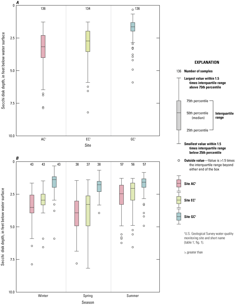
Secchi-disk depth measurements at sites AC, EC, and GC, depicting A, overall water-column variability by site; and B, seasonal variability by site, Lake Conroe near Conroe, Texas, 1974–2021.
Seasonal summary statistics for Secchi-disk depth are reported in tables 7, 10, and 13, and depicted in fig. 11B. Water transparency at the two deepest sites, sites AC and EC, was greatest during winter and spring and the least during summer. Water transparency at the shallowest site (site GC) remained consistent throughout the three seasons when water-quality data were collected. Seasonal variations in water transparency can be driven by vertical mixing (Hudson and Kirschner, 1997). During winter, the layers formed during thermal stratification that are resistant to wind mixing are dissipated, and the water at sites AC and EC becomes unstratified. This allows wind mixing forces to mix the entire water volume in the reservoir. Clear water from deeper in the reservoir is brought to the surface through the process of upwelling, which results in improved water transparency at sites AC and EC (Naranjo and others, 2022).
Major Ions and Water Hardness
Major ions occur naturally in water, although elevated concentrations can indicate anthropogenic inputs (Lewis and others, 2007). Summary statistics for major-ion concentrations are reported in table 5 and depicted in figs. 12 and 13. Calcium and chloride were the cation and anion, respectively, with the highest median concentrations at sites AC, EC, and GC. Water-column variability at each site was different for each major ion. Additionally, the water-column variability of major-ion concentrations depended on which site was described. For example, at site AC, the difference in median calcium concentration between the near-surface and near-bottom was 3 mg/L, whereas at site GC, there was no difference in median calcium concentrations between depths. Apart from sulfate, concentrations of major ions near the reservoir bottom were generally comparable to or higher than concentrations measured near the surface. Variability between the near-surface and near-bottom concentrations of potassium, sodium, and chloride was greater at site GC relative to sites AC and EC. Maximum concentrations of chloride, sulfate, and silica tended to be slightly higher upreservoir and lower near the dam. Higher maximum concentrations for some major ions upreservoir relative to downreservoir were measured for several reasons. Additional inflows from upstream sources can dilute ion concentrations as water moves downreservoir toward the Lake Conroe dam. Moreover, as water evaporates, ions remain in solution and increase in concentration over time. In the shallow, upreservoir part of Lake Conroe, a greater proportion of water is exposed to the atmosphere compared to the deeper areas of the reservoir. Water also warms faster at shallower depths (site GC) than at deeper depths (sites AC and EC) in the reservoir, likely promoting faster evaporation rates (Friedrich and others, 2018). Median concentrations of magnesium (2.0–2.3 mg/L), sodium (12–13 mg/L), potassium (3.1–3.3 mg/L), chloride (19–21 mg/L), and fluoride (0.11–0.12 mg/L) were consistent among all sites and depth intervals in Lake Conroe.
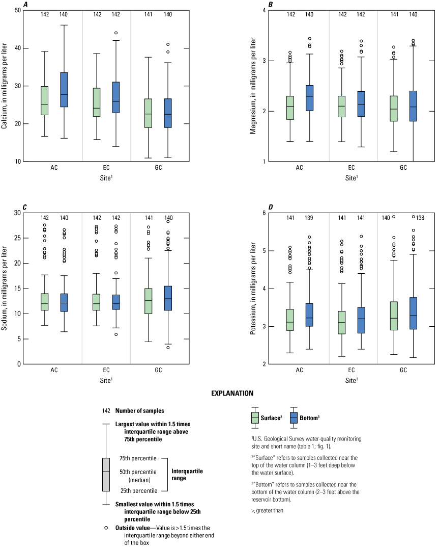
Water-column variability for concentrations of A, calcium; B, magnesium; C, sodium; and D, potassium measured in samples collected at Lake Conroe sites AC, EC, and GC, near Conroe, Texas, 1974–2021.
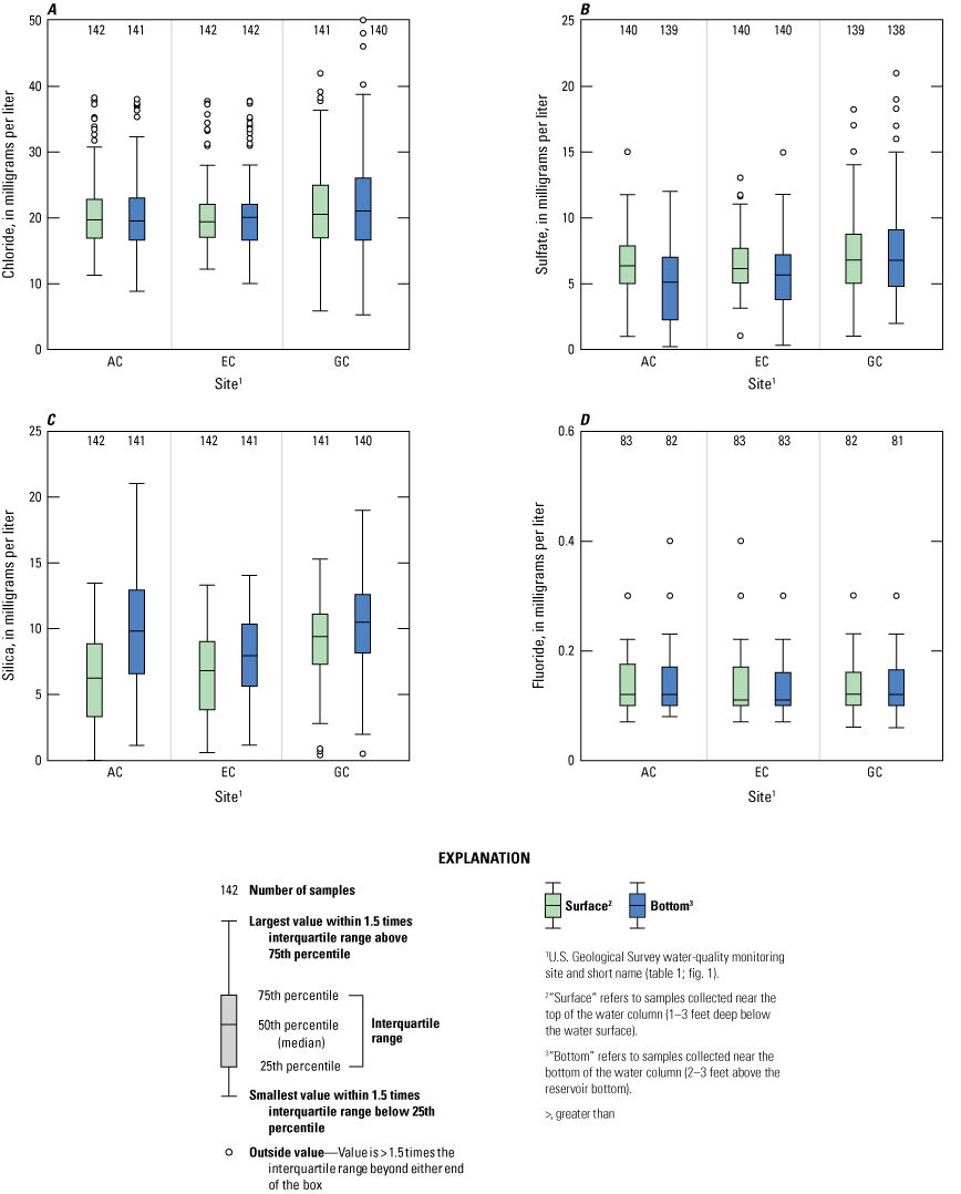
Water-column variability for concentrations of A, chloride; B, sulfate; C, silica; and D, fluoride concentrations measured in samples collected at Lake Conroe sites AC, EC, and GC, near Conroe, Texas, 1974–2021.
Seasonal summary statistics for major-ion concentrations are reported in tables 8, 11, and 14, and depicted in figures 14 and 15. Major-ion concentrations exhibited minimal seasonal variability between near-surface and near-bottom samples and among sites. Most of the measured concentrations of major ions, including calcium, magnesium, sodium, potassium, chloride, and fluoride, were fairly consistent throughout the three seasons when water-quality data were collected in both near-surface and near-bottom samples. Silica concentrations were the lowest in winter and increased throughout spring and summer, with peak concentrations in summer at sites AC and EC.
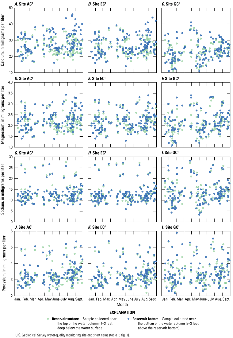
Monthly variability of selected major-ion concentrations measured in near-surface and near-bottom water samples collected at Lake Conroe sites AC, EC, and GC, near Conroe, Texas, 1974–2021. A–C, calcium; D–F, magnesium; G–I, sodium; and J–L, potassium.
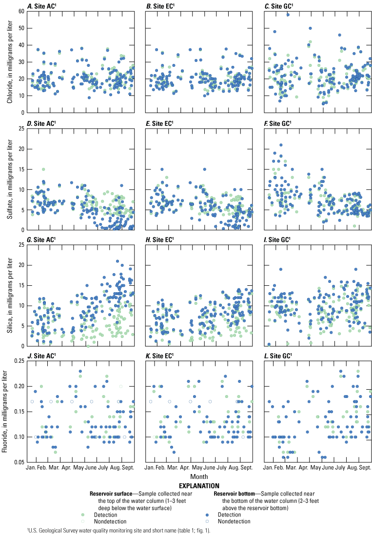
Monthly variability of selected major-ion concentrations measured in near-surface and near-bottom water samples collected at Lake Conroe sampling sites AC, EC, and GC, near Conroe, Texas, 1974–2021. A–C, chloride; D–F, sulfate; G–I, silica; and J–L, fluoride.
Unlike the other major ions that demonstrated a pattern of increasing concentrations or no discernable pattern between winter and summer, sulfate concentrations were generally highest during winter and lowest during summer for both depths at all sites. For example, at site AC, the median sulfate concentrations during winter near the surface and bottom were 6.7 and 6.8 mg/L, respectively. During summer, the median near-surface sulfate concentration at site AC was 5.2 mg/L, whereas the median near-bottom sulfate concentration was 1.9 mg/L. Sulfate concentrations at site GC followed a similar seasonal pattern of higher concentrations in winter than summer, but there was little variability between near-surface and near-bottom concentrations during summer. The decreasing sulfate concentrations with depth observed during summer at site AC and sometimes at site EC are likely related to reducing conditions in the hypolimnion during pronounced thermal stratification. Under anoxic conditions in the hypolimnion, sulfate ions are reduced to sulfide ions, resulting in decreased sulfate concentrations (Varis and Somlyody, 1996). The minimal variability observed between near-surface and near-bottom sulfate concentrations during summer at site GC is likely due to the minimal thermal stratification at that site.
Water hardness is a measure of the concentration of polyvalent cations, primarily calcium and magnesium, in a waterbody (Rubenowitz-Lundin and Hiscock, 2013). Hardness is an indicator of water quality and an important consideration for municipal-water supply purposes because it can cause mineral deposits to build up in pipes and water heaters (Farah and Torell, 2019). Hardness is commonly related to the geology surrounding a waterbody. The erosion and weathering of calcium and magnesium rich geologic units can increase the hardness of reservoir water (Hem, 1985). Hardness concentrations as calcium carbonate (CaCO3) ranged from 46 to 128 mg/L at site AC, 40 to 120 mg/L at site EC, and 27 to 120 mg/L at site GC (table 5). These ranges are categorized as moderately hard water (USGS, 2018b). Hardness concentrations were generally slightly higher near the bottom than near the surface. The median hardness concentration was 68 mg/L near the surface and 72 mg/L near the bottom. Similar to calcium concentrations, water hardness increased in the downstream direction at the three sites within the reservoir. Seasonally, water hardness was lowest in winter and highest in summer (tables 8, 11, and 14). Hardness in winter ranged from 27 to 107 mg/L as CaCO3 and ranged from 49 to 128 mg/L as CaCO3 during summer.
Nutrients
Nutrients, such as nitrogen and phosphorous, are primary elements essential to the health and diversity of surface waters and aquatic organisms (EPA, 2023c). However, excessive concentrations of nutrients can accelerate eutrophication in a reservoir. This process can result in reduced oxygen concentrations, excessive and harmful algal growth, increased sediment accumulation rates, fish kills, and taste-and-odor problems (EPA, 2000b; Paerl and others, 2001). Nutrients in a reservoir can originate from natural sources, such as weathering of rocks and soils containing phosphorous minerals (National Oceanic and Atmospheric Administration, 2024), precipitation, decomposing organic matter, and reservoir bottom sediments (Varis and Somlyody, 1996; Murray and others, 2006), as well as anthropogenic sources that can be related to runoff from agricultural fertilizers and livestock (USGS, 2018c), wastewater effluents (Carey and Migliaccio, 2009), industrial wastes, urban runoff (Yang and Toor, 2018), and changes in land use (Hem 1985). Pathways for the introduction of nitrogen to a reservoir include urban stormwater runoff, wastewater releases, and discharge of nitrogen-rich groundwater from septic systems into a reservoir (Stoliker and others, 2016). Anoxic conditions at the reservoir bottom can induce phosphorous mobilization from the bottom sediments into the water column (Varis and Somlyody, 1996). The rate of internal phosphorous loading, which introduces nutrients from reservoir sediment into the water column, increases under anoxic conditions and tends to increase with prolonged thermal stratification (Mortimer, 1941; Kling and others, 2003). Anthropogenic inputs of phosphorous into a reservoir include municipal sewage, wastewater, fertilizers, detergents, and agricultural drainage (Hem 1985; Olem and Flock, 1990). Phosphorous affects biological productivity and is most often the nutrient that controls the density of algae in the water column and reservoir productivity (Addy and Green, 1996). In high concentrations, phosphorous stimulates algal productivity, which can result in algal blooms.
Nutrient concentrations analyzed in discrete samples collected from Lake Conroe during 1993–2021 include filtered ammonia as nitrogen (hereinafter referred to as “ammonia”), filtered ammonia plus organic nitrogen as nitrogen (hereinafter referred to as “ammonia plus organic nitrogen”), filtered phosphorous (hereinafter referred to as “phosphorous”), filtered orthophosphate as phosphorous (hereinafter referred to as “orthophosphate”), filtered nitrite as nitrogen (hereinafter referred to as “nitrite”), and total nitrate plus nitrite as nitrogen (hereinafter referred to as “nitrate plus nitrite”). Summary statistics for nutrient concentrations are reported in table 6. Ammonia plus organic nitrogen, phosphorous, orthophosphate, and nitrate plus nitrite concentrations are depicted in figure 16. Nutrient concentrations were typically higher near the bottom than near the surface, particularly in the samples collected at sites AC and EC. Nutrient concentrations near the bottom generally exhibited more variability at sites AC and EC than at site GC. Median nutrient concentrations were generally similar in near-surface samples collected at all sites.
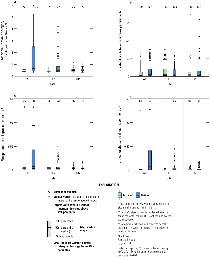
Water-column variability of selected nutrient concentrations measured in near-surface and near-bottom water samples collected from Lake Conroe sites AC, EC, and GC, near Conroe, Texas. A, ammonia plus organic nitrogen; B, nitrate plus nitrite; C, phosphorous; and D, orthophosphate.
Ammonia concentrations generally increased from upreservoir (site GC) to near the dam (site AC). Concentrations ranged from <0.01 to 5.1 mg/L in the samples collected at site AC, <0.01 to 3.2 mg/L at site EC, and <0.01 to 0.28 mg/L at site GC (table 6). The near-surface median ammonia concentration was <0.01 mg/L at all sites. The near-bottom median ammonia concentration was 0.39 mg/L at site AC, 0.08 mg/L at site EC, and 0.03 mg/L at site GC. Variability between near-surface and near-bottom ammonia concentrations was greater at sites AC and EC than at site GC.
Concentrations of ammonia plus organic nitrogen increased downreservoir. Concentrations ranged from 0.30 to 5.9 mg/L at site AC, 0.29 to 4.2 mg/L at site EC, and 0.30 to 1.1 mg/L at site GC (fig. 16A, table 6). Ammonia plus organic nitrogen concentrations were generally higher in near-bottom samples than near the surface, especially at sites AC and EC. The near-bottom median concentration was 0.62 mg/L at site AC, 0.48 mg/L at site EC, and 0.51 mg/L at site GC. The near-surface median ammonia plus organic nitrogen concentration was 0.40 mg/L at site AC, 0.42 mg/L at site EC, and 0.49 mg/L at site GC. Variability between near-surface and near-bottom ammonia plus organic nitrogen concentrations was greater at sites AC and EC than at site GC.
Concentrations of phosphorous ranged from <0.01 to 1.33 mg/L at site AC, <0.01 to 0.50 mg/L at site EC, and <0.01 to 0.20 mg/L at site GC (fig. 16C, table 6). Concentrations of phosphorous near the reservoir bottom were generally higher near the dam at site AC at a median concentration of 0.08 mg/L, relative to the midreservoir site EC (0.01 mg/L) and upreservoir site GC (0.03 mg/L). More than 80 percent of the phosphorous concentrations measured in the samples collected from sites AC and EC near the surface were less than the LRL of 0.01 mg/L. The median near-surface concentration at site GC was 0.02 mg/L.
Concentrations of orthophosphate ranged from <0.004 to 1.27 mg/L at site AC, <0.004 to 0.450 mg/L at site EC, and <0.004 to 0.190 mg/L at site GC (fig. 16D, table 6). The near-bottom median orthophosphate concentration was 0.085 mg/L at site AC, 0.009 mg/L at site EC, and 0.015 mg/L at site GC. The near-surface median orthophosphate concentration was 0.005 mg/L at site AC, <0.004 mg/L at site EC, and 0.008 mg/L at site GC. Variability between near-surface and near-bottom orthophosphate concentrations was higher at site AC relative to sites EC and GC.
Concentrations of nitrite ranged from <0.001 to 0.170 mg/L at site AC, <0.001 to 0.049 mg/L at site EC, and <0.001 to 0.030 mg/L at site GC (table 6). Median nitrite concentrations were <0.001 mg/L at all sites and depth intervals, except for the samples collected near the bottom at site AC where the median concentration was 0.002 mg/L. Variability between near-surface and near-bottom nitrite concentrations was greater at sites AC and EC relative to site GC.
Concentrations of nitrate plus nitrite ranged from <0.02 to 0.30 mg/L at site AC, <0.02 to 0.30 mg/L at site EC, and <0.02 to 0.69 mg/L at site GC (fig. 16B, table 6). Median nitrate plus nitrite concentrations varied minimally between the three sites and two depth intervals. The near-bottom median nitrate plus nitrite concentration was 0.04 mg/L site AC and 0.03 mg/L at sites EC and GC. The near-surface median nitrate plus nitrite concentration was 0.03 mg/L at site AC and 0.02 mg/L at sites EC and GC.
Seasonal summary statistics for nutrient concentrations are reported in tables 9, 12, and 15, and depicted in figure 17. Seasonal variability in nutrient concentrations were observed within the water column and among sites. During winter, nutrient concentrations remained similar with depth and across the reservoir. In summer, most nutrient concentrations were highest near the reservoir bottom, particularly at deep sites AC and EC. In shallow areas (site GC), nutrient concentrations were generally uniform in the water column throughout the three seasons when water-quality data were collected aside from some elevated concentrations of ammonia plus organic nitrogen in summer.
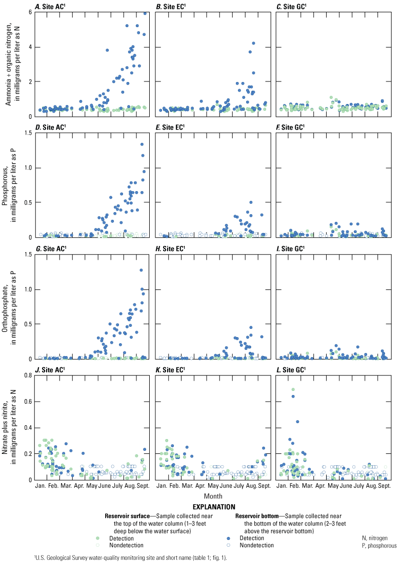
Monthly variability of selected nutrient concentrations in near-surface and near-bottom samples collected from Lake Conroe sites AC, EC, and GC, near Conroe, Texas. A–C, ammonia plus organic nitrogen; D–F, phosphorous; G–I, orthophosphate, 1993–2021; and for J–L, nitrate plus nitrite, 1974–2021.
Concentrations of ammonia were highest in summer near the reservoir bottom in deep areas, particularly at site AC. Near-bottom median concentrations of ammonia during summer were 2.40 mg/L at site AC (table 9), 0.36 mg/L at site EC (table 12), and 0.05 mg/L at site GC (table 15). Near-surface median ammonia concentrations during summer were <0.03 mg/L at all sites. During winter, there was less variability in ammonia concentrations within the water column and between sites relative to summer. Concentrations during winter were slightly higher near the bottom than near the surface at sites AC and EC.
Concentrations of ammonia plus organic nitrogen were highest in summer near the reservoir bottom, particularly at site AC. Near-bottom median concentrations of ammonia plus organic nitrogen during summer were 2.8 mg/L at site AC (table 9), 0.76 mg/L at site EC (table 12), and 0.52 mg/L at site GC (table 15). Near-surface median ammonia plus organic nitrogen concentrations in summer ranged from 0.42 to 0.50 mg/L. During winter, there was similar variability in ammonia plus organic nitrogen concentrations within the water column and between sites.
Concentrations of phosphorous were highest in summer near the reservoir bottom in deep areas, particularly at site AC. The near-bottom median concentration of phosphorous during summer was 0.49 mg/L at site AC (table 9), 0.04 mg/L at site EC (table 12), and 0.03 mg/L at site GC (table 15). Phosphorous concentrations during summer mostly were near or less than LRLs near the surface at sites AC and EC. The median near-surface concentration at GC during summer was 0.02 mg/L. During winter, there was minimal variability in phosphorous within the water column. Concentrations of phosphorous were generally higher at site GC than site AC during winter.
Concentrations of orthophosphate were highest in summer near the reservoir bottom in deep areas, particularly at site AC. The near-bottom median concentration of orthophosphate during summer was 0.470 mg/L at site AC (table 9), 0.018 mg/L at site EC (table 12), and 0.010 mg/L at site GC (table 15). The near-surface median orthophosphate concentration in summer ranged from 0.005 to 0.006 mg/L. Concentrations were generally higher at site GC than site AC during winter.
Median concentrations of nitrite during spring and summer near the surface at site AC and in summer near the bottom at sites EC and GC were less than the LRL of 0.001 mg/L (tables 9, 12, and 15). Median concentrations of nitrite were similar at all sites throughout the three seasons when water-quality data were collected. Median nitrite concentrations ranged from 0.002 to 0.004 mg/L during winter, <0.001 to 0.002 during spring, and <0.001 to 0.005 during summer. During winter, there was minimal variability between near-surface and near-bottom nitrite concentrations at all sites.
The seasonal pattern observed in the other nutrient species was not observed for nitrate plus nitrite. The highest concentrations of nitrate plus nitrite were observed in winter, where the maximum concentration was 0.30 mg/L for both depth intervals at sites AC and EC and was 0.69 and 0.64 mg/L near the surface and near the bottom, respectively, at site GC. During summer, concentrations were <0.20 mg/L near the surface and <0.25 mg/L near the bottom at all sites. Median concentrations of nitrate plus nitrite ranged from 0.06 to 0.12 mg/L during winter and 0.01 to 0.03 mg/L during spring (tables 9, 12, and 15). During winter, there was minimal variability observed between the near-surface and near-bottom concentrations.
Sites that exhibited summer thermal stratification also showed increasing concentrations for most nutrients with depth (fig. 17). The absence of vertical mixing during thermal stratification at sites AC and EC trapped nutrients released from decomposing organic matter and sediments under anoxic conditions in the hypolimnion. These release mechanisms contributed to the increased concentrations of ammonia, ammonia plus organic nitrogen, phosphorous, and orthophosphate measured in near-bottom samples collected from these sites. Nitrate and nitrite concentrations did not exhibit the same seasonal pattern as the other nutrient species described in this report and were generally higher in winter at all sites for both depth intervals (fig. 17). As nitrate and nitrite are typically produced by nitrification, a process that requires oxygen, it is expected for nitrate and nitrite concentrations to be lower in the oxygen-depleted hypolimnion during thermal stratification relative to well-mixed waters that contain higher concentrations of dissolved oxygen. Additionally, nitrate and nitrite are consumed by denitrification (a process that converts nitrate to nitrogen gas and does not occur for ammonia or phosphorous) under anoxic conditions, which ultimately decrease the nitrate and nitrite concentrations near the reservoir bottom during thermal stratification (Knowles, 1982). Nutrient concentrations (excluding nitrate plus nitrite) at shallower site GC remained consistent throughout the water column year-round, because in this shallow part of the reservoir there is relatively little thermal stratification (fig. 17).
Trace Metals
Reservoir processes, such as nutrient cycling, thermal stratification, deposition of particulate matter, and oxidation-reduction reactions, affect the concentrations of trace metals, particularly iron and manganese, within the water column and spatially within a reservoir (Nustad and Tatge, 2023). Geochemical conditions, including dissolved-oxygen concentrations and pH, can affect the solubility of iron and manganese in a reservoir (Gantzer and others, 2009). Iron and manganese, when present at high concentrations, can adversely affect aquatic wildlife by producing oxidative stress on a cellular level and damaging cell membranes and proteins, potentially leading to death (Linton and others, 2009; Sinha and others, 2009) and can otherwise affect water quality by altering taste, odor, and color (EPA, 2003). Natural sources of iron and manganese include weathering of soils, sediments, and rock in the watershed, as well as the dissolution of sediments containing trace metals near the sediment-water boundary (Zaw and Chiswell, 1999). Anthropogenic sources, such as industrial wastes, mining, roads, and vehicles, as well as commonly used items like paint and plastics, contribute to trace metal concentrations in a reservoir (EPA, 2003).
Summary statistics for trace metal concentrations are reported in table 6. The trace metals analyzed in the discrete samples collected from Lake Conroe include filtered iron and filtered manganese. Concentrations for iron ranged from <3.0 to 5,650 micrograms per liter (μg/L) at site AC, <3.0 to 2,400 µg/L at site EC, and <3.0 to 609 µg/L at site GC. Concentrations for manganese ranged from <0.20 to 8,400 µg/L at site AC, 0.27 to 5,950 µg/L at site EC, and 0.36 to 749 µg/L at site GC. Trace metal concentrations were generally higher in samples collected near the bottom than in the samples collected near the water surface. Near-surface iron concentrations ranged from <3.0 to 345 µg/L, whereas near-bottom iron concentrations ranged from 2.2 to 5,650 µg/L. Near-surface manganese concentrations ranged from <0.20 to 395 µg/L, whereas near-bottom concentrations ranged from 0.32 to 8,400 µg/L. The spatial pattern shows a slight increase in near-surface trace metal concentrations upreservoir, whereas near-bottom concentrations were substantially higher at site AC than at site GC. For example, the median manganese concentrations near the water surface at sites AC and EC were 1.2 and 1.4 µg/L, respectively, whereas the median concentration at site GC was 3.4 µg/L. The median manganese concentration near the bottom at site AC was 736 µg/L compared to median concentrations of 97 µg/L at site EC and 16 µg/L at site GC.
Seasonal summary statistics for trace metal concentrations are reported in tables 9, 12, and 15. To effectively visualize the wide range of iron and manganese concentrations, a logarithmic base-10 scale was applied to the y-axis of the seasonal plots in figure 18. Because the iron and manganese data span several orders of magnitude, applying a logarithmic base-10 scale to the data allows seasonal patterns and variations to be more discernible. By using the logarithmic scale, relative changes in concentration, particularly in the lower concentration range, are better visualized, as these concentrations may otherwise be obscured on a linear scale. Therefore, the seasonal summary statistics for trace metals reported in tables 9, 12, and 15 do not reflect the trace metals concentrations depicted in figure 18.

Monthly variability of iron and manganese concentrations measured in near-surface and near-bottom samples collected from Lake Conroe sites A, AC; B, EC; and C, GC, near Conroe, Texas, 1993–2021.
Trace metal concentrations followed similar seasonal patterns as nutrients (except for nitrate plus nitrite) (fig. 17). Concentrations varied seasonally (fig. 18) with depth in response to changes in thermal stratification that affect the vertical profile of dissolved-oxygen concentrations by limiting the mixing of waters from different layers in the reservoir. Low dissolved-oxygen concentrations in the hypolimnion during periods of pronounced thermal stratification often create reducing conditions that contribute to the release of soluble iron and manganese from bottom sediments into the water column (fig. 19) (Davison, 1993). During thermal stratification in summer at sites AC and EC, the highest trace metal concentrations generally were measured near the bottom. Variability between near-surface and near-bottom trace metal concentrations was also highest during thermal stratification in summer at sites AC and EC relative to site GC. For instance, during summer, the median iron concentration near the surface at site AC was 4.6 µg/L compared to 4.9 µg/L at site GC (tables 9, 15), whereas the median iron concentration near the bottom at site AC was 1,715 µg/L compared to 8.6 µg/L at site GC. A similar pattern of seasonal water-column variability was observed in manganese concentrations. Concentrations remained generally consistent in the water column during winter at all sites relative to summer concentrations. In Lake Conroe, elevated concentrations of iron (>500 µg/L; fig. 19A) and manganese (>1,000 µg/L; fig. 19B) corresponded with decreased concentrations of dissolved oxygen (<2.0 mg/L) near the reservoir bottom, particularly at sites AC and EC.
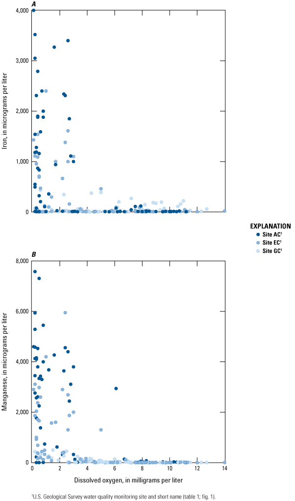
Concentrations of A, iron, and B, manganese as a function of dissolved-oxygen concentration measured in near-bottom samples collected from Lake Conroe sites AC, EC, and GC, near Conroe, Texas, 1993–2021.
Water-Quality Trends in Lake Conroe
Temporal trend test results, including estimated p-values, Kendall’s tau values, and Theil-Sen slope values, are summarized in tables 17–19. Annual temporal plots of selected data are shown to describe annual variability and the results of the trend test analysis. The Theil-Sen slope line is plotted on the temporal plots of physicochemical properties or constituents where a statistically significant trend was determined, indicating the estimated change in concentration over the trend analysis period. The overall change in concentration from the first year to the last year of a trend analysis period was calculated by multiplying the number of years in the trend analysis period of interest (47 years for the long-term trend analysis period and 28 years for the recent trend analysis period) by the Theil-Sen slope (tables 17–19).
Table 17.
Summary of long-term (1974–2021) and recent (1993–2021) trend results for physicochemical properties computed from discrete water-quality data collected from Lake Conroe.[Water-quality data include physicochemical properties collected at Lake Conroe sites AC, EC, and GC, near Conroe, Texas. °C, degree Celsius; Ia, long-term dataset with less than 5 percent censored data; mg/L, milligram per liter; µS/cm at 25 °C, microsiemens per centimeter at 25 °C; ft, foot; ns, not significant; <, less than; +, positive trend; (−), negative trend; --, insufficient data]
| Site short name (fig. 1) | Depth intervala | Data type | Long-term trend analysis period | Recent trend analysis period | ||||||
|---|---|---|---|---|---|---|---|---|---|---|
| p-value | Kendall's tau | Theil-Sen slope (unit/year) | Trend direction | p-value | Kendall's tau | Theil-Sen slope (unit/year) | Trend direction | |||
| AC | Surface | Ia | 0.01 | 0.149 | 0.029 | + | 0.62 | −0.045 | 0 | ns |
| AC | Bottom | Ia | <0.001 | 0.441b | 0.117 | + | 0.30 | 0.085 | 0.025 | ns |
| EC | Surface | Ia | 0.04 | 0.126 | 0.025 | + | 0.14 | −0.126 | −0.036 | ns |
| EC | Bottom | Ia | <0.001 | 0.394b | 0.102 | + | 0.88 | −0.020 | 0 | ns |
| GC | Surface | Ia | 0.005 | 0.166 | 0.051 | + | 0.59 | −0.058 | −0.014 | ns |
| GC | Bottom | Ia | <0.001 | 0.252b | 0.058 | + | 0.52 | −0.072 | −0.022 | ns |
| AC | Surface | Ia | <0.001 | 0.206 | 0.035 | + | 0.001 | 0.296b | 0.075 | + |
| AC | Bottom | Ia | <0.001 | 0.225 | 0.010 | + | 0.18 | −0.101 | −0.015 | ns |
| EC | Surface | Ia | 0.002 | 0.189 | 0.029 | + | 0.02 | 0.203 | 0.046 | + |
| EC | Bottom | Ia | <0.001 | 0.229 | 0.020 | + | 0.58 | −0.045 | −0.011 | ns |
| GC | Surface | Ia | 0.002 | 0.189 | 0.040 | + | 0.01 | 0.216 | 0.072 | + |
| GC | Bottom | Ia | <0.001 | 0.248 | 0.054 | + | 0.98 | −0.003 | 0 | ns |
| AC | Surface | Ia | 0.81 | 0.018 | 0.022 | ns | 0.001 | 0.276b | 1.91 | + |
| AC | Bottom | Ia | 0.14 | −0.088 | −0.385 | ns | 0.001 | 0.274b | 2.00 | + |
| EC | Surface | Ia | 0.99 | −0.001 | 0 | ns | 0.005 | 0.237b | 1.38 | + |
| EC | Bottom | Ia | 0.01 | −0.146 | −0.694 | (−) | 0.05 | 0.178 | 1.25 | + |
| GC | Surface | Ia | 0.68 | 0.025 | 0.067 | ns | 0.007 | 0.215 | 1.81 | + |
| GC | Bottom | Ia | 0.83 | −0.013 | 0 | ns | 0.02 | 0.186 | 1.86 | + |
| AC | Surface | Ia | 0.001 | 0.194 | 0.009 | + | 0.04 | 0.167 | 0.012 | + |
| AC | Bottom | Ia | <0.001 | 0.224 | 0.006 | + | 0.001 | 0.272b | 0.012 | + |
| EC | Surface | Ia | <0.001 | 0.223 | 0.010 | + | 0.57 | 0.058 | 0 | ns |
| EC | Bottom | Ia | <0.001 | 0.348b | 0.014 | + | 0.01 | 0.203 | 0.011 | + |
| GC | Surface | Ia | <0.001 | 0.300b | 0.018 | + | 0.07 | 0.145 | 0.014 | ns |
| GC | Bottom | Ia | <0.001 | 0.357b | 0.020 | + | 0.04 | 0.163 | 0.013 | + |
| AC | Surface | Ia | <0.001 | −0.320b | −0.044 | (−) | <0.001 | −0.307b | −0.051 | (−) |
| AC | Bottom | -- | -- | -- | -- | -- | -- | -- | -- | -- |
| EC | Surface | Ia | <0.001 | −0.351b | −0.041 | (−) | 0.003 | −0.252b | −0.033 | (−) |
| EC | Bottom | -- | -- | -- | -- | -- | -- | -- | -- | -- |
| GC | Surface | Ia | 0.01 | −0.149 | −0.010 | (−) | 0.54 | −0.058 | 0 | ns |
| GC | Bottom | -- | -- | -- | -- | -- | -- | -- | -- | -- |
Because sampling depths varied among sites and sampling events for the same site, the data were standardized to two sets of depth interval classifications: a “near-surface” interval that included the sample or measurement collected 1–3 ft below the water surface and a “near-bottom” interval that included the sample or measurement collected 2–3 ft above the reservoir bottom.
Table 18.
Summary of long-term (1974–2021) and recent (1993–2021) trend results for major ions and water hardness computed from discrete water-quality data collected from Lake Conroe.[Water-quality data include major ions and water hardness collected at Lake Conroe sites AC, EC, and GC, near Conroe, Texas. Ia, long-term dataset with less than 5 percent censored data; IIb, recent dataset with 5 to 80 percent censored data; ns, not significant; mg/L, milligram per liter; CaCO3, calcium carbonate; +, positive trend; <, less than; (−), negative trend; --, insufficient data]
| Site short name (fig. 1) | Depth intervala | Data type | Long-term trend analysis period | Recent trend analysis period | ||||||
|---|---|---|---|---|---|---|---|---|---|---|
| p-value | Kendall's tau | Theil-Sen slope (unit/year) | Trend direction | p-value | Kendall's tau | Theil-Sen slope (unit/year) | Trend direction | |||
| AC | Surface | Ia | 0.15 | −0.084 | −0.049 | ns | 0.01 | 0.223 | 0.164 | + |
| AC | Bottom | Ia | <0.001 | −0.223 | −0.136 | (−) | 0.02 | 0.210 | 0.150 | + |
| EC | Surface | Ia | 0.07 | −0.106 | −0.061 | ns | 0.03 | 0.185 | 0.133 | + |
| EC | Bottom | Ia | <0.001 | −0.223 | −0.143 | (−) | 0.12 | 0.124 | 0.081 | ns |
| GC | Surface | Ia | 0.50 | −0.039 | −0.018 | ns | 0.008 | 0.216 | 0.156 | + |
| GC | Bottom | Ia | 0.39 | −0.050 | −0.032 | ns | 0.02 | 0.198 | 0.157 | + |
| AC | Surface | Ia | 0.10 | −0.101 | −0.004 | ns | <0.001 | 0.339b | 0.017 | + |
| AC | Bottom | Ia | 0.003 | −0.178 | −0.009 | (−) | <0.001 | 0.328b | 0.020 | + |
| EC | Surface | Ia | 0.06 | −0.113 | −0.004 | ns | <0.001 | 0.293b | 0.013 | + |
| EC | Bottom | Ia | <0.001 | −0.207 | −0.009 | (−) | 0.002 | 0.269b | 0.015 | + |
| GC | Surface | Ia | 0.95 | 0.005 | 0 | ns | <0.001 | 0.289b | 0.018 | + |
| GC | Bottom | Ia | 0.81 | −0.015 | 0 | ns | 0.002 | 0.255b | 0.019 | + |
| AC | Surface | Ia | <0.001 | 0.314b | 0.016 | + | <0.001 | 0.510b | 0.044 | + |
| AC | Bottom | Ia | <0.001 | 0.267b | 0.014 | + | <0.001 | 0.580b | 0.047 | + |
| EC | Surface | Ia | <0.001 | 0.296b | 0.015 | + | <0.001 | 0.534b | 0.045 | + |
| EC | Bottom | Ia | <0.001 | 0.253b | 0.013 | + | <0.001 | 0.497b | 0.042 | + |
| GC | Surface | Ia | <0.001 | 0.212 | 0.014 | + | <0.001 | 0.445b | 0.041 | + |
| GC | Bottom | Ia | 0.002 | 0.183 | 0.014 | + | <0.001 | 0.368b | 0.037 | + |
| AC | Surface | Ia | 0.001 | 0.197 | 0.052 | + | <0.001 | 0.372b | 0.196 | + |
| AC | Bottom | Ia | 0.01 | 0.155 | 0.050 | + | <0.001 | 0.398b | 0.230 | + |
| EC | Surface | Ia | 0.009 | 0.160 | 0.038 | + | <0.001 | 0.349b | 0.173 | + |
| EC | Bottom | Ia | 0.01 | 0.156 | 0.042 | + | <0.001 | 0.352b | 0.188 | + |
| GC | Surface | Ia | 0.09 | 0.099 | 0.038 | ns | 0.002 | 0.259b | 0.179 | + |
| GC | Bottom | Ia | 0.35 | 0.056 | 0.025 | ns | 0.009 | 0.210 | 0.174 | + |
| AC | Surface | Ia | 0.79 | 0.023 | 0 | ns | <0.001 | 0.288b | 0.280 | + |
| AC | Bottom | Ia | 0.92 | 0.009 | 0 | ns | <0.001 | 0.289b | 0.292 | + |
| EC | Surface | Ia | 0.72 | −0.019 | 0 | ns | 0.001 | 0.261b | 0.244 | + |
| EC | Bottom | Ia | 0.93 | 0 | 0 | ns | <0.001 | 0.295b | 0.294 | + |
| GC | Surface | Ia | 0.52 | −0.036 | −0.028 | ns | 0.009 | 0.209 | 0.247 | + |
| GC | Bottom | Ia | 0.96 | −0.002 | 0 | ns | 0.005 | 0.225 | 0.283 | + |
| AC | Surface | Ia | 0.57 | −0.028 | −0.072 | ns | 0.37 | −0.063 | −0.021 | ns |
| AC | Bottom | Ia | 0.38 | −0.041 | −0.011 | ns | 0.64 | 0.057 | 0.007 | ns |
| EC | Surface | Ia | 0.67 | −0.020 | −0.005 | ns | 0.26 | −0.082 | −0.022 | ns |
| EC | Bottom | Ia | 0.36 | 0.056 | 0.016 | ns | 0.12 | 0.131 | 0.044 | ns |
| GC | Surface | Ia | 0.02 | −0.143 | −0.034 | (−) | 0.51 | −0.050 | −0.015 | ns |
| GC | Bottom | Ia | 0.11 | −0.099 | −0.025 | ns | 0.98 | 0 | −0.002 | ns |
| AC | Surface | Ia | <0.001 | 0.467 b | 0.150 | + | <0.001 | 0.401b | 0.207 | + |
| AC | Bottom | Ia | <0.001 | 0.331 b | 0.108 | + | <0.001 | 0.332b | 0.146 | + |
| EC | Surface | Ia | <0.001 | 0.471b | 0.147 | + | <0.001 | 0.406b | 0.186 | + |
| EC | Bottom | Ia | <0.001 | 0.303b | 0.090 | + | <0.001 | 0.308b | 0.133 | + |
| GC | Surface | Ia | <0.001 | 0.332b | 0.105 | + | 0.002 | 0.244 | 0.108 | + |
| GC | Bottom | Ia | 0.002 | 0.186 | 0.070 | + | 0.006 | 0.222 | 0.125 | + |
| AC | Surface | IIb | -- | -- | -- | -- | 0.01 | 0.190 | 0.010 | + |
| AC | Bottom | IIb | -- | -- | -- | -- | 0.02 | 0.180 | 0.013 | + |
| EC | Surface | IIb | -- | -- | -- | -- | 0.03 | 0.170 | 0.009 | + |
| EC | Bottom | IIb | -- | -- | -- | -- | 0.02 | 0.171 | 0.008 | + |
| GC | Surface | IIb | -- | -- | -- | -- | 0.43 | 0.060 | 0.004 | ns |
| GC | Bottom | IIb | -- | -- | -- | -- | 0.47 | 0.060 | 0.004 | ns |
| AC | Surface | Ia | 0.20 | −0.074 | −0.117 | ns | 0.005 | 0.238 | 0.489 | + |
| AC | Bottom | Ia | <0.001 | −0.207 | −0.372 | (−) | 0.005 | 0.239 | 0.472 | + |
| EC | Surface | Ia | 0.06 | −0.114 | −0.178 | ns | 0.01 | 0.201 | 0.443 | + |
| EC | Bottom | Ia | <0.001 | −0.237 | −0.418 | (−) | 0.09 | 0.156 | 0.303 | ns |
| GC | Surface | Ia | 0.64 | −0.026 | −0.048 | ns | 0.006 | 0.224 | 0.460 | + |
| GC | Bottom | Ia | 0.51 | −0.040 | −0.071 | ns | 0.01 | 0.210 | 0.515 | + |
Because sampling depths varied among sites and sampling events for the same site, the data were standardized to two sets of depth interval classifications: a “near-surface” interval that included the sample or measurement collected 1–3 ft below the water surface and a “near-bottom” interval that included the sample or measurement collected 2–3 ft above the reservoir bottom.
Table 19.
Summary of long-term (1974–2021) and recent (1993–2021) trend results for nutrients and trace metals computed from discrete water-quality data collected from Lake Conroe.[Water-quality data include nutrients and trace metals collected at Lake Conroe sites AC, EC, and GC, near Conroe, Texas. mg/L, milligram per liter; N, nitrogen; IIb, recent dataset with 5 to 80 percent censored data; B, slope not reported because censored values exceed 40 percent; ns, not significant; IIa, recent dataset with 5 to 80 percent censored data; IIc, recent dataset with more than 80 percent censored data; P, phosphorous; nt, no trend computation because left-censored values exceed 80 percent; Ib, long-term dataset with 5 to 80 percent censored data; µg/L, microgram per liter; ft, foot; --, insufficient data; (−), negative trend; +, positive trend; <, less than]
| Site short name (fig. 1) | Depth intervala | Data type | Long-term trend analysis period | Recent trend analysis period | ||||||
|---|---|---|---|---|---|---|---|---|---|---|
| p-value | Kendall's tau | Theil-Sen slope (unit/year) | Trend direction | p-value | Kendall's tau | Theil-Sen slope (unit/year) | Trend direction | |||
| AC | Surface | IIb | -- | -- | -- | -- | 0.06 | −0.128 | B | ns |
| AC | Bottom | IIb | -- | -- | -- | -- | 0.30 | −0.088 | −0.001 | ns |
| EC | Surface | IIb | -- | -- | -- | -- | 0.05 | −0.102 | B | (−) |
| EC | Bottom | IIb | -- | -- | -- | -- | 0.01 | −0.226 | −0.003 | (−) |
| GC | Surface | IIb | -- | -- | -- | -- | 0.03 | −0.145 | B | (−) |
| GC | Bottom | IIb | -- | -- | -- | -- | 0.21 | −0.100 | 0 | ns |
| AC | Surface | IIa | -- | -- | -- | -- | 0.01 | 0.215 | 0.003 | + |
| AC | Bottom | IIa | -- | -- | -- | -- | 0.98 | −0.003 | 0 | ns |
| EC | Surface | IIa | -- | -- | -- | -- | 0.02 | 0.189 | 0.002 | + |
| EC | Bottom | IIa | -- | -- | -- | -- | 0.18 | −0.098 | −0.030 | ns |
| GC | Surface | IIa | -- | -- | -- | -- | 0.01 | 0.238 | 0.003 | + |
| GC | Bottom | IIa | -- | -- | -- | -- | 0.10 | 0.140 | 0.002 | ns |
| AC | Surface | IIc | -- | -- | -- | -- | nt | nt | nt | nt |
| AC | Bottom | IIb | -- | -- | -- | -- | 0.16 | −0.042 | −0.001 | ns |
| EC | Surface | IIc | -- | -- | -- | -- | nt | nt | nt | nt |
| EC | Bottom | IIb | -- | -- | -- | -- | 0.02 | −0.146 | B | (−) |
| GC | Surface | IIb | -- | -- | -- | -- | 0.29 | −0.068 | B | ns |
| GC | Bottom | IIb | -- | -- | -- | -- | 0.35 | 0.066 | 0 | ns |
| AC | Surface | IIb | -- | -- | -- | -- | 0.11 | −0.068 | B | ns |
| AC | Bottom | IIb | -- | -- | -- | -- | 0.46 | −0.055 | 0 | ns |
| EC | Surface | IIb | -- | -- | -- | -- | 0.26 | −0.085 | B | ns |
| EC | Bottom | IIb | -- | -- | -- | -- | 0.06 | −0.125 | B | ns |
| GC | Surface | IIb | -- | -- | -- | -- | 0.20 | −0.090 | B | ns |
| GC | Bottom | IIb | -- | -- | -- | -- | 0.37 | 0.070 | 0 | ns |
| AC | Surface | IIb | -- | -- | -- | -- | 0.55 | −0.033 | B | ns |
| AC | Bottom | IIb | -- | -- | -- | -- | 1.0 | 0.001 | B | ns |
| EC | Surface | IIb | -- | -- | -- | -- | 0.34 | −0.046 | B | ns |
| EC | Bottom | IIb | -- | -- | -- | -- | 0.75 | 0.019 | B | ns |
| GC | Surface | IIb | -- | -- | -- | -- | 0.28 | −0.048 | B | ns |
| GC | Bottom | IIb | -- | -- | -- | -- | 0.07 | −0.096 | B | ns |
| AC | Surface | Ib | 0.13 | −0.063 | B | ns | 0.32 | −0.057 | B | ns |
| AC | Bottom | Ib | 0.21 | −0.053 | B | ns | 0.61 | −0.032 | B | ns |
| EC | Surface | Ib | 0.06 | −0.069 | B | ns | 0.27 | −0.057 | B | ns |
| EC | Bottom | Ib | 0.24 | −0.051 | B | ns | 0.56 | −0.037 | B | ns |
| GC | Surface | Ib | 0.28 | −0.039 | B | ns | 0.42 | −0.042 | B | ns |
| GC | Bottom | Ib | 0.48 | −0.028 | B | ns | 0.97 | 0.003 | B | ns |
| AC | Surface | IIb | -- | -- | -- | -- | 0.01 | −0.159 | B | (−) |
| AC | Bottom | IIb | -- | -- | -- | -- | 0.02 | −0.200 | −1.20 | (−) |
| EC | Surface | IIb | -- | -- | -- | -- | 0.89 | 0.011 | B | ns |
| EC | Bottom | IIb | -- | -- | -- | -- | 0.01 | −0.198 | −0.977 | (−) |
| GC | Surface | IIb | -- | -- | -- | -- | 0.24 | 0.090 | 0.254 | ns |
| GC | Bottom | IIb | -- | -- | -- | -- | 0.04 | 0.167 | 0.941 | (+) |
| AC | Surface | IIb | -- | -- | -- | -- | <0.001 | −0.287b | −0.088 | (−) |
| AC | Bottom | IIa | -- | -- | -- | -- | 0.28 | −0.094 | −0.174 | ns |
| EC | Surface | IIb | -- | -- | -- | -- | <0.001 | −0.361b | −0.121 | (−) |
| EC | Bottom | IIa | -- | -- | -- | -- | <0.001 | −0.341b | −1.43 | (−) |
| GC | Surface | IIb | -- | -- | -- | -- | 0.02 | −0.195 | −0.082 | (−) |
| GC | Bottom | IIa | -- | -- | -- | -- | 0.16 | −0.121 | −0.324 | ns |
Because sampling depths varied among sites and sampling events for the same site, the data were standardized to two sets of depth interval classifications: a “near-surface” interval that included the sample or measurement collected 1–3 ft below the water surface and a “near-bottom” interval that included the sample or measurement collected 2–3 ft above the reservoir bottom.
Physicochemical Properties
The SKT was applied to all sites and depth intervals to conduct a trend analysis of water temperature (table 16). In the long-term trend analysis period, the water temperature data indicated positive trends (all p-values ≤0.05) at all sites and depth intervals (fig. 20). Kendall’s tau values ranged from 0.126 to 0.166 for the near-surface water temperatures and from 0.252 to 0.452 for the near-bottom water temperatures (table 17). These trends represent a 1.2- to 2.4-°C increase in near-surface water temperature and a 2.7- to 5.5-°C increase in near-bottom water temperature over the long-term period. In the recent trend analysis period, the water temperature data indicated no trends (p-values >0.05) at any of the sites (fig. 21).
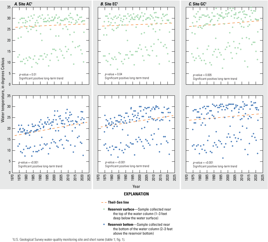
Annual variability and trend test results for water temperatures measured in conjunction with near-surface and near-bottom water sample collection at Lake Conroe sites A, AC; B, EC; and C, GC, near Conroe, Texas, for the long-term trend analysis period, 1974–2021.
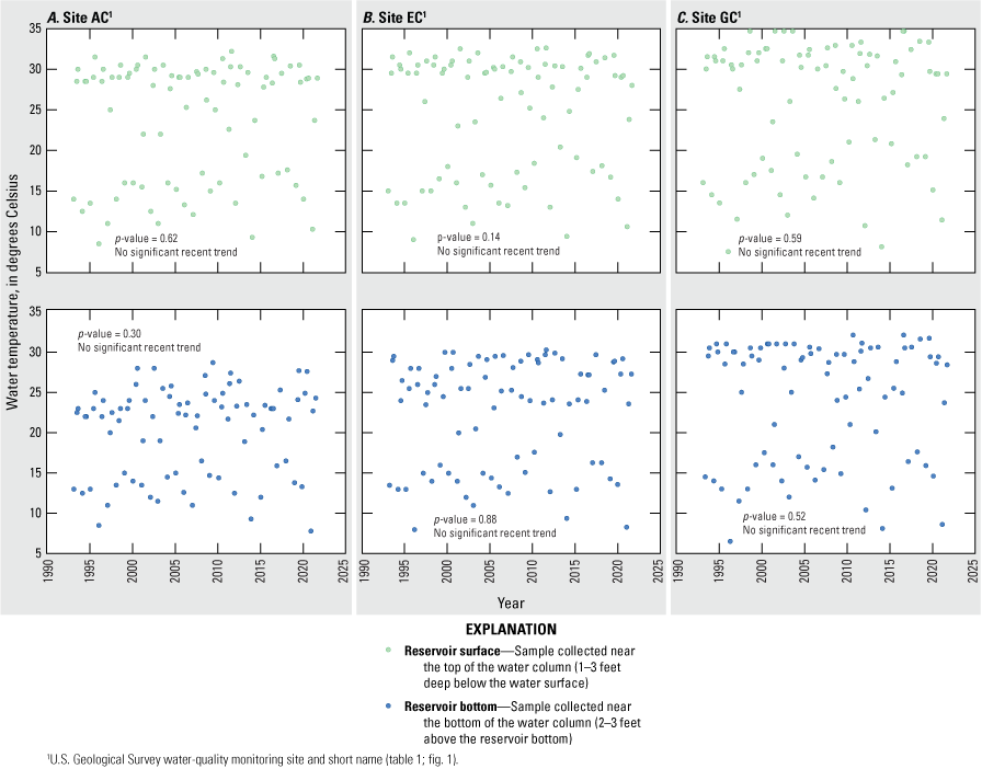
Annual variability and trend test results for water temperatures measured in conjunction with near-surface and near-bottom water sample collection at Lake Conroe sites A, AC; B, EC; and C, GC, near Conroe, Texas, for the recent trend analysis period, 1993–2021.
The positive trend in water temperature observed over the long-term period, followed by the absence of a significant trend in the recent period, may be attributed to a combination of sudden urbanization in the watershed and increases in air temperature (Gelca and others, 2014). Population growth in the watershed began to considerably increase in the mid-1970s (fig. 4), leading to substantial urban development, such as new construction and an increase in impervious surfaces (MRLC, 2023). Impervious surfaces are susceptible to absorbing and storing heat, which causes stormwater runoff to be warmer than runoff from natural landscapes (Roa-Espinosa and others, 2003; Simpson and Winston, 2022). The influx of this warmer stormwater runoff into Lake Conroe likely contributed to increasing water temperatures during the first two decades of the long-term period. For the recent period, the slopes for the water temperature data indicate smaller changes (table 17), and in some cases, no change, in water temperature per year relative to the long-term period. This stabilization could be a result of adaptations made in urban planning to mitigate heat island effects in the greater Houston area, such as planting trees to increase canopy cover, the installation of reflective roofing products on new and existing buildings, and repaving roads with reflective pavement (EPA, 2002). Additionally, the reservoir may have reached a thermal equilibrium in which the cumulative effects of urban heat and air temperature warming are balanced. Anthropogenic practices, such as increased urban vegetative cover (Gómez-Baggethun and Barton, 2013) and changes in water management practices that dissipate heat more effectively, and natural processes, such as increased evaporation rates and changes in reservoir inflow patterns (Hostetler, 1995), are all drivers for possible thermal equilibrium in the reservoir.
The SKT was applied to all sites and depth intervals to conduct a trend analysis of dissolved-oxygen concentration. During 1974–2021, positive trends in dissolved-oxygen concentration (p-values ≤0.05) were determined at all sites and depths (fig. 22). Kendall’s tau values ranged from 0.189 to 0.206 near the surface and from 0.225 to 0.248 near the bottom (table 17). These trends represent a 1.4- to 1.9-mg/L increase in near-surface dissolved-oxygen concentration and a 0.47- to 2.5-mg/L increase in near-bottom dissolved-oxygen concentration over the long-term period. For the recent period, positive trends in dissolved-oxygen concentration were computed at all surface sites (p-values ≤0.05), where Kendall’s tau values ranged from 0.203 to 0.296 (table 17), although no trends were observed near the reservoir bottom (fig. 23). These trends represent a 1.3- to 2.1-mg/L increase in dissolved-oxygen concentration over the recent period. In contrast with the expected decrease in dissolved-oxygen concentration with increasing water temperature, this relation between water temperature and dissolved-oxygen concentration was not observed in long-term dissolved-oxygen concentration trend results. Other factors besides temperature, such as precipitation, biological processes like photosynthesis, and organic material input, can also affect dissolved-oxygen concentrations within a waterbody (Wetzel and Likens, 2000).
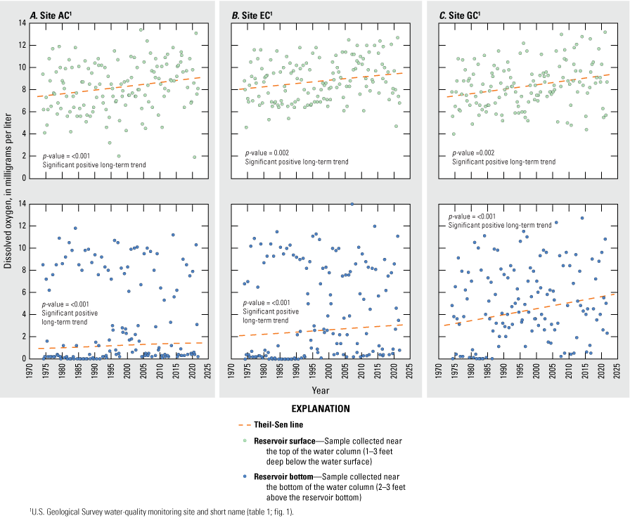
Annual variability and trend test results for dissolved-oxygen concentrations measured in conjunction with near-surface and near-bottom water sample collection at Lake Conroe sites A, AC; B EC; and C, GC, near Conroe, Texas, for the long-term trend analysis period, 1974–2021.
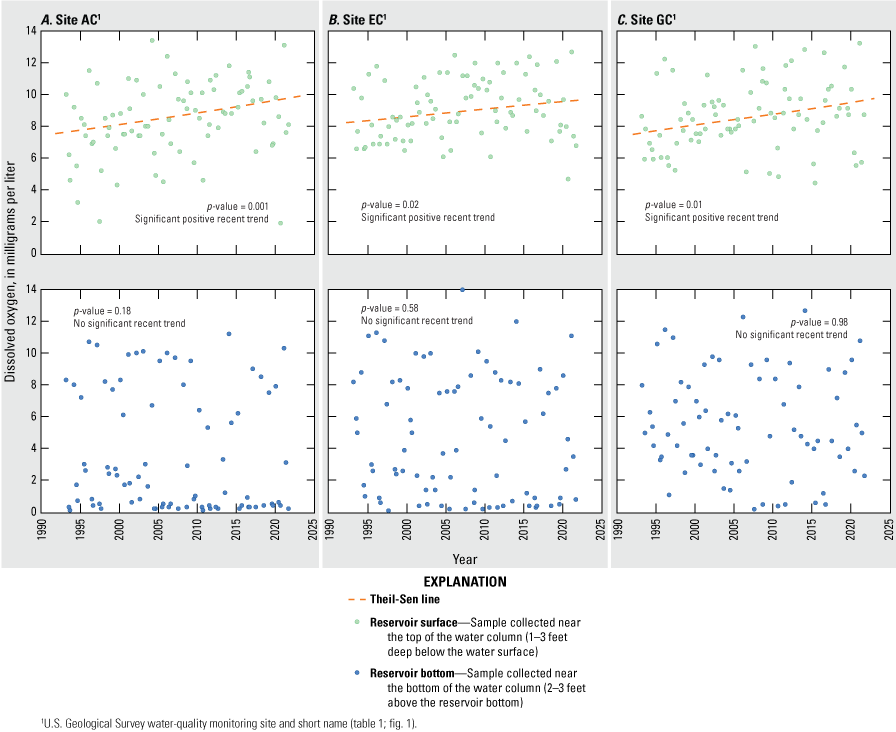
Annual variability and trend test results for dissolved-oxygen concentrations measured in conjunction with near-surface and near-bottom water sample collection at Lake Conroe sites A, AC; B, EC; and C, GC, near Conroe, Texas, for the recent trend analysis period, 1993–2021.
Specific conductance was categorized as data types Ia and IIa for all sites and depths during the long-term and recent trend analysis periods, respectively (table 16). In the long-term trend analysis period, the specific conductance data indicated a negative trend near the bottom at site EC (p-value ≤0.05; Kendall’s tau value −0.146), which represents a 33-µS/cm decrease between 1974 and 2021 (fig. 24). No other trends (p-values >0.05) were determined for specific conductance in the long-term period. During the recent trend analysis period, positive trends in specific conductance (p-values ≤0.05) were observed at all sites and depths (fig. 25). For the recent period, Kendall’s tau values ranged from 0.178 to 0.276 (table 17). These trends represent a 35- to 56-µS/cm increase over the recent period, with a median increase in specific conductance of 51 µS/cm.
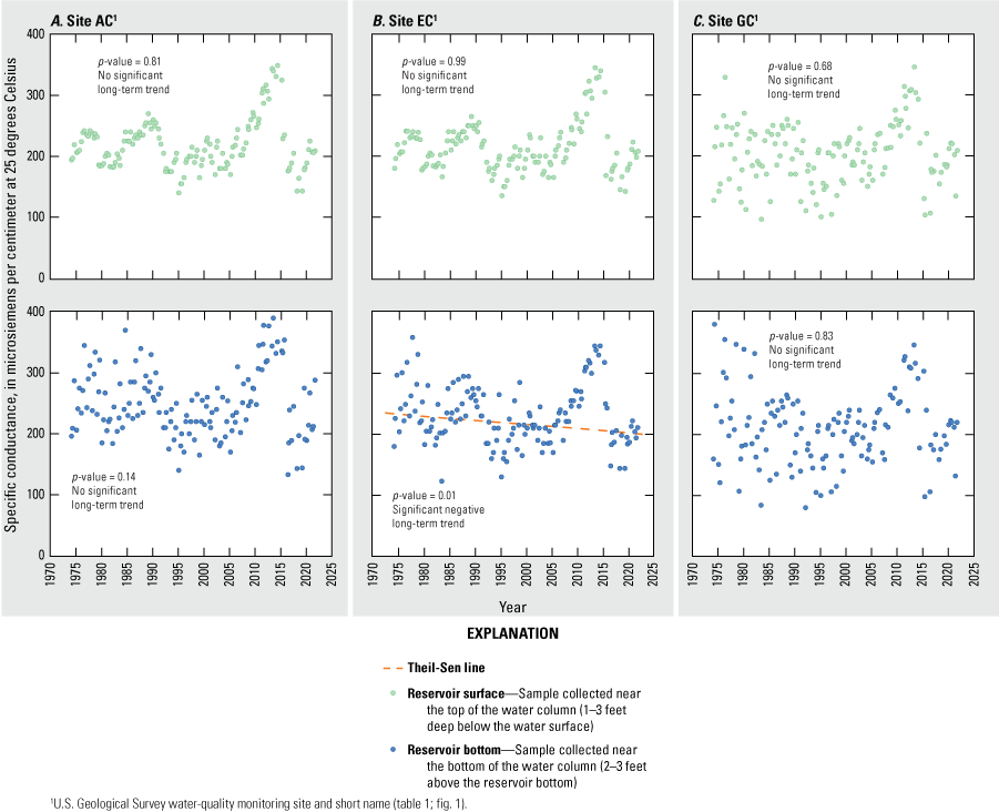
Annual variability and trend test results for specific conductance measured in conjunction with near-surface and near-bottom water sample collection at Lake Conroe sites A, AC; B, EC; and C, GC, near Conroe, Texas, for the long-term trend analysis period, 1974–2021.
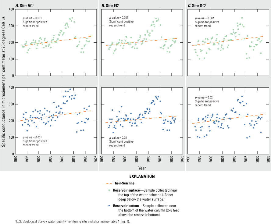
Annual variability and trend test results for specific conductance measured in conjunction with near-surface and near-bottom water sample collection at Lake Conroe sites A, AC; B, EC; and C, GC, near Conroe, Texas, for the recent trend analysis period, 1993–2021.
At all sites, low specific conductance values were typically measured during periods of high precipitation and reservoir storage, a pattern that could be attributed to increased dilution by runoff during storm events (figs. 2B, 24, 25). Relatively high specific conductance values were measured during periods of drought and decreased reservoir storage (figs. 2B, 24, 25). Periods of drought result in increased evaporation as well as decreased reservoir water levels and streamflow. Decreased streamflow could lead to decreased dilution of dissolved ions entering the reservoir through runoff (Sprague, 2005). As the water level in the reservoir lowers, the ions present become concentrated, which results in higher specific conductance values (Murdoch and others, 2000). The low reservoir storage during a drought in the early 2010s (fig. 2A, B) likely contributed to the elevated specific conductance values measured during that period and affected the trend analysis in the recent period. Positive trends in specific conductance could also be related to local patterns of population growth since 2000 (fig. 4) as well as increases in developed land and decreases in forested land.
Trends in pH were evaluated for all sites and depth intervals using the SKT. In the long-term record, positive trends in pH (p-values ≤0.05) were observed at all sites and depth intervals, where Kendall’s tau values ranged from 0.194 to 0.357 (fig. 26). For the long-term period, the pH near the surface has increased by a median value of 0.47 and the pH near the bottom has increased by a median value of 0.66, indicating that the reservoir has become more basic over time. Positive trends in pH (p-values ≤0.05; Kendall’s tau value range, 0.163–0.272, table 17) were observed near the bottom at all sites during the recent period and represent an increase of 0.31–0.36 in pH (fig. 27). A recent, positive trend was also determined near the surface at site AC (Kendall’s tau value 0.167, table 17) and represents an increase of 0.34. No trends in pH values measured near the surface were determined in the recent period at sites EC and GC. The long-term positive trends in water temperature (fig. 20) observed at all sites and depth intervals in Lake Conroe can result in greater productivity, thus increasing photosynthetic processes and pH levels. This is evidenced by the determination of long-term positive pH trends (fig. 26).
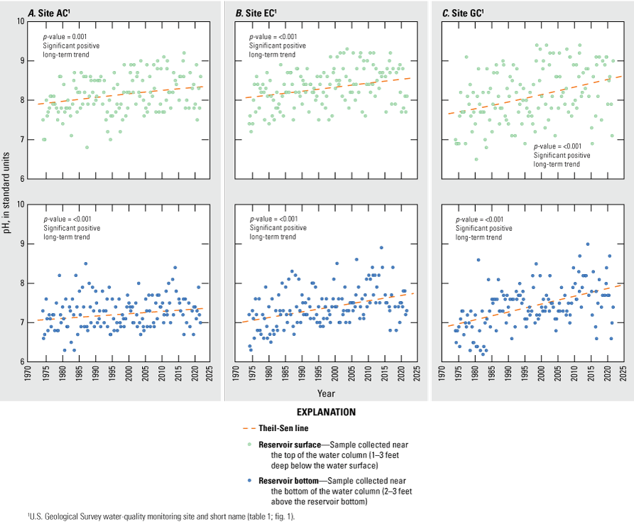
Annual variability and trend test results for pH measured in conjunction with near-surface and near-bottom water sample collection at Lake Conroe sites A, AC; B, EC; and C, GC, near Conroe, Texas, for the long-term trend analysis period, 1974–2021.
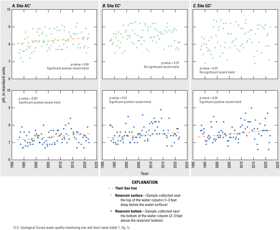
Annual variability and trend test results for pH measured in conjunction with near-surface and near-bottom water sample collection at Lake Conroe sites A, AC; B, EC; and C, GC, near Conroe, Texas, for the recent trend analysis period, 1993–2021.
The SKT was applied to the near-surface Secchi-disk measurements for both trend analysis periods. Secchi-disk depth exhibited negative trends (p-values ≤0.05) at all reservoir sites during the long-term period, indicating that water transparency worsened during 1974–2021 (fig. 28). The Secchi-disk depth data indicated a statistically strong negative trend at sites AC (Kendall’s tau value −0.320) and EC (Kendall’s tau value −0.351), whereas the negative trend identified at site GC was weaker (Kendall’s tau value −0.149). These trends represent a decrease in Secchi-disk depth of 2.1, 1.9, and 0.47 ft at sites AC, EC, and GC, respectively, over the long-term period. During the recent period, the Secchi-disk depth data indicated a strong negative trend at site AC (p-value ≤0.05; Kendall’s tau value −0.307) and at site EC (p-value ≤0.05; Kendall’s tau value −0.252) (fig. 28). These trends represent a 1.4-ft decrease in Secchi-disk depth at site AC and a 0.92-ft decrease at site EC over the long-term period. No recent trend was determined at site GC during the recent period. The long-term decreasing water transparency in Lake Conroe could be attributed to urbanization and increased impervious surface land cover in the watershed. For example, land development decreases vegetation cover and increases soil erosion and stormwater runoff, resulting in a greater amount of suspended particles entering the reservoir (Green and others, 1996; MRLC, 2023).
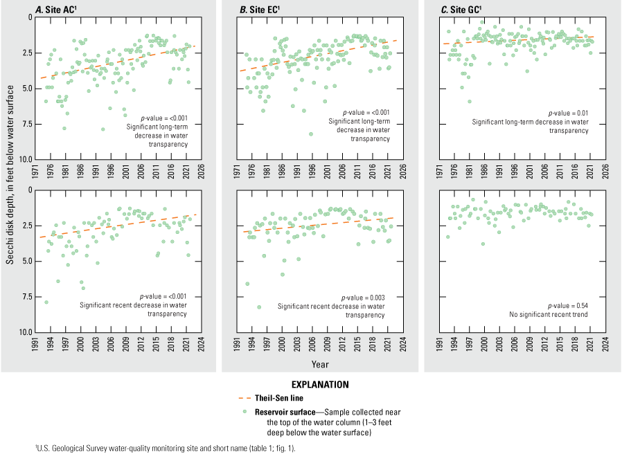
Annual variability and trend test results of Secchi-disk depth measured near the surface of Lake Conroe at sites A, AC; B, EC; and C, GC, near Conroe, Texas, during the long-term trend analysis period, 1974–2021, and recent trend analysis period, 1993–2021.
Major Ions and Water Hardness
Trend analysis results for major ions and water hardness are summarized in table 18. The SKT was applied to all major-ion concentrations, except for the recent period data for fluoride concentrations, to which the Mann-Kendall test was applied. Many major-ion concentrations (including those of calcium, magnesium, potassium, sodium, and chloride) are affected by dilution and evaporation, which are directly related to changes in reservoir volume. During 2011–12, severe drought conditions in the watershed led to increased evaporation (Wurbs and Ayala, 2014) and relatively low annual mean reservoir storage levels (fig. 2). These historically low storage levels may have contributed to the considerable increase in many major-ion concentrations measured during 2011–14. Statistical trends based on the recent period (1993–2021) may be biased because of the high concentrations measured during the severe drought conditions of 2011–12 and immediately thereafter during 2013–14.
Trends in calcium concentration (figs. 29, 30) were similar to those in specific conductance (figs. 24, 25), which is expected because the reservoir water contains a greater proportion of calcium compared to other major ions. In the long-term trend analysis period, negative trends in calcium concentration were determined in near-bottom samples collected at sites AC and EC, both with p-values ≤0.05 and Kendall’s tau values of −0.223 (fig. 29). For sites AC and EC, the calcium concentration trends in the long-term period represent 6.4- and 6.7-mg/L decreases, respectively. No long-term trends in calcium concentration (p-values >0.05) were observed in the near-bottom samples collected at site GC or in the near-surface samples collected at all three sites. In the recent period, positive trends in calcium concentration (p-values ≤0.05; Kendall’s tau range 0.198−0.223, table 18) were observed for all sites and depths except at site EC near the bottom (fig. 30). The trend results equate to an increase in calcium concentration ranging from 3.7 to 4.6 mg/L over the recent period.
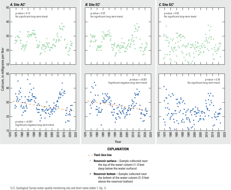
Annual variability and trend test results for calcium concentrations measured in near-surface and near-bottom water samples collected from Lake Conroe sites A, AC; B, EC; and C, GC, near Conroe, Texas, for the long-term trend analysis period, 1974–2021.
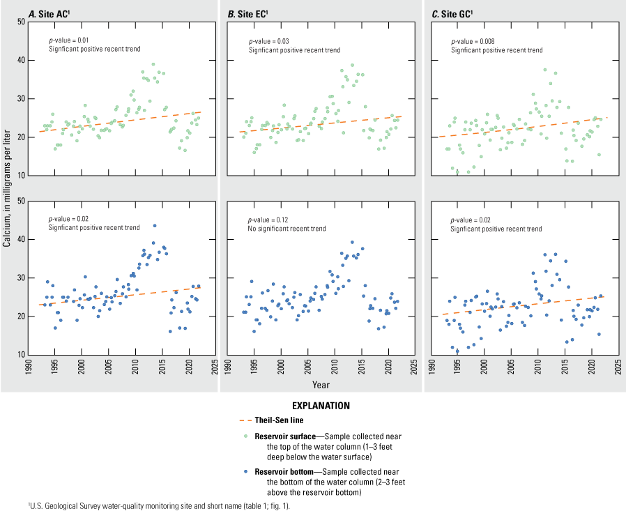
Annual variability and trend test results for calcium concentrations measured in near-surface and near-bottom water samples collected from Lake Conroe sites A, AC; B, EC; and C, GC, near Conroe, Texas, for the recent trend analysis period, 1993–2021.
Similar to calcium, magnesium concentrations exhibited negative trends (p-values ≤0.05) in near-bottom samples at sites AC (Kendall’s tau value −0.178, 0.42-mg/L decrease) and EC (Kendall’s tau value −0.207, 0.42-mg/L decrease) and no trends for either depth interval at site GC or in near-surface samples from sites AC and EC during 1974–2021 (fig. 31). In the recent trend analysis period, the magnesium concentration data indicated a strong positive trend at all sites and depths (p-values ≤0.05 and Kendall’s tau range 0.255−0.339, fig. 32, table 18). These trends represent a 0.36- to 0.56-mg/L increase in magnesium concentrations over the recent period.
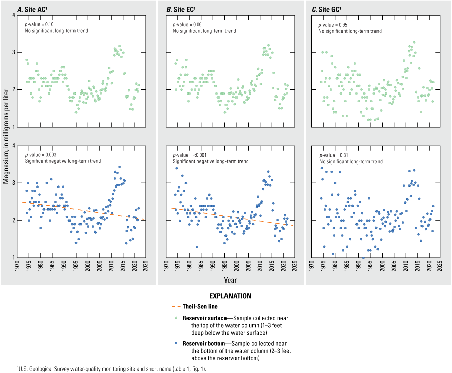
Annual variability and trend test results for magnesium concentrations measured in near-surface and near-bottom water samples collected from Lake Conroe sites A, AC; B, EC; and C, GC, near Conroe, Texas, for the long-term trend analysis period, 1974–2021.
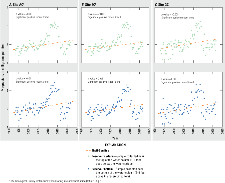
Annual variability and trend test results for magnesium concentrations measured in near-surface and near-bottom water samples collected from Lake Conroe sites A, AC; B, EC; and C, GC, near Conroe, Texas, for the recent trend analysis period, 1993–2021.
The recent positive trends determined for calcium and magnesium concentrations can likely be attributed to the drought in 2011, which resulted in decreased reservoir storage levels (fig. 2B) and subsequent increased calcium and magnesium concentrations. The concentrations of calcium and magnesium in more recent years after the drought (2015–21) are not higher than those before the drought (2004–10); in fact, concentrations tend be lower (figs. 30, 32). The concentrations of calcium and magnesium at the beginning of the recent trend analysis period (1993–98) are notably less than those measured at the beginning of the long-term period (1974–79) and tend to be the lowest of those in long-term period (figs. 29, 31). This observation further supports the conclusion that the positive trends in the recent period are driven by the drought conditions in 2011.
In the long-term trend analysis period, sodium concentration exhibited positive trends (p-values ≤0.05) at sites AC and EC for both depth intervals (fig. 33), although no trends were determined for site GC. For site-depth intervals in which a trend was determined, Kendall’s tau ranged from 0.155−0.197 (table 18). These trends represent a 1.8- to 2.4-mg/L increase in sodium concentration over the long-term period. For the recent period, positive trends in sodium concentration were observed (p-values ≤0.05) at all sites and depth intervals (fig. 34). Statistically strong positive trends were observed at all sites and depths (Kendall’s tau range 0.259−0.398, table 18) except near the bottom at site GC, where a weaker positive trend was observed (Kendall’s tau 0.210). These trends represent a 4.8- to 6.4-mg/L recent increase in sodium concentration.
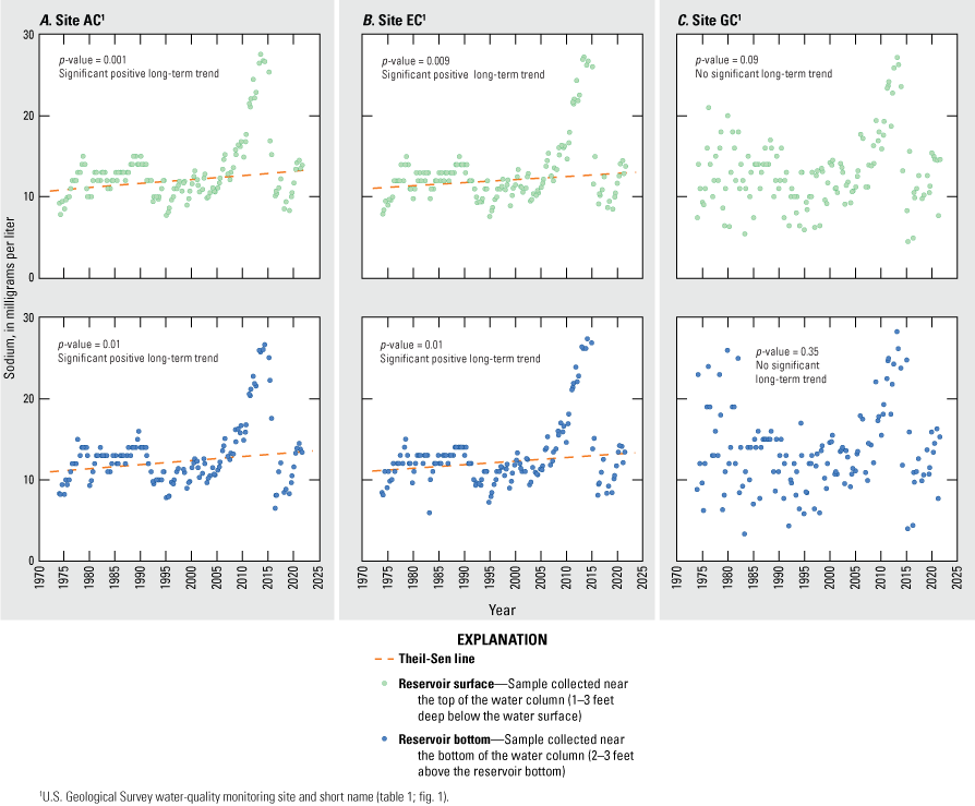
Annual variability and trend test results for sodium concentrations measured in near-surface and near-bottom water samples collected from Lake Conroe sites A, AC; B, EC; and C, GC, near Conroe, Texas, for the long-term trend analysis period, 1974–2021.
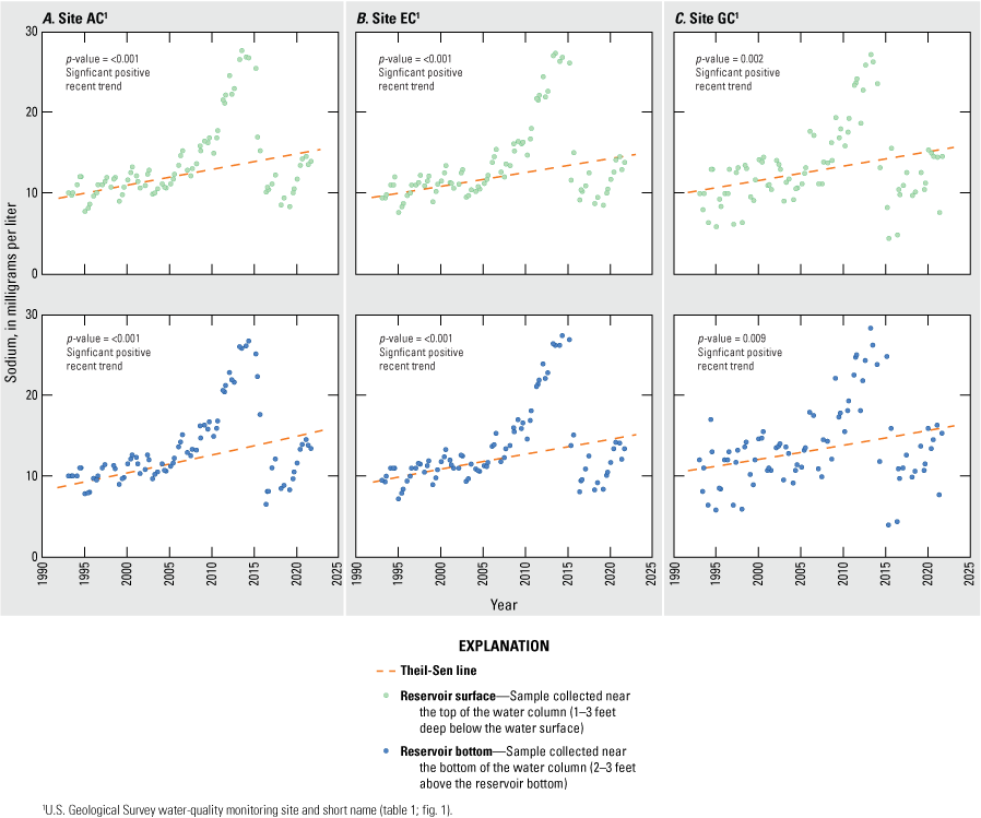
Annual variability and trend test results for sodium concentrations measured in near-surface and near-bottom water samples collected from Lake Conroe sites A, AC; B, EC; and C, GC, near Conroe, Texas, for the recent trend analysis period, 1993–2021.
Trends in potassium concentration were generally similar to those for sodium concentration, except positive trends (p-values ≤0.05) in potassium concentration were also detected for all sites and depth intervals for both trend analysis periods (figs. 35, 36). In the long-term potassium record, both depth intervals at sites AC and EC exhibited a strong positive trend, with Kendall’s tau ranging from 0.253−0.314, whereas the Kendall’s tau at site GC was 0.212 near the surface and 0.183 near the bottom. These trends represent a 0.6- to 0.8-mg/L increase in potassium concentration. In the recent record, all sites and depths exhibited strong positive trends (Kendall’s tau range 0.368−0.580, table 19), which represents a 1.0- to 1.3-mg/L increase in potassium concentration.
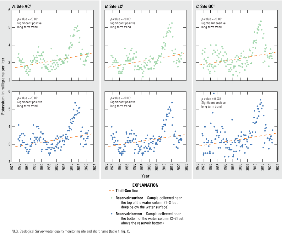
Annual variability and trend test results for potassium concentrations measured in near-surface and near-bottom water samples collected from Lake Conroe sites A, AC; B, EC; and C, GC, near Conroe, Texas, for the long-term trend analysis period, 1974–2021.
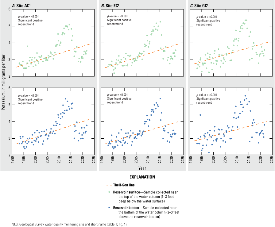
Annual variability and trend test results for potassium concentrations measured in near-surface and near-bottom water samples collected from Lake Conroe sites A, AC; B, EC; and C, GC, near Conroe, Texas, for the recent trend analysis period, 1993–2021.
Trends in potassium and sodium concentrations can be attributed to natural processes such as atmospheric deposition (Granato and others, 2015) or the dissolution of potassium- or sodium-rich minerals and soil in the watershed (Hem, 1985). Anthropogenic influences may also affect these trends, including septic effluent and wastewater discharges (Steele and Aitkenhead-Peterson, 2011), agricultural processes, and increased urbanization (Carle and others, 2007). However, the recent positive trends detected for potassium and sodium concentrations (figs. 34, 36) are likely driven by the drought period of 2011–12, which resulted in low reservoir storage amounts (fig. 2). The concentrations of potassium and sodium in more recent years following the drought (2015–21) are not substantially higher than those during the years before the drought (2004–10). The relatively high concentrations measured during the drought likely drive the positive trend in the recent period. Without streamflow data, it is difficult to discern whether the positive recent trends in potassium and sodium concentrations are more influenced by anthropogenic factors or by the period of low reservoir storage. A similar explanation can be applied to the long-term positive trends detected in potassium and sodium concentrations. The concentrations measured in the first 5 years of the study (1974–79) are not notably higher than those measured at the end of the trend analysis period (2015–21) (figs. 33, 35). The major drought conditions in 2011–12 and the subsequent elevated concentrations during 2011–14 likely drive the positive long-term trend.
No trends were determined for chloride concentration (p-values >0.05) in the long-term trend analysis period (fig. 37), although positive trends (p-values ≤0.05) were observed for both depths at all sites during the recent period (fig. 38). Strong positive trends were observed at sites AC and EC (Kendall’s tau range 0.261−0.295). These trends represent a 6.8- to 8.2-mg/L increase in chloride concentration over the recent period.
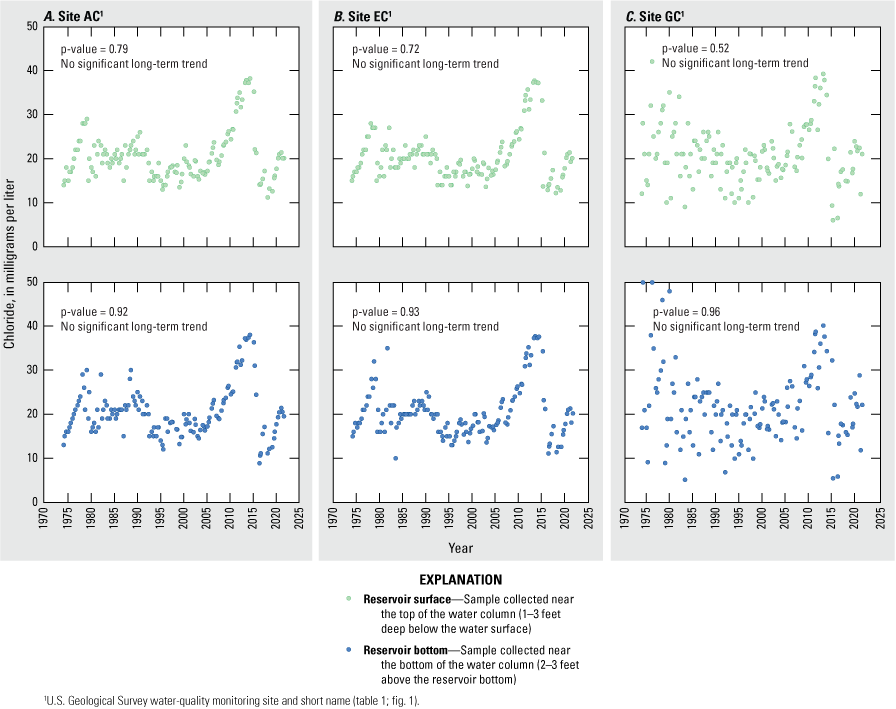
Annual variability and trend test results for chloride concentrations measured in near-surface and near-bottom water samples collected from Lake Conroe sites A, AC; B, EC; and C, GC, near Conroe, Texas, for the long-term trend analysis period, 1974–2021.
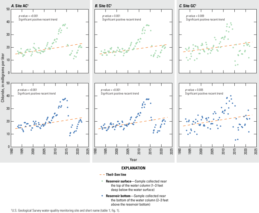
Annual variability and trend test results for chloride concentrations measured in near-surface and near-bottom water samples collected from Lake Conroe sites A, AC; B, EC; and C, GC, near Conroe, Texas, for the recent trend analysis period, 1993–2021.
Chloride concentration trends (figs. 37, 38) resembled those for specific conductance (figs. 24, 25), which is consistent with the relatively high chloride concentration measured in the reservoir water composition. Trends in chloride concentration may be affected by natural processes, including atmospheric deposition and dissolution of chloride-rich rock and soil, as well as anthropogenic factors like urbanization, wastewater discharges (Steele and Aitkenhead-Peterson, 2011), agricultural sources, and the use of chlorides for dust control and stabilization (Granato and others, 2015). Changes in land use also affect chloride concentrations in a waterbody. Some studies (Steele and Aitkenhead-Peterson, 2011) have linked increases in chloride concentrations in reservoirs and streams, specifically in warmer areas that do not use considerable amounts of deicing salts, to increases in the extent of impervious surfaces, including roads, sidewalks, and buildings. Widespread urbanization and population growth have resulted in an increased percentage of impervious surface coverage within in the watershed, particularly in recent years (MRLC, 2023). Stormwater runoff from impervious surfaces may gain salts from chloride-rich dusts, spills, overspray, urban turf irrigation runoff, or dissolution of the impervious surfaces themselves (Appel and Hudak, 2001). However, like the recent trends detected in potassium and sodium concentrations, the recent, positive trend in chloride concentration is likely driven by the drought conditions experienced in 2011. Concentrations measured during 2015–21 tend to be less than those measured before the drought (2005–10), particularly at sites AC and EC.
The sulfate concentration data indicated no trends (p-values >0.05) during either trend analysis period (figs. 39, 40), except for a long-term negative trend near the surface at site GC, where the p-value was ≤0.05 and Kendall’s tau was −0.143. This trend represents a 1.6-mg/L decrease in sulfate concentration over the long-term period. Although urbanization has been linked to increasing sulfate concentrations in other areas (Kaushal and others, 2018), no positive trends in sulfate concentration were observed in Lake Conroe (figs. 39, 40). In fact, long-term downtrend patterns were observed in near-surface samples at sites AC and EC (in addition to the negative trend at site GC) and in the near-bottom samples at sites AC and GC. These negative sulfate patterns could be attributed to decreasing atmospheric sulfate concentrations over recent decades (Falcone and others, 2018; Aas and others, 2019).
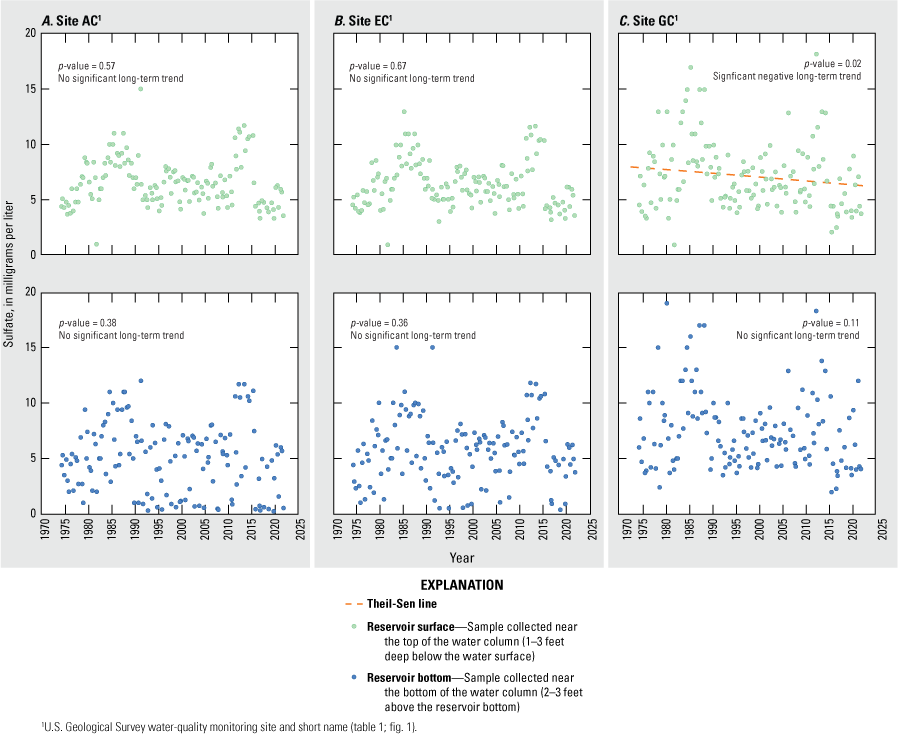
Annual variability and trend test results for sulfate concentrations measured in near-surface and near-bottom water samples collected from Lake Conroe sites A, AC; B, EC; and C, GC, near Conroe, Texas, for the long-term trend analysis period, 1974–2021.
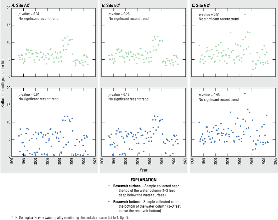
Annual variability and trend test results for sulfate concentrations measured in near-surface and near-bottom water samples collected from Lake Conroe sites A, AC; B, EC; and C, GC, near Conroe, Texas, for recent trend analysis period, 1993–2021.
Trends in silica concentration, like those for potassium, were positive (p-values ≤0.05) for both depths at all sites during both trend analysis periods (figs. 41, 42). Kendall’s tau for trends detected in silica concentration ranged from 0.186−0.471 in the long-term trend analysis period and 0.222−0.406 in the recent trend analysis period (table 18). These trends represent a 3.3- to 7.1-mg/L increase in silica concentration over the long-term period and a 3.0- to 5.8-mg/L increase over the recent period. Unlike other major ions, silica concentrations were not notably affected by the drought conditions in 2011. The substantial increase in potassium and sodium concentrations measured during 2011–14 was not observed in silica concentrations. Concentrations measured before the drought (2004–10) are generally similar to those measured after the drought (2015–21) (fig. 42). Over the long-term period, concentrations measured in the first 5 years of the trend analysis period (1974–79), particularly near the surface at sites AC and EC, tended to be less than those measured at the end of the trend analysis period (2015–21) (fig. 41). Near-surface silica concentrations measured at sites AC and EC during 1974–79 generally ranged from 1 to 5 mg/L, whereas the concentrations measured during 2015–21 generally ranged from 6 to 11 mg/L. Positive trends in silica concentration could be explained by accelerated weathering and localized erosion of silica-rich soils and silicate minerals in response to elevated temperatures (Gelca and others, 2014), sewage inputs, and other biological sources (Carey and Fulweiler, 2012).
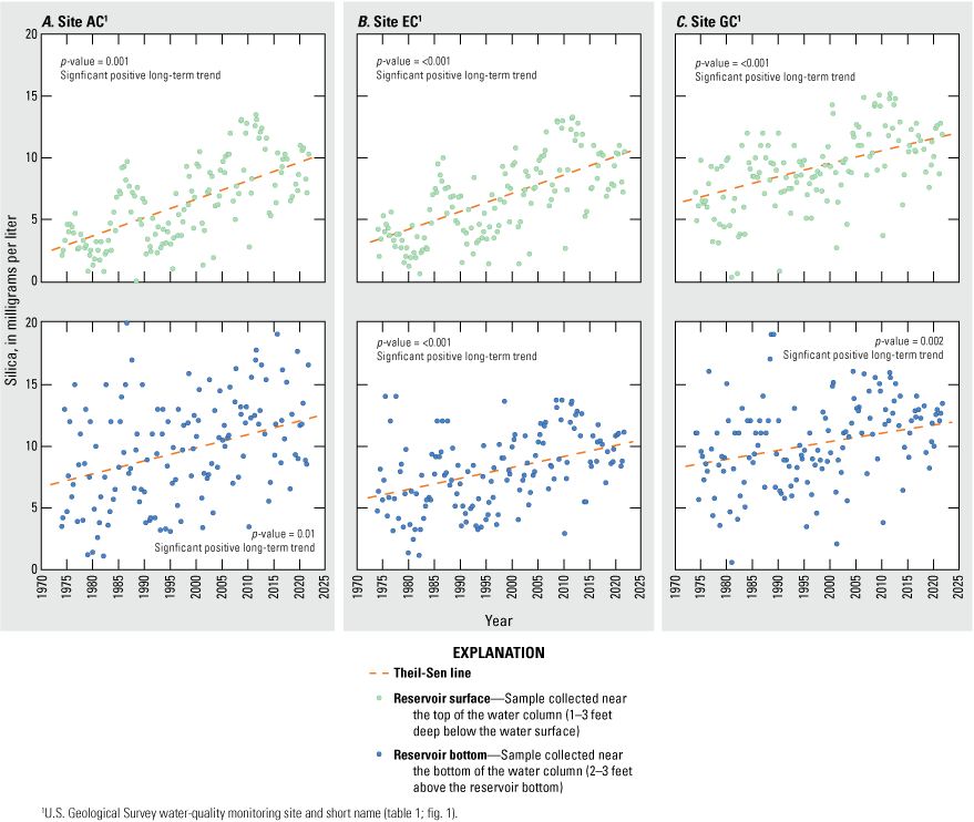
Annual variability and trend test results for silica concentrations measured in near-surface and near-bottom water samples collected from Lake Conroe sites A, AC; B, EC; and C, GC, near Conroe, Texas, for the long-term trend analysis period, 1974–2021.
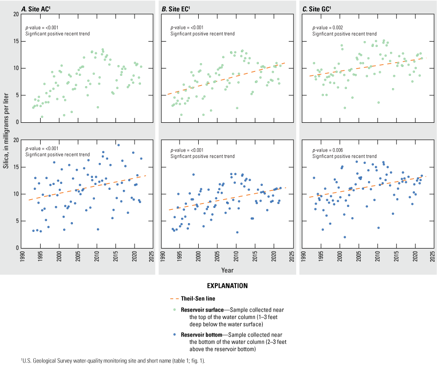
Annual variability and trend test results for silica concentrations measured in near-surface and near-bottom water samples collected from Lake Conroe sites A, AC; B, EC; and C, GC, near Conroe, Texas, for the recent trend analysis period, 1993–2021.
Because fluoride concentration data were not collected during 1979–89, trend analyses for this constituent were not possible for the long-term record; fluoride exhibited positive trends (p-values ≤0.05; Kendall’s tau range 0.170−0.190, table 18) in the recent period at both depths at sites AC and EC. These trends represent a 0.22-mg/L increase in fluoride concentration at site AC and a 0.36-mg/L increase in fluoride concentration at site EC over the recent period. No trends were detected for fluoride at site GC.
Trends in water hardness were similar to the trends observed in calcium and magnesium concentrations. Water hardness exhibited negative trends (p-values ≤0.05) in the long-term trend analysis period at sites AC and EC near the bottom, with Kendall’s tau of −0.207 and −0.237, respectively (table 18). The trend at site AC near the bottom represents a 17.5-mg/L decrease in water hardness and the trend at site EC near the bottom represents a 19.6-mg/L decrease over the long-term period. Positive trends (p-values ≤0.05) in hardness were determined for the recent trend analysis period for both depths at all sites (Kendall’s tau range 0.201−0.239, table 18), except at site EC near the bottom. These trends represent a 12.4- to 14.4-mg/L increase in water hardness over the recent period.
Nutrients
The data used to analyze trends in ammonia, ammonia plus organic nitrogen, phosphorous, orthophosphate, and nitrate concentrations were restricted to samples collected between 1993 and 2021 because of changes in laboratory analysis methods that were implemented in 1992. Trend analysis was not performed on phosphorous concentrations measured in samples collected near the surface of the reservoir (near-surface phosphorous samples) collected at sites AC and EC because more than 80 percent of the measured values were nondetections. The SKT was applied to the entirety of the ammonia plus organic nitrogen data. Positive trends (p-values ≤0.05) were determined for ammonia plus organic nitrogen concentrations measured in the samples collected near the surface at all sites (fig. 43), where Kendall’s tau ranged from 0.189−0.238 (table 19). The Mann-Kendall test was applied to the ammonia, phosphorous, orthophosphate, nitrite, and nitrate plus nitrite data where nondetections did not exceed 80 percent of the data. Negative trends (p-values ≤0.05) were determined for ammonia concentrations measured near the surface at sites EC and GC, where Kendall’s tau was −0.102 and −0.145, respectively. Negative trends were also determined for near-bottom ammonia concentrations (Kendall’s tau −0.226) and near-bottom phosphorous concentrations (Kendall’s tau −0.146) at site EC. No trends (p-values >0.05) were detected for orthophosphate, nitrate, or nitrate plus nitrite concentrations.
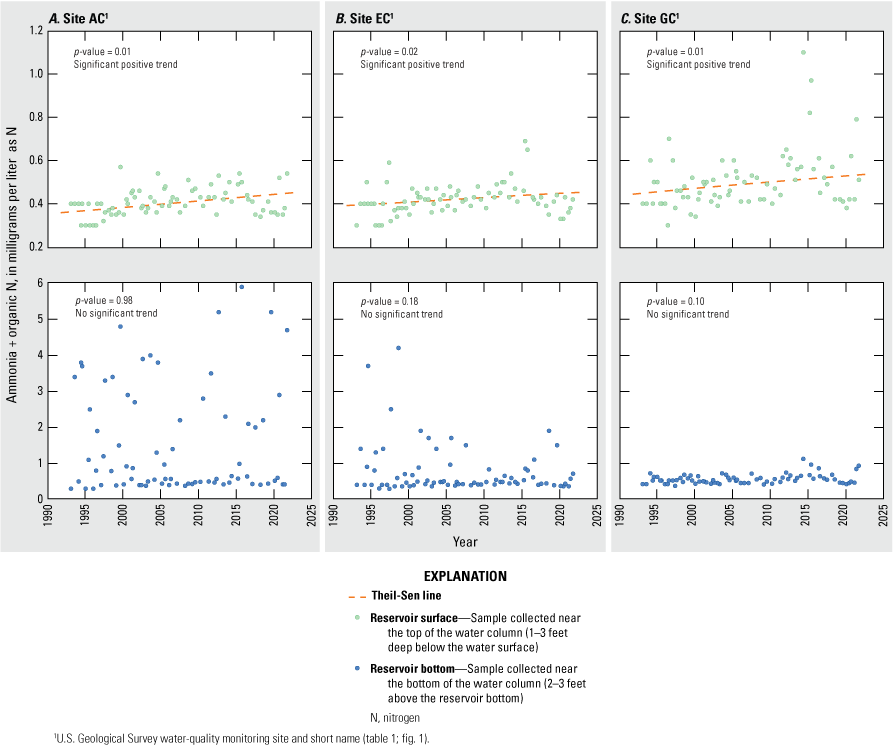
Annual variability and trend test results for ammonia plus organic nitrogen in near-surface and near-bottom samples collected from Lake Conroe sites A, AC; B, EC; and C, GC, near Conroe, Texas, for the recent trend analysis period, 1993–2021.
The positive trends determined for near-surface ammonia plus organic nitrogen concentrations (fig. 43) may be attributed to the increased urbanization occurring in the watershed over the recent period. Urbanization results in increased stormwater runoff that may be nutrient-rich as well as wastewater discharges from newly constructed WWTPs near the reservoir. However, the slope values for the positive trends in ammonia plus organic nitrogen concentrations were calculated to be either 0.002 mg/L per year (site EC) or 0.003 mg/L per year (sites AC and GC), which represents an increase of 0.056 mg/L or 0.084 mg/L over 28 years (table 19). Despite the detection of significant positive trends, the increase in absolute concentration is relatively small. For instance, the median concentration of ammonia plus organic nitrogen concentration near the surface at site GC increased by 0.05 mg/L, from 0.47 to 0.52 mg/L over the recent period.
Although some analytes included in the nutrient schedule were not analyzed for trends and many slope values were not calculated, annual time-series plots (figs. 44, 45) show that both near-surface and near-bottom nutrient concentrations did not exhibit noticeable increases or decreases over time. Ammonia plus organic nitrogen concentrations were highest in near-bottom measurements during summer (fig. 17, tables 9, 12, and 15), whereas nitrate plus nitrite values were generally higher in winter than summer at both depth intervals (fig. 17, tables 9, 12, and 15). These patterns, along with relatively low dissolved-oxygen concentrations in summer near the reservoir bottom (fig. 6), indicate that nutrient recycling was occurring at near-bottom depths, which has prevented nutrient accumulation and eutrophication in Lake Conroe (Sprague, 2002).
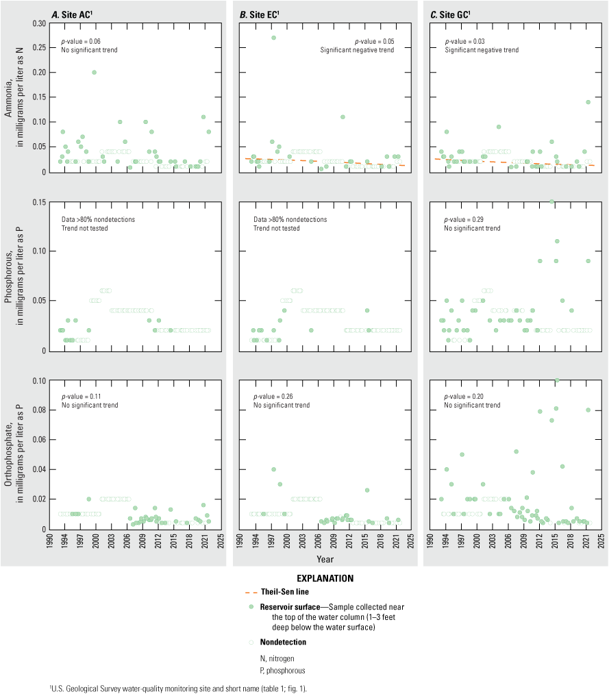
Annual variability and trend test results for ammonia, phosphorous, and orthophosphate in near-surface samples collected from Lake Conroe sites A, AC; B, EC; and C, GC, near Conroe, Texas, 1993–2021.
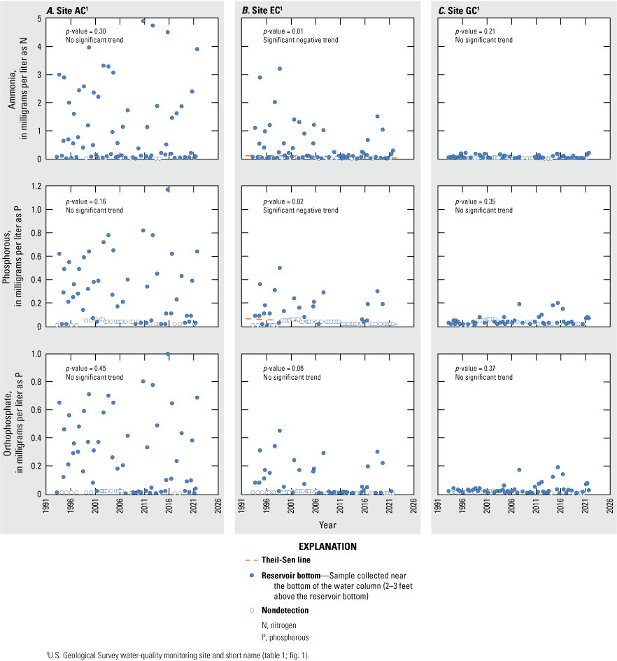
Annual variability and trend test results for ammonia, phosphorous, and orthophosphate in near-bottom samples collected from Lake Conroe sites A, AC; B, EC; and C, GC, near Conroe, Texas, 1993–2021.
Trace Metals
The data used to analyze trends in iron and manganese concentrations were collected between 1993 and 2021 because of changes in laboratory analysis methods in 1992. The Mann-Kendall test, adapted for censored data, was applied to the entirety of the iron concentration data as well as the near-surface manganese concentration data at all sites. The SKT was applied to the near-bottom manganese concentration data. Similar to figure 18, a logarithmic base-10 scale was applied to the y-axis of the plots in figures 46 and 47 to allow temporal trends to be more discernible. The changes in concentration over the trend analysis period are calculated by using the slope value reported in table 19; however, these changes in concentration are not visualized in the plots presented in figures 46 and 47.
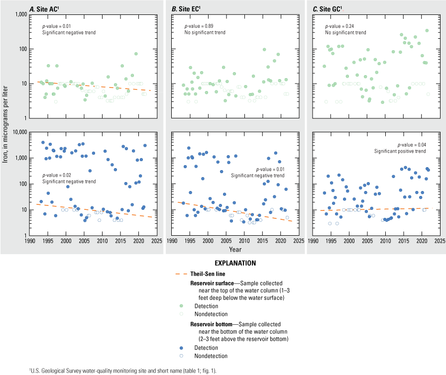
Annual variability and trend test results for iron concentrations measured in near-surface samples collected from Lake Conroe A, AC; B, EC; and C, GC, near Conroe, Texas, for the recent trend analysis period, 1993–2021.
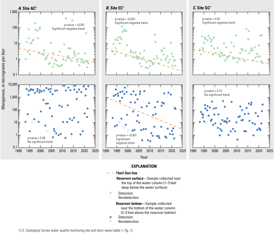
Annual variability and trend test results for manganese concentrations measured in near-surface samples collected from Lake Conroe sites A, AC; B, EC; and C, GC, near Conroe, Texas, for the recent trend analysis period, 1993–2021.
The iron concentration data indicated a negative trend (p-values ≤0.05) in near-surface samples collected at site AC (Kendall’s tau −0.159) and in near-bottom samples collected at site AC (Kendall’s tau −0.200) and site EC (Kendall’s tau −0.198) and a positive trend (p-values ≤0.05) in near-bottom samples collected at site GC (Kendall’s tau 0.167) (fig. 46). These near-bottom trends represent a 34-µg/L decrease at site AC, a 27-µg/L decrease at site EC, and a 26-µg/L increase at site GC between 1993 and 2021 (table 19). No other trends were determined for the iron concentration data. Manganese exhibited negative trends (p-values ≤0.05) near the surface at all sites (Kendall’s tau range −0.195 to −0.361) and at site EC near the bottom (Kendall’s tau −0.341) (fig. 47). These trends indicate a 2.3- to 3.4-µg/L decrease in the near-surface manganese concentrations and a 40-µg/L decrease at site EC near the bottom between 1993 and 2021 (table 19).
The trace metal trend analysis and seasonal data indicate that urbanization in the watershed is not a primary factor for the occurrences of elevated iron and manganese concentrations in the reservoir. Instead, fluctuations in these concentrations are driven by anoxic conditions causing sediment to release iron and manganese during thermal stratification. The weathering of iron- and manganese-rich soils and sediments may contribute to near-surface concentrations, although concentrations generally show an overall decrease over 1993–2021.
Study Limitations and Considerations for Future Work
The trend analyses presented in this report have certain limitations that require further investigation for a comprehensive understanding of water-quality trends in Lake Conroe. A lack of fall data (October, November, and December) resulted in only three seasons for analysis. The lack of fall data makes it challenging to describe certain aspects of seasonal variability in water quality in Lake Conroe, such as determining when thermal stratification ends and fall turnover begins, as stratification persists in the reservoir through at least late September. Additionally, historical records of streamflow data are lacking in the Lake Conroe watershed. Although streamflow data are available downstream from the reservoir, there is insufficient streamflow data from major tributaries that flow into Lake Conroe to provide a meaningful analysis of concentration data. Only a single streamgage (USGS streamgage 08067458) located on a tributary upstream of the reservoir provided a partial period of record (2009–21), which only encompasses the last 12 years of the 47-year period within the scope of this study. The general lack of historical streamflow data for the inflows to Lake Conroe reduces the accuracy and interpretation of the trend analysis. Streamflow data could be a source of some of the variability in water-quality concentrations over time as well as how concentrations relate to streamflow, but this possibility was not investigated because the data were not available. Additionally, constituent load and yield calculations, necessary for estimating inputs from source areas and identifying major contributors of various constituents (Day, 2021; Spaetzel and Smith, 2022), could not be performed because of the lack of streamflow data. Revisiting the analysis once a sufficient streamflow record for the watershed’s tributaries is established may provide a more comprehensive understanding of flow effects on constituent concentrations in Lake Conroe.
Although the available reservoir water-quality data for this trend analysis were considered robust, there were limitations. These limitations primarily included a lack of water-quality data for some constituents and changes in analytical methods and, consequently, reporting levels. Changes in analytical methods could be unidentified sources of bias and variability, as well as a contributing factor in the detection of, and trends in, water-quality data. For a given analyte, apparent trends in the data might be an artifact of changes in the analytical methods if (1) less accurate methods often associated with higher laboratory detection and reporting levels are used early in the record and (2) more accurate methods with lower laboratory detection and reporting levels are used later in the record (Smith and McCann, 2000). There are ways to verify that detected trends are not an artifact of changes in analytical methods. For example, reconstructing water-quality trends using sediment cores from reservoirs has proven effective in other areas (Van Metre and Callender, 1996). Conducting a sediment core sampling study of Lake Conroe and its tributaries could also provide crucial information on the presence and distribution of analytes that would otherwise be affected by limitations of the analysis, such as nutrients and trace metals. Additionally, sediment core data may offer further insights into potential sources and trends. Expanding the sediment core analysis to include constituents not previously sampled, such as pesticides and additional metals, could contribute necessary information for a more comprehensive assessment of temporal water-quality trends in Lake Conroe. Another possible investigation involves collecting streambed sediment and water-quality samples from Lake Conroe’s largest tributaries. Analyzing streambed sediment and water-quality data could provide further insight about different sources of analytes, such as pesticides, nutrients, or metals, to the reservoir based on land use in the watersheds of the respective sampled streams.
Summary
Lake Conroe is a reservoir on the West Fork San Jacinto River in Montgomery and Walker Counties near Conroe, Texas, that was constructed in 1973. Lake Conroe is an important resource for municipal and industrial water supply in the greater Houston area. In recent years, the rapidly growing population in the Lake Conroe watershed and the surrounding Montgomery County has increased concerns among water-quality managers about the effects of urbanization on water quality in Lake Conroe. Water-quality data collected by the U.S. Geological Survey (USGS), in cooperation with the San Jacinto River Authority, during the period from 1974 to 2021 were used to describe the vertical, spatial, and seasonal variability of selected physicochemical properties and constituents in Lake Conroe, characterize the relation between thermal stratification and selected physicochemical properties and constituents, and evaluate water-quality trends in Lake Conroe for two periods, 1974–2021 and 1993–2021. Discrete water-quality data were collected approximately three times per year (in winter, spring, and summer) during 1974–2021 at three monitoring sites. Water-quality monitoring sites were chosen to represent the main body of the reservoir and include (1) site USGS-302127095335501 Lake Conroe Site AC near Conroe, Tex. (hereinafter referred to as “site AC”), which is in the deep, downstream part of the reservoir at the Lake Conroe dam and has a mean depth of 53 feet (ft), (2) site USGS-302607095360901 Lake Conroe Site EC near Conroe, Tex. (hereinafter referred to as “site EC”), which is mid-reservoir and has a mean depth of 39 ft; and (3) site USGS-303129095360501 Lake Conroe Site GC near Conroe, Tex. (hereinafter referred to as “site GC”), which is in the shallow, upstream part of Lake Conroe and has a mean depth of 28 ft. Vertical profiles of water temperature, dissolved-oxygen concentration, specific conductance, and pH, and discrete samples for laboratory analysis of major ions, hardness, nutrients trace metals were collected at a “near-surface” interval that included the sample or measurement collected near the top of the water column (1–3 ft below the water surface) and a “near-bottom” interval that included the sample or measurement collected near the bottom of the water column (2–3 ft above the reservoir bottom).
Summary statistics, including minimum, median, mean, maximum, and standard deviation values, were calculated for the years 1974–2021 for each water-quality constituent measured or collected at each site and depth interval combination. Seasonal summary statistics were also calculated for each constituent-site-depth interval combination. Trend analyses were conducted on the water-quality data collected from Lake Conroe; no adjustments were made for variations in the streamflow entering the reservoir because historical streamflow inflow data were sparse. Two trend methods were used to characterize temporal changes in water quality in Lake Conroe: the Seasonal Kendall test (SKT) and the Mann-Kendall test, adapted for censored data. Temporal trends were determined for a long-term trend analysis period (1974–2021), a recent trend analysis period (1993–2021), or both, depending on the length of record of available data. Near-surface and near-bottom physicochemical properties and constituents were tested separately for trends.
Water temperatures near the bottom (median value of 22.5 degrees Celsius) were generally lower compared to water temperatures measured near the surface (median value of 27.5 degrees Celsius). Water temperatures were warmest in July and August and coldest in January in both depth intervals at all three sites. Surface-water warming in spring led to a temperature gradient that steepened in summer, and water temperatures decreased abruptly at approximately 30 ft below the water surface, where a well-defined thermocline developed at site AC and sometimes at site EC. Thermal stratification begins in spring, becomes established in summer, and is fully developed through at least the end of summer, primarily affecting deeper areas of the reservoir; site GC, where the reservoir is shallower, did not exhibit thermal stratification.
Dissolved-oxygen concentrations measured near the surface were consistent among the sites, and those measured near the bottom were lowest at site AC and highest at site GC. A general seasonal pattern was followed, with lower dissolved-oxygen concentrations in summer and higher concentrations in winter; dissolved-oxygen concentrations tended to decrease as water temperature increased. Sites that exhibited seasonal thermal stratification also exhibited decreasing dissolved-oxygen concentrations with increasing depth. When thermally stratified conditions existed, water became anoxic, with dissolved-oxygen concentrations being less than 0.5 milligram per liter at depths greater than 30 ft, which coincides with depths at which pronounced temperature decreases also occurred. At site GC or during seasons (winter) when thermal stratification was not established, anoxia in the reservoir was rare.
Specific conductance was generally higher near the bottom than near the water surface at all sites and generally increased downreservoir. Specific conductance profiles did not exhibit the strong thermal-stratification patterns observed in the water temperature or dissolved-oxygen profiles. During summer, changes in specific conductance values associated with thermal stratification were the most well-defined at site AC, with a pronounced increase at about the same depth where there was a pronounced decrease in temperature. The pH measured near the surface was always higher than pH measured near the bottom. During winter, pH values were nearly uniform with depth at all sites. During summer, pH values decreased consistently with depth at all three sites. Secchi-disk depth (and thus water transparency) was generally highest near the dam at site AC and lowest upreservoir at site GC. Water transparency at the two deepest sites, AC and EC, was greatest during winter, whereas transparency at the shallowest site, GC, remained consistent throughout the three seasons when water-quality data were collected.
Calcium and chloride were the cation and anion, respectively, with the highest median concentrations at all three sites. Water-column variability at each site was different for each major ion. Additionally, the water-column variability of major-ion concentrations depended on which site was described. Major-ion concentrations (including those of calcium, magnesium, sodium, potassium, chloride, and fluoride) exhibited minimal seasonal variability between near-surface and near-bottom samples and among sites. Sulfate concentrations were generally highest during winter and lowest during summer for both depths at all sites. The decreasing sulfate concentrations with depth observed during summer at site AC, and sometimes site EC, are likely related to reducing conditions in the hypolimnion during periods of pronounced thermal stratification, when sulfate ions are reduced to sulfide ions and result in decreased sulfate concentrations.
Nutrient concentrations were typically higher near the reservoir bottom than near the water surface, particularly in the samples collected at sites AC and EC. Median nutrient concentrations were generally similar in near-surface samples collected at all sites. During winter, nutrient concentrations remained similar with depth and across the reservoir. In summer, most nutrient concentrations were highest near the reservoir bottom, particularly at deep sites AC and EC. In shallow areas (site GC), nutrient concentrations were generally uniform in the water column throughout the three seasons when water-quality data were collected, aside from some elevated concentrations of ammonia plus organic nitrogen in summer. The seasonal pattern observed for the other nutrient species was not observed for nitrate plus nitrite. Median concentrations of nitrate plus nitrite were highest in winter for both depth intervals at all sites. Sites that exhibited summer thermal stratification also showed increasing concentrations for most nutrients with depth. The absence of vertical mixing during thermal stratification at sites AC and EC trapped nutrients released from decomposing organic matter and sediments under anoxic conditions in the hypolimnion. These release mechanisms contributed to increased concentrations of ammonia, ammonia plus organic nitrogen, phosphorous, and orthophosphate measured in near-bottom samples collected from these sites.
Trace metal (iron and manganese) concentrations were generally higher in samples collected near the reservoir bottom than in the samples collected near the water surface. The spatial pattern indicated a slight increase in near-surface trace metal concentrations upreservoir, whereas near-bottom concentrations were substantially higher at site AC than at site GC. Trace metal concentrations followed similar seasonal patterns as those for nutrients (except for nitrate plus nitrite), where the highest trace metal concentrations generally were measured near the bottom at sites AC and EC during summer. Concentrations remained generally consistent in the water column during winter at all sites relative to summer concentrations.
For the long-term trend analysis period (1974–2021), a positive trend in water temperature was determined and may be attributed to a combination of (1) sudden urbanization in the watershed, resulting in the construction of impervious surfaces, and (2) increases in air temperature. For the recent trend analysis period (1993–2021), no trends in water temperature were determined. The slopes for the water temperature data indicate smaller changes, and in some cases, no change, in water temperature per year relative to the long-term period. This stabilization could be a result of adaptations in urban planning to mitigate urban heat island effects, such as planting trees to increase canopy cover, the installation of reflective roofing products on new and existing buildings, and repaving roads with reflective pavement.
During 1974–2021, positive trends in dissolved-oxygen concentration were determined at all sites and depths, whereas during 1993–2021, positive trends in dissolved-oxygen concentration were computed at all surface sites. For the long-term trend analysis period, the specific conductance data indicated a negative trend near the bottom at site EC. During the recent trend analysis period, positive trends in specific conductance were observed at all sites and depths. The low reservoir storage during a drought in the early 2010s likely contributed to the elevated specific conductance values measured during that period and affected the trend analysis for the recent period. Positive trends in specific conductance could also be related to local patterns of population growth since 2000 as well as increases in the amount of developed land and decreases in forested land. In the long-term record, positive trends in pH were observed at all sites and depth intervals and were observed near the bottom at all sites during the recent period. The long-term positive water temperature trends in Lake Conroe can result in greater productivity, thus increasing photosynthetic processes and pH levels. This is evidenced by the determination of long-term positive pH trends. Secchi-disk depth exhibited negative trends at all reservoir sites during the long-term and recent period, indicating that water transparency worsened during 1974–2021. Long-term decreasing water transparency in Lake Conroe could be attributed to urbanization and increased impervious surface land cover in the watershed.
Many major-ion concentrations (including those of calcium, magnesium, potassium, sodium, and chloride) are affected by dilution and evaporation, which are directly related to changes in reservoir volume. During 2011–12, severe drought conditions in the watershed led to increased evaporation and relatively low annual mean reservoir storage levels. These historically low storage levels may have contributed to the considerable increase measured in many major-ion concentrations during 2011–14. In the long-term trend analysis period, negative trends in calcium and magnesium concentrations were determined in near-bottom samples collected at sites AC and EC. In the recent period, positive trends in calcium and magnesium concentrations were observed for all sites and depths except for calcium concentrations near the bottom at site EC. The recent positive trends determined for calcium and magnesium concentrations can likely be attributed to the drought in 2011, which resulted in decreased reservoir storage levels and subsequent increased calcium and magnesium concentrations.
Sodium concentration exhibited positive trends at sites AC and EC for both depth intervals during the long-term period and positive trends at all sites and depth intervals during the recent period. The recent positive trends detected for potassium and sodium are likely driven by the drought conditions in 2011, which resulted in low reservoir storage amounts. The concentrations of potassium and sodium in more recent years following the drought (2015–21) are not substantially higher than the years before the drought (2004–10). A similar explanation can be applied to the long-term positive trends detected in potassium and sodium concentrations. The concentrations measured in the first 5 years of the study (1974–79) are not notably higher than those measured at the end of the trend analysis period (2015–21). However, without streamflow data, it is difficult to discern whether the positive recent trend in potassium and sodium concentrations is more influenced by anthropogenic factors or by the period of low reservoir storage.
No trends were determined for chloride concentrations in the long-term trend analysis period, although positive trends were observed for both depths at all sites during the recent period. Like the recent trends detected in other major ions, the recent positive trend in chloride concentration is likely driven by the drought conditions in 2011. The sulfate concentration data indicated no trends during either trend analysis period, except for a long-term negative trend near the surface at site GC. These negative sulfate patterns could be attributed to decreasing atmospheric sulfate concentrations over recent decades.
Silica concentrations, like calcium, magnesium, sodium, potassium, and chloride concentrations, exhibited positive trends for both depths at all sites during both trend analysis periods. Unlike other major ions, silica concentrations were not notably affected by the drought conditions in 2011. The substantial increase in potassium and sodium concentrations measured during 2011–14 was not observed in the silica concentrations. Positive trends in silica concentration could be explained by accelerated weathering and localized erosion of silica-rich soils and silicate minerals in response to elevated temperatures, sewage inputs, and other biological sources.
Recent, positive trends were determined for ammonia plus organic nitrogen concentrations measured in the samples collected near the surface at all sites. These trends may be attributed to the increased urbanization occurring in the watershed over the recent period as urbanization can result in (1) increased stormwater runoff that may be nutrient-rich, and (2) wastewater discharges from newly constructed wastewater treatment plants near the reservoir. Negative trends were determined for near-surface ammonia concentrations measured at sites EC and GC and for near-bottom ammonia and phosphorous concentrations measured at all sites. No trends were detected for orthophosphate, nitrate, or nitrate plus nitrite concentrations. Annual time-series plots show that both near-surface and near-bottom nutrient concentrations did not exhibit noticeable increases or decreases over time, indicating that nutrient recycling was occurring at near-bottom depths.
Negative trends were observed in iron concentrations for both depths at site AC and near the bottom at site EC. A positive trend in iron concentration near the bottom at site GC was determined. Manganese concentration exhibited a negative trend near the surface at all sites and near the bottom at site EC. The trace metal trend analysis and seasonal data indicate that urbanization in the watershed is not a primary factor for the occurrences of elevated iron and manganese concentrations in the reservoir. Instead, fluctuations in these concentrations are driven by anoxic conditions causing sediment to release iron and manganese during thermal stratification.
References Cited
Aas, W., Mortier, A., Bowersox, V., Cherian, R., Faluvegi, G., Fagerli, H., Hand, J., Klimont, Z., Galy-Lacaux, C., Lehmann, C.M.B., Myhre, C.L., Myhre, G., Olivie, D., Sato, K., Quaas, J., Rao, P.S.P., Schulz, M., Shindell, D., Skeie, R.B., Stein, A., Takemura, T., Tsyro, S., Vet, R., and Xu, X., 2019, Global and regional trends of atmospheric sulfur: Scientific Reports, v. 9, no. 953, accessed November 17, 2023, at https://doi.org/10.1038/s41598-018-37304-0.
Addy, K., and Green, L., 1996, Phosphorous and lake aging: University of Rhode Island, College of Resource Development, Department of Natural Resources Science Fact Sheet No. 96–2, 4 p., accessed February 6, 2024, at https://web.uri.edu/wp-content/uploads/sites/1667/Phosphorus.pdf.
Adhikari, S., Shrestha, S.M., Singh, R., Upadhaya, S., and Stapp, J.R., 2016, Land use change at sub-watershed level: Hydrology—Current Research, v. 7, no. 3, 5 p., accessed March 17, 2024, at https://doi.org/10.4172/2157-7587.1000256.
Akritas, M.G., Murphy, S.A., and LaVallet, M.P., 1995, The Theil-Sen estimator with doubly censored data and applications to astronomy: Journal of the American Statistical Association, v. 90, no. 429, p. 170–177, accessed March 2, 2023, at https://doi.org/10.1080/01621459.1995.10476499.
Appel, P.L., and Hudak, P.F., 2001, Automated sampling of stormwater runoff in a urban watershed, North-Central Texas: Journal of Environmental Science and Health, Part A, Toxic/Hazardous Substances & Environmental Engineering, v. 36, no. 6, p. 897–907, accessed June 17, 2023, at https://doi.org/10.1081/ESE-100104119.
Bodkin, L.J., and Oden, J.H., 2010, Streamflow and water-quality properties in the West Fork San Jacinto River Basin and regression models to estimate real-time suspended-sediment and total suspended-solids concentrations and loads in the West Fork San Jacinto River in the vicinity of Conroe, Texas, July 2008–August 2009: U.S. Geological Survey Scientific Investigations Report 2010–5171, 35 p., accessed January 10, 2023, at https://doi.org/10.3133/sir20105171.
Boehrer, B., and Schultze, M., 2008, Stratification of lakes: Reviews of Geophysics, v. 46, no. 2, 27 p., accessed August 29, 2024, at https://doi.org/10.1029/2006RG000210.
Bolke, E.L., 1979, Dissolved-oxygen depletion and other effects of storing water in Flaming Gorge Reservoir, Wyoming and Utah: U.S. Geological Survey Water-Supply Paper 2058, 41 p., accessed January 18, 2024, at https://doi.org/10.3133/wsp2058.
Bolks, A., DeWire, A., and Harcum, J.B., 2014, Baseline assessment of left-censored environmental data using R: Tech Notes 10, U.S. Environmental Protection Agency, prepared by Tetra Tech, Inc., 28 p., accessed May 25, 2023, at https://www.epa.gov/sites/default/files/2016-05/documents/tech_notes_10_jun2014_r.pdf.
Bouvy, M., Nascimento, S.M., Molica, R.J.R., Ferreira, A., Huszar, V., and Azevedo, S.M.F.O., 2003, Limnological features in Tapacurá reservoir (northeast Brazil) during a severe drought: Hydrobiologia, v. 493, p. 115–130, accessed March 21, 2024, at https://doi.org/10.1023/A:1025405817350.
Buchanan, C., and Mandel, R., 2015, Water quality trend analysis at twenty-six West Virginia long-term monitoring sites: West Virginia Department of Environmental Protection, Division of Water and Waste Management, prepared by Interstate Commission on the Potomac River Basin, 64 p., accessed September 21, 2023, at https://dep.wv.gov/WWE/watershed/wqmonitoring/Documents/FINALWVTrendReportApril172015.pdf.
Carey, J.C., and Fulweiler, R.W., 2012, Human activities directly alter watershed dissolved silica fluxes: Biogeochemistry, v. 111, no. 1–3, p. 125–138, accessed February 27, 2025, at https://doi.org/10.1007/s10533-011-9671-2.
Carey, R.O., and Migliaccio, K.W., 2009, Contribution of wastewater treatment plant effluents to nutrient dynamics in aquatic systems—A review: Environmental Management, v. 44, no. 2, p. 205–217, accessed February 12, 2024, at https://doi.org/10.1007/s00267-009-9309-5.
Carle, M.V., Halpin, P.N., and Stow, C.A., 2007, Patterns of watershed urbanization and impacts on water quality: Journal of the American Water Resources Association, v. 41, no. 3, p. 693–708, accessed January 5, 2024, at https://doi.org/10.1111/j.1752-1688.2005.tb03764.x.
Childress, C.J.O., Foreman, W.T., Connor, B.F., and Maloney, T.J., 1999, New reporting procedures based on long-term method detection levels and some considerations for interpretations of water-quality data provided by the U.S. Geological Survey National Water Quality Laboratory: U.S. Geological Survey Open-File Report 99–193, 19 p., accessed March 21, 2024, at https://doi.org/10.3133/ofr99193.
Chislock, M.F., Doster, E., Zitomer, R.A., and Wilson, A.E., 2013, Eutrophication—Causes, consequences, and controls in aquatic ecosystems: Nature Education Knowledge, v. 4, no. 4, 10 p., accessed August 28, 2024, at https://www.nature.com/scitable/knowledge/library/eutrophication-causes-consequences-and-controls-in-aquatic-102364466/.
Colston, N.V., 1974, Characterization and treatment of urban land runoff: Environmental Protection Series, U.S. Environmental Protection Agency, Office of Research and Development, EPA-670/2-74/096, prepared by North Carolina State University, 119 p., accessed August 7, 2024, at https://www.osti.gov/servlets/purl/4206307.
Davison, W., 1993, Iron and manganese in lakes: Earth-Science Reviews, v. 34, no. 2, p. 119–163, accessed January 4, 2024, at https://doi.org/10.1016/0012-8252(93)90029-7.
Dawson, D., VanLandeghem, M.M., Asquith, W.H., and Patiño, R., 2015, Long-term trends in reservoir water quality and quantity in two major river basins of the southern Great Plains: Lake and Reservoir Management, v. 33, no. 31, p. 254–279, accessed August 2, 2024, at https://www.tandfonline.com/doi/full/10.1080/10402381.2015.1074324.
Day, N.K., 2021, Assessment of streamflow and water quality in the Upper Yampa River Basin, Colorado, 1992–2018: U.S. Geological Survey Scientific Investigations Report 2021–5016, 45 p., accessed January 12, 2024, at https://doi.org/10.3133/sir20215016.
Dillon, P.J., and Kirchner, W.B., 1975, The effects of geology and land use on the export of phosphorous from watershed: Water Research, v. 9, no. 2, p. 135–148, accessed December 18, 2023, at https://doi.org/10.1016/0043-1354(75)90002-0.
Douglas, R.W., and Rippey, B., 2000, The random redistribution of sediment by wind in a lake: Limnology and Oceanography, v. 45, no. 3, p. 686–694, accessed May 29, 2024, at https://doi.org/10.4319/lo.2000.45.3.0686.
Elçi, Ş., 2008, Effects of thermal stratification and mixing on reservoir water quality: Limnology, v. 9, p. 135–142, accessed September 12, 2024, at https://doi.org/10.1007/s10201-008-0240-x.
Falcone, J.A., Murphy, J.C., and Sprague, L.A., 2018, Regional patterns of anthropogenic influences on streams and rivers in the conterminous United States, from the early 1970s to 2021: Journal of Land Use Science, v. 13, no. 6, p. 585–614, accessed January 12, 2024, at https://doi.org/10.1080/1747423X.2019.1590473.
Farah, N., and Torell, G.L., 2019, Defensive investment in municipal water hardness reduction: Water Resources Research, v. 55, no. 6, p. 4886–4900, accessed January 16, 2024, at https://doi.org/10.1029/2018WR024422.
Fishman, M.J., 1993, Methods of analysis by the U.S. Geological Survey National Water Quality Laboratory—Determination of inorganic and organic constituents in water and fluvial sediments: U.S. Geological Survey Open-File Report 93–125, 217 p., accessed March 22, 2024, at https://doi.org/10.3133/ofr93125.
Fishman, M.J., and Friedman, L.C., 1989, Methods for determination of inorganic substances in water and fluvial sediments: U.S. Geological Survey Techniques of Water-Resource Investigations, book 5, chap. A1., p. 314–356, accessed October 2, 2023, at https://doi.org/10.3133/twri05A1.
Flugrath, M.L., Andrews, F.L., and McPherson, E., 1985, Water-quality of Lake Conroe on the West Fork San Jacinto River, southeastern Texas: U.S. Geological Survey Water Resources Investigation Report 85–4301, 153 p., accessed January 19, 2024, at https://doi.org/10.3133/wri854301.
Foley, J.A., DeFries, R., Asner, G.P., Barford, C., Bonan, G., Carpenter, S.R., Chapin, F.S., Coe, M.T., Daily, G.C., Gibbs, H.K., Helkowski, J.H., Holloway, T., Howard, E.A., Kucharik, C.J., Monfreda, C., Patz, J.A., Prentice, I.C., Ramankutty, N., and Snyder, P.K., 2005, Global consequences of land use: Science, v. 309, no. 5734, p. 570–574, accessed January 16, 2024, at https://doi.org/10.1126/science.1111772.
Foreman, W.T., Williams, T.L., Furlong, E.T., Hemmerle, D.M., Stetson, S.K., Jha, V.K., Noriega, M.C., Decess, J.A., Reed-Parker, C., and Sandstrom, M.W., 2021, Comparison of detection limits estimated using single- and multi-concentration spike-based and blank-based procedures: Talanta, v. 228, article 122139, accessed July 31, 2023, at https://doi.org/10.1016/j.talanta.2021.122139.
Foster, G.D., Roberts, E.C., Jr., Gruessner, B., and Velinsky, D.J., 2000, Hydrogeochemistry and transport of organic contaminants in an urban watershed of Chesapeake Bay (USA): Applied Geochemistry, v. 15, no. 7, p. 901–915, accessed March 18, 2024, at https://doi.org/10.1016/S0883-2927(99)00107-9.
Friedrich, K., Grossman, R.L., Huntington, J., Blanken, P.D., Lenters, J., Holman, K.D., Gochis, D., Livneh, B., Prairie, J., Skeie, E., Healey, N.C., Dahm, K., Pearson, C., Finnessey, T., Hook, S.J., and Kowalski, T., 2018, Reservoir evaporation in the western United States—Current science, challenges, and future needs: Bulletin of the American Meteorological Society, v. 99, no. 1, p. 167–187, accessed January 4, 2024, at https://doi.org/10.1175/BAMS-D-15-00224.1.
Gantzer, P.A., Bryant, L.D., and Little, J.C., 2009, Controlling soluble iron and manganese in a water-supply reservoir using hypolimnetic oxygenation: Water Research, v. 43, no. 5, p. 1285–1294, accessed January 5, 2024, at https://doi.org/10.1016/j.watres.2008.12.019.
Gelca, R., Hayhoe, K., and Scott-Fleming, I., 2014, Observed trends in air temperature, precipitation, and water quality for Texas reservoirs—1960–2010: Texas Water Journal, v. 5, no. 1, p. 36–54, accessed January 17, 2024, at https://doi.org/10.21423/twj.v5i1.7001.
Golubkov, M., and Golubkov, S., 2024, Patterns of the relationship between the Secchi disk depth and the optical characteristics of water in the Neva Estuary (Baltic Sea)—The influence of environmental variables: Frontiers in Marine Science, v. 11, article 1265382, accessed September 9, 2024, at https://doi.org/10.3389/fmars.2024.1265382.
Gómez-Baggethun, E., and Barton, D.N., 2013, Classifying and valuing ecosystem services for urban planning: Ecological Economics, v. 86, p. 235–245, accessed May 30, 2024, at https://doi.org/10.1016/j.ecolecon.2012.08.019.
Graham, J.L., Loftin, K.A., Ziegler, A.C., and Meyer, M.T., 2008, Cyanobacteria in lakes and reservoirs—Toxin and taste-and-odor sampling guidelines: U.S. Geological Survey Techniques of Water-Resource Investigations, book 9, chap. A7.5, 61 p., accessed March 21, 2024, at https://doi.org/10.3133/twri09A7.5.
Granato, G.E., DeSimone, L.A., Barbaro, J.R., and Jeznach, L.C., 2015, Methods of evaluating potential sources of chloride in surface waters and groundwaters of the conterminous United States: U.S. Geological Survey Open-File Report 2015–1080, 89 p., accessed January 12, 2024, at https://doi.org/10.3133/ofr20151080.
Green, L., Addy, K., and Sanbe, N., 1996, Measuring water clarity: University of Rhode Island, College of Resource Development, Department of Natural Resources Science Fact Sheet No. 96–1, accessed February 2, 2024, at https://web.uri.edu/wp-content/uploads/sites/1667/Secchi.pdf.
Harrison, M.D., 2016, Secchi disk, in Kennish, M.J., ed., Encyclopedia of estuaries of Finkl, C.W., ed., Encyclopedia of earth science series: Dordrecht, Springer, p. 549, accessed October 26, 2023, at https://doi.org/10.1007/978-94-017-8801-4_123.
Helsel, D.R., Hirsch, R.M., Ryberg, K.R., Archfield, S.A., and Gilroy, E.J., 2020, Statistical methods in water resources: U.S. Geological Survey Techniques and Methods, book 4, chap. A3, 458 p., accessed January 19, 2024, at https://doi.org/10.3133/tm4A3. [Supersedes USGS Techniques of Water-Resources Investigations, book 4, chap. A3, version 1.1.]
Hem, J.D., 1985, Study and interpretation of the chemical characteristics of natural water (3d ed): U.S. Geological Survey Water-Supply Paper 2254, 263 p., accessed January 19, 2024, at https://doi.org/10.3133/wsp2254.
Hirsch, R.M., and Slack, J.R., 1984, A nonparametric trend test for seasonal data with serial dependence: Water Resources Research, v. 20, no. 6, p. 727–732, accessed January 18, 2024, at https://doi.org/10.1029/WR020i006p00727.
Hirsch, R.M., Slack, J.R., and Smith, R.A., 1982, Techniques of trend analysis for monthly water quality data: Water Resources Research, v. 18, no. 1, p. 107–121, accessed January 19, 2024, at https://doi.org/10.1029/WR018i001p00107.
Hoffman, G.L., Fishman, M.J., and Garbarino, J.R., 1996, Methods of analysis by the U.S. Geological Survey National Water Quality Laboratory—In-bottle acid digestion of whole-water samples: U.S. Geological Survey Open-File Report 96–225, 28 p., accessed January 13, 2024, at https://doi.org/10.3133/ofr96225.
Hostetler, S.W., 1995, Hydrological and thermal responses of lakes to climate—Description and modeling in Lerman, A., Imboden, D.M., Gat, J.R., eds., Physics and chemistry of lakes: Berlin, Springer, p. 63–82, accessed August 5, 2024, at https://doi.org/10.1007/978-3-642-85132-2_3.
Hudson, H., and Kirschner, B., 1997, Lake stratification and mixing: Illinois Environmental Protection Agency Lake Notes, prepared by the Northeastern Illinois Planning Commission, 4 p., accessed May 29, 2024, at https://epa.illinois.gov/content/dam/soi/en/web/epa/documents/water/conservation/lake-notes/lake-stratification.pdf.
Interstate Technology Regulatory Council, 2013, Managing nondetects in statistical analyses, chap. 5.7 of Groundwater statistics and monitoring compliance—Statistical tools for the project life cycle: Washington, D.C., Interstate Technology & Regulatory Council Groundwater Statistics and Monitoring Compliance Team, 361 p., accessed March 18, 2024, at https://projects.itrcweb.org/gsmc-1/Content/Resources/GSMCPDF.pdf.
Kaushal, S.S., Likens, G.E., Pace, M.L., Utz, R.M., Haq, S., Gorman, J., and Grese, M., 2018, Freshwater salinization syndrome on a continental scale: Proceedings of the National Academy of Sciences of the United States of America, v. 115, no. 4, p. E574–E583, accessed January 5, 2024, at https://doi.org/10.1073/pnas.1711234115.
Kling, G.W., Hayhoe, K., Johnson, L.B., Magnuson, D.J., Polasky, S., Robinson, S.K., Shuter, B.J., Wander, M.M., Wuebbles, D.J., and Zak, D.R., 2003, Confronting climate change in the Great Lakes region—Impacts on our communities and ecosystems: Cambridge, Mass., Union of Concerned Scientists, and Washington, D.C., Ecological Society of America, 92 p., accessed August 7, 2024, at https://www.ucsusa.org/sites/default/files/2019-09/greatlakes_final.pdf.
Knowles, R., 1982, Denitrification: Microbiological Reviews, v. 46, no. 1, p. 43–70, accessed May 30, 2024, at https://doi.org/10.1128/mr.46.1.43-70.1982.
Larkin, T.J., and Bomar, G.W., 1983, Climatic atlas of Texas: Texas Department of Water Resources Report LP-192, 151 p., accessed January 3, 2024, at https://www.twdb.texas.gov/publications/reports/limited_printing/doc/LP192.pdf.
Leber, N., Holmquist, H., Iqbal, K., Duty, J., and Crouse, L., 2021, Volumetric and sedimentation survey of Lake Conroe, March–October 2020: San Jacinto River Authority, prepared by Texas Water Development Board, 58 p., accessed July 5, 2023, at https://www.twdb.texas.gov/surfacewater/surveys/completed/files/conroe/2020-10/Conroe2020_FinalReport.pdf.
Lewis, M.E., 2020, Dissolved oxygen: U.S. Geological Survey Techniques of Water-Resources Investigations, book 9, chap. A6.2, 33 p., accessed December 15, 2023, at https://doi.org/10.3133/tm9A6.2.
Lewis, G.P., Mitchell, J.D., Andersen, C.B., Haney, D.C., Liao, M.K., and Sargent, K.A., 2007, Urban influences on stream chemistry and biology in the Big Brushy Creek Watershed, South Carolina: Water, Air, and Soil Pollution, v. 182, p. 303–323, accessed August 28, 2024, at https://doi.org/10.1007/s11270-007-9340-1.
Linton, T.K., Pacheco, M.A.W., McIntyre, D.O., Clement, W.H., and Goodrich-Mahoney, J., 2009, Development of bioassessment-based benchmarks for iron: Environmental Toxicology and Chemistry, v. 26, no. 6, p. 1291–1298, accessed March 21, 2024, at https://doi.org/10.1897/06-431.1.
Livingstone, D.M., Lotter, A.F., and Kettle, H., 2005, Altitude-dependent differences in the primary physical response of mountain lakes to climatic forcing: Limnology and Oceanography, v. 50, no. 4, p. 1313–1325, accessed August 8, 2024, at https://doi.org/10.4319/lo.2005.50.4.1313.
Magee, M.R., and Wu, C.H., 2017, Response of water temperatures and stratification to changing climate in three lakes with different morphometry: Hydrology and Earth System Sciences, v. 21, no. 12, p. 6253–6274, accessed August 8, 2024, at https://doi.org/10.5194/hess-21-6253-2017.
Mortimer, C.H., 1941, The exchange of dissolved substances between mud and water in lakes: Journal of Ecology, v. 29, no. 2, p. 280–329, accessed March 21, 2024, at https://doi.org/10.2307/2256395.
Mosley, L.M., 2015, Drought impacts on the water quality of freshwater systems—Review and integration: Earth-Science Reviews, v. 140, p. 203–214, accessed February 2, 2024, at https://doi.org/10.1016/j.earscirev.2014.11.010.
Mueller, D.K., Martin, J.D., and Lopes, T.J., 1997, Quality-control design for surface-water sampling in the National Water-Quality Assessment Program: U.S. Geological Survey Open-File Report 97–223, 17 p., accessed September 6, 2024, at https://doi.org/10.3133/ofr97223.
Mueller, D.K., Schertz, T.L., Martin, J.D., and Sandstrom, M.W., 2015, Design, analysis, and interpretation of field quality-control data for water-sampling projects: U.S. Geological Survey Techniques and Methods, book 4, chap. C4, 54 p., accessed January 19, 2024, at https://doi.org/10.3133/tm4C4.
Multi-Resolution Land Characteristics Consortium [MRLC], 2023, MRLC NLCD EVA Tool [2001–21] database, accessed January 12, 2024, at https://www.mrlc.gov/eva/.
Murdoch, P.S., Baron, J.S., and Miller, T.L., 2000, Potential effects of climate change on surface-water quality in North America: Journal of the American Water Resources Association, v. 36, no. 2, p. 347–366, accessed August 28, 2024, at https://doi.org/10.1111/j.1752-1688.2000.tb04273.x.
Murray, L.G., Mudge, S.M., Newton, A., and Icely, J.D., 2006, The effect of benthic sediments on dissolved nutrient concentrations and fluxes: Biogeochemistry, v. 81, no. 2, p. 159–178, accessed January 24, 2024, at https://doi.org/10.1007/s10533-006-9034-6.
Naranjo, R., Work, P., Heyvaert, A., Schladow, G., Cortes, A., Watanabe, S., Tanaka, L., and Elci, S., 2022, Seasonal and long-term clarity trend assessment of Lake Tahoe, California–Nevada: U.S. Geological Survey Scientific Investigations Report 2022–5070, 86 p., accessed May 29, 2024, at https://doi.org/10.3133/sir20225070.
National Climatic Data Center, 2023, Climate Data Online: National Oceanic and Atmospheric Administration database, accessed June 5, 2023, at https://www.ncei.noaa.gov/cdo-web/.
National Oceanic and Atmospheric Administration, 2024, What is nutrient pollution?: National Ocean Service web page, accessed February 13, 2024, at https://oceanservice.noaa.gov/facts/nutpollution.html.
Nielsen-Gammon, J.W., 2011, The changing climate of Texas, chap. 2 of Schmandt, J., North, G.R., and Clarkson, J., eds., The impact of global warming on Texas: Austin, Tex., University of Texas Press, p. 39–68, accessed January 17, 2024, at https://www.edwardsaquifer.org/wp-content/uploads/2019/02/2011_Nielson-Gammon_TexasClimate.pdf.
Nustad, R.A., and Tatge, W.S., 2023, Comprehensive water-quality trend analysis for selected sites and constituents in the International Souris River Basin, Saskatchewan and Manitoba, Canada, and North Dakota, United States, 1970–2020: U.S. Geological Survey Scientific Investigations Report 2023–5084, 83 p., accessed January 19, 2024, at https://doi.org/10.3133/sir20235084.
Olem, H., and Flock, G., 1990, Lake and reservoir restoration guidance manual (2d ed.): U.S. Environmental Protection Agency, Office of Water, 440/4–90–006, prepared by North American Lake Management Society, 326 p., accessed January 29, 2024, at https://doi.org/doi:10.7282/T3JD4WCD.
Pacific Northwest Regional Economic Analysis Project, 2024, Texas REAP: Regional Economic Analysis Project web page, accessed August 7, 2024, at https://texas.reaproject.org/.
Paerl, H.W., Fulton, R.S., Moisander, P.H., and Dyble, J., 2001, Harmful freshwater algal blooms, with an emphasis on cyanobacteria: ScientificWorldJournal, v. 1, p. 76–113, accessed January 12, 2024, at https://pubmed.ncbi.nlm.nih.gov/12805693.
Patton, C.J., and Kryskalla, J.R., 2011, Colorimetric determination of nitrate plus nitrite in water by enzymatic reduction, automated discrete analyzer methods: U.S. Geological Survey Techniques and Methods, book 5, chap. B8, 34 p., accessed March 21, 2024, at https://doi.org/10.3133/tm5B8.
Patton, C.J., and Truitt, E.P., 1992, Methods of analysis by U.S. Geological Survey National Water Quality Laboratory–Determination of the total phosphorous by a Kjeldahl digestion method and an automated colorimetric finish that includes dialysis: U.S. Geological Survey Open-File Report 92–146, accessed March 22, 2024, at https://doi.org/10.3133/ofr92146.
Patton, C.J., and Truitt, E.P., 2000, Methods of analysis by the U.S. Geological Survey National Water Quality Laboratory—Determination of ammonium plus organic nitrogen by a Kjeldahl digestion method and an automated photometric finish that includes digest cleanup by gas diffusion: U.S. Geological Survey Open-File Report 00–170, 31 p., accessed March 22, 2024, at https://doi.org/10.3133/ofr00170.
Preisendorfer, R.W., 1986, Secchi disk science—Visual optics of natural waters: Limnology and Oceanography, v. 31, no. 5, p. 909–926, accessed January 4, 2024, at https://doi.org/10.4319/lo.1986.31.5.0909.
Roa-Espinosa, A., Wilson, T.B., Norman, J., and Johnson, K., 2003, Predicting the impact of urban development on stream temperature using a thermal urban runoff model (TURM), in National conference on urban stormwater—Enhancing programs at the local level, Chicago, Ill., 2003, Proceedings: Cincinnati, Ohio, U.S. Environmental Protection Agency, Office of Research and Development, National Risk Management Research Laboratory, Technology Transfer and Support Division, p. 369–389, accessed May 30, 2024, at https://www.researchgate.net/publication/241769213_Predicting_the_impact_of_urban_development_on_stream_temperature_using_a_thermal_urban_runoff_model _TURM.
Rubenowitz-Lundin, E., and Hiscock, K.M., 2013, Water hardness and health effects, in Selinus, O., eds., Essentials of medical geology: Dordrecht, Springer, p. 317–350, accessed January 13, 2024, at https://doi.org/10.1007/978-94-007-4375-5_14.
Saalidong, B.M., Aram, S.A., Otu, S., and Lartey, P.O., 2022, Examining the dynamics of the relationship between water pH and other water quality parameters in ground and surface water systems: PLoS One, v. 17, no. 1, accessed November 16, 2023, at https://doi.org/10.1371/journal.pone.0262117.
San Jacinto River Authority [SJRA], 2015, Lake Conroe watershed protection plan: Conroe, Tex., San Jacinto River Authority, 89 p., accessed October 18, 2023, at https://www.sjra.net/wp-content/uploads/2014/12/Lake-Conroe-Watershed-Protection-Plan.pdf.
San Jacinto River Authority [SJRA], [2023], History of Lake Conroe: San Jacinto River Authority web page, accessed December 12, 2023, at https://www.sjra.net/lakeconroe/history/.
Shoda, M.E., and Murphy, J.C., 2022, Water-quality trends in the Delaware River Basin calculated using multisource data and two methods for trend periods ending in 2018: U.S. Geological Survey Scientific Investigations Report 2022–5097, 60 p., accessed May 3, 2024, at https://doi.org/10.3133/sir20225097.
Simpson, I.M., and Winston, R.J., 2022, Effects of land use on thermal enrichment of urban stormwater and potential mitigation of runoff temperature by watershed-scale stormwater control measures: Ecological Engineering, v. 184, article 106792, accessed May 30, 2024, at https://doi.org/10.1016/j.ecoleng.2022.106792.
Sinha, S., Basant, A., Malik, A., and Singh, K.P., 2009, Iron-induced oxidative stress in a macrophyte—A chemometric approach: Ecotoxicology and Environmental Safety, v. 72, no. 2, p. 585–595, accessed March 21, 2024, at https://doi.org/10.1016/j.ecoenv.2008.04.017.
Smith, D.G., and McCann, P.B., 2000, Water quality trend detection in the presence of changes in analytical laboratory protocols, in NWQMC National Monitoring Conference 2000—Monitoring for the millennium, April 25–27, 2000, Austin Texas, [Proceedings]: National Water Quality Monitoring Council, p. 195–207, accessed December 30, 2024, at https://babel.hathitrust.org/cgi/pt?id=uc1.31210025593946&seq=205.
Soler-López, L.R., Gómez-Fragoso, J.M., and Val-Merníz, N.A., 2022, Hydrology, water quality, and biological characteristics of Levittown Lake, Toa Baja, Puerto Rico, April 2010–June 2011: U.S. Geological Survey Scientific Investigations Report 2022–5096, 32 p., accessed January 12, 2024, at https://doi.org/10.3133/sir20225096.
Spaetzel, A.B., and Smith, K.P., 2022, Water-quality conditions and constituent loads, water years 2013–19, and water-quality trends, water years 1983–2019, in the Scituate Reservoir drainage area, Rhode Island: U.S. Geological Survey Scientific Investigations Report 2022–5043, 102 p., accessed January 11, 2024, at https://doi.org/10.3133/sir20225043.
Sprague, L., 2002, Nutrient dynamics in five off-stream reservoirs in the lower South Platte River basin, March–September 1995: U.S. Geological Survey Water-Resources Investigation Report 2002–4142, 72 p., accessed May 9, 2024, at https://doi.org/10.3133/wri024142.
Sprague, L., 2005, Drought effects on water quality in the South Platte River Basin, Colorado: Journal of the American Water Resources Association, v. 41, no. 1, p. 11–24, accessed August 28, 2024, at https://doi.org/10.1111/j.1752-1688.2005.tb03713.x.
Steele, M.K., and Aitkenhead-Peterson, J.A., 2011, Long-term sodium and chloride surface water exports from the Dallas/Fort Worth region: Science of the Total Environment, v. 409, no. 16, p. 3021–3032, accessed January 19, 2024, at https://doi.org/10.1016/j.scitotenv.2011.04.015.
Stoliker, D.L., Repert, D.A., Smith, R.L., Song, B., LeBlanc, D.R., McCobb, T.D., Conaway, C.H., Hyun, S.P., Koh, D.-C., Moon, H.S., and Kent, D.B., 2016, Hydrologic controls on nitrogen cycling processes and functional gene abundance in sediments of a groundwater flow-through lake: Environmental Science & Technology, v. 50, no. 7, p. 3649–3657, accessed May 3, 2024, at https://doi.org/10.1021/acs.est.5b06155.
Strand, R.I., and Pemberton, E.L., 1982, Reservoir sedimentation—Technical guideline for Bureau of Reclamation: U.S. Bureau of Reclamation, Sedimentation and River Hydraulics Section, 49 p., accessed January 19, 2024, at https://www.usbr.gov/tsc/techreferences/reservoir/ReservoirSedimentationTechGuide10_1982.pdf.
Texas Commission on Environmental Quality, 2002, San Jacinto River Basin Narrative Summary: Texas Commission on Environmental Quality, 2 p., accessed March 15, 2024, at https://www.tceq.texas.gov/assets/public/waterquality/swqm/assess/02twqi/basin10.pdf.
Texas Water Development Board [TWDB], 2020, Region H 2021 regional water plan volume 1: Texas Water Development Board, prepared by Region H Water Planning Group, 340 p., accessed March 21, 2024, at http://www.twdb.texas.gov/waterplanning/rwp/plans/2021/index.asp#region-h.
Texas Water Development Board [TWDB], 2022, 2022 State water plan: Texas Water Development Board web page, accessed March 15, 2024, at https://www.twdb.texas.gov/waterplanning/swp/2022/index.asp.
Texas Water Development Board [TWDB], [2023], Lake Conroe: Texas Water Development Board Water Data for Texas Reservoirs web page, accessed December 13, 2023, at https://waterdatafortexas.org/reservoirs/individual/conroe.
U.S. Census Bureau, 2020, Texas—2020 Census: U.S. Census Bureau web page, accessed July 12, 2023, at https://www.census.gov/library/stories/state-by-state/texas-population-change-between-census-decade.html.
U.S. Environmental Protection Agency [EPA], 2000a, Guidance for data quality assessment—Practical methods for data analysis: Washington, D.C., Office of Environmental Information, 600/R–96/084, 219 p., accessed December 12, 2023, at https://www.epa.gov/sites/default/files/2015-06/documents/g9-final.pdf.
U.S. Environmental Protection Agency [EPA], 2000b, Ambient water quality criteria recommendations—Rivers and streams in nutrient ecoregion XIV: Washington, D.C., U.S. Environmental Protection Agency, Office of Water, 822–B–00–022, 20 p., accessed January 12, 2024, at https://www.epa.gov/sites/default/files/documents/rivers14.pdf.
U.S. Environmental Protection Agency [EPA], 2002, EPA urban heat island pilot project city profile—Houston: Urban Heat Island Pilot Project web page, 7 p., accessed September 17, 2024, at https://19january2017snapshot.epa.gov/sites/production/files/2014-08/documents/houston.pdf.
U.S. Environmental Protection Agency [EPA], 2003, Health effects support document for manganese: Washington, D.C., U.S. Environmental Protection Agency, Office of Water, 822–R–03–003, 164 p., accessed January 4, 2024, at https://www.epa.gov/sites/default/files/2014-09/documents/support_cc1_magnese_healtheffects_0.pdf.
U.S. Environmental Protection Agency [EPA], 2009, Statistical analysis of groundwater monitoring data at RCRA Facilities Unified Guidance: Washington, D.C., U.S. Environmental Protection Agency, Office of Resource Conservation and Recovery, EPA 530/R-09-007, 888 p., accessed March 18, 2024, at https://projects.itrcweb.org/gsmc-1/Content/Resources/Unified_Guidance_2009.pdf.
U.S. Environmental Protection Agency [EPA], 2023a, Polluted runoff—Nonpoint Source (NPS) pollution—Agriculture: U.S. Environmental Protection Agency web page, accessed February 8, 2024, at https://www.epa.gov/nps/nonpoint-source-agriculture#Q2.
U.S. Environmental Protection Agency [EPA], 2023b, pH: U.S. Environmental Protection Agency Causal Analysis/Diagnosis Decision Information System Volume 2 web page, accessed January 29, 2024, at https://www.epa.gov/caddis-vol2/ph.
U.S. Environmental Protection Agency [EPA], 2023c, Nutrients: U.S. Environmental Protection Agency Causal Analysis/Diagnosis Decision Information System Volume 2 web page, accessed January 29, 2024, at https://www.epa.gov/caddis-vol2/nutrients.
U.S. Geological Survey [USGS], 2006, Collection of water samples (version 2.0, revised September 2006): U.S. Geological Survey Techniques of Water Resources, book 9, chap. A4, [variously paged], accessed March 20, 2024, at https://doi.org/10.3133/twri09A4.
U.S. Geological Survey [USGS], 2018a, Temperature and water: USGS Water Science School web page, accessed August 8, 2024, at https://www.usgs.gov/special-topics/water-science-school/science/temperature-and-water.
U.S. Geological Survey [USGS], 2018b, Hardness of water: USGS Water Science School web page, accessed December 18, 2023, at https://www.usgs.gov/special-topics/water-science-school/science/hardness-water#:~:text=Measures%20of%20water%20hardness&text=General%20guidelines%20f or%20classification%20of,Some%20content%20may%20have%20restrictions.
U.S. Geological Survey [USGS], 2018c, Nitrogen and water: USGS Water Science School web page, accessed December 19, 2023, at https://www.usgs.gov/special-topics/water-science-school/science/nitrogen-and-water.
U.S. Geological Survey [USGS], 2024, USGS water data for the Nation: U.S. Geological Survey National Water Information System database, accessed January 10, 2024, at https://doi.org/10.5066/F7P55KJN.
U.S. Geological Survey [USGS], [variously dated], National field manual for the collection of water-quality data: U.S. Geological Survey Techniques of Water-Resources Investigations, book 9, chaps. A1–A10, accessed February 6, 2024, at https://doi.org/10.3133/twri09.
Van Metre, P.C., and Callender, E., 1996, Identifying water-quality trends in the Trinity River, Texas, USA, 1969–1992, using sediment cores from Lake Livingston: Environmental Geology, v. 28, no. 4, p. 190–200, accessed January 19, 2024, at https://doi.org/10.1007/s002540050093.
Varis, O., and Somlyody, L., 1996, Potential impacts of climatic change on lake and reservoir water quality, in Kaczmarek, Z., Strzepek, K., and Somylody, L, eds., Water resources management in the face of climatic/hydrologic uncertainties: Laxenburg, Austria, International Institute for Applied Systems Analysis, p. 46–69, accessed August 5, 2024, at https://pure.iiasa.ac.at/id/eprint/3788/7/WP-93-025.pdf.
Wetzel, R.G., and Likens, G.E., 2000, Dissolved oxygen, in Wetzel, R.G., and Likens, G.E., eds., Limnological Analyses: New York, Springer, p. 73–84, accessed February 2, 2024, at https://doi.org/10.1007/978-1-4757-3250-4_6.
Wurbs, R.A., and Ayala, R.A., 2014, Reservoir evaporation in Texas, USA: Journal of Hydrology, v. 510, p. 1–9, accessed January 16, 2024, at https://doi.org/10.1016/j.jhydrol.2013.12.011.
Yang, Y., and Toor, G.S., 2018, Stormwater runoff driven phosphorous transport in an urban residential catchment—Implications for protecting water quality in urban watersheds: Scientific Reports, v. 8, article 11681, accessed February 3, 2024, at https://doi.org/10.1038/s41598-018-29857-x.
Zaw, M., and Chiswell, B., 1999, Iron and manganese dynamics in lake water: Water Research, v. 33, no. 8, p. 1900–1910, accessed January 4, 2024, at https://doi.org/10.1016/S0043-1354(98)00360-1.
Conversion Factors
Datum
Vertical coordinate information is referenced to the National Geodetic Vertical Datum 1929 (NGVD 29).
Horizontal coordinate information is referenced to the North American Datum of 1983 (NAD 83).
Supplemental Information
Specific conductance is given in microsiemens per centimeter at 25 degrees Celsius (µS/cm at 25 °C).
Concentrations of chemical constituents in water are given in either milligrams per liter (mg/L) or micrograms per liter (µg/L).
Abbreviations
EPA
U.S. Environmental Protection Agency
LRL
laboratory reporting level
MLE
maximum likelihood estimation
MRLC
Multi-Resolution of Land Characteristics Consortium
NWIS
National Water Information System
NWQL
National Water Quality Laboratory
RPD
relative percent difference
SJRA
San Jacinto River Authority
SKT
Seasonal Kendall test
TWDB
Texas Water Development Board
USGS
U.S. Geological Survey
WWTP
wastewater treatment plant
For more information about this publication, contact
Director, Oklahoma-Texas Water Science Center
U.S. Geological Survey
1505 Ferguson Lane
Austin, TX 78754–4501
For additional information, visit
https://www.usgs.gov/centers/ot-water
Publishing support provided by
Lafayette Publishing Service Center
Disclaimers
Any use of trade, firm, or product names is for descriptive purposes only and does not imply endorsement by the U.S. Government.
Although this information product, for the most part, is in the public domain, it also may contain copyrighted materials as noted in the text. Permission to reproduce copyrighted items must be secured from the copyright owner.
Suggested Citation
Adams, A.C., 2025, Spatial and seasonal water-quality patterns and temporal water-quality trends in Lake Conroe on the West Fork San Jacinto River near Conroe, Texas, 1974–2021: U.S. Geological Survey Scientific Investigations Report 2025–5015, 114 p., https://doi.org/10.3133/sir20255015.
ISSN: 2328-0328 (online)
Study Area
| Publication type | Report |
|---|---|
| Publication Subtype | USGS Numbered Series |
| Title | Spatial and seasonal water-quality patterns and temporal water-quality trends in Lake Conroe on the West Fork San Jacinto River near Conroe, Texas, 1974–2021 |
| Series title | Scientific Investigations Report |
| Series number | 2025-5015 |
| DOI | 10.3133/sir20255015 |
| Publication Date | April 09, 2025 |
| Year Published | 2025 |
| Language | English |
| Publisher | U.S. Geological Survey |
| Publisher location | Reston, VA |
| Contributing office(s) | Oklahoma-Texas Water Science Center |
| Description | Report: x, 114 p.; Dataset |
| Country | United States |
| State | Texas |
| City | Conroe |
| Other Geospatial | San Jacinto River |
| Online Only (Y/N) | Y |