

Groundwater Response to Managed Aquifer Recharge at the Southeast Houghton Artificial Recharge Project in Tucson, Arizona
Links
- Document: Report (35 MB pdf) , HTML , XML
- Data Release: USGS data release - Repeat microgravity data from South Houghton Area Recharge Project, Tucson, Arizona, 2020-2022 (ver. 2.0, August 2024)
- NGMDB Index Page: National Geologic Map Database Index Page
- Download citation as: RIS | Dublin Core
Abstract
Managed aquifer recharge is a widespread practice for storing water in the subsurface as groundwater. At a managed aquifer recharge facility in southern Arizona, groundwater-level and repeat microgravity data were collected to monitor aquifer response. These data were used to inform parameter identification for an unsaturated-zone flow model used to simulate the recharge process. The facility, the Southeast Houghton Artificial Recharge Project (SHARP), consists of 3 surface basins (about 27,600 square meters [6.8 acres] total surface area) where recycled water is distributed in recharge cycles lasting several months, with dry periods in between. During the study period, December 2020–December 2022, Tucson Water (the City of Tucson’s water utility) reported 6.56×10⁶ cubic meters of water (5,320 acre-feet) recharged.
Monitoring included groundwater-level observations at 3 monitoring wells and repeat microgravity measurements at as many as 22 locations (some stations were destroyed between surveys). Six gravity surveys were carried out using absolute- and relative-gravity meters. Large gravity increases, more than 250 microgals, were observed during the first repeat survey, 3.5 months after the start of recharge, but only in the immediate vicinity of the recharge basins. Data show that water moved downward to the water table, and storage changes in the unsaturated zone away from the facility were likely minimal. Gravity decreased at stations more than 1 kilometer from the facility, consistent with regional groundwater-level changes. Groundwater-level increases in wells adjacent to the recharge basins began 2 months after the second repeat gravity survey, and 5.5 months after recharge began.
Unsaturated-zone flow modeling was carried out using software that simulates water movement and parameter estimation. Model calibration was carried out by minimizing an objective function calculated from the differences between simulated and observed groundwater levels, and between simulated and observed repeat microgravity data. Including repeat microgravity data in the objective function reduced the uncertainty in estimated parameter values for saturated hydraulic conductivity and saturated water content. Modeling indicated that the unsaturated zone between the recharge basins and the water table does not become saturated even after 685 days of simulated infiltration. This gradual wetting may account for increasing infiltration rates over time, as hydraulic conductivity increases with increasing water content. Unsaturated-zone water content decreased rapidly between recharge cycles. Model-simulated groundwater mounding extended about 1 kilometer from the center of SHARP after the 685-day period following the onset of recharge.
Introduction
The City of Tucson, located within the Sonoran Desert in southeastern Arizona (fig. 1), has long relied on groundwater for agriculture, industry, and residential uses, which has historically led to declines in groundwater levels in the regional aquifer system (Pool and Anderson, 2008; Eastoe and Gu, 2016). More recently, as groundwater was augmented with surface water supplies, researchers observed a rebound in groundwater levels and decrease in subsidence (Tillman and Leake, 2010; Miller and others, 2017). Surface water in this region is typically ephemeral, with runoff only occurring after storm events or during winter and spring snowmelt from the surrounding mountains. This runoff may recharge the aquifer as it infiltrates through channel beds, but precipitation is highly variable from year to year (period of record minimum and maximum are 10.6 centimeters [cm] in 2020 and 61.4 cm in 1905; National Weather Service, 2021), and the amount of water recharged naturally cannot provide the amount of water required to meet demand. One strategy for reducing the reliance on native groundwater is intentional infiltration and recharge, known as managed aquifer recharge (MAR). Water recharged to the aquifer through MAR may be left in the aquifer, or recovered later, depending on demand and the type of permit issued to the recharge facility. MAR in Arizona includes releasing Colorado River water delivered by the Central Arizona Project (CAP) into constructed recharge basins, delivering excess reclaimed water to existing natural channels or constructed basins, and directly delivering water to the aquifer using injection wells (Megdal and others, 2014).
The Southeast Houghton Area Recharge Project (SHARP) facility is a MAR project on the east side of the Tucson Basin (figs. 1, 2) that uses constructed recharge basins to promote infiltration and recharge of reclaimed wastewater to the aquifer. The facility, operated by the City of Tucson’s water utility (Tucson Water), includes 3 basins that have a total infiltration area of 27,600 square meters and doubles as a recreational area with paths around the basins that connect to local trails (fig. 3). SHARP has a maximum permitted capacity of approximately 4.9×10⁶ cubic meters (m3) (4,000 acre-feet) per year that can be delivered to the recharge basins (Tucson Water, 2023). The actual amount delivered depends on other demands for that water, which include irrigation for public parks and golf courses in the area. Water is delivered cyclically, with several weeks to months of active recharge typically followed by a similar period of non-recharge and drying, depending on reclaimed water availability and the demand for reclaimed water throughout the Tucson Basin. During active recharge periods within the study period, water was typically delivered to each basin once every third day in a rotation, which resulted in standing water in each basin most of the time. Water deliveries are generally avoided during the summer when evaporation is highest (Beth Scully, Tucson Water, personal commun.).
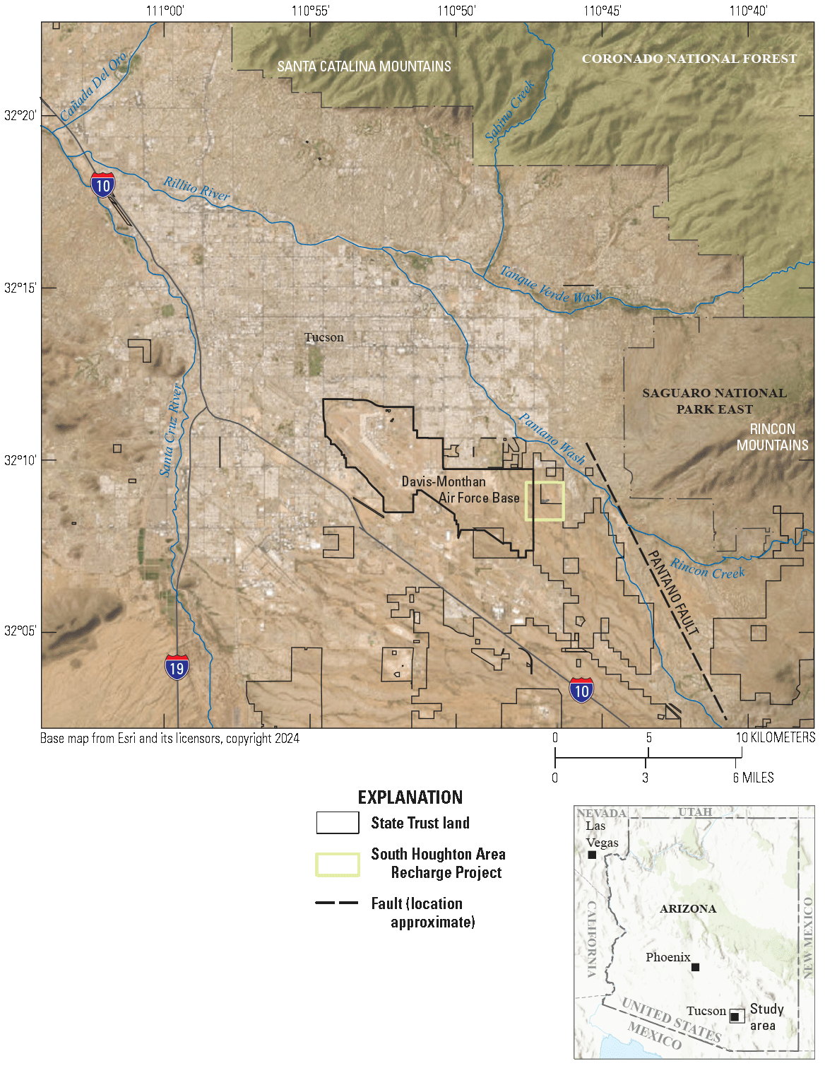
Regional map showing the Tucson Basin and the location of the Southeast Houghton Artificial Recharge Project.
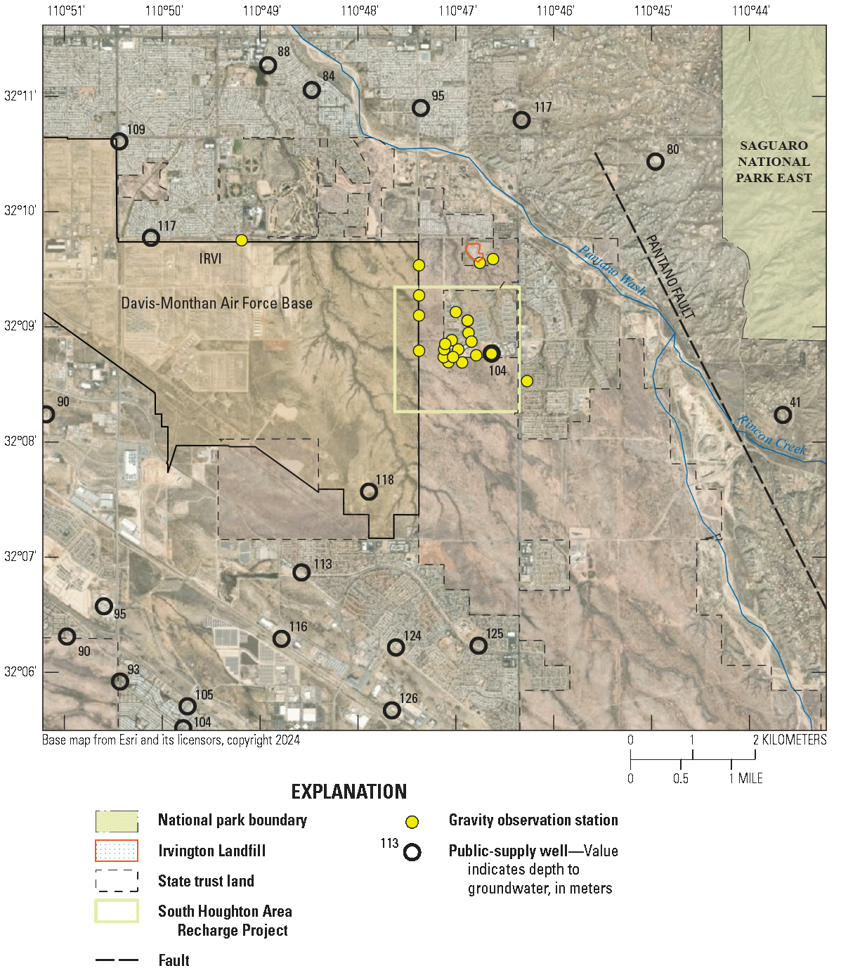
Map showing the study area and locations of public-supply wells, groundwater observation wells, and gravity observation stations. Numbers next to public-supply wells indicate depth to groundwater (in meters) in 2020 (Arizona Department of Water Resources, 2024).
In Arizona, operators of MAR projects are typically allowed to recover (pump) groundwater once water infiltrates at the land surface, with little restriction on where pumping occurs or whether it is the same physical water as that which was recharged (Arizona Department of Water Resources [ADWR], 2022a). Monitoring is often limited to measuring groundwater levels in a single or a few monitoring wells. Therefore, those operating MAR projects may benefit from improved monitoring and simulation of where recharged water is moving—both in the unsaturated zone and in the aquifer. In the unsaturated zone, fine-grained perching layers may limit infiltration rates or cause preferential flow above the regional aquifer to move water horizontally away from the facility. In the aquifer, groundwater flow in the regional aquifer may cause recharged water to move preferentially toward or away from recovery wells—a potential concern when reclaimed water (treated wastewater) is the recharge source. Additionally, where landfills or areas of contaminated soils are near recharge facilities, monitoring may be required to ensure recharged water is not at risk of mobilizing contaminants. There is a retired landfill approximately 1.5 kilometers (km) north of SHARP (figs. 2, 3), where depth to water was approximately 100 meters (m) below land surface before recharge began in December 2020.
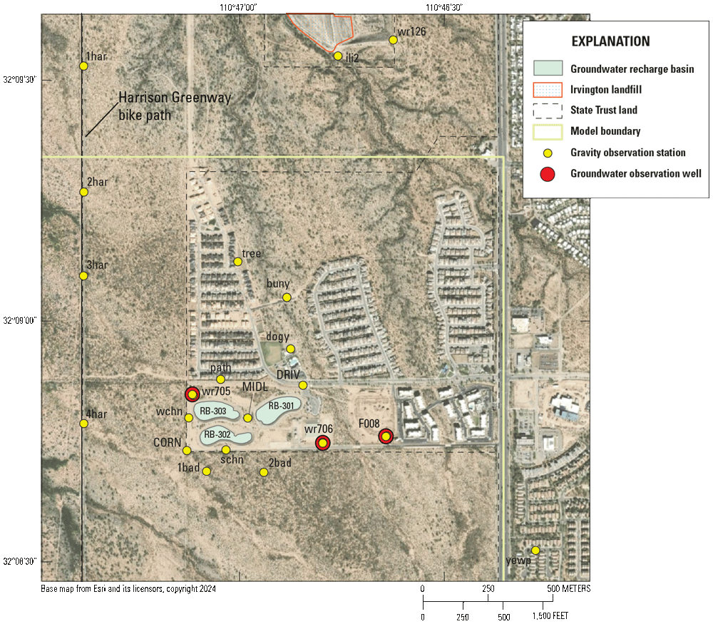
Map showing the Southeast Houghton Artificial Recharge Project, groundwater observation wells, and nearby gravity observation stations. Gravity stations where absolute-gravity data were collected are designated by capitalized station names; stations with relative-gravity data only are in lowercase letters.
Although groundwater-level monitoring is informative, it cannot provide complete understanding of how water moves through the subsurface. For a facility like SHARP, the volume of water delivered to the recharge basins is known and evaporation losses in the basins can be estimated, but the rate of the wetting front’s movement through the unsaturated zone, the degree of saturation in the unsaturated zone, and any horizontal dispersal as water moves through that zone cannot be determined from only groundwater-level measurements, which will not change until applied recharge reaches the water table and causes a head change in nearby wells. However, repeat microgravity observations (measurements of small changes in the acceleration due to Earth’s gravity caused by changes in subsurface mass) made on the land surface show a change in gravity immediately once water infiltrates, and are directly sensitive to changes in the total amount of water stored in the unsaturated zone and in the aquifer. Once recharged water reaches the aquifer, dispersal of that water into the aquifer depends on aquifer properties that are typically spatially heterogeneous or dependent on local geology such as faults. There are a few wells in the area (fig. 2), but because of differences in well construction and spatial heterogeneity of aquifer storage properties (that is, aquifer porosity), the same height of groundwater-level change in different wells may represent different amounts of storage change (that is, the change in height of freestanding water). Storage changes calculated from changes in water level in a well require an estimate of the aquifer storage coefficient (specific yield for an unconfined aquifer), because a well screened in a higher storage-coefficient unit will show a smaller change in groundwater level than a well screened in a lower storage-coefficient unit, given the same volume of storage change. In contrast, changes in storage derived from observed changes in gravity are independent of aquifer storage properties, and strictly related to the change in mass of water stored within the volume of the subsurface to which the measurement is sensitive.
To enhance understanding of groundwater-storage change in the subsurface, this study incorporates repeat microgravity monitoring at and around SHARP (fig. 3). Repeat microgravity is a direct, non-invasive measurement of mass change in the subsurface. These data are used to map the spatial distribution of subsurface water-storage change, and, in combination with groundwater-level data, identify soil infiltration and groundwater-flow parameters in a hydrologic simulation model. In turn, the calibrated model can be used to simulate storage changes resulting from future recharge inputs, which can support MAR management in any decision making.
Purpose and Scope
This report presents information about groundwater-storage change at SHARP based on groundwater-level measurements, repeat microgravity surveys, and groundwater-flow modeling. Monitoring was conducted in cooperation with Tucson Water, which operates the recharge facility. Groundwater-level measurements were collected by Tucson Water at three monitoring wells at daily to monthly intervals. Five gravity surveys, composed of as many as 22 stations, were completed from 2020 to 2022 and were timed to capture storage increases during periods of active recharge and storage losses during periods of no recharge when recharged water was dispersing away from the facility. The gravity changes were used to determine storage changes within the study area and to identify soil properties for the infiltration and groundwater-flow model Hydrus-3D (PC-Progress, Inc., 2022). The purposes of this project were to track infiltrated water moving within and away from the facility, estimate effective porosity and water content in the unsaturated zone, and develop an infiltration model for the facility that will allow for modeling of future recharge pulses.
Previous Investigations
A summary of the Tucson Basin’s formation, structure, and hydrogeology is provided in Davidson (1973), including references to older studies of the general basin geology not included here. Anderson (1987) provides a more detailed description of the Cenozoic stratigraphy of the basin, including the informal Tinaja beds of Davidson (1973) and the Fort Lowell Formation that are encountered within the study area of this report. Eastoe and others (2004) and Eastoe and Wright (2019) used isotope and other water chemistry data to delineate areas of distinct groundwater flow patterns within the basin and identified areas of preferential recharge to the aquifer along ephemeral channels, including Pantano Wash, a major ephemeral channel near the study area (fig. 2). A report prepared by Pima Association of Governments (2004) on groundwater conditions and hydrological characteristics within the Rincon Valley (east of and including the study area of this report) discusses trends in groundwater pumping and shallow groundwater areas observed at that time.
Groundwater storage changes have been estimated from repeat microgravity data for several previous studies in the Tucson Basin. A regional network consisting of more than 150 stations dispersed across the Tucson Basin and Avra Valley, including one of the stations used for this report (IRVI, formerly known as E09A), is described in Pool and Anderson (2008) and Carruth and others (2018). Ephemeral channel recharge was monitored along the Rillito River, and found to vary with climatic indicators, including the El Niño-Southern Oscillation (Pool, 2005). Discrete and continuous repeat microgravity data collected at a managed aquifer recharge project in Avra Valley, west of the Tucson Basin, were used in conjunction with groundwater levels to constrain parameters in a groundwater flow model (Kennedy and others, 2016), and to estimate the depth of the wetting front beneath a recharge basin (Kennedy and others, 2014).
Setting
The study area is within Pima County in southeastern Arizona, approximately 20 km southeast of downtown Tucson; it is located in the Sonoran Desert near the western flank of the Rincon Mountains, approximately 3 km west of the confluence of Pantano Wash and Rincon Creek, both of which are ephemeral channels (figs. 1, 2). The study area includes residential areas and largely undeveloped State Trust lands (fig. 2).
Climate
The climate of the Sonoran Desert and the study area is semiarid, with most precipitation occurring in the summer monsoon or winter rainy seasons. Average annual precipitation on the Tucson Basin floor is 26.9 cm (National Weather Service, 2021), but variability from year to year can be quite large: 10.6 cm of precipitation was measured in 2020, and 41.1 cm in 2021. The monsoon season, which officially occurs between June 15 and September 30, yields an average of 14.5 cm of rain but can also be highly variable from year to year.
Temperatures often rise above 100 degrees Fahrenheit in May through September, with a mean of 2 days per year above 110 degrees (National Weather Service, 2021). In both 2020 and 2021, there were 8 daily high temperatures over 110 degrees, close to the record of 10 days that occurred in both 1990 and 1994 (National Weather Service, 2021). The potential annual evapotranspiration is about four times the average annual precipitation (Laney, 1972; Davidson, 1973). Beyond ephemeral channels and managed aquifer recharge projects, high potential evapotranspiration and large depth to water results in little or no direct land-surface recharge from rainfall.
Geology
The Tucson Basin, a valley within the Basin and Range Province, is bounded by the Santa Catalina Mountains to the north and Rincon Mountains to the east (fig. 1). The Santa Catalina Mountains and Rincon Mountains formed at least 23 million years before present and are composed mostly of metamorphic and igneous rocks that have low porosity and permeability (Davidson, 1973). The bedrock is mostly granitic gneiss with evidence of uplift and faulting in the middle to late Tertiary (Anderson, 1987). The Tucson Basin, which formed throughout the Cenozoic, has accumulated more than 3,000 m of sedimentary deposition (Richard and others, 2007).
The primary stratigraphic units that fill the Tucson Basin are the Pantano Formation, the informal Tinaja beds of Davidson (1973), and the Fort Lowell Formation. The Tertiary Pantano Formation is the deepest potential water-bearing unit in the basin, but it is not well constrained in the study area, and none of the wells used for this report are screened in that unit. The late Tertiary Tinaja beds unconformably overlie the Pantano Formation and are generally composed of gravels, conglomerates, and silty clays; they are divided into three distinct, unconformable subunits—the lower, middle, and upper parts of the Tinaja beds (Anderson, 1987). The upper part of the Tinaja beds varies from 180 to 300 m thick, and many public-supply wells are screened in this subunit (Davidson, 1973). The Pleistocene Fort Lowell Formation overlies the Tinaja beds, is largely composed of layers of sand (with some gravel closer to the top of the unit), and is estimated to be about 90 m thick (Davidson, 1973). The Fort Lowell Formation is exposed near the foothills of the Rincon Mountains and is estimated to extend about 15–75 m below the surface (Anderson, 1987), with recent alluvial deposits overlying it in places.
The Pantano Fault, a northwest-trending fault approximately 10 km long, passes just east of the confluence of the Pantano Wash and Rincon Creek (fig. 2). The exact location of the Pantano Fault has not been mapped, though the approximate location has been inferred based on water levels and field observations by Anderson (1987) and Baird and others (2001) (fig. 2). Along the foothills of the Rincon Mountains, the Tucson Basin is downfaulted and deepens to the west (Anderson, 1987). The depth to groundwater in the study area also increases west of the fault, likely due to increased depth to bedrock and distance from the recharge source of the ephemeral washes.
Hydrogeology
Groundwater levels (that is, water-table elevations) within the Tucson Basin vary based on proximity to natural recharge sources, such as mountain front areas and ephemeral streams, and to spatially and temporally variable groundwater pumping. Generally, large depth to groundwater and a potential evaporation rate that far exceeds annual precipitation preclude precipitation that infiltrates the land surface from recharging the aquifer. Instead, over much of the basin, shallowly infiltrated water may be entirely lost to evapotranspiration. Of the precipitation that runs off to ephemeral channels, as much as 75 percent may ultimately infiltrate within the basin, though this does not include losses due to evapotranspiration (Davidson, 1973). This percentage likely fluctuates over time owing to variation in climate, vegetation, and impervious land cover resulting from urbanization.
The overall movement of groundwater in the southeastern part of the Tucson Basin, including the study area, is southeast to northwest (fig. 2). However, groundwater flow will be influenced locally by proximity to ephemeral channels, pumping wells, and spatially variable properties of the subsurface. Groundwater levels within the study area are highest near the convergence of Rincon Creek and Pantano Wash, because of runoff infiltrating through the channel bottoms, and relatively shallow near the foothills of the Rincon Mountains. Groundwater levels decrease rapidly west of Pantano Wash, and less rapidly along Pantano Wash to the northwest from its confluence with Rincon Creek (fig. 2). Groundwater levels at the confluence of Pantano Wash and Rincon Creek were approximately 16 m below land surface in 2010 (Postillion and Scalero, 2014, and references therein) but as of 2020 were approximately 41 m below land surface at a well located just south of the juncture between the channels (ADWR, 2024; fig. 2)—still the shallowest depth to water within the study area. However, this well appears to be just east of the estimated location of the Pantano Fault (well 41 on fig. 2), which may cause anomalously higher groundwater levels on the east (upthrown) side in places (Davidson, 1973).
SHARP (fig. 3) is located approximately 3 km west of the confluence of Pantano Wash and Rincon Creek and does not appear to overlie the relatively shallow zone of groundwater closer to the wash, as delineated in Davidson (1973). Reduced groundwater pumping in the last two decades has resulted in groundwater-level increases in some parts of the basin (Carruth and others, 2018). However, groundwater levels within the study area continue to decline, though in some locations that decline has slowed or stabilized in the past decade. Groundwater Site Inventory (GWSI) well 320845110463601 (F-008A) is a pumping well located within SHARP where absolute-gravity measurements were made for this study (fig. 3). Groundwater levels at this well remained relatively stable at around 104 m below land surface from 2010 to 2019, the period immediately preceding recharge at SHARP (fig. 2). Depth to groundwater at the two monitoring wells at the facility were relatively stable at 106.9 and 105.9 m below land surface prior to the beginning of recharge (wells WR-706A and WR-705A, respectively; fig. 3). There is active residential development, including developments completed during the study period north and east of SHARP, but the onsite supply well (F-008A) was not used during the study period, limiting the effect of these development areas on groundwater conditions in the study area during the study period.
Estimates of the bottom elevation of the Fort Lowell Formation suggest that the interface between the Fort Lowell Formation and the upper part of the Tinaja beds lies between the land surface and the water table at SHARP. This interface could occur between 60 and 90 m below land surface according to maps in Anderson (1987) or as deep as 100 m below land surface according to Davidson (1973). Differentiating between these two units in drill logs can be difficult or impossible (Davidson, 1973), but the degree of cementation of the Tinaja beds is generally greater than that of the Fort Lowell Formation (Davidson, 1973). The variation in hydraulic properties among the layers of the Fort Lowell Formation and the Tinaja beds raises the possibility of a perching layer and (or) preferential horizontal dispersal of infiltrating water above the regional water table. Driller’s logs for the three wells at SHARP were compared with a description of the layers of the Fort Lowell Formation in Davidson (1973), but there was no clear correlation with the layers of that unit, or of any transition that might be associated with the interface between the Fort Lowell Formation and the Tinaja beds. The logs describe coarse sand and (or) gravel with some intervals containing clay (ADWR, 2023). There was no clear correlation between wells in either the described units or the relative thicknesses of layers identified at each well.
Groundwater Table Mounding
Often at managed aquifer recharge facilities, a groundwater mound develops at the water table when the recharge rate is greater than the rate at which groundwater flows away into the aquifer (Hantush, 1967). The magnitude and extent of groundwater-level change is a function of infiltration rate and aquifer properties. Using the Hantush (1967) analytical solution for groundwater mound geometry, Carleton (2010) found that in higher permeability aquifers, the groundwater mound will be shorter and broader than the equivalent mound in a lower permeability aquifer (Carleton, 2010; fig. 4). Based on an analytical solution for transient recharge, Rai and Singh (1995) found that a high-specific-yield aquifer would develop a recharge mound that is shorter and less broad than an aquifer with lower specific yield. Simulated groundwater mounding for these scenarios (calculated using the Excel worksheet in Carleton [2010]) confirms these relations (fig. 4).
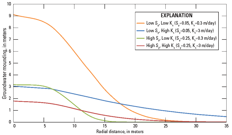
Groundwater mounding calculated using the Hantush (1967) analytical solution as implemented by Carleton (2010). Calculations are for a recharge basin 20 meters by 20 meters in area, after 2 days of infiltration at 0.4 meters per day (m/day) and an initial saturated thickness of 3 meters. Sy; specific yield, Ks; saturated hydraulic conductivity.
There are several limitations to these and other analytical solutions with respect to recharge at SHARP. For some analytical solutions (for example, Hantush, 1967), the unsaturated zone and transient recharge is ignored, and the solutions only provide the position of the water table for steady-state conditions, which are likely never reached at SHARP because of the thick unsaturated zone. Models that ignore the unsaturated zone have increased error relative to models that include it when the recharge cycle period is shortened, as the depth to the water table increases, with increasing subsurface anisotropy, and with the inclusion of fine-textured strata (Sumner and others, 1999). Other analytical solutions (Marino, 1974; Rai and Singh, 1995) assume the presence of nearby surface reservoirs (that is, constant-head boundaries), a condition dissimilar to the large, regional aquifer that receives recharge at SHARP. Finally, nearly all analytical solutions for groundwater mounding from surface reservoirs, and their applications, are developed for areas with relatively thin unsaturated zones. In contrast, the more than 100-m-thick unsaturated zone in the study area has the potential to store and divert substantial volumes of water before it can reach the water table. Conditions likely never reach steady state because facilities operate in cycles with periods (weeks to months) of recharge and non-recharge. The thick unsaturated zone likely contains successive wetting fronts moving downward in parallel, never fully saturating nor drying the subsurface.
Methods
Data collection included repeat microgravity data and accompanying global position system surveys (Landrum, 2024), recharge basin inflow data (ADWR, 2025), estimated evaporative losses from recharge basins (appendix 1) and groundwater-level data (appendix 2).
Recharge Volume and Groundwater Levels
The volume of water delivered to each recharge basin was measured directly by Tucson Water using ultrasonic flowmeters on the delivery pipes. Evaporation losses, estimated and subtracted for the period when basins were at least half covered in water, are relatively small (appendix 1). The average monthly evaporation loss is about 925 m3 (0.75 acre-foot), compared to daily delivery volumes when the basins are recharging that are consistently above 5,000 m3 (4 acre-feet). The method Tucson Water uses for calculating evaporation is defined by Arizona Department of Water Resources (ADWR) and required for use at permitted recharge facilities (ADWR, 2022a).
Continuous (transducer) and discrete (manual) groundwater-level data were collected at wells WR-705A and WR-706A (collocated with gravity stations wr705 and wr706, respectively, shown on fig. 3) by Tucson Water, and a subset of those data used in this report are included in appendix 2, as changes in depth to water below land surface datum. Discrete data were periodically collected at well F-008A (fig. 2) and those measurements are published in the ADWR GWSI database (ADWR, 2023). Although F-008A is a production well, no substantial pumping took place during the study period (small amounts of water, less than ~1,200 m3 [1 acre-foot] in total, were pumped for water quality testing).
Repeat Microgravity
Gravity data were collected at 22 locations—14 stations immediately surrounding the recharge facility and 8 stations located approximately 0.3 to 3.5 km away from the facility (fig. 2). Two initial stations north of the facility (path, tree) were destroyed between surveys due to residential development, and one station (dogy) was established later, in 2021, after development in the area was completed. Gravity data were collected using a combination of relative- and absolute-gravity meters (Kennedy and others, 2021a). Gravity stations where absolute-gravity data were collected are designated by capitalized station names (DRIV, MIDL, CORN, F008, IRVI); all other gravity station names are in lowercase letters. Where gravity stations and wells are collocated, the gravity station name is as similar as possible to the well name but follows the capitalization convention for gravity stations and excludes any symbols or unnecessary letters (for example, wr705 is the name of the gravity station that is collocated with well WR-705A). Of the eight stations located away from the facility, four stations were established along the Harrison Greenway bicycle path (1har, 2har, 3har, 4har); two were preexisting stations (IRVI, yewp) that are also monitored approximately every two years for a regional gravity project (Carruth and others, 2018); and two stations (ili2, wr126) were established at monitoring wells at the retired landfill north of the facility (fig. 2). These eight observation locations were chosen to (1) track any storage changes spreading immediately to the west or northwest of the facility, (2) obtain information about regional storage changes occurring in the broader study area during the study period, and (3) determine if recharge from the facility was approaching the landfill area. Permission to install additional stations between the facility and the Harrison Greenway could not be obtained from the landowner.
The absolute-gravity meter (Micro-g Lacoste, Inc. A-10, serial number 008) measures the acceleration of a free-falling mass, and relative-gravity meters (Lacoste & Romberg D meter and ZLS Burris meters) measure the difference in gravity between two locations. Both instruments are accurate to 3–8 microgals (µGal); one µGal is 1×10⁻⁸ m per second squared and equivalent to about 2.38 cm of water using the horizontal-infinite slab approximation (eq. 1). Absolute- and relative-gravity data were combined in a network adjustment using GSadjust software (Kennedy, 2020). Changes in the gravity field between two surveys can be directly related to changes in the amount of water stored in the unsaturated zone and the groundwater system (eq. 1).
Corrections to gravity data focus on accounting for the time-varying changes in the gravity field not related to water-mass change, including land-surface elevation (LSE) change, Earth tides, ocean loading, and atmospheric pressure change (Kennedy and others, 2021a). Sentinel-1 interferometric synthetic aperture radar (InSAR) data processed in the study area by ADWR show a maximum of 6 millimeters (mm) of LSE change between the study period start and end (specifically, between April 2020 and March 2022; ADWR, 2022b). The accuracy of Sentinel-1 InSAR data is typically assumed to be less than 8 mm and possibly as low as 5 mm (Cigna and others, 2021), which puts the observed LSE change for the study period into the range of accuracy for the method. Therefore, corrections to observed gravity values to account for changes in LSE were not required. Corrections for Earth tides and ocean loading are applied in real-time when collecting relative- and absolute-gravity data, and atmospheric pressure is accounted for when collecting absolute-gravity data. After data have been corrected for these terms, changes in gravity are directly related to the change in water stored at the water table, modeled as a “horizontal infinite slab” of free-standing water:
whereΔg
is the change in gravity caused by a change in the thickness of a slab of free-standing water, in µGal;
ΔStorage
is the change in thickness of that slab of free-standing water, in meters; and
41.9
is a constant derived from the horizontal infinite slab approximation (Telford and others, 1990).
Where water-storage changes are not in horizontal layers, the full three-dimensional region of sensitivity of a gravity measurement must be considered. Typically, and here, storage change below the water table (owing to compressibility of water and the aquifer) is assumed negligible, and therefore the water table is considered a lower bound to the region of sensitivity. Mass changes in the atmosphere are ignored. Between the land surface and the water table, sensitivity varies according to z/r3, where z is the vertical distance to a unit of mass change and r the radius, resulting in a cone-shaped region of sensitivity which expands with depth below the gravity meter. That is, the sensitivity to a unit of mass decreases with distance, but the region over which the gravity meter is sensitive expands with distance. Mass changes on the same horizontal level as the gravity meter (that is, at the land surface) are effectively invisible. For a single gravity station adjacent to a recharge basin, sensitivity increases as the infiltration wetting front moves deeper into the subsurface (Kennedy and others, 2014). In other words, as the wetting front moves from 0 to 1 m depth, that mass change is effectively invisible to the gravity meter; as the wetting front moves from 100 to 101 m depth, that mass change causes a much greater change in gravity. In some scenarios, modeling indicates that departure from the horizontal infinite slab approximation is minimal even when significant groundwater mounding occurs (Kennedy and others, 2022), and the horizontal infinite slab approximation (eq. 1) is probably suitable for gravity stations in this study that are more distant from the recharge basins. However, the unique spatial relation between mass change and the gravity meter’s region of sensitivity at stations closer to the recharge basins requires full three-dimensional modeling of mass change throughout the subsurface in order to extract maximum information from the data. One method for creating such mass-change distributions, which also furthers understanding of the site’s hydrology, is numerical infiltration and groundwater-flow modeling.
Modeling
The distribution of infiltrated water in the subsurface was simulated by numerical modeling for the purpose of (1) determining the change in water content between the initial dry condition and when recharge was active, (2) placing bounds on the spatial extent of mounding at the water table and the resultant density change, and (3) estimating groundwater conditions under future recharge scenarios.
Unsaturated-Zone Flow Modeling
To overcome the limitations of analytical solutions for groundwater mounding described above, a numerical model of unsaturated-zone flow was developed. For this purpose, Hydrus-3D (PC-Progress, Inc., 2022) was used to solve the three-dimensional Richards equation for subsurface water flow above and below the water table.
The Kosugi (1996) soil-water retention model was used because it provided better stability for the numerical solution compared to the van Genuchten and Brooks-Corey models also available in Hydrus-3D. The Kosugi model assumes a lognormal pore size distribution, resulting in the relation
whereSe
is effective saturation;
θ
is water content;
θr and θs
are residual and saturated water content, respectively;
erfc
is the complimentary error function;
h
is pressure head;
α
is the mode of the pore capillary pressure distribution; and
n
is a parameter that determines the value of Se at α.
The Hydrus-3D model was constructed as a square domain, 1,600 m by 1,600 m, aligned with the cardinal directions and centered on the three recharge basins. The base of the model is the pre-recharge water table, and the model only simulates unsaturated-zone flow, groundwater mounding, and unconfined water-storage change above the water table. All recharge is contained within the model boundaries for the duration of the simulation. The base of the model slopes to the northwest, consistent with the difference in groundwater levels at wells WR-705A and WR-706A and the slope of the regional potentiometric surface (Mason and Hipke, 2013). As a result of this slope (6.5 m per km), the water table is 18.8 m higher at the southeast corner of the model than at the northwest corner. The model is solved on a triangular finite-element mesh with approximately 90,000 elements. Variable element sizes were used to balance numerical accuracy with computation time. In the x and y directions, element size varied from approximately 90 m across at the edges of the model to 30 m across at the center of the model. Vertical discretization was finest, about 0.1 m, at the top and bottom of the model where hydraulic gradients in the unsaturated zone are greatest and increased to about 1.8 m near the vertical center of the model. The model is solved with adaptive time steps, depending on convergence criteria, between 0.00001 and 5 days in length (time steps with lengths between 0.1 and 0.5 days were typical).
Initial conditions were established by first running the model with pressure head equal to zero at the bottom boundary to create an equilibrium soil-water content profile above the water table. Negative pressure head was limited to −10 m (more negative values generally resulted in numerical non-convergence). This equilibrium water content was used as the initial condition for the model that simulates infiltration flux. Boundary conditions were constant pressure head (h=0) at the lower outside boundary of the model, and specified flux at nodes on the upper surface at the location of the recharge basins. Flux for each basin was set equal to the volume of recharge per day delivered to each basin as reported by Tucson Water, minus estimated evaporation losses. Although water is delivered to each basin approximately once every third day, average infiltration flux over each recharge cycle was used as model input in order to increase stability of the numerical solver (rapid, frequent flux changes cause instability). Modeled infiltration began on December 8, 2020 (model day 0), and flow simulation continued through the date of the last gravity survey, October 24, 2022 (model day 685).
All flux into the model is the result of infiltration recharge; regional groundwater flow is not simulated. The constant pressure head boundary in the model prevents the groundwater mound from extending outside the model boundaries. Over a long period, nearby pumping or recharge (such as infiltration from Pantano Wash) could alter the water table elevation in the vicinity of SHARP, thus influencing the groundwater mound developed from recharge. Therefore, to fully simulate the long-term evolution of recharge at SHARP, the unsaturated-zone model presented here would need to be coupled with a regional groundwater-flow model, such as MODFLOW (Harbaugh, 2005), that simulates the horizontal transport of recharged water in the aquifer.
Gravity Forward Modeling
Gravity forward modeling is the process of simulating gravity change at the measurement locations, as caused by the addition of recharged water in the subsurface. First, water content simulated by Hydrus-3D is output on the triangular mesh nodes used to simulate water flow. This water content is then interpolated on a regularly spaced, rectangular grid with 100 elements in each of the x, y, and z directions (grid cells were 16 m by 16 m by 1.06 m). Within each grid cell (voxel), mass change is calculated as the density change times the cell volume.
The forward gravity calculation is carried out by summing the gravitational attraction of the change in water content in each cell, relative to each gravity station location, at each time step. One of two equations were used, depending on the distance between the cell and the gravity station (Leirião and others, 2009):
whereG
is the gravitational constant (6.674×10⁻¹¹ cubic meters per kilogram seconds squared [m3kg-1s-2]);
Δm and Δρ
are the change in mass and change in density in a given cell, respectively;
x, y, and z
are the horizontal and vertical distances between the gravity station and the cell corners; and
r
is the straight-line distance between the gravity station and the cell center.
Gravity forward modeling for interpolation, using equations 4 and 5, was carried out in MATLAB (Kennedy, 2024). The change in density, Δρ, is the change in volumetric water content reported for each time step by Hydrus-3D. Computation time was on the order of 1–2 hours on a single central processing unit for each Hydrus-3D model run, plus about 3 minutes for the forward gravity modeling, most of which is interpolating water content from the triangular Hydrus-3D mesh to a prismatic grid.
Parameter Estimation
Parameter sensitivity analysis and estimation for the Hydrus-3D model was carried out using PEST++ (White and others, 2020), specifically using the pestpp-sen and pestpp-glm programs. Pestpp-sen carries out global sensitivity analysis by varying parameters over a range of acceptable values, using the method of Morris (1991) to vary parameters one at a time and evaluate the effect on model output. Pestpp-glm implements a gradient descent method to determine optimal parameter values by minimizing an objective function based on the misfit between simulated and observed values. Soil parameters varied were n, α (both fitting parameters for the Kosugi log-normal soil model, eq. 3), saturated soil water content (residual water content is fixed at 0.065), and saturated hydraulic conductivity. Sensitivity to horizontal and vertical anisotropy were also considered. The model outputs used to evaluate sensitivity were (1) the change in groundwater head at monitoring-well locations and (2) the change in gravity at each gravity station. These same outputs were compared to measured values to calculate an objective function.
Results
During the study period from winter 2020 through fall 2022, large gravity increases related to groundwater-storage change were observed, along with increases in groundwater level at the monitoring wells. Estimated monthly evaporation loss data reported by Tucson Water to ADWR are provided in appendix 1. Groundwater-level data are provided in appendix 2. Gravity data are published in Landrum (2024).
Groundwater Levels and Repeat Microgravity
Deliveries and recharge at SHARP began in December 2020 and continued periodically through the study period (fig. 5A). An initial groundwater-level rise in response to recharge was observed about 5.5 months after recharge began. At the two nearest wells, WR-705A and WR-706A, the increase appears to happen nearly simultaneously. However, the exact date that the increase began is difficult to determine, especially at WR-706A, owing to non-recharge related fluctuations in groundwater level. Following a period of no recharge from March 28, 2021, to July 1, 2021, recharge began again on July 2, 2021, and a steady increase in groundwater level at both wells was observed beginning in early August 2021 and continuing through May 2022, when groundwater levels in WR-705A and WR-706A peaked at about 21.6 m and 14.3 m, respectively, above their pre-recharge elevation. The date of peak groundwater level occurred less than a week after the end of the recharge period (the exact date cannot be determined because groundwater-level data were collected weekly during this period). Recharge operations began again on August 12, 2022, and continued through December 7, 2022, leading to a second period of rapidly increasing groundwater levels. The lag between the onset of recharge and the corresponding increase in groundwater level appears to decrease with each successive recharge cycle, although the exact progression cannot be determined because groundwater-level data were collected monthly during the fall 2022 recharge cycle.
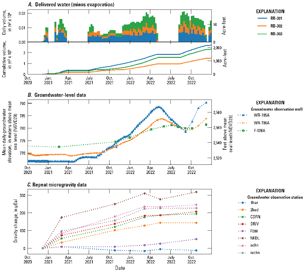
Plots showing (A) water deliveries, (B) groundwater-level elevation, and (C) repeat microgravity data at select stations at the Southeast Houghton Artificial Recharge Project from 2020 to 2022. Panel A shows the daily average volume, summarized per week, delivered to each basin. Recharge began on December 8, 2020. The first gravity survey was carried out in June 2020, representing baseline, pre-recharge conditions. To show the rapid increase in gravity following the onset of recharge, the June 2020 data are plotted as if occurring on December 8, 2020 (that is, all of the gravity change between June 2020 and March 2021 is assumed to be from recharge occurring between December 8, 2020 and March 2021). RB; recharge basin.
Gravity increases also accompanied recharge at SHARP. These increases were large at the stations nearest the 3 basins during the second gravity survey in March 2021, 4 months after recharge began and about 1.5 months before the initial groundwater-level increase. Gravity station MIDL, between the 3 basins, had the largest cumulative increase in gravity over the study period, with several other stations—all very close to the recharge basins—showing similar increases of 100 µGal or more (fig. 5C). These increases are maintained during the rest of the study period, but the data likely miss a decrease (and subsequent increase) in gravity between the May and October 2022 surveys during which the groundwater mound dissipated during a non-recharge period. The October 2022 gravity survey includes the effect of the recharge cycle that began in August 2022 (fig. 5C).
Gravity values decrease rapidly with distance from the recharge basins. All stations away from the facility show slight gravity declines and therefore groundwater-storage loss during the study period, and the losses are greater with distance from SHARP, consistent with ongoing groundwater declines and storage losses in the study area away from the recharge facility (figs. 6, 7; March 2021 was chosen as the starting date for fig. 7 because the maximum number of stations are available during that period). Stations buny, wr706, and F008—all located within about 500 m of SHARP—showed only small gravity increases ranging from 7.2 to 30.7 µGal. These data are consistent with water moving vertically through the unsaturated zone and not spreading horizontally (at least not to the west, north, and east). A smaller increase at wr706 (7.2 µGal) than at F008 (30.7 µGal)—despite the former station being 150 m closer to SHARP—is inconsistent with a model consisting only of vertical recharge through the unsaturated zone. This could be related to unreported pumping at well WR706-A, error in the gravity data, or non-hydrologic mass change affecting one or both stations.
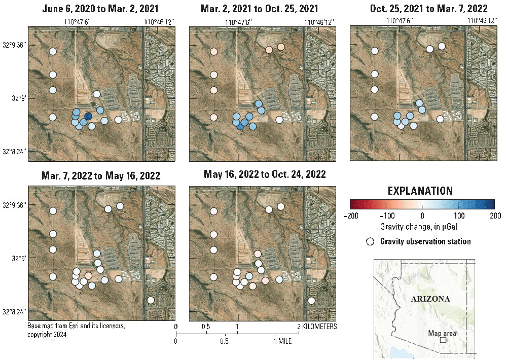
Maps showing gravity change at gravity observation stations near the Southeast Houghton Artificial Recharge Project between the dates indicated above each map.
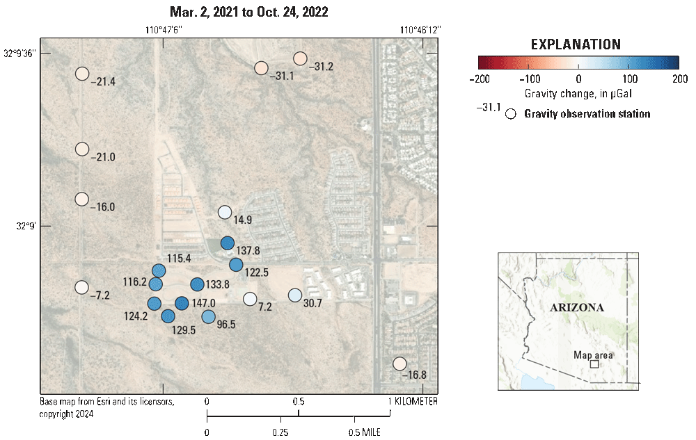
Map showing cumulative gravity change from March 2021 to October 2022 at gravity observation stations near the Southeast Houghton Artificial Recharge Project. Recharge began December 8, 2020.
Groundwater Modeling
A Hydrus-3D model was constructed to simulate infiltration and groundwater mounding during the study period (Kennedy, 2024). An initial sharp wetting front develops beneath the basins as shown in figure 8, which shows a one-dimensional profile of volumetric water content below recharge basin RB-301. At model day 0 the soil profile is uniform at the residual water content (0.065). The capillary fringe above the water table is visible at the bottom of the profile as water content increases to the saturated water content (0.38). By day 17, the wetting front is about 20 m below land surface. This represents just 10 days of recharge, as this basin was kept dry during the first week of operations (fig. 5). Inflow to recharge basin RB-301 is turned off on day 27, and simulated water content near the surface decreases substantially by day 34, although a sharp wetting front still exists at about 60 m below land surface. Simulated water content decreases further by days 51 and 240 but remains elevated above pre-recharge levels. At day 360 (153 days into the recharge cycle that began in summer 2021) simulated water content is nearly uniform throughout the unsaturated zone at about 0.20. Similarly, at day 685 (72 days into the recharge cycle that began in summer 2022) simulated water content above the water table is uniform at about 0.235, the maximum observed during the simulation period. During the simulation a groundwater mound develops on the sloping water table, growing and dissipating with successive recharge cycles (figs. 8, 9)
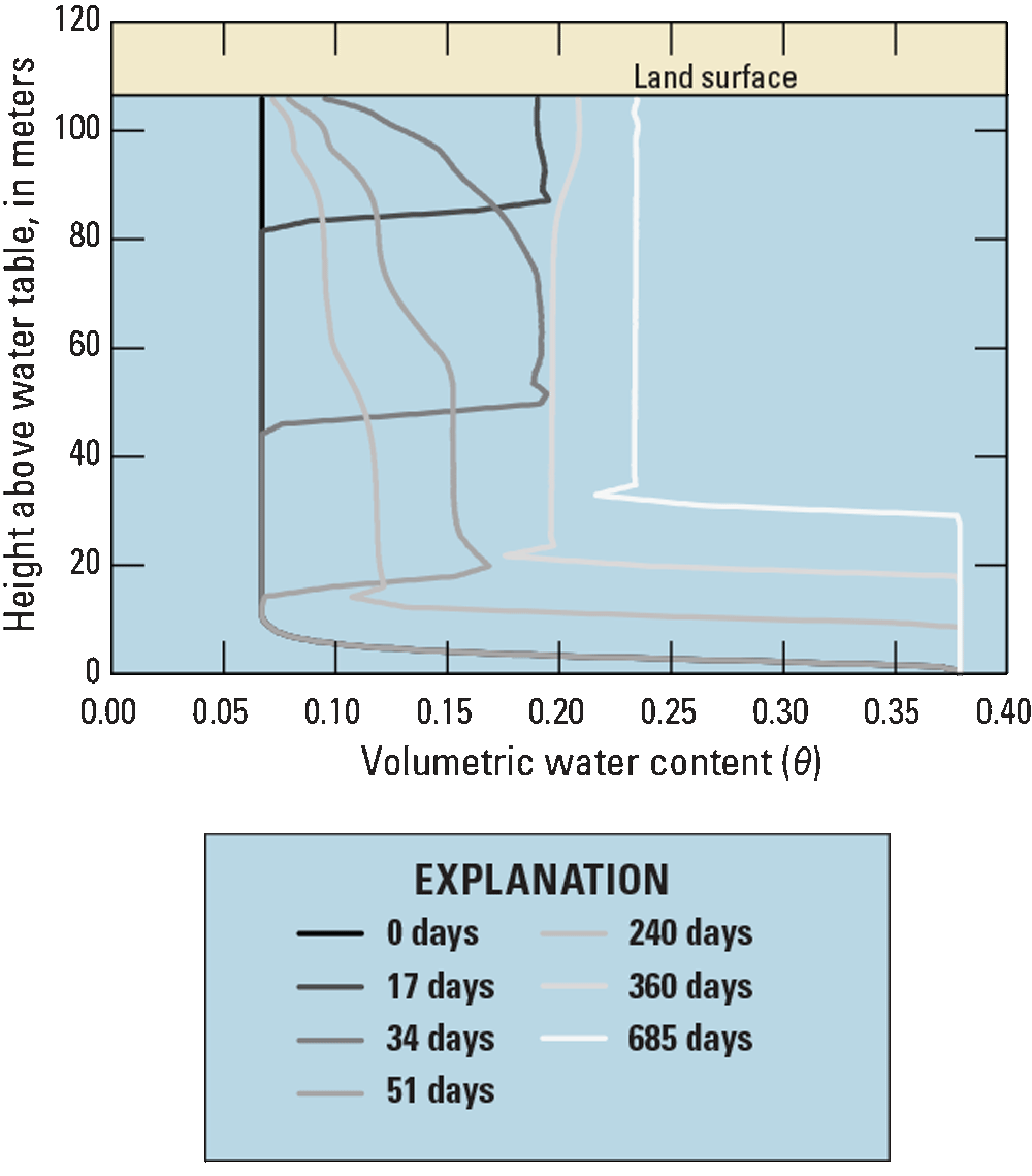
Plot showing water content above the water table as simulated by the model Hydrus-3D. The profile is located beneath recharge basin RB-301.
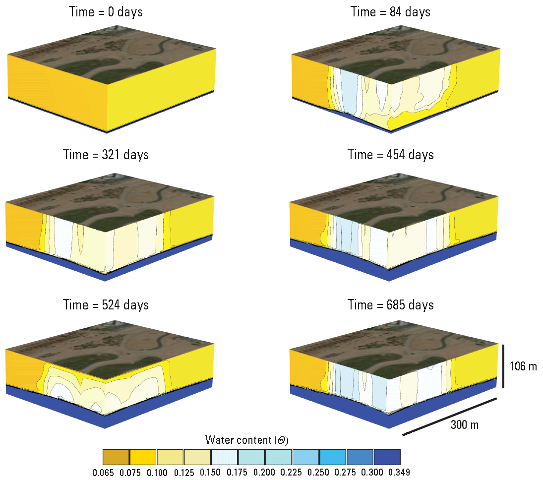
Cutaway views, looking northeast, of simulated water content at the Southeast Houghton Artificial Recharge Project using Hydrus-3D. Model output is at the time of each gravity survey, as indicated by the time above each panel. Only a portion of the model domain is shown. Scale bars are approximate; scale varies in this perspective view. θ, water content; m, meter.
Following model construction (defining initial and boundary conditions, generating the computational mesh, and assigning material properties), parameter sensitivity analysis was carried out to determine which model outputs (simulated gravity change and groundwater-level change) were sensitive to which parameters (n, α, saturated water content, and saturated hydraulic conductivity). Simulated gravity was calculated at each station in the gravity network, at the time of each survey. These surveys corresponded to model days 0 (December 7, 2020), 84 (March 2, 2021), 321 (October 25, 2021), 454 (March 7, 2022), 524 (May 16, 2022), and 685 (October 24, 2020). Although the initial gravity survey took place in June 2020, it was assumed to represent conditions at the start of recharge in December 2020 because the summer monsoon (which is responsible for the majority of annual rainfall in the study area) in 2020 was one of the driest on record (with a total of about 4 cm of precipitation, compared to the normal of about 14.5 cm; National Weather Service, 2021) and subsurface water storage change during June–December 2020 was probably small based on accumulated groundwater-level change during that period (appendix 2). Model predictions of groundwater-level change were extracted at approximately 40-day increments during the period that transducer (continuous) groundwater-level data were available, and on days when manual measurements were made during the period that transducer data were not available.
Model results from Hydrus-3D show infiltration reaching the water table by the time of the first gravity survey on model day 84 (fig. 9). Under all model simulations, infiltration takes place through an unsaturated subsurface. That is, the region between the infiltration basins and the water table never reaches the fully saturated water content. Infiltrated water spreads laterally in the unsaturated zone to some degree, but even through model day 685, the “infiltration footprint” beneath each basin remains distinct and the saturated areas do not coalesce into a single region (fig. 9). With successive recharge cycles, these subsurface interbasin areas will likely continue to increase in water content, thus increasing basin infiltration rates. Near the end of the model-simulated duration of the study, at 633 days, the radial extent of groundwater mounding is about 1 km (fig. 10).
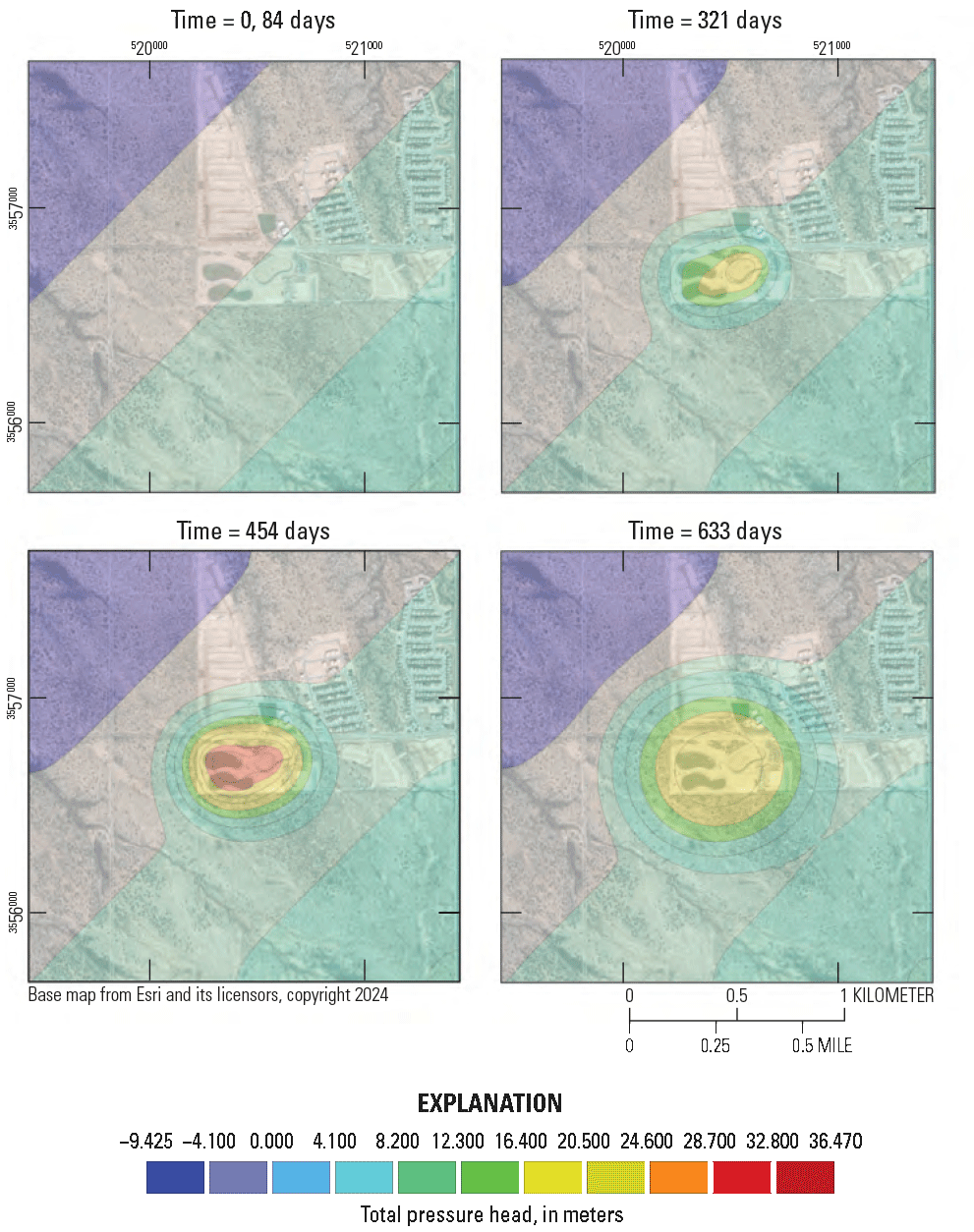
Total pressure head relative to a horizontal surface at the bottom of the model domain (h=0) simulated using the Hydrus-3D unsaturated-zone flow model. The water table slopes downward from the southeast to northwest. Pre-recharge depth to water underneath the recharge basins is about 106 meters.
Parameter sensitivity was initially evaluated by running four infiltration scenarios with high and low values of saturated hydraulic conductivity (Ks=10.0 and 1.0 m per day [m/day]) and saturated water content (θs=0.4 and 0.2). In each scenario, identical amounts of water were introduced to the subsurface through the variable flux boundary condition at each basin. These parameter scenarios simulated a wide range of gravity change and groundwater-level change (fig. 11). At the station central to the three recharge basins, MIDL, the simulated gravity increase ranges from less than 200 µGal for the high Ks, low θs scenario (orange line with square markers in fig. 11) to more than 700 µGal for the low Ks, high θs scenario (purple line with square markers in fig. 11). In this latter scenario, larger gravity changes occur at MIDL and DRIV because more of the infiltrated water is stored in the near-surface unsaturated zone, a region to which the gravity measurement is sensitive.
Similarly, groundwater-level changes were distinct with each scenario; at the monitoring well closest to the recharge basins, WR-705A, the increase in groundwater level ranged from just over 20 m for the high Ks, high θs scenario (green line with circle markers in fig. 11) to over 60 m for the low Ks, high θs scenario (pink line with circle markers in fig. 11). Although both data types show distinct behavior for different parameter scenarios, they represent different parts of the groundwater system. Groundwater-level changes reflect only the change in storage that occurs at the location of the monitoring well, after recharged water has infiltrated vertically to the water table and displaced water in the aquifer horizontally. Groundwater-level changes can vary substantially and unpredictably over short distances, resulting in data that are sensitive to the exact location of a monitoring well (Pool, 2005). Although groundwater-level changes can be measured precisely, uncertainty exists in how representative they are of the aquifer. In contrast, changes in gravity represent a quantity averaged over a large volume of the subsurface, including the unsaturated zone between the recharge basins and the water table. These data are insensitive to exact measurement location and subsurface heterogeneity, and the exact region of sensitivity can be calculated precisely from equation 4.
The sensitivity of model-simulated gravity change and groundwater-level change to soil properties was evaluated using the pestpp-sen program in the PEST++ suite (White and others, 2020). The properties and ranges evaluated were: horizontal anisotropy (0.5–1.5) and vertical anisotropy (0.3–1.3); the Kosugi log-normal soil model parameters α (2.5–4) and n (0.5–1.5); the soil saturated water content (θs; 0.22–0.45); and saturated hydraulic conductivity (Ks; 3–12 m/day). Horizontal anisotropy is defined as the ratio of hydraulic conductivity in the y (north) direction to hydraulic conductivity in the x direction (east), and vertical anisotropy is the ratio of vertical hydraulic conductivity to hydraulic conductivity in the x direction (east). Positive mean sensitivities indicate positive correlation with a water level and (or) gravity and negative mean sensitivities indicate negative correlation with an observation. Figure 12 shows unweighted sensitivities, and thus are only comparable within each measurement category (that is, the much higher sensitivity values of simulated gravity to saturated water content, relative to the sensitivity of simulated groundwater-level change to that parameter, does not reflect the magnitude of change in each measurement type relative to its measurement precision).
For simulated gravity change, stations nearest the basins were sensitive to each soil-property parameter, whereas distant stations had effectively zero sensitivity to any of them, indicating that storage change mostly occurred near the MAR project and has not spread to distant stations within the study period (fig. 12A). These distant stations include 1har, 2har, 3har, and 4har, which are located at the western edge of the study area, and buny, which is located only about 300 m north of basin RB-301 (fig. 3). At each station, sensitivity was highest at the last simulated time step, reflecting the fact that model behavior is similar in early time for all parameter values and divergence in simulated behavior increases over time. Simulated gravity was most sensitive to the model parameter saturated water content (fig. 12A), an expected result given that mass change in the form of water-content change is the process that causes gravity change. As saturated water content increases, so does gravity. The next-most-sensitive parameter is saturated hydraulic conductivity, which has an inverse relation relative to saturated water content; an increase in this parameter causes a decrease in gravity as water moves more quickly into the aquifer and away from the gravity stations closest to the infiltration basins (these relations are reverse at the most distant stations, 4har and buny). Sensitivity of simulated gravity to the other soil property parameters—anisotropy, α, and n—is much less and is relatively uniform. Unlike all other parameters, sensitivity to n (at the stations sensitive to this parameter: MIDL, schn, and wchn) is greatest at the time of the third gravity survey (model day 321) and thereafter decreases with time.
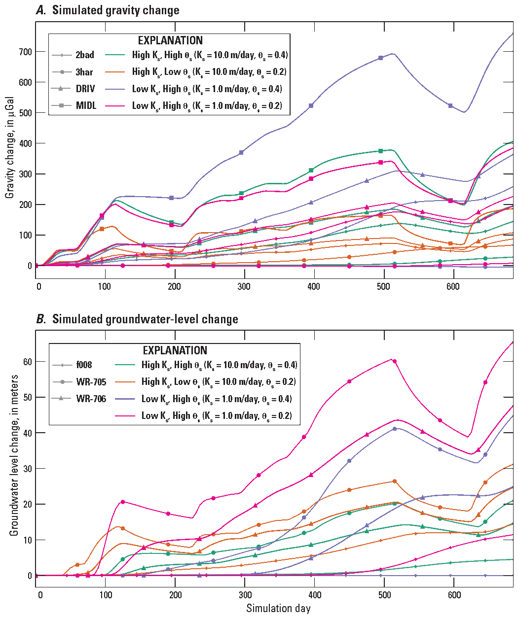
Model-simulated gravity change at four locations (A) and groundwater-level change at three locations (B). Line color indicates model parameter scenario (varying saturated hydraulic conductivity, Ks, and saturated soil water content, θs) and markers indicate the simulation location. m, meter.
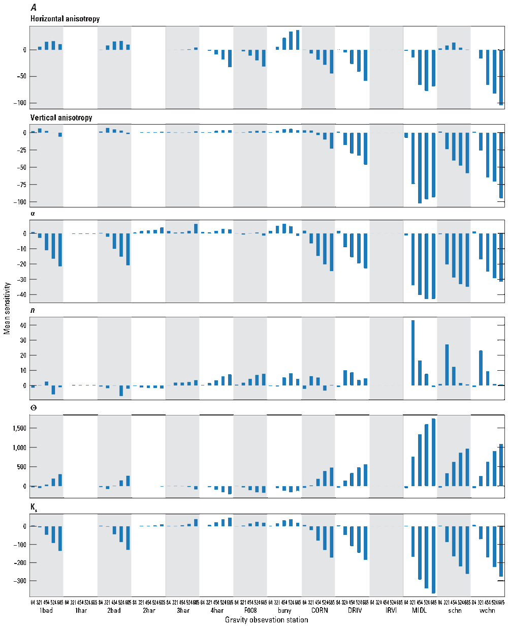
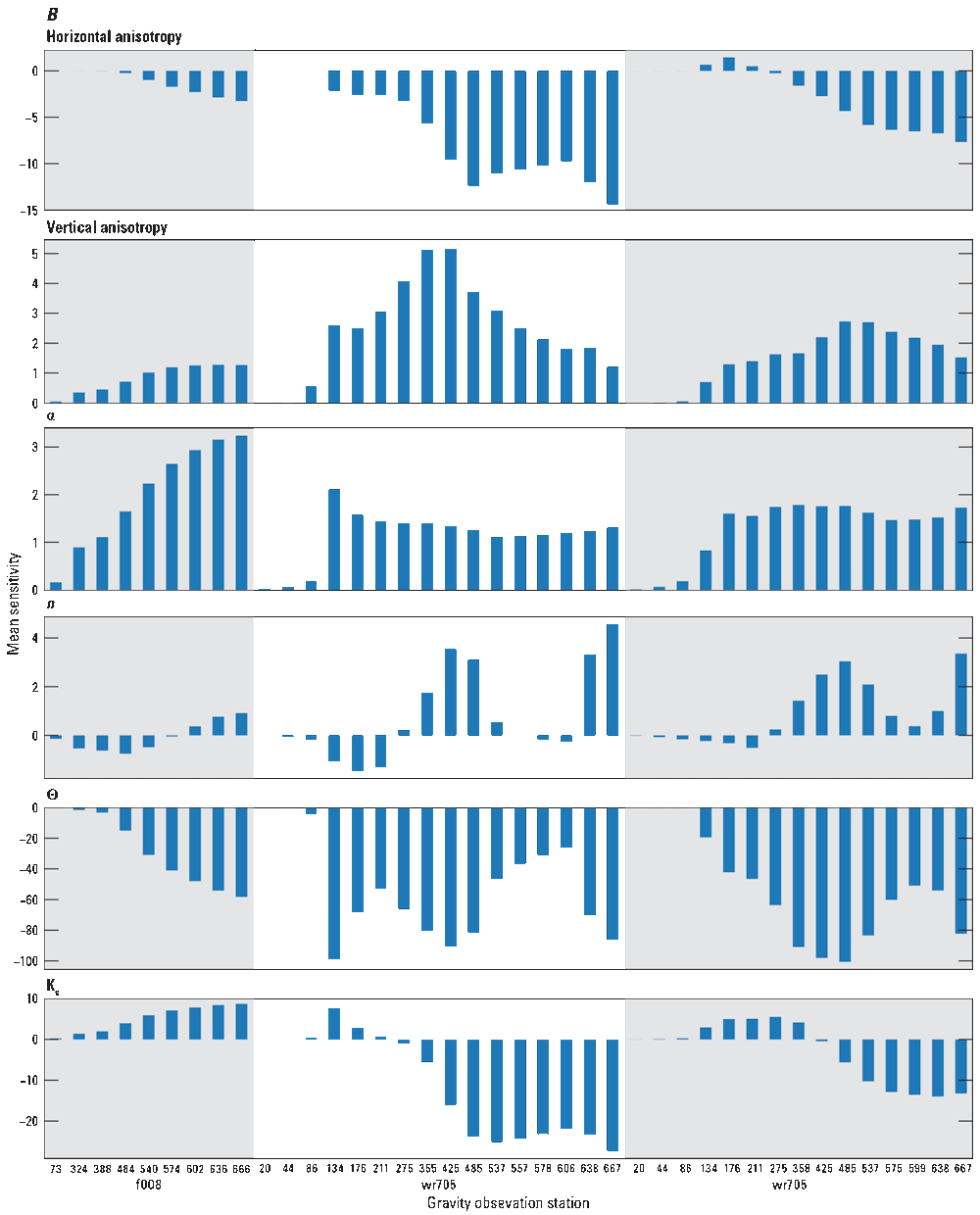
Mean sensitivity of Hydrus-3D simulations of gravity change (A) and groundwater-level change (B) relative to soil infiltration model parameters calculated using pestpp-sen and the PEST++ suite (White and others, 2020) and the method of Morris (1991). Numbers above the location label on the x-axis refer to model day.
Compared to simulated gravity, groundwater-level changes were more uniformly sensitive to soil properties among the three monitoring locations (fig. 12B). Sensitivities were similar at the two observation wells nearest the recharge basins, WR-705A and WR-706A, which are nearly equidistant from the basins to the northwest and east, respectively (fig. 3). Unlike simulated gravity, the highest sensitivity tended to occur toward the middle of the study period, around the time that groundwater levels first peaked (fig. 5). Well F-008A, further to the east, was more sensitive to α and less sensitive to other soil properties.
Following parameter estimation, the model was able to simulate observed gravity changes and groundwater-level change reasonably well (fig. 13). Using the default parameter values (based on soil texture alone, with no other prior information), the largest gravity and groundwater-level increases were overestimated by the model (fig. 13A). Generally, the default parameter values better simulated the gravity changes than the groundwater-level changes, especially for relatively small changes (less than 200 µGal), confirming that model parameter values are relatively insensitive to observed values at many of the gravity stations (fig. 13A). Simulated groundwater-level changes were consistently too high for wells WR-705A and WR-705B (points above the 1:1 line in fig. 13A and fig. 13B, right panels), and too low for well F-008A (points below the 1:1 line). This implies water arrived too quickly to the screened depths of WR-705A and WR-705B and too slowly to the screened depth of F-008A in the model simulation, relative to the observations. Using the final, best-fit parameter values identified by pestpp-glm (primarily, higher Ks and θs relative to initial values; table 1), the fit for both parameter types is much improved, especially at large values (fig. 13B). The largest observed gravity changes (greater than 200 µGal) where the greatest shift occurred during the calibration process were at stations MIDL, wchn, schn, DRIV, and 1bad.
Because all recharged water remains within the model domain during the simulation period, the model can only simulate an increase in gravity and does not capture the gravity decreases observed at some stations. These gravity decreases occur at stations distant from the recharge basins (fig. 6) where the gravity region of sensitivity does not intersect the recharged water, and likely reflect the regional trend of declining groundwater levels. The prior to calibration parameter ranges for the pestpp-glm run were larger than those used in pestpp-sen to reflect the lack of information available to constrain the estimated parameters (table 1). Initial observation weights were defined so that modeled residuals (observed minus simulated) from repeat microgravity data and groundwater level-data contributed equally to the pestpp-glm objective function. These initial weights were 0.15 and 1.0 for gravity and groundwater level, respectively. Often the initial observation weights are defined relative to the measurement uncertainty (that is, observation weight equals one over the standard deviation of the measurement; White and others, 2020). Although changes in groundwater level can be measured precisely (to the centimeter level), too-low measurement uncertainty results in excessive observation weight and therefore the maximum initial observation weight for groundwater levels was kept at 1.0. Weights are further adjusted by the pestpp-glm algorithm during the automatic parameter estimation process.
Output from pestpp-glm includes parameter mean values and standard deviations, which can be compared to estimates prior to calibration (table 1). To demonstrate the value of adding repeat microgravity data for model calibration, the prior and posterior (post calibration) parameter estimates for saturated hydraulic conductivity and saturated water content were compared (fig. 14). For both parameters, the standard deviation of the posterior estimate is lower than the prior estimate, which causes the width of the probability function to be narrower. The mean value is similar for saturated hydraulic conductivity but lower for saturated water content (0.37 when gravity data are included in calibration, compared to 0.41 when not included).
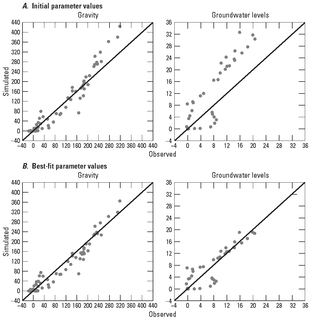
Measured (x-axis) and simulated (y-axis) gravity and groundwater-level changes at the Southeast Houghton Artificial Recharge Project. Simulated values are from (A) a Hydrus-3D model based on soil texture alone, and (B) the same model using the optimal post-calibration parameters determined using PEST++.
Table 1.
Optimized parameter values for a Hydrus-3D model of the Southeast Houghton Artificial Recharge Project determined using PEST++.[Std. dev., standard deviation; Ks, saturated hydraulic conductivity, meters per day; θs, saturated water content, cubic meters per cubic meter; α, log-Kosugi infiltration parameter; n, Kosugi log-normal infiltration parameter; cay, horizontal Ks anisotropy ratio; caz, vertical Ks anisotropy ratio (ratio of vertical to horizontal hydraulic conductivity).]
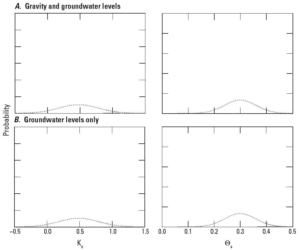
Prior (dashed line) and posterior (solid area) parameter estimates of log(saturated hydraulic conductivity) and saturated water content. Upper two plots (A) show parameter estimates using groundwater-level change and gravity change for calibration. Lower two plots (B) show parameter estimates using only groundwater-level change for calibration. Posterior parameter estimates were obtained from PEST++ inversion. log(Ks), log(saturated hydraulic conductivity); θs, saturated water content.
Summary
This report presents microgravity and water-level monitoring data and modeling results at the Southeast Houghton Artificial Recharge Project (SHARP) in Tucson, Arizona. Since December 2020, Tucson Water has used the facility to recharge water in surface infiltration ponds. Monitoring data consisted of groundwater level observations at 3 monitoring wells and repeat microgravity measurements at 22 locations. Six gravity surveys were carried out using absolute- and relative-gravity meters. Large gravity increases (more than 250 microgals) were observed during the first repeat gravity survey (3.5 months after the start of recharge) but only in the immediate vicinity of the recharge basins. Data show that water moves downward to the water table and that storage changes are likely zero or very small in the unsaturated zone away from the facility, including at the retired landfill located 1.5 kilometers (km) north of SHARP. Gravity at stations more than 1 km away from the facility decreased, consistent with regional groundwater level declines. Groundwater-level increases started 5.5 months after recharge began and remained elevated throughout the rest of the study period. Maximum observed groundwater-level rise during the study period of this report was about 14 meters (m; appendix 2), but Tucson Water reported a maximum rise of 20 m in May, 2022, after this study ended (Beth Scully, Tucson Water, oral commun., 2022).
Unsaturated-zone flow simulated using a water movement model produced physically realistic infiltration using the Kosugi log-normal infiltration model. Parameter sensitivity analysis showed gravity and groundwater-level change observations were primarily sensitive to the saturated water content and saturated hydraulic conductivity parameters, with gravity being especially sensitive to the former. Only the gravity stations within the near vicinity (that is, within about a 1-km radius) of the recharge basins were sensitive to soil-property parameters. Using a parameter estimation framework, optimal parameter values and their uncertainty were identified. Calibration was carried out using (1) groundwater-level change data only and (2) groundwater-level change plus gravity change data. The latter resulted in an improved (standard deviation of the parameter estimate was 0.01, compared to 0.06 for groundwater-level only calibration), lower (0.38 compared to 0.42) estimate of saturated water content and a higher estimate of saturated hydraulic conductivity (9.59 m per day [m/day] compared to 7.36 m/day). Adding gravity data for calibration only slightly reduced uncertainty for the saturated hydraulic conductivity estimate (from 1.16 to 1.09 m/day). Optimal anisotropy ratios, both horizontal and vertical, were close to one. Model simulated gravity and groundwater levels were insensitive to the parameters α and n in the Kosugi log-normal model.
The repeat microgravity network established for this project can be used for continued surveys to monitor the growth, if any, of the groundwater mound at SHARP. For this purpose, measurements could be continued at the more distant stations. Fewer stations could be observed in the near vicinity of the basins, as these appear to respond similarly and have overlapping regions of sensitivity. Additional stations to the south would help identify horizontal anisotropy or preferential flow (that is, horizontal dispersal of infiltrating water on perching layers between the land surface and the water table).
To the best of our knowledge, this project represents the first surface basin infiltration facility where gravity data were collected prior to the onset of infiltration. Thus, the gravity data reflect mass change in the subsurface—including the more than 100-m-thick unsaturated zone—as it transitioned from fully drained to a much higher water content. Nevertheless, the calibrated unsaturated-zone flow model indicated that (1) the unsaturated zone did not become fully saturated during the initial 22 months of recharge and (2) water content was still increasing at the end of the simulation period. Future monitoring could be useful for determining if the unsaturated zone maintains this less-than-saturated water content, as suggested by the consistent gravity values after the initial increase, or if it continues to “wet up” (approach saturated water content) over time, which would be indicated by continued increases in gravity at stations near the basins. The maximum possible infiltration rate at SHARP will likely not be achieved unless the subsurface nears a fully saturated state.
References Cited
Anderson, S.R., 1987, Cenozoic stratigraphy and geologic history of the Tucson Basin, Pima County, Arizona: U.S. Geological Survey Water-Reources Investigations Report 87–4190, 3 pls., scale 1:24,000, pamphlet 20 p., accessed July 3, 2023, at https://doi.org/10.3133/wri874190.
Arizona Department of Water Resources [ADWR], 2022a, Underground storage facility permit application guide: Arizona Department of Water Resources, R15, 32 p., accessed July 3, 2023, at https://new.azwater.gov/sites/default/files/media/Recharge%20Substantive%20Policy%20%28R15%29%20USF%20Application%20Guidelines.pdf.
Arizona Department of Water Resources [ADWR], 2022b, Total land subsidence in the Tucson metropolitan area: Arizona Department of Water Resources, accessed January 4, 2024, at https://www.azwater.gov/sites/default/files/2022-08/TucsonArea04-2020to03-2022_8x11.pdf.
Arizona Department of Water Resources [ADWR], 2023, Well registry search: Arizona Department of Water Resources, Water resource data website, accessed September 5, 2023, at https://app.azwater.gov/WellRegistry/SearchWellReg.aspx.
Arizona Department of Water Resources [ADWR], 2024, Interactive maps and data: Arizona Department of Water Resources web page, accessed July 26, 2024, at https://www.azwater.gov/gis-data-and-maps.
Arizona Department of Water Resources [ADWR], 2025, Supplemental Data Reports for 71-225060: Arizona Department of Water Resources web page, accessed March 7, 2025 at https://infoshare.azwater.gov/docushare/dsweb/View/Collection-19570.
Baird, K.J., Mac Nish, R., Guertin, P.D., 2001, An evaluation of hydrologic and riparian resources in Saguaro National Park, Tucson, Arizona: University of Arizona Department of Hydrology and Water Resources and Research Laboratory for Riparian Studies, HWR No. 01-010, accessed July 30 2024, at https://repository.arizona.edu/handle/10150/615752?show=full.
Carruth, R.L., Kahler, L.M., Conway, B.D., 2018, Groundwater-storage change and land-surface elevation change in Tucson Basin and Avra Valley, south-central Arizona—2003–2016: U.S. Geological Survey Scientific Investigations Report 2018–5154, 34 p., https://doi.org/10.3133/sir20185154.
Carleton, G.B., 2010, Simulation of groundwater mounding beneath hypothetical stormwater infiltration basins: U.S. Geological Survey Scientific Investigations Report 2010–5102, 64 p., https://doi.org/10.3133/sir20105102.
Cigna, F., Esquivel Ramírez, R., and Tapete, D., 2021, Accuracy of Sentinel-1 PSI and SBAS InSAR displacement velocities against GNSS and geodetic leveling monitoring data: Remote Sensing, v. 13, no. 23, 28 p., accessed September 5, 2023, at https://doi.org/10.3390/rs13234800.
Davidson, E.S., 1973, Geohydrology and water resources of the Tucson Basin, Arizona: U.S. Geological Survey Water-Supply Paper 1939–E, 81 p., 7 pls., https://doi.org/10.3133/wsp1939E.
Eastoe, C.J., Gu, A., and Long, A., 2004, The origins, ages and flow paths of groundwater in Tucson Basin—Results of a study of multiple isotope systems, in Hogan, J.F., Phillips, F.M., and Scanlon, B.R., eds., Groundwater recharge in a desert environment—The southwestern United States: Washington, D.C., American Geophysical Union, accessed July 3 2023, at https://doi.org/10.1029/009WSA12.
Eastoe, C.J. and Gu, A., 2016, Groundwater depletion beneath Downtown Tucson, Arizona—A 240‐year record: Journal of Contemporary Water Research & Education, v. 159, no. 1, p. 62–77, https://doi.org/10.1111/j.1936-704X.2016.03230.x.
Eastoe, C.J., Wright, W.E., 2019, Hydrology of mountain blocks in Arizona and New Mexico as revealed by isotopes in groundwater and precipitation: Geosciences, v. 9, no. 11, article 461, 22 p., accessed September 5, 2023, at https://doi.org/10.3390/geosciences9110461.
Hantush, M.S., 1967, Growth and decay of groundwater‐mounds in response to uniform percolation: Water Resources Research, vol. 3, no. 1, p. 227–234, https://doi.org/10.1029/WR003i001p00227.
Harbaugh, A.W., 2005, MODFLOW-2005, the U.S. Geological Survey modular ground-water model -- the Ground-Water Flow Process: U.S. Geological Survey Techniques and Methods 6-A16, https://doi.org/10.3133/tm6A16.
Kennedy, J.R., Ferré, T.P.A., Güntner, A., Abe, M., and Creutzfeldt, B., 2014, Direct measurement of subsurface mass change using the variable baseline gravity gradient method: Geophysical Research Letters, v. 41, no. 8, p. 2827–2834, accessed September 5, 2023, at https://doi.org/10.1002/2014GL059673.
Kennedy, J.R., Ferré, T.P.A., and Creutzfeldt, B., 2016, Time-lapse gravity data for monitoring and modeling artificial recharge through a thick unsaturated zone: Water Resources Research, v. 52, no. 9, p. 7244–7261, accessed September 5, 2023, at https://doi.org/10.1002/2016WR018770.
Kennedy, J., 2020, GSadjust—A graphical user interface for processing combined relative- and absolute-gravity surveys, ver. 1.0: U.S. Geological Survey Software Release, https://doi.org/10.5066/P9YEIOU8.
Kennedy, J.R., Pool, D.R., and Carruth, R.L., 2021a, Procedures for field data collection, processing, quality assurance and quality control, and archiving of relative- and absolute-gravity surveys: U.S. Geological Survey Techniques and Methods 2-D4, 50 p., https://doi.org/10.3133/tm2D4.
Kennedy, J.R., Wildermuth, L., Knight, J.E., Larsen, J., 2022, Improving groundwater model calibration with repeat microgravity measurements: Groundwater, v. 60, no. 3, p. 393–403, https://doi.org/10.1111/gwat.13167.
Kennedy, J.R., 2024, Hydrus-3D unsaturated-zone flow model for simulating recharge at the Southeast Houghton Artificial Recharge Project: U.S. Geological Survey data release, https://doi.org/10.5066/P1VH7C73.
Kosugi, K.I., 1996, Lognormal distribution model for unsaturated soil hydraulic properties: Water Resources Research, v. 32, no. 9, p. 2697–2703, https://doi.org/10.1029/96WR01776.
Landrum, M., 2024, Repeat microgravity data from the Southeast Houghton Artificial Recharge Project, 2020–2022 (version 2.0, August 2024): U.S. Geological Survey data release, https://doi.org/10.5066/P9E19SSK.
Laney, R.L., 1972, Chemical quality of the water in the Tucson basin, Arizona. U.S. U.S. Geological Survey Water-Supply Paper 1939-D, accessed July 30, 2024, at https://doi.org/10.3133/wsp1939D.
Leirião, S., He, X., Christiansen, L., Andersen, O.B., and Bauer-Gottwein, P., 2009, Calculation of the temporal gravity variation from spatially variable water storage change in soils and aquifers: Journal of Hydrology, v. 365, nos. 3–4, p. 302–309, accessed July 3, 2023, at https://doi.org/10.1016/j.jhydrol.2008.11.040.
Marino, M.A., 1974, Growth and decay of groundwater mounds induced by percolation: Journal of Hydrology, v. 22, no. 3–4, p. 295–301, accessed July 30, 2024 at https://doi.org/10.1016/0022-1694(74)90082-1.
Mason, D., and Hipke, W., 2013, Regional groundwater flow model of the Tucson Active Management Area, Arizona—Model update and calibration: Arizona Department of Water Resources Modeling Report No. 24, 109 p., accessed July 3, 2023, at https://www.azwater.gov/hydrology/groundwater-modeling/tucson.
Miller, M.M., Shirzaei, M., and Argus, D., 2017, Aquifer mechanical properties and decelerated compaction in Tucson, Arizona: Journal of Geophysical Research, Solid Earth, v. 122, p. 8402–8416, accessed July 3, 2023, at https://doi.org/10.1002/2017JB014531.
Megdal, S.B., Dillon, P., and Seasholes, K., 2014, Water banks: Using managed aquifer recharge to meet water policy objectives, Water, v. 6, no. 6, p. 1500–1514, https://doi.org/10.3390/w6061500.
Morris, M.D., 1991, Factorial sampling plans for preliminary computational experiments: Technometrics, v. 33, no. 2, p. 161–174, https://doi.org/10.1080/00401706.1991.10484804.
Mualem, Y., 1976, A new model for predicting the hydraulic conductivity of unsaturated porous media: Water Resources Research, v. 12, no. 3, p. 513–522, https://doi.org/10.1029/WR012i003p00513.
National Weather Service, 2021, Review of the 2020 monsoon across the southwest U.S: National Weather Service, 2020 monsoon review web page, accessed August 1, 2023, at https://www.weather.gov/psr/2020MonsoonReview.
PC-Progress, Inc., 2022., Hydrus 3-D (Version 5): PC-Progress, Inc. software release, accessed August 1, 2023, at https://www.pc-progress.com/en/Default.aspx?hydrus.
Pima Association of Governments, 2004, Groundwater Conditions in Rincon Valley, accessed July 25, 2023, through the Pima County repository, https://content.civicplus.com/api/assets/0c42a9e5-a3de-415c-8aa7-f23330853cf8.
Pool, D.R., 2005, Variations in climate and ephemeral channel recharge in southeastern Arizona, United States: Water Resources Research, v. 41, no. 11, accessed July 3, 2023, at https://doi.org/10.1029/2004WR003255.
Pool, D.R., and Anderson, M.T., 2008, Ground-water storage change and land subsidence in Tucson Basin and Avra Valley, Southeastern Arizona, 1998–2002: U.S. Geological Survey Scientific Investigations Report 2007–5275, 44 p., https://doi.org/10.3133/sir20075275.
Rai, S.N., and Singh, R.N., 1995, Two-dimensional modelling of water table fluctuation in response to localised transient recharge: Journal of Hydrology, v. 167, no. 1–4, p. 167–174, https://doi.org/10.1016/0022-1694(94)02607-D.
Sumner, D.M., Rolston, D.E., and Mariño. M.A., 1999, Effects of unsaturated zone on ground-water mounding: Journal of Hydrologic Engineering, v. 4, no. 1., p. 65–69, https://doi.org/10.1061/(ASCE)1084-0699(1999)4:1(65).
Telford, W.M, Geldart, L.P., Sheriff, R.E., 1990, Applied geophysics (2d ed.): Cambridge, U.K., Cambridge University Press, https://doi.org/10.1017/CBO9781139167932.
Tillman, F.D., and Leake, S.A., 2010, Trends in groundwater levels in wells in the active management areas of Arizona, USA: Hydrogeology Journal, v. 18, no. 6, p. 1515–1524, https://doi.org/10.1007/s10040-010-0603-3.
Tucson Water, 2023, One Water 2100 Plan: City of Tucson Report, accessed July 23, 2024 at https://tucsononewater.com/wp-content/uploads/2023/10/Tucson-Water-One-Water-2100-Plan_Spreads_Web-Version.pdf.
White, J.T., Hunt, R.J., Fienen, M.N., and Doherty, J.E., 2020, Approaches to highly parameterized inversion—PEST++ version 5, a software suite for parameter estimation, uncertainty analysis, management optimization and sensitivity analysis: U.S. Geological Survey Techniques and Methods 7-C26, 52 p., accessed July 3, 2023, at https://doi.org/10.3133/tm7C26.
Appendix 1. Estimated monthly evaporation loss
Table 1.1.
Estimated monthly evaporation loss from individual recharge basins as reported by Tucson Water at the South Houghton Artificial Recharge Project, in acre-feet. Published here with permission. Please contact Beth Scully at Tucson Water (beth.scully@tucsonaz.gov) for additional information.Appendix 2. Groundwater level data
Table 2.1.
Change in groundwater-table elevation relative to June 3, 2020, at wells WR-705A and WR-706A, provided by Tucson Water. Published here with permission. Please contact Beth Scully at Tucson Water (beth.scully@tucsonaz.gov) for additional information.[Depth to water below land surface on June 3, 2020, was 105.9 meters at WR-705A and 107.4 meters at WR706-A. Dates are in the format month/day/year. Data from June 3, 2020, through January 1, 2021, are mean daily values recorded by a pressure transducer. Measurements after January 1, 2021, are discrete measurements using an electric tape.]
Conversion Factors
Datum
Vertical coordinate information is referenced to the North American Vertical Datum of 1988 (NAVD 88).
Horizontal coordinate information is referenced to North American Datum of 1983 (NAD 83) epoch 2010.00.
Moffett Field Publishing Service Center, California
Manuscript approved for publication February 27, 2025
Edited by Mitchell Phillips and Timothy Herold
Layout and design by Kimber Petersen
Disclaimers
Any use of trade, firm, or product names is for descriptive purposes only and does not imply endorsement by the U.S. Government.
Although this information product, for the most part, is in the public domain, it also may contain copyrighted materials as noted in the text. Permission to reproduce copyrighted items must be secured from the copyright owner.
Suggested Citation
Wildermuth, L.M., Kennedy, J.R., and Conrad, J.L., 2025, Groundwater response to managed aquifer recharge at the Southeast Houghton Artificial Recharge Project in Tucson, Arizona: U.S. Geological Survey Scientific Investigations Report 2025–5017, 38 p., https://doi.org/10.3133/sir20255017.
ISSN: 2328-0328 (online)
Study Area
| Publication type | Report |
|---|---|
| Publication Subtype | USGS Numbered Series |
| Title | Groundwater response to managed aquifer recharge at the Southeast Houghton Artificial Recharge Project in Tucson, Arizona |
| Series title | Scientific Investigations Report |
| Series number | 2025-5017 |
| DOI | 10.3133/sir20255017 |
| Publication Date | November 19, 2025 |
| Year Published | 2025 |
| Language | English |
| Publisher | U.S. Geological Survey |
| Publisher location | Reston, VA |
| Contributing office(s) | Arizona Water Science Center |
| Description | Report: v, 38 p.; Data Release |
| Country | United States |
| State | Arizona |
| City | Tucson |
| Other Geospatial | Southeast Houghton Artificial Recharge Project |
| Online Only (Y/N) | Y |