

Development of Regression Equations to Estimate Flow Durations, Low-Flow Frequencies, and Mean Flows at Ungaged Stream Sites in Connecticut Using Data Through Water Year 2022
Links
- Document: Report (4.59 MB pdf) , HTML , XML
- Data Release: USGS data release - Data for development of regression equations to estimate flow durations, low-flow frequencies, and mean flows in Connecticut using data collected through water year 2022
- Download citation as: RIS | Dublin Core
Abstract
To aid Federal and State regulatory agencies in the effective management of water resources, the U.S. Geological Survey, in cooperation with the Connecticut Department of Energy and Environmental Protection and the Connecticut Department of Transportation, updated flow statistics for 118 streamgages and developed 47 regression equations to estimate selected flow duration, low flow, and mean flow statistics for the entire State of Connecticut, for the following: 1-, 5-, 10-, 25-, 50-, 75-, 90-, 99-percent flow durations; 7-day, 10-year low-flow frequency and 30-day, 2-year low-flow frequency; and mean flow, spring mean flow, and harmonic mean flow. In addition, regression equations were developed for monthly and seasonal flow durations, ranging from 25 to 99 percent for aquatic biological processes of salmonid spawning (November), overwinter (December–February), clupeid spawning (May), resident spawning (June), and rearing and growth (July–October) periods, and for flow durations ranging from 1 to 99 percent for the habitat forming (March–April) period. Statistics were derived from daily mean streamflow data collected from streamgages with at least 10 years of data through water year 2022 in southern New England and eastern New York.
Forty streamgages in Connecticut and adjacent areas of neighboring States were used in the regression analysis. Regression methods of weighted least squares and generalized least squares were used to derive the final coefficients and measures of uncertainty for the regression equations. The equations used to estimate selected streamflow statistics were developed by relating the flow statistics to different basin characteristics (physical, land cover, and climatic) at the 40 streamgages. Nine basin characteristics served as the explanatory variables in the statewide regression equations: drainage area, percentage of area with coarse-grained stratified deposits, stream density, mean basin slope, mean basin elevation, percentage of area with hydrologic soil group A, mean monthly precipitation for November, mean seasonal precipitation in the winter (December, January, and February), and mean annual temperature. The root mean square error of the 47 equations ranged from 7.9 to 121.9 percent, with an average of 27.9 percent. The equations estimate flows most accurately near the mean (50-percent flow duration), become less accurate for low flows, and are the least accurate for extreme low flows. The root mean square error for the 50-percent flow duration is 15.1 percent, with an average of 17.6 percent across the six periods. The extreme low flow statistics of 7-day, 10-year low-flow frequency, 99-percent flow duration, and 99-percent rearing and growth period flow durations have root mean square errors of 121.9, 105.1, and 121.9 percent, respectively. The adjusted coefficient of determination of the 47 equations ranged from 73.4 to 99.5 percent, with an average of 95.1 percent.
Plain Language Summary
The U.S. Geological Survey, the Connecticut Department of Energy and Environmental Protection, and the Connecticut Department of Transportation collaboratively updated flow statistics for 118 streamgages and developed 47 regression equations to estimate key flow statistics in Connecticut. These included various flow durations and low-flow frequencies, as well as mean flow statistics for specific aquatic biological processes. The analysis used daily mean streamflow data from 40 streamgages with at least 10 years of data and incorporated basin characteristics such as drainage area and precipitation. The equations were most accurate near the mean flow (50-percent flow duration), with an average root mean square error of 27.9 percent, while accuracy decreased for low and extreme low flows. The adjusted coefficient of determination ranged from 73.4 to 99.5 percent, averaging 95.1 percent.
Introduction
Streamflow statistics such as flow durations, low-flow frequencies, and seasonal and monthly mean flows are crucial to Federal and State regulatory agencies to effectively manage water resources. Connecticut’s water-quality standards (R.C.S.A. §§22a-426-1–22a-426-9) were established to protect designated water uses and establish critical low-flow values that maintain the integrity of the aquatic community and protection of human health. Water quality standards that apply to low flow are determined by Connecticut’s minimum flow regulations (R.C.S.A. §§22a-426-1–22a-426-9), the Connecticut Department of Energy and Environmental Protection (CT DEEP) Diversion Permit Program (R.C.S.A. §§22a-365–22a-378), or the Federal Energy Regulatory Commission’s hydropower licensing process (Federal Power Act; 16 U.S.C. §791a et seq.). The regulatory programs are dependent on understanding site-specific streamflow characteristics to ensure that the highest statutory and regulatory requirements are achieved.
The CT DEEP is tasked with water-quality and water-quantity regulatory activities through such programs as the Total Maximum Daily Load (TMDL) Program (CT DEEP, 2022) and the National Pollutant Discharge Elimination System (NPDES) permit program. The NPDS program regulates how pollutants are discharged into waters. The Total Maximum Daily Load Program operates under the authority of the Clean Water Act that identifies surface waters that have been affected by contaminants. A TMDL is the calculation of the maximum amount of a pollutant allowed to enter a waterbody so that the waterbody will meet and continue to meet water quality standards for that particular pollutant. Miles of river reaches in Connecticut are listed by the State as failing to meet water quality standards (U.S. Environmental Protection Agency, 2024). Specific water quality standards for surface waters apply to flow statistics, including the 7-day, 10-year low flow frequency (7Q10); 30-day, 2-year low flow frequency (30Q2); and harmonic mean flow. The 7Q10 (which represents the minimum 7-day average flow with a probability of occurring once every 10 years) and 30Q2 (which represents the minimum 30-day average flow with a probability of occurring once every 2 years) flows are used as criteria when setting wastewater limits and allowable contaminant loads. The U.S. Environmental Protection Agency (EPA) recommends using the harmonic mean flow as the basis for implementing human health criteria that allow for estimating the concentration of toxic contaminants. The assessment of stream dilution available for maintaining water quality is made at the harmonic mean flow and 7Q10 flow (EPA, 1991).
Flow durations also are needed by the CT DEEP for balancing instream and out-of-stream water uses. In 2005, the State adopted streamflow standards that provide an additional level of protection for Connecticut’s rivers and streams. The instream-flow standards safeguard rivers that support a natural flow regime on which the ecological integrity of the riverine ecosystems depends while balancing the needs of humans to use water for drinking and domestic purposes, fire and public safety, irrigation, manufacturing, and recreation. The CT DEEP uses monthly and seasonal flow durations based on bioperiods to regulate instream and out-of-stream (for example, drinking water supply, irrigation for agriculture, and industrial processes) water uses. Bioperiods are defined by the State of Connecticut according to the times of year when specific biological processes that are dependent on flow occur or are likely to occur (table 1; CT DEEP, 2009).
Table 1.
Bioperiods for seasonal streamflow linked to biological processes and associated periods, flow conditions, and biological significance, as defined by the Connecticut Department of Energy and Environmental Protection (2009).In addition to streamflow statistics for water quality and water supply regulatory and permitting purposes, streamflow statistics based on the average daily and average spring flows are needed by the Connecticut Department of Transportation (CT DOT) for water handling during the construction phase of projects that involve temporary hydraulic facilities (CT DOT, 2023). Temporary hydraulic facilities include temporary bridges and culverts, bypass channels, haul roads, or channel constrictions, such as cofferdams capable of isolating work areas from the streamflow during construction activities. The temporary hydraulic facilities are designed to safely convey selected streamflows while minimizing any effects to life or property, including the structure under construction. The equations used by CT DOT for estimating average daily flow and average spring flow were derived by CT DOT more than 40 years ago, and the documentation of the methods used to derive the equations was not published in peer-reviewed literature. Average daily flow (herein referred to as mean flow) is the arithmetic mean of all daily mean flows for the data series for a designated period. Average spring flow (herein referred to as spring mean flow) is the arithmetic mean of daily mean streamflow for March and April for a designated period.
Since 2000, Connecticut has experienced severe (category D2) and extreme (category D3) drought conditions in 5 of the past 23 years (2002, 2012, 2017, 2020, and 2022; National Oceanic and Atmospheric Administration, 2023). Concerns have arisen about the potential effects of these repeated drought conditions on the ability of water users to maintain existing water withdrawals and point-source discharges in the future. Streamflow statistics for gaged and ungaged stream locations can be used for water-supply planning and ultimately to make informed scientific and policy decisions on water supplies.
Reliable streamflow statistics are dependent on the availability and length of the streamflow records. The U.S. Geological Survey (USGS) operates a network of continuous-record streamgages in Connecticut and surrounding States that provide flow data needed for various purposes. Although flow statistics can be calculated at the locations with streamgages using historical data, regional regression equations that relate flow statistics with physical and climatic characteristics of drainage basins can be used to estimate flow statistics at locations where streamgages do not exist.
Regression equations for estimating streamflow statistics for Connecticut streams developed from this study are described in this report and are expected to be included in the USGS StreamStats web-based geographic information system (GIS) that provides users with access to analytical tools and streamflow statistics (USGS, 2024a). StreamStats integrates multiple datasets, including the National Hydrography Dataset (USGS, 2023b), the Watershed Boundary Dataset (USGS, 2022), and the 3D Elevation Program (USGS, 2023a), allowing users to delineate a watershed for a stream or water feature of interest. Users can also calculate flow statistics for a watershed of interest and compute basin characteristics such as National Land Cover Dataset land use and land cover values and average precipitation (USGS, 2018).
Purpose and Scope
The purpose of this report is to develop and present regional regression equations for estimating flow durations, low-flow frequencies, and mean flows at ungaged stream locations in Connecticut from basin and climatological characteristics. The streamflow statistics estimated with the regression equations are for natural flow conditions (minimally altered or unregulated streamflows). Streamflow statistics for which regression equations were developed include the 99-, 90-, 75-, 50-, 25-, 10-, 5-, and 1-percent flow durations (Q99, Q90, Q75, Q50, Q25, Q10, Q5, and Q1, respectively); the 7Q10 and 30Q2 low-flow frequencies; mean flow, spring (March and April) mean flow, and harmonic mean flow; and monthly and seasonal flow durations based on bioperiods (table 2). The report also includes an evaluation of the uncertainties of the equations and the limitations of the use of the equations.
Table 2.
Description of 47 streamflow statistics for development of regression equations at defined frequencies, durations, and mean flows using data through water year 2022.[A water year is from October 1 through September 30 of the following year; a climate year is defined as the period from April 1 through March 31 of the following year and is designated by the year in which it ends]
Additionally, streamflow statistics were updated for 118 streamgages in southern New England and eastern New York (fig. 1; appendix 1). The streamflow statistics and regression equations were developed using the streamflow data collected at each streamgage through water year 2022 (October 1 through September 30). These equations provide estimates of unregulated streamflow at locations where streamflow data are unavailable (ungaged sites).
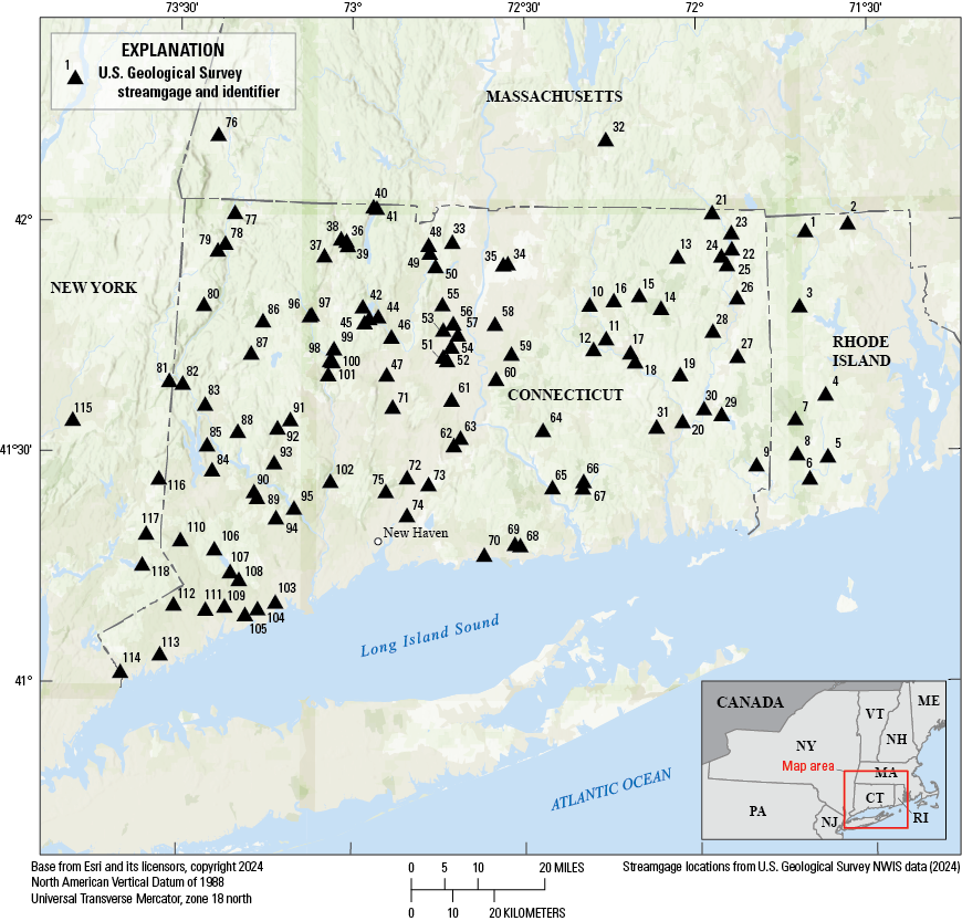
Map showing locations of 118 streamgages in Connecticut and adjacent areas of neighboring States. Map numbers refer to streamgages with updated flow statistics shown in appendix 1 and Ahearn and others (2025). NWIS, National Water Information System (U.S. Geological Survey, 2024b).
Previous Studies
Several studies by the USGS that provided streamflow statistic estimates in Connecticut have been published, including a series of basin studies (Randall and others, 1966; Thomas and others, 1968; Ryder and others, 1970, 1981; Thomas and Benson, 1970; Cervione and others, 1972, 1982; Wilson and others, 1974; Mazzaferro and others, 1979; Handman and others, 1986; Weiss and others, 1982). Ahearn (2008) published estimates of flow durations, low-flow frequencies, and monthly median flows for selected streams in Connecticut using data through 2005. The most recent USGS publications that provide estimates of streamflow statistics supersede previously published flow durations, low-flow frequencies, and monthly median flow estimates in Connecticut.
Regional regression techniques to estimate low- and mean-flow statistics at ungaged stream sites have been applied in Connecticut since the 1970s (Thomas and Benson, 1970). Cervione and others (1982) published a statewide regression equation to estimate the 7Q10 low flow statistic. Weiss (1983) provided statewide regression equations to estimate the 7Q10, 30Q2, and harmonic mean flow for Connecticut. Ahearn (2010) published statewide regression equations to estimate various flow durations ranging from 25 to 99 percent for six seasonal flow periods (bioperiods)—salmonid spawning (November), overwinter (December–February), habitat forming (March–April), clupeid spawning (May), resident spawning (June), and rearing and growth (July–October)—in Connecticut. The seasonal flows are based on aquatic habitat needs. Regression equations also were developed to estimate the Q25 and Q99 without reference to a bioperiod (Ahearn, 2010).
In the adjacent States of Massachusetts, New York, and Rhode Island, several studies have published regression equations for estimating selected low-flow statistics during the past 30 years. Fennessey and Vogel (1990), Ries (1990, 1994a, 1994b, 1997, and 1999), Vogel and Kroll (1990), Risley (1994), Ries and Friesz (2000), Ries and others (2000), and Archfield and others (2010) provided estimated streamflow statistics and regression equations for the 7Q10 and 7-day, 2-year low flows in Massachusetts. Armstrong and others (2008) provided regression equations for estimating median monthly streamflows in Massachusetts. Bent and Archfield (2002) and Bent and Steeves (2006) provided logistic regression equations for estimating the probability of a stream flowing perennially in Massachusetts. In New York, Randall (2011) published regression equations for estimating low-flow statistics. In Rhode Island, Bent and others (2014) provided regression equations for estimating flow durations and low-flow frequency statistics.
Physical Setting
Connecticut covers an area of 5,018 square miles (mi2) and is in the physiographic Appalachian Highlands province (Fenneman and Johnson, 1946). On the basis of geography, Connecticut is subdivided into four regions: the northwest highlands (where the Appalachian Mountains extend through the State), the central valley (with the Connecticut River bisecting the State), the eastern uplands, and the coastal lowlands (Brumbach, 1965). The northwest highlands generally have the steepest topography; land-surface elevations range from about 500 to 2,300 feet (ft) above the North American Vertical Datum of 1988 (NAVD 88) with average slopes of about 11 percent. Land-surface elevations in the eastern uplands range from about 500 to 1,300 ft above NAVD 88 with average slopes of about 8 percent. Topographic relief along the coastal lowlands and central valley generally is low with land-surface elevations ranging from 0 to about 500 ft above NAVD 88. Average basin slopes along the coastal lowlands and central valley are less than 7 percent.
The surficial geologic materials of Connecticut, described by Stone and others (1992), are primarily glacial deposits. Unconsolidated glacial deposits of varying thickness blanket the bedrock surface across most of the state. Glacial till is the most widespread surficial deposit and is generally thin (less than 15 ft thick). Till, deposited directly by glacial ice, is an unsorted material ranging in grain size from clay to large boulders and covers much of the slopes in the State and upland areas. Stratified deposits occur primarily in valleys and lower, flatter areas both inland and along the coast of Connecticut; these materials were laid down by glacial meltwater in streams and lakes and consist of layers of gravel, sand, silt, and clay. Stratified deposits are most widespread in the broad central Connecticut Valley and along the coast. Till, bedrock, and fine-grained stratified deposits (very fine sand, silt, and clay) generally have lower permeability than the coarse-grained, stratified deposits (gravel and sand), which generally have high permeability.
The climate in Connecticut generally is temperate and humid with four distinct seasons. Prevailing westerly winds alternately transport cool, dry, continental-polar and warm, moist, maritime-tropical air masses into the region, resulting in frequent weather changes. Precipitation is distributed fairly evenly throughout the year and averages about 48.75 inches (in.; recent 30-year normal, 1991–2020) or 46.88 in. (20th century mean, 1901–2020) annually (Northeast Regional Climate Center, 2024). Since 1900, the single driest year was 1965, with a statewide average of 30.7 in., and the wettest year was 2011, with 63.7 in. The average annual temperature is 49.9 degrees Fahrenheit (°F; recent 30-year normal, 1991–2020) or 48.0 °F (20th century mean, 1901–2020). Since 1900, the single coolest (44.3 °F) year was in 1904, and the warmest (52.5 °F) year was in 2012. The climate is moderated by maritime influences along coastal regions. Regional differences in topography, elevation, and proximity to the ocean can result in a substantial areal variation in temperature and snowfall amounts. Average annual temperatures range from 53.8 °F in coastal areas to 50.4 °F in the northwestern uplands. The average snowfall between 1991 and 2020 was 48.1 in.
Land cover in Connecticut is highly mixed, with forests dominating the north, and densely populated urban areas prominent along the southwestern coastal and central valley regions. In 2015, land cover in the State consisted of 54.9 percent forest (deciduous and coniferous forest), 19.2 percent developed (residential, commercial, industrial, and transportation routes), 7.4 percent agricultural fields, and 14.7 percent water, turf and grass, other grasses, tidal wetland, barren land, and utility corridor and 3.8 percent other. (University of Connecticut, 2016).
Computation of Streamflow Statistics at Streamgages
Streamflow records through water year 2022 at 118 continuous record streamgages in Connecticut and adjacent areas of neighboring States were compiled for computing flow durations, low-flow frequencies, and mean flow statistics and for potential use in the regionalization of the selected streamflow statistics in Connecticut (fig. 1; appendix 1). All the computed flow statistics (flow durations, low-flow frequencies, and mean flows) for the 118 streamgages generated by this study are presented in Ahearn and others (2025). Daily mean streamflows for current [2022] and discontinued streamgages with 10 or more years of daily mean flow data were retrieved from the USGS National Water Information System (NWIS) database (USGS, 2024b).
The set of 118 streamgages includes streamgages on unregulated and regulated streams. For this study, streamgages on unregulated streams are referred to as “index” streamgages. Index streamgages have natural or near-natural streamflow. A rigorous effort was made to identify streamgages with flow records that have been significantly affected by human activities and considered to be regulated. Indicators of disturbed watersheds pertinent to hydrologic modifications compiled from the USGS GAGE–II dataset (Falcone, 2011) along with State records on water-use activities were used to assess anthropogenic (human-caused) effects at streamgages. State records used to assess regulation included (1) registered and permitted surface-water or groundwater diversions, (2) wastewater discharges, including NPDES permits, and (3) dams and impoundments. The USGS GAGE–II hydrologic disturbance index is based on geospatial data of road density, basin fragmentation, reservoir storage, dam density, freshwater withdrawals, and distance to nearest NPDES discharges. Common types of streamflow regulation in Connecticut are (1) diversions and returns from various uses and (2) storage and releases from dams and reservoirs. After screening for anthropogenic effects, 40 streamgages were considered to be index streamgages suitable for the regression analysis (appendix 1). The other 78 streamgages were considered to be regulated and excluded from the regression analysis. Flow statistics were computed for index and regulated streamgages from the entire record of each streamgage. It was outside the scope of the study to evaluate historical changes related to regulation or compute at-site statistics using different parts of the streamflow record based on historical changes.
Flow duration and mean flow statistics are typically computed on the basis of the water year, and low-flow frequency statistics typically are computed on the basis of the climate year. A climate year is defined as the period April 1 through March 31 of the following year and designated by the year in which it ends). The annual low-flow period in most parts of the country is during the late summer and fall months. Use of the climate year for these statistics allows the entire low-flow period to fall within one time span. The USGS Hydrologic Toolbox statistical software was used to compute flow durations, low-flow frequencies, and mean flow statistics (Barlow and others, 2022), by retrieving USGS streamflow data from NWIS (USGS, 2024b).
Flow-Duration Statistics
Flow durations represent the percentage of time that a given flow is equaled or exceeded without regard to the sequence of recorded flows (Searcy, 1959). Typically, flow durations characterize the range of flow rates for the period over which data were collected. Flow durations were computed for complete water years for the entire period of record and for selected months and seasons for all 118 streamgages with 10 or more complete water years of record through water year 2022 (Ahearn and others, 2025). The streamflow data and flow statistics are based on the period of record for each streamgage, so starting and ending years vary.
Flow durations are computed by sorting the daily mean streamflows for the period of interest (such as the entire record or monthly) from largest to smallest and assigning each streamflow value a rank, starting with 1 for the largest value. The frequencies of exceedance are then computed by using the Weibull plotting-position formula (Weibull, 1939):
whereP
is the probability that a given streamflow will be equaled or exceeded (percent of time),
M
is the ranked position (dimensionless), and
n
is the number of events (daily mean streamflow values) for the period of record (dimensionless).
-
• period of record: Q99, Q90, Q75, Q50, Q25, Q10, Q5, and Q1;
-
• salmonid spawning (November): Q25, Q50, Q75, Q90, and Q99;
-
• overwinter (December–February): Q25, Q50, Q75, Q95, and Q99;
-
• habitat forming (March–April): Q1, Q5, Q10, Q25, Q50, Q75, Q90, Q95, and Q99;
-
• clupeid spawning (May): Q25, Q50, Q75, Q95, and Q99;
-
• resident spawning (June): Q25, Q50, Q75, Q90, and Q99; and
-
• rearing and growth (July–October): Q25, Q50, Q75, Q90, and Q99.
Low-Flow Frequency Statistics
Low-flow frequencies typically are computed for streamgages by using annual series of selected low flows based on the lowest mean streamflow for a specified number of consecutive days (Riggs, 1972). Any combination of number of days of mean minimum flow and years of recurrence may be used to determine the low-flow frequencies. The annual series for the determination of low-flow frequencies for this study was based on a climate year. Use of a climate year rather than a water year allows for an analysis of an uninterrupted low-flow period; in Connecticut, this low-flow period typically occurs from early August through mid-October.
A given low-flow frequency statistic is the minimum consecutive D-day mean streamflow that is expected to occur once in any Y-year period, or that has a probability of 1/Y of not being exceeded in any given year. (D is the number of days, and Y is the number of years.) For this study, 7Q10 and 30Q2 low-flow frequency statistics were computed. The 7Q10 is the annual minimum mean streamflow for 7 consecutive days that has a probability of 0.10 (or 10 percent chance) of not being exceeded in a given year, and the 30Q2 is the annual minimum average streamflow for 30 consecutive days that has a probability of 0.5 (or 50 percent chance) of not being exceeded in a given year. The 7Q10 and 30Q2 are commonly used in regulating wastewater discharge to streams by many States including Connecticut and by the EPA. For the frequency analysis, the USGS Hydrologic Toolbox software was used to compute the annual minimum flows and plot the fitted log-Pearson type III probability distribution and the selected minimum flows versus recurrence intervals (Barlow and others, 2022).
In Connecticut, the 7Q10 and Q99 are often considered similar in magnitude and have been used interchangeably for water planning and permitting purposes under limited situations. In cases where streamgages do not have a long enough record to perform a frequency analysis (a minimum of 10 years is needed), the Q99 has been used as a surrogate for the 7Q10. A comparison of 7Q10 and Q99 for 40 index streamgages shows that the Q99 is slightly larger than the 7Q10 (fig. 2; table 3). In figure 2, data points plot slightly right of the one-to-one line (line of equality). For the 40 index streamgages in Connecticut and adjacent areas of nearby States, the percent difference between the Q99 and 7Q10 (table 3) ranged from a minimum of 1.7 percent (Fishkill Creek at Hopewell Junction, N.Y. [station 01372800]) to a maximum of 98.4 percent (Indian River near Clinton, Conn. [station 01195100]), with an average of 32.5 percent. The streamgages used in the calculation of percentage difference had an average record length of 45 years. In general, the magnitude of the percentage differences between two streamflow statistics (Q99 and 7Q10) are relative to the size of the drainage area. Smaller drainage areas (less than 30 mi2) typically had larger percent differences, with an average of 40.2 percent, than larger drainage areas (greater than or equal to 30 mi2), with an average of 16.2 percent.
Table 3.
Differences between the 7-day, 10-year low-flow frequency and the 99-percent flow duration for 40 index streamgages in Connecticut and adjacent areas of neighboring States, using data through water year 2022.[Flow data are from Ahearn and others (2025); streamgage data are from U.S. Geological Survey (2024b). A water year is the period from October 1 to September 30 and is designated by the year in which it ends. USGS, U.S. Geological Survey; Q99, 99-percent flow duration; ft3/s, cubic foot per second; 7Q10, 7-day, 10-year low-flow frequency; NWIS, National Water Information System; mi2, square mile; RI, Rhode Island; CT, Connecticut; R, river; nr, near; Bk, brook; Rd., road; MA, Massachusetts; NY, New York]
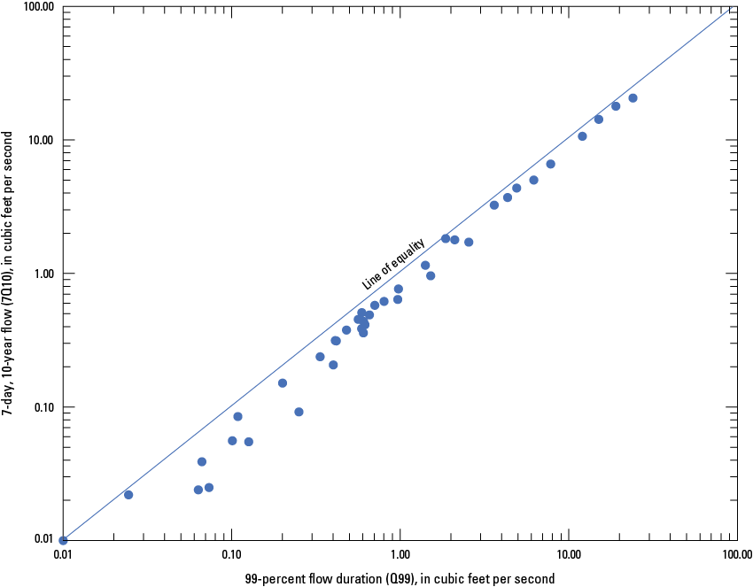
Graph comparing the 99-percent flow duration (Q99) and the 7-day, 10-year flow (7Q10) for 40 index streamgages in Connecticut and adjacent areas of neighboring States, using data through water year 2022.
Mean Flow, Spring Mean Flow, and Harmonic Mean Flow Statistics
Mean flow, spring mean flow, and harmonic mean flow were computed as the means of all available daily mean streamflow data for the period of record through water year 2022 (Ahearn and others, 2025) using the methods in this section.
Mean flow is computed as the arithmetic mean of all daily mean flows for the data series for a designated period. For example, the mean flow for a site with 20 years of data is computed as the arithmetic mean of 7,300 daily mean values (365 daily values per year). The CT DOT drainage manual refers to this flow statistic as the “average daily” flow (CT DOT, 2023).
Spring mean flow is computed similarly to mean flow as the arithmetic mean of daily mean streamflow for March and April for a designated period. For example, the mean flow for a site with 10 years of data is computed as the arithmetic mean of 610 values (61 daily values per year). The CT DOT drainage manual refers to this flow statistic as the “average spring” flow (CT DOT, 2023).
The harmonic mean flow is defined as the reciprocal of the arithmetic mean of the reciprocal daily streamflow values. Because traditional harmonic means cannot be calculated with zeroes in the dataset—including zero-flow data results in an undefined value—an adjusted harmonic mean can be calculated that considers the proportion of zero-flow days. In this adjustment, the harmonic mean is multiplied by the proportion of zero-flow days in the record. The equation is also used by the EPA in the DFLOW model (Rossman, 1990). To estimate concentrations of toxic pollutants contained in 2 liters of water per day, which is the recommended human health criterion, Rossman (1990) recommends using the harmonic mean flow when the daily variation in the flow rate is high (EPA, 2014). Harmonic means were computed using the USGS R code Hmean, which computes the harmonic mean according to the EPA DFLOW manual (Rossman, 1990), as follows:
whereStatistical Analysis of Trends in the Annual 7-Day Low Flows
The traditional assumption underlying regression analysis is stationarity in time (Helsel and others, 2020). The assumption of stationarity allows researchers to estimate the low-flow statistics from past records and apply them to the future without adjustments. Using nonstationary data in regression analysis can lead to inaccurate predictions of streamflow because the underlying statistical properties of the data change with time. Milly and others (2008) called the assumption of climate-related stationarity into question and advocated for new methods to replace models based on stationarity. Several studies have documented increases in low and median flows across the United States (McCabe and Wolock, 2002; Lins and Slack, 2005; Small and others, 2006; Hodgkins and Dudley, 2011; Dudley and others, 2020). In more recent studies, increased baseflow and the annual minimum 7-day flows from precipitation changes have been observed in basins in the northeast (Ficklin and others, 2016, Dudley and others, 2020).
Data and Methods
Subsets of streamgages with long records (more than 30 years) were created to evaluate trends in the annual 7-day low flow during the past 30, 50, 70, and 90 climate years from 2019. All 10-year blocks within each period analyzed were required to be at least 80 percent complete so that no part of the time series would have substantial missing data. These length and completeness criteria resulted in 39 streamgages for the 30-year period from 1990 to 2019 (table 4), 28 streamgages for the 50-year period from 1970 to 2019 (table 5), 19 streamgages for the 70-year period from 1950 to 2019 (table 6), and 10 streamgages for the 90-year period from 1930 to 2019 (table 7). The number of streamgages used in the analysis decreased as the years of analysis increased because of the length of available record. The streamgages used in the trend analysis include index streamgages and regulated streamgages. Trend analysis on regulated streamgages was used to determine if the degree of regulation was detectible in the period analyzed and to help the USGS categorize streamgages affected by anthropogenic influences.
Table 4.
Trend results for annual 7-day low flows for the 30-year period of climate years 1990 to 2019 at 39 streamgages in Connecticut and adjacent areas of neighboring States.[Trend data are from Ahearn and others (2025). Statistically significant (Spearman's rank correlation coefficient [p-value] less than or equal to 0.05) decreasing trends are highlighted in yellow. The Sen slope is multiplied by the number of years of annual 7-day low flow to obtain the magnitude of the trend or total change in the annual 7-day low flow over the period analyzed. USGS, U.S. Geological Survey; (ft3/s)/yr, cubic foot per second per year; MA, Massachusetts; RI, Rhode Island; CT, Connecticut]
Table 5.
Trend results for annual 7-day low flows for the 50-year period of climate years 1970 to 2019 at 28 streamgages in Connecticut and adjacent areas of neighboring States.[Trend data are from Ahearn and others (2025). Statistically significant (Spearman's rank correlation coefficient [p-value] less than or equal to 0.05) decreasing trends are highlighted in yellow. The Sen slope is multiplied by the number of years of annual 7-day low flow to obtain the magnitude of the trend or total change in the annual 7-day low flow over the period analyzed. USGS, U.S. Geological Survey; (ft3/s)/yr, cubic foot per second per year; MA, Massachusetts; RI, Rhode Island; CT, Connecticut]
Table 6.
Trend results for annual 7-day low flows for the 70-year period of climate years 1950 to 2019 at 19 streamgages in Connecticut and adjacent areas of neighboring States.[Trend data are from Ahearn and others (2025). Statistically significant (Spearman's rank correlation coefficient [p-value] less than or equal to 0.05) decreasing trends are highlighted in yellow and increasing trends are highlighted in blue. The Sen slope is multiplied by the number of years of annual 7-day low flow to obtain the magnitude of the trend or total change in the annual 7-day low flow over the period analyzed. USGS, U.S. Geological Survey; (ft3/s)/yr, cubic foot per second per year; MA, Massachusetts; RI, Rhode Island; CT, Connecticut]
Table 7.
Trend results for annual 7-day low flows for the 90-year period of climate years 1930 to 2019 at 10 streamgages in Connecticut and adjacent areas of neighboring States.[Trend data are from Ahearn and others (2025). Statistically significant (Spearman's rank correlation coefficient [p-value] less than or equal to 0.05) decreasing trends are highlighted in yellow, increasing trends are highlighted in blue. The Sen slope is multiplied by the number of years of annual 7-day low flow to obtain the magnitude of the trend or total change in the annual 7-day low flow over the period analyzed. USGS, U.S. Geological Survey; (ft3/s)/yr, cubic foot per second per year; MA, Massachusetts; CT, Connecticut]
The trends were computed with methods that consider the possibility of short- and long-term persistence in the temporal data. This is an important issue that is often ignored in trend studies. Trends over time are sensitive to assumptions of whether underlying hydroclimatic data are independent, have short-term persistence, or have long-term persistence (Cohn and Lins, 2005; Koutsoyiannis and Montanari, 2007; Hamed, 2008; Khaliq and others, 2009; Kumar and others, 2009). Short- and long-term persistence may represent the occurrence of wet or dry conditions that tend to cluster from year to year (Koutsoyiannis and Montanari, 2007; Hodgkins and others, 2017). Short-term can be a couple of years, and long-term can be decades and centuries. For further discussion and references on persistence, see Hodgkins and Dudley (2011). Because the long-term time-series structure of low-flow data is not well understood, temporal trend significance with three different null hypotheses of the serial structure of the data are reported: independence, short-term persistence, and long-term persistence (Hamed and Rao, 1998; Hamed, 2008). For the serial correlation structure of data referred to as “independence,” annual 7-day flow data from year to year are independent from each other (ignoring any short or long clusters of wet and dry years).
Trends were considered statistically significant at p-value less than or equal to (≤) 0.05; this magnitude represents a 5-percent probability that a trend is due to random chance. The magnitudes of the trends were computed with the Sen slope (also known as the Kendall-Theil robust line), the median of all possible pairwise slopes in each time series (Helsel and others, 2020). The Sen slope is multiplied by the number of years of annual 7-day low flow to obtain the magnitude of the trend or total change in the annual 7-day low flow over the period analyzed. For example, a Sen slope of 9.1 cubic feet per second (ft3/s) multiplied by 90 (for the 90-year period) results in a total change in the annual 7-day low flow of 819.64 ft3/s for the Connecticut River at Thompsonville (station 01184000) streamgage (table 7).
Trend Results in Annual 7-Day Low Flows
Results from the trend analysis for 30-, 50-, 70- and 90-year periods under the three serial correlation structures (independence, short-term persistence, and long-term persistence), magnitudes of Sen slopes, and p-values are shown in tables 4 through 7. For this study, the trend results of the annual 7-day low flow depend on the period of record analyzed and assumptions about the serial correlation structure. Decreasing trends were detected in all four periods (30, 50, 70, and 90 years) analyzed. In contrast, increasing and decreasing trends were detected in the 70- and 90-year periods. Increasing trends were found only at regulated streamgages. The trend analysis was performed using the entirety of the record. Using different parts of the streamflow record based on historical changes to streamflow in the trend analysis was outside the scope of this work. Three streamgages had trends in the three serial correlation structures: two decreasing (Pawcatuck River at Wood River Junction, R.I. [station 01117500; tables 5 and 7] and Naugatuck River at Beacon Falls, Conn. [station 01208500; table 5]), and one increasing (Connecticut River at Thompsonville, Conn. [station 01184000; table 7]).
Trend results at index streamgages (15 in the 30-year period, 11 in the 50-year period, 7 in the 70-year period, and 2 in the 90-year period) showed few statistically significant trends. Two nearby index streamgages in Rhode Island have statistically significant (decreasing) trends in two periods and in two of three of the serial correlation structures. None of the index streamgages in Connecticut have statistically significant trends in any of the periods analyzed. Trend results at regulated streamgages (24 in the 30-year period, 17 in the 50-year period, 12 in the 70-year period, and 8 in the 90-year period) showed some statistical evidence of trends in the annual 7-day low flow.
For the 30-year period (1990–2019), 39 sites (15 index streamgages and 24 streamgages with regulation) were analyzed for trends. Three of the streamgages (Quinnipiac River at Southington, Conn. [station 01195490]; Pomperaug River at Southbury, Conn. [station 01204000]; and Naugatuck River at Beacon Falls, Conn. [station 01208500]) showed a decreasing trend with short-term persistence (table 4), with a total change of 3.00, 7.29, and 35.43 ft3/s, respectively. There were no increasing trends in the 30-year period.
For the 50-year period (1970–2019), 28 sites (11 index streamgages and 17 streamgages with regulation) were analyzed for trends. Three streamgages showed a decreasing trend with independence and short-term persistence (Branch River at Forestville, R.I. [station 01111500]; Pawcatuck River at Wood River Junction, R.I. [station 01117500]; and Naugatuck River at Beacon Falls, Conn. [station 01208500]), with a total change of 9.66, 27.95, and 42.90 ft3/s, respectively (table 5). Two of these streamgages (stations 01111500 and 01117500) had decreasing trends in all three serial correlation structures. The third streamgage (station 01208500) showed decreasing trends in both the 30- and 50-year periods. There were no increasing trends in the 50-year period.
The 70- and 90-year periods included both increasing and decreasing trends (tables 6 and 7). For the 70-year period (1950–2019), 4 of the 19 streamgages analyzed showed trends with different serial correlation structures⸺three increasing (Connecticut River at Thompsonville, Conn. [station 01184000; independence, short-term persistence, and long-term persistence]; Quinnipiac River at Wallingford, Conn. [station 01196500; independence]; and Housatonic River at Stevenson, Conn. [station 01205500; independence]) and one decreasing (Pawcatuck River at Wood River Junction, R.I. [station 01117500; independence, short-term persistence, and long-term persistence]). The 01184000 streamgage (increasing trend of 1,160 ft3/s during 70 years) and 01117500 streamgage (decreasing trend of 17.74 ft3/s during 70 years) showed differing trends in the three serial correlation structures. When a trend was observed in all three serial correlation structures, there was a greater probability than not that the trend was not due to random chance. The 01196500 and 01205500 streamgages showed an increasing trend of 12.73 ft3/s and 144.83 ft3/s during 70 years, respectively.
For the 90-year period (1930–2019), 3 of the 10 streamgages analyzed had trends in two of three serial correlation structures (independence and short-term persistence). Two streamgages (Connecticut River at Thompsonville, Conn. [station 01184000; 819.64 ft3/s during 90 years], and Quinnipiac River at Wallingford, Conn. [station 01196500; 13.72 ft3/s during 90 years]) had an increasing trend, and one streamgage (Quinebaug River at Jewett City, Conn. [station 01127000]) had a decreasing trend (64.66 ft3/s during 90 years; table 7). All three of these streamgages are at regulated sites. No trends were detected at the two index streamgages or with long-term persistence in the 90-year period. Because of the lack of strong and consistent statistical evidence of long-term trends at index streamgages in Connecticut and the adjacent areas of neighboring States, the traditional assumption of stationarity was supported for this regional regression analysis.
Basin and Climatic Characteristics of Streamgages
Flow characteristics of streams are directly related to the physical, land-cover, geologic, and climatic features of the basin. Characteristics of the drainage basin were selected for use as potential explanatory variables in the regression analysis based on their theoretical relation to flows, the results of previous studies in Connecticut and similar hydrologic regions, and the ability to measure the basin characteristics using digital datasets and GIS technology. The basin and climatic characteristics considered for use in the Connecticut regression analysis are listed in table 8. The measured values of these characteristics for the streamgages in Connecticut and adjacent areas of neighboring States are available in Ahearn and others (2025). There are multiple geospatial data layers used in calculating topology-related characteristics of drainage basins from multiple sources. Data on the total length of streams are from the National Hydrography Dataset Plus High Resolution (USGS, 2023b). Elevation data, which were also used for basin slope calculations, are from the USGS 3D Elevation Program (USGS, 2023a). Land-cover and land-use data are from the National Land Cover Database 2016 (Dewitz, 2019). Climatic data (monthly and annual precipitation and annual temperature 1981–2010) are from the Parameter-Elevation Regressions on Independent Slopes Model (PRISM; PRISM Climate Group, 2021). Surficial geology data (at a 1:24,000 scale) are from CT DEEP (2022), Massachusetts Bureau of Geographic Information (2022), New York State Museum (Cadwell, 1989), and Rhode Island Geographic Information System (2022). Hydrologic soil group data are from the Natural Resources Conservation Service (2022) Soil Survey Geographic database.
Table 8.
Basin and climatic characteristics used as potential explanatory variables in the regression analysis for estimating selected frequency, duration, and mean flow statistics in Connecticut.[Land use characteristics are from the National Land Cover Dataset 2016 (Dewitz, 2019). Surficial geology is from Stone and others (1992). Soil characteristics are from the Soil Survey Geographic Database (SSURGO; Natural Resources Conservation Service, 2022). Climatological characteristics are from the Dataset; PRISM, Parameter-Elevation Regressions on Independent Slopes Model (PRISM Climate Group, 2021). NAVD 88, North American Vertical Datum of 1988; NA, not applicable; S&G, sand and gravel; &, and]
Development of Regression Equations for Estimating Selected Flow Statistics
Multiple-linear regression analysis was used to develop equations to estimate flows at ungaged stream sites in Connecticut. Multiple-linear regression analysis provides a mathematical equation of the relation between a response variable (streamflow statistic) and one or more explanatory variables (basin or climate characteristics). After developing such equations, if the explanatory variables are known (can be measured or quantified) at the ungaged locations, then the fitted equations can be used to estimate the response variables. Multiple-linear least-squares regression methods, including the ordinary-least-squares (OLS), weighted-least-squares (WLS), and generalized-least-squares (GLS) methods, were applied in the development of equations for estimating selected flow durations, low-flow frequency statistics, and select mean flows.
Of the 118 streamgages with updated streamflow statistics, 40 streamgages were used in the regression analysis (26 in Connecticut, 2 in Massachusetts, 4 in New York, and 8 in Rhode Island; fig. 3; table 9). The streamgages in the regression analysis were selected according to the following criteria: (1) a minimum of 10 years of streamflow data; (2) considered an index streamgage (natural or near-natural flow conditions); and (3) located within 15 miles of Connecticut. The set of streamgages selected for regionalizing flows was expanded to adjacent States to include index stations on nearby rivers that met the selection criteria. Inclusion of nearby streamgages outside the State can provide a more representative sample of the range of basin and streamflow characteristics found in Connecticut.
Table 9.
Streamgages used in the development of regional regression equations for estimating flow durations, low-flow frequencies, and mean flows in Connecticut.[Data are from U.S. Geological Survey (2024b). A water year is the period from October 1 to September 30 and is designated by the year in which it ends. USGS, U.S. Geological Survey; NWIS, National Water Information System; mi2, square mile; RI, Rhode Island; CT, Connecticut; MA, Massachusetts; NY, New York]
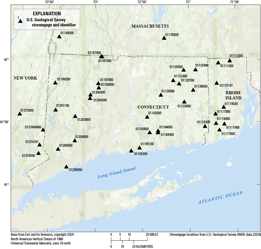
Map showing locations of the 40 index streamgages for developing regression equations to estimate durations, low-flow frequencies, and mean flows in Connecticut. NWIS, National Water Information System (U.S. Geological Survey, 2024b).
Regression Analysis for Estimating Selected Flow Statistics at Ungaged Stream Sites
Logarithmic (base 10) transformations were made of the flow statistics (response variable) and basin characteristics (explanatory variables) to linearize the relation between the explanatory variables and the predictor variables, stabilize the variance by obtaining equal variance about the regression line, and improve the spread of the data. OLS regression analyses using Spotfire S+ version 8.1 statistical software (TIBCO Software, Inc., 2008) were used to determine the best combinations of basin characteristics to use as explanatory variables in the multiple linear regression equations. The all-possible subsets statistical method was used for selecting explanatory variables. In all-possible subsets, all the equations created from all possible combinations of explanatory variables were examined, and the coefficient of determination (R2) was used to check for the best combination of explanatory variables. The explanatory variables were selected based on their relation to flow and correlation to other basin characteristics using Pearson’s correlation coefficient (r).
If a moderate correlation (r less than 0.6) existed between two explanatory variables, then the two variables were evaluated individually in the variable selection process. To identify the best combination of explanatory variables in the all-possible subsets method, different equations from the regression analysis were compared based on the following measurements:
-
• the adjusted-R2, also called the adjusted coefficient of determination, which is a measure of the percentage of the variation explained by the explanatory variables of the equation and is adjusted for the number of parameters in the equation;
-
• Mallow’s Cp statistic, which is an estimate of the standardized mean square error of prediction (Mallow’s Cp statistic is a compromise between maximizing the explained variance by including all relevant variables and minimizing the standard error by keeping the number of variables as small as possible [Helsel and others, 2020]);
-
• the predicted residual sum of squares statistic, which is a validation-type estimator of error (Helsel and others, 2020) and uses n−1 observations to develop the equation, then estimates the value of the observation that was left out; the process is repeated for each observation and the prediction errors are squared and summed; and
-
• the standard error of estimate (in percent), also referred to as the root mean square error (RMSE) of the residuals, which is the standard deviation of observed values about the regression line; it is computed by dividing the unexplained variation or the error sum of squares by its degrees of freedom (in this study, the standard error of estimate is based on one standard deviation).
The equations with a smaller standard error of estimate, Mallow’s Cp, and predicted residual sum of squares statistic and a higher adjusted-R2 were preferred. In addition, the explanatory variables were selected based on statistical significance at the 95-percent confidence level, an analysis of the residuals, and how the explanatory variables might affect flows. Explanatory variables that had a 95-percent probability of effectiveness (probably a good predictor of flow and not due to chance) were classified as significant. If an explanatory variable was significant but had only a small effect on the standard error (arbitrarily chosen as less than a 2-percent change), then it was left out of the equation.
WLS and GLS regressions were used for deriving the final coefficients (Helsel and others, 2020). In OLS regression, equal weight is given to all streamgages in the analysis regardless of record length. WLS regression can account for differences in the streamgage length of record and allows more emphasis to be placed on streamgages that are considered more robust due to a longer data record. Regression coefficients in the equations for estimating flow durations and mean flows were finalized using WLS regression methods. Regression coefficients in the equations for estimating the low-flow frequency statistics (7Q10 and 30Q2) were finalized using GLS regression methods, which compensate for differences in both the variability and reliability of and correlation among the low-flow frequency statistics at the streamgages included in the analysis. Stedinger and Tasker (1985) have shown that, where streamflow record lengths vary widely and flows (and, therefore, the flow statistics) at different streamgages are highly correlated, GLS regression provides more accurate estimates of the regression coefficients, better estimates of the accuracy of the regression coefficients, and almost unbiased estimates of the model error when compared with OLS regression. GLS regression gives more weight to long-term streamgages than short-term streamgages and more weight to the streamgages where flows are the least correlated to flows at other streamgages.
WLS and GLS regression analyses were performed using the USGS Weighted-Multiple-Linear Regression (WREG) software (version 3.0; Farmer and others, 2019), written in R version 3.6.2 (R Core Team, 2019). WREG was developed in 2009 (Eng and others, 2009) and was later updated by Farmer (2021). The output of WREG provides various measures of the reliability of the regression equations including the average variance of prediction (in log units), the standard error of prediction (in percent), the standard error of estimate (in percent), the pseudocoefficient of determination (pseudo-R2), the mean squared error (in log units), the RMSE (in percent), and leverage and influence of individual observations on the regression. Equations for calculating these metrics are available in Eng and others (2009).
An additional criterion in selecting explanatory variables for the final regression equations was to have no more than three variables (basin characteristics). This was done to minimize overfitting the regression equation and to avoid multicollinearity among variables, which makes it difficult to evaluate the relative importance of the individual explanatory variable in the regression equation.
Hydrologic Regions
In a regional regression study, dividing a large study area into smaller, more homogeneous regions can improve the accuracy of the regression equations. Historically, regression equations to estimate flow statistics in Connecticut have been developed as a set of single statewide equations. To potentially improve the predictive accuracy and precision of the regression models in Connecticut, streamgages were grouped into different regions and exploratory linear regression analysis was performed on subsets of streamgages.
The physiographic regions of southern New England (Denny, 1982) and boundaries of the EPA northeastern coastal zone and northeastern highland level III ecoregions (Omernik, 1995; EPA, 2022) were used to subdivide the streamgages and investigate smaller hydrologic regions. The physiographic regions and level III ecoregions are based on similarities in physiography, topography, geology, hydrology, vegetation, climate, soils, land use, and ecosystems. In addition, streamgages in eastern and western Connecticut, using the Connecticut River as the dividing line, were evaluated as separate hydrologic regions. Hydrologic unit code boundaries were followed wherever possible to avoid dividing basins into multiple regions. Error metrics (mean square error and RMSE) that are commonly used for evaluating and reporting the performance of a regression model were used in assessing the models based on the physiographic and ecoregions. Results from the regional analysis of smaller subregions did not indicate improvement in the predictive accuracy and precision of the regression models. The analysis indicated that assessing Connecticut as a statewide region, as used in previous regional low-flow regression analyses, is still appropriate.
Assessment of Regression Equations
Methods of assessing the accuracy of the regression equations (quality of model fit) included both visual and numerical measures. Checking the model assumptions for collinearity (known as the variance inflation factor [VIF]), normality, and heteroscedasticity indicated no problems with the models. Collinearity was evaluated by computing VIFs for each explanatory variable. VIF values express the ratio of the actual variance of the coefficient of the explanatory variable to its variance if it were independent of the explanatory variables (Cavalieri and others, 2000). VIF values greater than 5 indicate that an explanatory variable is so highly correlated to other explanatory variables that it is an unreliable explanatory variable and should not be included in the equations because the equations may provide erroneous results. None of the explanatory variables had a VIF value greater than 5.
The models were visually assessed for patterns using residual plots and through a spatial analysis of the residuals. The residuals were plotted at the centroid of their respective drainage basins to look for geographical biases. No apparent geographical biases with either large positive or negative residuals were found. The residual plots indicated overall good performance. The equations appeared to fit the data reasonably well and adequately described the relation between the predictor and explanatory variables. The model coefficients explained the response correctly. The p-values for the regression coefficients were found to be less than or equal to 0.05, indicating the probability that the regression coefficient was significant.
Numerical measures to assess the quality of the models include adjusted-R2 and RMSE (table 10). The adjusted R2 identifies the percentage of variance in the response variable (flow being estimated) that is explained by the explanatory variables (basin and climatic characteristics). The RMSE will be small if the predicted responses are very close to the true responses. Conversely, the RMSE will be large if the predicted and true responses differ substantially, at least for some of the observations. A value of zero would indicate a perfect fit to the data.
The RMSE of the 47 equations developed ranged from 7.9 to 121.9 percent, with an average of 27.9 percent (fig. 4). Regression equations to estimate flows in the interquartile range (25- to 75-percent exceedances) have much smaller RMSEs than the equations to estimate extreme low flows (Q99 or 7Q10). The RMSE for the Q25 was 10.5 percent for the period of record, with an average of 16.5 percent for the six bioperiods. The RSME for the Q75 was 24.2 percent for the period of record, with an average of 21.7 percent for the bioperiods. The RMSE for the Q50 was 15.1 percent for the period of record, and ranged from 10.5 to 30.2 percent, with an average of 17.6 percent for the bioperiods. In contrast, the RMSE for the Q99 was notably larger; 105.1 percent for the period of record and ranged from 20.0 to 121.9 percent, with an average of 50.0 percent for the bioperiods. The 7Q10 is an extreme low-flow statistic and has the largest RMSE (121.9 percent) of the set of regression equations.
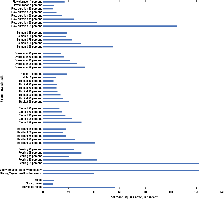
Graph showing the root mean square errors of 47 regression equations developed to estimate flow durations, low-flow frequencies, and mean flows at ungaged stream sites in Connecticut.
The habitat-forming (March–April) bioperiod has the smallest RMSE, ranging from 8.2 to 20.0 percent for the Q25 to Q99. Typically, flows are substantially higher during the habitat-forming bioperiod than other bioperiods (months or seasons). In contrast, the rearing and growth (July–October) bioperiod, which has the lowest flow conditions of all bioperiods, has the largest RMSE, ranging from 24.3 to 121.9 percent for the Q25 to Q99. The adjusted coefficient of determination (adjusted-R2) of the 47 equations ranged from 73.4 to 99.5 percent, with an average of 95.1 percent, which indicates that overall about 95.1 percent of the observed variation can be explained by the model’s inputs.
Diagnostic checks on the regression equations included evaluating outliers and influential observations. The presence of outliers is a subtle form of nonnormality, and influential observations are data that substantially change the fit of the regression line. The influence of an individual observation on the regressions is measured with Cook’s D statistic (Helsel and others, 2020). Cook’s D statistic is a measure of the change in the parameter estimates when an observation is deleted from the regression analysis. No influential observations that appreciably altered the slope of the regression line were found with Cook’s D statistic.
Scatterplots of the predicted flow from the regression model and observed flow from the streamgage were used to visualize the performance of the regression models. Scatterplots of the select streamflow statistics are shown in figures 5 and 6. The x-axis represents the observed streamflow (flow statistic from the streamgage record), and the y-axis represents the predicted streamflow (flow statistic from the regression model). When the points are close to the one-to-one (1:1) line (line of equality), then the predicted data are close to the observed data. Ideally, if the predictions are perfect, then all the points will lie on the 1:1 line. Scatterplots of the higher flows—mean (fig. 5A) and spring mean (fig. 5B)—show a narrow spread between the observed and predicted values. Scatterplots of low and medium flows—harmonic mean (fig. 5C) and 30Q2 (fig. 5D)⸺show a moderate spread between the observed and predicted data. Scatterplots of extremely low flows⸺7Q10 (fig. 5E) and Q99 (fig. 5F)⸺show a large spread between the observed and predicted data. Scatterplots of the Q50 for five of the six bioperiods (fig. 6A, B, C, D, E) show a narrow spread between the observed and predicted data. The Q50 scatterplot for the remaining bioperiod, the period with the lowest flow—rearing and growth (fig. 6F)—shows a moderate spread.
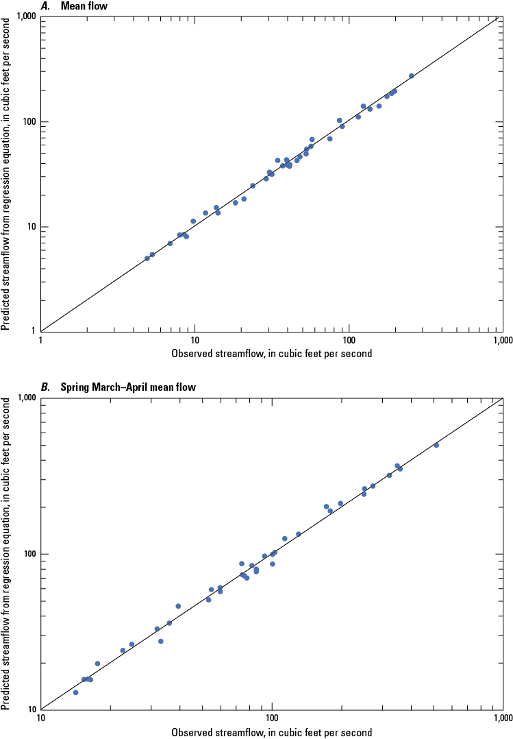
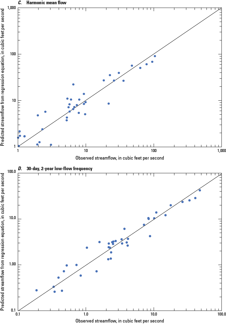
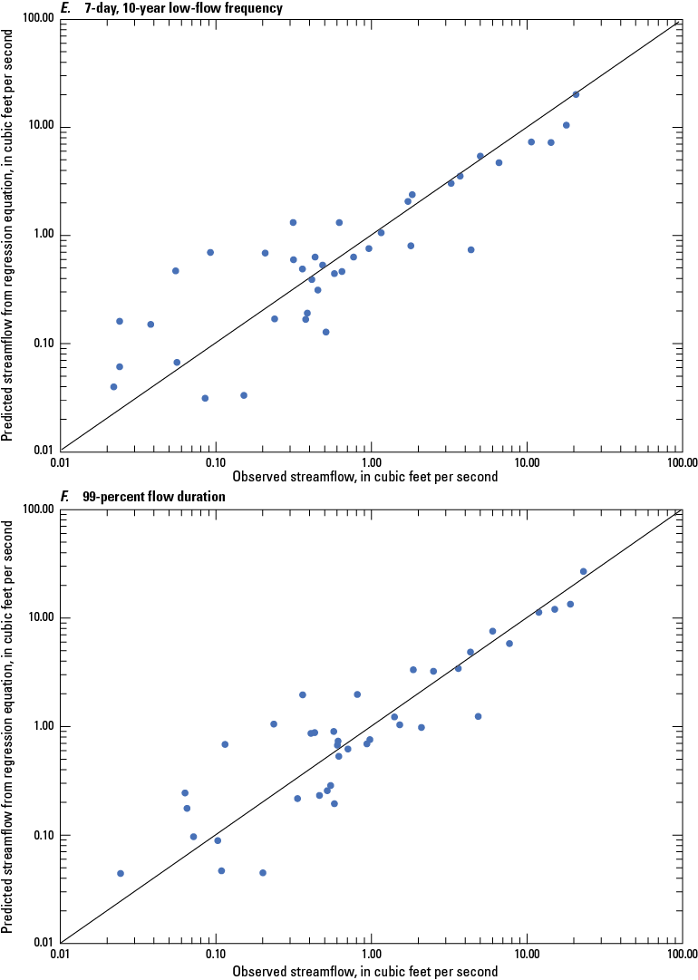
Scatterplot of observed versus predicted streamflow for the A, Mean, B, Spring mean, C, Harmonic mean, D, 30-day, 2-year low-flow frequency (30Q2), E, 7-day, 10-year low-flow frequency (7Q10), and F, 99-percent flow duration (Q99).
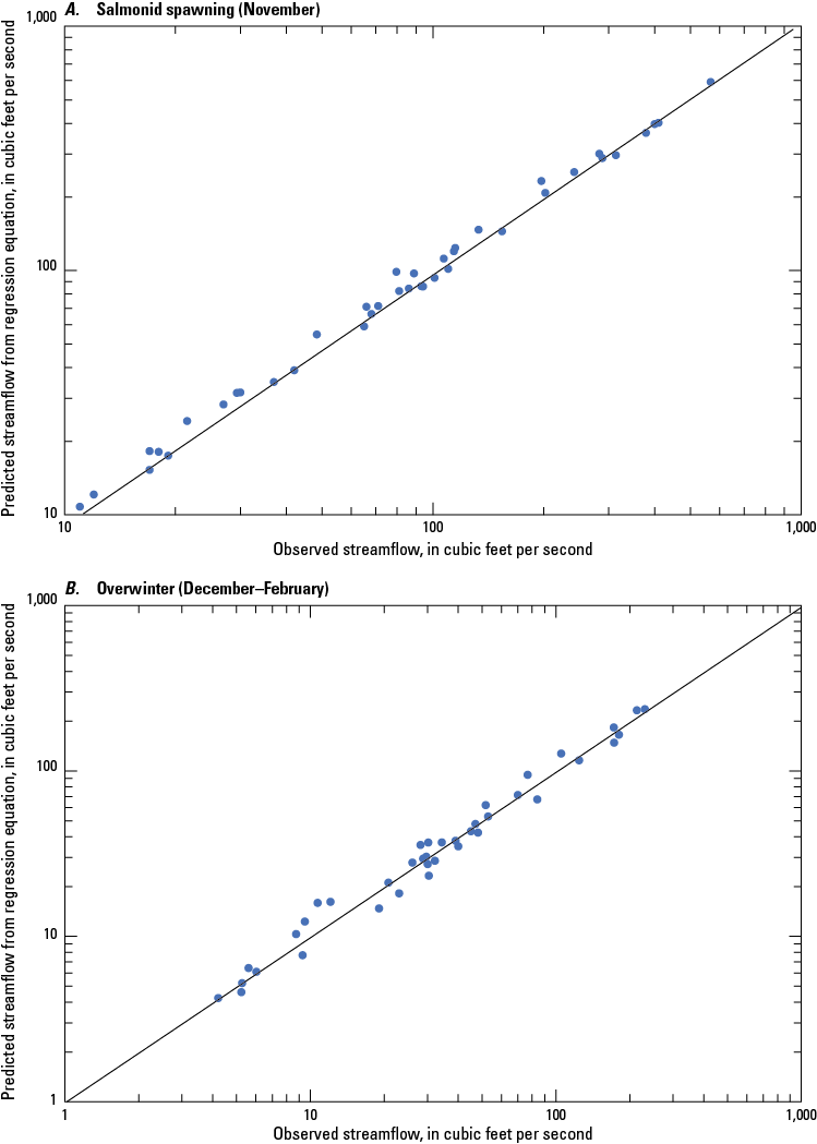
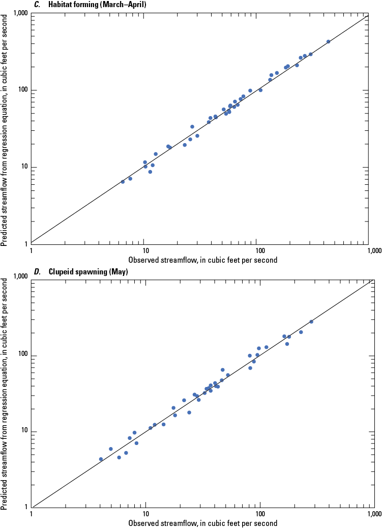
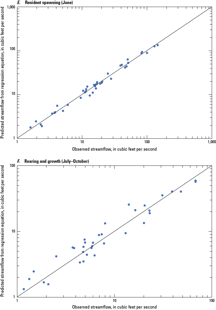
Scatterplot of the observed versus predicted streamflow for the 50-percent flow duration for the A, Salmonid spawning, B, Overwinter, C, Habitat forming, D, Clupeid spawning, E, Resident spawning, and F, Rearing and growth bioperiods for streamgages in and near Connecticut.
A wide range between the observed and predicted data is generally found in regression equations for estimating extreme low flows, also indicated by the RMSE in this study; 121.9 percent for 7Q10 and 105.1 percent for Q99. Predicting extreme low flows using regression equations remains challenging, as can be seen from the adjusted-R2 values (73.4 and 78.1 percent for the 7Q10 and Q99, respectively), suggesting that about 25 percent of variation in the streamflow is not explained by the explanatory variables (basin characteristics) in the equations. This may be improved with a more comprehensive look at the individual streamgages and effects of local geology and climatic characteristics.
In this study, bias correction factors were not used because they generally are very small in Connecticut. The transformation of the base-10 log-transformed regression equations to unlogged (original) units to calculate specific streamflow statistics at an ungaged site can introduce bias in the streamflow estimate. Bias correction factors were used in some studies in Massachusetts to remove the bias from the estimates from regression equations (Ries, 1994a, b; Ries and Friesz, 2000; Archfield and others, 2010); however, the bias correction factors were generally very small. Archfield and others (2010) shows that the bias correction factor resulted in a 0.3-percent increase in the 1-percent annual exceedance probability streamflow and 2.4-percent increase in the 99-percent annual exceedance probability streamflow for regression equations to estimate streamflow quantiles in Massachusetts. In a Rhode Island study (Bent and others, 2014), bias correction factors were not used because if they had been, then the streamflows estimated from the regression equations would not have an equal chance of being higher or lower than their actual values (Julie Kiang, USGS, oral commun., 2011). In studies by Risley (1994) in Massachusetts, Stuckey (2006) in Pennsylvania, Armstrong and others (2008) in Massachusetts; and Ahearn (2010) in Connecticut, bias correction factors were not used, likely because they were generally very small.
Final Regression Equations
Final regression equations are listed in table 10, along with the number of stations used in the regression analysis and several performance metrics. The explanatory variable names in the final equations are the StreamStats labels for the variables (USGS, 2024a). Nine basin characteristics—drainage area (DRNAREA); percentage of area with coarse-grained, stratified deposits (CRSDFT); stream density (total length of streams divided by the drainage area; STRDEN); mean basin slope (BSLDEM10M); mean basin elevation (ELEV); percentage of area with hydrologic soil group A (SSURGOA); mean monthly precipitation in November (NOVAVPRE10); mean precipitation in the winter (average of December, January, and February; PRCWINTER10); and mean annual temperature (TEMP)—are used as explanatory variables in the equations. The performance metrics used to report the quality of the final regression equations include the adjusted-R2 (in percent) and the RMSE (in percent).
Table 10.
Summary of 47 regression equations and performance metrics for estimating flow durations, low-flow frequencies, and mean flows for ungaged sites in Connecticut.[Performance metrics are from Ahearn and others (2025). R2, coefficient of determination; MSE, mean square error; RMSE, root mean square error; WLS, weighted least-squares regression analysis; DRNAREA, drainage area (in square miles); CRSDFT, percentage of area with coarse-grained, stratified deposits—sand and gravel (in percent); STRDEN, stream density—total length of streams divided by drainage area (in miles per square mile); NOVAVPRE10, mean monthly precipitation in November (in inches); ELEV, mean basin elevation (feet relative to the North American Vertical Datum of 1988; PRCWINTER10, mean seasonal precipitation in December, January, and February (in inches); TEMP, mean annual temperature (in degrees Fahrenheit); SSURGOA, percentage of area with hydrologic soil group A (in percent); BSLDEM10M, mean basin slope (in percent); 7Q10, 7-day, 10-year low-flow frequency; 30Q2, 30-day, 2- year low-flow frequency; GLS, generalized least-squares regression analysis]
Drainage area (DRNAREA) is an explanatory variable in all the equations and is considered a primary cause of streamflow variation between sites. Streamflow could logically be expected to increase in proportion to the size of the drainage area. The second most common explanatory variable is the percentage of the area with coarse-grained, stratified deposits in the basin. In general, the physical processes controlling streamflow during late summer or early fall in Connecticut are related to geologic and soil characteristics. Studies by Wandle and Randall (1994) and Cervione and others (1982) found drainage basins underlain with a large percent of coarse-grained, stratified deposits have larger base flows than drainage basins underlain with glacial till and bedrock. The differences in streamflow between basins may be increased further by variations in the infiltration capacity and delayed subsurface runoff indicated by the percentage of soil type in the basin. A basin’s soil index (percentage of the area with hydrologic soil type A) represents the potential maximum infiltration and average moisture conditions, which affect streamflow. For this study, the percentage of area with coarse-grained, stratified deposits or hydrologic soil type A were important explanatory variables for the Q25 to Q99 and low-flow frequencies.
Three climatic characteristics—monthly mean precipitation for November, seasonal mean precipitation for December through February, and annual mean temperature—were statistically significant explanatory variables in the salmonid spawning, overwinter, and habitat forming bioperiods that span November through April. Streamflow commonly reflects the regional precipitation and temperature. The western and eastern uplands have cooler temperatures than the other areas in the State and typically receive precipitation in the form of snow in winter, whereas the lowlands more often experience rain events, which could explain the importance of these climatic variables in these three bioperiods. The climatic variables have positive coefficients, thereby causing an increase in the estimated flow value when the climatic variable increases.
For this study, three of nine explanatory variables have negative coefficients, causing a decrease in the estimated flow value. Stream density, which is the total length of streams divided by the drainage area, was a significant explanatory variable in the flow duration, low-flow frequency, and mean flow regression equations. A greater stream density in a basin compared to a basin with a smaller stream density allows base flow to be routed out of the basin earlier in the runoff recession (causing less base flow to be available during lower flows) through its larger network of flow paths intercepting the water table. The decreasing streamflow is represented by the negative coefficient (Bent and others, 2014). In several other studies, stream density had a negative coefficient in equations for estimating low flows in Pennsylvania (Stuckey, 2006) and for estimating the probability of streams flowing perennially in Massachusetts (Bent and Archfield, 2002).
Two other significant physiographic characteristics with negative coefficients are mean basin values for elevation and slope. Elevation was included in the overwinter bioperiod for Q25 to Q95 and slope was an important predictor for mean flow. Although elevation may not directly cause streamflow variations, it may serve as an index for other factors (such as temperature or vegetation) that cause streamflow variation. Generally higher elevations and steeper slopes are associated with different geologic characteristics and subsequently different base flows. The geomorphic and climatic indices in the regressions can be measured conveniently using GIS technology and generally are perceived to estimate low and mean streamflow with reasonable accuracy.
Prediction Intervals
Flow estimates obtained from regression equations have a related degree of uncertainty that can be described by prediction intervals. Prediction intervals indicate the probability that the true flow for a site is within the given bounds of flow. For example, the 90-percent prediction interval for a flow estimate at a site indicates that there is a 90-percent confidence that the true flow for the site is between the given flow values obtained from the regression equation. The lower and upper boundaries of the 90-percent prediction intervals can be computed by:
whereQ
is the estimated streamflow statistic for the site,
QLPI
is the estimated lower boundary of the 90-percent prediction interval,
QUPI
is the estimated boundary of the upper 90-percent prediction interval, and
T
is the 90-percent prediction interval determined as follows:
t(α/2,n−p)
is the critical value from the Student’s t distribution, where α is the alpha level (α=0.10 for 90-percent prediction intervals), and (n–p)is the number of degrees of freedom with n data values (number of streamgages) used in the regression analysis, and p is the number of parameters in equation 4 (equal to the number of explanatory variables or basin characteristics plus one; equations in table 10), and
Si
is computed as follows:
γ2
is the model-error variance (equal to the RMSE squared);
xi
is a row vector of the logarithms of the basin characteristics for site i, which has been augmented by a 1 as the first element;
U
is the covariance matrix for the regression coefficients; and
xi'
is the transpose of xi, representing a row vector of logarithms of basic characteristics at site i plus one (Ludwig and Tasker, 1993).
The values of t(α/2,n−p) and U needed for equations 4 and 5 for the 47 regression equations are listed in table 11. The values of γ2 (model error variance, in log units) needed in equation 5 can be calculated by squaring the value of the mean square error (log10) in table 11. Example computations of prediction intervals can be found in Ahearn and Hodgkins (2020) and Bent and others (2014).
Table 11.
Model error variance and covariance matrix for estimating prediction intervals for flow durations, low-flow frequencies, and mean flows in Connecticut.[Model error variance and covariance values were determined from the Weighted-Multiple-Linear Regression (WREG) program, ver. 3.0 (Farmer and others, 2019). The matrix horizontal and vertical variables are defined by the constant and the independent variables in the regression equations in the order they are listed. Regression model error data are from Ahearn and others (2025). MSE, mean square error; 7Q10, 7-day, 10-year low-flow frequency; 30Q2, 30-day, 2- year low-flow frequency; —, no data]
Limitations of Regression Equations
Use of the regression equations presented in this report in determining selected streamflow statistics is limited by the range of the basin characteristics data used to develop the equations and by the accuracy of the estimates. The regression equations developed in this study are not intended to be used at ungaged sites in which the basin characteristics are outside of the range of those used to create the regression equations. The ranges of the basin characteristics data used as explanatory variables to develop the regression equations are listed in table 12; the corresponding accuracies of the estimates calculated by these equations are listed in table 11. The use of these regression equations requires that the physical and climatic basin characteristics be determined using the same datasets (Ahearn and others, 2025) that were used to develop the equations described in this report.
Table 12.
Ranges of basin and climatic characteristics used as explanatory variables in regression equations generated for estimating flow durations, low-flow frequencies, and mean flows for ungaged sites in Connecticut.[StreamStats labels are from U.S. Geological Survey (2024a)]
The equations, which are based on data from streams with little to no flow alteration, will give useable estimates only for the natural flows for selected sites. They will not give estimates for sites where the flow is altered by structures and artificial processes, such as dams, surface-water withdrawals, groundwater withdrawals (pumping wells), diversions, and wastewater discharges. The equations are not applicable at sites where the groundwater-contributing areas and the surface-water drainage areas to stream sites are substantially different in size. In these areas, groundwater can flow from one surface-water drainage area into another. Therefore, in basins whose groundwater-contributing areas are larger than their surface-water drainage areas, the equations would likely underestimate streamflows. Conversely, for areas whose groundwater-contributing areas are smaller than their surface-water drainage areas, the equation would likely overestimate streamflows. Additionally, the equations are not applicable to streams with losing stream reaches. Losing streams are defined as streams or stream reaches that lose water to the groundwater system (Winter and others, 1998, p. 9–10 and 16–17). Generally, a stream reach is losing where the groundwater table does not intersect the streambed in the channel (the water table is below the streambed) during low-flow periods. Losing stream reaches commonly begin where a stream flows from an area of the basin underlain by till or bedrock onto an area underlain by stratified deposits (such as where hillsides meet river valleys). At such junctures, a stream can lose a substantial amount of water through its streambed.
The accuracy of the regression equations is a function of the quality of the data used to develop the equations. These data include the streamflow data used to estimate the statistics, information about possible unknown flow alterations to the stream above a site, and the measured basin characteristics. Basin characteristics used in the development of the regression equations are limited by the accuracy of the digital data layers available and used at the time of this study [2024].
StreamStats Application
The streamflow statistics for the 118 streamgages and 47 regression equations for estimating flow statistics developed are expected to be included as part of this study in the USGS National StreamStats web application (USGS, 2024a) that provides analytical tools for water-resources planning and management and for engineering and design purposes. For nearly a quarter century, the StreamStats web application has been a source of information used by Federal, State, and local governments, the private sector, and other organizations to make decisions about how streamflow may affect the safety and well-being of the public (Ries and others, 2024). StreamStats (USGS, 2024a; Ries and others, 2017) provides users with the ability to obtain streamflow statistics such as the 1-percent annual exceedance probability, a peak flow, and the 7Q10, a low flow, from USGS streamgage sites, as well as estimates of streamflow statistics from regression equations for user-selected ungaged sites. An interactive geoprocessing map-based interface allows user to click on the centerline for any stream site to calculate selected streamflow statistics and the associated 90-percent prediction intervals from the regression equations. The basin-characteristic values for a user-selected stream site used as input for the regression equations are determined from digital map data from ArcGIS (Esri, 2024). StreamStats outputs include a map of the drainage basin boundary for the stream site, the values of the GIS-measured basin characteristics, the estimated streamflow statistics, and prediction intervals for the estimates.
Summary
Knowledge of streamflow characteristics is necessary for effective management of water resources in Connecticut. Decisions related to water-quality permitting, instream flow standards, and design flows depend on estimates of streamflow. Methods for estimating flow durations, low-flow frequencies, and mean flows at ungaged stream sites are part of this need. The U.S. Geological Survey, in cooperation with the Connecticut Department of Environmental Protection and the Connecticut Department of Transportation, updated flow statistics for 118 streamgages and developed 47 statewide regression equations for estimating selected flow statistics. The statewide regression equations include 1-, 5-, 10-, 25-, 50-, 75-, 90-, and 99-percent flow durations; 7-day, 10-year and 30-day, 2-year low-flow frequencies; annual, spring, and harmonic mean flows; and flow durations for six bioperiods, defined as salmonid spawning (November; 25-, 50-, 75-, 90-, and 99-percent flow durations), overwinter (December–February; 25-, 50-, 75-, 95-, and 99-percent flow durations), habitat forming (March–April; 1-, 5-, 10-, 25-, 50-, 75-, 90-, 95-, and 99-percent flow durations), clupeid spawning (May; 25-, 50-, 75-, 95-, and 99-percent flow durations), resident spawning (June; 25-, 50-, 75-, 90-, and 99-percent flow durations), and rearing and growth (July–October; 25-, 50-, 75-, 90-, and 99-percent flow durations).
Data from streamgages in Connecticut and adjacent areas of neighboring States with at least 10 years of data were used to evaluate low-flow trends in three serial correlation structures (independence, short-term persistence, and long-term persistence) and to assess the assumption of stationarity. The annual 7-day low flow, an index of low-flow characteristics, was analyzed using four periods (30, 50, 70, and 90 years) through climate year 2019. Thirty-nine streamgages for the 30-year period from 1990 to 2019, 28 streamgages for the 50-year period from 1970 to 2019, 19 streamgages for the 70-year period from 1950 to 2019, and 10 streamgages for the 90-year period from 1930 to 2019 met the criteria for trend analysis.
The results of the trend analysis varied on the period of record analyzed and assumptions about the serial correlation structure. Fewer than four streamgages had statistically significant trends in any one period analyzed. Three streamgages had statistically significant trends in all three serial correlation structures: a decreasing trend at Pawcatuck River at Wood River Junction, R.I. (station 01117500; 50- and 70-year periods), and Naugatuck River at Beacon Falls, Conn. (station 01208500; 50-year period), and an increasing trend at Connecticut River at Thompsonville, Conn. (station 01184000; 70-year period). Because of the lack of strong and consistent statistical evidence of long-term trends at the study streamgages for regression, stationarity in the annual low flows was assumed and no adjustment to the time-series data was applied.
Multiple-linear regression analysis was performed using a weighted-least-squares technique to determine flow-duration and mean-flow models, and a generalized-least-squares technique was used to determine low-flow frequency models. Data collected through water year 2022 (or climate year 2021 for the low-flow frequency statistics) were used to derive the at-site flow statistics for the streamgages. The regression equations relate flow statistics from streamgages to geographic information system-determined basin and climatic characteristics for the drainage areas of those streamgages used in the analysis. Nine basin characteristics served as the final explanatory variables in the statewide regression equations: drainage area; percentage of area with coarse-grained, stratified deposits; stream density; mean basin slope; mean basin elevation; percentage of area with hydrologic soil group A; mean monthly precipitation (November); mean seasonal precipitation (December, January, and February); and mean annual temperature.
The root mean square error (RMSE) of the 47 equations ranged from 7.9 to 121.9 percent, with an average of 27.9 percent. Regression equations to estimate streamflows within the interquartile range (25- to 75-percent flow durations) provide more accurate estimates than the equations to estimate extreme low flows (7-day, 10-year low-flow frequency and 99-percent flow duration). The 25-percent flow duration had an RMSE average of 10.5 percent for the period of record and 16.5 percent for the six bioperiods. The 75-percent flow duration had an RMSE average of 24.2 for the period of record and 21.7 percent for the six bioperiods. The 99-percent flow duration had an RMSE average of 105.1 percent for the period of record and 50.0 percent for the six bioperiods. The 7-day, 10-year low-flow frequency had an RMSE average of 121.9 percent. The habitat forming (March–April) bioperiod had the smallest RMSE, ranging from 8.2 to 20.0 percent. In contrast, the rearing and growth (July–October) bioperiod, which has the lowest streamflow for any season, had the largest RMSE, ranging from 24.3 to 121.9 percent. The adjusted coefficients of determination of the 47 equations ranged from 73.4 to 99.5 percent, with an average of 95.1 percent.
Acknowledgments
The author is most grateful for the help of Marla Stuckey (U.S. Geological Survey [USGS] Pennsylvania Water Science Center) and Meghan Bell (USGS New Mexico Water Science Center), who graciously provided thorough reviews of the report; Jenn Fair (USGS Eastern Ecological Science Center), Scott Olson (USGS New England Water Science Center), and Amy McHugh (USGS Office of the Delaware River Master), who provided invaluable assistance with parts of the trends and regionalization study, including technical reviews and assistance with the USGS Hydrologic Toolbox software; and Caroline Mazo and Alex Butcher (USGS New England Water Science Center), who provided assistance with assembling the geographic information system (GIS) data and compiling the drainage-basin characteristics. Finally, the author is also grateful to Alana Parkes, Bethany Fuss, and Anna Glover of the USGS Science Publishing Network for their exceptional editorial and illustration skills and guidance related to USGS publications.
Selected References
Ahearn, E.A., 2008, Flow durations, low-flow frequencies, and monthly median flows for selected streams in Connecticut through 2005: U.S. Geological Survey Scientific Investigations Report 2007–5270, 33 p., accessed September 11, 2024, at https://doi.org/10.3133/sir20075270.
Ahearn, E.A., 2010, Regional regression equations to estimate flow-duration statistics at ungaged stream sites in Connecticut: U.S. Geological Survey Scientific Investigations Report 2010–5052, 45 p., accessed September 11, 2024, at https://doi.org/10.3133/sir20105052.
Ahearn, E.A., and Hodgkins, G.A., 2020, Estimating flood magnitude and frequency on streams and rivers in Connecticut, based on data through water year 2015: U.S. Geological Survey Scientific Investigations Report 2020–5054, 42 p., accessed September 11, 2024, at https://doi.org/10.3133/sir20205054.
Ahearn, E.A., Bent, G.C., Fair, J.B., and Mazo, C.F., 2025, Data for development of regression equations to estimate flow durations, low-flow frequencies, and mean flows in Connecticut using data collected through water year 2022: U.S. Geological Survey data release, https://doi.org/10.5066/P147SYMU.
Archfield, S.A., Vogel, R.M., Steeves, P.A., Brandt, S.L., Weiskel, P.K., and Garabedian, S.P., 2010, The Massachusetts sustainable-yield estimator—A decision-support tool to assess water availability at ungaged stream locations in Massachusetts: U.S. Geological Survey Scientific Investigations Report 2009–5227, 41 p., accessed March 13, 2024, at https://doi.org/10.3133/sir20095227.
Armstrong, D.S., Parker, G.W., and Richards, T.A., 2008, Characteristics and classification of least altered streamflows in Massachusetts: U.S. Geological Survey Scientific Investigations Report 2007–5291, 113 p., accessed April 12, 2023, at https://doi.org/10.3133/sir20075291.
Barlow, P.M., McHugh, A.R., Kiang, J.E., Zhai, T., Hummel, P., Duda, P., and Hinz, S., 2022, U.S. Geological Survey hydrologic toolbox—A graphical and mapping interface for analysis of hydrologic data: U.S. Geological Survey Techniques and Methods, book 4, chap. D3, 23 p., accessed April 12, 2023, at https://doi.org/10.3133/tm4D3.
Bent, G.C., and Archfield, S.A., 2002, A logistic regression equation for estimating the probability of a stream flowing perennially in Massachusetts: U.S. Geological Survey Water-Resources Investigations Report 2002–4043, 45 p., accessed April 12, 2023, at https://doi.org/10.3133/wri024043.
Bent, G.C., and Steeves, P.A., 2006, A revised logistic regression equation and an automated procedure for mapping the probability of a stream flowing perennially in Massachusetts: U.S. Geological Survey Scientific Investigations Report 2006–5031, 107 p., accessed April 12, 2023, at https://doi.org/10.3133/sir20065031.
Bent, G.C., Steeves, P.A., and Waite, A.M., 2014, Equations for estimating selected streamflow statistics in Rhode Island: U.S. Geological Survey Scientific Investigations Report 2014–5010, 65 p., accessed June 23, 2024, at https://doi.org/10.3133/sir20145010.
Cadwell, D.H., ed., 1989, Surficial geologic map of New York—Lower Hudson sheet: New York State Museum Map and Chart Series 40, scale 1:250,000, accessed May 23, 2022, at https://nysm.nysed.gov/research-collections/geology/gis.
Cohn, T.A., and Lins, H.F., 2005, Nature’s style—Naturally trendy: Geophysical Research Letters, v. 32, no. 23, 5 p., accessed August 30, 2017, at https://doi.org/10.1029/2005GL024476.
Connecticut Department of Energy and Environmental Protection [CT DEEP], 2009, Definitions, sec. 26–141b-2 of Stream flow standards and regulations: State of Connecticut Regulations of State Agencies, accessed on January 12, 2010, at https://portal.ct.gov/-/media/deep/water/watershed_management/flowstandards/streamflowredlinedlco103111pdf.pdf.
Connecticut Department of Energy and Environmental Protection [CT DEEP], 2022, The Connecticut total maximum daily load (TMDL) program: Connecticut Department of Energy and Environmental Protection web page, accessed September 26, 2024, at https://portal.ct.gov/deep/water/tmdl/total-maximum-daily-load.
Connecticut Department of Transportation [CT DOT], 2023, 2000 drainage manual: Connecticut Department of Transportation web page, accessed September 12, 2023, at https://portal.ct.gov/DOT/Hydraulics-and-Drainage/Drainage-Manual.
Denny, C.S., 1982, Geomorphology of New England: U.S. Geological Survey Professional Paper 1208, 18 p., 1 pl., accessed April 12, 2023, at https://doi.org/10.3133/pp1208.
Dewitz, J., 2019, National land cover database (NLCD) 2016 land cover conterminous United States: U.S. Geological Survey data release, accessed June 23, 2024, at https://doi.org/10.5066/P96HHBIE.
Dudley, R.W., Hirsch, R.M., Archfield, S.A., Blum, A.G., and Renard, B., 2020, Low streamflow trends at human-impacted and reference basins in the United States: Journal of Hydrology: v. 580, article 124254, 13 p., accessed July 2, 2024, at https://doi.org/10.1016/j.jhydrol.2019.124254.
Eng, K., Chen, Y.Y., and Kiang, J.E., 2009, User’s guide to the weighted-multiple-linear regression program (WREG version 1.0): U.S. Geological Survey Techniques and Methods, book 4, chap. A8, 21 p., accessed April 12, 2023, at https://doi.org/10.3133/tm4A8.
Esri, 2024, ArcGIS—Esri’s enterprise geospatial platform: Esri software web page, accessed October 21, 2024, at https://www.esri.com/en-us/arcgis.
Falcone, J., 2011, GAGES–II—Geospatial attributes of gages for evaluating streamflow: U.S. Geological Survey data release, accessed July 21, 2021, at https://www.sciencebase.gov/catalog/item/521e4686e4b051c878dc35d0.
Farmer, W.H., 2021, R package WREG—Weighted least squares regression for streamflow frequency statistics; version 3.00: U.S. Geological Survey software release, accessed March 3, 2023, at https://doi.org/10.5066/P9ZCGLI1.
Fenneman, N.M., and Johnson, D.W., 1946, Physiographic divisions of the conterminous U.S.: U.S. Geological Survey data release, accessed February 2, 2024, at https://doi.org/10.5066/P9B1S3K8.
Fennessey, N., and Vogel, R.M., 1990, Regional flow-duration curves for ungauged sites in Massachusetts: Journal of Water Resources Planning and Management, v. 116, no. 4, p. 530–549, accessed June 23, 2024, at https://doi.org/10.1061/(ASCE)0733-9496(1990)116:4(530).
Ficklin, D.L., Robeson, S.M., and Knouft, J.H., 2016, Impacts of recent climate change on trends in baseflow and stormflow in United States watersheds: Geophysical Research Letters, v. 43, no. 10, p. 5079–5088, accessed June 23, 2024, at https://doi.org/10.1002/2016GL069121.
Helsel, D.R., Hirsch, R.M., Ryberg, K.R., Archfield, S.A., and Gilroy, E.J., 2020, Statistical methods in water resources: U.S. Geological Survey Techniques and Methods, book 4, chap. A3, 458 p., accessed May 23, 2024, at https://doi.org/10.3133/tm4A3. [Supersedes USGS Techniques of Water-Resources Investigations, book 4, chap. A3, version 1.1.]
Hodgkins, G.A., and Dudley, R.W., 2011, Historical summer base flow and stormflow trends for New England rivers: Water Resources Research, v. 47, no. 7, article W07528, 16 p., accessed September 2, 2023, at https://doi.org/10.1029/2010WR009109.
Hodgkins, G.A., Whitfield, P.H., Burn, D.H., Hannaford, J., Renard, B., Stahl, K., Fleig, A.K., Madsen, H., Mediero, L., Korhonen, J., Murphy, C., and Wilson, D., 2017, Climate-driven variability in the occurrence of major floods across North America and Europe: Journal of Hydrology, v. 552, p. 704–717. [Also available at https://doi.org/10.1016/j.jhydrol.2017.07.027.]
Khaliq, M.N., Ouarda, T.B.M.J., and Gachon, P., 2009, Identification of temporal trends in annual and seasonal low flows occurring in Canadian rivers—The effect of short- and long-term persistence: Journal of Hydrology, v. 369, no. 1–2, p. 183–197. [Also available at https://doi.org/10.1016/j.jhydrol.2009.02.045.]
Lorenz, D.L., 2020, smwrStats—An R package for the analysis of hydrologic data (ver. 0.7.5): Github software release, accessed September 30, 2023, at https://github.com/USGS-R/smwrStats/blob/master/R/smwrStats-package.R.
Ludwig, A.H., and Tasker, G.D., 1993, Regionalization of low-flow characteristics of Arkansas streams: U.S. Geological Survey Water-Resources Investigations Report 93–4013, 30 p., accessed March 23, 2024, at https://doi.org/10.3133/wri934013.
Massachusetts Department of Conservation and Recreation, 2008, 2008 index streamflows for Massachusetts: Massachusetts Water Resources Commission, 386 p., accessed January 8, 2023, at https://www.mass.gov/doc/2008-index-streamflows-in-massachusetts/download.
Massachusetts Bureau of Geographic Information, 2022, MassGIS data—USGS 1:24,000 surficial geology: Massachusetts Bureau of Geographic Information data, accessed May 23, 2022, at https://www.mass.gov/info-details/massgis-data-usgs-124000-surficial-geology.
Mazzaferro, D.L., Handman, E.H., and Thomas, M.P., 1979, Water resources inventory of Connecticut, part 8—Quinnipiac River basin: Connecticut Department of Environmental Protection, Connecticut Water Resources Bulletin 27, 88 p., 5 pls. [Also available at https://pubs.usgs.gov/publication/70038340.]
National Oceanic and Atmospheric Administration, 2023, National integrated drought information system—Connecticut: National Oceanic and Atmospheric Administration website, accessed December 23, 2024, at https://www.drought.gov/states/connecticut.
Natural Resources Conservation Service, 2022, Soil survey geographic database (SSURGO): Natural Resources Conservation Service data, accessed June 8, 2022, at https://www.nrcs.usda.gov/resources/data-and-reports/soil-survey-geographic-database-ssurgo.
Northeast Regional Climate Center, 2024, Monthly/seasonal climate summary tables: Cornell University data, accessed June 23, 2024, at https://www.nrcc.cornell.edu/regional/tables/tables.html.
Omernik, J.M., 1995, Ecoregions—A spatial framework for environmental management, chap. 5 of Davis, W.S., and Simon, T.P., eds., Biological assessment and criteria—Tools for water resource planning and decision making: Boca Raton, Fla., Lewis Publishers, p. 49–62. [Also available at https://www.researchgate.net/publication/281939217_Biological_Assessment_and_Criteria_Tools_for_Water_Resource_Planning_and_Decision_Making.]
PRISM Climate Group, 2021, Parameter-elevation regressions on independent slopes model climate mapping system: Oregon State University, PRISM Climate Group website, accessed June 8, 2021, at https://www.prism.oregonstate.edu/.
R Core Team, 2019, R—A language and environment for statistical computing, version 3.6.2 (Dark and Stormy Night): Vienna, Austria, R Foundation for Statistical Computing software release, accessed January 2020 at https://www.r-project.org/. [Now available at https://cran-archive.r-project.org/bin/windows/base/old/3.6.2/.]
Randall, A.D., 2011, Low flow of streams in the Susquehanna River basin of New York: U.S. Geological Survey Scientific Investigations Report 2010–5063, 57 p., accessed June 12, 2024, at https://doi.org/10.3133/sir20105063.
Randall, A.D., Thomas, M.P., Thomas, C.E., Jr., and Baker, J.A., 1966, Water resources inventory of Connecticut, part 1—Quinebaug River basin: Connecticut Water Resources Commission Bulletin 8, 102 p., 4 pls. [Also available at https://pubs.usgs.gov/publication/70038367.]
Rhode Island Geographic Information System, 2022, Glacial deposits: Rhode Island Geographic Information System dataset, accessed May 23, 2022, at https://www.rigis.org/datasets/f0c82668092240e0abc0128a89b07137_0/explore?location=41.577216%2C-71.498024%2C9.93.
Ries, K.G., III, 1990, Estimating surface-water runoff to Narragansett Bay, Rhode Island and Massachusetts: U.S. Geological Survey Water-Resources Investigations Report 89–4164, 44 p., 1 pl., scale 1:125,000, accessed July 23, 2024, at https://doi.org/10.3133/wri894164.
Ries, K.G., III, 1994a, Development and application of generalized-least-squares regression models to estimate low-flow duration discharges in Massachusetts: U.S. Geological Survey Water-Resources Investigations Report 94–4155, 33 p., accessed July 23, 2024, at https://doi.org/10.3133/wri944155.
Ries, K.G., III, 1994b, Estimation of low-flow duration discharges in Massachusetts: U.S. Geological Survey Water-Supply Paper 2418, 50 p., accessed July 23, 2024, at https://doi.org/10.3133/wsp2418.
Ries, K.G., III, 1997, August median streamflows in Massachusetts: U.S. Geological Survey Water-Resources Investigations Report 97–4190, 27 p., accessed July 23, 2024, at https://doi.org/10.3133/wri974190.
Ries, K.G., III, 1999, Streamflow measurements, basin characteristics, and streamflow statistics for low-flow partial-record stations operated in Massachusetts from 1989 through 1996: U.S. Geological Survey Water-Resources Investigations Report 99–4006, 162 p., accessed July 23, 2024, at https://doi.org/10.3133/wri994006.
Ries, K.G., III, and Friesz, P.J., 2000, Methods for estimating low-flow statistics for Massachusetts streams: U.S. Geological Survey Water-Resources Investigations Report 2000–4135, 81 p. [Also available at https://doi.org/10.3133/wri004135.]
Ries, K.G., III, Newson J.K., Smith, M.J., Guthrie, J.D., Steeves, P.A., Haluska, T., Kolb, K.R., Thompson, R.F., Santoro, R.D., and Vraga, H.W., 2017, StreamStats, version 4: U.S. Geological Survey Fact Sheet 2017–3046, 4 p., accessed June 23, 2024, at https://doi.org/10.3133/fs20173046. [Supersedes U.S. Geological Survey Fact Sheet 2008–3067.]
Ries, K.G., III, and Steeves, P.A., Freeman, A., and Singh, R., 2000, Obtaining streamflow statistics for Massachusetts streams on the world wide web: U.S. Geological Survey Fact Sheet 104–00, 4 p., accessed July 23, 2024, at https://pubs.er.usgs.gov/publication/fs10400.
Ries, K.G., III, Steeves, P.A., and McCarthy, P.M., 2024, StreamStats—A quarter century of delivering web-based geospatial and hydrologic information to the public, and lessons learned: U.S. Geological Survey Circular 1514, 40 p., accessed July 23, 2024, at https://doi.org/10.3133/cir1514.
Riggs, H.C., 1972, Low-flow investigations: U.S. Geological Survey Techniques of Water-Resources Investigations, book 4, chap. B1, 18 p., accessed July 23, 2024, at https://doi.org/10.3133/wri04B1.
Risley, J.C., 1994, Estimating the magnitude and frequency of low flows of streams in Massachusetts: U.S. Geological Survey Water-Resources Investigations Report 94–4100, 29 p., accessed July 23, 2024, at https://doi.org/10.3133/wri944100.
Rossman, L.A., 1990, DFLOW user’s manual: U.S. Environmental Protection Agency, 31 p., accessed September 16, 2024, at https://nepis.epa.gov/Exe/ZyPDF.cgi/30001JEH.PDF?Dockey=30001JEH.PDF.
Ryder, R.B., Cervione, M.A., Jr., Thomas, C.E., Jr., and Thomas, M.P., 1970, Water resources inventory of Connecticut, part 4—Southwestern coastal river basins: Connecticut Water Resources Commission Bulletin 17, 52 p., 3 pls. [Also available at https://pubs.usgs.gov/publication/70038238.]
Ryder, R.B., Thomas, M.P., and Weiss, L.A., 1981, Water resources inventory of Connecticut, part 7—Upper Connecticut River basin: Connecticut Water Resources Bulletin 24, 76 p., 4 pls. [Also available at https://pubs.usgs.gov/publication/70038303.]
Searcy, J.K., 1959, Flow-duration curves, chap. A of Low-flow techniques, pt. 2 of Manual of hydrology: U.S. Geological Survey Water-Supply Paper 1542–A, 33 p., accessed July 23, 2024, at https://doi.org/10.3133/wsp1542A.
Small, D., Islam, S., and Vogel, R.M., 2006, Trends in precipitation and streamflow in the eastern U.S.—Paradox or perception?: Geophysical Research Letters, v. 33, no. 3, article L03403, 4 p., accessed June 12, 2024, at https://doi.org/10.1029/2005GL024995.
Stedinger, J.R., and Tasker, G.D., 1985, Regional hydrologic analysis—1. Ordinary, weighted, and generalized least squares compared: Water Resources Research, v. 21, no. 9, p. 1421–1432. [Also available at https://doi.org/10.1029/WR021i009p01421.]
Stone, J.R., Schafer, J.P., London, E.H., Thompson, W.B., 1992, Surficial materials map of Connecticut: U.S. Geological Survey, 2 sheets, scale 1:125,000, accessed June 23, 2024, at https://doi.org/10.3133/70046712.
Stuckey, M.H., 2006, Low-flow, base-flow, and mean-flow regression equations for Pennsylvania streams: U.S. Geological Survey Scientific Investigations Report 2006–5130, 84 p., accessed June 23, 2024, at https://doi.org/10.3133/sir20065130.
Tasker, G.D., 1989, Regionalization of low flow characteristics using logistic and GLS regression, in Kavvas, M.L., ed., New directions for surface water modeling—Proceedings of the Third Scientific Assembly of the International Association of Hydrological Sciences, Baltimore, Md., May 15–17, 1989: Washington, D.C., International Association of Hydrological Sciences Publication 181, p. 323–331.
Thomas, C.E., Jr., Cervione, M.A., Jr., and Grossman, I.G., 1968, Water resources inventory of Connecticut, part 3—Lower Thames and southeastern coastal river basins: Connecticut Water Resources Commission Bulletin 15, 105 p., 4 pls. [Also available at https://pubs.usgs.gov/publication/70038235.]
Thomas, D.M., and Benson, M.A., 1970, Generalization of streamflow characteristics from drainage-basin characteristics: U.S. Geological Survey Water-Supply Paper 1975, 55 p. [Also available at https://doi.org/10.3133/wsp1975.]
University of Connecticut, 2016, CT land cover numbers and charts: Haddam, Conn., University of Connecticut Center for Land Use Education and Research website, accessed June 23, 2024, at https://clear.uconn.edu/projects/landscape/ct-stats/.
U.S. Environmental Protection Agency [EPA], 1991, Technical support document for water quality-based toxics control: U.S. Environmental Protection Agency EPA/505/2–90–001, 335 p. [Also available at https://www3.epa.gov/npdes/pubs/owm0264.pdf.]
U.S. Environmental Protection Agency [EPA], 2014, General policies, chap. 5 of Water quality standards handbook: U.S. Environmental Protection Agency EPA 820–B–14–004, 16 p., accessed September 26, 2024, at https://www.epa.gov/wqs-tech/water-quality-standards-handbook.
U.S. Environmental Protection Agency [EPA], 2022, Level III and IV ecoregions of the continental United States: U.S. Environmental Protection Agency website, accessed December 12, at https://www.epa.gov/eco-research/level-iii-and-iv-ecoregions-continental-united-states.
U.S. Environmental Protection Agency [EPA], 2024, Connecticut water quality: U.S. Environmental Protection Agency data, accessed September 26, 2024, at https://mywaterway.epa.gov/state/CT/water-quality-overview.
U.S. Geological Survey [USGS], 2018, National land cover database: U.S. Geological Survey website, accessed February 24, 2020, at https://www.usgs.gov/centers/eros/science/national-land-cover-database.
U.S. Geological Survey [USGS], 2022, Watershed boundary dataset: U.S. Geological Survey database, accessed February 28, 2023, at https://www.usgs.gov/national-hydrography/watershed-boundary-dataset.
U.S. Geological Survey [USGS], 2023a, 3D elevation program—National elevation dataset: U.S. Geological Survey website, accessed February 28, 2023, at https://www.usgs.gov/3d-elevation-program/.
U.S. Geological Survey [USGS], 2023b, National hydrography dataset: U.S. Geological Survey website, accessed February 28, 2023, at https://nhd.usgs.gov/index.html.
U.S. Geological Survey [USGS], 2024a, StreamStats—Streamflow statistics and spatial analysis tools for water-resources applications: U.S. Geological Survey web application, accessed March 2, 2024, at https://streamstats.usgs.gov/ss/.
U.S. Geological Survey [USGS], 2024b, USGS water data for the nation: U.S. Geological Survey National Water Information System database, accessed June 3, 2024, at https://doi.org/10.5066/F7P55KJN.
Vogel, R.M., and Kroll, C.N., 1990, Generalized low-flow frequency relationships for ungaged sites in Massachusetts: Journal of the American Water Resources Association, v. 26, no. 2, p. 241–253, accessed May 5, 2024, at https://doi.org/10.1111/j.1752-1688.1990.tb01367.x.
Wandle, S.W., Jr., and Randall, A.D., 1994, Effects of surficial geology, lakes and swamps, and annual water availability on low flows of streams in central New England, and their use in low-flow estimation: U.S. Geological Survey Water-Resources Investigations Report 93–4092, 57 p., accessed May 12, 2024, at https://doi.org/10.3133/wri934092.
Weibull, W., 1939, The phenomenon of rupture in solids: Stockholm, Ingeniörs Vetenskaps Akademien, Handlinga 153, 55 p. [Also available at https://www.scribd.com/document/348631487/The-Phenomenon-of-Rupture-in-Solids-Weibull-1939.]
Weiss, L.A., Bingham, J.W., and Thomas, M.P., 1982, Water resources inventory of Connecticut, part 10—Lower Connecticut River basin: Connecticut Department of Environmental Protection, Connecticut Water Resources Bulletin 31, 85 p., 5 pls. [Also available at https://pubs.usgs.gov/publication/70038344.]
Wilson, W.E., Burke, E.L., and Thomas, C.E., Jr., 1974, Water resources inventory of Connecticut, part 5—Lower Housatonic River basin: Connecticut Department of Environmental Protection, Connecticut Water Resources Bulletin 19, 79 p. [Also available at https://pubs.usgs.gov/publication/70038245.]
Winter, T.C., Harvey, J.W., Franke, O.L., and Alley, W.M., 1998, Ground water and surface water—A single resource: U.S. Geological Survey Circular 1139, 79 p., accessed March 16, 2024, at https://doi.org/10.3133/cir1139.
Appendix 1. Streamgages Used To Estimate Flow-Durations, Low-Flow Frequencies, and Mean Flows at Ungaged Stream Sites in Connecticut
Table 1.1.
Descriptions of 118 streamgages with 10 or more years of record in Connecticut and adjacent areas in neighboring States.[U.S. Geological Survey (USGS) station information is from the National Water Information System (NWIS) and are as given in NWIS (USGS, 2024). A water year is the period from October 1 to September 30 and is designated by the year in which it ends. mi2, square mile; RI, Rhode Island; Rd., road; CT, Connecticut; R, river; nr, near; Bk, brook; MA, Massachusetts; W, west; NY, New York]
| Map label (fig. 1) | USGS station number | USGS station name | Latitude (decimal degrees) | Longitude (decimal degrees) | NWIS drainage area (mi2) | State | Used in regional regression analysis | Period of record (water year) |
|---|---|---|---|---|---|---|---|---|
| 1 | 01111300 | Nipmuc River near Harrisville, RI | 41.9812093 | −71.6859005 | 16 | RI | Yes | 1965–91, 1994–2022 |
| 2 | 01111500 | Branch River at Forestdale, RI | 41.99648716 | −71.5620076 | 91.2 | RI | Yes | 1941–2022 |
| 3 | 01115187 | Ponaganset River at South Foster, RI | 41.8187102 | −71.7050677 | 14.4 | RI | Yes | 1995–2022 |
| 4 | 01115630 | Nooseneck River at Nooseneck, RI | 41.6267667 | −71.6325646 | 8.23 | RI | Yes | 1965–81, 2008–22 |
| 5 | 01117468 | Beaver River near Usquepaug, RI | 41.49260037 | −71.6281194 | 8.87 | RI | Yes | 1976–2022 |
| 6 | 01117500 | Pawcatuck River at Wood River Junction, RI | 41.44510024 | −71.6808983 | 100 | RI | Yes | 1942–2022 |
| 7 | 01117800 | Wood River near Arcadia, RI | 41.5739884 | −71.7206232 | 35.2 | RI | Yes | 1965–81, 1983–2022 |
| 8 | 01118000 | Wood River at Hope Valley, RI | 41.49815516 | −71.7164561 | 72.4 | RI | Yes | 1942–2022 |
| 9 | 01118300 | Pendleton Hill Brook near Clarks Falls, CT | 41.4748222 | −71.8342361 | 4.02 | CT | Yes | 1959–2022 |
| 10 | 01119382 | Willimantic River at Merrow Rd. near Merrow, CT | 41.8240111 | −72.3128472 | 96.3 | CT | — | 2010–22 |
| 11 | 01119500 | Willimantic River near Coventry, CT | 41.7506544 | −72.2656347 | 121 | CT | — | 1932–2022 |
| 12 | 01120000 | Hop R nr Columbia, CT | 41.7275989 | −72.3023026 | 74.8 | CT | Yes | 1933–71 |
| 13 | 01120500 | Safford Bk nr Woodstock Valley, CT | 41.92648615 | −72.0570197 | 4.15 | CT | Yes | 1951–81 |
| 14 | 01120790 | Natchaug River at Marcy Rd. near Chaplin, CT | 41.81616944 | −72.1061694 | 66.5 | CT | Yes | 2007–22 |
| 15 | 01121000 | Mount Hope River near Warrenville, CT | 41.8437089 | −72.1689662 | 28.6 | CT | Yes | 1941–2022 |
| 16 | 01121330 | Fenton River at Mansfield, CT | 41.83319444 | −72.2427806 | 18.3 | CT | — | 2007–22 |
| 17 | 01122000 | Natchaug River at Willimantic, CT | 41.7201 | −72.195575 | 174 | CT | — | 1931–89, 1996–2022 |
| 18 | 01122500 | Shetucket River near Willimantic, CT | 41.70037644 | −72.1820223 | 404 | CT | — | 1929–2022 |
| 19 | 01123000 | Little River near Hanover, CT | 41.6717651 | −72.0522981 | 30 | CT | Yes | 1952–2022 |
| 20 | 011230695 | Shetucket River at Taftville, CT | 41.57000278 | −72.0462444 | 512 | CT | — | 1990–96, 2008–22 |
| 21 | 01124000 | Quinebaug River at Quinebaug, CT | 42.0223189 | −71.9556289 | 155 | CT | — | 1932–2022 |
| 22 | 01124151 | Quinebaug River at West Thompson, CT | 41.94356667 | −71.8995972 | 172 | CT | — | 1967–89, 1999–2022 |
| 23 | 01125100 | French River at North Grosvenordale, CT | 41.97846389 | −71.9005139 | 101 | CT | — | 2001, 2003–22 |
| 24 | 01125490 | Little River at Harrisville, CT | 41.92784444 | −71.9300083 | 35.8 | CT | Yes | 1962–71, 2012–22 |
| 25 | 01125500 | Quinebaug River at Putnam, CT | 41.909475 | −71.9138639 | 328 | CT | — | 1931–69, 1996–2022 |
| 26 | 01126000 | Fivemile R at Killingly, CT | 41.8373206 | −71.8853498 | 57.8 | CT | — | 1939–71 |
| 27 | 01126500 | Moosup River at Moosup, CT | 41.7103766 | −71.8859055 | 83.6 | CT | — | 1933–71 |
| 28 | 01126600 | Blackwell Bk nr Brooklyn, CT | 41.76537638 | −71.9564625 | 17 | CT | Yes | 1964–76 |
| 29 | 01126950 | Pachaug R at Pachaug, CT | 41.5848207 | −71.933407 | 53 | CT | — | 1962–73 |
| 30 | 01127000 | Quinebaug River at Jewett City, CT | 41.59749167 | −71.9840944 | 713 | CT | — | 1919–2022 |
| 31 | 01127500 | Yantic River at Yantic, CT | 41.5587094 | −72.1214666 | 89.3 | CT | — | 1931–2022 |
| 32 | 01176000 | Quaboag River at West Brimfield, MA | 42.18231566 | −72.263691 | 150 | MA | Yes | 1913–2022 |
| 33 | 01184100 | Stony Brook near West Suffield, CT | 41.96083889 | −72.7104861 | 10.4 | CT | — | 1982–2022 |
| 34 | 01184490 | Broad Brook at Broad Brook, CT | 41.9138972 | −72.5497 | 15.5 | CT | — | 1962–76, 1983–2021 |
| 35 | 01184500 | Scantic R at Broad Brook, CT | 41.9117641 | −72.5628657 | 98.2 | CT | — | 1929–71 |
| 36 | 01186000 | West Branch Farmington River at Riverton, CT | 41.9628729 | −73.017606 | 131 | CT | — | 1956–2022 |
| 37 | 01186100 | Mad River at Winsted, CT | 41.93092856 | −73.0817752 | 18.5 | CT | — | 1957–69 |
| 38 | 01186500 | Still River at Robertsville, CT | 41.9679222 | −73.0334444 | 85 | CT | — | 1949–67, 1970–2003, 2005–20, 2022 |
| 39 | 01187000 | W Br Farmington River at Riverton, CT | 41.95370638 | −73.013717 | 217 | CT | — | 1930–55 |
| 40 | 01187300 | Hubbard River near West Hartland, CT | 42.0375 | −72.9393278 | 19.9 | CT | Yes | 1939–55, 1957–2022 |
| 41 | 01187400 | Valley Bk nr West Hartland, CT | 42.0342609 | −72.929824 | 7.03 | CT | Yes | 1941–72 |
| 42 | 01187800 | Nepaug R nr Nepaug, CT | 41.8206529 | −72.9701041 | 23.5 | CT | Yes | 1922–55, 1958–72, 1999–2001, 2018–22 |
| 43 | 01187850 | Clear Bk nr Collinsville, CT | 41.79565344 | −72.9512145 | 0.59 | CT | — | 1922–73, 1999–2001 |
| 44 | 01187980 | Farmington River at Collinsville, CT | 41.7992647 | −72.9253801 | 360 | CT | — | 1964–77 |
| 45 | 01188000 | Bunnell Brook near Burlington, CT | 41.786209 | −72.9648261 | 4.1 | CT | Yes | 1932–2022 |
| 46 | 01188090 | Farmington River at Unionville, CT | 41.7555472 | −72.8870417 | 378 | CT | — | 1978–2022 |
| 47 | 01189000 | Pequabuck R at Forestville, CT | 41.673154 | −72.9006574 | 45.8 | CT | — | 1942–2009, 2017–22 |
| 48 | 01189390 | E.Br.Salmon Bk at Granby, CT | 41.95426328 | −72.77954 | 39.5 | CT | — | 1964–76 |
| 49 | 01189500 | Salmon Bk near Granby, CT | 41.93731916 | −72.7762066 | 67.4 | CT | — | 1947–63 |
| 50 | 01189995 | Farmington River at Tariffville, CT | 41.9082833 | −72.7593528 | 577 | CT | — | 1972–2022 |
| 51 | 01190100 | Piper Bk at Newington Junction, CT | 41.7120445 | −72.73704 | 14.6 | CT | — | 1959–71 |
| 52 | 01190200 | Mill Bk at Newington, CT | 41.7045444 | −72.7256507 | 2.65 | CT | — | 1959–71 |
| 53 | 01190300 | Trout Brook at West Hartford CT | 41.7703779 | −72.7370396 | 14.6 | CT | — | 1959–71 |
| 54 | 01190500 | South Branch Park R at Hartford, CT | 41.7339891 | −72.7137056 | 39.9 | CT | — | 1937–81 |
| 55 | 01190600 | Wash Bk at Bloomfield, CT | 41.8253769 | −72.7392615 | 5.54 | CT | — | 1959–71 |
| 56 | 01191000 | North Branch Park River at Hartford, CT | 41.78443889 | −72.7080556 | 26.8 | CT | — | 1938–86, 2015–20 |
| 57 | 01191500 | Park R at Hartford, CT | 41.7601001 | −72.694538 | 72.5 | CT | — | 1937–61 |
| 58 | 01192500 | Hockanum River near East Hartford, CT | 41.7831548 | −72.5873114 | 73.4 | CT | — | 1920–21, 1929–71, 1977–2022 |
| 59 | 01192600 | South Branch Salmon Bk at Buckingham, CT | 41.71815496 | −72.5398099 | 0.94 | CT | — | 1961–76 |
| 60 | 01192650 | Roaring Bk at Hopewell, CT | 41.6639882 | −72.5842566 | 24.3 | CT | — | 1962–71 |
| 61 | 01192700 | Mattabesset River at East Berlin, CT | 41.61898795 | −72.7128729 | 46.5 | CT | — | 1962–71 |
| 62 | 01192883 | Coginchaug River at Middlefield, CT | 41.5202333 | −72.7065306 | 29.8 | CT | — | 1982–2022 |
| 63 | 01192890 | Coginchaug River at Rockfall, CT | 41.53620946 | −72.687317 | 34.7 | CT | — | 1962–80 |
| 64 | 01193500 | Salmon River near East Hampton, CT | 41.55232124 | −72.4492529 | 100 | CT | Yes | 1929–2022 |
| 65 | 01193800 | Hemlock Valley Bk at Hadlyme, CT | 41.4284322 | −72.422586 | 2.62 | CT | Yes | 1961–76 |
| 66 | 01194000 | Eightmile River at North Plain, CT | 41.44166944 | −72.3326778 | 20.1 | CT | Yes | 1938–66, 2008–22 |
| 67 | 01194500 | East Branch Eightmile River near North Lyme, CT | 41.42751667 | −72.3347778 | 22.3 | CT | Yes | 1938–81, 2002–22 |
| 68 | 01195000 | Menunketesuck R nr Clinton, CT | 41.3028772 | −72.5153677 | 11.2 | CT | — | 1942–63, 1966–67 |
| 69 | 01195100 | Indian River near Clinton, CT | 41.3061722 | −72.5310333 | 5.68 | CT | Yes | 1983–2022 |
| 70 | 01195200 | Neck R nr Madison, CT | 41.28259834 | −72.6192598 | 6.55 | CT | Yes | 1962–81 |
| 71 | 01195490 | Quinnipiac River at Southington, CT | 41.6034722 | −72.8832 | 17.4 | CT | — | 1989–2022 |
| 72 | 01196500 | Quinnipiac River at Wallingford, CT | 41.45026389 | −72.841275 | 115 | CT | — | 1931–2022 |
| 73 | 01196561 | Muddy River near East Wallingford, CT | 41.4356083 | −72.7794917 | 8.88 | CT | — | 2006–22 |
| 74 | 01196580 | Muddy R nr North Haven, CT | 41.36870827 | −72.8414888 | 18 | CT | — | 1963–73 |
| 75 | 01196620 | Mill River near Hamden, CT | 41.42041389 | −72.9026583 | 24.5 | CT | — | 1969–70, 1979–2022 |
| 76 | 01198000 | Green River near Great Barrington, MA | 42.1929083 | −73.3912306 | 51 | MA | Yes | 1952–71, 1995–96, 2008–22 |
| 77 | 01198500 | Blackberry River at Canaan, CT | 42.0239814 | −73.3417839 | 45.9 | CT | — | 1950–71 |
| 78 | 01199000 | Housatonic River at Falls Village, CT | 41.95731548 | −73.3692858 | 634 | CT | — | 1913–2022 |
| 79 | 01199050 | Salmon Creek at Lime Rock, CT | 41.94231548 | −73.3909532 | 29.4 | CT | — | 1962–2022 |
| 80 | 01199200 | Guinea Bk at West Woods Rd at Ellsworth, CT | 41.82426069 | −73.4301218 | 3.5 | CT | Yes | 1961–81 |
| 81 | 01200000 | Tenmile River near Gaylordsville, CT | 41.65876389 | −73.5286833 | 203 | CT | — | 1931–87, 1992–99, 2001–22 |
| 82 | 01200500 | Housatonic River at Gaylordsville, CT | 41.6531496 | −73.4898462 | 996 | CT | — | 1941–2022 |
| 83 | 01201190 | West Aspetuck R at Sand Rd nr New Milford, CT | 41.60787236 | −73.424566 | 23.8 | CT | Yes | 1963–72 |
| 84 | 01201487 | Still River at Route 7 at Brookfield Center, CT | 41.4658222 | −73.4032028 | 62.3 | CT | — | 2003–22 |
| 85 | 01201500 | Still R nr Lanesville, CT | 41.5200945 | −73.4181766 | 67.5 | CT | — | 1932–66 |
| 86 | 01201930 | Marshepaug R nr Milton, CT | 41.78954037 | −73.2590048 | 9.24 | CT | — | 1968–81 |
| 87 | 01202501 | Shepaug River at Peters Dam at Woodville, CT | 41.719575 | −73.2926028 | 38.1 | CT | — | 2001–22 |
| 88 | 01203000 | Shepaug R nr Roxbury, CT | 41.54981744 | −73.3298403 | 132 | CT | — | 1931–71, 2002–15 |
| 89 | 012035055 | Pootatuck River at Berkshire | 41.4065472 | −73.2731833 | 15.5 | CT | — | 2007–22 |
| 90 | 01203510 | Pootatuck River at Sandy Hook, CT | 41.41925 | −73.2821 | 24.8 | CT | — | 1966–73, 2007–22 |
| 91 | 01203600 | Nonewaug River at Minortown, CT | 41.57585 | −73.1784667 | 17.7 | CT | — | 1963–76, 1979, 2001–22 |
| 92 | 01203805 | Weekeepeemee River at Hotchkissville, CT | 41.5577083 | −73.2153528 | 26.8 | CT | Yes | 1979, 2001, 2003–22 |
| 93 | 01204000 | Pomperaug River at Southbury, CT | 41.48193889 | −73.2245722 | 75.1 | CT | — | 1933–2020, 2022 |
| 94 | 01204800 | Copper Mill Bk nr Monroe, CT | 41.3628738 | −73.2184474 | 2.45 | CT | Yes | 1959–76 |
| 95 | 01205500 | Housatonic River at Stevenson, CT | 41.38380278 | −73.1666389 | 1544 | CT | — | 1929–2022 |
| 96 | 01205600 | W Br Naugatuck R at Torrington, CT | 41.80092997 | −73.1234437 | 33.8 | CT | — | 1957–92, 1994–96 |
| 97 | 01205700 | East Branch Naugatuck River at Torrington, CT | 41.80342997 | −73.1178879 | 13.6 | CT | — | 1957–96 |
| 98 | 01206000 | Naugatuck R nr Thomaston, CT | 41.7042641 | −73.0642747 | 71 | CT | — | 1931–59 |
| 99 | 01206400 | Leadmine Bk nr Harwinton, CT | 41.72954207 | −73.0531631 | 19.6 | CT | Yes | 1961–73 |
| 100 | 01206500 | Leadmine Bk nr Thomaston, CT | 41.70176415 | −73.05733 | 24.3 | CT | Yes | 1931–59 |
| 101 | 01206900 | Naugatuck River at Thomaston, CT | 41.6737084 | −73.0695527 | 99.8 | CT | — | 1961–2022 |
| 102 | 01208500 | Naugatuck River at Beacon Falls, CT | 41.4423 | −73.0622833 | 260 | CT | — | 1919–24, 1929–2022 |
| 103 | 01208873 | Rooster River at Fairfield, CT | 41.1798189 | −73.2190022 | 10.6 | CT | — | 1978–2017, 2021–22 |
| 104 | 01208925 | Mill River near Fairfield, CT | 41.165475 | −73.2700083 | 28.6 | CT | — | 1973–2017 |
| 105 | 01208950 | Sasco Brook near Southport, CT | 41.15287436 | −73.3059495 | 7.38 | CT | Yes | 1965–2022 |
| 106 | 01208990 | Saugatuck River near Redding, CT | 41.29454 | −73.3951203 | 21 | CT | Yes | 1965–2022 |
| 107 | 01209005 | Saugatuck R below Saugatuck Res nr Lyons Plain, CT | 41.24551389 | −73.3492361 | 34.6 | CT | — | 2010–22 |
| 108 | 01209105 | Aspetuck River at Aspetuck, CT | 41.22874167 | −73.3241194 | 18 | CT | — | 2011–22 |
| 109 | 01209500 | Saugatuck River near Westport, CT | 41.17073056 | −73.3648167 | 79.8 | CT | — | 1933–67, 2010–22 |
| 110 | 012095493 | Ridgefield Brook at Shields Lane nr Ridgefield, CT | 41.31408889 | −73.4928944 | 3.39 | CT | — | 2004–22 |
| 111 | 01209700 | Norwalk River at South Wilton, CT | 41.16376667 | −73.4195444 | 30 | CT | — | 1963–2022 |
| 112 | 01209761 | Fivemile River near New Canaan, CT | 41.1743222 | −73.5110778 | 1 | CT | — | 1999–2004, 2006–22 |
| 113 | 01209901 | Rippowam River at Stamford, CT | 41.0661111 | −73.5492722 | 34 | CT | — | 1978–82, 2002–21 |
| 114 | 01212500 | Byram River at Pemberwick, CT | 41.0272972 | −73.66175 | 25.6 | CT | — | 2010–20, 2022 |
| 115 | 01372800 | Fishkill Creek at Hopewell Junction, NY | 41.57277778 | −73.8063889 | 57.3 | NY | Yes | 1964–75 |
| 116 | 0137449480 | East Branch Croton River near Putnam Lake, NY | 41.44725 | −73.5560833 | 62.1 | NY | Yes | 1996–2022 |
| 117 | 01374781 | Titicus River below June Road at Salem Center, NY | 41.3273611 | −73.5914722 | 12.9 | NY | Yes | 2008–22 |
| 118 | 01374890 | Cross River near Cross River, NY | 41.2602222 | −73.6018611 | 17.1 | NY | Yes | 1997–2022 |
Reference Cited
U.S. Geological Survey [USGS], 2024, USGS water data for the nation: U.S. Geological Survey National Water Information System database, accessed June 3, 2024, at https://doi.org/10.5066/F7P55KJN.
Conversion Factors
Datums
Vertical coordinate information is referenced to the North American Vertical Datum of 1988 (NAVD 88).
Horizontal coordinate information is referenced to the North American Datum of 1983 (NAD 83).
Elevation, as used in this report, refers to distance above the vertical datum.
Supplemental Information
A water year is the period from October 1 to September 30 and is designated by the year in which it ends; for example, water year 2020 describes the period from October 1, 2019, to September 30, 2020.
A climate year is the period from April 1 to March 31 and is designated by the year in which it ends.
A bioperiod is the period when certain biological processes that depend on streamflow rates happen or are likely to happen.
Flow volume change is given in cubic feet per second per year ([ft3/s]/yr).
Abbreviations
≤
less than or equal to
7Q10
7-day, 10-year low-flow frequency
30Q2
30-day, 2-year low-flow frequency
CT DEEP
Connecticut Department of Energy and Environmental Protection
CT DOT
Connecticut Department of Transportation
EPA
U.S. Environmental Protection Agency
GIS
geographic information system
GLS
generalized least squares
NPDES
National Pollutant Discharge Elimination System
NWIS
National Water Information System
OLS
ordinary least squares
PRISM
Parameter Elevation Regressions on Independent Slopes Model
Q1
1-percent flow duration
Q5
5-percent flow duration
Q10
10-percent flow duration
Q25
25-percent flow duration
Q50
50-percent flow duration
Q75
75-percent flow duration
Q90
90-percent flow duration
Q99
99-percent flow duration
r
Pearson’s correlation coefficient
R2
coefficient of determination
RMSE
root mean square error
TMDL
total maximum daily load
USGS
U.S. Geological Survey
VIF
variance-inflation factor
WLS
weighted least squares
WREG
Weighted-Multiple-Linear Regression
For more information, contact:
Director, New England Water Science Center
U.S. Geological Survey
10 Bearfoot Road
Northborough, MA 01532
dc_nweng@usgs.gov
or visit our website at
Disclaimers
Any use of trade, firm, or product names is for descriptive purposes only and does not imply endorsement by the U.S. Government.
Although this information product, for the most part, is in the public domain, it also may contain copyrighted materials as noted in the text. Permission to reproduce copyrighted items must be secured from the copyright owner.
Suggested Citation
Ahearn, E.A., and Bent, G.C., 2025, Development of regression equations to estimate flow durations, low-flow frequencies, and mean flows at ungaged stream sites in Connecticut using data through water year 2022: U.S. Geological Survey Scientific Investigations Report 2025–5027, 54 p., https://doi.org/10.3133/sir20255027.
ISSN: 2328-0328 (online)
Study Area
| Publication type | Report |
|---|---|
| Publication Subtype | USGS Numbered Series |
| Title | Development of regression equations to estimate flow durations, low-flow frequencies, and mean flows at ungaged stream sites in Connecticut using data through water year 2022 |
| Series title | Scientific Investigations Report |
| Series number | 2025-5027 |
| DOI | 10.3133/sir20255027 |
| Publication Date | July 23, 2025 |
| Year Published | 2025 |
| Language | English |
| Publisher | U.S. Geological Survey |
| Publisher location | Reston, VA |
| Contributing office(s) | New England Water Science Center |
| Description | Report: vi, 54 p.; Data Release |
| Country | United States |
| State | Connecticut |
| Online Only (Y/N) | Y |
| Additional Online Files (Y/N) | N |