

Peak-, Mean-, and Low-Streamflow Regional-Regression Equations for Natural Streamflow in Central and Western Colorado, 2019
Links
- Document: Report (5.86 MB pdf) , HTML , XML
- Additional Report Pieces:
- Table 1.1 (72.0 KB csv) Summary of the streamgages used in the regression analysis of natural streams in central and western Colorado, 2019
- Table 1.2 (16.0 KB csv) Basin and climate characteristics evaluated for use in the peak-, mean-, and low-streamflow regional-regression equations in central and western Colorado, 2019
- Data Release: USGS data release - Streamflow data and basin characteristics of natural streams in central and western Colorado, 2019
- NGMDB Index Page: National Geologic Map Database Index Page (html)
- Download citation as: RIS | Dublin Core
Acknowledgments
Matt Hardesty, formerly with the Colorado Division of Water Resources, provided streamflow data collected by that agency. Amy McHugh, U.S Geological Survey (USGS), offered invaluable technical assistance on the SWToolbox program, which was used to compute the mean-monthly streamflow values and the 7-day minimum and maximum streamflow rates; Samantha Sullivan, USGS, generated an R script to compute streamflow-duration values used in the study; and William Farmer, USGS, provided support and technical guidance throughout the study.
Abstract
The U.S. Geological Survey (USGS), in cooperation with the Colorado Department of Transportation, developed peak-, mean-, and low-streamflow regional-regression equations for estimating various statistics for natural streamflow in hydrologic regions of central and western Colorado. The peak-streamflow regression equations were developed using data from 418 streamgages, consisting of 15,202 years of record and a mean of approximately 36 years of record per streamgage. The mean- and low-streamflow regional-regression equations were developed using data from 323 streamgages where daily streamflow data were collected year-round. The annual exceedance-probability discharges for each streamgage were computed using the USGS software program PeakFQ. Mean monthly and 7-day minimum and maximum streamflows were computed using the USGS software program SWToolbox. Streamflow-duration values were computed using an R script. The regional-regression equations were determined using data for the period of record for a given streamgage through water year 2019. Geographic information systems datasets were used to develop 55 basin and 42 climatic characteristics, which were evaluated as candidate explanatory variables in the regression analysis.
For the peak-streamflow regional-regression equations, the study area was divided into four hydrologic regions based on mean basin elevation, including the Plateau (less than 8,014 feet), Mid-Elevation (8,015 feet to 9,492 feet), Sub-Alpine (9,493 feet to 10,490 feet), and Alpine (greater than 10,490 feet) regions. For the peak-streamflow equations, the selection of basin and climatic characteristics was based on the 1-percent annual exceedance-probability discharge for each hydrologic region.
For the mean streamflow, streamflow-duration values, and 7-day minimum and maximum streamflows, the study area was divided into four hydrologic regions based on river basin, including the (1) Colorado-East Slope Headwaters, (2) Green River, (3) Rio Grande, and (4) San Juan-Dolores. For mean streamflows, basin and climatic characteristics were evaluated separately for the annual period and each month for each hydrologic region. Regional regression equations published in this report are available for use in the USGS web-based program StreamStats.
Introduction
The U.S. Geological Survey (USGS), in cooperation with the Colorado Department of Transportation, developed peak-, mean-, and low-streamflow regional-regression equations (PMLSRREs) for estimating various statistics for natural streamflow in hydrologic regions of central and western Colorado. Reliable peak-streamflow information is important for the proper design of stream-related infrastructure, such as bridges, dams, and floodplain inundation maps (Kohn and others, 2016). At gaged sites, where sufficient long-term streamflow data were collected, statistics can be obtained from available publications by an analysis of available data in the USGS National Water Information System (NWIS) database (USGS, 2020b) or other sources of flood information. However, streamflow estimates also are needed at ungaged sites where no site-specific streamflow data are available. The use of PMLSRREs with expressions of predictive uncertainty generally represents a reliable and effective means for estimating peak, mean, and low streamflow at ungaged streams; thus, they are a common tool used to estimate streamflow statistics at ungaged sites in different hydrologic regions (Farmer and others, 2019). The PMLSRREs are based on statistical relations between streamflow data collected at streamgages and basin and climatic characteristics derived from readily available geographic information system (GIS) datasets.
Purpose and Scope
The purpose of this report is to present an updated set of regional-regression equations for estimating annual exceedance-probability discharge (AEPD; also known as peak streamflow), mean, and low streamflows for hydrologic regions of central and western Colorado. As a result, updated hydrologic regions for peak streamflow and mean and low streamflow are designated for this report. For this report, mean streamflow corresponds to mean monthly and mean annual streamflow, whereas low streamflow corresponds to flow-duration values and 7-day minimum and maximum streamflow. The PMLSRREs relate peak, mean, and low streamflows to drainage basin size, topography, hydrology, and climatology.
This report presents four sets of peak-streamflow regional-regression equations to estimate 8 AEPD statistics. These statistics are 50 percent (Q50%) with a 2-yr interval, 20 percent (Q20%) with a 5-yr interval, 10 percent (Q10%) with a 10-yr interval, 4 percent (Q4%) with a 25-yr interval, 2 percent (Q2%) with a 50-yr interval, 1 percent (Q1%) with a 100-yr interval, 0.5 percent (Q0.5%) with a 200-yr interval, and 0.2 percent (Q0.2%) with a 500-yr interval (England and others, 2019).
This report presents mean-streamflow regional-regression equations to estimate mean annual streamflow (Qann) and mean monthly streamflow for ungaged streams. Hereafter, in this report, these monthly statistics are denoted for each month in a water year as Qoct, Qnov, Qdec, Qjan, Qfeb, Qmar, Qapr, Qmay, Qjun, Qjul, Qaug, and Qsep. This report also presents the streamflow-duration values for annual exceedance probabilities of 10 percent (Q10th), 25 percent (Q25th), 50 percent (Q50th), 75 percent (Q75th), and 90 percent (Q90th).
This report presents four sets of low-streamflow regional-regression equations to estimate three different 7-day minimum streamflow statistics with probabilities of 50 (, 10 (, and 2 percent, which are equivalent to annual-recurrence intervals of 2, 10, and 50 years, respectively. Hereafter, these statistics are denoted as 7, 7, and 7, respectively. This report also presents four sets of regional-regression equations to estimate three different 7-day maximum streamflow statistics with probabilities of 50, 10, and 2 percent, which are equivalent to annual-recurrence intervals of 2, 10, and 50 years, respectively. Hereafter, these statistics are denoted as 7, 7, and 7, respectively.
The procedure to develop regional equations for estimating peak- and 7-day maximum streamflows included generalized least-squares (GLS) multilinear regression by using base-10 logarithmic transformations of streamflow and drainage area. In contrast, the procedure to develop the regional equations for estimating mean streamflows, 7-day minimum streamflows, and streamflow-duration included ordinary least-squares (OLS) multilinear regression by using base-10 logarithmic transformations of streamflow and drainage area.
Annual peak streamflow data from streamgages with a record of at least 10 years were compiled from the USGS NWIS database (USGS, 2020a) and the Colorado Division of Water Resources (CODWR; 2020) through water year 2019. Daily mean streamflow data from streamgages with a record of at least 10 years were compiled from the USGS NWIS database (USGS, 2020b) and the CODWR (CODWR, 2020) through water year 2019. A water year is the 12-month period from October 1 through September 30, designated by the calendar year in which it ends.
The limitations and accuracy of the PMLSRREs are presented in this report. The study area was extended 50 miles outside Colorado for PMLSRRE development, because hydrology is not affected by State boundaries. However, the PMLSRREs are only applicable in Colorado. Also, the PMLSRREs presented in this report are only applicable to natural streamflow with drainage areas between 0.22 and 22,600 square miles (mi2). To clarify, the PMLSRREs are based on analysis of peak-, mean-, and low-streamflow data for streams relatively unaffected by human activities such as storage, regulation, and diversion, by return streamflows from a municipality or mining operation, or by urban development in a basin. Kircher and others (1985) provide the description of natural streamflow as streamflow from drainage basins relatively unaffected by urban development or water-management activities such as substantial reservoir storage, streamflow diversions, or return streamflows of previously diverted streamflow. Further, those authors defined natural streamflow as streamflow having less than about 10 percent of the mean annual streamflow volume at the streamgage affected by human activity. The definition by Kircher and others (1985) was used in Capesius and Stephens (2009), Kohn and others (2016), and this report.
Description of the Study Area
Colorado has a diverse landscape and climate and includes the headwaters of the major river basins of the Colorado, Green, North Platte, San Juan, South Platte, and Arkansas Rivers, and the Rio Grande. The physiographic and hydrologic differences are discussed in the next two paragraphs.
Colorado can be described by three major physiographic provinces, which trend north to south across the State (Fenneman, 1931). The Great Plains, in the eastern 40 percent of the State, consists mostly of grasslands with scattered hills, bluffs, shallow river valleys, and some cultivated areas. The southern Rocky Mountains, west of the Great Plains, includes most of central Colorado from north to south and is characterized by mountain ranges and intermountain valleys. The Colorado Plateau is in western Colorado, between the Utah State line to the west and the Rocky Mountains to the east. The landscape is distinguished by mesas, plateaus, and eroded canyon terrain including much of the western quarter of Colorado from north to south. More detailed descriptions of the major physiographic provinces can be found in Fenneman (1931) and Capesius and Stephens (2009).
Hydrologic regions of Colorado (fig. 1) were defined based on the physiographic and climatic characteristics used to develop best-fit PMLSRREs for previous studies (McCain and Jarrett, 1976; Kircher and others, 1985; Vaill, 2000; Capesius and Stephens, 2009; Kohn and others, 2016). For this report, a hydrologic region is qualitatively defined as a region of similar hydrology and climatology. The study area includes the central and western parts of Colorado located between the Colorado-Wyoming State line and the Colorado-New Mexico State line. The study area includes areas in elevation from about 5,000 feet (ft) near the Colorado-Utah State line to more than 14,000 ft in the eastern parts of the study area on the east side of the Sangre de Cristo Mountains and Colorado Front Range. The study area encompasses the headwaters of most major river basins in Colorado, where the annual peak streamflow generally is produced by snowmelt runoff. Within Colorado, the study area is defined on the east side by the 7,500-ft contour from the Wyoming State line to the Chaffee-Fremont County line, then it follows the Chaffee-Fremont County line across the Arkansas River and transitions up to the 9,000-ft contour, which is followed south to the New Mexico State line (Kohn and others, 2016). The north, west, and south extents of the study area are defined by the Wyoming, Utah, and New Mexico State lines. The Foothills and Plains hydrologic regions in Colorado as defined by Kohn and others (2016) was outside the scope of this report. For PMLSRREs development, data were included for streamgages in the Mountain, Northwest, Rio Grande, and Southwest hydrologic regions in Colorado as defined in Capesius and Stephens (2009) as well as streamgages in adjacent states (Arizona, New Mexico, Utah, and Wyoming) within 50 miles of Colorado; however, the PMLSRREs are only applicable in Colorado.
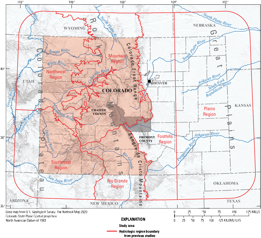
Map showing boundaries of the hydrologic regions of central and western Colorado, as defined by previous flood frequency studies (modified from Kohn and others, 2016 and Capesius and Stephens, 2009).
Previous Studies and Background Information
Previous studies that computed peak-streamflow regional regression equations (PSRREs) in Colorado are Patterson (1964, 1965), Patterson and Somers (1966), Matthai (1968), Hedman and others (1972), McCain and Jarrett (1976), Kircher and others (1985), Livingston and Minges (1987), Vaill (2000), Capesius and Stephens (2009), and Kohn and others (2016). Fewer studies developed mean-streamflow regional regression equations (MSRREs) and low-streamflow regional-regression equations (LSRREs) as done by Kircher and others (1985) and Capesius and Stephens (2009). Hydrologic regions in Colorado were originally defined by McCain and Jarrett (1976) and were incorporated as the regional framework in Kircher and others (1985) and Capesius and Stephens (2009). Kircher and others (1985) developed MSRREs in central and western Colorado for data collected through 1983. Capesius and Stephens (2009) published PMLSRREs for the entire State of Colorado (except for the Plains hydrologic region, where only PSRREs were published) using USGS streamflow data from the beginning of the period of record at each streamgage through water years 2006 for peak streamflow and 2007 for mean and low streamflow. Kohn and others (2015) evaluated the predictive uncertainty of the MSRREs developed by Capesius and Stephens (2009). Kohn and others (2016) published PSRREs for the Foothills and Plains hydrologic regions in Colorado using USGS streamflow data from the beginning of the period of record at each streamgage through water year 2013 and used paleoflood data at 41 streamgages to improve the uncertainty of the PSRREs.
Methods for Data Development for Streamgages
The development of PMLSRREs in central and western Colorado consisted of five steps:
-
1. Selection of unique streamgages having natural streamflow conditions, with a minimum of 10 years of record for inclusion in multilinear-regression analysis,
-
2. Flood-frequency analysis to compute AEPDs (peak flows) for all streamgages using systematic, historic peak streamflow, censored, and paleoflood data (if available),
-
3. Mean- and low-streamflow analysis to compute streamflow statistics for all streamgages by using daily mean streamflow,
-
4. Determination of basin and climatic characteristics for all the streamgages, and
-
5. Regionalization and development of the regression equations for peak, mean, and low streamflows in central and western Colorado.
Streamgage Selection
The streamgages selection used for this report was based on streamgages selected by Kircher and others (1985), Vaill (2000), Capesius and Stephens (2009), Kohn and others (2015), Kohn and others (2016), and the authors’ professional knowledge of hydrologic systems in Colorado. A comprehensive list of all CODWR streamgages in the Mountain, Northwest, Rio Grande, and Southwest hydrologic regions, as defined by Capesius and Stephens (2009), was compiled from the CODWR peak database (CODWR, 2020). A comprehensive list of all USGS streamgages in the study area and within 50 miles of the Colorado State line adjacent to those same hydrologic regions was compiled from the USGS (2020b) NWIS database. From the comprehensive list of candidate streamgages, those streamgages with at least 10 years of combined streamflow record through water year 2019, identified as representative of natural streamflow, were selected for this study. Following Kircher and others (1985), natural streamflow was defined as streamflow having less than about 10 percent of the mean annual streamflow volume at the streamgage affected by human activity.
Streamgages adjacent to one another and located in the same stream network were evaluated for data independence using the drainage-area ratio (DAR) and the proximity of the basin centroids, which was measured by standardized distance. Standardized distance is a measure of the normalized, or unitless distance, between the centroids of two basins, and DAR is used to determine if the size of two basins, when one basin is contained in the other, is sufficiently different such that precipitation generating the annual-maximum floods in each basin is likely to be different (Veilleux, 2009). Additional information on DAR and basin centroid proximity is found in Asquith and others (2006) and Veilleux (2009). If the DAR was less than or equal to 5.0, and the standardized distance was less than or equal to 0.5, the streamgages were determined to be redundant (Veilleux, 2009; Gotvald and others, 2012; Eash and others, 2013; Southard and Veilleux, 2014; Kohn and others, 2016). In such cases, the streamgage with the longer record was selected, and the other was removed. Excluding redundant streamgages based on relative DAR and basin-centroid location ensures the independence of the streamflow information among streamgages. This exclusion process removed redundant data or hydrologic information from the analysis. At the completion of the streamgage selection process, 418 streamgages, consisting of 15,202 years of record and a mean of approximately 36 years of record per streamgage, were used to develop the PSRREs (Kohn and others, 2026).
Many streamgages only collect annual peak streamflow data and do not collect daily streamflow, whereas other streamgages are only operated seasonally, so daily streamflow is collected during only a part of the year. As a result, only 323 of the 418 streamgages could be used to develop the mean- and low-streamflow regional regression equations (MLSRREs). Of those 418 streamgages, 379 were operated by USGS; 13 were operated by CODWR; and 26 were operated by both USGS and CODWR during the period of record. A map showing the location of the streamgages is in figure 2; each of the 418 streamgages and ancillary information are listed in appendix 1 (table 1.1); and each of the 418 streamgages, ancillary information, and basin and climatic characteristics are available in Kohn and others (2026). USGS streamgage names and other identifying characteristics also can be accessed through the USGS NWIS database (USGS, 2020b).
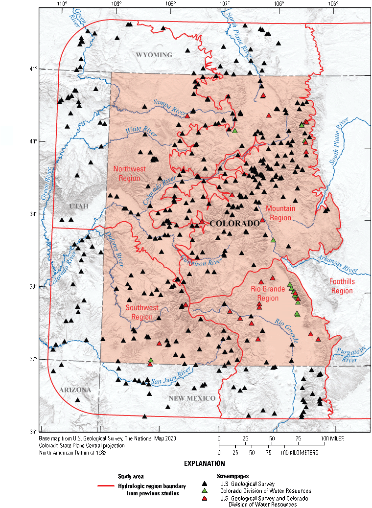
Map showing location of the 418 streamgages operated by the U.S Geological Survey and Colorado Division of Water Resources used in this study to develop regression equations for estimating peak, mean, and low streamflows and the boundaries of the hydrologic regions from previous flood-frequency studies in Colorado (figure modified from Kohn and others, 2016 and Capesius and Stephens, 2009; Kohn and others, 202623).
Peak Streamflow Analysis
The series of annual peak-streamflow data at 418 continuous-record, seasonal, and crest-stage streamgages were used to estimate AEPDs, such as the 100-year flood. The AEPDs from streamgage data provide the basis for developing the current peak-streamflow regression equations and were computed by using the USGS software program PeakFQ version 7.4 (Veilleux and others, 2014) with inputs of systematic data from the beginning of the record for a given streamgage through water year 2019. The peak-streamflow equations in this report express flood-frequency estimates in terms of annual exceedance probabilities (AEP), which are the reciprocals of the recurrence intervals. AEP can also be represented in percent, and a particular flood-frequency estimate is then termed the “P-percent chance streamflow,” where P is the probability (in percent) that the streamflow will be equaled or exceeded in any year. For example, a 10-year flood is the same as having a 0.10 AEP; this streamflow also is described as a 10-percent flood or Q10% (Southard and Veilleux, 2014).
For this report, the log-Pearson Type III frequency distribution was fit to the logarithms of the annual peak streamflows to determine flood frequency estimates by following the guidelines established by the Interagency Advisory Committee on Water Data (IACWD; 1982) and by England and others (2019). The mean and standard deviation of the annual peak streamflow, and streamgage skew coefficient at each streamgage were used to fit the distribution to describe the midpoint, slope, and curvature of the flood-frequency curve, respectively (Gotvald and others, 2012). Estimates of the P-percent AEPDs for each streamgage are computed by inserting the three statistics of the frequency distribution into equation 1:
whereis the P-percent annual exceedance-probability discharge, in cubic feet per second (ft3/s);
is the mean of the base 10 logarithms of the annual peak streamflows;
is a factor based on the streamgage-skew coefficient and the given percent AEP and is obtained from appendix 3 of IACWD (1982); and
is the standard deviation of the logarithms of the annual peak streamflows, which is a measure of the degree of variation of the annual-peak streamflows about the mean value.
The streamgage-skew coefficient is a measure of the asymmetry of the frequency distribution and is greatly affected by the presence of high or low outliers (annual peak streamflows substantially higher or lower than the trend of the data). Large positive streamgage skews typically are the result of high outliers, and large negative streamgage skews typically are the result of low outliers (Southard and Veilleux, 2014).
Skew Analysis
The streamgage-skew coefficient for a streamgage is sensitive to outliers, especially for streamgages with short records (less than 30 years). Because many records in Colorado are relatively short, the skew coefficient computed for stations having shorter records may be less reliable than coefficients for stations having longer periods of record. To compensate for effects of short record, the skew coefficient is combined with a generalized value derived from a regional skew map, which is included in IACWD (1982). The weighted skew used in the analysis for this report was determined by weighting the streamgage skew and the regional skew and is inversely proportional to their respective mean square errors, as shown in equation 5 of IACWD (1982) and equation 2 of this report:
whereis the weighted skew,
is the regional skew,
is the streamgage skew, and
and
are the mean square errors of the regional and streamgage skews, respectively.
Expected Moments Algorithm
In this study, the Expected Moments Algorithm (EMA) was used with the multiple Grubbs-Beck (MGB) test method (Grubbs and Beck, 1972) to compute Log-Pearson Type III exceedance-probability estimates for all 418 streamgages evaluated to develop PSRREs for central and western Colorado. The USGS software program PeakFQ version 7.4 (Veilleux and others, 2014) automates the EMA/MGB procedure described in this section of the report.
As described in England and others (2019), the EMA retains the essential structure and moments-based approach of the procedures developed in (IACWD, 1982) to determine flood frequency and addresses several concerns about the methods. The EMA in IACWD (1982) can accommodate interval data, simplifying the analysis of datasets containing censored observations, historic peak-streamflow data, low outliers, and data points with high and low uncertainties common in paleofloods, while also providing enhanced confidence intervals for the AEPDs. England and others (2019) recognized only two types of data: (1) systematic (annual peak streamflows observed during systematic streamgage record) and (2) historic peak streamflow (annual peak streamflows observed outside the streamgage record). England and others (2019) suggest using the EMA, which is a more general description of the historical period (the length of time including both systematic streamflow data and historic peaks). This is accomplished through streamflow intervals to describe the peak streamflow in each year and perception thresholds to describe the range of measurable potential streamflows in each year. Additional information on the EMA can be found in Eash and others (2013), Southard and Veilleux (2014), and England and others (2019).
Multiple Grubbs-Beck Test for Detecting Potentially Influential Low Floods
In flood frequency analysis, potentially influential low floods (PILFs) are annual peak streamflows meeting three criteria: (1) their magnitude is much smaller than the flood quantile of interest; (2) PILFs occur below a statistically significant break in the flood frequency plot; and (3) PILFs have great significance or leverage on the estimated frequency of large floods (Southard and Veilleux, 2014). IACWD (1982) and England and others (2019) suggested the use of the Grubbs-Beck test (Grubbs and Beck, 1972) to statistically identify low outliers in a sample of flood data. The MGB test is a generalization of the Grubbs-Beck method creating the standard procedure for recognizing multiple PILFs (Cohn and others, 2013), screens for PILFs at each streamgage, and excludes them from the flood frequency analysis. When an observation is identified as a PILF, the value of the smallest observation in the dataset determined to not be a PILF (Qs) is used as the censoring threshold in the EMA analysis (Southard and Veilleux, 2014). All annual peak streamflows smaller than this value will be treated as censored observations with streamflow intervals equal to (0, Qs) and perception thresholds equal to (Qs, inf) (Southard and Veilleux, 2014). Identifying PILFs and recording them as censored data can greatly improve estimator robustness with little or no loss of efficiency (Southard and Veilleux, 2014). Thus, use of the MGB test can improve the fit of the AEPDs, while minimizing lack-of-fit because of unimportant PILFs in an annual peak streamflow series (Cohn and others, 2013; Veilleux and others, 2014); however, it is crucial to distinguish between low outliers and PILFs.
The term “low outlier” typically refers to one or possibly two values in a dataset assumed to be homogenous and do not conform to the trend of the other observations (Southard and Veilleux, 2014). In contrast, PILFs may constitute up to one-half of the observations and are assumed to result from physical processes not relevant to the processes associated with large floods. Consequently, the actual magnitudes of PILFs reveal little about the upper right-hand tail of the frequency distribution representing large floods, thus having no effect when estimating the risk of large floods (Southard and Veilleux, 2014). Additional information on the MGB test and PILFs can be found in Gotvald and others (2012), Eash and others (2013), and Southard and Veilleux (2014).
The USGS software program PeakFQ version 7.4 (Veilleux and others, 2014) was used to compute the flood frequency estimates as AEPs with corresponding return periods as follows: 0.50 (2-yr return), 0.20 (5-yr return), 0.10 (10-yr return), 0.04 (25-yr return), 0.02 (50-yr return), 0.01 (100-yr return), 0.005 (200-yr return), and 0.002 (500-yr return). PeakFQ automates the EMA/MGB procedure previously described in this section of the report. Kohn and others (2026) includes the AEPD data from all 418 streamgages used to develop the PSRREs and all output and input files used and generated by PeakFQ for all 418 streamgages including the specifications files.
Mean Streamflow Analysis
Mean-annual streamflow values for the 323 selected streamgages were computed from daily mean streamflow data in the USGS NWIS database (USGS, 2020b) and in the CODWR database (CODWR, 2020) from the beginning of the record for a given streamgage through water year 2019. For each period of record representative of natural streamflow conditions, values of mean-annual streamflow were computed as the arithmetic mean of the daily mean streamflow in each water year. Streamgages without a minimum of 10 years of data were excluded from the computations of mean annual streamflow. Streamgages operated seasonally were also omitted from this computation not to bias the statistics. As a result, mean annual streamflows greater than zero were computed at 323 streamgages.
Similar to calculating mean-annual streamflow values, mean-monthly streamflow data from the 323 selected streamgages were computed from daily mean streamflow data in the USGS NWIS database (USGS, 2020b) and in the CODWR database (CODWR, 2020) through water year 2019. Mean monthly streamflows were computed as the arithmetic mean of each daily mean streamflow, in each month of the period of record representative of natural-streamflow conditions, by the USGS software program SWToolbox version 1.0.5 (Kiang and others, 2018). Streamgages without a minimum of 10 years of daily mean streamflow in a month were excluded from the mean-annual streamflow computations for that month. As a result, mean monthly streamflows were computed at streamgages ranging from a total of 325 for December to 347 for August with only three of those streamgages having mean monthly streamflows of zero for four to seven months of the year. The mean monthly streamflow data used and generated by SWToolbox for all streamgages are available in Kohn and others (2026).
Low Streamflow Analysis
Daily mean streamflow data at the 418 streamgages were compiled from the USGS NWIS database (USGS, 2020b) and the CODWR database (CODWR, 2020) from the beginning of the record for a given streamgage through water year 2019 to compute the 7-day minimum and maximum streamflows for return periods of 2-, 10, and 50-years (AEPs of 0.50, 0.10, and 0.02, respectively). The USGS software program SWToolbox version 1.05 (Kiang and others, 2018) was used to compute the 7-day minimum and maximum streamflows from the daily mean streamflow data. SWToolbox assumes the log-Pearson Type III distribution is suitable for low- and high-flow frequency analysis in Colorado. Daily mean streamflow values were computed as the arithmetic mean of the 15-minute streamflow recordings at a streamgage for each day in the entire period of record representative of natural-streamflow conditions. The SWToolbox computed the 7-day streamflow values by determining the product moments of mean, standard deviation, and streamgage skew of the logarithms of the streamflow values in a sliding window from April through March for minimum streamflows and from October through September for maximum streamflows. Finally, a log-Pearson Type III distribution was fit to the product moments, and the quantiles for the 2-year, 10-year, and 50-year recurrence intervals were extracted. Streamgages without 10 years of non-zero daily mean streamflow, in a month, were excluded from the 7-day minimum and maximum streamflow computations. Streamgages operated seasonally were omitted from this computation not to bias the statistics. As a result, the 7-day minimum and maximum streamflows were computed at streamgages ranging from 284 for the 7-day minimum streamflows to 319 for the 7-day maximum streamflows, with between 4 and 44 streamgages having 7-day minimum streamflows of zero, depending on the return period, and with 4 streamgages having 7-day maximum streamflows of zero (for all return periods). The 7-day minimum and maximum streamflow data used and generated by SWToolbox for all streamgages are available in Kohn and others (2026).
The streamflow-duration values were computed by ranking the daily mean streamflow data for the period of record representative of natural-streamflow conditions and linearly interpolating to the five exceedance percentiles of interest (10, 25, 50, 75, and 90) using an R script (R Core Team, 2022). As a result, the streamflow-duration values were computed for 323 of the 418 streamgages selected for the study. At those 323 streamgages, the streamflow-duration values were zero at 2–27 streamgages, depending on the exceedance probability, with two streamgages having streamflow-duration values of zero for all return periods. The streamflow-duration values used and generated by the R script (R Core Team, 2022) for all streamgages are available in Kohn and others (2026).
Basin and Climatic Characteristics
Based on previous studies conducted in Colorado and neighboring States (Kircher and others, 1985; Soenksen and others, 1999; Vaill, 2000; Rasmussen and Perry, 2000; Miller, 2003; Waltemeyer, 2008; Capesius and Stephens, 2009; Lewis, 2010; and Kohn and others, 2016) and on the availability of data, 97 characteristics (55 basin and 42 climatic characteristics) were evaluated as candidate explanatory variables in the regression analysis (table 1.2). The 97 characteristics consist of physical properties of the basin, precipitation amount, snowpack data, temperature, types of land cover, surficial lithology, and soil characteristics.
Basin and climatic characteristics were determined for the PSRRE analysis for each of the 418 streamgage drainage basins using Esri ArcMap 10.6.1 techniques, tools, and algorithms (Esri, 2017). The 1/3 arc-second 3-dimensional elevation data (3DEP) were processed through the ArcMap Spatial Analyst tool, as well as through the StreamStats online application (USGS, 2017, 202250) to delineate basins for the 418 streamgages found in this report. Additionally, 3DEP data (USGS, 2017) were analyzed to produce the characteristics of outlet elevation; basin elevation minimum and maximum values; mean, minimum, and maximum slope values; and the percentage of basin at an elevation above 7,500 ft, as listed in table 1.2. The basin perimeter, drainage area, and centroid latitude and longitude characteristic calculations were done on basin and pour-point geometry using the ArcMap Geometry Calculator tool. The percentage of basin with slopes greater than 30 percent characteristic was computed using StreamStats (USGS, 2022). The mean precipitation, precipitation amount, frequency, mean air temperature, soil, surficial lithology, snow data, and land cover data were processed with basin outlines using the National Water Quality Assessment Area-Characterization Toolset (Price and others, 2010) to produce the elevation-related characteristics for each basin presented in table 1.2, which also includes the data source.
Regional-Regression Analyses
Multilinear regression was used to define statistical relations between peak, mean, and low streamflow for 13 of the 97 basin and climatic characteristics from table 1.2. Detailed descriptions of the principles of regional regression are available in Farmer and others (2019), Helsel and others (2020), or Montgomery and others (2001). The statistical tests to evaluate model performance are described in Tasker and Stedinger (1989), Eng and others (2009), and Eash and others (2013).
Definition of Peak-, Mean-, and Low-Streamflow Regions
McCain and Jarrett (1976) originally defined five unique hydrologic regions in Colorado based on physiographic and climatic characteristics and peak streamflow. These same five hydrologic regions were used for all such Colorado streamflow studies with minor modifications (Kircher and others, 1985; Vaill, 2000; Capesius and Stephens, 2009) until Kohn and others (2016) subdivided the Plains hydrologic region into two unique hydrologic regions: the Plains and the Foothills hydrologic regions, which resulted in a total of six unique hydrologic regions in Colorado. The scope of this report was to update the PMLSRREs in central and western Colorado, which is defined as the Mountain, Northwest, Rio Grande, and Southwest hydrologic regions in Capesius and Stephens (2009). The study area was extended 50 miles into adjacent States to include more streamgages and improve statistical robustness for development of PMLSRREs.
After analyzing the study area for potential regional subdivisions based on river basin, elevation, latitude and longitude, and previous studies (Kircher and others, 1985; Vaill, 2000; Capesius and Stephens, 2009), the study area was divided into four updated hydrologic regions based on mean basin elevation in feet above North American Vertical Datum of 1988 (less than 8,014 feet, between 8,015 and 9,492 feet, between 9,493 and 10,490 feet, and greater than 10,490 feet) for the PSRREs and based on river basin (Colorado-East Slope Headwaters, Green River, Rio Grande, and San Juan-Dolores) for the MLSRREs, which resulted in the smallest standard model error (SME, in percent) and standard error of prediction (SEP, in percent) and largest pseudocoefficient of determination (pseudoR2, dimensionless).
The updated hydrologic regions for the PSRREs will be designated as (1) Alpine (mean basin elevation greater than 10,490 feet), (2) Sub-Alpine (mean basin elevation between 9,493 and 10,490 feet), (3) Mid-Elevation (mean basin elevation between 8,015 and 9,492 feet), and (4) Plateau (mean basin elevation less than 8,014 feet) hydrologic regions (fig. 3). Figure 3 shows the streamgages used in the development of the PSRREs color coded by hydrologic region; because the hydrologic regions are based on mean basin elevation, geographic region boundaries cannot be drawn. The distribution of the streamgages by color in figure 3 provides spatial context. Each hydrologic region included 104–105 streamgages, and figure 3 shows the hydrologic region boundaries previously defined by Capesius and Stephens (2009) and Kohn and others (2016). The new hydrologic regions for the MLSRREs will be designated as (1) Colorado-East Slope Headwaters, (2) Green River, (3) Rio Grande, and (4) San Juan-Dolores (fig. 4).
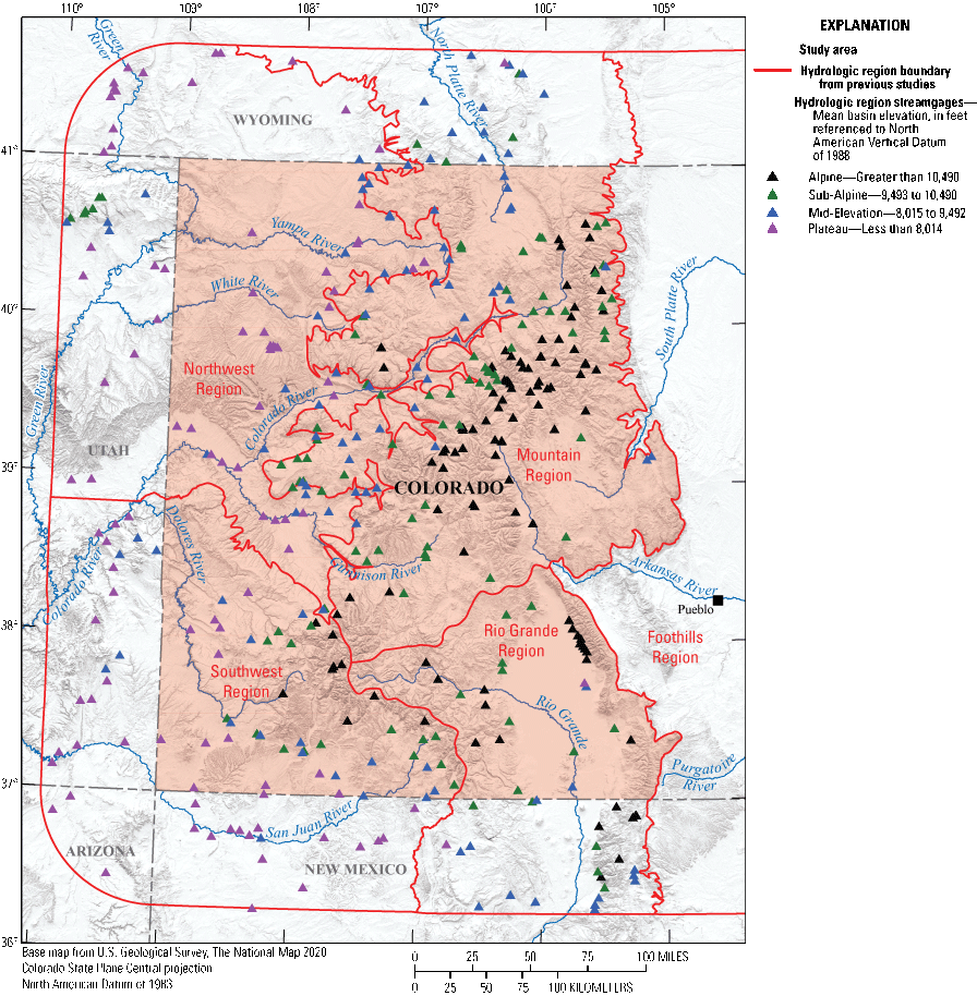
Map showing the updated hydrologic regions created in central and western Colorado for the peak-streamflow regional regression equations. Hydrologic regions with the location of the 105, 104, 104, and 105 streamgages used to develop the peak-streamflow regional-regression equations in the Alpine, Sub-Alpine, Mid-Elevation, and Plateau hydrologic regions, respectively. (Kohn and others, 2026)
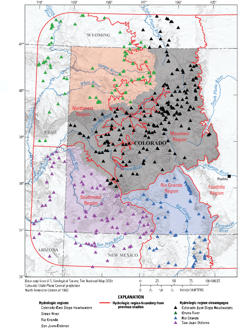
Map showing the updated hydrologic regions created in central and western Colorado for the mean- and low-streamflow regional regression equations. Hydrologic regions with the location of the 170, 57, 42, and 54 streamgages used to develop the mean- and low-streamflow regional-regression equations in the Colorado-East Slope Headwaters, Green River, Rio Grande, and San Juan-Dolores hydrologic regions, respectively. (Kohn and others, 2026)
Figure 4 includes each streamgage used in the development of the MLSRREs color coded by hydrologic region; the updated hydrologic regions based on major river basin are also included. Figure 4 provides spatial context of the study area by color coding each streamgage: 170 in the Colorado-East Slope Headwaters hydrologic region, 57 in the Green River hydrologic region, 42 in the Rio Grande hydrologic region, and 54 San Juan-Dolores hydrologic region. The eastern edge of the study area was established by Vaill (2000), and this report follows that boundary as described in the “Description of the Study Area” section of this report. The hydrologic regions outside the study area in eastern Colorado remain unchanged and designated as the Foothills and Plains hydrologic regions as defined by Kohn and others (2016).
The subdivision of central and western Colorado into four hydrologic regions, for both PSRREs and MLSRREs, was determined through the OLS regression procedures of maximizing the coefficient of determination (R2, dimensionless) and the adjusted coefficient of determination (adjR2, dimensionless) and by minimizing the standard error (Mallow’s Cp) and the predicted residual sum of squares (PRESS) statistic. By using GLS regression procedures, it was confirmed that the updated regions reduced uncertainty in the PSRREs compared to the unsubdivided regions used in previous studies (Kircher and others, 1985; Vaill, 2000; Capesius and Stephens, 2009). Prior to finalizing the updated regions, maps of streamgage residuals were created and various other subdivisions were analyzed based on latitude, longitude, basin outlet elevation, mean basin elevation, maximum basin elevation, and drainage area.
Development of the Peak-Streamflow Regional-Regression Equations
The PSRREs were developed for use in estimating peak streamflow at selected AEPs, from 50 to 0.2 percent, at gaged and ungaged locations for basins in the Alpine, Sub-Alpine, Mid-Elevation, and Plateau hydrologic regions of central and western Colorado. Regression analyses using OLS were performed to select the basin and climatic characteristics for use as independent variables. A linear relation between the dependent and independent variables is needed for OLS regression. To satisfy this criterion, variables often are transformed, and in hydrologic analyses, typically the log-transformation is used (Southard and Veilleux, 2014; Farmer and others, 2019). The dependent response variable is the AEPDs, and the independent explanatory variables are the basin and climatic characteristics that describe the AEPDs. For this study, the dependent variable AEPDs were transformed to base 10 logarithms, but the drainage area was the only independent variable transformed to base 10 logarithms to increase linearity prior to the development of the PSRREs.
Homoscedasticity, a constant variance in the dependent variable for the range of the independent variables about the regression line, and normality of residuals are also criteria for OLS regression. Transformation of the AEPDs and certain other variables to base 10 logarithms can enhance the homoscedasticity of the data about the regression line (Southard and Veilleux, 2014). Linearity, homoscedasticity, and normality of residuals were examined in residual plots.
The hydrologic model used in the regression analysis in this report is of the form (eq. 1):
whereis the dependent variable, P-percent AEPD, in cubic feet per second;
, ,
are explanatory (independent) variables; and
a, b, c, d
are regression coefficients.
If the dependent variable QP and the independent variable A are the only logarithmically transformed variables, then the hydrologic model has the following linear form (eq. 4):
where the variables are as previously defined. Equation 5 is commonly written as where the variables are as previously defined.The basin and climatic characteristics (table 1.2) with the strongest correlation to peak streamflow were identified, checked for any substantial cross correlation with other variables in the group using the variance inflation factor (VIF) statistic, and were selected as the potential explanatory variables for the PSRREs. The final AEPD values for the 418 streamgages used in the regional-regression analysis are available in Kohn and others (2026).
Ordinary-Least Squares Regression
The OLS regression technique described by Farmer and others (2019) was used in this report as an exploratory tool to determine potential explanatory variables for subsequent analysis by GLS regression. The subdivisions and explanatory variables were initially explored by using OLS in R (R Core Team, 2022), with the allReg function in the smwrStats R package (Lorenz, 2015). The potential explanatory variables were assessed for linear correlation with the Q1% AEPD using plots, adjR2, and the statistical significance (p-values) of each explanatory variable when regressed with peak streamflow to determine the strongest predictors of peak streamflow. Transformations of equation variables were considered to determine potential for improvement of correlations with streamflow and conformance to the assumptions of linear regression application. Prior to OLS regression, logarithmic transformation (base 10) of both the streamflow and the drainage-area explanatory variable was found to improve normality and homoscedasticity (assumptions for parametric regression), and in most cases, substantially improve the adjR2 and statistical significance of the slope of each explanatory variable in a regression with streamflow.
The strongest OLS regression models (with one-, two-, three-, and four-explanatory variables using the best of all subsets routine) for prediction of Q1% AEPDs were identified and used to limit the number of potential explanatory variables in the subsequent GLS analyses. The strongest PSRREs were determined by assessing the following metrics for each model: standard error of estimate, adjR2, Mallow’s Cp, and PRESS statistics. Statistical diagnostics and plots also were used to assess the regression model robustness for meeting the assumptions of parametric-regression methods. The adjR2 statistic is maximized, and the standard error of estimate, Mallow’s Cp, and PRESS statistics are minimized with accurate sets of independent variables in a regression model that explains more of the variance in the dependent variable. Additional information on OLS regression can be found in Eash and others (2013) and Southard and Veilleux (2014).
Multicollinearity (high correlation among the explanatory variables) can make multiple linear-regression model results misleading or erroneous and would generally disqualify the use of both variables within a single, final PSRRE. Early in the variable selection process, the VIF statistic and plots of a particular explanatory variable with each of the other explanatory variables were used to make preliminary assessments of potential multicollinearity. When assessing candidate variables and the apparent best OLS PSRRE for further refinement by GLS regression, multicollinearity was assessed primarily by using the VIF statistic (Gotvald and others, 2012) to screen for correlated or unnecessary variables in candidate PSRREs. There was no exact value of VIF greater than the data that were automatically excluded, but values less than 3 were given preference, and values greater than 10 were scrutinized, as serious problems can occur when using those explanatory variables in a regression (Helsel and others, 2020). After removal of highly correlated variables by visual inspection of the plots, all calculated VIFs were less than 3.
Generalized-Least Squares Regression
Multilinear regression using GLS, as described by Stedinger and Tasker (1985), Tasker and Stedinger (1989), Griffis and Stedinger (2007), and Farmer and others (2019), is a method of weighting streamgage AEPD data in the regression analysis according to differences in streamflow reliability (record lengths) and variability (record variance) and according to spatial cross correlations of concurrent streamflow among streamgages. Comparison of OLS, weighted-least squares (WLS), and GLS in a study by Stedinger and Tasker (1985) indicated that the weighted methods (WLS and GLS) produced results more accurate than the OLS regression method. When streamflow records of varying lengths or with correlated concurrent streamflows occurred in the dataset, the weighting technique used in GLS produces equations that are both improved in estimates of streamflow statistics and of the predictive accuracy of the statistics (Stedinger and Tasker, 1985).
Based on the exploratory results from OLS regression and explanatory variable multicollinearity analysis, the USGS R package WREG (Eng and others, 2009; Farmer, 2021) was used to compute GLS PSRREs from the most correlated candidate variables. Thirteen basin and climatic characteristics were used as potential explanatory variables to develop the PSRREs with Q1% AEPD streamflows based on OLS exploration. The general form of the equation was defined by equation 4. Final GLS regression models for PSRREs were selected based on minimizing values of the SME and the SEP and maximizing values of the pseudoR2 derived from OLS exploration.
In Capesius and Stephens (2009) and Kohn and others (2016), the error associated with the PMLSRREs was characterized using the SEP, pseudoR2SME, and adjR2. The SEP describes the sum of the model error and sampling error. The SEP is the square root of the mean GLS variance of prediction (Tasker and Stedinger, 1989; Eng and others, 2009). The pseudoR2 value is a measure of the percentage of the variation explained by the basin or climatic characteristics (explanatory variables) included in the model and is calculated based on the degrees of freedom in the regression (Eash and others, 2013). The adjR2 is a measure of the percentage of the variation explained by the basin or climatic characteristics (explanatory variables) included in the model, but it also compensates for multiple explanatory variables such that adding additional explanatory variables increases the value of adjR2 only when the predictive capability of the model increases (Lee and others, 2012). Griffis and Stedinger (2007) describe how the pseudoR2 is more appropriate than the R2 or adjR2 in measuring the true variation explained by the explanatory variables in the GLS model. The SME measures only the error of the model and does not include sampling error regression (Eash and others, 2013). The SME is the square root of the regression model error variance (Tasker and Stedinger, 1989).
Models using GLS use a correlation model and weighting matrix. The correlation smoothing function relates the correlation between annual peak streamflows at two streamgages to the geographic distance between the streamgages for every paired combination of the streamgages with a given number of years of concurrent streamflow. The correlation smoothing function was defined in equation 18 in Eng and others (2009), with an alpha of 0.001 and theta of 0.99. The correlation smoothing function was used by WREG to compute a weighting matrix for the four hydrologic regions of streamgages based on the mean elevation included in the development of the GLS PSRREs. Figure 5 displays the predicted 100-year peak streamflow using the regression equation compared to the streamgaged (observed) peak streamflow at each station in the four hydrologic regions. Figure 5 indicates a reasonable scatter distribution around the line of equality across the range of streamflows, particularly for the Alpine and Sub-Alpine hydrologic regions. A separate model was selected for each of the four hydrologic regions. Within each hydrologic region, the same explanatory variables were applied for each of the eight PSRREs in that region for consistency amongst different exceedance probabilities. All explanatory variables were statistically significant at a p-value of less than or equal to (≤) 0.05, and the VIF for explanatory variables was less than 3.
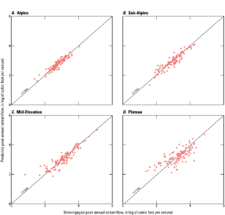
Graphs showing comparison of 100-year peak streamflows as predicted by the regression equations compared to the streamgaged peak streamflow at each station through water year 2019 in the four hydrologic regions of central and western Colorado. A, Alpine region; B, Sub-Alpine region; C, Mid-Elevation region; and D, Plateau region.
Development of the Mean-Streamflow Regional-Regression Equations
The MSRREs were developed for use in estimating the mean-annual and the 12 mean-monthly streamflows at gaged and ungaged locations for basins in the Colorado-East Slope Headwaters, Green River, Rio Grande, and San Juan-Dolores hydrologic regions of central and western Colorado. Regression techniques using OLS were performed to select the basin and climatic characteristics for use as independent variables following the same method as used for the PSRREs. The dependent response variables are the mean annual and mean monthly streamflows, and the independent explanatory variables are the basin and climatic characteristics. Logarithmic transformation of the values for mean-annual and mean-monthly streamflows and certain other variables can enhance the homoscedasticity of the data about the regression line (Southard and Veilleux, 2014). Therefore, to enhance homoscedasticity and to increase linearity prior to the development of the equations, values for mean-annual and mean-monthly streamflows were transformed to base 10 logarithms and the drainage areas (as the only dependent variable) were transformed to base 10 logarithms. Linearity, homoscedasticity, and normality of residuals were examined in residual plots.
The basin and climatic characteristics (table 1.2) with the strongest correlation to mean streamflow were identified, checked for any substantial cross correlation with other variables in the group, and were selected as the potential explanatory variables for the MSRREs. The final mean annual and the 12 mean monthly streamflows for the 323 streamgages used in the regional-regression analysis are available in Kohn and others (2026).
Ordinary Least-Squares Regression
The methods of Farmer and others (2019) were used to develop the MSRREs. The MSRREs were developed using OLS in R (R Core Team, 2022) with the allReg function in the smwrStats R package (Lorenz, 2015). Because the mean annual and mean monthly streamflows were computed without using the log-Pearson Type III frequency distribution, GLS regression cannot be used for the MSRREs. The potential explanatory variables were assessed for linear correlation with the mean annual and the 12 mean monthly streamflows using plots, VIF statistic, and the statistical significance (p-values) of each explanatory variable when regressed with peak streamflow to determine the strongest predictors of mean annual and the 12 mean monthly streamflows.
The most correlated OLS regression models (with one-, two-, three-, four- and five-explanatory variables using the best of all subsets routine) for prediction of the mean annual and the 12 mean monthly streamflows were identified. Following the PSRREs methods, multicollinearity (high correlation among the explanatory variables) can make results, which are based on a multiple linear-regression model, misleading or erroneous. This generally disqualifies the use of both variables within a single final MSRRE. Early in the variable selection process, the VIF statistic and plots comparing explanatory variables were used to make preliminary assessments of potential multicollinearity. Final OLS regression models for mean annual and the 12 mean-monthly streamflows were selected based on minimizing values of SEP and maximizing values of adjR2.
Figure 6 shows the predicted mean annual streamflow using the OLS regression equation compared to the streamgaged (observed) mean annual streamflow at each station in the four hydrologic regions. Figure 6 indicates a reasonable scatter distribution around the line of equality across the range of streamflows. Separate models were fit for each mean annual and mean monthly streamflow statistics for each of the hydrologic regions. All explanatory variables were statistically significant at a p-value of ≤0.05, and the VIF for explanatory variables was less than 3.
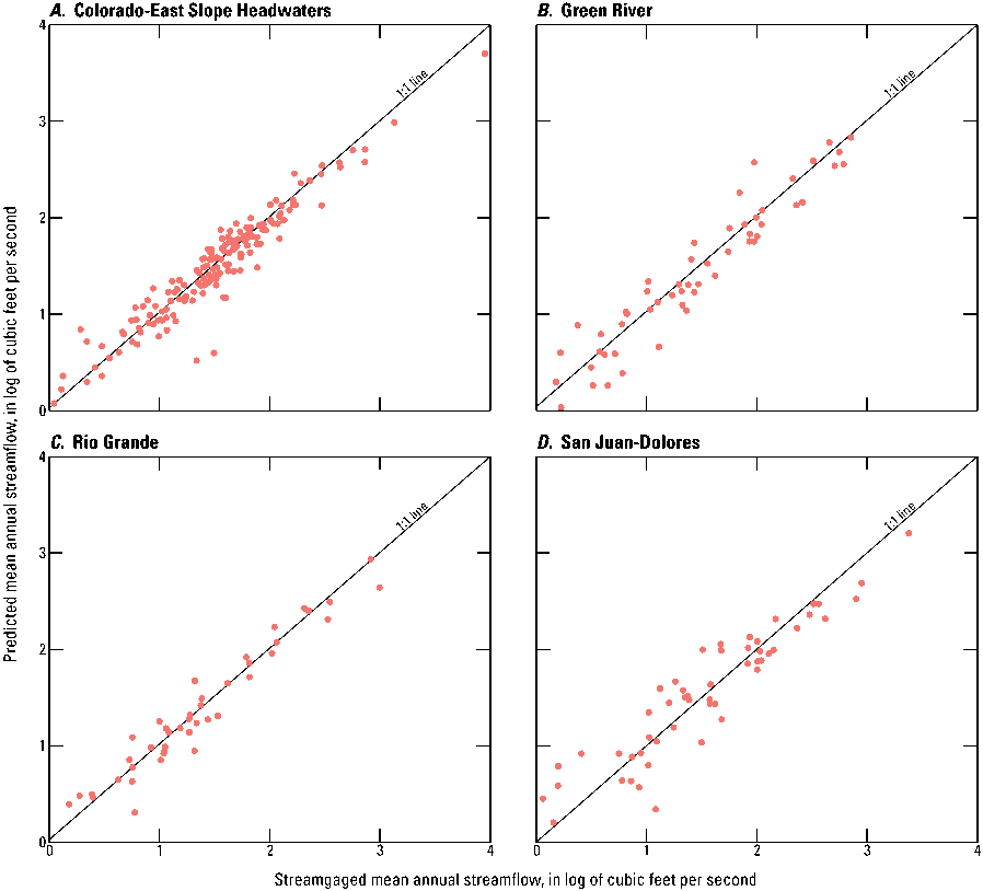
Graphs showing comparison of mean-annual streamflows as predicted by the regression equations compared to streamgaged mean annual streamflow at each station through water year 2019 in the four hydrologic regions of central and western Colorado. A, Colorado-East Slope Headwaters region; B, Green River; C, Rio Grande region; D, San Juan-Dolores region. (Kohn and others, 2026)
Development of the Low-Streamflow Regional-Regression Equations
The LSRREs were developed for use in estimating the 7-day minimum and maximum streamflows for return periods of 2-, 10-, and 50-years (AEP of 0.50, 0.10, and 0.02) and streamflow-duration values for five exceedance percentiles of interest (10, 25, 50, 75, and 90) at gaged and ungaged locations for basins in the Colorado-East Slope Headwaters, Green River, Rio Grande, and San Juan-Dolores hydrologic regions of central and western Colorado. Regression techniques using OLS were performed to select the basin and climatic characteristics for use as independent variables following the same method as used for the PSRREs. The dependent response variable is the 7-day minimum and maximum streamflows and streamflow-duration values, and the independent explanatory variables are the basin and climatic characteristics that describe the 7-day minimum and maximum streamflows and streamflow-duration values. For this study, the dependent variable 7-day minimum and maximum streamflows and streamflow-duration values were transformed to base 10 logarithms, but the drainage area was the only independent variable that was transformed to base 10 logarithms to increase linearity prior to the development of the LSRREs. For the 7-day minimum streamflows, all zero streamflow values were substituted with the smallest streamflow in each statistic (0.01 ft3/s for 7, 0.001 ft3/s for 7, and 0.005 ft3/s for 7) prior to model fitting so the dependent variable could be logarithmically transformed. In addition, for the 7-day minimum streamflows, a censored regression technique using the lowest non-zero value as the censoring level was analyzed. This technique yielded models and coefficients similar to the OLS, so it was determined that an OLS would be the preferred approach for the 7-day minimum streamflows. For the streamflow-duration values, all zero streamflow values were substituted with a value of 0.005 ft3/s prior to model fitting so the dependent variable could be logarithmically transformed. For the 7-day maximum streamflows, no zero streamflows were present, and no substitutions were made.
Homoscedasticity about the regression line and normality of residuals also is a criterion for OLS regression. Transformation of the 7-day minimum and maximum streamflows and streamflow-duration values and certain other variables to base 10 logarithms can enhance the homoscedasticity of the data about the regression line (Southard and Veilleux, 2014). Linearity, homoscedasticity, and normality of residuals were examined in residual plots.
The basin and climatic characteristics (table 1.2) with the strongest correlation to peak streamflow were identified, checked for any substantial cross correlation with other variables in the group, and were selected as the potential explanatory variables for the LSRREs. The final 7-day minimum and maximum streamflows and streamflow-duration values for the 323 streamgages used in the regional-regression analysis are available in Kohn and others (2026).
Ordinary Least-Squares Regression
The methods of Farmer and others (2019) were used to develop the LSRREs. A previous study (Hortness, 2006) determined that using GLS regression techniques for 7-day minimum streamflows is not preferred over OLS or WLS because of the extreme cross correlations present between streamgages. As a result, GLS regression was only used for the 7-day maximum streamflows. The WLS regression was analyzed for the 7-day minimum streamflows and streamflow-duration values using weights of record length and the variance of the logarithms of the observed values. After reviewing the uncertainty metrics for each model, it was determined that WLS regression did not improve the uncertainty of the models, and so the OLS regression methods were used for the 7-day minimum streamflows and streamflow-duration values.
The potential explanatory variables were assessed for linear correlation with the 7-day minimum streamflows and streamflow-duration values using plots, VIF statistic, and the statistical significance of each explanatory variable when regressed with peak streamflow (p-values), to determine the strongest predictors of 7-day minimum streamflows and streamflow-duration values. Final OLS regression models for 7-day minimum streamflows and streamflow-duration values were selected based on minimizing values of SEP and maximizing values of adjR2.
Figures 7 and 8 display the predicted 7-day minimum streamflows and streamflow-duration values, respectively, using the OLS regression equation compared to the streamgaged (observed) 7-day minimum streamflows and streamflow-duration values at each station in the four hydrologic regions. Figures 7 and 8 indicate a reasonable scatter distribution around the line of equality across the range of streamflows with larger uncertainty present in all equations for lower streamflows. Figures 7 and 8 display the substituted zero streamflow values as a vertical line above the 1:1 line, indicating the equations overpredict the statistic when streamflows are very low or zero, which is more common in the San Juan-Dolores and Green River hydrologic regions. The plots are in log units, and this phenomenon occurs when almost all the predicted streamflows would be less than 1 ft3/s, so caution may be beneficial when applying these equations when streamflows are very low (≤ 1 ft3/s). Separate equations were fit for each 7-day minimum streamflow and streamflow-duration value statistic for each hydrologic region. For the 7-day minimum streamflow, within each hydrologic region, the same explanatory variables based on the 7 statistic were applied for each of the three flow-duration statistics (7, 7, 7) in that region for consistency amongst different exceedance probabilities. For the streamflow-duration values, within each hydrologic region, the same explanatory variables based on the Q50th statistic were applied for each of the five flow-duration statistics (Q10th, Q25th, Q50th, Q75th, Q90th) in that region for consistency amongst different exceedance probabilities. All explanatory variables were statistically significant at a p-value of ≤0.05, and the VIF for explanatory variables was less than 3.
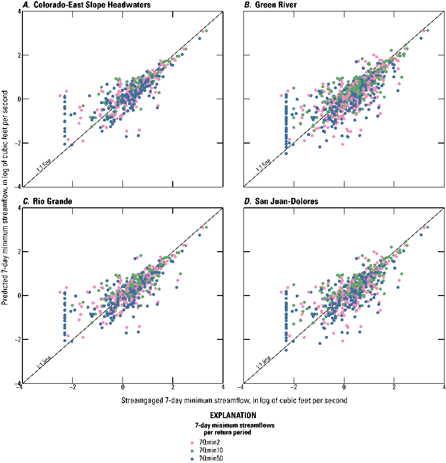
Graphs showing comparison of 7-day minimum streamflows for return periods of 2 years (7Qmin2), 10 years (7Qmin10), and 50 years (7Qmin50) as predicted by the regression equations to the streamgaged 7-day minimum streamflows at each station through water year 2019 in the four hydrologic regions of central and western Colorado. A, Colorado-East Slope Headwaters region; B, Green River region; C, Rio Grande region; D, San Juan-Dolores region. (Kohn and others, 2026)
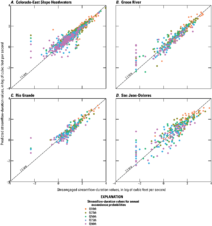
Graphs showing comparison of streamflow-duration values for annual exceedance probabilities of 10 percent (Q10th), 25 (Q25th), 50 percent (Q50th), 75 percent (Q75th), and 90 percent (Q90th) as predicted by the regression equations to the streamgaged streamflow-duration values at each station through water year 2019 in the four hydrologic regions of central and western Colorado. A, Colorado-East Slope Headwaters region; B, Green River region; C, Rio Grande region; D, San Juan-Dolores region. (Kohn and others, 2026)
Generalized-Least Squares Regression
For the 7-day maximum streamflows, regression techniques using GLS were performed to select the basin and climatic characteristics for use as independent variables following the same method as used for the PSRREs. Thirteen basin and climatic characteristics were used as potential explanatory variables to develop the 7-day maximum streamflows, and separate equations were created for each dependent variable in the four hydrologic regions. For the 7-day maximum streamflow, within each hydrologic region, the same explanatory variables based on the 7 statistic were applied for each of the three flow-duration statistics (7, 7, 7) in that region to maintain consistency between different exceedance probabilities.
The correlation smoothing function was defined in equation 18 in Eng and others (2009) with an alpha of 0.001 and theta of 0.99. The correlation smoothing function was used by WREG to compute a weighting matrix for the four hydrologic regions of streamgages based on the mean elevation included in the development of the GLS PSRREs. Final GLS regression models for 7-day maximum streamflows were selected based on minimizing values of SME and SEP and maximizing values of pseudoR2.
Figure 9 displays the predicted 7-day maximum streamflow using the regression equation compared to the streamgaged (observed) 7-day maximum streamflow at each station for the four hydrologic regions. Figure 9 indicates a reasonable scatter distribution around the line of equality across the range of streamflows, particularly for the Rio Grande and San Juan-Dolores hydrologic regions. All explanatory variables were statistically significant at a p-value of ≤0.05, and the VIF for explanatory variables was less than 3.
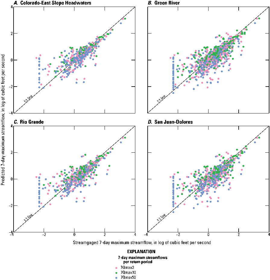
Graphs showing comparison of 7-day maximum streamflows for return periods of 2 years (7Qmax2), 10 years (7Qmax10), and 50 years (7Qmax50) as predicted by the regression equations to streamgaged 7-day maximum streamflows at each station through water year 2019 in the four hydrologic regions of central and western Colorado. A, Colorado-East Slope Headwaters hydrologic region; B, Green River hydrologic region; C, Rio Grande hydrologic region; and D, San Juan-Dolores hydrologic region. (Kohn and others, 2026)
Final Peak-, Mean-, and Low-Streamflow Regional-Regression Equations
The PSRREs in the Alpine, Sub-Alpine, Mid-Elevation, and Plateau hydrologic regions were developed using a total of 105, 104, 104, and 105 streamgages, respectively, and no streamgages were used in more than one region. The selection of the final basin and climatic characteristics and the evaluation of the accuracy of the PSRREs were based on the Q1% AEPD for each hydrologic region. Maintaining consistency between explanatory variables minimizes the possibility of predictive inconsistencies between estimates of different probabilities, so that streamflow estimates will increase as the streamflow probability decreases. The final peak-streamflow regional-regression equations from GLS regression with pseudoR2, SEP, SME, and the model coefficients are listed for each hydrologic region in table 1. The performance metrics pseudoR2 and SME describe how well the PSRREs perform on the streamgages used in the regression analyses, and the SEP measures how well the GLS regression models can predict AEPDs at ungaged sites (Eash and others, 2013).
The MSRREs in the Colorado-East Slope Headwaters, Green River, Rio Grande, and San Juan-Dolores hydrologic regions were developed using a total of 170, 57, 42, and 54 streamgages, respectively, and no streamgages were used in more than one region. The final mean annual and the 12 mean monthly streamflow regional-regression equations from OLS regression with adjR2, SEP, and the model coefficients are listed for each hydrologic region in table 2.
The 7-day minimum streamflow regional-regression equations in the Colorado-East Slope Headwaters, Green River, Rio Grande, and San Juan-Dolores hydrologic regions were developed using a total of 156, 44, 40, and 44 streamgages, respectively, and no streamgages were used in more than one region. The selection of the final basin and climatic characteristics and the evaluation of the accuracy of the 7-day minimum streamflow equations were based on the 7 statistic for each hydrologic region. Maintaining consistency between explanatory variables minimizes the possibility of predictive inconsistencies between estimates of different probabilities, so predicted streamflow will increase as the streamflow probability decreases. The final 7-day 2-, 10-, and 50-year minimum streamflow regional-regression equations from OLS regression with adjR2, SEP, and the model coefficients are listed for each hydrologic region in table 3.
The streamflow duration values and regional-regression equations in the Colorado-East Slope Headwaters, Green River, Rio Grande, and San Juan-Dolores hydrologic regions were developed using a total of 170, 57, 42, and 54 streamgages, respectively, and no streamgages were used in more than one region. The selection of the final basin and climatic characteristic and the evaluation of the accuracy of the streamflow-duration equations were based on the Q50th statistic for each hydrologic region. The final streamflow regional-regression equations for streamflow-duration values for annual exceedance probabilities of 10, 25, 50, 75, and 90 percent from OLS regression with adjR2, SEP, and the model coefficients are listed for each hydrologic region in table 4.
The 7-day maximum streamflow regional-regression equations in the Colorado-East Slope Headwaters, Green River, Rio Grande, and San Juan-Dolores hydrologic regions were developed using a total of 167, 52, 35, and 52 streamgages, respectively, and no streamgages were used in more than one region. The selection of the final basin and climatic characteristics and the evaluation of the accuracy of the 7-day maximum streamflow equations were based on the 7 statistic for each hydrologic region. The final 7-day 2-, 10-, and 50-year maximum streamflow regional-regression equations from GLS regression with pseudoR2, SEP, SME, and the model coefficients are listed for each hydrologic region in table 5. The final regression models for each equation and hydrologic region are available in Kohn and others (2026).
Table 1.
Regression equations and performance metrics determined by generalized least-squares method for predicting 2-, 5-, 10-, 25-, 50-, 100-, 200-, and 500-year peak streamflow for natural streams in each hydrologic region defined by elevation in central and western Colorado (Kohn and others, 2026).[Ranges of predictor variables: AREA, drainage area of basin (in square miles): 0.22–22,629; LONG, longitude of basin centroid (in decimal degrees of North American Datum of 1983): –110.219 to –105.093; SLOPE, mean basin slope (by percent): 3.37–69.4; MEANELEV, mean basin elevation (in feet, per North American Vertical Datum of 1988 {NAVD88}): 4,808–11,954; SWE, snow-water equivalent on April 1 (in inches): 0–33.8; 100Y24H, 24-hour precipitation amount that has a 1 percent chance of occurrence in a given year (in inches): 2.19–5.21; and PPTANN, annual precipitation (in inches): 7.71–61.6. Hydrologic regions defined by elevation (in feet, per NAVD88): Alpine, greater than 10,490; Sub-Alpine, 9,493–10,490; Mid-Elevation, 8,015–9,492; Plateau, less than 8,014. N, number of sites used in regression; PseudoR2, pseudo coefficient of determination (in percent); SEP, standard error of prediction (in percent); SME, standard model error (in percent); Q, streamflow (in cubic feet per second); Qpeak, peak streamflow in Q[year intervals] of 2, 5, 10, 25, 50, 100, 200, and 500 years]
Table 2.
Regression equations and performance metrics determined by using the ordinary least-squares method for predicting mean-annual and mean-monthly streamflows for natural streams in each hydrologic region in central and western Colorado (Kohn and others, 2026).[Ranges of predictor variables: AREA, drainage area of basin (in square miles): 0.89–22,629; LONG, longitude of basin centroid (in decimal degrees of North American Datum of 1983 [NAD 83]): –110.052 to –105.226; LAT, latitude of basin centroid (in decimal degrees of NAD83): 36.088 to 41.472; OUTELEV, elevation at basin outlet (in feet, per North American Vertical Datum of 1988 {NAVD88}): 3,995–10,499; ELEVMAX, maximum basin elevation (in feet per NAVD88): 6,061–14,426; RELIEF, basin relief (in feet): 533–10,035; SWE, snow-water equivalent on April 1 (in inches): 0–33.8; PPTANN, annual precipitation (in inches): 8.60–61.6; PPTAUG, precipitation measured during August (in inches): 0.90–4.89; SLOPE, mean basin slope (in percent): 6.82–69.4; 100Y6H, 6-hour precipitation amount that has a 1 percent chance of occurrence in a given year (in inches): 1.61–3.45. N, number of sites used in regression; Adj-R2, adjusted coefficient of determination (in percent); SEP, standard error of prediction (in percent); Q, streamflow (in cubic feet per second); Qann, mean-annual streamflow; Q[name of month], mean-monthly streamflows in: jan, January; feb, February; mar, March; apr, April; aug, August; sept, September; oct, October, nov, November; dec, December]
Table 3.
Regression equations and performance metrics determined by using the ordinary least-squares method for predicting 7-day minimum streamflows for return periods of 2, 10, and 50 years for natural streams in each hydrologic region in central and western Colorado (Kohn and others, 2026).[Ranges of predictor variables: AREA, drainage area of basin (in square miles): 0.89–22,629; LAT, latitude of basin centroid (in degrees of North American Datum of 1983): 36.246 to 41.472; RELIEF, basin relief (in feet): 694–10,035; SLOPE, mean basin slope (in percent): 6.82–69.4; OUTELEV, elevation at basin outlet (in feet, per North American Vertical Datum of 1988 {NAVD 88}): 3,995–10,499; MEANELEV, mean basin elevation (in feet, per NAVD88): 4,808–11,954; 100Y6H, 6-hour precipitation amount that has a 1 percent chance of occurrence in a given year (in inches): 1.61–3.45; PPTANN, annual precipitation (in inches): 8.60–60.4; SWE, snow-water equivalent on April 1 (in inches): 0–32.3; N, number of sites used in regression; Adj-R2, adjusted coefficient of determination (in percent); SEP, standard error of prediction (in percent); Q, streamflow (in cubic feet per second); 7Qmin, 7-day minimum streamflows in 7Q[return periods] of 2, 10, and 50 years]
Table 4.
Regression equations and performance metrics determined by using the ordinary least-squares method for predicting streamflow-duration values for annual exceedance probabilities of 10, 25, 50, 75, and 90 percent for natural streams in each hydrologic region in central and western Colorado (Kohn and others, 2026).[Ranges of predictor variables: AREA, drainage area of basin (in square miles): 0.89–22,629; LAT, latitude of basin centroid (in decimal degrees of North American Datum of 1983 {NAD83}): 36.088 to 41.472; LONG, longitude of basin centroid (in decimal degrees of NAD83): –110.052 to –105.226; MEANELEV, mean basin elevation (in feet, per North American Vertical Datum 1988): 4,808–11,954; SLOPE, mean basin slope (in percent): 6.82–69.4; RELIEF, basin relief (in feet): 533–10,035; SWE, snow-water equivalent on April 1 (in inches): 0–33.8; 100Y24H, 24-hour precipitation amount that has a 1 percent chance of occurrence in a given year (in inches): 2.19–5.21. N, number of sites used in regression; Adj-R2, adjusted coefficient of determination (in percent); SEP, standard error of prediction (in percent); Q, streamflow (in cubic feet per second); Q[annual exceedance probability] by percentiles (10th, 25th, 50th, 75th, and 90th) of flow duration]
Table 5.
Regression equations and performance metrics determined by using the ordinary least-squares method for predicting 7-day maximum streamflows for return periods of 2, 10, and 50 years for natural streams in each hydrologic region in central and western Colorado (Kohn and others, 2026).[Ranges of predictor variables: AREA, drainage area (in square miles): 0.89–22,629; LONG, longitude of basin centroid (in decimal degrees of North American Datum of 1983 [NAD 83): –110.052 to –105.226; LAT, latitude of basin centroid (in decimal degrees of NAD83): 36.088–41.472; SLOPE, mean basin slope (in percent): 6.82–69.4; MEANELEV, mean basin elevation (in feet, per North American Vertical Datum of 1988): 4,808–11,954; 100Y6H, the 6-hour precipitation amount that has a 1 percent chance of occurrence in a given year (in inches): 1.61–3.45; PPTANN, annual precipitation (in inches): 8.60–61.6; SWE, snow-water equivalent on April 1 (in inches): 0–33.8. N, number of sites used in regression; PseudoR2, pseudo coefficient of determination (in percent); SEP, standard error of prediction (in percent); SME, standard model error (in percent); Q, streamflow (in cubic feet per second); 7Qmax, 7-day maximum streamflows in 7Q[return years] of 2, 10, and 50]
Application and Limitations of Peak-, Mean-, and Low-Streamflow Regional-Regression Equations
This section of the report discusses four approaches to estimate peak-, mean-, and low-streamflow at streams in central and western Colorado. The strongest approach for a given application may depend on several factors that can be grouped into four categories: (1) weighting of streamflow estimates using more than one approach can result in more reliable AEPDs if the site of interest is located at a streamgage and sufficient record length exists, (2) the drainage-area ratio between the site of interest and the nearby streamgage, if the site of interest is on the same stream as the streamgage, (3) if the streamgage data are representative of the streamflow characteristics at the site of interest, and (4) whether or not the site of interest spans more than one hydrologic region.
Use of Peak-, Mean-, and Low-Streamflow Regional-Regression Equations at Streamgages
When determining streamflow statistics at streamgages, using the at-site streamflow estimates available in Kohn and others (2026) is preferred over the regional regression equations (England and others, 2019). Improved estimates of AEPDs at streamgages can also be obtained by weighting the AEPD EMA/MGB estimate with the PSRRE estimate as suggested by England and others (2019). Additional information on this approach can be found in Gotvald and others (2012), Kohn and others (2016), and England and others (2019). An online database of historical floods (Kohn and others, 2013) exists for Colorado and can be used as a reference for historical floods that have occurred at streamgages.
Use of Peak-, Mean-, and Low-Streamflow Regional-Regression Equations on Gaged Streams
Sites of interest, on streams with streamgages, may have estimates determined by area weighting the AEPDs based on the drainage-area ratio between the site of interest and the streamgage on the same stream (Olson, 2014). The weighting procedure is not applicable when the drainage-area ratio is less than 0.5 or greater than 1.5 or when the flood characteristics substantially change between sites (Eash and others, 2013). To compute the area-weighted estimate at the ungaged site, the gaged streamflow for the streamgage must be known, then the area-weighted streamflow for the ungaged site can be computed using equation 6 (Olson, 2014):
whereQuaw
is the area-weighted streamflow statistic estimate for the ungaged site, in cubic feet per second;
A(u)
is the drainage area of the ungaged site, in square miles;
A(g)
is the drainage area of the gaged site, in square miles;
Qg
is the gaged streamflow, in cubic feet per second; and
B
is the regional drainage-area exponent used as the adjustment for the streamflow statistic and hydrologic region of the streamgage (table 6).
Following McCarthy and others (2016), an OLS analysis using only drainage area as an independent variable was performed for each PMLSRRE to define the regional exponent for area-weighted estimates, and the resulting regional exponents and constants for each hydrologic region of central and western Colorado are in table 6. The regional constants represent the unit drainage area for a given streamflow occurrence for the reference basin (Vogel and Sankarasubramanian, 2000; Farmer and others, 2015).
Table 6.
Exponents and constants determined from regional regression of log-transformed drainage-area for the area-weighting equations used to estimate annual exceedance probability discharges for ungaged sites on gaged streams in the hydrologic regions of central and western Colorado.[The discharge (Q) equation based on the log-transformed drainage-area values takes the form of Q=Const. * Area^ (exp. B); where Exp., exponent “b” is the regional drainage-area adjustment for ungaged streamflow statistics based on the hydrologic region of referenced, proximal streamgages. Const., constant represents the regression coefficient when drainage area is the only explanatory variable for a given streamflow occurrence for the referenced hydrologic region. Hydrologic regions defined by elevation (in feet, per North American Vertical Datum 1988 {NAVD 88}): Alpine, greater than 10,490; Sub-Alpine, 9,493–10,490; Mid-Elevation, 8,015–9,492; Plateau, less than 8,014. Hydrologic regions defined by river basin: East Slope, Colorado-East Slope Headwaters; San Juan, San Juan-Dolores. Q, streamflow (in cubic feet per second); Qpeak, peak streamflow in Q[year intervals] of 2, 5, 10, 25, 50, 100, 200, and 500 years; 7Qmin; 7-day minimum streamflows in 7Q[return years] of 2, 10, and 50; 7Qmax, 7-day maximum streamflows in 7Q[return years] of 2, 10, and 50; Qann mean-annual streamflow; Q[name of month], mean-monthly streamflow in: jan, January; feb, February; mar, March; apr, April; aug, August; sept, September; oct, October, nov, November; dec, December; Q[exceedance probability] by percentiles (10th, 25th, 50th, 75th, and 90th) of streamflow duration]
The PMLSRREs can be used if the ungaged site meets the criteria for use of this approach. The PMLSRREs presented in tables 1–5 are applicable for streams minimally affected by human activities and urbanization within the basin. The applicable range of basin characteristics used as explanatory variables for the PSRREs is listed in tables 1–5. These PMLSRREs are to be used with caution at ungaged locations with basin characteristics outside the range of those used to develop the PMLSRREs. These PMLSRREs also are to be used with caution at ungaged locations outside Colorado or outside the study area.
Use of Peak-, Mean-, and Low-Streamflow Regional-Regression Equations on Ungaged Streams in Two Hydrologic Regions
For an ungaged site on a stream crossing hydrologic regions, the PMLSRREs for each hydrologic region can be applied separately using basin characteristics for the entire drainage basin above the ungaged site (Gotvald and others, 2012). The individual streamflows from each hydrologic region can then be weighted by the proportion of drainage area within each hydrologic region and added to produce final estimates for the ungaged site. For example, if 25 percent of the drainage area at an ungaged site is in the upstream hydrologic region and 75 percent is in the downstream region, the streamflow estimate based on PMLSRREs for the upstream hydrologic region are multiplied by 0.25 and added to 0.75 times the regression estimate based on PMLSRREs for the downstream region. The variance of prediction for such a weighted estimate can also be approximated by using the same weighting procedure based on proportional drainage areas (Gotvald and others, 2012).
StreamStats
StreamStats is a web-based program developed by USGS (Ries and others, 2004; USGS, 2022), which facilitates the computation of peak-, mean-, and low-streamflow using regional-regression equations (published in this report and Kohn and others, 2016) to estimate peak, mean, and low streamflows. StreamStats allows users to obtain streamflow statistics for both gaged and ungaged sites by selecting a specific stream location on a map interface. If a user selects the location of a USGS streamgage, the user will receive previously published streamflow statistics and related information for the streamgage from a database. If the location of interest lacks a streamgage, StreamStats delineates the basin upstream from the selected location, computes basin and climatic characteristics, and provides estimates of the streamflow statistics using the regression equations. The results are presented in a report with a map showing the basin-boundary outline. The estimates are applicable for natural stream sites not substantially affected by regulation, diversions, channelization, backwater, or urbanization.
StreamStats makes computing streamflow statistics for ungaged sites much faster, more accurate, and more consistent than the previously used manual method (Eash and others, 2013). Streamflow statistics for streamgages are also available without the need to locate, obtain, and read the publications in which streamflow statistics were originally provided. Examples of streamflow statistics that can be provided by StreamStats include Q1% streamflows; the mean-daily and mean-annual streamflows; and mean 7-day, 10-year low streamflows, along with all the other equations presented in tables 1–5 of this report. Examples of basin characteristics include the drainage area, basin elevation, mean-annual precipitation, percent of area underlain by hydrologic soil types, and so forth. Basin characteristics provided by StreamStats are the physical, geologic, and climatic properties statistically related to movement of water through a drainage basin to a stream site. Explanatory variables used to develop the PMLSRREs presented in this report were included in StreamStats.
Summary
The U.S. Geological Survey (USGS), in cooperation with the Colorado Department of Transportation, developed peak-, mean- and low-streamflow regional-regression equations for estimating various streamflow statistics for natural streamflow in central and western Colorado. At the completion of the streamgage-selection process, 418 streamgages, consisting of 15,202 years of record and a mean of approximately 36 years of record per streamgage, were used to develop the peak-streamflow regional-regression equations. Many streamgages only collect annual peak streamflow data and do not collect daily streamflow, whereas other streamgages are only operated seasonally so daily streamflow is collected only a portion of the year. There was sufficient year-round daily data for 323 of the 418 streamgages that were used to develop the mean- and low-streamflow regional-regression equations. The estimated annual exceedance-probability discharges for each streamgage were computed using the USGS software program PeakFQ version 7.4. Mean monthly streamflows and the 7-day minimum and maximum streamflows were computed by the USGS software program SWToolbox version 1.0.5. The streamflow-duration values were computed using an R script. The peak-, mean-, and low-streamflow regional-regression equations were determined using data from the beginning of the record for a given streamgage through water year 2019. Based on previous studies conducted in Colorado and neighboring States and on the availability of data, 97 characteristics (55 basin and 42 climatic characteristics) were evaluated as candidate explanatory variables in the regression analysis.
After analyzing the study area for potential regional subdivisions based on river basin, elevation, latitude and longitude, and previous studies, the study area was divided into four updated hydrologic regions based on mean basin elevation (less than 8,014 feet, 8,015 feet to 9,492 feet, 9,493 feet to 10,490 feet, and greater than 10,490 feet) for the peak-streamflow regional-regression equations and based on river basin (Colorado-East Slope Headwaters, Green River, Rio Grande, and San Juan-Dolores) for the mean-streamflow regional-regression equations. These subdivisions resulted in the smallest standard model error and standard error of prediction and largest pseudo coefficient of determination for the study area. Prior to finalizing the updated regions, maps of streamgage residuals were created and various other subdivisions were analyzed based on latitude, longitude, basin-outlet elevation, mean basin elevation, maximum basin elevation, and drainage area.
The peak-streamflow equations were developed by using 105 streamgages for the Alpine, 104 for Sub-Alpine, 104 for the Mid-Elevation, and 105 for the Plateau hydrologic regions, and no streamgages were used in more than one region. The selection of the final basin and climatic characteristics and the evaluation of the accuracy of the peak-streamflow regional-regression equations were based on the 1-percent annual exceedance-probability discharge for each hydrologic region. The mean-streamflow regional-regression equations were developed by using 170 streamgages for the Colorado-East Slope Headwaters, 57 for the Green River, 42 for the Rio Grande, and 54 for the San Juan-Dolores hydrologic regions. No streamgages were used in more than one region. The 7-day minimum streamflow equations were developed by using 156 streamgages for the Colorado-East Slope Headwaters, 44 for the Green River, 40 for Rio Grande, and 44 for the San Juan-Dolores hydrologic regions. No streamgages were used in more than one region. The 10-percent annual-recurrence interval of the 7-day minimum streamflow statistic was used as the basis for selecting the final basin and climatic characteristics and for evaluating the accuracy of the 7-day minimum streamflow equations for each hydrologic region. The streamflow-duration values and equations were developed by using 170 streamgages for the Colorado-East Slope Headwaters, 57 for the Green River, 42 for the Rio Grande, 54 for the San Juan-Dolores hydrologic regions. No streamgages were used in more than one region. The 50-percent streamflow-duration statistic was used as the basis for selecting the final basin and climatic characteristics and for evaluating the accuracy of the streamflow-duration equations for each hydrologic region. The 7-day maximum streamflow equations were developed by using 167 streamgages for the Colorado-East Slope Headwaters, 52 for the Green River, 35 for the Rio Grande, and 52 for the San Juan-Dolores hydrologic regions, and no streamgages were used in more than one region. The 10-percent annual-recurrence interval of the 7-day maximum streamflow statistic was used as the basis for selecting the final basin and climatic characteristics and for evaluating the accuracy of the 7-day minimum streamflow equations for each hydrologic region. Regional regression equations published in this report are available for use in the USGS web-based program StreamStats.
References Cited
Asquith, W.H., Roussel, M.C., and Vrabel, J., 2006, Statewide analysis of the drainage-area ratio method for 34 streamflow percentile ranges in Texas: U.S. Geological Survey Scientific Investigations Report 2006–5286, 34 p., accessed August 3, 2020, at https://doi.org/10.3133/sir20065286.
Capesius, J.P., and Stephens, V.C., 2009, Regional regression equations for the estimation of natural streamflow statistics in Colorado: U.S. Geological Survey Scientific Investigations Report 2009–5136, 46 p., accessed on August 1, 2020, at https://doi.org/10.3133/sir20095136.
Cohn, T.A., England, J.F., Berenbrock, C.E., Mason, R.R., Stedinger, J.R., and Lamontagne, J.R., 2013, A generalized Grubbs-Beck test statistic for detecting multiple potentially influential low outliers in flood series: Water Resources Research, v. 49, no. 8, p. 50475058, accessed August 1, 2020, at https://doi.org/10.1002/wrcr.20392.
Colorado Division of Water Resources [CODWR], 2020, Colorado’s Decision Support Systems data and tools—Stations—Current conditions & historical data [data category, surface water]: Colorado Division of Water Resources website, accessed May 21, 2020, https://dwr.state.co.us/Tools/Stations?Stations=All.
Eash, D.A., Barnes, K.K., and Veilleux, A.G., 2013, Methods for estimating annual exceedance-probability discharges for streams in Iowa, based on data through water year 2010: U.S. Geological Survey Scientific Investigations Report 2013–5086, 63 p. with appendix, accessed January 5, 2024, at https://doi.org/10.3133/sir20135086.
Eng, K., Chen, Y.-Y., and Kiang, J.E., 2009, User’s guide to the weighted-multiple-linear regression program (WREG version 1.0): U.S. Geological Survey Techniques and Methods, book 4, chap. A8, 21 p., accessed August 3, 2020, at https://doi.org/10.3133/tm4A8.
England, J.F., Jr., Cohn, T.A., Faber, B.A., Stedinger, J.R., Thomas, W.O., Jr., Veilleux, A.G., Kiang, J.E., and Mason, R.R., Jr., 2019, Guidelines for determining flood flow frequency—Bulletin 17C (ver. 1.1, May 2019): U.S. Geological Survey Techniques and Methods, book 4, chap. B5, 148 p., accessed June 2, 2020, at https://doi.org/10.3133/tm4B5.
Esri, 2017, ArcGIS—A complete integrated system [ArcMap 10.6.1]: Redlands, Calif., Esri, accessed July 17, 2020, at https://www.esri.com/en-us/arcgis/about-arcgis/overview?rsource=%2Fsoftware%2Farcgis.
Farmer, W.H., 2021, WREG—Weighted Least Squares Regression for Streamflow Frequency Statistics: U.S. Geological Survey software release, R package, Reston, Va., accessed August 3, 2020, at https://doi.org/10.5066/P9ZCGLI1.
Farmer, W.H., Kiang, J.E., Feaster, T.D., and Eng, K., 2019, Regionalization of surface-water statistics using multiple linear regression (ver. 1.1, February 2021): U.S. Geological Survey Techniques and Methods, book 4, chap. A12, 40 p., accessed August 3, 2020, at https://doi.org/10.3133/tm4A12.
Farmer, W.H., Over, T.M., and Vogel, R.M., 2015, Multiple regression and inverse moments improve the characterization of the spatial scaling behavior of daily streamflows in the Southeast United States: Water Resources Research, v. 51, no. no 3, p. 1775–1796, accessed August 3, 2020, at https://doi.org/10.1002/2014WR015924.
Gotvald, A.J., Barth, N.A., Veilleux, A.G., and Parrett, C., 2012, Methods for determining magnitude and frequency of floods in California, based on data through water year 2006: U.S. Geological Survey Scientific Investigations Report 2012–5113, 38 p., 1 pl., accessed June 1, 2020, at https://pubs.usgs.gov/sir/2012/5113/.
Griffis, V.W., and Stedinger, J.R., 2007, The use of GLS regression in regional hydrologic analyses: Journal of Hydrology, v. 344, no. 1–2, p. 82–95, accessed June 1, 2020, at https://doi.org/10.1016/j.jhydrol.2007.06.023.
Grubbs, F.E., and Beck, G., 1972, Extension of sample sizes and percentage points for significance tests of outlying observations: Technometrics, v. 14, no. 4, p. 847–854, accessed August 3, 2020, at https://doi.org/10.1080/00401706.1972.10488981.
Hedman, E.R., Moore, D.O., and Livingston, R.K., 1972, Selected streamflow characteristics as related to channel geometry of perennial streams in Colorado: U.S. Geological Survey Open-File Report 72–160, 24 p., accessed August 3, 2020, at https://doi.org/10.3133/ofr72160.
Helsel, D.R., Hirsch, R.M., Ryberg, K.R., Archfield, S.A., and Gilroy, E.J., 2020, Statistical methods in water resources: U.S. Geological Survey Techniques and Methods, book 4, chap. A3, 458 p., accessed August 3, 2020, at https://doi.org/10.3133/tm4A3. [Supersedes USGS Techniques of Water-Resources Investigations, book 4, chap. A3, version 1.1.]
Hortness, J.E., 2006, Estimating low-flow frequency statistics for unregulated streams in Idaho: U.S. Geological Survey Scientific Investigations Report 2006–5035, 31 p., accessed August 3, 2020, at https://doi.org/10.3133/sir20065035.
Interagency Advisory Committee on Water Data [IACWD], 1982, Guidelines for determining flood flow frequency—Hydrology Subcommittee Bulletin 17B: U.S. Geological Survey, Office of Water Data Coordination 17B, 28 p., 14 app., accessed March 18, 2022, at https://water.usgs.gov/osw/bulletin17b/dl_flow.pdf.
Kiang, J.E., Flynn, K.M., Zhai, T., Hummel, P., and Granato, G., 2018, SWToolbox—A surface-water tool-box for statistical analysis of streamflow time series: U.S. Geological Survey Techniques and Methods, book 4, chap. A–11, 33 p., accessed August 3, 2020, at https://doi.org/10.3133/tm4A11.
Kircher, J.E., Choquette, A.F., and Richter, B.D., 1985, Estimation of natural streamflow characteristics in western Colorado: U.S. Geological Survey Water-Resources Investigations Report 85–4086, 28 p. [Also available at https://doi.org/10.3133/wri854086.]
Kohn, M.S., Jarrett, R.D., Krammes, G.S., and Mommandi, A., 2013, Web-based flood database for Colorado, water years 1867 through 2011: U.S. Geological Survey Open-File Report 2012–1225, 26 p., accessed August 3, 2020, at https://doi.org/10.3133/ofr20121225.
Kohn, M.S., Mast, M.A., and Gross, T.S., 2026, Streamflow data and basin characteristics of natural streams in central and western Colorado, 2019: U.S. Geological Survey data release, https://doi.org/10.5066/P9Q5AMFV.
Kohn, M.S., Stevens, M.R., Bock, A.R., and Char, S.J., 2015, Evaluation of mean-monthly streamflow-regression equations for Colorado, 2014: U.S. Geological Survey Scientific Investigations Report 2015–5016, 53 p., accessed August 3, 2020, at https://doi.org/10.3133/sir20155016.
Kohn, M.S., Stevens, M.R., Harden, T.M., Godaire, J.E., Klinger, R.E., and Mommandi, A., 2016, Paleoflood investigations to improve peak streamflow regional-regression equations for natural streamflow in eastern Colorado, 2015: U.S. Geological Survey Scientific Investigations Report 2016–5099, 58 p., accessed August 3, 2020, at https://doi.org/10.3133/sir20165099.
Lee, M.T., Asquith, W.H., and Oden, T.D., 2012, Regression model development and computational procedures to support estimation of real-time concentrations and loads of selected constituents in two tributaries to Lake Houston near Houston, Texas, 2005–9: U.S. Geological Survey Scientific Investigations Report 2012–5006, 40 p., accessed August 3, 2020, at https://doi.org/10.3133/sir20125006.
Lewis, J.M., 2010, Methods for estimating the magnitude and frequency of peak streamflows for unregulated streams in Oklahoma: U.S. Geological Survey Scientific Investigations Report 2010–5137, 41 p., accessed August 3, 2020, at https://doi.org/10.3133/sir20105137.
Livingston, R.K., and Minges, D.R., 1987, Techniques for estimating regional flood characteristics of small rural watersheds in the plains of eastern Colorado: U.S. Geological Survey Water-Resources Investigations Report 87–4094, 72 p. [Also available at https://doi.org/10.3133/wri874094.]
Lorenz, D.L., 2015, smwrBase—An R package for managing hydrologic data, version 1.1.1: U.S. Geological Survey Open-File Report 2015–1202, 7 p. [Also available at https://doi.org/10.3133/ofr20151202 and has been superseded by USGS Open-File Report 2016-1188, available at https://doi.org/10.3133/ofr20161188.]
Matthai, H.F., 1968, Magnitude and frequency of floods in the United States—Part 6B, Missouri River Basin below Sioux City, Iowa: U.S. Geological Survey Water-Supply Paper 1680, 491 p., 1 pl. [Also available at https://doi.org/10.3133/wsp1680.]
McCarthy, P.M., Sando, Roy, Sando, S.K., and Dutton, D.M., 2016, Methods for estimating streamflow characteristics at ungaged sites in western Montana based on data through water year 2009: U.S. Geological Survey Scientific Investigations Report 2015–5019–G, 19 p., accessed August 3, 2020, at https://doi.org/10.3133/sir20155019G.
Miller, K.A., 2003, Peak-flow characteristics of Wyoming streams: U.S. Geological Survey Water-Resources Investigations Report 2003–4107, 79 p., accessed August 3, 2020, at https://doi.org/10.3133/wri034107.
Olson, S.A., 2014, Estimation of flood discharges at selected annual exceedance probabilities for unregulated, rural streams in Vermont, with a section on Vermont regional skew regression, by Veilleux, A.G.: U.S. Geological Survey Scientific Investigations Report 2014–5078, 27 p., accessed August 3, 2020, at https://doi.org/10.3133/sir20145078.
Patterson, J.L., 1964, Magnitude and frequency of floods in the United States, part 7—Lower Mississippi River Basin: U.S. Geological Survey Water-Supply Paper 1681, 636 p., 1 pl. [Also available at https://doi.org/10.3133/wsp1681.]
Patterson, J.L., 1965, Magnitude and frequency of floods in the United States, part 8—Western Gulf of Mexico Basins: U.S. Geological Survey Water-Supply Paper 1682, 506 p., 1 pl. [Also available at https://doi.org/10.3133/wsp1682.]
Patterson, J.L., and Somers, W.P., 1966, Magnitude and frequency of floods in the United States, part 9—Colorado River Basin: U.S. Geological Survey Water-Supply Paper 1683, 475 p., 1 pl. [Also available at https://doi.org/10.3133/wsp1683.]
Price, C.V., Nakagaki, N., and Hitt, K.J., 2010, National Water-Quality Assessment (NAWQA) area-characterization toolbox, release 1.0: U.S. Geological Survey Open-File Report 2010–1268, accessed January 8, 2021, at https://doi.org/10.3133/ofr20101268.
Rasmussen, P.P., and Perry, C.A., 2000, Estimation of peak streamflows for unregulated rural streams in Kansas: U.S. Geological Survey Water-Resources Investigations Report 2000–4079, 33 p. [Also available at https://doi.org/10.3133/wri004079.]
R Core Team, 2022, R: A language and environment for statistical computing: Vienna, Austria, R Foundation for Statistical Computing, accessed March 11, 2022, at https://www.R-project.org.
Ries, K.G., III, Steeves, P.A., Coles, J.D., Rea, A.H., and Stewart, D.W., 2004, StreamStats—A U.S. Geological Survey Web application for stream information: U.S. Geological Survey Fact Sheet 2004–3115, 4 p., accessed August 3, 2020, at https://doi.org/10.3133/fs20043115.
Soenksen, P.J., Miller, L.D., Sharpe, J.B., and Watton, J.R., 1999, Peak-flow frequency relations and evaluation of the peak-flow gaging network in Nebraska: U.S. Geological Survey Water-Resources Investigations Report 99–4032, 48 p. [Also available at https://doi.org/10.3133/wri994032.]
Southard, R.E., and Veilleux, A.G., 2014, Methods for estimating annual exceedance-probability discharges and largest recorded floods for unregulated streams in rural Missouri: U.S. Geological Survey Scientific Investigations Report 2014–5165, 39 p., accessed January 5, 2024, at https://doi.org/10.3133/sir20145165.
Stedinger, J.R., and Tasker, G.D., 1985, Regional hydrologic analysis—1. Ordinary, weighted, and generalized least squares compared: Water Resources Research, v. 21, no. 9, p. 1421–1432, accessed August 3, 2020, at https://doi.org/10.1029/WR021i009p01421.
Tasker, G.D., and Stedinger, J.R., 1989, An operational GLS model for hydrologic regression: Journal of Hydrology, v. 111, no. 1–4, p. 361–375, accessed August 3, 2020, at https://doi.org/10.1016/0022-1694(89)90268-0.
U.S. Geological Survey [USGS], 2017, Elevation products (3DEP)—1/3rd arc-second digital elevation models (DEM), in The National Map (TNM) download client, version 2.0: USGS, website, accessed November 27, 2022, at https://apps.nationalmap.gov/downloader/.
U.S. Geological Survey [USGS], 2020a, Peak streamflow for the Nation, in USGS water data for the Nation: U.S. Geological Survey National Water Information System database, https://doi.org/10.5066/F7P55KJN. [Site directly accessible at https://nwis.waterdata.usgs.gov/usa/nwis/peak], accessed May 21, 2020.
U.S. Geological Survey [USGS], 2020b, USGS water data for the Nation: U.S. Geological Survey National Water Information System database, accessed May 21, 2020, at https://doi.org/10.5066/F7P55KJN.
U.S. Geological Survey [USGS], 2022, StreamStats—Streamflow statistics and spatial analysis tools for water-resources applications: USGS, StreamStats website, accessed February 27, 2022, at https://www.usgs.gov/streamstats.
Vaill, J.E., 2000, Analysis of the magnitude and frequency of floods in Colorado: U.S. Geological Survey Water-Resources Investigations Report 99–4190, 35 p. [Also available at https://doi.org/10.3133/wri994190.]
Veilleux, A.G., 2009, Bayesian GLS regression for regionalization of hydrologic statistics, floods and bulletin 17 skew: Ithaca, New York, Cornell University, Master’s thesis, 155 p., accessed June 2, 2020, at https://ecommons.cornell.edu/bitstream/handle/1813/13819/Veilleux,%20Andrea.pdf?sequence=1.
Veilleux, A.G., Cohn, T.A., Flynn, K.M., Mason, R.R., Jr., and Hummel, P.R., 2014, Estimating magnitude and frequency of floods using the PeakFQ 7.0 program: U.S. Geological Survey Fact Sheet 2013–3108, 2 p., accessed June 2, 2020, at https://doi.org/10.3133/fs20133108.
Vogel, R.M., and Sankarasubramanian, A., 2000, Spatial scaling properties of annual streamflow in the United States: Hydrological Sciences Journal, v. 45, no. 3, p. 465–476, accessed August 3, 2020, at https://doi.org/10.1080/02626660009492342.
Waltemeyer, S.D., 2008, Analysis of the magnitude and frequency of peak discharge and maximum observed peak discharge in New Mexico and surrounding areas: U.S. Geological Survey Scientific Investigations Report 2008–5119, 105 p., accessed August 3, 2020, at https://doi.org/10.3133/sir20085119.
Appendix 1. Streamgage, Basin, and Climatic Characteristics Summary
Summary of the streamgages used in the regression analysis of natural streams in central and western Colorado, 2019 (Kohn and others, 2026).
[Table is available as a comma separated values (csv) format file for download at https://doi.org/10.3133/sir20255047; CO, Colorado; WY, Wyoming; NM, New Mexico; UT, Utah; AZ, Arizona; NA, not applicable; 999999XX, sites with U.S Geological Survey streamgage number starting with "999999" are not U.S. Geological Survey streamgages, operated by Colorado Division of Water Resources, and have been assigned arbitrary numbers; U.S. Geological Survey information from U.S. Geological Survey (2020b); Colorado Division of Water Resources information from Colorado Division of Water Resources (2020)]
Basin and climatic characteristics evaluated for use in the peak-, mean-, and low-streamflow regional-regression equations in central and western Colorado, 2019 (Kohn and others, 2026).
[Table is available as a comma separated values (csv) format file for download at https://doi.org/10.3133/sir20255047; 3DEP, 3D Elevation Program; USGS, U.S. Geological Survey; NWIS, National Water Information System; NAD83, North American Datum of 1983; PRISM, Parameter-Elevation Regressions on Independent Slopes Model; NOAA, National Oceanic and Atmospheric Administration; STATSGO, State Soil Geographic; NLCD, National Land Cover Database; NHD, National Hydrography Dataset; SNODAS, Snow Data Assimilation System; NSIDC, National Snow and Ice Data Center]
References Cited
Bonnin, G.M., Martin, D., Lin, B., Parzybok, T., Yekta, M., and Riley, D., 2011, Precipitation-frequency atlas of the United States—Volume 1 (ver. 5.0)—Semiarid southwest (Arizona, Southeast California, Nevada, New Mexico, Utah): National Weather Service, National Oceanic and Atmospheric Administration, accessed August 1, 2020, at https://geodesy.noaa.gov/library/pdfs/NOAA_Atlas_0014_Vol_0001.pdf.
Colorado Division of Water Resources [CODWR], 2020, Colorado’s Decision Support Systems data and tools—Stations—Current conditions & historical data [data category, surface water]: Colorado Division of Water Resources website, accessed May 21, 2020, https://dwr.state.co.us/Tools/Stations?Stations=All.
Homer, C.G., Dewitz, J.A., Yang, L., Jin, S., Danielson, P., Xian, G., Coulston, J., Herold, N.D., Wickham, J.D., and Megown, K., 2015, Completion of the 2011 National Land Cover Database for the conterminous United States—Representing a decade of land cover change information: Photogrammetric Engineering and Remote Sensing, v. 81, no. 5, p. 345–354, accessed September 6, 2019, at https://www.researchgate.net/publication/282254893_Completion_of_the_2011_National_Land_Cover_Database_for_the_Conterminous_United_States_-_Representi ng_a_Decade_of_Land_Cover_Change_Information.
Kohn, M.S., Mast, M.A., and Gross, T.S., 2026, Streamflow data and basin characteristics of natural streams in central and western Colorado, 2019: U.S. Geological Survey data release, https://doi.org/10.5066/P9Q5AMFV.
Miller, J.F., Frederick, R.H., and Tracy, R.J., 1973, Precipitation-frequency atlas of the western United States: National Weather Service, National Oceanic and Atmospheric Administration Atlas 2, Volume II—Wyoming, accessed April 30, 2020, at https://hdsc.nws.noaa.gov/pub/hdsc/data/papers/Atlas2_Volume2.pdf
Natural Resources Conservation Service, 2020, U.S. General Soil Map (STATSGO2): U.S. Department of Agriculture website, accessed September 6, 2020, at https://data.nal.usda.gov/dataset/united-states-general-soil-map-statsgo2.
National Operational Hydrologic Remote Sensing Center, 2004, Snow Data Assimilation System (SNODAS) data products at NSDIC, ver. 1: Boulder, Colorado, National Snow and Ice Data Center, accessed April 30, 2020, at https://doi.org/10.7265/N5TB14TC.
Perica, S., Martin, D., Pavlovic, S., Roy, I., St. Laurent, M., Trypaluk, C., Unruh, D., Yekta, M., and Bonnin, G., 2013, Precipitation-frequency atlas of the United States: National Weather Service, National Oceanic and Atmospheric Administration Atlas 14, v. 8, version 2.0; Midwestern States (Colorado, Iowa, Kansas, Michigan, Minnesota, Missouri, Nebraska, North Dakota, Oklahoma, South Dakota, Wisconsin): accessed August 30, 2020, at https://www.weather.gov/media/owp/oh/hdsc/docs/Atlas14_Volume8.pdf.
Price, C.V., Nakagaki, N., Hitt, K.J., and Clawges, R.C., 2006, Enhanced historical land-use and land-cover data sets of the U.S. Geological Survey: U.S. Geological Survey Data Series 240, accessed July 6, 2020, at https://doi.org/10.3133/ds240.
PRISM Climate Group, 2018, PRISM gridded climate data: Oregon State University, accessed November 6, 2018, at http://prism.oregonstate.edu.
Soil Survey Staff, 2020, Soil Survey Geodatabase (SSURGO): U.S. Department of Agriculture website, accessed July 6, 2020, at https://www.nrcs.usda.gov/resources/data-and-reports/soil-survey-geographic-database-ssurgo. https://data.nal.usda.gov/dataset/soil-survey-geographic-database-ssurgo.
U.S. Geological Survey [USGS], 2017, Elevation products (3DEP)—1/3rd arc-second digital elevation models (DEM), in The National Map (TNM) Download Client, version 2.0: USGS, website, accessed November 27, 2022, at https://apps.nationalmap.gov/downloader/.
U.S. Geological Survey [USGS], 2020a, National hydrography dataset: USGS, National Hydrography website, accessed June 29, 2020, at https://www.usgs.gov/national-hydrography.
U.S. Geological Survey [USGS], 2020b, USGS water data for the Nation: U.S. Geological Survey National Water Information System database, accessed May 21, 2020, at https://doi.org/10.5066/F7P55KJN.
U.S. Geological Survey [USGS], 2022, StreamStats—Streamflow statistics and spatial analysis tools for water-resources applications: USGS, StreamStats website, accessed February 27, 2022, at https://www.usgs.gov/streamstats.
Conversion Factors
U.S. customary units to International System of Units
Datums
Vertical coordinate information is referenced to the North American Vertical Datum of 1988 (NAVD 88) or National Geodetic Vertical Datum of 1929 (NGVD 29).
Horizontal coordinate information is referenced to the North American Datum of 1983 (NAD 83).
Elevation, as used in this report, refers to distance above the vertical datum.
Supplemental Information
Water year (WY) is the 12-month period from October 1 through September 30. The water year is designated by the year in which it ends.
Abbreviations
3DEP
3-Dimensional Elevation Data
adjR2
adjusted coefficient of determination
AEP
annual exceedance probability
AEPD
annual exceedance-probability discharge
CODWR
Colorado Division of Water Resources
DAR
drainage-area ratio
EMA
expected moments algorithm
GIS
geographic information system
GLS
generalized-least squares
LSRRE
low-streamflow regional-regression equation
Mallow’s Cp
measure of the total squared error for a subset model containing the number (n) of independent variables
MGB
multiple Grubbs-Beck test
MLSRRE
mean- and low-streamflow regional-regression equation
MSRRE
mean-streamflow regional-regression equation
NWIS
National Water Information System
OLS
ordinary least squares
PILF
potentially influential low flood
PRESS
predicted residual sum of squares
pseudoR2
pseudo coefficient of determination
PMLSRRE
peak-, mean-, and low-streamflow regional-regression equation
PSRRE
peak-streamflow regional-regression equation
R2
coefficient of determination or R-squared
SEP
standard error of prediction
SME
standard model error
USGS
U.S. Geological Survey
VIF
variance inflation factor
WLS
weighted least squares
WREG
weighted multiple-linear regression program
Publishing support provided by the Science Publishing Network,
Denver and Reston Publishing Service Centers
For more information concerning the research in this report, contact the
Director, USGS Colorado Water Science Center
Box 25046, Mail Stop 415
Denver, CO 80225
(303) 236-4882
Or visit the Colorado Water Science Center website at
Disclaimers
Any use of trade, firm, or product names is for descriptive purposes only and does not imply endorsement by the U.S. Government.
Although this information product, for the most part, is in the public domain, it also may contain copyrighted materials as noted in the text. Permission to reproduce copyrighted items must be secured from the copyright owner.
Suggested Citation
Kohn, M.S., Mast, M.A., and Gross, T.A., 2026, Peak-, mean-, and low-streamflow regional-regression equations for natural streamflow in central and western Colorado, 2019: U.S. Geological Survey Scientific Investigations Report 2025–5047, 38 p., https://doi.org/10.3133/sir20255047.
ISSN: 2328-0328 (online)
Study Area
| Publication type | Report |
|---|---|
| Publication Subtype | USGS Numbered Series |
| Title | Peak-, mean-, and low-streamflow regional-regression equations for natural streamflow in central and western Colorado, 2019 |
| Series title | Scientific Investigations Report |
| Series number | 2025-5047 |
| DOI | 10.3133/sir20255047 |
| Publication Date | April 24, 2026 |
| Year Published | 2026 |
| Language | English |
| Publisher | U.S. Geological Survey |
| Publisher location | Reston VA |
| Contributing office(s) | Colorado Water Science Center |
| Description | Report: viii, 38 p.; 2 Tables; Data Release |
| Country | United States |
| State | Colorado |
| Other Geospatial | central and western Colorado |
| Online Only (Y/N) | Y |