

An Inset Groundwater-Flow Model to Evaluate the Effects of Layering Configuration on Model Calibration and Assess Managed Aquifer Recharge near Shellmound, Mississippi
Links
- Document: Report (40 MB pdf) , HTML , XML
- Figure: Layered figures (pdf) Downloadable layered PDF files for figures 11, 12, and 13
- Dataset: USGS National Water Information System database - USGS water data for the Nation
- Data Release: USGS data release - Inset models used to evaluate the effects of layering configuration on model calibration from 1900 to 2018, and assess managed aquifer recharge near Shellmound, Mississippi, from 2019 to 2050
- NGMDB Index Page: National Geologic Map Database Index Page
- Download citation as: RIS | Dublin Core
Acknowledgments
The authors would like to acknowledge Connor Haugh, Leslie Duncan, J.R. Rigby, Wade Kress, Randy Hunt, and Mike Fienen for contributing to the discussions on conceptual modeling and the improvement of the modeling workflow from the onset of this project. The authors also thank Burke Minsley and Scott Ikard for iteratively providing airborne electromagnetic derived data for resistivity classes and hydraulic conductivity for testing the models as they evolved.
Thank you to the U.S. Department of Agriculture Agricultural Research Service, Andy O’Reilly, and the Groundwater Transfer and Injection Pilot project management for providing soft knowledge about the modeled area; data related to extraction and injection wells and the observation wells; and operation data including pumping rates and observations data.
Abstract
The U.S. Geological Survey has developed a high-resolution inset groundwater-flow model in the Mississippi Delta as part of an interdisciplinary collaboration coordinated by the Mississippi Alluvial Plain project to provide a tool that stakeholders can use to support water-resource management decisions. Groundwater withdrawals from the Mississippi River Valley alluvial (MRVA) aquifer have been vital to support agricultural production in the region, but substantial groundwater-level declines near Shellmound, Mississippi, have caused concerns for long-term sustainability of the aquifer. To better understand the subsurface and try to mitigate the long-term groundwater-level declines, stakeholders have undertaken actions including a Groundwater Transfer and Injection Pilot (GTIP) project using a riverbank filtration-based managed aquifer recharge approach. The pilot project consisted of extracting groundwater near the Tallahatchie River and reinjecting it into the aquifer 3 kilometers west where water levels have substantially declined. A high-resolution airborne electromagnetic (AEM) survey was also completed to collect electrical resistivity data to support the GTIP project and the development of the groundwater model.
The inset groundwater-flow model was developed to (1) integrate the AEM data into the optimal layering configuration of the MRVA aquifer that the available observation data can support through calibration, and (2) assess the potential effect of the GTIP project on the groundwater levels. The AEM data were processed into three different layering configurations leading to the development of model A (18 layers), model B (16 layers), and model C (8 layers), all at a 100- x 100-meter cell spatial resolution using the U.S. Geological Survey modular finite-difference flow model 6 code with Newton-Raphson formulation. The model development process integrated recent advances in modeling, such as the incorporation of AEM data, the use of outputs from the soil-water-balance (SWB) model, and the Aquaculture and Irrigation Water-Use Model, and was facilitated by robust automation using the open-source python packages Modflow-setup and SFRmaker. Using Parameter Estimation ++ Iterative Ensemble Smoother, the three numerical groundwater-flow models (models A, B, and C) were calibrated against a set of observations, which included aquifer groundwater levels, streamflows, stream stage, and aquifer transmissivity. Results indicate that the detailed representation of MRVA aquifer layers in model A produced the best calibrated model by history matching, and the integration of data representing surficial connectivity played a key role in improving groundwater recharge and enhancing the ability of the model to match groundwater levels in the cone of depression. A forecast model simulated the managed aquifer recharge approach, and the results indicated that, given average irrigation and recharge conditions (2010–15), the GTIP project has the potential to induce groundwater-level increases of as much as 3 meters around the injection site, but a sustained increase would require repetition in subsequent years of water transfer at 2022 rates or above.
Introduction
Several numerical groundwater-flow models (hereafter referred to as “groundwater-flow models”) have been used for water management in the Mississippi Alluvial Plain (MAP) for decades (Sumner and Wasson, 1990; Arthur, 2001; Hart and others, 2008; Clark and Hart, 2009; Barlow and Clark, 2011; Haugh, 2012, 2016). The U.S. Geological Survey (USGS) Water Availability and Use Science Program, through the MAP project, has been updating these previously developed models by integrating new data and state-of-science software and methods to provide stakeholders with tools that can be used to support water-resource management decisions. Groundwater withdrawals from the Mississippi River Valley alluvial (MRVA) aquifer have been vital to support agricultural production, but groundwater-level declines have heightened concerns about long-term sustainability. In a region near Shellmound, Mississippi (fig. 1), large groundwater-level declines (fig. 2) have prompted stakeholders to undertake several actions to better understand the subsurface and mitigate the declines. A Groundwater Transfer and Injection Pilot (GTIP) project was implemented by the U.S. Department of Agriculture, Agricultural Research Service whereby groundwater was extracted from the MRVA aquifer near the Tallahatchie River (fig. 1) and reinjected into the aquifer approximately 3 kilometers (km) west (O’Reilly and others, 2023). Additionally, a high-resolution airborne electromagnetic (AEM) survey was completed to collect geophysical data, help improve the current understanding of the subsurface, and support the GTIP project and groundwater modeling projects (Minsley and others, 2021). The MAP project supported the construction of a transient groundwater-flow model (the Shellmound model) using the modular finite-difference flow software (MODFLOW 6; Langevin and others, 2022). The model incorporates the hydrologic units inferred from the AEM data and serves as a tool to better understand processes associated with the groundwater system and the potential effects of GTIP project operations on groundwater levels.
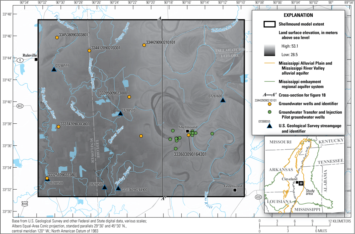
The Shellmound model extent with streamlines and streamgage locations, the digital elevation model of the land surface, and boundaries of the Mississippi Embayment Regional Aquifer Study and the Mississippi Alluvial Plain (Haugh and others, 2020a,b; Guira and Weisser, 2025).
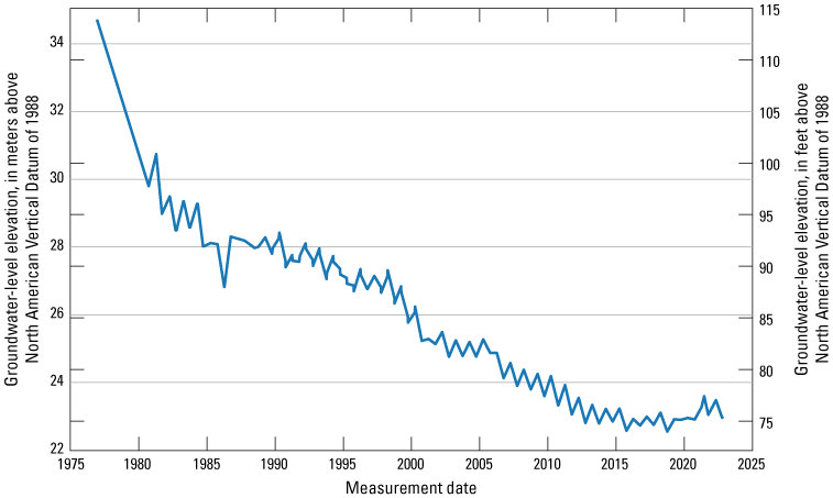
Groundwater-level elevation at U.S. Geological Survey site 334412090270301 (133F0190 Sunflower; U.S. Geological Survey, 2020).
Purpose and Scope
The purpose of this report is to describe an inset groundwater-flow model, based on the regional model by Leaf and others (2023), of the MRVA aquifer including the model construction, calibration, simulation, and analysis of the simulated effects of groundwater extraction and injection by the GTIP project on groundwater levels near Shellmound, Miss. This report describes the approaches used to incorporate high-resolution AEM data in the model construction process through a detailed representation of the MRVA aquifer in the focused area (Minsley and others, 2021). The report describes how the same geophysical data were processed into three different vertical resolutions, each integrated into the construction of a groundwater-flow model with a different layering configuration of the MRVA aquifer. The report describes the construction and calibration of a historical model to simulate hydrologic conditions from 1900 to 2018 and a forecast model that simulates future conditions from 2019 to 2050, including water transfer using riverbank filtration and injection wells.
Study Area Description
The Shellmound model study area covers the extent of the inset model domain, which lies entirely within the Mississippi River Delta and includes parts of Leflore, Sunflower, and Tallahatchie Counties (fig. 1). The area extends 35 km from the east to the west, 30 km from the north to the south, and covers a surface area of 1,050 square kilometers (km2; approximately 405 square miles [mi2]). The southeastern corner of the model is 1 mile (mi) south of Greenwood, Miss. (fig. 1), and the western boundary goes through the town of Ruleville, Miss., which is 10 mi east of Cleveland, Miss. (fig. 1).
Climate and Land Use
The climate in the Shellmound model study area is typical of the Mississippi River Delta (hereafter referred to as the “Delta”). Climate in the Delta is humid and subtropical (Arthur, 2001), and data from the meteorological station USW00013978 (National Centers for Environmental Information, 2022) near Greenwood, Miss. (fig. 1) indicate that the average minimum and maximum monthly temperatures were 11.6 degrees Celsius (°C) and 25 °C (53 °Fahrenheit [°F] to 77 °F), respectively. Long-term monthly averages indicate that the hottest months were July and August with temperatures around 32.2 °C (90 °F), whereas the coldest months were December and January with averages around 2 °C (35.6 °F; fig. 3; National Centers for Environmental Information, 2022). For the same period, 2010–20, the average annual precipitation was approximately 131 centimeters per year (cm/yr; 51.5 inches per year [in/yr]). April and December were the wettest months with an average precipitation of approximately 14 centimeters (5.5 inches) each (fig. 4). Land use in the Shellmound model study area is dominated by farmland with major agricultural crops including soybeans, corn, rice, and cotton. Farmlands in the area also include catfish ponds for aquaculture. Other land uses include wetlands, developed/urban, pasture, and forest (Wilson, 2021).
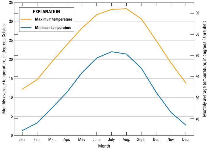
Average monthly temperatures from 2010 to 2020 based on climate data from meteorological station USW00013978, near Greenwood, Mississippi (National Centers for Environmental Information, 2022).
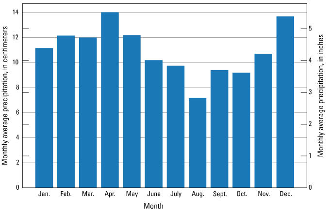
Average monthly precipitation from 2010 to 2020 based on climate data from meteorological station USW00013978, near Greenwood, Mississippi (National Centers for Environmental Information, 2022).
Surface-Water Features
Surface-water features in the Shellmound model study area include streams, ponds, and oxbow lakes. Many of these surface-water features are not connected to the MRVA aquifer based on a spring 2016 potentiometric map by McGuire and others (2019). The major streams in the Shellmound model study area are the Tallahatchie, Quiver, and Big Sunflower Rivers (fig. 1). The Tallahatchie River flows north to south and meanders along the eastern portion of the study area until approximately 3 km north of the southern boundary where it merges with the Yalobusha River to become the Yazoo River (not shown). At the western boundary, the Big Sunflower River enters the study area approximately 10 km south of the northern boundary and runs south (fig. 1). Across the middle of the study area and flowing south is a network of small streams, most of which originate within the study area and are tributaries to the Quiver River (fig. 1). The average daily streamflow for the Tallahatchie River at Money, Miss. (USGS station 07281600; U.S. Geological Survey, 2020) from 1996 to 2018 was approximately 18.8 million cubic meters per day (m3/d; 7,700 cubic feet per second [ft3/s]; fig. 5). The average streamflow on the Quiver River near Sunflower, Miss. (USGS station 07288580) was 1.2 million cubic meters (m3) (500 ft3/s) based on 20 discrete streamflow measurements (from calendar year 1995 to 2014), and 2.7 million m3 (1,100 ft3/s) on the Big Sunflower River near Sunflower (USGS station 07288500) based on 257 discrete streamflow measurements (from calendar year 1940 to 2018).
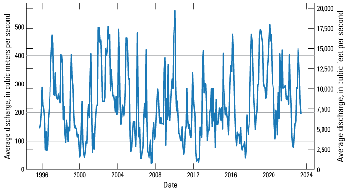
Average daily mean streamflows for the Tallahatchie River at Money, Mississippi (U.S. Geological Survey station 07281600; U.S. Geological Survey, 2020).
Major Hydrogeologic Units
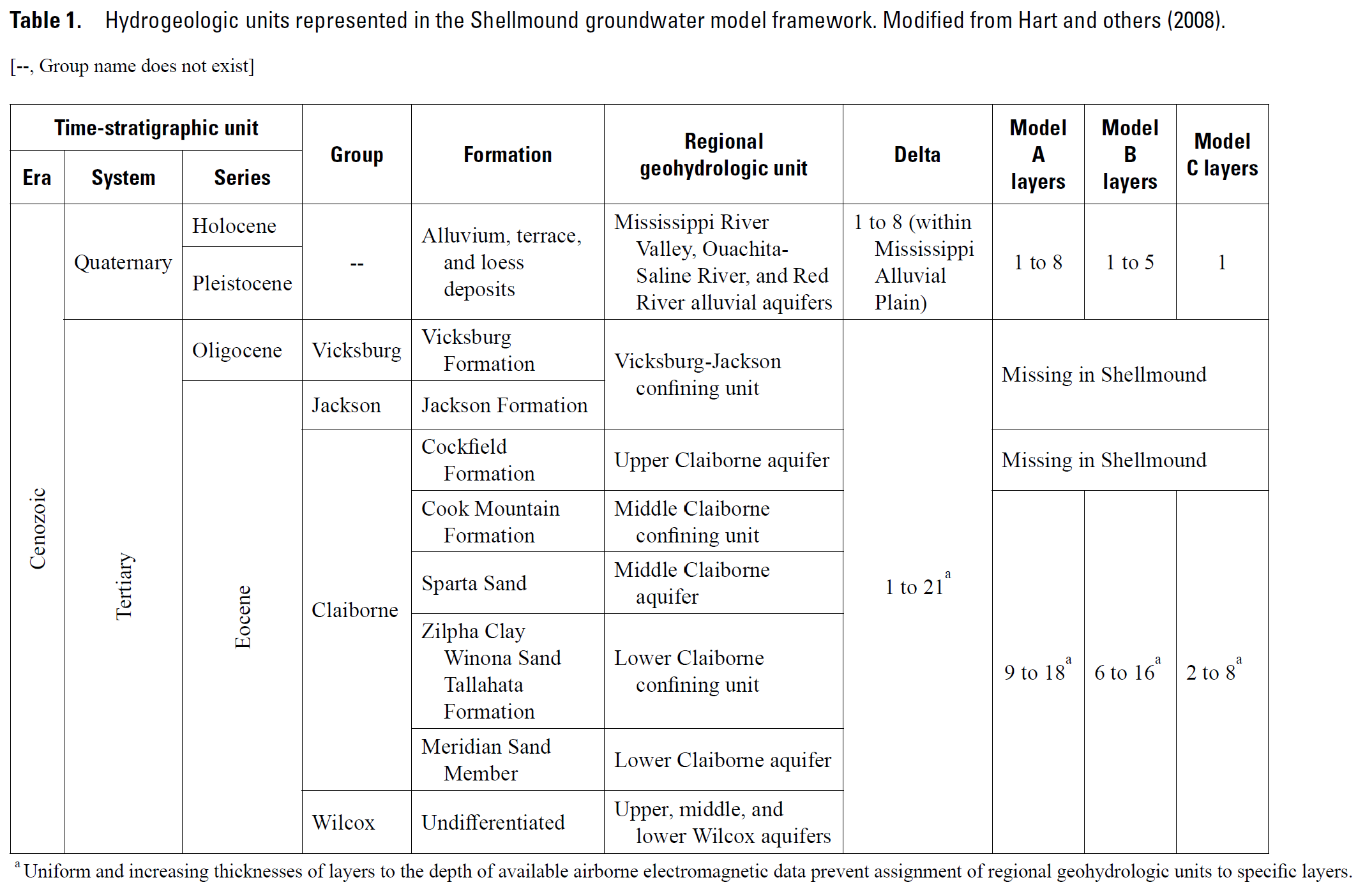
The major hydrogeologic units in the Shellmound model study area are Quaternary and Tertiary units (table 1; Clark and Hart, 2009). The surficial MRVA aquifer is the uppermost unit and mainly consists of sand and gravel that were deposited during the Quaternary period. The uppermost layer of the MRVA aquifer generally is finer with increased prevalence of silt and clay corresponding with lower vertical hydraulic conductivity. The average thickness of the MRVA aquifer in the study area, as computed from land surface elevation to the interpreted base of the alluvial aquifer from recent AEM data (Minsley and others, 2021), is 38.3 meters (m; 126 feet [ft]) with a maximum of 49.2 m (161 ft) and a minimum of 23.5 m (77 ft). Underlying the MRVA aquifer are the older Tertiary hydrogeologic units, which mainly consist of undifferentiated sediments and include the upper and lower Claiborne aquifers, the middle Claiborne confining unit, and the middle and lower Wilcox aquifers (Hart and others, 2008; Clark and Hart, 2009; Leaf and others, 2023). The Tertiary deposits have a combined average thickness of 607 m (1,994 ft) with a maximum of 780.3 m (2,560 ft) and a minimum of 436 m (1,430 ft). Hydrogeologic units represented in the Shellmound groundwater model framework are shown in table 1.
.
Groundwater and Water Use
The highly productive MRVA aquifer is the most important source of fresh water in the Mississippi embayment aquifer system (Clark and Hart, 2009), which fully encompasses the Shellmound model study area. Wells screened in the alluvial aquifer can pump between 1,635 and 16,350 m3/d (between 300 gallons per minute [gal/min] and 3,000 gal/min; Hewitt and others, 1949, Klein and others, 1950; Onellion, 1956; Bedinger and Reed, 1961). Outside of the Shellmound model study area, underlying Tertiary units were reported to have much lower well yield of 545 to 2,725 m3/day (100 to 500 gal/min) but can reach as much as 8,176 m3/day (1,500 gal/min; McKee and Hays, 2002; Clark and Hart, 2009). Killian and others (2019) reported that in 2000, groundwater withdrawal from the alluvial aquifer alone accounted for 10 percent of all groundwater use within the continental United States. Nearly all crop and catfish production is supported by groundwater pumping (Killian and others, 2019; Wilson, 202170; Bristow and Wilson, 2023; Leaf and others, 2023). Major crops in the Shellmound model study area and their estimated water use by the Aquaculture and Irrigation Water-Use Model (AIWUM) are shown in figure 6 (Bristow and Wilson, 2023). Other nonagricultural groundwater uses include municipal and industrial uses. Based on the geostatistical estimates for well screen elevation by Torak (2023), and the site-specific water-use data system (SWUDS) database (U.S. Geological Survey, 2020), it was determined that most groundwater use for crop and fish production within the limits of the Shellmound model study area is primarily supported by the MRVA aquifer, whereas the municipal and industrial groundwater use is supported by the underlying Tertiary units.
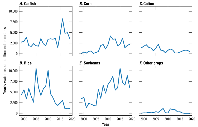
Plot of crop water use by crop type for the Shellmound model study area estimated from the Aquaculture and Irrigation Water-Use Model by Bristow and Wilson (2023). A, Catfish. B, Corn. C, Cotton. D, Rice. E, Soybeans. F, Other crops.
Shellmound Groundwater-Flow Model
This section of the report describes the methodology used in the development of the Shellmound model. It includes a brief overview of the groundwater model used as the parent model. It also includes a description of the conceptual design, the three-dimensional groundwater-flow model, the model calibration approach, and the calibration results for the Shellmound model.
Parent Model
An inset groundwater-flow model is one constructed from a previously developed and larger groundwater-flow model (Feinstein and others, 2010) that fully encompasses the inset model domain. The parent model used in the development of the Shellmound model is the three-dimensional groundwater-flow model described in Leaf and others (2023), which is an inset model. In this report, the parent model of the Shellmound model is hereafter referred to as the “Delta model.” The Delta model is a multilayer three-dimensional groundwater-flow model simulated by using the USGS MODFLOW 6 code (Langevin and others, 2017) and focused on simulating hydrologic processes in the Mississippi Delta region (figs. 1 and 7). The purpose of the Delta model was to provide a tool for calibration in the Mississippi River Delta and for forecasting groundwater levels under specific climate and water use stresses (Leaf and others, 2023). The robust workflow was created to facilitate a somewhat fast development and parameterization of inset models and was subsequently modified for the purpose of developing the Shellmound model. More details on the Delta model development, calibration, and results are provided in Leaf and others (2023).
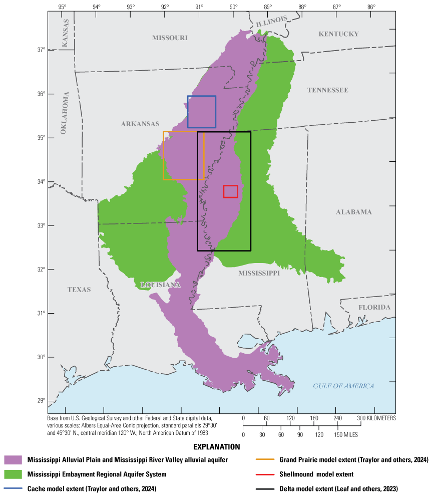
The Shellmound model study area within the Mississippi Embayment Regional Aquifer System, Mississippi Alluvial Plain, and Mississippi River Valley Alluvial aquifer extents (Haugh and others, 2020a,b; Guira and Weisser, 2025).
Conceptual Model
Prior to the construction of the groundwater-flow model, the hydrologic system in the Shellmound model study area was conceptualized into a framework that accounts for the regional groundwater flow and its interactions with other components of the hydrologic system. The conceptualization led to a general understanding regarding the major budget components and physical processes that are within the study area. A conceptual model of groundwater flow is often presented as a narrative describing the occurrence and movement of groundwater along with physical characteristics such as aquifer properties and the largest inflows and outflows within the model domain (Peterson and others, 2016), and that approach has been taken in this report. The inset model domain was defined to cover the GTIP project area of operations and modified based on the coverage of the high-resolution AEM survey (Minsley and others, 2021). The modifications resulted in model boundary segments with fluctuating regimes of exchanges of groundwater between the model domain and the surrounding aquifer based on regional groundwater flow (fig. 8). At the onset of this study, a prototype version of the conceptual model was constructed for the MRVA aquifer using the newly interpreted base of the alluvial aquifer from the AEM survey (Minsley and others, 2021) as the base of the model. The constructed groundwater-flow model based on that conception was unstable and did not adequately account for the hydrologic contribution of the underlying Tertiary units; therefore, a more comprehensive approach was adopted to include the Tertiary units present in the study area.
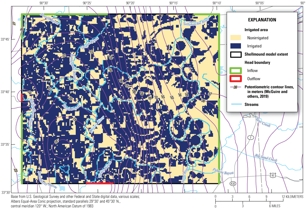
Lateral inflow and outflow boundary segments (Guira and Weisser, 2025) as determined using 2016 potentiometric surface (McGuire and others, 2019). Background image shows irrigated and nonirrigated cells based on Aquaculture and Irrigation Water-Use Model data (Bristow and Wilson, 2023).
The conceptual model described in this report is not meant to accurately quantify each budget component of the Shellmound model. It is meant to provide a rough estimate of budget components to guide the calibration and help the reader understand the relative magnitude of each component. Thus, the 2016 conditions used to estimate most budget components indicate that approximately 52 percent of inflows were from stream leakage, 23 percent from storage, 15 percent from recharge, 5 percent from irrigation return flow, and 4 percent from cross boundary flow from surrounding aquifers. Approximately 88 percent of outflows were from groundwater irrigation, 11 percent from stream leakage, and 1 percent from groundwater evapotranspiration.
Inflows
The two major inflows into the groundwater-flow system of the Shellmound model study area are (1) groundwater recharge, which consists of areal recharge and stream leakage; and (2) groundwater release from storage. Areal recharge represents the fraction of precipitation that infiltrates to the water table. The two minor inflows to the groundwater-flow system are from (1) lateral groundwater flow from areas surrounding the model domain and (2) irrigation return flow, which represents the portion of irrigation inefficiency that infiltrates back to the groundwater system. Below is a summary description of how each inflow component was calculated.
Areal recharge estimates were taken from Clark and Hart (2009) where a calibrated recharge map provided average recharge rates by calibration zones. The map section that overlaps the Shellmound model study area contained zones 103 and 108 with respective average calibrated recharge rates of 2.85 and 0.19 in/yr (Clark and Hart; 2009). The average volumetric annual rate computed by using those rates for their respective areas was approximately 30.7 million cubic m per year (m3/yr).
Irrigation return flow rates were computed using irrigation efficiencies based on the irrigation and crop type. A furrow irrigation efficiency of 65 percent and an irrigation return rate of 30 percent were used based on findings by Kandpal (2018) and Bryant and others (2021). Groundwater recharge is also affected by the thickness and permeability of the vadose zone. As a result, a spatially varying recharge rate was applied based on the surficial connectivity zones (fig. 9) generated by logarithmically binning “facies” classes of vertically averaged shallow electrical resistivity from AEM surveys (Minsley and others, 2021). The connectivity-based reduction resulted in an annual irrigation return rate estimated at 9.8 million m3/yr.
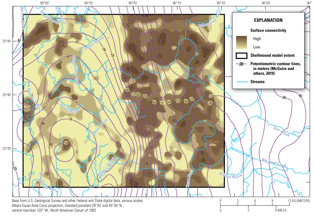
Surficial connectivity classifications based on the thickness of low electrical resistivity layers detected through airborne electromagnetic survey based on data from depths of 0 to 15 meters (Minsley and others, 2021).
The connection between streams and the groundwater system was examined using land surface elevations and the interpreted groundwater-level surface. A digital elevation model for land surface (U.S. Geological Survey, 2016) and a 2016 potentiometric surface by McGuire and others (2019) were used to compute the thickness of the unsaturated zone underlying all stream reaches. For this approximation, a stream segment was assumed to be in a losing condition if the unsaturated zone beneath was thicker than 1 ft; otherwise, the reach was assumed to be in a gaining condition. The assignments are based on the assumption that streambed elevation is likely lower compared to the digital elevation model altitude. Using stream length and width in each cell along with streambed vertical hydraulic conductivity and the distance between streambed elevation and the water table, an annual stream-leakage rate was computed for each stream reach (Barlow and others, 2000; McKay and others, 2012; Boyraz and Kazezyilmaz-Alhan, 2021). The estimation resulted in a net stream leakage to the groundwater-flow system of approximately 26.5 million m3/yr. It is important to note that the exchange between groundwater and surface water could vary with time for each reach. The exchange also can vary in magnitude and direction seasonally depending on the hydraulic head gradient between the groundwater and surface water. Therefore, a gaining reach in February, prior to the start of agricultural irrigation pumping when groundwater levels are likely at their highest, can become a losing reach in October after the irrigation pumping throughout the growing season lowers groundwater levels.
To account for change in groundwater storage, 17 wells across the Shellmound model study area were used to compute the average annual groundwater-level change from 1994 to 2016. The average groundwater-level change, along with the calibrated specific yield (Sy) of 0.3 (Clark and Hart, 2009), was used to approximate a rate of groundwater released from storage of 48 million m3/yr.
Lateral groundwater movement across the model domain was estimated using 2016 equipotential lines from the potentiometric surface (McGuire and others, 2019). It was assumed that groundwater-flow direction is perpendicular to equipotential lines; therefore, drawing the flowlines in the vicinity of the boundary provided a snapshot of the groundwater-flow direction between the model domain and the surrounding aquifer. The head boundary segments where the study area is gaining from lateral groundwater flow are shown in figure 8. The 9.5 million m3/year net positive groundwater flow into the study area is consistent with the observation that a large portion of the area is irrigated, and groundwater pumping from the aquifer is decreasing groundwater levels, forming a regional cone of depression, and is responsible for the gradient that contributes to the influx. Influx along the eastern boundary is consistent with the overall regional groundwater flow as documented through previous studies and field water-level observation data (Arthur, 2001; McGuire and others, 201945, 2021; Leaf and others, 2023).
Outflows
Hydrologic stresses that resulted in a net flow out of the Shellmound groundwater model study area consist of (1) irrigation pumping and (2) groundwater evapotranspiration. In this conceptual model, lateral groundwater flow out of the study area and groundwater discharge to streams as base flow were lower than their inflow counterparts. Below is a brief description of how flows out of the model were estimated.
Irrigation water use for the conceptual model was estimated based on crop water demand by using the 2016 land use dataset (Meredith and Blais, 2019; USDA, 2020). Major crops in the Shellmound model study area include corn, cotton, rice, and soybeans. Crop water demand estimation also accounted for well-known and documented inefficiencies associated with irrigation practices in the region (Meredith and Blais, 2019). The estimation resulted in approximately 187 million m3 of extracted water for irrigation purposes per year. Nonagricultural water use was estimated at 67,875 m3/yr using USGS SWUDS data (Diehl and Harris, 2014; Harris and Diehl, 2019a, b).
For this report, groundwater evapotranspiration is defined as the process by which plants uptake groundwater directly from the saturated zone through their roots and transpire that water to the atmosphere. Groundwater evapotranspiration is dependent on land cover and the thickness of the vadose zone, typically taking place in areas of shallow groundwater where plant roots reach the water table near gaining streams and in groundwater-fed swamps and marsh areas (Lubczynski, 2009). In most of the study area, the water table is deep enough that groundwater evapotranspiration is not expected, so plant water requirements are met predominantly by soil moisture in the vadose zone. Groundwater evapotranspiration is only expected in a small portion of the model domain along the gaining stream reaches. The estimates of groundwater evapotranspiration in the Shellmound model study area amounted to 2.5 million m3/yr.
Model Construction
This section of the report describes the construction of the MODFLOW 6 Shellmound model by using the approach described in Leaf and others (2023). The process involved a robust automated workflow facilitated by the use of Python tools (Leaf and others, 2021; Leaf and Fienen, 202241) to expedite the construction. The workflow allowed for a stepwise approach in the model construction whereby complexity is added and tested one step at the time. The workflow also allows for quickly rebuilding the model at different spatial and temporal resolutions. The model was simulated using the USGS MODFLOW 6 code (Langevin and others, 2022).
Spatial and Temporal Discretization
The plan view of the model domain footprint (the study area) is a rectangular shape that extends 30 km in the north to south direction and 35 km in the east to west direction (fig. 1). The model bounding box was chosen so that it aligns with the National Hydrologic Grid (Clark and others, 2018). The domain was spatially discretized into orthogonal blocks of 100 m by 100 m and organized in 300 rows and 350 columns (fig. 10).
The Shellmound model development process included the exploration of the effect of increased complexity in layering configurations that resulted in three different vertical discretizations corresponding to the three versions (models A, B, and C) of the Shellmound model. Model A retains the vertical discretization used in the Delta model and consists of uniform 5-meter-thick layers from land surface to the base of the MRVA aquifer as defined through the interpretation of the AEM data (Minsley and others, 2021). Below the base of the MRVA aquifer, the vertical discretization is represented by uniform and increasing thickness to the depth of the available AEM data, and then by nonuniform layer surfaces using the hydrostratigraphic surfaces described by Hart and others (2008). The Delta model layers 16–18 were inactive over the Shellmound model domain area and therefore were not represented in the inset model. Consequently, Shellmound model A layers 16, 17, and 18 correspond to the Delta model layers 19, 20, and 21, respectively. The discretization process resulted in 18 model layers for model A (fig. 11; table 1). More details on the Delta model layering and the extent of each layer are in Leaf and others (2023).
Model B has a vertical discretization that defines 10-m constant thickness and horizontal layers from the highest elevation of the land surface to the base of the MRVA aquifer (Minsley and others, 2021). The vertical discretization of model B below the base of the MRVA aquifer is identical to that of model A, which resulted in 16 model layers for model B (fig. 12; table 1).
The vertical discretization in model C is defined by a single layer that extends from land surface to the base of the MRVA aquifer. The vertical discretization of model C below the base of the MRVA aquifer is identical to those in models A and B, which resulted in eight model layers for model C (fig. 13; table 1). More information on the discretization for each model is provided in a USGS data release (Guira and Weisser, 2025).
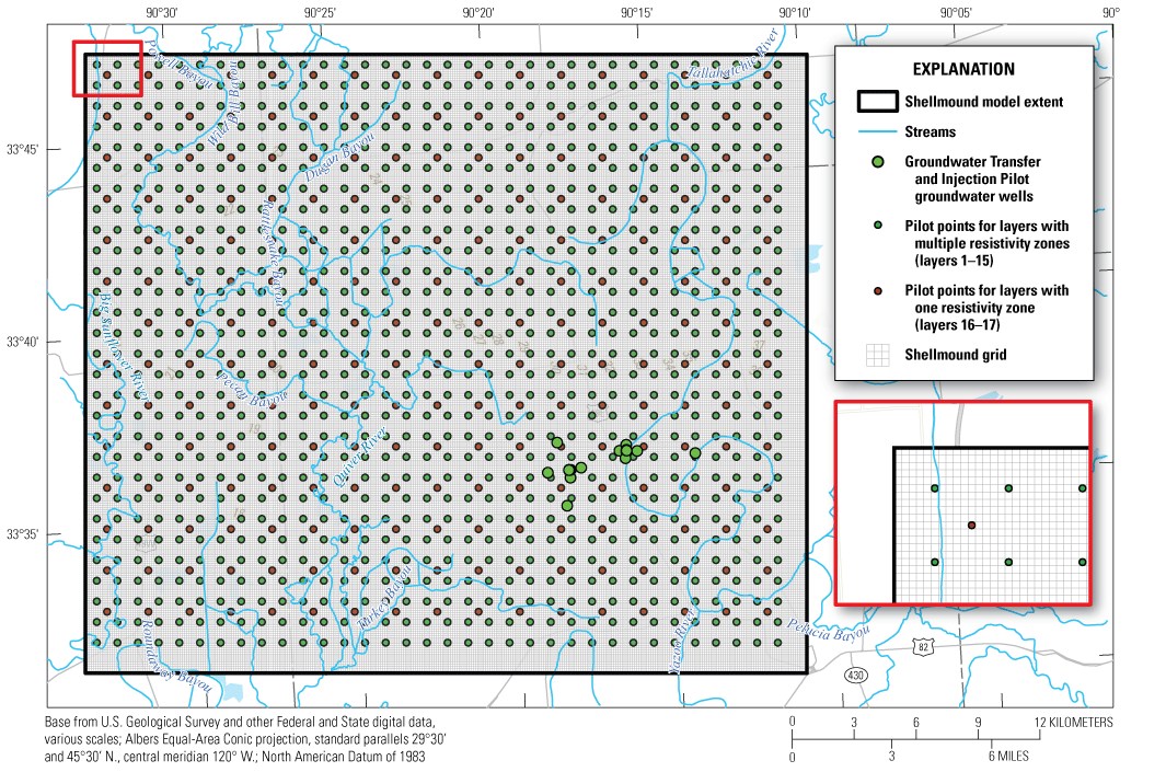
Shellmound model grid showing model cells along with regularly spaced pilot points used as multipliers to aquifer properties during model calibration (Guira and Weisser, 2025).
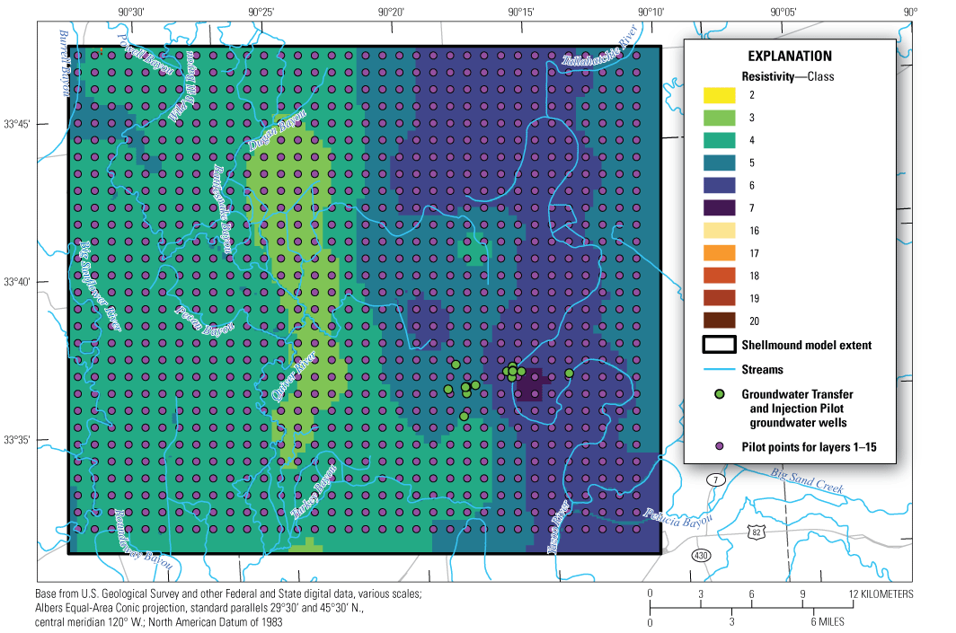
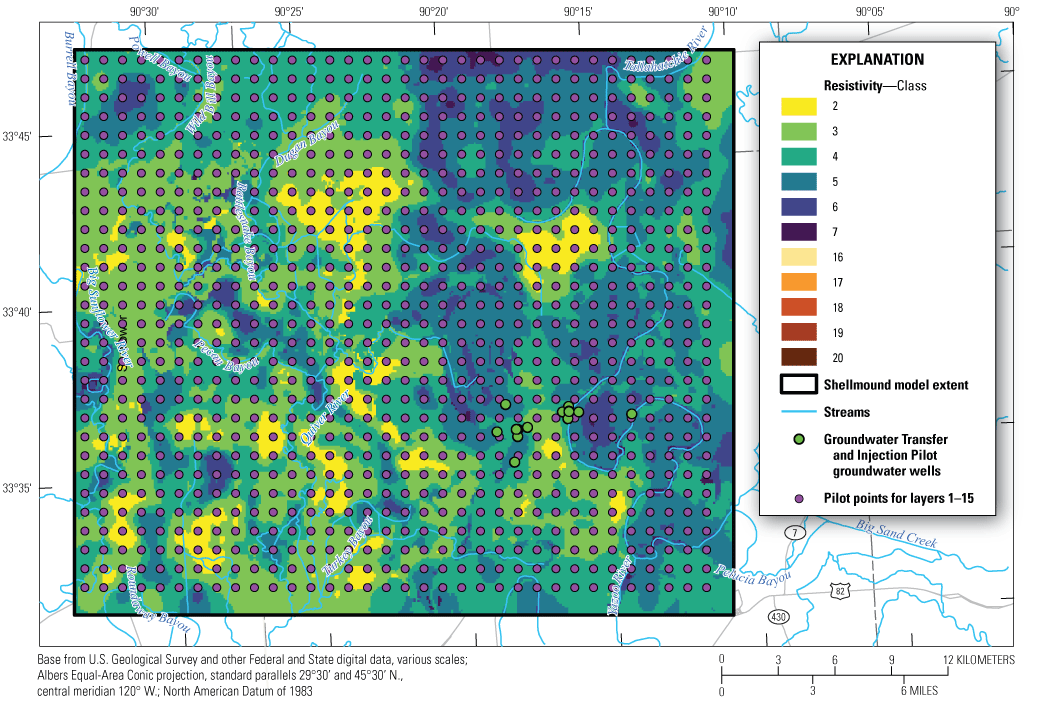
Electrical resistivity classes (Minsley and others, 2021) for the active area for layers 1–18 along with pilot points location in model A (this is a layered .pdf; download at https://doi.org/10.3133/sir20255055).
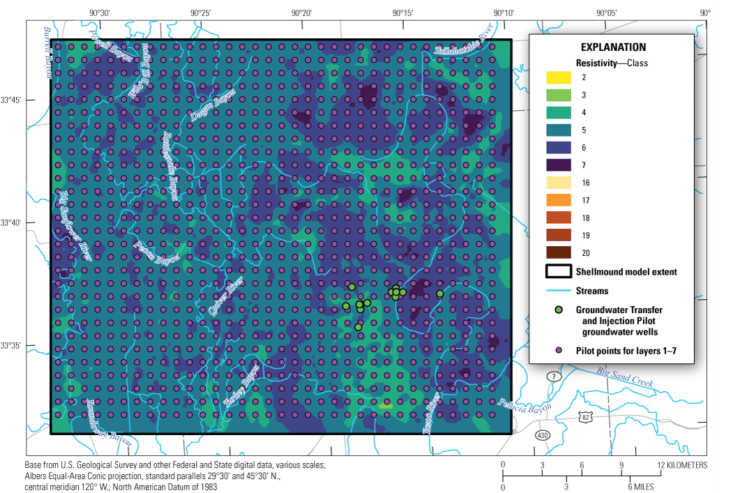
Electrical resistivity classes (Minsley and others, 2021) for the active area for layers 1–16 along with pilot points location in model B (this is a layered .pdf; download at https://doi.org/10.3133/sir20255055).
Electrical resistivity classes (Minsley and others, 2021) for the active area for layers 1–8 along with pilot points location in model C (this is a layered .pdf; download at https://doi.org/10.3133/sir20255055).
The temporal discretization of the Shellmound model is identical to that used in the Delta model (Leaf and others, 2023). A total of 148 stress periods of varying lengths were simulated from 1900 to 2018 (table 2). The period prior to April 2007 was subdivided into six stress periods of lengths of 1 year or more and represented varying stages of groundwater development within the MAP area as reported in previous studies (Clark and Hart, 2009; Leaf and others, 2023). The first stress period simulates a steady state condition, whereas stress periods 2 to 148 simulate transient conditions. The model simulates monthly stress periods from April 1, 2007, to January 1, 2019.
Table 2.
Temporal discretization in the Shellmound model (Guira and Weisser, 2025).[Dates shown as month/day/year]
Hydrologic Boundaries
This section of the report describes the hydrologic boundary conditions, and the exchanges between the groundwater system in the study area and the surrounding environment. MODFLOW 6 uses boundary condition packages to model these exchanges and calculates the gains and losses for the groundwater system during each stress period.
Areal Groundwater Recharge
Areal groundwater recharge was simulated in the Shellmound model using the MODFLOW 6 recharge package (Langevin and others, 2017). Input recharge grids for the Shellmound model were based on daily simulated net infiltration by the Shellmound soil-water-balance (SWB) model (Nielsen and Westenbroek, 2023). The Shellmound SWB model consists of 100×100-meter cells and computes a grid-based water budget of surface hydrology (from the vegetative canopy to the bottom of the root zone) that was constructed to provide inputs to the Shellmound model. Daily net infiltration rates were averaged to match the Shellmound model monthly temporal discretization from April 2007 to December 2018. The spatially distributed average daily net infiltration rates for 1999–2018 was used for the stress periods preceding 2007. The spatially distributed average net infiltration estimates from the SWB model are shown in figure 14 (Nielsen and Westenbroek, 2023).
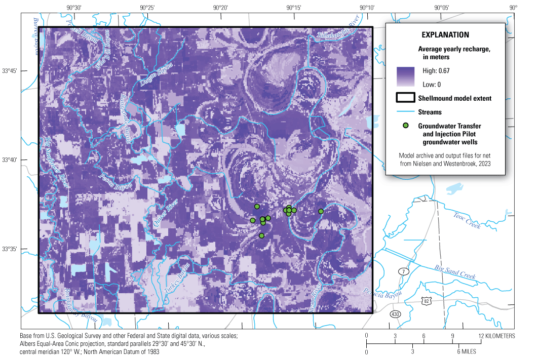
Yearly average (1999–2018) net infiltration estimates from soil-water-balance model representing noncalibrated groundwater recharge. Data from Nielsen and Westenbroek (2023).
Streams
All streams in the Shellmound model were simulated using the MODFLOW 6 Streamflow Routing (SFR) package (Langevin and others, 2017). The SFR package simulated the stream water budget for each stream reach including gains and losses. In addition to the stream water budgets, the SFR package simulated surface runoff, stream stage, and routing between connected reaches. The runoff inputs to the SFR package were provided by the SWB model (Nielsen and Westenbroek, 2023). In addition to the budget components, the SFR package simulated the streambed conductance by using vertical hydraulic conductivity, streambed thickness, and channel geomorphology represented by Manning’s coefficient (Prudic and others, 2004; Langevin and others, 2017). The SFR package was built using NHDPlus version 2 data (McKay and others, 2012), the SFRmaker (Leaf and others, 2021), and MODFLOW 6 setup (Leaf and Fienen, 2022) following methodology described in Leaf and others (2023). Stream reaches and streamgages that were simulated in the Shellmound model are shown in figure 15.
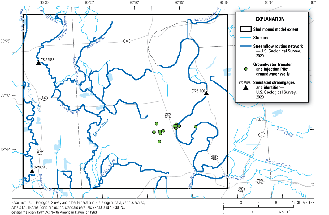
Simulated stream reaches using the modular finite-difference flow model 6 Streamflow Routing package.
Groundwater Pumping
Groundwater pumping in the Shellmound model was simulated using the MODFLOW 6 Well (WEL) package (Langevin and others, 2017). A single WEL package was used to simulate groundwater pumping for agricultural and nonagricultural use. Pumping locations and rates for stress periods prior to April 2007 were derived from the Mississippi Embayment River Aquifer Study (MERAS) 2.2 groundwater-flow model (Haugh and others, 2020a,b). There is no distinction between agricultural and nonagricultural water use in the Shellmound model prior to 2007. From April 2007 to December 2018, water-use data include pumping rates and locations for agricultural production and nonagricultural water use. Agricultural water use data were provided by the AIWUM version 1.1 (Wilson, 2021; Bristow and Wilson, 20238). The AIWUM estimates for annual average water use between 2000 and 2018 are shown in figure 16. Nonagricultural water-use data for the same period were provided by the USGS SWUDS and national estimates for water use associated with thermoelectric power generation (Diehl and Harris, 2014; Harris and Diehl, 2019a, b). Approximately 71.6 percent of all water from 1900 to 2018 were derived from the MERAS 2.2 model, whereas 28.3 and 0.09 percent were from AIWUM and SWUDS, respectively.
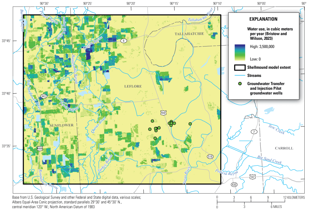
Average noncalibrated volumetric water use in cubic meters per year. Data processed from Aquaculture and Irrigation Water-Use Model estimates by Bristow and Wilson (2023).
Head Dependent Boundaries
Lateral groundwater flow into and out of the Shellmound model was simulated using the Constant Head (CHD) package (Leake and Prudic, 1991; Langevin and others 2017). The CHD package in MODFLOW 6, however, is classified as a hydrologic stress package where constant head values for specific cells were defined for every stress period (Langevin and others, 2017). Constant head boundary cells for the Shellmound model were specified at the perimeter boundary. Simulated groundwater levels from the parent model (Leaf and others, 2023) were used to specify hydraulic heads for every stress period in the CHD package. Lateral groundwater flow between the model and the surrounding aquifer for each stress period was computed based on the principle that groundwater flows downgradient, from higher groundwater levels to lower groundwater levels. The gradient between the CHD package cells and the neighboring cells determines the rates and direction of the exchange.
MODFLOW 6 Solver Settings
The Shellmound model solved systems of equations to achieve mass balance of the stresses applied to the system during each of the 148 stress periods. The Integrated Model Solution package (Langevin and others, 2017) employed the Newton-Raphson formulation with the “complex” Integrated Model Solution package option to iteratively solve the water balance equation for each stress period. The “complex” option was selected to improve solution stability when simulating the nonlinearity associated with local unconfined layers. For convergence criteria, the maximum allowable absolute value in head change was set to 1.0 m for non-linear iterations, and 0.01 m for linear iterations. The maximum number of iterations before convergence was set to 50 for non-linear iterations and 100 for linear iterations; the flow residual tolerance for linear iterations was set to 0.001. The same solver settings were used for all models and resulted in model run times of 58 minutes for model A, 28 minutes for model B, and 12 minutes for model C using MODFLOW 6 version 6.2.0.
Calibration
After construction, the Shellmound model went through a process where selected model inputs were adjusted to improve the match between the model’s simulated outputs and historical observations or calibration targets. This process is called “model calibration” or “parameter estimation” (Fienen and others, 2022). The parameter estimation of the Shellmound model included the identification of the calibration targets based on available observation data, adjustment selection of model parameters, manual adjustments of some parameters, and automated calibration using Parameter Estimation ++ (PEST++; White and others 2020). Manual calibration consisted of a trial-and-error approach to minimize the sum of the squared weighted differences between model simulated values and the equivalent calibration targets, the sum of which is the objective function (Φ, phi). Phi is a measure of the degree of mismatch between observed and simulated conditions and is tracked though the entire calibration process as an indicator of how well the model is capable of matching observations. The automated calibration of the groundwater model utilized PEST++ Iterative Ensemble Smoother (PESTPP–IES) software. The IES algorithm, along with select PEST++ and IES options (White, 2018; White and others, 2020), were activated to iteratively improve the model fit to the observations and reduce the uncertainty in parameter values during each iteration (table 3). The automated calibration process is based on Bayes’ Theorem (Tarantola, 2005; Fienen and others, 2022). It begins with a set of input parameter values known as the “prior,” which are then refined through a system conditioning step called the “update,” resulting in a new set of values referred to as the “posterior” (Fienen and others, 2022). The calibration process of the Shellmound model followed steps described in Leaf and others (2023) and Fienen and others (2022) using PEST++ (White and others, 2021), which was run on the USGS Denali supercomputer (Falgout and others, 2022).
Table 3.
Parameter Estimation ++ Iterative Ensemble Smoother (PESTPP–IES) settings for calibration.[PEST, Parameter Estimation; IES, Iterative Ensemble Smoother; --, option was not used]
Observations
Calibration targets are observation values that the calibration process aims to reproduce by adjusting parameters and simulating the model. Calibration targets in the Shellmound model include field observations and derivatives computed as spatial and temporal differences generated using the Modflow-obs Python package (Leaf, 2024). Field measurements of groundwater levels and total streamflows were used to compute average values corresponding to stress periods where there are available data. The USGS National Water Information System (NWIS) database (U.S. Geological Survey, 2020) was processed using methods described in two reports (Asquith and Seanor, 2019; Asquith and others, 2020) to produce synthetic groundwater-level observations, leading to 896 weighted and 375 non-weighted direct groundwater levels observations organized in six different observation groups (table 4). Only 30 of the groundwater-level observations were from the Tertiary deposits, 29 of which were weighted in the calibration, and represented 3 percent of weighted groundwater-level observations; the 97 percent remaining groundwater levels were measurements made in the MRVA aquifer. The number of field measurements and synthetic groundwater-level observations used for calibration in the Shellmound model are shown by the size of the circles on the map in figure 17.
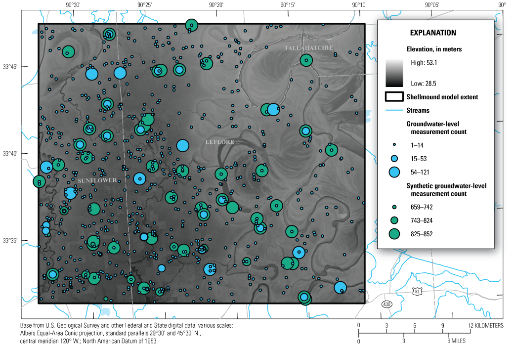
Field measurement and synthetic groundwater levels in the study area. The background image shows the digital elevation model of the land surface. Water-level measurements from U.S. Geological Survey (2020) and synthetic water-level measurements from Asquith and Seanor (2019) and Asquith and others (2020).
Table 4.
Observations used in the model calibration as calibration targets.[--, not applicable]
Streamflows and stage observations were processed from the NWIS database (U.S. Geological Survey, 2020) and from a random forest regression-based statistical model described in Dietsch and others (2022). Streamflow and stream stage observations were processed into monthly averages that resulted in 434 measured streamflow and 264 measured stage observations processed from the NWIS database and 142 estimated streamflow observations processed from the random forest model outputs (table 4). In addition to the measured and random forest output values, observations were also processed to produce secondary or derived observations based on long-term streamflow temporal differences. For details on how derived observations were produced, refer to Leaf and others (2023). Derived observations that were used in the calibration of the Shellmound model as calibration targets consisted of 1,937 groundwater-level temporal differences organized in four observation groups, 44 groundwater-level trends, 82 groundwater-level spatial differences, and 403 streamflow temporal differences organized in two observation groups (table 4).
Observation Weighting
The calibration process was primarily tracked by the objective function (eq. 1), which is a representation of the fit between the calibration targets and their equivalents from the model outputs. The difference between each observation and its equivalent in model outputs is referred to as a residual (Doherty, 2016; White and others, 2020) and was weighted using the equation of the objective function:
whereФ
is the objective function,
n
is the total number of observations,
wi
is the assigned weight of the ith observation, and
ri
is the residual associated with the ith observation and is calculated as observed minus simulated.
Initial observation weights were assigned based on uncertainty associated with the measurement and followed the approach used by Hunt and others (2013) and Leaf and others (2023). Weights were subsequently adjusted during manual calibration to approximately apportion the overall contribution of each observation group to the objective function (eq. 1) in accordance with the modeling objectives of simulating groundwater levels. This approach resulted in 2,462 weighted observations that included direct derivatives of groundwater-level measurements and 1,946 zero-weighted observations that included streamflows and some groundwater levels (table 4).
Parameterization
Parameterization consisted of linking PESTPP–IES to specific model inputs. Parameterization of the Shellmound model extensively relied on the use of multipliers to adjust inputs imported from the parent model and other sources such as AIWUM (Bristow and Wilson, 2023) and the SWB model (Nielsen and Westenbroek, 2023). The overall approach is similar to the method used in Leaf and others (2023) and Fienen and others (2022) following the multiscale approach described in White and others (2021). Coarse- and fine-scale parameterization was facilitated by the PstFrom routine from the pyEMU python package by White and others (2016, 2021). Coarse-scale parameters were generally multipliers used to allow for input bias correction such as data source and processes used in data preparation. Fine-scale parameters were applied where needed to allow for changes owing to local heterogeneity.
Aquifer Properties
Multiple levels of parameterization were applied to the aquifer properties, which comprise horizontal hydraulic conductivity (Kh), hydraulic conductivity vertical anisotropy (Kvani), Sy, and specific storage. Direct values were assigned to the two-dimensional grids based on zones defined by the resistivity classes (Minsley and others, 2021) for the MRVA aquifer section and hydrostratigraphic units defined in Hart and others (2008) for the underlying Tertiary layers. Cross sections of the Shellmound model with prior (noncalibrated) hydraulic conductivity values assigned based on resistivity classes are shown in figure 18. In addition to that initial coarse parameterization, multipliers for each zone and layer were added to allow for differences in zones based on layering. Finally, a dense network of regularly spaced pilot points (figs. 11–13) were added to Kh and Kvani layers. Pilot points for Sy were added to the first nine layers, which resulted in 40,150 aquifer-property parameters for model A; 39,202 for model B; and 23,780 for model C (tables 5–7).
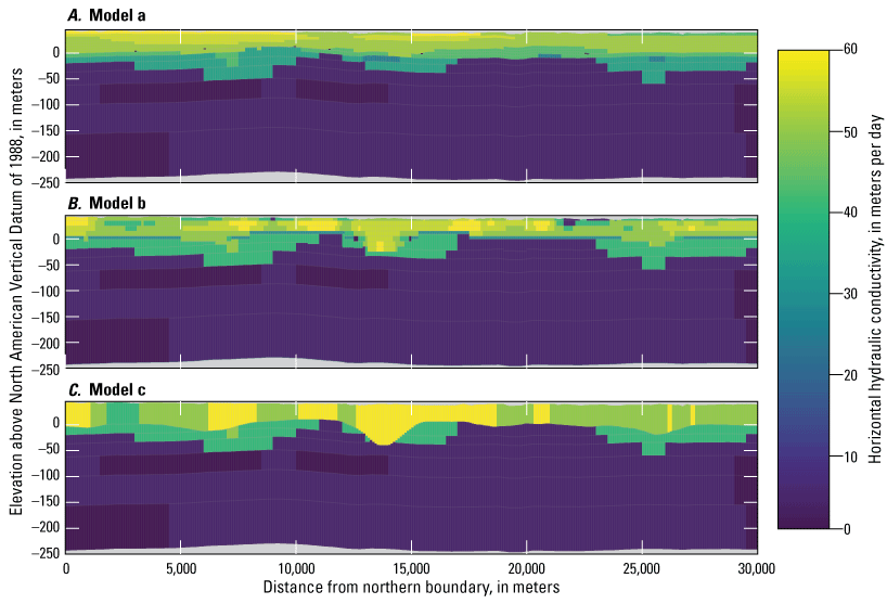
North to south cross section of models A, B, and C showing noncalibrated hydraulic conductivity values (Guira and Weisser, 2025).
Table 5.
Calibration parameters used in model A.Table 6.
Calibration parameters used in model B.Table 7.
Calibration parameters used in model C.Areal Recharge
Three levels of parameterization were applied to the areal groundwater recharge in the Shellmound model calibration. At the coarsest level, stress period multipliers were used to allow the calibration to correct for temporal bias in SWB model outputs. Additionally, recharge zone multipliers were added based on the surficial connectivity (fig. 9) and a spatial layer developed by Minsley and others (2021) based on electrical resistivity of the uppermost 15 m as interpreted by using the AEM survey data (Minsley and others, 2021). SWB model net infiltration does not simulate attenuation of recharge passing through the vadose zone that could affect recharge rates. Therefore, adding the surficial connectivity parameters improves the ability of the model to account for changes in recharge rates based on the degree of connection between the surface and the groundwater system. Finally, a network of pilot-point multipliers was added to account for local heterogeneity, which resulted in a total of 423 groundwater recharge parameters.
Streamflow Routing
Streams and their connection to the groundwater system were represented in the Shellmound model by the SFR package (Langevin and others, 2017). Parameterization of the SFR package inputs included surface-water inflows, surface runoff, and streambed vertical hydraulic conductivity. Multipliers to the inflows were added for stress periods 1 (steady-state), and 7–148 (monthly transient) and for the three inflow reaches. Surface runoff inputs were parameterized using multipliers by stress period but also by surficial connectivity (fig. 9) to account for the relation between infiltration capacity and runoff (Nielsen and Westenbroek, 2023). Unique multipliers were applied to streambed conductivity for each stream segment based on unique identifiers (COMID) associated with each stream segment in the NHDPlus version 2 (McKay and others, 2012). Additionally, coarse multiplier parameters were added based on the surficial connectivity. The parameterization of streamflow routing resulted in a total of 1,289 adjustable parameters (tables 5–7).
Water Use
Water use estimates in the Shellmound model were parameterized by stress period and data source. One multiplier was assigned to each of the three data sources (AIWUM, SWUDS, and MERAS 2.2) that supplied pumping rates to the Shellmound model (Harris and Diehl, 2019a; Haugh and others, 2020b; Wilson, 2021). There was no pumping simulated during the first, steady-state stress period because it represented naturalized conditions prior to groundwater development; therefore, only 147 additional stress-period-based multipliers were applied throughout the simulation. The process resulted in a total of 150 adjustable parameters used to constrain pumping rates in the Shellmound model (tables 5–7).
Calibration Results and Best Model
Following the construction and initial manual calibration, each model was transferred to the USGS Denali supercomputer (Falgout and others, 2022) for automated calibration. Calibration results were analyzed and evaluated for model fit and rationality of calibrated parameter values. One goal of this study was to explore the effects of integrating the AEM data (Minsley and others, 2021) and to evaluate which layering configuration (models A, B, or C) would yield the most useful model. The criteria used to decide on a good calibration included the value of Φ for the entire model, Φ for observations of particular interest, and calibrated parameters values.
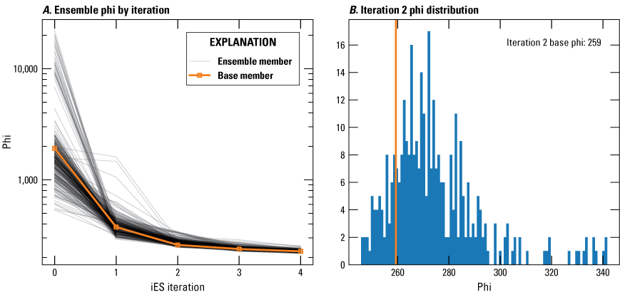
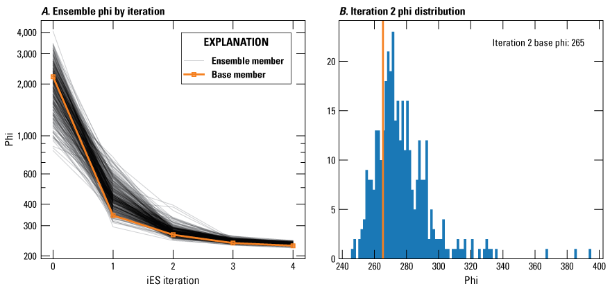
The IES method produces an ensemble of Φ values at the end of each iteration in the history matching process, corresponding to all realizations that successfully ran to completion, including the minimum error variance solution referred to as the “base realization.” Phi (Φ) values after four successive iterations for each model are shown in table 8. Mean Φ value for model A improved from 2,884.17 to 240.68 (table 8; fig. 19). Phi (Φ) values for models B and C changed from 2,473.32 to 231.03 and from 2,015.30 to 234.40, respectively (table 8; figs. 20 and 21). The “base” realization resulted in Φ values of 253.43, 258.72, and 265.25 for models A–C, respectively, after the second iteration. Calibration continued to improve throughout the process across all three models. However, to prevent potential overfitting of parameters, the analysis focused on results from the second iteration for the selection of one model configuration for the forecast. After the second iteration, model A outperformed models B and C. The global Φ value was not the sole indicator for optimal calibration but supported the observation that model A more accurately simulated water levels near the GTIP project operation sites. In addition to the acceptable calibration, the detailed representation of the MRVA aquifer in model A contributed to the decision to use model A for the forecast simulation.
Table 8.
Ensemble phi (Φ, objective function) values for models A–C following calibration run using Parameter Estimation++ Iterative Ensemble Smoother (PESTPP–IES) (White, 2018). [—Left]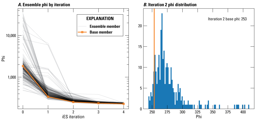
Ensemble phi (Φ, objective function) values from the calibration for model C. A, Reduction in the Φ value throughout iterations and B, histogram of ensemble members Φ values. In orange is Φ value for the base ensemble member.
Ensemble phi (Φ, objective function) values for model B history matching. A, Reduction in the Φ value throughout iterations and B, histogram of ensemble members Φ values. In orange is Φ value for the base ensemble member.
Ensemble phi (Φ, objective function) values for model C history matching. A, Reduction in the Φ value throughout iterations and B, histogram of ensemble members Φ values. In orange is Φ value for the base ensemble member.
A good model calibration does not solely rely on achieving a satisfactory fit between simulated and observed values, leading to the smallest Φ; it is also crucial that the calibration yield a realistic set of parameters that are also in agreement with the general understanding of the conceptual model. A thorough review of the posterior “base” parameter set over the successive iterations, along with subsequent corresponding model inputs, led to the conclusion that the calibrated parameters values were acceptable. Within the “base” parameter realization after the second iteration, only 2 out of 42,012 parameters reached their maximum acceptable values (upper parameter bound) set through the calibration constraints, which further supports the conclusion that the parameters values were acceptable and not overfit to match observations. Parameters that reached the maximum acceptable values were those representing constant multipliers for AIWUM pumping rates and recharge in stress period 5 (“pname:wel_datasource_mult_inst:0_ptype:gr_usecol:3_pstyle:m_idx0:iwum,” and “pname:rchspmult_inst:5_ptype:cn_pstyle:m”). All other posterior parameters in the “base” realization remained within bounds, further supporting that an acceptable calibration was achieved with model A.
The “base” member parameter set for iteration 2 of model A most closely matched observations compared to those of models B and C. Therefore, model A was selected to use as the forecast model. Consequently, results from the calibration and water budget estimates presented in this section of the report will focus on the best calibration model—model A. More results from the calibration of model A are presented in appendix 1. Results from the calibration and water budget estimates for models B and C are presented in appendix 2. Model calibration input and output files are available for download from the associated USGS data release (Guira and Weisser, 2025).
The best calibration of the Shellmound model was achieved with the improved representation of the interaction between surface water and groundwater. An earlier version of the model that used base flows as inflows to the SFR package and calibration targets did not yield realistic results and further exacerbated structural imperfections while accounting for the streambed leakance. The modeling approach was subsequently modified to employ streamflows as inputs and calibration targets at the streamgages. This approach was rendered possible thanks to the surface runoff inputs provided by the SWB model (Nielsen and Westenbroek, 2023).
The use of the surficial connectivity layer (fig. 9; Minsley and others, 2021) to parameterize groundwater recharge substantially improved the calibration particularly in the cone of depression. Because the SWB model does not account for potential barriers to vertical movement of water in the vadose zone, the net infiltration rates that the SWB model produces can be appreciably different from the actual net infiltration rates to the groundwater-flow system. The surficial connectivity zone multipliers adjusted during calibration showed a strong correlation between surficial connectivity and higher recharge. For example, the multiplier for zone 1 changed from 0.1 before automated calibration to approximately 0.07, thereby reducing SWB model recharge in that zone by approximately 25 percent. However, the multiplier for zone 5 during the same calibration changed from 0.4 to 0.53, resulting in a 20-percent increase of recharge in zone 5.
Calibration of the Shellmound model employed pilot point (Doherty, 2003) multiplier parameters for aquifer properties (Kh, Kvani, and Sy) and groundwater recharge to account for possible local heterogeneity (figs. 11–13). Interpolation between pilot points was only allowed within zones (fig. 11; Minsley and others, 2021), and this contributed to maintaining the contrast of lithologic fabric between zones while allowing local heterogeneity.
Calibration Results for Model A
Overall, the calibrated model achieved a good match for groundwater-level direct measurements and temporal trends such as seasonal fluctuations (fig. 22). Generally, groundwater-level measurements were collected biannually in April and October to capture seasonal high and low conditions at the end of the nongrowing (April) and growing seasons (October). A good fit between simulated and observed for observation groups “Shellmound heads,” “Priority embayment heads,” “Embayment heads,” and “Heads” with mean absolute errors of 0.57, 0.57, 0.90, and 1.01 m, respectively, are shown in figures 22A–D. Root-mean-squared error values for the same groups were 0.68, 0.72, 1.25, and 1.32 m, respectively. The mean absolute residual for weighted groundwater levels were 0.85 m and 4.40 m for the MRVA and Tertiary aquifers, respectively. The calibration did not yield a robust fit to the linear groundwater-level trends group (“head_trend”) even though only 7 out of 43 simulated trends were in the opposite direction compared to the observed trends, but the incorporation of that group appeared to help improve the fit in absolute groundwater level.
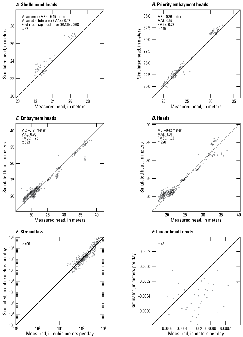
One-to-one plots comparing the Shellmound model outputs to field observations. A, Shellmound heads. B, Priority embayment heads. C, Embayment heads. D, Heads. E, Streamflow. F, Groundwater-level linear head trends.
Time series of groundwater levels for select observation sites purposefully chosen to cover the cone of depression and show the effect of the streams on groundwater levels from nearby wells are shown in figure 23. For USGS sites 334538090303801 (133F0600 Sunflower) and 334412090270301 (133F0190 Sunflower), located in the northwest corner of the Shellmound model domain (fig. 1), the model results show a good match between simulated and observed aquifer groundwater levels. The seasonal fluctuations between high water levels in April (the end of the nongrowing season) and low water levels in October (following the growing season) were well simulated (figs. 23A, B).
Time series groundwater-level plots for USGS sites 334429090210101 (083A0602 Leflore), and 332733090252901 (083C0074 Leflore), located between the Tallahatchie and the Quiver Rivers, are shown in figures 23C–D. Both stations show a good match between simulated and observed groundwater levels although groundwater levels at station 083A0602 tend to be underestimated, whereas groundwater levels at station 083C0074 were overestimated. Similarly, figures 23E and F show time series groundwater levels plots for USGS stations 333742090303801 (L0027) and 333251090323801 (083F0534) with a good match between simulated and observed groundwater levels. Although use of the surficial connectivity layer (fig. 9; Minsley and others, 2021) during calibration improved the match between simulated and observed groundwater levels, most groundwater levels at stations in lower surficial connectivity zones were slightly overestimated.
Simulated and observed time series for groundwater levels at USGS station 333603090164301 (083G0506 Sunflower) are shown in figure 23G. This station is 0.7 km from the Tallahatchie River and 0.8 km from the extraction site (fig. 1) used in the GTIP project. As a result, groundwater levels at this station are affected by stream seepage during seasonal high flows and long-term trends that remain relatively constant, thereby emphasizing interactions between surface water and groundwater.
Time series of simulated and observed groundwater levels at USGS station 333251090323801 (02058 Sunflower) are shown in figure 23H. This plot shows a significant difference between simulated and observed groundwater levels. Observed groundwater levels were approximately 5 m above the simulated groundwater levels and indicative of a perched system, which is consistent with findings from a previous study by O’Reilly and others (2020).
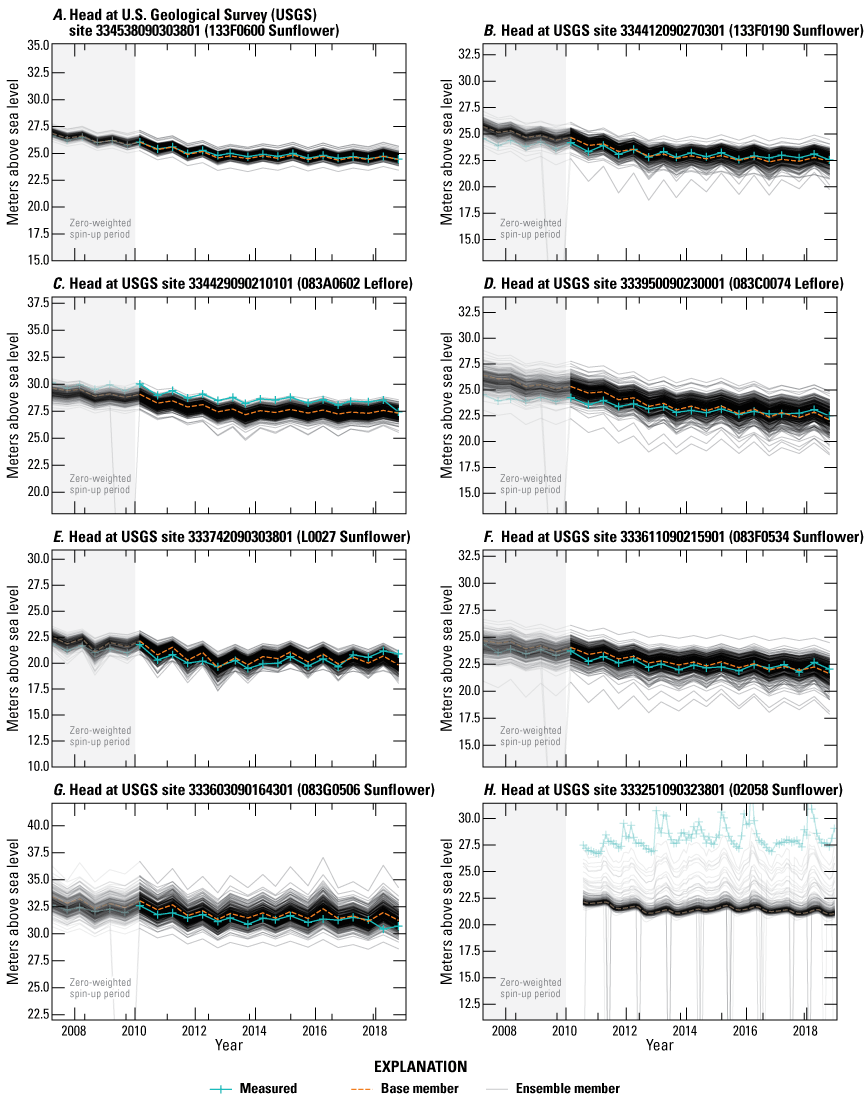
Time series of measured groundwater levels (U.S. Geological Survey, 2020) and simulated equivalents (Guira and Weisser, 2025) at selected wells. A, U.S. Geological Survey (USGS) site 334538090303801 (133F0600 Sunflower). B, USGS site 334412090270301 (133F0190 Sunflower). C, USGS site 334429090210101 (083A0602 Leflore). D, USGS site 332733090252901 (083C0074 Leflore). E, USGS site 333742090303801 (L0027). F, USGS site 333251090323801 (083F0534). G, USGS site 333603090164301 (083G0506 Sunflower). H, USGS site 333251090323801 (02058 Sunflower).
Monthly average time series of observed and simulated streamflows at the Big Sunflower River at Sunflower, Miss. (USGS station 07288500), and Tallahatchie River at Money, Miss. (USGS station 07281600) are shown in figure 24. Simulated streamflows at the Big Sunflower River at Sunflower, Miss., generally follow the observed patterns (fig. 24A). However, simulated streamflows at the Tallahatchie River at Money, Miss., tend to overestimate high flows and underestimate low flows (fig. 24B). During calibration, there was a tradeoff between slight improvements in streamflows during low flows where residuals on groundwater levels remained significantly high and achieved a better match between observed groundwater levels and their simulated equivalents near the Tallahatchie River at the expense of obtaining high residuals on streamflows (fig. 24).
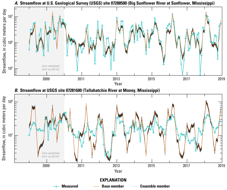
Streamflow time series showing monthly averages of measured streamflows (U.S. Geological Survey, 2020) and simulated equivalents (Guira and Weisser, 2025). A, Big Sunflower River at Sunflower, Mississippi (U.S. Geological Survey [USGS] station 07288500). B, Tallahatchie River at Money, Miss. (USGS station 07281600).
Calibrated Parameter Values
This section of the report presents calibration results for model A. A combination of coarse-, medium-, and fine-scale parameters resulted in a satisfactory calibration using PESTPP–IES (White, 2018). The “base” ensemble member after iteration 2 was chosen as the best parameter set to represent a calibrated version of the model (fig. 19).
Aquifer Properties
Calibrated aquifer properties by layer are shown in figures 25–28. Calibrated hydraulic conductivity for the entire model ranges from 0.02 meter per day (m/d) in the lower Claiborne confining unit to 300 m/d in the alluvial deposits, with an average value of 27 m/d. The MRVA aquifer portion of the model, as defined by aquifer material above the newly interpreted base using AEM data by Minsley and others (2021), calibrated to a slightly higher average Kh (27.6 m/d), whereas the Tertiary units calibrated to a lower average value (22.3 m/d). These hydraulic conductivity values were at the lower end of previously reported ranges of 1–500 m/d (Leaf and others, 2023). The calibrated hydraulic conductivity values in the MRVA aquifer were within the expected ranges and generally agree with the heterogeneity suggested by the interpretation of the AEM data.
Anisotropy (ratio of Kh to the vertical hydraulic conductivity) was calibrated to an average value of 116.2 (dimensionless) and ranged from 1 (isotropic situation) to 3,400. Average anisotropy for MRVA aquifer was 103 and ranged from 1 to 758, whereas the Tertiary deposits calibrated to an average anisotropy of 126 and ranges from 1 to 3,400. Calibrated Sy and specific storage ranged from 0.05 to 0.35 and from 2.7x10⁻⁷ to 10−5, respectively, and were close to values (0.19 to 0.32, and 2.4x10⁻⁶ to 3.8x10⁻⁵, respectively) reported by Arthur (2001), Clark and Hart (2009), and Leaf and others (2023).
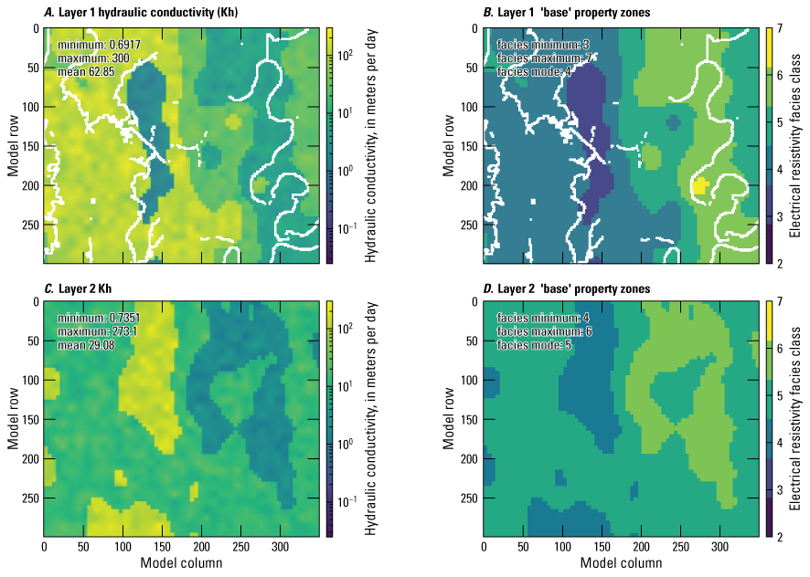
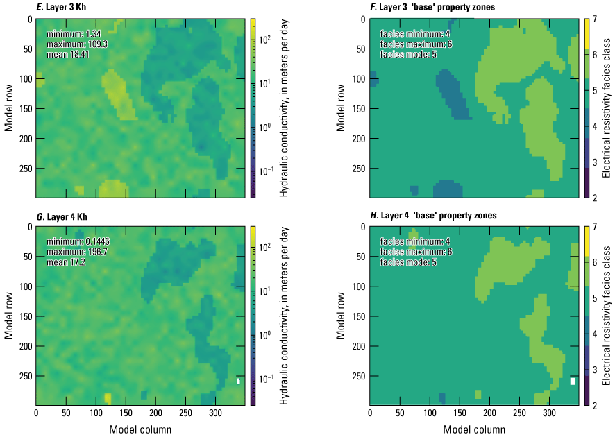
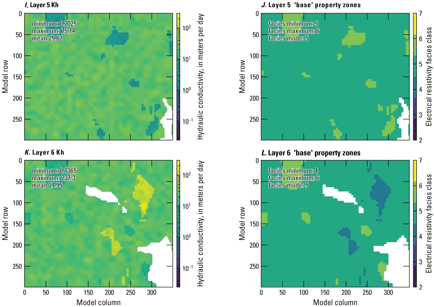
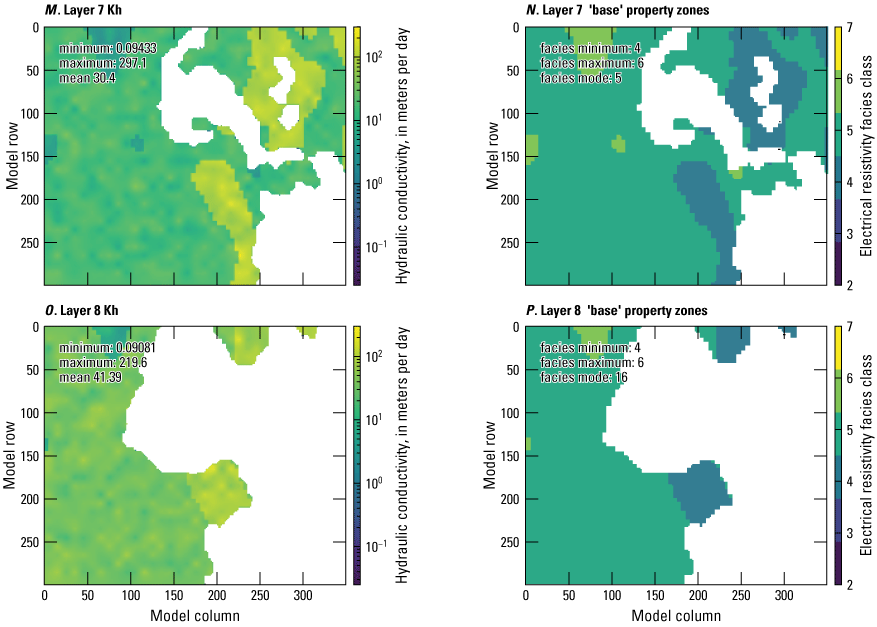
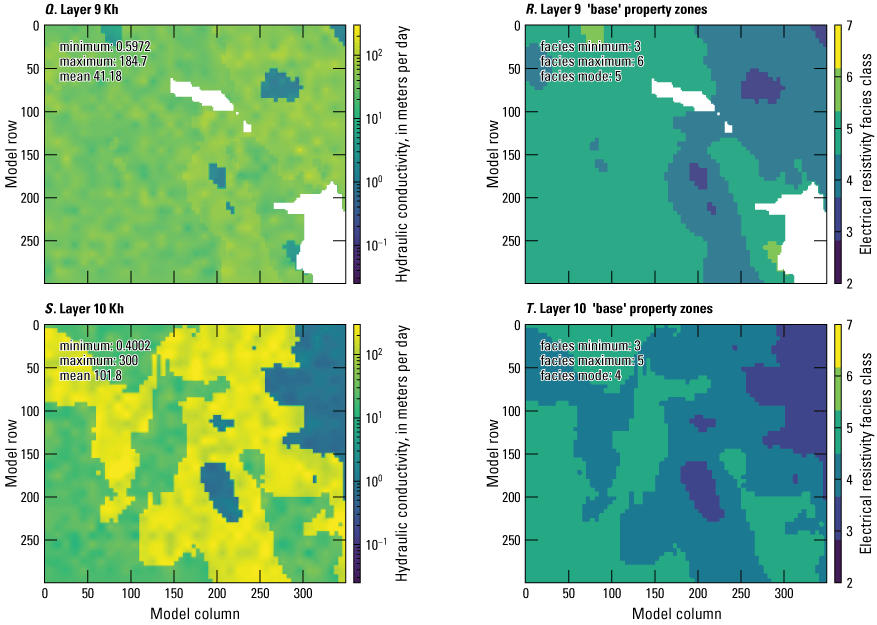
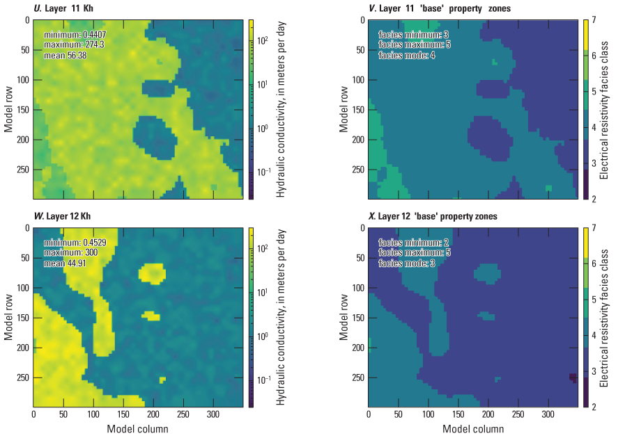
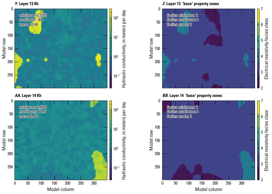
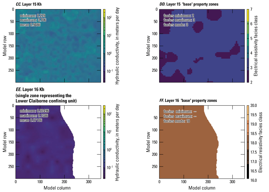
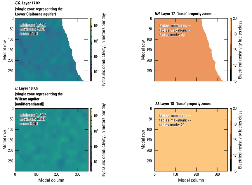
Horizontal hydraulic conductivity estimates for the Shellmound model (Guira and Weisser, 2025), compared to electrical resistivity-based zones from the airborne electromagnetic survey (James and Minsley, 2021; Minsley and others, 2021). A–JJ, Horizontal hydraulic conductivity and electrical resistivity zones for model layers 1–18.
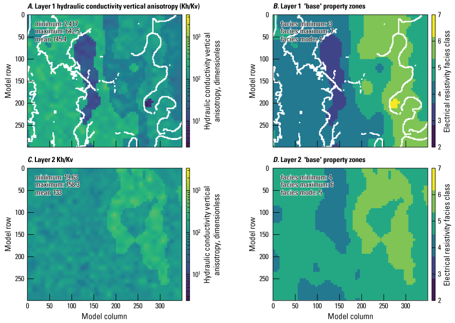
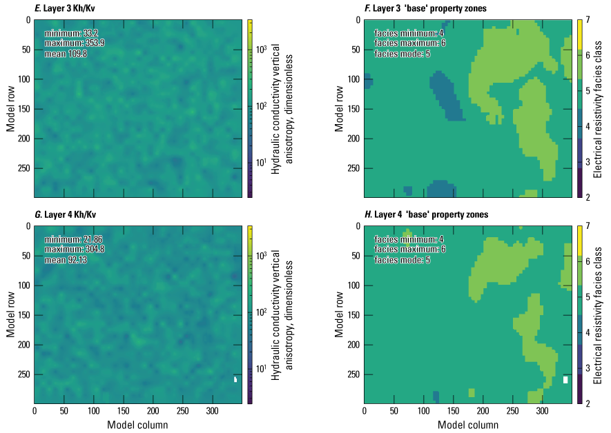
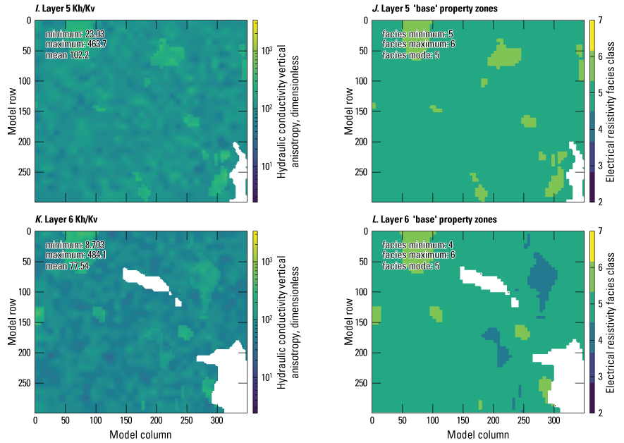
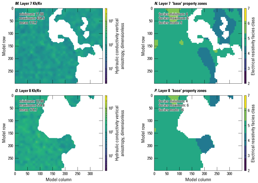
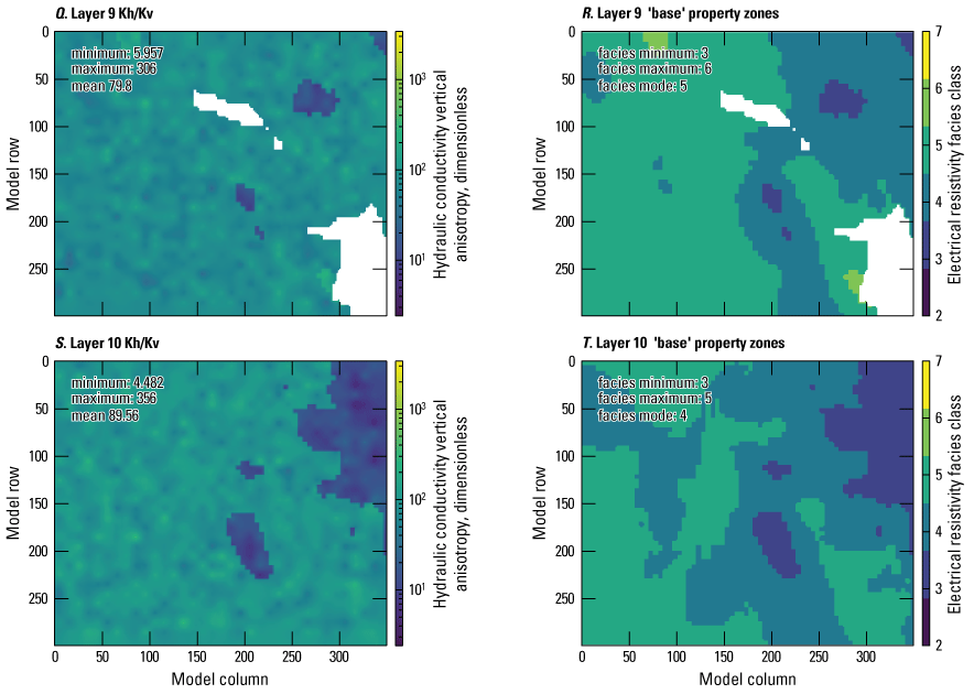
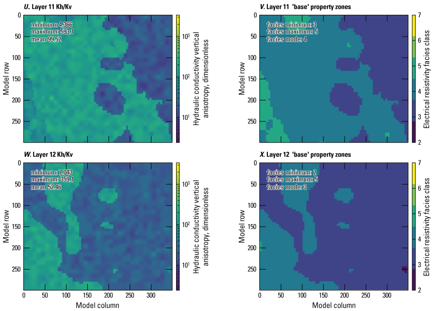
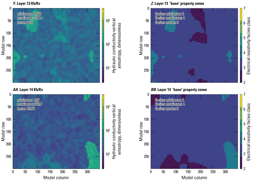
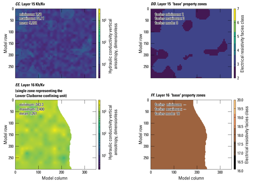
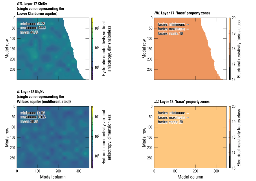
Hydraulic conductivity vertical anisotropy estimates for the Shellmound model (Guira and Weisser, 2025), compared to electrical resistivity-based zones from the airborne electromagnetic survey (James and Minsley, 2021; Minsley and others, 2021). A–JJ, Hydraulic conductivity vertical anisotropy and resistivity zones for model layers 1–18.
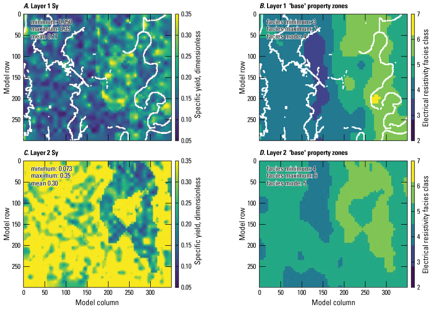
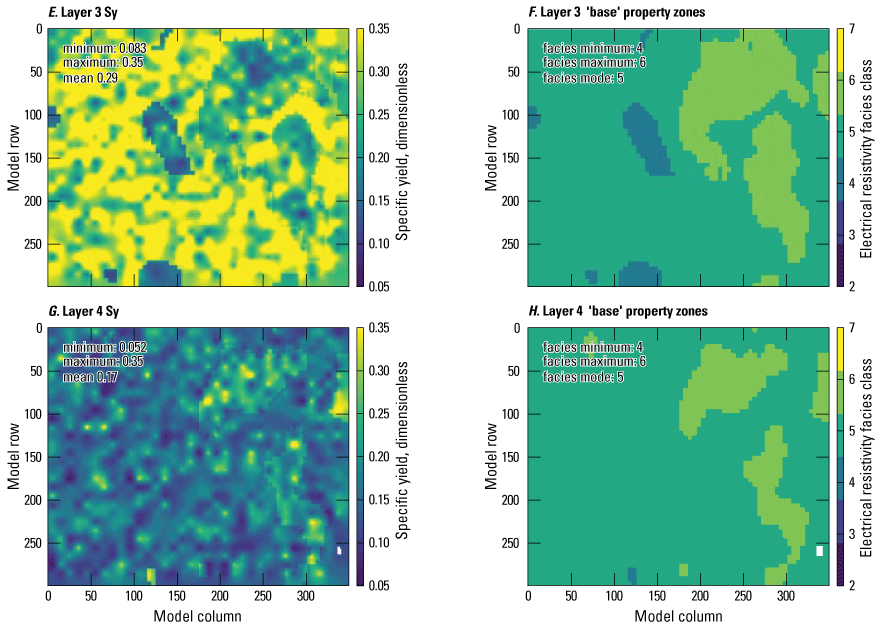
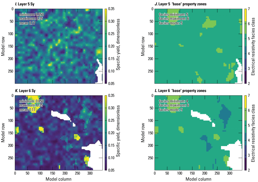
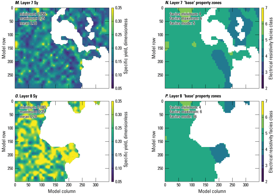
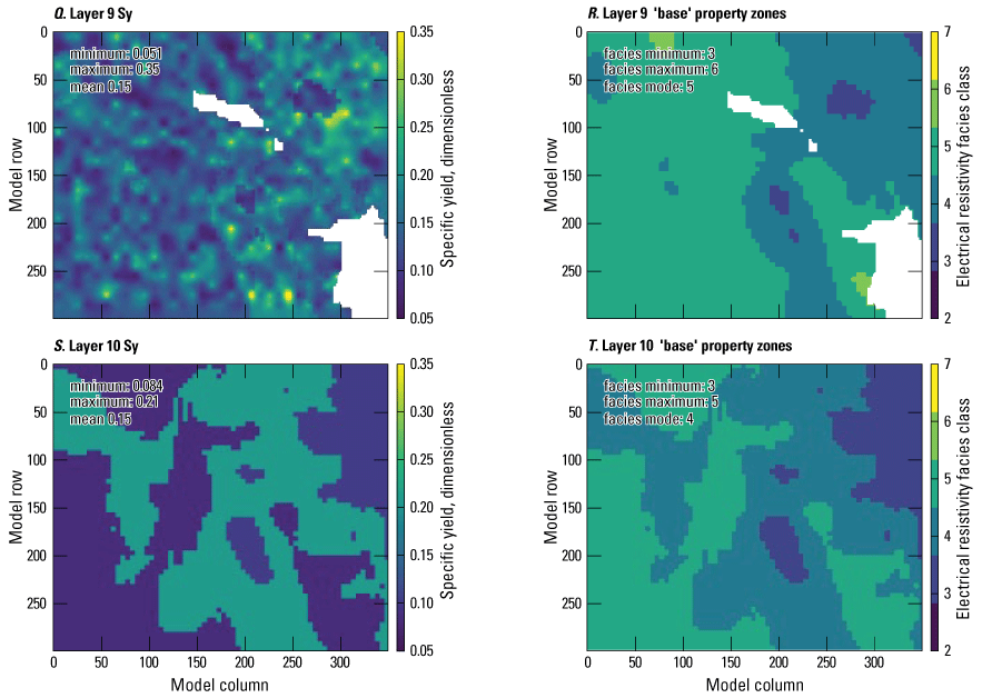
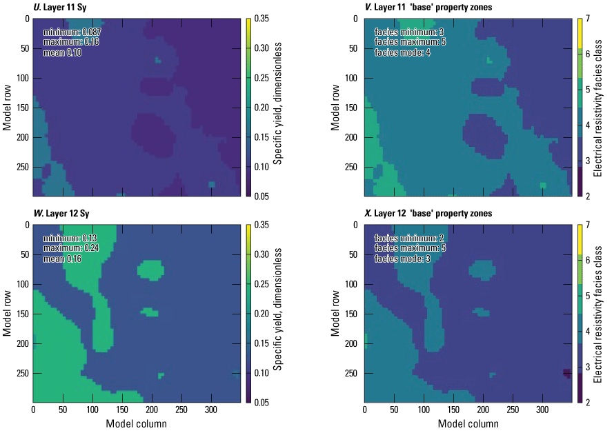
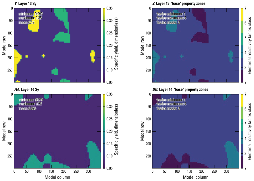
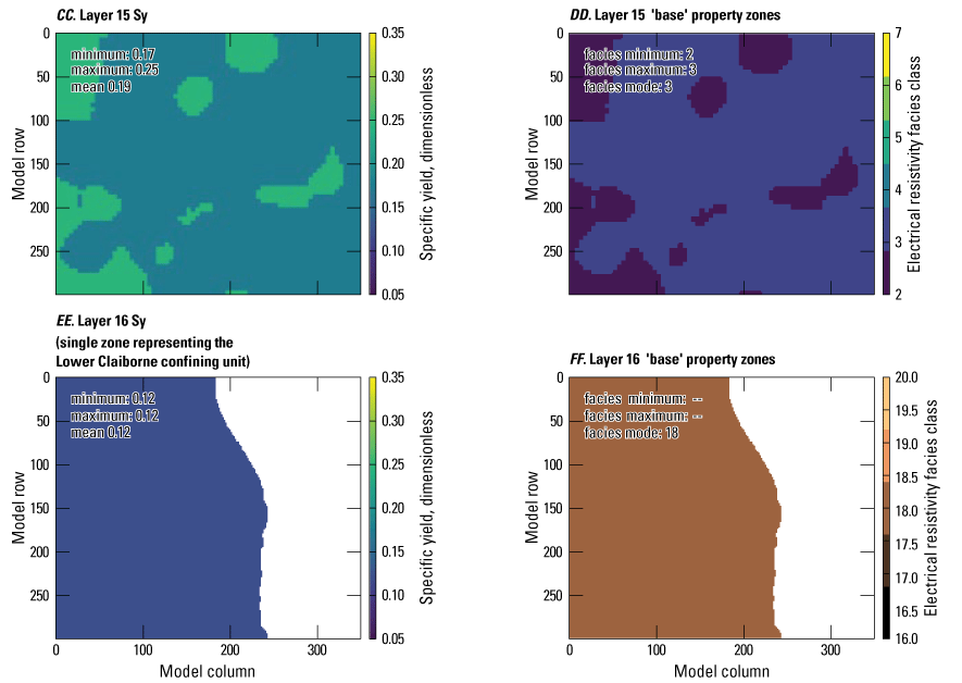
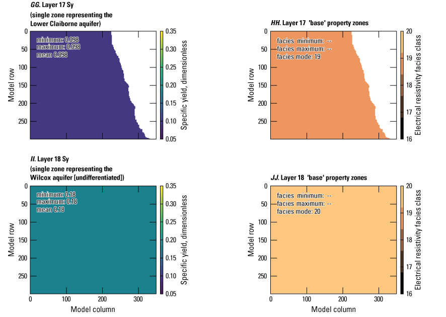
Specific yield estimates for the Shellmound model (Guira and Weisser, 2025), compared to electrical resistivity-based zones from the airborne electromagnetic survey (James and Minsley, 2021; Minsley and others, 2021). A–JJ, Specific yield and resistivity zones for model layers 1–18.

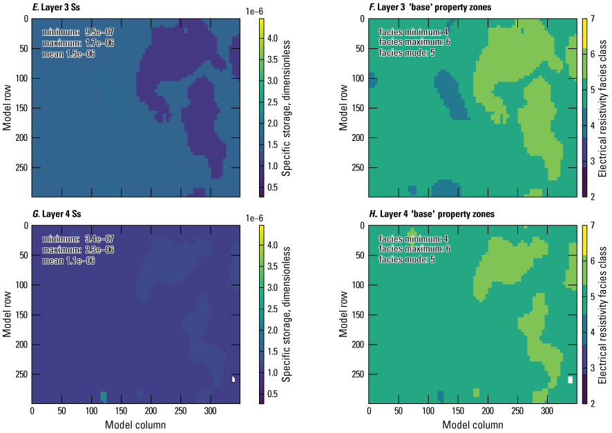
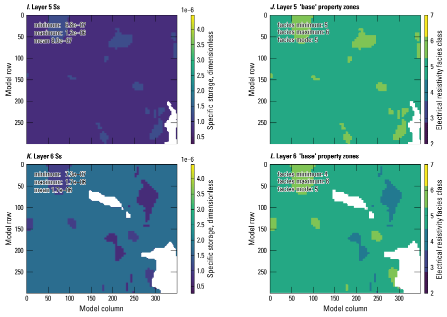
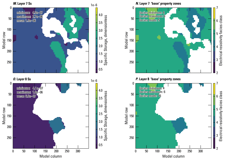
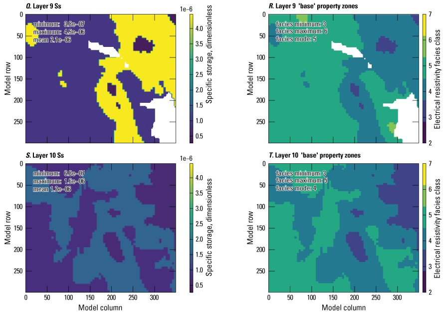
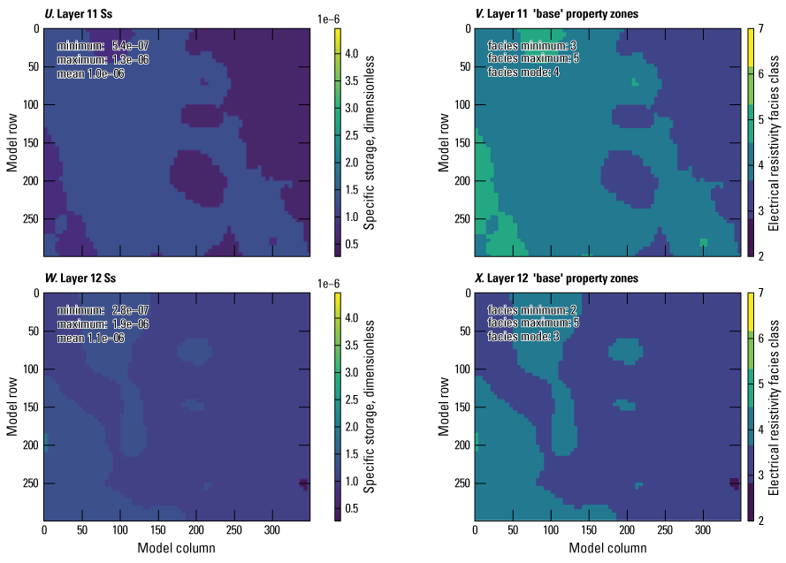
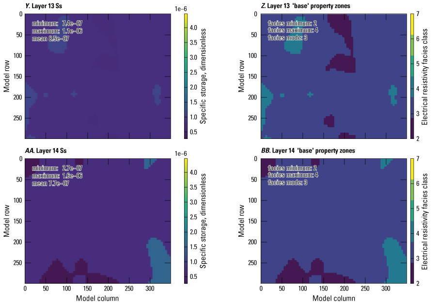
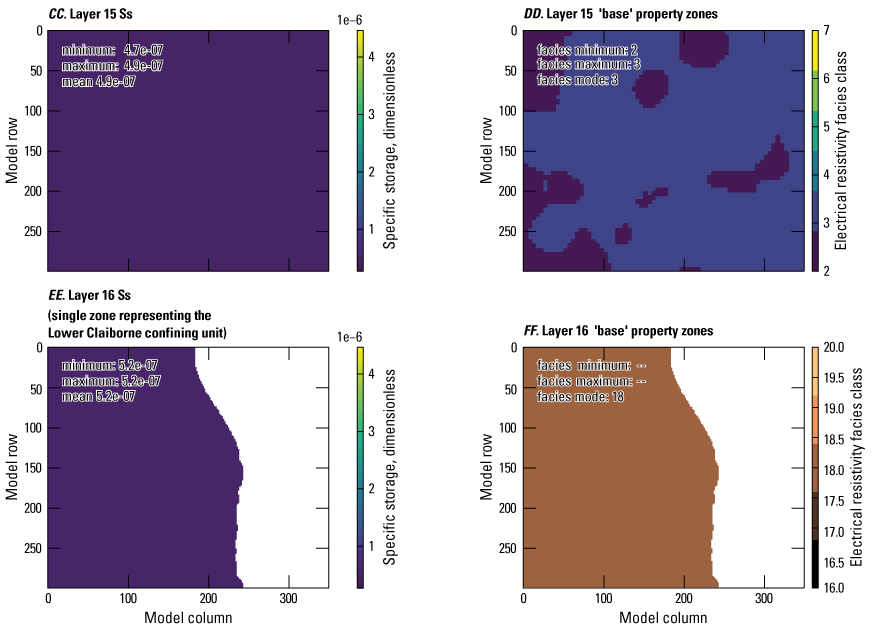
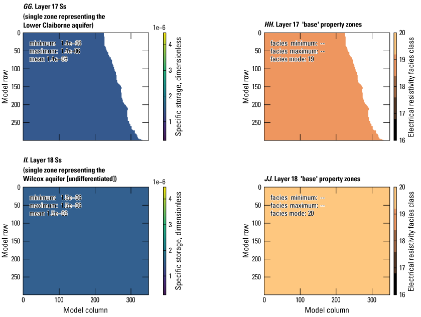
Specific storage estimates for the Shellmound model (Guira and Weisser, 2025), compared to electrical resistivity-based zones from the airborne electromagnetic survey (James and Minsley, 2021; Minsley and others, 2021). A–JJ, Specific storage and resistivity zones for model layers 1–18.
Streambed Vertical Hydraulic Conductivity
Calibrated streambed vertical hydraulic conductivity ranged from 10−5 to 1.37 m/d with an average value of 6.67x10⁻² m/d. Streambed vertical hydraulic conductivity plays an important role in the magnitude of the interactions between groundwater and surface water through base flows or stream leakage. Stream leakage immediately following dry (September 2016) and wet (February 2018) conditions, respectively, is shown in figures 29B and 29D. During dry conditions (fig. 29B), the simulation shows that segments of the Tallahatchie River gained base flows, whereas most reaches from the Quiver River and the Big Sunflower River lost water to the aquifer, and some reaches dried out. During wet conditions (fig. 29D), the simulation shows that most stream reaches including the Tallahatchie River lost water to the aquifer. During dry and wet conditions, reaches of the Yazoo River, as it meanders back to the model domain and around the City of Greenwood (fig. 1), remained dry in the simulation. This is mostly due to a structural error that resulted in no SFR inflows at that location. The model boundary truncated the Tallahatchie River (fig. 29B, D), which would otherwise route water to that dry stream reach.
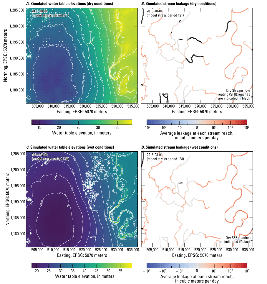
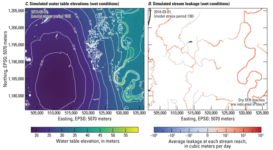
Simulated water table elevation along with estimates of streambed leakage in the Streamflow Routing package in two different conditions. A, Water table elevation with equipotential contour lines in a dry condition (September 2016). B, Streamflow segments in dry conditions with average leakage at each stream reach. C, Water table elevation with equipotential contour lines in a wet condition (February 2018). D, Streamflow segments in wet conditions with average leakage at each stream reach.
Recharge
Average SWB model and calibrated groundwater recharge maps from 2007 to 2018 are shown in figure 30. The surficial connectivity zone multipliers, along with pilot points and stress-period-based multipliers used in the calibration, contributed to a successful calibration of the model that required reduction in recharge particularly in areas with low surficial connectivity (Minsley and others, 2021). The lowest values for recharge multipliers corresponded to the zone with the lowest surficial connectivity (0.04) and pilot points (0.48). This spatial distribution and magnitude of the multipliers are consistent with the interpretation of the AEM data by Minsley and others (2021) that showed the existence of a low conductivity layer, potentially acting as a barrier, could significantly reduce effective groundwater recharge. The spatial mean annual recharge from the base member of the ensemble in for model A calibration was 1.09 in/yr (fig. 30A), whereas mean SWB model net infiltration (passed the root zone) was 10.82 in/yr (fig. 30B). The difference between SWB model net infiltration and calibrated recharge presented on figure 30C shows mean value −9.74 in/yr. The mean calibrated recharge value (1.09 in/yr) is less than one-half of the 2.84-in/yr value reported by Clark and Hart (2009).
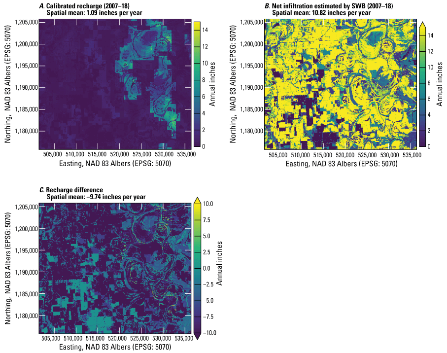
Comparative maps showing mean annual recharge. A, Shellmound calibrated recharge. B, soil-water-balance model (Nielsen and Westenbroek, 2023). C, Recharge difference between the soil-water-balance estimated and the calibrated.
Water Use Parameters
The calibration led to a 20-percent reduction of pumping rate multipliers for data imported from the MERAS 2.2 model, which covers simulation periods prior to April 2007, and a reduction of 1 percent for SWUDS. However, multipliers for pumping rates processed from AIWUM, which covers the simulation period starting from April 2007, increased by 25 percent. The average stress-period-based multipliers for the water use was 1.00 and ranged from 0.88 to 1.09. The minimum reduction happened in stress period 143 (July 2018), whereas the maximum increase was noted in stress period 1 (April 2014). Overall, the calibration resulted in a slight increase of water use. Yearly total water use from 2007 to 2018 before and after calibration is shown in figure 31.
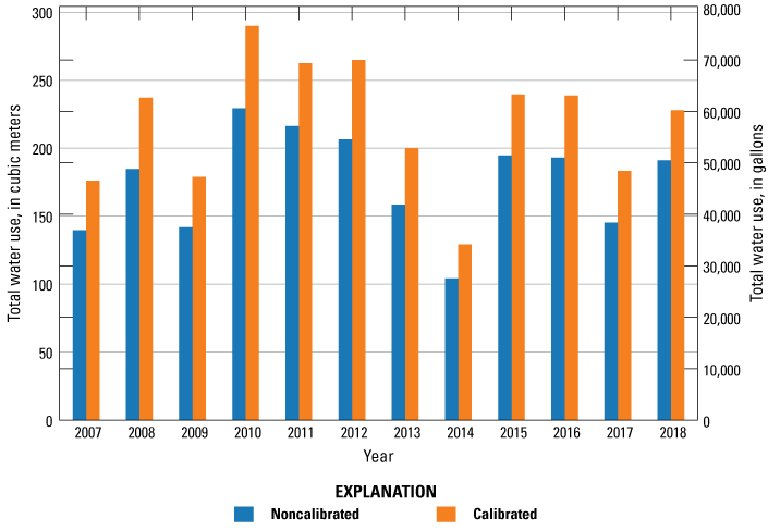
Total water use before and after calibration. Water-use data prior to calibration includes estimated rates from Aquaculture and Irrigation Water-Use Model (Bristow and Wilson, 2023) and nonagricultural rates from the U.S. Geological Survey site-specific water-use data system and national estimates for water use associated with thermoelectric power generation in 2010 and 2015 (Diehl and Harris, 2014; Harris and Diehl, 2019a,b).
Groundwater-Flow Model Budget Results
This section of the report presents water budget results for the calibrated groundwater-flow model. Budgets for the groundwater-flow system were computed for the entire model domain to produce yearly net terms for each budget component.
Simulated net budget components for the Shellmound model are shown in figure 32. Budget terms were summarized into averaged daily rates for the spin-up multiyear stress periods from 1900 to 2007 and averaged daily rates for each year from 2007 to 2018. The budget shows that groundwater pumping has been the largest outflow from the system since 1970, often approaching 100 percent of all outflows (for example, 2008, 2015–17). The second largest net outflow was the change in storage for some years (for example, 2009 and 2018). A negative change in storage represents water replenishing aquifer storage during years with high recharge and less pumping. The net storage change results in an inflow (release from storage) for most years, which represents an inflow of water to the groundwater-flow system as water leaving aquifer storage to help meet pumping demand. Prior to 1950, net outflows were dominated by groundwater discharge to the streams as base flows and lateral groundwater flows out of the model domain. Simulated net inflows include areal recharge, lateral groundwater flows, change in storage, and stream leakage.
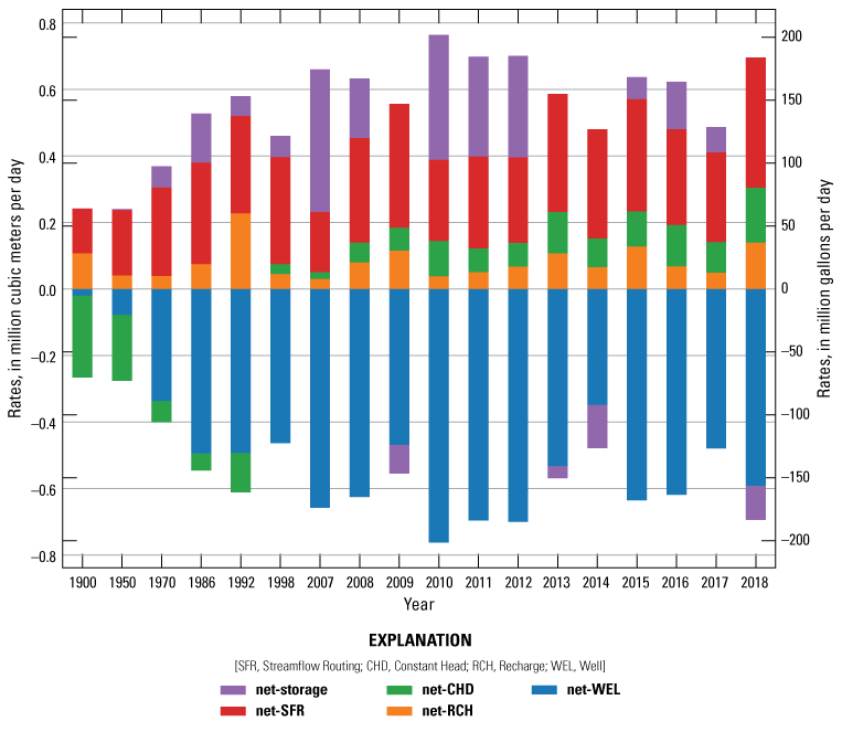
Simulated annual net budget results for the Shellmound model.
Managed Aquifer Recharge Scenario and Simulated Results
Groundwater Transfer and Injection Pilot (GTIP) Project
Following the construction and calibration of the historical version of the Shellmound model, a forecast scenario model was developed to simulate the extraction and reinjection of groundwater to and from the aquifer in accordance with the objectives of the GTIP project. The GTIP project is an interagency collaborative effort focused on finding sustainable solutions to long-term groundwater-level decline in the Delta. Partners in this collaboration include the U.S. Department of Agriculture Agricultural Research Service (in charge of leading the research and funding) and the U.S. Army Corps of Engineers Vicksburg District (in charge of operations design and construction), with support from stakeholders in the Delta including the Delta Council, Delta Farmers Advocating Resource Management, Mississippi Department of Environmental Quality, Mississippi Farm Bureau Federation, the Mississippi Soil and Water Conservation Commission, U.S. Department of Agriculture Natural Resources Conservation Service, USGS, and Yazoo Mississippi Delta Joint Water Management District. With increases in agricultural development in the region during the past century, groundwater withdrawals by high-capacity wells to support agricultural production have increased concerns about long-term sustainability of the MRVA aquifer. The GTIP project, along with other studies such as the high-resolution AEM data collection were initiated to improve understanding of the subsurface and explore potential solutions to groundwater-level declines. The GTIP project uses a managed aquifer recharge (MAR) approach to artificially replenish the groundwater. MAR is the purposeful recharge of water to aquifers to support subsequent aquifer recovery for agricultural and (or) environmental benefits (Dillon and others, 2009). There is a history of successful MAR implementation worldwide (Pyne, 2005; Dillon and others, 2019; Zheng and others, 2021) to mitigate flood, meet legal obligations, protect and (or) restore ecosystems, enhance water quality, manage water supply, and restore or protect aquifers, among others. Many methods can be used in the implementation of MAR. The ideal method used for a specific site incorporates factors such as hydrogeology, topography, hydrology, and land use around the site (Dillon and others, 2022). The MAR technique employed in this project is the bank filtration, which consists of pumping groundwater near a surface-water body to drive seepage caused by the cone of depression, combined with direct injection of the extracted groundwater, into the depleted aquifer at another location.
For the GTIP project, bank filtration is induced by extracting groundwater near the Tallahatchie River, and the extracted groundwater is transferred 3 km west before it is reinjected into the aquifer (fig. 33). Because of the high transmissivity of the MRVA aquifer at the injection site, water is injected into the aquifer by gravity flow, and the injection wells are not pressurized. The extraction well was constructed 35 m from the river, has a screen that extends from approximately 19 to 34 m below land surface, and is equipped with a high-capacity pump with variable frequency drive (500–1,500 gal/min). The injection site is organized into two injection wells approximately 150 m apart with screens extending from approximately 24 to 37 m below land surface and is equipped with submersible pumps for periodic backflushing to mitigate clogging. Each injection well can receive as much as 750 gal/min as allowed by the underground injection control permitted issued by the Mississippi Department of Environmental Quality.
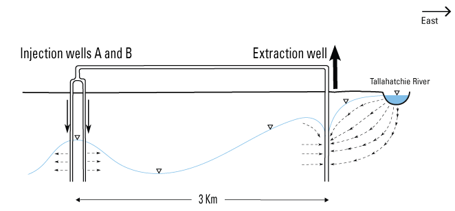
Schematic diagram of the Groundwater Transfer and Injection Project.
Forecast Model
The Shellmound forecast groundwater-flow model was constructed using the calibrated model inputs from the “base” realization of iteration 2. To ensure a smooth transition into “future” stress periods, the forecast model includes all stress periods in the historical model and 384 additional monthly stress periods from January 1, 2019, to January 1, 2051. Historical input data from 2010 to 2015 for recharge, water use, and lateral groundwater movement were processed into monthly averages for the forecast period. In addition to stresses simulated in the historical model, the forecast model construction included a new WEL package (Langevin and others, 2017) to simulate the GTIP project. The new WEL package only includes wells at the extraction and injection locations. Relevant information used for setting up the extraction and injection wells in the new WEL package is shown in table 9. Well screen information was used to apply pumping to the appropriate model layers and rates to be applied based on the proportion of the screen that intersects each layer. As a result, one-third of the pumping rate is applied to layers 5 and 6 individually, whereas one-sixth of the pumping rate was applied to layers 4 and 7 individually. Following the same process at the injection sites, one-half of the injection rate at injection well A was applied to layer 6, whereas one-quarter of the rate was applied to layers 5 and 7 individually. The same ratios of injection were applied at injection well B using the injection rates provided for well B. Effective extraction and injection rates accounted for times when pumping rate was reduced or stopped for maintenance purposes such as backflushing.
Table 9.
Information for extraction and injection wells involved in the Groundwater Transfer and Injection Pilot project (U.S. Geological Survey, 2020).[ft, feet; NAVD 88, North American Vertical Datum 88; BLS, below land surface; MRVAA, Mississippi River Valley Alluvial Aquifer ; INJ, injection site; EXT, extraction site; OW, observation well; --, not applicable]
During test periods 1 and 2 of the pilot project completed in 2021 and 2022, respectively, field operation data on extraction and injection rates and water levels at select observation wells were collected (O’Reilly and others, 2023). Effective monthly extraction and injection rates (fig. 34) were computed from the hourly data collection and applied to the Shellmound forecast model.
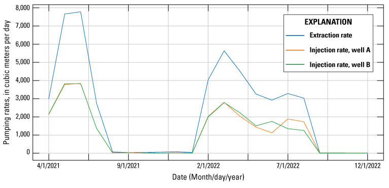
Effective monthly average pumping rates at the extraction and injections sites used in the Groundwater Transfer and Injection Pilot project.
Time series of simulated water levels at select observation sites around the injection wells, along with the available equivalent field observations collected during the two test periods of the GTIP project operations, are shown in figure 35. Water levels from a test simulation that did not account for the GTIP operations are also included. Declining groundwater levels prior to the end of the calibration period and the start of the GTIP project operations are consistent with general observations in wells around the area. The forecast results indicate a rise in simulated water levels at all observation sites starting in April 2021 when the water transfer operations began. Observed water levels also indicate rising water levels although the forecast shows an underestimation bias. Input data for the forecast (from January 2019) were average values computed from historical (2010–15) data and do not represent field conditions from a specific time.
Simulated water table elevation maps for selected stress periods are shown in figures 36 and 37. The full extent of the inset model domain is shown in figure 36, whereas figure 37 shows areas zoomed in around the GTIP project operation sites. Simulated water table elevation on January 1, 1900, prior to extensive groundwater development and water-level declines, is shown in figures 36A and 37A. Simulated water table elevation on December 31, 2018 (end of the calibration model), indicates significant declines in water levels, particularly on the western half of the model domain, leading to a cone of depression (figs. 36B and 37B). Simulated water table elevations on June 30, 2021, and February 28, 2022, when the GTIP project was in full operation and applying the maximum pumping rates during test periods 1 and 2, respectively, are shown in figures 36C–D and 37C–D. The rise in water table elevation around the injection sites resulted in groundwater mounding west of the contour line, delineating 30 m of altitude. Simulated water table elevation on August 31, 2022, when GTIP project operations for test period 2 ended, is shown in figures 36E and 37E. Simulated water table elevation shows that the groundwater mound had gently spread, indicating that the rise in water levels resulting from water transfer and injection in the area cannot be sustained for extended periods of time if operation is not continuous.
Finally, simulated water table elevation on May 31, 2050, indicating an increase in water table elevation of as much as 3m around the injection site, is shown in figures 36F and 37F. Contour lines indicate that water levels at the injection sites are still below water levels near the extraction site. Long-term injection of groundwater by the wells of the GTIP project could result in the reversal of the hydraulic head gradient between the extraction and injection sites, effectively leading to a “recirculation” situation whereby water pumped from the extraction site and injected into the aquifer at the injection sites would eventually flow back to the extraction well. Results of the forecast simulation indicate that for the 2022 GTIP project operation rates and average (2010–15) pumping and recharging conditions, yearly repetition until 2051 would not result in substantial water re-circulation and has the potential to increase groundwater levels around the injection site.
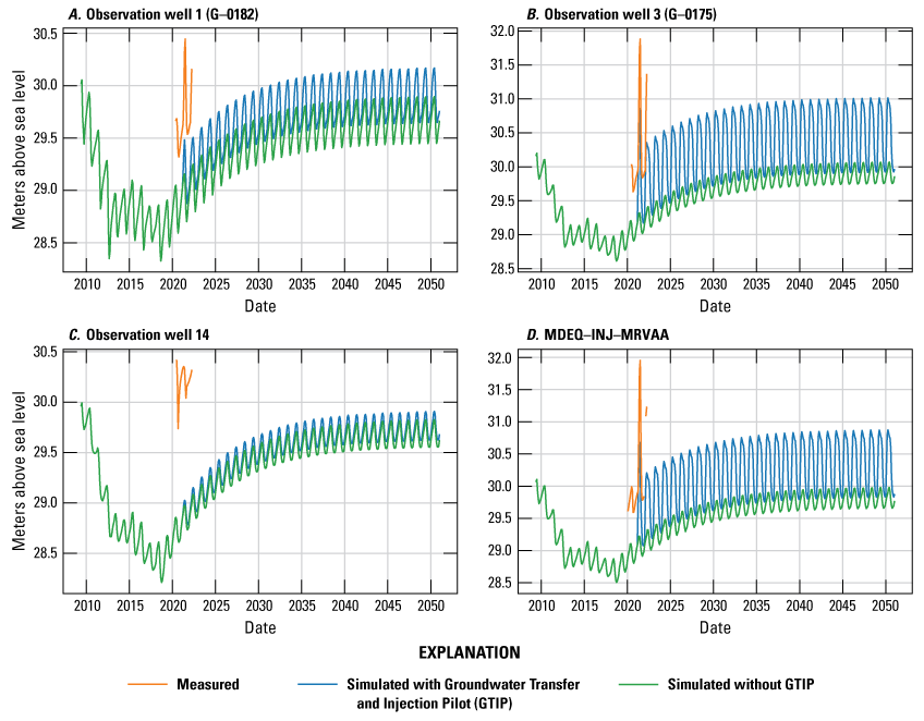
Time series plot of simulated water levels around the injection sites (U.S. Geological Survey, 2020; Guira and Weisser, 2025).
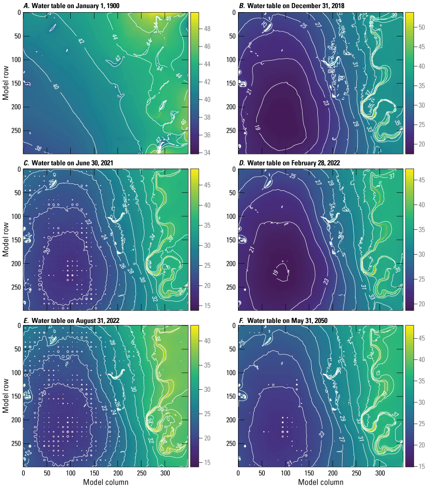
Simulated water table elevation of the study area at select stress periods (Guira and Weisser, 2025).
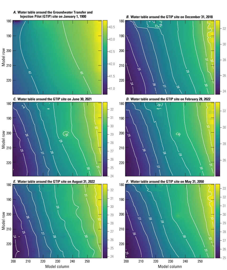
Simulated water table elevation of the Groundwater Transfer and Injection Pilot project area at select stress periods (Guira and Weisser, 2025).
Assumptions and Limitations
As in any modeling effort, the Shellmound model construction is an attempt to represent complex natural processes of the real world to address specific hydrologic questions, which requires some approximations and simplifications. This section of the report discusses some of the assumptions made in the model development and calibration and the limitations of the model capabilities. The 100×100-meter cell resolution used in spatial discretization is considered a high resolution but still required summarizing input data that were spatially distributed within a 10,000-square-meter model cell into a single value. The use of the CHD package to simulate lateral groundwater flow could be an unrealistic infinite source (or sink) of water, but in this simulation, the flow was constrained by realistic estimates of lateral groundwater flow from the conceptual model. To explore a more constrained representation of lateral groundwater flow, a prototype version of the Shellmound model used a specified flux boundary condition simulated using a MODFLOW 6 WEL package (Langevin and others, 2017) in lieu of the CHD package. Lateral groundwater-flow rates were extracted from the parent model using the USGS ZoneBudget software (Harbaugh, 1990) for boundary cells and converted into well pumping rates. The same approach was successfully used in Traylor and others (2024), but that did not yield a more stable Shellmound model; therefore, this approach was not used.
Input data such as hydraulic heads used as boundary conditions derived from the parent model come with the uncertainty associated with the parent model. Hydraulic head values used in the CHD package were constant during calibration, which most likely resulted in some changes in other parameters in places where calibration would potentially perform better if hydraulic heads were allowed to slightly fluctuate. The model did not accurately simulate streamflow routing in the Yazoo River as it re-enters the model domain near Greenwood, Miss. This inaccuracy only affected a small section of the study area but resulted in a dried-out stream reach for a substantial portion of the entire simulation time where it normally remains wet. The inaccuracy also led to lower simulated groundwater levels in the area immediately surrounding that stream reach. The model did not account for the perched aquifer in the southwest corner of the model domain, which was documented in previous studies (O’Reilly and others, 2020; Leaf and others, 202340). Simulation of perched aquifers requires a specific package in MODFLOW 6 that was not used in this study because the perched system was not an important component to the aquifers of interest such as the MRVA and Claiborne aquifers. Because of the thickness of the unsaturated zone in the area, the model could potentially be improved with the use of the Unsaturated Zone Flow package (Langevin and others, 2017) that could better simulate the lag between net infiltration as simulated by the SWB model and groundwater recharge.
Limitations of the forecast model include the limited capability to accurately predict water levels because of the lack of accurate input data. Most stresses in the forecast section were simulated by using averaged historical inputs from 2010 to 2015; therefore, the forecast model can be useful for making approximations based on how future conditions compare to the average conditions during this period. It is also useful for approximating how long the groundwater mound around the injection sites can be sustained based on average conditions, but results were not a definitive indication of future conditions.
Summary
The U.S. Geological Survey (USGS) Water Availability and Use Science Program, through the Mississippi Alluvial Plain (MAP) project, has been updating groundwater-flow models of the Mississippi Embayment and Mississippi River Valley alluvial (MRVA) aquifers to provide stakeholders with tools that can be used to support water-resource management decisions. Groundwater withdrawals from the MRVA aquifer have been vital to support a multibillion-dollar agricultural industry, but groundwater-level declines have heightened concerns about long-term sustainability. In a region near Shellmound, Mississippi, large groundwater-level declines have prompted stakeholders to undertake several actions to better understand the subsurface hydrogeology and mitigate water-level declines. The Groundwater Transfer and Injection Pilot project (GTIP) was implemented whereby groundwater was extracted from the MRVA aquifer near the Tallahatchie River and reinjected into the aquifer approximately 3 kilometers (km) (1.8 miles) west of the extraction point. Additionally, a high-resolution airborne electromagnetic (AEM) survey was completed to collect geophysical data, help improve current understanding of the subsurface, and support the GTIP project and groundwater modeling projects. The MAP project supported the construction of the Shellmound model, a transient groundwater-flow model using the modular finite-difference flow model (MODFLOW 6), which integrates the AEM data to serve as a tool to better understand processes associated with the groundwater system and the potential effects of GTIP project operations on groundwater levels.
The Shellmound model domain is within the Mississippi Delta (hereafter referred to as the “Delta”), including parts of Leflore, Sunflower, and Tallahatchie Counties, and extends 35 km east to west and 30 km north to south. The climate in the area is typical of the Delta, which is humid and subtropical; the average annual precipitation from 2010 to 2020 was approximately 131 centimeters per year. The average annual temperature ranged from 11.6 to 25 degrees Celsius. Land use in the area is dominated by farmland with major agricultural crops being soybeans, corn, rice, and cotton, but also includes catfish ponds, wetlands, developed/urban, pasture, and forest.
Surface-water features in the Shellmound model study area include streams, ponds, and oxbow lakes, many of which are not connected to the groundwater system. Streams in the area include the Tallahatchie, Quiver, and Big Sunflower Rivers. The average daily mean streamflow for the Tallahatchie River at the Money, Miss., streamgage (USGS station 07281600), from 1996 to 2018 was approximately 18.8 million cubic meters per day (m3/d). The major hydrogeologic units in the Shellmound model study area are Quaternary and Tertiary units. The MRVA aquifer, which is present at land surface throughout the study area, mainly consists of sand and gravel with an average thickness of 38.3 meters (m), ranging from 23.5 to 49.2 m. The uppermost layer of the MRVA aquifer generally is finer grained, with increased prevalence of silt and clay that limits areal recharge. Underlying the MRVA aquifer are the older Tertiary hydrogeologic units, which mainly consist of undifferentiated sediments, and include the upper and lower Claiborne aquifers, the middle Claiborne confining unit, and the middle and lower Wilcox aquifers. The Tertiary deposits have a combined average thickness of 607 m, ranging from 436 to 780.3 m.
The highly productive alluvial aquifer is the most important source of fresh water supply in the study area. Wells screened in the alluvial aquifer can pump between 1,635 and 16,350 m3/d. The underlying Tertiary units were reported to have a much lower well yield of 545 to 2,725 m3/d. In 2000, groundwater withdrawal from the alluvial aquifer alone accounted for 10 percent of all groundwater use within the continental United States. Other nonagricultural groundwater uses include municipal and industrial purposes. Most crop and fish production within the limits of the Shellmound model study area is primarily supported by the MRVA aquifer, whereas the municipal and industrial groundwater use is supported by the underlying Tertiary units.
The Shellmound model is a high-resolution (100-m cell size) inset model that uses the regional-scale Delta model (500-m cell size) as its parent model. The development process included the exploration of the effect of layering configurations of varying complexity that resulted in three different vertical discretizations corresponding to the three versions (models A, B, and C). Model A retains the vertical discretization used in the Delta model and consists of uniform 5-m-thick layers from land surface to the base of the MRVA aquifer as defined through the interpretation of the AEM data. Below the base of the MRVA aquifer, the vertical discretization is represented by uniform and increasing thickness to the depth of the available AEM data, and then by nonuniform layer surfaces following hydrostratigraphic surfaces. Because the Delta model layers 16, 17, and 18 were inactive over the Shellmound model domain, they were not represented in the inset models which resulted in 18 model layers for model A. Model B has a vertical discretization that defines 10-m constant thickness and horizontal layers from the highest elevation of the land surface to the deepest extent of the AEM data, but its vertical discretization is identical to model A below the depth of the AEM data and resulted in 16 model layers for model B. The vertical discretization in model C is defined by a single layer that extends from land surface to the deepest extent of the AEM data. The vertical discretization of model C below the deepest extent of the AEM data is identical to those in models A and B, which resulted in eight model layers for model C.
The temporal discretization of the Shellmound model defines 148 stress periods simulated from 1900 to 2018 with varying stress period lengths. The period prior to April 2007 was subdivided into six stress periods with lengths of 1 year or more and represented varying stages of groundwater development within the MAP area as reported in previous studies. The first stress period simulates a steady state condition, whereas stress periods 2 to 148 simulate transient conditions. The model simulates monthly stress periods from April 1, 2007, to January 1, 2019.
Areal groundwater recharge was simulated in the Shellmound model using the MODFLOW 6 recharge package. Input recharge grids for the Shellmound model were based on simulated net infiltration by the Shellmound soil-water-balance (SWB) model, which runs on a daily time step. The Shellmound SWB model computes grid-based water budget of surface hydrology (from the vegetative canopy to the bottom of the root zone) with 100×100-m cells that was specifically constructed to provide inputs to the Shellmound model. Daily net infiltration rates were averaged to match the Shellmound model monthly temporal discretization from April 2007 through December 2018. An average rate between 1999 and 2018 was used for the stress periods preceding 2007.
All streams in the Shellmound model were simulated using the MODFLOW 6 Streamflow Routing (SFR) package. The SFR package simulated the stream water budget for each stream reach including gains and losses. Other budget components simulated by the SFR package include surface runoff, stream stage, and routing between connected reaches. The runoff inputs to the SFR package were provided by the SWB model. The SFR package was built using NHDPlus version 2 data, and the open-source python packages SFRmaker, and Modflow-setup.
Groundwater use in the Shellmound model was simulated using the MODFLOW 6 well (WEL) package. Pumping well locations and rates for stress periods prior to April 2007 were derived from the Mississippi Embayment Regional Aquifer Study 2.2 groundwater-flow model. There is no distinction between agricultural and nonagricultural water use in the Shellmound model prior to 2007. From April 2007 to December 2018, water-use data included pumping rates and locations for agricultural production and nonagricultural water use. Agricultural water use data were provided by the AIWUM version 1.1. Nonagricultural water-use data for the same period were provided by the USGS site-specific water-use data system and national estimates for water use associated with thermoelectric power generation.
Lateral groundwater flow into and out of the Shellmound model was simulated using the Constant Head (CHD) package. Constant head boundary cells for the Shellmound model were specified at the perimeter boundary. Simulated groundwater-level values from the parent model were used to specify hydraulic heads for every stress period in the CHD package. Lateral groundwater flow between the model and the surrounding aquifer for each stress period was computed based on the gradient between the CHD package cells and the neighboring cells.
The parameter estimation of the Shellmound model consisted of the identification of the calibration targets, the selection of model parameters to adjust, some manual adjustments of parameters, and automated calibration. The calibration process of the Shellmound model employed the high-performance computing software Parameter Estimation ++ (PEST++) using the USGS Denali supercomputing resources.
Calibration results show that mean phi (Φ, objective function) value, which is a measure of the degree of mismatch between observed and simulated conditions, for model A improved from 2,884.17 to 240.68, whereas Φ values for models B and C changed from 2,473.32 to 231.03 and from 2,015.30 to 234.40, respectively. The minimum error variance set of “base” realization resulted in Φ values of 253.43, 258.72, and 265.25 for models A, B, and C, respectively, after the second iteration. Simulated budgets for model A indicate that groundwater pumping is the largest outflow from the system since 1970 often approaching 100 percent of all outflows. The second largest net outflow is change in storage representing water replenishing aquifer storage during years with high recharge and less pumping, although the net storage change results in an inflow for most years. Prior to 1950, net outflows were dominated by groundwater discharge to the streams as base flows and lateral groundwater flows out of the model domain.
Calibration results also show a good fit between simulated and calibration targets. For observation groups “Shellmound heads,” “Priority embayment heads,” “Embayment heads,” and “Heads” with mean absolute errors of 0.57, 0.57, 0.90, and 1.01 m, respectively, whereas root-mean-squared error for the same groups were 0.68, 0.72, 1.25, and 1.32 m.
Many assumptions were made in the development of the forecast model. Stresses such as groundwater pumping and recharge rates applied to the future stress period were obtained by computing monthly averages from the calibration period. Although this allows to see the potential effects of the GTIP operations, the forecast simulation outputs do not represent predictions under any climate forecasting scenario.
The Shellmound forecast groundwater-flow model was constructed using model A calibrated parameters and, in addition to the historical period, covers another 384 additional monthly stress periods from January 1, 2019, to January 1, 2051. A new WEL package was used to simulate the groundwater transfer and only included wells at the extraction and injection locations. Extraction rates were distributed so that one-third of the pumping rate was applied to layers 5 and 6 individually, whereas one-sixth of the pumping rate was applied to layers 4 and 7 individually. Following the same process at the injection sites, one-half of the injection rate at injection well A was applied to layer 6, whereas one-quarter was applied to layers 5 and 7 individually. The same ratios of injection were applied at injection well B using the injection rates provided for well B. Results indicate a notable groundwater-level rise of as much as 3 m around the injection sites and indicate that under average (2010–15) irrigation and recharge conditions, the GTIP project has the potential to increase groundwater levels around the injection site, but sustained mounding requires yearly repetition of GTIP project operations.
References Cited
Arthur, J.K., 2001, Hydrogeology, model description, and flow analysis of the Mississippi River alluvial aquifer in northwestern Mississippi: U.S. Geological Survey Water-Resources Investigations Report 2001–4035, 47 p. [Also available at https://doi.org/10.3133/wri014035.]
Asquith, W.H., and Seanor, R.C., 2019, infoGW2visGWDB—An R groundwater data-processing utility for manipulating, checking the veracity, and converting an “infoGW” object to the “GWmaster” object for the visGWDB software with demonstration for the Mississippi River Valley alluvial aquifer: U.S. Geological Survey software release, Reston, Va., accessed May 26, 2021, at https://doi.org/10.5066/P9MK0B6L.
Asquith, W.H., Seanor, R.C., McGuire, V.L., and Kress, W.H., 2020, Methods to quality assure, plot, summarize, interpolate, and extend groundwater-level information—Examples for the Mississippi River Valley alluvial aquifer: Environmental Modelling and Software, v. 134, 104758, 19 p., accessed October 2, 2023, at https://doi.org/10.1016/j.envsoft.2020.104758.
Barlow, J.R.B., and Clark, B.R., 2011, Simulation of water-use conservation scenarios for the Mississippi Delta using an existing regional groundwater flow model: U.S. Geological Survey Scientific Investigations Report 2011–5019, 14 p., October 2, 2023, at https://doi.org/10.3133/sir20115019.
Barlow, P.M., De-Simone, L.A., and Moench, A.F., 2000, Aquifer response to stream-stage and recharge variations. II. Convolution method and applications: Journal of Hydrology, v. 230, no. 3–4, p. 211–229, accessed October 2, 2023, at https://doi.org/10.1016/S0022-1694(00)00176-1.
Boyraz, U., and Kazezyılmaz-Alhan, C.M., 2021, An analytical solution for groundwater flow incorporating the effect of water bodies with sloping surfaces: Hydrological Sciences Journal, v. 66, no. 7, p. 1211–1221. [Also available at https://doi.org/10.1080/02626667.2021.1925675.]
Bristow, E.L., and Wilson, J.L., 2023, Aquaculture and irrigation water-use model (AIWUM) version 1.1 estimates and related datasets for the Mississippi Alluvial Plain: U.S. Geological Survey data release, accessed October 2, 2024, at https://doi.org/10.5066/P9RGZOBZ.
Bryant, C.J., Locke, M.A., Krutz, L.J., Reynolds, D.B., Golden, B.R., Irby, T., Steinriede, R.W., Jr., and Spencer, G.D., 2021, Furrow‐irrigation application efficiency in mid‐southern U.S. conservation tillage systems: Agronomy Journal, v. 113, no. 1, p. 397–406, accessed October 2, 2023, at https://doi.org/10.1002/agj2.20468.
Clark, B.R., Barlow, P.M., Peterson, S.M., Hughes, J.D., Reeves, H.W., and Viger, R.J., 2018, National-scale grid to support regional groundwater availability studies and a national hydrogeologic database: U.S. Geological Survey data release, accessed October 2, 2023, at https://doi.org/10.5066/F7P84B24.
Clark, B.R., and Hart, R.M., 2009, The Mississippi Embayment Regional Aquifer Study (MERAS)—Documentation of a groundwater-flow model constructed to assess water availability in the Mississippi embayment: U.S. Geological Survey Scientific Investigations Report 2009–5172, 61 p., accessed October 2, 2023, https://doi.org/10.3133/sir20095172.
Diehl, T.H., and Harris, M.A., 2014, Withdrawal and consumption of water by thermoelectric power plants in the United States, 2010: U.S. Geological Survey Scientific Investigations Report 2014–5184, 28 p. [Also available at https://doi.org/10.3133/sir20145184.]
Dillon, P., Pavelic, P., Page, D., Beringen, H., and Ward, J., 2009, Managed aquifer recharge—An introduction: Canberra, Australia, National Water Commission, Waterlines Report Series number 13, accessed October 2, 2023, at https://recharge.iah.org/files/2016/11/MAR_Intro-Waterlines-2009.pdf.
Dillon, P., Stuyfzand, P., Grischek, T., Lluria, M., Pyne, R.D.G., Jain, R.C., Bear, J., Schwarz, J., Wang, W., Fernandez, E., Stefan, C., Pettenati, M., van der Gun, J., Sprenger, C., Massmann, G., Scanlon, B.R., Xanke, J., Jokela, P., Zheng, Y., Rossetto, R., Shamrukh, M., Pavelic, P., Murray, E., Ross, A., Bonilla Valverde, J.P., Palma Nava, A., Ansems, N., Posavec, K., Ha, K., Martin, R., and Sapiano, M., 2019, Sixty years of global progress in managed aquifer recharge: Hydrogeology Journal, v. 27, no. 1, p. 1–30. [Also available at https://doi.org/10.1007/s10040-018-1841-z.]
Dietsch, B., Asquith, W.H., Breaker, B.K., Westenbroek, S.M., and Kress, W.H., 2022, Simulation of monthly mean and monthly base flow of streamflow using random forests for the Mississippi River Alluvial Plain, 1901 to 2018: U.S. Geological Survey Scientific Investigations Report 2022–5079, 17 p., accessed October 12, 2024, at https://doi.org/10.3133/ sir20225079.
Doherty, J., 2003, Ground water model calibration using pilot points and regularization: Ground Water, v. 41, no. 2, p. 170–177. [Also available at https://doi.org/10.1111/j.1745-6584.2003.tb02580.x.]
Falgout, J.T., Gordon, J., Williams, B., and Davis, M.J., 2022, Advanced research computing—USGS Denali supercomputer: U.S. Geological Survey, accessed October 2, 2023, at https://doi.org/10.5066/P9PSW367.
Feinstein, D.T., Dunning, C.P., Juckem, P.F., and Hunt, R.J., 2010, Application of the Local Grid Refinement package to an inset model simulating the interactions of lakes, wells, and shallow groundwater, northwestern Waukesha County, Wisconsin: U.S. Geological Survey Scientific Investigations Report 2010–5214, 30 p. [Also available at https://doi.org/10.3133/sir20105214.]
Fienen, M.N., Haserodt, M.J., Leaf, A.T., and Westenbroek, S.M., 2022, Simulation of regional groundwater flow and groundwater/lake interactions in the Central Sands, Wisconsin: U.S. Geological Survey Scientific Investigations Report 2022–5046, 110 p., accessed October 2, 2023, at https://doi.org/10.3133/sir20225046.
Guira, M., and Weisser, A.R., 2025, Inset models used to evaluate the effects of layering configuration on model calibration from 1900 to 2018, and assess managed aquifer recharge near Shellmound, Mississippi, from 2019 to 2050: U.S. Geological Survey data release, https://doi.org/10.5066/P13DWA86.
Harbaugh, A.W., 1990, A computer program for calculating subregional water budgets using results from the U.S. Geological Survey modular three-dimensional ground-water flow model: U.S. Geological Survey Open-File Report 90–392, 46 p. [Also available at https://doi.org/10.3133/ofr90392.]
Harris, M.A., and Diehl, T.H., 2019a, Withdrawal and consumption of water by thermoelectric power plants in the United States, 2015: U.S. Geological Survey Scientific Investigations Report 2019–5103, 15 p. [Also available at https://doi.org/10.3133/sir20195103.]
Harris, M.A., and Diehl, T.H., 2019b, Water withdrawal and consumption estimates for thermoelectric power plants in the United States, 2015: U.S. Geological Survey data release, accessed October 2, 2023, at https://doi.org/10.5066/P9V0T04B.
Hart, R.M., Clark, B.R., and Bolyard, S.E., 2008, Digital surfaces and thicknesses of selected hydrogeologic units within the Mississippi Embayment Regional Aquifer Study (MERAS): U.S. Geological Survey Scientific Investigations Report 2008–5098, 33 p., accessed October 2, 2023, at https://doi.org/10.3133/sir20085098.
Haugh, C.J., 2012, Effects of groundwater withdrawals associated with combined-cycle combustion turbine plants in west Tennessee and northern Mississippi: U.S. Geological Survey Scientific Investigations Report 2012–5072, 22 p., accessed October 2, 2023, at https://doi.org/10.3133/sir20125072.
Haugh, C.J., 2016, Evaluation of effects of groundwater withdrawals at the proposed Allen combined-cycle combustion turbine plant, Shelby County, Tennessee: U.S. Geological Survey Scientific Investigations Report 2016–5072, 8 p., accessed October 2, 2023, at https://doi.org/10.3133/sir20165072.
Haugh, C.J., Killian, C.D., and Barlow, J.R.B., 2020a, MODFLOW–2005 model used to evaluate water-management scenarios for the Mississippi Delta: U.S. Geological Survey data release, accessed October 12, 2024, at https://doi.org/10.5066/P9906VM5.
Hunt, R.J., Walker, J.F., Selbig, W.R., Westenbroek, S.M., and Regan, R.S., 2013, Simulation of climate-change effects on streamflow, lake water budgets, and stream temperature using GSFLOW and SNTEMP, Trout Lake Water- shed, Wisconsin: U.S. Geological Survey Scientific Investigations Report 2013–5159, 118 p. [Also available at https://doi.org/10.3133/sir20135159.]
James, S.R., and Minsley, B.J., 2021, Combined results and derivative products of hydrogeologic structure and properties from airborne electromagnetic surveys in the Mississippi Alluvial Plain: U.S. Geological Survey data release, accessed March 11, 2023, at https://doi.org/10.5066/P9382RCI.
Killian, C.D., Asquith, W.H., Barlow, J.R., Bent, G.C., Kress, W.H., Barlow, P.M., and Schmitz, D.W., 2019, Characterizing groundwater and surface-water interaction using hydrograph-separation techniques and groundwater-level data throughout the Mississippi Delta, USA: Hydrogeology Journal, v. 27, no. 6, p. 2167–2179. [Also available at https://doi.org/10.1007/s10040-019-01981-6.]
Kandpal, V., 2018, Evaluation of a solar powered variable flow tail water recovery system for furrow irrigation: University of Arkansas, Graduate Theses and Dissertations, accessed October 2, 2023, at https://scholarworks.uark.edu/etd/2880.
Langevin, C.D., Hughes, J.D., Banta, E.R., and Niswonger, R.G., Panday, S., and Provost, A.M., 2017, Documentation for the MODFLOW 6 Groundwater Flow Model: U.S. Geological Survey Techniques and Methods, book 6, chap. A55, 197 p., accessed October 2, 2023, at https://doi.org/10.3133/tm6A55.
Langevin, C.D., Hughes, J.D., Provost, A.M., Russcher, M.J., Niswonger, R.G., Panday, S., Merrick, D., and Banta, E.R., 2022, MODFLOW 6 Modular Hydrologic Model version 6.3.0: U.S. Geological Survey software release, accessed March 4, 2023, at https://doi.org/10.5066/P97FFF9M.
Leaf, A.T., 2024 Modflow-obs [GitHub repository]: accessed June 12, 2025, at https://github.com/aleaf/modflow-obs.
Leaf, A.T., Duncan, L.L., and Haugh, C.J., 2023, Modflow-6 models of the Mississippi embayment (MERAS 3) and Mississippi Delta: U.S. Geological Survey data release, accessed October 2, 2023, at https://doi.org/10.5066/P971LPOB.
Leaf, A.T., and Fienen, M.N., 2022, Modflow-setup—Robust automation of groundwater model construction: Frontiers in Earth Science, v. 10, art. 903965, 11 p., accessed October 2, 2023, at https://doi.org/10.3389/feart.2022.903965.
Leaf, A.T., Fienen, M.N., and Reeves, H.W., 2021, SFRmaker and Linesink-Maker—Rapid construction of streamflow routing networks from hydrography data: Ground Water, v. 59, no. 5, p. 761–771, accessed October 2, 2023, at https://doi.org/10.1111/gwat.13095.
Leake, S.A., and Prudic, D.E., 1991, Documentation of a computer program to simulate aquifer-system compaction using the modular finite-difference ground-water flow model: U.S. Geological Survey Techniques of Water-Resources Investigations, book 6, chap. A2, 68 p., accessed June 27, 2017, at https://doi.org/10.3133/twri06A2.
Lubczynski, M.W., 2009, The hydrogeological role of trees in water-limited environments: Hydrogeology Journal, v. 17, no. 1, p. 247–259, accessed October 2, 2023, at https://doi.org/10.1007/s10040-008-0357-3.
McGuire, V.L., Seanor, R.C., Asquith, W.H., Kress, W.H., and Strauch, K.R., 2019, Potentiometric surface of the Mississippi River Valley alluvial aquifer, spring 2016: U.S. Geological Survey Scientific Investigations Map 3439, 14 p., 5 sheets, accessed October 2, 2023, at https://doi.org/10.3133/sim3439.
McGuire, V.L., Seanor, R.C., Asquith, W.H., Strauch, K.R., Nottmeier, A.M., Thomas, J.C., Tollett, R.W., and Kress, W.H., 2021, Altitude of the potentiometric surface in the Mississippi River Valley alluvial aquifer, spring 2020: U.S. Geological Survey Scientific Investigations Map 3478, 5 sheets, includes 14-p. pamphlet, accessed October 2, 2023, at https://doi.org/10.3133/sim3478.
McKay, L., Bondelid, T., Dewald, T., Johnston, J., Moore, R., and Rea, A., 2012, NHDPlus Version 2: User guide (Data Model Version 2.1), accessed September 17, 2018, at https://nhdplus.com/NHDPlus/NHDPlusV2_home.php.
McKee, P.W., and Hays, P.D., 2002, The Sparta aquifer—A sustainable water resource?: U.S. Geological Survey Fact Sheet 111–02, 4 p. [Also available at https://doi.org/10.3133/fs11102.]
Meredith, E., and Blais, N., 2019, Quantifying irrigation recharge sources using groundwater modeling: Agricultural Water Management, v. 214, p. 9–16, accessed October 2, 2023, at https://doi.org/10.1016/j.agwat.2018.12.032.
Minsley, B.J., Rigby, J.R., James, S.R., Burton, B.L., Knierim, K.J., Pace, M.D.M., Bedrosian, P.A., and Kress, W.H., 2021, Airborne geophysical surveys of the lower Mississippi Valley demonstrate system-scale mapping of subsurface architecture: Communications Earth & Environment, v. 2, no. 1, art 131, 14p. , accessed October 1, 2022, at https://doi.org/10.1038/s43247-021-00200-z.
National Centers for Environmental Information, 2022. Daily summaries location details—Greenwood, Miss. US, CITY:US280007: Climate Data Online, National Climatic Data Center, accessed October 6, 2022, at https://www.ncei.noaa.gov/cdo-web/datasets/GHCND/stations/GHCND:USC00223614/detail.
Nielsen, M.G. and Westenbroek, S.M, 2023, Updated estimates of water budget components for the Mississippi Embayment Region, 2000–2020: U.S. Geological Survey Scientific Investigations Report 2023–5080, 58 p., accessed October 2, 2024, at https://doi.org/10.3133/sir20235080.
O'Reilly, A.M., Holt, R.M., Davidson, G.R., Patton, A.C., and Rigby, J.R., 2020, A dynamic water balance/nonlinear reservoir model of a perched phreatic aquifer–river system with hydrogeologic threshold effects: Water Resources Research, v. 56, no. 6, e2019WR025382. [Also available at https://doi.org/10.1029/2019WR025382.]
O’Reilly, A.M., Wren, D.G., Locke, M.A., Rossell, W.B., Ward, A.M., and Mirecki, J.E., 2023, Assessment of managed aquifer recharge feasibility for a pilot facility utilizing riverbank filtration and groundwater transfer and injection to support sustainable agroecosystems: Pittsburgh, Pennsylvania, Geological Society of America Connects 2023, accessed October 2, 2024, at https://doi.org/10.1130/abs/2023AM-394373
Peterson, S.M., Flynn, A.T., and Traylor, J.P., 2016, Groundwater-flow model of the Northern High Plains aquifer in Colorado, Kansas, Nebraska, South Dakota, and Wyoming: U.S. Geological Survey Scientific Investigations Report 2016–5153, 88 p., accessed October 2, 2023, at https://doi.org/10.3133/sir20165153.
Prudic, D.E., Konikow, L.F., and Banta, E.R., 2004, A new Streamflow-Routing (SFR1) Package to simulate stream-aquifer interaction with MODFLOW–2000: U.S. Geological Survey Open–File Report 2004–1042, 95 p. [Also available at https://doi.org/10.3133/ofr20041042.]
Sumner, D.M., and Wasson, B.E., 1990, Geohydrology and simulated effects of large ground-water withdrawals on the Mississippi River alluvial aquifer in northwestern Mississippi: U.S. Geological Survey Water Supply Paper 2292, 60 p. [Also available at https://doi.org/10.3133/wsp2292.]
Tarantola, A., 2005, Inverse problem theory and methods for model parameter estimation: Philadelphia, Pa., Society for Industrial and Applied Mathematics, 354 p. [Also available at https://doi.org/10.1137/1.9780898717921.]
Torak, L.J., 2023, Digital surfaces and site data of well-screen top and bottom altitudes defining the irrigation production zone of the Mississippi River Valley alluvial aquifer within the Mississippi Alluvial Plain project region: U.S. Geological Survey data release, accessed December 30, 2024, at https://doi.org/10.5066/P9TSDEAC.
Traylor, J.P., Duncan, L.L., Leaf, A.T., Weisser, A.R., Dietsch, B.J., and Guira, M., 2024, Inset groundwater-flow models for the Cache and Grand Prairie Critical Groundwater Areas, northeastern Arkansas: U.S. Geological Survey Scientific Investigations Report 2024–5088, 152 p., accessed on December 30, 2024, at https://doi.org/10.3133/sir20245088.
U.S. Department of Agriculture, 2020, Census of agriculture for 2012: National Agricultural Statistics Service digital data, accessed November 1, 2020, at http://www.agcensus.usda.gov/.
U.S. Geological Survey, 2016, USGS National Elevation Dataset (NED) 1 arc-second downloadable data collection from The National Map 3D Elevation Program (3DEP)—National Geospatial Data Asset (NGDA) National Elevation Data Set (NED): U.S. Geological Survey digital data, accessed September 2021 at https://data.globalchange.gov/dataset/usgs-national-elevation-dataset-ned-1-arc-second.
U.S. Geological Survey, 2020, USGS water data for the Nation: U.S. Geological Survey National Water Information System database, accessed December 2020 at https://doi.org/10.5066/F7P55KJN.
White, J.T., 2018, A model-independent iterative ensemble smoother for efficient history- matching and uncertainty quantification in very high dimensions: Environmental Modelling & Software, v. 109, p. 191–201, accessed October 2, 2023, at https://doi.org/10.1016/j.envsoft.2018.06.009.
White, J.T., Fienen, M.N., and Doherty, J.E., 2016, A python framework for environmental model uncertainty analysis: Environmental Modelling & Software, v. 85, p. 217–228 [Also available at https://doi.org/10.1016/j.envsoft.2016.08.017.]
White, J.T., Hunt, R.J., and Fienen, M.N., and Doherty, J.E., 2020, Approaches to highly parameterized inversion—PEST++ Version 5, a software suite for parameter estimation, uncertainty analysis, management optimization and sensitivity analysis: U.S. Geological Survey Techniques and Methods, book 7, chap. C26. 52 p., accessed October 2, 2023, at https://doi.org/10.3133/tm7C26.
White, J.T., Hemmings, B., Fienen, M.N., and Knowling, M.J., 2021, Towards improved environmental modeling outcomes—Enabling low-cost access to high-dimensional, geostatistical-based decision-support analyses: Environmental Modelling & Software, v. 139, art. 105022, 9 p. [Also available at https://doi.org/10.1016/j.envsoft.2021.105022.]
Wilson, J.L., 2021, Aquaculture and Irrigation Water-Use Model (AIWUM) version 1.0—An agricultural water-use model developed for the Mississippi Alluvial Plain, 1999–2017: U.S. Geological Survey Scientific Investigations Report 2021–5011, 36 p., accessed October 2, 2023, at https://doi.org/10.3133/sir20215011.
Zheng, Y., Ross, A., Villholth, K.G., and Dillon, P., eds., 2021, Managing aquifer recharge—A showcase for resilience and sustainability: Paris, United Nations Educational, Scientific and Cultural Organization, 379 p., accessed October 2, 2023, at https://unesdoc.unesco.org/ark:/48223/pf0000379962.
Appendix 1. Additional Calibration Results from Model A
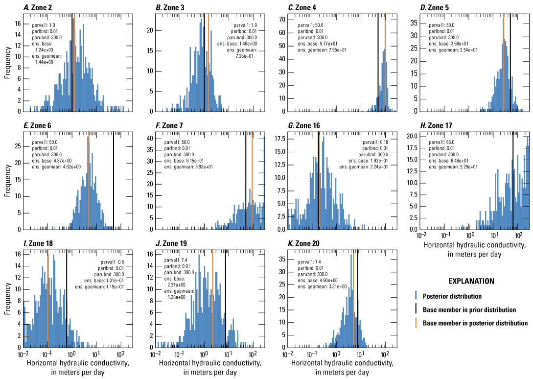
Model A histogram of hydraulic conductivity direct value parameters ensemble by zone after second iteration of Iterative Ensemble Smoother calibration run (Guira and Weisser, 2025). A, Zone 2. B, Zone 3. C, Zone 4. D, Zone 5. E, Zone 6. F, Zone 7. G, Zone 16. H, Zone 17. I, Zone 18. J, Zone 19. K, Zone 20. [parval1, parameter starting value; parlbnd, lower bound of parameter range; parubnd, upper bound of parameter range; ens. base, parameter value for the base member of the ensemble; ens. geomean, geometric mean of the ensemble parameter values].
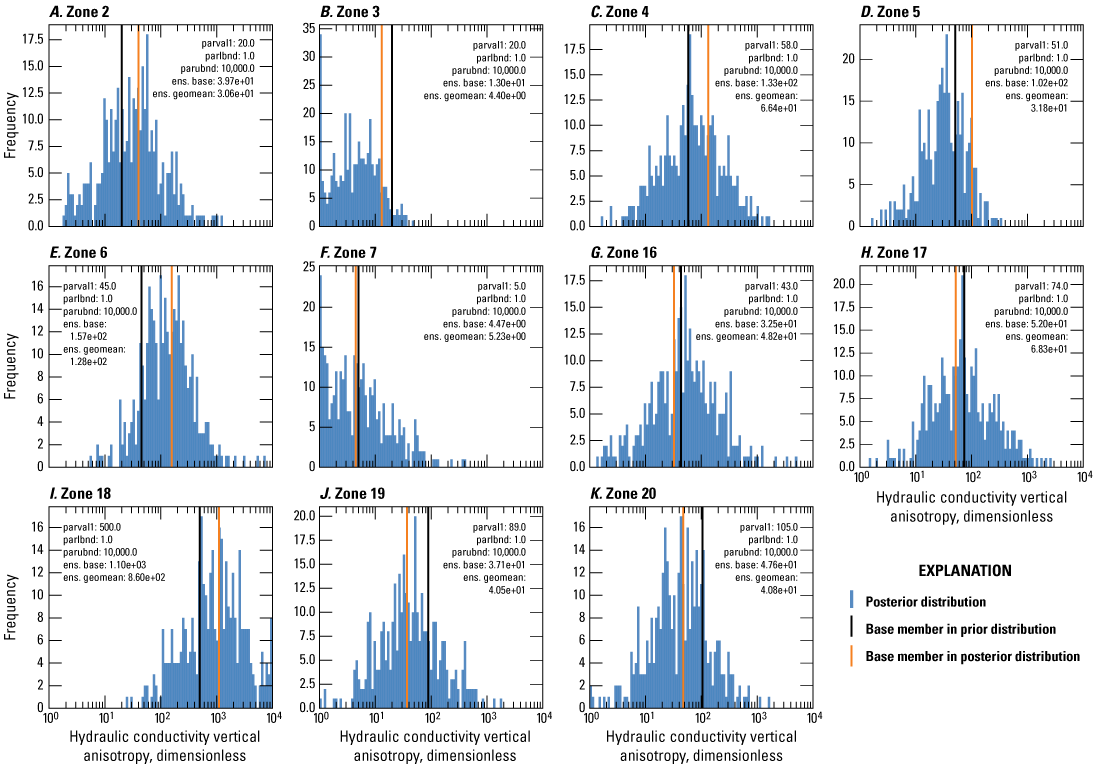
Model A histogram of hydraulic conductivity vertical anisotropy direct value parameters ensemble by zone after second iteration of Iterative Ensemble Smoother calibration run (Guira and Weisser, 2025). A, Zone 2. B, Zone 3. C, Zone 4. D, Zone 5. E, Zone 6. F, Zone 7. G, Zone 16. H, Zone 17. I, Zone 18. J, Zone 19. K, Zone 20.[parval1, parameter starting value; parlbnd, lower bound of parameter range; parubnd, upper bound of parameter range; ens. base, parameter value for the base member of the ensemble; ens. geomean, geometric mean of the ensemble parameter values]
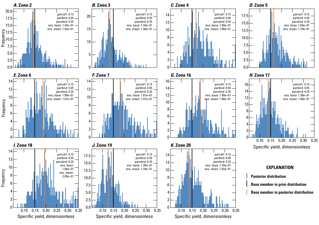
Model A histogram of specific yield direct value parameters ensemble by zone after second iteration of Iterative Ensemble Smoother calibration run (Guira and Weisser, 2025). A, Zone 2. B, Zone 3. C, Zone 4. D, Zone 5. E, Zone 6. F, Zone 7. G, Zone 16. H, Zone 17. I, Zone 18. J, Zone 19. K, Zone 20.[parval1, parameter starting value; parlbnd, lower bound of parameter range; parubnd, upper bound of parameter range; ens. base, parameter value for the base member of the ensemble; ens. geomean, geometric mean of the ensemble parameter values]
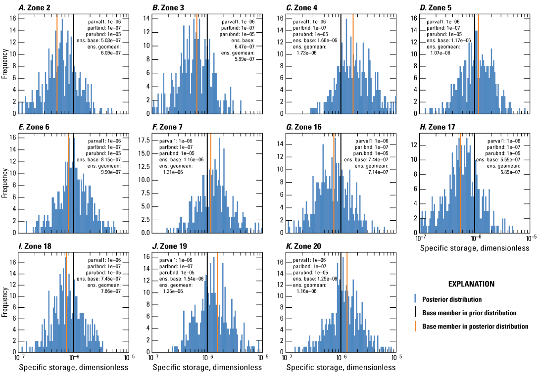
Model A histogram of specific storage direct value parameters ensemble by zone after second iteration of Iterative Ensemble Smoother calibration run (Guira and Weisser, 2025). A, Zone 2. B, Zone 3. C, Zone 4. D, Zone 5. E, Zone 6. F, Zone 7. G, Zone 16. H, Zone 17. I, Zone 18. J, Zone 19. K, Zone 20. [parval1, parameter starting value; parlbnd, lower bound of parameter range; parubnd, upper bound of parameter range; ens. base, parameter value for the base member of the ensemble; ens. geomean, geometric mean of the ensemble parameter values]
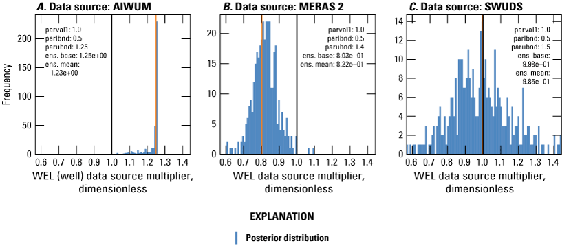
Histogram of well data source multiplier parameter ensemble following second iteration of Iterative Ensemble Smoother calibration run (Guira and Weisser, 2025). Well data sources comprise the Aquaculture and Irrigation Water-Use Model (Bristow and Wilson, 2023), Mississippi Embayment Regional Aquifer Study 2 (Hunt and others, 2021) and site-specific water-use data system (U.S. Geological Survey, 2020). A, Data source: Aquaculture and Irrigation Water-Use Model (AIWUM, Bristow and Wilson, 2023). B, Data source: Mississippi Embayment River Aquifer Study (MERAS, Hart and others, 2008) 2. C, Data source: site-specific water-use data system (SWUDS, U.S. Geological Survey, 2020). [parval1, parameter starting value; parlbnd, lower bound of parameter range; parubnd, upper bound of parameter range; ens. base, parameter value for the base member of the ensemble; ens. geomean, geometric mean of the ensemble parameter values]
References Cited
Bristow, E.L., and Wilson, J.L., 2023, Aquaculture and irrigation water-use model (AIWUM) version 1.1 estimates and related datasets for the Mississippi Alluvial Plain: U.S. Geological Survey data release, accessed October 2, 2024, at https://doi.org/10.5066/P9RGZOBZ.
Guira, M., and Weisser, A.R., 2025, Inset models used to evaluate the effects of layering configuration on model calibration from 1900 to 2018, and assess managed aquifer recharge near Shellmound, Mississippi, from 2019 to 2050: U.S. Geological Survey data release, https://doi.org/10.5066/P13DWA86.
Hart, R.M., Clark, B.R., and Bolyard, S.E., 2008, Digital surfaces and thicknesses of selected hydrogeologic units within the Mississippi Embayment Regional Aquifer Study (MERAS): U.S. Geological Survey Scientific Investigations Report 2008–5098, 33 p., accessed October 2, 2023, at https://doi.org/10.3133/sir20085098.
Hunt, R.J., White, J.T., Duncan, L.L., Haugh, C.J., and Doherty, J., 2021, Evaluating lower computational burden approaches for calibration of large environmental models: Groundwater, v. 59, no. 6, p. 788–798 [Also available at https://doi.org/10.1111/gwat.13106.]
U.S. Geological Survey, 2020, USGS water data for the Nation: U.S. Geological Survey National Water Information System database, accessed December 2020 at https://doi.org/10.5066/F7P55KJN.
Appendix 2. Calibration and Modeling Results for Model B and Model C
Calibration and Groundwater Budget Results for Models B
Below are figures from the Parameter Estimation++ Iterative Ensemble Smoother (PESTPP–IES) calibration results of model B. Direct parameter values for hydraulic conductivity, hydraulic conductivity vertical anisotropy, specific yield, and specific storage for model B are shown in figures 2.1–2.4. Pumping data source multipliers for model B are shown in figure 2.5. In each instance, the posterior ensemble values distribution histogram shows parameters organized in bins based on resistivity classes developed by Minsley and others (2021), and hydrostratigraphic layers defined in by Hart and others (2008). Also emphasized on these plots are prior and poster parameter values of the base member within the distribution.
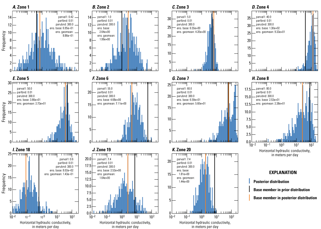
Model B histogram of hydraulic conductivity direct value parameters ensemble by zone after second iteration of Iterative Ensemble Smoother calibration run (Guira and Weisser, 2025). A, Zone 1. B, Zone 2. C, Zone 3. D, Zone 4. E, Zone 5. F, Zone 6. G, Zone 7. H, Zone 8. I, Zone 18. J, Zone 19. K, Zone 20. [parval1, parameter starting value; parlbnd, lower bound of parameter range; parubnd, upper bound of parameter range; ens. base, parameter value for the base member of the ensemble; ens. geomean, geometric mean of the ensemble parameter values]
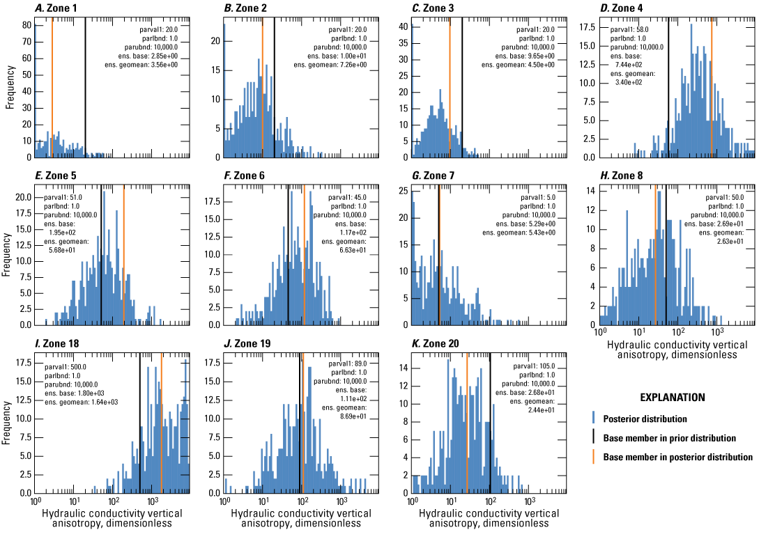
Model B histogram of hydraulic conductivity anisotropy direct value parameters ensemble by zone after second iteration of Iterative Ensemble Smoother calibration run (Guira and Weisser, 2025). A, Zone 1. B, Zone 2. C, Zone 3. D, Zone 4. E, Zone 5. F, Zone 6. G, Zone 7. H, Zone 8. I, Zone 18. J, Zone 19. K, Zone 20. [parval1, parameter starting value; parlbnd, lower bound of parameter range; parubnd, upper bound of parameter range; ens. base, parameter value for the base member of the ensemble; ens. geomean, geometric mean of the ensemble parameter values]
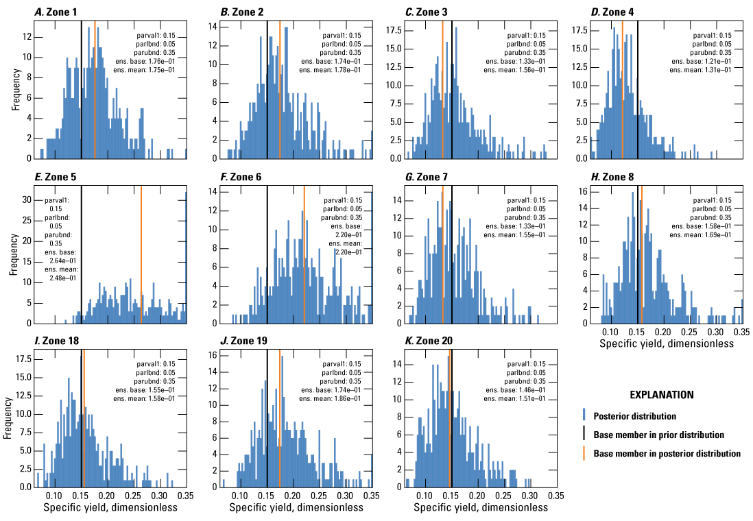
Model B histogram of specific yield direct value parameters ensemble by zone after second iteration of Iterative Ensemble Smoother calibration run (Guira and Weisser, 2025). A, Zone 1. B, Zone 2. C, Zone 3. D, Zone 4. E, Zone 5. F, Zone 6. G, Zone 7. H, Zone 8. I, Zone 18. J, Zone 19. K, Zone 20.[parval1, parameter starting value; parlbnd, lower bound of parameter range; parubnd, upper bound of parameter range; ens. base, parameter value for the base member of the ensemble; ens. geomean, geometric mean of the ensemble parameter values]
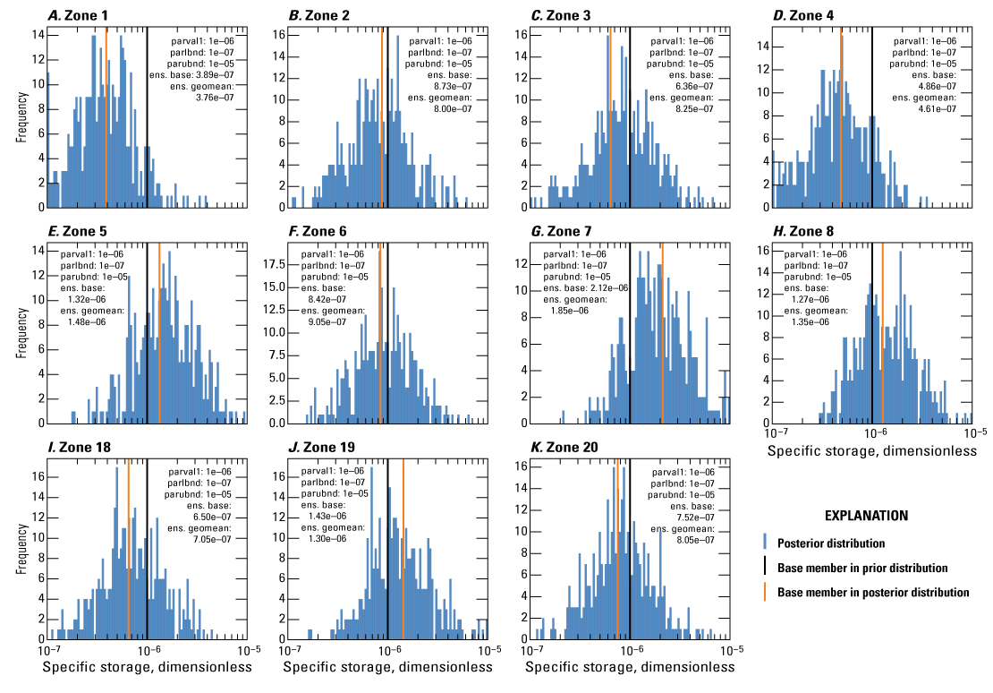
Model B histogram of specific storage direct value parameters ensemble by zone after second iteration of Iterative Ensemble Smoother calibration run (Guira and Weisser, 2025). A, Zone 1. B, Zone 2. C, Zone 3. D, Zone 4. E, Zone 5. F, Zone 6. G, Zone 7. H, Zone 8. I, Zone 18. J, Zone 19. K, Zone 20.[parval1, parameter starting value; parlbnd, lower bound of parameter range; parubnd, upper bound of parameter range; ens. base, parameter value for the base member of the ensemble; ens. geomean, geometric mean of the ensemble parameter values]
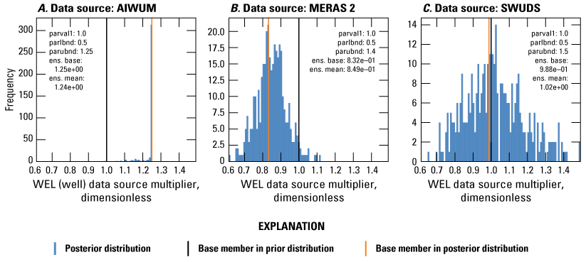
Model B histogram of well (WEL) package (Langevin and others, 2017) data source multiplier parameter ensemble following second iteration of Iterative Ensemble Smoother calibration run (Guira and Weisser, 2025). A, Data source: Aquaculture and Irrigation Water-Use Model (AIWUM). B, Data source: Mississippi Embayment River Aquifer Study (MERAS) 2. C, Data source: site-specific water-use data system (SWUDS). [parval1, parameter starting value; parlbnd, lower bound of parameter range; parubnd, upper bound of parameter range; ens. base, parameter value for the base member of the ensemble; ens. geomean, geometric mean of the ensemble parameter values]
One-to-one plots for aquifer direct heads, streamflows, and linear head derivatives are shown in figure 2.6. Measured and simulated aquifer heads and streamflows are shown in figures 2.7 and 2.8. Net infiltration estimates were determined from the SWB model (fig. 2.9A; Nielsen and Westenbroek, 2023), model B calibrated recharge (fig. 2.9B), and the spatial difference between SWB model estimates and model B calibrated recharge (fig. 2.9C). Noncalibrated and calibrated water use for model B is shown in figure 2.10. Noncalibrated water use data, which were processed from the Aquaculture and Irrigation Water-Use Model estimates, are lower than the calibrated water use across the simulation period. Net annual budgets simulated by model B are shown in figure 2.11.
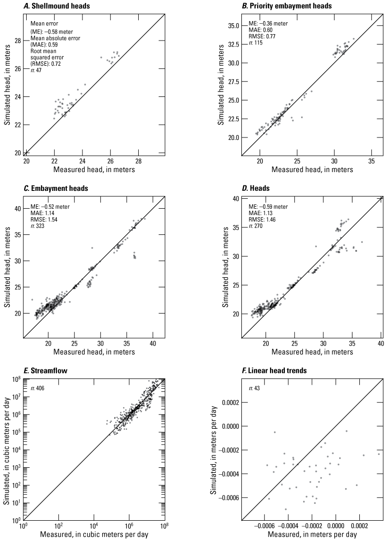
Model B one-to-one plots comparing the Shellmound model outputs (Guira and Weisser, 2025) to field observations. A, Shellmound heads. B, Priority embayment heads. C, Embayment heads. D, Heads. E, Streamflow (U.S. Geological Survey, 2020). F, Linear head trends.
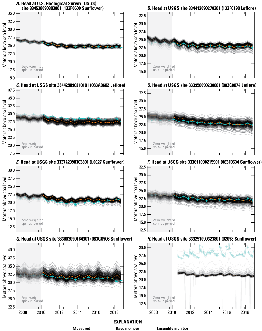
Model B time series of measured heads and simulated equivalents at selected wells (U.S. Geological Survey, 2020; Guira and Weisser, 2025). A, U.S. Geological Survey (USGS) site 334538090303801 (133F0600 Sunflower). B, USGS site 334412090270301 (133F0190 Leflore). C, USGS site 334429090210101 (083A0602 Leflore). D, USGS site 333950090230001 (083C0074 Leflore). E, USGS site 333742090303801 (L0027 Sunflower). F, USGS site 333611090215901 (083F0534 Sunflower). G, USGS site 333603090164301 (083G0506 Sunflower). H, USGS site 333251090323801 (02058 Sunflower).
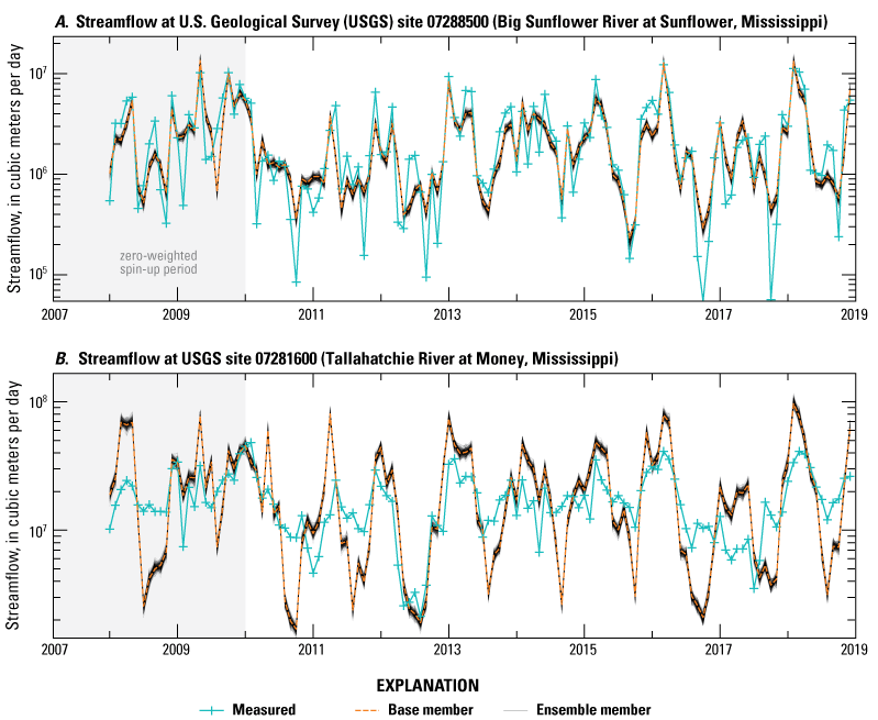
Model B streamflows time series showing monthly averages of measured streamflows (U.S. Geological Survey, 2020) and simulated equivalents (Guira and Weisser, 2025). A, U.S. Geological Survey station 07288500 (Big Sunflower River at Sunflower, Mississippi). B, U.S. Geological Survey station 07281600 (Tallahatchie River at Money, Mississippi). Simulated streamflows include base flows and surface runoff estimates from the soil-water-balance model by Nielsen and Westenbroek (2023).
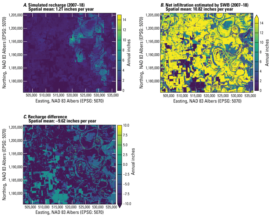
Comparative maps showing mean annual recharge for model B. A, Simulated recharge (Guira and Weisser, 2025). B, Net infiltration simulated by soil-water-balance (Nielsen and Westenbroek, 2023). C, Recharge difference between soil-water-balance estimate and calibrated.
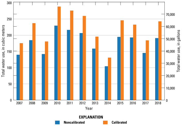
Model B total water use before and after calibration. Water-use data prior to calibration includes estimated rates from Aquaculture and Irrigation Water-Use Model (Bristow and Wilson, 2023) and nonagricultural rates from the U.S. Geological Survey site-specific water-use data system (U.S. Geological Survey, 2020) and national estimates for water use associated with thermoelectric power generation in 2010 and 2015 (Diehl and Harris, 2014; Harris and Diehl, 2019a,b).
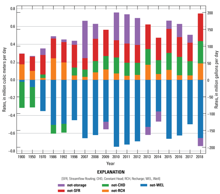
Model B simulated annual net budget results for the Shellmound model (Guira and Weisser, 2025).
Calibration and Groundwater Budget Results for Model C
Below are figures from the PESTPP–IES calibration results of model C. In each instance, a histogram shows the ensemble values distribution organized in bins. Also emphasized on these plots are prior and poster parameter values of the base member within the ensemble. Direct parameter values for hydraulic conductivity, hydraulic conductivity vertical anisotropy, specific yield, and specific storage for model C are shown in figures 2.12–2.15. Pumping data source multipliers for model C are shown in figure 2.16.
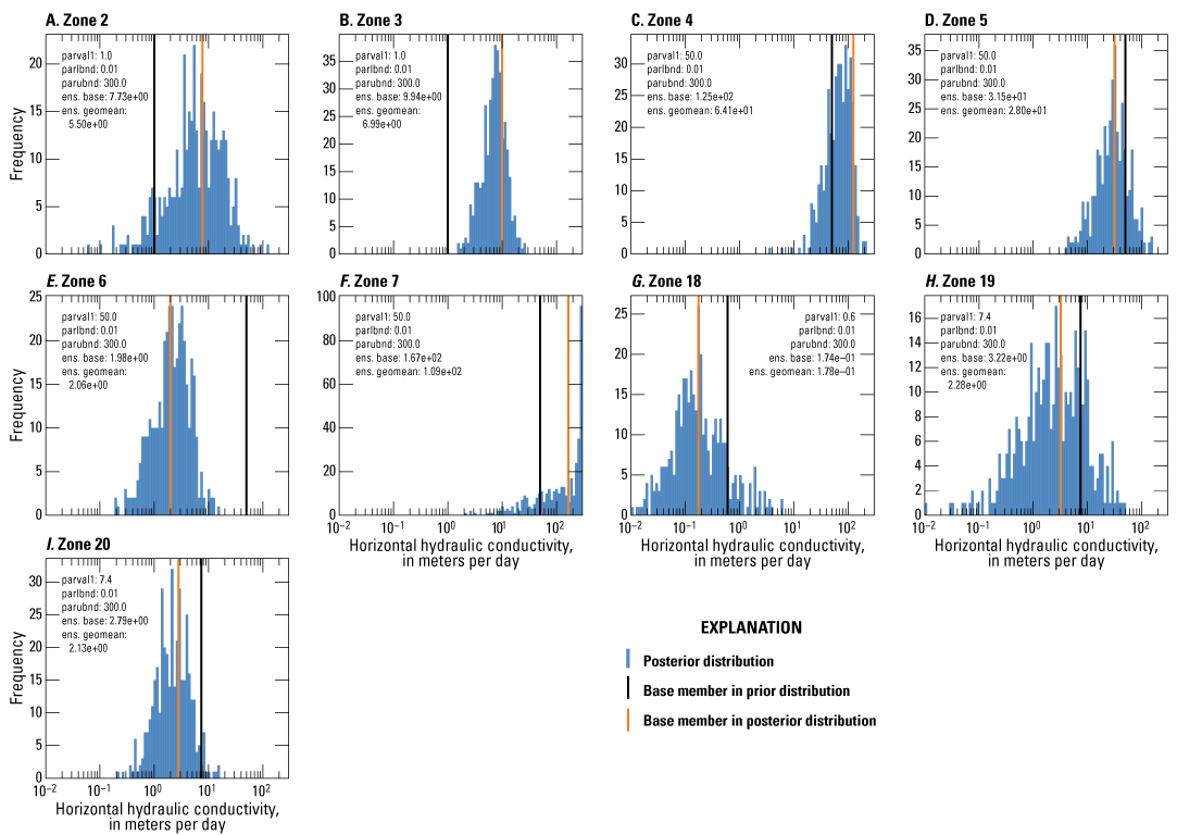
Model C histogram of hydraulic conductivity direct value parameters ensemble by zone after second iteration of Iterative Ensemble Smoother calibration run (Guira and Weisser, 2025). A, Zone 2. B, Zone 3. C, Zone 4. D, Zone 5. E, Zone 6. F, Zone 7. G, Zone 18. H, Zone 19. I, Zone 20. [parval1, parameter starting value; parlbnd, lower bound of parameter range; parubnd, upper bound of parameter range; ens. base, parameter value for the base member of the ensemble; ens. geomean, geometric mean of the ensemble parameter values]
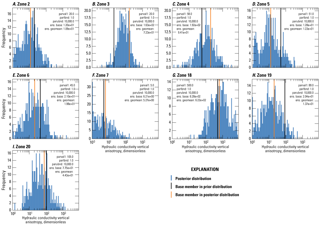
Model C histogram of hydraulic conductivity anisotropy direct value parameters ensemble by zone after second iteration of Iterative Ensemble Smoother calibration run (Guira and Weisser, 2025). A, Zone 2. B, Zone 3. C, Zone 4. D, Zone 5. E, Zone 6. F, Zone 7. G, Zone 18. H, Zone 19. I, Zone 20. [parval1, parameter starting value; parlbnd, lower bound of parameter range; parubnd, upper bound of parameter range; ens. base, parameter value for the base member of the ensemble; ens. geomean, geometric mean of the ensemble parameter values]
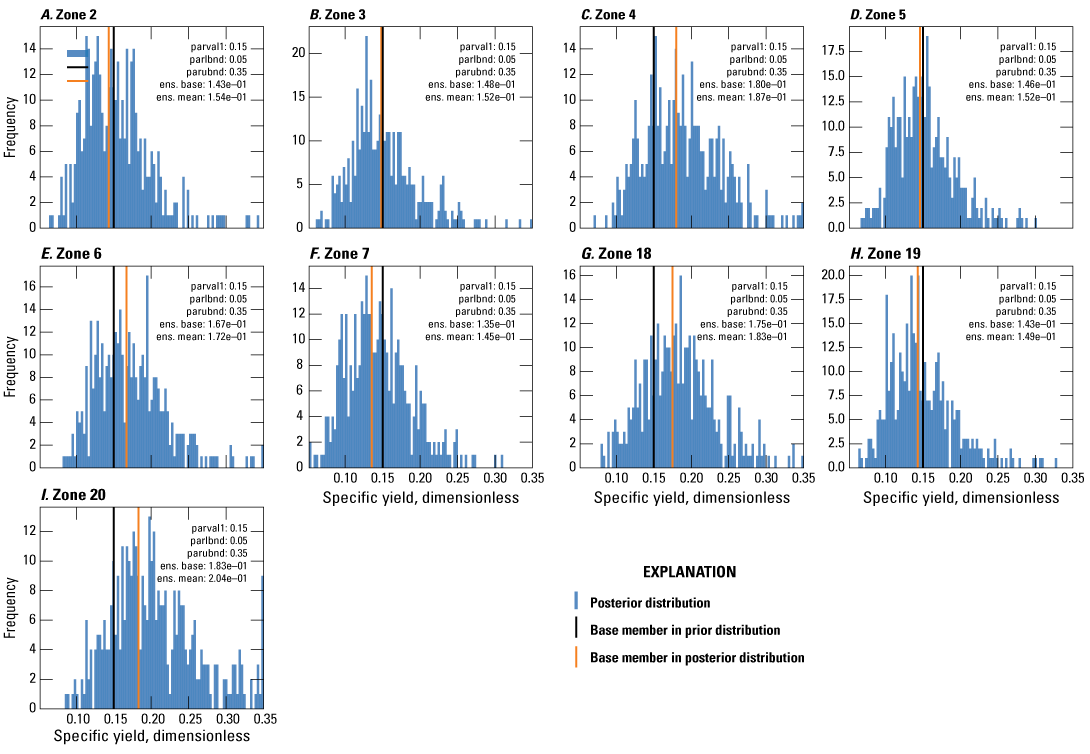
Model C histogram of specific yield direct value parameters ensemble by zone after second iteration of Iterative Ensemble Smoother calibration run (Guira and Weisser, 2025). A, Zone 2. B, Zone 3. C, Zone 4. D, Zone 5. E, Zone 6. F, Zone 7. G, Zone 18. H, Zone 19. I, Zone 20. [parval1, parameter starting value; parlbnd, lower bound of parameter range; parubnd, upper bound of parameter range; ens. base, parameter value for the base member of the ensemble; ens. geomean, geometric mean of the ensemble parameter values]
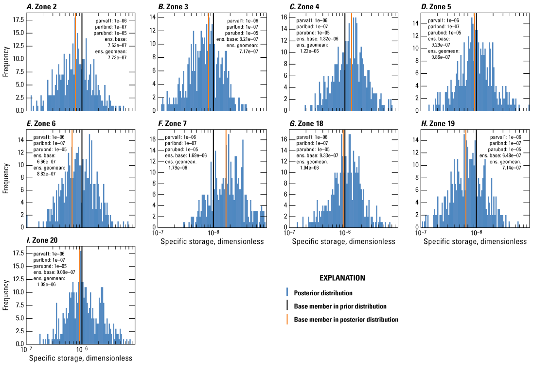
Model C histogram of specific storage direct value parameters ensemble by zone after second iteration of Iterative Ensemble Smoother calibration run (Guira and Weisser, 2025). A, Zone 2. B, Zone 3. C, Zone 4. D, Zone 5. E, Zone 6. F, Zone 7. G, Zone 18. H, Zone 19. I, Zone 20. [parval1, parameter starting value; parlbnd, lower bound of parameter range; parubnd, upper bound of parameter range; ens. base, parameter value for the base member of the ensemble; ens. geomean, geometric mean of the ensemble parameter values]
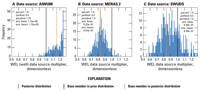
Model C histogram of well (WEL) package (Langevin and others, 2017) data source multiplier parameter ensemble following second iteration of Iterative Ensemble Smoother calibration run (Guira and Weisser, 2025). A, Data source: Aquaculture and Irrigation Water-Use Model (AIWUM). B, Data source: Mississippi Embayment River Aquifer Study (MERAS) 2. C, Data source: site-specific water-use data system (SWUDS). [parval1, parameter starting value; parlbnd, lower bound of parameter range; parubnd, upper bound of parameter range; ens. base, parameter value for the base member of the ensemble; ens. geomean, geometric mean of the ensemble parameter values]
One-to-one plots for aquifer direct heads, streamflows, and linear head derivatives are shown in figure 2.17. Time series plots showing measured and simulated heads and streamflows for model C are shown in figures 2.18 and 2.19. Net infiltration estimates were determined from SWB model (fig. 2.20A), model C calibrated recharge (fig. 2.20B) and the spatial difference between SWB model recharge estimates and calibrated recharge (fig. 2.20C). Noncalibrated and calibrated water use for model C are shown in figure 2.21. Net annual budgets simulated by model C are shown in figure 2.22.

Model C one-to-one plots comparing the Shellmound model outputs (Guira and Weisser, 2025) to field observations (U.S. Geological Survey, 2020). A, Shellmound heads. B, Priority embayment heads. C, Embayment heads. D, Heads. E, Streamflow. F, Linear head trends.
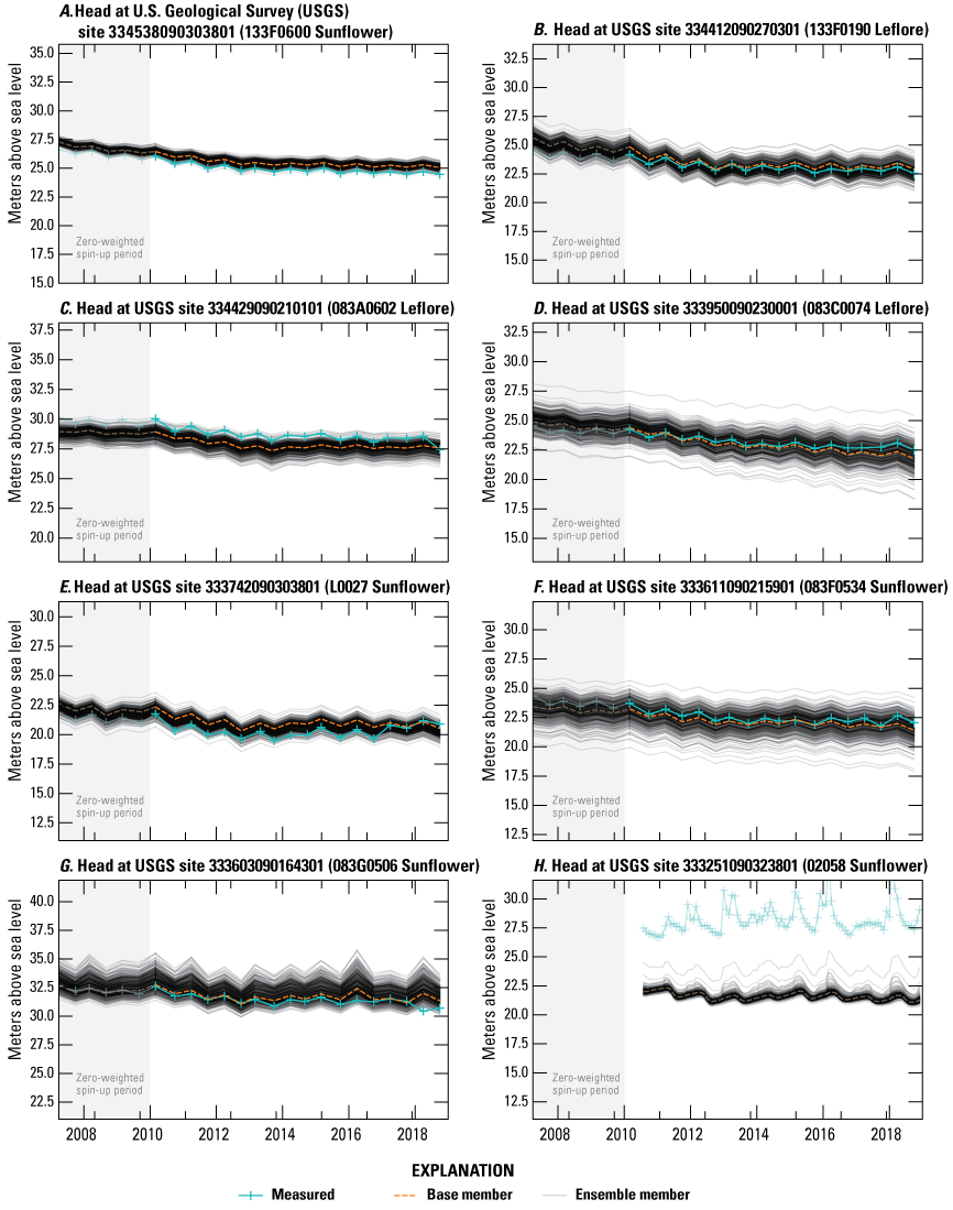
Model C time series of measured heads and simulated equivalents (Guira and Weisser, 2025) at selected wells (U.S. Geological Survey, 2020). A, U.S. Geological Survey (USGS) site 334538090303801 (133F0600 Sunflower). B, USGS site 334412090270301 (133F0190 Leflore). C, USGS site 334429090210101 (083A0602 Leflore). D, USGS site 333950090230001 (083C0074 Leflore). E, USGS site 333742090303801 (L0027 Sunflower). F, USGS site 333611090215901 (083F0534 Sunflower). G, USGS site 333603090164301 (083G0506 Sunflower). H, USGS site 333251090323801 (02058 Sunflower).
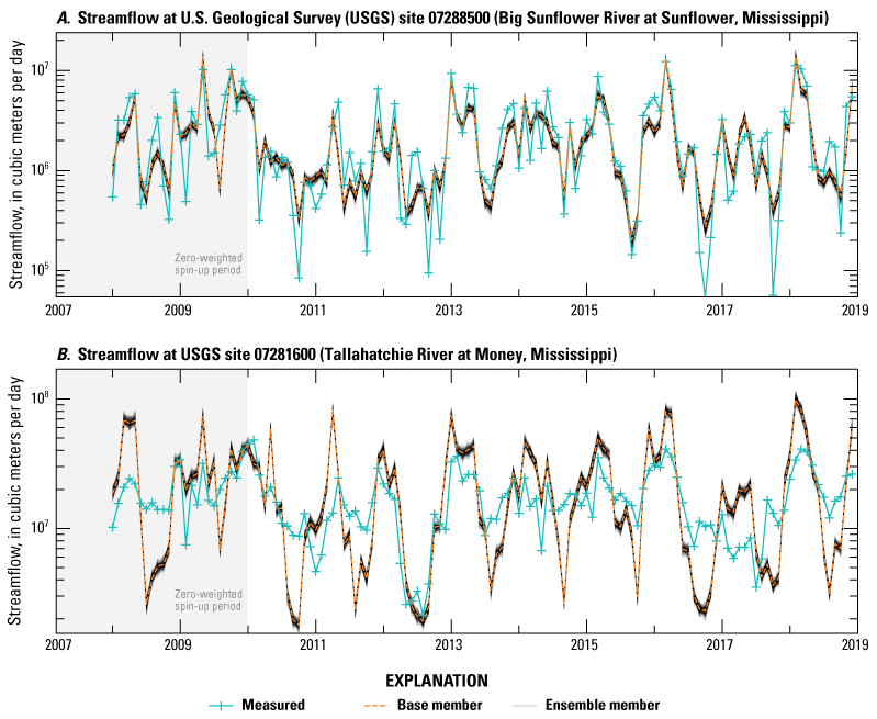
Model C streamflows time series showing monthly averages of measured streamflows (U.S. Geological Survey, 2020) and simulated equivalents (Guira and Weisser, 2025). A, U.S. Geological Survey station 07288500 (Big Sunflower River at Sunflower, Mississippi). B, U.S. Geological Survey station 07281600 (Tallahatchie River at Money, Mississippi). Simulated streamflows include base flows and surface runoff estimates from the soil-water-balance model by Nielsen and Westenbroek (2023).
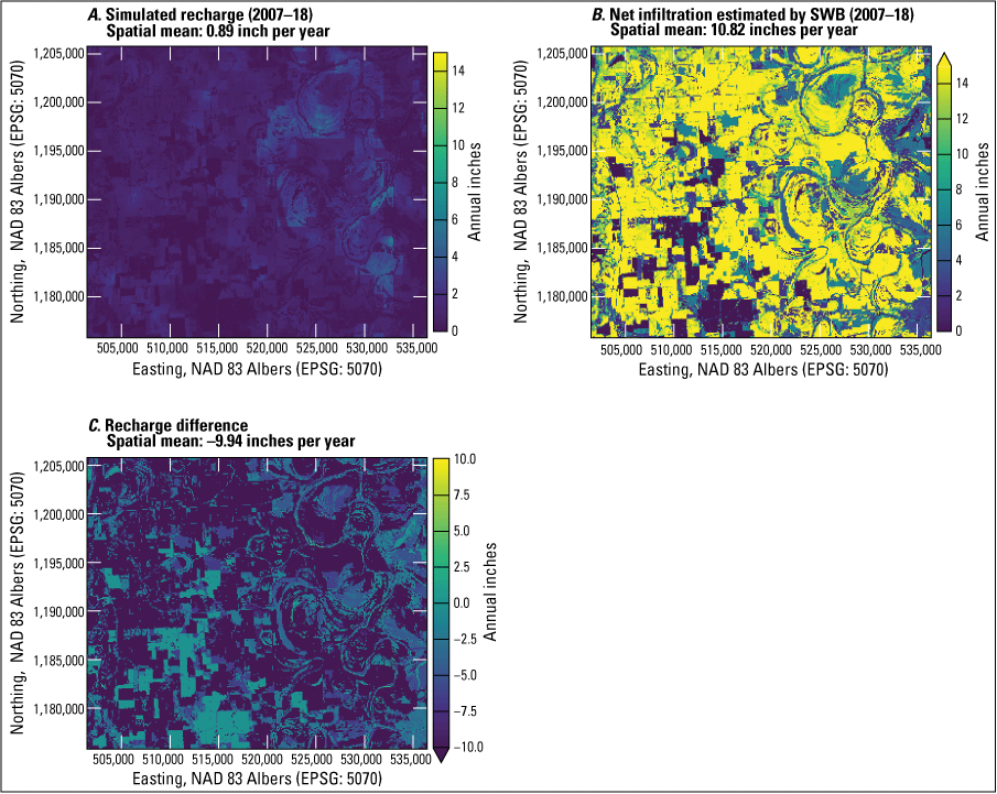
Comparative maps showing mean annual recharge for model C. A, Simulated recharge (Guira and Weisser, 2025). B, Net infiltration estimated by soil-water-balance (Nielsen and Westenbroek, 2023). C, Recharge difference between soil-water-balance estimate and calibrated.
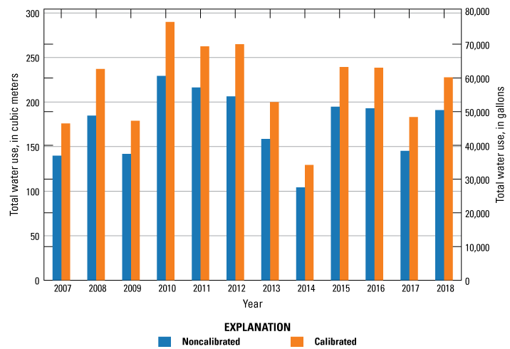
Model C total water use before and after calibration. Water-use data prior to calibration includes estimated rates from Aquaculture and Irrigation Water-Use Model (Bristow and Wilson, 2023) and nonagricultural rates from the U.S. Geological Survey site-specific water-use data system (U.S. Geological Survey, 2020) and national estimates for water use associated with thermoelectric power generation in 2010 and 2015 (Diehl and Harris, 2014; Harris and Diehl, 2019a,b).
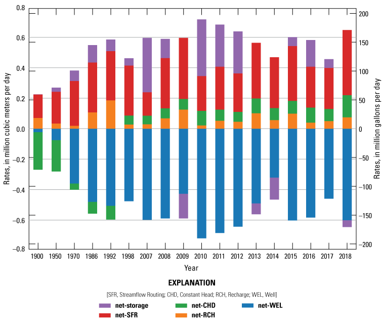
Model C simulated annual net budget results for the Shellmound model (Guira and Weisser, 2025).
Comparison of Recharge and Water Use
A comparative plot for annual average calibrated groundwater recharge simulated by models A, B, and C is shown in figure 2.23. Calibrated recharge rates have similar patterns for the entire simulation period for all three models. Minor differences can be perceived primarily for the steady state and during the multiyear spin-up period. However, after 2007, calibrated recharge rates for all three models were similar except for 2013 and 2018, when rates in model C were notably higher. Comparative plots of calibrated average annual water use simulated by models A, B, and C are shown in figure 2.24.
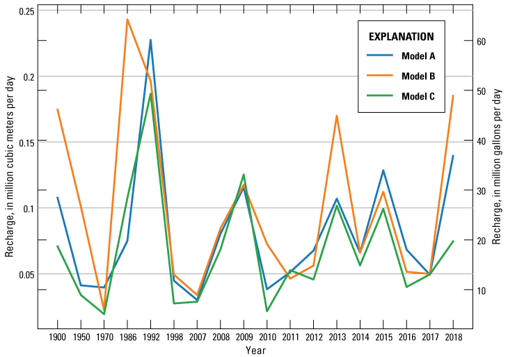
Comparative plot of calibrated annual groundwater recharge by models A, B, and C (Guira and Weisser, 2025).
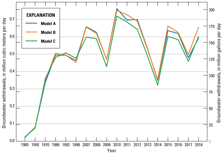
Comparative plot of calibrated annual water use by models A, B, and C (Guira and Weisser, 2025).
References Cited
Guira, M., and Weisser, A.R., 2025, Inset models used to evaluate the effects of layering configuration on model calibration from 1900 to 2018, and assess managed aquifer recharge near Shellmound, Mississippi, from 2019 to 2050: U.S. Geological Survey data release, https://doi.org/10.5066/P13DWA86.
Bristow, E.L., and Wilson, J.L., 2023, Aquaculture and irrigation water-use model (AIWUM) version 1.1 estimates and related datasets for the Mississippi Alluvial Plain: U.S. Geological Survey data release, accessed October 2, 2024, at https://doi.org/10.5066/P9RGZOBZ.
Diehl, T.H., and Harris, M.A., 2014, Withdrawal and consumption of water by thermoelectric power plants in the United States, 2010: U.S. Geological Survey Scientific Investigations Report 2014–5184, 28 p. [Also available at https://doi.org/10.3133/sir20145184.]
Harris, M.A., and Diehl, T.H., 2019a, Withdrawal and consumption of water by thermoelectric power plants in the United States, 2015: U.S. Geological Survey Scientific Investigations Report 2019–5103, 15 p. [Also available at https://doi.org/10.3133/sir20195103.]
Harris, M.A., and Diehl, T.H., 2019b, Water withdrawal and consumption estimates for thermoelectric power plants in the United States, 2015: U.S. Geological Survey data release, accessed October 2, 2023, at https://doi.org/10.5066/P9V0T04B.
Hart, R.M., Clark, B.R., and Bolyard, S.E., 2008, Digital surfaces and thicknesses of selected hydrogeologic units within the Mississippi Embayment Regional Aquifer Study (MERAS): U.S. Geological Survey Scientific Investigations Report 2008–5098, 33 p., accessed October 2, 2023, at https://doi.org/10.3133/sir20085098.
Langevin, C.D., Hughes, J.D., Banta, E.R., and Niswonger, R.G., Panday, S., and Provost, A.M., 2017, Documentation for the MODFLOW 6 Groundwater Flow Model: U.S. Geological Survey Techniques and Methods, book 6, chap. A55, 197 p., accessed October 2, 2023, at https://doi.org/10.3133/tm6A55.
Minsley, B.J., Rigby, J.R., James, S.R., Burton, B.L., Knierim, K.J., Pace, M.D.M., Bedrosian, P.A., and Kress, W.H., 2021, Airborne geophysical surveys of the lower Mississippi Valley demonstrate system-scale mapping of subsurface architecture: Communications Earth & Environment, v. 2, no. 1, art 131, 14p. , accessed October 1, 2022, at https://doi.org/10.1038/s43247-021-00200-z.
Nielsen, M.G. and Westenbroek, S.M, 2023, Updated estimates of water budget components for the Mississippi Embayment Region, 2000–2020: U.S. Geological Survey Scientific Investigations Report 2023–5080, 58 p., accessed October 2, 2024, at https://doi.org/10.3133/sir20235080.
U.S. Geological Survey, 2020, USGS water data for the Nation: U.S. Geological Survey National Water Information System database, accessed December 2020 at https://doi.org/10.5066/F7P55KJN.
Conversion Factors
International System of Units to U.S. customary units
U.S. customary units to International System of Units
Temperature in degrees Celsius (°C) may be converted to degrees Fahrenheit (°F) as follows:
°F = (1.8 × °C) + 32.
Datum
Vertical coordinate information is referenced to the North American Vertical Datum of 1988 (NAVD 88).
Horizontal coordinate information is referenced to North American Datum of 1983 (NAD 83).
Altitude, as used in this report, refers to distance above the vertical datum.
Abbreviations
Φ
phi, objective function
AEM
airborne electromagnetic
AIWUM
Aquaculture and Irrigation Water-Use Model
CHD
Constant Head
GTIP
Groundwater Transfer and Injection Pilot
IES
Iterative Ensemble Smoother
Kh
horizontal hydraulic conductivity
Kvani
hydraulic conductivity vertical anisotropy
MAP
Mississippi Alluvial Plain
MAR
managed aquifer recharge
MERAS
Mississippi Embayment River Aquifer Study
MODFLOW
modular finite-difference flow model
MRVA
Mississippi River Valley alluvial
NWIS
National Water Information System
PEST++
Parameter Estimation ++
PESTPP–IES
PEST++ Iterative Ensemble Smoother
SFR
Streamflow Routing
SWB
soil-water-balance
SWUDS
site-specific water-use data system
Sy
specific yield
USGS
U.S. Geological Survey
WEL
Well
For more information about this publication, contact:
Director, USGS Nebraska Water Science Center
5231 South 19th Street
Lincoln, NE 68512
402–328–4100
For additional information, visit: https://www.usgs.gov/centers/ne-water
Publishing support provided by the
Rolla and Sacramento Publishing Service Centers
Disclaimers
Any use of trade, firm, or product names is for descriptive purposes only and does not imply endorsement by the U.S. Government.
Although this information product, for the most part, is in the public domain, it also may contain copyrighted materials as noted in the text. Permission to reproduce copyrighted items must be secured from the copyright owner.
Suggested Citation
Guira, M., Traylor, J.P., Leaf, A.T., and Weisser, A.R., 2025, An inset groundwater-flow model to evaluate the effects of layering configuration on model calibration and assess managed aquifer recharge near Shellmound, Mississippi: U.S. Geological Survey Scientific Investigations Report 2025–5055, 134 p., https://doi.org/10.3133/sir20255055.
ISSN: 2328-0328 (online)
Study Area
| Publication type | Report |
|---|---|
| Publication Subtype | USGS Numbered Series |
| Title | An inset groundwater-flow model to evaluate the effects of layering configuration on model calibration and assess managed aquifer recharge near Shellmound, Mississippi |
| Series title | Scientific Investigations Report |
| Series number | 2025-5055 |
| DOI | 10.3133/sir20255055 |
| Publication Date | November 18, 2025 |
| Year Published | 2025 |
| Language | English |
| Publisher | U.S. Geological Survey |
| Publisher location | Reston, VA |
| Contributing office(s) | Nebraska Water Science Center, Upper Midwest Water Science Center, Central Plains Water Science Center |
| Description | Report: ix, 134 p.; 3 Figures: 11.00 x 8.50 inches; Data Release; Dataset |
| Country | United States |
| State | Mississippi |
| City | Shellmound |
| Online Only (Y/N) | Y |
| Additional Online Files (Y/N) | N |