

Selected Special Conditions Affecting Peak Streamflow and Extreme Floods in Alaska Through Water Year 2022
Links
- Document: Report , HTML , XML
- Data Releases:
- USGS data release - Selected peak-flow special conditions for USGS streamgages in Alaska (ver. 2.0)
- USGS data release - Selected basin boundaries for USGS streamgages in Alaska through 2014
- USGS data release - Selected basin boundaries for USGS streamgages in Alaska through 2019
- USGS data release - Summary of selected basin and streamflow special conditions for USGS streamgages in Alaska
- USGS data release - Extreme flood, atmospheric river presence, and basin characteristic data for a study of peak streamflow special conditions in Alaska
- NGMDB Index Page: National Geologic Map Database Index Page (html)
- Download citation as: RIS | Dublin Core
Acknowledgments
This study was conducted in cooperation with the Alaska Department of Transportation and Public Facilities. The author is grateful to Deanna Nash of the Center for Western Weather and Water Extremes at the Scripps Institution of Oceanography, University of California San Diego, for providing atmospheric river data, explanation of data acquisition methods, and discussion of atmospheric river concepts that helped guide report content.
The author thanks several individuals for contributions that improved study methods and content. Matt Schellekens and Jeff Conaway of the U.S. Geological Survey (USGS) Alaska Science Center provided history and context for Alaska Science Center streamgage data collection practices, information regarding selected floods, and helpful discussions of flood-generating mechanisms. Discussions with Brianna Rick of the USGS Alaska Climate Adaptation Science Center and University of Alaska Fairbanks improved report sections regarding glacial lake outburst floods, and Rick Thoman of the University of Alaska Fairbanks shared perspectives on atmospheric rivers and other types of storms in Alaska that improved interpretation of related study results. Crane Johnson of the National Weather Service Alaska-Pacific River Forecast Center and Dan Wagner of the USGS Lower Mississippi-Gulf Water Science Center are gratefully acknowledged for insightful reviews that strengthened the report.
Abstract
The U.S. Geological Survey, in cooperation with the Alaska Department of Transportation and Public Facilities, inventoried selected special conditions for annual peak flows and identified extreme floods at streamgages in Alaska through water year 2022 to facilitate hydrologic analysis. Special conditions identified from U.S. Geological Survey gaging records and basin characteristics included regulation and diversion, urbanization, indeterminate drainage areas, drainage areas less than the minimum used in regional analyses, glacial lake outburst floods, other outburst floods, and snowmelt floods. For peak flows that occurred during calendar years 1980–2019, an atmospheric river dataset was used to identify atmospheric river presence or absence on the dates peak flows occurred. Extreme floods (defined as peak flows exceeding the 1-percent annual exceedance probability flood magnitude or an empirical measure of relative magnitude using Creager’s coefficient C) were identified and associated with flood-generating mechanisms using the other inventoried special conditions and other information.
The gaging record contained glacial lake outburst floods at 15 streamgages and other types of outburst floods at 10 streamgages. Non-outburst peak flows in Alaska resulted from a mixture of rainfall and melt-based flood-generating mechanisms in all but the most rain-dominated seasonal flow regime. Melt-based flood-generating mechanisms included snowmelt, high-elevation snow and ice melt, or rain-on-snow events. Atmospheric rivers were common in Alaska and conterminous basins in Canada, occurring in that region on 67 percent of the days in the calendar year 1980–2019 period. Atmospheric rivers were more common on the days of peak flows and even more common on the days of non-outburst extreme floods. The percentage of days when an atmospheric river was present increased to 78 percent for the days of peak flows in that period and to 83 percent for the days of non-outburst extreme floods in that period. Of 149 extreme floods in the gaging record, 38 were generated by outburst floods. Of the non-outburst extreme floods, 72 percent were generated by rainfall and 26 percent were generated by melt-based processes or a combination of rainfall and melt-based processes. Flood-generating mechanisms could not be determined for the final 2 percent of the non-outburst extreme floods because the month and day of the peak flows were unknown and no other information was available. Secondary factors strongly associated with extreme floods included antecedent rain and streamflow conditions and warm storm conditions that produced rain instead of snow or generated snowmelt.
Introduction
Annual peak-flow data, the time series of maximum annual instantaneous streamflow values recorded at a streamgage, are used to represent flood characteristics and form one of the primary datasets for hydrologic analysis in support of management of water resources, protection of public life and property, and conservation of ecosystems. Statistical analyses such as flood-frequency analysis require peak-flow data that form a sample of random and homogeneous events, criteria that might not be met when special conditions are present (England and others, 2018). Special conditions can include basin conditions, data-collection conditions, or flood-generating mechanisms that create distinct subpopulations of peak flows. Access to and understanding of the special conditions affecting peak flows facilitates more accurate hydrologic analysis by guiding censoring of streamgages or peak flows, identifying subpopulations of peak flows for mixed-population analysis or other advanced treatment, and providing characteristics of extreme floods.
The U.S. Geological Survey (USGS) collects streamflow data for Alaska (U.S. Geological Survey, 2024a) and assigns qualification codes to peak-flow and stage values having special conditions that affect how the values should be interpreted or used (U.S. Geological Survey, 2024b). Some of the codes have a computational outcome in the USGS software PeakFQ commonly used for flood-frequency analysis (Siefken and others, 2024), triggering automatic inclusion or exclusion of the coded peak flow. The qualification codes are limited and standardized to allow for uniform application across the wide range of special conditions in the United States. However, local application of peak-flow qualification code 9 for selected events other than the prevailing regional peak-generating mechanisms can vary by region. In addition, guidance for peak-flow codes for glacial lake outburst floods (GLOFs) has variously incorporated code 3 (for dam failure) and code 9 over time (Ryberg and others, 2017), and local application of codes 5 and 6 indicating regulation or diversion can require interpretation for analysis. Documentation of how coded peak flows were used is thus a needed reporting element for hydrologic analysis and relies on ready access to code implications.
Some flood-generating mechanisms can produce subpopulations of peak flows that have statistically distinct frequency distributions, a link that can be analyzed to improve understanding of changes to flood characteristics associated with climate change. Selected flood-generating mechanisms can thus be considered a special condition that can be addressed using mixed-population analysis for flood frequency (England and others, 2018) or other techniques. The primary flood-generating mechanisms for Alaska are rainfall, snowmelt, and high-elevation snow and ice melt. These mostly seasonal processes can create weakly to strongly distinct subpopulations of peak flows at a stream site or within groups of stream sites that have similar seasonal flow regimes. Although complex combinations of rainfall and melt-based mechanisms are common, rainfall-dominated peak flows are generally larger in magnitude, on average, for sites within a seasonal flow regime, than snowmelt-dominated peak flows for most seasonal flow regimes in Alaska (Curran and Biles, 2021), motivating an interest in widespread identification of flood-generating mechanisms to assist hydrologic analysis. Some flood-generating mechanisms, including outburst floods and a limited group of snowmelt floods, can be identified from peak-flow qualification codes. Flood-generating mechanisms that can be identified from meteorologic conditions include long, narrow, plumes of intense water vapor transport located in the lower atmosphere, known as atmospheric rivers (ARs), that can result in heavy precipitation in Alaska (for example, Nash and others, 2024). Although ARs have been linked to peak flows for southeastern Alaska (Sharma and Déry, 2020), the association of peak flows with ARs across Alaska has not been explored.
Annual peak-flow records for a streamgage (U.S. Geological Survey, 2024a) can include one or more floods that are much larger than the more frequent floods in the gaged record, or much larger than would be expected from regional flood patterns. These extreme floods are of interest because of their potential to have an impact on the channel, streambanks, in-channel features, or engineered infrastructure that is of significance to ecological, cultural, or societal systems. Identifying extreme floods and assessing their magnitudes and flood-generating mechanisms provides valuable information for assessing design parameters and for anticipating the response of extreme floods to climate change.
The USGS inventoried selected streamflow and site special conditions and identified extreme floods to facilitate access to and understanding of selected special conditions often used for streamgage and period-of-record selection and to identify additional special conditions and their association with peak flows. This report describes methods for accessing information on special conditions, assesses links to flood-generating mechanisms for peak flows and for extreme floods, and discusses considerations for treatment of peak-flow special conditions in hydrologic analyses.
Purpose and Scope
This report presents the results of a study conducted in cooperation with the Alaska Department of Transportation and Public Facilities to identify and improve understanding of special conditions for peak flows through water year 2022 in support of hydrologic analyses for Alaska. By convention, a water year is defined as the period from October 1 to September 30 of the following year and named for the calendar year in which it ends. In this report, water years are denoted with the abbreviation WY. The study focuses on peak flows for USGS streamgages in Alaska and considers basin characteristics for conterminous basins in Canada to facilitate understanding of transboundary basins. For this report, floods were defined by their streamflow magnitude, not the areal extent of flooding, and were limited to annual peak flows because the time series of annual peak flows is readily available and commonly used for flood-frequency analysis (England and others, 2018). Although many special conditions affecting peak flows exist (England and others, 2018; U.S. Geological Survey, 2024b), this report is limited to selected streamflow, basin, and extreme flood conditions that were obtainable from existing datasets and required minimal site-specific analysis to maximize application to a large number of peak flows. The streamflow special conditions identified for this report were regulation and diversion, GLOFs, other outburst floods, snowmelt floods, and floods associated with ARs. The association of peak flows with ARs was limited to considering the presence of an AR on the day of a peak flow to provide a first-order inventory of AR-related peak flows in Alaska while minimizing data analysis beyond the scope of this project. The basin special conditions identified were urbanization, indeterminate drainage area, and drainage areas less than the minimum used for regional analysis. Extreme floods are defined in this report as peak flows exceeding a threshold based on flood-frequency statistics or an empirical measure of relative magnitude, depending on data availability, and were limited to floods observed in modern gaged records (that is, floods since the early 1900s), which excluded paleofloods such as megafloods associated with much older glacial lakes.
Previous Studies
Previous USGS reports discussing special conditions for USGS streamflow data for Alaska include flood-frequency reports (most recently, Curran and others, 2016) and other regional statistical analyses, such as Wiley and Curran (2003). These reports describe selected special conditions, including regulation and GLOFs, and detail their treatment (inclusion or exclusion) for the specific streamgages and analyses in the respective reports.
Historical reports documenting flood-generating mechanisms for regionally extreme and societally impactful floods in Alaska have described the nature and extent of flooding, primary flood-generating mechanisms, secondary processes, and contributing factors. Detailed, peer-reviewed reports described historical floods in calendar years 1967 (Boning, 1972; Childers and others, 1972); 1971 (Lamke, 1972); 1986 (Jones and Zenone, 1988; Lamke and Bigelow, 1988); 1994 (Meyer, 1995); and 2002 (Eash and Rickman, 2004). Other reports in newspapers or newsletters described flooding in 1971 (McGee, 1974), 2006 (Joling, 2006), 2012 (Pearson, 2012), and 2022 (Plumb and Ostman, 2023). Nearly all these large regional flooding events were associated with rainfall. However, regional floods in 1971 included unusually large high-elevation snowmelt floods, and outburst floods occurred in association with processes related to the 1971 and 1986 rainstorms. GLOFs pose hazards to downstream communities and infrastructure and have been described in numerous publications—for example, floods on the Knik River (Bradley and others, 1972); Taku River (Neal, 2007); Snow River (Beebee, 2023); and Mendenhall River (Kienholz and others, 2020).
Primary flood-generating mechanisms were previously inferred for seasonal concentrations of peak flows within nine subclasses of seasonal flow regimes in Curran and Biles (2021). Two subpopulations of peak flows, spring snowmelt and summer-to-winter rainfall, occurred in most seasonal flow regimes dominated by snowmelt or rainfall. In seasonal flow regimes dominated by summer high-elevation-melt processes, peak-flow subpopulations were less distinct and consisted of two groups (spring snowmelt and summer-to-fall rain) or three groups (spring snowmelt, summer high-elevation melt, and fall rain).
Description of Study Area
Drainage basins for USGS streamgages in Alaska collectively span much of Alaska and extend into neighboring areas in the Yukon and British Columbia Provinces in Canada (fig. 1). This study used the area consisting of Alaska and conterminous basins in Canada for analysis. This area is referred to hereinafter as the “Alaska region” and encompasses 750,000 square miles (mi2). One of the most hydrologically distinct areas of the study area is southeast Alaska. This area was used as a subregion for some analyses to show variations in seasonality and flood-generating mechanisms. Defined for this report as the area of the Alaska region from Yakutat south, it is referred to hereinafter as “Southeast Alaska.” Results from this study are most applicable in Alaska, excluding the Aleutian Islands and other islands off the west coast of Alaska, where data are limited.
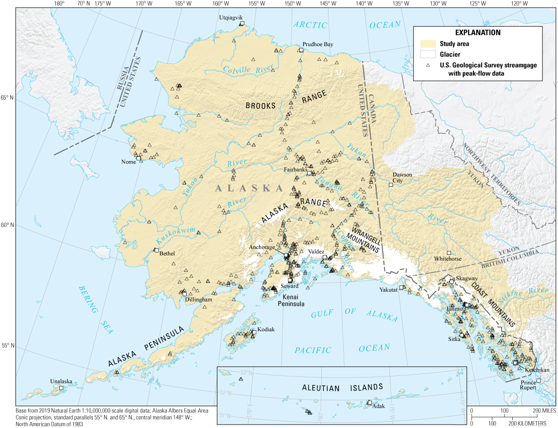
Physical features and streamgages (U.S. Geological Survey, 2024a) used in analyses of floods in Alaska and conterminous basins in Canada through water year 2022.
The Alaska region is geographically and climatically diverse and contains steeply mountainous coastal fjords, lower-elevation coastal islands and coastal plains, extensive high-elevation, glacier-covered mountains, and expansive intermontane plateaus. Wetlands, lakes, and areas of permafrost are abundant. The climate varies regionally along a roughly latitudinal gradient from temperate and wet in Southeast Alaska to cold and dry in the Arctic north, affected by elevation, orographic effects that influence the distribution of rain and snow, and maritime influences that moderate temperature extremes near coastal areas (Stewart and others, 2022).
Annual precipitation amounts range from more than 200 inches in parts of Southeast Alaska to less than 6 inches in the northernmost part of Alaska, falling most abundantly from August to October (Western Regional Climate Center, 2024) and varying from rain to snow depending on the season, elevation, and air temperature associated with individual storms. The most common extreme precipitation-generating storms in the Alaska region are ARs, which are common along coastal areas of western North America but can penetrate deeply into inland areas (Rutz and others, 2015; Gershunov and others, 2017). The remnants of typhoons, or tropical cyclones formed in the Pacific Ocean, can produce intense coastal flooding but can also generate intense precipitation and affect stream flooding when they move inland. ARs, typhoon remnants, and rainstorms associated with other regional processes can persist for multiple days, increasing the chance for elevated soil moisture to compound the effects of precipitation on flooding. In contrast, convective storms (thunderstorms) triggered by daytime heating are more locally sourced and of a shorter duration, generating floods sometimes referred to as flash floods because of the sudden and intense nature of the precipitation and associated runoff. Convective storms are most common in the central interior of Alaska, and most common in July, which is the hottest month in the study area (Poujol and others, 2020). Depending on the area, however, convective storms can also be common in June, August, or September. Although less common, convective storms do occur in Southeast Alaska (Wood, undated).
Cold winter temperatures across most of the Alaska region cause precipitation to be stored seasonally as snow at high elevations in most basins and at all elevations in colder areas. The onset of warmer temperatures can result in a strong flush of snowmelt runoff from nearly synchronous melt across a large area, generating a strong spring increase in streamflow. In high elevation basins, the increase in streamflow from snowmelt slows but persists into summer as snow melts from progressively higher elevations. In basins with glacier cover, further delayed snowmelt from the glacier surface and glacier ice melt provide a melt-based source of streamflow that can continue into fall.
Data Collection and Compilation Methods
Hydrologic data for analysis consisted of annual peak-flow data and daily mean flow data obtained from the USGS National Water Information System (NWIS; U.S. Geological Survey, 2024a) using the dataRetrieval R package (De Cicco and others, 2024). Streamflow values were retrieved for the available period of record for each streamgage through WY 2022. All analyses used the R language and programming environment (R Core Team, 2024).
Streamgages selected for most analyses in this study were drawn from 705 USGS streamgages having at least 1 peak flow in NWIS through WY 2022 (fig. 1), then censored using additional site-selection criteria specific to the analysis. Determination of special conditions for daily mean flows used 729 USGS streamgages that had any available daily mean flow data. Locations for streamgages named in this report or accompanying data releases are available from the NWIS database using the USGS station number (site_no) as an identifier.
Seasonal Flow Regimes
Seasonal flow regimes describe similarities in flow patterns across seasons for a group of streams. The cold climate of the Alaska region and variations in timing of delivery of precipitation facilitate the seasonal dominance of various rainfall-based and melt-based streamflow-generating mechanisms, creating a range of strongly seasonal streamflow patterns. Curran and Biles (2021) grouped hydrographs for 253 streamgages in Alaska into three classes of seasonal flow regimes that each had a different primary daily mean flow driver: (class 1) rainfall, primarily in fall; (class 2) snowmelt, primarily in spring; and (class 3) high-elevation melt, including glacier melt, primarily in summer. These classes were subdivided into nine subclasses that were named using the class plus a letter. The letters were assigned in rough order by increasing dominance of spring snowmelt for classes 1 and 2 and increasing dominance of summer high-elevation melt for class 3. For example, 1A is the most rainfall-dominated regime, 2D is the most strongly snowmelt-dominated regime, and 3C is the most glacier-melt-dominated regime (refer to table 1 of Curran and Biles, 2021, for more details). Hereinafter, this report refers to the subclasses as seasonal flow regimes. Within each seasonal flow regime, Curran and Biles (2021) identified two to three seasonal peak-flow subpopulations corresponding to seasonal spikes in the peak-flow day-of-year density for all streams in the regime and inferred the spring, summer, and fall-to-winter subpopulations to be associated with snowmelt, high-elevation melt, or rainfall, respectively. The dominant peak-flow subpopulation in a regime sometimes varied from the dominant daily mean flow driver, as for the case of regime 2A, a weakly snowmelt-dominated seasonal flow regime where the largest daily mean flows occurred in spring but fall rainfall generated the most peak flows.
Basin Characteristics
Basin Characteristics Data Sources
Basin characteristics were obtained from selected existing datasets for streamgages where data were available. Drainage areas were obtained for all streamgages from NWIS. Estimates of mean annual basin precipitation from Parameter-elevation Regressions on Independent Slopes Model (PRISM) data for Alaska and Canada (PRISM Climate Group, 2002; Gibson, 2009a, b) were available for 483 streamgages from Curran and others (2016) or Curran and Biles (2021), and the most recent value for the respective streamgage was obtained. The streamgage drainage basin boundaries used to obtain mean annual precipitation and other basin characteristics for Curran and others (2016) and Curran and Biles (2021) were retroactively published as data releases (Curran, 2024a, b, respectively) in support of this study.
Cluster Analysis of Drainage Area-Precipitation Groups
Independently, the drainage area and mean annual precipitation of a basin have a strong influence on peak-flow magnitudes at a streamgage, and the values of each of these basin characteristics vary widely throughout the Alaska region. Understanding the distribution of combinations of drainage area and mean annual precipitation can provide a first-order expectation of peak-flow magnitude characteristics. For example, the largest drainage basins are unlikely to only include the wettest areas, limiting the likelihood of the largest basins having the highest specific peak flow, or peak flow per unit drainage area. To find groups of streamgages with similar combinations of drainage area and mean annual precipitation for analysis of group peak-flow magnitude characteristics, a cluster analysis was performed.
Of streamgages where mean annual basin precipitation estimates were available, 455 had unregulated flows and determinate, non-urbanized basins with drainage areas greater than 0.4 mi2 and were selected for a drainage area-precipitation cluster analysis. The selected streamgages were grouped into three drainage area-precipitation categories using a k-means cluster analysis (kmeans function in the stats R package [R Core Team, 2024]) with the logarithms of drainage area and mean annual precipitation as variables. The number of groups was selected using a within-cluster sums of squares plot (fviz_nbclust function in the factoextra R package (Kassambara and Mundt [2020]), aided by visual observation that most streamgages grouped into three quadrants on a logarithmic plot of precipitation against drainage area.
The streamgages clustered relatively cleanly into small and wet (cluster 1), large and dry (cluster 2), and small and dry (cluster 3) drainage area-precipitation groups (fig. 2; Curran, 2025). Cluster-group boundaries were manually simplified to provide a classification tool for future use with other streamgages or ungaged sites (table 1). The simplified boundaries misclassified three streamgages (USGS stations 15264000, 15267900, 15896700) used in the development of the groups; these were not reclassified for the analyses in this study.
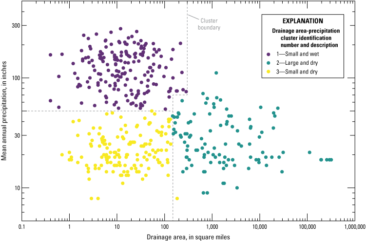
Drainage area and mean annual precipitation for streamgages used to develop drainage area-precipitation cluster groups in Alaska through water year 2022 (Curran, 2025). Simplified cluster boundaries that were developed to provide a tool for estimating drainage area-precipitation cluster groups for streamgages and ungaged sites in Alaska are shown. Values for the simplified cluster boundaries are given in table 1.
Table 1.
Drainage area and mean annual precipitation values determined as boundaries for estimating drainage area-precipitation groups for streamgages and ungaged sites in Alaska.[Cluster group boundaries shown in figure 2. <, less than; ≥, greater than or equal to]
Identification of Streamflow Special Conditions from NWIS Codes and Basin Characteristics
The USGS peak-flow qualification code, peak_cd (table 2), denotes special conditions including selected data-collection conditions, peak-flow-generating mechanisms, basin conditions, and other conditions. The codes are published with the peak-flow data and defined in the NWIS help system (U.S. Geological Survey, 2024b). The selected codes inventoried included those commonly used as site or period-of-record selection criteria in hydrologic analysis.
Table 2.
Peak-flow qualification codes used in the U.S. Geological Survey National Water Information System through water year 2022.[U.S. Geological Survey National Water Information System accessible from U.S. Geological Survey (2024a). Peak-flow qualification codes and definitions shown in this table from U.S. Geological Survey (2024b)]
Peak-flow codes 3 and 9, related to less common flood-generating mechanisms, were inventoried first to provide the primary basis for each code and to provide more detail about the type of flood-generating mechanism (Curran, 2023). A summary of selected special basin and streamflow conditions for all streamgages, including generalized information from the detailed code 3 and 9 inventory, was then prepared (Curran, 2024c). In this summary, the conditions are identified by water year or noted as applicable to all years. Water years for daily mean flows affected by regulation or outburst floods were also inventoried because daily mean flow data are often used to support analysis of peak flows. The summarized basin and streamflow special conditions were used in this report to guide the censoring of entire streamgages or selected water years of peak flows. Details of which conditions were censored varied by analysis and are specified in each respective section of the report.
Identification of Less Common Flood-Generating Mechanisms Using Peak-Flow Codes 3 and 9
Collectively, NWIS peak-flow qualification codes 3 and 9 associate peak flows for Alaska streamgages with special conditions related to less common flood-generating mechanisms, but these codes do not uniquely identify the mechanism. To resolve this, the special conditions forming the basis for code 3 or 9 assignment for all peak flows in the NWIS dataset for Alaska were disambiguated and identified as (1) snowmelt or (2) a sudden release of water. Sudden releases of water (generalized in this report to “outbursts” or “outburst floods”) were further subcategorized by mechanism using the following terms: “glacier dammed lake outburst,” “glacier and debris dammed lake outburst,” “sediment dammed lake outburst,” “mass failure/lake outburst,” “landslide debris dam breakup,” “beaver dam breakup,” “natural flow diversion,” or “subsidence from detonation.” Although several types of outbursts occurred in basins with glacier cover, GLOFs are narrowly defined for this report as glacier (ice) dammed lake outbursts. These types of outbursts can occur repeatedly at a given streamgage and form the most common type of lake drainage events in Alaska (Rick and others, 2023). Curran (2023) defines the mechanism subcategories and documents the peak-flow code basis (peak_code_basis) and peak-flow special condition (pk_spec_cond; that is, snowmelt or type of outburst) that were verified or inferred for each coded peak flow. Although initially associated with this report, Curran (2023) was designed as a versioned data release that can accommodate future updates for subsequent water years.
Code basis determination considered the local code assignment history for the USGS Alaska Science Center (ASC). Peak-flow code 3 is defined as “Discharge affected by Dam Failure” (U.S. Geological Survey, 2024b; table 2). The ASC historically applied peak-flow code 3 to sudden releases of water, including GLOFs and outburst floods from the breakup of debris jams and beaver dams. In response to changes in USGS guidance, code assignment for GLOFs shifted to code 3 plus code 9 in 2006, and then shifted to code 9 in 2018 as part of a nationwide standardization of code assignments (Ryberg and others, 2017). As guidance changed, previously applied codes 3 and 9 were revised for some streamgages in Alaska but were left intact for others to avoid the potential loss of information that would be associated with systematic code changes without site-specific review. The variation in codes assigned for GLOFs did not result from any change in GLOF characteristics. This report used peak-flow qualification codes as they existed in 2024. In April and May of 2025, the ASC systematically reviewed all Alaska peak flows with a code 3, alone or in combination with other peak-flow codes. Using the guidance in Ryberg and others (2017) and the identifications of peak-flow code basis and special conditions in the present study, the ASC revised nearly all code 3s to code 9s or dropped the code 3 if both were present. One code 3 was left intact for a peak generated by ground subsidence from a detonation because this met the intent of the code to denote events that do not represent future flood risk.
Peak-flow code 9 indicates an event other than the prevailing regional peak-generating mechanisms. At the time of this report, the code 9 definition in NWIS (U.S. Geological Survey, 2024b; table 2) lists possible events as snowmelt, hurricane, ice-jam, or debris dam breakup. Additional guidelines in Ryberg and others (2017) expand the list of possible events to include rain-on-snow, tropical storms, and glacial outbursts. The specific events for which a code 9 is assigned are determined by the local USGS office and can vary from region to region. For Alaska, code 9 was minimally assigned prior to 2006, and mostly for outburst floods. Beginning in 2006 and continuing through the time of this report, code 9 was also assigned to differentiate snowmelt from rainfall as the primary flood-generating mechanism for most streamgages, initially crest-stage streamgages and then continuous-record streamgages. Beginning in 2018, code 9 was the sole code assigned to GLOFs. In 2025, the comprehensive ASC update of previously assigned code 3s using newer code-assignment practices resulted in revisions of code 3s to code 9s for GLOFs and most other outburst floods.
Additional data sources used to verify or infer the basis for the codes included reports, online data, and USGS streamgaging notes. A table of references is provided in Curran (2023). The level of review for coded peaks scaled inversely with the number of codes applied in the database as of 2024. Code 3 peaks were less numerous and were individually reviewed. For the relatively few streamgages that had GLOF peaks, all coded peaks (regardless of code) were reviewed. Code 9 peaks were numerous and were reviewed using general criteria such as peak-flow seasonality to infer the code basis.
The interpretations of peak-flow special conditions from qualification codes and streamgaging information in this report can be considered reasonably accurate but depend on the level of review, availability of documentation, and accuracy of the original assessment of flood-generating mechanism. In 2025, as part of a more detailed review of GLOF peaks for USGS station 15052500 (Mendenhall River near Auke Bay, Alaska) for another study, peak-flow codes indicating GLOFs were removed from several peaks because the GLOF contribution to the peak magnitude was reinterpreted as not substantiated or not substantial. Although the 2024 peak-flow codes and Curran (2023) version 2 were used for the rest of the streamgages, the 2025 revised peak-flow codes for this streamgage were used in this report and will be used for subsequent updates of Curran (2023). A few discrepancies existed between dates noted as GLOFs in NWIS peak-flow codes and dates noted as GLOFs or potential GLOFs in other sources identifying GLOFs, including an inventory of glacier dammed lake outbursts compiled by the National Weather Service (National Oceanic and Atmospheric Administration, 2023), which uses USGS streamgage data and additional information. These differences were not resolved for this report and should be reviewed on a site-specific basis as needed. In some cases, for example, no qualification code was applied because, although a GLOF occurred on the date of the peak, it was not considered the primary flood-generating mechanism for the peak. Snowmelt codes were generally intended to be applied for spring snowmelt, but some cases of winter rain-on-snow peaks were given snowmelt codes.
Basin and Streamflow Special Conditions Summary
As a guide to site selection and period-of-record selection for hydrologic analysis using USGS streamgages in Alaska, selected special conditions affecting the basin or streamflow were summarized by streamgage and published in a data release (Curran, 2024c). Data sources included peak-flow codes assigned in NWIS, the disambiguation of selected peak-flow codes presented in the peak-flow special conditions data release associated with this report (Curran, 2023), USGS water-data publications, USGS streamgaging notes, and other sources. Details of data sources and methods are provided in the metadata associated with the data release. Information on special conditions was compiled from available information and not independently verified, making Curran (2024c) most useful for regional studies using multiple streamgages; use for individual streamgages could be accompanied by a more in-depth independent search for information to verify conditions.
The summarized data are described in table 3 and include the type of streamflow available for the streamgage (peak flows, daily mean flows); site special conditions related to the timing of data collection (alternate water years, seasonal water years); basin special conditions related to drainage area (indeterminate drainage area, drainage areas smaller than the minimum value of 0.4 mi2 used for regional studies such as Curran and others, 2016) and land use (urbanization); and a summary of water years for daily mean flows and peak flows affected by regulation or outburst flooding. The summarized data are presented as tabular data in a data release (Curran, 2024c) designed to accommodate future updates as additional water years of data become available or as information for additional conditions becomes available.
Table 3.
Descriptions of basin and streamflow special conditions summarized for U.S. Geological Survey streamgages in Alaska through water year 2022.[Refer to Curran (2024c) for detailed definitions and additional metadata. mi2, square mile; km2, square kilometer]
Inventory of Extreme Floods
Definitions of extreme floods vary with the intended purpose of the results. A goal of this study was to identify a sample of floods as a dataset for assessing the flood-generating mechanisms of very large floods in the region. Additional goals were to provide considerations of the range of possible floods to inform flood-frequency analysis of short-record streamgages, to inform flood forecasting, and to inform assessments of how the prevalence of flood-generating mechanisms could vary in the future with climate change. Although more than one flood can occur in a given water year, the gaging record of peak flows provides a readily available sample of large floods and is unlikely to omit many gaged floods that could be considered extreme.
Extreme floods, given the study goals and dataset, were defined as peak flows that (1) were very large relative to the rest of peak flows in the record or (2) were very large relative to other peaks in Alaska given the basin drainage area (and basin mean annual precipitation, if available). Peak flows could meet either of these criteria for magnitude to be considered extreme, and streamgages could have more than one extreme flood. Flood-frequency statistics (Curran and others, 2016) were used as an extreme flood threshold for the first group. Flood-frequency statistics were available for 49 percent of the streamgages used in this study, which collectively included 76 percent of the peak flows used. The second group consisted of streamgages where flood-frequency estimates had not yet been computed, or where criteria required for flood-frequency analysis such as record length or randomness could not be met. For this group, the 95th percentile of an empirical metric that scaled as a non-linear function of drainage area (Creager and others, 1945) was used to provide a measure of the departure of the flood magnitude from more common floods.
Prior to identification of extreme floods, streamgages and individual peaks were censored to remove peak flows affected by regulation or basin special conditions shown in table 3 using summaries of basin and streamflow special conditions in Curran (2024c). Peak flows having a peak-flow qualification code of 4 for “Discharge less than indicated value which is Minimum Recordable Discharge at this site” (U.S. Geological Survey, 2024b; table 2) were also removed. Although outburst and non-outburst floods were considered separately for some analyses in this report, they were subject to the same criteria for identification of extreme floods. Because flood-frequency statistics in Curran and others (2016) were developed from input data that excluded outbursts for streamgages having enough non-outburst data, this meant that outbursts were evaluated relative to non-outburst flood-frequency statistics, where available.
Floods Exceeding Selected Annual Exceedance Probability Statistics
Flood-frequency estimates are available for many streamgages in Alaska in a region-wide report with data compiled through WY 2012 (Curran and others, 2016). The report presents flood-magnitude estimates for the 50-, 20-, 10-, 4-, 2-, 1-, 0.5-, and 0.2-percent annual exceedance probabilities (AEPs), or the 2-, 5-, 10-, 25-, 50-, 100-, 200-, and 500-year return intervals, where the return interval is computed as 100 divided by the AEP in percent. In addition, the ASC maintains a collection of new or updated flood-frequency analyses that supersede the estimates through WY 2012 (Curran, 2022a). Estimates for five of the study streamgages (USGS stations 15320100, 15348000, 15478449, 15478093, and 15980000) were obtained from analyses in this collection (Curran, 2022b, c; Best, 2023). These sources all present estimated flood-frequency values using three methods: station (at-site) estimates from flood-frequency analysis of observed data at the streamgage, regression estimates computed from regional regression equations, and weighted estimates obtained by weighting the station and regression estimates by their variance. Peak flows were compared to the flood-frequency statistics to determine the largest flood-frequency statistic exceeded using the station and weighted estimates.
The minimum AEP-related threshold for identification as an extreme flood was defined as the streamflow value of the 1-percent AEP (100-year return interval) flood for streamgages having available flood-frequency statistics. This statistic is a standard metric for many design and analysis communities and generated a reasonable sample size for examining flood-generating mechanisms. Peak flows exceeding the 1-percent AEP flood using the station estimate are large relative to the gaged record but can range from exceptionally large to not notably large from a regional perspective. The weighted estimate of the 1-percent AEP flood can help detect floods that appear extreme from a regional perspective while still taking advantage of the site-specific information. To capture extreme floods from either an at-site or regional perspective, peak flows were considered extreme if they exceeded the magnitude of either the station or weighted estimate of the 1-percent AEP flood. This analysis did not consider whether the station or weighted estimate represented a better estimate for the streamgage.
To assess the potential misrepresentation of post-WY 2012 flood frequency caused by using flood-frequency statistics developed for data through WY 2012, post-WY 2012 and through-WY 2012 peak-flow magnitudes were compared for streamgages having post-WY 2012 floods identified as extreme. The number and magnitude of peak flows in each group were visually assessed using statistical summaries such as boxplots to identify substantial post-WY 2012 increases in peak flows that would likely result in mislabeling peaks as extreme. As a result of this screening, peak flows for USGS station 15052000 (Lemon Creek near Juneau, Alaska) were removed from consideration as extreme.
Floods Exceeding Empirical Relative Magnitude Metrics
For streamgages where flood-frequency estimates were not available, thresholds incorporating specific peak flow (the peak-flow value divided by the drainage area of the basin) provided an alternative measure of the departure of the flood magnitude from more common floods. Specific peak flow for the largest peak flow per streamgage varied by about two orders of magnitude across Alaska as a function of drainage area and precipitation (fig. 3), such that specific peak flow alone was not a sufficient metric for identifying extreme peaks. A method that quantifies the variation of specific peak flow with drainage area using empirical curves (Creager and others, 1945) was adapted to adjust for the wide range of precipitation in the Alaska region and applied to peaks as a group and within drainage area-precipitation clusters to determine extreme flood thresholds.
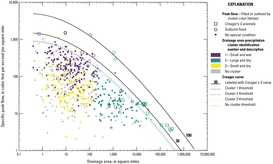
Variation of specific peak flow with drainage area, and drainage area-precipitation cluster group (Curran, 2025) where available, for the maximum flood for each streamgage in Alaska (U.S. Geological Survey, 2024a) through water year 2022. Empirical Creager curves (Creager and others, 1945) for Creager’s coefficient C of 100, 30, and the extreme flood thresholds in table 4 are shown.
Table 4.
Threshold values of Creager’s coefficient C that were used to identify extreme peak flows in Alaska through water year 2022.[Cluster group membership for each streamgage is provided in Curran (2025). Creager’s coefficient C calculated using methods described in Creager and others (1945). Minimum Creager’s C value for extreme peak flows does not apply to streamgages in table 5. Source of Creager’s C threshold excludes streamgages in table 5]
Creager and others (1945) developed a non-linear equation to fit curves of roughly equal relative magnitude to empirical observations of specific peak flow plotted against drainage area on a logarithmic scale. A coefficient, C, scaled the curves by relative magnitude. This resulted in a series of roughly concentric curves that showed the relation of specific peak flow to drainage area for large floods. In the original application, using a global sample of streams that were mostly from the United States, notably large floods were considered those between the Creager curves with values of Creager’s coefficient C equal to 30 and 100. The curves have been used for describing notably large events in Canada (Neill, 1986; refer to fig. 1 of Neill [1986], which shows a reproduction of the original Creager figure and equation) and adjusted to support estimating future design floods in Alberta (Maria and others, 2024).
Creager curves were computed using the Creager equation, with various values for C:
whereq
is the specific peak flow, in cubic feet per second per square mile;
C
is Creager’s coefficient, in variable units; and
A
is the drainage area, in square miles.
Equation 1 was rearranged to solve for Creager’s C:
and applied to the peak-flow values to find Creager’s C for each peak flow. To identify peak flows as extreme floods using the computed Creager’s C values, threshold Creager’s C values for each cluster group and a separate overall threshold were developed in several steps. First, draft thresholds were developed from a dataset of the maximum peak flow per streamgage, which leveraged use of any large floods at short-record streamgages and avoided overweighting long-record streamgages that might have multiple large floods. The 95th percentile of the Creager’s C values for the dataset of maximum peak flow per streamgage was selected as a threshold because it focused on very large floods and produced a reasonable sample size of extreme floods. Using these draft thresholds, the Creager’s C values for all peak flows were then evaluated to find streamgages having anomalous fits to the Creager curves. Following removal of anomalous streamgages from the dataset of maximum peak flow per streamgage, the Creager’s C thresholds were re-computed.
The Creager curves provided a reasonable approximation of relative magnitude for Alaska floods with several exceptions, such as streamgages on the Yukon River, where most or all peak flows exceeded a Creager’s C value of 30. A total of 17 streamgages (table 5) had more than 2 peak flows in the top 5 percent of Creager’s C values overall (Creager’s C greater than 21.1) or in their cluster group (Creager’s C greater than 19.2, 36.7, or 5.76 for cluster groups 1, 2, and 3, respectively) and were considered anomalous Creager’s C fits. Most of these streamgages had very large drainage areas, suggesting that the curves might not fit well for drainage areas larger than 10,000 mi2 in Alaska, results supported by analysis for large drainage areas in Alberta (Alberta Transportation, 2007). Anomalous fits for other basin sizes could relate to variations in the coefficient for different settings other than the drainage area-precipitation clusters used here (Maria and others, 2024).
Table 5.
Streamgages in Alaska having anomalously high Creager’s coefficient C values, determined as more than two peak flows per streamgage having Creager’s coefficient C above thresholds for uncensored data through water year 2022.[Station numbers and names from U.S. Geological Survey (2024a). USGS, U.S. Geological Survey; R, River; nr, near; AK, Alaska; C, Creek]
The streamgages with an anomalous fit to Creager’s C curves (table 5) were removed from consideration for developing Creager’s C thresholds, although they were still evaluated for extreme floods using flood-frequency statistics, if available. After this censoring, the 95th percentile of Creager’s C values was re-computed overall and within each cluster group from the rest of the dataset of maximum peak flow per streamgage. These revised 95th-percentile values are shown in table 4 and were used as an extreme flood threshold for all peak flows at streamgages with no flood-frequency statistics, except for the anomalous streamgages shown in table 5.
Inventories of Floods from Selected Flood-Generating Mechanisms
Groups of peak flows from selected flood-generating mechanisms were identified from qualification codes or inferred from associations with ARs and peak-flow subpopulations for seasonal flow regimes. The resulting information, along with date-specific data sources including historical flood reports and the National Oceanic and Atmospheric Administration Storm Events Database (National Oceanic and Atmospheric Administration, 2024), were used to help assess flood-generating mechanisms of extreme peaks.
Association of Floods with Atmospheric Rivers
To determine AR conditions on or near the dates of peak flows, a dataset of AR presence or absence on an hourly timescale for calendar years 1980–2019 was prepared using an algorithm applied to climate reanalysis data following the methods and data sources of Nash and others (2024). The Tracking Atmospheric Rivers Globally as Elongated Targets (tARget) algorithm (version 3) identifies ARs from their characteristic long, narrow shape, intense flow of water vapor, and poleward direction of movement (Guan and Waliser, 2019). The tARget algorithm was applied to the global, 6‐hour, 1.5-degree horizontal resolution European Centre for Medium-Range Weather Forecasts Re-Analysis (ERA) climate reanalysis dataset “ERA-Interim” (Copernicus Climate Change Service, 2023) to identify ARs, and a bounding box and additional grid points defining land areas were used to determine if the ARs reached land (table 6). If an AR was identified at any land grid point for any of the 6-hour timesteps for the day (coordinated universal time [UTC] 00, 06, 12, and 18), an AR was defined as present for the 6-hour period starting with the timestep. The hourly dataset was converted to Alaska standard time (UTC–9) to match the definition of a day for Alaska peak flows, then reduced to a daily timestep by defining an AR as present for the day if an AR was present for any hourly timestep in the day. Two land areas were considered (fig. 4): the Alaska region truncated at the end of the Alaska Peninsula and a subregion consisting of the Southeast Alaska area used in Nash and others (2024). The bounding box for Southeast Alaska from Nash and others (2024) includes a small area north of Yakutat and conterminous areas in Canada (fig. 4). This bounding box differs from the definition of Southeast Alaska used in this report but is used synonymously in the AR analysis of this study because the differences are small relative to the size of the Alaska region, and the area in the bounding box of Nash and others (2024) does not drain to any streamgages outside Southeast Alaska as used in this report. The resulting binary datasets identified days when at least 1 AR was present (AR days) and days when no ARs were present (non-AR days) within the respective areas for the 1980–2019 period and are available in the Curran (2025) data release.
Table 6.
Latitude and longitude of bounding box and additional grid points used to define land areas for detection of landfalling atmospheric rivers in the Alaska region and Southeast Alaska through water year 2022.[Southeast Alaska bounding box and additional grid points are defined in Nash and others (2024). Latitude and longitude are referenced to North American Datum of 1983]
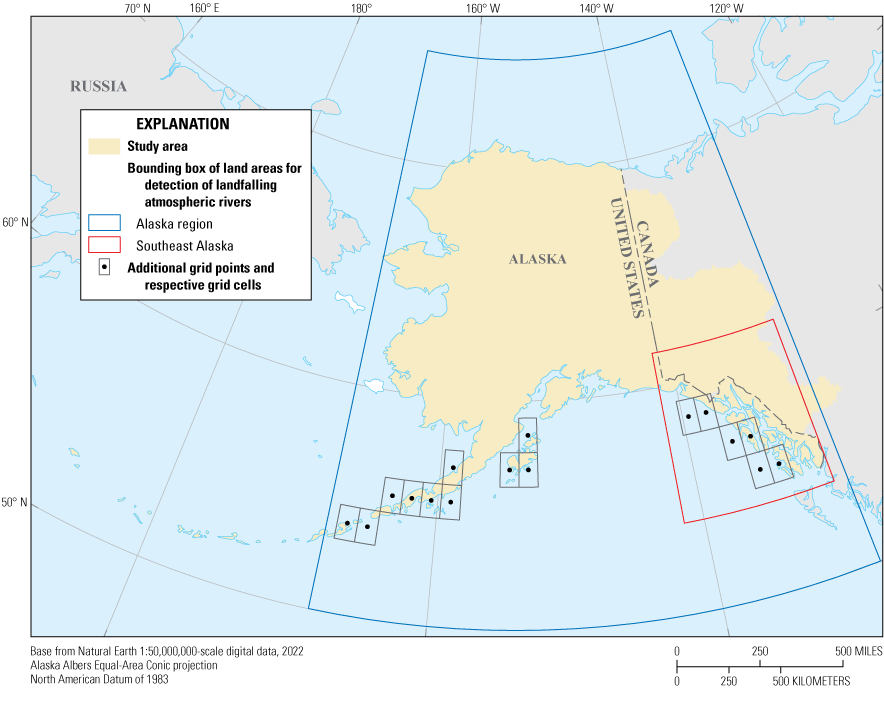
Bounding boxes and additional grid points (table 6) used to define land areas for detection of landfalling atmospheric rivers in the Alaska region and Southeast Alaska through water year 2022. Grid cells shown for the additional points illustrate the 1.5-degree resolution of the ERA-Interim dataset (Copernicus Climate Change Service, 2023). The Southeast Alaska bounding box and additional grid points are defined in Nash and others (2024).
Because ARs can cover large areas, the ARs detected within Southeast Alaska are not necessarily exclusive to the subregion. However, ARs detected in the Alaska region but not in Southeast Alaska can be considered exclusive to areas outside Southeast Alaska. Thus, the nested analysis areas allowed for comparisons of ARs occurring in the Alaska region outside Southeast Alaska to ARs occurring in Southeast Alaska alone or Southeast Alaska plus areas in the Alaska region outside Southeast Alaska.
The definition of an AR day as a day when at least one AR was present in the defined land area assumes that any precipitation falling in that area on that day is related to the AR and associated processes. Nash and others (2024) noted that exceptions to this assumption for Southeast Alaska could include convective post-frontal precipitation. This exception holds for the Alaska region as well, but additional exceptions must be assumed for the larger area of the Alaska region, where other processes unassociated with the AR, such as extratropical cyclones and associated frontal precipitation, could affect streamflow in areas distant from the AR footprint. The identification method also assumes flood-generating mechanisms other than intense precipitation, including smaller amounts of precipitation and warming-related processes such as snowmelt or precipitation falling as rain instead of snow, that occur on an AR day are related to the AR and associated processes. Although AR-related processes can extend beyond the footprint of the AR, the association of these additional flood-generating mechanisms with degraded AR remnants or with areas adjacent to ARs is less well defined and can generate additional errors.
The AR presence or absence data for the Alaska region were joined with the dates of peak flows to identify peak flows occurring on AR days, or AR peak flows. AR days on which at least one peak flow occurred (peak-flow days) were identified as AR-peak-flow days and used for most analyses to minimize overweighting densely gaged areas. The simple association of peak flows with AR days misses peak flows that were associated with an AR that ended on the previous day or previous several days, which could result in an undercount. Delayed response to ARs could occur for complex reasons, but one simple explanation is delayed runoff to the stream for large basins. For example, Sharma and Déry (2020), after constraining AR data to ARs delivering intense precipitation within the basin, considered the AR day and previous 6 days as potentially associated with a peak flow for Southeast Alaska and British Columbia. For the present study, the risk of an overcount related to the collectively high frequency of ARs in the large land areas of the study area contributed to the decision to limit the association of peak flows and ARs to the AR days. AR peaks consisted of unregulated peaks in basins that have none of the special conditions described in table 3 that occurred during the 1980–2019 period (using the peak-flow date, not water years). Stream regionality was assigned as Southeast Alaska for streamgage locations along the southeastern coast of Alaska from Yakutat south, and outside Southeast Alaska for locations north of Yakutat.
Flood-Generating Mechanisms Inferred from Seasonal Flow Regime Data
Curran and Biles (2021) estimated day-of-year boundaries for subpopulations of peaks from three dominant flood-generating mechanisms using low points in density curves of peak-flow day of year. The respective boundaries for each of 9 seasonal flow regimes were adopted for this study and applied to the 253 streams for which seasonal flow regimes were identified in Curran and Biles (2021), resulting in identification of subpopulations of peaks inferred to have a primary flood-generating mechanism of rainfall, snowmelt, or high-elevation melt (including snowmelt and glacier ice melt).
Inferring a dominant flood-generating mechanism from a day of year provides reasonable accuracy for groups of peaks within seasonal flow regimes (Curran and Biles, 2021) but less accuracy for an individual peak. The ability of a day-of-year-based analysis to differentiate mechanisms varies with the mechanism. Although snowmelt as a dominant mechanism can be ruled out for fall peaks, the contribution of rainfall to spring snowmelt or summer high-elevation melt peaks cannot be differentiated from a day of year alone. The inferred mechanisms were therefore considered to be supporting data rather than a definitive determination.
Snowmelt and Related Processes
Snowmelt floods were identified as peak flows assigned a peak-flow qualification code for snowmelt. Although spring snowmelt was the primary process for the snowmelt-coded peaks, other processes known to contribute to spring peak flows include ice-jam flooding. The ASC does not currently assign a peak-flow qualification code to document ice-jam floods. Ice-jam floods are difficult to systematically identify because they can develop long distances from the streamgage and can be difficult to detect during rapidly changing conditions, such as during a dynamic breakup when large pieces of broken ice cover interact. Backwater conditions associated with ice jams downstream from a streamgage can generate flooding (inundated lands) from the highest stage (also referred to as gage height) of the water year while not generating the largest peak flow of the water year, making stage-frequency analysis sometimes more useful than flood-frequency analysis for estimating magnitude and frequency of ice-jam flooding. Stage-related data are provided as part of the peak-flow information in NWIS (U.S. Geological Survey, 2024a). These include the stage associated with the annual peak flow and the annual peak stage if the maximum stage is not that associated with the maximum streamflow. The USGS assigns gage-height qualification code (gage_ht_cd) 1 for “Gage height affected by backwater” and gage-height qualification code 2 for “Gage height not the maximum for the year” (U.S. Geological Survey, 2024b). However, these codes do not necessarily indicate ice-jam floods because backwater conditions are common during spring breakup, when ice can still partly block the stream without generating flooding or peak flows. In addition, an ice jam upstream from a streamgage that breaks up suddenly can generate a peak flow at the streamgage during snowmelt that goes undetected as ice-jam related. For these reasons, ice-jam floods were not inventoried for this report.
High-elevation melt generates floods later in the season than snowmelt floods. High-elevation melt flows have reached large magnitudes, such as flows in late spring to early summer of 1971 across south-central Alaska that would have been notable annual peak flows had they not been exceeded by the extreme floods of fall 1971 (Lamke, 1972). High-elevation melt-dominated peak flows can be difficult to clearly identify because they can occur in association with rainfall. These peak flows are not assigned a peak-flow qualification code and were considered inferred mechanisms for this report using the day-of-year boundaries for seasonal flow regimes. Similarly, rain-on-snow peaks were not inventoried, but extreme winter peak flows were assumed to be associated with rain-on-snow.
Results of Inventories of Special Conditions for Peak Flows
Regulated Floods and Selected Basin Conditions
Streamflow affected by regulation or diversion is one of the special conditions most frequently excluded from regional analysis. Peak-flow qualification codes identified regulation or diversion affecting 607 peak flows, or about 5 percent of the peak flows, at a total of 39 streamgages (Curran, 2024c). Basin special conditions, including urbanization, indeterminate drainage areas, and drainage areas less than the minimum used for regional analysis, affected another 22 streamgages.
Glacial Lake Outburst Floods
The USGS peak-flow record for Alaska contained 150 GLOFs at 15 streamgages (table 7) distributed from the south side of the Alaska Range to Southeast Alaska (fig. 5). Although all the ice-dammed lakes associated with the GLOFs repeatedly released outburst floods, four of the streamgage records included only one or two identified GLOFs (table 7) and were omitted from analysis of patterns in the rest of this section. The gaged records for the 11 streamgages with more than 2 GLOFs are shown in fig. 6.
Table 7.
Gaged annual peak flows identified as glacial lake outburst floods from ice-dammed lakes in Alaska through water year 2022.[Station numbers and names from U.S. Geological Survey (2024a); source lakes from USGS streamgaging notes and National Oceanic and Atmospheric Administration (2023). USGS, U.S. Geological Survey; GLOF, glacial lake outburst flood; R, River; nr, near; AK, Alaska; WF, West Fork; EF, East Fork; Lk, Lake; bl, below; —, no extreme GLOF peak flow]
Unnamed lake at Tazlina Glacier opposite from Iceberg Lake and referred to as Big Lake in National Oceanic and Atmospheric Administration (2023).

U.S. Geological Survey streamgages (U.S. Geological Survey, 2024a) with peak flows affected by glacial lake outburst flooding in Alaska through water year 2022.

Time series of outburst and non-outburst peak flows for U.S. Geological Survey (USGS) streamgages (U.S. Geological Survey, 2024a) with at least three peak flows affected by glacial lake outburst flooding in Alaska (table 7) through water year 2022. Each graph is labeled with USGS station number and name. [NR, near; AK, Alaska; GLOF, glacial lake outburst flood.]
GLOF magnitude is dependent on lake volume and how quickly water can drain through pathways formed in the impounding glacier during the flood (O’Connor and others, 2013). Contributing factors are time-varying and site-specific, including glacier thickness, lake water levels, and rates of thermal erosion of subglacial drainage conduits. In addition, lakes can generate multiple GLOFs in a year, generate a GLOF every few years, or stop generating GLOFs completely when the impounding glacier retreats or thins below the minimum lake level. This makes GLOF magnitude and timing difficult to predict or generalize, although some GLOF peak flows have shown patterns in magnitude and timing that have varied over time.
GLOF peak flows varied in magnitude, with some being similar to floods from other mechanisms, and others being extreme floods. As a statistical group, however, the subpopulation of GLOF peak flows was consistently larger than the subpopulation of non-GLOF peak flows at the streamgage. At the eight study streamgages in table 7 with more than two peaks in both GLOF and non-GLOF peak-flow subpopulations, the median magnitude of GLOF peaks exceeded the median magnitude of non-GLOF peaks (fig. 7). Statistical tests comparing the subpopulations (Welch’s two-sample t-tests using t.test in the stats R package [R Core Team, 2024]) showed a strongly statistically significant (p ≤ 0.005) difference in the mean of the logarithms of the subpopulations for most streamgages in table 7 but no statistically significant difference in the mean of the logarithms of the subpopulations using a level of significance (α) of 0.05 for the streamgages on the Taku and Copper Rivers.
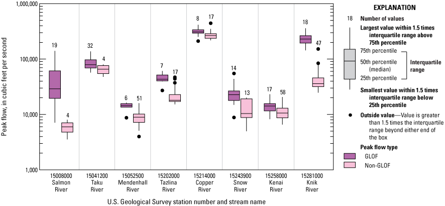
Comparison of the magnitude of outburst and non-outburst peak flows for U.S. Geological Survey (USGS) streamgages with more than two peak flows affected by glacial lake outburst flooding and more than two non-outburst peak flows in Alaska (table 7) through water year 2022. Each plot is labeled with USGS station number and stream name. Full USGS station names are given in table 7. [GLOF, glacial lake outburst flood.]
Differences in magnitude between subpopulations for the streamgages shown in fig. 7 were notable for streamgages subject to extreme GLOF peaks (table 7). Extreme GLOFs occurred repeatedly at the Salmon River streamgage, especially during the first period of discontinuous data collection, WYs 1964–73, and the Knik River streamgage, where GLOFs last occurred in WY 1966. A downstream decay in the strength of the difference between GLOF and non-GLOF subpopulations can be seen by comparing the response to Snow Lake GLOFs at the Snow River streamgage (USGS station 15243900; about 3 miles upstream from 22-mile-long Kenai Lake on the Kenai Peninsula) to the response at the Kenai River streamgage at the downstream end of Kenai Lake (USGS station 15258000), where the GLOF peaks diminished in proportion to non-GLOF peaks but remained larger than non-GLOF peaks, on average (figs. 6, 7). For the Taku River streamgage, Neal (2007) extracted the largest annual non-GLOF peak from the gaging record through WY 2004 and showed a considerable interannual range in the relative magnitudes of GLOF and non-GLOF peaks (fig. 10 of Neal [2007]).
Trends in GLOF magnitude are difficult to characterize and not consistent among streamgages. Several apparent patterns exist in the gaged records for the streamgages shown in fig. 6, including (1) a clear shift at the Salmon River streamgage from larger GLOF peaks during the initial period of gaging (ending in WY 1973) to smaller GLOF peaks during the second period (starting in WY 2010); (2) a weak positive trend at the Snow River streamgage (USGS station 15243900) found by Beebee (2023) using additional estimated magnitudes and analysis; and (3) a positive trend at the Knik River streamgage from the start of gaging in WY 1948 until the early 1960s, followed by a declining trend until the cessation of GLOFs after the WY 1966 GLOF. In many cases, however, systematic gaging began after the onset of GLOFs, such that patterns in gaged GLOFs might not be an accurate characterization of long-term annual maximum GLOF patterns. For example, the annual GLOFs from Lake George that affected the Knik River streamgage extend back to 1914 (Bradley and others, 1972), and Tulsequah Lake GLOFs, which affect flows at the Taku River streamgage, have occurred since the early 1900s (Neal, 2007).
The timing of the day of year of occurrence for recurring GLOFs ranged from June to December across the 11 streamgages and spanned several months during the period of record for most streamgages. At some streamgages, GLOF seasonality visibly trended toward occurring earlier in the year during the period of GLOF occurrence (fig. 8). Specifically, Salmon River GLOF peaks occurred later in the year during the initial period of gaging and earlier in the second period; Taku River GLOF peaks showed a trend toward earlier occurrence throughout the period of gaging, and Knik River GLOF peaks showed a strong trend toward earlier occurrence from the start of gaging through the last GLOF. Although this report only considers the largest GLOF in a year, and only GLOFs that are also the annual peak, Rick and others (2023) performed a more rigorous analysis on all GLOFs, regardless of size, from selected lakes and noted a trend toward earlier seasonality for Tulsequah Lake GLOFs, which affect streamflow at the Taku River streamgage. Because the gaging record for many GLOF streamgages starts well after the onset of GLOFs, the data shown in this report provide a snapshot of a variable period of GLOF occurrence.

Day of year of occurrence for outburst and non-outburst peak flows for U.S. Geological Survey (USGS) streamgages (U.S. Geological Survey, 2024a) with at least three peak flows affected by glacial lake outburst flooding in Alaska (table 7) through water year 2022. Each graph is labeled with USGS station number and stream name. Full USGS station names are given in table 7. [GLOF, glacial lake outburst flood.]
Other Outburst Floods
Outburst floods other than GLOFs in the peak-flow record included 10 peaks from a wide range of flood-generating mechanisms (table 8), all occurring in Southeast Alaska or south-central Alaska (fig. 9). The outburst floods other than GLOFs included beaver dam breakups at two different streamgages (USGS stations 15238986 and 15261000) in different years and breakup of temporary landslide debris dams at three streamgages (USGS stations 15238000, 15238010, and 15238600) that occurred during an October 1986 rainstorm in Seward (Jones and Zenone, 1988). In addition, a large regional rainstorm in south-central Alaska in August 1971 triggered outburst peaks through three separate mechanisms: (1) for the outburst flood at USGS station 15294500, rapid change of the outlet of Chakachamna Lake, the source lake for Chakachatna River, which was dammed by glacier ice and sediment at a glacier terminus (Lamke, 1972); (2) for the outburst flood at USGS station 15284000, failure of a sediment dam (reported as a moraine by McGee, 1974, but could be interpreted from elevation data as landslide debris) that had impounded a lake in the basin of Granite Creek, a tributary of the Matanuska River (Lamke, 1972); and (3) natural diversion of a stream from a flow path along Sheep Creek to a flow path along Goose Creek, creating an outburst flood at USGS station 15292900 that is considered an indeterminate drainage area case for the analyses in this report. In 2002, a mass failure involving a moraine and saturated sediments from a tributary valley entered a pro-glacial lake and generated an outburst flood at USGS station 15056210 in Southeast Alaska (Capps, 2004). Finally, detonation-induced ground subsidence generated a flood at USGS station 15297690 coded as an outburst and which is considered a regulated peak for the analyses in this report.
Table 8.
Gaged annual peak flows identified as outburst floods other than glacial lake outburst floods in Alaska through water year 2022.[Peak-flow special conditions from Curran (2023). Station numbers and names from U.S. Geological Survey (2024a). USGS, U.S. Geological Survey; R, River; nr, near; AK, Alaska; C, Creek; hwy, highway; mi, mile; ab, above; Is, Island]
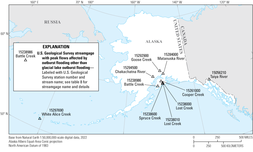
U.S. Geological Survey streamgages with peak flows affected by outburst flooding other than glacial lake outburst flooding in Alaska (Curran, 2023; U.S. Geological Survey, 2024a) through water year 2022.
The relative magnitude of the outburst floods other than GLOFs ranged considerably, from less than the maximum peak on record for the streamgage to peaks considered extreme for this study. Of the five streamgages in table 8 with weighted flood-frequency estimates, three streamgages had floods that exceeded the 0.2-percent AEP (500-year return interval) flood value. One of these was the 1971 flood recorded at the Matanuska River streamgage (USGS station 15284000), where flow had already crested at a peak of record from the 1971 rainstorm (Lamke, 1972) when the outburst floodwaters from tributary Granite Creek arrived and further swelled the river. The relative magnitude of the gaged peak flow, although notable for the large Matanuska River Basin, pales in comparison to the relative magnitude for the much smaller tributary basin (Lamke, 1972), providing insight into the potential magnitudes of the full subpopulation of outburst floods other than GLOFs in Alaska.
The conditions associated with these outburst floods other than GLOFs (table 8) were isolated events and have been considered unlikely to reoccur multiple times, or at all, at these streamgages for the purposes of flood-frequency analysis (Curran and others, 2016). However, beaver dams can be rebuilt, and landslides, although infrequent, can reoccur, highlighting the need for user interpretation for this type of special condition. Although the Taiya and Chakachatna River outburst floods involved lakes at or near the terminus of glaciers, the flood-generating mechanisms were associated with mass failure (Taiya River) or erosion of sediment (Chakachatna River), conditions that would be difficult to reconstruct.
Snowmelt Floods
The peak-flow qualification code for snowmelt, intended to differentiate snowmelt peak flows from rainfall peak flows, created a dataset of peaks with spring snowmelt as their dominant flood-generating mechanism. From WY 2006, when snowmelt codes began to be more systematically applied to many streamgages, to WY 2022, a total of 530 peaks that were not affected by regulation or diversion and were not in basins with a special condition affecting flow (table 3) received the code. This dataset is opportunistic in that the peak-flow codes were not applied to every streamgage where snowmelt peak flows existed, but for the streamgages where codes were applied, this dataset provides an opportunity to examine subpopulation characteristics.
The 141 streamgages with at least one snowmelt-coded peak flow were distributed across a wide range of the State (fig. 10), but 96 percent were located in areas outside Southeast Alaska. The dominant months for snowmelt-coded peak flows were May (70 percent of the peak flows) and June (23 percent). Six percent of the snowmelt-coded peaks occurred in April, and the 1 percent that occurred in winter (December–February) were likely rain-on-snow peak flows.
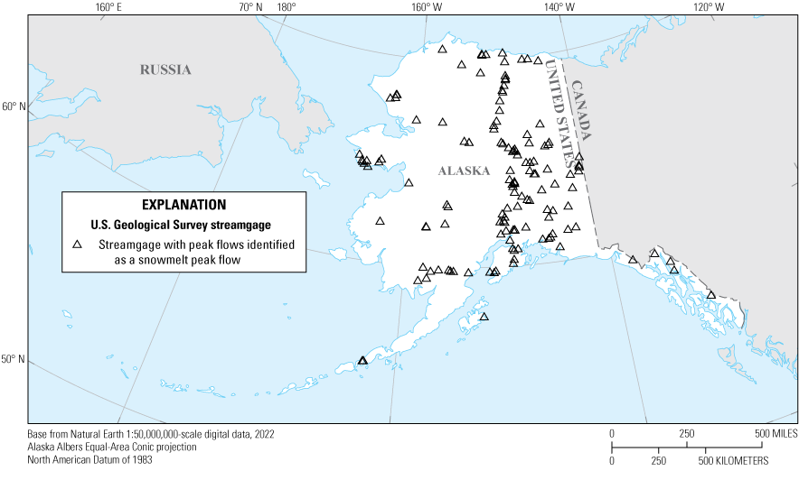
U.S. Geological Survey streamgages with peak flows identified as a snowmelt peak flow from peak-flow qualification codes in Alaska (Curran, 2023; U.S. Geological Survey, 2024a) through water year 2022.
For streamgages where seasonal day-of-year ranges for flood-generating mechanisms were available for seasonal flow regimes from Curran and Biles (2021), the primary flood-generating mechanism inferred from the peak day of year for the snowmelt-coded peak flows was consistently snowmelt, providing a one-directional check on the accuracy of the inferred primary flood-generating mechanism from the day-of-year data. The snowmelt-coded peak flows occurred at streamgages in every seasonal flow regime except regime 1A, the most rainfall-dominated regime, supporting observations of the existence of snowmelt-peak subpopulations in most flow regimes in Alaska.
Snowmelt peaks were assumed to be smaller, as a group, than peaks from other flood-generating mechanisms for all but the most snowmelt-dominated seasonal flow regimes (Curran and Biles, 2021), such as regime 2D, which includes USGS station 15896000, (Kuparuk River near Deadhorse, Alaska), where 16 of 17 peaks during WYs 2006–22 are snowmelt-coded. To quantify the difference in magnitude between snowmelt-coded peaks and other peaks, streamgages with (1) at least 3 snowmelt-coded peaks and 3 non-snowmelt-coded peaks, (2) a total of at least 10 years of unregulated, non-outburst peak flows, and (3) none of the basin special conditions affecting flow listed in table 3 were selected. The median magnitude of snowmelt-coded peaks was smaller than the median magnitude of non-snowmelt-coded peaks for 70 percent of the 50 selected streamgages.
Floods Associated with Atmospheric Rivers
ARs occur frequently in the Alaska region, with AR days amounting to 67 percent of the days in the 1980–2019 period. The frequency of ARs for the Alaska region and their ability to persist for multiple days created such frequent AR conditions that 92 percent of the days were AR days or within 3 days of an AR day. The count of days on which an AR occurred anywhere in the region is inflated relative to the count for any one location but can be used as a metric for assessing ARs that can cover multiple parts of the State. Although true subregion comparisons were not possible with only one subregion, ARs were frequent inside and outside Southeast Alaska (fig. 11A). The percentage of days in the period when an AR occurred in the Alaska region can be subdivided into the percentages when ARs were present or absent in Southeast Alaska. ARs were present in Southeast Alaska on 35 percent of the days in the period, occurring 8–15 days a month (first presented in Nash and others, 2024; identical results from the present study are shown in fig. 11A). ARs were present in the Alaska region but absent from Southeast Alaska on 32 percent of the days in the period (fig. 11A). This shows the relatively high frequency of ARs in Southeast Alaska (for its land area) and shows a substantial presence of ARs in the Alaska region outside Southeast Alaska.
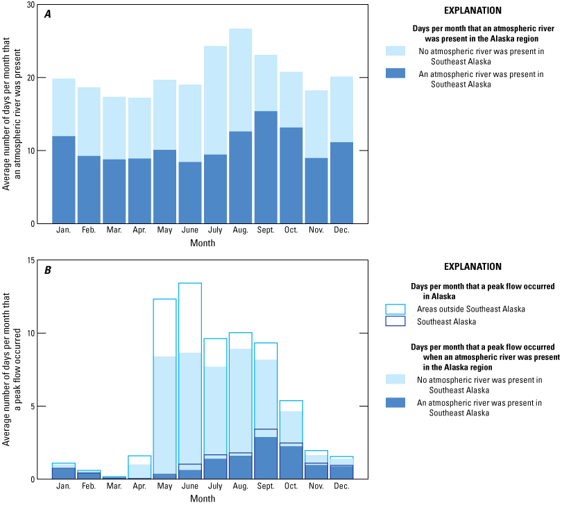
Mean monthly frequency of atmospheric rivers (Nash and others, 2024; Curran, 2025), peak flows (U.S. Geological Survey, 2024a), and coincident atmospheric rivers and peak flows, 1980–2019. Bounding boxes for detection of atmospheric rivers in the Alaska region and in Southeast Alaska are shown in fig. 4. Days when an atmospheric river was present in Southeast Alaska and an atmospheric river was also present in areas outside Southeast Alaska are included in the count for Southeast Alaska. A, Mean monthly frequency of atmospheric rivers in the bounding box for the Alaska region (overall bar height) and in subregional areas. The bounding box and atmospheric river presence data for Southeast Alaska are from Nash and others (2024). B, Mean monthly frequency of gaged peak flows in Alaska (overall outlined bar height) and subregional areas, and gaged peak flows that occurred on a day when an atmospheric river was present in the bounding box for the Alaska region (overall shaded bar height) and in subregional areas.
ARs occurred in every month of the year, most frequently during July–September for the Alaska region (fig. 11A). ARs had a slightly summer-dominated seasonality (July–August) in areas outside Southeast Alaska and a primary fall (August–October) and secondary winter (December–January) seasonality in Southeast Alaska. This pattern is consistent with the general southward-progressing timing of AR landfalls for the West Coast of North America (Gershunov and others, 2017). Relative to ARs, peak flows are more strongly seasonal, occurring primarily from spring to fall (May–October) for the Alaska region, and summer to winter (July–January) for Southeast Alaska (fig. 11B). Seasonal differences in amounts of moisture transport in ARs (Gershunov and others, 2017) and precipitation falling as snow contribute to the differences in seasonality of the relation of AR processes and peak flows.
Despite the high frequency of AR days, only 21 percent of the AR days in the full period and 35 percent of AR days from May to October coincided with peak-flow days. However, 78 percent of the peak-flow days in the full period and 78 percent from May to October occurred on AR days (fig. 11B), an association with ARs that is statistically greater than the percentage of days that are AR days (using a 1-sample proportions test with the “greater” alternative and p < 0.5 in the prop.test function in the stats R package [R Core Team, 2024]). Although streamgages with peak flows associated with ARs occurred across most of the State (fig. 12), peak-flow days for Southeast Alaska streamgages were more strongly associated with ARs, on average during the year, than those for streamgages outside Southeast Alaska. For streamgages in Southeast Alaska, 86 percent of peak-flow days were on AR days, whereas for streamgages outside Southeast Alaska, 76 percent of peak-flow days were on AR days. The observation that a small percentage of ARs are responsible for extremes in streamflow echoes findings of other studies relating ARs to extreme precipitation (Nash and others, 2024) or streamflow (Sharma and Déry, 2020) in Southeast Alaska. Using the same Southeast Alaska AR presence or absence dataset as this study, Nash and others (2024) found that 6 AR days per year accounted for as much as 91 percent of the precipitation extremes in 6 Southeast Alaska communities, despite the presence of ARs on 122 days per year on average during the period. They identified the strength of the water vapor transport and the direction of the water vapor transport with respect to complex local coastal topography as important factors for generating extreme precipitation events. For the present study, 458 streamgages, or 69 percent of the 663 streamgages used for analysis, had at least 1 peak associated with ARs (fig. 12). AR peak flows occurred in all 9 seasonal flow regimes and were most common in regime 1A, the most rainfall-dominated regime, where 96 percent of the peak flows occurred on AR days, and least common in regime 2D, the most snowmelt-dominated regime, where only 61 percent of the peak flows occurred on AR days.

U.S. Geological Survey streamgages in Alaska with at least one peak flow (U.S. Geological Survey, 2024a) on the day an atmospheric river was present in the Alaska region (Curran, 2025), 1980–2019.
The association of peak-flow days with ARs varied seasonally and to some degree with geographic area (fig. 11B; table 9). For the May–October period, the association with ARs for Alaska was greatest during the late summer and early fall, reaching a high of 89 and 88 percent of peak-flow days occurring on AR days in August and September, respectively (using the two areas shown in table 9 combined). The association was slightly stronger (91 percent) and peaked later (October) in Southeast Alaska. The association was notably lower for Alaska in spring, when snowmelt peaks are common. For WYs 2006–19, when snowmelt peak-qualification codes were consistently applied and AR data were available, ARs occurred from May to June on 67 percent of the days, and 63 percent of the 244 snowmelt-coded peak flow days coincided with an AR day. The snowmelt-coded peak association with ARs was not statistically significantly less than the general association with ARs for that time of year using a one-sample proportions test with the “less” alternative and p < 0.5 in the prop.test function in the stats R package (R Core Team, 2024). The overlap of peak-flow days and AR days in December and January, the winter months when peak flows were common enough to assess, was high for areas inside and outside Southeast Alaska, ranging from 86 to 93 percent (table 9).
Table 9.
Association of peak-flow days with days of atmospheric rivers by month and location of streamgage in Alaska, 1980–2019.[Peak flow data from U.S. Geological Survey (2024a). Association of peak flow days with days of atmospheric rivers done using data from Nash and others (2024) and Curran (2025). AR, atmospheric river; AR day, day on which an atmospheric river occurred]
Comparing the magnitude of AR peak flows to non-AR peak flows within streamgages shows some modest tendencies for AR peaks to be larger, especially for larger flow percentiles. To quantify the difference in magnitude, streamgages with (1) at least 3 AR peaks and 3 non-AR peaks, (2) a total of at least 10 years of unregulated, non-outburst peak flows, and (3) none of the basin special conditions affecting flow listed in table 3 were selected. The median magnitude of AR peaks was greater than the median magnitude of non-AR peaks for 60 percent of the 128 selected streamgages. The 75th percentile of AR peaks (corresponding to the upper quartile of a boxplot) exceeded the 75th percentile of non-AR peaks for 70 percent of the streamgages.
Some of the associations of peak flows with ARs are likely the result of ARs with rain-on-snow events, where processes associated with warmer ARs produce snow water equivalent loss that increases streamflow-to-precipitation ratios. For example, in winter months in the Sierra Nevada, Guan and others (2016) noted that AR conditions, more common in winter in that region, were associated with 50 percent of the rain-on-snow events and that ARs with rain-on-snow were warmer than ARs without rain-on-snow. The presence of ARs in the Alaska region during many snowmelt-coded peaks at many of the northernmost streamgages (streamgages near or north of the Brooks Range), where ARs footprints might not overlap the drainage basin of the streamgage, could be a non-causal association or could indicate that regional warming in association with an AR plays a contributing role for spring snowmelt peak flows.
Extreme Floods
The gaging record contained 149 peak flows identified as extreme floods, which amounted to 1.5 percent of the unregulated peaks in basins with no special conditions. Most of the extreme floods were identified using the 1-percent AEP flood magnitude as a minimum, although 19 percent did not have flood-frequency statistics and were identified using the Creager’s C values from table 4 as minimum thresholds. Figure 13 shows non-outburst extreme flood magnitudes and identification methods and figure 14 shows extreme outburst flood magnitudes by streamgage. All but one of the extreme outburst floods identified using flood-frequency statistics also exceeded the Creager’s C threshold for the streamgage. Extreme floods occurred in locations that were widely distributed around the State, although extreme outburst floods (fig. 14) occurred only in Southeast Alaska and south-central Alaska (fig. 15). A total of 12 streamgages recorded more than 1 non-outburst extreme flood, and 3 streamgages recorded multiple extreme outburst floods. Details of flood-frequency statistics exceeded, Creager’s C, flood-generating mechanisms, and other information are provided for the extreme peaks in a data release (Curran, 2025).

Specific peak flow, drainage area, and threshold used for identification for non-outburst extreme floods (Curran, 2025) at U.S. Geological Survey streamgages (U.S. Geological Survey, 2024a) in Alaska through water year 2022. Empirical Creager curves (Creager and others, 1945) for Creager’s coefficient C = 100, 30, and the extreme flood identification thresholds in table 4 are shown for reference. The water year 2022 peak flow for U.S. Geological Survey streamgage 15478499 is discussed in the text. [WY, water year.]
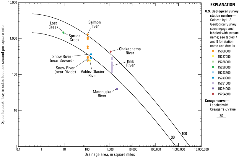
Specific peak flow, drainage area, and USGS station names for extreme outburst floods (Curran, 2025) at U.S. Geological Survey streamgages (U.S. Geological Survey, 2024a) in Alaska through water year 2022. Empirical Creager curves for Creager’s coefficient C = 100 and 30 are shown for reference (Creager and others, 1945).
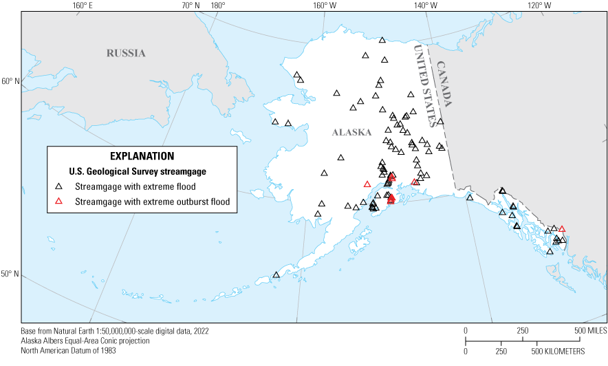
U.S. Geological Survey streamgages with extreme floods in Alaska (U.S. Geological Survey, 2024a; Curran, 2025) through water year 2022.
Results of Assessment of Flood-Generating Mechanisms for Extreme Floods
Extreme outburst floods, which constituted 26 percent of the extreme floods for Alaska streamgages, generated the largest specific peak flows and the largest relative magnitudes (Creager’s C values) in the gaged record (fig. 14; Curran, 2025). Landslide-debris-dam outburst floods recorded at Lost and Spruce Creeks, where the streamgages had relatively small drainage areas, generated the largest specific flows. However, outbursts from changes to a lake outlet at the Chakachatna River and from GLOFs at the Salmon and Knik Rivers had relative magnitudes larger than those at Lost and Spruce Creeks, including two outburst floods with Creager’s C values that exceeded 100. Although not all outbursts create extreme floods, the largest outbursts generated relative magnitudes (fig. 14) that far exceeded the largest relative magnitudes of non-outburst extreme floods (fig. 13). The magnitude of outburst floods is strongly dependent on basin conditions that can relate to geologic or geomorphic conditions, climate, or glacier dynamics. To the extent that these basin conditions can be considered regional factors relative to other global locations, the relative magnitudes of the extreme outburst floods provide perspective for understanding the historical severity and distribution of gaged outburst floods in Alaska.
About one-third (48) of the gaged extreme non-outburst floods were described in historical reports of 12 impactful floods (table 10). The historical flood reports provided opportunistic identification of the flood-generating mechanisms, supported by AR presence or absence data for flood dates within the period of AR data availability. Although the level of detail available varied, all events in the reports were documented as rainstorms or outburst floods during rainstorms, with rainstorm types including typhoon remnants, rainstorms when an AR was present (assumed to be AR-related rainstorms), convective storms, and undifferentiated rainstorms. Contributing factors noted in the reports included (1) elevated antecedent soil moisture from recent rainstorms, (2) warm temperatures and high freezing levels that delivered rain instead of snow to higher elevations than normal for the season or that melted recent snowfall, and (3) elevated antecedent streamflow from recent rainfall or warm temperatures that generated high-elevation melt.
Table 10.
Extreme-flood-generating mechanisms for notable regional floods in Alaska described in selected historical flood reports through water year 2022.[USGS, U.S. Geological Survey; AR, atmospheric river]
| Reported event dates | General location of flood | USGS station numbers for streamgages with extreme peaks | Flood-generating mechanism comments (and association with ARs in the Alaska region when available) | Data source citation |
|---|---|---|---|---|
| August 8–20, 1967 | East-central Alaska (near Fairbanks) | 15484000, 15511000, 15514000, 15515500, 15530000 | Typhoon remnants | Childers and others (1972) |
| September 15, 1967 | Lynn Canal area of Southeast Alaska (near Skagway) | 15056200, 115056210 | Rainstorm that moved inland from Pacific Ocean | Boning (1972) |
| August 8–11, 1971 | South-central Alaska | 15283500, 15285000, 15290000, 15291000, 15292780, 215294500 | Rainstorm (following a recent rainstorm in some locations) | Lamke (1972) |
| August 10, 1971 | South-central Alaska | 215284000 | Sediment-dammed lake outburst during rainstorm | McGee (1974) |
| October 9–12, 1986 | South-central Alaska | 215238000, 15238400, 215238600, 15243950, 15292780, 15292800, 15293000, 15294025, 15294100 | Rainstorm (AR present) | Jones and Zenone (1988); Lamke and Bigelow (1988) |
| 3August 15–18 and August 23–27, 1994 | Middle Koyukuk River Basin (about 200 miles northwest of Fairbanks) | 15564875, 15564884, 15564897, 15564900, 15743850 | Two consecutive rainstorms (AR present) | Meyer (1995) |
| September 19–October 2, 1995 | South-central Alaska | 15266300, 15277100, 15277410, 15281000 | Subtropical cyclone following recent cyclones (AR present except September 29 and October 2) | National Oceanic and Atmospheric Administration (1996) |
| October 22–24 and November 23, 2002 | Kenai Peninsula | 15239800, 15239900, 15240000, 15240500, 15241600, 15261000 | Rainstorms during prolonged wet and warm period (AR present) | Eash and Rickman (2004) |
| August 18–21, 2006 | South-central Alaska | 15292400 | Rainstorm (AR present) | Joling (2006) |
| October 9–11, 2006 | South-central Alaska | 15208000, 15212000, 15212500, 15226600, 15243950 | Rainstorm following recent snowfall (rain-on-snow) (AR present) | Associated Press (2006) |
| September 20–30, 2012 | Kenai Peninsula | 15276000, 15292780 | Rainstorm (AR present except September 29) | Pearson (2012) |
| July 10–11, 2022 | Richardson Highway (about 100 miles southeast of Fairbanks) | 15478093, 15478499 | Convective storm | Plumb and Ostman (2023) |
The examples from the reports provide a sample of rain-related processes for extreme floods in Alaska and detail for examples of primary and secondary flood-generating mechanisms. The potential for convective storms to generate extreme floods well beyond the magnitudes expected for other processes for small basins, especially small and dry basins, was highlighted by the record 2022 flooding along the Richardson Highway. The WY 2022 peak flow for USGS station 15478499 (Ruby Creek above Richardson Highway near Donnelly, Alaska), a basin of 4.9 mi2 in relatively dry cluster group 3, exceeded a Creager’s C of 30, making it one of the largest relative magnitudes on record for non-outburst peak flows in Alaska (fig. 13). The effects of secondary factors on generating extreme floods were well illustrated for the August 1994 flood on the Koyukuk River (Meyer, 1995). Extreme peak flows occurred at several streamgages (table 10) on August 31, which followed the second of two rainstorms spaced 5 days apart, each delivering similarly large amounts of precipitation to the basin. Meyer (1995) attributes the large magnitude of the flood peak to additional runoff from saturated soils and to already elevated river stages from the first storm.
Collectively for non-outburst extreme floods, the historical flood reports (table 10), AR associations (Curran, 2025), inferred mechanisms from date ranges for seasonal flow regimes (Curran and Biles, 2021), and generalized inferred mechanisms from seasonal associations confirmed rainfall as the dominant flood-generating mechanism and melt-based processes as an important contributor to extreme floods. Rainfall as the sole or strongly dominant mechanism generated 72 percent of the non-outburst extreme floods, and melt-based processes formed a primary or secondary mechanism for 26 percent (Curran, 2025). Flood-generating mechanisms could not be determined for 2 percent of the non-outburst extreme floods because the month and day of the peak flows were unknown and no other information was available. Non-outburst extreme floods were most common from June–October and relatively uncommon in winter and early spring (table 10; Curran, 2025).
Non-outburst extreme floods were more strongly associated with ARs than was the full dataset of peak flows. Rainfall-related floods on AR days made up 66 percent of the 65 non-outburst extreme floods during the period when AR data were available, and melt-related floods from snowmelt, rain-on-snow, or undifferentiated high-elevation melt and rainfall on AR days made up 17 percent. The 10 non-outburst extreme floods that occurred on a day in that period when ARs were absent were attributed nearly evenly to snowmelt (3 floods), rainfall from convective storms (4 floods), and rainfall from undifferentiated rainstorms (3 floods), and the AR status of 1 flood could not be determined because the day of the peak flow was unknown.
Considerations for Future Changes to Floods
Future flood-generating mechanisms are likely to include existing mechanisms shifted in their timing, intensity, or geographic extent. For example, modeling of changes associated with loss of sea ice along the western and northern coasts of Alaska and other warming-related effects predicts that convective storms will triple in number and increase in intensity in the northern parts of Alaska, including the North Slope and western Alaska (Poujol and others, 2020). A study of ice-dammed lakes in Alaska (Rick and others, 2023) found no change in GLOF frequency but also found decreases in lake size that could signal reduced GLOF magnitudes. The relatively recent (2011) onset of Suicide Basin GLOFs on the Mendenhall River demonstrates that new GLOFs in basins with no history of outbursts can be expected as glaciers thin and retreat. However, GLOF magnitudes continue to have the potential for a high degree of variability. A sudden and large increase in Suicide Basin GLOF magnitudes on the Mendenhall River occurred just after the period of record used for this study, impacting hundreds of homes near Juneau, Alaska. Mendenhall River GLOFs in WY 2023 and 2024 (U.S. Geological Survey, 2024a) were more than twice the magnitude of any GLOFs on the Mendenhall River through WY 2022 (fig. 16) and would have met the definition of extreme for this study. Accelerating glacier loss (Hugonnet and others, 2021) is expected to initially produce additional high-elevation melt in some basins and later less melt as glacier size diminishes (Huss and Hock, 2018). In other basins where substantial glacier loss has already occurred, less melt can be expected, and in either case, changes in melt that differ by month can be expected (Huss and Hock, 2018). As scaling metrics for AR intensity, duration, and effect are developed for Alaska (for example, Nash and others, 2024), a better understanding of future AR effects will emerge.

Time series of glacial lake outburst and non-glacial lake outburst peak flows (Curran, 2023; U.S. Geological Survey, 2024a) for U.S. Geological Survey (USGS) station 15052500 (Mendenhall River near Auke Bay, Alaska) through water year 2024. [NR, near; GLOF, glacial lake outburst flood.]
The translation of predictions in changes in flood-generating mechanisms to changes in flooding is facilitated by understanding the historical range and dominance of flood-generating mechanisms. However, the complex relations between rain-based and melt-based runoff, and the host of secondary factors associated with extreme flooding, create complicated feedbacks that can be explored by modeling. For example, a change in the rain-to-snow fraction resulting in precipitation falling as rain that would have fallen as snow can decrease or increase flooding, depending on the season. Reduced snowpack in winter can lead to a smaller snowmelt peak flow in spring, whereas late fall flooding associated with a warm AR can be enhanced by additional rain at elevations where precipitation would normally fall as snow that late in the season.
Discussion—Applications for Hydrologic Analysis
Identifying Special Conditions and Other Information
Identification of special conditions for peak flows or daily mean flows that form common site and period-of-record selection criteria—including regulation, selected basin conditions, and outburst flooding—can be obtained from NWIS (U.S. Geological Survey, 2024a) and selected data releases associated with this report (Curran, 2023; Curran, 2024c). First, qualification codes available from NWIS for peak flows (peak_cd) or gage height (gage_ht_cd and ag_gage_ht_cd) flag data requiring review and can help a user understand whether data censoring or special interpretation is necessary. Code definitions are provided in NWIS (U.S. Geological Survey, 2024b; refer to table 2 for peak-flow qualification code definitions in use at the time of this study [2024]). Second, for peak flows assigned a peak-qualification code of 3 or 9, code disambiguation and additional details in the Curran (2023) data release can be used to identify snowmelt, GLOF, and other outburst peak flows. Finally, the following can be obtained by streamgage from the Curran (2024c) data release: (1) types of flow data available, (2) data-collection special conditions, (3) basin special conditions, and (4) a water-year summary of peak flows and daily mean flows interpreted as affected by regulation or diversion or by outburst floods.
Peak flows from subpopulations associated with selected flood-generating mechanisms can be identified from peak-flow qualifications codes in NWIS, data releases, and other documents, such as the flood reports cited in table 10. Peak-flow qualification codes coupled with the detailed peak-flow special conditions data release (Curran, 2023) identify a selected group of snowmelt peak flows and all GLOF and other outburst floods in the gaged record. Peak flows that occurred on the day an AR was present or absent in the Alaska region or in Southeast Alaska can be identified using peak-flow dates together with the binary files of AR presence or absence for 1980–2019 for the Alaska region and Southeast Alaska that are provided in the Curran (2025) data release. For more generalized identification of subpopulations of peak flows that occur during periods inferred to be dominated by snowmelt, high-elevation melt, or rainfall, the day-of-year boundaries provided in Curran and Biles (2021) can be applied to peak-flow dates.
Extreme floods identified in this report are listed along with data used to determine their relative magnitude and flood-generating mechanisms in the Curran (2025) data release. For exploration of relative magnitude for other large floods, the Creager’s C, which provides one measure of relative magnitude, can be computed using equation 2. To compare the Creager’s C of the flood to the extreme flood thresholds for various drainage-area precipitation clusters shown in table 4, the drainage area-precipitation cluster for the streamgage can be found in Curran (2025) for the streamgages used in the analysis or estimated using the bounds in table 1 for other streamgages or ungaged sites.
Other resources can contribute to understanding site or peak-flow conditions. Streamgage drainage basin boundaries (including those for selected USGS streamgages in Curran [2024a, b]) can be used with other geospatial data to obtain additional climate, land cover, or other basin characteristics. To further understand GLOF conditions at a streamgage, and to identify GLOFs other than those associated with peak flows, inventories of glacier-dammed lakes or GLOFs can provide additional information. Compilations with recent data for Alaska include the National Weather Service glacier-dammed lake web page (National Oceanic and Atmospheric Administration, 2023), an inventory of ice-dammed lake drainage events in Alaska (refer to data available with Rick and others, 2023) and the global Glacier Lake Outburst Flood Database (Lützow and Veh, 2024).
Treatment of Flows with Special Conditions
Understanding and treating streamflow special conditions can be critical to obtaining accurate hydrologic analyses. This discussion focuses on peak flows and regional flood-frequency analysis using Curran and others (2016) as a general example but is generally applicable to flood-frequency analysis for a single streamgage and to other hydrologic analyses. For flood-frequency analysis, an important assumption is that the peaks are from a homogeneous population (England and others, 2018). When special conditions are present, a determination must be made whether the conditions represent a distinct subpopulation unsuitable for analysis together with other peak flows. Treatment of special conditions can include censoring selected peak flows or entire streamgages or applying advanced analysis techniques, depending on the special condition and the intent of the analysis. Although independent and analysis-specific evaluation of the data and site-selection criteria should always be conducted, several cases are common for regional studies in Alaska.
Basin special conditions typically considered ineligible for regional analysis of peak flows include indeterminate drainage areas, urbanized basins, and drainage areas less than the minimum drainage area for analysis. The entire record is omitted unless the condition did not apply for some part of the gaged period, in which case the unaffected period of record could be used. Periods of regulated streamflow are generally omitted from the record for analysis. In isolated cases (for example, when flow is generated below a complete diversion) regulated flow can be associated with a contributing drainage area and considered for use.
GLOFs and other outburst floods can be considered distinct subpopulations of peak flows that generally do not satisfy the assumptions for regional analysis and require site-specific review. The outburst floods other than GLOFs that were identified in this report are from events considered unlikely to reoccur and are generally omitted from the record for flood-frequency analysis. GLOFs can be considered likely to recur only as long as the basin conditions conducive to outbursts persist and are generally omitted from the record for analysis for streamgages where those conditions are presently absent. Recurring GLOFs represent future flood risk that could depart substantially from typical regional flood-generating mechanisms. Without site-specific assessment, GLOFs are assumed to (1) not be random and independent because of the potentially progressive basin conditions that are generating the GLOFs, (2) as a group, generally exceed the magnitude of non-GLOF peaks, and (3) not be responsive to meteorologic conditions in a manner similar to floods from primary regional flood-generating mechanisms. In addition, during the period when GLOFs occur, peak and daily mean flows can be potentially affected by changes in the basin response to meteorologic conditions because GLOF-related processes control storage and release of precipitation and meltwater runoff, whether or not GLOFs occur every year. Regional studies have, therefore, generally omitted from analysis entire periods of record when GLOFs are occurring.
Site-specific studies of future flood risk from recurring GLOFs can determine if assumptions for conventional flood-frequency analysis can be applied to produce an at-site estimate, even if the result is not applicable for regional analysis. Alternatively, more advanced analysis could improve at-site estimates. Advanced treatments can factor in special scenarios, such as for the Taku River, where Neal (2007) considered the possibility of simultaneous release of two lakes. Studies could consider mixed-population analysis, where the likelihoods of different subpopulations can be considered and combined. In some cases, studies might consider a worst-case scenario analysis that estimates compound peaks from synchronous sources, such as releases from multiple lakes or a GLOF occurring at the peak of large rainstorm- or snowmelt-generated flood or during tidally influenced high water levels. Finally, for analysis of recurring GLOFs in consideration of infrastructure design or community safety, long-term GLOF patterns might be of less interest than recent, or projected future, patterns. Time-variable lake volumes and impoundment conditions could make analysis of the basin conditions more productive than analysis of past floods.
Peak flows from rainfall and snowmelt flood-generating mechanisms have been considered as part of the same population for many regional flood-frequency analyses in Alaska (most recently, Curran and others, 2016). However, recent improvements in the understanding of the extent and distribution of multiple seasonal peak-flow subpopulations related to different flood-generating mechanisms (Curran and Biles, 2021, and this report) and the role of various types of rainstorms in producing extreme floods demonstrated in this report indicate that some subpopulations of peak flows from selected flood-generating mechanisms could be addressed using mixed-population analysis (England and others, 2018). Bulletin 17C (England and others, 2018) notes that mixed populations can result in abnormally large skew coefficients and abnormal slope changes in flood-frequency curves and that computing separate curves for each subpopulation and then combining the results can improve the estimates. Barth and others (2019) applied mixed-population analysis to 43 long-record streamgages across the western United States with AR and non-AR subpopulations and found notably different estimates for the upper tail of the distribution (the smaller AEPs, or larger floods) in 20 percent of the streamgages when compared to the single population method.
For Alaska peak flows, this report shows that streamgages for which mixed-population analysis might be considered include those with sizable snowmelt and rainfall subpopulations or AR and non-AR subpopulations. As shown by the Barth and others (2019) study, mixed-population analysis is not universally appropriate or helpful; there must be enough peak flows in each subpopulation to produce defensible results, and the flood-frequency curves must show differences between the subpopulations. Additionally, event-based identification beyond the inferred identifications for groups of peaks in this report might be required to isolate peak-flow subpopulations for a single streamgage. Treatment of GLOF and non-GLOF peak flows using mixed-population analysis could only be undertaken in cases where a flood-frequency curve could be determined for GLOF peak flows, which do not necessarily meet the requirements for randomness and might not be a representative sample of the population of future floods.
The treatment of peak flows from subpopulations not suitable for analysis with other peak flows in the record might require adjustments in PeakFQ (Siefken and others, 2024) beyond the built-in treatments for peak flows with selected qualification codes, which are summarized in Siefken and others (2024). In particular, peak flows assigned a code 9 will not be automatically excluded, using the version of PeakFQ that is current at the time of this report (8.0.2). Because most GLOFs and other outburst floods in Alaska were coded 9 as of the time of this report, the user should carefully review all code 9 peaks and supporting information to understand the peak-flow special condition, then interpret whether the peak represents future flood risks and is appropriate to analyze together with peaks from other flood-generating mechanisms. To omit peak flows assigned a code 9 from analysis, the user can adjust settings for each peak flow within PeakFQ following the guidelines in England and others (2018). Other techniques, such as the multiple Grubbs-Beck test for potentially influential low floods (PILFs) described in Bulletin 17C (England and others, 2018), help focus analysis on the largest floods. For streamgages dominated by ice-jam flooding not related to peak flows, other data and analysis types, such as stage frequency analysis using the maximum annual stage, might provide more useful information than flood-frequency analysis.
Regional and At-Site Exceptionality for Extreme Floods
When an independent estimate of flood-frequency statistics, such as a regional regression estimate, is available, weighting the station and regression estimate can reduce the uncertainty of the estimate (England and others, 2018). When floods are extreme and the differences between the station and regression estimates are large, it can be difficult to determine if the regression estimate is a reliable estimate. Considerations could include the intended use of the estimate, the record length, and the representation of the flood-generating mechanisms for the streamgage in the regional regression dataset. For example, convective storms that generated extreme floods, such as those in 2022 (table 10; Best, 2023), are not common and, therefore, not well-represented in the regional regression equations. Although the weighted estimate might more accurately convey the regional exceptionality of the flood, the station estimate might be a more representative estimate for at-site purposes such as the design of infrastructure. Appendix 9 of Bulletin 17C (England and others, 2018) provides guidance for the use of weighted estimates, including consideration of record length and whether the station estimate was used to develop the regional regression model.
Limitations
The primary dataset of floods used for this study is an annual time series and thus omits any secondary peaks in a given year. Some of these secondary peaks could qualify as extreme floods by the definitions used in this study. Thus, this study is insensitive to the occurrence of extreme floods from different populations in a single year, such as notably large high-elevation melt peak flows followed by larger fall rainfall peaks in WY 1971 (Lamke, 1972).
The method of association of peak flows with ARs was based on the presence or absence of an AR in a regional bounding box on the day of a peak flow, a relatively easy-to-apply metric that provided a first-order inventory of AR-related peak flows and potential AR-related processes. Verifying whether the peak flow was related to intense precipitation from the AR, other AR-related processes, another type of rainstorm that occurred on that day, or an AR on a previous day would improve understanding of flood-generating mechanisms related to ARs. Verification of flood-generating mechanisms could be accomplished by narrowing the geographic extent of the bounding box to several subregions of Alaska or the streamgage basin boundary and using terrestrial climate data to investigate the separate and combined influence of warming and intense precipitation. Nash and others (2024) showed that in addition to the location of an AR, amount of water vapor flow and wind direction were critical to the production of intense precipitation at a given location in Southeast Alaska. These are additional factors that could be considered to improve the understanding of how some ARs produce extreme floods.
Focusing on primary flood-generating mechanisms provides a strong base of understanding across the region but can miss the strong contributing role of secondary mechanisms. Flood-generating mechanisms in Alaska are a complex hybrid of rainfall- and melt-based processes that depend on the season, basin elevation, and other factors and might be important to resolve. Partitioning the influence of rainfall and melt-based flood-generating mechanisms for a single flood requires detailed analysis of climate data and is often accomplished using modeling. One study that focused on two basins in southern British Columbia—one rainfall-dominated and one with glacier cover but snowmelt-dominated—partitioned the flood mechanisms and found that primary mechanisms drove the overall flood characteristics (Loukas and others, 2000). Although limited in scope, the study indicated that primary mechanisms might be adequate characterization for some purposes.
The special conditions identified in this report and in the accompanying data releases are interpretations and are subject to change as additional information becomes available. Identification methods sufficient for characterizing a group of peak flows might not be sufficient for characterizing a single peak flow and the identifications provided in this report should be interpreted within the limits of the data and methods.
Summary
This report, prepared by the U.S Geological Survey in cooperation with the Alaska Department of Transportation and Public Facilities, summarizes special conditions for peak flows and extreme floods for Alaska through water year (WY) 2022 to facilitate hydrologic analysis. Analysis of basin characteristics, inventories of special conditions from gaging records, inventories of floods from selected flood-generating mechanisms, and identification of extreme floods provided data for future use in hydrologic analysis and for assessments of glacial lake outburst floods (GLOFs), snowmelt floods, floods associated with atmospheric rivers (ARs), and flood-generating mechanisms for extreme floods in this report. Applications for obtaining and treating special conditions for peak flows are discussed.
The basin characteristics most strongly associated with peak-flow magnitudes in Alaska are drainage area and mean annual basin precipitation. These metrics were used to group 455 streamgages into three clusters, described as small and dry, small and wet, and large and dry. Generalized cluster boundaries provide a method for estimating drainage area-precipitation cluster membership for streamgages or ungaged sites not used in the cluster analysis. Drainage area-precipitation cluster membership was strongly associated with the relative magnitude of peak flows for their drainage area, using Creager’s coefficient C as a metric. Small and dry basins produced the lowest peak-flow relative magnitudes, on average, but could also produce notably large floods. A convective storm in a small and dry basin produced some of the largest non-outburst relative magnitudes in the gaged record.
Special conditions summarized from qualification codes in the U.S. Geological Survey National Water Information System (NWIS) database, other data-collection information, and basin characteristics provided details of and streamlined access to conditions often used for site or period-of-record selection. A detailed inventory of 530 peak flows primarily affected by snowmelt, 150 GLOFs, and 10 other outburst floods was compiled to provide additional details for peak flows coded with peak-qualification codes 3 and 9. A summary of basin and streamflow special conditions included (1) the type of streamflow available for the streamgage (peak flows, daily mean flows); (2) site special conditions related to the timing of data collection (alternate water years, seasonal water years); (3) basin special conditions related to drainage area (indeterminate drainage areas, basins smaller than the minimum drainage area often used for regional studies) or land use (urbanization); and (4) a summary of water years for daily mean flows, which are often used to support peak-flow analyses, and annual peak flows affected by regulation or outburst flooding. Collectively, regulation, basin special conditions, and outburst flooding affected 11 percent of the streamgages with peak flows.
Identification of peak flows from subpopulations formed by different flood-generating mechanisms explored the extent and ease of widespread identification of these subpopulations and provided data for an assessment of flood-generating mechanisms for extreme floods. Peak flows from GLOFs were identified from qualification codes and, on average, were larger than other floods at the same streamgage. Although no consistent trends in magnitude or timing were observed, GLOFs at a few streamgages showed patterns in magnitude or arrived earlier over time. Peak flows from outburst floods other than GLOFs, also identified from qualification codes, occurred at relatively few streamgages (less than 2 percent of the streamgages with peak flows) and none occurred repeatedly at a streamgage. Although these other outburst floods ranged considerably in magnitude, most were relatively large, and several were identified as extreme floods for this report. Snowmelt floods identified from qualification codes were found in all but the single most rain-dominated of nine seasonal flow regimes for Alaska. Daily AR presence or absence data for calendar years 1980–2019 provided a simple association of peak flows with ARs as a first-order assessment. ARs were frequent in Alaska and conterminous basins in Alaska, occurring on 67 percent of the days in the 1980–2019 period, but they were more common during peak flows, occurring on 78 percent of the days when peak flows occurred. The seasonal timing of ARs was slightly earlier for Alaska and conterminous basins in Canada as a whole than for a subregion in southeast Alaska. Days when peak flows occurred were slightly more associated with ARs in the subregion in southeast Alaska. Future work that would help refine these assessments could include coupling AR presence with precipitation and temperature data to distinguish association with high-precipitation ARs from association with melt-based processes during ARs, and work narrowing the geographic area to additional subregions.
Extreme floods were identified as 149 peak flows exceeding minimum thresholds consisting of the 1-percent annual exceedance probability (AEP) flood or the 95th percentile of Creager’s coefficient C, for peak flows in each drainage area-precipitation cluster or for all peaks, depending on data available for the streamgage. Outburst floods, including repeated GLOFs at a few streamgages, accounted for 38 of the extreme floods. Non-outburst extreme floods in Alaska were most strongly associated with rainfall-dominated events, including ARs, typhoon remnants, convective storms, and undifferentiated rainstorms. However, melt-based mechanisms (including spring snowmelt, rain-on-snow, and summer high-elevation melt) contributed to 26 percent of non-outburst extreme floods, and 2 percent of the floods had an undetermined month or day and could not be assessed. Non-outburst extreme floods during the calendar year 1980–2019 period were more strongly associated with ARs than were smaller floods. Secondary processes associated with non-outburst extreme floods during the period included wet antecedent soil conditions from recent rainfall, higher than usual streamflow from high-elevation melt, warm temperatures that alter seasonal rain-to-snow proportions, and the contributions of snowmelt to rain-on-snow events. The prevalence of secondary processes for extreme floods indicates that intense precipitation alone is not necessarily a sufficient predictor for extreme floods.
References Cited
Alberta Transportation, 2007, Alberta flood envelope curve analysis: Alberta, Canada, Alberta Transportation, 17 p., accessed June 13, 2024, at https://www.transportation.alberta.ca/Content/docType30/Production/fldenvcurv.pdf.
Associated Press, 2006, Alaska highway, town cut off by flooding: NBC News, October 12, 2006, accessed September 3, 2024, at https://www.nbcnews.com/id/wbna15237143.
Barth, N.A., Villarini, G., and White, K., 2019, Accounting for mixed populations in flood frequency analysis—Bulletin 17C perspective: Journal of Hydrologic Engineering, v. 24, no. 3, p. 04019002, accessed April 7, 2022, at https://doi.org/10.1061/(ASCE)HE.1943-5584.0001762.
Beebee, R.A., 2023, Recent history of glacial lake outburst floods, analysis of channel changes, and development of a two-dimensional flow and sediment transport model of the Snow River near Seward, Alaska: U.S. Geological Survey Scientific Investigations Report 2022–5099, 39 p., accessed January 18, 2023, at https://doi.org/10.3133/sir20225099.
Best, H.R., 2023, Flood frequency data and 2022 observed flood probability for two streamgages in the Delta River Basin, Alaska, 1963–2022: U.S. Geological Survey data release, accessed August 23, 2024, at https://doi.org/10.5066/P9WANH3M.
Boning, C.W., 1972, Floods of September 15, in the Lynn Canal area of southeastern Alaska, in Rostvedt, J.O. and others, eds., Summary of floods in the United States during 1967: U.S. Geological Survey Water-Supply Paper 1880–C, p. C89–C93, accessed September 7, 2018, at https://doi.org/10.3133/wsp1880C.
Bradley, W.C., Fahnestock, R.K., and Rowekamp, E.T., 1972, Coarse sediment transport by flood flows on Knik River, Alaska: Geological Society of America Bulletin, v. 83, no. 5, p. 1261–1284, accessed June 12, 2023, at https://doi.org/10.1130/0016-7606(1972)83[1261:CSTBFF]2.0.CO;2.
Childers, J.M., Meckel, J.P., and Anderson, G.S., 1972, Floods of August 1967 in east-central Alaska: U.S. Geological Survey Water Supply Paper 1880A, 77 p., accessed October 4, 2022, at https://pubs.er.usgs.gov/publication/wsp1880A.
Copernicus Climate Change Service, 2023, ERA-Interim atmospheric reanalysis: Copernicus Climate Change Service (C3S) Climate Data Store (CDS), accessed March 2024, at https://doi.org/10.24381/cds.f2f5241d.
Curran, J.H., 2022a, Flood frequency data collection, Alaska and conterminous basins in Canada: U.S. Geological Survey data release, accessed August 23, 2024, at https://doi.org/10.5066/P9IZB7HH.
Curran, J.H., 2022b, Flood frequency data and 2020 observed flood probability for selected streamgages in the Fortymile River Basin, Alaska, 1911–2020: U.S. Geological Survey data release, accessed February 13, 2023, at https://doi.org/10.5066/P9JEL0UU.
Curran, J.H., 2022c, Flood frequency data for a streamgage in the Hulahula River Basin, Alaska, 2011–2021: U.S. Geological Survey data release, accessed August 23, 2024, at https://doi.org/10.5066/P9YGWNDR.
Curran, J.H., 2023, Selected peak-flow special conditions for USGS streamgages in Alaska (ver. 2.0, January 2024): U.S. Geological Survey data release, https://doi.org/10.5066/P9N798Z3.
Curran, J.H., 2024a, Selected basin boundaries for USGS streamgages in Alaska through 2014: U.S. Geological Survey data release, https://doi.org/10.5066/P143KNEJ.
Curran, J.H., 2024b, Selected basin boundaries for USGS streamgages in Alaska through 2019: U.S. Geological Survey data release, https://doi.org/10.5066/P13TMJUP.
Curran, J.H., 2024c, Summary of selected basin and streamflow special conditions for USGS streamgages in Alaska: U.S. Geological Survey data release, https://doi.org/10.5066/P1YZSU8P.
Curran, J.H., 2025, Extreme flood, atmospheric river presence, and basin characteristic data for a study of peak streamflow special conditions in Alaska: U.S. Geological Survey data release, https://doi.org/10.5066/P1C5KFBH.
Curran, J.H., Barth, N.A., Veilleux, A.G., and Ourso, R.T., 2016, Estimating flood magnitude and frequency at gaged and ungaged sites on streams in Alaska and conterminous basins in Canada, based on data through water year 2012: U.S. Geological Survey Scientific Investigations Report 2016–5024, 47 p., accessed March 16, 2016, at https://doi.org/10.3133/sir20165024.
Curran, J.H. and Biles, F.E., 2021, Identification of seasonal streamflow regimes and streamflow drivers for daily and peak flows in Alaska: Water Resources Research, v. 57, no. 2, p. e2020WR028425, accessed February 17, 2021, at https://doi.org/10.1029/2020WR028425.
De Cicco, L.A., Hirsch, R.M., Lorenz, D., Watkins, W.D., and Johnson, M., 2024, dataRetrieval—R packages for discovering and retrieving water data available from Federal hydrologic web services, ver. 2.7.15: U.S. Geological Survey software release, accessed September 4, 2024, at https://doi.org/10.5066/P9X4L3GE.
Eash, J.D., and Rickman, R.L., 2004, Floods on the Kenai Peninsula, Alaska, October and November 2002: U.S. Geological Survey Fact Sheet 2004–3023, 4 p., accessed April 1, 2013, at https://doi.org/10.3133/fs20043023.
England, J.F., Jr., Cohn, T.A., Faber, B.A., Stedinger, J.R., Thomas, W.O., Jr., Veilleux, A.G., Kiang, J.E., and Mason, R.R., Jr., 2018, Guidelines for determining flood flow frequency—Bulletin 17C (ver. 1.1, May 2019): U.S. Geological Survey Techniques and Methods, book 4, chap. B5, 148 p., accessed December 11, 2020, at https://doi.org/10.3133/tm4B5.
Gershunov, A., Shulgina, T., Ralph, F.M., Lavers, D.A., and Rutz, J.J., 2017, Assessing the climate-scale variability of atmospheric rivers affecting western North America: Geophysical Research Letters, v. 44, no. 15, p. 7900–7908, accessed October 20, 2022, at https://doi.org/10.1002/2017GL074175.
Gibson, W., 2009a, Mean precipitation for Alaska 1971–2000 [Geospatial dataset 2170508]: Anchorage, Alaska, National Park Service, Alaska Regional Office, accessed April 22, 2022, at https://irma.nps.gov/DataStore/Reference/Profile/2170508.
Gibson, W., 2009b, Mean average temperature for Alaska 1971–2000 [Geospatial dataset 2170516]: Anchorage, Alaska, National Park Service, Alaska Regional Office, accessed April 22, 2022, at https://irma.nps.gov/DataStore/Reference/Profile/2170516.
Guan, B., Waliser, D.E., Ralph, F.M., Fetzer, E.J., and Neiman, P.J., 2016, Hydrometeorological characteristics of rain-on-snow events associated with atmospheric rivers: Geophysical Research Letters, v. 43, no. 6, p. 2964–2973, accessed May 7, 2024, at https://doi.org/10.1002/2016GL067978.
Guan, B., and Waliser, D.E., 2019, Tracking atmospheric rivers globally—Spatial distributions and temporal evolution of life cycle characteristics: JGR [Journal of Geophysical Research] Atmospheres, v. 124, no. 23, p. 12523–12552, accessed June 7, 2024, at https://doi.org/10.1029/2019JD031205.
Hugonnet, R., McNabb, R., Berthier, E., Menounos, B., Nuth, C., Girod, L., Farinotti, D., Huss, M., Dussaillant, I., Brun, F., and Kääb, A., 2021, Accelerated global glacier mass loss in the early twenty-first century: Nature, v. 592, no. 7856, p. 726–731, accessed September 13, 2023, at https://doi.org/10.1038/s41586-021-03436-z.
Huss, M., and Hock, R., 2018, Global-scale hydrological response to future glacier mass loss: Nature Climate Change, v. 8, no. 2, p. 135–140, accessed January 23, 2020, at https://doi.org/10.1038/s41558-017-0049-x.
Joling, D., 2006, Flood waters begin to recede in southcentral Alaska: Juneau Empire, August 21, 2006, accessed December 2, 2015, at https://www.juneauempire.com/stories/082106/sta_20060821006.shtml#.Vl9MMit8nxy.
Jones, S.H., and Zenone, C., 1988, Flood of October 1986 at Seward, Alaska: U.S. Geological Survey Water-Resources Investigations Report 87–4278, 43 p., accessed October 4, 2022, at https://doi.org/10.3133/wri874278.
Kassambara, A., and Mundt, F., 2020, factoextra—Extract and visualize the results of multivariate data analyses—R package version 1.0.7: The Comprehensive R Archive Network web page, accessed September 4, 2024, at https://CRAN.R-project.org/package=factoextra.
Kienholz, C., Pierce, J., Hood, E., Amundson, J.M., Wolken, G.J., Jacobs, A., Hart, S., Wikstrom Jones, K., Abdel-Fattah, D., Johnson, C., and Conaway, J.S., 2020, Deglacierization of a marginal basin and implications for outburst floods, Mendenhall Glacier, Alaska: Frontiers in Earth Science, v. 8, article 137, accessed April 2, 2021, at https://doi.org/10.3389/feart.2020.00137.
Lamke, R.D., 1972, Floods of the summer of 1971 in south-central Alaska: U.S. Geological Survey Open-File Report 72–215, 88 p., accessed July 14, 2008, at https://doi.org/10.3133/ofr72215.
Lamke, R.D., and Bigelow, B.B., 1988, Floods of October 1986 in southcentral Alaska (revised 1988): U.S. Geological Survey Open-File Report 87–391, 31 p., accessed June 26, 2024, at https://pubs.usgs.gov/of/1987/0391/report.pdf.
Loukas, A., Vasiliades, L., and Dalezios, N.R., 2000, Flood producing mechanisms identification in southern British Columbia, Canada: Journal of Hydrology, v. 227, nos. 1–4, p. 218–235, accessed July 19, 2024, at https://doi.org/10.1016/S0022-1694(99)00182-1.
Lützow, N., and Veh, G., 2024, Glacier lake outburst flood database (ver. 4.0): University of Potsdam, accessed August 9, 2024, at http://glofs.geoecology.uni-potsdam.de/.
Maria, D., Sushama, L., Almansour, H., Khaliq, M.N., Nguyen, V., and Chouinard, L., 2024, Future flood envelope curves for the estimation of design flood magnitudes for highway bridges at river crossings: Results in Engineering, v. 22, p. 102038, accessed July 18, 2024, at https://doi.org/10.1016/j.rineng.2024.102038.
McGee, D.L., 1974, Evacuation of unnamed glacial lake contributed to 1971 Matanuska Valley flood: State of Alaska Department of Natural Resources Division of Geological Survey Mines Bulletin, v. 23, no. 5, p. 6–8, accessed August 13, 2009, at https://doi.org/10.14509/727.
Meyer, D.F., 1995, Flooding in the middle Koyukuk River Basin, Alaska, August 1994: U.S. Geological Survey Water-Resources Investigations Report 95–4118, 8 p., accessed June 21, 2021, at https://doi.org/10.3133/wri954118.
Nash, D., Rutz, J.J., and Jacobs, A., 2024, Atmospheric rivers in southeast Alaska— Meteorological conditions associated with extreme precipitation: JGR [Journal of Geophysical Research] Atmospheres, v. 129, no. 4, p. e2023JD039294, accessed July 1, 2024, at https://doi.org/10.1029/2023JD039294.
National Oceanic and Atmospheric Administration, 1996, South central Alaska floods, September 19–October 2, 1995: U.S. National Oceanic and Atmospheric Administration, National Weather Service flood report, 62 p., accessed January 10, 2023, at https://repository.library.noaa.gov/view/noaa/15636.
National Oceanic and Atmospheric Administration, [2023], Alaska glacier dammed lakes main page: National Oceanic and Atmospheric Administration National Weather Service Alaska-Pacific River Forecast Center webpage, accessed July 12, 2023, at https://www.weather.gov/aprfc/gdlMain.
National Oceanic and Atmospheric Administration, 2024, Storm events database: National Oceanic and Atmospheric Administration National Centers for Environmental Information webpage, (ver. 3.1), accessed August 8, 2024, at https://www.ncdc.noaa.gov/stormevents/.
Neal, E.G., 2007, Hydrology and glacier-lake-outburst floods (1987–2004) and water quality (1998–2003) of the Taku River near Juneau, Alaska: U.S. Geological Survey Scientific Investigations Report 2007–5027, 28 p., accessed May 5, 2022, at https://pubs.er.usgs.gov/publication/sir20075027. [Also available at https://doi.org/10.3133/sir20075027.]
Neill, C.R., 1986, Unusual Canadian floods and the Creager diagram: Canadian Journal of Civil Engineering, v. 13, no. 2, p. 255–257, accessed July 18, 2024, https://cdnsciencepub.com/doi/pdf/10.1139/l86-034. [Also available at https://doi.org/10.1139/l86-034.]
Pearson, S., 2012, Kenai Peninsula flooding disaster declared: Homer Tribune, September 26, 2012, accessed December 2, 2015, at http://homertribune.com/2012/09/kenai-peninsula-flooding-disaster-decl.
Plumb, E., and Ostman, J., 2023, Heavy rains wash out the Richardson Highway in the eastern Alaska Range: National Weather Service [NWS] Kuigmek, Newsletter of the Alaska-Pacific River forecast center and Alaska’s NWS Service hydrologists, January, 2023, p. 9, accessed August 12, 2024, at https://www.weather.gov/media/aprfc/newsletter/fall22.pdf.
Poujol, B., Prein, A.F., and Newman, A.J., 2020, Kilometer-scale modeling projects a tripling of Alaskan convective storms in future climate: Climate Dynamics, v. 55, nos. 11–12, p. 3543–3564, accessed February 25, 2021, at https://doi.org/10.1007/s00382-020-05466-1.
PRISM Climate Group, 2002, Western Canada average monthly or annual precipitation, 1961–1990 [gridded climate data]: Oregon State University, Corvallis, Oregon., accessed August 23, 2024, at https://prism.oregonstate.edu/projects/canw.php.
R Core Team, 2024, R—A language and environment for statistical computing: R Foundation for Statistical Computing software release, versions 4.2.0–4.3.3, last accessed August 23, 2024, at https://www.R-project.org/.
Rick, B., McGrath, D., McCoy, S.W., and Armstrong, W.H., 2023, Unchanged frequency and decreasing magnitude of outbursts from ice-dammed lakes in Alaska: Nature Communications, v. 14, no. 1, p. 6138–6147, accessed October 4, 2023, at https://doi.org/10.1038/s41467-023-41794-6.
Rutz, J.J., Steenburgh, W.J., and Ralph, F.M., 2015, The inland penetration of atmospheric rivers over western North America—A Lagrangian analysis: Monthly Weather Review, v. 143, no. 5, p. 1924–1944, accessed August 23, 2024, at https://doi.org/10.1175/MWR-D-14-00288.1.
Ryberg, K.R., Goree, B.B., Williams-Sether, T., and Mason, R.R. Jr., 2017, The U.S. Geological Survey peak-flow file data verification project, 2008–16: U.S. Geological Survey Scientific Investigations Report 2017–5119, 61 p., accessed April 23, 2021, at https://doi.org/10.3133/sir20175119.
Sharma, A.R., and Déry, S.J., 2020, Linking atmospheric rivers to annual and extreme river runoff in British Columbia and southeastern Alaska: Journal of Hydrometeorology, v. 21, no. 11, p. 2457–2472, accessed August 2, 2024, at https://doi.org/10.1175/JHM-D-19-0281.1.
Siefken, S.A., Crouch, S., Rucker, S., Wavra, H.N., Faunce, K.E., Boles, C., 2024, peakfq—Peak flow frequency (ver. 8.0.2, June 2025): U.S. Geological Survey software release, R package, accessed June 9, 2025, at https://doi.org/10.5066/P14NQH6T.
Stewart, B.C., Kunkel, K.E., Champion, S.M., Frankson, R., Stevens, L.E., Wendler, G., Simonson, J., and Stuefer, M., 2022, Alaska state climate summary 2022: Silver Spring, Md., National Oceanic and Atmospheric Administration [NOAA] technical report, NESDIS 150-AK, NOAA/NESDIS, 6 p., accessed August 23, 2024, at https://statesummaries.ncics.org/chapter/ak/.
U.S. Geological Survey, 2024a, USGS water data for the Nation: U.S. Geological Survey National Water Information System database, accessed August 23, 2024, at https://doi.org/10.5066/F7P55KJN.
U.S. Geological Survey, 2024b, USGS water data for the Nation peak streamflow and stage special conditions: U.S. Geological Survey water data for the Nation help system, accessed August 23, 2024, at https://help.waterdata.usgs.gov/codes-and-parameters/peak-streamflow-special-conditions-peak.peak_cd.
Western Regional Climate Center, 2024, Average statewide precipitation for western U.S. states: Western Regional Climate Center climate summaries, accessed August 23, 2024, at https://wrcc.dri.edu/Climate/summaries.php.
Wiley, J.B., and Curran, J.H., 2003, Estimating annual high-flow statistics and monthly and seasonal low-flow statistics for ungaged sites on streams in Alaska and conterminous basins in Canada: U.S. Geological Survey Water-Resources Investigations Report 03–4114, 61 p., accessed August 23, 2024, at https://pubs.usgs.gov/wri/wri034114/.
Wood, J., [undated], Southeastern Alaska thunderstorm climatology: Juneau, Alaska, National Weather Service, 3 p., accessed August 23, 2024, at https://www.weather.gov/media/ajk/articles/SEAKThunderstormClimatology.pdf.
Conversion Factors
U.S. customary units to International System of Units
Supplemental Information
A water year is the 12-month period from October 1 through September 30 of the following year and is designated by the calendar year in which it ends.
For information about the research in this report, contact
Director, Alaska Science Center
U.S. Geological Survey
4210 University Drive
Anchorage, Alaska, 99508
https://www.usgs.gov/centers/asc/
Manuscript approved on June 5, 2025
Publishing support provided by the U.S. Geological Survey
Science Publishing Network, Tacoma Publishing Service Center
Edited by Esther Pischel and John Osias
Cartography and illustration support by JoJo Mangano
Layout and design by Yanis X. Castillo
Disclaimers
Any use of trade, firm, or product names is for descriptive purposes only and does not imply endorsement by the U.S. Government.
Although this information product, for the most part, is in the public domain, it also may contain copyrighted materials as noted in the text. Permission to reproduce copyrighted items must be secured from the copyright owner.
Suggested Citation
Curran, J.H., 2025, Selected special conditions affecting peak streamflow and extreme floods in Alaska through water year 2022: U.S. Geological Survey Scientific Investigations Report 2025–5056, 41 p., https://doi.org/10.3133/sir20255056.
ISSN: 2328-0328 (online)
Study Area
| Publication type | Report |
|---|---|
| Publication Subtype | USGS Numbered Series |
| Title | Selected special conditions affecting peak streamflow and extreme floods in Alaska through water year 2022 |
| Series title | Scientific Investigations Report |
| Series number | 2025-5056 |
| DOI | 10.3133/sir20255056 |
| Publication Date | July 17, 2025 |
| Year Published | 2025 |
| Language | English |
| Publisher | U.S. Geological Survey |
| Publisher location | Reston, VA |
| Contributing office(s) | Alaska Science Center Water |
| Description | Report: viii, 41 p.; 5 Data Releases |
| Country | United States |
| State | Alaska |
| Online Only (Y/N) | Y |