

Hydrologic Budgets and Water Availability of Six Bedrock Aquifers in the Black Hills Area, South Dakota and Wyoming, 1931–2022
Links
- Document: Report (27 MB pdf) , HTML , XML
- Data Release: USGS data release - Datasets used in constructing hydrologic budgets for six bedrock aquifers in the Black Hills area of South Dakota and Wyoming, 1931–2022
- Download citation as: RIS | Dublin Core
Acknowledgments
The authors would like to acknowledge the Western Dakota Regional Water System for its contributions to this study by providing guidance and opportunities to present this work to the community. The authors also want to thank the many water system managers in the Black Hills region for access to well withdrawal records and their water system histories. The authors acknowledge the South Dakota Department of Agriculture and Natural Resources staff for providing well withdrawal datasets and information about well withdrawal permitting in South Dakota.
Daniel Driscoll and Janet Carter, both authors of the Black Hills hydrology study, were invaluable and provided insight to methodologies used in past studies that were the foundation of this work.
Abstract
Population growth and recurring droughts in the Black Hills region raised interest in water resources and future availability. The Black Hills hydrology study (BHHS) was initiated in the early 1990s to address questions regarding water resources. Since completion of the BHHS in the early 2000s, the population of the Black Hills region increased by about 39 percent, which has renewed interest in water demand and availability in the Black Hills. The U.S. Geological Survey, in cooperation with the Western Dakota Regional Water System, completed a study to update hydrologic budgets from the BHHS for six of the most used aquifers in the Black Hills. Water availability was determined by comparing results from hydrologic budgets to modern well withdrawals (2003–22) and water rights information. Key updates to the BHHS budgets included adding available data from 1999 to 2022 and determining hydrologic budgets for six aquifers in nine smaller areas (called “subareas”).
Inflows for the hydrologic budget included recharge from precipitation and streamflow losses to aquifers. Total mean annual recharge for the six aquifers in the study area was estimated at 278,900 acre-feet, with 205,100 acre-feet from precipitation recharge and 73,800 acre-feet from streamflow recharge. Mean annual precipitation recharge for the Madison and Minnelusa aquifers together accounted for 76 percent of the total mean annual precipitation recharge, with the Madison aquifer contributing 57,000 acre-feet and the Minnelusa aquifer contributing 98,100 acre-feet. Outflow components estimated for the hydrologic budget include artesian springflow and well withdrawals. Total mean annual artesian springflow in the study area was estimated as 166,100 acre-feet for the combined Madison and Minnelusa aquifers. Mean total annual well withdrawals for 2003–22 in the study area were about 50,000 acre-feet. No increased well withdrawal patterns corresponding to population increases were observed between 2003 and 2022.
Water availability was determined by comparing total annual appropriations and mean and maximum annual well withdrawals for 2003–22 to mean annual recharge for 1931–2022 for each aquifer in subareas 1–9. Modern well withdrawals (mean and maximum for 2003–22) exceeded mean annual recharge for only the Deadwood and Inyan Kara aquifers in subareas 9 and 4, respectively. Additionally, total annual appropriations did not exceed mean annual recharge in most subareas, except most notably in subarea 4 (Rapid City area) where appropriations exceeded recharge for the Madison, Minnelusa, and Inyan Kara aquifers. Total annual appropriations also exceeded mean annual recharge for the Inyan Kara aquifer in subareas 3 and 5. In addition to recharge, water availability includes the water stored in pore spaces of aquifer materials. Estimates of total volume of recoverable water in storage were updated as part of this study to include the portion of aquifers in Wyoming, which were omitted during the BHHS. In total, the estimated total amount of recoverable water in storage in the study area was 356.9 million acre-feet for six major aquifers in the Black Hills area of South Dakota and Wyoming.
Introduction
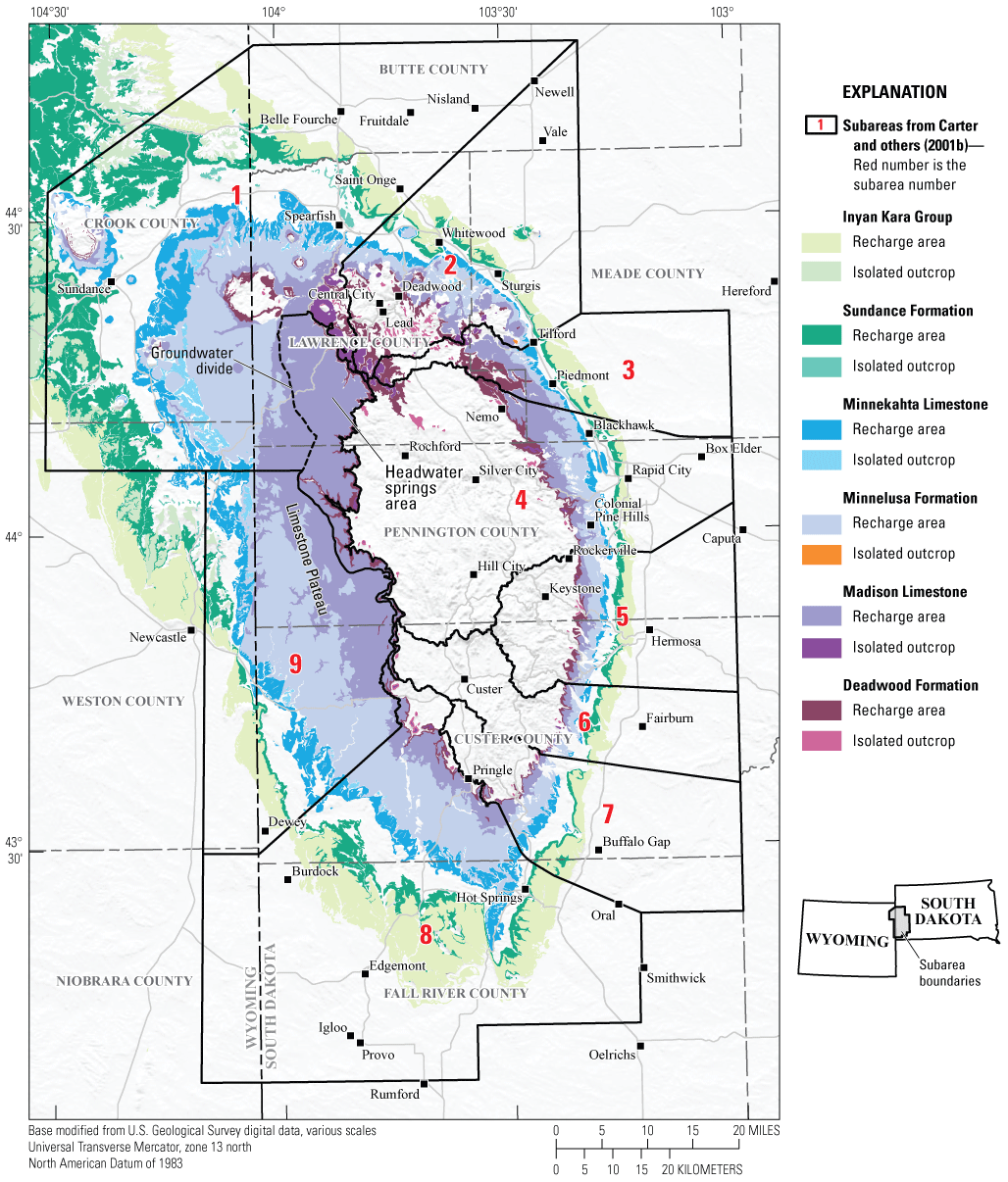
The Black Hills are a mountainous region in western South Dakota and eastern Wyoming (fig. 1) with important natural resources, such as timber and minerals, and popular tourist locations, such as Mount Rushmore National Memorial, that historically have served as the economic base for local communities (Driscoll and Carter, 2001). Water resources also are important to the region because the Black Hills are the origin of many streams and are a major recharge area for many local and regional aquifers (fig. 1) that supply water to residents, industry, irrigation, and tourism. Population growth and recurring droughts in the Black Hills region can affect water resources and future availability. Between 1980 and 2022, the region’s population grew by about 73 percent, from about 124,000 to 214,100 (U.S. Census Bureau, 1983, 2024). Drought conditions in the late 1980s and the early 2000s stressed local water systems that relied heavily on surface water as the population of the region was increasing. Consequently, water managers began exploring alternative water supplies, primarily utilizing underdeveloped groundwater resources. Municipalities, like Rapid City, South Dakota, also began securing future use permits (South Dakota Department of Agriculture and Natural Resources [SDDANR], 2024a) for additional groundwater withdrawals and surface water from the Missouri River to ensure a reliable future water supply amid growing demand.
The Black Hills hydrology study (BHHS) was initiated in the early 1990s to inventory and assess the region's water resources, focusing on the quantity, quality, and distribution of surface water and groundwater. The BHHS was a collection of work completed by the U.S. Geological Survey (USGS) and is described in greater detail in the “Previous Studies” section of this report. The population of the Black Hills region increased by about 39 percent since completion of the BHHS in 2000 compared to 2022 (U.S. Census Bureau, 2003, 2024), which has renewed interest in future water demand and availability in the Black Hills. Groundwater in the Black Hills region has been increasingly in demand since 2000 relative to surface water; water rights data from South Dakota (SDDANR, 2024a) showed nearly four times as many approved groundwater permits (302) than surface water permits (78). Historical well withdrawal patterns and availability estimates can inform effective resource management. The USGS has not comprehensively collected or analyzed detailed well withdrawal data and hydrologic budgets for aquifers in the Black Hills region since completion of the BHHS.
The USGS, in cooperation with the Western Dakota Regional Water System, completed a study to (1) update hydrologic budgets from the BHHS for six of the most used aquifers in the Black Hills and (2) to evaluate water availability by comparing results from hydrologic budgets to modern (2003–22) well withdrawals and water rights information from State agencies and (or) water systems. Hydrologic budgets provide a means for evaluating the availability and sustainability of a water supply by accounting for each component of the water cycle and how each components interacts and contributes to the cycle. A hydrologic budget quantifies the rate of change in water stored in an area and balances it with the rate at which water flows either into or out of the area. Inflows to aquifers in this study included recharge, inflows of regional groundwater, and leakage between adjacent aquifers. Outflow components to the hydrologic budget included springflow, well withdrawals, regional groundwater outflow, and leakage between adjacent aquifers. Water availability was estimated by comparing long-term recharge conditions from updated hydrologic budgets to modern well withdrawals and the total amount of withdrawable water from water rights information. Evaluating water availability also included estimating the volume of water stored in each aquifer.
Purposes and Scope
The purposes of this report are to (1) describe updates to hydrologic budgets from the BHHS for six regionally important aquifers in the Black Hills region for 1931–2022 and (2) estimate long-term water availability for each aquifer. Hydrologic budgets were developed by estimating the inflow and outflow components for each aquifer, following methods established by the BHHS (Carter and others, 2001a, 2001b8; Driscoll and Carter, 2001). This report summarizes the methods and results used to construct hydrologic budgets and estimate water availability for six bedrock aquifers. Surface water budgets and availability are outside the scope of this report and are not discussed.
Hydrologic budgets were constructed for six aquifers in the Black Hills region in South Dakota and Wyoming (hereafter referred to as the “study area”; fig. 1) for the period 1931–2022. Key updates to the BHHS budgets include (1) adding available data from 1999 to 2022 and (2) dividing hydrologic budgets for each aquifer into smaller areas. Previous studies collected data up to 1998, and newer data had since become available. The study area was divided into nine separate areas (hereafter referred to as “subareas”), consistent with the delineation by Carter and others (2001b; fig. 1). Dividing the study area into subareas allowed for the development of local hydrologic budgets for each aquifer, which had previously been analyzed for only two aquifers (the Madison and Minnelusa aquifers). Subarea hydrologic budgets were useful because budget components and water availability can vary considerably throughout the study area.
Hydrologic budgets developed in this study differed from previous studies in that budget components are presented by subarea for a different subset of aquifers for 1931–2022. Geologic units containing aquifers included in this study were the Deadwood Formation, Madison (Pahasapa) Limestone, Minnelusa Formation, Minnekahta Limestone, Sundance Formation, and Inyan Kara Group (fig. 1). Hydrologic budgets were not developed for aquifers within Tertiary and Precambrian igneous and metamorphic rocks, referred to as “crystalline core aquifers” by the BHHS, because these aquifers lack regional groundwater flow because of localized recharge (Driscoll and Carter, 2001). The Sundance aquifer, the saturated part of the Jurassic Sundance Formation, was the only Jurassic unit considered for recharge calculations by Driscoll and Carter (2001). The Sundance aquifer was termed the “Jurassic-sequence semiconfining unit” by Driscoll and Carter (2001) but was renamed to Sundance aquifer in this report for simplification. The Newcastle aquifer, the saturated part of the Cretaceous Newcastle Sandstone, was the only Cretaceous unit other than the Inyan Kara Group considered for recharge calculations by Driscoll and Carter (2001). The Newcastle aquifer was termed the “Cretaceous-sequence confining unit” but was renamed to Newcastle aquifer in this report for simplification. Additionally, after reviewing historical well withdrawals, the Newcastle aquifer was not included in this report because it was not considered a regionally important bedrock aquifer in the study area.
The subset of aquifers and the time period for budget components varied and were determined based on assumptions from previous studies and objectives of this report. Precipitation recharge, defined as the infiltration of precipitation on outcrops of geological units, was estimated for all six aquifers between 1931 and 2022. Streamflow recharge, which refers to water infiltrating geological units along streams, and springflow, characterized as water discharged from geological units to the land surface, were estimated exclusively for the Madison and Minnelusa aquifers (discussed in the “Hydrogeologic Setting” section of this report). Streamflow recharge was estimated between 1931 and 2022, whereas springflow estimates varied by site depending on the period of available data. Well withdrawals were estimated for all aquifers with available withdrawal data in the study area between 2003 and 2022. Although the authors acknowledge well withdrawals from aquifers other than the six analyzed in this report are an important source of water locally throughout the Black Hills, budgets were not estimated for these aquifers because they collectively represent a relatively small part of the groundwater resources used in the study area. Budgets were not created for aquifers other than the six regionally important aquifers because they were not considered regionally important based on available withdrawal data. Additionally, certain aquifers, including those within igneous, metamorphic, or alluvial materials, also were excluded from budget analyses because they received localized recharge and lacked regional groundwater flow.
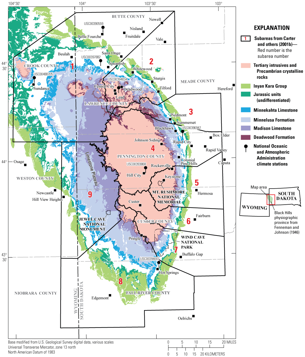
Study area with subareas 1–9 and recharge areas of aquifers evaluated in this report. Madison Limestone and Minnelusa Formation and South Dakota geology modified from Strobel and others (1999) and DeWitt and others (1989); Wyoming geology of Minnekahta Limestone, Jurassic units (undivided), Inyan Kara Group modified from Wyoming Geologic Survey 1:100,000 quadrangle maps of the Devils Tower (Sutherland, 2008), Sundance (Sutherland, 2007), Newcastle (McLaughlin and Ver Ploeg, 2006), and Lance Creek (Johnson and Micale, 2008) quadrangles. Black Hills physiographic province (shown in inset map) from Fenneman and Johnson (1946).
Study Area Description
The study area consists of the Black Hills of western South Dakota and eastern Wyoming (fig. 1). The hydrogeologic setting and population of the study area are described in the following sections. The hydrogeologic setting discussion includes descriptions of relevant geologic units present in the study area, the climatic conditions during the period of investigation (1931–2022), and the general hydrology of the Black Hills area.
Hydrogeologic Setting
The hydrogeologic setting of the Black Hills includes the geology, climate, and hydrology of the region. In general, precipitation falls on the elevated terrain of the Black Hills where it infiltrates and recharges aquifers of permeable geologic materials or becomes streamflow in areas of low permeability. The geological conditions of the area create extensive surface-water and groundwater interactions including headwater springs that feed base streamflow, streamflow loss zones where water from streams recharges aquifers, and artesian springs that discharge groundwater from deep aquifers at the land surface (fig. 2).
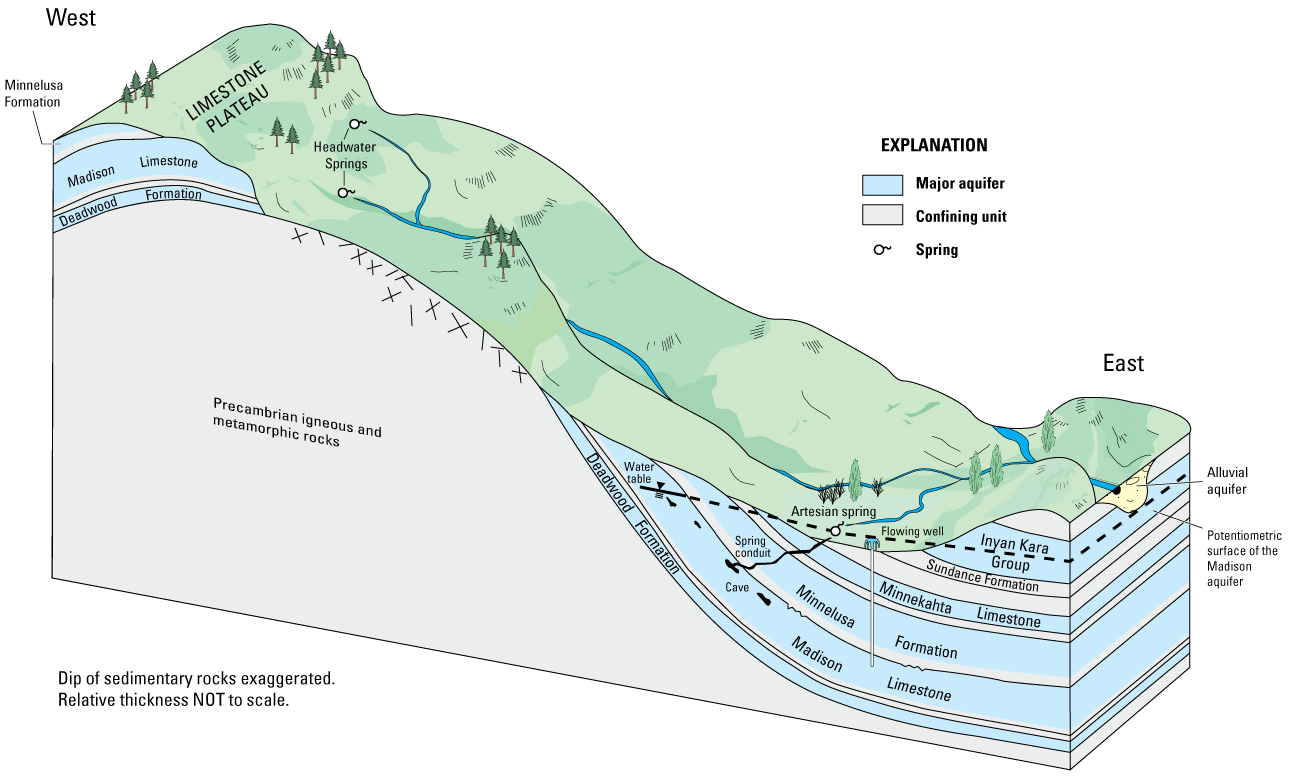
Schematic diagram illustrating hydrologic processes (modified from Driscoll and Carter, 2001; original from Anderson and others, 1999).
Geology
Uplift during the Late Cretaceous and early Tertiary, Tertiary intrusions, and subsequent erosion created the mountainous terrain of the Black Hills in western South Dakota and northeastern Wyoming (Carter and others, 2003). Darton and Paige (1925) described the general structure of the Black Hills as a north-northwest trending, irregularly shaped, doubly plunging anticline with a length of 125 miles and a width of 60 miles. The Black Hills are generally defined as the area contained within the extent of the erosion-resistant, dipping Cretaceous sandstone formations that form a hogback that surrounds the central part of the uplift. The uplift exposed the Precambrian geologic units consisting of igneous and metasedimentary rocks in the central core of the Black Hills, with younger Paleozoic and Mesozoic geologic units consisting of sedimentary rocks dipping radially away from the central crystalline core. Tertiary laccoliths, dikes, and sills intruded the sedimentary rocks in the northern Black Hills and formed geologic features such as Bear Butte, Crow Peak, and Devils Tower (not shown in fig. 1). Structural features in the Black Hills formed from deformation during the uplift and intrusions include fractures, folds, and faults that occur throughout the Black Hills on local and regional scales (DeWitt and others, 1986).
The Precambrian units of the crystalline core (fig. 3) are generally low permeability rocks and confining where overlain by Phanerozoic sedimentary rocks or sediment, but isolated local zones of highly fractured and weathered Precambrian rocks form important aquifers for communities in the central Black Hills, such as Custer, Keystone, and Hill City (fig. 1). Aquifers formed by the fractured zones of the Precambrian rocks are generally unconfined and are recharged where fractures are exposed at the land surface or are overlain by highly permeable unconsolidated material (Driscoll and others, 2002; Eldridge and others, 2021).
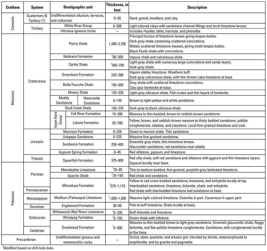
Generalized stratigraphic column for the Black Hills of western South Dakota and eastern Wyoming. Modified from Carter and others (2003) and originally from information furnished by the Department of Geology and Geological Engineering, South Dakota School of Mines and Technology (written commun., January 1994).
Paleozoic and Mesozoic sedimentary rocks surround the crystalline core and constitute aquifers that receive recharge where outcropping. The oldest sedimentary unit in the Black Hills is the Cambrian and Ordovician Deadwood Formation. The Deadwood Formation ranges from 0 to 500 feet (ft) in thickness and consists of sandstone, glauconitic shale, and conglomerate locally at the base (fig. 3). The sandstone layers within the Deadwood Formation form the Deadwood aquifer and are confined below by Precambrian igneous and metamorphic rocks and above by shales and siltstones of the Ordovician Winnipeg Formation and the dolomite layers of the Ordovician Whitewood Limestone, where present (fig. 3). Groundwater from the Deadwood aquifer is used mostly by domestic users within and near outcrops (Carter and others, 2001b). Where the Winnipeg Formation and Whitewood Limestone are not present, the Devonian and Mississippian Englewood Limestone overlies the Deadwood Formation. The Englewood Formation is a 30-to-60-ft pinkish limestone with shale at its base (fig. 3) and was included in the Madison hydrologic unit by Strobel and others (1999) and is considered part of the Madison aquifer in this study.
Overlying the Englewood Formation is the Mississippian Madison Limestone, also locally known as the Pahasapa Limestone, which consists of up to 1,000 ft of light-colored limestone and dolomite (fig. 3). The Madison Limestone has extensive secondary porosity in the upper 100 to 200 ft formed from fractures and solution features. The bottom part of the Madison Limestone generally lacks the solution features and fractures of the upper part and has a larger component of dolomite than the upper portion (Greene, 1993). The Madison aquifer receives water from precipitation on outcrops, streamflow loss where streams cross outcrops, and leakage from adjacent aquifers. Hydraulic connection between the Deadwood and Madison aquifers likely occurs in areas where the potentiometric head of the groundwater in the Deadwood aquifer is above the bottom potentiometric head of the Madison aquifer and the confining layers are thin or absent (Strobel and others, 1999). The Madison aquifer is artesian where confined and flowing wells are common where the potentiometric contour elevation exceeds the elevation of the land surface. Losses from the Madison aquifer include evapotranspiration, headwater and artesian spring flow, leakage to adjacent aquifers, and pumping from wells.
The Madison aquifer is confined from above by a red paleosol and shale from the basal unit of the Pennsylvanian and Permian Minnelusa Formation that is discontinuous in parts of the study area (Greene, 1993; Gries, 1996). The thickness of the Minnelusa Formation ranges from 375 to 1,175 ft, which generally increases to the south. Sequences of alternating deposits of sandstone, limestone, dolomite, and shale constitute the Minnelusa Formation (fig. 3), with the thick sandstone units in the upper 200 to 300 ft constituting most of the aquifer used for municipal and domestic use, although sandstone units in the middle and lower parts of the formation are used locally (Greene, 1993). Solution of anhydrite in the upper portions of the Minnelusa Formation caused collapse features such as breccia pipes, which are roughly funnel shaped cylindrical masses of angular blocks and fragments from overlying geologic materials that can be as much as 200 ft tall and 10 to several hundred feet in diameter (Bowles and Braddock, 1963). Leakage from the Madison aquifer into the overlying Minnelusa aquifer occurs in areas where the hydraulic gradient between the Madison and Minnelusa aquifers is large and the confining basal unit of the Minnelusa Formation does not exist or was deformed by tectonic stress (Rahn and Gries, 1973).
The Minnelusa aquifer is confined from above by the Permian Opeche Shale, a 25- to 150-ft thick, red shale with sandstone (fig. 3) that separates the Minnelusa aquifer from overlying aquifers. Leakage between the Minnelusa aquifer into the Opeche Shale can occur where the Opeche Shale is fractured and faulted. Areas where the Minnelusa Formation collapsed into solution cavities from the solution of anhydrite also are areas where the Minnelusa aquifer could potentially lose water to overlying geologic units.
The Permian Minnekahta Limestone overlies the confining Opeche Shale and is a 25- to 65-ft thick, thin to medium bedded, laminated limestone (fig. 3). Precipitation on the outcrops of the Minnekahta aquifer is the primary recharge mechanism, with only minor amounts of streamflow recharge occurring where streams flow over the outcrops. The Minnekahta Limestone is an aquifer with high permeability, but the thin nature of the aquifer limits well yields to volumes that can provide water for small, local users rather than large developments or municipalities. The Minnekahta aquifer is confined from above by the Permian and Triassic Spearfish Formation, a 375- to 800-ft thick, red shale and siltstone unit with white gypsum and thin limestone beds (fig. 3; DeWitt and others, 1989). The “red valley” or “red racetrack” of the Black Hills is an area where the shale of the Spearfish Formation was eroded into an area of low topographical relief between the cliff forming Minnekahta Limestone and the Jurassic and Cretaceous sandstone units of the hogback. A 0- to 45-ft thick white gypsum layer of the Jurassic Gypsum Spring Formation (fig. 3) overlies the Spearfish Formation and forms white cliffs that cap the Spearfish Formation in some locations along the hogback of the Black Hills. The Jurassic Sundance Formation overlies the Gypsum Spring Formation where present or the Spearfish Formation where the Gypsum Spring Formation is absent. The Sundance Formation ranges from 250 to 450 ft in thickness and consists of siltstone, sandstone, limestone, and shale (fig. 3; DeWitt and others, 1989). The sandstone units within the Sundance Formation form a minor aquifer where saturated.
Other Jurassic units overlying the Sundance Formation are the 0- to 225-ft thick Unkpapa Sandstone and the 0- to 220-ft thick silty shale and claystone units of the Morrison Formation (fig. 3). The Unkpapa Sandstone thins to the north and is not present on the western flank of the Black Hills, where it is replaced by the Morrison Formation completely (DeWitt and others, 1986). The Unkpapa Sandstone forms a minor aquifer where saturated (Driscoll and Carter, 2001). Jurassic geologic units (Sundance, Unkpapa, and Morrison Formations) were considered a semiconfining unit by Driscoll and Carter (2001) because of its interbedded shales, sandstones, and gypsum (Strobel and others, 1999). The sandstones within the Sundance Formation form an aquifer, the Sundance aquifer, where saturated. Aquifers in other Jurassic formations are used locally to lesser degrees than the Sundance aquifer and were not considered in recharge calculations in this report, which was consistent with Driscoll and Carter (2001).
Lower Cretaceous sandstone units of the Inyan Kara Group overly the Morrison Formation. The Inyan Kara Group ranges from 135 to 900 ft in thickness and is comprised of the Lakota Formation at its base and Fall River Formation at its top (fig. 3). The Inyan Kara aquifer consists of saturated sandstone layers and is used extensively in the study area (Driscoll and Carter, 2001). Inflows to the Inyan Kara aquifer are primarily from precipitation on the outcrop but leakage from the underlying Jurassic units is possible (Gott and others, 1974). The Inyan Kara aquifer is confined from above by Cretaceous shales and below by the shales of the Morrison Formation (fig. 3) and is the youngest aquifer considered for the budget analysis in the present study. Other minor aquifers in the Cretaceous units surrounding the Black Hills, such as the Newcastle Sandstone (fig. 3), exist but are not extensively used in the study area and were not considered for the budget analysis.
Climate
The abrupt rise in topography of the Black Hills from the surrounding plains creates an orographic effect that causes greater amounts of precipitation to fall in the higher elevations of the Black Hills than the lower elevations of the surrounding area (Driscoll and others, 2000). Precipitation is greatest in the northern Black Hills near Lead, S. Dak. (fig. 1), and lowest in the southern periphery of the Black Hills near Hot Springs, S. Dak. (fig. 1; Driscoll and others, 2000). Monthly precipitation varies across the different elevations and locations within the Black Hills. Precipitation in the Black Hills peaks in the late spring and early summer months of May and June, although a second peak in monthly precipitation occurs in the late fall as snow in the higher elevations (fig. 4). Precipitation records from the National Oceanic and Atmospheric Administration extending back to 1930 (Palecki and others, 2021) indicate precipitation fluctuates annually in the Black Hills region, with relatively long dry periods in the 1930s, the late 1940s through the mid-1960s, the late 1980s to the early 1990s, and the early to mid-2000s (fig. 5). Drought conditions during 1988–92 and 2002–07 in the Black Hills region caused reduced streamflow, declining reservoir and groundwater levels, increasing fire activity, and water supply shortages (South Dakota Drought Task Force, 2015; USGS, 2024a).
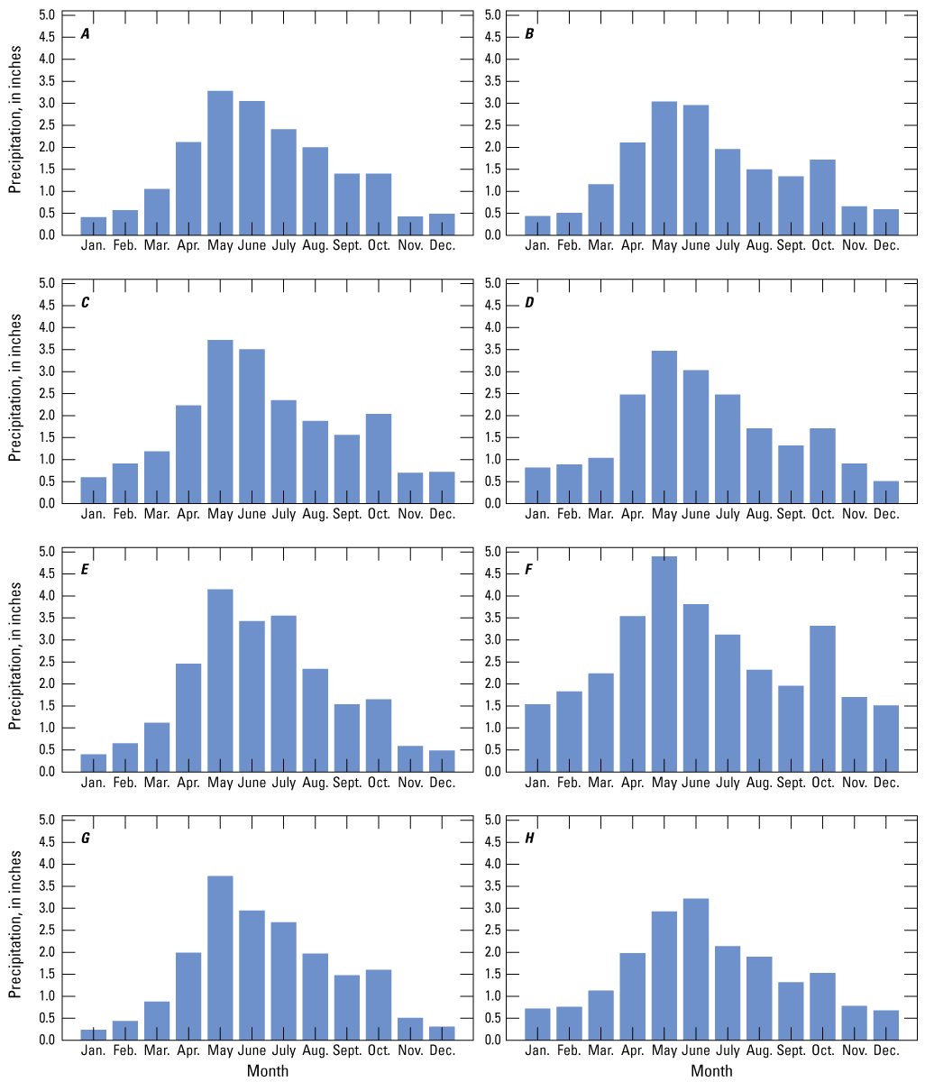
30-year normal precipitation from 1991 to 2020 for different locations and elevations within the Black Hills region. Data from National Oceanic and Atmospheric Administration National Centers for Environmental Information (Palecki and others, 2021). A, Hot Springs, SD US (USC00394007). B, Belle Fourche, SD US (USC00390559). C, Spearfish, SD US (USC00397882). D, Sundance, WY US (USC00488705). E, Hill City, SD US (USC00393868). F, Lead, SD US (USC00394834). G, Rapid City 4 NW, SD US (USC00396947). H, Devil’s Tower Number 2, WY US (USC00482466).
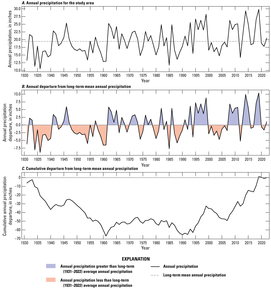
Mean annual precipitation totals for the Black Hills area, South Dakota for 1931–2022 using records from the climate stations in figure 4 (shown in fig. 1). A, Annual precipitation for the study area. B, Departure of annual precipitation from the long-term mean annual precipitation for the study area for water years 1931–2022. C, Cumulative departure of annual precipitation from the long-term mean annual precipitation for the study area for water years 1931–2022. Data from National Oceanic and Atmospheric Administration National Centers for Environmental Information (Palecki and others, 2021).
Temperatures in the Black Hills peak in the summer months of July and August with mean monthly maximums of almost 90 degrees Fahrenheit (°F) and mean monthly minimums of approximately 55 °F (fig. 6; Palecki and others, 2021). Additionally, monthly normal temperatures are greater at lower elevations and generally increase to the south near Hot Springs, S. Dak. (fig. 6A). Greater monthly normal temperatures at lower elevations and in the southern part of the study area cause greater evaporation that leads to less precipitation recharge. The coldest months are December and January with mean monthly temperatures below freezing (32 °F) and mean minimum monthly temperatures near 10 °F (fig. 6). In general, colder temperatures during winter months occur at the higher elevations and in the northern part of the study area (fig. 6). Temperatures generally increase at lower elevations and in the southern part of the study area.
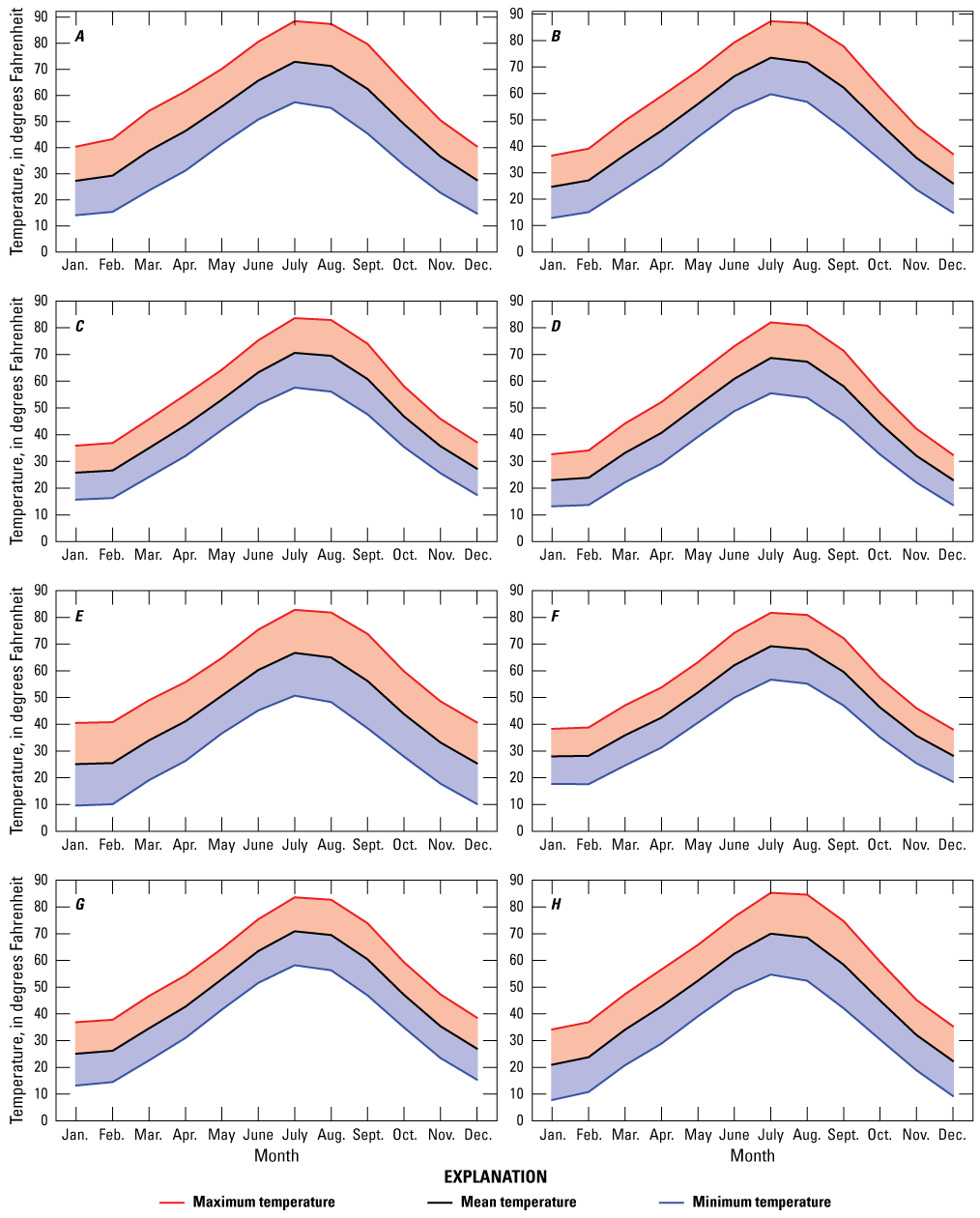
30-year normal temperature from 1991 to 2020 for different locations and elevations within the Black Hills. A, Hot Springs, SD US (USC00394007). B, Belle Fourche, SD US (USC00390559). C, Spearfish, SD US (USC00397882). D, Sundance, WY US (USC00488705). E, Hill City, SD US (USC00393868). F, Lead, SD US (USC00394834). G, Rapid City 4 NW, SD US (USC00396947). H, Devil’s Tower Number 2, WY US (USC00482466). Data from Palecki and others (2021).
Hydrology
The hydrology of the Black Hills region is characterized by interactions between climate, geology, and the landscape. Driscoll and others (2002) provide detailed descriptions of hydrologic processes occurring in the Black Hills region, which are discussed in general terms in this section. Precipitation falling on the landscape infiltrates into the soil horizon, becomes direct runoff if the soil is saturated or its infiltration capacity is exceeded, and (or) is returned to the land surface from the soil horizon through lateral movement within the soil layers (interflow). Where evaporation exceeds precipitation, most water is returned to the atmosphere through evapotranspiration. Water infiltrating past the soil horizon can recharge groundwater systems; however, a component of groundwater is discharged at the land surface and may contribute to streamflow (base flow). Soil horizon characteristics, such as soil type or thickness, are an important aspect of the hydrologic cycle where soils are present in the Black Hills region and can greatly affect groundwater recharge rates. In areas where soils are thin or absent, recharge rates are affected by the characteristics of geologic units.
Driscoll and Carter (2001) subdivided the hydrogeologic setting of the Black Hills in South Dakota into four areas: the crystalline core, the limestone headwater, the loss zone and artesian spring area, and the exterior. The crystalline core area is characterized by mostly impervious rocks of the Precambrian in the central part of the Black Hills. The limestone headwater area is the area of the western flank of the Black Hills where the Madison Limestone discharges groundwater as headwater springs that then flow away from the limestone as streamflow. The loss zone and artesian spring area encompasses the region where streamflow loss zones and artesian springs occur. Streams radiate outward from the elevated areas of the Black Hills and lose significant amounts of flow in regions where they intersect the fractured and permeable Madison Limestone and Minnelusa Formation. Water then reemerges as artesian springs that surround the Black Hills (Rahn and Gries, 1973). The loss zone and artesian spring area is bounded by the extent of the outcrops of the Inyan Kara Group (fig. 1), which is commonly considered the outer extent of the Black Hills. Areas outside of the extent of the Black Hills are in the exterior.
Springs are a common hydrologic feature in the Black Hills and are culturally important for local Tribes. Rahn and Gries (1973) classified springs in the Black Hills into different types based on the geologic controls and amount of flow of the springs. Headwater springs originate in the Limestone Plateau area (fig. 1) on the western flank of the Black Hills (Rahn and Gries, 1973). Headwater springs form where water percolates vertically through outcrops of the Madison Limestone and then discharges at the base of the limestone where it overlies less permeable surfaces. Base flow of several streams originates at the headwater springs area before flowing eastward across the Precambrian core to loss zones in the Madison and Minnelusa aquifers where surface water becomes groundwater again.
Artesian springs occur downstream from the loss zones where groundwater from aquifers in artesian conditions discharges at the land surface. Groundwater from aquifers in artesian conditions can be discharged through porous media or through structures, such as faults or breccia pipes, that extend to the land surface. Rahn and Gries (1973) classified artesian springs in the Black Hills as those that discharge groundwater from the Madison and Minnelusa aquifers at low elevations near the contact between the Minnekahta Limestone and Spearfish Formation or the contact between the Minnelusa Formation and Opeche Shale. Many of the artesian springs in the Black Hills discharge from the Madison and Minnelusa aquifers.
Surface water in the study area is present as streamflow and reservoirs. Streamflow follows precipitation patterns with high flows in the early spring months of June and July and lower flows in the fall (Driscoll and Carter, 2001). Streamflow is an important source of recharge to aquifers in the Black Hills area. During base flow conditions, most streams lose all or most of their flow as they cross loss zones of high permeability geologic materials. Each loss zone has a maximum streamflow (or threshold) that can recharge the aquifers. Hortness and Driscoll (1998) determined loss thresholds for 24 streams in the Black Hills area. The aquifers receiving relatively consistent recharge from streams flowing overtop outcrops are the Madison and Minnelusa aquifers. Other aquifers, such as the Deadwood and Minnekahta aquifers, also receive recharge from streams; however, streamflow losses to these aquifers are relatively small in comparison to the Madison and Minnelusa aquifers and often are difficult to quantify. Regulated releases from reservoirs can provide a constant source of water to loss zones, which are particularly important along Rapid and Spearfish Creeks (not shown).
Population
Population in the study area is an important factor for hydrologic budgets, because growth can increase the demand for water resources. Population estimates for the overall study area and each of the nine subareas (fig. 1) were derived from decadal census data between 1930 and 2022 provided by the U.S. Census Bureau (1952, 1973, 1983, 1992, 2003, 2012, 2024). Populations were assigned to each subarea based on their geographical location; however, some populated areas, such as townships or counties, overlapped multiple subareas, necessitating additional steps to distribute the population among the subareas. For these overlapping areas, portions of the population were allocated to each subarea in proportion to their respective areas. For example, the population of Custer County (fig. 1) was divided among subareas 5, 6, 7, 8, and 9, with 20 percent of the population value allocated to each subarea for every census decade. This allocation method introduced uncertainty into the population estimates for each subarea. Population estimates for each subarea are in table 1.
Table 1.
Estimated population by subarea and year in the study area from 1930 through 2022. Population data were obtained from the U.S. Census Bureau (1952, 1973, 1983, 1992, 2003, 2012, 2024) and modified to estimate population in the study area (fig. 1).The population of the study area from 1930 to 2022 varied across subareas 1–9. Overall, the population increased from about 60,000 in 1930 to approximately 214,100 in 2022 (table 1). Generally, subareas in the northern Black Hills (subareas 1–4) had larger populations and greater annual growth rates compared to those in the southern Black Hills (subareas 5–9; table 1). Throughout every decadal census from 1930 to 2020, subarea 4 consistently recorded the largest population, because it includes Rapid City, S. Dak. (fig. 1), which is the largest city in the region. Notably, subarea 4 surpassed 100,000 residents in 2020, making it the only subarea with over 100,000 residents. By 2022, subarea 1, which includes Spearfish and Belle Fourche, S. Dak. (fig. 1), had the second-largest population at about 39,000—about 76,500 less than subarea 4 (table 1). The populations of subareas 2, 3, and 5–9 either slightly increased or decreased from 1930 to 2022, with subarea 8 being the only region with a population decline.
Since completion of the BHHS, the population of the study area increased from 154,200 to 214,100, reflecting a 39-percent increase (table 1). The mean annual population growth rate for the study area from 2000 through 2022 was about 1.8 percent with the greatest mean annual growth rates for the same time observed for subareas 3 and 4 at 4.5 and 2.3 percent, respectively. In contrast, subareas 5 and 6 experienced the lowest growth rates during this time, with mean annual rates of −0.7 and 0.6 percent, respectively. The population of subareas 1–4 (northern Black Hills and Rapid City, S. Dak., area) grew by 58,428 between 2000 and 2022, with subarea 4 adding 39,206 residents. In comparison, the population in subareas 5–9 (southern Black Hills) increased by only 1,488 from 2000–22, with subarea 5 being the only subarea to report a population decline, losing an estimated 1,286 residents (table 1).
Previous Studies
Previous studies relevant to the scope of this research include numerous investigations from the BHHS—a long-term regional study initiated in 1990 focused on the quality, quantity, and distribution of surface water and groundwater resources in the Black Hills area. The BHHS consisted of two phases: data collection and interpretation. During the first phase, a network comprised of 71 observation wells, 94 precipitation gages, and 60 streamgages was established. Phase two produced various reports and products, including 21 reports and 11 maps. The objectives of the BHHS outlined in Driscoll (1992) were to (1) inventory and describe hydrologic data (precipitation, streamflow, groundwater levels, water-quality characteristics), (2) develop hydrologic budgets of selected watersheds, (3) describe the significance of bedrock aquifers in the Black Hills, and (4) develop conceptual models of the hydrogeologic system in the Black Hills area. Overviews of the BHHS are provided in Carter and others (2002) and Driscoll and others (2002).
Driscoll and others (2000) provided monthly and annual precipitation totals for water years—beginning October 1 of the year prior and ending September 30—from 1931 to 1998 for 94 precipitation gages in the Black Hills area of South Dakota, evaluating spatial and temporal precipitation patterns. Generally, precipitation totals increased from south to north and from lower to higher elevations within the region, with mean annual precipitation ranging from 16 to 17 inches per year in Fall River County, S. Dak., to more than 29 inches per year in parts of Lawrence County, S. Dak. (fig. 1). Temporal analysis indicated sustained periods of precipitation deficit during 1931–40 and 1948–61, whereas surplus precipitation was observed during 1941–47, 1962–68, and 1991–98.
Carter and others (2001a) estimated annual precipitation and streamflow recharge to the Madison and Minnelusa aquifers in the Black Hills area for water years 1931–98. Annual precipitation recharge was estimated by applying basin yield techniques to precipitation data from Driscoll and others (2000). Annual streamflow recharge for water years 1950–98 was computed using daily streamflow data and streamflow loss thresholds measured by Hortness and Driscoll (1998). Linear regression analyses were used to estimate streamflow recharge from 1931 to 1949 based on relations between precipitation and streamflow recharge from 1989 to 1998 when both datasets were most complete. Precipitation recharge averaged about 3.6 inches per year for the Madison aquifer and 2.6 inches per year for the Minnelusa aquifer during 1931–98. Streamflow recharge was not separated by aquifer; rather, the total combined annual streamflow recharge for the Madison and Minnelusa aquifers averaged about 93 cubic feet per second (ft3/s) for 1931–98. Mean annual combined precipitation and streamflow recharge to both aquifers for 1931–98 was 344 ft3/s.
Carter and others (2001b) developed hydrologic budgets for the Madison and Minnelusa aquifers in the Black Hills area for water years 1987–96. Hydrologic budgets were determined for two scenarios: the first scenario consisted of a general budget for the entire Black Hills area and the second scenario involved detailed budgets for nine subareas. Subarea boundaries were based on groundwater flow direction of the Madison and Minnelusa aquifers and were drawn to minimize groundwater flow across subarea boundaries. The period from 1987–96 was chosen because it represented a period of zero storage change because of offsetting wet and dry cycles. Inflow components included recharge (precipitation and streamflow), leakage from adjacent aquifers, and groundwater inflows across the study area boundaries. Outflow components were springflow (headwater and artesian), well withdrawals, leakage to adjacent aquifers, and groundwater outflows across study area boundaries. Leakage, groundwater inflows, and groundwater outflows were combined into net groundwater flow because all three components were difficult to quantify and could not be distinguished. Estimates of combined budget components from Carter and others (2001b) for the Madison and Minnelusa aquifers for 1987–96 include 395 ft3/s for recharge (precipitation and streamflow), 78 ft3/s for headwater springflow, 189 ft3/s for artesian springflow, and 28 ft3/s for well withdrawals. Net groundwater flow was calculated as difference between inflows and outflows, which was 100 ft3/s.
Hydrologic budgets determined by Carter and others (2001b) for nine subareas consisted of the same inflow and outflow components as the overall budget but also considered net groundwater inflows or outflows between subareas to account for budget surpluses or deficits. The intent of selected subareas was to minimize flow across the boundaries; however, zero-flow boundaries could not be established for both aquifers along all subarea boundaries. Therefore, inflows and outflows to each subarea for both aquifers were estimated using budget surpluses or deficits. Because the storage change from 1987 to 1996 was near zero, the net inflow (negative net groundwater flow) or outflow (positive net groundwater flow) could be calculated by summing the inflows and outflows from 1987 to 1996 for each subarea and dividing the sum by the number of years (10) to calculate mean annual groundwater inflow or outflow. Net groundwater outflows exceeded inflows for seven subareas and values ranged from 5.9 to 48.6 ft3/s. Net groundwater inflows exceeded outflows for two subareas where artesian springflow was greater than recharge. Net groundwater flows also were used to determine hydrologic properties, such as transmissivity, for each subarea. Transmissivity values estimated for subareas ranged from 90 to 7,400 feet squared per day (Carter and others, 2001b).
Driscoll and Carter (2001) developed mean hydrologic budgets for various bedrock aquifers and surface waters in the Black Hills area for water years 1950–98. The same methods used for calculating groundwater inflows (recharge) and outflows (springflow and well withdrawals) to the Madison and Minnelusa aquifers in Carter and others (2001a) and Carter and others (2001b) were used to develop budgets for other bedrock aquifers. Eight bedrock aquifers, some consisting of combinations of several geologic units, were investigated by Driscoll and Carter (2001), including the crystalline core, Deadwood, Madison, Minnelusa, Minnekahta, Jurassic-sequence semiconfining unit (Sundance aquifer), Inyan Kara, and Cretaceous-sequence confining unit (Newcastle aquifer) aquifers. Outcrop areas for geologic units containing the bedrock aquifers evaluated are shown in figure 1 except for the Cretaceous-sequence confining unit (Newcastle aquifer) because it was not included in recharge calculations in this report. Surface water budgets were estimated by Driscoll and Carter (2001) but were not included in this study.
The mean hydrologic budget for 1950–98 for all aquifers was summarized in Driscoll and Carter (2001). Annual total recharge for all eight aquifers was estimated as 348 ft3/s, of which 292 ft3/s was recharged to the Madison and Minnelusa aquifers. Precipitation and streamflow recharge accounted for 200 and 92 ft3/s, respectively. Outflows for all wells and springs were estimated as 259 ft3/s, of which the Madison and Minnelusa aquifers accounted for 206 ft3/s of total springflow and 28 ft3/s of well withdrawals. The Deadwood aquifer accounted for a total of 14 ft3/s, with springflow and well withdrawals of 12.6 and 1.4 ft3/s, respectively. Well withdrawals from other aquifers accounted for the remaining 11 ft3/s. Net groundwater outflow was calculated as 89 ft3/s by subtracting outflows from inflows in the study area.
Hydrologic Budgets
Hydrologic budgets were updated for the Deadwood, Madison, Minnelusa, Minnekahta, Sundance, and Inyan Kara aquifers between 1931 and 2022 using methods from Carter and others (2001a), Carter and others (2001b), and Driscoll and Carter (2001). Hydrologic budgets for each aquifer were separated into subareas 1–9 from Carter and others (2001b) and consisted of various budget components including inflows and outflows. For some components, data were not available for the entire period of investigation and (or) methods from previous studies were modified so that budgets could be prepared. This section presents the methods and results for each budget component.
All hydrologic budgets presented in this study were developed using the same basic continuity equation as Carter and others (2001b):
where∑Inflows
is the sum of inflows,
∑Outflows
is the sum of outflows, and
ΔStorage
is the change in storage (positive ΔStorage is when inflows exceed outflows).
Inflows included recharge, leakage from adjacent (underlying or overlying) aquifers, and groundwater inflows across the study area boundary (regional groundwater flow). Recharge included infiltration of precipitation on outcrops of geologic units and streamflow recharge where streams cross outcrops and lose all or part of their flow. The various methods used to estimate recharge from precipitation and streamflow losses are described in the following sections.
Outflows included springflow, well withdrawals, leakage to adjacent aquifers, and regional groundwater flow out of the study area. Springflow consisted of two types: headwater and artesian. Headwater springs generally are at the base of the Madison Limestone near the headwaters of many streams in the Black Hills (fig. 2). Artesian springs are formed where water in aquifers under artesian pressure leaks upward through structures or porous material and discharge at the land surface typically downgradient of outcrops. Headwater springflow was not a component of the hydrologic budget because the outcrop areas for the Madison aquifer contributing to discharge at springs were removed from precipitation recharge calculations because the streamflow contributions from headwater springflow were already considered in gaged streamflow downstream. Outcrops contributing to headwater springflow (fig. 7) were mapped by Jarrell (2000) and modified by Carter and others (2001b). Headwater springflow estimates from Carter and others (2001b) for 1931–98 were updated as part of this study and are in appendix 2.
Outcrop areas of geologic units containing aquifers in the study area used for estimating precipitation recharge in subareas 1–9. Outcrops east of the groundwater divide from Jarrell (2000) and modified by Carter and others (2001b) were excluded from calculations of precipitation recharge.
Leakage to and from adjacent aquifers was difficult to quantify, so Carter and others (2001b) included leakage with groundwater flows for budgeting purposes. Net groundwater flow (groundwater outflow minus groundwater inflow) was determined using an assumption of zero storage change (discussed later in this section). When storage change is assumed equal to zero, the sum of inflows equals the sum of outflows, and the hydrologic budget equation can be rewritten as
whereNet groundwater flow (left side of eq. 2) is more difficult to quantify than the budget items on the right side of equation 2. Therefore, net groundwater flow can be calculated as the residual of budget items on the right side of equation 2. Net groundwater flow for aquifers in the study area is discussed in the “Groundwater Budgets” section later in this report.
Groundwater budgets estimated in this study could not be directly compared to budgets from previous studies (Carter and others, 2001b; Driscoll and Carter, 2001) because of differences in study area boundaries and how budgets were prepared. Budgets were not comparable for the Deadwood, Minnekahta, Sundance, and Inyan Kara aquifers because the study area of Driscoll and Carter (2001) did not include Wyoming, and budgets were not previously divided among the nine subareas. Instead, differences between budget components from previous studies and this study are discussed for the entire study area to provide readers with context of how the budget changed by including additional area in Wyoming. Budget estimates from Carter and others (2001b) could be compared directly for the Madison and Minnelusa aquifers because their study area was used in this study; however, these budgets were developed only for 1987–96 and are not representative of long-term conditions.
Inflows—Precipitation and Streamflow Recharge, 1931–2022
Inflows of the hydrologic budget consisted of recharge from precipitation and streamflow losses to aquifers. Recharge estimates were calculated by water year for 1931 to 2022. Recharge estimates for 1931–98 for the Madison and Minnelusa aquifers from Carter and others (2001a) were updated to include water years 1999 through 2022. Recharge estimates for 1999–2022 were calculated as part of this study using methods from Carter and others (2001a), Carter and others (2001b), and Driscoll and Carter (2001); however, some methods were modified and are discussed in “Precipitation Recharge” and “Streamflow Recharge” sections of this report and in appendix 1. The recharge results presented in this study were separated into the nine subareas delineated by Carter and others (2001b) for each aquifer. Additional information regarding recharge estimates is available in Carter and others (2001a), Carter and others (2001b), and Driscoll and others (2000). Complete data for precipitation and streamflow recharge are provided in the accompanying data release (Medler and others, 2025).
Precipitation Recharge
Annual precipitation recharge was estimated for 1931–2022 by subarea for the aquifers in the Deadwood Formation, Madison Limestone, Minnelusa Formation, Minnekahta Limestone, Sundance Formation, and Inyan Kara Group in the study area (fig. 7). Precipitation recharge was calculated only for connected outcrops contributing to the regional groundwater flow system of each aquifer (fig. 7). Carter and others (2001a) noted recharge to disconnected (or isolated) outcrops surrounded by igneous and metamorphic rocks likely does not directly join the regional groundwater flow system and, therefore, should be excluded from calculations of precipitation recharge. Outcrop areas of the Madison aquifer on the Limestone Plateau east of the groundwater divide (Jarrell, 2000; fig. 7) contributing to headwater springflow also were excluded because recharge in this area was believed to contribute to springflow rather than the regional aquifer (Driscoll and Carter, 2001).
Precipitation recharge was estimated using the total yield equation developed by Carter and others (2001a) for outcrops contributing to the regional groundwater flow. The total yield equation (eq. 3) consists of variables for annual precipitation, average annual precipitation, and average yield efficiency.
whereQannual
is the annual yield,
Pannual
is the annual precipitation,
Pmean
is the mean annual precipitation, and
YEmean
is the mean annual yield efficiency.
Inverse distance weighting (IDW) interpolation was used to interpolate annual precipitation (Pannual) from 94 stations given in Driscoll and others (2000) to create annual precipitation 1-kilometer (km) grids for water years 1931–80. Settings used for the IDW interpolation tool in geographic information system software (ArcGIS Pro, Esri, 2024a) were the same as those used in the Driscoll and others (2000) report and were as follows: a power of 2, a maximum search area of 50 km, and a maximum number of points of 15. Gridded annual precipitation data for 1981–2022 were aggregated from Daymet daily climate data on a 1-km grid (Thornton and others, 2022). Daymet data are available for 1981 through present and use a workflow that processes weather station observations and gridded terrain data along with cross-validation statistics to produce a standardized gridded dataset of daily climate data on a 1-km grid on a national scale (Thornton and others, 2021). When possible, Daymet data were utilized for the standardized quality, ease-of-use, and public accessibility. The mean of the annual precipitation grids from 1931 to 2022 was calculated on a cell-by-cell basis (fig. 8) to create the mean annual precipitation (Pmean) grid used in the yield equation (eq. 3).
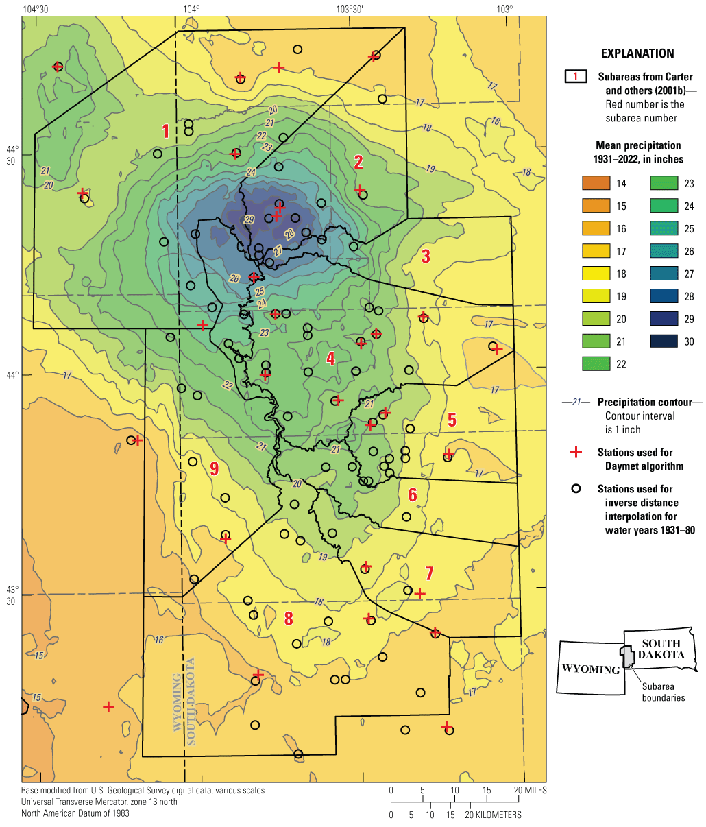
Mean annual precipitation for the study area showing weather stations used for the inverse distance weighting interpolation for water years 1931–80 and weather stations used in the Daymet algorithm (Thornton and others, 2021) for water years 1981–2022.
Mean yield efficiency contours for the study area published by Carter and others (2001a) were gridded into a 1-km grid and used for the total yield calculation. Gridded annual recharge was calculated by multiplying the results from equation 3 by the recharge factor (table 2) of a given aquifer using the following equation:
whereThe recharge factor was developed by Driscoll and Carter (2001) to simulate the recharge fraction of total yield (sum of runoff plus recharge). The value of recharge factors was based on hydrologic properties of each aquifer and the extent of outcrop areas.
Table 2.
Recharge factors and outcrop areas used in calculating precipitation recharge for the Deadwood, Madison, Minnelusa, Minnekahta, Sundance, and Inyan Kara aquifers. Recharge factors were developed by Driscoll and Carter (2001).[NA, not applicable]
Gridded recharge was clipped to the aquifer boundary and zonal statistics (ArcGIS Pro, Esri, 2024b) were calculated for each of the nine subareas (fig. 7). The annual precipitation recharge for each subarea, in inches, was converted to feet and then multiplied by the area, in acres, of the non-isolated outcrops of each aquifer in the subarea to calculate an annual volume of precipitation recharge in acre-feet. Outcrop areas for all Paleozoic geologic units identified by Carter and others (2001b) as contributing to headwater springs on the Limestone Plateau were excluded from subareas before calculating zonal statistics so that precipitation recharge estimates would not include outcrops recharging headwater springs. Additionally, 50 percent of the precipitation recharge calculated for the Deadwood aquifer in the Spearfish Creek, Little Elk Creek, and Meadow Creek drainages was excluded to be consistent with Driscoll and Carter (2001) in assuming that some fraction of precipitation recharge in those drainages contributes to headwater springflow.
Streamflow Recharge
Streamflow recharge was estimated annually for 1931–2022 for the regional Madison and Minnelusa aquifers for the nine subareas delineated by Carter and others (2001b). The Madison and Minnelusa aquifers receive recharge from streams flowing overtop outcrop areas of both formations up to a certain threshold that is unique to each loss zone. Loss thresholds for 24 streams in the Black Hills were determined by Hortness and Driscoll (1998). Streamflow losses to aquifers other than the Madison and Minnelusa were not calculated because recharge to other aquifers, such as the Deadwood and Minnekahta aquifers, was relatively small in comparison and often was difficult to distinguish from other aquifers. Streamflow recharge values for 1931–98 were originally estimated by Carter and others (2001b) but were recalculated using new information and were separated into nine subareas. Streamflow recharge was calculated for 1999–2022 using the methods outlined in Carter and others (2001b) and is discussed in the following sections. Extrapolation techniques used to extend streamflow recharge records differed from those in previous studies and are discussed in appendix 1.
Methods for Quantifying Streamflow Recharge
Methods and assumptions outlined in Carter and others (2001a) were used to quantify recharge from streamflow losses to the Madison and Minnelusa aquifers for 55 basins in the study area (fig. 9). In general, streamflow data from USGS streamgages (table 3) and loss threshold rates determined by Hortness and Driscoll (1998; table 4) were used to calculate streamflow recharge, when possible, from drainage basins upstream from loss zones delineated by Carter and others (2001a). Streamflow data were downloaded from the USGS National Water Information System (NWIS; USGS, 2024a). For basins without daily streamflow records, daily streamflow was synthesized using statistical relations between drainage areas of nearby basins. Loss threshold rates for streams were available either from Hortness and Driscoll (1998) for 24 streams in the study area or were selected from a representative nearby site. Loss threshold rates were quantified individually for the Madison and Minnelusa aquifers for some streams, which allowed for determination of individual and combined streamflow recharge. Combined recharge to the Madison and Minnelusa aquifers was calculated for streams where loss thresholds could not be differentiated between the aquifers. Additionally, loss threshold rates were adjusted by Carter and others (2001a) for some streams to account for unmeasured flow from additional minor drainage areas (table 4).
Table 3.
Selected site information for streamgages (shown in fig. 9) used in determining streamflow recharge from Carter and others (2001a).[C, continuous-record; M, miscellaneous-record]
Table 4.
Loss thresholds and associated drainage areas of selected streams (shown in fig. 9) used to calculate streamflow recharge by Carter and others (2001a).[ft3/s, cubic feet per second; C, continuous-record; --, none used; M, miscellaneous-record; >, greater than; e, estimated; UG, ungaged; <, less than; ND, not determined; NA, not applicable]
Drainage basins were delineated based on the availability and distribution of USGS streamgages in the study area and adjusted using outcrop areas of the Madison Limestone and Minnelusa Formation. Streamgages (table 3) were used to delineate drainage basins using watershed boundaries downloaded from USGS StreamStats (USGS, 2024b). Adjustments to drainage basins involved removing areas of outcrop of the Madison and Minnelusa connected to the regional groundwater flow system of both aquifers. It was assumed by Carter and others (2001a) that precipitation on these outcrops of Madison and Minnelusa did not contribute to runoff. Isolated outcrops of the Madison and Minnelusa were not excluded from drainage basins because Carter and others (2001a) assumed these outcrops were disconnected from the regional groundwater flow system of both aquifers and contributed to streamflow. Additional adjustments were necessary to account for unmeasured streamflow from tributary basins upgradient of loss zones. Basins with unmeasured streamflow were delineated by including outcrop areas of geologic units older than the Madison and Minnelusa aquifers that were not within the boundaries of basins delineated using streamgages (fig. 9). In total, 55 drainage basins were delineated and closely resembled those of Carter and others (2001a; fig. 9). Drainage area adjustments are shown in table 4 for basins that required adjustment except for basins with unmeasured streamflow.
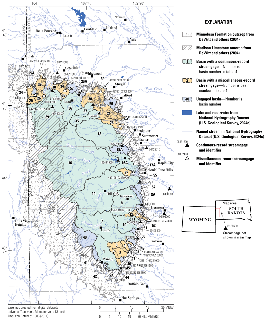
Drainage basins used to estimate annual streamflow recharge in the Black Hills area, South Dakota.
Estimates of streamflow recharge were calculated for drainage basins using three types of streamflow records: (1) those with continuous records, (2) those with miscellaneous discrete measurements, and (3) those with no measurements (ungaged). All available streamflow data were downloaded for each streamgage from the USGS NWIS database (USGS, 2024a). Site information, drainage area, type of streamflow data available, and period of record for each site are summarized in table 3. Of the 55 drainage basins, 13 had continuous streamflow data, 19 had miscellaneous streamflow data, and 23 had no streamflow data (fig. 9). The drainage area for streamgages with continuous records accounted for about 78 percent of the total drainage area. The drainage area for streamgages with miscellaneous or no measurements accounted for 13 and 9 percent, respectively, of the total drainage area.
Recharge From Streams with Continuous Records, 1950–2022
Annual streamflow recharge was calculated for 11 of the 13 basins with continuous-record streamgages. The other two basins were either combined with another basin or excluded from the analysis based on assumptions by Carter and others (2001a). Basins 16 and 16A were combined for recharge calculations, and streamflow losses in basin 36 (Whitewood Creek) were considered negligible based on streamflow observations by Hortness and Driscoll (1998). Recharge calculations for five basins with continuous-record streamgages (Battle, Boxelder, Elk, Spearfish, and Bear Butte Creeks) involved consideration of four basins with miscellaneous-record streamgages (basins 21, 30, 38, and 39) and two ungaged basins (basins 8A and 18A). These six basins were included in calculations of streamflow recharge for basins with continuous-record streamgages and are not addressed in subsequent discussions of recharge for basins with miscellaneous-record streamgages or ungaged basins.
Recharge calculations for basins with continuous-record streamgages involved comparing mean daily streamflow values to loss threshold rates. Loss threshold rates determined by Hortness and Driscoll (1998) or adjusted rates from Carter and others (2001a) were available for all 11 streams with continuous-record streamgages. Loss thresholds were applied to Madison aquifer first and Minnelusa aquifer second if loss thresholds were provided individually for both aquifers because streamflow typically flows overtop outcrops of the Madison Limestone before the Minnelusa Formation. If daily mean flows were less than the loss threshold rate, then daily recharge to the Madison and (or) Minnelusa aquifers was equal to the mean daily flow value. If daily mean flows were equal to or exceeded the loss threshold rate, then the daily recharge to the Madison and (or) Minnelusa aquifers was equal to the loss threshold rate. Calculated daily streamflow losses were aggregated to provide annual streamflow recharge for 1999–2022 and were combined with estimates from Carter and others (2001a) for 1950–98 (table 5).
Table 5.
Annual streamflow recharge for basins with continuous-record gages, water years 1950–2022, for the Madison and Minnelusa aquifers. Daily streamflow data used in calculations were downloaded from the U.S. Geological Survey National Water Information System database (USGS, 2024a).[All cells contain values derived from extrapolation of streamflow recharge estimates unless otherwise noted]
Estimation of annual streamflow recharge for basins involving continuous- and miscellaneous-record streamgages required adjustments to account for contributions from tributaries. Carter and others (2001a) provided detailed descriptions of considerations for each stream used to calculate annual streamflow recharge. For some basins with shared streams, miscellaneous-record streamgages were combined with basins with continuous-record streamgages to create a synthetic daily streamflow record that accounted for losses in ungaged tributaries. Drainage-area ratios and linear-regression analyses were used to create synthetic daily streamflow records. Drainage-area ratios were calculated by adding the drainage areas contributing to runoff for basins with continuous- and miscellaneous-record streamgages and dividing by the drainage area of the continuous-record streamgage. Drainage-area ratios were used for Battle Creek (basins 8 and 8A), Boxelder Creek (basins 18 and 18A), Elk Creek (basins 20 and 21), and Bear Butte Creek (basins 37, 38, and 39; fig. 9).
Linear regression analyses were used to create synthetic daily streamflow for Spearfish Creek (basins 29, 30, and 31) by developing relations between continuous daily flows and miscellaneous flows. Other considerations discussed in Carter and others (2001a) involved accounting for aqueduct influences on recharge along Spearfish Creek, the effect of Pactola Dam on recharge along Rapid Creek (basins 16 and 16A), and the location of streamgages and outcrops of the Madison and Minnelusa aquifers along Bear Gulch (basin 11) and Bear Butte Creek (basins 37, 38, and 39). The same methods used by Carter and others (2001a) for basins with continuous and miscellaneous records were used in this study for consistency. Additional information on special considerations for each stream are provided in Carter and others (2001a) and are not further discussed in this report. Recharge estimates for 1999–2022 for basins requiring adjustments were combined with estimates from Carter and others (2001a) for 1950–98 (table 5).
Annual recharge estimates for 1950–98 were estimated by Carter and others (2001a) using streamflow data and (or) statistical analyses. If available, mean daily streamflow data were used to calculate annual streamflow recharge; however, many sites had sparse streamflow records before the 1980s. Carter and others (2001a) provided annual streamflow recharge for 1950–98 despite only two of the streamgages used to calculate annual streamflow recharge having streamflow records extending back to 1950. Single and multiple linear regression techniques were used by Carter and others (2001a) to extend the record of recharge estimates back to 1950. Streamflow data from Battle (site 9 in table 3; fig. 9) and Boxelder Creeks (site 18 in table 3; fig. 9) were used to extrapolate recharge estimates from 1967 to 1991. Four streamgages (sites 9, 15, 22, and 35 in table 3; fig. 9)—three of which are downstream from loss zones and were not used to calculate streamflow losses—were used as representative streamgages to estimate recharge from 1950 to 1966. Carter and others (2001a) performed a stepwise regression analysis using annual mean flow from the four representative streamgages to estimate recharge for sites without available streamflow data. Additional details regarding statistical analyses are provided in Carter and others (2001a).
Statistical techniques also were used to estimate annual recharge for two sites because streamflow data were unavailable between 1999 and 2022. Streamgages along Bear Gulch (basin 11) and Elk Creek (basins 20 and 21) did not have complete streamflow records because streamgages were decommissioned before 2022. Linear regression equations were developed using the period of available data and a nearby representative streamgage. For Bear Gulch (basin 11) and Elk Creek (basins 20 and 21), the representative streamgage with the best coefficient of determination was Boxelder Creek (basin 18; table 6). Regression equations were used to estimate annual streamflow recharge during 1999–2022 for Bear Gulch (basin 11) and during 2021–22 for Elk Creek (basins 20 and 21) using relations with Boxelder Creek (basin 18; fig. 9).
Table 6.
Linear regression equations used to estimate annual streamflow recharge for streams with continuous, miscellaneous, and ungaged records.[R2, coefficient of determination]
Recharge from Streams with Miscellaneous Records, Water Years 1992–2022
In total, 11 basins had miscellaneous-record streamgages (table 4). Four of the 11 basins were considered previously in calculations of recharge for basins with continuous-record streamgages and were not analyzed using methods for basins with miscellaneous-record streamgages. Additionally, two more basins, Iron Creek (basin 26) and Higgins Gulch (basin 32), were excluded from streamflow recharge calculations because Hortness and Driscoll (1998) determined streams in both basins gained flow across outcrops of the Madison and Minnelusa aquifers. Loss thresholds determined by Hortness and Driscoll (1998) or adjusted by Carter and others (2001a) were used for the remaining five basins. Loss thresholds for Victoria Creek (basin 17) and Beaver Creek (basin 25) included losses from drainage areas in ungaged basins 17A and 25A. Therefore, these two ungaged basins are included in analyses in this section and are not addressed in the subsequent section addressing ungaged streams.
The methods used to quantify recharge for basins with continuous-record streamgages could not be used for basins with miscellaneous-record streamgages because mean daily streamflow data were unavailable. Instead, Carter and others (2001a) computed synthetic daily streamflow data for basins with miscellaneous-record streamgages using representative streamgages. A representative streamgage with continuous records was selected for each basin with a miscellaneous streamgage based on proximity, streamflow characteristics, and elevation. A drainage-area ratio was calculated for each basin pair by dividing the drainage area of the miscellaneous streamgage by the drainage area of the representative continuous streamgage (table 7). If applicable, adjusted drainage areas that excluded outcrops of the regional Madison and Minnelusa aquifers were used in drainage-area ratio calculations. Representative streamgages included French Creek (site 7), Battle Creek (site 8), Annie Creek (site 27), and Cleopatra Creek (site 28; table 4). Mean daily streamflow data for two representative streamgages with continuous records were not available for all years from 1999 to 2022 because the streamgages were decommissioned. The streamgages along Annie Creek (site 27) and Cleopatra Creek were decommissioned in 2018 and 1998, respectively. Therefore, statistical regression techniques instead of drainage-area ratios were used to estimate recharge for years without streamflow data.
Table 7.
Selected information used to estimate recharge from streams with miscellaneous-record streamgages. Drainage basins shown for streams shown in figure 9.Drainage-area ratios and (or) statistical regression techniques were used to estimate recharge for 1992–2022 for basins with miscellaneous-record streamgages depending on the availability of mean daily streamflow data. If mean daily streamflow data were available, then drainage-area ratios (table 7) were multiplied by mean daily streamflow data from the representative continuous-record streamgage to create a synthetic daily streamflow record for each basin with a miscellaneous-record streamgage. Loss thresholds (table 4) were applied to the synthetic daily streamflow record and aggregated by water year to calculate annual streamflow recharge. Noted recharge values in table 8 were calculated using synthetic daily streamflow data and loss thresholds.
Table 8.
Annual streamflow recharge for streams with miscellaneous measurements sites, water years 1992–2022. Daily streamflow data used in calculations were synthesized from daily streamflow records downloaded from the U.S. Geological Survey National Water Information System database (U.S. Geological Survey, 2024a).[All cells contain values derived from extrapolation of streamflow recharge estimates unless otherwise noted]
If mean daily streamflow were unavailable at representative continuous-record streamgages, then statistical regression techniques were used to estimate recharge. Linear regression equations were developed for Bear Gulch (basin 24), Beaver Creek (basins 25 and 25A), and False Bottom Creek (basins 33 and 34) using relations between annual recharge estimates for each of the three streams and streams with continuous records (table 6). Annual recharge estimates for Bear Gulch (basin 24), Beaver Creek (basins 25 and 25A), and False Bottom Creek (basins 33 and 34) were regressed with annual recharge estimates from representative continuous-record streamgages based on proximity, streamflow characteristics, and elevation. Spearfish Creek (basins 29 and 30) was excluded because it is controlled by an aqueduct that alters the natural streamflow characteristics along the loss zone. Some of the annual streamflow recharge estimates in table 8 were estimated using linear regression.
Carter and others (2001a) used statistical regression techniques to estimate annual streamflow recharge to the combined Madison and Minnelusa aquifers for 1950–91 for basins with miscellaneous-record streamgages. The techniques used in this study to estimate recharge deviated slightly from Carter and others (2001a) and are discussed in appendix 1.
Recharge From Ungaged Streams, Water Years 1992–2022
Ungaged basins were relatively small drainage areas (fig. 9) with undetermined loss thresholds. In total, 18 basins were ungaged and five of the ungaged basins were included in recharge calculations for basins with a continuous-record (8A, 18A, 36A) or miscellaneous-record (basins 17A and 25A) streamgage. Hortness and Driscoll (1998) did not determine loss thresholds for ungaged basins, so Carter and others (2001a) assumed 90 percent of streamflow generated within ungaged basins became recharge to the Madison and Minnelusa aquifers. The loss threshold of 90 percent of streamflow was considered appropriate because Carter and others (2001a) observed that streamflow seldom occurred downstream from loss zones in each basin.
Drainage-area ratios and (or) statistical regression techniques were used to estimate recharge for water years 1992–2022 for ungaged basins, depending on the availability of mean daily streamflow data. Because mean daily streamflow data were unavailable for ungaged basins, a representative basin with a continuous-record streamgage was selected for each basin with an ungaged stream. Four basins with a continuous-record streamgage represented streamflow in 18 ungaged basins (table 9). Drainage-area ratios were calculated by Carter and others (2001a) by dividing the total drainage area of ungaged basins associated with each streamgage by the drainage area of the representative continuous-record streamgage (table 9). Mean annual daily streamflow for each water year from the representative continuous-record streamgage was multiplied by the drainage-area ratio and by 0.90 (90-percent loss threshold) to calculate annual streamflow recharge. Annual streamflow recharge for ungaged basins represents recharge to the Madison and Minnelusa aquifers because individual recharge estimates could not be calculated. Annual streamflow recharge for basins in Wyoming were estimated using the same methods as Carter and others (2001a) by multiplying the combined recharge for Bear Gulch (basin 24) and Beaver Creek (basins 25 and 25A) in table 8 by a factor of 2.
Table 9.
Summary of selected information used to estimate recharge from ungaged streams.| Basin numbers | Drainage area, in square miles | Representative continuous-record streamgage (table 3) |
Representative continuous-record streamgage drainage area | Drainage-area ratio |
|---|---|---|---|---|
| 40–50 | 51.47 | French Creek (site 7) | 105 | 0.49 |
| 51–55 | 12.41 | Battle Creek (site 8) | 163.33 | 0.20 |
| 56 | 10.55 | Bear Butte Creek (site 37) | 16.6 | 0.64 |
| 57 | 6.96 | Cleopatra Creek (site 28) | 6.95 | 1.00 |
Adjusted drainage area from table 4.
Mean daily streamflow data were available for 1999–2022 for representative streamgages along French Creek (site 7 in table 3), Battle Creek (site 8 in table 3), and Bear Butte Creek (site 37 in table 3). Synthetic mean daily streamflow records generated from representative streamgages and the loss threshold of 0.90 were used to calculate annual streamflow recharge estimates for basins 40–50, basins 51–55, and basin 56 (table 10). Mean daily streamflow data were unavailable for 1999–2022 for the representative streamgage along Cleopatra Creek because it was decommissioned in 1998. Instead, linear regression using relations among annual recharge estimates for basin 56 and basin 57 between 1992 and 1998 from Carter and others (2001a) was used to develop a regression equation for basin 57 (table 6). Annual streamflow recharge estimates from the linear regression equation for basin 57 are provided in table 10.
Table 10.
Annual streamflow recharge from ungaged basins, water years 1992–2022, for the Madison and Minnelusa aquifers. Daily streamflow data used in calculations were synthesized from daily streamflow records downloaded from the U.S. Geological Survey National Water Information System database (U.S. Geological Survey, 2024a).[--, not determined]
Carter and others (2001a) used statistical regression techniques to estimate annual recharge to the combined Madison and Minnelusa aquifers for 1950–91 for ungaged basins. The techniques used to estimate recharge deviated slightly from Carter and others (2001a) and are discussed in the appendix 1.
Precipitation and Streamflow Recharge, 1931–2022
Summary statistics for precipitation and streamflow recharge were calculated by aquifer, if applicable, for the study area and by aquifer for subareas 1–9 (table 11) using annual recharge estimates from 1931 to 2022 in appendix 1. Statistics include minimum; maximum; mean; and the 25th, 50th (median), and 75th percentiles. Statistics were calculated for each aquifer for estimates of precipitation recharge. Streamflow recharge estimates were considered only for the Madison and Minnelusa aquifers and were combined because streamflow loss thresholds for some streams could not be differentiated by aquifer. Recharge estimates from this study (table 11) also were compared, if appropriate, to estimates from Driscoll and Carter (2001) and Carter and others (2001a, 2001b).
Total mean annual recharge for all aquifers in the study area for 1931–2022 was estimated as 278,900 acre-feet (acre-ft), with 205,100 acre-ft from precipitation recharge and 73,800 acre-ft from streamflow recharge (table 11). Mean annual precipitation recharge was greatest for the Madison (57,000 acre-ft) and Minnelusa (98,100 acre-ft) aquifers, which combined accounted for about 76 percent (or 155,100 acre-ft) of the total mean annual precipitation recharge (table 11). Mean annual precipitation recharge for the Deadwood, Minnekahta, Sundance, and Inyan Kara aquifers combined accounted for 24 percent (or 50,100 acre-ft) of the total mean annual precipitation recharge (table 11). Mean annual streamflow recharge, considered only for the Madison and Minnelusa aquifers, was about 73,800 acre-ft (table 11). Combined mean annual recharge was 228,900 for the Madison and Minnelusa aquifers (sum of mean annual precipitation and streamflow recharge in table 11), or about 82 percent of the total recharge in the study area. Total mean annual recharge for 1950–98 estimated by Driscoll and Carter (2001) could not be directly compared to results from this study because recharge to outcrops in Wyoming were excluded.
Recharge estimates for the combined Madison and Minnelusa aquifers from this study were directly compared to estimates from Carter and others (2001a) and Driscoll and Carter (2001). Mean annual precipitation recharge for the Madison (57,000 acre-ft) and Minnelusa (98,100 acre-ft) aquifers for 1931–2022 from this study were 34 and 7 percent, respectively, greater than estimates from Carter and others (2001a). Driscoll and Carter (2001) estimated precipitation recharge to the combined Madison and Minnelusa aquifers as 144,500 acre-ft for the wetter period from 1950 to 1998, which was about 7 percent less than estimates of combined precipitation recharge in this study (155,100 acre-ft; table 11). Greater precipitation recharge estimates were expected for this study because the mean precipitation for 1999–2022 (21.16 inches; Palecki and others, 2021) was greater than the long-term mean precipitation from 1950 to 1998 presented in Driscoll and Carter (2001; 18.98 inches).
Mean annual streamflow recharge for 1931–2022 was about 73,800 acre-ft (table 11), which was 9 percent greater than estimates by Carter and others (2001a; about 67,500 acre-ft) for 1931–98 and 4 percent greater than estimates by Driscoll and Carter (2001; 70,900 acre-ft) for 1950–98. Greater streamflow recharge was expected because streamflow increased in response to greater mean annual precipitation during 1999–2022. Carter and others (2001a) estimated mean annual recharge of 202,000 acre-ft for the combined Madison and Minnelusa aquifers, which was about 13 percent less than total recharge estimates in this study (228,900 acre-ft). Driscoll and Carter (2001) estimated combined recharge as 215,400 acre-ft or about 6 percent less than in this study.
Table 11.
Annual precipitation and streamflow recharge statistics for the Deadwood, Madison, Minnelusa, Minnekahta, Sundance, and Inyan Kara aquifers by subarea. Streamflow recharge values are given only for the combined Madison and Minnelusa aquifers. Recharge values do not include inflows from aquifer exchange or regional groundwater flow.Streamflow recharge considered only for the Madison and Minnelusa aquifers. Streamflow recharge in Subarea 9 was assumed to be zero based on assumptions by Carter and others (2001b).
Precipitation and streamflow recharge varied among subareas 1–9 (fig. 10A; table 11) depending on the spatial variability of precipitation, outcrop surface area, and the distribution of streamflow loss zones. Precipitation recharge generally was greatest in the northern and western Black Hills (subareas 1–4 and 9; fig. 10A; table 11) where mean annual precipitation was relatively high (fig. 8) and outcrop areas were extensive for many aquifers (fig. 7). Mean annual precipitation recharge in subareas 1 (Spearfish area) and 9 (Jewel Cave area) combined accounted for 80 percent of the precipitation recharge in the study area. In contrast, precipitation recharge was lowest in the southern and eastern Black Hills (subareas 5–8; fig. 10A; table 11) because of lower mean annual precipitation (fig. 8) and, except for subarea 8 (Hot Springs area), limited outcrops of aquifers (fig. 7). Subarea 8 had extensive outcrops of the Madison and Minnelusa aquifers but received relatively little precipitation compared to subareas further north.
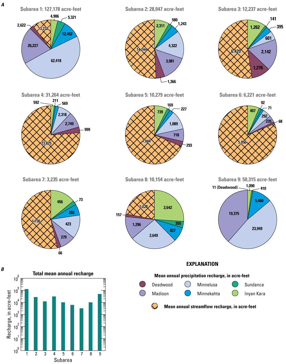
Mean annual precipitation and streamflow recharge for the Deadwood, Madison, Minnelusa, Minnekahta, Sundance, and Inyan Kara aquifers in subareas 1–9. A, Pie charts showing the distribution of recharge in subareas 1–9 for each aquifer. Streamflow recharge was considered only for the Madison and Minnelusa aquifers and was separated from precipitation recharge for comparison. B, Mean total recharge (sum of precipitation and streamflow recharge) for subareas 1–9 on a logarithmic y-axis.
Streamflow recharge also generally was greatest for subareas in the northern and western Black Hills (fig. 10A; table 11). Greater precipitation (fig. 8) and relatively high loss thresholds for many streams contributed to the relatively high streamflow recharge for subareas in the northern Black Hills. An exception was subarea 9 (Jewel Cave area) where Carter and others (2001b) noted precipitation predominantly infiltrates the extensive outcrops of the Madison and Minnelusa aquifers or evaporates before reaching any streams. Streamflow recharge was greatest in subarea 4 (Rapid City area; fig. 10A; table 11) and contributed to about 76 percent of total recharge in the subarea. Similarly, most of the total recharge was streamflow recharge for subareas along the eastern flank of the Black Hills (subareas 2–7). Streamflow recharge in subarea 1 also was relatively high but did not constitute most of the recharge in the subarea (fig. 10A).
Outflows—Artesian Springflow and Well Withdrawals
Outflow components estimated for the hydrologic budget include artesian springflow and well withdrawals. Artesian springflow consists of springs discharging at the land surface from confined aquifers located downstream from loss zones, which are typically present at the periphery of the Black Hills. These springs are generally situated near or within outcrops of the Spearfish Formation and originate from the Madison or Minnelusa aquifers (Carter and others, 2001b). Some artesian springs, such as Cleghorn/Jackson Springs, are located within the outcrops of the Minnelusa Formation, where the Madison aquifer is confined by the Minnelusa Formation. Artesian springflow was estimated only for the Madison and Minnelusa aquifers. Well withdrawals include water pumped from wells, with water rights information gathered from the SDDANR (2024a) and Wyoming State Engineer’s Office (WYSEO, 2024a). These withdrawals were estimated by calendar year instead of water year, because most users report their water usage in calendar years.
Artesian Springflow
Artesian springflow in the study area was estimated using similar methods as Carter and others (2001b) for the Madison and Minnelusa aquifers (appendix 3). Artesian springflow was assumed to be zero for all other aquifers. It is possible artesian springflow exists for one or more of the Deadwood, Minnekahta, Sundance, and Inyan Kara aquifers; however, information on possible springs and their discharge rates was unavailable and, therefore, was not estimated in this study.
Mean annual springflow estimates were based on streamflow records from streamgages (fig. 11; table 12). The period of record and the methods used to estimate mean annual artesian springflow varied for each site and are discussed in appendix 3. Streamflow records at these streamgages were analyzed for the available period of record through 2022 using data from the USGS NWIS (USGS, 2024a). Annual streamflow and base flow estimates were determined using the USGS Groundwater Toolbox version 1.3.1 (Barlow and others, 2014; 2017). Base flow for this study was calculated using the base flow index (BFI) standard hydrograph-separation method (Barlow and others, 2014). Streamgages were assigned to a subarea based on location to estimate artesian springflow for each subarea budget (table 12).
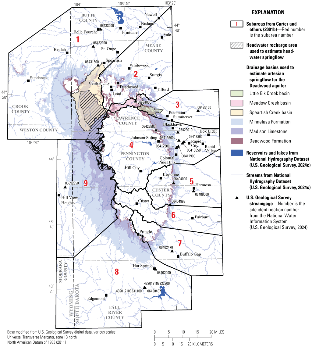
U.S. Geological Survey streamgages used for estimating artesian springflow.
Table 12.
Site information for streamgages and miscellaneous-record streamgages used for estimating mean annual artesian springflow.[NWIS, National Water Information System; ID, identification; WY, water year; ft3/s, cubic feet per second; BFI, base flow index; --, not applicable or no data]
Well Withdrawals
Well withdrawals were determined for all aquifers monitored by State agencies in South Dakota and Wyoming, which included some aquifers that were not part of the hydrologic budget but were included to estimate the total mean annual well withdrawals in the study area. Regional aquifers included in the hydrologic budget were the Deadwood, Madison, Minnelusa, Minnekahta, Sundance, and Inyan Kara. Additional aquifers for which well withdrawals were estimated include the crystalline core aquifer (consisting of Tertiary and Precambrian igneous and metamorphic rocks); an undifferentiated group of minor aquifers termed “other aquifers” within the Opeche Shale, Spearfish Formation, Unkpapa Sandstone, Newcastle Sandstone, and Pierre Shale; and Quaternary alluvial deposits. The following sections summarize the methods used to collect and analyze well withdrawal data for aquifers in the study area. Additionally, annual well withdrawal patterns from 2003 to 2022 in the study area and in each subarea are discussed.
Methods of Data Collection for Groundwater Permits and Well Withdrawals
The process for estimating well withdrawals in the study area involved three steps. First, water rights from South Dakota and Wyoming were reviewed and downloaded to calculate the total annual volume of water allowed to be diverted from each aquifer in each subarea. Second, well withdrawal data were obtained from water systems, the SDDANR (2024a), and the WYSEO (2024a). In some instances, water users are not required to report well withdrawals and did not provide historical well withdrawal data; therefore, the third step was to synthesize well withdrawal data for these systems, which is described in the following sections. A well withdrawal dataset consisting of real and synthetic well withdrawal information was constructed from 2003 to 2022 using compiled well withdrawal datasets and synthetic data.
Water Rights and Permit Information
Laws regarding water rights in South Dakota and Wyoming were reviewed before downloading permit information and estimating well withdrawals. A brief discussion of laws in each State is provided so that readers are aware of the uncertainty in well withdrawal estimates. In South Dakota, water users are required to obtain a water right permit for groundwater depending on the type of water use and if the requested maximum diversion rate exceeds a certain threshold. According to South Dakota Codified Law 46–1–6 (South Dakota State Legislature, 2024a), the only type of water use that does not require a permit is domestic, unless one of the following apply: the water use exceeds 18 gallons per minute (gal/min); irrigation of noncommercial land exceeds 1 acre in size; or the peak pumping rate exceeds 25 gal/min. Additionally, water distribution systems using 18 gal/min or less do not need to apply for a water right permit for groundwater. In Wyoming, all water users intending to utilize groundwater must obtain a permit from the State Engineer before construction and development (Wyoming Statutes Title 41, Chapter 3, Provision 930; Wyoming State Legislature, 2024). Well withdrawals for users in South Dakota with systems using 18 gal/min or less were not included in analyses because no information was available on the number of active wells and most wells did not specify the aquifer in which it was completed. It is likely well withdrawals from smaller systems constitutes a relatively small proportion of the total well withdrawals but may be locally important in some areas of the Black Hills.
Groundwater permit and license information were obtained from the SDDANR water rights database (SDDANR, 2024a) and the WYSEO permit database (WYSEO, 2024a). The criteria used for downloading water rights permit data include (1) permits with a priority date on or before December 31, 2022; (2) only permits from groundwater sources; (3) only permits within the study area; and (4) the status of the permit was “Licensed,” “Permitted,” or “Future use” in the SDDANR database and “Adjudicated” in the WYSEO database. Cancelled and unused water rights were not included, although it is acknowledged that some cancelled permits may have been active during the period of investigation. Location information provided in each permit was used to exclude those outside the study area and to separate water rights into the nine subareas constituting the study area. In total, the study area included 808 total active and future use permits (table 13), with 796 in South Dakota and 12 in Wyoming.
Table 13.
The total number of active permits and active appropriated annual volume by aquifer for water rights in the study area as of 2022.| Aquifer (fig. 1) |
Number of permits1 | Appropriated volume1 (acre-feet) |
|---|---|---|
| Crystalline | 182 | 14,788 |
| Deadwood | 35 | 3,203 |
| Madison2 | 165 | 72,000 |
| Minnelusa | 191 | 31,285 |
| Minnekahta | 31 | 3,826 |
| Inyan Kara | 112 | 12,074 |
| Sundance | 5 | 185 |
| Alluvial | 70 | 33,833 |
| Other3 | 17 | 5,584 |
| Total | 808 | 176,777 |
Permits from SDDANR and WYSEO databases contain diversion rates (maximum pumping rate), and, if specified, the maximum annual diversion volume. The diversion rate, typically given in cubic feet per second or gallons per minute, was used to calculate the maximum annual diversion volume for permits with unspecified annual diversion volumes by converting the given rate into an annual volume. For example, the maximum annual diversion volume of a water right with a maximum diversion rate of 1.0 ft3/s would equal about 724 acre-ft of water annually. The maximum annual diversion volume was summed for each aquifer in each subarea to obtain the total amount of appropriated water by aquifer in each subarea.
The SDDANR and WYSEO permit data provide the type(s) of water use (municipal, irrigation, and so forth) for each permit. Types of water-use categories included commercial, domestic, fish and wildlife propagation, geothermal, groundwater remediation, industrial, institutional, irrigation, municipal, recreation, rural water system, suburban housing development, and water distribution system. Some permits had two or more types of water use that were revised to one type to simplify analyses that determined water use by category. The major use was selected by inspecting permit documentation to determine which type of use likely required the greatest annual volume. For example, if a groundwater permit for a year-round cattle operation listed “commercial” and “domestic” as types of water use, then it was assumed the cattle required most of the water use and the water-use type was simplified to “commercial.” In total, 104 of the 808 permits specified more than one type of use and were revised to one use type.
Well Withdrawal Data Collection
Well withdrawal data were obtained from water systems, the SDDANR (Adam Mathiowetz, SDDANR, written commun., 2024), and the WYSEO (WYSEO, 2024b). USGS staff contacted operators of water systems in the Black Hills area inquiring about obtaining withdrawal records spanning as far back as possible. Most system operators provided either monthly or annual withdrawal data for the last 5 to 10 years; however, some water users provided withdrawal records into the 1980s and 1990s. The most complete withdrawal record was provided by Rapid City, the largest city and greatest water user in the Black Hills, which provided annual consumption back to 1950. The SDDANR provided annual well withdrawal data from 2003 to 2022 for nonirrigation purposes from certain water systems and individual users (Adam Mathiowetz, SDDANR, written commun., 2024). Additionally, the SDDANR provided annual well withdrawal data from 1994 to 2022 for irrigation purposes (Nakaila Steen, SDDANR, written commun., 2024). Well withdrawal data for water users in Wyoming were downloaded from WYSEO Water Usage Data Across Wyoming database (WYSEO, 2024b). The timeframe for well withdrawal data collected for Wyoming was from 2016 to 2022. All available annual well withdrawal data are provided in the data release accompanying this report (Medler and others, 2025).
Methods for Creating the Well Withdrawal Dataset for 2003–22
The well withdrawal dataset for 2003–22 was generated using annual well withdrawal data and by synthesizing annual well withdrawals for permits. Annual well withdrawal data provided by water systems, SDDANR, and WYSEO were applied to their respective permits to inventory how many permits would require synthetic data and to help calculate a multiplier that will be discussed later in this section. The year of the priority date—the date an application was filed—provided in each permit was used to determine the starting year each permit became active regardless of the month and day. In total, partial or complete well withdrawal records were provided for 298 of 808 permits (about 37 percent; table 14). Permits with partial well withdrawal records accounted for 35 of those 298 permits and the years with missing data were estimated as the mean annual well withdrawals only if 3 or more years of data were available. Synthetic annual well withdrawal data were generated for the remaining 510 permits using three methods. The well withdrawal dataset, including both data collected from users or State agencies and synthetic data for 2003–22, is provided in the data release accompanying this report (Medler and others, 2025).
Table 14.
Summary of the methods used to construct the well withdrawal dataset for 2003–22 for subareas 1–9 from Carter and others (2001b).Missing data for partial records were synthesized by replacing missing values with the mean annual use only if three of more years of data were available.
Water permits or well withdrawal records indicated the well either has not yet been drilled or used during 2003–2022.
Well withdrawal values were extrapolated to annual well withdrawal estimates using daily withdrawal estimates provided in drinking water quality records from the South Dakota Department of Agriculture and Natural Resources (2024b).
A multiplier of 0.5 was multiplied by the maximum annual appropriated volume of each permit. The value of 0.50 was the mean ratio of mean annual well withdrawals for 2003–2022 to the maximum appropriated volume for 44 permits within the study area.
The first method involved inspecting water permit documentation (SDDANR, 2024a) and well withdrawal records from SDDANR (Adam Mathiowetz, SDDANR, written commun., 2024) to determine if permits were actively diverting water. Annual well withdrawals for 2003–22 were excluded for permits meeting specified criteria. The criteria included (1) a type of “future use,” (2) standby wells only used for emergency purposes, (3) permits that added an additional diversion point but no increase of the diversion rate or volume, and (4) permits with well withdrawals that were combined with or indistinguishable from other permits. Future use permits were excluded because the permits do not become consumptive until the permittee receives approval from the SDDANR. Standby wells used for emergency purposes were excluded because annual well withdrawals for 2003–22 averaged to nearly zero for water systems that provided well withdrawal data for standby wells. Permits for adding an additional point of diversion or changing a point of diversion were excluded only if the diversion rate or volume of the original permit did not change. Well withdrawal data provided by some water users and the SDDANR grouped well withdrawals from multiple permits into a single permit. In these instances, the well withdrawals were either assigned to the permit with the greatest diversion rate or volume if the aquifer for all grouped permits was the same; otherwise, if the aquifer was different among the permit, then the well withdrawals were divided evenly among each permit. In total, 42 of the 510 permits (about 8 percent) met the criteria for exclusion (table 14).
The second method involved estimating mean annual well withdrawals for public water systems from mean daily well withdrawal rates provided in drinking water quality reports (SDDANR, 2024b). Mean daily well withdrawal rates in drinking water quality reports were calculated by the SDDANR using annual well withdrawal totals provided by the water system (Mark McIntire, SDDANR, written commun., 2024). The mean annual well withdrawal estimated from daily rates was applied to each year from 2003 to 2022. The year of the priority date in each permit was used to determine the length of the annual well withdrawal record for each permit. In total, synthetic well withdrawal data were generated for 68 of 510 permits (about 13 percent) using the mean daily rate from drinking water quality reports (table 14).
The third method was applied to permits for water users not required to report well withdrawal data to the SDDANR or to publish drinking water quality reports. The third method involved multiplying the maximum annual diversion volume either specified in permits or calculated using maximum diversion rates by a multiplier. The SDDANR uses a multiplier of 0.6 (60 percent) to estimate well withdrawals for permits not required to report withdrawals as part of the approval process for new permits (Adam Mathiowetz, SDDANR, written commun., 2024). However, a new multiplier of 0.5 was calculated using annual well withdrawal data and maximum annual appropriated volumes for selected water permits. Permits were selected if they were within the study area and had at least 3 years of annual well withdrawal data. In total, 44 permits met the specified criteria. The multiplier was calculated by dividing the mean annual withdrawal of each permit from 2003 to 2022 by the maximum appropriated annual volume specified by each permit. The water use type of permits used in calculating the new multiplier included 15 commercial, 10 municipal, 6 suburban housing development, 6 water distribution system, 5 rural water system, 1 domestic, and 1 industrial. It is possible the new multiplier may not accurately calculate the fraction of actual well withdrawals by permitted volume for certain water use type categories that were underrepresented in calculations. In total, synthetic well withdrawal data were generated for 400 of the 510 permits (about 78 percent) using the multiplier of 0.5 (table 14).
Artesian Springflow and Annual Well Withdrawals
Artesian springflow and annual well withdrawals were estimated for the study area and for subareas 1–9. Summary statistics were not calculated for artesian springflow because the period of record was inconsistent between sites (table 12). Summary statistics were calculated for annual well withdrawals by subarea and aquifer. Statistical calculations included values of zero annual well withdrawals and synthetic withdrawal estimates. Zero values were included in statistical calculations because they represent true well withdrawals. Synthetic withdrawal estimates were included to provide the best estimate possible; however, statistical estimates of annual withdrawals may not represent the true withdrawals.
Total mean annual artesian springflow in the study area was estimated as 229 ft3/s (or 166,100 acre-ft) for the Madison and Minnelusa aquifers (table 12). Artesian springflow ranged from 0.5 ft3/s (360 acre-ft) along Boxelder Creek to 103.6 ft3/s (75,000 acre-ft) along the Redwater River (table 12). Artesian springflow and well withdrawals estimated for this study were compared to results from Carter and others (2001b) and Driscoll and Carter (2001). Artesian springflow estimated in this study (166,100 acre-ft) was about 21 and 36 percent greater than mean annual artesian springflow estimated by Carter and others (2001b; 136,800 acre-ft) and Driscoll and Carter (2001; 122,400 acre-ft), respectively. Greater artesian springflow was expected because the precipitation totals were relatively high for the 23 years of additional data added for 1999–2022. Additionally, estimates of artesian springflow for this study likely were biased to wetter conditions because calculations generally included years with relatively high precipitation from the 1970s to 2022 and did not capture the drier conditions from the 1930s to the 1960s. Therefore, artesian springflow may be overestimated compared to other budget components.
Artesian springflow also was estimated for each subarea. Artesian springflow was observed in all subareas except subarea 2 (Sturgis area; table 12). For subareas containing artesian springs, springflow ranged from 6.1 ft3/s in subarea 3 (Piedmont area) to 114.5 ft3/s in subarea 1 (Spearfish area; table 12). Mean annual artesian springflow was highest in subareas 1, 4, and 8 (table 12) where large artesian springs, such as those along Spearfish Creek and Redwater River (subarea 1; Spearfish area), Jackson and Cleghorn Springs (subarea 4; Rapid City area), and Cascade Springs (subarea 8; Hot Springs area), contribute to streamflow in the study area’s largest perennial streams (Spearfish Creek, Redwater River, Rapid Creek, and Fall River). Mean annual artesian springflow was lowest in subareas 3, 5 (Hermosa area), and 7 (Wind Cave area) where springs contribute to relatively small streams (Elk Creek, Battle Creek, and Beaver Creek).
Total annual well withdrawals (sum of well withdrawals for all aquifers) varied annually but no long-term patterns were observed (fig. 12). Mean total annual well withdrawals for 2003–22 in the study area were about 50,000 acre-ft, which was about 33 percent higher than groundwater-withdrawal estimates from 1995 and 2000 (Amundson, 1998, 2002) during the BHHS. Annual well withdrawal estimates ranged from about 45,100 acre-ft in 2019 to about 52,800 acre-ft in 2017 (fig. 12; table 15). Variability of the total annual well withdrawals was attributed to climate conditions, which were evaluated by determining annual precipitation totals for climate stations in the study area (National Oceanic and Atmospheric Administration, 2024; fig. 12). Total annual well withdrawals generally increased during dry conditions (below normal precipitation) and decreased during wet conditions (above normal precipitation; fig. 12). For example, the lowest annual well withdrawals occurred during 2019, which was the wettest year on record (National Oceanic and Atmospheric Administration, 2024). Conversely, the greatest annual well withdrawals occurred during periods of below normal precipitation from 2003 to 2005 and 2016 to 2017 (fig. 12). Other than annual variations from precipitation variations, no long-term patterns corresponding to population increases were observed (fig. 12) despite the study area population increasing by about 39 percent from 2000 to 2022 (table 1).
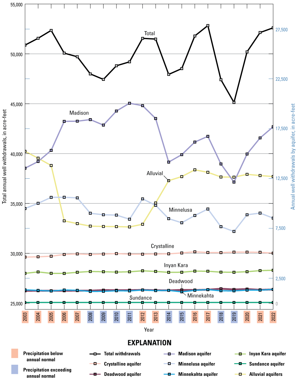
Total annual well withdrawals and annual well withdrawals for each aquifer for 2003–22.
Table 15.
Summary statistics of total annual well withdrawals for each aquifer for 2003–22.Annual well withdrawal variations and mean annual withdrawals were greatest for the Madison, Minnelusa, and alluvial aquifers (fig. 12; table 15). Annual withdrawal variations for the Madison and Minnelusa aquifers generally correlated with total annual withdrawals and annual climate variations except for a period of abnormally high withdrawals from the Madison aquifer from 2006 to 2012 (fig. 12). This period coincided with abnormally low withdrawals from alluvial aquifers (fig. 12). Water system operators for Rapid City, S. Dak., were performing maintenance on their system that withdraws water from an alluvial aquifer and were supplementing by withdrawing water from wells completed in the Madison aquifer (City of Rapid City, written commun., 2024). Other than 2006 to 2012, annual well withdrawals were relatively consistent for alluvial aquifers (fig. 12).
Mean annual withdrawals for the Madison and Minnelusa aquifers for 2003–22 were 16,500 and 9,100 acre-ft, respectively (table 15). Combined mean annual well withdrawals for the Madison and Minnelusa aquifers (25,600 acre-ft) accounted for 51 percent of the total mean annual withdrawals for aquifers in table 15. Carter and others (2001b) and Driscoll and Carter (2001) estimated well withdrawals totaling about 20,300 acre-feet per year from the Madison and Minnelusa aquifers, which was 5,300 acre-ft (or about 26 percent) less than estimates provided in this study (table 15). Mean annual withdrawals for alluvial aquifers were 11,200 acre-ft between 2003 and 2022 (table 15). Well withdrawals for alluvial aquifers were not previously estimated by the BHHS and, therefore, were not comparable to previous estimates.
Annual well withdrawals for the crystalline core, Deadwood, Minnekahta, Sundance, Inyan Kara, and “other” aquifers were relatively consistent from 2003 to 2022 (fig. 12). Withdrawals for these aquifers did not correlate with precipitation patterns or population increases in the study area because synthetic well withdrawal data were generated for more than one-half of the permits used to estimate well withdrawals. Mean annual well withdrawals for each of these aquifers were less than 5,000 acre-ft each (table 15). Well withdrawals in this study were 1.4, 1.3, 1.8, and 2.2 greater than withdrawals in Driscoll and Carter (2001) for the crystalline core, Deadwood, Minnekahta, and Inyan Kara aquifers, respectively. Withdrawals for the Sundance aquifer were 10.6 times smaller in this study than in Driscoll and Carter (2001).
Annual well withdrawal statistics also were computed for each aquifer in subareas 1–9 (table 16). Mean annual well withdrawals in subareas 1–9 ranged from about 600 acre-ft in subarea 9 (Jewel Cave area) to about 19,900 acre-ft in subarea 4 (Rapid City area; table 16). Generally, subareas 1–4, located in the northern and northeastern parts of the Black Hills, had the highest well withdrawals, whereas subareas 5–9 in the southern and southeastern Black Hills had the lowest well withdrawals. Mean annual well withdrawals were greatest in subareas 1 (Spearfish area) and 4 (Rapid City area), which corresponds with the relatively large population in both subareas (table 1). In contrast, rural subareas with smaller populations, such as subareas 6 (Custer area) and 9 (Jewel Cave area; table 1) reported the least annual well withdrawals.
The amount of water withdrawn from each aquifer varied by subarea but generally was highest for the crystalline core, Madison, Minnelusa, and alluvial aquifers (table 16). The crystalline core aquifer was most used in subareas 2 (Sturgis area) and 4 (Rapid City area), with mean annual withdrawals of about 900 and 2,000 acre-ft, respectively. The crystalline core aquifer contributed to about 53 and nearly 100 percent of the total withdrawals of all aquifers in subareas 5 (Keystone area) and 6 (Custer area; table 16). The Madison and Minnelusa aquifers were the most used in subarea 4, with mean annual withdrawals of about 8,100 acre-ft and 3,900 acre-ft, respectively (table 16). Well withdrawals also were relatively high for the Madison and Minnelusa aquifers in subarea 1, with mean withdrawals of about 5,200 and 3,000 acre-ft, respectively (table 16). Alluvial aquifers were most used in subareas 4 and 7 (Buffalo Gap area) with mean withdrawals of 4,400 and 4,000 acre-ft, respectively.
Table 16.
Summary statistics for annual well withdrawals by subarea and aquifer for 2003–22.Storage Considerations
To calculate net groundwater outflow (inflows minus outflows) in equation 2 like Carter and others (2001b), the assumption of a net zero change of storage was needed for the period of investigation from 1931 to 2022. Carter and others (2001b) used hydrographs of the Madison and Minnelusa aquifers and recharge estimates to assume zero storage change for their selected period of investigation from 1987 to 1996. Water-level datasets for hydrographs of the Madison and Minnelusa were not available before the 1960s and generally the datasets were most complete for 1990–2022; therefore, a different technique was needed to simulate water levels before the 1960s. Annual precipitation data for the study area was used to construct a curve representing the cumulative difference between each year’s annual precipitation value and the long-term mean annual precipitation from 1931 to 2022 (departure from mean annual precipitation; fig. 5). This curve can be used as a proxy for water-level changes in aquifers if correlation exists with hydrographs. Storage considerations were evaluated by comparing hydrographs to the cumulative departure from long-term mean annual precipitation curve (hereafter referred to as “cumulative departure curve”). Additionally, the cumulative departure curve was used to identify three time periods when recharge estimates were either decreasing, constant, or increasing that were evaluated to verify comparisons of hydrographs and the cumulative departure curve.
Observation wells used to evaluate correlation between water-level changes and the cumulative departure curve were selected based on several criteria. Observation well data were downloaded from the SDDANR (2024c) observation well database and the USGS NWIS database (USGS, 2024a). Wells were selected only if they were within subareas 1–9 and completed in the Deadwood, Madison, Minnelusa, Minnekahta, and Inyan Kara aquifers. Additionally, water-level records had to be 20 years or greater so that long-term comparisons could be made. In total, 72 observation wells met the selection criteria (table 17). Each observation well had continuous and (or) discrete water-level records with varying periods of record that ranged from 20 to 65 years (table 17). The oldest water-level records were from the 1960s; however, the completeness of water-level records varied by well. The mean annual water level (mean of water levels within a calendar year) was calculated for each observation well to show annual patterns that were compared to annual patterns for the cumulative departure curve.
Table 17.
Observation wells within the study area selected for analysis with site information, length of the water-level record, and Pearson correlation coefficient.[NAVD88; North American Vertical Datum of 1988; SDDANR, South Dakota Department of Agriculture and Natural Resources; USGS, U.S. Geological Survey]
The Pearson correlation coefficient was calculated to evaluate the linear relation between each hydrograph and the cumulative departure curve. Additional information on the Pearson correlation coefficient, including mathematical derivations and descriptions of the method, are summarized in Helsel and others (2020). Correlation coefficients range from −1 (perfect negative correlation) to 1 (perfect positive correlation), where negative values indicate negative correlation, a value equal to 0 indicates no correlation, and positive values indicate positive correlation. Additionally, larger absolute values indicate stronger correlation and smaller absolute values indicate weaker correlation. Correlation was considered weak if correlation coefficients were less than 0.4 and moderate to strong if correlation coefficients were greater than or equal to 0.4. The mean correlation coefficient was greater than zero for all aquifers and ranged from 0.38 for the Deadwood aquifer to 0.64 for the Minnelusa aquifer (table 18). Correlation was moderate to strong for the Madison, Minnelusa, and Minnekahta aquifers and weak for the Deadwood and Inyan Kara aquifers (table 18).
Table 18.
Summary statistics of Pearson correlation coefficient calculations for the Deadwood, Madison, Minnelusa, Minnekahta, and Inyan Kara aquifers.Hydrographs displaying the best correlation with the cumulative departure curve were selected for each aquifer to discuss general patterns for various timescales (fig. 13). Water-level records for most wells were most complete for 1990–2022 when water levels in all aquifers generally increased because of above normal precipitation. Similar patterns were observed for all aquifers—water levels increased during the 1990s, decreased during the early 2000s, and increased during the 2010s and 2020s (fig. 13). These patterns resembled the cumulative departure curve, which was expected because of the strong correlation coefficients (fig. 13). Some wells, such as LA–63A for the Minnelusa aquifer, had water-level records back to the 1960s, which were useful for determining patterns before 1990. Between 1969 and 1990 water levels at well LA–63A followed patterns of increasing and decreasing precipitation values from the cumulative departure curve (fig. 13C).
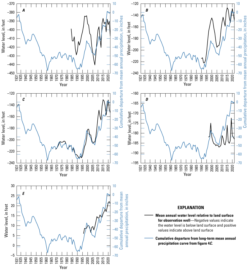
Hydrographs for observation wells completed in the Deadwood, Madison, Minnelusa, Minnekahta, and Inyan Kara aquifers. A, Deadwood aquifer (observation well PE–84A). B, Madison aquifer (observation well LA–90A). C, Minnelusa aquifer (observation well LA–63A). D, Minnekahta aquifer (observation well CU–96A). E, Inyan Kara aquifer (observation well PE–95B). Observation well data were from the South Dakota Department of Agriculture and Natural Resources (2024c).
Of the 72 total wells evaluated, negative correlation coefficients were observed for 5 wells and weak correlation coefficients (values less than 0.4) were observed for 13 wells (table 18). Negative correlation was observed for wells with decreasing water levels during the 2010s and 2020s when the cumulative departure curve increased. It is possible water-level decreases were caused by nearby pumping wells, which was true for at least one well (PE–65A) completed in Madison aquifer that was within 1 mile of an active pumping well in Rapid City, S. Dak. Hydrographs for wells with weak correlation followed the same general increasing and decreasing patterns as the cumulative departure curve; however, the maximum water level for 11 of the 13 wells was greater in the early 2000s than in 2022, which did not match the cumulative departure curve. It is possible varying recharge mechanisms may be responsible for the discrepancy, such as a greater percentage of recharge coming from streamflow rather than precipitation or greater influences from regional groundwater flow.
Correlation between hydrographs and the cumulative departure curve were verified using combined recharge estimates for 1931–2022 (fig. 13). The cumulative departure curve was used to identify a period of decreasing water levels (decreasing storage) from 1931 to 1964, a period of relatively stable water levels (zero storage change) from 1965 to 1986, and a period of increasing water levels (increasing storage) from 1987 to 2022 (fig. 13). Recharge mechanisms likely have not changed since the 1930s, so it was assumed that recharge estimates for each period were comparable. The period from 1931 to 1964 was considered a deficit for recharge because the cumulative departure curve decreased throughout nearly the entire period (fig. 13). Near zero storage change was considered for the period from 1965 to 1986 when the cumulative departure curve was relatively stable with no long-term increasing or decreasing precipitation patterns. A surplus of recharge was observed for the period from 1987 to 2022, which was confirmed by hydrographs (fig. 13).
Combined mean annual recharge was calculated for each period and compared to combined mean annual recharge for 1931–2022. Combined mean annual recharge for 1965–86 was 220,861 acre-ft, which was about 7,890 acre-ft (or 3.5 percent) less than the combined mean annual recharge for 1931–2022 (228,751 acre-ft; table 1.3). The relatively small difference between the combined mean annual recharge for 1931–2022 and combined mean annual recharge for 1965–86 was expected because hydrographs showed that storage change was minimal. The absolute difference between combined mean annual recharge for 1931–2022 and combined mean annual recharge for 1931–64 (171,576 acre-ft) and 1987–2022 (287,571 acre-ft) were approximately equal at about 57,175 (deficit) and 58,820 (surplus) acre-ft, respectively. The combined mean annual recharge values for 1931–64 and 1987–2022 verified that storage change was minimal between 1931 and 2022 because their recharge values were nearly equal in magnitude but opposite in sign (negative for 1931–64 and positive for 1987–2022).
Discussion of Groundwater Budget and Availability
Groundwater budgets and availability are discussed for the Deadwood, Madison, Minnelusa, Minnekahta, Sundance, and Inyan Kara aquifers in subareas 1–9. Budget items for the Madison and Minnelusa aquifers were combined because streamflow recharge could not be differentiated for loss zones in many basins. Groundwater budgets were evaluated by calculating net groundwater flow (inflows minus outflows) for each aquifer in subareas 1–9. Net groundwater flow values are discussed by aquifer and subarea. Water availability is discussed by comparing inflows (recharge) to well withdrawals and total appropriations from water permits and by updating the volume of extractable water in storage for aquifers in the Black Hills region.
Table 19.
Hydrologic budget including inflows from recharge and outflows from springs and well withdrawals for the Deadwood, Madison and Minnelusa, Minnekahta, Sundance, and Inyan Kara aquifers in subareas 1–9.Mean values were used for inflows and outflows in the groundwater budget to calculate net groundwater flow. The time span from which mean values were calculated varied by budget item. Mean values were chosen so that budget estimates were as unbiased as possible to wet or dry periods that may skew long-term mean values. Mean precipitation and streamflow recharge were calculated for 1931–2022 using recharge estimates in table 19. The period of available data used for calculating artesian springflow varied by spring (table 12) but generally was from wetter periods from the 1970s to the 2020s. Therefore, the artesian springflow estimates provided in the groundwater budget (table 19) may be more biased toward wetter periods than other budget items. Mean well withdrawals were calculated for the shortest period (2003–22) but were considered adequate because the purpose of this study was to compare long-term budgets to modern well withdrawals. Mean values used for budget items were considered adequate representations of the long-term mean because storage change was estimated to be near zero with the study area experiencing both wet and dry periods.
Groundwater Budgets
Net groundwater flow was calculated using equation 2 for each aquifer in subareas 1–9 based on the assumption of zero storage change for aquifers in the study area (table 19). Net groundwater flow included inflows and outflows from regional groundwater in and out of subarea boundaries and for leakage between adjacent aquifers occurring within subareas. Vertical leakage to and from adjacent aquifers could not be distinguished from groundwater inflow or outflows. Driscoll and Carter (2001) considered vertical leakage a relatively small component of the budget and, therefore, included it with net groundwater flow. Aquifers with positive net groundwater flow values (inflows greater than outflows) likely had a surplus of groundwater that contributed to regional groundwater flow out of a subarea. Aquifers with negative net groundwater flow values (outflows greater than inflows) likely had a deficit of groundwater and relied on inflows from regional groundwater flow to account for the deficit. Carter and others (2001b) used potentiometric contours of the Madison and Minnelusa aquifers to determine the direction of regional groundwater flow in and out of subareas. Potentiometric contours for the study area were available only for the Madison and Minnelusa aquifers, and, therefore, are not discussed for other aquifers.
Net groundwater flow was positive for most aquifers in subareas 1–9 with exceptions for the Madison and Minnelusa aquifers in subareas 4, 7, and 8 and for the Deadwood and Inyan Kara aquifers in subareas 9 and 4 respectively (table 19). Negative net groundwater flow for the Madison and Minnelusa aquifers in subareas 7 and 8 can be accounted for by inflows from regional groundwater flow across subarea boundaries and from outside the study area. Based on generalized potentiometric contours of the Madison and Minnelusa aquifers from Carter and others (2001b; figs. 14 and 15), subarea 8 receives regional groundwater flow from subarea 9 and from outside the study area, which then flows into subarea 7. The groundwater deficit for the Madison and Minnelusa aquifers in subarea 8 (about −29,400 acre-ft; table 19) was accounted for by the surplus in subarea 9 (about 33,300 acre-ft); however, it is possible subarea 8 also receives additional inflows from regional groundwater flow of the Madison and Minnelusa aquifers that is recharged outside of the study area. The Madison and Minnelusa aquifers in subarea 7 also had a groundwater deficit (−4,800 acre-ft) but likely received inflows from subareas 6 and 8 based on potentiometric contours of the Madison and Minnelusa aquifers (figs. 14 and 15; table 19). The combined surplus of groundwater for the Madison and Minnelusa aquifers in subareas 6 (5,600 acre-ft) and 8 after receiving inflows from subarea 9 (3,900 acre-ft; totaling 9,500 acre-ft; table 19) accounted for the groundwater deficit in subarea 7 (about −4,800 acre-ft) and likely contributed to regional groundwater flow east of the study area. Negative net groundwater flow in subarea 9 was −3 acre-ft, which was within the margin of error for estimates of inflows and outflows and, therefore, may not actually be negative.
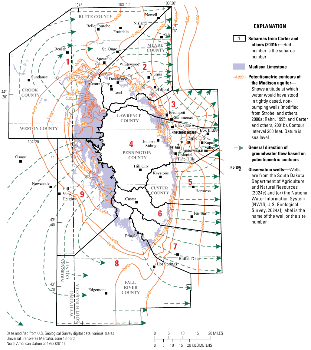
Generalized potentiometric contours of the Madison aquifer in the study area from Strobel and others (2000a) and modified by Carter and others (2001b).
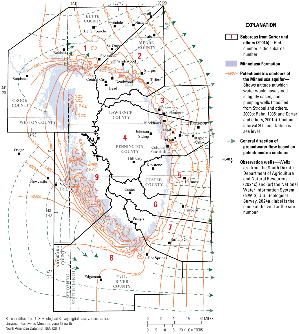
Generalized potentiometric contours of the Minnelusa aquifer in the study area from Strobel and others (2000b) and modified by Carter and others (2001b).
In subarea 4, the net groundwater flow for the Madison and Minnelusa aquifers was negative (about −4,400 acre-ft; table 19). Based on potentiometric contours of the Madison and Minnelusa aquifers (figs. 14 and 15), relatively large inflows from other subareas and (or) regional groundwater flow were unlikely; however, potentiometric contours are generalized and may not accurately represent localized flow across subarea boundaries. It is also possible that leakage from adjacent aquifers, such as the Deadwood aquifer, may contribute water that was not accounted for in the hydrologic budget. Aquifer exchange is difficult to quantify and, therefore, was included in net groundwater flow. Budget uncertainty also may be a factor when considering net groundwater flow because outflows (artesian springflow and well withdrawals) could be overestimated, or inflows (recharge from precipitation and streamflow losses) could be underestimated. It is likely that one or more of the possible explanations discussed contribute to the negative net groundwater flow calculated for subarea 4 (table 19).
Hydrographs for wells completed in the Madison and Minnelusa aquifers in subarea 4 were evaluated to determine if storage in both aquifers was decreasing near Rapid City, S. Dak., because it was the largest water user in subarea 4 and, on average, accounted for about 49 percent of the mean annual well withdrawals from the Madison and Minnelusa aquifers. In total, five wells completed in the Madison or Minnelusa aquifers near Rapid City, S. Dak., with greater than 20 years of water-level data were evaluated (fig. 16). Hydrographs for observation wells near or downgradient of pumping wells in Rapid City, S. Dak., generally show similar annual water-level increases and decreases as other wells in the study area that correlate with precipitation patterns (fig. 13); however, water levels in 2022 were similar or lower than water levels in the late 1990s for wells near and downgradient of pumping wells (fig. 16). Water levels were greater in 2022 than in the late 1990s for most observation wells away from pumping, which correlated with the cumulative departure curve for precipitation (fig. 13). Well withdrawals at pumping wells may be responsible for water-level discrepancies and it is possible that pumping may have reduced the amount of water added to storage in the Madison aquifer in subarea 4. Additional observation wells downgradient of pumping wells in subarea 4 could help further determine the influence of pumping wells on the aquifers, such as the Madison aquifer.
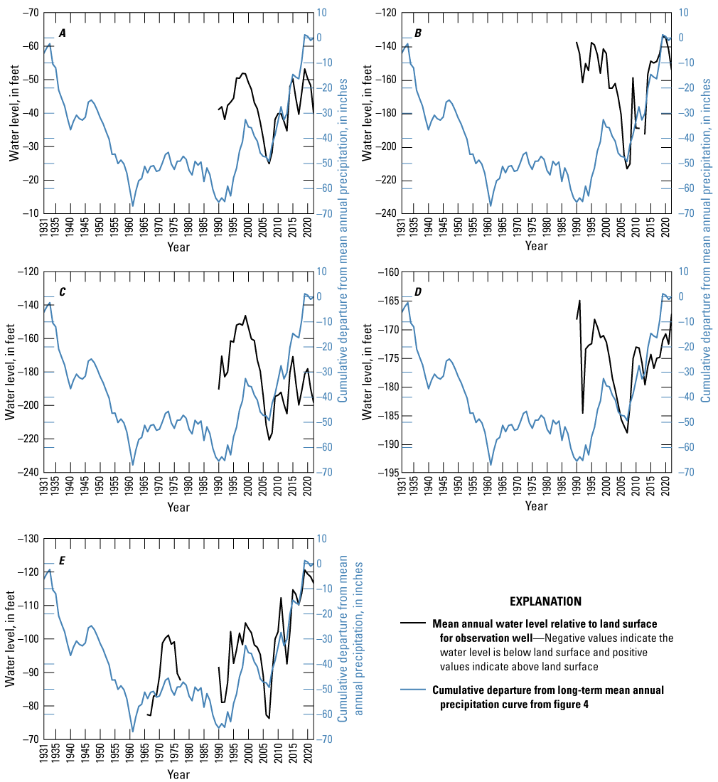
Hydrographs of wells completed in the Madison and Minnelusa aquifers near Rapid City, South Dakota (shown in figs. 14 and 15). A, Madison aquifer (observation well PE–89A). B, Madison aquifer (observation well 440430103160202). C, Madison aquifer (observation well 440427103131701). D, Minnelusa aquifer (observation well PE–64A). E, Minnelusa aquifer (observation well PE–64B).
Groundwater Availability
Groundwater availability in the study area is affected by many factors and varies spatially. Aquifer-related factors affecting groundwater availability include location, local recharge, groundwater flow conditions, historical well withdrawals, and structural features (Carter and others, 2003). Other factors affecting groundwater availability are the laws governing entities use to issue water rights or manage aquifers and the water quality of groundwater resources. Previous sections of this report discussed aquifer-related factors affecting groundwater availability, but not State laws or groundwater quality. Therefore, discussions of groundwater availability in this section are focused on relevant State laws and groundwater quality. Carter and others (2003) provide a detailed summary of groundwater availability in the Black Hills area of South Dakota and some parts of their analysis are either used or updated in this section.
Water availability for aquifers in the study area was evaluated for subareas 1–9 by comparing estimated mean annual recharge to estimated mean annual well withdrawals. According to South Dakota State Codified Law 46–6–3.1 (South Dakota State Legislature, 2024b), applications to appropriate groundwater cannot be approved if the proposed quantity of water withdrawn annually would exceed the quantity of estimated mean annual recharge to an aquifer; however, applications can be approved for instances where appropriations exceed mean annual recharge for withdrawals from formations older than or stratigraphically lower than the Cretaceous Greenhorn Formation for water distribution systems, such as municipalities or rural water systems. The State codified law does not divide mean annual recharge into the subareas used in this report, so water availability estimates (“Total annual appropriations as a percentage of mean annual recharge” in table 20) do not indicate compliance or noncompliance with codified laws. Annual appropriations generally are greater than actual well withdrawals because most water users do not use the total annual amount appropriated by permits. Total annual appropriations (excluding appropriations for future use) and mean and maximum annual well withdrawals for 2003–22 are included in table 20 for comparison with mean annual recharge for 1931–2022 for each aquifer in subareas 1–9. It should be noted that artesian springflow was the greatest outflow component for Madison and Minnelusa aquifers but was not included as an outflow in table 20.
Table 20.
Total mean annual recharge (table 11), mean annual well withdrawals (table 15), maximum annual well withdrawals (table 15), and total annual appropriations (as of 2022) for aquifers in subareas 1–9.| Subarea | Aquifer | Total mean annual recharge, in acre-ft (1931–2022)1 |
Mean annual well withdrawals, in acre-ft (2003–22; table 16) |
Maximum annual well withdrawals, in acre-ft (year varies; table 16) | Total annual appropriated volume as of 2022, in acre-ft2 | Total annual appropriations as a percentage of mean annual recharge3 |
|---|---|---|---|---|---|---|
| 1 | Deadwood | 2,622 | 497 | 540 | 1,014 | 38.7 |
| Madison and Minnelusa | 101,877 | 8,283 | 10,045 | 34,536 | 33.9 | |
| Minnekahta | 12,452 | 965 | 1,091 | 3,219 | 25.9 | |
| Sundance | 5,321 | 10 | 10 | 69 | 1.3 | |
| Inyan Kara | 4,906 | 854 | 887 | 2,862 | 58.3 | |
| 2 | Deadwood | 1,366 | 84 | 138 | 263 | 19.2 |
| Madison and Minnelusa | 22,547 | 2,387 | 2,949 | 9,298 | 41.2 | |
| Minnekahta | 1,243 | 16 | 17 | 34 | 2.7 | |
| Sundance | 580 | 58 | 58 | 116 | 20.0 | |
| Inyan Kara | 2,311 | 518 | 592 | 1,869 | 80.9 | |
| 3 | Deadwood | 1,276 | 0 | 0 | 0 | 0.0 |
| Madison and Minnelusa | 9,163 | 1,408 | 1,693 | 5,722 | 62.4 | |
| Minnekahta | 395 | 44 | 44 | 88 | 22.3 | |
| Sundance | 141 | 0 | 0 | 0 | 0.0 | |
| Inyan Kara | 1,262 | 383 | 447 | 1,473 | 116.7 | |
| 4 | Deadwood | 999 | 681 | 769 | 1,826 | 182.8 |
| Madison and Minnelusa | 28,894 | 11,932 | 16,099 | 32,480 | 112.4 | |
| Minnekahta | 569 | 227 | 233 | 470 | 82.6 | |
| Sundance | 211 | 0 | 0 | 0 | 0.0 | |
| Inyan Kara | 592 | 647 | 718 | 2,828 | 477.5 | |
| 5 | Deadwood | 293 | 35 | 35 | 71 | 24.2 |
| Madison and Minnelusa | 8,851 | 390 | 472 | 1,465 | 16.6 | |
| Minnekahta | 227 | 0 | 0 | 0 | 0.0 | |
| Sundance | 169 | 0 | 0 | 0 | 0.0 | |
| Inyan Kara | 739 | 211 | 339 | 1,533 | 207.3 | |
| 6 | Deadwood | 68 | 0 | 0 | 0 | 0.0 |
| Madison and Minnelusa | 5,583 | 0 | 4 | 618 | 11.1 | |
| Minnekahta | 71 | 0 | 0 | 0 | 0.0 | |
| Sundance | 92 | 0 | 0 | 0 | 0.0 | |
| Inyan Kara | 407 | 0 | 0 | 0 | 0.0 | |
| 7 | Deadwood | 66 | 0 | 0 | 0 | 0.0 |
| Madison and Minnelusa | 2,438 | 67 | 378 | 790 | 32.4 | |
| Minnekahta | 202 | 0 | 0 | 0 | 0.0 | |
| Sundance | 73 | 0 | 0 | 0 | 0.0 | |
| Inyan Kara | 456 | 69 | 69 | 138 | 30.2 | |
| 8 | Deadwood | 157 | 0 | 0 | 0 | 0.0 |
| Madison and Minnelusa | 6,173 | 734 | 1,160 | 6,065 | 98.3 | |
| Minnekahta | 827 | 16 | 35 | 15 | 1.8 | |
| Sundance | 355 | 0 | 0 | 0 | 0.0 | |
| Inyan Kara | 2,642 | 366 | 455 | 1,191 | 45.1 | |
| 9 | Deadwood | 11 | 14 | 14 | 29 | 261.5 |
| Madison and Minnelusa | 43,324 | 468 | 715 | 2,400 | 5.5 | |
| Minnekahta | 5,480 | 0 | 0 | 0 | 0.0 | |
| Sundance | 410 | 0 | 0 | 0 | 0.0 | |
| Inyan Kara | 1,090 | 90 | 90 | 180 | 16.5 |
Mean annual recharge was not exceeded by mean annual well withdrawals, maximum annual well withdrawals, or total annual appropriations in subareas 1, 2, and 6–8 for all aquifers. Total annual appropriations as a percentage of mean annual recharge was calculated for each aquifer to assess the approximate availability of each aquifer in subareas 1–9 by dividing mean annual recharge by total annual appropriations (as of 2022). More than 50 percent was available for all aquifers in subareas 1 and 2 except for the Inyan Kara aquifer (table 20). In subarea 6 (Custer area), the percentage of mean annual recharge was near zero for all aquifers except for the Madison and Minnelusa aquifers. Percentage of mean annual recharge was greater than 30 percent for the Madison and Minnelusa and Inyan Kara aquifers in subarea 7 (Wind Cave area) but was near zero for other aquifers. Total appropriations in subarea 8 (Hot Springs area) were less than 50 percent for all aquifers except for the Madison and Minnelusa aquifers, which were nearly equal to the total recharge and differed by about 100 acre-ft (table 20). As stated previously, subarea 8 receives regional groundwater flow from subarea 9 (Jewel Cave area) and, therefore, availability may be slightly underestimated in subarea 8.
Total annual appropriations, mean annual well withdrawals, and (or) maximum annual well withdrawals exceeded mean annual recharge for various aquifers in 4 of the 9 subareas (table 20). In subarea 3 (Piedmont area), total annual appropriations for the Inyan Kara aquifer exceeded mean annual recharge by about 200 acre-ft. Mean and maximum well withdrawals, however, did not exceed mean annual recharge for the Inyan Kara aquifer in subarea 3. Mean annual recharge was exceeded by total appropriations in subarea 4 for the Madison and Minnelusa aquifers and the Inyan Kara aquifer (table 20). Total appropriations for the Madison and Minnelusa aquifers exceeded mean annual recharge by about 3,600 acre-ft. Mean and maximum annual well withdrawals for the Madison and Minnelusa aquifers were about 41 and 56 percent, respectively, of mean annual recharge in subarea 4. Total appropriations, mean annual well withdrawals, and maximum annual well withdrawals all exceeded mean annual recharge for the Inyan Kara aquifer in subarea 4 (Rapid City area; table 20). In subarea 5 (Hermosa area), mean annual recharge for the Inyan Kara aquifer was nearly two times less than total annual appropriations but was greater than mean and maximum well withdrawals. Total annual appropriations for the Deadwood aquifer were more than two times greater than mean annual recharge in subarea 9 (Jewel Cave area) and mean and maximum annual well withdrawals were nearly equal to recharge.
In addition to recharge, water availability also includes the water stored in pore spaces of aquifer materials. It is important to note that not all water stored in aquifers can be removed, so Carter and others (2003) used effective porosity values for each aquifer from Rahn (1985) to estimate the volume of recoverable water in six major aquifers in the Black Hills area (table 21). Effective porosity was multiplied by the area encompassed by each aquifer and the mean or maximum saturated thickness of each aquifer depending on whether the aquifers were unconfined or confined to calculate the volume of recoverable water. Estimates of total volume of recoverable water were updated as part of this study to include areas in Wyoming and used the same saturated thickness and effective porosity estimates as Carter and others (2003). Estimates of total recoverable volume were not provided by Carter and others (2003) for the Sundance aquifer and the total volume of recoverable water was not calculated in this report because the information needed for calculations was unavailable.
Table 21.
Aquifer characteristics, including area, maximum thickness, mean saturated thickness, and effective porosity, and the estimated total amount of recoverable water in storage.[--, not applicable]
From Rahn (1985).
The area used in storage calculation was the area of the exposed Precambrian rocks, which is 825 square miles.
In total, the estimated total amount of recoverable water in storage in the study area was 356.9 million acre-ft for six major aquifers in the Black Hills area of South Dakota and Wyoming (table 21), which is more than 15 times greater than the maximum storage capacity of Oahe Reservoir on the Missouri River (23,137,000 acre-ft; U.S. Army Corps of Engineers, 2012) east of the Black Hills in South Dakota (not shown). Estimates provided in this study were about 40 percent greater than in Carter and others (2003) because of the additional area added in Wyoming. The largest storage volume was for the Inyan Kara aquifer (127.2 million acre-ft) because of its relatively large effective porosity (0.17). Estimated storage volumes for the Madison (83.6 million acre-ft) and Minnelusa (96.9 million acre-ft) aquifers were the third and second largest, respectively, because of the relatively large saturated thickness of both aquifers (table 21). The Precambrian, Deadwood, and Minnekahta aquifers had the smallest estimated storage volumes of all major aquifers because of relatively small areas, saturated thicknesses, and (or) low effective porosity.
The estimated volume of recoverable water in storage in the study area was large; however, water quality varies throughout the study area and, in some areas, may not be suitable for all types of water use. Water quality is an important consideration because the desired quality varies depending on the type of use. For example, water systems supplying drinking water require greater water quality than systems used for industrial and irrigation purposes. Groundwater quality can be affected by many factors and can contain numerous constituents from natural and (or) human sources. Natural sources primarily are introduced from the geologic materials within aquifers and the length of time water is in contact with geological materials, which can increase the concentration of constituents (Winter and others, 1998). Human-related constituents can be introduced to groundwater from many sources, such as chemicals used in agricultural practices leaching into the groundwater table or biologic constituents leaking into aquifers from septic tanks or sewer systems. In the Black Hills area, groundwater quality is affected by natural and human sources and heavily affected by interactions between groundwater and surface water. Williamson and Carter (2001) provide a detailed overview of groundwater quality for aquifers in the Black Hills area.
Carter and others (2003) evaluated the spatial variability of groundwater quality in the Black Hills area of South Dakota. In general, water quality was best within and near outcrop areas of aquifers and decreased downgradient of outcrop areas as aquifer depth increased. Groundwater quality varied by aquifer but in most cases physical properties (temperature, specific conductance, and hardness) and chemical constituents (arsenic, iron, manganese, sodium, sulfate) that could require water treatment increased downgradient. Radionuclide concentrations also were relatively high for some aquifers, such as the Deadwood and Inyan Kara aquifers, and exceeded U.S. Environmental Protection Agency standards in some areas (Carter and others, 2003). Municipal pumping wells completed in the Madison aquifer for the cities of Hot Springs, Rapid City, Spearfish, Sturgis, and Whitewood generally were within 20 miles of outcrops and had adequate groundwater quality for drinking water. Conversely, water was relatively hot and salty for municipal wells completed in the Madison aquifer for the cities of Box Elder and Edgemont, which were farther than 20 miles from outcrops. Therefore, the amount of recoverable water in storage adequate for drinking water systems without treatment likely is considerably less than estimates provided in table 21.
Limitations
Limitations affecting the datasets and methods used in this study were identified and are discussed in this section. Limitations are discussed for the various inflow and outflows of the hydrologic budget and groundwater availability. Carter and others (2001a), Carter and others (2001b), and Driscoll and Carter (2001) each provide discussions of limitations and uncertainty for their studies, which also apply to this study because many of the same methods and datasets were used. Uncertainty was not quantified for any of the results presented in this study but is discussed in general terms by evaluating datasets and methods used to construct hydrologic budgets and estimate water availability.
Precipitation recharge estimates were limited by the data and methods used to estimate recharge. Older precipitation datasets, especially records before the 1950s, have greater uncertainty than more recent datasets because fewer climate stations were available with complete records (Driscoll and others, 2000). Uncertainty was also introduced by interpolation of precipitation data between climate station locations. Inherently, precipitation data for areas with sparse climate stations have higher uncertainty than areas with dense climate station distributions.
The recharge calculation for this study simplified a complex system of evapotranspiration and precipitation infiltration that is affected by many variables including land cover, soil permeability and thicknesses, temperature, soil saturation, precipitation intensities, and so forth, into a simple equation with annual precipitation, mean annual precipitation, and mean annual yield efficiency as the only variables. The use of the annual yield equation (eq. 3) was based on multiple assumptions that make the quantification of uncertainty difficult. The assumption that equation 3 was sufficient in estimating annual yield efficiency was based on regressions between yield efficiency and precipitation from different streamgages with varying amounts of data (Carter and others, 2001a). The recharge factor used to estimate how much precipitation from the yield equation becomes groundwater recharge was also a simplifying factor that increased uncertainty of the recharge estimates. The infiltration rates of soil horizons and hydrologic units of the study area likely vary spatially with higher infiltration rates in some areas. Although many assumptions and simplifications were made, the general estimates of the groundwater recharge were reasonable and close to estimates made in previous studies.
Streamflow recharge estimates had fewer limitations and less uncertainty than precipitation recharge because estimates were based on measured values of streamflow and loss thresholds for most basins; however, the data and methods used to calculate streamflow recharge presented limitations that varied by site. Streamflow records and loss thresholds were available for most basins in the study area, but the length and completeness of streamflow records varied by streamgage. In general, streamflow records were sparse before 1990 for most streamgages and only a few streamgages had records back to the 1950s. Some streamgages had relatively long streamflow records but were not complete because streamflow was not measured for some years. The period from 1990 to 2022 had the most complete streamflow records and the least uncertainty.
Streamgages with relatively long streamflow records had the least uncertainty, whereas sites with short streamflow records and (or) no measured loss thresholds presented the greatest uncertainty and required additional methods to estimate streamflow recharge. The synthetically generated streamflow records and loss thresholds from representative basins used to estimate recharge for some basins may not accurately represent true basin conditions; however, no additional information was available and, therefore, these estimates were considered adequate for calculating streamflow recharge. Statistical linear regression techniques were used to lengthen streamflow records and (or) estimate annual recharge for various basins and time periods, such as 1931–50 when almost no streamflow records were available. Linear regression techniques inherently introduced uncertainty because relations among sites were not perfect, and the variability of natural systems, such as streams, cannot be captured by linear regression. The best regression equation with the highest coefficient of determination value was used to reduce uncertainty as much as possible.
Uncertainty in estimates of headwater and artesian springflow were from the method used to estimate precipitation recharge, which was used to estimate headwater springflow, and the varying data available for estimating artesian springflow. Headwater springflow was assumed to equal the recharge from infiltration of precipitation in the part of the Limestone Plateau east of the groundwater divide. The accuracy of the estimates depends on the accuracy of the yield efficiencies used to estimate precipitation recharge, which was discussed earlier in this section. Jarrell (2000) compared headwater springflow estimates using yield efficiency to the measured runoff or base flow at several springs with multiple years of discharge records. Differences in the annual values for the period of record between the estimated basin yield and the measured discharge ranged from 1 percent to about 70 percent of the measured discharge (Carter and others, 2001b). However, all but one site had differences less than 22 percent. This range of differences likely represents the uncertainty of headwater springflow estimates. Uncertainty for artesian springflow estimates varied for each site based on the availability of discharge measurements at each site. Sites with more discharge data had more accurate annual mean estimates; however, sites with few discharge measurements, such as the springs near Cascade Springs (432013103332200 and 432012103331100) in the southern Black Hills had more uncertainty and less accurate annual mean estimates.
The data and methods used to estimate well withdrawals had several limitations. The water rights dataset (SDDANR, 2024a) used in this study likely was not complete for 1931–2022. Only water rights active as of 2022 were included in the dataset and all cancelled permits were excluded. It is probable that some permits cancelled before 2022 were active for some time between 1931 and 2022 and exclusions of these permits would underestimate the true number of permits and appropriations for years spanning the active period of cancelled permits. Another limitation was that some permits were for two or more aquifers, which made differentiating appropriations difficult for each aquifer. Only one permit for multiple aquifers was identified, so this limitation likely did not have a large effect on the results of this study; however, it is possible more permits with two or more aquifers were missed. In addition to multiple aquifers, some permits specified one or more types of water use. Permits with several water-use types were simplified to one type—the inferred major type of water use—to evaluate how water was used in the study area because permits do not specify appropriations for each type of water use. The simplification likely either underestimated or overestimated the number of permits and (or) appropriations for the various water use types.
Well withdrawal estimates for 2003–22 were affected by the same limitations as water rights data but also by inherent uncertainty of well withdrawal datasets and the methods used to estimate well withdrawals if well withdrawal data were unavailable. Estimating annual well withdrawals involved matching reported annual water-use data from the SDDANR (Adam Mathiowetz, SDDANR, written commun., 2024), WYSEO (2024b), or provided by water users to permit information. Therefore, the same limitations regarding cancelled permits, permits with two or more aquifers, and simplification of water use types for permits apply to the spatial and temporal evaluations of groundwater. Well withdrawal datasets were provided by either State agencies in South Dakota and Wyoming or from individual water users. Water users are responsible for tracking and reporting well withdrawals, which involves installing devices that measure withdrawals. The devices used by water users to track water usage can break, causing a data gap, or can give erroneous readings that may underestimate or overestimate withdrawals. The uncertainty of well withdrawals measured by these devices was acknowledged but likely was relatively small compared to other sources of uncertainty in the following paragraphs.
Annual well withdrawal data were unavailable for many permits because State agencies in South Dakota and Wyoming did not require water users to report their withdrawals until the 2000s. Water users for some permits still are not required to report their use as of 2022 and some users did not report withdrawals despite requirements. Additionally, well withdrawal estimates for certain types of water use were more uncertain than others. For example, many commercial and industrial permits did not require users to report water usage, whereas most municipal and irrigation permits required annual reporting. The most complete dataset was for 2003–22 when the greatest number of permits had available well withdrawal data. Before 2003, annual well withdrawal data were sparse and, therefore, withdrawals were not estimated. The scope of this study was to compare modern well withdrawals to long-term recharge, so the lack of well withdrawal data before 2003 did not affect the objectives of this study.
Missing well withdrawal data between 2003 and 2022 were estimated using three methods that all introduced various degrees of uncertainty. The first method involved determining permits with zero well withdrawals based on information provided in permits and (or) by water users. Many water systems have backup systems that are used when a primary system goes offline or when water demand exceeds the maximum capacity of the primary system. Unless well withdrawal data were provided by water systems, well withdrawals for permits for backup systems were assumed to be zero, which may have underestimated the true withdrawals. The second method consisted of calculating annual well withdrawals using mean daily withdrawal rates. Daily rates were calculated from annual well withdrawal data collected by State agencies for an unspecified year. The mean daily withdrawal rate represents well withdrawals for only 1 year and likely either underestimates or overestimates well withdrawals for a different year. The third method involved multiplying maximum annual diversion volumes by a ratio of 0.5 to determine annual well withdrawals, which was based on permits that were required to report withdrawals. Estimates derived using the third method (ratio) had the greatest uncertainty and estimated the same annual well withdrawals every year, which is not realistic because well withdrawals vary annually.
In general, well withdrawal data had the least uncertainty relative to other budget items because the data were based on recorded numbers provided by water users. Additionally, most of the largest water users in the study area, such as municipalities, were required to report water usage, which made estimates of annual well withdrawals more accurate. Domestic well withdrawals for smaller users were not considered and, therefore, the annual total well withdrawal estimates provided in this study may be slightly underestimated for each aquifer. Domestic well withdrawals are difficult to quantify because users are not required to report withdrawals and the true number of wells actively being used is unknown.
Groundwater availability presented in this report included discussion of the volume of recoverable water in storage for major bedrock aquifers. The data and methods used to estimate the volume of recoverable water in storage had several limitations. Storage calculations were based on generalized aquifer properties that may not accurately represent true conditions throughout the study area. The area encompassed by aquifers in the study area is not known and the estimates provided in this study were derived from spatial datasets of bedrock geology covering a large area. The uncertainty of geologic maps generally increases as the size of the mapped area increases. Despite the uncertainty associated with geologic maps, the size of each aquifer relative to one another likely was adequate for calculations. Greater uncertainty for storage calculations was from the other aquifer properties used in storage calculations—including maximum aquifer thickness, mean saturated thickness, and effective porosity values. Aquifer properties are known to vary considerably over short distances in the study area based on well drilling logs and aquifer tests (Carter and others, 2003).
Summary
Population growth and recurring droughts in the Black Hills region can affect water resources and future availability. Drought conditions in the late 1980s and the early 2000s stressed local water systems that relied heavily on surface water as the population of the region was increasing. The Black Hills hydrology study (BHHS) was initiated in the early 1990s to inventory and assess the region's water resources, focusing on the quantity, quality, and distribution of surface water and groundwater. The population of the Black Hills region increased by about 39 percent since completion of the BHHS in 2000 compared to 2022, which has renewed interest in future water demand and availability in the Black Hills. Historical well withdrawal patterns and availability estimates can inform effective resource management. The U.S. Geological Survey (USGS) has not comprehensively collected or analyzed detailed well withdrawal data and hydrologic budgets for aquifers in the Black Hills region since completion of the BHHS.
The USGS, in cooperation with the Western Dakota Regional Water System, completed a study to (1) update hydrologic budgets from the BHHS for six of the most used aquifers in the Black Hills and (2) to evaluate water availability by comparing results from hydrologic budgets to modern well withdrawals and water rights information from State agencies and (or) water systems. Key updates to the BHHS budgets include (1) adding available data from 1999 to 2022 and (2) dividing hydrologic budgets for each aquifer into subareas. The aquifers included in this study were the Deadwood, Madison, Minnelusa, Minnekahta, Sundance, and Inyan Kara. Hydrologic budgets consisted of various budget components including inflows and outflows. Inflows included recharge, leakage from adjacent (underlying or overlying) aquifers, and groundwater inflows across the study area boundary (regional groundwater flow). Outflows included springflow, well withdrawals, leakage to adjacent aquifers, and regional groundwater flow out of the study area. Leakage to and from adjacent aquifers was difficult to quantify, so previous studies and this study included leakage with groundwater flows for budgeting purposes.
Recharge included infiltration of precipitation on outcrops of geologic units and streamflow recharge where streams cross outcrops and lose all or part of their flow. Total mean annual recharge for all aquifers in the study area was estimated at 278,900 acre-feet (acre-ft), with 205,100 acre-ft from precipitation recharge and 73,800 acre-ft from streamflow recharge. Mean annual precipitation recharge for the Madison and Minnelusa aquifers together accounted for 76 percent of the total mean annual precipitation recharge, with the Madison aquifer contributing 57,000 acre-ft and the Minnelusa aquifer contributing 98,100 acre-ft. Mean annual precipitation recharge for the Madison (57,000 acre-ft) and Minnelusa (98,100 acre-ft) aquifers for 1931–2022 from this study were 34 and 7 percent, respectively, greater than estimates from Carter and others (2001a). Mean annual streamflow recharge for 1931–2022 was about 73,800 acre-ft, which was 9 percent greater than estimates for 1931–98 (67,500 acre-ft) and 4 percent greater than estimates for 1950–98 (70,900 acre-ft). Mean annual precipitation recharge for the Deadwood, Minnekahta, Sundance, and Inyan Kara aquifers combined accounted for 24 percent (or 50,100 acre-ft) of the total mean annual precipitation recharge.
Precipitation recharge generally was greatest in the northern and western Black Hills (subareas 1–4 and 9) where mean annual precipitation was relatively high and outcrop areas were extensive for many aquifers. Mean annual precipitation recharge in subareas 1 (Spearfish area) and 9 (Jewel Cave area) combined accounted for about 80 percent of the precipitation recharge in the study area. In contrast, precipitation recharge was lowest in the southern and eastern Black Hills (subareas 5–8) because of lower mean annual precipitation and, except for subarea 8 (Hot Springs area), limited outcrops of aquifers. Streamflow recharge also generally was greatest for subareas in the northern and western Black Hills except in subarea 9 (Jewel Cave area) where a previous study noted precipitation predominantly infiltrates the extensive outcrops of the Madison and Minnelusa aquifers or evaporates before reaching any streams. Streamflow recharge was greatest in subarea 4 (Rapid City area) and contributed to about 76 percent of total recharge in the subarea. Similarly, most of the total recharge was streamflow recharge for subareas along the eastern flank of the Black Hills (subareas 2–7).
Outflow components estimated for the hydrologic budget include artesian springflow and well withdrawals. Artesian springflow was estimated only for the Madison and Minnelusa aquifers. Total mean annual artesian springflow in the study area was estimated as 229 cubic feet per second (ft3/s; or 166,100 acre-ft) for the Madison and Minnelusa aquifers. Artesian springflow estimated in this study (166,100 acre-ft) was about 21 and 36 percent greater than mean annual artesian springflow estimated for 1987–96 (136,800 acre-ft) and 1950–98 (122,400 acre-ft), respectively. Outflows from artesian springflow also were estimated for each subarea. Artesian springflow was observed in all subareas except subarea 2 (Sturgis area). Springflow ranged from 6.1 ft3/s in subarea 3 (Piedmont area) to 114.5 ft3/s in subarea 1 (Spearfish area). Mean annual artesian springflow was highest in subareas 1 (Spearfish area), 4 (Rapid City area), and 8 (Hot Springs area) where large artesian springs contribute to streamflow in the largest perennial streams in the study area. Mean annual artesian springflow was lowest in subareas 3 (Piedmont area), 5 (Hermosa area), and 7 (Wind Cave area) where springs contribute to relatively small streams.
Mean total annual well withdrawals for 2003–22 in the study area were about 50,000 acre-ft, which was about 33 percent higher than groundwater-withdrawal estimates from 1995 and 2000 during the BHHS. Annual well withdrawal estimates ranged from about 45,100 acre-ft in 2019 to about 52,800 acre-ft in 2017. No increased well withdrawal patterns corresponding to population increases were observed between 2003 and 2022 despite the study area population increasing by about 39 percent from 2000 to 2022. Mean annual withdrawals for the Madison and Minnelusa aquifers for 2003–22 were 16,500 and 9,100 acre-ft, respectively. Mean annual withdrawals for alluvial aquifers were 11,200 acre-ft. Annual well withdrawals for the crystalline core, Deadwood, Minnekahta, Sundance, Inyan Kara, and “other” aquifers were each less than 5,000 acre-ft.
Mean annual well withdrawals in subareas 1–9 ranged from about 600 acre-ft in subarea 9 (Jewel Cave area) to about 19,900 acre-ft in subarea 4 (Rapid City area). Generally, subareas 1–4, located in the northern and northeastern parts of the Black Hills, had the highest well withdrawals, whereas subareas 5–9 in the southern and southeastern Black Hills had lower withdrawals. Well withdrawals were greatest in subareas 1 and 4 because of the relatively large municipal use for the cities of Rapid City and Spearfish, South Dakota, respectively. The amount of water withdrawn from each aquifer varied by subarea but generally was highest for the crystalline core, Madison, Minnelusa, and alluvial aquifers. The crystalline core aquifer contributed to about 53 and nearly 100 percent of the total withdrawals of all aquifers in subareas 5 (Keystone area) and 6 (Custer area). The Madison and Minnelusa aquifers were the most used in subarea 4, with mean annual withdrawals of about 8,100 acre-ft and 3,900 acre-ft, respectively. Well withdrawals also were relatively high for the Madison and Minnelusa aquifers in subarea 1, with mean withdrawals of about 5,200 and 3,000 acre-ft, respectively. Alluvial aquifers were most used in subareas 4 and 7 (Buffalo Gap area) with mean withdrawals of 4,400 and 4,000 acre-ft, respectively.
Net groundwater flow included inflows and outflows from regional groundwater in and out of subarea boundaries and for leakage between adjacent aquifers occurring within subareas. Net groundwater was positive for most aquifers in subareas 1–9 with exceptions for the Madison and Minnelusa aquifers in subareas 4, 7, and 8 and for the Deadwood and Inyan Kara aquifers in subareas 9 and 1, respectively. Negative net groundwater flow for the Madison and Minnelusa aquifers in subareas 7 and 8 can be accounted for by inflows from regional groundwater flow across subarea boundaries and from outside the study area. Negative net groundwater flow in subarea 9 was −3 acre-ft, which was within the margin of error for estimates of inflows and outflows and, therefore, may not actually be negative.
Based on potentiometric contours of the Madison and Minnelusa aquifers in subarea 4, relatively large inflows from other subareas and (or) regional groundwater flow were unlikely; however, potentiometric contours are generalized and may not accurately represent localized flow across subarea boundaries. It is also possible that leakage from adjacent aquifers in subarea 4, such as the Deadwood aquifer, may contribute water that was not accounted for in the hydrologic budget. Hydrographs for wells completed in the Madison and Minnelusa aquifers in subarea 4 were evaluated to determine if storage in both aquifers was decreasing near Rapid City, S. Dak., because it was the largest water user in subarea 4 and, on average, accounted for about 49 percent of the mean annual well withdrawals from the Madison and Minnelusa aquifers.
Hydrographs for observation wells near or downgradient of pumping wells in Rapid City, S. Dak., generally show similar annual water-level increases and decreases as other wells in the study area that correlate with precipitation patterns; however, water levels in 2022 were similar or lower than water levels in the late 1990s for wells near and downgradient of pumping wells. Water levels were greater in 2022 than in the late 1990s for most observation wells away from pumping, which correlated with the cumulative departure curve for precipitation. Well withdrawals at pumping wells may be responsible for water-level discrepancies and it is possible that pumping may have reduced the amount of water added to storage in the Madison aquifer in subarea 4.
Aquifer-related factors affecting groundwater availability include location, local recharge, groundwater flow conditions, historical well withdrawals, and structural features. Other factors affecting groundwater availability are the laws governing entities’ use to issue water rights or manage aquifers and the water quality of groundwater resources. Total annual appropriations (excluding appropriations for future use) and mean and maximum annual well withdrawals for 2003–22 were compared to mean annual recharge for 1931–2022 for each aquifer in subareas 1–9. Mean annual recharge was not exceeded by mean annual well withdrawals, maximum annual well withdrawals, and total annual appropriations in subareas 1, 2, and 6–8 for all aquifers.
In subarea 3 (Piedmont area), total annual appropriations for the Inyan Kara aquifer exceeded mean annual recharge by about 200 acre-ft. Mean and maximum well withdrawals, however, did not exceed mean annual recharge for the Inyan Kara aquifer in subarea 3. Mean annual recharge was exceeded by total appropriations in subarea 4 for the Madison and Minnelusa aquifers and the Inyan Kara aquifer. Total appropriations for the Madison and Minnelusa aquifers exceeded mean annual recharge by about 3,600 acre-ft. Mean and maximum annual well withdrawals for the Madison and Minnelusa aquifers were about 41 and 56 percent, respectively, of mean annual recharge in subarea 4. Total appropriations, mean annual well withdrawals, and maximum annual well withdrawals all exceeded mean annual recharge for the Inyan Kara aquifer in subarea 4 (Rapid City area). In subarea 5 (Hermosa area), mean annual recharge for the Inyan Kara aquifer was nearly two times less than total annual appropriations but was greater than mean and maximum well withdrawals. Total annual appropriations for the Deadwood aquifer were more than two times greater than mean annual recharge in subarea 9 (Jewel Cave area) and mean and maximum annual well withdrawals were nearly equal to recharge.
In addition to recharge, water availability also includes the water stored in pore spaces of aquifer materials. Estimates of total volume of recoverable water were updated as part of this study to include areas in Wyoming and used the same saturated thickness and effective porosity estimates as a previous study. In total, the estimated total amount of recoverable water in storage in the study area was 356.9 million acre-ft for six major aquifers in the Black Hills area of South Dakota. The largest storage volume was for the Inyan Kara aquifer (127.2 million acre-ft) because of its relatively large effective porosity (0.17). Estimated storage volumes for the Madison (83.6 million acre-ft) and Minnelusa (96.9 million acre-ft) aquifers were the third and second largest, respectively, because of the relatively large saturated thickness of both aquifers. The Precambrian, Deadwood, and Minnekahta aquifers had the smallest estimated storage volumes of all major aquifers because of relatively small areas, saturated thicknesses, and (or) low effective porosity.
The estimated volume of recoverable groundwater in storage in the study area was large; however, water quality varies throughout the study area and, in some areas, may not be suitable for all types of water use. In the Black Hills area, groundwater quality is affected by natural and human sources and heavily affected by interactions between groundwater and surface water. In general, water quality was best within and near outcrop areas of aquifers and decreased downgradient of outcrop areas as aquifer depth increased. Therefore, the amount of recoverable water in storage adequate for drinking water systems without treatment likely is considerably less than estimates provided in this study.
References Cited
Amundson, F.D., 1998, Estimated use of water in South Dakota, 1995: U.S. Geological Survey Open-File Report 98–268, 18 p., accessed December 2024 at https://doi.org/10.3133/ofr98268.
Amundson, F.D., 2002, Estimated use of water in South Dakota, 2000: U.S. Geological Survey Open-File Report 02–440, 17 p., accessed December 2024 at https://doi.org/10.3133/ofr02440.
Anderson, M.T., Driscoll, D.G., and Williamson, J.E., 1999, Ground-water and surface-water interactions along Rapid Creek near Rapid City, South Dakota: U.S. Geological Survey Water-Resources Investigations Report 98–4214, 99 p., accessed April 2025 at https://pubs.usgs.gov/publication/wri984214.
Barlow, P.M., and Cunningham, W.L., Zhai, T., and Gray, M., 2014, U.S. Geological Survey Groundwater Toolbox, a graphical and mapping interface for analysis of hydrologic data (version 1.0)—User guide for estimation of base flow, runoff, and groundwater recharge from streamflow data: U.S. Geological Survey Techniques and Methods, book 3, chap. B10, 27 p., accessed April 2025 at https://doi.org/10.3133/tm3B10.
Barlow, P.M., and Cunningham, W.L., Zhai, T., and Gray, M., 2017, U.S. Geological Survey Groundwater Toolbox version 1.3.1—A graphical and mapping interface for analysis of hydrologic data: U.S. Geological Survey software release, accessed April 2025 at https://doi.org/10.5066/F7R78C9G.
Bowles, C.G., and Braddock, W.A., 1963, Solution breccias of the Minnelusa Formation in the Black Hills, South Dakota and Wyoming, in Water Resources Division, U.S. Geological Survey, Short papers in geology and hydrology, Articles 60–121—Geological Survey research 1963: U.S. Geological Survey Professional Paper 475–C, p. C91–C95, accessed August 2024 at https://doi.org/10.3133/pp475C.
Carter, J.M., Driscoll, D.G., and Hamade, G.R., 2001a, Estimated recharge to the Madison and Minnelusa aquifers in the Black Hills area, South Dakota and Wyoming, water years 1931–98: U.S. Geological Survey Water Resources Investigations Report 00–4278, 66 p., accessed August 2024 at https://doi.org/10.3133/wri004278.
Carter, J.M., Driscoll, D.G., Hamade, G.R., and Jarrell, G.J., 2001b, Hydrologic budgets for the Madison and Minnelusa aquifers, Black Hills of South Dakota and Wyoming, water years 1987–96: U.S. Geological Survey Water-Resources Investigations Report 01–4119, 51 p., accessed August 2024 at https://doi.org/10.3133/wri014119.
Carter, J.M., Driscoll, D.G., and Williamson, J.E., 2002, The Black Hills hydrology study, U.S. Geological Survey: U.S. Geological Survey Fact Sheet 046–02, 6 p. [Also available at https://doi.org/10.3133/fs04602.]
Carter, J.M., Driscoll, D.G., and Foster Sawyer, J., 2003, Ground-water resources in the Black Hills area, South Dakota: U.S. Geological Survey Water-Resources Investigations Report 03–4049, 36 p., accessed December 2024 at https://doi.org/10.3133/wri034049.
Darton, N.H., Paige, S., 1925, Central Black Hills folio, South Dakota: U.S. Geological Survey Numbered Series 219, 34 p., 7 plates, accessed August 2024 at https://doi.org/10.3133/gf219.
DeWitt, E., Redden, J.A., Wilson, A.B., Buscher, D., and Dersch, J.S., 1986, Mineral resource potential and geology of the Black Hills National Forest, South Dakota and Wyoming: U.S. Geological Survey Bulletin 1580, 135 p., accessed August 2024 at https://doi.org/10.3133/b1580.
DeWitt, E., Redden, J.A., Buscher, D.P., and Wilson, A.B., 1989, Geologic map of the Black Hills area, South Dakota and Wyoming: U.S. Geological Survey Map I–1910, scale 1:250,000., accessed August 2024 at https://doi.org/10.3133/i1910.
Driscoll, D.G., 1992, Plan of study for the Black Hills hydrology study, South Dakota: U.S. Geological Survey Numbered Series 92–84, 10 p., accessed August 2024 at https://doi.org/10.3133/ofr9284.
Driscoll, D.G., and Carter, J.M., 2001, Hydrologic conditions and budgets for the Black Hills of South Dakota through water year 1998, U.S. Geological Survey Water-Resources Investigations Report 01–4226, 148 p., accessed July 2024 at https://pubs.usgs.gov/wri/wri014226/pdf/wri014226.pdf.
Driscoll, D.G., Carter, J.M., William, J., and Putman, L., 2002, Hydrology of the Black Hills area, South Dakota: U.S. Geological Survey Water-Resources Investigations Report 02–4094, accessed August 2024 at https://doi.org/10.3133/wri024094.
Driscoll, D.G., Hamade, G.R., and Kenner, S.J., 2000, Summary of precipitation data for the Black Hills area of South Dakota, water years 1931–98: U.S. Geological Survey Open-File Report 00–329, 151 p., accessed August 2024 at https://doi.org/10.3133/ofr00329.
Eldridge, W.G., Hoogestraat, G.K., and Rice, S.E., 2021, Borehole analysis, single-well aquifer testing, and water quality for the Burnpit well, Mount Rushmore National Memorial, South Dakota: U.S. Geological Survey Scientific Investigations Report 2021–5059, 29 p., accessed April 2025 at https://doi.org/10.3133/sir20215059.
Esri, 2024a, How IDW works: Esri, ArcGIS Pro Desktop Tool Reference, accessed April 2025 at https://pro.arcgis.com/en/pro-app/latest/tool-reference/spatial-analyst/how-idw-works.htm.
Esri, 2024b, How zonal statistics tools work: Esri, ArcGIS Pro Desktop Tool Reference, accessed April 2025 at https://pro.arcgis.com/en/pro-app/latest/tool-reference/spatial-analyst/how-zonal-statistics-works.htm.
Fenneman, N.M., and Johnson, D.W., 1946, Physiographic divisions of the conterminous U.S.: U.S. Geological Survey data release, accessed July 2025 at https://doi.org/10.5066/P9B1S3K8.
Gott, G.B., Wolcott, D.E., and Bowles, C.G., 1974, Stratigraphy of the Inyan Kara group and localization of uranium deposits, southern Black Hills, South Dakota and Wyoming: U.S. Geological Survey Professional Paper 763, 57 p., 5 plates. [Also available at https://doi.org/10.3133/pp763.]
Greene, E.A., 1993, Hydraulic properties of the Madison aquifer system in the western Rapid City area, South Dakota: U.S. Geological Survey Water-Resources Investigations Report 93–4008, 56 p., accessed April 2025 at https://doi.org/10.3133/wri934008.
Helsel, D.R., Hirsch, R.M., Ryberg, K.R., Archfield, S.A., and Gilroy, E.J., 2020, Statistical methods in water resources: U.S. Geological Survey Techniques and Methods, book 4, chap. A3, 458 p., accessed August 2024 at https://doi.org/10.3133/tm4A3.
Hortness, J.E., and Driscoll, D.G., 1998, Streamflow losses in the Black Hills of western South Dakota: U.S. Geological Survey Water-Resources Investigations Report 98–4116, 99 p., accessed August 2024 at https://doi.org/10.3133/wri984116.
Johnson, J.F., and Micale, D.C., 2008, Geologic map of the Lance Creek 30' x 60' quadrangle, Niobrara and Converse counties, Wyoming, Fall River and Custer counties, South Dakota, and Sioux County, Nebraska: Wyoming State Geological Survey Map Series 79, scale 1:100,000, accessed July 2025 at https://www.wsgs.wyo.gov/pubs-maps/publication-search.aspx?PubID=MS-79.
McLaughlin, J.F., and Ver Ploeg, A.J., 2006, Geologic map of the Newcastle 30' x 60' quadrangle, Weston and Niobrara counties, Wyoming, and Pennington and Custer counties, South Dakota: Wyoming State Geological Survey Map Series 71, scale 1:100,000, accessed April 2025 at https://www.wsgs.wyo.gov/pubs-maps/publication-search.aspx?PubID=MS-71.
Medler, C.J., Anderson, T.M., and Eldridge, W.G., 2025, Datasets used in constructing hydrologic budgets for six bedrock aquifers in the Black Hills area of South Dakota and Wyoming, 1931–2022: U.S. Geological Survey data release, https://doi.org/10.5066/P1QWKUKP.
National Oceanic and Atmospheric Administration, 2024, U.S. climate normals: National Oceanic and Atmospheric Administration National Centers for Environmental Information, accessed July 1, 2024, at https://www.ncei.noaa.gov/products/land-based-station/us-climate-normals.
Palecki, M., Durre, I., Applequist, S., Arguez, A., and Lawrimore, J., 2021: U.S. climate normals 2020—U.S. monthly climate normals (1991–2020): National Oceanic and Atmospheric Administration, National Centers for Environmental Information, accessed April 2025 at https://www.ncei.noaa.gov/access/search/data-search/normals-monthly-1991-2020.
South Dakota Department of Agriculture and Natural Resources [SDDANR], 2024a, Water rights in South Dakota: South Dakota Department of Agriculture and Natural Resources, accessed August 2024 at https://danr.sd.gov/OfficeOfWater/WaterRights/Databases/WaterRights.aspx
South Dakota Department of Agriculture and Natural Resources [SDDANR], 2024b, Drinking water program: South Dakota Department of Agriculture and Natural Resources, accessed August 2024 at https://danr.sd.gov/OfficeOfWater/DrinkingWater/default.aspx.
South Dakota Department of Agriculture and Natural Resources [SDDANR], 2024c, Observation wells: South Dakota Department of Agriculture and Natural Resources, accessed April 2025 at https://apps.sd.gov/NR69obswell/default.aspx.
South Dakota Drought Task Force, 2015, South Dakota Drought Mitigation Plan—November 2015: South Dakota Department of Public Safety, accessed December 2024 at https://dps.sd.gov/application/files/5615/0161/4504/2015-SD-Drought-Mitigation-Plan_LR.pdf.
South Dakota State Legislature, 2024a, Codified laws—46–1–6. Definition of terms: South Dakota State Legislature, accessed August 2024 at https://sdlegislature.gov/Statutes/46-1-6.
South Dakota State Legislature, 2024b, Codified laws—46–6–3.1. Annual withdrawal of groundwater not to exceed recharge—Except for water distribution systems: South Dakota State Legislature, accessed August 2024 at https://sdlegislature.gov/Statutes/46-6-3.1.
Strobel, M.L., Galloway, J.M., Hamade, G.R., and Jarrell, G.L., 2000a, Potentiometric surface of the Madison aquifer in the Black Hills area, South Dakota: U.S. Geological Survey Hydrologic Atlas 745–D, 1 map, 2 sheets, accessed August 2024 at https://doi.org/10.3133/ha745D.
Strobel, M.L., Galloway, J.M., Hamade, G.R., and Jarrell, G.L., 2000b, Potentiometric surface of the Minnelusa aquifer in the Black Hills area, South Dakota: U.S. Geological Survey Hydrologic Atlas 745–C, 1 map, 2 sheets, accessed August 2024 at https://doi.org/10.3133/ha745C.
Strobel, M.L., Jarrell, G.J., Sawyer, J.F., Schleicher, J.R., and Fahrenbach, M.D., 1999, Distribution of hydrogeologic units in the Black Hills area, South Dakota: U.S. Geological Survey Hydrologic Investigations Atlas 743, 3 sheets, scale 1:100,000., accessed August 2024 at https://doi.org/10.3133/ha743.
Sutherland, W.M., 2007, Geologic map of the Sundance 30' x 60' quadrangle, Crook and Weston counties, Wyoming, and Lawrence and Pennington counties, South Dakota: Wyoming State Geological Survey Map Series 78, scale 1:100,000, accessed April 2025 at https://www.wsgs.wyo.gov/pubs-maps/publication-search.aspx?PubID=MS-78.
Sutherland, W.M., 2008, Geologic map of the Devils Tower 30' X 60' quadrangle, Crook County, Wyoming, Butte and Lawrence counties, South Dakota, and Carter County, Montana: Wyoming State Geological Survey Map Series 81, scale 1:100,000, accessed April 2025 at https://www.wsgs.wyo.gov/pubs-maps/publication-search.aspx?PubID=MS-81.
Thornton, P.E., Shrestha, R., Thornton, M., Kao, S.-C., Wei, Y., and Wilson, B.E., 2021, Gridded daily weather data for North America with comprehensive uncertainty quantification: Scientific Data, v. 8, no. 190, 17 p., accessed August 2024 at https://doi.org/10.1038/s41597-021-00973-0.
Thornton, M.M., Shrestha, R., Wei, Y., Thornton, P.E., Kao, S.-C., and Wilson, B.E., 2022, Daymet—Daily surface weather data on a 1-km grid for North America, Version 4 R1: Oak Ridge, Tenn., Oak Ridge National Laboratory, accessed December 2024 at https://doi.org/10.3334/ORNLDAAC/2129.
U.S. Army Corps of Engineers, 2012, Oahe Project statistics: U.S. Army Corps of Engineers, accessed April 2025 at https://www.nwo.usace.army.mil/Media/Fact-Sheets/Fact-Sheet-Article-View/Article/487631/oahe-project-statistics/.
U.S. Census Bureau, 1952, Census of population 1950—Volume II, Characteristics of the population—Part 41, South Dakota: U.S. Census Bureau, 23 p., accessed July 2024 at https://www2.census.gov/library/publications/decennial/1950/population-volume-2/41601746v2p41ch1.pdf.
U.S. Census Bureau, 1973, Census of population 1970—Volume II, Charcteristics of the population—Part 43, South Dakota: U.S. Census Bureau, 36 p., accessed July 2024 at https://www2.census.gov/library/publications/decennial/1970/population-volume-1/00496492v1p43ch2.pdf.
U.S. Census Bureau, 1983, Detailed population characteristics—South Dakota, chap. D43 of 1980 Census population, Volume 1. Characteristics of the population: U.S. Census Bureau, 448 p., accessed July 2024 at https://www2.census.gov/library/publications/decennial/1980/volume-1/south-dakota/1980censusofpopu80143u_bw.pdf.
U.S. Census Bureau, 1992, 1990 Census of population, General population characteristics—South Dakota: U.S. Census Bureau, 272 p., accessed July 2024 at https://www2.census.gov/library/publications/decennial/1990/cp-1/cp-1-43.pdf.
U.S. Census Bureau, 2003, South Dakota—2000, Summary population and housing characteristics, 2000 Census of population and housing: U.S. Census Bureau, 357 p., accessed July 2024 at https://www2.census.gov/library/publications/2002/dec/phc-1-43.pdf.
U.S. Census Bureau, 2012, South Dakota—2001, Population and housing unit counts, 2010 Census of population and housing: U.S. Census Bureau, 96 p., accessed July 2024 at https://www2.census.gov/library/publications/decennial/2010/cph-2/cph-2-43.pdf.
U.S. Census Bureau, 2024, City and town population totals—2020-2023: U.S. Census Bureau, accessed July 2024 at https://www.census.gov/data/tables/time-series/demo/popest/2020s-total-cities-and-towns.html.
U.S. Geological Survey [USGS], 2024a, USGS water data for the Nation: U.S. Geological Survey National Water Information System database, accessed August 2024 at https://doi.org/10.5066/F7P55KJN.
U.S. Geological Survey [USGS], 2024b, StreamStats: U.S. Geological Survey digital data, accessed August 2024 at https://streamstats.usgs.gov/ss/.
U.S. Geological Survey [USGS], 2024c, National Hydrography Dataset (ver. USGS National Hydrography Dataset Plus High Resolution (NHDPlus HR) for 4-digit Hydrologic Unit - 1012 (published 20180503)): accessed January 2024 at https://www.usgs.gov/national-hydrography/access-national-hydrography-products.
Williamson, J.E., and Carter, J.M., 2001, Water-quality characteristics in the Black Hills area, South Dakota: U.S. Geological Survey Water-Resources Investigations Report 2001–4194, 196 p., accessed August 2024 at https://doi.org/10.3133/wri20014194.
Winter, T.C., Harvey, J.W., Franke, O.L., and Alley, W.M., 1998, Groundwater and surface water—A single resource: U.S. Geological Survey Circular 1139, 79 p., accessed August 2024 at https://doi.org/10.3133/cir1139.
Wyoming State Engineer’s Office [WYSEO], 2024a, e-Permit and Instructions: Wyoming State Engineer’s Office, accessed August 2024 at https://seo.wyo.gov/home/e-permit-and-instructions.
Wyoming State Engineer’s Office [WYSEO], 2024b, Water usage data across Wyoming: Wyoming State Engineer’s Office, accessed August 2024 at https://lookerstudio.google.com/reporting/dcd8ee98-02fa-4718-b2cc-b0e87d0928e5/page/43OhB.
Wyoming State Legislature, 2024, Chapter 1—General provisions: Wyoming State Legislature, Title 41—Water, accessed August 2024 at https://wyoleg.gov/statutes/compress/title41.pdf.
Appendix 1. Streamflow Recharge Extrapolation Methods
Table 1.1.
Estimated streamflow recharge for selected continuous-record, miscellaneous-record, and ungaged basins, water years 1992–2022.[ft3/s, cubic feet per second]
Mean from Carter and others (2001).
Table 1.2.
Estimated total streamflow recharge, in cubic feet per second, from all sources, water years 1950–2022.[--, not computed]
Other streams with minimal regulation, including Battle Creek, Boxelder Creek, Grace Coolidge Creek, French Creek, Spring Creek, Bear Butte Creek, Bear Gulch, Beaver Creek, and Elk Creek.
Mean from Carter and others (2001).
Table 1.3.
Summary of streamflow, precipitation, and combined recharge, water years 1931–2022.[ft3/s, cubic feet per second; --, not applicable]
Updated annual streamflow recharge values differ from Carter and others (2001).
Table 1.4.
Extrapolated streamflow recharge to the Madison and Minnelusa aquifers for subareas 1–9 for 1931–2022 with minimum, maximum, mean, and median annual streamflow.References Cited
Carter, J.M., Driscoll, D.G., and Hamade, G.R., 2001, Estimated recharge to the Madison and Minnelusa aquifers in the Black Hills area, South Dakota and Wyoming, water years 1931–98: U.S. Geological Survey Water Resources Investigations Report 00–4278, 66 p., accessed August 2024 at https://doi.org/10.3133/wri004278.
Hortness, J.E., and Driscoll, D.G., 1998, Streamflow losses in the Black Hills of western South Dakota: U.S. Geological Survey Water-Resources Investigations Report 98–4116, 99 p., accessed August 2024 at https://doi.org/10.3133/wri984116.
Appendix 2. Headwater Springflow Estimates, 1931–2022
Table 2.1.
Estimated mean annual recharge to contributing areas for headwater springs, water years 1931–2022.[ft3/s, cubic feet per second]
References Cited
Bunkers, M.J., Smith, M., Driscoll, D., and Hoogestraat, G., 2015, Hydrologic response for a high-elevation storm in the South Dakota Black Hills: Rapid City, South Dakota, National Oceanic and Atmospheric Administration/National Weather Service Internal Report 2015-01, 21 p., accessed September 2024 at www.weather.gov/media/unr/soo/reports/2015-01/NWSUNR-Report-2015-01.pdf.
Carter, J.M., Driscoll, D.G., Hamade, G.R., and Jarrell, G.J., 2001, Hydrologic budgets for the Madison and Minnelusa aquifers, Black Hills of South Dakota and Wyoming, water years 1987–96: U.S. Geological Survey Water-Resources Investigations Report 01–4119, 51 p., accessed August 2024 at https://doi.org/10.3133/wri014119.
Miller, L.D., and Driscoll, D.G., 1998, Streamflow characteristics for the Black Hills of South Dakota, through water year 1993: U.S. Geological Survey Water-Resources Investigations Report 97–4288, 322 p., accessed August 2024 at https://doi.org/10.3133/wri974288.
Appendix 3. Artesian Springflow Estimates, 1931–2022
References Cited
Anderson, M.T., Driscoll, D.G., and Williamson, J.E., 1999, Ground-water and surface-water interactions along Rapid Creek near Rapid City, South Dakota: U.S. Geological Survey Water-Resources Investigations Report 98–4214, 99 p., accessed April 2025 at https://pubs.usgs.gov/publication/wri984214.
Carter, J.M., Driscoll, D.G., Hamade, G.R., and Jarrell, G.J., 2001, Hydrologic budgets for the Madison and Minnelusa aquifers, Black Hills of South Dakota and Wyoming, water years 1987–96: U.S. Geological Survey Water-Resources Investigations Report 01–4119, 51 p., accessed August 2024 at https://doi.org/10.3133/wri014119.
Hortness, J.E., and Driscoll, D.G., 1998, Streamflow losses in the Black Hills of western South Dakota: U.S. Geological Survey Water-Resources Investigations Report 98–4116, 99 p., accessed August 2024 at https://doi.org/10.3133/wri984116.
Medler, C.J., Anderson, T.M., and Eldridge, W.G., 2025, Datasets used in constructing hydrologic budgets for six bedrock aquifers in the Black Hills area of South Dakota and Wyoming, 1931–2022: U.S. Geological Survey data release, https://doi.org/10.5066/P1QWKUKP.
U.S. Geological Survey [USGS], 2024, USGS water data for the Nation: U.S. Geological Survey National Water Information System database, accessed August 2024 at https://doi.org/10.5066/F7P55KJN.
Conversion Factors
U.S. customary units to International System of Units
Temperature in degrees Fahrenheit (°F) may be converted to degrees Celsius (°C) as follows:
°C = (°F – 32) / 1.8.
Datums
Vertical coordinate information is referenced to the North American Vertical Datum of 1988 (NAVD 88).
Horizontal coordinate information is referenced to the North American Datum of 1983 (NAD 83).
Altitude, as used in this report, refers to distance above the vertical datum.
Abbreviations
BFI
base flow index
BHHS
Black Hills hydrology study
GW
groundwater
IDW
inverse distance weighting
NAD 83
North American Datum of 1983
NAVD 88
North American Vertical Datum of 1988
NGVD 29
National Geodetic Vertical Datum of 1929
NWIS
National Water Information System
R2
coefficient of determination
SDDANR
South Dakota Department of Agriculture and Natural Resources
USGS
U.S. Geological Survey
WYSEO
Wyoming State Engineer’s Office
For more information about this publication, contact:
Director, USGS Dakota Water Science Center
821 East Interstate Avenue, Bismarck, ND 58503
1608 Mountain View Road, Rapid City, SD 57702
605–394–3200
For additional information, visit: https://www.usgs.gov/centers/dakota-water
Publishing support provided by the
Rolla and Sacramento Publishing Service Centers
Disclaimers
Any use of trade, firm, or product names is for descriptive purposes only and does not imply endorsement by the U.S. Government.
Although this information product, for the most part, is in the public domain, it also may contain copyrighted materials as noted in the text. Permission to reproduce copyrighted items must be secured from the copyright owner.
Suggested Citation
Medler, C.J., Anderson, T.M., and Eldridge, W.G., 2025, Hydrologic budgets and water availability of six bedrock aquifers in the Black Hills area, South Dakota and Wyoming, 1931–2022: U.S. Geological Survey Scientific Investigations Report 2025–5067, 87 p., https://doi.org/10.3133/sir20255067.
ISSN: 2328-0328 (online)
Study Area
| Publication type | Report |
|---|---|
| Publication Subtype | USGS Numbered Series |
| Title | Hydrologic budgets and water availability of six bedrock aquifers in the Black Hills area, South Dakota and Wyoming, 1931–2022 |
| Series title | Scientific Investigations Report |
| Series number | 2025-5067 |
| DOI | 10.3133/sir20255067 |
| Publication Date | July 30, 2025 |
| Year Published | 2025 |
| Language | English |
| Publisher | U.S. Geological Survey |
| Publisher location | Reston, VA |
| Contributing office(s) | Dakota Water Science Center |
| Description | Report: ix, 87 p.; Data Release |
| Country | United States |
| State | South Dakota, Wyoming |
| Other Geospatial | Black Hills area |
| Online Only (Y/N) | Y |
| Additional Online Files (Y/N) | N |