

Tracking Status and Trends in Seven Key Indicators of River and Stream Condition in the Chesapeake Bay Watershed
Links
- Document: Report (98.9 MB pdf) , HTML , XML
- Data Release: USGS data release - Status and trends in stream temperature, salinity, flow, hydromorphology, and biological assemblages across the Chesapeake Bay watershed
- NGMDB Index Page: National Geologic Map Database Index Page (html)
- Download citation as: RIS | Dublin Core
Abstract
Freshwater streams and rivers are recognized as vital habitats within the Chesapeake Bay watershed, which has been undergoing extensive restoration efforts for more than 30 years. Resource managers need to understand stream and river condition and how these conditions are changing over time to determine whether regional long-term restoration and conservation goals are being met. The objective of this report was to document the spatial and temporal variability of conditions for seven indicators of river and stream health across the nontidal Chesapeake Bay watershed. The framework for the U.S. Geological Survey’s Nontidal Network (NTN), a network of more than 100 nutrient and suspended sediment monitoring locations, was extended to assess conditions for six additional indicators of stream health: temperature, salinity, toxic contaminants, streamflow, hydromorphology, and biological aquatic communities. For each indicator, the latest available data from multiple sources were compiled and harmonized, and key metrics were identified to describe indicator conditions across space and time. A status condition was defined for each indicator to describe overall spatial variability in recent condition, and trend analyses were used to describe changes in each indicator metric over time. The analysis revealed clear differences in spatial and temporal data coverage across the seven indicators, so individual indicator trend analyses were not constrained to a common time interval. However, a status snapshot was conducted across all indicators for the 2015–17 period to simultaneously explore spatial variability across all indicators. The status snapshot highlighted general degraded conditions across multiple indicators in large metropolitan regions, such as the Baltimore–Washington, D.C., metropolitan area. Regression analyses between indicator status metrics and major land cover for the sites suggest urbanization as a potential driver of degraded conditions for many of the indicator metrics, including total phosphorus, salinity, temperature, high-flow frequency, and metrics of habitat and biological assemblage quality. A final analysis exploring the spatial representation of each indicator network showed that some indicator monitoring networks did not cover certain settings, such as small watersheds. These results provided an initial assessment of stream health status and trends and will continue to be leveraged to describe conditions across the Chesapeake Bay watershed to help inform local and regional management decisions. These results also highlighted the need for improved coordination among monitoring organizations to support long-term multi-indicator monitoring and assessment.
1. Introduction
The Chesapeake Bay watershed is one of the most fertile and productive ecosystems in North America. It spans more than 64,000 square miles and feeds the lush and flourishing estuary of the Chesapeake Bay (fig. 1; Horton, 2003). Fifty large rivers and many more streams and creeks are the lifeblood of this vast resource, providing essential habitat for myriad flora and fauna while carrying throughout the watershed water and food necessary to sustaining the life of its inhabitants.
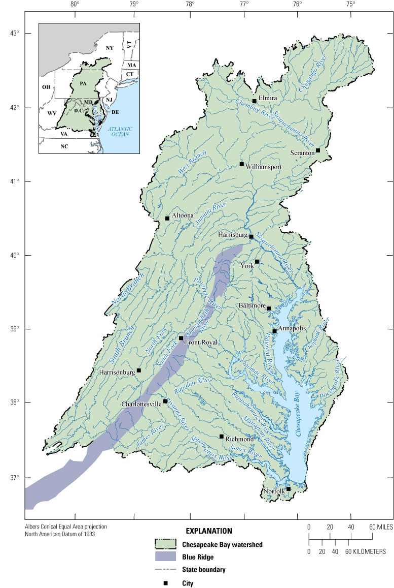
Map showing features of the Chesapeake Bay watershed. [NY, New York; VT, Vermont; MA, Massachusetts; CT, Connecticut; OH, Ohio; PA, Pennsylvania; WV, West Virginia; D.C., Washington D.C.; MD, Maryland; NJ, New Jersey; DE, Delaware; VA, Virginia; NC, North Carolina]
Understanding the status (condition at any given point in time) and trends (change in condition over time) of a stream’s water quality parameters provides valuable information to enable informed management of resources. This report describes the methods and results of status and trend analysis for seven key indicators of freshwater river and stream condition in the Chesapeake Bay watershed: nutrients and suspended sediment, salinity, temperature, toxic contaminants, streamflow, hydromorphology, and biological aquatic communities. Additionally, this report documents initial attempts to synthesize and contextualize status results across all indicators. The scope of the report is limited to tracking these seven indicators, some of which have temporally and spatially disparate datasets; the challenges and limitations associated with these datasets are summarized herein.
1.2. Background
Much of the monitoring and research focused on understanding and protecting the health of the Chesapeake Bay ecosystem, including its rivers and streams, began at the formation of the Chesapeake Bay Program in 1983. The original Chesapeake Bay Agreement, a one-page pledge signed by the chair of the Chesapeake Bay Commission, the administrator of the U.S. Environmental Protection Agency (EPA), the mayor of the District of Columbia, and the governors of Maryland, Pennsylvania, and Virginia, established a Chesapeake Executive Council and a Chesapeake Bay liaison office to oversee plans to improve water quality and living resources in the Chesapeake Bay estuary (Chesapeake Bay Program, 1983).
The first numeric goals for reducing pollution and restoring the Chesapeake Bay (hereafter referred to as “the Bay”) ecosystem were established as part of a second Chesapeake Bay Agreement in 1987. This second agreement set goals to develop and adopt a Bay-wide plan for the assessment, management, and protection of living resources and set specific numeric goals to reduce the amount of nitrogen and phosphorus entering the mainstem of the Bay by 40 percent by the year 2000 (Chesapeake Bay Program, 1987). This agreement was amended in 1992 to incorporate upstream tributaries into the water quality goals, incorporate air deposition as a source to be included in nutrient reduction strategies, and recognize submerged aquatic vegetation as an early measure of restoration progress (Chesapeake Bay Program, 1992).
A new agreement in 2000 added Delaware, New York and West Virginia as state partners and set 102 goals focused on living resource, habitat, and water quality protection and restoration, as well as the development of land use practices and community engagement (Chesapeake Bay Program, 2000). The implementation of regulations and restoration efforts was greatly accelerated after U.S. President Barack Obama issued an executive order in 2009 tasking the Federal Government to lead efforts to control pollution and protect and restore living resources through a series of clear strategies and goals (Executive Order No. 13,508, 2009). This executive order motivated several additional measures of monitoring and progress including the establishment of 2-year restoration goals by the Chesapeake Executive Council and the establishment of the Chesapeake Bay Total Maximum Daily Load (TMDL), the largest cleanup plan ever developed to limit nutrients and suspended sediment entering the Bay. Additionally, the Chesapeake Bay Watershed Agreement was drafted and set adaptive management goals that have been amended over time to align with Federal directives, State regulations and changing land use and development within the watershed (Chesapeake Bay Program, 2014). Each of the described initiatives and amended agreements set goals that require regular monitoring and analysis to measure progress. These agreements, and the large amount of monitoring data that has grown from them, are largely responsible for driving the need for the methods and evaluations described in this report.
1.3. Study Rationale
Previous efforts to describe and track conditions across the Chesapeake Bay watershed have primarily focused on nitrogen and phosphorus based on the original goals of the Chesapeake Bay Agreement (Chanat and others, 2015; Zhang and Hirsch, 2019; Mason and others, 2023). A network of monitoring sites where high-quality flow and water-quality data are collected was established as a cooperative effort between the EPA, U.S. Geological Survey (USGS), Susquehanna River Basin Commission, and agencies in the States of the Chesapeake Bay watershed. Initiated in 1985 as 9 River Input Monitoring sites located where major rivers flow into the Chesapeake Bay, the network has grown to 123 continuous monitoring sites across the watershed, now known as the Nontidal Network (NTN; U.S. Geological Survey, 2016).
The NTN is optimized to determine nitrogen, phosphorus, and suspended sediment loads and trends thereof, biannually, using continuous streamflow monitoring and discrete water-quality data collected using standardized protocols and quality-assurance procedures (Mason and others, 2023). Although nutrients and sediment are important stream indicators for measuring progress toward total maximum daily load (TMDL) goals, assessing additional stream heath indicators may provide a more holistic view of stream health in freshwater streams and rivers. Moreover, because the NTN has been optimized for monitoring trends in stream nutrients and sediment, it may not be ideal for monitoring other indicators, such as stream temperature or fish population metrics, that are influenced by processes at different scales.
To enhance understanding of trends in stream conditions, the USGS compiled and analyzed data from six additional indicators of river and stream conditions, guided by the framework of the NTN. This report presents the status and trend results for nutrients and suspended sediment from the NTN and details the assessment of six additional indicators within the Chesapeake Bay watershed. Each indicator was assigned to dedicated USGS specialists responsible for compiling data, calculating key metrics, and using the best methods for analysis. The results and authorship for each indicator are presented separately in sections 2.1 through 2.7. Furthermore, all authors contributed to a comprehensive overview of recent conditions across all indicators and a summary of the challenges encountered in synthesizing trend results from temporally and spatially disparate datasets in section 2.8.
2. Status and Trends Methods, Analyses, and Results
Gathering, analyzing, and synthesizing results for determining the status and trends of seven different indicator groups comes with a host of challenges. Indicators differ markedly in available data types and frequencies, ranging from discrete data collected once per year to continuous data collected every 15 minutes. Datasets differ substantially in sample size, frequency, and geographic distribution, and these characteristics are important considerations for determining status and trend approaches. Continuous datasets with evenly spaced measurements at high-frequency time intervals (such as every 15 minutes) have become more common over the past decade with the installation of more high-resolution streamgages and increased availability of continuous data sensors. Continuous data are often collected at fixed locations along a reach and are representative of diurnal and seasonal fluctuations at a single point in a river; however, sites are not spatially balanced in abundance and distribution, and data gaps may still exist because of environmental fouling and sensor maintenance. In comparison, discrete datasets with unevenly spaced time series and infrequent sampling (as few as one or fewer samples per year, depending on indicator) may be available over longer periods. Discrete samples may not be collected at fixed locations or regular intervals and can be less representative of the sample population. However, such data can still provide acceptable information for long-term trend analysis depending on the indicator.
In addition to data collection frequency, each indicator is subject to implicit biases that come from long-term data collection, such as changes in the accuracy of instrumentation over time, changes in field sampling methods, temporal gaps in the data, missing or incomplete metadata, and observer bias for hand collected discrete data such as biological data. To determine appropriate analytical methods for trend analysis, these biases were considered along with data type, collection frequency, and expected linear or nonlinear patterns over time. For some indicators, linear models were appropriate for trend analysis. For others, more flexible modeling approaches were required to capture nonlinear trends. Indicators like streamflow and salinity have longstanding methodology for trend analysis; other indicators, such as geomorphology and stream temperature, required development of analysis approaches. Table 1 provides a summary of metrics analyzed, status definition, and trend intervals for each indicator. Status and trend methods and results are described in the following sections for each of the seven indicators of stream conditions in the Chesapeake Bay watershed.
Table 1.
A summary of the metrics, status definition, and trend interval utilized for analysis of seven indicators of stream conditions in the Chesapeake Bay watershed.[Indicators from Boyle and others (2025) unless stated otherwise. A water year (WY) is the 12-month period from October 1 through September 30 of the following year and is designated by the calendar year in which it ends]
Nutrients and suspended sediment from Mason and others (2023).
Toxic contaminants from Banks and others (2022).
2.1. Status and Trends in Stream Nutrients and Suspended Sediment
By Christopher A. Mason and Douglas L. Moyer
Nutrients and sediment are necessary to sustain ecosystem function, but an overabundance of either can be detrimental to aquatic ecosystem health. Elevated nitrogen and phosphorus concentrations are a pervasive issue in freshwaters across the United States, leading to eutrophication of streams and altered fish and macroinvertebrate assemblage structure (Carpenter and others, 1998; Wang and others, 2007; Davidson and others, 2012; Dodds and Smith, 2016). Sediment derived from natural or anthropogenic sources can also cause decline in stream condition by impairing the growth of aquatic vegetation, burying filter feeding organisms, and reducing hard-bottom habitat availability (Box and Mossa, 1999; Madsen and others, 2001; Davis and others, 2018). The Chesapeake Bay has experienced unnatural acceleration of nutrient loading attributed to anthropogenic inputs from point-source sewage disposal and nonpoint-source runoff from either agricultural or urban land uses (Nixon, 1987). The Chesapeake Bay Program partnership has set goals and implemented practices to reduce nutrient and sediment loading to the Bay, and the NTN provides an essential service by monitoring progress towards reducing nutrient and suspended sediment loads. The methods and results of the 1985–2020 NTN analysis of nitrogen, phosphorus, and suspended sediment loads and trends are described in this section and can also be found in Mason and others, 2023.
2.1.1. Data Compilation
As of 2024, the NTN has 123 sites near USGS streamgages to monitor status (yields) and trends (change in flow-normalized loads) in nitrogen, phosphorus, and suspended sediment loads in the Chesapeake Bay watershed. Load is the product of constituent concentration and streamflow that passes a point of reference at a measured unit of time, and yield is the load normalized by watershed area. Discrete water-quality data and continuous daily streamflow data from the NTN were used to analyze the status and trends of nitrogen, phosphorus, and suspended sediment in rivers and streams of the Chesapeake Bay watershed. All data compilation and analyses were completed in R (ver. 4.1.3; R Core Team, 2022a). Streamflow time series were retrieved from the National Water Information System (NWIS) using the R package “dataRetrieval” (ver. 2.7.7; Hirsch and De Cicco, 2015; U.S. Geological Survey, 2023). Continuous (15-minute internal logging) data were used to calculate a daily mean of streamflow for each USGS streamgage. The Chesapeake Bay Program nontidal water quality monitoring program upholds high standards for NTN data quality; thus, a water year (WY) was discarded if it contained days with missing streamflow measurements that could not be remedied. Discrete nutrients (total nitrogen and total phosphorous) and total suspended sediment data were obtained from the Water Quality Portal (WQP; U.S. Geological Survey and U.S. Environmental Protection Agency, 2021). After rigorous quality-assurance checks to remove outliers and duplicates, discrete water-quality data from each site (typically 20 samples per year) were paired to the corresponding daily mean streamflows to estimate daily concentration before flow-normalization was applied for trend analysis.
2.1.2. Analysis
For nutrients and sediment, status was defined as the 10-year (WY 2011–20) average yield delivered to the Chesapeake Bay. Trends were defined as the change in flow-normalized load for a given trend interval. Trends for nitrogen, phosphorus, and suspended sediment at eligible NTN sites were estimated for two trend intervals: 1985–2020 (long term) and 2011–20 (short term). For status and the short-term trend interval, 89 total nitrogen sites, 70 total phosphorus sites, and 70 suspended sediment sites qualified for analysis. For the long-term trend interval, 44 total nitrogen sites, 18 total phosphorus sites, and 18 suspended sediment sites qualified for trend analysis.
The R package “EGRET” (ver. 3.0.7; Hirsch and De Cicco, 2015) contains the statistical model used for load and trend calculations called Weighted Regressions on Time, Discharge and Season (herein referred to as WRTDS; Hirsch and others, 2010). WRTDS is used to compute nitrogen, phosphorus, and suspended sediment daily concentration and load estimates. WRTDS was run using a dataset comprised of about 20 samples per year for each site and trend interval. After WRTDS was applied, a dynamic autocorrelation Kalman-filter (WRTDS-K) was used to adjust the estimated values based on the serial correlation of the residuals. WRTDS-K creates a daily time series of concentrations and loads that use the observed value when available and the serial-adjusted values otherwise. This approach provides more accurate concentration and load estimates, especially on sub-annual timescales (Zhang and Hirsch, 2019). These values were area-normalized to compute status estimates as yields.
The flow-normalized estimates from WRTDS were used to characterize trends over the two intervals. Estimates remove the influence of year-to-year variability of stationary streamflow on water quality and by doing so, provide a measure of temporal change in nitrogen, phosphorus, and suspended sediment loads independent of weather-driven streamflow variations. The flow-normalized values provide an indication of the effect of changing sources, delays associated with storage and transport of historical inputs, and any implemented management actions on stream water quality. Sites with flow-normalized loads that were lower at the end of the WY 1985–2020 or WY 2011–20 periods were classified as having “improved” conditions; whereas sites with flow-normalized loads higher at the end of each period were classified as having “degraded” conditions. WRTDS provides a likelihood estimate of a trend’s existence based on a probability score. A trend’s likelihood was categorized as “likely” (score was greater or equal to 0.67 and less than 0.9), “very likely” (greater or equal to 0.9 and less than 0.95), or “extremely likely” (greater or equal to 0.95). A site was classified as having no trend (meaning an improving or degrading trend is as likely to exist as it is not) if there is no discernable difference (likelihood estimate probability score between 0.33 and 0.67) between the flow-normalized loads in the start year and those in the end.
2.1.3. Results and Discussion
Status estimates for nitrogen yields ranged from 1.27 to 32.6 pounds per acre (lb/acre), total phosphorus yields ranged from 0.11 to 1.89 lb/acre, and suspended sediment yields ranged from 23.9 to 1,210 lb/acre (fig. 2; Mason and others, 2023). Higher total nitrogen yields were concentrated in the lower Susquehanna River Basin and Delmarva Peninsula, and lower yields were observed in the upper Susquehanna River and upper and lower Potomac River Basins and throughout the Rappahannock, York, and James River Basins. Similar high and low patterns for total phosphorus existed throughout the Susquehanna River Basin. Low yields were observed in the upper and lower Potomac River Basin, and in central Virginia saw a spread of high and low total phosphorus yields. Suspended sediment yields were highest towards the mouths of the Susquehanna and Potomac Rivers, and in central Virginia. The central Susquehanna River Basin, upper Potomac River Basin, and Eastern Shore recorded low yields relative to the rest of the Bay.
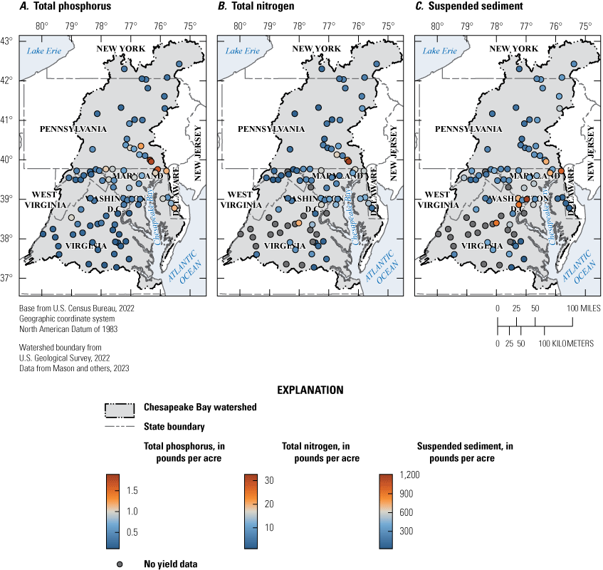
Maps of the Chesapeake Bay watershed showing the 10-year average (water years 2011–20) nutrient and suspended sediment status estimates for A, total nitrogen (89 sites), B, total phosphorus (70 sites), and C, suspended sediment (70 sites) yields. A water year (WY) is the 12-month period from October 1 through September 30 of the following year and is designated by the calendar year in which it ends.
For short-term trends, 34 of 89 sites (38 percent) showed improvement for total nitrogen with yield reductions ranging from 0.06 to 2.26 lb/acre, and 37 sites (42 percent) had degrading trends with yield increases ranging from 0.02 to 2.62 lb/acre. Eighteen sites (20 percent) had no trend for total nitrogen. For total phosphorus, 31 of 70 sites (44 percent) had improving trends with yield reductions ranging from 0.007 to 0.31 lb/acre, and 16 (23 percent) had degrading trends with yield increases ranging from 0.009 to 0.82 lb/acre. Twenty-three sites (33 percent) had no trend for total phosphorus. For suspended sediment, 13 of 70 sites (18 percent) had improving trends and yield reductions ranging from 16.7 to 552 lb/acre; 32 sites (46 percent) had degrading trends and yield increases ranging from 9.11 to 2310 lb/acre. Twenty-five sites (36 percent) had no trend in suspended sediment (fig. 3).
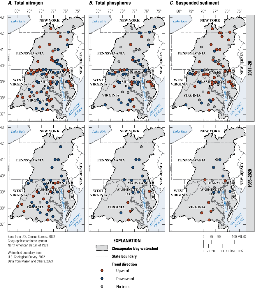
Maps of the Chesapeake Bay watershed showing the short-term (water years 2011–20) and long-term (water years 1985–2020) trend direction of qualifying nutrient and suspended sediment sites for A, total nitrogen (89 sites), B, total phosphorus (70 sites), and C, suspended sediment loads (70 sites). A water year (WY) is the 12-month period from October 1 through September 30 of the following year and is designated by the calendar year in which it ends.
Of the 44 sites analyzed, long-term trend results for total nitrogen show 24 sites improving, 15 sites degrading, and 5 sites with no discernable trend direction. The change in load ranged from −64.7 to 44.4 percent. Long-term trend results for the 18 sites analyzed for total phosphorus show 12 sites improving, 4 sites degrading, and 2 sites with no trend. The change in load ranged from −71.7 to 86.6 percent. Long-term trend results for the 18 sites analyzed for suspended sediment show 7 sites improving, 7 sites degrading, and 4 sites with no trend. The change in load ranged from −68.4 to 56.8 percent (fig. 3).
Additional information for each monitoring site is available through the USGS website “Water-Quality Loads and Trends at Nontidal Monitoring Stations in the Chesapeake Bay Watershed” (U.S. Geological Survey, 2016). This website provides State, Federal, local partners, and the public access to a wide range of data for nutrient and sediment conditions across the Chesapeake Bay watershed.
2.2. Status and Trends in Stream Salinity
By Rosemary M. Fanelli and Kaitlyn E.M. Elliott
Salinity represents the concentration of dissolved salt ions in water, and increasing salinity in freshwater ecosystems (often called freshwater salinization) is an emerging global water-quality issue (Kaushal and others, 2018; Cañedo-Argüelles, 2020). Excess salinity originates from a variety of sources, including deicer applications; resource extraction; agricultural and urban applications of fertilizer, lime, or other soil amendments; weathering of concrete; and point-source discharges (Cañedo-Argüelles, 2020). Specific conductance (SC) is often used as a proxy for salinity and measures the electrical conductance of one cubic centimeter of water at 25 degrees Celsius (°C; U.S. Geological Survey, 2023). Increasing SC and associated salinity may disrupt osmotic regulation in benthic macroinvertebrates (Kefford, 2018), and other classes of aquatic organisms respond negatively to increased salinity (Walker and others, 2023). The effects of freshwater salinization extend beyond stream ecosystems; elevated levels of certain ions, like chloride, may increase the corrosivity of water and impact the quality of municipal drinking water supplies, as well (Stets and others, 2018).
Natural levels of SC are generally low in freshwater streams and rivers within the Chesapeake Bay watershed (about 20–400 microsiemens per centimeter [µS/cm]; Olson and Cormier, 2019). Increasing levels of SC and associated ions, however, has been documented in some streams in the Chesapeake Bay watershed (Bird and others, 2018) and across the Nation (Shoda and others, 2019). Recent work in the Delaware River Basin highlighted increasing SC trends at 35 monitoring sites from 1998 to 2018, especially during winter months (December through February), suggesting deicer applications could be a significant source of elevated salinity in the mid-Atlantic United States (Rumsey and others, 2023). Many regional stakeholders now recognize salinity as a potential cause of biological impairment in the watershed’s streams and rivers (Fanelli and others, 2022), but more information is needed to document the extent and severity of freshwater salinization and changes in salinity levels within the freshwater stream network of the Chesapeake Bay watershed.
2.2.1. Data Compilation
A status analysis was conducted to describe the spatial variability of observed SC levels relative to background SC across the Chesapeake Bay watershed, and a trend analysis was conducted to quantify changes in SC over time. SC data for these analyses were obtained from a recently published SC inventory, which contains SC data compiled for the Chesapeake Bay watershed from 1901 to 2022 (Fanelli and others, 2023). These data originated from the WQP, which serves as a national repository for local, State, and Federal data collection efforts (U.S. Geological Survey and U.S. Environmental Protection Agency, 2021). The WQP also contains all available discrete data in NWIS.
Freshwater nontidal streams and rivers were the focus of these analyses, and sites with known tidal influence were removed from further analysis. This was done by evaluating and excluding sites that intersected areas near the Chesapeake Bay estuary that were designated by the National Oceanic and Atmospheric Administration as tidally influenced (Chesapeake Bay Program, 2004). Tidal influence was also manually verified by screening the remaining sites for high values of SC (1,000 µS/cm or greater at sites adjacent to the tidal zone), which may indicate tidal influence. The remaining sites were considered for subsequent status and trend analyses.
2.2.2. Analysis
All 278 sites identified in the tidal screening process were utilized for status and trend analysis. For the salinity analysis seasons were defined as December through February (winter), March through May (spring), June through August (summer), and September through November (fall). To accommodate these seasonal intervals and maximized the number of sites eligible for analysis across the watershed, a ‘year’ was defined as December 1 of the previous year to November 30 of the current year (for example the year 2008 was defined as December 1, 2007, through November 30, 2008). Hereafter within section 2.2, all years and year ranges refer to this defined time interval (for example, 2008–17 refers to December 1, 2007-November 30, 2017). At each site, SC status was computed as the median of the annual medians of 2015, 2016, and 2017. These 3-year median values were then compared to previously published background SC estimates that used SC observations from 2001–15 taken at reference sites and represent natural SC levels that would occur in the absence of anthropogenic inputs (Olson and Cormier, 2019). Background estimates were generated on a monthly timescale for years 2001–15 using a random forest model that predicted background SC using geological and climate variables across the United States for all National Hydrography Dataset (NHD) version 2.1 stream reaches (McKay and others, 2012). For the SC status analysis, the predicted monthly background SC estimates from Olson and Cormier (2019) were summarized as median annual background SC values for each of the years 2008–15, and a median of those values was computed to represent a long-term median annual background SC estimate. This long-term median annual background SC estimate was then compared to the observed 3-year median SC values.
For this comparison, each site was first associated to the National Hydrography Dataset version 2.1 flowlines to generate a list of stream segment unique identifiers (COMIDs) for each site. Next, the site COMID list was joined to the background SC dataset. Of the 278 sites, 269 (97 percent) had background SC data associated with their COMID; the remaining nine sites either did not have an associated COMID or there was no background SC reported in the 2019 study dataset for that COMID. Finally, the observed 3-year median was divided by the long-term median background SC to represent an “observed versus expected” metric. This metric characterizes the extent to which observed SC departed from background SC. SC departure classes were defined as “at or below the background SC estimate”, “slightly elevated” (1–2 times the background SC estimate), “moderately elevated” (2–3 times the background SC estimate), and “highly elevated” (greater than 3 times the background SC estimate).
Two trend analyses were conducted in R (ver. 4.2.3; R Core Team, 2023) using the compiled data: WRTDS (Hirsch and others, 2010) and Seasonal Mann-Kendall (SMK) trend tests (Helsel and others, 2020). WRTDS is a robust statistical model used to quantify water-quality trends, but it requires daily streamflow information, which limits its application to those sites with streamflow (discharge) data. SMK trend tests, however, only require water-quality information and can therefore be applied to a larger number of sites across the watershed. Results from both analyses can be found in Boyle and others (2025).
2.2.2.1. WRTDS
The first trend analysis conducted used WRTDS statistical model (refer to section 2.1 for more details on WRTDS). Sites with sufficient data that were co-located with USGS streamgages were selected for this analysis. For a site to be eligible for WRTDS trend analysis, a minimum data criterion of three samples per season for the 10-year period was applied to capture seasonal variability in SC. A 10-year trend interval from December 1, 2007, to November 30, 2017 (herein referred to as 2008–17) was selected because it maximized the number of sites eligible for analysis across the watershed (35 sites) and accommodated the defined season intervals.
WRTDS was run using the coupled SC and streamflow data and the modelEstimation function from the R package “EGRET” (ver. 3.0.8; Hirsch and De Cicco, 2015). An additional function, WRTDSKalman, was used to produce more accurate estimates of daily concentrations by replacing estimated values with observed values on days with SC observations and using serial correlation from the model residuals to adjust the remaining daily estimates around the observations. WRTDS model results were screened for excessive extrapolation by comparing the maximum estimated concentrations to the maximum observed concentration at each site (Oelsner and others, 2017). Finally, WRTDS trend uncertainty analysis was run using the wBT function from the R package “EGRETci” (ver. 2.0.4; Hirsch and others, 2015), which determines the likelihood of the trend direction between the start and end of the trend period using the annual flow-normalized concentrations and a resampling with replacement technique called the block bootstrap procedure (nBoot, the maximum number of bootstrap replicates to be used, was 100; bootBreak, the minimum number of bootstrap replicates to be used, was 100; and blockLength, the length of the block replicate, was 100 days). Trend significance and direction were assessed by applying standard cut-off criteria to these likelihood estimates (refer to Hirsch and others, 2015). Following the approach used by Rumsey and others (2023), annualized seasonal change estimates were also quantified to better describe changing conditions in the watershed. These estimates were computed by averaging the predicted daily concentrations estimated by WRTDS for each season and year and computing the difference for each season by subtracting the 2008 value from the 2017 value. These seasonal change values were then normalized by the starting year seasonal average concentration and converted to a percentage. Finally, the seasonal percentages were divided by 10 (the length of the trend period) to generate an annualized value (in other words, percent change per year).
2.2.2.2. Seasonal Mann-Kendall
The second trend analysis used the SMK trend test, which is a non-parametric test for constituents that vary seasonally. The SMK trend test does not require daily streamflow, so it can be applied to more sites and thereby provide trend information across a larger portion of the watershed. For a site to be eligible for the SMK trend analysis, a minimum criterion of one sample per season for the 10-year period (December 1, 2007, through November 30, 2017) was applied to capture seasonal variability in SC, using the same season definitions and trend interval listed in section 2.2.2.1 (278 sites), and to also facilitate comparison among the two trend approaches. The SMK test was performed using the smk.test function from the R package “trend” (ver. 1.1.6; Pohlert, 2015). The Theil-Sen slope, which estimates the rate of change in SC over time, was also computed using the sea.sens.slope function from the same package. Trends were categorized based on the p-value of the SMK test and direction of the Theil-Sen slope (table 2).
Table 2.
P-values, Theil-Sen slope estimates, and trend categories for the Seasonal Mann-Kendall (SMK) trend analysis of stream salinity at 278 sites across the Chesapeake Bay watershed, December 1, 2007, through November 30, 2017.[Data are from Boyle and others (2025). >, greater than; NA, not applicable; <, less than; ≥, greater than or equal to]
2.2.3. Results and Discussion
2.2.3.1. Status Results
The average long-term median background SC was 82 µS/cm for the 278-site network and ranged from 21 to 312 µS/cm (fig. 4). The lowest background SC estimates were in central Virginia and northern Pennsylvania. The highest background SC estimates were in carbonate regions in central Virginia and southeastern Pennsylvania. The average 3-year median for observed SC for all sites was 242 µS/cm across the 278-site network for the time period of December 1, 2014 to November 30, 2017 and ranged from 9 to 1,189 µS/cm across the watershed. The sites with the lowest 3-year median SC values were typically in central Virginia, in northwest Pennsylvania, and in the Delmarva Peninsula. The sites with the highest values were clustered in Maryland, especially throughout the Baltimore–Washington, D.C. metropolitan area, and in southeastern Pennsylvania. Departures from background SC follow a similar spatial pattern. Sites with values at or below background SC were mainly clustered in central Virginia (fig. 4). Only 43 sites (16 percent) had 3-year median SC values that were at or below background SC (table 3). Fifty-seven sites (21 percent) had slightly elevated values; these sites were clustered in central Virginia and western Pennsylvania. Sites that had moderately elevated or highly elevated values were throughout northern Virginia, Maryland, and Pennsylvania, and clustered in the Baltimore–Washington, D.C., metropolitan area, and in southeast Pennsylvania. These moderate and high departures from background SC were observed at 169 of the 269 sites with available background SC data (63 percent), indicating the effects of freshwater salinization are prevalent through much of the watershed. These results were consistent with a modeling study that estimated two-thirds of nontidal stream reaches were elevated above background SC in the Chesapeake Bay watershed (Fanelli and others, 2024).
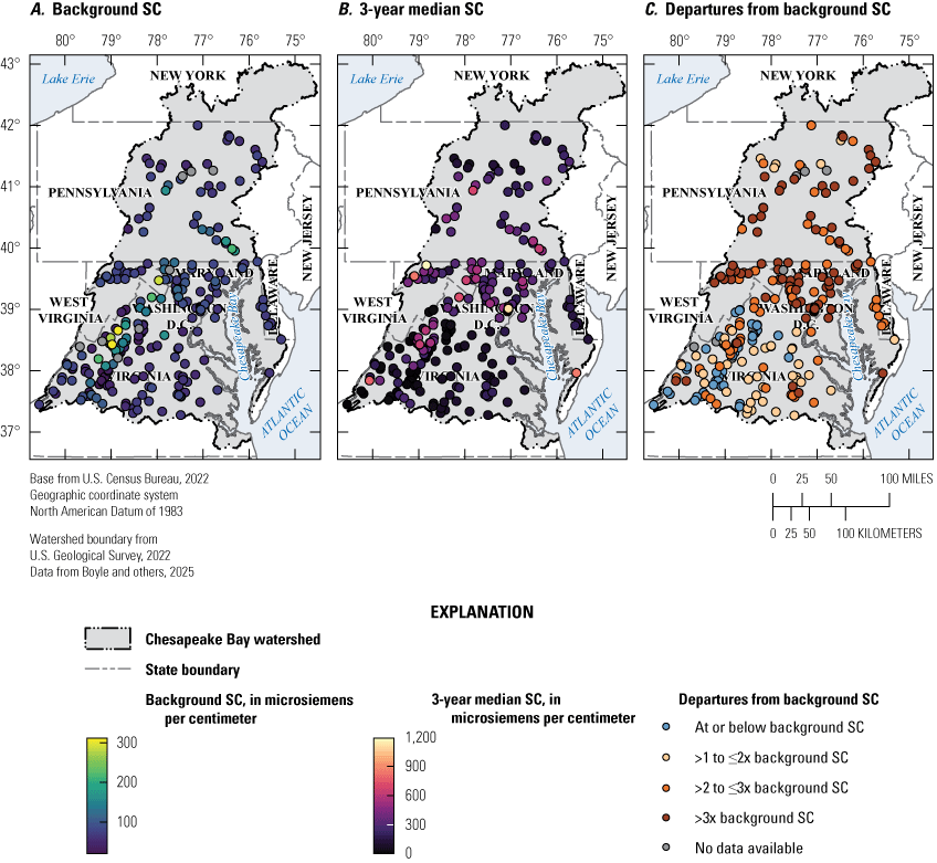
Maps of the Chesapeake Bay watershed showing A, median annual (December 1, 2007, through November 30, 2015) background specific conductance (SC) values, B, 3-year (2015–17) median SC values, and C, SC departure classes in 2015–17 for 278 salinity sites. [>, greater than; ≤, less than or equal to]
Table 3.
Counts and percentages of salinity sites with specific conductance (SC) status values for 2015–17 per SC departure class, and counts of salinity sites located where SC predicted background data are available.[Data are from Boyle and others (2025). >, greater than; ≤, less than or equal to; NA, not applicable]
2.2.3.2. WRTDS Trend Results
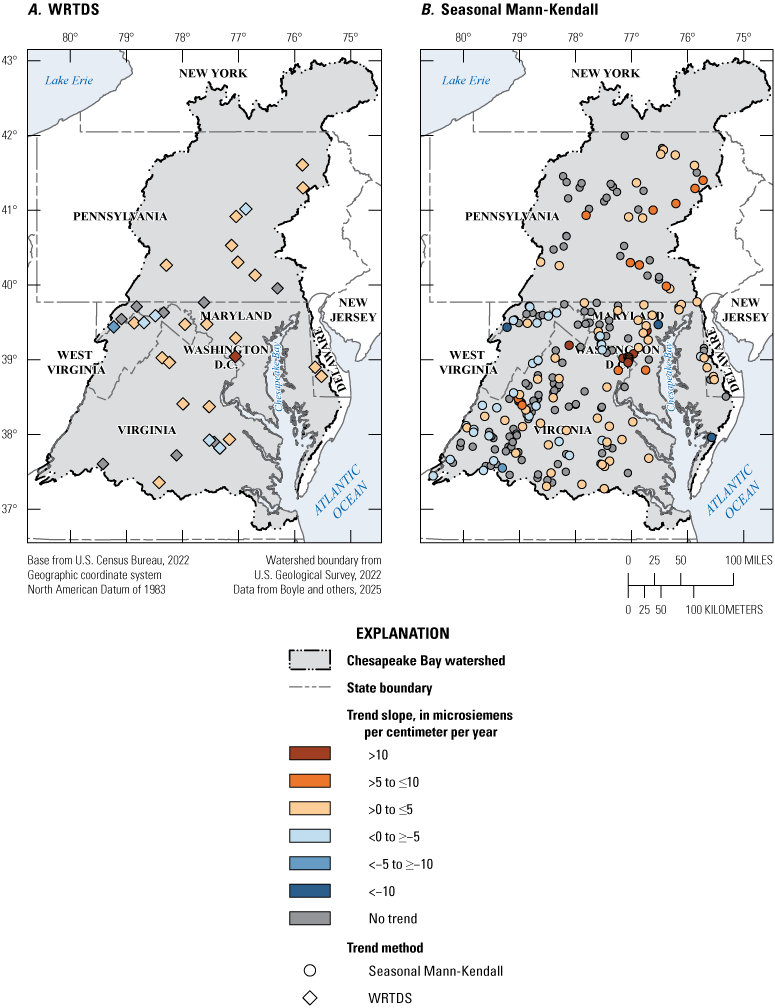
Ten-year SC trends from 2008 to 2017 were significant at most of the 35 sites in the WRTDS analysis; 21 sites (60 percent) had significantly increasing trends, and 6 sites (17 percent) had significantly decreasing trends (table 4). These results were consistent with other regional and national SC trend analyses that found general increases in SC (Kaushal and others, 2018; Bird and others, 2018; Baker and others, 2019). Trends were in the “highly likely” category for 14 of the 21 sites with significantly increasing trends, indicating higher confidence in those patterns. Sites with increasing trends were scattered throughout the Chesapeake Bay watershed (fig. 5). Sites with decreasing trends were largely found in the Potomac River Basin in Maryland and in central Virginia. In general, rates of change estimates by WRTDS were small; annual increases were below 5 µS/cm per year in all but one of the upward trending sites (fig. 6). The exception was a site in downtown Washington, D.C., at which the median annual SC was estimated to be increasing approximately 11 µS/cm per year during the trend period. Declines in SC at most of the six downward trending sites were also modest (less than −5 µS/cm per year). Annual seasonal change estimates indicated that greater changes in SC occurred in the winter and spring seasons at sites with increasing trends (fig. 7), which aligns with patterns observed in the Delaware River Basin (Rumsey and others, 2023). By contrast, the largest declines in annual seasonal change estimates occurred in the summer and fall seasons in sites with significant decreasing trends.

Maps of the Chesapeake Bay watershed showing salinity site trend results from A, the Weighted Regressions on Time, Discharge, and Season (WRTDS) analysis of 35 sites and B, the Seasonal Mann-Kendall analysis of 278 sites for the 2008–17 trend period.
Maps of the Chesapeake Bay watershed showing the estimated annual rate of change for salinity site specific conductance (SC) as estimated by A, the Weighted Regressions on Time, Discharge, and Season (WRTDS) trend analysis of 35 sites and B, the Seasonal Mann-Kendall trend analysis of 278 sites for the 2008–17 trend period. [>, greater than; ≤, less than or equal to; <, less than; ≥, greater than or equal to]
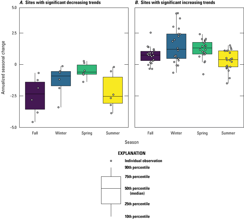
Boxplots showing the annual seasonal change estimates for salinity sites computed from Weighted Regressions on Time, Discharge, and Season daily concentrations for the four seasons in the 2008–17 trend period for sites in the Chesapeake Bay watershed with overall A, significant decreasing trends and B, significant increasing trends. Data are from Boyle and others (2025).
Table 4.
Trend direction and significance categories for salinity sites across the Chesapeake Bay watershed analyzed using Weighted Regressions in Time, Discharge, and Season (WRTDS) and Seasonal Mann-Kendall (SMK) trend analyses, 2008–17.[Data are from Boyle and others (2025). NA, not applicable]
2.2.3.3. Seasonal Mann-Kendall Trend Results
Significant trends were detected at slightly less than half of the SMK trend sites; increasing trends were detected at 92 sites (33 percent) and decreasing trends, 34 sites (12 percent; table 4). No trends were detected at the remaining 152 sites. Half of the detected increasing trends were in the “highly likely” category (46 sites), indicating high confidence in these trends. By contrast, only 38 percent of the detected decreasing trends were in the “highly likely” category (13 sites). Upward trending sites were scattered throughout the Chesapeake Bay watershed, following a similar pattern seen in the WRTDS results (fig. 5). There was also a cluster of upward trending sites with high trend certainty in the Baltimore–Washington, D.C., metropolitan area. Sites with decreasing trends, however, were only found in the southern portion of the watershed, typically south of the Pennsylvania border and especially in central Virginia (fig. 5).
Theil-Sen slope estimates provide annual estimates of rates of change in SC for those sites with significant trends. Most (61 sites or 66 percent) of the upward trending sites had small change estimates (increasing at a rate of less than 5 µS/cm per year), following the same pattern seen in the WRTDS results (fig. 6). However, 13 percent of the upward trending sites have change estimates greater than 10 µS/cm per year, suggesting rapidly worsening conditions at these sites, almost all of which were in the Baltimore–Washington, D.C., metropolitan area. Sites with moderate annual increases in SC (increases between 5 and 10 µS/cm per year) were also found scattered throughout Pennsylvania. By contrast, most (85 percent of the 34 sites) annual change estimates in sites with decreasing trends were small (less than −5 µS/cm per year), indicating modest declines over time.
The SMK and WRTDS trend results for the 35 sites that fit criteria for both analyses were compared. Results among the two methods generally agreed, and trend directions from the two methods were not found to be contradictory. More information on the comparison may be found in appendix 1.
In general, many of the increasing trends in SC co-occurred in areas with elevated SC (fig. 8). For example, 40 of the 93 SMK sites (43 percent) that have highly elevated 3-year median SC values also have a significantly increasing trend in SC (table 3). The WRTDS sites show a similar pattern: 8 of the 14 sites (57 percent) in the highly elevated SC departure class also have increasing SC trends. The highly elevated SC values at these sites result from 10 years of increasing SC. By contrast, almost all (91 percent) of the SMK sites that had 3-year median SC values at or below background SC also had either no change or decreasing SC trends, suggesting that low SC conditions have persisted at these sites. One possible reason for this is that these sites are in areas that are protected from land-use change or other anthropogenic disturbance. It is important to note that the distribution of trend sites among the departure classes is different between the two trend types; the SMK sites are more evenly distributed among the four departure classes, suggesting they cover a range of land-use settings. There are no WRTDS sites in the “at or below background” departure class, however, indicating little representation of undisturbed settings within those results.
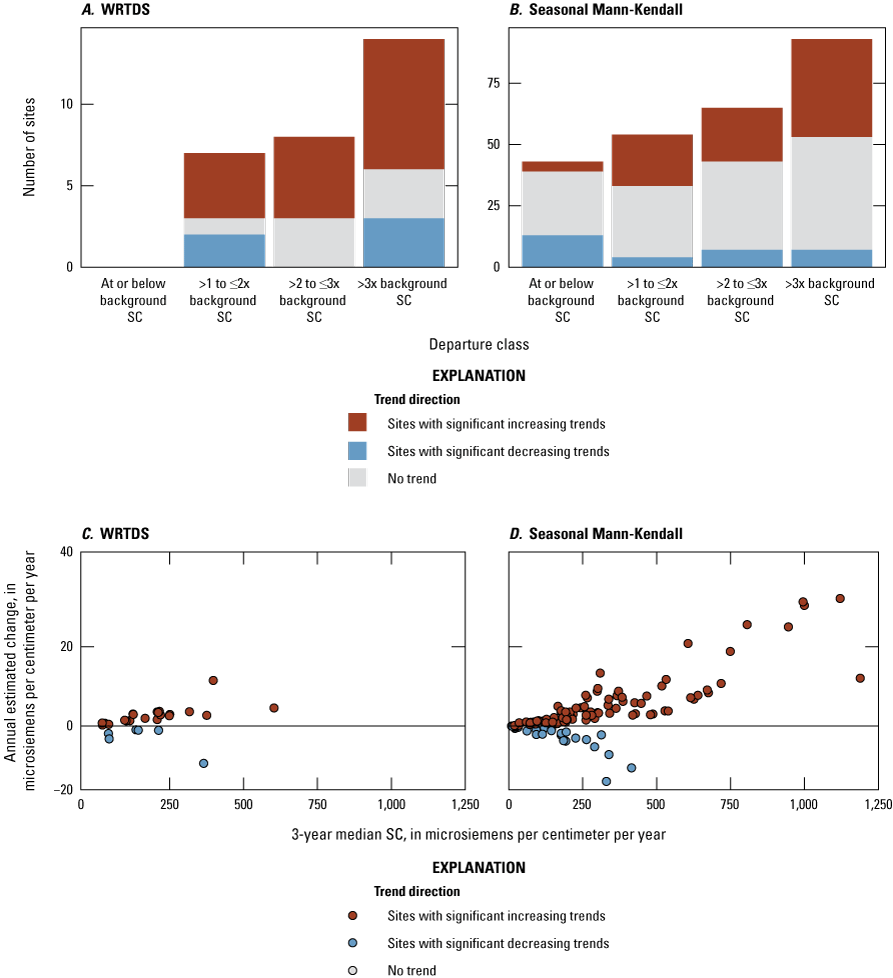
A, Barplot showing the number of salinity sites in the Chesapeake Bay watershed that have increasing, decreasing, or no trend in each departure class for the Weighted Regressions on Time, Discharge, and Season (WRTDS) trend analysis. B, Barplot showing the number of sites in the Chesapeake Bay watershed that have increasing, decreasing, or no trend in each departure class for the Seasonal Mann-Kendall (SMK) trend method. C, Scatterplot showing the relationship between 3-year (2015–17) median specific conductance (SC) and the estimated annual change estimate for the WRTDS trend method. D, Scatterplot showing the relationship between 3-year (2015–17) median SC and the estimated annual change estimate for the SMK trend method. One outlier site that had a 3-year median SC of 851 microsiemens per centimeter (µS/cm) and an annual estimated change of −63.8 µS/cm per year was excluded from the figure 8D. Data are from Boyle and others (2025). [>, greater than; ≤, less than or equal to]
The largest annual rates of increase and decrease were observed at sites with highly elevated SC (fig. 8), suggesting the conditions in these sites are highly dynamic. Rates of increase exceeded 20 µS/cm per year at a handful of sites, all of which had 3-year medians at or above 500 µS/cm. The same pattern is noted in sites with declining trends—the largest SC declines are also at sites with high 3-year median SC values. This could be due to point-source reduction efforts. Another trend study documented some decreasing SC trends in the region (Bowen and others, 2015), but the drivers of those patterns were not investigated. Additional studies could help fully understand the factors controlling these spatial and temporal patterns in SC.
2.3. Status and Trends in Stream Temperature
By John W. Clune, Guoxiang Yang, Nathaniel P. Hitt, Karli M. Rogers, James E. Colgin, Elizabeth A. Hittle, and Tammy M. Zimmerman
Stream productivity and the metabolic rate of aquatic organisms depend on stream temperature (Cushing and Allan, 2001). Increases in stream temperature decrease the solubility of oxygen in water, and these suboxic conditions are a primary stressor for aquatic species among the Nation’s rivers (Zhi and others, 2023). Stream temperature can fluctuate naturally because of solar radiation, atmospheric conditions, topography, streamflow, and streambed heat transfer, or as the result of human influences, such as land use, thermal pollution, water storage impoundments, and channel modification (Caissie, 2006; Webb and others, 2008). The ecological implications of rising stream temperatures are a concern to resource managers throughout the Chesapeake Bay watershed (Batiuk and others, 2023).
Despite the widespread recognition and importance of stream temperature, there are relatively few studies that have evaluated status and trends in the northeastern United States for use in adaptive resource management compared to other water-quality parameters (Kaushal and others, 2010; Rice and Jastram, 2015; Wagner and others, 2017). Unlike air temperature, there is no systematic monitoring network with long-term, reliable, and continuous datasets that are representative of temporal and spatial variability of stream temperature in the Chesapeake Bay watershed. This motivated the compilation of available multi-agency water temperature measurements for streams within the Chesapeake Bay watershed to develop estimates of status and trends (Clune and others, 2023).
2.3.1. Data Compilation
Continuous and discrete datasets can differ substantially in sample size, frequency, and spatial distribution, and these population dynamics are important considerations for determining status and trend approaches. Continuous stream temperature datasets with evenly spaced high-frequency time series (such as every 15 minutes) have become more common over the past decade. These data are often collected at fixed locations along a reach and are representative of diurnal and seasonal temperature fluctuations but are collected at a small number of sites that are often not spatially representative across the watershed. In comparison, discrete stream temperature datasets with unevenly spaced time series and infrequent measurements (6–8 per year) may be available over longer periods. However, discrete measurements may be less representative of site conditions, and diurnal and seasonal temperature fluctuations because measurements are not always collected at fixed locations or time intervals.
Data compilation and analyses were completed in R (ver. 4.2.1; R Core Team, 2022b). Stream temperature measurements were collated across the Chesapeake Bay watershed from NWIS, the WQP, and the USGS Aquarius Time-Series database (Aquarius) for consideration in status and trend analysis (fig. 9; Clune and others, 2023). Continuous unit values (high-frequency, evenly spaced time series) and daily aggregate data (minimum, maximum, and mean) of stream temperature were retrieved for USGS sites from NWIS using the R package “dataRetrieval” (ver. 2.7.11; Hirsch and De Cicco, 2015; U.S. Geological Survey, 2023). Depending on the site, daily stream temperature values can have long historical records. In contrast, many continuous unit values are only available after 2007. Stream temperature was measured with a sensor at fixed locations or depths. Sometimes, multiple overlapping time series are available if the sensor was relocated or replaced (Clune and others, 2023). These continuous unit values and aggregate daily data have been approved or considered provisional, revised, or estimated under USGS guidelines and procedures for measurement of stream temperature (Wagner and others, 2006). Any data point that was outside five standard deviations from the monthly mean was verified with the responsible USGS Water Science Center and represents infrequent or atypical stream temperature measurements that are deemed accurate.
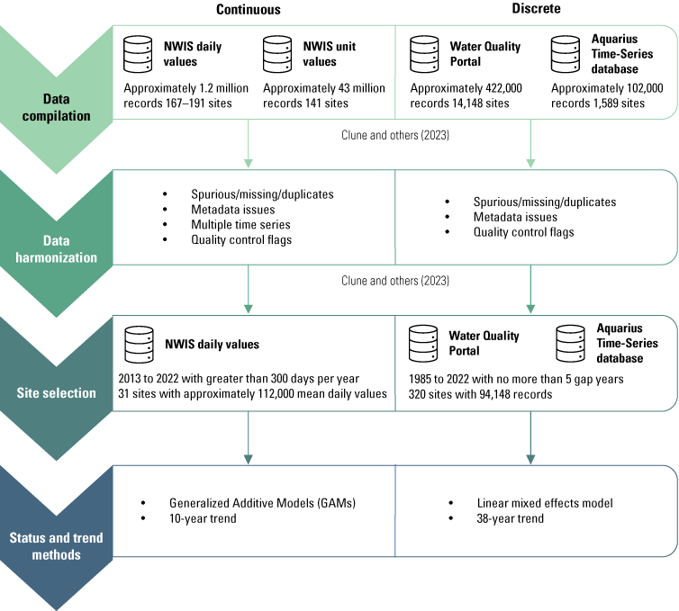
Data flow diagram showing how continuous and discrete data were used to develop status and trends for stream temperature. [NWIS, National Water Information System]
Discrete values (infrequent, unevenly spaced time series) for stream temperature from multiple agencies stored in the WQP for streams within the Chesapeake Bay watershed were also obtained using the R package “dataRetrieval” (ver. 2.7.11; Hirsch and De Cicco, 2015). Additionally, discrete stream temperature values collected by the USGS while measuring streamflow were obtained from an internal pull of the Aquarius database. These stream temperature measurements were collected as an instrumentation check following techniques and standards for streamflow measurements (Turnipseed and Sauer, 2010). Measured accuracies are not available because these temperature measurements have not been approved under USGS guidelines and procedures for measurement of stream temperature (Wagner and others, 2006; U.S. Geological Survey, 2024). The measuring point of these discrete stream temperature measurements is not based on a fixed location or depth and may vary horizontally and vertically within the stream channel. Missing and unreasonable stream temperature discrete values outside the range of −5 and 40 °C were removed.
2.3.2. Analysis
Developing status and trends of stream temperature can be challenging, and there are advantages and limitations to using these data for analysis. Data bias and errors may be inherent, especially with multi-agency discrete data (Wilby and others, 2017). Temperatures can vary horizontally and vertically within the stream, and changing measurement points during collection could therefore influence results. Sites downstream of local dams, impervious areas, or water treatment outfalls can have altered thermal regimes and may present break points in the time series and introduce bias in regional models for stream temperature. Changes in the accuracy of instrumentation (mercury bulb thermometer to thermistor) during the period of record are often unknown. The collection times of discrete stream temperature data often exclude nights and weekends and may favor the morning or afternoon or may change over the period of record. Further, important metadata, such as sampling date and time, site description, and hydrologic condition, are often incomplete, inaccurate, or unavailable for discrete data. For example, 77 percent of Aquarius data were provided with quality control flags for stream temperature sample times that may be erroneous (outside working hours), not accurate (up to 4 hours off), or not available and only accurate to the day. Identifying such issues is not always feasible for multiple agency datasets like the WQP. Lastly, information on environmental conditions that can profoundly influence stream temperature, such as streamflow, is often missing from discrete stream temperature data.
Distinguishing whether a relation between two variables changes in a monotonic or nonmonotonic fashion can help determine the appropriate procedures and inferences for trend analysis (Wagner and others, 2017; Helsel and others, 2020). Monotonic trend approaches assume a gradual increase or decrease in stream temperature over time and have been used frequently for trend analysis of stream temperature (Ashizawa and Cole, 1994; Kaushal and others, 2010; Rice and Jastram, 2015). Trend analysis of annual or monthly mean stream temperature often employs parametric (linear regression) or non-parametric (Mann-Kendall with Theil-Sen slope) methods. Additional techniques that adjust for seasonality in monthly water-quality data (such as SMK) have been applied to stream temperature trend analysis.
These methods can be informative if the annual or monthly means are based on continuous data. Monthly and annual means of stream temperature computed from a small population of discrete data collected at varying points within the diurnal and seasonal cycle are seldom comparable to similar aggregate values based on routine, evenly spaced, continuous measurements over the same period. Nonmonotonic trend approaches, such as Seasonal-Trend decomposition using locally estimated scatterplot smoothing (LOESS) or WRTDS, have been developed to address the diurnal and seasonal patterns with environmental data that do not follow a unidirectional change over time (Cleveland and others, 1990; Hirsch and others, 2010). Although these methods have been widely used to detect trends in other water-quality data, they do not fully address the assumption of sample independence (serial correlation) inherent with continuous stream temperature time-series data, nor issues with the time of day or where in stream channel the measurement was made. Stream temperature trend approaches need to have the flexibility to capture nonlinear relationships and allow for inclusion of multiple predictors such as day, time of day, and streamflow while not assuming independence among measurements. Given the characteristics of the data and this consideration, different approaches were used to estimate the status and trends for the continuous and discrete temperature datasets.
2.3.2.1. Continuous Data
Generalized additive models (GAMs) were the chosen trend analysis method for this study because they are ideal for capturing a smooth, nonmonotonic trend estimation and nonlinear effects of covariates for datasets that have a limited number of sites with extended continuous time series (Murphy and others, 2019; Yang and Moyer, 2020). Continuous stream temperature records from NWIS datasets (daily mean values) published by Clune and others (2023) were used for the GAMs (fig. 9). The sites selected for this study had stream temperature collection data from at least one of four contemporary periods (WY 2013–20, WY 2013–21, WY 2013–22, and WY 2014–22) during which at least 300 daily values per year were available. Though differing trend start dates prevent direct trend comparison (Helsel and others, 2020), the use of these multiple contemporary periods maximizes the site count, spatial coverage, period of record and sample size across the Chesapeake Bay watershed. Using longer trend intervals (those greater than 10 years) or excluding contemporary periods that may be missing only 1 year at the beginning or end of the record would significantly reduce the spatial extent of sites across the watershed. Datasets with less than 8 years of data are considered too short for separating trends from seasonal fluctuations in water quality (Murphy and others, 2019). Thirty-one sites met these criteria with an average of 346 daily value measurements per site (fig. 10). Drainage areas ranged from 1.01 to 11,220 square miles and had a median size of 49.1 square miles. No duplicate or erroneous values were apparent. Continuous data are considered to be representative of mean fluctuations in stream temperature over a 24-hour period.
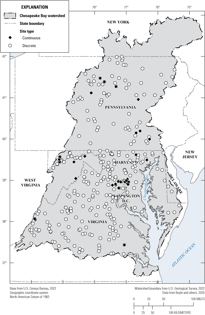
Map of the Chesapeake Bay watershed showing continuous and discrete data sites selected for evaluating status and trends in stream temperature.
Continuous stream temperature trends were fit for each selected site using a GAM that uses a penalized regression-spline smoothing approach (Yang and Moyer, 2020). The response of continuous stream temperature (daily values) by site was expressed as a smooth function of covariates in the following form:
whereg(Tcontinuous)
is stream temperature (daily values),
Bo
is the modeled intercept,
s(log(Q))
is the smooth function by log-transformed streamflow,
s(year)
is the smooth function by time (decimal year),
s(doy)
is the smooth function by season (day of year), and
ti(log(Q), doy)
is the tensor product interaction of covariates of log-transformed streamflow and day of year (doy).
The R package “mgcv” was utilized to fit the GAMs for each site (ver. 1.8-42; Wood, 2017). Based on the effective degrees of freedom for each response variable, a k-value (number of knots) of 10 was used for the log-transformed streamflow and time smooth functions with cubic spline, and a k of 20 was used for the seasonal smooth function (Yang and Moyer, 2020). The direction and magnitude of the trend was calculated as the difference between stream temperature from the start and end of the trend interval. Trend results at the 95-percent confidence level were computed for each site and likelihood values were calculated to provide a nuanced inference and gradual estimation of probabilities (p-values; McBride, 2019). The upward or downward trend likelihood categories included “unlikely” (less than 33 percent), “about as likely as not” (33–67 percent), “likely” (67–90 percent), “very likely” (90–95 percent), and “extremely likely” (95–100 percent; McBride, 2019). The performance of each GAM by site was based on adjusted coefficients of determination (). Significance of covariate effects on water temperature were based on the p-value provided by the Wald statistics in the “mgcv” package (ver. 1.8-42; Wood, 2017). Additionally, the effective degrees of freedom (EDF) provided by the GAMs was used to quantify the degree of nonlinearity of the smooth functions.
In addition to computing trends in continuous stream temperature, these sites and daily values were used to provide the current status of stream temperature across the Chesapeake Bay watershed. The status of stream temperature was computed for each site as the departure of 2022 temperatures, in degrees Celsius above or below the mean annual temperature for the reference period (trend interval). The sparse distribution of continuous sites selected was too heterogenous in topography, land use, and ecoregion to develop an effective, regional status based on a specific species benchmark (such as Salvelinus fontinalis [Mitchill, 1814; brook trout]), disparate reference conditions, or contrasting statewide water-quality standards and criteria (Hawkins and others, 2010). Results from the status and trend analysis of continuous stream temperature data can be found in Boyle and others (2025).
2.3.2.2. Discrete Data
Datasets that have an abundant number of sites with infrequent and limited collection of discrete data at each site were evaluated with linear mixed models (LMMs) to produce a single, watershed-wide trend that accounts for seasonal and diurnal effects (Bolker and others, 2009). Discrete stream temperature records from the WQP and Aquarius datasets published by Clune and others (2023) were used in LMMs (fig. 9). Stream water temperature sites with discrete data were selected to maximize the spatial coverage across the Chesapeake Bay watershed and to provide the longest possible record and comparability in sample size for the trend period. The selected sites had data collected from calendar years 1985 to 2022 and had no more than 5 years of missing data. Within the Aquarius database, data before 1985 within the Aquarius database lacks important metadata (such as the time of day a sample was collected) needed for analysis. Additionally, data during the 1985–2022 trend interval provides good spatial representation and consistent sample size primarily because of the inception of the Chesapeake Bay Water Quality Monitoring program in 1985. The selected discrete stream temperature records included 116,535 measurements from 369 sites (fig. 11). On average, the number of stream temperature observations ranged from approximately 3 to 11 per year. Manual geospatial inspection of site locations revealed duplicate values for 49 sites, which were excluded from subsequent analysis. An additional 608 measurements were excluded because reported stream temperatures were below 0 °C. The final dataset for analysis of discrete data included 94,148 measurements across 320 sites with an average of 294 measurements per site.
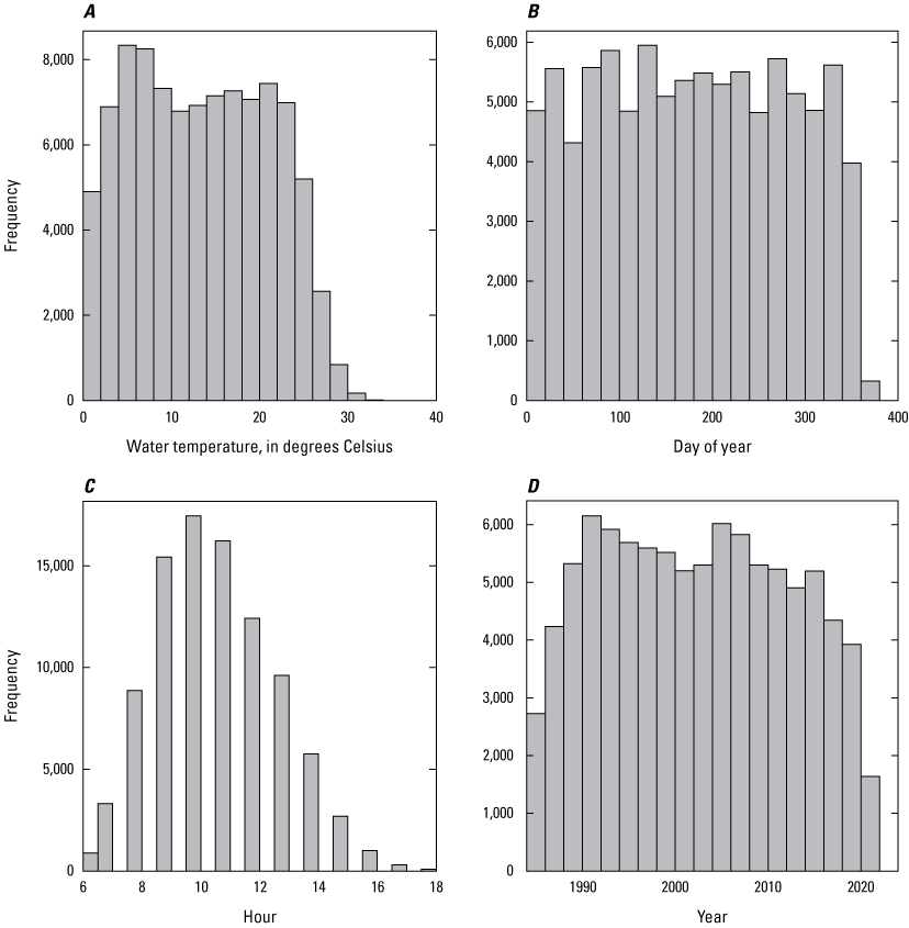
Barplots showing the distribution of discrete stream temperature observations by A, temperature, B, day of year, C, hour of data collection, and D, year of data collection.
Discrete stream temperature data ranged from 0.1 to 39.0 °C, and more than 90 percent of the samples were between 1 and 25 °C (fig. 11A). The dataset equally encompassed all seasons, as seen through the even distribution of samples across all days of the calendar year (day of year; fig. 11B) almost exclusively represented daytime hours of collection between 9 a.m. and 5 p.m. (eastern time; fig. 11C) and included samples each year from 1985 to 2022 (fig. 11D). The dataset contained an average of 2,478 measurements per year. The expected pattern of variation across day of year in discrete stream temperature data was apparent (fig. 12); the highest values were observed during summer months and lowest values, during winter months. This nonlinear association between temperature and day of year justified the incorporation of a quadratic term for day of year in the LMMs.
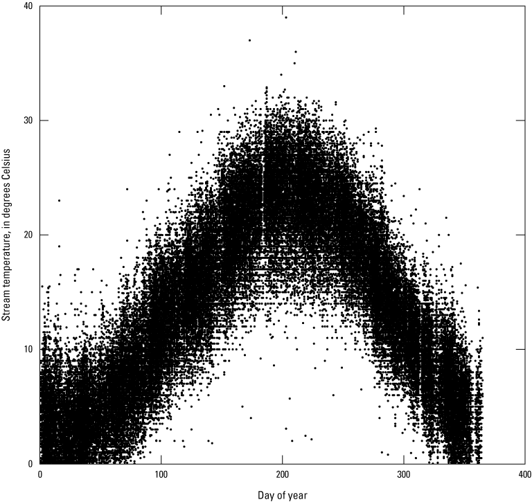
Scatterplot showing the seasonal variation of 94,148 discrete stream temperature datapoints.
Using the screened discrete data, LMMs with fixed and random effects were used to characterize a watershed-wide trend in stream water temperature. Fixed-effect covariates included day of year, day-of-year squared to account for nonlinear seasonal effects, hour of day to account for diurnal variation, and year to assess temporal trends. Covariates were scaled to a mean of 0 and standard deviation of 1 (z-score transformation) to facilitate comparison of covariate effects. The model, which includes a random effect (intercept) by site to account for unmeasured effects of elevation, land use, stream volume, and other local effects on baseline water temperatures, was in the following form:
wheref(Tdiscrete)
is discrete stream temperature,
z(doy)
is the season variation by day of year (z-score transformation),
z(doy2)
is the season variation by day of year (z-score transformation) squared,
z(year)
is the annual variation by decimal year (z-score transformation),
z(hour)
is the diurnal variation by hour of day (z-score transformation), and
RE(site)
is the location specific random effect (intercept) by site.
Functions in the R package “lme4” (ver. 1.1-32; Bates and others, 2015) were used to fit LMMs, and functions in R package “MuMIn” (ver. 1.47.5; Bartoń, 2010) were used to evaluate all pairwise additive combinations of candidate covariates based on Akaike information criterion (AIC). Interpretation of the goodness of fit of the best model was based on R2 values for the conditional (fixed effects only) and marginal (fixed and random effects) coefficients of determination following Nakagawa and Schielzeth (2013) with functions in R package “performance” (ver. 0.10.3; Lüdecke and others, 2021).
Interpretation of the significance of covariate effects on stream temperature, including the time trend represented by z(year) in the model (eq. 2), was based on the departure of 95-percent confidence intervals from zero. Functions in the R package “glmmTMB” (ver. 1.1.7; Brooks and others, 2017) were used to estimate covariate confidence intervals, and functions in R package “sjPlot” (ver. 2.8.15; Lüdecke, 2013) were used to visualize the variation in random effects (random intercepts) among sites. Results from the analysis of discrete stream temperature data can be found in Boyle and others (2025).
2.3.3. Results and Discussion
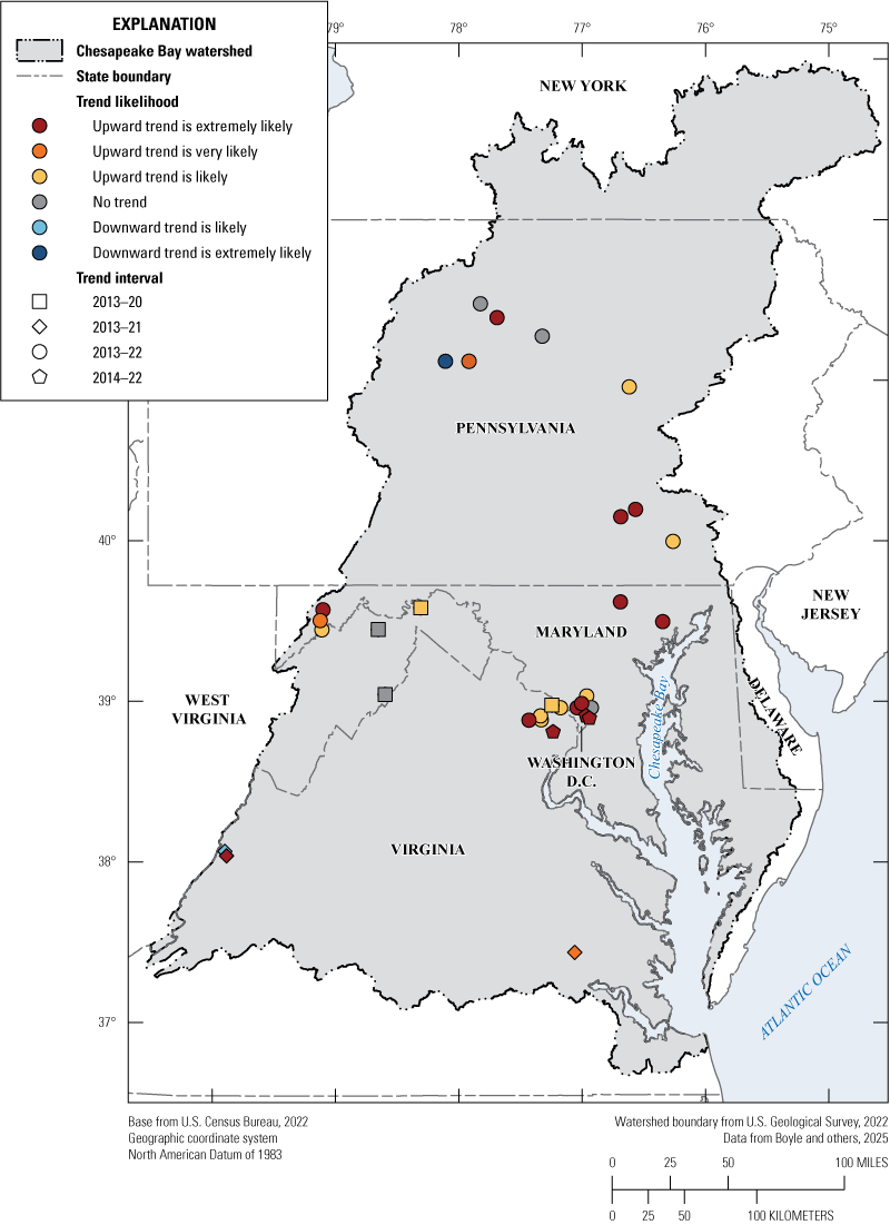
In this section, the status of stream temperature is presented as the departure of 2022 water temperature from the mean of annual temperatures for the trend interval (WY 2013–20, WY 2013–21, WY 2013–22, or WY 2014–22, depending on site). Next, the site-specific trend results derived from the continuous stream temperature data and the generalized additive models are summarized. Finally, the watershed-wide temperature trend derived from discrete stream temperature data and the LMM is presented.
2.3.3.1. Status
WY 2022 was the second warmest year for stream temperature on average for sites with a 9- or 10-year reference period of record that starts in WY 2013 or WY 2014 and ends in WY 2022 (24 of 31 sites; table 5). The average mean annual temperature for the select sites in WY 2022 ranged from 9.66 to 16.14 °C. The departures were positive at all sites and ranged from 0.01 to 0.85 °C above the average for the period. These departures from the average for the period for each site differed spatially and the seasonal fluctuation in stream temperature represents a substantial fraction of the annual variability (table 5, fig. 13).
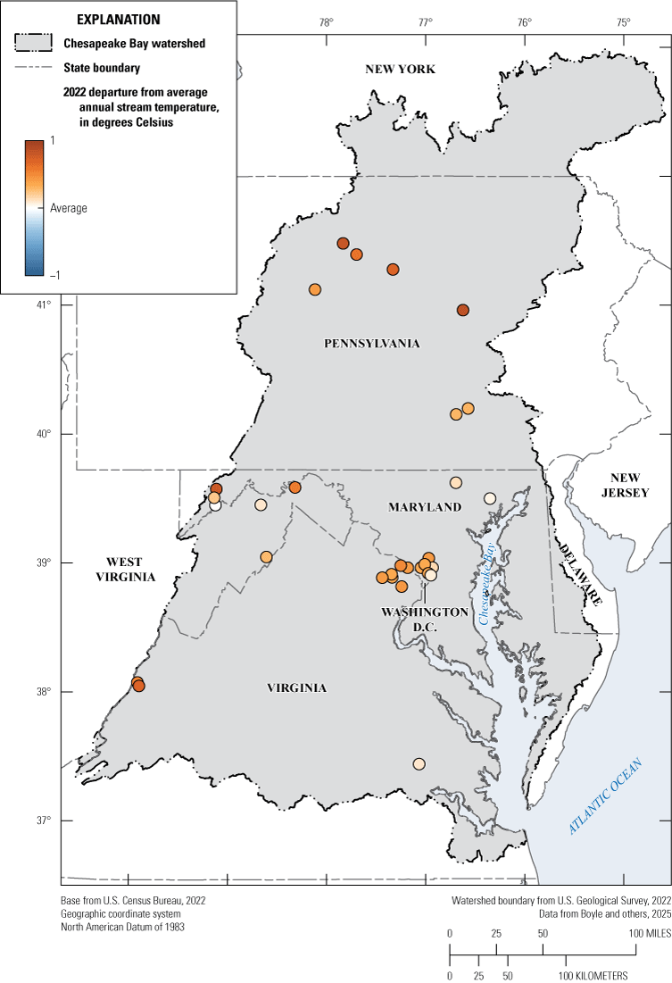
Map of the Chesapeake Bay watershed showing the stream temperature status of 31 sites in 2022. Status was computed as the departure of the average annual stream temperature of 2022 from that of 2013–22 or 2014–22.
2.3.3.2. Continuous Data Trends
GAM methodologies that use the covariates of streamflow, season, year, and interaction term (streamflow and season) were selected to develop trends across sites with daily mean values derived from continuous stream temperature in the Chesapeake Bay watershed. Overall, the GAMs performed well across all 31 continuous data sites. The ranged from 0.86 to 0.96. Nearly all smooth functions for covariates except two were significant in the fitted GAMs. Additionally, the effective degrees of freedom were consistent, providing a balance between model complexity and fit (table 5).
Table 5.
Generalized additive model (GAM) comparison of 31 sites with continuous (daily) stream temperature in the Chesapeake Bay watershed.[Data are from Boyle and others (2025). Values are not significant unless otherwise marked by asterisks: *, value has a significance level of 0.01; and **, value has a significance level of 0.05. USGS, U.S. Geological Survey; , adjusted coefficient of determination; Geo mean, geometric mean; s(log(Q)), streamflow (log); s(doy), season (day of year); s(year), time period (decimal year); ti(log(Q),doy), interaction term for streamflow and season; °C, degrees Celsius; WY, water year; NA, not applicable]
The semidecadal (8–10 years) trend estimates in stream temperature were calculated for four contemporary periods (WY 2013–20, WY 2013–21, WY 2013–22, and WY 2014–22; table 5). Increasing trends in stream temperature were “likely” to “extremely likely” for 79 percent of the sites across the Chesapeake Bay watershed, and only two sites indicated downward trends (fig. 14). For sites with increasing trends, total warming from the beginning to the end of the trend interval ranged from 0.19 to 1.09 °C (table 5).
Map of the Chesapeake Bay watershed showing trends for 31 stream temperature sites with continuous (daily) stream temperature.
GAMs provide the ability to further examine temporal change and the effect of each covariate on the trend. For example, there is an extremely likely and significant increasing trend of 1.56 °C at Flatlick Branch above Frog Branch at Chantilly, Virginia (USGS 01656903) from 2012 to 2022 (fig. 15A). The most significant rate of change occurred at this site from 2014 to 2017 (fig. 15B). Besides the temperature variation during the year (approximately 20 °C), rising stream temperature at this site is only slightly affected by streamflow and more influenced by the time (year) smooth function (figs. 15C–E).
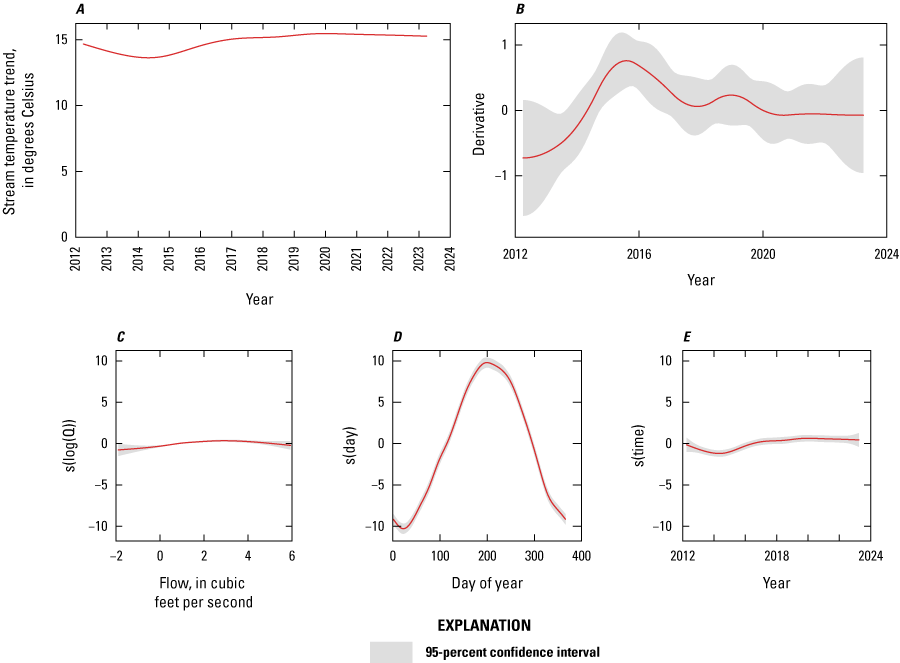
Stream temperature generalized additive model (GAM) for Flatlick Branch above Frog Branch at Chantilly, Virginia (U.S. Geological Survey station 01656903; U.S. Geological Survey, 2023), showing A, the stream temperature trend over time in degrees Celsius, B, the rate of change over time (derivative) and 95-percent confidence interval, C, a smooth function for flow (s(log(Q))), D, a smooth function for day of year (s(doy)), and E, a smooth function for year (s(time)). Data are from Boyle and others (2025).
These trend results for continuous stream temperature (table 5; fig. 14) demonstrate that the use of the novel GAMs approach by Yang and Moyer (2020) is suitable for wider use in the Chesapeake Bay watershed. Contemporary studies that also use continuous daily mean data have shown similar increasing trends in stream temperature for rivers nationally (Tassone and others, 2022; Zhi and others, 2023). Continued warming of streams over extended periods may surpass the thermal limits of aquatic species, especially those in cold water streams, and is a concern for native brook trout and other fisheries. Additionally, there is growing concern the implementation of best management practices for specific water-quality goals (for example, nutrient and sediment reduction) may be having adverse impacts on stream temperature and be acting as “heaters” rather than “coolers” to streams (Batiuk and others, 2023). Future work could utilize continuous daily mean, minimum and maximum values from the USGS and other agencies to better evaluate the full range of thermal regime (magnitude, variability, frequency, duration, and timing) that impact warm and cold water biota (Arismendi and others, 2013). Ultimately, the use of covariate effects in a GAM can be coupled with other analyses of climate, land use, and additional factors to better detect and explain the spatial and temporal drivers of change in stream temperature throughout Chesapeake Bay watershed.
2.3.3.3. Discrete Data Trends
LMMs using discrete data were utilized to produce a watershed-wide trend that accounts for seasonal and diurnal effects. Comparison of alternative combinations of covariates revealed one LMM for stream temperature that strongly outperformed all others (table 6). This model included an effect of hour of day, day of year, day-of-year squared, year, and random intercepts by site. The importance of the year effect was evident because the best-performing model (M1) included all covariates, whereas the next-best model (M2) lacked a year effect and had a much higher AIC value than M1, indicating M1 had a better fit. M1 accounted for 73.0 percent of the observed variation in stream temperature by fixed effects alone (marginal R2) and 77.2 percent of the measurement variation with the inclusion of fixed and random effects (conditional R2).
Table 6.
The four top-performing linear mixed models of stream temperature in the Chesapeake Bay watershed based on all pairwise additive combination of covariates.[Data are from Boyle and others (2025). All models included random intercepts for each site and a global y-intercept of 13.50. Coefficients are given for model covariates with degrees of freedom (df) and Akaike information criterion (AIC) values for candidate models. ΔAIC; difference in AIC value between each model and the top model (M1), NA; not applicable]
Inspection of confidence intervals for covariates in M1 revealed a significant warming trend in stream temperature from 1985 to 2022 (table 7). Specifically, the 95-percent confidence interval for the model coefficient on the year effect (0.14) ranged from 0.11 to 0.16; because these values do not encompass zero, they indicate a significant warming trend over the years and sites included in the discrete stream temperature dataset. The magnitude of seasonal effects exceeded the magnitude of hour effects or year effects in M1 (greater absolute value of scaled coefficients; tables 6, 7). Estimated increases in mean annual stream temperatures across all sites were within 1 °C (fig. 16).
Table 7.
The 95-percent confidence intervals defining the effect direction and magnitude for covariates in M1, the top-ranked model for stream temperature in the Chesapeake Bay watershed.[Data are from Boyle and others (2025), Model rankings shown in table 6. Covariates were scaled to facilitate comparison]
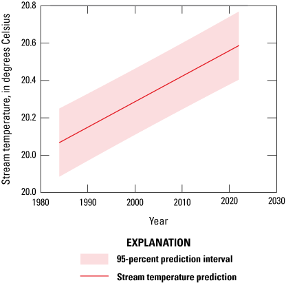
Line graph showing the stream temperature prediction for 1985–2022 from the best-performing model (M1), and the 95-percent prediction interval for mean stream temperature change when accounting for seasonal and diurnal effects.
Prior research that also used discrete data reported increasing stream temperatures in the headwaters of the Chesapeake Bay watershed (Kaushal and others, 2010; Rice and Jastram, 2015). Results from this study support previous findings that stream temperatures in the Chesapeake Bay watershed are increasing and demonstrate the utility of discrete data for temporal trend analysis of water temperature. Additional research could help understand spatial variation in warming trends within the study area, including analysis of riparian cover, land-use change, and effects of geology on groundwater-stream water interactions that may regulate stream sensitivity to atmospheric change (Snyder and others, 2015; Hitt and others, 2023; Kessler and others, 2023).
The ecological implications of rising stream temperatures are a concern to resource managers throughout the Chesapeake Bay watershed. WY 2022 was the second warmest year for stream temperature on average for continuous sites with a 9- or 10-year period of record (WY 2013–22 or WY 2014–22). Increasing trends (0.19–1.09 °C) in stream temperature were “likely” to “extremely likely” for 79 percent of the continuous sites across the Chesapeake Bay watershed, and only two sites indicated downward trends. Additionally, estimated increases in mean annual water temperatures across all discrete sites were within 1 °C. Identifying the magnitude and geographic variability of warming stream temperatures across the watershed is the first step in identifying problematic areas and supporting healthy aquatic ecosystems into the future. Recent advances in the public availability of discrete monitoring data and increased use of continuous monitoring data offer opportunities to better assess thermal regimes in freshwater systems. These results will provide a foundation for more routine and systemic tracking of status and trends of stream temperature for use by environmental managers in the Chesapeake Bay watershed.
2.4. Status and Trends in Stream Toxic Contaminants
By Trevor P. Needham, Ellie P. Foss, and Emily H. Majcher
Many toxic contaminants (for example, compounds that cause toxic effects in fish, which can lead to human exposure) are detected in the Chesapeake Bay watershed (Chesapeake Bay Program, 2021); however, there are no Bay-wide total maximum daily loads (TMDLs) for individual toxic contaminants. Investigation strategies and datasets of toxic contaminants are more variable than other constituents with regards to sampling methodology, frequency, location, and approach across the watershed. Further, regulatory programs and their goals, under which the toxic contaminants are addressed, differ from one another, which complicates efforts to transfer knowledge and technical advances across these programs. Despite the lack of Bay-wide TMDLs, local TMDLs for certain toxic contaminants, such as polychlorinated biphenyls (PCBs) and organochlorine pesticides, are being implemented by the various State and local jurisdictions (Chesapeake Bay Program, 2021). A toxic contaminant inventory focusing on PCBs, mercury (Hg), and organochlorine pesticides was therefore created to assess available data and determine potential for a toxic contaminant status and trend analysis within the Chesapeake Bay watershed (Banks and others, 2022). This section identifies sites where additional monitoring would allow for status and trend analysis in the future.
2.4.1. Data Compilation
In June 2019, the USGS contacted Federal and State agencies across six States (Delaware, Pennsylvania, Maryland, New York, Virginia, and West Virginia) and the District of Columbia (Washington, D.C.) to request available data on toxic contaminants within the Chesapeake Bay watershed. In addition, NWIS and the WQP were queried to retrieve relevant toxic contaminant data. The purpose was to create an inventory of available data across multiple jurisdictions within the Chesapeake Bay watershed. Data compiled for the inventory were limited to only sites where Hg, PCBs, or organochlorine pesticides were collected with sufficient metadata such as sample media, analytical method, sample date, sampling coordinates, and frequency of collection. These toxic contaminants were selected because of their toxicity, prevalence, and TMDL enforcement within the watershed. The related analytical results (concentrations) were not retrieved or used in this analysis because the focus was on data availability.
Data were formatted into two consolidated datasets in a USGS data release (Banks and others, 2022). The “detailed” dataset contains a record of each sample by unique site number, constituent (PCB, pesticide, and Hg), and sampling date. If available, each record includes the site name, data source (provider of the data), location (latitude and longitude), parameter code, analytical method description, collecting agency, and media type. It does not include the analytical results. The other dataset summarizes basic information associated with each unique site: the sampling start and end date, an indication of whether the location was sampled multiple times, the site’s location, the data source, the collecting agency, and the number of sampling records for PCBs, pesticides, and Hg (Banks and others, 2022). Additional information on the agencies and consolidation methods applied to create the “detailed” dataset are provided in the metadata for the data release. When available, total PCB concentrations were also compiled from NWIS, the WQP, and the data provided by Federal and State agencies across Chesapeake Bay watershed. These data were consolidated in a separate table to provide a tool to access comparable PCB data within the Chesapeake Bay watershed. A detailed discussion on compatibility of PCB data and why only total PCBs were compiled can be found in appendix 2 of this report.
2.4.2. Analysis
Spatial distribution of sites, number of records, sample frequency, and the period of record for each site provided the basis for assessing the toxic contaminant inventory (Banks and others, 2022). Analytical method compatibility for PCBs between sampling periods at a given location was also evaluated.
Most sites had few samples collected or samples collected at irregular intervals insufficient for trend analysis. An evaluation was performed to locate sites with repeat sampling events where trend analysis could occur if sampling continued. To identify sites that may qualify for potential future trend analysis, a decision tree was developed based on the available data in the contaminant inventory. The evaluation was limited to PCBs because of data availability and to avoid duplicating work completed by Willacker and others (2020) for Hg in the Chesapeake Bay. Pesticides were not included in this evaluation because of the non-uniformity in pesticides analyzed across the watershed and a priority on pollutants with a TMDL. Future assessments may be possible to assess status and trends for pesticides by evaluating the number of toxic pollutants in a given watershed over time.
The following criteria were used to identify sites where PCB trend analysis could occur in the future if data collection efforts continue:
-
• Temporal duration—Sites with a period of record of 5 years or greater with a minimum of three sampling points.
-
• Recency—Sites need to have been sampled between 2014 and 2019 or 2014 and 2020 (end of data record).
-
• Method compatibility—The method of PCB analysis must report total PCB concentration or individual PCB congeners. Aroclor methods were excluded.
-
• Media compatibility—Only similar media can be used in a trend analysis. The selection was limited to solids, water, and biological samples from fish of the same species or from different fish species with a reported lipid content because these media types contained enough data for within-media trend comparisons.
2.4.3. Results and Discussion
The inventory created for this effort contains information about data availability for pesticides, PCBs, and Hg, and about concentration data for PCBs, from 1938 through 2019 for various sites across the Chesapeake Bay watershed. A comparison of the number of records compiled by media type (table 8) found that more records for pesticides and PCBs are available in NWIS than in State data sources. Some States, such as Pennsylvania, utilized the USGS for monitoring studies, which resulted in most records being in NWIS instead of separate State databases. The number of records available associated with a single sampling point varies by reporting agency and data source. For example, each individual pesticide and media in NWIS has a separate parameter code generating a unique record. A State agency record may only contain total PCBs for a given sample generating one record.
Table 8.
Number of samples with pesticides, polychlorinated biphenyls (PCBs), or mercury (Hg) toxic contaminants detected in media gathered across the Chesapeake Bay watershed, 1938–2019.[Data are from Banks and others (2022)]
Different distributions of data were observed when comparing PCB, Hg, and pesticides by sample media and data source. Most PCB records were available from States (12,546 records), of which 71 percent were biological samples, 21 percent were sediment samples, and 7 percent were water samples. This is consistent with EPA guidance for the development of PCB TMDLs that utilize biological samples (fish tissue) to assess the potential impacts to human health, and derive empirical bioaccumulation factors from water, sediment, and fish concentrations measured within the impacted watershed (U.S. Environmental Protection Agency, 2011). State records for Hg also contained more biological data (79 percent) than any of the other media. Records of Hg water samples were only reported within NWIS (U.S. Geological Survey, 2023). Pesticide data were primarily from NWIS and consisted mostly of water samples.
Sampling by State and local jurisdictions for toxic contaminants is primarily focused on assessing the risk to human health and therefore targets the media responsible for the exposure pathway for the specific contaminant. These exposure pathways may not fully encompass the potential ecological impacts for these contaminants or bioaccumulation models, making it difficult to assess broader impacts (Fuchsman and others, 2006; Rattner and McGowan, 2007; Gobas and Arnot, 2010). For example, EPA guidance for fish sample preparation differs by fish species to reflect how that species is typically consumed by people (U.S. Environmental Protection Agency, 2000).
A total of 89 sites met criteria for potential future trend analysis for PCBs (table 9; fig. 17). The most common media at these sites was biological, but some water samples were taken in the Potomac River and James River Basins. Future trend analysis could consist of evaluating PCB concentrations in fish tissue collected within the major drainage basins identified in table 9. Where applicable, additional factors such as land use could be incorporated to assess significant differences in PCB recovery of the watersheds. Evaluating statistical significance will be difficult because of the low number of records available at each site. Aggregating samples by watershed could increase the sample size but could increase variability in levels. PCB contamination and recovery is very site specific even within a small watershed. For example, a 5-acre lake on the St. James River was treated with activated carbon to reduce PCB bioaccumulation in fish (Patmont and others, 2020). This remedial action was successful; however, the reduction in fish tissue concentration was only observed in resident fish within the lake. Similarly, elevated levels of PCB contamination can be isolated to specific tributaries within a watershed. Beaverdam Creek (Washington, D.C.) within the Anacostia River watershed is one of the five primary tributaries and responsible for most of PCB inputs to the main stem of the river (Wilson, 2020; Lombard and others, 2023).
Table 9.
The number of toxic contaminant sites identified for future trend analysis for polychlorinated biphenyls per watershed at the 6-digit hydrologic unit code (HUC6) scale and 8-digit hydrologic unit code (HUC8) scale within the Chesapeake Bay watershed.[Data are from Banks and others (2022)]
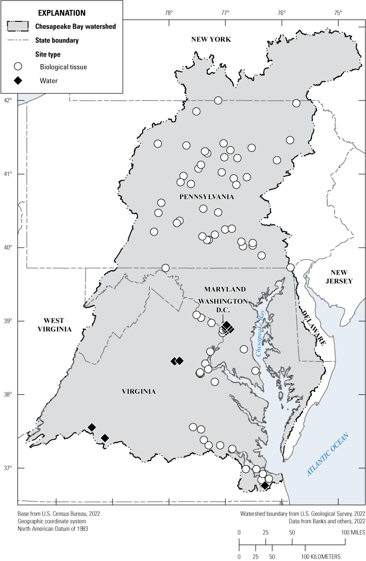
Map of the Chesapeake Bay watershed toxic contaminant sites showing the 89 water or biological tissue sampling sites that meet data criteria for polychlorinated biphenyls (PCBs).
2.5. Status and Trends in Streamflow
By Lindsey Boyle, Rosemary Fanelli, and Samuel H. Austin
Variations in the amount and timing of freshwater flows in the Chesapeake Bay watershed can affect water temperatures, salinity levels, and amounts of nutrients, suspended sediment, and contaminants, while potentially changing the availability of instream habitat for freshwater flora and fauna (Poff and Ward, 1989; Alexander and others, 1996; Gibson and Najjar, 2000). Anthropogenic alterations to natural streamflow regimes caused by land-use activities and climate change are increasingly common, driving a need to track long-term patterns in streamflow and identify areas that are most altered (Dunn and Leopold, 1978). The Chesapeake Bay watershed contains hundreds of rivers and streams. Estimates of average annual streamflows into Chesapeake Bay over an 87-year period of record beginning in 1937 have ranged from less than 50,000 cubic feet per second (ft3/s) to more than 120,000 ft3/s (U.S. Geological Survey, 2019). Knowledge of freshwater flow from streams and rivers draining the Chesapeake Bay watershed, interpreted from analyses of continuous USGS streamflow data, can be used to understand ecosystem change and evaluate status and trends in stream condition. Metrics characterizing streamflow extremes such as magnitude, frequency, and duration of high and low flows are helpful indicators of long-term patterns and shifts in streamflow regimes, which can be interpreted to determine a given metric’s effect on stream biota (Eng and others, 2017; Maloney and others, 2021).
2.5.1. Data Compilation
All data compilation and analyses were completed in R (ver. 4.4.0; R Core Team 2024). Streamflow daily value data were acquired from NWIS (U.S. Geological Survey, 2023) using the R package “dataRetrieval” (ver. 2.7.16; Hirsch and De Cicco, 2015) for 587 streamgages in the Chesapeake Bay watershed that have records from WY 1986 through the close of WY 2022. Within this interval, site selection criteria required 37 complete water years of streamflow data to ensure accurate estimation of streamflow trends, resulting in a final selection of 211 qualifying sites.1
Specific Gage Analyses of hydromorphology, also appearing in this report, use different site selection criteria to identify 346 streamgages for analysis. Refer to section 2.6 “Status and Trends in Stream Hydromorphology” for details.
2.5.2. Analysis
To analyze streamflow status and trends, six metrics of streamflow extrema describing high- and low-flow magnitude, frequency, and duration were calculated for each year in the 37-year interval (table 10). These metrics provide a representation of distinct flow regime components and have been linked to stream biological condition (Carlisle and others, 2017; Eng and others, 2017, 201952). Though all sites had 37 complete years of data, some sites had fewer than 37 years of low- or high-flow duration values because some years did not have any daily values exceeding the low- or high-flow percentile threshold. To calculate a streamflow status for each metric, the percentage difference between a given metric’s value in WY 2022 and the same metric’s WY 1986–2022 average value was used to calculate streamflow status for each metric. Trends in streamflow metrics were estimated using GAMs for each site with metric values available for at least 30 years in the 37-year interval, because the nonlinear qualities of GAM responses support characterization of changes in extrema over time. GAMs were fit using the R package “mgcv” (ver. 1.9-1; Wood, 2017) with a smoothed year covariate and compared to a null model with no year covariate to determine trend significance. A trend was considered strong and significant if the year covariate p-value was less than 0.05 and the AIC value was more than 7 points smaller than found in the null model. Conversely, failure to meet these criteria were interpreted as no trend. Results from the status and trend analysis of streamflow data can be found in Boyle and others (2025).
Table 10.
Descriptions of six metrics characterizing streamflow extrema and analyzed for trends.[Modified from Eng and others (2019, table 1). (ft3/s)/mi2, cubic feet per second per square mile; WY, water year]
2.5.3. Results and Discussion
Low- and high-flow duration status values could not be calculated for 46 sites; 43 sites did not have any low-flow events (flows below the 10th percentile of all daily value site flows in WY 1986–2022), and 3 sites did not have any high-flow events (flows above the 90th percentile of all daily value site flows in WY 1986–2022) in WY 2022. For most sites, high-flow frequency was above average and high-flow magnitude and duration were below average, indicating that though high flows were more common in WY 2022, those high flows were shorter in duration and generally smaller in magnitude than the 37-year average (fig. 18). Most sites had above average low-flow magnitude and below average low-flow duration and frequency, indicating that low flows in WY 2022 were not as low as the 37-year average and occurred less often and over fewer total days than the 37-year average of low flows (fig. 18). During WY 2022, above average high-flow frequencies and below average high-flow magnitudes and durations were most prevalent in the lower portion of the watershed. Most above average low-flow frequencies were associated with sites in the lower portion of the watershed, as were most sites with above average low-flow magnitudes. Most sites where below average low-flow durations were observed, however, were in the upper portion of the watershed (fig. 18).
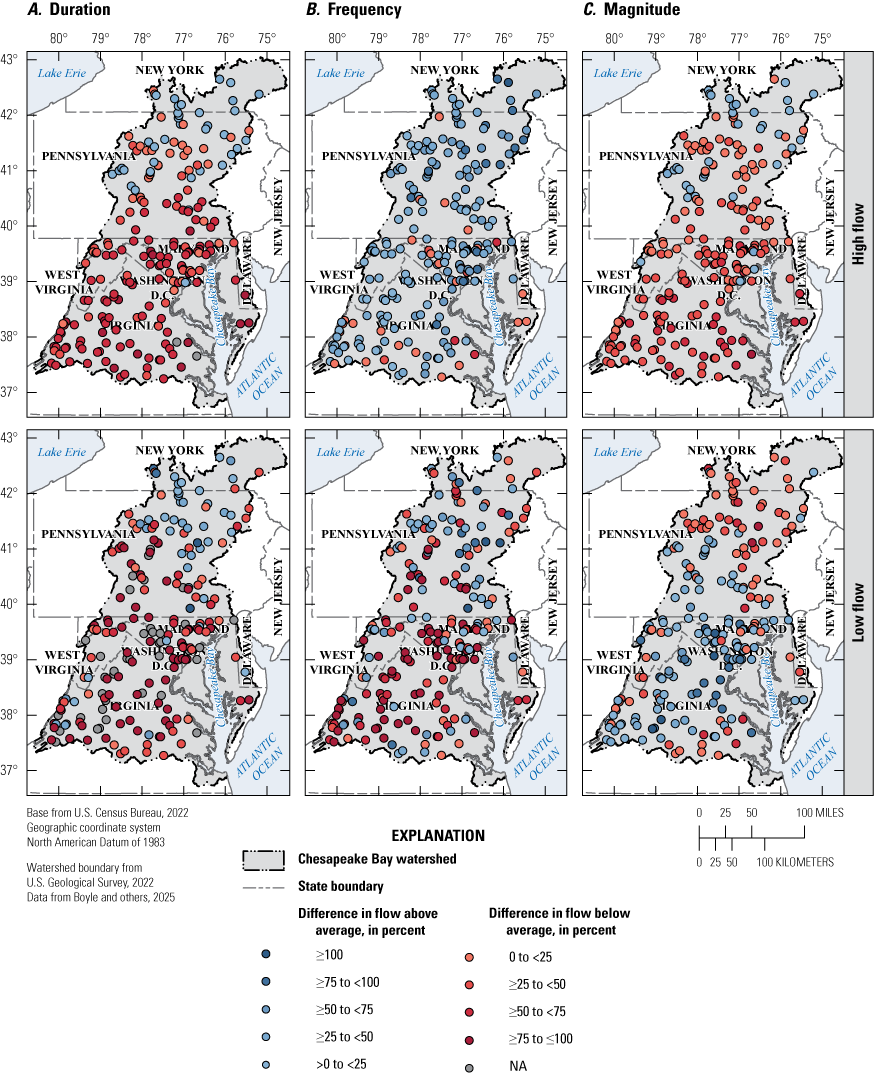
Maps of the Chesapeake Bay watershed showing the status of streamflow sites in water year (WY) 2022 based on high-flow and low-flow A, duration (days), B, frequency, and C, magnitude (cubic feet per second per square mile). Status was computed as the percentage difference between WY 2022 and the WY 1986–2022 long-term average of each metric. [≥, greater than or equal to; ≤, less than or equal to; <, less than; >, greater than; NA, not applicable]
For most sites across the watershed, values of high- and low-flow metrics were extremely variable and had no strong directional trends over time. Low-flow metrics had a greater number of significant trends overall than high-flow metrics. Trends in low-flow metrics revealed increases in low-flow magnitude, decreases in low-flow frequency, and few trends in low-flow duration. Of the few sites with significant trends in high-flow metrics, most had increasing trends in high-flow magnitude and duration (table 11; fig. 19). Sites with significant trends in streamflow metrics were sparse and scattered across the watershed. However, sites with increasing trends in low-flow magnitude and decreasing trends in low-flow frequency were clearly clustered in the Baltimore-Washington, D.C., metropolitan area, especially in tributaries of the Potomac River (fig. 19), indicating that low-flow events in this area have become less frequent and less extreme in magnitude over time.
Table 11.
Number of increasing, decreasing, and no-trend estimates associated with low-flow and high-flow extrema metrics for streamflow sites in the Chesapeake Bay watershed.[Data are from Boyle and others (2025)]
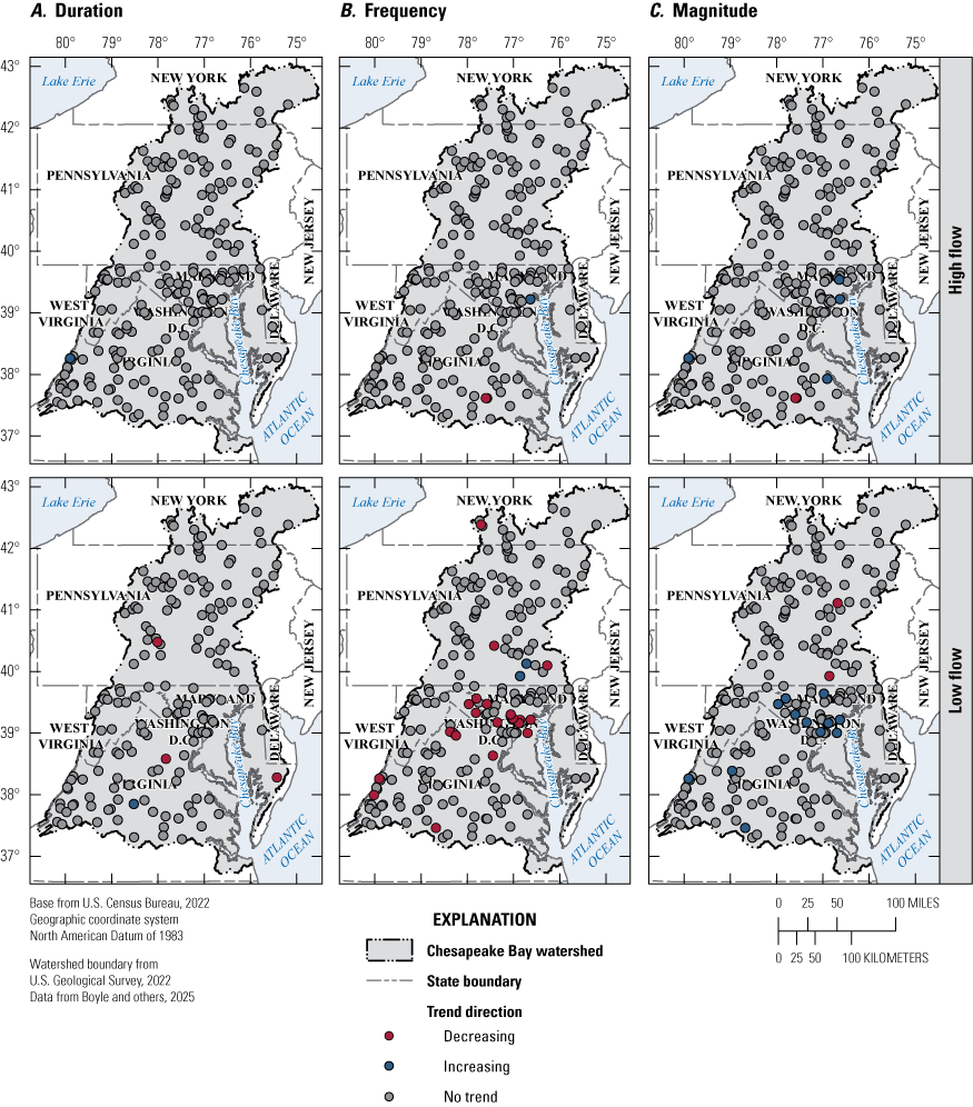
Maps of the Chesapeake Bay watershed streamflow sites showing the 37-year trends in low-flow and high-flow A, duration (days), B, frequency, and C, magnitude (cubic feet per second per square mile).
Natural fluctuations in flow are important for maintaining healthy stream biological assemblages (Poff and others, 1997). Climate change and anthropogenic activities such as urban development or water withdrawals can drive unnatural variations in streamflow that harm aquatic life (Döll and Zhang, 2010; Brown and others, 2013). Extreme low flows can cause declines in sensitive macroinvertebrate taxa and taxa richness and decreases in fish growth rates, survival, and abundance—both directly through reductions in available swift water habitats and, more often, indirectly through increases in water temperature and SC during low-flow conditions (Dewson and others, 2007; Miller and others, 2007; Walters, 2016). Extreme high flows also influence stream biological assemblages by physically washing organisms downstream, scouring away algal food sources, destroying habitat, and introducing pulses of sediment and nutrients, all of which lead to decreasing macroinvertebrate densities, richness, and abundance and altered fish population densities and structure (Scrimgeour and Winterbourn, 1989; Carline and McCullough, 2003; Chattopadhyay and others, 2021). At most sites across the watershed, values of high- and low-flow metrics were extremely variable with no strong directional trends over time. The lack of general watershed-wide patterns in streamflow metrics (assuming these are not the result of Type II errors [when analysis fails to detect an existing trend]) suggests that low or high-flow metrics at the few sites with significant change may be driven by site-specific factors rather than watershed-wide factors such as climate. Future investigation of site-specific drivers, incorporation of climatic variables into the modeling framework, and evaluations of additional streamflow metrics will aid in a comprehensive understanding and maintenance of freshwater flows in the Chesapeake Bay watershed.
2.6. Status and Trends in Stream Hydromorphology
By Matthew J. Cashman, Coral M. Howe, Zachary J. Clifton, Marina J. Metes, and Joshua J. Thompson
Hydromorphology is the complex interplay of streamflow, sediment, vegetation, geomorphic forms, and connectivity (Wang and others, 2015; Castro and Thorne, 2019) that creates the physical habitat template to support aquatic organisms and communities (Orr and others, 2008). Because these factors interact across temporal and spatial scales, they create a diverse patchwork of physical habitats characterized by varying water depths, streamflow types and velocities, substrates, and channel forms. Available hydromorphic conditions then can act as diversity filters for what organisms can persist in a local river segment or reach (Lamouroux and others, 2004).
Sediment and physical habitat degradation have been identified as a leading cause of local ecological impairment across the Chesapeake Bay watershed (Fanelli and others, 2022). However, sediment is only one aspect among many contributing to hydromorphologic conditions, and other facets of physical habitat that contribute to ecological condition may be overlooked unless explicitly and directly evaluated (Cashman and others, 2024). The direct assessment of the different aspects of hydromorphic conditions, and how they might be changing through time and space, may assist in explaining the various stressors contributing to stream health and more directly track physical habitat changes in response to management activities.
2.6.1. Data Compilation
Two distinct but complementary analyses using different data sources were undertaken to evaluate the status and trends in hydromorphology across the Chesapeake Bay watershed: (1) status and trends in multi-jurisdictional rapid habitat assessment data, and (2) trends in channel dimensions and hydraulics at USGS streamgages, referred to as specific gage analysis (Cashman and others, 2021), a methodological update to specific-stage analysis originally defined by Gilbert (1917). These two methods have different but complementary hydromorphic foci and provide different spatial coverages across the Chesapeake Bay watershed. Data compilation for specific-gage data and quality assurance and quality control (QA/QC) for rapid habitat data were completed in R (ver. 4.2.1; R Core Team, 2022b).
2.6.1.1. Rapid Habitat Assessment Data
Rapid habitat assessments are field-based monitoring methods of hydromorphic and physical habitat conditions that can be quickly conducted at a site, often in conjunction with other data collections, such as biological monitoring. Although several methods exist, the most common is the EPA rapid assessment method (Barbour and others, 1999). Most metrics are scored on a quality scale from 0 to 20 based on visually qualitative rankings. A given metric’s score was used to classify it as either “poor” (0–5), “marginal” (6–10), “suboptimal” (11–15), and “optimal” (16–20). These values are scored against an ideal reference condition for a river type in its region and should therefore be comparable across regions. Rapid habitat assessment metrics cover a range of different hydromorphic features and processes that are relevant to components of the local ecosystem, such as fishes, macroinvertebrates, and general hydromorphic functions. The metrics also cover aspects of the reach through mesohabitat and microhabitat spatial scales (table 12).
Table 12.
Hydromorphology rapid habitat assessment metric names, metric descriptions, and number of sites in the Chesapeake Bay watershed that qualify for trend analyses per metric.[Data are from Boyle and others (2025). Each metric value ranges from 0 indicating “poor” metric quality to 20 indicating “optimal” metric quality]
Rapid habitat assessment data were obtained from the Chesapeake Bay Program’s DataHub database (Chesapeake Bay Program, undated), which contains a compiled dataset from 19 different Federal, State, and local agencies and jurisdictions. These data were then evaluated for QA/QC for use within status and trend analyses (refer to appendix 3 for QA/QC methods).
Because the habitat metrics collected tended to vary within and among the monitoring sites and events, each unique combination of habitat metric and monitoring site was evaluated separately for meeting qualifying trend criteria. For sites with multiple monitoring events per year, only the first field assessment of each year was retained such that the datasets contained one monitoring event per metric per year.
The trend interval of analysis comprised calendar years 2008–17, and each metric and site combination qualified for trend analyses if it contained 7 years or more of data. The final set of trend metrics were selected for analysis based on meeting a criterion of 50 or more qualifying trend sites across the Chesapeake watershed. The total number of qualifying sites varied by metric, from a minimum of 51 (Frequency of Riffles) to a maximum of 101 sites (Embeddedness; table 12).
2.6.1.2. Specific Gage Analysis Data
Specific gage analyses examine changes to river channel dimensions and hydraulics using data collected during routine streamflow measurements at USGS streamgages (Juracek and Fitzpatrick, 2009). These river-segment and reach-scale changes can represent the state of channel evolution (Cluer and Thorne, 2014), which has been related to fish community trajectories by Stearman and Schaefer (2023) and capture the timescale of hydromorphic recovery in response to disturbances (Cashman and others, 2021). The type of specific gage analysis used in this study is a field measurement analysis (Cashman and others, 2021), modified to use GAMs for additional nonlinear covariate normalization, which tracks flow-normalized changes to bed elevation, channel area, and channel velocity (additional details are in appendix 3).
Qualifying trend sites were identified by querying NWIS (U.S. Geological Survey, 2023) using the R package “dataRetrieval” (ver. 2.7.11; Hirsch and De Cicco, 2015) for all active USGS streamgages in the Chesapeake Bay watershed that reported both streamflow and stage data. The full site record of daily streamflow was retrieved for all sites, and each site was evaluated at various trend intervals of interest (10-, 25-, 50-, and 75-year records), which was measured as years prior to the end of WY 2022. A gap of more than 201 days of missing streamflow in a water year resulted in the end of the potential trend interval (working backwards in time), even if data existed prior to that year, to avoid large operational differences with gage discontinuities. For example, if a streamgage’s period of record spanned from WY 1946 to WY 2022 and contained a period of 202 consecutive days during WY 1975 wherein streamflow data was not recorded, the trend intervals at this streamgage would be a 10-year interval (WY 2012–22) and a 25-year interval (WY 1997–2022), but not a 50-year interval nor a 75-year interval because WY 1975 falls between the start and end of the intervals. Other periods of missing data were allowed if the limit of 201 consecutive days of missing streamflow data was not exceeded. In total, this method identified 342 USGS streamgages that qualified for a 10-year trend analysis and declining numbers for longer trend intervals (table 13).2 For each qualifying site, information on site history and establishment was retrieved from the internal USGS Site Information Management System database to identify any interventions that could alter hydromorphic trends such as streamgage relocations, datum changes, and other physical step-change alterations, such as a local bridge building, and dates of which are summarized in Boyle and others (2025).
Streamflow analyses appearing earlier in this report use different site selection criteria to identify 417 streamgages for a dedicated streamflow analysis. Refer to section 2.5 “Status and Trends in Streamflow” for details.
Table 13.
The number of qualifying U.S. Geological Survey streamgages in the Chesapeake Bay watershed examined for hydromorphology specific gage trend analyses at various trend intervals.[Data are from Boyle and others (2025). All streamgages were active as of May 2023. The trend intervals are the minimum number of active years with sufficient data completeness leading up to the end of water year 2022]
Channel metrics were directly contained in, or derived from, metrics in NWIS (U.S. Geological Survey, 2023). The expanded field measurement tables for each site were pulled from NWIS using the R package “dataRetrieval” (ver. 2.7.11; Hirsch and De Cicco, 2015). A series of pre-processing steps were conducted on these data before trend analysis, including deriving additional field measurement metrics, labeling data for possible confounding step-change factors, and QA/QC of the data for outliers. Refer to appendix 3 for more data pre-processing details.
2.6.2. Analysis
Generalized additive models (GAMs) were used to evaluate trends across the Chesapeake Bay watershed in (1) multi-jurisdictional rapid habitat assessment data and (2) channel dimensions and hydraulics at USGS gages via specific gage analysis. Status was only evaluated for the multi-jurisdictional rapid habitat data. All analyses for both the specific-gage data and rapid-habitat data were completed in R (ver. 4.2.1; R Core Team, 2022b).
2.6.2.1. Rapid Habitat Assessment
Statuses for each site and metric were calculated by averaging the most recent three observations in the trend record. Trends for all repeat rapid habitat assessment metrics were then estimated using GAMs to capture nonlinear changes and threshold effects. GAMs were fit using the R package “mgcv” (ver. 1.9-1; Wood, 2017), and k was set as a minimum default to no more than one-third of the total data points per trend. Following methods from Murphy and others (2019), trends from each GAM were compared to a null model (GAM fit without a date or year covariate) and were considered “strong” if AIC values were 7 or more points smaller than the null model, “possible” if AIC values were 4 or more points and less than 7 points, and “unlikely” if AIC values were less than 4 points smaller than the null model. A linearized trend slope was calculated as the difference of the model predictions for the beginning and end years of the trend interval, divided by the length of the trend. Additional analysis was done to answer the following question: Are strong negative trends occurring at sites that began in “optimal” condition and degraded or at sites that were in “poor” condition and worsened, and vice versa for sites with positive trends? To answer this question, a 3-year average metric condition score was calculated from the beginning of the record for each site to determine starting condition, which was then compared to trend slopes. Results from the status and trend analysis of rapid habitat data can be found in Boyle and others (2025).
2.6.2.2. Specific Gage Analyses
The field measurement analysis used GAMs to create a flow- and confounding-variable normalized time trend for three field-derived metrics: bed elevation, channel area, and channel velocity. Eight GAMs were fit for each field metric using the R package “mgcv” (ver. 1.9-1; Wood, 2017) with varying levels of complexity to best capture the nonlinear and confounding factors influencing results particular to a specific site. Possible model forms included terms for date, year, streamflow, seasonality (represented as day of year), measurement type, intervention (a categorical variable representing the periods before and after any recorded alteration in and around a streamgage), nonlinear interactions between day of year and time, and nonlinear interactions between time and streamflow. K term was adjusted according to an iterative procedure to optimize model fit. An example of model fits for each of the 8 GAM model forms can be found in figure 3.1. Multi-model selection was then performed based on minimum AIC scores across all eight model forms to choose the best fitting and most parsimonious model to represent the dynamics of each site. For more details on the GAM flow- and confounder-normalized method, and multi-model selection, refer to appendix 3.
Following methods from Murphy and others (2019), the optimally selected GAM was compared to a null model (the optimally selected GAM fit without a date or year covariate) and was considered strong (and the null model was rejected) if its AIC value was at least 7 points smaller than the null model. GAM models that did not strongly reject the null model (referred to hereafter as a “null result”) were deemed insufficient to recreate the channel dynamics at a site and were removed from consideration for further analyses. A null result does not indicate the lack of a trend, but rather the lack of the ability to evaluate a trend. In the context of this study, a null result would be caused by a lack of change through time or a lack of statistical power to detect any change. Because of the high-temporal resolution of the data, the analysis is able to detect even minor changes associated with the adjustments and shifts to field-measurement rating curves (Cashman and others, 2021) that routinely occur when operating and maintaining USGS streamgages (Sauer, 2002). Even without a directional temporal trend, short-duration channel responses to single storm events and cyclical seasonal dynamics should be detected and result in a strong rejection of the null model. A lack of short-term, event-based changes or cyclical seasonal dynamics suggests that the streamgage has artificial controls in the measurement area, precluding our ability to detect meaningful channel changes elsewhere in the channel. Similarly, the failure to strongly reject the null model may be caused by poor model fit and high variance, likely due to missing covariates in the model, and thus indicates an inability for the model to report channel changes, rather than an indication of no channel change. If included in the analysis, the null results would increase the likelihood of false negative “no trend” results.
Flow- and confounder-normalized predictions were made from the optimal site models to capture a normalized temporal trend. In this prediction, any streamflow, day of year, and interactions between streamflow or day of year were excluded from the prediction function, effectively removing the effects of these variables. Interventions were fixed to be predicted against only the most recent intervention ‘datum’, and field measurement type was fixed to the method used most frequently at a site.
Trend rates and uncertainties were calculated from the confounder-normalized predictions of the best model, with confidence intervals. Although a status for channel dimensions and hydraulics at streamgages was not assessed on its own, the year-long normalized predictions in the most recent year (WY 2022) were averaged to represent the end year for each trend interval, and the values within the WYs covering the 10-, 25-, 50-, and 75-year intervals were averaged to represent the beginning year of each interval. Significant difference between the timesteps was then evaluated using a t-test of the mean and confidence intervals for the averaged year-long predictions at each timestep, and significance was determined at p-value less than or equal to 0.05. The magnitude of change was divided by the length of the trend interval to create a linearized trend slope. Specific gage analysis results can be found in Boyle and others (2025).
2.6.3. Results and Discussion
Results of GAMs for (1) multi-jurisdictional rapid habitat assessment data and (2) channel dimensions and hydraulics at USGS gages via specific gage analysis are conveyed and discussed. Results of the rapid habitat assessment analysis found evidence suggesting degrading hydromorphic conditions at the majority of sites with significant trends. However, the limited number of trend sites and spatial clustering of available sites prevented conclusions about hydromorphic conditions on a watershed-wide scale. Specific gage analysis revealed patterns consistent with channel evolution following disturbance, including decreasing bed elevation and increasing channel area trends indicating channel incision and expansion over a 75-year interval followed by occasional fill and widening, indicated by increasing bed elevation and channel area trends in the 10-year interval.
2.6.3.1. Rapid Habitat Assessment
On the scale of 0 (“poor” habitat quality) to 20 (“optimal” habitat quality), the status of rapid habitat assessment metrics averaged from 12.0 to 16.4. The lowest average scores were in Embeddedness (12.0), and the greatest average scores were in Channel Alteration (16.4). Status varied across the watershed. Low scores for some metrics were notably clustered in the Delmarva Peninsula and in the urbanized Baltimore–Washington, D.C., metropolitan area, and metrics with greater scores were generally in western parts of the watershed (fig. 20). The sites used for the analysis were also distributed unevenly across the watershed and tended to concentrate within Maryland and the southwestern portion of the watershed (Virginia and West Virginia).
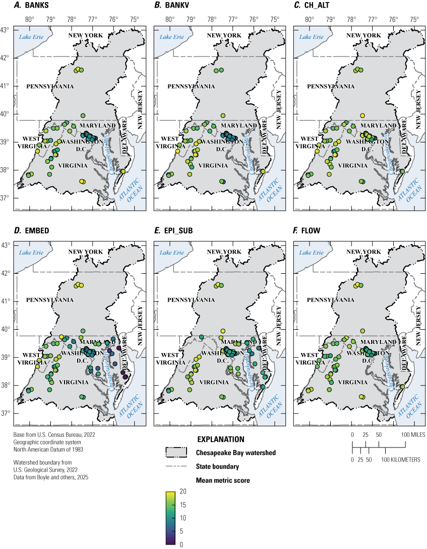
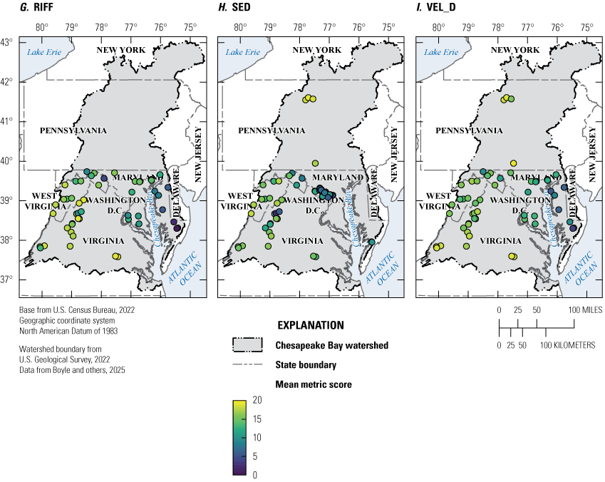
Maps of the Chesapeake Bay watershed showing the status of all rapid habitat hydromorphology sites analyzed for the following qualifying metrics: A, Bank Stability (BANKS), B, Bank Vegetation (BANKV), C, Channel Alternation (CH_ALT), D, Embeddedness (EMBED), E, Epifaunal Substrate/Available Cover (EPI_SUB), F, Channel Flow Status (FLOW), G, Frequency of Riffles (RIFF), H, Sediment Deposition (SED), and I, Velocity/Depth Combinations (VEL_D). Status computed using the average of most recent 3-year observations. Qualifying trend site counts are in table 12.
Most sites that showed a change in habitat conditions were degrading, with relatively few sites showing positive, improving conditions. Of the 955 unique metric and site combinations tested for trends, 86 (9 percent) had “strong” trends, 96 (10 percent) had “possible” trends, 764 (80 percent) had “unlikely” trends, and 9 sites had no measured change across their record. Of those with “strong” trends, 54 (77 percent) were negative and indicated degrading condition, 13 (19 percent) were positive and indicated improving condition, and 3 results had nonmonotonic trends that indicated no net change in condition across the time interval. Although some metrics showed slightly different proportions of negative or positive trends, most metrics showed slight to moderate negative trends of degrading condition through time at most sites, and few sites showed positive, improving conditions (fig. 21). On average, linearized slopes for ”strong” trends changed by an absolute magnitude of change of about 0.55 points per year in either positive or negative directions, and the mean change across all metrics, –0.37 points per year, indicating overall degrading conditions. Across the trend interval of 2008–17, this would result in a change of nearly 5 points of change, and mean degradation of nearly 3.7 points, out of the 20-point scale, across our period of analysis. Areas with significant changes were scattered throughout the watershed, although with notable significant trends around the Baltimore–Washington, D.C., metropolitan area for many metrics (fig. 22).
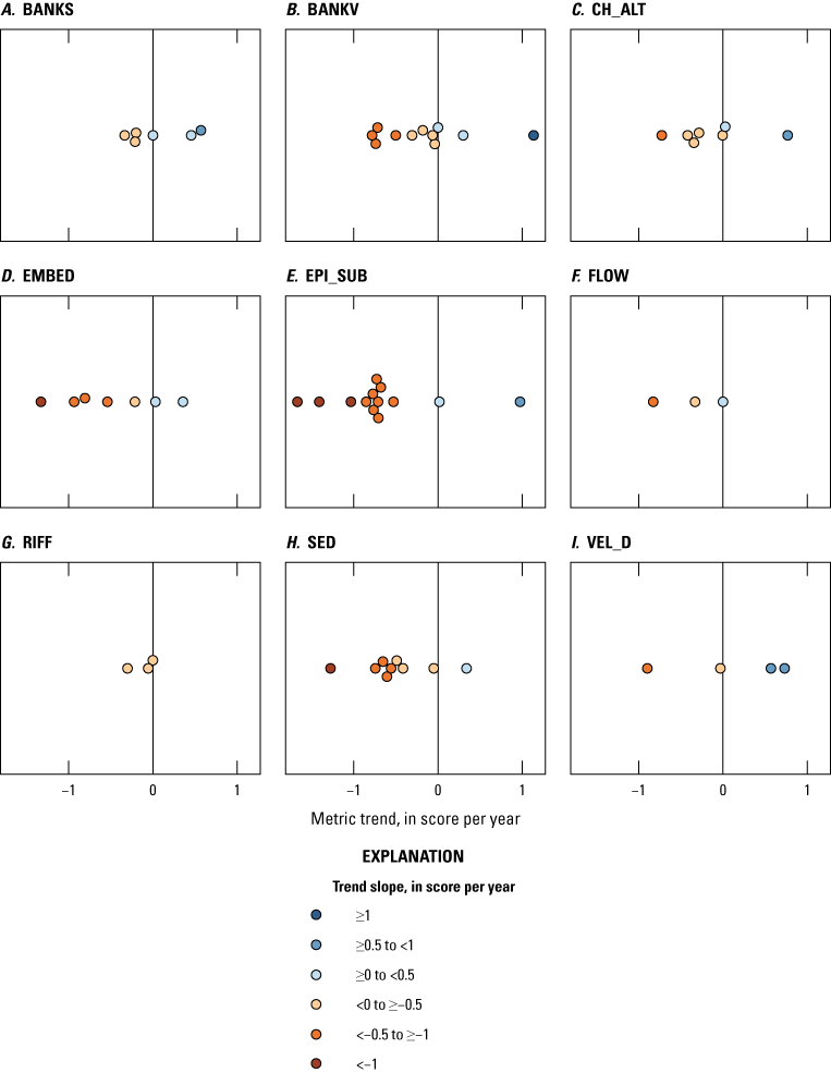
Linearized trend slopes for rapid habitat hydromorphology sites across the Chesapeake Bay watershed for the following metrics: A, Bank Stability (BANKS), B, Bank Vegetation (BANKV), C, Channel Alternation (CH_ALT), D, Embeddedness (EMBED), E, Epifaunal Substrate/Available Cover (EPI_SUB), F, Channel Flow Status (FLOW), G, Frequency of Riffles (RIFF), H, Sediment Deposition (SED), and I, Velocity/Depth Combinations (VEL_D). Slopes are presented in change in the metric score per year. Qualifying trend site counts are in table 12. Data are from Boyle and others (2025). [≥, greater than; <, less than]
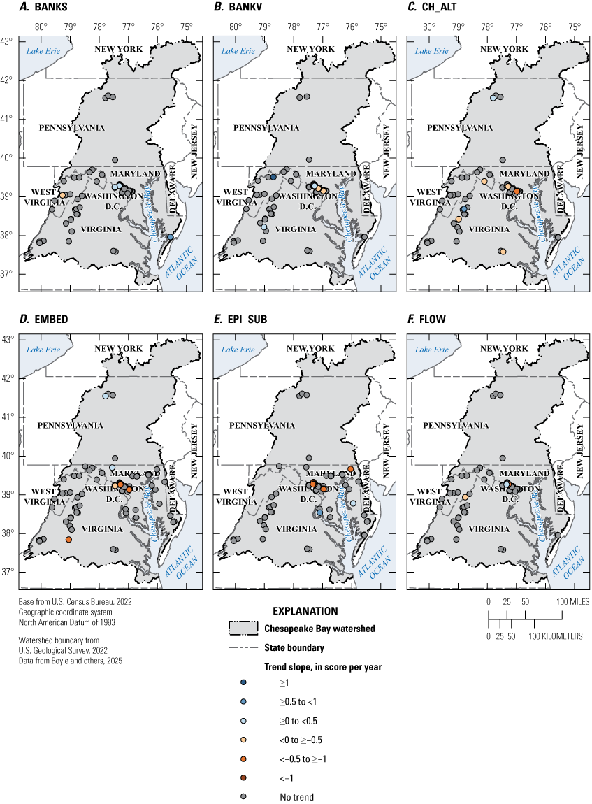
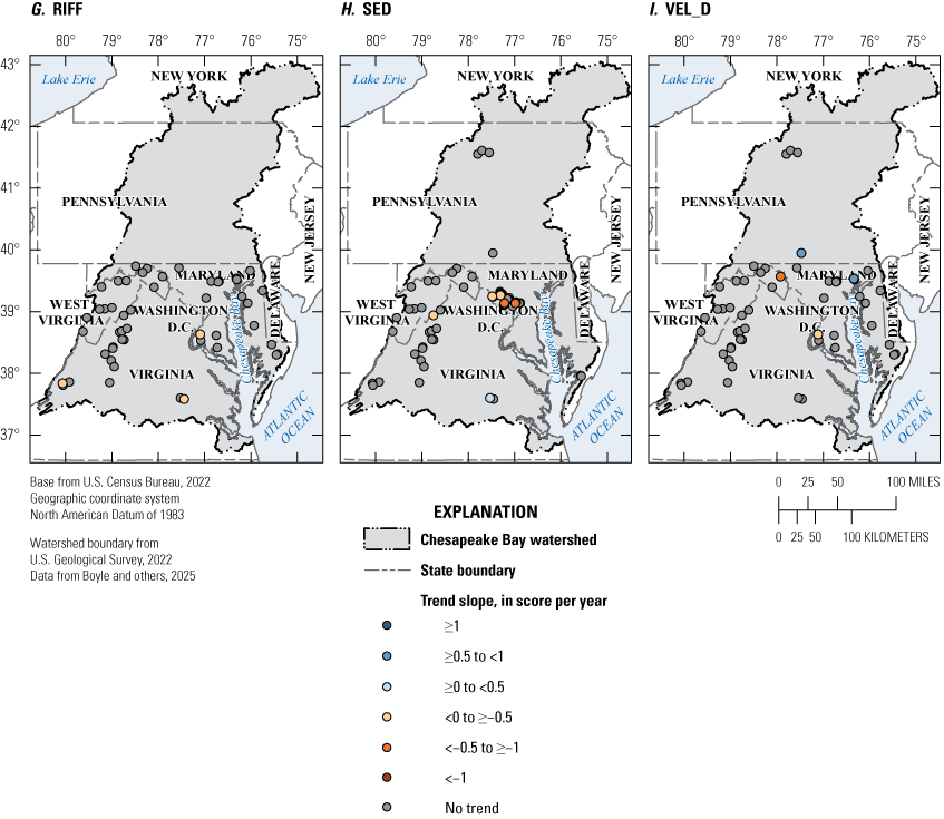
Maps of the Chesapeake Bay watershed showing the trend slopes of rapid habitat hydromorphology sites analyzed for the following metrics: A, Bank Stability (BANKS), B, Bank Vegetation (BANKV), C, Channel Alternation (CH_ALT), D, Embeddedness (EMBED), E, Epifaunal Substrate/Available Cover (EPI_SUB), F, Channel Flow Status (FLOW), G, Frequency of Riffles (RIFF), H, Sediment Deposition (SED), and I, Velocity/Depth Combinations (VEL_D). Slopes are presented in change in the metric score per year. Qualifying trend site counts are in table 12. [≥, greater than; <, less than]
Trend slopes were compared against metric scores from the beginning of the record to evaluate whether there were any management-relevant patterns in trend slopes based on a site’s initial condition. Epifaunal Substrate/Available Cover exhibited a significant relationship between trend slope and initial metric score, indicating that negative trends in epifaunal substrate were more likely to be observed at higher-quality sites (fig. 23). However, this trend analysis excluded some earlier data available at each site, which may provide additional perspective on how these sites may have changed through time. To achieve Chesapeake Bay Program targets, conserving sites currently in good condition and targeting lower quality sites for management interventions and (or) restoration may be necessary.
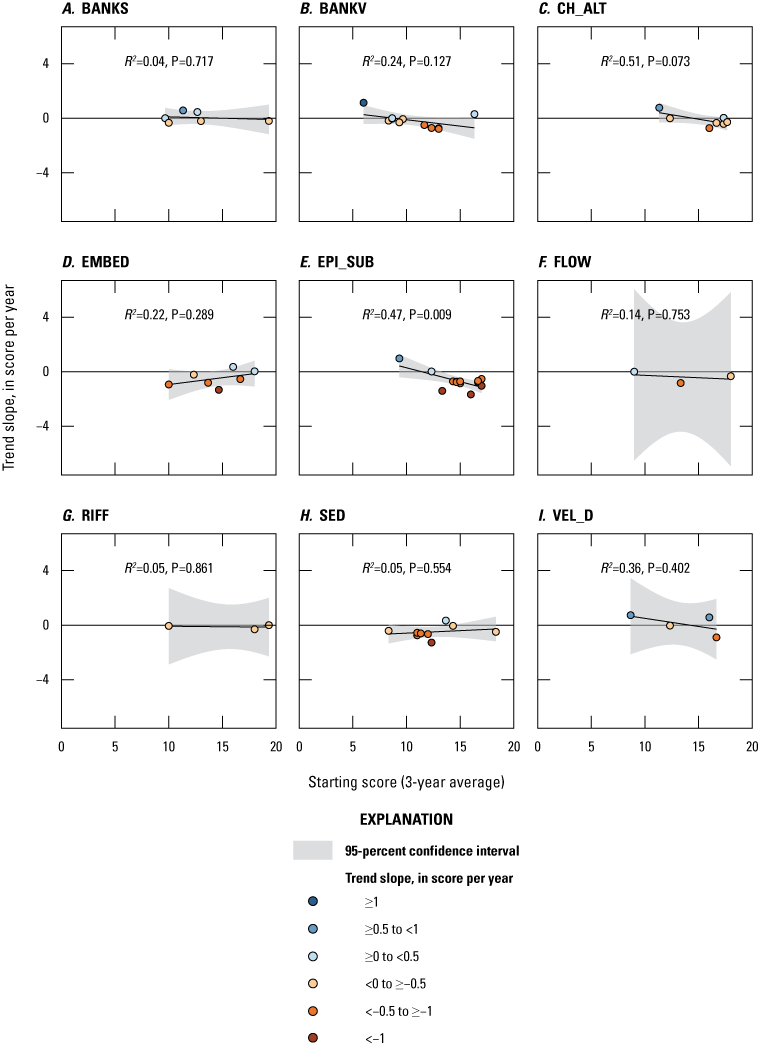
Trend slopes for all hydromorphology rapid habitat assessment metrics compared to the 3-year average starting score, which represents an initial quality condition for each site at the beginning of the trend interval: A, Bank Stability (BANKS), B, Bank Vegetation (BANKV), C, Channel Alternation (CH_ALT), D, Embeddedness (EMBED), E, Epifaunal Substrate/Available Cover (EPI_SUB), F, Channel Flow Status (FLOW), G, Frequency of Riffles (RIFF), H, Sediment Deposition (SED), and I, Velocity/Depth Combinations (VEL_D). The coefficient of determination (R2) and p-values are from linear regression output according to the linear model fit line. Slopes are presented in change in the metric score per year. Qualifying trend site counts are in table 12. Data are from Boyle and others (2025). [≥, greater than; <, less than]
Overall, the field-based rapid habitat assessment data indicated that metrics of physical habitat condition that were significantly changing through time were degrading in condition, and only a few sites showed improvement. However, site locations included in this analysis were not evenly distributed throughout the watershed. Sites were instead clustered within a few jurisdictions and overrepresented many of the watershed’s metropolitan areas, which contain more urban stressors of physical habitat. Future analyses, which can incorporate additional data at more locations, may provide additional spatial and temporal perspective for these trends across the watershed. For example, if agencies and jurisdictions continue to collect rapid habitat assessments, additional sites should have enough data to meet the criteria for a trend analysis. Although representative of the conditions in these monitored rivers and streams, these locations might overlook other key drivers of change throughout the watershed, including areas of forest conservation, forest harvest, or mixed farming. This method also relies on visual-based scoring and subjective judgement, so uncertainty can be introduced by differing field personnel, differing standards among jurisdictions conducting the surveys, or guidelines to differentiate between similar scores in a similar quality category. Refer to section 2.8 “Indicator Results Synthesis” for more information.
2.6.3.2. Specific Gage Analyses
Across the 342 sites analyzed and the four trend intervals, all sites had at least one strong field measurement model that was sufficient for trend analysis. Overall, between 36 and 51 percent of trends analyzed in each time interval were significant at p-values less than or equal to 0.05. The greatest proportion of significant trends were within the 75-year trend interval. Among metrics, channel velocity and channel area had the least number of significant trends (41 percent), and bed elevation had the most (47 percent). Overall, trends were more likely to be significantly decreasing across the time interval for bed elevation and channel velocity, and the proportion of decreasing trends was greatest at 50- and 75-year intervals. In contrast, trends were more likely to be increasing for channel area, and the proportion of increasing trends was greatest at 50- and 75-year intervals (table 14). Overall, these patterns demonstrate the sequence of channel evolution following disturbance, like that from urban development, and demonstrate multiple channel evolution stages, including initial channel incision (negative bed elevation trends), expansion (increasing channel area), followed by occasional fill and widening (positive bed elevation trends and increasing channel area), and approaching new quasi-equilibrium conditions (indicating lesser change in metrics in recent years compared to previous change). Channel fill and constriction (decreasing channel area and increasing bed elevation) are also channel responses expected from increased upstream sediment supply. This also likely indicates decadal-scale channel adjustment to changing land use, rapid urbanization, and other development throughout regions of the Chesapeake Bay watershed because altered patterns of flow and sediment delivery have resulted in long-term changes and adjustments (Wolman, 1967). Widespread channel changes captured in 50- and 75-year trends (fig. 24) are likely driven by suburban expansion and other widespread change. More recent trend patterns, as evidenced in the 10-year trend interval (fig. 25), represent a mixed combination of recovery from former disturbance, more localized recent disturbances or development, and other site-specific factors, such as dam removals (Cashman and others, 2021).
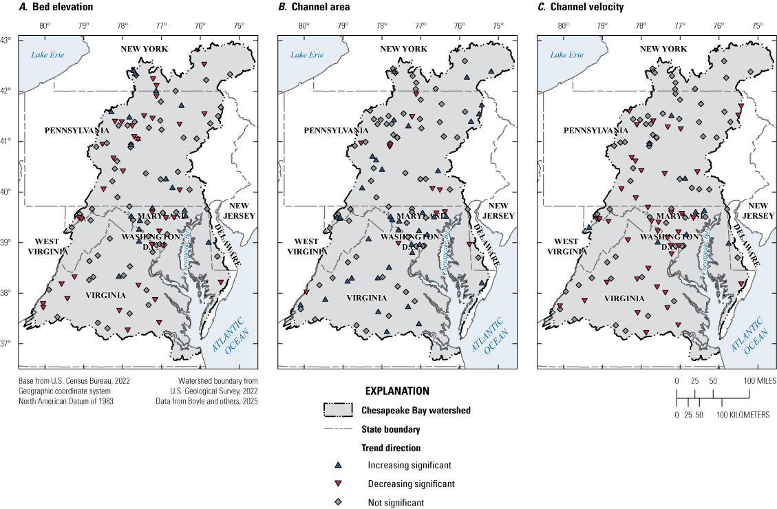
Maps of the Chesapeake Bay watershed showing the trend results for channel metrics at specific gage hydromorphology sites (116 sites) for the 50-year (1972–2022) trend interval: A, bed elevation, B, channel area, and C, channel velocity.
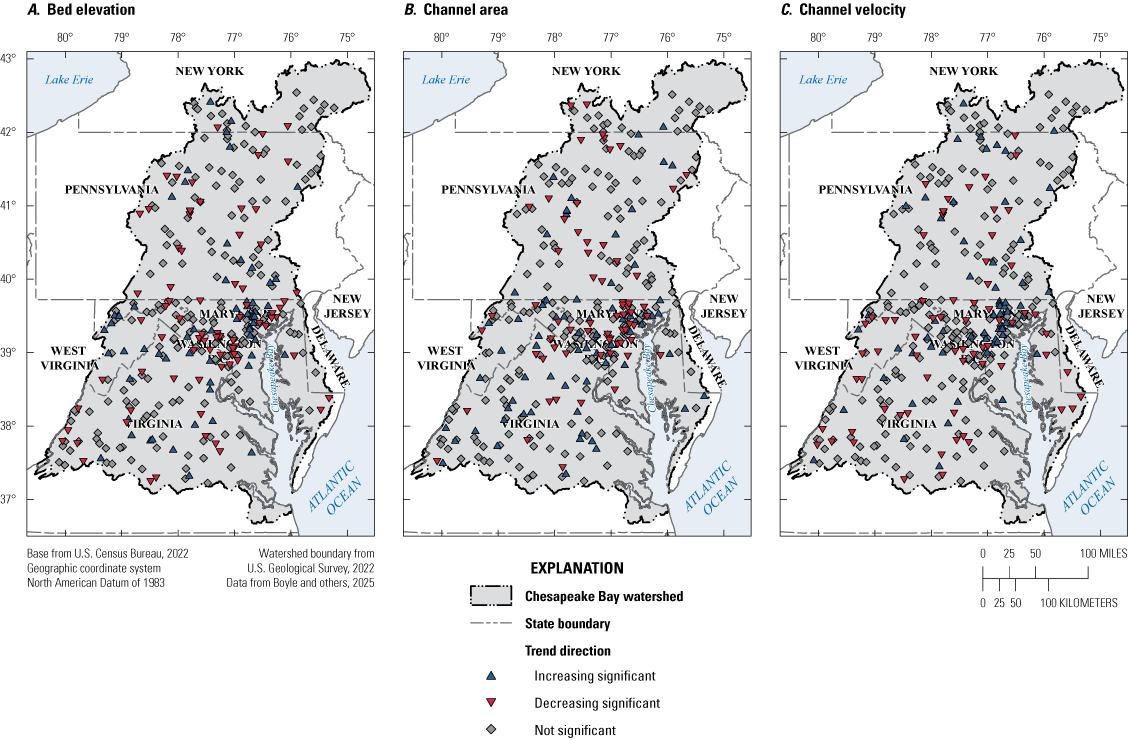
Maps of the Chesapeake Bay watershed showing the trend results for channel metrics at specific gage hydromorphology sites for the 10-year (2012–22) trend interval: A, bed elevation, B, channel area, and C, channel velocity.
Table 14.
Number and direction of significant trend results in the Chesapeake Bay watershed for hydromorphology-specific gage analyses broken down by field metric and trend interval.[Data are from Boyle and others (2025). Qualifying streamgage counts are in table 13. Trend interval years are 10 (water years [WY] 2012–22), 25 (WY 1997–2022), 50 (WY 1972–2022), and 75 (WY 1947–2022)]
This study empirically demonstrates the decadal-scale response of channel evolution and geomorphic change across many rivers throughout a region. In addition, this analysis highlights additional factors associated with changes in hydraulic character, such as flow-normalized velocity (refer to appendix 3), which co-occurs with channel evolution and geomorphic disturbance. As channel area increased in many rivers across the watershed, especially in response to urbanization, the flow-normalized channel velocity decreased, a habitat condition which may be relevant to many species, particularly lithophilic and other flow-sensitive species.
The trend results from specific gage analysis provide a comprehensive, watershed-wide approach for hydromorphic trends and multiple results covering jurisdictions throughout the Chesapeake Bay watershed. These trends highlight large-scale response to changes in watershed conditions over time but also locally driven patterns of geomorphic change demonstrating the timing and type of local watershed factors. As a result, individual streamgage results should be interpreted within the context of a local watershed’s history of disturbance and other changes. In addition, many USGS streamgages are operated to address specific management questions, such as a targeted restoration. These gages may provide additional local interpretive context but may not be generally representative of all streams in a region. Lastly, USGS streamgages are generally known to be biased toward larger rivers compared to the overall drainage network (refer to section 2.8 “Results Synthesis”); therefore, these results may not generally capture the range of channel changes occurring within headwaters. However, the results of the specific gage analysis capture unique information about channel change throughout the watershed and can help interpret the magnitude of geomorphic change and the timeframe for geomorphic recovery after disturbance (Cashman and others, 2021).
2.7. Status and Trends in Stream Biological Aquatic Communities
By Lindsey J. Boyle and Kelly O. Maloney
Freshwater rivers and streams are home to thousands of species with diverse requirements for habitat condition. Shifts in stream biological assemblages can indicate changes in habitat quality such as alterations to riparian and instream habitat, changes in streamflow, and degradation of water quality. Two freshwater assemblages, benthic macroinvertebrates and fishes, are key indicators of stream health and habitat condition. Shifts in fish assemblages historically have been linked to changes in streamflow and physical instream habitat (Gardner and others, 2013; Perkin and others, 2015). Benthic macroinvertebrates are indicators of overall stream health because they respond strongly to changes in water quality and to multiple stressors associate with land development (Kenney and others, 2009; Clapcott and others, 2012). Thus, identifying trends in both assemblages provides holistic insight into the overall changing biological condition of streams in the Chesapeake Bay watershed.
Often, to assess stream biological condition, many metrics of a biological assemblage are calculated and then collated into a single multi-metric index of biological health with numeric score ranges for different condition categories. Such a multi-metric index can help assess whether a stream may be in good or poor condition (Karr, 1999; Morse and others, 2003), and individual metric components are helpful for identifying what specific stressors may be affecting the stream. For analysis of trends in benthic macroinvertebrates and fish, four metrics were selected based on previous studies (cited in the following paragraphs) showing metric responsiveness to anthropogenic stressors: a multi-metric index of integrity, an assemblage sensitivity metric, a functional feeding strategy, and a habitat preference metric.
For benthic macroinvertebrates, metrics used in this analysis were the Chesapeake Basin-wide Index of Biotic Integrity (hereafter termed Chessie BIBI) score (Smith and others, 2017); the percentage of Ephemeroptera, Plecoptera and Trichoptera taxa excluding the family Hydropsychidae, which is tolerant to pollution and habitat disturbance (hereafter EPT-H); the percentage of taxa classified as filterer feeders; and percentage of taxa classified as preferring clinger habitat (metric definitions are in table 15). The Chessie BIBI is a metric of overall assemblage structure and function. Low scores indicate some disturbance large enough to greatly alter expected assemblage. Chessie BIBI scores range from 0 to 100 and correspond to the narrative categories of “very poor,” “poor,” “fair,” “good,” or “excellent.” Decreasing percentages of EPT-H taxa are linked to many stressors that increase as a result of urbanization (Cuffney and others, 2010). Clinger taxa adapted to cling to substrate in swift water are often sensitive to decreasing streamflow and increasing sedimentation, because deposited particles can cover suitable cobble habitat (Drover and others, 2020). Abundance of filter feeding taxa may decrease with decreasing streamflows, because they depend on water movement to distribute food particles (Woodcock and Huryn, 2007; Graeber and others, 2013).
For fish, metrics used in this analysis were the EPA fish multi-metric index (MMI) score (U.S. Environmental Protection Agency, 2020), the percentage of nontolerant individuals, the percentage of individuals that feed on benthic invertebrates, and the percentage of rheophilic habitat individuals (metric definitions are in table 15). Like the Chessie BIBI, the MMI is a metric of overall structure and function. Its scores range from 0 to 100 and correspond to the narrative categories of “poor,” “fair,” and “good.” Decreases in scores over time can indicate a decrease in assemblage quality. Decreases in sensitive fish populations can indicate decreasing habitat quality from multiple stressors. Rheophilic species are adapted to live in swift water habitats, and decreases in abundance can be linked to decreases in streamflow (Musil and others, 2012). Benthic invertivore individuals primarily depend on benthic invertebrates as a food source and are sensitive to increased pesticides and agricultural development (Marion and Scott, 2010; Waite and others, 2019).
Table 15.
Definitions of metrics used to track biological condition in benthic macroinvertebrate and fish assemblages.[Benthic macroinvertebrate metric definitions are in Smith and others (2017). Fish metric definitions are in U.S. Environmental Protection Agency (2020). For both assemblages, the selected metrics are known to be responsive to anthropogenic stressors, and thus good indicators of changes in stream condition and were not strongly correlated with each other. Chessie BIBI, Chesapeake Basin-wide Index of Biotic Integrity; EPT-H, Ephemeroptera, Plecoptera and Trichoptera taxa, excluding the tolerant family Hydropsychidae; MMI, multi-metric index]
2.7.1. Data Compilation
Data were gathered from two Chesapeake Bay watershed-wide compilation efforts: Smith and others’ (2017) generation of the Chessie BIBI, which compiled benthic macroinvertebrate (hereafter termed macroinvertebrate) data; and Maloney and Krause’s (2021) development of a fish habitat assessment, which compiled fish sampling data. The two resulting datasets allow numerous approaches for which site-specific measures of benthic macroinvertebrates and fishes may be characterized, including multi-metric composite indices and summary metrics that describe assemblage composition (for example, life histories and tolerance classifications), taxonomic composition, and presence or abundance of specific species.
Long-term biological monitoring sites are generally sampled only once per year or less. To identify trend sites, datasets were separated by season [winter (December–February), spring (March–May), summer (June–August), and fall (September–November)], because season can have a strong effect on macroinvertebrate and fish community structure (Gelwick, 1990; Linke and others, 1999). To incorporate the largest number of sites possible within a trend interval long enough for trend analysis, the trend interval was set from 2008 to 2017. Sites qualified for trend analysis if samples were collected in the same season for at least 7 total years within the interval. The total needed to include at least one sample each in 2008 and 2017. If a trend site had multiple samples within the same season and year, one sample was randomly selected for analysis and the others were discarded. Following these steps, there were 92 spring, 4 summer, and 2 fall trend sites for macroinvertebrates and 36 summer and 8 fall sites for fish trend analyses (table 16).
Table 16.
Number of biological assemblage trend sites in the Chesapeake Bay watershed per season, 2008–17.[Data are from Boyle and others (2025). Spring is March through May; summer, June through August; and fall, September through November]
2.7.2. Analysis
All analyses were completed in R (ver. 4.2.1; R Core Team, 2022b). Status of biological sites was defined as the average value of the 3 most recent years of data for each metric at each site. Both multi-metric indices, the macroinvertebrate Chessie BIBI and the fish MMI, have built-in narrative categories based on score ranges. The Chessie BIBI scores sites amongst five categories ranging from “very poor” to “excellent.” The fish MMI categorizes sites as “poor” or “good,” and sites in between these two categories are listed as “fair.” After averaging the index scores from the most recent 3 years at each site, the resulting values were placed into their corresponding narrative categories. The remaining three metrics (assemblage sensitivity, functional feeding strategy, and habitat preference) are presented as the percentage of the total assemblage composition, and the values from the last 3 years at each site were averaged to provide status.
For each site, trends were estimated separately for each macroinvertebrate and fish metric using GAMs. In total, 572 individual GAMs (396 for macroinvertebrates and 176 for fish) were fit using the R package “mgcv” (ver. 1.9-1; Wood, 2017). Because samples sizes were small (7–10 years per site with one measurement per year), the flexibility of the smooth function was limited for all GAMs by setting the upper limit on the degrees of freedom (k) associated with a smooth to be an integer no more than half of the total data points per trend. This allowed greater flexibility in model fit for sites with larger samples sizes but limited trend detection to highly linear trends for sites with small samples. Figure 26 displays the difference in function flexibility between a site with 7 data points and a site with 10 data points. Following methods from Murphy and others (2019), trends from each GAM were compared to a null model (GAM fit without year covariate) and were considered “strong” and “extremely likely” if the AIC value was at least 7 points lower than the null model and the p-value was less than or equal to 0.05. Results from this analysis can be found in Boyle and others (2025).

Line graphs showing how trend line shapes are affected by sample size with the following examples: A, a site with seven data points and B, a site with 10 data points. In the R package “mgcv,” k (the upper limit on the degrees of freedom associated with a smooth) was set to be an integer no more than half of the total data points in a trend.
2.7.3. Results and Discussion
Patterns in status metrics varied greatly across the watershed but generally showed that around half of macroinvertebrate sites and one-third of fish sites were in poor condition and had few sensitive taxa and few taxa preferring swift water habitat. Analysis of status revealed that 56 of the 99 macroinvertebrate sites (57 percent) were in the “poor” or “very poor” Chessie BIBI condition categories, and 28 (28 percent) were in the “good” or “excellent” condition categories. At 21 sites (21 percent), less than 50 percent of the assemblage consisted of sensitive EPT-H taxa and clinger taxa (table 17; fig. 27). Sites in poor condition categories were clustered near the greater Baltimore–Washington, D.C., metropolitan area. Among the additional macroinvertebrate metrics, there were many more EPT-H and clinger taxa and fewer filterer taxa within assemblages in the Blue Ridge range of Virginia, compared to assemblages clustered near the Baltimore–Washington, D.C., metropolitan area (fig. 27).
Table 17.
Number of sites in the Chesapeake Bay watershed with significantly strong or no trend for fish and benthic macroinvertebrate assemblage metrics from 2008–17.[Data are from Boyle and others (2025). Chessie BIBI, Chesapeake Basin-wide Index of Biotic Integrity; EPT-H, Ephemeroptera, Plecoptera and Trichoptera taxa excluding the tolerant family Hydropsychidae; MMI, multi-metric index; ≥, greater than or equal to; ≤, less than or equal to; <, less than; >, greater than]
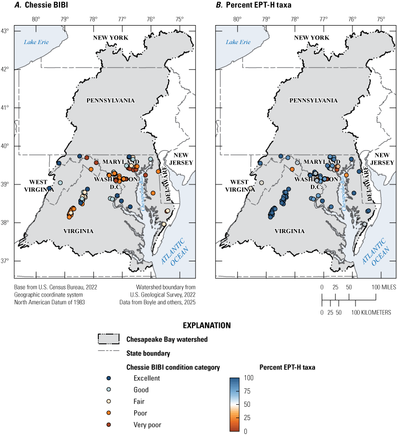
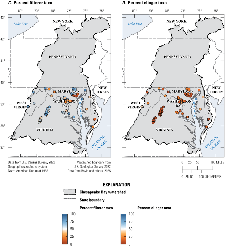
Maps of the Chesapeake Bay watershed showing the status of the following metrics at benthic macroinvertebrate biological community sites: A, Chesapeake Basin-wide Index of Biotic Integrity (Chessie BIBI) condition category (Smith and others, 2017), B, percentage of Ephemeroptera, Plecoptera, and Trichoptera taxa (excluding the tolerant family Hydropsychidae) (EPT-H), C, percentage of clinger taxa, and D, percentage of filterer taxa.
Of the fish biological community sites analyzed, 14 (32 percent) were classified as “poor,” 9 (20 percent) were classified as “good,” and 21 (47 percent) had intermediate scores classified as “fair” (table 17; fig. 28). Percentages of nontolerant fish varied greatly among site locations. Percentages of rheophilic individuals followed geographic patterns of slope within the watershed. Assemblages generally consisted of less than 50-percent rheophilic individuals in sites near the Bay where low-slope gradients create slow water habitat, whereas assemblages in streams with swifter flows in the western portion of the watershed consisted of between 85 and 100 percent rheophilic individuals. Percentages of benthic invertivores varied greatly among sites with no consistent spatial pattern (fig. 28).
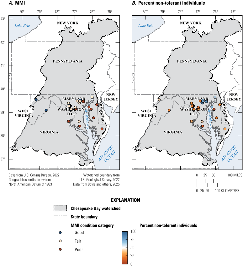
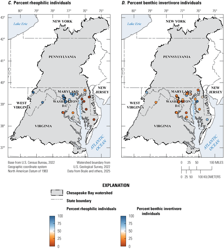
Maps of the Chesapeake Bay watershed showing the status of the following metrics at fish biological community sites: A, U.S. Environmental Protection Agency (EPA) multi-metric index (MMI) condition category (U.S. Environmental Protection Agency, 2020), B, percentage of nontolerant individuals, C, percentage of rheophilic individuals, and D, percentage of benthic invertivore individuals.
Many sites exhibited no strong directional trend in their biological metrics, indicating that biological composition quality is not increasing or decreasing at a detectable rate. Of the 572 trends in macroinvertebrate and fish metrics tested, 60 (11 percent) had strong increasing or decreasing trends (table 17). For both fish and macroinvertebrates, the assemblage sensitivity metric had the most strong trends of any metric, and most trends indicated declines in the percentage of sensitive organisms. Most sites had strong trends in only one metric (figs. 29, 30). Interestingly, strong trends in sensitive taxa did not often co-occur with strong trends in biotic index scores, highlighting the importance of analyzing individual metrics in addition to multimeric indices to capture patterns in specific groups of organisms that may be masked by an overall assemblage condition score. The lack of strong trends could be due to the small sample size and stringent analysis parameters rather than truly static biological condition through time. Though limiting the flexibility of the GAMs allowed for very high confidence in the reported strong trends, it likely prevented detection of trends with small sample sizes (7–8 years) and more variable or nonlinear patterns.
The current biological sites suitable for trend analysis are spatially biased; most sites are in Maryland, and some are also in and around the Blue Ridge range of Virginia. Sites with the most detectable trends were clustered around the highly urban Baltimore-Washington, D.C., metropolitan area or the protected and forested Blue Ridge Mountain (figs. 29, 30). There is no representation of the northern portion of the Chesapeake Bay watershed. Though the current dataset does not provide adequate coverage to interpret co-occurring trends or trend patterns for the entire Chesapeake Bay watershed, incorporating more data from a future data retrieval may help resolve both sample size and spatial distribution issues. Many sites have 5–6 years of data within the 2008–17 trend interval and are therefore close to meeting trend analysis criteria. If more recent data are identified for these sites, the overall number of sites suitable for trend analyses may greatly increase. Such recent data may also increase the sample size of current trend sites and the overall spread of trend sites across the watershed.
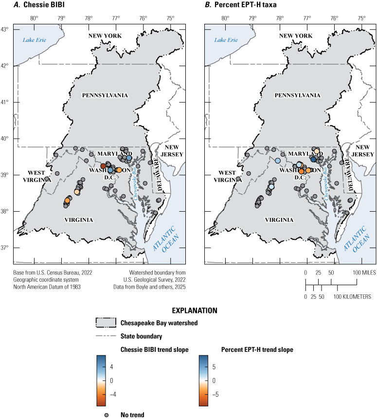
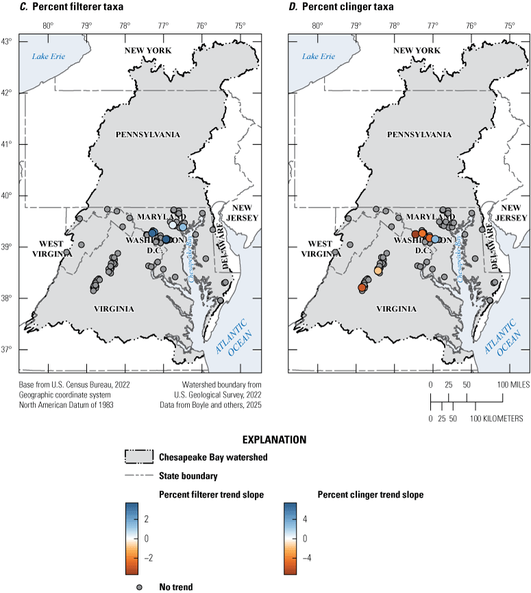
Maps of the Chesapeake Bay watershed showing benthic macroinvertebrate biological community site trend slopes for A, Chesapeake Basin-wide Index of Biotic Integrity (Chessie BIBI; Smith and others, 2017), B, percentage of Ephemeroptera, Plecoptera, and Trichoptera taxa (excluding the tolerant family Hydropsychidae) (EPT-H), C, percentage of filterer taxa, and D, percentage of clinger taxa.
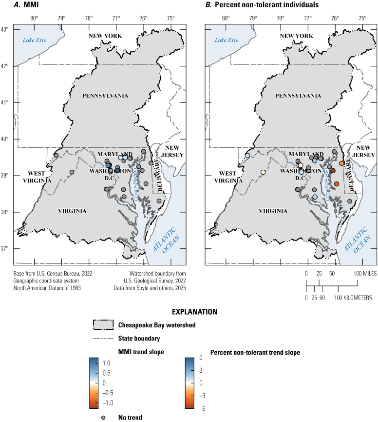

Maps of the Chesapeake Bay watershed showing fish biological community site trend slopes for A, U.S. Environmental Protection Agency (EPA) multi-meter index (MMI; U.S. Environmental Protection Agency, 2020), B, percentage of nontolerant, C, percentage of rheophilic, and D, percentage of benthic invertivore.
2.8. Indicator Results Synthesis
The trends presented in this report represent vastly different data types that were compiled from a wide variety of sources and span varied temporal and spatial scales. Some indicators have 75 years of high-quality continuous data, and others have too few data points to evaluate any trend. The amount of spatial and temporal variability among indicators makes teasing out patterns in trend co-occurrence across indicators difficult. The purpose of sections 2.1 through 2.7 is to establish initial datasets, methods, and results for each individual indicator. The following section describes an initial attempt to synthesize results and explore patterns across indicators by (1) determining the number of sites with co-occurring trends for multiple indicators, (2) quantifying the representation of various landscape types in indicator watersheds, and (3) investigating potential drivers of indicator status values.
2.8.1. Trend Site Co-Occurrence
To assess the feasibility of a multi-indicator trend synthesis, trend sites of all seven indicators were overlayed to determine locations where multiple indicators co-occur. Sites representing multiple indicators that were clustered within a 200-meter radius of each other were identified as a potential co-occurrence location. Each cluster was visually inspected in ArcGIS Pro (ver. 3.3.2; Esri Inc., 2024) to ensure the potential cluster did not contain points falling on different streams. Most trend sites in this report were not co-located (table 18). There were no locations that had data for all seven indicators. One site, the Susquehanna River at Danville, Pennsylvania (USGS 01540500), had data for six of the seven indicators but did not have biological data (fig. 31). Indicators that regularly co-occurred were split into two general groups: (1) nutrients and sediment, salinity, flow, and stream temperature data, which were often collected at or near streamgages; and (2) biology and habitat data, which were often collected in the same sampling event by a stream sampling crew at wadeable locations (table 19). These two groupings highlight the mismatch between hydrology and water-quality data and biological community sample locations. Many gaged sites are not wadeable and difficult to accurately sample for biology. Similarly, many biological samples are collected at small streams, which are not well represented by the streamgaging network.
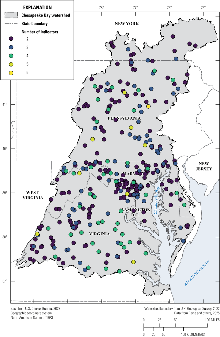
Map of the Chesapeake Bay watershed showing trend sites with data from multiple indicators.
The limited instances of trend co-occurrence locations make integrating trend patterns across indicators difficult. Even when long-term data for multiple indicators co-occur spatially, differing trend intervals among indicators may prevent trend comparison unless enough data exists to truncate datasets to uniform start and end dates. Integrating trend results from multiple indicators at specific locations will require new and creative methods.
Table 18.
Number of sites with 2 to 6 co-occurring indicator data among the 1,353 indicator sites in the Chesapeake Bay watershed.[Data are from Boyle and others (2025)]
Table 19.
Pairwise counts of co-occurring trend sites in the Chesapeake Bay watershed among the following indicators: nutrients and sediment, streamflow, temperature, hydromorphology (habitat and specific gage), salinity, toxic contaminants, and biological aquatic communities (fish and macroinvertebrates).[Data are from Boyle and others (2025). For nutrients and sediment, there were 123 co-occurring trend sites, and for streamflow, 211; temperature, 31; hydromorphology (habitat), 105; hydromorphology (specific gage), 344; salinity, 313; toxic contaminants, 72; biological aquatic communities (fish), 44; and biological aquatic communities (macroinvertebrates), 99]
2.8.2. Status Snapshot
Although synthesizing trends results across indicators remained a challenge, status conditions were synthesized across indicators, and potential drivers were explored by assessing status conditions during a period shared among all indicators. The most recent status period shared by all indicators (calendar years 2015 through 2017) was selected as the common period of interest to assess if land cover is a driver of status condition. The salinity, hydromorphology, and biological assemblage indicators had status values that already corresponded with this time interval. For the status snapshot, status values for salinity departure from background SC, all nine hydromorphological metrics, and the multi-metric indices and assemblage sensitivity metrics for fish and macroinvertebrate biological assemblages were utilized. For the remaining indicators (stream temperature, nutrients and sediment, and streamflow), additional status metrics were calculated from 2015–17 data for each site. Temperature was represented by mean temperature, nutrients and sediment were represented by mean nutrient and suspended sediment concentrations, and streamflow was represented as the mean flow metric values for 2015–17.
The spatial distribution of the highest and lowest quality sites for each indicator was assessed using data from the shared status interval for all indicators. High-quality sites were sites with the status metric values most indicative of good stream condition for each indicator, whereas low-quality sites represent the poorest status values for each indicator. Metric values were divided into quartiles and coded as “degraded condition” or “good condition” if the status value fell within the top or bottom 25 percent of values. Which percentile was coded as degraded or good varied among the metrics. For example, 75th-percentile temperature values were categorized as degraded condition, whereas 75th-percentile macroinvertebrate biological index scores were categorized as good condition. To categorize flow metric values as good condition or degraded condition, the percentage difference between mean annual flow metric values for 2015–17 and the mean annual metric values for 1985–2022 (the full interval of flow data) was calculated and divided into quartiles.
After coding, sites for each metric were then assigned to the overall high-, low-, or intermediate-quality categories. Temperature sites were assigned the quality category that corresponded to their single temperature status metric (mean temperature). For example, sites with degraded temperature values were assigned to the low-quality temperature site category. For the nutrients and suspended sediment and biology indicators, a low-quality site was one associated with any degraded metric(s), and a high-quality site was one associated with any good metric(s) and no degraded condition metric(s). The streamflow and hydromorphology indicators had many metrics with sometimes conflicting scores. For these indicators, a site was categorized as low-quality if it was associated with any degraded metric(s) and no good metric(s), and vice versa for high-quality categorization. Sites with both good and degraded metrics were assigned to the intermediate category because of uncertainty. For salinity, a different definition was used; sites were considered low-quality if the status metric was greater than 3 times the predicted background SC and high-quality if the status value was at or below background SC. Status values and quality categories for each indicator site can be found in Boyle and others (2025).
The high-quality and low-quality sites were mapped individually to compare the overall spatial distribution of high- and low-quality sites. High-quality sites for all indicators were spread mostly evenly across the watershed, but some distinct clusters of high-quality biological assemblage, salinity, nutrients and sediment, and hydromorphology sites were apparent along the Blue Ridge range in Virginia and along the northern West Virginia–Maryland border (fig. 32). In contrast, the low-quality sites for multiple indicators were clearly clustered around the urban centers of Washington, D.C., and Baltimore, as well as within the Delmarva Peninsula (fig. 32). Maps showing the spatial distribution of high- and low-quality sites for each indicator individually can be found in appendix 4.
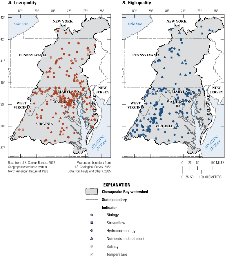
Maps of the Chesapeake Bay watershed showing the sites with the A, low-quality status values and B, the high-quality status values for each indicator.
Potential drivers of status conditions were further investigated through a simple linear regression, which was used to determine if different major land-cover categories explained status values for each indicator. To characterize land cover for each status site, sites were associated with flowlines from the National Hydrography Dataset Plus High Resolution (NHDPlus HR) network and were subsequently joined to a dataset that summarized the total watershed area and National Land Cover Database (NLCD) land cover for each flowline (U.S. Geological Survey, 2022; Gressler and others, 2023;). The 2016 NLCD dataset was used because 2016 marked the middle of the 3-year common status interval. Multiple land-cover percentages were summed to create the following predictor variables: (1) the percentage of developed land cover (open space, low intensity, medium intensity, and high intensity), (2) the percentage of agriculture land cover (pasture or hay, and cultivated crops), and (3) the percentage of forest land cover (deciduous, evergreen, and mixed). Individual linear models were run for each combination of indicator metric and predictor variable and categorized relationships as significant at p-values less than or equal to 0.05. Linear model results are shown in table 20 and appendix 4 and can be found in Boyle and others (2025).
Table 20.
Linear model results showing relationships between six indicators’ status metrics and percentage of urban, agriculture, or forest land-cover predictors.[Data are from Boyle and others (2025). Blue cells indicate a positive relationship between the metric and the predictor, red cells indicate a negative relationship, and gray cells indicate no relationship between the metric and predictor. ≤, less than or equal to; mg/L, milligram per liter; °C, degrees Celsius; µS/cm, microsiemens per centimeter; (ft3/s)/mi2, cubic feet per second per mile squared; SC, specific conductance; Chessie BIBI, Chesapeake Basin-wide Index of Biotic Integrity; EPT-H, Ephemeroptera, Plecoptera, and Trichoptera taxa excluding the tolerant family Hydropsychidae; MMI, multi-metric index]
Many metrics representing the seven indicators had significant relationships with the land-cover predictor variables. Of the 24 metrics, 14 (58 percent) had significant relationships with developed land cover. High percentages of developed land cover were significantly associated with higher total phosphorus, stream temperature, and stream salinity; less extreme low-flow magnitudes; greater frequency of low and high-flow events; and shorter duration of high-flow events than low percentages of developed land cover. High percentages of developed land cover are also significantly associated with low values of habitat metrics, including bank stability, embeddedness, and epifaunal substrate, and low values of metrics characterizing macroinvertebrate sensitive taxa and assemblage condition. Fewer metrics (11 of the 24 metrics [46 percent]) had significant relationships with agriculture land cover. High percentages of agriculture land cover was associated with elevated total nitrogen, total phosphorus and, salinity concentrations; less extreme low-flow magnitudes; higher habitat velocity-depth combination scores; decreased high-flow duration, frequency, and magnitude; lower habitat streambed sedimentation scores; and fewer sensitive fishes (nontolerant individuals) compared to low percentages of agriculture land cover. Conversely, indicator responses to forest land cover were a near-perfect inverse of the responses to developed land cover. Forest land cover was significantly associated with lower nutrient and SC concentrations, lower stream temperatures, less frequent high-flow events, lower low-flow magnitude, longer high-flow duration, larger high-flow magnitude, and higher habitat scores and metrics for sensitive macroinvertebrates.
Together, the patterns between indicator status conditions and land-cover predictors demonstrate the negative impact of anthropogenic activity on stream condition. Urban development increases the amount of impervious surface and necessitates deicer application, leading to high salt loading into streams and groundwater systems (Kaushal and others, 2005). Increased sedimentation as a result of urban development also effects habitat quality. The removal of riparian buffers and alterations to natural flow regime that are prevalent in urban areas can cause additional degradation of instream habitat and increases in streamflow flashiness and stream temperature (LeBlanc and others, 1997; Paul and Meyer, 2001; Nelson and Palmer, 2007; Rosburg and others, 2017; Anim and others, 2018). High percentages of agriculture land cover were similarly associated to poorer water quality than watersheds with low percentages of agriculture land cover as agricultural practices can introduce high amounts of nutrients and increase SC in streams (Kaushal and others, 2018). Water withdrawals for agricultural practices can also alter flow regimes, creating more extreme low-flow events (Eheart and Tornil, 1999; Almahawis and others, 2024). Poorer water quality, flow, and habitat conditions associated with these anthropogenic activities were especially represented in the macroinvertebrate metrics. Overall macroinvertebrate assemblage condition scores (Chessie BIBI), and the percentage of sensitive taxa (EPT-H) were significantly lower at sites with greater urban development and the percentage of sensitive fish (percentage of nontolerant individuals) was significantly lower at sites with high percentages of agriculture land cover.
The association of indicators to the percentage of forest land cover was a near-perfect inverse relationship to that of developed and agriculture land covers. This is unsurprising, because the percentage of forest land cover is often negatively correlated with developed and agriculture land cover, but these results further highlight the importance of forested watershed and riparian buffers for maintaining good stream condition. Forested watersheds and riparian buffers reduce runoff of nutrients and shade streams, limiting stream warming (Lowrance and others, 1984; Bowler and others, 2012). Forested areas often have higher-quality habitat for biological assemblages by limiting streambank erosion and allowing for natural flow regime processes as shown by higher amounts of forested land covers being associated with less extreme low-flow magnitudes and less frequent high-flow events (Wang and others, 1997; Schoonover and others, 2006).
2.8.3. Land Cover and Spatial Representation of Indicator Site Networks
Multiple factors influence the location, frequency, and duration of the stream monitoring efforts highlighted in this study. Some sites may have been selected randomly, others may have been targeted for long-term sampling to monitor a pre- and (or) post-disturbance event (such as dam removal, bridge construction, or restoration project), and yet others may have been selected as longstanding reference sites in least-disturbed areas. To begin understanding how the indicator sites in this report represent the Chesapeake Bay watershed as a whole, cumulative-distribution plots were created for watershed area, urban, agriculture, and forest land covers for all indicator site networks (fig. 33). These distributions were compared visually to cumulative-distribution curves of all NHDPlus HR stream segments in the Chesapeake Bay watershed.

Cumulative distribution plots showing A, the watershed area, and the percentage of B, urban, C, agriculture, and D, forest land covers in 2016 for watersheds of indicator trend sites and all National Hydrography Dataset Plus High Resolution stream segments in the Chesapeake Bay watershed. Trend sites are from Boyle and others (2025), and associated land-cover data is from Gressler and others (2023). [km2, square kilometer]
Small watershed settings were poorly represented by all indicator site networks except biological aquatic community sites. Biological aquatic community sites most closely followed the distribution of Chesapeake Bay watersheds because biological data are most often collected in the small, wadeable streams that make up most of the Chesapeake Bay watershed’s stream network. Toxic contaminants, nutrients and sediment, and salinity site networks had the highest proportions of large watersheds; 75 percent of sites in each network represented watersheds larger than 2,093 square miles (mi2), 928 mi2, and 544 mi2, respectively. In comparison, only 22 percent of Chesapeake Bay watershed NHDPlus HR segments represent watersheds greater than 40 mi2. Areas with intensive agriculture (greater than 50 percent agriculture land cover) were under-represented by all indicator networks compared to agricultural intensity across all streams in the Chesapeake Bay watersheds. Distribution of urban settings across the salinity network was similar to the full watershed, but all other indicators represented more urban land cover within their watersheds than is represented across the full Chesapeake Bay watershed. All indicator sites had somewhat similar representation of forested land cover compared to the full Chesapeake Bay watershed, though the salinity network had more sites with moderately forested watersheds (50-percent forest land cover) compared to other indicators.
In addition to differences in land-cover representation compared to the full Chesapeake Bay watershed, indicator site networks have clustered and disparate spatial coverage across the watershed. Almost all indicators had low to no representation of sites in New York, except for streamflow, and all indicators had more sites in the southern half of the watershed compared to the northern half. Many indicator networks, especially temperature, stream habitat, and biology, had limited data for trend analysis, and criteria for trend inclusion were chosen to maximize the spatial coverage across the watershed and to provide the adequate record lengths for trend analysis. Many biological and stream habitat sites in the northern half of the watershed are close to meeting trend criteria, and temperature monitoring at gaged sites is becoming more prevalent. Thus, the spatial coverage and length of the trend intervals for all indicators will likely increase over time if data collection continues.
3. Summary
The Chesapeake Bay watershed is one of the most fertile and productive ecosystems in North America. Over the years, many regional and watershed-wide goals have been set to improve stream condition. Analysis of status (condition at a point in time) and trends (change in condition over time) aids in the tracking of progress towards stream improvement goals and pinpointing locations with improving or degrading conditions. This report describes methods of analyzing status and trends in seven key indicators of river and stream condition within the Chesapeake Bay watershed (nutrients and sediment, salinity, temperature, toxic contaminants, streamflow, hydromorphology, biological aquatic communities), and documents the initial results of each indicator. Additionally, an integrated summary of recent status conditions across all indicators and regression analysis between indicator status metrics and major land cover for the sites is provided.
Stream nutrients and suspended sediment were analyzed for total nitrogen, total phosphorus, and suspended sediment loads at 123 sites. Status estimates were calculated as the average yield (load normalized by watershed area) from 2011 to 2020. Trends were estimated using Weighted Regressions on Time, Discharge and Season (WRTDS) over short-term (2011–20) and long-term (1985–2020) intervals. Status values for total nitrogen and total phosphorus were highest in the Susquehanna River Basin and on the Delmarva Peninsula, and for suspended sediment they were highest towards the mouth of the Susquehanna and Potomac Rivers and in central Virginia. Trend results for 1985–2020 showed that most sites had decreasing trends in total nitrogen and phosphorus loads, indicating improving condition, and equal numbers of sites with increasing and decreasing trends for suspended sediment. Trend results for 2011–20 showed most sites had increasing trends or no change for total nitrogen and suspended sediment and decreasing trends or no change for total phosphorus.
Stream water salinity analyses utilized specific conductance (SC) as a metric of stream salinity at 278 sites. Status was estimated as the 3-year median of SC from 2015 through 2017, compared to predicted background salinity for the region. Trends were calculated for 2008–17 using WRTDS and Seasonal Mann-Kendall (SMK) trend tests. Status results revealed that 84 percent of sites had SC values higher than their predicted background SC values. For both WRTDS and SMK trend analysis, most sites had significant increasing trends or no trends in SC.
Stream temperature analyses used continuous temperature data to analyze trends at 31 sites and used discrete temperature data to derive a general watershed-wide trend. Status estimates for the 31 sites were calculated as the change in 2022, in degrees Celsius above or below the mean annual temperature for the trend interval. Trends were estimated using generalized additive models (GAMs) over one of four trend intervals (2013–20, 2013–21, 2013–22, and 2014–22) depending on years where at least 300 daily values per year were available for each site. A linear mixed effect model was used to estimate an overall trend in stream temperature for the watershed from 1985 to 2020 using discrete temperature records. Status results indicated that water year (WY) 2022 was the second warmest year for stream temperatures. Trend results revealed that increases stream temperature were “likely” or “extremely likely” at 24 of the 31 sites, and the linear mixed effect model of discrete data indicated a significant increasing trend in stream temperature for the entire watershed, in aggregate, over the trend interval.
Data compiled for stream water toxic contaminants such as mercury (Hg), polychlorinated biphenyls (PCBs), and pesticides were insufficient for analysis of status or trends. Eighty-nine PCB sites were identified as having three or more PCB samples from the same media type over a time span of 5 years or more, meeting criteria for possible future trend analyses. Future data collection could provide enough information for toxic contaminants trend analyses at these sites.
Streamflow analyses utilized stream hydrologic metrics of high-flow and low-flow magnitude, frequency, and duration for 211 sites. Status was calculated as the percentage difference between annual metric values for 2022 and metric means for WY 1985–22. Trends were analyzed using GAMs for each metric at each site. Status results indicated that high-flow frequency and low-flow magnitude were above average for most of the watershed and all other streamflow metrics were below average for WY 2022. Trend results revealed very few significant trends in any metric. Low-flow magnitude had the most significant trends of any metric with 12 sites increasing and 2 sites decreasing.
Stream hydromorphology analyses utilized two distinct datasets: (1) nine metrics from rapid habitat assessment data, which scores instream metrics of habitat quality (101 sites); and (2) three metrics of channel dimension and hydraulic metrics from gaged locations computed with a specific gage analysis method (342 sites). Status was estimated for rapid habitat data as the mean metric values for 2015–17. Trends for both datasets were analyzed using distinct but complementary GAM analyses. Trends in rapid habitat metrics were analyzed from 2008 to 2017, and trends in specific gage metrics were analyzed over four intervals (WY 2013–22, WY 1998–22, WY 1972–22, and WY 1948–22). Status values varied across the watershed, but low habitat scores for some metrics were notably clustered in the Delmarva Peninsula and in the urbanized Baltimore- Washington, D.C., metropolitan area. Trend results for rapid habitat metrics revealed that most sites had decreasing trends in habitat condition. Trends in specific gage metrics were more likely to be significantly decreasing for bed elevation and channel velocity, and significantly increasing in channel area; this pattern was most apparent at the 50 (WY 1972–2022), and 75 (WY 1948–2022) year intervals.
Stream biological assemblages were analyzed for four metrics describing overall biotic assemblage condition, sensitivity, functional feeding strategy, and habitat preference for benthic macroinvertebrate (99 sites) and fish (44 sites) assemblages. Status was defined as the average metric value for 2015–17 at each site. Trends were analyzed using GAMs for each metric at each site with either fish or macroinvertebrate data. Status results for an index of overall biotic condition placed 57 percent of macroinvertebrate sites in “poor” or “very poor” condition categories and 32 percent of fish sites in a “poor” condition category. There were very few sites with significant trends in any metric and increasing and decreasing trends were scattered across the lower half of the watershed. The metric of assemblage sensitivity had the most significant trends for both macroinvertebrate and fish assemblages, and most trends indicated decreases in the percentage of sensitive taxa over time.
Status and trends of the seven key indicators represent different data types compiled from a variety of sources spanning temporal and spatial scales. Sites associated with each indicator were overlayed to determine locations where multiple indicators co-occur, revealing that no site had available trend data for all seven indicators. This spatial variability and the temporal variability among indicators prevented direct comparison of trends between indicators, but status values from an interval of 2015–17 were utilized to identify areas of the watershed where high-quality and low-quality sites were present and to analyze the association between status values and watershed land covers. Low-quality sites were clustered around the Baltimore-Washington, D.C., metropolitan area, and high-quality sites were clustered along the western portion of the watershed and the Blue Ridge range. Developed land cover was associated with degraded condition status values for at least one status metric of every indicator, and forest land cover was associated with good condition status values. Agriculture land cover was associated with higher nutrient and salinity status values, increased metrics of high flow and decreased metrics of low flow, and fewer sensitive fish individuals. Further analysis of the spatial representation of indicator sites across different land covers and stream sizes revealed that all indicators except biological assemblages were under representative of small watersheds. Sites for most indicators were also over representative of urban land covers and unrepresentative of agriculture land covers compared to all stream segments in the Chesapeake Bay watershed.
The scope of this report is limited to the initial status and trend results for each indicator of stream condition, and a brief investigation of site locations and representation across the watershed and landscape drivers of status condition. Results generally indicate more decline than improvement in selected metrics of stream condition for each indicator; however, differences in trend intervals and site locations among indicators prevent direct comparison of patterns and drivers.
References Cited
Alexander, R.B., Murdoch, P.S., and Smith, R.A., 1996, Streamflow-induced variations in nitrate flux in tributaries to the Atlantic Coastal Zone: Biogeochemistry, v. 33, no. 3, p. 149–177, accessed October 22, 2024, at https://doi.org/10.1007/BF02181070.
Almahawis, M.K., Bailey, R.T., Abbas, S.A., Arnold, J.G., and White, M.J., 2024, Investigating the impact of irrigation practices on hydrologic fluxes in a highly managed river basin: Agricultural Water Management, v. 301, p. 108954, accessed September 21, 2023, at https://doi.org/10.1016/j.agwat.2024.108954.
Anim, D.O., Fletcher, T.D., Vietz, G.J., Pasternack, G.B., and Burns, M.J., 2018, Effect of urbanization on stream hydraulics: River Research and Applications, v. 34, no. 7, p. 661–674, accessed October 22, 2024, at https://doi.org/10.1002/rra.3293.
Arismendi, I., Johnson, S.L., Dunham, J.B., and Haggerty, R., 2013, Descriptors of natural thermal regimes in streams and their responsiveness to change in the Pacific Northwest of North America: Freshwater Biology, v. 58, no. 5, p. 880–894, accessed October 22, 2024, at https://doi.org/10.1111/fwb.12094.
Ashizawa, D., and Cole, J.J., 1994, Long-term temperature trends of the Hudson River—A study of the historical data: Estuaries, v. 17, no. 1, p. 166–171, accessed October 22, 2024, at https://doi.org/10.2307/1352565.
Baker, M.E., Schley, M.L., and Sexton, J.O., 2019, Impacts of Expanding Impervious Surface on Specific Conductance in Urbanizing Streams: Water Resources Research, v. 55, no. 8, p. 6482–6498, accessed September 21, 2023, at https://doi.org/10.1029/2019WR025014.
Banks, B.D., Needham, T.P., Dugan, C.M., Foss, E.P., and Majcher, E.H., 2022, Priority toxic contaminant metadata inventory and associated total polychlorinated biphenyls concentration data: U.S. Geological Survey data release, accessed October 22, 2024, at https://doi.org/10.5066/P9R78SQ6.
Barbour, M.T., Gerritsen, J., Snyder, B.D., and Stribling, J.B., 1999, Rapid bioassessment protocols for use in streams and wadeable rivers—Periphyton, benthic macroinvertebrates, and fish, second edition: U.S. Environmental Protection Agency EPA 841-B-99-002, [variously paged, 337 p.]. [Also available at https://www3.epa.gov/region1/npdes/merrimackstation/pdfs/ar/AR-1164.pdf.]
Bartoń, K., 2010, MuMIn—Multi-model inference (ver. 1.47.5, March 22, 2023): The Comprehensive R Archive Network, accessed November 10, 2023, at https://doi.org/10.32614/CRAN.package.MuMIn.
Bates, D., Mächler, M., Bolker, B., and Walker, S., 2015, Fitting Linear Mixed-Effects Models Using lme4: Journal of Statistical Software, v. 67, no. 1, p. 1–48, accessed November 20, 2022, at https://doi.org/10.18637/jss.v067.i01.
Batiuk, R., Brownson, K., Dennison, W., Ehrhart, M., Hanson, J., Hanmer, R., Landry, B., Reichert-Nguyen, J., Tassone, S., and Vogt, B., 2023, Rising Watershed and Bay Water Temperatures—Ecological Implications and Management Responses: Chesapeake Bay Program STAC Publication 23-001, 505 p., accessed September 21, 2023, at https://www.chesapeake.org/stac/document-library/rising-watershed-and-bay-water-temperatures-ecological-implications-and-management-responses/.
Bird, D.L., Groffman, P.M., Salice, C.J., and Moore, J., 2018, Steady-state land cover but non-steady-state major ion chemistry in urban streams: Environmental Science & Technology, v. 52, no. 22, p. 13015–13026, accessed September 21, 2023, at https://doi.org/10.1021/acs.est.8b03587.
Bolker, B.M., Brooks, M.E., Clark, C.J., Geange, S.W., Poulsen, J.R., Stevens, M.H.H., and White, J.S., 2009, Generalized linear mixed models—A practical guide for ecology and evolution: Trends in Ecology & Evolution, v. 24, no. 3, p. 127–135, accessed October 22, 2024, at https://doi.org/10.1016/j.tree.2008.10.008.
Bowen, Z.H., Oelsner, G.P., Cade, B.S., Gallegos, T.J., Farag, A.M., Mott, D.N., Potter, C.J., Cinotto, P.J., Clark, M.L., Kappel, W.M., Kresse, T.M., Melcher, C.P., Paschke, S.S., Susong, D.D., and Varela, B.A., 2015, Assessment of surface water chloride and conductivity trends in areas of unconventional oil and gas development—Why existing national data sets cannot tell us what we would like to know: Water Resources Research, v. 51, no. 1, p. 704–715, accessed October 22, 2024, at https://doi.org/10.1002/2014WR016382.
Bowler, D.E., Mant, R., Orr, H., Hannah, D.M., and Pullin, A.S., 2012, What are the effects of wooded riparian zones on stream temperature?: Environmental Evidence, v. 1, no. 3, p. 1–9, accessed October 22, 2024, at https://doi.org/10.1186/2047-2382-1-3.
Box, J.B., and Mossa, J., 1999, Sediment, land use, and freshwater mussels—Prospects and problems: Journal of the North American Benthological Society, v. 18, no. 1, p. 99–117, accessed December 11, 2023, at https://doi.org/10.2307/1468011.
Boyle, L.J., Austin, S.H., Cashman, M.J., Clune, J.W., Colgin, J.E., Elliott, K.E.M., Fanelli, R.M., Maloney, K.O., and Zimmerman, T.M., 2025, Status and trends in stream temperature, salinity, flow, hydromorphology, and biological assemblages across the Chesapeake Bay watershed: U.S. Geological Survey data release, https://doi.org10.5066/P13FB2KQ.
Brooks, M.E., Bolker, B., Kristensen, K., Maechler, M.Magnusson, A., Berg, C.W., Nielsen, A., Skaug, H.J., Mächler, M., and Bolker, B.M., 2017, glmmTMB balances speed and flexibility among packages for zero-inflated generalized linear mixed modeling: The R Journal, v. 9, no. 2, p. 378–400, accessed October 22, 2024, at https://doi.org/10.32614/RJ-2017-066.
Brown, T.C., Foti, R., and Ramírez, J.A., 2013, Projected freshwater withdrawals in the United States under a changing climate: Water Resources Research, v. 49, no. 3, p. 1259–1276, accessed October 22, 2024, at https://doi.org/10.1002/wrcr.20076.
Caissie, D., 2006, The thermal regime of rivers—A review: Freshwater Biology, v. 51, no. 8, p. 1389–1406, accessed October 22, 2024, at https://doi.org/10.1111/j.1365-2427.2006.01597.x.
Cañedo-Argüelles, M., 2020, A review of recent advances and future challenges in freshwater salinization: Limnetica, v. 39, no. 1, p. 185–211, accessed September 21, 2023, at https://doi.org/10.23818/limn.39.13.
Carline, R.F., and McCullough, B.J., 2003, Effects of floods on brook trout populations in the Monongahela National Forest, West Virginia: Transactions of the American Fisheries Society, v. 132, no. 5, p. 1014–1020, accessed October 22, 2024, at https://doi.org/10.1577/T02-112.
Carlisle, D.M., Grantham, T.E., Eng, K., and Wolock, D.M., 2017, Biological relevance of streamflow metrics—Regional and national perspectives: Freshwater Science, v. 36, no. 4, p. 927–940, accessed October 22, 2024, at https://doi.org/10.1086/694913.
Carpenter, S.R., Caraco, N.F., Correll, D.L., Howarth, R.W., Sharpley, A.N., and Smith, V.H., 1998, Nonpoint pollution of surface waters with phosphorus and nitrogen: Ecological Applications, v. 8, no. 3, p. 559–568, accessed December 11, 2023, at https://doi.org/10.1890/1051-0761(1998)008[0559:NPOSWW]2.0.CO;2.
Cashman, M.J., Gellis, A.C., Boyd, E., Collins, M.J., Anderson, S.W., McFarland, B.D., and Ryan, A.M., 2021, Channel response to a dam‐removal sediment pulse captured at high‐temporal resolution using routine gage data: Earth Surface Processes and Landforms, v. 46, no. 6, p. 1145–1159, accessed October 22, 2024, at https://doi.org/10.1002/esp.5083.
Cashman, M.J., Lee, G., Staub, L.E., Katoski, M.P., and Maloney, K.O., 2024, Physical habitat is more than a sediment issue: A multi-dimensional habitat assessment indicates new approaches for river management: Journal of Environmental Management, v. 371, 19 p., accessed March 28, 2025, at https://doi.org/10.1016/j.jenvman.2024.123139.
Castro, J.M., and Thorne, C.R., 2019, The stream evolution triangle—Integrating geology, hydrology, and biology: River Research and Applications, v. 35, no. 4, p. 315–326, accessed October 22, 2024, at https://doi.org/10.1002/rra.3421.
Chattopadhyay, S., Oglęcki, P., Keller, A., Kardel, I., Mirosław-Świątek, D., & Piniewski, M., 2021, Effect of a summer flood on benthic macroinvertebrates in a medium-sized, temperate, lowland river: Water, v. 13, no. 7, 885 p., accessed October 22, 2024, at https://doi.org/10.3390/w13070885.
Chesapeake Bay Program, 1983, The Chesapeake Bay Agreement of 1983: Chesapeake Bay Program, [unpaged, 2 p.], accessed March 12, 2025, at https://www.chesapeakebay.net/files/documents/1983_CB_Agreement2.pdf.
Chesapeake Bay Program, 1987, 1987 Chesapeake Bay Agreement: Chesapeake Bay Program, 7 p., accessed March 12, 2025, at https://d38c6ppuviqmfp.cloudfront.net/content/publications/cbp_12510.pdf.
Chesapeake Bay Program, 1992, Chesapeake Bay Agreement--1992 amendments: Chesapeake Bay Program, [unpaged, 3 p.], accessed March 12, 2025, at https://d38c6ppuviqmfp.cloudfront.net/content/publications/cbp_12507.pdf.
Chesapeake Bay Program, 2000, Chesapeake 2000: Chesapeake Bay Program, 13 p., accessed March 12, 2025, at https://www.chesapeakebay.net/files/documents/cbp_12081.pdf.
Chesapeake Bay Program, 2004, Chesapeake Bay Program Analytical Segmentation Scheme—Revisions, decisions and rationales 1983–2003: Chesapeake Bay Program Monitoring and Analysis Subcommittee Tidal Monitoring and Analysis Workgroup Annapolis, Maryland, 64 p., accessed: May 1, 2024, at https://www.chesapeakebay.net/content/publications/cbp_13272.pdf.
Chesapeake Bay Program, 2014, Chesapeake Bay Watershed Agreement (amended October 5, 2022): Chesapeake Bay Program, 17 p., accessed March 12, 2025, at https://www.chesapeakebay.net/files/Chesapeake-Bay-Watershed-Agreement-Amended.pdf.
Chesapeake Bay Program, 2021, Toxic contaminants policy and prevention outcome—Management strategy, 2015–2025 (ver. 3): Chesapeake Bay Program, 26 p., accessed February 10, 2022, at https://www.chesapeakebay.net/documents/22048/toxic_contaminanats_policy_and_prevention_management_strategy_v3.pdf.
Chesapeake Bay Program, [undated], DataHub: Chesapeake Bay Program database, accessed December 15, 2022, at https://datahub.chesapeakebay.net/Home.
Chanat, J.G., Moyer, D.L., Blomquist, J.D., Hyer, K.E., and Langland, M.J., 2015, Application of a weighted regression model for reporting nutrient and sediment concentrations, fluxes, and trends in concentration and flux for the Chesapeake Bay Nontidal Water-Quality Monitoring Network, results through water year 2012: U.S. Geological Survey Scientific Investigations Report 2015–5133, 76 p., accessed January 14, 2015, at https://doi.org/10.3133/sir20155133.
Clapcott, J.E., Collier, K.J., Death, R.G., Goodwin, E.O., Harding, J.S., Kelly, D., Leathwick, J.R., and Young, R.G., 2012, Quantifying relationships between land‐use gradients and structural and functional indicators of stream ecological integrity: Freshwater Biology, v. 57, no. 1, p. 74–90, accessed October 22, 2024, https://doi.org/10.1111/j.1365-2427.2011.02696.x.
Cleveland, R.B., Cleveland, W.S., McRae, J.E., and Terpenning, I., 1990, STL—A seasonal-trend decomposition procedure based on loess: Journal of Official Statistics, v. 6, no. 1, p. 3–73. [Also available at https://www.proquest.com/scholarly-journals/stl-seasonal-trend-decomposition-procedure-based/docview/1266805989/se-2.]
Cluer, B., and Thorne, C., 2014, A stream evolution model integrating habitat and ecosystem benefits: River Research and Applications, v. 30, no. 2, p. 135–154, accessed October 22, 2024, at https://doi.org/10.1002/rra.2631.
Clune, J., Colgin, J.E., and Zimmerman, T.M., 2023, Compilation of multi-agency water temperature observations for streams within the Chesapeake Bay watershed: U.S. Geological Survey data release, accessed October 22, 2024, at https://doi.org/10.5066/P92SHG66.
Cuffney, T.F., Brightbill, R.A., May, J.T., and Waite, I.R., 2010, Responses of benthic macroinvertebrates to environmental changes associated with urbanization in nine metropolitan areas: Ecological Applications, v. 20, no. 5, p. 1384–1401, accessed October 22, 2024, at https://doi.org/10.1890/08-1311.1.
Davidson, E.A., David, M.B., Galloway, J.N., Goodale, C.L., Haeuber, R., Harrison, J.A., Howarth, R.W., Jaynes, D.B., Lowrance, R.R., Thomas Nolan, B., Peel, J.L., Pinder, R.W., Porter, E., Snyder, C.S., Townsend, A.R., and Ward, M.H., 2012, Excess nitrogen in the U.S. environment—Trends, risks, and solutions: Issues in Ecology, v. 15, 16 p. [Also available at https://www.esa.org/wp-content/uploads/2013/03/issuesinecology15.pdf.]
Davis, S.J., Ó hUallacháin, D., Mellander, P.-E., Kelly, A.M., Matthaei, C.D., Piggott, J.J., and Kelly-Quinn, M., 2018, Multiple-stressor effects of sediment, phosphorus and nitrogen on stream macroinvertebrate communities: Science of the Total Environment, v. 637–638, p. 577–587, accessed December 11, 2023, at https://doi.org/10.1016/j.scitotenv.2018.05.052.
Dewson, Z.S., James, A.B., and Death, R.G., 2007, A review of the consequences of decreased flow for instream habitat and macroinvertebrates: Journal of the North American Benthological Society, v. 26, no. 3, p. 401–415, accessed October 22, 2024, at https://doi.org/10.1899/06-110.1.
Dodds, W.K., and Smith, V.H., 2016, Nitrogen, phosphorus, and eutrophication in streams: Inland Waters, v. 6, no. 2, p. 155–164, accessed December 11, 2023, at https://doi.org/10.5268/IW-6.2.909.
Döll, P., and Zhang, J., 2010, Impact of climate change on freshwater ecosystems—A global-scale analysis of ecologically relevant river flow alterations: Hydrology and Earth System Sciences, v. 14, no. 5, p. 783–799, accessed September 21, 2023, at https://doi.org/10.5194/hess-14-783-2010.
Drover, D.R., Schoenholtz, S.H., Soucek, D.J., and Zipper, C.E., 2020, Multiple stressors influence benthic macroinvertebrate communities in central Appalachian coalfield streams: Hydrobiologia, v. 847, no. 1, p. 191–205, accessed September 21, 2023, at https://doi.org/10.1007/s10750-019-04081-4.
Eheart, J.W., and Tornil, D.W., 1999, Low‐flow frequency exacerbation by irrigation withdrawals in the agricultural midwest under various climate change scenarios: Water Resources Research, v. 35, no. 7, p. 2237–2246, accessed September 21, 2023, at https://doi.org/10.1029/1999WR900114.
Eng, K., Carlisle, D.M., Grantham, T.E., Wolock, D.M., and Eng, R.L., 2019, Severity and extent of alterations to natural streamflow regimes based on hydrologic metrics in the conterminous United States, 1980–2014: U.S. Geological Survey Scientific Investigations Report 2019–5001, 25 p., accessed September 21, 2023, at https://doi.org/10.3133/sir20195001.
Eng, K., Grantham, T.E., Carlisle, D.M., and Wolock, D.M., 2017, Predictability and selection of hydrologic metrics in riverine ecohydrology: Freshwater Science, v. 36, no. 4, p. 915–926, accessed October 22, 2024, at https://doi.org/10.1086/694912.
Esri Inc., 2024, ArcGIS Pro (ver. 3.3.2): Esri Inc., accessed June 15, 2024, at https://www.esri.com/en-us/arcgis/products/arcgis-pro/overview.
Fanelli, R.M., Moore, J., Stillwell, C.C., Sekellick, A.J., and Walker, R.H., 2024, Predictive modeling reveals elevated conductivity relative to background levels in freshwater tributaries within the Chesapeake Bay watershed, USA: ACS EST Water, v. 4, p. 4978–4989, accessed September 21, 2023, at https://doi.org/10.1021/acsestwater.4c00589.
Fanelli, R.M., Sekellick, A.J., and Hamilton, W.B., 2023, Compilation of multi-agency specific conductance observations for streams within the Chesapeake Bay watershed: U.S. Geological Survey data release, accessed January 10, 2024, at https://doi.org/10.5066/P98O2HQJ.
Fanelli, R.M., Cashman, M.J., and Porter, A.J., 2022, Identifying key stressors driving biological impairment in freshwater streams in the Chesapeake Bay watershed, USA: Environmental Management, v. 70, no. 6, p. 926–949, accessed November 10, 2022, at https://doi.org/10.1007/s00267-022-01723-7.
Fuchsman, P.C., Barber, T.R., Lawton, J.C., and Leigh, K.B., 2006, An evaluation of cause-effect relationships between polychlorinated biphenyl concentrations and sediment toxicity to benthic invertebrates: Environmental Toxicology and Chemistry, v. 25, no. 10, p. 2601–2612, accessed September 21, 2023, at https://doi.org/10.1897/05-614R.1.
Gardner, C., Coghlan, S.M., Jr., Zydlewski, J., and Saunders, R., 2013, Distribution and abundance of stream fishes in relation to barriers—Implications for monitoring stream recovery after barrier removal: River Research and Applications, v. 29, no. 1, p. 65–78, accessed September 21, 2023, at https://doi.org/10.1002/rra.1572.
Gelwick, F.P., 1990, Longitudinal and temporal comparisons of riffle and pool fish assemblages in a northeastern Oklahoma Ozark stream: Copeia, v. 1990, no. 4, p. 1072–1082, accessed September 21, 2023, at https://doi.org/10.2307/1446491.
Gibson, J.R., and Najjar, R.G., 2000, The response of Chesapeake Bay salinity to climate-induced changes in streamflow: Limnology and Oceanography, v. 45, no. 8, p. 1764–1772, accessed October 22, 2024, at https://doi.org/10.4319/lo.2000.45.8.1764.
Gilbert, G.K., 1917, Hydraulic-mining debris in the Sierra Nevada: U.S. Geological Survey Professional Paper 105, 154 p., accessed April 1, 2025, at https://doi.org/10.3133/pp105.
Gobas, F.A., and Arnot, J.A., 2010, Food web bioaccumulation model for polychlorinated biphenyls in San Francisco Bay, California, USA: Environmental Toxicology and Chemistry, v. 29, no. 6, p. 1385–1395, https://doi.org/10.1002/etc.164.
Graeber, D., Pusch, M.T., Lorenz, S., and Brauns, M., 2013, Cascading effects of flow reduction on the benthic invertebrate community in a lowland river: Hydrobiologia, v. 717, no. 1, p. 147–159, accessed September 21, 2023, at https://doi.org/10.1007/s10750-013-1570-1.
Gressler, B.P., Young, J.A., Gordon, S.E., Wieferich, D.J., Maloney, K.O., Woods, T.E., Emmons, S.C., Kiser, A.H., and Boyle, L.J., 2023, “ChesBay 24k – LU”: Land Use/Land Cover Related Data Summaries for the Chesapeake Bay Watershed Within NHD Plus HR catchments (ver. 2.0, October 2024): U.S. Geological Survey data release, accessed November 10, 2024, at https://doi.org/10.5066/P95CMWEM.
Hawkins, C.P., Olson, J.R., and Hill, R.A., 2010, The reference condition—Predicting benchmarks for ecological and water-quality assessments: Journal of the North American Benthological Society, v. 29, no. 1, p. 312–343, accessed September 21, 2023, at https://doi.org/10.1899/09-092.1.
Helsel, D.R., Hirsch, R.M., Ryberg, K.R., Archfield, S.A., and Gilroy, E.J., 2020, Statistical methods in water resources: U.S. Geological Survey Techniques and Methods, book 4, chap. A3, 458 p., accessed September 21, 2023, at https://doi.org/10.3133/tm4A3. [Supersedes USGS Techniques of Water-Resources Investigations, book 4, chap. A3, version 1.1.]
Hirsch, R.M., Archfield, S.A., and DeCicco, L.A., 2015, A bootstrap method for estimating uncertainty of water quality trends: Environmental Modelling & Software, v. 73, p. 148–166, accessed October 21, 2023, at https://doi.org/10.1016/j.envsoft.2015.07.017.
Hirsch, R.M., and De Cicco, L.A., 2015, User guide to Exploration and Graphics for RivEr Trends (EGRET) and dataRetrieval: R packages for hydrologic data (ver. 2.0): U.S. Geological Survey Techniques and Methods book 4, chap. A10, 93 p., accessed March 10, 2023, at https://doi.org/10.3133/tm4A10.
Hirsch, R.M., Moyer, D.L., and Archfield, S.A., 2010, Weighted regressions on time, discharge, and season (Wrtds), with an application to Chesapeake Bay River inputs: Journal of the American Water Resources Association, v. 46, no. 5, p. 857–880, accessed September 21, 2023, at https://doi.org/10.1111/j.1752-1688.2010.00482.x.
Hitt, N.P., Rogers, K.M., Kessler, K.G., Briggs, M.A., and Fair, J.H., 2023, Stabilising effects of karstic groundwater on stream fish communities: Ecology Freshwater Fish, v. 32, no. 3, p. 538–551, accessed December 15, 2022, at https://doi.org/10.1111/eff.12705.
Juracek, K.E., and Fitzpatrick, F.A., 2009, Geomorphic applications of stream‐gage information: River Research and Applications, v. 25, no. 3, p. 329–347, accessed September 21, 2023, at https://doi.org/10.1002/rra.1163.
Karr, J.R., 1999, Defining and measuring river health: Freshwater Biology, v. 41, no. 2, p. 221–234, accessed May 19, 2023, at https://doi.org/10.1046/j.1365-2427.1999.00427.x.
Kaushal, S.S., Groffman, P.M., Likens, G.E., Belt, K.T., Stack, W.P., Kelly, V.R., Band, L.E., and Fisher, G.T., 2005, Increased salinization of fresh water in the northeastern United States: Proceedings of the National Academy of Sciences of the United States of America, v. 102, no. 38, p. 13517–13520, accessed September 21, 2023, at https://doi.org/10.1073/pnas.0506414102.
Kaushal, S.S., Likens, G.E., Pace, M.L., Utz, R.M., Haq, S., Gorman, J., and Grese, M., 2018, Freshwater salinization syndrome on a continental scale: Proceedings of the National Academy of Sciences of the United States of America, v. 115, no. 4, p. E574–E583, accessed September 21, 2023, at https://doi.org/10.1073/pnas.1711234115.
Kaushal, S.S., Likens, G.E., Jaworski, N.A., Pace, M.L., Sides, A.M., Seekell, D., Belt, K.T., Secor, D.H., and Wingate, R.L., 2010, Rising stream and river temperatures in the United States: Frontiers in Ecology and the Environment, v. 8, no. 9, p. 461–466, accessed September 21, 2023, at https://doi.org/10.1890/090037.
Kefford, B.J., 2018, Why are mayflies (Ephemeroptera) lost following small increases in salinity? Three conceptual osmophysiological hypotheses: Philosophical Transactions of the Royal Society of London. Series B, Biological Sciences, v. 374, no. 1764, p. 20180021, accessed September 21, 2023, at https://doi.org/10.1098/rstb.2018.0021.
Kenney, M.A., Sutton-Grier, A.E., Smith, R.F., and Gresens, S.E., 2009, Benthic macroinvertebrates as indicators of water quality—The intersection of science and policy: Terrestrial Arthropod Reviews, v. 2, no. 2, p. 99–128, accessed September 21, 2023, at https://doi.org/10.1163/187498209X12525675906077.
Kessler, K., Rogers, K.M., Marsh, C., and Hitt, N.P., 2023, Karst terrain promotes thermal resiliency in headwater streams: Proceedings of the West Virginia Academy of Science, v. 95, no. 3, p. 1–8, accessed September 21, 2023, at https://doi.org/10.55632/pwvas.v95i3.947.
Lamouroux, N., Dolédec, S., and Gayraud, S., 2004, Biological traits of stream macroinvertebrate communities—Effects of microhabitat, reach, and basin filters: Journal of the North American Benthological Society, v. 23, no. 3, p. 449–466, accessed September 21, 2023, at https://doi.org/10.1899/0887-3593(2004)023<0449:BTOSMC>2.0.CO;2.
LeBlanc, R.T., Brown, R.D., and FitzGibbon, J.E., 1997, Modeling the effects of land use change on the water temperature in unregulated urban streams: Journal of Environmental Management, v. 49, no. 4, p. 445–469, accessed September 21, 2023, at https://doi.org/10.1006/jema.1996.0106.
Linke, S., Bailey, R.C., and Schwindt, J., 1999, Temporal variability of stream bioassessments using benthic macroinvertebrates: Freshwater Biology, v. 42, no. 3, p. 575–584, accessed September 21, 2023, at https://doi.org/10.1046/j.1365-2427.1999.00492.x.
Lombard, N.J., Bokare, M., Harrison, R., Yonkos, L., Pinkney, A., Murali, D. and Ghosh, U., 2023, Codeployment of passive samplers and mussels reveals major source of ongoing PCB inputs to the Anacostia River in Washington, DC: Environmental Science & Technology, v. 57, no. 3, p.1320-1331, accessed January 20, 2024, at https://doi.org/10.1021/acs.est.2c06646.
Lowrance, R., Todd, R., Fail, J., Jr., Hendrickson, O., Jr., Leonard, R., and Asmussen, L., 1984, Riparian forests as nutrient filters in agricultural watersheds: Bioscience, v. 34, no. 6, p. 374–377, accessed September 21, 2023, at https://doi.org/10.2307/1309729.
Lüdecke, D., Ben-Shachar, M.S., Patil, I., Waggoner, P., and Makowski, D., 2021, Performance—An R package for assessment, comparison, and testing of statistical models: Journal of Open Source Software, v. 6, no. 60, 8 p., accessed September 21, 2023, at https://doi.org/10.21105/joss.03139.
Lüdecke, D., 2013, sjPlot—Data visualization for statistics in social science (ver. 2.8.15, August 17, 2023): The Comprehensive R Archive Network, accessed November 14, 2023, at https://doi.org/10.32614/CRAN.package.sjPlot.
Madsen, J.D., Chambers, P.A., James, W.F., Koch, E.W., and Westlake, D.F., 2001, The interaction between water movement, sediment dynamics, and submersed macrophytes: Hydrobiologia, v. 444, no. 1-3, p. 61–84. [Also available at https://link.springer.com/article/10.1023/A:1017520800568.]
Maloney, K.O., and Krause, K.P., 2021, Community metrics from inter-agency compilation of inland fish sampling data within the Chesapeake Bay Watershed: U.S. Geological Survey data release, accessed May 19, 2023, at https://doi.org/10.5066/P9D6JU4X.
Maloney, K.O., Carlisle, D.M., Buchanan, C., Rapp, J.L., Austin, S.H., Cashman, M.J., and Young, J.A., 2021, Linking altered flow regimes to biological condition—An example using benthic macroinvertebrates in small streams of the Chesapeake Bay Watershed: Environmental Management, v. 67, no. 6, p. 1171–1185, accessed October 19, 2024, at https://doi.org/10.1007/s00267-021-01450-5.
Marion, C.A., and Scott, M.C., 2010, Influence of land use on in-stream substrate and single-metric fish indicators in South Carolina Coastal Plain streams in Proceedings of the 2010 South Carolina Water Resources Conference, Columbia, S.C., October 13–14, 2010: Clemson, S.C., Clemson University. [Also available at https://open.clemson.edu/scwrc/2010/2010basin/16/.]
Mason, C.A., Colgin, J.E., and Moyer, D.L., 2023, Nitrogen, phosphorus, and suspended-sediment loads and trends measured at the Chesapeake Bay Nontidal Network stations—Water years 1985–2020 (ver. 2.0, January 2023): U.S. Geological Survey data release, accessed February 20, 2023, at https://doi.org/10.5066/P96H2BDO.
McBride, G.B., 2019, Has Water Quality Improved or Been Maintained? A Quantitative Assessment Procedure: Journal of Environmental Quality, v. 48, no. 2, p. 412–420, accessed September 21, 2023, at https://doi.org/10.2134/jeq2018.03.0101.
McKay, L., Bondelid, T., Dewald, T., Johnston, J., Moore, R., and Rea, A., 2012, NHDPlus version 2—User guide (ver. 2.1; March 13, 2019): U.S. Environmental Protection Agency, accessed May 13, 2023, at https://www.epa.gov/system/files/documents/2023-04/NHDPlusV2_User_Guide.pdf.
Miller, S.W., Wooster, D., and Li, J., 2007, Resistance and resilience of macroinvertebrates to irrigation water withdrawals: Freshwater Biology, v. 52, no. 12, p. 2494–2510, accessed September 21, 2023, at https://doi.org/10.1111/j.1365-2427.2007.01850.x.
Morse, C.C., Huryn, A.D., and Cronan, C., 2003, Impervious surface area as a predictor of the effects of urbanization on stream insect communities in Maine, USA: Environmental Monitoring and Assessment, v. 89, no. 1, p. 95–127, accessed May 19, 2023, at https://doi.org/10.1023/A:1025821622411.
Murphy, R.R., Perry, E., Harcum, J., and Keisman, J., 2019, A Generalized Additive Model approach to evaluating water quality—Chesapeake Bay case study: Environmental Modelling & Software, v. 118, p. 1–13, accessed September 21, 2023, at https://doi.org/10.1016/j.envsoft.2019.03.027.
Musil, J., Horký, P., Slavík, O., Zbořil, A., and Horká, P., 2012, The response of the young of the year fish to river obstacles—Functional and numerical linkages between dams, weirs, fish habitat guilds and biotic integrity across large spatial scale: Ecological Indicators, v. 23, p. 634–640, accessed September 21, 2023, at https://doi.org/10.1016/j.ecolind.2012.05.018.
Nakagawa, S., and Schielzeth, H., 2013, A general and simple method for obtaining R2 from generalized linear mixed-effects models: Methods in Ecology and Evolution, v. 4, no. 2, p. 133–142, accessed September 21, 2023, at https://doi.org/10.1111/j.2041-210x.2012.00261.x.
Nelson, K.C., and Palmer, M.A., 2007, Stream temperature surges under urbanization and climate change—Data, models, and responses 1: Journal of the American Water Resources Association, v. 43, no. 2, p. 440–452, accessed September 21, 2023, at https://doi.org/10.1111/j.1752-1688.2007.00034.x.
Nixon, S.W., 1987, Chesapeake Bay nutrient budgets-A reassessment: Biogeochemistry, v. 4, no. 1, p. 77–90, accessed December 11, 2023, at https://doi.org/10.1007/BF02187363.
Oelsner, G.P., Sprague, L.A., Murphy, J.C., Zuellig, R.E., Johnson, H.M., Ryberg, K.R., Falcone, J.A., Stets, E.G., Vecchia, A.V., Riskin, M.L., DeCicco, L.A., Mills, T.J., and Farmer, W.H., 2017, Water-quality trends in the nation’s rivers and streams, 1972–2012—Data preparation, statistical methods, and trend results: U.S. Geological Survey Scientific Investigations Report 2017–5006, accessed September 21, 2023, at https://doi.org/10.3133/sir20175006.
Olson, J.R., and Cormier, S.M., 2019, Modeling spatial and temporal variation in natural background specific conductivity. Environmental Science &: Environmental Science & Technology, v. 53, no. 8, p. 4316–4325, accessed August 10, 2022, at https://doi.org/10.1021/acs.est.8b06777.
Orr, H.G., Large, A.R.G., Newson, M.D., and Walsh, C.L., 2008, A predictive typology for characterising [sic] hydromorphology: Geomorphology, v. 100, no. 1-2, p. 32–40, accessed September 21, 2023, at https://doi.org/10.1016/j.geomorph.2007.10.022.
Patmont, E., Jalalizadeh, M., Bokare, M., Needham, T., Vance, J., Greene, R., Cargill, J., and Ghosh, U., 2020, Full-scale application of activated carbon to reduce pollutant bioavailability in a 5-acre lake: Journal of Environmental Engineering, v. 146, no. 5, p. 04020024, accessed February 2, 2021, at https://doi.org/10.1061/(ASCE)EE.1943-7870.0001667.
Paul, M.J., and Meyer, J.L., 2001, Streams in the urban landscape: Annual Review of Ecology and Systematics, v. 32, no. 1, p. 333–365, accessed September 21, 2023, at https://doi.org/10.1146/annurev.ecolsys.32.081501.114040.
Perkin, J.S., Gido, K.B., Cooper, A.R., Turner, T.F., Osborne, M.J., Johnson, E.R., and Mayes, K.B., 2015, Fragmentation and dewatering transform Great Plains stream fish communities: Ecological Monographs, v. 85, no. 1, p. 73–92, accessed September 21, 2023, at https://doi.org/10.1890/14-0121.1.
Poff, N.L., Allan, J.D., Bain, M.B., Karr, J.R., Prestegaard, K.L., Richter, B.D., Sparks, R.E., and Strombergm, J.C., 1997, The natural flow regime: BioScience, v. 47, no. 11, p. 769–784, accessed March 19, 2025, at https://doi.org/10.2307/1313099.
Poff, N.L., and Ward, J.V., 1989, Implications of streamflow variability and predictability for lotic community structure—A regional analysis of streamflow patterns: Canadian Journal of Fisheries and Aquatic Sciences, v. 46, no. 10, p. 1805–1818, accessed October 22, 2024, at https://doi.org/10.1139/f89-228.
Pohlert, T., 2015, trend—Non-parametric trend tests and change-point detection (ver. 1.1.5, March 26, 2023): R package, accessed September 21, 2023, at https://doi.org/10.32614/CRAN.package.trend.
R Core Team, 2022a, R—A language and environment for statistical computing (ver. 4.1.3): R Foundation for Statistical Computing software release, accessed April 4, 2022, at https://www.R-project.org/.
R Core Team, 2022b, R—A language and environment for statistical computing (ver. 4.2.1): R Foundation for Statistical Computing software release, accessed July 13, 2022, at https://www.R-project.org/.
R Core Team, 2023, R—A language and environment for statistical computing (ver. 4.2.3): R Foundation for Statistical Computing software release, accessed March 25, 2023, at https://www.R-project.org/.
R Core Team, 2024, R—A language and environment for statistical computing (ver. 4.4.0): R Foundation for Statistical Computing software release, accessed May 10, 2024, at https://www.R-project.org/.
Rattner, B.A., and McGowan, P.C., 2007, Potential hazards of environmental contaminants to avifauna residing in the Chesapeake Bay estuary: Waterbirds, v. 30, no. sp1, p. 63-81. [Also available at https://doi.org/10.1675/1524-4695(2007)030[0063:PHOECT]2.0.CO;2.]
Rice, K., and Jastram, J.D., 2015, Rising air and stream-water temperatures in the Chesapeake Bay region, USA: Climatic Change, v. 128, no. 1-2, p. 127–138, accessed September 21, 2023, at https://doi.org/10.1007/s10584-014-1295-9.
Rosburg, T.T., Nelson, P.A., and Bledsoe, B.P., 2017, Effects of urbanization on flow duration and stream flashiness—A case study of Puget Sound streams, western Washington, USA: Journal of the American Water Resources Association, v. 53, no. 2, p. 493–507, accessed September 21, 2023, at https://doi.org/10.1111/1752-1688.12511.
Rumsey, C.A., Hammond, J.C., Murphy, J., Shoda, M., and Soroka, A., 2023, Spatial patterns and seasonal timing of increasing riverine specific conductance from 1998 to 2018 suggest legacy contamination in the Delaware River Basin: Science of the Total Environment, v. 858, p. 159691, accessed September 21, 2023, at https://doi.org/10.1016/j.scitotenv.2022.159691.
Sauer, V.B., 2002, Standards for the Analysis and Processing of Surface-Water Data and Information Using Electronic Methods: U.S. Geological Survey Water-Resources Investigations Report 2001–4044, accessed September 21, 2023, at https://doi.org/10.3133/wri20014044.
Schoonover, J.E., Lockaby, B.G., and Helms, B.S., 2006, Impacts of land cover on stream hydrology in the west Georgia piedmont, USA: Journal of Environmental Quality, v. 35, no. 6, p. 2123–2131, accessed September 21, 2023, at https://doi.org/10.2134/jeq2006.0113.
Scrimgeour, G.J., and Winterbourn, M.J., 1989, Effects of floods on epilithon and benthic macroinvertebrate populations in an unstable New Zealand river: Hydrobiologia, v. 171, no. 1, p. 33–44, accessed September 21, 2023, at https://doi.org/10.1007/BF00005722.
Shoda, M.E., Sprague, L.A., Murphy, J.C., and Riskin, M.L., 2019, Water-quality trends in U.S. rivers, 2002 to 2012—Relations to levels of concern: Science of the Total Environment, v. 650, p. 2314–2324, accessed September 21, 2023, at https://doi.org/10.1016/j.scitotenv.2018.09.377.
Snyder, C.D., Hitt, N.P., and Young, J.A., 2015, Accounting for the influence of groundwater on thermal sensitivity of headwater streams to climate change: Ecological Applications, v. 25, no. 5, p. 1397–1419, accessed September 21, 2023, at https://doi.org/10.1890/14-1354.1.
Stearman, L.W., & Schaefer, J.F., 2023, Fluvial geomorphic evolution and stream fish community trajectories in the Bayou Pierre, Mississippi, USA: Freshwater Biology, v. 68, no. 11, p. 2011–2026, accessed September 21, 2023, at https://doi.org/10.1111/fwb.14174.
Stets, E.G., Lee, C.J., Lytle, D.A., and Schock, M.R., 2018, Increasing chloride in rivers of the conterminous U.S. and linkages to potential corrosivity and lead action level exceedances in drinking water: Science of the Total Environment, v. 613–614, p. 1498–1509, accessed September 21, 2023, at https://doi.org/10.1016/j.scitotenv.2017.07.119.
Tassone, S.J., Besterman, A.F., Buelo, C.D., Ha, D.T., Walter, J.A., and Pace, M.L., 2022, Increasing heatwave frequency in streams and rivers of the United States: Limnology and Oceanography Letters, v. 8, no. 2, p. 295–304, accessed September 21, 2023, at https://doi.org/10.1002/lol2.10284.
Turnipseed, D.P., and Sauer, V.B., 2010, Discharge measurements at gaging stations: U.S. Geological Survey Techniques and Methods 3-A8, accessed September 21, 2023, at https://pubs.usgs.gov/publication/tm3A8.
U.S. Census Bureau, 2022, TIGER/Line Shapefiles: U.S. Census Bureau data release, accessed February 2025 at https://www.census.gov/geographies/mapping-files/time-series/geo/tiger-line-file.html.
U.S. Environmental Protection Agency, 2000, Guidance for assessing chemical contaminant data for use in fish advisories, volume 1—Fish sampling and analysis (3d ed.): U.S. Environmental Protection Agency 823-B-00-007, accessed October 25, 2023, at https://www.epa.gov/sites/default/files/2015-06/documents/volume1.pdf.
U.S. Environmental Protection Agency, 2011, PCB TMDL handbook: U.S. Environmental Protection Agency 841-R-11-006, accessed DATE, at https://www.epa.gov/system/files/documents/2021-08/p100dp8k.pdf.
U.S. Geological Survey, 2016, Chesapeake Bay water-quality loads and trends: U.S. Geological Survey website, accessed September 30, 2022, at https://www.usgs.gov/centers/chesapeake-bay-activities/science/chesapeake-bay-water-quality-loads-and-trends.
U.S. Geological Survey, 2019, Freshwater flow into Chesapeake Bay: U.S. Geological Survey website, accessed September 30, 2022, at https://www.usgs.gov/centers/chesapeake-bay-activities/science/freshwater-flow-chesapeake-bay.
U.S. Geological Survey, 2022, NHDPlus High Resolution (NHDPlus HR): U.S. Geological Survey data release, accessed March 20, 2023, at https://prd-tnm.s3.amazonaws.com/index.html?prefix=StagedProducts/Hydrography/NHDPlusHR/VPU/Current/.
U.S. Geological Survey, 2023, USGS water data for the nation: U.S. Geological Survey National Water Information System database, accessed March 20, 2023, at https://doi.org/10.5066/F7P55KJN.
U.S. Geological Survey, 2024, Temperature: U.S. Geological Survey Techniques and Methods, book 9, chap. A6.1, 14 p., accessed September 21, 2023, at https://doi.org/10.3133/tm9A6.1. [Supersedes USGS Techniques of Water-Resources Investigations, book 9, chap. A6.1, version 2.0.]
U.S. Geological Survey and U.S. Environmental Protection Agency, 2021, Water quality portal: U.S. Geological Survey and U.S. Environmental Protection Agency database, accessed November 12, 2023, at https://doi.org/10.5066/P9QRKUVJ.
Wagner, R.J., Boulger, R.W., Jr., Oblinger, C.J., and Smith, B.A., 2006, Guidelines and standard procedures for continuous water-quality monitors—Station operation, record computation, and data reporting: U.S. Geological Survey Techniques and Methods 1-D3, accessed September 21, 2023, at https://pubs.usgs.gov/publication/tm1D3. [Supersedes Water-Resources Investigations Report 00–4252.]
Wagner, T., Midway, S., Whittier, J., DeWeber, J., and Paukert, C., 2017, Annual changes in seasonal river water temperatures in the eastern and western United States: Water, v. 9, no. 2, 13 p., accessed September 21, 2023, at https://doi.org/10.3390/w9020090.
Waite, I.R., Munn, M.D., Moran, P.W., Konrad, C.P., Nowell, L.H., Meador, M.R., Van Metre, P.C., and Carlisle, D.M., 2019, Effects of urban multi-stressors on three stream biotic assemblages: Science of the Total Environment, v. 660, p. 1472–1485, accessed September 21, 2023, at https://doi.org/10.1016/j.scitotenv.2018.12.240.
Walker, R.H., Belvin, A.C., Mouser, J.B., Pennino, A., Plont, S., Robinson, C.D., Smith, L.B., Thapa, J., Zipper, C.E., Angermeier, P.L., and Entrekin, S.A., 2023, Global Review reveals how disparate study motivations, analytical designs, and focal ions limit understanding of salinization effects on freshwater animals: Science of the Total Environment, v. 892, p. 164061, accessed September 21, 2023, at https://doi.org/10.1016/j.scitotenv.2023.164061.
Walters, A.W., 2016, The importance of context dependence for understanding the effects of low-flow events on fish: Freshwater Science, v. 35, no. 1, p. 216–228, accessed September 21, 2023, at https://doi.org/10.1086/683831.
Wang, C., Zheng, S.S., Wang, P.F., and Hou, J., 2015, Interactions between vegetation, water flow and sediment transport—A review: Journal of Hydrodynamics, v. 27, no. 1, p. 24–37, accessed December 11, 2023, at https://doi.org/10.1016/S1001-6058(15)60453-X.
Wang, L., Lyons, J., Kanehl, P., and Gatti, R., 1997, Influences of watershed land use on habitat quality and biotic integrity in Wisconsin streams: Fisheries (Bethesda, Md.), v. 22, no. 6, p. 6–12, accessed September 21, 2023, at https://doi.org/10.1577/1548-8446(1997)022<0006:IOWLUO>2.0.CO;2.
Wang, L., Robertson, D.M., and Garrison, P.J., 2007, Linkages between nutrients and assemblages of macroinvertebrates and fish in wadeable streams—Implication to nutrient criteria development: Environmental Management, v. 39, no. 2, p. 194–212, accessed September 21, 2023, at https://doi.org/10.1007/s00267-006-0135-8.
Wilby, R.L., Clifford, N.J., De Luca, P., Harrigan, S., Hillier, J.K., Hodgkins, R., Johnson, M.F., Matthews, T.K., Murphy, C., Noone, S.J., Parry, S., Prudhomme, C., Rice, S.P., Slater, L.J., Smith, K.A., and Wood, P.J., 2017, The ‘dirty dozen’ of freshwater science—Detecting then reconciling hydrological data biases and errors: WIREs. Water, v. 4, no. 3, p. e1209, accessed September 21, 2023, at https://doi.org/10.1002/wat2.1209.
Willacker, J.J., Eagles-Smith, C.A., and Blazer, V.S., 2020, Mercury bioaccumulation in freshwater fishes of the Chesapeake Bay watershed: Ecotoxicology (London, England), v. 29, no. 4, p. 459–484, accessed September 21, 2023, at https://doi.org/10.1007/s10646-020-02193-5.
Wilson, T.P., 2020, Sediment and chemical contaminant loads in tributaries to the Anacostia River, Washington, District of Columbia, 2016–17: U.S. Geological Survey Scientific Investigations Report 2019–5092, 146 p., accessed September 21, 2023, at https://doi.org/10.3133/sir20195092.
Webb, B.W., Hannah, D.M., Moore, R.D., Brown, L.E., and Nobilis, F., 2008, Recent advances in stream and river temperature research: Hydrological Processes, v. 22, no. 7, p. 902–918, accessed September 21, 2023, at https://doi.org/10.1002/hyp.6994.
Wolman, M.G., 1967, A cycle of sedimentation and erosion in urban river channels: Geografiska Annaler. Series A. Physical Geography, v. 49, no. 2-4, p. 385–395, accessed September 21, 2023, at https://doi.org/10.1080/04353676.1967.11879766.
Wood, S.N., 2017, Generalized additive models—An introduction with R (2d ed.): New York, Chapman and Hall/CRC. [Also available at https://doi.org/10.1201/9781315370279.]
Woodcock, T.S., and Huryn, A.D., 2007, The response of macroinvertebrate production to a pollution gradient in a headwater stream: Freshwater Biology, v. 52, no. 1, p. 177–196, accessed September 21, 2023, at https://doi.org/10.1111/j.1365-2427.2006.01676.x.
Yang, G., and Moyer, D.L., 2020, Estimation of nonlinear water-quality trends in high-frequency monitoring data: Science of the Total Environment, v. 715, p. 136686, accessed September 21, 2023, at https://doi.org/10.1016/j.scitotenv.2020.136686.
Zhang, Q., and Hirsch, R.M., 2019, River water-quality concentration and flux estimation can be improved by accounting for serial correlation through an autoregressive model: Water Resources Research, v. 55, no. 11, p. 9705–9723, accessed November 20, 2022, at https://doi.org/10.1029/2019WR025338.
Zhi, W., Klingler, C., Liu, J., and Li, L., 2023, Widespread deoxygenation in warming rivers: Nature Climate Change, v. 13, no. 10, p. 1105–1113, accessed November 20, 2022, at https://doi.org/10.1038/s41558-023-01793-3.
Appendix 1. Stream Salinity Supplemental InformationByGiven (First) Names: Rosemary M.Fanelli and Given (First) Names: Kaitlyn E.M.Elliott
Table 1.1.
Comparison of Seasonal Mann-Kendall (SMK) and Weighted Regression on Time, Discharge, and Season (WRTDS) trend results for the 35 sites in the Chesapeake Bay watershed to which both methods were applied.[Values are the percentage of sites that fell into each category divided by the total number of sites with results from both methods.]
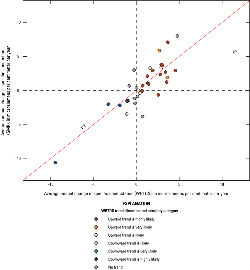
Plot comparing the average annual change in specific conductance estimates computed by the Seasonal Mann-Kendall (SMK) and Weighted Regressions on Time, Discharge (WRTDS), and Season approaches for the 35 sites that have results for both approaches.
References Cited
Oelsner, G.P., Sprague, L.A., Murphy, J.C., Zuellig, R.E., Johnson, H.M., Ryberg, K.R., Falcone, J.A., Stets, E.G., Vecchia, A.V., Riskin, M.L., DeCicco, L.A., Mills, T.J., and Farmer, W.H., 2017, Water-quality trends in the nation’s rivers and streams, 1972–2012—Data preparation, statistical methods, and trend results: U.S. Geological Survey Scientific Investigations Report 2017–5006, accessed November 20, 2022, at https://doi.org/10.3133/sir20175006.
Appendix 2. Stream Toxic Contaminants Supplemental InformationByGiven (First) Names: Trevor P.Needham, Given (First) Names: Ellie P.Foss, and Given (First) Names: Emily H.Majcher
References Cited
Banks, B.D., Needham, T.P., Dugan, C.M., Foss, E.P., and Majcher, E.H., 2022, Priority toxic contaminant metadata inventory and associated total polychlorinated biphenyls concentration data: U.S. Geological Survey data release, accessed October 22, 2024, at https://doi.org/10.5066/P9R78SQ6.
U.S. Geological Survey, 2023, USGS water data for the nation: U.S. Geological Survey National Water Information System database, accessed March 20, 2023, at https://doi.org/10.5066/F7P55KJN.
Appendix 3. Stream Hydromorphology Supplemental InformationByGiven (First) Names: Matthew J.Cashman, Given (First) Names: Coral M.Howe, and Given (First) Names: Joshua J.Thompson
Rapid Habitat Assessment—Data Pre-processing
Several quality assurance and quality control (QA/QC) issues were identified in the multi-jurisdictional dataset obtained from the Chesapeake Bay Program DataHub (Chesapeake Bay Program, undated) and were resolved in the following ways. All metric data were evaluated, and values that fell outside of the expected range (0–20) were removed from the dataset. Some monitoring site identifying information was found to be non-unique because a given site may have been reported with modified names based on field personnel or date, and (or) with different location information for the same site. For sites with a unique name and multiple sets of location coordinates (latitude and longitude), the following procedure was used:
-
1) If the locations were manually assessed to be on the same National Hydrography Dataset Plus (NHDPlus) High-Resolution (U.S. Geological Survey, 2022) flowline and otherwise comparable, the first set of location coordinates were retained for the site.
-
2) For other cases, a clustering procedure was created using the dbscan function in the dbscan package in R (Hahsler and Piekenbrock, 2019), using a minimum of 7 unique points within 200 meters, to create a new clustered site, which was given a new site name and location based on the centroid of all included points.
-
3) If site locations that shared a name were not clustered and were on different flowlines, then sites were split into new sites with unique names and locations.
Specific Gage Analyses
Data Pre-processing
For each field measurement, mean channel depth was estimated by dividing each measurement’s cross-sectional area by wetted channel width. Mean riverbed elevation was estimated by subtracting mean measurement channel depth from stage, corrected for the local gage datum, and reported with respect to North American Vertical Datum of 1988 (NAVD 88).
Streamgage relocations, datum changes, and other physical step-change alterations, such as a local bridge building, may affect channel-flow relationships without representing meaningful hydromorphic trends in overall channel condition through time. As such, these changes were considered a “site intervention” and evaluated for potential step-changes to field measurement values. Information on Site History and Establishment was scraped from the internal USGS Site Information Management System database, and dates of potential interventions were recorded for each site. Time series of stage were also visually examined for any other step-changes missing from site history metadata. When a site intervention occurred, a site’s time series and field measurement data were coded with an additional categorical variable to represent the before-after step change: 0, before intervention; 1, after (first) intervention; 2, after possible second intervention; and so on).
Measurement data went through an iterative QA/QC process that included inspection of outliers (especially of derived metrics), evaluation of poor model fits, and comparison with other measurements at similar streamflows. A number of field measurement metrics were identified as outliers, primarily because of decimal place transcription errors in the historical database entry and were removed from the analysis.
Multi-Model GAM Trend Method
This section provides additional detail about the methods used in the specific gage analyses for calculating trends. For each site, a multi-model procedure, which uses a variety of model forms to best capture the site-specific processes that may affect these relationships among varying streamgages, was utilized. As a result, for each site and metric, GAMs were fit according to the following model forms:
-
0) gam(Metric ~ s(measurement_dt, k=adjust.k) + s(log10_discharge) + meas_type + intervention)
-
1) gam(Metric ~ cyear + s(log10_discharge) + meas_type + intervention)
-
2) gam(Metric ~ s(cyear, k=adjust.k) + s(log10_discharge) + meas_type + intervention)
-
3) gam(Metric ~ s(cyear, k=adjust.k) + s(log10_discharge) + s(doy, bs=”cc”) + meas_type + intervention)
-
4) gam(Metric ~ s(cyear, k=adjust.k) + s(flow_res) + s(doy, bs=”cc”) + meas_type + intervention)
-
5) gam(Metric ~ s(cyear, k=adjust.k) + s(log10_discharge) + s(doy, bs=”cc”) + ti(cyear, log10_discharge) + meas_type + intervention)
-
6) gam(Metric ~ s(cyear, k=adjust.k) + s(log10_discharge) + s(doy, bs=”cc”) + ti(doy, log10_discharge, bs = c(cc, tp) + meas_type + intervention)
-
7) gam(Metric ~ s(cyear, k=adjust.k) + s(log10_discharge) + s(doy, bs=”cc”) + ti(cyear, log10_discharge) + ti(doy, log10_discharge, bs = c(cc, tp) + meas_type + intervention)
Metric
indicates one of the three field response metrics being evaluated for trends;
cyear
indicates a centered integer year;
measurement_dt
indicates a decimal date;
log10_discharge
indicates a log10-transformation of discharge;
flow_res
indicates the residual from a prior-GAM-fitted seasonally detrended streamflow;
doy
indicates the day of year;
meas_type
indicates the discrete measurement code of the measurement method used by the technician (wading, bridge, cableway, boat, and so on), which can affect results because of different measurement cross-sections for various types;
intervention
intervention effect, added to all model forms only when an intervention was detected in the record;
k
adjust.k indicates the degrees of freedom (k) were a flexibly fit with a variable value based on the length of the record and number of observations (see below);
s()
indicates a nonlinear smooth term;
ti()
indicates a nonlinear tensor product interaction;
bs
”cc” indicates the basis spline uses is a cyclic cubic regression; and
bs
c(cc, tp) indicates the basis splines used are a cyclic cubic regression and penalized thin plate regression applied to their respective nonlinear product interaction terms.
An example of model fits for each of the 8 GAM model forms can be found in figure 3.1. Variable product interactions between streamflow with year and season were considered to be due to the potential for changes to localized regions of the streamflow rating curve. For example, seasonal emergent vegetation growth in the channel may affect readings at low streamflows but have negligible effects at larger flows; bank failure and channel expansion throughout the record might affect ratings at higher streamflows on the rating in incised channels but not affect baseflow ratings constrained by channel bars.
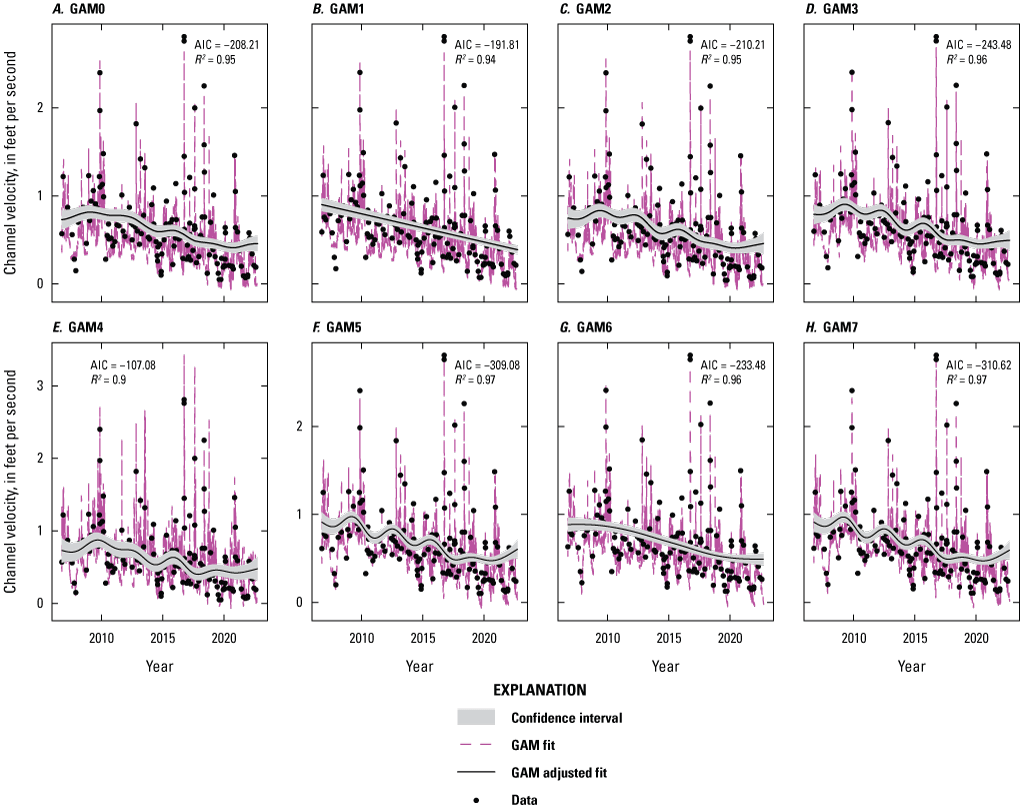
An example of the multi-model Generalized Additive Model (GAM) and fitting procedure conducted for each metric and site in the Specific Gage Trend Analyses: eight GAM forms for the average channel velocity metric at U.S. Geological Survey site 01485000, Pocomoke River near Willards, Maryland (U.S. Geological Survey, 2023).
Unless otherwise specified, all smooth terms were fit with a default of thin plate (bs = “tp”); a cyclic cubic smooth term (bs =“cc”) was used to represent cyclical dynamics and was used for day of year.
Adjust.k indicates that k values—the upper limit on the degrees of freedom associated with the corresponding smooth term—were initially set according to the length of the trend record in a ruleset modified from Murphy and others (2019). The k value was initially set as 2/3 the number of years in the site’s largest trend interval (rounded down), with a minimum k of 10 for a maximum 10-year trend interval. Because it is recommended to evaluate and refit the k value to ensure sufficient flexibility within your dataset (Wood, 2004), an iterative k adjustment process was applied to each site. For each model, k was increased by 10 percent, and the model was tested for improved effective degrees of freedom; the new model was accepted if effective degrees of freedom increased by 20 percent or more. This process was repeated until effective degrees of freedom did not increase beyond the threshold, which then resulted in the penultimate adjusted k value being selected. Null versions of each model, which omitted the yearly time trend component, were also fit, and the change in AIC between the null and original GAM was compared. Following methods from Murphy and others (2019), time trends were considered strong if AIC values decreased by more than 7 points from the null model. Confounder-normalized predictions were then made for all models to capture a signal being driven by exclusively a yearly trend. In this confounder-normalized trend prediction, any streamflow, seasonality, and interactions with either streamflow or seasonality were excluded from the prediction function, effectively removing any non-time trend variable effects. Predictions were made as if the metric were collected with the majority field measurement method. Predictions were then made throughout the time interval, including confidence intervals. Then, a multi-model selection based on minimal AIC scores across all 8 model forms was used to choose the best fitting and parsimonious model that best captures the dynamics of each site.
Trend rates and uncertainties were then calculated taking the confounder-normalized predictions of the best model, with confidence intervals, and averaging the values for each month of the beginning and end years of each trend intervals, which are then averaged for a mean annual beginning and end-year value. The magnitude of change was divided by the length of the trend interval to create a trend slope as a linearized rate of change, and the significant difference between the timesteps was evaluated according to a t-test between the mean and confidence intervals for the normalized predictions at each timestep. This approach, incorporating variability within the beginning and end years of the trend interval, and greater statistical uncertainty in the underlying model of a site (not being able to accurately capture site dynamics), propagates greater uncertainty in evaluating trend significance. In effect, increased rates of Type II (false negative) results were preferentially accepted as conservative tradeoff to avoid Type I (false positive) results, or differences typically within intra-year variability.
References Cited
Chesapeake Bay Program, [undated], DataHub: Chesapeake Bay Program database, accessed December 15, 2022, at https://datahub.chesapeakebay.net/Home.
Hahsler, M., Piekenbrock, M., 2019, dbscan—Fast Density-Based Clustering with R: Journal of Statistical Software, v. 91 no. 1 p. 1–30, accessed February, 12, 2024, at https://doi.org/10.18637/jss.v091.i01.
Murphy, R.R., Perry, E., Harcum, J., and Keisman, J., 2019, A Generalized Additive Model approach to evaluating water quality—Chesapeake Bay case study: Environmental Modelling & Software, v. 118, p. 1–13, accessed October 13, 2023, at https://doi.org/10.1016/j.envsoft.2019.03.027.
U.S. Geological Survey, 2022, NHDPlus High Resolution (NHDPlus HR): U.S. Geological Survey data release, accessed March 20, 2023, at https://prd-tnm.s3.amazonaws.com/index.html?prefix=StagedProducts/Hydrography/NHDPlusHR/VPU/Current/.
U.S. Geological Survey, 2023, USGS water data for the nation: U.S. Geological Survey National Water Information System database, accessed March 20, 2023, at https://doi.org/10.5066/F7P55KJN.
Wood, S.N., 2004, Stable and efficient multiple smoothing parameter estimation for generalized additive models: Journal of the American Statistical Association, v. 99, p. 673–686, accessed March 20, 2025, https://doi.org/10.1198/016214504000000980.
Appendix 4. Status Snapshot


Maps of the Chesapeake Bay watershed showing the locations of the high-quality and low-quality sites for A, nutrients and sediment, B, salinity, C, temperature, D, biological aquatic communities, E, streamflow, and F, hydromorphology based on 2015–17 mean status data.
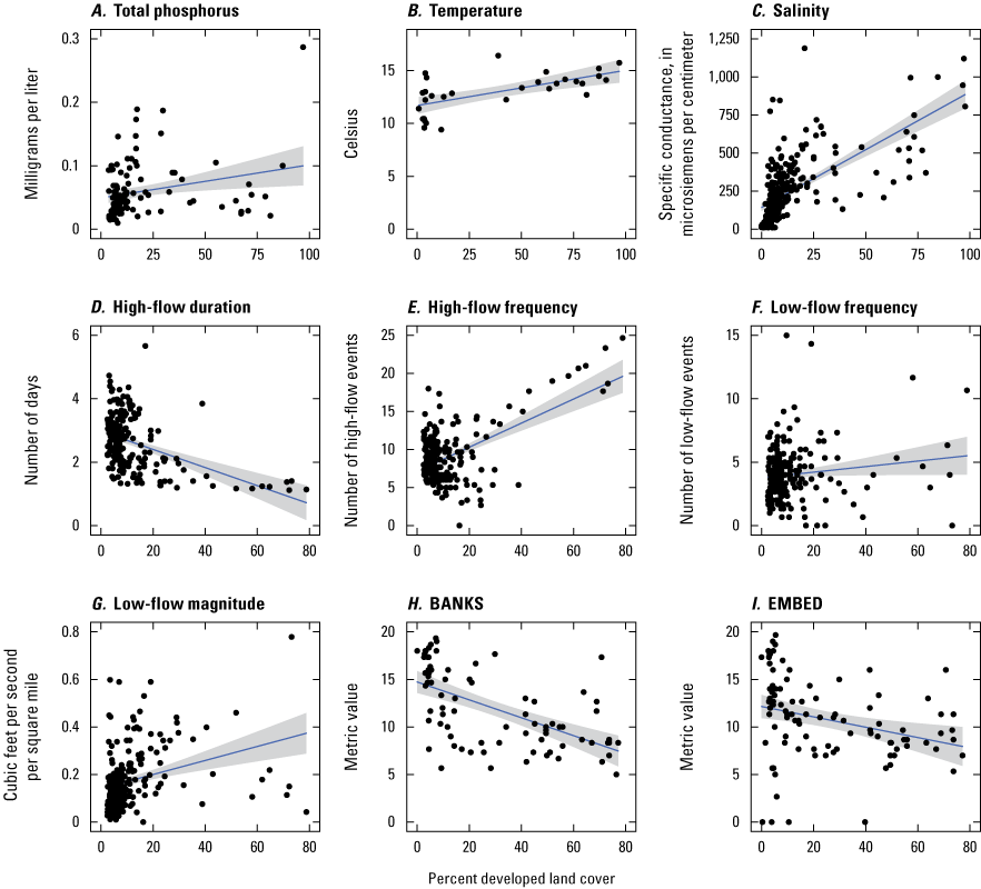
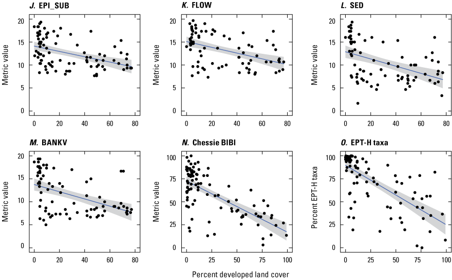
Plots showing linear model results with significant relationships between the percentage of 2016 developed land cover in a given site’s watershed and the following indicator metrics: A, total phosphorus, B, temperature, C, salinity, D, high-flow frequency, E, low-flow frequency, F, low-flow magnitude, G, Bank Stability (BANKS), H, Embeddedness (EMBED), I, Epifaunal Substrate/Available Cover (EPI_SUB), J, Channel Flow Status (FLOW), K, Sediment Deposition (SED), L, Bank Vegetation (BANKV), M, macroinvertebrate Chesapeake Basin-wide Index of Biotic Integrity (Chessie BIBI), and N, percentage Ephemeroptera, Plecoptera, and Trichoptera taxa (excluding the tolerant family Hydropsychidae) (EPT-H).

Plots showing linear model results with significant relationships between the percentage of 2016 agricultural land cover in a given site’s watershed and the following indicator metrics: A, total nitrogen, B, total phosphorus, C, salinity, D, high-flow duration, E, high-flow frequency, F, high-flow magnitude, G, low-flow magnitude, H, Sediment Deposition (SED), I, Velocity/Depth Combinations (VEL_D), and J, percentage of nontolerant fish individuals.

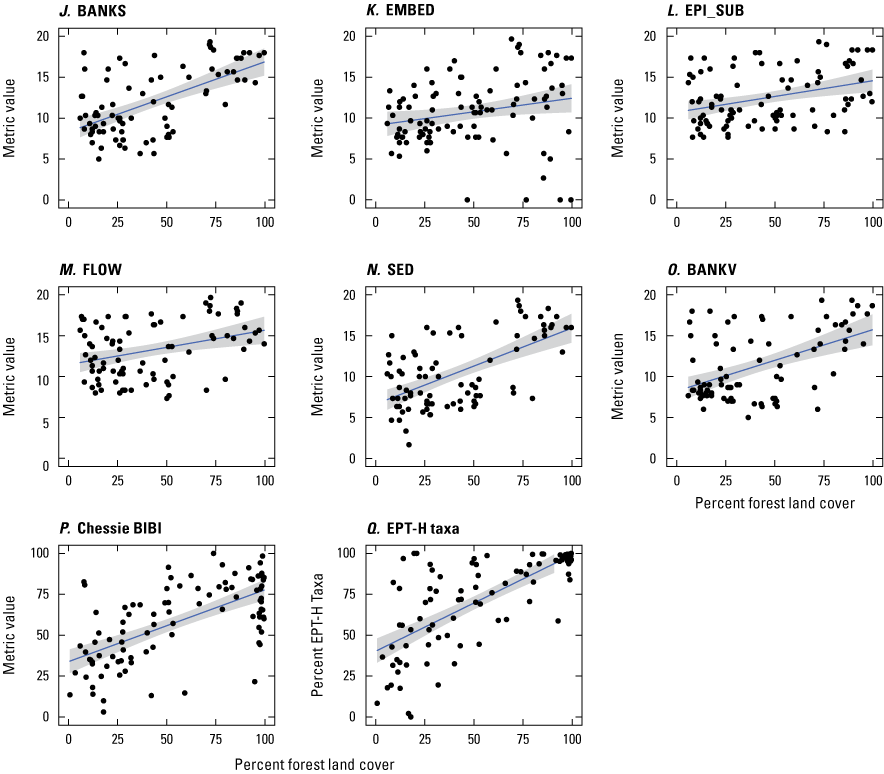
Plot showing linear model results with significant relationships between the percentage of 2016 forest land cover in a given site’s watershed and the following indicator metrics: A, total nitrogen, B, total phosphorus, C, suspended sediment, D, temperature, E, salinity, F, high-flow duration, G, high-flow frequency, H, high-flow magnitude, I, low-flow magnitude, J, Bank Stability (BANKS), K, Embeddedness (EMBED), L, Epifaunal Substrate/Available Cover (EPI_SUB), M, Channel Flow Status (FLOW), N, Sediment Deposition (SED), O, Bank Vegetation (BANKV), P, macroinvertebrate Chesapeake Basin-wide Index of Biotic Integrity (Chessie BIBI), and Q, percentage of Ephemeroptera, Plecoptera, and Trichoptera taxa.
References Cited
Boyle, L.J., Austin, S.H., Cashman, M.J., Clune, J.W., Colgin, J.E., Elliott, K.E.M., Fanelli, R.M., Maloney, K.O., and Zimmerman, T.M., 2025, Status and trends in stream temperature, salinity, flow, hydromorphology, and biological assemblages across the Chesapeake Bay watershed: U.S. Geological Survey data release, https://doi.org10.5066/P13FB2KQ.
U.S. Census Bureau, 2022, TIGER/Line Shapefiles: U.S. Census Bureau data release, accessed February 2025 at https://www.census.gov/geographies/mapping-files/time-series/geo/tiger-line-file.html.
U.S. Geological Survey, 2022, NHDPlus High Resolution (NHDPlus HR): U.S. Geological Survey data release, accessed March 20, 2023, at https://prd-tnm.s3.amazonaws.com/index.html?prefix=StagedProducts/Hydrography/NHDPlusHR/VPU/Current/.
Conversion Factors
U.S. customary units to International System of Units
International System of Units to U.S. customary units
Temperature in degrees Celsius (°C) may be converted to degrees Fahrenheit (°F) as follows:
°F = (1.8 × °C) + 32.
Temperature in degrees Fahrenheit (°F) may be converted to degrees Celsius (°C) as follows:
°C = (°F – 32) / 1.8.
Datums
In map figures, horizontal coordinate information is referenced to the North American Datum of 1983 (NAD 83).
Abbreviations
AIC
Akaike information criterion
Chessie BIBI
Chesapeake Basin-wide Index of Biotic Integrity
COMID
Stream segment unique identifiers for the National Hydrography Dataset Plus dataset
EPA
U.S. Environmental Protection Agency
EPT-H
Ephemeroptera, Plecoptera, and Trichoptera taxa, excluding the tolerant family Hydropsychidae
EST
Eastern Standard Time
GAM
generalized additive model
Hg
mercury
LMM
linear mixed model
MMI
multi-metric index
NHDPlus HR
National Hydrography Dataset Plus High Resolution Dataset
NTN
Nontidal Network
NWIS
National Water Information System
PCB
polychlorinated biphenyl
QA/QC
quality assurance and quality control
R2
coefficient of determination
adjusted coefficient of determination
SC
specific conductance
SMK
Seasonal Mann-Kendall
TMDL
total maximum daily load
USGS
U.S. Geological Survey
WQP
Water Quality Portal
WRTDS
Weighted Regressions on Time, Discharge and Season
For additional information contact:
Director, Virginia and West Virginia Water Science Center
U.S. Geological Survey
1730 East Parham Road
Richmond, Virginia 23228
or visit our website at
https://www.usgs.gov/centers/virginia-and-west-virginia-water-science-center
Publishing support provided by the Baltimore Publishing Service Center.
Disclaimers
Any use of trade, firm, or product names is for descriptive purposes only and does not imply endorsement by the U.S. Government.
Although this information product, for the most part, is in the public domain, it also may contain copyrighted materials as noted in the text. Permission to reproduce copyrighted items must be secured from the copyright owner.
Suggested Citation
Boyle, L.J., Austin, S.H., Cashman, M.J., Clifton, Z.J., Clune, J.W., Colgin, J.E., Elliott, K.E.M., Fanelli, R.M., Foss, E.P., Hitt, N.P., Hittle, E.A., Howe, C.M., Majcher, E.H., Maloney, K.O., Mason, C.A., Metes, M.J., Moyer, D.L., Needham, T.P., Rogers, K.M., Thompson, J.J., Yang, G., and Zimmerman, T.M., 2025, Tracking status and trends in seven key indicators of river and stream condition in the Chesapeake Bay watershed: U.S. Geological Survey Scientific Investigations Report 2025–5072, 104 p., https://doi.org/10.3133/sir20255072.
ISSN: 2328-0328 (online)
Study Area
| Publication type | Report |
|---|---|
| Publication Subtype | USGS Numbered Series |
| Title | Tracking status and trends in seven key indicators of river and stream condition in the Chesapeake Bay watershed |
| Series title | Scientific Investigations Report |
| Series number | 2025-5072 |
| DOI | 10.3133/sir20255072 |
| Publication Date | August 18, 2025 |
| Year Published | 2025 |
| Language | English |
| Publisher | U.S. Geological Survey |
| Publisher location | Reston, VA |
| Contributing office(s) | Virginia and West Virginia Water Science Center |
| Description | Report: x, 104 p.; Data Release |
| Country | United States |
| Other Geospatial | Chesapeake Bay watershed |
| Online Only (Y/N) | Y |
| Additional Online Files (Y/N) | N |