

Controls on Sediment Transport and Storage in the Little Snake, Yampa, and Green Rivers in the Vicinities of Dinosaur National Monument and Ouray National Wildlife Refuge, Colorado and Utah, with Implications for Fish Habitat in the Middle Green River
Links
- Document: Report (15.2 MB pdf) , HTML , XML
- Related Works:
- Journal article - Long-term evolution of sand transport through a river network—Relative influences of a dam versus natural changes in grain size from sand waves
- Open-File Report 2023-1070 - Resurvey of cross sections on the Yampa and Little Snake Rivers in Lily and Deerlodge Parks, Colorado
- Scientific Investigations Report 2025-5078 - Channel and floodplain cross-section and bed-elevation analyses of the Green River in Echo, Island, and Rainbow Parks, Dinosaur National Monument, Colorado and Utah
- Data Release: USGS data release - Surveyed coordinates and elevations in a 2020 resurvey of previously established cross sections on the Green River between Jensen and Ouray, Utah
- Download citation as: RIS | Dublin Core
Acknowledgments
This study was funded by the National Park Service and Upper Colorado River Endangered Fish Recovery Program, with additional support provided in 2013 by the Bureau of Land Management. Jack Schmidt (Utah State University and formerly U.S. Geological Survey [USGS]) and Mark Wondzell (National Park Service) were instrumental in garnering support for this study within the Department of the Interior. Without their tireless efforts and dedication to river science, this study would never have been conducted. Discussions with Jack Schmidt, Erich Mueller (Southern Utah University), and Paul Grams (USGS) greatly improved the science. Tom Sabol and Nick Voichick of the USGS Grand Canyon Monitoring and Research Center helped with data collection throughout this study. Cory Williams, Rodney Richards, and Jennifer Moore of the USGS also helped with data collection during 2013. Tom Chart and Jonathan Friedman provided thoughtful reviews that greatly improved the quality of this report.
Abstract
The transport of sand and finer sediment in the Yampa and Green river network is typically in disequilibrium with the local sediment supply because of the partial decoupling of the sources of water and sediment: most of the water is supplied farther upstream than most of the sediment. This decoupling leads to sand being transported in the main-stem rivers as elongating sand waves following sand resupply during tributary floods. Because of the large amount of sand supplied to the Yampa River by the Little Snake River, Yampa River annual floods generate sand waves that migrate downstream in the Green River causing longitudinal patterns in bed-sand grain size that, in turn, lead to large spatial changes in sand transport. These changes in bed-sand grain size dominate over changes in water discharge in regulating sand transport in the sand-bedded reaches of these rivers. Furthermore, at any given discharge, these changes in bed-sand grain size dominate over all other processes in regulating sand transport in both sand- and gravel-bedded reaches of these rivers. Consequently, erosion or deposition of sand, and the associated changes in fish habitat in the Uinta Basin segment of the Green River are only indirectly related to Green River discharge and Flaming Gorge Dam operations. Owing to the longitudinal patterns of bed-sand grain size associated with the downstream migration of sand waves generated by the Yampa River, a multi-year sequence of large, and likely slightly declining, annual floods on the Yampa River is the probable mechanism that increases backwater fish habitat in the Uinta Basin segment of the Green River.
Cross-section resurveys indicate that the Uinta Basin (Jensen to Ouray) segment of the Green River has undergone sand erosion caused by slight channel widening since the 1990s (a channel response in opposition to that observed farther downstream in Canyonlands National Park during this period). These resurveys indicate that sand deposition leads to a decrease in channel complexity whereas sand erosion generally leads to an increase in channel complexity. The backwaters used as native fish nursery habitat consist of deep pools downstream from and adjacent to large bank-attached sandbars; thus, more extensive backwater habitat equates to greater channel complexity. The generation of the sand wave during the first large Yampa River flood in a sequence (that is, the year-1 flood) causes fining of the bed sand near Jensen. The downstream coarsening associated with bed sand that is finer near Jensen than downstream near Ouray causes a downstream decrease in sand transport in the Uinta Basin segment, leading to net sand deposition and decreased channel complexity. Continued downstream migration of this sand wave during the following year’s annual flood (that is, the year-2 flood) then causes downstream fining, leading to erosion of sand and increased channel complexity in this segment.
Although the year-1 Yampa River flood supplies the sand and deposits the large sandbars required to form backwaters, and thereby makes possible future backwater habitat, these floods cause a temporary reduction in backwater habitat in the Uinta Basin segment because they tend to cause net sand deposition. It is the subsequent out-year Yampa River floods of likely equal or lesser magnitude that maintain or increase backwater habitat because these are the floods that convey sand through or erode sand from this segment. These typically smaller out-year Yampa River floods rework the sandbars deposited during the year-1 annual flood, thereby leading to the increases in both backwater area and volume that have been measured upon recession of these floods. Although artificial floods released from Flaming Gorge Dam might be used to simulate the habitat maintenance achieved by out-year Yampa River floods, the limited sand supply and stage associated with such dam releases precludes their use as a replacement for the sandbar-depositing role of year-1 Yampa River floods that is a prerequisite for backwater formation in the Uinta Basin segment of the Green River.
Introduction
The network of the Green River and its largest tributary, the Yampa River, is characterized by natural disequilibrium sediment transport that has been modified in the Green River by the construction and operation of Flaming Gorge Dam (Andrews, 1986; Schmidt and Wilcock, 2008; Topping and others, 2018). Disequilibrium transport for sand and finer size classes of sediment arises in this river network because the sources of water and sediment are not uniformly distributed over space or time. Most of the water in this network is supplied from snowmelt in the headwaters, whereas most of the sand and finer sediment is supplied by tributaries lower in the network during floods that can occur during different seasons (Andrews, 1978, 1980; Resource Consultants, Inc., 1991; U.S. Environmental Protection Agency, 2014; Topping and others, 2018). These tributary floods can supply large quantities of sediment during floods that precede the annual snowmelt flood, coincide with the annual snowmelt flood, or occur in the summer thunderstorm season after the annual snowmelt flood. Thus, there are both spatial and temporal disconnects between the sources of the water and the sediment that lead to main-stem sediment transport that is commonly in local disequilibrium with the sediment supply.
Tributary floods supply sand that is typically finer than the antecedent sand present on the bed in the main-stem rivers, resulting in discrete bed-sand fining events below these tributaries in the main-stem rivers (Topping and others, 2018; Dean and others, 2020). This finite, episodic resupply of sand to the main-stem rivers that is largely disconnected from main-stem river discharge leads to the generation of sand-dominated sediment waves (Topping and others, 2000, 2021; Wohl and Cenderelli, 2000; Cui and others, 2003a, b; Lisle, 2007; James, 2010; Ferguson and others, 2015). These sand waves migrate downstream through the river network, causing large associated changes in bed-sand grain size and sand transport (Topping and others, 2018). In addition to this direct sand-wave-grain-size control on sand transport, the downstream migration of sand waves can also affect sand transport indirectly by affecting channel, bar, and dune geometry. Thus, there are multiple discharge-independent mechanisms that may lead to substantial variation in sand transport in the Yampa and Green river network, causing different longitudinal patterns in sand transport under similar discharge conditions.
By virtue of mass conservation, differing longitudinal patterns in sand transport give rise to differing longitudinal patterns of erosion and deposition, and thereby differing patterns of fish habitat. Because these differing longitudinal patterns will occur at the same discharge of water, water discharge is a poor predictor of the response of both sediment and sediment-related fish habitat in the Yampa and Green river network. Herein, we present the results from a 9-year study (2013–2021) to investigate sediment transport, deposition, and erosion, in the Little Snake, Yampa, and Green Rivers and then use the understanding gleaned from that effort to evaluate the conditions that can lead to improved habitat for endangered fish.
Study Area
The study area is the part of the network of the Little Snake, Yampa, and Green Rivers located in Moffat County, Colorado, and Uintah County, Utah, in the vicinities of Dinosaur National Monument and Ouray National Wildlife Refuge (fig. 1). The Little Snake River is the major sediment-supplying tributary of the Yampa River and joins the Yampa River just upstream from Dinosaur National Monument. The Yampa River is the largest tributary of the Green River and joins the Green River in the heart of Dinosaur National Monument in Echo Park (fig. 1B). For the purposes of this report, the Yampa River is divided into “upper” and “lower” segments at its confluence with the Little Snake River, and the Green River is divided into “upper” and “middle” segments at its confluence with the Yampa River (fig. 1B). The division between the “middle” and “lower” Green River occurs at Green River, Utah, south of our study area. As reviewed in Topping and others (2018), the Yampa and Little Snake Rivers are largely unregulated and are affected by only small dams, trans-basin diversions, and other human uses that together deplete ~13 percent of the natural flow. Despite these depletions, no significant trends have existed in either annual mean or annual peak discharge in the Yampa or Little Snake Rivers, although large inter-annual variability has existed in both annual mean and peak discharge (Manners and others, 2014; Topping and others, 2018). Thus, the annual snowmelt floods in these two rivers are still largely natural. In contrast to the minimal regulation of the Yampa and Little Snake Rivers, the upper Green River has been highly regulated since Flaming Gorge Dam was closed on December 10, 1962 (Linenburger, 1998). Operation of this dam has flattened the annual hydrograph of the upper Green River below the dam by largely removing the annual flood and increasing baseflow (Grams and Schmidt, 1999, 2002; Vinson, 2001). Beginning in the early 1990s, operation of this dam was modified to include a typically short-duration artificial spring flood for endangered native fish (U.S. Fish and Wildlife Service, 1992; Bureau of Reclamation, 2005, 2006); the magnitude of this peak was increased and the timing was adjusted to coincide with appearance of larval Xyrauchen texanus (razorback sucker) starting in 2012 (Bestgen and others, 2011; LaGory and others, 2012). Operation of Flaming Gorge Dam was modified again in 2021 to include a second short-duration artificial flood to disadvantage nonnative fish (LaGory and others, 2019). Downstream from the Yampa River confluence, the middle Green River exhibits flow characteristics of both the highly regulated upper Green River and the quasi-natural Yampa River (Grams and Schmidt, 2002).
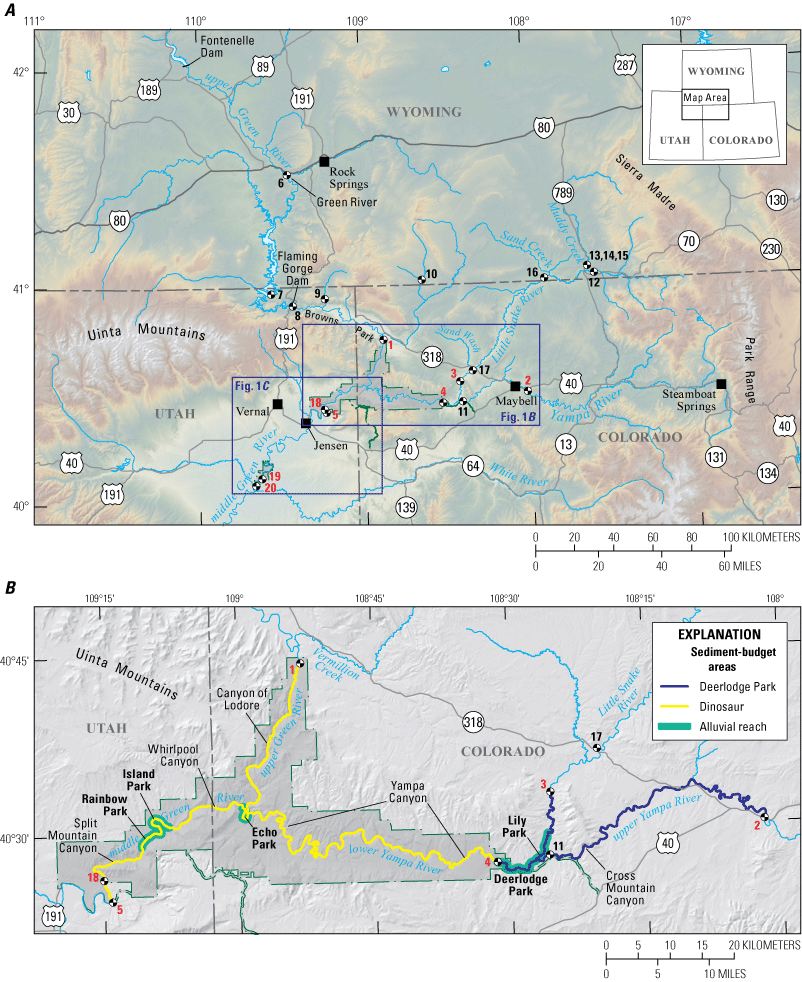
Maps of our study area on the Little Snake, Yampa, and Green Rivers in Colorado and Utah depicting the river segments, geographic features, and sediment-budget areas and segments referred to herein. Shown are the gaging and monitoring stations (black and white checkered circles) at which data were collected; red numbers are keyed to the following stations used in this study: 1, Green River above Gates of Lodore, Colorado, 404417108524900; 2, Yampa River near Maybell, Colo., 09251000; 3, Little Snake River near Lily, Colo., 09260000; 4, Yampa River at Deerlodge Park, Colo., 09260050; 5, Green River near Jensen, Utah, 09261000; 18, Green River above Jensen, Utah; 19, Green River above Ouray, Utah; 20, Green River at Ouray, Utah, 09272400. Black numbers 6–17 indicate the regional ancillary gaging stations that were used for analyses in Topping and others (2018); refer to table 1 in Topping and others (2018) for the names and information on the data collected at those stations. Extents of Dinosaur National Monument and Ouray National Wildlife Refuge are shown with gray shading in parts A and B and labeled in part C. Panels A and B modified from Topping and others (2018). Cross sections that were resurveyed during our study are indicated in C; BB, Bonanza Bridge; HB, Horseshoe Bend; ST, Stirrup; BA, Baeser Bend; AB, Above Brennan; LEB, Leota Bottom; CB, Cindy’s Bar; WYB, Wyasket Bottom.
Our study was conducted near six U.S. Geological Survey (USGS) streamflow gaging stations (USGS, 2022c) on the Little Snake, Yampa, and Green Rivers (fig. 1), and in various reaches of the Uinta Basin segment of the middle Green River where cross sections were resurveyed (fig. 1C). Sediment-transport measurements made at or near the streamflow gaging stations were used to construct continuous mass-balance sediment budgets in the river segments bracketed by these gaging stations. The principal gaging and monitoring stations used in this study, and depicted in figure 1 using the following numbering scheme, are
-
1. Green River above Gates of Lodore, Colo., gaging station 404417108524900, herein referred to as the Green-Lodore station;
-
2. Yampa River near Maybell, Colo., gaging station 09251000, herein referred to as the Yampa-Maybell station;
-
3. Little Snake River near Lily, Colo., gaging station 09260000, herein referred to as the LS-Lily station;
-
4. Yampa River at Deerlodge Park, Colo., gaging station 09260050, herein referred to as the Yampa-Deerlodge station;
-
5. Green River near Jensen, Utah, gaging station 09261000, one of the two parts of a station herein referred to as the Green-Jensen station;
-
18. Green River above Jensen, Utah, monitoring station, one of the two parts of a station herein referred to as the Green-Jensen station;
-
19. Green River above Ouray, Utah, monitoring station, herein referred to as the Green-Ouray station; and
-
20. Green River at Ouray, Utah, gaging station 09272400, herein referred to as the Green-Ouray gaging station.
By convention in our study area, water discharge (Q) is generally reported in units of cubic feet per second. Therefore, for maximum utility of this report for water managers and the public, we use units of cubic feet per second for Q throughout this report; metric (International System) units are used for all other parameters. In equations that relate other parameters to Q, the appropriate conversion factors are embedded in the mathematics.
Purpose and Scope
The purpose and scope of this report are fourfold. First, this report provides an update on the study of Topping and others (2018) through water year 2021 and presents detailed analyses of the importance of the controls on sand transport at the gaging stations in that study. Second, this report presents results on an extension of that study investigating sediment transport and changes in sediment mass (erosion and deposition) in the Uinta Basin segment of the middle Green River (fig. 1C). Third, cross-section-based results are presented on short- and long-term geomorphic change in the Uinta Basin segment and how erosion and deposition relate to geomorphic complexity. Fourth, this report relates how Yampa River floods control changes in sand mass in the Uinta Basin segment of the middle Green River and thereby can enlarge or reduce backwater habitat in this river segment.
Importance of Tributary-Generated Sand Waves in the Study Area
Sand waves generated during large tributary floods dominate sand transport in our study area and have had much greater influence on sand transport in the middle Green River than has construction and operation of Flaming Gorge Dam (Topping and others, 2018). Since the 1960s, suspended-sand transport in the middle Green River at the Green-Jensen station has declined by ~75 percent as the result of the bed-sand coarsening caused by the winnowing of the tail of sand waves that originated in the Little Snake River basin in 1956–1966. By comparison, suspended-sand transport only declined by ~37 percent in response to the 1962 closure and subsequent operation of Flaming Gorge Dam (Topping and others, 2018). Of the sand waves that have been documented in our study area since the onset of streamflow gaging by the USGS in October 1921, the three largest sand waves were generated in the Little Snake River basin by extreme floods in March 1956, 1962, and 1966 (Topping and others, 2018). Gaging-station data indicate that the 1962 and 1966 events originated in Sand Creek (fig. 1A), with the 1956 event also likely from Sand Creek (Topping and others, 2018). The March 27, 1962, Sand Creek flood was, by far the largest of these three floods and resulted in a peak Q of 10,200 cubic feet per second (ft3/s) at the LS-Lily station on March 28, 1962, a peak much larger than the 4,490 ft3/s peak Q of the annual snowmelt flood on May 14, 1962 (Topping and others, 2018; USGS, 2022a, b). Similarly, the March 14 or 15, 1966, Sand Creek flood caused a peak Q of 7,720 ft3/s at the LS-Lily station, a peak also much larger than the 2,940 ft3/s peak Q of the snowmelt flood on May 12, 1966 (Topping and others, 2018; USGS, 2022a, b).
The 1956–1966 Sand Creek floods were such large sand-supplying events that they affected sand transport by causing bed-sand fining as far downstream in the Green River as the Green River at Green River, Utah, 0931500 gaging station (hereafter, the Green-Green River station), located ~450 km downstream from the mouth of the Little Snake River and ~285 km downstream from the Green-Jensen station (Dean and others, 2020). The 1962 flood alone caused the bed-sand grain size to fine by ~30 percent at both the LS-Lily station and the Green-Jensen station (Topping and others, 2018). Similarly, the bed-sand grain size fined by ~30 percent at the Green-Green River station between 1959 and 1965, in likely a cumulative response to the 1956 and 1962 Sand Creek floods (Dean and others, 2020). Following the late-1950s to mid-1960s period of bed-sand fining detected at gaging stations throughout the part of the Green River basin downstream from Sand Creek, the bed-sand grain-size distribution at the LS-Lily, Yampa-Deerlodge, Green-Jensen, and Green-Green River stations slowly coarsened in response to the reduced upstream supply of sand during the post-1966 period of relative quiescence on Sand Creek (Topping and others, 2018; Dean and others, 2020).
Though no other extremely large sand-supplying events other than the 1956–1966 Sand Creek floods were detected in the post-October 1921 period of gaging on the Little Snake River (Topping and others, 2018), earlier large sediment-supplying events were deduced by Kemper and others (2022a, b) to have emanated from Little Snake River tributaries. Through analyses of cadastral surveys and aerial photographs, Kemper and others (2022b) detected large-scale erosion occurring sometime between 1881 and 1906 in Sand Wash, between 1882 and 1937 in Sand Creek, and between 1915 and 1938 in Muddy Creek (fig. 1A). Most of this erosion and the associated sediment delivery to the Little Snake River likely preceded 1921 based on the hydrologic analyses of Topping and others (2018). One of the larger sand-supplying events of Muddy Creek and (or) Sand Wash probably occurred in 1912, as evidenced from a dated ~0.5-meter (m)-thick sand-rich Yampa River floodplain deposit likely sourced from one or both of these tributaries (Kemper and others, 2022a). Consequently, an earlier 1881–1921 period of large sand-wave generation, perhaps centered in 1912, likely preceded the 1956–1966 generation of extremely large sand waves in the Little Snake River basin.
Tributary floods generate sand waves in a river by introducing large amounts of sand that is finer than the antecedent sand on the riverbed (Topping and others, 2000, 2018, 2021). These sand waves elongate as they migrate downstream and have components in transport and on the bed (Topping and others, 2000). Grain-size segregation occurs in the sand wave as it migrates downstream because it takes progressively less “finer sand” on the bed to support a given amount of sand in suspension (after Rouse, 1937a, b; McLean, 1992). Consequently, progressively more of the finer size classes are in transport and not temporarily stored in the bed, thereby leading to longitudinal grain-size segregation and elongation of the wave such that the wave becomes highly asymmetric with the topographic peak of the sand wave closer to the front than the tail. The tributary introduction of a large amount of finer sand to a river causes an overloaded disequilibrium sand-transport condition, with a net flux of sand from suspension to the bed (Parker, 1978; Topping and others, 2021). This abrupt increase in the upstream sand supply thereby causes the bed sand to fine and possibly increase in area (Topping and others, 2007). The cessation of tributary flooding causes the opposite, underloaded condition. This decrease in the upstream sand supply then causes a net flux of sand from the bed to suspension, leading the bed-sand grain-size distribution to coarsen by winnowing the finest size classes from the bed (Rubin and others, 1998).
Sand-wave migration accordingly causes coupled changes in suspended-sand concentration and the suspended- and bed-sand grain-size distributions, and it likely also changes the amount of sand covering gravel-bedded reaches. At an instant in time, the bed-sand grain-size distribution in a sand wave fines in the upstream direction over the relatively short distance between the front and the topographic peak of the sand wave and then coarsens in the upstream direction over the longer distance between the peak and the tail (Topping and others, 2021). The minimum in bed-sand grain size thus coincides with the topographic peak of the sand wave. At a gaging station, the passage of a sand wave can therefore be detected by rapid bed-sand fining followed by slow bed-sand coarsening. Sand waves detected based on their grain-size effects were revealed to be a dominant process in our study area associated with Q-independent changes in suspended-sand concentration of between a factor of 3 to 10, manifest mostly through changes in the concentrations of the finer sand size classes (Topping and others, 2018). Though the sand waves generated by the extremely large Sand Creek floods of 1956–1966 were extraordinary with a grain-size and sand-transport legacy of ~50 years, the detection of those waves indicates that smaller sand waves likely migrate downstream in the rivers in our study area every year as a result of the more common smaller tributary floods that occur each year.
Sand waves are a likely feature of river networks where the sources of water and sediment are largely to fully decoupled, as has been perhaps most extensively documented in the Colorado River downstream from Glen Canyon Dam in Marble and Grand Canyons (Topping and others, 2021). In the case of our study area and based on the 2013–2021 streamflow and sediment data and the historical analyses of Topping and others (2018), the sources of water and sand are almost fully decoupled in the Little Snake River and largely decoupled in the lower Yampa River and the middle Green River. In the Little Snake River, most of the sand is likely supplied by Sand Creek whereas almost all the water is supplied from the Little Snake River upstream from the mouth of Sand Creek. At the confluence of the Little Snake and Yampa Rivers, the Little Snake River supplies roughly three-quarters of the sand, whereas the Yampa River supplies roughly three-quarters of the water.1 At the confluence of the Yampa and Green Rivers, the Yampa River supplies roughly three-quarters of the sand whereas the upper Green River supplies roughly half of the water,2 almost all of it from Flaming Gorge Dam releases. Though the decoupling between the supplies of water and sand appears less in the middle Green River, this is not really the case because of a key difference in the timing of the water and sand supplies. Most of the sand from the Yampa River is supplied during only the few months of the annual flood, whereas most of the water supplied from the upper Green River is spread out over the entire year owing to Flaming Gorge Dam operations. The decoupling of the water and sand supplies means that floods on Sand Creek (a tributary to the Little Snake River) will cause sand waves in the Little Snake River; floods on the Little Snake River (a tributary to the Yampa River) will cause sand waves in the lower Yampa River; and floods on the Yampa River (a tributary to the Green River) will cause sand waves in the middle Green River. Consequently, sand-transport measurements made in these rivers downstream from these tributaries are expected to show evidence of rapid bed-sand fining and associated elevated sand transport immediately following tributary floods (a period of increased upstream sand supply) followed by slower bed-sand coarsening and associated reduced sand transport during periods of tributary quiescence (a period of reduced upstream sand supply).
These crude estimates utilize measurements from the Yampa-Maybell and LS-Lily stations and do not include any estimates of sand erosion or deposition between these stations and the Little Snake-Yampa confluence.
These crude estimates utilize measurements from the Green-Lodore and Yampa-Deerlodge stations and do not include any estimates of sand erosion or deposition between these stations and the Yampa-Green confluence.
Field Methods
Sediment-Transport and Bed-Sediment Measurements at Gaging Stations
Suspended-sediment, bedload, and bed-sediment measurements were made at six of the principal gaging and monitoring stations in figure 1. These measurements were used to compute continuous mass-balance sediment budgets for three distinct river segments or areas, as described below in the “Analytical Methods” section. The suspended-sediment measurements were made continuously during ice-free periods at 15-minute intervals using bank-mounted arrays of side-looking acoustic-Doppler profilers (ADPs) utilizing the two-frequency or single-frequency acoustical method of Topping and Wright (2016), depending on the station (table 1). These acoustical measurements were augmented by episodic 10-vertical equal-width-increment (EWI) measurements made using depth-integrating samplers (Edwards and Glysson, 1999), and calibrated-pump measurements as described in Topping and others (2018). Depending on the water depth, the EWI measurements were made using US DH-81, US D-74, or US D-96-A1 samplers (Edwards and Glysson, 1999; Davis and others, 2005). The EWI measurements were made by wading at a tagline at low Q, and typically from a boat at a tagline at high Q, except at the LS-Lily station, and during water years 2013–2016 at the original Green-Jensen station, where these measurements were made from bridges at high Q. During May, August, and October 2016, back-to-back EWI measurements were made at the new upstream Green-Jensen station and at the original Green-Jensen station; these measurements confirmed that sediment transport was equivalent between these two locations of the Green-Jensen station, thus indicating that only negligible erosion or deposition occurred within the intervening 4.1-km-long reach. Moving the ADPs and pump sampler 4.1 km upstream at the Green-Jensen station in 2016 did therefore not affect the results from our study. The samples from all 10 sampling verticals in the EWI measurements made during our study were analyzed for the full sand grain-size distribution. This approach differs from that used to make EWI measurements during much of the historical period. During the historical period, only 1–3 verticals were sampled in the cross section, and the suspended-sand grain-size distribution was typically analyzed at only one of these verticals; refer to Text S1 in the Supporting Information document for Topping and others (2018) for the sources and sampling-methods for the historical EWI measurements. Refer to Text S2 in the Supporting Information document for Topping and others (2018) for the methods used to identify and remove the likely bed-contaminated EWI measurements.
Table 1.
Names and abbreviations for the gaging and monitoring stations where sediment measurements were made, with ancillary information on dates and methods for acoustical suspended-sediment measurements and bed-sediment measurements.[Dates in month-day-year format. CO, Colorado; UT, Utah; freq., frequency]
15-minute single-frequency acoustical measurements were also made at this station during a pilot acoustic-Doppler profiler test on July 19–20, 2012.
This monitoring station was installed within Dinosaur National Monument, 4.1 kilometers upstream from the Green River near Jensen, Utah, gaging station because of vandalism of the acoustic-Doppler profilers and pump sampler at the previous installation near that gaging station.
Acoustical and calibrated-pump suspended-sediment measurements were discontinued at this gaging station on Oct. 16, 2015, because of vandalism; episodic, paired equal-width-increment measurements continued to be made at the above Jensen station and this station through Oct. 4, 2016, as described in the text.
The pump-sampler measurements made during our study were calibrated using the EWI measurements; the acoustical measurements were calibrated using primarily the EWI measurements and secondarily the calibrated-pump measurements, as described in Topping and Wright (2016). Following this calibration process, all three measurement types measured the velocity-weighted suspended-silt-and-clay concentration (CSILT-CLAY), velocity-weighted suspended-sand concentration (CSAND), and velocity-weighted suspended-sand median grain size (DS) in the river cross section at each gaging station. The EWI measurements were used to verify the calibrated-pump measurements during the post-calibration period, and the EWI and calibrated-pump measurements were both used to verify the calibrated-acoustical measurements during the post-calibration period. Plots evaluating the calibrations of the pump and acoustical measurements are provided in Text S1 in the Supporting Information document for Topping and others (2018). Errors in the acoustical suspended-sediment measurements are described in Topping and Wright (2016); field and laboratory errors associated with the pump and EWI measurements are described in Topping and others (2010, 2011, 2021). Data from all stations are available at the USGS Grand Canyon Monitoring and Research Center (GCMRC) website, https://www.gcmrc.gov/discharge_qw_sediment/ (described by Sibley and others, 2015).
Sand bedload measurements were made episodically using the bedform-migration methods described in Topping and others (2018) and elaborated upon in Dean and others (2020); these methods were pioneered by Simons and others (1965). High-Q bedform-migration bedload measurements were made using repeat multibeam sonar surveys, whereas low-Q measurements were generally made using a method employing a stationary echosounder mounted to a pole driven into the riverbed or, in a few cases at low Q in the Little Snake River, using repeat photographs or direct observations. In the stationary-echosounder method, the measurements of bedform height and migration rate made by the stationary echosounder were combined with the average bedform wavelength calculated from either direct measurements or longitudinal acoustic-Doppler-current-profiler (ADCP) measurements to estimate bedload. The stationary-echosounder bedload measurements were made concurrently with those using physical bedload samplers at three gaging stations in March 2018 to allow comparison with historical bedload measurements made in our study area. These historical measurements were made using Helley-Smith samplers (Edwards and Glysson, 1999) by Elliott and others (1984), Martin and others (1998), and Elliott and Anders (2005) and were used in the analyses of Topping and others (2018).
Bed-sediment measurements were made on the same days as the EWI measurements at the gaging stations where sand-bedded conditions existed at least some of the time (table 1). These bed-sediment measurements generally consisted of 10 individual samples collected at the EWI verticals using a US BMH-60 bed-material sampler (Edwards and Glysson, 1999), a “can” on a pole, or hand grabs, depending on flow depth. The median grain sizes and percent of very fine sand among these 10 samples were both averaged to allow analysis of the cross-section-averaged median grain size of the bed sand (DB) and the cross-section-averaged fractional amount of very fine sand on the bed (fVF). To ensure that DB and fVF were calculated based on a sufficient amount of sampled bed sediment distributed across the cross section to be representative of the average bed-sand conditions in the cross section, we imposed thresholds for the minimum sampled sand mass at each sampling location and the minimum number of such sampled locations in the cross section. DB and fVF were thus calculated for only those bed-sediment measurements where samples containing ≥20 grams (g) of sand were collected at ≥50 percent of all verticals; this method follows Topping and others (2021) and uses their threshold for the minimum amount of sampled sediment mass at each vertical but uses a slightly lower threshold for the minimum number of samples in the cross section (≥50 percent instead of ≥60 percent), because of the much larger number of bed-sediment sampling verticals at each gaging station in our study than in the historical measurements analyzed by Topping and others (2021). We also used the bed-sediment measurements at the post-2015 location of the Green-Jensen station (table 1) to estimate changes in the areal coverage of sand. This station was the one station in our study where we observed the amount of sand overlying the cobbles on the bed to vary over time. At this station, we estimated the bed-sand area as the fraction of the 10 sampling verticals where a bed-sediment sample was possible and contained ≥20 g of sand.
We initiated continuous suspended-sediment monitoring in our study area at five gaging stations (fig. 1A, B, stations 1–5) on the Green, Yampa, and Little Snake Rivers during water year 2013 (beginning either in October 2012 or March 2013), and then expanded this effort with data collection at a new station on the middle Green River in Ouray National Wildlife Refuge in March 2017 (fig. 1C, station 19). The start dates for the continuous suspended-sediment measurements and the acoustical method used at each gaging station are listed in table 1. Data from the first five stations were originally published and analyzed in Topping and others (2018). During 2020–2021, several aspects of the acoustical calibrations at these original five stations were revised. All aspects of the acoustical calibrations were rederived for the LS-Lily station on the Little Snake River in December 2020; the previous calibration, used in Topping and others (2018), was poorly constrained owing to a relative paucity of EWI measurements made at higher flows when the ADP was submerged and making measurements. In addition, the correction for the excess backscatter arising from silt and clay (described in Topping and Wright, 2016) was recalculated at all five original stations in 2021 using the larger amount of data available post publication of Topping and others (2018). This recalculation used a silt-and-clay median grain size of 5 microns (μm), a silt-and-clay geometric standard deviation of 1.5ϕ, and a silt-and-clay wet density of 2.8 grams per cubic centimeter (g/cm3) (a density slightly higher than the quartz density of 2.65 g/cm3 owing to the likely presence of illite); ϕ units are defined as ϕ = −log2D, where D is the sediment grain diameter in millimeters (mm) (Krumbein, 1934). These recalibrations caused slight changes in the annual loads at these five stations (appendix 1), and only slightly affected the sediment budgets in Topping and others (2018).
Cross-Section Resurveys
In October 2020, we resurveyed 27 cross sections in the Uinta Basin segment of the middle Green River that were last surveyed between 1994 and 1996 by FLO Engineering (1996, 1997) or Rakowski (1997). These cross sections provide reasonable coverage of the downstream half of this river segment and are located between river kilometer (RK) 196.4 and RK 252.6 (fig. 1); river kilometers in our study are measured downstream from Flaming Gorge Dam. As part of this effort, we resurveyed all 20 of the cross sections at the Bonanza Bridge (BB), Horseshoe Bend (HB), Stirrup (ST), Baeser Bend (BA), and Above Brennan (AB) study sites of FLO Engineering (1997), located between RK 196.4 and 231.5. Each of these study sites contained four cross sections that were originally surveyed in June 1996. In addition, we resurveyed 2 of the 13 cross sections at Leota Bottom (LEB; at RKs 244.3 and 246.6) and one of the six cross sections at Wyasket Bottom (WYB; at RK 252.6) originally surveyed by FLO Engineering (1996) in March, May, and September 1995. We resurveyed 4 of the 12 cross sections established in 1992 by Rakowski (1997) at her study site, which we refer to as “Cindy’s Bar” (CB). These four cross sections at Cindy’s Bar are located between RK 251.4 and 252.1. In addition to the three Leota Bottom and Wyasket Bottom cross sections that we resurveyed, FLO Engineering (1996) established 33 other tightly spaced cross sections along this part of the river segment, from approximately RK 236.5 to 263.5, that we did not resurvey. Rakowski (1997) resurveyed each of the Cindy’s Bar cross sections seven times during 1994, from before the rise through after the recession of the annual flood: March 17, April 30, May 14, May 28, June 16, July 16, and October 8. We used these multiple repeat surveys spanning the annual floods in 1994 at Cindy’s Bar and in 1995 at Leota and Wyasket bottoms in conjunction with our October 2020 resurvey of these cross sections to compare the magnitudes and styles of seasonal and long-term cross-section change. Though Rakowski (1997) also surveyed the Cindy’s Bar cross sections in November 1992 and four times during and following the recession of the 1993 flood, we did not include those surveys in our analyses because they did not provide the greater resolution throughout the rise and fall of the annual flood captured by Rakowski’s 1994 repeat surveys. We used the last (most recent) of the repeat surveys at Leota Bottom, Cindy’s Bar, and Wyasket Bottom in 1994–1995 and the surveys of the other 20 cross sections in 1996 in conjunction with our October 2020 resurvey of all 27 cross sections to evaluate the long-term (that is, 1990s–2020) cross-section change in the Uinta Basin segment of the middle Green River.
The 2020 resurvey was conducted during October 11–16, 2020, using the Real-Time-Kinematic Global-Positioning-System (RTK-GPS) method with one permanent base station that we deployed at the Ouray National Wildlife Refuge headquarters, one local base station moved between each cross-section cluster, and one rover. We also incorporated data in this resurvey from the U.S. National Geodetic Survey Continuously Operating Reference Station CNC1 in Rangely, Colorado (https://www.ngs.noaa.gov/CORS/Sites/cnc1.html). Based on an analysis of the 1,342 RTK-GPS vectors in our survey, the 95-percent-confidence-level error in the 2020 survey was found to be ±2.0 centimeters (cm) in the horizontal dimension and ±2.4 cm in the vertical dimension. During the 2020 survey, we also collected one bed-sediment sample in the center of the main flow in each cross section for comparison with bed-sediment measurements collected by FLO Engineering (1996); these 2020 bed-sediment measurements are available from the USGS GCMRC website at https://www.gcmrc.gov/discharge_qw_sediment/ under the “Ancillary Sediment Data” link for the Dinosaur network, or directly from the USGS ScienceBase website at https://www.sciencebase.gov/catalog/item/5c002a4fe4b0815414cbb856.
Horizontal positions and elevations in the original FLO Engineering (1996, 1997) and Rakowski (1997) cross sections were determined by digitizing the cross-section plots. By convention, the left and right directions in a river cross section are defined facing downstream. Comparison of the reported endpoint coordinates in FLO Engineering (1997) and Rakowski (1997) with our digitized horizontal and vertical coordinates of the endpoints of these cross sections indicate that the error in our digitization of the cross-section topography was generally sub-decimeter. Our digitized horizontal positions of the endpoints were, on average, only 0.04 meter (m) less than (that is, to the left of) the reported positions in FLO Engineering (1997); the standard deviation about this mean discrepancy in horizontal position was 0.15 m. Our digitized elevations of the endpoints were, on average, only 0.02 m higher than the reported elevations in FLO Engineering (1997); the standard deviation about this mean discrepancy in elevation was 0.03 m. During this step, we detected 12 outliers in the endpoint coordinates and two outliers in endpoint elevations reported by FLO Engineering (1997) that we excluded from the error analysis. These exclusions were justified because the endpoints digitized from the cross-section plots in FLO Engineering (1997) agreed with our 2020 field-surveyed positions and elevations of these endpoints but were not consistent with the tabular-reported coordinates of these endpoints in FLO Engineering (1997). Likely because of the smaller size of the cross-section plots in Rakowski (1997), the absolute value of the discrepancy between the digitized and reported horizontal endpoints were greater for Rakowski’s (1997) cross sections than for FLO Engineering’s (1997) cross sections. Our digitized horizontal positions of the endpoints were, on average, 0.41 m greater than (that is, to the right of) the reported positions in Rakowski (1997); the standard deviation about this mean discrepancy was 0.42 m. Despite the small figure size, our digitized elevations of the endpoints were, on average, only 0.01 m higher than the reported elevations in Rakowski (1997); the standard deviation about this mean discrepancy was 0.04 m. We could not conduct an error analysis for our digitization of the FLO Engineering (1996) cross-section plots because of insufficient information in that report. The digitizing errors associated with FLO Engineering’s (1996) cross sections are assumed to be similar in magnitude to those associated with FLO Engineering’s (1997) cross sections because the style and size of the cross-section plots in these reports are identical.
The original cross-section endpoints were found in the field during our 2020 resurvey using the reported coordinates and (or) maps in FLO Engineering (1996, 1997) and Rakowski (1997), and a magnetic detector (table 2). The FLO Engineering (1996, 1997) endpoints consisted of aluminum-capped rebar driven flush with the ground surface, stamped with the cross-section abbreviation and riverbank, left (L) or right (R). FLO Engineering (1996, 1997) placed a T-post 10–40 cm from the capped rebar in line with the cross section, typically, but not always, closer to the bank than the rebar endpoint. FLO Engineering (1996, 1997) drove these T-posts into the ground so that the top of the post was typically 0.3–0.6 m above the ground surface. The Rakowski (1997) endpoints consisted of uncapped rebar driven to within several centimeters of the ground surface, with T-posts placed in line with the cross section, several centimeters closer to the bank than the rebar. In the seven cases where a cross-section-endpoint rebar or T-post was not found (table 2), we used triangulation from nearby located endpoints to reoccupy the missing endpoint. Once the endpoints of each cross section were located, we surveyed between these endpoints and collected points at each topographic breakpoint. We resurveyed the subaerial part and shallower subaqueous parts of each cross section using an RTK-GPS rover mounted on a 1.8-m survey rod. For the subaqueous parts of each cross section with water depths exceeding 1.8 m, we used a boat-mounted single-beam sonar in combination with the RTK-GPS rover.
Table 2.
Condition of the cross-section endpoints during the 2020 resurvey and NAVD 88 vertical offsets applied to each cross section in the Uinta Basin segment of the middle Green River, Utah.[River kilometers (RK) are measured downstream from Flaming Gorge Dam. Left and right directions in a river cross section and left and right banks are defined facing downstream. NAVD 88, North American Vertical Datum of 1988; BB, Bonanza Bridge; HB, Horseshoe Bend; ST, Stirrup; BA, Baeser Bend; AB, Above Brennan; LEB, Leota Bottom; CB, Cindy’s bar; WYB, Wyasket Bottom; m, meter; ~, approximately; —, no notes. For locations of cross sections, refer to figure 1C]
| RK | Cross section | Left-bank T-post found? | Left-bank rebar found? | Right-bank T-post found? | Right-bank rebar found? | Notes | NAVD 88 vertical offset (m) |
|---|---|---|---|---|---|---|---|
| 196.4 | BB-4 | No | No | No | No | Plowed field on right bank | 1.515 |
| 196.6 | BB-3 | Yes | No | No | No | Plowed field on right bank | 1.515 |
| 197.0 | BB-2 | No | Yes | No | No | Plowed field on right bank | 1.515 |
| 197.3 | BB-1 | Yes | No | Yes | No | — | 1.515 |
| 203.9 | HB-4 | Yes | Yes | No | Yes | Right-bank T-post recently removed, scar from post in ground surveyed | 1.390 |
| 204.2 | HB-3 | No | No | Yes | Yes | — | 1.332 |
| 204.4 | HB-2A a | Yes | Yes | Yes | No | Right-bank endpoint of HB-2A used as the new left-bank endpoint of HB-2B because it is approximately in line with HB-2B | 1.352 |
| 204.4 | HB-2B a | No | No | Yes | Yes | Left-bank endpoint eroded by ~61 m of bank retreat on island | 1.369 |
| 204.6 | HB-1A b | No | Yes | No | Yes | Right-bank endpoint of HB-1A used as the new left-bank endpoint of HB-1B because it is approximately in line with HB-1B | 1.349 |
| 204.6 | HB-1B b | No | No | Yes | Yes | Left-bank endpoint eroded by ~29 m of bank retreat on island | 1.320 |
| 218.2 | ST-4 | Yes | Yes | Yes | Yes | — | 1.188 |
| 218.4 | ST-3 | Yes | Yes | Yes | Yes | — | 1.235 |
| 218.6 | ST-2 | Yes | Yes | Yes | Yes | — | 1.235 |
| 218.7 | ST-1 | Yes | Yes | Yes | Yes | — | 1.231 |
| 223.9 | BA-4 | Yes | Yes | Yes | No | Found left-bank T-post and capped rebar 20.2 m closer to the bank than the position reported in FLO Engineering (1997) | 1.171 |
| 224.0 | BA-3 | No | Yes | Yes | Yes | — | 1.154 |
| 224.2 | BA-2 | Yes | Yes | No | No | Farmed land and old trash pile on right bank | 1.219 |
| 224.3 | BA-1 | Yes | Yes | No | No | Farmed land on right bank | 1.202 |
| 230.8 | AB-4 | Yes | Yes | Yes | Yes | — | 1.712 |
| 231.2 | AB-3 | Yes | No | Yes | No | — | 1.700 |
| 231.3 | AB-2 | Yes | Yes | Yes | Yes | — | 1.664 |
| 231.5 | AB-1 | Yes | Yes | Yes | Yes | — | 1.723 |
| 244.3 | LEB-24 | Yes | No | Yes | No | — | 1.378 |
| 246.6 | LEB-21 | Yes | Yes | No | Yes | — | 1.184 |
| 251.4 | CB-9 | Yes | No | Yes | Yes | Left-bank T-post eroded and found out-of-place | 1,326.380 |
| 251.7 | CB-7 | Yes | No | Yes | No | Left-bank T-post eroded and found out-of-place | 1,326.462 |
| 251.9 | CB-6 | Yes | No | Yes | No | Left- and right-bank T-posts eroded and found out-of-place | 1,326.534 |
| 252.1 | CB-4 | Yes | No | Yes | No | Right-bank T-post eroded and found out-of-place | 1,326.380 |
| 252.6 | WYB-12 | Yes | No | Yes | Yes | Left-bank T-post labeled “WYB-12” | 1.231 |
Orthometric elevations in the 2020 resurvey were referenced to the North American Vertical Datum of 1988 (NAVD 88) using the Geoid 18 model. Though FLO Engineering (1996, 1997) reported their surveyed elevations above sea level, we could not determine whether they used the National Geodetic Vertical Datum of 1929 (NGVD 29) or NAVD 88; Rakowski (1997) used a local vertical datum. We thus converted the elevations in the FLO Engineering (1996, 1997) and Rakowski (1997) surveys to the NAVD 88 datum by applying a vertical offset unique to each cross section, determined from our 2020 resurveyed elevations of FLO Engineering’s (1996, 1997) capped rebar and Rakowski’s (1997) uncapped rebar (table 2). The 2020 resurvey data are available from the USGS data release that accompanies this report (Griffiths and others, 2024).
Analytical Methods
Silt-and-Clay Load and Suspended-Sand Load
The cross-sectionally integrated suspended-silt-and-clay flux (QSILT-CLAY) and suspended-sand flux (QSS) at each 15-minute timestep were respectively calculated by multiplying CSILT-CLAY and CSAND by Q, the same method used by Topping and others (2018). The values of CSILT-CLAY and CSAND used to calculate these fluxes primarily were those measured by ADPs; in cases where the ADPs were out of the water (as happened during low Q at the LS-Lily, Yampa-Maybell, and Yampa-Deerlodge stations) or buried and (or) blocked by sandbars (as happened episodically at the Green-Ouray station), the values of CSILT-CLAY and CSAND from the calibrated-pump and EWI measurements were linearly interpolated to the 15-minute timesteps. These instantaneous values of QSILT-CLAY and QSS were then integrated over time to compute the silt-and-clay load and the suspended component of the sand load through the river cross section over a given time interval (Porterfield, 1972). At the two stations where the ADPs were located upstream from the streamflow gaging station (that is, the post-2015 Green-Jensen station and the Green-Ouray station) discharge travel-time relations were developed using 15-minute stage measurements at the locations of the ADP array and the streamflow gaging station. This method resulted in best-fit average times of −45 minutes at Green-Jensen and −150 minutes at Green-Ouray that were then applied to the Q timestamps at the gaging stations. The worst period of ADP burial and (or) blockage at the Green-Ouray station occurred from June 3 through October 1, 2021, when CSILT-CLAY and CSAND had to be estimated based on previous measurements at similar Q and based on the continuous measurements made during this period at the Green-Jensen station. During prior episodes of ADP burial at this station, sufficient calibrated-pump measurements were available to interpolate reasonably accurate values of CSILT-CLAY and CSAND at the 15-minute timestamps. Given that Q was mostly very low during the 2021 period of ADP burial at the Green-Ouray station, however, these estimations of CSILT-CLAY and CSAND did not introduce unacceptably high levels of uncertainty in the values of QSILT-CLAY, QSS, or QSB integrated to compute the loads during the annual-flood period of March–July (appendix 1) that were used in the sediment-budget analyses herein.
Sand Bedload and Sand Total Load
The cross-sectionally integrated bedload-sand flux (QSB) at each timestep was calculated using log-linear relations between Q and T (following Topping and others, 2018). T is defined as the ratio T = QSB/QSS; the sand bedload thus dominates over the suspended-sand load when T is >1, whereas the suspended-sand load dominates over the sand bedload when T is <1. The instantaneous values of QSB were then integrated over time to compute the bedload component of the sand load through the river cross section over a given time interval (also as in Topping and others, 2018). The cross-sectionally integrated total sand flux (QSAND) at each timestamp was calculated by summing QSS and QSB; these instantaneous values of QSAND were then integrated over time to compute the sand total load through the river cross section over a given time interval (also as in Topping and others, 2018).
Dean and others (2022) showed that, under the moderate transport-stage conditions that are typically characterized by the presence of dunes on the riverbed, the Q-dependent T-ratio-based approach is a more accurate estimator of QSB than the typical method of using Q—QSB rating curves. Transport stage is defined as the ratio of the skin-friction boundary shear stress (τsf) to the critical shear stress (τcr) associated with DB. Changes in Q, manifest through changes in shear velocity (), and changes in bed-sand grain size exert roughly similar influence on QSB and QSS at moderate transport stage (after equation 2 in Dean and others, 2022). The shear velocity is a standard measure of the flow strength and is defined as , where τb is the boundary shear stress and ρ is the density of water. The Q-dependent T-ratio-based approach thus provides a more accurate method for estimating QSB because this approach incorporates both the influence of Q on QSB (which is included in the Q—QSB rating-curve approach) and the influence of changing bed-sand conditions on QSB (which is excluded from the rating-curve approach). Given that moderate transport-stage conditions likely dominate at the gaging stations in our study area, substantial changes in both Q and bed-sand grain size occur at these stations (Topping and others, 2018). Therefore, because our continuous suspended-sediment measurements capture the effects of changing bed-sand conditions on QSS, the Q-dependent T-ratio-based approach for estimating QSB is ideally suited to the rivers in our study.
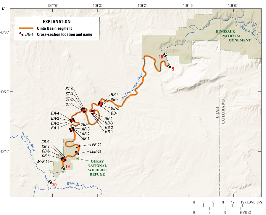
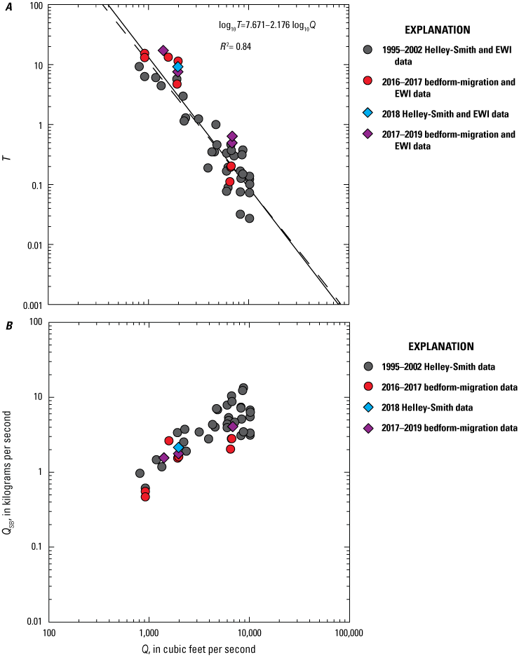
As in Topping and others (2018), T was calculated using paired EWI and bedload measurements; the bedload measurements were made using either Helley-Smith samplers or bedform-migration methods. At the largely gravel-bedded Yampa-Maybell and Green-Jensen stations, we used the Q—T relations used in Topping and others (2018). These relations were derived by Topping and others (2018) using the historical EWI and Helley-Smith measurements of Elliott and Anders (2005) that were filtered to remove likely bed-contaminated measurements. At the sand-bedded Green-Lodore, LS-Lily, and Yampa-Deerlodge stations, we developed revised Q—T relations using the data in Topping and others (2018) augmented by new paired EWI and bedload measurements made during water years 2017–2019 (figs. 2–4). We also developed a new Q—T relation at the new Green-Ouray station installed in 2017 using paired EWI and bedload measurements made during water years 2017–2018 (fig. 5). One of the new bedload measurements made at the Green-Lodore, LS-Lily, and Green-Ouray stations was made using a Helley-Smith sampler, and the others were made using bedform-migration methods. Upon development of the revised Q—T relations, we recalculated QSB at the Green-Lodore, LS-Lily, and Yampa-Deerlodge stations for water years 2013–2016, which were originally analyzed in Topping and others (2018).
Plots of sand bedload relations at the Green River above Gates of Lodore, Colorado, gaging station 404417108524900 (Green-Lodore station). A, T, the ratio of cross-sectionally integrated bedload-sand flux (QSB) to cross-sectionally integrated suspended-sand flux (QSS), plotted as a function of instantaneous water discharge (Q). Black line is the least-squares log-linear regression used to estimate T; the equation for this regression is shown (R2 is the coefficient of determination). Dashed black line is the least-squares log-linear regression from Topping and others (2018) fit to the 1995–2017 data (dark-gray filled circles and red filled circles). B, Cross-sectionally integrated bedload-sand flux (QSB) plotted as a function of Q. Because the 2017–2018 measurements (purple diamonds) that post-date Topping and others (2018) occupy the same region in Q—QSB space as the 1995–2017 measurements (dark-gray filled circles and red filled circles) used by Topping and others (2018), the bounding relations applied to preclude QSB outside the range observed at a given Q are unchanged from Topping and others (2018). EWI, equal-width increment.
Plots of sand bedload relations at the Little Snake River near Lily, Colorado, gaging station 09260000 (LS-Lily station). A, T, the ratio of cross-sectionally integrated bedload-sand flux (QSB) to cross-sectionally integrated suspended-sand flux (QSS), plotted as a function of instantaneous water discharge (Q). Black line is the least-squares log-linear regression used to estimate T; the equation for this regression is shown (R2 is the coefficient of determination). Dashed black line is the least-squares log-linear regression from Topping and others (2018) fit to the 2001–2017 data (dark-gray filled circles and red filled circles). B, Cross-sectionally integrated bedload-sand flux (QSB) plotted as a function of Q. Because the 2017–2018 measurements (purple diamonds) that post-date Topping and others (2018) occupy a slightly larger region in Q—QSB space than the 2001–2017 measurements (dark-gray filled circles and red filled circles) used by Topping and others (2018), the bounding relations applied to preclude QSB outside the range observed at a given Q are slightly expanded from those in Topping and others (2018) to encompass the 2017–2018 measurements. EWI, equal-width increment.
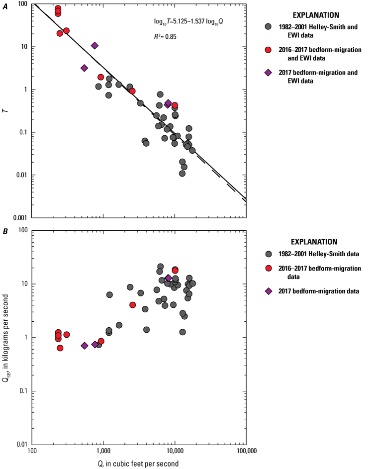
Plots of sand bedload relations at the Yampa River at Deerlodge Park, Colorado, gaging station 09260050 (Yampa-Deerlodge station). A, T, the ratio of cross-sectionally integrated bedload-sand flux (QSB) to cross-sectionally integrated suspended-sand flux (QSS), plotted as a function of instantaneous water discharge (Q). Black line is the least-squares log-linear regression used to estimate T; the equation for this regression is shown (R2 is the coefficient of determination). Dashed black line is the least-squares log-linear regression from Topping and others (2018) fit to the 1982–2017 data (dark-gray filled circles and red filled circles). B, Cross-sectionally integrated bedload-sand flux (QSB) plotted as a function of Q. Because the 2017 measurements (purple diamonds) that post-date Topping and others (2018) occupy the same region in Q—QSB space as the 1982–2017 measurements (dark-gray filled circles and red filled circles) used by Topping and others (2018), the bounding relations applied to preclude QSB outside the range observed at a given Q are unchanged from Topping and others (2018). EWI, equal-width increment.
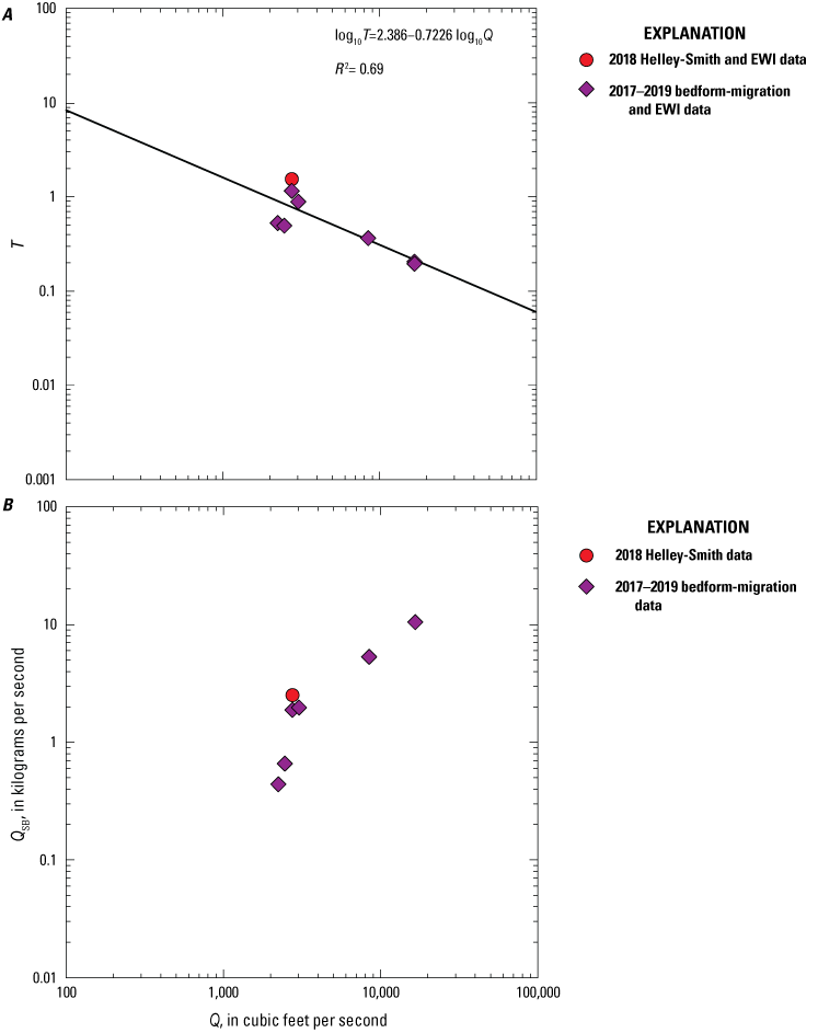
Plots of sand bedload relations at the Green River above Ouray, Utah (Green-Ouray station). A, T, the ratio of cross-sectionally integrated bedload-sand flux (QSB) to cross-sectionally integrated suspended-sand flux (QSS), plotted as a function of instantaneous water discharge (Q). Black line is the least-squares log-linear regression fit to these measurements and used to estimate T; the equation for this regression is shown (R2 is the coefficient of determination). B, Cross-sectionally integrated bedload-sand flux (QSB) plotted as a function of Q. These measurements were used to develop the bounding relations to preclude QSB outside the range observed at a given Q. EWI, equal-width increment.
Equivalency of Helley-Smith and bedform-migration bedload measurements was evaluated in tests conducted at the Green-Lodore, LS-Lily, and Green-Ouray stations in March 2018. These tests were required to determine whether the Q—T relations developed in Topping and others (2018), and revised herein, were unbiased, given that both the historical Helley-Smith measurements of Martin and others (1998) and Elliott and Anders (2005), and the modern bedform-migration measurements of Topping and others (2018) were used in these relations. For additional context, these tests also included the US BLH-84 bedload sampler (Edwards and Glysson, 1999; Davis and others, 2005), a bedload sampler found to be generally more accurate than the Helley-Smith sampler (Gray and others, 2021). These tests consisted of sequential single-vertical bedload samples, alternating between the Helley-Smith and US BLH-84 samplers, collected adjacent to a pole-mounted echosounder used to make bedform-migration measurements. To be consistent with the historical bedload measurements, both samplers were deployed using bags with a 0.25-mm mesh size. These tests were conducted at verticals in the left and right parts of the cross sections at the Green-Lodore and Green-Ouray stations and at one vertical in the center of the cross section at the LS-Lily station. In addition, one 10-vertical Helley-Smith bedload measurement was made over the full width of the cross section at each of these stations during these tests. The sequential single-vertical bedload samples were collected minutes apart at each vertical. At the Green-Lodore and Green-Ouray stations, three sequential samples were collected, alternating between the two bedload sampler types, in two sampling sets spaced hours apart to allow improved comparison with the bedform-migration bedload measurements (which were made over many hours). At the Green-Lodore station, the sampling sets extended for ~30 minutes at each vertical and were spaced 6 hours apart. At the Green-Ouray station, the sampling sets extended for ~20 minutes at each vertical and were spaced 4.5 hours apart. Among the two sets, six samples were collected with each bedload sampler type at each vertical. At the LS-Lily station, five sequential samples were collected, alternating between the two bedload sampler types, in only one sampling set extending for 45 minutes.
Results from the bedload-sampler tests indicate that, despite Gray and others’ (2021) finding that the US BLH-84 sampler was more accurate than the Helley-Smith sampler, our Helley-Smith measurements were in better agreement with the bedform-migration measurements than were the US BLH-84 measurements (table 3, fig. 6). Substantial overlap between the Helley-Smith and bedform-migration measurements at the 95-percent confidence level occurred in three of the five tests, with near overlap occurring in one additional test and substantial disagreement occurring in only one test (table 3, fig. 6). In contrast, only slight overlap between the US BLH-84 and bedform-migration measurements at the 95-percent confidence level occurred in two of the five tests, with substantial disagreement occurring in two of the five tests and near overlap occurring in only one test. Substantial 95-percent-confidence-level overlap between the US BLH-84 and bedform-migration measurements never occurred. Thus, bedload measurements made using a Helley-Smith sampler appear to be equivalent to those made using bedform-migration methods in our study area, thereby verifying that the Q—T relations of Topping and others (2018) were derived using data that were internally unbiased. Given the equivalency of the Helley-Smith and bedform-migration bedload measurements, we included the 10-vertical Helley-Smith bedload measurements made during the 2018 tests at the Green-Lodore, LS-Lily, and Green-Ouray stations in the revised and (or) new Q—T relations used herein to estimate QSB.
Table 3.
Comparison of single-vertical bedload measurements with stationary-echosounder bedform-migration bedload measurements.[The mean values and ±1 standard error values indicated for the US BLH-84 and Helley-Smith measurements are calculated among 6 sequential samples at each sampling vertical at the Green-Lodore and Green-Ouray stations and 5 sequential samples at the LS-Lily station. The total bedload flux is the combined sand and gravel flux. Station name abbreviations are defined in table 1; locations are shown in figure 1. Sampling vertical locations in the cross section: L, left; C, center; R, right. kg/s/m, kilogram per second per meter width]
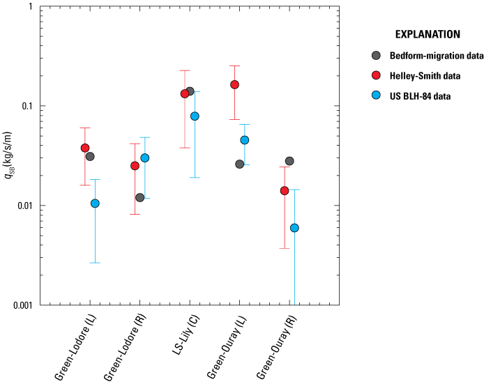
Plot comparing the unit bedload-sand fluxes (qSB) measured during the single-vertical bedload-sampler tests. Error bars indicate the 95-percent-confidence-level error in the mean computed based on the calculated sample standard error and the assumption of a Gaussian normal error distribution. Station name abbreviations are defined in table 1. Abbreviations for sampling vertical location in the cross section are L, left; C, center; and R, right. kg/s/m, kilogram per second per meter width.
Sediment Budgets
Continuous mass-balance sediment budgets for silt and clay and for sand were calculated using the same methods described in Topping and others (2018) for two sediment-budget areas and one river segment (fig. 1). The Deerlodge Park sediment-budget area includes the lower segment of the Little Snake River that extends from the LS-Lily station (fig. 1B, station 3) downstream to the confluence with the Yampa River, the segment of the upper Yampa River that extends from the Yampa-Maybell station (fig. 1B, station 2) downstream to the confluence with the Little Snake River, and the short sand-bedded reach of the lower Yampa River that extends from the confluence of the Little Snake and Yampa Rivers downstream to the Yampa-Deerlodge station (fig. 1B, station 4). The Dinosaur sediment-budget area includes the segment of the lower Yampa River that extends from the Yampa-Deerlodge station (fig. 1B, station 4) downstream to the Yampa-Green confluence in Echo Park, the segment of the upper Green River (mostly in the Canyon of Lodore) that extends from the Green-Lodore station (fig. 1B, station 1) downstream to the Yampa-Green confluence, and the segment of the middle Green River that extends from the Yampa-Green confluence downstream to the original pre-2016 location of the Green-Jensen station (at the USGS streamflow gaging station) (fig. 1B, station 5). The Uinta Basin sediment-budget river segment includes the Uinta Basin segment of the middle Green River that extends from the original location of the Green-Jensen station (fig. 1C, station 5) downstream to the Green-Ouray station (fig. 1C, station 19). The 4.1-km-long reach of the Green River between the current (post-2015) and original locations of the Green-Jensen station (fig. 1, stations 18 and 5) is mostly gravel bedded and relatively steep. Thus, changes in sand mass and in silt and clay mass within this short reach are negligible compared to the changes in mass over the much longer river segments within the Dinosaur sediment-budget area (fig. 1B), as confirmed by back-to-back EWI measurements made throughout 2016 at both locations of the Green-Jensen station that indicated equivalency of CSAND and CSILT-CLAY at both station locations. Therefore, it was not necessary to change the location of the downstream end of the Dinosaur sediment-budget area when the Green-Jensen station was moved. Because the continuous suspended-sediment measurements at the three gaging stations that bracket these sediment-budget areas started at different times, the periods of record for the Deerlodge Park and Dinosaur sediment budgets began at slightly different times during the early part of water year 2013 (table 1 and as described in Topping and others, 2018). The period of record for the Uinta Basin sediment budget began on March 25, 2017, upon the initiation of continuous suspended-sediment measurements at the Green-Ouray station (table 1). The periods of record for the two sediment-budget areas and the one sediment-budget river segment extend through at least the end of water year 2021.
As described in Topping and others (2018), the sediment input to each continuous mass-balance sediment budget is computed using the 15-minute silt-and-clay loads and sand loads at the gaging station(s) bracketing the upstream extent of that area or segment. The sediment export from each continuous mass-balance sediment budget is computed using the 15-minute silt-and-clay loads and sand loads at the gaging station bracketing the downstream extent of that area or segment. No tributary sediment inputs are estimated the two sediment-budget areas or the one sediment-budget river segment because most of the tributaries are small, mainly ephemeral, and likely supply mainly silt and clay. The ramification of this sediment-budgeting approach with respect to the tributaries is that, though the sand budgets are almost certainly accurate to within the uncertainties applied to the sand loads (as justified in Topping and others, 2018), the possibility exists that neglecting the small, but not zero, amounts of silt and clay supplied by the tributaries causes negative step changes in the silt-and-clay budgets that are not the result of erosion.
The uncertainties in the sediment budgets are calculated by applying uncertainties to the 15-minute cross-sectionally integrated sediment fluxes at the bracketing gaging stations. These applied uncertainties are then included in the integration of the fluxes over time that yield the loads over a selected period, and then finally propagated through the standard sediment-budget calculation (export minus input yields the change in sediment mass). As justified in Topping and others (2018), 10-percent uncertainties are applied to the 15-minute values of both QSILT-CLAY and QSAND. We applied a 50-percent uncertainty to the 15-minute estimations of QSB used in the sediment budgets. These levels of uncertainty were chosen based on the likely magnitudes of the persistent biases that could be present over longer timescales in the values of Q, CSILT-CLAY, CSAND, and QSB (Topping and others, 2018). As in Topping and others (2018), the sediment budgets are indeterminate when the propagated uncertainty is ≥2 times the absolute value of the zero-bias value; the sediment budgets are demonstrably positive (thus indicating deposition) or negative (thus indicating erosion) when the uncertainty is less than the absolute value of the zero-bias value; and the sediment budgets are likely positive (thus indicating likely deposition) or likely negative (thus indicating likely erosion) when the uncertainty falls between these bounds.
Bed Stage
The average elevation of the bed in the measurement cross section (that is, bed stage) was calculated for the EWI measurements at the four sand-bedded stations (Green-Lodore, LS-Lily, Yampa-Deerlodge, and Green-Ouray). These calculations of bed stage were used to evaluate changes in the bed-sand grain-size distribution as a function of elevation within the bed (by utilizing bed scour and fill to access different elevations within the bed). Bed stage is defined as the gage height measured at the gaging station at the midpoint time of the EWI measurement minus the mean flow depth among the 10 EWI verticals; flow depths at each vertical in each EWI measurement can be downloaded from the USGS GCMRC website at https://www.gcmrc.gov/discharge_qw_sediment/. Because this calculation of bed stage includes neither the water-surface slope nor the longitudinal distance between the gaging station and the EWI-measurement cross section, the calculated bed stage is relative to a sloping datum parallel to the water surface. Thus, bed stage is only approximately in the same datum as gage height, depending on the water-surface slope and longitudinal distance. However, because the EWI-measurement cross sections tend to be at similar longitudinal positions relative to each gaging or monitoring station, the bed stages at each station are internally consistent and thus can be analyzed for the purpose of relating bed-sand grain size to relative elevation within the bed. Except at the Green-Ouray station, the ADP arrays and EWI measurements are located near the stage sensor used to measure gage height at the associated USGS streamflow gaging station. Thus, the gage heights used to calculate bed stage at the Green-Lodore, LS-Lily, and Yampa-Deerlodge stations are those measured at these gaging stations. Because the gaging station associated with the Green-Ouray station (a monitoring station) is located 8.6 km downstream, gage heights were measured at the Green-Ouray station using a stage sensor mounted with the ADP array near the EWI measurement cross-section location.
Regulation of Suspended-Sand Concentration by Flow, Grain Size, and Other Processes
We used a modified version of the theory-derived parameter α of Rubin and Topping (2001, 2008) to evaluate the relative importance of changes in flow and changes in the bed-sand grain-size distribution in regulating CSAND. The original version of α was used by Topping and others (2018) to evaluate the relative importance of historical changes in flow and bed-sand grain size in regulating sand transport in the Green, Little Snake, and Yampa Rivers. Changes in bed-sand grain size caused by downstream migration of sand waves were important in regulating sand transport in these rivers historically (Topping and others, 2018). For the analyses herein, we used the approach described in this section to calculate a modified version of |α| separately for the EWI, calibrated-pump, and acoustical suspended-sand measurements; the need for this separation resulted from the different error magnitudes between these three measurement types. In addition, we also investigated whether other processes, such as Q-independent changes in the shear velocity or changes in the area of the bed covered by sand (for example, Topping and others, 2007; 2021; Rubin and others, 2020) had important roles in regulating sand transport. The importance of these other processes in our study area was evaluated graphically.
As defined by Rubin and Topping (2001),
is a quantitative measure of the relative importance of the shear velocity () versus the median grain size of the bed sand (DB) in regulating the depth-integrated suspended-sediment flux over a point on the bed, that is, the unit suspended-sand flux (qSS). The numerator in α describes the variation in qSS associated with a change in DB, whereas the denominator in α describes the variation in qSS associated with a change in . is a measure of the flow strength and is linearly related to velocity (von Karman, 1930), and thereby positively correlated with Q; DB is the proxy used to simplify all changes in the bed-sand grain-size distribution. Δ signifies the ratio of a quantity at two different times. α is defined so that qSS is equally regulated by and DB when |α| equals the critical value of one, meaning that an observed change in qSS is attributable to an equal change in and DB. Moreover, is more important than DB in regulating qSS when |α| < 1, whereas DB is more important than in regulating qSS when |α| > 1. Changes in sand transport are caused entirely by changes in flow when |α| = 0 (that is, the flow-regulated case), whereas changes in sand transport are caused entirely by changes in the bed-sand grain-size distribution when |α| = ∞ (that is, the grain-size-regulated case).The values of J, K, L, and M in equation 1 are derived from theory (Rubin and Topping, 2001) and depend on the sorting of the bed-sand grain-size distribution and whether dunes are present on the bed. These exponents are associated with the following proportionalities in Rubin and Topping (2001):
where, as defined early in this report, DS is the median grain size of the suspended sand. Rubin and Topping (2001) determined the values of the exponents J, K, L, and M by contouring the results from a numerical suspended-sediment model based on McLean (1992) that was run for 129 size classes of sediment in more than 1,000 combinations of flow and bed-sediment conditions, with cases for dunes present and absent on the bed. In essence, this approach allowed Rubin and Topping (2001) to distill the complexities present in the full suspended-sediment theory of McLean (1992) to these simple proportionalities to allow easier, but still rigorous, physically based analyses of suspended-sediment data.Analysis of our bed-sediment data indicates that the mean geometric standard deviations of the bed-sand grain-size distributions in our study area are intermediate to those used by Rubin and Topping (2001) for poorly and well-sorted beds. Consequently, and for consistency with Topping and others (2018), we set J = 3.5, K = −2.5, L = 0.35, and M = 0.75, values within the range of exponents in Rubin and Topping (2001) and the same as those used by Topping and others (2018). These values are slightly different from the well-sorted bed-sand values of J = 4.3, K = −2.8, L = 0.18, and M = 0.85 used by Dean and others (2020) on the lower Green River and Colorado River near Canyonlands National Park and by Topping and others (2021) on the Colorado River in Grand Canyon National Park. Use of these different sets of exponents can cause |α| to vary by over 20 percent for the same values of σ(log10CSAND) and σ(log10DS), where σ indicates standard deviation. Therefore, although the choice of exponents can affect interpretations of flow versus grain-size regulation of sand transport when |α| is close to unity, interpretations of clearly flow- or grain-size-regulated conditions based on |α| values much less than (<<) 1 or much greater than (>>) 1 are generally unaffected by the values of the exponents because of the behavior of α depicted in figure 4 in Rubin and Topping (2001).
Though Rubin and Topping (2001) derived |α| to evaluate the relative importance of versus DB in regulating qSS, |α| can also be used to evaluate the relative importance of Q versus DB in regulating qSS (Dean and others, 2016, 2020; Topping and others, 2018, 2021). Analysis of Q measurements from water years 2013–2021 using the method of Topping and others (2021) with appropriate ranges of the bed roughness parameter indicates that the relations between Q and are nonlinear described by the proportionality
where the exponent ε is estimated by regression, as described below. The value of in equation 3 is estimated using equation 1 in Text S3 in the Supporting Information document for Topping and others (2021). At the four sand-bedded stations (Green-Lodore, LS-Lily, Yampa-Deerlodge, and Green-Ouray), the range of the bed roughness parameter used in these estimations was 1 to 2 cm, based on the Columbia River measurements of Smith and McLean (1977). The bed roughness parameter includes the spatially averaged roughness of all bed-roughness elements (for example, bars and dunes) and is larger than the skin-friction roughness parameter that is mostly associated with grain-scale and bedload roughness (Smith and McLean, 1977; Wiberg and Rubin, 1989). At the two largely gravel-bedded stations (Yampa-Maybell and Green-Jensen), the range of the bed-roughness parameter used in these estimations was 0.1 to 0.2 cm, based on Wiberg and Smith (1991) and the observation that the 84th-percentile grain size (D84) of the gravel comprising the bed at these stations was likely within the cobble size class (that is, 6.4–25.6 cm). The values of ε estimated by least-squares log-linear regression using these highly approximate ranges of the bed roughness parameter were ~0.2 at Green-Lodore, ~0.05 at LS-Lily, ~0.1 at Yampa-Deerlodge, ~0.2 at Green-Ouray, ~0.3 at Yampa-Maybell, and ~0.4 at Green-Jensen. Given these values of ε, a large change in Q will cause only a relatively small change in at all the gaging and monitoring stations in our study area. Though the value of the exponent ε is inversely related to the assumed value of the bed roughness parameter, this inverse dependence is relatively weak. Hence, the result that the relations between Q and are steeper at the largely gravel-bedded Yampa-Maybell and Green-Jensen stations than at the four sand-bedded stations is relatively insensitive to the chosen value of the bed roughness parameter. The steeper relations between Q and at the Yampa-Maybell and Green-Jensen stations will therefore cause CSAND to increase more rapidly as a function of Q at these stations than at the other stations.The correlations between Q and are positive and generally strong, thus indicating that we can effectively exchange Q for when interpreting |α| at the gaging and monitoring stations in our study area. The correlation coefficient (r) between Q and ranges from a low of ~0.6 at the Green-Ouray station to a high of almost 1.0 at the Green-Jensen station. Thus, we use the proportionality and the above-derived station-specific values of ε to convert to Q for the analyses herein. Despite the strength of the correlations between Q and , however, it is important to remember that, at especially the sand-bedded stations in our study area, substantial variation in exists at any given Q about the relation , and this variation can cause roughly a factor-of-2 variation in CSAND at any given Q, as elaborated upon below.
Because we ultimately wanted to evaluate the relative importance of Q versus the bed-sand grain size in regulating CSAND, not qSS, we derived a new version of α for CSAND to compare with the standard version of α derived for qSS. As defined in Rubin and Topping (2001), and . After making the appropriate substitutions in equation 1, the CSAND version of α thus becomes
where αC is the measure of the relative importance of the shear velocity () versus the median grain size of the bed sand (DB) in regulating CSAND. For the values of J = 3.5 and K = −2.5 used herein, comparison of equations 1 and 4 indicates that αC = 1.3α, and for the well-sorted-bed values of J = 4.3 and K = −2.8 used by Dean and others (2020) and Topping and others (2021), αC = 1.2α. Consequently, the critical value of the standard version of |α| to evaluate whether CSAND is regulated by flow or bed-sand grain size is roughly 1.2 to 1.3. It should be noted, however, that |α| and |αC| can be used interchangeably when they are <<1 or >>1 because of the uncertainty in the choice of the values of J and K (because bed-sand sorting is not constant over time and dunes may not always be present on the bed), and because of the behavior of α depicted in figure 4 in Rubin and Topping (2001). It is only for cases where |α| or |αC| are near unity that it is important to recognize the 20 to 30 percent difference between |α| and |αC| when evaluating the relative importance of flow versus bed-sand grain size in regulating either qSS or CSAND.To allow application of equation 4 to our datasets, with typically over 100,000 suspended-sediment measurements at each gaging station, we used the approximation of Rubin and Topping (2001):
We then used the method of Topping and others (2018) to evaluate the sign of log10ΔCSAND/log10ΔDS in equation 4 and calculate |αC|. By this method, the sign of log10ΔCSAND/log10ΔDS was the sign of the slope of log10CSAND regressed on log10DS for cases where an F-test indicated that this regression was significant (that is, level of significance [p] < 0.05) and the correlation between log10DS and log10CSAND was at least moderate (that is, correlation coefficient [r] > 0.4). When this regression was insignificant or this correlation was weak, the sign of log10ΔCSAND/log10ΔDS was indeterminate, and |αC| was set equal to the mean |αC| calculated using positive and negative σ(log10CSAND)/σ(log10DS) ratios.Bed-Sand Grain Size
Following Topping and others (2018), we used the nondimensional measure of bed-sand coarseness (β) of Rubin and Topping (2001, 2008) to link the suspended-sand transport to the bed-sand grain-size distribution, and thereby detect the changes in the upstream sand supply associated with sand-wave migration. Rubin and Topping (2001, 2008) derived β using the suspended-sediment theory of McLean (1992), and then tested β against the flume data of Einstein and Chien (1953) and data from the Colorado River. β utilizes suspended-sand measurements to back-calculate the relative coarseness of the spatially averaged bed-sand grain-size distribution in equilibrium with the suspended sand in the reach upstream from the location of the suspended-sediment measurements. β thereby takes advantage of the physical processes governing the suspension of sediment to spatially “sample” the bed sand in exactly the way the flow interacts with the bed. Consequently, β is more representative of the spatially averaged bed-sand grain-size distribution over the reach extending hundreds of meters upstream from a measurement cross section than are direct bed-sediment measurements made only at that cross section (Topping and others, 2021). In addition, β has the added benefit of allowing the calculation of the bed-sand grain size at the time of every suspended-sediment measurement. Because there are many more suspended-sediment measurements than bed-sediment measurements, β allows a more continuous estimation of bed-sand grain size than is possible using only the episodically made direct bed-sediment measurements.
where CSAND is from a single measurement, CSAND-REF is the reference CSAND, DS is from a single measurement, and DS-REF is the reference DS. Reference values are mean values over an entire dataset; hence, the bed sand is finer than the mean condition when β < 1. Unlike in Topping and others (2018), who used the entire period of suspended-sand record at each gaging station to calculate the reference values, we use only the water year 2013–2021 EWI measurements to calculate the reference values at each station; thus, the values of β herein are shifted slightly from those in Topping and others (2018). Our approach has the benefit of normalizing the bed-sand grain size to the modern sediment conditions observed during the period of our study. The reference values from the EWI measurements were used as the reference values for the other measurement types (acoustical and calibrated pump) so that the β values among the various measurement types would be consistent at each station.Even though Rubin and Topping (2001, 2008) defined β to be a nondimensional measure of DB, the bed-sand grain-size metric tracked by β in practice depends on the dominant transport mode of the bed sand. Rubin and Topping (2001, 2008) derived equation 6 using log-normal bed-sediment grain-size distributions in their McLean-based numerical model. They conducted two series of model runs for bed sediment with two different geometric standard deviations that remained constant among the runs in each series. Because the shapes of the bed-sediment grain-size distributions in these model runs remained fixed (that is, log-normal with a constant geometric standard deviation) no change in the bed-sediment grain-size distribution could occur without a change in DB. In real rivers where the shape of the bed-sand grain-size distribution is free to change, however, and especially in rivers where a large part of the bed-sand grain-size distribution is transported as bedload, β can be uncorrelated with DB and only relate to the amount of finer sand on the bed (Topping and others, 2018, 2021). Changes in the bed-sand grain-size distribution in these rivers typically involve changes mostly in the fine tail of the bed-sand grain-size distribution without necessarily a major change in DB. Moreover, because the fractional amount (f, expressed as a percentage) of a sand size class on the bed surface required to support a given amount of sand in suspension increases nonlinearly with grain size (after McLean, 1992), relations between β and f in the fine tail of the bed-sand grain-size distribution are semi-logarithmic such that (Topping and others, 2021). Small changes in the cross-section-averaged fractional amount of very fine sand (fVF) on the bed thereby cause large changes in β. Consequently, changes in β are typically more sensitive to changes in log10(fVF) than they are to changes in DB.
Changes in Cross-Sectional Sediment Area and Topographic Complexity
The change in cross-sectional sediment area between surveys was determined in each cross section by differencing the cross-sectionally integrated NAVD 88 elevations over the horizontal domains common to all surveys. By this approach, positive changes in cross-sectional sediment area corresponded to deposition between surveys and negative changes corresponded to erosion between surveys. Because of bank retreat between the last survey conducted in 1994–1996 and our 2020 resurvey, and the need to measure the erosion caused by this bank retreat, we had to estimate bank-top elevations in 1994–1996 at eight cross sections, as documented below in the “Cross-Section Resurveys” subsection in the “Results with Discussion” section. Of these eight cases, the horizontal extents of these estimations were short except at two cross sections, HB-1B and HB-2B, where large-scale bank retreat had occurred between 1996 and 2020 on the right side of an island (table 2). In addition, we had to estimate the 2020 floodplain topography over relatively short horizontal distances at two cross sections, HB-3 and AB-4, as documented below in the “Cross-Section Resurveys” subsection in the “Results with Discussion” section. At cross section HB-3, this estimation was required because we terminated the left-bank survey near where the 2020 ground surface merged with the 1996 ground surface at the edge of an extremely dense willow thicket; the capped-rebar endpoint and T-post on the left bank could not be found in this thicket. At cross section AB-4, this estimation was required because we terminated our left-bank survey at an apparently misreported capped-rebar endpoint and T-post that we found 20.2 m closer to the bank than was reported in FLO Engineering (1997) (table 2). The channel width in each cross section was measured at the elevation associated with the top of the lower of the two banks (the approximate floodplain elevation), at the lowest elevation of this bank top among the 1990s and 2020 surveys.
The topographic complexity in each cross section during each survey was evaluated by resampling the surveyed elevations at 0.5-m intervals over the domain used to compute changes in cross-sectional sediment area and then computing the topographic variance among the elevations at these fixed intervals, that is, nodes. We used the topographic variance among these nodes as a measure of the cross-section channel complexity. Changes in the topographic variance between surveys could then be used to evaluate our hypothesis that erosion of sediment corresponds to an increase in channel complexity and conversely that sediment deposition corresponds to a decrease in channel complexity. There is an important caveat that must be first acknowledged, however, when using topographic variance to detect changes in channel complexity. In the case where only a small part of the analyzed domain includes the higher elevations associated with the tops of floodplains or terraces, as in the resurveyed cross sections presented herein, changes in topographic variance provide an accurate measure of changes in channel complexity only when minimal change in channel width occurs. When only a small part of the domain is at higher elevation, the transfer of nodes between high and low elevations caused by changes in channel width can dominate over the signal in topographic variance arising from the bed-elevation variability across the channel that is associated with channel complexity (fig. 7). Thus, cross sections with substantial changes in channel width must be segregated from those exhibiting minimal changes in width when analyzing relations between sediment erosion or deposition and cross-section topographic variance.
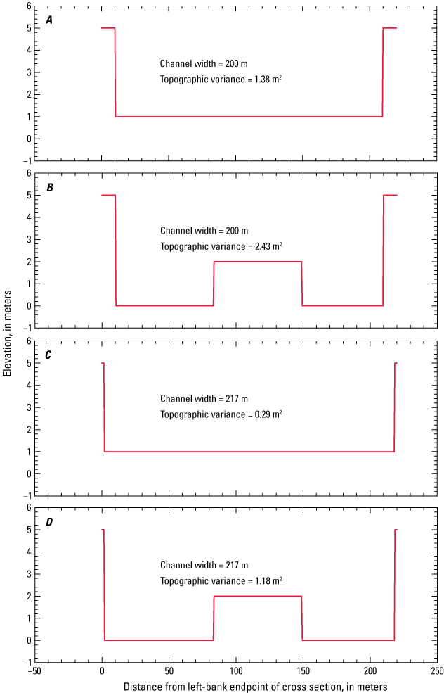
Plots of idealized river cross sections showing the offsetting effects of increased variability in bed elevation and channel widening on cross-section topographic variance. Topographic variance in A–D calculated among the elevations at 0.5-meter (m) intervals over a 220-m-wide domain. Topographic variance increases between A and B because of the development of a mid-channel bar and deeper thalwegs. Topographic variance decreases between A and C owing to channel widening from bank retreat. Although topographic variance increases between C and D because of the development of the mid-channel bar and deeper thalwegs, channel variance decreases between A and D because the effect of channel widening offsets and dominates over the effect of the development of the mid-channel bar and deeper thalwegs. m2, square meter.
Results with Discussion
Controls on Sediment Transport
Supply-Driven Decrease and Variation in Suspended-Silt-and-Clay Concentration
Substantial decreases in CSILT-CLAY have occurred at all stations except at the Green-Lodore station between the historical and 2013–2021 periods (fig. 8). The lack of a discernable decrease in CSILT-CLAY at the Green-Lodore station (fig. 8A) owes to this station’s relatively short 1997–2002 period of historical sediment record, and to the lack of suspended-sediment data collected before the construction of Flaming Gorge Dam. No historical period of sediment record exists at the Green-Ouray station. Among the other stations, the mean CSILT-CLAY at any given Q has shifted downward by between a factor of 2 and 10, with the greatest decreases in CSILT-CLAY observed at the LS-Lily and Green-Jensen stations (fig. 8C, E). These large decreases in CSILT-CLAY indicate that there has been a large decrease in the amount of silt and clay supplied to the rivers in our study area. Despite this net decrease in CSILT-CLAY between the historical and 2013–2021 periods, however, roughly two to four orders of magnitude variation in CSILT-CLAY in response to changes in the upstream supply of silt and clay is still possible at the stations in our study area (fig. 8). Most of this variation occurs during lower Q in the summer following thunderstorm-driven floods on upstream tributaries. As it did historically, the greatest amount of variation in CSILT-CLAY at any given Q still occurs at the LS-Lily station (fig. 8C), and the least amount of variation in CSILT-CLAY at any given Q still occurs at the Yampa-Maybell station (fig 8B).
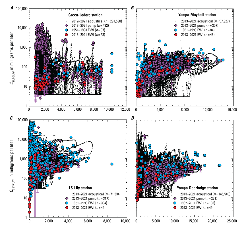
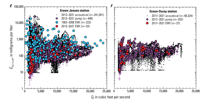
Plots of velocity-weighted suspended-silt-and-clay concentration (CSILT-CLAY) as a function of the instantaneous water discharge (Q) at the Green-Lodore (A), Yampa-Maybell (B), LS-Lily (C), Yampa-Deerlodge (D), Green-Jensen (E), and Green-Ouray stations (F). CSILT-CLAY measurements are plotted individually for each measurement type (acoustical, calibrated pump [pump], and equal-width increment [EWI]), with the number of measurements (n) indicated. Historical (pre-2013) EWI measurements of CSILT-CLAY are also plotted. Error bars on the 2013–2021 EWI and calibrated-pump measurements of CSAND and DS are the 95-percent-confidence-level combined field and laboratory errors (Topping and others, 2010, 2011); error bars on the acoustical measurements not shown to avoid clutter (refer to Topping and Wright, 2016, for the equations for these errors). Error bars could not be calculated for the historical EWI measurements owing to insufficient information. Years shown in explanation are water years. Station name abbreviations are defined in table 1; locations are shown in figure 1.
Flow versus Grain-Size Regulation of Suspended-Sand Concentration
The αC analyses summarized in table 4 indicate that CSAND is primarily regulated by changes in bed-sand grain size and not changes in flow at the four sand-bedded gaging stations in our study area: Green-Lodore, LS-Lily, Yampa-Deerlodge, and Green-Ouray (fig. 1). In addition, |αC| generally increases at each of these stations as the data type becomes more continuous. The reaches of these rivers upstream from these stations in which the suspended sand equilibrates with the bed are characterized by multiple thalwegs and downstream migrating mid-channel bars, with dunes present in the thalwegs and on the bars. On average among these stations, |αC| increases from ~1.4 for the EWI measurements (typically made 3–5 times per year), to ~2.7 for the calibrated-pump measurements (typically made every 3–4 days during periods of higher discharge3 ), and again to ~3.8 for the 15-minute acoustical measurements. Although part of the increase in |αC| can be explained by the increased error associated with individual measurements as the measurement type becomes more continuous (Topping and others, 2010, 2011, 2021; Topping and Wright, 2016), the increase in |αC| mostly arises from the more continuous measurements sampling a more complete range of flow and sediment conditions. Thus, for the limited flow and sediment conditions sampled by the relatively sparse EWI measurements, changes in bed-sand grain size are associated with slightly more (that is, ~1.4 times more) of the variation in CSAND than are changes in . And, for the more complete range of flow and sediment conditions sampled by the calibrated-pump and acoustical measurements, changes in bed-sand grain size are associated with much more (that is, ~3.3 times more) of the variation in CSAND than are changes in . Based on the proportionality, however, Q increases roughly 1.7 to 2.1 times faster than at the sand-bedded stations; the 1.7–2.1 range owes to the 0.05–0.2 range in the ε exponent on Q among the four sand-bedded stations estimated above in the “Regulation of Suspended-Sand Concentration by Flow, Grain Size, and Other Processes” subsection in the “Analytical Methods” section. Consequently, the average ~3.3 value of |αC| evaluated using the pump and acoustical measurements indicates that the variation in CSAND associated with changes in bed-sand grain size is almost twice as great as the variation in CSAND caused by changes in Q. This grain-size regulation of CSAND at the sand-bedded stations arises from two distinct processes: (1) changes in the bed-sand grain size caused by the downstream migration of sand waves (Topping and others, 2018), and (2) a tendency for the flow to access finer bed sand at higher Q (as described in detail in the next two sections).
The only exception to this pump-sampling scheme was at the Green-Lodore station, where pump samples were also collected in some summers during periods of higher turbidity. These turbidity-triggered samples were consequently clustered during periods following floods on upstream tributaries and collected at roughly hourly increments.
Table 4.
Results from the αC analyses at each station.[αC, measure of the relative importance of bed-sand grain size versus shear velocity in regulating the velocity-weighted suspended-sand concentration (CSAND). Station name abbreviations are defined in table 1; locations are shown in figure 1. EWI, equal-width-increment; n, number of measurements; r, correlation coefficient; DS, velocity-weighted suspended-sand median grain size; EWI, equal-width increment; Q, water discharge; ft3/s, cubic feet per second; mg/L, milligrams per liter; p, level of significance]
Only those acoustical measurements made when Q ≥ 2,000 ft3/s were used in this analysis to avoid using the acoustical measurements with the greatest error. At the Yampa-Deerlodge station, the acoustical measurements made when Q < 2,000 ft3/s are associated with acoustical measurements of DS that have much greater variation than the other more accurate measurement types (refer to fig. 11B), thus giving rise to unrealistically large values of |αC|.
Only those acoustical measurements with CSAND ≥ 2 mg/L were used in this analysis to avoid using the acoustical measurements with the greatest error. At the Green-Jensen station, the acoustical measurements where CSAND < 2 mg/L are associated with acoustical measurements of DS that have greater variation and much coarser values than the other more accurate measurement types (refer to fig. 14D), thus giving rise to unrealistically large values of |αC|. Because relatively little sand transport occurs when CSAND < 2 mg/L, it was deemed best to exclude these acoustical measurements from this analysis.
Correlation is not significant at the p = 0.05 critical level; no sign assigned to log10ΔCSAND/log10ΔDS in equation 4.
Correlation is significant at the p = 0.05 critical level but less than the r = |0.4| threshold used to assign sign to log10ΔCSAND/log10ΔDS in equation 4.
In contrast to the results at the sand-bedded stations, αC analyses indicate that CSAND is primarily regulated by changes in flow at the two largely gravel-bedded stations in our study area, Yampa-Maybell and Green-Jensen (fig. 1), although changes in bed-sand grain size still had important, though differing roles at these two stations. Comparison of the 2013–2021 αC analyses herein with the pre-2013 α analyses in Topping and others (2018)4 indicates that the relative importance of flow and bed-sand grain size in regulating CSAND at the Yampa-Maybell station has not changed over time between the historical (1951–1979) and the modern (2013–2021) periods. However, this same comparison indicates that a large change in the relative importance of flow versus bed-sand grain-size regulation of CSAND has occurred at the Green-Jensen station. The relatively abrupt decrease in the importance of grain-size regulation of CSAND at the Green-Jensen station between 2007 and 2013 represents the greatest fundamental change in the boundary conditions that control sand transport in our study area, as we elaborate upon below.
The α values in Topping and others (2018) must be divided by 1.3 to allow a direct comparison with the αC values provided herein, as described in the “Regulation of Suspended-Sand Concentration by Flow, Grain Size, and Other Processes” subsection in the “Analytical Methods” section.
At the Yampa-Maybell station, αC analyses indicate that changes in flow are more important than changes in bed-sand grain size in regulating CSAND, with the relative importance of flow regulation likely increasing as Q increases. The Yampa River at this station is largely gravel bedded. Though sand is present in the interstices of the cobbles on the bed, most of the sand in this segment of the Yampa River occurs in point bars that are inundated at only higher Q. Based on the EWI measurements that yield |αC| = 0.69, the variation in CSAND caused by changes in is slightly more (that is, ~1.4 times more) than the variation in CSAND associated with changes in bed-sand grain size. Analysis of the calibrated-pump measurements suggests that flow regulation of CSAND becomes more important when the lowest flows are excluded; these measurements are more continuous than the EWI measurements but restricted to only higher Q. αC analysis of these pump data suggest that at higher Q, the variation in CSAND caused by changes in is almost 6 times the variation in CSAND associated with changes in bed-sand grain size. Based on the proportionality , however, Q increases ~1.6 times faster than at the Yampa-Maybell station; the 0.3 value of the ε exponent on Q was estimated above in the “Regulation of Suspended-Sand Concentration by Flow, Grain Size, and Other Processes” subsection in the “Analytical Methods” section. Consequently, the αC analysis of the EWI data suggest that, over the entire range in Q sampled by the EWI measurements, the variation in CSAND caused by changes in Q is roughly twice the variation in CSAND associated with changes in bed-sand grain size. At only the higher Q sampled by the calibrated-pump measurements, however, the αC analysis of the pump data suggests that variation in CSAND caused by changes in Q is perhaps 10 times greater than the variation in CSAND associated with changes in bed-sand grain size. These results further suggest that the greatest variation in bed-sand grain size occurs at lower Q at this station, and that less variation occurs in the bed-sand grain-size distribution accessed by the flow once the sandy point bars are inundated at higher Q.
At the Green-Jensen station, αC analyses of the modern water year 2013–2021 data indicate that changes in flow are more important than changes in bed-sand grain size in regulating CSAND. Moreover, these analyses indicate that the relative importance of grain-size regulation increases as the data type analyzed progress from least continuous (EWI) to most continuous (acoustical). Analysis of the EWI measurements yields |αC| = 0.13, thus indicating that, over the more limited range of flow and sediment conditions sampled by these measurements, roughly 8 times more of the variation in CSAND is caused by changes in than is associated with changes in bed-sand grain size. Analyses of the more continuous calibrated-pump measurements and 15-minute acoustical measurements yield an average |αC| of 0.32, thus indicating roughly 3 times more of the variation in CSAND is caused by changes in than is associated with changes in bed-sand grain size. Conversion of to Q using the proportionality indicates that, for the relatively complete range of flow and sediment conditions sampled by the calibrated-pump and acoustical measurements, ~4.5 times more variation in CSAND is caused by changes in Q than is associated with changes in bed-sand grain size at the Green-Jensen station. As above, the 0.4 value of the ε exponent on Q was estimated in the “Regulation of Suspended-Sand Concentration by Flow, Grain Size, and Other Processes” subsection in the “Analytical Methods” section.
Comparison of the αC analyses of the historical 1951–2007 and modern 2013–2021 data at the Green-Jensen station indicate that changes in bed-sand grain size were far more important in regulating CSAND as recently as 2007. Because no continuous suspended-sand measurements were made historically, detection of changes in the controls on sand transport must unfortunately rely on the relatively sparse EWI measurements. Reanalysis of the EWI α analyses in Topping and others (2018) as αC analyses indicates that, during water years 1951–2007, changes in caused twice the variation in CSAND as was associated with changes in bed-sand grain size. Analysis of only the water year 1996–2007 EWI measurements confirm that this condition persisted through 2007 and was not a direct result of the 1962 closure of Flaming Gorge Dam. Consequently, comparison of the αC analyses of the water year 1951–2007 and 2013–2021 EWI measurements indicates that a factor-of-4 decrease in the importance of bed-sand grain size in regulating CSAND occurred at the Green-Jensen station between 2007 and 2013. Thus, it is likely that changes in bed-sand grain size were associated with the same amount of variation in CSAND as were changes in Q prior to 2007 (that is, dividing the factor-of-4.5 result in the previous paragraph by 4 yields 1.1). This result indicates that the historical influence of changing bed-sand grain size on CSAND at the Green-Jensen station was more like that observed both historically and currently at the four sand-bedded stations (that is, at the Green-Lodore, LS-Lily, Yampa-Deerlodge, and Green-Ouray stations).
The modern Green River in the vicinity of the Green-Jensen station is typically gravel bedded, with patches of sand that have been observed to vary in size. After this station was moved 4.1 km upstream in 2016 (fig. 1B), the collection of bed-sediment samples became a routine part of the sampling program. Large changes in bed-sand area have been observed between visits, with sand covering large parts of the bed during some sampling visits and sand too scarce to be sampled during other visits. Because greater grain-size regulation of CSAND likely requires a larger amount of sand on the bed, it is possible that the post-2007 increase in flow regulation of CSAND at this station was associated with a decrease in the average amount of sand covering the cobble bed.
Placement of the αC Results in Context
Graphical analyses of the suspended-sediment measurements in our study area provide guidance on the cause of grain-size regulation at each station (figs. 9–14). We describe the interrelations observed between water discharge (Q), suspended-sand concentration (CSAND), suspended-sand median grain size (DS), and nondimensional bed-sand grain size (β) at the four sand-bedded stations first.
The mean behavior of CSAND as a function of Q at the four sand-bedded stations (Green-Lodore, LS-Lily, Yampa-Deerlodge, and Green-Ouray) is well-described by suspended-sediment theory. Using equation 3 to substitute Qε for in equation 2A while holding bed-sand grain size constant yields the following:
where a0 is a station-specific constant determined by regression, the station-specific values of ε were estimated in the “Regulation of Suspended-Sand Concentration by Flow, Grain Size, and Other Processes” subsection of the “Analytical Methods” section, and J = 3.5 (defined in that same section). Equation 7 is the theoretical relation between Q and CSAND for the condition of constant bed-sand grain size, derived for a particular station using the mean relation between Q and at that station. This equation was used to fit the orange curves in figures 9A, 10A, 11A, and 12A to the modern EWI measurements, with a0 evaluated by regression to provide the best fit at each station. Because the flow at all four sand-bedded stations accesses finer bed sand at higher Q, however, agreement between the theory-derived mean behavior of CSAND as a function of Q and that observed among the measurements is improved by including the systematic effect of fining bed-sand grain size with increasing Q.At all four sand-bedded stations, DS generally either remains constant or decreases slightly as Q increases (figs. 9B, 10B, 11B, 12B) because the flow accesses finer bed sand as Q increases (figs. 9C, 10C, 11C, 12C). As shown in the next section, the most probable cause of this response is that increasing Q causes scour through an inversely graded bed at or in the reach upstream from each station, thereby causing an increase in the “local” sand supply. By the simplification of suspended-sediment theory in equation 2B (that is, ) and because generally increases with increasing Q, DS will generally increase with increasing Q unless DB decreases with increasing Q. Access of the flow to a constant bed-sand grain-size distribution would thus cause both CSAND and DS to increase as Q increases. At all four sand-bedded stations, the fact that DS does not increase (coarsen) with increasing Q is the reason β decreases (fines) with increasing Q (figs. 9C, 10C, 11C, 12C). We added this effect of bed-sand fining with increasing Q to the analysis in the previous paragraph by first evaluating power-law regression of β on Q for the modern EWI measurements, with ζ being the regression-estimated exponent on Q. The proportionality describing this power law was thus . We then included this power law in a version of equation 7 modified to include changing bed-sand grain size. The values of ζ estimated by power-law regression at each station were −0.3 at Green-Lodore, −0.1 at LS-Lily, −0.06 at Yampa-Deerlodge, and −0.2 at Green-Ouray. By using this approach, all changes in the bed-sand grain-size distribution detected by β are assigned to be from changes in DB (Rubin and Topping, 2001, 2008). We do this for simplicity, even though the β-detected changes are likely from changes mostly in the fine tail of the bed-sand grain-size distribution, as shown by Topping and others (2018), and demonstrated in the next section of this report. Substitution of Qε for in equation 2A (as in equation 7), followed by substitution of β for DB in equation 2A, re-substitution of Qζ for β, and inclusion of a new station-specific regression constant a1 yielded the following modified version of equation 7:
that is, the green curves fit to the modern EWI measurements in figures 9A, 10A, 11A, and 12A. As defined in the “Regulation of Suspended-Sand Concentration by Flow, Grain Size, and Other Processes” subsection of the “Analytical Methods” section, J = 3.5 and K = −2.5.Although the theoretical fits capture the mean behavior of CSAND as a function of Q at the sand-bedded stations, substantial variation exists about the orange and green curves in figures 9A, 10A, 11A, and 12A. At least a factor-of-3 variation in CSAND above and below these curves exists at most Q (for a total factor-of-6 variation), with perhaps a factor-of-10 variation in CSAND present at lower Q. In descending order of importance, the two main processes that give rise to this Q-independent variation in CSAND at the four sand-bedded stations are (1) changes in the bed-sand grain size caused by changes in the upstream sand supply (described in the next paragraph), and (2) changes related to . The magnitude of the variation in CSAND caused by Q-independent changes related to is documented below in the “Importance of Discharge-Independent Flow Regulation of Suspended-Sand Concentration at the Sand-Bedded Stations Likely Arising from the Downstream Migration of Sand Waves” subsection.
The magnitude of the Q-independent variation in bed-sand grain size caused by changes in the upstream sand supply is of the same magnitude as the decrease in bed-sand grain size associated with increasing Q described above. This result is indicated by the magnitude of the mean decrease in β with increasing Q being similar to the magnitude of the variation in β at any given Q in figures 9C, 10C, 11C, and 12C. Thus, the dominance of grain-size regulation of CSAND at all four sand-bedded stations indicated by the values of |αC| in table 4 is caused by changes in bed-sand grain size associated with (1) the changes in the upstream sand supply associated with the downstream migration of sand waves that were generated by floods on upstream tributaries, and (2) the changes in the local sand supply associated with the flow accessing finer bed sand at higher Q. Because CSAND is mostly regulated by bed-sand grain size and not Q (although Q is associated with changes in bed-sand grain size as recognized in the previous two paragraphs), CSAND is inversely related to DS at the four sand-bedded stations (figs. 9D, 10D, 11D, 12D). Thus, the largest values of CSAND are associated with the smallest (finest) values of DS. This result is the opposite of that expected if CSAND were mainly regulated by Q and bed-sand grain size remained constant. This inverse relation between DS and CSAND arises because CSAND is inversely related to bed-sand grain size, as inferred from β (figs. 9E, 10E, 11E, 12E). Consequently, β is almost as good a predictor of CSAND as is Q at the four sand-bedded stations because the negative correlation between β and CSAND is significant and moderate to strong at these stations (table 5), and because the largest values of CSAND always correspond to the smallest (finest) values of β (figs. 9E, 10E, 11E, 12E). Thus, predictions of CSAND at the Green-Lodore, LS-Lily, Yampa-Deerlodge, and Green-Ouray stations must take both Q and bed-sand grain size into account.
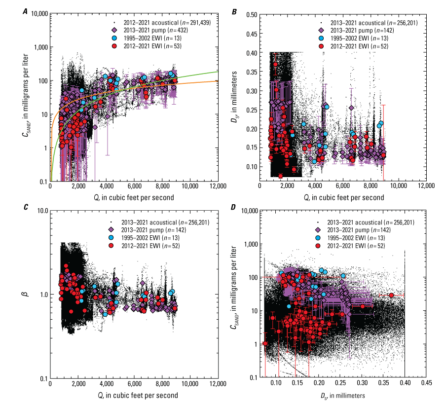
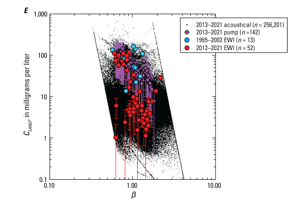
Plots of relations between the instantaneous water discharge (Q), velocity-weighted suspended-sand concentration (CSAND), velocity-weighted suspended-sand median grain size (DS), and nondimensional bed-sand coarseness (β) at the Green River above Gates of Lodore, Colorado, gaging station 404417108524900 (Green-Lodore station). Values plotted individually for each measurement type: acoustical, calibrated pump, historical (pre-2013) equal-width increment (EWI), and modern (2012–2021) EWI, with the number of measurements (n) indicated. Error bars on the 2012–2021 EWI and calibrated-pump measurements of CSAND and DS are the 95-percent-confidence-level combined field and laboratory errors (Topping and others, 2010, 2011); error bars on the acoustical measurements not shown to avoid clutter (refer to Topping and Wright, 2016, for the equations for these errors). Error bars could not be calculated for the historical EWI measurements owing to insufficient information. Years shown are water years. A, CSAND plotted as a function of Q. Orange curve is the theoretical fit to the 2012–2021 EWI measurements using the mean relation between Q and shear velocity () at this station estimated from Q measurements and equation 2A. Green curve is the modification of the orange curve that includes a power-law fit to the β-inferred fining of the bed sand with increasing Q at this station. B, DS plotted as a function of Q. C, β plotted as a function of Q. D, CSAND plotted as a function of DS. E, CSAND plotted as a function of β.
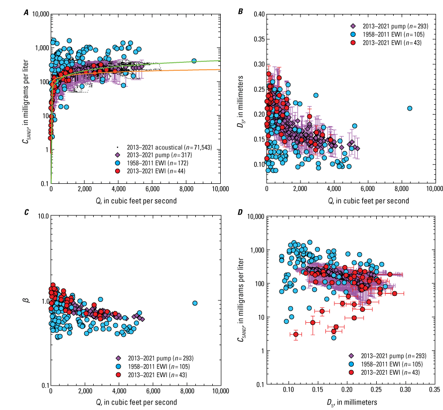
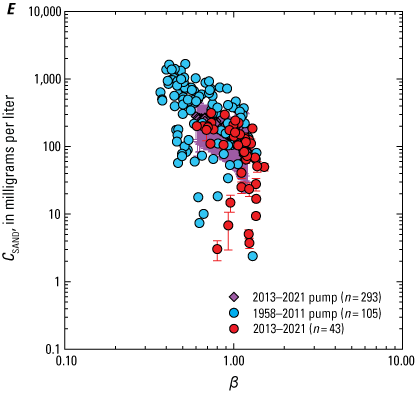
Plots of relations between the instantaneous water discharge (Q), velocity-weighted suspended-sand concentration (CSAND), velocity-weighted suspended-sand median grain size (DS), and nondimensional bed-sand coarseness (β) at the Little Snake River near Lily, Colorado, gaging station 09260000 (LS-Lily station). Values plotted individually for each measurement type: acoustical, calibrated pump, historical (pre-2013) equal-width increment (EWI), and modern (2013–2021) EWI, with the number of measurements (n) indicated. Error bars on the 2013–2021 EWI and calibrated-pump measurements of CSAND and DS are the 95-percent-confidence-level combined field and laboratory errors (Topping and others, 2010, 2011); error bars on the acoustical measurements not shown to avoid clutter (refer to Topping and Wright, 2016, for the equations for these errors). Error bars could not be calculated for the historical EWI measurements owing to insufficient information. Years shown are water years. A, CSAND plotted as a function of Q. Orange curve is the theoretical fit to the 2013–2021 EWI measurements using the mean relation between Q and shear velocity () at this station estimated from Q measurements and equation 2A. Green curve is the modification of the orange curve that includes a power-law fit to the β-inferred fining of the bed sand with increasing Q at this station. B, DS plotted as a function of Q. C, β plotted as a function of Q. D, CSAND plotted as a function of DS. E, CSAND plotted as a function of β.
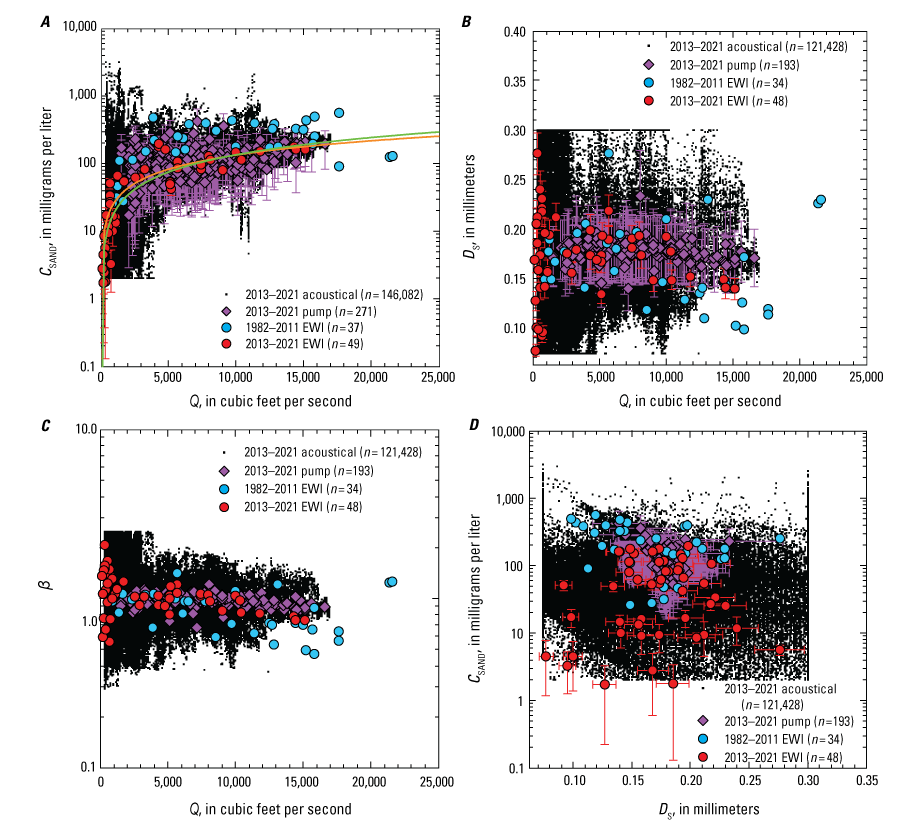
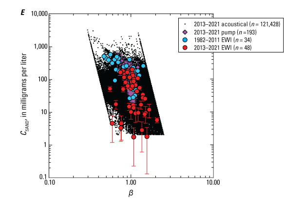
Plots of relations between the instantaneous water discharge (Q), velocity-weighted suspended-sand concentration (CSAND), velocity-weighted suspended-sand median grain size (DS), and nondimensional bed-sand coarseness (β) at the Yampa River at Deerlodge Park, Colorado, gaging station 09260050 (Yampa-Deerlodge station). Values plotted individually for each measurement type: acoustical, calibrated pump, historical (pre-2013) equal-width increment (EWI), and modern (2013–2021) EWI, with the number of measurements (n) indicated. Error bars on the 2013–2021 EWI and calibrated-pump measurements of CSAND and DS are the 95-percent-confidence-level combined field and laboratory errors (Topping and others, 2010, 2011); error bars on the acoustical measurements not shown to avoid clutter (refer to Topping and Wright, 2016, for the equations for these errors). Error bars could not be calculated for the historical EWI measurements owing to insufficient information. Years shown are water years. A, CSAND plotted as a function of Q. Orange curve is the theoretical fit to the 2013–2021 EWI measurements using the mean relation between Q and shear velocity () at this station estimated from Q measurements and equation 2A. Green curve is the modification of the orange curve that includes a power-law fit to the β-inferred fining of the bed sand with increasing Q at this station. B, DS plotted as a function of Q. C, β plotted as a function of Q. D, CSAND plotted as a function of DS. E, CSAND plotted as a function of β.
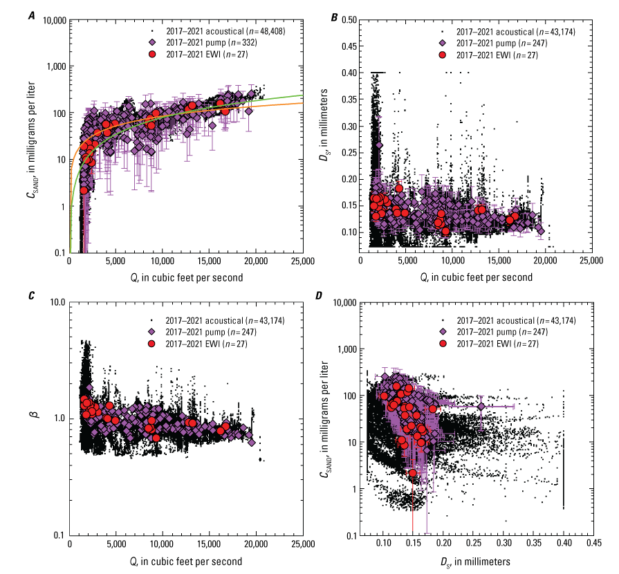
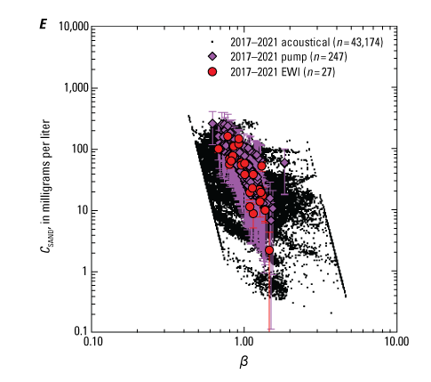
Plots of relations between the instantaneous water discharge (Q), velocity-weighted suspended-sand concentration (CSAND), velocity-weighted suspended-sand median grain size (DS), and nondimensional bed-sand coarseness (β) on the Green River above Ouray, Utah, monitoring station (Green-Ouray station). Values plotted individually for each measurement type: acoustical, calibrated pump, and 2017–2021 equal-width increment (EWI), with the number of measurements (n) indicated. Error bars on the 2017–2021 EWI and calibrated-pump measurements of CSAND and DS are the 95-percent-confidence-level combined field and laboratory errors (Topping and others, 2010, 2011); error bars on the acoustical measurements not shown to avoid clutter (refer to Topping and Wright, 2016, for the equations for these errors). Years shown are water years. A, CSAND plotted as a function of Q. Orange curve is the theoretical fit to the 2017–2021 EWI measurements using the mean relation between Q and shear velocity () at this station estimated from Q measurements and equation 2A. Green curve is the modification of the orange curve that includes a power-law fit to the β-inferred fining of the bed sand with increasing Q at this station. B, DS plotted as a function of Q. C, β plotted as a function of Q. D, CSAND plotted as a function of DS. E, CSAND plotted as a function of β.
Table 5.
Significance, signs, and magnitudes of correlations between β and CSAND.[β, measure of relative coarseness of the bed sand; CSAND, velocity-weighted suspended-sand concentration. Historical equal-width increment (EWI) indicates pre-2012. n, number of measurements; p, level of significance; r, correlation coefficient; Q, water discharge; ft3/s, cubic feet per second; DS, velocity-weighted suspended-sand median grain size; mg/L, milligrams per liter]
As in table 4, only those acoustical measurements made when Q ≥ 2,000 ft3/s were used in this analysis to avoid using the acoustical measurements with the greatest error. At the Yampa-Deerlodge station, the acoustical measurements made when Q < 2,000 ft3/s are associated with acoustical measurements of DS that have much greater variation than the other more accurate measurement types (refer to fig. 11B), thus giving rise to potentially anomalous values of β.
The values in this row utilize only those EWI measurements made after closure of Flaming Gorge Dam on December 10, 1962.
As in table 4, only those acoustical measurements with CSAND ≥ 2 mg/L were used in this analysis to avoid using the acoustical measurements with the greatest error. At the Green-Ouray station, the acoustical measurements where CSAND < 2 mg/L are associated with acoustical measurements of DS that have greater variation and much coarser values than the other more accurate measurement types (refer to fig. 14D), thus giving rise to potentially anomalous values of β.
The mean behavior of CSAND as a function of Q at the two largely gravel-bedded stations (Yampa-Maybell and Green-Jensen) is also well-described by suspended-sediment theory, but with some key underlying differences from the behavior at the four sand-bedded stations. Using the same approach as at the sand-bedded stations for constant bed-sand grain size, equation 7 yields the orange curves fit to the modern EWI measurements in figures 13A and 14A. Unlike at the four sand-bedded stations where the flow universally accesses finer bed sand at higher Q, however, the flow accesses finer bed sand at higher Q at only the Yampa-Maybell station. At this station, DS decreases slightly as Q increases between baseflow and ~2,000 ft3/s, and then increases as Q continues to increase (fig. 13B). This Q-dependent behavior in DS arises because the bed-sand grain size (inferred from β) decreases as Q increases between baseflow and ~2,000 ft3/s, and then remains constant as Q continues to increase above 2,000 ft3/s (fig. 13C). Because the bed is largely composed of gravel at the Yampa-Maybell station, this behavior does not arise from scour through an inversely graded bed (as at the sand-bedded stations) and likely owes to a different process, as elaborated upon in the next section of this report. Conversely, at the Green-Jensen station, DS generally increases as Q increases (fig. 14B) and, although variable, no Q-dependent trend exists in the bed-sand grain size accessed by the flow (fig. 14C). Thus, the theoretical effect of decreasing bed-sand grain size with increasing Q was included in the predicted mean behavior of CSAND by applying equation 8 at the Yampa-Maybell station (ζ = −0.1; green curve in fig. 13A) but not at the Green-Jensen station. As at the sand-bedded stations, inclusion of this effect at the Yampa-Maybell station improved the agreement between the theory-predicted and observed mean behavior of CSAND at this station.
Substantial variation exists about the orange and green curves defining the theory-derived mean behavior of CSAND as a function of Q at both gravel-bedded stations (figs. 13A, 14A). As at the sand-bedded stations, at least a factor-of-3 variation in CSAND is present about these curves at most Q (for a total factor-of-6 variation), with perhaps a factor-of-10 variation in CSAND present at lower Q. Although the primary process responsible for this Q-independent variation in CSAND is the same as at the sand-bedded stations (that is, changes in the bed-sand grain size caused by changes in the upstream sand supply) the secondary process is different. At the sand-bedded stations, differences in cross-section, bar, and dune geometry can affect either or the skin-friction component of (that is, ), as documented below in the “Importance of Discharge-Independent Flow Regulation of Suspended-Sand Concentration at the Sand-Bedded Stations Likely Arising from the Downstream Migration of Sand Waves” subsection. However, the secondary process that gives rise to Q-independent variation in CSAND at the gravel-bedded stations is likely a change in bed-sand area caused by changes in the upstream sand supply, as documented below in the “Partial Regulation of Suspended-Sand Concentration by Discharge-Independent Changes in Bed-Sand Area at the Largely Gravel-Bedded Stations” subsection.
Although Q is more important than bed-sand grain size in regulating CSAND at the Yampa-Maybell station and post-2007 at the Green-Jensen station, Q-independent variation in bed-sand grain size still has an important role at these two largely gravel-bedded stations. As at the sand-bedded stations, the Q-independent variation in bed-sand grain size caused by changes in the upstream sand supply is reasonably large (figs. 13C, 14C). In fact, the Q-independent variation in β at the Green-Jensen station is as large as that observed at any of the sand-bedded stations (figs. 9C, 10C, 11C, 12C, 14C). In addition, the largest values of CSAND at both stations tend to be associated with the smallest values of β (that is, the finest bed-sand grain size) and are not necessarily associated with the largest Q (figs. 13E, 14E). This result differs from that expected when Q regulation of CSAND dominates, where changes in bed-sand grain size do not greatly influence CSAND. At the Yampa-Maybell station, CSAND is inversely related to bed-sand grain size (fig. 13E; table 5), as also observed at the four sand-bedded stations. Unlike at the sand-bedded stations, however, there is no clear relation between CSAND and DS at the Yampa-Maybell station (fig. 13D). Pre-2007, CSAND was also inversely related to bed-sand grain size at the Green-Jensen station (fig. 14E), although the negative correlation between β and CSAND was weaker than at all other stations (table 5).
Conditions at the Green-Jensen station changed between 2007 and 2013, such that no clear relation has existed between bed-sand grain size and CSAND at this station since at least 2013, though the largest values of CSAND still tend to be associated with the smallest values of β (fig. 14E). Moreover, there was a tendency for the largest values of CSAND to be associated with the finest values of DS at the Green-Jensen station before 2007 (fig. 14D), as also observed currently at the four sand-bedded stations. Since at least 2013, however, CSAND has increased with increasing DS at the Green-Jensen station. Although the calibrated-pump measurements suggest a positive relation between β and CSAND at the Green-Jensen station, no significant relation exists between β and CSAND for the 2013–2021 EWI measurements, and the extremely weak (r = 0.076) positive relation between β and CSAND for the acoustical measurements is negligible, though significant because of the large number of measurements (table 5). Despite Q being more important than bed-sand grain size in regulating CSAND, predictions of CSAND at the Yampa-Maybell and Green-Jensen stations must take both Q and bed-sand grain size into account because the largest values of CSAND tend to be associated with the smallest values of β (just like at all the sand-bedded stations where bed-sand grain size was found to be more important than Q in regulating CSAND).
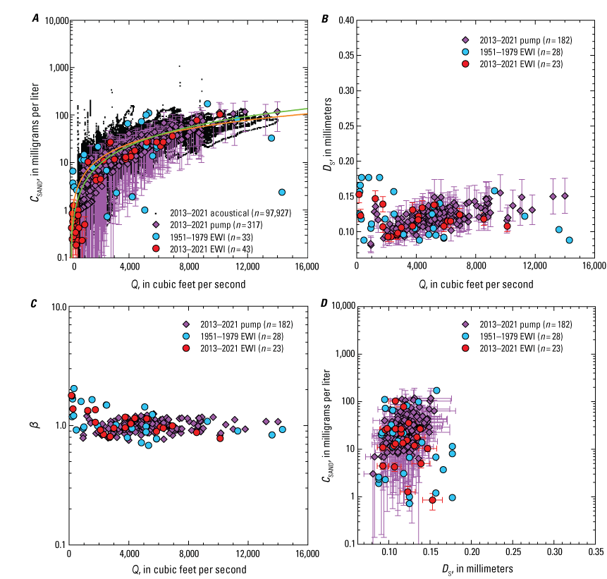
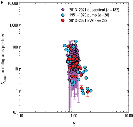
Plots of relations between the instantaneous water discharge (Q), velocity-weighted suspended-sand concentration (CSAND), velocity-weighted suspended-sand median grain size (DS), and nondimensional bed-sand coarseness (β) at the Yampa River near Maybell, Colorado, gaging station 09251000 (Yampa-Maybell station). Values plotted individually for each measurement type: acoustical, calibrated pump, historical (pre-2013) equal-width increment (EWI), and modern (2013–2021) EWI, with the number of measurements (n) indicated. Error bars on the 2013–2021 EWI and calibrated-pump measurements of CSAND and DS are the 95-percent-confidence-level combined field and laboratory errors (Topping and others, 2010, 2011); error bars on the acoustical measurements not shown to avoid clutter (refer to Topping and Wright, 2016, for the equations for these errors). Error bars could not be calculated for the historical EWI measurements owing to insufficient information. Years shown are water years. A, CSAND plotted as a function of Q. Orange curve is the theoretical fit to the 2013–2021 EWI measurements using the mean relation between Q and shear velocity () at this station estimated from Q measurements and equation 2A. Green curve is the modification of the orange curve that includes a power-law fit to the β-inferred fining of the bed sand with increasing Q at this station. B, DS plotted as a function of Q. C, β plotted as a function of Q. D, CSAND plotted as a function of DS. E, CSAND plotted as a function of β.
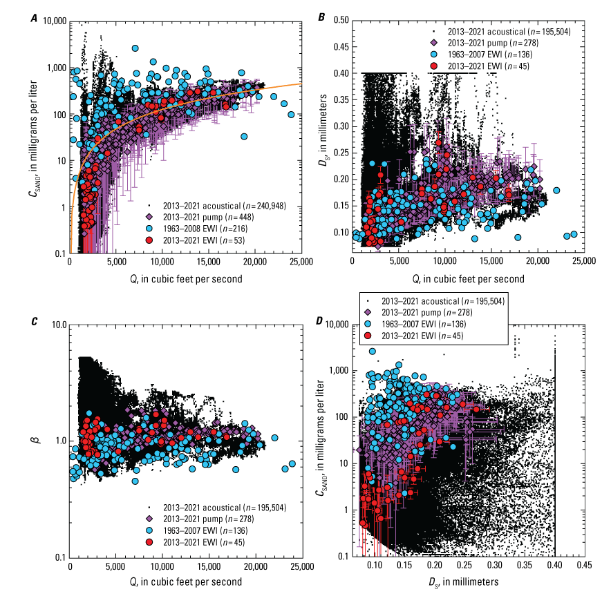
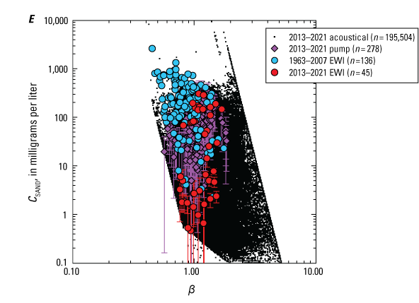
Plots of relations between the instantaneous water discharge (Q), velocity-weighted suspended-sand concentration (CSAND), velocity-weighted suspended-sand median grain size (DS), and nondimensional bed-sand coarseness (β) at the Green River near Jensen, Utah, gaging station 09261000 and Green River above Jensen, Utah, monitoring station. These two nearby stations have equivalent sediment-transport conditions and are collectively referred to as the Green-Jensen station in the text. Values plotted individually for each measurement type: acoustical, calibrated pump, historical (pre-2013) equal-width increment (EWI), and modern (2013–2021) EWI, with the number of measurements (n) indicated. Error bars on the 2013–2021 EWI and calibrated pump measurements of CSAND and DS are the 95-percent-confidence-level combined field and laboratory errors (Topping and others, 2010, 2011); error bars on the acoustical measurements not shown to avoid clutter (refer to Topping and Wright, 2016, for the equations for these errors). Error bars could not be calculated for the historical EWI measurements owing to insufficient information. Years shown are water years. A, CSAND plotted as a function of Q. Orange curve is the theoretical fit to the 2013–2021 EWI measurements using the mean relation between Q and shear velocity () at this station estimated from Q measurements and equation 2A. B, DS plotted as a function of Q. C, β plotted as a function of Q. D, CSAND plotted as a function of DS. E, CSAND plotted as a function of β.
Grain-Size-Associated Long-Term Change in Suspended-Sand Concentration
Substantial decreases in CSAND have occurred in the Little Snake, lower Yampa, and middle Green Rivers since the 1960s resulting from the bed-sand coarsening caused by the winnowing of the tail(s) of the sand wave(s) generated by the large Sand Creek floods of March 1956, 1962, and 1966 (Topping and others, 2018). These decreases in CSAND are manifest by downward shifts in the Q—CSAND “point clouds” coupled with upward steps in the Q—DS and Q—β point clouds defined by the historical and 2013–2021 EWI measurements at the LS-Lily (fig. 10A–C), Yampa-Deerlodge (fig. 11A–C), and Green-Jensen stations (fig. 14A–C). We use the term “point cloud” and not “relation” because of the large systematic variation in CSAND, DS, and β when plotted as a function of Q, variation which is caused by changes in bed-sand grain size, bed-sand area, , and , as documented in the previous sections of this report. In addition, the net bed-sand coarsening that has occurred at these stations has resulted in the loss of the largest CSAND values that were historically associated with the finest DS and bed-sand grain size (β) at these stations (figs. 10D–E, 11D–E, 14D–E). In contrast, relatively little change in the Q—CSAND, Q—DS, and Q—β point clouds has occurred at either the Green-Lodore or Yampa-Maybell stations (figs. 9A–C, 13A–C) because only negligible changes in the bed-sand grain size have occurred at these stations between the historical and modern (2013–2021) periods (Topping and others, 2018). At the Yampa-Maybell station, the greater variation in the historical data is the likely consequence of a change in the measurement location for this station between the collection of the historical and modern data, as described in Text S1 in the Supporting Information document for Topping and others (2018).
Evidence for Scour Through an Inversely Graded Bed During the Annual Flood
The most probable cause of the decreases in bed-sand grain size (that is, bed-sand fining) associated with increases in Q at the four sand-bedded stations is the progressive scour through an inversely graded bed during the rising limb of the annual flood, as evidenced from paired EWI and bed-sediment measurements. In our study area, this inverse grading is manifest mainly in the fine tail of the bed-sand grain-size distribution and is not evident in the median grain size of the bed sand (DB). We thus use the mean amount of very fine sand on the bed in the cross section (fVF) as the metric to detect inverse grading. Scour through an inversely graded bed has been previously documented through direct measurements of bed-sand grain size as a function of scour depth in the lower Green River at the measurement cross section at the Green River at Mineral Bottom near Canyonlands National Park gaging station 09328920 (Dean and others, 2020). Moreover, though annual snowmelt floods no longer occur on the Colorado River downstream from Glen Canyon Dam, this process was also shown to be one of the most likely mechanisms to explain the negative correlation between bed-sand grain size and Q observed in both direct bed-sediment measurements and in β at multiple gaging stations on the Colorado River in Marble and Grand Canyons (Topping and others, 2021). Thus, bed-sand fining produced by scour through an inversely graded bed is likely a common occurrence in the sand-bedded parts of the rivers of the Colorado River basin. Presumably, the mechanism that would create the inversely graded bed would be the winnowing of the fine tail of the bed-sand grain-size distribution as the scoured parts of the bed refill during periods of reduced upstream sand supply under the influence of the moderate and lower Q during and following recession of the annual flood.
The LS-Lily station provides the clearest example of this process in our study area, with progressively weaker evidence observed at the Yampa-Deerlodge, Green-Ouray, and Green-Lodore stations. Before examining this evidence, however, it is important to note that the location of the measurement cross section varies slightly between sampling visits at some of these stations, thus the bed-sediment conditions measured (scour depth and grain size) are not always in the same cross section. EWI and bed-sediment measurements are always made in the same cross section only at higher Q at the LS-Lily station (at the upstream side of the County Road 10 bridge), and, except during one visit, at all Q at the Green-Ouray station (at the fishing platform in Ouray National Wildlife Refuge; location of cross section within photographed view on cover). EWI and bed-sediment measurements are typically made at cross sections located within tens of meters of the same longitudinal position at lower Q at the LS-Lily station and during all Q at the Green-Lodore and Yampa-Deerlodge stations; thus, more variability may exist in the bed-sediment conditions analyzed at these stations than those at the Green-Ouray station and at higher Q at the LS-Lily station.
At the LS-Lily station, the negative correlation between Q and bed stage (hB) is very strong (r = −0.93) and highly significant (fig. 15A). Though there is no significant relation between bed stage and DB (fig. 15B), the negative correlation between bed stage and log10(fVF) is also very strong (r = −0.73, fig. 15C), and the associated positive correlation between bed stage and β is also very strong (r = 0.81, fig. 15D). In our analyses, fVF is log-transformed where it is compared to β because β is linearly and negatively related to log10(fVF) by the physics that govern suspended sediment (Topping and others, 2021). As shown previously for the rivers in this study, changes in β track much more strongly with changes in the fine tail of the bed-sand grain-size distribution than with changes in DB (Topping and others, 2018). Thus, the negative correlation between log10(fVF) and β is very strong (r = −0.70, fig. 15E). And, because the bed at the LS-Lily station tends to scour with increasing Q, thereby exposing finer bed sand deeper in the inversely graded bed (that is, increasing fVF), β decreases linearly as Q increases (r = −0.76, fig. 15F).
At the Yampa-Deerlodge station, the negative correlation between Q and bed stage is also very strong (r = −0.80) and highly significant (fig. 16A). As at the LS-Lily station, there is also no significant relation between bed stage and DB (fig. 16B). The negative correlation between bed stage and log10(fVF) is much weaker (r = −0.21, fig. 16C) than at LS-Lily, and unlike at LS-Lily, is insignificant (p = 0.16). The relative weakness and insignificance of this correlation owes to one bed-sediment measurement (circled in blue in fig. 16C), however, in which bed sediment could be sampled at only half of the 10 EWI verticals. Of all the bed-sediment measurements made at the four sand-bedded stations, this bed-sediment measurement is, by far, the measurement covering the lowest percentage of the cross section. Thus, the likelihood exists that this one measurement is not as representative of the bed-sand grain-size distribution in the reach upstream from the measurement cross section as are the other bed-sediment measurements. Exclusion of this one measurement results in the negative correlation between bed stage and log10(fVF) becoming stronger, though still weak (r = −0.36), and significant (p = 0.022). Because the negative correlation between bed stage and log10(fVF) is weaker at Yampa-Deerlodge than at LS-Lily, the positive correlation between bed stage and β is also weaker (r = −0.31, fig. 16D) than at LS-Lily (where r = −0.81). In association with these weaker correlations between bed stage and bed-sand grain size, the negative correlation between log10(fVF) and β at Yampa-Deerlodge is also weaker (r = −0.23, fig. 16E) than at LS-Lily and is insignificant.
Part of the weakness in the correlation between log10(fVF) and β at Yampa-Deerlodge is likely because the bed-sand grain-size distribution at the measurement cross section becomes less representative of the bed-sand grain-size distribution in equilibrium with the suspended sand at higher Q. The reach length over which suspended sand equilibrates with the bed increases as Q increases (Topping and others, 2007, 2021). Consequently, β is expected to provide a better measure of the reach-averaged bed-sand grain-size distribution than do direct bed-sediment measurements made at only one cross section because β uses the physical processes that govern suspended sediment to “sample” the bed (Rubin and Topping, 2001). Thus, for the flow conditions that exist near the Yampa-Deerlodge station at higher Q, the suspended sand is likely equilibrating with the bed-sand grain-size distribution in a spatially averaged sense over hundreds of meters upstream from the measurement cross section. Evidence for this effect is provided by the fact that the negative correlation between log10(fVF) and β increases to moderate (r = −0.58) and becomes significant (p = 0.039) when discharges larger than 600 ft3/s are excluded from the analysis (fig. 16E). Thus, the bed-sediment grain size measured at the cross section is in much better agreement with β at lower Q, in which the suspended sand is equilibrating with the bed over a shorter reach length. Despite the additional complexities at the Yampa-Deerlodge station that were not observed at the LS-Lily station, the evidence is still moderately strong that scour through an inversely graded bed at Yampa-Deerlodge exposes finer bed sand that then causes β to decrease linearly as Q increases (fig. 16F), albeit with a weaker correlation (r = −0.42) than at LS-Lily (where r = −0.81, fig. 15D).
The evidence is weaker at the Green-Ouray and Green-Lodore stations that scour through an inversely graded bed is the mechanism that explains the negative correlations between Q and β, though these correlations are still very strong at Green-Ouray and strong at Green-Lodore. No significant relation exists between Q and bed stage at either of these stations (figs. 17A, 18A). In addition, no significant relation exists between bed stage and DB, log10(fVF), or β (figs. 17B–D, 18B–D). As at Yampa-Deerlodge, however, the tendency exists at both Green-Ouray and Green-Lodore for the negative correlation between log10(fVF) and β to strengthen and become more significant when larger discharges are excluded from the analysis, though this tendency is weaker than at Yampa-Deerlodge and the correlations never become truly significant as a function of the exclusion of higher Q (figs. 17E, 18E). Taken together, these results indicate that the bed-sand grain-size distributions sampled at the measurement cross sections at the Green-Ouray and Green-Lodore stations are much less representative than that equilibrating with the suspended sand over the hundreds of meters upstream from these cross sections. By extension, the lack of scour and fill at the measurement cross sections is also likely not representative of the scour that is likely occurring in upstream cross sections during increases in Q. During periods of higher Q in rivers with mobile beds, some cross sections scour while others fill as a function of the interaction of the boundary-shear-stress field with the local channel geometry (Colby, 1964; Andrews, 1979; Howard and Dolan, 1981; Topping and others, 2000). Consequently, even though the measurement cross sections at the Green-Ouray and Green-Lodore stations do not scour with increasing Q, there are likely other cross sections upstream that do. Furthermore, it is likely that the bed at the cross sections that do scour is inversely graded because there is very little difference in the overall characteristics between the river channels upstream from the Green-Ouray and Green-Lodore stations compared to upstream from the LS-Lily and Yampa-Deerlodge stations; all are multi-thalweg streams with downstream migrating bars and have dunes on the bed. Thus, scour through an inversely graded bed is still the most plausible mechanism explaining the negative correlations between Q and β at the Green-Ouray and Green-Lodore stations (figs. 17F, 18F).
Differences in the shape of the best-fit relations between Q and β at the Green-Ouray and Green-Lodore stations compared to at the LS-Lily and Yampa-Deerlodge stations could, however, suggest a difference in the grain-size architecture between the stations. The best-fit relations between Q and β are log-linear at Green-Ouray and Green-Lodore, whereas these relations are linear at LS-Lily and Yampa-Deerlodge. At Green-Ouray, β decreases (fines) relatively quickly as Q increases from baseflow to ~8,000 ft3/s, and then remains relatively constant as Q continues to increase (fig. 16F). Similarly, at Green-Lodore, β fines relatively quickly as Q increases from baseflow to ~2,000 ft3/s, and then remains relatively constant as Q continues to increase (fig. 18F). Conversely, at both LS-Lily and Yampa-Deerlodge, β fines at a roughly constant rate as scour depth and Q both increase (figs. 15D, F, 16D, F). The two scenarios that best explain the nonlinear relation between Q and β at Green-Ouray and Green-Lodore are as follows: (1) increasing Q causes scour through a thin coarser sand armor layer on the bed that overlies a more uniform finer sand substrate, or (2) increasing Q accesses finer bed sand stored at higher elevations in the channel. According to scenario 1, the beds at Green-Ouray and Green-Lodore would still be inversely graded, it is just that the inverse grading would be restricted to a relatively thin layer near the bed surface as opposed to occurring over a much thicker layer, for example, a 1-m-thick layer as observed at LS-Lily (fig. 15A) and Yampa-Deerlodge (fig. 16A).
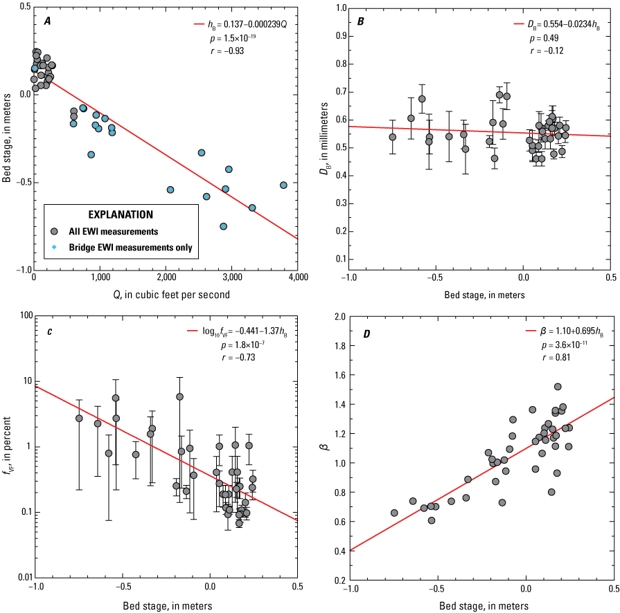
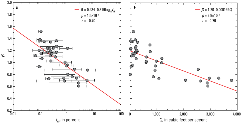
Plots of relations between the instantaneous water discharge (Q), bed stage (hB), bed-sand median grain size (DB), the amount of very fine sand on the bed (fVF), and nondimensional bed-sand coarseness (β) at the Little Snake River near Lily, Colorado, gaging station 09260000 (LS-Lily station). The level of significance (p) evaluated using an F-test and correlation coefficient (r) associated with each least-squares linear regression (red line) are shown. Error bars on DB and fVF are one standard error, calculated among the samples collected at each vertical in the bed-sediment measurement. A, Bed stage plotted as a function of Q. Though regression was fit to the bed stages from all equal-width-increment (EWI) measurements, the subset of bed stages for those measurements made at only the cross section at the upstream side of the bridge are indicated by blue diamonds for reference. B, DB plotted as a function of bed stage. C, fVF plotted as a function of bed stage; the regression depicted by the red line was calculated using log10(fVF). D, β plotted as a function of bed stage. E, β plotted as a function of fVF; the regression depicted by the red line was calculated using log10(fVF). F, β plotted as a function of Q.
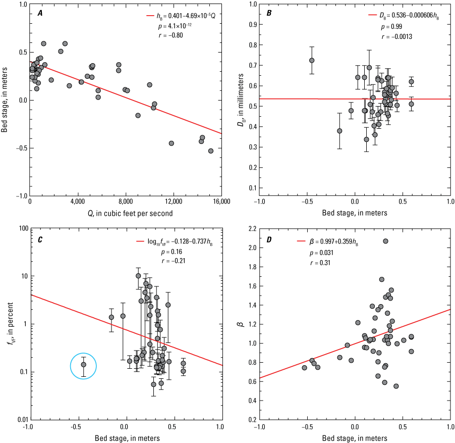
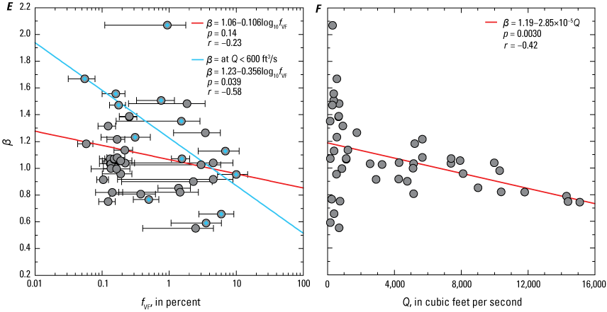
Plots of relations between the instantaneous water discharge (Q), bed stage (hB), bed-sand median grain size (DB), the amount of very fine sand on the bed (fVF), and nondimensional bed-sand coarseness (β) at the Yampa River at Deerlodge Park, Colorado, gaging station 09260050 (Yampa-Deerlodge station). The level of significance (p) evaluated using an F-test and correlation coefficient (r) associated with each least-squares linear regression (red line) are shown. Error bars on DB and fVF are one standard error, calculated among the samples collected at each vertical in the bed-sediment measurement. A, Bed stage plotted as a function of Q. B, DB plotted as a function of bed stage. C, fVF plotted as a function of bed stage; the regression depicted by the red line was calculated using log10(fVF). The point circled in blue is the value described in the text that alone prevents this regression from being significant. D, β plotted as a function of bed stage. E, β from all equal-width-increment (EWI) measurements plotted as a function of fVF; the regression depicted by the red line was calculated using log10(fVF). Those values of β from EWI measurements made at Q < 600 cubic feet per second (ft3/s) are indicated by blue diamonds, and the associated least-squares linear regression with its p and r values are indicated in blue. F, β plotted as a function of Q.
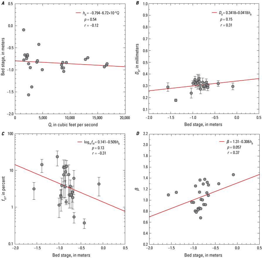

Plots of relations between the instantaneous water discharge (Q), bed stage (hB), bed-sand median grain size (DB), the amount of very fine sand on the bed (fVF), and nondimensional bed-sand coarseness (β) on the Green River above Ouray, Utah, monitoring station (Green-Ouray station). The level of significance (p) evaluated using an F-test and correlation coefficient (r) associated with each least-squares linear regression (red line) are shown. Error bars on DB and fVF are one standard error, calculated among the samples collected at each vertical in the bed-sediment measurement. A, Bed stage plotted as a function of Q. B, DB plotted as a function of bed stage. C, fVF plotted as a function of bed stage; the regression depicted by the red line was calculated using log10(fVF). D, β plotted as a function of bed stage. E, β from all equal-width-increment (EWI) measurements plotted as a function of fVF; the regression depicted by the red line was calculated using log10(fVF). Those values of β from EWI measurements made at Q < 4,500 cubic feet per second (ft3/s) are indicated by blue diamonds, and the associated least-squares linear regression with its p and r values are indicated in blue. F, β plotted as a function of Q. Unlike at the LS-Lily and Yampa-Deerlodge stations, where the best-fit relations between Q and β are linear, the best-fit regression of β on Q at the Green-Ouray station is not the linear regression (blue line) but rather the log-linear regression shown in red.
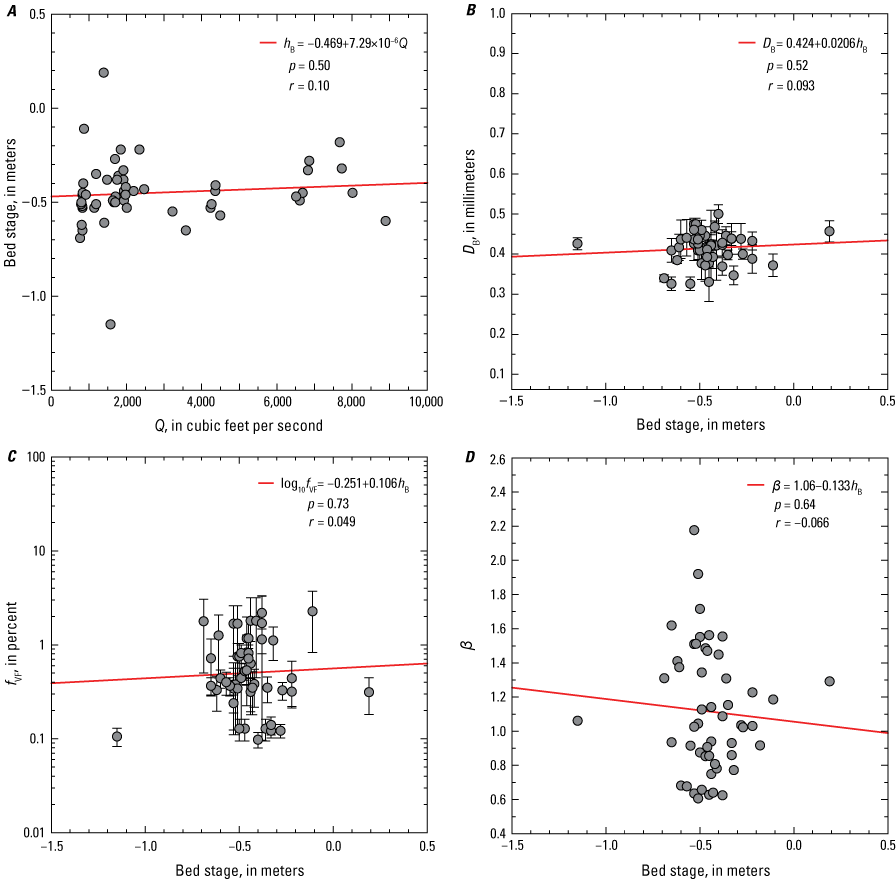
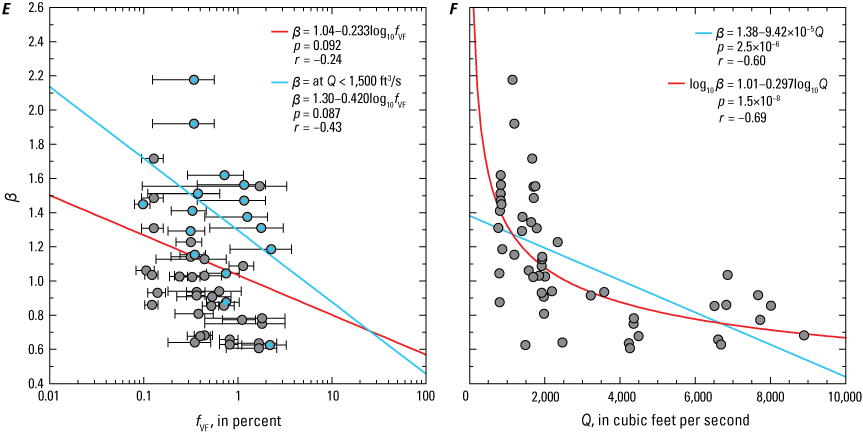
Plots of relations between the instantaneous water discharge (Q), bed stage (hB), bed-sand median grain size (DB), the amount of very fine sand on the bed (fVF), and nondimensional bed-sand coarseness (β) at the Green River above Gates of Lodore, Colorado, gaging station 404417108524900 (Green-Lodore station). The level of significance (p) evaluated using an F-test and correlation coefficient (r) associated with each least-squares linear regression (red line) are shown. Error bars on DB and fVF are one standard error, calculated among the samples collected at each vertical in the bed-sediment measurement. A, Bed stage plotted as a function of Q. B, DB plotted as a function of bed stage. C, fVF plotted as a function of bed stage; the regression depicted by the red line was calculated using log10(fVF). D, β plotted as a function of bed stage. E, β from all equal-width-increment (EWI) measurements plotted as a function of fVF; the regression depicted by the red line was calculated using log10(fVF). Those values of β from EWI measurements made at Q < 1,500 cubic feet per second (ft3/s) are indicated by blue diamonds, and the associated least-squares linear regression with its p and r values are indicated in blue. F, β plotted as a function of Q. Unlike at the LS-Lily and Yampa-Deerlodge stations, where the best-fit relations between Q and β are linear, but like at the Green-Ouray station, the best-fit regression of β on Q at the Green-Lodore station is not the linear regression (blue line) but rather the log-linear regression shown in red.
Relations Between Discharge and Bed-Sand Grain Size at the Largely Gravel-Bedded Stations
Relations between Q and bed-sand grain size differ between the two largely gravel-bedded stations. At the Yampa-Maybell station, the β-inferred bed-sand grain size that interacts with the flow decreases as Q increases (fig. 19), but at the Green-Jensen station, it remains constant as Q increases (fig. 20A), albeit with large variance. Given that the bed of the Yampa River at the Yampa-Maybell station is almost always entirely composed of gravel, no bed-sediment measurements could be made at this station to evaluate how β might relate to DB or fVF. At the post-2015 location of the Green-Jensen station, however, enough bed-sediment measurements could be made (that is, with ≥50 percent of the verticals returning samples containing ≥20 g of sand) to show a moderate negative correlation between β and log10(fVF) (fig. 20B), with r = −0.53, though this correlation has low significance (p = 0.18) given the small number of measurements. Though insignificant, the strength of this correlation exceeds that observed between β and log10(fVF) at higher Q at the sand-bedded Green-Ouray (fig. 17E) and Green-Lodore (fig. 18E) stations.
The mechanism that causes the bed-sand grain size at the largely gravel-bedded Yampa-Maybell station to fine with increasing Q cannot be the same mechanism (scour through an inversely graded bed) that most likely explains this effect at all four sand-bedded stations. The relation between Q and β is nonlinear at the Yampa-Maybell station, just as at the sand-bedded Green-Ouray and Green-Lodore stations. β fines relatively quickly as Q increases from baseflow to ~2,000 ft3/s, and then remains relatively constant as Q continues to increase (fig. 19). Because an inversely graded sand bed does not exist at Yampa-Maybell, the most likely explanation for this physical behavior is that increasing Q accesses finer bed sand stored at higher elevations in the channel (that is, the second scenario described in the previous section of this report). This mechanism is plausible at Yampa-Maybell because the largest amounts of sand in this part of the Yampa River are stored in point bars that are not completely inundated until flows greatly exceed baseflow.
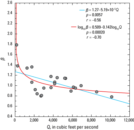
Plot of nondimensional bed-sand coarseness (β) as a function of instantaneous water discharge (Q) for the equal-width-increment (EWI) measurements at the Yampa River near Maybell, Colorado, gaging station 09251000 (Yampa-Maybell station). The levels of significance (p) evaluated using F-tests and correlation coefficients (r) associated with each least-squares regression are shown. As at the Green-Ouray station (fig. 17F) and Green-Lodore station (fig. 18F), the best-fit regression of β on Q at the Yampa-Maybell station is not the linear regression (blue line) but rather the log-linear regression shown in red.
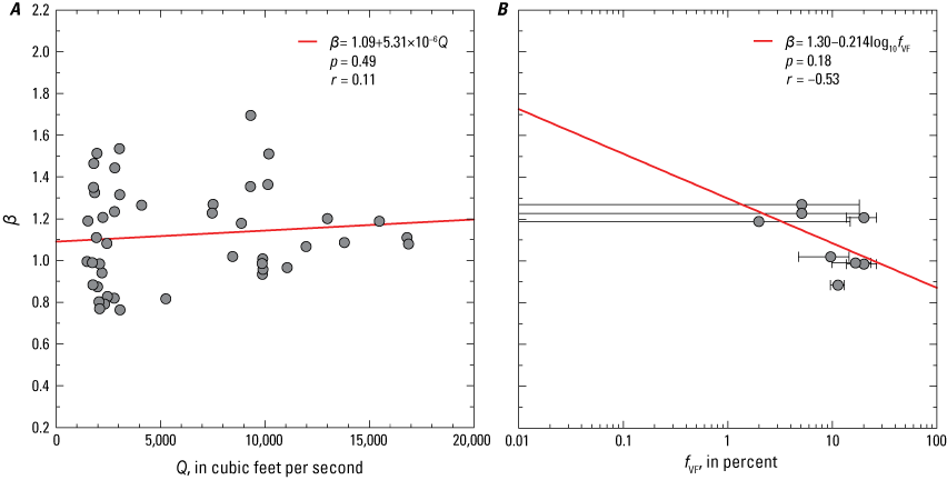
Plots of nondimensional bed-sand coarseness (β), as functions of instantaneous water discharge (Q), and the amount of very fine sand on the bed (fVF) for the equal-width-increment measurements at the Green River near Jensen, Utah, gaging station 09261000 and the post-2015 Green River above Jensen, Utah monitoring station. These two nearby stations have equivalent sediment-transport conditions and are collectively referred to as the Green-Jensen station in the text. The level of significance (p) evaluated using an F-test and correlation coefficient (r) associated with each least-squares linear regression (red line) are shown. A, β plotted as a function of Q at both the original and post-2015 locations. Unlike at all other stations in our study, no relation exists between Q and β at the Green-Jensen station. The least-squares linear regression shown has almost zero slope and is not significant at the p = 0.05 critical level of significance. B, β plotted as a function of fVF at the post-2015 location of the Green-Jensen station. Although the least-squares linear regression of β on log10(fVF) is not significant owing to too few measurements, the negative correlation associated with this regression is moderate.
Implications of Discharge-Associated Bed-Sand Fining for the Detection of Tributary-Generated Sand Waves
Although Topping and others (2018) did not recognize the effect of scour through an inversely graded bed during increases in Q on β at the LS-Lily and Yampa-Deerlodge stations, exclusion of this effect did not affect their ability to detect changes in bed-sand grain size caused by the downstream migration of the sand waves generated by the large Sand Creek floods of 1956–1966. Inclusion of this effect by detrending β using the linear relations between Q and β in figures 15F and 16F does not greatly affect the β time series at these stations (fig. 21). Though the slopes of the trends in β are affected, the long-term trends in β remain significant at the p = 0.05 critical level after β is detrended by Q (fig. 21A, B).
The downstream migration of the sand waves generated by the large Sand Creek floods of 1956–1966 caused β-inferred bed-sand fining at downstream gaging stations followed by β-inferred bed-sand coarsening (Topping and others, 2018). At the LS-Lily station, significant bed-sand fining during water years 1958–1964 was followed by significant bed-sand coarsening (fig. 21A); the lack of suspended-sand data during water years 1956, 1957, 1965, and 1966 prevent knowing if this fining began earlier or ended later. Significant bed-sand coarsening also occurred during at least the post-1982 period at the Yampa-Deerlodge station (fig. 21B); the lack of suspended-sand data precludes knowledge of trends in bed-sand grain size at this station before 1982. Though the bed-sand fining during 1956–1966 was not significant at the Green-Jensen station, this lack of significance (p = 0.12) owes to only two abnormally large β values from EWI measurements made at very low Q (938 and 1,490 ft3/s) in July 1961 (circled in fig. 21C). Exclusion of these two outliers reveals that significant bed-sand fining also likely occurred at Green-Jensen during 1956–1966 (p = 0.036), followed by significant bed-sand coarsening. As described above, Dean and others (2020) detected a similar pattern ~285 km downstream from the Green-Jensen station at the Green-Green River station, where significant bed-sand fining occurred between 1959 and 1965, followed by significant bed-sand coarsening.
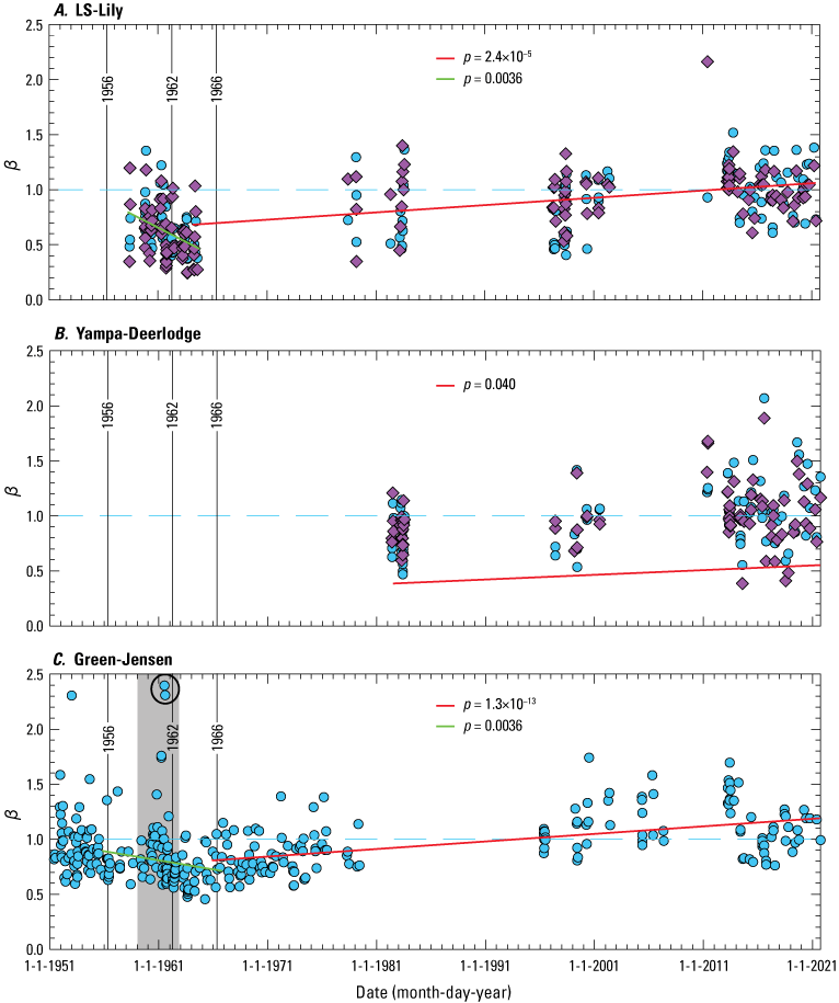
Time series of nondimensional bed-sand coarseness (β) for the entire record of grain-size-analyzed equal-width-increment measurements at the LS-Lily (A), Yampa-Deerlodge (B), and Green-Jensen stations (C). Bed-sand fines during the 1956–1966 period of large Sand Creek floods and subsequently coarsens at all three downstream stations. Plots show the effect of Q-detrending β on the β time series at the LS-Lily and Yampa-Deerlodge stations, where the bed sand fines with increasing Q. Blue filled circles depict the raw values of β; purple diamonds depict the values of β detrended as a linear function of Q. β was not Q-detrended at the Green-Jensen station because no significant relation exists between Q and β at that station. Solid black vertical lines labeled “1956”, “1962”, and “1966” indicate the dates of large sand-supplying floods in Sand Creek. Solid green lines are the least-squares linear regressions fit to the Q-detrended β values during water years 1958–1964 at LS-Lily and fit to the raw β values at Green-Jensen during water years 1956–1966; solid red lines are the least-squares linear regressions fit to the Q-detrended β values during water years 1964–2021 at LS-Lily and during water years 1982–2021 at Yampa-Deerlodge and fit to the raw β values during water years 1966–2021 at Green-Jensen; significance, p, of each regression is indicated. Circled values in C are the two outliers described in the text that were excluded from the 1956–1966 regression at the Green-Jensen station. Horizontal blue dashed lines indicate β = 1. Gray shaded box in C indicates construction period of Flaming Gorge Dam. Raw values of β in A–C are equal to those in Topping and others (2018) divided by 1.44, 1.10, and 1.21, respectively, at the LS-Lily, Yampa-Deerlodge, and Green-Jensen stations, owing to the different values of the reference velocity-weighted suspended-sand concentration (CSAND-REF) and suspended-sand median grain size (DS-REF) used in equation 6. In Topping and others (2018), these reference values were evaluated over the entire period of record; in our study, these reference values were evaluated over only the 2013–2021 period. Station name abbreviations are defined in table 1; locations are shown in figure 1.
Discharge-Independent Flow Regulation of Suspended-Sand Concentration at the Sand-Bedded Stations Likely Arising from the Downstream Migration of Sand Waves
Although CSAND at the sand-bedded stations is more strongly regulated by changes in bed-sand grain size than it is by changes in flow, the amount of variation in CSAND caused by changes in flow-related processes is not small. Consequently, it is important to understand the mechanisms by which the shear velocity, , and the skin-friction component of the shear velocity, , influence CSAND at these stations and to know the magnitude of the variation in CSAND caused by these changes. Because some of the variation in CSAND caused by changes in and occur independently of Q, it is especially important to know how the resultant Q-independent changes in CSAND compare in magnitude to those caused by changes in bed-sand grain size. Moreover, it is important to understand the magnitude of the variation in CSAND caused by Q-independent changes in and because these changes are associated with the often subtle topographic signature of the downstream migration of sand waves. Though the dominant mechanism by which flow regulates CSAND at the sand-bedded stations is through the changes in caused directly by changes in Q, as described in the “Regulation of Suspended-Sand Concentration by Flow, Grain Size, and Other Processes” subsection in the “Analytical Methods” section, other Q-independent changes in (caused by changes in channel geometry) and Q-independent changes in (caused by changes in dune and bar geometry) both help regulate CSAND at the sand-bedded stations.
Q-independent changes in arise from changes in channel geometry that are not perfectly coupled with changes in Q. This decoupling between Q and channel geometry in a sand-bedded river occurs because scour and fill of the riverbed are driven both by changes in Q and changes in the upstream sediment supply (Colby, 1964; Andrews, 1979; Howard and Dolan, 1981; Topping and others, 2000). Though Q is the dominant driver of scour and fill in rivers through the interaction of the boundary-shear-stress field with the local channel geometry, substantial modification of the timing of scour and fill during floods will occur as a function of changes in the upstream sediment supply owing to the downstream migration of sand waves (Topping and others, 2000). Consequently, substantial Q-independent variation in the area and shape of river cross sections can occur because scour or fill of the riverbed is not necessarily exactly in phase or 180° out of phase with the hydrograph during floods. Because Q is the product of the cross-section area and velocity, the Q-independent variation in cross-section area causes commensurate but opposing Q-independent variation in the mean velocity in the cross section. Moreover, because mean velocity is linearly related to (von Karman, 1930), variation in mean velocity causes variation in . These Q-independent changes in caused by changes in cross-section area can be detected as a positive relation between mean velocity and CSAND at constant Q. Topping and others (2021) estimated that this cause of Q-independent variation in could lead to an approximate factor-of-2 variation in CSAND at any given Q on the Colorado River in Marble and Grand Canyons. In addition to this topographic mechanism of CSAND regulation, associated changes in the geometry of the dunes and (or) bars at the same Q can also regulate CSAND by causing Q-independent variation in , as described below.
Following Einstein (1950), Smith and McLean (1977), Nelson and Smith (1989), and Wiberg and Smith (1989), we use spatially averaged steady, uniform-flow theory to partition the boundary shear stress (τb) into a component arising from the form drag associated with dunes and bars, and a skin-friction component (τsf) associated with sediment transport. It is important, however, to recognize that although this stress-partitioning approach provides a valid method for estimating the influence of dunes and bars on sediment transport, it is not completely correct in detail (Nelson and others, 1993; McLean and others, 1999). Because larger dunes or bars are associated with greater relative form drag, and because larger dunes or bars are also associated with greater variation in the bed topography in a river cross section, greater topographic variance in a river cross section will be associated with a smaller value of the ratio . Moreover, because and , greater topographic variance will be associated with smaller values of the ratio . The lower boundary condition that regulates the flux of sand between the bed and suspension scales with , whereas the vertical distribution of suspended sand in the interior of the flow above the dunes or bars is related to (McLean, 1992). By their influence on , relatively larger dunes or bars will thereby result in smaller CSAND and finer DS at constant (after McLean, 1992). To detect this effect in the EWI measurements, we use the variance in flow depth among the 10 sampling verticals in each EWI measurement as a measure of topographic variance. We then relate greater values of the variance in flow depth at a given Q to smaller values of , and therefore smaller values of CSAND. Q-independent changes in caused by changes in dune and (or) bar geometry are thus detected as a negative relation between the variance in flow depth among the 10 EWI verticals and CSAND at constant Q.
We analyzed the EWI-measurement datasets among the four sand-bedded stations over narrow ranges in Q to search for examples of Q-independent changes in CSAND that could not be readily explained by changes in bed-sand grain size. Only the EWI measurements could be used for this purpose because only they include measurements of cross-section topography, that is, the flow depth at each vertical. For these analyses, we evaluated the influence on CSAND of the bed-sand grain size in both the reach upstream from the measurement cross section using β, and at the measurement cross section using the direct bed-sediment measurements. We then evaluated relations (1) between the mean velocity in the EWI-measurement cross section (as a proxy for ) and CSAND, and (2) between the variance in flow depth among the 10 EWI verticals (as a proxy for ) and CSAND. By this approach, we found three examples at the LS-Lily station and one example at the Yampa-Deerlodge station that serve as good indicators of the importance of these types of Q-independent changes in or in regulating CSAND. The EWI measurements in each of the narrow ranges in Q in these examples were made over years and are in good agreement with the continuous acoustical measurements, which showed only slow changes in CSAND over time. Consequently, the process causing the variation in CSAND detected by the EWI measurements in these examples was persistent and was therefore a systematic, not random, process.
At the LS-Lily station, we found useful examples in three narrow ranges of Q: 210–280 ft3/s, 2,500–2,600 ft3/s, and 2,900–3,000 ft3/s (fig. 22A). Positive relations between DS and CSAND exist for the two higher Q ranges (fig. 22B), thus suggesting that the variation in CSAND in these two examples owes to Q-independent variation in (by equations 2A and B). The two types of bed-sand data analyzed for these three examples provide conflicting information. The positive relations between β and CSAND for the two higher Q ranges also suggests that the variation in CSAND for these two examples owes to Q-independent variation in (fig. 22C); the slightly coarser bed sand associated with the greater values of CSAND would require greater by equation 2A to explain these greater values of CSAND. Negative relations between DB and CSAND for the two lower Q ranges (fig. 22D), and a positive relation between log10(fVF) and CSAND for the mid-Q range (fig. 22E), however, indicate that changes in the bed-sand grain-size distribution cannot be completely ruled out for causing some of the Q-independent variation in CSAND. The positive relations observed between the mean velocity in the cross section and CSAND for the two higher Q ranges (fig. 22F) do, nevertheless, indicate that changes in are involved in the variation in CSAND in at least these two higher Q examples. Moreover, all three Q ranges exhibit very strong negative relations between the variance in flow depth among the 10 EWI verticals and CSAND (fig. 22G), with |r| > 0.9 for all three Q ranges. This result indicates that changes in the geometry of the dunes or bars are largely responsible for the Q-independent variation in CSAND at the LS-Lily station that cannot be attributed to changes in bed-sand grain size. The magnitude of the Q-independent variation in CSAND at the LS-Lily station arising from changes in and is roughly a factor of 2, similar to the amount of Q-independent variation in CSAND arising from changes in estimated by Topping and others (2021) for the Colorado River.
At the Yampa-Deerlodge station, the best example for evaluating the importance of Q-independent changes in or in regulating CSAND is also the Q range with the largest variation in CSAND observed among the EWI measurements: Q = 4,300–5,200 ft3/s (fig. 23A). Although no relation exists between DS or β and CSAND (fig. 23B, C), a strong negative relation between DB and CSAND (r = −0.74, fig. 23D) in conjunction with a very strong positive relation between log10(fVF) and CSAND (r = 0.96, fig. 23E) suggests that changes in the bed-sand grain-size distribution are responsible for some of the observed factor-of-4 variation in CSAND in this example. Unlike at the LS-Lily station, no relation exists between the mean velocity in the cross section and CSAND (fig. 23F), thereby indicating that changes in are not responsible for the Q-independent variation in CSAND in this example. However, and as at the LS-Lily station, a very strong negative relation exists between the variance in flow depth among the 10 EWI verticals and CSAND (r = −0.90, fig. 23G). This result indicates that changes in the geometry of the dunes or bars also has a dominant role in the Q-independent variation in CSAND at the Yampa-Deerlodge station, and likely contributes to at least half of the observed factor-of-4 variation in CSAND in this example.
Taken together, the examples shown in figures 22 and 23 thus suggest that changes in caused by changes in dune or bar geometry are responsible for between a factor of 2 and a factor of 4 of the Q -independent variation in CSAND observed at the sand-bedded stations. It is important to recognize, however, that this magnitude of variation in CSAND is less than the minimum factor-of-6 Q-independent variation in CSAND observed in figures 9A, 10A, 11A, and 12A. Moreover, this magnitude of variation in CSAND is also smaller than the greater-than-factor-of-6 Q-independent variation in CSAND implied by application of equation 2A to the greater than factor-of-2 variation in β in figures 9C, 10C, 11C, and 12C. In addition, this magnitude of variation in CSAND is also less than the factor-of-6 Q-independent variation in CSAND implied by application of equation 2A to the roughly factor-of-2 variation in DB among figures 15B, 16B, 17B, and 18B. Thus, even though important, the magnitude of the Q-independent variation in CSAND associated with changes in or is less than that associated with the Q-independent changes in the bed-sand grain-size distribution that are caused by changes in the upstream sand supply. Therefore, the grain-size signature of the downstream migration of sand waves has a larger influence on CSAND than does the topographic signature of the downstream migration of sand waves, as manifest through Q-independent changes in or .
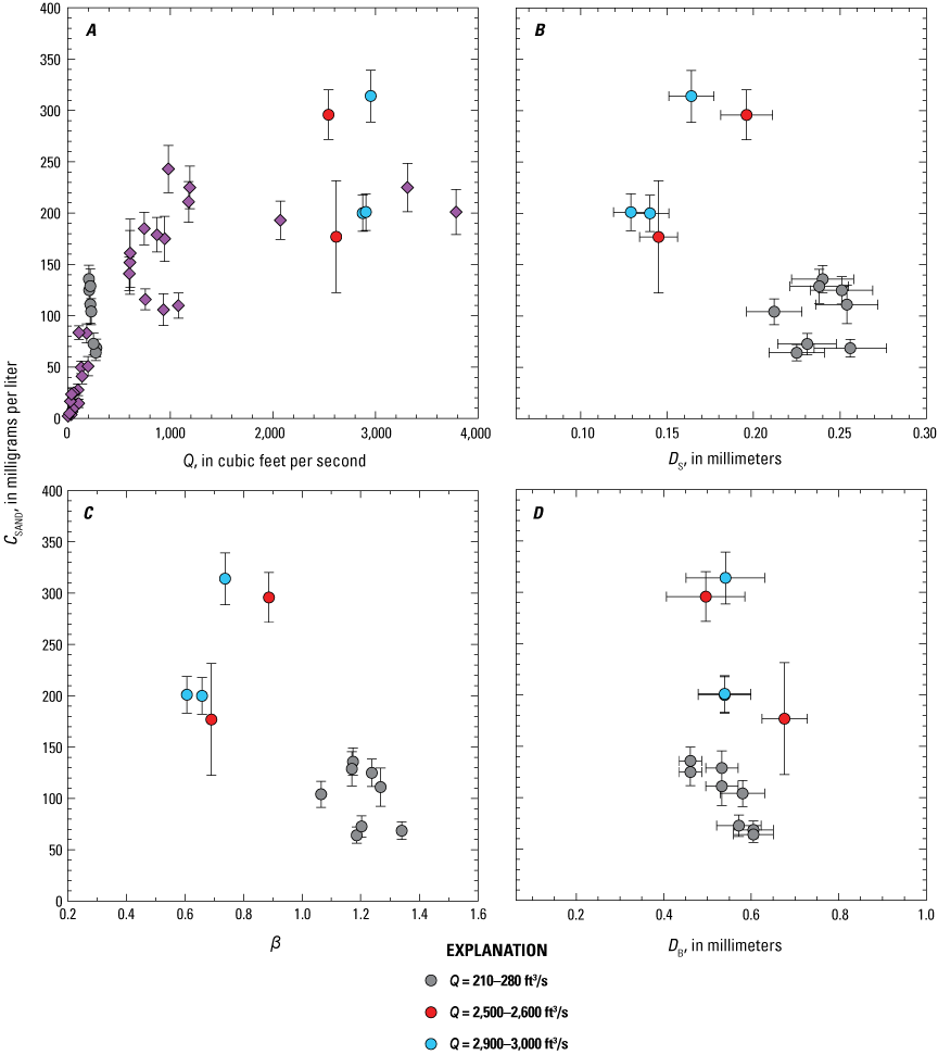
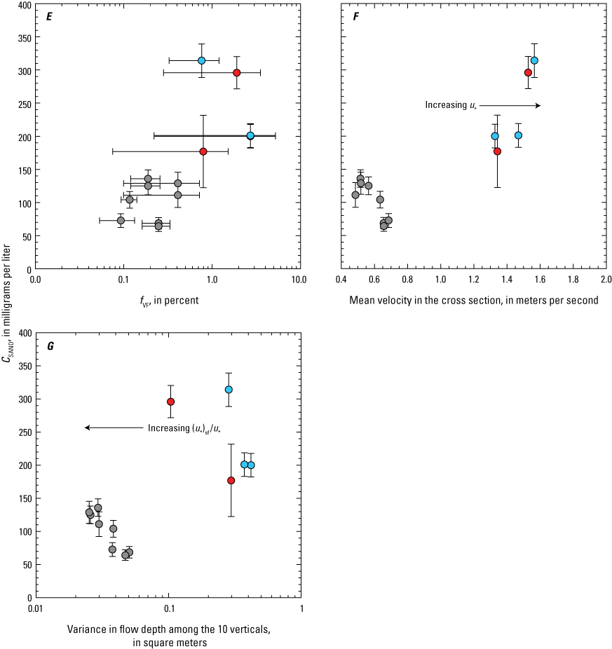
Plots evaluating the importance of water-discharge- (Q-) independent changes in shear velocity () and the skin-friction component of the shear velocity () in helping to regulate the velocity-weighted suspended-sand concentration (CSAND) at the Little Snake River near Lily, Colorado, gaging station 09260000 (LS-Lily station). Values plotted are from paired equal-width-increment (EWI) and bed-sediment measurements; error bars on CSAND and the velocity-weighted suspended-sand median grain size (DS) are the 95-percent-confidence-level combined field and laboratory errors (Topping and others, 2010, 2011); error bars on bed-sand median grain size (DB) and the amount of very fine sand on the bed (fVF) are one standard error. A, CSAND plotted as a function of Q; values in the three narrow ranges of Q used in the examples are indicated, and only these values are plotted in B–G; values outside these narrow ranges of Q depicted as purple diamonds. B, CSAND plotted as a function of DS. C, CSAND plotted as a function of the nondimensional bed-sand coarseness (β). D, CSAND plotted as a function of DB. E, CSAND plotted as a function of fVF. F, CSAND plotted as a function mean velocity in the EWI cross section; the direction of increasing is indicated. G, CSAND plotted as a function of the variance in flow depth among the 10 EWI verticals; the direction of increasing is indicated. ft3/s, cubic feet per second.
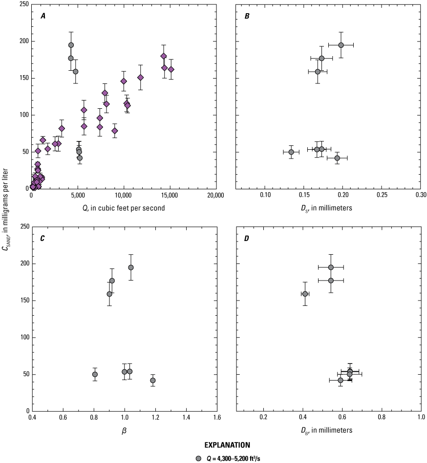
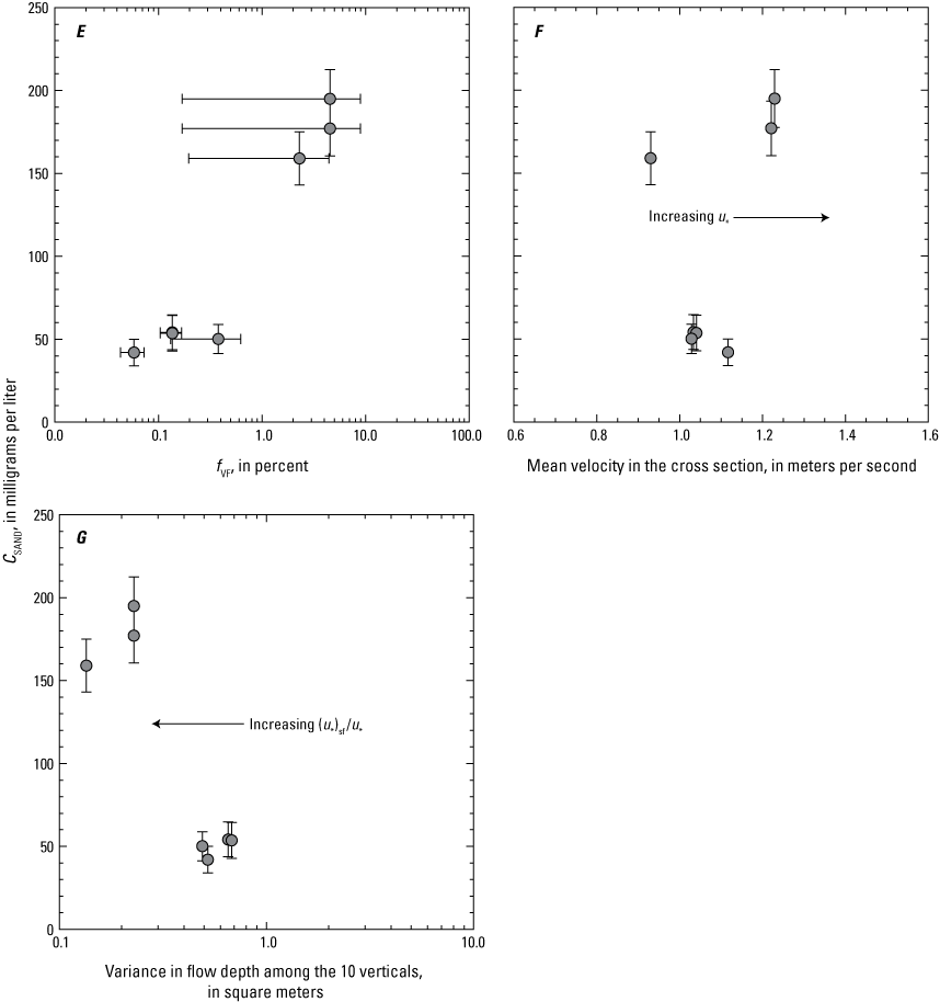
Plots evaluating the importance of water-discharge- (Q-) independent changes in shear velocity () and the skin-friction component of the shear velocity () in helping to regulate the velocity-weighted suspended-sand concentration (CSAND) at the Yampa River at Deerlodge Park, Colorado, gaging station 09260050 (Yampa-Deerlodge station). Values plotted are from paired equal-width-increment (EWI) and bed-sediment measurements; error bars on CSAND and the velocity-weighted suspended-sand median grain size (DS) are the 95-percent-confidence-level combined field and laboratory errors (Topping and others, 2010, 2011); error bars on bed-sand median grain size (DB) and the amount of very fine sand on the bed (fVF) are one standard error. A, CSAND plotted as a function of Q; values in the narrow range of Q used in the example are indicated, and only these values are plotted in B–G; values outside this narrow range of Q depicted as purple diamonds. B, CSAND plotted as a function of DS. C, CSAND plotted as a function of the nondimensional bed-sand coarseness (β). D, CSAND plotted as a function of DB. E, CSAND plotted as a function of fVF. F, CSAND plotted as a function mean velocity in the EWI cross section; the direction of increasing is indicated. G, CSAND plotted as a function of the variance in flow depth among the 10 EWI verticals; the direction of increasing is indicated. ft3/s, cubic feet per second.
Partial Regulation of Suspended-Sand Concentration by Discharge-Independent Changes in Bed-Sand Area at the Largely Gravel-Bedded Stations
The spatially averaged areal coverage of sand on the bed (bed-sand area) regulates CSAND through the lower boundary condition for suspended sediment, where changes in bed-sand area cause approximately linear changes in the near-bed suspended-sand concentration (Grams and Wilcock, 2007, 2014; Topping and others, 2007). Thus, unlike the changes in bed-sand grain size, which exert a strong nonlinear control on CSAND (eq. 2A; Topping and others, 2000, 2007; Rubin and Topping, 2001, 2008), changes in bed-sand area exert a weaker quasi-linear control on CSAND (Grams and Wilcock, 2007, 2014; Topping and others, 2007). Following Topping and others (2010), equation 2A can be modified to include this quasi-linear control of bed-sand area as follows:
where AB is the spatially averaged fractional area of sediment on the bed. Increases in bed-sand area are not expected to cause changes in DS unless the progressive burial of a relatively rough gravel bed results in a substantial reduction in the form drag produced by the gravel protruding into the flow (after Nelson and others, 1991; Wiberg and Smith, 1991; Topping, 1997). Such a large reduction in gravel form drag would cause DS to increase as AB increases, not because of the increase in bed-sand area, but rather because of an increase in . Given the value of K = −2.5 used herein, changes in DB of a factor of 2 are associated with the same change in CSAND as are changes in AB of a factor of 5.7. Thus, in rivers where changes in bed-sand grain size that exceed a factor of 2 are likely, changes in bed-sand grain size thus exert a much stronger influence on CSAND than do changes in bed-sand area (Topping and others, 2007, 2021; Rubin and others, 2020), and can easily offset the sometimes-opposing influence on CSAND of changes in bed-sand area (Topping and others, 2007). Because changes in bed-sand grain size in our study area typically do not greatly exceed a factor of 2, however, it is important to quantify the likely Q-independent variation of CSAND associated with the changes in bed-sand area observed at the gravel-bedded stations in our study area.Changes in bed-sand area have been shown to be associated with both changes in the upstream sand supply (as are also changes in bed-sand grain size) and changes in Q (Topping and others 2021). Because changes in Q change the loci of convergence in the boundary shear stress that determines where sand can deposit on a gravel bed, large increases in Q tend to redistribute sand from deep pools to larger areas of the bed (Topping and others, 2000), with sand slowly recollecting in these pools after Q decreases. Consequently, sand can occur on different parts and cover differing amounts of the bed in a gravel-bedded river at different Q. For example, large increases in Q have been observed to cause up to an approximately factor-of-3 increase in bed-sand area in the Colorado River downstream from Glen Canyon Dam in Marble and Grand Canyons (Anima and others, 1998; Schmidt and others, 2007). To allow exclusion of the effect of changing Q on AB, we thus analyzed the effect of changing bed-sand area on CSAND in narrow ranges of Q, thus ensuring that the observed changes in bed-sand area arose from changes in the upstream sand supply. Because the post-2015 location of the Green-Jensen station was the only largely gravel-bedded station that had both the EWI measurements and bed-sediment measurements required to evaluate the effect of bed-sand area on CSAND, we conducted this analysis at that station. We used the fraction of the 10 EWI verticals comprising each bed-sediment measurement that returned at least 20 g of sand as the measure of AB, as described above in the “Sediment-Transport and Bed-Sediment Measurements at Gaging Stations” subsection of the “Field Methods” section; AB thus ranged from 0 when no sand was present on the bed to 1.0 when the bed was fully sand-covered. Most other aspects of this analysis were the same as in the analyses in the previous section, including using the mean velocity in the cross section as a proxy for and using the variance in flow depth among the 10 EWI verticals as a proxy for the variation in caused by changes in dune or bar geometry. Because most of these bed-sediment measurements returned sand-size sediment at fewer than 50 percent of the verticals, greater uncertainty in DB or fVF existed at the Green-Jensen station than at the sand-bedded stations. Thus, we did not include DB or fVF in this analysis in the same way as in the analyses in the previous section of this report.
At the Green-Jensen station, we found good examples of relatively large variations in CSAND in two narrow ranges of Q: 8,500–9,900 ft3/s, and 15,500–16,900 ft3/s, (fig. 24A). The EWI measurements in these two narrow ranges of Q were made over years and are in good agreement with the continuous acoustical measurements, which showed only slow changes in CSAND over time. Thus, as with the variation in CSAND caused by Q-independent changes in or , the variation in CSAND in these examples was also systematic and occurred over longer timescales. Positive relations between DS and CSAND exist for both these Q ranges (fig. 24B). This result suggests that the variation in CSAND in these two examples owes to three possible scenarios (1) Q-independent variation in owing to changes in cross-section geometry, (2) increases in caused by increasing bed-sand area reducing the gravel form drag, or (3) positively coupled changes in bed-sand area and grain size. Scenario one can be ruled out because the Q-independent variation in cross-section geometry is minimal at the Green-Jensen station because the bed is largely composed of cobble-size gravel, and the sand patches that sometimes overlie parts of this gravel bed tend to be thin. Thus, the range in mean velocity associated with the variation in CSAND in the two Q ranges is very small, and no consistent positive relation between mean velocity and CSAND exists among the two Q ranges (fig. 24D). Scenario two cannot be ruled out because we have no way to estimate the changes in that could result from changes in bed-sand area. Although the lack of relations between the variance in flow depth among the 10 EWI verticals and CSAND for ether Q range (fig. 24E) does allow us to conclude that Q-independent changes in caused by changes in dune or bar geometry do not occur; this result is not surprising because neither large dunes nor sand bars occur at the Green-Jensen station. Though scenario three is deemed most likely as a result of the presence of positive relations between β and CSAND for both examples (fig. 24C) and very strong positive relations between bed-sand area and CSAND (r = 0.80 for lower Q range and 0.99 for higher Q range; fig. 24F), the positive relations between β and CSAND could be an artifact arising from the influence in equation 6 of the positive relations between DS and CSAND in figure 24B. Although support for scenario three is provided by a very strong negative relation between log10(fVF) and β for the cases used in the examples (r = −91; fig. 24G), the certainty of this relation is low despite its significance (p = 0.0046). Five of the seven measurements in this relation in figure 24G are from bed-sediment measurements where <50 percent of the 10 EWI verticals returned a sand sample with mass ≥20 g; thus, it is uncertain whether these measurements are representative of fVF over the entire cross section.
Despite the uncertainty associated with the interpretation of β in the examples in figure 24, it is likely that the Q-independent variation in CSAND in both examples does arise from scenario three (changes in bed-sand area that are likely positively coupled with changes in bed-sand grain size). The relations in figure 24F indicate that the Q-independent increases in CSAND in both examples are associated with increases in bed-sand area. This result requires that either scenarios two or three are correct. In addition, the positive relations between β and CSAND (fig. 24C) and negative relation between log10(fVF) and β (fig. 24G) together strongly suggest that these increases in bed-sand area are more likely associated with increases in bed-sand grain size than they are with decreases in gravel form drag. Though the progressive burial of the gravel caused by the increase in bed-sand area could cause a decrease in the form drag arising from the gravel protruding into the flow (scenario two), this effect is not required to explain the data. Presumably, the increase in bed-sand area associated with the increase in CSAND in each of these examples was large enough to overwhelm the opposing nonlinear influence on CSAND of the coarsening bed-sand grain size (eq. 9). The Q-independent variation in CSAND owing to changes in bed-sand area in these examples is roughly a factor of 2, much smaller than the minimum factor-of-6 Q-independent variation in CSAND at the Green-Jensen station associated with changes in bed-sand grain size inferred from the 2013–2021 values of β at any given Q (figs. 14C, 20A). Thus, changes in bed-sand area at the Green-Jensen station are unlikely to overwhelm the increases in the upstream sand supply indicated by large decreases in β. Finally, this factor-of-2 Q-independent variation in CSAND is consistent with the Q-independent variation in CSAND observed at the Yampa-Maybell station, where only minimal Q-independent changes in β occur (fig. 13C). Thus, it is plausible that the maximum Q-independent variation in CSAND caused by changes in bed-sand area is roughly a factor of 2 at both largely gravel-bedded stations in our study area: Green-Jensen and Yampa-Maybell.
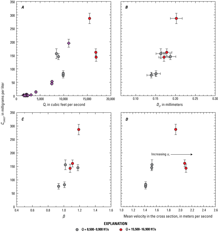
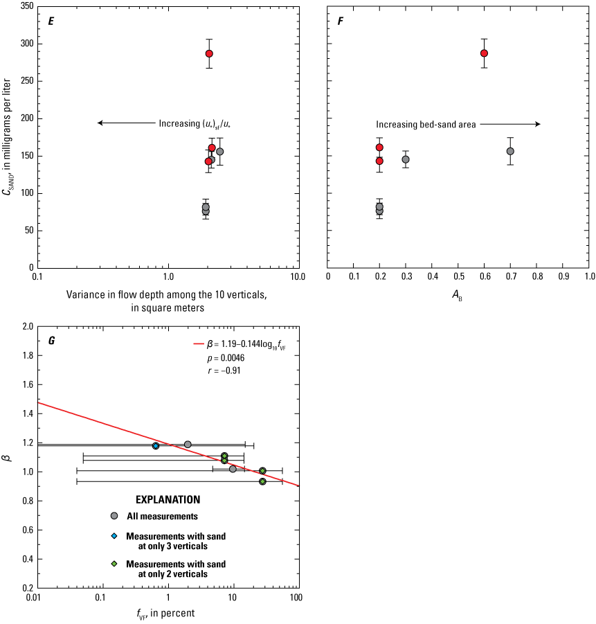
Plots evaluating the importance of water-discharge- (Q-) independent changes in bed-sand area in helping to regulate the velocity-weighted suspended-sand concentration (CSAND) at the Green River above Jensen, Utah, monitoring station (post-2015 location of the Green-Jensen station). Values plotted are from paired equal-width-increment (EWI) and bed-sediment measurements; error bars on CSAND and the velocity-weighted suspended-sand median grain size (DS) are the 95-percent-confidence-level combined field and laboratory errors (Topping and others, 2010, 2011); error bars on the amount of very fine sand on the bed (fVF) are one standard error. A, CSAND plotted as a function of Q; values in the two narrow ranges of Q used in the examples are indicated, and only these values are plotted in (B–F); values outside these narrow ranges of Q depicted as purple diamonds. B, CSAND plotted as a function of DS. C, CSAND plotted as a function of the nondimensional bed-sand coarseness (β). D, CSAND plotted as a function mean velocity in the EWI cross section; the direction of increasing is indicated. E, CSAND plotted as a function of the variance in flow depth among the 10 EWI verticals; the direction of increasing is indicated. F, CSAND plotted as a function of bed-sand area (AB); the direction of increasing bed-sand area is indicated. G, β plotted as a function of fVF for all bed-sediment measurements in both Q ranges used in the examples in A–F; the less certain values of fVF from the bed-sediment measurements with bed sand present at fewer than 5 of the 10 verticals in the cross section are indicated. The least-squares linear regression of β on log10(fVF) (red line) is significant and the negative correlation associated with this regression is very strong. The level of significance (p) evaluated using an F-test and correlation coefficient (r) are shown. ft3/s, cubic feet per second.
Grain-Size Evidence for Sand Waves During the Annual Flood
In addition to the episodic sand waves generated by tributary floods during other times of the year (the most notable example of which are the large Sand Creek floods of 1956–1966), annual sand waves are also generated during the annual snowmelt flood. Bed-sand grain-size data indicate that these annual sand waves originate in the Yampa River basin as the result of the flow accessing finer bed sand as Q increases. The most likely mechanism responsible for the bed-sand fining with increasing Q differs between the sand- and gravel-bedded parts of the rivers in the Yampa River basin. At the sand-bedded LS-Lily and Yampa-Deerlodge stations, the most likely mechanism is scour through an inversely graded bed (figs. 15–16). At the gravel-bedded Yampa-Maybell station, the most likely mechanism is access to finer sand stored at higher elevations in sandy point bars (fig. 19). Both mechanisms result in the generation of a sand wave that migrates downstream in the middle Green River, as evidenced by β calculated from our annual high-flow EWI measurements (fig. 25). Although bed-sand grain size tends to be inversely related to Q at the Yampa-Maybell, LS-Lily, Yampa-Deerlodge, and Green-Ouray stations, no relation exists between bed-sand grain size and Q at the Green-Jensen station (figs. 15–17, 19, 20). Thus, bed-sand fining at the Green-Jensen station during or immediately following Yampa River floods would indicate the likely arrival of a sand wave from the Yampa River. In addition, bed-sand fining at the Green-Ouray station that is uncorrelated with increases in Q would indicate the arrival of a sand wave from upstream.
For the analysis in figure 25, we used the β values calculated from the EWI measurements made at the highest Q during the last week of May through the first week in June. Though these measurements were not necessarily made at peak Q during the annual flood, they were typically made within a week of peak Q. Though no natural annual flood exists on the upper Green River downstream from Flaming Gorge Dam, the EWI measurements made during the typically short-duration artificial floods released from the dam to advantage native fish (U.S. Fish and Wildlife Service, 1992; Bureau of Reclamation, 2005, 2006; Bestgen and others, 2011; LaGory and others, 2012) were used to calculate high-flow β at the Green-Lodore station. Even though most of these EWI measurements were not made at peak Q, we chose the EWI measurements over the calibrated-pump or acoustical measurements made at peak Q because of the much greater accuracy of the EWI measurements. Thus, the greater accuracy of the high-flow β values calculated using these EWI measurements was given preference over the possible change in β between the time of the EWI measurements and peak Q that may not be accurately reflected by the β values calculated from the less accurate calibrated-pump or acoustical measurements. When two EWI measurements were made at similar Q within 24 hours, we averaged the β values calculated among these two measurements. To easily compare the high-flow β time series between the stations, we normalized the β values using the mean β of those calculated among all high-flow EWI measurements at a given station. Although the much-shorter period of record at the Green-Ouray station caused β to be normalized over a much-shorter period (2017–2021) than at the Green-Jensen station (2013–2021), this difference in record length did not introduce much error in this analysis because the mean of the normalized high-flow β values at Green-Jensen during 2017–2021 differed from that at Green-Ouray by only 1.5 percent.
We use two metrics to describe the annual flood in the analysis in figure 25 and in the subsequent analyses in this report: peak Q, and the March–July median Q. This approach is similar to that used by Dean and others (2020) on the lower Green River and the Colorado River upstream from Canyonlands National Park. The March–July period encompasses the entire annual snowmelt flood; thus, the March–July median Q serves as a reasonable proxy for the duration of the higher Q within the annual flood. Although peak Q is commonly used as a key flood measure in geomorphic analyses, it is not necessarily the best metric to use in analyses of sediment transport and associated geomorphic change in the case where (1) the “slope” of the Q—sediment-concentration point clouds are relatively low (meaning that a substantial amount of sediment transport occurs at Q lower than peak), and (2) the hydrograph shape is not well-correlated with the peak Q during the annual flood. Both aspects of this case occur in our study area. Because Q increases much faster than at all the stations in our study area, the slopes of the Q—CSAND point clouds in figures 9–14 are relatively low. In addition, the correlations between peak Q and the March–July median Q are only significant (p < 0.05) and very strong (r ≥ 0.8) at two stations: Yampa-Maybell and Yampa-Deerlodge (fig. 26A). Finally, the construction and operation of Flaming Gorge Dam has eliminated the annual snowmelt flood on the upper Green River in our study area. Although artificial floods are released from this dam to advantage native fish or disadvantage nonnative fish (U.S. Fish and Wildlife Service, 1992; Bureau of Reclamation, 2005, 2006; Bestgen and others, 2011; LaGory and others, 2012, 2019), the peak Q of these artificial floods is limited by the dam such that the correlation between peak Q and the March–July median Q at the Green-Lodore station is insignificant and weak (p = 0.44, r = 0.3; fig 26A). Thus, the March–July median Q is a more universal metric than the peak Q in evaluating the sediment effects of the annual flood in our study area.
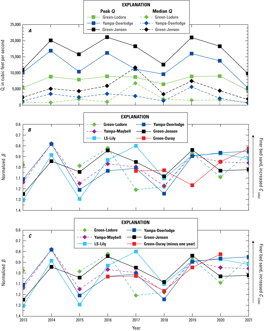
Plots comparing the time series of peak water discharge (Q), March–July median Q, and normalized high-flow nondimensional bed-sand coarseness (β) at the Green-Lodore, Yampa-Deerlodge, and Green-Jensen stations. A, Peak Q and March–July median Q. B, Normalized high-flow β calculated from the high-flow equal-width-increment measurements made at each station. C, Same as B except normalized β at the Green-Ouray station is shifted minus 1 year to better align with the values of normalized β at the upstream stations. Color-coding is consistent among A–C; y-axes on B–C inverted for visual clarity to show that fine peaks in normalized β would better align with the peaks in Q in A. The β time series at stations associated with a minority of the sand passing the downstream stations are depicted using diamonds and dashed lines in B–C; because these stations are associated with only a minority of the sand passing the downstream stations, β at these stations is expected to have less influence on the values of β at the downstream stations. Station name abbreviations are defined in table 1; locations are shown in figure 1. CSAND, velocity-weighted suspended-sand concentration.
Because both bed-sand and suspended-sand grain size are inversely related to Q at the stations on the Little Snake and Yampa Rivers (fig. 1), larger Yampa River floods generate finer sand waves, as evidenced by the smallest values of β at the Yampa-Maybell, LS-Lily, and Yampa-Deerlodge stations generally aligning with the larger peaks in both peak Q and March–July median Q at the Yampa-Deerlodge station (fig. 25). For simplicity, the values of peak Q and March–July median Q at the Yampa-Maybell and LS-Lily stations are not shown in figure 25 because they are respectively very strongly correlated with the values of peak Q (r = 0.95, 0.81, respectively) and March–July median Q (r = 0.99, 0.90, respectively) at the Yampa-Deerlodge station. Similarly, the values of peak Q and March–July median Q at the Green-Ouray station are not shown in figure 25 because they are almost identical to the values of peak Q at the Green-Jensen station. Though barely insignificant at the Yampa-Deerlodge station (p = 0.063), the negative correlations between Q at the time of the EWI measurement used to calculate β and normalized β are significant at the Yampa-Maybell and LS-Lily stations, and strong to very strong at the Yampa-Maybell (r = −0.8), LS-Lily (r = −0.7), and Yampa-Deerlodge (r = −0.6) stations (fig. 26B). This result indicates that the signal detected in the β values calculated from only the high-flow EWI measurements is generally consistent with the inverse relation between Q and β indicated by all EWI measurements at these stations (figs. 15F, 16F, 19). Thus, by accessing finer bed sand at higher Q, larger values of peak Q or March–July median Q at the Yampa-Deerlodge station are associated with the generation of finer sand waves.
The annual sand waves introduced to the middle Green River during the annual flood of the Yampa River migrate downstream past the Green-Jensen station within the same flood and arrive at the Green-Ouray station the following year (fig. 25B, C). This result is indicated by the general alignment of the peaks and troughs in the high-flow β time series among the Yampa-Maybell, LS-Lily, Yampa-Deerlodge, and Green-Jensen stations (fig. 25B), and the 1-year lag between the peaks and troughs between the high-flow β time series at the Green-Jensen and Green-Ouray stations (fig. 25C). The similar magnitudes of the peaks and troughs in the high-flow β time series among the Yampa-Maybell, LS-Lily, Yampa-Deerlodge, and Green-Jensen stations indicate that finer annual sand waves in the Yampa River cause greater bed-sand fining in the middle Green River at the Green-Jensen station. No relation exists between Q at the time of the EWI measurement and normalized β at either the Green-Jensen or Green-Ouray station (fig. 26B), thus confirming that the pattern in high-flow β at these stations (fig. 25) arises from the downstream migration of annual sand waves and not from changes in Q.
Given that the Yampa River supplies most of the sand at the confluence of the Yampa and Green Rivers, sand waves generated in the upper Green River likely have only minimal influence on the bed-sand grain size in the middle Green River at the Green-Jensen station. Thus, even though the peaks and troughs in the high-flow β time series are also somewhat aligned between the Green-Lodore and Green-Jensen stations, the influence of the high-flow β time series at the Green-Lodore station on the high-flow β time series at the Green-Jensen station is likely restricted to years like 2017 (figs. 25A, 26A). Sustained large releases from Flaming Gorge Dam in 2017 resulted in elevated March–July median Q values at both the Green-Lodore and Green-Jensen stations (figs. 25A, 26A), likely causing the coarsest value of normalized β (from extended bed-sand winnowing) at the Green-Lodore station (fig. 25B). Importantly, even though high-flow β was at its coarsest value at the Green-Lodore station in 2017, this major bed-sand coarsening event had, at most, minimal downstream influence on β at the Green-Jensen station.
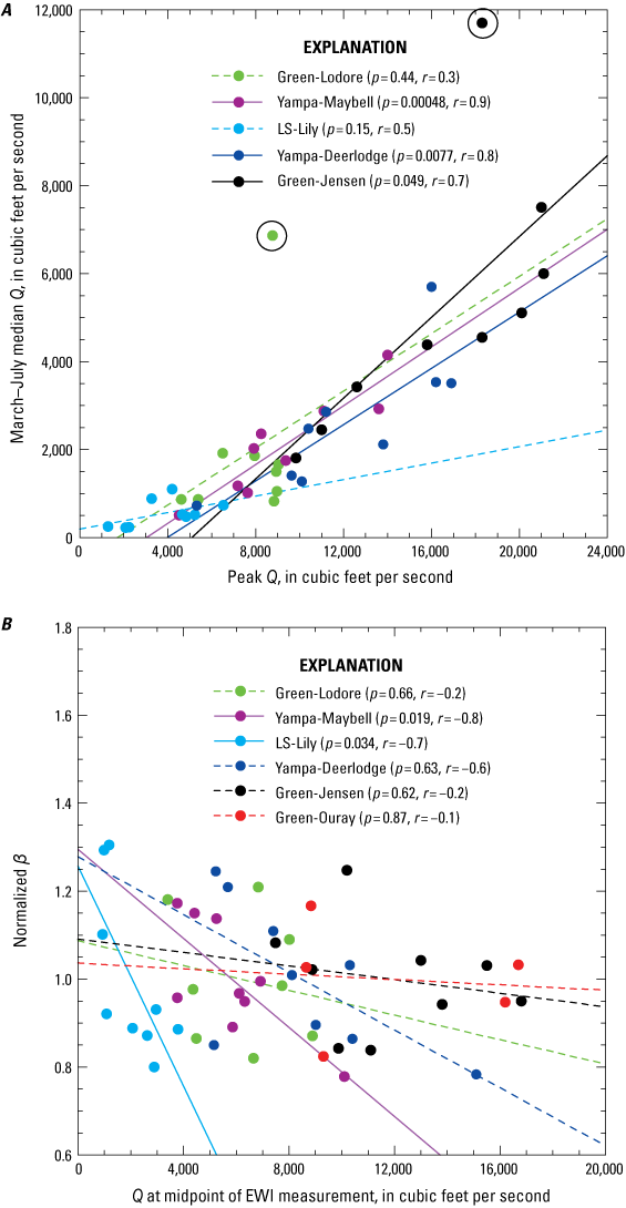
Plots of correlations at the six stations in our study between peak water discharge (Q) and the March–July median Q (A), and between Q at the midpoint time of the equal-width-increment (EWI) measurement (used to calculate the normalized high-flow nondimensional bed-sand coarseness [β] values in figure 25) and normalized high-flow β (B). Solid and dashed lines are the least-squares linear regressions fit to the data at each station; the level of significance (p) and correlation coefficient (r) are shown for each station; dashed lines indicate the regressions and associated correlations that are insignificant at the p = 0.05 critical level. Peak and median Q values for the Green-Ouray station are not depicted in A to avoid clutter because they are almost identical to those at the Green-Jensen station. Circled points in A are those associated with the 2017 sustained large releases from Flaming Gorge Dam described in the text. Station name abbreviations are defined in table 1; locations are shown in figure 1.
Effects of Sand-Wave Migration on Sand Transport at the Green-Jensen and Green-Ouray Stations Leading to Changes in Sand Mass in the Uinta Basin Segment of the Middle Green River
Changes in sand mass (that is, net deposition or erosion) in the Uinta Basin segment of the middle Green River are controlled by Q-independent shifts in sand transport at the Green-Jensen and Green-Ouray stations associated with the downstream migration of sand waves generated during a sequence of annual floods on the Yampa River. We refer to the first large flood in a sequence of annual Yampa River floods as the “year-1 flood,” the second flood in this sequence as the “year-2 flood,” and collectively to all floods in this sequence after the year-1 flood as “out-year floods.” The Q-independent shifts in sand transport at the Green-Jensen and Green-Ouray stations result from the changes in bed-sand grain size associated with the longitudinal positions of the Yampa-generated sand waves.
As inferred from β (fig. 25A, B), large Yampa River floods (that is, year-1 floods) generate sand waves with fine fronts that emanate into the Green River and migrate into the Uinta Basin segment past the Green-Jensen station but may not reach the Green-Ouray station (fig. 27). This longitudinal position of the year-1 sand wave is associated with bed-sand fining at the Green-Jensen station (fig. 25B). Because the Green-Ouray station is downstream from the front of the year-1 sand wave, the Green-Ouray station is in the coarser tail of an out-year sand wave from a preceding flood sequence (fig. 27A). In addition, because this tail of the preceding out-year sand wave is winnowed as this sand wave migrates downstream during the year-1 flood, this longitudinal position of the year-1 sand wave, with its front located between the Green-Jensen and Green-Ouray stations, is associated with bed-sand coarsening at the Green-Ouray station (fig. 25B). Consequently, increased sand transport occurs at the Green-Jensen station while decreased sand transport occurs at the Green-Ouray station during the year-1 flood. As described below in the “Influence of Flood Magnitude and Source on Sediment Budgets During Annual Floods” section of this report, sand deposition in the Uinta Basin segment thus occurs during the year-1 flood owing to a downstream decrease in sand transport associated with downstream bed-sand coarsening between the Green-Jensen and Green-Ouray stations.
The downstream migration of the year-1 sand wave during out-year Yampa River floods in combination with the generation of out-year sand waves results in either no substantial net downstream change in bed-sand grain size between the Green-Jensen and Green-Ouray stations or downstream fining between these stations (fig. 27B, C). During the year-2 flood, the front of the year-1 sand wave migrates downstream past the Green-Ouray station causing bed-sand fining at this station (figs. 25C, 27B, C). Depending on the magnitudes of the year-2 and other out-year floods, however, the bed-sand grain size at the Green-Jensen station will either not change substantially or will coarsen during these floods. The tail of the year-1 sand wave will be winnowed as it migrates downstream, thereby causing bed-sand coarsening. The degree of this coarsening at the Green-Jensen station may be offset depending on the magnitudes of the out-year floods. As inferred from β (fig. 25A, B), a series of similar-magnitude Yampa River floods will likely generate a succession of similar-sized sand waves of similar grain size in the Uinta Basin segment. Under this scenario, the resupply of sand during each flood could offset the bed-sand coarsening at the Green-Jensen station caused by the downstream migration of the year-1 sand wave, thereby leading to no substantial downstream change in bed-sand grain size between the Green-Jensen and Green-Ouray stations (fig. 27B). Moreover, a series of declining Yampa River floods will likely generate a succession of smaller, coarser sand waves in the Uinta Basin segment. Under this scenario, the bed sand at the Green-Jensen station would progressively coarsen mostly from the winnowing of the tail(s) of the year-1 or amalgamated preceding sand wave(s) and possibly also from the addition of coarser sand during these smaller out-year floods, thereby leading to downstream fining between the Green-Jensen and Green-Ouray stations (fig. 27C).
Successive floods in a sequence of annual Yampa River floods of equal or declining Q thus generate annual sand waves in the middle Green River of roughly similar or coarsening grain size, as inferred from the normalized high-flow β values in figure 25. Consequently, the continued downstream migration of sand waves in the middle Green River during out-year floods can result in either no net downstream change in bed-sand grain size or downstream fining in the Uinta Basin segment. Thus, out-year floods will typically be associated with sand conveyance through (fig. 27B) or sand erosion in (fig. 27C) the Uinta Basin segment. Because the upper Green River supplies far less sand to the middle Green River than does the Yampa River, sustained large releases from Flaming Gorge Dam are likely to limit bed-sand fining at Green-Jensen and increase bed-sand coarsening at Green-Ouray and thereby modify the downstream migration of the sand waves generated by Yampa River floods (fig. 27C).
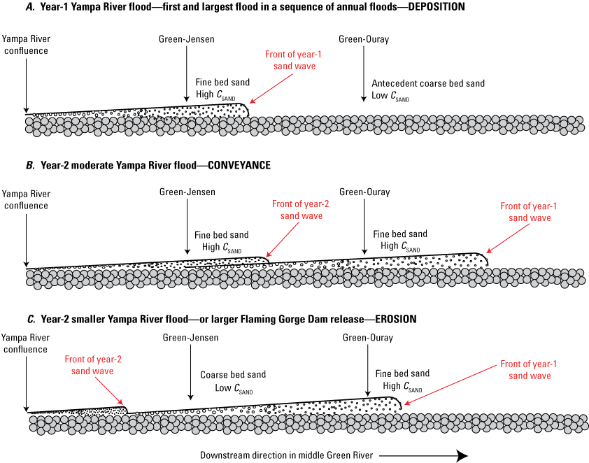
Conceptual model showing the longitudinal positions of the year-1 and year-2 Yampa-generated sand waves in the middle Green River, Colorado and Utah. A, A year-1 flood; B, a moderate year-2 flood; and C, either a smaller year-2 flood or larger release from Flaming Gorge Dam. These generalized positions were inferred from the values of water discharge (Q) and normalized high-flow nondimensional bed-sand coarseness (β) in figure 25. The relative bed-sand grain size and the velocity-weighted suspended-sand concentration (CSAND) near and above Jensen, Utah (Green-Jensen station) and above Ouray, Utah (Green-Ouray station) are indicated for each case. The longitudinal difference in bed-sand grain size and associated magnitude of CSAND controls whether sand is deposited in (A), conveyed through (B), or eroded from (C) the Uinta Basin segment of the middle Green River between the Green-Jensen and Green-Ouray stations. Locations of stations are shown in figure 1.
The observed shifts in the Q—CSAND point clouds at the Green-Jensen and Green-Ouray stations are consistent with the above-described changes in bed-sand grain size associated with the downstream migration of sand waves generated during the annual flood of the Yampa River (fig. 28). In figure 28, the Q—CSAND point clouds at Green-Jensen and Green-Ouray are plotted for all measurement types during the March–July annual-flood period in each year. Because the sand bedload during March–July at Green-Ouray is a much larger percentage of the sand total load (that is, sand bedload plus suspended-sand load) than at Green-Jensen, and because CSAND does not include bedload, large overlap of the Q—CSAND point clouds at these two stations indicates sand erosion in the Uinta Basin segment. Among the 2017–2021 March–July annual-flood periods, the sand bedload at Green Jensen ranged from 4 to 12 percent of the sand total load, whereas the sand bedload at Green-Ouray ranged from 20 to 34 percent of the sand total load (appendix 1). To place the positions of the Q—CSAND point clouds each year in context, the March–July median Q at the Yampa-Deerlodge and Green-Lodore stations are reported, the normalized high-flow β and measured bed-sand area (AB) associated with the high-flow EWI measurements are indicated, and the “CSAND slopes” are indicated. The “CSAND slope” is simply the slope of the least-squares linear regression of CSAND on Q, forced through the origin, and is used as a metric for the steepness of a Q—CSAND point cloud; all CSAND measurement types are included in this regression (EWI, calibrated pump, and acoustical). For example, an increase in the CSAND slope indicates an upward shift in CSAND at any given Q and thereby an increase in sand transport, whereas a decrease in the CSAND slope indicates a downward shift in CSAND at any given Q and thereby a decrease in sand transport.
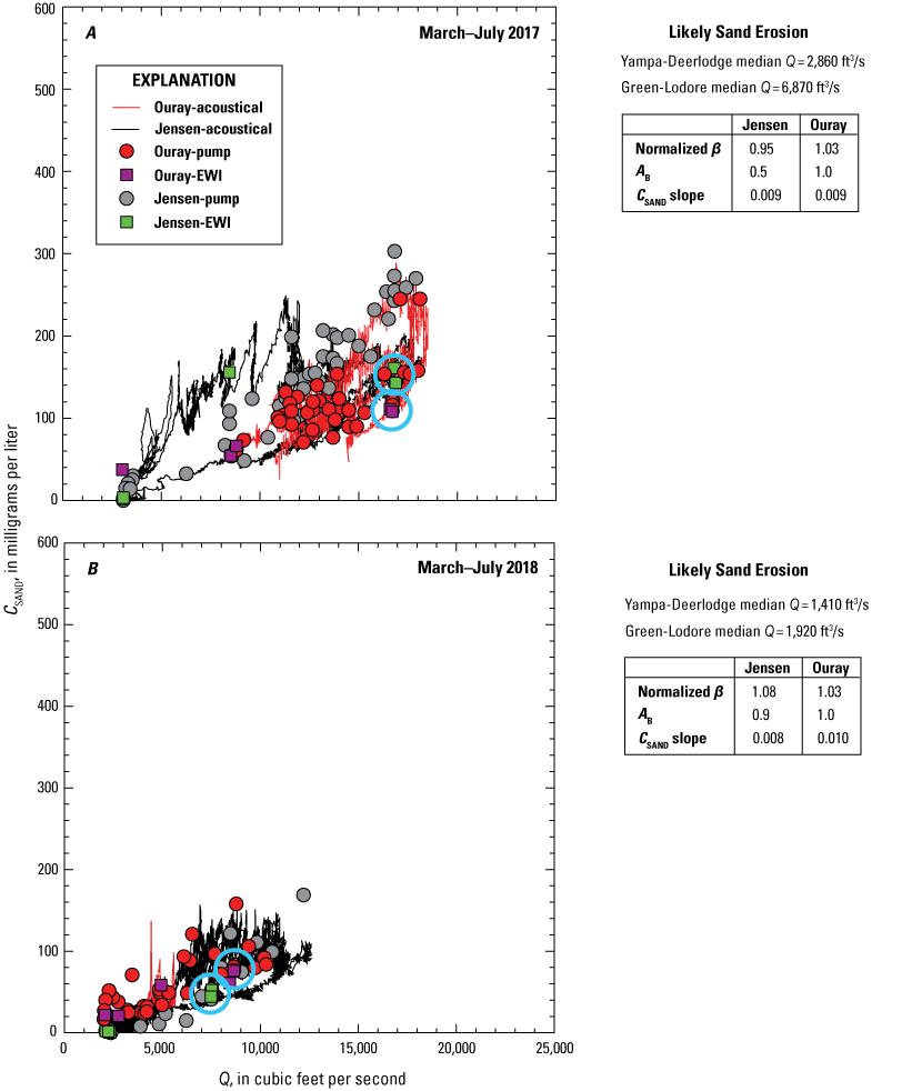
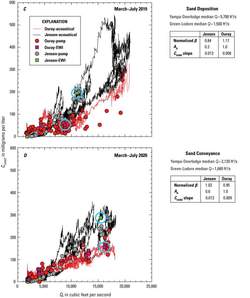
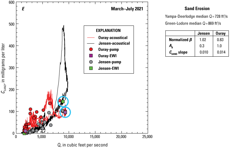
Plots of water-discharge—sand-concentration (Q—CSAND) point clouds during the March–July annual-flood period at the Green-Jensen and Green-Ouray stations. A, 2017; B, 2018; C, 2019; D, 2020; and E, 2021. The interpreted March–July change in sand mass in the Uinta Basin segment (from fig. 31), the Yampa-Deerlodge and Green-Lodore station March–July median Q, the normalized high-flow nondimensional bed-sand coarseness (β) and bed-sand area (AB) associated with the high-flow equal-width-increment (EWI) measurements at each station (circled in blue), and the CSAND slope at each station are shown. Station name abbreviations are defined in table 1; locations are shown in figure 1. ft3/s, cubic feet per section. Pump, calibrated pump; ft3/s, cubic feet per second.
For direct comparison of the results in figure 28 to those presented in the next section of this report, the geomorphic implication of the March–July change in sand mass from the continuous mass-balance sand budgets for the Uinta Basin segment (from the “Influence of Flood Magnitude and Source on Sediment Budgets During Annual Floods” section below) is also indicated for each year. This implication is given in each figure panel in terms of sand erosion, likely sand erosion, sand conveyance, or sand deposition (no years fell into the likely sand deposition category). The uncertainty thresholds used to determine whether sediment budgets are indeterminate or indicate erosion, likely erosion, deposition, or likely deposition are the same as in Topping and others (2018) and were reviewed in the “Sediment Budgets” subsection in the “Analytical Methods” section. Although indeterminate sand budgets typically arise from erosion offsetting deposition in a river segment, and not necessarily from sand being transported through a segment with zero local erosion and deposition, we neglect this complexity to be consistent with the conceptual model in figure 17 and simply use the term “sand conveyance” for cases with indeterminate sand budgets.
Out-Year Floods of 2017 and 2018
Between the 2017 and 2018 annual floods (out-year floods) that preceded the large 2019 Yampa River flood (a year-1 flood), the Q—CSAND point cloud at the Green-Jensen station shifted slightly downward (QSAND slope decreased slightly from 0.009 to 0.008) as the Q—CSAND point cloud at the Green-Ouray station shifted slightly upward (QSAND slope increased slightly from 0.009 to 0.010) (fig. 28A, B). The slight downward shift in the Q—CSAND point cloud at Green-Jensen was associated with bed-sand coarsening (normalized β increased from 0.95 to 1.08) that was perhaps slightly offset by an increase in bed-sand area (AB increased from 0.5 to 0.9). The slight upward shift in the Q—CSAND point cloud at Green-Ouray was associated with negligible change in bed-sand grain size (normalized β remained constant at ~1.03) and no change in bed-sand area (the bed is fully sand covered at the Green-Ouray station). Given the similarity of the CSAND slopes between the Green-Jensen and Green-Ouray stations during the March–July 2017 and March–July 2018 annual floods, sand was “likely eroded” from the Uinta Basin segment during each of these out-year floods because the uncertainty was between 1 and 2 times the absolute value of the zero-bias value of the change in sand mass, as discussed below in the “Influence of Flood Magnitude and Source on Sediment Budgets During Annual Floods” section of this report.
Year-1 Flood of 2019
As the result of the large year-1 Yampa River flood in 2019, the Q—CSAND point cloud at the Green-Jensen station shifted upward (QSAND slope increased from 0.008 to 0.013) as the Q—CSAND point cloud at the Green-Ouray station shifted downward (QSAND slope increased from 0.010 to 0.008) between 2018 and 2019 (fig. 28B, C). The major upward shift in the Q—CSAND point cloud at Green-Jensen was associated with bed-sand fining (β decreased from 1.08 to 0.84) that was perhaps slightly offset by a decrease in bed-sand area (AB decreased from 0.9 to 0.2); this upward shift was thus caused by the fine front of the 2019 Yampa-generated sand wave passing this station. The downward shift in the Q—CSAND point cloud at Green-Ouray was associated with bed-sand coarsening (normalized β increased from 1.03 to 1.17) and no change in bed-sand area; this downward shift was caused by the continued downstream migration of an older sand wave generated during an earlier Yampa River flood in combination with the 2019 Yampa-generated sand wave not yet arriving at this station. Given the much steeper CSAND slope at Green-Jensen than at Green-Ouray during March–July 2019, sand was deposited in the Uinta Basin segment during the 2019 annual flood, as discussed below in the “Influence of Flood Magnitude and Source on Sediment Budgets During Annual Floods” section of this report.
Year-2 Flood of 2020 and the Downstream Migration of the Year-1 Sand Wave
Following the year-1 2019 flood, the position of the Q—CSAND point cloud at the Green-Jensen station remained stable (QSAND slope remained constant at ~0.013) as the Q—CSAND point cloud at the Green-Ouray station shifted slightly upward (QSAND slope increased slightly from 0.008 to 0.009) between 2019 and 2020 (fig. 28C, D). The lack of change in the Q—CSAND point cloud at Green-Jensen was associated with bed-sand coarsening (normalized β increased from 0.84 to 1.03); the effect of this coarsening on CSAND was apparently completely offset by an increase in bed-sand area (AB increased from 0.2 to 0.6). The upward shift in the Q—CSAND point cloud at Green-Ouray was associated with bed-sand fining (β decreased from 1.17 to 0.95) and no change in bed-sand area. The bed-sand coarsening at Green-Jensen coincident with the bed-sand fining at Green-Ouray indicated the continued downstream migration of the year-1 sand wave generated during the 2019 Yampa River flood, with the fine front of this sand wave passing the Green-Ouray station during 2020. Although the CSAND slope remained much steeper at Green-Jensen than at Green-Ouray during March–July 2020, sand was likely conveyed through the Uinta Basin segment during the year-2 2020 annual flood, as discussed below in the “Influence of Flood Magnitude and Source on Sediment Budgets During Annual Floods” section of this report. The reason for the sand conveyance in 2020 and not sand deposition (as in 2019) arises mainly from the 2019 Yampa River flood being much larger than the 2020 Yampa River flood. Thus, despite the CSAND slopes being similar at Green-Jensen between these two annual floods, the sand loads were much larger at Green-Jensen during the 2019 annual flood because of the much higher Q; Yampa River median Q during March–July 2019 was 2.7 times larger than in during March–July 2020 (fig. 28C, D).
Out-Year Flood of 2021 and Continued Downstream Migration of the Year-1 Sand Wave
Between the 2020 and 2021 out-year floods, the Q—CSAND point cloud at the Green-Jensen station shifted downward (QSAND slope decreased from 0.013 to 0.010) as the Q—CSAND point cloud at the Green-Ouray station shifted upward (QSAND slope increased from 0.009 to 0.014) (fig. 28D, E). The major downward shift in Q—CSAND at Green-Jensen was associated with only slight bed-sand fining (normalized β decreased from 1.03 to 1.02), the negligible effect of which on CSAND was completely offset by a large decrease in bed-sand area (AB decreased from 0.6 to 0.3). The major upward shift in the Q—CSAND point cloud at Green-Ouray was associated with bed-sand fining (normalized β decreased from 0.95 to 0.83) and no change in bed-sand area. The continued bed-sand coarsening at Green-Jensen coincident with bed-sand fining at Green-Ouray results from the continued 2020–2021 downstream migration of the year-1 sand wave generated during the 2019 Yampa River flood combined with the likely arrival at Green-Jensen of the coarser sand waves generated during the smaller 2020–2021 out-year Yampa River floods. Given the much steeper CSAND slope at Green-Ouray than at Green-Jensen during March–July 2021, sand was eroded from the Uinta Basin segment during the 2021 annual flood, as discussed in the next section of this report.
Influence of Flood Magnitude and Source on Sediment Budgets During Annual Floods
Larger Yampa River floods cause erosion in the Deerlodge Park and Dinosaur sediment-budget areas but tend to cause deposition farther downstream in the Uinta Basin segment of the Green River (figs. 29–31). Conversely, although longer duration large releases from Flaming Gorge Dam cause no detectable change in sand mass in the Dinosaur sediment-budget area (fig. 30B), these releases may cause erosion in the Uinta Basin segment (fig. 31B). Though small in magnitude, unequivocal erosion of sediment from the Uinta Basin segment has only been observed during low-flow years with small Yampa River floods (fig. 31). These results are consistent with the earlier results of Topping and others (2018) for the Deerlodge Park and Dinosaur sediment-budget areas. In addition, these results are those expected for the Dinosaur and Uinta Basin sediment budgets given the bed-sand grain-size changes (fig. 25), and associated shifts in sand transport (fig. 28), caused by the downstream migration of the sand waves generated during annual floods of the Yampa River (fig. 27).
The Deerlodge Park sediment-budget area has been a likely source of sand for the lower Yampa River for many years. Although minor overlap of the error bars with the line of zero change exists for a few cases, net sand erosion has occurred from this part of the Yampa River basin during all annual floods where the peak Q and the March–July median Q, respectively, exceed ~7,800 and ~1,500 ft3/s at the Yampa-Maybell station (fig. 29A, B), ~2,800 and ~360 ft3/s at the LS-Lily station (fig. 29C, D), and ~10,300 and ~1,800 ft3/s at the Yampa-Deerlodge station (fig. 29E, F). The negative correlations between these annual-flood metrics (peak Q and March–July median Q) and the change in sand mass in this sediment-budget area during the March–July annual-flood period is moderate to strong (with r ranging from 0.4 to 0.6). On average, ~70,000±62,000 metric tons of sand were eroded from the Deerlodge Park area each year during the March–July annual-flood period between 2013 and 2021. Given the uncertainties in the loads at the Yampa-Maybell and LS-Lily stations, this amount was equal to between 5 and 130 percent of the average amount of sand supplied to the Deerlodge Park area by the upper Yampa and Little Snake Rivers during the annual flood. Thus, a considerable amount of sand supplied to the middle Green River during the annual floods of the Yampa River during 2013–2021 could have been eroded from the Deerlodge Park sediment-budget area.
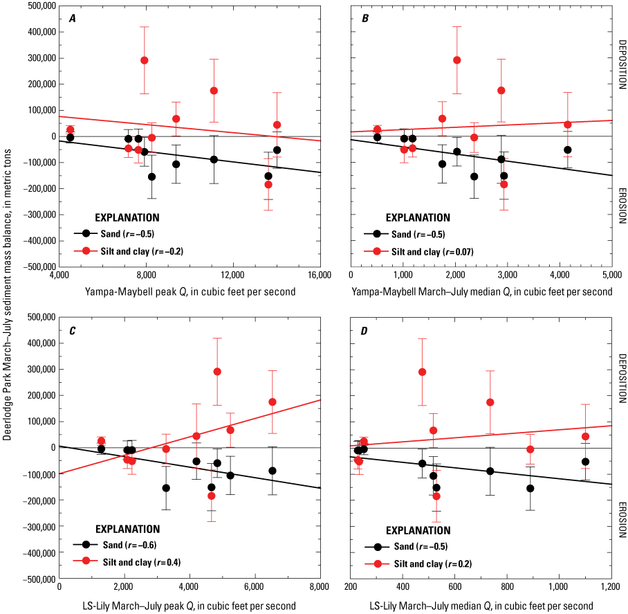
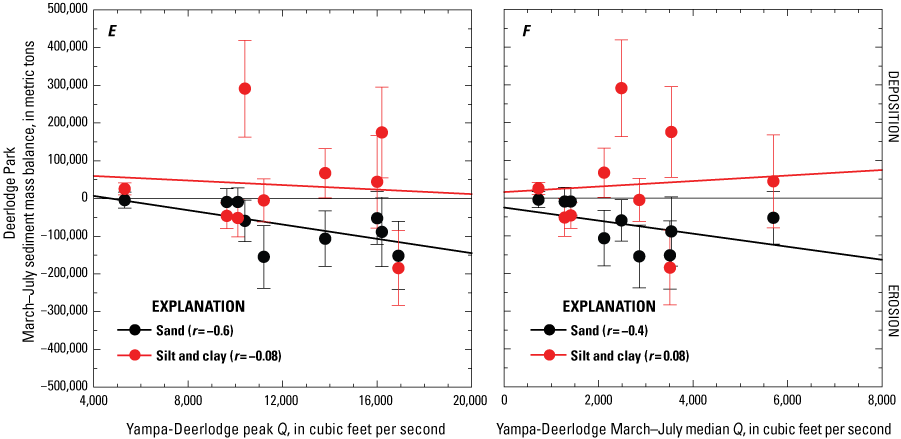
Plots of changes in the sediment mass balance in the Deerlodge Park sediment-budget area (refer to fig. 1) during the annual-flood period of March–July as a function of peak water discharge (Q) (A) and March–July median Q (B) at the Yampa-Maybell station, peak Q (C) and March–July median Q (D) at the LS-Lily station, and peak Q (E) and March–July median Q (F) at the Yampa-Deerlodge station. Lines are the least-squares linear regressions fit to the zero-bias mass-balance values (depicted as filled circles); correlation coefficients (r) associated with these regressions are shown. Error bars indicate the uncertainty in the calculated changes in sediment mass balance resulting from the propagation of the uncertainties in the sediment loads through the sediment-budget calculation. Positive values of the sediment mass balance indicate deposition whereas negative values indicate erosion during March–July. Station name abbreviations are defined in table 1; locations are shown in figure 1.
Analysis of aerial lidar (light detection and ranging) surveys indicates that ~50,000±130,000 (±95-percent-confidence-level uncertainty) cubic meters (m3) of sediment were eroded from the downstream ~3.7 km of the Yampa River in Deerlodge Park between 2011 and 2015 (Leonard, 2022; volume of sediment erosion and uncertainty revised by C. Leonard, National Park Service, written commun., May 7–8, 2024). The river segment in which this erosion was measured encompassed the lower ~3.1 km of the Deerlodge Park sediment-budget area and extended ~0.6 km downstream from the Yampa-Deerlodge station. This erosion resulted from a combination of slight net channel-bed scour (−0.07±0.24 m) and the lateral migration of the Yampa River, which caused the erosion of higher cut banks on the outsides of meanders and the deposition of lower banks on the insides of meanders (Leonard, 2022; value of net channel-bed scour and 95-percent-confidence-level uncertainty revised by C. Leonard, National Park Service, written commun., May 6, 2024). Conversion of this volume of sediment erosion to mass yields 80,000±210,000 metric tons of erosion between 2011 and 2015, assuming 40 percent porosity (after Curry and others, 2004) and a quartz density of 2,650 kilograms per cubic meter (kg/m3). This magnitude of likely predominantly sand erosion equates to a mean-annual erosion rate of ~20,000 metric tons, an erosion rate in agreement with that determined for the 2013–2021 annual-flood period from the continuous mass-balance sediment budget calculated for the longer river segments that comprise the entire Deerlodge Park sediment-budget area. Moreover, repeat surveys of cross sections suggest that erosion of sand from the Deerlodge Park area has been ongoing since at least 1983, with a 1997–2017 mean-annual sand erosion rate of ~37,000 metric tons (Griffiths and others, 2024), an erosion rate also in agreement with that for the 2013–2021 annual-flood period determined from our continuous mass-balance sediment budget. Therefore, it is likely that sand has been eroded from the Deerlodge Park sediment-budget area during the annual flood of the Yampa River for quite some time. Although this long-term erosion may be a legacy of the bed-sand coarsening associated with the downstream migration of the tail(s) of the sand wave(s) generated by the 1956–1966 Sand Creek floods, as suggested by Topping and others (2018), this erosion likely also owes to the natural lateral migration of the river (Leonard, 2022).
In contrast to the sediment-budgeting results for sand, no net change in the amount of silt and clay stored in the Deerlodge Park sediment-budget area has occurred during the annual floods of 2013–2021, although large changes in the stored amount of silt and clay did occur during some years. The mean change in March–July silt and clay mass in the Deerlodge Park area among the 2013–2021 annual floods was +35,000±77,000 metric tons. Following Topping and others (2018), we conclude that sediment budgets are indeterminate when the uncertainty is ≥2 times the absolute value of the zero-bias value, demonstrably positive or negative when the uncertainty is less than the zero-bias value, and either likely positive or negative when the uncertainty falls between these bounds. In this case, the uncertainty is 2.2 times the zero-bias value of 35,000 metric tons, and therefore no net change in silt and clay mass can be demonstrated among the 2013–2021 annual floods. The only annual-flood metric possibly related to changes in silt and clay mass in the Deerlodge Park sediment-budget area is the peak Q of the Little Snake River flood (fig. 29C); the correlation between peak Q at the LS-Lily station and deposition of silt and clay in the Deerlodge Park area during the annual flood is moderate (r = 0.4).
Sand eroded from the Dinosaur sediment-budget area during larger Yampa River floods can be deposited farther downstream in the Uinta Basin segment of the middle Green River (figs. 30–31). The strong tendency toward erosion of sand from the Dinosaur sediment-budget area during large Yampa River floods is indicated by the strong negative correlation between the peak Q of the annual flood at the Yampa-Deerlodge station and sand mass balance in the Dinosaur sediment-budget area (r = −0.7, fig. 30C), and the very strong negative correlation between the March–July median Q at Yampa-Deerlodge and sand mass balance in the Dinosaur sediment-budget area (r = −0.9, fig. 30D). It is not simply the magnitude of the annual flood that causes erosion in the Dinosaur sediment-budget area, otherwise the very strong negative correlation between the March–July median Q at Yampa-Deerlodge and the sand mass balance in the Dinosaur sediment-budget area would be reflected in a similar negative correlation at the Green-Jensen station, where this correlation is, in fact, only weak (r = −0.3, fig. 30F). The annual floods that cause the greatest amount of erosion in the Dinosaur sediment-budget area are thus the large Yampa River floods that also supply the largest amounts of sand to the Dinosaur sediment-budget area.
Although more sediment-transport data at the stations bracketing the Uinta Basin segment during larger Yampa River floods would help solidify this relation, an equally strong tendency toward deposition of sand in the Uinta Basin segment during large Yampa River floods is strongly suggested by the strong positive correlation between the peak Q of the annual flood at Yampa-Deerlodge and the sand mass balance in the Uinta Basin segment (r = 0.7, fig. 31C), and the very strong positive correlation between the March–July median Q at Yampa-Deerlodge and the sand mass balance in the Uinta Basin segment (r = 0.8, fig. 31D). Sand is eroded from the Uinta Basin segment during the annual-flood period in years with smaller Yampa River floods (fig. 31C, D), and possibly also eroded during years with larger sustained Flaming Gorge Dam releases (r = −0.5, fig. 31B). Sand deposition occurs in the Dinosaur sediment-budget area during smaller Yampa River floods (fig. 30C, D), and in the lower Q periods during the months of the year outside the March–July annual-flood period.
Larger peak Q of Flaming Gorge Dam releases (r = −0.5, fig. 30A) or larger March–July median Q in the Yampa River (r = −0.4, fig. 30D) provide the most likely mechanisms for erosion of silt and clay from the Dinosaur sediment-budget area. As with the sand, much of the net deposition of silt and clay in the Dinosaur sediment-budget area occurs during the months of the year outside the March–July annual-flood period shown in figure 30. Flows during the annual flood have little effect on the amount of silt and clay stored in the Uinta Basin segment of the middle Green River, although larger sustained Flaming Gorge Dam releases may erode silt and clay from this segment (r = −0.7, fig. 31B).
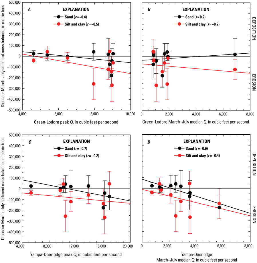
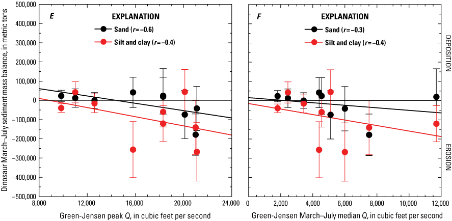
Plots of changes in the sediment mass balance in the Dinosaur sediment-budget area (refer to fig. 1) during the annual-flood period of March–July as a function of peak water discharge (Q) (A) and March–July median Q (B) at the Green-Lodore station, peak Q (C) and March–July median Q (D) at the Yampa-Deerlodge station, and peak Q (E) and March–July median Q (F) at the Green-Jensen station. Lines are the least-squares linear regressions fit to the zero-bias mass-balance values; correlation coefficients (r) associated with these regressions are shown. Error bars indicate the uncertainty in the calculated changes in sediment mass balance resulting from the propagation of the uncertainties in the sediment loads through the sediment-budget calculation. Positive values of the sediment mass balance indicate deposition whereas negative values indicate erosion during March–July. Station name abbreviations are defined in table 1; locations are shown in figure 1.
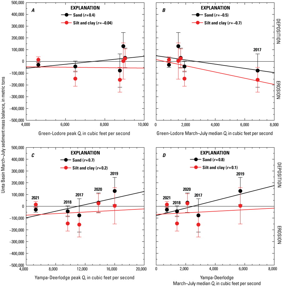
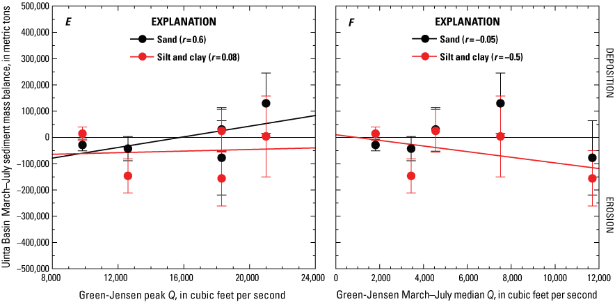
Plots of changes in the sediment mass balance in the Uinta Basin sediment-budget segment of the middle Green River (refer to fig. 1) during the annual-flood period of March–July as a function of peak water discharge (Q) (A) and March–July median Q (B) at the Green-Lodore station, peak Q (C) and March–July median Q (D) at the Yampa-Deerlodge station, and peak Q (E) and March–July median Q (F) at the Green-Jensen station. Lines are the least-squares linear regressions fit to the zero-bias mass-balance values; correlation coefficients (r) associated with these regressions are shown. Error bars indicate the uncertainty in the calculated changes in sediment mass balance resulting from the propagation of the uncertainties in the sediment loads through the sediment-budget calculation. Positive values of the sediment mass balance indicate deposition whereas negative values indicate erosion during March–July. The changes in sand mass balance during the annual floods indicated by year in B–D are discussed in the text. Station name abbreviations are defined in table 1; locations are shown in figure 1.
Over longer sequences of floods in both the Dinosaur sediment-budget area and Uinta Basin segment, the change in sand mass has been negligible whereas slight silt and clay erosion may have occurred. Among the 2013–2021 annual floods in the Dinosaur sediment-budget area, the change in March–July sand mass was −19,000±88,000 metric tons (indeterminate change) and the change in March–July silt and clay mass was −90,000±95,000 (likely negative but small change). Similarly, among the 2017–2021 annual floods in the Uinta Basin segment, the change in March–July sand mass was 2,600±82,000 metric tons (indeterminate change) and the change in March–July silt and clay mass was −52,000±86,000 metric tons (likely negative but small change). Because tributaries, which likely supply much more silt and clay than sand, are not included in these sediment-budget calculations (as described in the “Analytical Methods” section), it remains possible, however, that these “likely negative” results for silt and clay are artifacts of the exclusion of tributaries. If the silt-and-clay loads of tributaries were measured and then included in the sediment-budget calculations, the changes in silt and clay mass, like the changes in sand mass, could also be indeterminate when integrated over many annual floods.
Given that most of the demonstrable changes in sediment mass in the Dinosaur sediment-budget area during the annual-flood period involve Yampa River flows, it is most likely that these changes in sediment mass occur within the lower Yampa and alluvial reaches of the middle Green River and not within the upper Green River in the Canyon of Lodore. The geographic scope of where most of the changes in sand mass are likely located can be further refined based on the stations where the largest shifts in the Q—CSAND point clouds occur as a function of changes in bed-sand grain size. The large Yampa River floods that cause substantial upward shifts in the Q—CSAND point clouds at the Green-Jensen station cause relatively little change in the Q—CSAND point clouds at the Yampa-Deerlodge station (for example, the large 2019 flood). Thus, the location of the net erosion of sand from the Dinosaur sediment-budget area associated with the bed-sand fining and increase in sand transport at Green-Jensen was likely much closer to the Green-Jensen station than the Yampa-Deerlodge station. Thus, as suggested by Topping and others (2018), it is likely that most of the changes in sediment mass occur in the shorter alluvial reaches with the greatest sediment accommodation space, for example, Echo, Island, and Rainbow Parks (fig. 1B), all of which are along the middle Green River, much closer to the Green-Jensen station than the Yampa-Deerlodge station.
Although it may seem counterintuitive for large Yampa River floods to erode sand from the middle Green River in the Dinosaur sediment-budget area because these floods supply the largest amount of sand to this river segment, the physical basis for this effect is well-established and arises from changes in bed-sand grain size. Einstein and Chien (1953) were perhaps the first to show that changes in bed-sand grain size have a much stronger effect on sand transport than changes in sand transport have on the bed-sand grain-size distribution (Rubin and Topping, 2001). Consequently, the bed-sand fining caused by the downstream migration of the front of a sand wave is associated with an immediate increase in CSAND and thereby an immediate increase in sand transport. Thus, although the finest size classes of sand in a sand wave may migrate downstream quickly (Topping and others, 2000, 2021), the associated increase in CSAND occurs even faster. Because of the nonlinear relation between bed-sand grain size and CSAND (eq. 2A), small changes in bed-sand grain size thus cause large and immediate shifts in sand transport at constant , and thereby at constant Q. Depending on the rate and depth of the mixing of the fine front of a sand wave with the antecedent coarser sand bed, these shifts in the Q—CSAND point clouds may persist for long enough during the annual flood so that the bed-sand fining caused by a large Yampa River flood has a larger and longer effect on sand transport at Green-Jensen than does the actual amount of sand supplied during the Yampa River flood. In essence, the large reservoir of sand present on the bed buffers the rate at which the bed-sand grain-size distribution can change in response to a change in the upstream sand supply. This reservoir effect was observed in the laboratory by Einstein and Chien (1953) and formed the basis for their conclusion that changes in the bed-sand grain-size distribution had a “strong and immediate” effect on sand transport, whereas changes in sand transport had only a “weak and slow” effect on the bed-sand grain-size distribution. More extensive fining of the bed sand upstream from the Green-Jensen station during a larger Yampa River flood may therefore cause an increase in the sand export from the Dinosaur sediment-budget area that exceeds the amount of sand supplied to the Dinosaur sediment-budget area from both the Yampa and upper Green Rivers, as suggested by the increased sand erosion during progressively larger Yampa River floods (fig. 30C, D).
Sand deposition in the Uinta Basin segment of the middle Green River during a large year-1 annual flood on the Yampa River, and sand erosion from this segment during subsequent out-years also occur as the result of the longitudinal patterns in bed-sand grain size associated with the downstream migration of sand waves generated during Yampa River floods, as described in the previous section of this report. Consequently, large year-1 floods, like the 2019 Yampa River flood, can cause deposition in the Uinta Basin segment (fig. 31C, D). Because of the continued downstream migration of the year-1 sand wave and the addition of generally smaller and coarser sand waves during out-year Yampa River floods, the bed sand generally coarsens and sand transport decreases at the Green-Jensen station while the bed sand fines and sand transport increases at the Green-Ouray station during out-year floods (fig. 28D, E). As described in the previous section, the degree to which the bed sand coarsens at Green-Jensen during these out-year floods is of course limited or potentially offset by the magnitude of each out-year flood, thereby affecting whether sand will be eroded or deposited in the Uinta Basin segment. For example, it took 2 years for the bed sand to coarsen sufficiently at Green-Jensen and fine sufficiently at Green-Ouray for sand to be eroded from the Uinta Basin segment following the large (year-1) Yampa River flood of 2019 (fig. 31C, D). Over the first year following this large flood (year-2), the bed sand coarsened at Green-Jensen and fined at Green-Ouray only to the extent that sand was conveyed through this river segment during the 2020 annual flood. Differences between the sequencing of flows from the Yampa River and upper Green River increase the complexity of this problem. For example, sustained large releases from Flaming Gorge Dam may increase the degree of bed-sand coarsening at Green-Jensen (fig. 28A), and thereby increase the potential for sand erosion from the Uinta Basin segment (fig. 31B). Similarly, the degree to which the bed sand fines and sand transport increases at Green-Ouray during the years following a large year-1 flood on the Yampa River flood depends on magnitude of subsequent out-year floods.
Cross-Section Resurveys
Long-Term and Changes in Sediment Storage and Cross-Section Geometry
Resurvey of the 27 cross sections suggests that slight net erosion of sediment from the Uinta Basin segment of the middle Green River occurred between the surveys conducted in 1994–1996 and the resurvey in 2020, with most of this decrease in sediment storage occurring through channel widening owing to bank retreat (figs. 32–39, table 6). We use the word “suggest” and not “indicate” because the sample size of 27 cross sections is likely too small to state this result with absolute certainty (Grams and others, 2019). The mean change in cross-sectional sediment area among the 27 cross sections between 1994–1996 and 2020 was −13.5±9.1 m2 (±1 standard error). Though the mean amount of erosion was slight, the erosion was pervasive, with 19 of the 27 cross sections exhibiting erosion. Though most cross sections eroded, the fewer cross sections that gained sediment exhibited larger changes in sediment storage. The mean change in cross-sectional sediment area among the 19 cross sections that lost sediment was −39.0±6.5 m2, whereas the mean change in cross-sectional sediment area among the 8 cross sections that gained sediment was +47.2±5.7 m2. Among all 27 cross sections, the mean change in minimum bed elevation was positive, at +0.46±0.22 m, thus indicating that the slight net erosion observed between the last survey in 1994–1996 and the 2020 resurvey did not involve net scour of the bed.
Channel widening was almost as ubiquitous as erosion in the resurveyed cross sections in the Uinta Basin segment of the middle Green River. Nineteen of the 27 cross sections eroded between 1994–1996 and 2020, with 17 of these cross sections widening. Though widening was almost as pervasive as erosion, the amount of net change in channel width among all 27 cross sections was negligible. Unlike the slight decrease in sediment storage among the 27 cross sections, the mean 1990s–2020 change in channel width was 0.0±2.0 m. This mean of zero change in width, however, resulted from extremely large amounts of channel narrowing at only 2 of the 27 cross sections, HB-1 and AB-4, which narrowed by 36.2 and 23.1 m, respectively. Among the 17 cross sections that widened, the mean amount of channel widening was +4.7±1.1 m, with the maximum amount of channel widening observed at cross section CB-6, where the river widened by 18.7 m.
Although widening was associated with net erosion, narrowing was not necessarily associated with deposition, but rather with a redistribution of sediment within the cross section. The mean change in the cross-sectional area of sediment storage among the 17 cross sections that widened was −24±8.5 m2, whereas the mean change in the cross-sectional area of sediment storage among the 10 cross sections that narrowed was 5.7±19.0 m2. The much larger standard error (19.0) than the mean (5.7) indicates that a substantial amount of net erosion occurred at some of the cross sections that narrowed. Indeed, net erosion occurred at 4 of the 10 cross sections that narrowed. In contrast, net erosion occurred at 15 of the 17 cross sections that widened, thus indicating the much tighter association of widening and erosion.
Although most of the long-term decrease in sediment storage among the 27 cross sections was associated with channel widening without net bed scour, changes in bed elevation did have a role. Bed aggradation was much larger in the cross sections that gained sediment than in those that lost sediment. The minimum bed elevation increased by 0.24±0.24 m among the 19 cross sections that lost sediment, whereas the minimum bed elevation increased by 1.00±0.43 m among the 8 cross sections that gained sediment. Thus, the slight 1990s–2020 decrease in the cross-sectional sediment area of −13.5±9.1 m2 was associated with widening and bed aggradation, such that the channel of the Uinta Basin of the middle Green River likely became slightly wider but shallower between 1994–1996 and 2020. As shown in the next section, it is likely that the 1990s–2020 channel widening and its associated erosion was indicative of a long-term, multi-decadal change in cross-section geometry and sediment storage in the Uinta Basin segment of the middle Green River. However, it is less certain that the bed aggradation was indicative of a long-term change or an artifact of a seasonal change in cross-section geometry.
The net erosion by channel widening in the Uinta Basin segment of the middle Green River between the mid-1990s and 2020 is essentially the opposite of the style of channel change observed during this period in the lower Green River. Unlike in the Uinta Basin segment of the middle Green River, net deposition by channel narrowing occurred in the lower Green River upstream from and in Canyonlands National Park between the mid-1980s and 2014, with almost half of the channel narrowing occurring between 1993 and 2009 (Walker and others, 2020). This narrowing of the Canyonlands segment of the lower Green River occurred episodically during periods of smaller annual floods (Grams and others, 2020) and may have been ongoing as of 2020 (Walker and others, 2020).
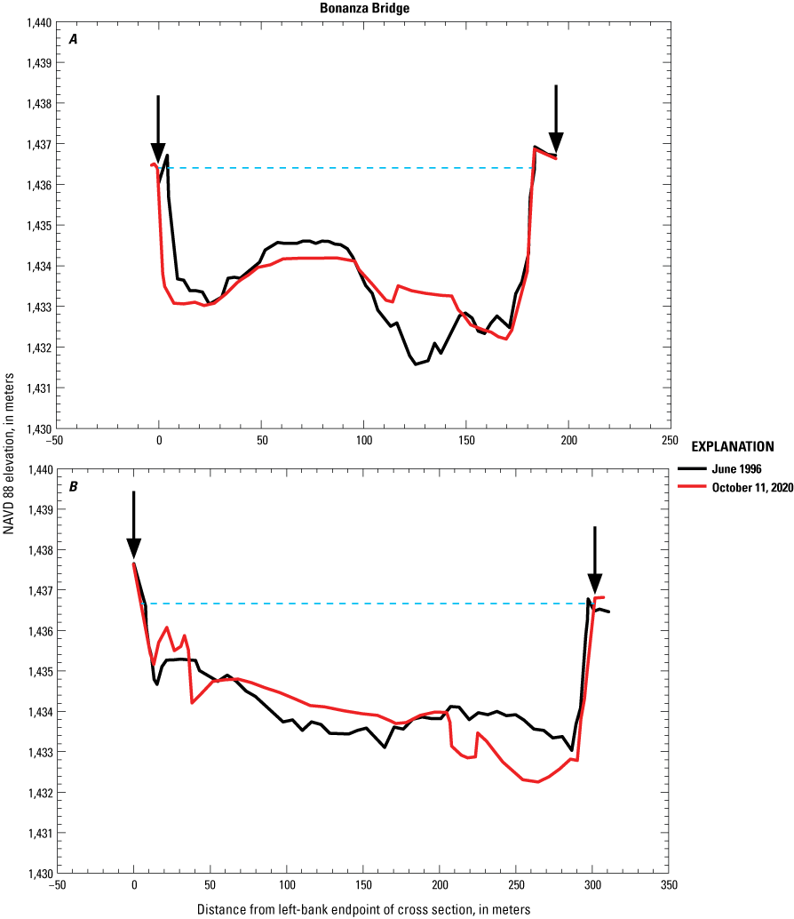
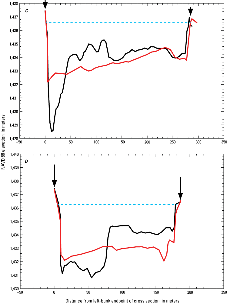
Plots comparing the Bonanza Bridge (BB) cross sections in the Uinta Basin segment of the middle Green River, Utah, in June 1996 and on October 11, 2020. A, BB-4 at river kilometer (RK) 196.4; B, BB-3 at RK 196.6; C, BB-2 at RK 197.0; and D, BB-1 at RK 197.3. Vertical arrows indicate the bounds of the domain over which the changes in cross-sectional sediment area and topographic variance were evaluated between surveys. Horizontal dashed blue line indicates the elevation at which channel width was measured (excluding the widths of shallow floodplain depressions behind levees). The elevations of the tops of the right bank in B and C in 2020 were likely affected by farming. NAVD 88, North American Vertical Datum of 1988; m, meter.
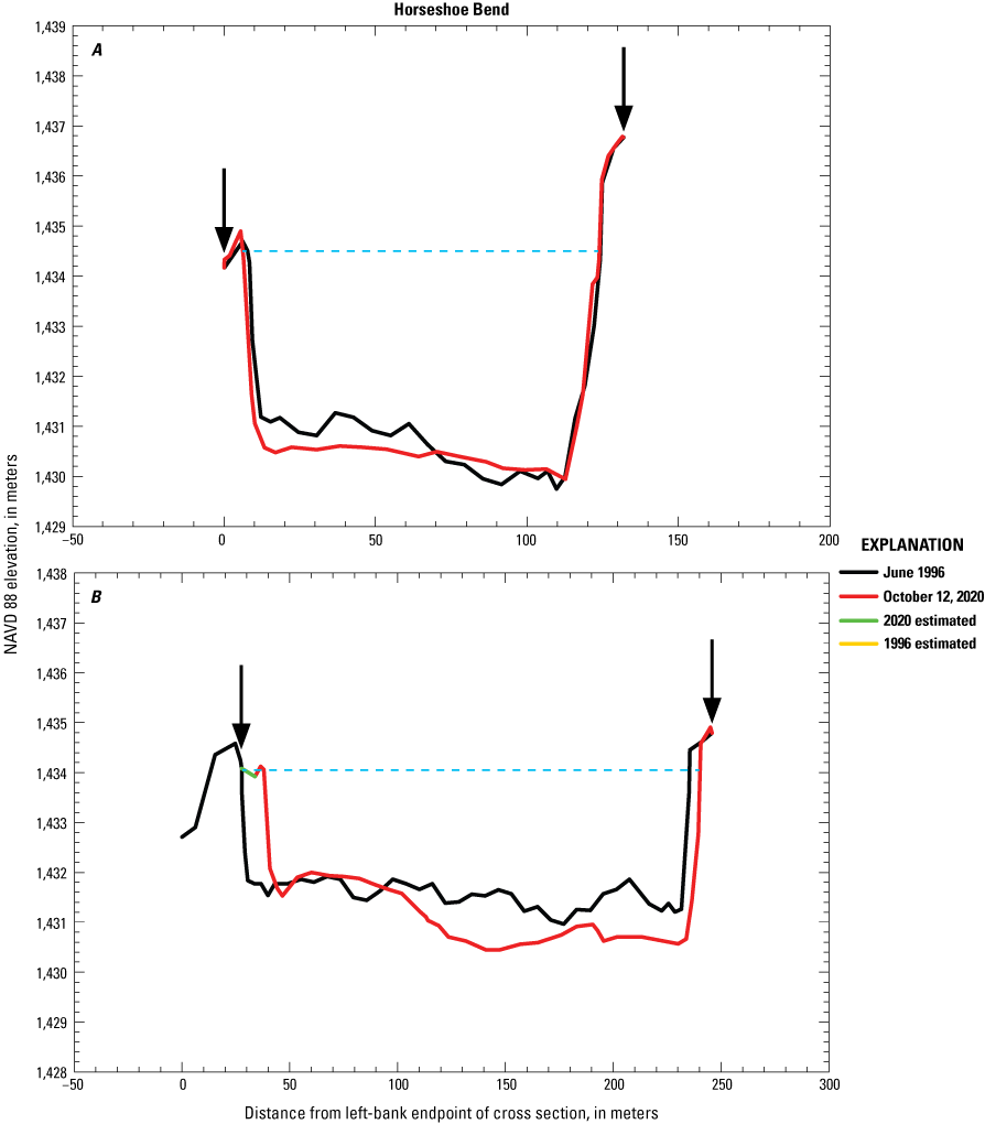
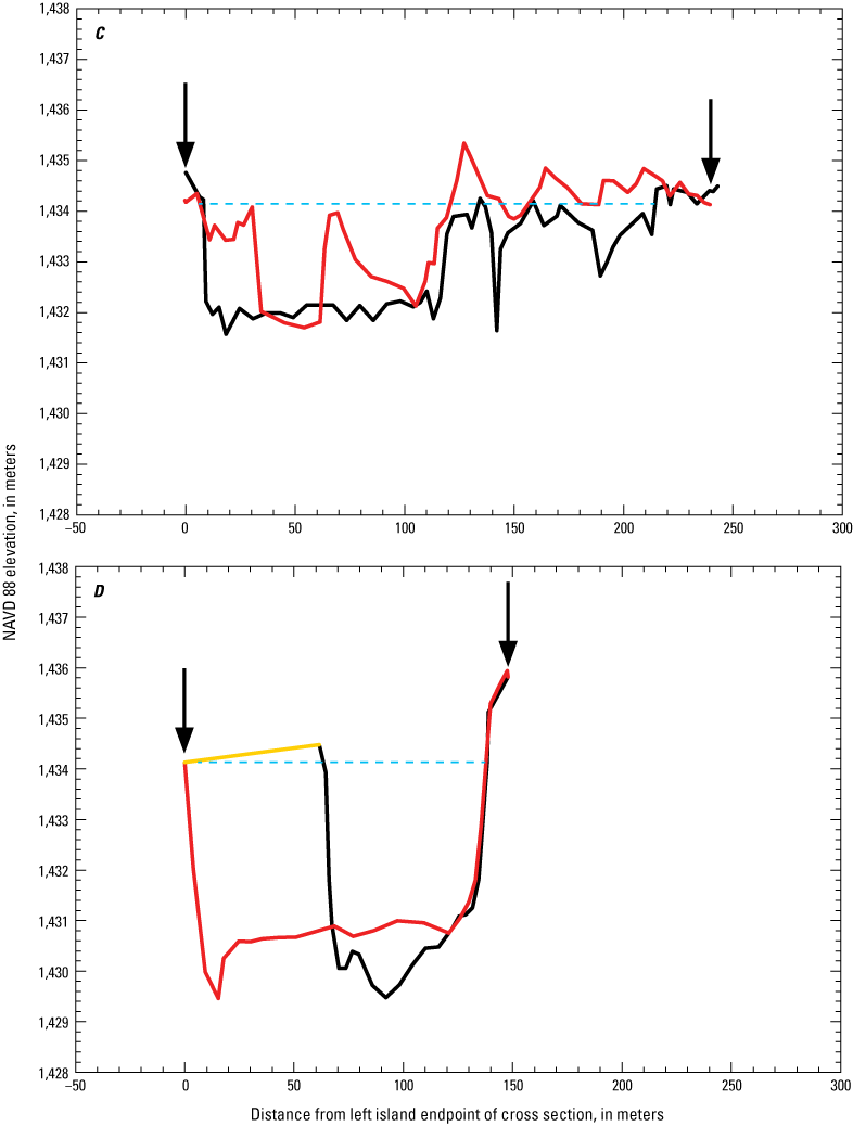
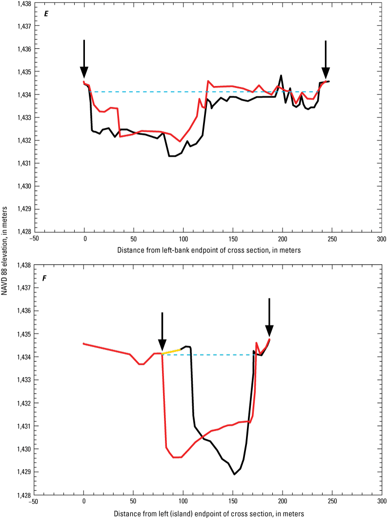
Plots comparing the Horseshoe Bend (HB) cross sections in the Uinta Basin segment of the middle Green River, Utah, in June 1996 and on October 12, 2020. A, HB-4 at river kilometer (RK) 203.9; B, HB-3 at RK 204.2; C, HB-2A (left part) at RK 204.4; D, HB-2B (right part) at RK 204.4; E, HB-1A (left part) at RK 204.6; and F, HB-1B (right part) at RK 204.6. Because of an island in the middle of the river, cross sections HB-2 and HB-1 were surveyed in two parts, with an angle between these two parts. Vertical arrows indicate the bounds of the domain over which the changes in cross-sectional sediment area and topographic variance were evaluated between surveys. Horizontal dashed blue line indicates the elevation at which channel width was measured (excluding the widths of shallow floodplain depressions behind levees). The 2020 ground-surface elevations in cross section HB-3 were estimated in the region 6.2 m beyond the left-most extent of the 2020-surveyed topography to smoothly merge with the 1996-surveyed topography, as shown in B; the 1996 ground-surface elevations in cross section HB-2B were estimated in the region 61.4 m beyond the left-most extent of the 1996-surveyed topography to smoothly merge with the 2020-surveyed topography, as shown in D; the 1996 ground-surface elevations in cross section HB-1B were estimated in the region 17.9 m beyond the left-most extent of the 1996-surveyed topography to smoothly merge with the 2020-surveyed topography, as shown in F. NAVD 88, North American Vertical Datum of 1988; m, meter.
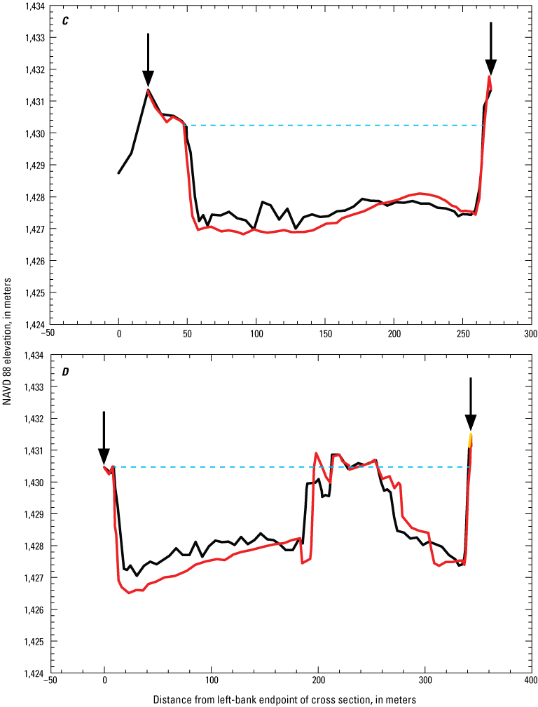
Plots comparing the Stirrup (ST) cross sections in the Uinta Basin segment of the middle Green River, Utah, in June 1996 and on October 13, 2020. A, ST-4 at river kilometer (RK) 218.2; B, ST-3 at RK 218.4; C, ST-2 at RK 218.6; and D, ST-1 at RK 218.7. Vertical arrows indicate the bounds of the domain over which the changes in cross-sectional sediment area and topographic variance were evaluated between surveys. Horizontal dashed blue line indicates the elevation at which channel width was measured (excluding the widths of shallow floodplain depressions behind levees). The 1996 ground-surface elevations in cross section ST-1 were estimated in the region 1.7 m beyond the right-most extent of the 1996-surveyed topography to smoothly merge with the 2020-surveyed topography, as shown in D. NAVD 88, North American Vertical Datum of 1988; m, meter.
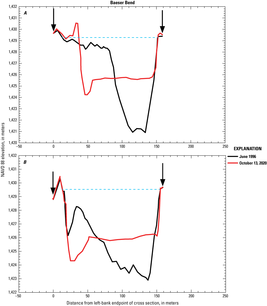
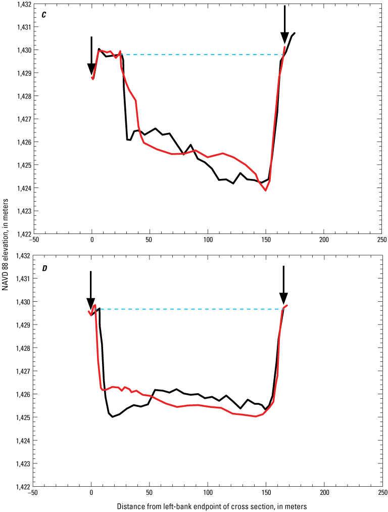
Plots comparing the Baeser Bend (BA) cross sections in the Uinta Basin segment of the middle Green River, Utah, in June 1996 and on October 13, 2020. A, BA-4 at river kilometer (RK) 223.9; B, BA-3 at RK 224.0; C, BA-2 at RK 224.2; and D, BA-1 at RK 224.3. Vertical arrows indicate the bounds of the domain over which the changes in cross-sectional sediment area and topographic variance were evaluated between surveys. Horizontal dashed blue line indicates the elevation at which channel width was measured (excluding the widths of shallow floodplain depressions behind levees). NAVD 88, North American Vertical Datum of 1988; m, meter.
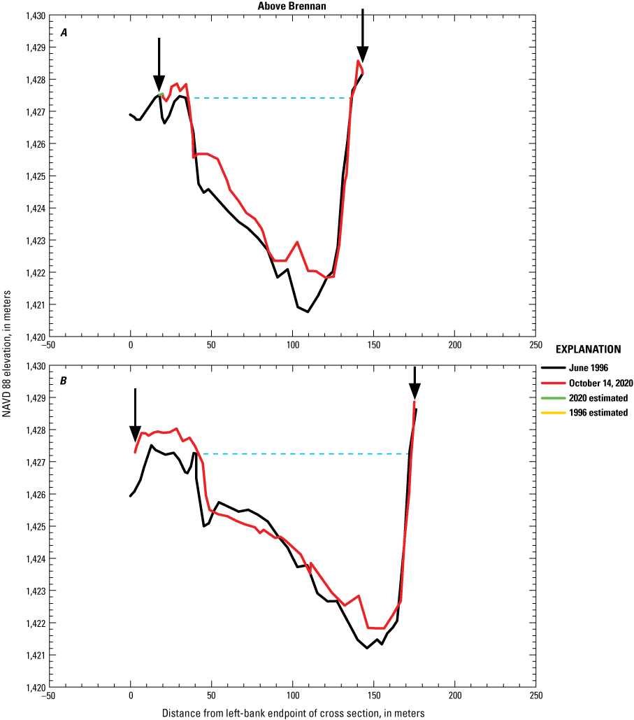
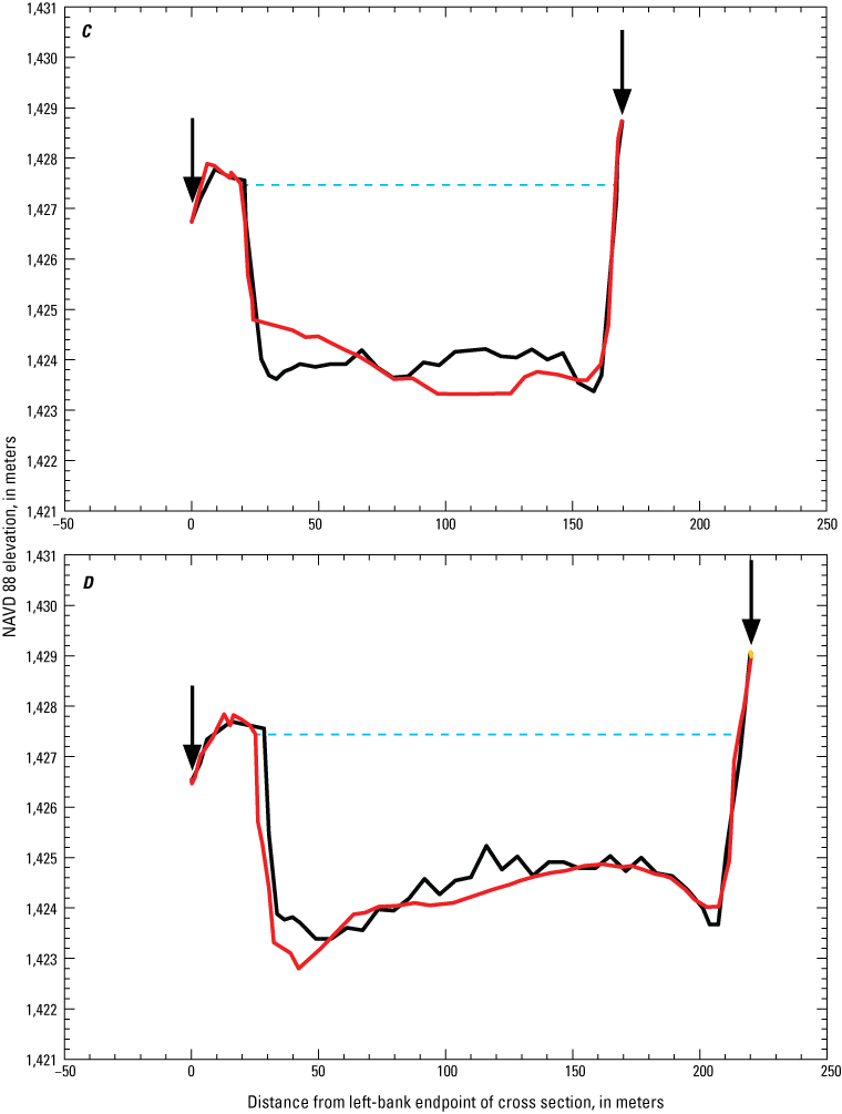
Plots comparing the Above Brennan (AB) cross sections in the Uinta Basin segment of the middle Green River, Utah, in June 1996 and on October 14, 2020. A, AB-4 at river kilometer (RK) 230.8; B, AB-3 at RK 231.2; C, AB-2 at RK 231.3; and D, AB-1 at RK 231.5. Vertical arrows indicate the bounds of the domain over which the changes in cross-sectional sediment area and topographic variance were evaluated between surveys. Horizontal dashed blue line indicates the elevation at which channel width was measured (excluding the widths of shallow floodplain depressions behind levees). The 2020 ground-surface elevations in cross section AB-4 were estimated in the region 1.9 m beyond the left-most extent of the 2020-surveyed topography to smoothly merge with the 1996-surveyed topography, as shown in A; the 1996 ground-surface elevations in cross section AB-1 were estimated in the region 0.3 m beyond the right-most extent of the 1996-surveyed topography to smoothly merge with the 2020-surveyed topography, as shown in D. NAVD 88, North American Vertical Datum of 1988; m, meter.
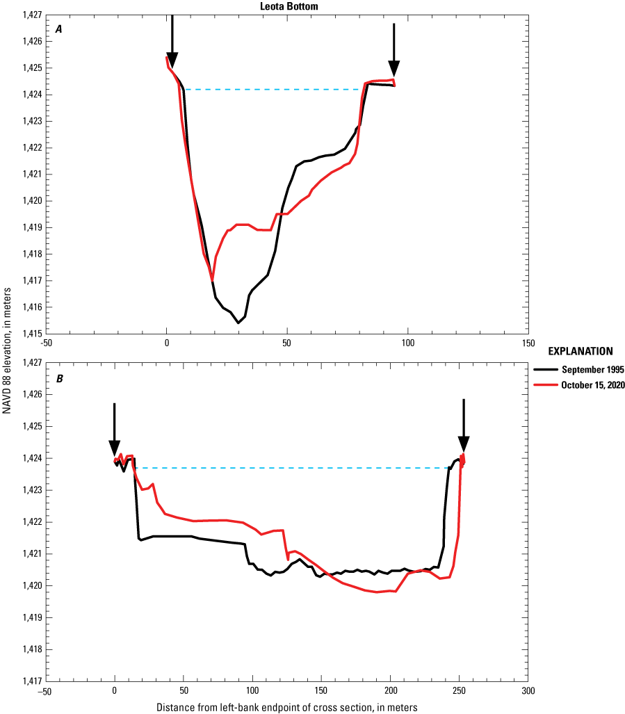
Plots comparing the Leota Bottom (LEB) cross sections in the Uinta Basin segment of the middle Green River, Utah, in September 1995 and on October 15, 2020. A, LEB-24 at river kilometer (RK) 244.3 and B, LEB-21 at RK 246.6. Vertical arrows indicate the bounds of the domain over which the changes in cross-sectional sediment area and topographic variance were evaluated between surveys. Horizontal dashed blue line indicates the elevation at which channel width was measured (excluding the widths of shallow floodplain depressions behind levees). NAVD 88, North American Vertical Datum of 1988; m, meter.
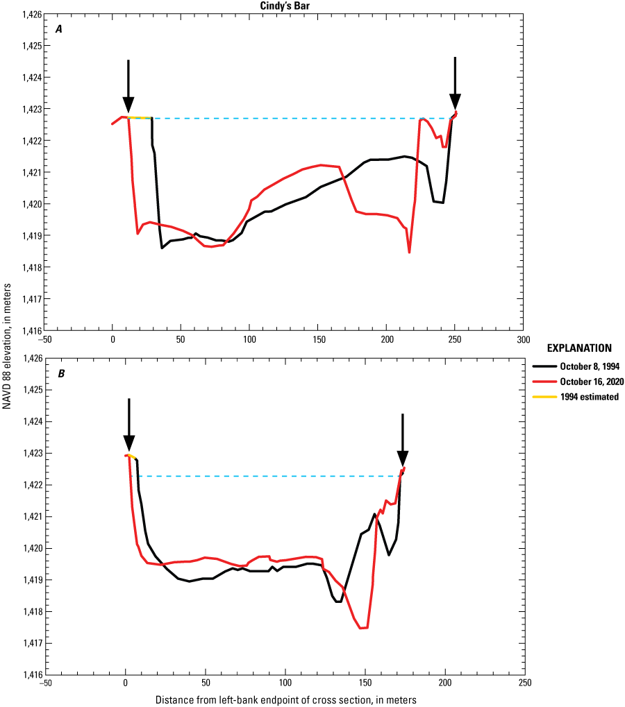
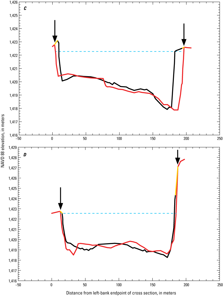
Plots comparing the Cindy’s Bar (CB) cross sections in the Uinta Basin segment of the middle Green River, Utah, on October 8, 1994, and October 15, 2020. A, CB-9 at river kilometer (RK) 251.4; B, CB-7 at RK 251.7; C, CB-6 at RK 251.9; and D, CB-4 at RK 252.1. Vertical arrows indicate the bounds of the domain over which the changes in cross-sectional sediment area and topographic variance were evaluated between surveys. Horizontal dashed blue line indicates the elevation at which channel width was measured (excluding the widths of shallow floodplain depressions behind levees). The 1994 ground-surface elevations in cross section CB-9 were estimated in the region 15.7 m beyond the left-most extent of the 1994-surveyed topography to smoothly merge with the 2020-surveyed topography, as shown in A; the 1994 ground-surface elevations in cross section CB-7 were estimated in the region 3.4 m beyond the left-most extent of the 1994-surveyed topography to smoothly merge with the 2020-surveyed topography, as shown in B; the 1994 ground-surface elevations in cross section CB-6 were estimated in both the regions 4.2 m beyond the left-most extent and 2.2 m beyond the right-most extent of the 1994-surveyed topography to smoothly merge with the 2020-surveyed topography, as shown in C; the 1994 ground-surface elevations in cross section CB-4 were estimated in both the regions 2.6 m beyond the left-most extent and 3.6 m beyond the right-most extent of the 1994-surveyed topography to smoothly merge with the 2020-surveyed topography, as shown in D. NAVD 88, North American Vertical Datum of 1988; m, meter.
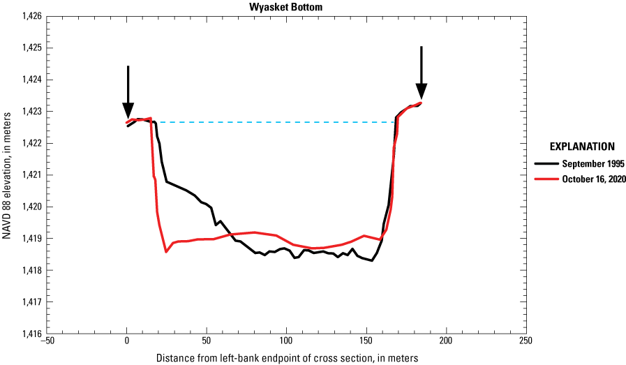
Plots comparing the Wyasket Bottom (WYB) cross section in the Uinta Basin segment of the middle Green River, Utah, WYB-12 at river kilometer (RK) 252.6, in September 1995 and on October 16, 2020. Vertical arrows indicate the bounds of the domain over which the changes in cross-sectional sediment area and topographic variance were evaluated between surveys. Horizontal dashed blue line indicates the elevation at which channel width was measured (excluding the widths of shallow floodplain depressions behind levees). NAVD 88, North American Vertical Datum of 1988; m, meter.
Table 6.
Channel widths and minimum bed elevations during the last 1994–1996 survey and the 2020 resurvey, and the changes in channel width, minimum bed elevation, and sediment area between these surveys.[“1990s” refers to the last survey conducted during 1994–1996. RK, river kilometer measured downstream from Flaming Gorge Dam; m, meter; m2, square meter; BB, Bonanza Bridge; HB, Horseshoe Bend; ST, Stirrup; BA, Baeser Bend; AB, Above Brennan; LEB, Leota Bottom; CB, Cindy’s Bar; WYB, Wyasket Bottom. For locations of cross sections, refer to figure 1C. Elevations are referenced to the North American Vertical Datum of 1988 (NAVD 88). For graphical representations of the data, refer to figures 32–39]
Width is the combined width of the channels in the left (that is, A) and right (that is, B) parts of this cross section. Because of an island in the middle of the river, this cross section was surveyed in two parts; minimum bed elevation is the minimum of the bed elevations measured in both the A and B parts of this cross section.
Comparison of Long-Term and Seasonal Changes in Sediment Storage and Cross-Section Geometry
There are two key differences that distinguish the long-term changes from the seasonal changes in sediment storage and cross-section geometry, based on analysis of the repeat surveys of the Leota Bottom, Cindy’s Bar, and Wyasket Bottom cross sections conducted within the same year by FLO Engineering (1996) and Rakowski (1997) (figs. 40–42; table 7). First, unlike the typically larger changes in channel width in these cross sections between the 1990s and 2020, only minor changes in channel width occurred in these cross sections between surveys conducted within the same year. Second, although the changes in cross-sectional sediment area in individual cross sections were large between the intra-annual surveys and similar to those observed between the 1994–1995 and 2020 resurveys, a significant intra-annual mean change in cross-sectional sediment area occurred in only the Cindy’s Bar cross sections between the May 28 and June 16, 1994, surveys and in the FLO Engineering (1996) cross sections between the May 1995 and September 1995 surveys. No significant change in mean cross-sectional sediment area occurred between any of the other six 1994–1995 surveys. In contrast, a large significant change in mean cross-sectional sediment area did occur among the four Cindy’s Bar cross sections and among the three FLO Engineering (1996) cross sections between the last 1994–1995 survey and our 2020 resurvey. Consequently, the changes in channel width and cross-sectional sediment area reported in the previous section are likely not overly affected by seasonal changes and are thereby likely indicative of real long-term, multi-decadal changes in sediment storage and cross-section geometry. Conversely, the changes in minimum bed elevation at individual cross sections and in the means among cross sections observed between the intra-annual surveys were similar to those observed between the 1994–1995 and 2020 resurveys. This result indicates that the changes in minimum bed elevation between the 1994–1996 and 2020 resurveys in table 6 could be artifacts of seasonal changes, and therefore not indicative of long-term, multi-decadal changes in cross-section geometry. Therefore, there has likely been a long-term, 1990s–2020 decrease in sediment storage in the Uinta Basin segment of the middle Green River that has been manifest mainly by channel widening, with likely negligible changes in minimum bed elevation. The important implication of this result is that long-term changes in sediment storage are more likely to include changes in channel width, whereas shorter term, intra-annual seasonal changes in sediment storage are more likely restricted to bed-elevation changes without a major change in channel width.
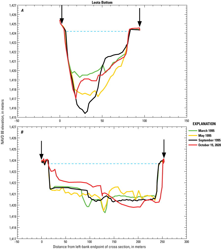
Plots comparing the Leota Bottom (LEB) cross sections in the Uinta Basin segment of the middle Green River, Utah, in March, May, and September 1995 and on October 15, 2020. A, LEB-24 at river kilometer (RK) 244.3 and B, LEB-21 at RK 246.6. Vertical arrows indicate the bounds of the domain over which the changes in cross-sectional sediment area and topographic variance were evaluated between surveys. Horizontal dashed blue line indicates the elevation at which channel width was measured (excluding the widths of shallow floodplain depressions behind levees). NAVD 88, North American Vertical Datum of 1988; m, meter.
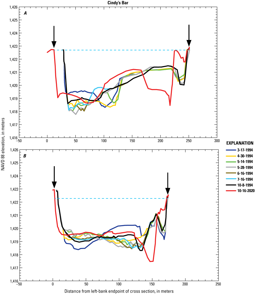
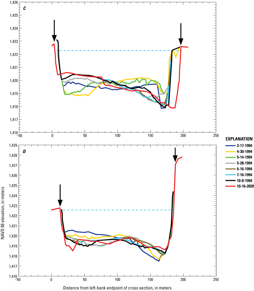
Plots comparing the Cindy’s Bar (CB) cross sections in the Uinta Basin segment of the middle Green River, Utah, on March 17, April 30, May 14, May 28, June 16, July 16, and October 8, 1994, and on October 16, 2020. A, CB-9 at river kilometer (RK) 251.4; B, CB-7 at RK 251.7; C, CB-6 at RK 251.9; and D, CB-4 at RK 252.1. Vertical arrows indicate the bounds of the domain over which the changes in cross-sectional sediment area and topographic variance were evaluated between surveys. Horizontal dashed blue line indicates the elevation at which channel width was measured (excluding the widths of shallow floodplain depressions behind levees). NAVD 88, North American Vertical Datum of 1988; dates in month-day-year format.
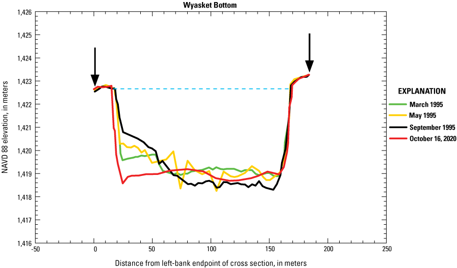
Plots comparing the Wyasket Bottom (WYB) cross section in the Uinta Basin segment of the middle Green River, Utah, WYB-12 at river kilometer (RK) 252.6, in March, May, and September 1995 and on October 16, 2020. Vertical arrows indicate the bounds of the domain over which the change in cross-sectional sediment area was measured between surveys. Horizontal dashed blue line indicates the elevation at which channel width was measured (excluding the widths of shallow floodplain depressions behind levees); the topographic variance was evaluated over that part of the domain where the channel perimeter was below this elevation (also excluding depressions behind levees). NAVD 88, North American Vertical Datum of 1988.
Table 7.
Comparison of changes in channel width, minimum bed elevation, and cross-sectional sediment area between surveys conducted during the same year and between the last 1990s survey and the 2020 resurvey.[Dates in month-day-year or month-year format. m, meter; m2, square meter; CB, Cindy’s Bar; LEB, Leota Bottom; WYB, Wyasket Bottom. Indicated ± values associated with the mean values are ± one standard error. For locations of cross sections, refer to figure 1C. For graphical representations of the data, refer to figures 40–42]
Changes in Sediment Storage and Channel Complexity
Analysis of the seven cross sections we resurveyed in 2020 that had multiple surveys conducted within the same year (table 8) and analysis of all 27 cross sections resurveyed in 2020 (table 9; fig. 43) indicate that, in cross sections with negligible changes in channel width, an increase in the cross-sectional sediment area is negatively correlated with an increase in topographic variance. This result supports our hypothesis that erosion of sediment corresponds to an increase in channel complexity and conversely that sediment deposition corresponds to a decrease in channel complexity.
Although only very strong and significant in one case (that is, at cross section CB-9), the correlation between changes in cross-sectional sediment area and topographic variance between surveys conducted within the same year is almost universally negative (table 8). The significance of these correlations is limited by the extremely small sample size; cross sections LEB-24, LEB-21, and WYB-12 were only surveyed three times in 1995 (corresponding to n = 2 in our analysis of change between surveys), and cross sections CB-9, CB-7, CB-6, and CB-4 were only surveyed seven times (corresponding to n = 6 in our analysis of change between surveys). The change in channel width between surveys was negligible, with only the channel at cross section CB-9 changing in width by more than 2.7 m (that is, 4.4 m) between surveys conducted within the same year (table 7). Thus, regardless of the lack of significance owing to small sample size, this result suggests that sediment erosion is more likely to lead to an increase in topographic relief and or variability across the cross section than is sediment deposition during the passage of a single annual flood when minimal changes in channel width are likely to dominate.
Table 8.
Correlations between changes in cross-sectional sediment area and topographic variance at individual cross sections between surveys conducted within the same year.[RK, river kilometer measured downstream from Flaming Gorge Dam; p, level of significance; r, correlation coefficient; n/a, not applicable because n = 2. LEB, Leota Bottom; CB, Cindy’s Bar; WYB, Wyasket Bottom. For locations of cross sections, refer to figure 1C]
Table 9.
Topographic variance in each cross section during the last 1994–1996 survey and the 2020 resurvey, and the changes in topographic variance, channel width, and cross-sectional sediment area between these surveys.[“1990s” refers to the last survey conducted during 1994–1996. RK, river kilometer measured downstream from Flaming Gorge Dam; m2, square meter; m, meter; BB, Bonanza Bridge; HB, Horseshoe Bend; ST, Stirrup; BA, Baeser Bend; AB, Above Brennan; LEB, Leota Bottom; CB, Cindy’s Bar; WYB, Wyasket Bottom. For locations of cross sections, refer to figure 1C]
Because of an island in the middle of the river, this cross section was surveyed in two parts. Topographic variance, and the changes in topographic variance, channel width, and sediment area were evaluated over the combined domains in both the A and B parts of this cross section (delineated by blue arrows in fig. 33C, D).
Because of an island in the middle of the river, this cross section was surveyed in two parts. Topographic variance, and the changes in topographic variance, channel width, and sediment area were evaluated over the combined domains in both the A and B parts of this cross section (delineated by blue arrows in fig. 33E, F).
Analysis of all 27 cross sections resurveyed in 2020 reinforces the result that, in cross sections with negligible changes in channel width, an increase in the cross-sectional sediment area is negatively correlated with an increase in topographic variance. Among the 27 cross sections, the correlation between changes in cross-sectional sediment area and topographic variance between the last 1994–1996 survey and the 2020 resurvey is negative (r = −0.39) and significant (p = 0.043) (fig. 43A). The weakness of this correlation arises not from increased scatter, however, but rather from the influence of changes in channel width on topographic variance (described in the “Analytical Methods” section). When cross sections with changes in channel width >3 m are excluded, the strength of the negative correlation between changes in cross-sectional sediment area and topographic variance becomes moderate (r = −0.49), though the correlation also becomes insignificant (p = 0.13) because the sample size decreases from 27 to 11 (fig. 43B). Channel widening leads to a decrease in topographic variance, by definition (fig. 7). Consequently, the correlation between changes in cross-sectional sediment area and topographic variance is strongly negative (r = −0.78) though insignificant (p = 0.12) because of small sample size among the five cross sections that narrowed by more than 3 m (fig. 43C). Furthermore, the correlation between changes in cross-sectional sediment area and topographic variance is strongly positive (r = 0.64) and significant (p = 0.032) among the 11 cross sections that widened by more than 3 m (fig. 43D). It is this significant, strong correlation among the 11 cross sections that widened mixed with the insignificant, negative correlations among the 16 cross sections that either did not change in width or narrowed that leads to the significant, weak negative correlation between changes in cross-sectional sediment area and topographic variance among all 27 cross sections (fig. 43A). Finally, although the correlation between changes in cross-sectional sediment area and topographic variance is generally negative for cases without channel widening, this negative correlation arises mainly from sediment deposition and not erosion. The largest decreases in topographic variance are all associated with increases in cross-sectional sediment area, that is, they all occur in the lower right quadrant in figure 43.
Taken together, these results suggest that channel complexity is maintained or increased when sediment does not accumulate in a river segment. When the positive relation between channel width and topographic variance is taken into account, the cross-section analyses indicate that sediment deposition (that is, an increase in cross-sectional sediment area) is generally negatively correlated with channel complexity (that is, an increase in topographic variance). Though there is a moderate tendency for topographic variance to increase as sediment erodes in cross sections of constant width (fig. 43B), this increase in channel complexity is small compared to the substantial decrease in channel complexity associated with the largest decreases in topographic variance, all of which are associated with sediment deposition (fig. 43A–C).
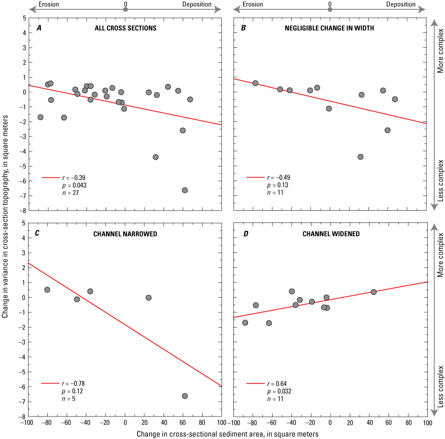
Plots of change in the variance in cross-section topography at 0.5-meter (m) intervals as a function of the change in the cross-sectional sediment area between the last survey in 1994–1996 and the 2020 resurvey of the Uinta Basin segment of the middle Green River, Utah. A, All 27 cross sections; B, the 11 cross sections with a change in channel width of less than 3 m; C, the 5 cross sections that narrowed by more than 3 m; and D, the 11 cross sections that widened by more than 3 m. The correlation coefficient, r, level of significance, p, associated with the best-fit least-squares linear regression (red line) are shown; n indicates the number of cross sections in each category. The largest decreases in topographic variance (leading to the least complex cross sections) are all associated with increases in the cross-sectional sediment area (that is, sediment deposition).
Bed-Sand Grain Size in the Cross Sections
The available data do not suggest that any substantial changes in the reach-averaged bed-sand grain size have occurred among the cross sections in the Uinta Basin segment of the middle Green River between the 1990s and our 2020 resurvey. For this comparison, we used the bed-sediment measurements made by FLO Engineering (1996) in both March and September 1995 but excluded the measurements they made at higher Q in May 1995. This approach was used to ensure that this comparison was not adversely affected by changes in the bed-sand grain size associated with changes in Q (that we detected at all four sand-bedded stations). The daily mean discharges at the Green-Jensen station were most similar on the days of their measurements on March 14–20, 1995, (Q = 1,630–2,300 ft3/s) and September 12–16, 1995, (Q = 1,760–1,880 ft3/s) and our measurements on October 11–16, 2020 (Q = 1,250–1,450 ft3/s). FLO Engineering (1996) made bed-sediment measurements in four cross sections in March and September 1995. These measurements were made in a total of six cross sections because only two of the four cross sections sampled in March 1995 were resampled in September 1995. Although FLO Engineering (1996) did not make bed-sediment measurements in the subset of their cross sections that we resurveyed in 2020, t-tests indicate that the values of DB and log10(fVF) in the cross sections they sampled in either March or September 1995 cannot be concluded to have come from different distributions than the values of DB and log10(fVF) in the cross sections we resurveyed in October 2020 (at the p = 0.05 critical level of significance). The distribution of the March 1995 values of DB is different than the distribution of the October 2020 values of DB at p = 0.60; the distribution of the March 1995 values of log10(fVF) is different than the distribution of the October 2020 values of log10(fVF) at p = 0.38. The distribution of the September 1995 values of DB is different than the distribution of the October 2020 values of DB at p = 0.59; the distribution of the September 1995 values of log10(fVF) is different than the distribution of the October 2020 values of log10(fVF) at p = 0.72. The respective mean values of DB in March 1995, September 1995, and October 2020 were 0.31, 0.31, and 0.35 mm. The respective re-transformed mean values of log10(fVF) in March 1995, September 1995, and October 2020 were 3.3, 1.8, and 1.2 percent.
Despite the lack of evidence of a net reach-averaged change in bed-sand grain size between 1995 and 2020, the bed-sediment samples collected in the center of the main flow in the cross sections during the October 2020 resurvey do indicate significant downstream bed-sand fining in terms of both DB (p = 0.027) and log10(fVF) (p = 0.033). These p values are associated with F-tests conducted on the least-squares linear regressions of DB and log10(fVF) on river kilometer. Over the 56-km-long segment of Green River encompassing the resurveyed cross sections, DB decreased by ~40 percent while log10(fVF) increased by ~230 percent (reflecting a downstream ~15-fold increase in fVF). The downstream fining observed in October 2020 is consistent with the continued downstream migration of the sand wave generated by the large 2019 Yampa River flood. During the high-flow part of the 2019 flood, the β-inferred bed-sand grain-size distribution was finer at the upstream end of the Uinta Basin segment at Jensen than downstream at Ouray, owing to the ongoing large influx of finer sand from the Yampa River (fig. 25). Owing to the downstream migration of this sand wave and the much smaller 2020 Yampa River flood (that supplied a much smaller amount of finer sand), the β-inferred bed-sand grain-size distribution during the high-flow part of the 2020 annual flood fined downstream between the Green-Jensen and Green-Ouray stations (fig. 25). The values of β calculated from EWI measurements at Green-Jensen between the 2020 and 2021 floods suggest that the bed-sand grain size at this station remained constant between the 2020 and 2021 floods. Although the values of β calculated from low-flow EWI measurements suggest armoring of the bed sand at Green-Ouray after recession of the 2020 flood and before the rise of the 2021 flood, β decreased between the high-flow parts of the 2020 and 2021 floods (fig. 25). Thus, the downstream fining observed in the bed sand during the October 2020 cross-section resurvey is consistent with the high-flow β-inferred 2020–2021 increase in downstream fining from Green-Jensen to Green-Ouray caused by the likely continued downstream migration of the sand wave generated by the large 2019 Yampa River flood.
Influence of Yampa River Floods and Flaming Gorge Dam Releases on Fish Habitat in the Uinta Basin Segment of the Green River
The low-velocity, warmer water backwater nursery habitat utilized by native fish in the middle Green River forms downstream of large, bank-attached sandbars that are deposited and reworked during the annual flood (Pucherelli and Clark, 1989; Rakowski, 1997; Bestgen and Hill, 2016; Grippo and others, 2017). Because sandbars tend to grow to the water surface during floods given sufficient upstream sand supply and time (Cant and Walker, 1978; Andrews and Nelson, 1989; Fujita, 1989), the largest sandbars in terms of both area and elevation difference in the Uinta Basin segment of the middle Green River are deposited during longer duration floods with large upstream sand supplies and large peak Q, that is, during the annual flood of the Yampa River (Rakowski, 1997). Owing to sand-supply and stage limitations, artificial floods released from Flaming Gorge Dam cannot be used as a replacement for the role of large Yampa River floods in depositing large sandbars in this river segment. Though large sandbars form the obstacle to upstream flow that forms the backwater and allows for warming, the occurrence of large sandbars does necessarily indicate the presence of large backwaters (Rakowski, 1997). Optimal backwater habitat consists of a deep pool with no through-going current, blocked from upstream flow yet connected to the main channel over the widest range in stage possible (Rakowski, 1997). Thus, optimal backwater habitat requires a large, sand-rich flood to deposit large sandbars followed by a sequence of flows that scour and (or) maintain deep pools downstream from these bars. The greater channel complexity associated with this planform geometry (that is, large sandbars upstream and adjacent to deep backwaters) translates to greater topographic variance when viewed in cross section. Consequently, greater topographic variance in a river cross section should indicate greater backwater area and volume. In the Uinta Basin segment of the middle Green River, the largest reductions in topographic variance are all associated with sediment deposition (fig. 43). Increased topographic variance is generally associated with erosion, especially over the intra-annual seasonal timescales that are most appropriate for interpreting the sediment response during an individual annual flood (table 8). Because they can cause net deposition of sand in this river segment (fig. 31), large Yampa River floods can result in a decrease in topographic variance. Thus, even though large Yampa River floods are required to deposit the large sandbars associated with backwaters, isolated large Yampa River floods will not likely create or maintain optimal backwater habitat. Therefore, we hypothesize that the greatest extent of backwater habitat in this segment of the middle Green River is likely created and (or) maintained by a sequence of flows following a large Yampa River flood that either erode sand from or convey sand through this river segment.
We tested this hypothesis by comparing the predicted sand response in the Uinta Basin segment conceptualized in figure 27 to repeat surveys of backwaters in the downstream part of this river segment conducted between 1992 and 1996 and between 2003 and 2013 by Grippo and others (2017). The 1992–1996 surveys are the post-flood surveys of Day and others (1999) digitized from figure 23 in Bestgen and Hill (2016). Day and others (1999) conducted repeat surveys of a total of 1,043 backwaters three times per year from August 1990 through September 1996; the 1990 and 1991 surveys used preliminary methods and were not used by Bestgen and Hill (2016). The backwaters surveyed by Day and others (1999) were located between RK ~242 and ~258, bracketing the Green-Ouray station at RK 255.3. The 2003–2013 surveys made after recession of the annual flood by Grippo and others (2017) consisted of repeat annual surveys of 13 possible backwaters, located between RK ~237 and ~261. The surveyed backwaters were mostly located in the lower 18-km-long reach of the 103-km-long Uinta Basin segment, with 12 of the 13 backwaters located upstream of the Green-Ouray station at RK 255.3 and only one backwater located downstream of the Green-Ouray station. During each survey, Grippo and others (2017) surveyed each of the 13 possible backwaters that exceeded their minimum area and depth thresholds, resulting in 4–6 backwaters being surveyed each year. They did not survey every backwater every year because not every backwater was present every year. Given the sometimes-ephemeral nature of backwaters at a single location, we chose to use their total backwater area and volume measured among all 13 backwaters as the integrated measures of the extent of backwater habitat over the reach scale in our comparison. F-tests conducted on regressions of total backwater area and volume on the mean Q during each survey indicate that there were no significant relations between Q and total backwater area (p = 0.63) or volume (p = 0.79). Thus, the backwater areas and volumes Grippo and others (2017) measured arose not from flow conditions during their surveys but rather from the flow and sediment conditions that preceded their surveys, therefore making these surveys suitable for the comparison used to test our hypothesis.
For this comparison, we predicted that sand deposition in the Uinta Basin segment would occur during the first large Yampa River flood (that is, the year-1 flood) in a sequence of annual floods, and sand conveyance or erosion would occur during the subsequent typically smaller out-year Yampa River floods. These predictions directly arise from figures 25, 27, 28, and 31C, D that together show that the year-1 Yampa River flood causes sand deposition in the Uinta Basin segment because the bed sand is finer upstream at the Green-Jensen station than downstream at the Green-Ouray station. To identify these likely net depositional year-1 floods, we selected abrupt large increases in the time series of peak and March–July median Q in the Yampa River that exceeded thresholds of ~12,000 ft3/s for peak Q and ~2,400 ft3/s for March–July median Q. These thresholds were based on the ranges of Q in figure 31C, D at which the regressions predict a March–July sand mass balance greater than zero. As the Yampa River sand wave migrates downstream, and the bed sand coarsens at Green-Jensen and fines at Green-Ouray (figs. 27B, C, 28D, E), sand is either conveyed through or eroded from this river segment during the out-year Yampa River floods that follow, likely regardless of their peak or median Q. Thus, we assumed sand conveyance or erosion occurred in the Uinta Basin segment during the Yampa River floods that followed each year-1 flood. In addition, based on the results in figures 28A and 31B, we assume that longer duration large releases from Flaming Gorge Dam will cause greater bed-sand coarsening at Green-Jensen and thus a tendency toward greater erosion in the Uinta Basin segment. These longer duration large dam releases would thereby also limit the sand deposition in this river segment if these sustained high dam releases coincided with large Yampa River floods (for example, in 2011). Based on the results in figure 31B, we assume that the threshold March–July median Q for the dam releases that are likely to cause this effect is roughly 3,000–4,000 ft3/s.
The results from this comparison indicate that there is generally good agreement between the expected sand response during annual floods in the Uinta Basin segment (fig. 27) and the measured response in backwater total area in the lower reach in this segment (fig. 44). Thus, these results provide strong support for our hypothesis, stated earlier in this section, that “the greatest extent of backwater habitat in this segment of the middle Green River is likely created and (or) maintained by the sequence of flows following a large Yampa River flood that either erode sand from or convey sand through this river segment.” We surmise that because the March–July median Q in the Yampa River (r = 0.8; fig. 31D) is a slightly better predictor of changes in sand mass in the Uinta Basin segment than peak Q in the Yampa River (r = 0.7; fig. 31C), the pattern between the expected sand response in this river segment as a function of median Q is in slightly better agreement with the measured backwater response than is the expected sand response as a function of peak Q.
As predicted, major decreases in backwater total area were measured upon recession of the year-1 floods where March–July median Q in the Yampa River exceeded the threshold identified for net sand deposition in the Uinta Basin segment, that is, the year-1 floods of 1993, 1995, 2003, 2005, 2008, and 2011 (fig. 44A, C). In addition, large increases in backwater total area were measured upon recession of the year-2 floods with lower March–July median Q in the Yampa River (1994, 2006, 2009, and 2012); these floods were predicted to erode sand from this river segment based on median Q. Although the year-2 2004 flood was predicted to erode sand from this river segment based on peak Q, this flood was instead predicted to convey sand through this river segment based on median Q. Continued increases in backwater total area were then measured during subsequent out-year floods (2010 and 2013) until the median-Q thresholds for expected net sand deposition were again exceeded during another year-1 flood.
Similarly, major reductions in backwater total area were measured upon recession of the year-1 floods where peak Q in the Yampa River exceeded the threshold identified for net sand deposition in the Uinta Basin segment (1993, 1995, 2003, 2005, 2008, and 2011) (fig. 44B, D). Large increases in backwater total area were measured upon recession of the subsequent year-2 floods with lower peak Q in the Yampa River (1994, 2004, 2009, and 2012); these floods were predicted to erode sand from this river segment based on peak Q. Although the year-2 2006 flood was predicted to erode sand from this river segment based on median Q, this flood was instead predicted to convey sand through this river segment based on peak Q. Moreover, although the peak Q of the 2009 and 2010 Yampa River floods exceeded the peak-Q threshold for a year-1 flood, these two floods were instead out-year floods because they followed the much larger year-1 2008 flood. Accordingly, the 2009 and 2010 floods were associated with measured increases in total backwater area, in agreement with the expected sand response in figure 27. Likewise, even though the 1996 Yampa River flood also exceeded the median and peak Q values used to identify year-1 floods, no decrease in backwater total area was measured between recession of the 1995 and 1996 floods. This result likely arises because the 1996 flood was a year-2 flood of similar magnitude to the 1995 flood and was therefore predicted to be associated with sand conveyance through the Uinta Basin segment (based on fig. 27B). Finally, the coincidence of the largest Yampa River flood with the sustained large releases from Flaming Gorge Dam in 2011 may have limited the sand deposition and thereby also limited the associated decrease in backwater total area (fig. 44C–D), as expected based on figures 28A and 31B.
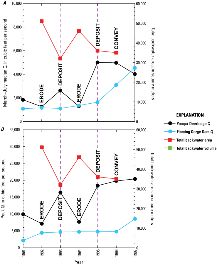
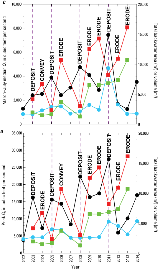
Plots comparing the time series of water discharge (Q) with the time series of total backwater area and volume in the Uinta Basin segment of the middle Green River, Utah, following recession of the annual flood. A, B, 1992–1996 time series of March–July median Q (A) and peak Q (B) and total backwater area surveyed by Day and others (1999). C, D, 2003–2013 time series of March–July median Q (C) and peak Q (D) and total backwater area and volume surveyed by Grippo and others (2017). The year-1 floods predicted to deposit sand in the Uinta Basin segment are indicated by the vertical purple dashed line and the word “DEPOSIT”; the out-year floods of similar Q to the year-1 flood and are therefore predicted to cause conveyance of sand through this segment are indicated by the word “CONVEY”; the smaller out-year floods that are predicted to cause erosion of sand from this segment are indicated by the word “ERODE.” Because 15-minute Q values were not available for this entire period, the March–July median Q at the Yampa River at Deerlodge Park, Colorado, gaging station 09260050 (Yampa-Deerlodge station) was calculated using reported daily mean Q values; the median Q calculated by this approach is only slightly different from that calculating using 15-minute values. Because the Green River above Gates of Lodore, Colorado, gaging station 404417108524900 (Green-Lodore station) was not operated for continuous 15-minute Q until October 2012, the Q values shown for Flaming Gorge Dam releases were calculated using the reported daily mean and peak Q at the Green River near Greendale, Utah, gaging station 09234500. m2, square meter; m3, cubic meter.
The measured response in backwater total volume (Grippo and others, 2017) also provides support for our hypothesis, but this support is slightly weaker than that associated with the response in backwater total area. As with backwater total area, upward steps in backwater total volume were typically measured upon recession of the year-2 floods. These upward steps in volume were measured upon recession of the 2006 and 2009 floods that followed the 2005 and 2008 year-1 floods with larger median and peak Q in the Yampa River (fig. 44C–D). Although an upward step in backwater total volume was not measured upon recession of the year-2 2012 flood that followed the large year-1 2011 flood, an upward step in backwater total volume was measured after the subsequent out-year 2013 flood. Although backwater total volume was measured to decrease only once during the 2003–2013 surveys of Grippo and others (2017), this decrease was measured upon recession of the 2008 flood, an annual flood we predict to have caused sand deposition and a reduction in backwater habitat based on both the median and peak Q in the Yampa River.
Our results indicate that larger Yampa River floods are not directly responsible for forming large backwaters in the Uinta Basin segment because larger floods tend to be net depositional for sand in this segment. However, the available evidence suggests that larger Yampa River floods do facilitate the formation of more extensive backwater habitat in subsequent years. Over the period of the 2003–2013 backwater surveys of Grippo and others (2017), the time series of backwater total area and volume both significantly increase over time (with respective p values of 0.024 and 0.00055). Though no significant trend exists in either March–July median or peak Q in the Yampa River during this period, the median and peak Q of the three Yampa River floods identified to have probably caused sand deposition in this river segment based on both median and peak Q (2005, 2008, and 2011) did increase over time. Thus, even though no significant correlation exists between median or peak Q in the Yampa River and backwater total area or volume, the increase in median and peak Q among the 2005, 2008, and 2011 Yampa River floods does suggest the importance of larger Yampa River floods as a prerequisite to the formation of more extensive backwater habitat in the Uinta Basin segment, in agreement with Rakowski (1997). Larger year-1 floods likely form larger sandbars that are then reworked during subsequent out-year floods (Rakowski, 1997), when sand is ultimately eroded from this river segment. Consequently, larger year-1 floods likely facilitate the formation of larger backwaters downstream from these bars following the out-year floods. Thus, although the size of backwaters in the Uinta Basin segment is likely diminished during the years with the largest Yampa River floods, the largest backwaters are likely formed during the out-year floods that follow these largest floods. Hence, the largest total backwater area and volume measured by Grippo and others (2017) occurred 2 years after the extremely large 2011 Yampa River flood.
Though we have no topographic measurements to evaluate the response of backwaters in the upstream Dinosaur segment of the middle Green River between the Yampa-Green confluence and the Green-Jensen station, it is likely that backwaters would be largest in the Dinosaur segment while they are smallest in the Uinta Basin segment because of the opposing effects of large annual Yampa River floods on the sand mass balance in these two segments of the middle Green River. Large annual Yampa River floods would thus erode sand from the Dinosaur segment, thereby forming larger backwaters, while they deposit sand reducing the size of backwaters in the Uinta Basin segment. The backwaters in the Dinosaur segment could possibly then decrease in size as sand deposits in that river segment during the smaller annual Yampa River floods that follow, while the backwaters in the Uinta Basin segment enlarge during these same smaller annual floods. Additional monitoring could be used to evaluate this possibility.
Conclusions
The major conclusions from this study of sediment transport, sediment-storage change, and fish habitat in the Little Snake, Yampa, and Green Rivers are as follows.
-
• Silt-and-clay concentration in the rivers in our study area is largely determined by the upstream supply. Large decreases in silt-and-clay concentration have occurred throughout our study area since the mid-20th century, particularly in and downstream from the Little Snake River. However, a factor-of-100 to 10,000 discharge-independent variation in silt-and-clay concentration is still possible as the result of upstream tributary activity, mostly during the summer thunderstorm season. The greatest amount of modern variation in silt-and-clay concentration in our study area occurs in the Little Snake River at the LS-Lily station, whereas the least amount of variation in silt-and-clay concentration occurs in the Yampa River at the Yampa-Maybell station.
-
• Suspended-sand concentration at the sand-bedded stations in our study area (Green-Lodore, LS-Lily, Yampa-Deerlodge, Green-Ouray) is regulated mainly by changes in bed-sand grain size and not by changes in flow. Changes in the bed-sand grain-size distribution at these stations are associated with almost twice the variation in suspended-sand concentration caused by changes in discharge. The highest suspended-sand concentration at these stations is associated with the finest bed-sand grain size and not the highest discharge. Changes in bed-sand grain size at these stations arise from two distinct processes: (1) the downstream migration of sand waves generated during floods on upstream tributaries (which affects the upstream sand supply), and (2) scour through an inversely graded bed during the annual flood (which affects the local sand supply). The amount of variation in suspended-sand concentration caused by each of these processes is roughly equal.
-
• Suspended-sand concentration at the largely gravel-bedded stations in our study area (Yampa-Maybell and Green-Jensen) is regulated mainly by changes in flow, although changes in bed-sand grain size have important though differing roles in controlling suspended-sand concentration. At the Yampa-Maybell station, the flow accesses finer bed sand at higher discharge; at the Green-Jensen station, there is no discharge dependence on bed-sand grain size. Changes in bed-sand grain size at the Green-Jensen station are caused mainly by the downstream migration of sand waves. Changes in discharge at the Yampa-Maybell station cause greater than 2 times the variation in suspended-sand concentration associated with changes in bed-sand grain size, a result consistent with the analyses of historical data at this station. Changes in discharge at the Green-Jensen station during water years 2013–2021 caused approximately 4.5 times the variation in suspended-sand concentration associated with changes in bed-sand grain size, a result very different than that determined from the analyses of historical data at this station. Despite discharge being a stronger regulator of suspended-sand concentration than bed-sand grain size at these stations, the highest suspended-sand concentration at the Yampa-Maybell and Green-Jensen stations tends to be associated with the finest bed-sand grain size and not necessarily the highest discharge, as also observed at the sand-bedded stations.
-
• Prior to 2007, changes in bed-sand grain size were as important as changes in discharge in regulating suspended-sand concentration at the Green-Jensen station. The relatively abrupt decrease in the importance of grain-size regulation of suspended-sand concentration at the Green-Jensen station between 2007 and 2013 represents the greatest fundamental change in the boundary conditions that control sand transport in our study area. This change may have been caused by a decrease in the proportion of the gravel bed that was covered by sand at this station between 2007 and 2013.
-
• At the sand-bedded stations, changes in the shear velocity caused by changes in channel geometry and changes in the skin-friction component of the shear velocity caused by changes in dune and bar geometry cause roughly a factor-of-2 systematic variation in suspended-sand concentration at any given discharge. Though large, this magnitude of variation is smaller than the greater-than-factor-of-6 discharge-independent variation in suspended-sand concentration at these stations associated with changes in bed-sand grain size at these stations. Thus, it is unlikely that the changes in suspended-sand concentration caused by changes in channel, bar, or dune geometry can completely offset the variation in suspended-sand concentration associated with changes in bed-sand grain size.
-
• At the largely gravel-bedded stations, changes in bed-sand area cause roughly a factor-of-2 systematic variation in suspended-sand concentration at any given discharge. Although changes in bed-sand area may be the dominant source of discharge-independent variation in suspended-sand concentration at the Yampa-Maybell station, the factor-of-2 magnitude of this variation is less than the greater-than-factor-of-6 discharge-independent variation in suspended-sand concentration at the Green-Jensen station associated with changes in bed-sand grain size. Thus, it is unlikely that the changes in suspended-sand concentration caused by changes in bed-sand area can completely offset the variation in suspended-sand concentration associated with the changes in bed-sand grain size at the Green-Jensen station caused by the downstream migration of sand waves.
-
• Given that the changes in suspended-sand concentration caused by changes in channel, bar, and dune geometry or changes in bed-sand area are generally smaller than those associated with changes in bed-sand grain size, changes in bed-sand grain size are the primary mechanism by which changes in the upstream sand supply affect sand transport in our study area.
-
• The longitudinal pattern in bed-sand grain size in the middle Green River resulting from sand waves generated during sequences of annual floods on the Yampa River determines whether sand will be eroded from, conveyed through, or deposited in different segments of the middle Green River. Because the upper Green River supplies much less sand to the middle Green River than does the Yampa River, Flaming Gorge Dam releases may modify but do not likely erase the longitudinal pattern in bed-sand grain size in the middle Green River caused by a sequence of Yampa River floods. Therefore, because of the limited sand supply associated with Flaming Gorge Dam releases, these releases may not provide sufficient sand to replace the dominant role the Yampa River has in controlling sand transport, erosion, and deposition in the middle Green River.
-
• Although the Little Snake River supplies most of the sand transported by the lower Yampa River, the Deerlodge Park sediment-budget area has also likely been a major source of the sand supplied to the middle Green River by the Yampa River for many years. Larger annual floods on the Yampa River erode larger amounts of sand from the Deerlodge Park sediment-budget area, with this erosion associated with slight net bed scour in combination with the erosion of higher banks and the deposition of lower banks during the lateral migration of the Yampa River (Leonard, 2022).
-
• Because of their effect on the longitudinal pattern of bed-sand grain size in the middle Green River, larger annual floods on the Yampa River erode sand from the Dinosaur sediment-budget area and likely deposit sand downstream in the Uinta Basin segment. Moreover, smaller annual floods on the Yampa River deposit sand in the Dinosaur sediment-budget area while they erode sand from the Uinta Basin segment. Sustained large releases from Flaming Gorge Dam likely modify the sand response in the Uinta Basin segment and may also erode sand from this segment depending on the magnitude of the Yampa River flood.
-
• Repeat cross-section surveys suggest that slight net erosion of sand by channel widening has occurred in the Uinta Basin segment between the 1990s and 2020. This geomorphic response is the opposite of the channel narrowing observed during this same period in the lower Green River in Canyonlands National Park by Walker and others (2020).
-
• Repeat cross-section surveys indicate that deposition is associated with a decrease in cross-section topographic variation and is thus associated with a decrease in channel complexity. In cases without a substantial change in channel width, erosion is associated with an increase in cross-section topographic variation and is therefore conversely associated with an increase in channel complexity. The repeat surveys of the cross sections in the Uinta Basin segment indicate that only minor changes in channel width are likely to occur seasonally. Therefore, within one annual flood, erosion most likely leads to an increase in cross-section topographic variation and consequently a likely increase in backwater habitat.
-
• Available backwater measurements support our hypothesis based on sand-transport and cross-section measurements that backwater habitat in the lower part of the Uinta Basin segment of the middle Green River is maximized following a sequence of likely equal or declining annual floods on the Yampa River. The longitudinal gradients in bed-sand grain size associated with the longitudinal positions of the Yampa-generated sand waves during these floods control whether sand deposition, conveyance, or erosion occurs in the Uinta Basin segment. Accordingly, because the first large flood in sequence, termed the year-1 flood, is generally associated with finer bed sand at the Green-Jensen station than downstream at the Green-Ouray station, this flood tends to deposit sand in this river segment and builds the large bank-attached sandbars required for backwater formation. Although large annual floods on the Yampa River are required to supply the sand, deposit large sandbars, and thereby facilitate the formation of future backwater habitat in the Uinta Basin segment, these floods do not themselves directly form the largest backwaters. Because the large year-1 floods deposit sand in this river segment, these floods lead to a decrease in channel complexity, and a measured decrease in total backwater area. It is during the subsequent out-year floods of typically lesser magnitude, when the bed sand is usually finer at the Green-Ouray station than upstream at the Green-Jensen station, that sand is eroded from this segment and increases in total backwater area and volume have been measured. Thus, optimal backwater habitat in the Uinta Basin segment is likely maintained by the sequence of net-erosive out-year Yampa River floods that rework the sandbars deposited during the large year-1 Yampa River flood. Although artificial floods released from Flaming Gorge Dam might be used to simulate the habitat maintenance achieved by out-year Yampa River floods, the limited sand supply and stage associated with such dam releases means that they cannot serve in the sandbar-depositing role of year-1 Yampa River floods that is a prerequisite for backwater formation. Despite larger year-1 Yampa River floods not directly forming larger backwaters in the Uinta Basin segment, these floods do form larger sandbars. Consequently, the most extensive backwater habitat in this river segment has been measured following the declining sequence of out-year floods that follow the largest year-1 Yampa River floods.
References Cited
Andrews, E.D., 1978, Present and potential sediment yields in the Yampa River basin, Colorado and Wyoming: U.S. Geological Survey Water-Resources Investigations Report 78-105, 33 p. [Available at https://doi.org/10.3133/wri78105.]
Andrews, E.D., 1979, Scour and fill in a stream channel, East Fork River, western Wyoming: U.S. Geological Survey Professional Paper 1117, 49 p. [Available at https://doi.org/10.3133/pp1117.]
Andrews, E.D., 1980, Effective and bankfull discharges of streams in the Yampa River basin, Colorado and Wyoming: Journal of Hydrology, v. 46, no. 3–4, p. 311–330. [Available at https://doi.org/10.1016/0022-1694(80)90084-0.]
Andrews, E.D., 1986, Downstream effects of Flaming Gorge Reservoir on the Green River, Colorado and Utah: Geological Society of America Bulletin, v. 97, no. 8, p. 1012–1023. [Available at https://doi.org/10.1130/0016-7606(1986)97<1012:DEOFGR>2.0.CO;2.]
Andrews, E.D., and Nelson, J.M., 1989, Topographic response of a bar in the Green River, Utah, to variation in discharge, in Ikeda, S., and Parker, G., eds., River Meandering: American Geophysical Union, Water Resources Monograph 12, p. 463–485. [Available at https://doi.org/10.1029/WM012p0463.]
Anima, R.J., Marlow, M.S., Rubin, D.M., and Hogg, D.J., 1998, Comparison of sand distribution between April 1994 and June 1996 along six reaches of the Colorado River in Grand Canyon, Arizona: U.S. Geological Survey Open-File Report 98-141, 33 p. [Available at https://doi.org/10.3133/ofr98141.]
Bestgen, K.R., Haines, G.B., and Hill, A.A., 2011, Synthesis of flood plain wetland information: Timing of razorback reproduction in the Green River, Utah, related to stream flow, water temperature, and flood plain wetland availability: Final Report prepared for the Upper Colorado River Endangered Fish Recovery Program, Colorado River Recovery Implementation Program Projects 22F and FR-FP Synthesis, 190 p., accessed December 1, 2022, at https://coloradoriverrecovery.org/uc/wp-content/uploads/sites/2/2022/02/TechnicalReport-HAB-Bestgen-2011.pdf.
Bestgen, K.R., and Hill, A.A., 2016, Reproduction, abundance, and recruitment dynamics of young Colorado pikeminnow in the Green River Basin, Utah and Colorado, 1979–2012: Final Report prepared for the Upper Colorado River Endangered Fish Recovery Program, Project FR BW-Synth, 115 p., accessed December 1, 2022, at https://coloradoriverrecovery.org/uc/wp-content/uploads/sites/2/2021/11/TechnicalReport-ISF-Bestgen-2016-BWtopoGreenRiverpikeminnowreport.pdf.
Bureau of Reclamation, 2005, Operation of Flaming Gorge Dam, Final Environmental Impact Statement, accessed July 1, 2022, at https://www.usbr.gov/uc/envdocs/eis/fgFEIS/index.html.
Bureau of Reclamation, 2006, Record of Decision, Operation of Flaming Gorge Dam, Final Environmental Impact Statement, 10 p., accessed July 1, 2022, at https://www.usbr.gov/uc/envdocs/rod/fgFEIS/final-ROD-15feb06.pdf.
Cant, D.J., and Walker, R.G., 1978, Fluvial processes and facies sequences in the sandy braided South Saskatchewan River, Canada: Sedimentology, v. 25, no. 5, p. 625–648. [Available at https://doi.org/10.1111/j.1365-3091.1978.tb00323.x.]
Colby, B.R., 1964, Scour and fill in sand-bed streams: U.S. Geological Survey Professional Paper 462-D, 32 p. [Available at https://doi.org/10.3133/pp462D.]
Cui, Y., Parker, G., Lisle, T.E., Gott, J., Hansler-Ball, M.E., Pizzuto, J.E., Allmendinger, N.E., and ReedJ.M., 2003a, Sediment pulses in mountain rivers—1. Experiments: Water Resources Research, v. 39, no. 9, 12 p., article 1239. [Available at https://doi.org/10.1029/2002WR001803.]
Cui, Y., Parker, G., Pizzuto, J., and Lisle, T.E., 2003b, Sediment pulses in mountain rivers—2. Comparison between experiments and numerical predictions: Water Resources Research, v. 39, no. 9, 11 p., article 1240. [Available at https://doi.org/10.1029/2002WR001805.]
Curry, C.W., Bennett, R.H., Hulbert, M.H., Curry, K.J., and Faas, R.W., 2004, Comparative study of sand porosity and a technique for determining porosity of undisturbed marine sediment: Marine Georesources and Geotechnology, v. 22, no. 4, p. 231–252. [Available at https://doi.org/10.1080/10641190490900844.]
Davis, B.E., and the Federal Interagency Sedimentation Project, 2005, A guide to the proper selection and use of federally approved sediment and water-quality samplers: U.S. Geological Survey, Open File Report 2005–1087, 20 p. [Available at https://doi.org/10.3133/ofr20051087.]
Day, K.S., Christopherson, K.D., and Crosby, C., 1999, An assessment of young-of-the-year Colorado pikeminnow (Ptychocheilus lucius) use of backwater habitats in the Green River, Utah, Report B of Flaming Gorge Studies—Assessment of Colorado pikeminnow nursery habitat in the Green River—Final Report, Recovery Implementation Program, Flaming Gorge Studies project #33, Utah Division of Wildlife Resources publication number 99-30, Utah Department of Natural Resources, accessed December 1, 2022, at https://dnrweblink.state.co.us/CWCB/0/doc/133961/Page1.aspx?searchid=40dbf311-1dde-4156-8607-64a2e989b5c0.
Dean, D.J., Topping, D.J., Buscombe, D.D., Groten, J.T., Ziegeweid, J., Fitzpatrick, F.A., Lund, J.W., and Coenen, E.N., 2022, The use of continuous sediment-transport measurements to improve sand-load estimates in a large sand-bedded river—The lower Chippewa River, Wisconsin: Earth Surface Processes and Landforms, v. 47, no. 8, p. 2006–2023, https://doi.org/10.1002/esp.5360.
Dean, D.J., Topping, D.J., Grams, P.E., Walker, A.E., and Schmidt, J.C., 2020, Does channel narrowing by floodplain growth necessarily indicate sediment surplus? Lessons from sediment transport analyses in the Green and Colorado Rivers, Canyonlands, Utah: Journal of Geophysical Research—Earth Surface, v. 125, no. 11, article e2019JF005414, https://doi.org/10.1029/2019JF005414.
Dean, D.J., Topping, D.J., Schmidt, J.C., Griffiths, R.E., and Sabol, T.A., 2016, Sediment supply versus local hydraulic controls on sediment transport and storage in a river with large sediment loads: Journal of Geophysical Research—Earth Surface, v. 121, no. 1, p. 82–110, https://doi.org/10.1002/2015JF003436.
Edwards, T.K., and Glysson, G.D., 1999, Field methods for measurement of fluvial sediment: U.S. Geological Survey Techniques of Water-Resources Investigations 03-C2, 89 p. [Available at https://doi.org/10.3133/twri03C2.]
Einstein, H.A., 1950, The bed-load function for sediment transportation in open channel flows: U.S. Department of Agriculture, Soil Conservation Service Technical Bulletin no. 1026, 71 p., accessed February 1, 2024, at https://search.nal.usda.gov/discovery/delivery/01NAL_INST:MAIN/12286564220007426.
Einstein, H.A., and Chien, N., 1953, Transport of sediment mixtures with large ranges of grain size: U.S. Army Corps of Engineers, Missouri River District Sediment Series and University of California, Berkeley, Institute of Engineering Research, Technical Report, M.R.D. Sediment Series, v. 2, 72 p., accessed February 1, 2024, at https://usace.contentdm.oclc.org/digital/collection/p266001coll1/id/9836/rec/74.
Elliott, J.G., and Anders, S.P., 2005, Summary of sediment data from the Yampa River and upper Green River Basins, Colorado and Utah, 1993–2002: U.S. Geological Survey Scientific Investigations Report 2004–5242, 35 p. [Available at https://doi.org/10.3133/sir20045242.]
Elliott, J.G., Kircher, J.E., and Von Guerard, P., 1984, Sediment transport in the lower Yampa River, northwestern Colorado: U.S. Geological Survey Water-Resources Investigations Report 84-414, 44 p. [Available at https://doi.org/10.3133/wri844141.]
Ferguson, R.I., Church, M., Rennie, C.D., and Venditti, J.G., 2015, Reconstructing a sediment pulse—Modeling the effect of placer mining on Fraser River, Canada: Journal of Geophysical Research—Earth Surface, v. 120, no. 7, p. 1436–1454, https://doi.org/10.1002/2015JF003491.
FLO Engineering, 1996, Green River flooded bottomlands investigation, Ouray Wildlife Refuge and Canyonlands National Park: Denver, Colorado, Final Report prepared for Recovery Program for the Endangered Fishes of the Upper Colorado River, Habitat Restoration Program, Recovery Program Project no. CAP-6 HG, U.S. Fish and Wildlife Service, accessed February 1, 2024, at https://dnrweblink.state.co.us/CWCB/0/doc/133375/Page1.aspx?searchid=29f1c5d8-e083-4a5f-be6b-75426f0223d3.
FLO Engineering, 1997, Green River floodplain habitat restoration investigation, Bureau of Land Management Sites and Ouray National Wildlife Refuge sites near Vernal, Utah: Final Report prepared for Recovery Program for the Endangered Fishes of the Upper Colorado River, Habitat Restoration Program, Recovery Program Project No. CAP-6 HG (Hydrology/Geomorphology), U.S. Fish and Wildlife Service, accessed February 1, 2024, at https://dnrweblink.state.co.us/CWCB/0/doc/133875/Page1.aspx?searchid=47e9dfa2-58d2-4a98-acb3-c19d13a17803.
Fujita, Y., 1989, Bar and channel formation in braided streams, chap. 13 of Ikeda, S., and Parker, G., eds., River Meandering: American Geophysical Union, Water Resources Monograph 12, p. 417–462. [Available at https://doi.org/10.1029/WM012p0417.]
Grams, P.E., Buscombe, D., Topping, D.J., Kaplinski, M., and Hazel, J.E., Jr., 2019, How many measurements are required to construct an accurate sand budget in a large river? Insights from analyses of signal and noise: Earth Surface Processes and Landforms, v. 44, no. 1, p. 160–178, https://doi.org/10.1002/esp.4489.
Grams, P.E., Dean, D.J., Walker, A.E., Kasprak, A., and Schmidt, J.C., 2020, The roles of flood magnitude and duration in controlling channel width and complexity on the Green River in Canyonlands, Utah, USA: Geomorphology, v. 371, article 107438, 14 p, https://doi.org/10.1016/j.geomorph.2020.107438.
Grams, P.E., and Schmidt, J.C., 2002, Streamflow regulation and multi-level flood plain formation—Channel narrowing on the aggrading Green River in the eastern Uinta Mountains, Colorado and Utah: Geomorphology, v. 44, no. 3–4, p. 337–360. [Available at https://doi.org/10.1016/S0169-555X(01)00182-9.]
Grams, P.E., and Wilcock, P.R., 2007, Equilibrium entrainment of fine sediment over a coarse immobile bed: Water Resources Research, v. 43, no. 10, article W10420, 14 p. [Available at https://doi.org/10.1029/2006WR005129.]
Grams, P.E., and Wilcock, P.R., 2014, Transport of fine sediment over a coarse, immobile river bed: Journal of Geophysical Research—Earth Surface, v. 119, no. 2, p. 188–211, https://doi.org/10.1002/2013JF002925.
Gray, J.R., Schwarz, G.E., Dean, D.J., Czuba, J.A., and Groten, J.T., 2021, Instruments, methods, rationale, and derived data used to quantify and compare the trapping efficiencies of four types of pressure-difference bedload samplers: U.S. Geological Survey Open-File Report 2021–1064, 61 p., https://doi.org/10.3133/ofr20211064.
Griffiths, R.E., Kohl, K.A., and Unema, J.A., 2023, Surveyed coordinates and elevations in a 2020 resurvey of previously established cross sections on the Green River between Jensen and Ouray, Utah: U.S. Geological Survey data release, https://doi.org/10.5066/P9ND61HI.
Griffiths, R.E., Topping, D.J., Leonard, C., and Unema, J.A., 2024, Resurvey of cross sections on the Yampa and Little Snake Rivers in Lily and Deerlodge Parks, Colorado: U.S. Geological Survey Open-File Report 2023–1070, 12 p., https://doi.org/10.3133/ofr20231070.
Grippo, M., LaGory, K.E., Waterman, D., Hayse, J.W., Walston, L.J., Weber, C.C., Magnusson, A.K., and Jiang, X.H., 2017, Relationships between flow and the physical characteristics of Colorado Pikeminnow backwater nursery habitats in the middle Green River, Utah: Final Report prepared for the Upper Colorado River Endangered Fish Recovery Program, Project FR BW-Synth, Argonne National Laboratory Report ANL/EVS-16/2, 196 p., accessed December 1, 2022, at https://coloradoriverrecovery.org/uc/wp-content/uploads/sites/2/2021/11/TechnicalReport-ISF-2017-Grippo-BackwaterNursery.pdf.
Howard, A., and Dolan, R., 1981, Geomorphology of the Colorado River in the Grand Canyon: Journal of Geology, v. 89, no. 3, p. 269–298. [Available at https://doi.org/10.1086/628592.]
James, L.A., 2010, Secular sediment waves, channel bed waves, and legacy sediment: Geography Compass, v. 4, no. 6, p. 576–598. [Available at https://doi.org/10.1111/j.1749-8198.2010.00324.x.]
Kemper, J.T., Rathburn, S.L., Friedman, J.M., Nelson, J.M., Mueller, E.R., and Vincent, K.R., 2022a, Fingerprinting historical tributary contributions to floodplain sediment using bulk geochemistry: Catena, v. 214, article 106231, 16 p., https://doi.org/10.1016/j.catena.2022.106231.
Kemper, J.T., Thaxton, R.D., Rathburn, S.L., Friedman, J.M., Mueller, E.R., and Scott, M.L., 2022b, Sediment-ecological connectivity in a large river network: Earth Surface Processes and Landforms, v. 47, no. 2, p. 639–657, https://doi.org/10.1002/esp.5277.
Krumbein, W.C., 1934, Size frequency distributions of sediments: Journal of Sedimentary Petrology, v. 4, no. 2, p. 65–77. [Available at https://doi.org/10.1306/D4268EB9-2B26-11D7-8648000102C1865D.]
LaGory, K., Bestgen, K., Patno, H., Wilhite, J., Speas, D., and Trammell, M., 2019, Evaluation and suggested revisions of flow and temperature recommendations for endangered fish in the Green River downstream of Flaming Gorge Dam: Final Report prepared for the Upper Colorado River Endangered Fish Recovery Program, accessed December 1, 2022, at https://coloradoriverrecovery.org/uc/wp-content/uploads/sites/2/2022/07/GREAT-Final-Report_Oct-2019_508_2.pdf.
LaGory, K., Chart, T., Bestgen, K., Wilhite, J., Capron, S., Speas, D., Hermansen, H., McAbee, K., Mohrman, J., Trammell, M., and Albrecht, B., 2012, Study plan to examine the effect of using larval razorback sucker occurrence in the Green River as a trigger for Flaming Gorge Dam peak releases: Final Report prepared for the Upper Colorado River Endangered Fish Recovery Program, 24 p, accessed December 1, 2022, at https://coloradoriverrecovery.org/uc/wp-content/uploads/sites/2/2021/11/TechnicalReport-ISF-Lagory-2012-LarvalTriggerStudy.pdf.
Leonard, C.M., 2022, River Response to Sediment Supply—The Sand Bed Case: Logan, Utah, Utah State University, Ph.D. dissertation, 223 p., accessed March 1, 2023, at https://digitalcommons.usu.edu/etd/8642.
Linenburger, T.R., 1998, The Flaming Gorge Unit, Colorado River Storage Project: Bureau of Reclamation History Program, Research on Historic Reclamation Projects, 34 p. [Available at https://www.usbr.gov/projects/pdf.php?id=85.]
Lisle, T.E., 2007, The evolution of sediment waves influenced by varying transport capacity in heterogeneous rivers, chap. 17 of Habersack, H., Piegay, H., and Rinaldi, M., eds., Gravel-Bed Rivers VI—From Process Understanding to River Restoration: Developments in Earth Surface Processes, v. 11, p. 443–469. [Available at https://doi.org/10.1016/S0928-2025(07)11136-6.]
Manners, R.B., Schmidt, J.C., and Scott, M.L., 2014, Mechanisms of vegetation-induced channel narrowing of an unregulated canyon river—Results from a natural field-scale experiment: Geomorphology, v. 211, p. 100–115, https://doi.org/10.1016/j.geomorph.2013.12.033.
Martin, J.A., Grams, P.E., Kammerer, M.T., and Schmidt, J.C., 1998, Sediment transport and channel response of the Green River in the Canyon of Lodore between 1995–1997, including measurements during high flows, Dinosaur National Monument, Colorado: Draft Final Report prepared for the National Park Service and Bureau of Reclamation, Utah State University Cooperative Agreements 1268-1-9006 (National Park Service) and 1425-97-FC-40_21650 (Bureau of Reclamation), 190 p.
McLean, S.R., 1992, On the calculation of suspended load for noncohesive sediments: Journal of Geophysical Research—Oceans, v. 97, no. C4, p. 5759–5770. [Available at https://doi.org/10.1029/91JC02933.]
McLean, S.R., Wolfe, S.R., and Nelson, J.M., 1999, Spatially averaged flow over a wavy boundary revisited: Journal of Geophysical Research—Oceans, v. 104, no. C7, p. 15743–15753. [Available at https://doi.org/10.1029/1999JC900116.]
Nelson, J.M., Emmett, W.W., and Smith, J.D., 1991, Flow and sediment transport in rough channels, in Fan, S.-S., and Kuo, Y.-H., eds., Proceedings of the Fifth Federal Interagency Sedimentation Conference, March 18–21, 1991, Las Vegas, Nevada, Interagency Advisory Committee on Water Data, Subcommittee on Sedimentation, p. 4–55 to 4–62, accessed December 1, 2022, at https://pubs.usgs.gov/misc/FISC_1947-2006/pdf/1st-7thFISCs-CD/5thFISC/5Fisc-V1/5Fisc1-4.PDF#page=57.
Nelson, J.M., McLean, S.R., and Wolfe, S.R., 1993, Mean flow and turbulence fields over two-dimensional bed forms: Water Resources Research, v. 29, no. 12, p. 3935–3953. [Available at https://doi.org/10.1029/93WR01932.]
Nelson, J.M., and Smith, J.D., 1989, Flow in meandering channels with natural topography, cap. 3 of Ikeda, S., and Parker, G., eds., River Meandering: American Geophysical Union, Water Resources Monograph 12, p. 69–102. [Available at https://doi.org/10.1029/WM012p0069.]
Parker, G., 1978, Self-formed straight rivers with equilibrium banks and mobile bed. Part 1. The sand-silt river: Journal of Fluid Mechanics, v. 89, no. 1, p. 109–125. [Available at https://doi.org/10.1017/S0022112078002499.]
Porterfield, G., 1972, Computation of fluvial sediment discharge: U.S. Geological Survey Techniques of Water-Resources Investigations 03-C3, 66 p. [Available at https://doi.org/10.3133/twri03C3.]
Pucherelli, M.J., and Clark, R.C., 1989, Comprehensive Report (1986–1988) on the effects of Green River flows on backwater habitat availability as determined by remote sensing techniques: Bureau of Reclamation, Final Report prepared for the Upper Colorado River Endangered Fish Recovery Program, Applied Sciences Referral Memorandum no. AP-89-4-5b.
Rakowski, C.L., 1997, The geomorphic basis of Colorado Squawfish Nursery Habitat in the Green River near Ouray, Utah: Logan, Utah, Utah State University M.S. thesis, 171 p., accessed March 1, 2020, at https://digitalcommons.usu.edu/etd/6929.
Resource Consultants, Inc., 1991, Sediment transport studies of the Little Snake, Yampa, and Green River systems: Final report prepared for the Colorado River Water Conservation District, Glenwood Springs, CO, and Wyoming Water Development Commission, Cheyenne, WY, Reference 90-478, 177 p., accessed July 1, 2022, at http://library.wrds.uwyo.edu/ims/Uinta.html.
Rouse, H., 1937a, Modern conceptions of mechanics of fluid turbulence: Transactions of the American Society of Civil Engineers, v. 102, no. 1, p. 463–505. [Available at https://doi.org/10.1061/TACEAT.0004872.]
Rouse, H., 1937b, Closure to “Rouse on Mechanics of Fluid Turbulence”: Transactions of the American Society of Civil Engineers, v. 102, no. 1, p. 523–543. [Available at https://doi.org/10.1061/TACEAT.0004871.]
Rubin, D.M., Buscombe, D., Wright, S.A., Topping, D.J., Grams, P.E., Schmidt, J.C., Hazel, J.E., Kaplinski, M.A., and Tusso, R., 2020, Causes of variability in suspended-sand concentration evaluated using measurements in the Colorado River in Grand Canyon: Journal of Geophysical Research—Earth Surface, v. 125, no. 9, article e2019JF005226, 23 p., https://doi.org/10.1029/2019JF005226.
Rubin, D.M., Nelson, J.M., and Topping, D.J., 1998, Relation of inversely graded deposits to suspended-sediment grain-size evolution during the 1996 Flood Experiment in Grand Canyon: Geology, v. 26, no. 2, p. 99–102. [Available at https://doi.org/10.1130/0091-7613(1998)026<0099:ROIGDT>2.3.CO;2.]
Rubin, D.M., and Topping, D.J., 2001, Quantifying the relative importance of flow regulation and grain-size regulation of suspended-sediment transport α, and tracking changes in bed-sediment grain size β: Water Resources Research, v. 37, no. 1, p. 133–146. [Available at https://doi.org/10.1029/2000WR900250.]
Rubin, D.M., and Topping, D.J., 2008, Correction to “Quantifying the relative importance of flow regulation and grain-size regulation of suspended-sediment transport α, and tracking changes in bed-sediment grain size β”: Water Resources Research, v. 44, no. 9, article W09701, 5 p. [Available at https://doi.org/10.1029/2008WR006819.]
Schmidt, J.C., Topping, D.J., Rubin, D.M., Hazel, J.E., Jr., Kaplinski, M., Wiele, S.M., and Goeking, S.A., 2007, Streamflow and sediment data collected to determine the effects of Low Summer Steady Flows and Habitat Maintenance Flows in 2000 on the Colorado River between Lees Ferry and Bright Angel Creek, Arizona: U.S. Geological Survey Open-File Report 2007–1268, 79 p. [Available at https://doi.org/10.3133/ofr20071268.]
Schmidt, J.C., and Wilcock, P.R., 2008, Metrics for assessing the downstream effects of dams: Water Resources Research, v. 44, no. 4, article W04404, 19 p. [Available at https://doi.org/10.1029/2006WR005092.]
Sibley, D., Topping, D.J., Hines, M., and Garner, B., 2015, User-interactive sediment budgets in a browser—A web application for river science and management: Proceedings of the 3rd Joint Federal Interagency Conference (10th Federal Interagency Sedimentation Conference and 5th Federal Interagency Hydrologic Modeling Conference), April 19–23, 2015, Reno, Nevada, p. 595–605, accessed March 1, 2024, at https://www.sedhyd.org/past/Proceedings%20(1).pdf.
Simons, D.B., Richardson, E.V., and Nordin, C.F., Jr., 1965, Bedload equation for ripples and dunes: U.S. Geological Survey Professional Paper 462-H, 9 p. [Available at https://doi.org/10.3133/pp462H.]
Smith, J.D., and McLean, S.R., 1977, Spatially averaged flow over a wavy surface: Journal of Geophysical Research—Oceans and Atmospheres, v. 82, no. 12, p. 1735–1746. [Available at https://doi.org/10.1029/JC082i012p01735.]
Topping, D.J., 1997, Physics of flow, sediment transport, hydraulic geometry, and channel geomorphic adjustment during flash floods in an ephemeral river, the Paria River, Utah and Arizona: Seattle, Washington, University of Washington, Ph.D. dissertation, 405 p. [Also available in two parts at http://www.riversimulator.org/Resources/GCMRC/PhysicalResources/Topping1997V1.pdf and http://www.riversimulator.org/Resources/GCMRC/PhysicalResources/Topping1997V2.pdf.]
Topping, D.J., Grams, P.E., Griffiths, R.E., Dean, D.J., Wright, S.A., and Unema, J.A., 2021, Self-limitation of sand storage in a bedrock-canyon river arising from the interaction of flow and grain size: Journal of Geophysical Research—Earth Surface, v. 126, no. 5, article e2020JF005565, 37 p., https://doi.org/10.1029/2020JF005565.
Topping, D.J., Mueller, E.R., Schmidt, J.C., Griffiths, R.E., Dean, D.J., and Grams, P.E., 2018, Long-term evolution of sand transport through a river network—Relative influences of a dam versus natural changes in grain size from sand waves: Journal of Geophysical Research—Earth Surface, v. 123, no. 8, p. 1879–1909, https://doi.org/10.1029/2017JF004534.
Topping, D.J., Rubin, D.M., Grams, P.E., Griffiths, R.E., Sabol, T.A., Voichick, N., Tusso, R.B., Vanaman, K.M., and McDonald, R.R., 2010, Sediment transport during three controlled-flood experiments on the Colorado River downstream from Glen Canyon Dam, with implications for eddy-sandbar deposition in Grand Canyon National Park: U.S. Geological Survey Open-File Report 2010–1128, 111 p. [Available at https://doi.org/10.3133/ofr20101128.]
Topping, D.J., Rubin, D.M., and Melis, T.S., 2007, Coupled changes in sand grain size and sand transport driven by changes in the upstream supply of sand in the Colorado River—Relative importance of changes in bed-sand grain size and bed-sand area: Sedimentary Geology, v. 202, no. 3, p. 538–561. [Available at https://doi.org/10.1016/j.sedgeo.2007.03.016.]
Topping, D.J., Rubin, D.M., Nelson, J.M., Kinzel, P.J., III, and Corson, I.C., 2000, Colorado River sediment transport—2. Systematic bed-elevation and grain-size effects of sand supply limitation: Water Resources Research, v. 36, no. 2, p. 543–570. [Available at https://doi.org/10.1029/1999WR900286.]
Topping, D.J., Rubin, D.M., Wright, S.A., and Melis, T.S., 2011, Field evaluation of the error arising from inadequate time averaging in the standard use of depth-integrating suspended-sediment samplers: U.S. Geological Survey Professional Paper 1774, 95 p. [Available at https://doi.org/10.3133/pp1774.]
Topping, D.J., and Wright, S.A., 2016, Long-term continuous acoustical suspended-sediment measurements in rivers—Theory, application, bias, and error: U.S. Geological Survey Professional Paper 1823, 98 p., https://doi.org/10.3133/pp1823.
U.S. Environmental Protection Agency, 2014, Constructed wetlands control sedimentation in Wyoming’s Muddy Creek, Nonpoint source program success story: U.S. Environmental Protection Agency, Section 319, EPA 841-F-14-001SS, accessed July 1, 2022, at https://19january2017snapshot.epa.gov/sites/production/files/2015-10/documents/wy_lowermuddy.pdf.
U.S. Fish and Wildlife Service, 1992, Final Biological Opinion on the Operation of Flaming Gorge Dam, accessed July 1, 2022, at http://www.riversimulator.org/Resources/LawOfTheRiver/HooverDamDocs/Supplements/1992FinalBOFlamingGorgeDam.pdf.
U.S. Geological Survey [USGS], 2022a, USGS water data for the Nation: U.S. Geological Survey National Water Information System database, accessed June 16, 2022, at https://doi.org/10.5066/F7P55KJN.
U.S. Geological Survey [USGS], 2022b, Peak Streamflow for the Nation, USGS, 09260000, Little Snake River near Lily, CO, accessed June 16, 2022, at https://nwis.waterdata.usgs.gov/nwis/peak/?site_no=09260000&agency_cd=USGS&.
U.S. Geological Survey [USGS], 2022c, Surface-Water Daily Data for the Nation, USGS, 09260000, Little Snake River near Lily, CO, accessed June 16, 2022, at https://waterdata.usgs.gov/nwis/dv/?site_no=09260000&agency_cd=USGS&referred_module=sw.
Vinson, M.R., 2001, Long-term dynamics of an invertebrate assemblage downstream from a large dam: Ecological Applications, v. 11, no. 3, p. 711–730. [Available at https://doi.org/10.1890/1051-0761(2001)011[0711:LTDOAI]2.0.CO;2.]
von Karman, T., 1930, Mechanische Ähnlichkeit und Turbulenz [Mechanical similitude and turbulence]: Nachrichten von der Gesellschaft der Wissenschaften zu Göttingen, Mathematisch-Physikalische Klasse, p. 58–76. [Reprinted in English, 1931, as National Advisory Committee for Aeronautics (NACA) Technical Memorandum 611, 21 p., accessed July 1, 2022, at https://ntrs.nasa.gov/citations/19930094805.] [Also available in German at https://gdz.sub.uni-goettingen.de/id/PPN252457811_1930.]
Walker, A.E., Moore, J.N., Grams, P.E., Dean, D.J., and Schmidt, J.C., 2020, Channel narrowing by inset floodplain formation of the lower Green River in the Canyonlands region, Utah: Geological Society of America Bulletin, v. 132, no. 11–12, p. 2333–2352, https://doi.org/10.1130/B35233.1.
Wiberg, P.L., and Rubin, D.M., 1989, Bed roughness produced by saltating sediment: Journal of Geophysical Research—Oceans, v. 94, no. C4, p. 5011–5016. [Available at https://doi.org/10.1029/JC094iC04p05011.]
Wiberg, P.L., and Smith, J.D., 1989, Model for calculating bed load transport of sediment: Journal of Hydraulic Engineering, v. 115, no. 1, p. 101–123. [Available at https://doi.org/10.1061/(ASCE)0733-9429(1989)115:1(101).]
Wiberg, P.L., and Smith, J.D., 1991, Velocity distribution and bed roughness in high-gradient streams: Water Resources Research, v. 27, no. 5, p. 825–838. [Available at https://doi.org/10.1029/90WR02770.]
Wohl, E.E., and Cenderelli, D.A., 2000, Sediment deposition and transport patterns following a reservoir sediment release: Water Resources Research, v. 36, no. 1, p. 319–333. [Available at https://doi.org/10.1029/1999WR900272.]
Appendix 1. Sediment Loads at Six U.S. Geological Survey Gaging Stations in the Vicinities of Dinosaur National Monument and Ouray National Wildlife Refuge
Table 1.1.
Sediment loads at four U.S. Geological Survey gaging/monitoring stations on the Green, Yampa, and Little Snake Rivers in the vicinities of Dinosaur National Monument and Ouray National Wildlife Refuge, Colorado and Utah.[Green-Lodore station, Green River above Gates of Lodore, Colorado (CO), gaging station 404417108524900; Yampa-Maybell station, Yampa River near Maybell, CO, gaging station 09251000; LS-Lily station, Little Snake River near Lily, CO, gaging station 09260000; Yampa-Deerlodge station, Yampa River at Deerlodge Park, CO, gaging station 09260050; Green-Jensen station, Green River near Jensen, Utah (UT), gaging station 09261000; Green-Ouray station, monitoring station located upstream from the Green River at Ouray, UT, gaging station 09272400; Q, water discharge; ft3/s, cubic feet per second; EWI, equal-width increment. T is defined as the ratio T = QSB/QSS, where QSB is the cross-sectionally integrated bedload-sand flux, and QSS is the cross-sectionally integrated suspended-sand flux]
Value is 6 percent lower than that reported in Topping and others (2018) owing to a discharge revision.
Value is 5 percent lower than that reported in Topping and others (2018) owing to a discharge revision.
Value is slightly higher than that reported in Topping and others (2018) owing to a discharge revision and a revision of the silt-and-clay backscatter correction used in the acoustical measurements of suspended-sand concentration.
Value is higher than that reported in Topping and others (2018) owing to a discharge revision and the application of a revised Q–T relation that incorporated additional paired EWI—bedform-migration measurements and a paired EWI—Helley-Smith measurement made during water years 2017–2019; refer to figure 2 in main body of report.
Value is 4 percent lower than that reported in Topping and others (2018) owing to a discharge revision applied by the U.S. Geological Survey Colorado Water Science Center.
Value is 3 percent higher than that reported in Topping and others (2018) owing to a revision of the silt-and-clay backscatter correction used in the acoustical measurements of suspended-sand concentration.
Value is 100 metric tons lower than that reported in Topping and others (2018) owing to the effect on the calculated sand bedload of the revision of the silt-and-clay backscatter correction used in the acoustical measurements of suspended-sand concentration.
Value is slightly different than that reported in Topping and others (2018) owing to the application of a revised acoustical-measurement calibration that incorporated the EWI and calibrated-pump measurements made during water years 2013–2020.
Value is higher than that reported in Topping and others (2018) owing to the application of a revised Q–T relation that incorporated additional paired EWI—bedform-migration measurements and a paired EWI—Helley-Smith measurement made during water years 2017–2018; refer to figure 3 in main body of report.
Value is higher than that reported in Topping and others (2018) owing to the application of a revised Q–T relation that incorporated additional paired EWI—bedform-migration measurements made during water year 2017; refer to figure 4 in main body of report.
Value is slightly higher than that reported in Topping and others (2018) owing to a revision of the silt-and-clay backscatter correction used in the acoustical measurements of suspended-sand concentration.
Value is slightly different from that reported in Topping and others (2018) owing to the effect on the calculated sand bedload of the revision of the silt-and-clay backscatter correction used in the acoustical measurements of suspended-sand concentration.
110,000 metric tons of this load (that is, 52 percent) were estimated owing to equipment burial that started on June 3, 2021.
14,000 metric tons of this load (that is, 29 percent) were estimated owing to equipment burial that started on June 3, 2021.
9,000 metric tons of this load (that is, 31 percent) were estimated owing to equipment burial that started on June 3, 2021.
25,000 metric tons of this load (that is, 21 percent) were estimated owing to equipment burial that started on June 3, 2021.
Conversion Factors
Inch/Pound to International System of Units
International System of Units to Inch/Pound
Temperature in degrees Celsius (°C) may be converted to degrees Fahrenheit (°F) as °F = (1.8 × °C) + 32.
Temperature in degrees Fahrenheit (°F) may be converted to degrees Celsius (°C) as °C = (°F – 32) / 1.8.
Datum
Vertical coordinate information is referenced to the North American Vertical Datum of 1988 (NAVD 88).
Horizontal coordinate information is referenced to the 2011 adjustment of the North American Datum of 1983 (NAD 83 [2011]).
Supplemental Information
Concentrations of suspended sediment in water are given in milligrams per liter (mg/L).
By convention, a “water year” is the 12-month period extending from October 1 of the preceding calendar year through September 30 of the calendar year used to specify the water year.
By convention, the left and right directions in a river cross section are defined facing downstream.
River kilometers are measured downstream from Flaming Gorge Dam, Utah.
Abbreviations
AB
Above Brennan
ADCP
acoustic-Doppler current profiler
ADP
acoustic-Doppler profiler
BA
Baeser Bend
BB
Bonanza Bridge
CB
Cindy’s Bar
EWI
equal-width increment
GCMRC
Grand Canyon Monitoring and Research Center
HB
Horseshoe Bend
L
left
LEB
Leota Bottom
NAVD 88
North American Vertical Datum of 1988
NGVD 29
National Geodetic Vertical Datum of 1929
R
right
RK
river kilometer downstream from Flaming Gorge Dam
RTK-GPS
Real-Time-Kinematic Global Positioning System
ST
Stirrup
USGS
U.S. Geological Survey
WYB
Wyasket Bottom
Notation
AB
spatially averaged fractional area of sediment on the bed, ranges from 0 to 1
a0
station-specific constant determined by regression
a1
station-specific constant determined by regression
CSAND
velocity-weighted suspended-sand concentration
CSAND-REF
reference (that is, mean) CSAND over a specified period
CSILT-CLAY
velocity-weighted suspended-silt-and-clay concentration
D
sediment grain diameter, in millimeters
D84
84th-percentile grain size
DB
cross-section-averaged median grain size of the bed sand
DS
velocity-weighted suspended-sand median grain size
DS-REF
reference (that is, mean) DS over a specified period
f
fractional amount of a given sand size class on the bed, expressed as a percentage
fVF
cross-section-averaged fractional amount of very fine sand (that is, 0.0625–0.125 mm sand) on the bed, expressed as a percentage
hB
bed stage
J
3.5; value used in equation 1
K
−2.5; value used in equation 1
L
0.35; value used in equation 1
M
0.75; value used in equation 1
n
number of measurements
p
level of significance
Q
water discharge
QSAND
cross-sectionally integrated total sand flux
QSB
cross-sectionally integrated bedload-sand flux
QSS
cross-sectionally integrated suspended-sand flux
qSB
bedload-sand flux over a point on the bed (that is, the unit bedload-sand flux)
qSS
depth-integrated suspended-sand flux over a point on the bed (that is, the unit suspended-sand flux)
QSILT-CLAY
cross-sectionally integrated suspended-silt-and-clay flux
R2
coefficient of determination associated with least-squares linear regression
r
correlation coefficient
T
the ratio QSB/QSS
shear velocity
skin-friction component of the shear velocity
α
measure of the relative importance of bed-sand grain size versus shear velocity in regulating qSS
αC
measure of the relative importance of bed-sand grain size versus shear velocity in regulating CSAND
β
measure of the relative coarseness of the bed sand
Δ
the ratio of a quantity at two different times
ε
exponent on Q in proportionality relating Q to
ϕ
phi unit of sediment grain size, defined as ϕ = −log2D (Krumbein, 1934)
σ
standard deviation
ρ
density of water
τb
boundary shear stress
τcr
critical shear stress
τsf
skin-friction component of the boundary shear stress
ζ
exponent on Q in proportionality relating β to Q
Moffett Field Publishing Service Center, California
Manuscript approved for publication July 21, 2025
Edited by Regan Austin
Layout and design by Cory Hurd
Illustration support by Katie Sullivan
Disclaimers
Any use of trade, firm, or product names is for descriptive purposes only and does not imply endorsement by the U.S. Government.
Although this information product, for the most part, is in the public domain, it also may contain copyrighted materials as noted in the text. Permission to reproduce copyrighted items must be secured from the copyright owner.
Suggested Citation
Topping, D.J., Griffiths, R.E., Unema, J.A., and Dean, D.J., 2025, Controls on sediment transport and storage in the Little Snake, Yampa, and Green Rivers in the vicinities of Dinosaur National Monument and Ouray National Wildlife Refuge, Colorado and Utah, with implications for fish habitat in the middle Green River: U.S. Geological Survey Scientific Investigations Report 2025–5075, 117 p., https://doi.org/10.3133/sir20255075.
ISSN: 2328-0328 (online)
Study Area
| Publication type | Report |
|---|---|
| Publication Subtype | USGS Numbered Series |
| Title | Controls on sediment transport and storage in the Little Snake, Yampa, and Green Rivers in the vicinities of Dinosaur National Monument and Ouray National Wildlife Refuge, Colorado and Utah, with implications for fish habitat in the middle Green River |
| Series title | Scientific Investigations Report |
| Series number | 2025-5075 |
| DOI | 10.3133/sir20255075 |
| Publication Date | September 29, 2025 |
| Year Published | 2025 |
| Language | English |
| Publisher | U.S. Geological Survey |
| Publisher location | Reston, VA |
| Contributing office(s) | Southwest Biological Science Center |
| Description | Report: xiii, 117 p.; Data Release |
| Country | United States |
| State | Colorado, Utah |
| Other Geospatial | Green River, Little Snake River, Yampa River |
| Online Only (Y/N) | Y |