

Conceptual and Numerical Groundwater Flow Model of the Iowa River Alluvial Aquifer near Tama County, Iowa, 1980 through 2022
Links
- Document: Report (20.8 MB pdf) , HTML , XML
- Dataset: USGS National Water Information System database - USGS water data for the Nation
- Data Release: USGS data release - MODFLOW 6 groundwater flow model for the Iowa River alluvial aquifer near Tama, Iowa, 1980 through 2022
- NGMDB Index Page: National Geologic Map Database Index Page
- Download citation as: RIS | Dublin Core
Acknowledgments
The authors would like to thank the Sac & Fox Tribe of the Mississippi in Iowa Meskwaki Natural Resource Department for their continued collaboration.
The authors would also like to thank Emilia Bristow and Evin Fetkovich, with the U.S. Geological Survey, who provided colleague reviews of this report, and the dedicated hydrologic technicians and hydrologists at the U.S. Geological Survey who collected the water-level and streamflow data used to calibrate the model described in this report.
Abstract
The Iowa River alluvial aquifer is an important source of water on the Meskwaki Settlement in Tama County, Iowa, which is land owned by the Sac & Fox Tribe of the Mississippi in Iowa (commonly known as the Meskwaki Nation). The U.S. Geological Survey constructed a groundwater flow model, including a conceptual and numerical model, of the Iowa River alluvial aquifer and underlying hydrogeologic units near the Meskwaki Settlement in Tama County, Iowa, for the period of January 1980–August 2022 to estimate the fraction of water pumped from the Iowa River alluvial aquifer by Meskwaki Settlement wells that is derived from streamflow depletion in the Iowa River and its tributaries. Streamflow depletion is a reduction in streamflow caused by groundwater pumping and includes the interception by groundwater production wells of water that otherwise would have been discharged to streams (called “captured groundwater discharge”) and induced infiltration of streamflow to the production wells. Calibrated model runs were performed with no simulated pumping and simulated pumping only at Meskwaki Settlement wells, and the change in simulated flow rates between the groundwater system and streams for the two model runs represents the amount of streamflow depletion in the Iowa River and tributary streams resulting from pumping at the Meskwaki Settlement wells. Streamflow depletion in the Iowa River and its tributaries as a percentage of simulated pumping at the Meskwaki Settlement wells was calculated by dividing this difference by the total simulated pumping rate for the Meskwaki Settlement wells. The model results demonstrate that the mean monthly streamflow depletion, including induced infiltration and captured discharge, in the Iowa River and its tributary streams as a percentage of mean monthly pumping at the Meskwaki Settlement wells was 97.4 percent and ranged from 65.4 to 112 percent. Of the total streamflow depletion, mean monthly induced recharge was 20.9 percent and ranged from 4.9 to 37.2 percent. Mean monthly captured discharge was 76.5 percent and ranged from 57.1 to 97.1 percent. These results indicate that most of the of water pumped from the Meskwaki Settlement wells is the result of streamflow depletion, in the form of both induced infiltration and captured discharge.
Introduction
The Sac & Fox Tribe of the Mississippi in Iowa (commonly known as Meskwaki Nation) owns approximately 25 square kilometers (km2) in Tama County in east-central Iowa (fig. 1), which is referred to as the Meskwaki Settlement. The Meskwaki Settlement had a population of 1,142 people as of the 2020 census (U.S. Census Bureau, 2020). The nearest town is Tama, Iowa, which is located approximately 8 kilometers (km) east of the Meskwaki Settlement and had a population of 3,130 people in 2020 (fig. 1). The production wells on the Meskwaki Settlement, which provide drinking water to residents of the Meskwaki Settlement, primarily withdraw water from the Iowa River alluvial aquifer. In Iowa, alluvial aquifers are usually hydraulically connected with adjoining rivers (Prior and others, 2003), so water quality and availability in the Iowa River alluvial aquifer in the study area are assumed to be in close hydrologic connection to that of the adjacent Iowa River. Therefore, the Iowa River alluvial aquifer in the study area is assumed to be susceptible to adverse changes in water quality and availability of the Iowa River.
![[There are 7 streamgages in the model area and 22 monitoring wells, including 9 sets
of nested wells, on the Meskwaki Settlement, which is in the center of the model area.]](https://pubs.usgs.gov/sir/2025/5086/images/sir20255086_fig01.png)
Map showing model area and U.S. Geological Survey streamgages and monitoring wells within the model area.
Together with the Meskwaki Natural Resources Department, the U.S. Geological Survey (USGS) constructed a groundwater flow model, including a conceptual and numerical model, to estimate the quantity of streamflow in the Iowa River that contributes to the alluvial aquifer and wells in the area of the Meskwaki Settlement. The primary goal of this model was to provide a better understanding of the availability, vulnerability, and resilience of the Iowa River alluvial aquifer, quantify surface-water and groundwater interactions, and provide the Meskwaki Natural Resources Department with a tool to help manage their water resources.
Purpose and Scope
The purpose of this report is to describe the construction, calibration, and results of a groundwater flow model for the Iowa River alluvial aquifer near the Meskwaki Settlement in Tama County, Iowa, for the period of January 1980–August 2022. This model was constructed to estimate the fraction of water pumped from the Iowa River alluvial aquifer by Meskwaki Settlement wells that originates as streamflow in the Iowa River and its tributaries. The groundwater flow model includes a conceptual and numerical model of groundwater flow for the Iowa River alluvial aquifer and underlying hydrogeologic units in the model area from Marshalltown, Iowa, in the northwest along the Iowa River to Belle Plaine, Iowa, in the southeast (fig. 1). The conceptual model includes a hydrogeologic framework, an overview of groundwater flow, and descriptions of water budget components in the model area. The hydrogeologic framework and other aspects of the conceptual model provide the basis for the vertical, spatial, and temporal boundaries of the numerical model. The numerical model is a three-dimensional, numerical groundwater flow model constructed using the USGS modular hydrologic simulation program MODFLOW 6 (Langevin and others, 2017). This report documents the boundary conditions, model input parameters, calibration approach, and results of the numerical model. All numerical model input and output files are available in the USGS data release that accompanies this report (Davis and Goldstein, 2025).
Description of Model Area
The active model area encompasses approximately 330 km2 of the Iowa River Basin in east-central Iowa and includes a 69-km reach of the Iowa River from Marshalltown, Iowa in the northwest to Belle Plaine, Iowa in the southeast (fig. 1). The extent of the active model area was delineated based on the 10-digit hydrologic unit code (HUC) boundaries of tributaries to the Iowa River between Marshalltown and Belle Plaine, including HUCs 0708020802, 0708020803, 0708020804, 0708020805, 0708020806, and 0708020807 (Seaber and others, 1987). The active model area is rural; land cover is primarily corn, soybeans, and grass, which make up approximately 34 percent, 33 percent, and 20 percent, respectively, of land cover by area in the active model area (Iowa Department of Natural Resources, 2009). Structures, roads, and other impervious surfaces make up less than approximately 3 percent of land cover in the active model area (Iowa Department of Natural Resources, 2009).
The model area is in the Dissected Till Plains of the Central Lowland physiographic province in Iowa (Fenneman, 1946). Land altitude in the model area ranges from 345 meters (m) above the North American Vertical Datum of 1988 (NAVD 88) in the uplands in the western portion of the model area to 234 m above NAVD 88 in the Iowa River Valley at the southeastern model boundary. The Southern Iowa Drift Plain and the Iowan Surface are the primary landforms within the model area (Prior, 1991). The Southern Iowa Drift Plain is composed of glacial deposits that were left behind by ice sheets nearly 500,000 years ago and is characterized by rills, creeks, and rivers that influence the shape of glacial deposits, forming steeply rolling hills and valleys (Prior, 1991). The Iowan Surface is characterized by its gently rolling, long slopes of low relief (Prior, 1991). Within both the Southern Iowa Drift Plain and the Iowan Surface in the model area, the surficial geology is composed primarily of glacial and alluvial deposits, with some areas covered by wind-blown loess (Prior, 1991).
The Iowa River is a major river in Iowa that flows from the northwest to the southeast and is the primary river in the model area. It flows from its headwaters in Hancock County, Iowa (not shown), to its confluence with the Mississippi River at the eastern border of the state in Louisa County, Iowa (not shown). Seven continuous USGS streamgages are located within the model area that have streamflow records during the model period (fig. 1). Listed from upstream to downstream, with tributary streamgages listed between streamgages on the main stem of the Iowa River, they include: Iowa River at Marshalltown, Iowa (USGS streamgage 05451500); Timber Creek near Marshalltown, Iowa (USGS streamgage 05451700); Iowa River at County Highway E49 near Tama, Iowa (USGS streamgage 05451770); Richland Creek near Haven, Iowa (USGS streamgage 05451900); Walnut Creek near Hartwick, Iowa (USGS streamgage 05452200); Salt Creek near Elberon, Iowa (USGS streamgage 05452000); and Iowa River near Belle Plaine, Iowa (USGS streamgage 05452500) (U.S. Geological Survey, 2024; table 1; fig. 1). The period of record for each streamgage varies; the common period of record for these streamgages is 2015–21. The median daily mean at USGS continuous streamgage Iowa River at Marshalltown, Iowa (USGS streamgage 05451500) during its period of record from 1980 to 2022 was about 33 cubic meters per second (m3/s; U.S. Geological Survey, 2024).
Table 1.
U.S. Geological Survey streamgages and monitoring wells within the model area.[n/a, not applicable]
The climate in Iowa is defined as humid continental, which is characterized by large seasonal temperature differences. The mean annual temperature for 1991–2020 near Marshalltown is 8.67 degrees Celsius (°C), with mean temperatures ranging from a high of 21.8 °C in the summer to a low of −5.67 °C in the winter (National Oceanic and Atmospheric Administration, 2023a). The mean annual precipitation for 1991–2020, excluding snow, in Marshalltown is 96 centimeters (cm), with the highest monthly mean precipitation of 15 cm occurring in June (National Oceanic and Atmospheric Administration, 2023b). The mean annual snowfall for 1991–2020 in Marshalltown is 64 cm and occurs primarily from October to April, with more than three-quarters occurring from December to February (National Oceanic and Atmospheric Administration, 2023b).
Groundwater Monitoring Methods
Groundwater levels in the Iowa River alluvial aquifer on the Meskwaki Settlement have been measured since 2011 using a network of monitoring wells (U.S. Geological Survey, 2024; fig. 1; table 1). In 2011, 22 monitoring wells were installed on the Meskwaki Settlement, including 9 sets of nested wells; all monitoring wells are completed in the unconsolidated Iowa River alluvial aquifer with depths ranging from about 3.5 to 13 m below ground surface. Beginning in July 2017, continuous groundwater-level data were collected at 6 of the 22 monitoring wells (4A, 7A, 8A, 9A, 11A, 12A; U.S. Geological Survey, 2024; fig. 1; table 1) using pressure transducers following methods established by the USGS for collecting groundwater-level data (Cunningham and Schalk, 2011). In the summer of 2019, the collection of continuous groundwater-level data was expanded to include another four wells (2A, 3A, 5A, 6A; U.S. Geological Survey, 2024; fig. 1; table 1). In the winter of 2020, well 6A was damaged and replaced with well 6B, where continuous monitoring of groundwater-level data continued. For the duration of the model period, the monitoring wells on the Meskwaki Settlement were visited quarterly by USGS personnel to download data from the pressure transducers. Manual measurements with an electric tape were also made at all 22 monitoring wells during these visits, and the independent measurements at the monitoring wells that also had pressure transducers were used to verify the continuous data and apply corrections, if necessary.
Previous Investigations
The relation between Iowa River stage and groundwater levels at the monitoring well network was explored by Gruhn and Haj (2021). Water-table altitudes determined from water levels measured at these wells indicate that, within most of the study area, groundwater generally flows toward the Iowa River, which runs southeast through the study area (Gruhn and Haj, 2021). However, near the Meskwaki Settlement well field, groundwater withdrawals have the potential to create a cone of depression, where water levels are lower than the surrounding area (Gruhn and Haj, 2021). Gruhn and Haj (2021) analyzed data for June 2017 to September 2020 and described the interaction of groundwater and surface water based on the relative stage of the Iowa River for three conditions: (1) sustained low stage, (2) sustained high stage, and (3) variable stage. Their analysis determined that during low stage, groundwater in the unconfined Iowa River alluvial aquifer generally flows toward the Iowa River, following the river stage gradient as it flows from upstream to downstream in the channel. Pumping from the Meskwaki Settlement wells has a more pronounced effect on water table altitude during low stage than during high stage (Gruhn and Haj, 2021). The observed relationship between precipitation and unconfined water levels during sustained low stage suggests infiltration of precipitation into the alluvial aquifer (Gruhn and Haj, 2021). The analysis also determined that during sustained high stage, groundwater flows toward the Meskwaki Settlement wells from the uplands and the Iowa River, and pumping does not have a pronounced effect on unconfined water levels (Gruhn and Haj, 2021). During variable stage, water levels can respond differently depending on whether increases in stage on the Iowa River resulted from upstream streamflow or localized precipitation events (Gruhn and Haj, 2021).
Although the Iowa River alluvial aquifer has not previously been modeled in this area, numerical models have been developed for the bedrock aquifers in the region. These include models of the Silurian aquifer in east-central Iowa and the Mississippian aquifer in north-central Iowa, which were developed by the Iowa Geological Survey (Gannon and others, 2011; Gannon and McKay, 2013). Values for hydrogeologic unit properties from those studies were used to define initial values used in the model developed as part of this study, as well as the range of parameter values used during model calibration, which is discussed further in the “Numerical Model Calibration Approach” section of this report. Other studies used to inform the hydrologic properties assigned in this model include investigations of Pleistocene stratigraphy in east-central Iowa (Hallberg, 1980); Mississippian and Silurian-Devonian bedrock aquifers in Iowa (Horick, 1973; Iowa Geological Survey, 2020), alluvial, buried channel, basal Pleistocene aquifers in west-central Iowa (Runkle, 1985); and surficial geology in Iowa (Miller and Burras, 2015).
Conceptual Model of Groundwater Flow
A simple conceptual model of the landscape, hydrologic materials, and water budget components was developed for the model area to aid in construction of the numerical groundwater flow model (fig. 2). The conceptual model was informed by previous investigations by Prior and others (2003), Twenter and Coble (1965), Olcott (1992), Wahl and others (1978), and Witzke and others (2003). In the model area, surficial sediments and bedrock were conceptualized as five layered hydrogeologic units: (1) fine-grained alluvium, (2) coarse-grained alluvium, (3) glacial drift, (4) buried-valley sediment, and (5) bedrock (fig. 2). The fine- and coarse-grained alluvial units constitute the Iowa River alluvial aquifer and have a high permeability relative to the glacial drift hydrogeologic unit, which is considered a confining unit (meaning it does not readily transmit groundwater) in the model area. The buried valley sediments are composed of alluvial and glacial outwash sand and gravels that have been covered by impermeable glacial drift, creating confined aquifers within the buried-valley sediment. The bedrock hydrogeologic unit represents the uppermost bedrock unit in each part of the model area; the strata slope towards the southwest and have been eroded across their upper leading edges, which affects their outcrop patterns across the bedrock surface (Prior and others, 2003).
![[The conceptual model is composed of inflows and outflows to the groundwater system
and five layered hydrogeologic units.]](https://pubs.usgs.gov/sir/2025/5086/images/sir20255086_fig02.png)
Diagram of the conceptual model for the model area near Tama, Iowa.
Surficial aquifers in the model area include alluvial and buried channel aquifers and are present above bedrock in the Quaternary unconsolidated sediments, which were deposited by rivers and glaciers. Alluvial aquifers are composed of the shallow sand and gravel deposits found along and below river channels (Prior and others, 2003). In the model area, alluvial aquifers along the Iowa River are used for municipal supply because of their dependability, abundant yields, and shallow well depths (Prior and others, 2003). However, owing to their proximity to the land surface and the unconfined nature of alluvial aquifers, they are susceptible to contamination from the land surface and fluctuations in response to variations in precipitation and river levels (Prior and others, 2003).
Groundwater and surface water generally interact closely in alluvial settings (Prior and others, 2003). Because alluvial aquifers are usually hydraulically connected to the adjoining river, water quality in alluvial aquifers can be affected by water quality in the adjoining river (Prior and others, 2003). In gaining streams, the subsurface gradient of the water table slopes toward the river, while in losing streams the gradient slopes away. Perennial rivers, such as the Iowa River, flow throughout the year, even during drought conditions, because of the consistent discharge of groundwater to these streams, called base flow. Base flow is the component of streamflow that is supplied by the discharge of groundwater to streams (Barlow and Leake, 2012).
Where surface water and the underlying aquifer are hydraulically connected by a continuous saturated zone, as is assumed to be the case for the Iowa River and the Iowa River alluvial aquifer in the model area, groundwater pumping can reduce the amount of groundwater that flows to streams and, in some cases, draw water from the surface water into the underlying groundwater system, which is referred to as “induced infiltration” (Barlow and Leake, 2012). Streamflow depletion is the term used to refer to both the interception of water by groundwater production wells that otherwise would have been discharged to streams (called “captured groundwater discharge”) and induced infiltration of streamflow to the production wells, which both result in reductions in the total amount of streamflow (Barlow and Leake, 2012).
Quantifying induced infiltration is an important factor in estimating the reliability of water quality from wells because of the potential for pollution of groundwater and surface water from various sources (Wilson, 1993). Studies at water supply plants that utilize subsurface intake of induced infiltration demonstrate that, under continued operation and with a highly permeable connection to the associated stream, average water quality conditions of induced infiltration reflect average water quality conditions of the connected surface water (Ferris and others, 1954). The water pumped from the Meskwaki Settlement wells that is sourced from induced infiltration of water from the Iowa River and its tributaries may therefore be affected by water quality conditions in those streams. More research would be needed, however, to investigate the effect of transport through the Iowa River alluvial aquifer on water quality as water moves from the Iowa River and its tributaries to discharge at the Meskwaki Settlement wells, specifically, and the dilution potential of water that is not sourced from induced infiltration.
Buried-valley aquifers were formed from ancient river channels that were carved into underlying bedrock and were subsequently filled with alluvial and glacial outwash sand and gravels (Prior and others, 2003). These unconsolidated buried-valley sediments have since been covered by impermeable glacial drift, creating confined aquifers within the buried-valley sediment. Where these buried-valley aquifers occur, they can act as an important source of groundwater, as they can produce yields of 0.5 cubic meter per minute or more where they coincide with modern river valleys (Prior and others, 2003). The Poweshiek and Belle Plaine channels are the major buried-valley aquifers in the model area (Prior and others, 2003).
The glacial drift hydrogeologic unit is composed of the unconsolidated sand and gravel deposits left by glaciers that are occasionally found between the pebbly clay of glacial till. The glacial drift hydrogeologic unit tends to be shallow, discontinuous, and not very productive for groundwater withdrawals, with mean yields of about 5 to 10 cubic meters per day (m3/d; Prior and others, 2003). These glacial drift hydrogeologic units are not generally suited to provide water for municipal or industrial use in the model area but are occasionally used by rural homeowners. Because of this, the glacial drift hydrogeologic unit in the model area was conceptualized as a confining unit for the purposes of this study.
From youngest to oldest, the bedrock hydrogeologic units underlying the model area include: the Pennsylvanian confining unit, which is primarily shale; the Mississippian aquifer, which is primarily dolomite and limestone; the Devonian confining unit, which is primarily shale; and the Silurian-Devonian aquifer, which is primarily dolomite and limestone (Prior and others, 2003). The bedrock hydrogeologic units slope toward the southwest and have been eroded across their upper leading edges, which affects their outcrop patterns across the bedrock surface (Prior and others, 2003). Younger layers are exposed at the bedrock surface in the west in the model area but have eroded in the east, so successively older bedrock units are expressed at the bedrock surface toward the east (fig. 2). These deeper bedrock aquifers are used for municipal supply in only a few locations within the model area due to their depth.
Hydrogeologic Framework
A hydrogeologic framework is a three-dimensional model of the hydrogeologic units, the hydrologic relations among these units, and the inflows to and outflows from the groundwater flow system within the model area. The framework was constructed using the conceptual model of groundwater flow, detailed bedrock altitude and surficial geology maps, and hydrologic relations and characteristics published in previous reports (Horick, 1973; Hallberg, 1980; Runkle, 1985; Miller and Burras, 2015; Iowa Geological Survey, 2020). The framework was discretized to the numerical model grid with 100-m square cells.
Hydrogeologic Units
The hydrogeologic framework consists of the five hydrogeologic units described in the conceptual model: (1) fine-grained alluvium, (2) coarse-grained alluvium, (3) glacial drift, (4) buried-valley sediment, and (5) bedrock. Each of these hydrologic units was incorporated as a distinct layer of the hydrogeologic framework and numerical model. These units were identified, delineated, and interpolated in three dimensions for the framework using previous lithostratigraphic models and existing maps of bedrock altitude and surficial geology (Horick, 1973; Hallberg, 1980; Runkle, 1985; Miller and Burras, 2015; Iowa Geological Survey, 2020). Hydrologic parameter zones were assigned to each layer; the glacial drift and buried-valley sediment were assigned one zone each, and the fine-grained alluvium, coarse-grained alluvium, and bedrock layers were subdivided into multiple hydrogeologic zones based on compositional or landform variations within the layer.
Fine- and Coarse-Grained Alluvium
The Iowa River alluvial aquifer consists of fine- and coarse-grained alluvial units in the model area. Fine- and coarse-grained alluvium is present in the historical and present channels of the Iowa River and its tributaries (“river valleys”) and consists of sand and gravels that were deposited by these rivers and streams. The thicknesses of the alluvial units in the model area were estimated using land surface altitude and driller’s logs, where available, in the model area (Iowa Geological Survey, 2024). Land surface altitude for the hydrogeologic framework was determined using the mean land surface altitude over the 100-m model cell size from a hydro-conditioned and hydro-enforced digital elevation model (DEM; Iowa State University, 2020).
The extent of the alluvial units in the model area was estimated using a map of alluvial deposits in Iowa from the Iowa Department of Natural Resources (DNR; Iowa Department of Natural Resources, 2020). Thickness of the alluvial units was estimated using driller’s logs from the Iowa GeoSam database (Iowa Geological Survey, 2024), and logs from wells drilled near the Meskwaki Settlement were prioritized. Fine-grained alluvium, where present, was assigned a thickness in the active model area ranging from about 5 to 19.5 m, and coarse-grained alluvium, where present, was assigned a uniform thickness of 13.7 m (figs. 3 and 4). The fine- and coarse-grained alluvium were each divided into three zones based on their location: fine-grained alluvium in the Iowa River valley (zone 1); fine-grained alluvium in the valleys of the major tributaries of the Iowa River (zone 2); fine-grained alluvium underlying minor tributaries of the Iowa River which, in the model area, are generally third- or fourth-order streams with respect to the Iowa River (zone 3); coarse-grained alluvium in the Iowa River valley (zone 4); coarse-grained alluvium in the valleys of the major tributaries of the Iowa River (zone 5); and coarse-grained alluvium underlying minor tributaries of the Iowa River (zone 6; table 2).
Table 2.
Hydrologic properties of each hydrogeologic unit in the numerical model.[Kh, horizontal hydraulic conductivity; m/d, meter per day; Kz/Kh, vertical hydraulic conductivity; Ss, specific storage; m-1, per meter; Sy, specific yield]
![[Fine-grained alluvium underlies the Iowa River and its major and minor tributaries
throughout the model area, with a generally consistent thickness of about 5 meters.]](https://pubs.usgs.gov/sir/2025/5086/images/sir20255086_fig03.png)
Map showing extent and thickness of fine-grained alluvium in the model area.
![[Coarse-grained alluvium underlies the Iowa River and its major and minor tributaries
throughout the model area, with a generally consistent thickness of about 13 meters.]](https://pubs.usgs.gov/sir/2025/5086/images/sir20255086_fig04.png)
Map showing extent and thickness of coarse-grained alluvium in the model area.
Glacial Drift
In the valleys of the Iowa River and its tributaries, glacial drift has been eroded by streamflow, and alluvial sediments are present at the land surface. Outside of the river valleys, glacial drift typically overlies the bedrock unit and is exposed at the land surface. The thickness of the glacial drift unit not within the river valleys was estimated by taking the difference between land surface altitude, estimated from a DEM of the model area (Iowa State University, 2020), and the altitude of the top of the bedrock unit or, where present, the altitude of the top of the buried-valley sediment (fig. 5). In the river valleys, the thickness of the glacial drift unit was estimated by taking the difference between the bottom of the coarse-grained alluvial unit and the top of the bedrock unit or, where present, the altitude of the top of the buried-valley sediment. Where glacial drift is present within the model area, its thickness ranges from about 5 m in the river valleys to about 130 m outside the river valleys (fig. 5). Glacial drift in the model area was assigned to zone 7 (table 2).
![[Glacial drift is present throughout the model area and is thickest in the uplands
outside the river valleys of the Iowa River and its tributaries.]](https://pubs.usgs.gov/sir/2025/5086/images/sir20255086_fig05.png)
Map showing extent and thickness of glacial drift within the model area.
Buried-Valley Sediment
Buried valleys are ancient river channels that carved into underlying bedrock and were subsequently filled in with alluvial and glacial outwash sand and gravels (buried-valley sediment). Buried-valley aquifers are documented in the model area, including the Poweshiek and Belle Plaine channels (Prior and others, 2003). The exact location and extent of buried-valley sediment can be difficult to determine since there is little to no evidence of its presence at the land surface. The location and thickness of buried-valley sediment within the model area was therefore estimated by geo-referencing mapped buried-valley aquifers in Iowa provided by the Iowa DNR (Prior and others, 2003) and outlining the major buried valleys (fig. 6). These surfaces were then intersected with bedrock altitude and interpolated using the nearest-neighbor method. This method was confirmed by the Iowa DNR as the same method used to produce their map of buried-valley aquifers (Stephanie Tassier-Surine, Iowa Department of Natural Resources, written commun., 2023). Where buried-valley sediment is present in the model area, its thickness ranges from about 5 to 75 m (fig. 6). Buried-valley sediment in the model area was assigned to zone 8 (table 2).
![[Buried valley sediment is present in ancient river channels that are oriented northwest
to southeast in the model area.]](https://pubs.usgs.gov/sir/2025/5086/images/sir20255086_fig06.png)
Map showing extent and thickness of buried valley sediment within the model area.
Bedrock
The altitude of the top of the bedrock unit in the model was estimated using Iowa Geological Survey bedrock altitude maps (rasters) and lithologic logs from the GeoSam database (Iowa Department of Natural Resources, 2017; Iowa Geological Survey, 2024). The top altitude of the bedrock unit was determined using the mean bedrock surface altitude over the 100-m cell size (fig. 7). The bottom of the bedrock unit was uniformly set to 200 m below the top of the bedrock unit. The bedrock hydrogeologic units slope toward the southwest and have been eroded across their upper leading edges (Prior and others, 2003), which results in younger layers being exposed at the bedrock surface in the west in the model area, with successively older bedrock units expressed at the bedrock surface toward the east (fig. 2). There are four upper bedrock units present within the study area, which were divided into five zones: (1) Pennsylvanian shale, which forms the Pennsylvanian confining unit, was assigned zone 9; (2) Mississippian limestone/dolomite, which forms the Mississippian aquifer, was assigned zones 10 and 13; (3) Devonian shale, which forms the Devonian confining unit, was assigned zone 11; and (4) Silurian-Devonian limestone/dolomite, which forms the Silurian-Devonian aquifer, was assigned zone 12. The Mississippian limestone/dolomite was divided into two zones, an area of higher horizontal hydraulic conductivity (zone 10) and an area of lower horizontal hydraulic conductivity (zone 13), based on results from initial numerical model calibration. The Pennsylvanian and Devonian shale act as confining units in the model area, meaning they do not readily transmit groundwater, while the Mississippian and Silurian-Devonian limestone/dolomite are considered aquifers in the model area as they contain sufficient saturated permeable material to yield substantial quantities of water to wells.
![[Bedrock altitude is highest in the northwest-central of the model area, where bedrock
outcrops at the land surface, and lowest in the ancient river channels that are oriented
northwest to southeast.]](https://pubs.usgs.gov/sir/2025/5086/images/sir20255086_fig07.png)
Map showing extent and altitude contours of the top of bedrock within the model area.
Water Budget Components
A water budget consists of inflows to and outflows from the groundwater system. Inflows to the Iowa River alluvial aquifer and underlying hydrogeologic units in the model area include recharge from precipitation, contributions of streamflow to the groundwater system from both losing streams and induced infiltration from groundwater production wells near the Iowa River, and flow between hydrogeologic units; outflows include groundwater withdrawal from production wells for municipal and industrial use, evapotranspiration directly from groundwater (ETg), contributions to streamflow from the groundwater system along gaining streams, and flow between hydrogeologic units (fig. 2). The active model area was based on the HUC-10 boundaries of tributaries to the Iowa River from Marshalltown, Iowa, to Belle Plaine, Iowa, under the assumption that the surface water divide approximately represents the groundwater divide for the model area; as such, there is assumed to be no inflow to or outflow from the groundwater system across the lateral boundaries of the active extent of the model area. There are no interbasin streamflow diversions into or out of the model area.
Precipitation Recharge and Evapotranspiration
In the model area, the Iowa River alluvial aquifer, glacial drift, and bedrock outcrops receive recharge from infiltration of precipitation that falls on the land surface. ETg in the model area is evaporation from the saturated groundwater zone as well as from plant transpiration (Wilson and Moore, 1998). Recharge from precipitation and ETg were estimated using a Precipitation-Runoff Modeling System (PRMS) model that was previously created for nine river basins in eastern Iowa, including the Iowa River Basin (Haj and others, 2015). The PRMS model of the Iowa River Basin was calibrated for the period of October 2002 through September 2012 to estimate daily streamflow at sites without streamgages within the basin. PRMS is a deterministic, distributed-parameter, physical-process-based modeling system developed to evaluate the response of various combinations of climate and land use on streamflow and general watershed hydrology (Markstrom and others, 2015). It simulates hydrologic processes including evaporation, transpiration, runoff, infiltration, and interflow using computer source code called “modules” and can simulate hydrologic water budgets at the watershed scale for temporal scales ranging from days to centuries (Markstrom and others, 2008).
In PRMS, basins are subdivided into a series of contiguous and internally homogenous spatial units called hydrologic response units (HRUs) based on hydrologic and physical characteristics such as land surface altitude, slope, aspect, plant type and cover, land use, soil morphology, geology, drainage boundaries, distribution of precipitation, temperature, solar radiation, and flow direction (Markstrom and others, 2008). The area of an HRU is a type of PRMS “parameter,” or an input value that does not change during the course of a simulation. The parameters required for a simulation depend on which modules are used. HRUs produce streamflow and transfer it to other HRUs and to the drainage network, represented by stream segments (Markstrom and others, 2015). The Iowa River Basin PRMS model consists of 2,340 HRUs and 1,174 stream segments; of these, 165 HRUs and 88 stream segments are within the active model area of this study.
The PRMS model of the Iowa River Basin was run for the HRUs and stream segments located within the active model area using a temporally expanded input dataset for the period of January 1, 1980, through August 30, 2022, to generate input datasets for the MODFLOW 6 model (figs. 8 and 9). In PRMS, a user specifies which variables (values that can change each time step during a simulation) to compute and output. The implemented variables for the PRMS HRUs were “recharge,” which is the simulated recharge to the groundwater system, and “potet,” which is the simulated potential evapotranspiration (PET) for each HRU. Each model cell was spatially joined to its associated HRU from the PRMS model using ArcGIS, and the recharge and PET values calculated for an HRU were assigned to each active model cell.
![[Mean recharge rates range from 6.9E-05 to 6.8E-4meters per day throughout the model
area.]](https://pubs.usgs.gov/sir/2025/5086/images/sir20255086_fig08.png)
Map showing spatial distribution of mean recharge rates over the period 1980–2021 determined from the Precipitation-Runoff Modeling System within the active model area.
![[Mean potential evapotranspiration rates range from 2.4E-3 to 3.1E-3 meters per day
throughout the model area.]](https://pubs.usgs.gov/sir/2025/5086/images/sir20255086_fig09.png)
Map showing spatial distribution of mean potential evapotranspiration rates over the period 1980–2021 determined from the Precipitation-Runoff Modeling System within the active model area.
Groundwater Withdrawal
The Meskwaki Settlement has several drinking water production wells completed in the unconsolidated Iowa River alluvial aquifer. Monthly groundwater withdrawal data for these wells and screened well depths were provided by the Meskwaki Natural Resources Department (Leland Searles, Meskwaki Natural Resources Department, written commun., 2023). Supply wells were first installed in 1984 and currently serve a population of approximately 1,100 people on the Meskwaki Settlement. Pumping records were available on a monthly basis from 2018 to 2022 as a total volume withdrawn from all wells.
Groundwater withdrawals from an additional 39 production wells within the model area were included in the model. These volumes were obtained from the Iowa DNR Water Allocation Compliance and Online Permitting database (Iowa Department of Natural Resources, 2024). Monthly records of pumping were available for 2011–22 for all wells, and annual records were available for 1993–2022 for most wells. Groundwater withdrawals for irrigation, domestic, or livestock uses are relatively small compared to withdrawals for municipal and industrial uses in the model area and were not included in the numerical model.
Groundwater and Surface-Water Interactions
Water in the Iowa River alluvial aquifer is assumed to be in hydraulic connection with the Iowa River and its tributaries in the model area (Prior and others, 2003); therefore, groundwater discharge to, and groundwater recharge from, surface water likely occurs in the model area. Base flow is the portion of streamflow that is not attributable to direct runoff or melting snow, and it is sustained by groundwater discharge (Barlow and Leake, 2012). During dry periods, the base flow of the Iowa River is primarily water released from groundwater storage, and during periods of high streamflow, water from the river recharges the aquifer through the streambanks (Prior and others, 2003). Base flow can be calculated from streamflow recorded at streamgages using a process called hydrograph separation, in which a hydrograph is graphically separated into base flow and the portion of the streamflow hydrograph that exceeds base flow (Koch, 1970). The part of the streamflow hydrograph that exceeds base flow is referred to as runoff or residual flow (Koch, 1970). Base-flow gains and losses can then be estimated by subtracting base flow calculated using hydrograph separation at an upstream streamgage (or, if there are multiple upstream streamgages, the sum of base flow from all contributing upstream streamgages) from base flow calculated at a downstream streamgage (Koch, 1970). The calculated difference in base flow between a downstream streamgage and any upstream streamgage(s) that contributed to the downstream streamflow in the model area for a given month is the groundwater flux through the streambed between two or more streamgages and is hereafter referred to as “streambed flux.”
Streamflow data were available for USGS streamgages in the model area (U.S. Geological Survey, 2024; fig. 1; table 1). Base flow for each streamgage was calculated with the HYSEP sliding interval method of hydrograph separation (Sloto and Crouse, 1996), which uses an algorithm to draw connecting lines between low points of the streamflow hydrograph, using the software Groundwater Toolbox (Barlow and others, 2015). For the common period of record from 2015 to 2022, streambed flux was calculated in the model area by subtracting the base flow at the upstream USGS streamgages (Iowa River at Marshalltown, Iowa; Timber Creek near Marshalltown, Iowa; Iowa River at County Highway E49 near Tama, Iowa; Richland Creek near Haven, Iowa; Walnut Creek near Hartwick, Iowa; and Salt Creek near Elberon, Iowa) from the streamflow at downstream USGS streamgage Iowa River near Belle Plaine, Iowa, for the same period. For 1980–2015, the model period not within the common period of record for these streamgages, a percent difference ratio of median winter (October–March) base flows throughout the entire model period (1980–2022) to median winter base flows for the common period of record (2015–22) was calculated for the USGS streamgage Iowa River at Marshalltown, Iowa, which was the streamgage with the longest period of record in the model area. The calculated percent difference ratio of median winter base flows at USGS streamgage Iowa River at Marshalltown, Iowa, was then multiplied by the base flow recorded during the common period of record at the other streamgages in the model area to estimate base flow during the model period for which there was no recorded base flow. The streambed flux values tended to be low during lower streamflow, and higher streambed flux values typically corresponded to higher streamflow in the Iowa River.
The PRMS model of the Iowa River Basin was also used to calculate inflow to the model from the Iowa River and Linn Creek, a tributary of the Iowa River, where it enters the active model area. The PRMS variables implemented for the stream segments were “seg_inflow,” which is the total streamflow entering a segment, and “seg_outflow,” which is the total streamflow leaving a segment.
Numerical Model of Groundwater Flow
A numerical model of groundwater flow was created for the Iowa River alluvial aquifer and underlying hydrogeologic units in the area of the Meskwaki Settlement for the period of January 1980–August 2022. The model was created to simulate the effect of pumping from the Meskwaki Settlement wells on streamflow in the Iowa River and to estimate the amount of water that originates as streamflow in the Iowa River that is pumped from these wells. All numerical model input and output files are available in the USGS data release that accompanies this report (Davis and Goldstein, 2025).
Numerical Model Design
The numerical model was constructed using MODFLOW 6 (version 6.4.1; Langevin and others, 2017, 2022), a numerical generalized control-volume finite-difference model designed to simulate groundwater flow, and calibrated using Parameter Estimation software, PEST++, using an iterative ensemble smoother (PESTPP–IES; version 5.0.9; White, 2018; White and others, 2020). MODFLOW 6 solves the groundwater-flow equation for a set of discrete blocks, called “cells,” and balances all inflows and outflows for each cell in the model area. MODFLOW 6 uses packages, parts of the model that manage a single aspect of the stimulation, to simulate various components of the water budget. The four types of packages available in MODFLOW 6 are Internal, Stress, Advanced Stress (which are all types of Hydrologic packages), and Output packages (Langevin and others, 2017). Various packages of each type were used to simulate groundwater flow in the model area. All packages available in MODFLOW 6 are described in Langevin and others (2017).
Internal packages calculate terms required to solve the groundwater-flow equation. Internal packages used in the numerical model were the Discretization (DIS), Time Discretization (TDIS), Initial Conditions (IC), Node Property Flow (NPF), and Storage (STO) packages. The DIS package was used to define the extent and geometry of layers included in the numerical model; the TDIS package was used to set the number and length of the time steps and stress periods for the simulation; the IC package was used to provide initial starting hydraulic heads for each layer; the NPF package was used to define the horizontal and vertical hydraulic conductivity for each layer; and the STO package was used to define the aquifer storage properties for each layer.
Stress and Advanced Stress packages in MODFLOW 6 formulate the coefficients in the groundwater-flow equation that describe an external or boundary flow and are used to calculate the flow between a numerical model cell and the package representing a particular stress. Stress packages used in the numerical model include the Well (WEL), Recharge (RCH), and Evapotranspiration (EVT) packages. The only Advanced Stress package used in the numerical model was the Streamflow Routing (SFR) package. The WEL package was used to simulate groundwater withdrawal from production wells in the model area; the RCH package was used to represent infiltration from precipitation in the model area; the EVT package was used to represent ETg in the model area; and the SFR package was used to represent the surface-water features in the model area.
Output packages generate output files associated with the numerical model simulation. The Output Control Option package (OC) was used to generate time-series outputs for hydraulic head and streamflow. The output files that were generated include for the steady-state condition and for each month of the transient simulation include cell-by-cell flow terms, which are available in the accompanying data release (Davis and Goldstein, 2025), and hydraulic heads.
Spatial and Vertical Discretization
The active model area was designed to include the total area of the Meskwaki Settlement and is based on the HUC–10 boundary of the Iowa River and its major tributaries surrounding the Meskwaki Settlement. This area was chosen to include the USGS streamgage Iowa River at Marshalltown, Iowa, located upstream of the Meskwaki Settlement, and USGS streamgage Iowa River near Belle Plaine, Iowa, located downstream from the Meskwaki Settlement, for the purposes of streamflow routing and assigning calibration targets. The numerical model was spatially discretized into 100-m square cells of varying thickness and arranged in a grid with five layers, 496 rows, and 856 columns (fig. 10).
![[The uppermost active area is layer 1 in the valleys of the Iowa River and its major
and minor tributaries, layer 3 in the uplands outside the river valleys, and layer
5 in limited areas to the northwest where bedrock outcrops are present.]](https://pubs.usgs.gov/sir/2025/5086/images/sir20255086_fig10.png)
Map showing spatial discretization of the uppermost active area of the MODFLOW model, including numerical model row and column locations.
The model was vertically discretized into five layers based on the extent and thicknesses of the five hydrogeologic units described in the hydrogeologic framework: layer one consists of fine-grained alluvium, layer two consists of coarse-grained alluvium, layer three consists of glacial drift, layer four consists of buried-valley sediment, and layer five consists of bedrock. Because MODFLOW 6 allows units to “pinch out” where they are not present due to lateral tapering or thinning out, each layer corresponds to one hydrogeologic unit. If an inactive, “pinched out” cell is vertically between two active cells, the inactive cell was designated as a “vertical pass-through cell” using the IDOMAIN array in the DIS package (Langevin and others, 2017). MODFLOW 6 directly connects the active cells overlying and underlying the vertical pass-through cells, effectively removing them from the simulation (Langevin and others, 2017). The active model area and layering includes 808,265 active cells, excluding pass-through cells.
The altitude of the top of the model was estimated using a hydro-enforced and hydro-conditioned DEM (Iowa State University, 2020), as described in the “Hydrogeologic Units” section of this report. The bottom altitude of the model was set at an arbitrary 200 m below the top of the bedrock unit to give the bottom layer of the model a uniform thickness. Altitudes of the top and bottom of each cell for each layer used in the numerical model were estimated using the methods described in the “Hydrogeologic Units” section of this report and are available in the accompanying USGS data release (Davis and Goldstein, 2025).
Temporal Discretization
The numerical model for the Iowa River alluvial aquifer and underlying hydrogeologic units was temporally discretized using blocks of time called “stress periods,” within which all hydrologic stresses are constant and numerical model output applies to the end of each stress period. The groundwater flow model was temporally discretized into a single steady-state stress period followed by 512 monthly transient stress periods. The steady-state part of the model was constructed to approximate steady-state (mean) conditions and was assumed to generally represent low-flow conditions. Inputs to the steady-state part of the model were assumed to be representative of steady-state conditions and include recharge and ETg, which was based on the mean daily rate from the PRMS model over the period 1980–2021, and mean streamflow data from 1979. Aquifer storage is considered negligible under steady-state conditions and is therefore not included in formulations of the groundwater flow equation for steady-state models (Langevin and others, 2017). The steady-state part of the model was used to provide starting conditions for the time-varying transient model.
The transient part of the model was used to simulate conditions for January 1, 1980–August 30, 2022, using monthly stress periods and the temporal unit of days. Aquifer stresses during the transient stress periods were representative of the mean of hydrologic stresses during each month. The rate of change in aquifer storage in a model cell during a transient stress period is equal to the sum of all flows into and out of the model cell and is not required to equal zero like in the steady-state part of the model. Aquifer storage was therefore considered during the transient formulations of the groundwater-flow equation calculated by MODFLOW 6.
Hydrologic Properties
The model utilized a series of discrete locations (pilot points) to which initial parameter values were applied and allowed to change during model calibration. Pilot points were evenly distributed within each hydrogeologic unit zone. The final distribution of hydrologic properties in each zone was interpolated to the model grid from pilot point values determined during model calibration using the kriging tool in ArcGIS (Esri, 2024).
Initial values of horizontal hydraulic conductivity were assigned at pilot points for the fine-grained (layer 1) and coarse-grained (layer 2) alluvial units within the model area based on the zones from the hydrogeologic framework: zone 1 was for fine-grained alluvium in the valleys of the Iowa River, zone 2 was for fine-grained alluvium in the valleys of the major tributaries of the Iowa River, zone 3 was for fine-grained alluvium underlying minor tributaries of the Iowa River, zone 4 was for coarse-grained alluvium in the valleys of the Iowa River, zone 5 was for coarse-grained alluvium in the valleys of the major tributaries of the Iowa River, and zone 6 was for coarse-grained alluvium underlying minor tributaries of the Iowa River (fig. 11A, 11B; table 2). Initial horizontal hydraulic conductivity values were based on values for similar hydrogeologic materials suggested in Morris and Johnson (1967), Freeze and Cherry (1979), and Bayless and others (2017). For the fine-grained alluvium in layer 1, pilot points in zones 1 and 2 were assigned hydraulic conductivities of 20 meters per day (m/d) and in zone 3 they were assigned a value of 10 m/d (table 2). For the coarse-grained alluvium in layer 2, pilot points in zones 4 and 5 were assigned a value of 100 m/d and in zone 6 they were assigned a value of 50 m/d (table 2). Horizontal hydraulic conductivity pilot points for the glacial drift (layer 3) were initially set to a uniform value of 0.001 m/d using one zone (zone 7; table 2), and horizontal hydraulic conductivity pilot points for the buried-valley alluvium (layer 4) were initially set to a uniform value of 50 m/d using one zone (zone 8; table 2). Bedrock in layer 5 was subdivided into five zones: zone 9 for Pennsylvanian shale, zone 10 for the higher conductivity Mississippian limestone/dolomite, zone 11 for Devonian shale, zone 12 for Silurian-Devonian limestone/dolomite, and zone 13 for the lower conductivity Mississippian limestone/dolomite (fig. 11C; table 2). The pilot points in these zones were initially assigned horizontal hydraulic conductivity values of 0.0003, 142, 0.0003, 2.2, and 0.5 m/d, respectively (table 2). Vertical hydraulic conductivity values for all layers were initially assigned using a vertical hydraulic conductivity anisotropy ratio that was 10 percent of the horizontal hydraulic conductivity at the same location (Todd, 1980).
![[a) Zone 1 is near the Iowa River valley that runs northwest to southeast in the model
area, zone 2 is near the major tributaries of the Iowa River, and zone 3 is near the
minor tributaries of the Iowa River. b) Zone 4 is near the Iowa River valley that
runs northwest to southeast in the model area, zone 5 is near the major tributaries
of the Iowa River, and zone 6 is near the minor tributaries of the Iowa River. c)
Zones 9 and 10 are in the west in the model area, zone 11 is in the central part of
the model area, zone 12 is in the east, and zone 13 is in the northwest.]](https://pubs.usgs.gov/sir/2025/5086/images/sir20255086_fig11a.png)
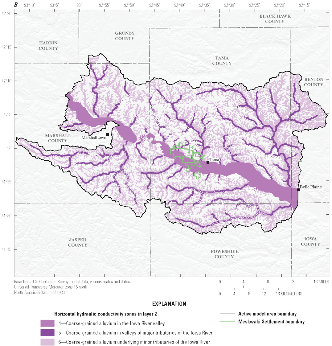
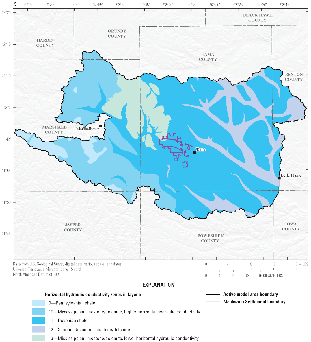
Map showing horizontal hydraulic conductivity zones. A, Fine-grained alluvium (layer 1). B, Coarse-grained alluvium (layer 2). C, Bedrock (layer 5).
Aquifer storage properties, used during the formulations of the groundwater-flow equation during the transient part of the simulation, consisted of specific yield and specific storage. These properties were assigned as constant for each model layer using pilot points and subsequently adjusted further during numerical model calibration. Initial values for specific yield and specific storage for all layers were from published ranges (Freeze and Cherry, 1979; Bayless and others, 2017) for similar hydrogeologic materials. Fine-grained alluvium (layer 1, zones 1–3) had an initial specific storage of 1.00x10⁻⁵ inverse meters (m−1) and an initial specific yield of 5 percent; coarse-grained alluvium (layer 2, zones 4–6) had an initial specific storage of 3.54x10⁻⁵ m−1 and an initial specific yield of 15 percent; glacial drift (layer 3, zone 7) had an initial specific storage of 2.74x10⁻⁷ m−1 and an initial specific yield of 3 percent; buried valley sediment (layer 4, zone 8) had an initial specific storage of 5.25x10⁻⁵ m−1 and an initial specific yield of 10 percent; bedrock other than the lower Kh Mississippian limestone/dolomite (layer 5, zones 9–12) had an initial specific storage of 2.74x10⁻⁷ m−1 and an initial specific yield of 1 percent; and the lower Kh Mississippian limestone/dolomite (layer 5, zone 13) had an initial specific storage of 5.25x10⁻⁶ m−1 and an initial specific yield of 5 percent (table 2).
Boundary Conditions
Aquifer stresses in the numerical model were simulated using various MODFLOW 6 Stress and Advanced Stress packages. Lateral and lower numerical model boundaries were simulated as no-flow boundaries and, as such, no specific package was used. Recharge from infiltration of precipitation in the model area was simulated using the RCH package; direct ETg was simulated using the EVT package; groundwater withdrawal was simulated using the WEL package; and the interaction of groundwater and surface water in the model area was simulated using the SFR package.
Lateral and Lower Boundaries
The model area boundary aligns with the HUC–10 watersheds in the study area, which were considered as no-flow boundaries for the numerical model under the assumption that surface water divides approximate groundwater divides for the model area. Therefore, no specific model package was required to simulate the lateral boundaries of the active model extent. Similarly, the lower boundary of the numerical model was set at an arbitrary altitude of 200 m below the top of the bedrock unit. Because it is assumed that there is no flow into the alluvial aquifer from this depth, the lower boundary was also considered a no-flow boundary, and no specific model package was required to represent it in the numerical model.
Recharge from Precipitation
Recharge from infiltration of precipitation on the land surface was simulated using the RCH package. The RCH package is designed to simulate aerially distributed recharge to the groundwater system (Langevin and others, 2017). The rate of recharge is specified for each stress period in units of meters per day, and the rate is multiplied by the cell horizontal area to obtain the recharge flow rate for each numerical model cell (Langevin and others, 2017). Spatially distributed recharge rates were estimated using the PRMS model, described in the “Water Budget Components” section of this report, and were used as initial estimates of recharge for the numerical model.
The PRMS-calculated spatially distributed mean daily recharge rate over the period 1980–2021 was used for the steady-state stress period in the numerical model. Spatially distributed PRMS-calculated monthly recharge rates were applied to the monthly stress periods in the transient part of the simulation for 1980–2022. The PRMS-calculated recharge rates for the steady-state and transient parts of the model were adjusted during numerical model calibration using recharge multipliers that corresponded with the HRUs used in the PRMS model, described in the “Numerical Model Calibration Approach” section of this report. Additionally, a uniform multiplier of 1.2 was used to scale the PRMS-estimated recharge rates and was not adjusted during model calibration. Spatially distributed estimates of monthly recharge used in the numerical model are available in the accompanying USGS data release (Davis and Goldstein, 2025).
Evapotranspiration from Groundwater
The ETg from direct evaporation of groundwater and from plant transpiration was simulated using the EVT package. The EVT package simulates the effects of plant transpiration and direct evaporation by removing water from the saturated groundwater regime (Langevin and others, 2017). ETg simulation was based on the following assumptions (Langevin and others, 2017): (1) when the water table is at or above a specified altitude (called the “ET surface” in this report), ETg loss is at a specified fixed rate, the maximum allowable ETg rate (ETg(max)); (2) when the depth of the water table below the ET surface exceeds a specified value (called the “extinction depth” in this report), ETg ceases; and (3) when between the ET surface and the extinction depth, ETg varies in a piecewise-linear fashion with water-table altitude. The ETg(max) was specified for each stress period in units of meters per day and was assumed to be equivalent to the PRMS-estimated PET rates for HRUs in the model area, defined in the “Water Budget Components” section of this report. The linear ETg(max) rates were multiplied by the horizontal cell areas to obtain the volumetric ETg(max) flow rate for each cell in the numerical model (Langevin and others, 2017). The ET surface in the numerical model was set equal to the land surface which is also the top of the model. An extinction depth of 3 m was used for woodland areas and was determined by the land cover database obtained from Iowa Department of Natural Resources (2009) for the model area; in all other cells, extinction depth was set to 1 m. Spatially distributed ETg(max) rates were estimated using the PET rates simulated by the PRMS model, described in the “Water Budget Components” section of this report. The PRMS-estimated PET rates were used as initial estimates of ETg(max) for the numerical model. The PRMS-calculated spatially distributed mean daily ETg(max) rate over the period 1980–2021 was used for the steady-state stress period in the numerical model. Spatially distributed PRMS-calculated monthly PET rates were used for ETg(max) for the monthly stress periods in the transient part of the simulation for 1980–2022. The spatially distributed PRMS-calculated steady-state and transient ETg(max) rates were adjusted during numerical model calibration using evapotranspiration multipliers that corresponded with the HRUs that were used in the PRMS model, described in the “Numerical Model Calibration Approach” section of this report. Additionally, a uniform multiplier of 0.83 was used to scale the PRMS-estimated PET rates and was not adjusted during model calibration. Spatially distributed estimates of ETg(max) used in the numerical model are available in the accompanying USGS data release (Davis and Goldstein, 2025).
Groundwater Withdrawal
Groundwater withdrawal from wells in the model area was simulated using the WEL package. The WEL package is designed to simulate features such as wells that withdraw water from or add water to the aquifer at a specified rate, where the rate is independent of the cell area and the head in the cell (Langevin and others, 2017). Groundwater withdrawal rates were specified for each stress period in units of cubic meters per day. Groundwater withdrawal before 1980 was assumed to be minimal; therefore, no withdrawals were specified during the steady-state part of the model. Monthly mean groundwater withdrawal rates at production wells were assigned to the transient part of the model for 1980–2022. Groundwater withdrawal for irrigation, livestock, and domestic uses existed in the model area but were small in comparison to all other water budget components; therefore, groundwater withdrawal for these uses was not included in the numerical model. The locations of groundwater withdrawal wells were converted to the equivalent model row, column, and layer coordinates. Simulated production well withdrawals are available in the accompanying USGS data release (Davis and Goldstein, 2025). Uncertainties in reported pumping data were addressed with the addition of well pumping multipliers that were assigned to each well during numerical model calibration and is described in the “Numerical Model Calibration Approach” section of this report. The WEL package has an option to reduce the withdrawal rate of a well as the water-table altitude in the cell approaches the cell bottom called the “automatic flow reduction.” The automatic flow reduction option is activated when the saturated cell thickness is less than a percentage of the cell thickness (Langevin and others, 2017). The automatic flow reduction saturated thickness threshold for wells in the numerical model was set uniformly to 20 percent.
Surface-Water Features
Surface-water features in the model area contribute water to or drain water from the groundwater system depending on the hydraulic gradient between the surface-water feature and the groundwater head. Streams and rivers were the only surface-water features represented in the numerical model and were simulated using the SFR package (Langevin and others, 2017). The SFR package uses the continuity equation and assumption of piecewise steady (nonchanging in discrete periods), uniform (nonchanging in location), and constant-density streamflow (Langevin and others, 2017). This assumption ensures that during all times, volumetric inflow and outflow rates are equal, and no water is added to or removed from storage in the surface channels. The numerical model routes streamflow through a network of rectangular channels (which may include rivers, streams, canals, and ditches, and are referred to collectively as reaches in the remainder of the report; Langevin and others, 2017). In addition to calculating streamflow, the SFR package also calculates seepage between the surface-water feature and the aquifer. The stream network represented by the SFR package was divided into reaches with each reach representing a section of a stream that corresponds to a specific model cell (Langevin and others, 2017). Reaches were numbered sequentially beginning at USGS streamgage Iowa River at Marshalltown, Iowa, and ending at USGS streamgage Iowa River near Belle Plaine, Iowa (fig. 12). The sequential numbering provided a reference for routing surface-water flow among the SFR reaches.
![[There are 147 streamflow routing segments that represent the Iowa River and its tributaries
in the active model area.]](https://pubs.usgs.gov/sir/2025/5086/images/sir20255086_fig12.png)
Map showing streamflow routing segments in the active model area.
Attributes required for each SFR reach were length, width, gradient, altitude of the top of the streambed, streambed hydraulic conductivity, streambed thickness, and Manning’s roughness coefficient of the stream channel (Arcement and Schneider, 1989). Stream length and width and streambed top altitude and thickness were assigned in units of meters, river gradients were assigned in units of meters per meter, streambed hydraulic conductivity values were assigned in units of meters per day, and Manning’s roughness coefficients were unitless. Additional information used in the SFR package included surface-water inflow to SFR reaches at USGS streamgages Iowa River at Marshalltown, Iowa, and Iowa River near Belle Plaine, Iowa. SFR reaches were assigned to the highest active numerical model layer. The length of each SFR reach was calculated using ArcGIS geoprocessing tools (Esri, 2024) by intersecting the stream features with the model grid, and the width of each SFR reach was estimated from aerial imagery. The stream network in the model area was segmented at river and tributary confluences (hereafter referred to as “segments”; fig. 12). The length of each segment was calculated using ArcGIS geoprocessing tools (Esri, 2024), and the upstream and downstream altitudes of each segment were determined based on a DEM for the model area (Iowa State University, 2020). Downstream altitudes that were either equal to or higher than upstream altitudes, as determined from the DEM, were manually adjusted and set equal to 0.1 m below the upstream altitude. The upstream and downstream altitudes and length of each segment were used to calculate river gradients for each SFR reach. River gradients less than 1.0x10⁻⁴ meters per meter were assigned a minimum gradient of 1.0x10⁻⁴ meters per meter. The upstream and downstream altitudes, length of each segment, and length of each SFR reach were used to calculate the riverbed top for the midpoint of each SFR reach. Riverbed thicknesses for each SFR reach were assigned a nominal and uniform value of 1.0 m. If the riverbed bottom altitude for an individual SFR reach (calculated by subtracting riverbed thickness from top altitude) was below the bottom of the uppermost active layer, the layer bottom altitude for that cell was assigned to 1.0 m below riverbed bottom altitude. In some cases, this method produced reach altitudes that were above the top of the model layer to which the reach was assigned. The reach altitudes that were above the top of the numerical model were manually adjusted to ensure the altitude was below the top of the numerical model layer to which each reach was assigned. SFR reaches were initially assigned a uniform riverbed hydraulic conductivity of 0.3048 m/d and a uniform Manning’s roughness coefficient of 0.037; however, these values were adjusted during numerical model calibration, as described in the “Numerical Model Calibration Approach” section of this report.
Numerical Model Calibration Approach
Model calibration is the process of estimating numerical model parameters to minimize the differences, or residuals, between hydrologic observations of interest (“calibration targets”) and numerical model outputs. The groundwater flow model was calibrated using PESTPP–IES (version 5.0.9; White, 2018; White and others, 2020) with calibration targets selected from observed or estimated values from available hydrologic data. PESTPP–IES is a member of the PEST++ suite of calibration programs first developed by Welter and others (2015). White (2018) described the background and methods employed by PESTPP–IES. PESTPP–IES iterates ensembles of random model parameter values to minimize the difference, or residuals, between observed (measured observation) values and simulated (model-computed) values. The ensemble of model parameters is modified iteratively until an acceptable model to measurement fit is obtained through a “base” set of model parameters. An advantage of PESTPP–IES over other iterative calibration methods is its efficiency compared to traditional least squares methods in that the model only runs once for each user-selected number of ensemble members instead of one or more times for each model parameter (Hunt and others, 2021). Hunt and others (2021) used a test problem to show that the traditional least squares method (singular value decomposition) required more than 25 times the number of model forward runs compared to more efficient methods, including an iterative ensemble smoother approach, to obtain an acceptable model-to-measurement fit.
The numerical model was calibrated for steady-state and transient monthly conditions for January 1980–August 2022 using pilot points (Doherty, 2003). Calibration targets were observations of hydraulic head and changes in hydraulic head from the USGS National Water Information System (NWIS) and Iowa Geological Survey GeoSam databases and monthly mean streambed flux and cumulative monthly streambed flux from the USGS NWIS database (fig. 13; table 3; Iowa Geological Survey, 2024; U.S. Geological Survey, 2024). The method of pilot points was used to interpolate a smooth hydrologic-property field and apply the resulting spatially variable distribution of hydrologic properties to the numerical model grid.
![[Hydraulic head altitude calibration targets in layer 1 and 3 are found throughout
the active model area, targets in layer 5 are primarily in the northwest of the model
area, and limited targets are in layers 2 and 4. There are seven streamflow calibration
targets on the Iowa River and its tributaries.]](https://pubs.usgs.gov/sir/2025/5086/images/sir20255086_fig13.png)
Map showing location of streamflow calibration targets and hydraulic head altitude targets by layer in the model area.
Table 3.
Parameters used in model calibration.[PRMS, Precipitation Runoff Modeling System; HRU, hydrologic response unit]
Calibration Targets and Weighting
Model calibration is completed using a process called history matching. History matching refers to the process of attempting to closely match real-world hydrologic observations of interest (calibration targets) to model-simulated values for a defined period (Welter and others, 2015). In general, calibration targets are direct measurement values, such as hydraulic head. However, in some cases, calibration targets may be calculated from measurement values, such as changes in hydraulic head. History matching is accomplished by attempting to reduce the sum of squared weighted residuals, or the objective function, for all calibration targets (Welter and others, 2015). Each calibration target in the history matching process is assigned a weight, and a residual is the difference between a calibration target and model-simulated value. Each observation is assigned to a group of similar observation types. Calibration targets for hydraulic head and changes in hydraulic head were assigned to groups based on model layer, and calibration targets for monthly mean streambed flux and cumulative monthly streambed flux each were assigned to their own group (table 4). Weighting adjusts the contribution of each residual to the overall objective function and combining calibration targets into groups ensures that no single observation type or group becomes a dominant contributor in the calibration process (Welter and others, 2015). Highly weighted calibration targets will have greater importance in the calibration process compared to calibration targets with lower weights because smaller changes in a residual for highly weighted calibration targets will generate larger changes to the overall objective function (Welter and others, 2015).
Table 4.
Calibration observations and associated weights.Hydraulic Head Measurements
Hydraulic head measurements in the model area were available in the USGS NWIS database (U.S. Geological Survey, 2024) and the Iowa Geological Survey GeoSam database (Iowa Geological Survey, 2024) at 143 wells primarily in layers 1, 3, and 5, with 17,345 unique observations (fig. 13). These measurements were used as calibration targets for hydraulic head and changes in hydraulic head for numerical model calibration. Measurement dates ranged from 1905 to 2022, with measurements before 1980 used to calibrate the steady-state portion of the model. Where a measurement date was not listed in the GeoSam database (Iowa Geological Survey, 2024), the completion or drilled date of the well from the GeoSam database was used, which was the case for 130 out of 739 water-level measurements. Measurements in the GeoSam database (Iowa Geological Survey, 2024) were converted from feet below ground surface to meters above NAVD 88 by first converting the measurement to meters with two decimal places of precision, then subtracting that value from the land surface altitude reported for the well, converted from feet to meters. Water levels from the USGS NWIS database (U.S. Geological Survey, 2024) were reported in feet above NAVD 88 and were converted to meters for use in model calibration.
Calibration targets for hydraulic head included both single water-level measurements made at a well and multiple water-level measurements made on different days at a single well. Single water-level measurements made up 703 of the 17,345 observations; the remaining were multiple water-level measurements made at 12 wells, including USGS continuous monitoring wells located on the Meskwaki Settlement (table 1). Measurements made on multiple days at a single well were used for hydraulic head change targets, with change in hydraulic head calculated as the difference between the measured water-level altitude on that date and the previously recorded water-level measurement. For the wells with multiple water-level measurements, the first recorded water-level measurement made at the well was also utilized as a hydraulic head altitude target.
Streambed Flux
Monthly streambed flux, which is the calculated change in base flow through the streambed between two or more streamgages in the model area, and cumulative monthly streambed flux were used as calibration targets. Monthly streambed flux was estimated using base flow calculated from streamflow recorded at USGS streamgages using base-flow separation in the Groundwater Toolbox (Barlow and others, 2015), as described in the “Groundwater and Surface-Water Interactions” section of this report. Calibration targets for the monthly streambed flux were calculated as the difference in base flow between a downstream streamgage and any upstream streamgage or streamgages that contributed to the downstream streamflow in the model area for a given month. Cumulative monthly streambed flux calibration targets were calculated from the monthly streambed flux values by multiplying the monthly streambed flux values by the number of days in each month to calculate the volumetric flux through the streambed for a given month and adding each successive monthly streambed flux value.
Calibration Parameters
Model parameters adjusted during numerical model calibration include horizontal hydraulic conductivity, vertical anisotropy ratio, specific storage, specific yield, streambed hydraulic conductivity, recharge, evapotranspiration from groundwater, and well multipliers. Horizontal hydraulic conductivity, vertical anisotropy ratio, specific storage, and specific yield were estimated at pilot point locations distributed within the model area; recharge and ETg multipliers were estimated for each of the PRMS HRUs; well pumping multipliers were estimated for each well; and streambed hydraulic conductivity values were estimated for each stream segment in the SFR package (fig. 12). The upper and lower bounds for each calibration parameter, except for the recharge, ETg, and well multipliers, were set at one-tenth and ten times the initial value. The estimates of recharge, ETg, and pumping from wells were adjusted independently during the calibration process using multipliers. The multipliers were applied uniformly to all numerical model stress periods (steady-state and transient stress periods) for the spatially varied PRMS estimates used in the RCH and EVT packages and for each production well represented in the model. The initial value of the recharge and ETg multipliers was set at 1 and allowed to range from 0.33 to 1.66, and the initial value of the well multiplier was set at 1 and allowed to range from 0.85 to 1.20.
Horizontal and vertical hydraulic conductivity, specific storage, and specific yield were calibrated at pilot point locations (figs. 15 and 16). Pilot points are discrete locations distributed throughout the active model area that represent surrogate parameters from which hydrologic property values are interpolated to the numerical model grid using a kriging algorithm (Doherty and Hunt, 2010). The use of pilot points and the method of kriging allows for greater variation in hydrologic properties compared to using either a single value for each model layer or subdividing each layer into piecewise zones of uniform hydraulic conductivity (Doherty and Hunt, 2010). As a result, the process allows a smooth variation in hydrologic properties in the model area interpolated from estimated values at pilot points. Final parameter estimates were checked to ensure that they were appropriate based on literature values.
![[a) Calibrated horizontal hydraulic conductivity ranges from 1 to 200 meters per day
in layer 1, which represents fine-grained alluvium in the valleys of the Iowa River
and its major and minor tributaries. b) Calibrated horizontal hydraulic conductivity
ranges from 5 to 1,000 meters per day in layer 2, which represents coarse-grained
alluvium in the valleys of the Iowa River and its major and minor tributaries. c)
Calibrated horizontal hydraulic conductivity ranges from 0.03 to 3 meters per day
in layer 3, which represents glacial drift. d) Calibrated horizontal hydraulic conductivity
ranges from 5 to 500 meters per day in layer 4, which represents buried-valley sediment.
e) Calibrated horizontal hydraulic conductivity ranges from 0.001 to 142.92 meters
per day in layer 5, which represents bedrock.]](https://pubs.usgs.gov/sir/2025/5086/images/sir20255086_fig14a.png)
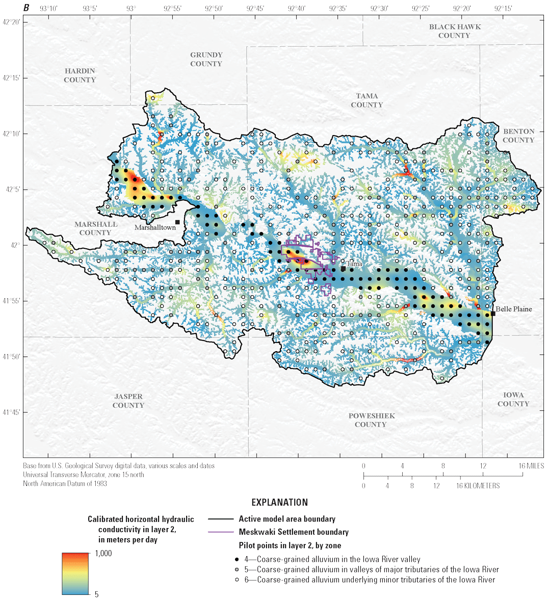
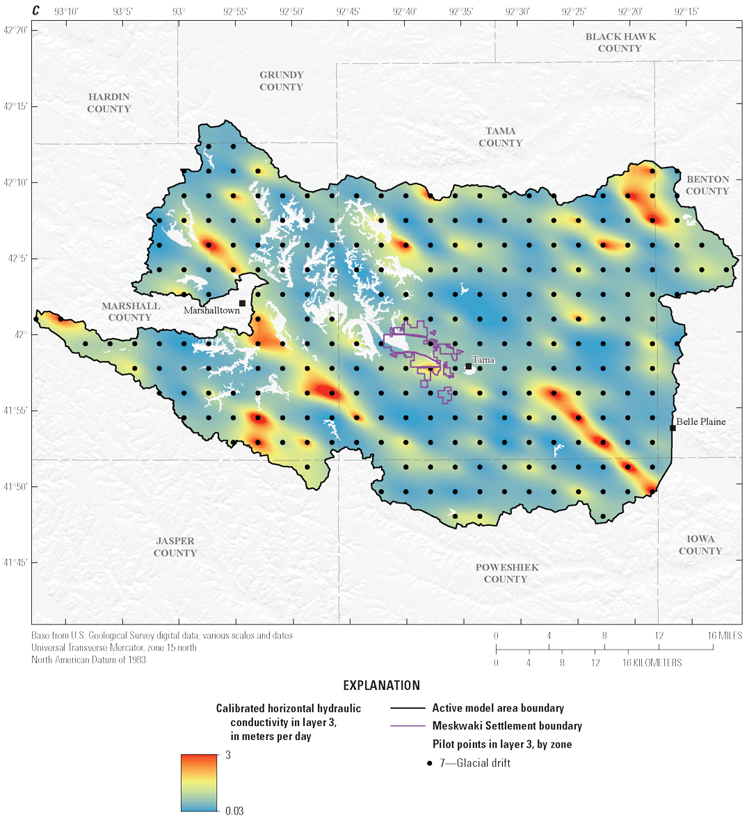
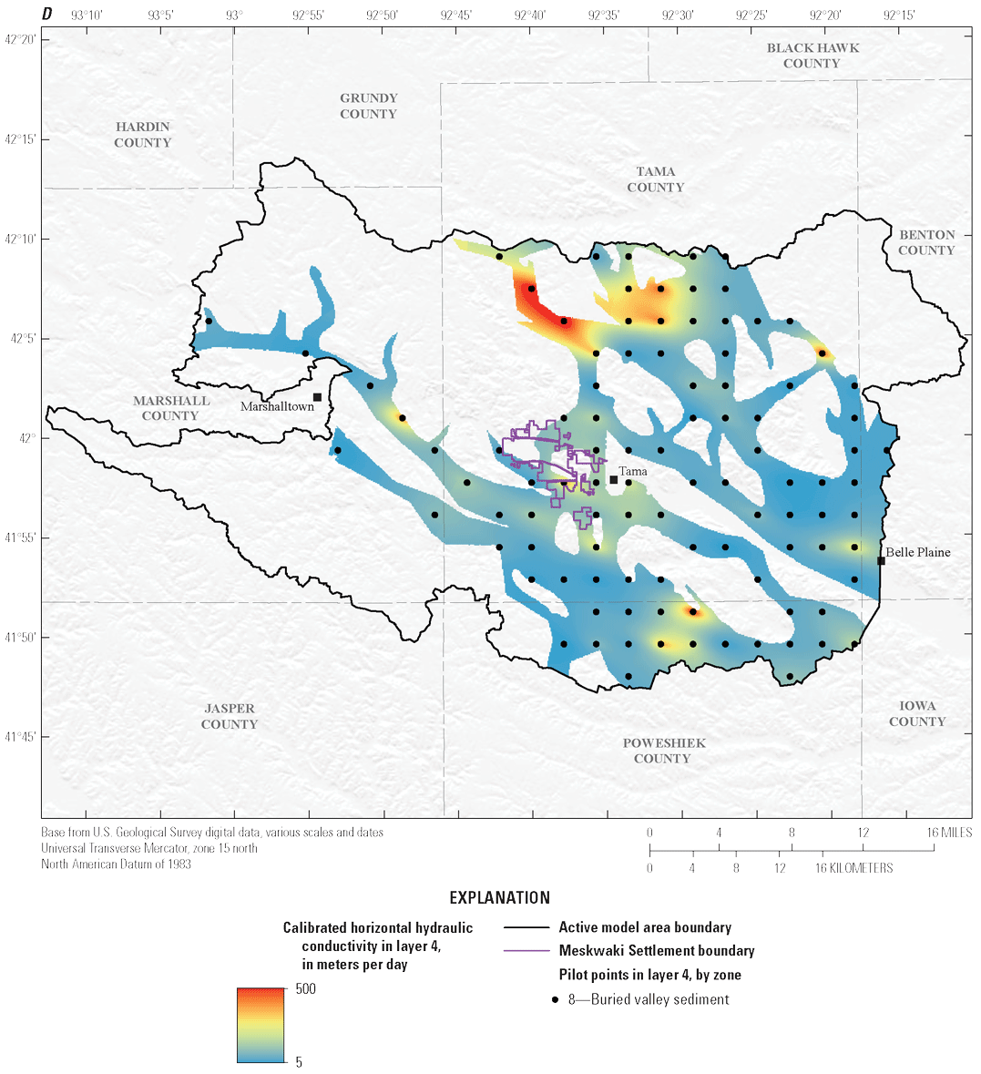
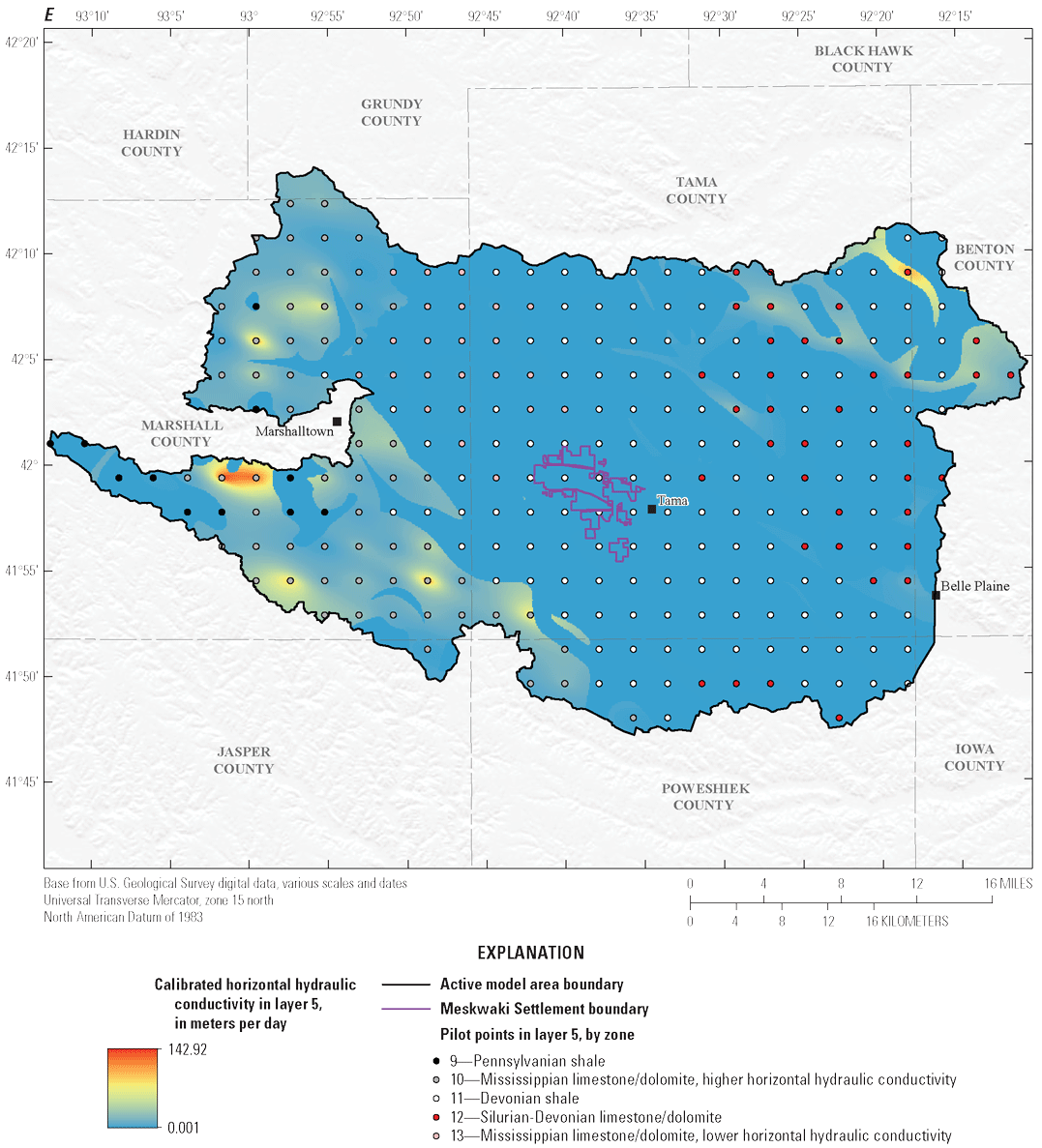
Calibrated horizontal hydraulic conductivity and spatial distribution of pilot points. A, Fine-grained alluvium (layer 1). B, Coarse-grained alluvium (layer 2). C, Glacial drift (layer 3). D, Buried-valley sediment (layer 4). E, Bedrock (layer 5).
![[a) Calibrated vertical anisotropy ratio ranges from 0.01 to 1 in layer 1, which represents
fine-grained alluvium in the valleys of the Iowa River and its major and minor tributaries.
b) Calibrated vertical anisotropy ratio ranges from 0.01 to 1 in layer 2, which represents
coarse-grained alluvium in the valleys of the Iowa River and its major and minor tributaries.
c) Calibrated vertical anisotropy ratio ranges from 0.01 to 1 in layer 3, which represents
glacial drift. d) Calibrated vertical anisotropy ratio ranges from 0.01 to 1 in layer
4, which represents buried-valley sediment. e) Calibrated vertical anisotropy ratio
ranges from 0.01 to 1 in layer 5, which represents bedrock.]](https://pubs.usgs.gov/sir/2025/5086/images/sir20255086_fig15a.png)
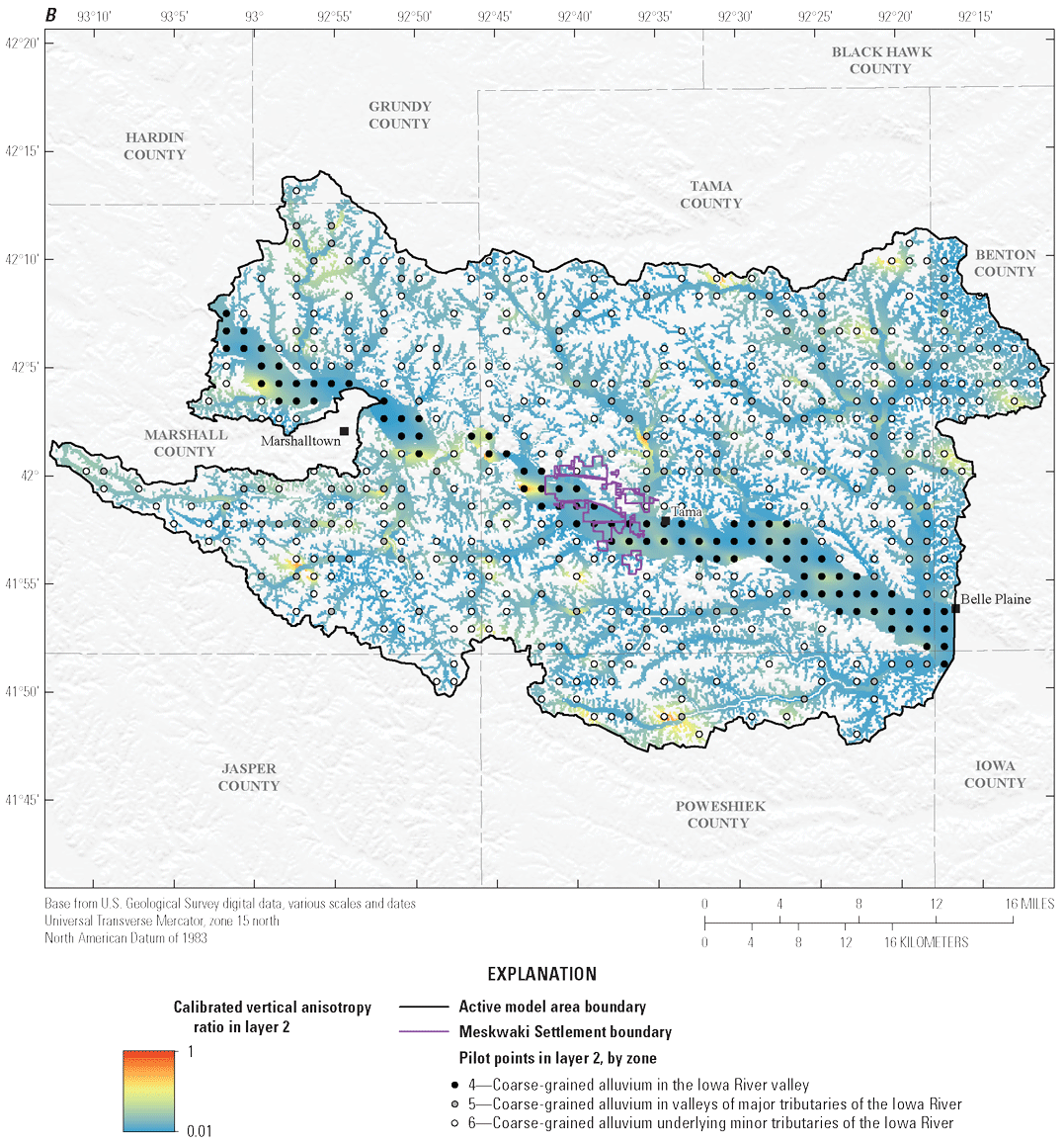
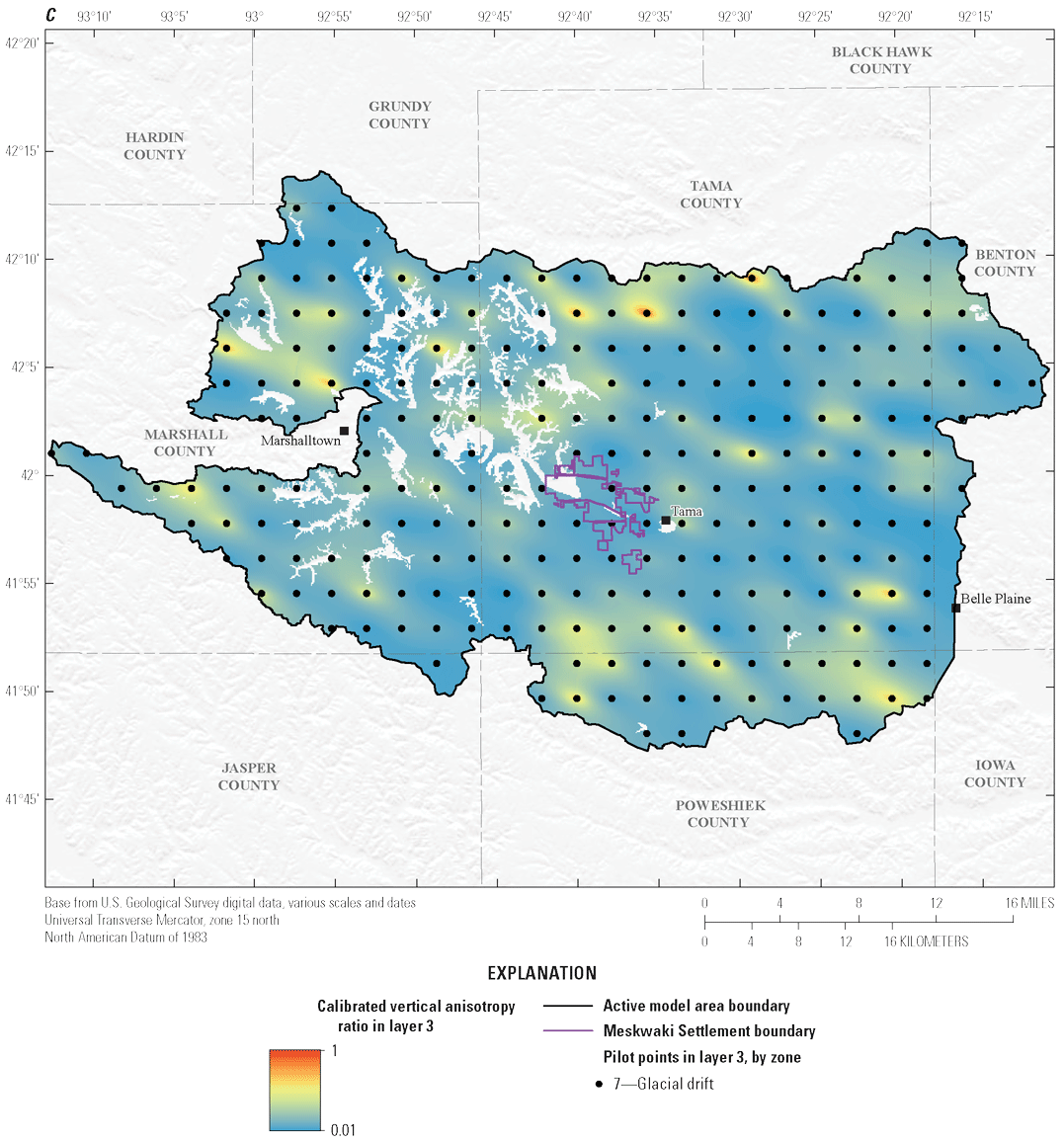
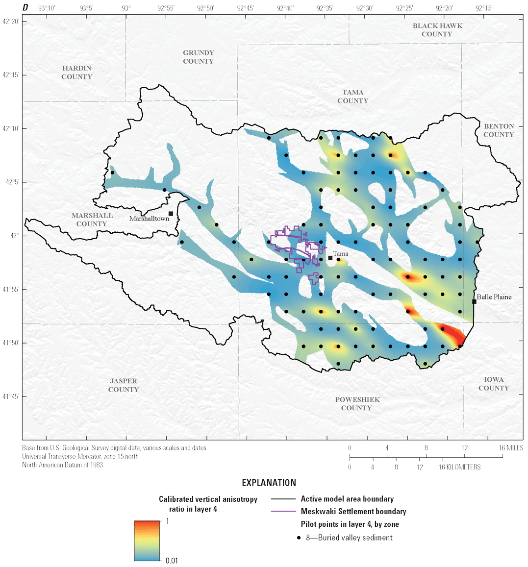
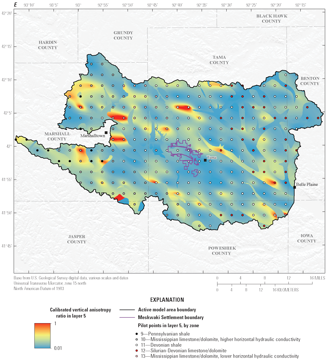
Calibrated vertical hydraulic conductivity anisotropy ratio and spatial distribution of pilot points. A, Fine-grained alluvium (layer 1). B, Coarse-grained alluvium (layer 2). C, Glacial drift (layer 3). D, Buried-valley sediment (layer 4). E, Bedrock (layer 5).
Numerical Model and Calibration Results
Calibration results included optimal parameter estimates and a comparison of calibration targets to model-simulated values. Optimal parameter estimates for horizontal and vertical hydraulic conductivity, specific yield, specific storage, streambed hydraulic conductivity, and recharge and ETg multipliers compared well with literature values. Optimal parameter estimates were obtained primarily based on the automated comparison of model-simulated values to calibration targets of hydraulic head, changes in hydraulic head, monthly mean streambed flux, and cumulative monthly streambed flux. A secondary assessment of numerical model performance included a qualitative assessment of streambed flux.
Optimal Parameter Estimates
The final calibrated parameter values of horizontal and vertical hydraulic conductivity, specific yield, specific storage, streambed hydraulic conductivity, recharge, and ETg were considered reasonable for the hydrogeologic materials and conditions in the model area for January 1980–August 2022. In general, the mean calibrated parameter values were reasonably close to previously published values (table 5). The mean horizontal hydraulic conductivity for the fine-grained alluvium, estimated at pilot points during the calibration process, was about 36 m/d in the Iowa River valley (zone 1), 33 m/d in valleys of the major tributaries of the Iowa River (zone 2), and 17 m/d underlying minor tributaries of the Iowa River (zone 3; fig. 14A; table 5). Calibrated horizontal hydraulic conductivity ranged from about 2 to 179 m/d, 2 to 200 m/d, and 1 to 100 m/d at pilot point locations in zones 1, 2, and 3, respectively (fig. 14A; table 5). The mean calibrated vertical anisotropy ratio for the fine-grained alluvium was 25 percent at pilot points in zone 1, 15 percent in zone 2, and 17 percent in zone 3 (fig. 15A), which were generally similar to the initial value of 10 percent (table 5), and ranged from about 1 to 100 percent at pilot point locations in zones 1, 2, and 3 (table 5; fig. 15A). The mean calibrated specific storage was 1.58x10⁻⁵ m−1 in zone 1, 2.08x10⁻⁵ m−1 in zone 2, and 1.75x10⁻⁵ m−1 in zone 3, which are similar to the initial specific storage for all three zones of 1.00x10⁻⁵ m−1 (table 5). For specific yield of the fine-grained alluvium, the mean calibrated values were 8 percent in zones 1 and 2, and 9 percent in zone 3, which are similar to the initial specific yield for all three zones of 5 percent (table 5).
Table 5.
Initial and calibrated model parameters. [—Left][Kh, horizontal hydraulic conductivity; m/d, meter per day; Kz, vertical hydraulic conductivity; Ss, specific storage; Min, minimum; Max, maximum; m-1, per meter; Sy, specific yield]
Table 5.
Initial and calibrated model parameters. [—Right]The mean horizontal hydraulic conductivity for the coarse-grained alluvium, estimated at pilot points during the calibration process, was 181 m/d in the Iowa River valley (zone 4), 190 m/d in valleys of major tributaries of the Iowa River (zone 5), and 95 m/d underlying minor tributaries of the Iowa River (zone 6; fig. 14B; table 5). Calibrated horizontal hydraulic conductivity ranged from 10 to 1,000 m/d in zones 4 and 5, and 5 to 500 m/d at pilot point locations in zone 6 (fig. 14B; table 5). The mean calibrated vertical anisotropy ratios for the coarse-grained alluvium were 16 percent at pilot points in zones 4, 5, and 6 (fig. 15B), which were generally similar to the initial value of 10 percent (table 5). Mean calibrated vertical anisotropy ratios for the coarse-grained alluvium ranged from 1 to 100 percent in zones 4, 5, and 6 (fig. 15B; table 5). The mean calibrated specific storage was 6.53x10⁻⁵ m−1 in zone 4, 6.43x10⁻⁵ m−1 in zone 5, and 5.56x10⁻⁵ m−1 in zone 6, which were similar to the initial specific storage of 3.45x10⁻⁵ m−1 for all three zones. For specific yield of the coarse-grained alluvium, the mean calibrated values were 17 percent in zone 4, 26 percent in zone 5, and 23 percent in zone 6, which are similar to the initial specific yield for all three zones of 15 percent (table 5).
The mean horizontal hydraulic conductivity for the glacial drift (zone 7), estimated at pilot points during the calibration process, was 0.53 m/d and ranged from 0.03 to 3 m/d (fig. 14C; table 5). The mean calibrated vertical anisotropy ratio for the glacial drift was 18 percent, which was similar to the initial value of 10 percent (table 5) and ranged from 1 to 100 percent (fig. 15C; table 5). The mean calibrated specific storage was 4.85x10⁻⁷ m−1, which was similar to the initial specific storage of 2.74x10⁻⁷ m−1, and the mean calibrated specific yield was 5 percent, which was similar to the initial specific yield of 3 percent (table 5).
The mean horizontal hydraulic conductivity for the buried valley sediment (zone 8), estimated at pilot points during the calibration process, was 92 m/d and ranged from 5 to 500 m/d (fig. 14D; table 5). The mean calibrated vertical anisotropy ratio for the buried valley sediment was 20 percent, which was similar to the initial value of 10 percent (table 5) and ranged from 1 to 100 percent (fig. 15D; table 5). The mean calibrated specific storage for the buried valley sediment was 9.48x10⁻⁵ m−1, which was similar to the initial specific storage of 5.25x10⁻⁵ m−1, and the mean calibrated specific yield was 17 percent, which was similar to the initial specific yield of 10 percent (table 5).
The mean horizontal hydraulic conductivity for the Pennsylvanian shale (zone 9), higher hydraulic conductivity Mississippian limestone/dolomite (zone 10), Devonian shale (zone 11), Silurian-Devonian limestone/dolomite (zone 12), and lower hydraulic conductivity Mississippian limestone/dolomite (zone 13), estimated at pilot points during the calibration process, was 0.62 m/d, 26 m/d, 0.42 m/d, 11 m/d, and 0.77 m/d, respectively (fig. 14E; table 5). Calibrated horizontal hydraulic conductivity ranged from 0.07 to 3 m/d, 1.5 to 143 m/d, 0.03 to 2.5 m/d, 0.25 to 101 m/d, and 0.09 to 2.8 m/d at pilot point locations in zones 9, 10, 11, 12, and 13, respectively (fig. 14E; table 5). The mean calibrated vertical anisotropy ratio for the bedrock unit was 23 percent at pilot points in zone 9, 21 percent in zone 10, 16 percent in zone 11, 13 percent in zone 12, and 24 percent in zone 13 (fig. 15E), which were generally similar to the initial value of 10 percent (table 5). The vertical anisotropy ratio ranged from 5 to 62 percent at pilot point locations in zone 9, 1 to 100 percent in zones 10, 11, and 13, and 1 to 70 percent in zone 12 (table 5). The mean calibrated specific storage of the bedrock units were 9.74x10⁻⁷ m−1 in zone 9, 4.40x10⁻⁷ m−1 in zone 10, 4.24x10⁻⁷ m−1 in zone 11, 3.75x10⁻⁷ m−1 in zone 12, and 9.52x10⁻⁶ m−1 in zone 13, which are similar to the initial specific storage of 2.74x10⁻⁷ m−1 for zones 9–12 and 5.25x10⁻⁶ for zone 13. For specific yield of the bedrock units, the mean calibrated values were 1 percent in zone 9, 20 percent in zone 10, 1 percent in zone 11, 22 percent in zone 12, and 11 percent in zone 13, which are similar to the initial specific yield of 1 percent for zones 9-12 and 5 percent for zone 13 (table 5).
The calibrated streambed hydraulic conductivity for stream segments in the SFR package ranged from 0.003 to 3.05 m/d with a mean of 0.84 m/d. The mean calibrated streambed hydraulic conductivity was greater than the initial value of 0.003 m/d. The mean calibrated recharge multiplier was 1.08 and ranged from 0.33 to 1.67, the mean calibrated evapotranspiration multiplier was 1.01 and ranged from 0.33 to 1.67, and the mean calibrated well multiplier was 1.00 and ranged from 0.85 to 1.20.
Comparison of Simulated and Observed Water Table Altitudes
Numerical model performance was assessed primarily on its ability to match calibration targets for groundwater levels (hydraulic head altitudes) and changes in hydraulic head. Hydraulic head altitude targets were assessed for 738 wells (fig. 16), and hydraulic head change targets were assessed for 33 wells that had more than one measurement.
![[The best-fit trend line for observations in layers 1 and 2 approximates the 1:1 line
and has a coefficient of determination of 0.92.]](https://pubs.usgs.gov/sir/2025/5086/images/sir20255086_fig16.png)
Graph showing observed and simulated hydraulic head for hydraulic head altitude targets, including a best-fit line from linear regression. The 1:1 perfect-fit line also is shown for reference to visualize bias.
The hydraulic head altitude targets used in numerical model calibration were compared with numerical model-simulated hydraulic head calculated at the same location and time as the observations. Observed hydraulic head altitudes were plotted with simulated hydraulic head altitudes and compared to a 1:1 perfect-fit line (fig. 16). The linear regression coefficient of determination (R2) for the simulated versus observed hydraulic head altitudes in layers 1 and 2, which make up the Iowa River alluvial aquifer, was 0.92, and the R2 value for the simulated versus observed hydraulic head altitudes within all layers was 0.56 (fig. 16). In general, simulated hydraulic head altitudes in layers 1 and 2 tended to underestimate observed values, and as observed hydraulic head altitudes increased, so did the difference between simulated and observed hydraulic head altitudes (fig. 16). For all model layers, simulated hydraulic head altitudes tended to overestimate observed hydraulic head altitudes for observed values less than about 270 m above NAVD 88 and underestimate hydraulic head altitudes for observed values greater than about 270 m above NAVD 88 (fig. 16).
The differences between observed and simulated hydraulic head altitudes, otherwise known as residuals, were plotted by layer using a histogram (fig. 17) to assess the overall model-to-measurement fit. The differences were calculated as observed minus simulated values, so a negative residual indicates that the simulated hydraulic head altitude was greater than the observed hydraulic head altitude at the given location. The histogram shows that, in general, hydraulic head altitude residuals for wells in layer 1 tended to be positive, residuals for wells in layer 5 tended to be negative, and residuals for wells in layers 2 and 3 tended to be more evenly distributed between positive and negative (fig. 17).
![[Residuals range from −62.5 to 47.0 meters, with about 47 percent of residuals between
−5.0 and 5.0 meters.]](https://pubs.usgs.gov/sir/2025/5086/images/sir20255086_fig17.png)
Histogram showing residuals (observed minus simulated values) of hydraulic head altitude targets.
The absolute hydraulic head altitude residuals (which do not take into account whether simulated values were over- or underestimations of observed values) for all model layers ranged from 0 to 62.5 m (fig. 17), with a mean of 8.8 m and a standard deviation of 9.6 m. Absolute hydraulic head altitude residuals were evenly distributed spatially across the active model area. For layers 1 and 2, absolute hydraulic head residuals ranged from 0 to 57.5 m, with a mean of 5.7 m and standard deviation of 7.3 m. For all model layers, 46.5 percent of simulated groundwater levels were within plus or minus 5 m of the observed values, 68.6 percent were within plus or minus 10 m (with 11.1 percent being positive residuals and 11.1 percent being negative), and 93.4 percent were within plus or minus 25 m (with 11.1 percent being positive residuals and 13.7 percent being negative; fig. 17).
Observed and simulated hydraulic head hydrographs were created for select observation wells in layers 1 and 2 with more than three water-level observations for their period of record during the model time period (fig. 18). The hydrographs are a visual representation of hydraulic head altitude and hydraulic head change observation targets. The first value in a hydrograph represents the hydraulic head altitude at the time of the first measurement at an observation well. A visual assessment of the hydrographs indicated that in general, for wells located in layers 1 and 2, the numerical model underestimated observed hydraulic head altitudes and tended to underestimate the magnitude of the change in hydraulic head observed at wells. The timing of simulated lowest hydraulic head altitudes at wells generally matched the timing of observed lowest hydraulic head altitudes, and the timing of simulated highest hydraulic head altitudes generally matched the timing of observed highest hydraulic head altitudes (fig. 18).
![[Simulated hydraulic heads tend to underestimate observed hydraulic heads for the
monitoring wells displayed, but the timing of simulated highest and lowest hydraulic
head altitudes generally match the timing of observed highest and lowest hydraulic
head altitudes.]](https://pubs.usgs.gov/sir/2025/5086/images/sir20255086_fig18a.png)
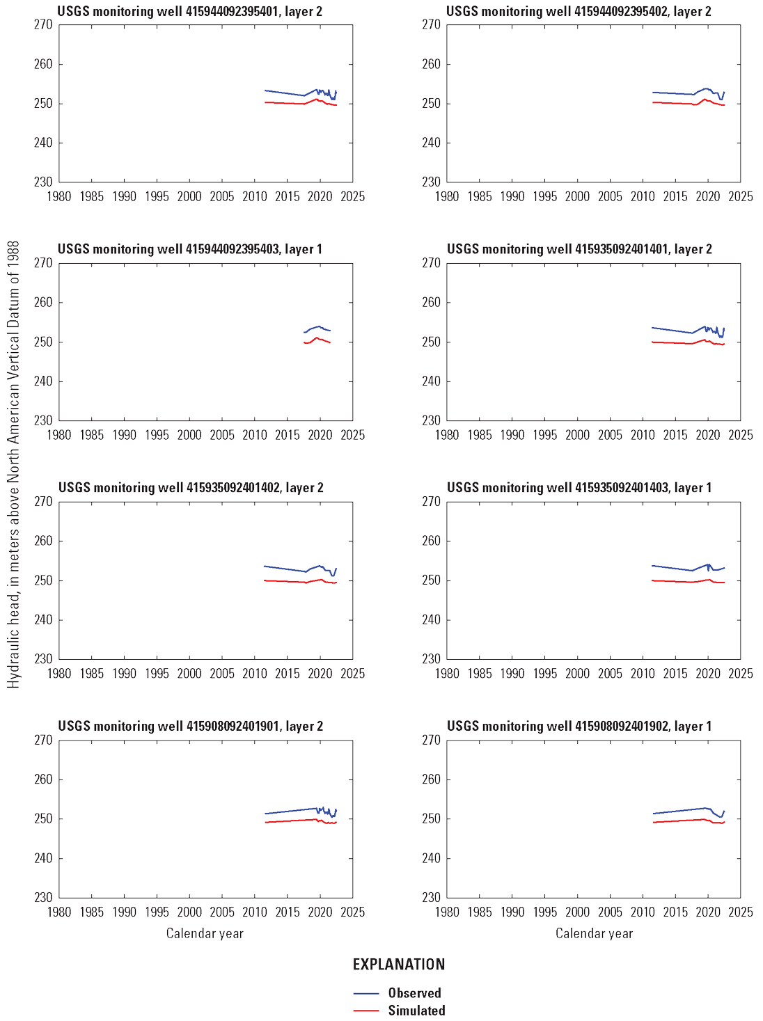
Hydrographs of observed and simulated hydraulic head for selected observation wells near the Meskwaki Settlement.
Comparison of Streambed Fluxes
Numerical model performance was also assessed based on the differences (or change) in observed and simulated base flow. Streambed fluxes were calculated for each cell of the SFR package in the active model area during the period of record for each streamgage and were plotted as the change in streambed flux between streamgages in the active model area (fig. 19). When compared to observed streambed fluxes (fig. 19), the simulated streambed fluxes are underestimated, and in some cases simulated streambed flux accounted for one-fifth of observed streambed flux, typically during periods with higher streambed flux (fig. 19). In particular, the model accurately simulates the lower streambed flux values but does not accurately represent periods where there is an observed peak in streambed flux. This underestimation may be due, in part, to the fact that base flow was calibrated using only values for the winter months (October–March), when streamflow is generally lowest, although base flow tends to remain relatively steady during the year compared to streamflow. Additionally, inflows to the model area where the Iowa River and Linn Creek cross the active model boundary were determined from base flow estimated by the PRMS model, as described in the “Groundwater and Surface-Water Interactions” section of this report. These streambed flux values, calculated using the inflows to the model from the Iowa River or Linn Creek, may be underestimated and could lead to larger differences in observed and simulated streambed flux when compared to streambed fluxes calculated from the differences in observed and simulated base flow calculated using upstream and downstream streamgages.
![[Simulated streambed fluxes generally underestimate observed streambed fluxes, with
the model more accurately simulating lower streambed flux values than higher ones.]](https://pubs.usgs.gov/sir/2025/5086/images/sir20255086_fig19a.png)
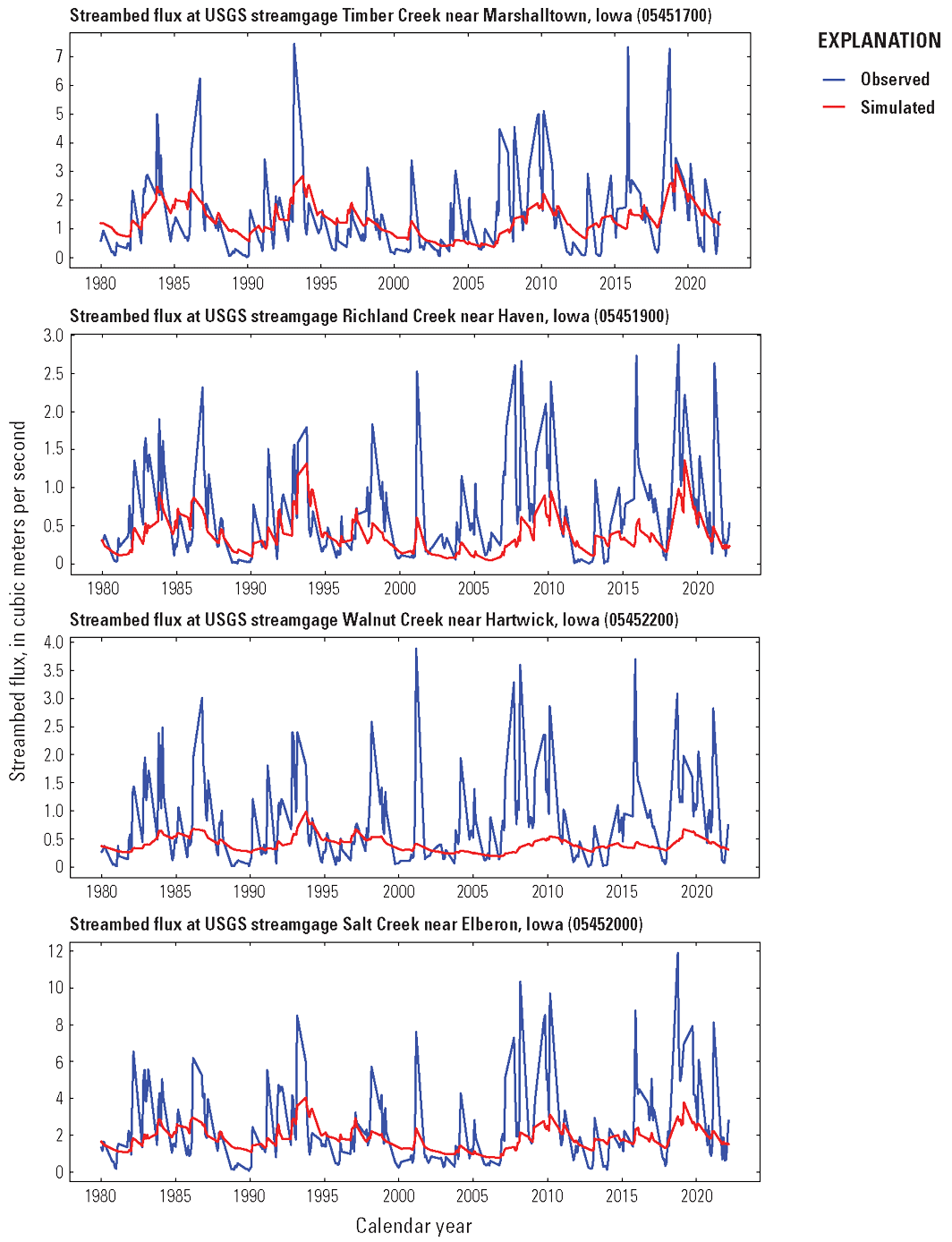
Observed and simulated streambed fluxes for U.S. Geological Survey streamgages for the transient period.
Simulated Groundwater Budget
The simulated groundwater budget characterizes inflows and outflows to the Iowa River alluvial aquifer and underlying hydrogeologic units. Steady-state and transient groundwater budgets were calculated using the program ZONEBUDGET distributed with MODFLOW 6 (Langevin and others, 2017) using cell-by-cell flow data from the numerical model output. Groundwater withdrawals were not simulated during the steady-state stress period; therefore, the steady-state groundwater budget does not include a groundwater withdrawal component. The simulated steady-state groundwater budget for the model consisted of inflows from precipitation recharge (RCH package) and stream infiltration (SFR package) and outflows from ETg (EVT package) and groundwater discharge to streams (SFR package). During the steady-state stress period, simulated inflow for the active model area was about 817,500 m/d from precipitation recharge and about 63,000 m/d from the infiltration of streamflow (table 6). Simulated outflow for the steady-state period was about 51,300 m/d from ETg and 829,900 m/d from groundwater discharge to streams (table 6).
Table 6.
Steady-state groundwater flow budget.[m/d, meter per day; RCH, Recharge; EVT, Evapotranspiration; SFR, Streamflow Routing; n/a, not applicable]
The groundwater budget for the transient period consisted of the same components from the steady-state period and also included inflows from and outflows to storage (STO package) and outflows from well withdrawals (WEL package). The groundwater budget for the transient period presented in this report was calculated as the mean of each monthly budget component for the entire transient period (January 1980–August 2022) and was expressed as percentages of the mean total monthly inflow and outflow. The percentage of total inflow or total outflow presented in this paragraph equal slightly more than 100 percent (100.1 percent) because of rounding. Based on the mean budget components calculated for the transient period, precipitation recharge accounts for about 60.6 percent of the total inflow, inflow from storage accounts for about 34.5 percent, and stream infiltration accounts for about 5.0 percent (table 7). For the mean outflows for the transient period, groundwater discharge to streams accounts for about 60.3 percent of the total outflow, outflow to storage accounts for about 34.5 percent, ETg accounts for about 3.8 percent, and well withdrawals account for about 1.5 percent of total outflows (table 7).
Streamflow Depletion Analysis
Streamflow depletion is a reduction in streamflow caused by groundwater pumping and includes the interception by groundwater production wells of water that otherwise would have been discharged to streams (called “captured groundwater discharge”) and induced infiltration of streamflow to the production wells (Barlow and Leake, 2012). A streamflow depletion analysis was performed using a version of the calibrated numerical model with tightened convergence factors to estimate the fraction of water that is pumped from the Iowa River alluvial aquifer by Meskwaki Settlement wells that is derived from streamflow depletion in the Iowa River and its tributaries. Convergence factors were tightened for these stream depletion runs to minimize the difference between total inflows and outflows in the simulated groundwater budget.
The stream depletion analysis was performed using a modified approach described in Barlow and Leake (2012). First, the calibrated model was run with all modeled pumping turned off, and model-computed inflow and outflow rates for the SFR package were recorded for all model stress periods. The model was then run with modeled pumping at the Meskwaki Settlement wells turned on, and the model-computed inflow and outflow rates for the SFR package were recorded for all model stress periods. Third, the computed flow rates for the SFR package from the model with pumping at the Meskwaki Settlement wells were subtracted from the computed flow rates for the SFR package from the model with no pumping to calculate the change in simulated flow rates between surface water and the groundwater system. The change in simulated net flow rates, which were calculated as SFR inflows minus SFR outflows, represents the amount of total streamflow depletion in the Iowa River and tributary streams resulting from pumping at the Meskwaki Settlement wells. This total streamflow depletion can be broken out into its components, induced recharge and captured discharge, using the SFR inflows and outflows computed for each stress period. The change in simulated inflow to the groundwater system from streams represents the amount of induced recharge that results from pumping at the Meskwaki Settlement wells, and the change in simulated outflow from the groundwater system to streams represents the amount of captured discharge. The calculated total streamflow depletion was expressed as a percentage of pumping at the Meskwaki Settlement wells during each time step and was calculated by dividing the net change in flow between the groundwater system and streams by the total simulated pumping at the Meskwaki Settlement wells for each month that pumping data were available for Meskwaki Settlement wells (2018–22). Calculated induced infiltration and captured discharge were also expressed as a percentage of pumping at the Meskwaki Settlement wells during each time step by dividing the change in inflows to and outflows from the groundwater system, respectively, by the total simulated pumping at the Meskwaki Settlement wells for each month that pumping data were available for the Meskwaki Settlement wells. Using this method, the mean monthly streamflow depletion, including induced infiltration and captured discharge, in the Iowa River and its tributary streams as a percentage of mean monthly pumping at the Meskwaki Settlement wells was 97.4 percent, and ranged from 65.4 to 112 percent (fig. 20). Mean annual streamflow depletion as a percentage of mean annual pumping for 2018–22 was calculated to be 91.7, 96.9, 98.6, 99.7, and 97.3 percent, respectively. Of the total mean monthly streamflow depletion, mean monthly induced recharge was calculated to be 20.9 percent, ranging from 4.9 to 37.2 percent, and mean monthly captured discharge was calculated to be 76.5 percent, ranging from 57.1 to 97.1 percent (fig. 20). Percentages of total streamflow depletion greater than 100 percent indicate a residual effect from pumping in previous months that occurs when there is a decrease in simulated pumping from one time step to the next. The cone of depression that results from pumping may persist even when pumping is decreased, which may result in a calculated streamflow depletion that is greater than the simulated pumping from the Meskwaki Settlement wells during that particular time step. This demonstrates that the effects of pumping on stream depletion do not cease immediately once pumping is stopped or lessened. It is also likely that the streamflow depletion estimates for the first few months of available pumping data, in January–February 2018, are underestimates. It is likely that streamflow depletion is lower when pumping begins because the cone of depression has not yet deepened and expanded, which occurs more slowly in a well completed in an unconfined aquifer (Barlow and Leake, 2012). Pumping is simulated as starting in January 2018 in the model due to the availability of pumping data, but in reality pumping began earlier, when the wells were constructed in 1987 and 2011, meaning that the streamflow depletion estimates for January–February 2018 are likely underestimates. These results indicate that the large majority of water pumped from the Meskwaki Settlement wells is the result of streamflow depletion, in the form of both induced infiltration and captured discharge.
![[Mean monthly streamflow depletion is primarily from captured discharge and ranges
from 65.40 to 111.62 percent, with lower percentages occurring at the beginning of
the modeled time period.]](https://pubs.usgs.gov/sir/2025/5086/images/sir20255086_fig20.png)
Mean monthly streamflow depletion in the Iowa River and its tributaries as a percentage of pumping at the Meskwaki Settlement wells.
Sensitivity of Model Parameters
Model parameter sensitivity indicates how much a change in a parameter affects the model output; the most sensitive parameters cause the most change in model output. The sensitivity of a parameter gives the modeler a relative understanding of how much a change in the parameter will affect the output (or calibration) of the model. Model parameter sensitivity was estimated using the global sensitivity analysis module of PEST++ (Welter and others, 2015; White and others, 2020). To simplify parameter sensitivity calculations and to reduce model run time for sensitivity analysis, parameters were tied to their assigned parameter group, and each group was tested for sensitivity. The Morris method of global sensitivity analysis (White and others, 2020) was used, and the mean absolute sensitivity for each group was calculated (fig. 21). The mean absolute sensitivity of a parameter is a unitless value that indicates the parameter types or parameter groups with the most influence on the objective function for history matching during calibration. During the global sensitivity analysis, large changes to streambed hydraulic conductivity caused the model to fail. This likely indicates that streambed hydraulic conductivity had a relatively high sensitivity, but that sensitivity was unable to be quantified because of the model failures. After streambed hydraulic conductivity, the ten next most sensitive parameter groups are shown in figure 21 and include, in order: recharge, vertical hydraulic conductivity in zone 7, horizontal hydraulic conductivity in zone 10, horizontal hydraulic conductivity in zone 8, horizontal hydraulic conductivity in zone 7, specific yield in zone 1, horizontal hydraulic conductivity in zone 5, horizontal hydraulic conductivity in zone 4, ETg, and vertical hydraulic conductivity in zone 11.
![[The mean absolute sensitivity for the most sensitive parameter groups, after streambed
hydraulic conductivity, is recharge, with a mean absolute sensitivity around 6,000.]](https://pubs.usgs.gov/sir/2025/5086/images/sir20255086_fig21.png)
Mean absolute sensitivity (unitless indicator of effect on model output) for the 10 most sensitive parameter groups, after streambed hydraulic conductivity, used in model calibration.
Numerical Model Limitations
As with all numerical models of groundwater flow, the model of the Iowa River alluvial aquifer and underlying hydrogeologic units as described in this report is a simplified mathematical representation of a complex natural system. As such, there are limits to the accuracy with which it can be used to simulate the groundwater system, and it is important to acknowledge these limitations when evaluating model results. First, in order to construct the hydrogeologic framework and numerical model, the model area had to be discretized using a spatial resolution that provided a high enough resolution to represent variable hydrologic properties and to accurately represent conceptual budget components like streams and wells that also was computationally efficient. The discretization chosen for this model, a uniformly spaced grid consisting of 100-m square cells, is a simplified representation of reality that has a resolution that is sufficient for the objectives of this model. Although aquifer properties, such as hydraulic conductivity, can be highly heterogeneous for spatial resolutions greater than what can be represented by the current model discretization, for the purposes of this numerical model, these properties were averaged over each cell. For this reason, the model may not be able to simulate localized conditions on a scale smaller than 10,000 m2. Similarly, the model also was temporally discretized using monthly stress periods. Model inputs and calibration targets, such as groundwater withdrawal and base flow, were scaled to be representative of monthly rates and were equivalent to the temporal model discretization. Therefore, the model cannot be used to estimate the aquifer response to stresses applied at a daily or weekly timescale. While these simplifications are required in the construction of a numerical model, they are important to consider when evaluating model results.
The hydrogeologic framework developed as a part of the conceptual model informed the construction and calibration of the numerical model, but simplifications were required to represent the aquifers and hydrogeologic units at an appropriate scale. Alluvial aquifers are especially heterogeneous, often comprising of intermixes of fine- and coarse-grained silt, sand, and gravels. For the purposes of the conceptual and numerical models, the Iowa River alluvial aquifer was represented using two layers, one thinner layer of fine-grained alluvium overlying one thicker layer of coarse-grained alluvium. The thicknesses of these units generally were based on logs from wells drilled near the Meskwaki Settlement, so the model is better suited to simulate conditions in that area of the active model area. In addition, the exact locations of buried valley aquifers in the model area can be difficult to determine since they are not easily detected on the land surface. As a result, it is possible that the extent and thicknesses of the buried valley aquifers, as represented in the model, may vary from reality. It is also important to note that this model was developed and calibrated to simulate groundwater flow in the Iowa River alluvial aquifer in the model area, so it is not appropriate for simulation of groundwater flow in the buried valley sediment and bedrock aquifers.
Components of the groundwater budget, including the interactions between surface water and groundwater and inflow and outflow from the model area, also were simplified. The SFR cells were selected based on the spatial discretization of the numerical model, using 100-m square cells. Stream channels were represented using rectangular cross-sections, with the stream widths estimated from areal imagery and interpolated between the uppermost upstream point and lowermost downstream point for each stream segment. Streambed altitudes were manually adjusted to ensure that stream segments always flowed to lower altitudes, and a uniform Manning’s roughness coefficient (Arcement and Schneider, 1989) was used for each segment.
The calibration of horizontal hydraulic conductivity, vertical hydraulic conductivity anisotropy, specific storage, and specific yield utilized the method of pilot points, which is a simplification of the heterogeneity of these properties. The hydrologic property assigned to each model cell was derived from interpolation of the values calibrated at the pilot points. The smoothing that resulted from this interpolation prevented the presence of large changes in a hydrologic property over short distances, which could destabilize the numerical model.
The calibrated model tended to underestimate hydraulic head altitudes and streambed flux, potentially because it was calibrated using streambed flux for lower-flow periods, and model inflows were from PRMS-estimated values. The timing of simulated lowest hydraulic head altitudes at wells generally matched observed lowest hydraulic head altitudes, and the timing of simulated highest hydraulic head altitudes generally matched observed highest hydraulic head altitudes. The model also reasonably represented both the timing and magnitude of the lowest streambed fluxes.
For the stream depletion analysis, it is important to consider that the limitations, assumptions, and biases present in the numerical model also affected the estimates made from the stream depletion analysis. For example, streamflow depletion should not be estimated using this model for time periods smaller than a month or areas less than 10,000 m2 because of the temporal and spatial discretization, respectively, of the model. Also, it is likely that the streamflow depletion estimates from the model for the first few months of available pumping data, in January–February 2018, are underestimates. It is likely that streamflow depletion is lower when pumping begins because the cone of depression has not yet formed. In the model, this occurs in January 2018 due to the lack of available pumping data before that date, but pumping actually began when the wells were constructed in 1987 and 2011. This means that streamflow depletion estimates from the model for January–February 2018 are likely underestimates of actual streamflow depletion during those months.
Summary
The Sac & Fox Tribe of the Mississippi in Iowa (commonly known as the Meskwaki Nation) owns approximately 25 square kilometers (km2) in Tama County in east-central Iowa, which is referred to as the Meskwaki Settlement. The production wells on the Meskwaki Settlement, which provide drinking water to Meskwaki Settlement residents, primarily withdraw water from the Iowa River alluvial aquifer, and water quality and availability in the Iowa River alluvial aquifer are assumed to be in close hydrologic connection to that of the adjacent Iowa River. Together with the Meskwaki Natural Resources Department, the U.S. Geological Survey (USGS) constructed a groundwater flow model, including both a conceptual and numerical model, to estimate the quantity of streamflow in the Iowa River that contributes to the alluvial aquifer and to wells in the area of the Meskwaki Settlement.
The active model area encompasses approximately 330 km2 of the Iowa River Basin in east-central Iowa and includes a 69-kilometer reach of the Iowa River from Marshalltown, Iowa, in the northwest to Belle Plaine, Iowa, in the southeast. A simple conceptual model of the landscape, hydrologic materials, and water budget components was developed for the model area to aid in construction of the numerical groundwater flow model. Surficial sediments and bedrock were conceptualized as five layered hydrogeologic units: (1) fine-grained alluvium, (2) coarse-grained alluvium, (3) glacial drift, (4) buried-valley sediment, and (5) bedrock. Inflows to the Iowa River alluvial aquifer and underlying hydrogeologic units in the model area include recharge from precipitation, contributions of streamflow to the groundwater system from both losing streams and induced infiltration from groundwater production wells near the Iowa River, and flow between hydrogeologic units; outflows include groundwater withdrawal from production wells for municipal and industrial use, evapotranspiration directly from groundwater (ETg), contributions to streamflow from the groundwater system along gaining streams, and flow between hydrogeologic units.
The numerical model was constructed using MODFLOW 6 (version 6.4.1), a numerical generalized control-volume finite-difference model designed to simulate groundwater flow, and calibrated using Parameter Estimation software, PEST++, using an iterative ensemble smoother (PESTPP–IES; version 5.0.9). It was spatially discretized into 100-meter (m) square cells of varying thickness and arranged in a grid with five layers, 496 rows, and 856 columns. The numerical model was calibrated for steady-state and transient monthly conditions for January 1980–August 2022 using pilot points to interpolate a smooth hydrologic-property field and apply the resulting spatially variable distribution of hydrologic properties to the numerical model grid. Calibration results included optimal parameter estimates and a comparison of calibration targets to model-simulated values.
Numerical model performance was assessed primarily on its ability to match calibration targets for groundwater levels (hydraulic head altitudes) and changes in hydraulic head. The linear regression coefficient of determination (R2) for the simulated versus observed hydraulic head altitudes in layers 1 and 2, which make up the Iowa River alluvial aquifer, was 0.92, and the R2 value for the simulated versus observed hydraulic head altitudes within all layers was 0.56. In general, simulated hydraulic head altitudes in layers 1 and 2 tended to underestimate observed values, and as observed hydraulic head altitudes increased, so did the difference between simulated and observed hydraulic head altitudes. The absolute hydraulic head altitude residuals (which do not take into account whether simulated values were over- or underestimations of observed values) for all model layers ranged from 0 to 62.5 m, with a mean of 8.8 m and a standard deviation of 9.6 m. For layers 1 and 2, absolute hydraulic head residuals ranged from 0 to 57.5 m, with a mean of 5.7 m and standard deviation of 7.3 m. For all model layers, 46.5 percent of simulated groundwater levels were within plus or minus 5 m of the observed values, 68.6 percent were within plus or minus 10 m (with 11.1 percent being positive residuals and 11.1 percent being negative), and 93.4 percent were within plus or minus 25 m (with 11.1 percent being positive residuals and 13.7 percent being negative). Observed and simulated hydraulic head hydrographs were created for select observation wells and showed that, in general, for wells located in layers 1 and 2, the numerical model underestimated observed hydraulic head altitudes and tended to underestimate the magnitude of the change in hydraulic head observed at wells. The timing of simulated lowest hydraulic head altitudes at wells generally matched observed lowest hydraulic head altitudes, and the timing of simulated highest hydraulic head altitudes generally matched observed highest hydraulic head altitudes.
A streamflow depletion analysis was performed using a version of the calibrated numerical model with tightened convergence factors to estimate the fraction of water that is pumped from the Iowa River alluvial aquifer by Meskwaki Settlement wells that is derived from streamflow depletion in the Iowa River and its tributaries. Streamflow depletion is a reduction in streamflow caused by groundwater pumping and includes the interception by groundwater production wells of water that otherwise would have been discharged to streams (called “captured groundwater discharge”) and induced infiltration of streamflow to the production wells. The stream depletion analysis was performed using a modified approach. First, the calibrated model was run with all modeled pumping turned off, and model-computed inflow and outflow rates for the Streamflow Routing (SFR) package were recorded for all model stress periods. The model was then run with modeled pumping at the Meskwaki Settlement wells turned on, and the model-computed inflow and outflow rates for the SFR package were recorded for all model stress periods. Third, the computed flow rates for the SFR package from the model with pumping at the Meskwaki Settlement wells were subtracted from the computed flow rates for the SFR package from the model with no pumping to calculate the change in simulated flow rates between surface water and the groundwater system. The calculated total streamflow depletion was expressed as a percentage of pumping at the Meskwaki Settlement wells during each time step and was calculated by dividing the net change in flow between the groundwater system and streams by the total simulated pumping at the Meskwaki Settlement wells for each month that pumping data were available for Meskwaki Settlement wells (2018–22).
Using this method, the mean monthly streamflow depletion, including induced infiltration and captured discharge, in the Iowa River and its tributary streams as a percentage of mean monthly pumping at the Meskwaki Settlement wells was calculated to be 97.4 percent, ranging from 65.4 to 112 percent. Mean annual streamflow depletion as a percentage of mean annual pumping for 2018–22 was calculated to be 91.7, 96.9, 98.6, 99.7, and 97.3 percent, respectively. Of the total mean monthly streamflow depletion, mean monthly induced recharge was calculated to be 20.9 percent, ranging from 4.93 to 37.2 percent, and mean monthly captured discharge was calculated to be 76.5 percent, ranging from 57.1 to 97.1 percent. Percentages of total streamflow depletion greater than 100 percent indicate a residual effect from pumping in previous months that occurs when there is a decrease in simulated pumping from one time step to the next. These results indicate that the large majority of water pumped from the Meskwaki Settlement wells is the result of streamflow depletion, in the form of both induced infiltration and captured discharge, and that the effects of pumping on stream depletion do not cease immediately once pumping is stopped or lessened.
References Cited
Arcement, G.J., and Schneider, V.R., 1989, Guide for selecting Manning’s roughness coefficients for natural channels and flood plains: U.S. Geological Survey Water Supply Paper 2339, 38 p. [Also available at https://doi.org/10.3133/wsp2339.]
Barlow, P.M., and Leake, S.A., 2012, Streamflow depletion by wells—Understanding and managing the effects of groundwater pumping on streamflow: U.S. Geological Survey Circular 1376, 84 p. [Also available at https://doi.org/10.3133/cir1376.]
Barlow, P.M., Cunningham, W.L., Zhai, T., and Gray, M., 2015, U.S. Geological Survey Groundwater Toolbox, a graphical and mapping interface for analysis of hydrologic data (version 1.0)—User guide for estimation of base flow, runoff, and groundwater recharge from streamflow data: U.S. Geological Survey Techniques and Methods, book 3, chap. B10, 27 p., accessed December 2022 at https://doi.org/10.3133/tm3B10.
Bayless, E.R., Arihood, L.D., Reeves, H.W., Sperl, B.J.S., Qi, S.L., Stipe, V.E., and Bunch, A.R., 2017, Maps and grids of hydrogeologic information created from standardized water-well drillers’ records of the glaciated United States: U.S. Geological Survey Scientific Investigations Report 2015–5105, 34 p., accessed August 2022 at https://doi.org/10.3133/sir20155105.
Cunningham, W.L., and Schalk, C.W., comps., 2011, Groundwater technical procedures of the U.S. Geological Survey: U.S. Geological Survey Techniques and Methods, book 1, chap. A1, 151 p., accessed March 2024 at https://doi.org/10.3133/tm1A1.
Davis, K.W., and Goldstein, K.M.F., 2025, MODFLOW 6 groundwater flow model for the Iowa River alluvial aquifer near Tama, Iowa, 1980 through 2022: U.S. Geological Survey data release, https://doi.org/10.5066/P1CPXXGM.
Doherty, J.E., 2003, Ground water model calibration using pilot points and regularization: Ground Water, v. 41, no. 2, p. 170–177, accessed September 2023 at https://doi.org/10.1111/j.1745-6584.2003.tb02580.x.
Doherty, J.E., and Hunt, R.J., 2010, Approaches to highly parameterized inversion—A guide to using PEST for groundwater-model calibration: U.S. Geological Survey Scientific Investigations Report 2010–5169, 59 p., accessed September 2023 at https://doi.org/10.3133/sir20105169.
Esri, 2024, ArcGIS Pro—Release 3.1.2: Redlands, Calif., Esri software release, accessed May 2023 at https://support.esri.com/en-us/patches-updates/2023/arcgis-pro-3-1-patch-2-3-1-2-announcement.
Fenneman, N.M., 1946, Physical divisions of the United States: U.S. Geological Survey Unnumbered Series, 1 plate. [Also available at https://doi.org/10.3133/70207506.]
Ferris, J.G., Burt, E.M., Stramel, G.J., and Crosthwaite, E.G., 1954, Ground water resources of southeastern Oakland County, Michigan: State of Michigan Department of Conservation Geological Survey Division Progress Report 16, 68 p., accessed November 2024 at https://pubs.usgs.gov/publication/70185545.
Gannon, J.M., Witzke, B., and Langel, R., 2011, Groundwater availability modeling of the Silurian aquifer in east-central Iowa: Iowa Geological and Water Survey Water Resources Investigation Report 5, 187 p.. accessed May 2022 at https://publications.iowa.gov/id/eprint/26588.
Gannon, J.M., and McKay, R.M., 2013, Groundwater availability modeling of the Mississippian aquifer north-central Iowa: Iowa Geological and Water Survey Water Resources Investigation Report 8, 77 p., accessed June 2022 at https://www.iihr.uiowa.edu/igs/publications/uploads/WRI-8.pdf.
Gruhn, L.R., and Haj, A.E., 2021, Effect of groundwater withdrawals, river stage, and precipitation on water-table elevations in the Iowa River alluvial aquifer near Tama, Iowa, 2017–20: U.S. Geological Survey Open-File Report 2021–1019, 11 p., accessed June 2021 at https://doi.org/10.3133/ofr20211019.
Hallberg, G.R., 1980, Pleistocene stratigraphy in east-central Iowa: Iowa Geological Survey Technical Information Series Number 10, 168 p., accessed April 2022 at https://www.iihr.uiowa.edu/igs/publications/uploads/TIS-10.pdf.
Haj, A.E., Christiansen, D.E., and Hutchinson, K.J., 2015, Simulation of daily streamflow for nine river basins in eastern Iowa using the Precipitation-Runoff Modeling System: U.S. Geological Survey Scientific Investigations Report 2015–5129, 29 p., accessed July 2022 at https://doi.org/10.3133/sir20155129.
Horick, P.J., 1973, Some hydrologic aspects of the Mississippian of Iowa: Proceedings of the Iowa Academy of Science, v. 80, no. 1, p. 8–14, accessed May 2022 at https://scholarworks.uni.edu/pias/vol80/iss1/5.
Hunt, R.J., White, J.T., Duncan, L., Haugh, C., and Doherty, J., 2021, Evaluating lower computational burden approaches for calibration of large environmental models: Groundwater, v. 59, no. 6, p. 788–798, accessed September 2023 at https://doi.org/10.1111/gwat.13106.
Iowa Department of Natural Resources, 2009, High resolution landcover: Iowa Department of Natural Resources geodatabase, accessed October 2022 at https://programs.iowadnr.gov/geospatial/rest/services/LandCover/LC_2009_1m/MapServer.
Iowa Department of Natural Resources, 2017, Bedrock geology of Iowa: Iowa Department of Natural Resources geodatabase, accessed February 2021 at https://programs.iowadnr.gov/geospatial/rest/services/Geology/BedrockGeology/MapServer.
Iowa Department of Natural Resources, 2020, Alluvial deposits in Iowa: Iowa Geospatial Data, accessed January 2021 at https://geodata.iowa.gov/documents/ff9e411fd7424980a3ab10340e5579f2/about.
Iowa Department of Natural Resources, 2024, Water allocation compliance and online permitting (WACOP)—Home page: Iowa Department of Natural Resources web page, accessed May 2023, at https://programs.iowadnr.gov/wacop/.
Iowa Geological Survey, 2020, Silurian-Devonian aquifer characteristics: Iowa Geospatial Data , accessed April 2022 at https://geodata.iowa.gov/documents/iowadnr::silurian-devonian-aquifer-characteristics/about.
Iowa Geological Survey, 2024, GeoSam—Iowa Geological Survey: Iowa Geological Survey digital data, accessed May 2021 at https://www.iihr.uiowa.edu/igs/geosam/home.
Iowa State University, 2020, Hydro-Conditioned and Hydro-Enforced 2m DEM (ACPF): Iowa State University elevation data, accessed January 2021 at https://www.gis.iastate.edu/DEM.
Koch, N.C., 1970, A graphic presentation of stream gain or loss as an aid in understanding streamflow characteristics: Water Resources Research, v. 6, no. 1, p. 239–245, accessed February 2024 at https://doi.org/10.1029/WR006i001p00239.
Langevin, C.D., Hughes, J.D., Banta, E.R., Provost, A.M., Niswonger, R.G., and Panday, S., 2017, MODFLOW 6 Modular Hydrologic Model: U.S. Geological Survey software, accessed July 2021 at https://doi.org/10.5066/F76Q1VQV.
Langevin, C.D., Hughes, J.D., Provost, A.M., Russcher, M.J., Niswonger, R.G., Panday, S., Merrick, D., Morway, E.D., Reno, M.J., Bonelli, W.P., and Banta, E.R., 2022, MODFLOW 6 Modular Hydrologic Model version 6.4.1: U.S. Geological Survey software release, accessed December 2022, at https://doi.org/10.5066/P9FL1JCC.
Markstrom, S.L., Niswonger, R.G., Regan, R.S., Prudic, D.E., and Barlow, P.M., 2008, GSFLOW—Coupled water and surface-water flow model based on the integration of the Precipitation-Runoff Modeling System (PRMS) and the Modular Ground-Water Flow Model (MODFLOW-2005): U.S. Geological Survey Techniques and Methods, book 6, chap. D1, 240 p., accessed June 2021 at https://pubs.usgs.gov/tm/tm6d1.
Markstrom, S.L., Regan, R.S., Hay, L.E., Viger, R.J., Webb, R.M.T., Payn, R.A., and LaFontaine, J.H., 2015, PRMS-IV, the Precipitation-Runoff Modeling System, version 4: U.S. Geological Survey Techniques and Methods, book 6, chap. B7, 158 p., accessed July 2022 at https://doi.org/10.3133/tm6B7.
Miller, B.A., and Burras, C.L., 2015, Comparison of surficial geology maps based on soil survey and in depth geological survey: Soil Horizons, v. 56, no. 1, p. 1–12, accessed February 2022 at https://doi.org/10.2136/sh14-05-0005.
Morris, D.A., and Johnson, A.I., 1967, Summary of hydrologic and physical properties of rock and soil materials as analyzed by the Hydrologic Laboratory of the U.S. Geological Survey, 1948–60: U.S. Geological Survey Water-Supply Paper 1839–D, 42 p., accessed April 2022 at https://doi.org/10.3133/wsp1839D.
National Oceanic and Atmospheric Administration, 2023a, Data tools—1991–2020 U.S. climate normals: National Centers for Environmental Information digital data, accessed June 12, 2023, at https://www.ncdc.noaa.gov/cdo-web/datatools/normals.
National Oceanic and Atmospheric Administration, 2023b, NOWData—NOAA online weather data: National Weather Service digital data, accessed June 12, 2023, at https://www.weather.gov/wrh/climate?wfo=dmx.
Olcott, P.G., 1992, Ground water atlas of the United States—Iowa, Michigan, Minnesota, Wisconsin: U.S. Geological Survey Hydrologic Investigations Atlas 730–J, accessed April 2022 at https://pubs.usgs.gov/ha/ha730/ch_j/.
Runkle, D.L., 1985, Hydrology of the alluvial, buried channel, basal Pleistocene and Dakota aquifers in west-central Iowa: U.S. Geological Survey Water-Resources Investigations Report 85–4239, 111 p., accessed May 2022 at https://doi.org/10.3133/wri854239.
Seaber, P.R., Kapinos, F.P., and Knapp, G.L., 1987, Hydrologic unit maps: U.S. Geological Survey Water-Supply Paper 2294, 63 p., accessed August 2024 at http://pubsdata.usgs.gov/pubs/wsp/wsp2294/.
Sloto, R.A., and Crouse, M.Y., 1996, HYSEP—A computer program for streamflow hydrograph separation and analysis: U.S. Geological Survey Water-Resources Investigations Report 96–4040, 46 p., accessed December 2022 at https://doi.org/10.3133/wri964040.
Twenter, F.R., and Coble, R.W., 1965, The water story in central Iowa: Iowa Geological Survey Water Atlas, vol. 1, 96 p., accessed March 2022 at https://doi.org/10.17077/rep.006530.
U.S. Census Bureau, 2020, 2020 Decennial census: Sac and Fox/Meskwaki Settlement and Off-Reservation Trust Land, Iowa, accessed December 2024 at https://data.census.gov/table?g=2500000US3280&y=2020&d=DEC+Redistricting+Data+(PL+94-171).
U.S. Geological Survey, 2024, USGS water data for the Nation: U.S. Geological Survey National Water Information System database, accessed November 2024 at https://doi.org/10.5066/F7P55KJN.
Wahl, K.D., Ludvigson, G.A., Ryan, G.L., and Steinkampf, W.C., 1978, Water resources of east-central Iowa: Iowa Geological Survey Water Atlas Number No. 6, 91 p., accessed March 2022 at https://www.iihr.uiowa.edu/igs/publications/uploads/WA-06.pdf.
Welter, D.E., White, J.T., Hunt, R.J., and Doherty, J.E., 2015, Approaches in highly parameterized inversion—PEST++ Version 3, a Parameter ESTimation and uncertainty analysis software suite optimized for large environmental models: U.S. Geological Survey Techniques and Methods, book 7, chap. C12, 54 p., accessed September 2023 at https://doi.org/10.3133/tm7C12.
White, J.T., 2018, A model-independent iterative ensemble smoother for efficient history-matching and uncertainty quantification in very high dimensions: Environmental Modelling and Software, v. 109, p. 191–201, accessed October 2023 at https://doi.org/10.1016/j.envsoft.2018.06.009.
White, J.T., Hunt, R.J., Fienen, M.N., and Doherty, J.E., 2020, Approaches to Highly Parameterized Inversion: PEST++ Version 5, a software suite for parameter estimation, uncertainty analysis, management optimization and sensitivity analysis: U.S. Geological Survey Techniques and Methods, book 7, chap. C26, 52 p., accessed September 2023 at https://doi.org/10.3133/tm7C26.
Wilson, J.L., 1993, Induced infiltration in aquifers with ambient flow: Water Resources Research, v. 29, no. 10, p. 3503–3512, accessed November 2024 at https://doi.org/10.1029/93WR01393.
Witzke, B.J., Anderson, R.R., Bunker, G.J., and Ludvigson, G.A., 2003, Bedrock geology of east-central Iowa: Iowa Geological Survey Digital Geologic Map of Iowa Phase 6, accessed December 2021 at https://www.iihr.uiowa.edu/igs/publications/uploads/ofm-2003-2.pdf.
Conversion Factors
International System of Units to U.S. customary units
Temperature in degrees Celsius (°C) may be converted to degrees Fahrenheit (°F) as follows:
°F = (1.8 × °C) + 32.
Datums
Vertical coordinate information is referenced to the North American Vertical Datum of 1988 (NAVD 88).
Horizontal coordinate information is referenced to the North American Datum of 1983 (NAD 83).
Altitude, as used in this report, refers to distance above the vertical datum.
Abbreviations
°C
degrees Celsius
DEM
digital elevation model
DIS
Discretization (package)
DNR
Department of Natural Resources
ETg
evapotranspiration from groundwater
ETg(max)
maximum evapotranspiration from groundwater
EVT
Evapotranspiration (package)
HRU
hydrologic response unit
HUC
hydrologic unit code
IC
Initial Conditions (package)
Kh
horizontal hydraulic conductivity
Kz
vertical hydraulic conductivity
NAVD 88
North American Vertical Datum of 1988
NPF
Node Property Flow (package)
NWIS
National Water Information System
OC
Output Control Option (package)
PET
potential evapotranspiration
PEST–IES
Parameter Estimation iterative ensemble smoother
PRMS
Precipitation-Runoff Modeling System
R2
linear regression coefficient of determination
RCH
Recharge (package)
Ss
specific storage
Sy
specific yield
SFR
Streamflow Routing (package)
STO
Storage (package)
TDIS
Time Discretization (package)
USGS
U.S. Geological Survey
WEL
Well (package)
For more information about this publication, contact:
Director, USGS Central Midwest Water Science Center
400 South Clinton Street, Suite 269
Iowa City, IA 52240
319–337–4191
For additional information, visit: https://www.usgs.gov/centers/cm-water
Publishing support provided by the
Rolla Publishing Service Center
Disclaimers
Any use of trade, firm, or product names is for descriptive purposes only and does not imply endorsement by the U.S. Government.
Although this information product, for the most part, is in the public domain, it also may contain copyrighted materials as noted in the text. Permission to reproduce copyrighted items must be secured from the copyright owner.
Suggested Citation
Goldstein, K.M.F., and Davis, K.W., 2025, Conceptual and numerical groundwater flow model of the Iowa River alluvial aquifer near Tama County, Iowa, 1980 through 2022: U.S. Geological Survey Scientific Investigations Report 2025–5086, 55 p., https://doi.org/10.3133/sir20255086.
ISSN: 2328-0328 (online)
Study Area
| Publication type | Report |
|---|---|
| Publication Subtype | USGS Numbered Series |
| Title | Conceptual and numerical groundwater flow model of the Iowa River alluvial aquifer near Tama County, Iowa, 1980 through 2022 |
| Series title | Scientific Investigations Report |
| Series number | 2025-5086 |
| DOI | 10.3133/sir20255086 |
| Publication Date | December 08, 2025 |
| Year Published | 2025 |
| Language | English |
| Publisher | U.S. Geological Survey |
| Publisher location | Reston, VA |
| Contributing office(s) | Nevada Water Science Center, Central Midwest Water Science Center |
| Description | Report: viii, 55 p.; Data Release; Dataset |
| Country | United States |
| State | Iowa |
| County | Tama County |
| Other Geospatial | Iowa River alluvial aquifer |
| Online Only (Y/N) | Y |
| Additional Online Files (Y/N) | N |