

Simulation of Groundwater Flow in Wake County, North Carolina, 2000 Through 2070
Links
- Document: Report (21.1 MB pdf) , HTML , XML
- Data Releases:
- USGS Data Release - MODFLOW-NWT model used to simulate groundwater flow in Wake County, North Carolina, 2000 through 2070
- USGS Data Release - Water-level data and results for slug tests performed in 17 wells in Wake County, North Carolina, 2020 and 2021
- NGMDB Index Page: National Geologic Map Database Index Page
- Download citation as: RIS | Dublin Core
Acknowledgments
The authors thank personnel with the Water Quality Division of Wake County Environmental Services and the Onsite Water Protection Division of Wake County Health and Human Services, especially Nancy Daly and Evan Kane, for their support of and assistance with this investigation. The authors also thank the property owners who graciously permitted access to their wells for this study.
Gratitude is extended to Jessica Diaz, Sean Egen, William Hamilton, Brad Huffman, Sarina Little, Eric Sadorf, Erik Staub, Ryan Rasmussen, and Deanna Hardesty of the U.S. Geological Survey (USGS) for their assistance with data-collection activities in the field and assistance with data compilation and visualization. The authors also are very appreciative of the modeling support and valuable technical discussions provided by USGS personnel, especially Bruce Campbell (emeritus) and Brad Harken.
Abstract
In 2019, the U.S. Geological Survey and Wake County Environmental Services began a collaborative study to evaluate groundwater resources and long-term groundwater availability in the county’s fractured-rock groundwater system. Wake County, in central North Carolina, is experiencing rapid population growth, associated land development, and changing water use. Hydrogeologic data including groundwater levels, aquifer testing, borehole fracture flow measurements, water-quality samples, and groundwater age-dating tracers were collected, along with findings from previous investigations, to help inform a conceptual model of the flow system used to develop a modular three-dimensional finite-difference groundwater-flow model (MODFLOW) for simulating historical and future groundwater conditions from 2000 to 2070.
Hydraulic conductivity and transmissivity ranges were estimated from 17 slug tests and 21 borehole-flow measurements. Groundwater-quality analytical results from 19 sampling sites indicate that oxidation-reduction (redox) conditions varied within the regolith and bedrock and that minimal evaporation occurred before recharge entered the groundwater system. Age dating revealed mixtures of older and younger water, ranging from the 1940s to the 1990s—indicating variable flow pathways of recharge within permeable bedrock fracture zones.
To simplify the complex fractured-rock groundwater system, two layers representing the regolith and the fractured bedrock were used in the MODFLOW model. Model calibration included parameter estimation and provided a reasonable fit to observed groundwater levels and estimated stream base flows. The model forecast scenarios incorporated future climate-model data for two emissions scenarios with land cover change projections to simulate potential impacts to future groundwater levels, recharge, and base flows. Recharge and base flow projections were largely within historical ranges, with no apparent long-term trends, but did indicate a slight downward shift in median values—likely, in part, because of differences in spatial resolution of input climate datasets. Seasonal patterns were consistent with historical data, with projections of possible increases in future winter recharge. Model limitations are discussed, and additional monitoring and model refinement needs are highlighted to support decision making for local groundwater management.
Introduction
Wake County, located in central North Carolina, is home to the State capital City of Raleigh and is one of the fastest growing counties in the United States. From 2010 to 2020, the population of Wake County grew by 25 percent to more than 1.1 million residents (U.S. Census Bureau, 2020), which is expected to double over the next 40 years at the same rate. Ongoing growth in Wake County continues to increase the demand on local water supplies.
Most of the water-resource needs of Wake County are met by municipal surface water supplies (Wake County, 2024). However, groundwater resources also play a crucial role in supplying water to local communities, industry, and individual residences in Wake County, with more than 25 percent of water use in the county supplied by groundwater (Dieter and Maupin, 2017). Nearly 20 percent of county residents depend on groundwater as their primary drinking-water source, withdrawing an estimated 16 million gallons per day (Mgal/d; U.S. Geological Survey, 2015a). Most rural households in Wake County rely on groundwater withdrawals, with about 50 percent of groundwater withdrawals from domestic (residential) wells and about 35 percent from public self-supply community water system (CWS) wells in the fractured-rock groundwater system as their primary source of water supply (Dieter and Maupin, 2017). More than 40,000 private wells have been drilled in the county to supply needs in areas not served by municipal surface water supplies (Wake County, 2024).
Wake County regulates private domestic wells and supports the development of a local water-supply plan to better understand the sustainability of groundwater resources in the fractured-rock groundwater system (Wake County, 2024). The effects of the county’s increasing development and urbanization on the underlying groundwater system may include changes in groundwater recharge, surface runoff, and base flow to streams because of increased impervious surfaces (Yang and others, 1999; Minnig and others, 2018). Continued population growth and development could potentially lead to increased groundwater withdrawal rates to meet increasing demand.
In 2019, the U.S. Geological Survey (USGS) and Wake County Environmental Services began a collaborative study to assess the hydrogeologic setting and groundwater-flow conditions for Wake County. As part of the study, a regional groundwater-flow model was developed as an assessment tool for Wake County that synthesized conceptual understanding and available hydrologic data to help assess current groundwater conditions and predict potential future impacts to the groundwater system. The study results are intended to provide a scientific foundation for the ongoing management and future planning of Wake County’s groundwater resources.
Purpose and Scope
The primary purpose of this report is to present results of hydrogeologic data collection for 2019–22 and to document the development of a regional groundwater-flow model for 2000–19. The developed model was also used to simulate potential future impacts to the groundwater system in Wake County through 2070. Specifically, this report aims to enhance the understanding of local groundwater resources, help identify critical hydrogeologic parameters using a developed modeling tool, and assess the groundwater system response to future climate variability and urban development. This report presents the description of the development and calibration of a groundwater-flow model, a discussion of both historical and future simulation results, and the limitations of the model.
The scope of work included compilation of existing data, such as historical water levels and groundwater use, and collection of new data to characterize hydraulic properties and geochemical conditions of the fractured-rock groundwater system. Results from 17 monitoring well slug tests and 21 vertical borehole-flow measurements were used to estimate bulk aquifer hydraulic properties. Water samples for 19 sites were collected for laboratory analysis of naturally emplaced stable isotopes of water, dissolved gases, and compounds used as tracers for age dating of groundwater. Analytical results were used to describe the source composition of local precipitation, groundwater, and surface water, as well as identify potential groundwater mixing along flow paths. Building on the established regional hydrogeologic framework, this study integrated local data from Wake County that culminated in a groundwater-flow model for the greater Wake County area to assess current groundwater conditions. As part of this work, a data release with the groundwater model and associated compiled datasets was made publicly available. The model also served as a tool that evaluated current groundwater conditions and how the sensitive components of the groundwater system might respond to various future scenarios.
Description of the Study Area
Although the area of study for this report is primarily focused on Wake County (referred to hereinafter as the “study area”) (fig. 1), the model area used in this study extends into portions of neighboring counties (Durham, Orange, Alamance, Chatham, Harnett, Johnston, Nash, Franklin, Granville, and Person Counties) (fig. 2) to capture regional hydrologic influences and groundwater flow into and out of the Wake County study area. The Wake County study area has a total area of about 857 square miles (mi2), representing about 26 percent of the entire model area (3,325 mi2). Twelve municipalities, including the State capital City of Raleigh, are located within Wake County: Morrisville, Cary, Apex, Holly Springs, Fuquay-Varina, Garner, Knightdale, Wendell, Zebulon, Rolesville, and Wake Forest (fig. 1). As of 2020, the population of Wake County exceeded 1 million people (1,129,393; U.S. Census Bureau, 2020).

Location of the study area in the Piedmont and Coastal Plain physiographic provinces, including major rivers, major cities, and relevant drainage basins, Wake County, North Carolina. Physiographic provinces from Fenneman (1938); boundaries from U.S. Geological Survey (2021).
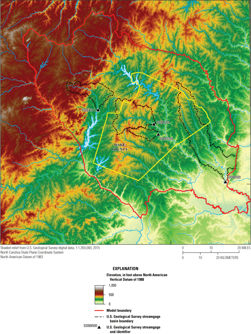
Land-surface elevation and U.S. Geological Survey streamgage drainage basins within the model area, Wake County, North Carolina. Streamgage information from U.S. Geological Survey (2022).
Wake County is located predominantly within the Piedmont physiographic province (Fenneman, 1938) (fig. 1). A small section of southeastern Wake County (about 35 mi2) extends across the fall line into the Coastal Plain physiographic province. The county is characterized by a hill and valley topography with rounded slopes, where land elevation ranges from 137 to 558 feet (ft) above the North American Vertical Datum of 1988 (NAVD 88) (fig. 2). Wake County has a humid subtropical climate with daily-mean air temperatures ranging from 47 to 71 degrees Fahrenheit (°F) and annual precipitation of about 46 inches (National Oceanic and Atmospheric Administration, 2020). Based on 2019 data, 42 percent of land cover in Wake County is classified as developed, while only 23.3 percent of the entire model area is classified as developed (fig. 3; table 1) (Dewitz and U.S. Geological Survey, 2021). Other predominant land cover classes in the county study area include forest (36 percent), pasture/hay (6.5 percent), cultivated crops (4.6 percent), and wetlands (4.3 percent).
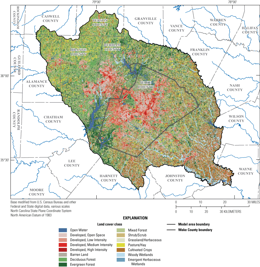
National Land Cover Database 2019 land cover data for the model area, Wake County, North Carolina.
Table 1.
Land cover classes and percentages for the study and model areas, Wake County, North Carolina.[The 2019 land cover information was obtained from Dewitz and U.S. Geological Survey (2021). mi2, square mile]
Wake County lies within the Neuse River and Cape Fear River Basins (fig. 1). More than 80 percent of the county is within the Neuse River Basin with major streams that include Crabtree Creek, Walnut Creek, and Middle Creek. Several Wake County lakes are within the Neuse River Basin including Falls Lake, which serves as one of the primary sources of water supply for the City of Raleigh, as well as smaller lakes such as Lake Crabtree, Lake Wheeler, and Lake Benson. The Cape Fear River Basin in the southwestern corner of the county includes B. Everett Jordan Lake and Shearon Harris Reservoir. The USGS operates a streamgage network within both basins that includes four continuous streamgage sites used for hydrologic analysis in the model area (figs. 1 and 2).
Compilation of USGS 5-year national water-use estimates for the years 1995–2015 show that total annual surface water and groundwater use in Wake County ranged from about 56.3 to 88.9 Mgal/d (fig. 4A) (Solley and others, 1998; Hutson and others, 2004; Kenny and others, 2009; Maupin and others, 2014; Dieter and Maupin, 2017). Surface water sources provided about 40.4 Mgal/d in 1995 and about 72.8 Mgal/d in 2005, throughout the county. Total annual groundwater withdrawals in Wake County ranged from about 15 Mgal/d in 2000 to about 19.8 Mgal/d in 2010, composing about 20–30 percent of all water use in the county (fig. 4A). Groundwater withdrawals were highest for domestic self-supply followed by public supply, which together were increasing through 2010 and then remained nearly constant through 2015 (fig. 4B). The USGS data include an estimated withdrawal coefficient of per capita use from domestic wells in Wake County of 70 gallons per day (Dieter and Maupin, 2017). Previous studies have assumed that most groundwater withdrawn from domestic wells is returned to the aquifer if the residence has an onsite wastewater (septic) system, given some consumptive loss to evapotranspiration (Daniel and Harned, 1998; Horn and others, 2008; Goode and Senior, 2020). There does remain uncertainty regarding the fate of septic discharge through the shallow subsurface to recharge deeper bedrock.
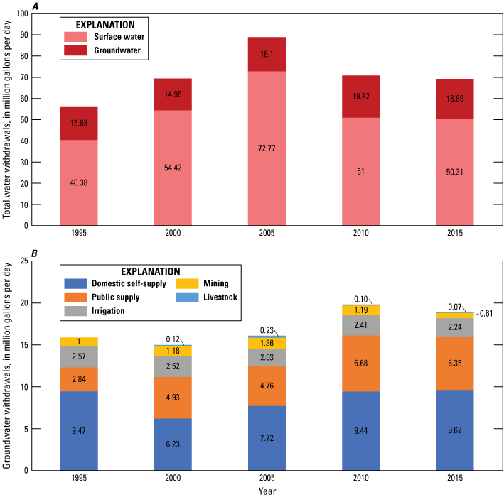
Water-use estimates for 1995–2015, by (A) total water withdrawals and (B) groundwater withdrawals, Wake County, North Carolina (from Solley and others, 1998; Hutson and others, 2004; Kenny and others, 2009; Maupin and others, 2014; Dieter and Maupin, 2017).
Hydrogeologic Setting and Conceptual Model of Flow System
The Wake County study area is located at the eastern edge of the Piedmont physiographic province and is underlain by regional geologic formations that generally trend northeast to southwest (Horton and Zullo, 1991). The rock types include stratified sedimentary basin rock, crystalline rock with varying degrees of metamorphism, and younger unconsolidated coastal plain sediments that overlie fractured bedrock eastward toward the Piedmont and Coastal Plain boundary (figs. 1 and 5). Lithologic units defined across North Carolina were compiled into distinct hydrogeologic units for the Piedmont and Blue Ridge physiographic provinces by Daniel (1989) with an associated map by Daniel and Payne (1990) (fig. 5). Hydrogeologic unit classification is associated with the water-bearing potential of the rock types, where primary and secondary porosity is related to composition, texture, and weathering rates of rock. The study area is underlain by massive and foliated crystalline rocks and sedimentary basin rocks. A large part of Wake County primarily is composed of closely folded metasedimentary and metavolcanic rocks, including phyllite, graphite-bearing mica schists, biotite-hornblende gneiss, quartzite, and amphibolite (Parker, 1979). Coarse-grained granitic plutons are found within the study area (fig. 5, IFI unit), including one of the largest in the Eastern United States that stretches across eastern Wake County (Farrar, 1985). Unmetamorphosed igneous intrusive rocks are present as diabase dikes and granitic veins. The Durham subbasin in the Triassic Deep River Basin is located on the western edge of Wake County (fig. 5, TRI unit) and is composed of stratified fanglomerate and red silty sandstone to mudstone sourced from the erosion of uplifted crystalline rocks after Mesozoic rift faulting (Parker, 1979; Bain and Brown, 1981). Triassic sedimentary rocks are bounded to the east by the north-northeast trending Jonesboro Fault (Campbell and Kimball, 1923), separating the basin from the metaigneous and metavolcanic rock types to the east (May and Thomas, 1968; Parker, 1979) (fig. 5). Onlapping coastal plain sediments of gray to white sand with interbedded clay lenses lie nonconformably atop metamorphic and igneous rock in the southeastern part of the county (May and Thomas, 1968).
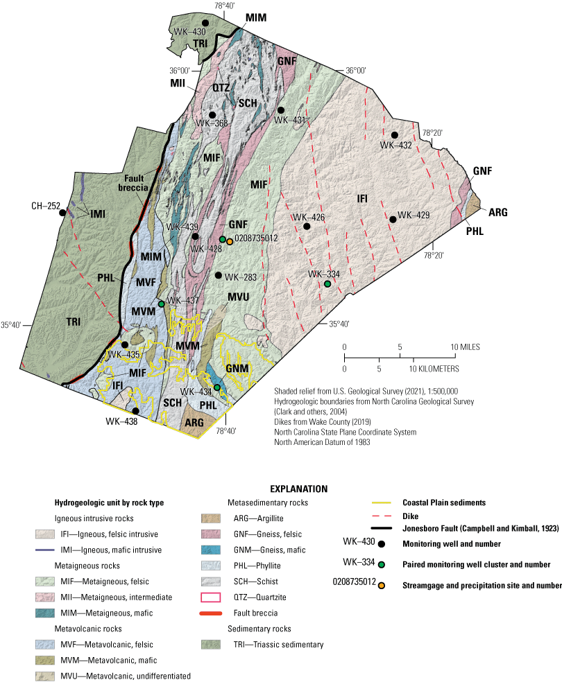
Hydrogeologic units, Jonesboro Fault, dikes, and monitoring well network in Wake County, North Carolina. Figure modified from Antolino and Gurley (2022, fig. 4); hydrogeologic unit map information based on May and Thomas (1968), Parker (1979), Daniel (1989), Daniel and Payne (1990), and Clark and others (2004) and available in Antolino (2022).
A conceptual model of groundwater flow within the Piedmont of North Carolina was described by LeGrand (1967), Heath (1980, 1984), and LeGrand and Nelson (2004) and was adapted for this study. Groundwater flow generally follows the hydraulic gradient, moving from topographic highs to lows and forming local flow systems within small drainage basins that exhibit some topographic relief. Water-table levels are typically highest near the highest points of land-surface altitude near drainage basin boundaries, such as hills and ridges, whereas the lowest water-levels occur near streams. Recharge to the hydrogeologic units originates from precipitation that infiltrates, through the soil and root zone, down to the water table, continuously moving downgradient toward streams until discharge. Some groundwater may be lost to evapotranspiration as it flows near the surface, before being discharged as seepage to gaining streams. In areas with minimal topographic relief, these local flow systems are less distinct, where slower moving intermediate and regional groundwater flow can be predominant (Tóth, 1963).
Groundwater occurs in two primary layers of the flow system: shallow regolith and deeper fractured bedrock. The regolith consists of soil, local alluvium, residuum (sandy clay from the weathering of feldspar and mica minerals), and in situ weathered bedrock, also known as saprolite. Saprolite may retain some relict structural features of the parent bedrock, such as foliation and filled fractures. Regolith thickness varies geographically and is influenced by factors such as parent rock, topographic setting, and geologic history (LeGrand and Nelson, 2004). In the Piedmont, regolith typically is thinnest near streams and thicker on slopes, with variable thickness along hilltops and ridges. The lower regolith may contain a transition zone from saprolite to bedrock as weathering decreases with depth, often less gradually and more abruptly in highly foliated parent rock (Harned and Daniel, 1992). Where present, the transition zone has been described as more permeable than the upper regolith and soil layers, a condition likely occurring because intermediate weathering has not progressed to the formation of clay (Stewart, 1962; Nutter and Otton, 1969; Daniel and Harned, 1998). Groundwater within the regolith layer flows both vertically and laterally through intergranular spaces before discharging to nearby streams. Lateral flow primarily is driven by the rolling topography of the landscape that creates short flow paths in local flow systems. This lateral flow can be enhanced by the presence of clay horizons and relict structural features in the regolith, which impede some vertical flow. At the base of the regolith, the partially weathered material of a transition zone can provide increased permeability and act as a conduit for lateral groundwater movement. Some groundwater in the transition zone flows downward into the underlying bedrock, moving through a network of connected permeable fractures before discharging upwards into downgradient streams (Heath, 1984; Daniel and Harned, 1998).
Groundwater flow in the fractured bedrock depends on the hydraulic connection with the base of the regolith in recharge and discharge areas, as well as the connectivity of fractures. Most groundwater storage occurs within the overlying regolith, as the fractured bedrock has little to no storage capacity because of its relatively impermeable rock matrix (Heath, 1980). In the Piedmont, fracture features primarily form by fault displacement, shear (typically occurring in zones), and stress relief that can result in orthogonal vertical fracture sets and nearly horizontal sets, depending on the rock fabric. The various mechanisms of fracture development and nonuniform distribution of fracture networks contribute to the heterogeneity in aquifer properties of the bedrock and provide preferential flow paths that can cause groundwater flow to deviate from the typical flow paths observed in more homogeneous, porous media. These flow pathways within the connected fracture networks are largely part of local flow systems, yet some pathways may be part of broader flow systems that cross small drainage basin boundaries. Most of the groundwater flow in the Piedmont is constrained by increasing lithostatic pressure at depth, limiting most groundwater circulation primarily to the upper 800 ft of bedrock, with the most productive fractures within 350 ft from the top of bedrock (Daniel, 1989; Daniel and others, 1997; LeGrand and Nelson, 2004).
Previous Investigations
Previous hydrogeologic work in the study area was summarized in Antolino and Gurley (2022), which is adapted for parts of this section. The summary by Antolino and Gurley included a detailed groundwater study in Wake County by May and Thomas (1968), who identified correlations between well yields, rock types, and topographical locations. Welby and Wilson (1982) examined the connection between geological factors and well yields, noting that an increase in the proportion of impervious surface from future development may decrease groundwater recharge and result in local water-supply problems. A 2003 groundwater study by CDM (2003) estimated water budgets across major drainage basins in the study area and highlighted the need for information that would help to quantify local effects of increased development on groundwater sources. Chapman and others (2011) investigated declining groundwater levels in northern Wake County following reports of dry domestic wells in 2005 and 2007. Findings from the study revealed substantial aquifer storage loss from increased withdrawals for domestic irrigation and CWS supply, as well as identified groundwater-level data trends that could be correlated with local dominant geological structural features.
Antolino and Gurley (2022) compiled and analyzed well depth, casing depth, and reported well yield for well sites in Wake County. They collected geophysical logs and determined the orientation of geologic structure in 15 bedrock wells in different hydrogeologic units in the county. They used the Soil-Water-Balance (SWB) model (Westenbroek and others, 2010, 2018) to calculate the spatial and temporal variation of water budget components in the greater Wake County area from 1981 to 2019, including net infiltration below the root zone (or potential groundwater recharge). Estimates of mean-annual recharge determined with the SWB model ranged from 5.6 to 9.2 inches across the gaged basins. These estimates of potential recharge were compared with stream base flows derived from hydrograph separation for drainage basins with USGS streamgages, within the model area. The comparison showed that the model produced recharge values generally within 2 inches of base flow estimates for most basins. The SWB model also provided estimates of daily evaporation rates that ranged from 0.04 to 0.13 inches per day and daily runoff rates that ranged from 0.02 to 0.05 inches across the gaged basins. The monthly mean-daily rates for the major inputs and outputs determined for the SWB model area by Antolino (2022) are shown in figure 6.
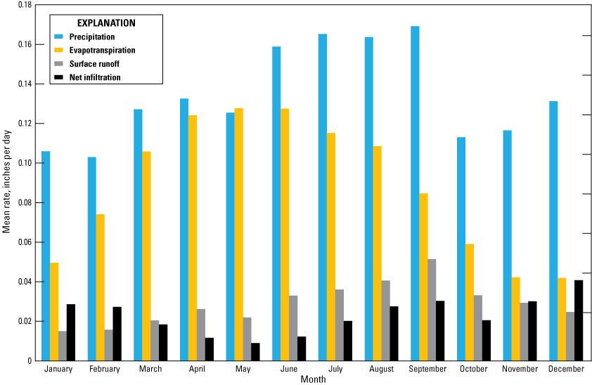
Mean daily rates for each month for the major components of the Soil-Water-Balance (SWB) model for the total model area for the greater Wake County area from 2000 to 2019, North Carolina (Antolino, 2022).
Chapman and others (2005, 2007) studied the fractured-rock hydrogeology at the Lake Wheeler Road Field Laboratory, situated at a North Carolina State University research farm, including groundwater-quality analysis. Analytical results indicated that groundwater nitrate concentrations were highest in the shallower regolith and transition wells, whereas concentrations of fluoride, calcium, sulfate, molybdenum, uranium, radon, and arsenic were highest in the deeper bedrock wells. Using various groundwater age-dating tracers, the study identified longer flow paths with greater residence times in groundwater discharge areas and estimated that modern groundwater in the regolith is younger than deeper groundwater in the bedrock by several decades. McSwain and others (2013) conducted a study in the vicinity of the Neuse River Resource Recovery Facility (located near WK–334, fig. 5) to examine potential effects of historical use of biosolids applications in nearby fields on water quality in the subsurface and in the Neuse River. High nitrate levels were found in both the shallow regolith and deeper fractured bedrock layers of the groundwater system, highlighting the direct influence of land-use activities on groundwater in the area. The study also documented substantial nitrate flux from groundwater at the site to the adjacent Neuse River, indicating important interactions between the local groundwater and surface water systems.
As part of the Appalachian Valleys and Piedmont Regional Aquifer-System Analysis study, Daniel and others (1997) developed an interpretive steady-state numerical model for the Indian Creek Basin in the southwestern North Carolina Piedmont to understand the relation between groundwater-flow components and streams within the fractured crystalline bedrock groundwater system. The multilayered model was developed assuming an equivalent porous media for bulk fractured-rock aquifer properties and provided insights into the regional groundwater system. Most of the simulated groundwater flow was along short flow paths within the shallowest layers to streams. The model simulation showed that groundwater flow decreased with depth by two orders of magnitude between the top and bottom model layers, about 700 ft below land surface. Particle tracking simulated movement of groundwater flow by using numerous particles distributed across the top model layer to indicate groundwater travel times through regolith to the stream that ranged from 10 to 20 years at horizontal distances less than 1,000 and 2,000 ft, respectively. Travel times within the bedrock increased with depth. For horizontal distances between 2,000 and 5,000 ft, flow paths in the upper 100 ft of bedrock had travel times that ranged from 20 to 90 years, whereas the few flow paths in the lower bedrock (675 ft below land surface) had travel times that exceeded 300 years.
Development-related future water demand across North Carolina, including Wake County, was projected from 2012 to 2065 by Sanchez and others (2018, 2020a). Water demand was quantified as the sum of public supply, industrial self-supply, and domestic self-supply uses from both surface water and groundwater sources obtained from the 2010 county-level USGS national water-use estimates (Maupin and others, 2014). To obtain locally relevant representation of the spatial distribution of water use, county-level water-use estimates were spatially disaggregated to census tract units by using a population weighted procedure. This modeling framework evaluated the joint effects of social and environmental conditions on urban water demand under different future climate scenarios and urban growth. To evaluate the effects of growing populations, expanding development, and temperature change, the modeling framework assumed that all other predictors remained at 2010 conditions. Probabilistic model projections from Sanchez and others (2020a, 2020b) indicated increasing trends for future development-related water demand across Wake County census tracts, with upper limit estimates showing an increase of 78 percent to more than 500 percent by 2065 (relative to 2010 estimates). Within Wake County, the forecast percentage change was highest in southeast and north Raleigh and urban peripheries of Morrisville, Cary, and Apex (fig. 1), which are all areas expected to experience rapid low-density development in coming decades (Terando and others, 2014; Sanchez and others, 2020a).
Methods
This section provides a discussion of the methods used to compile groundwater-level datasets and to determine aquifer hydraulic properties. The methods for collecting groundwater, rainfall, and surface water samples for laboratory analyses also are presented. The approaches used for developing the groundwater-flow model and model forecast scenarios are discussed. Documentation of the input and output datasets for the groundwater model developed for Wake County is archived as a USGS data release by Antolino (2025).
Well-Construction and Groundwater-Level Data
Datasets on well construction and groundwater levels were compiled for wells located throughout the model area. This study primarily relied on existing well-construction and groundwater-level data that were retrieved from the USGS National Water Information System (NWIS) database (U.S. Geological Survey, 2022) and the North Carolina Department of Environmental Quality Division of Water Resources (NCDEQ DWR) monitoring well database (North Carolina Department of Environmental Quality, Division of Water Resources, 2022). These well-construction and groundwater-level data were primarily used for groundwater-flow model development and calibration. Information on well-casing depths was retrieved from the USGS NWIS database (U.S. Geological Survey, 2022) for more than 2,800 wells located in the model area and used to estimate the top of the bedrock layer in the model simulation. Both historical and recent groundwater levels that were available for the period 1941–2021 from the USGS NWIS and NCDEQ DWR databases were used for calibrating the groundwater-flow model.
Discrete water-level measurements were made using a chalked graduated steel tape or electric water-level tape, consistent with techniques described in Cunningham and Schalk (2011), and yielded data having an accuracy within 0.01 ft. The water-level tapes are routinely checked for quality assurance by USGS field staff and the USGS Hydrologic Instrumentation Facility based on USGS policy and techniques (U.S. Geological Survey, 2015b; Fulford and Clayton, 2015). Water-level measurements were made from a measuring point established at both discrete and continuous sites. In instances where obstructions within the well (such as submersible pumps) prevented the use of established measurement methods, sonic water-level meters were utilized, providing a measurement accuracy within 0.1 ft. Prior to sonic water-level measurements, air temperature within the well was recorded using a thermistor to configure the meter to account for variations in sound velocity between wells (Ravensgate Corporation, 2025).
For this study, two synoptic water-level surveys were completed in and adjacent to Wake County to provide spatial snapshots of the groundwater system across different seasons. This approach provides information on the influence of seasonal variations on groundwater levels. The first water-level survey included discrete water-level measurements for 102 domestic and monitoring wells during November and December 2020, when evapotranspiration rates are typically lower (fig. 6). The second water-level survey included measurements for 100 of mostly the same domestic and monitoring wells during June and July 2021, when evapotranspiration rates are typically highest (fig. 6).
Continuous groundwater-level measurements also were collected to improve spatial and temporal records of groundwater-level data for Wake County and to serve as observations for the groundwater model. As described by Antolino and Gurley (2022), a network of 17 USGS wells was established in 2019 to monitor continuous groundwater levels in the fractured-rock groundwater system for Wake County. The USGS monitoring-network wells (4 regolith and 13 bedrock), as well as the additional two NCDEQ DWR wells used for project data collection, are shown in figure 5 and summarized in table 2. The NCDEQ DWR operated and maintained continuous data-collection activities for two well sites in the study area, 353320078483101 (WK–438) and 354703078424401 (WK–439), which correspond to NCDEQ DWR sites N41G3 and K40M1, respectively (table 2). Water-level data for sites WK–438 (N41G3) and WK–439 (K40M1) are available through the NCDEQ DWR monitoring well database (North Carolina Department of Environmental Quality, Division of Water Resources, 2022).
Table 2.
Information for monitoring well network sites in the study area, Wake County, North Carolina.[Well information from Antolino and Gurley (2022) and U.S. Geological Survey (2022). USGS, U.S. Geological Survey; CH, Chatham County well prefix; WK, Wake County well prefix; ft, foot; NAVD 88, North American Vertical Datum of 1988; in., inch; gal/min, gallon per minute; --, no data or not applicable; TRI, Triassic sedimentary; MIF, metaigneous, felsic; IFI, igneous, felsic intrusive; SCH, schist; GNM, gneiss, mafic; MVF, metavolcanic, felsic; GNF, gneiss, felsic; NCDEQ DWR, North Carolina Department of Environmental Quality Division of Water Resources]
Lithologic descriptions for the hydrogeologic unit codes are summarized in Daniel (1989) and Antolino and Gurley (2022).
This USGS site corresponds to NCDEQ DWR monitoring well site N41G3 for Fuquay-Varina (North Carolina Department of Environmental Quality, Division of Water Resources, 2022).
This USGS site corresponds to NCDEQ DWR monitoring well site K40M1 for Powell Drive (North Carolina Department of Environmental Quality, Division of Water Resources, 2022).
Continuous water levels were measured at 15-minute intervals in each well by using a vented submersible pressure transducer (Cunningham and Schalk, 2011). USGS data are recorded using a data-collection platform and are relayed hourly through satellite transmission for upload to the USGS NWIS database (U.S. Geological Survey, 2022). The water-level monitoring sites are inspected on a routine basis, and the recorded water-level data are field verified with discrete steel-tape measurements approximately every 6 to 8 weeks.
Aquifer Testing
Slug tests and borehole-flowmeter logging were conducted in selected monitoring wells to estimate bulk hydraulic properties of the fractured-rock groundwater system. Measurement and analysis of groundwater-level response to induced stress, along with the identification of vertical flow zones within the regolith and bedrock wells, provided data used to estimate values of transmissivity (T) and horizontal hydraulic conductivity (Kh) within the fractured-rock groundwater system.
Slug Tests
Slug tests were performed during 2020 and 2021 in the 17 USGS wells within the monitoring well network (table 2; fig. 5) to estimate Kh within the local fractured-rock groundwater system. A detailed discussion of methods used to conduct the slug tests and analyze compiled datasets is provided by Gonthier and Antolino (2023). The slug-test data were analyzed using concepts from the Bouwer and Rice (1976) method. Assumptions within this analytical method include that the aquifer (1) can be represented as an equivalent porous medium, (2) is isotropic with no directional variation in hydraulic properties within the zone being tested, (3) is under unconfined conditions, and (4) has conditions where the effects of elastic storage can be neglected. The method may also be applied to confined and stratified aquifers in cases where the top of the well screen or open section is located at a distance below the upper confining or semiconfining unit (Bouwer, 1989). The slug tests were conducted within the fractured-rock groundwater system, assuming it to be homogeneous for the purpose of the analysis, despite its heterogeneity, asymmetric hydraulic properties, and potential for semiconfined conditions in some areas. Shapiro and Hsieh (1998) investigated the accuracy of using slug-test methods that assume homogeneous formation properties in fractured rock. They found that discrepancies in water-level response were attributed more to nonradial flow than to heterogeneity in hydraulic properties and that such slug tests can provide estimates of T within an order of magnitude.
Values of T were computed as the product of Kh and the tested aquifer thickness. For the regolith wells, the tested aquifer thickness was defined as the vertical distance from the measured water table to the top of bedrock. For the regolith T estimates, it is assumed that the screened interval used in the slug test is representative of the entire saturated thickness of the regolith layer at that well location. In the bedrock wells, the tested aquifer thickness was defined as the vertical distance from the bottom of well casing to the measured borehole depth. The bedrock T estimates only apply to the depth interval of the open hole within the bedrock well.
Borehole-Flowmeter Logging
Flow logging and analysis also were used to estimate T and Kh of the fractured-rock groundwater system. Borehole-flowmeter logging was used to measure vertical groundwater flow within the open interval of the borehole between transmissive fracture zones within bedrock wells. Raw vertical flow measurement data collected for wells in this study are available from the USGS GeoLog Locator tool (U.S. Geological Survey, 2024). Geophysical logging by Antolino and Gurley (2022) identified fracture zones within each of the bedrock wells; the fracture zones consisted of primary water-bearing fractures with measurable flow, secondary open fractures without evidence of iron or biological staining or measurable flow, and sealed fractures. The flow with respect to depth in the well was interpreted using vertical flow measurements under both ambient and stressed conditions. Vertical flow, measured under ambient conditions, indicates hydraulic head differences between transmissive fracture zones that intersect the well borehole. Vertical flow observed under stressed or pumped conditions can help identify transmissive fracture zones that may show similar hydraulic heads under ambient conditions, and therefore no detectable flow between the zones can be measured. Pumping disrupts the state of equilibrium, leading to detectable vertical flow from zones that contribute water to or receive water from the borehole. The interpreted flow was analyzed using the Flow-Log Analysis of Single Holes (FLASH) program (Day-Lewis and others, 2011; Barbosa and others, 2020).
Vertical flow within a particular borehole was measured with a Mount Sopris HFP-2293 heat-pulse flowmeter (Mount Sopris Instrument Co., Inc., Denver, Colorado), first under ambient (natural flow) conditions and then under stressed (pumping) conditions using a portable submersible pump. Borehole-flowmeter measurements were taken at multiple depths within a particular well, between suspected transmissive fracture zones identified by Antolino and Gurley (2022). Flow was measured multiple times at each selected depth. Values near the lower resolution of the heat-pulse flowmeter (0.01 gallon per minute [gal/min]) mostly were considered noise and interpreted as no flow. Water-level measurements were collected during both ambient and stressed conditions, and pump discharge flow rate was manually measured during the stressed phase of the flow survey. Borehole-flowmeter measurements during pumping conditions were calibrated to expected flow within the well, which is the combination of pump-flow rate and the change in storage resulting from a rate of change in water level during the measurement. Ideally, a quasi-steady flow condition would be reached where water level and pump rate had little to no change during the pumping phase. For instances where pumping rates changed when quasi-equilibrium conditions could not be achieved, measurements were normalized to the pump-flow rate.
The interpreted flows were input to the FLASH program (Day-Lewis and others, 2011) to estimate T values. Flows were simulated using the radial flow equation from Thiem (1906) that was modified for multiple flow features under ambient and stressed conditions (Day-Lewis and others, 2011). This approach attempts to address the limitations of the radial flow assumption by providing a more realistic representation of the discrete and localized flow in fractured-rock systems. Input parameters used to simulate observed flows include hydraulic head difference, fracture zone T, total T of the open interval in the well, and the radius of influence. The solver method within FLASH does not specifically estimate the T or the radius of influence, but rather estimates the total T divided by the natural log of the ratio of the radius of influence to the well radius. To provide the solver method with a starting estimate for the radius of influence, T was estimated from specific capacity by using a numerical method from Bradbury and Rothschild (1985). Specific capacity, in gallons per minute per foot, was determined as the ratio of the effective pumping rate to the observed drawdown in each well.
Water-Quality Sampling
The primary focus for collecting water-quality samples for laboratory analysis was to better understand the geochemical and hydrologic conditions of the groundwater-flow system. Groundwater samples were collected during November and December 2019 from all 17 USGS wells in the monitoring network and WK–439 (NCDEQ DWR well K40M1), with the exception of WK–438 (NCDEQ DWR well N41G3), for a total of 14 bedrock wells and 4 regolith wells (fig. 5; table 2). Water temperature, specific conductance, pH, and dissolved oxygen (DO) were monitored in the field while the well was being purged of at least one well volume of stagnant water. Water-quality multiparameter sondes were calibrated each sampling day and used to monitor field parameters prior to sampling. Groundwater samples were collected after stabilization of these physical and chemical properties (U.S. Geological Survey, 2006). Wells were purged at pump rates ranging from 0.25 to 4 gal/min depending on well yield and water-level response. Submersible pumps were used to purge and collect samples at all wells except WK–436, which was sampled using a double-ball bailer after removing three well volumes of water. Field equipment was cleaned between sampling sites by following established methods (U.S. Geological Survey, 2006). Groundwater samples primarily were collected for analysis of stable isotopes of water, dissolved gases, and age-dating tracers.
Samples of surface water and precipitation also were collected for analysis of stable isotopes of water. These samples were collected at USGS monitoring station 0208735012 (Rocky Branch below Pullen Road at Raleigh, N.C.), which has a continuous streamgage site and colocated rain gage (fig. 5) (U.S. Geological Survey, 2022). Eight surface water grab samples from the midpoint of the stream were intermittently collected from Rocky Branch between April 2021 and January 2022. A total of 48 precipitation samples were collected about every 2–4 weeks from December 2019 to April 2022 by using a commercial version (Palmex Ltd., Zagreb, Croatia) of the rain collector described in Gröning and others (2012). The rain collector was installed next to the Rocky Branch rain gage to relate the accumulated rainfall amount in the composite precipitation sample. The rain collector is designed to thermally isolate the sample from sunlight and limit exposure to the atmosphere to minimize fractionation effects from evaporation. Precipitation samples that were collected and exposed to freezing conditions, that may have potentially contributed to potential isotopic fractionation effects, were excluded from analysis.
All water-quality samples were collected and processed using techniques described in the “National Field Manual for the Collection of Water-Quality Data” (U.S. Geological Survey, 2006). Analytical results for all water-quality samples collected during the study are available from the USGS NWIS database (U.S. Geological Survey, 2022).
Stable Isotopes of Water
Groundwater, surface water, and precipitation samples were shipped to the USGS Reston Stable Isotope Laboratory (RSIL) in Reston, Virginia, and analyzed for stable isotopes of water (deuterium/hydrogen-1 [2H/1H] and oxygen-18/oxygen-16 [18O/16O]) by mass spectrometry following methods outlined in Révész and Coplen (2008a, b). The ratios of the stable isotopes of a sample are reported using the delta (δ) notation in units of parts per thousand (denoted as per mil or ‰) relative to a known standard of Vienna Standard Mean Ocean Water according to the following equation,
where Rsample and Rstandard are the ratios of the heavy to light isotope (2H/1H or 18O/16O) in the sample and standard, respectively. The reported results have an analytical uncertainty of plus or minus (±) 2.0 per mil for δ2H and ±0.2 per mil for δ18O.Variations in δ2H and δ18O isotopic compositions of water reflect physicochemical processes within the hydrologic cycle. As water evaporates, there is a preferential release of the lighter isotopes (1H and 16O) to the atmosphere leaving behind water that becomes more enriched in the heavier isotopes (2H and 18O). Using samples collected from a worldwide network of stations, Craig (1961) showed that there is a linear relation between δ2H and δ18O in precipitation samples that have not undergone excessive evaporation. This relation, known as the Global Meteoric Water Line (GMWL), is expressed as a linear equation:
When local precipitation values of δ2H are plotted against δ18O, a Local Meteoric Water Line (LMWL) can be determined for the associated regional area. The stable isotopic composition of water samples can be compared to these meteoric water lines to infer the origin of the water. Samples that have been influenced by evaporation will typically deviate from these meteoric water lines along a line of shallower slope due to evaporation fractionating δ18O more strongly than δ2H. As a result, evaporated waters generally will plot below the meteoric water line.The regression line for δ2H and δ18O values in water samples that have undergone evaporation is known as the evaporation line, which typically has a slope that is less than that of the LMWL. The slope of the evaporation line reflects the relative fractionation of δ18O and δ2H during evaporation, with shallower slopes indicating greater evaporative enrichment. The intersection of the evaporation line with the LMWL indicates the isotopic composition of the water before evaporation. This intercept with the evaporation line is influenced by factors such as temperature and humidity, providing insight into the initial conditions of the original source, which is often local precipitation (Kendall and Caldwell, 1998).
In addition to δ2H and δ18O values, deuterium excess was calculated for each sample as the difference between the measured δ2H value and the value predicted by the GMWL. Deuterium excess provides a secondary isotopic parameter that can be used to assess the effects of humidity and atmospheric processes on water sources (Dansgaard, 1964; Kendall and Caldwell, 1998). Higher deuterium-excess values generally reflect moisture derived from drier or cooler source regions with less evaporation, whereas lower values indicate stronger evaporative influence or moisture from humid sources.
Dissolved Gases and Age-Dating Tracers
Groundwater samples collected from bedrock wells were analyzed for dissolved gases and age-dating tracers. The dissolved gases measured in samples included methane, carbon dioxide, nitrogen, oxygen, and argon. The age-dating tracers included analysis of chlorofluorocarbons (CFCs), tritium (3H), helium (He) isotopes, and neon. Three CFCs were analyzed, including trichlorofluoromethane (CFC-11), dichlorodifluoromethane (CFC-12), and trichlorotrifluoroethane (CFC-113).
The groundwater samples collected for analysis of dissolved gases were used to provide information on hydrological processes and conditions in the groundwater-flow system. DO and methane concentrations can provide information about the oxidation-reduction (redox) environment of the groundwater (Freeze and Cherry, 1979). Dissolved nitrogen and argon can provide information to help reconstruct the temperature when the recharge occurred (Heaton and Vogel, 1981), which is important when using dissolved gases in the age dating of groundwater, as gas solubility is dependent on temperature (Weiss, 1970). By measuring the concentrations of dissolved nitrogen and argon in a sample, any excess air above expected atmospheric equilibrium concentrations can be identified and corrected for to refine the age dating (Heaton and Vogel, 1981). Excess air occurs when small air bubbles are entrapped during infiltration of precipitation through the unsaturated zone with rapid rises in the water table, especially in fine-grained sediments (Heaton and Vogel, 1981; Klump and others, 2007). The dissolved-gas samples were collected in accordance with the USGS Reston Groundwater Dating Laboratory (RGDL) methods by bottom filling two 125-milliliter glass septum bottles while fully submerged in a 2-liter (L) beaker filled with raw groundwater to avoid atmospheric contamination (Nelms and Harlow, 2003). Dissolved-gas samples were kept chilled during storage at or below the water temperature at time of collection and shipped to the USGS RGDL in Reston, Virginia, for analysis by gas chromatography (U.S. Geological Survey, 2023a).
Apparent ages of groundwater can be determined by measuring the concentrations of CFC-11, CFC-12, and CFC-113 in groundwater samples. The apparent age of groundwater is defined as the time since water in the sample was last in contact with the atmosphere. The use of an environmental tracer to determine the apparent groundwater age involves relating a measured tracer concentration within a sample to known historical concentrations, accounting for changes in concentration because of tracer decay or production (Plummer and Busenberg, 2000). When sampled for together, each of the three CFCs provides an independent estimate to determine groundwater apparent age with increasing reliability if multiple CFCs converge to support a similar age. Age dating of groundwater with CFCs is ideal under aerobic shallow water-table conditions outside of developed areas, as age dating with CFCs is sensitive to anerobic microbial degradation, groundwater-flow path mixing, and local contaminant sources (Plummer and Busenberg, 2000).
Groundwater samples for CFC analyses were collected in accordance with the USGS RGDL methods by bottom filling four 125-milliliter glass bottles while fully submerged in a 2-L beaker that overflowed with pumped groundwater during the collection process. Sample bottles were filled from a refrigerator-grade copper tube discharge line connected to the submersible pump to avoid possible CFC contamination from other sample line materials. The sample bottles were capped underwater with an aluminum-foil-lined screw-on cap. The CFC samples were analyzed at the USGS RGDL using gas chromatography-mass spectrometry (U.S. Geological Survey, 2023b).
Tritium (3H) is naturally produced from the interaction of nitrogen, oxygen, and argon with cosmic radiation within the upper atmosphere (Cook and Herczeg, 2000). In the 1950s and 1960s, thermonuclear testing released a substantial amount of 3H into the atmosphere, thereby creating an event marker within the hydrologic cycle. The radioactive decay of 3H (half-life of 12.3 years) to helium-3 (3He) forms the basis of the 3H/3He age-dating method to estimate groundwater residence times (Clark and Fritz, 1997). Any 3He sourced from the radiogenic decay of uranium and thorium minerals or from deeper mantle gas sources can be differentiated using the concentrations of helium-4 (4He) (Craig and others, 1978; Plummer and others, 2000). 3He/4He ratios less than 1 generally reflect radiogenic helium and higher ratios generally reflect mantle-derived helium (Ballentine and Burnard, 2002). Any 3He sourced from excess air in a sample can be determined by measuring the dissolved neon concentration, as it is only derived from the atmosphere (Solomon and Cook, 2000). The apparent age is calculated by reconstructing the original 3H concentration in rainfall by using the helium-isotope mass balance with measured 3H and tritiogenic (helium from the decay of tritium) 3He (Schlosser and others, 1988, 1989).
Groundwater samples for analysis of 3H were collected in accordance with the USGS RGDL methods by bottom filling a 1-L high-density polyethylene bottle with unfiltered groundwater. Groundwater samples for analysis of 3He and neon gas were collected in two 3/8-inch-inner-diameter copper tubes with a nylon sample line. Groundwater was flushed through the tubing to carefully dislodge air bubbles before flow was restricted with a back-pressure valve. Clamps on each end of the copper tubes were then tightened to isolate the sample for subsequent analysis. Samples were shipped to the USGS RSIL for analysis by the helium ingrowth technique with a minimum reporting limit of ±0.01 tritium units (TU) using methods from Clarke and others (1976), Jean-Baptiste and others (1992), Beyerle and others (2000), Lucas and Unterweger (2000), and Papp and others (2012). The sample concentrations were entered into the USGS Dissolved Gas Modeling and Environmental Tracer Analysis (DGMETA) program (Jurgens and others, 2020) to distinguish tritiogenic and terrigenic (helium from radioactive decay of crustal uranium and thorium) sources of 3He.
Analyzing age-dating tracer datasets (CFC and 3H/3He) together helps to account for uncertainties in the individual tracer methods. The USGS TracerLPM program (Jurgens and others, 2012) provides a comprehensive interpretive technique using multiple tracers in an error-weighted inverse modeling approach to determine groundwater ages. TracerLPM uses lumped parameter models (LPMs) in the program to model transport with simplified aquifer geometry and flow configurations using five LPMs, including models that account for dispersion and mixing.
Groundwater-Flow Model Development
Existing and new hydrologic data were integrated to develop a groundwater-flow model to simulate historical groundwater conditions and to forecast future groundwater availability in the Wake County study area. The model was constructed using the USGS modular three-dimensional finite-difference groundwater-flow model code MODFLOW–2005 (Harbaugh, 2005), specifically the Newton formulation version, MODFLOW–NWT (Niswonger and others, 2011). MODFLOW simulates an aquifer as porous media, meaning that water is assumed to move through pore space between granular materials. However, in the study area, groundwater within the fractured bedrock flows through fracture networks of discrete transmissive conduits within a relatively impermeable rock matrix. The application of MODFLOW for this study assumes that flow through the fractured-rock groundwater system is at the scale of miles and can be represented on a regional scale as a single-continuum porous-equivalent medium. This modeling approach using bulk effective aquifer properties has previously been used with discrete conduit groundwater flow in other groundwater systems (Tiedeman and others, 1997; McCoy and others, 2015; Kuniansky, 2016; Harte, 2021).
Model Geometry and Discretization
The model grid was oriented northwest to southeast (at 315 degrees) to align with the predominant direction of streamflow in the modeled area (fig. 7). The MODFLOW model grid consists of 1,085 rows, extending 102.7 miles, and 631 columns, extending 59.7 miles, yielding a total area of about 6,131 mi2. However, the active area of the model grid is about 3,325 mi2. The row and column spacing is uniform across the model, 500 by 500 ft (fig. 7). The fractured-bedrock groundwater system is vertically discretized into two layers, with the regolith and transition zone grouped into the top layer and the underlying fractured bedrock in the bottom layer to a depth of 1,000 ft. There are no distinctive confining units within the groundwater system, so the model cells are convertible: unconfined conditions are modeled when the water level occurs below the top of a given cell, and confined conditions are modeled when the water level occurs above the top of the cell.

Map showing study area with uniform 500-foot by 500-foot cell size model grid, grid orientation, active cells, inactive cells, model boundaries, and wells used in the study, Wake County, North Carolina.
The regolith-transition-zone layer thickness was estimated by using the well-casing depth information for 2,899 wells from the USGS NWIS database (U.S. Geological Survey, 2022) for the model area. The availability of well-construction records that included well-casing depths varied for wells across the model area, influencing the spatial distribution of data used for interpolation. During well construction, the well casing typically is set into competent bedrock to seal off the unconsolidated regolith and transition zone from the open borehole completed in the underlying fractured bedrock below. Therefore, the depth to the bottom of the well casing provides an approximation of the regolith/transition-zone layer thickness.
The elevation of the top of the bedrock model layer was derived from the regolith-transition-zone layer thickness subtracted from the land-surface digital elevation model (DEM; U.S. Geological Survey, 2021). The resulting elevation values were interpolated using the inverse distance weighting method (Shepard, 1968) to generate the surface for the top of the bedrock model layer. Although bedrock outcrops occur within the study area, the regolith/transition-zone layer is continuous throughout the model with a minimum thickness of 2 ft to avoid the creation of thin cells after interpolation of layer surface altitudes to the model grid. Higher densities of well-construction data were available for certain counties, such as Wake and Orange Counties. Interpolation in these areas was higher resolution owing to the increased number of local data points, whereas the resolution of interpolation in areas with sparse data was likely reduced. The regolith-transition-zone layer, in the active model area, ranges in thickness from 2 to 187 ft with an average thickness of 25 ft (fig. 8). The bedrock layer was set to a constant thickness of 1,000 ft across the entire model area to incorporate the deepest supply wells.
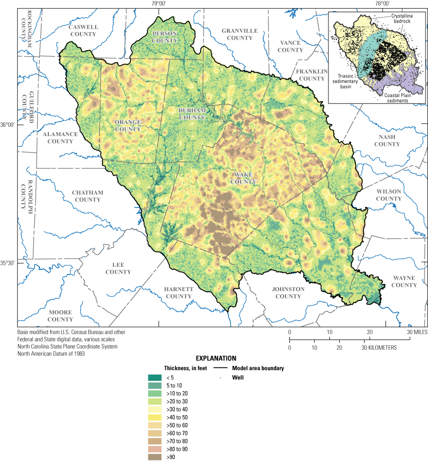
Map showing the layer thickness for model layer 1 in the study area (regolith-transition-zone and Coastal Plain sediments), Wake County, North Carolina.
The MODFLOW model was developed using a temporal discretization of quarterly time intervals for model stress periods. Model stress periods were based on seasonal recharge and base flow data. The seasonal recharge data were grouped by the meteorological seasons, that reflect the annual temperature cycle: winter (December–February), spring (March–May), summer (June–August), and fall (September–November). Groundwater recharge input data from the SWB model (Antolino and Gurley, 2022) began in 1981, and base flow estimates for the four USGS streamgage sites have 22–39 years of record through 2019 (U.S. Geological Survey, 2022). Publicly available annual groundwater-use data were utilized in the model beginning in 2002. The first MODFLOW stress period was simulated as a steady-state system to represent long-term average conditions in the regional groundwater-flow system. This simulation established initial conditions using a broader distribution of observations across the model area and served as a baseline for the following transient simulation periods. The subsequent 82 transient stress periods, spanning winter 1999–2000 to winter 2019–20, are each 3 months long and coincide with the meteorological seasons, except for the final stress period, which represents an incomplete season, spanning only the month of December 2019. Each stress period was subdivided into three time steps to improve model stability and resolution for simulating groundwater response to transient conditions. The transient simulation captures seasonal recharge, stream base flow, and groundwater withdrawals.
Lateral Boundaries
No-flow and drain boundary conditions were used for the lateral boundaries of the model area (fig. 7). No-flow lateral boundaries were used along the drainage basin boundary between the Cape Fear River, Tar-Pamlico River, and Neuse River Basins (fig. 1; North Carolina Department of Environmental Quality, Division of Water Resources, 2025a) for both model layers. A no-flow boundary was located at the base of the model. Drain boundaries were simulated with the MODFLOW Drain (DRN) package (Harbaugh and others, 2000). The drain cells were specified in model layer 1 within the model domain, as well as along the model boundaries, to represent groundwater discharge to the major river drainages, including the Tar-Pamlico, Cape Fear, and Neuse Rivers (figs. 1 and 7). Drains were used to represent the gaining stream conditions within the model domain. The drains only allow groundwater to leave the model, reflecting a conception of groundwater flow as continuously moving toward and discharging along the modeled stream reaches. Drain altitudes were calculated from the DEM (U.S. Geological Survey, 2021) and upscaled to the model grid resolution by using the mean altitude across each cell and then interpolated to drain nodes to approximate the stream bottom altitude represented by those cells. The conductance (C) of the drain boundaries is defined as
whereK
is hydraulic conductivity,
A
is the cross-sectional flow area of the boundary, and
L
is the flow-path length across the boundary.
The initial Kh for the drain boundaries was specified as 3 feet per day (ft/d) prior to model calibration. The flow area, A, was computed for each cell as the product of the length of the stream channel crossing the cell and the assumed stream width. Assumed stream widths were based on the location of the channel within the drainage network. The widths of the drains in the urban drainage basins within Wake County ranged from 4 to 82 ft (Doll and others, 2002). It is assumed that this range in stream width is also representative for the rest of the model area. Aerial imagery was used to estimate widths of the Cape Fear River (range of 150–1,000 ft), the Tar-Pamlico River (range of 40–100 ft), and the Neuse River (range of 80–180 ft) along model boundaries. For drain cells, the flow-path length, L, is the streambed thickness, which was initially set to 3 ft prior to model calibration.
Discharge to Streams
Groundwater discharges to gaining streams as base flow where the water table intersects the stream channel, contributing to sustained and increased flow downstream. Estimates of stream base flow, or groundwater discharge, were determined by Antolino and Gurley (2022) by using hydrograph separation analysis of continuous streamflow records from four USGS streamgage sites (table 3 and fig. 2). The PART hydrograph separation program (Rutledge, 1998) was used to analyze the daily streamflow data (Antolino and Gurley, 2022). This method resulted in mean base flow estimates ranging from 33 to 54 percent of streamflow (table 3), indicating that one-third to slightly more than half of the measured streamflow is derived from groundwater discharge within the four drainage basins. These estimates have some degree of uncertainty, as flow is regulated upstream from all streamgages within the study area.
Table 3.
Hydrograph separation analysis for selected streamgage sites for the model area,1980 to 2019, Wake County, North Carolina.[Data from Antolino and Gurley (2022) and U.S. Geological Survey (2022). USGS, U.S. Geological Survey; mi2, square mile; nr, near; NC, North Carolina; US, United States]
Recharge
Areal recharge to the groundwater-flow model was simulated with the MODFLOW Recharge (RCH) package (Harbaugh and others, 2000). Recharge rates were based on net infiltration rates derived from the SWB model for daily time steps between 2000 and 2019 (Antolino, 2022). These daily time steps were aggregated into 3-month periods based on the meteorological seasons for input into the model. The SWB model uses the Soil Conservation Service runoff-curve method (Cronshey and others, 1986) and a modified Thornthwaite-Mather soil-water-balance approach (Thornthwaite, 1948; Thornthwaite and Mather, 1957) to partition precipitation into surface runoff, evapotranspiration, recharge, and water storage in the soil column on a daily time step. The components of the water budget computed by the model rely on the relations among surface runoff, land cover, and hydrologic soil group (Cronshey and others, 1986) and estimated values of evapotranspiration and air temperature (Hargreaves and Samani, 1985). Net infiltration in the SWB model is the amount of water below the root zone beyond the maximum soil-water capacity. Net infiltration is calculated for each individual cell by determining the difference between its inputs (precipitation and surface runoff from upslope cells) and its outputs (evapotranspiration, interception by vegetation, and surface runoff).
Groundwater Use
Large CWS and mine-dewatering wells within the model area were simulated with the MODFLOW Well (WEL) package (Harbaugh and others, 2000). Annual groundwater withdrawal data for public supply and mine-dewatering operations were compiled from publicly available local water-supply plans and water withdrawal and transfer reports submitted to the NCDEQ DWR (North Carolina Department of Environmental Quality, Division of Water Resources, 2025b, c). All CWSs that regularly serve 1,000 or more service connections or serve more than 3,000 people are required to prepare a local water-supply plan (General Statute 143–355(l); North Carolina General Assembly, 2003). Pumping rates were held constant at the 2002 annual rate for the initial steady state through 2002 stress periods in the model simulation until published annual rates became consistently available for the years after 2002. Domestic withdrawals were not simulated in the model with the assumption that onsite wastewater (septic) systems return most water, resulting in negligible net withdrawals at the regional model scale (Anderson and others, 2015). Available groundwater-use data during the period from 2002 to 2019 that were incorporated into the model simulation are provided in Antolino (2025).
Model Calibration
The groundwater-flow model parameters were calibrated to groundwater-level observations from 1941 to 2019 and base flow observations, derived from streamflow data, from 1980 to 2019. Synoptic water levels were incorporated into the groundwater-flow model calibration of the steady-state model because the data approximate equilibrium conditions, despite potential nearby pumping effects within the dataset. During model calibration, the groundwater-level and base flow observations were weighted to reflect measurement precision and the degree of information they may convey about the modeled system relative to the parameters being simulated (Doherty and Hunt, 2010). Equal weights were applied within each of the observation groups. Weighting between the two observation groups resulted in flow observations contributing about 20 percent of the weighted sum of squares differences, also known as the objective function. This weighting reflects the frequency and spatial distribution over the model area between the groundwater-level and base flow observation data.
The model contained 308 parameter values that were included in the calibration process from 6 parameter groups: hydraulic conductivity, horizontal anisotropy and vertical anisotropy (directional variation in hydraulic conductivity within and between model layers), specific yield, specific storage, and drain conductance. The Parameter Estimation (PEST) program was used to automate parameter estimation, also known as inversion, through a process that seeks the inverse solution to the groundwater-flow equation to identify the best estimates of model input parameters using the given observations within the model (Doherty, 2003). The approach described by Doherty and Hunt (2010) that employs Tikhonov regularization and single-value decomposition (SVD) was used for parameter estimation. By using Tikhonov regularization and SVD within the inversion, variation in the estimated parameters is constrained by the observation data and user input of a priori knowledge of parameter value ranges in the system. This approach results in a good model fit to the observed data with a less complex solution that maintains model stability and realistic values, limiting any unnecessary heterogeneity in areas with natural variations.
Kh values were represented by using pilot points (Marsily and others, 1984), with 44 points in layer 1 and 251 points in layer 2, that were interpolated within zones via kriging for each of the three major rock types: crystalline rock, Triassic sedimentary basin rock, and Coastal Plain sediments. Abrupt changes in aquifer properties may be reflected at the boundaries between these hydrogeologic groups, as interpolation was constrained within each zone. The pilot points were spatially distributed near well locations with available hydraulic conductivity data. Initial hydraulic conductivity values were based on data collected in the monitoring-network wells and values from previous studies (Daniel and others, 1997; Hockensmith, 1997) prior to calibration. In areas without field-measured hydraulic conductivity data, pilot points were placed between well sites with observed water levels assuming unknown hydraulic conductivity between wells can be represented using hydraulic head differences. During calibration, values for the pilot points were permitted to vary within the range of published values for hydraulic conductivity from previous studies in similar hydrogeologic settings (Domenico, 1972; Daniel and others, 1997; Hockensmith, 1997; McCoy and others, 2015; Campbell and Landmeyer, 2023). The remaining 13 model parameter values for horizontal and vertical anisotropy, specific yield, specific storage, and drain conductance were estimated as single uniform values that were applied across the model domain. All parameter values represent mean bulk aquifer properties at a regional scale, averaging out local heterogeneities in those parameters within the groundwater system. All model parameters were iteratively calibrated for best possible model fit such that the objective function was minimized. Parameter sensitivities were computed during the PEST process by using the Jacobian matrix, which records the degree of change in model output with respect to the change in each parameter. These sensitivities help to guide the calibration process by identifying which parameters have the most influence on model simulation results.
Groundwater Model Forecast Scenarios
The calibrated groundwater-flow model was used to simulate forecast scenarios to assess responses of the groundwater system to future climate conditions and land cover change from 2020 to 2070. The forecast scenarios are based on global climate models (GCMs) for the representative concentration pathway (RCP) 4.5 and RCP 8.5 scenarios used by the Intergovernmental Panel on Climate Change (IPCC) (Moss and others, 2010; van Vuuren and others, 2011; Intergovernmental Panel on Climate Change, 2019). RCP 4.5 represents a moderate emissions scenario where levels peak around 2040 before declining, whereas RCP 8.5 represents a high emissions scenario with continuously increasing emissions. Including both scenarios provides a range of uncertainty in plausible future conditions regarding potential climate variability. The statistically downscaled GCMs were obtained from the Multivariate Adaptive Constructed Analogs (MACA) datasets, version 2 (MACAv2-METDATA; Abatzoglou and Brown, 2012; Taylor and others, 2012). The MACA approach uses the 4-kilometer (km) gridMET dataset (Abatzoglou, 2013) as the baseline for statistical downscaling, which matches large-scale GCM patterns with observed relations between meteorological variables in the historical climate data, such as precipitation and temperature.
A clustering multivariate algorithm outlined by Gray (2018) provided the basis for the selection of three GCMs that represent more frequent and extended durations of drier, moderate, and wetter conditions for the southeastern United States: INMCM4.0 (Volodin and others, 2010), MRI-CGCM3 (Yukimoto and others, 2011; Yukimoto and others, 2012), and NorESM1-M (Tjiputra and others, 2013), respectively. The forecast scenarios also included projected land cover changes from a FUTure Urban-Regional Environment Simulation (FUTURES) (Meentemeyer and others, 2013) urban development model for the region, which was modified with the 2019 National Land Cover Database (Sanchez and others, 2020b; Dewitz and U.S. Geological Survey, 2021). Sanchez and others (2020a) simulated probabilistic projections of urban growth to 2065 by using the FUTURES land change model to anticipate future changes in land development patterns for two growth scenarios representing historical (status quo) and more clustered development (urban infill) patterns. For Wake County, the status quo scenario of growth projected an average of about 396 mi2 of total developed land by 2065 that represents about a 28-percent increase over the 2011 estimate of about 309 mi2 (table 4). The FUTURES status quo scenario by Sanchez and others (2020b) was incorporated into the forecast scenario simulations because of the larger urban footprint relative to the urban infill scenario that indicates a 5.6 percent increase from the 2011 estimate and represents a more likely future development pattern for the area overall. The status quo replicate run 2 was determined to be most representative of all 10 probabilistic simulation replicates and was modified with the 2019 National Land Cover Database to update the 2011 National Land Cover Database data on which the probabilistic simulation was based.
Table 4.
Projected changes in land cover by 2065 for a status quo future development scenario for Wake County, North Carolina.[Adapted from Sanchez and others (2020b). Projected changes are relative to 2011 National Land Cover Database estimates; 2019 National Land Cover Database estimates are given for comparison (Dewitz and U.S. Geological Survey, 2021). The standard deviation refers to the 10 simulation replicates for the future development scenario. mi2, square mile; S.D., standard deviation; %, percent]
The modified land cover dataset was combined with the climate data from the three GCMs for both RCP scenarios 4.5 and 8.5 to be used as input to the SWB model (Antolino, 2022) for the years 2020–70 in 280 quarterly stress periods. The SWB model results provided estimates of net infiltration (Antolino, 2022) that were used as future recharge rates for input into the calibrated groundwater-flow model for the forecast scenario simulations. Unlike the 2000–19 recharge dataset used in the calibrated model that was derived from the higher resolution Daymet version 3 climate dataset (Thornton and others, 2016), the recharge datasets for the forecast scenarios were derived from MACA climate data (Abatzoglou and Brown, 2012; Taylor and others, 2012). MACA applies statistical pattern matching to downscale GCM data using gridMET historical observational data as a baseline for bias correction, whereas Daymet uses spatial interpolation with a truncated Gaussian weighting function at a finer 1-km resolution that incorporates topographic influences and captures localized variability. The higher spatial resolution of the Daymet dataset was preferred for the 2000–19 calibration period. At the time of this study, no finer scale downscaled datasets for GCM data were available beyond the resolution of the MACA dataset.
The supply-well withdrawals were held constant at the 2019 pumping rates for each supply well throughout the entire forecast scenario simulation period (2020–70). This approach was used to highlight potential impacts to the groundwater system related to changing climate variables and increasing development. Although supply withdrawal rates have historically been observed to increase during drier periods (Chapman and others, 2011), likely to offset surface water resource depletion, no adjustment was applied to account for potential future trends in groundwater use for the climate-based forecast scenarios in this report.
Characterization of Aquifer Hydraulic Properties
Aquifer tests performed in the 17 USGS monitoring-network wells and WK–439 (NCDEQ DWR well K40M1) provided estimates of Kh and T within the regolith and bedrock layers of the local fractured-rock groundwater system (table 5). The results of aquifer testing indicate that values for Kh based on the slug-test results ranged from 0.03 to 10 ft/d for the regolith wells and 0.002 to 2 ft/d for the bedrock wells. Values for T based on the slug-test results ranged from 2 to 400 feet squared per day (ft2/d) for the regolith wells and 0.7 to 200 ft2/d for the bedrock wells. Additional results are provided by Gonthier and Antolino (2023).
Table 5.
Transmissivity and horizontal hydraulic conductivity estimated for monitoring-network well sites in the study area Wake County, North Carolina.[Data from Gonthier and Antolino (2023) and Antolino (2025). CH, Chatham County well prefix; WK, Wake County well prefix; ft, foot; ft/d, foot per day; ft2/d, foot squared per day; FLASH, Flow-Log Analysis of Single Holes (Day-Lewis and others, 2011); --, no data or not applicable]
The test interval represents the well screen length for the regolith wells and the total open borehole depth below casing for the bedrock wells.
Measured and reported by Chapman and others (2005).
Measured and reported by McSwain and others (2013).
Borehole vertical flow data collected for 10 of the bedrock wells during ambient and stressed (pumping) conditions are shown in table 6. Wells WK–428 and WK–429 had measurable flow under stressed conditions in only one fracture at the base of the well casing. This response indicates that the largest hydraulic connection occurs near the interface between the transition zone and the top of bedrock, with little to no hydraulic contribution from deeper fractures. All other measured bedrock wells had measurable flow under stressed conditions in two or more deeper fractures below the casing depth, indicating the intersection of multiple flow zones within the well.
Table 6.
Borehole vertical flow measurements for monitoring-network bedrock wells for the study area, Wake County, North Carolina, 2022.[Data from U.S. Geological Survey (2024). Flow measurements were conducted under ambient (without pumping) and stressed (with pumping) test conditions. Negative flow values indicate downward vertical flow in the borehole, and positive flow values indicate upward vertical flow in the borehole. CH, Chatham County well prefix; WK, Wake County well prefix; ft, foot; gal/min, gallon per minute; --, no data or not applicable]
Ambient vertical flow directions measured in wells revealed hydraulic gradients within surrounding fractured rock. When connected fracture zones intersect a well borehole, the zones are likely to exhibit similar hydraulic heads, resulting in lower potential for flow between zones under ambient conditions. However, a well borehole intersecting flow zones in different fracture networks is likely to have greater hydraulic differences, leading to higher ambient vertical flow within the borehole. Vertical borehole flow could be measured in six of the bedrock wells under ambient conditions where there were no observable effects of nearby pumping. Wells WK–426, WK–431, WK–435, and WK–439 had the highest upward ambient flow with values ranging from 0.02 to 0.03 gal/min (table 6). Wells CH–252 and WK–434 had measurable downward ambient flow values of 0.04 and 0.10 gal/min, respectively. A downward ambient flow of 0.45 gal/min also was measured in well WK–437, which can likely be attributed to pumping from a nearby supply well.
Vertical flow measurements were analyzed with the FLASH program that uses a simple analytical model based on the Thiem equation for steady-state borehole flow (Thiem, 1906; Day-Lewis and others, 2011). Values for T based on the FLASH results ranged from 8 to 2,000 ft2/d for the bedrock wells (table 5). T values derived from estimates of specific capacity associated with flow log pumping ranged from 5 to 5,000 ft2/d for the bedrock wells. Slug-test values for T and Kh ranged within two orders of magnitude of values derived using the borehole vertical flow and specific capacity data (table 5). Both methods of determining the T by using specific capacity and FLASH have limitations. The FLASH estimates of T are highly sensitive to the initial estimates of the radius of influence--which can be challenging in heterogeneous systems where preferential flow paths may exist and skew localized flow contributions. The estimation of T from specific capacity assumes steady-state conditions, so there is sensitivity to transient changes in the flow dynamics from pumping drawdown within the fractured-rock groundwater system at short durations.
Groundwater Geochemistry
Results of water-quality sampling and analysis of stable isotopes of water and dissolved gases were used to describe the geochemical context within the fractured-rock groundwater system. This context helps to inform and constrain apparent groundwater ages determined using CFCs, 3H, and 3He results. Groundwater quality and age dating provide additional insights into recharge processes, redox conditions, and some understanding of residence time within the fractured-rock groundwater system.
Physical Properties and Chemical Constituents
Results for physical properties and chemical constituents (water temperature, pH, specific conductance, and DO) measured during groundwater sample collection are summarized in table 7. Water temperatures ranged from 15.1 to 19.0 degrees Celsius (°C) in the regolith and 16.4 to 24.3 °C in the bedrock. Values for pH ranged from 4.8 to 5.7 in the regolith and 5.3 to 7.7 in the bedrock. Results for the four sets of paired wells tended to indicate higher values of pH (more basic) and specific conductance in the deeper bedrock wells as compared to the shallower regolith wells (table 7). Specific conductance ranged from 72 to 367 microsiemens per centimeter at 25 °C (µS/cm) in the regolith and 89 to 598 µS/cm in the bedrock. The highest specific conductance measurements were likely related to land use near the well site, namely agricultural practices at the WK–283 site (598 µS/cm) at the North Carolina State University Lake Wheeler Road Field Laboratory and land application of biosolids at the WK–334 site (549 µS/cm) at the Neuse River Resource Recovery Facility. Concentrations of DO ranged from 2.1 to 6.9 milligrams per liter (mg/L) in the regolith and 0.15 to 8.1 mg/L in the bedrock wells. The highest observed DO concentration of 8.1 mg/L was measured in bedrock well WK–368, caused by water from shallower fractures cascading down the well borehole because of depressed water levels from nearby pumping--cascading water along the borehole wall was confirmed by a well camera survey. Six of the bedrock wells had DO concentrations less than 1 mg/L, indicating more reduced geochemical conditions for these sites.
Table 7.
Field measurements of physical properties and chemical constituents during groundwater sample collection for wells in the monitoring network for Wake County, North Carolina, 2019.[Data from U.S. Geological Survey (2022). Times shown in 24-hour format. CH, Chatham County well prefix; WK, Wake County well prefix; USGS, U.S. Geological Survey; ft, foot; °C, degree Celsius; μS/cm, microsiemens per centimeter at 25 degrees Celsius; mg/L, milligram per liter]
Stable Isotopes of Water
The results of the analysis of stable isotopes of water in precipitation, surface water, and groundwater samples are listed in table 8. The relation between the δ18O and δ2H isotopic composition in precipitation samples is plotted in figure 9A. The isotope values for the precipitation samples (n = 47) ranged from −10.05 to −1.92 and −67.20 to 4.25 per mil for δ18O and δ2H, respectively. The samples did not show strong seasonal variation, but those samples collected during spring (March–May) had the most variation in isotopic composition. This range in isotopic concentration reflects the dynamic seasonal transition from drier northern air masses to more humid air masses originating from the south bringing fluctuating temperatures with a mixture of precipitation events across the study area. For example, the March 17, 2021, precipitation sample slightly deviates from the general trend of the data that may reflect a cooler, drier continental air mass as the moisture source. An LMWL of
was determined for the Wake County study area by linear regression (R2 = 0.93) by using precipitation data collected from the rain gage located at USGS monitoring station 0208735012 (Rocky Branch below Pullen Road at Raleigh, N.C.) (fig. 9A; U.S. Geological Survey, 2022). The LMWL has a slightly lower slope of 7.77 compared to the GMWL slope of 8.0 defined by Craig (1961). This difference in slope with the GWML likely reflects the specific climatic conditions and moisture sources of the Raleigh area in contrast to the broader range of global conditions captured in the GMWL. The LMWL has a steeper slope than the river water line developed for the State of North Carolina using isotopic data from river sites by Kendall and Coplen (2001), δ2H = 6.32 * δ18O + 2.9 ‰ (n = 87). The river water line, acting as a proxy for the isotopic composition of modern precipitation, is based on the assumption that most of the surface water represented base flow and recent precipitation, yet the shallower slope likely reflects some influence of evaporation effects in the water samples, possibly due to mixing with older, evaporated waters in the basins.Table 8.
Results of the analysis of stable isotopes of water in precipitation, surface water, and groundwater samples for the study area, Wake County, North Carolina, 2019–22.[Data from U.S. Geological Survey (2022). Samples were analyzed by the U.S. Geological Survey, Reston Stable Isotope Laboratory (RSIL) in Reston, Virginia. USGS, U.S. Geological Survey; δ2H, delta deuterium of water; ‰, per mil; δ18O, delta oxygen-18 of water; --, not applicable; PR, precipitation; SW, surface water; GW, groundwater; CH, Chatham County well prefix; WK, Wake County well prefix]
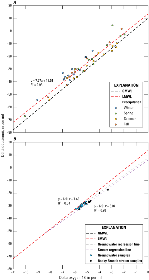
Delta oxygen-18 and delta deuterium composition for (A) precipitation samples and (B) groundwater and stream samples in the study area in Wake County, North Carolina. δ2H, delta deuterium of water; δ18O, delta oxygen-18 of water; GMWL, Global Meteoric Water Line; LMWL, Local Meteoric Water Line.
The δ2H and δ18O results for groundwater generally plotted along and slightly below the LMWL with a regression line with a slope equation of δ2H = 6.91 * δ18O + 7.49 ‰ (R2 = 0.84) (fig. 9B). This pattern suggests that the groundwater is isotopically similar to modern local precipitation, indicating that the recharge from rainfall has undergone minimal evaporation before entering the aquifer. This isotopic signature highlights that local precipitation is the predominant source for all of the sampled wells across the county, implying that any changes in rainfall directly impact recharge to the groundwater system. Ranges for δ2H and δ18O in the groundwater samples were from −32.67 to −26.82 per mil and −5.88 to −5.04 per mil, respectively. Results for all groundwater samples fell within a relatively narrow isotopic range, reflecting an averaged isotopic composition where short-term and seasonal variations from similar precipitation events across the county have been smoothed out and integrated into a composite signature.
The isotopic results for the Rocky Branch stream samples plotted along a regression line with a slope equation of δ2H = 6.91 * δ18O + 6.04 ‰ (R2 = 0.98) (fig. 9B). Except for the January 2022 sample, all stream samples were collected during low-flow conditions (less than 1 cubic foot per second) and generally plotted in the same isotopic range as the groundwater samples, indicating that groundwater discharge is the predominant source of streamflow during low-flow conditions. The larger spread in the isotopic concentrations for the stream samples likely reflects the influence of seasonal evaporation during warmer periods, as well as variability with water-source mixing of recent rainfall and groundwater discharge.
Groundwater Dissolved Gases
Based on field meter readings of DO in the bedrock wells, 10 wells were considered to have oxic groundwater conditions (greater than 0.5 mg/L), and 4 wells were considered to have anoxic groundwater conditions (less than 0.5 mg/L) (McMahon and Chapelle, 2008) (table 7). Most of the sampled wells having oxic conditions suggest some degree of connection with more oxygenated sources, possibly through connected fracture networks at the top of bedrock with shallow groundwater in the regolith. Anoxic conditions may be present in deeper fracture zones where oxygen is consumed along the flow path. The laboratory results of the concentrations of the dissolved gases methane, carbon dioxide, nitrogen, oxygen, and argon in the 14 bedrock groundwater samples are provided in table 9. Three of the well sites (WK–428, WK–429, and WK–431) had laboratory-analyzed dissolved-gas samples with reported DO concentrations greater than 0.5 mg/L, whereas the remaining 11 well sites had anoxic concentrations of reported DO around 0.1 mg/L in the samples (table 9). This discrepancy between the field and laboratory results suggests potential changes in DO within the sample during storage. Laboratory analyses of DO can often be biased toward lower concentrations because of rapid microbial oxygen consumption during sample storage, despite proper preservation techniques (U.S. Geological Survey, 2006). Therefore, field measurements of DO generally are considered more reliable when interpreting groundwater conditions. The other dissolved gases measured in this study are less reactive and, if preserved properly, maintain stability prior to analysis.
Table 9.
Laboratory results of the concentrations of the dissolved gases methane, carbon dioxide, nitrogen, oxygen, and argon and calculated recharge temperature in duplicate groundwater samples for wells in the monitoring network for Wake County, North Carolina, 2019.[Data from U.S. Geological Survey (2022). Samples were analyzed by the U.S. Geological Survey, Reston Groundwater Dating Laboratory (RGDL) in Reston, Virginia, using gas chromatography. CH, Chatham County well prefix; WK, Wake County well prefix; USGS, U.S. Geological Survey; °C, degree Celsius; ft, foot; NAVD 88, North American Vertical Datum of 1988; mg/L, milligram per liter; cm3 STP/L, cubic centimeter at standard temperature and pressure per liter]
Trace levels of dissolved methane were measured in the samples from 6 of 14 bedrock wells, and relatively higher concentrations were measured in samples from wells WK–429 and WK–439 (table 9). The presence of methane is suggestive of reducing conditions within the fractured-rock groundwater system and aligns with anoxic levels seen in well WK–439. However, the groundwater sample from well WK–429 is oxic and has the highest levels of dissolved methane. As previously discussed in the section “Characterization of Aquifer Hydraulic Properties,” the largest source of inflow to this well occurs from a fracture at the top of bedrock below the well casing, possibly providing a source of more oxygenated groundwater. This inflow may be mixing with anoxic water where methane production may be occurring in more stagnant zones deeper in the well. This mixing may have been enhanced, or even induced in the case where the natural flow regime is reversed, during sample collection, by pumping in wells that have fractures within different redox zones. Additional geochemical information outside the scope of this study would be needed, such as hydrogen sulfide and acetate concentrations, to verify the occurrence of methanogenic conditions in the wells.
Dissolved carbon dioxide concentrations ranged across two orders of magnitude from 0.8219 mg/L in well WK–283 to 95.3804 mg/L in well WK–426 (table 9). The values near the lower end of this range are closer to atmospheric equilibrium, and the larger values suggest more direct connection with shallow groundwater that has infiltrated soil zones that are high in organic matter, where microbial activity is elevated. Additionally, in more urban and industrial areas, it is possible that these levels may be influenced by the aerobic degradation of contaminants, such as volatile organic compounds (Appelo and Postma, 2005; Clark, 2015).
Ranges in dissolved nitrogen and argon concentrations in groundwater samples were from 14.0851 to 33.8943 mg/L and 0.5170 to 0.8596 mg/L, respectively (table 9). In this study, average excess air values ranged from 0.3 to 11.5 cubic centimeters (at standard temperature and pressure per liter) with the highest levels in well WK–283. Because nitrogen can also be produced from denitrification processes in the subsurface, excess nitrogen within samples from the wells was assessed by comparing observed concentration to expected values for nitrogen based on the air-water equilibrium derived from argon (Böhlke, 2002). Estimates of excess nitrogen present in wells WK–430, WK–283, and WK–334 suggest active denitrification processes in the aquifer near these wells. Laboratory corrections were applied for the presence of excess nitrogen above expected solubility for the nitrogen values reported for these three wells in table 9.
Accounting for excess air in groundwater samples refines the temperature-dependent gas solubility, leading to more accurate estimates of recharge temperature and aiding in determining when groundwater was recharged. Recharge temperatures calculated by the USGS RGDL from the dissolved-gas concentrations of nitrogen and argon are listed in table 9. The average recharge temperature was 15.2 °C, consistent with the average annual temperature for the study area (National Oceanic and Atmospheric Administration, 2020). The calculated recharge temperature for well WK–368 was higher than those of other wells, likely influenced by significant drawdown from nearby supply well pumping, which may have altered local flow dynamics to draw more groundwater from shallower, recently recharged fractures. These shallow fractures likely have shorter flow paths, reflecting recent recharge from prior events before sampling, likely during the warmer summer months. Deeper fractures, typically with longer flow paths, may contain a mixture of groundwater from multiple seasons. Cascading water observed along the open borehole during a borehole camera survey suggests a shallow productive fracture zone below the bottom of casing contributing more recently recharged groundwater. Refined recharge temperature estimates improve the reliability of dissolved-gas and tracer concentrations used in groundwater age dating (Stute and Schlosser, 2000).
Groundwater Age Dates
Concentrations of CFC-11, CFC-12, and CFC-113 measured in samples from the 14 bedrock wells were used by the USGS RGDL to calculate apparent groundwater ages based on the assumption of piston-type flow within the aquifer. The apparent ages based in the CFC analyses ranged from the 1950s to the 1990s (table 10). The groundwater age for a sample is a function of recharge and groundwater flow rates, as well as source and flow path mixing. As with all dissolved constituents in groundwater, the CFC concentrations can be influenced by flow transport processes, including the mixing of older and younger waters from different flow paths. Because groundwater samples were pumped from deep, open well boreholes, each sample likely contains some mixture of groundwater having different recharge ages.
Table 10.
Concentrations of chlorofluorocarbons in groundwater samples and apparent groundwater age dates for the study area, Wake County, North Carolina.[Data from U.S. Geological Survey (2022). Samples were analyzed by the U.S. Geological Survey, Reston Groundwater Dating Laboratory (RGDL) in Reston, Virginia. Samples were analyzed in duplicate for concentrations of chlorofluorocarbons (CFCs), and results are reported for one sample used for dating from each well; the analyses of the three CFCs were used to assign a CFC recharge time. CH, Chatham County well prefix; WK, Wake County well prefix; USGS, U.S. Geological Survey; pg/kg, picogram per kilogram; CFC, chlorofluorocarbon; CFC-11, trichlorofluoromethane; CFC-12, dichlorodifluoromethane; CFC-113, trichlorotrifluoroethane; :, ratio; C, CFC concentration is in excess of air-water equilibrium, indicating that nonatmospheric sources may have added CFCs to groundwater; --, no data available; NP, not possible to date using ratio ages]
Assuming there is a binary mixing of older CFC-free water and younger water containing CFCs, the tracer age date will be based on the younger water fraction within the sample. The younger and older fractions within the binary mixture can be assessed from ratios of the CFCs. Based on laboratory evaluations of information derived from the CFC tracer ratios, the mixing of younger, more modern recharge water with older groundwater could be derived for 5 of the 14 bedrock wells (table 10). Both samples for wells WK–435 and CH–252 contained less than 25 percent of young water. Mixing of the sample for well WK–430 reflected nearly equal parts of older and younger water. Younger water made up about 75 percent of the sample from well WK–434 and nearly all the sample from well WK–431.
Plummer and Busenberg (2000) suggested that CFC-11 may be, at least partially, degraded in groundwater having DO concentrations less than 0.5 mg/L. Four of the 14 bedrock groundwater samples had field-measured DO concentrations less than or equal to 0.3 mg/L (table 7). Other studies have shown that CFC-11 is more sensitive to anerobic microbial degradation than CFC-113 and CFC-12, especially once redox conditions reach sulfate reduction (Semprini and others, 1990; Katz and others, 1995; Shapiro and others, 1997). Five of the wells that had trace concentrations of dissolved methane also had oxic levels of DO, which suggests the mobilization of methane from groundwater in deeper fracture zones mixing with more oxic water in shallower zones (tables, 7, 9, 10). All CFCs would have likely undergone some degradation in low sulfate, methanogenic environments (Oster and others, 1996; Deipser and Stegmann, 1997; Plummer and Busenberg, 2000). This degradation would result in a bias toward older recharge ages for samples with a large fraction of highly reduced, methanogenic groundwater. Higher levels of methane were detected in two groundwater samples, from wells WK–429 and WK–439 (table 9), but oxic levels were such that the effect on the groundwater age is minimal (table 7).
Concentrations of all three CFCs measured in groundwater samples from well WK–428 were more than the air-water equilibrium and were likely influenced by an unknown anthropogenic source. In addition to microbial degradation, contamination will also increase the uncertainty in CFC concentrations. The CFC-derived groundwater ages were examined in combination with results from the additional environmental tracers of 3H, 3He, 4He, and neon to reduce uncertainty in groundwater age-dating results.
The results for 3H, 3He, 4He, and neon are listed in table 11. Concentrations of 3H measured in the groundwater samples ranged from 0.05 to 3.92 TU. The samples contained tritiogenic 3He concentrations ranging from less than 1 to 19.2 TU. Of the 14 bedrock wells sampled, 5 wells had samples with very low concentrations of tritiogenic 3He. All samples contained measurable amounts of terrigenic helium, with most samples showing some mixing with tritiogenic-sourced helium. Apparent ages based on the 3H and 3He concentrations ranged from the mid-1930s to the late 2000s, reflecting a broader range of apparent age dates for groundwater within the fractured-rock groundwater system compared to the CFC tracer data (tables 10 and 11).
Table 11.
Concentrations of helium, neon, and tritium in groundwater samples and apparent groundwater age dates for the study area, Wake County North Carolina.[Data from U.S. Geological Survey (2022). Samples were analyzed by the U.S. Geological Survey, Reston Stable Isotope Laboratory (RSIL) in Reston, Virginia. Duplicate samples were analyzed, and results are reported for the mean value used for age dating. CH, Chatham County well prefix; WK, Wake County well prefix; USGS, U.S. Geological Survey; cm3/g STP, cubic centimeter per gram of water at standard temperature and pressure; 3He/4He, ratio of helium-3 to helium-4 in the sample; TU, tritium unit; 3H, tritium; E[-x], ×10[–x]; <, less than; --, no data]
Conceptually, groundwater moves from porous flow in the regolith to complex fracture flow in the bedrock; therefore, a binary-mixing LPM was initially used to analyze both CFC and 3H/3He tracer data. The binary-mixing model was unsuccessful at producing optimized computed ages within the expected ranges based on historical atmospheric concentrations and the previously discussed results for both tracer datasets. A simplified model for piston flow was used to compute ages, despite assumptions in the model that cannot adequately account for flow-path mixing that exists in the bedrock. The apparent ages computed by TracerLPM along with the environmental tracers used in the model optimization are shown in table 12. The groundwater ages range from the early 1940s for well WK–439 to the late 1990s for wells WK–426 and WK-431.
Table 12.
Groundwater-recharge dates derived through optimization analysis of multiple age-dating tracers for bedrock wells in the study area, Wake County, North Carolina.[Data from U.S. Geological Survey (2022). The apparent ages were computed and optimized by TracerLPM (Jurgens and others, 2012). CH, Chatham County well prefix; WK, Wake County well prefix; USGS, U.S. Geological Survey; 3H, tritium; CFC-11, trichlorofluoromethane; CFC-12, dichlorodifluoromethane; CFC-113, trichlorotrifluoroethane; 3He(trit), tritiogenic helium-3]
Groundwater age provides insight into recharge dynamics across the study area, with implications for groundwater sustainability. Higher amounts of younger water indicate areas with more frequent recharge events and shorter flow paths to supply wells, whereas older water reflects areas with slower recharge rates and longer flow paths. Understanding this age distribution within the aquifer helps identify areas more prone to depletion or at higher risk of rapid transport of contamination from the surface. This information supports the development of management strategies aimed at protecting long-term water availability and quality.
Evaluation of Model Calibration and Performance
The calibrated model produced a groundwater-flow simulation with a reasonable fit to the water-level and base flow observations. All model files are archived in and available as a USGS data release (Antolino, 2025). Calibrated Kh pilot point values for model layer 1 (regolith and Coastal Plain sediments) ranged from 0.01 to 20 ft/d (table 13; fig. 10). Mean values for layer 1 in the three major rock types—crystalline rock, sedimentary basin, and coastal plain sediments—were 1.71, 2.47, and 18.69 ft/d, respectively. Calibrated Kh pilot point values for model layer 2 (bedrock) ranged from 0.01 to 5 ft/d, and mean values for crystalline bedrock and sedimentary basin rock were 1.26 and 1.11 ft/d, respectively (table 13; fig. 11). Calibrated specific storage and specific yield values for the regolith were 0.1 and 0.002 ft−1, respectively (table 14).
Table 13.
Summary statistics for the calibrated horizontal hydraulic conductivity in the groundwater-flow model, Wake County, North Carolina.[Data from Antolino (2025). ft/d, foot per day]
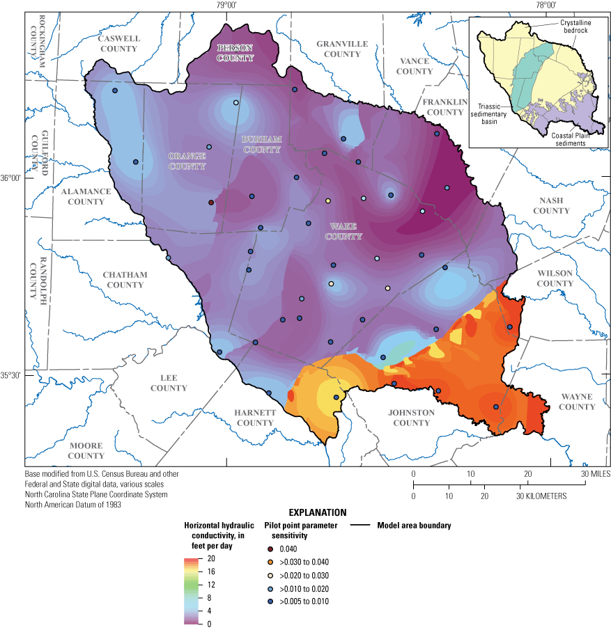
Calibrated horizontal hydraulic conductivities for model layer 1 (regolith and Coastal Plain sediments), Wake County, North Carolina.
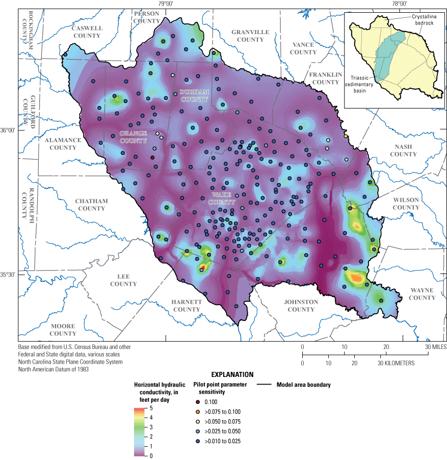
Calibrated horizontal hydraulic conductivities for model layer 2 (bedrock), Wake County, North Carolina.
Table 14.
Hydrogeologic properties calibrated and specified in the groundwater-flow model with associated parameter sensitivity, Wake County, North Carolina.[Data from Antolino (2025). --, not applicable; E[-x], ×10[–x]. All specific-storage values are in per foot; all specific-yield values are dimensionless]
Calibrated specific storage and specific yield values for the bedrock layer were 0.002 and 1.5 × 10⁻⁷ ft−1, respectively (table 14). Calibrated horizontal anisotropy was 5.45 (dimensionless) for the regolith layer, showing dominant horizontal flow in the x direction of the model grid (northeast to southwest direction), which aligns with the regional geologic trend direction. This anisotropy reflects the influence of clay horizons and relict structures in the regolith, which enhances lateral flow along the direction of foliation (northeast to southwest) and impedes some vertical flow. The general groundwater flow direction, which is largely perpendicular to the general direction of streamflow across the study area, reinforces this preferential flow. Calibrated horizontal anisotropy in the fractured bedrock layer was 0.55 (dimensionless), which reflects dominant flow along the y direction of the model grid (northwest to southeast direction). This anisotropy aligns with the conceptual model in that streams form along zones of structural weakness in the underlying rock, such as bedrock fractures. The calibrated vertical anisotropy values across the model were 4.57 (dimensionless) in the regolith (layer 1) and 1.09 (dimensionless) in the bedrock (layer 2), indicating that simulated groundwater predominantly flows laterally within the regolith and flows more uniformly in all directions within the bedrock layer. The vertical anisotropy likely reflects the influence of hydraulic gradients in the areas of high topographic relief, the layered structure of the regolith, and the model’s simplified representation of fractures within the bedrock, assuming various pathways for horizontal and vertical flow. Although the bedrock likely exhibits high anisotropy at local scales, the model assumes uniform flow properties to accommodate data and scale limitations.
Parameter Sensitivity
As part of the PEST calibration process, sensitivity values were determined for all the individual calibrated parameter values (n = 308) within the six examined hydraulic parameter groups. The parameter groups included in the sensitivity analysis were horizontal hydraulic conductivity, horizontal anisotropy, vertical anisotropy, specific yield, specific storage, and drain conductance. Sensitivity values for the 308 model parameters were calculated by PEST to identify those that had the greatest influence on model results and model fit and those that were insensitive or had little to no effect on the model. Parameters with higher sensitivity values have more impact on how the model matches water-level and flow observations, whereas parameters with lower sensitivity values may reflect that there are insufficient relevant data to constrain parameter estimates or simply that the corresponding property plays a limited role in the flow system.
Both model layers had sensitive pilot points for Kh in the crystalline bedrock and overlying regolith (figs. 10 and 11). The most sensitive parameters were within the bedrock (layer 2), indicating variability in fractured-bedrock hydraulic conductivity is an important parameter to simulate the flow system dynamics. Horizontal and vertical anisotropy parameters for the bedrock layer were also among the most sensitive calibration parameters in the model (table 14). The sensitivity of the anisotropy parameters reflects the directional flow of groundwater in the fractured bedrock, where flow is highly dependent on the orientation and connectivity of fractures, as well as the vertical connection with the regolith. The high sensitivity of horizontal anisotropy in the regolith layer highlights the importance of lateral flow toward streams in the model. This flow is influenced by the orientation of relict structural geologic features and clay horizons within the regolith, as well as topography-induced hydraulic gradients. For simulating streamflow observations, the storage parameters for the regolith/transition-zone layer (layer 1) had the highest composite sensitivities, a reflection of the regolith’s capacity to store and release water as the primary reservoir in the groundwater system--critical in maintaining groundwater balance and flow. The very low storage capacity in the bedrock layer is reflected in the relative insensitivity of the bedrock storage parameters in the model such that iterative changes to the parameter value had little to no effect on the simulation results. Drain conductance for the four streamgage drainage basins were among the most insensitive parameters, likely because of hydraulic head gradients primarily driving the flow of groundwater discharge.
The sensitivity analysis identifies the most influential parameters in this groundwater-flow model simulation. This analysis also helps to identify areas where new data collection could be beneficial for improving model accuracy and reducing uncertainty. For example, including additional regolith monitoring wells with associated aquifer testing data will provide more data points to enhance the resolution of the aquifer storage properties, which were found to be highly sensitive in layer 1. Similarly, focusing on local areas of interest and those with more known variation in hydraulic conductivity data could improve the model’s simulation of groundwater flow. Given that horizontal anisotropy and vertical anisotropy were the most sensitive parameters, new data collection could be prioritized where existing information for these properties is lacking, especially in the bedrock layer.
Residuals of Water Levels and Flow Rates
Calibration of the groundwater-flow model was executed across 82 stress periods for initial steady-state conditions and the transient period 2000–19 by using field observations that included 35,749 historical groundwater levels from 1,100 wells (28 regolith or transition-zone wells and 1,072 bedrock wells; fig. 12) and 560 quarterly stream base flow measurements from four streamgage sites in the model area (fig. 2). Most of these groundwater levels consisted of single measurements at domestic wells, with few at monitoring-network wells with higher frequency measurements. The steady-state stress period contained 6,853 water levels. The subsequent transient stress periods had a range of 18–1,833 water levels with a mean of 357 per stress period.
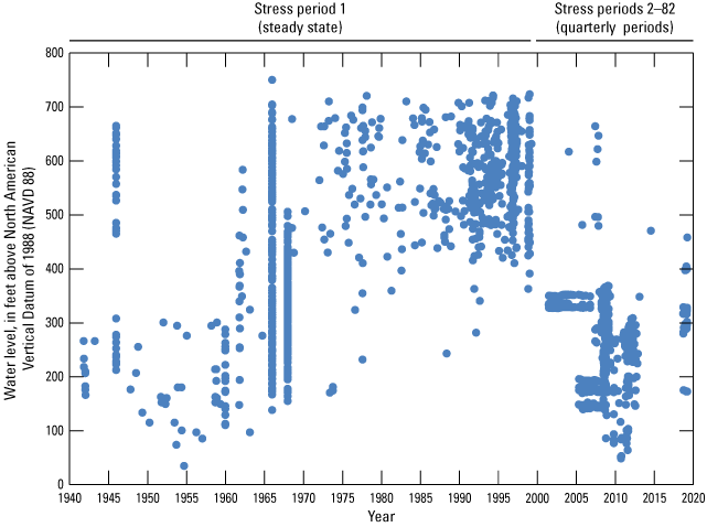
Water levels used for calibration of the groundwater-flow model, Wake County, North Carolina.
The 14,802 water-level observations from the 28 regolith wells ranged about 420 ft, from a low of 135.32 ft to a high of 555.56 ft above NAVD 88 (table 15; fig. 13). The absolute value of the mean residual (difference between observed and simulated water levels) for the regolith wells was 8.1 ft with a root mean square error (RMSE) of 9.4 ft. The 20,947 observed water levels from the 1,072 bedrock wells ranged about 713 ft, from a low of 31.38 ft to a high of 744.48 ft above NAVD 88 (table 15; fig. 14). The absolute value of the mean residual for the bedrock wells was 19.9 ft with an RMSE of 26 ft. The normalized standard deviation (the weighted residuals divided by the range of water levels) was 0.01 and 0.02 for the regolith and bedrock layers, respectively, indicating a good calibration fit that accounted for the variation in water-level data. A normalized standard deviation less than or equal to 0.1 reflects the ideal that most of the residuals fall within 10 percent of the observational range (Kuniansky and others, 2004; Fine and Kuniansky, 2014).
Table 15.
Summary statistics for model calibration fits for groundwater-level observations in the groundwater-flow model, Wake County, North Carolina.[Data from Antolino (2025). ft, foot]
Calibration fit, or normalized standard deviation, is the standard deviation of weighted residuals divided by the range of observations (Kuniansky and others, 2004). A good fit to the data would be reflected in a ratio less than or equal to 0.1.
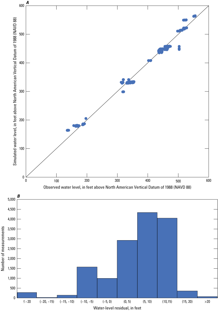
(A) Observed and simulated groundwater levels (1941–2019) and (B) water-level residuals for the regolith wells, Wake County, North Carolina. NAVD 88, North American Vertical Datum of 1988.

(A) Observed and simulated groundwater levels (1941–2019) and (B) water-level residuals for the bedrock wells, Wake County, North Carolina. NAVD 88, North American Vertical Datum of 1988.
A target calibration criterion of ±20 ft was used for the observed water levels considering hydrogeologic context and data uncertainty (Hill and Tiedeman, 2007). This criterion balances the need to reasonably represent regional trends in water levels while acknowledging the complexities within a fractured crystalline bedrock groundwater system at this scale. The ±20 ft threshold reflects about 5 percent of the observed water-level range within the regolith layer and about 3 percent of the range within the bedrock layer. For the regolith groundwater levels (14,802 total), 3 percent were outside of the ±20 ft calibration target (table 15), with 288 measurements exceeding the −20 ft tolerance and 75 exceeding the +20 ft tolerance. For the bedrock groundwater levels (20,947 total), 38 percent were outside of the ±20 ft calibration target, with 4,945 measurements that exceeded the −20 ft tolerance and 2,957 measurements that exceeded the +20 ft tolerance. The higher residuals in the bedrock layer reflect the inherent challenges of modeling fractured-bedrock groundwater systems, where spatially variable hydraulic conductivity and fracture density complicate calibration efforts.
Several additional factors may also contribute to the observed residuals involving the data uncertainty of the well locations and altitudes and the hydraulic conditions at the time of measurement. Hydraulic condition data remarks were not available for most of the domestic well water-level measurements, which may have been obtained during active pumping, after being recently pumped, or influenced by nearby pumping conditions and not representative of ambient conditions. The horizontal coordinates for many of the historical well locations were established using topographic maps having 10-ft contour intervals; thus, there is some inherent uncertainty in the reported water-levels to land surface at those mapped locations. The water level below land surface measurements used for model calibration were updated to water-level altitudes above NAVD 88 by using a 10-meter (32.81 ft) DEM obtained from The National Map (U.S. Geological Survey, 2021) that was upscaled to the resolution of the model grid to minimize uncertainty.
The simulated water-level surfaces of model layers 1 and 2 for the end of the 2019 calibration period are shown in figures 15 and 16, respectively. Groundwater flows perpendicular to equal altitude contour lines in the direction of the steepest downward slope. The water-level surface reflects the gaining stream conditions that prevail within the study area. Contours that form V-shaped patterns around streams convey how groundwater interacts with streamflow, where contour patterns that point upstream suggest groundwater discharge into streams (gaining stream conditions) and those pointing downstream would indicate potential groundwater recharge (losing stream conditions). Groundwater flow paths can be somewhat inferred from contour line spacing, with denser contours indicating local flow systems driven by the topographic highs within small basins.
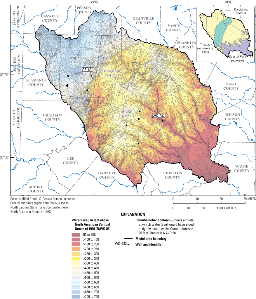
Simulated groundwater-level altitude for the end of the calibration period (2019) for model layer 1 (regolith and Coastal Plain sediments) for the study area Wake County, North Carolina.
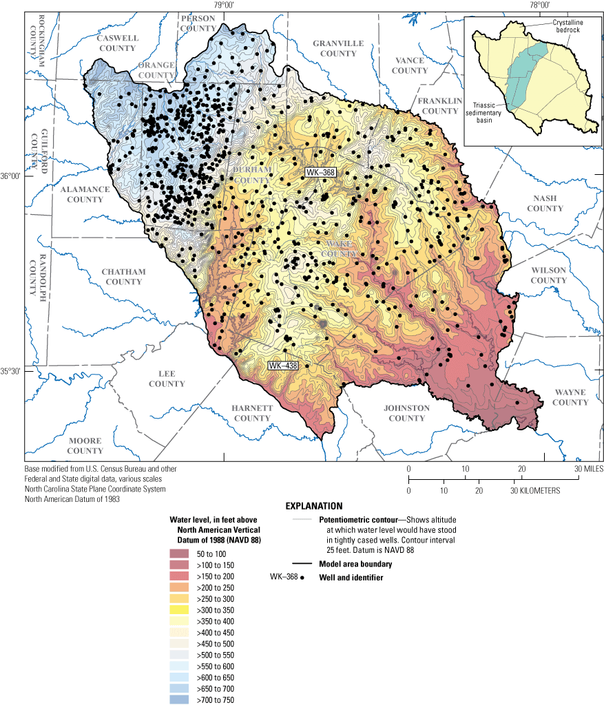
Map showing simulated groundwater-level altitude for the end of the calibration period (2019) for model layer 2 (bedrock) for the study area, Wake County, North Carolina.
The water-level surfaces simulated for the regolith and bedrock layers have similar contour patterns (figs. 15 and 16), reflecting the hydraulic connection between the two layers. Some slight differences exist in upland areas where water levels in the bedrock are below water levels in the regolith, reflecting the downward vertical hydraulic gradient in recharge areas. Large surface water features such as B. Everett Jordan Lake, Falls Lake, the Neuse River, and the Cape Fear River show some influence on the fractured-rock groundwater system (figs. 1, 15, and 16). The western boundary of the Triassic sedimentary basin shows a steep drop in water-level altitude from the higher topography underlain by crystalline bedrock in the northwest part of the model area into the sedimentary basin as groundwater flows toward B. Everett Jordan Lake and Falls Lake (figs. 2, 15, and 16). Areas near public supply wells show drawdown--resulting in cones of depression--ranging from 20 to more than 100 ft below regolith water levels and extending out to 1,500 ft from the supply well within the model simulation. The largest drawdowns were simulated in southeastern Wake County.
Two wells within the regolith model layer, WK–332 and OR-691 (USGS station 354315078300101 and 355944079013401; U.S. Geological Survey, 2022; table 2 and fig. 15) were selected for comparison between simulated and observed hydrographs (fig. 17). Well WK–332, screened within the regolith, is located in eastern Wake County near the Neuse River. Observed groundwater levels for well WK–332 were available from 2005 to 2009 and beginning in 2019 when continuous monitoring resumed, with a water level range of 169–174 ft above NAVD 88 (fig. 17A). Simulated groundwater levels at this location generally match the observed levels and ranged from 177 to 183 ft above NAVD 88. This agreement indicates that the model adequately represents hydraulic conditions in the regolith near this major discharge feature.
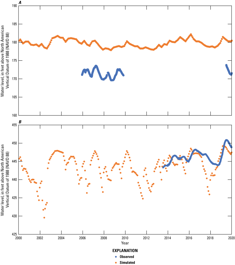
Hydrographs of simulated and observed water levels at (A) U.S. Geological Survey (USGS) regolith monitoring well 354315078300101 WK–332 in Wake County, North Carolina, and (B) USGS transition zone monitoring well 355944079013401 OR–691 in Orange County, North Carolina. Observed water levels from U.S. Geological Survey (2022).
Well OR–691, screened within the transition zone between the regolith and bedrock and grouped with the regolith model layer, is in eastern Orange County (fig. 15). Observed groundwater levels for well OR–691 from 2013 to 2019 ranged from 443 to 451 ft above NAVD 88 (fig. 17B). Simulated groundwater levels at this location also show reasonable agreement, with a range of 429–450 ft above NAVD 88, which indicates that simulated hydraulic gradients were adequate where the transition zone contributes to the groundwater-flow system.
For the bedrock model layer, two wells (WK–438 and WK–368; table 2; fig. 16) were also selected to compare simulated and observed hydrographs (fig. 18). Well WK–438, located near the southern Wake County border, is open within the fractured bedrock with observed groundwater levels that ranged from 276 to 293 ft above NAVD 88 over the period 1982–2019. Simulated groundwater levels for well WK–438 are within 20 ft of the observed variability, ranging from 301 to 312 ft above NAVD 88, which would indicate somewhat reasonable model performance for long-term water level trends in this area of the model (fig. 18A).
Well WK–368, also open within the fractured bedrock, is located in northern Wake County in an area affected by supply well withdrawals (Chapman and others, 2011). Observed groundwater levels for well WK–368 for 2008, 2011–12, and 2019 show large variability, ranging from 187 to 315 ft above NAVD 88 (fig. 18B). However, the simulated groundwater levels at this location, with a range of 356 to 366 ft above NAVD 88, are much higher than the observed levels and do not reflect the observed drawdown effects from nearby pumping wells. This discrepancy highlights the model’s limitation in simulating local drawdown impacts away from the immediate location of the supply well. Refined grid size with higher resolution in the hydraulic conductivity field of the bedrock may improve the simulation of these localized pumping impacts.
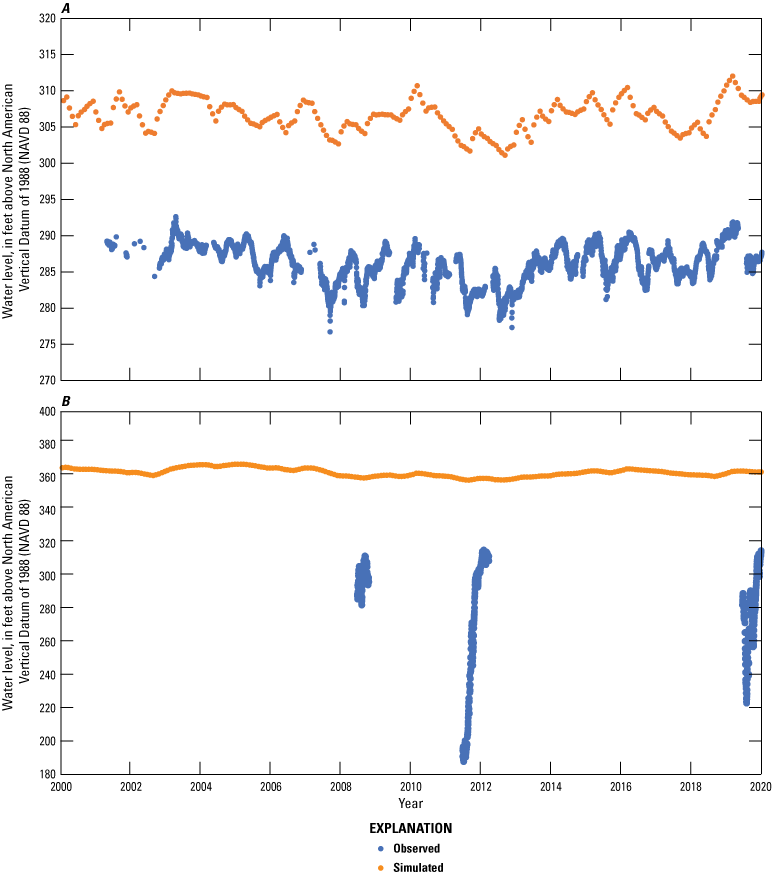
Hydrographs of simulated and observed water levels at (A) North Carolina Department of Environmental Quality Division of Water Resources bedrock monitoring well N41G3 (U.S. Geological Survey [USGS] 353320078483101 WK–438) and (B) USGS bedrock monitoring well 355635078385101 WK–368 in Wake County, North Carolina. Observed water levels from U.S. Geological Survey (2022).
The spatial distribution of groundwater-level residuals across the model domain for model layer 1 (regolith and coastal plain sediments) and layer 2 (bedrock) are shown in figures 19 and 20, respectively. Positive residuals indicate that simulated values are lower than observed values, and negative residuals indicate that simulated values are higher than observed values. Positive and negative residuals were generally well distributed across the model domain with no clear spatial pattern. Smaller residuals within the acceptable calibration criterion (−20 to 20 ft) tended to occur in areas near surface water features, such as the Neuse River, B. Everett Jordan Lake, and Falls Lake (figs. 1, 19, and 20). This pattern suggests better model performance in discharge areas where flow dynamics are more stable compared to upland areas with more variable recharge. Areas with limited observation data from single well measurements tend to have larger residuals--underscoring the importance of having a more robust temporal and spatial water-level dataset to further improve model calibration.
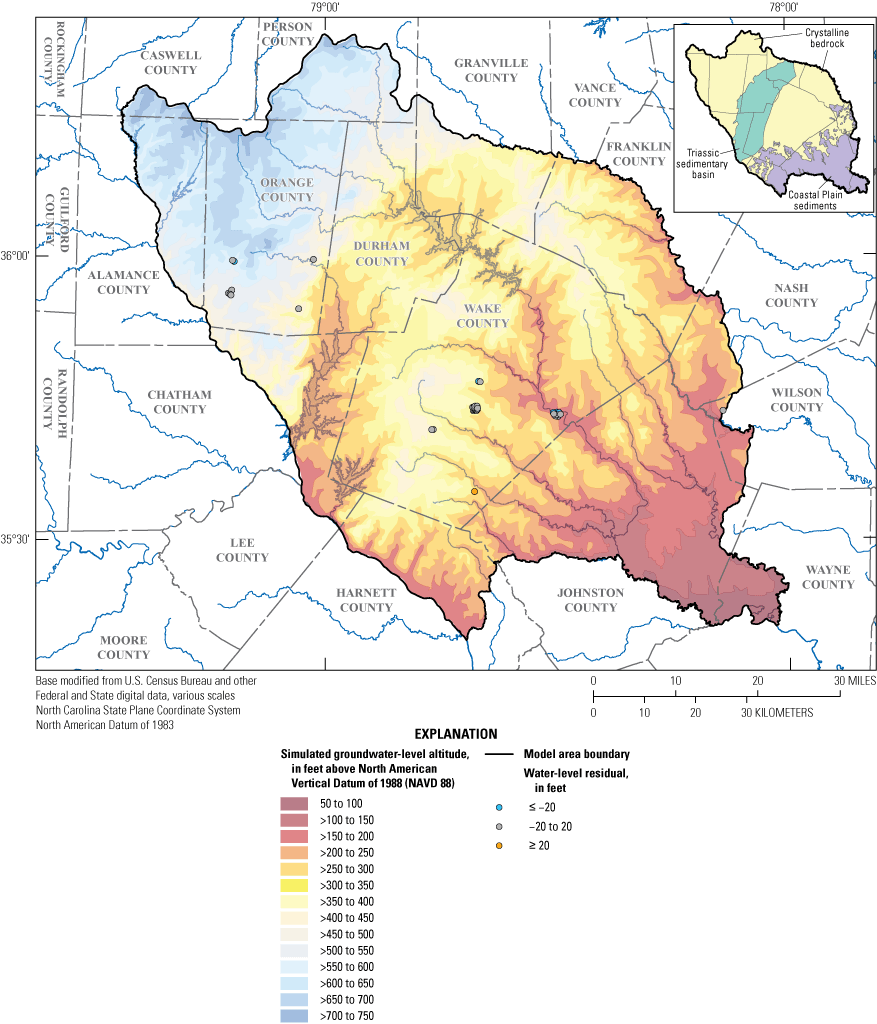
Spatial distribution of mean water-level residuals (observed versus simulated) in model layer 1 (regolith and Coastal Plain sediments) for the calibration period. Positive residuals (orange) indicate simulated values lower than observed values; negative residuals (blue) indicate simulated values higher than observed values. Background color flood map showing simulated groundwater-level altitude for the end of the calibration period (2019), Wake County, North Carolina.
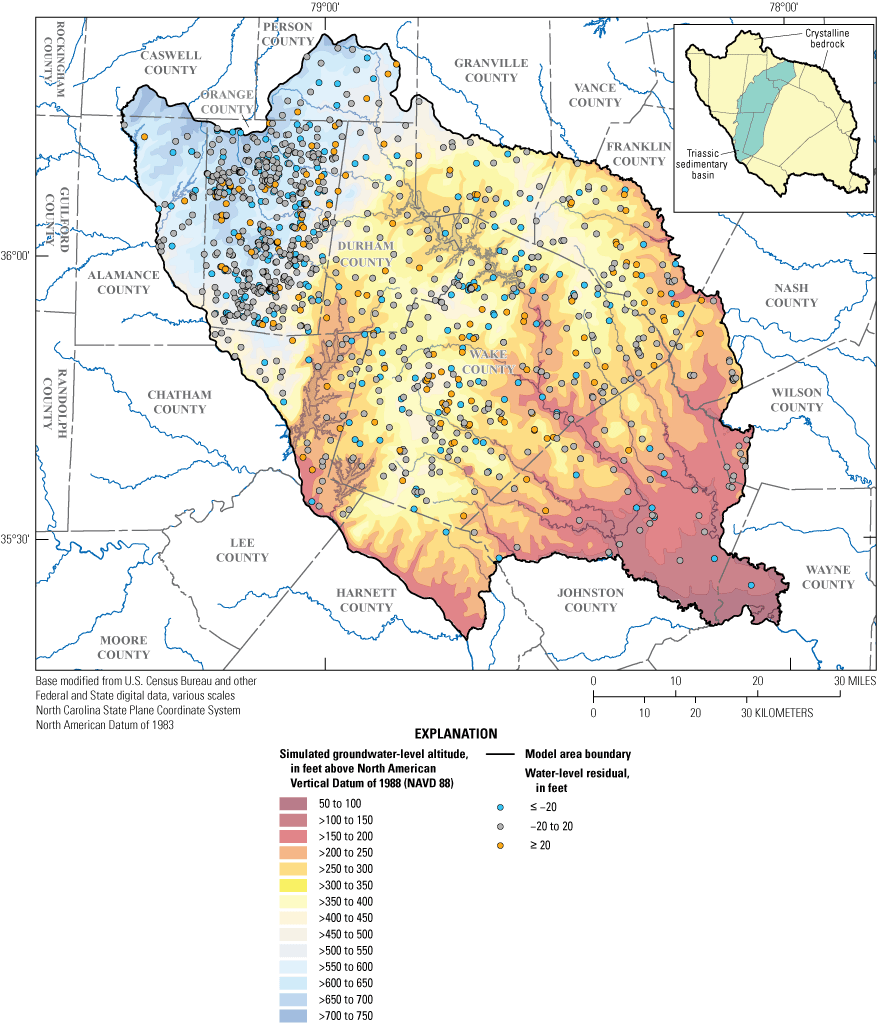
Spatial distribution of mean water-level residuals (observed versus simulated) for model layer 2 (bedrock) for the calibration period. Positive residuals (orange) indicate simulated values lower than observed values; negative residuals (blue) indicate simulated values higher than observed values. Background color flood map showing simulated groundwater-level altitude for the end of the calibration period (2019) Wake County, North Carolina.
Simulated discharge to streams in the model was compared with stream base flow estimates. The monthly base flow estimates determined from the hydrograph separation analysis of four USGS streamgage sites with multiple years of daily streamflow records performed by Antolino and Gurley (2022) form the basis of the groundwater-flow calibration. A calibration criterion of ±50 percent of the observed flow in million cubic feet per day (Mft3/d) was applied to assess the fit between the observed and simulated flows. Three of the four drainage basins have, on average, acceptable fits for the observed and simulated data. Site 02087359, with the smallest of the four drainage basins (fig. 2), had observed base flows during the simulation period ranging from 0.19 to 2.2 Mft3/d (fig. 21A). Simulated base flows were within calibration criteria with a slightly smaller range from 0.8 to 1.9 Mft3/d. Streamgage site 02097314 had observed base flows that ranged from 0.9 to 13.7 Mft3/d, with simulated base flows that ranged from 1.5 to 5.2 Mft3/d and were within the calibration criteria (fig. 21B). Streamgage site 02087324 had observed base flows ranging from 1.4 to 12.1 Mft3/d and simulated flows that ranged from 3.2 to 8.1 Mft3/d (fig. 21C). Streamgage site 02088500, with the largest of the four drainage basins, had simulated flows outside the criterion that ranged from 6.9 to 22.9 Mft3/d yet were within the range of observed flows for the simulation period from 0.08 to 32.7 Mft3/d (fig. 21D). Hydrographs of simulated and observed flows for all four drainage basins show that simulated flows largely only capture the central tendency of the variability in observed base flow trends and low flows within each basin.
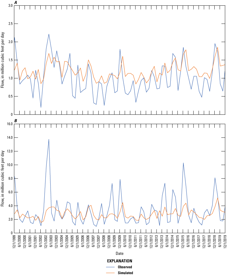
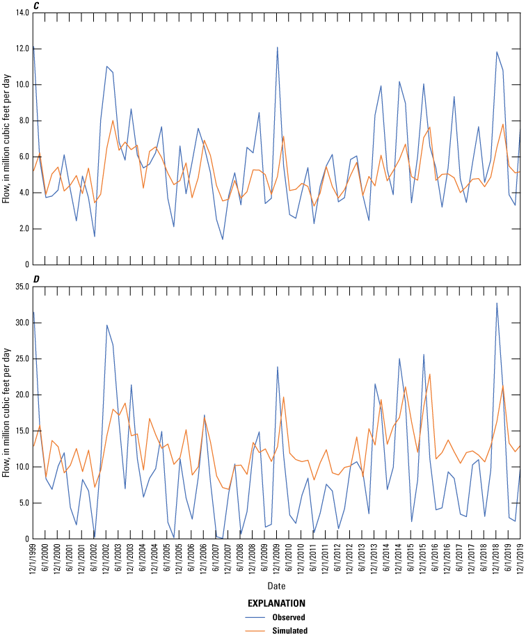
Hydrographs of simulated and observed base flow for (A) U.S. Geological Survey (USGS) streamgage 02087359, (B) USGS streamgage 02097314, (C) USGS streamgage 02087324, and (D) USGS streamgage 02088500 in Wake County, North Carolina.
Groundwater Budget
The calibrated groundwater-flow model was used to simulate a regional groundwater budget for Wake County for 2000–19. The simulated budget highlights the major components of inflow and outflow and the resulting changes in aquifer storage for both the regolith and bedrock model layers. These components are recharge, groundwater discharge to surface water bodies (base flow), supply well withdrawals, and transfers between the regolith and bedrock layers, as well as with the regional groundwater system outside the county. The dynamic balance of these flow exchanges varies in response and magnitude to changing seasonal patterns across the simulation period, providing insights into the groundwater system under variable hydrologic conditions.
Flow rates, in million gallons per day, for the individual groundwater budget components simulated for all transient stress periods are summarized in table 16. The average budget component flows into and out of the regolith and bedrock layers are schematically illustrated in figure 22. For the overall budget, the mean total inflows equal the mean total outflows for the regolith (536.8 Mgal/d) and bedrock (181.9 Mgal/d) layers. On average, recharge (303.7 Mgal/d) composes the dominant inflow, whereas base flow (296.7 Mgal/d) represents the dominant outflow within the groundwater system. This balance reflects near-steady-state conditions for the groundwater system under average climate conditions.
Table 16.
Summary statistics for simulated groundwater budget components, 2000–19, Wake County, North Carolina.[Data from Antolino (2025). Mgal/d, million gallons per day; --, not applicable]
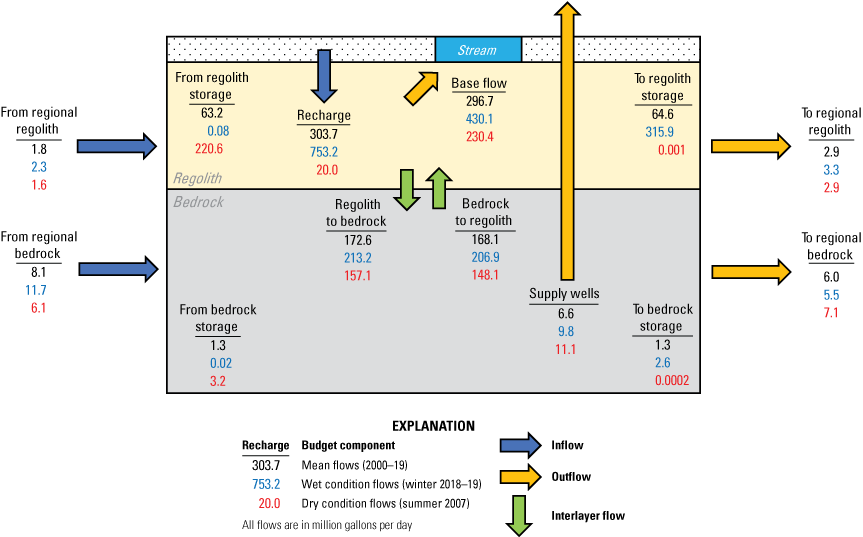
Mean simulated groundwater budget component flows for the transient period (2000–19) and representative examples of wet (winter 2018–19) and dry (summer 2007) condition flows in Wake County, North Carolina.
Aquifer storage is substantially higher in the regolith layer than in the bedrock layer. The mean flow within the groundwater system is 64.6 Mgal/d into regolith storage and 1.3 Mgal/d into bedrock storage (table 16). The influence of seasonal extremes on the groundwater system is illustrated in figure 22 for a representative wet period (winter 2018–19) and a representative dry period (summer 2007). The above-average recharge of 753.2 Mgal/d under wet conditions for winter 2018–19 led to higher base flow to streams (430.1 Mgal/d) and an increase in regolith storage (315.9 Mgal/d). In contrast, during the dry conditions of summer 2007, recharge rates declined to 20.0 Mgal/d, which resulted in decreased base flow and large losses from aquifer storage. During wet periods, excess recharge replenishes regolith storage and, to a much lesser extent, bedrock storage. During dry periods, regolith storage acts as a buffer, supplying groundwater to sustain streamflow and other outflows when recharge is low.
The temporal variability of the simulated water budget components for each seasonal stress period over the 20-year transient simulation period is illustrated in figure 23. Periods of seasonal extremes, shown by peaks and lows in recharge inflow, further illustrate the dynamics of the groundwater budget. One of the wettest periods simulated occurred from summer 2018 to winter 2018–19, characterized by the highest seasonal recharge rates in the simulation period. This period followed high antecedent recharge conditions that increased aquifer storage and supported higher base flow. The driest period simulated, from spring 2007 to fall 2007, had low rates of recharge, causing lower baseflow and proportionally larger contributions from aquifer storage. These periods highlight the sensitivity of the groundwater system to changes in recharge and the critical role of regolith storage in buffering against climatic variability.
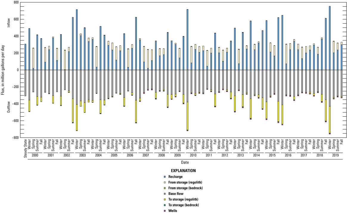
Simulated water budget, by season, from 2000 to 2019. Positive values represent inflows, and negative values represent outflows, Wake County, North Carolina.
Recharge exhibited substantial variability, ranging from 5.4 Mgal/d in spring 2002 (driest period) to 753.2 Mgal/d in winter 2018–19 (wettest period), with a mean of 303.7 Mgal/d (table 16; fig. 23). This variability reflects the direct response of infiltration through the unsaturated zone from precipitation events-- which often occur as short, intense storm events. In contrast, base flow showed less variability than recharge, ranging from 222.7 Mgal/d during the driest period to 430.1 Mgal/d during the wettest period, with a mean discharge rate of 296.7 Mgal/d. The lower variability for the base flow budget component reflects the storage capacity of the groundwater system, where the amount of time groundwater takes to move through the aquifer along various flow paths buffers the flashy extremes of recharge inflow.
The largest changes in storage within the groundwater system ranged from a maximum loss of 246.7 Mgal/d from total aquifer storage into the flow system to a maximum gain of 335 Mgal/d from the flow system into aquifer storage (table 16). This range highlights the sensitivity to variations in recharge and discharge conditions. The mean net change in storage (“to storage” minus “from storage”) was a gain of 1.4 Mgal/d, whereas the median indicated a loss of 26.6 Mgal/d. This discrepancy reflects the impact of more variable recharge events on the mean compared to the relatively constant discharge to streams that is better captured by the median. Storage for the fractured-rock groundwater system is primarily concentrated in the overlying regolith, with minimal storage capacity in the fractured bedrock. The regolith accumulates storage during wet periods yet is prone to notable losses during dry periods. This dynamic is crucial in understanding the groundwater system response to prolonged droughts, particularly in areas dependent on groundwater withdrawals.
Groundwater withdrawal to supply wells was one of the smallest components in the county-wide simulated budget. Reported supply withdrawals ranged from 0.8 to 11.4 Mgal/d with a mean of 6.6 Mgal/d over the simulation period 2000–19 (table 16). Whereas these withdrawals appear minimal at the county scale, their localized impact at a small basin scale can be substantial where supply wells are concentrated. The magnitude of observed drawdowns in monitoring-network wells near large community-supply wells, such as USGS monitoring well WK–368 (figs. 5 and 7), highlights the limited storage capacity of the fractured-bedrock groundwater system in such areas.
Forecast Scenario Simulations
The calibrated groundwater-flow model for Wake County was used to simulate future scenarios that included 204 stress periods representing seasonal data from winter 2019–20 through fall 2070, hereinafter referred to as the “forecast period.” These scenarios incorporated projected development patterns based on the FUTURES model and climate variability under the RCP 4.5 and RCP 8.5 emissions scenarios for three GCMs that represent a range of dry to wet climatic conditions (Meentemeyer and others, 2013; Sanchez and others, 2020b). The simulations were to assess potential future impacts of climate variability and increased development on recharge and base flow, the two major components of the Wake County groundwater budget. The model forecast results were compared against simulated recharge and base flow for 2000–19 in the calibrated model (referred to as the “calibrated simulation”) to highlight potential future changes in recharge and base flow projections from 2000–19 conditions. The discussion focuses on the results of the RCP 4.5 and RCP 8.5 emissions scenarios, which reflect the aggregated results of the three GCMs used to represent the overall range in potential future climate conditions. Aggregating forecast models by RCP scenario may reduce apparent spread of variability within individual model runs, yet this presentation emphasizes the central tendency and overlapping range across all runs for each RCP scenario. The difference in the number of simulations and timeframes should be considered when comparing variability and central tendency between the calibrated and aggregated forecast simulation results. Percentiles of the simulation results, including the medians (50th percentiles), interquartile range (IQR, difference between the 25th and 75th percentiles), and the extremes (10th and 90th percentiles), are displayed as box plots in figures 24 and 25 to examine temporal and seasonal changes in the distributions of the recharge and base flow forecast results. The percentile dataset is provided in table 1.1 in appendix 1.
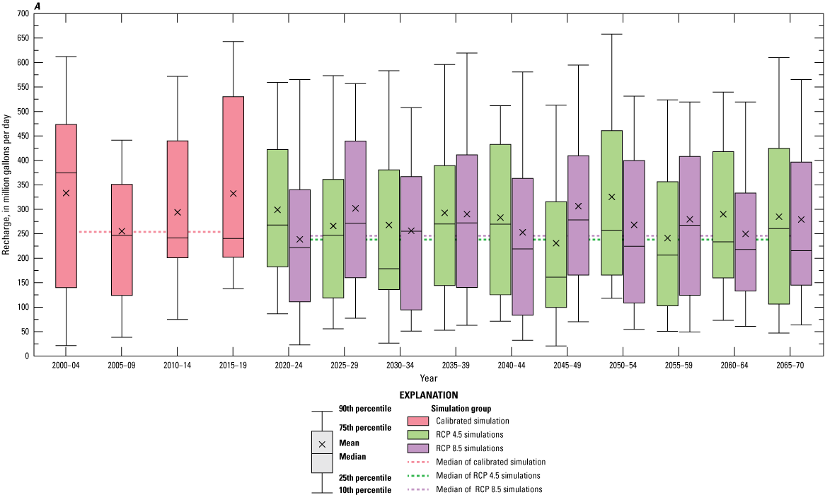
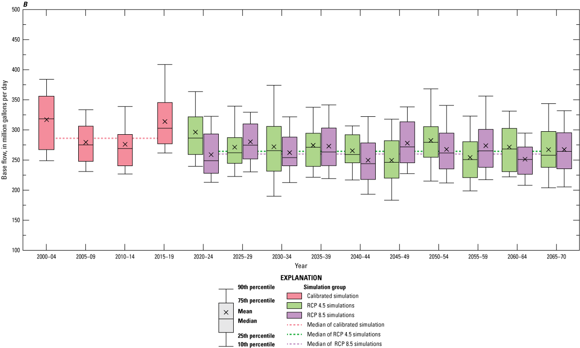
Recharge A, and base flow B, water budget components of model forecast simulations for both representative concentration pathway (RCP) 4.5 and RCP 8.5 emissions scenarios for 2020–70 compared with the calibrated simulation for 2000–19 for the study area, Wake County, North Carolina.
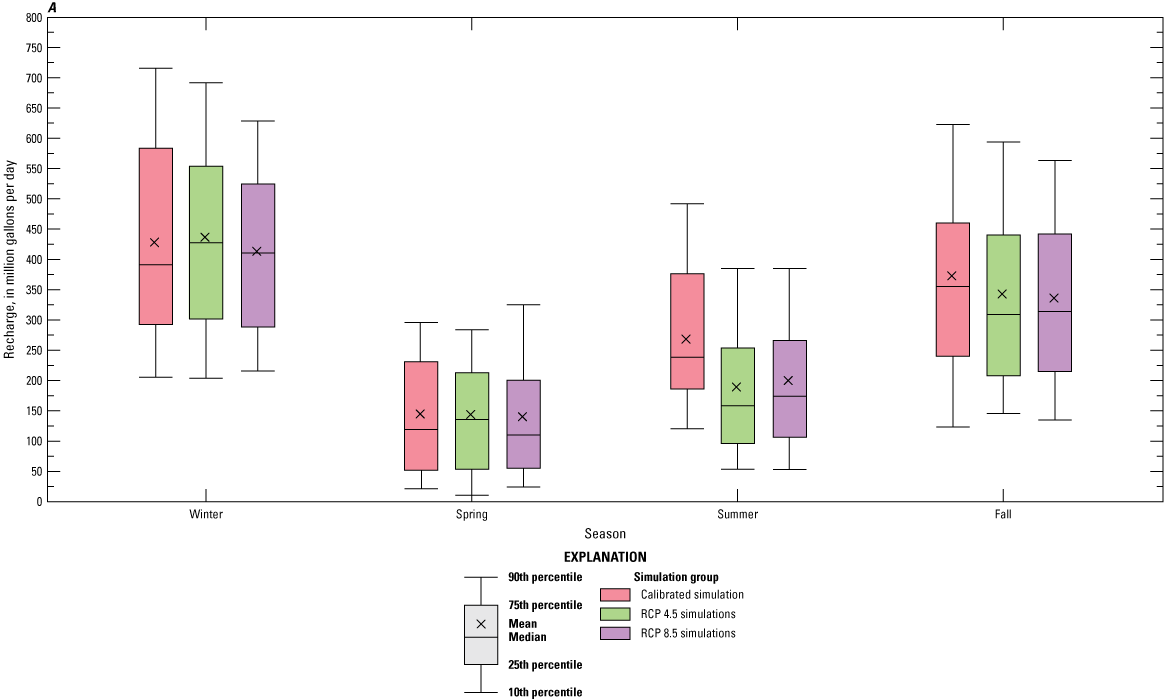
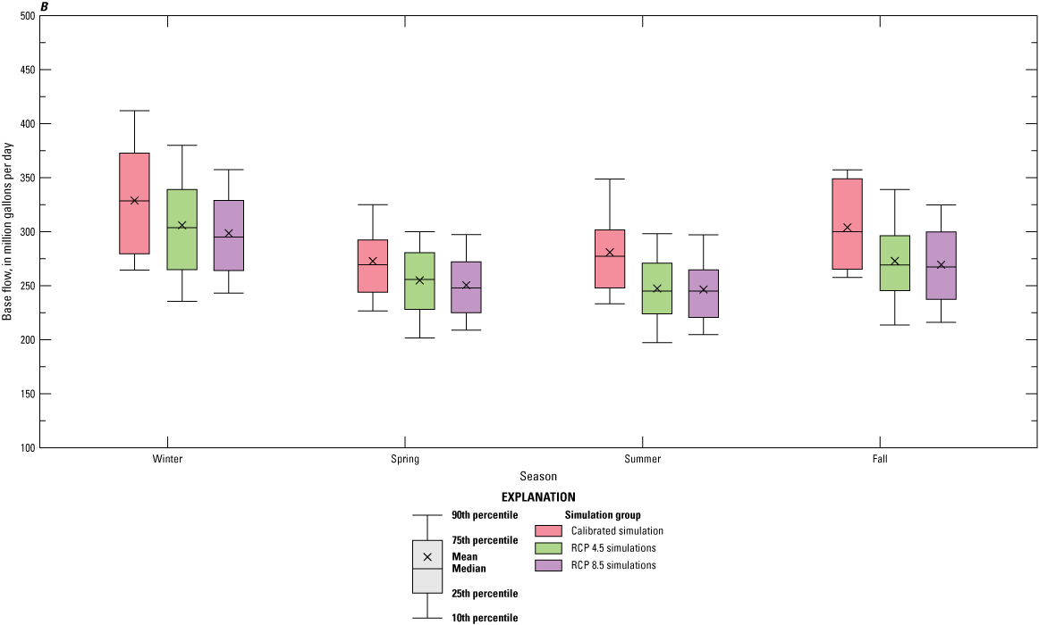
Seasonal recharge A, and base flow B, water budget components of model forecast simulations for both representative concentration pathway (RCP) 4.5 and RCP 8.5 emissions scenarios for 2020–70 compared with the calibrated simulation for 2000–19 for the study area, Wake County, North Carolina.
The temporal results for simulated recharge and base flow rates across the calibrated and forecast periods are shown in figure 24. Data were arbitrarily grouped by 5-year intervals, with a 6-year interval used for 2065–70, to aid visualization and comparisons across the entire forecast period. Examination of recharge results indicate a slight downward shift in recharge rates between the IQRs of the calibrated simulation dataset and the forecast simulation dataset (fig. 24A). This shift likely is influenced by a combination of factors, including changes in climate conditions projected by the GCMs, such as increased evapotranspiration because of warmer temperatures, and impacts of increased urban development, such as a larger impervious footprint reducing infiltration and altering runoff dynamics. Additionally, differences in the spatial resolution of the climate datasets used in the SWB model (Antolino, 2022) that provided recharge input to the groundwater model simulations may contribute to the shift. The finer 1-km resolution of the Daymet dataset, used for the calibration period, captures localized variability that would include high recharge events that contribute a notable portion of the total recharge component. In contrast, the coarser 4-km resolution of the MACAv2 dataset at 4-km scale, used for the forecast simulations, likely smooths out these events, leading to a slightly more muted recharge estimate. A similar downward shift was noted in the base flow results between the calibrated and forecast simulation datasets (fig. 24B). Because base flow is coupled to seasonal and annual recharge dynamics, changes to values in future recharge may propagate as changes in groundwater discharge to streams.
No apparent trends were noted in the forecast simulation period of 2020–70 that would suggest potential long-term changes in future recharge or base flow (figs. 24A and 24B, respectively). However, future recharge and base flow rates could have considerable yearly variability as indicated by the temporal variability within and among individual time intervals for RCP 4.5 and RCP 8.5 forecast simulations. End members in forecast recharge rates across all forecast time intervals, based on the 10th and 90th percentiles, ranged from 20.8 Mgal/d (2045–49) to 658.1 Mgal/d (2050–54) for RCP 4.5 and 23.0 Mgal/d (2020–24) to 619.5 Mgal/d (2035–39) for RCP 8.5. These ranges were similar to the low of 21.5 Mgal/d (2000–04) and high of 643.0 Mgal/d (2015–19) for the calibrated simulation. For all time intervals, median recharge values for RCP 4.5 varied by a factor of about 1.7, ranging from 161.4 to 270.1 Mgal/d. For RCP 8.5, median recharge values varied by a factor of about 1.3, ranging from 215.3 to 278.3 Mgal/d. Median recharge values for the calibrated simulation varied by a factor of about 1.6, ranging from 240.3 to 374.6 Mgal/d.
Similarly, end members in base flow rates across all forecast time intervals ranged from 183.1 Mgal/d (2045–49) to 374.3 Mgal/d (2030–34) for RCP 4.5 and 193.0 Mgal/d (2040–44) to 356.3 Mgal/d (2055–59) for RCP 8.5 (fig. 24B). The calibrated simulation exhibited a wider range in base flow end members, from a low of 226.7 Mgal/d (2010–14) to a high of 408.8 Mgal/d (2015–19). Across all time intervals, median base flow values for RCP 4.5 varied by a factor of about 1.2, ranging from 246.2 to 286.4 Mgal/d. For RCP 8.5, median base flow values varied by a factor of about 1.1, with a range of 244.0 to 274.7 Mgal/d. Median base flow values for the calibrated simulation varied by a factor of about 1.2, ranging from 269.2 to 318.5 Mgal/d. Overall variability between RCPs 4.5 and 8.5 was similar across the forecast period for both recharge and base flow. Simulated recharge rates showed more variability than did base flow rates, likely reflecting the episodic nature of precipitation that directly influences groundwater recharge. Meanwhile, groundwater discharge was moderated by aquifer storage, which buffered short-term variability and provided more consistent base flow to streams. Although the model effectively captured the central tendency of base flow conditions, it underrepresented observed low base flows (fig. 21A–D)—a limitation to be considered when interpreting forecast results of base flow, especially for periods of extended dry conditions with low recharge when extreme low flows are likely.
Seasonal analysis of recharge and base flow indicated a similar pattern of higher rates occurring in winter and fall and lower rates in spring and summer for both the calibrated and forecast simulation periods (fig. 25). Recharge rates (fig. 25A) and base flow rates (fig. 25B) were most variable during the winter season, reflecting the interaction of increased precipitation and reduced evapotranspiration. A downward shift in recharge and base flow for RCPs 4.5 and 8.5 is noted for all seasons except for recharge in winter and spring. As stated above, a downward shift between the calibrated and forecast datasets likely reflects a combination of dataset resolution differences and potential climate-driven changes. Median recharge values in winter for RCPs 4.5 and 8.5 (427.5 and 410.7 Mgal/d, respectively) were slightly higher than the winter median of 391.0 Mgal/d for the calibrated simulation that may suggest a potential for increased winter recharge under future climate scenarios. Across seasons, median recharge values varied by a factor of about 3.1 for RCP 4.5, a factor of about 3.7 for RCP 8.5, and a factor of about 3.3 for the calibrated simulation. Median base flow values for RCP 4.5, RCP 8.5, and the calibrated simulation all varied across seasons by a factor of 1.2. These seasonal patterns suggest that, while overall recharge rates do not deviate outside historical observational ranges, potential increases in winter recharge may slightly offset potential reductions during other seasons.
Forecast scenario simulations highlight the sensitivity of the regional groundwater system to potential future climate variability, with some impacts on rates of recharge and base flow. These impacts are driven by shifts in precipitation patterns, evapotranspiration rates, and overall seasonal dynamics. Winter recharge may increase under future conditions, partially offsetting reduced recharge during spring and summer. During periods of extended dry conditions when recharge becomes more intermittent and driven by specific episodic events, aquifer storage in forecast simulations gradually depletes because of limited recharge. This depletion lowers groundwater levels and consequently reduces groundwater discharge to streams. Whereas the buffering capacity of aquifer storage helps stabilize base flow rates during short-term dry conditions, extended dry periods can diminish this capacity over the duration of drought. Monitoring groundwater levels, changes in aquifer storage, recharge rates, and streamflow (especially during low flow conditions) provides valuable data to aid with tracking changes, validating and updating projections, and informing adaptive management strategies for sustaining groundwater resources under variable climate conditions.
Model Limitations and Future Considerations
As with all models, development of the groundwater-flow model for this study involved the simplification of a complex natural system. This simplification can introduce limitations arising from assumptions about uniform aquifer geometry and averaging aquifer properties over large areas with incomplete information. These limitations relate to the model structure, model parameters, and input data uncertainty.
Structural limitations in the model include the discretization of the model grid and layering. The 500 by 500 ft grid resolution smooths fine-scale topographic and geologic variability, limiting the model’s ability to resolve localized hydraulic gradients near streams and reservoirs. Refining the model grid resolution in sensitive and critical areas, such as zones with dense fracturing, could improve the simulation of localized flow paths and groundwater/surface water interactions.
The model has a two-layer configuration to represent the regolith and fractured bedrock and assumes uniform groundwater flow within each layer. This simplification overlooks more complex vertical variations in hydraulic conductivity and fracture density--critical for understanding groundwater flow in fractured-rock aquifers. Incorporating additional model layers to represent these vertical variations could improve the simulation of fracture flow. The thickness of the regolith layer was interpolated using well-construction data, which varied in availability across the model area. Areas with fewer available well-construction records had higher uncertainty in the interpolation, potentially introducing spatial bias. Sparse data coverage may result in underestimated layer thickness for some areas because of a lack of local data points. These artificially thin cells within the layer could reduce storage capacity in the model, potentially leading to flooded cells and requiring hydraulic conductivity parameter compensation to increase flow out of the cells. This uncertainty affects the accuracy of the aquifer storage simulations, as saturated regolith thickness is a critical parameter for estimating groundwater availability and local water budgets. Future improvements could include collecting additional well-construction information and conducting high-resolution geophysical surveys in data-poor areas to refine regolith thickness estimates and improve the simulation of aquifer storage and flow dynamics in the model.
Recharge is represented as net infiltration using the SWB model, which assumes that all infiltrated water below the root zone contributes to groundwater recharge. This simplification neglects lateral flow in the unsaturated zone and areas with high water tables, potentially overestimating recharge in some regions. Incorporating additional MODFLOW packages, such as the Unsaturated Zone Flow (UZF) package (Niswonger and others, 2006), could improve recharge estimates by better representing lateral flow and unsaturated zone dynamics.
Drain cells are used to simulate streams and reservoirs in the model, but these cells do not fully capture the dynamic groundwater/surface water interactions, especially during low-flow conditions. The Drain (DRN) package (Harbaugh and others, 2000) assumes one-way flow from the groundwater system into the drain feature without accounting for feedback mechanisms such as streamflow depletion from nearby pumping or losing stream reaches. Using MODFLOW packages like the Streamflow-Routing (SFR2) (Niswonger and Prudic, 2005) or Lake (LAK) (Merritt and Konikow, 2000) packages could improve the representation of surface water bodies and their interactions with the groundwater system.
Hydraulic properties are represented as bulk averages over large distances, reducing model accuracy in reflecting the heterogeneity of fractured bedrock. Collecting additional site-specific data, such as aquifer tests and high-resolution geophysical surveys, could help better constrain hydraulic parameters and improve spatial accuracy in fracture property characterization. A hybrid modeling approach, combining regional equivalent-porous-media models with local discrete-fracture-network models, could enhance simulations in fracture-dominated systems (Normani and Sykes, 2018; Kuniansky, 2016).
Groundwater withdrawals were assumed to remain constant at 2019 rates throughout the forecast period to highlight potential impacts to the groundwater system related to changing climate variables and land cover changes from increasing development. Therefore, the presented forecast scenarios do not account for potential increases in groundwater demand due to population growth or management strategies. Additional scenarios can be developed from the calibrated model simulation that also incorporate changes in future groundwater demand. Developing expanded scenarios that incorporate dynamic groundwater withdrawals, informed by historically increasing trends or future projections of population growth and water demand, could provide more comprehensive projections of groundwater availability under varying demand conditions.
Calibration relied on limited spatial and temporal datasets for water levels and streamflow, reducing the ability to simulate extreme hydrologic conditions. Expanding the calibration dataset to include more high-frequency and continuous water-level measurements, especially in paired regolith and bedrock wells, could improve model reliability and the representation of short-term fluctuations, such as pumping impacts. Additional base flow measurements during extreme low-streamflow conditions may also improve the simulation of groundwater contribution to streams during these extreme conditions.
Summary
In 2019, the U.S. Geological Survey partnered with Wake County Environmental Services to initiate a study to assess groundwater resources and long-term groundwater availability within the fractured-rock groundwater system in Wake County, North Carolina. Study tasks included the collection and compilation of hydrogeologic data including groundwater levels, aquifer testing, borehole fracture flow measurements, and water-quality sampling that included groundwater stable isotope and age-dating tracers. These datasets helped to provide a better understanding of the hydrologic and geochemical conditions within the groundwater system and were used to inform the development of a baseline groundwater-flow model for Wake County. The regional groundwater-flow model was developed to represent a simplified, conceptual understanding of the local groundwater system and was used to assess future groundwater availability, as well as identify data uncertainty and data needs to inform future investigation efforts.
Aquifer hydraulic properties were estimated through slug tests and borehole vertical flow measurements conducted in a monitoring well network established for Wake County. The horizontal hydraulic conductivity and transmissivity data obtained from these tests provided information on how groundwater moves and is stored in the fractured-rock groundwater system. Borehole geophysical logs and measurements of borehole-flow dynamics within the monitoring-network wells helped to identify the location and transmissivity of primary water-bearing fractures in the local aquifer. Understanding the fracture network is critical for evaluating the dynamics of groundwater flow paths and connectivity within the fractured-bedrock groundwater system.
The stable isotope results indicated that the groundwater closely resembles modern local precipitation with minimal evaporation before entering the aquifer. This information confirms precipitation as the critical recharge source and provides distinct isotopic signatures for precipitation, groundwater, and surface water, enabling the identification of evaporative processes within the study area. Dissolved oxygen levels indicated the occurrence of oxic conditions in the regolith and mixed anoxic-oxic conditions in the bedrock. The presence of dissolved methane in some bedrock wells indicated more enhanced reducing conditions in the aquifer at some locations. The groundwater age-dating results indicated apparent ages ranging from the 1940s to the 1990s, with some samples showing evidence of mixing between older and younger groundwater. This age distribution can provide insight into groundwater sustainability, where younger waters indicate areas of frequent recharge and greater resilience, and older waters suggest slower recharge rates with higher risk of depletion.
The developed MODFLOW groundwater-flow model provided a framework for simulating groundwater conditions over time in the fractured-rock groundwater system. The model was discretized to simplify the complex aquifer into two layers, with the upper layer representing the regolith and transition zone (layer 1) and the lower layer representing the fractured bedrock (layer 2). Spatial and temporal variations in groundwater recharge estimates were included as input into the model. Model parameter groups used in the calibration process were horizontal hydraulic conductivity, horizontal and vertical anisotropy, specific yield, specific storage, and drain conductance. Distributed pilot points were used in the iterative calibration of the horizontal hydraulic conductivity parameter to account for spatial heterogeneity across the model. Horizontal anisotropy values showed that shallow groundwater flows perpendicular to general streamflow direction in the regolith layer and more parallel to streams within the bedrock layer across the study area. Vertical anisotropy values showed that groundwater flows more laterally within the regolith layer and relatively uniformly within the bedrock layer. Parameter sensitivity analysis showed that horizontal and vertical anisotropy were highly sensitive within the simulation, reflective of the heterogeneity in the fractured-rock groundwater system. The calibrated modular three-dimensional finite-difference groundwater-flow model produced a reasonable fit to observed groundwater levels from 1,100 wells, including both regolith and bedrock well sites, while accounting for the range of water levels and inherent structural simplifications in the model. Results indicated a mean water-level residual of 8.1 feet (ft) and root mean square error (RMSE) of 9.4 ft for the regolith wells. The mean water-level residual for the bedrock wells was 19.9 ft with an RMSE of 26 ft.
The groundwater budget developed for Wake County identified recharge and groundwater discharge to streams (base flow) as the dominant inflow and outflow components, respectively, primarily balancing the water budget under steady-state conditions. Recharge had a mean recharge rate of 303.7 million gallons per day (Mgal/d), and groundwater discharge to streams had a mean of 296.7 Mgal/d. The low storage capacity of the fractured-rock groundwater system makes the groundwater system sensitive to changes in seasonal recharge. This sensitivity can be seen regionally with water-level fluctuations ranging 5–10 ft. Although groundwater withdrawals were the smallest component of the county-wide budget, with a mean pumping rate near 6.6 Mgal/d, simulated localized impacts included significant drawdown, as large as 100 ft in observation wells near supply wells, demonstrating the influence of pumping at small basin scale.
The calibrated groundwater-flow model was used to simulate forecast scenarios with global climate models from two emissions scenarios and future land cover projections from 2020 to 2070. These forecast scenarios projected recharge and base flow rates to assess the major responses of the groundwater system under a range of potential future climate conditions. The results indicated no apparent long-term trends in recharge or base flow rates between the calibrated and forecast periods. Projected recharge and base flow rates show seasonal and annual variability across the forecast period for the RCP 4.5 and RCP 8.5 simulations. Recharge showed greater variability than base flow showed, reflecting episodic precipitation events that directly influence recharge, compared to the buffered short-term variability in base flow because of the nature of the aquifer flow and storage properties. The variability within the projected recharge and base flow rates does not reflect large long-term deviations from historical ranges, though year-to-year variability shows instances where extreme values exceeded those of the calibrated simulation.
References Cited
Abatzoglou, J.T., 2013, Development of gridded surface meteorological data for ecological applications and modelling: International Journal of Climatology, v. 33, no. 1, p. 121–131, accessed December 5, 2022, at https://doi.org/10.1002/joc.3413.
Abatzoglou, J.T., and Brown, T.J., 2012, A comparison of statistical downscaling methods suited for wildfire applications: International Journal of Climatology, v. 32, no. 5, p. 772–780, accessed December 5, 2022, at https://doi.org/10.1002/joc.2312.
Antolino, D.J., 2022, Soil-Water-Balance (SWB) model datasets for the greater Wake County area, North Carolina, 1981–2019: U.S. Geological Survey data release, accessed December 5, 2022, at https://doi.org/10.5066/P95XKK5V.
Antolino, D.J., 2025, MODFLOW-NWT model used to simulate groundwater flow in Wake County, North Carolina, 2000 through 2070: U.S. Geological Survey data release, https://doi.org/10.5066/P9N3EQ86.
Antolino, D.J., and Gurley, L.N., 2022, Assessment of well yield, dominant fractures, and groundwater recharge in Wake County, North Carolina (ver. 1.1, May 2022): U.S. Geological Survey Scientific Investigations Report 2022–5041, 35 p., accessed December 5, 2022, at https://doi.org/10.3133/sir20225041.
Bain, G.L., and Brown, C.E., 1981, Evaluation of the Durham Triassic Basin of North Carolina and technique used to characterize its waste-storage potential: U.S. Geological Survey Open-File Report 80–1295, 138 p., 1 pl. [Also available at https://doi.org/10.3133/ofr801295.]
Ballentine, C.J., and Burnard, P.G., 2002, Production, release and transport of noble gases in the continental crust, in Porcelli, D., Ballentine, C.J., and Wieler, R., eds., Noble gases in geochemistry and cosmochemistry: Reviews in Mineralogy and Geochemistry, v. 47, p. 481–538. [Also available at https://doi.org/10.2138/rmg.2002.47.12.]
Beyerle, U., Aeschbach-Hertig, W., Imboden, D.M., Baur, H., Graf, T., and Kipfer, R., 2000, A mass spectrometric system for the analysis of noble gases and tritium from water samples: Environmental Science and Technology, v. 34, no. 10, p. 2042–2050, accessed August 18, 2022, at https://doi.org/10.1021/es990840h.
Bouwer, H., and Rice, R.C., 1976, A slug test for determining hydraulic conductivity of unconfined aquifers with completely or partially penetrating wells: Water Resources Research, v. 12, no. 3, p. 423–428, accessed January 3, 2023, at https://doi.org/10.1029/WR012i003p00423.
Campbell, B.G., and Landmeyer, J.E., 2023, Groundwater availability, geochemistry, and flow pathways to public-supply wells in the Atlantic Coastal Plain and bedrock aquifers, Aiken County and part of Lexington County, South Carolina, 2015–2019: U.S. Geological Survey Scientific Investigations Report 2022–5036, 117 p., accessed December 3, 2023, at https://doi.org/10.3133/sir20225036.
CDM, 2003, Wake County comprehensive groundwater investigation: CDM, 147 p., accessed October 8, 2020, at https://s3.us-west-2.amazonaws.com/wakegov.com.if-us-west-2/prod/documents/2020-10/06%20L5%20-%20WakeCountyCGIFinalReport_web.pdf.
Chapman, M.J., Almanaseer, N., McClenney, B., and Hinton, N., 2011, Fluctuations in groundwater levels related to regional and local withdrawals in the fractured-bedrock groundwater system in northern Wake County, North Carolina, March 2008–February 2009: U.S. Geological Survey Scientific Investigations Report 2010–5219, 60 p.
Chapman, M.J., Bolich, R.E., and Huffman, B.A., 2005, Hydrogeologic setting, ground-water flow, and ground-water quality at the Lake Wheeler Road research station, 2001–03, North Carolina Piedmont and Mountains Resource Evaluation Program: U.S. Geological Survey Scientific Investigations Report 2005–5166, 85 p.
Chapman, M.J., Schlegel, M., Huffman, B.A., and McSwain, K.B., 2007, Hydraulic gradients in recharge and discharge areas and apparent ground-water age dates from the characterization of multiple regolith-fractured bedrock ground-water research stations in North Carolina, in 2007 Georgia Water Resources Conference, Athens, Ga., March 27–29, 2007, [Proceedings]: Statesboro, Ga., Georgia Southern University, 4 p.
Clark, T.W., Blake, D.E., Stoddard, E.F., Carpenter, P.A., III, and Carpenter, R.H., 2004, Preliminary bedrock geologic map of the Raleigh 30’ x 60’ quadrangle, North Carolina: North Carolina Geological Survey Open File Report 2004–02, 1 sheet, scale 1:100,000, in color. [Also available at https://deq.nc.gov/energy-mineral-and-land-resources/geological-survey/ofrs-geological-survey/ncgs-ofr-2004-02-raleigh-100k-bedrock-geopdf/download.]
Clarke, W.B., Jenkins, W.J., and Top, Z., 1976, Determination of tritium by mass spectrometric measurement of 3He: International Journal of Applied Radiation and Isotopes, v. 27, no. 9, p. 515–522, accessed August 19, 2022, at https://doi.org/10.1016/0020-708X(76)90082-X.
Craig, H., Lupton, J.E., Welhan, J.A., and Poreda, R., 1978, Helium isotope ratios in Yellowstone and Lassen Park volcanic gases: Geophysical Research Letters, v. 5, no. 11, p. 897–900, accessed October 16, 2023, at https://doi.org/10.1029/GL005i011p00897.
Cunningham, W.L., and Schalk, C.W., comps., 2011, Groundwater technical procedures of the U.S. Geological Survey: U.S. Geological Survey Techniques and Methods, book 1, chap. A1, 151 p., accessed October 16, 2023, at https://doi.org/10.3133/tm1A1.
Daniel, C.C., III, and Harned, D.A., 1998, Ground-water recharge to and storage in the regolith-fractured crystalline rock groundwater system, Guilford County, North Carolina: U.S. Geological Survey Water-Resources Investigations Report 97–4140, 65 p., accessed August 27, 2020, at https://pubs.er.usgs.gov/publication/wri974140.
Dansgaard, W., 1964, Stable isotopes in precipitation: Tellus, v.16, no. 4, p. 436–468, accessed November 2, 2023, at https://doi.org/10.3402/tellusa.v16i4.8993.
Dewitz, J., and U.S. Geological Survey, 2021, National Land Cover Database (NLCD) 2019 products (ver. 2.0, June 2021): U.S. Geological Survey data release, accessed December 5, 2022, at https://doi.org/10.5066/P9KZCM54.
Dieter, C.A., and Maupin, M.A., 2017, Public supply and domestic water use in the United States, 2015: U.S. Geological Survey Open-File Report 2017–1131, 6 p., accessed December 5, 2022, at https://doi.org/10.3133/ofr20171131.
Doherty, J., 2003, Ground water model calibration using pilot points and regularization: Ground Water, v. 41, no. 2, p. 170–177, accessed December 5, 2022, at https://doi.org/10.1111/j.1745-6584.2003.tb02580.x.
Fine, J.M., and Kuniansky, E.L., 2014, Simulation of groundwater flow and saltwater movement in the Onslow County area, North Carolina—Predevelopment–2010: U.S. Geological Survey Scientific Investigations Report 2013–5236, 106 p., accessed December 5, 2022, at https://doi.org/10.3133/sir20135236.
Fulford, J.M., and Clayton, C.S., 2015, Accuracy testing of steel and electric groundwater-level measuring tapes—Test method and in-service tape accuracy: U.S. Geological Survey Open-File Report 2015–1137, 31 p., accessed November 2, 2023, at https://doi.org/10.3133/ofr20151137.
Gonthier, G.J., and Antolino, D.J., 2023, Water-level data and results for slug tests performed in 17 wells in Wake County, North Carolina, 2020 and 2021 (ver. 1.1, May 2025): U.S. Geological Survey data release, accessed May 7, 2025, at https://doi.org/10.5066/P9UC8F3Z.
Goode, D.J., and Senior, L.A., 2020, Groundwater withdrawals and regional flow paths at and near Willow Grove and Warminster, Pennsylvania—Data compilation and preliminary simulations for conditions in 1999, 2010, 2013, 2016, and 2017: U.S. Geological Survey Open-File Report 2019–1137, 127 p., accessed December 14, 2023, at https://doi.org/10.3133/ofr20191137.
Harbaugh, A.W., Banta, E.R., Hill, M.C., and McDonald, M.G., 2000, MODFLOW-2000, the U.S. Geological Survey modular ground-water model—User guide to modularization concepts and the ground-water flow process: U.S. Geological Survey Open-File Report 00–92, 121 p., accessed July 1, 2022, at https://doi.org/10.3133/ofr200092.
Harned, D.A., and Daniel, C.C., III, 1992, The transition zone between bedrock and regolith—Conduit for contamination?, in Daniel, C.C., III, White, R.K., and Stone, P.A., eds., Ground water in the Piedmont, Proceedings of a Conference on Ground Water in the Piedmont of the Eastern United States, Charlotte, N.C., Oct. 16–18, 1989: Clemson, S.C., Clemson University, p. 336–348.
Harte, P.T., 2021, Numerical modeling of groundwater flow in the crystalline-rock aquifer in the vicinity of the Savage Municipal Water-Supply Well Superfund site, Milford, New Hampshire: U.S. Geological Survey Scientific Investigations Report 2020–5137, 47 p., accessed December 5, 2022, at https://doi.org/10.3133/sir20205137.
Heath, R.C., 1984, Ground-water regions of the United States: U.S. Geological Survey Water Supply Paper 2242, 78 p., accessed August 27, 2020, at https://pubs.er.usgs.gov/publication/wsp2242.
Horn, M.A., Moore, R.B., Hayes, L., and Flanagan, S.M., 2008, Methods for and estimates of 2003 and projected water use in the Seacoast region, southeastern New Hampshire: U.S. Geological Survey Scientific Investigations Report 2007–5157, 87 p., 2 app. [on CD-ROM], accessed January 16, 2025, at https://pubs.usgs.gov/sir/2007/5157.
Hutson, S.S., Barber, N.L., Kenny, J.F., Linsey, K.S., Lumia, D.S., and Maupin, M.A., 2004, Estimated use of water in the United States in 2000: U.S. Geological Survey Circular 1268, 46 p., accessed December 5, 2022, at https://pubs.usgs.gov/circ/2004/circ1268/.
Intergovernmental Panel on Climate Change, 2019, Scenario process for AR5—Scenarios background information: Intergovernmental Panel on Climate Change Data Distribution Centre web page, accessed September 1, 2022, at https://sedac.ciesin.columbia.edu/ddc/ar5_scenario_process/scenario_background.html.
Jean-Baptiste, P., Mantisi, F., Dapoigny, A., and Stievenard, M., 1992, Design and performance of a mass spectrometric facility for measuring helium isotopes in natural waters and for low-level tritium determination by the 3He ingrowth method: International Journal of Radiation Applications and Instrumentation. Part A. Applied Radiation and Isotopes, v. 43, no. 7, p. 881–891, accessed November 5, 2023, at https://doi.org/10.1016/0883-2889(92)90150-D.
Jurgens, B.C., Böhlke, J.K., Haase, K., Busenberg, E., Hunt, A.G., and Hansen, J.A., 2020, DGMETA (version 1)—Dissolved gas modeling and environmental tracer analysis computer program: U.S. Geological Survey Techniques and Methods, book 4, chap. F5, 50 p., accessed December 5, 2022, at https://doi.org/10.3133/tm4F5.
Kendall, C., and Coplen, T.B., 2001, Distribution of oxygen-18 and deuterium in river waters across the United States: Hydrological Processes, v. 15, no. 7, p. 1363–1393, accessed December 5, 2022, at https://doi.org/10.1002/hyp.217.
Kenny, J.F., Barber, N.L., Hutson, S.S., Linsey, K.S., Lovelace, J.K., and Maupin, M.A., 2009, Estimated use of water in the United States in 2005: U.S. Geological Survey Circular 1344, 52 p., accessed December 5, 2022, at https://pubs.usgs.gov/circ/1344/.
Kuniansky, E.L., 2016, Simulating groundwater flow in karst aquifers with distributed parameter models—Comparison of porous-equivalent media and hybrid flow approaches: U.S. Geological Survey Scientific Investigations Report 2016–5116, 14 p. [Also available at https://doi.org/10.3133/sir20165116.]
Kuniansky, E.L., Gómez-Gómez, F., and Torres-González, S., 2004, Effects of aquifer development and changes in irrigation practices on ground-water availability in the Santa Isabel area, Puerto Rico: U.S. Geological Survey Water-Resources Investigations Report 03–4303, 56 p., accessed December 5, 2022, at https://doi.org/10.3133/wri20034303.
Lucas, L.L., and Unterweger, M.P., 2000, Comprehensive review and critical evaluation of the half-life of tritium: Journal of Research of the National Institute of Standards and Technology, v. 105, no. 4, p. 541–549, accessed August 19, 2022, at https://doi.org/10.6028/jres.105.043.
Marsily, G., Lavedan, G., Boucher, M., and Fasanino, G., 1984, Interpretation of interference tests in a well field using geostatistical techniques to fit the permeability distribution in a reservoir model, in Verly, G., David, M., Journel, A.G., and Marechal, A., eds., Geostatistics for natural resources characterization, part 2—Proceedings of the NATO Advanced Study Institute, Stanford Sierra Lodge, South Lake Tahoe, Calif., September 6–17, 1983: Boston, D. Reidel, NATO ASI series C, v. 122, p. 831–849, accessed August 21, 2020, at https://doi.org/10.1007/978-94-009-3701-7_16.
Maupin, M.A., Kenny, J.F., Hutson, S.S., Lovelace, J.K., Barber, N.L., and Linsey, K.S., 2014, Estimated use of water in the United States in 2010: U.S. Geological Survey Circular 1405, 56 p., accessed December 5, 2022, at https://doi.org/10.3133/cir1405.
McCoy, K.J., Yager, R.M., Nelms, D.L., Ladd, D.E., Monti, J., Jr., and Kozar, M.D., 2015, Hydrologic budget and conditions of Permian, Pennsylvanian, and Mississippian aquifers in the Appalachian Plateaus physiographic province: U.S. Geological Survey Scientific Investigations Report 2015–5106, 77 p., accessed March 12, 2021, at https://doi.org/10.3133/sir20155106.
Meentemeyer, R.K., Tang, W., Dorning, M.A., Vogler, J.B., Cunniffe, N.J., and Shoemaker, D.A., 2013, FUTURES—Multilevel simulations of emerging urban–rural landscape structure using a stochastic patch-growing algorithm: Annals of the Association of American Geographers, v. 103, no. 4, p. 785–807, accessed December 5, 2022, at https://doi.org/10.1080/00045608.2012.707591.
Minnig, M., Moeck, C., Radny, D., and Schirmer, M., 2018, Impact of urbanization on groundwater recharge rates in Dübendorf, Switzerland: Journal of Hydrology, v. 563, p. 1135–1146, accessed December 5, 2022, at https://doi.org/10.1016/j.jhydrol.2017.09.058.
Moss, R.H., Edmonds, J.A., Hibbard, K.A., Manning, M.R., Rose, S.K., Van Vuuren, D.P., Carter, T.R., Emori, S., Kainuma, M., Kram, T., Meehl, G.A., Mitchell, J.F.B., Nakicenovic, N., Riahi, K., Smith, S.J., Stouffer, R.J., Thomson, A.M., Weyant, J.P., and Wilbanks, T.J., 2010, The next generation of scenarios for climate change research and assessment: Nature, v. 463, no. 7282, p. 747–756, accessed December 26, 2019, at https://doi.org/10.1038/nature08823.
National Oceanic and Atmospheric Administration, 2020, NOAA National Centers for Environmental Information (NCEI)—U.S. Climate Normals 2020: National Oceanic and Atmospheric Administration database, accessed January 10, 2020, at https://www.ncei.noaa.gov/products/land-based-station/us-climate-normals.
Niswonger, R.G., Panday, S., and Ibaraki, M., 2011, MODFLOW-NWT, a Newton formulation for MODFLOW-2005: U.S. Geological Survey Techniques and Methods, book 6, chap. A37, 44 p., accessed December 5, 2022, at https://doi.org/10.3133/tm6A37.
Normani, S.D., and Sykes, J.F., 2018, Embedding discrete, irregular fracture zone networks in three-dimensional groundwater flow models, in International Discrete Fracture Network Engineering Conference, 2d, Seattle, Wash., June 2018, [Proceedings]: Society of Petroleum Engineers, paper D023S010R002. [Also available at https://onepetro.org/ARMADFNE/proceedings-pdf/DFNE18/DFNE18/D023S010R002/4090764/arma-dfne-18-0241.pdf.]
North Carolina Department of Environmental Quality, Division of Water Resources, 2022, Monitoring well database: North Carolina Department of Environmental Quality, Division of Water Resources web page, accessed January 5, 2022, at https://www.ncwater.org/?page=343.
North Carolina Department of Environmental Quality, Division of Water Resources, 2025a, Tar-Pamlico River Basinwide Water Resources Management Plan 2014 summary: North Carolina Department of Environmental Quality web page, accessed August 20, 2025, at https://edocs.deq.nc.gov/WaterResources/DocView.aspx?dbid=0&id=3061442&cr=1.
North Carolina Department of Environmental Quality, Division of Water Resources, 2025b, Local water supply planning: North Carolina Department of Environmental Quality web page, accessed January 22, 2025, at https://www.ncwater.org/WUDC/app/LWSP/.
North Carolina Department of Environmental Quality, Division of Water Resources, 2025c, Water withdrawal and transfer registration: North Carolina Department of Environmental Quality web page, accessed January 22, 2025, at https://www.ncwater.org/WUDC/app/WWATR/report.
North Carolina General Assembly, 2003, 143–355—Powers and duties of the Department: North Carolina General Assembly, 6 p. [Also available at https://www.ncleg.gov/enactedlegislation/statutes/pdf/bysection/chapter_143/gs_143-355.pdf.]
Papp, L., Palcsu, L., Major, Z., Rinyu, L., and Tóth, I., 2012, A mass spectrometric line for tritium analysis of water and noble gas measurements from different water amounts in the range of microlitres and millilitres: Isotopes in Environmental and Health Studies, v. 48, no. 4, p. 494–511, accessed November 2, 2023, at https://doi.org/10.1080/10256016.2012.679935.
Parker, J.M., III, 1979, Geology and mineral resources of Wake County: North Carolina Department of Natural Resources and Community Development, Division of Land Resources, Geological Survey Section, NCGS Bulletin 86, 122 p., accessed August 20, 2025, at https://www.deq.nc.gov/energy-mineral-and-land-resources/geological-survey/bulletins-ncgs/ncgs-bulletin-86-geology-wake-county/open.
Plummer, L.N., and Busenberg, E., 2000, Chlorofluorocarbons, in Cook, P.G., and Herczeg, A.L., eds., Environmental tracers in subsurface hydrology: Boston, Kluwer Academic Publishers, p. 441–478, accessed January 15, 2023, at https://doi.org/10.1007/978-1-4615-4557-6_15.
Plummer, L.N., Rupert, M.G., Busenberg, E., and Schlosser, P., 2000, Age of irrigation water in ground water from the eastern Snake River Plain aquifer, south-central Idaho: Ground Water, v. 38, no. 2, p. 264–283, accessed January 15, 2023, at https://doi.org/10.1111/j.1745-6584.2000.tb00338.x.
Ravensgate Corporation, 2025, Model 300—State of the art sonic water level meter: Ravensgate Corporation web page, accessed July 10, 2025, at https://ravenscorp.com/model-300-2/.
Rutledge, A.T., 1998, Computer programs for describing the recession of ground-water discharge and for estimating mean ground-water recharge and discharge from streamflow records—Update: U.S. Geological Survey Water-Resources Investigations Report 98–4148, 43 p., accessed June 4, 2020, at https://doi.org/10.3133/wri984148.
Sanchez, G.M., Smith, J.W., Terando, A., Sun, G., and Meentemeyer, R.K., 2018, Spatial patterns of development drive water use: Water Resources Research, v. 54, no. 3, p. 1633–1649, accessed January 6, 2021, at https://doi.org/10.1002/2017WR021730.
Sanchez, G.M., Terando, A., Smith, J.W., Garcia, A.M., Wagner, C.R., and Meentemeyer, R.K., 2020a, Forecasting water demand across a rapidly urbanizing region: Science of the Total Environment, v. 730, article 139050, accessed January 6, 2021, at https://doi.org/10.1016/j.scitotenv.2020.139050.
Sanchez, G.M., Terando, A., Smith, J.W., Garcia, A.M., Wagner, C.R., and Meentemeyer, R.K., 2020b, Land-use and water demand projections (2012 to 2065) under different scenarios of environmental change for North Carolina, South Carolina, and coastal Georgia: U.S. Geological Survey data release, accessed January 6, 2021, at https://doi.org/10.5066/P95PTP5G.
Shepard, D., 1968, A two-dimensional interpolation function for irregularly spaced data, in ACM ’68, Proceedings of the 1968 23rd ACM National Conference, New York, N.Y., August 27–29, 1968: Association for Computing Machinery, p. 517–524, accessed December 12, 2024, at https://doi.org/10.1145/800186.810616.
Solley, W.B., Pierce, R.R., and Perlman, H.A., 1998, Estimated use of water in the United States in 1995: U.S. Geological Survey Circular 1200, 71 p. [Also available at https://pubs.usgs.gov/publication/cir1200.]
Taylor, K.E., Stouffer, R.J., and Meehl, G.A., 2012, An overview of CMIP5 and the experiment design: Bulletin of the American Meteorological Society, v. 93, no. 4, p. 485–498, accessed December 13, 2024, at https://doi.org/10.1175/BAMS-D-11-00094.1.
Terando, A., Costanza, J., Belyea, C., Dunn, R.R., McKerrow, A., and Collazo, J.A., 2014, The southern megalopolis—Using the past to predict the future of urban sprawl in the southeast U.S.: PLoS One, v. 9, no. 7, article 102261, 8 p., accessed January 6, 2021, at https://doi.org/10.1371/journal.pone.0102261.
Thornthwaite, C.W., 1948, An approach toward a rational classification of climate: Geographical Review, v. 38, no. 1, p. 55–94. [Also available at https://doi.org/10.2307/210739.]
Thornton, P.E., Thornton, M.M., Mayer, B.W., Wei, Y., Devarakonda, R., Vose, R.S., and Cook, R.B., 2016, Daymet—Daily surface weather data on a 1-km grid for North America, version 3: Oak Ridge, Tenn., ORNL DAAC, accessed February 21, 2022, at https://doi.org/10.3334/ORNLDAAC/1328.
Tiedeman, C.R., Goode, D.J., and Hsieh, P.A., 1997, Numerical simulation of ground-water flow through glacial deposits and crystalline bedrock in the Mirror Lake area, Grafton County, New Hampshire: U.S. Geological Survey Professional Paper 1572, 50 p., accessed March 30, 2022, at https://pubs.er.usgs.gov/publication/pp1572.
Tjiputra, J.F., Roelandt, C., Bentsen, M., Lawrence, D.M., Lorentzen, T., Schwinger, J., Seland, Ø., and Heinze, C., 2013, Evaluation of the carbon cycle components in the Norwegian Earth System Model (NorESM): Geoscientific Model Development, v. 6, no. 2, p. 301–325, accessed September 15, 2021, at https://doi.org/10.5194/gmd-6-301-2013.
U.S. Census Bureau, 2020, Quick facts for Wake County, North Carolina: U.S. Census Bureau web page, accessed December 1, 2020, at https://www.census.gov/quickfacts/wakecountynorthcarolina.
U.S. Geological Survey, 2006, Collection of water samples (ver. 2.0, September 2006): U.S. Geological Survey Techniques of Water-Resources Investigations, book 9, chap. A4, 166 p., accessed June 4, 2021, at https://doi.org/10.3133/twri09A4.
U.S. Geological Survey, 2015a, Water use data for North Carolina, in USGS water data for the Nation: U.S. Geological Survey National Water Information System database, accessed January 2025 at https://doi.org/10.5066/F7P55KJN. [State information directly accessible at https://waterdata.usgs.gov/nc/nwis/water_use?wu_year=2015&wu_area=County&wu_county=183&submitted_form=introduction&wu_county_nms=Wake+County.]
U.S. Geological Survey, 2015b, Policy for quality assurance checks of steel and electric groundwater level measurement tapes: U.S. Geological Survey, Office of Groundwater Technical Memorandum 2015.03, accessed January 2025 at https://water.usgs.gov/admin/memo/GW/GW2015.03_Tape_Calibration.pdf.
U.S. Geological Survey, 2021, The National Map—Data delivery homepage, advanced viewer, lidar visualization: U.S. Geological Survey, accessed June 4, 2021, at https://www.usgs.gov/the-national-map-data-delivery.
U.S. Geological Survey, 2022, USGS water data for the Nation: U.S. Geological Survey National Water Information System database, accessed January 14, 2022, at https://doi.org/10.5066/F7P55KJN.
U.S. Geological Survey, 2023a, USGS Reston Groundwater Dating Laboratory—Analytical procedures for dissolved gases N2/Ar, CO2, CH4, O2: U.S. Geological Survey web page, accessed July 10, 2023, at https://water.usgs.gov/lab/dissolved-gas/lab/analytical_procedures/.
U.S. Geological Survey, 2023b, USGS Reston Groundwater Dating Laboratory—Analytical procedures for CFCs: U.S. Geological Survey web page, accessed July 10, 2023, at https://water.usgs.gov/lab/chlorofluorocarbons/lab/analytical_procedures/.
U.S. Geological Survey, 2024, USGS GeoLog Locator: U.S. Geological Survey database, accessed August 12, 2024, at https://doi.org/10.5066/F7X63KT0.
van Vuuren, D.P., Edmonds, J., Kainuma, M., Riahi, K., Thomson, A., Hibbard, K., Hurtt, G.C., Kram, T., Krey, V., Lamarque, J.-F., Masui, T., Meinshausen, M., Nakicenovic, N., Smith, S.J., and Rose, S.K., 2011, The representative concentration pathways—An overview: Climatic Change, v. 109, nos. 1–2, p. 5–31, accessed September 1, 2022, at https://doi.org/10.1007/s10584-011-0148-z.
Volodin, E.M., Dianskii, N.A., and Gusev, A.V., 2010, Simulating present-day climate with the INMCM4.0 coupled model of the atmospheric and oceanic general circulations: Izvestiya, Atmospheric and Oceanic Physics, v. 46, no. 4, p. 414–431, accessed September 1, 2022, at https://doi.org/10.1134/S000143381004002X.
Wake County, 2019, Wake County diabase dikes GIS layer: Wake County database, accessed August 13, 2019, at https://data.wake.gov/datasets/ae83a0a725a1449999da37e385bcce30_0/about.
Wake County, 2024, Wake County One Water Plan fact sheet: Wake County web page, accessed July 1, 2024, at https://www.wake.gov/departments-government/water-quality-division/one-water-plan.
Weiss, R.F., 1970, The solubility of nitrogen, oxygen, and argon in water and seawater: Deep-Sea Research and Oceanographic Abstracts, v. 17, no. 4, p. 721–735, accessed June 1, 2021, at https://doi.org/10.1016/0011-7471(70)90037-9.
Westenbroek, S.M., Engott, J.A., Kelson, V.A., and Hunt, R.J., 2018, SWB version 2.0—A soil-water-balance code for estimating net infiltration and other water-budget components: U.S. Geological Survey Techniques and Methods, book 6, chap. A59, 118 p., accessed September 1, 2022, at https://doi.org/10.3133/tm6A59.
Westenbroek, S.M., Kelson, V.A., Dripps, W.R., Hunt, R.J., and Bradbury, K.R., 2010, SWB—A modified Thornthwaite-Mather Soil-Water-Balance code for estimating groundwater recharge: U.S. Geological Survey Techniques and Methods, book 6, chap. A31, 60 p. [Also available at https://doi.org/10.3133/tm6A31.]
Yang, Y., Lerner, D., Barrett, M., and Tellam, J., 1999, Quantification of groundwater recharge in the city of Nottingham, UK: Environmental Geology (Berlin), v. 38, no. 3, p. 183–198, accessed September 1, 2022, at https://doi.org/10.1007/s002540050414.
Yukimoto, S., Adachi, Y., Hosaka, M., Sakami, T., Yoshimura, H., Hirabara, M., Tanaka, T.Y., Shindo, E., Tsujino, H., Deushi, M., Mizuta, R., Yabu, S., Obata, A., Nakano, H., Koshiro, T., Ose, T., and Kitoh, A., 2012, A new global climate model of the Meteorological Research Institute—MRI-CGCM3—Model description and basic performance: Journal of the Meteorological Society of Japan, v. 90A, p. 23–64, accessed May 24, 2021, at https://doi.org/10.2151/jmsj.2012-A02.
Yukimoto, S., Yoshimura, H., Hosaka, M., Sakami, T., Tsujino, H., Hirabara, M., Tanaka, T.Y., Deushi, M., Obata, A., Nakano, H., Adachi, Y., Shindo, E., Yabu, S., Ose, T., and Kitoh, A., 2011, Meteorological Research Institute—Earth System Model version 1 (MRI-ESM1)—Model description: Meteorological Research Institute, Technical Reports of the Meteorological Research Institute, no. 64, 88 p., accessed May 24, 2021, at https://www.mri-jma.go.jp/Publish/Technical/DATA/VOL_64/tec_rep_mri_64.pdf.
Appendix 1. Summary of Percentile Data for Recharge and Base Flow Simulations for Calibrated and Forecast Periods for a Groundwater Model in Wake County, North Carolina
Table 1.1.
Summary of percentile data for recharge and base flow simulations for calibrated and forecast periods for a groundwater model in Wake County, North Carolina.[Data from Antolino (2025). Mgal/d, million gallons per day; IQR, interquartile range; RCP, representative concentration pathway]
Reference Cited
Antolino, D.J., 2025, Groundwater-flow model archive and associated datasets for Wake County, North Carolina, 2000–2070: U.S. Geological Survey data release, https://doi.org/10.5066/P9N3EQ86.
Conversion Factors
U.S. customary units to International System of Units
Temperature in degrees Celsius (°C) may be converted to degrees Fahrenheit (°F) as follows:
°F = (1.8 × °C) + 32.
Temperature in degrees Fahrenheit (°F) may be converted to degrees Celsius (°C) as follows:
°C = (°F – 32) / 1.8.
Datum
Vertical coordinate information is referenced to the North American Vertical Datum of 1988 (NAVD 88).
Horizontal coordinate information is referenced to the North American Datum of 1983 (NAD 83).
Altitude, as used in this report, refers to distance above the vertical datum.
Supplemental Information
Specific conductance is given in microsiemens per centimeter at 25 degrees Celsius (µS/cm at 25 °C).
Concentrations of chemical constituents in water are given in milligrams per liter (mg/L).
Activities for radioactive constituents in water are given in tritium units (TU; 1 TU = 3.22 picocuries per liter [pCi/L]) and cubic centimeters per gram (cm3/g).
Results for measurements of stable isotopes of an element (with symbol E) in water commonly are expressed as the relative difference in the ratio of the number of the less abundant isotope (iE) to the number of the more abundant isotope (E) of a sample with respect to a measurement standard.
Abbreviations
δ
delta
‰
per mil
±
plus or minus
2H
hydrogen-2 or deuterium
2H/1H
hydrogen-2 or deuterium/hydrogen-1
3H
tritium
3He
helium-3
4He
helium-4
18O
oxygen-18
18O/16O
oxygen-18/oxygen-16
CFC
chlorofluorocarbon
CFC-11
trichlorofluoromethane
CFC-12
dichlorodifluoromethane
CFC-113
trichlorotrifluoroethane
CWS
community water system
DEM
digital elevation model
DO
dissolved oxygen
FLASH
Flow-Log Analysis of Single Holes
FUTURES
FUTure Urban-Regional Environment Simulation
GCM
global climate model
GMWL
Global Meteoric Water Line
He
helium
IPCC
Intergovernmental Panel on Climate Change
Kh
horizontal hydraulic conductivity
LMWL
Local Meteoric Water Line
LPM
lumped parameter model
MACA
Multivariate Adaptive Constructed Analogs
MODFLOW
modular three-dimensional finite-difference groundwater-flow model
NAD 83
North American Datum of 1983
NAVD 88
North American Vertical Datum of 1988
NCDEQ DWR
North Carolina Department of Environmental Quality Division of Water Resources
NWIS
National Water Information System
per mil
part per thousand
PEST
Parameter Estimation software package
ppm
part per million
RCP
representative concentration pathway
redox
oxidation-reduction
RGDL
Reston Groundwater Dating Laboratory
RMSE
root mean square error
RSIL
Reston Stable Isotope Laboratory
SVD
single-value decomposition
SWB
Soil-Water-Balance
T
transmissivity
TU
tritium unit
USGS
U.S. Geological Survey
For more information about this publication, contact
Director, South Atlantic Water Science Center
U.S. Geological Survey
1770 Corporate Drive, suite 500
Norcross, GA 30093
For additional information, visit
https://www.usgs.gov/centers/sawsc
Publishing support provided by
U.S. Geological Survey Science Publishing Network,
Lafayette Publishing Service Center
Disclaimers
Any use of trade, firm, or product names is for descriptive purposes only and does not imply endorsement by the U.S. Government.
Although this information product, for the most part, is in the public domain, it also may contain copyrighted materials as noted in the text. Permission to reproduce copyrighted items must be secured from the copyright owner.
Suggested Citation
Antolino, D.J., Gonthier, G.J., and Sanchez, G.M., 2025, Simulation of groundwater flow in Wake County, North Carolina, 2000 through 2070: U.S. Geological Survey Scientific Investigations Report 2025–5087, 77 p., https://doi.org/10.3133/sir20255087.
ISSN: 2328-0328 (online)
Study Area
| Publication type | Report |
|---|---|
| Publication Subtype | USGS Numbered Series |
| Title | Simulation of groundwater flow in Wake County, North Carolina, 2000 through 2070 |
| Series title | Scientific Investigations Report |
| Series number | 2025-5087 |
| DOI | 10.3133/sir20255087 |
| Publication Date | December 03, 2025 |
| Year Published | 2025 |
| Language | English |
| Publisher | U.S. Geological Survey |
| Publisher location | Reston, VA |
| Contributing office(s) | South Atlantic Water Science Center |
| Description | Report: xii, 77 p.; 2 Data Releases |
| Country | United States |
| State | North Carolina |
| County | Wake County |
| Online Only (Y/N) | Y |