

Estimating Flood Discharges at Selected Annual Exceedance Probabilities for Unregulated, Rural Streams in Vermont, 2023
Links
- Document: Report (3.55 MB pdf) , HTML , XML
- Appendix: Appendixes (csv)
- Data Release: USGS Data Release - Data for the estimation of flood discharges at selected annual exceedance probabilities for unregulated, rural streams in Vermont, 2023
- NGMDB Index Page: National Geologic Map Database Index Page
- Download citation as: RIS | Dublin Core
Acknowledgments
The authors thank the Federal Emergency Management Agency for providing support for this study. Thanks are also given to the many hydrologic technicians in the U.S. Geological Survey, past and present, for collecting the data that made these analyses possible.
Abstract
This report provides estimates of flood discharge at selected annual exceedance probabilities (AEPs) for streamgages in and adjacent to Vermont and equations for estimating flood discharges at AEPs of 50-, 20-, 10-, 4-, 2-, 1-, 0.5-, and 0.2-percent (recurrence intervals of 2-, 5-, 10-, 25-, 50-, 100-, and 500-years, respectively) for ungaged, unregulated, rural streams in Vermont with drainage areas between 0.47 and 851 square miles. The equations were developed using generalized least-squares regression and flood-frequency and drainage-basin characteristics from 156 streamgages. Flood-frequency analyses were completed using data through the 2023 water year. The drainage-basin characteristics used as explanatory variables in the regression equations are drainage area, percentage of wetland area, and basin-wide mean of the average annual precipitation. The average standard errors of prediction used to estimate flood discharges at the 50-, 20-, 10-, 4-, 2-, 1-, 0.5-, and 0.2-percent AEP with these equations are 34.9, 37.1, 38.2, 41.6, 43.8, 46.0, 49.1, and 53.2 percent, respectively.
Flood discharges at selected AEPs for streamgages were computed using the Expected Moments Algorithm. Techniques used to adjust an AEP discharge computed from a streamgage record with results from the regression equations and to estimate flood discharge at a selected AEP for an ungaged site upstream or downstream from a streamgage using a drainage-area adjustment are both described.
The final regression equations and the flood-discharge frequency data used in this study will be available in StreamStats. StreamStats is an internet-based application that provides automated regression-equation solutions for user-selected sites on streams.
Introduction
Flooding is the costliest natural hazard experienced in Vermont. Flooding in Vermont has been caused by a variety of factors such as intense precipitation, a series of closely spaced major storms, springtime storms combined with snowmelt, tropical storms, and ice jams. Floods in Vermont tend to be localized; rarely do floods in Vermont have the same severity statewide. Since systematic monitoring of Vermont streams and their floods began in the early 1900s, flood discharges with an annual exceedance probability (AEP) of less than 2 percent, which is equivalent to having a recurrence interval greater than 50 years, have happened in parts of the State in 1927, 1936, 1938, 1973, 1982, 1984 (Hammond, 1991), 1995, 1996, 1997, 1998, 2002, 2011, and 2023.
In response to extensive damage caused by a series of major floods in 1927, 1936, and 1938, flood-control dams and reservoirs were built by the U.S. Army Corps of Engineers in the Winooski and Connecticut River Basins in Vermont to decrease damage caused by the flooding of major rivers. However, flooding continues to be a threat statewide. In 2011, the maximum discharges resulting from Tropical Storm Irene were the greatest recorded at the 26 Vermont streamgages that had more than 5 years of record (Olson and Bent, 2013). Flooding in 2023 resulted in maximum discharges that were the greatest ever recorded at 11 streamgages on rivers and streams in Vermont (Smith and others, 2025).
The U.S. Geological Survey (USGS) and other agencies have been measuring and recording discharge at many streamgages throughout Vermont for over 100 years. One use of the data collected from these streamgages is the ability to characterize the magnitudes and frequencies of flood discharges for rivers in the State. In 2023, 52 continuously operating streamgages and 27 crest-stage gages (only maximum annual discharge is determined) were available on Vermont rivers and streams.
Estimates of the magnitude and frequency of flood discharges are needed to design safe and economical bridges, culverts, and other structures in or near streams; identify flood-hazard areas; and manage floodplains. Computing flood-discharge magnitude and estimating AEP require a statistical analysis of peak-discharge data collected at streamgages. However, estimates of peak-discharge data are often required for ungaged sites where no data are available. Several investigations that provide methods for estimating flood-discharge frequency at ungaged sites have been published, including Potter (1957a, 1957b), Benson (1962), Johnson and Tasker (1974), Dingman and Palaia (1999), Olson (2002; 2014) and Jacobs and Jardin (2010). Updated flood-discharge frequency estimates that benefit from additional years of peak-discharge data can improve techniques used to estimate flood-discharge frequency at ungaged sites. To get these data, the USGS, in cooperation with the Federal Emergency Management Agency, carried out this study to develop updated methods to estimate the flood discharges at selected recurrence intervals for unregulated and ungaged stream locations in and adjacent to Vermont. The methods and equations provided in this report supersede those in previous publications.
Purpose and Scope
This report (1) provides estimates of flood discharges at AEPs of 50-, 20-, 10-, 4-, 2-, 1-, 0.5- and 0.2-percent (recurrence intervals of 2-, 5-, 10-, 25-, 50-, 100-, and 500-years, respectively) for streamgages in and adjacent to Vermont and (2) describes methods, including the use of equations developed from regression analyses, to estimate flood discharges at selected AEPs for rural, ungaged, unregulated Vermont streams. Additionally, this report (3) presents a method to estimate the standard error of prediction for each estimate made using the regression equations and (4) describes methods for transferring a flood-discharge estimate for a selected AEP at a streamgage to a site upstream or downstream on the basis of drainage area.
Description of Study Area
Vermont encompasses 9,250 square miles (mi2) of land area in the northeastern United States, nearly one-eighth of the total land area of New England. The State is about 155 miles long from north to south and ranges from being about 35 miles wide (east to west) at the southern end of the State to being nearly 90 miles wide at its northern end. Vermont is bordered on the northern half of its western boundary by Lake Champlain and is bordered on its eastern border by the Connecticut River. The state of Vermont has more than 7,000 miles of rivers and streams and more than 800 lakes and ponds (Vermont Fish and Wildlife Department, 2025).
Vermont is largely forested and has rolling hills and the more mountainous terrain of the Appalachian Mountains running north-south through much of the center of the State. Land-surface elevations range from approximately 100 feet at the shoreline of Lake Champlain along the northwestern border of Vermont to more than 3,000 feet at numerous peaks. The climate of the region is temperate and humid with four distinct seasons. Precipitation is well distributed throughout the year with averages ranging from about 38 to 45 inches (in.) per year; however, the mountainous character of the State results in a great amount of variability in these ranges of precipitation. High elevation regions can receive over 70 in. of precipitation annually. Annual snowfall also varies across the State. Normal snowfall amounts range from 35 to 60 in. annually, and high elevation locations in the State receive over 100 in. of snowfall annually. The annual mean temperature ranges from 43 to 46 degrees Fahrenheit (°F) throughout the State; however, elevation and aspect can affect these ranges. The average number of days per year the minimum temperature is less than or equal to 0 °F ranges from 10 to 60 days across the State (Office of the Vermont State Climatologist, 1996).
Estimating Flood Discharges at Selected Annual Exceedance Probabilities for Streamgages
To develop techniques to estimate flood-discharge magnitudes and frequencies for ungaged stream locations, flood-discharge magnitude and frequency are first computed at long-term streamgages for which sufficient unregulated annual peak-discharge information is available. The magnitude and frequency of floods at these streamgages then can be statistically related to the physical and climatic characteristics of the contributing drainage basin (fig. 1) upstream from the streamgage (drainage-basin characteristics). The statistical relations that are established at the streamgages then can be used to estimate the magnitudes and frequencies of floods at an unregulated, ungaged site using drainage-basin characteristics.
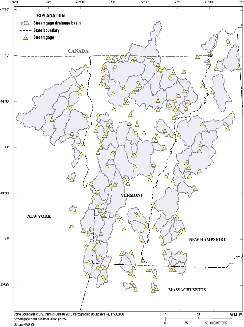
Map showing the location of selected drainage basins with streamgages used in this investigation in Vermont and its vicinity.
Peak-Discharge Data Used in this Study
All available annual peak-discharge data for Vermont and adjacent physiographically similar areas in the States of New Hampshire, Massachusetts, and New York and Quebec, Canada, were considered for this study (Olson, 2025). Streamgages within 30 miles of the Vermont border that recorded annual peak-discharge data were considered adjacent. These data include records from continuously recording streamgages and crest-stage streamgages (streamgages that record only the annual peak discharge), both current (2023) and discontinued. This report includes records through water year (WY) 2023. The WY is designated by the calendar year in which it ends. It begins October 1 of the previous calendar year and ends September 30.
Of the sites considered, 156 streamgages were selected for use in this study (fig. 1; app. 1). The selection criteria required the streamgage to have a minimum of 10 years of annual peak-discharge data that were unaffected by regulation or urbanization. Regulation was assumed to have a negligible effect on peak discharges if the usable storage in the basin was less than 4.5 million cubic feet per square mile of drainage area (Benson, 1962). Peak-discharge data from sites that had greater than 4.5 million cubic feet of usable storage per square mile of drainage area were not used. None of the streamgages used for this investigation have drainage basins considered to be urbanized. The average percentage of urbanized land for basins in this study is 5.5 percent (Commission for Environmental Cooperation, 2023). The streamgages selected for this study are spatially well distributed in and adjacent to Vermont (fig. 1).
Peak-Discharge Data Stationarity
In recent decades, stationarity (the assumption that the mean and variability of data from past observations will continue unchanged in the future) of annual peak-discharge data has been challenged (Milly and others, 2008) in light of climatic and land-use changes. To determine whether trends in the annual peak-discharge data exist, a two-sided Kendall Tau trend test (Helsel and Hirsch, 1992) was done. The trend test was done with software called PeakFQ developed by the USGS to analyze peak-flow data (Flynn and others, 2006). Streamgage records with less than 30 years of annual peak-discharge data were not tested for trends because of the uncertainty in defining a trend in a period of record of this length.
Some trends in the peak discharge data from this study were found using the Kendall Tau test. The Kendall Tau statistics indicated an upward trend in annual peak-discharge data (p-value less than or equal to 0.05) for 22 of the 104 streamgages with at least 30 years of record. For an additional two streamgages, the upward trend was considered marginal (p-value less than or equal to 0.1 and greater than 0.05).
For the streamgaging data that indicate a trend, the trend can often be explained as being the result of extreme climatic anomalies near the beginning or end of the peak-discharge record. For instance, for 12 of the 22 streamgages indicating an upward trend, the trend began during the drought of 1960–69 (Hammond, 1991). The evidence of trends did not exist or was statistically insignificant when extreme events near the beginning or end of the record were eliminated. Although some streamgage data indicate trends, the annual peak-discharge data used in this study are analyzed as random, independent events that are homogeneous for a streamgage throughout the period of record. Furthermore, a consensus on best practices to adjust for with trends has not yet emerged (England and others, 2018).
Determining the Magnitude and Annual Exceedance Probabilities of Flood Discharges for Streamgages
Flood discharges with AEPs of 50-, 20-, 10-, 4-, 2-, 1-, 0.5-, and 0.2-percent (app. 1) were computed for the 156 streamgages using methods outlined in Guidelines for Determining Flood Flow Frequency, Bulletin 17C (England and others, 2018). The Bulletin 17C guidelines incorporate the Expected Moments Algorithm, apply a Multiple Grubbs-Beck test to identify low outliers, provide procedures that accommodate interval and censored data, and compute accurate confidence intervals that account for historical data and regional skew. A summary of the historical, interval, and censored discharge data that was input is provided in appendix 2. Software developed by the USGS to analyze peak-discharge data (PeakFQ version 7.5.1) was used for these computations (U.S. Geological Survey, 2024). The annual peak-flow data that was input to the PeakFQ program were retrieved from the National Water Information System (U.S. Geological Survey, undated). Peak discharges affected by dam failure, ice jam breach, or a similar event are not included in the frequency analyses. There is evidence of mixed populations of annual peak discharges—tropical and non-tropical storm events— at streamgages in Vermont and its vicinity; however, even at streamgages with many decades of annual peak-discharge data insufficient tropical storm events were available to do mixed population analyses. Annual peak discharges through WY 2023 were included in the frequency analysis (Olson, 2025).
Generalized Skew
Estimates of the magnitude and frequency of flood discharges are sensitive to skew—the measure of the lack of symmetry in the probability distribution of annual peak-flow data. Extreme flood events often affect skews computed from a streamgage’s peak-discharge record, and the impact of an extreme flood on skew is greater the shorter the length of streamgage record. To compensate for this effect, the skew used to estimate flood discharges for selected recurrence intervals at a streamgage is weighted with a generalized skew estimated by pooling the skews from nearby streamgages. This generalized skew was developed specifically for Vermont (Olson, 2014) and was 0.445 with a standard error of 0.279.
Combined Records of Nearby Streamgages
Three active streamgages in this investigation were a short distance upstream or downstream from a discontinued streamgage. In each case, the location of the discontinued streamgage and the newer, active streamgage are proximate enough to have similar drainage-basin characteristics and to represent a single streamgage peak-flow dataset, warranting the combination of their discharge records. Before combining the peak-discharge record of the discontinued streamgage and peak-discharge record of the newer, active streamgage, the peak discharges from the discontinued streamgage record were adjusted by the drainage area ratio of the two sites. Streamgages that had their peak-discharge records adjusted for drainage area and combined to create a longer period of record are shown in table 1.
Table 1.
Peak-discharge records from discontinued and active streamgages combined to create a longer period of record, Vermont and vicinity.[Data are from Olson (2025). USGS, U.S. Geological Survey; mi2, square mile; NH, New Hampshire; VT, Vermont]
Magnitude and Annual Exceedance Probabilities of Flood Discharges for Streamgages
The magnitudes of flood discharges at selected annual exceedance probabilities for streamgages used in this study (Olson, 2025) are listed in appendix 3. The variance of each streamgage’s estimated discharge magnitude is reported in appendix 4. The discharges reported in appendix 3 supersede discharges reported in Olson (2014) and Smith and others (2025) because of additional available data and the updated regression equations.
Maximum Recorded Floods
The maximum recorded annual-peak discharges (app. 1) plotted in relation to drainage area for each streamgage in this study are displayed on figure 2. Annual-peak discharges that are affected by dam failure, ice jam breach, or a similar event are not included. A New England regional envelope curve of potential maximum flood discharges developed by Crippen and Bue (1977) is also shown on figure 2 along with a line developed using generalized least-squares regression analysis showing the relation between drainage area and the peak discharge with a 1-percent annual exceedance probability. Figure 2 can be used to evaluate the reasonableness of flood estimates made using techniques described in this report.
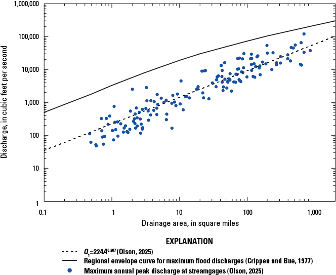
Graph showing the maximum recorded annual-peak discharges at streamgages in Vermont and its vicinity in water year 2023 in relation to drainage area, and a regional envelope curve and a regression line relating the 1-percent annual exceedance probability flood discharge (Q1) to drainage area.
Characteristics of Streamgage Drainage Basins
In flood-frequency regression analysis, the variations in the magnitude of flood discharges at a selected AEP are related to variations in basin characteristics. The flood discharges are the dependent variables, and the basin characteristics are the independent or explanatory variables. For this study, 92 basin characteristics were determined for each streamgage, including physical properties, such as drainage area, channel slope, elevation, forest cover, lake area, soil permeability, and climatic characteristics, such as precipitation and temperature.
Boundaries for each streamgage drainage basin were obtained from StreamStats (Ries and others, 2017). StreamStats is a USGS web application that can delineate drainage basins and determine selected basin characteristics for user selected locations on a stream or river. Dimensional properties of the drainage basins were computed with the geographic information system (GIS) software, ArcGIS Pro (Environmental Systems Research Institute, Inc., undated).
With appropriate GIS datasets, other basin characteristics were also computed with the GIS software. Digital elevation models from the 3D Elevation Program (USGS, 2023) were used to compute basin characteristics associated with elevation. For parts of basins that extended into Canada beyond the coverage of the 3D Elevation Program datasets, digital elevation models from the high-resolution Digital Elevation Model (Natural Resources Canada, 2024) were used. The National Hydrography Dataset (USGS, 2023), the 2020 Land Cover of North America (Commission for Environmental Cooperation, 2023), the 2021 National Land Cover Database (Dewitz, 2023), the State Soil Geographic (STATSGO) database (Schwarz and Alexander, 1995), and the gridded National Soil Survey Geographic (gNATSGO) database (Boiko and others, 2021) were the source GIS datasets for land-surface properties.
The sources for climatic data were the Precipitation Frequency for Northeastern states datasets (National Oceanic and Atmospheric Administration, 2015) and the 1991–2020 PRISM (Parameter-elevation Regressions on Independent Slopes Model; PRISM Climate Group, 2022a and b; 2024a and b) 30-year normals of precipitation and temperature. For parts of basins that extended into Canada beyond the coverage of the PRISM datasets, precipitation data from the 1991–2020 Derived Normal Climate Data provided by Agriculture and Agri-food Canada (2023) supplemented the PRISM data. A complete list of basin characteristics that were tested as explanatory variables in the regression analysis is in appendix 5.
Regression Equations Used to Estimate Flood Discharges at Selected Annual Exceedance Probabilities for Ungaged Stream Sites
Multiple-regression techniques, using generalized least-squares regression (Stedinger and Tasker, 1985), were used to define relations between the flood discharges determined for the streamgages at the 50-, 20-, 10-, 4-, 2-, 1-, 0.5-, and 0.2-percent AEP (dependent variables) and the basin characteristics (independent variables) of those streamgages. Using generalized least-squares regression allows streamgage data to be weighted to compensate for differences in record length and the cross-correlation of concurrent records among streamgages. Furthermore, Stedinger and Tasker (1985) showed that generalized least-squares regression equations are more accurate and provide better estimates of model error than ordinary least-squares regression equations when working with flood frequency.
The regression results provide equations to estimate the values of dependent variables from one or more independent variables. The regression equations take the general form
whereYP
is the magnitude of the flood discharge that has an annual exceedance probability of P percent,
X1 to Xj
are the basin characteristics, and
b0 to bj
are coefficients developed from the regression analysis.
When transformations to the explanatory and response variables are logarithmic, equation 1 can be manipulated to take the form
The limitations, sensitivity, and accuracy of the regression equations are reported following the final regression equations. In addition, techniques are discussed in this report that can be used to determine the accuracy and confidence intervals of each individual estimate from the regression equations. Methods of weighting regression equation estimates with streamgage data when the regression equations are used for a site near or at a streamgage are also discussed.
Regression Analysis and Final Regression Equations
A total of 92 basin characteristics were determined for each streamgage and tested for potential use as explanatory variables in the regression equations (app. 5). Mathematical transformations of logarithms and squares were also applied to each basin characteristic and flood-discharge statistic to obtain the most linear relations. Correlation (R Core Team, 2024a) and ordinary least squares regression (Hebbali, 2024) data computed in R (R Core Team, 2024b)—a software environment for statistical computing—were used together to evaluate which basin characteristics, transformed or untransformed, were the most significant explanatory variables while not being correlated with another explanatory variable. This initial evaluation determined that drainage area was a significant explanatory variable when discharge and drainage area were logarithmically transformed (fig. 2). This evaluation also eliminated numerous basin characteristics that were correlated with drainage area.
Next, all combinations of the remaining explanatory variables, using up to four regressors, were evaluated using ordinary least squares (Hebbali, 2024). The evaluations were based upon the R-square, adjusted R-square, root-mean-square error, Mallow’s Cp, and the Akaike information criteria of each regression model. This evaluation left 20 potential explanatory variables to be analyzed for the final regression equations.
Finally, generalized least-squares regression techniques were used to analyze and determine the final significant basin characteristics and to compute the final regression equations (Olson, 2025). The generalized least-squares regression analysis was done using the Weighted-Multiple-Linear Regression program (WREG; Farmer, 2021), a hydrologic regression package that works within the R software. The WREG package uses the generalized least-squares regression procedures outlined in Farmer and others (2019). The three basin characteristics used to develop the final regression equations—drainage area, percentage of the basin that is wetlands, and mean annual precipitation—are listed in appendix 6, by streamgage. The final regression equations (eqs. 3–10) used to estimate flood discharges on ungaged, unregulated streams in rural drainage basins in Vermont are as follows:
whereQp
is the estimated flood discharge, in cubic feet per second, at the p-percent annual exceedance probability;
A
is the drainage area of the basin, in square miles;
W
is the percentage of the basin with land cover categorized as wetlands or open water from the 2020 Land Cover of North America (Commission for Environmental Cooperation, 2023); and
P
is the basin-wide mean of the average annual precipitation, in inches, determined with the PRISM 1991–2020 average annual precipitation dataset (PRISM Climate Group, 2022a) supplemented by the 1991–2020 Derived Normal Climate Data (Agriculture and Agri-food Canada, 2023) in basins that extend into Canada.
The procedure for estimating the flood discharge at a selected recurrence interval for an ungaged stream site using the regression equations is described in appendix 7.
Attempts were made to group streamgages with similar geographic or drainage-basin characteristics into subregions to reduce the standard error of the regression equations. This grouping would have resulted in a set of regression equations for each subregion. To evaluate whether subregions should be generated, residuals, the difference between the flood discharges estimated from the frequency analysis and the flood discharges predicted from the regression equations, were determined for each streamgage and for each regression equation. These residuals were plotted spatially at the centroid of the drainage basin of the streamgage and in relation to drainage-basin characteristics. Residuals of the 10- and 1-percent annual exceedance probability regression equations in relation to drainage-basin characteristics are shown as examples in figures 3A and 3B. No apparent trends or patterns were observed in any of the plots. Thus, the streamgages were not grouped into subregions, and the equations in this report are intended for statewide use and not for subregions.
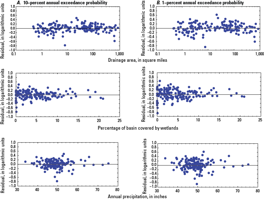
Graphs showing the residuals of the regression equations used to estimate the magnitude of a discharge with A, 10-percent and B, 1-percent exceedance probability in relation to basin characteristics in Vermont and its vicinity.
The residual plots shown in figures 3A and 3B were used as a diagnostic tool for the regression equations. The random scatter of the points above and below the zero-reference line verifies that the model is satisfactorily meeting the assumptions of multiple-linear-regression techniques. Other diagnostics are the evaluation leverage and influence metrics of each observation—the data used to develop the regression equations. Leverage is a measure of the distance an observation is from the centroid of all the other observations giving an indication of whether the observation is unusual compared to the other observations. An influence metric, such as Cook’s D (Helsel and Hirsch, 1992), is a measure of the sensitivity of regression parameters to a particular observation (Farmer and others, 2019). The combination of high leverage and influence metrics indicate an observation may be an outlier or require additional analysis. However, after evaluating an observations’ leverage and influence metrics, the data were determined to be accurate and there was no justification for excluding any observations from the regression analysis.
Another diagnostic tool used was the variance inflation factor (VIF) (Helsel and Hirsch, 1992). The VIF may be used to evaluate collinearity of explanatory variables. VIF does not have any formal criteria, although some authors suggest that a VIF exceeding 10 may be cause for concern (Freund and Littell, 2000) because explanatory variables may then be correlated. None of the VIF values were close to this level; the greatest VIF computed for a variable used in the final regression equations was 1.2.
Limitations and Sensitivity
Basin characteristics used to develop equations 3 through 9 were determined with ArcGIS Pro (Environmental Systems Research Institute, Inc., undated) software using datasets described in “Regression Analysis and Results” section of this report. This is important because determining the basin characteristics to use in the regression equations with alternate data sources or using different computational methods than those of a GIS software may produce statistics that are different from those reported in this report and may introduce bias and yield discharge estimates that have unknown error.
In addition, although wetland area and annual precipitation values were used in the equations to estimate flood discharges in Vermont in Olson (2014) and in this investigation, the source of these basin characteristics is not the same. Basin characteristics used in the equations published in 2014 cannot be used in these new set of equations, nor vice versa. For instance, the annual precipitation values used in the equations published in 2014—which were 30-year precipitation normals from 1981–2010—should not be applied to the equations developed for this study—which use the 30-year precipitation normals from 1991–2020. Use of basin characteristics from the wrong source will produce unreliable results with unknown error.
The regression equations are applicable to sites on ungaged, unregulated streams in rural basins that are within the region encompassed by the drainage basins used for this investigation. Use of these equations is appropriate for sites with drainage-basin characteristics that are within the range of drainage-basin characteristics used to develop the equations. In general, the uncertainty in the regression equation results will be greater when the explanatory variables used in the equations are further from their mean. The mean and ranges of drainage-basin characteristics used for the analysis are shown in table 2 and figure 4. If the independent variables used in the regression equations are outside of these ranges, the results of the equations are considered extrapolations, and the accuracy of the predictions is unknown. For sites that have drainage-basin characteristics outside the acceptable ranges, a simplified equation that uses drainage area as the only explanatory variable is used for this study and is provided in this report in the section titled “Drainage-Area-Only Regression Equations.” For sites that are considered urban, Moglen and Shivers (2006) describe techniques that transform rural flood-discharge frequency estimates to estimates for urban watersheds.
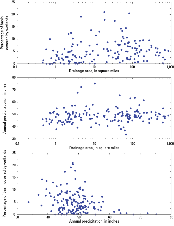
Graphs showing two-dimensional ranges of explanatory variables used to develop the regression equations that can be used to estimate flood discharges at selected annual exceedance probabilities for streams in Vermont and its vicinity.
Table 2.
Ranges of values for explanatory variables used to develop regression equations to estimate flood discharges at selected annual exceedance probabilities for ungaged, unregulated streams in Vermont and its vicinity.[Data are from Olson (2025).]
The sensitivity of each regression equation to changes in the magnitude of the independent variables was tested to evaluate the amount of error that can be introduced if basin characteristics are incorrectly computed. The sensitivity analysis was done by adjusting basin characteristic values by plus or minus 10 percent while holding the other basin characteristics constant at their respective mean magnitudes (Olson, 2025). The results of the sensitivity analysis listed in table 3 indicate that the regression equations are most sensitive to changes in drainage area and changes in the basin-wide mean of the average annual precipitation. However, a 10-percent change in the basin-wide mean of the average annual precipitation value accounts for a greater change in the computed flood discharge than does a 10-percent change in drainage area.
Table 3.
Results of the sensitivity analysis calculated from regression equations for Vermont and its vicinity as percentage change in computed flood discharge because of a 10-percent change in the input basin characteristic.[Data are from Olson (2025).]
Accuracy of the Regression Equations
The accuracy of regression equations can be measured in several ways. The coefficient of determination, R2, indicates the proportion of variability of the dependent variable and is explained by combining the explanatory variable in the regression model. The pseudo coefficient of determination, R2pseudo, can be described in the same way but accounts for the effect of the time-sampling error (Farmer and others, 2019). The closer the R2 or R2pseudo is to 1, the better the regression explains the variation in the dependent variables. The R2 and R2pseudo for each regression equation (Olson, 2025) is in table 4.
Table 4.
Measures of accuracy of the regression equations for estimating flood discharges at selected annual exceedance probabilities for ungaged, unregulated streams in rural drainage basins in Vermont and its vicinity.[Data are from Olson (2025). R2, coefficient of determination; Log, logarithmic]
One of the most common measures of accuracy is the root mean square error (table 4); it measures how much the regression results deviate from the observed data. The root mean square error represents the standard deviation of the residuals.
Another measure of accuracy is the average standard error of prediction (table 4). The average standard error of prediction has a model error component—the error resulting from the model—and a sampling error component—the error that results from model parameters that are developed from samples of the population. Thus, the average standard error of prediction is a measure of the expected accuracy of a regression model when applied at an ungaged location with basin characteristics like those used to develop the regression equation. This measure of accuracy is needed because regression equations are typically used for ungaged locations. About two-thirds of the estimates made using a regression equation for ungaged locations will have errors less than the average standard error of prediction for that equation.
Accuracy Analysis of Individual Estimates from the Regression Equations
Because the coefficient of determination, the pseudo coefficient of determination, the root mean square error, and the average standard error of prediction (table 4) are computed using available streamgage data, they are approximations of the overall accuracy of the regression equations for ungaged sites. Techniques for computing the accuracy of individual regression equation estimates for ungaged sites are available and are discussed in this section. Individual estimates are measured for accuracy by means of the standard error of prediction and prediction intervals.
Standard Error of Prediction
Hodge and Tasker (1995) describe how to compute the variance of prediction (Vpred) of a flood-discharge frequency estimate as
whereVpred
is the standard error of prediction;
γ2
is the model error variance (refer to table 5);
xi
is a row vector containing 1, log10(A), W, and log10(P) for the study site i;
tr
is the matrix algebra symbol for transposing a matrix; and
(XtrΛ-1X)-1 is the (p×p) matrix with X being a (n×p) matrix that has rows of logarithmically transformed basin characteristics augmented by one, and Λ being the (n×n) covariance matrix used for weighting sample data in the generalized least-squares regression; n is the number of streamgages used in the regression analysis, and p is the number of basin characteristics plus 1. The (XtrΛ-1X)-1 matrices for selected recurrence intervals are shown in table 5.
Table 5.
Flood-frequency characteristic, model error variance, and the basin characteristics matrices for the regression equations.[Data are from Olson (2025). Numbers in matrices are in scientific notation. Annual precipitation refers to the basin-wide mean of the average annual precipitation. AEP, annual exceedance probability]
The variance of prediction can be used to weight a result from a regression equation with the AEP from the analysis of the streamgage record and is discussed in the “Use of Regression Equations at or near Streamgages” section of this report. A streamgage’s weighted AEP result will have reduced uncertainty (U.S. Interagency Advisory Committee on Water Data, 1982).
The standard error of prediction is computed with the following formula:
whereThe standard error of prediction for an estimate can be converted to positive and negative percent errors with the following formulas:
whereSpos
is the positive percent error of prediction,
SEpred
is the standard error of prediction in logarithmic units, and
Sneg
is the negative percent error of prediction.
The probability that the true value of flood discharge at a given frequency is between the positive- and negative-percent standard error of prediction is approximately 68 percent. For example, if Sneg is −27.1 percent and Spos is 37.1 percent, there is a 68-percent chance that the true AEP discharge at a site ranges from −27.1 percent to +37.1 percent of the estimated AEP discharge.
Prediction Intervals
Prediction intervals indicate the uncertainty in the equation results. For example, there is a 90 percent probability that the true value of a flood-discharge estimate lies within the 90-percent prediction interval. Prediction intervals for selected percentages can be computed as follows:
wherePIupper
is the upper prediction interval, in cubic feet per second;
PIlower
is the lower prediction interval, in cubic feet per second;
Qpred
is the computed discharge at a selected frequency from the regression equation, in cubic feet per second;
tα/2,n−p
is the critical value from a Student’s-t distribution at alpha level α (α=0.10 for a 90-percent prediction interval; α=0.05 for a 95-percent prediction interval) with n-p degrees of freedom; n=156, the number of stations used in the regression analysis; and p=4, the number of basin characteristics in the regression equation, plus 1 (for the 95- and 90-percent prediction interval tα/2,n−p is 1.98 and 1.66, respectively); and
SEpred
is the standard error of prediction of a flood-discharge frequency estimate.
Use of Regression Equations for Streamgages
An estimate of flood discharge at a selected annual exceedance probability made at a streamgage can be improved by combining regression equation results with the frequency curve computed from the streamgage record. The procedure recommended by Cohn and others (2012) is to compute a flood discharge using the regression equation estimate and the result of the frequency analysis of the streamgage record for a given annual exceedance probability weighted by the inverse of the variance of each of the discharge estimates. The procedure was applied to all the streamgages used in this study, and the weighted flood-discharge results are in appendix 3. Generally, the weighted flood discharge estimate provides better estimates of the true discharges than those determined from either the flood-frequency analysis or the regression analysis alone. The weighted discharges were computed using the following equation:
whereQw
is the weighted flood discharge, in cubic feet per second,
Qs
is the flood discharge for the selected annual exceedance probability computed from the streamgage record, in cubic feet per second,
Qr(g)
is the flood discharge for the selected annual exceedance probability from the regression equation at the streamgage, in cubic feet per second,
Vpred
is the variance of prediction for the result of the regression equation (Qr(g)) in logarithmic units computed using equation 11, and
Vs
is the variance in the estimate of annual exceedance probability discharge given in logarithmic units computed from the streamgage record (Qs) (see app. 4).
Prediction intervals for the weighted discharge (Qw) can be computed with equations 15 and 16; however, the standard error of prediction for the weighted discharge (SEw) is to be substituted for the standard error of prediction for the regression estimate (SEpred). The standard error of prediction for the weighted discharge can be computed with the following formula:
Use of Regression Equations for Areas near Streamgages
Estimates of flood-discharge magnitude at selected annual exceedance probabilities for ungaged sites that are not at, but are near, a streamgage and are on the same unregulated stream can be improved by combined use of the regression equations and the nearby streamgage data. A method to adjust the weighted discharge for a streamgage (Qw) developed from equation 17 to a site of interest upstream or downstream from the streamgage is given in this report. This method increases the weight of a discharge estimate derived from a regression-equation over the weight of a discharge estimate derived from streamgage data the farther upstream or downstream the site of interest is from the streamgage. This method is modified from a technique described in Ries (2007) that adjusts the weight linearly in logarithmic units, satisfying the logarithmic relation between flood discharge and drainage area. The logarithmic slope (c) of a line that goes through the weighted estimate of the discharge at the streamgage and converges on a location upstream or downstream where full weight will be given to the regression equations at a selected annual exceedance probability is computed as follows:
whereQr(u)
is the flood-discharge estimate generated using the regression equation for the ungaged site, in cubic feet per second;
Qr(g)
is the flood-discharge estimate generated using the regression equation for the streamgage, in cubic feet per second;
Au
is the drainage area of the ungaged site, in square miles;
Ag
is the drainage area at the streamgage, in square miles;
Qw
is the weighted flood-discharge estimate at the streamgage location computed using equation 17, in cubic feet per second; and
a
is the percentage of the gaged drainage area, where full weight is given to the regression equation results. As a rule, a=0.5 for Au less than Ag, and a=1.5 for Au greater than Ag.
The value of a determines where, as a percentage of the gaged drainage area, full weight will be given to the regression equation. Hence, when the site of interest is upstream from the streamgage, a=0.5, the site is required to have a drainage area no smaller than 50 percent of the streamgage drainage area. When the site of interest is downstream from the gage, a=1.5, the site is required to have a drainage area no larger than 150 percent of the streamgage drainage area.
The final step is to compute the weighted flood-frequency estimate for the ungaged site, Qu, using
An example that uses this technique is in appendix 7. As with any technique used to compute a weighted flood-discharge estimate, unexpected results could happen if there is a substantial difference between the discharges being weighted. If the difference in discharges being weighted is substantial, c could become negative, indicating discharge and drainage area are inversely related and making the procedure invalid
Drainage-Area-Only Regression Equations
For some ungaged sites, the percentage of the basin covered by wetlands or the basin-wide mean of the average annual precipitation may be outside the acceptable ranges required for the full regression equations (eqs. 3–10). The acceptable basin characteristic ranges are described in this report in the section titled “Limitations and Sensitivity.” In addition, some users of the equations may not have access to basin characteristics beyond drainage area. Because of this, a set of simplified regression equations (Olson, 2025) that incorporate drainage area as the only independent variable was developed. Generalized least-squares regression techniques were used to compute the coefficients in the equations. The simplified regression equations (eqs. 21–28) used to estimate flood discharges from ungaged, unregulated streams in rural drainage basins in Vermont are as follows:
whereQP
is the estimated flood discharge, in cubic feet per second, at the P-percent exceedance probability; and
A
is the drainage area of the basin, in square miles.
The same 156 streamgages used to develop the previous regression equations were used to develop the simplified regression equations. The simplified regression equations are still applicable to sites with drainage areas ranging from 0.47 to 851 mi2. Because the equations have only one explanatory variable, they are less accurate than the full regression equations in this report. The coefficient of determination, the pseudo coefficient of determination, the root mean square error, and the average standard error of prediction of the simplified equations are in table 6.
Table 6.
Accuracy measures for the simplified regression equations (drainage area only) that are used to estimate flood discharges at selected annual exceedance probabilities for ungaged, unregulated streams in rural drainage basins in Vermont and its vicinity.[Data are from Olson (2025). R2, coefficient of determination; log, logarithmic]
Although drainage-area-only regression equations are less accurate than the multivariable equations, these simplified equations are still valuable. The exponent in each of the drainage-area-only regression equations is the slope of the average linear logarithmic relation between drainage area and flood discharge for a selected AEP. Hence, the exponent can be used as an alternate method to adjust flood-frequency data from a streamgage to flood-frequency data from streamgages upstream and downstream. This use of the method is to be limited to streamgages within 50- to 150-percent of the streamgage drainage area (Wandle, 1983). To use this method, one would use equation 19 with the exponent from the simplified regression equation at a selected recurrence interval substituted for c.
Vermont StreamStats
StreamStats, an internet-based application (https://www.usgs.gov/streamstats/), allows users to obtain drainage-basin characteristics, discharge statistics, and other information for user-selected sites on streams. StreamStats users choose stream sites of interest from an interactive map. If a user selects the location of a USGS streamgage, they can get previously published information for the site from a database. If a user selects an ungaged site, the StreamStats application will determine the boundary of the drainage basin upstream from the site and measure the basin characteristics required by the regression equations to estimate discharge statistics for the site. The application then solves the equations. The results are then in a table along with a map showing the basin outline.
Furthermore, the application ensures that the basin characteristics input into the regression equations are determined using the same data and methodologies as the basin characteristics used to develop the equations. Doing this avoids bias that could be introduced by improperly estimating basin characteristics.
The equations published in this report will be available online in StreamStats after the publication of this report. StreamStats will provide flood-discharge frequency data for streamgages used in this study and compute flood-discharge frequency estimates for ungaged locations using the final regression equations (eqs. 3–10). StreamStats does not determine flood-discharge frequency estimates for streamgages that are weighted with the regression equations results.
Summary
This report, prepared by the U.S. Geological Survey in cooperation with the Federal Emergency Management Agency, documents how regression equations were developed and used to estimate flood-discharge magnitudes for rural, unregulated streams in Vermont at annual exceedance probabilities of 50-, 20-, 10-, 4-, 2-, 1-, 0.5-, and 0.2-percent using flood-discharge data through the 2023 water year. Regression techniques were used to determine relations between the flood-discharge magnitudes and selected basin characteristics at 156 streamgages in and adjacent to Vermont.
The flood-discharge magnitudes at selected recurrence intervals for the 156 streamgages were determined following the Guidelines for Determining Flood Flow Frequency, Bulletin 17C. A generalized skew coefficient of 0.445 with a standard error of 0.279 was used in the frequency analysis.
A total of 92 basin characteristics for each streamgage were determined using a geographic information system. Using correlation data, ordinary least-squares regression techniques, and generalized least-squares regression techniques, the 92 basin characteristics were narrowed down to the three variables that best explained the magnitude and variability of flood discharges: the drainage area, the percentage of the basin covered by wetlands, and the basin-wide mean of the average annual precipitation. The final regression equations were developed using generalized least-squares regression techniques. The average standard error of prediction to estimate peak discharges with 50-, 20-, 10-, 4-, 2-, 1-, 0.5-, and 0.2-percent annual exceedance probability with these equations are 34.9, 37.1, 38.2, 41.6, 43.8, 46.0, 49.1, and 53.2 percent, respectively.
The regression equations developed from these relations can be used as a method to estimate flood discharges at selected recurrence intervals for ungaged, unregulated, rural streams. This report also presents methods of how to adjust a flood-discharge frequency curve computed from a streamgage record with results from the regression equations. In addition, a technique is described of how to estimate flood discharge at a selected recurrence interval for an ungaged site upstream or downstream from a streamgage using a drainage-area adjustment.
The equations and flood-discharge frequency data used in this study are available in StreamStats, an internet-based application (https://www.usgs.gov/streamstats/) that provides statistics, drainage-basin characteristics, and other information for user-selected sites on streams.
References Cited
Agriculture and Agri-food Canada, 2023, Derived normal climate data—30-year average precipitation: Natural Resources Canada: Government of Canada web page, accessed January 27, 2025, at https://open.canada.ca/data/en/dataset/acd4c9f2-0598-47e8-aa4d-0a8a0964ce55.
Boiko, O., Kagone, S., and Senay, G.B., 2021, Soil properties dataset in the United States: U.S. Geological Survey data release, accessed July 18, 2024, at https://doi.org/10.5066/P9TI3IS8.
Commission for Environmental Cooperation, 2023, North America Land Cover, 2020, North American Land Change Monitoring System: Canada Centre for Remote Sensing, U.S. Geological Survey, Ed. 1.0, Raster digital data. [Also available at http://www.cec.org/north-american-environmental-atlas/land-cover-30m-2020/S.]
Dewitz, J., 2023, National land cover database (NLCD) 2021 products: U.S. Geological Survey data release, accessed July 18, 2024, at https://doi.org/10.5066/P9JZ7AO3.
Dingman, S.L., and Palaia, K.J., 1999, Comparison of models for estimating flood quantiles in New Hampshire and Vermont: Journal of the American Water Resources Association, v. 35, no. 5, p. 1233–1243. [Also available at https://doi.org/10.1111/j.1752-1688.1999.tb04210.x.]
England, J.F., Jr., Cohn, T.A., Faber, B.A., Stedinger, J.R., Thomas, W.O., Jr., Veilleux, A.G., Kiang, J.E., and Mason, R.R., Jr., 2018, Guidelines for determining flood flow frequency—Bulletin 17C: U.S. Geological Survey Techniques and Methods, book 4, chap. B5, 148p. [Also available at https://doi.org/10.3133/tm4B5.]
Environmental Systems Research Institute, Inc., [undated], ArcGIS Pro: Redlands, Calif., Environmental Systems Research Institute, Inc. web page, accessed February 10, 2025, at https://www.esri.com/en-us/arcgis/products/arcgis-pro/overview.
Farmer, W.H., Kiang, J.E., Feaster, T.D., and Eng, K., 2019, Regionalization of surface-water statistics using multiple linear regression: U.S. Geological Survey Techniques and Methods, book 4, chap. A12, 40 p., accessed February 12, 2025, at https://doi.org/10.3133/tm4A12.
Farmer, W.H., 2021, WREG—Weighted least squares regression for streamflow frequency statistics (ver. 3.0): Reston, Va., U.S. Geological Survey software release, accessed January 31, 2025, at https://doi.org/10.5066/P9ZCGLI1.
Hebbali, A., 2024, olsrr—Tools for building OLS regression models: R package version 0.6.0, accessed July 18, 2024, at https://olsrr.rsquaredacademy.com.
Johnson, C.G., and Tasker, G.D., 1974, Progress report on flood magnitude and frequency of Vermont streams: U.S. Geological Survey Open-File Report 74–130, 37 p. https://doi.org/10.3133/ofr74130.
Milly, P.C.D., Betancourt, J., Falkenmark, M., Hirsch, R.H., Kundzewicz, Z.W., Lettenmaier, D.P., and Stouffer, R.J., 2008, Stationarity is dead—Whither water management?: American Association for the Advancement of Science, accessed August 19, 2008, at www.sciencemag.org/.
National Oceanic and Atmospheric Administration, 2015, Precipitation frequency for Northeastern states, USA—NOAA Atlas 14 Volume 10: National Oceanic and Atmospheric Administration web site, accessed July 17, 2024, at https://hdsc.nws.noaa.gov/pfds/pfds_gis.html.
Natural Resources Canada, 2024, High resolution digital elevation model (HRDEM)—CanElevation series: Natural Resources Canada web page, accessed July 18, 2024, at https://open.canada.ca/data/en/dataset/957782bf-847c-4644-a757-e383c0057995.
Office of the Vermont State Climatologist, 1996, Climate of Vermont—Office of the Vermont State Climatologist: University of Vermont website, accessed February 7, 2025, at https://www.uvm.edu/~statclim/.
Olson, S.A., 2014, Estimation of flood discharges at selected annual exceedance probabilities for unregulated, rural streams in Vermont, with a section on Vermont regional skew regression, by Veilleux, A.G.: U.S. Geological Survey Scientific Investigations Report 2014–5078, 27 p., plus app., https://doi.org/10.3133/sir20145078.
Olson, S.A., 2025, Data for the estimation of flood discharges at selected annual exceedance probabilities for unregulated, rural streams in Vermont, 2023: U.S. Geological Survey data release, https://doi.org/10.5066/P1MGCBK9.
Olson, S.A., and Bent, G.C., 2013, Annual exceedance probabilities of the peak discharges of 2011 at streamgages in Vermont and selected streamgages in New Hampshire, western Massachusetts, and northeastern New York: U.S. Geological Survey Scientific Investigations Report 2013–5187, 17 p., https://pubs.usgs.gov/sir/2013/5187/.
PRISM Climate Group, 2022a, United States average total precipitation, 1991–2020, 800 m grid cell resolution, created December 5, 2022: Corvallis, Oreg., Oregon State University, accessed July 18, 2024, at http://www.prism.oregonstate.edu/.
PRISM Climate Group, 2022b, United States average monthly total precipitation, 1991–2020, 800 m grid cell resolution, created December 5, 2022: Corvallis, Oreg., Oregon State University, accessed July 18, 2024, at http://www.prism.oregonstate.edu/.
PRISM Climate Group, 2024a, United States average daily mean temperature, 1991–2020, 800 m grid cell resolution, created February 1, 2024: Corvallis, Oreg., Oregon State University, accessed July 18, 2024, at http://www.prism.oregonstate.edu/.
PRISM Group, 2024b, United States average monthly daily mean temperature, 1991–2020, 800 m grid cell resolution, created February 1, 2024: Corvallis, Oreg., Oregon State University, accessed July 18, 2024, at http://www.prism.oregonstate.edu/.
R Core Team, 2024a, The R stats package version 4.4.0: Vienna, Austria, R Foundation for Statistical Computing, accessed July 18, 2024, at https://stat.ethz.ch/R-manual/R-devel/library/stats/html/00Index.html.
R Core Team, 2024b, R—A language and environment for statistical computing version 4.4.0: Vienna, Austria, R Foundation for Statistical Computing, accessed July 18, 2024, at, https://www.R-project.org.
Ries, K.G., III, Newson J.K., Smith, M.J., Guthrie, J.D., Steeves, P.A., Haluska, T.L., Kolb, K.R., Thompson, R.F., Santoro, R.D., and Vraga, H.W., 2017, StreamStats, version 4: U.S. Geological Survey Fact Sheet 2017–3046, 4 p., https://doi.org/10.3133/fs20173046.
Smith, T.L., Olson, S.A., LeNoir, J.M., Kalmon, R.D., and Ahearn, E.A., 2025, Flood of July 2023 in Vermont: U.S. Geological Survey Scientific Investigations Report 2025–5016, 21 p., http://dx.doi.org/10.3133/sir20255016.
Stedinger, J.R., and Tasker, G.D., 1985, Regional hydrologic analysis—1. Ordinary, weighted, and generalized least squares compared: Water Resources Research, v. 21, no. 9, p. 1421–1432. [Also available at https://doi.org/10.1029/WR021i009p01421.]
Schwarz, G.E., and Alexander, R.B., 1995, Soils data for the conterminous United States derived from the NRCS state soil geographic (STATSGO) data base [Original title: State soil geographic (STATSGO) data base for the conterminous United States.]: U.S. Geological Survey data release, accessed July 17, 2024, at https://doi.org/10.5066/P94JAULO.
U.S. Geological Survey, 2023, National hydrography dataset (NHD)—USGS National map downloadable data collection: USGS—National Geospatial Technical Operations Center web page, accessed July 17, 2024, at https://www.sciencebase.gov/catalog/item/4f5545cce4b018de15819ca9.
U.S. Geological Survey, 2024, 1/3rd arc-second digital elevation models (DEMs)—USGS National map 3DEP downloadable data collection: U.S. Geological Survey data release, accessed July 17, 2024, at https://www.sciencebase.gov/catalog/item/4f70aa9fe4b058caae3f8de5.
U.S. Geological Survey, 2024, PeakFQ—U.S. Geological Survey data analysis tools: U.S. Geological Survey web page, accessed February 7, 2025, at https://www.usgs.gov/tools/peakfq.
U.S. Geological Survey, [undated], Peak streamflow for the Nation: National Water Information System website, accessed February 7, 2025, at https://nwis.waterdata.usgs.gov/usa/nwis/peak.
Vermont Fish & Wildlife Department, 2025, Fishing opportunities: Vermont Fish & Wildlife Department web page, accessed July 30, 2025, at https://www.vtfishandwildlife.com/doc/fish/fishing-opportunities.
Appendix 1. Streamgages with Data Used in this Investigation and the Maximum Annual Peak Discharge Recorded at the Streamgages in Vermont and Vicinity
Appendix 2. Summary of Peak-Discharge Data Used in the Flood-Frequency Analyses at Streamgages in Vermont and Vicinity
Appendix 3. Flood Discharges for Selected Annual Exceedance Probabilities for Selected Streamgages in Vermont and Vicinity
Appendix 4. Variance of Estimate at Selected Annual Exceedance Probabilities for Streamgages in Vermont and Vicinity
Appendix 5. Basin Characteristics Tested for Use in the Regression Equations
Appendix 6. Basin Characteristics Used to Develop the Regression Equations
Appendix 7. Example Application
Conversion Factors
U.S. customary units to International System of Units
Temperature in degrees Fahrenheit (°F) may be converted to degrees Celsius (°C) as follows:
°C = (°F – 32) / 1.8.
Datums
Vertical coordinate information is referenced to the North American Vertical Datum of 1988 (NAVD 88).
Horizontal coordinate information is referenced to the North American Datum of 1983 (NAD 83).
Altitude, as used in this report, refers to distance above the vertical datum.
Supplemental Information
A water year is the 12-month period from October 1 through September 30 of the following year and is designated by the calendar year in which it ends.
For more information about this report, contact:
Disclaimers
Any use of trade, firm, or product names is for descriptive purposes only and does not imply endorsement by the U.S. Government.
Although this information product, for the most part, is in the public domain, it also may contain copyrighted materials as noted in the text. Permission to reproduce copyrighted items must be secured from the copyright owner.
Suggested Citation
Olson, S.A., 2025, Estimating flood discharges at selected annual exceedance probabilities for unregulated, rural streams in Vermont, 2023: U.S. Geological Survey Scientific Investigations Report 2025–5088, 22 p., https://doi.org/10.3133/sir20255088.
ISSN: 2328-0328 (online)
Study Area
| Publication type | Report |
|---|---|
| Publication Subtype | USGS Numbered Series |
| Title | Estimating flood discharges at selected annual exceedance probabilities for unregulated, rural streams in Vermont, 2023 |
| Series title | Scientific Investigations Report |
| Series number | 2025-5088 |
| DOI | 10.3133/sir20255088 |
| Publication Date | November 24, 2025 |
| Year Published | 2025 |
| Language | English |
| Publisher | U.S. Geological Survey |
| Publisher location | Reston, VA |
| Contributing office(s) | New England Water Science Center |
| Description | Report: vii, 22 p.; Data Release; Appendix |
| Country | United States |
| State | Vermont |
| Online Only (Y/N) | Y |
| Additional Online Files (Y/N) | Y |