

Characterization of Suspended Sediment Flux and Streamflow Trends in the Fountain Creek Watershed, Colorado, 1998 Through 2022
Links
- Document: Report (4.74 MB pdf) , HTML , XML
- Data Release: USGS data release - Suspended Sediment Data and Loads in the Fountain Creek Watershed, Colorado (ver 2.0, June 2025)
- Database: Database USGS water data for the Nation: U.S. Geological Survey National Water Information System database
- Version History: Version History (8.00 KB txt)
- NGMDB Index Page: National Geologic Map Database Index Page (html)
- Download citation as: RIS | Dublin Core
Abstract
The U.S. Geological Survey evaluated long-term suspended sediment flux and streamflow datasets for temporal trends (monotonic and step trends) at 10 streamgage sites within the Fountain Creek watershed in central Colorado using the Mann-Kendall test (monotonic trend) and the Wilcoxon signed-rank test (step trend). Data were collected in cooperation with Colorado Springs Stormwater Enterprise. In this study, 10 sites with long-term suspended sediment records were evaluated during their operational periods, which ranged from 1998 through 2022. To assess how stream behavior might relate to shifts in suspended sediment transport, the Richards-Baker flashiness index, a measure of flashiness, was evaluated for each site. The Richards-Baker flashiness index was calculated for the same months as streamflow and suspended sediment (April through September) using all available streamflow data for a given site. Additionally, cumulative double-mass curves were developed to define temporal variation in the relation between streamflow and suspended sediment loads. This was completed by assessing differences in slopes before and after an observed break in the double-mass curve plots.
Five streamgage sites showed statistically significant (p<0.05) negative trends for suspended sediment flux, and nonsignificant decreases were indicated at the other five sites. The statistically significant negative trends are distributed across the watershed and include smaller tributaries and the main stem of Fountain Creek closer to its confluence with the Arkansas River. Such a broad distribution of negative trends is most likely an indication of improved water quality in the watershed with regards to suspended sediment. Assessing causes for the decreases in suspended sediment loads is beyond the scope of this report; however, spatially distributed bank erosion control projects, stormflow retention projects in the watershed, and changes in climate and storm patterns could be some of the potential drivers of the suspended sediment load trends in this watershed. The flashiness of the streamflow was assessed and can be dismissed on the basis of this study as a potential driver of trends in suspended sediment flux because the magnitude of changes was found to be negligible at all sites.
Introduction
Prolonged, uncharacteristically high suspended sediment concentration (SSC) in streams is known to negatively affect stream ecosystem health and water quality, making SSC a major concern for water resource managers worldwide (U.S. Environmental Protection Agency [EPA], 2022). Sediment can negatively affect water availability by reducing reservoir storage and increasing treatment costs at water utilities (EPA, 2022). Erosion and sediment-related issues, including scouring of streambeds and streambanks impaired by deteriorated stormwater management structures, have previously been identified as key problems within the Fountain Creek watershed, Colorado (Stogner and others, 2013; EPA, 2020). Water use and management within the Fountain Creek watershed can cause hourly, daily, and seasonal changes in streamflow through the import of water from outside the watershed, diversions for municipal water supply and irrigation, return flows from agricultural irrigation, discharge from wastewater treatment plants, and other operations (Stogner, 2000). Increased streamflows have the potential to increase erosion and mobilize additional sediment into streams. Long-term suspended sediment and streamflow datasets can be utilized to quantify the magnitude of suspended sediment transport through time and provide insight into the potential cause of sediment transport changes within a watershed.
Within the Fountain Creek watershed, suspended sediment data were collected at 10 U.S. Geological Survey (USGS) streamgage sites, some of which have been monitored for as much as 25 years (fig. 1; table 1). Because the datasets span multiple sites, comparisons can be made from upstream to downstream locations and between subwatersheds within the watershed (Mau and others, 2007; Stogner and others, 2013). Such datasets represent long-term records that can be used to identify temporal trends for different hydrologic conditions (for example, drought or flood year) that could be associated with land use, disturbance, or resource management. The USGS, in cooperation with Colorado Springs Stormwater Enterprise, have been collecting data to calculate suspended sediment loads (SSL) at select sites within the Fountain Creek watershed since 1998. To better understand changes in suspended sediment transport in the watershed, the USGS evaluated long-term suspended sediment and streamflow datasets for temporal trends (monotonic and step trends) from 1998 through 2022 at 10 sites within the Fountain Creek watershed in central Colorado.
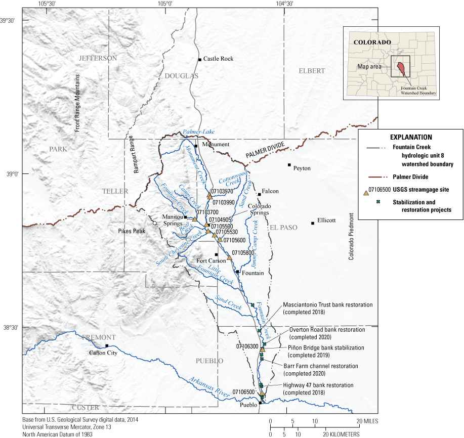
Map showing locations of U.S. Geological Survey (USGS) streamgage sites (USGS, 2024) and stabilization and restoration projects (Fountain Creek Watershed District, 2024) in the Fountain Creek watershed, Colorado, 1998–2022.
Table 1.
Streamgage site identification information (U.S. Geological Survey [USGS], 2024) and a summary of monthly mean suspended sediment flux and streamflow for the corresponding years of available data.[ID, identification; USGS, U.S. Geological Survey; ft3/s, cubic feet per second; Colo., Colorado]
Purpose and Scope
This report describes trends in streamflow and suspended sediment flux (SSF, mass or load transported per unit of time, in tons per day) through time for 10 USGS sites in the Fountain Creek watershed, Colo. (fig. 1). All sites in this report are operated seasonally, so only monthly data from April through September were used in the analysis. The 10 sites have different operational periods spanning from 1998 to 2022, yet data collection and load calculation methods were consistent for all sites and operational periods (table 1). Individual sites were evaluated for two types of change: monotonic trends and step changes. Monotonic trends are defined by steady change through time, either positive or negative. Step changes represent abrupt, statistically significant, positive or negative shifts between two groups of data separated in time (Helsel and others, 2020). Monthly mean SSF, in tons per day, and monthly mean streamflow, in cubic feet per second (ft3/s), were evaluated for possible trends and used to characterize potential changes in the watershed. The analysis presented in this report is complementary to geomorphic and water-quality assessments that are also ongoing within the Fountain Creek watershed (Hempel and others, 2021). Trend analysis on SSF was done to assess potential changes through time in the Fountain Creek watershed, but assessing the potential causes of such changes is beyond the scope of this report.
Study Background
The “Study Background” section outlines the relevant geographical, climatic, and population characteristics of the study area. Comprehending the distinct features of the Fountain Creek Basin is essential for interpreting the results and implications of this research. The subsequent sections will provide a detailed examination of specific aspects of the region, including hydrology, land use, and other related environmental factors.
Description of Study Area
Fountain Creek watershed has a drainage area of 927 square miles (mi2) and flows into the Arkansas River at Pueblo, Colo. (USGS, 2019b; fig. 1). The Fountain Creek watershed has a maximum elevation of 14,100 feet (ft) at the summit of Pikes Peak, and a minimum elevation of 4,630 ft at the confluence of Fountain Creek and the Arkansas River. The Fountain Creek watershed comprises two physiographic regions: the Front Range of the Southern Rocky Mountains and the Colorado Piedmont (Hansen and Crosby, 1982; Miller and Stogner, 2017; fig.1). The Front Range region makes up the western one-third of the watershed and is primarily underlain by granite and other crystalline rocks (von Guerard, 1989). The eastern two-thirds of the Fountain Creek watershed is made up of the Colorado Piedmont region, a subregion of the Front Range (Hansen and Crosby, 1982; Kohn and others, 2014). The geologic formations of the Colorado Piedmont are sedimentary in nature; soils are readily erodible and are thus a key source of sediment to Fountain Creek (Larsen, 1981). A more detailed description of surface geology and soils in the Fountain Creek watershed is presented by Larsen (1981) and von Guerard (1989).
The main stem channel of Fountain Creek can be separated into three distinct segments with differing characteristics. The upper reach, located upstream from Manitou Springs (fig. 1), has pool-and-riffle channel morphology, and bed material comprises sand and gravel to cobble- and boulder-size particles (Stogner and others 2013; Miller and Stogner, 2017). The middle segment, which begins at the confluence of Monument Creek and ends at USGS site 07105800 (Fountain Creek at Security, Colo.; fig. 1), is channelized and dominated by runs with intermittent pools. The bed material consists of sand, gravel, and cobble and is locally scoured to bedrock in some areas. Additionally, some locations in this section have been lined with concrete to lessen streambank erosion during high flow (Stogner and others, 2013; Miller and Stogner, 2017). The lower reach extends downstream from USGS site 07105800 (Fountain Creek at Security, Colo.) to the confluence with the Arkansas River. The channel is braided through this section with meanders more prevalent than in the upper reaches. The channel is wider throughout the lower reach, resulting in shallower stream depths. The streambed in the lower reach is almost exclusively composed of sand and small gravel, which can be easily transported at the full range of flows (Stogner and others 2013; Miller and Stogner, 2017).
Tributaries of Fountain Creek important to this study include Camp Creek, South Cheyenne Creek, Monument Creek, Bear Creek, Sand Creek, Jimmy Camp Creek, and Little Fountain Creek (USGS, 2019b; fig. 1). Monument Creek is the main tributary to Fountain Creek and originates in the Rampart Range. From its origin, Monument Creek flows eastward toward Palmer Lake and then south toward Colorado Springs and its confluence with Fountain Creek. The upper reach of Monument Creek is meandering and contains pools, riffles, and runs. Bed material in the upper reaches of Monument Creek consists primarily of sand, gravel, and cobble. In the lower reach of Monument Creek (beginning at the confluence of Cottonwood Creek), the channel is often braided and characterized by finer bed material, including sand and small gravel. Additionally, Monument Creek is affected by urbanization in the lower reaches, with intermittent concrete-lined stream banks and extensive channelization (Kohn and others 2014; Miller and Stogner, 2017).
Land Use and Climate
According to the 2021 National Land Cover Database, 21.0 percent of the Fountain Creek watershed can be described as developed (urban) land, 24.9 percent is forested, 37.6 percent is covered by herbaceous growth including grassland, and 12.8 percent can be described as shrubland (Dewitz, 2023). Although the watershed has a variety of land uses, increased population and urban land use in the upper watershed has the potential to intensify sediment transport in the lower reaches of Fountain Creek. Urban land use commonly creates impermeable surfaces, which can accelerate storm runoff, increase the magnitude of storm runoff peaks, and thereby increase the amount of stream energy available for bed and bank erosion and sediment transport (Kohn and others, 2014).
The Fountain Creek watershed has experienced urban development and population growth in the last century, with a steady increase beginning in the 1980s (Colorado Department of Local Affairs, 2024). El Paso County, in which a majority of the Fountain Creek watershed lies, is the most populous county in the State as of 2022 and experienced the fifth largest population increase in Colorado from 2021 to 2022. The population of El Paso County has grown from about 515,000 in 2000 to about 740,000 in 2022 (Miller and Stogner, 2017; Colorado Department of Local Affairs, 2024).
Mean annual precipitation in Fountain Creek watershed is 18.85 inches (in) and generally decreases with decreasing elevation (Miller and Stogner, 2017; USGS, 2019b). Mean monthly precipitation ranges from a minimum of 0.32 in in January to a maximum of 3.34 in in August (Weather Service, 2019). Mean annual precipitation in the study area varies considerably from year to year; however, most precipitation occurs from May through August (Miller and Stogner, 2017; Weather Service, 2019). Flow in Fountain Creek has more influence from snowmelt from April through June and is characterized by diurnal patterns affected by heating during the day and cooling during the night, and from increased daily flows from wastewater-treatment-plant output (Stogner and others, 2013). From mid-June through October, flow regimes are defined by rapid increases in streamflow in response to convectional thunderstorms that build throughout the day. These rapid rises result in flash floods, have the potential to transport high loads of sediment, and can cause drastic changes in stream channel geometry (Stogner and others, 2013).
Study Methods
Beginning in 1998, Teledyne ISCO autosamplers were deployed at select USGS streamgage sites within the Fountain Creek watershed (table 1; fig. 1) to collect sequential samples for different hydrologic conditions, with a focus on high temporal-resolution sampling during storm runoff. Autosampler collection was automatically triggered at each site by changes in gage height (stream water level). The gage height used to trigger the autosamplers is unique to each site and is based on the relation between stage and streamflow (Lurry, 2011). Samples collected by the autosamplers were analyzed at a USGS sediment laboratory (the Iowa sediment laboratory, from 2012 through 2025) for SSC (in milligrams of sediment per liter) following methods described in Guy (1969). Additionally, sites were visited by USGS personnel on a routine basis (1–2 times per month) where isokinetic, depth-and-width-integrated cross-section samples were collected simultaneously with samples collected by the autosamplers to determine how well the autosampler results represented the entire cross section at each site. If necessary, the storm sample results from the autosamplers had a coefficient applied to correct the bias of the autosampler results prior to the SSC data being used for load calculations (Koltun and others, 2006; Wilson and others, 2024). As a quality assurance step, sequential replicates—samples that are collected consecutively one after the other, using isokinetic, depth-and-width-integrated methods—were collected during each visit to establish the amount of data variability contributed by the sample collection and laboratory analytical process (USGS, variously dated).
Each year, for each site, the SSC laboratory results were loaded into the Graphical Constituent Loading Analysis System (GCLAS) software (various versions), along with instantaneous streamflow (Koltun and others, 2006; USGS, 2019a). Using methods described in Koltun and others (2006) and Wilson and others (2024), GCLAS was then used to create a record of daily SSL and daily mean SSC, which are publicly available in the USGS National Water Information System (NWIS) database (USGS, 2024). For USGS streamgage sites 07106500 (Fountain Creek at Pueblo, Colo.) and 07103700 (Fountain Creek near Colorado Springs, Colo.), continuous turbidity data were used as a reference curve within GCLAS (beginning in 2018) to help assess fluctuations in sediment concentration that occurred when no change in streamflow was observed. These turbidity time series are not published through USGS NWIS database but are available in a data release by Downhour and Hennessy (2024).
The dataRetrieval package version 2.7.17.9 in the R statistical software version 4.2.2 was used to retrieve the daily mean streamflow, and daily mean SSL time-series data from the NWIS database (De Cicco and others, 2022; R Core Team, 2022; USGS, 2024). These data were used as inputs to calculate monthly mean SSF (expressed as tons per day) and monthly mean streamflow (expressed as ft3/s) for use in trend analysis. Additionally, these daily mean data serve as the input data that are cumulated monthly and used for the double-mass curve analysis. All calculations were done in the R statistical software version 4.2.2 (R Core Team, 2022).
Selection of Data for Trend Analysis
Monthly mean SSF (expressed as tons per day) and monthly mean streamflow (expressed as ft3/s) at 10 USGS streamgage sites (table 1) within the Fountain Creek watershed were analyzed for trends during their respective operational periods, ranging from 1998 to 2022. Monthly mean SSF and monthly mean streamflow, used for trend analysis, were calculated from daily mean SSL and daily mean streamflow, compiled from USGS NWIS database (USGS, 2024), and published by Downhour and Hennessy (2024). Daily mean data were used to calculate monthly mean values to avoid introducing autocorrelation in robust linear regression analysis (Theil-Sen estimator). Monthly mean was found to be the most appropriate statistic because data-point frequency remained unchanged during the period of analysis and ensured each summary statistic was computed using a near equal number of observations (Helsel and others, 2020). Monthly mean SSF and monthly mean streamflow were transformed using natural log prior to use in trend analysis. When a log transformation was used, quantile plots displayed a more normal distribution, and residual plots were more heteroscedastic. Additionally, linearity was improved when using log transformation. Data used for analysis are summarized in table 1.
To further assess stream behavior, the Richards-Baker flashiness index (RBI), a measure of flashiness, was analyzed (Baker and others, 2004). The RBI was calculated monthly for the same months as streamflow and suspended sediment (April through September) using all available streamflow data for a given site (USGS, 2024). The resulting monthly values were then assessed for trends using the Mann-Kendall trend test as described in the “Temporal Trends Statistical Analysis” section of this report. Daily mean SSC and daily mean streamflow data were used to calculate daily mean SSL independently for each seasonal period (using GCLAS; Porterfield, 1972; USGS, 2019a) in the analysis, allowing any year-to-year changes in the relation between streamflow and SSL to be observable when plotted in a double-mass curve. Monthly total (April through September) SSL (expressed in tons; calculated from sum of daily mean load for each month) and monthly total streamflow (expressed in acre-feet [acre-ft]; calculated from sum of daily mean streamflow for each month), were used to create double-mass curves for all study sites regardless of the presence of a significant trend in either SSF or streamflow data.
Temporal Trends Statistical Analysis
A Mann-Kendall trend test, in conjunction with the Thiel-Sen slope (robust linear regression) to quantify rate of change, was used for evaluating trends in monthly mean SSF and streamflow to detect monotonic trends for 9 out of 10 sites in this analysis (app. 1, fig. 1.1–1.18). Monotonic trends are those that have generally consistent increases or decreases through time (Helsel and others, 2020). No assumption of normality is needed for the Mann-Kendall trend test that determines whether the median changes through time (Helsel and others, 2020). Because of the presence of occasional outliers in suspended sediment and streamflow data during periods of high flow or floods, ordinary least squares regression slope calculations may have been disproportionately affected, making the Thiel-Sen slope better suited for the analysis. Although log transformations improved the data distribution, some nonnormality was still observed in exploratory plots, violating the assumption of a linear relation necessary to use ordinary least squares for obtaining a best linear unbiased estimator (Helsel and others, 2020). Ordinary least squares regression may have been appropriate for some sites with normal distribution; however, a consistent method that works for all sites is preferred. One site, 07103700 (Fountain Creek near Colorado Springs, Colo.), required a Wilcoxon signed-rank test as there were two distinct time periods available for analysis, with a relatively long gap between them. There is no specific rule on how long a gap in data needs to be to require step trend procedures; however, the general rule of gap length greater than a third of the entire period of data collection was followed (Helsel and others, 2020). Site 07104905 (Monument Creek at Bijou Street at Colorado Springs, Colo.) had a gap in the data from 2011 to 2016; however, it was not long enough to require step trend procedures.
Mann-Kendall Trend Test
The Mann-Kendall trend test was used to assess monotonic temporal trends in monthly mean SSF and monthly mean streamflow. The Mann-Kendall statistical test is a nonparametric test for monotonic trends through time by use of a hypothesis test. The test is used to determine if the central tendency of the variables of interest (monthly mean SSF and monthly mean streamflow) is changing with time. The Mann-Kendall test is carried out by computing the Kendall’s S statistic from the explanatory variable (time) and dependent variable data pairs (sediment flux and streamflow). The null hypothesis (H0) is rejected if the S value is determined to be statistically significantly (p<0.05) different from 0 (Helsel and others, 2020). The test results of the Mann-Kendall analysis are unaffected by transformations made to the dependent variable.
If a site was found to have a statistically significant trend based on the Mann-Kendall test, the Thiel-Sen slope was then used to quantify the rate of change in the dependent variable. The Thiel-Sen slope (also known as the Thiel-Sen robust line) is closely related to the S statistic and the hypothesis test. It is most appropriate to think of the Thiel-Sen slope as an estimate of the conditional median of the data. Additionally, because the streamflow is more affected by snowmelt from April through June and monsoons from July through September, a Mann-Kendall analysis was run separately for each of these periods to verify that no additional trends may have been masked by analyzing the entire seasonal period together. All Mann-Kendall tests and Thiel-Sen slope calculations were done in the R statistical software version 4.2.2 using the EnvStats package developed by Millard (2013); R Core Team, 2022).
Wilcoxon Signed-Rank Test
One site within the analysis group (07103700, Fountain Creek near Colorado Springs, Colo.) required an alternate statistical test due to a large gap in the analyzed period. Data were available from 1998 through 2002 and from 2016 through 2022 (table 1). For this site, the Wilcoxon signed-rank test was preferred because it is a hypothesis test on the difference between the two grouped time periods and can infer a step trend rather than a monotonic temporal trend (Helsel and others, 2020). The two groups included monthly mean SSF and monthly mean streamflow data from the earlier period (1998–2002) and the later period (2016–22). The step trend was considered statistically significant at the 95 percent confidence level (p<0.05). The Wilcoxon signed-rank test was done using the function wilcox.test in the R Stats package using the R Statistical Software version 4.2.2 (R Core Team, 2022).
Double-Mass Curve Analysis
A cumulative double-mass curve was created for each site in the analysis by using monthly totals of SSL, in tons, and monthly totals of streamflow, in acre-ft. Daily mean data used to calculate monthly totals for each site are available in Downhour and Hennessy (2024). Consistent methods were used for all sites throughout the entire study period to calculate SSL (using GCLAS) and streamflow; therefore, changes in the consistency (slope) of the curve have the potential to indicate changes in physical conditions of the watershed (Searcy and others, 1960).
Double-mass analysis is based on the cumulative quantity of one variable graphed against the cumulative quantity of another variable plotting in a straight line if the data are proportional. An abrupt change in the slope of the double-mass curve indicates a change in the proportion between the two variables has occurred (Searcy and others, 1960). Any observed changes in the slope of the double-mass curve indicate a point in time when the relation has changed. The degree of change in the relation can be determined by the difference in slope on either side of the break point (Searcy and others, 1960). When using two measured variables (rather than using one measured variable and the cumulation of a pattern of many records in a given area), the double-mass analysis may give indefinite results because it is not always possible to determine which variable is responsible for the break in slope (Searcy and others, 1960).
The first step in the double-mass curve analysis was to plot the cumulative monthly total data (that is, the total monthly streamflow versus the total monthly load) and apply a locally estimated scatterplot smoothing (LOESS) smooth line (using a span of 0.75 and degree of 2) to the plot (app. 2, fig. 2.1–2.10; Helsel and others, 2020). The use of the LOESS line was to aid in identifying break points (if present) in the data, without considering any known watershed changes to avoid bias in break-point selection. After break points were identified, each group (that is, each time period) was given a condition term: either A, B, or C (app. 2, fig. 2.1–2.10). Next, a permutation test was used to determine whether group means differed due to factor effects (rather than group percentiles or geometric means). Permutation tests were preferred to the two-way analysis of variance due to nonnormal distribution of data and unequal variance in the datasets. If the permutation tests indicated a significance in the interaction (condition) term, it was assumed that the difference in means for each grouped time period was significantly affected by the time period (condition; Aho, 2013). The function perm.fact.test in the asbio package in the R Statistical Software version 4.2.2 was used to do the permutation test (R Core Team, 2022).
If the permutation test indicated that an interaction effect (based on condition and time period) was present in the data, linear regression and hypothesis tests were used to compare the slopes of each period of data. Slopes were attained for each period by using the lstrends function in the lsmeans package of the R statistical software (Lenth, 2016). The pairs function was then used to compare the pairwise slopes from each group. If differences in slopes were found to be significant (p<0.05), it was assumed that the relation between SSL and streamflow had changed. These tests only indicate if an observed change was statistically significant, not necessarily why the change occurred. In this report, known watershed changes that coincide with break points will be stated in the discussion, but further analysis to identify causality of the change is outside the scope of this report.
Flashiness Using Richards-Baker Flashiness Index
Flashiness refers to the temporal rapidity of the rise and fall of streamflow in response to precipitation (Noe and others, 2020). Higher degrees of flashiness in streamflow runoff are often associated with increased erosion of streambeds and streambanks, contributing to increases in SSL. Urban development and the emplacement of impervious surfaces in a watershed can also increase flashiness (Paul and Meyer, 2001). To assess how stream behavior might relate to changes in suspended sediment transport, the RBI, a measure of flashiness, was used (Baker and others, 2004). The RBI was calculated monthly for the same months as streamflow and suspended sediment (April through September) using all available streamflow data for a given site (USGS, 2024). The function RBIcalc from the package ContDataQC was used to make the calculations (R Core Team, 2024). The resulting monthly values were then assessed for trends using the Mann-Kendall trend test as described in the “Mann-Kendall Trend Test” section of this report.
Suspended Sediment Flux and Streamflow Trends
The SSF and streamflow trends were evaluated for 10 sites in the Fountain Creek watershed (fig. 2; table 2) using the Mann-Kendall test to evaluate data from 9 sites and the Wilcoxon signed-rank test to evaluate data at USGS site 07103700 (Fountain Creek near Colorado Springs, Colo.).
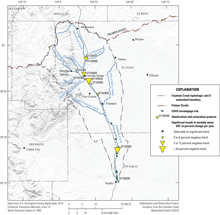
Map showing the distribution of significant trends in suspended sediment flux (SSF) for U.S. Geological Survey (USGS) streamgage sites in the Fountain Creek watershed, Colorado.
Table 2.
Streamgage site identification information (U.S. Geological Survey [USGS], 2024) and a summary of monotonic or step trends for monthly mean suspended sediment flux and monthly mean streamflow data, 1988–2022, Fountain Creek watershed, Colorado.[Mann-Kendall trend, Theil-Sen slope, Wilcoxon Signed Rank tests (Helsel and others, 2020) were used to calculate trends. Trends were considered statistically significant if the p value was less than or equal to the defined alpha of 0.05. USGS, U.S. Geological Survey; n, number of data points; SSF, suspended sediment flux; p, probability value; Colo., Colorado; na, not applicable; %, percent; <, less than]
During the seasonal period of April through September, statistically significant negative trends in monthly mean SSF were detected at 5 sites, and 3 sites showed statistically significant negative trends in monthly mean streamflow (table 2). At one site (07105500, Fountain Creek at Colorado Springs, Colo.), no significant trend was detected during the seasonal period (April through September); however, a significant negative trend in SSF during the snowmelt period (April through June) was detected. Only trends covering the entire seasonal period are included in table 2. The Wilcoxon signed-rank test showed no statistically significant step trend in monthly mean SSF or streamflow for USGS site 07103700 (Fountain Creek near Colorado Springs, Colo.).
The monthly mean suspended sediment statistically significant trends varied from 6 to 25 percent decrease per year for each site’s respective operational period (table 2). The monthly mean streamflow statistically significant trends varied from 7 to 11 percent decrease per year for each site’s respective operational period (table 2). Sites that showed a significant trend in sediment or streamflow did not show a pattern based on their location within the watershed (upstream compared to downstream). Additionally, two sites (Fountain Creek below Janitell Road below Colorado Springs, Colo., and Fountain Creek near Piñon, Colo.) that showed a significant negative trend in suspended sediment also showed a significant negative trend in streamflow. Further evaluation would need to be completed to quantify how much of an effect the negative streamflow trend potentially had on the observed trends in SSF. The remaining three sites that had a significant negative trend in suspended sediment flux (Cottonwood Creek at Mouth at Pikeview, Colo.; Monument Creek at Bijou Street at Colorado Springs, Colo.; and Fountain Creek at Security, Colo.) did not have an associated significant trend in streamflow (table 2), indicating lower sediment concentrations could potentially drive the trend.
Double-Mass Curves
Double-mass curves were used to check the consistency of the relation between streamflow and SSL. Both monthly sediment load and monthly streamflow from the same site were used as measured variables in each of the double-mass curves, which is discussed further in the “Other Considerations” section of this report. The method used in this study can show changes in the relations between the variables but can lack power to determine which variable is responsible for the break in certain circumstances. Additionally, this method cannot determine if changes in watershed characteristics or hydrology are the cause of any observed shifts in the relation.
Of the 10 sites included in this study, 9 displayed observable break points in the double-mass plots, determined by application of a nonparametric LOESS smooth line (fig. 2.1–2.10). Permutation tests run on these nine sites determined that the period (used as the interaction variable) was statistically significant at the 95 percent confidence level (p<0.05), indicating an interaction effect was present. All sites with an observable break point in the plot and a significant interaction effect were then analyzed using regression analysis and hypothesis tests. The slope values for each period (determined by observed break points in time) were calculated and compared pairwise (table 3). The results of the slope comparison determined that the null hypothesis (no difference) could be rejected for all sites and all periods, indicating that the slope change was statistically significant at the 95-percent confidence level (p<0.05). One exception to these results was at USGS site 07105600 (Sand Creek above Mouth at Colorado Springs, Colo.). The null hypothesis for slope comparison of periods A (2003–05) and C (2008–11) at site 07105600 could not be rejected, indicating there is not a significant difference in the relation of SSL and streamflow between these two groups. Known watershed changes that coincide with these break points in the double-mass curves are discussed in the “Characterization of Suspended Sediment Flux and Streamflow Trends” section of this report.
Table 3.
Streamgage site identification information (U.S. Geological Survey [USGS], 2024) and regression slope comparison with p values indicated for each period (A, B, or C) in double-mass curve plots for sites in Fountain Creek watershed, Colorado.[Refer to figures 2.1–2.10 in appendix 2 for graphical representation of conditions and definition of the respective periods for each site. ID, identification; USGS, U.S. Geological Survey; p, probability value; Colo., Colorado; <, less than; na, not applicable]
Flashiness Index
One method to classify streams is to position them on a spectrum ranging from extremely stable groundwater-based streams on one end to very flashy streams on the other. The RBI is a quantitative measure that can be used to establish this continuum (Baker and others, 2004). The highest mean RBI values, which represent more flashy streamflow behavior, were shown by USGS sites 07105600 (Sand Creek above Mouth at Colorado Springs, Colo.; fig. 1) and 07103990 (Cottonwood Creek at Mouth at Pikeview, Colo.; fig. 1), which are two small tributaries to Fountain Creek that drain entirely from the Colorado Piedmont region (fig 1; table 4). In contrast, the least mean flashy behavior was shown by USGS sites 07103700 (Fountain Creek near Colorado Springs, Colo.; fig. 1) and 07103970 (Monument Creek above Woodmen Road at Colorado Springs, Colo.; fig.1), which were the most upstream sites on the main stems of Fountain Creek and Monument Creek and include the Front Range physiographic region in their headwaters. USGS site 07105530 (Fountain Creek below Janitell Road below Colorado Springs, Colo.; fig. 1) had a similarly low mean RBI value, but streamflow at that site was moderated by substantial discharge from an upstream wastewater treatment plant (Bern and others, 2024). Farther downstream along the main stem of Fountain Creek, mean RBI values were intermediate to those calculated for upstream sites (table 4).
Table 4.
Streamgage site identification information (U.S. Geological Survey [USGS], 2024) and a summary of calculated trends in monthly mean Richards-Baker flashiness index (RBI) value (Baker and others, 2004).[Mann-Kendall trend and Theil-Sen slope tests (Helsel and others, 2020) were used to calculate trends. Trends were considered statistically significant if the p value was less than or equal to the defined alpha of 0.05. USGS, U.S. Geological Survey; n, number of data points used in analysis; p, probability value; Colo., Colorado; %, percent]
Monthly mean RBI decreased insignificantly through time at all but one site, but percent change per year was 0 percent for all sites (table 4). At USGS site 07103970 (Monument Creek above Woodmen Road at Colorado Springs, Colo.), there was a significant (p=0.06) increase in RBI through time, but as with the other sites, the magnitude of change was negligible. Because changes in flashiness through time are negligible, changes in flashy stream behavior can be excluded as a potential driver of observed changes in SSL in the watershed.
Other Considerations
This report focused on trends of SSF, which are calculated by multiplying SSC, from samples collected at varying stages along the hydrograph, by streamflow. Increases or decreases in monthly mean streamflow can result in a related increase or decrease in SSF if the SSC remains unchanged. For this reason, it was necessary to also evaluate trends in streamflow in this report to provide a possibly more accurate perspective of any significant trends identified in SSF. Two sites (Fountain Creek below Janitell Road below Colorado Springs, Colo. and Fountain Creek near Piñon, Colo.) where a statistically significant negative trend in monthly mean SSF was identified also had a statistically significant negative trend in monthly mean streamflow (table 2). For these two sites, caution may be beneficial when evaluating the negative trend in SSF. Further analysis would be required to quantify how much of the observed trend in SSF is due to the associated decrease in streamflow. Three sites (Cottonwood Creek at Mouth at Pikeview, Colo., Monument Creek at Bijou Street at Colorado Springs, Colo., and Fountain Creek at Security, Colo.) that had a statistically significant negative trend in SSF did not have an associated significant negative trend in streamflow (table 2). For these three sites, it can be assumed that the decrease in sediment load is most likely due to a decrease in SSC at the sites as there is less sediment per volume of water at those locations (USGS, 2024).
Caution needs to be used when drawing conclusions from the double-mass curve plots in this report. When using two measured variables (rather than using the preferred one measured variable and the cumulation of a pattern of many records in an area), the double-mass analysis may give indefinite results because it is not always possible to determine which variable is responsible for the break in slope (Searcy and others, 1960). The presence of known large-scale watershed changes that have occurred during the operational periods could help to overcome this limitation. Additionally, the SSF data used in this report are not directly measured; rather, they are calculated by the interpolation method described by Porterfield (1972) using the GCLAS software (Koltun and others, 2006). The inherent variability of hydrologic data needs to be considered as well when considering spurious breaks in the double-mass curve plots. Numerous sites in this study show a visible break in the double-mass curves between 2013 and 2015 (app. 2, fig. 2.1–2.10) and may be due to effects from the Waldo Canyon Fire in 2012 and the abnormally high precipitation observed during the 2013 and 2015 seasonal periods (Cole and others, 2014; USGS, 2024). Although these break points are observable on the graph, any break in a curve that persists for fewer than 5 years is not considered reliable. Breaks that persist for 5 years or longer could be due to chance or a real change, and unless the break coincides with a known change in the watershed, statistical methods would be beneficial to evaluate the differing slopes (Searcy and others, 1960).
Characterization of Suspended Sediment Flux and Streamflow Trends
Although all but one site showed statistically significant differences in slopes before and after break points in the double-mass curve plots (table 3), two sites are of particular interest when considering upstream bank stabilization and restoration projects: USGS sites 07106500 (Fountain Creek at Pueblo, Colo.; fig. 1) and 07106300 (Fountain Creek near Piñon, Colo.; fig. 1). Relevant bank stabilization or restoration projects are the Masciantonio Trust bank restoration (completed 2018), Overton Road bank restoration (completed 2020), Piñon Bridge bank stabilization (completed 2019), Barr Farm channel restoration (completed 2020), and the Highway 47 bank restoration (completed 2018; Fountain Creek Watershed District, 2024). The locations of these bank stabilization and restoration projects are shown in fig. 1. The break points identified in the double-mass curve plot for USGS site 07106500 (Fountain Creek at Pueblo, Colo., fig. 2.1) did not coincide with any of these project completion dates. One of the break points identified in the double-mass curve plot for USGS site 07106300 (Fountain Creek near Piñon, Colo., fig. 2.2) was in 2019, which coincides with the completion of the Piñon Bridge bank stabilization project. The slope of the double-mass curve decreased at this point, meaning less sediment was transported per volume of water. The goals of these bank projects were to reduce erosional hazards along Fountain Creek and reduce the total sediment loads in the stream. Although this analysis indicated that the relation between monthly SSL and monthly streamflow was changing at USGS site 07106300 (Fountain Creek near Piñon, Colo., fig. 2.2 in app. 2), the reduction in loads cannot be accurately quantified using this method.
Statistically significant negative SSF trends (p<0.05) were detected at multiple sites (table 2), from smaller tributaries to the main stem of Fountain Creek closer to its confluence with the Arkansas River (fig. 2), and were found to be distributed across the watershed. Such broad distribution of negative trends is most likely an indication of improved water quality in the watershed with regards to suspended sediment. Spatially distributed bank erosion control projects, stormflow retention projects, or changes in climate and storm patterns could be some of the potential causes of changes to SSL trends in a watershed, though assessing specific causes for the decreases in SSL is beyond the scope of this report. One potential driver of SSL trends that can be dismissed on the basis of this study is the flashiness of streamflow as represented by RBI because the magnitude of changes in monthly mean RBI was negligible at all sites (table 4).
Summary
The Fountain Creek watershed drains 927 square miles of south-central Colorado. Extensive population growth and urbanization throughout the watershed has occurred during the last 30 years, and the watershed’s hydrology has been altered by importing nonnative water to support the growing population through water diversions, wastewater-treatment-plant discharges, and changes in water management and operations. These alterations in watershed hydrology could affect geomorphology through streambed and streambank erosion and water quality, including suspended sediment concentrations and load, as assessed in this study. Sampling and analysis of suspended sediment at the U.S. Geological Survey (USGS) streamgage sites along Fountain Creek and its tributaries has established long-term records, making it possible to do statistical analysis to better understand the changes in suspended sediment conditions between 1998 and 2022.
The USGS, in cooperation with Colorado Springs Stormwater Enterprise, have been collecting data to calculate suspended sediment loads at select sites within the Fountain Creek watershed since 1998. The USGS evaluated long-term suspended sediment flux and streamflow datasets for temporal trends (monotonic and step trends) at 10 sites within the Fountain Creek watershed in central Colorado using the Mann-Kendall test (monotonic trend) and the Wilcoxon signed-rank test (step trend). Although all 10 sites included in this study showed a decrease in monthly mean suspended sediment flux (in tons per day), only 5 showed a statistically significant negative trend at the 95 percent confidence level (p<0.05). Of the 5 sites with a statistically significant negative trend in monthly mean suspended sediment flux, 2 of those also showed an associated statistically significant negative trend in streamflow at the same confidence level, indicating the need for further or alternate analyses to assess whether streamflow changes could have affected sediment transport. The spatially broad distribution of negative trends is most likely an indication of decreased suspended sediment throughout the watershed.
Cumulative double-mass curve plots, which provide comparisons between cumulative streamflow and suspended sediment load, were created for all sites. The plots were used to identify break points in the curve, indicating a temporal change in the relation between streamflow and suspended sediment load. All site plots with break points showed statistically significant differences in slopes before and after observed break points in the double-mass curve plots. Two streamgage sites were of interest when considering previously mentioned upstream bank stabilization and restoration projects: USGS sites 07106500 (Fountain Creek at Pueblo, Colorado) and 07106300 (Fountain Creek near Piñon, Colo.). One of the break points identified in the double-mass curve plot of USGS site 07106300 was in 2019, which coincided with the completion of the Piñon Bridge bank stabilization project. The slope of the double-mass curve decreased at this point, meaning less sediment was transported per volume of water. Although the decrease in slope was found to be statistically significant, it is not possible to accurately quantify the reduction in sediment load using this method. Similarly, multiple sites in the watershed showed a significant negative trend in suspended sediment loads during the study period; however, identifying the underlying cause of those trends is beyond the scope of this report. The flashiness (as determined by the Richards-Baker flashiness index) of streamflow was assessed and can be dismissed based on this study as a potential driver of trends in suspended sediment flux as the magnitude of changes was found to be negligible at all sites.
Spatially distributed bank erosion control projects, stormflow retention projects in the watershed, or changes in climate and storm patterns could be some of the potential drivers of the suspended sediment load trends in a watershed. More recently, multiple projects have been implemented in the watershed to address and remediate erosional issues and associated sediment entrainment, most notably bank stabilization and restoration projects along the lower reaches of Fountain Creek.
References Cited
Baker, D.B., Richards, R.P., Loftus, T.T., and Kramer, J.W., 2004, A new flashiness index—Characteristics and applications to Midwestern rivers and streams: Journal of the American Water Resources Association, v. 40, no. 2, p. 503–522, accessed July 3, 2024, at https://doi.org/10.1111/j.1752-1688.2004.tb01046.x.
Bern, C.R., Ruckhaus, M., and Hennessy, E., 2024, Potential climate and water-use effects on water-quality trends in a semiarid, Western U.S. watershed—Fountain Creek, Colorado, USA: Water, v. 16, no. 10, p. 1343, accessed July 3, 2024, at https://doi.org/10.3390/w16101343.
Cole, C.J., Friesen, B.A., and Wilson, E.M., 2014, Use of satellite imagery to identify vegetation cover changes following the Waldo Canyon Fire event, Colorado, 2012–2013: U.S. Geological Survey Open-File Report 2014–1078, 1 sheet, accessed June 2024 at https://doi.org/10.3133/ofr20141078.
Colorado Department of Local Affairs, 2024, Data tools and resources—County population and housing lookups: Colorado Department of Local Affairs State Demography Office web page, accessed May 2024 at https://demography.dola.colorado.gov/.
De Cicco, L.A., Hirsch, R.M., Lorenz, D., Watkins, W.D., and Johnson, M., 2022, dataRetrieval—R packages for discovering and retrieving water data available from Federal hydrologic web services (ver. 2.7.17.9): U.S. Geological Survey software release, accessed November 2023 at https://doi.org/10.5066/P9X4L3GE.
Dewitz, J., 2023, National Land Cover Database (NLCD) 2021 products: U.S. Geological Survey data release, accessed June 2024 at https://doi.org/10.5066/P9JZ7AO3.
Downhour, M.S., and Hennessy, E.K., 2024, Suspended sediment data and loads in the Fountain Creek watershed, CO: U.S. Geological Survey data release, https://doi.org/10.5066/P94UW017.
Fountain Creek Watershed District, 2024, Completed projects: Fountain Creek Watershed District web page, accessed May 2024 at https://www.fountain-crk.org/completed-projects.
Guy, H.P., 1969, Laboratory theory and methods for sediment analysis; U.S. Geological Survey Techniques of Water-Resources Investigations, book 5, chap. C1, 58 p., accessed June 2024 at https://doi.org/10.3133/twri05C1.
Hansen, W.R., and Crosby, E.J., 1982, Environmental geology of the Front Range urban corridor and vicinity, Colorado: U.S. Geological Survey Professional Paper 1230, 99 p. [Also available at https://pubs.usgs.gov/pp/1230/report.pdf.]
Helsel, D.R., Hirsch, R.M., Ryberg, K.R., Archfield, S.A., and Gilroy, E.J., 2020, Statistical methods in water resources: U.S. Geological Survey Techniques and Methods, book 4, chap. A3, 458 p., accessed May 2024 at https://doi.org/10.3133/tm4A3. [Supersedes USGS Techniques of Water-Resources Investigations, book 4, chap. A3, version 1.1.]
Hempel, L.A., Creighton, A.L., and Bock, A.R., 2021, Elevation and elevation-change maps of Fountain Creek, southeastern Colorado, 2015–20: U.S. Geological Survey Scientific Investigations Map 3481, 10 sheets, 12 p. pamphlet, accessed February 20, 2025, at https://doi.org/10.3133/sim3481.
Kohn, M.S., Fulton, J.W., Williams, C.A., and Stogner, R.W., Sr., 2014, Remediation scenarios for attenuating peak flows and reducing sediment transport in Fountain Creek, Colorado, 2013: U.S. Geological Survey Scientific Investigations Report 2014–5019, 62 p., accessed May 2024 at https://doi.org/10.3133/sir20145019.
Koltun, G.F., Eberle, M., Gray, J.R., and Glysson, G.D., 2006, User's manual for the Graphical Constituent Loading Analysis System (GCLAS): U.S. Geological Survey Techniques and Methods, book 4, chap. C1, 51 p., accessed May 2024 at https://doi.org/10.3133/tm4C1.
Lenth, R.V., 2016, Least-Squares Means—The R Package lsmeans: Journal of Statistical Software, v. 69, no. 1, p. 1–33, accessed May 22, 2024, at https://doi.org/10.18637/jss.v069.i01.
Lurry, D.L., 2011, How does a U.S. Geological Survey streamgage work?: U.S. Geological Survey Fact Sheet 2011–3001, 2 p., accessed June 2024 at https://pubs.usgs.gov/fs/2011/3001/.
Mau, D.P., Stogner, R.W., Sr., and Edelmann, P., 2007, Characterization of stormflows and wastewater treatment-plant effluent discharges on water quality, suspended sediment, and stream morphology for Fountain and Monument Creek watersheds, Colorado, 1981–2006: U.S. Geological Survey Scientific Investigations Report 2007–5104, 76 p., accessed May 2024 at https://doi.org/10.3133/sir20075104.
Millard, S.P., 2013, EnvStats—An R package for environmental statistics: New York, Springer, accessed May 2, 2024, at https://link.springer.com/book/10.1007/978-1-4614-8456-1.
Miller, L.D., and Stogner, R.W., Sr., 2017, Characterization of water quality and suspended sediment during cold-season flows, warm-season flows, and stormflows in the Fountain and Monument Creek watersheds, Colorado, 2007–2015: U.S. Geological Survey Scientific Investigations Report 2017–5084, 47 p., accessed May 2024 at https://doi.org/10.3133/sir20175084.
Noe, G.B., Cashman, M.J., Skalak, K., Gellis, A., Hopkins, K.G., Moyer, D., Webber, J., Benthem, A., Maloney, K., Brakebill, J., Sekellick, A., Langland, M., Zhang, Q., Shenk, G., Keisman, J., and Hupp, C., 2020, Sediment dynamics and implications for management—State of the science from long-term research in the Chesapeake Bay watershed, USA: WIREs Water, v. 7, no. 4, art. e1454, 28 p., accessed June 2024 at https://doi.org/10.1002/wat2.1454.
Paul, M.J., and Meyer, J.L., 2001, Streams in the urban landscape: Annual Review of Ecology and Systematics, v. 32, no. 1, p. 333–365, accessed July 2024 at https://doi.org/10.1146/annurev.ecolsys.32.081501.114040.
Porterfield, G., 1972, Computation of fluvial-sediment discharge: U.S. Geological Survey Techniques of Water-Resources Investigations, book 3, chap. C3, 66 p., accessed February 19, 2024, at https://doi.org/10.3133/twri03C3.
R Core Team, 2022, R—A language and environment for statistical computing (ver. 4.2.2): R Foundation for Statistical Computing software release, Vienna, Austria, accessed June 2024 at http://www.R-project.org/.
R Core Team, 2024, R—A language and environment for statistical computing (ver. 4.4.0): R Foundation for Statistical Computing software release, Vienna, Austria, accessed July 2024 at http://www.R-project.org/.
Searcy, J.K., Hardison, C.H., and Langbein, W.B., 1960, Double-mass curves, with a section fitting curves to cyclic data: U.S. Geological Society Water Supply Paper 1541-B, 36 p., accessed May 14, 2024, at https://doi.org/10.3133/wsp1541B.
Stogner, R.W., 2000, Trends in precipitation and streamflow and changes in stream morphology in the Fountain Creek watershed, Colorado, 1939–99: U.S. Geological Survey Water-Resources Investigations Report 2000–4130, 48 p., accessed May 2024 at https://doi.org/10.3133/wri004130.
Stogner, R.W., Sr., Nelson, J.M., McDonald, R.R., Kinzel, P.J., and Mau, D.P., 2013, Prediction of suspended-sediment concentrations at selected sites in the Fountain Creek watershed, Colorado, 2008–09: U.S. Geological Survey Scientific Investigations Report 2012–5102, 36 p., accessed May 2024 at https://pubs.usgs.gov/sir/2012/5102/.
U.S. Environmental Protection Agency [EPA], 2020, Colorado Springs settlement information sheet: U.S. Environmental Protection Agency web page, accessed June 2023 at https://www.epa.gov/enforcement/colorado-springs-settlement-information-sheet.
U.S. Environmental Protection Agency [EPA], 2022, Climate impacts on water utilities: U.S. Environmental Protection Agency web page, accessed June 2023 at https://www.epa.gov/arc-x/climate-impacts-water-utilities. [Updated March 27, 2025.]
U.S. Geological Survey [USGS], 2019a, GCLAS (Graphical Constituent Loading Analysis System)—A tool for computing loads of constituents transported in rivers [multiple versions used]: U.S. Geological Survey software release, accessed February 2024 at https://water.usgs.gov/water-resources/software/GCLAS/.
U.S. Geological Survey [USGS], 2019b, The StreamStats program for Colorado: U.S. Geological Survey web page, accessed March 2024 at https://streamstats.usgs.gov/ss/.
U.S. Geological Survey [USGS], 2024, USGS water data for the Nation: U.S. Geological Survey National Water Information System database, accessed April 2024 at https://doi.org/10.5066/F7P55KJN.
U.S. Geological Survey [USGS], [variously dated], National field manual for the collection of water-quality data, section A of Handbooks for water-resources investigations: U.S. Geological Survey Techniques of Water-Resources Investigations, book 9, 10 chap. (A1–A8, A10), accessed February 2025 at https://www.usgs.gov/mission-areas/water-resources/science/national-field-manual-collection-water-quality-data-nfm.
von Guerard, Paul, 1989, Suspended sediment and sediment-source areas in the Fountain Creek drainage basin upstream from Widefield, southeastern Colorado: U.S. Geological Survey Water-Resources Investigations Report 88–4136, 36 p., accessed May 2024 at https://doi.org/10.3133/wri884136.
Weather Service, 2019, Climate Colorado Springs—Colorado, U.S.: U.S. Climate Data webpage, accessed October 2024 at https://www.usclimatedata.com/climate/colorado-springs/colorado/united-states/usco0078.
Wilson, T.P., Miller, C.V., and Lechner, E.A., 2024, Guidelines for the use of automatic samplers in collecting surface-water quality and sediment data: U.S. Geological Survey Techniques and Methods, book 1, chap. D12, 89 p., accessed February 2025 at https://doi.org/10.3133/tm1D12.
Appendix 1. Plots of Monthly Mean Suspended Sediment Flux and Monthly Mean Streamflow Through Time with Thiel-Sen Robust Linear Regression Line for Each Site
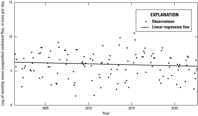
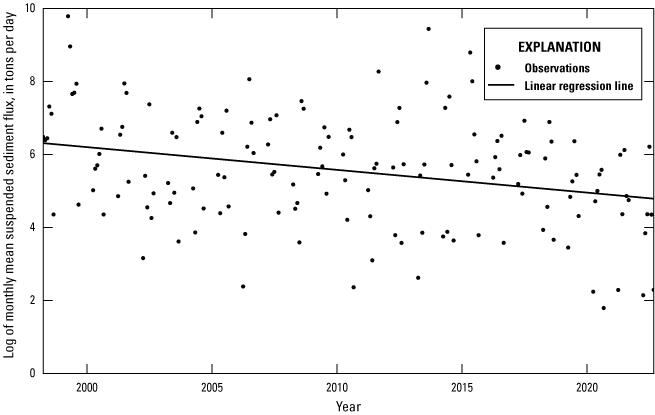
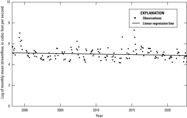
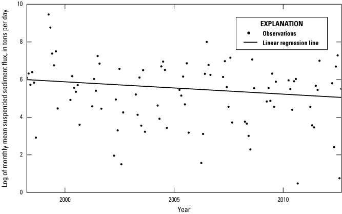
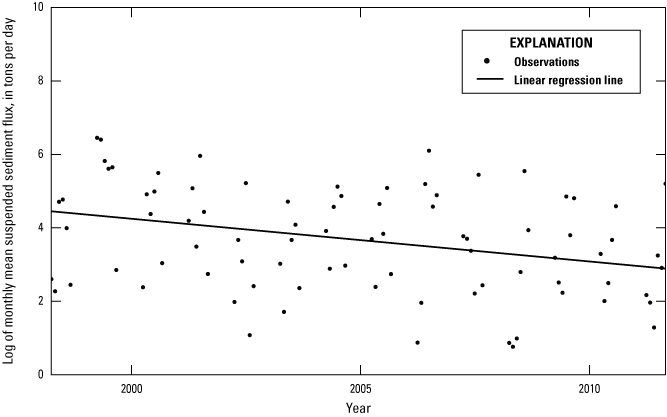
Graph of monthly mean suspended sediment flux, in tons per day, 2001–22, for U.S. Geological Survey site 07106500 (Fountain Creek at Pueblo, Colorado), with Theil-Sen robust linear regression line. Theil-Sen slope (Helsel and others, 2020); data available at Downhour and Hennessy (2024).
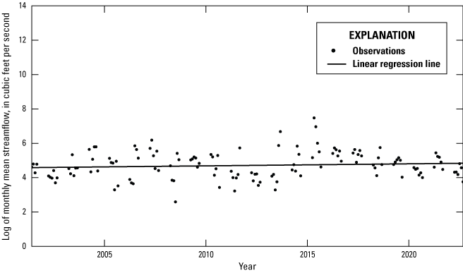
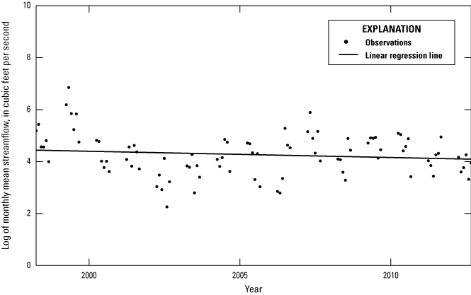
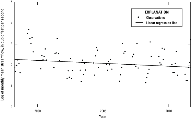
Graph of monthly mean streamflow, in cubic feet per second, 2001–22, for U.S. Geological Survey site 07106500 (Fountain Creek at Pueblo, Colorado), with Theil-Sen robust linear regression line. Theil-Sen slope (Helsel and others, 2020); data available at Downhour and Hennessy (2024).
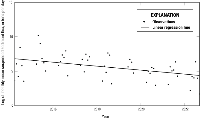
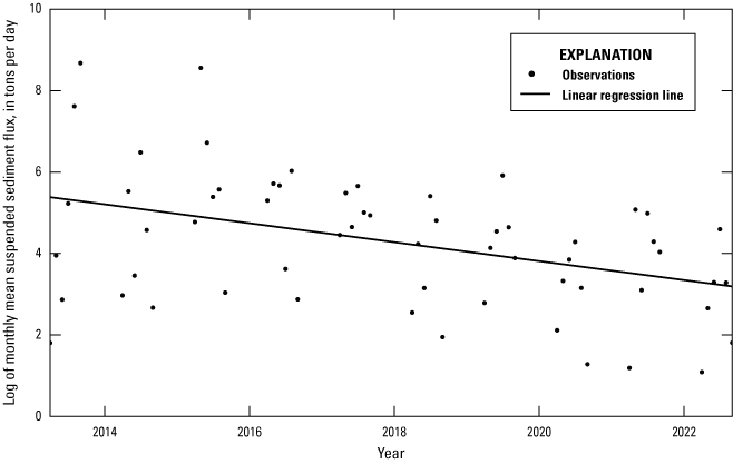
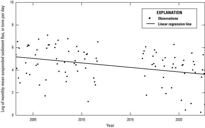
Graph of monthly mean suspended sediment flux, in tons per day, 2014–22, for U.S. Geological Survey site 07106300 (Fountain Creek near Piñon, Colorado), with Theil-Sen robust linear regression line. Theil-Sen slope (Helsel and others, 2020); data available at Downhour and Hennessy (2024).
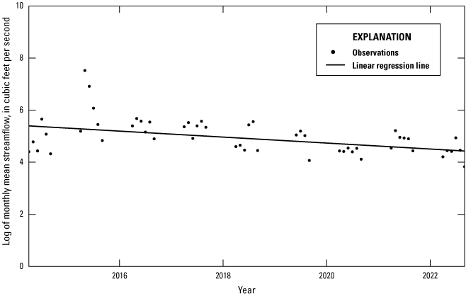
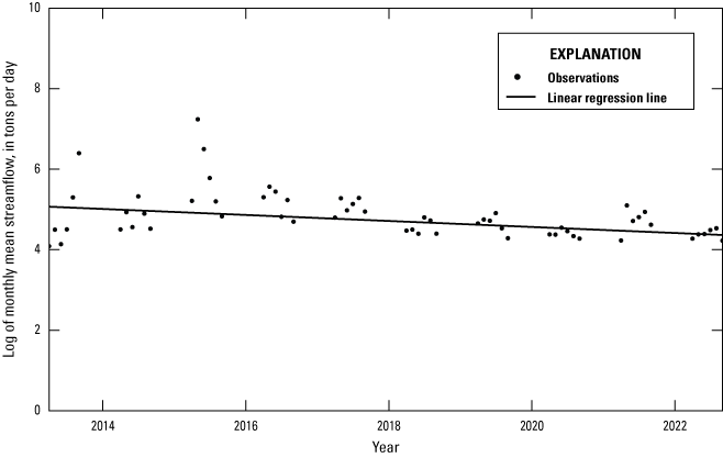
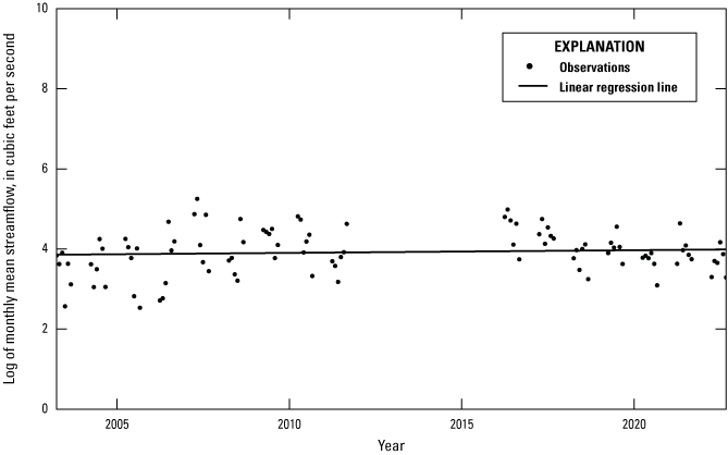
Graph of monthly mean streamflow, in cubic feet per second, 2014–22, for U.S. Geological Survey site 07106300 (Fountain Creek near Piñon, Colorado), with Theil-Sen robust linear regression line. Theil-Sen slope (Helsel and others, 2020); data available at Downhour and Hennessy (2024).
Graph of monthly mean suspended sediment flux, in tons per day, 1998–2022, for U.S. Geological Survey site 07105800 (Fountain Creek at Security, Colorado), with Theil-Sen robust linear regression line. Theil-Sen slope (Helsel and others, 2020); data available at Downhour and Hennessy (2024).
Graph of monthly mean streamflow, in cubic feet per second, 1998–2022, for U.S. Geological Survey site 07105800 (Fountain Creek at Security, Colorado), with Theil-Sen robust linear regression line. Theil-Sen slope (Helsel and others, 2020); data available at Downhour and Hennessy (2024).
Graph of monthly mean suspended sediment flux, in tons per day, 2003–11, for U.S. Geological Survey site 07105600 (Sand Creek above Mouth at Colorado Springs, Colorado), with Theil-Sen robust linear regression line. Theil-Sen slope (Helsel and others, 2020); data available at Downhour and Hennessy (2024).
Graph of monthly mean streamflow, in cubic feet per second, 2003–11, for U.S. Geological Survey site 07105600 (Sand Creek above Mouth at Colorado Springs, Colorado), with Theil-Sen robust linear regression line. Theil-Sen slope (Helsel and others, 2020); data available at Downhour and Hennessy (2024).
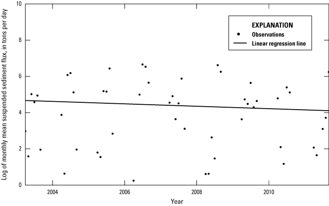
Graph of monthly mean suspended sediment flux, in tons per day, 2013–22, for U.S. Geological Survey site 07105530 (Fountain Creek below Janitell Road below Colorado Springs, Colorado), with Theil-Sen robust linear regression line. Theil-Sen slope (Helsel and others, 2020); data available at Downhour and Hennessy (2024).
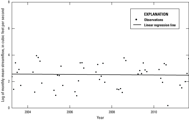
Graph of monthly mean streamflow, in cubic feet per second, 2013–22, for U.S. Geological Survey site 07105530 (Fountain Creek below Janitell Road below Colorado Springs, Colorado), with Theil-Sen robust linear regression line. Theil-Sen slope (Helsel and others, 2020); data available at Downhour and Hennessy (2024).
Graph of monthly mean suspended sediment flux, in tons per day, 1998–2012, for U.S. Geological Survey site 07105500 (Fountain Creek at Colorado Springs, Colorado), with Theil-Sen robust linear regression line. Theil-Sen slope (Helsel and others, 2020); data available at Downhour and Hennessy (2024).
Graph of monthly mean streamflow, in cubic feet per second, 1998–2012, for U.S. Geological Survey site 07105500 (Fountain Creek at Colorado Springs, Colorado), with Theil-Sen robust linear regression line. Theil-Sen slope (Helsel and others, 2020); data available at Downhour and Hennessy (2024).
Graph of monthly mean suspended sediment flux, in tons per day, 2003–11 and 2016–22, for U.S. Geological Survey site 07104905 (Monument Creek at Bijou Street at Colorado Springs, Colorado), with Theil-Sen robust linear regression line. Theil-Sen slope (Helsel and others, 2020); data available at Downhour and Hennessy (2024).
Graph of monthly mean streamflow, in cubic feet per second, 2003–11 and 2016–22, for U.S. Geological Survey site 07104905 (Monument Creek at Bijou Street at Colorado Springs, Colorado), with Theil-Sen robust linear regression line. Theil-Sen slope (Helsel and others, 2020); data available at Downhour and Hennessy (2024).
Graph of monthly mean suspended sediment flux, in tons per day, 1998–2011, for U.S. Geological Survey site 07103990 (Cottonwood Creek at Mouth at Pikeview, Colorado), with Theil-Sen robust linear regression line. Theil-Sen slope (Helsel and others, 2020); data available at Downhour and Hennessy (2024).
Graph of monthly mean streamflow, in cubic feet per second, 1998–2011, for U.S. Geological Survey site 07103990 (Cottonwood Creek at Mouth at Pikeview, Colorado), with Theil-Sen robust linear regression line. Theil-Sen slope (Helsel and others, 2020); data available at Downhour and Hennessy (2024).
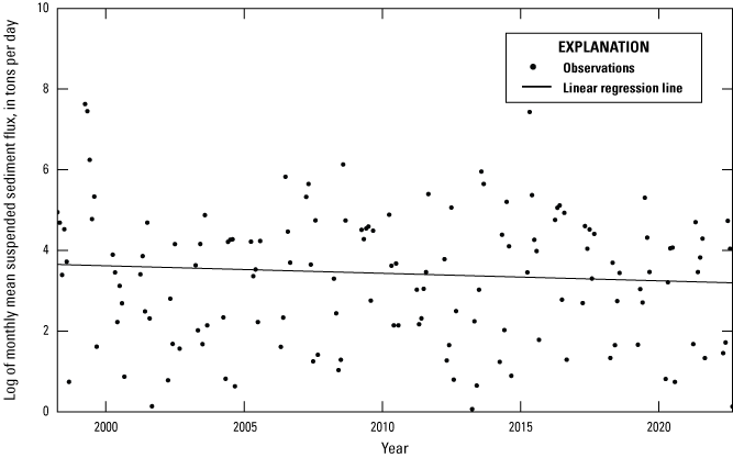
Graph of monthly mean suspended sediment flux, in tons per day, 1998–2022, for U.S. Geological Survey site 07103970 (Monument Creek above Woodmen Road at Colorado Springs, Colorado), with Theil-Sen robust linear regression line. Theil-Sen slope (Helsel and others, 2020); data available at Downhour and Hennessy (2024).
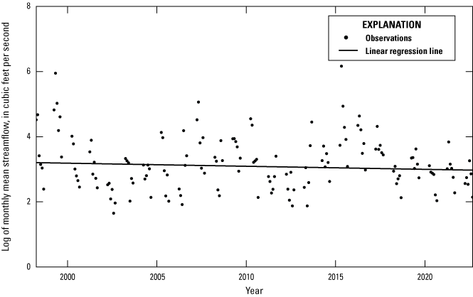
Graph of monthly mean streamflow, in cubic feet per second, 1998–2022, for U.S. Geological Survey site 07103970 (Monument Creek above Woodmen Road at Colorado Springs, Colorado), with Theil-Sen robust linear regression line. Theil-Sen slope (Helsel and others, 2020); data available at Downhour and Hennessy (2024).
References Cited
Downhour, M.S., and Hennessy, E.K., 2024, Suspended sediment data and loads in the Fountain Creek watershed, CO: U.S. Geological Survey data release, https://doi.org/10.5066/P94UW017.
Helsel, D.R., Hirsch, R.M., Ryberg, K.R., Archfield, S.A., and Gilroy, E.J., 2020, Statistical methods in water resources: U.S. Geological Survey Techniques and Methods, book 4, chap. A3, 458 p., accessed May 2024 at https://doi.org/10.3133/tm4A3. [Supersedes USGS Techniques of Water-Resources Investigations, book 4, chap. A3, version 1.1.]
Appendix 2. Double Mass Plots of Cumulative Monthly Suspended Sediment Loads and Cumulative Monthly Streamflow Through Time with LOESS Smooth Line
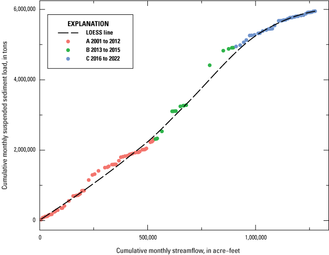
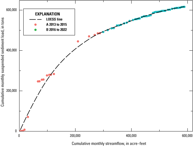
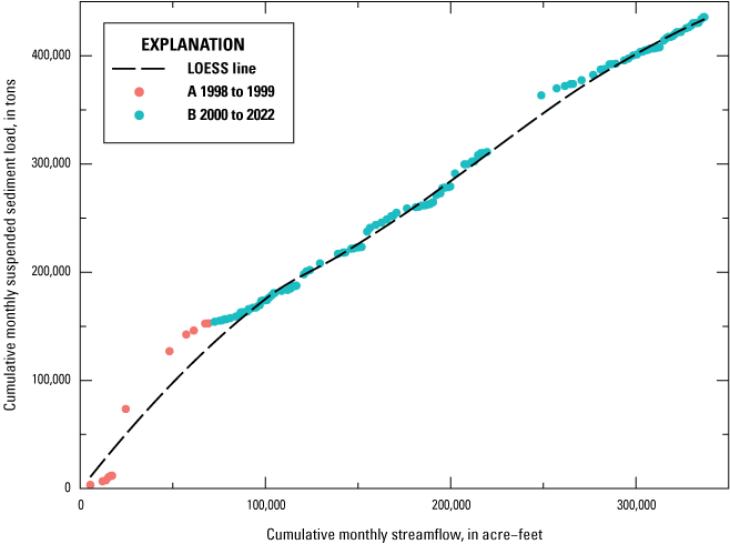
Cumulative double-mass curve plot for U.S. Geological Survey site 07106500 (Fountain Creek at Pueblo, Colorado) with cumulative monthly mean streamflow, in acre-feet, and cumulative monthly mean suspended sediment load, in tons, with a nonparametric locally estimated scatterplot smoothing (LOESS) smooth line. Periods with differing slopes are separated by data point color and defined by year. LOESS smooth line, Helsel and others (2020); double-mass curve, Searcy and others (1960); data available at Downhour and Hennessy (2024).
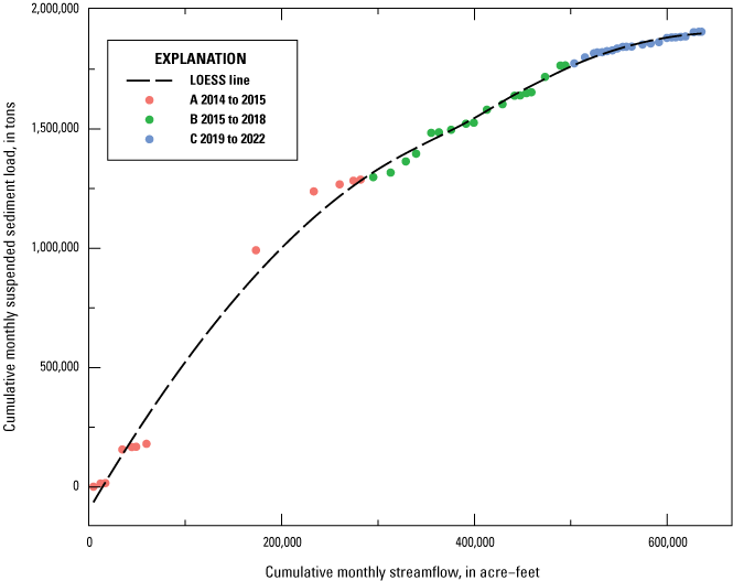
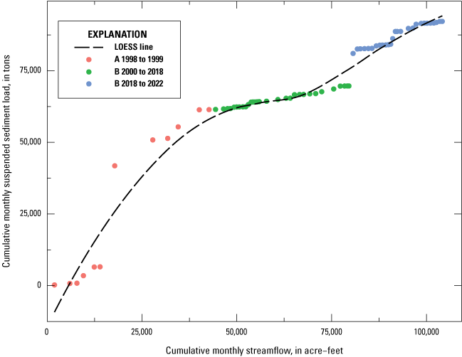
Cumulative double-mass curve plot for U.S. Geological Survey site 07106300 (Fountain Creek near Piñon, Colorado) with cumulative monthly mean streamflow, in acre-feet, and cumulative monthly mean suspended sediment load, in tons, with a nonparametric locally estimated scatterplot smoothing (LOESS) smooth line. Periods with differing slopes are separated by data point color and defined by year. LOESS smooth line, Helsel and others (2020); double-mass curve, Searcy and others (1960); data available at Downhour and Hennessy (2024).
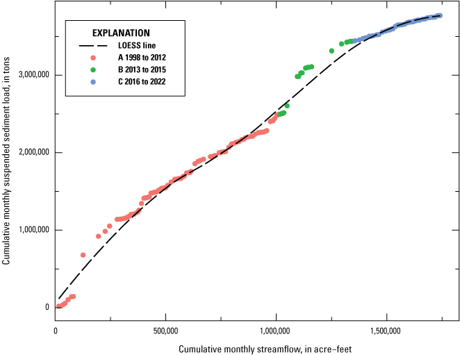
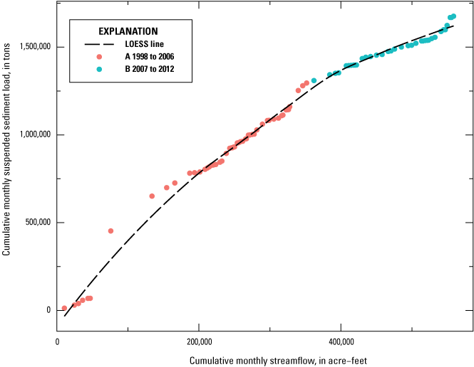
Cumulative double mass curve plot for U.S. Geological Survey site 07105800 (Fountain Creek at Security, Colorado) with cumulative monthly mean streamflow, in acre-feet, and cumulative monthly mean suspended sediment load, in tons, with a nonparametric locally estimated scatterplot smoothing (LOESS) smooth line. Periods with differing slopes are separated by data point color and defined by year. LOESS smooth line, Helsel and others (2020); double-mass curve, Searcy and others (1960); data available at Downhour and Hennessy (2024).
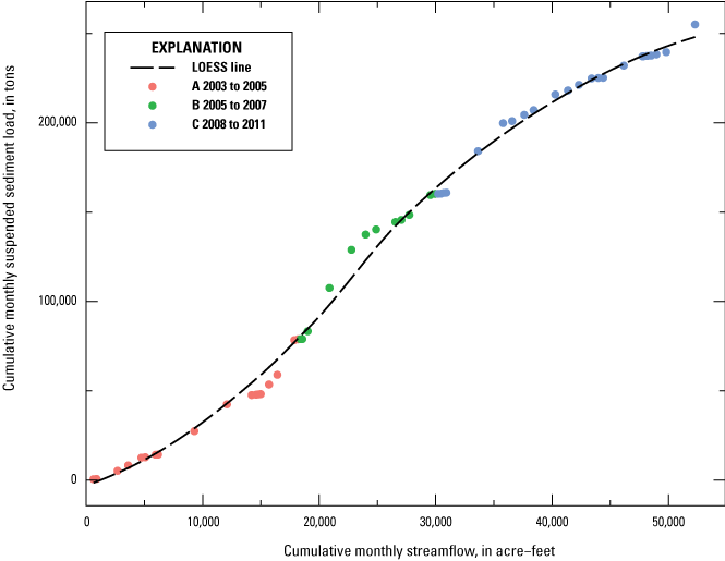
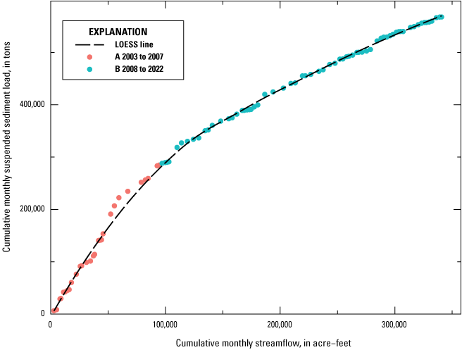
Cumulative double-mass curve plot for U.S. Geological Survey site 07105600 (Sand Creek above Mouth at Colorado Springs, Colorado) with cumulative monthly mean streamflow, in acre-feet, and cumulative monthly mean suspended sediment load, in tons, with a nonparametric locally estimated scatterplot smoothing (LOESS) smooth line. Periods with differing slopes are separated by data point color and defined by year. LOESS smooth line, Helsel and others (2020); double-mass curve, Searcy and others (1960); data available at Downhour and Hennessy (2024).
Cumulative double-mass curve plot for U.S. Geological Survey site 07105530 (Fountain Creek below Janitell Road below Colorado Springs, Colorado) with cumulative monthly mean streamflow, in acre-feet, and cumulative monthly mean suspended sediment load, in tons, with a nonparametric locally estimated scatterplot smoothing (LOESS) smooth line. Periods with differing slopes are separated by data point color and defined by year. LOESS smooth line, Helsel and others (2020); double-mass curve, Searcy and others (1960); data available at Downhour and Hennessy (2024).
Cumulative double-mass curve plot for U.S. Geological Survey site 07105500 (Fountain Creek at Colorado Springs, Colorado), with cumulative monthly mean streamflow, in acre-feet, and cumulative monthly mean suspended sediment load, in tons, with a nonparametric locally estimated scatterplot smoothing (LOESS) smooth line. Periods with differing slopes are separated by data point color and defined by year. LOESS smooth line, Helsel and others (2020); double-mass curve, Searcy and others (1960); data available at Downhour and Hennessy (2024).
Cumulative double-mass curve plot for U.S. Geological Survey site 07104905 (Monument Creek at Bijou Street at Colorado Springs, Colorado) with cumulative monthly mean streamflow, in acre-feet, and cumulative monthly mean suspended sediment load, in tons, with a nonparametric locally estimated scatterplot smoothing (LOESS) smooth line. Periods with differing slopes are separated by data point color and defined by year. LOESS smooth line, Helsel and others (2020); double-mass curve, Searcy and others (1960); data available at Downhour and Hennessy (2024).
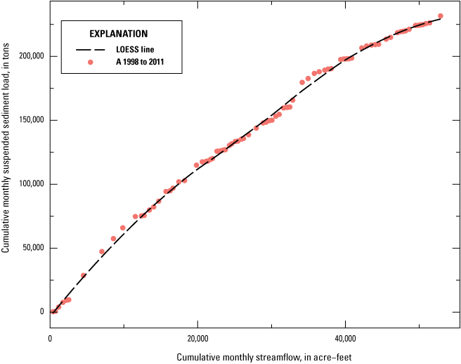
Cumulative double-mass curve plot for U.S. Geological Survey site 07103990 (Cottonwood Creek at Mouth at Pikeview, Colorado) with cumulative monthly mean streamflow, in acre-feet, and cumulative monthly mean suspended sediment load, in tons, with a nonparametric locally estimated scatterplot smoothing (LOESS) smooth line. Periods with differing slopes are separated by data point color and defined by year. LOESS smooth line, Helsel and others (2020); double-mass curve, Searcy and others (1960); data available at Downhour and Hennessy (2024).
Cumulative double-mass curve plot for U.S. Geological Survey site 07103970 (Monument Creek above Woodmen Road at Colorado Springs, Colorado) with cumulative monthly mean streamflow, in acre-feet, and cumulative monthly mean suspended sediment load, in tons, with a nonparametric locally estimated scatterplot smoothing (LOESS) smooth line. Periods with differing slopes are separated by data point color and defined by year. LOESS smooth line, Helsel and others (2020); double-mass curve, Searcy and others (1960); data available at Downhour and Hennessy (2024).
Cumulative double-mass curve plot for U.S. Geological Survey site 07103700 (Fountain Creek near Colorado Springs, Colorado) with cumulative monthly mean streamflow, in acre-feet, and cumulative monthly mean suspended sediment load, in tons, with a nonparametric locally estimated scatterplot smoothing (LOESS) smooth line. Periods with differing slopes are separated by data point color and defined by year. LOESS smooth line, Helsel and others (2020); double-mass curve, Searcy and others (1960); data available at Downhour and Hennessy (2024).
References Cited
Downhour, M.S., and Hennessy, E.K., 2024, Suspended sediment data and loads in the Fountain Creek watershed, CO: U.S. Geological Survey data release, https://doi.org/10.5066/P94UW017.
Helsel, D.R., Hirsch, R.M., Ryberg, K.R., Archfield, S.A., and Gilroy, E.J., 2020, Statistical methods in water resources: U.S. Geological Survey Techniques and Methods, book 4, chap. A3, 458 p., accessed May 2024 at https://doi.org/10.3133/tm4A3. [Supersedes USGS Techniques of Water-Resources Investigations, book 4, chap. A3, version 1.1.]
Searcy, J.K., Hardison, C.H., and Langbein, W.B., 1960, Double-mass curves, with a section fitting curves to cyclic data: U.S. Geological Society Water Supply Paper 1541-B, 36 p., accessed May 2024 at https://doi.org/10.3133/wsp1541B.
Conversion Factors
U.S. customary units to International System of Units
Datums
Vertical coordinate information is referenced to the North American Vertical Datum of 1988 (NAVD 88).
Horizontal coordinate information is referenced to the North American Datum of 1983 (NAD 83).
Elevation, as used in this report, refers to distance above the vertical datum.
Supplemental Information
Flux is mass or load transported per unit of time, short tons per day.
Suspended sediment loads are in short tons.
Abbreviations
EPA
U.S. Environmental Protection Agency
GCLAS
Graphical Constituent Loading Analysis System
LOESS
locally estimated scatterplot smoothing
NWIS
National Water Information System
SSC
suspended sediment concentration
SSF
suspended sediment flux
SSL
suspended sediment load
RBI
Richards-Baker flashiness index
USGS
U.S. Geological Survey
For more information concerning the research in this report, contact the
Director, USGS Colorado Water Science Center
Box 25046, Mail Stop 415
Denver, CO 80225
(303) 236-4882
Or visit the Colorado Water Science Center website at
https://www.usgs.gov/centers/colorado-water-science-center
Publishing support provided by the Science Publishing Network,
Denver, Moffett, and Reston Publishing Service Centers
Disclaimers
Any use of trade, firm, or product names is for descriptive purposes only and does not imply endorsement by the U.S. Government.
Although this information product, for the most part, is in the public domain, it also may contain copyrighted materials as noted in the text. Permission to reproduce copyrighted items must be secured from the copyright owner.
Suggested Citation
Downhour, M.S., Hennessy, E.K., and Bern, C.R., 2025, Characterization of suspended sediment flux and streamflow trends in the Fountain Creek watershed, Colorado, 1998 through 2022 (ver. 1.1, December 2025): U.S. Geological Survey Scientific Investigations Report 2025–5089, 30 p., https://doi.org/10.3133/sir20255089.
ISSN: 2328-0328 (online)
ISSN: 2328-031X (print)
Study Area
| Publication type | Report |
|---|---|
| Publication Subtype | USGS Numbered Series |
| Title | Characterization of suspended sediment flux and streamflow trends in the Fountain Creek watershed, Colorado, 1998 through 2022 |
| Series title | Scientific Investigations Report |
| Series number | 2025-5089 |
| DOI | 10.3133/sir20255089 |
| Edition | Version 1.0: September 22, 2025; Version 1.1: December 30, 2025 |
| Publication Date | September 22, 2025 |
| Year Published | 2025 |
| Language | English |
| Publisher | U.S. Geological Survey |
| Publisher location | Reston VA |
| Contributing office(s) | Colorado Water Science Center |
| Description | Report: v, 30 p.; Data Release: Database |
| Country | United States |
| State | Colorado |
| Other Geospatial | Fountain Creek watershed |
| Online Only (Y/N) | N |