

Evaluating Hydrologic Data Products for Scientific and Management Applications Related to Potential Future Streamflow Conditions in the Upper Mississippi and Illinois Rivers
Links
- Document: Report (5.91 MB pdf) , HTML , XML
- Dataset: USGS National Water Information System database - USGS water data for the Nation
- NGMDB Index Page: National Geologic Map Database Index Page (html)
- Download citation as: RIS | Dublin Core
Acknowledgments
This report was supported by the U.S. Army Corps of Engineers (USACE) Upper Mississippi River Restoration program with assistance from the USACE Infrastructure and Installation Resilience Community of Practice. The authors appreciate Michael Dougherty’s (USACE) reviews of statistical software scripts used in the data analysis.
The authors thank Jeff Houser (U.S. Geological Survey [USGS]), Karen Ryberg (USGS), and Thomas Over (USGS) for providing thoughtful reviews that substantially improved the report. The authors are grateful to Jason J. Rohweder (USGS) for creating the map figure and to SPN staff for publication assistance.
The authors acknowledge the effort and funding that support the streamgages in this analysis. Yellow Medicine River near Granite Falls, Minnesota (05313500); Mississippi River at Prescott, Wisconsin (05344500); Jump River at Sheldon, Wisconsin (05362000); Turkey River at Garber, Iowa (05412500); Skunk River at Augusta, Iowa (05474000); Cedar River near Conesville, Iowa (05465000); Elkhorn Creek near Penrose, Illinois (05444000); Cedar Creek near Bussey, Iowa (05489000); Raccoon River at Van Meter, Iowa (05484500); Fox River at Wayland, Missouri (05495000); and the Illinois River at Marseilles, Illinois (05543500) are operated as USGS Federal Priority Streamgages (formerly the National Streamflow Information Program). In addition, the Turkey River at Garber, Iowa, and the Skunk River at Augusta, Iowa, are operated in cooperation with the Iowa Department of Natural Resources and with USGS Cooperative Matching Funds; the Cedar River at Conesville, Iowa, is operated in cooperation with the USACE Rock Island District; the Cedar Creek at Bussey, Iowa, is operated in cooperation with the Iowa Department of Transportation and the USACE Rock Island District; the Raccoon River at Van Meter, Iowa, is operated in cooperation with Des Moines Water Works and the Iowa Department of Natural Resources (DNR) with USGS cooperative matching funds; and the Fox River at Wayland, Missouri, is operated with cooperation from the Missouri DNR with USGS cooperative matching funds. The following streamgages are not in the USGS Federal Priority Streamgage program but are operated in partnership with cooperating agencies: Trempealeau River at Dodge, Wisconsin (05379500) is operated in cooperation with the USACE St. Paul District; Kickapoo River at La Farge, Wisconsin (05408000) with the Kickapoo Valley Reserve and with USGS cooperative matching funds; Mississippi River at Clinton, Iowa (05420500) with the City of Clinton, Constellation Energy Generation, LLC, and the USACE Rock Island District; Kankakee River near Wilmington, Illinois (05527500) with Constellation Energy Generation, LLC; Vermilion River near Leonore, Illinois (05555300), Illinois River at Kingston Mines, Illinois (05568500), and Spoon River at Seville, Illinois (05570000) with the USACE Rock Island District; and the Meramec River near Eureka, Missouri (07019000) with the USACE St. Louis District.
We acknowledge the World Climate Research Programme’s Working Group on Coupled Modelling, which is responsible for the Climate Model Diagnosis and Intercomparison Project (CMIP), and we thank the climate modeling groups (listed in appendix 2, table 2.1 of this report) for producing and making available their model output. For CMIP, the U.S. Department of Energy’s Program for Climate Model Diagnosis and Intercomparison provides coordinating support and led development of software infrastructure in partnership with the Global Organization for Earth System Science Portals.
Abstract
The hydrology of the Upper Mississippi and Illinois Rivers is a fundamental driver of ecosystem patterns and processes across a large portion of the United States. Quantitative hydrologic data for the main stems of these rivers underlie numerous scientific investigations, statistical models, and decision-making processes for local, State, and Federal agencies involved in the Upper Mississippi River Restoration program. Although historical hydrologic data exist, data representing potential future conditions of the Upper Mississippi and Illinois Rivers lack the resolution necessary to anticipate biotic and abiotic responses to altered hydrology and to determine resilient management actions. A source of future hydrologic scenarios is the readily available LOCA–VIC–mizuRoute hydrologic data products (named for the chain of models the data are produced from—localized constructed analogs, Variable Infiltration Capacity macroscale hydrological model, and the mizuRoute hydrologic routing model—that we shorten further to LVM in this report) that include simulated discharges for historic and future timeframes. The objective of this study is to assess the reliability of the hydrologic data products for their use in Upper Mississippi River Restoration program applications. Key study questions are (1) do the hydrologic data products reproduce characteristics of hydrology necessary to support ecological modeling and restoration decision-making applications within the Upper Mississippi River Restoration program? and (2) are there geographic differences in the reliability of the hydrologic data products?
Seven characteristics of river hydrology were selected related to flow magnitude, seasonality, and regime for evaluation. The seven characteristics were calculated using observed and historical simulated hydrologic data at 19 U.S. Geological Survey streamgages throughout the basins of the Upper Mississippi and Illinois Rivers; two streamgages are located on the main stem of the Mississippi River and two streamgages are located on the main stem of the Illinois River. Statistical comparisons between observed and historical simulated characteristics indicated that the hydrologic data products did not reliably represent historical hydrologic conditions in the basin or main stem. The hydrologic data products we evaluated could not reliably capture the overall hydrologic regime or flow magnitudes; the latter is evidenced by substantial underestimates of discharge at most streamgages. Seasonal hydrologic characteristics were captured more reliably than flow magnitude, but overall correspondence was low for most streamgages. A weak latitudinal pattern in seasonal characteristics indicated the hydrologic data products poorly represent streamflow timing in snow-affected regions of the basin. Discrepancies in magnitude, seasonality, and regime indicate the potential for multiple sources of error. Because poor correspondence was present across all 19 streamgages, it was not possible to identify specific drivers of poor performance (that is, drainage area or geography). The modeling chain should be evaluated for biases associated with meteorologic forcing data, as well as hydrologic model formulation and calibration.
We conclude that the hydrologic data products we evaluated appear unsuitable for applications tied to habitat and ecosystem restoration and management in the Upper Mississippi and Illinois Rivers. Plans to develop a future hydrology dataset for the Upper Mississippi River Restoration program would benefit from ongoing work to improve global climate model output downscaling methods, to improve hydrologic models, to make use of innovations in machine-learning approaches for projecting hydrology, and other efforts. The framework developed herein to evaluate hydrometeorological outputs generated using global climate models for a specific water resources application is a transferrable approach that could be applied to other data products and river systems.
Introduction
Climate change is expected to alter the terrestrial water cycle with consequences for the volume and timing of discharge in rivers around the globe (Arnell and Gosling, 2016; Winsemius and others, 2016; Eisner and others, 2017). Because inter- and intra-annual patterns of discharge are fundamental to river structure and function (Poff and others, 1997), changes to hydrologic regimes can affect riverine ecosystem processes and properties often through dynamic and complex pathways (Palmer and Ruhi, 2019). Anticipating how ecosystems are likely to respond to potential future hydrologic conditions under various climate scenarios is a grand scientific challenge yet is critical for making informed management decisions (Palmer and others, 2008; Palmer and others, 2009).
Quantitative projections of hydrology affected by climate change can be useful for decision-makers by providing alternative scenarios of potential future river conditions. Alternative scenarios can then be combined with ecological knowledge and expertise to help bound expectations about potential future responses in river structure and function that guide decision-making (for example, Delaney and others, 2021). Complex modeling chains are typically used to develop datasets of projected discharge. The choice of models in the workflow, their parameterization and methods of implementation, and the unknown trajectory in greenhouse gas (GHG) emissions driven by socioeconomic changes (Intergovernmental Panel on Climate Change, 2022; Crimmins and others, 2023) introduce uncertainties in the resulting hydrologic projections (Clark and others, 2016). It is important, therefore, to evaluate model outputs as a means of building confidence that uncertain projections can have utility for decision-making applications (Krysanova and others, 2018).
The Upper Mississippi River System is recognized nationally and internationally for its economic importance and ecological value. The system is defined by the U.S. Congress as the river reaches that support commercial navigation on the Mississippi River main stem north of Cairo, Illinois; the Minnesota River; Black River; Saint Croix River; Illinois River and Waterway; and Kaskaskia River, but it does not include the Missouri River (Water Resources Development Act of 1986, 33 U.S.C. § 652). It is managed for a wide range of uses, including commercial navigation and ecosystem health and resilience (Upper Mississippi River Restoration Program, 2015). The U.S. Army Corps of Engineers’ (USACE) Upper Mississippi River Restoration (UMRR) program is a large, multi-agency partnership that carries out environmental restoration and conducts research and monitoring on the Upper Mississippi River System. Decision-making by natural resource management agencies within the UMRR program has incorporated scientific investigations, data, and tools when feasible (McCain and others, 2018), including observation-based hydrologic data for the main stem of the Mississippi and Illinois Rivers.
The resilience of the Upper Mississippi River System to perturbations has been linked to its hydrologic regime (Bouska and others, 2018, 2019a). Like other rivers, inter- and intra-annual variability in river discharge affects longitudinal and lateral connectivity, which enables material and energy exchanges, thus affecting ecological productivity and river functioning (Poff and others, 1997; Sparks and others, 1998). Historically, the annual hydrograph was characterized by a spring flood pulse largely driven by snowmelt or snowmelt and rainfall followed by a period of low water levels that could include a slight rise in the fall (Sparks and others, 1998; WEST Consultants, Inc., 2000). In recent decades, however, shifts in the seasonality of high- and low-flow conditions have been observed along with overall wetter conditions (Turner, 2022; Van Appledorn, 2022). The changing hydrology is likely due to shifts in precipitation and temperature patterns interacting with altered watershed land uses (for example, conversion to cropland, tile drainage system installations, urbanization; Zhang and Schilling, 2006; Frans and others, 2013; Ryberg, 2024). The relative contributions of each factor can be difficult to determine (refer to Gupta and others [2015] and replies like Schilling [2016] and Gupta and others [2016]). There are several changes to weather patterns that are anticipated as the climate changes into the mid- and late century in the Upper Midwest that could affect the Upper Mississippi River System’s hydrologic regime despite uncertainty in projecting societal shifts in GHG emissions and how radiative forcing will affect climate in the future (Wilson and others, 2023). Specifically, increasing temperatures (Polasky and others, 2022), reduced snowpack (Demaria and others, 2016), wetter springs and drier summers (Grady and others, 2021; Zhou and others, 2021), increased intensity and variability, and more rapid transitions between wet and dry extremes are anticipated in the Upper Midwest (Chen and Ford, 2022). All these factors are likely to alter the nature and seasonality of flow conditions of the Upper Mississippi River System, as evidenced by modeling studies of a subset of its subbasins (Jha and others, 2004; Chien and others, 2013; Byun and others, 2019).
The possibility of additional shifts in the Upper Mississippi River System’s hydrologic regime under a changing climate presents challenges for engineers and river managers within the UMRR program who design restoration projects and ecological interventions with multidecadal planning horizons (McCain and others, 2018; Van Appledorn and Sawyer, 2025). Quantitative hydrologic data for the main stem of the Mississippi and Illinois Rivers are fundamental to the work of the UMRR program and are regularly integrated into scientific investigations, statistical models, and decision-making processes (Van Appledorn and Sawyer, 2025). For example, daily water-surface elevations are used as inputs to drive models of aquatic vegetation and floodplain inundation (De Jager and others, 2016; Carhart and De Jager, 2019; Van Appledorn and others, 2021). In addition, long-term hydrologic records are used to derive maps of water depth (Rogala, 2019), characterize changes in water quality (for example, Houser and Richardson, 2010; Jankowski, 2022), understand species interactions and distributions (for example, Houser, 2022), assess habitat conditions and distribution (for example, De Jager and others, 2018; Bouska and others, 2019b), and to support other investigations and restoration project designs. Such studies and their associated data products and tools are integrated into the management process whenever possible (McCain and others, 2018). Although observed, historical hydrologic data are available and have been applied to support the UMRR program, the application of quantitative data representing potential future hydrologic conditions within the Upper Mississippi River System has not yet been explored. The lack of data limits the ability of the UMRR program to understand how potential future conditions may affect the system’s biota and habitats, and how to best design and implement resilient management actions.
To explore the use of projected hydrologic data to applications relevant to the UMRR program, the UMRR hosted a series of meetings with a goal of developing a blueprint for acquiring hydrology projections to support analysis within the Upper Mississippi River System (Van Appledorn and Sawyer, 2025). The meeting series brought together UMRR program experts from State and Federal agencies to discuss specific needs, methodological approaches, and desired outcomes for understanding climate-changed hydrology in relation to the UMRR mission. Participants discussed and developed a list of key hydrologic characteristics important to carrying out the UMRR mission, defined the temporal and spatial resolution of an ideal future hydrology dataset, and identified projected hydrologic datasets that are readily available in the Upper Mississippi River System. Finally, participants developed a workflow to evaluate projected hydrologic datasets for use in UMRR program applications. The workflow, which we demonstrate in this study, thus aligns with a “fit-for-purpose” demonstration, which is a concept that describes the degree to which data, methods, models, or tools are developed to be useful for a particular application or set of applications.
Participants identified a collection of hydrologic data products described by Vano and others (2020) as an existing set of routed streamflow projections that could be evaluated for UMRR applications. The hydrologic datasets meet a set of criteria developed by scientists, managers, and stakeholders involved in the UMRR program because they are readily available, provide coverage of the conterminous United States (CONUS), and are available at a temporal and spatial scale that supports the water resources applications identified during the UMRR workshop (Van Appledorn and Sawyer, 2025). The data products themselves represent an ensemble of daily outputs of meteorology, hydrological fluxes, and routed river discharge for a historical period (1950–2005) and a future period (2006–99) for the CONUS. Model-simulated discharges represent unimpaired basin conditions; agricultural withdrawals, diversions, hydropower operations, regulation, and so forth, are not modeled. The hydrologic data products are described further in the “Methods” section.
An evaluation of the selected hydrologic data products for the Upper Mississippi River System is necessary because the CONUS-wide downscaled meteorology and the hydrologic models used to generate the selected data products are not tailored to a specific watershed or application. Important processes that drive the Upper Mississippi River System’s climate and flow regime may not be well represented in the chain of models used to develop the hydrologic data products, leading to random error and (or) systematic biases. The selected downscaling approach (including the observation-based reanalysis product used to perform downscaling) and elements of the hydrologic modeling approach can introduce error, biases, and additional uncertainty that can undermine the reliability of results. Examples of potential issues might be gridded precipitation products with systematic errors (for example, underestimates of rainfall), poor representation of basin response to precipitation events, insufficient groundwater accounting, or inaccurate representation of snowmelt timing and dynamics. Because of the potential for multiple sources of error throughout the chain of models, it is important to evaluate reliability of the selected data products by comparing the simulated historical period (water years 1951–2005) discharge outputs to observed historical discharge data from the same period using selected reliability metrics. If biases exist, an evaluation of reliability further informs whether streamflow bias-correction methods can be applied to overcome hydrologic model shortcomings and (or) error introduced by global climate model (GCM)-derived forcings.
Purpose and Scope
The primary purpose of this report is to assess whether the selected hydrologic data products are appropriate for supporting ecological modeling, restoration decision-making applications, and other UMRR program activities. We expect that hydrologic characteristics generated from the hydrologic data products for a historical period should be representative of observed hydrologic characteristics during the same period if the simulations capture physical conditions and processes well. Such a result would imply that the hydrologic data products adequately reflect the hydrometeorological conditions (for example, precipitation, temperature) and physical processes that drive Upper Mississippi River System hydrology (for example, runoff generation, groundwater, snowpack dynamics). We address the following questions: (1) do the hydrologic data products reproduce characteristics of hydrology necessary to support ecological modeling and restoration decision-making applications within the UMRR program? and (2) are there geographic differences in the reliability of the hydrologic data products in the Upper Mississippi River System? Agreement between hydrologic data products and observed hydrologic conditions across a suite of hydrologic characteristics identified by UMRR scientists, engineers, and river managers is assessed to determine if the hydrologic data products can be used to support analysis of future hydrology for UMRR applications. The results of the evaluation are used to identify potential deficiencies and provide recommendations for the types of applications the data could reliably serve. A secondary goal of this study is to demonstrate a framework for evaluating the reliability of GCM-based hydrologic data products using the Upper Mississippi River System and the UMRR program’s specific applications as a case study. In doing so, the approach can be a model for developing reliability assessments in other study systems.
Methods
The following sections describe the study area, the selected hydrologic data products, streamgage selection and observed hydrologic records, hydrologic characteristics and statistical analyses. Numerous statistical methods and graphical analyses are employed to evaluate multiple hydrologic characteristics for each streamgage. The interpretation thereof requires a degree of synthesis across multiple lines of evidence. Because of the complexity of the evaluation, there is a final section that provides guidance for interpreting results using a single streamgage as a case study.
Study Area
This study focuses on the Upper Mississippi River System, whose basin encompasses 500,000 square kilometers (km2; fig. 1). The system includes the commercially navigable reaches of the main-stem Mississippi River north of Cairo, Illinois, and its commercially navigable tributaries but does not include the Missouri River; the Upper Mississippi River System extends laterally to also include the rivers’ floodplains. A series of low-head dams began operation in the 1930s to support commercial navigation upriver from St. Louis, Missouri, and along the Illinois River. These dams maintain a minimum water depth in the navigation channel and do not alter high-flow conditions. The main stems of the Upper Mississippi and Illinois Rivers have been divided into 12 geomorphic reaches that exhibit variation in hydrologic and geomorphic constraints on river form and function, such as valley and floodplain morphology, regional geology, and sediment transport characteristics (WEST Consultants, Inc., 2000). Historically, the hydrology of the Upper Mississippi and Illinois Rivers has been characterized by an annual spring flood pulse driven by snowmelt, with lower discharges the rest of the year (Sparks and others, 1998). In more recent years, there is evidence of higher annual minimum, mean, and maximum discharges; longer high-discharge events; and seasonal shifts in the timing of peak discharge (Turner, 2022; Van Appledorn, 2022).
The Upper Mississippi River System’s basin extends across 13 U.S. Environmental Protection Agency Level 3 ecoregions including the Northern Lakes and Forests, Driftless Area, Western and Central Corn Belt Plains, and Interior River Valleys and Hills (fig. 1; Omernik, 1987). Basin land use is mainly annual row crop agriculture (Monfreda and others, 2008), with lesser amounts of forest and pastureland. The basin falls within a humid continental climate with substantial temperature variability from summer to winter, with average daily temperatures ranging from 4 degrees Celsius (°C) in the north to 13 °C in the south (Chen and others, 2020). Between 1917 and 2007, average annual precipitation in most of the basin was approximately 800 millimeters (31.5 inches) (Frans and others, 2013).
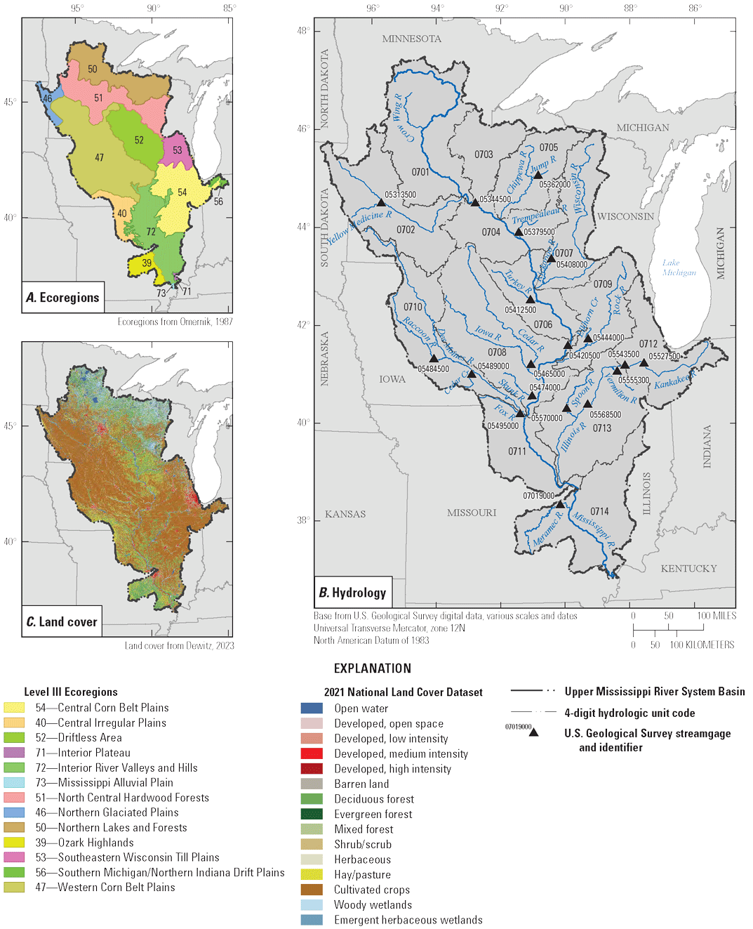
The distribution of U.S. Geological Survey streamgages within the Upper Mississippi River System Basin used in this analysis. Streamgages represent 12 different four-digit Hydrologic Unit Code subbasins that comprise varying 2021 National Land Cover classifications and U.S. Environmental Protection Agency Level 3 Ecoregions. A, Ecoregions. B, Hydrology. C, Land cover.
Hydrologic Data Products
The LOCA–VIC–mizuRoute (LVM) series of hydrologic data products (Vano and others, 2020) are used in this study. The name “LOCA–VIC–mizuRoute” comes from the chain of models from which the data products are produced: localized constructed analogs (LOCA) downscaled Coupled Model Intercomparison Project Phase 5 (CMIP5) global climate data (Pierce and others, 2014; Vano and others, 2020), Variable Infiltration Capacity (VIC) macroscale hydrologic model (Liang and others, 1994), and the mizuRoute hydrologic routing model (Mizukami and others, 2016).
The LVM hydrologic data products (Vano and others, 2020) are a set of routed streamflow projections for the CONUS generated at every segment in the U.S. Geological Survey’s (USGS) geospatial fabric (Viger and Bock 2014), which is a vector-based river network developed for the purposes of national hydrologic modeling. These products were produced by collaborators from Federal agencies including the Bureau of Reclamation, USACE, USGS, and other collaborating academic and research institutions. The products result from a chain of models that begins with CMIP5 GCMs. First, the LOCA statistical downscaling method is applied to the precipitation and temperature outputs from 32 CMIP5 GCMs (table 2.1) (Pierce and others, 2014). The Livneh observationally based reanalysis product (Livneh and others, 2013) is used as the reference meteorological dataset for LOCA downscaling. To translate the downscaled precipitation and temperature outputs into a streamflow response, the VIC macroscale hydrologic model (Liang and others, 1994, 1996; Nijssen and others 1997) and the mizuRoute hydrologic routing model are implemented using the LOCA precipitation and temperature forcings as described in Mizukami and others (2016). The application of the VIC–mizuRoute models generates simulated streamflow at a daily timestep for the CONUS by applying two separate routing procedures: kinematic wave tracking and impulse response function (unit-hydrograph). Details of each routing method are described by Mizukami and others (2016). Because mizuRoute was developed for continental-scale applications, it does not explicitly account for river regulation structures or their operations (Mizukami and others, 2016).
The LVM hydrologic data products consist of a historical (1950–2005) and future (2006–99) period. The assumed GHG forcings in the 32 CMIP5 GCMs during the historical period is a reconstitution of observed GHG emissions and is used uniformly across all 32 CMIP5 GCMs. The future period outputs of LVM hydrologic data products consist of GCMs run over potential future GHG emissions scenarios that are not evaluated as part of our study. Instead, we evaluate only the historical portion of the LVM hydrologic data products to infer the reliability of the entire collection of LVM hydrologic data products. Hereafter, we refer to this period of record (1950–2005) as the “historical period.” For the historical period outputs, the LVM hydrologic data products consist of an ensemble of 64 GCM-based historical period outputs (32 outputs for each GCM per routing method) for every river segment across the CONUS. Hereafter, we refer to individual hydrologic simulations as “ensemble members.” Only the impulse response function routed flows are analyzed in this study because preliminary analyses revealed insensitivity to routing method, resulting in a total of 32 historical ensemble members in our analysis.
Streamgage Selection and Observed Hydrologic Records
A spatially distributed sampling design is applied to evaluate the LVM hydrologic data products at USGS streamgage (U.S. Geological Survey, 2024) locations throughout the Upper Mississippi River System Basin (table 1). Streamgages were selected for inclusion using three criteria: available period of record, location, and degree of watershed modification. To facilitate comparison with the LVM-simulated historical period discharge outputs, streamgages were limited to those that had a complete record of daily mean streamflow from water years 1951 to 2005 (October 1, 1950, to September 30, 2005). We sought to select at least one streamgage per four-digit hydrologic unit code (HUC) basin within the Upper Mississippi River System basin (table 1) so that the range of physiographic and climate variability of the basin was captured across the catchments. No streamgage was selected for HUC 0703, the St. Croix River, because it only had two streamgages (at St. Croix Falls, Wisconsin, and at Stillwater, Minnesota) and flows at both sites were impacted by power plant operations. There were no continuous unimpaired streamgages within HUC 0701, the Mississippi Headwaters, and thus this HUC was also not included in this analysis. No streamgages on the Missouri River or on the Mississippi River below St. Louis, Mo., were selected owing to substantial regulation of the Missouri River. Because our focus was on the Upper Mississippi River System’s main stems (particularly the portions of the Illinois and Mississippi Rivers with commercial navigation channels), the most downstream streamgage along a major tributary to the main stem of the Upper Mississippi or Illinois Rivers was used when multiple streamgages were present in a HUC to integrate the largest portion of the HUC possible. Two streamgages along the Mississippi River and two streamgages along the Illinois River were used to evaluate how the LVM hydrologic data products captured main-stem hydrologic response. Streamgages represented flows derived from drainage areas where limited changes in land use and flow regulation have occurred throughout the period of record to minimize the potential effect of watershed and hydrologic modifications on the analyses. The national Hydro-Climate Data Network (Slack and Landwehr, 1992; Falcone, 2011), which identifies USGS streamgages that have the least amount of anthropogenic impact, was referenced to help inform streamgage selection. Nineteen streamgages were identified as suitable for analysis using these criteria (table 1). Daily mean discharge records for the historical period were imported from the USGS’s National Water Information System (U.S. Geological Survey, 2024) for each streamgage. Hereafter, we refer to these daily discharge records as the “observed records.”
Table 1.
U.S. Geological streamgages (U.S. Geological Survey, 2024) from the Upper Mississippi River System Basin used in this analysis.[USGS, U.S. Geological Survey; dd, decimal degrees referenced to North American Datum of 1983; km2, square kilometer]
Hydrologic Characteristics
Seven hydrologic characteristics are used to evaluate the LVM data products (table 2). These hydrologic characteristics are chosen from a larger list generated in discussions during the UMRR Future Hydrology Meeting Series (Van Appledorn and Sawyer, 2025). The hydrologic characteristics are relevant to the UMRR program because they capture aspects of the flow regime important to a variety of ecosystem processes: critical flow magnitudes, seasonality, and overall annual distribution of flows and their timing.
Table 2.
Seven hydrologic characteristics used to evaluate the LOCA–VIC–mizuRoute data products, including measures of flow magnitude and timing, as well as the entire flow regime. All hydrologic characteristics were computed for water years 1951–2005 to be consistent with the Coupled Model Intercomparison Project Phase 5 historical simulation period.The seven hydrologic characteristics are computed using the observed records at each streamgage; these are hereafter referred to as “observed characteristics.” The hydrologic characteristics are also computed using simulated daily discharges for the ensemble members from the LVM data products (“simulated characteristics”). All observed and simulated characteristics are computed for the historical period of record, water years 1951 to 2005 (October 1, 1950, through September 30, 2005), for every ensemble member.
Statistical Analyses
Observed timeseries reflect local environmental conditions, natural variability, and fine-scale processes to drive day-to-day temperature, precipitation, and streamflow responses. However, daily weather patterns simulated using downscaled, GCM-based outputs do not replicate daily observations owing to variation in model assumptions and initialization states of individual GCMs even though identical historically reconstituted GHG emissions are assumed and the same downscaling methods are applied (Taylor and others, 2012). Therefore, hydrologic dynamics need to be summarized at coarser time scales (for example, during the period of record) than that of the simulated, daily streamflow output. As a result, we compare distributions of hydrologic characteristics rather than making direct comparisons between observed and simulated discharges at daily time steps.
We quantitatively and qualitatively compared observed and simulated hydrologic characteristics and their distributions using several statistical tests and visualizations. The software R (R Core Team, 2022) packages dataRetrieval (De Cicco and others, 2022), hydroGOF (Zambrano-Bigiarini, 2020), and stats (R Core Team, 2022) are used for all statistical analyses. We used the R package ggplot2 (Wickham, 2016) for visualizations.
For the five hydrologic characteristics related to flow magnitude and seasonality (table 2), a two-sample Kolmogorov-Smirnov (KS) nonparametric test (hereafter referred to as “KS test”; Chakravarti and others [1967] as implemented by Schröer [1991] and Schröer and Trenkler [1995]) was applied to test for differences (shape and magnitude) between distributions of observed and simulated hydrologic characteristics. Statistical significance is assessed at alpha=0.05 with the null hypotheses being the observed and simulated characteristics are drawn from the same distribution. In addition to considering statistical significance, the KS test statistic, D, is also considered to aid in interpretation of results. D represents the maximum absolute distance between the empirical cumulative distribution functions of the observed and simulated outputs. The critical value of D at a significance level of 0.05 is used in the hypothesis test to define if there is a statistically significant difference between two cumulative distribution functions. We also qualitatively evaluate the relation between simulated and observed characteristics by plotting sorted values of the characteristics against a 1:1 line. Based on correspondence to the 1:1 line, we visually infer the degree to which the LVM data products reliably account for important hydrometeorological conditions and physical processes represented in the observed data.
We compute the root mean square error (RMSE) on sorted hydrologic characteristics as a measure of similarity between observed and simulated values, with RMSE of zero indicating perfect correspondence. Because RMSE has the same units as the input data and is dependent on the scale of input data, we also report Normalized Root Mean Square Error (NRMSE) to allow for comparisons across ensemble members and streamgages (NRMSE is sometimes referred to as the ratio of the RMSE to the standard deviation ratio and abbreviated as RSR, but we use NRMSE in this report). NRMSE is calculated by dividing RMSE by the standard deviation of the observed values. We categorize differences in performance based on the median NRMSE across ensemble members using a rating scheme established in Moriasi and others (2007). Using this rating scheme, unsatisfactory performance is assumed when NRMSE is greater than (>) 0.7, satisfactory performance is when 0.6 is less than (<) NRMSE is less than or equal to (≤) 0.7, good performance is when 0.5<NRMSE≤0.6, and very good performance is when 0.00≤NRMSE≤0.5. The performance rating scheme is intended to guide interpretation of LVM data product reliability rather than be used as a definitive classification for accepting or rejecting results for two reasons. First, these criteria were developed for data with monthly time steps; stricter performance ratings may be warranted because our hydrologic characteristics are computed at annual time steps and are also ranked by magnitude prior to analysis (Moriasi and others, 2007). Second, the performance ratings were developed for summaries of continuous streamflow, but we apply them to statistics based on extreme events and day of year, which is an application that has not been evaluated. Thus, some caution is necessary in interpreting performance rating classification results.
Observed and simulated annual hydrographs of the mean daily discharges and the 30-day average discharges, and characterizations of flow regime (table 2) are compared using the Nash-Sutcliffe Efficiency (NSE; Nash and Sutcliffe, 1970) and the Kling-Gupta Efficiency (KGE; Gupta and others, 2009) goodness-of-fit metrics. Mean daily discharges are computed as the average of discharges observed for a given day-of-year across all years in the period of record (n=55). NSE is formulated from a normalization of the mean squared error and is sensitive to errors in high flows because of its dependence on the squared deviation. KGE was developed to address shortcomings in the NSE evaluation metric that include a tendency to favor simulations that underestimate variability in observed flows (Gupta and others, 2009). KGE is formulated by a decomposition of NSE into its components: Pearson’s correlation coefficient (r), the ratio between the standard deviation of the simulated and observed values (α), and the ratio between the mean simulated and observed values (ß). We report each of the KGE components individually to better understand the correlation, variability, and mean bias between observed and simulated hydrologic characteristics. Ideal values of r, α, and ß are 1. Note that NSE and KGE are separate metrics, and their values cannot be directly compared. Although the interpretation of “good” or “poor” NSE and KGE varies across the literature, an NSE or a KGE equal to 1 indicates perfect agreement between observations and simulations (Knoben and others, 2019). For hydrologic modeling, NSE values of <0.5 are typically considered unsatisfactory (Moriasi and others, 2015). NSE values below zero indicate that the model is a worse predictor than the mean. Unlike for NSE, there are no established KGE benchmarks to discriminate acceptable compared with poor model performance (Knoben and others, 2019). Note that NSE and KGE are typically used to evaluate calibrated hydrologic model performance and thus directly compare daily timeseries of observed discharges with simulated discharges. In this report, we are comparing timeseries of observed daily discharges with simulated daily discharges during a yearlong period with each day representing an average (either mean or a 30-day running mean) discharge for that day across the historical period. It is possible, therefore, that any established benchmarks may not be directly comparable with our results.
Annual hydrographs derived from observed discharge are qualitatively compared to those derived from model simulations using different plotting methods (fig. 2). A direct overlay is used for the annual hydrograph of average daily discharge (for example, fig. 2K). The distributions of the 30-day running average daily discharges are compared using Gaussian kernel density estimation functions (for example, fig. 2L). Flow duration curves are plotted to visualize the mean daily discharge from water year 1951 to 2005 (for example, fig. 2M); due to similarities between the annual hydrographs of mean daily and 30-day running mean daily discharge, we do not plot flow duration curves for the 30-day running mean daily discharges.
Guidance for Interpreting the Hydrologic Data Product Performance
This section provides an example of how the evaluation results are interpreted together in the context of this study. Evaluation of the LVM hydrologic data products is based on interpreting results from the statistical tests on seven hydrologic characteristics across 32 ensemble members for each streamgage location. In addition, relations between observed and simulated data are qualitatively evaluated based on graphical comparisons. Therefore, it is necessary to synthesize a substantial amount of information across multiple lines of evidence, often without well-established performance thresholds in the literature, to assess if the LVM hydrologic data products are reliable for applications in the UMRR program. In general, consistently high agreement between observed and simulated characteristics across ensemble members that is also consistent within and among the seven hydrologic characteristics across streamgages would indicate the LVM hydrologic data products are reliably capturing important hydrologic processes and are suitable for applications in the UMRR program. Results for all streamgages are summarized in table 3 and figures 3 and 4. Results are also presented for each streamgage in appendixes 1 and 2.
We developed a classification scheme for assessing KS test agreement among the 32 ensemble members to help assess the reliability of the LVM hydrologic data products. KS test results are summarized for each streamgage location with shading indicating agreement level among ensemble members (table 3). All agreement levels were defined a priori. A strong level of agreement is indicated using dark grey when KS test results from more than 16 ensemble members suggest observed and simulated characteristics are drawn from the same population. Medium grey shading illustrates moderate ensemble member agreement in KS test results with 8–16 ensemble members, suggesting observed and simulated characteristics are drawn from the same population. Light grey shading illustrates weak ensemble member agreement in KS test results with less than eight but more than one ensemble members, indicating that observed and simulated characteristics are drawn from the same population. No shading illustrates no agreement in KS test results with either one or zero ensemble members, indicating that observed and simulated characteristics are drawn from the same population.
An example of how results may be interpreted at a single streamgage location is presented using USGS streamgage 07019000 (Meramec River near Eureka, Mo.). KS test results for the Meramec River indicate that the observed and simulated flow magnitude characteristics (annual maximum 3-day discharge and annual minimum 7-day discharge) are statistically different (probability value [p-value]<0.05) across all ensemble members (table 3). This result is depicted by the lack of overlap between observed and simulated cumulative frequency distributions (fig. 2A and 2B). Most ensemble members underestimate annual maxima 3-day and overestimate annual minima 7-day discharge demonstrated by low and high biases as compared to a 1:1 dashed line (fig. 2F and 2G). NRMSE results indicate unsatisfactory performance (NRMSE>0.7; Moriasi and others, 2007; fig. 3A). Overall, these results indicate that the LVM simulated hydrologic data products do not robustly capture these measures of extremes in the observed flow record for the Meramec River.
The LVM hydrologic data products exhibit mixed levels of performance in their ability to capture the seasonality of hydrologic response for the Meramec River. For the timing of the annual maximum 3-day discharge and timing of the center of mass, KS test results indicate statistically similar (p-value>0.05) observed and simulated distributions, with strong agreement among ensemble members (table 3, fig. 2C and 2E). Very good performance was also observed for both these hydrologic characteristics according to the NRMSE (0.00<NRMSE<0.5; Moriasi and others, 2007; fig. 3B). However, when the observed annual maxima occur between June and July (approximately days 150–190), there is poor correspondence between the timing of simulated annual maxima and observed annual maxima; the best correspondence is observed when peak flow occurs earlier in the year. This effect is illustrated by a stepwise relation between the Meramec River’s observed and simulated dates of annual maximum 3-day discharge values (fig. 2H). The relation between observed and simulated distributions of center of mass timing, in comparison, were more linear and thus had greater correspondence to the 1:1 line (fig. 2J).
For the timing of annual minima on the Meramec River near Eureka, Mo., test results show moderate agreement among ensemble members, indicating statistical similarity between observed and simulated characteristics (11 ensemble members, table 3). Direct comparisons of simulated versus observed distributions exhibited deviations from one-to-one correspondence (fig. 2I). For example, there are early biases for 7-day annual minima occurring prior to early August (approximately day 215) and late biases for minimum flows occurring after early October (approximately day 275); most observed annual minimum flows appear to occur between August and October. The median ensemble NRMSE indicates unsatisfactory agreement (NRMSE>0.7; Moriasi and others, 2007; fig. 3B). However, there is high variability among ensemble members in NRMSE values (fig. 3B) with values ranging from 0.64 to 1.9 (fig. 2.8).
Plots of the annual hydrograph, discharge frequency as measured by a kernel density estimator function, and flow duration curves for the Meramec River aid in interpretation of how well simulations capture the overall magnitude and seasonality of the observed streamflow response (figs. 2K, 2L, and 2M). Visual comparison of the average annual hydrographs reveal that simulated peak discharges are smaller in magnitude and occur earlier than observed maxima (fig. 2K). Distributions of observed and simulated flows generated in the Meramec River are characterized as being bimodal. However, simulated flows generally exhibit higher density maxima than observed flows. Most significantly, lower discharges tend to occur more frequently in the simulated outputs relative to the observed flows (fig. 2L). Higher estimates of the density maxima, combined with lower density at higher flows, of simulated 30-day running averages compared to the observed flows may reflect a poor ability to capture the variability in short-term hydrologic responses (flashiness) at USGS streamgage 07019000 (Meramec River near Eureka, Mo.; hereafter referred to as the “Meramec streamgage”). Based on a comparison of flow duration curves, simulated data from the Meramec streamgage tend to underestimate higher flows and overestimate lower flows (fig. 2M).
NSE and KGE metrics comparing observed and simulated flow hydrographs (mean daily and 30-day average) for Meramec streamgage are positive for all ensemble members; however, the median NSE falls just below the accepted threshold for satisfactory agreement (<0.5; Moriasi and others, 2007) (fig. 4). The three KGE components had median values of 0.75 (r), 0.75 (α), and 0.85 (ß) (fig. 5). Differences among ensemble members are greatest for α, indicating different ensemble members expressed contrasting degrees of variability compared to the observed values.
Overall, the LVM hydrologic data products did not reliably capture the hydrology of the Meramec River. Certain aspects of the basin’s hydrologic response were more reasonably captured than others (for example, the timing of center of mass). However, some hydrologic characteristics were not well represented; for example, there was no agreement among ensemble members with regards to characteristics of flow magnitude (table 3). Such differences cannot adequately be addressed with secondary bias-correction methods owing to nonlinearities between observed and simulated values (for example, timing of annual maximum discharge).
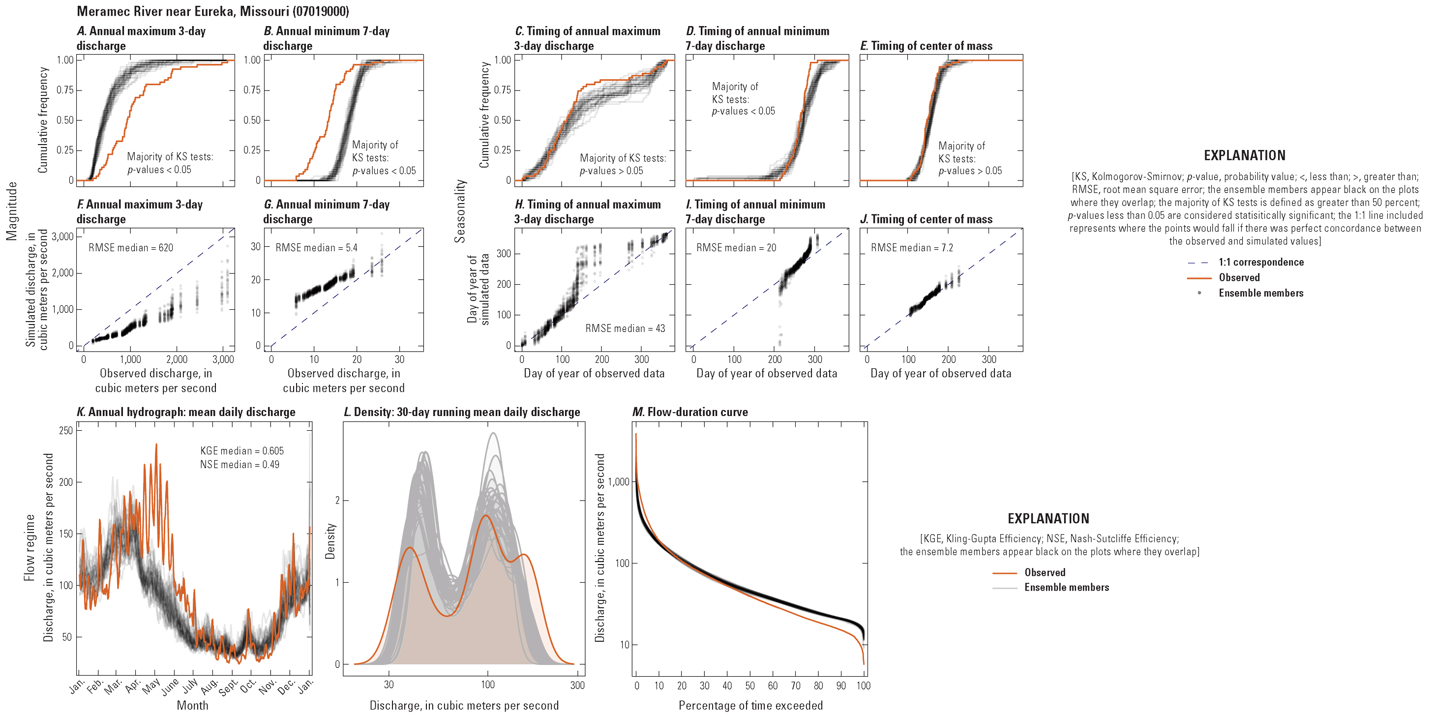
Comparisons between seven hydrologic characteristics related to flow magnitude, seasonality, and flow regime as derived from observed discharge data and 32 ensemble members of simulated discharge data for the Meramec River near Eureka, Missouri (U.S. Geological Survey streamgage 07019000). A, Annual maximum 3-day discharge. B, Annual minimum 7-day discharge. C, Timing of annual maximum 3-day discharge. D, Timing of annual minimum 7-day discharge. E, Timing of center of mass. F, Observed and simulated annual maximum 3-day discharges. G, Observed and simulated annual minimum 7-day discharges. H, Observed and simulated timing of annual maximum 3-day discharges. I, Observed and simulated timing of annual minimum 7-day discharges. K, Annual hydrograph of mean daily discharge. L, Density plot of the annual hydrograph of the 30-day running mean daily discharge. M, Flow-duration curve of mean daily discharge for the period of record.
Evaluation Results
Reliability of Hydrologic Data Products for the Upper Mississippi River System
Overall, observed hydrologic dynamics in the UMRS are not well captured by the tested hydrologic data products, which suggests that important hydrometeorological inputs and (or) watershed processes are not being accurately represented by the modeling framework at the scale necessary to support UMRR program applications of interest. The level of within-ensemble member agreement varied by streamgage and by hydrologic characteristic (table 3). Inconsistencies between observed and simulated output are also readily apparent in visualizations comparing observed and simulated distributions of hydrologic characteristics (appendix 1). Patterns in these graphical disparities vary depending on the output being evaluated and on the location. These findings indicate that universal application of a post-hoc secondary bias correction technique may not be appropriate to rectify the discrepancies between observed and simulated streamflow outputs in the UMRS.
The KS test statistic was calculated for five hydrologic characteristics to understand how well simulated output captures observed flow magnitudes and seasonality (timing). There are no streamgages where there is agreement between observed and simulated flows in all five hydrologic characteristics based on KS test results (table 3). In fact, the greatest number of characteristics having some level of agreement (that is, at least two ensemble members producing statistically similar results as the observed characteristics) for any streamgage is three. This result occurs at 6 of the 19 streamgages evaluated (table 3). At 18 of the 19 streamgages, there is some agreement between observed and simulated flows for one or more of the hydrologic characteristics evaluated (table 3). The Turkey River at Garber, Iowa (USGS streamgage 05412500) show no agreement for any of the five characteristics analyzed. Across all streamgages, KS test results indicate that the timing of annual minimum 7-day discharge is the characteristic most reliably produced by the simulations, and the annual maximum 3-day discharge and the timing of the center of mass are the least reliably produced characteristics (table 3).
Differences in performances across streamgages and hydrologic characteristics are also apparent from ensemble median NRMSE values (fig. 3; refer to appendix 2 for heatmaps with NRMSE values for each streamgage and ensemble member combination). The metrics evaluating agreement in magnitude have poorer performance than the seasonality metrics: an unsatisfactory rating (NRMSE>0.7; Moriasi and others, 2007) is observed at 17 streamgages for annual maximum 3-day discharge and at 17 streamgages for annual minimum 7-day discharge. For the seasonality metrics, unsatisfactory ratings are determined for 10 streamgages for timing of annual maximum 3-day discharge, 7 streamgages for timing of annual minimum 7-day discharge, and 14 streamgages for timing of center of mass. NRMSE is rated as very good (0.00<NRMSE<0.5; Moriasi and others, 2007) for the seasonality metrics at a portion of the streamgage sites evaluated: 7 streamgages for timing of annual maximum 3-day discharge, 10 streamgages for timing of annual minimum 7-day discharge, and 2 streamgages for timing of center of mass.
Overall, results across most streamgages show negative NSE values for mean daily and rolling 30-day average hydrographs (fig. 4), indicating substantial discrepancies between the observed and simulated flows. KGE values for 18 of 19 streamgages are <0.5, similarly suggesting poor performance. Poor performance is further confirmed by breaking out KGE into its three components (fig. 5). All 19 streamgages have α values <1 (median α mean daily: 0.25–0.76; 30-day average: 0.26–0.80), indicating that the variability in the simulations is less than the observed. Only one streamgage (Kickapoo River at La Farge, Wis. [0540800]) has β values >1 (median β mean daily: 1.23; 30-day average: 1.23). This streamgage is the only site where mean observed discharge is overestimated by the simulations throughout most of the year. Simulated output generated for all other streamgages generally underrepresent mean observed discharge (median β mean daily: 0.34–0.87; 30-day average: 0.34–0.87). Median r values range from 0.25 to 0.83 for the annual hydrograph of mean daily discharges and between 0.30 to 0.86 for the annual hydrograph of running 30-day mean daily discharges. Substantial differences between the observed and simulated flows are apparent across most streamgages through visual comparisons of average annual daily hydrograph plots, density plots of 30-day running average flow, and annual flow duration curves (figs. 1.1–1.19).
We observe poor correspondence between observed and simulated hydrologic characteristics across basins of differing sizes, land covers and physiography (table 3, appendix 1). However, there is some evidence of a latitudinal pattern in how well simulated data estimate the timing of annual maximum 3-day discharge events based on the KS test results. This observation suggests that the tested hydrologic data products’ modeling chain may better capture rainfall driven events compared to snowmelt-driven hydrologic pulses. NRMSE results show a similar, general latitudinal trend with overall lower error rates to the south, indicating more agreement between observed and simulated flow seasonality at these streamgages known to be less affected by snowmelt driven processes (fig. 3B).
Heatmaps of the KS test D statistic and NRMSE for each of the 32 GCM-based ensemble members at each of the 19 streamgage locations confirm that results derived from individual ensemble members are consistent with one another and that a minority of ensemble members are not unduly biasing interpretation of results (figs. 2.1–2.10; that is, the heatmap results indicate that no individual member(s) exhibit divergent behavior relative to the other ensemble members for each streamgage location).
Table 3.
The number of the 32 ensemble members with a statistically similar distribution of hydrologic characteristics generated from simulated and observed discharge timeseries according to two-sample Kolmogorov-Smirnov non-parametric tests at the alpha = 0.05 level.[USGS, U.S. Geological Survey]
Degree of agreement among ensemble members and the observations: 8–16 members agree (Moderate Agreement).
Degree of agreement among ensemble members and the observations: less than 2 members agree (No Agreement).
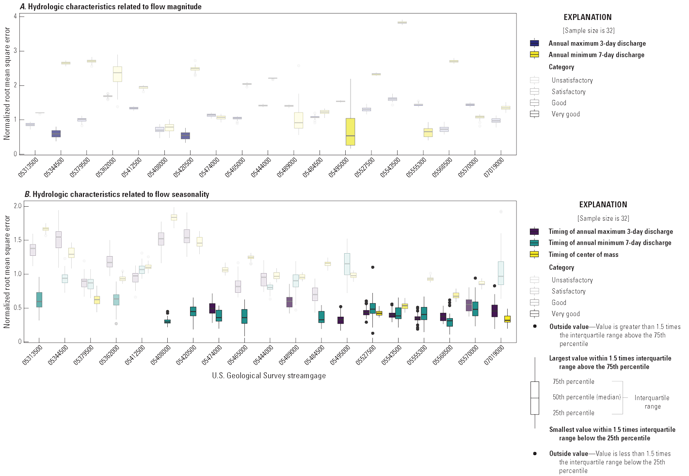
Distributions of normalized root mean square error (NRMSE) from comparisons of observed versus simulated flows from 32 ensemble members at 19 U.S. Geological Survey streamgages within the Upper Mississippi River System Basin. A, Two hydrologic characteristics related to flow magnitude. B, Three characteristics related to seasonality.
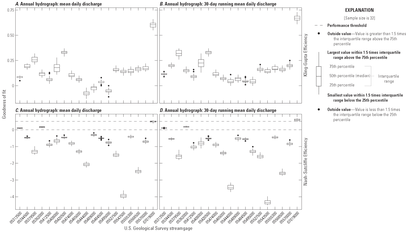
Goodness of fit statistics derived from Kling-Gupta Efficiency and Nash-Sutcliffe Efficiency tests for the mean daily and 30-day average hydrograph at 19 U.S. Geological Survey streamgage locations within the Upper Mississippi River System Basin. A, Mean daily hydrograph, Kling-Gupta Efficiency. B, 30-day average hydrograph, Kling-Gupta Efficiency. C, Mean daily hydrograph, Nash-Sutcliffe Efficiency. D, 30-day average hydrograph, Nash-Sutcliffe Efficiency.
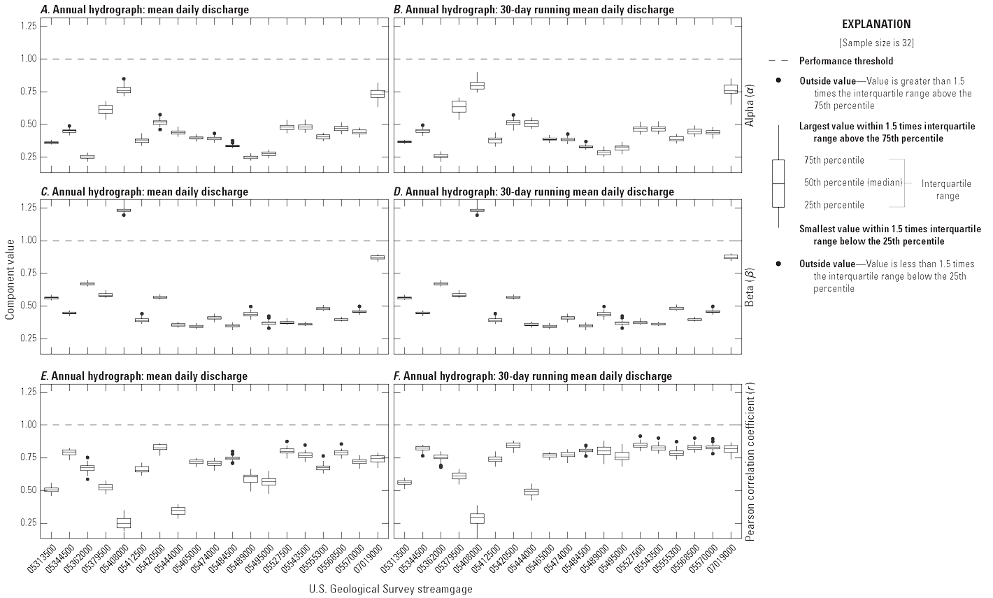
Distributions of Kling-Gupta Efficiency component values of alpha (the ratio between the standard deviation of the simulated and observed values), beta (the ratio between the mean simulated and observed values), and Pearson’s r value for the mean daily and 30-day running mean daily discharges at 19 U.S. Geological Survey streamgage locations within the Upper Mississippi River Basin. A, Mean daily annual hydrograph, alpha. B, 30-day running mean daily, alpha. C, Mean daily annual hydrograph, beta. D, 30-day running mean daily, beta. E, Mean daily annual hydrograph, r-value. F, 30-day running mean daily, r-value.
Hydrologic Characteristics of Flow Magnitude
In general, the tested hydrologic data products are not able to reliably capture hydrologic characteristics of annual maximum or minimum discharges. There is little agreement between observed and simulated distributions of annual maximum 3-day discharge according to the KS test results: only 4 of the 19 streamgages (21 percent of streamgages) demonstrate some level of correspondence between ensemble members and the observed data for annual maximum 3-day discharge (table 3). Of the four streamgages where annual maximum 3-day discharge derived from the ensemble of simulated outputs show statistical similarity to those derived from observed data, three streamgages exhibit a moderate level of agreement among ensemble members and one of the streamgages (Mississippi River at Prescott, Wisconsin) exhibits strong agreement among ensemble members. Two of the four streamgages are located on the main stem of the Mississippi River, whereas the other two streamgages (Yellow Medicine River near Granite Falls, Minn. [05313500], and Kickapoo River at La Farge, Wis. [05408000]) are on unregulated tributaries with drainage areas less than 1,800 km2 (table 1). Median NRMSE is rated unsatisfactory at 17 of the 19 streamgages (0.70–1.69) and rated good at the remaining two streamgages (0.55–0.59) for annual maximum 3-day discharge (fig. 3A). Plots of observed and simulated distributions of annual maximum 3-day discharge at most of the streamgages indicate poor one-to-one correspondence, with slopes <1 (figs. 1.1F–1.19F). This result indicates that the simulated annual maximum discharges tend to underestimate peak flow.
Distributions of observed annual minimum 7-day discharge are also poorly captured by simulations at most streamgages. Based on KS test results, only 5 of the 19 streamgages (26 percent) exhibit any degree of agreement between simulated and observed annual minimum 7-day discharge (table 3). Of these five streamgages, two (Kickapoo River at La Farge, Wisconsin [05408000], and Fox River at Wayland, Missouri [05495000]) exhibit strong agreement among ensemble members, indicating statistical similarity between observed and simulated distributions of annual minimum 7-day discharge. One of the five streamgages shows moderate ensemble member agreement, and two streamgages show low ensemble member agreement. Median NRMSE is rated unsatisfactory at 17 of the 19 streamgages (0.79–3.82) with one streamgage rated as satisfactory (0.66) and one streamgage rated as good (0.53) for annual minimum 7-day discharge (fig. 3A). Substantial differences in magnitude are apparent between simulated and observed annual minimum 7-day discharges as evidenced by no overlap with the one-to-one line for most streamgages (figs. 1.1G–1.19G). Additionally, in several cases, the relation between simulated and observed distributions of the annual minimum 7-day discharge appears to be nonlinear. An example of this is illustrated by the results for the Turkey River at Garber, Iowa (05412500) (fig. 1.5G).
Hydrologic Characteristics of Seasonality (Flow Timing)
Substantial disparities exist between simulated and observed seasonality hydrologic characteristics for many of the streamgages analyzed. However, the seasonality of the hydrologic response in the UMRS is captured more reliably by the simulated data as compared to measures of flow magnitude.
Nine streamgages (47 percent) exhibit some agreement between the observed and simulated timing of the annual maximum 3-day discharge, based on the classification scheme for assessing KS test results. Six streamgages show strong agreement (>16 members) among ensemble members, whereas two streamgages show moderate agreement (8–16 members) among ensemble members and one streamgage (Illinois River at Marseilles, Illinois [05543500]) shows weak agreement among ensemble members (table 3). Simulations for these nine streamgages capture peaks that are dominated by rainfall; the 10 streamgages with no agreement between observed and simulated data are located farther north in the study area and have early to mid-spring peaks driven primarily by snowmelt (fig. 1, appendix 1). NRMSE results comparing observed and simulated timing of the annual maximum 3-day discharge indicate seven streamgages rated as very good (0.33–0.49), two streamgages rated as good (0.55–0.6), and 10 streamgages rated as unsatisfactory (0.70–1.6; fig. 3B, appendix 1, fig. 2.6). Despite relatively low NRMSE values (fig. 2.6), results for many streamgage locations visually exhibit poor one-to-one correspondence between the observed and simulated timing of annual maximum 3-day discharge (appendix 1). The streamgages showing observed and simulated timing of annual maximum 3-day flows furthest from the one-to-one line are those sites where KS test results do not indicate a high degree of correspondence between distributions and have NRMSE values indicating unsatisfactory performance. These values tend to be observed in the northern portions of the study area where snowmelt influence is greater (figs. 3B, 2.6).
Based on the KS test results, the hydrologic data products appear to capture the timing of annual minimum 7-day discharge events relatively well, with 84 percent of the streamgages (16 streamgages) exhibiting some level of agreement: nine streamgages show strong agreement among ensemble members (>16 members) and five streamgages show moderate agreement among ensemble members (8–16 members) (table 2). Two of the three streamgages with no agreement (Mississippi River at Prescott, Wis. [05344500], and Trempealeau River at Dodge, Wis. [05379500]) are from the same 4-digit HUC (0704) but have significantly different contributing areas (116,031 versus 1,665 km2, respectively) (table 1). Of the 16 streamgages with at least some agreement, the average proportion of ensemble members in agreement with observed data was 58 percent. NRMSE results comparing the observed and simulated timing of annual minimum 7-day discharge indicate 10 streamgages with very good ratings (0.30–0.49) (table 3, fig. 3B). In addition, one streamgage was rated good (0.60), one streamgage was rated satisfactory (0.64), and seven streamgages were rated as unsatisfactory for NRMSE of observed and simulated timing of annual minimum 7-day discharge (fig. 3B). Despite having a strong degree of correspondence based on KS test results and relatively low NRMSE ratings, graphical comparisons of observed versus simulated annual timing of 7-day minimum flows indicate poor qualitative correspondence. For example, for the Mississippi River at Clinton, Iowa (05420500), KS test results reflect strong agreement among ensemble members (31 ensemble members), indicating similarities between the observed and modeled distribution in timing of annual minimum 7-day discharge, and the NRMSE value was rated very good (0.50) but shows poor one-to-one correspondence (table 3, fig. 1.7I).
According to KS test results for the timing of the center of mass, only 4 of the 19 streamgages (21 percent of streamgages) have some level of agreement in terms of the date by which the streamgage has received one-half of its annual volume (table 3). These four streamgages differ in drainage area (table 1), ecoregion (fig. 1), and expected runoff mechanism (snowmelt versus rainfall driven peaks). Similar to the KS test results, the median NRMSE values indicated only two streamgages had very good ratings (0.32, 0.43) one streamgage had a good rating (0.54), and two had satisfactory ratings (0.62, 0.67). Of the 19 streamgages, 14 had unsatisfactory NRMSE ratings (fig. 3B). Based on graphical comparison, in general, observed and simulated date of center of mass plot close to the one-to-one lines for most of the streamgages (appendix 1). The center of mass typically occurs between early April and mid-August (approximately day 91 through day 222) for the observed and simulated data across streamgage locations, demonstrating that the simulated data can estimate that the center of mass will occur during the growing season, typically considered April through October.
Hydrologic Characteristics Across Flow Regimes
Period of analysis (1950–2005) observed and simulated flows are compared across the three summaries of flow regimes (mean daily discharge, 30-day running mean daily discharge, and flow duration curves) graphically and by computing NSE, KGE, and KGE components (appendix 1, figs. 4 and 5). NSE values for annual hydrographs of the mean daily discharge and the rolling 30-day mean daily discharge are below zero for 16 out of 19 streamgages evaluated indicating poor correspondence between observed and simulated flows (fig. 4). At many streamgage locations, the low NSE values are driven, at least in part, by large discrepancies between observed and simulated streamflow volume. This pattern is particularly apparent for the Illinois River at Marseilles, Ill. (05543500) (fig. 1.15), and the Illinois River at Kingston Mines, Ill. (05568500) (fig. 1.17), which have large volume discrepancies throughout the year and for the full range of discharges. The Meramec River near Eureka, Mo. (07019000), is the only streamgage where NSE is above 0.5 for some LVM ensemble members (fig. 4). This pattern is reflected within the Meramec River summary hydrographs and flow duration curve, which demonstrate that the ensemble members reasonably approximate the observed streamflow volume for the range of discharges observed (fig. 1.19). Based on the flow regime hydrograph comparisons, the tested hydrologic data products usually capture streamflow timing, especially in the more southerly locations, though discharge magnitudes may have large discrepancies.
KGE values are consistent with NSE findings. The Meramec River at Eureka, Mo. [07019000]) has the largest relative KGE value, with all other locations presenting lower KGE values (fig. 4). Relatively high α and β values appear to have contributed to the high KGE value for the Meramec River (fig. 5) and suggest that hydrologic variability and magnitude were better captured for this site as compared to the other sites analyzed. The streamgages with the lowest KGE values for the mean daily hydrograph are Elkhorn Creek near Penrose, Ill. (05444000) (fig. 1.10); Cedar Creek near Bussey, Iowa (05489000) (fig. 1.12; and Fox River at Wayland, Mo. (05495000) (fig. 1.13). Notably, these sites represent some of the smallest drainage areas associated with the streamgages analyzed (table 1). In part because of their drainage areas, these sites also tend to have flashy flow dynamics that do not appear to be well represented in the historical simulations. All three KGE components are comparatively low for these streamgage locations for the annual hydrographs of mean daily discharge and running 30-day mean daily discharges (fig. 5).
Performance in the Mississippi and Illinois River Main Stems
Overall, the hydrologic data products we evaluated do not reliably replicate hydrologic response along the main stem of the Mississippi (Mississippi River at Prescott, Wis. [05344500], and Mississippi River at Clinton, Iowa [05420500]) (figs. 1.2 and 1.7) and Illinois Rivers (Illinois River at Marseilles, Ill. [05543500] and Illinois River at Kingston Mines, Ill. [05568500]) (figs. 1.15 and 1.17). KS tests results are mixed across different characteristics of flow magnitude and seasonality (timing) and vary for main-stem streamgages (table 3).
Based on KS tests applied to evaluate correspondence in flow magnitude, the main stem Mississippi River streamgages are two of only four streamgages that show statistical similarity between the distributions of observed and simulated annual maximum 3-day discharge; main-stem Illinois River streamgages show poor correspondence. There is no agreement between the distributions of annual minimum 7-day discharge at any of the four Mississippi and Illinois main-stem streamgages (table 3). NRMSE results are consistent with KS test results: good performance is achieved between observed and simulated annual maximum 3-day discharge for main-stem Mississippi streamgages, unsatisfactory performance is observed for the Illinois streamgages, and annual minimum 7-day discharge was unsatisfactory at all four streamgages (fig. 3). Qualitative comparisons of the observed and simulated flow regimes for the four main-stem streamgages show flow magnitudes frequently being underestimated across the entire annual flow regime, as well as range of discharges (appendix 1). Some discrepancies in discharge estimates during the observed annual maximum seasonal daily flow are substantial, about 25–65 percent less than observed values. Low β values give quantitative evidence that flow magnitudes are underestimated (fig. 5).
Model performance is relatively strong in seasonal characteristics of the timing of annual minimum and maximum flows at the Illinois River streamgages. KS test results indicate strong agreement among ensemble members and the observed data for the timing of annual minimum flows at both sites (table 3). There is also strong agreement for the timing of annual maximum flows at streamgage 05568500 (Illinois River at Kingston Mines, Ill.) and for the timing of the center of mass at streamgage 05543500 (Illinois River at Marseilles, Ill.) (table 3). Better model performance in these seasonal characteristics may reflect adequate representation of precipitation event timings within the modeling framework because hydrology of the Illinois River is largely driven by rainfall (Demissie and Knapp 2000), though additional investigation is necessary given only two streamgages are analyzed. Mississippi River streamgages, where peak runoff is affected more by snowmelt or a combination of rain and snowmelt (WEST Consultants, Inc., 2000), show no agreement between observed and simulated timing of annual maximum flows. KS test results indicating statistical similarity between observed and simulated timing of annual minimum flows show mixed results for the Mississippi River streamgages, with no agreement at streamgage 05344500 (Mississippi River at Prescott, Wis.) and strong agreement among ensemble members at streamgage 05420500 (Mississippi River at Clinton, Iowa) (table 3). Main-stem Mississippi and Illinois River streamgages do not show similarity between observed and simulated timing of center of mass, except for the Illinois River at Marseilles, Ill. (streamgage 05543500), which exhibits strong agreement among ensemble members and the observations based on KS test results. Overall, seasonality (timing) of flows based on NRMSE are consistent with KS test results, showing worse performance for Mississippi streamgages, compared to Illinois River streamgages (fig. 3B). Observed timing of annual maximum streamflow is not captured by the hydrologic data product simulations at the Mississippi River streamgages, however both Illinois River streamgages, where peak flows are driven by rainfall, show very good performance for NRMSE between observed and simulated timing of annual maximum flows (fig. 3B). NRMSE results for timing of annual minimum flow are like KS results, with both Illinois River streamgages showing very good ratings among ensemble members in NRMSE and the Mississippi River at Clinton, Iowa (streamgage 05420500) also showing very good rating, with the Mississippi River at Prescot, Wis. (streamgage 05344500) exhibiting an unsatisfactory rating (fig. 3B). Unlike the poor correspondence indicated by KS test results, center of mass timing shows good and satisfactory ratings among ensemble members for both Illinois River streamgages. Like the KS test results, NRMSE results indicate unsatisfactory ratings for the Mississippi River streamgages.
Poor model performance for simulating average annual mean daily hydrographs and average annual 30-day running mean daily hydrographs is evidenced by relatively low KGE values and negative NSE values for all main-stem Mississippi and Illinois River streamgages (figs. 4, 1.2, 1.7, 1.15, and 1.17). The Illinois River at Marseilles, Ill. (streamgage 05543500) and Illinois River at Kingston Mines, Ill. (streamgage 05568500) have some of the lowest NSE values in the study area for mean daily and 30-day rolling mean average annual hydrographs. These results illustrate the discrepancies between the observed and historical simulations across the full range of hydrologic regime response along the main stem of the Mississippi and Illinois Rivers.
Implications
The hydrologic data products we evaluated appear unsuitable for project specific applications that require modeling of discharge characteristics tied to habitat and ecosystem restoration and management in the Upper Mississippi River System. These applications include addressing the following important questions within the UMRR partnership: (1) how are geomorphic, hydrologic, and ecological patterns and processes likely to change in the future? and (2) how should management practices be implemented to be resilient to these changes? Relative to the observational records, simulated output underestimates discharge at most locations analyzed and does not consistently capture streamflow timing at the resolution necessary to support UMRR analysis and decision-making about resilient ecosystem restoration design.
Overall, discrepancies in the magnitude and seasonality of discharge indicate the potential for multiple sources of error affecting the relation between simulated and observed hydrologic data. Although the streamgages analyzed were selected to be representative of relatively unregulated conditions, it is possible that the inability of the modeling framework to account for anthropogenic influences on local hydrology (Mizukami and others, 2016), such as the diversion of Lake Michigan water to the Illinois River (Lewis and others, 2024), may contribute to some of the discrepancies. However, the consistent underestimation of the annual maximum and minimum discharges suggests a systematic volume error that could be driven by several factors. One potential source of error is bias associated with hydrologic model parameterization and (or) calibration within the UMRS basin. Another potential source of error is systematic bias associated with the downscaled, GCM-based meteorologic forcings driving the VIC hydrologic model (that is, the LOCA downscaled temperature and precipitation products).
For example, precipitation undercatch (underestimation of precipitation events in rain gage observations) in the gridded data products (spatially continuous uniform grids of values where gaps are filled by interpolating between station observations) applied to statistically downscale GCM meteorology has been identified as a likely source of error in downscaled precipitation in the Midwest (Huidobro and others, 2023). Byun and Hamlet (2018) determined that by correcting for the precipitation undercatch issue prior to performing downscaling, improved VIC model streamflow simulations could be generated for watersheds located in the Midwest and encompassing the Great Lakes. Another potential source of error associated with the gridded meteorological products used to statistically downscale GCM meteorological forcing data is related to the methods used to spatially distribute meteorological gage observations to a continuous grid. Translating point data to a grid can result in reduced extremes (precipitation and temperature). Efforts are underway to improve gridded meteorological products used for downscaling. For instance, Pierce and others (2023) have published a new observational training dataset that better represents daily extreme precipitation values and has been applied to improve the Coupled Model Intercomparison Project Phase 6 (CMIP6) LOCAv2 products. Investigation and identification of the cause of the discrepancies between observed and simulated flow magnitudes and seasonality is beyond the scope of this analysis but could inform the development of new simulated data products in the future.
Discrepancies in observed and simulated hydrologic characteristics are present across streamgages throughout the entire study area with varying drainage area sizes and land cover compositions. Although results indicate little geographic difference in the performance and reliability of the data products overall, KS test results and NRMSE results for the timing of annual maximum flow indicate better performance for streamgages less affected by snowmelt. This apparent latitudinal trend could be examined in further investigation.
Systematic errors in streamflow quantity within a reasonable range of magnitudes can be corrected for using statistically based secondary post-processing techniques such as quantile mapping, which adjust each quantile of the modeled output to better match the corresponding quantile of the observed period of record (for example, Snover and others, 2003; Hamlet and others, 2013). One shortcoming associated with this approach is that discrepancies in timing are not directly corrected. Because of substantial errors in streamflow magnitude and timing that are not clearly attributable to any particular source, the application of secondary bias correction methods is not appropriate here. In this case, the downscaled precipitation and temperature data could be evaluated for reliability, and consideration could be given to additional calibration of the hydrologic modeling to further develop reliable future hydrology datasets that support UMRR decision-making.
Although the outcome of this evaluation indicates that the hydrologic data products we evaluated cannot reliably be applied in support of modeling discharge-ecological relations intended for supporting relatively fine temporal and spatial scale analyses within the UMRS, this does not imply that they cannot be used to support other applications. For instance, the hydrology data products can appropriately be applied to generate comparative analysis over longer timescales (for example, decadal summaries), targeted at answering broader questions than those posed by this project. Comparisons of hydrologic and meteorologic results between the simulated historical and future periods (that is, model-to-model comparisons) can provide insight into if hydrologic conditions in the basin are expected to change. For example, ensemble-based results illustrating epoch-based changes (that is, 1976–2005, base epoch, compared to 2035–64, mid-century epoch) in temporally aggregated output for variables such as annual minimum temperature, annual accumulated precipitation, or annual maximum streamflow can be used to effectively illustrate the direction and relative magnitude of change under different emissions scenarios.
Next Steps
Potential next steps include performing a detailed examination of the discrepancies in observed and simulated output to determine if and to what extent the biases are related to GCM meteorologic forcings and (or) the VIC hydrologic model. An examination could include investigating potential issues related to the precipitation and temperature reanalysis products used to downscale GCM meteorology and evaluation of hydrologic model calibration. Better understanding biases will guide the selection of additional analyses necessary to develop reliable data products for the UMRR program.
The scientific community continues to generate new downscaled products seeking to improve upon the ability to capture the effects of climate change at higher resolutions than the raw GCM outputs provide. Examples of such products include dynamically downscaled meteorology generated using regional climate models and alternate statistically downscaled products. Examples of other readily available statistically downscaled products include the recently published CMIP6-based LOCAv2 (Pierce and others, 2023) and the University of Wisconsin Probabilistic Downscaling (Wright and others, 2021) products. Efforts to improve hydrologic model fidelity in support of long-term climate change modeling is also an active area of research. These research areas, as well as other innovations in the field such as machine-learning-based approaches to generating projected hydrology (Hasan and others, 2024), offer potential next steps towards the development of reliable future hydrology datasets for the Upper Mississippi River System.
Value of the Reliability Assessment Framework
The framework used here to evaluate hydrologic data products offers a repeatable set of operations that can be applied to aid in the evaluation of whether hydrology derived from GCMs can serve specified applications. Model performance evaluations are useful because they can increase confidence in projected results—and thus subsequent applications—when historical conditions are generally well-reproduced (Krysanova and others, 2018). Development and application of the framework to evaluate the suitability of the hydrologic data products for UMRR applications originated from organized discussions among river resource managers, research scientists, and technical experts in the fields of ecosystem restoration, hydrology, hydraulic modeling, and climate change modeling. Based on these discussions, seven key hydrologic characteristics capturing aspects of the flow regime relevant to ecosystem process and of critical importance to the UMRR program’s mission were identified (Van Appledorn and Sawyer, 2025). The framework applied in this study evaluates how well these characteristics are captured by the hydrologic data products we evaluated and should be useful to the UMRR in the future if the needs of the program do not change.
The reliability assessment framework consists of (1) identifying key questions end-users are seeking to answer related to climate change influenced futures; (2) defining key hydrologic characteristics to evaluate the reliability of available climate change influenced, future hydrology products; (3) applying statistical metrics to assess the reliability of these products; and (4) assessing whether these products can be used in support of a given application either with or without secondary streamflow bias-correction (if appropriate). Based on the outcome of applying this reliability assessment framework to the LVM products, future research needs necessary to improve aspects of the climate modeling chain applied to generate projected hydrology were identified. The framework described herein can be directly applied to other GCM-based products to assess reliability for application to the UMRR program, and the framework can be adapted by other teams for their own “fit-for-purpose” assessments.
Summary
The hydrology of the Upper Mississippi and Illinois Rivers is a fundamental driver of ecosystem patterns and processes across a large portion of the United States. Quantitative hydrologic data for the main stems of these rivers underlie numerous scientific investigations, statistical models, and decision-making processes for local, State, and Federal agencies involved in the Upper Mississippi River Restoration program. Although historical hydrologic data exist, data representing potential future conditions of the Upper Mississippi and Illinois Rivers lack the resolution necessary to anticipate biotic and abiotic responses to altered hydrology and to determine resilient management actions. One source of future hydrologic scenarios is the readily available LOCA–VIC–mizuRoute (LVM) hydrologic data products (named for the chain of models the data are produced from—localized constructed analogs, Variable Infiltration Capacity macroscale hydrological model, and the mizuRoute hydrologic routing model—that we shorten further to LVM in this summary) that include simulated discharges for historic and future timeframes.
We evaluated how well the hydrologic data products simulate hydrologic characteristics related to flow magnitude, seasonality, and overall hydrologic regime within the Upper Mississippi River System Basin. We determined that the hydrologic data products appear unsuitable for priority Upper Mississippi River Restoration applications targeted at informing resilient ecosystem restoration design. When compared to observed flows, hydrologic data product outputs cannot replicate the critical hydrologic characteristics at the resolution necessary to support integration with existing quantitative models of hydrologic-ecological relations in the Upper Mississippi River System.
There was poor correspondence between simulated and observed hydrologic characteristics for all 19 USGS streamgage sites analyzed. Streamgages analyzed capture runoff from drainage areas, which range in size, land cover, and physiography. Discrepancies indicate that biases in the meteorologic model forcings, hydrologic model parameterization, or both, may contribute to poor correspondence between hydrologic data products and observed records. Because there are significant discrepancies in streamflow magnitudes and timing, secondary bias-correction techniques cannot be effectively applied to improve the reliability of hydrologic data product-derived discharges.
Although the hydrologic data products we evaluated cannot reliably support quantitative modeling tied to habitat and ecosystem restoration and management at the desired spatial and temporal scales for the Upper Mississippi River Restoration program, these products can be used to support broad, relative comparisons of simulated historical and projected output over long time horizons. These comparisons can provide insight into direction of future trends. The direction and relative magnitude of changes between hydrologic data product-modeled historical and future hydrometeorological variables, at coarser spatial resolution and time scales, can qualitatively inform water resources decision-making.
The reliability assessment framework developed to evaluate hydrologic data products offers a repeatable set of operations that can be applied to evaluate other similar data products in the future. This evaluation also serves as a case study illustrating the need for conducting study-specific reliability assessments of climate change products (that is, fit-for-purpose assessments) and provides a framework demonstrating how hydrologic projections may be evaluated in support of other study areas or applications.
References Cited
Arnell, N.W., and Gosling, S.N., 2016, The impacts of climate change on river flood risk at the global scale: Climatic Change, v. 134, no. 3, p. 387–401, accessed December 2024, at https://doi.org/10.1007/s10584-014-1084-5.
Bouska, K.L., Houser, J.N., De Jager, N.R., and Hendrickson, J., 2018, Developing a shared understanding of the Upper Mississippi River—The foundation of an ecological resilience assessment: Ecology and Society, v. 23, no. 2, accessed August 2018 at https://doi.org/10.5751/ES-10014-230206.
Bouska, K.L., Houser, J.N., De Jager, N.R., Van Appledorn, M., and Rogala, J.T., 2019a, Applying concepts of general resilience to large river ecosystems—A case study from the Upper Mississippi and Illinois rivers: Ecological Indicators, v. 101, p. 1094–1110, accessed June 2022 at https://doi.org/10.1016/j.ecolind.2019.02.002.
Bouska, K.L., Whitledge, G.W., Lant, C., and Schoof, J., 2019b, Drivers and uncertainties of forecasted range shifts for warm-water fishes under climate and land cover change: Canadian Journal of Fisheries and Aquatic Sciences, v. 76, no. 3, p. 415–425, accessed May 2025 at https://doi.org/10.1139/cjfas-2018-0002.
Byun, K., and Hamlet, A.F., 2018, Projected changes in future climate over the Midwest and Great Lakes region using downscaled CMIP5 ensembles: International Journal of Climatology, v. 38, S1, p. e531–e553, accessed July 2022 at https://doi.org/10.1002/joc.5388.
Byun, K., Chiu, C.-M., and Hamlet, A.F., 2019, Effects of 21st century climate change on seasonal flow regimes and hydrologic extremes over the Midwest and Great Lakes region of the US: Science of the Total Environment, v. 650, no. 1, p. 1261–1277, accessed July 2022 at https://doi.org/10.1016/j.scitotenv.2018.09.063.
Carhart, A.M., and De Jager, N.R., 2019, Spatial and temporal changes in species composition of submersed aquatic vegetation reveal effects of river restoration: Restoration Ecology, v. 27, no. 3, p. 672–682, accessed May 2022 at https://doi.org/10.1111/rec.12911.
Chen, L., and Ford, T.W., 2022, Future changes in the transitions of monthly‐to‐seasonal precipitation extremes over the Midwest in Coupled Model Intercomparison Project Phase 6 models: International Journal of Climatology, v. 43, no. 1, p. 255–274, accessed March 2024 at https://doi.org/10.1002/joc.7756.
Chen, M., Gassman, P.W., Srinivasan, R., Cui, Y., and Arritt, R., 2020, Analysis of alternative climate datasets and evapotranspiration methods for the Upper Mississippi River Basin using SWAT within HAWQS: Science of the Total Environment, v. 720, 137562, accessed March 2024 at https://doi.org/10.1016/j.scitotenv.2020.137562.
Chien, H., Yeh, P.J.-F., and Knouft, J.H., 2013, Modeling the potential impacts of climate change on streamflow in agricultural watersheds of the Midwestern United States: Journal of Hydrology, v. 491, p. 73–88, accessed January 2015 at https://doi.org/10.1016/j.jhydrol.2013.03.026.
Clark, M.P., Wilby, R.L., Gutmann, E.D., Vano, J.A., Gangopadhyay, S., Wood, A.W., Fowler, H.J., Prudhomme, C., Arnold, J.R., and Brekke, L.D., 2016, Characterizing uncertainty of the hydrologic impacts of climate change: Current Climate Change Reports, v. 2, no. 2, p. 55–64, accessed December 2024, at https://doi.org/10.1007/s40641-016-0034-x.
Crimmins, A.R., Avery, C.W., Easterling, D.R., Kunkel, K.E., Stewart, B.C., and Maycock, T.K., eds., 2023, Fifth National Climate Assessment: Washington, D.C., U.S. Global Change Research Program, accessed January 2025 at https://doi.org/10.7930/NCA5.2023.
De Cicco, L.A., Hirsch, R.M., Lorenz, D., Watkins, W.D., and Johnson, M., 2022, dataRetrieval—R packages for discovering and retrieving water data available from Federal hydrologic web services (v.2.7.12): U.S. Geological Survey website, accessed August 2024 at https://doi.org/10.5066/P9X4L3GE.
De Jager, N.R., Rogala, J.T., Rohweder, J.J., Van Appledorn, M., Bouska, K.L., Houser, J.N., and Jankowski, K.J., 2018, Indicators of ecosystem structure and function for the Upper Mississippi River System: U.S. Geological Survey Open-File Report 2018–1143, 115 p. including 4 appendixes, accessed June 2022 at https://doi.org/10.3133/ofr20181143.
De Jager, N.R., Rohweder, J.J., Yin, Y., and Hoy, E., 2016, The Upper Mississippi River floodscape—Spatial patterns of flood inundation and associated plant community distributions: Applied Vegetation Science, v. 19, no. 1, p. 164–172, accessed June 2022 at https://doi.org/10.1111/avsc.12189.
Delaney, J.T., Bouska, K.L., Eash, J.D., Heglund, P.J., and Allstadt, A.J., 2021, Mapping climate change vulnerability of aquatic-riparian ecosystems using decision-relevant indicators: Ecological Indicators, v. 125, p. 107581, accessed June 2024 at https://doi.org/10.1016/j.ecolind.2021.107581.
Demaria, E.M.C., Roundy, J.K., Wi, S., and Palmer, R.N., 2016, The effects of climate change on seasonal snowpack and the hydrology of the northeastern and Upper Midwest United States: Journal of Climate, v. 29, no. 18, p. 6527–6541, accessed May 2025 at https://doi.org/10.1175/JCLI-D-15-0632.1.
Demissie, M., and Knapp, H.V., 2000, Hydrology and hydraulics of the Illinois River. Pages 1–10 Building Partnerships. American Society of Civil Engineers, Minneapolis, Minnesota, United States. [Also available at https://doi.org/10.1061/40517(2000)102.]
Eisner, S., Flörke, M., Chamorro, A., Daggupati, P., Donnelly, C., Huang, J., Hundecha, Y., Koch, H., Kalugin, A., Krylenko, I., Mishra, V., Piniewski, M., Samaniego, L., Seidou, O., Wallner, M., and Krysanova, V., 2017, An ensemble analysis of climate change impacts on streamflow seasonality across 11 large river basins: Climatic Change, v. 141, no. 3, p. 401–417, accessed January 2024, at https://doi.org/10.1007/s10584-016-1844-5.
Falcone, J.A., 2011, STREAMGAGES–II, Geospatial attributes of streamgages for evaluating streamflow: U.S. Geological Survey data release, accessed June 2022 at https://doi.org/10.5066/P96CPHOT.
Frans, C., Istanbulluoglu, E., Mishra, V., Munoz-Arriola, F., and Lettenmaier, D.P., 2013, Are climatic or land cover changes the dominant cause of runoff trends in the Upper Mississippi River Basin?: Geophysical Research Letters, v. 40, no. 6, p. 1104–1110, accessed May 2022 at https://doi.org/10.1002/grl.50262.
Grady, K.A., Chen, L., and Ford, T.W., 2021, Projected changes to spring and summer precipitation in the Midwestern United States: Frontiers in Water, v. 3, p. 780333, accessed March 2024 at https://doi.org/10.3389/frwa.2021.780333.
Gupta, H.V., Kling, H., Yilmaz, K.K., and Martinez, G.F., 2009, Decomposition of the mean squared error and NSE performance criteria—Implications for improving hydrological modelling: Journal of Hydrology, v. 377, no. 1–2, p. 80–91, accessed March 2024 at https://doi.org/10.1016/j.jhydrol.2009.08.003.
Gupta, S.C., Kessler, A.C., Brown, M.K., and Zvomuya, F., 2015, Climate and agricultural land use change impacts on streamflow in the upper midwestern United States: Water Resources Research, v. 51, no. 7, p. 5301–5317, accessed June 2024 at https://doi.org/10.1002/2015WR017323.
Gupta, S.C., Kessler, A.C., Brown, M.K., and Schuh, W.M., 2016, Reply to comment by Keith E. Schilling on “Climate and agricultural land use change impacts on streamflow in the upper Midwestern United States”: Water Resources Research, v. 52, no. 7, p. 5697–5700, accessed May 2025, at https://doi.org/10.1002/2016WR018656.
Hamlet, A.F., Elsner, M.M., Mauger, G.S., Lee, S.Y., Tohver, I., and Norheim, R.A., 2013, An overview of the Columbia Basin Climate Change Scenarios Project—Approach, methods, and summary of key results: Atmosphere–Ocean, v. 51, no. 4, p. 392–415, accessed May 2025 at https://doi.org/10.1080/07055900.2013.819555.
Hasan, F., Medley, P., Drake, J., and Chen, G., 2024, Advancing hydrology through machine learning—Insights, challenges, and future directions using the CAMELS, Caravan, GRDC, CHIRPS, PERSIANN, NLDAS, GLDAS, and GRACE Datasets: Water (Basel), v. 16, no. 13, p. 1904, accessed May 2025 at https://doi.org/10.3390/w16131904.
Houser, J.N., ed., 2022, Ecological status and trends of the Upper Mississippi and Illinois Rivers (ver. 1.1, July 2022), U.S. Geological Survey Open-File Report 2022–1039, 199 p., accessed July 2022 at https://doi.org/10.3133/ofr20221039.
Houser, J.N., and Richardson, W.B., 2010, Nitrogen and phosphorus in the Upper Mississippi River—Transport, processing, and effects on the river ecosystem: Hydrobiologia, v. 640, no. 1, p. 71–88, accessed April 2023 at https://doi.org/10.1007/s10750-009-0067-4.
Huidobro, G., Chiu, C., Byun, K., and Hamlet, A.F., 2023, Meteorological driving datasets for the U.S. Midwest and Great Lakes Region incorporating precipitation gauge undercatch corrections: Journal of Hydrometeorology, v. 24, no. 5, p. 873–895, accessed May 2025 at https://doi.org/10.1175/JHM-D-22-0148.1.
Intergovernmental Panel on Climate Change, 2022, Climate Change 2022—Impacts, adaptation and vulnerability—Working Group II contribution to the sixth assessment report of the Intergovernmental Panel on Climate Change (1st ed.). Cambridge University Press, accessed May 2023 at https://doi.org/10.1017/9781009325844.
Jankowski, K.J., 2022, Water quality indicators, chap. E of Houser, J.N., ed., Ecological status and trends of the Upper Mississippi and Illinois Rivers (ver. 1.1, July 2022): U.S. Geological Survey Open-File Report 2022–1039, 28 p. [Also available at https://doi.org/10.3133/ofr20221039.]
Jha, M., Pan, Z., Talke, E.S., and Gu, R., 2004, Impacts of climate change on streamflow in the Upper Mississippi River Basin—A regional climate model perspective: Journal of Geophysical Research, v. 109, no. D9, 12 p., accessed July 2016 at https://doi.org/10.1029/2003JD003686.
Knoben, W.J.M., Freer, J.E., and Woods, R.A., 2019, Technical note—Inherent benchmark or not? Comparing Nash–Sutcliffe and Kling–Gupta efficiency scores: Hydrology and Earth System Sciences, v. 23, no. 10, p. 4323–4331, accessed May 2025 at https://doi.org/10.5194/hess-23-4323-2019.
Krysanova, V., Donnelly, C., Gelfan, A., Gerten, D., Arheimer, B., Hattermann, F., and Kundzewicz, Z.W., 2018, How the performance of hydrological models relates to credibility of projections under climate change: Hydrological Sciences Journal, v. 63, no. 5, p. 696–720, accessed December 2024 at https://doi.org/10.1080/02626667.2018.1446214.
Lewis, J.W., Melching, C.S., and Oberg, K.A., 2024, Lake Michigan Diversion Committee—Findings of the Ninth Technical Committee for review of Lake Michigan diversion accounting. U. S. Army Corps of Engineers, Chicago Division, Technical Report, 173 p., accessed September 2025 at https://usace.contentdm.oclc.org/digital/collection/p266001coll1/id/11572/rec/1.
Liang, X., Lettenmaier, D.P., Wood, E.F., and Burges, S.J., 1994, A simple hydrologically based model of land surface water and energy fluxes for general circulation models: Journal of Geophysical Research, v. 99, no. D7, p. 14415–14428, accessed August 2022 at https://doi.org/10.1029/94JD00483.
Liang, X., Wood, E.F., and Lettenmaier, D.P., 1996, Surface soil moisture parameterization of the VIC-2L model—Evaluation and modification: Global and Planetary Change, v. 13, no. 1-4, p. 195–206, accessed May 2025 at https://doi.org/10.1016/0921-8181(95)00046-1.
Livneh, B., Rosenberg, E.A., Lin, C., Nijssen, B., Mishra, V., Andreadis, K.M., Maurer, E.P., and Lettenmaier, D.P., 2013, A long-term hydrologically based dataset of land surface fluxes and states for the conterminous United States—Update and extensions: Journal of Climate, v. 26, no. 23, p. 9384–9392, accessed March 2017 at https://doi.org/10.1175/JCLI-D-12-00508.1.
McCain, K., Schmuecker, S., and De Jager, N.R., 2018, Habitat Needs Assessment-II—Linking science to management perspectives: Rock Island, Ill., U.S. Army Corps of Engineers, Rock Island District, Upper Mississippi River Restoration Program, 140 p., accessed May 2025 at https://usace.contentdm.oclc.org/utils/getfile/collection/p266001coll1/id/8323.
Mizukami, N., Clark, M.P., Sampson, K., Nijssen, B., Mao, Y., McMillan, H., Viger, R.J., Markstrom, S.L., Hay, L.E., Woods, R., Arnold, J.R., and Brekke, L.D., 2016, mizuRoute version 1—A river network routing tool for a continental domain water resources applications: Geoscientific Model Development, v. 9, no. 6, p. 2223–2238, accessed May 2022 at https://doi.org/10.5194/gmd-9-2223-2016.
Monfreda, C., Ramankutty, N., and Foley, J.A., 2008, Farming the planet—2. Geographic distribution of crop areas, yields, physiological types, and net primary production in the year 2000: Global Biogeochemical Cycles, v. 22, no. 1, GB1022, accessed March 2024 at https://doi.org/10.1029/2007GB002947.
Moriasi, D.N., Arnold, J.G., Van Liew, M.W., Bigner, R.L., Harmel, R.D., and Veith, T.L., 2007, Model evaluation guidelines for systematic quantification of accuracy in watershed simulations: Transactions of the ASABE, v. 50, no. 3, p. 885–900, accessed May 2022 at https://doi.org/10.13031/2013.23153.
Moriasi, D.N., Gitau, M.W., Pai, N., and Daggupati, P., 2015, Hydrologic and water quality models—Performance measures and evaluation criteria: Transactions of the ASABE, v. 58, no. 6, p. 1763–1785, accessed May 2022 at https://doi.org/10.13031/trans.58.10715.
Nash, J.E., and Sutcliffe, J.V., 1970, River flow forecasting through conceptual models—Part 1. A discussion of principles: Journal of Hydrology, v. 10, no. 3, p. 282–290, accessed May 2022 at https://doi.org/10.1016/0022-1694(70)90255-6.
Nijssen, B., Lettenmaier, D.P., Liang, X., Wetzel, S.W., and Wood, E.F., 1997, Streamflow simulation for continental‐scale river basins: Water Resources Research, v. 33, no. 4, p. 711–724, accessed May 2024 at https://doi.org/10.1029/96WR03517.
Omernik, J.M., 1987, Ecoregions of the conterminous United States: Annals of the Association of American Geographers, v. 77, no. 1, p. 118–125, accessed May 2022 at https://doi.org/10.1111/j.1467-8306.1987.tb00149.x.
Palmer, M.A., Lettenmaier, D.P., Poff, N.L., Postel, S.L., Richter, B., and Warner, R., 2009, Climate change and river ecosystems—Protection and adaptation options: Environmental Management, v. 44, no. 6, p. 1053–1068, accessed February 2013 at https://doi.org/10.1007/s00267-009-9329-1.
Palmer, M.A., Reidy Liermann, C.A., Nilsson, C., Flörke, M., Alcamo, J., Lake, P.S., and Bond, N., 2008, Climate change and the world’s river basins—Anticipating management options: Frontiers in Ecology and the Environment, v. 6, no. 2, p. 81–89, accessed February 2013 at https://doi.org/10.1890/060148.
Palmer, M., and Ruhi, A., 2019, Linkages between flow regime, biota, and ecosystem processes—Implications for river restoration: Science, v. 365, no. 6459, eaaw2087, accessed June 2022 at https://doi.org/10.1126/science.aaw2087.
Pierce, D.W., Cayan, D.R., Feldman, D.R., and Risser, M.D., 2023, Future increases in North American extreme precipitation in CMIP6 downscaled with LOCA: Journal of Hydrometeorology, v. 24, no. 5, p. 951–975, accessed May 2025 at https://doi.org/10.1175/JHM-D-22-0194.1.
Pierce, D.W., Cayan, D.R., and Thrasher, B.L., 2014, Statistical downscaling using localized constructed analogs (LOCA): Journal of Hydrometeorology, v. 15, no. 6, p. 2558–2585, accessed August 2022 at https://doi.org/10.1175/JHM-D-14-0082.1.
Poff, N.L., Allan, J.D., Bain, M.B., Karr, J.R., Prestegaard, K.L., Richter, B.D., Sparks, R.E., and Stromberg, J.C., 1997, The natural flow regime: Bioscience, v. 47, no. 11, p. 769–784, accessed April 2010 at https://doi.org/10.2307/1313099.
Polasky, A.D., Evans, J.L., Fuentes, J.D., and Hamilton, H.L., 2022, Statistical climate model downscaling for impact projections in the Midwest United States: International Journal of Climatology, v. 42, no. 5, p. 3038–3055, accessed May 2025 at https://doi.org/10.1002/joc.7406.
R Core Team, 2022, R—A language and environment for statistical computing: accessed March 2022 at https://www.R-project.org/.
Rogala, J., 2019, Water depth at the 75% exceeded discharge condition for the Upper Mississippi River System (Mississippi River): U.S. Geological Survey data release, accessed January 2024 at https://doi.org/10.5066/P92PSPHG.
Ryberg, K.R., comp., 2024, Peak streamflow trends and their relation to changes in climate in Illinois, Iowa, Michigan, Minnesota, Missouri, Montana, North Dakota, South Dakota, and Wisconsin: U.S. Geological Survey Scientific Investigations Report 2023–5064, [variously paged], accessed March 2024 at https://doi.org/10.3133/sir20235064.
Schilling, K.E., 2016, Comment on “Climate and agricultural land use change impacts on streamflow in the upper midwestern United States” by Satish C. Gupta et al: Water Resources Research, v. 52, no. 7, p. 5694–5696, accessed July 2016 at https://doi.org/10.1002/2015WR018482.
Schröer, G., and Trenkler, D., 1995, Exact and randomization distributions of Kolmogorov-Smirnov tests for two or three samples: Computational Statistics & Data Analysis, v. 20, no. 2, p. 185–202, accessed May 2025 at https://doi.org/10.1016/0167-9473(94)00040-P.
Slack, J.R., and Landwehr, J.M., 1992, Hydro-climatic data network (HCDN); A U.S. Geological Survey streamflow data set for the United States for the study of climate variations, 1874–1988: U.S. Geological Survey Open-File Report 92–129, 193 p. [Also available at https://doi.org/10.3133/ofr92129.]
Snover, A.K., Hamlet, A.F., and Lettenmaier, D.P., 2003, Climate-change scenarios for water planning studies—Pilot applications in the Pacific Northwest: Bulletin of the American Meteorological Society, v. 84, no. 11, p. 1513–1518, accessed May 2025 at https://doi.org/10.1175/BAMS-84-11-1513.
Sparks, R.E., Nelson, J.C., and Yin, Y., 1998, Naturalization of the flood regime in regulated rivers the case of the upper Mississippi River: BioScience, v. 48, no. 9, p. 706–720, accessed August 2018 at https://doi.org/10.2307/1313334.
Taylor, K.E., Stouffer, R.J., and Meehl, G.A., 2012, An overview of CMIP5 and the experiment design: Bulletin of the American Meteorological Society, v. 93, no. 4, p. 485–498, accessed May 2025 at https://doi.org/10.1175/BAMS-D-11-00094.1.
Turner, R.E., 2022, Variability in the discharge of the Mississippi River and tributaries from 1817 to 2020: PLoS One, v. 17, no. 12, p. e0276513, accessed February 2025 at https://doi.org/10.1371/journal.pone.0276613.
Upper Mississippi River Restoration Program, 2015, Enhancing restoration and advancing knowledge of the Upper Mississippi River—A strategic plan for the Upper Mississippi River Restoration Program, 2015–2025: U.S. Army Corps of Engineers, Final Report, 20 p., accessed January 6, 2024, at https://usace.contentdm.oclc.org/utils/getfile/collection/p16021coll11/id/3969.
U.S. Geological Survey, 2024, USGS water data for the Nation: U.S. Geological Survey National Water Information System database, accessed September 10, 2024, at https://doi.org/10.5066/F7P55KJN.
Van Appledorn, M., 2022, Hydrologic indicators, chap. B of Houser, J.N., ed., Ecological status and trends of the Upper Mississippi and Illinois Rivers (ver. 1.1, July 2022): U.S. Geological Survey Open-File Report 2022–1039, 18 p. [Also available at https://doi.org/10.3133/ofr20221039.]
Van Appledorn, M., De Jager, N.R., and Rohweder, J.J., 2021, Quantifying and mapping inundation regimes within a large river‐floodplain ecosystem for ecological and management applications: River Research and Applications, v. 37, no. 2, p. 241–255, accessed May 2025 at https://doi.org/10.1002/rra.3628.
Van Appledorn, M., and Sawyer, L., 2025, Upper Mississippi River Restoration future hydrology meeting series: U.S. Geological Survey Open-File Report 2025-1050, 93 p., accessed September 22, 2025, at https://doi.org/10.3133/ofr20251050.
Vano, J., Hamman, J., Gutmann, E., Wood, A., Mizukami, N., Clark, M., Pierce, D., Cayan, D., Wobus, C., Nowak, K., and Arnold, J., 2020, Comparing downscaled LOCA and BCSD CMIP5 climate and hydrology projections—Release of downscaled LOCA CMIP5 hydrology: accessed May 2025 at https://gdo-dcp.ucllnl.org/downscaled_cmip_projections/techmemo/LOCA_BCSD_hydrology_tech_memo.pdf.
Viger, R.J., and Bock, A., 2014, GIS features of the Geospatial Fabric for National Hydrologic Modeling (1st ed.): U.S. Geological Survey data, accessed May 2025 at https://doi.org/10.5066/F7542KMD.
WEST Consultants, Inc., 2000, Upper Mississippi River and Illinois Waterway cumulative effects study, Volume 1—Geomorphic assessment: WEST Consultants, Inc., Contract No. DACW25-97-R-0012, ENV Report 40–1, 244 p., accessed May 2022 at https://www.mvs.usace.army.mil/Portals/54/docs/navigation/SEIS/Library/Other_Documents/Nav_Study_Cumulative_Effects_Vol_1_Geomorphic_Assessment.pdf.
Wickham, H., 2016, ggplot2—Elegant graphics for data analysis: Springer-Verlag, New York, accessed March 2022 at https://ggplot2.tidyverse.org.
Wilson, A.B., Baker, J.M., Ainsworth, E.A., Andresen, J., Austin, J.A., Dukes, J.S., Gibbons, E., Hoppe, B.O., LeDee, O.E., Noel, J., Roop, H.A., Smith, S.A., Todey, D.P., Wolf, R., and Wood, J.D., 2023, Midwest, chap. 24 of Crimmins, A.R., Avery, C.W., Easterling, D.R., Kunkel, K.E., Stewart, B.C., and Maycock, T.K., eds., Fifth National Climate Assessment: U.S. Global Change Research Program, accessed May 2025 at https://doi.org/10.7930/NCA5.2023.CH24.
Winsemius, H.C., Aerts, J.C.J.H., Van Beek, L.P.H., Bierkens, M.F.P., Bouwman, A., Jongman, B., Kwadijk, J.C.J., Ligtvoet, W., Lucas, P.L., van Vuuren, D.P., and Ward, P.J., 2016, Global drivers of future river flood risk: Nature Climate Change, v. 6, no. 4, p. 381–385, accessed December 2024 at https://doi/org/10.1038/nclimate2893.
Wright, D., Lorenz, D., and Zhe, L., 2021, Updating present and future rainfall statistics for resilient infrastructure design, management, and planning: Final project report for State of Wisconsin, Department of Natural Resources and University of Wisconsin-Madison, 49 p., accessed May 2025 at https://uwmadison.app.box.com/s/fpunkic9bvn0cfbs94c39eq7sxfw1jgk
Zambrano-Bigiarini, M., 2020, HydroGOF—Goodness-of-fit functions for comparison of simulated and observed hydrological time series R package (V0.4-0): accessed March 2022 at https://github.com/hzambran/hydroGOF.
Zhang, Y.K., and Schilling, K.E., 2006, Increasing streamflow and baseflow in the Mississippi River since the 1940’s—Effect of land use change: Journal of Hydrology, v. 324, no. 1-4, p. 412–422, accessed June 2022 at https://doi.org/10.1016/j.jhydrol.2005.09.033.
Zhou, W., Leung, L.R., and Lu, J., 2021, Seasonally dependent future changes in the U.S. Midwest hydroclimate and extremes: Journal of Climate, v. 35, no. 1, p. 17–27, accessed May 2025 at https://doi.org/10.1175/JCLI-D-21-0012.1.
Appendix 1. Graphical Comparisons of Observed and Simulated Distributions of Hydrologic Characteristics
Overview
In our study we compare observed and simulated distributions of seven hydrologic characteristics at 19 USGS streamgage locations within the Upper Mississippi River System Basin. Here, we compare a range of observed versus simulated outputs graphically for every streamgage location.
All figures below have an identical layout, with USGS streamgage number and site name displayed at the bottom of each figure. Hydrologic characteristics related to flow magnitude and seasonality are displayed on the top. Each characteristic is represented by two figures arranged vertically: a cumulative frequency curve (top) and a direct comparison of observed and simulated values against a one-to-one line (bottom). A hydrograph (mean daily), a density plot (30-day running mean daily), and a flow duration curve are displayed on the bottom of the panel. For all figure components, the 32 ensemble members representing outputs from different CMIP5 GCMs are shown in grey. Darker shades indicate greater overlap among ensemble members. Visualizations based on observed values are shown in orange. Results of two-sample Kolmogorov-Smirnov (KS) nonparametric tests, Normalized Root Mean Square Error (NRMSE), Nash Sutcliffe Efficiency (NSE), and the Kling-Gupta Efficiency (KGE) are shown within the relevant figures on the panel. Test statistics are computed for each individual ensemble member. On the plots median NRMSE, KGE, and NSE values are displayed, along with whether p-values are greater than or less than 0.05 for most KS test results (>16). For distributions of test statistics across ensemble members by streamgage, refer to appendix 2.
Figure Library
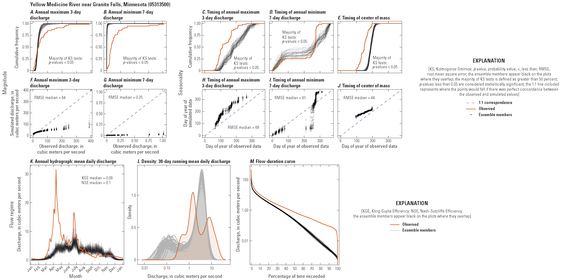
Composite panel figure comparing observed and simulated hydrologic characteristics related to flow magnitude (top left), flow seasonality (top right), and flow regime (bottom) for the Yellow Medicine River near Granite Falls, Minnesota. Simulated hydrologic characteristics are derived from the selected hydrologic data products and comprise results from 32 ensemble members. A, Annual maximum 3-day discharge. B, Annual minimum 7-day discharge. C, Timing of annual maximum 3-day discharge. D, Timing of annual minimum 7-day discharge. E, Timing of center of mass. F, Observed and simulated annual maximum 3-day discharges. G, Observed and simulated annual minimum 7-day discharges. H, Observed and simulated timing of annual maximum 3-day discharges. I, Observed and simulated timing of annual minimum 7-day discharges. K, Annual hydrograph of mean daily discharge. L, Density plot of the annual hydrograph of the 30-day running mean daily discharge. M, Flow-duration curve of mean daily discharge for the period of record.
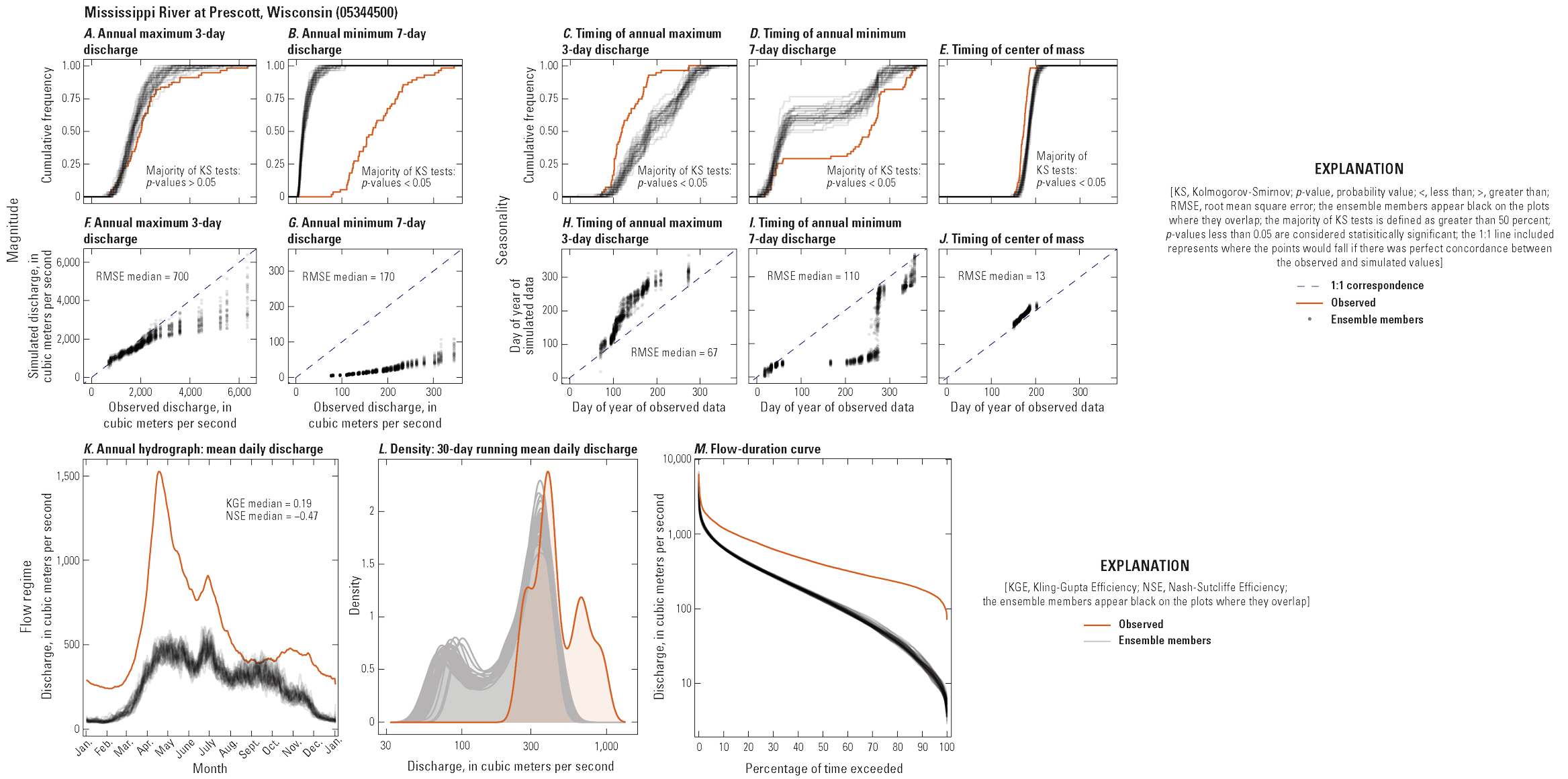
Composite panel figure comparing observed and simulated hydrologic characteristics related to flow magnitude (top left), flow seasonality (top right), and flow regime (bottom) for the Mississippi River at Prescott, Wisconsin. Simulated hydrologic characteristics are derived from the selected hydrologic data products and comprise results from 32 ensemble members. A, Annual maximum 3-day discharge. B, Annual minimum 7-day discharge. C, Timing of annual maximum 3-day discharge. D, Timing of annual minimum 7-day discharge. E, Timing of center of mass. F, Observed and simulated annual maximum 3-day discharges. G, Observed and simulated annual minimum 7-day discharges. H, Observed and simulated timing of annual maximum 3-day discharges. I, Observed and simulated timing of annual minimum 7-day discharges. K, Annual hydrograph of mean daily discharge. L, Density plot of the annual hydrograph of the 30-day running mean daily discharge. M, Flow-duration curve of mean daily discharge for the period of record.
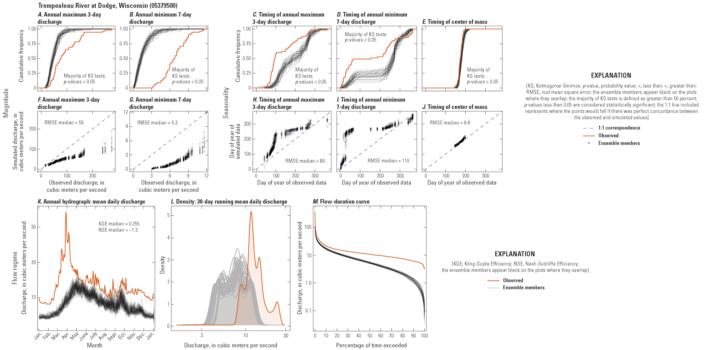
Composite panel figure comparing observed and simulated hydrologic characteristics related to flow magnitude (top left), flow seasonality (top right), and flow regime (bottom) for the Trempealeau River at Dodge, Wisconsin. Simulated hydrologic characteristics are derived from the selected hydrologic data products and comprise results from 32 ensemble members. A, Annual maximum 3-day discharge. B, Annual minimum 7-day discharge. C, Timing of annual maximum 3-day discharge. D, Timing of annual minimum 7-day discharge. E, Timing of center of mass. F, Observed and simulated annual maximum 3-day discharges. G, Observed and simulated annual minimum 7-day discharges. H, Observed and simulated timing of annual maximum 3-day discharges. I, Observed and simulated timing of annual minimum 7-day discharges. K, Annual hydrograph of mean daily discharge. L, Density plot of the annual hydrograph of the 30-day running mean daily discharge. M, Flow-duration curve of mean daily discharge for the period of record.
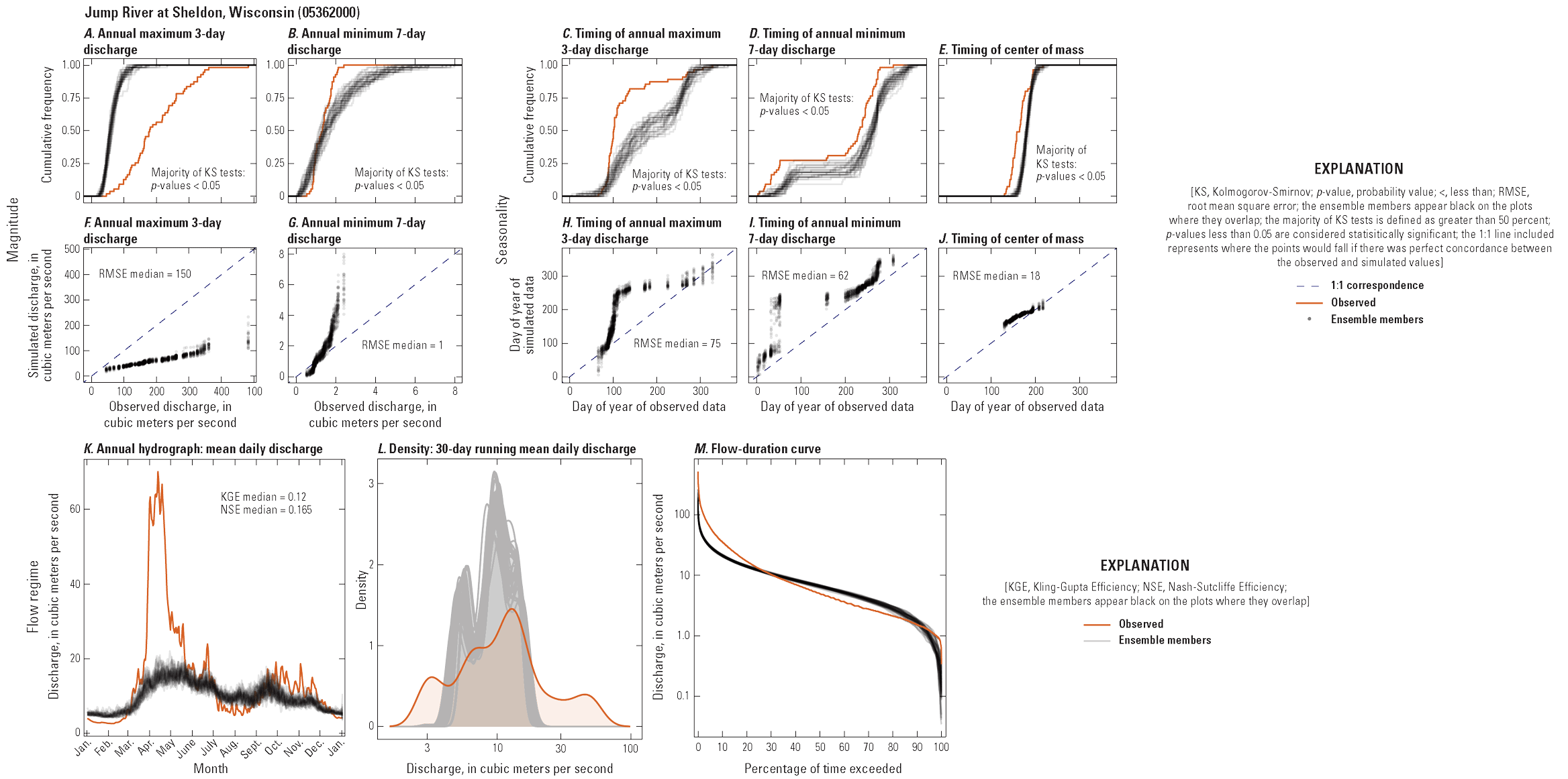
Composite panel figure comparing observed and simulated hydrologic characteristics related to flow magnitude (top left), flow seasonality (top right), and flow regime (bottom) for the Jump River at Sheldon, Wisconsin. Simulated hydrologic characteristics are derived from the selected hydrologic data products and comprise results from 32 ensemble members. A, Annual maximum 3-day discharge. B, Annual minimum 7-day discharge. C, Timing of annual maximum 3-day discharge. D, Timing of annual minimum 7-day discharge. E, Timing of center of mass. F, Observed and simulated annual maximum 3-day discharges. G, Observed and simulated annual minimum 7-day discharges. H, Observed and simulated timing of annual maximum 3-day discharges. I, Observed and simulated timing of annual minimum 7-day discharges. K, Annual hydrograph of mean daily discharge. L, Density plot of the annual hydrograph of the 30-day running mean daily discharge. M, Flow-duration curve of mean daily discharge for the period of record.
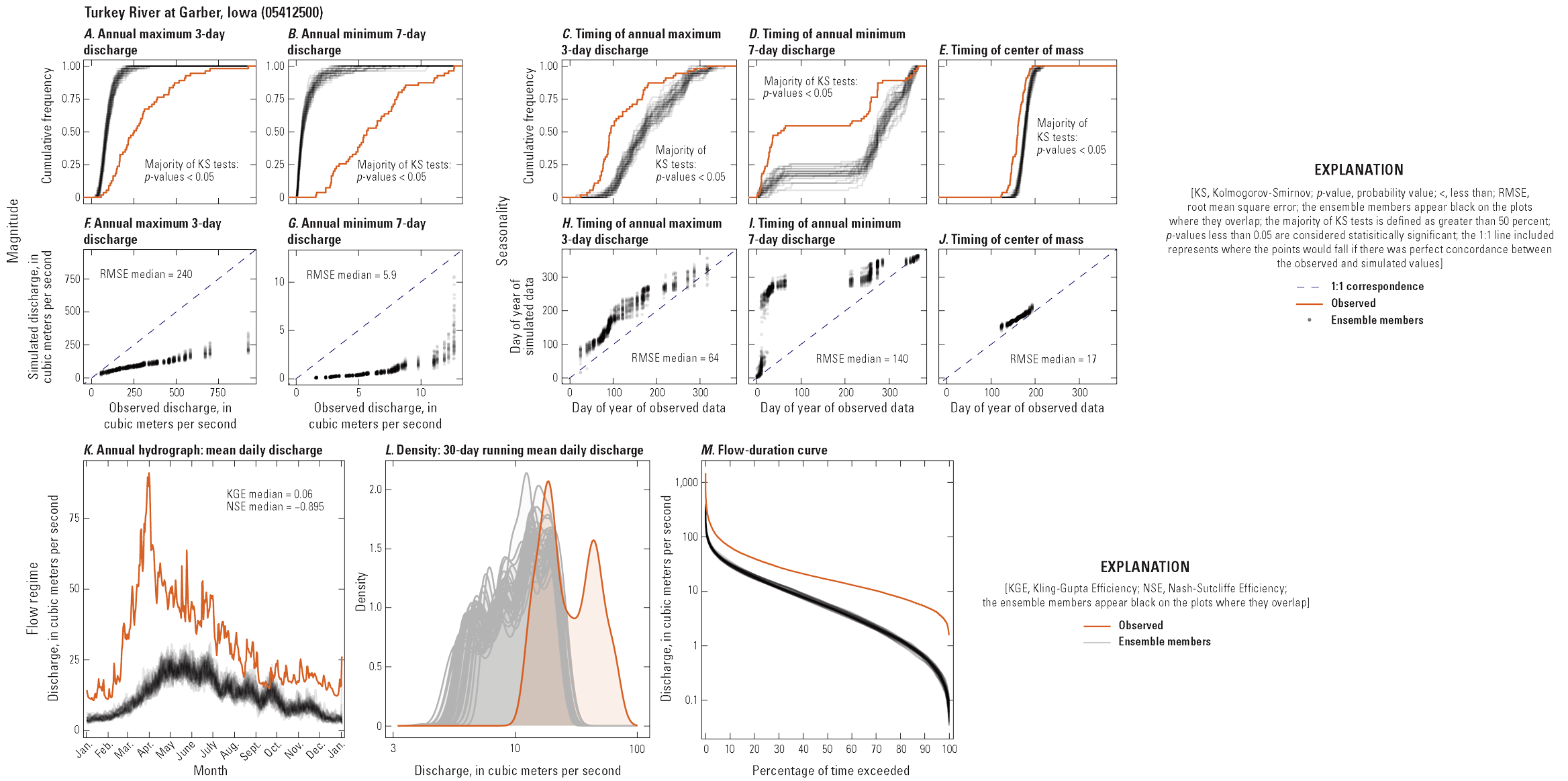
Composite panel figure comparing observed and simulated hydrologic characteristics related to flow magnitude (top left), flow seasonality (top right), and flow regime (bottom) for the Turkey River at Garber, Iowa. Simulated hydrologic characteristics are derived from the selected hydrologic data products and comprise results from 32 ensemble members. A, Annual maximum 3-day discharge. B, Annual minimum 7-day discharge. C, Timing of annual maximum 3-day discharge. D, Timing of annual minimum 7-day discharge. E, Timing of center of mass. F, Observed and simulated annual maximum 3-day discharges. G, Observed and simulated annual minimum 7-day discharges. H, Observed and simulated timing of annual maximum 3-day discharges. I, Observed and simulated timing of annual minimum 7-day discharges. K, Annual hydrograph of mean daily discharge. L, Density plot of the annual hydrograph of the 30-day running mean daily discharge. M, Flow-duration curve of mean daily discharge for the period of record.
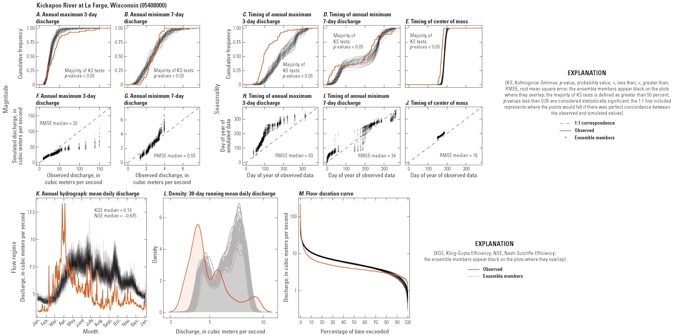
Composite panel figure comparing observed and simulated hydrologic characteristics related to flow magnitude (top left), flow seasonality (top right), and flow regime (bottom) for the Kickapoo River at La Farge, Wisconsin. Simulated hydrologic characteristics are derived from the selected hydrologic data products and comprise results from 32 ensemble members. A, Annual maximum 3-day discharge. B, Annual minimum 7-day discharge. C, Timing of annual maximum 3-day discharge. D, Timing of annual minimum 7-day discharge. E, Timing of center of mass. F, Observed and simulated annual maximum 3-day discharges. G, Observed and simulated annual minimum 7-day discharges. H, Observed and simulated timing of annual maximum 3-day discharges. I, Observed and simulated timing of annual minimum 7-day discharges. K, Annual hydrograph of mean daily discharge. L, Density plot of the annual hydrograph of the 30-day running mean daily discharge. M, Flow-duration curve of mean daily discharge for the period of record.
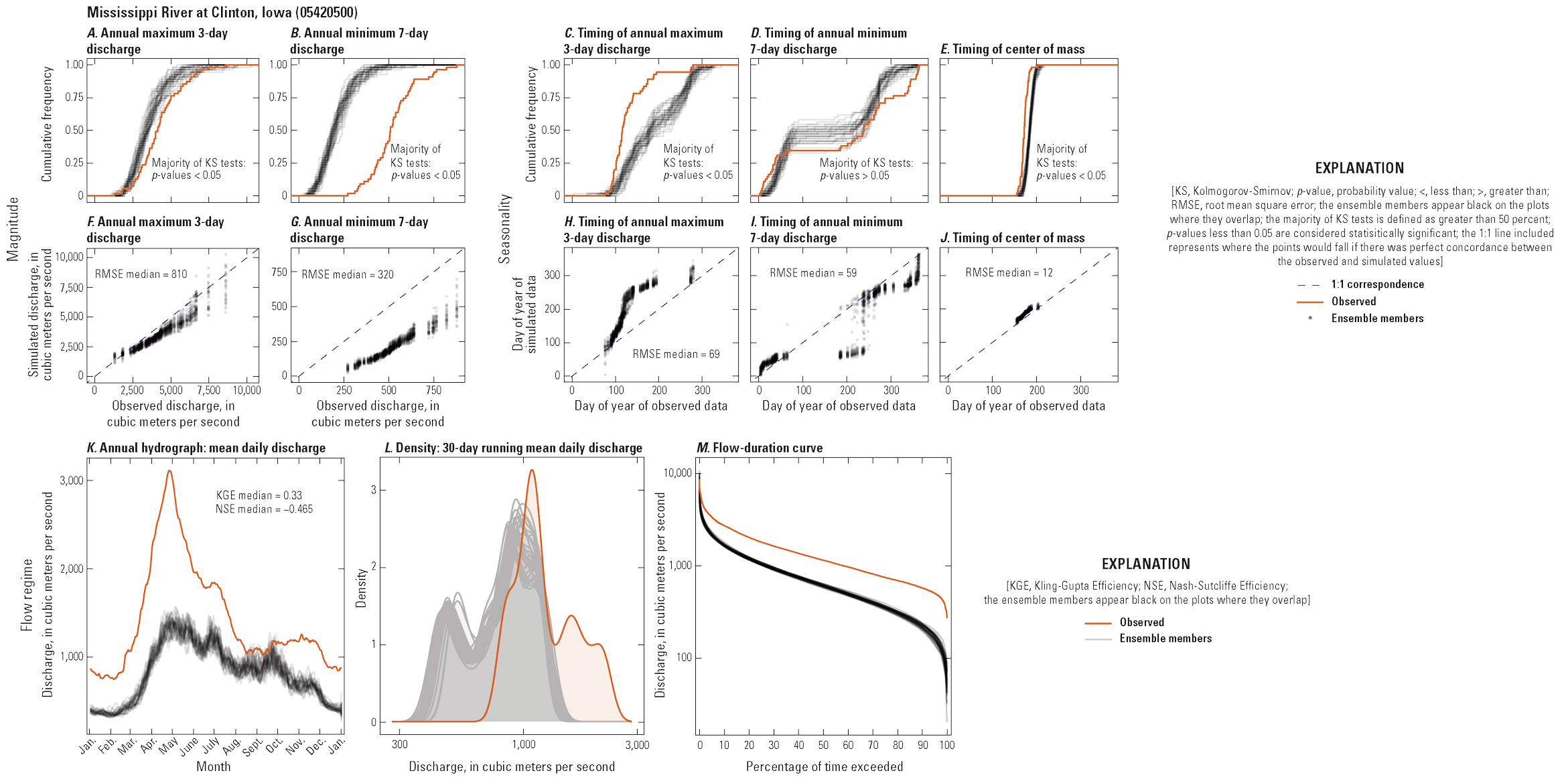
Composite panel figure comparing observed and simulated hydrologic characteristics related to flow magnitude (top left), flow seasonality (top right), and flow regime (bottom) for the Mississippi River at Clinton, Iowa. Simulated hydrologic characteristics are derived from the selected hydrologic data products and comprise results from 32 ensemble members. A, Annual maximum 3-day discharge. B, Annual minimum 7-day discharge. C, Timing of annual maximum 3-day discharge. D, Timing of annual minimum 7-day discharge. E, Timing of center of mass. F, Observed and simulated annual maximum 3-day discharges. G, Observed and simulated annual minimum 7-day discharges. H, Observed and simulated timing of annual maximum 3-day discharges. I, Observed and simulated timing of annual minimum 7-day discharges. K, Annual hydrograph of mean daily discharge. L, Density plot of the annual hydrograph of the 30-day running mean daily discharge. M, Flow-duration curve of mean daily discharge for the period of record.
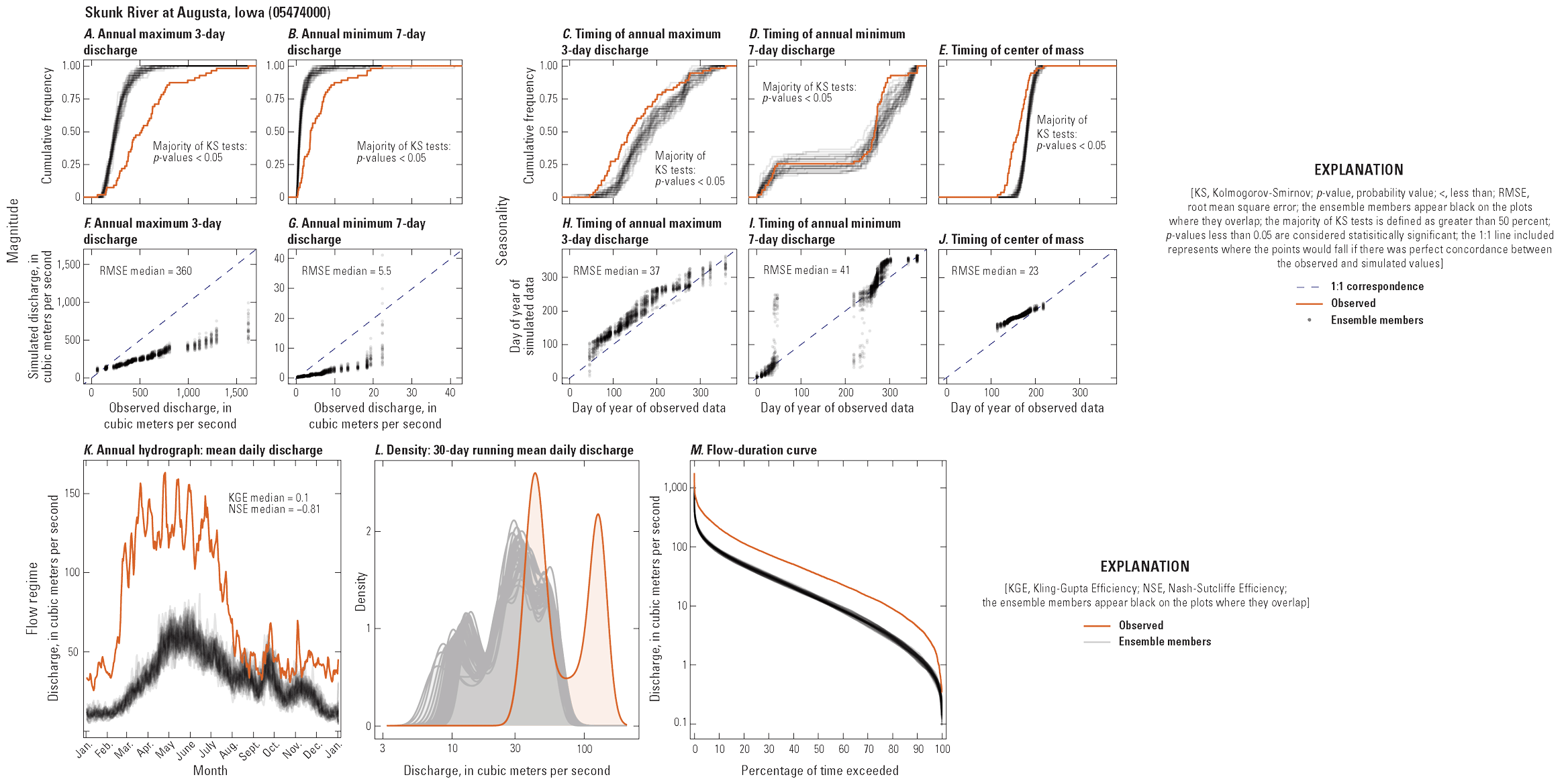
Composite panel figure comparing observed and simulated hydrologic characteristics related to flow magnitude (top left), flow seasonality (top right), and flow regime (bottom) for the Skunk River at Augusta, Iowa. Simulated hydrologic characteristics are derived from the selected hydrologic data products and comprise results from 32 ensemble members. A, Annual maximum 3-day discharge. B, Annual minimum 7-day discharge. C, Timing of annual maximum 3-day discharge. D, Timing of annual minimum 7-day discharge. E, Timing of center of mass. F, Observed and simulated annual maximum 3-day discharges. G, Observed and simulated annual minimum 7-day discharges. H, Observed and simulated timing of annual maximum 3-day discharges. I, Observed and simulated timing of annual minimum 7-day discharges. K, Annual hydrograph of mean daily discharge. L, Density plot of the annual hydrograph of the 30-day running mean daily discharge. M, Flow-duration curve of mean daily discharge for the period of record.
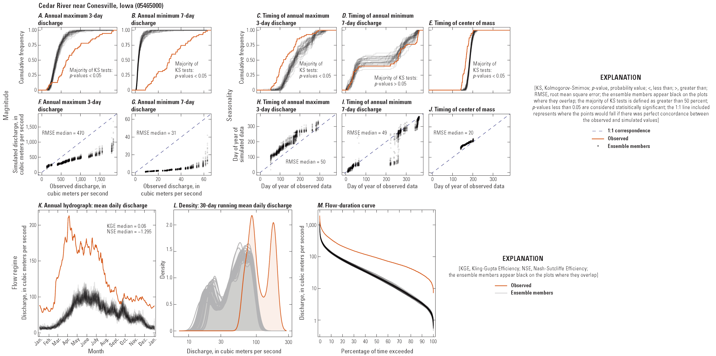
Composite panel figure comparing observed and simulated hydrologic characteristics related to flow magnitude (top left), flow seasonality (top right), and flow regime (bottom) for the Cedar River near Conesville, Iowa. Simulated hydrologic characteristics are derived from the selected hydrologic data products and comprise results from 32 ensemble members. A, Annual maximum 3-day discharge. B, Annual minimum 7-day discharge. C, Timing of annual maximum 3-day discharge. D, Timing of annual minimum 7-day discharge. E, Timing of center of mass. F, Observed and simulated annual maximum 3-day discharges. G, Observed and simulated annual minimum 7-day discharges. H, Observed and simulated timing of annual maximum 3-day discharges. I, Observed and simulated timing of annual minimum 7-day discharges. K, Annual hydrograph of mean daily discharge. L, Density plot of the annual hydrograph of the 30-day running mean daily discharge. M, Flow-duration curve of mean daily discharge for the period of record.
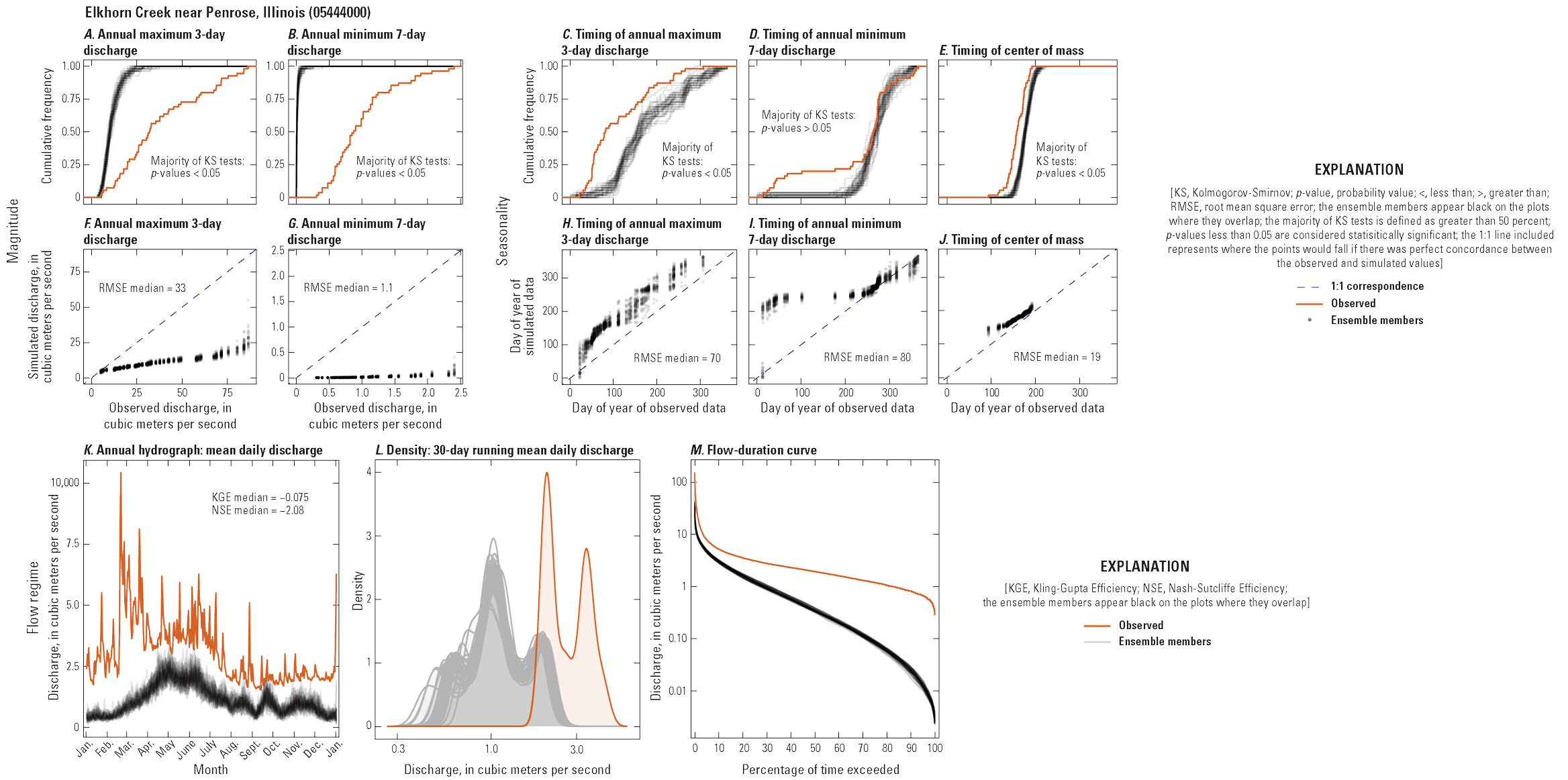
Composite panel figure comparing observed and simulated hydrologic characteristics related to flow magnitude (top left), flow seasonality (top right), and flow regime (bottom) for Elkhorn Creek near Penrose, Illinois. Simulated hydrologic characteristics are derived from the selected hydrologic data products and comprise results from 32 ensemble members. A, Annual maximum 3-day discharge. B, Annual minimum 7-day discharge. C, Timing of annual maximum 3-day discharge. D, Timing of annual minimum 7-day discharge. E, Timing of center of mass. F, Observed and simulated annual maximum 3-day discharges. G, Observed and simulated annual minimum 7-day discharges. H, Observed and simulated timing of annual maximum 3-day discharges. I, Observed and simulated timing of annual minimum 7-day discharges. K, Annual hydrograph of mean daily discharge. L, Density plot of the annual hydrograph of the 30-day running mean daily discharge. M, Flow-duration curve of mean daily discharge for the period of record.
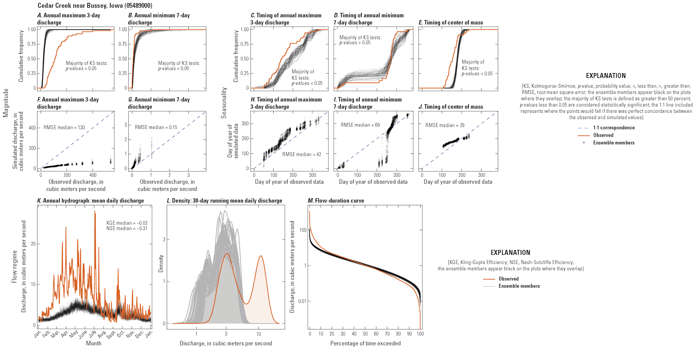
Composite panel figure comparing observed and simulated hydrologic characteristics related to flow magnitude (top left), flow seasonality (top right), and flow regime (bottom) for Cedar Creek near Bussey, Iowa. Simulated hydrologic characteristics are derived from the selected hydrologic data products and comprise results from 32 ensemble members. A, Annual maximum 3-day discharge. B, Annual minimum 7-day discharge. C, Timing of annual maximum 3-day discharge. D, Timing of annual minimum 7-day discharge. E, Timing of center of mass. F, Observed and simulated annual maximum 3-day discharges. G, Observed and simulated annual minimum 7-day discharges. H, Observed and simulated timing of annual maximum 3-day discharges. I, Observed and simulated timing of annual minimum 7-day discharges. K, Annual hydrograph of mean daily discharge. L, Density plot of the annual hydrograph of the 30-day running mean daily discharge. M, Flow-duration curve of mean daily discharge for the period of record.
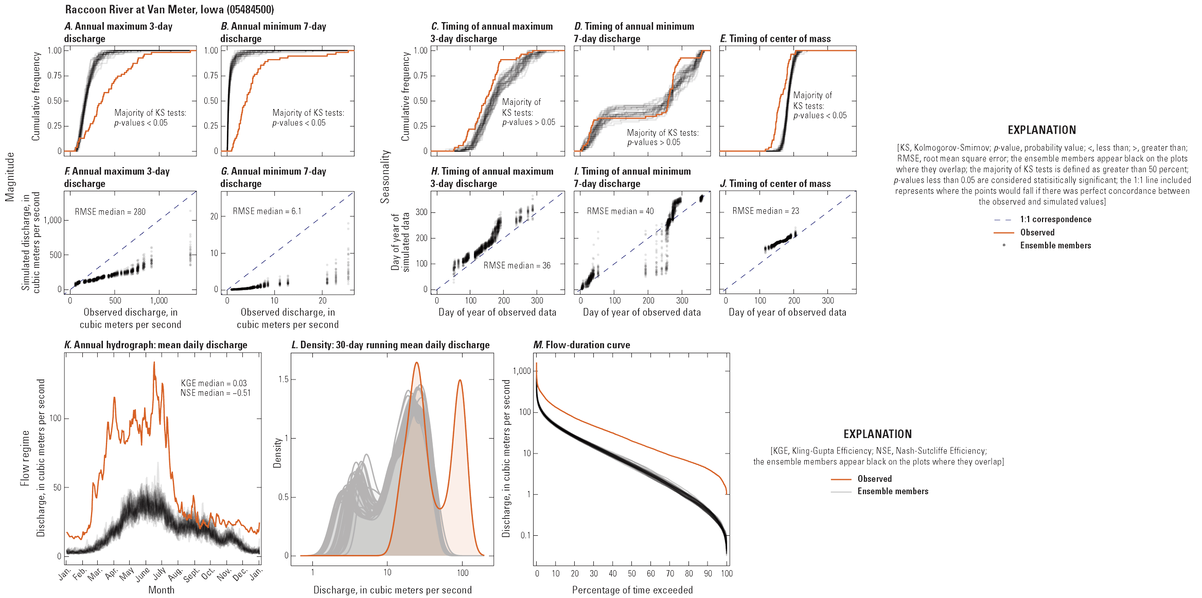
Composite panel figure comparing observed and simulated hydrologic characteristics related to flow magnitude (top left), flow seasonality (top right), and flow regime (bottom) for the Raccoon River at Van Meter, Iowa. Simulated hydrologic characteristics are derived from the selected hydrologic data products and comprise results from 32 ensemble members. A, Annual maximum 3-day discharge. B, Annual minimum 7-day discharge. C, Timing of annual maximum 3-day discharge. D, Timing of annual minimum 7-day discharge. E, Timing of center of mass. F, Observed and simulated annual maximum 3-day discharges. G, Observed and simulated annual minimum 7-day discharges. H, Observed and simulated timing of annual maximum 3-day discharges. I, Observed and simulated timing of annual minimum 7-day discharges. K, Annual hydrograph of mean daily discharge. L, Density plot of the annual hydrograph of the 30-day running mean daily discharge. M, Flow-duration curve of mean daily discharge for the period of record.
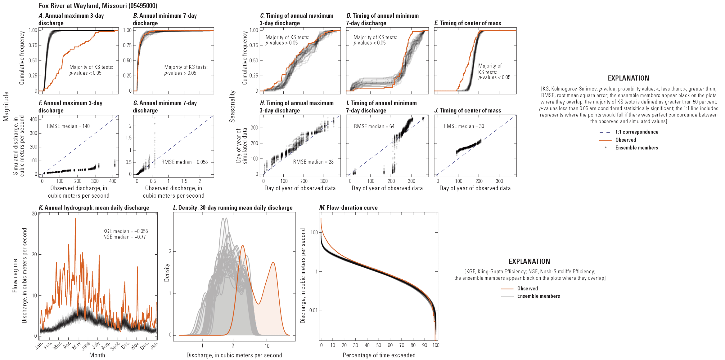
Composite panel figure comparing observed and simulated hydrologic characteristics related to flow magnitude (top left), flow seasonality (top right), and flow regime (bottom) for the Fox River at Wayland, Missouri. Simulated hydrologic characteristics are derived from the selected hydrologic data products and comprise results from 32 ensemble members. A, Annual maximum 3-day discharge. B, Annual minimum 7-day discharge. C, Timing of annual maximum 3-day discharge. D, Timing of annual minimum 7-day discharge. E, Timing of center of mass. F, Observed and simulated annual maximum 3-day discharges. G, Observed and simulated annual minimum 7-day discharges. H, Observed and simulated timing of annual maximum 3-day discharges. I, Observed and simulated timing of annual minimum 7-day discharges. K, Annual hydrograph of mean daily discharge. L, Density plot of the annual hydrograph of the 30-day running mean daily discharge. M, Flow-duration curve of mean daily discharge for the period of record.
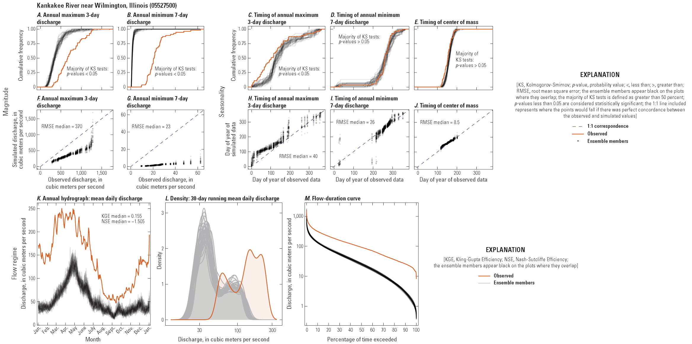
Composite panel figure comparing observed and simulated hydrologic characteristics related to flow magnitude (top left), flow seasonality (top right), and flow regime (bottom) for the Kankakee River near Wilmington, Illinois. Simulated hydrologic characteristics are derived from the selected hydrologic data products and comprise results from 32 ensemble members. A, Annual maximum 3-day discharge. B, Annual minimum 7-day discharge. C, Timing of annual maximum 3-day discharge. D, Timing of annual minimum 7-day discharge. E, Timing of center of mass. F, Observed and simulated annual maximum 3-day discharges. G, Observed and simulated annual minimum 7-day discharges. H, Observed and simulated timing of annual maximum 3-day discharges. I, Observed and simulated timing of annual minimum 7-day discharges. K, Annual hydrograph of mean daily discharge. L, Density plot of the annual hydrograph of the 30-day running mean daily discharge. M, Flow-duration curve of mean daily discharge for the period of record.
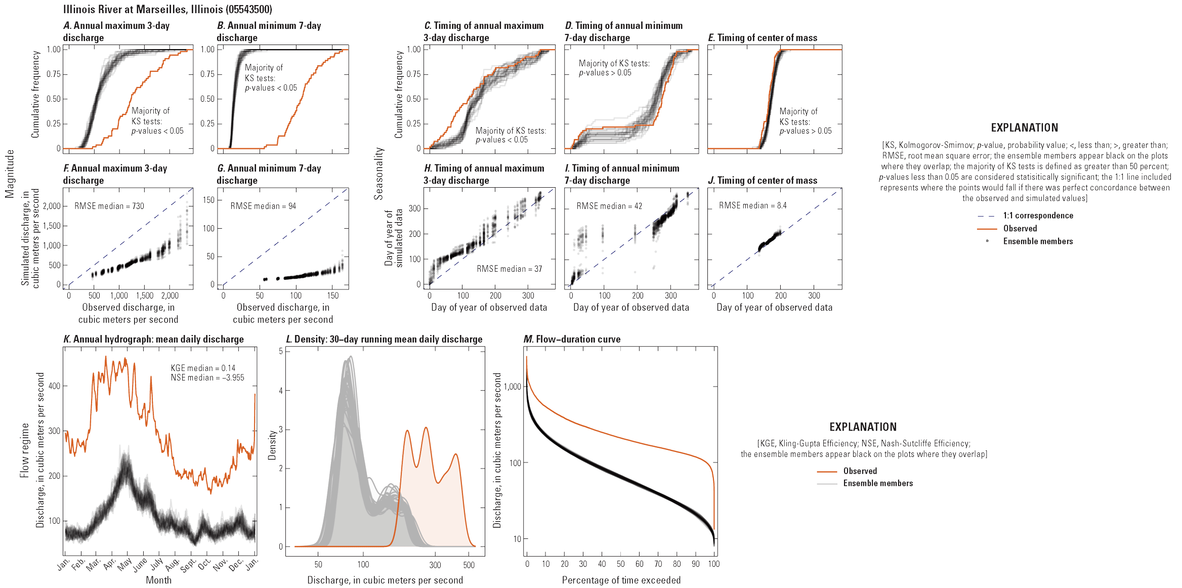
Composite panel figure comparing observed and simulated hydrologic characteristics related to flow magnitude (top left), flow seasonality (top right), and flow regime (bottom) for the Illinois River at Marseilles, Illinois. Simulated hydrologic characteristics are derived from the selected hydrologic data products and comprise results from 32 ensemble members. A, Annual maximum 3-day discharge. B, Annual minimum 7-day discharge. C, Timing of annual maximum 3-day discharge. D, Timing of annual minimum 7-day discharge. E, Timing of center of mass. F, Observed and simulated annual maximum 3-day discharges. G, Observed and simulated annual minimum 7-day discharges. H, Observed and simulated timing of annual maximum 3-day discharges. I, Observed and simulated timing of annual minimum 7-day discharges. K, Annual hydrograph of mean daily discharge. L, Density plot of the annual hydrograph of the 30-day running mean daily discharge. M, Flow-duration curve of mean daily discharge for the period of record.
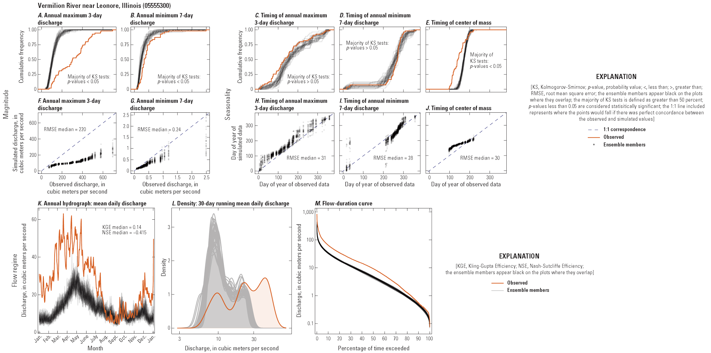
Composite panel figure comparing observed and simulated hydrologic characteristics related to flow magnitude (top left), flow seasonality (top right), and flow regime (bottom) for the Vermilion River near Leonore, Illinois. Simulated hydrologic characteristics are derived from the selected hydrologic data products and comprise results from 32 ensemble members. A, Annual maximum 3-day discharge. B, Annual minimum 7-day discharge. C, Timing of annual maximum 3-day discharge. D, Timing of annual minimum 7-day discharge. E, Timing of center of mass. F, Observed and simulated annual maximum 3-day discharges. G, Observed and simulated annual minimum 7-day discharges. H, Observed and simulated timing of annual maximum 3-day discharges. I, Observed and simulated timing of annual minimum 7-day discharges. K, Annual hydrograph of mean daily discharge. L, Density plot of the annual hydrograph of the 30-day running mean daily discharge. M, Flow-duration curve of mean daily discharge for the period of record.
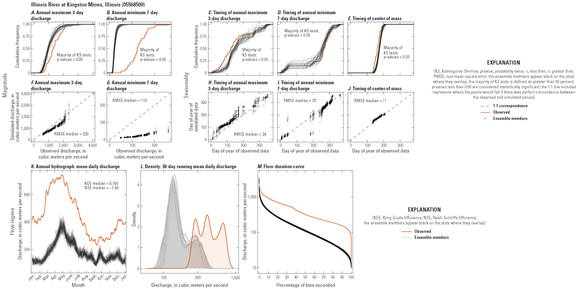
Composite panel figure comparing observed and simulated hydrologic characteristics related to flow magnitude (top left), flow seasonality (top right), and flow regime (bottom) for the Illinois River at Kingston Mines, Illinois. Simulated hydrologic characteristics are derived from the selected hydrologic data products and comprise results from 32 ensemble members. A, Annual maximum 3-day discharge. B, Annual minimum 7-day discharge. C, Timing of annual maximum 3-day discharge. D, Timing of annual minimum 7-day discharge. E, Timing of center of mass. F, Observed and simulated annual maximum 3-day discharges. G, Observed and simulated annual minimum 7-day discharges. H, Observed and simulated timing of annual maximum 3-day discharges. I, Observed and simulated timing of annual minimum 7-day discharges. K, Annual hydrograph of mean daily discharge. L, Density plot of the annual hydrograph of the 30-day running mean daily discharge. M, Flow-duration curve of mean daily discharge for the period of record.
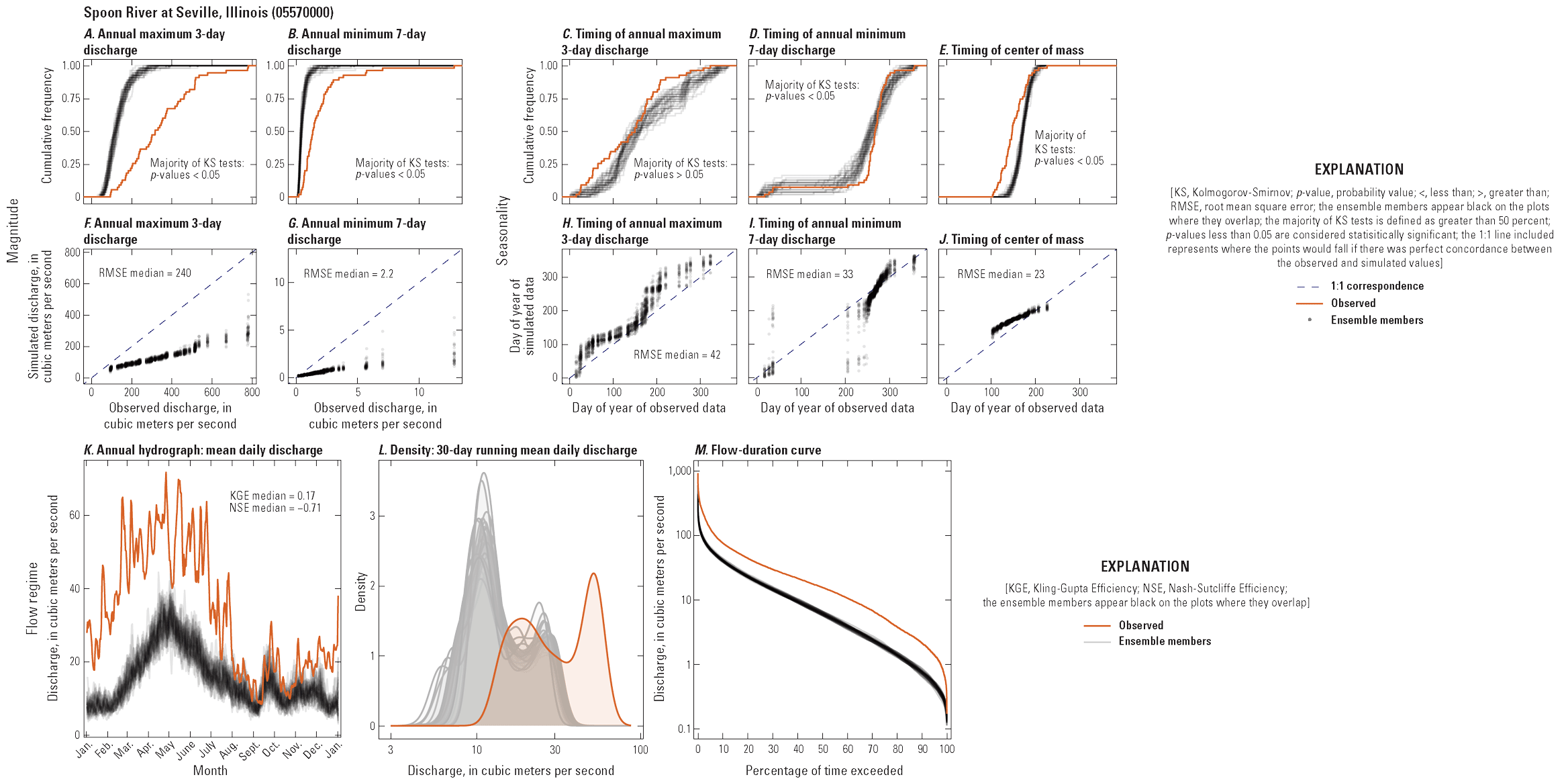
Composite panel figure comparing observed and simulated hydrologic characteristics related to flow magnitude (top left), flow seasonality (top right), and flow regime (bottom) for the Spoon River at Seville, Illinois. Simulated hydrologic characteristics are derived from the selected hydrologic data products and comprise results from 32 ensemble members. A, Annual maximum 3-day discharge. B, Annual minimum 7-day discharge. C, Timing of annual maximum 3-day discharge. D, Timing of annual minimum 7-day discharge. E, Timing of center of mass. F, Observed and simulated annual maximum 3-day discharges. G, Observed and simulated annual minimum 7-day discharges. H, Observed and simulated timing of annual maximum 3-day discharges. I, Observed and simulated timing of annual minimum 7-day discharges. K, Annual hydrograph of mean daily discharge. L, Density plot of the annual hydrograph of the 30-day running mean daily discharge. M, Flow-duration curve of mean daily discharge for the period of record.

Composite panel figure comparing observed and simulated hydrologic characteristics related to flow magnitude (top left), flow seasonality (top right), and flow regime (bottom) for the Meramec River near Eureka, Missouri. Simulated hydrologic characteristics are derived from the selected hydrologic data products and comprise results from 32 ensemble members. A, Annual maximum 3-day discharge. B, Annual minimum 7-day discharge. C, Timing of annual maximum 3-day discharge. D, Timing of annual minimum 7-day discharge. E, Timing of center of mass. F, Observed and simulated annual maximum 3-day discharges. G, Observed and simulated annual minimum 7-day discharges. H, Observed and simulated timing of annual maximum 3-day discharges. I, Observed and simulated timing of annual minimum 7-day discharges. K, Annual hydrograph of mean daily discharge. L, Density plot of the annual hydrograph of the 30-day running mean daily discharge. M, Flow-duration curve of mean daily discharge for the period of record.
Appendix 2. Heatmap Figure Library
Overview
In our study we compare distributions of hydrologic characteristics derived from each ensemble member separately with distributions of hydrologic characteristics derived from observed historical discharge data. In this appendix we report Kolmogorov-Smirnov test statistics (D) and Normalized Root Mean Square Error (NRMSE) for every ensemble member at every streamgage location (number of streamgage sites, n=19; table 1 in main report) in the form of heatmaps. The heatmaps are organized by the hydrologic characteristics described in table 2 in main report.
A higher D statistic reflects less correspondence. Heatmap results are applied to verify that ensemble members for the historical period are consistent with one another and that a minority of ensemble members are not unduly biasing interpretation of results. At each streamgage location, the 32 ensemble members produce similar results for hydrologic characteristics related to streamflow magnitude and seasonality. In other words, the heatmap results (for D statistics and NRMSE) indicate that no individual member(s) exhibit divergent behavior relative to the other ensemble members for each streamgage location.
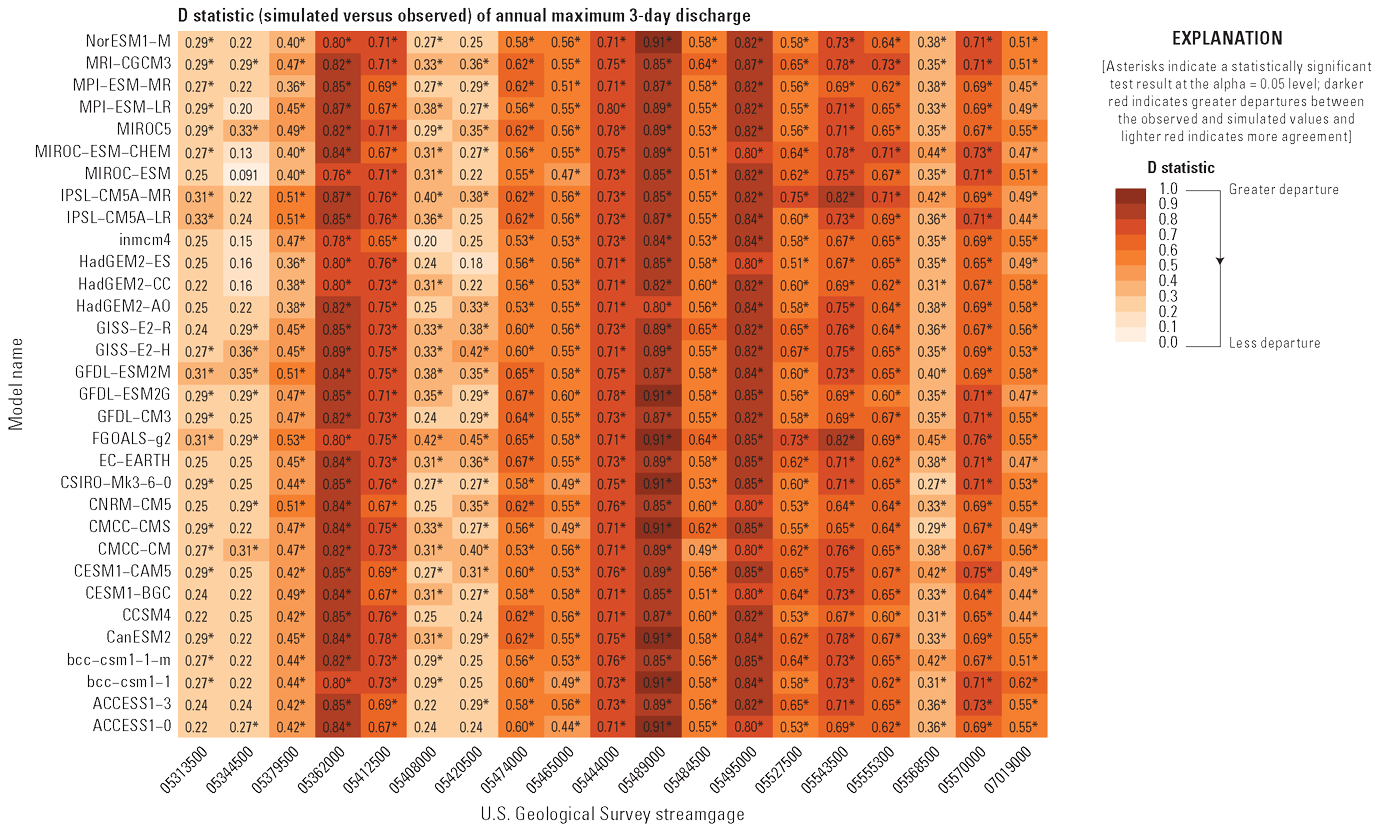
Heat map of the Kolmogorov-Smirnov test statistic (D) that compares observed values of the 3-day annual maximum discharge at 19 U.S. Geological Survey streamgage locations to simulated values from 32 ensemble members of the selected hydrologic data products. The global climate model associated with each ensemble member is listed in the first column and is further described in table 2.1. Asterisks indicate a statistically significant test result at the alpha = 0.05 level. Darker shading indicates greater departures between the observed and simulated distributions and lighter shading indicates more agreement.
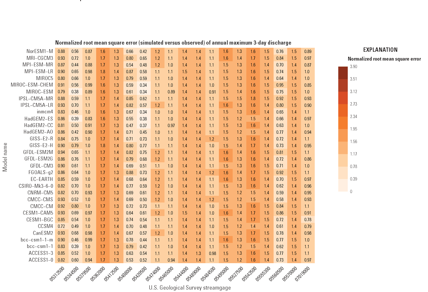
Heat map of Normalized Root Mean Square Error between observed values of the 3-day annual maximum discharge at 19 U.S. Geological Survey streamgage locations to simulated values from 32 ensemble members of the selected hydrologic data products. The global climate model associated with each ensemble member is listed in the first column and is further described in table 2.1. Darker shading indicates greater correspondence between the observed and simulated values and lighter shading indicates less correspondence.
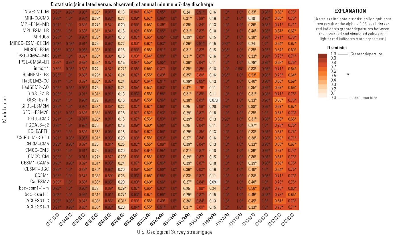
Heat map of the Kolmogorov-Smirnov test statistic (D) that compares observed values of the 7-day annual minimum discharge at 19 U.S. Geological Survey streamgage locations to simulated values from 32 ensemble members of the selected hydrologic data products. The global climate model associated with each ensemble member is listed in the first column and is further described in table 2.1. Asterisks indicate a statistically significant test result at the alpha = 0.05 level. Darker shading indicates greater departures between the observed and simulated distributions and lighter shading indicates more agreement.
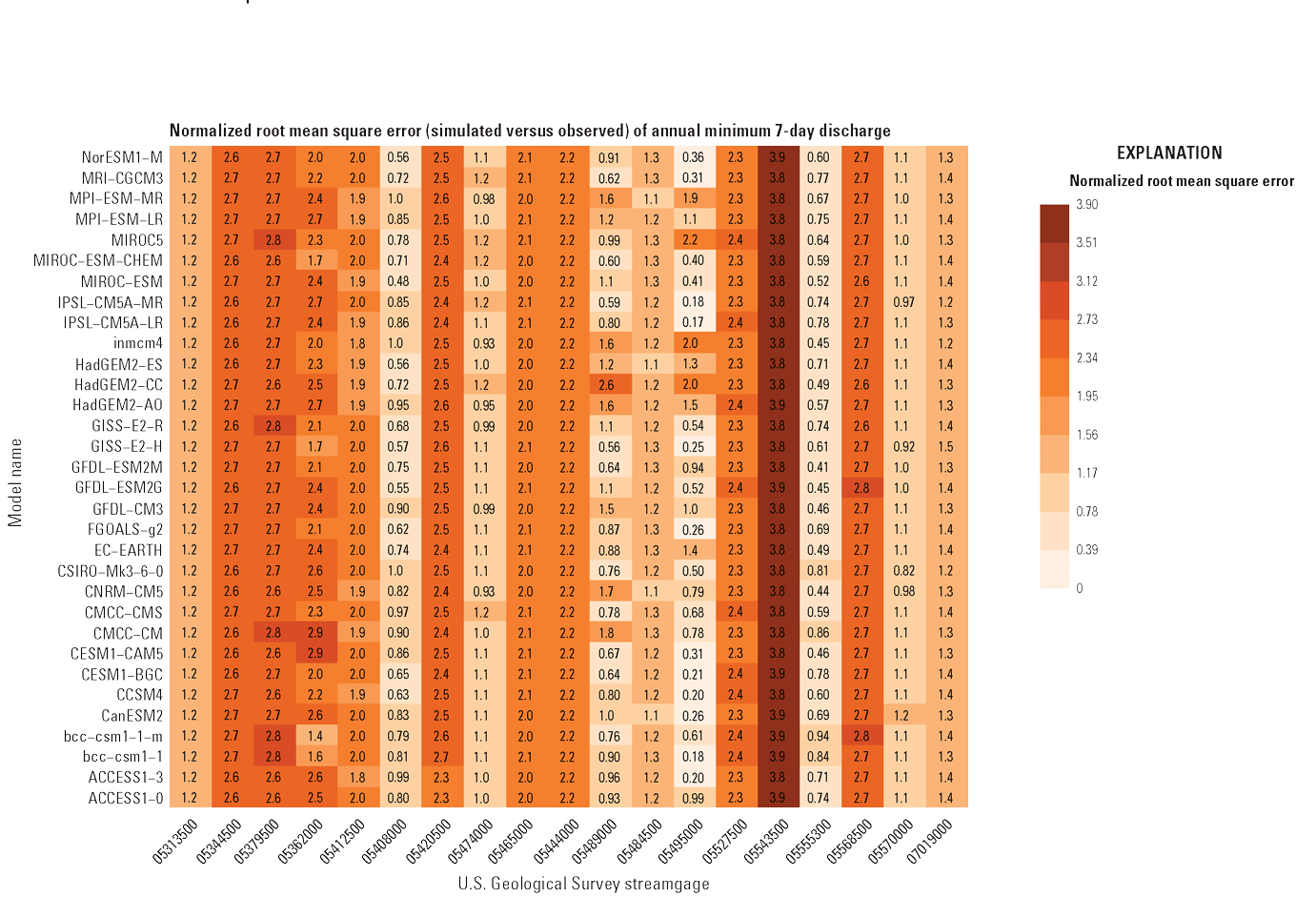
Heat map of Normalized Root Mean Square Error between observed values of the 7-day annual minimum discharge at 19 U.S. Geological Survey streamgage locations to simulated values from 32 ensemble members of the selected hydrologic data products. The global climate model associated with each ensemble member is listed in the first column and is further described in table 2.1. Darker shading indicates greater correspondence between the observed and simulated values and lighter shading indicates less correspondence.
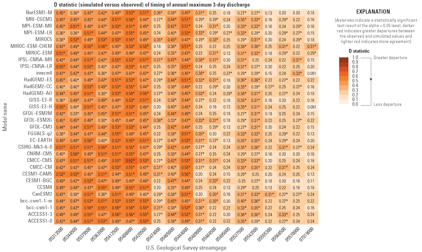
Heat map of the Kolmogorov-Smirnov test statistic (D) that compares observed timing of the 3-day annual maximum discharge at 19 U.S. Geological Survey streamgage locations to simulated timing from 32 ensemble members of the selected hydrologic data products. The global climate model associated with each ensemble member is listed in the first column and is further described in table 2.1. Asterisks indicate a statistically significant test result at the alpha = 0.05 level. Darker shading indicates greater departures between the observed and simulated distributions and lighter shading indicates more agreement.
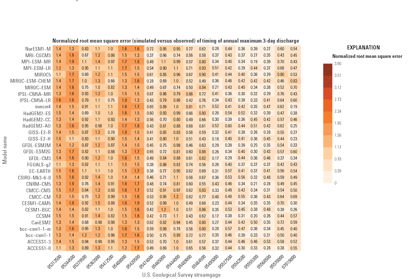
Heat map of Normalized Root Mean Square Error between observed timing of the 3-day annual maximum discharge at 19 U.S. Geological Survey streamgage locations to simulated timing from 32 ensemble members of the selected hydrologic data products. The global climate model associated with each ensemble member is listed in the first column and is further described in table 2.1. Darker shading indicates greater correspondence between the observed and simulated timing and lighter shading indicates less correspondence.
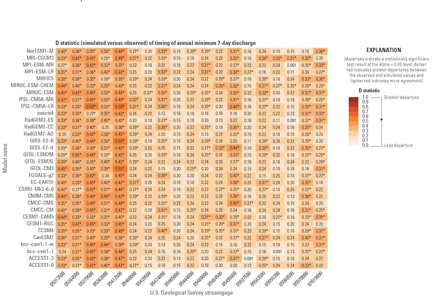
Heat map of the Kolmogorov-Smirnov test statistic (D) that compares observed timing of the 7-day annual minimum discharge at 19 U.S. Geological Survey streamgage locations to simulated timing from 32 ensemble members of the selected hydrologic data products. The global climate model associated with each ensemble member is listed in the first column and is further described in table 2.1. Asterisks indicate a statistically significant test result at the alpha = 0.05 level. Darker shading indicates greater departures between the observed and simulated distributions and lighter shading indicates more agreement.
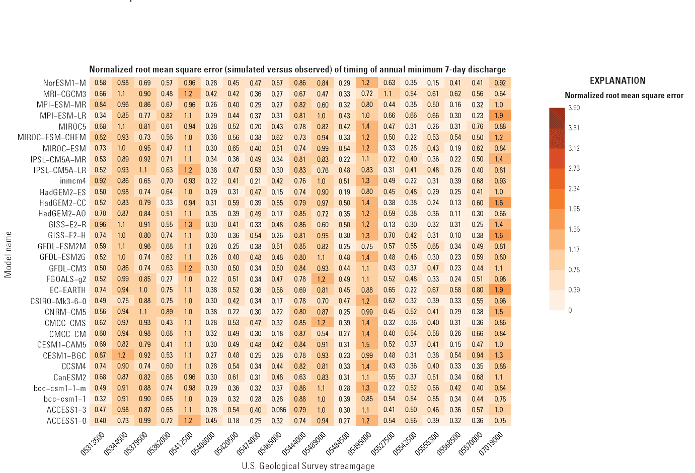
Heat map of Normalized Root Mean Square Error that compares observed timing of the 7-day annual minimum discharge at 19 U.S. Geological Survey streamgage locations to simulated timing from 32 ensemble members of the selected hydrologic data products. The global climate model associated with each ensemble member is listed in the first column and is further described in table 2.1. Darker shading indicates greater correspondence between the observed and simulated timing and lighter shading indicates less correspondence.
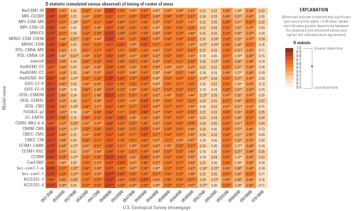
Heat map of the Kolmogorov-Smirnov test statistic (D) that compares observed timing of the center of mass at 19 U.S. Geological Survey streamgage locations to simulated timing from 32 ensemble members of the selected hydrologic data products. The global climate model associated with each ensemble member is listed in the first column and is further described in table 2.1. Asterisks indicate a statistically significant test result at the alpha = 0.05 level. Darker shading indicates greater departures between the observed and simulated distributions and lighter shading indicates more agreement.
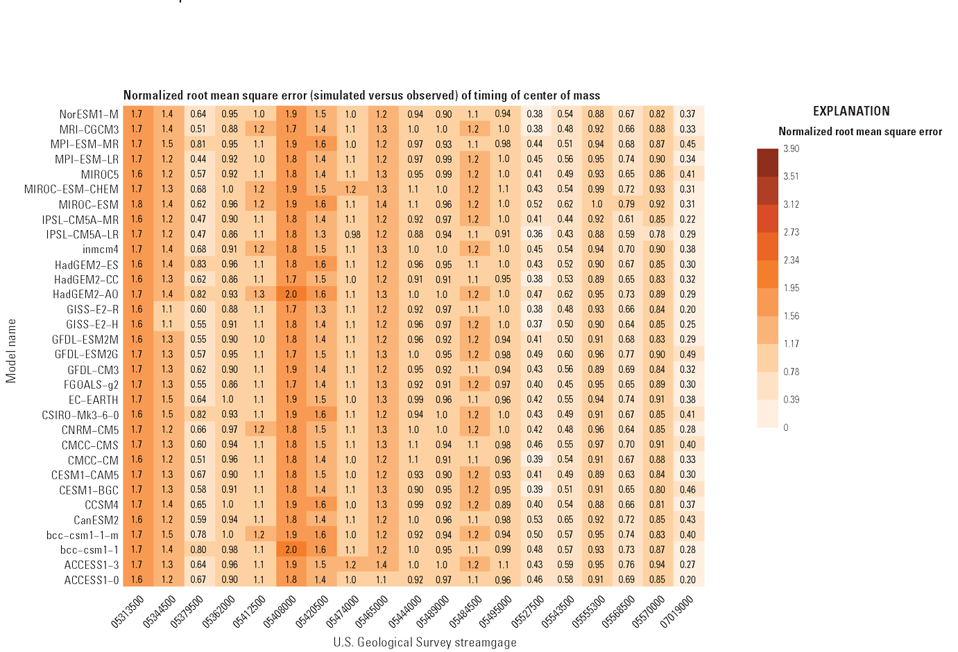
Heat map of Normalized Root Mean Square Error that compares observed timing of the center of mass at 19 U.S. Geological Survey streamgage locations to simulated timing from 32 ensemble members of the selected hydrologic data products. The global climate model associated with each ensemble member is listed in the first column and is further described in table 2.1. Darker shading indicates greater correspondence between the observed and simulated timing and lighter shading indicates less correspondence.
Table 2.1.
Names of global climate models associated with ensemble members from the selected hydrologic data products and the institutional associations as derived from the Climate Model Diagnosis and Intercomparison Project Phase 5 (CMIP5).| Model | Institution | Citation |
|---|---|---|
| NorESM1-M | Norwegian Climate Centre, Norway | Bentsen and others, 2013 |
| MRI-CGCM3 | Meteorological Research Institute, Tsukuba, Japan | Yukimoto and others, 2012 |
| MPI-ESM-MR | Max Planck Institute for Meteorology, Hamburg, Germany | Giorgetta and others, 2013 |
| MPI-ESM-LR | Max Planck Institute for Meteorology, Hamburg, Germany | Giorgetta and others, 2013 |
| MICROC5 | Japan Agency for Marine‐Earth Science and Technology, Kanagawa, Japan; Atmosphere and Ocean Research Institute, The University of Tokyo, Chiba, Japan; and National Institute for Environmental Studies, Ibaraki, Japan | Watanabe and others, 2010 |
| MIROC-ESM-CHEM | Japan Agency for Marine‐Earth Science and Technology, Kanagawa, Japan; Atmosphere and Ocean Research Institute, The University of Tokyo, Chiba, Japan; and National Institute for Environmental Studies, Ibaraki, Japan | Watanabe and others, 2011 |
| MIROC-ESM | Japan Agency for Marine‐Earth Science and Technology, Kanagawa, Japan; Atmosphere and Ocean Research Institute, The University of Tokyo, Chiba, Japan; and National Institute for Environmental Studies, Ibaraki, Japan | Watanabe and others, 2011 |
| IPSL-CM5A-MR | Institut Pierre Simon Laplace, Paris, France | Dufresne and others, 2013 |
| IPSL-CM5A-LR | Institut Pierre Simon Laplace, Paris, France | Dufresne and others, 2013 |
| inmcm4 | Institute for Numerical Mathematics, Moscow, Russia | Volodin and others, 2010 |
| HadGEM2-ES | Met Office Hadley Centre, Fitzroy Road, Exeter, Devon, EX1 3PB, United Kingdom | Martin and others, 2011 |
| HadGEM2-CC | Met Office Hadley Centre, Fitzroy Road, Exeter, Devon, EX1 3PB, United Kingdom | Martin and others, 2011 |
| HadGEM2-AO | NIMR (National Institute of Meteorological Research, Seoul, South Korea) in association with the Met Office Hadley Centre, United Kingdom | Martin and others, 2011 |
| GISS-E2-R | NASA/GISS (Goddard Institute for Space Studies) New York, New York, United States | Schmidt and others, 2014 |
| GISS-E2-H | NASA/GISS (Goddard Institute for Space Studies) New York, New York, United States | Schmidt and others, 2014 |
| GFDL-ESM2M | NOAA Geophysical Fluid Dynamics Laboratory, Princeton, New Jersey, United States | Dunne and others, 2013 |
| GFDL-ESM2G | NOAA Geophysical Fluid Dynamics Laboratory, Princeton, New Jersey, United States | Dunne and others, 2013 |
| GFDL-CM3 | NOAA Geophysical Fluid Dynamics Laboratory, Princeton, New Jersey, United States | Donner and others, 2011; Griffies and others 2011 |
| FGOALS-g2 | Institute of Atmospheric Physics, Chinese Academy of Sciences, Beijing, China; and Tsinghua University | Li and others, 2013 |
| EC-EARTH | EC‐Earth (European Earth System Model) | Hazeleger and others, 2010, 2012 |
| CSIRO-Mk3-6-0 | Australian Commonwealth Scientific and Industrial Research Organization Marine and Atmospheric Research (Melbourne, Australia) in collaboration with the Queensland Climate Change Centre of Excellence (Brisbane, Australia) | Collier and others, 2011 |
| CNRM-CM5 | Centre National de Recherches Meteorologiques, Meteo-France, Toulouse, France; and Centre Europeen de Recherches et de Formation Avancee en Calcul Scientifique, Toulouse, France | Voldoire and others, 2013 |
| CMCC-CMS | Centro Euro‐Mediterraneo per i Cambiamenti, Italy | Vichi and others, 2007 |
| CMCC-CM | Centro Euro‐Mediterraneo per i Cambiamenti, Italy | Scoccimarro and others, 2011 |
| CESM1-CAM5 | The National Science Foundation, The Department of Energy, and the National Center for Atmospheric Research, United States | Hurrell and others, 2013 |
| CESM1-BGC | The National Science Foundation, The Department of Energy, and the National Center for Atmospheric Research, United States | Hurrell and others, 2013 |
| CCSM4 | The National Science Foundation, The Department of Energy, and the National Center for Atmospheric Research, United States | Gent and others, 2011 |
| CanESM2 | Canadian Centre for Climate Modelling and Analysis, Victoria, BC, Canada | Chylek and others, 2011 |
| bcc-csm1-1-m | Beijing Climate Center, China Meteorological Administration, China | Wu and others, 2014 |
| bcc-csm1-1 | Beijing Climate Center, China Meteorological Administration, China | Wu and others, 2014 |
| ACCESS1-3 | Commonwealth Scientific and Industrial Research Organization, Australia, and Bureau of Meteorology, Australia | Dix and others, 2013 |
| ACCESS1-0 | Commonwealth Scientific and Industrial Research Organization, Australia, and Bureau of Meteorology, Australia | Dix and others, 2013 |
References Cited
Bentsen, M., Bethke, I., Debernard, J.B., Iversen, T., Kirkevåg, A., Seland, Ø., Drange, H., Roelandt, C., Seierstad, I.A., Hoose, C., and Kristjánsson, J.E., 2013, The Norwegian Earth System Model, NorESM1-M, Part 1—Description and basic evaluation of the physical climate: Geoscientific Model Development, v. 6, no. 3, p. 687–720, accessed February 2024 at https://doi.org/10.5194/gmd-6-687-2013.
Chylek, P., Li, J., Dubey, M.K., Wang, M., and Lesins, G., 2011, Observed and model simulated 20th century Arctic temperature variability—Canadian Earth System Model CanESM2: Atmospheric Chemistry and Physics Discussion, v. 11, p. 22893–22907, accessed February 2024 at https://doi.org/10.5194/acpd-11-22893-2011.
Collier, M.A., Jeffrey, S.J., Rotstayn, L.D., Wong, K.K.-H., Dravitzki, S.M., Moeseneder, C., Hamalainen, C., Syktus, J.I., Suppiah, R., Antony, J., El Zein, A., and Atif, M., 2011, The CSIRO-Mk3.6.0 Atmosphere-Ocean GCM—Participation in CMIP5 and data publication, in Chan, F., Marinova, D. and Anderssen, R.S., eds., MODSIM2011: Perth, Australia, 19th International Congress on Modelling and Simulation, p. 2691–2697, accessed February 2024 at https://doi.org/10.36334/modsim.2011.F5.collier.
Dix, M., Vohralik, P., Bi, D., Rashid, H., Marsland, S., O’Farrell, S., Uotila, P., Hirst, T., Kowalczyk, E., Sullivan, A., Yan, H., Franklin, C., Sun, Z., Watterson, I., Collier, M., Noonan, J., Rotstayn, L., Stevens, L., Uhe, P., and Puri, K., 2013, The ACCESS coupled model—Documentation of core CMIP5 simulations and initial results: Australian Meteorological and Oceanographic Journal, v. 63, no. 1, p. 83–99, accessed February 2024 at https://doi.org/10.22499/2.6301.006.
Donner, L.J., Wyman, B.L., Hemler, R.S., Horowitz, L.W., Ming, Y., Zhao, M., Golaz, J.-C., Ginoux, P., Lin, S.-J., Schwarzkopf, M.D., Austin, J., Alaka, G., Cooke, W.F., Delworth, T.L., Freidenreich, S.M., Gordon, C.T., Griffies, S.M., Held, I.M., Hurlin, W.J., Klein, S.A., Knutson, T.R., Langenhorst, A.R., Lee, H.-C., Lin, R., Magi, B.I., Malyshev, S.L., Milly, P.C.D., Naik, V., Nath, M.J., Pincus, R., Ploshay, J.J., Ramaswamy, V., Seman, C.J., Shevliakova, E., Sirutis, J.J., Stern, W.F., Stouffer, R.J., Wilson, R.J., Winton, M., Wittenberg, A.T., and Zeng, F., 2011, The dynamical core, physical parameterizations, and basic simulation characteristics of the atmospheric component AM3 of the GFDL global coupled model CM3: Journal of Climate, v. 24, no. 13, p. 3484–3519, accessed February 2024 at https://doi.org/10.1175/2011JCLI3955.1.
Dufresne, J.-L., Foujols, M.-A., Denvil, S., Caubel, A., Marti, O., Aumont, O., Balkanski, Y., Bekki, S., Bellenger, H., Benshila, R., Bony, S., Bopp, L., Braconnot, P., Brockmann, P., Cadule, P., Cheruy, F., Codron, F., Cozic, A., Cugnet, D., de Noblet, N., Duvel, J.-P., Ethé, C., Fairhead, L., Fichefet, T., Flavoni, S., Friedlingstein, P., Grandpeix, J.-Y., Guez, L., Guilyardi, E., Hauglustaine, D., Hourdin, F., Idelkadi, A., Ghattas, J., Joussaume, S., Kageyama, M., Krinner, G., Labetoulle, S., Lahellec, A., Lefebvre, M.-P., Lefevre, F., Levy, C., Li, Z.X., Lloyd, J., Lott, F., Madec, G., Mancip, M., Marchand, M., Masson, S., Meurdesoif, Y., Mignot, J., Musat, I., Parouty, S., Polcher, J., Rio, C., Schulz, M., Swingedouw, D., Szopa, S., Talandier, C., Terray, P., Viovy, N., and Vuichard, N., 2013, Climate change projections using the IPSL-CM5 Earth System Model—From CMIP3 to CMIP5: Climate Dynamics, v. 40, no. 9–10, p. 2123–2165, accessed February 2024 at https://doi.org/10.1007/s00382-012-1636-1.
Dunne, J.P., John, J.G., Shevliakova, E., Stouffer, R.J., Krasting, J.P., Malyshev, S.L., Milly, P.C.D., Sentman, L.T., Adcroft, A.J., Cooke, W., Dunne, K.A., Griffies, S.M., Hallberg, R.W., Harrison, M.J., Levy, H., Wittenberg, A.T., Phillips, P.J., and Zadeh, N., 2013, GFDL’s ESM2 global coupled climate–carbon Earth system models. Part II—Carbon system formulation and baseline simulation characteristics: Journal of Climate, v. 26, no. 7, p. 2247–2267, accessed February 2024 at https://doi.org/10.1175/JCLI-D-12-00150.1.
Gent, P.R., Danabasoglu, G., Donner, L.J., Holland, M.M., Hunke, E.C., Jayne, S.R., Lawrence, D.M., Neale, R.B., Rasch, P.J., Vertenstein, M., Worley, P.H., Yang, Z.-L., and Zhang, M., 2011, The Community Climate System Model version 4: Journal of Climate, v. 24, no. 19, p. 4973–4991, accessed February 2024 at https://doi.org/10.1175/2011JCLI4083.1.
Giorgetta, M.A., Jungclaus, J., Reick, C.H., Legutke, S., Bader, J., Böttinger, M., Brovkin, V., Crueger, T., Esch, M., Fieg, K., Glushak, K., Gayler, V., Haak, H., Hollweg, H.-D., Ilyina, T., Kinne, S., Kornblueh, L., Matei, D., Mauritsen, T., Mikolajewicz, U., Mueller, W., Notz, D., Pithan, F., Raddatz, T., Rast, S., Redler, R., Roeckner, E., Schmidt, H., Schnur, R., Segschneider, J., Six, K.D., Stockhause, M., Timmreck, C., Wegner, J., Widmann, H., Wieners, K., Claussen, M., Marotzke, J., and Stevens, B., 2013, Climate and carbon cycle changes from 1850 to 2100 in MPI-ESM simulations for the Coupled Model Intercomparison Project phase 5: Journal of Advances in Modeling Earth Systems, v. 5, no. 3, p. 572–597, accessed February 2024 at https://doi.org/10.1002/jame.20038.
Griffies, S.M., Winton, M., Donner, L.J., Horowitz, L.W., Downes, S.M., Farneti, R., Gnanadesikan, A., Hurlin, W.J., Lee, H.-C., Liang, Z., Palter, J.B., Samuels, B.L., Wittenberg, A.T., Wyman, B.L., Yin, J., and Zadeh, N., 2011, The GFDL CM3 coupled climate model—Characteristics of the ocean and sea ice simulations: Journal of Climate, v. 24, no. 13, p. 3520–3544, accessed February 2024 at https://doi.org/10.1175/2011JCLI3964.1.
Hazeleger, W., Severijns, C., Semmler, T., Ştefănescu, S., Yang, S., Wang, X., Wyser, K., Dutra, E., Baldasano, J.M., Bintanja, R., Bougeault, P., Caballero, R., Ekman, A.M.L., Christensen, J.H., Van Den Hurk, B., Jimenez, P., Jones, C., Kållberg, P., Koenigk, T., McGrath, R., Miranda, P., van Noije, T., Palmer, T., Parodi, J.A., Schmith, T., Selten, F., Storelvmo, T., Sterl, A., Tapamo, H., Vancoppenolle, M., Viterbo, P., and Willén, U., 2010, EC-Earth—A seamless Earth-system prediction approach in action: Bulletin of the American Meteorological Society, v. 91, no. 10, p. 1357–1364, accessed February 2024 at https://doi.org/10.1175/2010BAMS2877.1.
Hazeleger, W., Wang, X., Severijns, C., Ştefănescu, S., Bintanja, R., Sterl, A., Wyser, K., Semmler, T., Yang, S., Van Den Hurk, B., Van Noije, T., Van Der Linden, E., and Van Der Wiel, K., 2012, EC-Earth V2.2—Description and validation of a new seamless earth system prediction model: Climate Dynamics, v. 39, no. 11, p. 2611–2629, accessed February 2024 at https://doi.org/10.1007/s00382-011-1228-5.
Hurrell, J.W., Holland, M.M., Gent, P.R., Ghan, S., Kay, J.E., Kushner, P.J., Lamarque, J.-F., Large, W.G., Lawrence, D., Lindsay, K., Lipscomb, W.H., Long, M.C., Mahowald, N., Marsh, D.R., Neale, R.B., Rasch, P., Vavrus, S., Vertenstein, M., Bader, D., Collins, W.D., Hack, J.J., Kiehl, J., and Marshall, S., 2013, The Community Earth System Model—A framework for collaborative research: Bulletin of the American Meteorological Society, v. 94, no. 9, p. 1339–1360, accessed February 2024 at https://doi.org/10.1175/BAMS-D-12-00121.1.
Li, L., Lin, P., Yu, Y., Wang, B., Zhou, T., Liu, L., Liu, J., Bao, Q., Xu, S., Huang, W., Xia, K., Pu, Y., Dong, L., Shen, S., Liu, Y., Hu, N., Liu, M., Sun, W., Shi, X., Zheng, W., Wu, B., Song, M., Liu, H., Zhang, X., Wu, G., Xue, W., Huang, X., Yang, G., Song, Z., and Qiao, F., 2013, The flexible global ocean-atmosphere-land system model, Grid-point Version 2—FGOALS-g2: Advances in Atmospheric Sciences, v. 30, no. 3, p. 543–560, accessed February 2024 at https://doi.org/10.1007/s00376-012-2140-6.
Martin, G.M., Bellouin, N., Collins, W.J., Culverwell, I.D., Halloran, P.R., Hardiman, S.C., Hinton, T.J., Jones, C.D., McDonald, R.E., McLaren, A.J., O’Connor, F.M., Roberts, M.J., Rodriguez, J.M., Woodward, S., Best, M.J., Brooks, M.E., Brown, A.R., Butchart, N., Dearden, C., Derbyshire, S.H., Dharssi, I., Doutriaux-Boucher, M., Edwards, J.M., Falloon, P.D., Gedney, N., Gray, L.J., Hewitt, H.T., Hobson, M., Huddleston, M.R., Hughes, J., Ineson, S., Ingram, W.J., James, P.M., Johns, T.C., Johnson, C.E., Jones, A., Jones, C.P., Joshi, M.M., Keen, A.B., Liddicoat, S., Lock, A.P., Maidens, A.V., Manners, J.C., Milton, S.F., Rae, J.G.L., Ridley, J.K., Sellar, A., Senior, C.A., Totterdell, I.J., Verhoef, A., Vidale, P.L., and Wiltshire, A., 2011, The HadGEM2 family of Met Office Unified Model climate configurations: Geoscientific Model Development, v. 4, no. 3, p. 723–757, accessed February 2024 at https://doi.org/10.5194/gmd-4-723-2011.
Schmidt, G.A., Kelley, M., Nazarenko, L., Ruedy, R., Russell, G.L., Aleinov, I., Bauer, M., Bauer, S.E., Bhat, M.K., Bleck, R., Canuto, V., Chen, Y., Cheng, Y., Clune, T.L., Del Genio, A., De Fainchtein, R., Faluvegi, G., Hansen, J.E., Healy, R.J., Kiang, N.Y., Koch, D., Lacis, A.A., LeGrande, A.N., Lerner, J., Lo, K.K., Matthews, E.E., Menon, S., Miller, R.L., Oinas, V., Oloso, A.O., Perlwitz, J.P., Puma, M.J., Putman, W.M., Rind, D., Romanou, A., Sato, M., Shindell, D.T., Sun, S., Syed, R.A., Tausnev, N., Tsigaridis, K., Unger, N., Voulgarakis, A., Yao, M.-S., and Zhang, J., 2014, Configuration and assessment of the GISS ModelE2 contributions to the CMIP5 archive: Journal of Advances in Modeling Earth Systems, v. 6, no. 1, p. 141–184, accessed February 2024 at https://doi.org/10.1002/2013MS000265.
Scoccimarro, E., Gualdi, S., Bellucci, A., Sanna, A., Giuseppe Fogli, P., Manzini, E., Vichi, M., Oddo, P., and Navarra, A., 2011, Effects of tropical cyclones on ocean heat transport in a high-resolution coupled general circulation model: Journal of Climate, v. 24, no. 16, p. 4368–4384, accessed February 2024 at https://doi.org/10.1175/2011JCLI4104.1.
Vichi, M., Pinardi, N., and Masina, S., 2007, A generalized model of pelagic biogeochemistry for the global ocean ecosystem. Part I—Theory: Journal of Marine Systems, v. 64, no. 1–4, p. 89–109, accessed February 2024 at https://doi.org/10.1016/j.jmarsys.2006.03.006.
Voldoire, A., Sanchez-Gomez, E., Salas y Mélia, D., Decharme, B., Cassou, C., Sénési, S., Valcke, S., Beau, I., Alias, A., Chevallier, M., Déqué, M., Deshayes, J., Douville, H., Fernandez, E., Madec, G., Maisonnave, E., Moine, M.-P., Planton, S., Saint-Martin, D., Szopa, S., Tyteca, S., Alkama, R., Belamari, S., Braun, A., Coquart, L., & Chauvin, F., 2013, The CNRM-CM5.1 global climate model: Description and basic evaluation: Climate Dynamics, v. 40, nos. 9–10, p. 2091–2121, accessed February 2024 at https://doi.org/10.1007/s00382-011-1259-y.
Volodin, E.M., Dianskii, N.A., and Gusev, A.V., 2010, Simulating present-day climate with the INMCM4.0 coupled model of the atmospheric and oceanic general circulations: Izvestiya, Atmospheric and Oceanic Physics, v. 46, no. 4, p. 414–431, accessed February 2024 at https://doi.org/10.1134/S000143381004002X.
Watanabe, M., Suzuki, T., O’ishi, R., Komuro, Y., Watanabe, S., Emori, S., Takemura, T., Chikira, M., Ogura, T., Sekiguchi, M., Takata, K., Yamazaki, D., Yokohata, T., Nozawa, T., Hasumi, H., Tatebe, H., and Kimoto, M., 2010, Improved climate simulation by MIROC5—Mean states, variability, and climate sensitivity: Journal of Climate, v. 23, no. 23, p. 6312–6335, accessed February 2024 at https://doi.org/10.1175/2010JCLI3679.1.
Watanabe, S., Hajima, T., Sudo, K., Nagashima, T., Takemura, T., Okajima, H., Nozawa, T., Kawase, H., Abe, M., Yokohata, T., Ise, T., Sato, H., Kato, E., Takata, K., Emori, S., and Kawamiya, M., 2011, MIROC-ESM 2010—Model description and basic results of CMIP5-20c3m experiments: Geoscientific Model Development, v. 4, no. 4, p. 845–872, accessed February 2024 at https://doi.org/10.5194/gmd-4-845-2011.
Wu, T., Song, L., Li, W., Wang, Z., Zhang, H., Xin, X., Zhang, Y., Zhang, L., Li, J., Wu, F., Liu, Y., Zhang, F., Shi, X., Chu, M., Zhang, J., Fang, Y., Wang, F., Lu, Y., Liu, X., Wei, M., Liu, Q., Zhou, W., Dong, M., Zhao, Q., Ji, J., Li, L., and Zhou, M., 2014, An overview of BCC climate system model development and application for climate change studies: Journal of Meteorlogical Research, v. 28, no. 1, p. 34–56, accessed February 2024 at https://doi.org/10.1007/s13351-014-3041-7.
Yukimoto, S., Adachi, Y., Hosaka, M., Sakami, T., Yoshimura, H., Hirabara, M., Tanaka, T.Y., Shindo, E., Tsujino, H., Deushi, M., Mizuta, R., Yabu, S., Obata, A., Nakano, H., Koshiro, T., Ose, T., and Kitoh, A., 2012, A new global climate model of the Meteorological Research Institute: MRI-CGCM3: Model description and basic performance: Journal of the Meteorological Society of Japan, v. 90A, no. 0, p. 23–64, accessed February 2024 at https://doi.org/10.2151/jmsj.2012-A02.
Abbreviations
<
less than
>
greater than
≤
less than or equal to
α
ratio between the standard deviation of the simulated and observed values
ß
ratio between the mean simulated and observed values
r
Pearson’s correlation coefficient
CMIP5
Coupled Model Intercomparison Project Phase 5
CMIP6
Coupled Model Intercomparison Project Phase 6
CONUS
conterminous United States
GCM
global climate model
GHG
greenhouse gas
HUC
hydrologic unit code
KGE
Kling-Gupta Efficiency
KS
Kolmogorov-Smirnov
LOCA
Localized Constructed Analogs
LVM
LOCA–VIC–mizuRoute
NRMSE
normalized root mean square error
NSE
Nash-Sutcliffe Efficiency
RCP
representative concentration pathway
RMSE
root mean square error
UMRR
Upper Mississippi River Restoration
USACE
U.S. Army Corps of Engineers
USGS
U.S. Geological Survey
VIC
Variable Infiltration Capacity
For more information about this publication, contact:
Director, USGS Upper Midwest Environmental Sciences Center
2630 Fanta Reed Road
La Crosse, Wisconsin 54603
For additional information, visit: https://www.usgs.gov/centers/umesc
Publishing support provided by the
Rolla Publishing Service Center
Disclaimers
Any use of trade, firm, or product names is for descriptive purposes only and does not imply endorsement by the U.S. Government.
Although this information product, for the most part, is in the public domain, it also may contain copyrighted materials as noted in the text. Permission to reproduce copyrighted items must be secured from the copyright owner.
Suggested Citation
Van Appledorn, M., Sawyer, L., Delaney, J., Mueller, C., Youngblood, L., Harrell, J., Breaker, B., and Frans, C., 2025, Evaluating hydrologic data products for scientific and management applications related to potential future streamflow conditions in the Upper Mississippi and Illinois Rivers: U.S. Geological Survey Scientific Investigations Report 2025–5101, 61 p., https://doi.org/10.3133/sir20255101.
ISSN: 2328-0328 (online)
Study Area
| Publication type | Report |
|---|---|
| Publication Subtype | USGS Numbered Series |
| Title | Evaluating hydrologic data products for scientific and management applications related to potential future streamflow conditions in the Upper Mississippi and Illinois Rivers |
| Series title | Scientific Investigations Report |
| Series number | 2025-5101 |
| DOI | 10.3133/sir20255101 |
| Publication Date | December 31, 2025 |
| Year Published | 2025 |
| Language | English |
| Publisher | U.S. Geological Survey |
| Publisher location | Reston, VA |
| Contributing office(s) | Upper Midwest Environmental Sciences Center |
| Description | Report: vii, 61 p.; Dataset |
| Country | United States |
| State | Illinois, Indiana, Iowa, Minnesota, Missouri, South Dakota, Wisconsin |
| Other Geospatial | Upper Mississippi and Illinois Rivers |
| Online Only (Y/N) | Y |
| Additional Online Files (Y/N) | N |