

Estimating the Magnitude and Frequency of Floods at Ungaged Locations on Urban Streams in Tennessee and Parts of Alabama, Georgia, Mississippi, North Carolina, and South Carolina, Using Data Through the 2022 Water Year
Links
- Document: Report (4.03 MB pdf) , HTML , XML
- Data Releases:
- USGS Data Release - Basin characteristics in support of generalized least-squares (GLS) regression for 136 USGS streamgages in urban areas in Tennessee and parts of Alabama, Georgia, Mississippi, North Carolina, and South Carolina (ver. 2.0, September 2025)
- USGS Data Release - At-site flood frequency for 139 urban streamgages in Tennessee and parts of Alabama, Georgia, Mississippi, North Carolina, and South Carolina using data through water year 2022
- USGS Data Release - Results of generalized least-squares (GLS) regression for 136 USGS streamgages in urban areas in Tennessee and parts of Alabama, Georgia, Mississippi, North Carolina, and South Carolina (ver. 1.1, January 2026)
- NGMDB Index Page: National Geologic Map Database Index Page (html)
- Download citation as: RIS | Dublin Core
Abstract
In 2024, the U.S. Geological Survey, in cooperation with the Tennessee Department of Transportation, updated the methods for predicting the magnitude and frequency of floods at ungaged locations on streams in urban areas in Tennessee. The study area included 136 streamgages in urban areas in Tennessee, Mississippi, Alabama, Georgia, South Carolina, and North Carolina that had at least 10 percent developed imperviousness in their basins as indicated by data from the 2011 National Land Cover Database. Regression equations were developed to predict streamflows corresponding to the 50-, 20-, 10-, 4-, 2-, 1-, 0.5-, and 0.2-percent annual exceedance probabilities (AEPs) and were incorporated into the StreamStats application. In generalized least-squares regression, the base-10 logarithm of drainage area, the percentages of the streamgage basins in developed land use, and the percentages of the streamgage basins in the Piedmont and Ridge and Valley Level 3 ecoregions were statistically significant in explaining the variability in annual peak streamflows in the study area. Drainage areas ranged from 0.164 to 93.4 square miles, the percentage of the streamgage basins in developed land use ranged from 26 to 100 percent, and the percentage of the streamgage basins in Piedmont and Ridge and Valley Level 3 ecoregions ranged from 0 to 100 percent. Pseudo R-squared values for the regression equations ranged from 0.86, or 86 percent, for the 50- and 20-percent AEPs (2- and 5-year floods) to 0.71, or 71 percent, for the 0.2-percent AEP (500-year flood). The average variance of prediction (in log base-10 units) ranged from 0.023 for the 20- and 10-percent AEPs to 0.05 for the 0.2-percent AEP. The average variance of prediction can be reported as a percentage of the predicted value, known as the standard error of prediction, which ranged from 35.8 percent for the 20-percent AEP (5-year flood) to 55.4 percent for the 0.2-percent AEP (500-year flood). Methods are presented for estimating annual peak streamflows for gaged locations, ungaged locations on gaged streams, and locations on ungaged streams.
Introduction
Engineers need to predict the magnitude and frequency of floods to design infrastructure for transportation, zoning, emergency response, and for a better understanding of channel instability and other environmental impacts. In urban areas, increased impervious area within watersheds can influence the amount and spatial distribution of surface-water runoff. The hydrologic response in urban areas can vary over time because of changes in impervious area, extreme precipitation, and storm control measures within a given watershed over time.
The U.S. Geological Survey (USGS) last published regression equations for estimating the magnitude and frequency of peak streamflow in urban areas for Memphis and Shelby County, Tennessee, in 1984 (Neely, 1984). The scope of that study was limited to western Tennessee, excluding other larger cities in the State, such as Nashville in central Tennessee and Knoxville in eastern Tennessee (fig. 1). Even with the addition of these cities, too few USGS streamgages in Tennessee have sufficient annual peak streamflow record to represent the magnitude and frequency of floods in urban areas in the State. Expanding the spatial extent of the study area allowed for a sufficient number of additional streamgages to be used in the calculation of peak-flow statistics and development of regression equations, but it necessitated disregarding the flood regions used for estimating the magnitude and frequency of annual peak flows in rural areas in Tennessee (Ladd and Ensminger, 2025) in favor of a regionalization scheme based on the percentages of the streamgage basins in ecoregions in the study area.

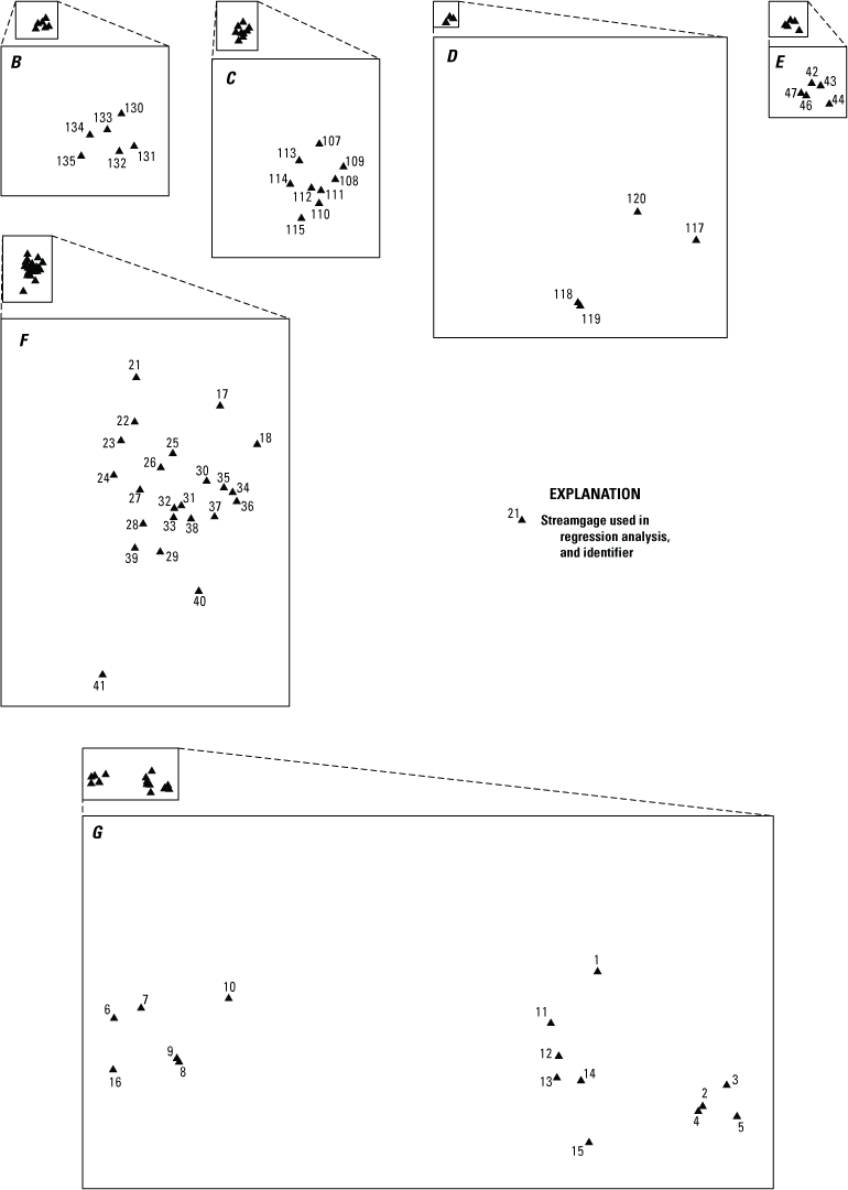
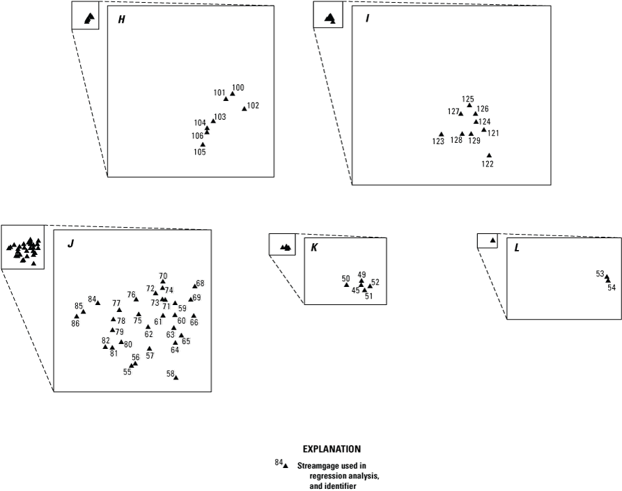
U.S. Geological Survey streamgages used to estimate the magnitude and frequency of floods at ungaged locations in urban areas in Tennessee and parts of Alabama, Georgia, Mississippi, North Carolina, and South Carolina and Level 3 ecoregions in the study area.
In 2024, the USGS, in cooperation with the Tennessee Department of Transportation, updated the methods for predicting the magnitude and frequency of floods at ungaged locations on streams in urban areas in Tennessee. To increase the number of streamgages available for flood-frequency analysis, the study area was expanded to include those in urban areas in the neighboring States of Mississippi, Alabama, Georgia, South Carolina, and North Carolina. Regression equations were developed to predict streamflows corresponding to the 50-, 20-, 10-, 4-, 2-, 1-, 0.5-, and 0.2-percent annual exceedance probabilities (AEPs) that correspond to the 2-, 5-, 10-, 25-, 50-, 100-, 200-, and 500-year recurrence intervals, respectively. For urban streams in Tennessee, the regression equations were incorporated into the StreamStats web application (U.S. Geological Survey, 2019; https://streamstats.usgs.gov/ss/), which automates the process of predicting streamflows at ungaged locations. For 136 streamgages used in the study, results of at-site flood-frequency analysis, results of generalized least-squares (GLS) regression, and basin polygons and geospatial data associated with statistically significant basin characteristics are available in the associated USGS data releases (Ladd and Wagner, 2024; Wagner and Ladd, 2024a, b).
The purpose of the report is to present methods used to develop GLS regression equations that can be used to predict streamflows corresponding to the 50, 20-, 10-, 4-, 2-, 1-, 0.5-, and 0.2-percent AEPs at ungaged locations in urban areas of Tennessee, results of the GLS regression analysis, and applications of the GLS regression equations.
Description of Study Area
The study area includes the State of Tennessee and parts of the surrounding States of Alabama, Georgia, Mississippi, North Carolina, and South Carolina that are within the Mississippi Valley Loess Plains, Southeastern Plains, Interior Plateaus, Southwestern Appalachians, Ridge and Valley, and Piedmont Level 3 (L3) ecoregions (U.S. Environmental Protection Agency, 2013; fig. 1). No urban streamgages were in the Mississippi Alluvial Plain, Central Appalachians, or Blue Ridge L3 ecoregions. Streamgages located in urban areas in the Middle Atlantic and Southern Coastal Plain L3 ecoregions in Georgia, North Carolina, and South Carolina were not considered because of the small number of available streamgages and because of tidal effects. The 136 streamgages selected for use in the study had a minimum of 10 percent developed imperviousness in their drainage basins, as indicated by data from the 2011 National Land Cover Database (NLCD) (Homer and others, 2015; Dewitz and U.S. Geological Survey, 2021) and a minimum of 10 years of annual peak streamflow data available through the 2022 water year. A water year is defined as the period October 1–September 30, named for the year in which it ends. Drainage areas for the streamgages ranged from 0.164 to 93.4 square miles (mi2) (refer to file “GLSresults.csv” in Wagner and Ladd, 2024b). Percent developed imperviousness (from 2011 NLCD; Homer and others, 2015; Dewitz and U.S. Geological Survey, 2021) in the drainage basins of the streamgages ranged from 10 to 79 percent. The percentage of developed land use (sum of classes 21–24 from 2011 NLCD) in the drainage basins of the streamgages ranged from 26 to 100 percent. The number of streamgages in each State was as follows: 21 in Alabama, 32 in Georgia, 9 in Mississippi, 38 in North Carolina, 16 in South Carolina, and 20 in Tennessee.
Previous Investigations
Several previous investigations have determined the magnitude and frequency of floods on urban streams in Tennessee and surrounding States (Wibben, 1976; Neely, 1984; Robbins, 1984; Feaster and others, 2014). Wibben (1976) used streamflow data from 14 basins in Davidson County, Tennessee, that ranged in size from 1.58 to 64 mi2 and had impervious cover ranging from 3 to 37 percent of the basin area. Average record length was 11 years; records were extended using a digital model of the hydrologic system. Estimates of streamflow corresponding to the 2-, 5-, 10-, 25-, 50-, and 100-year recurrence intervals (50-, 20-, 10-, 4-, 2-, and 1-percent AEPs, respectively) were compared to those from regional equations for estimating peak-flows at ungaged locations in rural basins. In fully developed residential areas, flood peaks and lag times were not significantly different from those for undeveloped areas. However, the data were not sufficient to determine whether an increase in flood peaks would occur from extremely intensive development in extremely small basins.
Neely (1984) presented techniques for estimating the magnitude and frequency of peak streamflow and storm runoff of streams in urban areas of Memphis, Tennessee. Data from 27 streamgages with 8 or more years of annual peak streamflow record and drainage areas ranging from 0.04 to 19.4 mi2 were used in the study; flood-frequency at each streamgage was computed using a rainfall-runoff model. Equations derived from regression analyses provided estimates of annual peak streamflow corresponding to recurrence intervals of 2–100 years (50- to 1-percent AEPs) for streams with drainage areas less than 20 mi2. Statistically significant basin characteristics in the regression equations were drainage area and channel condition (paved or unpaved).
Robbins (1984) used 22 rainfall-runoff streamgages located in urban areas across Tennessee with drainage areas ranging from 0.21 to 24.3 mi2 and impervious areas (based on aerial photographs) ranging from 4.7 to 74 percent of the streamgage basin areas. Flood-frequency estimates for each streamgage were computed using a rainfall-runoff model. Equations derived from regression analyses provided estimates of annual peak streamflow corresponding to recurrence intervals of 2–100 years (50- to 1-percent AEPs).
Feaster and others (2014) used annual peak-flow data from 116 urban streamgages and 32 rural streamgages with drainage areas less than 1 mi2, along with annual peak-flow data from an additional 340 rural streamgages in Georgia, South Carolina, and North Carolina. The Expected Moments Algorithm (EMA), which fits a log-Pearson type III (LP3) distribution to the logarithms of the annual peak-flow data from the streamgages, was used to compute at-site flood-frequency for the streamgages. GLS regression was used to generate regression equations for three hydrologic regions (Piedmont and Ridge and Valley, Sand Hills, and Coastal Plain). Annual peak-flow data from urban streamgages in Florida and New Jersey were used in the regression analysis for the Coastal Plain region, which allowed the applicability of the regression equations in that region to be expanded from 3.5 to 53.5 mi2. Average standard error of prediction for the regression equations ranged from 25 percent for the 10-percent AEP for the Piedmont Ridge and Valley region to 73.3 percent for the 0.2-percent AEP for the Sand Hills region. Statistically significant basin characteristics in the regression models were drainage area, percent developed imperviousness from the 2006 NLCD (Fry and others, 2011; U.S. Geological Survey, 2011), percent developed land use in the streamgage basins from the 2006 NLCD, and the 24-hour, 50-year precipitation from the National Oceanic Atmospheric Administration’s Atlas 14 precipitation frequency estimates (National Oceanic and Atmospheric Administration, 2013).
At-Site Flood-Frequency Analysis
USGS streamgages located in urban areas in Tennessee, Alabama, Georgia, Mississippi, North Carolina, and South Carolina were considered for use in the study if they had 10 or more years of annual peak-flow data and 10 percent or more of their drainage basins covered by developed imperviousness (2011 NLCD; Homer and others, 2015; Dewitz and U.S. Geological Survey, 2021), and were not redundant (Wagner and Ladd, 2024a). The streamgages used in this study were either continuous-record or crest-stage gages (CSGs). Continuous-record gages are equipped with instrumentation to record the height of the water surface above the gage datum, or gage height, at fixed time intervals. Gage height data are transmitted by satellite to USGS offices, and the associated streamflows are determined using what is referred to as a “stage-discharge rating,” which is a model of the relation of gage height to streamflow; in this nomenclature, stage is equivalent to gage height, and discharge is equivalent to streamflow. CSGs can only record the gage height above a minimum recordable level, which has an associated minimum recordable streamflow (Sauer and Turnipseed, 2010; supplemental information provided at https://www.usgs.gov/special-topics/water-science-school/science/crest-gage-a-quick-way-measure-river-stage). During a site visit, the peak gage height that occurred since the previous visit is determined, and the associated streamflow is determined later from the stage-discharge rating. Continuous-record gages and CSGs are referred to collectively as “streamgages.”
To help determine what parts of the periods of record for the streamgages represented relatively stable urban conditions for at-site flood frequency analysis, the historical change in total impervious area for each streamgage during the 1940–2020 water years was computed using housing density data from the 2000 U.S. Census (Theobald, 2005) and percent developed imperviousness from the 2001, 2006, 2011, 2016, and 2019 NLCDs according to methods described by Over and others (2016), Oudin and others (2018), and Glas and others (2023). The housing density data were reclassified into impervious percentages for each pixel, resampled, clipped, and averaged for each streamgage basin. Decadal values were then linearly interpolated to annual timesteps for each basin. Plots of the decadal values for each streamgage were used in conjunction with qualification code C (if present) on annual peak flows in the peak-flow files of the streamgages to determine the appropriate periods of record to use in the at-site flood-frequency analyses (Wagner and Ladd, 2024a). Qualification code C indicates annual peak flow is affected by urbanization, mining, agricultural changes, channelization, or other anthropogenic effects (U.S. Geological Survey, 2025).
For each of 139 streamgages in the study area for which at-site frequency was computed (Wagner and Ladd, 2024a), the EMA was used in version 7.4.1 of USGS PeakFQ software (Flynn and others, 2006; Veilleux and others, 2014; supplemental information provided at https://water.usgs.gov/water-resources/legacy-software/) to fit an LP3 probability distribution to the logarithms of the annual peak streamflows and estimate streamflows corresponding to the 50-, 20-, 10-, 4-, 2-, 1-, 0.5-, and 0.2-percent AEPs. Using perception thresholds and flow intervals, the EMA allows for the incorporation of historical peaks and historical periods, censored observations (annual peak streamflows known to be greater or less than a certain value, particularly from CSGs) and uncertain annual peaks (England and others, 2018). The EMA incorporates the Multiple Grubbs-Beck Test (MGBT) to statistically screen for low outliers, known as potentially influential low floods (PILFs); however, the PILF threshold can also be manually selected. Version 7.4.1 of PeakFQ software also incorporates the Mann-Kendall test for monotonic trends to test for nonstationarity in the annual peak streamflow data (Flynn and others, 2006; Veilleux and others, 2014; supplemental information provided at https://www.usgs.gov/tools/peakfq and https://water.usgs.gov/water-resources/legacy-software/).
Perception Thresholds
For continuous-record streamgages, perception thresholds for periods of gaged record were set to (0, infinity), meaning the entire range of streamflow could be observed (refer to “Data Representation” in England and others, 2018, p. 67–70); also refer to files “TNurbanFFreq.pkf” and “TNurbanFFreq.psf” in Wagner and Ladd, 2024a). For CSGs, perception thresholds for periods of gaged record were set to (minimum recordable streamflow, infinity). If the minimum recordable streamflow was unknown or unavailable, perception thresholds were set to (0, infinity). For all streamgages, perception thresholds for years or periods of missing record where historical information was unavailable were set to (infinity, infinity). If historical information was available, perception thresholds for missing years or historical periods were set to (value of historical peak, infinity), indicating that the flow is assumed to have been less than the magnitude of the historical peak. For annual peak streamflows assigned qualification code 4 (flow is less than indicated value; refer to table B.4 in appendix B.4 of Flynn and others, 2006), perception thresholds were set to (indicated value, infinity). In almost all cases, this occurred at CSGs during years when the gage height did not exceed the minimum recordable level. For annual peak streamflows assigned qualification code 8 (flow is greater than indicated value), in most cases perception thresholds were set to (0, infinity) because the entire range of streamflow could be observed that year. In cases where it was not known whether the entire range of streamflow was able to be observed, perception thresholds were set to (0, indicated value). For annual peak streamflows assigned qualification codes 4 and 8, associated flow intervals were also assigned to the affected annual peak streamflows.
Flow Intervals
Flow intervals were assigned to uncertain data points, including annual peak streamflows assigned qualification codes 4 or 8, in cases where the annual peak gage height was recorded but the annual peak streamflow was not determined or recorded, and for years when the annual peak streamflow was affected by backwater. In the latter case, the annual peak gage height is assigned a qualification code 1 (files “TNurbanFFreq.pkf” and “TNurbanFFreq.psf” in Wagner and Ladd, 2024a). For annual peak streamflows assigned qualification code 4, the associated flow interval was (0, indicated value). For annual peak streamflows assigned qualification code 8, the associated flow interval was (indicated value, infinity). For years when the annual peak gage height was recorded but the annual peak streamflow was not determined or recorded, the associated flow interval was determined from other annual peak streamflows in the dataset and assigned as either (0, selected value), (selected value, infinity), or (selected value, selected value), depending on whether the annual peak gage height could be determined to be less than another known annual peak, greater than another known annual peak, or between two known annual peaks, respectively. For years when the annual peak streamflow was affected by backwater, the associated flow interval was determined from other known annual peaks with similar annual peak gage heights and assigned as (0, selected value) based on the assumption that when affected by backwater, the flow is less than that normally associated with a given annual peak gage height.
Low Outliers
For 135 of 139 streamgages for which at-site flood frequency was computed, MGBT was used to screen for PILFs in the annual peak streamflow records (column “PILFmethod” in file “TNURBANFFREQ.csv” in Wagner and Ladd, 2024a). To help better fit the upper tail (above the median) of the frequency distribution, MGBT statistically determines whether annual peak streamflows are low outliers by using (1) an outward sweep from the median toward the smallest annual peak to determine if some break in the lower half of the data would suggest the sample is best treated as if it had a number of low outliers and (2) an inward sweep from the smallest annual peak toward the median (refer to appendix 6, “Potentially Influential Low Floods,” in England and others, 2018). MGBT detected and screened 1–14 low outliers at 33 streamgages (columns “PILFs” and “PILFthresh” in file “TNURBANFFREQ.csv” in Wagner and Ladd, 2024a). For 4 of the 139 streamgages (02173495, 02217274, 02218565, and 0357587728, column “Site_No” in file “TNURBANFFREQ.csv” in Wagner and Ladd, 2024a), analysts determined that MGBT did not sufficiently detect or screen low outliers to better fit the upper tail of the frequency distribution, and the low outlier threshold had to be manually specified (refer to values “FIXED” in column “PILFmethod” in file “TNURBANFFREQ.csv” in Wagner and Ladd, 2024a).
Trends in Annual Peak Streamflow
Annual peak-flow data were examined for trends using the Mann-Kendall test, which is implemented in version 7.4.1 of the PeakFQ software (Flynn and others, 2006; Veilleux and others, 2014; supplemental information provided at https://www.usgs.gov/tools/peakfq and https://water.usgs.gov/water-resources/legacy-software/). Seventeen of the 139 streamgages for which at-site flood frequency was computed exhibited statistically significant trends for which the p-value associated with the Mann-Kendall test was less than or equal to 0.05 (column “p-value” in file “TNURBANFFREQ.csv” in Wagner and Ladd, 2024a). All but 2 of the 17 streamgages (USGS site numbers 0208735012 and 02135518; U.S. Geological Survey, 2024) had positive trends. The annual peak-flow records of the streamgages with statistically significant trends were examined, but those trends could not be attributed to anthropogenic activity. The absence of trends in the annual peak streamflow records of most streamgages in the study area indicates the observed trends are also not related to a regional trend in climate. The trends appear to be the result of the available or selected periods of record used in the analysis. Some streamgages with positive trends have periods of record that either began in the late 1980s, which was a generally dry period across the region, or had large annual peak streamflows late in their periods of record. Other streamgages with positive trends were affected by Hurricanes Matthew (October 2016) and Florence (September 2017), which resulted in large annual peak streamflows late in their periods of record. Because only 17 streamgages exhibited statistically significant trends, and because those trends could not be attributed to anthropogenic activity or increasing urbanization in the respective drainage basins, no streamgages were removed from the study for trends.
Basin Characteristics
Polygons representing the drainage basins of the streamgages used in the study were generated in the USGS StreamStats application (U.S. Geological Survey, 2019) through the StreamStats batch processor (https://streamstats.usgs.gov/ss/?BP=submitBatch; file “TNurbanFFreq_Basins.shp” in Ladd and Wagner, 2024). These polygons were derived from analysis of flow-direction grids from the National Hydrography Dataset Plus (U.S. Environmental Protection Agency and U.S. Geological Survey, 2012) or obtained from published drainage basin polygons in the GAGES-II streamgage dataset (Falcone, 2011). The basin polygons were used to generate 20 basin characteristics that were then tested as covariates in the regression model (file “BasinCharsTested.csv” in Ladd and Wagner, 2024). Basin characteristics were as follows:
-
• physical (drainage area, mean and maximum basin elevations, relief, average basin slope, and basin compactness);
-
• land-use/land-cover (percent developed imperviousness, percent developed land use, and percent storage);
-
• climatic (1-, 2-, 6-, 12-, and 24-hour, 100-year precipitation frequencies); and
-
• physiographic (percentage of streamgages basins in six Level 3 ecoregions in the study area).
Four basin characteristics were statistically significant (p-value ≤ 0.05) in explaining the variability in streamflows corresponding to the selected AEPs for streamgages in the study area: drainage area (DRNAREA), percent developed land use from the 2011 NLCD (LC11DEV), and the percentages of the streamgage basins in the Piedmont (L3_PIEDMNT) and Ridge and Valley (L3_RDGVLY) Level 3 ecoregions (file “GLSresults.csv” in Wagner and Ladd, 2024b; also refer to U.S. Environmental Protection Agency, 2013; Homer and others, 2015; Dewitz and U.S. Geological Survey, 2021). Polygons representing the drainage basins of the streamgages used in the study and datasets used to generate the other three statistically significant basin characteristics are available in a USGS data release (Ladd and Wagner, 2024).
Regression Equations
Exploratory Regression
A total of 139 streamgages for which at-site frequency analysis was conducted (Wagner and Ladd, 2024a) were considered for use in developing regression equations for estimating streamflows corresponding to the 50-, 20-, 10-, 4-, 2-, 1-, 0.5-, and 0.2-percent AEPs at ungaged locations on streams in the study area. All-subsets, ordinary least-squares (OLS) regression was used to relate the basin characteristics to the selected AEPs and test the statistical significance and predictive power of all possible combinations of basin characteristics. All subsets regression was conducted using the allReg() function in the smwrStats package (Lorenz and DeCicco, 2017) in version 4.1.1 of R software (R Core Team, 2021). The best three 1–4 variable models for each AEP, based on the adjusted coefficient of determination (adjusted R-squared), were identified as candidate models. These candidate models were then further tested using the multReg() function in the smwrStats package to output the full suite of performance metrics for the OLS regression models. Visual examination of plots relating drainage area to estimates of streamflows corresponding to the selected AEPs indicated that two streamgages with drainage areas greater than 100 mi2 (USGS site numbers 02087324 and 02207120) and one other streamgage (USGS site number 02169570) were obvious outliers (U.S. Geological Survey, 2024). A decision was made to limit the drainage area of streamgages used in the study to less than 100 mi2 and remove streamgages 02087324 and 02207120 from the regression analysis. Streamgage 02169570 was investigated and found to be downstream from a reservoir, although the annual peak streamflow data were not coded as regulated. This streamgage was also removed from the regression analysis, leaving 136 streamgages for use in the final regression model.
Exploratory regression indicated that the base-10 logarithm of drainage area, the percentages of the streamgage basins in developed land use (the sum of developed land use classes 21–24 from 2011 NLCD), and the percentages of the streamgage basins in the Piedmont and Ridge and Valley L3 ecoregions were the best combination of basin characteristics for predicting the selected AEPs by means of the adjusted R-squared values. Multicollinearity of the final selection of basin characteristics was evaluated by means of the variance inflation factor, which was desired to be less than 5; the variance inflation factors for all four characteristics were less than 2.
Generalized Least-Squares Regression
After the covariates were determined using exploratory OLS regression, GLS regression was used to generate the final regression models. Because there is often a high degree of similarity among streamflow statistics and basin characteristics (response variables) from neighboring streamgages, streamflow statistics and response variables cannot be assumed to be independent (Farmer and others, 2019). In addition to the length of the annual peak-flow records and variances of the streamflow estimates, GLS regression accounts for both correlated streamflows and time-sampling errors by incorporating the concurrent record lengths and the estimated cross-correlation of the time series of streamflows for pairs of streamgages used in the regression.
GLS regression was conducted using version 3.0 of USGS weighted regression software (Eng and others, 2009; Farmer, 2021) in R software (R Core Team, 2021). To account for the cross-correlation of streamflows between pairs of streamgages, the weighted regression software incorporates a correlation smoothing function that is developed by the user. Streamgage pairs with 35 or more years of concurrent annual peak-flow record and 200 kilometers (km) or more distance between the streamgages exhibited a relatively even spread of correlation around zero (fig. 2). The alpha and theta values that define the correlation smoothing function used in the study were adjusted to make the correlation smoothing function range from a value of 1 at 0 km to a value of 0 at distances greater than 200 km.

Cross-correlation smoothing function used in generalized least-squares regression. NSE, Nash-Sutcliffe Efficiency. The closer alpha is to zero, the closer the asymptote of the function lies to zero, and the closer theta is to one, the more slowly the function decreases with distance.
In GLS regression, all basin characteristics were statistically significant (p-value < 0.05) in the regression models for all AEPs except for the percentage of streamgage basins in developed land use, which was not statistically significant (p-value = 0.07) in the regression model for the 0.2-percent AEP (500-year flood). Regression coefficients ranged from 0.6208 to 0.6518 for drainage area, from 0.0024 to 0.0062 for percentage of developed land use in the streamgage basins, from −0.0027 to −0.0020 for the percentage of the streamgage basins in the Piedmont L3 ecoregion, and from −0.0025 to −0.0021 for the percentage of the streamgage basins in the Ridge and Valley L3 ecoregion (Wagner and Ladd, 2024b). The positive coefficients for drainage area and the percentage of streamgage basins in developed land use are consistent with the assumption that streamflow should increase with drainage area and developed land use because of greater coverage by impervious surfaces and rapid delivery of runoff to streams via storm drain networks. The coefficient for the percentage of streamgage basins in developed land use was greatest for the 50-percent AEP and decreased with AEP. The coefficients for the percentages of the streamgage basins in the Piedmont and Ridge and Valley L3 ecoregions are negative because the annual peak streamflows were generally lesser in magnitude for the streamgages in these ecoregions used in this study when compared to streamgages with equivalent drainage areas in the other L3 ecoregions. The negative coefficients are small and have no effect on the predictions of streamflow for streamgages outside these ecoregions.
The relation between observed (at-site) and predicted (regression equation) streamflows corresponding to the selected AEPs was generally good but showed greater scatter for the 2-, 1-, 0.5-, and 0.2-percent AEPs (100-, 200-, and 500-year floods, respectively, fig. 3) than for larger AEPs. The greater scatter in this relation for the smaller AEPs is not surprising, given the large uncertainty associated with estimating small AEPs for streamgages with short record lengths and relatively high positive skews of the LP3 statistical distribution, which were numerous in the study (fig. 4). Record lengths used in the study ranged from 10 to 76 years, with a median of 26 years and third quartile of 37 years, whereas the at-site skews ranged from −1.227 to 3.592, with a median of 0.153 and third quartile of 0.6025 (columns “HistPeriod” and “AtSiteSkew” in file “TNURBANFFREQ.csv” in Wagner and Ladd, 2024a).

Relation between base-10 logarithms of observed (at-site) and predicted (regression equation) streamflows corresponding to selected annual exceedance probabilities (AEPs). %, percent.

Example of output from the U.S. Geological Survey PeakFQ program showing a fitted frequency curve for a streamgage used in the study with a short record length and high positive skew. EMA, Expected Moments Algorithm; PILF, potentially influential low flood; sq, square.
Depending on AEP, 12–13 streamgages had high leverage (greater than 0.0735; eqs. 40 and 42 in Eng and others, 2009) and 10–16 streamgages had high influence (greater than 0.0294; eqs. 43 and 44 in Eng and others, 2009) on the regression models (columns beginning with “Lev” and “Inf” for each corresponding AEP in file “GLSresults.csv” in Wagner and Ladd, 2024b). Streamgages with high leverage and influence on the regression models were investigated, but no reasons were found to remove them from the regression models.
Accuracy and Limitations of Regional Regression Equations
The regression equations are applicable at locations on urban streams that have basin characteristics within the range of those used to develop the equations. The methods described in this report do not apply to locations on streams that are substantially affected by regulation from upstream impoundments or other man-made structures or that are subject to tidal effects. The accuracy of the regression equations is not known for locations outside the study area or that have basin characteristics outside the following ranges used to develop the equations: 10 percent or greater developed imperviousness in the basin (LC11IMP; refer to file “GLSresults.csv” in Wagner and Ladd, 2024b); 0.164–93.4 mi2 of drainage area (DRNAREA); 26–100 percent developed land use in the basin (LC11DEV); 0–100 percent of the basin in the Piedmont L3 ecoregion (L3_PIEDMNT); and 0–100 percent of the basin in the Ridge and Valley L3 ecoregion (L3_RDGVLY). The regression equations are not valid in the Middle Atlantic or Southern Coastal Plain Level 3 ecoregions in North Carolina, South Carolina, Georgia, Mississippi, and Alabama; no urban streamgages in these ecoregions were used to develop the equations because of the small number of available urban streamgages and potential tidal effects.
The accuracy of the GLS regression model is expressed as the residual mean squared error (MSE; eq. 31 in Eng and others, 2009, p. 5), which is the sum of the model and time-sampling errors, and the model error variance (MEV), which is the same as the MSE only if the time-sampling error variance is zero. MSE ranged from 0.025 for the 50- and 20-percent AEPs (2- and 5-year floods) to 0.104 for the 0.2-percent AEP (500-year flood; column “MSE” in file “RegressionEquations.csv” in Wagner and Ladd, 2024b). The time-sampling error variance was not zero in this study, and the MEV ranged from 0.022 for the 20- and 10-percent AEPs (5- and 10-year floods) to 0.047 for the 0.2-percent AEP (500-year flood; column “MEV” in file “RegressionEquations.csv” in Wagner and Ladd, 2024b).
The overall accuracy of predictions from the regression equations is expressed in terms of the coefficient of determination, or R-squared value, the average variance of prediction (AVP), and standard error of prediction (Sp). The R-squared value represents the proportion of the variation in the dependent variable (streamflow estimates for the selected AEPs) that is explained by the basin characteristics in the regression model. For GLS regression, the pseudo R-squared value is reported (column “R2pseudo” in file “RegressionEquations.csv” in Wagner and Ladd, 2024b), which is based on the variability in streamflow explained by the regression after removing the effect of the time-sampling error (eq. 39 in Eng and others, 2009, p. 6). Pseudo R-squared values ranged from 0.86, or 86 percent, for the 50- and 20-percent AEPs (2- and 5-year floods) to 0.71, or 71 percent, for the 0.2-percent AEP (500-year flood). The AVP (in base-10 logarithmic units; eq. 32 in Eng and others, 2009, p. 5) ranged from 0.023 for the 20- and 10-percent AEPs to 0.05 for the 0.2-percent AEP (column “AVP” in file “RegressionEquations.csv” in Wagner and Ladd, 2024b). Because the base-10 logarithms of the streamflow estimates were used to develop the regression equations, the AVP can be reported as a percentage of the predicted value, known as the standard error of prediction (eq. 33 in Eng and others, 2009, p. 5). The standard error of prediction ranged from 35.8 percent for the 20-percent AEP (5-year flood) to 55.4 percent for the 0.2-percent AEP (500-year flood; column “AVP” in file “RegressionEquations.csv” in Wagner and Ladd, 2024b). The standard errors of prediction were similar to those for the rural regression equations for Tennessee, which ranged from 30.44 to 51.4 percent, depending on flood region (table 7 in Ladd and Ensminger, 2025).
Six streamgages in Tennessee, 03491544, 03535400, 03536450, 03536550, 03538235, and 07032200, that were used to develop the urban equations were also used to develop the rural equations. For the selected AEPs, the predictions using the urban equations were greater than those using the rural equations, with two exceptions. First, for streamgage 07032200, the predictions from the urban equations were less than those predicted using the rural equations. Second, for streamgage 03535400, the predictions for the 50-, 20-, 10-, and 1-percent AEPs were greater using the urban equations and the predictions for the 4-, 2-, 0.5-, and 0.2-percent AEPs were greater using the rural equations. For locations in Tennessee having 10 percent or greater developed imperviousness in their drainage basins, the urban regression equations in this report should be used to predict streamflows; for locations with less than 10 percent developed imperviousness, the rural equations should be used (refer to table 4 in Ladd and Ensminger, 2025).
Applications of Regression Equations
When applying the regression equations, users are advised not to interpret the empirical results as exact. Regression equations are statistical models that must be interpreted and applied within the limits of the data and with the understanding that the results are best-fit estimates with an associated variance. Methods for estimating streamflows corresponding to selected AEPs for urban streams in the study area differ between gaged locations, ungaged locations on gaged streams, and locations on ungaged streams.
Gaged Locations
For streamgages with short record lengths, the uncertainty of at-site estimates of streamflows corresponding to various AEPs can be reduced by weighting those estimates with predictions from the regression equations (refer to appendix 9, “Weighting of Independent Estimates,” in England and others, 2018). If the two are assumed to be independent and unbiased and are weighted in inverse proportion to their associated variances, the variance of the weighted estimate will be less than the variance of either of the independent estimates. A weighted estimate of streamflow corresponding to a selected AEP can be computed using equation 9-2 in England and others (2018):
whereXweighted,i
is the base-10 logarithm of the weighted estimate of streamflow corresponding to the selected AEP;
Xsite,i
is the base-10 logarithm of the at-site estimate of streamflow at the streamgage corresponding to the selected AEP;
Vreg,i
is the variance of prediction for the regression equation corresponding to the selected AEP, in base-10 logarithmic units;
Xreg,i
is the base-10 logarithm of the regression estimate of streamflow at the streamgage corresponding to the selected AEP; and
Vsite,i
is the variance of prediction of the at-site estimate of streamflow at the streamgage corresponding to the selected AEP, in base-10 logarithmic units.
A 95-percent confidence interval for the weighted estimate (in cubic feet per second; refer to eq. 8 in Wagner and others, 2016) can be calculated as
where95%CIupper,i
is the upper 95-percent confidence interval for the weighted estimate of the selected AEP for streamgage i;
Yweighted,i
is the weighted estimate of the selected AEP for streamgage i, in base-10 logarithmic units;
Vweighted,i
is the variance of the weighted estimate of the selected AEP for streamgage i, in base-10 logarithmic units; and
95%CIlower,i
is the lower 95-percent confidence interval for the weighted estimate of the selected AEP for streamgage i.
The variance of the weighted estimate for streamgage i (in base-10 logarithmic units) can be calculated as
Ungaged Locations on Gaged Streams
If the drainage area at an ungaged location on a stream is within 50 percent of the drainage area at a streamgage (drainage area ratio is more than 0.5 or less than 1.5) on the same stream, streamflows corresponding to selected AEPs at the ungaged location can be computed from the streamgage data using a drainage area ratio method (refer to eq. 13 in Wagner and others, 2016). The drainage area ratio can be calculated by using the following equation:
whereQu
is the estimate of streamflow corresponding to the selected AEP for the ungaged location, u, in cubic feet per second;
Au
is the drainage area of the ungaged location, in square miles;
Ag
is the drainage area of the upstream or downstream streamgage, in square miles;
b
is the exponent of drainage area from the regression equation corresponding to the selected AEP (column “a” in file “RegressionEquations.csv” in Wagner and Ladd, 2024b); and
Qg
is the at-site estimate of streamflow (weighted with regression equations using eq. 1, if appropriate) corresponding to the selected AEP for the upstream or downstream streamgage, in cubic feet per second.
Qu(w)
is the weighted estimate of streamflow corresponding to the selected AEP at the ungaged location, in cubic feet per second;
│ΔA│
is the absolute difference in drainage area between the ungaged location and the streamgage, in square miles; and
Qu(r)
is the prediction of streamflow from the regression equation for the ungaged location for the selected AEP, in cubic feet per second.
If the drainage area at the ungaged location differs by more than 50 percent from the drainage area of the streamgage, the predicted streamflow from the regression equations for the ungaged location should be used. If an ungaged location is between two streamgages on the same stream, the streamgage with the longest period of record or that yields the smallest drainage area ratio should be used.
Locations on Ungaged Streams
For locations on ungaged streams, streamflows corresponding to selected AEPs should be determined using the regression equations. The USGS StreamStats application (U.S. Geological Survey, 2019; https://streamstats.usgs.gov/ss/) provides a platform for delineating drainage basins, computing basin characteristics, and estimating streamflows corresponding to selected AEPs at ungaged locations using the regression equations.
Summary
In 2024, the U.S. Geological Survey (USGS), in cooperation with the Tennessee Department of Transportation, updated the methods for predicting the magnitude and frequency of floods at ungaged locations on streams in urban areas in Tennessee. To increase the number of streamgages available for flood-frequency analysis, the study area was expanded to include those in urban areas in the neighboring States of Mississippi, Alabama, Georgia, South Carolina, and North Carolina. Regression equations were developed to predict streamflows corresponding to the 50-, 20-, 10-, 4-, 2-, 1-, 0.5-, and 0.2-percent annual exceedance probabilities (AEPs). For urban streams in Tennessee, the regression equations will be incorporated into the StreamStats web application. For streamgages used in the study, results of at-site flood-frequency analysis, results of generalized least-squares (GLS) regression, and basin polygons and geospatial data associated with statistically significant basin characteristics are available in associated USGS data releases.
USGS streamgages located in urban areas in Tennessee, Alabama, Georgia, Mississippi, North Carolina, and South Carolina that had 10 or more years of annual peak-flow data, 10 percent or more of their drainage basins covered by developed imperviousness, and that were not redundant were considered for use in the study. The Expected Moments Algorithm was used in version 7.4.1 of USGS PeakFQ software to fit a log-Pearson Type III probability distribution to the logarithms of the annual peak streamflows and estimate streamflows corresponding to the 50-, 20-, 10-, 4-, 2-, 1-, 0.5-, and 0.2-percent AEPs.
Polygons representing the drainage basins of the streamgages used in the study were generated in the USGS StreamStats application, derived from National Hydrography Dataset Plus flow-direction analysis, or obtained from existing published streamgage data. Using the basin polygons, 20 basin characteristics were generated and tested as covariates in the regression model.
A total of 136 streamgages for which at-site frequency analysis was conducted were considered for use in developing regression equations. All-subsets, ordinary least-squares regression was used to relate the basin characteristics to the selected AEPs and test the statistical significance and predictive power of all possible combinations of basin characteristics. Exploratory regression indicated that four basin characteristics—the base-10 logarithm of drainage area, percent developed land use from the 2011 National Land Cover Database, and the percentages of the streamgage basins in the Piedmont and Ridge and Valley Level 3 ecoregions—were the best combination of basin characteristics and statistically significant (p-value ≤ 0.05) in explaining the variability in streamflows corresponding to the selected AEPs for streamgages in the study area. Drainage areas ranged from 0.164 to 93.4 square miles, percentages of the streamgage basins in developed land use ranged from 26 to 100 percent, and percentages of the streamgage basins in Piedmont and Ridge and Valley Level 3 ecoregions ranged from 0 to 100 percent.
GLS regression was used to generate the final regression models. In addition to the length of the annual peak-flow records and variances of the streamflow estimates, GLS regression accounts for both correlated streamflows and time-sampling errors by incorporating the concurrent record lengths and the estimated cross-correlation of the time series of streamflows for pairs of streamgages used in the regression. GLS regression was conducted using version 3.0 of USGS weighted regression software, which incorporates a correlation smoothing function to account for the cross-correlation of streamflows between pairs of streamgages. Using streamgage pairs with 35 or more years of concurrent annual peak-flow record, the correlation smoothing function was adjusted to range from a value of 1 at 0 kilometers to a value of 0 at distances greater than 200 kilometers. The base-10 logarithm of drainage area, the percentages of the streamgage basins in developed land use, and the percentages of the streamgage basins in the Piedmont and Ridge and Valley L3 ecoregions were statistically significant (p-value < 0.05) in the regression models for all AEPs except for the percentage of the streamgage basins in developed land use, which was not statistically significant (p-value = 0.07) in the regression model for the 0.2-percent AEP (500-year flood). Regression coefficients ranged from 0.6208 to 0.6518 for drainage area, from 0.0024 to 0.0062 for percentage of developed land use in the streamgage basins, from −0.0027 to −0.0020 for the percentage of the streamgage basins in the Piedmont L3 ecoregion, and from −0.0025 to −0.0021 for the percentage of the streamgage basins in the Ridge and Valley L3 ecoregion. The relation between observed (at-site) and predicted (regression equation) streamflows corresponding to the selected AEPs was generally good but showed greater scatter for the 2-, 1-, 0.5-, and 0.2-percent AEPs (100-, 200-, and 500-year floods, respectively). The greater scatter in this relation for the smaller AEPs is not surprising, given the large uncertainty associated with estimating small AEPs for streamgages with short record lengths and relatively high positive skews of the log-Pearson Type III statistical distribution, which were numerous in the study. Streamgages whose data had high leverage and influence on the regression models were investigated, but no reasons were found to remove them from the regression models.
The overall accuracy of predictions from the regression equations is expressed in terms of the pseudo coefficient of determination, or pseudo R-squared, the average variance of prediction and standard error of prediction. Pseudo R-squared values ranged from 0.86, or 86 percent, for the 50- and 20-percent AEPs (2- and 5-year floods) to 0.71, or 71 percent, for the 0.2-percent AEP (500-year flood). The average variance of prediction (in log base-10 units) ranged from 0.023 for the 20- and 10-percent AEPs (5- and 10-year floods) to 0.05 for the 0.2-percent AEP (500-year flood). The average variance of prediction can be reported as a percentage of the predicted value, known as the standard error of prediction, which ranged from 35.8 percent for the 20-percent AEP (5-year flood) to 55.4 percent for the 0.2-percent AEP (500-year flood). The standard errors of prediction were similar to those for the rural regression equations for Tennessee, which ranged from 30.44 to 51.4 percent, depending on flood region. For locations in Tennessee with 10 percent or greater developed imperviousness in their drainage basins, the regression equations in this report should be used to predict streamflows; for locations with less than 10 percent developed imperviousness, the rural equations should be used.
Methods for estimating streamflows corresponding to selected AEPs for urban streams in the study area are presented for gaged locations, ungaged locations on gaged streams, and locations on ungaged streams. For gaged locations with short record lengths, the uncertainty of at-site estimates of streamflows corresponding to selected AEPs can be reduced by weighting those estimates with predictions from the regression equations. If the streamgage of interest was used in the development of the regression equations, this weighting method is inappropriate because the estimates are not independent. Equations for computing the weighted estimates, their variances, and associated confidence intervals are provided. For ungaged locations on gaged streams, if the drainage area at an ungaged location is within 50 percent of the drainage area at a streamgage (drainage area ratio is more than 0.5 or less than 1.5), streamflows at the ungaged location can be computed from the streamgage data using a drainage area ratio method. For ungaged locations on ungaged streams, streamflows should be determined using the regression equations in the USGS StreamStats application, which provides a platform for delineating drainage basins, computing basin characteristics, and estimating streamflows corresponding to selected AEPs.
Acknowledgments
The authors would like to acknowledge the following U.S. Geological Survey hydrologists for their assistance during this project. Liz Heal provided technical assistance and reviewed metadata for the data releases associated with the project. Toby Feaster reviewed the at-site flood-frequency analyses used in the project. Robin Glas reviewed the results of the generalized least-squares regression equations. Ryan Thompson reviewed the basin characteristics used in the generalized least-squares regression equations.
References Cited
Dewitz, J., and U.S. Geological Survey, 2021, National Land Cover Database (NLCD) 2019 products (ver. 2.0, June 2021): U.S. Geological Survey data release, accessed May 6, 2022, and July 18, 2023, at https://doi.org/10.5066/P9KZCM54.
Eng, K., Chen, Y.-Y., and Kiang, J.E., 2009, User’s guide to the weighted-multiple-linear-regression program (WREG version 1.0): U.S. Geological Survey Techniques and Methods, book 4, chap. A8, 21 p. [Also available at https://pubs.usgs.gov/tm/tm4a8.]
England, J.F., Jr., Cohn, T.A., Faber, B.A., Stedinger, J.R., Thomas, W.O., Jr., Veilleux, A.G., Kiang, J.E., and Mason, R.R., Jr., 2018, Guidelines for determining flood flow frequency—Bulletin 17C (ver. 1.1, May 2019): U.S. Geological Survey Techniques and Methods, book 4, chap. B5, 148 p. [Also available at https://doi.org/10.3133/tm4B5.]
Falcone, J., 2011, GAGES-II—Geospatial attributes of gages for evaluating streamflow: U.S. Geological Survey data release, accessed December 2, 2021, at https://doi.org/10.5066/P96CPHOT.
Farmer, W.H., 2021, R package WREG—Weighted least squares regression for streamflow frequency statistics: Reston, Va., U.S. Geological Survey software release, accessed March 1, 2024, at https://doi.org/10.5066/P9ZCGLI1.
Farmer, W.H., Kiang, J.E., Feaster, T.D., and Eng, K., 2019, Regionalization of surface-water statistics using multiple linear regression (ver. 1.1, February 2021): U.S. Geological Survey Techniques and Methods, book 4, chap. A12, 40 p. [Also available at https://doi.org/10.3133/tm4A12.]
Feaster, T.D., Gotvald, A.J., and Weaver, J.C., 2014, Methods for estimating the magnitude and frequency of floods for urban and small, rural streams in Georgia, South Carolina, and North Carolina, 2011 (ver. 1.1, March 2014): U.S. Geological Survey Scientific Investigations Report 2014–5030, 104 p., accessed March 1, 2023, at https://doi.org/10.3133/sir20145030.
Flynn, K.M., Kirby, W.H., and Hummel, P.R., 2006, User’s manual for program PeakFQ, annual flood-frequency analysis using Bulletin 17B guidelines: U.S. Geological Survey Techniques and Methods, book 4, chap. B4, 42 p., accessed March 1, 2023, at https://pubs.usgs.gov/tm/2006/tm4b4/tm4b4.pdf.
Glas, R., Hecht, J., Simonson, A., Gazoorian, C., and Schubert, C., 2023, Adjusting design floods for urbanization across groundwater-dominated watersheds of Long Island, NY: Journal of Hydrology, v. 618, article 129194, 18 p., accessed March 15, 2023, at https://doi.org/10.1016/j.jhydrol.2023.129194.
Homer, C.G., Dewitz, J.A., Yang, L., Jin, S., Danielson, P., Xian, G., Coulston, J., Herold, N.D., Wickham, J.D., and Megown, K., 2015, Completion of the 2011 National Land Cover Database for the conterminous United States—Representing a decade of land cover change information: Photogrammetric Engineering and Remote Sensing, v. 81, no. 5, p. 345–354, accessed March 18, 2024, at https://doi.org/10.1016/j.isprsjprs.2018.09.006.
Ladd, D.E., and Ensminger, P.A., 2025, Estimating the magnitude and frequency of floods at ungaged locations on streams in Tennessee through the 2013 water year: U.S. Geological Survey Scientific Investigations Report 2024–5130, 19 p, accessed June 1, 2025, at https://doi.org/10.3133/sir20245130.
Ladd, D.E., and Wagner, D.M., 2024, Basin characteristics in support of generalized least-squares (GLS) regression for 136 USGS streamgages in urban areas in Tennessee and parts of Alabama, Georgia, Mississippi, North Carolina, and South Carolina (ver. 2.0, September 2025): U.S. Geological Survey data release, https://doi.org/10.5066/P1JTPBQY.
Lorenz, D., and DeCicco, L.A., 2017, R package smwrStats—R functions to support statistical methods in water resources (ver. 0.7.6): U.S. Geological Survey software release, accessed March 15, 2023, at https://code.usgs.gov/water/analysis-tools/smwrStats.
National Oceanic and Atmospheric Administration, 2013, Precipitation frequency for southeastern states, USA—NOAA Atlas 14, volume 9: Office of Hydrologic Development, Hydrometeorological Design Studies Center database accessed December 26, 2023, at https://hdsc.nws.noaa.gov/pfds/pfds_gis.html.
Neely, B.L., 1984, Flood-frequency and storm runoff of urban areas of Memphis and Shelby County, Tennessee: U.S. Geological Survey Water-Resources Investigation Report 84–4110, 51 p., accessed March 18, 2024, at https://pubsdata.usgs.gov/pubs/wri/wrir_84-4110/.
Oudin, L., Salavati, B., Furusho-Percot, C., Ribstein, P., and Saadi, M., 2018, Hydrological impacts of urbanization at the catchment scale: Journal of Hydrology, v. 559, p. 774–786, accessed March 15, 2023, at https://doi.org/10.1016/j.jhydrol.2018.02.064.
Over, T.M., Saito, R.J., and Soong, D.T., 2016, Adjusting annual maximum peak discharges at selected stations in northeastern Illinois for changes in land-use conditions: U.S. Geological Survey Scientific Investigations Report 2016–5049, 33 p., accessed March 1, 2023, at https://doi.org/10.3133/sir20165049.
R Core Team, 2021, R—A language and environment for statistical computing (ver. 4.1.1, August 10, 2021): Vienna, Austria, R Foundation for Statistical Computing software release, accessed January 10, 2022, at https://www.R-project.org/.
Ries, K.G., III, and Dillow, J.J.A., 2006, Magnitude and frequency of floods on nontidal streams in Delaware: U.S. Geological Survey Scientific Investigations Report 2006–5146, 59 p., accessed May 21, 2025, at https://pubs.usgs.gov/sir/2006/5146/.
Robbins, C.H., 1984, Synthesized flood frequency for small streams in Tennessee: U.S. Geological Survey Water Resources Investigations Report 84–4182, 24 p., accessed July 15, 2024, at https://pubs.usgs.gov/wri/wrir84-4182.
Sauer, V.B., and Turnipseed, D.P., 2010, Stage measurement at gaging stations: U.S. Geological Survey Techniques and Methods, book 3, chap. A7, 45 p., accessed November 17, 2025, at https://pubs.usgs.gov/publication/tm3A7.
Theobald, D.M., 2005, Landscape patterns of exurban growth in the USA from 1980–2020: Ecology and Society, v. 10, no. 1, article 32, 29 p. [Also available at http://www.ecologyandsociety.org/vol10/iss1/art32/.]
U.S. Environmental Protection Agency, 2013, Level III and IV ecoregions of the continental United States: Corvallis, Oreg., U.S. Environmental Protection Agency Office of Research and Development (ORD), National Health and Environmental Effects Research Laboratory (NHEERL), accessed January 10, 2023, at https://www.epa.gov/eco-research/level-iii-and-iv-ecoregions-continental-united-states.
U.S. Environmental Protection Agency and U.S. Geological Survey, 2012, NHDPlus—National Hydrography Dataset Plus (ver. 2.1): U.S. Environmental Protection Agency database, accessed August 2020 and July 2022 at https://www.epa.gov/waterdata/nhdplus-national-hydrography-dataset-plus.
U.S. Geological Survey, 2011, National Land Cover Database (NLCD) 2006 Land Cover Conterminous United States (ver. 2.0, July 2024): U.S. Geological Survey data release, https://doi.org/10.5066/P9HBR9V3.
U.S. Geological Survey, 2019, StreamStats: U.S. Geological Survey database, accessed October 15, 2023, at https://streamstats.usgs.gov/ss/.
U.S. Geological Survey, 2024, USGS water data for the Nation: U.S. Geological Survey National Water Information System database, accessed December 16, 2024, at https://doi.org/10.5066/F7P55KJN.
U.S. Geological Survey, 2025, Peak streamflow and stage special conditions (PEAK.peak_cd and PEAK.gage_ht_cd): USGS National Water Information System website, accessed May 20, 2025, at https://help.waterdata.usgs.gov/codes-and-parameters/peak-flow-special-conditions-peak.peak_cd.
Veilleux, A.G., Cohn, T.A., Flynn, K.M., Mason, R.R., Jr., and Hummel, P.R., 2014, Estimating magnitude and frequency of floods using the PeakFQ 7.0 program: U.S. Geological Survey Fact Sheet 2013–3108, 2 p., accessed March 1, 2023, at https://doi.org/10.3133/fs20133108.
Wagner, D.M., Krieger, J.D., and Veilleux, A.G., 2016, Methods for estimating annual exceedance probability discharges for streams in Arkansas, based on data through water year 2013: U.S. Geological Survey Scientific Investigations Report 2016–5081, 136 p., accessed March 1, 2023, at https://doi.org/10.3133/sir20165081.
Wagner, D.M., and Ladd, D.E., 2024a, At-site flood frequency for 139 urban streamgages in Tennessee and parts of Alabama, Georgia, Mississippi, North Carolina, and South Carolina using data through water year 2022: U.S. Geological Survey data release, https://doi.org/10.5066/P9VMP56R.
Wagner, D.M., and Ladd, D.E., 2024b, Results of generalized least-squares (GLS) regression for 136 USGS streamgages in urban areas in Tennessee and parts of Alabama, Georgia, Mississippi, North Carolina, and South Carolina (ver. 1.1, January 2026): U.S. Geological Survey data release, https://doi.org/10.5066/P1TE9KTH.
Wibben, H.C., 1976, Effects of urbanization on flood characteristics in Nashville-Davidson County, Tennessee: U.S. Geological Survey Water-Resources Investigations Report 76–121, 33 p., accessed March 18, 2024, at https://doi.org/10.3133/wri76121.
Abbreviations
AEP
annual exceedance probability
AVP
average variance of prediction
CSG
crest-stage gage
DRNAREA
drainage area
EMA
Expected Moments Algorithm
GLS
generalized least-squares
L3
Piedmont Level 3
L3_PIEDMNT
percentage of basin in the U.S. Environmental Protection Agency Piedmont Level 3 ecoregion
L3_RDGVLY
percentage of basin in the U.S. Environmental Protection Agency Ridge and Valley Level 3 ecoregion
LC11DEV
percentage developed land from 2011 National Land Cover Database
LP3
log-Pearson type III
MEV
model error variance
MGBT
Multiple Grubbs-Beck Test for low outliers
MSE
mean squared error
NLCD
National Land Cover Database
OLS
ordinary least-squares
PILF
potentially influential low flood
USGS
U.S. Geological Survey
VIF
variance inflation factor
For more information about this publication, contact
Director, Lower Mississippi-Gulf Water Science Center
U.S. Geological Survey
640 Grassmere Park, Suite 100
Nashville, TN 37211
For additional information, visit
https://www.usgs.gov/centers/lmg-water/
Publishing support provided by
U.S. Geological Survey Science Publishing Network,
Lafayette Publishing Service Center
Disclaimers
Any use of trade, firm, or product names is for descriptive purposes only and does not imply endorsement by the U.S. Government.
Although this information product, for the most part, is in the public domain, it also may contain copyrighted materials as noted in the text. Permission to reproduce copyrighted items must be secured from the copyright owner.
Suggested Citation
Wagner, D.M., and Ladd, D.E., 2026, Estimating the magnitude and frequency of floods at ungaged locations on urban streams in Tennessee and parts of Alabama, Georgia, Mississippi, North Carolina, and South Carolina, using data through the 2022 water year: U.S. Geological Survey Scientific Investigations Report 2025–5104, 17 p., https://doi.org/10.3133/sir20255104.
ISSN: 2328-0328 (online)
Study Area
| Publication type | Report |
|---|---|
| Publication Subtype | USGS Numbered Series |
| Title | Estimating the magnitude and frequency of floods at ungaged locations on urban streams in Tennessee and parts of Alabama, Georgia, Mississippi, North Carolina, and South Carolina, using data through the 2022 water year |
| Series title | Scientific Investigations Report |
| Series number | 2025-5104 |
| DOI | 10.3133/sir20255104 |
| Publication Date | February 05, 2026 |
| Year Published | 2026 |
| Language | English |
| Publisher | U.S. Geological Survey |
| Publisher location | Reston, VA |
| Contributing office(s) | Lower Mississippi-Gulf Water Science Center |
| Description | Report: vi, 17 p.; 3 Data Releases |
| Country | United States |
| State | Alabama, Georgia, Mississippi, North Carolina, South Carolina, Tennessee |
| Online Only (Y/N) | Y |