

Estimation of Magnitude and Frequency of Floods for Rural, Unregulated Streams in and Near Virginia and West Virginia
Links
- Document: Report (34.5 MB pdf) , HTML , XML
- Data Release: USGS data release - Data in support of estimation of magnitude and frequency of floods for rural, unregulated streams in and near Virginia and West Virginia
- NGMDB Index Page: National Geologic Map Database Index Page (html)
- Download citation as: RIS | Dublin Core
Acknowledgments
This study would not have been possible without the contribution of generations of U.S. Geological Survey hydrographers in and near Virginia and West Virginia who made direct measurements during floods, and indirect streamflow measurements in the aftermath of floods. We would also like to thank Early Miller, Scott Runner, Jim Bisese, Jeff Wiley, and Sam Austin of the U.S. Geological Survey for leading the previous flood-frequency studies in Virginia and West Virginia that led to this one. Shaun Wicklein of the U.S. Geological Survey provided assistance in project planning and management. Russ Lotspeich of the U.S. Geological Survey provided assistance in project planning and initial data analysis. Pete McCarthy of the U.S. Geological Survey provided helpful advice on the application of new analysis techniques and methods. Mark Roland and Mackenzie Marti of the U.S. Geological Survey provided technical reviews.
Abstract
Magnitude and frequency of annual peak streamflows were computed for 813 streamgages on rural, unregulated streams with annual peak streamflow data from 1791 through the 2021 water years in and near Virginia and West Virginia. The study was done in cooperation with the Federal Emergency Management Agency, the West Virginia Department of Transportation, and the Virginia Department of Transportation.
Regression equations were developed for estimating flood frequency and magnitude. Twelve regions with homogeneous flood characteristics were identified. Generalized least squares regression equations relating logarithmic-transformed drainage area and peak streamflow were developed for the 0.5, 0.2, 0.1, 0.04, 0.02, 0.01, 0.005, and 0.002 annual exceedance probabilities (AEPs). Drainage area was the only significant variable for all equations. The range of drainage areas used to develop the equations differed for each region; the smallest drainage area in any region was 0.21 square miles (mi2) and the largest drainage area in any region is 2,966 mi2. Pseudo coefficient of determination (pseudo-R2) values for regression equations ranged from 0.481 to 0.995 for all regions and AEPs. Performance metrics and diagnostic plots indicated that equations for 11 of the 12 regions showed generally good performance, with pseudo-R2 values ranging from 0.762 to 0.968 for the 0.01 AEP.
The overall average change in at-site 0.01 AEP annual peak streamflows at individual streamgages was 0.5 percent compared to the most recent 2011 Virginia study and 2.3 percent compared to the most recent 2010 West Virginia study. Changes from the previous studies for estimates from regional equations for the 0.01 AEP, solved specifically for a 50 mi2 basin, ranged from a 30 percent increase to a 45 percent decrease in areas where the previous regions overlapped with the current regions by 750 mi2 or more.
New regional skews were developed using Bayesian weighted least-squares/Bayesian generalized least-squares regression for two skew regions that included the study area. A constant regional skew of 0.50 was computed for streams in Virginia, West Virginia, and Maryland that drain to the Atlantic Ocean. A constant regional skew of 0.048 was computed for streams that drain to the Gulf of America, including streams in Kentucky and Tennessee, most of West Virginia, far southwestern Virginia, and part of western Maryland.
About 12 percent of the 418 streamgages with 30 or more gaged peaks had statistically significant (p-value [significance level] less than or equal to 0.05) trends, with 40 of these exhibiting positive trends and 11 exhibiting negative trends. Streamgages with 30 percent or greater development were excluded from regression analyses.
A regulation index was developed that accounted for storage and drainage area of dams and drainage area at the streamgage; a value of 0.0040 or more for the regulation index indicates regulated peak streamflow. Frequency analyses were done at 86 streamgages on regulated streams.
Regression procedures developed in this study are applicable only to rural, unregulated streams within Virginia and West Virginia with drainage basins that (1) are within the range of drainage areas used to develop the equations for each region, (2) included less than 30 percent of developed area, and (3) had a regulation index less than 0.0040.
Introduction
Floods may affect people who live, work, or travel near streams. Information on past flooding and estimates of the magnitude and frequency of floods are used for the effective management of floodplains and the safe and economical design of roads, bridges, culverts, dams, and other hydraulic structures (Feaster and others, 2023). This report presents the results of flood-frequency analysis for Virginia and West Virginia to provide information on the magnitude and frequency of floods. The study was done in cooperation with the Federal Emergency Management Agency, the West Virginia Department of Transportation, and the Virginia Department of Transportation. Statistics and equations developed for this study are intended to be implemented in the Virginia and West Virginia StreamStats applications (U.S. Geological Survey, 2019).
Although flood-frequency analysis can be done using the partial-duration series, which may include more than one peak per year, all analyses in this report use annual peaks, or the instantaneous peak streamflow documented for a water year. Any mention of a “peak” or “peak streamflow” made in this report without specific descriptions is intended to refer to an annual peak. The frequency of floods determined from annual peaks is expressed as an annual exceedance probability (AEP). The AEP is the probability of an annual peak of that magnitude being observed in a year. AEPs may be expressed as a number, which is the convention in this report, and which represent a probability. For example, a 0.01 AEP has a probability of 0.01 in any year. Alternatively, the AEP may be expressed as a percentage, by multiplying the probability by 100; a 1-percent AEP is the same as a 0.01 AEP. Flood frequencies are also expressed in terms of average recurrence intervals. A recurrence interval is the reciprocal of the probability and uses years as a unit when applied to an annual series. A flood with a 100-year recurrence interval (or a 100-year flood) is an annual peak streamflow that will be observed once, on average, in 100 years. A 100-year recurrence interval is the same as the 0.01 or 1-percent AEP (England and others, 2018).
Purpose and Scope
This study updates the previously developed statistics and equations for estimating the magnitude and frequency of flood streamflows on rural, unregulated streams in and near Virginia and West Virginia. This study supersedes previous studies by Wiley and Atkins (2010) and Austin and others (2011) and is the first study to combine Virginia and West Virginia as a study unit. This report presents revised regional skew coefficients developed using Bayesian generalized least squares (B–GLS) regression of at-site skews developed using the expected moments algorithm (EMA) as described in England and others (2018). This report and an accompanying data release (Duda and others, 2025) document the information used to estimate flood-frequency streamflows and includes a list of regional floods in Virginia and West Virginia; a discussion of climatic conditions and drainage basin characteristics affecting flooding; a presentation of results from previous studies; and an inventory of data sources containing peak streamflows, basin characteristics, and skew coefficients. At-site statistics are presented for gaged streams, both regulated and unregulated. At-site statistics are also presented as equations for estimating the streamflows of the 0.5, 0.2, 0.1, 0.04, 0.02, 0.01, 0.005, and 0.002 AEPs (2-, 5-, 10-, 25-, 50-, 100-, 200-, and 500-year floods) on rural, unregulated streams in and near Virginia and West Virginia. The statistical methods described, including an accounting of error, provide users with the associated uncertainty of flood streamflow estimates determined from applying flood-frequency streamflow equations to Virginia and West Virginia streams. Changes since the previous studies, procedures for estimating flood-frequency streamflows, and the Virginia and West Virginia StreamStats web applications are discussed in this report.
Peak Streamflow Records
The annual peak streamflow series for streamgages are documented by U.S. Geological Survey (USGS) in the peak streamflow file in the National Water Information System (NWIS) database (U.S. Geological Survey, 2023a). Flood-frequency analysis incorporates information about the annual peak streamflow series, a time series of the instantaneous maximum streamflow recorded during a water year, for streamgages of interest in an area. Streamflow information includes both systematic and historical records. Systematic records are collected at an active streamgage. Historical records are obtained from reliable documentation of flood elevations and timing at or near streamgage locations outside of their systematic period of record.
Some streamgages were operated in Virginia and West Virginia beginning in 1876 (Grover and others, 1925; Follansbee, 1994). Statewide streamgaging networks intended for long-term data collection and supported by cooperative State and Federal funding were established in Virginia in 1925 and in West Virginia in 1930 (Follansbee, 1953). The earliest streamgages relied on local observers to make daily or twice-daily water-level measurements. During the 1920s and 1930s, continuous-record streamgages with stage recorders replaced observers or were established at new locations (Grover and others, 1925; Follansbee, 1994). The number of streamgages, and thus recorded annual peaks available for this study, increased steadily until 1965 (figs. 1 and 2) (U.S. Geological Survey, 2023a). Crest-stage streamgaging networks on predominantly small streams were developed in Virginia during the 1950s and in West Virginia during the 1960s to augment systematic records from the continuous-record streamgaging network (Miller, 1978; Runner, 1980). Crest-stage streamgages record the maximum water level between inspections and are suitable for collected annual peak-flow records.
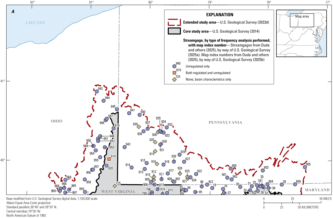
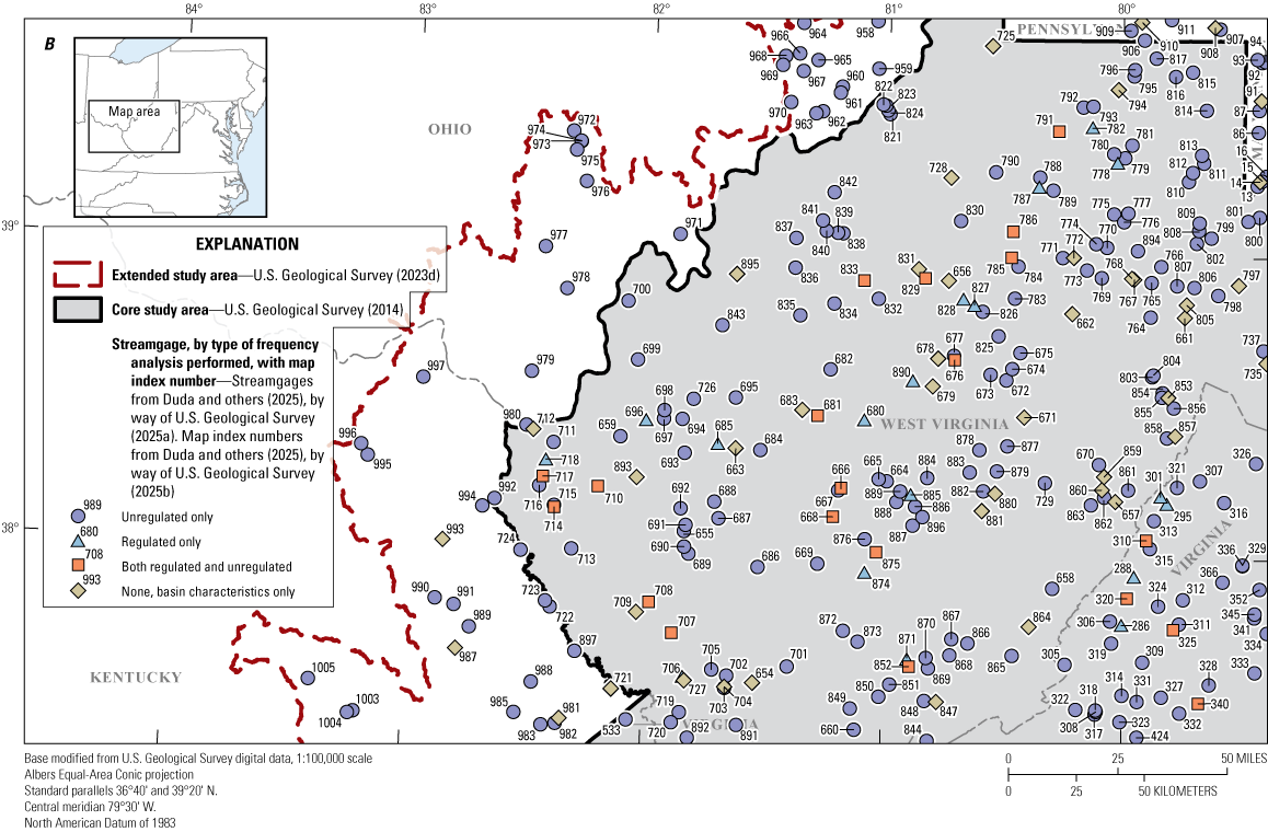
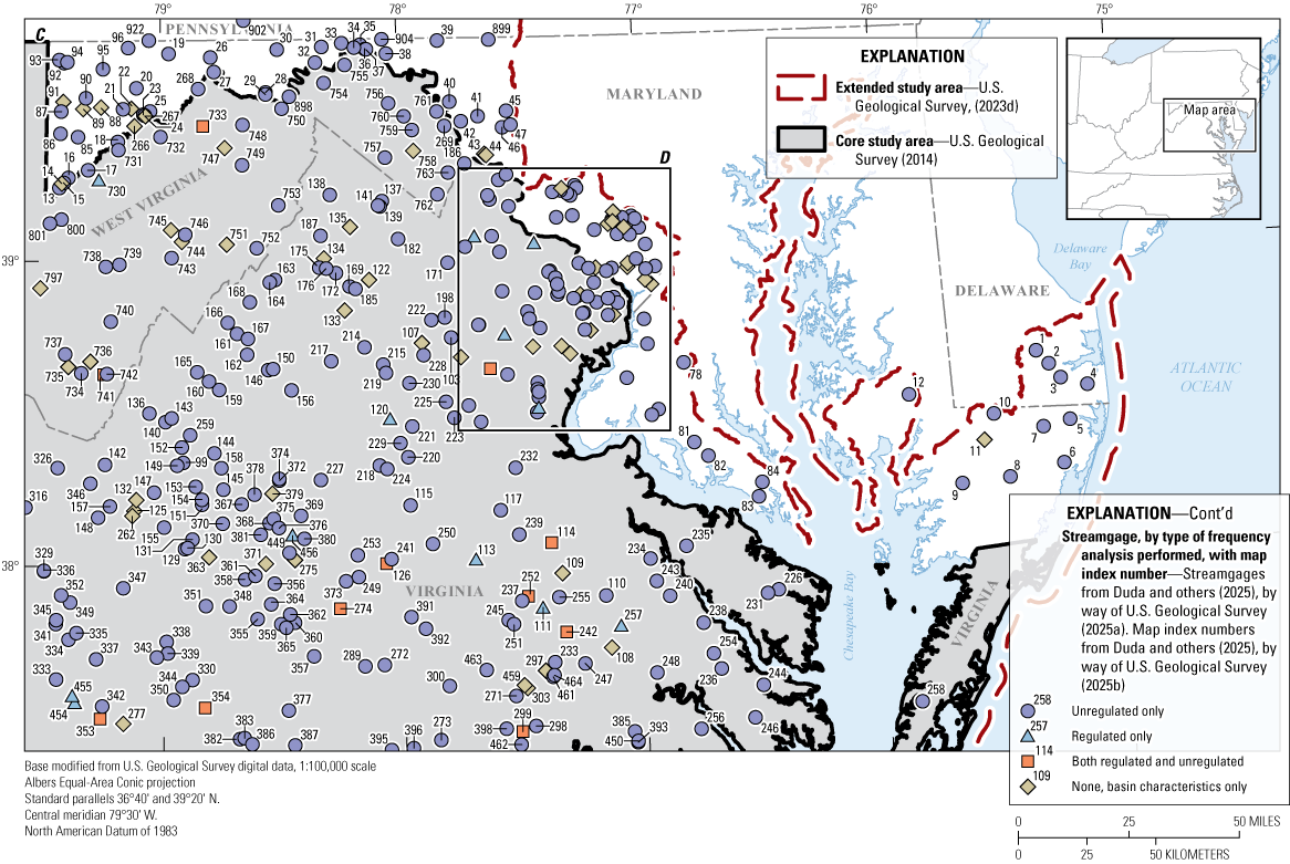
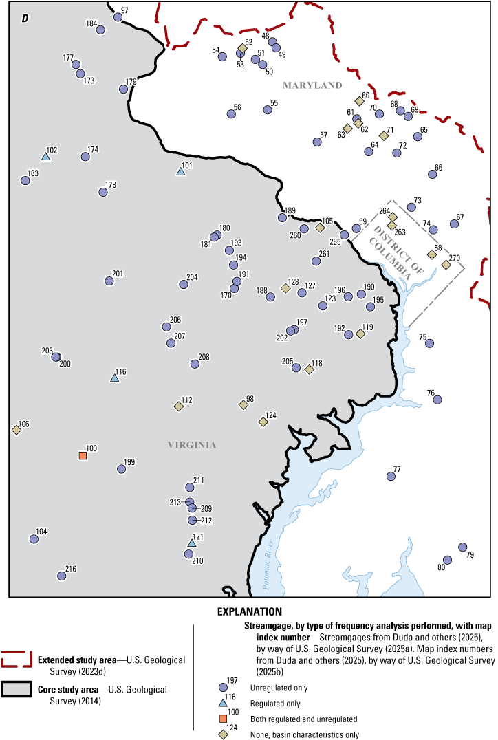
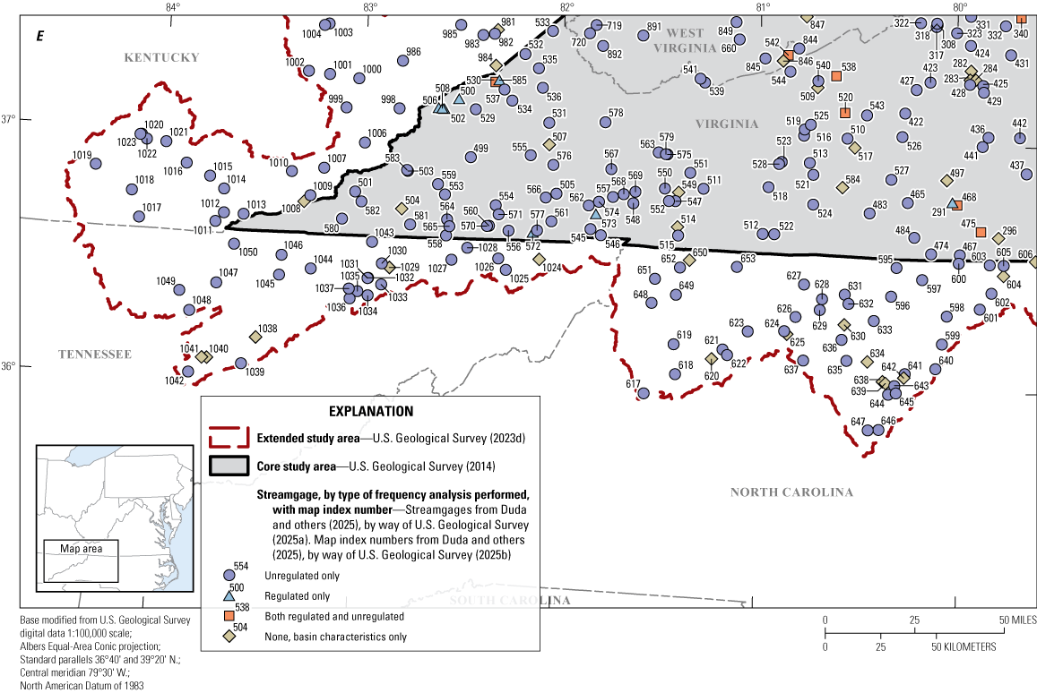
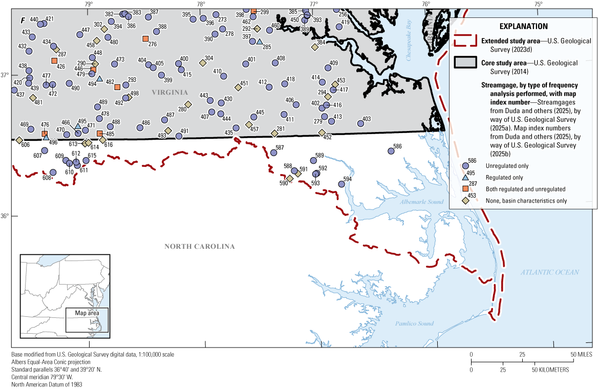
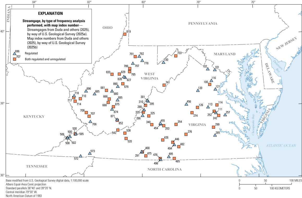
Maps showing the streamgages considered for analysis in and near Virginia and West Virginia. A, in the northern portion of the study area. B, in the northwestern portion of the study area. C, in the northeastern portion of the study area. D, in the District of Columbia and surrounding portions of the study area. E, in the southwestern portion of the study area. F, in the southeastern portion of the study area.
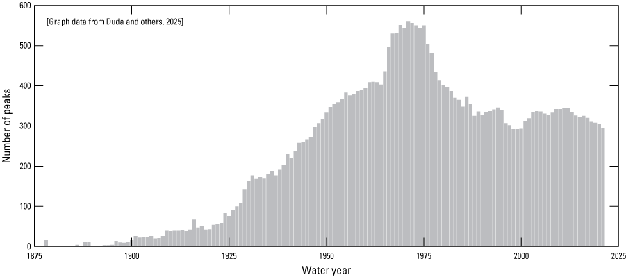
Graph showing the number of annual peaks available, by year, among streamgages considered for regression analysis in and near Virginia and West Virginia, water years 1875–2021.
This crest-stage streamgaging network was largely implemented between 1965 and 1970. Among the streamgages in and near Virginia and West Virginia that were considered for regression analysis for this study, the largest number of annual peaks in any water year was 561, in 1971 (fig. 2). The number of peaks decreased from 550 in 1975 to 348 in 1985. In 1986, 372 peaks were recorded, including 7 historical peaks from the flood of November 1985. Since then, the number of available annual peaks has been stable, fluctuating between 292 in 1998 and 1999 and 348 in 1985. The number of available peaks for regression analysis each year does not match the number of active streamgages, because it includes historical peaks but excludes streamgages with fewer than 10 years of record and streamgages on regulated streams.
Generally, historical floods may be better documented on major rivers than on small streams (fig. 3). There was a total of 209 recorded historical peaks representative of 857 streamgages used in unregulated frequency analysis. Of these, only 47 peaks (22.5%) were recorded amongst the 526 smaller streamgages (61.4%) that drained less than 100 mi2 (table 3 in Duda and others, 2025). Historical floods in the Tennessee River and its major tributaries were inventoried in 1961, through interviews with residents, reviews of historical documents, and reviews of floodmarks (Tennessee Valley Authority, 1961). Historical floods in the rest of the study area have been documented, although less thoroughly than in the Tennessee River Basin. Sometimes, historical floodmarks are obtained when a new streamgage is established, but often, historical floods were investigated to put a major contemporary flood in a historical context.
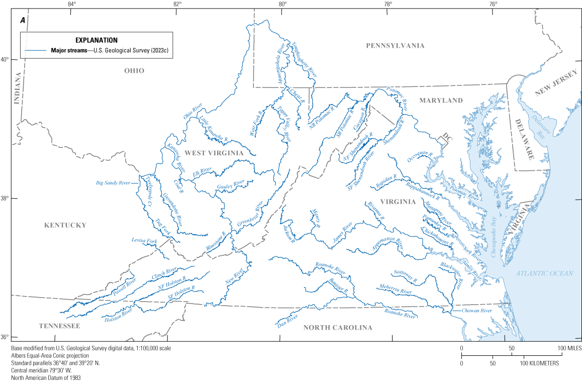
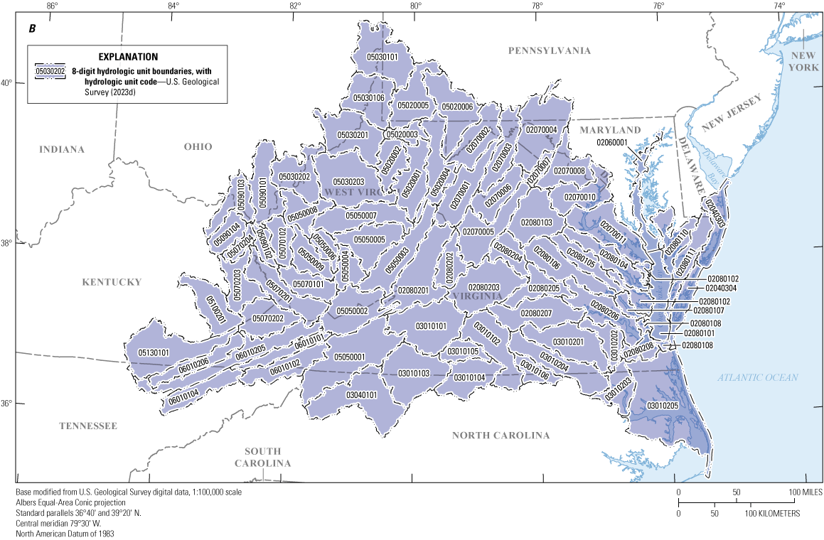
Maps of selected hydrologic features in and near Virginia and West Virginia. A, showing major streams. B, showing 8-digit hydrologic unit codes. Cr, creek; NB, North Branch; NF, North Fork; R, river; SB, South Branch; SF, South Fork.
Historical peaks may be recorded for isolated floods that are locally memorable, but they are more often recorded for widespread floods; the peak streamflow file includes 353 historical peaks for unregulated, nonurban, and non-dam-break peaks. Of these, 158 were recorded in years with 10 or more historical peaks, and 234 were recorded in years with 5 or more historical peaks (table 1). More historical peaks (24) were recorded for 1940 than in any other year because of major floods in southern Virginia and western North Carolina caused by an unnamed hurricane.
Table 1.
Water years with the most historical peaks from selected streamgages in and near Virginia and West Virginia, 1791–2021.Historical peaks were formerly considered to be any annual peaks that were collected or known from periods outside systematic data collection. However, the default settings in USGS computer program PeakFQ treat the values for peaks coded as “historical” as representing large, historically significant floods, even though the peak streamflow file contains many nonsystematic peaks that represent ordinary floods. Some historical peaks were obtained from floodmarks that were available from shortly before or after a streamgage was active rather than because this flood was extraordinarily large. Some apparently historical peaks were salvaged from erroneous systematic records obtained from problematic daily observer readings because the annual peaks had been verified by a hydrographer. Some post-flood inspections near the flooded area may find evidence of an ordinary flood; for such inspections, the peak values previously were coded as “historical” for lack of a better designation. After the development of the EMA methodology, the USGS introduced a specific designation for “opportunistic” peaks, or peaks of ordinary magnitude that were documented outside systematic data collection, for use in peak-flow analyses (Sando and McCarthy, 2018). This study was the first done in either Virginia or West Virginia since the development of the opportunistic code. During the initial flood-frequency analysis, the coding of all the historical peaks was reviewed in the context of other annual peak data for that site. Historical peaks that had been frequently exceeded were recoded as opportunistic and excluded from the flood-frequency analysis.
Major Floods
At-site analyses include all annual peaks but are sensitive to the largest flood streamflows known or recorded at a streamgage, referred to as the “peak of record.” The peaks of record often represent large regional floods. Most annual peaks in both Virginia and West Virginia were caused by continental frontal systems from February to April (table 2). Many of the largest, most widespread floods, however, have been caused by tropical cyclones in the summer and fall. The most common month for the peak of record in Virginia was August, and in West Virginia was November. Tropical cyclones accounted for 7 of the 8 storms that caused the peak of record through water year 2021 at more than 15 streamgages among the 686 streamgages from Virginia and West Virginia that were considered for unregulated frequency analysis; streamgages from adjacent states were not included in this analysis (table 3). These tropical cyclones have included storms from both the Atlantic Ocean and the Gulf of America, and storms from both water bodies have crossed the Appalachian Mountains and subsequently caused major floods. The regional floods that resulted in the largest number of peaks of record among the streamgages considered for regression analysis in this study are listed later in this section, along with other selected memorable floods. The number of peaks of record caused by a given flood is a function not only of the magnitude of the flood, but also the extent of the streamgaging network at the time of the flood and the subsequent effort to obtain historical peaks documenting the flood.
Table 2.
All annual peaks and peaks of record by month for selected streamgages in and near Virginia and West Virginia, water years 1791–2021.Table 3.
Months with 10 or more peaks of record for streamgages considered for regression analysis and the principal storm for that month in and near Virginia and West Virginia, water years 1791–2021.[West Va., West Virginia]
-
March 1936.—This flood on the Potomac and Cheat Rivers (fig. 3), which was documented by Grover (1937) as having a regional extent including the upper Ohio, Potomac, and James Rivers, was caused by four separate cyclonic storms passing over the northeastern United States, resulting in multiple peak streamflows and superposition of later peak streamflows on earlier peak streamflows. This flood was about equal in magnitude to those in November 1877 on the South Branch Potomac River, May through June 1889 on the North Branch Potomac River, and September 1996 on the upper Potomac River (both North and South Branch).
-
August 1940.—The flood of August 14–18, 1940, was caused by an unnamed hurricane that moved inland at Beaufort, South Carolina, traveled north along the Appalachian Mountains, and then moved east through southern Virginia to the Atlantic Coast at Norfolk, Va. It caused record floods in the New, Roanoke, and Tennessee River Basins. Peaks from this flood remain the peak of record at 38 streamgages considered for regression analysis in this study, despite the flood having preceded the full development of the streamgage network; 381 peaks are available for the water year 1940, compared to the high of 918 peaks for 1969 (U.S. Geological Survey, 1949).
-
October 1942.—The flood of October 15–16, 1942 (water year 1943) was caused by an unnamed tropical storm that made landfall in northeastern North Carolina and stalled over northern Virginia, where it produced record rainfall. The Shenandoah, Rappahannock, and James River Basins were the most affected (U.S. Geological Survey, 1990). Peak streamflows from this storm remain the largest recorded for 21 streamgages considered for regression analysis in this study.
-
March 1963.—Flooding was documented on the Big Sandy (including the Tug Fork in West Virginia), Guyandotte, Little Kanawha, Cheat, and Greenbrier Rivers. This flood, which was documented by Barne (1963) as having affected the western slopes of the Appalachian Mountains from Alabama to West Virginia, was caused by three separate frontal storms in which rain fell on a snowpack and was followed by two additional storms.
-
August 1969.—Hurricane Camille, after making landfall in Mississippi and tracking quickly along the Mississippi and Ohio Rivers, turned east, stalled over central Virginia, and produced up to 28 inches (in.) of rain during the night of August 19 and the morning of August 20 (Camp and Miller, 1970; Bailey and others, 1975). Peak streamflows in the James, Potomac, Rappahannock, and York River Basins exceeded previous known maximums. Peaks produced during this flood remain the highest recorded at 43 streamgages considered for regression analysis in this study. This flood took place when the streamgaging network was near its highest number of streamflow monitoring locations; 551 peaks are available for 1969, including historical peaks.
-
June 1972.—The flood of June 21–24, 1972, was caused by intense prolonged rainfall from the remnants of Hurricane Agnes, which formed in the Caribbean Sea and moved north along the east coast of the United States (U.S. Geological Survey, 1990). This flood was one of the most widespread and disastrous floods of record in Virginia, Maryland, Pennsylvania, and New York. Peaks from this storm remain the largest recorded at 72 streamgages considered for regression analysis, including many that had recorded record peaks in August 1969. The Rappahannock, James, and Roanoke River Basins were the most affected. This flood took place when the streamgaging network was near its highest number of streamflow monitoring locations; 556 peaks are available for 1972, including historical peaks.
-
April 1977.—Widespread flooding in northeastern Tennessee, southwestern Virginia, eastern Kentucky, and southern West Virginia resulted from a frontal storm that moved southeast through the region, became stationary, then moved slowly northwest to combine with a warm moist maritime airmass from the Gulf of America to produce heavy rainfall (Runner, 1979; Runner and Chin, 1980). The Big Sandy, Guyandotte, and Tennessee River Basins were most affected by this storm. Peak streamflows during this flood remain the largest recorded at 22 streamgages considered for regression analysis in this study.
-
November 1985.—Flooding was documented on the Monongahela, Potomac, upper Little Kanawha, upper Elk, upper Greenbrier, upper James, and upper Roanoke River Basins. This flood was documented by Lescinsky (1987), and Carpenter (1990) as having affected eastern West Virginia, western and northern Virginia, southwestern Pennsylvania, and western Maryland. This flood resulted from a complex sequence of meteorological events. Hurricane Juan moved from the Gulf of America through southern Mississippi, ultimately causing precipitation as far north as Michigan and generating less than 2 in. of rainfall in West Virginia. This rainfall was caused by a second low-pressure system that developed from the hurricane remnants. The low pressure developed near the Tennessee-North Carolina border and traveled rapidly east to the Atlantic Ocean. A third low-pressure system moved from the Gulf of America into the Florida panhandle, then moved slowly up the east coast of the United States, resulting in additional rainfall in West Virginia of up to 9 in. The highest peak streamflows recorded on the upper Monongahela and Potomac Rivers resulted from this flood.
-
January 1996.—About 2 in. of rain fell on a 3- to 4- foot (ft) snowpack, resulting in flooding in the upper Potomac, upper Cheat, upper Elk, and Greenbrier Rivers.
-
September 1996.—Tropical storm Fran caused regional flooding on the upper Potomac River. This flood was about equal in magnitude to the one in November 1877 on the South Branch Potomac River, to the one in May through June 1889 on the North Branch Potomac River, and to the one in March 1936 on the upper Potomac River. This storm produced the peak of record for 24 streamgages considered for regression analysis for this study; most of the streamgages are in eastern West Virginia and northern Virginia.
-
September 2004.—Hurricane Ivan made landfall in Alabama, weakened to a tropical depression, and moved north and east on the west side of the Appalachian Mountains (Stewart, 2004). It caused widespread flooding in eastern Ohio, the northern panhandle of West Virginia, and western Pennsylvania, with maximum precipitation totals between 5 and 7 inches in northern West Virginia. Peaks caused by this storm are the maximum recorded for 11 streamgages in the study area. Other storms in September 2004 caused 9 peaks of record on several short-term streamgages in eastern and southeastern Virginia.
-
June 2016.—A series of intense thunderstorms caused major flooding in parts of central and southern West Virginia (Austin and others, 2018). More than 8 in. of rain fell over part of the affected area in the Greenbrier River Basin in two to four hours, and more than 5 in. of rain fell during the storm throughout much of central and southern West Virginia. This storm resulted in the peak of record for five streamgages considered for regression analysis in this study.
-
October 2018.—Remnants of Hurricane Michael caused major floods in southeastern Virginia. Hurricane Michael made landfall in western Florida and crossed Georgia, South Carolina, and North Carolina before arriving in Virginia (Beven and others, 2019). Between 5 and 10 in. of rain fell in parts of southeast Virginia during about 24 hours on October 12. This storm caused peaks of record for six streamgages considered for regression analysis in this study.
Previous Studies
Methods have been developed to estimate the frequency and magnitude of annual peak streamflows for rural, unregulated streams in and near Virginia and West Virginia beginning in 1954. Tice (1954) documented this process for the Shenandoah Valley region of Virginia, using the probability method proposed by Gumbel (1945). In the 1960s, a collection of works were published as part of a national effort to regionalize flood-frequency statistics using new methods outlined by Dalrymple (1960). These works included streams within Virginia and West Virginia that spanned the South Atlantic Slope Basins (Speer and Gamble, 1964a), the Cumberland and Tennessee River Basins (Speer and Gamble, 1964b), the Ohio River Basin, except the Cumberland and Tennessee River Basins (Speer and Gamble, 1965), and the North Atlantic Slope Basins (Tice, 1968). Statewide flood frequency and magnitude estimation methods were first developed in Virginia for the large hydrologic basins in 1969 (Miller, 1969) and for the small streams program in 1978 (Miller, 1978). In West Virginia, statewide flood frequencies were computed by Frye and Runner (1969, 1970, and 1971) using methods defined in the previous reports by Speer and Gamble (1965) and Tice (1968), and those proposed by Benson (1962a, 1962b)8.
In 1965, the Water Resources Planning Act recognized the need for the Federal Government, States, localities, and private enterprises to establish a comprehensive and coordinated approach to water resource conservation, development, and use (U.S. Water Resources Council, 1967). This act led to the establishment of the Hydrology Committee of the U.S. Water Resources Council which was assigned responsibility for developing and improving methods for flood-frequency analysis and providing a set of techniques based on the best known hydrological and statistical procedures. In 1967, the Hydrology Committee published Bulletin 15, titled “A Uniform Technique for Determining Flood Flow Frequencies.” This publication established the framework for standard methodology, analysis, and reporting that could be replicated between study areas. The ongoing improvements and refinements of these techniques led to periodic updates and revisions to these standards.
In 1976, the first update was issued in Bulletin 17, which introduced methods for dealing with outliers, historical flood information, and regional skew. In 1977, Bulletin 17 was revised and reissued as Bulletin 17A, which clarified the computation of weighted skew. In 1982, the committee—now known as the Interagency Advisory Committee on Water Data—released Bulletin 17B. This version provided improvements and new techniques, including better methods for estimating and applying regional skew, weighting skew, detecting outliers, and using conditional probability (England and others, 2018).
In Virginia, updated analyses for rural, unregulated streams were provided using the techniques identified in Bulletin 17 (Miller, 1978) and Bulletin 17B (Bisese, 1995; Austin and others, 2011). These studies incorporated the generalized skews developed for the United States in Bulletins 17 and 17B, respectively. In West Virginia, rural, unregulated streams were analyzed in accordance with Bulletin 17 (Runner, 1980), and Bulletin 17B (Wiley and others, 2000). Additionally, Atkins and others (2009) developed a generalized skew study for West Virginia using Bulletin 17B methods. The skews developed for West Virginia were used in the most recent update of rural, unregulated flood-frequency statistics and equations (Wiley and Atkins, 2010).
In 2018, the Subcommittee on Hydrology for the Advisory Committee on Water Information published the most recent methods for determining flood frequencies in Bulletin 17C. This version of standards adopts a generalized representation of flood data that incorporates interval and censored data types, introduces the application of the EMA, and improves methods for computing confidence intervals (England and others, 2018).
This study of flood magnitude and frequency in Virginia and West Virginia includes improvements over previous studies by identifying new regions, computing new regional skews for the combined study area, updating analytics based on methods introduced in Bulletin 17C, and incorporating additional years of data since the most recent studies (Wiley and Atkins, 2010; Austin and others, 2011).
Description of Study Area
The core study area was Virginia and West Virginia. To increase the number of streamgages available for analysis and decrease the uncertainty as to the representativeness of streamgages at the periphery of the core study area, streamgages at the 8-digit hydrologic unit code (HUC 8s) that bordered the core study area were considered for the study; the core study area and the adjacent HUC 8s comprise the extended study area.
The U.S. Environmental Protection Agency (EPA) delineated ecoregions, areas of similar geology, landforms, soils, vegetation, climate, land use, wildlife, and hydrology, to use as a framework for research, assessment, and management of terrestrial and aquatic resources. Landforms and geology are the primary components of physiography (Omernik, 1987). Ecoregions are often aligned with physiographic province boundaries but are mapped at a finer scale and account for more factors relevant to hydrology. A recent USGS flood-frequency regionalization study that borders Virginia used EPA Level III (L3) ecoregions as its regionalization framework (Feaster and others, 2023). The extended study area of Virginia, West Virginia, and adjacent HUC 8s (fig. 3B) includes parts of 10 EPA L3 ecoregions—Erin Drift Plain, Northern Piedmont, Piedmont, Southeastern Plains, Ridge and Valley, Central Appalachians, Western Allegheny Plateau, Blue Ridge, Southwestern Appalachians, and Middle Atlantic Coastal Plain (fig. 4) (U.S. Environmental Protection Agency, 2013). The 10 EPA L3 ecoregions are described from west to east (fig. 4). The climate of the entire study area is humid continental with hot or warm summers (Kottek and others, 2006). Precipitation and precipitation intensity are discussed by 10 L3 ecoregions.
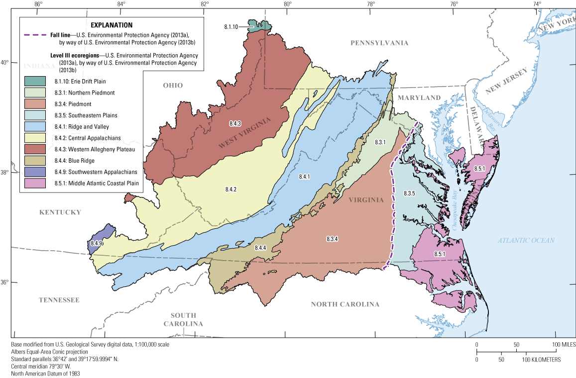
Map showing Omernik’s Level III ecoregions in and near Virginia and West Virginia.
A small part of the extended study area in eastern Kentucky is within the Southwestern Appalachians, an area of low mountains, hills, and intervening valleys (Woods and others, 2002). Moderate- to high-gradient streams are common and have cobble- or boulder-dominated substrates. Low-gradient streams also occur and have gravelly or sandy bottoms. Land cover is predominantly mixed-age forest (Woods and others, 1996). In the part of the Southwestern Appalachians within the study area, the 100-year 24-hour precipitation intensity (I100Y24H) ranges from 6.02 to 6.36 in. (Bonnin and others, 2006). Mean 30-year precipitation (1991–2020 calendar years) within the study area ranges from 53 to 54 in. (PRISM Climate Group, 2021).
Another small part of the extended study area is the Erie Drift Plain ecoregion in eastern Ohio. The ecoregion is glaciated and characterized by ground moraines and rolling terrain. Most soils are poorly drained. The climate in the area is continental and not influenced by Lake Erie (Woods and others, 1996). Within the Erie Drift Plain in the study area, the I100Y24H ranges from 4.92 to 5.10 in. (Bonnin and others, 2006). Mean 30-year precipitation (1991–2020 calendar years) within the same area ranges from 40 to 41 in. (PRISM Climate Group, 2021).
The Western Allegheny Plateau, in southwestern Pennsylvania, southeastern Ohio, western West Virginia, and northeastern Kentucky, is a low, dissected, and mostly unglaciated plateau. From west to east, the terrain gradually becomes more rugged. Maximum elevations are less than 2,000 feet (ft; North American Vertical Datum of 1988) and local relief is approximately 200 to 550 ft. It is composed of horizontally bedded sandstone, shale, siltstone, limestone, and coal of Pennsylvanian and Permian age. The potential natural vegetation is primarily Appalachian oak forest (Woods and others, 1996; Woods and others, 2002; Duda and others, 2025). Within the Western Allegheny Plateau in the study area, the I100Y24H ranges from 4.84 to 5.97 in. (Bonnin and others, 2006). Mean 30-year precipitation (1991–2020 calendar years) in the study area ranges from 40 to 58 in., with a median of 46 in. (PRISM Climate Group, 2021).
The Central Appalachians ecoregion includes parts of south-central Pennsylvania, western Maryland, central West Virginia, southwest Virginia, eastern Kentucky, and eastern Tennessee. This ecoregion is a high, dissected, and rugged plateau made up of sandstone, shale, conglomerate, and coal of Pennsylvanian and Mississippian age. The plateau is locally punctuated by a limestone valley and a few anticlinal ridges (Woods and others, 1996). Local relief varies from less than 50 ft in mountain glades to over 1,950 ft. High gradient streams are common. Maximum elevations generally increase towards the east and range from about 1,200 to 4,600 ft. Elevations can be high enough to ensure a short growing season, a great amount of rainfall, and extensive forest cover (Woods and others, 1996; Duda and others, 2025). Within the Central Appalachians in the study area, the I100Y24H ranges from 4.62 to 7.83 in. (Bonnin and others, 2006). Mean 30-year precipitation (1991–2020 calendar years) in the study area ranges from 39 to 73 in., with a median of 50 in. (PRISM Climate Group, 2021).
The Ridge and Valley ecoregion extends from New York to Alabama, and within the study area comprises large parts of central Pennsylvania, western Maryland, eastern West Virginia, western Virginia, and northeastern Tennessee. It is characterized by alternating forested ridges and agricultural valleys that are elongated and folded and faulted. Elevations range from about 500 to 4,800 ft. Local relief varies widely from approximately 50 to 1,500 ft. Valleys were formed from relatively weak rock, generally shale and limestone. Caves, springs, and sinkholes are common in the limestone valleys. In contrast with the rest of the study area, most streamgaging networks are trellised (Omernik, 1987; Woods and others, 1996; Duda and others, 2025). Within the part of the Ridge and Valley in the study area, the I100Y24H ranges from 4.16 to 8.71 in. (Bonnin and others, 2006). Mean 30-year precipitation (1991–2020 calendar years) in the study area ranges from 35 to 67 in., with a median of 46 in. (PRISM Climate Group, 2021). The minimum of both I100Y24H and mean 30-year precipitation in the entire study area are in the Ridge and Valley ecoregion. The minimum I100Y24H is in southern West Virginia in parts of the Bluestone and Greenbrier River Basins. The minimum mean 30-year precipitation is in areas of the South Branch Potomac and Shenandoah River Basins that are in a rain shadow from the mountains to their west.
The Blue Ridge Mountains ecoregion is a narrow strip of mountainous ridges that are forested and well-dissected (Omernik, 1987; Woods and others, 1996). This ecoregion runs from Pennsylvania to Georgia and, in the study area, comprises a narrow strip of southeastern Pennsylvania, central Maryland, the easternmost tip of West Virginia, and north-central Virginia. South of the Roanoke River, the Blue Ridge Mountains widen through south-central Virginia, western North Carolina, and eastern Tennessee. North of the Roanoke River, just three different rock types form the crest of the Blue Ridge Mountains. Maximum elevations are about 1,000 ft. In contrast, south of the Roanoke River, the Blue Ridge Mountains are higher and have more complex lithology. Maximum elevations are more than 5,700 ft near Mount Rogers. Local relief is high, and both the side slopes and channel gradients are steep (Woods and others, 1996; Duda and others, 2025). Within the part of the Blue Ridge in the study area, the I100Y24H ranges from 4.75 to 12.4 in. (Bonnin and others, 2006). Mean 30-year precipitation (1991–2020 calendar years) in the study area ranges from 39 to 77 in., with a median of 50 in. (PRISM Climate Group, 2021). The maximums of both the I100Y24H and mean 30-year precipitation in the study area are in the Blue Ridge ecoregion near Charlottesville, Va.
The Piedmont ecoregion is a transitional area between the mostly mountainous ecoregions of the Appalachians to the northwest and the relatively flat Coastal Plain to the southeast (Omernik, 1987; Griffith and others, 2002). This ecoregion is a complex mosaic of metamorphic and igneous rocks of Precambrian and Paleozoic age, with moderately dissected irregular plains and some hills. The soils tend to be finer textured than those in the Coastal Plain ecoregions to the south. Once largely cultivated, much of this ecoregion has reverted to pine and hardwood forests, with increasing conversion to urban and suburban land cover (Omernik, 1987; Griffith and others, 2002). Within the part of the Piedmont in the study area, the I100Y24H ranges from 7.17 to 10.8 in. (Bonnin and others, 2006). Mean 30-year precipitation (1991–2020 calendar years) in the study area ranges from 44 to 57 in., with a median of 46 in. (PRISM Climate Group, 2021).
The Northern Piedmont ecoregion, in southeastern Pennsylvania, east-central Maryland, and northern Virginia, consists of low rounded hills, irregular plains, and open valleys, and is underlain by metamorphic, igneous, and sedimentary rocks. Maximum elevations typically range from 325 ft on limestone to 1,050 ft on metamorphic rock. The climate is humid continental, characterized by cold winters and hot summers. Land cover is a mix of forest, agriculture, and some of the largest urban areas in the United States (Omernik, 1987; Woods and others, 1996; Duda and others, 2025). Within the part of the Northern Piedmont in the study area, the I100Y24H ranges from 6.70 to 10.3 in. (Bonnin and others, 2006). Mean 30-year precipitation (1991–2020 calendar years) in the study area ranges from 44 to 57 in., with a median of 46 in. (PRISM Climate Group, 2021).
The Southeastern Plains ecoregion extends from Louisiana and Mississippi to Delaware and, in the study area, comprises part of eastern North Carolina, eastern Virginia, and eastern Maryland (Omernik, 1987). This ecoregion is composed of irregular plains with a mixture of cropland, pasture, woodland, and forest. The sand, silt, and clay geology of this ecoregion contrasts with the older rocks of the Piedmont ecoregion. Altitudes and relief are greater than in the Middle Atlantic Coastal Plain ecoregion, but generally are less than in much of the Piedmont ecoregion. Streams have a relatively low gradient (as compared to the Piedmont ecoregion) with sandy bottoms. Within the study area, a natural feature, the Fall Line (fig. 4), is the western border of the Southeastern Plains ecoregion, separating it from the Piedmont and Northern Piedmont ecoregions (Griffith and others, 2002). Within the part of the Southeastern Plains in the study area, the I100Y24H ranges from 8.08 to 9.45 in. (Bonnin and others, 2006). Mean 30-year precipitation (1991–2020 calendar years) in the study area ranges from 44 to 51 in., with a median of 50 in. (PRISM Climate Group, 2021).
The Middle Atlantic Coastal Plain ecoregion extends from Georgia to New Jersey and, in the study area, includes the easternmost parts of North Carolina, areas bordering the Chesapeake Bay in Virginia and Maryland, and the Delmarva Peninsula (Omernik, 1987). This ecoregion consists of low-altitude flat plains with many swamps, marshes, and estuaries. Unconsolidated sediments underlie the low terraces, marshes, dunes, barrier islands, and beaches. Poorly drained soils are common, and the ecoregion has a mix of coarse and finer textured soils compared to the mostly coarse soils in much of the Southeastern Plains ecoregion. The Middle Atlantic Coastal Plain ecoregion is typically lower, flatter, and more poorly drained than the Southern Coastal Plain ecoregion. Streams in the Middle Atlantic Coastal Plain ecoregion have the lowest gradients and are the most sinuous in the study area (Griffith and others, 2002). Within the part of the Middle Atlantic Coastal Plain in the study area, the I100Y24H ranges from 7.98 to 11.1 in. (Bonnin and others, 2006). Mean 30-year precipitation (1991–2020 calendar years) in the study area ranges from 43 to 56 in., with a median of 50 in. (PRISM Climate Group, 2021).
Magnitude and Frequency of Floods at Streamgages
Magnitude and frequency of annual peak streamflows were computed for 813 streamgages on unregulated streams with a minimum of 10 years of uncensored systematic peaks prior to and including the 2021 water year in the extended study area (fig. 1; table 4; tables 1 and 2 in Duda and others, 2025). A streamgage was considered in the study area if its basin centroid was in the study area. Guidelines established by Bulletin 17C (England and others, 2018) require that streamgages used in the analysis have a minimum of 10 years of uncensored peak streamflows. The 813 streamgages were selected from 1,050 streamgages in the extended study area that had 8 or more annual peaks in the NWIS at the beginning of this project (U.S. Geological Survey, 2023a); the initial set of peaks included regulated periods of record, numerous peaks that were censored for various reasons, and represented streamgages at the outlets of basins that were unrepresentative of regional hydrology for reasons that were determined during analysis. The process of identifying streamgages suitable for different levels of analysis is described with each level of analysis. Levels of analysis are summarized in table 4 and table 1 from Duda and others (2025).
Table 4.
Numbers of streamgages included or not included in various types of analyses in and near Virginia and West Virginia, water years 1791–2021.[Data from Duda and others (2025). Indented rows beginning with “--” represent subsets of the top row in the block with the same shading. NA, not applicable; USGS, U.S. Geological Survey; mi2, square miles; <, less than; >, greater than]
Annual peak streamflow data are maintained in the USGS peak streamflow database (U.S. Geological Survey, 2023a). This database includes quantitative information on the magnitude and timing of floods. Some annual peak streamflows are censored and not used in frequency analyses. The status of the data with respect to being censored comes from codes that provide qualitative information, including qualifications on magnitude and timing of annual peak streamflow and stage. Among the qualification codes are those for regulation and urbanization status, historical status, dam breaks, uncertain dates, months, and magnitudes (values that are less than or greater than the threshold). Other qualification codes pertain to data furnished by other agencies, maximum daily averages, estimates, ice jams, debris jams, hurricanes, and snowmelt. For gage height data, important codes include those indicating backwater effects, data from different sites or datums, values that are less than or greater than the threshold, values that are not the peak for the year, or estimates. Among these qualifications, some indicated that values were unsuitable for frequency analysis or that the record for that year was unrepresentative of regional hydrology. A primary challenge in developing frequency analyses was interpreting and expanding the qualification data. When some qualifying information could be determined to mean that a peak was not representative of regional conditions, that peak was “censored,” and not used in frequency analyses. Peaks could also be censored through some steps of frequency analyses; these steps are discussed later in this report.
The flood-frequency streamflows at the 813 streamgages on rural, unregulated streams were determined following the guidelines established by Bulletin 17C (England and others, 2018). The USGS computer program PeakFQ version 7.5.1 (U.S. Geological Survey, 2024) was used to compute the flood-frequency streamflows. At-site frequency and magnitude of annual peak streamflow were also determined for streamgages on regulated streams.
Time Trends in Flood Magnitudes
The randomness of the systematic annual-peak series was statistically tested to detect a time trend using Kendall’s test for correlation, and the Kendall’s tau statistic (Kendall, 1975; Hirsch and others, 1982). Kendall’s tau and the level of significance (the probability or “p-value”) were computed with PeakFQ, version 7.5.1 (Flynn and others, 2006; Veilleux and others, 2014; U.S. Geological Survey, 2024). Kendall’s tau and the level of significance were determined for the annual peak series of 813 streamgages in the study area (table 3 in Duda and others, 2025). Streamgages were further limited to 418, each with a minimum of 30 gaged peaks, to reduce short-term effects related to streamgages that began operation in wet years and ended in dry years, or vice versa. The annual-peak series for 51 streamgages (about 12 percent of the 418 streamgages) indicated a statistically significant (p-value≤0.05) trend, with 40 of these exhibiting positive trends and 11 exhibiting negative trends. Assuming a significance level of 0.05, 21 streamgages would be expected to indicate a positive or negative trend by chance (about 5 percent of the 418 streamgages). Trends were significant at slightly more than twice that many streamgages.
Streamgages with annual peak records coded as “C” for urban were excluded from the study. However, some streamgages that drained urban areas were not coded as “urban.” A comprehensive review of urbanization coding of historical records would have required developing geospatial data to represent historical changes in urbanization, which was beyond the scope of this study. Some streamgages that drained urban areas indicated a strong positive trend, especially among smaller, more frequent peaks, that might plausibly indicate urbanization during the period of record, such as the streamgage at Chickahominy River near Providence Forge, Va. (USGS site 02042500), in the Richmond, Va. metropolitan area (fig. 5). However, many urban streamgages were established in areas that were already urbanized, where little or no trend would be expected from urbanization. Other streamgages in areas that transitioned to urbanization during the period of record indicated no trend.
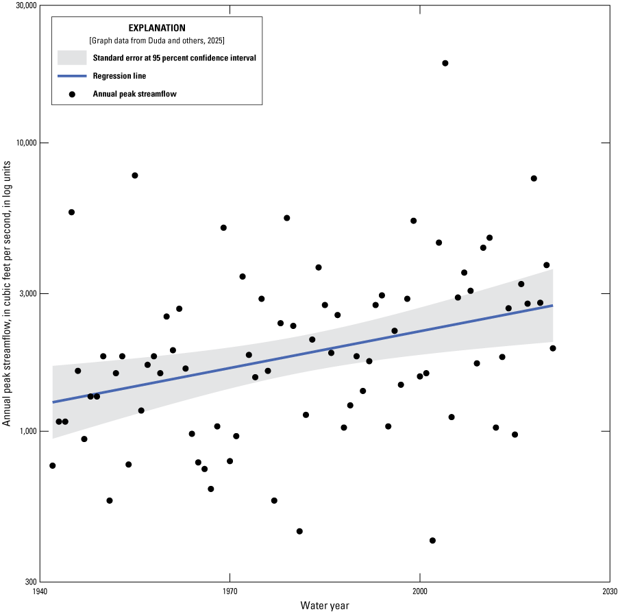
Graph showing annual peak streamflow for U.S. Geological Survey streamgage 02042500, Chickahominy River near Providence Forge, Virginia, water years 1942–2021.
Trends were compared to NLCD land-cover percentages from the National Land Cover Dataset (NLCD) (fig. 6). Of the 51 streamgages with significant trends and 30 or more years of record, 17 drained basins with 10 percent or more total developed land, as determined by the sum of the four developed land classes from the 2019 NLCD; 13 of these had positive trends. Among streamgages with 30 or more gaged peaks and 10 percent or more developed land in the basin, an ordinary least-squares (OLS) regression found a positive relationship between the value of Kendall’s tau and total development percentage (p-value less than [<] 0.001; adjusted coefficient of determination [R2]=0.162). The relationship was stronger among streamgages with 50 or more gaged peaks and 10 percent or more developed land in the basin (p-value<0.001; adjusted R2=0.550). For these 218 streamgages, 23 tau values were significant (p-value<0.05), and 22 of the significant values were positive. The greater strength of the relationship among streamgages with longer records indicates that 30 years is too short a period to reliably distinguish the effects of development from climatic cycles on trends in annual peaks at streamgages. Some of the positive trends seem likely to have been caused by something other than urbanization; about 66 percent (143 of 218) of the streamgages with 50 or more gaged peaks that drained basins with less than 10 percent developed land had a positive Kendall’s tau.
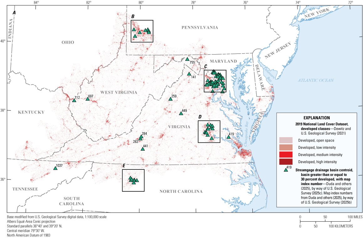
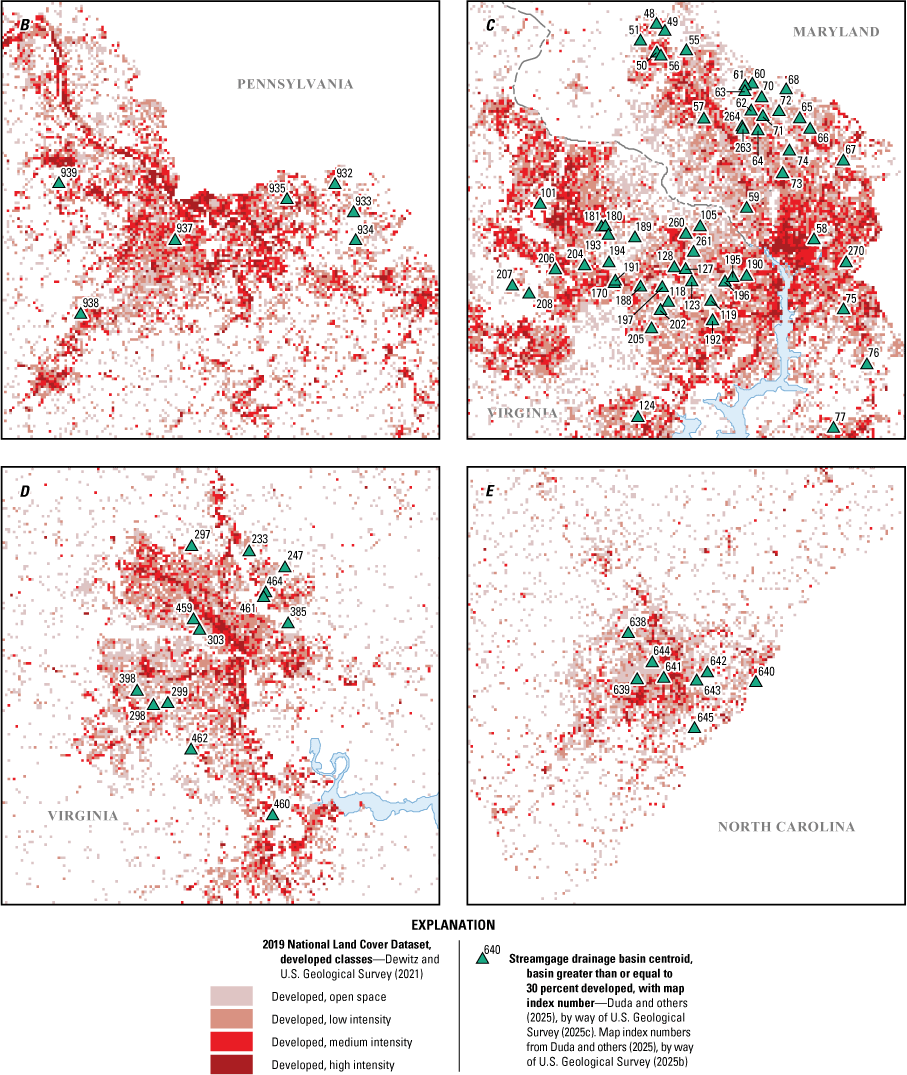
Map showing the sum of 2019 National Land Cover Dataset development classes, and streamgages that were excluded from regression analyses because the sum of classes of developed land greater than or equal to 30 percent in the basin. A, in and near Virginia and West Virginia. B, in the Pittsburgh, Pennsylvania metropolitan region. C, in the District of Columbia metropolitan region. D, in the Richmond, Virginia metropolitan region. E, in the Winston-Salem, North Carolina metropolitan region.
Analyses indicated that the presence of a positive trend alone was not a reliable indicator of urbanization and that few streamgages with high development and long periods of record lacked positive trends. Because the undeveloped or moderately developed streamgage basins (less than 10 percent development) included enough with significant positive trends, basins were not considered urbanized solely because of a significant positive trend. The data from these streamgages were all retained for regression analysis because of uncertainty about causation and a lack of guidance on how to account for climate change in flood frequency.
With the undeveloped and moderately developed streamgage basins excluded, the weak linear relationship between development and tau among streamgages with 50 or more gaged peaks was the strongest line of evidence. Hints of threshold effects were present among the remaining streamgage basins (fig. 7). A little of the effect was related to climate conditions throughout the periods of record (fig. 8). The threshold was not clear and distinct, and plausibly might have been any value between 20 and 40 percent development. The most recent urban flood-frequency study for Virginia found significant effects of development beginning at 10 percent, and that nearly all basins containing more than 30 percent of development indicated effects (Austin, 2014). Present analyses were broadly consistent with these patterns. Using a threshold lower than 30 percent would have excluded more sites with negative trends or ambiguous causes of trends, and there was no specific evidence that a threshold higher than 30 percent would be effective at excluding affected basins from further analysis. Streamgages draining developed areas were included in preliminary regression analysis to check if regression analysis allowed a threshold percentage of development to categorize streams as urban. These analyses are discussed later in the report, but they did not provide a clearer threshold for distinguishing the effects of development on trends in annual peaks than did the previous Virginia urban peak-flows study (Austin, 2014). All 97 streamgages with 30 percent or greater development were ultimately excluded from final regression analysis in this study, although setups and results of frequency analyses are included in the data release associated with this report (table 3 in Duda and others, 2025).
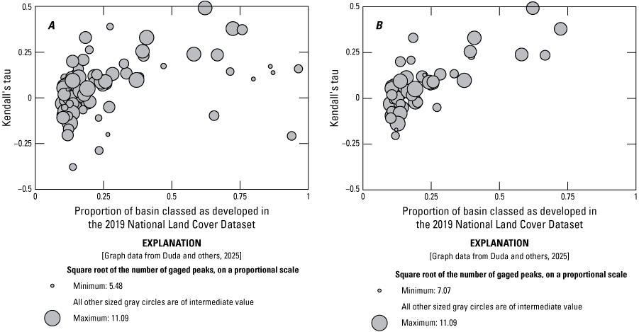
Graphs showing relation of Kendall's tau in the annual peak-series and basin development among streamgages in and near Virginia and West Virginia draining 10 percent or more developed land with A, 30 or more gaged peaks and B, 50 or more gaged peaks.
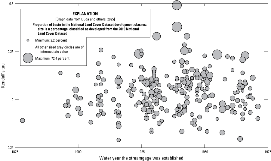
Graph showing relation of Kendall's tau in the annual peak-series and the water year the streamgage was established among streamgages in and near Virginia and West Virginia with 50 or more gaged peaks.
The most urbanized parts of the study area are near Washington, D.C.; Richmond, Va.; and Pittsburgh, Pennsylvania (fig. 6). Areas that have undergone urbanization were different from areas that remain undeveloped. Because of this difference, and because other choices were not available, the entire record for sites that had 30 percent or more development from the 2019 NLCD data was excluded from regression analysis. The early, pre-urbanized record presumably represented places that eventually became urban, and therefore, did not need rural regression equations to characterize present conditions. Urban regression equations are available for urbanized parts of Virginia in Austin (2014).
At-Site Frequency Analyses for Unregulated Streams
The flood-frequency streamflows at the 813 streamgages on rural, unregulated streams in and near Virginia and West Virginia were determined following the guidelines established by Bulletin 17C (England and others, 2018). The USGS computer program PeakFQ version 7.5.1 (Flynn and others, 2006) was used to perform initial frequency analyses to compute the station skew and flood-frequency streamflow estimates. Frequency analyses were developed for streamgages in and near Virginia and West Virginia (tables 3, 4, 5, and 6 in Duda and others, 2025). Many of these frequency analyses were used to determine regional skew for Kentucky, Tennessee, Virginia, and West Virginia (Wagner and others, 2025a; Wagner and others, 2025b). Determining regulation status is discussed in appendix 1.
The base-10 logarithm (log10)-transformed systematic (continuous record or broken record that can be statistically treated as a continuous record) annual-peak series for each streamgage was fitted to the log-Pearson Type III probability curve. The EMA requires users to review historical peaks, perception thresholds, flow intervals, and low-outlier thresholds (England and others, 2018). Although the PeakFQ program populates some of these fields with default values, the default values are often suboptimal or inappropriate. Analytical evaluation and knowledge of streamgage history are required to appropriately fit the probability curve to the annual peak streamflow data, especially because of the importance of historical peak streamflows to frequency analysis.
Historical peaks are crucial for frequency analyses in this study because they are used to define periods with “interval data,” thereby extending a streamgage’s period of record with usable flood-related data outside the periods with systematic records. When considering historical conditions for a frequency analysis, it was assumed that the historical peak streamflows for that streamgage were not exceeded during the periods between the historical peak and the periods with systematic records. The historical values (or the values of other large floods for that streamgage) were used as the minimum “perception threshold” for times without systematic record between the historical peak and the period of systematic record (fig. 9). A “flow interval” from the perception threshold to zero was applied for those periods and incorporated in the frequency analysis. For all streamgage records used in this study, the upper perception threshold was infinity, meaning that an arbitrarily large flood would have been measured if it had occurred. For most periods at streamgages with systematic records, the lower perception threshold was zero, meaning that any flood greater than zero could have been measured, and the resulting flow interval was zero to infinity. Minimum perception thresholds were changed for cases when the lowest recordable streamflow was greater than zero, which is common for crest-stage gages. In these cases, the perceptible streamflows ranged between the minimum detectable stage and infinity. Minimum perception thresholds for crest-stage gages were not historically recorded in the NWIS database but instead were typically documented in paper station records in field offices. They were obtained for this study and used to create PeakFQ setup files and are available in the associated data release (Duda and others, 2025).
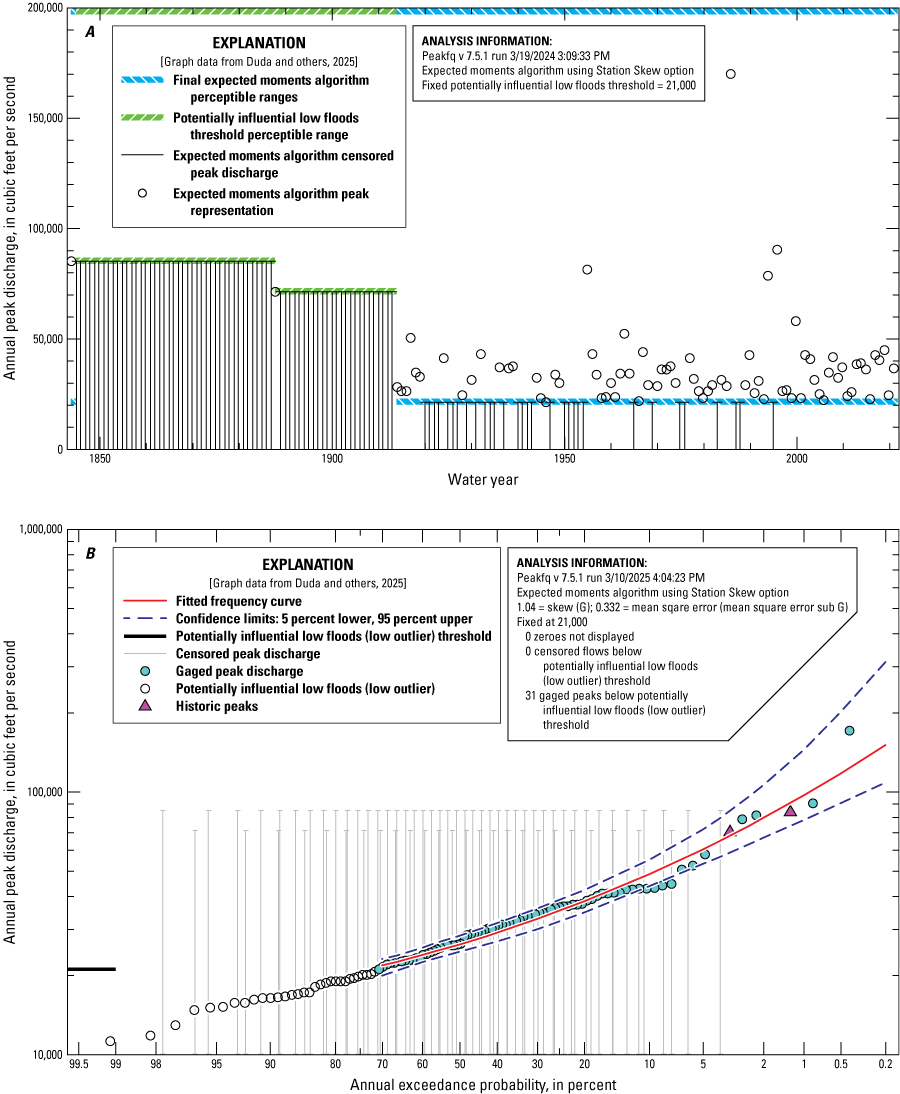
A, Graph showing U.S. Geological Survey computer program PeakFQ input graph and B, graph showing frequency curve (bottom) for U.S. Geological Survey streamgage 03069500, Cheat River near Parsons, West Virginia, for annual and historical peaks, water years 1844–2021.
The fit of frequency curves may be affected by potentially influential low floods (PILFs). Along with the interpretation of historical peaks, identifying PILFs and their effect on the fit of the frequency curve is one of the major analytical tasks in developing flood-frequency analyses. The default method for detecting PILFs in PeakFQ is the multiple Grubbs-Beck test (England and others, 2018). Once identified, the PILFs are censored and removed from the frequency analysis. For many annual-peak series, however, the multiple Grubbs-Beck test does not exclude enough PILFs, and the resulting frequency curve fits high peaks poorly. In these cases, a single outlier threshold was identified and used to fit the frequency curve; this was done for 74 streamgages in this study (table 3, Duda and others, 2025). Common scenarios for a poor fit that can be improved by a manual PILF threshold include populations of peaks generated by mixed mechanisms, annual peak-series with one or two extraordinary floods relative to the rest of the series, crest-stage gages with poor ratings or stage record for part or all of the range of annual peaks, and crest-stage gages with a minimum recordable stage that excluded too many annual peaks. PeakFQ fails if more than half of the streamflow record is excluded, so a PILF threshold cannot be greater than the median annual peak. Annual peaks that remained within the streambanks or were below bankfull levels, however, were in many cases irrelevant to the fit of the upper tail of the frequency curve. In much of the study area, field surveys of bankfull channel characteristics suggested that between a quarter and a third of annual peaks were less than bankfull (Keaton and others, 2005; Lotspeich, 2009; Messinger, 2009). When field evidence of a bankfull condition was available, it was considered as a preliminary line of evidence when analysts fit frequency curves to poorly fitting upper tails and considered using a manual PILF threshold to improve the fit. Field evidence included (1) channel surveys made as part of studies that evaluated bankfull characteristics, including estimates of bankfull streamflow; and (2) cross sections obtained during streamflow measurements made during floods, for which a breakpoint between the channel and floodplain was taken as bankfull stage and streamflow was estimated from a rating in effect at that streamgage location and datum.
The key customization parameters for the frequency analyses are included in the PeakFQ output (table 3, Duda and others, 2025). Of the 813 streamgages with unregulated frequency analyses, 165 streamgages had 1 or more historical peaks in the analysis; 122 had 1, 34 had 2, 5 had 3, and 1 had 4. Manual PILF thresholds were specified for 74 streamgages. Frequency analyses censored PILFs for 189 streamgages, and the maximum number of PILFs at a streamgage was 60 (in Duda and others, 2025). Selected statistics representing the magnitude and variance of selected AEPs for the flood-frequency analyses for the 813 streamgages in Virginia, West Virginia, and adjacent states also are listed in table 4 in Duda and others (2025).
Regional Skew Coefficient
This section is an overview of the regional skew coefficients generated for the study area and the criteria used for the selection of streamgages to develop the regional skew. More details about the methodology used to generate the regional skew are in appendix 2.
To improve estimates of annual peak streamflows corresponding to the selected AEPs—particularly for streamgages with short annual peak-flow records (less than 30 years)—Federal guidance for flood-frequency analysis (Bulletin 17C; England and others, 2018) recommends using a weighted average of the at-site and a generalized, or regional, skew. Previous guidance (Bulletin 17B; England and others, 2018) supplied a national map of regional skew but encouraged hydrologists to develop more localized models when appropriate. Tasker and Stedinger (1986) developed a weighted least-squares (WLS) regression approach for estimating regional skew that accounted for the precision of the at-site skew, depending on the length of the record and the accuracy of a mean regional skew computed using OLS regression. Tasker and Stedinger (1989) also developed a generalized least-squares (GLS) model for hydrologic regression that accounts for the cross-correlation of streamflows among the streamgages. More recently, Reis and others (2005) introduced a Bayesian approach to GLS regression for regional analysis of skew, and Feaster and others (2009) used B–GLS regression to estimate regional skew. Veilleux (2011) presented a Bayesian weighted least squares/Bayesian generalized least squares (B–WLS/B–GLS) regression, wherein the regression parameters of regional skew models for California (Parrett and others, 2011) were determined using Bayesian weighted least squares (B–WLS) regression and the accuracy of the regression parameters and models were determined using B–GLS regression. Since 2011, B–WLS/B–GLS has been used by the USGS in regional skew studies (Veilleux and others, 2019; Veilleux and Wagner, 2019; Veilleux and Wagner, 2021; Feaster and others, 2023; Mitchell and others, 2023).
In this study, the EMA (Cohn and others, 1997) was used to estimate the at-site skew and its mean squared error of skew. The EMA allows for (1) the censoring of low annual peak streamflows by use of the multiple Grubbs-Beck test or use of manual low-outlier thresholds for screening PILFs and (2) the use of flow intervals to describe missing, censored, and historical data; therefore, the EMA complicates calculations of effective record length (and effective concurrent record length) used to describe the precision of skew estimates because the annual peak streamflows are not always represented by single values. To properly account for these complications and large cross-correlations between annual peak streamflows at pairs of streamgages, a B–WLS/B–GLS regression framework was developed to provide stable and defensible results for regional skew (Parrett and others, 2011; Veilleux, 2011). B–WLS/B–GLS uses OLS regression to fit an initial model of regional skew that is used to generate a stable estimate of regional skew for each streamgage. This estimate is the basis for computing the variance of each estimate of at-site skew used in the B–WLS analysis. B–WLS is then used to generate estimators of the regional skew model parameters. Finally, B–GLS is used to estimate the precision of those estimators, assess the model error variance and its precision, and compute various diagnostic statistics.
For this study, two unique skew regions were identified: Skew Region 1 encompasses streams in Virginia, West Virginia, and Maryland that drain to the Atlantic Ocean, including the eastern panhandle of West Virginia and most of western Maryland in appendix 2 (fig. 2.1). Skew Region 2 encompasses all the study area that drains to the Gulf of America, including Kentucky and Tennessee, most of West Virginia, and far southwestern Virginia. A total of 114 streamgages that were not redundant and had a pseudo-record length (refer to “Computing Pseudo-Record Length” in app. 2) of 50 years or greater were used to develop the final regional skew model for Skew Region 1 (refer to “VA_SkewRegion1.csv” in Wagner and others, 2025a). To explain the variability in skew, 24 basin characteristics were tested as covariates, but none provided sufficient predictive power. Therefore, a constant stable estimate of regional skew of 0.50 was selected for Skew Region 1. The average variance of prediction, 0.33 (standard error 0.574), is equivalent to the mean squared error of the regional skew and corresponds to an effective record length of 28 years (Griffis and others, 2004), an improvement over the Bulletin 17B regional skew map which has an effective record length of 17 years. A total of 387 streamgages that were not redundant and had a pseudo-record length of 30 years or greater were used to develop the final regional skew model for Skew Region 2 (refer to “VA_SkewRegion2.csv” in Wagner and others, 2025b). To explain the variability in skew, 24 basin characteristics were tested as covariates, but none provided sufficient predictive power. Therefore, a constant stable estimate of regional skew of 0.048 was selected for Skew Region 2. The average variance of prediction, 0.16 (standard error 0.400), is equivalent to the mean squared error of the regional skew and corresponds to an effective record length of 45 years, which is also an improvement over the Bulletin 17B regional skew map.
Regional Skew-Weighted Frequency Analyses for Rural, Unregulated Streams
Regional skew was used to complete frequency analyses for unregulated streams. Because of the relatively large uncertainty in the at-site skew for short to modest record lengths, the at-site skew can be combined with the regional skew to generate a weighted estimate of skew for a given streamgage basin (refer to “Weighted Skew Coefficient Estimator,” p. 25–26, and appendix 7 in England and others, 2018). All frequency analyses were recomputed using the same customization parameters described in the “At-Site Frequency Analyses for Unregulated Streams,” section, but with the key difference of applying weighted skews using either the new regional skews for Virginia, West Virginia, Kentucky, and Tennessee, or the EMA-compatible skew for the respective adjacent states (Koltun, 2019; Roland and Stuckey, 2019; Hammond and others, 202239; Feaster and others, 2023). The resulting frequency curves were compared to frequency curves produced with at-site skew, following the recommendation of England and others (2018, p. 26). A majority of the 417 long-term streamgages (those with 30 or more gaged peaks) indicated a better fit with at-site skew than with weighted skew, so the frequency curves produced using station skews were used for subsequent analyses for these streamgages. Large deviations between the at-site and regional skew may indicate that the flood-frequency characteristics of the basin of the streamgage of interest differ from those used to estimate the regional skew. Regional skew was used to weight frequency curves for the 404 streamgages with a short period of record (fewer than 30 gaged annual peaks), and these weighted frequency curves were used for subsequent analyses for these streamgages. The numbers of gaged peaks, the skew types used to produce the systematic statistics, and the systematic statistics themselves are in tables 3 and 4 in Duda and others (2025).
For streamgages in adjacent states where flood frequency and magnitude have been investigated using EMA, setup files for frequency analyses done from those states were acquired and used for this study (Koltun, 2019; Roland and Stuckey, 2019; Feaster and others, 2023). Frequency analyses for Kentucky and Tennessee are included with the frequency analyses for Virginia and West Virginia in Wagner and others (2025a and 2025b)96. Existing PeakFQ setup files were used for treatment of historical peaks, perception thresholds, flow intervals, and PILFs, and were modified only to allow the analysis of peak streamflow series prior to and including the 2021 water year. The skew options used by the original analysts were retained. The regional skews developed for the adjacent states were applied to streamgages from those states. Weighted-skew frequency analyses for streamgages on the Delmarva Peninsula used regional skew developed for Delaware (Hammond and others, 2022).
Frequency Analyses for Regulated Streams
Flood-frequency streamflows were computed for 86 streamgages on regulated streams in Virginia and West Virginia, for which 10 or more systematic peaks are available that represent present flow-regulation conditions (fig. 10; tables 5 and 6 in Duda and others, 2025). Regulated frequencies are not published for historical streamgages that were discontinued before existing major dams were built in the basins.
Map of streamgages on regulated streams with flood-frequency analyses in Virginia and West Virginia.
Streamgage record was assessed for regulation using a regulation index (RI) that was computed with a modification of the formula from Wieczorek and others (2021):
wheren is the total number of dams upstream from the streamgage;
d is the sum index, 1;
Sd is the dam(s) storage, in acre-feet;
DAd is the drainage area of the dam(s) storage, in acres;
DAg is the drainage area at the streamgage, in acres; and
P is the total mean 30-year (1991–2020) upstream annual precipitation, in feet.
Details of the regulation assessment are discussed in appendix 1 of this report. The RI is a unitless ratio that accounts for total dam storage and drainage area in a streamgage basin. It assigns large weights to dams that have large values of both storage and drainage area relative to the streamgage drainage area, and small weights to dams that have small values of storage or drainage area (or both). Streams were considered to be regulated if the RI for a year of record exceeded 0.0040. Drainage basins were delineated and drainage areas were computed for all dams without published drainage areas in the National Inventory of Dams (NID) but with storage that would account for 1 acre-feet per square mile at any streamgage in the study (app. 1; table 7 in Duda and others, 2025). Dams without drainage areas were manually snapped to the stream grids used in the StreamStats applications for Virginia and West Virginia (U.S. Geological Survey, 2019).
Regulation conditions may change for a given streamgage as dams are built, modified, or removed in a basin. The present extent of regulation for streamflows on a stream grid from the Virginia or West Virginia StreamStats application, then delineated in StreamStats, are likely to be the most relevant condition to characterize. To accomplish this characterization, frequency analyses were done for periods of record that were homogeneous through time with the present intensity of regulation. Homogeneous periods of regulation compared to present conditions were determined primarily by reference to dam construction dates from the NID (U.S. Army Corps of Engineers, 2024). Construction dates were determined or estimated for dams that lacked construction dates in the NID for dams that accounted for 5 percent or more of the RI for streamgage record when the RI was greater than (>) 0.0040. If construction dates were available in the NID, they were used, but if the construction dates were not available in the NID, they were obtained from published documents and historical aerial photography and topographic maps (app. 1).
Once the RI had been computed and homogeneous periods of regulation had been determined, the RI was compared to the regulation coding for the peak streamflow record of all streamgages in the core study area that were downstream from dams in the NID. Codes in the peak streamflow file were corrected as necessary. Peak flow files included in the PeakFQ specification files in Duda and others (2025) were coded using the RI to identify regulated periods. The peak streamflow file in NWIS was also coded to be consistent with the peak flow files.
The computation procedure for regulated streams differed from that for unregulated streams in two principal ways: (1) at-site skew coefficients were applied to record from all streamgages without regional weighting, and (2) frequencies were computed only for homogeneous periods of regulation. Frequency curves were adjusted with manual PILF thresholds for 22 streamgages. AEP values from the frequency analyses that were computed for the regulated streamgages are available (tables 5 and 6 in Duda and others, 2025).
Development of Flood-Frequency Regression Equations
Annual peak streamflow data, basin characteristic data, and generalized skew coefficients for 813 streamgages on unregulated streams in and near Virginia and West Virginia were analyzed to determine regional equations to be used to estimate the magnitude of flood streamflows for selected AEPs in ungaged basins. Basin characteristics, generalized skew coefficients, and flood-frequency streamflows for streamgages in adjacent states developed for this study do not supersede values used by adjacent states. The equations for the 0.01-AEP (100-year) streamflows were regionalized by plotting the spatial distribution of residuals from OLS regression models. Spatial distributions of residual plots from regressions of the 0.01-AEP (100-year) streamflows were used to represent flood streamflows expected in Virginia and West Virginia and to determine regional boundaries. The initial regional equations for the selected AEPs were developed with the use of OLS regression models and by testing the significance of independent variables. The final regional equations were derived with the use of a WLS regression model and the significant independent variables from the initial regional equations.
Streamgage Redundancy
Streamgage redundancy was determined by considering (1) the distance between basin centroids, the drainage area of each streamgage in a pair, and the drainage area ratio; (2) the record length and common years of each pair of streamgages; (3) the Spearman’s rank correlation coefficient (rho) and Pearson’s correlation coefficient (r) correlation coefficients between common, unregulated record and the percentage of overlap between pairs of basins (table 8 in Duda and others, 2025). The distances between basin centroids and the percentage of overlap between pairs of basin polygons were determined using the Near Distance and Tabulate Area geoprocessing tools, respectively, in ArcGIS 10.6 (Esri, 2017). Drainage area and record length were available from the NWIS database (U.S. Geological Survey, 2023a). Spearman’s rho and Pearson’s r were computed in R using the base and Hmisc R packages (R Core Team, 2021; Harrel and Dupont, 2023). This process of identifying redundant streamgages was adopted following discussions with the National StreamStats Coordinator (Peter M. McCarthy, U.S. Geological Survey, oral commun., 2024).
Using these metrics to identify potential redundancy, streamgage pairs were evaluated to determine which to retain for regression analysis. Pairs of streamgages with 25 percent or more overlap were screened, although when screening was complete, only members of pairs of streamgages with 50 percent or greater overlap were excluded from regression analysis. Correlation coefficients were reviewed to determine whether they provided additional usable information, but they generally confirmed patterns shown by spatial and temporal overlap. Record length and drainage area were the primary factors used to evaluate pairs of streamgages for redundancy. Longer record length was the first consideration in deciding which streamgage to keep from a pair. If the two streamgages had similar record lengths, the streamgage with a smaller basin was generally preferred to better represent smaller basins in the analysis. An exception to the basin-size criterion was that in pairs of streamgages on streams flowing into the core study area from an adjacent state, the streamgage that drained a greater percentage of the core study area was preferred. In a few cases, the secondary criteria were considered. In 2 cases when drainage basins had a high overlap percentage (>40 percent) but the streamgages had little record in common (2 years in one case and 10 years in the other), both were retained. In the Blackwater River Basin in the Virginia Coastal Plain, the streamgage at Blackwater River near Dendron, Va. (USGS site 02047500) had the most accurate stage-streamflow rating and stage record in the basin and was included in preference to other candidate streamgages.
In cases where more than two streamgages had potentially redundant relationships, they were screened as a group using the same criteria used to screen a pair of streamgages. For instance, when there were three streamgages on the same river and the middle one was potentially redundant with streamgages upstream and downstream, the advantages and disadvantages of the three were considered together. In these cases, the streamgage with more advantages was retained, even when it meant that two streamgages were excluded. Streamgages that were excluded from regression analysis for being redundant with another streamgage are identified in tables 1 and 8 in Duda and others (2025). While not included in the regression analysis, at-site flood frequencies are available for the redundant streamgages (table 4 in Duda and others, 2025). Basin characteristics were developed for streamgage basins that were not considered for this study because the geographic information system processing for extra basins required little extra effort and the characteristics are now available for other analyses. The extra streamgages included streamgages in the extended study area with either eight or nine annual peak streamflow values in the NWIS peak streamflow database and active streamgages in and near Virginia and West Virginia
Basin Characteristics
Characteristics of the basins draining to 1,050 streamgages in and near Virginia and West Virginia were developed for use as independent (or predictor) variables in regression analysis (tables 9, 10, 11, 12, 13, and 14 in Duda and others, 2025). Basin characteristics were developed if they had been significant in regression equations for flood magnitude and frequency in other parts of the eastern United States. The 121 quantitative basin characteristics included:
• characteristics of the basin polygon geometry (including drainage area, perimeter, centroid latitude and longitude), and compactness ratio;
• percentage of areas in Level III and IV ecoregions and physiographic provinces;
• climate characteristics (including 30-year mean precipitation for 1991–2020 and selected mean n-hour m-year precipitation intensity values);
• mean, maximum, and minimum elevation;
• area and percentage in each basin in each NLCD class, and sums of NLCD classes representing storage, forest, agriculture, and development;
• miles and density of hurricane tracks within basins;
• area and percentage of each basin with carbonate or unconsolidated surface geology;
• and the longest flow path and the slope of the main stream channel between points at 10 and 85 percent of its length.
Specific dataset sources and processing information are available in Duda and others (2025).
The basin characteristics for 693 streamgages (table 4; table 1 in Duda and others, 2025) were evaluated for linear correlation by using Pearson’s r and for nonlinear correlation by using Spearman’s rho (Helsel and others, 2020). The 693 streamgages were all considered candidates for regression analysis. They do not include the 111 streamgages that were identified as redundant (refer to “Streamgage Redundancy” section,) or some other streamgages that were ultimately excluded from regression analysis for various reasons discussed elsewhere in this report. The candidates for regression analysis included all 565 streamgages that were used to develop regression equations.
Basin characteristics with a logarithmic distribution were transformed using log10 and evaluated for linear correlation. Both logarithmic and untransformed independent variables were evaluated in this study because some variables, such as the percentage of hydrologic regions, were not logarithmically distributed, and their transformation did not improve the linear relation with streamflow.
The set of 121 basin characteristics was screened for correlation and plausible relations with flood frequency and magnitude. An initial review of the EPA Level IV ecoregion data documented limited representation of streamgages in most of the 51 ecoregions, and they were excluded from further consideration (table 9 in Duda and others, 2025). The 70 characteristics that were retained were included in the correlation analysis; some were transformed and included as both untransformed and transformed values (table 15 in Duda and others, 2025).
Basin characteristics were evaluated for correlation using correlation and scatterplot matrices. Characteristics were considered highly correlated if the absolute value of Pearson’s r or Spearman’s rho was greater than or equal to 0.80. When one or more basin characteristics were highly correlated, the characteristic of the group with the most plausible effect on regional flood hydrology was retained for regression analysis, while the other characteristics were excluded from further analysis (table 15 in Duda and others, 2025). Three characteristics were excluded at this stage because they had implausible relations with flood magnitude. Two NLCD categories, barren land and shrub-scrub, were poorly represented in the study area and had small maximum values. Non-zero values of hurricane density had an inverse relation with flood magnitude; a low density of hurricane tracks seemed unlikely to increase rather than decrease flood magnitudes. Six other NLCD categories correlated weakly with other basin characteristics but were included in one of the four summations of NLCD categories instead of treated separately in regression analysis. The basin characteristics that were excluded from further analysis were highly correlated with one or more of the retained basin characteristics. Several groups of variables were highly cross-correlated with each other; the precipitation intensity variables were all highly correlated with each other, as were the elevation variables. Drainage area, basin perimeter, and longest flow path were highly correlated with each other. Streamgage and centroid latitude and longitude were highly correlated.
Fifteen basin characteristics were identified for evaluation in regional regression analysis (table 5). Of these, the mean 60-minute 100-year precipitation intensity and the mean 24-hour 100-year precipitation intensity were correlated at rho=0.82. Both were retained because their correlation was near the screening threshold of 0.80 and because they would be expected to affect basins of different sizes. Small basins with short times of concentration might produce peak streamflows correlated to the 60-minute 100-year precipitation intensity, whereas large basins with long times of concentration might produce peak streamflows correlated to the 24-hour 100-year precipitation intensity.
Table 5.
Maximum, minimum, mean, and median of selected basin characteristics among streamgages evaluated for regional regression analysis in and near Virginia and West Virginia.[Data from Duda and others, 2025. NLCD, National Land Cover Dataset]
Regionalization Using Ordinary Least-Squares Regression Analysis
Regression equations and regions were defined iteratively through exploratory regression analysis. After redundant sites were excluded, 565 streamgages were retained for regression analysis. The median record length was 32 years. Several different measures of record length are available; this analysis used the number of gaged annual peak streamflows during unregulated periods of record. The median basin size was 35.8 mi2 (fig. 11). Exploratory regression procedures and visualizations were performed using base R statistical packages, as well as dplyr, ggplot2, and Hmisc packages (Wickham, 2016; R Core Team, 2021; Harrel and Dupont, 2023; Wickham and others, 202398). An initial OLS regression equation was developed for the log10 of the 0.01-AEP (100-year) streamflow and drainage area for all streamgages in the study area. Residuals were plotted on interactive maps, both as basin polygons and on the centroids of the basin, in ArcGIS Pro (Esri, 2024) and compared to regional boundaries from the previous cycle and 10 EPA L3 ecoregions. These ecoregions represented a better starting point than the last-cycle regions. The extended study area included parts of 10 EPA L3 ecoregions (discussed in the “Description of Study Area” section). The areas within the Erie Drift Plain and Southwestern Appalachians were small. Streamgages within the Erie Drift Plain were grouped with the Western Allegheny Plateau. Streamgages within the Southwestern Appalachians were included within the Central Appalachians for exploratory analysis but ultimately excluded from regressions.
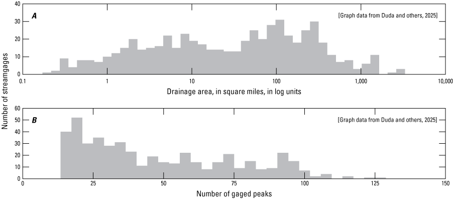
Histograms showing numbers of streamgages in and near Virginia and West Virginia included in flood−frequency regression equations, binned by A, drainage area classes and B, number of gaged annual peak streamflows.
The ecoregions were not necessarily continuous. Some residuals indicated that islands of ecoregions, exemplified by isolated pockets of the Ridge and Valley and Blue Ridge ecoregions surrounded by the Central Appalachians, Piedmont, or Northern Piedmont ecoregions, were not predictive, so regional boundaries were moved from the ecoregion border to nearby basin divides from the Watershed Boundary Dataset (WBD) (U.S. Geological Survey, 2023b). A series of regional regressions were developed for the 0.01-AEP (100-year) streamflows. They were tested in turn, and regional borders were refined to include streamgage basins with similar residuals, by adjusting the border to the HUC 8 border nearest the ecoregion border. Clusters of streamgages with similar regression residuals were grouped. Regions were reviewed on an interactive map, graphically assessed, and tested for significance as a categorical variable against the wider region. This process resulted in 12 regions (fig. 12; table 6). Many of the hydrologic region names are similar to ecoregion or physiographic province names. For clarity, the hydrologic regions are referred to by abbreviations, while the full name of ecoregions or physiographic provinces is used when discussing the ecoregion or province.
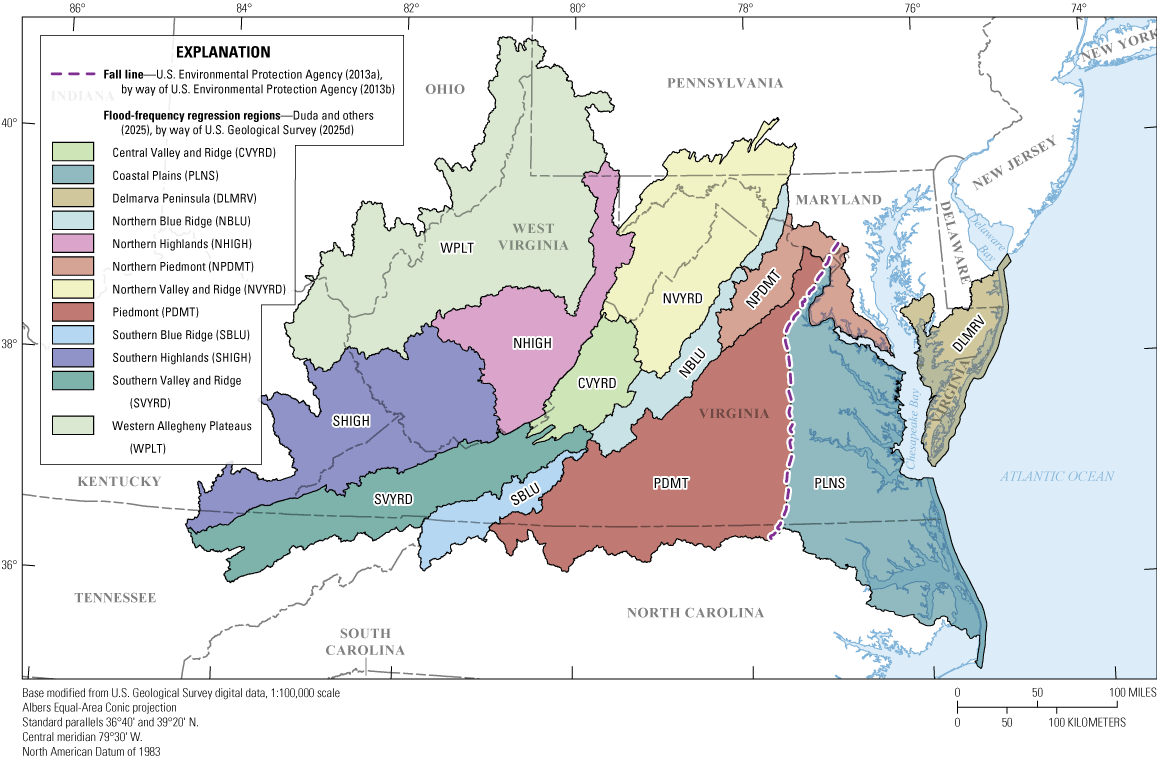
Map showing flood-frequency regression regions in and near Virginia and West Virginia.
Table 6.
Names, abbreviations, figure codes, numbers of streamgages, weighted-multiple-linear regression program input parameters, and valid range limits for flood-frequency regression regions in Virginia and West Virginia (modified from Duda and others, 2025).[WREG, weighted-multiple-linear regression program; mi2, square mile]
Regional boundaries were adjusted to the nearest HUC 8 borders, but there were several exceptions. The largest differences were that the entire Tygart Valley River Basin was included in Western Allegheny Plateaus (WPLT); the Cheat and Greenbrier River Basins were included in Northern Highlands (NHIGH), although large parts of their drainages are within the Ridge and Valley L3 ecoregion; parts of the Central Appalachians L3 ecoregion in the Potomac River Basin were included in Northern Valley and Ridge (NVYRD); areas of the Northern Piedmont L3 ecoregion are included in the Northern Blue Ridge (NBLU); the Delmarva Peninsula is a separate region, DLMRV; the part of the Middle Atlantic Coastal Plain ecoregion outside the Delmarva Peninsula is combined with most of the Southern Plains ecoregion in Coastal Plains (PLNS); and areas around Washington, D.C., and in northern Maryland with flood characteristics similar to the Northern Piedmont region but in the Middle Atlantic Coastal Plain were included in the Northern Piedmont (NPDMT).
The L3 ecoregion boundary between (1) the Piedmont and Northern Piedmont ecoregions and (2) the Southeast Plains ecoregion is a natural feature, the Fall Line. It was used as the boundary between the Piedmont and Costal Plains regions without adjustments. The Fall Line was an appropriate boundary because the differences in topography and stream channel slope and the sinuosity between the regions were likely to cause the differences in flood characteristics between the regions. Too many streams in this region formed in the Piedmont and drained across the Fall Line into the Coastal Plain region to make basin borders feasible as regional borders.
Although most of the regional boundaries in the Tennessee River Basin were adjusted to HUC 8 boundaries, tributaries of the Powell River in Southern Highlands (SHIGH) had flood histories and flood characteristics similar to SHIGH. The border between SHIGH and Southern Valley and Ridge (SVYRD) was adjusted by the 12-digit hydrologic unit code (HUC 12) borders so that these streams were included in SHIGH. The Bluestone River Basin drains both SVYRD and SHIGH. The regional border through the Bluestone River Basin follows the ecoregion border. Streamgages were included in the region that included the majority of their drainage area.
Three hydrologic regions that were developed from L3 ecoregions were split. The Blue Ridge was split into the NBLU and Southern Blue Ridge (SBLU) regions at the discontinuity in the Blue Ridge L3 ecoregion (figs. 4 and 12). Streamgages from the New, Tennessee, and part of the Roanoke River Basins were included in SBLU, while streamgages from the rest of the Roanoke River Basin and the James, Rappahannock, and Potomac River Basins were included in NBLU. The Ridge and Valley ecoregion was split into NVYRD, CVYRD, and SVYRD. Streamgages from the Potomac River Basin were included in NVYRD; streamgages from the James River Basin were included in the CVYRD; and streamgages from the Roanoke, New, and Tennessee River Basins were included in the SVYRD. The Central Appalachians ecoregion was split into NHIGH and SHIGH. The centerline of the New and Kanawha Rivers divides the two regions. The NHIGH includes the Cheat, Greenbrier, Gauley, and Elk River Basins, and tributaries to the New and Kanawha Rivers that enter from the right descending bank. The SHIGH includes part or all of the Bluestone, Coal, Guyandotte, Big Sandy, Kentucky, Cumberland, and Powell River Basins, and tributaries to the New and Kanawha Rivers that enter from the left descending bank.
Some streamgages in the extended study area were evaluated for the regressions and ultimately excluded because the results made the regression diagnostics worse for their prospective region, and the streamgages were on streams that drained away from the core study area. These included some streamgages in the Yadkin River Basin in North Carolina and the Cumberland River Basin in Kentucky, and all streamgages in the Youghiogheny River Basin in Maryland and Pennsylvania. Streamgages in HUC 8s adjacent to Virginia in the Cumberland and Kentucky River Basins were included in exploratory regressions. Neither basin drains any area in Virginia. Streamgage records from these HUC8s were retrieved, frequencies were computed, and streamflows were examined in preliminary regression analysis; there were no apparent graphical differences between the Cumberland and Kentucky River Basins and the rest of SHIGH. Testing these basins as a categorical variable against the rest of SHIGH found differences were not significant (p-value=0.778 and n=8 for Kentucky; p-value=0.556 and n=12 for Cumberland). The Cumberland River Basin included three streamgages in the Southern Appalachians L3 ecoregion; they were included in SHIGH for exploratory analysis but excluded from the final regressions.
For the Yadkin River Basin, three headwater streamgages that drain substantial amounts of Virginia were included in the Piedmont region. Streamgages further downstream from the North Carolina and Virginia border, with less than half of their basins in Virginia, when included, made regression diagnostics worse for their regions, and they were excluded from the final equations.
All 15 streamgages with valid unregulated frequency analyses in the Youghiogheny River Basin were excluded from the regressions for the Central Appalachian Highlands and Western Allegheny Plateaus ecoregions. The slope of an OLS regression for that specific area was significantly different from the slope of an OLS regression for the rest of the region, suggesting they would be part of a different region had the study area included more of Maryland and Pennsylvania (p-value=0.006). None of the streamgage basins had a 50 percent drainage area within West Virginia. Flood statistic estimates may be made for the part of West Virginia drained by the Youghiogheny River using the NHIGH regional equations, although with unknown errors. Users may compare the estimates for this area to estimates made using Maryland or Pennsylvania regression equations.
A broad suite of basin characteristics discussed previously was condensed to a subset of 15 basin characteristics thought to be relevant to stream flood characteristics while minimizing cross-correlation among variables. The subset of basin characteristics was tested as potential independent variables for each of the regions. None were significant as independent variables, largely because the characteristics were homogeneous within regions developed from regression residuals (fig. DR–1 of Duda and others, 2025).
The percentage of carbonate rock in the three Valley and Ridge regions was examined closely for threshold effects, which might serve as criteria for numeric valid range limits for regressions. No threshold effects were found. Streamgages with greater percentages of carbonate rock may have had higher regression residuals than streamgages draining lesser percentages of carbonate rock, but they included nearly equal numbers of positive and negative values. Streams in karst areas exchange flow with groundwater in cave and sinkhole systems; streams may either gain or lose streamflow to groundwater and affect peak streamflows. The geospatial data available to characterize carbonate rock in a consistent manner throughout the study area lacked the detail that would allow reaches that gained or lost streamflow to be analyzed separately. However, geospatial datasets that characterize karst sinkholes that were recently published or in development during this study have the potential to be valuable covariate data in future flood-frequency studies (Virginia Department of Energy, Geology and Mineral Resources Program, 2023; Shank, 2024; Ladd, 2025). These datasets, as well as geological maps that depicted sinkholes (Brezinski, 2014; Brezinski and others, 2021), were used to characterize five influential observations in Valley and Ridge regions that were ultimately excluded from regression analysis because of apparent flow loss through sinkholes (table 1 in Duda and others, 2025).
Development, as a land-cover class, was also examined closely for threshold effects, which has been discussed in the “Time Trends in Flood Magnitudes” section. Streamgages on streams that drained 30 percent or more developed land, as the sum of all development classes in the 2019 NLCD, tended to have larger regression residuals than other streamgages in the same regions, including both negative and positive residual values. Austin (2014) identified a threshold value of 30 percent development for Virginia for excluding urbanized basins from rural regressions, and this study did not find clear evidence that a different threshold was appreciably better. All streamgages at the outlets of basins that were 30 percent or more developed in 2019 were excluded from regressions (fig. 6; table 1 in Duda and others, 2025).
Streamgages with high leverage were removed from the regressions if they were unrepresentative of the regional conditions the regression equations are intended to model. Streamgages that drained more than 3,000 mi2 were removed from regressions; these included main stem streamgages on the Potomac, Shenandoah, Roanoke, Monongahela, Big Sandy, Holston, James, Roanoke, Kanawha, and New Rivers. Streamgages that drained less than 0.2 mi2 were all excluded because all of them had high leverage; most of them had high influence relative to their region; there were not enough of them in any single region to say whether they were representative of all small streams in the region; and other methods are available to estimate flood characteristics in streams that drain less than 0.20 mi2. In general, excluding them reduced measures of variance for the regressions. The exception was the Coastal Plains region, which included a group of 4 streamgages that drained between 0.008 and 0.041 mi2. As a group, they had large leverage on the regional regression equation, but when plotted, they were close to a regression line extended from streamgages that drained larger areas, indicating that this group unduly reduced measures of regression variance. They were excluded because they were unrepresentative of regional conditions; all were within a small area, the Richmond, Va. metropolitan area; drained basins more than an order of magnitude smaller than the next smallest streamgage in the region (0.99 mi2); and because they were on small streams that required different methodology than the rest of the streamgaging network (Hayes and Young, 2005).
Checks on regionalization included the examination of measured quantile compared to predicted quantile plots (plots of residuals compared to expected quantiles), plotting residuals against fitted values and the independent variable, investigating streamgages with the highest Cook’s distance values and largest residuals relative to their prospective region for errors in streamflow records and basin characteristics, checking for spatial clusters of streamgages with similar high or low residuals, and iterative review of residuals from regional regressions in interactive maps. When regions had been defined for the 0.01 AEP (100-year flood), regression equations were developed for the 0.2 AEP (5-year flood), and the same set of checks was performed for them. In every region, regression equations for the 0.2 AEP (5-year flood) had less variance than did the equation for the 0.01 AEP (100-year flood).
Development of and Accuracy of Generalized Least-Squares Regression Equations
GLS multiple-linear regression (Stedinger and Tasker, 1985; Tasker and Stedinger, 1989; Farmer and others, 2019) was used to determine the final coefficients and performance metrics for the regional regression equations. GLS regressions were developed for the 0.5, 0.2, 0.1, 0.04, 0.02, 0.01, 0.005, and 0.002 AEPs (2-, 5-, 10-, 25-, 50-, 100-, 200-, and 500-year floods) for the 12 regions with drainage area as the only independent variable (tables 6 and 7; tables 16 and 18 in Duda and others, 2025; fig. 13). GLS regression techniques are preferred for regionalization of streamflow-frequency statistics because they improve estimates of streamflows and accuracy of the regression model by accounting for (1) unequal record lengths from streamgages and (2) cross-correlation of streamflow statistics from streamgages (Farmer and others, 2019, p. 18). Streamgages with shorter records are given less weight than streamgages with longer records. Additionally, less weight is given to streamgages where concurrent peak streamflows are correlated with nearby streamgages.
Table 7.
Regional generalized least-squares regression constants, coefficients, and regression equations for selected annual exceedance probabilities in Virginia and West Virginia.[AEP, annual exceedance probability; WPLT, Western Alleghany Plateaus; NHIGH, Northern Highlands; SHIGH, Southern Highlands; NVYRD, Northern Valley and Ridge; CVYRD, Central Valley and Ridge; SVYRD, Southern Valley and Ridge; NBLU, Northern Blue Ridge; SBLU, Southern Blue Ridge; PDMT, Piedmont; NPDMT, Northern Piedmont; PLNS, Coastal Plains; DLMRV, Delmarva Peninsula; log10, base-10 logarithm; DRNAREA, drainage area in square miles]
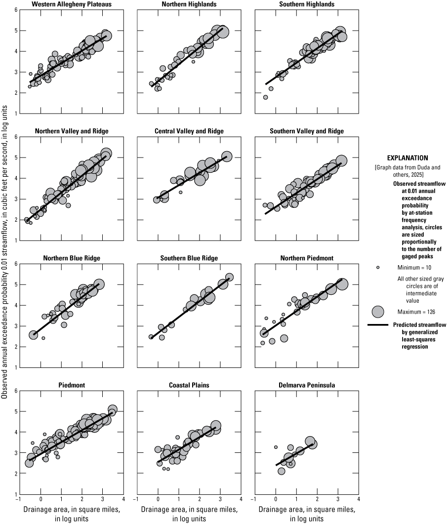
Graphs showing relation of 0.01 annual exceedance probability streamflows and drainage area among selected streamgages in and near Virginia and West Virginia, shown by flood-frequency region, including generalized least-squares regression lines.
Based on results from the OLS analysis, explanatory and response variables were log-transformed prior to use in the GLS regression analysis. The weighted-multiple-linear regression (WREG) program (Farmer, 2021), written in the R programming language (R Core Team, 2021), was used to compute the final GLS equations and model performance metrics. Default values of alpha and theta, the correlation-smoothing parameters in the weighted-multiple-linear regression program, were adjusted for each regional regression equation to improve model fit (table 6). The range of drainage areas used to develop the equations for each region is also given in table 6; the smallest valid drainage area in any region is 0.21 mi2, and the largest valid drainage area in any region is 2,966 mi2.
Scatterplots of observed and predicted values filtered by region were examined to assess the fit of the regression equations (fig. 14). Most regions had a good fit, although for PLNS, NPDMT, SVYRD, and possibly CVYRD, the fit was only fair and was better for larger magnitudes of observed and predicted values than for smaller magnitudes. The fit for DLMRV was poor, which was expected because of the poor performance metrics of the regression. Plots of residuals and predicted values generally indicated little unexplained structure, although the pattern of larger residuals, compared to smaller predicted streamflows, was observed for the same three regions—PLNS, NPDMT, and SVYRD—that had a worse fit for smaller than larger predicted streamflows, as did DLMRV. Measured quantile compared to predicted quantile plots were generally linear with some exceptions of for one to three points. The exceptions were NBLU, with a concave downward distribution; SVYRD and NPDMT, which indicated departures at both ends of the plot, and DLMRV, which indicated a poor fit.
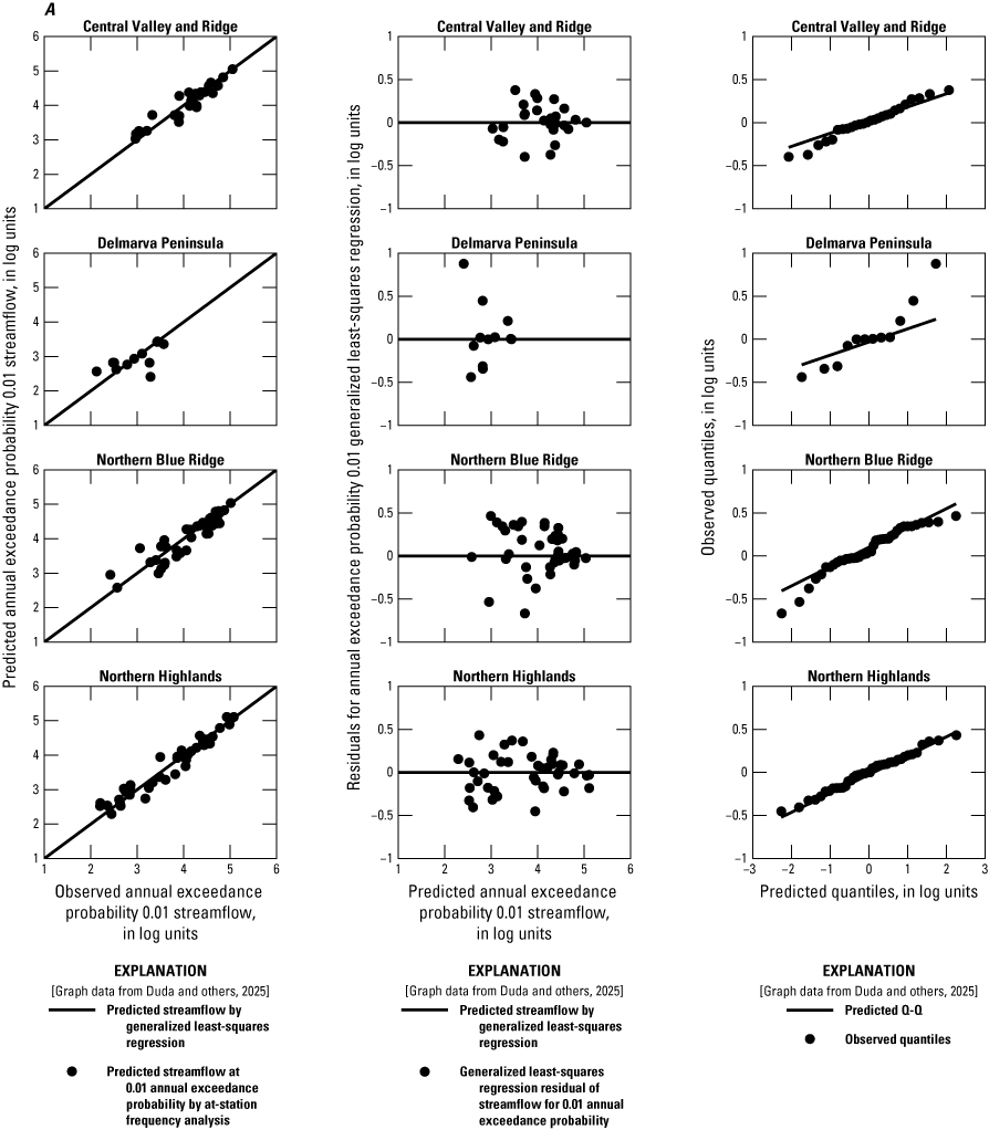
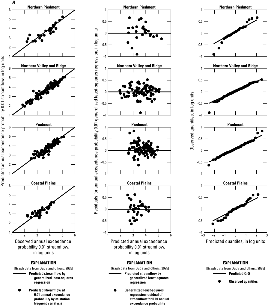
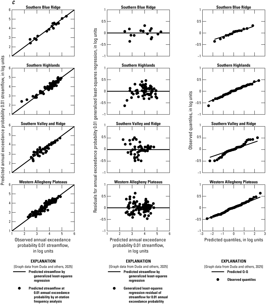
Graph showing generalized least-squares regression diagnostic plots for the 0.01 annual exceedance probability streamflow for A, for the Central Valley and Ridge, Delmarva Peninsula, Northern Blue Ridge, and Northern Highlands; B, for the Northern Piedmont, Northern Valley and Ridge, Piedmont, and Coastal Plains; and C, for the Southern Blue Ridge, Southern Highlands, Southern Valley and Ridge, and Western Allegheny Plateaus flood-frequency regions in and near Virginia and West Virginia. Left column: relation of predicted with observed streamflows; middle column, regression residuals related to predicted values; third column, measured quantile compared to predicted quantile plot of regression residuals related to predicted quantiles.
Several performance metrics from the weighted-multiple-linear regression program can be used to evaluate the accuracy of the regression equations. Performance metrics for the final regression equations include the model error variance, the root mean square error, the pseudo coefficient of determination (pseudo-R2), the average variance of prediction (AVP), and the average standard error of prediction (table 8; table 18 in Duda and others, 2025). The model error variance and standard model error variance describe the portion of the total error that can be attributed to having an imperfect model, in log units and percent, respectively. The root mean square error and pseudo-R2 are measures of model accuracy for streamgages used in the model development. Root mean square error describes how much the predicted peak streamflows deviate from the observed peak streamflows. The pseudo-R2 is a measure of the predictive strength of the regression model and describes the variability of the response variable that is explained by the explanatory variables after accounting for the effect of time-sampling error. The pseudo-R2 is similar to the R2, where the closer the value is to 1.0 (or 100 percent), the greater the amount of variance that is explained by the regression. The AVP and the average standard error of prediction are measures of how well the regression model performs at predicting peak streamflows for ungaged sites not used to develop the regression equations—lower values indicate greater predictive power. Pseudo-R2 and AVP were the most important metrics for selecting the final regression equations. Equations for calculating these performance metrics are available in England and others (2018).
Table 8.
Selected performance metrics for generalized least-squares regional flood-frequency regression equations for Virginia and West Virginia.[AEP, Annual exceedance probability; VP, variance of prediction of the regression; AVP, average variance of prediction; MEV, model error variance; MSE, mean square error; R2_adj, adjusted coefficient of determination; R2_pseudo, pseudo coefficient of determination; RMSE, root mean square error; SEPavg, average standard error of prediction; WPLT, Western Allegheny Plateaus; NHIGH, Northern Highlands; SHIGH, Southern Highlands; NVYRD, Northern Valley and Ridge; CVYRD, Central Valley and Ridge; SVYRD, Southern Valley and Ridge; NBLU, Northern Blue Ridge; SBLU, Southern Blue Ridge; PDMT, Piedmont; NPDMT, Northern Piedmont; PLNS, Coastal Plains; DLMRV, Delmarva Peninsula]
The pseudo-R2 values for the final regression equations ranged from 0.481 percent (DLMRV; 0.002 AEP or 500-year flood) to 0.995 percent (SBLU; 0.5 AEP or 2-year flood) for all regions and AEPs. They ranged from 0.499 (DLMRV) to 0.968 percent (SBLU) for the 0.01-AEP (100-year) streamflows (table 8). The AVP values for the final regression equations ranged from 0.005 (SBLU; 0.5 AEP or 2-year flood) to 0.154 (NPDMT; 0.002 AEP or 500-year flood) for all regions and AEPs. They ranged from 0.026 (PDMT) to 0.115 (DLMRV) for the 0.01-AEP streamflows. The average standard error of prediction values ranged from 16.5 percent (SBLU; 0.5 AEP or 2-year flood) to 112 percent (NPDMT; 0.002 AEP or 500-year flood) for all regions and AEPs. Performance metrics were better for the statistics that characterize high-frequency floods than for those that characterize low-frequency floods; as an example, pseudo-R2 values for 0.5-AEP (2-year flood) streamflows, excluding DLMRV, ranged from 0.862 (PLNS) to 0.995 (SBLU), in contrast to values for 0.002-AEP (500-year flood) streamflows, that ranged from 0.662 (PLNS) to 0.951 (SBLU). Overall, the final regression models performed poorly for DLMRV, with a pseudo-R2 value of 0.4987 for the 0.01 AEP. They performed poorly to fairly well for NPDMT and PLNS, with pseudo-R2 values of 0.8212 and 0.7618, respectively, and well for all other regions, which had pseudo-R2 values ranging from 0.8725 to 0.9684 for the 0.01 AEP (Duda and others, 2025). Performance metrics for equations for NPDMT and PLNS show larger error terms than most of the study area and Ohio, Pennsylvania, and North Carolina (Koltun, 2019; Roland and Stuckey, 2019; Feaster and others, 2023). NPDMT and PLNS have fairly large error terms compared to many other studies, but pseudo-R2 is about the same as last cycle, and standard error of prediction is somewhat to substantially larger, as discussed in the “Changes in 0.01 AEP Streamflows Since Most Recent Studies” section. These are regions with high natural variation in peak streamflows, and large error terms may indicate this natural variability. However, many streamgages in NPDMT are on streams with unstable streambanks and streambeds that make ratings unstable and difficult to develop and maintain (Messinger and Burgholzer, 2018). Because of natural rating instability, streamflow data quality throughout the region is likely to be worse than in regions where streambanks and streambeds are stable. Streambanks and streambeds in PLNS are more stable than those in NPDMT, but collecting high-quality streamflow data in the low-gradient streams typical of the region is also difficult. Station records for influential streamgages in these regions did not show specific problems in streamgage operation or the quality of indirect streamflow and other flood measurements. The basins were representative of the region according to all available basin characteristics. Arbitrarily removing the most influential streamgages from these regression analyses would have improved the regression diagnostics but would be inappropriate without a specific reason (Helsel and others, 2020).
All equations for the DLMRV are poor. The most obvious option to improve DLMRV would have been to include streamgages from Delaware and Maryland farther from the core study area in the analysis. However, Delaware has recently published updated flood-frequency regressions that include most of the streamgages that are included in the DLMRV; expanding analysis of the Delmarva Peninsula would amount to repeating that study (Hammond and others, 2022). No compelling reason was evident to repeat that study. Flood-frequency and magnitude estimates for the Delmarva Peninsula may be made with the Delaware Coastal Plain regression equations from Hammond and others (2022; app. 3), which are intended to be added to the Virginia StreamStats application (U.S. Geological Survey, 2019).
Regression-Weighted Flood-Frequency Estimates and Confidence Limits at Gaged Sites
The uncertainty in a flood-frequency estimate can be reduced by computing a weighted average of the at-site estimate and the regional regression estimate; Bulletin 17C (England and others, 2018) describes a weighting method in which the log10 of the regression and at-site LP3 estimates are weighted inversely proportional to their respective variances. Qi is the estimated peak-flow statistic at site i, and Xi is the log-transformed variable. All subsequent operations are performed on the transformed variable Xi. The weighted estimate is calculated using variances as
where all X and V variables are in log10 units;Xweighted,i is the weighted estimate for site i;
Xsite,i is the at-site estimate at site i;
Xreg,i is the regional estimate at site i;
Vsite,i is the variance of the at-site estimate at site i; and
Vreg,i is the variance of the regional estimate at site i.
As described in another section of the report, “At-Site Frequency Analyses for Unregulated Streams,” PeakFQ uses the EMA to provide a direct fit of the log-Pearson Type III distribution, which includes an estimate of the variance Vsite,i corresponding to each computed AEP.
For independent Xsite,i and Xreg,i, the variance of the weighted estimate for site i is calculated (with all V variables in log10 units) as
whereConfidence intervals on the weighted estimate can also be calculated. For example, upper and lower 95 percent confidence limits on the weighted quantile estimate are calculated as
and note that Xweighted,i, Vweighted,i, and CIi must be calculated separately for each site i and for each AEP of interest.
Because of the difficulty in computing the sampling error variance, similar computations to those listed in equations 2, 3, and 4 can be used (with reduced accuracy) to compute weighted estimates and confidence limits for estimates at sites not used in model development. The only difference is that the average variance of prediction for the regression equations is substituted for Vreg. Regression-weighted estimates are provided for all streamgages where frequency analyses were computed, that were not used in valid regression analyses, estimates can be computed and for which valid regression estimates can be computed (table 19 in Duda and others, 2025).
Weighting Flood-Frequency Estimates at Ungaged Sites with Statistics from a Nearby Gage
A different method of combining information from gaged and ungaged streams is used for a location on an unregulated stream that is near a streamgage. If the drainage area of an ungaged site is between 50 and 150 percent of the drainage area of a gaged site on the same stream and flood-frequency characteristics have been or can be computed for the gaged site, then the following method of adjusting the estimated flood-peak streamflow of the ungaged site is available (Feaster and others, 2023; Mitchell and others, 2023):
whereQw(u) is the weighted estimate of peak streamflow for the selected P-percent AEP at the ungaged site, in cubic feet per second;
ΔA is the absolute value of the difference in drainage area between the gaged and ungaged sites, in square miles;
A(g) is the drainage area for the gaged site, in square miles;
Qr(g) is the peak-flow estimate derived from the applicable regional equations for the selected P-percent AEP at the gaged site, in cubic feet per second;
Qw(g) is the weighted estimate of peak streamflow for the selected P-percent AEP at the gaged site, in cubic feet per second; and
Qr(u) is the peak-flow estimate derived from the applicable regional equations for the selected P-percent AEP at the ungaged site, in cubic feet per second.
Changes in 0.01 AEP Streamflows Since Most Recent Studies
Changes in 0.01-AEP (100-year) peak streamflows computed for streamgages in frequency analyses for this study were compared with those available from the previous cycles of studies for Virginia and West Virginia. The last-cycle West Virginia study included streamgages from adjacent states including Virginia (Wiley and Atkins, 2010). In contrast, the last-cycle Virginia study was limited to streamgages inside Virginia (Austin and others, 2011). Comparisons were possible for 560 of the 813 streamgages with frequency analyses for unregulated streams; this cycle’s streamflows were compared to 360 last-cycle streamflows for Virginia and 236 for West Virginia; 36 of the 560 streamgages were included in both last-cycle studies (table 20 in Duda and others, 2025). Differences in frequency-derived estimates (Qfq) of the 0.01-AEP (100-year) peak streamflow ranged from −46 percent to 91 percent compared to streamflows from the West Virginia study and −84 percent to 269 percent compared to streamflows from the Virginia study, both in untransformed cubic feet per second (ft3/s). The overall average change in at-site Qfq was 2.3 percent for streamgages compared to the West Virginia study and 0.5 percent increase for streamgages compared to the Virginia study. The magnitude of differences was 20 percent or more for 38 of the 236 streamgages for which AEPs were computed in the West Virginia study, and 85 of the 360 streamgages for which AEPs were computed for the Virginia study.
Most of the largest differences in streamflows were observed at streamgages with 25 or fewer gaged peaks (fig. 15). Differences also tended to be larger among streamgages on smaller streams, although the individual streamgages with large differences also had short periods of record. Five of the 360 Virginia streamgages indicated differences greater than 100 percent; none of these had new data collected since 2011. All changes exceeding 100 percent were the result of differences in methodology, notably the greater emphasis in Bulletin 17C on historical peaks and the use of interval data, but also including updated regional skew.
Larger differences since last cycle were more likely to coincide with short record in some regression regions than others (fig. 16). In most regions, changes between weighted (Qw) estimates and unweighted estimates made through streamgage frequency analyses (Qfq) were similar.
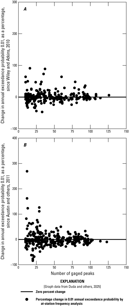
Graphs showing change in 0.01 annual exceedance probability from at-streamgage frequency analyses, as a percentage, among streamgages in and near Virginia and West Virginia compared to A, Wiley and Atkins (2010), for West Virginia flood frequency report and B, Austin and others (2011), for Virginia flood frequency report.
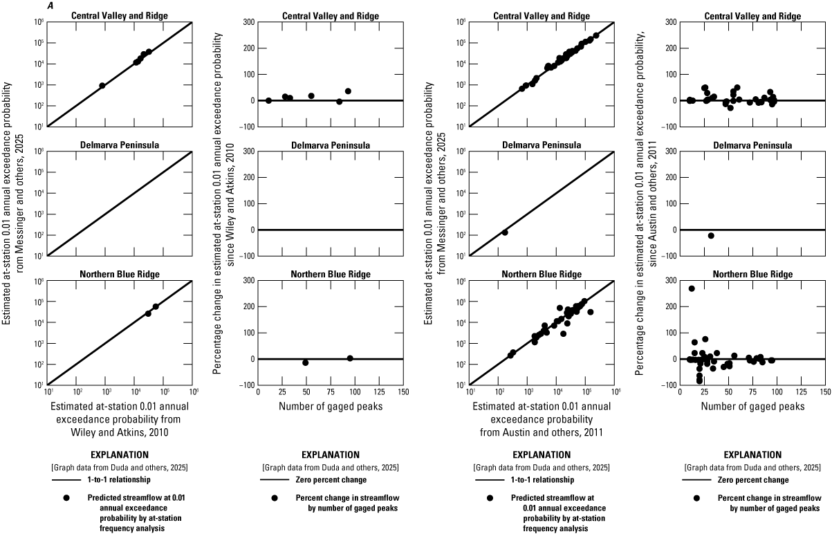
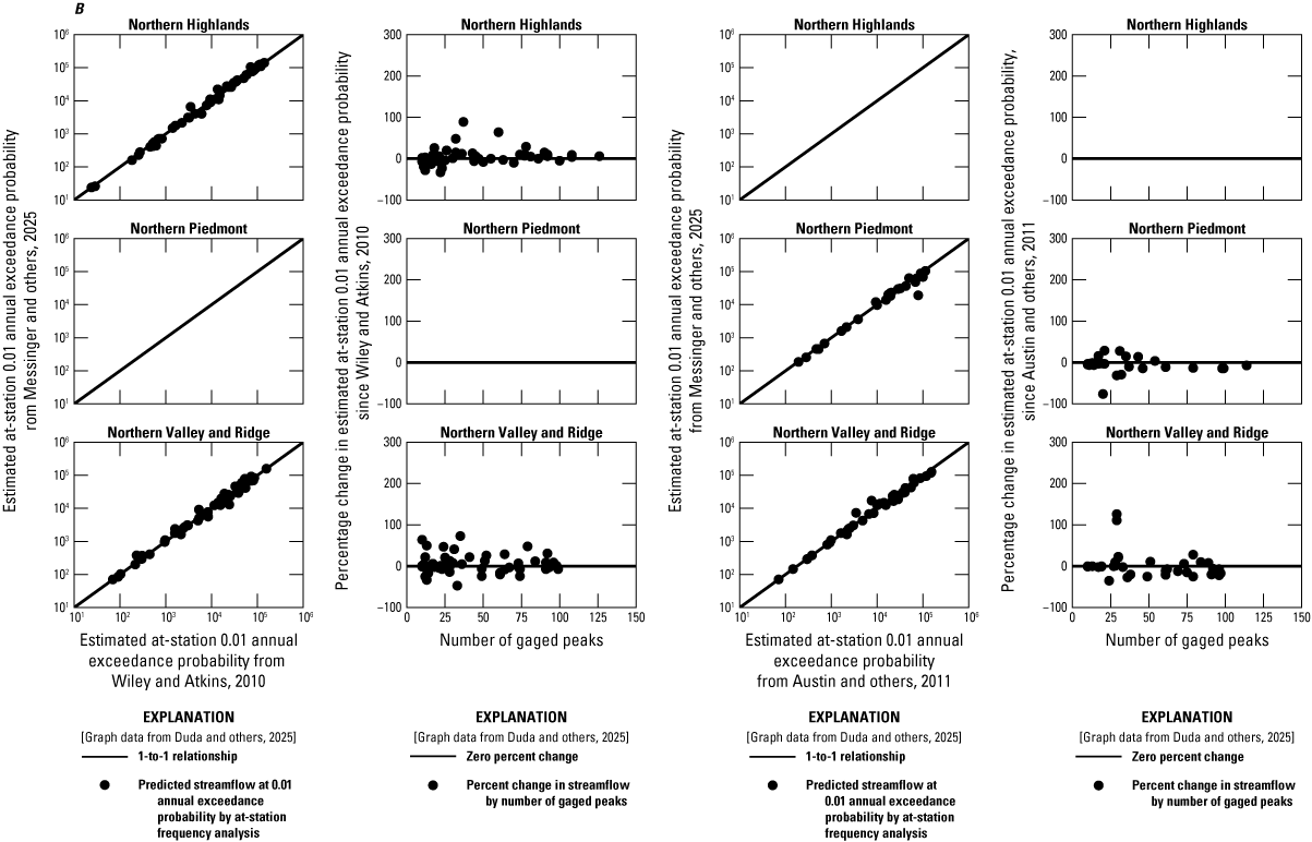
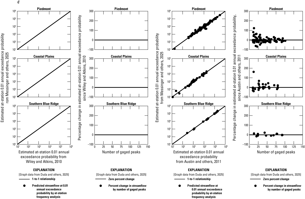
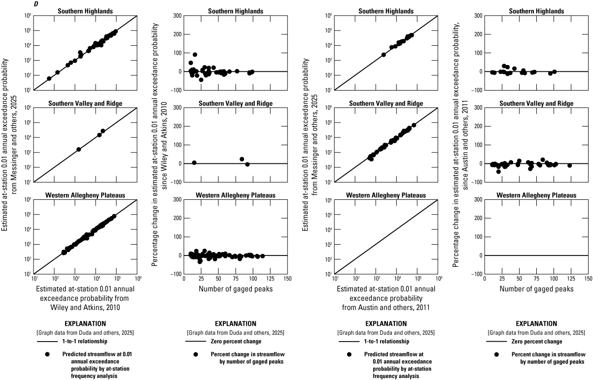
Graphs showing change in 0.01 annual exceedance probability, among streamgages within the A, Central Valley and Ridge, Delmarva Peninsula, and Northern Blue Ridge; B, Northern Highlands, Northern Piedmont, and Northern Valley and Ridge; C, Piedmont, Coastal Plains, and Southern Blue Ridge; D, Southern Highlands, Southern Valley and Ridge, and Western Allegheny Plateaus flood-frequency regions in and near Virginia and West Virginia compared to Wiley and Atkins (2010), frequency analysis as a scatterplot for West Virginia (leftmost column) and difference from Wiley and Atkins (2010), as a percentage relative to number of gaged peaks, for West Virginia (second column from left), and among streamgages in Virginia compared to Austin and others (2011), frequency analysis as a scatterplot for Virginia (third column from left), and difference from Austin and others (2011), as a percentage relative to number of gaged peaks for Virginia (rightmost column).
One of the 5 unregulated streamgages where the peak of record was established during the June 2016 flood increased 64 percent in the 0.01 AEP (100-year flood) for Qfq, but 2 decreased by >20 percent (table 20 in Duda and others, 2025). Three of the 6 streamgages where the peak of record was established in the October 2018 (water year 2019) flood increased >20 percent in Qfq., but 1 of the 6 decreased by 18 percent. For the rest of the streamgaging network, though, no unusual floods have been recorded since the last cycle. These patterns indicate that the changes are a result of changes in methodology from Bulletin 17B to Bulletin 17C, including the updated regional skew. Larger regional changes were observed in Virginia than in West Virginia, and a contributing factor may be that the last-cycle West Virginia study included regional skews updated according to Bulletin 17B methods (Atkins and others, 2009).
At-site changes in frequencies since the last cycle of flood-frequency studies are relevant for those streams, but changes in the regression equations are relevant for assessing changes to estimates on ungaged streams. Changes to estimates of AEP streamflows made from regression equations for hypothetical basins draining 5, 50, and 500 mi2 integrate differences in regional boundaries, updated flood-frequency computations including the updated regional skews, differences in regression equations between the two studies in the previous cycle, and data collected since the previous cycle (fig. 17).
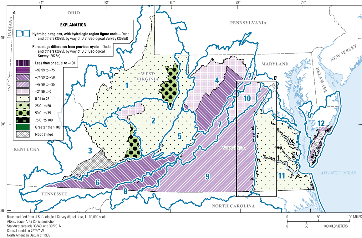
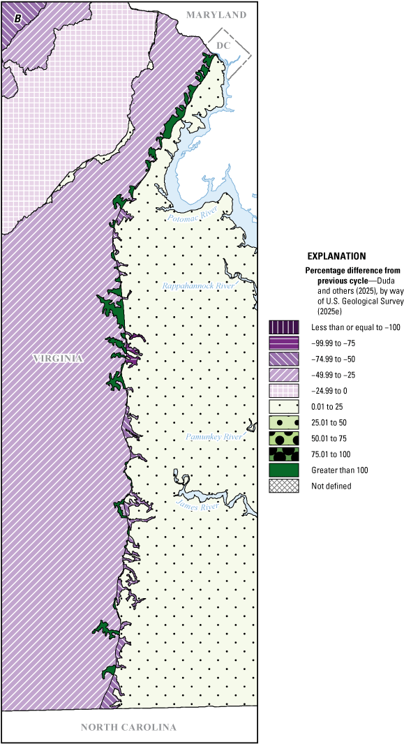
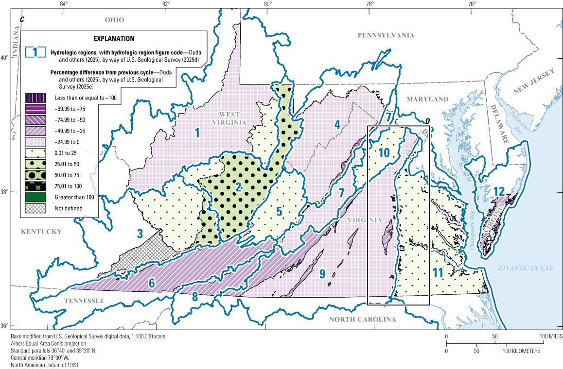
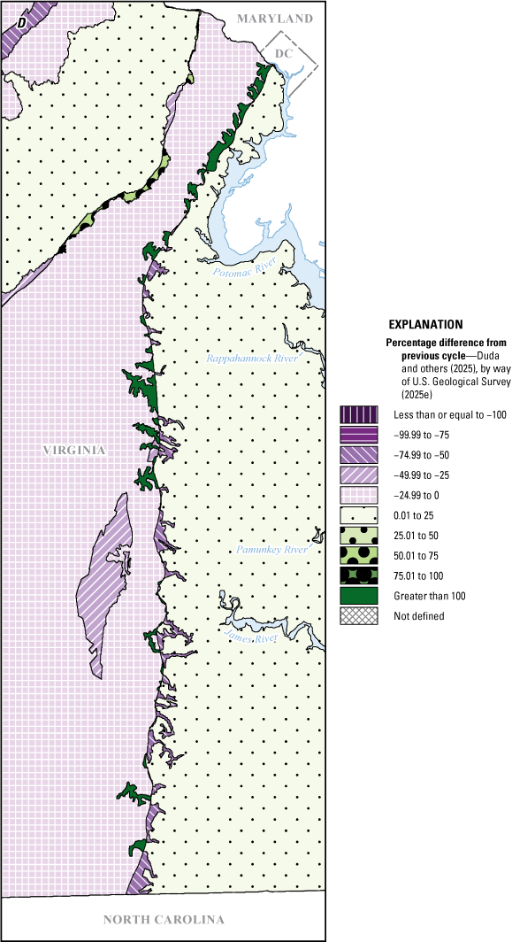
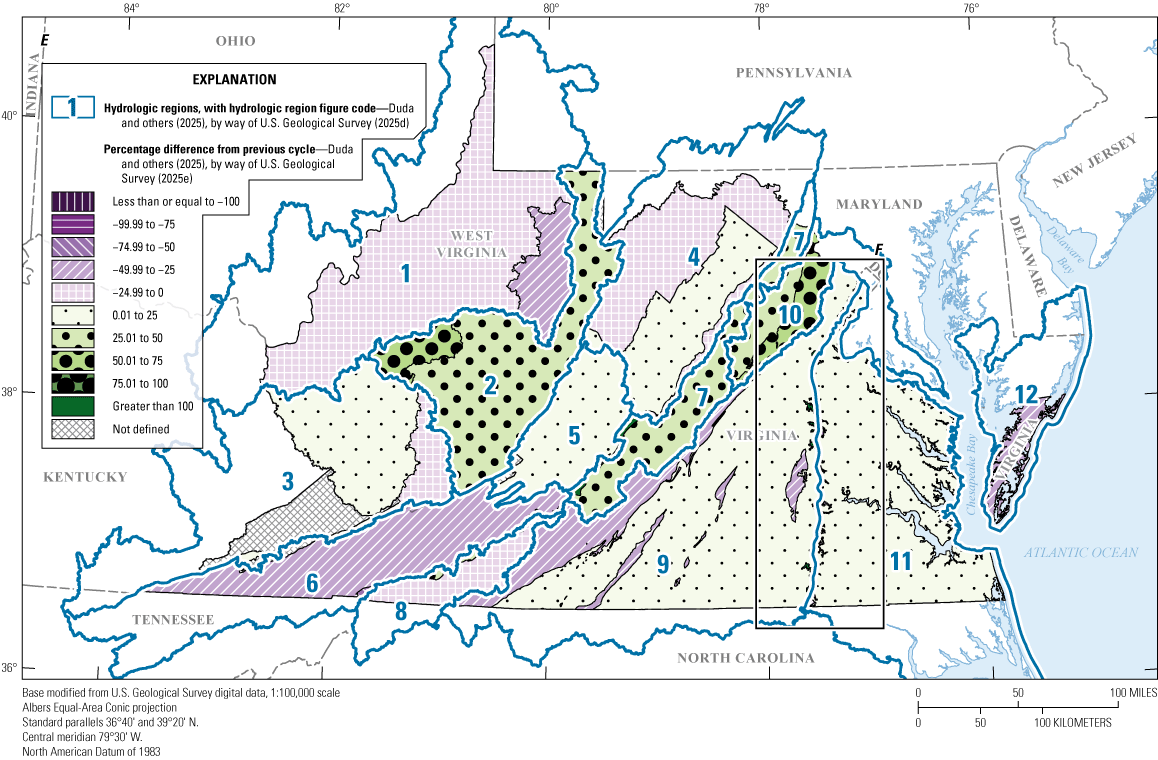
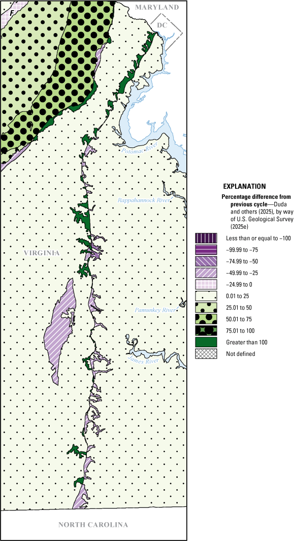
Map showing change in 0.01 annual exceedance probability streamflow estimated from regional regression equations from this study compared either to estimates from the equation from Wiley and Atkins (2010), in West Virginia, or Austin and others (2011), in Virginia, for A, a 5-square mile stream basin within Virginia or West Virginia. B, a 5-square mile basin along the Fall Line in Virginia. C, a 50-square mile basin within Virginia or West Virginia. D, a 50-square mile basin along the Fall Line in Virginia. E, a 500-square mile basin within Virginia or West Virginia. F, a 500-square mile basin along the Fall Line in Virginia.
Overall changes from the previous cycle for any areas solved for regional equations for the 0.01 AEP (100-year flood) solved for a hypothetical 50 mi2 basin range from 74 percent decrease to 129 percent increase (fig. 17B). Some of the largest magnitudes in changes from the previous cycle are areas that were transferred from the last-cycle Piedmont region into this-cycle PLNS region (60 percent decrease for the 117 mi2 that overlaps between the two regions overlap), last-cycle Mesozoic Basins region into this-cycle PLNS region (74 percent decrease for the 12 mi2 overlap), and the last-cycle Coastal Plain region into this-cycle PDMT (129 percent for the 126 mi2 overlap). The underlying change in regionalization along this border demonstrates the judgment that differences in stream pattern and channel slope drive the differences in flood streamflows between the Piedmont and Coastal Plain; therefore, the Fall Line is an appropriate regional boundary. Some of the other areas that experienced large magnitudes of changes include areas where the updated regional boundaries follow river basin boundaries instead of physiographic borders. These include parts of the Shenandoah River Basin that were part of the last-cycle Blue Ridge region but are now included in the NVYRD region (51 percent decrease for 422 mi2 overlap), and parts of the Roanoke and New River Basins that were formerly part of the last-cycle Blue Ridge region that are now part of the SVYRD region (63 percent decrease for 93 mi2 overlap).
Because regional boundaries in this study did not closely follow last-cycle boundaries, the size of the areas that have been split or reassigned from last-cycle regions varies greatly (table 9). The areas intersected by last-cycle and this-cycle regions range in size from 2 to 10,300 mi2. Large areas (>750 mi2) that have been split or reassigned from last-cycle regions represent smaller magnitudes of change since the last cycle than the smaller areas (fig. 17; table 9). Seventeen areas larger than 750 mi2 changed from one last-cycle region to one this-cycle region with regional equations defined for the 0.01 AEP. Using as a standard of comparison the regional equations for the 0.01 AEP (100-year flood) solved for a hypothetical 50 mi2 basin from figure 17B, percentage changes in areas larger than 750 mi2 ranged from a 30 percent increase to a 45 percent decrease. Six of these 17 areas changed by more than 20 percent among regional equations: an area that was in the last-cycle Virginia Valley and Ridge region and in the 2025 SVYRD region decreased by 44 percent; an area that was in the last-cycle Blue Ridge Region and the 2025 PDMT region decreased by 45 percent; an area that was in the last-cycle Blue Ridge region and the 2025 SBLU Region decreased by 40 percent; an area that was in the last-cycle Virginia Valley and Ridge region and the 2025 NVYRD regions decreased by 25 percent; and two regions that were in last cycle’s West Virginia Central Mountains region, one of which is in the 2025 NHIGH region and the other is in the 2025 SHIGH region increased by 30 and 26 percent, respectively. The other 11 areas >750 mi2 overlap changed by 20 percent or less since the last cycle.
Table 9.
Changes in estimates of the 0.01 annual exceedance probability annual peak flow from regional equations from the last flood-frequency cycle to this study in and near Virginia and West Virginia.[Last-cycle studies are for West Virginia, Wiley and Atkins (2010) (gray shading), and for Virginia, Austin and others (2011) (gold shading). This study is Duda and others (2025). mi2, square mile; AEP, annual exceedance probability; WPLT, Western Allegheny Plateaus; West Va., West Virginia; NHIGH, Northern Highlands; Va., Virginia; SHIGH, Southern Highlands; Not defined, the equation was not defined in previous cycle study; NVYRD, Northern Valley and Ridge; CVYRD, Central Valley and Ridge; SVYRD, Southern Valley and Ridge; NBLU, Northern Blue Ridge; SBLU, Southern Blue Ridge; PDMT, Piedmont; NPDMT, Northern Piedmont; PLNS, Coastal Plains; DLMRV, Delmarva Peninsula]
| 2025 region | Last-cycle region | Last-cycle study | Intersecting area (mi2) |
Percentage difference in streamflow predicted by the 0.01 AEP regression equations from last cycle and this cycle | ||
|---|---|---|---|---|---|---|
| Hypothetical 5 mi2 basin | Hypothetical 50 mi2 basin | Hypothetical 500 mi2 basin | ||||
| WPLT | Central Mountains | West Va.; Wiley and Atkins (2010) | 1,375 | 64 | 4 | −34 |
| WPLT | Western Plateaus | West Va.; Wiley and Atkins (2010) | 8,300 | 7 | −9 | −23 |
| NHIGH | Valley and Ridge | Va.; Austin and others, (2011) | 9 | −46 | −13 | 38 |
| NHIGH | Central Mountains | West Va.; Wiley and Atkins (2010) | 5,709 | 24 | 30 | 35 |
| NHIGH | Western Plateaus | West Va.; Wiley and Atkins (2010) | 756 | −19 | 13 | 58 |
| SHIGH | Valley and Ridge | Va.; Austin and others (2011) | 177 | −30 | −16 | 2 |
| SHIGH | Appalachian Plateau | Va.; Austin and others (2011) | 1,391 | Not defined | Not defined | Not defined |
| SHIGH | Central Mountains | West Va.; Wiley and Atkins (2010) | 885 | 60 | 26 | 0 |
| SHIGH | Western Plateaus | West Va.; Wiley and Atkins (2010) | 3,502 | 5 | 10 | 16 |
| NVYRD | Blue Ridge | Va.; Austin and others (2011) | 422 | −71 | −51 | −18 |
| NVYRD | Valley and Ridge | Va.; Austin and others (2011) | 2,962 | −53 | −25 | 19 |
| NVYRD | Eastern Panhandle | West Va.; Wiley and Atkins (2010) | 3,508 | −4 | −12 | −20 |
| CVYRD | Blue Ridge | Va.; Austin and others (2011) | 49 | −22 | −22 | −21 |
| CVYRD | Valley and Ridge | Va.; Austin and others (2011) | 2,731 | 25 | 20 | 15 |
| SVYRD | Blue Ridge | Va.; Austin and others (2011) | 93 | −69 | −63 | −56 |
| SVYRD | Valley and Ridge | Va.; Austin and others (2011) | 4,592 | −50 | −44 | −37 |
| SVYRD | Appalachian Plateau | Va.; Austin and others (2011) | 115 | Not defined | Not defined | Not defined |
| SVYRD | Central Mountains | West Va.; Wiley and Atkins (2010) | 38 | 14 | −16 | −38 |
| NBLU | Blue Ridge | Va.; Austin and others (2011) | 2,691 | −38 | −6 | 44 |
| NBLU | Valley and Ridge | Va.; Austin and others (2011) | 96 | −1 | 44 | 109 |
| NBLU | Piedmont Mesozoic | Va.; Austin and others (2011) | 2 | −44 | −2 | 69 |
| SBLU | Blue Ridge | Va.; Austin and others (2011) | 1,304 | −60 | −40 | −11 |
| SBLU | Valley and Ridge | Va.; Austin and others (2011) | 121 | −35 | −8 | 30 |
| PDMT | Coastal Plain | Va.; Austin and others (2011) | 126 | 133 | 129 | 126 |
| PDMT | Piedmont non-Mesozoic | Va.; Austin and others (2011) | 10,269 | −28 | −13 | 7 |
| PDMT | Blue Ridge | Va.; Austin and others (2011) | 1,928 | −43 | −45 | −47 |
| PDMT | Piedmont Mesozoic | Va.; Austin and others (2011) | 484 | −48 | −43 | −38 |
| NPDMT | Piedmont non-Mesozoic | Va.; Austin and others (2011) | 36 | 3 | 67 | 168 |
| NPDMT | Blue Ridge | Va.; Austin and others (2011) | 893 | −18 | 5 | 33 |
| NPDMT | Piedmont Mesozoic | Va.; Austin and others (2011) | 803 | −25 | 8 | 56 |
| PLNS | Coastal Plain | Va.; Austin and others (2011) | 7,882 | 0 | 4 | 8 |
| PLNS | Piedmont non-Mesozoic | Va.; Austin and others (2011) | 117 | −69 | −60 | −49 |
| PLNS | Piedmont Mesozoic | Va.; Austin and others (2011) | 12 | −78 | −74 | −70 |
| DLMRV | Coastal Plain | Va.; Austin and others (2011) | 674 | −34 | −35 | −36 |
| Maximum | — | — | 10,269 | 133 | 129 | 168 |
| Minimum | — | — | 2 | −78 | −74 | −70 |
| Median | — | — | 780 | −27 | −11 | 4 |
Regression equations were not defined for the part of West Virginia that drains to the James River (76 mi2) in the previous cycle (Wiley and Atkins, 2010). Although regression equations for some AEPs were defined for the part of Virginia in the Appalachian Plateaus physiographic province (1,391 mi2), the equation for the 0.01 AEP (100-year flood) was not defined in that report (Austin and others, 2011). This study did not define equations for the part of West Virginia that drains to the Youghiogheny River (72 mi2). No comparison was possible for these areas, and they are identified as undefined in figure 17.
Performance metrics for the regression equations were similar to or slightly larger than the performance metrics from the previous cycle in areas where the intersecting area was >400 mi2 (table 10). Exceptions included areas that were in the Virginia Blue Ridge region or the West Virginia Eastern Panhandle region during the last cycle; both last-cycle regions had unusually small uncertainty terms (33 and 21.7 percent standard error of prediction for the 0.01 AEP), in contrast to uncertainty terms this cycle that were about 46 percent or more. This cycle’s NPDMT and DLMRV regions also had large uncertainty terms in comparison to the last-cycle regions that they replaced; standard error of prediction for the 0.01-AEP equation for the NPDMT region increased to 91.9 percent from 33 percent for areas that had been in the last-cycle Blue Ridge region, and from 41 percent for areas that had been in the last-cycle Mesozoic Basins region.
Table 10.
Standard errors of prediction and pseudo coefficient of determination for regression regions from the previous studies compared with those in this study, in and near Virginia and West Virginia, through 2021, for flood-frequency regions with intersecting areas of 400 square miles or more.[Last-cycle studies are for West Virginia, Wiley and Atkins (2010) (gray shading), and for Virginia, Austin and others (2011) (gold shading). This study is Duda and others, 2025. SEP, standard error of prediction; AEP, annual exceedance probability; R2, coefficient of determination; WPLT, Western Allegheny Plateaus; NR, not reported; NHIGH, Northern Highlands; SHIGH, Southern Highlands; NVYRD, Northern Valley and Ridge; CVYRD, Central Valley and Ridge; SVYRD, Southern Valley and Ridge; NBLU, Northern Blue Ridge; SBLU, Southern Blue Ridge; PDMT, Piedmont; NPDMT, Northern Piedmont; PLNS, Coastal Plains; DLMRV, Delmarva Peninsula; NR]
Guidelines for Estimating Flood-Frequency Streamflows
Estimating procedures for the 0.5-, 0.2-, 0.1-, 0.04-, 0.02-, 0.01-, 0.005-, and 0.002-AEP flood streamflows were developed for streamgages and ungaged locations in Virginia and West Virginia. The method for estimating flood-frequency characteristics for sites on Virginia and West Virginia streams depends on the data available for the site of interest as follows:
-
1. If an estimate is needed at the location of a streamgage with 10 or more years of record, techniques described in Bulletin 17C (England and others, 2018) and this report will provide the best estimates. If the streamgage was analyzed for this report, the estimates may be looked up in table 19 in Duda and others (2025), or on StreamStats (U.S. Geological Survey, 2019). If peak streamflows are unregulated at the streamgage and the streamgage was not used to develop regression equations, the at-site frequency estimates can be improved by computing a weighted average with estimates determined from regional regression equations following the procedures described in Bulletin 17C, appendix 9 and the “Regression-Weighted Flood-Frequency Estimates and Confidence Limits at Gaged Sites” section in this report. If regression-weighted estimates (Qw) are available in table 19 of Duda and others (2025), they will be the best available at-site estimates. If they are not available, the at-site frequency estimates (the unweighted results of at-site frequency analyses, or Qfq) will be the best available at-site estimates. If 10 or more years of record have been collected at a streamgage after this report is published, flood-frequency estimates may be computed using techniques described in Bulletin 17C and weighted with estimates from the appropriate regression equations.
-
2. If an estimate is needed at an ungaged site that is within 50 and 150 percent of the drainage area of a nearby streamgage on the same unregulated stream for which flood-frequency streamflows have been or can be computed, then the best flood-frequency estimates can be made using the regional regression equations and then adjusted with equation 5 using data for the gaged site.
-
If an estimate is needed for an ungaged site that is between two streamgages on the same stream, both of which are within 50 and 150 percent of the drainage area of the ungaged site, two flow estimates can be made using equation 5. Professional judgment may be necessary to determine which of the estimates, or an interpolation of them, is most appropriate. Differences in the length of record among streamgages and whether the record at them includes known major floods on that stream are important to consider as part of assessing the streamgages.
-
3. If an estimate is needed for an ungaged site and no streamgages are nearby on the same unregulated stream, then flood-frequency estimates can be made by applying the regional regression equations from this report. This method is intended to be available in StreamStats upon publication of this report. The regression equations were developed using streamgages with 50 percent or more of their drainage area within a region. Flood characteristics for streams that drain multiple regions and 50 percent or more of their drainage area within a single region are to be estimated by applying the regional equation for that region. No streamgages were available within the valid range of drainage areas for the regression equations that drained multiple regions, all of which represented less than 50 percent of the drainage area, so it was not possible to test the most appropriate way to apply the regression equations; therefore, it is reasonable to make an area-weighted estimate for these streams using the different regional equations.
-
4. If an estimate is needed on a regulated stream near a streamgage for which regulated frequencies have been computed, estimates may be made using equation 5. Treatment of the regulated area in determining whether a site is near the streamgage may require judgment and obtaining information on the dams and streamgages in the basin. Depending on the purpose for the estimate, for instance, design of a project expected to remain in use longer than the dams in the basin, estimates of unregulated streamflows may be more appropriate than estimates of regulated streamflows.
-
5. If an estimate is needed for a stream that is not described in items 1–4 (for example, a site on a regulated stream with no nearby streamgage, or an ungaged site that has basin characteristics outside the valid range of independent variables for the region), then other methods must be used to estimate flood-frequency characteristics. The best method to use depends on the stream and basin characteristics, availability of data and resources, and the purpose for which the estimate is needed.
Examples of Estimation Procedures
The techniques for estimating peak discharges described in this report can be applied to four different situations:
-
1. A gaged location with at least 10 usable annual peak streamflows and was not used to develop the regional regression equations.
-
2. An ungaged location or a gaged location with less than 10 usable annual peaks near a streamgage for which peak-flow statistics have been or can be computed.
-
3. An ungaged location or a gaged location with less than 10 usable annual peaks not near a streamgage for which peak-flow statistics have been or can be computed.
Examples of these procedures are described below.
-
Example 1—Weighted Peak-Flow Estimate at a Gaged Location.—Calculate the 0.01-AEP (or 100-year flood) weighted peak streamflow (Qw) for a streamgage at Little Coal River at Julian, West Virginia (USGS site 03199400), with a basin centroid at latitude 37.9466 N and longitude 81.7492 W. U.S. Geological Survey site 03199400 has a drainage area (DRNAREA) of 318 mi2. From table 11 in Duda and others (2025), the development is 4.2 percent, and from table 7 in Duda and others (2025), the RI is 0.0007.
-
1. From table 19 in Duda and others (2025), a predicted 0.01-AEP (100-year) peak streamflow estimate (Qr) of 31,200 ft3/s (converted to 4.49 ft3/s log units) was computed using the appropriate regression equation for region SHIGH (table 7).
-
2. From table 8, the variance of prediction for the regression estimate is reported as 0.028 log units.
-
3. From table 4 in Duda and others (2025), the observed 0.01-AEP (100-year) at-site peak streamflow estimate (Qfq) and corresponding at-site variance of prediction (logVar0.01 in the table) are reported as 40,100 ft3/s (converted to 4.60 ft3/s log units) and 0.0275 log units, respectively.
-
4. Using equation 5, a weighted peak streamflow estimate in log units (Xw) can be computed as follows and converted to a weighted estimate of peak streamflow in ft3/s (Qw):
-
-
Example 2—Peak Flow Estimate with a Drainage Area Ratio.—An estimate of the 0.01-AEP (100-year) peak streamflow is needed for the location of the bridge over Anthony Creek on Forest Service Road 1219 at latitude 37.9192 N, longitude 80.2600 W, 2.2 road miles upstream from the streamgage at Anthony Creek near Anthony, West Virginia (USGS site 03182700). From StreamStats, the drainage area (DRNAREA) at the ungaged site is 136 mi2, which is more than 0.5×DRNAREA at USGS site 03182700, 143 mi2 (drainage area for the gaged site (A(g)) in equation 5). From StreamStats, 3.2 percent of the basin is developed, and the RI is <0.0001; the drainage area, percent development, and RI are all within the valid range of the regression equations. The entire basin is within the NHIGH regression region.
-
1. The absolute value of the difference in drainage area between the gaged and ungaged sites (ΔA) is 143 mi2–136 mi2=7 mi2.
-
2. Streamgage 03182700, Anthony Creek near Anthony Creek, was included in regression analysis. Regression-weighted at-site statistics would not be independent of the regression, so a weighted estimate of peak streamflow (Qw) is not available for this streamgage, and an at-site peak streamflow estimate (Qfq) is the best available flood-frequency statistic. From table 19 in Duda and others (2025), at-site peak streamflow at the gaged site (Qfq(g))=26,000 ft3/s and peak streamflow derived from the applicable regional equation at the gaged site (Qr(g))=20,900 ft3/s.
-
3. From the 0.01-AEP (100-year flood) regression equation for NHIGH, the peak streamflow derived from the regional equation at the ungaged site Qr(u)=19,800 ft3/s.
-
-
Example 3—Peak Streamflow Estimate with Regional Regression Equations.— Calculate the 0.01-AEP (100-year) peak streamflow using the regional regression equations (Qr) for an ungaged location at the mouth of Ellis Creek, a tributary to Flat Creek in the Appomattox River Basin, at latitude 37.2729 N and longitude 78.1802 W. From StreamStats, Ellis Creek has a drainage area (DRNAREA) of 7.54 mi2, is 4.3 percent developed in the 2019 NLCD, and the RI=0.0000. The basin is completely within the PDMT regression region and the valid range of all variables.
-
1. From table 7, the regional regression equation for the 0.01-AEP (100-year) peak streamflow in PDMT is:
-
2. Substitution of the basin characteristics into the equation produces:
StreamStats may be used to make estimates with the regional regression equations. If StreamStats is unavailable, the regression equations can be solved using other tools. Users who wish to use spreadsheet software may load table 16 from Duda and others (2025) in Microsoft Excel, LibreOffice Calc, or another spreadsheet, and copy the regression coefficients into formulas set up to solve the regression equations.
Limitations of Procedures for Estimating Flood-Frequency Streamflows
Procedures developed in this study are applicable only to rural, unregulated streams within the boundaries of Virginia and West Virginia. Procedures also are limited to the range of drainage areas used to develop the equations for each region, given in table 6; the smallest valid drainage area in any region is 0.21 mi2 and the largest valid drainage area in any region is 2,966 mi2.
Caution should be applied if flood-characteristic estimates are needed for urban areas with paved surfaces, concrete channels, or culverts that substantially alter runoff or infiltration. Streamgages used to develop regression equations drained basins that contained as much as 30 percent development from the 2019 NLCD (Dewitz and U.S. Geological Survey, 2021). However, annual peak data that were coded as affected by urbanization were excluded from the regressions and the equations published in this report are not valid for any basin that includes 30 percent or more developed area. For developed areas with between 10 and 30 percent development, users should compare results of the regression equations in this report to other available equations for estimating urban peak streamflows (Austin, 2014, for Virginia), and to investigate and consider local conditions.
The regional regression equations are not meant to be applied to streams that are regulated by dams or with large lakes and ponds that substantially retain runoff, measured by an RI greater than or equal to 0.0040. Procedures may not provide accurate estimates for extensively or intensively mined areas if excessive runoff is affected by landscape or subsurface alteration. Few streamgages were available to quantify the effects of large percentages of swamps within a basin; only two streamgages included in the PLNS region drained more than 20 percent of swamps, measured as the woody wetlands land cover class in the 2019 NLCD. Although DLMRV included 12 streamgages that drained 20 percent or more woody wetlands, the regression equations for DLMRV were poor, with pseudo-R2 values ranging from 0.481 to 0.558. Regression equations from this report may not provide accurate estimates for basins that drain 20 percent or more area in the woody wetlands NLCD class.
Regression procedures may not provide accurate estimates for karst areas if excessive runoff is diverted into, outside, or deep within the basin through solution channels or other cavities in carbonate rocks. Available geospatial data depict the presence of carbonate rock, but comprehensive, quantitative information on flow paths through karst is not available. Report users who have access to detailed local information on flow paths through solution openings in carbonate rock may be able to develop localized methods of estimating flood magnitude and frequency in specific karst areas that are more accurate than regression equations in this report. Uncertainty terms for Valley and Ridge regression equations are larger than for equations for some other regions, and some of that variability may result from gains and losses to streams underlain by carbonate rock.
Equations developed for the Delmarva Peninsula for this study are poor because only one streamgage has been operated in the part of the peninsula in Virginia and only a few streamgages have been operated in the southern Delmarva Peninsula. Equations recently developed for the Coastal Plain of Delaware include the streamgages in the southern Delmarva Peninsula (Hammond and others, 2022). The equations are expected to provide better estimates of flood statistics than the equations presented in this report. These equations are included in appendix 3 of this report and are intended to be integrated in the Virginia StreamStats application.
Improved methodology may become available for applying the regression equations and weighting the at-site statistics published in this report. New methods that are deployed to the Virginia and West Virginia StreamStats web applications will have been assessed by the USGS for use in many situations but might or might not meet the needs of all users. The methods described in this report are intended to be integrated in StreamStats as the default method for estimating flood characteristics for rural, unregulated streams in Virginia and West Virginia.
Summary
Magnitude and frequency of annual peak streamflows were computed for 813 streamgages on unregulated streams with a minimum of 10 years of uncensored systematic peaks through the 2021 water year in and near Virginia and West Virginia, and for 86 streamgages on regulated streams. The flood frequency streamflows at the 813 streamgages on rural, unregulated streams were determined following the guidelines established in Bulletin 17C (England and others, 2018). Regression equations were developed for use in estimating flood frequency and magnitude for rural, unregulated streams in and near Virginia and West Virginia. The study was done in cooperation with the Federal Emergency Management Agency, the West Virginia Department of Transportation, and the Virginia Department of Transportation.
The annual-peak series for 51 streamgages (about 12 percent of the 418 streamgages evaluated) indicated statistically significant (p-value [significance level] less than or equal to 0.05) trends, with 40 of these exhibiting positive trends and 11 exhibiting negative trends, at slightly more than twice as many streamgages as would be expected by chance. A significant positive trend alone was not a reliable indicator of urbanization; most streamgage basins with high development and long records had positive trends, but so did many streamgage basins with low or moderate development. The relationship was stronger among the streamgages with 50 or more gaged peaks and having 10 percent or more developed land in the basin (p-value<0.001; adjusted coefficient of determination=0.550). All 97 streamgages with 30 percent or greater development were ultimately excluded from final regression analysis in this study.
Frequency analyses were done with the U.S. Geological Survey computer program PeakFQ to compute station skew and flood-frequency streamflow estimates. Flow intervals were adjusted using historical peaks. Potentially influential low floods (PILFs) were excluded using the default multiple-Grubbs Beck test, and when it performed poorly in fitting the upper tail of the frequency curve, setting a manual PILF threshold. Of the 813 streamgages with unregulated frequency analyses, 160 streamgages had 1 or more historical peaks in the analysis. Frequency analyses censored PILFs for 176 streamgages, and the maximum number of PILFs at a streamgage was 60.
At-site skew values that were computed as part of initial frequency analysis were used to compute regional skew. To properly account for complications with frequency analyses and large cross-correlations between annual peak streamflows at pairs of streamgages, a Bayesian weighted least-squares/Bayesian generalized least-squares regression framework was developed to provide stable and defensible results for regional skew. Two unique skew regions were identified: Skew Region 1 encompassed streams in Virginia, West Virginia, and Maryland that drain to the Atlantic Ocean, including the eastern panhandle of West Virginia and most of western Maryland. A total of 114 streamgages that were not redundant and had a pseudo-record length of 50 years or greater were used to develop the final regional skew model for Skew Region 1. No covariates were significant, and a constant regional skew of 0.50 was selected. Skew Region 2 encompassed all the study area that flows to the Gulf of America, including Kentucky and Tennessee, most of West Virginia, far southwestern Virginia, and part of western Maryland. A total of 387 streamgages that were not redundant and had a pseudo-record length of 30 years or greater were used to develop the final regional skew model for Skew Region 2. No covariates were significant, and a constant regional skew of 0.048 was selected for Skew Region 2.
The regional skew values were used to perform final frequency analyses for streamgages on rural, unregulated streams. Frequency curves were weighted with regional skew values for streamgages with fewer than 30 gaged peaks. The original frequency analyses that used station skew without weighting were used for streamgages with 30 or more gaged peaks.
Redundant streamgages were identified by considering the distance between basin centroids, the drainage area of each streamgage in a pair and drainage area ratio, the record length and common years of each pair of streamgages, and the percentage of overlap between pairs of basins. Only members of pairs of streamgages with 50 percent or greater overlap were removed from regression analysis. Longer record was the first consideration in deciding which streamgage to keep from a pair. If the two streamgages had similar record lengths, the streamgage with a smaller basin was preferred; 111 streamgages were identified as redundant and removed from the analysis.
A set of 121 basin characteristics was developed from geospatial data to test as candidate predictor variables for multiple regression analysis. Correlation analysis was used to identify 15 uncorrelated basin characteristics with plausible effects on the magnitude and frequency of floods. No basin characteristics other than drainage areas were significant either at the scale of the entire study unit or within a region.
Twelve regions with homogeneous flood characteristics were identified through analysis of residuals from a regression of all streamgages. Streamgages with high leverage were removed from analysis, as were those that did not represent regional conditions; 565 streamgages were retained for use in the regression equations. Generalized least-squares regression equations between logarithmic-transformed drainage area and peak streamflow were developed for the 0.5, 0.2, 0.1, 0.04, 0.02, 0.01, 0.005, and 0.002 annual exceedance probabilities (AEPs) (2-, 5-, 10-, 25-, 50-, 100-, 200-, and 500-year floods). The range of drainage areas used to develop the equations differed for each region; the smallest valid drainage area in any region was 0.21 square miles and the largest valid drainage area in any region is 2,966 mi2. The pseudo coefficient of determination (pseudo-R2) values for the final regression equations ranged from 0.481 to 0.995 for all regions and AEPs. They ranged from 0.499 to 0.968 for the 0.01-AEP (100-year) peak streamflows. Regression performance metrics and diagnostic plots indicated that equations for 11 of the 12 regions showed generally good performance with pseudo-R2 values ranging from 0.762 to 0.968 for the 0.01 AEP. The exception, the equations for the Delmarva Peninsula, performed poorly with a pseudo-R2 value of 0.499 for the 0.01 AEP. Regression equations developed for the Coastal Plain of Delaware (Hammond and others, 2022) should be used to estimate flood characteristics for the Delmarva Peninsula.
The 0.01-AEP (100-year flood) peak streamflows computed for streamgages in frequency analyses for this study were compared with those from the previous cycle of studies. Differences in regression-weighted estimates of the 0.01-AEP (100-year flood) peak streamflow at individual streamgages ranged from −46 to 91 percent compared to streamflows from the West Virginia study and −84 to 269 percent compared to streamflows from the Virginia study, both in untransformed cubic feet per second. The overall average change in at-site differences in regression-weighted estimates was 2.3 percent for streamgages compared to the West Virginia study and 0.5 percent for streamgages compared to the Virginia study. The magnitude of differences was 20 percent or more for 38 of the 236 streamgages for which streamflows were computed in the West Virginia study, and 85 of the 360 streamgages for which streamflows were computed for the Virginia study. Most of the largest differences in streamflows were observed at streamgages with 25 or fewer gaged peaks, including streamgages that have been inactive since the last cycle; this indicates that much of the change between cycles is a result of changes in methodology. Overall changes from the previous cycle for regional equations for the 0.01 AEP (100-year flood) that were solved for a hypothetical 50 square miles basin ranged from a 30 percent increase to a 45 percent decrease, among areas where last-cycle and this-cycle regression regions overlapped by 750 square miles or more.
Frequency analyses were done at 86 streamgages on regulated streams. At-site skew was used for all the regulated streamgages. Regulation was determined using a regulation index that accounted for dam storage in the basin, drainage area of the dams, and drainage area at the streamgage. A value of 0.0040 or more for the regulation index indicates regulated peak streamflow.
Regression procedures developed in this study are applicable only to rural, unregulated streams within the boundaries of Virginia and West Virginia. Procedures are also limited to the range of drainage areas used to develop the equations for each region. The equations published in this report are not valid for any basin that includes 30 percent or more developed area or for any stream with a regulation index greater than 0.0040. Statistics and equations developed for this study are intended to be integrated in the Virginia and West Virginia StreamStats applications when this report is published.
References Cited
Atkins, J.T., Jr., Wiley, J.B., and Paybins, K.S., 2009, Generalized skew coefficients of annual peak flows for rural, unregulated streams in West Virginia: U.S. Geological Survey Open-File Report 2008–1304, 13 p., accessed October 30, 2023, at https://doi.org/10.3133/ofr20081304.
Austin, S.H., Krstolic, J.L., and Wiegand, U., 2011, Peak-flow characteristics of Virginia streams: U.S. Geological Survey Scientific Investigations Report 2011–5144, 106 p. plus 3 tables and 2 appendixes on CD, accessed October 30, 2023, at https://doi.org/10.3133/sir20115144.
Austin, S.H., 2014, Methods and equations for estimating peak streamflow per square mile in Virginia’s urban basins: U.S. Geological Survey Scientific Investigations Report 2014–5090, 25 p., accessed October 2023, at https://doi.org/10.3133/sir20145090.
Austin, S.H., Watson, K.M., Lotspeich, R.R., Cauller, S.J., White, J.S., and Wicklein, S.M., 2018, Characteristics of peak streamflows and extent of inundation in areas of West Virginia and southwestern Virginia affected by flooding, June 2016 (ver. 1.1, September 2018): U.S. Geological Survey Open-File Report 2017–1140, 35 p., accessed April 15, 2024, at https://doi.org/10.3133/ofr20171140.
Bailey, J.F., Patterson, J.L., and Paulhus, J.L.H., 1975, Hurricane Agnes rainfall and floods, June-July 1972: U.S. Geological Survey Professional Paper 924, 403 p., accessed October 30, 2023, at https://doi.org/10.3133/pp924.
Barne, H.H., Jr., 1963, Floods of March 1963, Alabama to West Virginia: U.S. Geological Survey Open-File Report 63–8, 44 p., accessed October 30, 2023, at https://doi.org/10.3133/ofr638.
Benson, M.A., 1962a, Evaluation of methods for evaluating the occurrence of floods, USGS Water Supply Paper 1580-A, 30 p., accessed May 30, 2023, at https://doi.org/10.3133/wsp1580A.
Benson, M.A., 1962b, Factors influencing the occurrence of floods in a humid region of diverse terrain: U.S. Geological Survey Water-Supply Paper 1580–B, 64 p., accessed October 30, 2023, at https://doi.org/10.3133/wsp1580B.
Beven, J.L., II, Berg, R., and Hagen, A., 2019, National hurricane center tropical cyclone report, Hurricane Michael (AL142018), 7–11 October 2018: National Oceanic Atmospheric Administration, National Weather Service, accessed April 16, 2024, at https://www.nhc.noaa.gov/data/tcr/AL142018_Michael.pdf.
Bisese, J.A., 1995, Methods for estimating the magnitude and frequency of peak discharges of rural, unregulated streams in Virginia: U.S. Geological Survey Water-Resources Investigations Report 94–4148, 70 p., accessed October 30, 2023, at https://doi.org/10.3133/wri944148.
Bonnin, G.M., Martin, D., Lin, B., Parzybok, T., Yekta, M., and Riley, D., 2006, Delaware, District of Columbia, Illinois, Indiana, Kentucky, Maryland, New Jersey, North Carolina, Ohio, Pennsylvania, South Carolina, Tennessee, Virginia, West Virginia, v. 2 of Precipitation-frequency atlas of the United States (ver. 3.0, 2006): National Oceanic and Atmospheric Administration, National Weather Service Atlas 14, 295 p. [Also available at https://www.weather.gov/media/owp/oh/hdsc/docs/Atlas14_Volume2.pdf.]
Brezinski, D.K., 2014, Geologic and karst features map of the Williamsport Quadrangle, Washington County, Maryland: Maryland Geological Survey Quadrangle Geologic Map, WILLI2014.1, 1:24,000. [Also available at http://discovery.mgs.md.gov/publications/data_pages/quadrangle_geo.html.]
Brezinski, D.K., Kavage Adams, R., and Connallon, C.B., 2021, Geologic map of Frederick and Washington Counties, Maryland: Maryland Geological Survey County Geologic Map, FredWashCoGeologyV1, 1:100,000. [Also available at http://discovery.mgs.md.gov/publications/map_pages/frederick_washington_co_geo_map.html ]
Camp, J.D., and Miller, E.M., 1970, Flood of 1969 in Virginia: U.S. Geological Survey Open-File Report 70–51, 120 p., accessed October 30, 2023, at https://doi.org/10.3133/ofr7051.
Carpenter, D.H., 1990, Floods in West Virginia, Virginia, Pennsylvania, and Maryland, November 1985: U.S. Geological Survey Water-Resources Investigations Report 88–4213, 86 p., accessed October 30, 2023, at https://doi.org/10.3133/wri884213.
Cohn, T.A., Lane, W.L., and Baier, W.G., 1997, An algorithm for computing moments-based flood quantile estimates when historical flood information is available: Water Resources Research, v. 33, no. 9, p. 2089–2096, accessed March 5, 2020, at https://doi.org/10.1029/97WR01640.
Dalrymple, T., 1960, Flood-frequency analyses; manual of hydrology--Part 3, flood-flow techniques: U.S. Geological Survey Water-Supply Paper 1543-A, 80 p., accessed May 30, 2023, at https://doi.org/10.3133/wsp1543A.
Dewitz, J., and U.S. Geological Survey, 2021, National Land Cover Database (NLCD) 2019 products (ver. 2.0, June 2021): U.S. Geological Survey data release, accessed December 12, 2023, at https://doi.org/10.5066/P9KZCM54.
Duda, J.M., Messinger, T., Scott, J.D., Kandel, C., Hamilton, W.B., and Hopkins, A.L., 2025, Data in support of estimation of magnitude and frequency of floods for rural, unregulated streams in and near Virginia and West Virginia: U.S. Geological Survey data release, https://doi.org/10.5066/P9RBZ8OJ.
Eng, K., Chen, Y.-Y., and Kiang, J.E., 2009, User’s guide to the weighted-multiple-linear-regression program (WREG ver. 1.0): U.S. Geological Survey Techniques and Methods, book 4, chap. A8, 21 p., accessed April 2023, at https://doi.org/10.3133/tm4A8.
England, J.F., Jr., Cohn, T.A., Faber, B.A., Stedinger, J.R., Thomas, W.O., Jr., Veilleux, A.G., Kiang, J.E., and Mason, R.R., Jr., 2018, Guidelines for determining flood flow frequency—Bulletin 17C (ver. 1.1, May 2019): U.S. Geological Survey Techniques and Methods, book 4, chap. B5, 148 p., accessed October 30, 2023, at https://doi.org/10.3133/tm4B5.
Esri, 2017, ArcGIS 10.6: Esri software release, accessed August 11, 2017, at https://www.esri.com/en-us/arcgis/products/arcgis-desktop/overview.
Esri, 2024, ArcGIS Pro 3.3.1: Esri software release, accessed October 2024, at https://www.esri.com/en-us/arcgis/products/arcgis-pro/overview.
Farmer, W.H., Kiang, J.E., Feaster, T.D., and Eng, K., 2019, Regionalization of surface-water statistics using multiple linear regression (ver. 1.1, February 2021): U.S. Geological Survey Techniques and Methods, book 4, chap. A12, 40 p., accessed March 23, 2023, at https://doi.org/10.3133/tm4A12.
Farmer, W.H., 2021, WREG: Weighted Least Squares Regression for Streamflow Frequency Statistics (ver. 3.00): U.S. Geological Survey software release, R package, Reston, Va., https://doi.org/10.5066/P9ZCGLI1.
Feaster, T.D., Gotvald, A.J., and Weaver, J.C., 2009, Magnitude and frequency of rural floods in the southeastern United States, 2006: Volume 3, South Carolina: U.S. Geological Survey Scientific Investigations Report 2009–5156, 226 p., accessed February 23, 2022, at https://doi.org/10.3133/sir20095156.
Feaster, T.D., Gotvald, A.J., Musser, J.W., Weaver, J.C., Kolb, K.R., Veilleux, A.G., and Wagner, D.M., 2023, Magnitude and frequency of floods for rural streams in Georgia, South Carolina, and North Carolina, 2017—Results: U.S. Geological Survey Scientific Investigations Report 2023–5006, 75 p., accessed October 2023, at https://doi.org/10.3133/sir20235006.
Flynn, K.M., Kirby, W.H., and Hummel, P.R., 2006, Users manual for PeakFQ, annual flood frequency analysis using Bulletin 17B Guidelines: U.S. Geological Survey Techniques and Methods Report Book 4, Chap. B4, 42 p., accessed August 2021, at https://pubs.usgs.gov/tm/2006/tm4b4/tm4b4.pdf.
Follansbee, R., 1953, A history of the Water Resources Branch, U.S. Geological Survey—Volume 2, years of increasing cooperation, July 1, 1919 to June 30, 1928: USGS Unnumbered Series, 202 p., accessed October 30, 2023, at https://doi.org/10.3133/70047297.
Follansbee, R., 1994, A history of the Water Resources Branch, U.S. Geological Survey—Volume 1, from predecessor surveys to June 30, 1919: USGS Unnumbered Series, 286 p., accessed October 30, 2023, at https://doi.org/10.3133/7000087.
Frye, P.M., and Runner, G.S., 1970, A proposed streamflow data program for West Virginia, U.S. Geological Survey Open-File Report, 38 p. https://doi.org/10.3133/ofr70132.
Griffith, G.E., Omernik, J.M., Comstock, J.A., Schafale, M.P., McNab, W.H., Lenat, D.R., MacPherson, T.F., Glover, J.B., and Shelburne, V.B., 2002, Ecoregions of North Carolina and South Carolina, (color poster with map, descriptive text, summary tables, and photographs): Reston, Va., U.S. Geological Survey, scale 1:1,500,000, accessed October 30, 2023, at https://web.archive.org/web/20170622154855/http://ecologicalregions.info/htm/ncsc_eco.htm.
Grover, N.C., Horton, A.H., and Stevens, G.C., 1925, Surface water supply of the New-Kanawha River Basin, West Virginia, Virginia, and North Carolina: U.S. Geological Survey Water-Supply Paper 536, 282 p., accessed October 30, 2023, at https://doi.org/10.3133/wsp536.
Grover, N.C., 1937, The floods of March 1936, Part 3, Potomac, James, and upper Ohio Rivers: U.S. Geological Survey Water-Supply Paper 800, 351 p., accessed November 15, 2023, at https://doi.org/10.3133/wsp800.
Hammond, J.C., Doheny, E.J., Dillow, J.J.A., Nardi, M.R., Steeves, P.A., and Warner, D.L., 2022, Peak-flow and low-flow magnitude estimates at defined frequencies and durations for nontidal streams in Delaware: U.S. Geological Survey Scientific Investigations Report 2022–5005, 46 p., accessed April 17, 2024, at https://doi.org/10.3133/sir20225005.
Harrel, F.H., and Dupont, C.T., 2023, Hmisc 5.1-1: accessed November 6, 2023, at https://hbiostat.org/r/hmisc/.
Hayes, D.C., and Young, R.L., 2005, Comparison of peak discharge and runoff characteristic estimates from the rational method to field observations for small basins in central Virginia: U.S. Geological Survey Scientific Investigations Report 2005–5254, 38 p. [Also available at https://pubs.usgs.gov/sir/2005/5254/sir05_5254.pdf.]
Helsel, D.R., Hirsch, R.M., Ryberg, K.R., Archfield, S.A., and Gilroy, E.J., 2020, Statistical methods in water resources: U.S. Geological Survey Techniques and Methods, book 4, chap. A3, 458 p., accessed August 2024, at https://doi.org/10.3133/tm4A3. [Supersedes USGS Techniques of Water-Resources Investigations, book 4, chapter A3, version 1.1.]
Hirsch, R.M., Slack, J.R., and Smith, R.A., 1982, Techniques of trend analysis for monthly water quality data: Water Resources Research, v. 18, no. 1, p. 107–121. https://doi.org/10.1029/WR018i001p00107.
Keaton, J.N., Messinger, T., and Doheny, E.J., 2005, Development and analysis of regional curves for streams in the non-urban Valley and Ridge Physiographic Province, Maryland, Virginia, and West Virginia: U.S. Geological Survey Scientific Investigations Report 2005–5076, 109 p., accessed November 15, 2023, at https://doi.org/10.3133/sir20055076.
Koltun, G.F., 2019, Flood-frequency estimates for Ohio streamgages based on data through water year 2015 and techniques for estimating flood-frequency characteristics of rural, unregulated Ohio streams: U.S. Geological Survey Scientific Investigations Report 2019–5018, 25 p., accessed October 30, 2023, at https://doi.org/10.3133/sir20195018.
Kottek, M., Grieser, J., Beck, C., Rudolf, B., and Rubel, F., 2006, World map of the Köppen-Geiger climate classification updated: Meteorologische Zeitschrift (Berlin), v. 15, no. 3, p. 259–263, accessed April 15, 2024, at https://doi.org/10.1127/0941-2948/2006/0130.
Ladd, D.E., 2025, Geospatial dataset of depressions, sinking streams, and associated watersheds in karst areas of Tennessee and parts of surrounding states: U.S. Geological Survey data release, accessed August 2024, at https://doi.org/10.5066/F74F1PZJ.
Lescinsky, J.B., 1987, Flood of November 1985 in West Virginia, Pennsylvania, Maryland, and Virginia: U.S. Geological Survey Open-File Report 86–486, 33 p., accessed November 15, 2023, at https://doi.org/10.3133/ofr86486.
Lotspeich, R.R., 2009, Regional curves of bankfull channel geometry for non-urban streams in the Piedmont Physiographic Province, Virginia: U.S. Geological Survey Scientific Investigations Report 2009–5206, 51 p., accessed November 15, 2023, at https://doi.org/10.3133/sir20095206.
Messinger, T., 2009, Regional curves for bankfull channel characteristics in the Appalachian Plateaus, West Virginia: U.S. Geological Survey Scientific Investigations Report 2009–5242, 43 p., accessed November 15, 2023, at https://doi.org/10.3133/sir20095242.
Messinger, T., and Burgholzer, R.W., 2018, Rating stability, and frequency and magnitude of shifts, for streamgages in Virginia through water year 2013: U.S. Geological Survey Scientific Investigations Report 2017–5137, 91 p., accessed October 9, 2024, at https://doi.org/10.3133/sir20175137.
Miller, E.M., 1969, Floods in Virginia—Magnitude and frequency: U.S. Geological Survey Open-File Report, 54 p. https://doi.org/10.3133/ofr69168
Mitchell, J.N., Wagner, D.M., and Veilleux, A.G., 2023, Magnitude and frequency of floods on Kauaʻi, Oʻahu, Molokaʻi, Maui, and Hawaiʻi, State of Hawaiʻi, based on data through water year 2020: U.S. Geological Survey Scientific Investigations Report 2023–5014, 66 p. plus 4 appendixes, accessed September 12, 2023, at https://doi.org/10.3133/sir20235014.
Omernik, J.M., 1987, Ecoregions of the conterminous United States: Annals of the Association of American Geographers, v. 77, no. 1, p. 118–125. https://doi.org/10.1111/j.1467-8306.1987.tb00149.x.
Parrett, C., Veilleux, A., Stedinger, J.R., Barth, N.A., Knifong, D.L., and Ferris, J.C., 2011, Regional skew for California, and flood frequency for selected sites in the Sacramento-San Joaquin River Basin, based on data through water year 2006: U.S. Geological Survey Scientific Investigations Report 2010–5260, 94 p., accessed April 16, 2024, at https://doi.org/10.3133/sir20105260.
PRISM Climate Group, 2021, PRISM 30-year normals—30-year normal precipitation, annual, 1991–2020: Corvallis, Oreg., Oregon State University, PRISM Climate Group web page, accessed November 14, 2023, at https://prism.oregonstate.edu/normals/.
R Core Team, 2021, R—A language and environment for statistical computing: Vienna, Austria, R Foundation for Statistical Computing, accessed September 11, 2023, at http://www.R-project.org/.
Reis, D.S., Jr., Stedinger, J.R., and Martins, E.S., 2005, Bayesian generalized least squares regression with application to the log Pearson type 3 regional skew estimation: Water Resources Research, v. 41, no. 10, article W10419, 14 p., accessed April 16, 2024, at https://doi.org/10.1029/2004WR003445.
Roland, M.A., and Stuckey, M.H., 2019, Development of regression equations for the estimation of flood flows at ungaged streams in Pennsylvania: U.S. Geological Survey Scientific Investigations Report 2019–5094, 36 p., accessed September 2023, at https://doi.org/10.3133/sir20195094.
Runner, G.S., 1979, Flood of April 1977 on the Tug Fork, Matewan to Williamson, West Virginia and Kentucky: U.S. Geological Survey Hydrologic Investigations Atlas HA–588, scale 1:12,000, accessed November 15, 2023, at https://doi.org/10.3133/ha588.
Runner, G.S., 1980, Technique for estimating magnitude and frequency of floods in West Virginia: U.S. Geological Survey Open-File Report 80–1218, 44 p., accessed November 15, 2023, at https://doi.org/10.3133/ofr801218.
Runner, G.S., and Chin, E.H., 1980, Flood of April 1977 in the Appalachian region of Kentucky, Tennessee, Virginia, and West Virginia: U.S. Geological Survey Professional Paper 1098, 43 p., accessed November 15, 2023, at https://pubs.usgs.gov/pp/1098/report.pdf.
Sando, S.K., and McCarthy, P.M., 2018, Methods for peak-flow frequency analysis and reporting for streamgages in or near Montana based on data through water year 2015: U.S. Geological Survey Scientific Investigations Report 2018–5046, 39 p., accessed December 15, 2025, at https://doi.org/10.3133/sir20185046.
Shank, M., 2024, Eastern Panhandle sink analysis: West Virginia Department of Environmental Protection data, accessed August 21, 2024, at https://tagis.dep.wv.gov/portal/apps/instant/minimalist/index.html?appid=ea0ad632a59d4110aa501e7ae1409141.
Speer, P.R., and Gamble, C.R., 1964a, Magnitude and frequency of floods in the United States, part 2-A, South Atlantic slope basins, James River to Savannah River: U.S. Geological Survey Water-Supply Paper 1673, 329 p., accessed May 30, 2023, at https://doi.org/10.3133/wsp1673.
Speer, P.R., and Gamble, C.R., 1964b, Magnitude and frequency of floods in the United States, part 3-B, Cumberland and Tennessee River Basins: U.S. Geological Survey Water-Supply Paper 1676, 340 p., accessed May 30, 2023, at https://doi.org/10.3133/wsp1676.
Speer, P.R., and Gamble, C.R., 1965, Magnitude and frequency of floods in the United States, part 3-A—Ohio River Basin except Cumberland and Tennessee River Basins: U.S. Geological Survey Water-Supply Paper 1675, 630 p., accessed November 15, 2023, at https://doi.org/10.3133/wsp1675.
Stedinger, J.R., and Tasker, G.D., 1985, Regional hydrologic analysis 1—Ordinary, weighted, and generalized least squares compared: Water Resources Research, v. 21, no. 9, p. 1421–1432. https://doi.org/10.1029/WR021i009p01421.
Stewart, S.R., 2004, Tropical cyclone report—Hurricane Ivan—2–24 September 2004: National Oceanic Atmospheric Administration, National Hurricane Center, accessed May 11, 2023, at https://www.nhc.noaa.gov/data/tcr/AL092004_Ivan.pdf.
Tasker, G.D., and Stedinger, J.R., 1986, Regional skew with weighted LS regression: Journal of Water Resources Planning and Management, v. 112, no. 2, p. 225–237, accessed April 16, 2024, at https://doi.org/10.1061/(ASCE)0733-9496(1986)112:2(225).
Tasker, G.D., and Stedinger, J.R., 1989, An operational GLS model for hydrologic regression: Journal of Hydrology, v. 111, nos. 1–4, p. 361–375, accessed December 1, 2021, at https://doi.org/10.1016/0022-1694(89)90268-0.
Tennessee Valley Authority, 1961, Floods and flood control: Tennessee Valley Authority Technical Report No. 26, 302 p., accessed October 30, 2023, at https://www.nrc.gov/docs/ML0819/ML081910196.pdf. [Also available at https://web.archive.org/web/20170317080127/.]
Tice, R.H., 1954, Magnitude and frequency of floods in the Shenandoah Valley of Virginia: U.S. Geological Survey Open-File Report 54-314, 33 p., accessed May 30, 2023, at https://doi.org/10.3133/ofr54314.
Tice, R.H., 1968, Magnitude and frequency of floods in the United States; Part 1-B—North Atlantic Slope Basins, New York to York River: U.S. Geological Survey Water-Supply Paper 1672, 585 p., accessed November 15, 2023, at https://pubs.usgs.gov/publication/wsp1672.
U.S. Army Corps of Engineers, 2024, National inventory of dams: U.S. Army Corps of Engineers database, accessed March 14, 2024, at https://nid.sec.usace.army.mil/.
U.S. Environmental Protection Agency, 2013, Level III and IV ecoregions of the continental United States: U.S. Environmental Protection Agency web page, accessed August 14, 2023, at https://www.epa.gov/eco-research/level-iii-and-iv-ecoregions-continental-united-states.
U.S. Geological Survey, 1949, Floods of August 1940 in the Southeastern States: U.S. Geological Survey Water-Supply Paper 1066, 554 p., accessed October 2023, at https://doi.org/10.3133/wsp1066.
U.S. Geological Survey, 1990, National water summary 1987—Hydrologic events and water supply and use: U.S. Geological Survey Water-Supply Paper 2350, 553 p., accessed October 30, 2023, at https://doi.org/10.3133/wsp2350.
U.S. Geological Survey, 2014, USGS small-scale dataset—1:1,000,000-scale state boundaries of the United States 201403 shapefile: U.S. Geological Survey dataset, accessed October 17, 2023, at https://www.sciencebase.gov/catalog/item/581d052de4b08da350d524e5.
U.S. Geological Survey, 2019, The StreamStats program, online at https://streamstats.usgs.gov/ss/.
U.S. Geological Survey, 2023a, Peak streamflow for the nation: U.S. Geological Survey National Water Information System database, accessed November 6, 2023, at https://doi.org/10.5066/F7P55KJN. [Peak streamflow information directly accessible at https://nwis.waterdata.usgs.gov/nwis/peak.]
U.S. Geological Survey, 2023b, The National Map: U.S. Geological Survey web page, accessed November 15, 2023, at https://www.usgs.gov/programs/national-geospatial-program/national-map.
U.S. Geological Survey, 2023c, USGS National Hydrography Dataset Best Resolution (NHD)— Virginia (published 20230505) shapefile, accessed October 2, 2023, at https://apps.nationalmap.gov/downloader/.
U.S. Geological Survey, 2023d, USGS Watershed Boundary Dataset (WBD)—National (published 20230327) FileGDB, accessed April 12, 2023, at https://apps.nationalmap.gov/downloader/.
U.S. Geological Survey, 2024, PeakFQ (ver. 7.5.1): U.S. Geological Survey software release, accessed March 14, 2024, at https://water.usgs.gov/software/PeakFQ/.
U.S. Water Resources Council, 1967, A uniform technique for determining flood flow frequencies: U.S. Water Resources Council Bulletin no. 15, 15 p., accessed May 6, 2025, at https://water.usgs.gov/osw/bulletin17b/Bulletin_15_1967.pdf.
Veilleux, A.G., Cohn, T.A., Flynn, K.M., Mason, R.R., Jr., and Hummel, P.R., 2014, Estimating magnitude and frequency of floods using the PeakFQ 7.0 program: U.S. Geological Survey Fact Sheet 2013–3108, 2 p., accessed October 30, 2023, at https://doi.org/10.3133/fs20133108.
Veilleux, A.G., and Wagner, D.M., 2019, Methods for estimating regional skewness of annual peak flows in parts of the Great Lakes and Ohio River Basins, based on data through water year 2013: U.S. Geological Survey Scientific Investigations Report 2019–5105, 26 p., accessed February 1, 2020, at https://doi.org/10.3133/sir20195105.
Veilleux, A.G., Zariello, P.J., Hodgkins, G.A., Ahearn, E.A., Olson, S.A., and Cohn, T.A., 2019, Methods for estimating regional coefficient of skewness for unregulated streams in New England, based on data through water year 2011: U.S. Geological Survey Scientific Investigations Report 2017–5037, 29 p., accessed April 2024, at https://doi.org/10.3133/sir20175037.
Veilleux, A.G., and Wagner, D.M., 2021, Methods for estimating regional skewness of annual peak flows in parts of eastern New York and Pennsylvania, based on data through water year 2013: U.S. Geological Survey Scientific Investigations Report 2021–5015, 26 p., accessed February 1, 2020, at https://doi.org/10.3133/sir20215015.
Virginia Department of Energy, Geology and Mineral Resources Program, 2023, Reconnaissance Mapping of Karst-related Sinkholes in Virginia (updated July 2023): Virginia Department of Energy database, accessed August 23, 2024, at https://www.energy.virginia.gov/geology/documents/DGMRSinkholes_Update_202307.gdb.zip.
Wagner, D.M., O’Shea, P.S., Thompson, R.R., Messinger, T., Duda, J.M., and Kandel, C., 2025a, Regional flood skew for parts of the Mid-Atlantic and South-Atlantic-Gulf regions (hydrologic unit codes 02 and 03) in eastern Virginia, eastern West Virginia, and western Maryland: U.S. Geological Survey data release, https://doi.org/10.5066/P9TQP5T5.
Wagner, D.M., O’Shea, P.S., Thompson, R.R., Messinger, T., Duda, J.M., and Kandel, C., 2025b, Regional flood skew for the Tennessee and parts of the Ohio and Lower Mississippi River basins (hydrologic unit codes 06, 05, and 08, respectively) in Tennessee, Kentucky, western Virginia, western West Virginia, far western Maryland and parts of North Carolina, Georgia, Alabama, and Mississippi: U.S. Geological Survey data release, https://doi.org/10.5066/P1M9VJQV.
Wickham, H., 2016, ggplot2—Elegant Graphics for Data Analysis (2nd. ed.). New York: Springer Publishing Company, Incorporated, 212 p., also available at https://doi.org/10.1007/978-3-319-24277-4.
Wickham, H., François, R., Henry, L., Müller, K., and Vaughan, D., 2023, dplyr—A grammar of data manipulation (version 1.1.4, November 2023): Github software release, accessed November 17, 2023, at https://github.com/tidyverse/dplyr.
Wieczorek, M.E., Wolock, D.M., and McCarthy, P.M., 2021, Dam impact/disturbance metrics for the conterminous United States, 1800 to 2018: U.S. Geological Survey data release, accessed February 9, 2024, at https://doi.org/10.5066/P92S9ZX6.
Wiley, J.B., and Atkins, J.T., Jr., 2010, Estimation of flood-frequency discharges for rural, unregulated streams in West Virginia: U.S. Geological Survey Scientific Investigations Report 2010–5033, 78 p., accessed March 17, 2023, at https://doi.org/10.3133/sir20105033.
Wiley, J.B., Atkins, J.T., Jr., and Tasker, G.D., 2000, Estimating magnitude and frequency of peak discharges for rural, unregulated streams in West Virginia: U.S. Geological Survey Water-Resources Investigations Report 00–4080, 93 p., accessed November 15, 2023, at https://pubs.usgs.gov/wri/wri004080/pdf/wri00-4080.pdf.
Woods, A.J., Omernik, J.M., Brown, D.D., and Kiilsgaards, C.W., 1996, Level III and IV ecoregions of Pennsylvania and the Blue Ridge Mountains, the Central Appalachian Ridge and Valley, and the Central Appalachians of Virginia, West Virginia, and Maryland, EPA/600/R-96/077: Corvallis, Oreg., U.S. Environmental Protection Agency, 50 p., accessed October 30, 2023, at https://nepis.epa.gov/Exe/ZyPURL.cgi?Dockey=91024W05.TXT.
Appendix 1. Streamflow Regulation Coding of the Peak Streamflow File for Virginia and West Virginia
n is the total number of dams upstream from the streamgage;
d is the sum index, 1;
Sd is the dam(s) storage, in acre-feet;
DAd is the drainage area of the dam(s) storage, in acres;
DAg is the drainage area at the streamgage, in acres; and
P is total mean 30-year (water years 1991–2020) upstream annual precipitation, in feet.
References Cited
Benson, M.A., 1963, Factors influencing the occurrence of floods in a humid region of diverse terrain: U.S. Geological Survey Water-Supply Paper 1580–B, 64 p., 1 pl., accessed March 14, 2024, at https://doi.org/10.3133/wsp1580B.
Duda, J.M., Messinger, T., Scott, J.D., Kandel, C., Hamilton, W.B., and Hopkins, A.L., 2025, Data in support of estimation of magnitude and frequency of floods for rural, unregulated streams in and near Virginia and West Virginia: U.S. Geological Survey Data Release, https://doi.org/10.5066/P9RBZ8OJ.
England, J.F., Jr., Cohn, T.A., Faber, B.A., Stedinger, J.R., Thomas, W.O., Jr., Veilleux, A.G., Kiang, J.E., and Mason, R.R., Jr., 2018, Guidelines for determining flood flow frequency—Bulletin 17C (ver. 1.1, May 2019): U.S. Geological Survey Techniques and Methods, book 4, chap. B5, 148 p., accessed October 30, 2023 at https://doi.org/10.3133/tm4B5.
Esri, 2017, ArcGIS 10.6: Esri software release, accessed August 11, 2017, at https://www.esri.com/en-us/arcgis/products/arcgis-desktop/overview.
Marti, M.K., and Ryberg, K.R., 2023, Method for identification of reservoir regulation within U.S. Geological Survey streamgage basins in the Central United States using a decadal dam impact metric: U.S. Geological Survey Open-File Report 2023–1034, 15 p., accessed February 13, 2024, at https://doi.org/10.3133/ofr20231034.
Sando, S.K., and McCarthy, P.M., 2018, Methods for peak-flow frequency analysis and reporting for streamgages in or near Montana based on data through water year 2015: U.S. Geological Survey Scientific Investigations Report 2018–5046, 39 p., accessed March 14, 2024, at https://doi.org/10.3133/sir20185046.
U.S. Army Corps of Engineers, 2024, National inventory of dams: U.S. Army Corps of Engineers database, accessed March 14, 2024, at https://nid.sec.usace.army.mil/.
U.S. Geological Survey, 2022, 20220707, USGS National Hydrography Dataset Plus High Resolution National Release 1 FileGDB: U.S. Geological Survey, accessed December 15, 2025 at https://doi.org/10.5066/P9WFOBQI.
U.S. Geological Survey, 2024a, PeakFQ (ver. 7.5.1): U.S. Geological Survey software release, accessed March 14, 2024, at https://water.usgs.gov/software/PeakFQ/.
U.S. Geological Survey, 2024b, Peak streamflow and stage special conditions (PEAK.peak_cd and PEAK.gage_ht_cd): U.S. Geological Survey National Water Information System web page, accessed March 14, 2024, at https://help.waterdata.usgs.gov/codes-and-parameters/peak-streamflow-special-conditions-peak.peak_cd.
Veilleux, A.G., Cohn, T.A., Flynn, K.M., Mason, R.R., Jr., and Hummel, P.R., 2014, Estimating magnitude and frequency of floods using the PeakFQ 7.0 program: U.S. Geological Survey Fact Sheet 2013–3108, 2 p., accessed October 30, 2023, at https://doi.org/10.3133/fs20133108.
Wieczorek, M.E., Wolock, D.M., and McCarthy, P.M., 2021, Dam impact/disturbance metrics for the conterminous United States, 1800 to 2018: U.S. Geological Survey data release, accessed February 9, 2024, at https://doi.org/10.5066/P92S9ZX6.
Appendix 2. Regional Skew Regression Analysis for Virginia, West Virginia, Kentucky, and Tennessee
Regional Skew
Skew, the third moment of the log-Pearson Type III distribution, describes the asymmetry of the distribution of annual peak flow data around the mean. In flood-frequency analysis, skew is the most uncertain of the moments because for relatively short annual peak flow records (less than 30 years), the at-site skew is sensitive to extreme events (Veilleux and Wagner, 2021). To stabilize the skew and improve estimates of annual peak streamflow, current guidance for flood-frequency analysis by Federal agencies (Bulletin 17C) recommends regional skew information be incorporated in the analysis by use of a weighted average of the at-site and regional skew (England and others, 2018). Previous guidance (Bulletin 17B; Interagency Advisory Committee on Water Data, 1982) supplied a national map of regional skew but encouraged hydrologists to develop more localized models. Since Bulletin 17B was published, nearly 50 years of additional annual peak streamflow data have been collected, and better estimation procedures have been developed.
Tasker and Stedinger (1986) developed a weighted least-squares (WLS) procedure for estimating regional skew based on at-site skew computed from the logarithms of annual peak streamflow data from streamgages. The procedure accounts for the precision of at-site skew, which depends on the record length and the accuracy of an ordinary least-squares (OLS) mean regional skew. Tasker and Stedinger (1989) also developed a generalized least-squares (GLS) model for hydrologic regression that accounts for the cross-correlation of flows between streamgages. More recently, Reis and others (2005) developed a Bayesian generalized least squares (B–GLS) regression model for regional skew analyses. The Bayesian methodology allows for the computation of a posterior distribution of both the regression parameters and the model error variance. For cases where the model error variance is small compared to the sampling error of the at-site skew estimates, the Bayesian posterior distribution provides a more reasonable description of the model error variance than the GLS method-of-moments and the maximum likelihood point estimates (Veilleux, 2011). WLS regression accounts for the precision of the regional model and the effect of record length on the variance of skew estimators, but the GLS regression model also considers the cross-correlation amongst the skew estimators. In early B–GLS studies, the cross-correlation had a large effect on the precision of various parameter estimates (Parrett and others, 2011; Feaster and others, 2009; Gotvald and others, 2009, Weaver and others, 2009).
Because of complications introduced by using the expected moments algorithm (EMA), including historical and censored data (annual peaks that are stated to be greater than or less than a known value), for flood-frequency analysis (Cohn and others, 1997) and large cross-correlations between annual peak streamflows from pairs of streamgages, an alternate regression procedure was developed to provide stable and defensible results for regional skew. This procedure is referred to as the Bayesian weighted least squares/ Bayesian generalized least squares (B–WLS/B–GLS) regression framework (Veilleux, 2011; Veilleux and others, 2011; Veilleux and others, 2012). The B–WLS/B–GLS framework uses OLS regression to fit an initial model of regional skew that is used to generate a stable estimate of regional skew for each streamgage. This estimate is the basis for computing the variance of each estimate of at-site skew used in the Bayesian weighted least squares (B–WLS) analysis. B–WLS is then used to generate estimators of the regional skew model parameters. Finally, B–GLS is used to estimate the precision of those estimators, the model error variance and its precision, and compute various diagnostic statistics.
In this study, EMA was used to estimate the at-site skew, skew (G), and its mean squared error (MSE), mean squared error of skew (MSEG), for 1,190 candidate streamgages in Virginia, West Virginia, Kentucky, Tennessee, and parts of Maryland, North Carolina, Georgia, Alabama, and Mississippi (refer to “VA_SkewRegion1.csv” in Wagner and others, 2025a, and “VA_SkewRegion2.csv” in Wagner and others, 2025b). Of the 1,190 candidate streamgages, 16 were removed for urbanization, regulation, data quality, or for being outside the study area, and 158 were considered redundant and not used in the skew study, leaving 1,016 streamgages for regional skew analysis. Redundant streamgages were selected using the same process detailed in the main body of the report. This included using a standardized distance between basin centroids (Veilleux and Wagner, 2019; Veilleux and Wagner, 2021) of 0.35 or more, a drainage area ratio of less than 4, examining the percentage of overlap between pairs of basins, and considering the record lengths (longer records are preferred) and correlations of common years of record for each pair of streamgages.
Regionalization schemes based on physiographic regions, U.S. Environmental Protection Agency Level III ecoregions (U.S. Environmental Protection Agency, 2010), and major drainage basins were considered. Two unique skew regions were identified based on major drainage basins: Skew Region 1 (346 nonredundant streamgages) encompasses streams in Virginia, West Virginia, and Maryland that drain to the Atlantic Ocean, including the eastern panhandle of West Virginia and most of western Maryland (Wagner and others, 2025a). Skew Region 2 (670 nonredundant streamgages) encompasses all of the study area that drains to the Gulf of America, including Kentucky and Tennessee, most of West Virginia, and far southwestern Virginia (fig. 2.1; Wagner and others, 2025b). Because EMA allows for the censoring of potentially influential low floods [by use of the multiple Grubbs-Beck test or user-defined potentially influential low floods thresholds] and the use of flow intervals to describe missing, censored, and historical data, it complicates the calculations of effective record length (and effective concurrent record length) used to describe the precision of skew estimates because the annual peak streamflows are no longer represented by a single value. To properly account for these complications, the B–WLS/B–GLS procedure was used, as was done for previous regional skew studies in surrounding states, which had some overlap with the study area and used some of the same streamgages (Veilleux and Wagner, 2019; Veilleux and Wagner, 2021; Feaster and others, 2023).
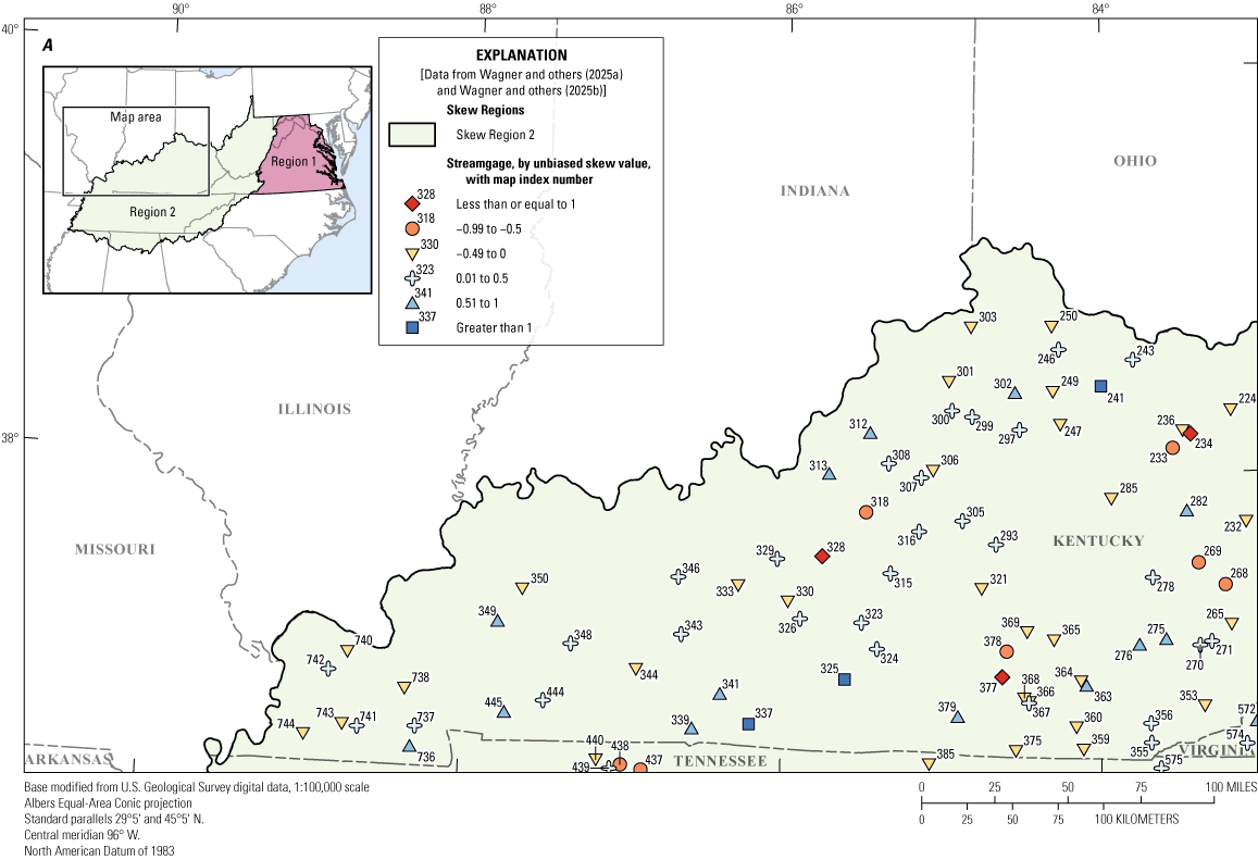
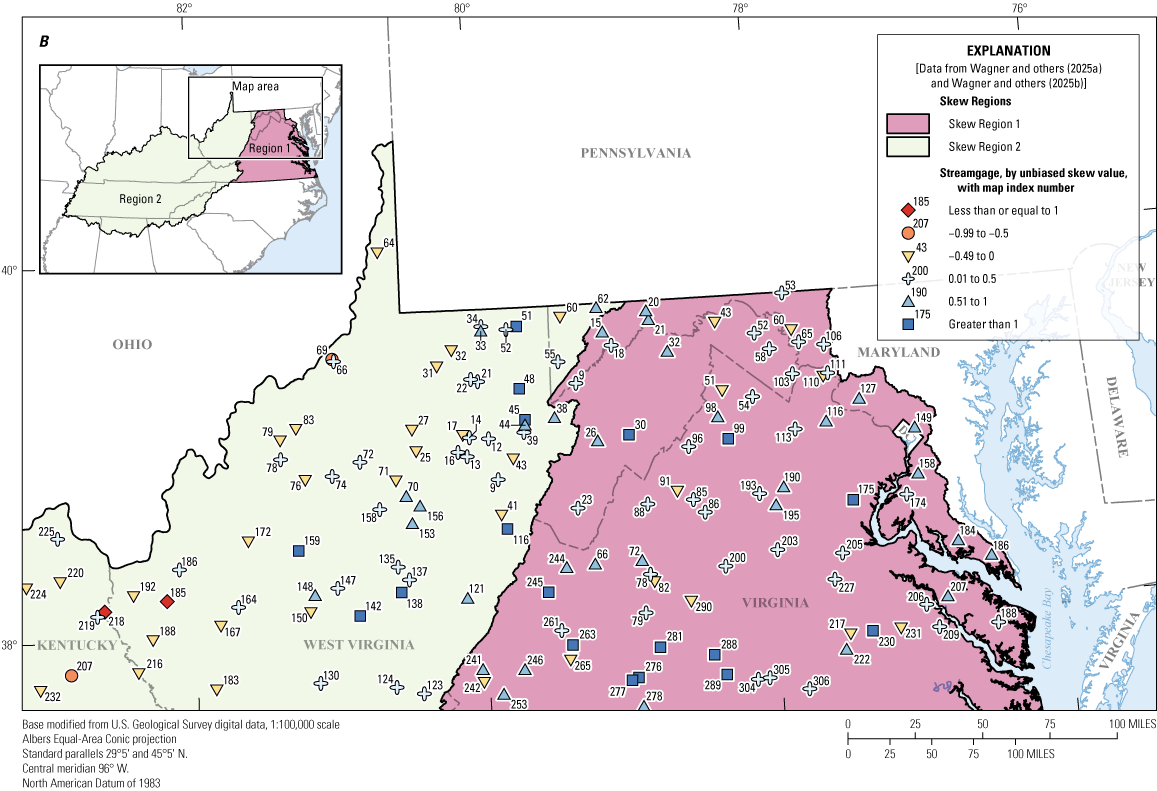
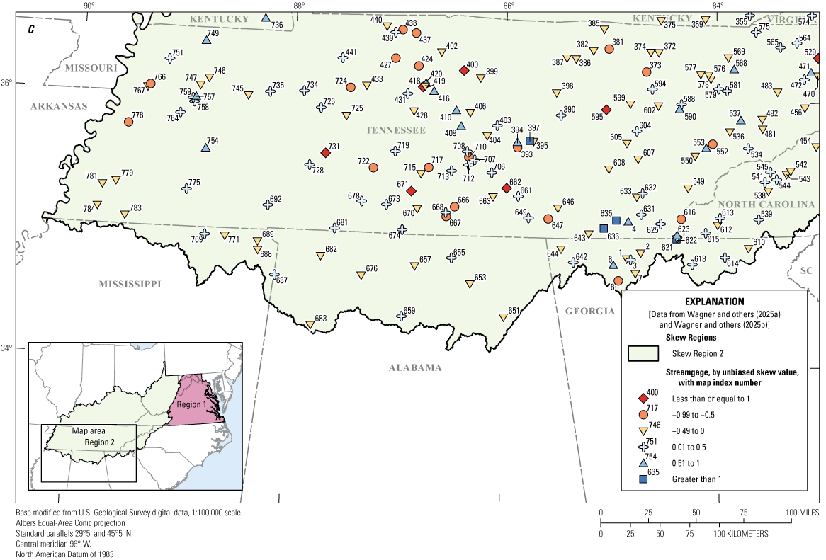
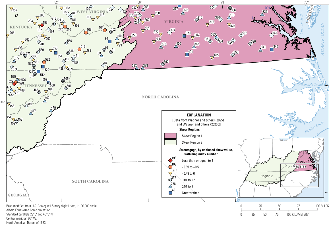
Map showing locations of skew regions and streamgages used to develop regional skew for Virginia, West Virginia, Kentucky, and Tennessee. A, northwestern portion of Skew Region 2. B, northeastern portion of Skew Region 2 and northern portion of Skew Region 1. C, southwestern portion of Skew Region 2. D, southeastern portion of Skew Region 2 and southern portion of Skew Region 1.
Ordinary Least-Squares Analysis
The first step in the B–WLS/B–GLS regional skew analysis is the estimation of a regional skew model using OLS regression (Veilleux and Wagner, 2021). The OLS regression yields coefficients () and a model that can be used to generate unbiased and relatively stable estimates of regional skew coefficients for all streamgages:
whereare the estimated regional skew values;
X is an (n x k) matrix of basin characteristics;
is an (k x 1) vector of estimated regression parameters;
n is the number of streamgages; and
k is the number of basin characteristics, including a column of ones to estimate the constant.
The regional skew coefficient estimates (), are then used to calculate the unbiased variances of the regional skew for each streamgage using equation 7 in Griffis and Stedinger (2009). These variances are based on the OLS estimator of the regional skew coefficient instead of the at-site skew estimator, thus making the weights in the subsequent steps relatively independent of the at-site skew.
Bayesian Weighted Least-Squares Analysis
A B–WLS analysis is used to develop estimators of the regression coefficients () for each regional skew model (Veilleux, 2011; Veilleux and others, 2011). The B–WLS analysis explicitly reflects variations in record length but intentionally neglects cross-correlations, thereby avoiding problems experienced with GLS parameter estimators.
Bayesian Generalized Least-Squares Analysis
After the regression coefficients () are determined using a B–WLS analysis, the precision of the fitted model and regression coefficients are estimated using a B–GLS analysis (Veilleux, 2011; Veilleux and others, 2011). Precision metrics include: (1) the standard error of the regression parameters, ; (2) the model error variance, ; (3) the pseudo coefficient of determination, pseudo-R2; and (4) the average variance of prediction for streamgages that were not used in the regional model.
Computing Pseudo-Record Length
Annual peak streamflow records often include historical information and censored data—for example, information that the annual peak streamflow at a crest-stage streamgage did not exceed the minimum recordable streamflow—that need to be accounted for when computing the precision of skew estimates (England and others, 2018). While historical information and censored peaks are valuable, they provide less information than an equal number of years of systematic peaks (Stedinger and Cohn, 1986). The following calculations yield a pseudo-record length (PRL) which appropriately accounts for all types of data available for a streamgage.
The PRL is defined in terms of the number of years of systematic record that would be required to yield the same mean squared error of skew (MSEG) as the combination of historical and systematic records available at a streamgage; thus, the PRL of the skew is a ratio of MSEG when only the systematic record is analyzed () to MSEG when the complete record, including historical and censored data, are analyzed ().
wherePRL
is the pseudo-record length for the entire period of record at the streamgage, in years;
Ps
is the number of systematic peaks in the record;
is the estimated mean squared error of the at-site skew when only the systematic record is considered; and
is the estimated mean squared error of the at-site skew when the complete record, including historical and censored data, are considered.
Because the is an estimate, the following conditions must also be met to ensure a valid approximation: (1) the PRL must be nonnegative; if the PRL is greater than PH (the length of the historical period), then PRL should be set to equal PH; and (2) If the PRL is less than PS, then the PRL is set to PS. This ensures that the PRL will not be larger than PH or less than PS.
The estimate of at-site skew is sensitive to extreme events, and more accurate estimates can be obtained from longer records, typically 50 years or greater (England and others, 2018; Veilleux and Wagner, 2021). However, 50 years of record are not available for most streamgages; therefore, streamgages that have 30 or more years of PRL are normally used for regional skew analysis. Skew Region 1 had a sufficient number of streamgages with 50 or more years of PRL available for skew analysis; therefore, the minimum PRL used in Skew Region 1 was 50 years, and the maximum was 141 years. Skew Region 2 did not have a sufficient number of streamgages with 50 or more years of PRL available for skew analysis; therefore, the minimum PRL used in Skew Region 2 was 30 years, and the maximum was 188 years. Of 1,016 nonredundant streamgages, 234 of the 346 streamgages in Skew Region 1 were removed for PRL less than 50 years, and 283 of the 670 streamgages in Skew Region 2 were removed for PRL less than 30 years (refer to “VA_SkewRegion1.csv” in Wagner and others, 2025a, and “VA_SkewRegion2.csv” in Wagner and others, 2025b), leaving 499 streamgages for regional skew analysis, 112 in Skew Region 1 and 387 in Skew Region 2 (fig. 2.1).
Unbiasing the At-Site Skew
For the 499 streamgages used in the regional skew analysis (fig 2.1), the at-site skews were unbiased using the correction factor developed by Tasker and Stedinger (1986) and employed by Reis and others (2005). The unbiased at-site skew, computed using the PRL, is
whereis the unbiased at-site skew estimate for streamgage i,
is the pseudo-record length, in years, for streamgage i, as calculated in equation 2.1, and
Gi is the traditional biased estimate of at-site skew based on the flood frequency analysis for streamgage i.
The variance of the unbiased at-site skew includes the correction factor developed by Tasker and Stedinger (1986):
where is calculated using equation 3 from Griffis and Stedinger (2009) whereThere is more than one way to estimate the MSE of the unbiased at-site skew (MSEU). The approach used by EMA (refer to equation 55 in Cohn and others, 2001) generates a first-order estimate of the MSEU, which should perform well when interval data are present; however, the preferred option is to use the formula in equation 2.5 (the variance is equated to the MSE). The length of the systematic record or historical period (Hp) might be used in the denominator; however, neither metric accounts for censored data, which could lead to an inaccurate and under-estimated MSEU. This issue is addressed by using PRL, which indicates the impact of the censored data and the number of systematic peaks. Thus, MSEU, computed using equation 2.5, was used in the regional skew model because it is stable and relatively independent of the at-site skew.
Cross-Correlation Model
A critical step in a GLS analysis is the estimation of the cross-correlation of the at-site skew estimates. Martins and Stedinger (2002) used Monte Carlo experiments to derive a relation between the cross-correlation of the at-site skew estimates for two streamgages, i and j, as a function of the cross-correlation of concurrent annual peak streamflows, ρij:
whereis the cross-correlation of concurrent annual peak streamflows for two streamgages;
κ is a constant between 2.8 and 3.3; and
cfij is a factor that accounts for the sample size difference between streamgages and their concurrent record length and is defined as follows:
CYij is the pseudo-record length of the period of concurrent record; and
, and are the pseudo-record lengths corresponding to streamgages i and j, respectively (refer to equation 2.2).
After calculating the PRL for each streamgage in the study, the pseudo concurrent record length between pairs of streamgages can be calculated. Because of the use of censored data and historical data, the calculation of the effective concurrent record length is more complex than determining in which years the two streamgages both have recorded systematic peaks. First, the number of years of historical period in common between the two streamgages are determined. Next, for the years in common, with beginning year YBij and ending year YEij, the following equation is used to calculate the concurrent years of record between site i and site j.
The computed pseudo concurrent record length depends upon the years of historical period in common between the two streamgages, as well as the ratios of the PRL to the Hp for each of the streamgages.
To relate the concurrent annual peak streamflows at the two streamgages, a cross-correlation model using 74 streamgages with at least 55 years of concurrent systematic annual peaks (zero flows not included) was considered for Skew Region 1, and a model using 78 streamgages with at least 50 years of concurrent systematic annual peaks (zero flows not included) was considered for Skew Region 2. A logit model, termed the Fisher Z-Transformation (Z =log[(1+r)/(1−r)]), provided a convenient transformation of the sample correlations, rij, from the (−1, +1) range to the (-¥, +¥) range. The model used to estimate the cross-correlations of concurrent annual peak streamflows at two streamgages, which incorporated the distance between basin centroids, Dij, as the only explanatory variable, is
wherefor Skew Region 1 and
for Skew Region 2.
Figure 2.2 shows the fitted relation between the un-transformed cross-correlation and distance between basin centroids and points representing the streamgage pairs. Figure 2.3 shows the fitted relation between Z and the distance between basin centroids and points representing the streamgage pairs. These cross-correlation models were used to estimate cross-correlation of concurrent annual peak streamflows for all streamgage pairs.
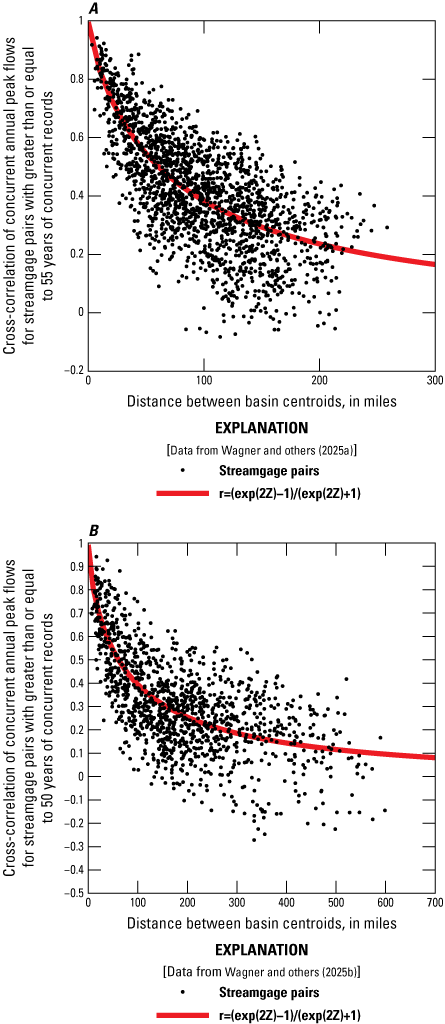
Graph showing the relation between un-transformed cross-correlation of logarithms of annual peak streamflows and distance between basin centroids for streamgages in A, Skew Region 1 and B, Skew Region 2. r, sample correlations; exp, natural exponential function.
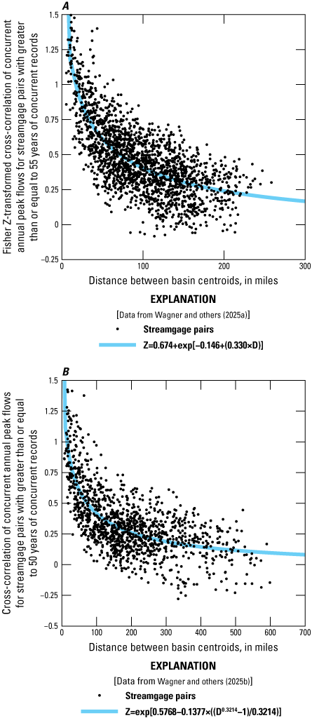
Graph showing the relation between Fisher Z-transformed cross-correlation of logarithms of annual peak streamflows and distance between basin centroids for streamgages in A, Skew Region 1 and B, Skew Region 2. Z, Fisher Z-transformation; exp, natural exponential function; D, distance between basin centroids, in miles.
Regional Skew Model
Skew Region 1
Twenty-four basin characteristics were tested as covariates in the B–WLS/B–GLS analysis of regional skew (Wagner and others, 2025a). Although mean annual precipitation and the percentage of forested land use in the streamgage basins were statistically significant in the initial OLS regression, neither had sufficient predictive power in the B–WLS / B–GLS analysis. Therefore, a constant model of regional skew, 0.50, was selected for Skew Region 1.
A good regional skew model will have the smallest possible model error variance, , and largest possible pseudo-R2. A constant model does not explain variability in the true skews, so the pseudo-R2, which describes the estimated fraction of the variability in the at-site skews explained by the model (Gruber and Stedinger, 2008; Parrett and others, 2011), is zero. The posterior mean of the model error variance, , is 0.315. The average sampling error variance, ASEV, is 0.015 and represents the average error in the regional skew for the streamgages in the dataset. The average variance of prediction at a new site is 0.33 (standard error 0.574), which is equivalent to the MSE of the regional skew and corresponds to an effective record length of 28 years—an improvement over the effective record length of the generalized skew map in Bulletin 17B (17 years).
Diagnostic statistics for B–WLS/B–GLS regression
To evaluate how well a regression model fits a regional hydrologic dataset, diagnostic statistics have been developed (Griffis, 2006; Gruber and Stedinger, 2008). A pseudo analysis of variance (pseudo ANOVA) was conducted for the constant model of regional skew for Skew Region 1. The pseudo ANOVA shows how much of the variation in the observed skews can be explained by the regional model, and how much of the variation in residuals can be attributed to model error and sampling error, respectively (Veilleux, 2011). Difficulties arise in determining these quantities. The model errors cannot be resolved because the values of the sampling errors, , for each site, i, are not known. However, the total sampling error sum of squares can be described by its mean value, . Because there are n equations, the total variation because of the model error for a model with k parameters has a mean equal to ; thus, the residual variation attributed to the sampling error is , and the residual variation attributed to the model error is . This division of the variation in the observations is referred to as a pseudo ANOVA because the contributions of the three sources of error are estimated or constructed, rather than being determined from the residuals and the model predictions, while also ignoring the effect of correlation among the sampling errors.
For a model with no parameters other than the mean (a constant skew model), the estimated model error variance, , describes all of the anticipated variation in , where is the mean of the estimated at-site sample skews; thus, the total expected sum of squares variation because of model error, , and because of sampling error, in expectation should equal . The expected sum of squares attributed to a regional skew model with k parameters should then equal , because the sum of the model error variance and the variance explained by the model must sum to . The constant model does not have any explanatory variables, thus the variation attributed to the models is 0 and k=0.
The error variance ratio (EVR) is the ratio of the average sampling error variance to the model error variance and is a diagnostic statistic that is used to evaluate if a simple OLS regression is sufficient or if a more sophisticated WLS or GLS analysis is appropriate (Veilleux, 2011). Generally, an EVR greater than 0.20 indicates that the sampling variance is not negligible when compared to the model error variance, suggesting the need for a WLS or GLS regression analysis. The EVR is calculated as:
The EVR for the constant model is 0.4. The sampling variability in the at-site skew was larger than the error in the regional model; thus, an OLS model that neglects sampling error in the at-site skew might not provide a statistically reliable analysis of the data. A WLS or GLS analysis can be used to account for sampling error and the variation in record lengths among streamgages, and to evaluate the final precision of the model.
The misrepresentation of the beta variance (MBV) is a diagnostic statistic that is used to determine whether a WLS regression is sufficient or a GLS regression is appropriate to determine the precision of the estimated regression parameters (Griffis, 2006; Veilleux, 2011). The MBV describes the error produced by a WLS regression analysis in its evaluation of the precision of , which is the estimator of the constant , because the covariance among the estimated at-site skews, , generally has its greatest impact on the precision of the constant term (Stedinger and Tasker, 1985). If the MBV is substantially greater than 1, then a GLS error analysis should be employed. The MBV is calculated as
where.
MBV for the constant model was 3.8, and this large value indicates that the cross-correlation among the at-site skew estimates affected the precision with which the regional skew could be estimated. If a WLS analysis were used to estimate the precision of the constant, the variance would be underestimated by a factor of 3.8; moreover, a WLS model would underestimate the variance of prediction given that the sampling error in the constant term was sufficiently large to make an appreciable contribution to the average variance of prediction.
Leverage and Influence
Leverage and influence diagnostics statistics can be used to identify rogue observations and effectively address the lack of fit when estimating skew coefficients. Leverage identifies those streamgages in the analysis where the observed values have a large effect on the fitted (or predicted) values (Hoaglin and Welsch, 1978). Generally, leverage takes into consideration whether an observation or explanatory variable is unusual and thus likely to have a large effect on the estimated regression coefficients and predictions. Unlike leverage, which highlights points that have the ability or potential to affect the fit of the regression, influence attempts to describe those points that have an unusual impact on the regression analysis (Belsley and others, 1980; Cook and Weisberg, 1982; Tasker and Stedinger, 1989). An influential observation is one with an unusually large residual that has a disproportionate effect on the fitted regression. Influential observations often have high leverage. Detailed descriptions of the equations used to determine leverage and influence for a B–WLS/B–GLS analysis can be found in Veilleux (2011) and Veilleux and others (2011).
Thirty-six streamgages in the regional skew analysis exhibited high leverage (greater than 0.018). The differences in leverage values for the constant model indicate the variation in record lengths among streamgages. Four U.S. Geological Survey streamgages (01674200, 02027000, 02028500, and 02049500; U.S. Geological Survey, 2023) exhibited high influence (Cook’s distance greater than 0.036) and thus had an unusual impact on the fitted regression (refer to “VA_SkewRegion1.csv” in Wagner and others, 2025a). These streamgages were investigated, but there were no reasons to remove them, and they were included in the analysis.
Skew Region 2
Twenty-six basin characteristics were tested as covariates in the B–WLS / B–GLS analysis of regional skew (Wagner and others, 2025b). Although the latitude of the basin centroids, the minimum, maximum, and mean basin elevations, and the percentages of the streamgages basins in the Ridge and Valley and Southwestern Appalachians U.S. Environmental Protection Agency Level III ecoregions (U.S. Environmental Protection Agency, 2010) were statistically significant in the initial OLS regression, none had sufficient predictive power in the B–WLS / B–GLS analysis. Therefore, a constant model of regional skew, 0.048, was selected for Skew Region 2.
A good regional skew model will have the smallest possible model error variance, , and largest possible pseudo-R2. A constant model does not explain variability in the true skews, so the pseudo-R2, which describes the estimated fraction of the variability in the at-site skews explained by the model (Gruber and Stedinger, 2008; Parrett and others, 2011), is zero. The posterior mean of the model error variance, , is 0.155. The average sampling error variance, ASEV, is 0.0036 and represents the average error in the regional skew for the streamgages in the dataset. The average variance of prediction at a new site is 0.16 (standard error 0.4), which is equivalent to the MSE of the regional skew and corresponds to an effective record length of 45 years which is an improvement over the effective record length of the generalized skew map in Bulletin 17B (17 years).
Diagnostic statistics for B–WLS/B–GLS regression
To evaluate how well a regression model fits a regional hydrologic dataset, diagnostic statistics have been developed (Griffis, 2006; Gruber and Stedinger, 2008). A pseudo analysis of variance (pseudo ANOVA) was conducted for the constant model of regional skew for Skew Region 1. The pseudo ANOVA shows how much of the variation in the observed skews can be explained by the regional model, and how much of the variation in residuals can be attributed to model error and sampling error, respectively. Difficulties arise in determining these quantities. The model errors cannot be resolved because the values of the sampling errors, , for each site, i, are not known. However, the total sampling error sum of squares can be described by its mean value, . Because there are n equations, the total variation because of the model error for a model with k parameters has a mean equal to ; thus, the residual variation attributed to the sampling error is , and the residual variation attributed to the model error is. This division of the variation in the observations is referred to as a pseudo ANOVA because the contributions of the three sources of error are estimated or constructed, rather than being determined from the residuals and the model predictions, while also ignoring the effect of correlation among the sampling errors.
For a model with no parameters other than the mean (a constant skew model), the estimated model error variance, , describes all of the anticipated variation in , where is the mean of the estimated at-site sample skews; thus, the total expected sum of squares variation because of model error, , and because of sampling error, in expectation should equal . The expected sum of squares attributed to a regional skew model with k parameters should then equal , because the sum of the model error variance and the variance explained by the model must sum to . The constant model does not have any explanatory variables, thus the variation attributed to the models is 0 and k=0.
The ratio of the average sampling error variance to the model error variance is called the error variance ratio (EVR) and is a diagnostic statistic used to evaluate if a simple OLS regression is sufficient or if a more sophisticated WLS or GLS analysis is appropriate. Generally, an EVR greater than 0.20 indicates that the sampling variance is not negligible when compared to the model error variance, suggesting the need for a WLS or GLS regression analysis. The EVR is calculated as:
The EVR for the constant model is 0.9. The sampling variability in the at-site skew was larger than the error in the regional model; thus, an OLS model that neglects sampling error in the at-site skew might not provide a statistically reliable analysis of the data. A WLS or GLS analysis can be used to account for sampling error and the variation in record lengths among streamgages, and to evaluate the final precision of the model.
The misrepresentation of the beta variance (MBV) is a diagnostic statistic is used to determine whether a WLS regression is sufficient or a GLS regression is appropriate to determine the precision of the estimated regression parameters (Griffis, 2006; Veilleux, 2011). The MBV describes the error produced by a WLS regression analysis in its evaluation of the precision of , which is the estimator of the constant , because the covariance among the estimated at-site skews, , generally has its greatest impact on the precision of the constant term (Stedinger and Tasker, 1985). If the MBV is substantially greater than 1, then a GLS error analysis should be employed. The MBV is calculated as
where.
MBV for the constant model was 4.8. This is a large value, indicating that the cross-correlation among the at-site skew estimates affected the precision with which the regional skew could be estimated. If a WLS analysis were used to estimate the precision of the constant, the variance would be underestimated by a factor of 4.8; moreover, a WLS model would underestimate the variance of prediction, given that the sampling error in the constant term was sufficiently large to make an appreciable contribution to the average variance of prediction.
Leverage and Influence
Leverage and influence diagnostic statistics can be used to identify rogue observations and to effectively address the lack of fit when estimating skew coefficients. Leverage identifies those streamgages in the analysis where the observed values have a large effect on the fitted (or predicted) values (Hoaglin and Welsch, 1978). Generally, leverage takes into consideration whether an observation or explanatory variable is unusual and thus likely to have a large effect on the estimated regression coefficients and predictions. Unlike leverage, which highlights points that have the ability or potential to affect the fit of the regression, influence attempts to describe those points that have an unusual impact on the regression analysis (Belsley and others, 1980; Cook and Weisberg, 1982; Tasker and Stedinger, 1989). An influential observation is one with an unusually large residual that has a disproportionate effect on the fitted regression. Influential observations often have high leverage. Detailed descriptions of the equations used to determine leverage and influence for a B–WLS/B–GLS analysis can be found in Veilleux (2011) and Veilleux and others (2011).
None of the streamgages in the regional skew analysis exhibited high leverage (greater than 0.005). The differences in leverage values for the constant model reflect the variation in record lengths among the streamgages. Twenty-four streamgages exhibited high influence (Cook’s distance greater than 0.01) and, thus, had an unusual impact on the fitted regression (refer to “VA_SkewRegion2.csv” in Wagner and others, 2025b). These streamgages were investigated, but there were no reasons to remove them, and they were included in the final analysis.
References Cited
Belsley, D.A., Kuh, E., and Welsch, R.E., 1980,Detecting influential observations and outliers, chap. 2 of Belsley, D.A., Kuh, E., and Welsch, R.E., 1980, Regression diagnostics—Identifying influential data and sources of collinearity: New York, John Wiley and Sons, Inc., p. 6–84. https://doi.org/10.1002/0471725153.ch2.
Cohn, T.A., Lane, W.L., and Baier, W.G., 1997, An algorithm, for computing moments-based flood quantile estimates when historical flood information is available: Water Resources Research, v. 33, no. 9, p. 2089–2096. accessed October 30, 2023, at: https://doi.org/10.1029/97WR01640.
Cohn, T.A., Lane, W.L., and Stedinger, J.R., 2001, Confidence intervals for expected moments algorithm flood quantile estimates: Water Resources Research, v. 37, no. 6, p. 1695–1706. accessed October 30, 2023, at: https://doi.org/10.1029/2001WR900016.
England, J.F., Jr., Cohn, T.A., Faber, B.A., Stedinger, J.R., Thomas, W.O., Jr., Veilleux, A.G., Kiang, J.E., and Mason, R.R., Jr., 2018, Guidelines for determining flood flow frequency—Bulletin 17C (ver. 1.1, May 2019): U.S. Geological Survey Techniques and Methods, book 4, chap. B5, 148 p., accessed October 30, 2023, at https://doi.org/10.3133/tm4B5.
Feaster, T.D., Gotvald, A.J., Musser, J.W., Weaver, J.C., Kolb, K.R., Veilleux, A.G., and Wagner, D.M., 2023, Magnitude and frequency of floods for rural streams in Georgia, South Carolina, and North Carolina, 2017—Results: U.S. Geological Survey Scientific Investigations Report 2023–5006, 75 p., Accessed online at: https://doi.org/10.3133/sir20235006.
Feaster, T.D., Gotvald, A.J., and Weaver, J.C., 2009, Magnitude and frequency of rural floods in the Southeastern United States, 2006—Volume 3, South Carolina: U.S. Geological Survey Scientific Investigations Report 2009–5156, 226 p. Accessed online at: https://doi.org/10.3133/sir20095156
Gotvald, A.J., Feaster, T.D., and Weaver, J.C., 2009, Magnitude and frequency of rural floods in the southeastern United States, 2006—Volume 1, Georgia: U.S. Geological Survey Scientific Investigations Report 2009–5043, 120 p. Accessed online at: https://doi.org/10.3133/sir20095043
Griffis, V.W., and Stedinger, J.R., 2009, Log-Pearson type 3 distribution and its application in flood frequency analysis III—Sample skew and weighted skew estimators: Journal of Hydrologic Engineering, v. 14, no. 2, p. 121–130. Accessed October 30, 2023, at: https://doi.org/10.1061/(ASCE)1084-0699(2009)14:2(121).
Gruber, A.M., and Stedinger, J.R., 2008, Models of LP3 regional skew, data selection and Bayesian GLS regression, paper 596, in Babcock, R.W. and Watson, R., eds., Proceedings of the World Environmental and Water Resources Congress, Ahupua’a, Honolulu, Hawai’i, May 12–16, 2008, 10 p. Accessed October 30, 2023 at: https://doi.org/10.1061/40976(316)563
Hoaglin, D.C., and Welsch, R.E., 1978, The hat matrix in regression and ANOVA: The American Statistician, v. 32, no. 1, p. 17–22. Accessed October, 30, 2023, at: https://doi.org/10.1080/00031305.1978.10479237.
Martins, E.S., and Stedinger, J.R., 2002, Cross-correlation among estimators of shape: Water Resources Research, v. 38, no. 11, p. 34–1 to 34–7,Accessed October 30, 2023, at:https://doi.org/10.1029/2002WR001589.
Parrett, C., Veilleux, A., Stedinger, J.R., Barth, N.A., Knifong, D.L., and Ferris, J.C., 2011, Regional skew for California, and flood frequency for selected sites in the Sacramento–San Joaquin River Basin, based on data through water year 2006: U.S. Geological Survey Scientific Investigations Report 2010–5260, 94 p. Accessed online at: https://doi.org/10.3133/sir20105260.
Reis, D.S., Jr., Stedinger, J.R., and Martins, E.S., 2005, Bayesian generalized least squares regression with application to the log Pearson type III regional skew estimation: Water Resources Research, v. 41, article W10419, 14 p., accessed October 30, 2023, at: https://doi.org/10.1029/2004WR003445.
Stedinger, J.R., and Cohn, T.A., 1986, Flood frequency analysis with historical and paleoflood information: Water Resources Research, v. 22, no. 5, p. 785–793. Accessed October 30, 2023, at: https://doi.org/10.1029/WR022i005p00785.
Stedinger, J.R., and Tasker, G.D., 1985, Regional hydrologic analysis 1—Ordinary, weighted and generalized least squares compared: Water Resources Research, v. 21, no. 9, p. 1421–1432. Accessed October 30, 2023, at: https://doi.org/10.1029/WR021i009p01421.
Tasker, G.D., and Stedinger, J.R., 1986, Regional skew with weighted LS regression: Journal of Water Resources Planning and Management, v. 112, no. 2, p. 225–237. Accessed October 30, 2023, at: https://doi.org/10.1061/(ASCE)0733-9496(1986)112:2(225).
Tasker, G.D., and Stedinger, J.R., 1989, An operational GLS model for hydrologic regression: Journal of Hydrology, v. 111, nos. 1–4, p. 361–375. Accessed October 30, 2023, at: https://doi.org/10.1016/0022-1694(89)90268-0.
U.S. Environmental Protection Agency, 2010, Level III and IV ecoregions of the continental United States: U.S. Environmental Protection Agency, accessed October 5, 2022 at https://www.epa.gov/eco-research/level-iii-and-iv-ecoregions-continental-united-states.
U.S. Geological Survey, 2023, Peak streamflow for the nation: U.S. Geological Survey National Water Information System database, accessed November 6, 2023, at https://doi.org/10.5066/F7P55KJN. [Peak streamflow information directly accessible at https://nwis.waterdata.usgs.gov/nwis/peak.]
Veilleux, A.G. and Wagner, D.M., 2021, Methods for estimating regional skewness of annual peak flows in parts of eastern New York and Pennsylvania, based on data through water year 2013: U.S. Geological Survey Scientific Investigations Report 2021–5015, 26 p. Accessed online at:https://doi.org/10.3133/sir20195105.
Veilleux, A.G. and Wagner, D.M., 2019, Methods for estimating regional skewness of annual peak flows in parts of the Great Lakes and Ohio River Basins, based on data through water year 2013: U.S. Geological Survey Scientific Investigations Report 2019–5105, 26 p. Accessed online at: https://doi.org/10.3133/sir20195105.
Veilleux, A.G., Stedinger, J.R., and Eash, D.A., 2012, Bayesian WLS/GLS regression for regional skewness analysis for regions with large crest stage gage networks, in Loucks, E.D., ed., Proceedings of the World Environmental and Water Resources Congress 2012—Crossing boundaries, Albuquerque, N. Mex., May 20–24, 2012: Reston, Va., American Society of Civil Engineers, p. 2253–2263.
Veilleux, A.G., Stedinger, J.R., and Lamontagne, J.R., 2011, Bayesian WLS/GLS regression for regional skewness analysis for regions with large cross-correlations among flood flows in Beighley, R.E., II, and Killgore, M.W., eds., Proceedings of the World Environmental and Water Resources Congress 2011—Bearing knowledge for sustainability, Palm Springs, Calif., May 22–26, 2011: Reston, Va., American Society of Civil Engineers, p. 3103–3112.
Wagner, D.M., O’Shea, P.S., Thompson, R.R., Messinger, T., and Duda, J.M., 2025a, Regional flood skew for parts of the mid-Atlantic and South-Atlantic-Gulf regions (hydrologic unit codes 02 and 03) in eastern Virginia, eastern West Virginia, and western Maryland: U.S. Geological Survey data release, https://doi.org/10.5066/P9TQP5T5.
Wagner, D.M., O’Shea, P.S., Thompson, R.R., Messinger, T., and Duda, J.M., 2025b, Regional flood skew for the Tennessee and parts of the Ohio and Lower Mississippi River Basins (hydrologic unit codes 06, 05, and 08, respectively) in Tennessee, Kentucky, western Virginia, western West Virginia, far western Maryland and parts of North Carolina, Georgia, Alabama, and Mississippi: U.S. Geological Survey data release, https://doi.org/10.5066/P1M9VJQV.
Weaver, J.C., Feaster, T.D., and Gotvald, A.J., 2009, Magnitude and frequency of rural floods in the Southeastern United States, through 2006—Volume 2, North Carolina: U.S. Geological Survey Scientific Investigations Report 2009–5158, 111 p. [Also available at https://pubs.usgs.gov/sir/2009/5158/.] Accessed online at: https://doi.org/10.3133/sir20095158.
Appendix 3. Delaware Regression Equations
Generalized Least-Squares Regression for Peak Flow Estimation
Generalized least-squares (GLS) multiple-linear regression was used to compute the final regression coefficients and measures of accuracy for the regression equations to estimate peak flows at defined frequencies. The GLS method weights data from streamflow-gage sites in the regression analysis according to differences in streamflow reliability (record length), variability (record variance), and spatial cross correlations of concurrent streamflow among streamflow-gage sites (Farmer and others, 2019). Compared to OLS regression, the GLS regression approach provides improved estimates of streamflow statistics and increases the predictive accuracy of the regression equations (Stedinger and Tasker, 1985). The weighted-multiple-linear regression (WREG) program, developed by Eng and others (2009), updated to run in R (Farmer, 2017) was used to perform the GLS regressions. A correlation smoothing function is used by the WREG to compute a weighting matrix for the streamflow-gage sites in each subregion. The smoothing function relates the correlation between annual peak discharges from each pair of streamflow-gage sites to the geographic distance between the sites. Smoothing functions were developed iteratively and generated separately for the Coastal Plain and Piedmont subregions. The statistical parameters needed to perform prediction-interval computations for peak-flow magnitude estimates can be found in table 6 of Hammond and others (2022). The resulting GLS-derived regression equations follow the general structure shown below:
whereQp
is the dependent variable, the P-percent AEP, in cubic feet per second (ft3/s);
A and B
are independent (explanatory) variables; and
a, b, and c
are regression coefficients.
If the dependent variable, Qp, and the independent variables, A and B, are logarithmically transformed, the model takes the following form:
GLS-derived regression equations for Coastal Plain subregions:
whereReferences Cited
Farmer, W.H., 2017, WREG: USGS WREG (v. 2.02): U.S. Geological Survey R package web page, accessed September 2020 at https://rdrr.io/github/USGS-R/WREG/.
Hammond, J.C., Doheny, E.J., Dillow, J.J.A., Nardi, M.R., Steeves, P.A., and Warner, D.L., 2022, Peak-flow and low-flow magnitude estimates at defined frequencies and durations for nontidal streams in Delaware: U.S. Geological Survey Scientific Investigations Report 2022–5005, 46 p., accessed April 17, 2024, at https://doi.org/10.3133/sir20225005.
Conversion Factors
U.S. customary units to International System of Units
Datums
Vertical coordinate information is referenced to the North American Vertical Datum of 1988 (NAVD 88).
Horizontal coordinate information is referenced to the North American Datum of 1983 (NAD 83).
Supplemental Information
A water year is the 12-month period from October 1 through September 30 of the following year and is designated by the calendar year in which it ends.
Abbreviations
>
greater than
<
less than
AEP
annual exceedance probability
AVP
average variance of prediction
B–GLS
Bayesian generalized least squares
B–WLS
Bayesian weighted least squares
EMA
expected moments algorithm
EPA
U.S. Environmental Protection Agency
GLS
generalized least-squares
HUC
hydrologic unit code
HUC 8
8-digit hydrologic unit code
HUC 12
12-digit hydrologic unit code
I100Y24H
100-year, 24-hour precipitation intensity
L3
U.S. Environmental Protection Agency level III ecoregion
log10
base-10 logarithm
MSE
mean squared error
MSEG
mean squared error of skew
MSEU
mean squared error unbiased at-site skew
NID
National Inventory of Dams
NLCD
National Land Cover Dataset
NWIS
National Water Information System
OLS
ordinary least-squares
PILF
potentially influential low flood
PRL
pseudo-record length
pseudo-R2
pseudo coefficient of determination
p-value
significance level
R2
coefficient of determination
RI
regulation index
USGS
U.S. Geological Survey
WLS
weighted least-squares
For additional information contact:
Director, Virginia and West Virginia Water Science Center
U.S. Geological Survey
1730 East Parham Road
Richmond, Virginia 23228
or visit our website at
https://www.usgs.gov/centers/virginia-and-west-virginia-water-science-center
Publishing support provided by the U.S. Geological Survey, Science Publishing Network, Baltimore Publishing Service Center.
Disclaimers
Any use of trade, firm, or product names is for descriptive purposes only and does not imply endorsement by the U.S. Government.
Although this information product, for the most part, is in the public domain, it also may contain copyrighted materials as noted in the text. Permission to reproduce copyrighted items must be secured from the copyright owner.
Suggested Citation
Messinger, T., Duda, J.M., Wagner, D.M., O'Shea, P.S., Scott, J.D., and Kandel, C., 2026, Estimation of magnitude and frequency of floods for rural, unregulated streams in and near Virginia and West Virginia: U.S. Geological Survey Scientific Investigations Report 2025–5110, 85 p., https://doi.org/10.3133/sir20255110.
ISSN: 2328-0328 (online)
ISSN: 2328-031X (print)
Study Area
| Publication type | Report |
|---|---|
| Publication Subtype | USGS Numbered Series |
| Title | Estimation of magnitude and frequency of floods for rural, unregulated streams in and near Virginia and West Virginia |
| Series title | Scientific Investigations Report |
| Series number | 2025-5110 |
| ISBN | 978-1-4113-4656-7 |
| DOI | 10.3133/sir20255110 |
| Publication Date | February 25, 2026 |
| Year Published | 2026 |
| Language | English |
| Publisher | U.S. Geological Survey |
| Publisher location | Reston, VA |
| Contributing office(s) | Virginia and West Virginia Water Science Center |
| Description | Report: vii, 85 p.; Data Release |
| Country | United States |
| State | Kentucky, Maryland, North Carolina, Ohio, Pennsylvania, Tennessee, Virginia, West Virginia |
| Online Only (Y/N) | N |
| Additional Online Files (Y/N) | N |