

Evaluation of Nutrient, Alkalinity, and Acid-Neutralizing Capacity Stabilities in Water Samples Analyzed by the U.S. Geological Survey National Water Quality Laboratory, 2023–24
Links
- Document: Report (5.03 MB pdf) , HTML , XML
- Data Release: USGS data release - Data for Evaluation of Nutrient, Alkalinity, and Acid Neutralizing Capacity Stabilities in Water Samples Analyzed by the National Water Quality Laboratory -- 2023-2024
- NGMDB Index Page: National Geologic Map Database Index Page (html)
- Download citation as: RIS | Dublin Core
Abstract
The U.S. Geological Survey evaluated the stability of water-sample chemical analysis of nutrient, alkalinity, and acid-neutralizing capacity constituents with respect to the duration between sample collection and laboratory analysis, also known as the sample holding time. A study began in the spring of 2023 to evaluate the sample stability, between 2 and 180 days after sample collection, of the chemical properties and chemical constituents of alkalinity as calcium carbonate, filtered; acid-neutralizing capacity as calcium carbonate, unfiltered; total ammonia as nitrogen, filtered; total ammonia plus organic nitrogen as nitrogen, filtered and unfiltered; nitrite as nitrogen, filtered; nitrate plus nitrite as nitrogen, filtered; total nitrogen, filtered and unfiltered; orthophosphate as phosphorous, filtered; and total phosphorus as phosphorus (filtered and unfiltered) in water. Both surface water and groundwater matrices were represented.
Sample instability varied by observed property and matrix; therefore, providing general guidance for sample holding time is not possible based on matrices alone. No correlations between field measurements of sample characteristics and sample instability were observed. Although observations for some properties indicate sample stability that exceeds the recognized U.S. Geological Survey National Water Quality Laboratory method holding times, this is not necessarily the case for matrices and seasonal characteristics that were not investigated.
Based on the limited number of six sample sources used in this study, some patterns emerge for the 12 observed properties studied. Five observed properties generally indicate stability for as many as 180 days after sampling (total nitrogen as nitrogen, both filtered and unfiltered; orthophosphate as phosphorus, filtered; and phosphorus as phosphorus, both filtered and unfiltered). Other observed properties indicate stability for as many as 180 days for some matrices, but not for others. Finally, some observed properties indicate instability well before 180 days.
Plain Language Summary
In 2023–24, the U.S. Geological Survey (USGS) studied how long different chemical measurements in water samples remain reliable if analysis is delayed after collection. This question became important after the National Water Quality Laboratory (NWQL) experienced a large backlog of sample analyses causing many samples to be analyzed outside the timeframe required by the NWQL, which affected many USGS studies, some of which were being done for regulatory purposes (such as to meet requirements set by the Environmental Protection Agency). There are specific time frames in place to ensure that analyte concentrations do not change significantly between sampling and the time of analysis. The study focused on those water‑quality measurements that tend to be most affected by delayed analysis including forms of nitrogen and phosphorus (nutrients), alkalinity, and acid‑neutralizing capacity. Because the type of water can affect sample stability, samples used in the study were collected from six separate locations (five streams and one well) from across the United States. Samples were analyzed repeatedly for periods ranging from two days to 180 days after collection. The study found that sample stability depends on what is being measured and on the type of water the measurement comes from. Overall, the study found that some analyses performed after the required timeframe can still be useful, but data quality depends on the specific chemical measurement, the water type, and the intended use of the data.
Introduction
In 2022, the U.S. Geological Survey (USGS) National Water Quality Laboratory (NWQL) experienced a large sample backlog that resulted in many nutrient, alkalinity, and acid-neutralizing capacity (ANC) samples not being analyzed within their holding times as required by the NWQL. This issue persisted through May 2024. Chemical properties and constituents, otherwise referred to as observed properties, for which a large number of holding-time exceedances were observed, are shown in table 1. Nearly 80,000 individual analyses were completed on samples after the recognized NWQL method holding time. This affected numerous USGS studies. Many of these specific observed properties are used in the computation of total nitrogen in water and are often associated with analyses done for regulatory purposes.
Table 1.
Custom Laboratory Schedule 3077 used in the holding-time study.[National Water Information System (NWIS) parameter, laboratory (lab), and method codes from National Water Quality Laboratory (2023). NWQL, National Water Quality Laboratory; USGS, U.S. Geological Survey; mg/L, milligrams per liter; CaCO3, calcium carbonate; fltd, filtered; EP, end point; titr, titrated; lab, analysis done in laboratory; ANC, acid-neutralizing capacity; unfltd, unfiltered; NH3, ammonia; +, plus; NH4+, ammonium; N, nitrogen; P, phosphorous]
Detection limit based on actual detection limit associated with routine environmental sample data from NWQL for October 2021 through September 2024.
Container type or sample treatment abbreviations: FU, filtered (sample), high-density polyethylene, 250 milliliters (mL), unacidified; RU, unfiltered (sample), high-density polyethylene, 250 mL, unacidified; WCA, unfiltered (sample), chilled, high-density polyethylene, 125 mL, acidified; FCC, filtered (sample), chilled, high-density polyethylene, amber, 125 mL, unacidified
The U.S. Environmental Protection Agency (EPA) defines sample holding time as the period of time a sample may be stored before analysis (EPA, 2002). According to the EPA, although exceeding the holding time does not necessarily negate the veracity of analytical results, exceeding the holding time requires any data not meeting all the specified acceptance criteria be qualified or flagged. The EPA sets holding-time and preservation requirements for nonpotable waters to ensure that analyte concentrations do not change significantly between sampling and the time of analysis. Specific sample holding-time and sample preservation requirements are provided under 40 CFR part 136 as authorized by section 304(h) of the Clean Water Act (33 U.S.C. 1251 et seq.). The effects of sample storage duration on sample integrity and resulting data could vary and depend on many variables, including inherent microbial activity, sample matrix (for example, saline compared to freshwater), whether the samples were filtered or unfiltered, sample preservation (Degobbis, 1973; Klingaman and Nelson, 1976; Gardolinski and others, 2001), and possible redox conditions (Tate and others, 1995).
As the issue of samples being analyzed after their elapsed holding times came into focus, USGS scientists from around the country formed a study group and met to discuss what was needed to evaluate these sample results. The meetings began in the spring of 2023 to discuss ways to evaluate data from samples analyzed after NWQL method holding times. To understand the effects more fully on data quality from samples being analyzed after their listed holding times, a holding-time study (HTS) was designed to evaluate the potential changes in sample quality from a variety of water matrices and environmental conditions.
Previous Investigations
Previous investigations of analytical methods for nutrients include studies to evaluate different nutrient preservation methods (Patton and Truitt, 1995; Bartholomay and Williams, 1996; Patton and Gilroy, 1999) and to compare alternate analytical methods for nitrogen (N) and phosphorus (P) by alkaline persulfate digestion and Kjeldahl digestion (Patton and Kryskalla, 2003). In 1992, the USGS experimented with comparing preservation methods for eight nutrient analyses from 15 sites across the United States (Patton and Truitt, 1995). In the 1992 study (Patton and Truitt, 1995), natural water samples and synthetic reference samples were used to evaluate the analysis comparisons. This study focused on various preservation methods for five time intervals (3, 7, 14, 22, and 35 days) for filtered ammonia (NH3), nitrite plus nitrate (NO2- plus NO3-), nitrate (NO3-), and orthophosphate (PO43-) as well as unfiltered and filtered Kjeldahl N and P. Samples that were preserved with either mercury (II) chloride (HgCl2) or sulfuric acid (H2SO4) showed no statistically significant difference on the 30-day stability of P concentrations in unfiltered samples. In a subset of samples where ammonia was half the concentration of the Kjeldahl N, preservation stabilized unfiltered Kjeldahl concentrations (Patton and Truitt, 1995).
Studies of nutrient stability in natural waters through extended time periods (more than 30 days) using storage methods comparable to those of the USGS samples include Maher and Woo (1998), Yorks and McHale (2000), Gardolinski and others (2001), and Kaiser and others (2016). An experiment by Gardolinski and others (2001) analyzed total oxidized nitrogen (TON, NO2- plus NO3-,) and filterable reactive phosphorus (FRP, PO43-) in four samples of river and estuary water of varying salinities, collected once in winter and once in early fall. The samples were stored at varying temperatures with and without preservation and were analyzed at time intervals up to 247 days after sampling. The authors found that TON and FRP stability was highly matrix dependent; TON was stable in most samples and storage treatments during extended time periods, whereas FRP declined with most treatments. Yorks and McHale (2000) investigated the stability of NO3-, NH3, and total N in 16 samples of soil water during a 24-week period with refrigeration and no preservation. They found that total N was stable up to 8 weeks and had decreased only slightly by the end of the study; NO3- decreased only slightly after 3–16 weeks; and NH3, where present, decreased throughout and especially during the first week. Kaiser and others (2016) reported on a 2009 study in which NO3- in groundwater with low, medium, and high concentration levels was stable during a 74-day period, with and without refrigeration. Maher and Woo (1998) summarized many studies of P species stability, including some that extended longer than 30 days and included refrigeration only.
Purpose and Scope
This report presents the design and results of the HTS done in 2024. The USGS collected the samples and analyzed the data. The results of previous investigations are summarized in this report to provide background and context for understanding the HTS results. This report also provides an evaluation of the effects of extended holding times on nutrient concentrations in environmental water samples and observations for consideration when using data pertaining to such samples in interpretive studies.
The results of the HTS pertain specifically to samples collected by the USGS and analyzed at the NWQL. Custom NWQL laboratory schedule 3077 was used for the study. The evaluated observed properties are listed in table 1.
Wide application of the HTS results outside of the USGS should be done with an understanding of the study’s limitations. The results may not necessarily be applicable to samples collected, handled, and analyzed by methods that differ from those of the NWQL. Although the HTS was designed to replicate actual field and laboratory conditions imposed upon the affected environmental samples collected, the HTS samples were not necessarily handled the same as routine environmental samples. This was because the HTS samples were part of a large study and required some handling logistics that varied from that of routine environmental samples.
Holding-Time Study Design
The HTS was designed to evaluate how the results of specific observed properties from a water sample varied during a period of approximately 6 months after the time of collection. The observed properties selected for the HTS were based on the high frequency of holding-time exceedances for those parameters. These observed properties and the associated NWQL methods are shown in table 1.
The sampling sites selected for the HTS were chosen to replicate sample types (matrices), as closely as possible, to the sample types that were analyzed outside the NWQL-method holding time at the NWQL. The HTS included sites that were distributed geographically, had long-term monitoring records, had data affected by the holding-time exceedances, and included groundwater and surface-water sites. Also, the study group recommended inclusion of sites that were part of ongoing monitoring networks so that samples could be collected as part of ongoing sampling activities. Potential sampling locations were identified after reviewing historical concentrations of nutrients and alkalinity (the observed properties affected by the holding-time exceedances) as well as dissolved oxygen, dissolved organic carbon, specific conductance, and other characteristics that possibly could affect sample stability. In addition, seasonality was considered, but time constraints prevented incorporating this variable into the study. Based on available resources, ultimately six USGS sites from a wide geographic distribution were selected and sampled in November and December 2023. The locations of the sites sampled for this study are shown in figure 1. Average concentrations and their subjective categorical classifications (low, moderate, and high) for the six sites are shown in table 2 (U.S. Geological Survey, 2024).
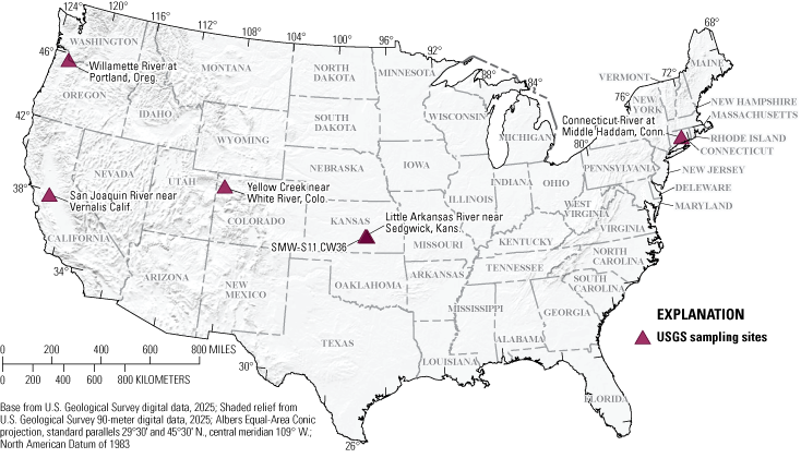
Map showing U.S. Geological Survey (USGS) surface-water and groundwater sites sampled for the holding-time study. Site names and numbers are from U.S. Geological Survey, 2024.
Table 2.
U.S. Geological Survey (USGS) sites and selected historical water-quality data from the National Water Information System used for site selection in the holding-time study (U.S. Geological Survey, 2024).[HTS, holding-time study; ID, identification; unfltd, unfiltered; μS/cm, microsiemens per centimeter; °C, degrees Celsius; O2, oxygen; mg/L, milligrams per liter; N, nitrogen; fltd, filtered; +, plus; CaCO3, calcium carbonate; titr, titrated; field, analysis done in field; WS, surface water; --, no data; WG, groundwater]
Seven time intervals were initially chosen for analysis of the HTS test samples. Time intervals include three intervals within the NWQL holding time to look for early sample instability, and four intervals outside the NWQL method holding time to investigate long-term sample stability. The time intervals for the study were 48 hours (2 days; referred to as “day 2” in the report), 2 weeks (14 days), 4 weeks (30 days), 8 weeks (60 days), 12 weeks (90 days), 16 weeks (120 days), and 20 weeks (150 days) after sample collection. Due to laboratory logistics, the intervals were not always exactly met. An additional eighth time interval at 26 weeks (180 days) was added by using an additional set of sample bottles submitted for most sites. No spare sample bottles were submitted for site number 01193050 (Connecticut River at Middle Haddam, Conn.), so no data were collected for this site for the 180-day interval.
Sample Collection, Processing, and Handling
Surface-water and groundwater samples were collected and processed for filtered and unfiltered water analysis in accordance with the USGS National Field Manual for the Collection of Water-Quality Data, which includes standard USGS sample collection methods (U.S. Geological Survey, variously dated). Field measurements of water temperature, specific conductance, pH, and dissolved oxygen were collected and recorded following standard USGS protocols (U.S. Geological Survey, variously dated). In addition, field titrations were performed for unfiltered ANC and filtered alkalinity at each site. Field replicates for ANC and alkalinity measurements were performed at some, but not all, sites. Information for each sample is provided in table 3.
Table 3.
Sample information for each sample in the holding-time study.[HTS, holding-time study; ID, identification; USGS, U.S. Geological Survey; WS, surface water; WG, groundwater]
Stream site numbers and names from U.S. Geological Survey, 2024.
A large sample volume was collected to ensure enough sample water for all required analyses in the HTS. The overall sample volume needed for all the sample bottle rinses, filter conditioning, sample splits, field titrations, and analyses was at least 12 liters (L). For samples to be as uniform as possible, surface-water samples were collected and composited in a large churn (14.0 L) where possible. Groundwater samples were collected from a pumped well. The volume of sample for each bottle was approximately 100–125 milliliters (mL).
A minimum of 21 sets of bottles (4 bottles per set), plus an additional 3 sets of spare bottles (96 bottles total), were submitted to the NWQL for each site to accommodate three replicate analyses for each of the seven time intervals. Separate bottles for each time interval and each replicate were collected so that bottles could be opened immediately prior to analysis instead of reusing samples that had been previously opened and exposed to the atmosphere for various amounts of time. The use of three separate bottles for each time interval allowed for comparing bottle-to-bottle sample stability as well as stability through time.
This effort required the following bottles to be collected as a bottle set: 125 mL filtered, chilled, high-density polyethylene, amber, unacidified (FCC); 125 mL unfiltered, chilled, high-density polyethylene, acidified (WCA); 250 mL (125 mL minimum volume) filtered, high-density polyethylene, unacidified (FU); 250 mL (125 mL minimum volume) unfiltered, high-density polyethylene, unacidified (RU; table 1).
All samples were shipped overnight to the NWQL. Upon sample receipt at the NWQL, the bottles were checked for proper labelling. The first set of bottles (FCC, WCA, FU, and RU) for each site was logged into the NWQL Laboratory Information Management System (LIMS) as a routine sample and received an NWQL Analytical Services Request (ASR) number. No other bottles were logged into the NWQL LIMS for that site for that date and time, but all bottles from that site had the NWQL ASR number on the label for tracking purposes. Bottle labels indicated the following: the proposed analysis date after collection (eight time intervals total); bottle number (1, 2, or 3 for each of the selected time intervals); container type; and analytical tests required for each container type (table 4).
Table 4.
Example of bottle labels used in the holding-time study.[Dates shown as month/day/year. Laboratory codes (LCs) from National Water Quality Laboratory (2023). STAID, site identifier; T, time; =, equals; #, number; FCC, filtered, chilled, high-density polyethylene, amber, 125-milliliter, unacidified bottle]
The specific requirements of the HTS created a challenge to the NWQL’s routine procedure for one-time analysis of LIMS-tracked environmental samples. To ensure that samples could be analyzed within 48 hours of arriving at the NWQL, sample labelling and distribution to the NWQL analysts were managed separately from the routine NWQL log-in procedure and uniquely designed for this particular study to ensure that all analytical time periods would be met as needed. Samples treated as FCCs and WCAs were shipped to and stored at the NWQL as chilled samples, whereas the FU and RU samples were stored at room temperature.
Approaches to Evaluating Sample Stability
Sample stability was evaluated by using three approaches, two of which accounted for the variability of the analytical methods: (1) by evaluating sample results with respect to blind-blank quality-control data for the analytical methods; (2) by evaluating sample results with respect to natural matrix water or spiked reagent water quality-control data for the analytical methods; and (3) by comparing day-2 HTS analytical results to subsequent measurements within a criterion of ±10 percent difference from the day-2 results. These approaches are described in this section and explained in further detail in the “Interpretation of Analytical Results” section of this report. Two additional approaches of evaluating sample stability, from the American Society for Testing and Materials (ASTM, 2002) and from Gardolinski and others (2001), were investigated but were found to be too sensitive for the HTS results. These approaches are also described in this section.
The American Society for Testing and Materials (ASTM) provides a standard protocol for determining holding times that incorporates the range of variation among replicate measurements at the start of the holding time period. The ASTM allowable range of variation is described by equation 1:
whered
is the range of tolerable variation from the initial mean concentration (in concentration units, for example, milligrams per liter [mg/L]),
t
is the Student’s t (based on the number of replicates used in the precision study),
SD
is the standard deviation (in concentration units, for example, mg/L), and
n
is the number of replicates.
A high percentage of sample results from the HTS would be considered instable when evaluated using the ASTM approach and day-2 replicate (triplicate) measurements to represent initial concentration in the samples at the start of the holding time period. The mean results for some observed properties from time intervals well after two days were within ±2 percent of the original mean value but would be considered instable according to the ASTM approach. Because the allowable range of variation calculated from the initial triplicate values determined on day 2 indicated unusually low variability, there was an unrealistically small allowable range of variation by the ASTM approach. For example, for the observed property ANC as calcium carbonate (CaCO3), water, unfiltered, the allowable range that indicates stability for sample 3 based on day-2 results is 158.7 mg/L±1.4 mg/L. This acceptance range is less than ±1 percent from the initial mean value. Using the range allowed by the ASTM approach results for days 60, 90, 150, and 180 are all flagged as instable (fig. 2). Therefore, the ASTM approach was considered not applicable for the sample stability evaluation.
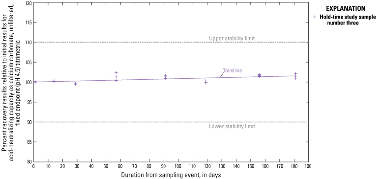
Percent recovery results for the holding-time study sample 3 for acid-neutralizing capacity as calcium carbonate, water, unfiltered, fixed endpoint (pH 4.5) by titration.
An approach similar to the ASTM approach, by Gardolinski and others (2001), was also explored. The Gardolinski approach provided a more generous allowable range of variation because the variability from the initial triplicate values determined on day 2 and the variability associated with subsequent triplicate values were considered. Although this approach does consider more than single-day, single-analyst variability, it does not take into account long-term method variability, and this approach proved to be oversensitive for this study.
We believe that the oversensitivity of both the ASTM and Gardolinski approaches is due to the fact that single-operator variability on a single day and single instrument is significantly less than that of long-term (multiday and possibly multi-instrument and [or] operator) variability (ASTM, 2002). Because all original day-2 results are based on single-operator variability, it is reasonable to conclude that many results after day 2 that failed to fall within the allowable range of variation for the ASTM and Gardolinski approaches were from a stable sample, but the results did not meet the stringent criteria of the ASTM and Gardolinski approaches.
To determine when subsequent results varied significantly from the day-2 values, long-term method variability had to be considered. By properly characterizing actual method variability, it was possible to create limits (referred to as “stability limits” in this report) around the day-2 results within which subsequent results would fall if the sample was stable. Samples with results falling outside of those limits, or outside of expected method variability, could be considered instable.
Method variability depends on concentration. As concentrations decrease, absolute variability decreases, and as the concentration approaches the detection level, the variability stabilizes at a level whereby the noise starts to outweigh the signal. This is illustrated for the variation of the SD with mean concentration in figure 3 (Mueller and others, 2015). One of the challenges with the six samples in this study is that they all had different concentrations. Some analyte results are less than the detection level; some are more than 40 times the detection level. Method variability at all concentration ranges had to be considered to calibrate appropriate expectations.
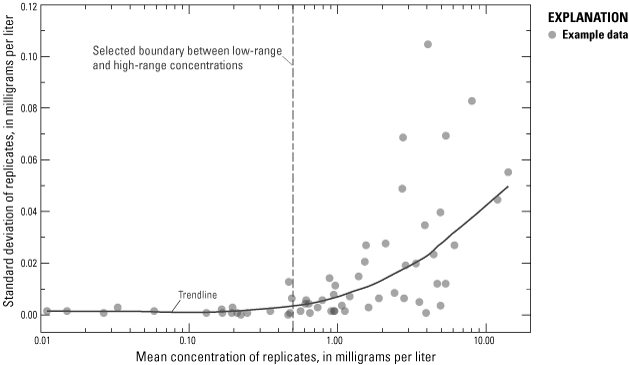
Scatterplot from Mueller and others (2015) showing how standard deviation in results increases with concentration.
Three separate approaches were used to calculate method and concentration-specific allowable ranges of variation (from the initial day-2 concentrations) for each observed property. The largest computed range of the three approaches is used in this study as the criterion to distinguish between (that is, identify) stable and instable analytical results. The three approaches are defined in the next three sections of this report.
Approach 1: Stability Limits Determined Using Blank Water
The first approach determined the lowest theoretical possible variability using data for blanks submitted blind to the NWQL (blind-blank data) for samples analyzed from October 2021 through June 2024 (Struzeski, 2025).
As analyte concentrations decrease, the variability of analyte concentration results decreases until a low-level concentration is reached at which the variability becomes constant and remains so as the concentration approaches zero (Childress and others, 1999). An example of this concept is illustrated by the vertical line at approximately 0.50 mg/L in figure 3. By calculating the variability at zero concentration, the lowest possible range of variation can be established, predicating a best-case confidence interval in which differences between analytical results cannot be estimated with statistical confidence. In this study, the lowest possible range of variation is also the range within which potential sample stability or instability cannot be differentiated.
The EPA protocol for calculation of a method detection limit (MDL) models the lowest achievable variance as follows (eq. 2; EPA, 2016):
whereMDL
is based on method blanks,
mean
is the mean of the method blank results (zero was used for all cases as this term helps adjust for method bias and does not help predict method variability),
n
is the number of results in the dataset,
t(n−1,1−α=0.99)
is the Student’s t-value appropriate for the single-tailed 99th percentile t statistic and an SD estimate with n−1 degrees of freedom, and
SD
is the standard deviation of the method blank results.
Using this model, Approach 1 is based on the ±1 MDL as the allowable range of variation (eq. 3), where:
For this study, the number of results used (n) was greater than 100 for all parameters.
Approach 2: Stability Limits Determined Using U.S. Geological Survey Standard Reference Samples
For Approach 2, limits were determined by calculating SDs for spiked reagent water and environmental matrices from USGS standard reference samples (SRSs) for any given concentration using data collected from the NWQL from October 2013 through June 2024 (Struzeski, 2025). The data used for this approach were from before, during, and after the period of holding-time exceedances to obtain a larger, hence more robust, dataset for assessment of the method variability for a wide range of concentrations.
The SD values were determined as follows:
-
1. A table of SDs for various SRS concentrations was compiled.
-
2. SDs were sorted by concentration.
-
3. The SD values associated with the three SRS concentrations higher and the three SRS concentrations lower (n=6) than the day-2 mean concentration were averaged. When there were not three SRS concentrations higher and three SRS concentrations lower than the day-2 mean concentration, the SD values associated with the five closest SRS concentrations were averaged. When the day-2 mean concentration was lower than all available SRS concentrations, the stability limits were determined using Approach 1, the blind-blank procedure. When the day-2 mean concentration exceeded all available SRS concentrations, the SD was determined using equation 4. The percent relative standard deviation (%RSD) was determined by making a scatterplot of %RSD compared to mean concentration, finding the region where the %RSD was constant, and then calculating the %RSD from the raw data within that region (fig. 4).
This stability limit for Approach 2 is based on ± 2 SD.
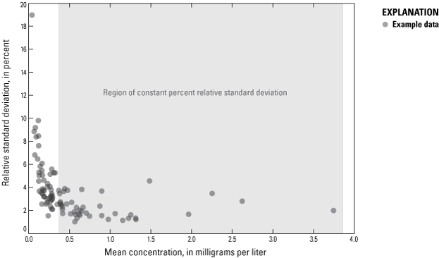
Percent relative standard deviation (%RSD) chart from Inorganic Blind Sample Project data (U.S. Geological Survey, 2025) showing a region of constant %RSD within a concentration range in milligrams per liter.
The Approach 2 (based on USGS SRSs) allowable range of variation was found using equation 5:
This SD-based approach should yield a robust measure of expected method variability at the mean concentration determined on day 2, because it includes multiday, multi-operator and, in some cases, multi-instrument variability. Thus, this approach is more representative of the conditions during the entire holding-time study. The total number of results ranged from 41 to 114 for the six (or in some cases five) SDs averaged.
Approach 3: Stability Limits Determined by Percentage of Mean Concentration
For Approach 3, stability limits were determined by calculating 10 percent of the mean concentration determined on day 2. The range of variability calculated by this approach is simply ±10 percent of the mean concentration determined on the second day after sample collection (day 2; eq. 6):
whereThe Approach 3 (based on 10 percent) stability limits were found using equation 7:
Once the range of variability was calculated for an observed property for a given sample using the three different approaches, the largest range of the three approaches was selected and applied to the mean sample concentration determined on day 2 (table 5). Ultimately, the ranges calculated using the variability in SRS results at different concentrations (Approach 2) were not used as they were never found to be the largest of the three approaches examined. This means that degradation could have been detected at levels within ±10 percent, but instability was not indicated because the more generous limits of ±10 percent were imposed.
Table 5.
Summary of initial mean concentration, allowable range of variation (stable or instable limits) calculations by three approaches, and the approach used to determine the stability limits (indicated by *).[HTS, holding-time study; ID, identification; MDL, method detection limit; mg/L, milligrams per liter; n, number of samples; ≤, less than or equal to; S/I, stable/instable; ±, plus or minus; SRSs, U.S. Geological Survey standard reference samples; %, percent; RSD, relative standard deviation; CaCO3, calcium carbonate; fltd, filtered; EP, end point; titr, titrated; lab, analysis done in laboratory; *, approach used to determine the stability limits; NA, not applicable; ANC, acid neutralization capacity; unfltd, unfiltered; N, nitrogen; blanks, stability limits based on blanks approach; P, phosphorous; --, no data]
Using the more generous limits of ±10 percent to indicate instability could have noteworthy consequences for data users with data-quality objectives more stringent than ±10 percent. For example, data from samples with minor levels of degradation yet that are indicated as stable (within stability limits of ±10 percent) could still be used, but they might underrepresent daily constituent loads for a stream. Comparing the computed loads to permitted total maximum daily load criteria could result in a false determination of compliance if the sample concentration decreased by as much as 10 percent, but not if the concentration decreased by only 5 percent. Data-quality objectives of a project are critical to the proper use and qualification of the data from all samples considered to be stable. Overall, limits based on blanks (Approach 1) were used in 49 percent of the stability test cases, and limits based on ±10 percent (Approach 3) were used in 51 percent of the stability test cases.
Interpretation of Analytical Results
A summary of field measurements and information on conditions at each sampling site for each set of samples used in the HTS are shown in table 6. The data in table 6 are intended to characterize the general status of the samples at the time of collection. Time series data for each set of triplicate results obtained for each sample are shown in appendix 1, figure 1.1 and 1.2. All the data shown in appendix 1, figure 1.1 and 1.2, are available in the data release that accompanies this report (Struzeski, 2025).
Table 6.
Field measurements for samples included in the holding-time study.[HTS, hold-time study, ID, identification; temp., temperature; °C, degrees Celsius; unfltd, unfiltered; μS/cm, microsiemens per centimeter; mg/L, milligrams per liter; %, percent; ANC, acid-neutralizing capacity; CaCO3, calcium carbonate; titr, titration; CO32-, carbonate; HCO3-, bicarbonate; field, analysis done in field; fltd, filtered; --, no data; <, less than]
For the 12 observed properties studied, the goal was to determine how long after sampling would changes in initial property concentrations be first detected (table 1). Initial concentrations are represented by the mean concentration of the triplicates analyzed within 48 hours of sampling, otherwise referred to as day-2 measurements. Observed properties were evaluated by reviewing percent recovery results and concentration results through time (app. 1, fig. 1.1 and 1.2). Changes from initial day-2 concentrations were considered relevant when differences in subsequently determined mean concentrations were greater than the expected method variability adjusted for concentration or greater than ±10 percent, whichever was larger. Mean concentrations determined after day 2 were binned into the following intervals, in days: 2, 14, 30, 60, 90, 120, 150, and 180. Actual days varied within each bin. Percent recoveries were calculated using equation 8:
The time series charts shown in figure 1.1A–H (app. 1) include parameters and triplicate sample results evaluated with allowable range-of-variation limits set at the day 2 ±10 percent approach. The time series shown in figure 1.2A–H (app. 1) include parameters and triplicate sample results evaluated using stability limits from method precision based on the blind-blank data method (Approach 1) described in the “Approach 1: Stability Limits Determined Using Blank Water” section of this report. Ultimately, limits using the natural matrix and spiked reagent water data (Approach 2) were not used to evaluate stability for this study because there were no cases in which those limits were the largest of the three approaches investigated.
Mean concentrations for time intervals after day 2 falling within the selected limits were assigned an “S” (stable). Mean concentrations falling outside the limits were assigned an “I” (instable). Note that while the largest of the three limits calculated was used for this analysis, individual projects should consider their data quality objectives and use a more conservative approach when warranted. A summary of S and I ratings used to determine data usability are listed by initial mean concentrations in table 7.
Table 7.
Overall analyte stability classification based on days analyzed after sample collection[HTS, holding-time study; ID, identification; CaCO3, calcium carbonate; fltd, filtered; EP, end point; titr, titration; lab, analysis done in laboratory; S, stable; I, instable; ND, no data due to no sample submitted; ANC, acid-neutralizing capacity; unfltd, unfiltered; N, nitrogen; M, missing data from lab; P, phosphorous]
Determination of Observed Property Stability
Observed property stability was assessed based on mean triplicate concentrations after day 2 relative to upper and lower stability limits. Some observed properties, such as orthophosphate as P, water, filtered, exhibited little change in concentrations through time (fig. 1.1H), and mean sample concentration results were between the upper and lower stability limits for all samples studied. However, the assessment of stability was more difficult when analyte recoveries started to show large changes in concentrations through time, such as changes more than ±20 percent of day-2 results for total ammonia as N, filtered (fig. 5). Therefore, it is important to note that sample instability is specific to each analyte and sample matrix combination.
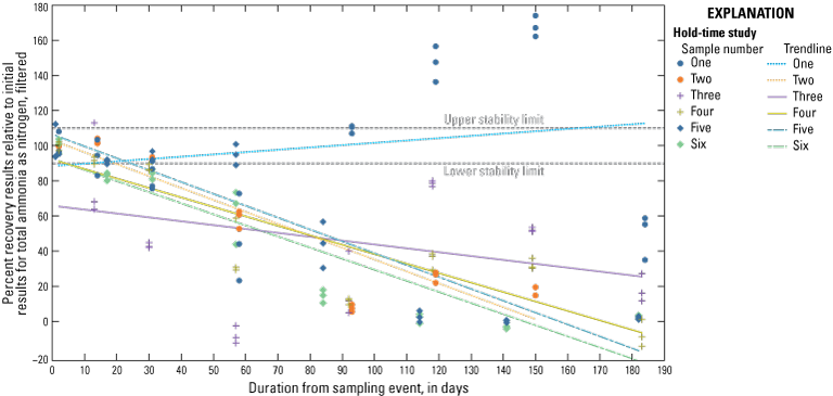
Scatterplot showing percent recovery results for specific time intervals for total ammonia as nitrogen, water, filtered, with stability limits based on day-2 results plus or minus 10 percent. Trend lines (method of least squares as determined by Microsoft Excel 365, version 2408 software) are added to aid in visualizing changes from starting recoveries of 100 percent on day 2.
Differences in analytical results among the triplicate sample bottles for each single-time interval and site could be due to several sources, which include analytical method bias and variability, variation in field processing, and within-bottle reaction kinetics.
Based on the limited number of six sample sources used in this study, some patterns emerge for the 12 observed properties studied (table 7). Five observed properties generally indicate stability (S rating) for as many as 180 days (total nitrogen as N, both filtered and unfiltered; orthophosphate as P, filtered; and phosphorus as P, both filtered and unfiltered.) Other observed properties indicate stability for as many as 180 days for some matrices but not for others. Finally, some observed properties indicate stability at 180 days but some instability (I rating) before that. General determinations of analyte stability are listed below by observed property.
-
Alkalinity as CaCO3, water, filtered, fixed endpoint (pH 4.5) titrated, lab—For the six HTS samples, the data generally indicated stability up to the NWQL method holding time of 30 days. After 30 days, results for some matrices indicated recoveries outside the stability limits. For all matrices, Approach 3 (±10 percent) was used as the acceptance criteria in place of the more conservative limits derived from method variability. Although this helped reduce the number of instable ratings, confidence in the stability of samples analyzed after the 30-day holding time did not improve. Based on the results of this limited study, sample stability cannot be presumed after the NWQL method holding time of 30 days.
-
ANC as CaCO3, water, unfiltered, fixed endpoint (pH 4.5) titrated, lab—For the six HTS samples, the data generally indicated stability for as many as 60 days after the day of sampling. After 60 days, sample results for half of the matrices indicated recoveries outside the lower stability limits. At day 60, two matrices demonstrated low recovery for one of the triplicate values, which might indicate a trend of instability starting prior to day 60 for those samples (fig. 1.1B). For this reason, sample stability cannot be presumed after the NWQL method holding time of 30 days.
-
Total ammonia as N, water, filtered—Data generally indicated acceptable stability for the NWQL method holding time of 28 days for most matrices in this study. Results for one sample indicated slight instability by day 14. By day 60, results for four of the six sample matrices indicated obvious instability. Although some results are flagged as acceptable after day 30, the relatively low concentration of total ammonia in the samples relative to the method detection level (between one-half and three times the detection level for five of the six samples) makes reliable detection of instability a challenge. Based on the results and limitations of this study, sample stability cannot be presumed after 30 days.
-
Total ammonia plus organic nitrogen as N, water, filtered and unfiltered—The instable-rated results for the six HTS samples are just outside stability limits except for one matrix that indicated significantly low recoveries at day 90 (unfiltered) and day 120 (filtered). These low recoveries are not associated with analytical run performance based on inspection of the results for the quality control samples analyzed before and after the HTS samples (Struzeski, 2025). By day 180 all results for filtered and unfiltered samples received stable ratings. Blind sample results from the Inorganic Blind Sample Project managed by the USGS Quality Systems Branch indicate that the method variability for these two observed properties is higher than for any other observed properties considered in this HTS, making it more difficult to differentiate method variability from sample instability (Struzeski, 2025). In addition, the concentration of total ammonia plus organic N in the samples is low relative to the method detection level (between one-half and six times the detection level for five of the six samples). This information, in conjunction with the fact that nearly 16 percent of the HTS data were missing for these constituents (many at the crucial day-60 interval), suggest using caution when considering sample stability outside of the NWQL method holding time. Sample stability beyond 30 days cannot be presumed.
-
Nitrite as N, water, filtered—There is no indication of stability in HTS samples analyzed after 30 days from sampling. In fact, most of the matrices indicated an instable rating by day 14 (within the NWQL method holding time of 30 days), but by day 30 all but one matrix indicated stable ratings once again. There are no indications of analytical bias for day-14 results. This suggests that some oxidation-reduction reactions may have occurred between day 2 and day 30. Sample stability cannot be presumed after the NWQL method holding time of 30 days.
-
Nitrate + nitrite as N, water, filtered—Data indicated acceptable stability for as many as 60 days. After day 60, there appeared to be possible oxidation occurring in samples 2 and 6 resulting in higher recoveries compared to the day-2 analyses. Although there are some instable ratings for this constituent, the five instable ratings are all within 13 percent of the mean of the day-2 triplicates. Consideration of how sample stability aligns with data-quality objectives is important for determining the utility of the nitrate plus nitrite as N, filtered data. For example, if a project evaluated its water-quality data by assigning stability limits to ±13 percent, then the nitrate plus nitrite as N samples for such a project would be considered stable for as many as 180 days.
-
Total nitrogen as N, water, filtered and unfiltered—For the six HTS samples, data generally indicated stability for at least 180 days. The two instable ratings indicated in the study are within 2 percent of the stability limits and might be due to method bias on that day.
-
Orthophosphate as P, water, filtered—For the six HTS samples, data indicated stability for as many as 180 days. All results were rated stable.
-
Total phosphorus as P, water, filtered and unfiltered—For the six HTS samples, data generally indicated stability for as many as 180 days. The three instable ratings (indicated for filtered and unfiltered samples) are from 18 results acquired on a single analytical run within 24 minutes of each other. Results for the same time interval that were analyzed about three weeks later were rated stable. Therefore, the instable ratings that occurred from data acquired together might be indicative of an analytical issue rather than a phosphorus stability issue. About 16 percent of the results were never acquired, but based on the acquired results, data generally indicated sample stability for at least 180 days.
Correlation Between Matrix and Sample Stability
Table 8 summarizes general observations regarding sample stability for selected observed properties in surface-water and groundwater samples based on the six sample matrices analyzed within and outside of NWQL method holding times. The times at which sample results indicate sample instability vary by observed property and matrix. Results for a selected matrix may indicate instability early in the sample lifetime for a given observed property but better stability than other matrices for a different observed property. Therefore, it is not possible to give general guidance for sample stability duration based on matrices alone.
Table 8.
General observations regarding data reliability for selected observed properties in surface-water and groundwater samples based on six sample matrices analyzed after standard holding-time durations in the U.S. Geological Survey holding-time study, 2023–2024.[National Water Information System (NWIS) parameter, method, laboratory (lab), holding time, and method codes from National Water Quality Laboratory (2023). NWQL, National Water Quality Laboratory; CaCO3, calcium carbonate; fltd, filtered; EP, end point; titr, titration; lab, analysis performed in the laboratory, not at the collection site; ANC, acid-neutralizing capacity; N, nitrogen; unfltd, unfiltered; P, phosphorous]
By ranking the percentage of mean results flagged as stable compared to mean results flagged as instable, general patterns were observed for the individual matrices (table 9). Samples 4 and 6 had the highest percentage of mean results flagged as instable at 29 and 30 percent, respectively, followed by samples 1 and 2, each indicating 19 percent of the mean results flagged for instability. Sample 5 had 14 percent of mean results flagged as instable, and the sole groundwater matrix had only 6 percent of mean results flagged as instable, supporting the expectation that groundwater samples are less biologically active (therefore more stable) than surface-water samples. No correlations between field measurements of sample characteristics and the number of results flagged as instable were observed. Because no correlations were observed, no suggestions can be made regarding overall sample stability based on field results.
Table 9.
Summary of sample instability ratings by sample matrix.[HTS, holding-time study; ID, identification; USGS, U.S. Geological Survey; NWIS, National Water Information System; WS, surface water; WG, groundwater]
Stream site numbers from U.S. Geological Survey, 2024. Refer to table 2 for stream site names.
Biological activity was visually observed in some of the unfiltered and unpreserved bottles by day 70; however, this condition was not methodically monitored. Therefore, no correlations can be drawn pertaining to biological causes of sample degradation.
Conclusions from this study are based on a limited number of matrices (six in total; table 3), and that all samples were collected in the fall, which may not have biological activity representative of other seasons. Although observations for some properties indicate sample stability that exceeds the recognized NWQL method holding times, this may not be the case for matrices and seasonal characteristics that were not investigated. By comparison, the USGS Patton and Gilroy (1999) study, which is considered comprehensive, used more than double the number of sampling sites (15) but considered a total duration of only 35 days. Gardolinski and others (2001) used only four samples for their study, which was repeated in two seasons, but resulted in no important differences in results by season. Therefore, the scope of this study is comparable to previous investigations.
Summary
The conclusions of this study are based on the following:
-
1. Mean values determined from the triplicates analyzed on day 2 are considered to be the samples’ true concentrations, and
-
2. Concentration stability can be adequately assessed by comparing mean values for triplicates analyzed on day 14 through day 180 against the largest of the stability limits calculated by three different approaches, those being (1) plus or minus 10 percent from mean values determined from the triplicates analyzed on day 2, (2) acceptable variability based on blank (no concentration present) results for samples submitted blindly, or (3) acceptable variability based on spiked reference material results for samples submitted blindly.
Based on the limited number of six sample sources used in this study, the general determinations of analyte stability for each observed property are as follows:
-
Alkalinity as calcium carbonate (CaCO3), water, filtered, fixed endpoint (pH 4.5) titrated, lab—Sample stability cannot be presumed after the National Water Quality Laboratory (NWQL) method holding time of 30 days.
-
Acid-neutralizing capacity as CaCO3, water, unfiltered, fixed endpoint (pH 4.5) titrated, lab—Sample stability cannot be presumed after the NWQL method holding time of 30 days.
-
Total ammonia as nitrogen (N), water, filtered—Sample stability cannot be presumed after 30 days.
-
Total ammonia plus organic nitrogen as N, water, filtered and unfiltered—Sample stability cannot be presumed after 30 days.
-
Nitrite as N, water, filtered—Sample stability cannot be presumed after the NWQL method holding time of 30 days.
-
Nitrate plus nitrite as N, water, filtered—Data generally indicated acceptable stability for as many as 60 days. After day 60, there appeared to be possible oxidation occurring in samples as compared to the day-2 triplicate analyses. Consideration of how sample stability aligns with data-quality objectives is important for determining the utility of the nitrate plus nitrite as N, filtered data.
-
Total nitrogen as N, water, filtered and unfiltered—For the six holding-time study (HTS) samples, data generally indicated stability for as many as 180 days.
-
Orthophosphate as phosphorus (P), water, filtered—For the six HTS samples, data indicated stability for as many as 180 days.
-
Total phosphorus as P, water, filtered and unfiltered—For the six HTS samples, data generally indicated stability for as many as 180 days.
Sample instability varied by observed property and matrix. However, it is not possible to give general guidance for sample stability duration based on matrices alone. No correlations between field measurements of sample characteristics and sample instability were observed. No conclusions can be drawn pertaining to biological causes of sample degradation. Although observations for some properties indicate sample stability well beyond the recognized NWQL method holding times, this is not necessarily the case for matrices and seasonal characteristics that were not investigated.
The effect of sample stability on the outcomes of water-quality studies is linked to study-specific data-quality objectives. For this report, upper and lower stability limits were set at plus or minus 10 percent for Approach 3. Water-quality studies with more flexible data-quality requirements could use a wider stability interval.
Acknowledgments
The authors would like to acknowledge and thank Roy Bartholomay, Trudy Bennett, Leslie DeSimone, Miranda Fram, Delia Ivanoff, Lisa Olsen, Sarah Stetson, Mandy Stone, and Rebecca Travis—for their contributions in designing the study, selecting sites, and reviewing procedures. The authors would also like to thank Sharon Pickersgill for the programming behind the Tableau charts that were invaluable for the initial data assessments. The authors would also like to thank Leslie DeSimone, Deborah Repert, and Rebecca Travis for their thorough review of this document. Finally, acknowledged are members of the National Water Quality Laboratory (NWQL) for their work in analyzing the additional samples as part of the study, and acknowledged are the various field team members involved in the study for collecting and processing the additional samples required for the study.
References Cited
Bartholomay, R.C., and Williams, L.M., 1996, Evaluation of preservation methods for selected nutrients in ground water at the Idaho National Engineering Laboratory, Idaho: U.S. Geological Survey Water-Resources Investigations Report 96–4260, 16 p. [Also available at https://doi.org/10.3133/wri964260.]
Childress, C.J., Foreman, W.T., Connor, B.F., and Maloney, T.J., 1999, New reporting procedures based on long-term method detection levels and some considerations for interpretation of water-quality data provided by the U.S. Geological Survey National Water Quality Laboratory: U.S. Geological Survey Open-File Report 99–193, accessed September 10, 2024, at https://pubs.usgs.gov/publication/ofr99193.
Degobbis, D., 1973, On the storage of seawater samples for ammonia determination: Limnology and Oceanography, v. 18, no. 1, p. 146–150, accessed April 15, 2024, at https://doi.org/10.4319/lo.1973.18.1.0146.
Fishman, M.J., ed., 1993, Methods of analysis by the U.S. Geological Survey National Water Quality Laboratory-Determination of inorganic and organic constituents in water and fluvial sediments: U.S. Geological Survey Open-File Report 93–125, 217 p., accessed April 11, 2024, at https://pubs.er.usgs.gov/publication/ofr93125.
Gardolinski, P.C.F.C., Hanrahan, G., Achterberg, E.P., Gledhill, M., Tappin, A.D., House, W.A., and Worsfold, P.J., 2001, Comparison of sample storage protocols for the determination of nutrients in natural waters: Water Research, v. 35, no. 15, p. 3670–3678, accessed May 21, 2024, at https://doi.org/10.1016/s0043-1354(01)00088-4.
Kaiser, K., McCullough, A., Schaefer, B., and VanRyswik, B., 2016, An analysis of nitrate groundwater sample preservation and storage methods: Minnesota Department of Agriculture Pesticide and Fertilizer Management Division webpage, accessed July 29, 2024, at https://wrl.mnpals.net/islandora/object/WRLrepository%3A2412.
Klingaman, E.D., and Nelson, D.W., 1976, Evaluation of methods for preserving the levels of soluble inorganic phosphorus and nitrogen in unfiltered water samples: Journal of Environmental Quality, v. 5, no. 1, p. 42–46, accessed May 21, 2024, at https://doi.org/10.2134/jeq1976.00472425000500010009x.
Maher, W., and Woo, L., 1998, Procedures for the storage and digestion of natural waters for the determination of filterable reactive phosphorus, total filterable phosphorus, and total phosphorus: Analytical chimica Acta, v. 375, p. 5–47, accessed May 23, 2024, at https://doi.org/10.1016/S0003-2670(98)00274-8.
National Water Quality Laboratory, 2023, Method holding times used by the National Water Quality Laboratory (NWQL): U.S. Geological Survey National Water Quality Laboratory webpage, 6 p., accessed November 8, 2024, at https://wwwnwql.cr.usgs.gov/qas/NWQLMethodHoldtimes.pdf.
Patton, C.J., and Gilroy, E.J., 1999, U.S. Geological Survey nutrient preservation experiment—Experimental design, statistical analysis, and interpretation of analytical results: U.S. Geological Survey Water-Resources Investigations Report 98–4118, 115 p. [Also available at https://doi.org/10.3133/wri984118.]
Patton, C.J., and Kryskalla, J.R., 2003, Methods of analysis by the U.S. Geological Survey National Water Quality Laboratory—Evaluation of alkaline persulfate digestion as an alternative to Kjeldahl digestion for determination of total and dissolved nitrogen and phosphorus in water: U.S. Geological Survey Water-Resources Investigations Report 03–4174, 33 p. [Also available at https://doi.org/10.3133/wri034174.]
Patton, C.J., and Truitt, E.P., 1992, Methods of analysis by the U.S. Geological Survey National Water Quality Laboratory—Determination of total phosphorus by a Kjeldahl digestion method and an automated colorimetric finish that includes dialysis: U.S. Geological Survey Open-File Report 92–146, 39 p., accessed July 15, 2024, at https://pubs.usgs.gov/of/1992/0146/report.pdf.
Patton, C.J., and Truitt, E.P., 1995, U.S. Geological Survey nutrient preservation experiment—Nutrient concentration data for surface-, ground-, and municipal-supply water samples and quality-assurance samples: U.S. Geological Survey Open-File Report 95–141, 140 p., accessed July 28, 2024, at https://doi.org/10.3133/ofr95141.
Patton, C.J., and Truitt, E.P., 2000, Methods of analysis by the U.S. Geological Survey National Water Quality Laboratory—Determination of ammonium plus organic nitrogen by a Kjeldahl digestion method and an automated photometric finish that includes digest cleanup by gas diffusion: U.S. Geological Survey Open-File Report 00–170, 31 p., accessed July 15, 2024, at https://pubs.usgs.gov/of/2000/0170/report.pdf.
Struzeski, T.M., 2025, Data for evaluation of nutrient, alkalinity, and acid neutralizing capacity stabilities in water samples analyzed by the National Water Quality Laboratory—2023–2024: U.S. Geological Survey data release, https://doi.org/10.5066/P1BRC2GJ.
Tate, C.M., Broshears, R.E., and McKnight, D.M., 1995, Phosphate dynamics in an acidic mountain stream—Interactions involving algal uptake, sorption by iron oxide, and photoreduction: Limnology and Oceanography, v. 40, no. 5, p. 938–946, accessed March 2, 2026, at https://doi.org/10.4319/lo.1995.40.5.0938.
U.S. Environmental Protection Agency [EPA], 2002, Guidance for quality assurance project plans: U.S. Environmental Protection Agency web page, 111 p., accessed February 13, 2025, at https://www.epa.gov/quality/guidance-quality-assurance-project-plans-epa-qag-5.
U.S. Environmental Protection Agency [EPA], 2016, Appendix B to part 136, Title 40—Definition and procedure for the determination of the method detection limit—Revision 2: Federal Register, 6 p., accessed June 12, 2024, at https://www.ecfr.gov/current/title-40/part-136/appendix-Appendix%20B%20to%20Part%20136. [Last amended September 22, 2025.]
U.S. Geological Survey, [variously dated], National field manual for the collection of water-quality data, section A of Handbooks for water-resources investigations: U.S. Geological Survey Techniques of Water-Resources Investigations, book 9, 10 chap. (A1–A10), accessed April 24, 2024, at https://pubs.usgs.gov/publication/tm9A0.
U.S. Geological Survey, 2024, USGS water data for the Nation: U.S. Geological Survey National Water Information System database, accessed April 8, 2024, at https://doi.org/10.5066/F7P55KJN.
U.S. Geological Survey, 2025, Inorganic Blind Sample Project (IBSP) current and historical performance chart/data access page: U.S. Geological Survey Inorganic Blind Sample Project website, accessed February 11, 2025, at https://qsb.usgs.gov/ibsp/charts.php.
Yorks, T.E., and McHale, P.J., 2000, Effects of cold storage on anion, ammonium, and total nitrogen concentrations in soil water: Communications in Soil Science and Plant Analysis., v. 31, no. 1–2, p. 141–148, accessed April 15, 2024, at https://doi.org/10.1080/00103620009370425.
Appendix 1. Time Series Charts Showing Sample Stability Through Time
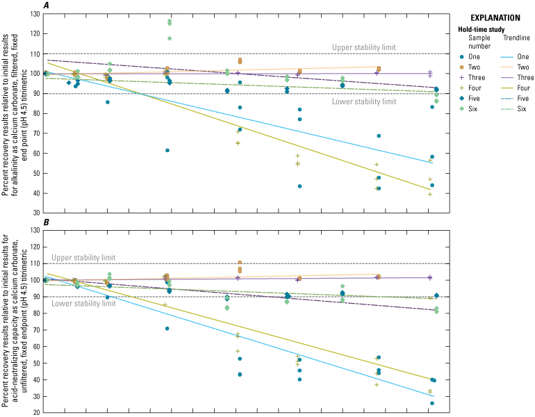
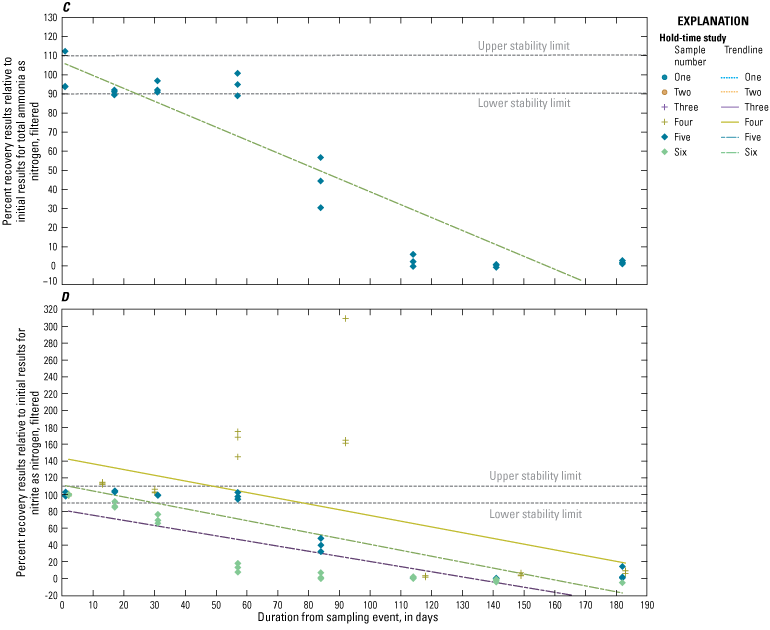
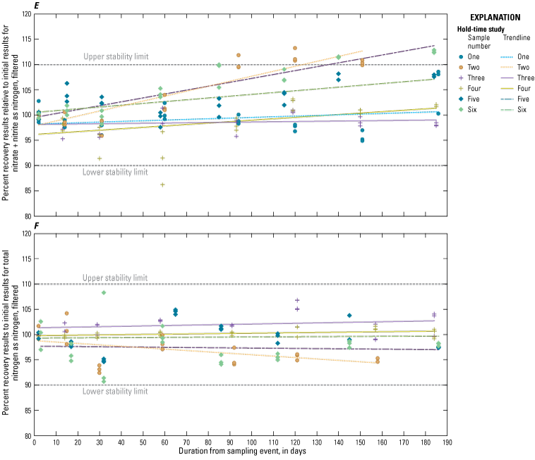
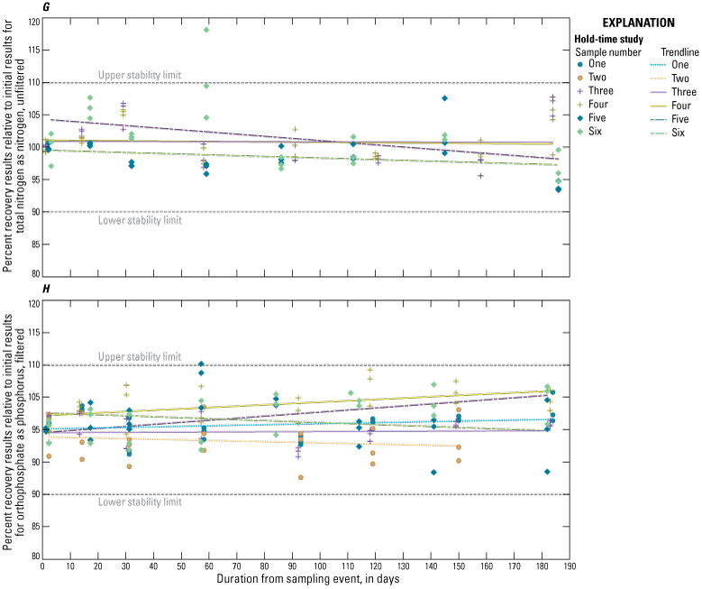
Scatterplots showing percent recovery results for specific time intervals and observed properties with stability limits based on day-2 results plus or minus 10 percent: A, alkalinity as calcium carbonate, filtered, fixed endpoint (pH 4.5) titrimetric, laboratory; B, acid-neutralizing capacity as calcium carbonate, unfiltered, fixed endpoint (pH 4.5) titrimetric, laboratory; C, total ammonia as nitrogen, filtered; D, nitrite as nitrogen, filtered; E, nitrate + nitrite as nitrogen, filtered; F, total nitrogen as nitrogen, filtered; G, total nitrogen as nitrogen, unfiltered; H, orthophosphate as phosphorus, filtered. Trend lines (method of least squares as determined by Microsoft Excel 365, version 2408 software) are added to aid in visualizing changes from starting recoveries of 100 percent on day 2.
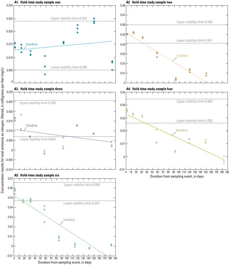
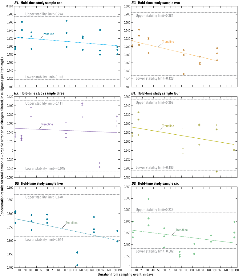
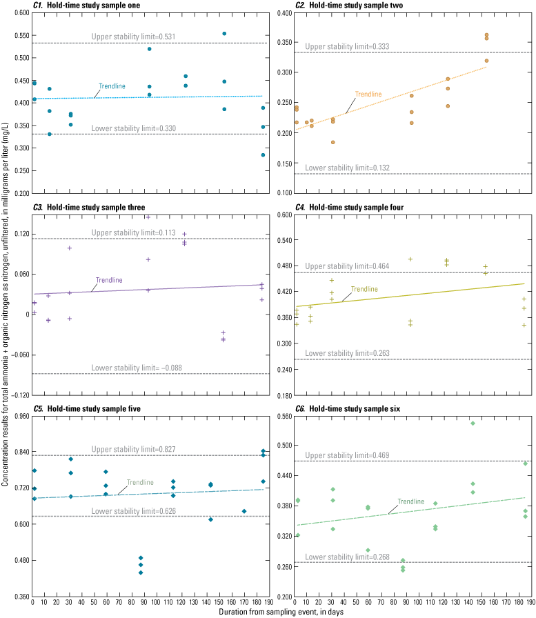
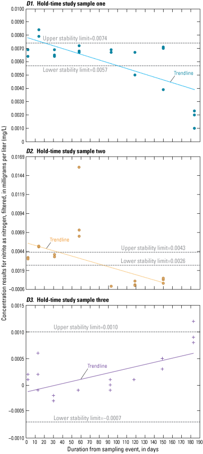
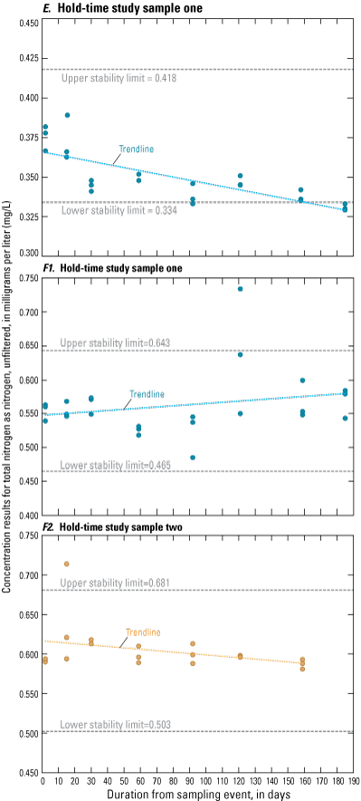
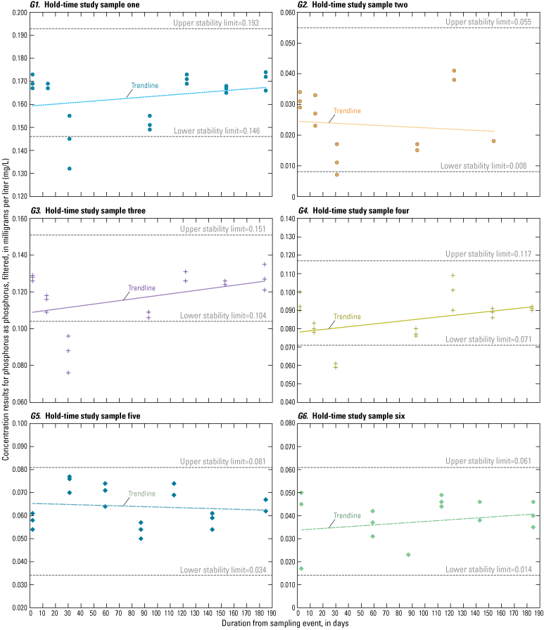
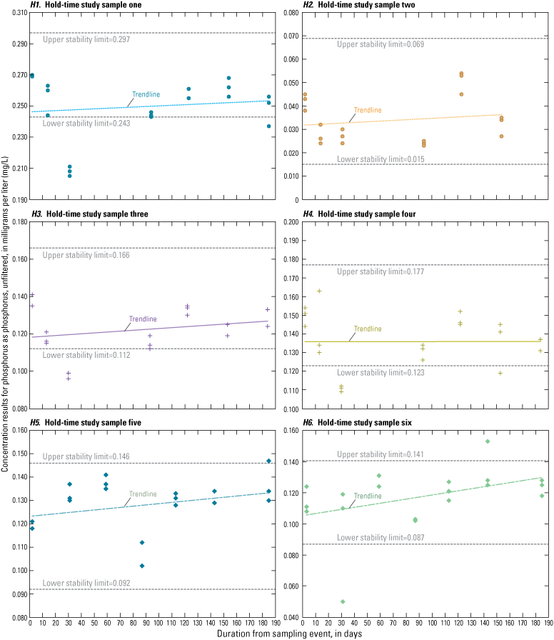
Scatterplots showing concentration results for specific time intervals and observed properties with stability limits based on method precision: A1–5, total ammonia as nitrogen, filtered; B1–6, total ammonia + organic nitrogen as nitrogen, filtered; C1–6, total ammonia + organic nitrogen as nitrogen, unfiltered; D1–3, nitrite as nitrogen, filtered; E, total nitrogen as nitrogen, filtered; F1–2, total nitrogen as nitrogen, unfiltered; G1–6, phosphorus as phosphorus, filtered; H1–6, phosphorus as phosphorus, unfiltered. Trend lines (method of least squares as determined by Microsoft Excel 365, version 2408 software) indicate general trends.
Conversion Factors
Supplemental Information
Specific conductance is in microsiemens per centimeter at 25 degrees Celsius (μS/cm at 25 °C).
Concentrations of chemical constituents in water are given in milligrams per liter (mg/L).
Abbreviations
%RSD
percent relative standard deviation
ANC
acid-neutralizing capacity
ASR
Analytical Services Request
ASTM
American Society for Testing and Materials
EPA
U.S. Environmental Protection Agency
FCC
filtered (sample), chilled, high-density polyethylene, amber, 125 milliliters, unacidified
FRP
filterable reactive phosphorus
FU
filtered (sample), high-density polyethylene, 250 milliliters, unacidified
HTS
holding-time study
I
instable
LASD
Laboratory Analytical Services Division
LIMS
Laboratory Information Management System
MDL
method detection limit
NWQL
National Water Quality Laboratory
RU
unfiltered (sample), high-density polyethylene, 250 milliliters, unacidified
S
stable
SD
standard deviation
SRS
standard reference sample
TON
total oxidized nitrogen
USGS
U.S. Geological Survey
WCA
unfiltered (sample), chilled, high-density polyethylene, 125 milliliters, acidified
For more information concerning the research in this report, contact the
Chief, USGS Quality Systems Branch
Box 25046, Mail Stop 401
Denver, CO 80225-0585
(303) 236-1835
Or visit the Inorganic Blind Sample Project website at
Publishing support provided by the Science Publishing Network,
Denver Publishing Service Center
Disclaimers
Any use of trade, firm, or product names is for descriptive purposes only and does not imply endorsement by the U.S. Government.
Any use of trade, firm, or product names is for descriptive purposes only and does not imply endorsement by the U.S. Government.
Although this information product, for the most part, is in the public domain, it also may contain copyrighted materials as noted in the text. Permission to reproduce copyrighted items must be secured from the copyright owner.
Suggested Citation
Struzeski, T.M., Wetherbee, G.A., and Morrison, J., 2026, Evaluation of nutrient, alkalinity, and acid-neutralizing capacity stabilities in water samples analyzed by the U.S. Geological Survey National Water Quality Laboratory, 2023–24: U.S. Geological Survey Scientific Investigations Report 2026–5014, 36 p., https://doi.org/10.3133/sir20265014.
ISSN: 2328-0328 (online)
| Publication type | Report |
|---|---|
| Publication Subtype | USGS Numbered Series |
| Title | Evaluation of nutrient, alkalinity, and acid-neutralizing capacity stabilities in water samples analyzed by the U.S. Geological Survey National Water Quality Laboratory, 2023–24 |
| Series title | Scientific Investigations Report |
| Series number | 2026-5014 |
| DOI | 10.3133/sir20265014 |
| Publication Date | June 08, 2026 |
| Year Published | 2026 |
| Language | English |
| Publisher | U.S. Geological Survey |
| Publisher location | Reston VA |
| Contributing office(s) | WMA - Laboratory & Analytical Services Division |
| Description | Report: vi, 36 p.; Data Release |
| Online Only (Y/N) | Y |