

Flood-Frequency Estimates for Kentucky Streamgages Based on Data Through Water Year 2021 and Results of Updating the Fundamental Layers in Kentucky StreamStats
Links
- Document: Report (9.59 MB pdf) , HTML , XML
- Data Releases:
- USGS data release - At-site flood frequency estimates for 261 Kentucky streamgages using data through water year 2021
- USGS data release - Elevation, flow direction, flow accumulation, and stream network rasters for Kentucky StreamStats update, 2026
- Download citation as: RIS | Dublin Core
Acknowledgments
The authors would like to acknowledge the Kentucky Transportation Cabinet for their assistance and support for this study.
Abstract
The U.S. Geological Survey, in cooperation with the Kentucky Transportation Cabinet, analyzed flood-frequency statistics for streamgages in Kentucky. Using annual peak-flow data through water year 2021, flood-frequency estimates were computed for 261 streamgages, including unregulated and regulated sites as well as sites with mixed regulation records. Methods followed those outlined in “Guidelines for Determining Flood Flow Frequency—Bulletin 17C” (U.S. Geological Survey Techniques and Methods 4–B5). These estimates included flows corresponding to annual exceedance probabilities of 50, 20, 10, 4, 2, 1, and 0.2 percent. Temporal trend analyses using the Mann-Kendall test indicated that 18 percent of unregulated streamgages with (1) at least 30 years of peak-flow record and (2) peak-flow record at least as recent as water year 2000 showed statistically significant trends, most of which were weak to moderate increases in peak flows. Concurrently, the fundamental geospatial datasets that support the Kentucky StreamStats application were updated by using high-resolution digital elevation models and hydrography datasets to derive flow direction, flow accumulation, and stream definition rasters. Comparisons of regression-based flood-frequency models using the old and new layers demonstrated consistent results, with a statewide root-mean-square error of 0.019, in the base-10 logarithm of cubic feet per second. Furthermore, to assess model performance, flood-frequency estimates made by using the updated layers and previously published regression-based models were compared to flood-frequency estimates newly computed by following Bulletin 17C. This analysis showed the models performed adequately for most Kentucky stream locations. The updated statistics and geospatial layers provide stakeholders with more accurate, current data for flood-risk assessment, infrastructure design, and water-resource management.
Introduction
The U.S. Geological Survey (USGS), in cooperation with the Kentucky Transportation Cabinet, completed a study to (1) compute flood-frequency statistics for long-term streamgages (defined as streamgages with at least 10 years of peak-flow record) in Kentucky, (2) analyze selected computed statistics for trends, and (3) update the fundamental geospatial data layers in the Kentucky StreamStats web application (https://streamstats.usgs.gov/ss/). For the purposes of this study, flood-frequency statistics are estimates of the magnitudes of flood-peak flows (hereafter referred to as “peak flows”) corresponding to selected annual exceedance probabilities (AEPs) (hereafter referred to as “AEP flows”). The term “frequency” comes from the commonly used average recurrence interval of a peak flow during a long period of time (given as the reciprocal of the AEP). For example, a peak flow that has a 0.01 (1-percent) AEP is the same as a peak flow that occurs on average once every 100 years and therefore is often called a “100-year flood.”
Flood-frequency statistics are used by many Federal, State, and local stakeholders. They are used in the design of bridges, culverts, dams, and spillways to ensure the structures can contain or convey design flows, in flood-insurance studies to determine the boundaries of inundation, and by emergency managers to assess flood risk. The decisions made based on these statistics can be financially consequential and affect human safety.
One way that the USGS makes flood-frequency statistics available is through StreamStats. StreamStats is a map-based web application that allows users to view flow statistics for USGS streamgages and provides tools to estimate statistics at ungaged, user-selected stream locations (Ries and others, 2017). To estimate flow statistics at ungaged stream locations, StreamStats computes basin characteristics from geospatial datasets. The computed basin characteristics are then used in regression models specific to each AEP to compute estimates. As more peak-flow data are collected at streamgages and new (and sometimes more accurate) geospatial data are published, it is critical to update flow statistics and StreamStats’ geospatial layers so that stakeholders can make decisions using the best available data.
The USGS last published flood-frequency statistics for Kentucky streamgages in 2003 (Hodgkins and Martin, 2003). The 2003 report detailed the methods and results of estimating selected AEP flows at Kentucky streamgages and developed methods for estimating those AEP flows at unregulated, rural stream locations that are ungaged. The results of that study are valid and representative of their analytical period, which included annual peak flows through water year 2000 (a water year is defined as the period from October 1 through September 30 and is designated by the calendar year that it ends in). Since then, two key factors prompted this study: (1) 20 years of additional data were collected, and (2) the recommended methods for computing flood-frequency statistics were superseded. The previous study’s methods were based on “Guidelines for Determining Flood Flow Frequency—Bulletin 17B” (Interagency Advisory Committee on Water Data, 1982), which was superseded by “Guidelines for Determining Flood Flow Frequency—Bulletin 17C” (England and others, 2018; hereafter referred to as “Bulletin 17C”). Bulletin 17C includes the following improvements:
-
• a method-of-moments process (referred to as the expected moments algorithm [Cohn and others, 1997]) for fitting log-Pearson Type III (LPIII) distributions to peak flows; this new process can include interval estimates of peak flow, censored peak flow, and multiple thresholds of observation;
-
• a generalized Grubbs-Beck low-outlier test (multiple Grubbs-Beck test [Cohn and others, 2013]) that allows the identification of potentially influential low floods (PILFs); and
-
• updated methods of estimating regional skew and uncertainty (Veilleux and others, 2011).
The prior fundamental layers (USGS, 2025) were created by using a digital elevation model (DEM) with a 30-foot spatial resolution that was derived from the National Elevation Dataset (Gesch and others, 2009) and the 1:24,000-scale National Hydrography Dataset (NHD; USGS, 2021).
Purpose and Scope
The purpose of this report is to describe the methods and results of a study to (1) compute selected flood-frequency statistics at long-term continuous-record streamgages in Kentucky; (2) analyze selected statistics for temporal trends; and (3) update Kentucky StreamStats’ fundamental layers. Flood-frequency statistics computed for this study were the 50-, 20-, 10-, 4-, 2-, 1-, and 0.2-percent AEP flows based on peak-flow data through water year 2021. Updates to Kentucky StreamStats’ fundamental layers included an update to the DEM, flow direction raster (FDR), flow accumulation raster (FAC), and stream definition raster (SDR). Finally, this report presents the results of analyses that (1) compared regression-based flood frequency estimates and (2) evaluated the performance of the previously published regression equations in estimating updated flood-frequency statistics using basin characteristics derived from the updated layers.
Description of Study Area
The study area was limited to the State of Kentucky. Certain study area characteristics, such as those related to climate, physiography, geology, and land cover, are direct factors in a stream’s flood-frequency characteristics (Chow, 1964). Some of Kentucky’s characteristics that are related to flood frequency are described in the following subsections.
Climate
Kentucky’s climate is characterized by somewhat large seasonal variations in temperature. In summer (June–August), highs range from 82 degrees Fahrenheit (°F) in the eastern part of the State to 91 °F in the west, and days are typically sunny and humid. In winter (December–March), highs range from 40 °F in the north to 47 °F in the south, and cloudy skies are common. Spring and fall are often characterized by milder temperatures; however, frontal systems can cause temperatures to change drastically (National Oceanic and Atmospheric Administration National Climatic Data Center, undated).
The State typically receives abundant precipitation; average annual totals range from 38 inches (in.) in the northeast to 58 in. in the southeast. In typical years, Kentucky receives the most precipitation in the spring and least in the fall; however, it is well distributed throughout the year. It is not uncommon for precipitation intensities to reach as high as 1 inch per hour for short durations and up to 5 inches per day. Most precipitation falls as rain, and average annual snowfall ranges from 10 in. in the south to approximately 20 in. in the north. Snow cover rarely lasts for more than 1 week in the south or 2 weeks in the north (Runkle and others, 2022).
Physiography and Geology
The physiographic regions of Kentucky closely resemble its geologic regions. That is because the State’s topography is a result of the weathering and erosion of its underlying bedrock. Broadly, the State can be divided into six physiographic regions (fig. 1; Kentucky Geological Survey, 2012):
-
1. Jackson Purchase or Mississippi Embayment—Surface geology is mostly unconsolidated sediment that is easily eroded, and therefore this region is relatively flat and includes many lakes and swamps.
-
2. Mississippian Plateau or Pennyroyal Region—This region is defined by its karst terrain, which is caused by the underlying soluble limestone bedrock. This limestone plain has abundant sink holes, sinking streams, springs, and caverns.
-
3. Western Kentucky Coal Field—This region is part of the larger Mississippi Plateau Region. Its border is marked by an escarpment of weathering-resistant sandstone.
-
4. Knobs—This region is characterized by steep, isolated, cone-shaped hills caused by weathering-resistant limestone or sandstone “caps” over less resistant shales.
-
5. Bluegrass region—This region is characterized by rolling hills with rich soils, caused by the weathering of limestone bedrock. This weathered limestone is also responsible for the area’s karst geology.
-
6. Eastern Kentucky Coal Field—This region is part of the larger physiographic area known as the Cumberland Plateau. The western edge of the Eastern Kentucky Coal Field is formed from weathering-resistant sandstone and conglomerates with stepped-in bands of shales less resistant to weathering. These differences in resistance result in cliffs, gorges, and waterfalls. The interior of the region is dominated by steep hills and valleys.
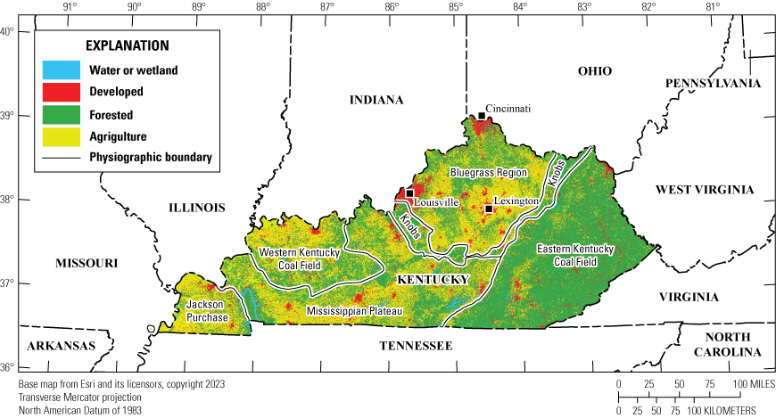
Map of study area showing Kentucky’s physiographic regions, major cities, land use, and surrounding States. Physiographic regions are from Kentucky Geological Survey (2012). Land use from U.S. Geological Survey (2024).
Land Cover and Land Use
Kentucky’s borders encompass approximately 40,000 square miles (mi2) (Elbon, 2025). Of that area, most land is categorized as forested (52 percent), followed by agricultural (33.7 percent), developed (8.3 percent), and water or wetland (3.2 percent); the remaining land is categorized as “other” (USGS, 2024) (fig. 1). However, these land covers are not evenly distributed across the State; broadly, the eastern part of the State has more extensive forests, the western has more agriculture, and much of the developed land is near the cities of Louisville, Lexington, and the Kentucky portion of the Cincinnati metropolitan area, which are the State’s largest metropolitan areas (Taulbee, 2025).
Computation of Flood-Frequency Statistics at Gaged Sites
Flood-frequency statistics, consisting of AEP flows of 50, 20, 10, 4, 2, 1, and 0.2 percent, were computed for selected Kentucky streamgages. Separate flood-frequency analyses were completed for streamgages with regulated peak flows and unregulated peak flows. For this study, a regulated peak-flow record was identified as one in which peak flows were substantially altered from what would be the site’s “natural” peak flows by such anthropogenic influences as dams, urbanization, channelization, and mining. Regulation status was determined by peak-flow qualifier codes stored in the USGS National Water Information System (https://waterdata.usgs.gov/). Peak flows qualified with a code of 5 (indicating the peak flow was affected to an unknown degree by regulation or diversion), 6 (indicating the peak flow was affected by regulation or diversion), or C (indicating the peak flow was affected by urbanization, mining, agricultural changes, channelization, or other factors) were categorized as regulated. Some streamgages had records of unregulated peak flow before or after periods of regulation. The record for each of those streamgages was divided into regulated and unregulated periods, and a separate flood-frequency analysis was completed on each period that had a minimum of 10 years of peak-flow record (the minimum recommended by Bulletin 17C [England and others, 2018]). Analyses were made on 223 streamgages with unregulated records, 11 streamgages with regulated records, and 27 streamgages with records that included both regulated and unregulated periods (fig. 2).
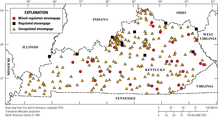
Map of Kentucky showing sites analyzed as part of this study as unregulated, regulated, and mixed regulation. Streamgage regulation information is in VonIns and others (2026).
Flood-frequency analyses were completed by using the USGS peak-flow frequency application (PeakFQ), version 8.1.0 (Siefken and others, 2024), which implements the methodology of Bulletin 17C (England and others, 2018). At its core, Bulletin 17C (and thus, PeakFQ) provides methods for estimating AEP flows by using a LPIII distribution to fit the logarithms of each streamgage’s annual peak flows. In its simplest form, the logarithm of the flow associated with a given AEP is estimated as:
whereis the flow associated with a given AEP, in cubic feet per second (ft3/s),
is the mean of the logarithms of the annual peak flows,
is a frequency factor that depends on the AEP and the coefficient of skewness of the logarithms of the annual peak-flow record, and
is the standard deviation of the logarithm of annual peak-flow record.
Bulletin 17C extends this framework to accommodate additional information types that are sometimes available in peak-flow records (England and others, 2018, app. 7). Those used in this report are regional skew, flow intervals, perception thresholds, and potentially influential low floods (PILFs). These data types are described in more detail in the following subsections. All data related to the flood-frequency analysis, including PeakFQ inputs and results, are available in this report’s associated USGS data release (VonIns and others, 2026).
Regional Skew
A skewed frequency distribution—such as the LPIII distribution used in this study—arises when peak-flow data are not symmetrically distributed around the mean. Properly accounting for skew is critical to obtaining accurate AEP flow estimates. However, at-site skew computed from peak-flow records of short or moderate length is often highly uncertain. Bulletin 17C (England and others, 2018, app. 7, eqs. 7–10) recommends improving the skew estimate by weighting the at-site value with regional skew information.
For Kentucky, a regional skew coefficient ( of 0.048 was used. This value came from a regional flood-skew study of the Tennessee, parts of the Ohio, and the Lower Mississippi River Basins (hydrologic unit codes [HUC] 06, 05, and 08, respectively; Wagner and others, 2025). This included the States of Kentucky and Tennessee, as well as parts of Virginia, West Virginia, Maryland, North Carolina, Georgia, Alabama, and Mississippi (Wagner and others, 2025). Regulated records used only station skew because regional skew values may not represent their altered peak-flow distributions.
Flow Intervals, Perception Thresholds, and Potentially Influential Low Floods
In previous Kentucky flood-frequency studies, at-gage statistics were computed by using flood observations recorded every year at streamgages, which could be represented as point data. However, the expected moments algorithm described in Bulletin 17C made it possible to include in the analysis information from peak-flow records that cannot be represented by points, such as information about peak flows that were known to be within a range of values or to be greater than or less than a known value. Bulletin 17C (England and others, 2018) describes these concepts as flow intervals and perception thresholds. A brief discussion of each and how they were commonly applied in this study follows:
-
1. Flow interval—Each year in a streamgage’s record (including gaps) required a flow interval defined by a lower and upper bound for the peak flow. For most peak flows in a record, the lower and upper bound was the observed peak flow. However, for years when no peak flow was recorded, the lower bound was set to zero and the upper bound was set to infinity. If a peak flow had definable uncertainty, the range was specified accordingly.
-
2. Perception threshold—The expected moments algorithm also requires that perception thresholds be entered. Perception thresholds are the range of flows that could have been recorded if they had occurred. For most peak flows in a record, this range was set from zero to infinity because all annual peak flows were assumed to have been measured during the record period. For gaps in the record, the lower and upper thresholds were set to infinity. If a peak had a definable perception range, the threshold was specified accordingly.
Most interest in flood-frequency analyses is in large floods, which have small AEPs. Some peak-flow records include smaller peak flows that do not follow the pattern of large peak flows. These relatively small peak flows are referred to in Bulletin 17C as potentially influential low floods (PILFs). For the majority of sites, the multiple Grubbs-Beck test (Cohn and others, 2013) was used to identify PILFs and censor them from the frequency distribution within PeakFQ. However, occasionally the multiple Grubbs-Beck test did not detect a PILF threshold that was evident upon inspection of the annual peak-flow distribution. In these instances, a user-defined PILF threshold was applied based on inspection of the annual peak-flow distribution. Removing PILFs from the distribution generally results in a better fit of the LPIII distribution to the large-flood observations. However, it can also lead to a worse fit to the small peak-flow portion of the frequency distribution.
Tests for Temporal Trends in Peak Flows
Long-term trends in annual peak flows can be an indication of changes in an area’s hydrology, climate, or both. Furthermore, a key assumption of LPIII-based flood-frequency analysis, as presented in Bulletin 17C and used in this study, is that the peak-flow records are a representative sample of future peak flows. To test that assumption, a two-sided Mann-Kendall test was applied to the annual peak-flow record for each streamgage included in the analysis (VonIns and others, 2026; refer to the file “KY_Unregulated_trd.csv”). The Mann-Kendall test is a nonparametric statistical test used to detect monotonic trends over time. Kendall’s tau (τ) quantifies the strength and direction of a monotonic trend: a value of 1 indicates a perfectly increasing trend in a site’s annual peak flow record, and a value of −1 indicates a perfectly decreasing trend; values near 0 indicate no monotonic trend. The associated p-value is used to determine whether to reject the null hypothesis of no monotonic trend (τ=0). In this analysis, trends were considered statistically significant when p≤ 0.05 (alpha level of 0.05).
Recent Long-Term Trends in Unregulated Annual Peak Flows
To look for patterns that could indicate recent (since the analysis period of Hodgkins and Martin [2003]) or ongoing changes to Kentucky’s hydrology, this discussion focuses on unregulated streamgage records that had recorded peak flows since water year 2000. Furthermore, to minimize the influence of spurious trends that could result from an unrepresentative sampling period, this discussion only includes streamgages that had at least 30 years of annual peak-flow record. After applying those criteria, there were 51 qualifying gages. Of those, nine (18 percent) had statistically significant trends in their peak flow record (fig. 3); seven of those were positive trends, and two were negative. The significant trends, both positive and negative, tended to be weak to moderate with absolute tau values ranging from 0.15 to 0.34. Three notable observations were made; however, further investigation could improve conclusions about their importance or cause could be assigned. Those observations are the following:
-
• All streamgages with significant trends were located east of the 86° longitude line.
-
• All streamgages with significant trends had relatively small drainage basins (four have drainage areas less than 30 mi2, four between 30 and 100 mi2, and the largest 188 mi2).
-
• Four streamgages with significant trends were near the urban centers of Louisville (three) and Lexington (one).
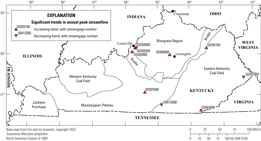
Map showing unregulated streamgages in Kentucky with (1) at least 30 years of annual peak-flow record and (2) some of that record being collected since water year 2000 that had statistically significant trends in their annual peak flow record (alpha level <0.05). Physiographic regions are from Kentucky Geological Survey (2012). Trend data are available in VonIns and others (2026).
Fundamental Layers Update
The Kentucky StreamStats application provides spatial analytic tools designed to delineate drainage areas, summarize basin characteristics, and apply regression-based models (hereafter referred to as regression models) to estimate flow statistics. To enable the use of those tools, StreamStats relies on four primary geographic information system (GIS) layers (often called the “fundamental layers”):
-
1. digital elevation model (DEM)—a three-dimensional digital representation of an area’s topography;
-
2. flow direction raster (FDR)—a grid in which every cell represents the direction water would flow; the flow direction of a cell is found by determining the steepest downslope neighbor of every cell;
-
3. flow accumulation raster (FAC)—a grid in which every cell represents the number of upslope cells that would drain into it; and
-
4. stream definition raster (SDR)—the FAC raster filtered to include only cells that have a minimum number of upslope cells draining to it. The minimum is set to try to include only paths of channelized flow.
The DEM update began with 5-foot resolution products from the Kentucky Aerial Photography and Elevation Data Program (KyFromAbove) light detection and ranging (lidar) program (2010–17; KyFromAbove, 2020). These DEMs were resampled to 30-foot resolution to (1) match the scale of the National Hydrography Dataset Plus High Resolution (USGS, 2021) and the Watershed Boundary Dataset and (2) reduce processing time for StreamStats basin computations. For basins extending beyond Kentucky, 10-meter DEMs from surrounding States (USGS, 2021) were resampled to 30-foot resolution and reprojected to the Kentucky State Plane Coordinate System. All DEMs were merged into a single seamless layer and clipped to include only drainage basins that drained into Kentucky.
The updated DEM and Watershed Boundary Dataset boundaries were used to create new FDRs. For each eight-digit hydrologic unit code, DEM cells were hydrologically enforced by assigning flow to the downslope neighbor with the lowest elevation, producing rasters that represent drainage connectivity across the landscape. The FAC raster, derived directly from the FDRs, quantifies the number of upstream cells contributing flow to each location. Both FDRs and FACs were created with the USGS StreamStats Data Preparation Tools (Barnhart and others, 2020) and mosaicked into statewide layers. The stream definition raster was then generated by filtering the FAC to cells with at least 900 upstream contributors, representing channelized flow paths.
The FDR, FAC, and stream definition rasters were reviewed against high-resolution aerial imagery. In dense drainage networks, it was observed that flow paths within three raster cells sometimes merged incorrectly. To address this, drainage-line enforcement tools (Barnhart and others, 2020) were used in those areas with dense drainage networks to force the flowlines to match the paths of the NHD. The final layers were implemented on a StreamStats test server and verified for compatibility with basin delineation, basin characteristics, and regression tools. The fundamental layers and associated metadata are presented in Webber and others (2026).
Assessment of Regression Models
Hodgkins and Martin (2003) developed a series of regression models to estimate selected AEP flows at unregulated, ungaged stream locations. The regression models currently implemented in StreamStats were developed by using LPIII-based AEP flows (based on peak flows through water year 2000; Hodgkins and Martin, 2003) as the response variable and by using physiographic region, drainage area, and, for some models, main channel slope as explanatory variables. To ensure that the regression models were effective after updates to the fundamental layers and computation of updated LPIII-based AEP flows, the following analyses were completed:
-
1. Peak-flow estimates computed by using explanatory variables from the previously published fundamental layers were compared to estimates computed by using the newly created fundamental layers to ensure that the new layers did not introduce bias.
-
2. Statistics assessed how peak-flow estimates computed by using the regression models with the new fundamental layers compared to the newly computed at-site flood-frequency statistics to ensure that the regression models, using the new fundamental layers as explanatory variables, could reasonably predict the new LPIII- based AEP flows.
Comparison of Model Results Using Previously Published and Newly Developed Fundamental Layers
Model results from before and after the fundamental-layer update were compared. The evaluation began by computing basin characteristics and flow statistics at selected streamgage locations using (1) the previously implemented StreamStats layers and (2) the newly developed layers. Summary statistics and scatterplots were then generated to compare each basin characteristic and flow statistic.
A comparison of differences between flow estimates derived from the new and previously published layers produced a root-mean-square difference (RMSD) of 0.019 log10(ft3/s), corresponding to a multiplicative factor of 1.045 (that is, flow estimates typically differ by about ±4.5 percent). Figure 4 shows a scatterplot of the 1-percent AEP flow estimated using the old versus new fundamental layers, which is representative of all the AEP flows. These results were consistent across all regression models. The consistency across all regression models of RMSD and the relation shown in figure 4 reflects that the changes in the basin characteristics used as predictors were typically very small and that the regression models share the same form and differ only in their fitted coefficients. Most estimates fall on or very near the one-to-one line, with two notable exceptions. The two points plotting to the lower right of the one-to-one line—representing USGS streamgages Lick Creek Tributary near Kirbyton, Ky. (07023040), and Perry Creek near Mayfield, Ky. (07022500)—show larger relative differences than points representing the other streamgages evaluated. These larger differences result from discrepancies in delineated drainage area, which is the primary explanatory variable in the regression models. Both streamgages are in the relatively flat Jackson Purchase region of western Kentucky, where low-relief terrain and a dense drainage network can complicate accurate delineation of watersheds. It is incumbent on users working in areas with low relief or dense drainage networks, or both, to review their delineations before using peak-flow estimates. Overall, based on the low RMSD and visual inspection of the comparison plots, the results were considered satisfactory.
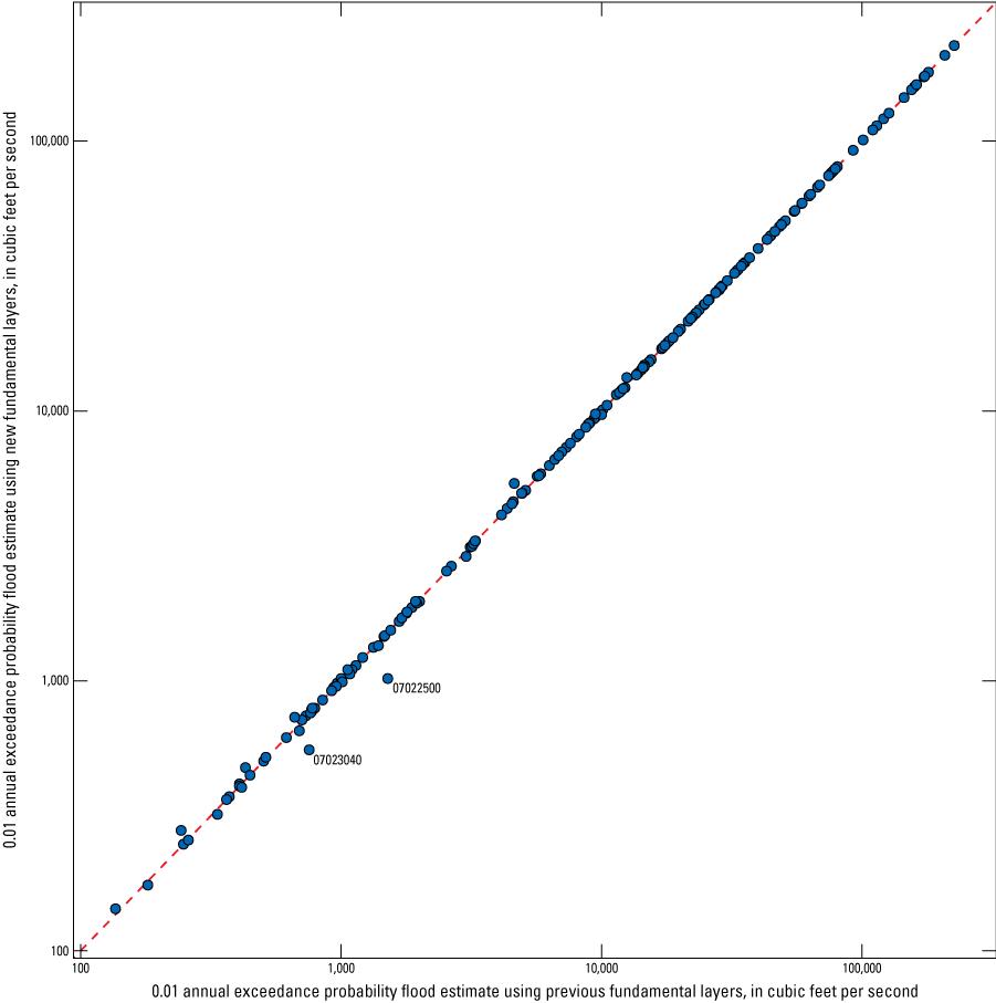
Scatter plot of 0.01 annual exceedance probability peak flows estimated for streamgages in Kentucky by using the Kentucky StreamStats Application (U.S. Geological Survey, 2025) with (1) previously published fundamental layers implemented and (2) new fundamental layers developed as part of this study implemented.
Assessment of Fit: Previously Published Models Compared to New Flood-Frequency Estimates
Selected fit statistics and scatter plots were used to evaluate how well the flood-frequency models implemented in StreamStats (Hodgkins and Martin, 2003) predicted at-site LPIII estimates from this study. Two statistics were included:
-
1. The geometric mean of the ratio of regression estimates to LPIII estimates—This statistic was used to assess the central tendency of the multiplicative bias between the two methods (Helsel and others, 2020). A geometric mean of 1 indicates no bias, <1 indicates underestimation, and >1 indicates overestimation. As an example, a value of 1.01 means the predictions from the regression model are, on average, 1 percent greater than the at-site LPIII estimates.
-
2. The standard deviation of the log-transformed residuals (expressed in real space as the geometric standard deviation [GSD])—This statistic was used to quantify the multiplicative variability of the residuals. The GSD represents the average factor by which regression estimates differ from the LPIII estimates. For example, a GSD of 1.50 indicates that regression estimates typically vary by a factor of 1.50 above or below the corresponding LPIII estimate (that is, approximately ±50 percent).
The fit statistics (table 1) and scatterplots (fig. 5) indicate that the regression models performed reasonably well in predicting the newly computed statistics. One notable observation was the consistent overestimation of flow by the regression models compared to the LPIII estimates at streamgages with the largest flows for a given AEP. An example of this pattern, along with the general fit, is shown in figure 5, where the 1-percent AEP regression estimate generally exceeded the LPIII estimate for flows greater than approximately 100,000 ft3/s. Further investigation found that these flows correspond to streamgages with drainage areas greater than approximately 1,000 mi2, suggesting a potential large-basin bias. However, this potential bias is of limited practical concern because unregulated basins of that size are rare in Kentucky. All the streamgages in figure 5 with flows greater than 100,000 ft3/s (and corresponding drainage areas greater than 1,000 mi2) have been regulated since at least 1983 (VonIns and others, 2026). Furthermore, since 1991, only two streams have unregulated streamgages with drainage basins greater than 900 mi2 (USGS streamgages [Big] South Fork Cumberland River near Stearns, Ky. [03410500], and South Fork Licking River at Hayes, Ky. [03253000], which have drainage basins of 954 and 915 mi2, respectively). This is evidence (based on the assumption that large, unregulated streams are a top priority for the operation of streamgages due to their importance for flood risk, water supply, and navigation) that few unregulated streams in Kentucky would be affected by this potential large-basin bias.
Table 1.
Fit statistics of regression-based estimates of flood frequency in relation to log-Pearson Type III estimates, for streamgages in Kentucky.[The geometric mean of the ratio of regression-model-based estimates (Hodgkins and Martin, 2003) to the log-Pearson Type III–based estimates from this analysis represents the central tendency of the multiplicative bias. The geometric standard deviation characterizes the multiplicative dispersion of the ratios about the geometric mean. AEP, annual exceedance probability; t-test p, one-sample t-test-based probability that the geometric mean of regression to LPIII ratios was 1]
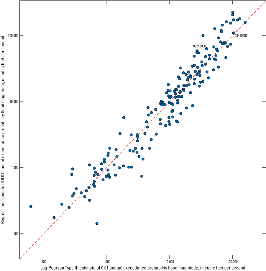
Scatter plot of 0.01 annual exceedance probability peak flows estimated for unregulated streamgages in Kentucky by using (1) log-Pearson Type III estimates (VonIns and others, 2026) and (2) StreamStats regression-based estimates using updated fundamental layers (U.S. Geological Survey, 2025).
Summary
This study, by the U.S. Geological Survey in cooperation with the Kentucky Transportation Cabinet, provides updated flood-frequency information and updated StreamStats-related geospatial layers for the State of Kentucky. Flood-frequency statistics were computed for long-term U.S. Geological Survey streamgages by using peak-flow data through water year 2021 and the methods outlined in “Guidelines for Determining Flood Flow Frequency—Bulletin 17C” (U.S. Geological Survey Techniques and Methods 4–B5). A total of 261 streamgages on unregulated and regulated streams were analyzed, including some streamgages analyzed for both regulated and unregulated periods of record. Annual exceedance probabilities of 50, 20, 10, 4, 2, 1, and 0.2 percent were estimated by using the expected moments algorithm in U.S. Geological Survey PeakFQ software, with regional skew information incorporated using a weighted skew to improve estimates at gages on unregulated streams. The analysis included censoring of potentially influential low floods using the multiple Grubbs-Beck test.
The Mann-Kendall test for monotonic trends showed that 9 of 51 unregulated streamgages with (1) relatively recent records (since water year 2000) and (2) long-term records (minimum 30 years) had statistically significant trends. Seven of the nine gages had upward trends in peak flows, had small to mid-sized basins, were east of 86° longitude, and were disproportionally near urban centers.
New fundamental layers used in Kentucky StreamStats were developed from 5-meter resolution light detection and ranging (lidar)-derived digital elevation models resampled to a 30-foot resolution to match the scale of the National Hydrography Dataset Plus and the Watershed Boundary Dataset. From the resampled digital elevation models, new statewide flow direction, flow accumulation, and stream network rasters were developed, reviewed against aerial imagery, and edited for drainage-line consistency. The new layers were tested by comparing basin characteristics and flow estimates derived from the old and new layers.
When the regression models were tested with the new fundamental layers used as inputs to predict the flood-frequency statistics computed for this study, it was found that flow was commonly overestimated for drainage basins greater than 1,000 square miles. However, the overestimation is of minor consequence because few unregulated streams in Kentucky have drainage basins greater than 1,000 square miles.
Together, the updated statistics and geospatial layers help ensure that the Kentucky StreamStats application reflects the best available data. This work supports infrastructure design, floodplain management, and emergency planning. The results provide decision makers with modernized tools to evaluate flood hazards and manage water resources in Kentucky.
References Cited
Barnhart, T.B., Smith, M., Rea, A., Kolb, K., Steeves, P., and McCarthy, P., 2020, StreamStats Data Preparation Tools, version 4: U.S. Geological Survey software release, accessed October 5, 2022, at https://doi.org/10.5066/P9UM2NUL.
Cohn, T.A., England, J.F., Berenbrock, C.E., Mason, R.R., Stedinger, J.R., and Lamontagne, J.R., 2013, A generalized Grubbs-Beck test statistic for detecting multiple potentially influential low outliers in flood series: Water Resources Research, v. 49, no. 8, p. 5047–5058, accessed July 8, 2025, at https://doi.org/10.1002/wrcr.20392.
Cohn, T.A., Lane, W.L., and Baier, W.G., 1997, An algorithm for computing moments-based flood quantile estimators when historical flood information is available: Water Resources Research, v. 33, no. 9, p. 2089–2096, accessed July 8, 2025, at https://doi.org/10.1029/97WR01640.
Elbon, D.C., 2025, Kentucky Atlas and Gazetteer: Kentucky Atlas and Gazetteer website, accessed August 8, 2025, at https://www.kyatlas.com.
England, J.F., Jr., Cohn, T.A., Faber, B.A., Stedinger, J.R., Thomas, W.O., Jr., Veilleux, A.G., Kiang, J.E., and Mason, R.R., Jr., 2018, Guidelines for determining flood flow frequency—Bulletin 17C (ver. 1.1, May 2019): U.S. Geological Survey Techniques and Methods, book 4, chap. B5, 148 p., accessed September 18, 2024, at https://doi.org/10.3133/tm4B5.
Gesch, D., Evans, G., Mauck, J., Hutchinson, J., and Carswell, W.J., Jr., 2009, The National Map—Elevation: U.S. Geological Survey Fact Sheet 2009–3053, 4 p., accessed August 8, 2025, at https://doi.org/10.3133/fs20093053.
Helsel, D.R., Hirsch, R.M., Ryberg, K.R., Archfield, S.A., and Gilroy, E.J., 2020, Statistical methods in water resources: U.S. Geological Survey Techniques and Methods, book 4, chap. A3, 458 p., accessed July 8, 2025, at https://doi.org/10.3133/tm4A3.
Hodgkins, G.A., and Martin, G.R., 2003, Estimating the magnitude of peak flows for streams in Kentucky for selected recurrence intervals: U.S. Geological Survey Water-Resources Investigations Report 03–4180, accessed August 8, 2025, at https://doi.org/10.3133/wri034180.
Interagency Advisory Committee on Water Data, 1982, Guidelines for determining flood flow frequency: Interagency Advisory Committee on Water Data, Hydrology Subcommittee Bulletin 17B, 28 p. plus appendixes, October 14, 2024, at http://water.usgs.gov/osw/bulletin17b/bulletin_17B.html.
Kentucky Geological Survey, 2012, Physiographic map of Kentucky: Kentucky Geological Survey website, accessed August 8, 2025, at https://www.uky.edu/KGS/geoky/physiographic.htm.
KyFromAbove, 2020, Kentucky Elevation Data & Aerial Photography Program, 5 foot digital elevation model (DEM) [map server]: KyFromAbove website, accessed, July 29, 2020, at https://kygeonet.maps.arcgis.com/home/item.html?id=785e6040154e4050bda80049fc12d4a6.
National Oceanic and Atmospheric Administration National Climatic Data Center, undated, Climate of Kentucky: Asheville, N.C., National Oceanic and Atmospheric Administration, National Climatic Data Center, 6 p., accessed June 2, 2025, at https://www.ncei.noaa.gov/data/climate-normals-deprecated/access/clim60/states/Clim_KY_01.pdf.
Ries, K.G., III, Newson, J.K., Smith, M.J., Guthrie, J.D., Steeves, P.A., Haluska, T.L., Kolb, K.R., Thompson, R.F., Santoro, R.D., and Vraga, H.W., 2017, StreamStats, version 4: U.S. Geological Survey Fact Sheet 2017–3046, 4 p., accessed November 26, 2018, at https://doi.org/10.3133/fs20173046.
Runkle, J., Kunkel, K.E., Champion, S.M., Frankson, R., and Stewart, B.C., 2022, Kentucky State Climate Summary 2022: National Oceanic and Atmospheric Administration Technical Report NESDIS 150–KY, 4 p., accessed May 16, 2025, at https://statesummaries.ncics.org/chapter/ky/.
Siefken, S.A., Crouch, S., Rucker, S., Wavra, H.N., Faunce, K.E., and Boles, C., 2024, PeakFQ: Peak Flow Frequency: U.S. Geological Survey software release [R package], accessed July 3, 2025, at https://doi.org/10.5066/P14NQH6T.
Taulbee, L., 2025, An overview of changes in land cover and developed land in Kentucky counties from 2001–2021: Lexington, Ky., University of Kentucky, Housing Engagement and Research Initiative, 6 p., accessed August 8, 2025, at https://blueprintkentucky.ca.uky.edu/sites/blueprintkentucky.ca.uky.edu/files/Taulbee_Changes_in_Land_Cover_paper_HERI_JAN2025.pdf.
U.S. Geological Survey, [USGS], 2021, National Hydrography Dataset Plus High Resolution (NHDPlus HR)—USGS National Map downloadable data collection [map server]: U.S. Geological Survey dataset, accessed November 23, 2021, at https://www.sciencebase.gov/catalog/item/57645ff2e4b07657d19ba8e8.
U.S. Geological Survey, [USGS], 2024, Annual NLCD Collection 1 science products (ver. 1.1, June 2025): U.S. Geological Survey data release, accessed September 19, 2025, at https://doi.org/10.5066/P94UXNTS.
U.S. Geological Survey, [USGS], 2025, StreamStats Information Portal—Kentucky: U.S. Geological Survey web page, accessed August 25, 2025, at https://streamstats.usgs.gov/information-portal/regionalInformation.html?region=KY.
Veilleux, A.G., Stedinger, J.R., and Lamontagne, J.R., 2011, Bayesian WLS/GLS regression for regional skewness analysis for regions with large cross-correlations among flood flows, in Beighley, R.D., and Kilgore, M.W., eds., World Environmental and Water Resources Congress 2011—Bearing Knowledge for Sustainability, Palm Springs, Calif., 2011, Proceedings: Reston, Va., American Society of Civil Engineers Environmental and Water Resources Institute, p. 3103–3112, accessed October 29, 2024, at https://doi.org/10.1061/41173(414)324.
VonIns, B.L., Follette, D.D., Webber, J.J., and Jeffords, T.G., 2026, At-site flood frequency estimates for 261 Kentucky streamgages using data through water year 2021: U.S. Geological Survey data release, https://doi.org/10.5066/P13HGU8D.
Wagner, D.M., O’Shea, P.S., Thompson, R.R., Messinger, T., Duda, J.M., and Kandel, C., 2025, Regional flood skew for the Tennessee and parts of the Ohio and Lower Mississippi River basins (hydrologic unit codes 06, 05, and 08, respectively) in Tennessee, Kentucky, western Virginia, western West Virginia, far western Maryland and parts of North Carolina, Georgia, Alabama, and Mississippi: U.S. Geological Survey data release, accessed June 16, 2025, at https://doi.org/10.5066/P1M9VJQV.
Webber, J.J., Follette, D.D., Jeffords, T.G., and VonIns, B.L., 2026, Elevation, flow direction, flow accumulation, and stream network rasters for Kentucky StreamStats update, 2026: U.S. Geological Survey data release, https://doi.org/10.5066/P91BD6SD.
Conversion Factors
U.S. customary units to International System of Units
Temperature in degrees Celsius (°C) may be converted to degrees Fahrenheit (°F) as follows:
°F = (1.8 × °C) + 32.
Temperature in degrees Fahrenheit (°F) may be converted to degrees Celsius (°C) as follows:
°C = (°F – 32) / 1.8.
Datum
Horizontal coordinate information is referenced to the North American Datum of 1983 (NAD 1983).
Supplemental Information
A water year is the 12-month period from October 1 through September 30 of the following year and is designated by the calendar year in which it ends.
Abbreviations
AEP
annual exceedance probability
DEM
digital elevation model
FAC
flow accumulation raster
FDR
flow direction raster
GIS
geographic information system
GSD
geometric standard deviation
KyFromAbove
Kentucky Aerial Photography and Elevation Data Program
lidar
light detection and ranging
LPIII
log-Pearson Type III
NHD
National Hydrography Dataset
NHDPlus HR
National Hydrography Dataset Plus High Resolution
PeakFQ
U.S. Geological Survey peak-flow frequency application
PILF
potentially influential low flood
RMSD
root-mean-square difference
SDR
stream definition raster
USGS
U.S. Geological Survey
For more information about this report, contact:
Director, Ohio-Kentucky-Indiana Water Science Center
U.S. Geological Survey
6460 Busch Blvd, Suite 100
Columbus, OH 43229-1737
GS-W-OKI_Director@usgs.gov
or visit our website at
https://www.usgs.gov/centers/oki-water
Publishing support provided by the
USGS Science Publishing Network
Pembroke and Baltimore Publishing Service Centers
Disclaimers
Any use of trade, firm, or product names is for descriptive purposes only and does not imply endorsement by the U.S. Government.
Although this information product, for the most part, is in the public domain, it also may contain copyrighted materials as noted in the text. Permission to reproduce copyrighted items must be secured from the copyright owner.
Suggested Citation
VonIns, B.L., Webber, J.J., Follette, D.D., and Jeffords, T.G., 2026, Flood-frequency estimates for Kentucky streamgages based on data through water year 2021 and results of updating the fundamental layers in Kentucky StreamStats: U.S. Geological Survey Scientific Investigations Report 2026–5036, 12 p., https://doi.org/10.3133/sir20265036.
ISSN: 2328-0328 (online)
| Publication type | Report |
|---|---|
| Publication Subtype | USGS Numbered Series |
| Title | Flood-frequency estimates for Kentucky streamgages based on data through water year 2021 and results of updating the fundamental layers in Kentucky StreamStats |
| Series title | Scientific Investigations Report |
| Series number | 2026-5036 |
| DOI | 10.3133/sir20265036 |
| Publication Date | June 30, 2026 |
| Year Published | 2026 |
| Language | English |
| Publisher | U.S. Geological Survey |
| Publisher location | Reston, VA |
| Contributing office(s) | Ohio-Kentucky-Indiana Water Science Center |
| Description | Report: vii, 12 p.; Data Releases |
| Online Only (Y/N) | Y |
| Additional Online Files (Y/N) | N |