

Assessing Natural Recharge in Indian Wells Valley, California: A Basin Characterization Model Case Study
Links
- Document: Report (4.7 MB pdf) , HTML , XML
- Version History: Version History (txt)
- NGMDB Index Page: National Geologic Map Database Index Page (html)
- Download citation as: RIS | Dublin Core
Abstract
The communities in Indian Wells Valley (IWV), in the northern Mojave Desert in California, rely on groundwater for domestic and agricultural use. Mountain front recharge from the surrounding Sierra Nevada is the main source of natural recharge to the valley. Increased urbanization, agricultural development, and groundwater pumping during recent decades put IWV in a state of critical overdraft. The U.S. Geological Survey Basin Characterization Model, version 8 (BCMv8) was used to evaluate historical and future climate and hydrologic conditions in IWV. The BCMv8 estimated natural recharge in IWV at 10.7 million cubic meters (Mm3) per year for the period from 1981 to 2010. Future patterns of water balance variables using three future climate scenarios, hot-wet, hot-dry, and warm-moderately wet, were calculated for mid-century (2040–69) and end-of-century (2070–99) periods. Results for both wet models projected an increase in recharge in both periods, whereas the hot-dry model projected a decrease in recharge in both periods. All models reported a large increase in seasonal variability in recharge, indicating more future availability and frequent occurrences of drought years. All climate scenarios projected an increase in climatic water deficit in both periods. These increases in irrigation demand and variability of water supply highlight the importance of strategic management planning for the sustainability of water resources in IWV.
Introduction
Climate change and unpredictable precipitation with associated increases in temperatures, along with urbanization and agricultural development, are increasingly competing for and stressing the water resources in the southwestern United States desert (Allen and others, 2019). In California, overdrafts have become far more common, especially in arid basins. As a result of the 2012–15 drought (Langridge and Van Schmidt, 2020), many wells went dry and increased land subsidence. These overdrafts prompted the 2014 legislation called the “Sustainable Groundwater Management Act” (SGMA; California Department of Water Resources, 2014), which authorizes local agencies to form Groundwater Sustainability Agencies (GSAs) to manage basins sustainably, requiring them to adopt plans for crucial groundwater basins. These GSAs require tools and information to develop their sustainability plans. Within these plans, recharge is one of the most uncertain processes requiring characterization or quantification. Demonstrating sustainability involves showing that the water management of a basin is not allowing more groundwater use than is being recharged to the basin. With changing climate conditions, estimating future recharge rates can inform long-term sustainability and the adoption of suitable management plans.
Groundwater is the sole source of drinking and irrigation water for residents of Indian Wells Valley (IWV), which is in east-central California in the northern part of the Mojave Desert (fig. 1). Since 1959, annual pumping from the aquifer has exceeded estimates of mean annual recharge, resulting in an overdraft of the groundwater basin (Berenbrock and Martin, 1991; Todd Engineers, 2014). Indian Wells Valley is critically over drafted and classified as a “high priority” SGMA basin. It has been well documented that the IWV groundwater basin has been in overdraft since at least the 1960s and that currently, basin outflows exceed basin inflows by approximately four times (Flint and others, 2021a). Updated estimates by the IWV Groundwater Sustainability Plan (GSP) concurs with that rate, with a magnitude of overdraft of approximately 25,000 acre-feet per year (acre-ft/yr). The IWV GSA is co-managed with the Kern County GSA by the City of Ridgecrest, Inyo County, San Bernardino County, IWV Water District, the U.S. Navy—Naval Air Weapons Station China Lake, and the Bureau of Land Management (Indian Wells Valley Groundwater Authority, 2023).
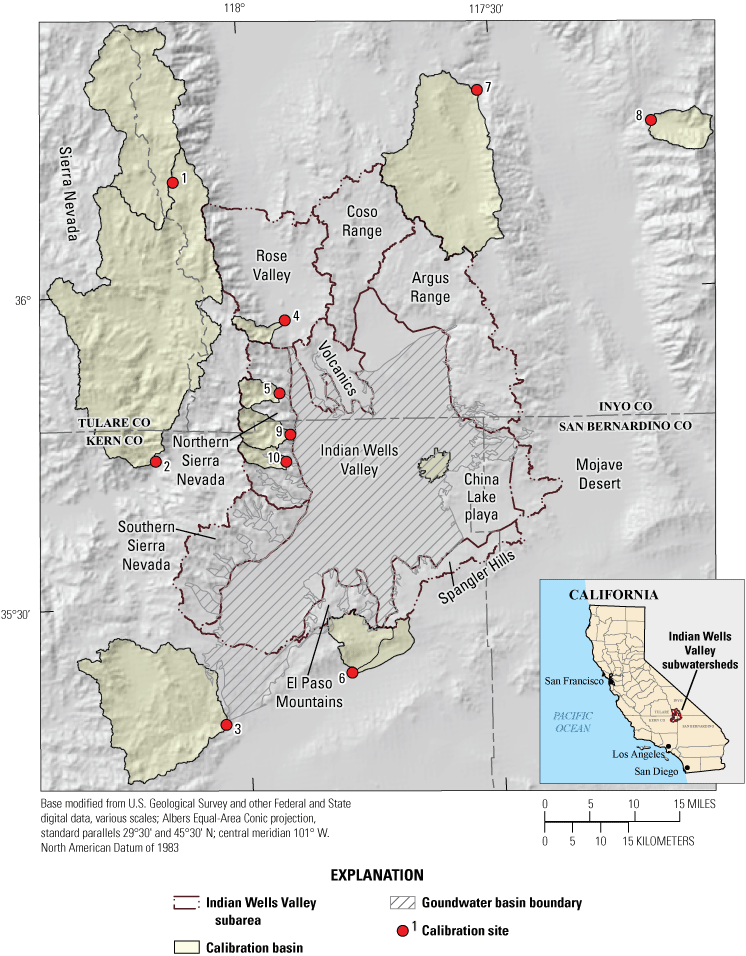
Study area of the Indian Wells Valley, California, showing subareas, calibration sites, and the groundwater basin boundary (California Department of Water Resources, 2025). Site names and descriptions are shown in table 2.
Because of the heavy reliance on groundwater in IWV, numerous studies have evaluated natural recharge in the valley. Early studies by Lee (1913) and Thompson (1929) estimated recharge in IWV at 33.3 million cubic meters (Mm3; 27,000 acre-feet) and 48.1 Mm3 (39,000 acre-feet) per year, respectively. In the 1960s, groundwater pumping in IWV began to exceed the water yield from the lower aquifer, causing the upper aquifer to become a source of recharge to the deep aquifer (Berenbrock and Schroeder, 1994; Todd Engineers, 2014). This state of overdraft led to several other studies using various methods, resulting in a range of natural recharge estimates during the last few decades, from 11.96 Mm3 (9,700 acre-feet) per year (Bean, 1989) to 12.10 Mm3 (9,806 acre-feet) per year (Todd Engineers, 2014). Table 1 includes a range of previous studies with estimates of recharge in subareas within the IWV Basin. These studies identified mountain front recharge as the main source of natural recharge in IWV, with 60–75 percent of the recharge generated from the eastern slopes of the Sierra Nevada, 20–30 percent from the Coso and Argus Ranges, and 0.5–4 percent from the El Paso Mountains (table 1). The most recent study on recharge (Flint and others, 2021a) was calibrated regionally at the statewide scale and had lower estimates for Sierra Nevada and Argus than previous studies and included estimates for the valley floor and volcanic subareas.
Table 1.
Previous estimates of natural recharge to the principal aquifer in Indian Wells Valley, California.[There is no surface drainage from volcanic subareas. Abbreviations: Mm3, million cubic meter; —, no data]
| Data source | Surface and subsurface drainage from Sierra Nevada Range (Mm3) |
Surface drainage from Coso Range (Mm3) |
Surface drainage from Argus Range (Mm3) |
Surface drainage from El Paso Mountains (Mm3) |
Surface drainage from volcanics (Mm3) |
Recharge to valley floor (Mm3) |
Inflow from Rose Valley (Mm3) |
Total natural recharge (not including Rose Valley) (Mm3) |
|---|---|---|---|---|---|---|---|---|
| Lee (1913) | — | 33.30 | — | — | — | — | — | 33.30 |
| Thompson (1929) | — | 48.10 | — | — | — | — | 12.30 | 48.10 |
| Kunkel and Chase (1969) | — | — | — | — | — | — | — | 13.6 to 18.5 |
| Bloyd and Robson (1971) | 7.69 | 3.90 | — | 0.49 | — | — | 0.06 | 12.08 |
| Dutcher and Moyle (1973) | — | — | — | — | — | — | — | 13.57 |
| St. Amand (1986) | — | — | — | — | — | — | — | 13.57 |
| Austin (1988) | at least 37.0 | — | — | — | — | — | — | 37.00 |
| Bean (1989) | 7.77 | 2.47 | 1.20 | 0.49 | — | — | 0.49 | 11.96 |
| Berenbrock and Martin (1991) | 7.69 | 3.90 | — | 0.49 | — | — | 0.06 | 12.10 |
| Watt (1993) | 10.95 | 1.20 | — | 0.00 | — | — | — | 12.15 |
| Thyne and others (1999) | 9.90 | — | — | — | — | — | 1.60 | 9.90 |
| Brown and Caldwell Consultants (2013) | 7.27 | 0.37 | 2.00 | 0.06 | — | — | 1.23 | 9.67 |
| Todd Engineers (2014) | 3.8 to 7.3 | 0.37 | 2.00 | 0.06 | — | — | 1.23 | 12.10 |
| Reitz and others (2017) | — | — | — | — | — | — | — | 9.04 |
| Flint and others (2021a) | 2.45 | 0.43 | 0.40 | 0.15 | 0.27 | 0.03 | 3.44 | 3.73 |
Because of the SGMA requirements and a high level of public concern over the adequacy of water supply for municipal and agricultural uses, the GSA decided to estimate current and future natural recharge in IWV, not only to provide additional confirmation of the water balance in the basin, but also to evaluate how changes in climate conditions could further affect the limited water resources. Previous studies agree that natural recharge to the IWV groundwater system is primarily from mountain front recharge from the surrounding Sierra Nevada on the western edge of the IWV Basin (table 1). Recharge from infiltration of surface runoff and snowmelt occurs at high elevations where precipitation is higher, snowmelt can exceed soil water holding capacity, and air temperature and evapotranspiration (ET) is lower. Recharge from the Coso and Argus Ranges and El Paso Mountains to the northern and eastern boundaries of the IWV Basin is less than 30 percent because of the smaller amount of rainfall in these subareas (Todd Engineers, 2014).
Basin wide recharge quantification was achieved by using an analytical method, the Basin Characterization Model (BCMv8; Flint and others, 2013), that was revised to improve recharge estimates (Basin Characterization Model, version 8, BCMv8; Flint and others, 2021a), calibrating it in IWV with local data and information to improve on the statewide regional calibration. With little groundwater data in the basin, it is important to evaluate all of the various components of the water balance to improve estimates of recharge, which is the most uncertain component.
Purpose and Scope
This study was done in cooperation with Kern County, California. The objective of this study is to utilize all available data to calibrate the various components of the water balance. By utilizing all available data, this study aims to provide a more refined and accurate estimate of the average annual natural recharge and other hydrologic water balance variables in the IWV Basin. This study validates the many historical estimates and provides a more realistic view of the basin's hydrologic conditions. Additionally, the calibrated model was used to apply future climate projections, thus providing insight into potential future hydrologic conditions. The information obtained from this study may be used to guide sustainable resource management planning for the IWV Basin.
Study Area
The IWV is in the Mojave Desert east of the Sierra Nevada, about 200 kilometers (km) north of Los Angeles (fig. 1). The valley floor covers an area of 777 square kilometers, ranging in elevation from 655 to 732 meters (m) above sea level. The valley is bounded on the west by the Sierra Nevada, on the north by a low ridge of volcanic rocks and the Coso Range, on the east by the Argus Range, and on the south by the El Paso Mountains and Spangler Hills. In contrast to the steep topography surrounding the valley, the valley floor gently slopes toward China Lake, a large dry lake or playa, in the central northeastern valley. At an altitude of 655 m, it is the primary natural groundwater discharge point in the valley (fig. 1).
The IWV has an arid climate, with annual precipitation ranging from 10 to 15 centimeters (cm) falling on the valley floor (primarily in winter and spring, October through March). During the remainder of the year, rain falls infrequently during summer thundershowers. Mean air temperatures range from about 4 degrees Celsius (°C) in winter to about 28 °C in summer. Native vegetation covers most of the IWV study area, with desert scrub covering more than 56 percent of the valley floor. Barren lands cover about 4 percent of the study area, mostly over the volcanic rocks and in the China Lake playa. The rest of the basin is covered with other vegetation types, including desert scrub, alkali desert scrub, sagebrush, juniper, mixed chaparral, grasslands, and pines (fig. 2).
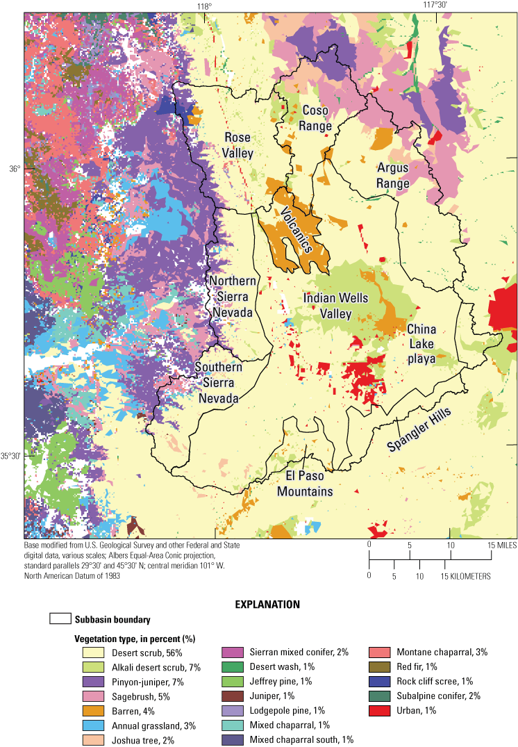
Indian Wells Valley, California, vegetation types. Legend shows the percentage of coverage of each vegetation type in the basin (Multi-Resolution Land Characteristics Consortium, 2018).
The IWV basin is bounded to the west along the Sierra Nevada by a north trending fault that is present in the center and eastern part of the valley (Berenbrock and Schroeder, 1994; Todd Engineers, 2014; fig. 3). Surficial geologic types in the IWV Basin include granites, which surround the valley, volcanics mostly in the north, conglomerates in the south, and small inclusions of metasediments. Desert fill covers the entire valley floor and western drainages. Unconsolidated deposits from lakebed, stream, and alluvial fans make up an upper aquifer and a lower aquifer. The primary deep aquifer in the IWV consists of alluvial deposits as much as 300 m thick, covering the main valley floor. The lower aquifer is generally unconfined except in the eastern part of the valley where the aquifer is confined by silt and clay lenses, lake deposits, and playa deposits. In the east-central part of the valley, beneath China Lake and other dry lakebeds (fig. 3), the lower aquifer is overlain by an upper aquifer that consists of lacustrine, alluvial, playa, and sandstone deposits (Berenbrock and Schroeder, 1994; Todd Engineers, 2014).
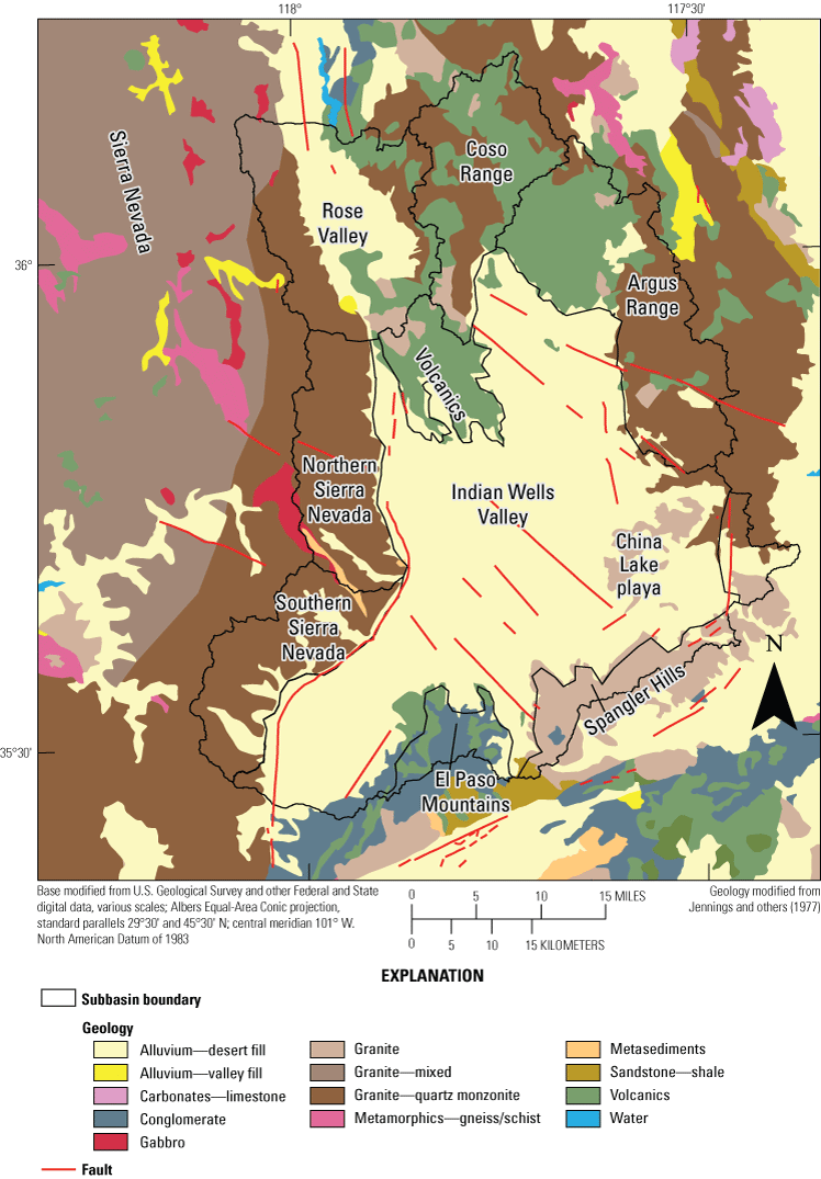
Geology for the Indian Wells Valley, California (Jennings and others, 1977). National Geologic Map Database, California Division of Mines and Geology geologic data, map number 2, scale 1:750,000.
Methods
The BCMv8 was used to simulate the hydrologic variables for the IWV Basin. The BCMv8 is a mechanistic, grid based, water-balance model that is run on a monthly time step. Version 8 of the model (Flint and others, 2021b) incorporates vegetation-specific actual evapotranspiration and uses available spatial data of vegetation, topography, physical soil properties, and geology (to provide bedrock permeability values). The BCMv8 uses these spatially distributed inputs, which are parameterized during calibration, and transient climate data to spatially distribute and quantify the amount of rainfall or snowmelt that is evaporated or transpired, remains in the soil profile, or becomes either recharge or runoff. This process depends on the storage properties of the underlying soil and saturated hydraulic conductivity of the shallow bedrock. These components comprise those of a typical water budget for a basin but do not include deliveries or extractions of water. The BCMv8 was originally developed and calibrated on a statewide regional scale for the state of California (Flint and others, 2021a, b; https://doi.org/10.5066/P9PT36UI). In this study, the BCMv8 was calibrated on a local scale to ensure that parameterization was not averaged over large regions but was specific to the IWV area.
All spatial data were developed to a scale of 270 m. Transient climate data, such as precipitation and maximum and minimum air temperature, were estimated using the Parameter-elevation Regressions on Independent Slopes Model (PRISM; Daly and others, 2008) and then spatially downscaled to a scale of 270 m using methods described in Flint and Flint (2012). Monthly potential evapotranspiration (PET) was calculated using simulated solar radiation, topographic shading, atmospheric properties, and cloudiness and calibrated to 120 measurement sites in California (Flint and others, 2021b). Snow accumulation and melt were calibrated to 99 snow courses throughout California, and spatially distributed model parameters were developed to optimize the match to measured snow throughout the state (Flint and others, 2021b). The BCMv8 was run to calculate the monthly water balance components, including snow accumulation and melt, actual evapotranspiration (AET), and changes in soil moisture storage, runoff, and natural recharge. Natural recharge was calculated as the water that penetrates below the rooting depth of vegetation and may take many years to reach the groundwater table depending on the thickness of the unsaturated zone. The climatic water deficit (CWD) is the evaporative demand that exceeds available water and was calculated by subtracting AET from PET (PET-AET; Reitz and others, 2017). The CWD defines the amount of water in the soil that can be maintained for plant use throughout the growing season and summer dry season as the amount of water necessary to maintain crop water demand, which can be used to track landscape stress over time.
Basin Characterization Model, version 8 Local Calibration for Indian Wells Valley
Local model calibration was done in two steps to match AET and streamflow measurements. The first step was done by parameterizing the BCMv8 to match estimates of AET reported by Reitz and others (2017) by vegetation type for the IWV Basin to create monthly time series of AET for October 2000 through September 2013. In IWV, there are 19 vegetation types, with desert scrub covering more than 56 percent of the study area (fig. 2). Parameterization was done first by calculating monthly scaling factors (Kv) for each vegetation type using the AET values estimated by Reitz and others (2017) divided by PET calculated using the BCMv8 for each month and averaged during the measurement period. These Kv values represent the proportion of AET below potential for each month that a vegetation type transpires. Additional vegetation parameters included adjustments to the effective rooting depth to increase the amount of effective soil storage and increase AET, which is often required to match the AET values estimated by Reitz and others (2017), while reducing the water available for recharge and runoff. There also were growth parameters that allowed for the seasonality of AET for vegetation types that are sensitive to seasonal and annual variations in precipitation. More details on parameterization can be found in Flint and others (2021b).
The second step to local model calibration was to assemble streamflow measurements and accumulate the BCMv8 recharge plus runoff values for drainages upstream from each streamgage. Streamflow data measured at 10 gaging stations (8 U.S. Geological Survey stations and 2 Kern County stations, and data are available in Saleh and Flint, 2019) in relatively unimpaired streams were used for model calibration (fig. 1). Because of scarcity of streamflow data within the basin, it was necessary to use streamflow data from outside the IWV sub-watersheds to calibrate all local soils, vegetation, and geologic types (fig. 1). Table 2 provides the location, collecting agency, numerical identifier, and the period of record available from these gaging stations used for calibration (Saleh and Flint, 2019). Note that two streamgages measure drainage from the Sierra Nevada to the west, streamgages 7 and 8 measure drainage from lower mountains to the northeast, streamgages 3 and 6 measure drainage from intermittent lower elevation sites to the south, and streamgages 4, 5, 9, and 10 measure drainage from locations at the Sierra Nevada front where excess flow becomes runoff instead of mountain front recharge. Post-processing in a spreadsheet was done to accumulate monthly recharge and runoff values upstream from every streamgage. Post-processing used exponential decay values to calculate basin discharge to match peak flows, recession flows, and baseflows of the measured hydrographs (Flint and others, 2021b). Calibration statistics included the coefficient of determination (R2) and Nash-Sutcliffe Efficiency (NSE; Nash and Sutcliffe, 1970) and were used to evaluate calibration results and optimize the goodness-of-fit. Bedrock permeability was adjusted to change the ratio of recharge to runoff in the BCMv8 runs and to optimize the shape of the calculated hydrograph for each subarea. Adjustments to AET parameters were done iteratively with bedrock permeability to ensure the best fit of modeled to measured streamflow and to optimize the different components of the water balance. Additional calibrations to the model included matching observations of ponding on the China Lake playa. This calibration was done by reducing the bedrock permeability of the consolidated valley fill materials to allow for intermittent ponding during high precipitation events.
Table 2.
Site name, longitude, latitude, site number, agency, and period of record for each streamflow calibration site in Indian Wells Valley, California.[Site locations are shown on figure 1. Abbreviations: NAD 83, North American Datum of 1983; CA, California; USGS, U.S. Geological Survey; —, no data]
| Site number (on fig. 1) |
Site name | Longitude, NAD 83 |
Latitude, NAD 83 |
USGS site number |
Agency | Period of record |
|---|---|---|---|---|---|---|
| 1 | South Fork Kern River near Onyx, CA | −118.1737 | 35.7374 | 11189500 | USGS | 1955–76 |
| 2 | South Fork Kern River near Olancha, CA | −118.1290 | 36.1832 | 11188200 | USGS | 1957–69 |
| 3 | Cottonwood Creek near Cantil, CA | −118.0448 | 35.3138 | 10264770 | USGS | 1966–72 |
| 4 | Goler Gulch near Randsburg, CA | −117.7962 | 35.3927 | 10264710 | USGS | 1966–72 |
| 5 | Darwin Wash near Darwin, CA | −117.5225 | 36.3207 | 10250800 | USGS | 1962–89 |
| 6 | Wildrose Creek near Wildrose Station, CA | −117.1787 | 36.2649 | 10250600 | USGS | 1960–75 |
| 7 | Ninemile Creek near Brown, CA | −117.9273 | 35.8430 | 10264878 | USGS | 1961–72 |
| 8 | Little Lake Creek near Little Lake, CA | −117.9131 | 35.9591 | 10264870 | USGS | 1964–73 |
| 9 | Sand Canyon Creek | −117.9075 | 35.7759 | — | Kern County Water Agency | 1999–2016 |
| 10 | Grapevine Canyon Creek | −117.9167 | 35.7330 | — | Kern County Water Agency | 1997–2016 |
Future Climate Scenarios
To evaluate future hydrologic conditions in IWV, the calibrated IWV model was run using three future climate models (table 3) from the Global Climate Models (GCMs) selected for California’s Fourth Climate Change Assessment (4CCA) as best representing historical climatic patterns in California (California Department of Water Resources Climate Change Technical Advisory Group, 2015). The three selected models correspond to the Representative Concentration Pathway (RCP) 8.5, representing a future with a high global population, slow economic growth and technological change, and a high dependence on fossil fuels, without any consideration to reductions into greenhouse gas emissions (Riahi and others, 2011; Pierce and others, 2014). These three climate scenarios were statistically downscaled using the Localized Constructed Analogs (LOCA) method described in Pierce and others (2014) from the native model resolution (table 3) to a 6-km resolution. The statistical downscaling was done to improve estimates of extreme events and reduce the common downscaling problem of too many light-precipitation days (Pierce and others, 2014). The data were then further downscaled spatially to 270 m for BCMv8 application following the methods described in Flint and Flint (2012). The selected future scenarios represent a range of projected conditions, with the Second-generation Canadian Earth System Model (CanESM2) representing hot-wet conditions, the Community Climate System Model version 4 (CCSM4) representing warm-moderately wet conditions, and the Hadley Centre Global Environmental Model version 2 climate configurations (HadGEM2-CC) representing hot-dry conditions (table 3). The resulting datasets provided monthly minimum and maximum air temperature and precipitation for the 1981–2099 period. A historical baseline climate dataset from water years 1976 to 2005 (Livneh and others, 2013) was used to train the LOCA GCMs. Bias correction was applied to each LOCA scenario to match the modeled historical climate statistics with those of the historical observational data for that period (Pierce and others, 2014). As a result, to account for any slight differences between the historical GCM climate data and PRISM data (Daly and others, 2008), all calculations comparing BCM-derived results for historical and future 30-year mean periods were made using BCMv8 results based on the GCM-simulated historical data.
Table 3.
Global Climate Models used for future climate modeling in Indian Wells Valley, California, with modeling center information.[CanESM2, Second-generation Canadian Earth System Model; CCSM4, Community Climate System Model version 4; HadGEM2-CC, Hadley Centre Global Environmental Model version 2 climate configurations; ID, identification; km, kilometer]
Figure 4 shows temperature and precipitation data available from the PRISM dataset used to run the historical BCM, along with simulated data from the model projections, which are run from 1950 to 2099 with carbon dioxide forcings beginning in 2006. Figure 4 shows that the bias-correction of the LOCA downscaled data to historical climate data (Livneh and others, 2013) do not exactly match the PRISM data. The difference can be partially explained by the fact that even though the Livneh and others (2013) dataset was based on PRISM, it used a consistent lapse rate throughout the domain (allowing for the dataset to extend outside of the continental United States), whereas PRISM used a variable lapse rate. More importantly, the bias correction was done to match the statistics (mean and variance) for the period 1976–2005, not 1981–2010, as shown in table 4.
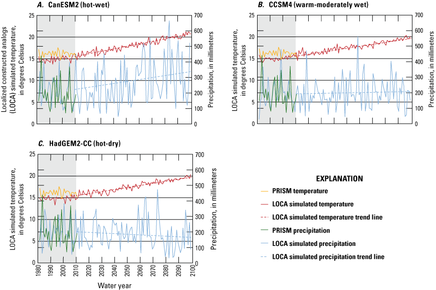
Annual climate data from historical Parameter-elevation Regressions on Independent Slopes Model (PRISM) data (1981–2010) and from three Localized Constructed Analogs (LOCA) climate scenarios (1981–2099): A, Canadian Centre for Climate Modeling and Analysis, Second-generation Canadian Earth System Model (CanESM2), representing hot-wet projected conditions; B, National Center for Atmospheric Research, United States of America, Community Climate System Model version 4 (CCSM4) representing warm-moderately wet projected conditions; and C, Met Office Hadley Centre, United Kingdom, Hadley Centre Global Environmental Model version 2 climate configurations (HadGEM2-CC), representing hot-dry projected conditions. LOCA climate is simulated from 1950 to 2099, with five carbon dioxide forcing beginning in 2006. The five carbon dioxide forcings refer to the five different greenhouse gas concentration scenarios (or radiative forcing pathways) that drive future climate projections. These scenarios are based on Representative Concentration Pathways (RCPs), which specify the level of radiative forcing (measured in watts per square meter) caused by greenhouse gases like carbon dioxide by the year 2100 relative to pre-industrial levels (Pierce and others, 2014).
Table 4.
Mean and standard deviation (SD) of precipitation data for the Localized Constructed Analogs (LOCA) simulations for three periods in Indian Wells Valley.[CanESM2, Second-generation Canadian Earth System Model; CCSM4, Community Climate System Model version 4; HadGEM2-CC, Hadley Centre Global Environmental Model version 2 climate configurations; mm, millimeter]
The mean temperature rises for all models for both future periods, ranging from 4 to more than 5 °C by end of century. Precipitation is variable among models. The CanESM2 model increases the most for precipitation and has the most annual variability in the future run for precipitation and air temperature of all models, with the mean increasing from 221 millimeters per year (mm/yr) in the historical period to 324 mm/yr by end of century. The standard deviation also increases by nearly 30 percent by end of century, indicating that the future is projected to have more extreme precipitation years that also are hotter. The CCSM4 model also has increases in precipitation, with additional variability mid-century but not in the end-of-century period. HadGEM2-CC has variable changes in precipitation, rising mid-century and lowering by end of century, but the variability indicates more extreme rises by end of century.
Uncertainty
There are many sources of uncertainty in this study; however, improving the spatial distribution of physical properties during parameterization, hydraulic function tables, and local data used for model calibration, can reduce uncertainty and improve estimates of potential hydrologic outcomes. The BCMv8 addresses some of these uncertainties by incorporating vegetation-specific AET and using available spatial data of vegetation, topography, physical soil properties, and geology. Calibrations are done to optimize the fit to measured data for each hydrologic component of the water balance calculated by the model. Additional uncertainties in the BCM and extrapolation to ungaged basins are discussed at length in Flint and others (2013). Addressing uncertainties related to future climate-hydrology scenarios using GCMs is particularly difficult; however, we reduced this uncertainty by selecting a subset of the GCMs that were analyzed specifically to represent the range of historical climatic conditions in California and were selected for California’s 4CCA (California Department of Water Resources Climate Change Technical Advisory Group, 2015). In this study, we selected the CanESM2, CCSM4, and HadGEM2-CC to represent a range of projected hydrologic conditions in IWV.
Results
The application of the BCMv8 to simulate hydrologic conditions in IWV relies on the model calibration to obtain the best fit between simulated model outputs and field observations. Figure 5 shows a comparison of BCMv8 actual AET to the observed AET from Reitz and others (2017), hereafter referred to as “Reitz AET,” for the eight widely occurring vegetation types in the IWV Basin. Monthly simulated BCMv8 AET for the years 2000–13 compared well to measured Reitz AET values, especially in locations in the mountains (montane chaparral and Sierran mixed conifer). The BCMv8 values were overestimated for vegetation in the valley floor subarea (desert scrub, sagebrush, and alkali desert scrub) during summer 2005 and spring 2011 (fig. 5). These vegetation types are very responsive to precipitation on a sub monthly basis, and although the BCMv8 incorporates all precipitation and AET for each month, the Reitz AET is developed based on the Moderate Resolution Imaging Spectroradiometer (MODIS) remotely sensed data. These data are collected as a snapshot and may undersample the AET of vegetation that actively responds to precipitation. Notably, the barren vegetation type, which occupies the area over the volcanics geology in the northern part of the basin, has low AET, although not as low as desert scrub or alkali desert scrub. This low AET provides more water for recharge and runoff in the water balance calculation, and in this relatively permeable geology, it results in a higher proportion of recharge. Although there was no measured streamflow in this location to constrain the estimates of bedrock permeability locally, there were ample stations throughout the arid and semi-arid locations in California with this geologic type, and the regional calibration value for this geologic type was used for this local calibration.
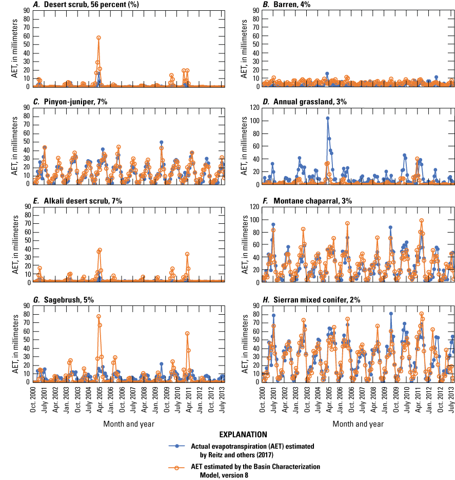
Indian Wells Valley, California, Basin Characterization Model, version 8 model calibration using model estimated actual evapotranspiration (AET; orange) compared to measured AET from Reitz and others (2017; blue). A, desert scrub; B, barren; C, pinyon-juniper; D, annual grassland; E, alkali desert scrub; F, montane chaparral; G, sagebrush; and H, Sierran mixed conifer. Percentage value represents the percentage of the three-vegetation types within the study area (Multi-Resolution Land Characteristics Consortium, 2018).
The BCMv8 also was calibrated against selected monthly streamflow measurements at 10 streamgages (fig. 1; table 2). Comparisons of the BCMv8 basin discharge and measured streamflow indicated a relatively good match for most of the streamgages and poorer fits for streamgages with intermittent flows. Figure 6 shows an example comparison of measured streamflow from four of the streamgages in the study area used for model calibration. Calibration results indicated that the BCMv8 was more successful in effectively capturing the magnitude and timing of peaks in the monthly time step for sites with more frequent measured streamflow data (figs. 6A, 6B, 6D) and not as successful for sites with minimal measured data (fig. 6C). These results also are reflected in the calibration statistics (table 5), which indicated relatively better goodness-of-fit based on the NSE statistic for sites with continuous streamflow (table 5). These sites had average monthly NSE values of 0.80, and R2 values of 0.73 (sites not used in average calculations because of minimal streamflow are marked in table 5).
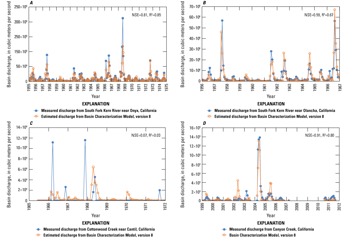
Calibration time series comparing monthly measured discharge and Basin Characterization Model, version 8 estimated basin discharge in cubic meters per second for four basins in Indian Wells Valley, California: A, South Fork Kern River near Onyx, California; B, South Fork Kern River near Olancha, California; C, Cottonwood Creek near Cantil, California; and D., Canyon Creek, California. Calibration statistics, Nash-Sutcliffe Efficiency (NSE) statistic, and monthly coefficient of determination (R2) are included.
Table 5.
Basin Characterization Model, version 8 (BCMv8) calibration statistics for sites in Indian Wells Valley, California (Nash and Sutcliffe, 1970).[R2, coefficient of determination; NSE, Nash-Sutcliffe efficiency; CA, California]
| Site number (on fig. 1) |
Site name | Period of record |
Number of days with streamflow measurements |
R2 | NSE |
|---|---|---|---|---|---|
| 1 | South Fork Kern River near Onyx, CA | 1955–76 | 239 | 0.85 | 0.81 |
| 2 | South Fork Kern River near Olancha, CA | 1957–69 | 131 | 0.67 | 0.59 |
| 13 | Cottonwood Creek near Cantil, CA | 1966–72 | 6 | 0.03 | 0.07 |
| 14 | Goler Gulch near Randsburg, CA | 1966–72 | 8 | 0.65 | 0.86 |
| 5 | Darwin Wash near Darwin, CA | 1962–89 | 323 | 0.2 | 0.17 |
| 16 | Wildrose Creek near Wildrose Station, CA | 1960–75 | 18 | 0 | 0.84 |
| 7 | Ninemile Creek near Brown, CA | 1961–72 | 63 | 0.48 | 0.72 |
| 18 | Little Lake Creek near Little Lake, CA | 1964–73 | 12 | 0 | 0.36 |
| 9 | Sand Canyon Creek | 1999–2016 | 93 | 0.8 | 0.91 |
| 10 | Grapevine Canyon Creek | 1997–2016 | 125 | 0.83 | 0.98 |
Sites not used in average calculations due to minimal streamflow; on-site locations are shown on figure 1.
Historical Climate Evaluation
Historical climatological and hydrological conditions for all subareas in IWV averaged during the 1981–2010 period are summarized in table 6. Total recharge for IWV from BCMv8 local calibration using historical PRISM data was estimated at about 10.7 Mm3 (8,680 acre-feet) per year. This recharge value corresponds well with estimates from previous studies (table 2), developing a consensus among estimates during the last 50 years. Spatial distribution of natural recharge in IWV is shown on figure 7 and is a function of climate, geology, soil storage, and vegetation type. Most of the recharge in IWV is mountain front recharge from the Sierra Nevada (48 percent), volcanics subarea (21 percent), and the Argus Range (12 percent). Rose Valley subarea is not included in the sum of total recharge. Rose Valley is a subbasin northwest of Indian Wells Valley that—under wetter conditions more than 10,000 years ago—was part of a river system that flowed from Owens Valley through Rose Valley and Indian Wells Valley to Death Valley. Surface flow between the basins now occurs rarely, if ever. Subsurface flow is obstructed by geologically recent basalts, which force most of the groundwater to the surface as it crosses between basins (Todd Engineers, 2014).

Indian Wells Valley, California, average annual recharge (1981–2010) calculated using the Basin Characterization Model, version 8.
Table 6.
Annual Parameter-elevation Regressions on Independent Slopes Model (PRISM) historical climate and hydrological parameters from the Basin Characterization Model, version 8, averaged during the 1981–2010 period in Indian Wells Valley, California. Recharge is in million cubic meters (Mm3).[km2, square kilometer; mm, millimeter; °C, degree Celsius; —, no data; w/o, without]
Figure 8 shows the relation between precipitation and natural recharge estimated from the BCMv8 for each of the subareas in IWV during the 1981–2010 period. In all subareas, the relation had a low slope until enough precipitation occurred to exceed the requirements of soil-moisture storage, ponding, evaporation, and transpiration, after which recharge occurred. This threshold is approximately 150–250 mm/yr for all of the subareas, except for the volcanics, with a threshold of less than 100 mm/yr because of this subarea’s higher permeability (fig. 8). The distance that the recharge curve is offset from the 1:1 line is controlled by the potential for precipitation to be diverted to the other pre-recharge processes. For example, in the arid valley floor, where there is less precipitation and substantial soil storage, the estimated recharge was about 8 percent of the total BCMv8 estimated IWV recharge, and most of the precipitation was diverted to evapotranspiration (table 6); whereas, the Sierra Nevada subareas have more precipitation, much of it as snow.
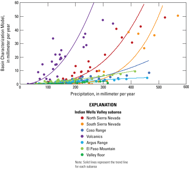
Power function regression between precipitation and natural recharge estimated from the Basin Characterization Model, version 8 from 1981 to 2010 for Indian Wells Valley, California.
The CWD is correlated with landscape stress, forest die-off, wildfire risk, and irrigation demand, and its variability is largely dominated by air temperature and available water. The spatial distribution of CWD over IWV is shown on figure 9, with the mean annual CWD of 1,200 mm/yr in the Sierra Nevada subareas. The melting of the snowpack in the Sierra Nevada subareas provides a longer seasonal duration of available water, thus maintaining a lower annual deficit. The highest CWD is present in the valley floor subarea of IWV, with more than 1,450 mm/yr, because of increased air temperature and PET and lower precipitation (table 6).
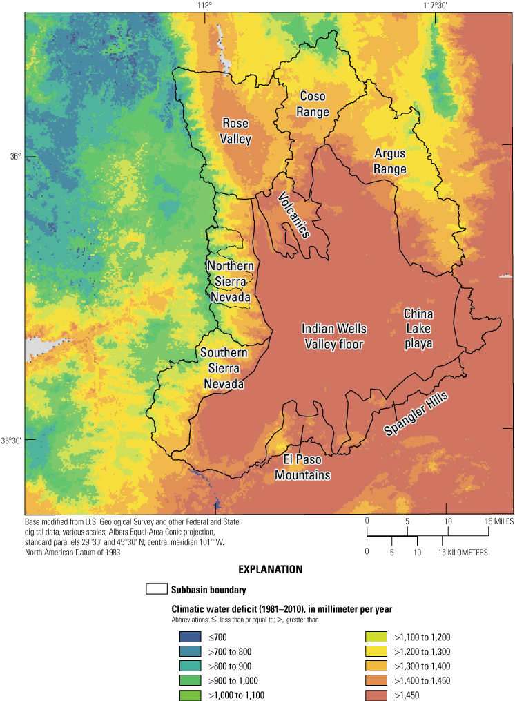
Average annual climatic water deficit (1981–2010) for Indian Wells Valley, California, estimated using the Basin Characterization Model, version 8.
Future Climate Projections
Future projected hydrological conditions from three future climate scenarios for all subareas in IWV averaged during the 2040–69 mid-century and 2070–99 end-of-century periods were compared to simulated historical LOCA 1981–2010 conditions. Tables 7 and 8 show the percentage of change in projected climatic and hydrologic conditions when compared to 1981–2010 historical LOCA conditions. All three models show projected increases in average air temperature for IWV, and this increase is greater for end of century (table 7). The CanESM2 model projected the highest (as much as 29 percent, about 5 °C) increase in temperature in the end-of-century period compared to the other two models (table 7). There was large variation in the projected precipitation from the three GCMs for both periods. The CanESM2 model, a hot-wet projection, showed an average of 20-percent (about 4 cm) increase in precipitation in the mid-century period and an average of 31-percent (about 6 cm) increase in the end-of-century period when compared to historical LOCA data. The HadGEM2-CC model, a hot-dry projection, showed a decrease in precipitation in both periods, with a larger decrease for all subareas in the end-of-century period and reaching anywhere from a 23-percent decrease in the Coso Range to a 40-percent decrease in the Spangler Hills and El Paso Mountains (table 7). The CCSM4 warm-moderately wet model showed a small change in precipitation in both periods, with a slightly larger increase in the end-of-century period (table 7).
Table 7.
Percentage of change in average climatic and hydrologic conditions in Indian Wells Valley, California, in comparison to historical period (1981–2010) using three future climate models for mid-century (2040–69) and end-of-century (2070–99) periods: Second-generation Canadian Earth System Model (CanESM2) representing hot-wet projected conditions, Community Climate System Model version 4 (CCSM4) representing warm-moderately wet projected conditions, and Hadley Centre Global Environmental Model version 2 climate Configuration (HadGEM2-CC) representing hot-dry projected conditions.[CanESM2 representing hot-wet projected conditions; CCSM4 representing warm-moderately wet projected conditions; and HadGEM2-CC representing hot, dry projected conditions. Abbreviations: %diff, percentage difference; N, northern; S, southern; Mtns, mountains; —, no data]
Future projected runoff for IWV was estimated using the three GCMs for the mid-century and end-of-century periods and compared to historical LOCA data (table 7). Results from the CanESM2 and CCSM4 models projected an increase in runoff in both future periods. CanESM2 projected a greater increase in runoff in the end-of-century period, whereas the more moderate CCSM4 model projected a similar increase in both periods. The hot-dry HadGEM2-CC model projected an increase in runoff in the mid-century period and decrease in the end-of-century period. This decrease is most significant (38 percent and 39 percent) in the El Paso Mountains and valley floor subarea, respectively. These results compare well with the HadGEM2-CC projected decrease in precipitation during the end-of-century period (table 7).
Generally, the trends shown in table 7, based on comparisons of 30-year annual means, indicate that there is a consensus among models that temperature is predicted to rise approximately 20–29 percent by end of century, which corresponds with the prediction from all models that CWD will also rise for all locations. However, there is not a consensus among models about whether it is predicted for more or less precipitation available in IWV, which determines how much water is available for AET, runoff, or recharge. Table 8 shows the percentage of change in the standard deviation of climatic and hydrologic conditions in comparison to historical conditions. In all subareas for all models, the annual variability in precipitation and air temperature increased in the mid-century and end of century by 1–42 percent for precipitation and 8–38 percent for temperature. Results from the CCSM4 model indicated an increase in annual variability in precipitation and air temperature only during the mid-century, followed by a decrease in precipitation, AET, CWD, and recharge in some subareas by the end of the century (table 8). However, most importantly for planning purposes, there is strong model consensus that by mid-century, variability in annual precipitation, runoff, and recharge—the primary water-supply variables—will increase, with recharge projected to rise by as much as 57 percent in the Sierra Nevada and 76 percent on the valley floor. This rise is caused by the increased variability in precipitation and the increase in the precipitation thresholds for recharge projected by all the models. These projections point to wet years where decisions to capture or store water are prudent. Also notable, results for all models indicated that all hydrologic variables increased on average in the Rose Valley subarea by end of century, except for HadGEM2-CC for precipitation, AET, runoff, and recharge (table 7).
Table 8.
Percentage of change in the standard deviation of climatic and hydrologic conditions in Indian Wells Valley, California, in comparison to the historical period (1981–2010) using three future climate models for mid-century (2040–69) and end-of-century (2070–99) periods: Second-generation Canadian Earth System Model (CanESM2) representing hot-wet projected conditions, Community Climate System Model version 4 (CCSM4) representing warm-moderately wet projected conditions, and Hadley Centre Global Environmental Model version 2 climate Configuration (HadGEM2-CC) representing hot-dry projected conditions.[CanESM2 representing hot-wet projected conditions, CCSM4 representing warm-moderately wet projected conditions, and HadGEM2-CC representing hot-dry projected conditions. Abbreviations: %diff, percentage difference; Mtns, mountains; —, no data]
Table 7 shows the change in AET and CWD from historical (1981–2010) to mid-century (2040–69) and to end-of-century (2070–99) periods for each of the three GCMs. The three scenarios varied in their projections of AET because HadGEM2-CC has lower projected precipitation and less available water for AET. The CanESM2 scenario showed the largest projected increase in AET in both periods in comparison to the historical period, with a larger increase in the end-of-century period, reflected in a more than 60-percent increase in AET in some subareas (Spangler Hills, El Paso Mountain, and valley floor) during the end-of-century period. This increase in AET corresponds with an increase in CWD among all sites in mid-century and end-of-century periods, with average CWD increases of 4 and 6 percent, respectively (table 7). Results from the HadGEM2-CC model indicate an overall increase in mid-century AET projections; however, there are large variations in AET projections in this period when evaluated on a subarea scale. AET increased as much as 35 percent in the Argus Range subbasin and decreased 17 percent in the Spangler Hills (table 7). The HadGEM2-CC model projected a decrease in AET for all the subareas in the end-of-century period except for a 13-percent increase in the Argus Range subarea. The HadGEM2-CC model showed an increase in CWD for both periods; however, HadGEM2-CC showed a bigger increase (almost double) in CWD projections for all subareas in the end-of-century period (table 7). Results from the CCSM4 model projected an increase in AET in all IWV subareas during both periods except for Spangler Hills and valley floor subareas, where CCSM4 projected a 26-percent and 5-percent decrease in AET by end of century, respectively. The CCSM4 results also indicated an increase in CWD in both periods: an average of 4 percent in mid-century and 7 percent in the end-of-century period compared to historical conditions. Spatial distribution of percentage of change in CWD estimations in the IWV projected by the GCMs for mid-century (2040–69) and end of century (2070–99) compared to the historical LOCA data are shown on figure 10. Although all the GCMs projected an increase in CWD in both periods, CanESM2 and CCSM4, the wet models, projected the largest spatial variation in all the subareas in both periods, with the greatest increases projected to be in the end-of-century period in the Sierra Nevada and valley floor subareas. HadGEM2-CC projected a lower spatial variation in CWD in both periods, with the larger projected increase in CWD in the end-of-century period.
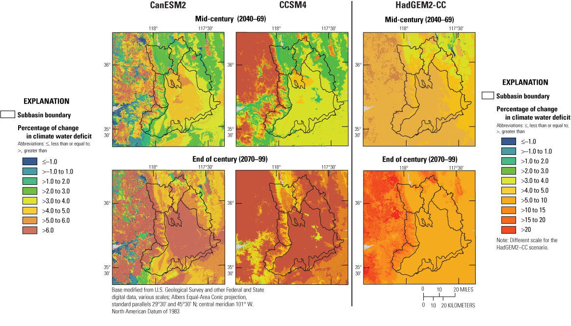
Percentage of change in climatic water deficit in comparison to the historical period (1981–2010), using three future climate models for mid-century (2040–69) and end-of-century (2070–99) periods in Indian Wells Valley, California. Second-generation Canadian Earth System Model (CanESM2) representing hot-wet projected conditions, Community Climate System Model version 4 (CCSM4) representing warm-moderately wet projected conditions, and Hadley Centre Global Environmental Model version 2 climate Configuration (HadGEM2-CC) representing hot-dry projected conditions.
Table 7 shows the percentage of change in projected recharge from the three GCMs when compared to 1981–2010 historical LOCA conditions. The three scenarios varied in their estimations; however, most recharge projections from the three models were greater than the model’s projection of precipitation for each period, except for the HadGME2-CC model in the end-of-century period, because most recharge occurs in years when precipitation exceeds the recharge threshold illustrated on figure 8. The change in the annual variability of precipitation (table 8) is much greater than historical precipitation, particularly for the two wet models (CanESM2 and CCSM4), ranging from 9 to 36 percent in the mid-century period, thus resulting in more opportunities for recharge in the future scenarios. All models showed an increase in recharge in the mid-century period for all IWV subareas, except for the 8-percent (0.09 Mm3; 750 acre-feet) decrease projected by HadGEM2-CC for the Argus Range. Overall, the CanESM2 scenario projected the largest increase in recharge during the mid-century period, with a projected 51–61 percent increase in recharge in the Sierra Nevada subareas; however, CCSM4 projected a 77-percent increase (the largest estimate, Rose Valley, not included in this evaluation) in recharge in the valley floor subarea (table 7). There is a great variation in recharge projections from the three GCMs during the end-of-century period. CanESM2 projected an increase in recharge for all IWV subareas (Rose Valley not included in this evaluation) from an average of 70-percent (4.3 Mm3; 3,456 acre-feet) increase in recharge in the South Sierra Nevada subarea to a 67-percent (0.6 Mm3; 490 acre-feet) increase in recharge in the valley floor subarea. The CCSM4 model also projected an increase in recharge in all the subareas during the end-of-century period (except for a small decrease in the Argus Range). However, CCSM4 projections are smaller in magnitude than CanESM2 estimates in all subareas, except for the valley floor and Rose Valley where the CCSM4 estimate was larger, with a 73-percent (0.2 Mm3; 154 acre-feet) increase in recharge (table 7). The HadGEM2-CC model showed a different pattern than the CanESM2 and CCSM4 models in the end-of-century period. HadGEM2-CC results indicated a large decrease in recharge for all subareas in IWV, from a 45-percent (2.4 Mm3; 1,900 acre-feet, Rose Valley not included in this evaluation) decrease in the Sierra Nevada, to a 75-percent (0.6 Mm3; 486 acre-feet) decrease in the valley floor (table 7).
Spatial distribution of percentage of change in recharge estimations in all IWV subareas projected by the GCMs for mid-century (2040–69) and end-of-century (2070–99) periods compared to the historical LOCA data are shown on figure 11. As previously stated, natural recharge in IWV is mostly generated from mountain front subareas (Todd Engineers, 2014), and results from CanESM2, a hot-wet scenario, and CCSM4, a warm-moderately wet scenario, show an increase in recharge in mid-century and end-of century periods in comparison to the historical period, particularly in the mountain front subareas. CanESM2 shows a larger increase in recharge in the end-of-century period compared to the mid-century period (recharge averaged among all sites, except Rose Valley, was 12-percent higher in the end-of-century period; table 7). This increase can be related to the increase in other CanESM2 projected climate conditions, such as the 11-percent increase in precipitation and 8-percent increase in average air temperature (averaged among all sites, except Rose Valley) in the end-of-century period compared to the mid-century period. CCSM4, unlike CanESM2, shows a greater increase (about 5 percent more, when all sites except Rose Valley were averaged) in recharge at mid-century when compared to recharge at the end of the century. Results from the HadGEM2-CC hot-dry scenario indicated a greater variation in projected recharge in the two periods. Results indicated an increase in recharge at mid-century in IWV (as much as 22 percent in the valley floor), except for an 8-percent decrease in the Argus Range (table 7). However, there was a large decrease in recharge (as much as 75 percent in the valley floor) in the end-of-century period, accompanied by a large decrease in the HadGEM2-CC projected precipitation of 32 percent (averaged among all sites, except Rose Valley; table 7).
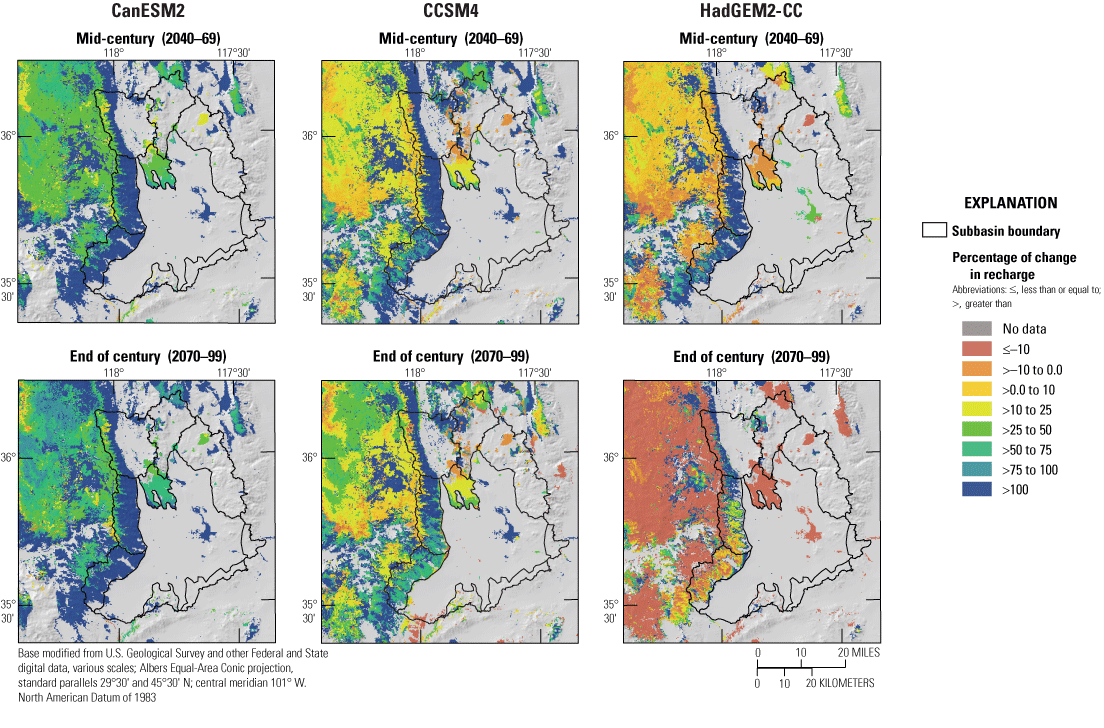
Percentage of change in recharge in comparison to the historical period (1981–2010), using three future climate models for mid-century (2040–69) and end-of-century (2070–99) periods in Indian Wells Valley, California. Second-generation Canadian Earth System Model (CanESM2) representing hot-wet projected conditions, Community Climate System Model version 4 (CCSM4) representing warm-moderately wet projected conditions, and Hadley Centre Global Environmental Model version 2 climate Configuration (HadGEM2-CC) representing hot-dry projected conditions.
The BCMv8 model’s interannual variability in recharge and runoff was evaluated using the standard deviation of seasonal (winter: October–March; summer: April–September) means simulated for the historical (1981–2010) and mid-century (2040–69) periods projected by the three GCMs (fig. 12). The standard deviation reveals only the magnitude of the variability and nothing about the seasonality of when water-year extremes generally occur. Results indicate that for all the IWV subareas, there is a large interannual variation in historical (1981–2010) recharge and runoff, particularly in the winter months, as well as a large difference among subareas (fig. 12A). This variability is more significant in subareas with more estimated recharge and runoff like the Sierra Nevada and the volcanic subareas, which increases the differences among subareas for recharge (fig. 12A). Projections from the GCMs indicated a similar variability in recharge and runoff in the mid-century period, with variability being more significant in the winter than in summer. However, the wet scenario from CanESM2 and the dry scenario from HadGEM2-CC showed greater seasonal variation. As figures 12B and 12C show, regardless of the larger magnitude of the CanESM2 wet scenario, both models showed almost double recharge and runoff in winter than in summer, specifically in subareas like the Sierra Nevada and El Paso Mountains, which provide most of the surface runoff and mountain front recharge to IWV. CCSM4, the moderate scenario, showed lower seasonal variations in runoff and recharge (fig. 12D). Given the large seasonal increases projected in the variability of runoff, these results illustrate that runoff also may be a valuable water resource in some years and, if managed strategically, could be used to supplement the groundwater supply.
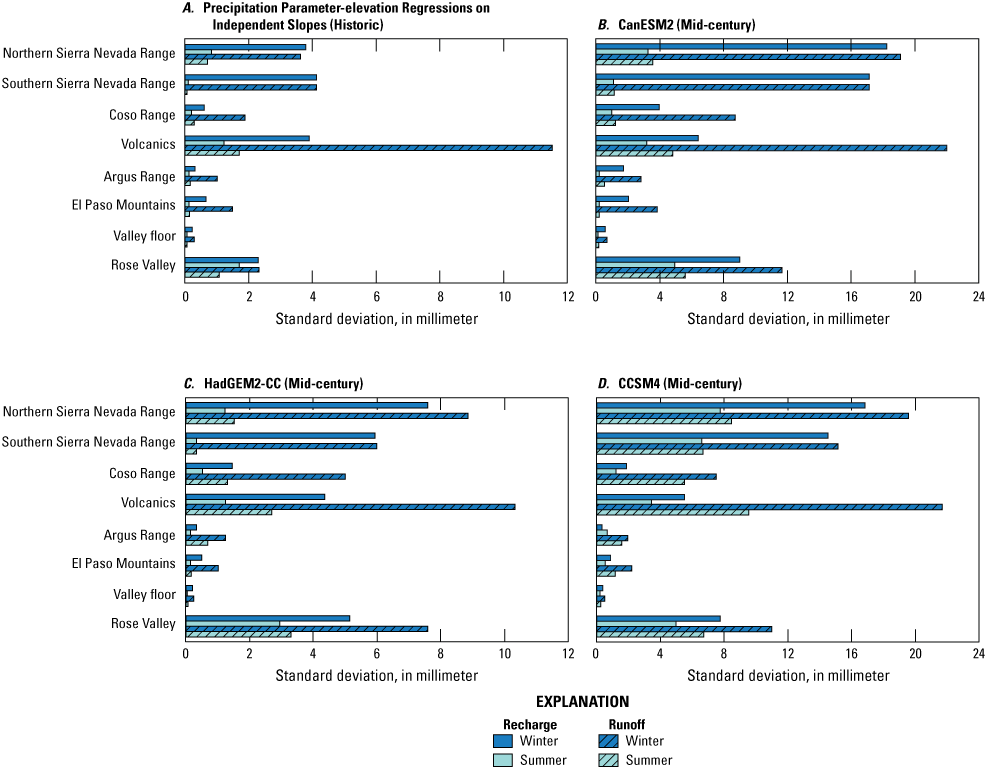
Indian Wells Valley, California, seasonal interannual variability in recharge and runoff from A, the Basin Characterization Model, version 8, for historical (1981–2010) period, and three LOCA projections for mid-century (2040–69); B, Second-generation Canadian Earth System Model (CanESM2) representing hot-wet projected conditions; C, Hadley Centre Global Environmental Model version 2 climate Configuration (HadGEM2-CC) representing hot-dry projected conditions; and D, Community Climate System Model version 4 (CCSM4) representing warm-moderately wet projected conditions. Seasonal time step is winter (October–March) and summer (April–September).
Discussion
Seasonal timing of precipitation and snowmelt and their effects on the hydrologic response of recharge and runoff drive the ability to manage scarce water resources in desert valleys. Distinct thresholds exist for the amount of precipitation that will result in recharge in any given year in IWV, overcoming the soil storage and evaporative demands. These thresholds vary throughout the basin as a result of the distribution of the different water balance components. An understanding of how these variables will change with climate, given the relatively static nature of the controlling properties of soils, geology, and vegetation, can help to facilitate decision-making and planning to ensure sustainable management of this resource.
It's important to keep in mind that future changes in annual water magnitudes and reaching recharge thresholds don't tell the whole story because of the seasonality of precipitation and the projected variability of water recharge and runoff. It is also prudent to consider runoff as an important aspect of available water supply, even if it is difficult to manage under historical conditions. The average change in recharge from historical to future periods indicates generally more water recharge and runoff because an increase in extreme weather conditions allows for more precipitation to exceed the recharge threshold. However, the increased variability indicates that the increase in water recharge won't occur every year. Resource management planning can be done to consider these possibilities. The increases in extremes, which have model consensus through mid-century, and only for the wet models by end of century, indicate more dry years and droughts. Although runoff has been of limited consequence historically, it may become more of a resource in coming years.
The projected changes in runoff and recharge in the Rose Valley subarea indicated increases in inflows to IWV some years, which may be captured and managed. Consider, for example, managed aquifer recharge as a practice to increase groundwater recharge during years when there are more extreme precipitation events and runoff. Although the relative proportion of inflows from Rose Valley was small for the historical studies, the calculation of recharge and runoff using the BCMv8 indicated that Rose Valley may be a source of water supply. The statewide-calibrated BCM calculated 3.44 Mm3 of recharge, which is slightly less than the recharge calculated for IWV at 3.73 Mm3 (table 1). The locally calibrated version had Rose Valley natural recharge at 5.8 Mm3, which is 54 percent of the total recharge in IWV (10.7 Mm3; table 6). The future climate models all projected fairly large increases in runoff and recharge by mid-century (table 7), and the two wetter models (CanESM2 and CCSM4) projected even larger increases by end of century, 81 percent increase in runoff in the South Sierra Nevada subarea and 73 percent increase in recharge in the Indian Wells Valley Floor subarea. Depending on the mechanisms responsible for resulting inflows to IWV, increase in runoff and recharge could be an asset in which to develop management plans.
Climatic water deficit generally is increasing with all model projections because of the consistent rise in air temperatures and evaporative demand consistent across models. The implications of rising CWD in mountains indicate more plant water use and more frequent development of landscape and forest stress, which leads to forest die-off (Anderegg and others, 2015) and wildfire risk (van Mantgem and others, 2013; Mann and others, 2016). The greatest increases were projected to be in the Sierra Nevada subareas. Increases of CWD on the valley floor have implications for crop demand. CanESM2 and CCSM4 projected a spatial variation in the increases, likely related to differences in soil properties and vegetation in the southwestern part of the valley and may provide some guidance for future crop development. However, it is important that changes in crop water demand of as much as 7 percent (Anderegg and others, 2015) are taken into consideration for irrigation planning to coincide with a more variable water-supply resource.
Summary
Groundwater is the main source of water in Indian Wells Valley (IWV) and is used for municipal, industrial, and agricultural use. Throughout the last several decades, overpumping of the main aquifer in the valley has critically depleted water availability in the valley and has classified IWV as a “high priority” Sustainable Groundwater Management Act basin. The locally calibrated Basin Characterization Model, version 8 (BCMv8) for IWV provided historical spatially distributed estimates of recharge and landscape stress in the valley. The BCMv8 was calibrated to actual evapotranspiration and historical measured streamflow data to constrain estimates of water-balance variables. Long-term average (1981–2010) natural recharge in IWV was estimated to be 10.7 million cubic meters (Mm3) per year, generated mainly from mountain front subareas. These findings are consistent with historical estimates of recharge from previous studies; however, BCMv8 provides an improved estimate of the IWV water balance by incorporating vegetation-specific actual evapotranspiration and using available spatial data of vegetation, topography, physical soil properties, and geology.
Three localized constructed analog Global Climate Models (GCMs), corresponding to the Representative Concentration Pathway 8.5, were used to evaluate future climate conditions in the IWV through the end of the century. The three GCMs represent different projected climatic conditions: Second-generation Canadian Earth System Model (CanESM2), hot-wet; Community Climate System Model version 4 (CCSM4), warm-moderately wet; and Hadley Centre Global Environmental Model version 2 climate configurations (HadGEM2-CC), hot-dry. Results from the three models provide useful information to understand future changes in water availability (as recharge and runoff) and landscape stress and irrigation demand (as climatic water deficit). All three GCMs showed an increase in climatic water deficit through the end of the century, corresponding with an increase of potential evapotranspiration because of higher air temperatures. The mid-century and end-of-century projections estimated by the three GCMs provide insights into potential variations in future hydrological conditions. The CanESM2 hot-wet model projected an increase in recharge at both mid-century and end of century, with a greater increase by end of century. This pattern of increase in recharge corresponds well with the models projected to increase in precipitation for the same periods. On the other hand, the HadGEM2-CC hot-dry scenario projected a decrease in recharge in both periods, with a larger decrease projected for the end-of-century period. This pattern of decrease also corresponds well with the HadGEM2-CC model projected precipitation in mid-century and end of century.
All models agreed that the change in annual and seasonal variability will be large through mid-century with a greater variability by end of century, as projected in the two wet models. This change in variability provides information that is important for consideration when developing water-supply management strategies. Regardless of the magnitude of projected change from each model, these results provide the two end points of extreme future climate conditions (wet or dry) and can be useful in addressing IWV future water needs. The projected increases in climatic water deficit will be important for land and water managers in IWV for planning in mid- to long-term time scales regarding availability of irrigation water because the demand is likely to increase. Knowing the historical interannual variability and the potential changes to recharge can help Groundwater Sustainability Agencies manage uncertainty and reduce the undesirable effects of groundwater overdraft, including land subsidence, water-level declines, and water-quality issues.
References Cited
Allen, D.C., Kopp, D.A., Costigan, K.H., Datry, T., Hugueny, B., Turner, D.S., Bodner, G.S., and Flood, T.J., 2019, Citizen scientists document long-term streamflow declines in intermittent rivers of the desert southwest, USA: Freshwater Science, v. 38, no. 2, p. 244–256. [Available at https://doi.org/10.1086/701483.]
Anderegg, W.R., Flint, A.L., Huang, C.-Y., Flint, L.E., Berry, J.A., Davis, F.W., Sperry, J.S., and Field, C.B., 2015, Tree mortality predicted from drought-induced vascular damage: Nature Geoscience, v. 8, no. 5, p. 367–371. [Available at https://doi.org/10.1038/ngeo2400.]
Austin, C.F., 1988, Hydrology of Indian Wells Valley: Memorandum outlining a review of recharge analyses in Indian Wells Valley, Department of the Navy, 21 p. [Available at https://www.ekcrcd.org/files/dc715d81b/06-19880610-AustinC-MemoGeohydrologyIWV.pdf.]
Bean, R.T., 1989, Hydrogeologic conditions in Indian Wells Valley and vicinity: California Department of Water Resources, contract no. DWR B-56783, 51 p. [Available at https://www.ekcrcd.org/files/77f6a7f6b/Hydrogeologic+Conditions+in+Indian+Wells+Valley+and+Vicinity.pdf.]
Berenbrock, C.E., and Martin, P.M., 1991, The ground-water flow system in Indian Wells Valley, Kern, Inyo, and San Bernardino counties, California: U.S. Geological Survey Water-Resources Investigation Report 89–4191, 81 p. [Available at https://doi.org/10.3133/wri894191.]
Berenbrock, C., and Schroeder, R.A., 1994, Ground‐water flow and quality, and geochemical processes, in Indian Wells Valley, Kern, Inyo and San Bernardino counties, California, 1987–88: U.S. Geological Survey Water‐Resources Investigations Report 93–4003, 59 p., 1 pl., scale 1:24,000. [Available at https://doi.org/10.3133/wri934003.]
Bloyd, R.M., Jr., and Robson, S.G., 1971, Mathematical ground-water model of Indian Wells Valley, California: U.S. Geological Survey Open-File Report 72–41, 36 p., 2 pls. [Available at https://doi.org/10.3133/ofr7241.]
California Department of Water Resources, 2014, Sustainable Groundwater Management Act (SGMA): California Department of Water Resources web page, California Water Code sections 10720–10737. [Available at https://water.ca.gov/Programs/Groundwater-Management/SGMA-Groundwater-Management.]
California Department of Water Resources, 2025, California’s Groundwater Bulletin 118: California Department of Water Resources web page, accessed October 1, 2025, at https://water.ca.gov/Programs/Groundwater-Management/Bulletin-118.
Daly, C., Halbleib, M., Smith, J.I., Gibson, W.P., Doggett, M.K., Taylor, G.H., Curtis, J., and Pasteris, P.P., 2008, Physiographically sensitive mapping of climatological temperature and precipitation across the conterminous United States: International Journal of Climatology, v. 28, no. 15, p. 2031–2064. [Available at https://doi.org/10.1002/joc.1688.]
Dutcher, L.C., and Moyle, W.R., Jr., 1973, Geologic and hydrologic features of Indian Wells Valley, California: U.S. Geological Survey Water-Supply Paper 2007, 30 p., 6 pls. [Available at https://doi.org/10.3133/wsp2007.]
Flint, L.E., and Flint, A.L., 2012, Downscaling future climate scenarios to fine scales for hydrologic and ecological modeling and analysis: Ecological Processes, v. 1, no. 2, 15 p. [Available at https://ecologicalprocesses.springeropen.com/articles/10.1186/2192-1709-1-2.]
Flint, L.E., Flint, A.L., and Stern, M.A., 2021a, The Basin Characterization Model—A monthly regional water balance software package (BCMv8) data release and model archive for hydrologic California (ver. 5.0, June 2025): U.S. Geological Survey data release, accessed October 1, 2025, at https://doi.org/10.5066/P9PT36UI.
Flint, L.E., Flint, A.L., and Stern, M.A., 2021b, The Basin Characterization Model—A regional water balance software package: U.S. Geological Survey Techniques and Methods book 6, chap. H1, 85 p., [Available at https://doi.org/10.3133/tm6H1.]
Flint, L.E., Flint, A.L., Thorne, J.H., and Boynton, R., 2013, Fine-scale hydrological modeling for climate change applications—The California Basin Characterization Model development and performance: Ecological Processes, v. 2, no. 25, 21 p. [Available at https://doi.org/10.1186/2192-1709-2-25.]
Indian Wells Valley Groundwater Authority, 2023: Indian Wells Valley Groundwater Authority web page, accessed October 2023 at https://iwvga.org.
Jennings, C.W, Strand, R.G., Rogers, T.H., Boylan, R.T., Moar, R.R., and Switzer, R.A., 1977, Geologic map of California: California Division of Mines and Geology Geologic Data Map GDM-2.1977, map scale; 1:750,000. [Available at https://ngmdb.usgs.gov/Prodesc/proddesc_16320.htm.]
Kunkel, F., and Chase, G.H., 1969, Geology and groundwater in Indian Wells Valley, California: U.S. Geological Survey Open-File Report 69–329, 84 p., 7 pls. [Available at https://doi.org/10.3133/ofr69329.]
Langridge, R., and Van Schmidt, N.D., 2020, Groundwater and drought resilience in the SGMA era: Society & Natural Resources, v. 33, no. 12, p. 1530–1541. [Available at https://doi.org/10.1080/08941920.2020.1801923.]
Livneh, B., Rosenberg, E.A., Lin, C., Nijssen, B., Mishra, V., Andreadis, K., Maurer, E.P., and Lettenmaier, D.P., 2013, A long‐term hydrologically based dataset of land surface fluxes and states for the conterminous United States—Update and extensions: Journal of Climate, v. 26, no. 23, p. 9384–9392. [Available at https://doi.org/10.1175/JCLI-D-12-00508.1.]
Mann, M.L., Batllori, E., Moritz, M.A., Waller, E.K., Berck, P., Flint, A.L., Flint, L.E., and Dolfi, E., 2016, Incorporating anthropogenic influences into fire probability models—Effects of human activity and climate change on fire activity in California: PLOS ONE, v. 11, no. 4, 21 p. [Available at https://doi.org/10.1371/journal.pone.0153589.]
Multi-Resolution Land Characteristics Consortium, 2018, National Land Cover Database 2011 (NLCD, 2011): Multi-Resolution Land Characteristics Consortium web page, accessed March 2023 at https://data.nal.usda.gov/dataset/national-land-cover-database-2011-nlcd-2011.
Nash, J.E., and Sutcliffe, J.V., 1970, River flow forecasting through conceptual models part I—A discussion of principles: Journal of Hydrology, v. 10, no. 3, p. 282–290. [Available at https://doi.org/10.1016/0022-1694(70)90255-6.]
Pierce, D.W., Cayan, D.R., and Thrasher, B.L., 2014, Statistical downscaling using Localized Constructed Analogs (LOCA): Journal of Hydrometeorology, v. 15, no. 6, p. 2558–2585. [Available at https://doi.org/10.1175/JHM-D-14-0082.1.]
Reitz, M., Sanford, W.E., Senay, G.B., and Cazenas, J., 2017, Annual estimates of recharge, quick‐flow runoff, and evapotranspiration for the contiguous U.S. using empirical regression equations: Journal of the American Water Resources Association, v. 53, no. 4, p. 961–983. [Available at https://doi.org/10.1111/1752-1688.12546.]
Riahi, K., Rao, S., Krey, V., Cho, C., Chirkov, V., Fischer, G., Kindermann, G., Nakicenovic, N., and Rafaj, P., 2011, RCP 8.5—A scenario of comparatively high greenhouse gas emissions: Climatic Change, v. 109, no. 33, p. 33–57. [Available at https://doi.org/10.1007/s10584-011-0149-y.]
Saleh, D., and Flint, L.E., 2019, Indian Wells Valley, California, sub-watersheds for the Basin Characterization Model: U.S. Geological Survey data release, accessed October 1, 2025, at https://doi.org/10.5066/F7JM28XZ.
Thompson, D.G., 1929, The Mohave Desert region, California, a geographic, geologic, and hydrologic reconnaissance: U.S. Geological Survey Water-Supply Paper 578, 759 p., 7 pls. [Available at https://doi.org/10.3133/wsp578.]
Thyne, G.D., Gillespie, J.M., and Ostdick, J.R., 1999, Evidence for interbasin flow through bedrock in the southeastern Sierra Nevada: Geological Society of America Bulletin, v. 111, no. 11, 1,600 p. [Available at https://doi.org/10.1130/0016-7606(1999)111<1600:EFIFTB>2.3.CO;2.]
van Mantgem, P.J., Nesmith, J.C.B., Keifer, M., Knapp, E.E., Flint, A.L., and Flint, L.E., 2013, Climatic stress increases forest fire severity across the western United States: Ecology Letters, v. 16, no. 9, p. 1151–1156. [Available at https://doi.org/10.1111/ele.12151.]
Watt, D.E. 1993, Indian Wells Valley Groundwater Project: Technical Report Prepared by Bureau of Reclamation, Lower Colorado Region, December 1993 for the Indian Wells Valley community. [Available at https://www.ekcrcd.org/files/1876f29db/174-19930012-USBureauReclaimation-IndianWellsValleyGroundwaterProjectTechnicalReport.pdf.]
Conversion Factors
U.S. customary units to International System of Units
International System of Units to U.S. customary units
Temperature in degrees Celsius (°C) may be converted to degrees Fahrenheit (°F) as follows:
°F = (1.8 × °C) + 32.
Temperature in degrees Fahrenheit (°F) may be converted to degrees Celsius (°C) as follows:
°C = (°F − 32) / 1.8.
Datums
Vertical coordinate information is referenced to the North American Vertical Datum of 1988 (NAVD 88).
Horizontal coordinate information is referenced to the North American Datum of 1983 (NAD 83).
Elevation, as used in this report, refers to distance above the vertical datum. Measurements of the distance to subsurface data are referred to as below land surface (bls).
Supplemental Information
Recharge is estimated in million cubic meters (Mm3).
A water year is the period from October 1 to September 30 and is designated by the year in which it ends; for example, water year 2015 was from October 1, 2014, to September 30, 2015.
Representative Concentration Pathway (RCP) is measured in watts per square meter.
Abbreviations
4CCA
California’s Fourth Climate Change Assessment
AET
actual evapotranspiration
BCMv8
Basin Characterization Model, version 8
CanESM2
Second-generation Canadian Earth System Model
CCSM4
Community Climate System Model version 4
CWD
climatic water deficit
ET
evapotranspiration
GCM
Global Climate Model
GSA
Groundwater Sustainability Agency
GSP
Groundwater Sustainability Plan
HadGEM2-CC
Hadley Centre Global Environmental Model version 2 climate configurations
IWV
Indian Wells Valley
LOCA
Localized Constructed Analogs
MODIS
Moderate Resolution Imaging Spectroradiometer
NSE
Nash-Sutcliffe Efficiency
PET
potential evapotranspiration
PRISM
Parameter-elevation Regressions on Independent Slopes Model
RCP
Representative Concentration Pathway
SGMA
Sustainable Groundwater Management Act
For more information concerning the research in this report, contact the
Director, California Water Science Center
U.S. Geological Survey
6000 J Street, Placer Hall,
Sacramento, California 95819
https://www.usgs.gov/centers/california-water-science-center
Publishing support provided by the USGS Science Publishing Network,
Sacramento Publishing Service Center
Disclaimers
Any use of trade, firm, or product names is for descriptive purposes only and does not imply endorsement by the U.S. Government.
Although this information product, for the most part, is in the public domain, it also may contain copyrighted materials as noted in the text. Permission to reproduce copyrighted items must be secured from the copyright owner.
Suggested Citation
Saleh, D., Flint, L., and Stern, M., 2026, Assessing natural recharge in Indian Wells Valley, California—A Basin Characterization Model case study (ver. 1.1, March 2026): U.S. Geological Survey Scientific Investigations Report 2026–5114, 34 p., https://doi.org/10.3133/sir20265114.
ISSN: 2328-0328 (online)
Study Area
| Publication type | Report |
|---|---|
| Publication Subtype | USGS Numbered Series |
| Title | Assessing natural recharge in Indian Wells Valley, California: A Basin Characterization Model case study |
| Series title | Scientific Investigations Report |
| Series number | 2026-5114 |
| DOI | 10.3133/sir20265114 |
| Edition | Version 1.0: February 18, 2026; Version 1.1: March 18, 2026 |
| Publication Date | February 18, 2026 |
| Year Published | 2026 |
| Language | English |
| Publisher | U.S. Geological Survey |
| Publisher location | Reston, VA |
| Contributing office(s) | California Water Science Center |
| Description | vi, 34 p. |
| Country | United States |
| State | California |
| Other Geospatial | Indian Wells Valley |
| Online Only (Y/N) | Y |