

Methods for Estimating Selected Streamflow Statistics at Ungaged Sites in Wyoming Based on Data Through Water Year 2021
Links
- Document: Report (7.2 MB pdf) , HTML , XML
- Table: Table 1.1 (60 KB xlsx)
- Dataset: USGS National Water Information System database - USGS water data for the Nation
- Data Release: USGS data release - Regression equations for selected streamflow statistics based on data through water year 2021 in and near Wyoming
- NGMDB Index Page: National Geologic Map Database Index Page (html)
- Download citation as: RIS | Dublin Core
Acknowledgments
The authors would like to thank the Wyoming Water Development Office staff who supported this work, especially Barry Lawrence, Mabel Jones, and Chace Tavelli, as well as Jodi Pring (retired Wyoming Water Development Office).
Olivia Drukker of the U.S. Geological Survey helped review scripts that were used for preliminary regression analysis for this report. Peter McCarthy and Ken Eng of the U.S. Geological Survey provided expertise on statistical methods.
Abstract
The U.S. Geological Survey, in cooperation with the Wyoming Water Development Office, developed regional regression equations based on basin characteristics and streamflow statistics for streamgages through water year 2021 (October 1, 2020, to September 30, 2021). The regression equations allow estimates of mean annual maximum, mean annual, mean seasonal, and mean monthly streamflows; frequency statistics for the 7-day mean low flows with 2-year and 10-year recurrence intervals, 14- and 30-day mean low flows with 5-year recurrence intervals, and 60- and 1-day mean high flow with 2-year and 5-year recurrence intervals, respectively; and the 0.1-, 0.2-, 0.5-, 1-, 2-, 4-, 5-, 10-, 20-, 25-, 30-, 50-, 60-, 70-, 75-, 80-, 90-, 95-, 98-, and 99-percent durations for annual streamflows and 0.1-, 0.5-, 10-, 15-, 20-, 25-, 30-, 40-, 50-, 60-, 70-, 75-, 80-, 85-, 90-, 95-, and 99-percent durations for monthly streamflows for most months for ungaged locations in Wyoming that are largely unaltered by diversions or upstream reservoirs.
Regression equations were developed for 243 streamflow statistics. Best-subset selection was used to assess explanatory variables for respective streamflow statistics. Exploratory data analyses determined that, of the 81 basin characteristics evaluated as potential explanatory variables, characteristics such as drainage area and precipitation often produced models with the highest adjusted coefficient of determination and lowest mean squared error, as determined in the best-subset selection. To address heteroskedasticity of model residuals, model variables were regionalized using fixed-effects models; the percentages of the streamgage basins in selected ecoregions were defined as interaction terms, which represent the model slope for specific ecoregions. Most models were determined to be statistically significant for probability values less than or equal to 0.1 for one or more regional explanatory variables. The final regional regression equations defined in this report are available for use in the U.S. Geological Survey’s StreamStats web application at https://streamstats.usgs.gov/ss/.
Introduction
Information about streamflow statistics is used for the development and management of surface-water resources. Statistics can be directly calculated for streamgages with the appropriate streamflow record; however, streamgages only represent a small part of the Wyoming stream network. Thus, models such as regression equations can be developed to estimate streamflow statistics at ungaged locations.
Streamflow statistics are used across the Nation for engineering; water-quality; wildlife management; and other everyday planning, research, and management problems (Risley and others, 2008; Feaster and Guimaraes, 2014). For example, annual, seasonal, and monthly streamflow statistics provide water users with expected streamflow during specific timeframes, aiding in water resource management and wildlife conservation. Flow-duration streamflow statistics provide streamflow-exceedance probabilities used to design stream-related infrastructure, including bridges and dams, and inform hydrologic modeling. Streamflow statistics describing the mean high- and low-streamflows for consecutive days (n-day high- and low-flow statistics) indicate the duration and frequency of maximum and minimum daily mean streamflows and are used to inform wastewater treatment methods, determine total maximum daily loads of streams, and assess the health of aquatic habitats. These streamflow statistics were previously calculated for all 176 streamgages used in this study in and near the State of Wyoming (fig. 1) based on data through water year 2021 (October 1, 2020, to September 30, 2021; Armstrong and others, 2025a, b).
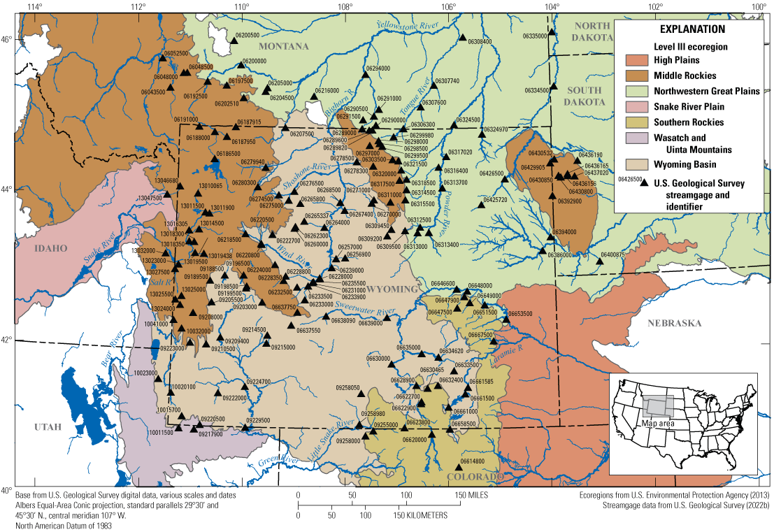
Map showing study area, U.S. Environmental Protection Agency level III ecoregions that intersect Wyoming (U.S. Environmental Protection Agency, 2013), and the locations of U.S. Geological Survey streamgages (U.S. Geological Survey, 2022b) used to develop the regional regression equations.
To predict streamflow statistics at ungaged locations, regional regression equations are commonly used. The U.S. Geological Survey (USGS), in cooperation with the Wyoming Water Development Office, developed regional regression equations for mean annual maximum, mean annual, mean seasonal, and mean monthly streamflows; n-day statistics; and annual and monthly flow-duration statistics using streamflow statistics at streamgages in and near Wyoming (fig. 1; table 1) that are unaffected by major regulation or diversions (hereinafter referred to as “unaltered”).
Table 1.
List of U.S. Geological Survey streamgages used in developing regression equations.[Streamgage data from U.S. Geological Survey (2022b). USGS, U.S. Geological Survey; NAD 83, North American Datum of 1983; MT, Montana; Lk, Lake; YNP, Yellowstone National Park; Cr, Creek; Bndry, Boundary; nr, near; ab, above; WY, Wyoming; SF, South Fork; L, Little; Ft, Fort; C, Creek; Rnch, Ranch; R, River; bl, below; N F, North Fork; Sta, Station; SD, South Dakota; CO, Colorado; Riv, River; E Fk, East Fork; Med, Medicine; Cv, Cave; UT, Utah; Res, Reservoir; ID, Idaho]
The n-day statistics describe the minimum or maximum streamflow during a consecutive period of days during an annual period for a selected recurrence interval. For example, the 7-day, 2-year low-flow statistic (M7D2Y) represents the streamflow value that is expected to be equaled or exceeded during a 7-day period, on average, once every 2 years. The 1-day, 5-year high-flow statistic (V1D5Y) represents the maximum daily streamflow that occurs every 5 years on average. High-flow n-day statistics use the water year (the 12-month period from October 1 through September 30 of the following year that is designated by the calendar year in which it ends), while low-flow n-day statistics use the climatic year instead of the water year as the annual period of record. Although a climatic year has no standard start and end date (Langbein and Iseri, 1960), other studies have commonly used April 1 to March 31 of the following year as the season boundaries for low-flow statistics (Risley and others, 2008; Feaster and Guimaraes, 2014). Regression equations were developed for the 7-day, 2-year low flow (M7D2Y); 7-day, 10-year low flow (M7D10Y); 14-day, 5-year low flow (M14D5Y); 30-day, 5-year low flow (M30D5Y); 60-day, 2-year high flow (V60D2Y); and 1-day, 5-year high flow (V1D5Y).
Flow-duration streamflow statistics (also referred to as “exceedance probabilities”) indicate how frequently streamflow observed at the location would be expected to meet or exceed the estimated streamflow for the year (annual flow duration) or month (monthly flow duration). For example, an annual exceedance probability of 0.01 indicates that a daily mean streamflow at a location, measured in cubic feet per second, has a 1-percent chance of being equaled or exceeded in a year. Regional regression equations were assessed for 0.1-, 0.2-, 0.5-, 1-, 2-, 4-, 5-, 10-, 20-, 25-, 30-, 50-, 60-, 70-, 75-, 80-, 90-, 95-, 98-, 99-, 99.5-, 99.8-, and 99.9-percent durations for annual streamflows and 0.1-, 0.5-, 10-, 15-, 20-, 25-, 30-, 40-, 50-, 60-, 70-, 75-, 80-, 85-, 90-, 95-, and 99-percent durations for monthly streamflows. Owing to the nature of weighted left-censored regression models, several statistics (99.5-, 99.8-, and 99.9-percent durations for annual streamflow and July 99-, August 95- and 99-, and September 95- and 99-percent durations for monthly streamflow) had too many censored streamflow values (zero values) to develop final models.
Purpose and Scope
The USGS, in cooperation with the Wyoming Water Development Office, continues efforts to update relevant data and develop streamflow models for the StreamStats application for the State of Wyoming. StreamStats is a web application that can be used to delineate drainage areas, determine basin characteristics, and compute streamflow statistics at gaged and ungaged locations (https://streamstats.usgs.gov/ss/; Ries and others, 2017, 2024; USGS, 2019a, 2022b). The purpose of this report is to describe the methods used in developing regression equations for estimating selected streamflow statistics using current (2025) basin characteristics (table 2; Hallberg and others, 2023b) for ungaged basins in Wyoming. The regression equations were developed using newly updated streamflow statistics from Armstrong and others (2025a, b). A total of 176 streamgages were used for developing equations for mean annual maximum, mean annual, mean seasonal, and mean monthly streamflow; and annual and monthly flow-duration streamflow statistics. A subset of only 145–156 streamgages was used for developing equations for n-day statistics, which include M7D2Y, M7D10Y, M14D5Y, M30D5Y, V60D2Y, and V1D5Y. The equations presented in this report are loaded to the Wyoming StreamStats application and can be used to derive the previously mentioned streamflow statistics for ungaged locations on streams in Wyoming.
Table 2.
Basin characteristics considered for best-subset selection in regression analysis for each group of streamflow statistics.[n-day, streamflow statistic describing a streamflow event over a number of days; x, statistic is relevant to StreamStats abbreviation; --, not applicable; NLCD, National Land Cover Database]
| StreamStats abbreviation | Definition | Mean periodical statistics | Flow-duration statistics | Minimum n-day statistics | Maximum n-day statistics |
|---|---|---|---|---|---|
| AUGAVTMP | Mean August temperature, in degrees Fahrenheit | -- | -- | -- | x |
| BASINPERIM | Perimeter of the contributing drainage area, in miles | x | x | -- | x |
| COMPRAT | Compactness ratio for the contributing drainage area, computed using the DRNAREA and BASINPERIM basin characteristics | x | -- | -- | x |
| DECAVPRE | Mean December precipitation, in inches | x | -- | x | -- |
| DECAVTMP | Mean December temperature, in degrees Fahrenheit | -- | x | -- | x |
| DRNAREA | Drainage area, in square miles | x | x | x | x |
| ET0306MOD | Spring (March–June) mean-monthly evapotranspiration (2001–11), in inches per month | x | -- | -- | -- |
| FEBAVPRE | Mean February precipitation, in inches | -- | -- | x | -- |
| FEBAVTMP | Mean February temperature, in degrees Fahrenheit | -- | -- | -- | x |
| JANAVPRE | Mean June precipitation, in inches | x | -- | x | -- |
| JANAVTMP | Mean January temperature, in degrees Fahrenheit | -- | x | -- | x |
| JULAVTMP | Mean July temperature, in degrees Fahrenheit | -- | -- | x | x |
| JUNAVTMP | Mean June temperature, in degrees Fahrenheit | -- | -- | x | x |
| LC16SHRUB | Percentage of shrub or scrub land from NLCD 2016 (Dewitz, 2019) class 52 | -- | -- | -- | x |
| MARAVPRE | Mean March precipitation, in inches | -- | -- | x | -- |
| MARAVTMP | Mean March temperature, in degrees Fahrenheit | -- | -- | -- | x |
| NOVAVPRE | Mean November precipitation, in inches | x | -- | x | -- |
| NOVAVTMP | Mean November temperature, in degrees Fahrenheit | -- | x | x | x |
| OCTAVTMP | Mean October temperature, in degrees Fahrenheit | -- | -- | -- | x |
| RELIEF | Difference between the maximum and minimum elevations of the basin, in feet | x | x | x | x |
| SEPAVTMP | Mean September temperature, in degrees Fahrenheit | -- | -- | x | x |
| SLOP50_10M | Percentage of basin with slopes greater than or equal to 50 percent | -- | -- | x | -- |
| SNOAPR | Mean April 1 water equivalent of snow cover (2004–22) | x | x | x | x |
| SNOFEB | Mean February 1 water equivalent of snow cover (2004–22) | x | x | x | x |
| SNOJAN | Mean January 1 water equivalent of snow cover (2004–22) | x | x | x | x |
| SNOMAR | Mean March 1 water equivalent of snow cover (2004–22) | x | x | x | -- |
| SNOMAY | Mean May 1 water equivalent of snow cover (2004–22) | x | x | x | x |
| SOILPERM | Mean soil permeability, in inches per hour | x | -- | -- | x |
| TEMP | Mean annual daily mean temperature, in degrees Fahrenheit | -- | -- | x | x |
Description of Study Area
The study area includes Wyoming, an area of about 98,000 square miles, and some basins that extend into Colorado, Idaho, Utah, Montana, Nebraska, North Dakota, and South Dakota (fig. 1). The study area contains parts of four large hydrologic regions: the Great Basin, Missouri, Pacific Northwest, and Upper Colorado regions (Hallberg and others, 2023a). Wyoming has diverse ecosystems and landscapes with elevations ranging from 3,125 to 13,785 feet. These ecosystems consist of forested mountains and glaciated peaks, semiarid shrub- and grass-covered hills and plains, high-elevation plateaus, and wetlands (Chapman and others, 2004).
The diversity of Wyoming’s ecosystems is captured by the U.S. Environmental Protection Agency (EPA) level III ecoregions (EPA, 2013; Omernik and Griffith, 2014), which define spatial patterns in geology, physiography, vegetation, climate, soils, land use, wildlife, and hydrology. In the study area, seven level III ecoregions define the diverse ecology of the state. Two ecoregions, Snake River Plain, and Wasatch and Uinta Mountains, cover less area in Wyoming and are not represented as well by streamgage basins from this study. The five ecoregions that contain most of this study’s basins are the Middle Rockies, Southern Rockies, Wyoming Basin, High Plains, and Northwestern Great Plains (fig. 1). The EPA Office of Research and Development, National Health and Environmental Effects Research Laboratory (EPA, 2013) descriptions of these ecoregions are in the following paragraphs.
The Middle Rockies ecoregion is composed of steep-crested, high mountains that are largely covered by coniferous forests. These forests differ in species from the Southern Rockies, having more Pinus contorta Douglas ex Loudon (lodgepole pines). The Black Hills part of the Middle Rockies is also distinct with a more montane climate than surrounding parts of South Dakota (Chapman and others, 2004). Numerous mountain-fed, perennial streams originate in this ecoregion from snowmelt and flow into surrounding ecoregions, and annual peak streamflows are typically during the spring.
The Southern Rockies ecoregion is characterized by steep mountains, intermontane valleys, and high-elevation plateaus. Vegetation varies across this region largely by elevation: from alpine wildflowers, subalpine coniferous forests, and shrubs and grass at the lowest elevations (Chapman and others, 2004). Similar to streamflow in the Middle Rockies, the causal mechanism for streamflow is predominantly snowmelt; however, mixed rain-on-snow runoff and rainfall are more common at lower elevations.
The Wyoming Basin ecoregion is primarily a broad arid intermontane basin covered by grasslands and shrublands and flanked by the Middle Rockies to the west and east (Chapman and others, 2004). Although similar in topography and vegetation, the Wyoming Basin is drier than the Northwestern Great Plains to the northeast. Many streams are supplied by runoff from the surrounding montane ecoregions.
The Northwestern Great Plains ecoregion is defined by semiarid rolling plains in the northeastern corner of Wyoming. Cattle grazing and agriculture are common, and many streams are affected by irrigation (Chapman and others, 2004). Coal-bed methane production is also prevalent, and production water from groundwater pumping during methane extraction has effects on discharge to streams, especially during low flow. Snowmelt is often earlier in the season compared to montane ecoregions, and rainfall from summer storms also contributes to streamflow.
The High Plains ecoregion consists of undulating plains in the southeastern corner of Wyoming. The Rocky Mountains to the west cause a rain shadow, which greatly limits the precipitation in this ecoregion. Along with drought-resistant shortgrass, agricultural crops are common in this region because much of the precipitation falls during the growing season (spring–summer) (Chapman and others, 2004). Many of the basins with streamgages in this region experience some effect from irrigation.
Mean annual precipitation in Wyoming for 1991–2020 ranged from less than 10 inches per year in parts of the Green River, Great Divide, Wind River, and Bighorn Basins largely defined by the Wyoming Basin ecoregion to more than 70 inches per year in mountainous areas (Middle Rockies ecoregion) in the northwestern part of the State (PRISM Climate Group, 2022). The large range of elevations and precipitation in the State results in diverse hydrology and unique mechanisms for high and low streamflows. Land uses in Wyoming include grassland pasture and range (72 percent), forest cover (12 percent), urban and special use areas (12 percent), and cropland (4 percent) (University of Wyoming, 2019). Because of the small percentage of urbanized area, streams in Wyoming are generally less affected by urbanization than streams in many other states. Physiographic regions and the orientation of basins are mainly driven by the location of mountain ranges and the Continental Divide. Much of the land cover consists of high-elevation sagebrush and grassland that receives less precipitation than the mountain ranges. Precipitation in Wyoming results from two regional climate patterns. Winter months consist of high-elevation snow accumulation and intermittent snow cover at lower elevations. Spring and early summer rainstorms and snowmelt create peak streamflow conditions on many streams and rivers during this period. Midsummer through fall is often hotter and drier than the spring and early summer, and isolated, large thunderstorms during this period can cause high-flow events on smaller streams (University of Wyoming, 2019).
Previous Studies
Previous studies in Wyoming developing streamflow regression equations focused on estimating peak-flow frequency from instantaneous streamflow records. Lowham (1988) developed regression equations for estimating peak streamflows and annual streamflow for streams in mountain, plains, and high desert physiographic regions. Miller (2003) updated peak-flow frequency regression equations for six hydrologic regions based on similar physiographic boundaries (Fenneman and Johnson, 1946) and patterns in model residuals. No previous studies in Wyoming have developed regression equations to estimate low-flow frequencies or flow-duration statistics from daily streamflow data. However, low-flow regression equations that have been developed in Montana (McCarthy and others, 2016) share basin boundaries with Wyoming. Thus, methods for estimating low-flow stream statistics in Montana were used to inform the workflow developed for this study.
Criteria for Selecting Streamgages for Regression Equations
An affiliated study computed streamflow statistics for 615 streamgages in and near Wyoming with periods of record for water years 1868–2021 (Armstrong and others, 2025a). Neither crest-stage gages nor streamgages with daily streamflow records of fewer than 10 years were included in this study. Streamflow statistics used in this regression analysis include mean annual maximum, mean annual, mean seasonal, and mean monthly streamflows; n-day statistics; and annual and monthly flow-duration statistics. All statistics were computed using daily streamflow records available in the USGS National Water Information System (NWIS) database (USGS, 2022b).
Streamflow statistics from Armstrong and others (2025a) were assessed for all streamgages that have at least 10 years of daily streamflow data through water year 2021 and are in an 8-digit hydrologic unit code region (commonly known as HUC 8) within or intersecting the Wyoming boundary. To ensure accurate representation of streamflow at ungaged basins, only streamgages that were predominantly unaffected by alteration from diversions or regulation by upstream reservoirs were used.
To determine the alteration status of streamgages in Wyoming, Armstrong and others (2025a) assessed the influence of dam storage or irrigation on basins using methods from Wieczorek and others (2021). Those data were processed to determine total accumulated upstream storage from dams and irrigation in relation to drainage area. Equations for dam and diversion disturbance indices are described in Armstrong and others (2025a). The streamflow record at each streamgage was classified as “altered—major alteration (dams)” for dam disturbance-index values greater than or equal to 0.02, as “altered—minor alteration (dams)” for values greater than 0.01 and less than 0.02, and “unaltered (dams)” for values less than or equal to 0.01. For diversion disturbance indices, streamgages were classified as “altered by diversions” for values greater than or equal to 10 and “unaltered” for values less than 10. Data used to develop the disturbance indices were provided by the Wyoming State Engineer’s Office and are not complete for neighboring states. Thus, this study used additional references from the USGS NWIS database (USGS, 2022b), StreamStats application for each state (USGS, 2019a; Colorado, Idaho, Montana, South Dakota, North Dakota, Utah, and Nebraska), and USGS Water Supply Papers (USGS, 1973) to assess the alteration status of non-Wyoming streamgages. In addition to removing streamgages based on alteration status, redundant streamgages were also removed. Spatial autocorrelation from redundant streamgage records, which can happen when streamgages are on the same stream channel or major tributaries, can have adverse effects on regression models (Gruber and Stedinger, 2008). For streams with multiple streamgages, the overlapping drainage area of each streamgage was used to determine redundancy. Of the 285 streamgages with unaltered status, 51 were removed for redundancy to limit spatial autocorrelation in regression models. An additional 58 streamgages were removed after the initial analysis for various reasons, including non-Wyoming streamgages with major alteration described by NWIS or StreamStats records, spring-fed streamgages or streamgages with records affected by coal-bed methane or urbanization, and streamgages with basins predominantly in the High Plains ecoregion because of factors described below. Details on the removed streamgages are available in the accompanying USGS data release (Drukker and others, 2026). The final streamgage list used in developing regression equations is provided in table 1.
Streamgages with 75 percent or more of their respective basins in the High Plains ecoregion demonstrated large model residuals (app. 1) as compared to streamgages in other regions. Because of the lack of thorough representation of hydrologic conditions within this region, these 12 streamgages were removed from further analysis. One USGS streamgage (Blue Creek near Lewellen, Nebraska; 06687000; not shown) was spatially isolated from other basins after removing the High Plains region and, thus, was also removed.
Exploring Basin Characteristics as Explanatory Variables
Basin characteristics from Hallberg and others (2023b) were investigated as potential explanatory variables in the regression analyses. Basin characteristics are represented as gridded parameters describing various environmental, geological, and land use attributes for respective drainage areas for each streamgage (Hallberg and others, 2023b). Drainage areas were delineated by Dutton and others (2025) for each streamgage using a combination of National Hydrography Dataset (USGS, 2022a) and an integrated set of geospatial data layers, including the 10-meter Digital Elevation Model from the USGS 3D 02Elevation Program (USGS, 2019b) and the national Watershed Boundary Dataset (USGS, 2022a), all processed by Hallberg and others (2023a). These data can also be accessed in the Wyoming StreamStats application for streams in Wyoming (USGS, 2019a).
To best represent the relation of streamflow to basin geography and climate, basin characteristics were assessed as candidate explanatory variables for each of the streamflow statistic groups: mean annual maximum, mean annual, mean seasonal, and mean monthly streamflow statistics (referred to as mean periodical statistics); flow-duration statistics; minimum n-day (M7D2Y, M7D10Y, M14D5Y, M30D5Y) statistics; and maximum n-day statistics (V60D2Y and V1D5Y). For example, drainage area has been determined to be a statistically significant variable in explaining low-flow variability (Kroll and others, 2004; Funkhouser and others, 2008). As such, investigating these types of basin characteristics as candidate explanatory variables in predictive modeling of low-flow statistics is common practice. For each group of streamflow statistics, a subset of the 81 basin characteristics published by Hallberg and others (2023b) was assessed (table 2). Subsets were composed of the most correlated (highest Pearson’s correlation coefficient) variables for all streamflow statistics in a respective group; normality of the candidate explanatory variables was also considered, avoiding variables whose distributions were skewed by a few values. Final explanatory variables for the regression models were selected by best-subset selection, described in the “Selection of Explanatory Variables” section of this report.
Regression Analysis
Regression analysis involves determining relations between streamflow statistics (the dependent variables) and respective basin characteristics (the explanatory variables) for streamgages to estimate streamflow statistics at ungaged locations in similar regions. Streamflow statistics are related to the physical, geologic, and climatic properties of drainage basins (Smakhtin, 2001). As described in the following sections, drainage basin properties and regional boundaries (defined by basin characteristics) were selected based on the performance of regression models and their theoretical relation to river hydrology.
Selection of Explanatory Variables
Best-subset selection was used to assess optimal explanatory variables because this technique is recommended by Helsel and others (2020). Best-subset selection requires that all possible combinations of candidate explanatory variables be tested to find the optimal regression model(s). Because this method is computationally intensive, only the most highly correlated variables were considered for each streamflow statistic group. Additionally, an arbitrary limit on the maximum number of variables, 1 per 20 streamgages, was followed to reduce the risk of model overfitting. Statsmodels version 0.14.4 (Seabold and Perktold, 2010), a Python package for statistical analysis, was used to generate weighted least squares (WLS) regression models for best-subset selection. To reduce multicollinearity between variables, only variable combinations with variance inflation factors less than 5 were considered (Helsel and others, 2020). Similarly, to avoid statistically insignificant models, combinations were excluded if any variable had a statistical probability level (p-value) greater than 0.05. The remaining combinations were ranked based on the adjusted coefficient of determination (R2) and mean squared error (MSE). The adjusted R2, a metric of model fit, decreases when additional explanatory variables fail to reduce the residual sum of squares (Farmer and others, 2019). The MSE quantifies the average squared difference between predicted and observed values; a smaller MSE indicates a better model fit. After best-subset selection, final weighted left-censored regression models (described in the “Final Regression Equations” section) were developed to account for left-censored values (zero streamflow) and variation in streamgage record lengths. Because streamflow statistics estimated at streamgages with short records may have greater uncertainty (Farmer and others, 2019), streamgages were weighted by record length. Weighting was computed as the number of years of record at the streamgage divided by the mean record length across all streamgages used in the regression model (Eng and others, 2009; Lorenz, 2014).
Because of nonlinear relations between streamflow statistics and the explanatory variables, all variables were log transformed (base 10) before analysis. Basin characteristics that were computed as a percentage of the basin (percentage of forest, for example) could potentially have a value of 0; therefore, a value of 1 was added to these basin characteristics before log transformation. Transformations for respective variables are represented in the final models (app. 1, table 1.1).
A statewide (pooled) regression model for mean periodical streamflow statistics was first developed to assess candidate explanatory variables. Combining regions containing fewer streamgages can be beneficial if physiographic differences are not significant. For each streamflow statistic, WLS regression models were developed for the entire study area using basin characteristics selected by a best-subset procedure defined previously. Because spatial patterns in model residuals can indicate regional differences, residuals from pooled models were compared to those from fixed-effects models (Griffis and Stedinger, 2007), which use regional boundaries as additional explanatory variables. EPA level III ecoregions (EPA, 2013; Omernik and Griffith, 2014) and hydrologic regions from previous streamflow regression studies (Miller, 2003) were considered as explanatory variables in fixed-effects models. Ecoregions were designed to stratify the environment by the probable response to disturbance (Bryce and others, 1999), which makes them ideal candidates as variables in the fixed-effects models.
Residuals from pooled models were examined spatially to assess geographical patterns of bias. Heteroskedasticity, unequal variance across residuals, was minor with some regional differences in residuals (app. 1); however, many models demonstrated large residuals for streamgages in the High Plains ecoregion as compared to streamgages in other regions. Because of the lack of representation of hydrologic conditions in this region, streamgages within the High Plains ecoregion were ultimately excluded from the final regression models.
Regionalization was further assessed using fixed-effects models. Fixed-effects models were used to test for differences between model intercepts and slope coefficients for basins within a given ecoregion as compared to a common model. To test the difference between intercepts of each region, fixed-effects models using indicator variables, defined as the percentage of drainage area of the respective streamgage basin within a selected ecoregion, were assessed (Griffis and Stedinger, 2007). Using a percentage allows for a smooth transition for ungaged locations on streams that flow through multiple ecoregions (Feaster and others, 2023). Differences in slope can be assessed by including interaction terms in the fixed-effects model, which are the cross products of the pooled model explanatory variables and the percentage of the drainage areas in the respective ecoregions (Griffis and Stedinger, 2007). The Middle Rockies ecoregion was assigned as the base ecoregion, and thus all indicator variables and interaction terms corresponded to other ecoregions. For example, all indicator variables and interaction terms equal 0 when estimating streamflow for a basin entirely in the Middle Rockies ecoregion. Although physiographic differences may exist among ecoregions, these differences may be insignificant in the coefficients of the modeled slope or intercept, implying the base ecoregion is representative of all ecoregions evaluated. The statistical significance of explanatory variables was assessed at the 10-percent level (p-value greater than 0.1) for a chi-square distribution. A consistent slope between regions may indicate that, across ecoregion boundaries, the time of concentration for streamflow has a consistent linear relation to the explanatory variables. For example, precipitation may relate differently to peak streamflow statistics in basin or plains regions, where floods are often caused by localized rainstorms, compared to mountain regions, where floods typically result from rain on snow and snowmelt (Miller, 2003). However, for low streamflows, snowpack is a dominant factor statewide, and the model slope does not vary across regions, which is the case for the low-flow n-day regression models in this study. A difference in intercept alone may indicate differences in the volume of runoff in ecoregions because of differences in soil, land cover, storage, and slope (Griffis and Stedinger, 2007). In this study, interaction terms were often more statistically significant for evaluated models than indicator variables, indicating streamflow and model explanatory variables have different linear relations across ecoregions. The p-values for all explanatory variables used in the fixed-effects models are listed in table 1.1 to highlight the dominant patterns in the significance of regional explanatory variables and the potentially unnecessary (insignificant) regional variables for selected statistics.
Log-transformed drainage area and mean April 1 snow-water equivalent were ranked high in best-subset selection for mean periodical and flow-duration statistics groups. Because these groups contain a range of streamflow statistics calculated over various temporal periods, fixed-effects models were first assessed for individual flow statistics to identify regional patterns; flow statistics were then regrouped based on model similarity. For example, monthly flow-duration statistics generally indicated similar statistical significance for ecoregion interaction terms for most exceedance intervals, and thus, the same explanatory variables were used for the final models. Seasonal and monthly mean statistics demonstrated slightly different statistically significant ecoregion interaction terms and thus have unique explanatory variables. For example, regional patterns are similar for most streamflow statistics associated with early spring months (April–May), which often do not have statistically significant interaction terms from the Southern Rockies ecoregion. This similarity of regional patterns could be due to spring snowmelt contributing to runoff in both the Southern Rockies ecoregion and Middle Rockies base ecoregion. For many streamflow statistics during the summer months (July–September), the model interaction terms for snow-water equivalent for the Wyoming Basin ecoregion are generally not statistically significant, which may reflect streamflow response to the runoff from the Middle Rockies ecoregion that supplies and sustains many streams in the Wyoming Basin. Most annual flow-duration statistics have statistically significant interaction terms for all ecoregions, although for low-percentage durations, few terms were statistically significant, which may emphasize the significance of mountain snowpack in high streamflow statewide.
Low-flow and high-flow n-day statistics produced different best-subset results for pooled models; thus, regionalization was evaluated separately for each statistics group using fixed-effects models. For low-flow n-day statistics models, drainage area interaction terms were statistically significant across all ecoregions. In contrast, the log-transformed mean March precipitation (table 2) interaction term was generally not statistically significant in the Southern Rockies ecoregion and Wyoming Basin relative to the Middle Rockies base ecoregion, which may indicate that low streamflows in these regions respond similarly to late-winter precipitation.
For high-flow n-day statistics, the best-subset models incorporated additional physiographic variables beyond drainage area and precipitation. The explanatory variables in the pooled model included drainage area, relief, mean November temperature, and mean April 1 snow-water equivalent. In fixed-effects models, only the Northwestern Great Plains had statistically significant interaction terms for both weather variables; however, for V1D5Y, the interaction term for snow-water equivalent is not statistically significant, indicating regional differences are mostly captured by drainage area.
Final Regression Equations
Regression equations were developed for all streamflow statistics using weighted left-censored regression models (Helsel and others, 2020). Weights were based on the number of years of record available at each streamgage (Armstrong and others, 2025b). Because many streamgages in this study had values of 0 for some streamflow statistics, common regression techniques such as WLS or generalized least squares could create additional bias (Helsel and others, 2020). Thus, zero-flow values were treated as left-censored data using weighted left-censored regressions (Kroll and Stedinger, 1996; Kroll and Vogel, 2002).
To develop the final regression equations, weighted left-censored regression was implemented using the smwrQW R package developed by the USGS (Lorenz, 2014). When flow statistics do not have censored data, weighted left-censored regressions produce results equivalent to WLS (Helsel and others, 2020). Censored data in this study were defined as streamflows below a perceptible threshold of 0.1 cubic foot per second; therefore, all streamflow statistics with observed values less than 0.1 cubic foot per second were treated as left censored (Kroll and Stedinger, 1996; Kroll and Vogel, 2002). For statistics in which fewer than 20 percent of the streamgages are censored, weighted left-censored regression was considered appropriate (Helsel and others, 2020). When 20 percent or more of the streamgages had censored data, an alternative modeling approach, such as logistic regression, would be required. Such statistics were uncommon (table 1.1) and were removed from this study. The generalized least squares regression method (Tasker and Stedinger, 1989), which is often used for frequency statistics, such as n-day statistics, was not suitable because many statistics had censored data (Eng and others, 2009).
The mean standard error of estimates, in percent, for the regression equations is given in table 1.1. The mean standard error of estimates is a measure of the uncertainty of predictions made for all streamgages used in the model; however, the standard error of prediction should be calculated for individual estimates at the ungaged site of interest and subsequently used to determine the prediction intervals for the selected streamflow statistic. The following equation can be used to calculate the standard error of prediction for an ungaged site:
whereSEP
is the standard error of prediction, in logarithmic units, for an estimate of the selected streamflow statistic at an ungaged site;
MSE
is the mean squared error (table 1.1), in logarithmic units, for the appropriate regression equation;
x0
is a row vector consisting of the value 1.0 in the first column, followed by the log-transformed values of the p explanatory variables (basin characteristics) for the ungaged site used in the regression equation;
is the transpose of the vector x0; and
(XTX)−1
is the covariance matrix for the WLS regional regression equation (Drukker and others, 2026).
The SEP can be used to calculate a confidence interval for the same estimate using equation 2, and the prediction interval can be estimated using equation 3.
whereCI0,α
is the confidence interval, in logarithmic units, for the ungaged site;
is the Student’s t value for a significance level, α, and (n−p−1) degrees of freedom; and
n and p
are the number of streamgages used in the regression equation and the number of explanatory variables (basin characteristics) used in the regression equation, respectively.
is the prediction interval, in cubic feet per second, for the estimated Q0 at the ungaged site with a significance level of α;
U0
is for the upper prediction interval for the ungaged site;
L0
is for the lower prediction interval for the ungaged site; and
Q0
is the estimated streamflow statistics, in cubic feet per second, for the ungaged site.
Limitations of Regression Equations
The regression equations were developed to estimate selected streamflow statistics for ungaged streams in Wyoming that are unaffected or minimally affected by streamflow alteration. Alteration indices defining the degree of alteration from dams or diversion are available for streamgage basins within Wyoming (Armstrong and other, 2025b) but do not comprehensively extend to basins partially contained in neighboring states. Also, the alteration threshold defined by these indices may not be applicable to all basins in Wyoming because water-use data may be incomplete. Streamflow statistics used to develop these regression equations were selected from streamgages (table 1) classified as unaltered for the period of record analyzed. Therefore, the final regression equations (table 1.1) can be used for predicting streamflows at similarly unaltered basins in Wyoming.
Multivariate models, such as these regression equations, may have unreliable results when estimating streamflow statistics for basins with explanatory variables outside the range of values used to develop the equations. The range of explanatory variables for respective regression equations is listed in table 1.1.
Streamgages with high leverage and influence were flagged in the final weighted left-censored regression models using thresholds defined in this section. Leverage is a function of the distance from a dependent variable value to the regression model mean. Leverage identifies streamgages with explanatory variables far from the mean of the joint distribution of all explanatory variables in the model. The leverage value for a prediction should not exceed the largest leverage from the modeled dataset (Helsel and others, 2020).
Streamgages with high influence can have a disproportionate effect on the estimated regression parameters in equations. Influence is measured by Cook’s D (Cook, 1977), an estimate of the change in model fit if a particular observation is omitted. Equations for determining high leverage and influence are described in Helsel and others (2020). High influence is defined as Cook’s D greater than F(p+1, n−p) at α=0.1, where F(p+1, n−p) is the value of the F-distribution at 10 percent for p+1 and n−p degrees of freedom. All streamgages also were checked for high leverage, defined as leverage greater than 3p/n, where p is the number of coefficients in the model and n is the number of observations. For most models, few streamgages demonstrated high leverage and influence; for the three streamgages that did (USGS streamgages Muscrat Creek near Shoshoni, Wyoming [06239000]; East Fork Nowater Creek near Colter, Wyo. [06267400]; and Fifteen Mile Creek near Worland, Wyo. [06268500]), records did not indicate significant alteration or other reasons to remove them from the final models.
Summary
Streamflow statistics can be used for the effective development and management of surface-water resources, particularly in Wyoming, where the existing network of streamgages covers only a small fraction of the extensive stream network. To address this limitation, regional regression equations were developed to estimate streamflow statistics at ungaged locations on streams in Wyoming. These equations expand the access and application of hydrologic data across disciplines such as engineering, water-quality assessment, wildlife management, and general resource planning. The U.S. Geological Survey, in cooperation with the Wyoming Water Development Office, updated and refined regression equations using newly computed streamflow statistics from 176 streamgages across Wyoming.
The study area encompasses about 98,000 square miles of Wyoming, characterized by diverse ecosystems, ranging from high-elevation mountains to semiarid plains. Five EPA level III ecoregions contain most of this study’s basins. They are the Middle Rockies, Southern Rockies, Wyoming Basin, High Plains, and Northwestern Great Plains. Preliminary analysis indicated that, for basins in the High Plains ecoregion, streamflow statistics were poorly resolved (large residuals) using developed regression equations. For the remaining ecoregions, regional similarities and differences among streamgage basins are represented by the statistical significance of ecoregion explanatory variables in the regression equations. Characteristics such as vegetation, topography, and weather often vary across ecoregions; however, many Wyoming streams are supplied by runoff during spring from the melting of mountain snowpack, which may account for regional similarities in streamflow predictions across equations.
The development of regional regression equations is described for the following statistics: mean annual maximum, mean annual, mean seasonal, and mean monthly streamflows; frequency statistics for the 7-day mean low flows with 2-year and 10-year recurrence intervals, 14- and 30-day mean low flows with 5-year recurrence intervals, and 60- and 1-day mean high flow with 2-year and 5-year recurrence intervals, respectively; and the 0.1-, 0.2-, 0.5-, 1-, 2-, 4-, 5-, 10-, 20-, 25-, 30-, 50-, 60-, 70-, 75-, 80-, 90-, 95-, 98-, and 99-percent durations for annual streamflows and 0.1-, 0.5-, 10-, 15-, 20-, 25-, 30-, 40-, 50-, 60-, 70-, 75-, 80-, 85-, 90-, 95-, and 99-percent durations (flow durations) for monthly streamflows for most months. Mean streamflow statistics define normal magnitudes and timing for streamflow. The frequency statistics define the duration and recurrence of daily streamflow. Flow durations define the distribution of streamflow magnitudes. Collectively, all these statistics inform water users and managers.
The methodology for selecting streamgages for the regression equations emphasizes the use of streamgages minimally affected by upstream diversions or dam storage to ensure representation of natural streamflow conditions. Of 285 streamgages unaffected by major regulation or diversions, 51 were removed for spatial autocorrelation, and 58 were removed because of other signs of alteration or because basins were in the High Plains ecoregion. Best-subset selection was used to define explanatory variables from existing basin characteristics for all streamflow statistics; drainage area and precipitation (for example, mean April 1 snow-water equivalent), which are known to be drivers in Wyoming hydrology, were most often selected. Left-censored regression models were used to account for left-censored values (zero streamflow) and variation in streamgage record lengths. To address heteroskedasticity detected in preliminary pooled model residuals, model variables were regionalized using fixed-effects models, where the percentages of the streamgage basins in selected ecoregions were defined as interaction terms, which represent the model slope for specific ecoregions. Most models were determined to be statistically significant for probability values less than or equal to 0.1 for one or more regional explanatory variables.
The limitations of the regression equations are also addressed. The models are specifically designed for estimating streamflow statistics in basins unaffected by major regulation or diversions, and predictions made outside the range of the modeled dataset may be unreliable, particularly for basins with characteristics that differ substantially from those used in the regression analysis.
References Cited
Armstrong, D.W., Lange, D.A., and Chase, K.J., 2025a, Methods to determine streamflow statistics based on data through water year 2021 for selected streamgages in or near Wyoming: U.S. Geological Survey Scientific Investigations Report 2024–5104, 10 p., accessed April 1, 2025, at https://doi.org/10.3133/sir20245104.
Armstrong, D.W., Lange, D.A., and Chase, K.J., 2025b, Streamflow statistics based on data through water year 2021 for selected streamgages in and near Wyoming: U.S. Geological Survey data release, accessed April 1, 2025, at https://doi.org/10.5066/P9E3LEG6.
Bryce, S.A., Omernik, J.M., and Larsen, D.P., 1999, Environmental review—Ecoregions—A geographic framework to guide risk characterization and ecosystem management: Environmental Practice, v. 1, no. 3, p. 141–155, accessed April 25, 2025, at https://doi.org/10.1017/S1466046600000582.
Chapman, S.S., Bryce, S.A., Omernik, J.M., Despain, D.G., ZumBerge, J., and Conrad, M., 2004, Ecoregions of Wyoming (color poster with map, descriptive text, summary tables, and photographs): Reston, Va., U.S. Geological Survey map, scale 1:1,400,000, accessed April 1, 2025, at https://dmap-prod-oms-edc.s3.us-east-1.amazonaws.com/ORD/Ecoregions/wy/wy_front.pdf.
Cook, R.D., 1977, Detection of influential observation in linear regression: Technometrics, v. 19, no. 1, p. 15–18, accessed June 6, 2019, at https://doi.org/10.1080/00401706.1977.10489493.
Dewitz, J., 2019, National Land Cover Database (NLCD) 2016 products (ver. 3.0, November 2023): U.S. Geological Survey data release, accessed April 1, 2025, at https://doi.org/10.5066/P96HHBIE.
Drukker, O.A., Taylor, N.J., and Sando, T.R., 2026, Regression equations for selected streamflow statistics based on data through water year 2021 in and near Wyoming: U.S. Geological Survey data release, https://doi.org/10.5066/P14WLVAH.
Dutton, D.M., Hallberg, L.L., Brown, H.M., and Taylor, N.J., 2025, Delineated watersheds and snapped locations for select streamgages in and near Wyoming: U.S. Geological Survey data release, accessed April 1, 2025, at https://doi.org/10.5066/P1TFBN4M.
Eng, K., Chen, Y.-Y., and Kiang, J.E., 2009, User’s guide to the weighted-multiple-linear-regression program (WREG version 1.0): U.S. Geological Survey Techniques and Methods, book 4, chap. A8, 21 p., accessed April 1, 2025, at https://doi.org/10.3133/tm4A8.
Farmer, W.H., Kiang, J.E., Feaster, T.D., and Eng, K., 2019, Regionalization of surface-water statistics using multiple linear regression (ver. 1.1, February 2021): U.S. Geological Survey Techniques and Methods, book 4, chap. A12, 40 p., accessed April 1, 2025, at https://doi.org/10.3133/tm4A12.
Feaster, T.D., Gotvald, A.J., Musser, J.W., Weaver, J.C., Kolb, K.R., Veilleux, A.G., and Wagner, D.M., 2023, Magnitude and frequency of floods for rural streams in Georgia, South Carolina, and North Carolina, 2017—Results: U.S. Geological Survey Scientific Investigations Report 2023–5006, 75 p., accessed April 1, 2025, at https://doi.org/10.3133/sir20235006.
Feaster, T.D., and Guimaraes, W.B., 2014, Low-flow frequency and flow duration of selected South Carolina streams in the Catawba-Wateree and Santee River Basins through March 2012: U.S. Geological Survey Open-File Report 2014–1113, 34 p., accessed April 24, 2025, at https://doi.org/10.3133/ofr20141113.
Fenneman, N.M., and Johnson, D.W., 1946, Physical divisions of the United States: U.S. Geological Survey map, scale 1:7,000,000, accessed December 17, 2025, at https://doi.org/10.3133/70207506.
Funkhouser, J.E., Eng, K., and Moix, M.W., 2008, Low-flow characteristics and regionalization of low-flow characteristics for selected streams in Arkansas: U.S. Geological Survey Scientific Investigations Report 2008–5065, 161 p., accessed April 1, 2025, at https://pubs.usgs.gov/sir/2008/5065/.
Griffis, V.W., and Stedinger, J.R., 2007, The use of GLS regression in regional hydrologic analyses: Journal of Hydrology, v. 344, nos. 1–2, p. 82–95, accessed December 17, 2025, at https://doi.org/10.1016/j.jhydrol.2007.06.023.
Gruber, A.M., and Stedinger, J.R., 2008, Models of LP3 regional skew, data selection, and Bayesian GLS regression, paper 596 in Babcock, R.W., Jr., and Walton, R., eds., Proceedings of the World Environmental and Water Resources Congress: American Society of Civil Engineers, Honolulu, Hawai‘i, May 12–16, 10 p. [Also available at https://ascelibrary.org/doi/abs/10.1061/40976%28316%29563.]
Hallberg, L.L., Dutton, D.M., and Brugger, C.L., 2023a, Fundamental datasets for Wyoming StreamStats: U.S. Geological Survey data release, accessed August 2023 at https://doi.org/10.5066/P9MCZ44X.
Hallberg, L.L., Hamilton, W.B., Dutton, D.M., and Brugger, C.L., 2023b, Basin characteristic datasets for Wyoming StreamStats: U.S. Geological Survey data release, accessed April 2023 at https://doi.org/10.5066/P93JP0VQ.
Helsel, D.R., Hirsch, R.M., Ryberg, K.R., Archfield, S.A., and Gilroy, E.J., 2020, Statistical methods in water resources: U.S. Geological Survey Techniques and Methods, book 4, chap. A3, 458 p., accessed April 1, 2025, at https://doi.org/10.3133/tm4A3. [Supersedes USGS Techniques of Water-Resources Investigations, book 4, chap. A3, version 1.1.]
Kroll, C.N., Luz, J., Allen, B., and Vogel, R.M., 2004, Developing a watershed characteristics database to improve low streamflow prediction: Journal of Hydrologic Engineering, v. 9, no. 2, p. 116–125, accessed December 17, 2025, at https://doi.org/10.1061/(ASCE)1084-0699(2004)9:2(116).
Kroll, C.N., and Stedinger, J.R., 1996, Estimation of moments and quantiles using censored data: Water Resources Research, v. 32, no. 4, p. 1005–1012, accessed April 1, 2025, at https://doi.org/10.1029/95WR03294.
Kroll, C.N., and Vogel, R.M., 2002, Probability distribution of low streamflow series in the United States: Journal of Hydrologic Engineering, v. 7, no. 2, p. 137–146, accessed April 1, 2025, at https://doi.org/10.1061/(ASCE)1084-0699(2002)7:2(137).
Langbein, W.B., and Iseri, K.T., 1960, General introduction and hydrologic definitions, part 1 of Manual of hydrology: U.S. Geological Survey Water Supply Paper 1541–A, p. 1–29, accessed April 24, 2025, at https://doi.org/10.3133/wsp1541A.
Lorenz, D.L., 2014, smwrQW—R functions to support water-quality data analysis for statistical methods in water resources: U.S. Geological Survey Official Source Code Archive, accessed April 24, 2025, at https://code.usgs.gov/water/analysis-tools/smwrQW.
Lowham, H.W., 1988, Streamflows in Wyoming: U.S. Geological Survey Water-Resources Investigations Report 88–4045, 78 p., 1 pl., accessed April 1, 2025, at https://doi.org/10.3133/wri884045.
McCarthy, P.M., Sando, R., Sando, S.K., and Dutton, D.M., 2016, Methods for estimating streamflow characteristics at ungaged sites in western Montana based on data through water year 2009: U.S. Geological Survey Scientific Investigations Report 2015–5019–G, 19 p., accessed April 1, 2025, at https://doi.org/10.3133/sir20155019G.
Miller, K.A., 2003, Peak-flow characteristics of Wyoming streams: U.S. Geological Survey Water-Resources Investigations Report 2003–4107, 79 p., accessed April 1, 2025, at https://doi.org/10.3133/wri034107.
Omernik, J.M., and Griffith, G.E., 2014, Ecoregions of the conterminous United States—Evolution of a hierarchical spatial framework: Environmental Management, v. 54, no. 6, p. 1249–1266, accessed December 17, 2025, at https://doi.org/10.1007/s00267-014-0364-1.
PRISM Climate Group, 2022, Mean annual precipitation (1991–2020) for Wyoming: Oregon State University website, accessed January 18, 2024, at https://prism.oregonstate.edu/data.
Ries, K.G., III, Newson, J.K., Smith, M.J., Guthrie, J.D., Steeves, P.A., Haluska, T.L., Kolb, K.R., Thompson, R.F., Santoro, R.D., and Vraga, H.W., 2017, StreamStats, version 4: U.S. Geological Survey Fact Sheet 2017–3046, 4 p., accessed October 31, 2023, at https://doi.org/10.3133/fs20173046. [Supersedes USGS Fact Sheet 2008–3067.]
Ries, K.G., III, Steeves, P.A., and McCarthy, P., 2024, StreamStats—A quarter century of delivering web-based geospatial and hydrologic information to the public, and lessons learned: U.S. Geological Survey Circular 1514, 40 p., accessed May 29, 2024, at https://doi.org/10.3133/cir1514.
Risley, J., Stonewall, A.J., and Haluska, T., 2008, Estimating flow-duration and low-flow frequency statistics for unregulated streams in Oregon: U.S. Geological Survey Scientific Investigations Report 2008–5126, 23 p., accessed April 1, 2025, at https://doi.org/10.3133/sir20085126.
Seabold, S., and Perktold, J., 2010, Statsmodels—Econometric and statistical modeling with Python: Proceedings of the 9th Python in Science Conference, p. 92–96, accessed April 24, 2025, at https://doi.org/10.25080/Majora-92bf1922-011.
Smakhtin, V.U., 2001, Low flow hydrology—A review: Journal of Hydrology, v. 240, nos. 3–4, p. 147–186, accessed April 1, 2025, at https://doi.org/10.1016/S0022-1694(00)00340-1.
University of Wyoming, 2019, The climate of Wyoming: Wyoming Water Resources Data System and State Climate Office website, accessed January 2023 at https://www.wrds.uwyo.edu/sco/wyoclimate.html.
U.S. Environmental Protection Agency [EPA], 2013, Level III ecoregions of the continental United States: U.S. Environmental Protection Agency website, accessed April 24, 2025, at https://www.epa.gov/eco-research/level-iii-and-iv-ecoregions-continental-united-states.
U.S. Geological Survey [USGS], 1973, Surface water supply of the United States, 1966–70—Part 6, Missouri River Basin from Williston, North Dakota, to Sioux City, Iowa: U.S. Geological Survey Water Supply Paper 2117, 612 p., accessed April 1, 2025, at https://doi.org/10.3133/wsp2117.
U.S. Geological Survey [USGS], 2019a, StreamStats: U.S. Geological Survey digital data, accessed September 2022 at https://streamstats.usgs.gov/ss/.
U.S. Geological Survey [USGS], 2019b, Elevation products (3D Elevation Program products and services) dataset [ver. 1/3 arc-second DEM]: U.S. Geological Survey digital data, accessed August 1, 2023, at https://apps.nationalmap.gov/downloader.
U.S. Geological Survey [USGS], 2022a, Hydrography (3D Hydrography Program products and services) dataset [ USGS National Hydrography Dataset best resolution (NHD) for hydrologic unit (HU) 4 - 2001 (published 20191002)]: U.S. Geological Survey digital data, accessed April 24, 2025, at https://apps.nationalmap.gov/downloader.
U.S. Geological Survey [USGS], 2022b, USGS water data for the Nation: U.S. Geological Survey National Water Information System database, accessed September 2022 at https://doi.org/10.5066/F7P55KJN.
Wieczorek, M.E., Wolock, D.M., and McCarthy, P.M., 2021, Dam impact/disturbance metrics for the conterminous United States, 1800 to 2018: U.S. Geological Survey data release, accessed September 2022 at https://doi.org/10.5066/P92S9ZX6.
Appendix 1. Regression Equations and Residual Plots for Pooled Regression Models to Assess Regionalization
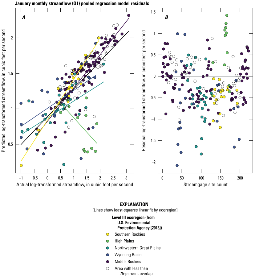
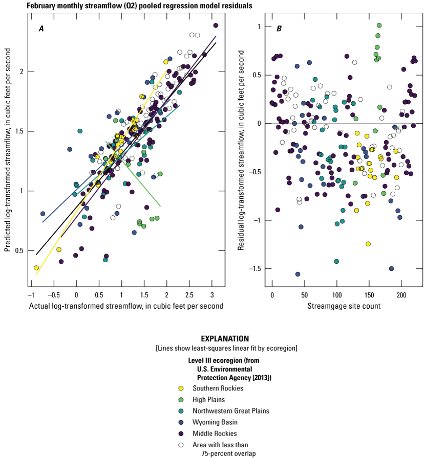
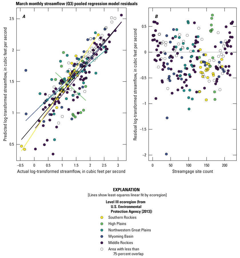
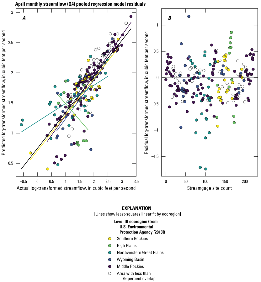
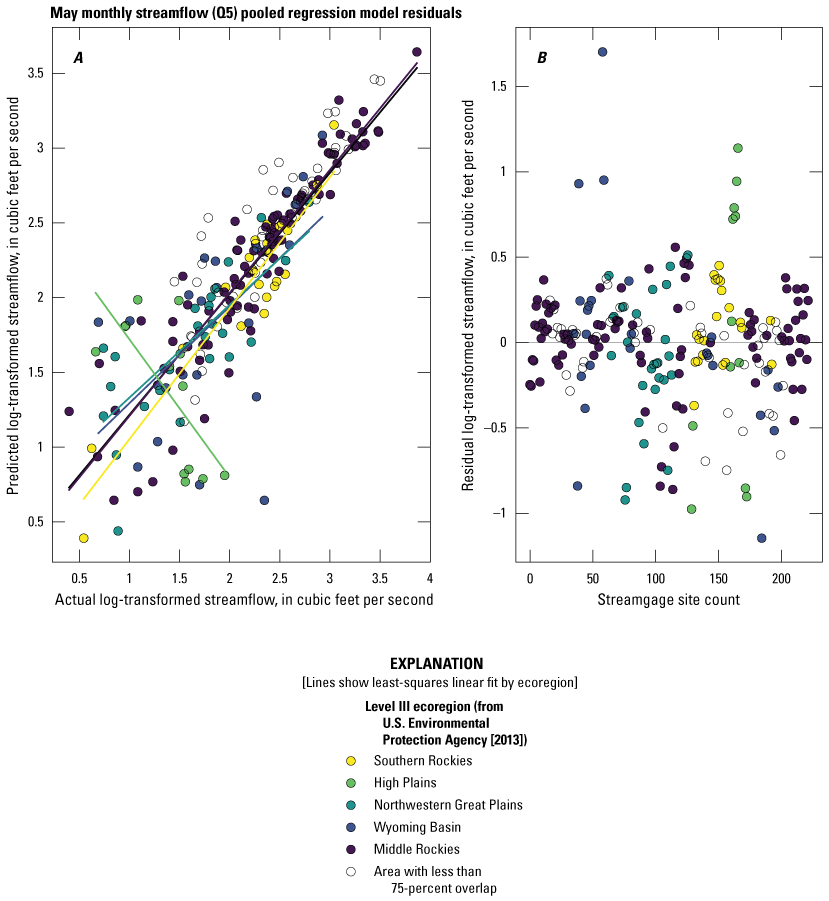
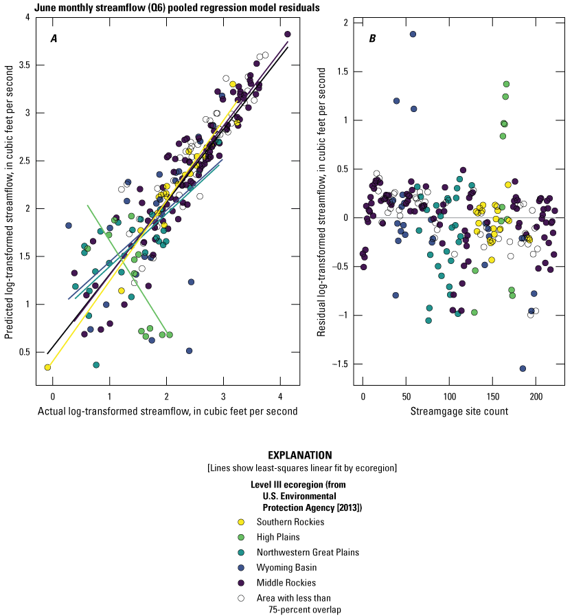
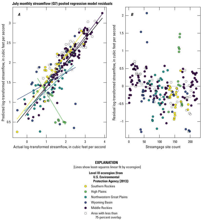
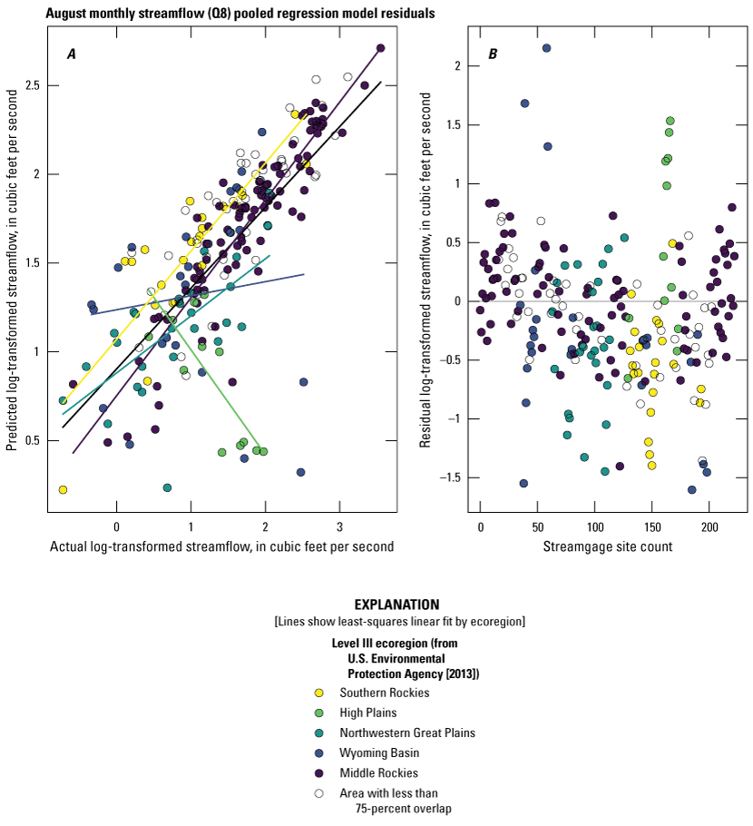
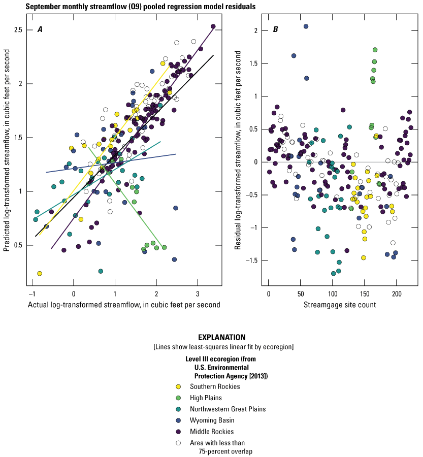
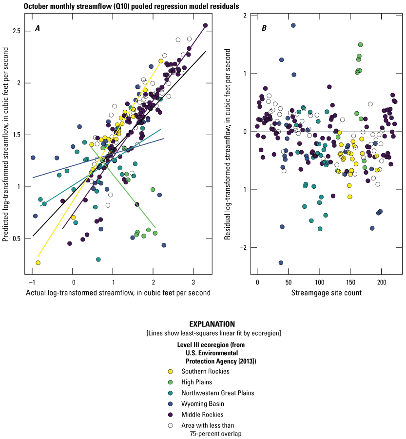
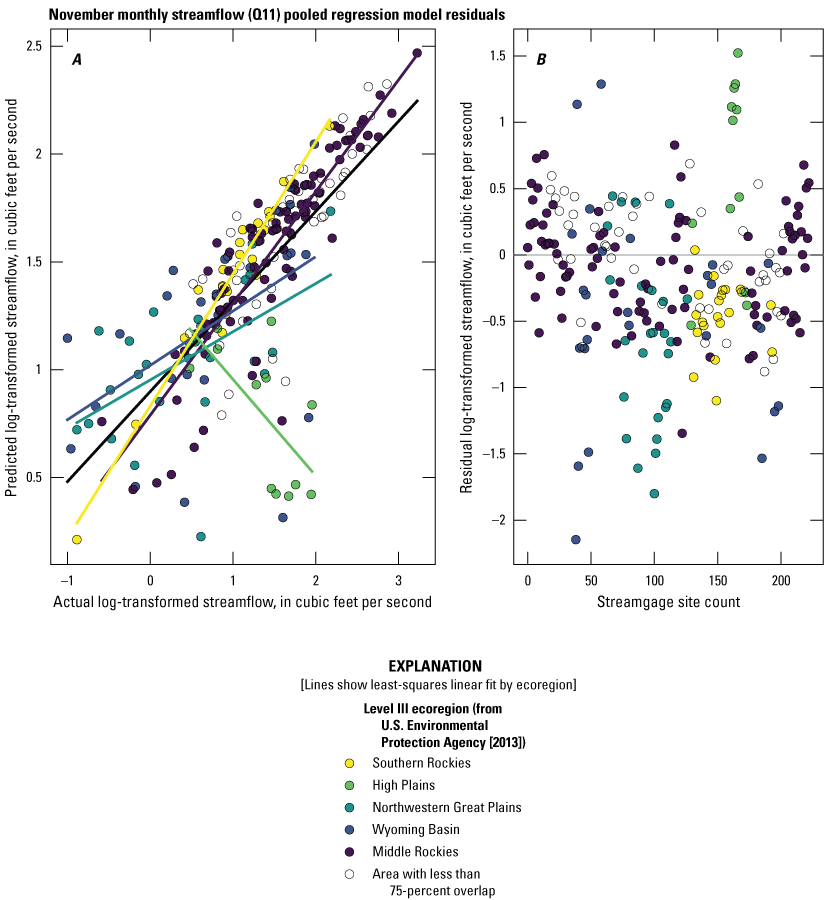
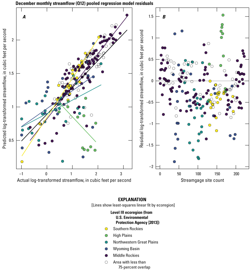
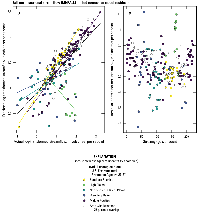
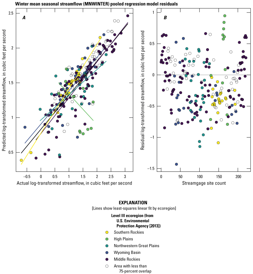
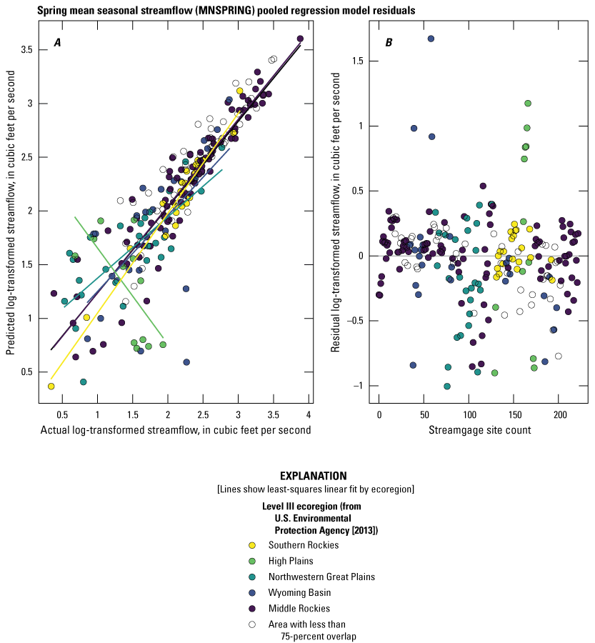
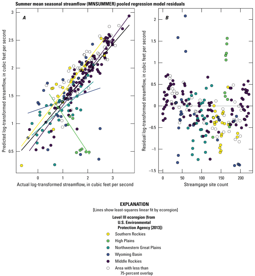
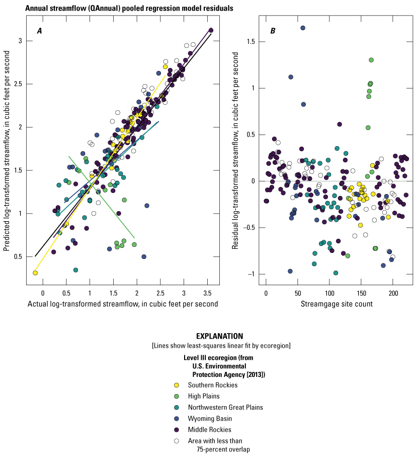
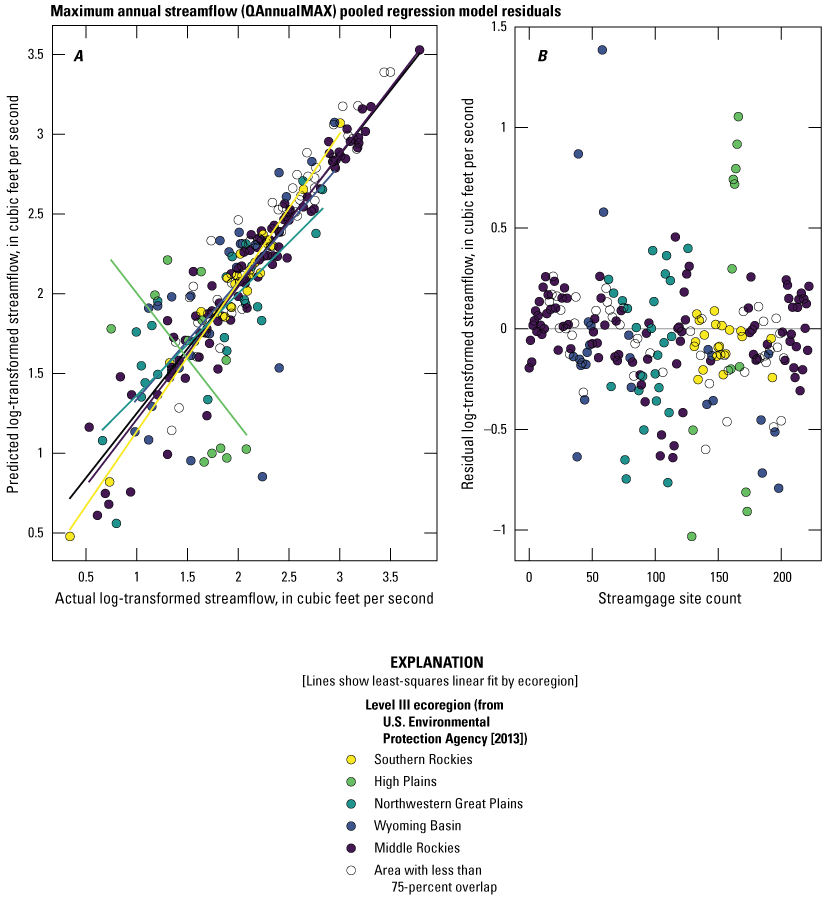
Residual plots for selected streamflow statistics from preliminary statewide regression models. The color bar signifies the level III ecoregion that overlap with streamgages’ drainage areas. Streamgages with drainage areas that do not have 75-percent or more overlap with a U.S. Environmental Protection Agency level III ecoregion do not have a color. Each plot pair consists of (A) axes depicting streamflow, in log-transformed cubic feet per second, for the measured (actual streamflow) and model-estimated (predicted streamflow) values at each streamgage, and (B) axes depicting modeled streamflow residual, in log-transformed cubic feet per second, and the streamgage site count for an arbitrary order (level III ecoregion data from U.S. Environmental Protection Agency [2013]).
Reference Cited
U.S. Environmental Protection Agency, 2013, Level III ecoregions of the continental United States: U.S. Environmental Protection Agency website, accessed April 24, 2025, at https://www.epa.gov/eco-research/level-iii-and-iv-ecoregions-continental-united-states.
Conversion Factors
U.S. customary units to International System of Units
Temperature in degrees Fahrenheit (°F) may be converted to degrees Celsius (°C) as follows:
°C = (°F – 32) / 1.8.
Datums
Vertical coordinate information is referenced to the North American Vertical Datum of 1988 (NAVD 88).
Horizontal coordinate information is referenced to the North American Datum of 1983 (NAD 83).
Elevation, as used in this report, refers to distance above the vertical datum.
Supplemental Information
A water year is the 12-month period from October 1 through September 30 of the following year and is designated by the calendar year in which it ends.
Abbreviations
EPA
U.S. Environmental Protection Agency
M7D2Y
7-day, 2-year low-flow statistic
M7D10Y
7-day, 10-year low-flow statistic
M14D5Y
14-day, 5-year low-flow statistic
M30D5Y
30-day, 5-year low-flow statistic
MSE
mean squared error
n-day
streamflow statistic describing a streamflow event over a number of days
NWIS
National Water Information System
p-value
statistical probability level
R2
coefficient of determination
USGS
U.S. Geological Survey
V1D5Y
1-day, 5-year high-flow statistic
V60D2Y
60-day, 2-year high-flow statistic
WLS
weighted least squares
For more information about this publication, contact:
Director, USGS Wyoming-Montana Water Science Center
3162 Bozeman Avenue
Helena, MT 59601
406–457–5900
For additional information, visit: https://www.usgs.gov/centers/wy-mt-water/
Publishing support provided by the
USGS Science Publishing Network,
Rolla Publishing Service Center
Disclaimers
Any use of trade, firm, or product names is for descriptive purposes only and does not imply endorsement by the U.S. Government.
Although this information product, for the most part, is in the public domain, it also may contain copyrighted materials as noted in the text. Permission to reproduce copyrighted items must be secured from the copyright owner.
Suggested Citation
Taylor, N.J., and Sando, R., 2026, Methods for estimating selected streamflow statistics at ungaged sites in Wyoming based on data through water year 2021: U.S. Geological Survey Scientific Investigations Report 2026–5120, 38 p., https://doi.org/10.3133/sir20265120.
ISSN: 2328-0328 (online)
Study Area
| Publication type | Report |
|---|---|
| Publication Subtype | USGS Numbered Series |
| Title | Methods for estimating selected streamflow statistics at ungaged sites in Wyoming based on data through water year 2021 |
| Series title | Scientific Investigations Report |
| Series number | 2026-5120 |
| DOI | 10.3133/sir20265120 |
| Publication Date | February 26, 2026 |
| Year Published | 2026 |
| Language | English |
| Publisher | U.S. Geological Survey |
| Publisher location | Reston, VA |
| Contributing office(s) | Wyoming-Montana Water Science Center |
| Description | Report: vii, 38 p.; 1 Linked Appendix Table; Data Release; Dataset |
| Country | United States |
| State | Colorado, Idaho, Montana, North Dakota, South Dakota, Utah, Wyoming |
| Online Only (Y/N) | Y |
| Additional Online Files (Y/N) | Y |