

Field Techniques for Fluorescence Measurements Targeting Dissolved Organic Matter, Hydrocarbons, and Wastewater in Environmental Waters: Principles and Guidelines for Instrument Selection, Operation and Maintenance, Quality Assurance, and Data Reporting
Links
- Document: Report (3.61 MB pdf) , HTML , XML
- Data Release: USGS data release - Comparisons from an Aqualog fluorometer standardized to quinine sulfate equivalents (QSE) with excitation (ex) and emissions (em) equivalent to fluorescence of dissolved organic Matter (fDOM) sensors from multiple manufacturers
- Download citation as: RIS | Dublin Core
Abstract
The use of field deployable fluorescence sensors by the U.S. Geological Survey has become increasingly common for a wide variety of surface water and groundwater investigations. This report addresses field deployable fluorometers that measure the fluorescence response of various substances in water exposed to incident light generated by the sensor. An introduction to the basic principles of field measurements of fluorescence is provided, as well as technical background information on sensors that target dissolved organic matter, wastewater, and hydrocarbons, including sensor selection, operating principles, key features, and design elements. General deployment, operation and maintenance protocols, quality-assurance techniques, and suggestions for data reporting are presented to facilitate and standardize the collection and accurate communication of data collected by the U.S. Geological Survey across studies, sites, and sensor types. Sensor performance issues and common interferences are also described. An appendix is included to describe sensor calibration criteria and procedures, reporting units, and specific approaches to correct for interferences for fluorescence of dissolved organic matter sensors.
Introduction
Field deployable sensors (field fluorometers) that use absorbance or fluorescence measurements to characterize constituents in water have been used for more than 50 years (Lorenzen, 1966; Vincent, 1983), but the technology is now sufficiently mature and commercially available to warrant broader application for research and monitoring. There are two main groups of field fluorometers: (1) those that measure nonphytopigment substances in the water, such as dissolved organic matter, wastewater effluent, hydrocarbons, and various other compounds that fluoresce; and (2) those that measure the fluorescence of particulates of mainly biological origin, such as chlorophyll a, phycocyanin, phycoerythrin, and other pigment-containing cells and organisms. Each type uses the same foundational principles of fluorescence and is subject to the same general interferences, but the types differ markedly with respect to how they are operated and calibrated because of the different characteristics of the respective wavelengths of the excitation-emission pairs. Fluorescence sensors that target dissolved organic matter, hydrocarbons, and wastewater applications are the focus of this document. Sensors that measure biological fluorescence are discussed elsewhere (Foster and others, 2022).
The phenomenon of fluorescence can be observed within a wide variety of substances, including organic matter. The wavelengths at which light is absorbed and re-emitted as fluorescence are determined by chemical bonds within the fluorescing material (known as fluorophores). Because these wavelengths are relatively specific, it is often possible to make concentration-related measurements of specific substances within the complex mixture of absorbing and fluorescing materials found in natural waters. This is accomplished by providing a light source at the wavelengths that correspond to characteristic absorption (excitation [ex]) and emission (em) maxima (Lakowicz, 2006; Coble and others, 2014).
Field fluorometers have been deployed by the U.S. Geological Survey (USGS) for a variety of purposes, such as providing proxy measurements to better understand (1) the transport and concentration of dissolved organic carbon (DOC; Spencer and others, 2007; Saraceno and others, 2009; Pellerin and others, 2012; Booth and others, 2020), (2) the formation of disinfection byproducts following drinking water treatment (Carpenter and others, 2013), and (3) seasonal and annual variations in mercury and methylmercury concentrations (Bergamaschi and others, 2011, 2012; Booth and others, 2020). Beyond the use of these measurements as surrogates, continuous monitoring of fluorescence establishes a “baseline” specific to a given site, with deviations from that normal range indicating changes in concentration and (or) changes in organic matter composition resulting from changes in dissolved organic matter (DOM) source mixtures (runoff, seepage, effluent discharges) or environmental processing (photodegradation, microbiological activity, algal production).
Fluorescence of dissolved organic matter (fDOM) sensors currently (2022) are commonly deployed by the USGS. The abbreviation “fDOM” is used in this report for the fluorescence that targets humic materials (Coble and others, 2014). Although the term “colored (or chromophoric) dissolved organic matter” (CDOM) has sometimes been used in the literature to describe this fluorescence, CDOM most often refers to absorbance measurements at wavelengths throughout the ultraviolet and the visible spectrum, particularly within the remote sensing community. For clarity, we recommend using the term “fDOM” for fluorescence measurements specifically from fluorescent dissolved organic matter consisting of humic substances and other compounds associated with a relatively small region of the excitation-emission matrix (EEM) near ex370 em460.
Much of the guidance given for instrument maintenance, data analysis, and quality assurance in USGS Techniques and Methods report “Guidelines and Standard Procedures for Continuous Water-Quality Monitors—Station Operation, Record Computation, and Data Reporting” (Wagner and others, 2006) is also applicable to fluorescence sensors, although they are not explicitly discussed in that publication. Our report is intended to provide additional information on differences among sensors, deployment, operation and maintenance, data analysis and reporting, and quality assurance to meet stated objectives and protocols of USGS data collection efforts.
Purpose and Scope
This report is intended to assist USGS personnel and others in collecting field-based fluorescence data that target DOM, wastewater, and hydrocarbons that are consistent and comparable across studies and sites and to ensure that data meet high-quality standards by following tested and established protocols. For those who have selected fluorometers for continuous data collection in the field, this report provides guidance on deployment, maintenance and field operations, quality-assurance procedures, and data reporting. Additionally, appendix 1 provides further guidance on fDOM sensors, such as calibration criteria and procedures, guidance on correcting for interferences, and parameter and method codes. The goal is for additional appendixes to be added over time for additional sensor types. This report supplements, but does not replace, the manufacturers’ user manuals for individual sensors.
Related Information
This report is designed to supplement other USGS documents that describe the collection and reporting of water-quality data, including the deployment and use of continuous water-quality monitors. The following list briefly summarizes related USGS policies and publications, ordered from general to specific in terms of the guidance provided:
-
• USGS Fundamental Science Practices (SurveyManual chapters 502.1, 502.2, 502.3, and 502.4).—The Fundamental Science Practices are a collection of policies for ensuring the quality and integrity of USGS science (502.1) that includes procedures for planning and conducting data collection and research (502.2), peer review (502.3), and review, approval, and release of information products (502.4) (U.S. Geological Survey, variously dated a). This report facilitates adherence to fundamental science practices by providing specific guidelines for the deployment, maintenance and field operations, quality assurance, and data reporting of fDOM data collected by optical sensors.
-
• USGS Quality Management System (QMS) Instructional Memorandum (IM-OSQI-2022-01) and Manual.—The USGS QMS (U.S. Geological Survey, 2022a) provides a foundation to ensure that laboratory activities, including instrument checks and calibrations, meet a defined standard of quality. The instructional memorandum and manual establish a set of core elements that constitute the foundation of the QMS for USGS laboratories. This report facilitates adherence to QMS by providing specific guidelines for documenting laboratory checks and calibration of nonphytopigment fluorometers.
-
• USGS National Field Manual for the Collection of Water-Quality Data.—The National Field Manual (NFM; U.S. Geological Survey, variously dated b) provides information and guidelines on preparing for sampling, selecting, and cleaning equipment, collecting and processing water samples, and taking field measurements. Chapters A1–A6 of the NFM provide important information on preparation for water sampling, selection and cleaning of sampling equipment, sample collection and processing, and methods for making ancillary field measurements that are useful for understanding the fluorescence sensor results, such as those for temperature, dissolved oxygen, specific electrical conductance, pH, and turbidity. Chapter A7 includes guidelines for the determination of biological indicators, including biochemical oxygen demand, fecal indicator bacteria, fecal indicator viruses, protozoan pathogens, algal biomass indicators, cyanotoxins, and taste and odor compounds in surface waters. All chapters are updated as needed. Personnel who use fluorescence sensors in USGS studies can benefit from a solid understanding of the guidelines provided in these chapters. Much of the information in the NFM is directly applicable to deploying fluorescence sensors and collecting the metadata needed for interpreting the results.
-
• “Guidelines and Standard Procedures for Continuous Water-Quality Monitors: Station Operation, Record Computation, and Data Reporting”.—Techniques and Methods 1–D3 (TM1–D3; Wagner and others, 2006) provides basic guidelines and procedures for use by USGS personnel for site and water-quality monitor selection, installation, field procedures, calibration of continuous water-quality monitors, record computation and review, and data reporting. Although the use of fluorescence sensors requires specific guidelines beyond those provided in TM1–D3, the general workflow for their use is similar to the workflow described for the other sensors in TM1–D3. The terminology and processes described in TM1–D3 thus form the general background for these guidelines for the use of fluorescence sensors.
-
• “Optical Techniques for the Determination of Nitrate in Environmental Waters: Guidelines for Instrument Selection, Operation, Deployment, Maintenance, Quality Assurance, and Data Reporting”.—Techniques and Methods 1–D5 (TM1–D5; Pellerin and others, 2013) provides information about the selection and use of ultraviolet (UV) nitrate sensors deployed by the USGS to facilitate the collection of high-quality data across studies, sites, and instrument types. Although the focus of TM1–D5 is UV nitrate sensors, many of the principles can be applied to other optical sensors for water-quality studies.
-
• “Field Techniques for the Determination of Algal Pigment Fluorescence in Environmental Waters—Principles and Guidelines for Instrument and Sensor Selection, Operation, Quality Assurance, and Data Reporting”.—Techniques and Methods 1–D10 (TM1–D10; Foster and others, 2022) provides information about selection and use of algal fluorescence sensors by the USGS to facilitate the collection of high-quality data across studies, sites, and instrument types. Although the focus of TM1–D10 is algal fluorescence sensors, many of the principles can be applied to other fluorescence sensors for water-quality studies.
-
• Office of Water Quality Technical Memorandum 2017.7 on procedures for processing, approving, publishing, and auditing time-series records for water data.—USGS Technical Memorandum 2017.7 defines the procedural steps required for processing, approving, publishing, and auditing water-quality time-series data collected in support of USGS activities (U.S. Geological Survey, 2017). These procedures revise workflow terminology for consistency, establish formal audit procedures, and improve the efficiency of the records processing and approval workflow by explicitly outlining the steps required to analyze, approve, and audit time-series records for all data types, including data from fluorescence sensors.
-
• Office of Water Quality Technical Memorandum 2016.10 on policy and guidance for approval of surrogate regression models for computation of time-series suspended-sediment concentrations and loads.—Surrogate measure is defined as a measurement made with the intent to gain insight into a variable that is either impractical to measure directly or is not possible to measure at the desired continuous time interval (U.S. Geological Survey, 2016). This technical memorandum describes reliable methods to develop statistical models specifically for suspended-sediment concentrations and loads based on surrogate measurements. Although the memorandum specifically applies to suspended sediment, the guidance provided on the number and type of samples and model development, documentation, and validation is useful when considering the development of surrogate models for other water-quality constituents, including those that may be based on fluorescence sensor data (such as DOC).
Future USGS policy updates or changes should be sought out before beginning new data collection efforts in order to ensure that the references used are up to date and that all current policies are being followed.
Background
Effective selection, deployment, and operation of deployable field sensors—particularly optical instrumentation—require a general understanding of the underlying principles of the measurements, and their applications, benefits, and limitations in water monitoring and research programs.
Principles of Fluorescence
Fluorescence occurs when an electron is in an excited state and absorbs light, then emits light as the electron returns to its former state. This emission of light can then be measured by a fluorometer. The intensity of emitted light as measured by a fluorometer in a water medium is directly proportional to the concentration of the constituent, according to the Beer-Lambert law (Lakowicz, 2006). The transmission of light through water is determined by the physical and chemical properties of the constituents in the water sample (fig. 1). Scattering is a process whereby light energy passing through the water column is redirected in multiple directions, primarily by particles. Scattering forms the basis for measurements such as turbidity, which will only be discussed in this report in the context of interferences. Absorption is a process by which light energy is converted into nonradiant energy by exciting an electron in a substance dissolved or suspended in the water column, such as DOM, from the ground state to an excited state. Absorption of light (attenuation) by particles or by solutes (commonly DOM) can occur, and either can be the dominant effect. Absorbed energy is subsequently released through multiple competing pathways that include thermal pathways, such as vibrational relaxation and nonradiative decay, and the near instantaneous release of light energy in the form of fluorescence. Fluoresced light is always re-emitted with less energy and therefore at longer wavelengths than the original light that was absorbed, a phenomenon known as the Stokes shift (fig. 2) (Stokes, 1852). For more detail on the chemistry and physics of fluorescence and absorbance, numerous reviews include those by Lakowicz (2006) and Coble and others (2014).
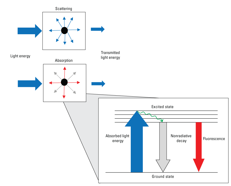
Conceptual diagram of light scattering and absorption by particles or dissolved constituents in water. The inset Jablonski diagram shows how a fluorophore such as dissolved organic matter absorbs ultraviolet light (blue arrow) and releases energy as fluorescence at longer wavelengths (red arrow) and nonradiative decay (gray arrow).
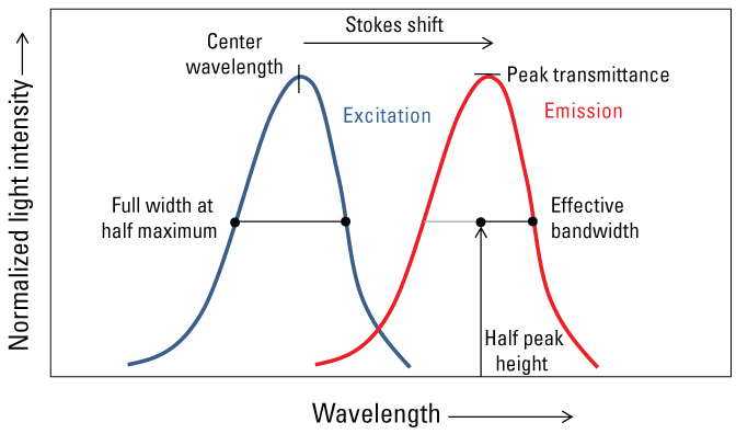
Conceptual graph showing light excitation emission wave properties of a theoretical substance.
The overall mixture of substances dissolved in water determines the fluorescent response of excitation-emission pairs across the UV and visible spectra, and this information is used to generate three-dimensional EEM plots (fig. 3). DOM, hydrocarbons, wastewater indicators such as optical brighteners, and even some dyes (that is, fluorescein) all fluoresce in the shorter wavelengths (excitation 240–500 nanometers [nm] and emission 250–600 nm). Because this document focuses on sensors that target these substances, the figures presented henceforth focus on the area defined by these wavelength ranges (fig. 3). Notably, commonly used red dyes, such as rhodamine, do not fluoresce within this region of focus.
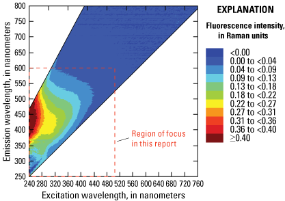
Three-dimensional excitation-emission (EEM) matrix of a typical river water sample measured on the Aqualog (Horiba Scientific, New Jersey). <, less than; ≥, greater than or equal to. Figure is for illustrative purposes only.
Application of Fluorescence Spectrometry to Water-Quality Studies
The ability of a fluorophore to convert absorbed light into fluorescence depends on the molecular structure of the dissolved substances in the water, including the composition of the dissolved fraction of the natural organic matter (Aiken, 2014). The resulting fluorescence EEM for a water sample represents the complex mixture of fluorophores within the water, representing the origin and processing of the dissolved organic materials (Hansen and others, 2016, 2018). These regions of the EEMs are commonly denoted by letters referred to as fluorescence “peaks” within the fluorescence literature, as shown in figure 4. The characteristics of the identified EEM regions are described in table 1 and expressed in Raman-normalized intensity units (RU; Murphy and others, 2010).
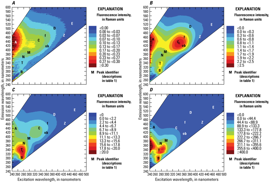
Example excitation-emission matrix (EEM) plots showing the intensity of fluorescence at different excitation-emission wavelengths for, A, typical river water, B, wastewater effluent, C, plant leachates/extracts, and D, “produced water” from an oil and gas field. Note difference in color scales. Fluorescence peak identifiers, denoted by letters in the graph areas, are defined in table 1. <, less than; ≥, greater than or equal to. Figure is for illustrative purposes only.
Table 1.
Description of fluorescence peaks.[CDOM, colored dissolved organic matter; fDOM, fluorescence of dissolved organic matter; max, maximum]
| Peak identification | Description | Excitation max (nanometers) |
Emission max (nanometers) |
Reference |
|---|---|---|---|---|
| A | Humic like | 260 | 400–460 | Coble (2007) |
| B | Tyrosine-like fluorescence. Derived from phytoplankton and (or) microbial processes | 275 | 305 | Coble (2007) |
| C | Humic like | 340 (320–360) | 440 (420–460) | Coble (2007) |
| D | Soil fulvic acid | 390 | 509 | Stedmon and others (2003) |
| E | Soil fulvic acid | 455 | 521 | Stedmon and others (2003) |
| f | Humic like, area of overlap among sensors named fDOM and CDOM | 370 | 460 | Hansen and others (2018) |
| M | Marine humic like | 290–310 | 370–410 | Coble (2007) |
| N | Associated with phytoplankton productivity | 280 | 370 | Stedmon and others (2003) |
| ob | Optical brighteners, fluorescent whitening agents | 360 (340–380) | 420 (400–460) | -- |
| T | Tryptophan-like fluorescence. Derived from autochthonous processes | 275 | 340 | Coble (2007) |
| Z | Photosensitive | 420 | 460 | Fleck and others (2014) |
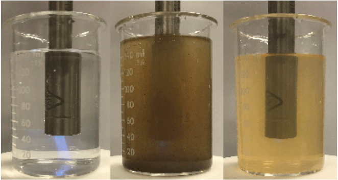
Attenuation of fluorescence (blue light) in a quinine sulfate solution (left) in the presence of colored dissolved organic matter (center) and suspended particles (right). Photograph by J. Rosen, U.S. Geological Survey.
Factors Affecting Fluorescence Measurements
Several physical and chemical properties of water and its environment can affect fluorescence measurements. Several properties of water that affect how much light and what wavelengths of light are able to pass through from the source to detector, such as suspended particles and absorbing substances like DOM, interfere with the fluorescence measurement because of “matrix effects” (figs. 5 and 6). Interferences from matrix effects are correctable as long as the signal-to-noise ratio remains sufficiently high to meet the sensitivity requirements for the site’s conditions. Other water properties, such as temperature, pH, and the presence of some dissolved metals, can quench fluorescence at the molecular level. Quenching from temperature effects is correctable, whereas the effects of pH and various metals are either not correctable or have not been sufficiently tested to determine whether corrections may be possible. The collective extent of these effects can reduce fluorescence measurements from a few percent to over 90 percent in the most extreme cases, but the loss of signal in most systems will typically be less than 20 percent (Downing and others, 2012). Further descriptions of these factors are provided next.
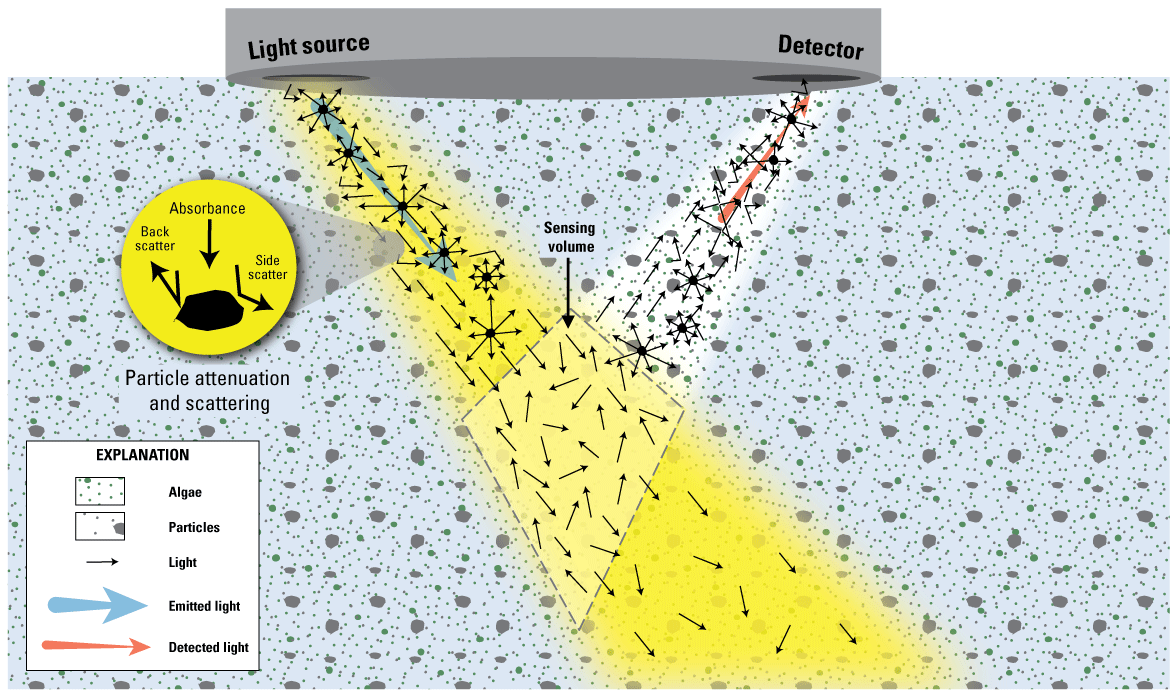
Effects of scattering and absorbance on emitted light in natural waters.
Interferences
The most common sources of interference are the scattering of light by particles, or turbidity, and the attenuation of light by particles and absorption caused by dissolved substances, most commonly from DOM (figs. 5 and 6). Scattering of the source excitation light by particles in the optical path of the sensor redirects light outside the measurement area, reducing the amount of excitation energy that reaches fluorescent materials within the sampling volume, and thus lowering corresponding fluorescent emissions. Furthermore, the emitted fluoresced light is scattered out of the light path from the sampling volume to the detector, lowering the amount of light measured by the detector. Particle attenuation (absorption of light by particles) and absorption of light by solutes (most commonly DOM) have the same overall effect, with the excitation energy from the instrument light source and the fluorescence emission both lowered. Ultimately, at high suspended sediment concentrations (often measured as turbidity) or at high concentrations of DOM, the instrument signal-to-noise ratio decreases until the sensor cannot measure changes in the concentration of the target analyte.
The effects of particles and DOM concentration on field fluorescence measurements can be substantial and vary among instrument types. Corrections based on concurrent measurements of turbidity and approximations of the concentrations of interfering absorbing solutes are often required (Downing and others, 2012), and these corrections may be site specific (Saraceno and others, 2017). Design differences among manufacturers or among instruments from a single manufacturer typically require that sensor-specific data corrections be made. Beyond a certain range of matrix interferences, however, corrections are not possible because insufficient light is available to make the measurement, and the affected data should not be published. Strategies for reducing matrix effects may be necessary in many environments. For example, it is possible to physically filter out particles prior to collecting field fluorescence measurements, but the added complexity (for example, power and infrastructural requirements) and costs (incurred from filter replacements and associated site visits) make this approach impractical in many settings.
Other potential interferences, such as air bubbles and stray light, can have a substantial effect on optical measurements. Because these interferences are not properties of the water matrix but instead are derived from variable and inconsistent sources like turbulence and sunlight reflection and refraction, they are typically not correctable after collection. These interferences are usually addressed by means of solutions such as wipers, stray light filters, tandem measurement with internal stray light detectors for “blank correcting,” and (or) simple shade caps. Often, with these features used, simply orienting the sensors in a manner that reduces stray light and protects the sensor faces (and effective sampling volumes) from exposure to bubbles can be most effective in addressing these interferences.
Fluorescence Quenching
Several environmental and chemical variables affect fluorescence yield because they affect the capacity or the pathways of the target molecules within the sampling volume to dissipate energy internally without fluorescing. The most common form of quenching is related to water temperature. Temperature is inversely related to fluorescence because of the higher vibrational energy and increased collisions of molecules at higher temperatures, which affords a more facile path for energy loss than via fluorescence. Quenching caused by temperature follows the laws of physics and thus is amenable to empirically derived corrections to a reference temperature, typically averaging 1 percent loss of signal per increase of 1 degree Celsius (°C) (Henderson and others, 2009; Watras and others, 2011; Downing and others, 2012). For standardization across the USGS, the reference temperature proposed for fluorescence measurements is 25 °C, to align with standardization to standard temperature and pressure as is done with specific conductance (U.S. Geological Survey, 2019). Most fluorometers designed for field use have either an internal thermistor or a reference temperature sensor that can be integrated into the monitor so that measurements can be compensated for temperature effects on electronics. This temperature correction, commonly applied within the manufacturer’s software, should not be confused with the correction required to address temperature effects on the fluorescence itself. Fluorescence measurements generally are not internally compensated for temperature effects on the target analyte. Those corrections are applied by the user as a postprocessing step, as described in appendix 1 for fDOM.
Changes in pH may also cause fluorescence quenching because pH changes can alter the electron density associated with the fluorophore and thus affect the intensity and wavelength of fluorescent emissions. The effect is typically small over pH values ranging from 6 to 8 (Aiken, 2014), a span that encompasses a large proportion of natural waters for most of the time. However, the effects on fluorescence measurements in waters with pH below 6 and above 8 are highly variable and not particularly amenable to correction, at least with the current body of evidence and extent of data review. Therefore, in areas or time periods where the pH falls below 6 or rises above 8, additional scrutiny of the data is warranted. The collection of pH time-series data may assist in determining the reliability of the data. Further evaluation of pH effects on fluorescence measurements would benefit measurements in waters with extreme pH ranges.
Quenching can also occur in natural waters with elevated concentrations of metals such as iron, aluminum, and copper, which can form complexes with organic compounds, affecting the molecular structure and electron state (Weishaar and others, 2003; Poulin and others, 2014). The concentration and speciation of these metals and their complexes can facilitate the dissipation of light energy, allowing it to be transferred via other pathways in lieu of fluorescence. Similar to pH, the effects of metals on fluorescence yield are highly variable and not amenable to correction of data collected by field sensors. Although guidance is currently not available on the specific metal concentrations affecting quenching of field fluorometers, users should be aware of the potential issue and the potential for additional investigation if quenching is suspected.
Sensor and Monitor Selection
The overall design of commercial fluorometers is generally similar among manufacturers and includes features for physical configuration, optics, and data processing; however, the physical configuration may affect the instrument’s range and resolution, and its tolerance for interferences. Although several commercially available field fluorometers may meet the necessary specifications (for example, detection limit, dynamic range, resolution, and accuracy) for most freshwater and coastal applications, several factors are worth considering when selecting a sensor. A clear understanding of differences in the physical configuration and data output specifications will facilitate choosing the appropriate fluorometer for different aquatic environments and applications.
Field deployable fluorometers generally work as follows: a light-emitting diode (LED) is used to generate a nearly uniform beam of light at a given range of wavelengths determined by the excitation bandpass filter. The light passes through a water sample of known dimensions and volume that is internal or external to the sensor body. A photodetector measures the light emitted from any fluorophores that may be present in the sample at designated wavelengths. Unwanted wavelengths are filtered out by the emission bandpass filter at nearly the same time, as the process of fluorescence is nearly instantaneous (10−12 to 10−6 seconds) (Itagaki, 2000). After filtering of the electronic signal and, in some cases, integrated processing to remove interferences, fluorescence is measured in volts or counts and is transmitted to a data collection platform in analog or digital format (for example, RS–232, SDI–12, or RS–485). The collected data can then be converted to other fluorescence or concentration units on the basis of manufacturer or user-defined scaling factors. It is often recommended to use the calibration standard in the reporting units. fDOM data are recommended to be reported in micrograms per liter as quinine sulfate equivalents (QSE) because that is the recommended calibration standard.
The physical components of field and laboratory fluorometers are essentially the same and include a light source, optical interference filters, and a photodetector; however, a few important physical modifications were necessary when laboratory instruments were miniaturized and adapted for field deployments. For field fluorometers, a single measurement is reported per sensor. Field fluorometers typically use low-power LEDs as a light source instead of high-intensity xenon or mercury lamps to limit power consumption and (or) demand and to decrease sensor size. Field fluorometers also do not have an excitation monochromator, which is used in benchtop fluorometers to scan across a range of excitation and emission wavelengths. The result is that a sensor may either be specific to a small region of the EEM or may group the fluorescence response over a wide range of excitation-emission pairs to increase signal. These and other modifications, including ruggedized housings and components, efficient power and heat handling, and antifouling components, not only affect the ability to make accurate fluorescence measurements in the field, but also affect the serviceability, longevity, stability, and cost of field fluorometers.
Fluorometric instruments of different designs commonly do not yield identical or equivalent outputs in environmental waters. Different makes and models of sensors having the same units and calibrated with the same standards may not yield identical or equivalent results in environmental water, particularly if there is variation in the excitation and emission bandpass filters.
Wavelength Array
The excitation and emission bandpass filters define what fluorophores a sensor targets within the full array of excitation and emission wavelengths. For the purpose of this discussion, the range of wavelengths for a particular sensor is defined as the wavelength array. Manufacturers have developed a variety of sensors for specific applications, often balancing the importance of low detection limit with the need for specificity of fluorophores. For example, many sensors used in the ocean sciences often have large wavelength arrays to increase the fluorescence signal to lower detection limits, whereas sensors used for estuarine to riverine studies often have sufficient fluorescence to target specific fluorophore regions of the full excitation-emission array. Choosing the proper sensor for the intended application is critical to successful measurement in the field. The general “families” of sensors are summarized next. It is important to note that manufacturer specifications are often reported using different conventions and that specifications of bandpass and (or) filters may not reflect the actual range of effective excitation wavelengths. To ensure the most precise estimate of a sensor’s wavelength array, it is recommended that the user confirms the actual effective wavelength array with the manufacturers’ engineers or product managers.
Humic DOM Sensors
In the field fluorometer vernacular, fDOM (sometimes also written as FDOM or fdom) has most commonly been associated with a relatively small region of the EEM spectra near excitation 370 emission 460, which is most closely related to terrestrial, humic-like organic matter (McKnight and others, 2001;Stedmon and others, 2003;Coble and others, 2014). However, this region is not always the convention used across manufacturers for the reasons mentioned earlier, despite the similar use of the term “fDOM” or “CDOM” as a sensor name. Therefore, we recommend the adoption of a new naming convention that captures more specific information with respect to the region of the fluorescence spectra where the field fluorometers collect their measurements. For the greatest clarity and consistency, the parameter name will include the wavelength array described as the full-width half-maximum range of the excitation-emission channels. For example, the YSI EXO fDOM sensor is commonly used throughout the USGS community and the parameter name is “Fluorescence, water, in situ, excitation 360–370, emission 440–520, micrograms per liter as quinine sulfate equivalents (QSE).”
For data to be comparable, the same wavelength array must be used. To illustrate the variability, a laboratory benchtop instrument (an Aqualog 800) was used to compare the various wavelength arrays used by various field fluorometers in two standard reference materials (SRMs) and 76 environmental samples (collected from multiples States, including Pennsylvania, Colorado, Texas, California, Florida, and Iowa). Comparing the different wavelength arrays using the Aqualog 800 allowed the comparisons to be made with the potential interferences removed (Fleck and others, 2022). The first SRM was the International Humic Substances Society 2R101N equivalent to 4.0 milligrams per liter (mg/L). The second SRM was Pure Leaf brand unsweetened black tea diluted to 1 percent concentration (Hansen and others, 2018). The Aqualog 800 readings are reported in RU and then converted to QSE (Fleck and others, 2022). The International Humic Substances Society 2R101N, equivalent to 4.0 mg/L, was analyzed 15 times on the Aqualog 800 for each wavelength array, and the equivalent field fluorometer outputs ranged from 26.1 to 82.3 QSE. The tea SRM was analyzed 47 times on the Aqualog 800, and readings for the different wavelength arrays ranged from 4.2 to 8 QSE.
Additionally, the Aqualog 800 took readings of the 76 environmental samples using the equivalent wavelength arrays from field fluorometers and the output values for some arrays were more than double the output values for other arrays, illustrating the potential differences among sensor outputs (table 2).
Table 2.
Comparisons from an Aqualog 800 standardized to quinine sulfate equivalents (QSE) with excitation (ex) and emissions (em) equivalent to fluorescence of dissolved organic matter (fDOM) sensors from multiple manufacturers.[Data summarized from Fleck and others (2022). Data are provided for two standard reference materials (SRMs) and the mean, minimum, and maximum from 76 environmental samples. No replicates were collected for environmental samples; therefore, the relative standard deviation is not available. IHSS, International Humic Substances Society; mg/L, milligram per liter; DOC, dissolved organic carbon; N, sample size; %, percent; CDOM, colored dissolved organic matter]
| Equivalent wavelength arrays set on the Aqualog 800 to simulate the wavelength arrays from various field fluorometers (equivalent sensor name in parentheses) | Aqualog 800 mean value in QSE, IHSS 2R101N equivalent to 4.0 mg/L DOC; N=14 |
Relative standard deviation (percent) |
Aqualog 800, mean value in QSE, tea SRM (Hansen and others, 2018); N=51 |
Relative standard deviation (percent) |
Aqualog 800 value in QSE, environmental samples; N=76 |
||
|---|---|---|---|---|---|---|---|
| Mean | Minimum | Maximum | |||||
| Fluorescence, field, excitation 360–370 and emission 440–520 (YSI EXO fDOM) | 48.4 | 4.86 | 5.7 | 4.36 | 56.2 | 5.4 | 369.3 |
| Fluorescence, field, excitation 355–375 and emission 440–500 (Turner Designs CDOM) | 45.5 | 4.87 | 5.6 | 4.34 | 54 | 5.3 | 351.1 |
| Fluorescence, field, excitation 365–375 and emission 400–520 (Sea-Bird/Wetlabs fDOM/CDOM) | 55.6 | 4.87 | 6.3 | 4.97 | 71.3 | 7.2 | 446.7 |
| Fluorescence, field, excitation 360–390 and emission 455–530 (in situ fDOM) | 182.4 | 5.24 | 18.1 | 5.05 | 195.5 | 19.1 | 1632 |
| Fluorescence, field, excitation 364–376 and emission 420–460 (Seapoint CDOM) | 45.8 | 4.82 | 5.6 | 5.10 | 64.2 | 6.6 | 385.5 |
| Fluorescence, field, excitation 240–270 and emission 422–478 (Chelsea Technologies Group CDOM) | 226.3 | 4.55 | 24.3 | 5.53 | 234.8 | 23.7 | 2259.2 |
Different manufacturers use a wide range of wavelength arrays under the fDOM and CDOM sensor names, but all measure various portions of the humic regions of the EEM spectra (fig. 7). The various arrays reflect the intended marketable application for each sensor rather than any physically or chemically based naming convention. Most manufacturers target the “peak C” region of fluorescence, while at least one specifically targets the “peak A” region (table 1, fig. 4). The relative contribution of different humic substances to the overall fluorescence of DOM can vary among locations and seasons, depending on the environmental setting. This variability contributes to variation among measurements performed by the different sensors, despite the sensors having a common name. The C:A ratio has even been used as an indicator of DOM composition and source tracing (table 3; Moran and others, 2000; Hansen and others, 2016), highlighting the need to specify wavelength arrays rather than using the sensor name in the parameter name. When selecting a sensor for deployment, consideration should be given to the location and specificity of the wavelength arrays and their relation to the project objectives.

Comparison of various commercially available wavelength arrays within the laboratory-measured excitation-emission matrix for an environmental water sample having a high concentration of dissolved organic carbon. The box outlines for the various sensor arrays are close approximations overlain on the laboratory-based matrix of a sample from the Sacramento River for the purpose of illustration. <, less than; ≥, greater than or equal to.
Table 3.
Commonly used excitation-emission matrix (EEM) ratios for dissolved organic matter characterization.[ex, excitation; em, emission; DOM, dissolved organic matter; nm, nanometer; >, greater than]
| Peak ratio | Calculation | Purpose | Reference |
|---|---|---|---|
| A:T | The ratio of peak A (ex260em450) to peak T (ex275em340) intensity | An indication of the amount of humic-like (recalcitrant) versus fresh-like (labile) fluorescence in a sample | Hansen and others (2016, 2018) |
| C:A | The ratio of peak C (ex340em440) to peak A (ex260em450) intensity | An indication of the relative amount of photosensitive humic-like DOM fluorescence in a sample | Moran and others (2000); Hansen and others (2016) |
| C:M | The ratio of peak C (ex340em440) to peak M (ex300em390) intensity | An indication of the amount of diagenetically altered (blue shifted) fluorescence in a sample | Coble (1996); Burdige and others (2004); Para and others (2010); Helms and others (2013) |
| C:T | The ratio of peak C (ex340em440) to peak T (ex275em340) intensity | An indication of the amount of humic-like (recalcitrant) versus fresh-like (labile) fluorescence in a sample | Baker and others (2008) |
| Fluorescence index (FI) | The ratio of fluorescence intensity at em wavelengths at 470 nm and 520 nm, obtained at ex 370 nm | Shown to identify the relative contribution of terrestrial and microbial sources to the DOM pool | McKnight and others (2001); Cory and others (2010) |
| Humification index (HIX) | The sum of fluorescence intensities from em wavelengths 435–480 nm divided by the sum of fluorescence intensities from em wavelengths 300–345nm and 435–480 nm obtained at ex 254 nm | An indicator of humic substance content or extent of humification. Higher values indicate an increasing degree of humification. | Ohno (2002) |
| Freshness index (b:a) | The fluorescence intensity at em 380 nm divided by the maximum fluorescence intensity between em 420 nm and 435 nm, obtained at ex 310 nm | An indicator of recently produced DOM, with higher values representing a higher proportion of fresh DOM | Parlanti and others (2000); Wilson and Xenopoulos (2009) |
| Biological index (BIX) | The ratio of fluorescence intensity at em 380 nm and 430 nm, obtained at ex 310 nm | An indicator of autotrophic productivity. High values (>1) correspond to recently produced DOM of autochthonous origin. | Huguet and others (2009) |
Wastewater Sensors
Wastewater sensors typically target contributions from publicly owned treatment work effluents and (or) septic discharges and leaks rather than industrial wastewater effluents (addressed in the following section). These sensors typically target fluorescence of microbial byproducts that fluoresce near the T and B peaks (fig. 4) of the fluorescence spectra (excitation near 275 nm, emission 300–350 nm) or with the fluorescence associated with optical brighteners (for example, fluorescent whitening agents) commonly used in laundry detergents and the textile and paper/pulp industries (excitation 340–380 nm, emission 400–480 nm) (fig. 8).
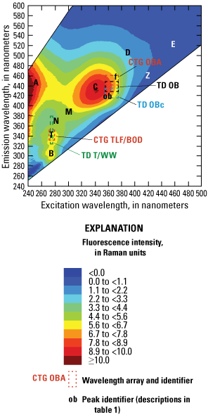
Examples of some commercially available wavelength arrays intended to measure the presence of wastewater overlain on the laboratory-measured excitation-emission matrix of a wastewater effluent sample. The box outlines for the various sensor arrays are close approximations overlain on the laboratory-based matrix for the purpose of illustration. <, less than; ≥, greater than or equal to.
Hydrocarbon Sensors
The hydrocarbon class of sensors typically target industrial effluents including hydrocarbons, oil spills, and solvents. The sensors used for petroleum and its various byproducts often use large wavelength arrays because they are typically used as a screening tool for spills and plume characterization and thus need a wide response range to detect a wide range of substances (fig. 9). With the expansion of hydraulic fracturing and more widespread use of hydraulic fluids in oil and gas exploration and recovery, more specific sensors are likely to be developed to discriminate sources and specific contaminants.
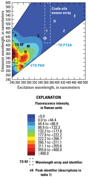
Examples of some commercially available wavelength arrays intended to measure the presence of crude oil and refined fuels overlain on the laboratory-measured excitation-emission matrix of water from an oil and gas production area. The box outlines for the various sensor arrays are close approximations overlain on the laboratory-based matrix for the purpose of illustration. <, less than; ≥, greater than or equal to.
Configuration
The overall design of commercial fluorometers generally follows one of two physical configurations. The first is an open-face design in which optical windows are located on the outside of the sensor body, and fluorescence is measured in a sample volume external to the sensor housing. The second is a flow-through design, which uses a quartz tube within the sensor body to measure a fixed sample volume as it passes through the sensor (fig. 10). The optical windows of the open-face sensors protect the light source and photodetector elements and are made from materials (typically sapphire) that minimize abrasion and degradation of the sensing windows. Most sensors used for freshwater monitoring are of the open-face design, which allows for easy integration into existing monitors and the incorporation of wipers to reduce biofouling. Flow-through systems are a good option when water filtration is desired, boat-based measurements are made, or other pumped-water operations are necessary.
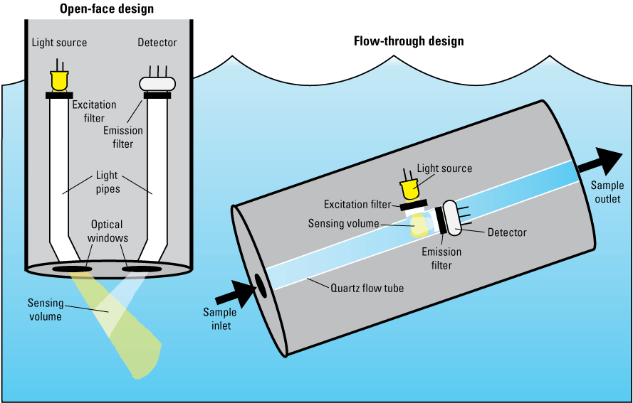
General configuration of open-face (left) and flow-through (right) fluorometer designs.
For open-face sensors, the angle at which the excitation light source and the emission detector are placed relative to each other (typically 90–140 degrees) determines the sensing volume, which is the geometrically defined volume where the excitation light beam intersects with the detector’s cone of reception (fig. 10). For closed sensors, the path length is defined by the geometry of the unit. As the acceptance angle or source beam cone increases, the length of the sensing volume shortens and attenuation along the sample path decreases.
Field fluorometers can be configured as a single fluorescence sensor, with multiple fluorescence sensors within a single housing, or as part of a sonde that contains a variety of sensor types. All field fluorometers are equipped with an electronic signal processor that converts the raw voltage from a photodetector to a useful measurement output. Instruments can use a system of analog and digital electronic circuits, or a specialized microcontroller known as a digital signal processor to detect, convert, and output signals at very high internal sample frequencies, which are then integrated to output high-frequency data (from 1 to 20 hertz) via an analog or digital (RS–232) signal output. A microcontroller also controls the modulation of the LED so that the system can detect and differentiate between fluorophores and background noise (for example, photodetector dark current).
Multisensor Monitors
Some multisensor monitors allow for the simultaneous deployment of multiple sensors, allowing for simultaneous measurements to be made in different regions of the EEM to better isolate specific substances from a general increase in fluorophore concentration across the EEM spectra (table 2). If the desired application benefits from fluorophore specificity and ratios among those fluorophore regions (table 3), it may be best to select a monitor that is capable of multiple sensor deployment. The codeployment of turbidity and temperature sensors is also required in many applications. If the sensor is not correcting for variations in temperature on the fluorescence itself, a temperature sensor must be deployed. If independent testing has not been conducted to verify that the fluorescence signal is temperature compensated internally, an independent temperature sensor should be deployed with the fluorescence sensor as a best practice until temperature compensation can be evaluated. If particle interference alters sensor readings by more than or equal to the calibration criteria (fDOM calibration criteria listed in appendix 1), then the deployment of a turbidity sensor is required. Multisensor monitors capable of integrating temperature and turbidity with fluorometers within the same monitor may perform better than units where turbidity is measured meters away from the fluorometers, as turbidity can differ substantially within a site at that scale. It should be noted that independent optical sensors located too close to one another can interfere with optical sensor measurements.
Materials
Component materials for the instrument and sensor body differ among manufacturers and among different models from the same manufacturer, depending on applications like fresh to saline waters and various depth ratings. Instrument housings can be made from a variety of materials (for example, acetal resin, 316L stainless steel, polyoxymethylene, or titanium) that affect their resistance to corrosion and fouling, as well as their pressure and temperature rating.
Spectral filters are made of glass or other materials that filter out unwanted wavelengths from the light source and from the emitted light returning to the detector. Bandpass filters used in most field fluorometers are commonly described by the wavelength with peak transmittance, the center wavelength (the average of two half-height wavelengths in a spectrum), and the full width at half maximum (the wavelength range at half of the maximum transmittance) (fig. 2).
The stability, lifetime, and quantum yield of LEDs vary by wavelength (λ), and LEDs exciting at wavelengths used for nonphytopigments (λ approximately 240–370 nm) typically drift more at the lower range (less than [<] 280 nm) as compared to the higher range (greater than [>] 320 nm) (Talbott and Clifford, 2013).
System Integration
Most field fluorometers are designed to be integrated with external data collection platforms that provide power to the sensors and a data logger controller to record the output of the fluorometer. Field fluorometers equipped with digital output in the form of serial communication (for example, RS–232, RS–485, USB, or SDI–12) are common and desirable compared to analog output fluorometers for most continuous-monitoring deployments. Although there are many other protocols for serial communication, the majority of data collection platforms currently in use are designed to directly interface to RS–232, SDI–12, and RS–485 serial protocols. Data loggers and controllers may be integrated in some field fluorometers, particularly when the sensors are developed to operate a component of a multiparameter sonde and to transmit continuous real-time data. Proprietary or generic data transfer protocols may be used, depending on the manufacturer, to control the instruments and collect and transmit data.
Performance
Field fluorometers are typically characterized by four data-quality specifications: (1) detection limit, (2) dynamic range, (3) signal resolution, and (4) temporal resolution. In addition, the accuracy of field fluorometers is the degree of agreement between the sensor measured and fluorescence intensity in the absence of interferences, which is primarily affected by two important sources of uncertainty: (1) instrument noise and (2) matrix interferences within environmental waters. Although instrument noise caused by the electronic components, the light source, and the detector resolution is often random (Skoog and others, 2007), a systematic error can result in good precision but poor accuracy (that is, bias). Therefore, instruments with low electronic noise and a greater tolerance for interferences from suspended particles or dissolved organic matter have greater accuracy. Although modern instruments typically have a very good signal-to-noise ratio, the noise can become an issue as the desired detection limit decreases, in which case the sensor selected should have increased sensitivity. Although it is important to recognize that these specifications relate to the fluorescence measurements themselves, they do not reflect the correlation of a measurement to a laboratory-measured constituent such as DOC concentration.
Manufacturer specifications are often determined under controlled operating conditions, averaged for a limited number of sensors, and by using reference materials in solutions that typically result in greater accuracy, greater precision, and lower detection limits than would be observed if measured in natural waters where matrix interferences are a factor. Prior to deploying an instrument in the field, it is important to independently verify instrument performance in a controlled laboratory environment with standards and spikes of substances that would potentially cause matrix interferences. The baseline performance data collected prior to deployment serves as a basis for evaluating instrument performance after deployments and during instrument servicing.
The detection limit for fluorometers can be defined as the lowest value measurable by a given sensor that can be distinguished from a blank value with some level of statistical confidence, usually 99 percent (U.S. Environmental Protection Agency, 2017). Detection limits for field deployable fluorometers are a function of a variety of factors, including the wavelength array, integration interval, signal amplification, size of the optical window, size of the wavelength array, and the instrument electronic noise (for example, “signal to noise”). The detection limits of the current generation of field deployable fluorometers such as those listed in table 4 are very low, and those detection limits are typically suitable for measuring fDOM in surface waters. Nevertheless, lower detection limits may be needed for making accurate measurements in environments such as groundwater, oligotrophic lakes, coastal waters, and more pristine rivers and creeks. Generally, specificity for “peak” fluorescence signal intensity targeting specific fluorophores is balanced with the detection limit. Repeated measurements or instrument-specific calibrations can be used to determine a true detection limit above or below that reported by the manufacturer if needed to meet project requirements.
Table 4.
Manufacturers reported specifications and suggested reporting units for field fluorometers.[μg/L, microgram per liter; fDOM, fluorescence of dissolved organic matter; CDOM, colored dissolved organic matter; mg/L, milligram per liter; --, not reported]
The dynamic range is defined as the difference between the lowest and greatest concentrations that can be measured, although the range over which the instrument response is linear (namely, the linear dynamic range) is often of greater interest. Linearity is typically reported by the manufacturer as the coefficient of determination (r2) or can be determined by users from a calibration curve across the dynamic range. The maximum detectable value is particularly important for fluorometers and is determined by numerous factors, including the chemical composition of the target constituent and the instrument’s sampling volume. Some sensors are equipped with adjustable gain settings that can be used to scale the linear range, which may be useful for specific applications at the low or high end of the dynamic range. Although field fluorometers have a manufacturer-reported linearity (typically r2 > 0.99) that covers the range of values expected in most natural environments, it is important to note that the range may be assessed in colorless laboratory standards. Therefore, the linear range in natural waters may be lower than observed in laboratory testing because of inner-filter effects (IFE), which are the attenuation of light by colored dissolved organic matter and other dissolved substances that cause a loss of linearity in the sensor response and result in an underestimate of the true value.
The term “signal resolution” is defined as the minimum difference between measured values reliably detected by the sensor. With the current (2022) generation of field fluorometers, the resolution can typically be measured to three significant figures of the calibration solution’s concentration units.
The term “temporal resolution” is defined as the amount of time between truly independent measured values. Most sensors average their data over an unspecified interval—one that can exceed the reporting interval. For some sensors, such as the YSI EXO, this interval is selectable. The test for this is to bias the sensor and then see how long it takes for the sensor to return to a baseline value. This test can be performed by altering the concentration of a standard or SRM and determining the time it takes for the sensor to stabilize.
Considerations/Checklist for Sensor Selection
The instrument selected for continuous monitoring will depend on several considerations, including the following:
-
• Data collection objectives.—The end goal of sensor deployment needs to be considered; for example, to answer a specific question, to develop a surrogate model, or to conduct long-term monitoring. The wavelength array should be a primary consideration.
-
• Sensor specifications.—Each sensor manufacturer and sensor model differs in wavelength array, signal resolution, detection limit, temporal resolution, and dynamic range. It is beneficial to learn about the experience other users have had with various sensors before making a final decision about what instrument is best for a given application. For new sensors that have not previously been used by a water science center or the USGS, careful laboratory testing and assessment should be conducted before deployment.
-
• Expected range of conditions of temperature and turbidity.—Fluorescence is known to be affected by both temperature and light attenuation/scattering resulting from suspended particles. Changes in suspended particle concentrations can often be accounted for using turbidity (Downing and others, 2012). Sensors must always be deployed with a temperature sensor if the field fluorometer is not already temperature compensated for the fluorescence of the target analyte and a turbidity sensor if turbidity influences the fluorescence measurement more than sensor calibration criteria.
-
• Calibration procedures.—Different manufacturers will have instrument-specific calibration procedures. The calibration requirements should be reviewed to ensure that useful calibration data can be produced routinely for quality assurance.
-
• User-friendliness.—Depending on staff experience operating field fluorometers, ease of use could play a key role in maintaining and operating sensors.
-
• Options for biofouling reduction.—Most sensors now come with various antibiofouling options such as wipers that typically use nylon bristles or silicon rubber blades and can be either integrated or externally mounted to the sensor. Other measures to reduce fouling or contamination during the measurement include removable or fixed copper components, sacrificial galvanic anodes, shade caps, and external pump and filtration systems via a flow-through cup. Selecting options that perform most effectively for the desired application or site characteristics would be beneficial.
-
• Power consumption.—Power consumption of these instruments is typically low, as electronic circuit components including LED drivers are designed using low power, solid-state semiconductors, with overall power consumption ranging from 2 to 7.5 watts operating on 12-volt direct current nominal voltage. Total power consumption increases with the need for ancillary components, such as pumps for flow-through applications and addition of external antibiofouling wipers. Power cables and connectors are commonly replaceable, wet-pluggable components that come in a variety of materials and configurations that affect their strength, durability, and corrosion resistance.
-
• Infrastructure.—Proper installation of the instruments in the environmental setting is critical to maintaining quality data. Consider whether instruments will be physically accessible across the range of hydrologic and weather conditions expected for the site and whether high-value data could be lost during extreme events when instruments lack accessibility. The sensor should be deployed in a manner that ensures the sampling volume or sensing volume of the sensor is not obstructed.
-
• Cost.—Sensor cost is also an important factor, as the current (2022) generation of commercially available field fluorometers range from about $2,000 to $30,000, based on several factors. Integrated wipers, internal data loggers, and controllers are included with some but not all sensors. The choices of housing materials, microprocessors, and the number of LEDs—which may be important considerations in some environments, particularly for long-term deployments in coastal waters—affect the cost of the instruments.
Many of these questions can be answered with historical water-quality data, site documentation, and data-quality objectives determined for the project. The user can then evaluate instrument needs, relative to manufacturer-stated or user-defined specifications, and relevant publications. It is important to note that field fluorescence measurements might simply be impractical in some systems during times when color, turbidity, or both are extremely high.
Reporting Units, Parameter Codes, and Method Codes
The output from field fluorometers may include raw units, relative fluorescence units (RFU), and output scaled to a reference material. Raw units can be expressed as digital counts or volts, whereas RFU are an arbitrary scale of intensity where the output in raw units is converted to a percentage of full scale. Although laboratory fluorometers are often expressed in RU, field fluorometers typically do not output data in RU. It is possible to convert time-series data to RU if a sufficient number and range of samples from both the laboratory and field fluorometers were collected and used to develop the relation. Comparing laboratory and field fluorescence data is recommended; however, the preferred approach is to convert the laboratory data to the field-collected units. The use of fluorometer measurements in RFU, RU, or raw units is not recommended for reporting results for dissolved fluorescence, because such results are not standardized among manufacturers or models.
Results in the USGS National Water Information System (NWIS) must be reported with the parameter and method codes that accurately describe the details of the sensor measurement. As described previously, the sensor window can vary substantially for sensors having the same name but made by different manufacturers. For example, data from a sensor referred to as an “fDOM sensor” from one manufacturer may not be directly comparable to data collected from an fDOM sensor from another manufacturer, even after corrections for interferences are applied. Therefore, to ensure clarity on which datasets are comparable, the excitation-emission wavelengths are included in the parameter name (appendix 1, table 1.3 [for fDOM sensors], and https://nwis.waterdata.usgs.gov/usa/nwis/pmcodes [for a current list of parameter codes]).
Method codes should be used to identify the manufacturer and model of sensor used. New parameter codes and method codes can be requested for sensors or configurations not currently available. Additional details on method codes are available in the appendixes. In rare scenarios when time-series fluorescence data are used to compute a constituent of interest (such as DOC) in a regression model, it may be appropriate to publish fluorescence data with only the temperature compensation algorithm applied. The data must be clearly identified so that they are not corrected for scattering and light attenuation and should only be publicly available when the peer-reviewed model archive summary is approved. The time-series fluorescence data used to generate model results would also need to be approved on the basis of guidance for applying fouling and drift corrections (Wagner and others, 2006) as well as temperature compensation corrections described in this document. In cases where the time-series fluorescence data are used to show computed results from a regression model, both time series should be made public with the approved model archive and reviewed at least annually, similar to procedures outlined in U.S. Geological Survey (2016).
Calibration, Standards, and Standard Reference Materials
Ensuring an accurate calibration is critical to collecting quality data, and proper calibration allows data to be comparable over time and space. Calibration should not be confused with calibration verification (often referred to as “calibration checks”). Calibration alters and updates the sensor output. Calibration verifications are readings collected in standards or solutions of known concentrations to verify that the sensor is reading within the data quality objective or calibration criteria; however, the sensor output is not changed. It is not necessary to calibrate a sensor during every calibration verification. A calibration should only be performed when a sensor reading is outside the limits of the calibration criteria (calibration criteria for fDOM sensors are available in table 1.1 of appendix 1) in one or more standards. Although sensors arrive with a manufacturer “factory calibration,” it is necessary to verify calibration for USGS standardization and to document that sensor readings are within the calibration criteria in a minimum of three standard solutions prior to deployment. Sensors may only require a one- or two-point calibration; however, verifying the sensor in three standards, at varying concentrations that span the range of expected field conditions, ensures the sensor is functioning as expected.
Sensor calibration frequency varies with the sensor model and design. As sensors have improved, the interval between recalibrations has increased. Calibration verifications should be done more frequently than recalibrations, and they should be done on deployed sensors at a frequency that allows for continuous records processing goals to be attained. Calibration verifications are generally recommended quarterly for deployed sensors and always before deployment and after retrieval. Sensors used for discrete applications should have the calibration verified no more than 7 days before use and again after use (if used for multiple days). Although instrument drift is not expected within a short timespan, verifying the calibration before and after use ensures data quality.
Standards are used for accurate calibration and calibration verifications of field fluorometers. For fluorescence sensors targeting the humic substances (fDOM, CDOM), quinine sulfate dihydrate (QS) is the most commonly used standard for calibrating benchtop fluorometers (Velapoldi and Mielenz, 1980) and field fluorometers given its peak fluorescence at relevant wavelengths (fig. 11A) and its commercial availability in crystalline form. Optical brightener dyes may also be effective standards for sensors specifically targeting the peak C region of the EEMs, given their similarity to QS in the peak C fluorescence region (fig. 11B), but the use of QS is widespread and maintaining this convention may be beneficial for consistency.
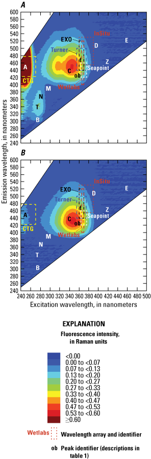
Comparison of wavelength arrays relative to primary calibration standards, A, quinine sulfate dihydrate and, B, fluorescent brightener 28 (Uvitex). <, less than; ≥, greater than or equal to.
Considering the wide variety of fluorometers on the market and the inherent differences caused by different wavelength arrays and manufacturing approaches, a universal approach to calibrations is unlikely to be achieved. Specific recommendations for calibrations are provided in the appendix, but each instrument’s operating manual should be the authoritative reference for calibrating any given fluorescence sensor. Calibration procedures should be weighed against data quality objectives and the requirements of other overarching USGS standard protocols found in the NFM, TM1–D3, and guidance within this report (Wagner and others, 2006; U.S. Geological Survey, variously dated b).
Calibration standards, such as QS, are not always conducive to routine use in field applications because of issues with the stability of the solution and difficulties in maintaining purity and controlling the quality of the prepared mixture. SRMs include a variety of dyes, solutions, and solid materials that are relatively inexpensive, more stable, and (or) easier-to-use alternatives to calibration standards for verifying sensor calibration status. The SRMs should be selected to reflect the wavelength array. For the humic sensors limited to peak C fluorescence, the optical brighteners may reasonably perform as an SRM. Recent efforts have explored the potential for an SRM that may be widely applicable to several sensors, and particularly effective for multiprobe platforms. Solid-phase humic acids, fulvic acids, and natural organic matter isolate standards are available commercially (International Humic Substances Society, Sigma-Aldrich HA), are well characterized, and have been used in previous sensor testing (Downing and others, 2012; Pellerin and others, 2013). These standards show potential for widespread use as SRMs for the whole suite of humic sensors. Although these standards differ from natural waters in several ways, they are currently being tested for use as SRMs over a range of concentrations comparable to natural waters (fig. 12A). A multiparameter standard solution is currently being developed for simultaneous calibration verification of some humic probes, chlorophyll-a fluorescence probes, and pH (fig. 12B). Several products commercially available for other uses may serve as reasonable SRMs, such as unsweetened iced tea (fig. 12C; Hansen and others, 2018), but they are largely untested across the range of fDOM concentrations encountered in natural waters.
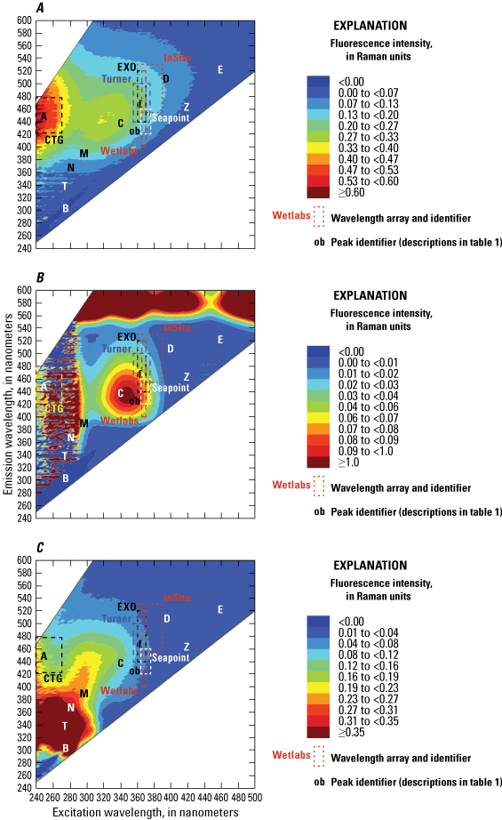
Comparison of wavelength arrays relative to the laboratory-based excitation-emission matrices of, A, Suwannee River natural organic matter isolate (2R101N) obtained from the International Humic Substances Society, prepared at 1-milligram-per-liter dissolved organic carbon concentration, B, a multiparameter field standard, and C, a 1-percent solution of commercially available iced tea mixed into organic-free blank water (Hansen and others, 2018). <, less than; ≥, greater than or equal to.
Ideally, modern field fluorometers should not need frequent recalibration unless one or both of the lenses get scratched, or the light source degrades. The lenses are made of hard minerals, such as quartz or sapphire, to reduce the chance of scratches. The LED or lamp brightness is controlled within some sensors so that differences over time are minimized. In sensors where the light intensity is not controlled, the light source will eventually fade and fail. A fading light source will require recalibration and could indicate that the sensor needs to be replaced.
When a field fluorometer or sensor fails calibration verification, the user should verify that an unintentional mistake was not made (such as inadequate sonde cleaning, using a contaminated standard, failing to triple rinse the sonde or calibration cup, air bubbles in the standard) by performing a second check, this time with extra effort to be sure the protocols and guidelines are followed. Recalibrations should be performed in a laboratory or mobile laboratory where temperature and light conditions can be better controlled. Note that the instrument response in standard solutions is temperature dependent, and the calibration must take temperature into account.
Verification of Standards
Reference sensors and benchtop fluorometers are useful in ensuring that the standard solutions are not made in error and can guide calibration verifications to determine when to calibrate and when to verify the standard solution (table 5). A laboratory reference sensor (of the same model as the field fluorometer) is recommended for any project that is not using a benchtop fluorometer to quality assure the standard solution. A laboratory reference sensor serves no other purpose than to provide a calibrated reference measurement. A well-documented quality-assurance plan, like that used to track National Institute of Standards and Technology thermometers, would need to be maintained to ensure that the laboratory reference sensor retains its accuracy and that its calibration history can be traced.
Table 5.
Calibration procedures for verifying standards on a benchtop fluorometer and using a laboratory reference sensor.A reference sensor should
-
• never be brought into the field;
-
• rarely be calibrated, and if so, only after extensive testing; and
-
• always be used during calibration checks.
Another approach to verifying successful calibration is to compare field measurements from the fluorometer with laboratory measurements on a benchtop spectrophotometer set to the same wavelength array as the field fluorometer. Comparisons between laboratory and field measurements can also ensure that there is not a systematic error in the standard preparation, such as one caused by expired chemicals or LED degradation.
Field Data Collection Procedures
Field protocols ensure that sensors are working properly and include visual inspections, instrument cleaning, calibration checks, and data downloads (if appropriate). The protocols defined in TM1–D3 (Wagner and others, 2006) for continuous monitors apply to the field servicing of fluorometers, although additional guidelines for fluorometers are included in this report. Users should always review manufacturer recommendations, given differences in sensor design and data specifications. Consider which steps need to be completed under field conditions and which steps are better accomplished in a laboratory setting. For example, assessing the causes of potential drift is better completed in a controlled laboratory setting rather than under potentially difficult field conditions, especially considering the sensitivity of fluorescence readings to changes or extremes in ambient light and temperature.
For the purpose of this report, the site monitor is defined as the deployed sensor(s). The field reference monitor is defined as the monitor used during a site visit. The field reference monitor serves as an independent check of waterbody conditions and quantifies changes in those conditions during the site visit. The field reference monitor is also used for collecting vertical and cross-sectional measurements at the site. Like a field fluorometer used for discrete sampling applications, the field reference monitor should have the calibration verified within 7 days of use. A calibration check post use is not necessary for a reference monitor used in continuous applications if the reference meter and the site monitor compare within two times the calibration criteria during the final readings. The steps for making a typical site visit to a nonphytopigment fluorescent sensor installation are as follows:
-
• Perform a site inspection.—Observe and document the site conditions and state of the infrastructure in field notes and photographs. Document any changes in the biological, physical, and hydrologic conditions at the site, such as high algal productivity, exposed channel, stagnant water, increased light exposure, or any signs of vandalism. Note the condition of the sensor infrastructure in the water, such as damaged cages or pipes, corrosion, snagged debris, or changes in instrument depth since the last deployment.
-
• Collect site monitor and field reference monitor measurements.—An independent field reference monitor serves as a check on the site monitor and can document changing environmental conditions during servicing. Field reference monitors should have the same manufacturer and design as the deployed site monitor. Fluorometers with different designs should not be used for comparison, as they may report substantially different values. At sites with rapidly changing environmental conditions that make obtaining simultaneous readings from the site monitor and the reference monitor difficult, ambient water can be collected in a clean, 5-gallon, dark, insulated bucket (or similar container), and used for readings before and after cleaning (see “Modified Standard Protocol” in Wagner and others [2006]). However, be aware that changing conditions such as the settling of particles and changes in temperature in the bucket will affect fluorometers that are not automatically compensated for these effects. It may be necessary to filter the water to remove particles prior to measuring the fluorescence of water in the bucket at such sites.
-
• Remove sensor from the monitoring location and perform an inspection of the sonde.—Observe and document in field notes and photographs the condition of the instrument, cables, connectors, wipers, and infrastructure. This includes a careful inspection of the sensor for (1) fouling, staining, or scratching on the optical windows; (2) degraded seals around the optical windows or wiper housings; (3) damage to the sensor housing and connectors; (4) damage or wear of the wiper assembly, brushes, or other antifouling components; and (5) cracks, cuts, kinks, or wear on the cables. If the instrument is being used in a flow-through design, additional inspection of the pumps, tubing, filters and filter housings, flow cells, and collection vessels can be performed to detect damage, clogging, and (or) fouling. Some routine maintenance may not be possible in the field, requiring temporary removal of equipment.
-
• Clean the sensors.—Field cleaning of optical sensors requires extra diligence with regard to the optical windows. Abrasive cleaners should not be used, and the optical windows should only be cleaned with soft-bristled brushes or lint-free lens paper. With appropriate safety precautions and waste collection, a diluted hydrochloric acid solution (less than 5 percent), isopropyl alcohol, or ethanol can be used in the field to efficiently remove staining or severe fouling, including the iron and manganese precipitates that form in some systems. In addition, the use of chemical cleaners and detergents recommended by the manufacturer is always followed by a triple rinse with deionized water (DIW). The sensor housing, cables, and wipers can also be cleaned with DIW, and pump tubing (if used) that shows signs of fouling can be replaced. After the final rinse step, verify the efficacy of the cleaning by gently agitating the sensor in a clean container of DIW, ensuring that the water is free from particles, and then verify that the sonde measures within acceptable limits. If necessary, repeat the cleaning procedure.
-
• Return the sensor to the monitoring location (or bucket) and collect comparison readings.—Return the sensor to the deployment location (or bucket) and record the after-cleaning sensor readings to determine the fouling correction, as described in TM1–D3. As previously stated, be aware that particle settling and rapid changes in temperature in a bucket will substantially affect the readings of some fluorometers. Although no quantitative limits are available, changes of more than 5 °C or 10 formazin nephelometric units (FNU) may require corrections for matrix effects, as described previously.
-
• Remove the sensor and perform a calibration check (or swap with a precalibrated sensor).—Calibration verifications can be done in the field in some instances; however, it is generally preferable to swap sensors and perform calibration verifications in the laboratory. It is recommended that sensors not be calibrated in the field, but field calibration verifications using SRMs can be useful to determine when a sensor may need to be swapped and fully assessed for calibration drift in the laboratory. It is not necessary to verify the sensor in calibration standards every visit or swap sensors with a recently verified sensor. It is recommended to check in calibration standards quarterly if the site has a continuous records processing designation of category 1. It is recommended to record sensor readings in an SRM every visit or compare the field reference monitor values to the clean site monitor values. If the SRM values are not within the expected range, or the reference and (or) the deployed sensor does not compare within two times the calibration criteria, the site monitor should be checked in calibration standards. Verification frequency can vary and should be documented in the project and USGS Science Center data-management and quality-assurance plans, as well as the continuous records processing policies.
-
• Periodically obtain filtered and unfiltered readings from the field reference monitor.—Collect site monitor readings in unfiltered native water, filter the water through a 0.45-micron capsule filter, and record readings in the filtered water. Over time, these readings can be used to build a site-specific relation to correct for interferences from particle attenuation and scatter or justify the use of the theoretical corrections. Samples can also be collected in the field and analyzed in a laboratory with the reference monitor. Samples should be stored in a dark cooler on ice or in a refrigerator and analyzed within 24 hours. Additional information on the frequency of this comparison is provided in appendix 1 for fDOM.
-
• Periodically collect environmental water to determine corrections for interferences.—Typically, 1 liter of environmental water is sufficient. Sensor readings in serial dilutions of environmental water filtered through a 0.45-micron filter and organic-free blank water (OBW) can be used to determine corrections from interferences or validate that no correction is necessary. Additional information can be found in appendix 1 for fDOM sensors.
-
• Recommendation: Collect discrete water samples for laboratory analysis.—Collect a representative sample, filter it, then send it to a laboratory for determination of fluorescence on a benchtop fluorometer. Results can be used to apply corrections for interferences to sensor data or to verify that no data corrections are necessary to remove the effect of interferences.
-
• Perform cross-sectional profiles.—Cross-sectional profiles should be performed a minimum of two times per year, as described in TM1–D3. Consider the site monitor objective when determining how frequently to perform cross-sectional profiles.
Troubleshooting
As with all sensors, issues with the electronics and other components can affect fluorometer performance in the field. Some of the more common problems observed for field fluorometers are listed in table 6, and users should follow manufacturer recommendations for troubleshooting. Some sensors and controllers can store or output data that may prove useful for diagnosing sensor performance issues. For example, information on wiper position, gain setting, and diagnostic parameters vary by manufacturer and are typically described in instrument user manuals.
Table 6.
Common issues and guidelines on troubleshooting fluorometers.Data Evaluation and Processing Procedures
Data quality-assurance procedures for fluorescence sensors generally follow USGS methods for continuous monitors (TM1–D3, Wagner and others, 2006). Automatic screening thresholds should be set up within database infrastructure as new sensors are deployed. At a minimum, these should be used to remove erroneous spikes greater than the sensor operating range. As time goes on, thresholds can be narrowed on the basis of the observed range of typical conditions at a specific site. Continuous records first undergo an initial evaluation in which erroneous data are flagged or deleted. Next, data corrections to account for sensor fouling and calibration drift are applied on the basis of information collected during site visits and during sensor performance checks. Corrections for continuous water-quality sensors should be applied when the calibration criteria are exceeded. Calibration criteria for fDOM sensors are available in appendix 1, table 1.1. Drift and fouling corrections should be considered independently of one another. For example, if the calibration criteria were exceeded for fouling but not for drift, only the fouling correction should be applied. Data correction thresholds suggested in this report for fluorescence sensors are set such that corrections smaller than the calibration criteria need not be applied. Users may wish to evaluate instrument accuracy in the laboratory to determine if more stringent criteria are justified to meet specific project objectives.
The fouling- and drift-corrected signal reflects the true fluorescence that was observed, expressed in terms of the selected output units of a given sensor. Corrections to compensate for temperature effects on the phenomenon of fluorescence and signal loss caused by interferences from particles and organic matter are then applied.
The raw and final data—as well as the data corrections for fouling, calibration drift, temperature compensation, and signal attenuation—are archived electronically along with project or site information. USGS project and science center data management and quality-assurance plans, as well as continuous records processing policies, should be followed when archiving data. Data corrections are applied as soon as possible after site visits, and data in certain time intervals (between site visits or up to a few months) are analyzed and reviewed within the timelines specified by USGS continuous records processing policy (U.S. Geological Survey, 2010).
Fouling Corrections
Fouling corrections for fluorescence sensors account for reductions in transmittance of the excitation or emission light signals caused by biological growth, staining, or sediment accumulation on the optical windows of the sonde. For most sites and deployment configurations, the sensors can be kept clean using antifouling measures, such as wipers and copper components, and fouling corrections might not be needed. When fouling corrections are needed, they may be applied routinely, or they may be limited to periods when a wiper failed or when extreme biological fouling occurred that was not easily removed by mechanical action.
Data from sensors of different makes and models are not equivalent in environmental water. The field reference monitor should be the same make and model as the site monitor. Finally, careful evaluation of the field reference monitor readings against site monitor readings is needed because of the many confounding factors discussed earlier in this document. Differences in readings between the field reference monitor and site monitor might not be due to changes in environmental conditions, but instead might be caused by more localized factors like differences in light or suspended particles. Because of this, the field reference monitor readings should be used with caution in determination of fouling corrections, and if other water-quality measurements are recorded concurrently, they will provide an additional basis to evaluate whether conditions are meeting the criteria for “rapidly changing conditions” as defined by TM1–D3 (Wagner and others, 2006). Equations and guidance for applying fouling corrections can be found in TM1–D3, and are applicable to time-series data, assuming the guidance in the previous paragraphs is considered in their application.
Fouling corrections often take the form of either a simple arithmetic shift or a percentage correction, both of which are described in TM1–D3. In either case, a fouling correction can be prorated to slowly increase over the time elapsed since the last cleaning. Fouling corrections can be prorated starting on an obvious fouling event or held constant depending on hydrographer judgement and knowledge of observed site conditions. In a simple arithmetic correction, values are shifted up or down according to the magnitude of the computed correction, and this can be prorated or held constant based on user judgement.
Percentage corrections can be useful to force a zero correction at a zero value, thus avoiding the creation of negative values that sometimes can arise from the use of a simple arithmetic correction. Percentage corrections also can be subject to extrapolation problems if the sensor signal increases but tend to be more appropriate for sensor readings near zero. Any time a step change is observed in the data stream, field protocols should be reviewed. If the sensor was swapped, the step change could indicate a lack of sensor intercalibration or a sensor quality issue.
Fouling typically is assumed to accumulate linearly over time starting from the previous sensor cleaning, but in some instances the onset of fouling coincides with a noteworthy event such as a storm runoff that carries a large, suspended sediment load. Sensor diagnostic data or data statistics, if available, sometimes can be used to identify the onset of fouling. If the onset of fouling is identified from such data, fouling corrections can be applied from that moment onward rather than from the date of the previous service visit.
Drift Corrections
Fluorescence sensors may experience some variation in their response over time if changes occur in the performance of their light sources or detectors; however, as noted previously, fluorometer drift is often minimal because of the stability of the solid-state components. Calibration drift can be evaluated using the difference between the expected sensor response and the measured response in at least three standards, where one is as a zero solution (often OBW or DIW) and multiple known concentrations of a calibration standards such as QS. The magnitude of the calibration drift error measured in this way follows the approach documented in TM1–D3 (Wagner and others, 2006). Only readings in calibration standards should be used to determine drift corrections; SRM readings should be used to determine when a full calibration check is needed but should not be directly used to determine a drift correction. SRM readings can be useful in determining when a drift correction should begin.
As with fouling corrections, calibration-drift corrections can be implemented as a simple datum shift, as a percentage correction, or as a multipoint correction when nonlinear drift is observed in a laboratory. The calibration drift correction is interpolated linearly over time from the date and time of one sensor performance check to the date and time of the next check unless specific information is available to indicate a different date and time for the initiation of sensor drift.
Temperature, Turbidity, and Inner-Filter Effect Corrections
The measured output from a field fluorometer can be affected by the temperature, turbidity, and color in sample water, as described previously (see the “Factors Affecting Fluorescence Measurements” section). The effects of temperature, turbidity, and colored water are not the same for all fluorometers or monitored locations; however, interferences still occur with most field fluorometers in turbid and (or) colored waters. All sensors should be corrected for temperature, turbidity, and IFE (unless it can be demonstrated that turbidity and [or] IFE corrections are not necessary) for measurements to be comparable among sites and through time. The corrections can be substantial relative to the final corrected values (fig. 13). In the example provided in figure 13, the IFE correction is the largest correction to the data; however, this is only an example. Some sites may be influenced to a greater degree by turbidity or even temperature corrections.
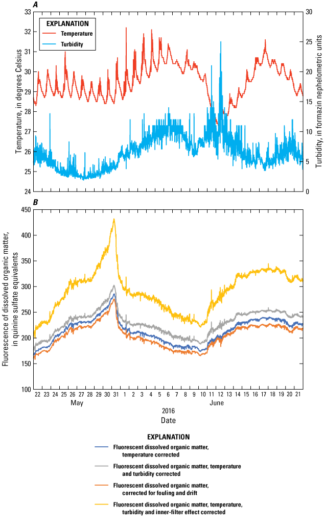
A, Temperature and turbidity at U.S. Geological Survey (USGS) station 02292900 (data from U.S. Geological Survey [2022b]) and B, fluorescence of dissolved organic matter (fDOM) at different stages of corrections applied at USGS station 02292900.
Although the relative magnitude of interferences and temperature effects are known in standard solutions (Downing and others, 2012), standard corrections for these effects have not been established by the USGS or instrument manufacturers for the range of instrument designs, sediment sizes, and DOM types found in natural waters (Saraceno and others, 2017). Therefore, the user will need to characterize the sensor response, apply the appropriate corrections, and determine acceptable limits for corrections beyond those for fouling and drift. It is important to note that as the effects of turbidity and IFE increase, the practical dynamic range of the sensor decreases and can decrease to the point that the sensor has little or no response to an actual change in concentration. The accuracy of corrected values should be viewed with caution when accounting for 50 percent or more signal loss caused by interferences. Additional details on how to assess the effects of turbidity and IFE on fDOM sensors are described in appendix 1.
Temperature corrections for the phenomenon of fluorescence are needed to ensure sensor consistency and comparability over a wide range of temperatures. A consistent reference temperature should be used for corrections; 25 °C is recommended for use as the reference temperature across the USGS. Temperature corrections are potentially instrument and site specific and should be verified using native water from the monitoring location.
Turbidity corrections for fluorescence increase the sensor signal to account for the excitation-emission light energy scattered away by suspended particles. The turbidity correction for fluorescence sensor data is dependent upon the manufacturer and model of the fluorescence and turbidity sensors used. For any change in either sensor model, the correction should be reevaluated. At extremely elevated turbidities, the practical dynamic range of the sensor decreases and can decrease to the point that the sensor has little or no response to an actual change in concentration. Using theoretical temperature and turbidity corrections based on experimental data in published reports is acceptable; however, the theoretical equations should always be verified for individual sensors and site-specific conditions.
IFE cause field measurements to differ from true values and can vary substantially among sites. Previous efforts used absorption spectra to derive corrections using laboratory measurements (Downing and others, 2012); however, serial dilutions can provide a simpler, more direct correction factor for field-based sensor measurements. Readings in serial dilutions of native water with OBW have been used to accurately determine the IFE correction for fDOM sensors.
One approach to verifying corrections is to compare fully corrected sensor readings to concurrently collected discrete samples analyzed on a benchtop spectrophotometer set to the same wavelength array as the field sensor. Benchtop spectrophotometer measurements are performed on water after necessary filtration; dilutions can be performed to eliminate interferences from particles and IFE as well as temperature variations. A combination of serial dilutions and validation with discrete samples for laboratory analysis is recommended. Although the collection of discrete samples requires additional demand on time and effort, this approach can provide further insights into whether or not other interferences, such as pH and salinity, are affecting the fluorescence measurements in the field. Additional guidance for correcting fDOM for temperature, turbidity, and IFE is available in appendix 1.
Final Data Evaluation and Approval
Final data evaluations and approval for fluorescence measurements follow the general guidelines of TM1–D3 (Wagner and others, 2006) for analyzing, approving, and auditing continuous water-quality data.
The maximum allowable limit for corrections—defined as the maximum value for the absolute sum of all data corrections where data are reported, stored in the NWIS database, or both (Wagner and others, 2006)—has important implications for field sensors. If the limit is too large, the ability to interpret results is compromised; if the limit is too low, the costs of instrument servicing and field visits can be excessive. As for other field sensors (Wagner and others, 2006; Pellerin and others, 2013), six times the calibration criteria have been suggested as the maximum allowable limit for fouling and drift corrections of field fluorometers. Temperature compensation and corrections for interferences are not included here as part of the maximum allowable limit, as they are theoretical corrections for the phenomenon of fluorescence. The point at which an interference correction is no longer justified is not yet known, but caution is warranted when corrections of greater than 50 percent are needed. Data requiring corrections large enough to be deemed unacceptable for publication or storage can be flagged in NWIS and archived according to USGS science center quality-assurance plans.
Corrections for drift and fouling are applied to fluorescence data prior to corrections for temperature, turbidity, and IFE. A final corrected time series is derived from the drift- and fouling-corrected time series, often using an equation that combines the corrections for temperature, turbidity, and IFE. Table 7 summarizes the different types of corrections.
Table 7.
Types of corrections applied to fluorescence time-series data.[TM1–D3, U.S. Geological Survey Techniques and Methods book 1, section D, chapter 3 (Wagner and others, 2006)]
| Type of correction | Correction criteria (variation outside the value shown requires a correction) | Guidance for computing the correction | Should be considered in maximum allowable limits | Maximum allowable limits |
|---|---|---|---|---|
| Fouling | Calibration criteria (see appendix 1). | TM1–D3 | Yes | Six times the calibration criteria |
| Drift | Calibration criteria (see appendix 1). | TM1–D3 | Yes | Six times the calibration criteria |
| Temperature | Temperature corrections should always be applied. | Appendix 1 | No | User defined |
| Turbidity | Turbidity corrections should be applied if turbidity influences fluorescence values by more than the calibration criteria. | Appendix 1 | No | User defined |
| Inner-filter effect | Inner-filter-effect corrections should be applied if inner-filter effect influences fluorescence values by more than the calibration criteria. | Appendix 1 | No | User defined |
It is reasonable that fluorescence sensor data would be initially classified as category 3 under USGS Water Mission Area continuous records processing guidelines (U.S. Geological Survey, 2010), providing additional time to characterize site-specific confounding effects not otherwise accounted for by the instrument. Associated data may need to be stored and archived in support of data review (and possible future model development), such as high-frequency burst data, instrument diagnostic data, and laboratory quality-assurance data for the sensor calibrations. A category 1 designation (approval within 150 days) may become appropriate when the site conditions are well understood and field operations become routine.
Summary
Many water-quality programs use field-based sensors to collect fluorescence data targeting dissolved organic matter, hydrocarbons, and wastewater. The wavelengths at which light is absorbed and re-emitted as fluorescence are determined by chemical bonds within the fluorescing material (known as fluorophores). Because these wavelengths are relatively specific, it is often possible to make concentration-related measurements of specific substances within the complex mixture of absorbing and fluorescing materials found in natural waters. Fluorescence sensors are often used as surrogates and can provide valuable insights into watershed changes over time. In order to ensure that fluorescence data are comparable, the same wavelength array must be used. Parameter names must include the wavelength array described as the full-width half-maximum range of the excitation-emission channels. Fluorescence sensors are also susceptible to interferences and often require additional corrections to account for these interferences. Effective and consistent deployment and operation requires thorough planning and setting realistic expectations for sensor performance and data objectives.
Guidance is provided herein on deployment, maintenance and field operations, quality-assurance techniques, and data reporting. Sensor performance issues and common interferences are also described. Additionally, the appendix provides further guidance on specific sensors, such as calibration criteria and procedures, guidance on correcting for interferences, and parameter and method codes. Adherence to the guidelines included in this report will help U.S. Geological Survey personnel and others collect field data by using fluorometers in ways that are consistent and comparable across different studies, sites, and instruments.
Acknowledgments
The authors are grateful for USGS funding and support from the National Hydrologic Monitoring program. The authors also gratefully acknowledge the members of the USGS Continuous Water Quality Committee for helpful comments and discussions.
References Cited
Aiken, G.F., 2014, Fluorescence and dissolved organic matter—A chemist’s perspective, p. 35–74, in Coble, P.G., Lead, J., Baker, A., Reynolds, D.M., and Spencer, R.G.M. (eds.), Aquatic organic matter fluorescence: New York, Cambridge University Press, 375 p., accessed September 8, 2022, at https://doi.org/10.1017/cbo9781139045452.005.
Baker, A., Bolton, L., Newson, M., and Spencer, R.G.M., 2008, Spectrophotometric properties of surface water dissolved organic matter in an afforested upland peat catchment: Hydrological Processes, v. 22, no. 13, p. 2325–2336, accessed September 8, 2022, at https://doi.org/10.1002/hyp.6827.
Bergamaschi, B.A., Fleck, J.A., Downing, B.D., Boss, E., Pellerin, B., Ganju, N.K., Schoellhamer, D.H., Byington, A.A., Heim, W.A., Stephenson, M., and Fujii, R., 2011, Methyl mercury dynamics in a tidal wetland quantified using in situ optical measurements: Limnology and Oceanography, v. 56, no. 4, p. 1355–1371, accessed September 8, 2022, at https://doi.org/10.4319/lo.2011.56.4.1355.
Bergamaschi, B.A., Krabbenhoft, D.P., Aiken, G.R., Patino, E., Rumbold, D.G., and Orem, W.H., 2012, Tidally driven export of dissolved organic carbon, total mercury, and methylmercury from a mangrove-dominated estuary: Environmental Science & Technology, v. 46, no. 3, p. 1371–1378, accessed September 8, 2022, at https://doi.org/10.1021/es2029137.
Booth, A.C., Poulin, B.A., and Krabbenhoft, D.P., 2020, Observed and modeled mercury and dissolved organic carbon concentrations and loads at control structure S-12D, Florida Everglades, 2013–17: U.S. Geological Survey Open-File Report 2020–1092, 27 p., accessed September 8, 2022, at https://doi.org/10.3133/ofr20201092.
Burdige, D.J., Kline, S.W., and Chen, W.H., 2004, Fluorescent dissolved organic matter in marine sediment pore waters: Marine Chemistry, v. 89, no. 1–4, p. 289–311, accessed September 8, 2022, at https://doi.org/10.1016/j.marchem.2004.02.015.
Carpenter, K.D., Kraus, T.E.C., Goldman, J.H., Saraceno, J.F., Downing, B.D., Bergamaschi, B.A., McGhee, G., and Triplett, T., 2013, Sources and characteristics of organic matter in the Clackamas River, Oregon, related to the formation of disinfection by-products in treated drinking water: U.S. Geological Survey Scientific Investigations Report 2013–5001, 78 p., accessed September 8, 2022, at https://doi.org/10.3133/sir20135001.
Coble, P.G., 1996, Characterization of marine and terrestrial DOM in seawater using excitation-emission matrix spectroscopy: Marine Chemistry, v. 51, no. 4, p. 325–346, https://doi.org/10.1016/0304-4203(95)00062-3.
Coble, P.G., 2007, Marine optical biogeochemistry—The chemistry of ocean color: Chemical Reviews, v. 107, no. 2, p. 402–418, accessed September 8, 2022, at https://doi.org/10.1021/cr050350+.
Coble, P., Lead, J., Baker, A., Reynolds, D.M., and Spencer, R.G.M., eds., 2014, The principles of fluorescence, part 1 in Aquatic organic matter fluorescence: Cambridge, England, Cambridge University Press, p. 3–34, accessed September 9, 2022 at https://doi.org/10.1017/CBO9781139045452.004.
Cory, R.M., Miller, M.P., McKnight, D.M., Guerard, J.J., and Miller, P.L., 2010, Effect of instrument-specific response on the analysis of fulvic acid fluorescence spectra: Limnology and Oceanography, Methods, v. 8, no. 2, p. 67–78, accessed September 8, 2022, at https://doi.org/10.4319/lom.2010.8.67.
Downing, B.D., Pellerin, B.A., Bergamaschi, B.A., Saraceno, J.F., and Kraus, T.E.C., 2012, Seeing the light—The effects of particles, dissolved materials, and temperature on in situ measurements of DOM fluorescence in rivers and streams: Limnology and Oceanography, Methods, v. 10, no. 10, p. 767–775, accessed September 8, 2022, at https://doi.org/10.4319/lom.2012.10.767.
Fleck, J.A., Gill, G., Bergamaschi, B.A., Kraus, T.E.C., Downing, B.D., and Alpers, C.N., 2014, Concurrent photolytic degradation of aqueous methylmercury and dissolved organic matter: Science of the Total Environment, v. 484, p. 263–275, accessed September 8, 2022, at https://doi.org/10.1016/j.scitotenv.2013.03.107.
Fleck, J.A., Hansen, A.M., Oros, D.M., and Booth, A.C., 2022, Comparisons from an Aqualog Fluorometer Standardized to Quinine Sulfate Equivalents (QSE) with Excitation (ex) and Emissions (em) Equivalent to Fluorescence of Dissolved Organic Matter (fDOM) Sensors from Multiple Manufacturers: U.S. Geological Survey data release, https://doi.org/10.5066/P9VJUCTP.
Foster, G.M., Graham, J.L., Bergamaschi, B.A., Carpenter, K.D., Downing, B.D., Pellerin, B.A., Rounds, S.A., and Saraceno, J.F., 2022, Techniques for the determination of algal pigment fluorescence in environmental waters—Principles and guidelines for instrument and sensor selection, operation, quality assurance, and data reporting: U.S. Geological Survey Techniques and Methods, book 1, chap. D10, 34 p., accessed December 29, 2022 at https://pubs.er.usgs.gov/publication/tm1D10.
Hansen, A.M., Fleck, J.A., Kraus, T.E.C., Downing, B.D., von Dessonneck, T., and Bergamaschi, B.A., 2018, Procedures for using the Horiba Scientific Aqualog fluorometer to measure absorbance and fluorescence from dissolved organic matter: U.S. Geological Survey Open-File Report 2018–1096, 31 p., accessed September 8, 2022, at https://doi.org/10.3133/ofr20181096.
Hansen, A.M., Kraus, T.E.C., Pellerin, B.A., Fleck, J.A., Downing, B.D., and Bergamaschi, B.A., 2016, Optical properties of dissolved organic matter (DOM)—Effects of biological and photolytic degradation: Limnology and Oceanography, v. 61, no. 3, p. 1015–1032, accessed September 8, 2022, at https://doi.org/10.1002/lno.10270.
Henderson, R.K., Baker, A., Murphy, K.R., Hambly, A., Stuetz, R.M., and Khan, S.J., 2009, Fluorescence as a potential monitoring tool for recycled water systems: Water Research, v. 43, no. 4, p. 863–881, accessed September 8, 2022, at https://doi.org/10.1016/j.watres.2008.11.027.
Huguet, A., Vacher, L., Relexans, S., Saubusse, S., Froidefond, J.M., and Parlanti, E., 2009, Properties of fluorescent dissolved organic matter in the Gironde Estuary: Organic Geochemistry, v. 40, no. 6, p. 706–719, accessed September 8, 2022, at https://doi.org/10.1016/j.orggeochem.2009.03.002.
Itagaki, H., 2000, Fluorescence spectroscopy, chap. 3 in Tanaka, T., (ed.), Polymer, interfaces and biomaterials—Experimental methods in polymer science: San Diego, California, Academic Press, p. 155–260, accessed September 8, 2022, at https://doi.org/10.1016/B978-0-08-050612-8.50009-X.
Lakowicz, J.R., 2006, Principles of fluorescence spectroscopy (3d ed.): New York, Springer Science and Business Media, 954 p., accessed September 8, 2022, at https://doi.org/10.1007/978-0-387-46312-4.
Lorenzen, C.J., 1966, A method for the continuous measurement of in vivo chlorophyll concentration: Deep-Sea Research and Oceanographic Abstracts, v. 13, no. 2, p. 223–227, accessed September 8, 2022, at https://doi.org/10.1016/0011-7471(66)91102-8.
McKnight, D.M., Boyer, E.W., Westerhoff, P.K., Doran, P.T., Kulbe, T., and Andersen, D.T., 2001, Spectrofluorometric characterization of dissolved organic matter for indication of precursor organic material and aromaticity: Limnology and Oceanography, v. 46, no. 1, p. 38–48, accessed September 8, 2022, at https://doi.org/10.4319/lo.2001.46.1.0038.
Moran, M.A., Sheldon, W.M., Jr., and Zepp, R.G., 2000, Carbon loss and optical property changes during long-term photochemical and biological degradation of estuarine dissolved organic matter: Limnology and Oceanography, v. 45, no. 6, p. 1254–1264, accessed September 8, 2022, at https://doi.org/10.4319/lo.2000.45.6.1254.
Murphy, K.R., Butler, K.D., Spencer, R.G.M., Stedmon, C.A., Boehme, J.R., and Aiken, G.R., 2010, Measurement of dissolved organic matter fluorescence in aquatic environments—An interlaboratory comparison: Environmental Science & Technology, v. 44, no. 24, p. 9405–9412, accessed September 8, 2022, at https://doi.org/10.1021/es102362t.
Ohno, T., 2002, Fluorescence inner-filtering correction for determining the humification index of dissolved organic matter: Environmental Science & Technology, v. 36, no. 4, p. 742–746, accessed September 8, 2022, at https://doi.org/10.1021/es0155276.
Para, J., Coble, P.G., Charrière, B., Tedetti, M., Fontana, C., and Sempéré, R., 2010, Fluorescence and absorption properties of chromophoric dissolved organic matter (CDOM) in coastal surface waters of the northwestern Mediterranean Sea, influence of the Rhône River: Biogeosciences, v. 7, no. 12, p. 4083–4103, accessed September 8, 2022, at https://doi.org/10.5194/bg-7-4083-2010.
Parlanti, E., Wörz, K., Geoffroy, L., and Lamotte, M., 2000, Dissolved organic matter fluorescence spectroscopy as a tool to estimate biological activity in a coastal zone submitted to anthropogenic inputs: Organic Geochemistry, v. 31, no. 12, p. 1765–1781, accessed September 8, 2022, at https://doi.org/10.1016/S0146-6380(00)00124-8.
Pellerin, B.A., Bergamaschi, B.A., Downing, B.D., Saraceno, J.F., Garrett, J.D., and Olsen, L.D., 2013, Optical techniques for the determination of nitrate in environmental waters: Guidelines for instrument selection, operation, deployment, maintenance, quality assurance, and data reporting: U.S. Geological Survey Techniques and Methods, book 1, chap. D5, 37 p., accessed October 1, 2017, at https://pubs.usgs.gov/tm/01/d5/.
Poulin, B.A., Ryan, J.N., and Aiken, G.R., 2014, Effects of iron on optical properties of dissolved organic matter: Environmental Science & Technology, v. 48, no. 17, p. 10098–10106, accessed September 8, 2022, at https://doi.org/10.1021/es502670r.
Saraceno, J.F., Pellerin, B.A., Downing, B.D., Boss, E., Bachand, P.A.M., and Bergamaschi, B.A., 2009, High frequency in situ optical measurements during a storm event—Assessing relationships between dissolved organic matter, sediment concentrations, and hydrologic processes: Journal of Geophysical Research, v. 114, no. G4, G00F09, accessed September 8, 2022, at https://doi.org/10.1029/2009JG000989.
Saraceno, J.F., Shanley, J.B., Downing, B.D., and Pellerin, B.A., 2017, Clearing the waters—Evaluating the need for site-specific field fluorescence corrections based on turbidity measurements: Limnology and Oceanography, Methods, v. 15, no. 4, p. 408–416, accessed September 8, 2022, at https://doi.org/10.1002/lom3.10175.
Spencer, R.G.M., Pellerin, B.A., Bergamaschi, B.A., Downing, B.D., Kraus, T.E.C., Smart, D.R., Dahlgren, R.A., and Hernes, P.J., 2007, Diurnal variability in riverine dissolved organic matter composition determined by in situ optical measurement in the San Joaquin River (California, USA): Hydrological Processes, v. 21, no. 23, p. 3181–3189, accessed September 8, 2022, at https://www.onlinelibrary.wiley.com/doi/abs/10.1002/hyp.6887.
Stedmon, C.A., Markager, S., and Bro, R., 2003, Tracing dissolved organic matter in aquatic environments using a new approach to fluorescence spectroscopy: Marine Chemistry, v. 82, no. 3–4, p. 239–254, accessed September 8, 2022, at https://doi.org/10.1016/S0304-4203(03)00072-0.
Stokes, G.G., 1852, On the change of refrangibility of light: Philosophical Transactions of the Royal Society of London, v. 142, p. 463–562, accessed September 8, 2022, at https://doi.org/10.1098/rstl.1852.0022.
Talbott, C.M., and Clifford, R.H., 2013, Characterization of light emitting diodes (LEDs) and compact fluorescent lamps (CFLs) by UV-visible spectrophotometry: Shimadzu Scientific Instruments, Inc., web page, accessed September 2, 2022, at https://www.ssi.shimadzu.com/sites/ssi.shimadzu.com/files/pim/pim_document_file/ssi/applications/posters/14887/SSI-Pittcon12-UV-001.pdf.
U.S. Geological Survey, 2010, Continuous records processing of all water time series data: Water Resources Discipline policy memorandum 2010.02, accessed March 17, 2021, at https://water.usgs.gov/admin/memo/policy/wrdpolicy10.02.html.
U.S. Geological Survey, 2016, Office of Water Quality Technical Memorandum 2016.10 on policy and guidance for approval of surrogate regression models for computation of time-series suspended-sediment concentrations and loads: U.S. Geological Survey web page, accessed September 16, 2022, at https://water.usgs.gov/admin/memo/SW/sw.2016.07+wq.2016.10.pdf.
U.S. Geological Survey, 2017, Office of Water Quality Technical Memorandum 2017.7 on procedures for processing, approving, publishing, and auditing time-series records for water data: U.S. Geological Survey web page, accessed November 21, 2022, at https://water.usgs.gov/admin/memo/QW/qw2017.07.pdf.
U.S. Geological Survey, 2019, Specific conductance: U.S. Geological Survey Techniques and Methods, book 9, chap. A6.3, 15 p., accessed September 8, 2022 https://doi.org/10.3133/tm9A6.3. [Supersedes U.S. Geological Survey Techniques of Water-Resources Investigations, book 9, chap. A6.3, version 1.2.]
U.S. Geological Survey, 2022a, Instructional memorandum OSQI 2022–01—Quality management system for U.S. Geological Survey laboratories: U.S. Geological Survey web page, accessed November 21, 2022, at https://www.usgs.gov/survey-manual/im-osqi-2022-01.
U.S. Geological Survey, 2022b, USGS 02292900 CALOOSAHATCHEE RIVER AT S-79, NR.OLGA, FLA, in USGS water data for the Nation: U.S. Geological Survey National Water Information System database, accessed November 22, 2022, at https://doi.org/10.5066/F7P55KJN. [Site information directly accessible at https://waterdata.usgs.gov/nwis/dv?referred_module=sw&site_no=02292900.]
U.S. Geological Survey, [variously dated] a, Program series, 500.1–1100.7: U.S. Geological Survey website, accessed September 22, 2022, at https://www.usgs.gov/survey-manual/program-series-5001-11007.
U.S. Geological Survey, [variously dated] b, National field manual for the collection of water-quality data: U.S. Geological Survey Techniques of Water-Resources Investigations, book 9, 9 chap. (A1–A9), accessed September 8, 2022, at https://water.usgs.gov/owq/FieldManual/.
Vincent, W.F., 1983, Fluorescence properties of the freshwater phytoplankton—Three algal classes compared: British Phycological Journal, v. 18, no. 1, p. 5–21, accessed September 8, 2022, at https://doi.org/10.1080/00071618300650021.
Wagner, R.J., Boulger, R.W., Jr., Oblinger, C.J., and Smith, B.A., 2006, Guidelines and standard procedures for continuous water-quality monitors—Station operation, record computation, and data reporting: U.S. Geological Survey Techniques and Methods, book 1, chap. D3, 51 p., plus 8 attachments, accessed August 6, 2021, at https://pubs.water.usgs.gov/tm1d3.
Watras, C.J., Hanson, P.C., Stacy, T.L., Morrison, K.M., Mather, J., Hu, Y.-H., and Milewski, P., 2011, A temperature compensation method for CDOM fluorescence sensors in freshwater: Limnology and Oceanography: Methods, v. 9, no. 7, p. 296–301, accessed September 8, 2022, at https://doi.org/10.4319/lom.2011.9.296.
Weishaar, J.L., Aiken, G.R., Bergamaschi, B.A., Fram, M.S., Fujii, R., and Mopper, K., 2003, Evaluation of specific ultraviolet absorbance as an indicator of the chemical composition and reactivity of dissolved organic carbon: Environmental Science & Technology, v. 37, no. 20, p. 4702–4708, accessed September 8, 2022, at https://doi.org/10.1021/es030360x.
Wilson, H.F., and Xenopoulos, M.A., 2009, Effects of agricultural land use on the composition of fluvial dissolved organic matter: Nature Geoscience, v. 2, no. 1, p. 37–41, accessed September 8, 2022, at https://doi.org/10.1038/ngeo391.
Appendix 1. Fluorescence of Dissolved Organic Matter (Humic) Sensors
Calibration
Calibrations and calibration verifications should be performed in a laboratory or mobile laboratory where temperature and light conditions can be controlled. This may require that a sensor be removed for a short period of time or ideally that the sensor can be exchanged with a sensor having a verified calibration and then taken back to the laboratory for a calibration verification. Note that the standards are temperature dependent, and the calibration must take temperature into account. Directions for calibrating individual sensors are provided in the manufacturer instrument manuals. A two-point calibration is recommended when possible; however, the sensor is required to be verified at a minimum of three points.
Calibration Criteria
Ideally, modern field fluorometers should not need frequent recalibration unless one or both of the lenses get scratched or the light source fades. The time between calibrations will likely vary among sensor manufacturers and models. Refer to guidance from the manufacturers on expected period between calibrations. Calibration is not recommended if the criteria in table 1.1 are not exceeded.
Table 1.1.
Calibration verification and criteria, calibration, maximum allowable limits, and other considerations for fluorescence of dissolved organic matter (fDOM) sensors.[QSE, quinine sulfate equivalents; μg/L, microgram per liter; mg/L, milligram per liter; SRM, standard reference material; ±, plus or minus; %, percent]
Calibration Safety
-
· Users must never look directly into the measurement path of these instruments while the instruments are operating. Ultraviolet (UV) light can cause immediate injury and permanent damage to the eye.
-
· Quinine sulfate dihydrate (QS) is highly acidic and oxidizing; care must be taken when using it. All staff should be familiar with safety protocols and safety data sheets for all chemicals used.
-
· Appropriate personal protective equipment must be worn; at a minimum, this includes eye protection and gloves.
-
· Waste management associated with making the QS standards in 0.1 normal sulfuric acid (H2SO4) will vary from area to area and all local requirements should be followed.
Supplies for Calibration
Commonly used supplies for calibration can be found in table 1.2. The accuracy of all pipettes, volumetric glassware, and scales should be verified. Glassware should be cleaned as described in the U.S. Geological Survey National Field Manual (Wilde, 2004). QS standard values are temperature dependent; follow the guidance provided by the manufacturer. The initial dilutions are often stored in a refrigerator (for up to 5 days), and ample time must be allowed for standard solutions to reach room temperature before proceeding with their use. A temperature sensor must be placed in the standard solution during the calibration. Sensors should also be at room temperature prior to starting the calibration or verification.
Table 1.2.
Equipment and supplies used for calibrating fluorescence of dissolved organic matter (fDOM).[mg, milligram; mL, milliliter; μL, microliter; --, none]
Preparation of Standard Solution
The following steps can be used to prepare 150- and 300-microgram-per-liter (µg/L) solutions of QS that can be used for verification or calibration purposes. Site-specific concentration ranges should be used to guide the concentration range used in the calibration procedure, and the actual calibration solution concentrations used for individual projects will vary among studies. The concentrations provided below are only an example.
-
1 Ensure that all glassware and equipment are clean.
-
2 Verify accuracy of scales, pipettes, and volumetric glassware.
-
3 Weigh out 0.100 gram of QS powder and transfer it to a 100-milliliter (mL) volumetric flask. Add 0.1-normal concentration (0.05 molar concentration) sulfuric acid (H2SO4) to the 100-mL fill line. It is often easiest to fill the flask with a small beaker of sulfuric acid. Add a stir bar and stir for a minimum of 5 minutes. This solution is 1,000-milligram-per-liter QS.
-
4 Transfer 0.3 mL of the 1,000-part-per-million QS solution to a 1,000-mL volumetric flask and the fill the flask with 0.1-normal sulfuric acid to the 1,000-mL fill line. Add a stir bar and stir for a minimum of 2 minutes. This solution is 300-μg/L QS.
-
5 Transfer 0.15 mL of the 1,000-part-per-million QS solution to a 1,000-mL volumetric flask and the fill the flask with 0.1-normalsulfuric acid to the 1,000-mL fill line. Add a stir bar and stir for a minimum of 2 minutes. This solution is 150-μg/L QS.
Procedures for Calibration and Calibration Verifications
-
1 Ensure that the temperature sensor is used during standard checks. If a temperature sensor is used on a multiparameter sonde, ensure that it is verified against a National Institute of Standards and Technology thermometer.
-
2 Ensure the sensor is thoroughly cleaned and wipe the sensor face with a lint-free laboratory wipe. All efforts should be made to avoid any potential contamination. See below for additional guidance on potential contamination.
-
3 Rinse the sensors three times with OBW, then fully submerge the sensors in OBW and record the temperature and fDOM values.
-
4 Rinse the sensors three times with the middle concentration QS standard. Submerge the sensors in the standard and record the temperature and the fDOM values.
-
5 Rinse the sensors three times with a QS standard that brackets the expected field values. Submerge the sensors in the standard, and record the temperature and the fDOM values.
-
6 Compare the recorded values with the temperature-compensated fDOM values (often provided by the manufacturer) to determine if a calibration is necessary.
-
7 If the drift check determines that calibration is necessary, then a two-point calibration that spans the range of conditions expected during the subsequent deployment is recommended. Follow calibration guidance provided by the manufacturer.
-
8 After calibration, recheck the sensors in the three standards, following the steps above to ensure the calibration was successful.
-
9 Rinse with deionized water prior to storage.
-
10 If sensors are not being stored as part of a multiparameter sonde, ensure sensors are either dry before storing or are stored as recommended by the manufacturer.
An alternative to the method described above is to do serial additions of QS of a known concentration to a known volume of 0.1-N sulfuric acid. If this approach is followed, a detailed standard operating procedure should document the process.
Potential Calibration Issues
-
• QS standard is colorless, and contamination is often not visible to the naked eye. All equipment, from sensors to labware, must be free of contamination before use in calibrations or verifications.
-
• Contamination can cause interference with QS checks. Chloride and other halide ions in conductivity standards, brackish or seawater, as well as Zobell’s solution, are known to cause contamination. Ensure each sensor is adequately cleaned and rinsed before beginning calibration checks. Maintaining labware that is only used during calibrations and verifications is recommended.
-
• It is important to note that copper, which is often used in wipers and guards to inhibit biofouling, should not be used during fDOM calibration procedures. Copper can degrade in acidified QS solutions and interfere with calibrations.
-
• QS standards can degrade over time and thus should be used within 5 days of preparation and stored within the refrigerator in a darkened bottle when not in use.
-
• Efforts must be taken to reduce possible external light source interference.
-
• Best practice is to perform calibrations in a laboratory setting where light conditions are likely to remain stable over time, barring major laboratory lighting changes (such as switching from fluorescent to light-emitting diode [LED] lighting). Consider whether any windows in the laboratory space should be covered during calibrations.
-
• Always use a darkened or blacked-out calibration standard vessel (calibration cup). Many manufacturers provide accessories that are purposely built to limit light interferences. If using a YSI EXO instrument, the calibration cup can be used, although it is recommended to darken the cup by covering it in electrical tape.
-
• Glass beakers or white plastic containers should not be used because of the reflection of light from the container surfaces.
-
Corrections for Interferences
Sensors currently on the market (as of 2022) do not internally compensate for the effects of temperature, light attenuation caused by particles (herein referred to as the “turbidity correction”), or colored substances that cause inner-filter effects (IFE, herein referred to as the “IFE correction”). To have fDOM data that are comparable seasonally and across environments, these corrections must be applied. Corrections for interferences should be applied after drift and fouling corrections have already been applied.
Temperature Corrections
An equation for corrections for temperature should take the following form as described by Watras and others (2011):
wherefDOMT
is the temperature-corrected sensor signal;
fDOMo
is the original sensor signal not corrected for temperature effects;
ρ
is a sensor-specific temperature coefficient;
Tm
is the measured water temperature, in degrees Celsius; and
Tr
is the reference temperature, in degrees Celsius (25 °C).
The values for fDOMo and Tm are measured, whereas ρ and Tr are constants. The temperature coefficient ρ can be determined by the following equation:
Studies by Watras and others (2011) and Downing and others (2012) and data provided by manufacturers, indicate that the combined temperature effects may result in a 0.45–3 percent decrease in signal per 1 °C increase (for example, ρ = −0.0045 to −0.03). It is recommended that users conduct simple temperature tests in the laboratory with environmental water and a National Institute of Standards and Technology traceable thermometer to determine the temperature coefficient for their specific manufacturer and model of sensors, as well as individual site conditions. This can be done by taking sensor readings in environmental waters at a minimum of five temperatures that span the range of temperatures observed in the field and assessing the change in fDOM, per degree of water temperature, in order to calculate the ρ for the environmental water.
Turbidity Corrections
A correction to fDOM data for particle interference has been proposed by Downing and others (2012) using the following exponential equation:
wherefDOMT,t
is the sensor signal corrected for temperature (T) and turbidity (t) effects,
e
is the exponential function,
α
is a sensor-specific turbidity coefficient (a value often in the range of −0.001 to −0.006), and
tm
is the measured turbidity in appropriate units (commonly formazin nephelometric units [FNU] or nephelometric turbidity units).
The α value depends on several factors including the sensor design, manufacturer, and the source and characteristics of the particles and their effectiveness in scattering signals to and from the fluorescence sensor (Merten and others, 2014; Saraceno and others, 2017). The α values should be determined for each project as sensors from the same manufacturer may have variable α values. The α value should be determined from four or five environmental samples spanning the range of turbidity values observed at the site. A black 5-gallon bucket of native water should be collected from the field at a minimum of quarterly for the first year, and efforts should be made to collect a sample near the maximum turbidity values observed. The initial temperature, turbidity, and fDOM values should be recorded within the 5-gallon black bucket after ensuring the turbidity has been resuspended in the sample. After the initial values for fDOM, temperature, and turbidity are recorded, a portion of the environmental water should be filtered through a 0.45-micron filter and returned to the original black bucket. Once the water is well mixed, record the temperature, turbidity, and fDOM values. Repeat this process in order to achieve a minimum of five points (continuous recording of data is ideal) and to ensure that the final turbidity measurement is close to zero. The test can be conducted in the field or in the laboratory within 24 hours. An alternative to using environmental water would be to use Elliot silt loam (ESL) and OBW. Using ESL could be helpful when obtaining a field sample with elevated turbidities is difficult due to the short duration of periods with elevated turbidities and when the turbidities at the site do not exceed 300 FNU. Plot the data with the turbidity on the x-axis and the percentage of fDOM removed by the effect of turbidity on the y-axis and determine the exponential trendline (fig. 1.1). The calculated coefficient of the mathematical constant e (the base of the natural logarithm) is the α value.
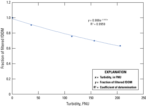
Relation between fraction of filtered fluorescence of dissolved organic matter (fDOM) and turbidity, in formazin nephelometric units (FNU). The dashed blue line is the fit of all data using a second-order polynomial function. Figure is for illustrative purposes only.
After the initial establishment of the α value, the data are still required to be compared regularly to filtered field data that span the range of conditions observed in the field; making comparisons at quarterly or more frequent intervals is recommended. This can be accomplished by taking fDOM readings on filtered and unfiltered samples. Ideally, sensor readings in the filtered sample and the turbidity-corrected, unfiltered sample should differ no more than two times the calibration criteria. If a previously determined correction does not meet data quality or project objectives, it is recommended that the user explore a site-specific turbidity correction; in this case, the frequency of comparisons should be increased if the comparisons differ by more than 10 percent.
It is important to note that research has shown that the ESL-based turbidity correction equations can overcompensate fDOM when turbidity values exceed 300 FNU (Saraceno and others, 2017). In that research, fDOM was corrected using a laboratory-derived equation based upon ESL and was compared to a second fDOM sensor installed in a filtered pump system to remove turbidity at the same location. It was determined that the ESL-based turbidity correction was not an accurate representation of the instream conditions when turbidity exceeded 300 FNU. The equation above should not be used at turbidities greater than 300 FNU unless comparisons among filtered and unfiltered samples show that the equation accurately represents conditions observed in the field.
The second approach for correcting humic fluorescence data for turbidity is to develop a site-specific turbidity correction by collecting samples during site visits, recording the turbidity and fDOM values in a native water sample, filtering the sample, and then recording the values again and building the relation over time. A minimum of 24 samples that span the range of conditions observed in the field should be collected to develop a robust, site-specific turbidity correction. This could also be done by deploying a second fDOM sensor in a filtered pump system that removes the effect of turbidity, as described in Saraceno and others (2017). Samples must be collected periodically for comparison and at a recommended quarterly or more frequent interval to verify that no changes in the relation have occurred.
Inner-Filter Corrections
IFE result from the attenuation of excitation or emission light by colored dissolved organic matter and other dissolved substances that cause a loss of linearity in the sensor response and result in an underestimate of the true value. In laboratory settings, benchtop fluorescence methods call for a dilution based on measured absorbance values prior to making a fluorescence measurement to avoid IFE (Ohno, 2002). Correcting for IFE requires that the linearity in the fDOM response be restored.
The correction for IFE is dependent upon the manufacturer and model of fDOM sensor used and is site specific (Downing and others, 2012). IFE corrections, when needed, should be determined for each site and ideally for different samples that span a range of hydrologic conditions. Serial dilutions of environmental water (filtered through a 0.45-micron filter to remove the influence of turbidity) with OBW can be used to determine the IFE correction. A corresponding sample collected for laboratory analysis of absorbance at a wavelength of 254 nanometers (A254) on a benchtop spectrophotometer can be used to quality assure the dilution. Additionally, samples analyzed on a benchtop spectrophotometer for fDOM (using the same excitation-emission wavelengths as the field fluorometer) can be useful, although not required, in verifying the IFE correction. Ideally, the fDOM value determined from the serial dilution should compare within two times the calibration criteria (10 percent) of the fDOM value calculated from the benchtop fluorometer using the same excitations-emission range as the field fluorometer.
A minimum of four sensor readings in serial dilutions of native water with OBW should be collected. In most natural waters, the IFE correction for open-face sensors is minimal when A254 is less than 0.1 (Downing and others, 2012). Undiluted, filtered native water should be sent to a laboratory for analysis of A254. If the environmental water is relatively clear, the IFE will be small. A correction for IFE is not necessary if the influence of the IFE is less than the calibration criteria. When this correction is needed, the predicted fDOM with the IFE removed can be calculated by developing a polynomial trendline between A254 and the temperature-corrected fDOM values collected during the serial dilution (fig. 1.2). The advantage of developing a polynomial trendline between A254 and temperature-corrected fDOM is that errors in the dilution process are minimized relative to those obtained when the serial dilution approach alone is used. Also verifying the initial A254 value allows confirmation that the lowest serial dilution value is not biased by IFE. The A254 values from each of the serial dilutions can be calculated from the dilution rates, and thus, submitting samples from each dilution step is not recommended.
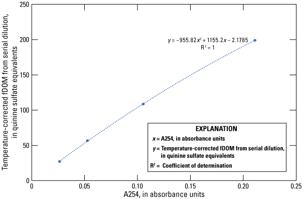
Relation between temperature-corrected fluorescence of dissolved organic matter (fDOM) and absorbance at wavelength of 254 nanometers (A254) predicted from dilution. The dashed blue line is the fit of all data using a second-order polynomial function.
The IFE correction equation can then be developed by using a polynomial trendline between the temperature-corrected fDOM and the fDOM with the IFE removed (fig. 1.3). It is important to note that the IFE correction should never decrease the fDOM values. It is also important to note that the IFE correction should be developed using temperature-compensated fDOM values and that temperature compensation may not occur within the instrument. The IFE correction, as determined using serial dilutions, should be verified over the expected range of environmental conditions observed. It is possible for the sources and characteristics of the organic matter that create the need for an IFE correction to change over time; therefore, the IFE correction should be verified periodically and is recommended at a quarterly or more frequent interval. Once the IFE correction has been documented to not change seasonally over a period of 3 years or more, the frequency of the correction verifications can be reduced; however, the IFE correction should still be verified at a minimum of two times per year or whenever watershed or land-use conditions change substantially.
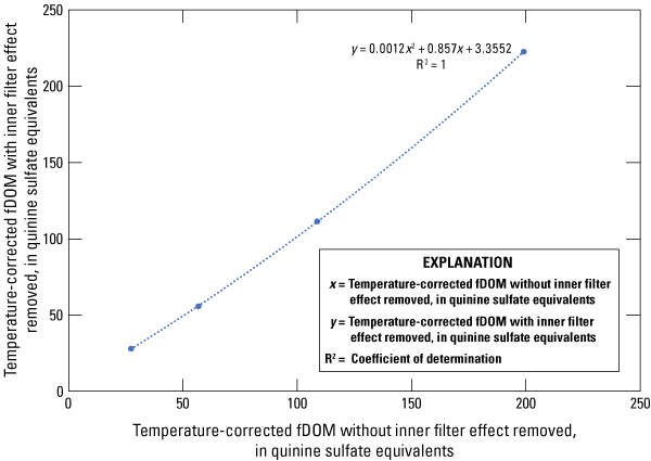
Relation between temperature-corrected fluorescence of dissolved organic material (fDOM) with the inner-filter effect (IFE) removed and temperature-corrected fDOM without the IFE removed. The dashed blue line is the fit of all data using a second-order polynomial function.
Reporting Units, Parameter Codes, and Method Codes
Results in the USGS National Water Information System (NWIS) database must be reported with the parameter and method codes that accurately describe the details of the sensor measurement. It is recommended to report all fDOM data in micrograms per liter as quinine sulfate equivalents (QSE), as that is the official calibration standard. Data should be reported to three significant figures but no more than the nearest 0.1 microgram per liter QSE. Recommended (2022) parameter codes and method codes are listed in table 1.3. New parameter and method codes can be requested for new sensors. Parameter names should include the excitation-emission wavelengths as well as the reporting units. Method codes should include the instrument model and manufacturer. It should be noted that the YSI EXO sensors report the values in quinine sulfate units, which are interchangeable to QSE.
Table 1.3.
Recommended parameter codes, description including wavelength array, units for fluorescence sensor output, method codes, and method code descriptions.[NWIS, National Water Information System; QSE, quinine sulfate equivalent; μg/L, microgram per liter; CDOM, colored dissolved organic matter; nm, nanometer; fDOM, fluorescence of dissolved organic matter; ±, plus or minus]
References Cited
Downing, B.D., Pellerin, B.A., Bergamaschi, B.A., Saraceno, J.F., and Kraus, T.E.C., 2012, Seeing the light—The effects of particles, dissolved materials, and temperature on in situ measurements of DOM fluorescence in rivers and streams: Limnology and Oceanography, Methods, v. 10, no. 10, p. 767–775, accessed April 19, 2019, at https://doi.org/10.4319/lom.2012.10.767.
Ohno, T., 2002, Fluorescence inner-filtering correction for determining the humification index of dissolved organic matter: Environmental Science & Technology, v. 36, no. 4, p. 742–746, accessed September 8, 2022, at https://doi.org/10.1021/es0155276.
Saraceno, J.F., Shanley, J.B., Downing, B.D., and Pellerin, B.A., 2017, Clearing the waters—Evaluating the need for site-specific field fluorescence corrections based on turbidity measurements: Limnology and Oceanography, Methods, v. 15, no. 4, 9 p., accessed September 8, 2022, at https://doi.org/10.1002/lom3.10175.
Watras, C.J., Hanson, P.C., Stacy, T.L., Morrison, K.M., Mather, J., Hu, Y.-H., and Milewski, P., 2011, A temperature compensation method for CDOM fluorescence sensors in freshwater: Limnology and Oceanography, Methods, v. 9, no. 7, p. 296–301, accessed September 8, 2022, at https://doi.org/10.4319/lom.2011.9.296.
Wilde, F.D., ed., 2004, Cleaning of equipment for water sampling (ver. 2.0, April 2004): U.S. Geological Survey Techniques of Water-Resources Investigations, book 9, chap. A3, 68 p., accessed September 13, 2016, at https://water.usgs.gov/owq/FieldManual/chapter3/final508Chap3book.pdf.
Conversion Factors
Supplemental Information
Specific conductance is given in microsiemens per centimeter at 25 degrees Celsius (µS/cm at 25 °C).
Concentrations of chemical constituents in water are given in either milligrams per liter (mg/L) or micrograms per liter (µg/L).
Abbreviations
A254
absorbance at wavelength of 254 nanometers
CDOM
colored dissolved organic matter
DIW
deionized water
DOC
dissolved organic carbon
DOM
dissolved organic matter
EEM
excitation-emission matrix
ESL
Elliot silt loam
fDOM
fluorescence of dissolved organic matter
FNU
formazin nephelometric units
IFE
inner-filter effects
LED
light-emitting diode
NFM
National Field Manual
NWIS
National Water Information System
OBW
organic-free blank water
QMS
quality management system
QS
quinine sulfate dihydrate
QSE
quinine sulfate equivalents
RFU
relative fluorescence units
RU
Raman-normalized intensity units
SRM
standard reference materials
USGS
U.S. Geological Survey
UV
ultraviolet
For more information about this publication, contact
Director, Caribbean-Florida Water Science Center
U.S. Geological Survey
4446 Pet Lane, Suite 108
Lutz, FL 33559
For additional information, visit
https://www.usgs.gov/centers/car-fl-water
Publishing support provided by
Lafayette Publishing Service Center
Disclaimers
Any use of trade, firm, or product names is for descriptive purposes only and does not imply endorsement by the U.S. Government.
Although this information product, for the most part, is in the public domain, it also may contain copyrighted materials as noted in the text. Permission to reproduce copyrighted items must be secured from the copyright owner.
Suggested Citation
Booth, A., Fleck, J., Pellerin, B.A., Hansen, A., Etheridge, A., Foster, G.M., Graham, J.L., Bergamaschi, B.A., Carpenter, K.D., Downing, B.D., Rounds, S.A., and Saraceno, J., 2023, Field techniques for fluorescence measurements targeting dissolved organic matter, hydrocarbons, and wastewater in environmental waters: Principles and guidelines for instrument selection, operation and maintenance, quality assurance, and data reporting: U.S. Geological Survey Techniques and Methods, book 1, chap. D11, 41 p., https://doi.org/10.3133/tm1D11.
ISSN: 2328-7055 (online)
| Publication type | Report |
|---|---|
| Publication Subtype | USGS Numbered Series |
| Title | Field techniques for fluorescence measurements targeting dissolved organic matter, hydrocarbons, and wastewater in environmental waters: Principles and guidelines for instrument selection, operation and maintenance, quality assurance, and data reporting |
| Series title | Techniques and Methods |
| Series number | 1-D11 |
| DOI | 10.3133/tm1D11 |
| Publication Date | March 13, 2023 |
| Year Published | 2023 |
| Language | English |
| Publisher | U.S. Geological Survey |
| Publisher location | Reston, VA |
| Contributing office(s) | California Water Science Center, New York Water Science Center, Oregon Water Science Center, Caribbean-Florida Water Science Center |
| Description | Report: vi, 41 p.; Data Release |
| Online Only (Y/N) | Y |