

Guidelines for the Use of Automatic Samplers in Collecting Surface-Water Quality and Sediment Data
Links
- Document: Report (19.8 MB pdf) , HTML , XML
- Download citation as: RIS | Dublin Core
Abstract
The importance of fluvial systems in the transport of sediment, dissolved and suspended contaminants, nutrients, and bacteria through the environment is well established. The U.S. Environmental Protection Agency (EPA) identifies sediment as the single most widespread water contaminant affecting the beneficial uses of the Nation’s rivers and streams. The evaluation of water-quality as it relates to agriculture, urbanization, highway and residential construction, mining, industrial and human wastes, and other activities requires an extensive data and sample-collection effort. This is especially the case when studying urbanized river basins, where during hydrologic events, concentration of suspended sediment and contaminants can vary rapidly and over large ranges. Where synoptic studies of watersheds are called for, sampling may be needed at many sites throughout the basin; a complicated and difficult task in some settings. Automatic pumping samplers (autosamplers) are one method for conducting intensive time-varying sampling throughout watersheds.
This report presents guidelines for the use of autosamplers for collecting surface-water samples by the U.S. Geological Survey. An autosampler is an automatic, pump-based sampler that collects a prescribed volume of water from streams, lakes, reservoirs, storm drains, or other bodies of water after receiving a command from an internal or external control unit. It deposits this sample into a specified container for later analysis of physical, chemical, or biological constituents. This report provides a general background on types of autosamplers and how they work; guidance for designing, selecting, installing, servicing, and calibrating autosamplers; guidance on standardized operating procedures, and guidance on quality-assurance and quality-control efforts when using an autosampler.
Introduction
The importance of sediment, dissolved and suspended contaminants, nutrients, and bacteria on the quality of aquatic and riparian systems is well established. The U.S. Environmental Protection Agency (EPA) identifies sediment as the single most widespread water constituent affecting the beneficial uses of the Nation’s rivers and streams (U.S. Environmental Protection Agency, 1998). Suspended sediment and particulate organic carbon (POC) are a primary transport mechanism for hydrophobic contaminants in surficial hydrologic systems. Intensive and repetitive detailed sampling is often required to properly characterize the suspended-sediment load and water quality in surface waters. Runoff from agriculture, urbanization, highway and residential construction, mining, industrial and human wastes, and other activities affect temporal water quality in rivers and lakes in complex ways that require detailed monitoring. This is especially the case in urbanized areas where streamflow and water quality may change rapidly during a hydrologic event. Likewise, regional studies of surface water often require synoptic sampling at many locations throughout a large basin. The site locations, streamflow conditions, frequency of sample collections, and operational costs may make manual sampling impractical, hurdles that may be overcome using automatic pumping sampler (autosampler) equipment.
An autosampler is a device that, on its own, collects a prescribed volume of water (aliquot) from a stream, lake, reservoir, storm drain, or other water body (Keith, 1996). Sampling can be initiated at a preset time or triggered by selected hydrologic conditions. Once initiated, the autosampler transfers each sample to a container for subsequent analysis. Autosamplers use a pre-programmed logic to determine the initiation of sampling and the timing when successive samples are collected. An autosampler can be programmed to collect and mix multiple aliquots to produce a flow- or time-weighted composite sample that represents the “average” chemistry of the sampled water body. This report focuses on active autosamplers that use pumps to collect samples from flowing rivers, culverts, and pipes.
Many justifications can be given for using an autosampler, but the basic tenet is the need to leave the sampling equipment in place and prepared to collect samples at remote locations, at specified times, or under specific flow conditions when field crews cannot be present. Autosampler systems are typically equipped to monitor stream conditions, like stage or discharge, and then initiate a preprogrammed sampling routine when certain conditions are met. The use of an autosampler removes the need for a human to monitor environmental conditions and reduces the physical labor involved in collecting samples. However, considerable human effort is still required to prepare, calibrate, and maintain an autosampler system. As discussed in this document, the costs of outfitting a site with an autosampler and conducting quality assurance (QA) work needed to demonstrate representativeness of samples needs to be weighed against the benefits and costs of deploying an autosampler.
Description of an Autosampler
An autosampler is an automatic, pump-based sampler that collects water upon a command from an internal or external control unit. This command, referred to as a “triggering” or “initiation” signal, may come from a human operator offsite through a communication link, or conditions at the site (such as time or flow) which automatically start a sampling routine. Most commonly, the triggering command is issued from a timer, or a stage-sensor placed in the stream and connected to an onsite computer either built into the sampler or as a stand-alone data logger. The triggering command can occur at a preset time or time interval, when a prescribed stage of flow discharge is reached, at the onset of precipitation, or upon other environmental parameters. When a continuous water-quality monitoring device is collocated at the site, sampling can be triggered by water-quality parameters such as turbidity, temperature, or specific conductance. Once collected, the autosampler stores the samples, usually chilled in a closed container, until field personnel can retrieve the samples. Appendix 1 list definitions of terms used in this report.
Autosamplers provide a means to collect samples from water bodies for which chemistry varies over time on scales ranging from a few minutes to days. A typical use of an autosampler is sampling of a river where the discharge rate varies over time due to storm runoff, snowmelt, a diversion of water for off-stream use, or the release of water from a dam. Another typical use is collecting samples from industrial discharge and waste-treatment systems over time at outfall pipes. Autosamplers provide a means for characterizing the short-term temporal variation in stream chemistry that is needed for calculating accurate mass-loading of contaminants of interest in flowing water. The specific design and implementation of auto-sampling methods depend upon the environmental setting being monitored and the project goals. Major characteristics and contrasts in design and operation of autosamplers are identified in this report as they apply to sampling for dissolved and particulate constituents in natural waters.
Background on the Development and Use of Autosamplers
Early use of autosamplers by the U.S. Geological Survey (USGS) focused on suspended sediment in streams, where high-frequency sampling (on the order of hours to days) was needed to estimate sediment loads in streams. From the early 1960s through the 1980s, the Federal Interagency Sedimentation Project (FISP1) designed, tested, and manufactured autosamplers specifically to support USGS programs to estimate loads of suspended sediment in streams across the United States. Other automatic-type samplers were also designed, mainly to capture representative water samples for suspended sediment (for example, Colby, 1961; U.S. Army Corps of Engineers and others, 1966). These autosamplers were large, complex, required significant understanding of their operation, and often were very labor intensive to operate. A number of different automatic sampler designs soon became available through commercial sources. In 1981, FISP evaluated and compared some of the commonly used autosamplers in that time period (Skinner and Beverage, 1981). From that study they were able to recommend future design elements such as proper orientation of the intake in the stream, optimal numbers and volumes of sampling containers, the use of chemically inert tubing and containers, and the limits of pumping lift such as optimal length, elevation, and diameters of intake lines. Since that time, commercial autosamplers have been tested and refined to eliminate many of the early problems and simplify their use.
Presently there are a number of commercial autosamplers available with flexible controls that allow sampling under numerous different scenarios. These provide samples of water that would otherwise be difficult or impossible to collect using traditional sampling methods. Autosamplers provide the ability to collect detailed information during periods of rapid change, such as storm events at remote stream locations that are otherwise not easily accessible on short notice. Figure 1, for example, shows the complex changes that occurred in a stream with a 72.8-square-mile (mi2) watershed during a single storm, and helps emphasize the importance of collecting the first flush of a storm event.
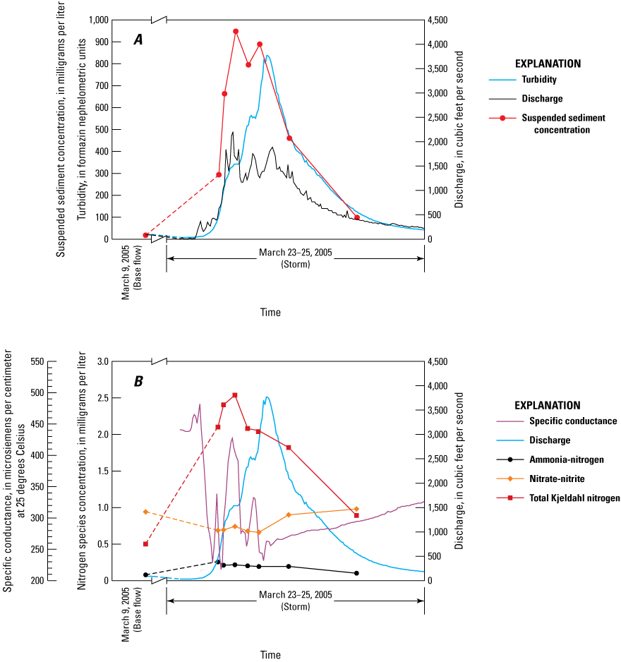
Plots showing water quality and discharge data gathered from U.S. Geological Survey monitoring station 01649500 during a storm in March 2005: A, time series of discharge, turbidity, and suspended sediment, and, B, time series of discharge, specific conductance, and concentrations of nitrogen species. X-axis is broken during the two-week period between the base-flow sample on March 9 and the storm events of March 23–25, 2005. Modified from Miller and others (2007).
Figure 1A shows the time series of discharge, turbidity and suspended-sediment concentrations; these peak early in the storm hydrograph prior to peak flow. Figure 1B demonstrates the complexity of variations in concentrations of dissolved and whole-water fractions (dissolved plus particulate-bound fractions) of nitrogen species over this single storm event and the wealth of information that was made possible with an autosampler. It shows that total Kjeldahl nitrogen peaked early in the storm, coincident with the first peaks in turbidity and suspended sediment but are much lower during the second peak in suspended material. Dissolved nitrogen, ammonia, nitrate, and nitrite exhibited complex variations with time, often independent from the behavior of the suspended material, as they are affected by dilution and arrival of groundwater and interflow.
Davis and others (2012) provide a good example of a situation where autosamplers were critical for collecting runoff in grass swales along a highway that experiences flash floods during storm events. Using autosamplers, they were able to evaluate the hydraulic and chemical performance of different designs for infiltration strips with frequent samples collected over the course of multiple storm events. At the other extreme, large watersheds (such as the major tributaries flowing into the Chesapeake Bay) have been successfully sampled using monthly fixed intervals to estimate annual loads of nutrients and sediment, and storm chasing to collect samples directly from the rivers (Langland and others, 2012). As a general rule, autosamplers prove most useful in studies of smaller watershed (less than tens of square miles) where stream conditions change rapidly, whereas hand-sampling methods prove suitable for sampling rivers draining large watersheds (Harmel and others, 2003; Dahlgren and others, 2004; Joiner and others, 2014).
There are a number of factors that influence the efficacy of autosamplers, including the cost of deployment, determining the location of the intake relative to the heterogeneous cross section of the stream, the potential for bias as the sample transits through the lines, and selection of methods for monitoring the triggering conditions (Yorke, 1986). The efficiency of pumping water with suspended sediment varies with particle size and the dimensions and pumping velocity of the intake system; variables that must also be evaluated while designing a deployment. Numerous studies have tested the design and function of autosamplers and provide ample information for modern autosamplers to collect samples that are representative of a stream system and minimally biased.
Monitoring studies conducted by the USGS have successfully utilized and tested autosamplers in a variety of situations to meet project objectives. Horowitz and others (2008), for example, monitored urban streams in Atlanta, Georgia; they were able to provide useful details on transport of sediment, trace elements, and nutrients in small, flashy streams using a network of autosamplers. They recommended using turbidity or specific conductance as sampling triggers rather than flow, because using flow as a trigger tended to miss the initial pulse of sediment (the first flush) common in storm events. Krug and Goddard (1985) used autosamplers to demonstrate the effects of urbanization on channel geomorphology and sediment loads in the Pheasant Branch Basin near Middleton, Wisconsin, and Selbig and Bannerman (2011a; 2011b) used an autosampler to collect flow-weighted composite samples in a pipe at a basin outlet and characterize the size distribution of particles in suspended sediment.
In all these examples, quality-control (QC) samples were collected to document the representativeness and potential bias of samples collected by autosamplers. One of the most important aspects of QA/QC is to collect samples integrated across the entire stream cross section, using methods such as equal-width increment (EWI) or equal-discharge increment (EDI) isokinetic sampling developed by USGS. These samplers are then compared to point (grab) samples collected by the autosampler. If the variance between the methods is enough to bias monitoring objectives, then corrections to the autosampler-based results will be needed. If the variance is within acceptable limits, then the autosampler data can be used unadjusted. In all cases, additional comparison samples will be needed throughout the study to ensure that conditions have not changed in the stream.
Horowitz and others (1990; 1994) provided a detailed comparison of EWI, EDI, and pump sampler methods. A two-person crew was deployed to collect samples at multiple EWI and EDI stations; the crew collected pairs of samples using a USGS D-77 sampler, one sample of each pair was composited following standard USGS churn methods, and the second was analyzed as a discrete sample (U.S. Geological Survey, 1990). The EWI and EDI sampling was conducted while an autosampler collected multiple discrete samples from the centroid of flow in the channel. These results of the different methods were then compared. The discrete EWI and EDI samples showed substantial spatial variability over the cross section among the methods, particularly for particles greater-than 63 micrometers (µm) in the suspended sediment. Concentrations of trace elements on the particles were relatively constant, even though the concentrations of particles varied considerably. However, when compared with the concentration of suspended sediment in the cross-channel composited sample, the point samples underestimated the concentration, while the autosamples overestimated the concentration. This was thought to be related to a reduction in the collection efficiency for larger particles.
The results of Martin and others (1992) supported the results of Horowitz and others (1990), as they also compared water quality in samples collected by surface-grab samples at center of flow and composited samples collected using EWI isokinetic composite methods in four rivers in Kentucky. This study, conducted as part of the USGS National Water Quality Assessment Program, collected samples at monthly fixed-time intervals along with storm samples. They analyzed nutrients, suspended sediment, major ions, and dissolved and total-recoverable metals associated with suspended sediment. The results showed considerable cross-sectional and temporal variation in concentrations, which Martin and others (1992) attributed to multiple factors, including incomplete mixing of upstream tributary inflows, groundwater seepage, point-source discharges, variations in stream velocity and geomorphology, and photosynthesis in surface water. They broke down their analysis into less-than versus greater-than 62 µm grain sizes and observed that surface water had lower concentrations of both size fractions. Total and particulate constituents had the greatest differences between methods and the magnitude of the differences increased proportionately with the concentration. Concentrations and variances for particulate constituents were observed to be greater for samples collected by EWI than by surface grabs, and grab sampling consistently underestimated suspended sediment and particulate concentrations of other constituents for both size fractions. Understandably, the negative bias for grab samples was greater for the larger size fraction. These differences could be expected to remain if the grab samples had been collected using autosampler methods.
However, other studies to make these comparisons have shown that within error and under normal sampling conditions, autosamplers provide reasonable estimates of representative stream chemistry. Bartsch and others (1996) collected sediment in side-by-side sediment traps and autosampler intakes, then compared particle-size distribution, finding no observable difference between the methods. Bossong and others (2006) used automatic pumping samplers to composite time-weighted and volume-weighted samples and summarized stormwater quality over a 13-year period in Denver, Colorado. Their study compared time-weighted and volume-weighted composites to samples collected at center of flow and by EWI isokinetic sampling. In their analysis, the relative percent deviation was less than 1-percent for time-weighted versus volume-weighted composites and approximately 75-percent of the replicates comparing EWI to fixed-point intakes had rapid percent deviations with an absolute value of less than 20-percent. Bent and others (2000) used a different approach for sampling by using multiple intakes (in a manifold) across the stream channel to produce composite samples. Their results provided very good agreement between the composite and samples collected using an autosampler.
Tests on the bias introduced by intake lines are another important consideration when using autosamplers. Anderson and Rounds (2010) used an autosampler and tested carryover between samples using 3/8-inch (in.) diameter vinyl tubing at various pumping distances of 12–25 feet (ft) and pumping heights of 2–10 ft. This was done in a laboratory environment by sequentially running water and samples through the lines. They concluded that the ideal rinsing strategy with minimal carryover between samples was to flush the lines with air followed by three rinses of sampling water. In an experiment with an autosampler on the Tualatin River in Oregon, they collected a sample, stirred up bed sediment and collected a second sample, and finally collected a sample after turbidity returned to baseline. The initial and final samples showed negligible differences, demonstrating that carryover of water and sediment in sampling lines was not an issue.
Burton and Pitt (2001) provide data to estimate the potential loss of sediment during pumping based on particle size and flow rates. They recommended a pumping velocity of at least 100 centimeters per second to minimize loss of particles during pumping. Clark and others (2009) conducted controlled experiments to determine efficiency of sampling different particle sizes and concluded that the upper limit for reliably sampling particles was between 250 to 500 µm with a specific gravity of 2.65. This size range may be more likely to be in the bedload, so it may not be an issue except at very high stream velocities.
Koopman and others (1989) identified an interesting side effect of biofilms that may develop in intake lines, which may have the ability to nitrify samples and thus bias nitrogen results. Using biological oxygen demand (BOD) as a measure, they demonstrated that nitrifying bacteria in the sampling line created a high nitrogenous oxygen demand, which biased results. The largest bias was in lines having continuous circulation, but the effect was much less when intermittent aspiration was used to clear the sampling lines.
Graczyk and others (2000) compared siphon samplers (passive-point samplers) with ISCO autosamplers in a Wisconsin stream. They concluded that there was no statistical difference between siphon and ISCO autosamplers, but their plots suggest possible high bias for suspended sediment in high flows when using the siphon samplers.
One approach to collecting a vertically integrated sample was developed by Selbig and Bannerman (2011a; 2011b) who used a depth-integrated sample arm (DISA; a programable robot arm) to move the autosampler intake up and down in the water column. In their testing, fixed point samples collected near the bottom were approximately twice those collected by the DISA. Organic material was about the same and particle densities were lower for samples collected by the DISA. Selbig and others (2013) also developed an in-line filter design that progressively filters by particle size. In their design, water was pumped up to a series of plate filters ranging from 63 µm to 1 µm, at a flow rate regulated at 1 liter per minute using a ball-valve system that shut off pumping when the inline back pressure reached a threshold (in this case, 345 kilopascals). Using this design, they were able to measure the concentrations of polycyclic aromatic hydrocarbons, trace metals, and estimate toxicity indicators in the different size fractions collected by the autosampler.
There are many situations where autosamplers can provide unique and valuable information on stream chemistry during rapidly changing hydrologic events, and a myriad of ways that the methods for conducting autosampling can be applied. This report provides guidance for making decisions on the correct applications and detailed support to design auto-sampling methods.
The success of any project that uses an autosampler depends strongly on collecting representative samples that are relevant to clear project and data-quality objectives. Representative sampling determines the design and installation of the equipment, logic used to trigger each of the electronic and mechanical components in the sampling system, and the application of QC sampling to document the results. It should be understood that a successful program that uses one or more autosamplers will require considerable human thought and effort. Ultimately the advantages of using an auto-sampling system are weighed against the ability to collect representative samples and the increased cost of quality assurance to verify the data.
Advantages and Disadvantages of Autosamplers
There are a number of advantages and disadvantages to using an autosampler as a replacement to traditional sampling methods (table 1). The more important considerations include:
-
Comparison with traditional manual collection methods.—Autosamplers collect water from a single-point in the flow channel and, therefore, at best only approximate the results that would be obtained from traditional integrated isokinetic composite sampling. As a result, it is the user’s responsibility to document the representativeness of samples collected by the autosampler, by comparing them with samples collected using traditional representative sampling methods. It is also necessary to conduct measurements to locate the intake at a point that produces the most representative sample possible.
-
Triggering.—Sampling can be initiated by automatic onsite means, or through remote means (radio, telephone, or cellular) thereby reducing the human oversight needed to ensure that sampling occurs at the appropriate time or condition. This is especially advantageous when attempting to catch the “first flush” response to precipitation in a stream or channel. However, careful thought must be given to the relation between triggering signals and the behavior of the constituents of interest (suspended sediment, for example). Additionally, electronic equipment used to initiate and conduct sampling are not foolproof, and still require continuous oversight to ensure that sampling occurs as expected.
-
Coverage of the hydrologic event sampling (day and night).—Autosamplers can provide samples over the entire hydrologic event, from hours to days or weeks, either as multiple discrete samples or as a single composited sample. This is advantageous because they provide detailed information on the natural variations that occur or can provide an appropriate measure of the “average” composition in a river during a storm event. However, autosamplers are limited in the number of sample containers that can be held. As a result, bottles still must be replaced, the autosamplers will need servicing, and the intake lines will need periodic cleaning to ensure sample integrity. Thus, a regular schedule of maintenance visits will be required when using these samplers.
-
Limited return of effort.—There is a limited return for the effort in deploying and using autosamplers compared with manual methods. These returns are based on the size of the studied watershed. For very small, flashy, watersheds (less than 1– 5 mi2 total area), the autosampler may be essential for sampling storm events. In larger watersheds, the delay in response shown by a river to precipitation may allow sufficient time for manual sampling to be conducted. Therefore, a tradeoff exists between the effort and costs involved in deploying an autosampler (including the quality assurance sampling required for properly siting the autosampler) and using field crews to conduct sampling.
-
Potential for unexpected bias.—Introducing autosamplers into a pre-existing, long-term monitoring program that historically used traditional manual sampling techniques may introduce unexpected bias in future data. Theoretically, significant effort may be needed to conduct calibration studies to demonstrate an acceptable correlation exists between autosampler and cross-channel samples over all expected flow regimes, then little or no bias in future trends would be expected. The effort involved in conducting studies to quantify this bias should be considered carefully before introducing an autosampler into a long-term monitoring program. Along with the data, complete documentation is needed of the automated sampling methods for future reference.
Table 1.
Advantages and disadvantages for using autosamplers.[EWI, equal-width increment; EDI, equal-discharge increment, —, no comment]
Design and Installation of Stations, Sampling Equipment, and Intakes
Considerations for Station or Shelter Installations
Autosamplers can be deployed in many different settings including streams, large rivers, reservoir outfalls, lakes, ponds, lagoons, culverts, and in pipe outfalls for storm water, industrial, or treated wastes. Each deployment will have its unique site characteristics and hurdles to overcome in accessing, constructing, powering, and equipping a station, and many unforeseen obstacles to their deployment should be expected. For example, when autosamplers are deployed at sewer or industrial outfalls, consideration must be given to working in confined spaces, the mitigation of electrical sparks, and the extreme hydraulic velocities that often occur in sewer pipes. Flow velocities in culverts, pipes and outfalls, as well as in large rivers, may be so extreme that it becomes difficult or even impossible to keep the intake lines secure. These factors must be taken into account when planning and developing autosampler stations. If, during planning, a given location is found to be inaccessible or dangerous, another site should be selected for the project.
Site characteristics, such as stream bank conditions, wadeability, the presence of nearby bridges, and others, often constrain where a new station can be sited. Often the ideal physical site cannot be found, even after much effort is expended to find the best possible location. Other site characteristics that need to be considered include obtaining legal access, power, the installation of structure footings, how the inlet lines will be secured, the ability to measure the stream cross-section (either by wading or a from nearby bridge), and others. This section discusses some of these issues.
Site Security and Access
The main consideration when evaluating a potential autosampler station is safety. Primarily this relates to the access and work area used by the field crew, but also relates to the physical safety of the structure and equipment. Wherever a site is accessible to the public, the station and equipment should be considered vulnerable to vandalism. Extra effort and expense will be needed to build a safe, secure structure. Structures should have a solid locking steel door and generally should not have windows. Depending on the location, it may be necessary to install power lines to a new station. Figure 2 shows a “hardened” pre-cast concrete sampling station in a public park equipped with a locking steel door and sited on a gravel pad. The structure was delivered to the site by the manufacturer. It is usually beneficial to locate the station at an existing secure site such as in a fenced-in area or within an existing building in a public park, for example. In these instances, a wood, metal, or fiberglass shed may suffice, saving considerable resources and time.
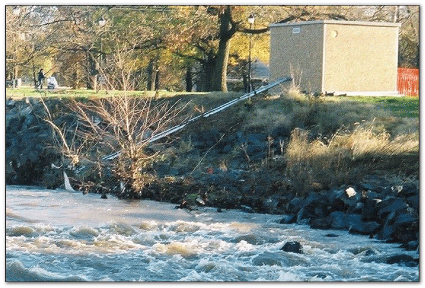
Photograph showing U.S. Geological Survey monitoring station 01649500 with intake lines for autosampler. Located at Northeast Branch Anacostia River at Riverdale, Maryland. Photograph by U.S. Geological Survey.
Legal Access and Permitting
Depending upon the location of a proposed station, it may be necessary to obtain Federal, State, county, or local permits. These may include stream encroachment permits, construction permits, and electrical permits if a power line is to be installed. Likewise, other legal agreements may be necessary to access land or limit liability. Obtaining such a permit may pose a significant delay in project work and should be considered when developing the project timeline.
Operating Conditions and Climate
Sampling stations may be subjected to extremes in operating temperatures. Sites that operate during freezing weather will need insulation and heaters for equipment, lines, and samples. Heat lamps or electric heaters can be used, but care must be taken to ensure proper electrical connections. Heat tape, which is often used to de-ice house gutters and water pipes, can be wrapped around the inlet line between the station and the stream channel and will usually necessitate access to alternating current (AC) line power. As the air temperature drops, power usage will increase and hasten the depletion of batteries. If subjected to hot temperatures, it may become necessary to cool sensitive electronic equipment using fans, vents, and air conditioning that require electrical service. As discussed later in this document, a critical concern in hot weather is sample preservation. Refrigerated autosampler units are optimal but may require AC power, or extra batteries that must be changed on an increased frequency, or if ice is used to preserve samples, then additional field trips will be required by crews.
Vulnerability to Flooding
Sampling sites are, by their nature, located along the banks of rivers, streams, and culverts that are subject to periodic flooding. Although rare, extreme floods can cause bank erosion and even destroy a station and its equipment. It is recommended that sampling equipment be located above the height of any likely flood stage; this stage may be estimated from the historic record of the streamgage (or nearby streamgages). However, if a peristaltic pump system is used, the height of a station must be below the limiting head of approximately 25 ft. Generally, peristaltic pump systems are most reliable if the pumping head and length of intake lines are minimized, which reduce pumping times, wear on pump tubing, and drainage of battery power. Careful consideration must also be given to the station foundation and the method used to secure the structure along the stream bank. Foundations are vulnerable to undercutting or destruction by flood water, and considerable effort is involved in pouring concrete footers and foundations for permanent stations; such steps often require following local building codes. For temporary stations, or sites not likely to be flooded, a suitable foundation may be created using crushed stone with shelters being simply staked down.
Utilizing an Existing Streamgage Station
In many instances, an existing streamgage station can be used to deploy the sampling equipment. If sufficient space is not available within the station, a semi-permanent shelter may be sited to house the autosampler equipment adjacent to the streamgage station; then the autosampler is connected to the existing electronic stage sensing and communication equipment and electrical service (if present). This add-on style of station can save considerable costs and time.
Deploying autosampler equipment in conjunction with an existing streamgage station also allows historic stage-discharge information to be accessed, which when combined with sampling data, allows constituent loads to be calculated. Stage data can be obtained either as an analog output from the existing pressure measuring system (digital stage recorder, pressure transducer, bubbler, sonic or radar system), or by obtaining digital data from the site’s data transmission system (radio, satellite, phone line).
Another advantage of deploying at or near an existing station is the access to the target stream. Additionally, most stations are located where cross-channel calibration sampling, either by wading or from a nearby bridge, can be safely conducted.
Shelters and Trailers
It is often possible to deploy temporary or semi-permanent shelters to house equipment short-term studies. There are numerous commercial or hand-built shelter designs available. Figure 3 shows examples of shelters that have been used by the USGS across the country; these include wooden, fiberglass, steel, or concrete structures. For temporary installations, inexpensive trailers can be deployed which are chained and locked to bridge railings and trees. Regardless of the installation, the shelter needs to sit on a solid foundation as close as possible to the stream but at an elevation above expected flooding level, and be secured with locks, chains, or cables.
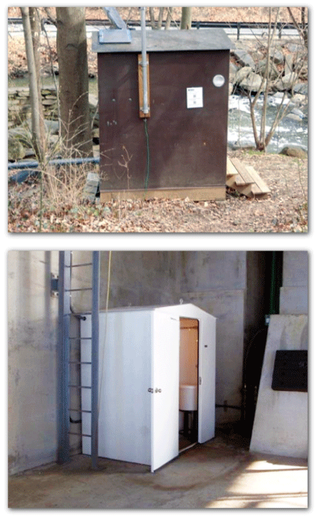
Photographs showing two examples of pre-constructed sampling station shelters. The brown stream-side shelter is constructed of wood; the white shelter is constructed of fiberglass. Photograph by U.S. Geological Survey.
Special Sampling Conditions
Autosamplers have been deployed to sample at many different non-riverine settings, these include:
-
Sampling at dams and sewage treatment plant outfalls.—Installations at dam outfalls, sewage treatment plants, and industrial plants are generally of a more permanent and straightforward design. At these locations, it is often possible to deploy an autosampler inside or near secured structures or buildings with access to electrical power, and in some instances, to connect sampling inlets directly into the plant structures or piping (fig. 4). Permission should always be obtained from facility owners, and deployments should be coordinated with the assistance of plant supervisors and crew.
-
Bridges and abutments.—Shelters can be placed adjacent to or under road bridges and walkways. For example, the white fiberglass shelter shown in figure 3 (lower photo) was deployed under a lift-bridge of a public road crossing a shipping channel. Bridge deployments provide several advantages, for example, they provide a solid foundation to lock equipment and often provide protection of the inlet lines from high-velocity water occurring during storm events. They also allow for safe cross-channel sampling needed for calibration. It is important to obtain written permission from state and local transportation departments or bridge owner (for private bridges) before deploying equipment.
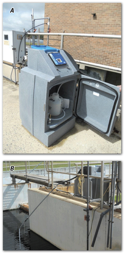
Photographs showing, A, an autosampler deployed at the outfall of a large public sewage treatment plant that collects daily composited samples for regulatory monitoring, and, B, the inlet line hanging into the outfall raceway. Photographs by U.S. Geological Survey.
Equipment Design
Active Sampler Systems
Active autosampler systems consist of five general parts (figs. 5 and 6): (1) an intake line running between the autosampler and the sampled stream; (2) a pump to pull or push water through the intake line; (3) a source of electrical power (if applicable); (4) an electronic system that monitors environmental conditions, initiates and controls the autosampler, and records sampling data; and (5) a container and distributor system that allows one or more sampling containers to be filled. Commercially available active autosamplers are available that incorporate these five components, but in some instances, it may be necessary either to customize these autosamplers, or develop specialized autosamplers based on standalone components.
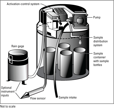
Components of a peristaltic-pump-based autosampler utilizing a self-contained control and data-logging system, rain gage, and flow sensor. Modified from Bent and others (2000).
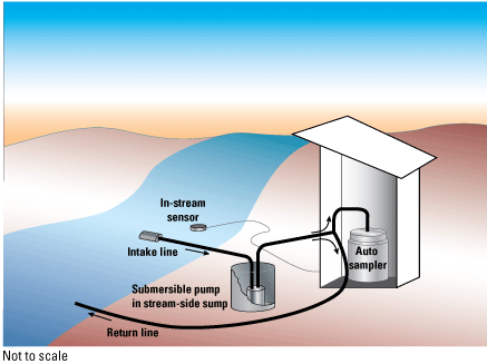
Components of a submersible pump-assisted auto-sampling system showing the five key elements of a pump-assisted system: the autosampler, intake and return lines, submersible pump, and the in-stream stage sensor.
Passive Samplers
Passive samplers do not utilize electrically powered pumps to obtain water, but rather use chemical sequestration to remove constituents of concern from water bodies. This document is not intended to discuss passive sampling systems in detail; however, a brief discussion of this kind of sampler is available in Box 1 to help the reader understand the differences in information provided by passive and active sampling systems.
Box 1. Passive Samplers
Passive samplers consist of a material that has a high affinity for sorption of chemicals of concern, such as hydrophobic organic compounds, pharmaceuticals, or trace metals. The materials are typically polyethylene plastic bags filled with organic solvent, lipid materials, or distilled water. Other types use man-made polymer resins, termed ion-exchange resin (XAD), to sequester dissolved constituents. Examples of passive samplers made of these materials include dialysis bags (such as semi-permeable membrane devices and activated charcoal samplers), and targeted resin-exchange sampler cartridges.
Passive samplers have been used successfully in rivers, sewers, channels, lakes, and other natural and man-made water bodies, and have been deployed in groundwater wells. They are deployed over long periods (weeks to months) and therefore produce concentrations representing both low-flow and storm discharge. Upon retrieval, the solid materials, films, or internal solutions are removed and sent for laboratory analysis.
Unlike active samplers, passive samplers collect only the dissolved phase chemicals of concern in the water body and produce an operationally defined “time-averaged” concentration. Indeed, a major drawback to their use is they do not define dissolved concentrations at a specific hydrologic condition, rather only a composite concentration over the length of deployment. Questions also arise concerning the reversibility of the membrane when deployed in the environment (that is, whether they can both gain and loose sequestered chemicals). Passive samplers are most useful for detecting the presence or absence of trace-level dissolved chemicals of concern, those present at levels too low to be measured in discrete samples (such as provided using active samplers).
The low-cost involved with their deployment, and the fact that elaborate sampling stations are not required, are advantages that passive samplers have over active types. Passive sampling techniques provide a low-cost method that can aid in designing active sampling programs, especially when large-volume sampling schemes are needed to detect extremely low-concentrations in a water body, and in conducting initial contaminant track-down studies throughout a watershed.
Pumping Devices
Commercially available autosamplers generally rely upon a peristaltic pump with internal, self-contained control, and a sample distribution and holding system. A typical autosampler is shown schematically in figure 7; this system includes a refrigerated chamber to hold sample containers. Alternatively, a component system can be developed around a peristaltic pump controlled by a stand-alone data logger. Usually, this system will produce only single bottle samples, either discrete or composited, although various more complicated systems utilizing valves can be designed to dispense to multiple containers.
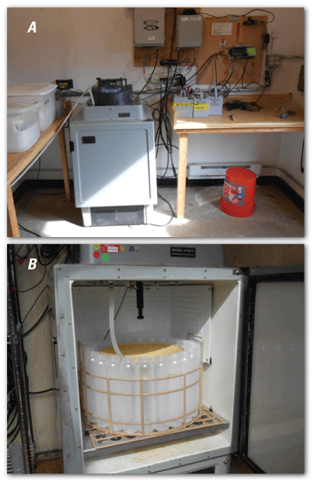
Photographs showing, A, a peristaltic-pump-based autosampler with refrigerated sample chamber, and, B, the multiple plastic sample bottles held within the chamber. Photographs by U.S. Geological Survey.
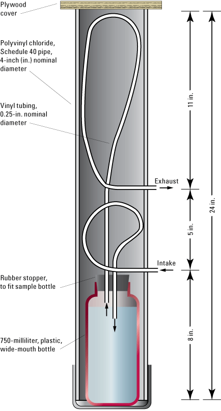
An example of a novel autosampler used to collect multiple samples of stream water is shown in figure 8. This system uses a small submersible pump and valve system to collect multiple 40-milliliter (mL) volume samples for volatile organic compounds. The unit contains an internal microcontroller (or data logger), and the autosampler is lowered into a standpipe set into the riverbed (fig. 8B). A separate housing at the upper end of the standpipe contains communication equipment for remote monitoring. The controller turns the pump on at preselected time intervals and operates a valve system that selects the bottle to be filled. Water flows directly into the bottle through a needle; each sample requires no further handling or processing in the field and is sent directly to the analytic laboratory. Although this system was designed to collect samples on preset timed intervals, the programing system is adaptable to other triggering signals.
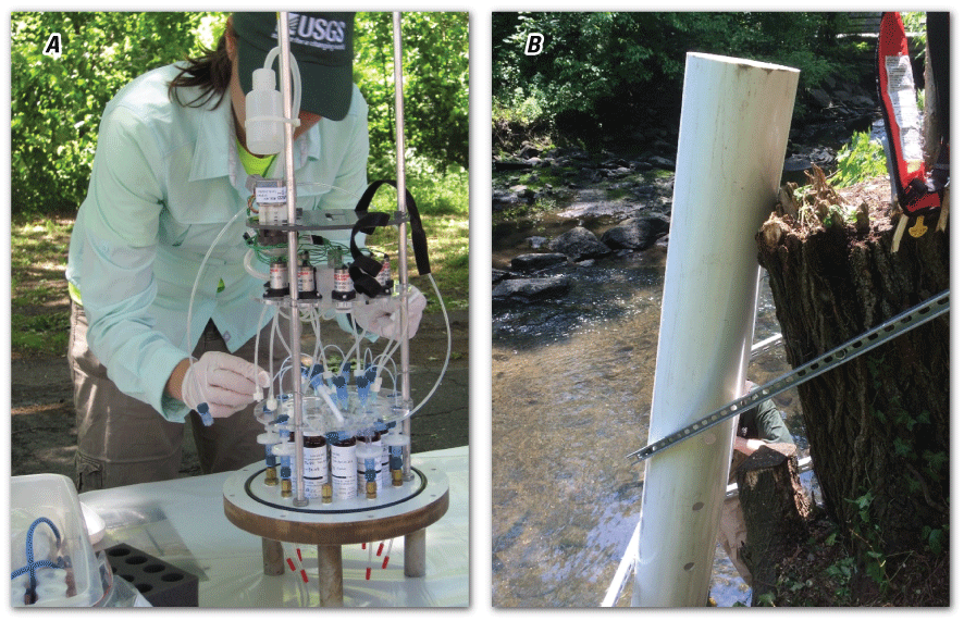
Photographs showing an automatic sampler first designed and described by Fitzgerald (2014) and its deployment: A, an autonomous autosampler designed for collecting multiple samples for dissolved volatile organic compounds, and, B, the plastic standpipe set in the river channel in which the autosampler is deployed. The autosampler uses a small microcontroller to open solenoid valves allowing sample vials to be filled during specified conditions (such as time or stage). Photographs by U.S. Geological Survey.
It is possible to modify commercially available autosamplers to fit specific project needs. For example, figure 9 shows an autosampler that was adapted to collect large volume samples (in this case, up to 75 liters [L] of water) required for analysis of trace organic constituents; in this instance the autosampler is housed in a small trailer to facilitate temporary deployments.
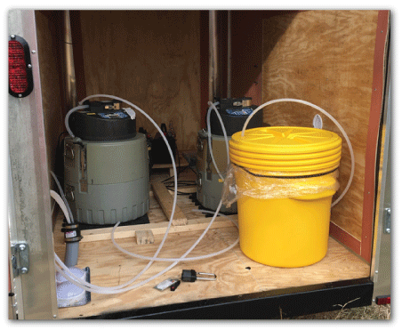
Photograph showing autosamplers deployed streamside in a small trailer. One autosampler has been adapted to collect a large-volume composite sample in a Teflon bag held in a 75-liter yellow plastic tub. Photograph by U.S. Geological Survey.
Advantages of the peristaltic pump systems include their commercial availability, their ability to be powered using batteries or line electricity, and their ability to reverse pumping direction, allowing the intake line to be rinsed and purged before each sample or aliquot is collected. Disadvantages include the limited height over which they can obtain water (generally less than 25 ft total head lift), a limited intake-line distance (due to head loss in the line), the need to replace worn or contaminated pump tubing, and the susceptibility of samples to degradation while stored in the sampler before retrieval.
The second type of active system uses a submersible pump that is installed in the streambed (figs. 10 and 11) and comes with a range of advantages and disadvantages (table 2). Submersible pumps push water directly to a sample container, or alternatively, into a tub from which a peristaltic autosampler can be used to retrieve a sample. These systems are generally (but not always) powered by electrical line service, with the submersible pump buried in a sump in the streambed or adjacent shoreline. The pump can be left to run continuously or by using a data logger or timer, set to operate only when a sample is needed. Like peristaltic systems, submersible systems rely upon separate electronic control equipment to initiate the sampling, control the volume of each sample or aliquot, and record sample information.
Table 2.
Advantages and disadvantages for using submersible pumps.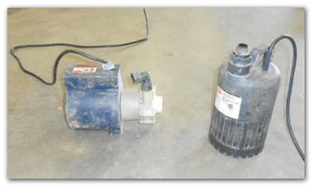
Photograph showing two types of submersible pumps suitable for use in an autosampler system. Left to right: pump with an epoxy coated motor and standard sump pump. Photograph by U.S. Geological Survey.
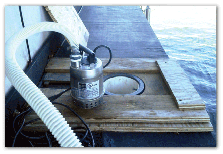
Photograph showing a stainless-steel submersible pump used in a sampling system installed on a bridge footing in an estuary setting. Photograph by U.S. Geological Survey.
It is also sometimes advantageous to combine both submersible and peristaltic pumps to collect water samples. These systems generally fall into two categories where the submersible pump either (1) delivers water at pre-selected time intervals to a vat where it is available to a second peristaltic-based autosampler, or (2) continuously delivers river water through a line, from which a second autosampler withdraws water at preselected intervals. An example is shown in figure 12, where a data-logging control system is used to operate the submersible pump that periodically (15-minute intervals, concurrent with stage and discharge measurements at the streamgage) fills a plastic tub. Water-quality data sondes were set in the vat to measure a variety of parameters including dissolved nitrogen and various chlorophyll compounds. The inlet line from a peristaltic-pump based autosampler (not shown) could be secured into the tub allowing samples to be obtained from the vat immediately following each sonde measurement; an electric solenoid valve then automatically opens to drain the vat.
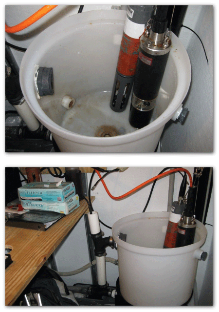
Photographs showing a component-type sampling system. The submersible pump shown in figure 11 is used to periodically rinse and fill the tub holding several water-quality data sondes shown here. If needed, the inlet line from a peristaltic pump autosampler (not shown) can be secured in the tub. Photographs by U.S. Geological Survey.
An example of another automated system was used by Bonin and Wilson (2006; modified from Litten, 1998) to sample river water for trace organic compounds in suspended sediment and water is shown schematically in figure 13. A submersible pump was used to continuously deliver water to the sampling station during storm events. The inlet of a peristaltic pump was attached to the submersible discharge line and used to periodically force a measured volume of water through a canister and flat filter, where suspended sediment was removed. A portion of the filtered water was then diverted using a positive displacement pump and was forced through a column containing XAD. Flow meters and water-weight were used to measure the volume of water processed; total volumes processed were typically 150 L through the filters, and 50 L through the XAD column. The sediment trapped on the filters for sediment-bound contaminants, and the XAD were eluted and analyzed for dissolved-phase constituents.
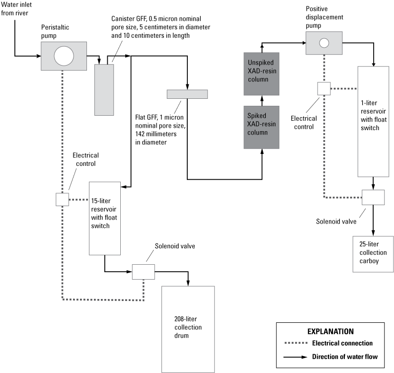
Schematic of a large volume auto-sampling system designed to collect suspended sediment and extract dissolved organic compounds for chemical analysis using ion-exchange resin cartridges. Modified from Bonin and Wilson (2006). [GFF, glass fiber filter; XAD, ion-exchange resin]
The third type of active system is the vacuum or siphon sampler; these use an evacuated sample container within the vacuum that causes water to be drawn directly into the container. An advantage of this system is cleanliness, as the water sample does not contact the pump. Disadvantages include the limitations of intake line length and height of water draw (typically less than 25 ft), vacuum leaks in the system may be difficult to eliminate, and these samplers cannot be used to collect water for analysis of dissolved gases or volatile organic compounds. An example of siphon sampler system is shown in figure 14.
Cross-section of a siphon sampler showing a bottle and tubing used to collect samples. Modified from Graczyk and others (2000).
Operating Power
All active autosamplers require electrical power and consideration must be given to power sources when designing and installing a system. At sites where the distance between the water source and the pump are short, or when deployments are temporary, 12-volt direct-current batteries can be used. Batteries may be provided by the autosampler supplier, or high-amperage automotive and marine batteries can be used. Typically, the electronic data-logging and telemetry equipment will use lower voltage-amperage batteries, solar power, or both. When batteries are used to power pumps, it is generally necessary to install freshly charged batteries immediately prior to a sampling event, and to connect several batteries in series as backup. If the autosamplers are prepared and ready to operate but are subjected to long intervals between uses or if extended pumping time is expected, then extra field effort must be planned.
Wherever possible, the use of AC-line power is preferred, especially when autosamplers are deployed for long periods of time and when submersible pumps are used. The use of heaters required for cold-weather deployments, or refrigeration during hot weather, will also generally require AC-line power. Line power will provide sufficient amperage, and removes the need to monitor and change batteries, and will certainly reduce the chance for missing samples due to battery failure. The possibility of unexpected voltage drops must be considered if long-runs of lines are needed between the service and remote pumps and equipment.
Finally, if line power is available or can be installed, the electrical service must be installed and checked by a certified electrician and must meet all applicable local and state electrical codes. It is imperative that special care is given to protecting field crews from electrical shock by using proper grounding and ground fault interrupter outlets by keeping floors dry and periodically inspecting the insulation of electrical lines.
Control Systems
Autosampler equipment is controlled using electronic systems that monitor time, stream, or other environmental parameters that determine the appropriate time to power the autosamplers to collect a sample, monitor specified volume of each sample or aliquot, record a date or time stamp for each sample, and log ancillary environmental data. The choice of using built-in control systems or stand-alone control systems to record, store, or transmit data should be made after careful consideration of project goals, budgetary constraints, distance from office to field sites, and other such factors.
Regardless of the autosampler system deployed, the system needs to record certain information for each sample or aliquot collected. At a minimum, a record of the date and time each sample or aliquot was collected. It is also advantageous to log additional instrument parameters such as number of pump rotations (per sample and total), battery power, pump pressure or suction, and other such mechanical and electrical variables. For example, monitoring the pump pressure and pump-head rotations per sample allows the condition of the pump tubing and intake line to be assessed. Table 3 presents some of the typical parameters to collect when operating an autosampler system.
Table 3.
Typical parameters for operating an autosampler system.[NA, not applicable]
Built-In Control Systems
Generally, the control systems of commercially available autosamplers are proprietary and specific to each manufacturer. It is imperative that the ease of operation, programming, and control adaptation are considered before new equipment is purchased. It is also imperative that the field crew be familiar with the programming and operation of the autosampler controls. Operation programs should be extensively tested in-house, and tested in the field, before project sampling is conducted. If difficulties are experienced in programing or selecting equipment, help can be obtained from the manufacturer (ISCO, 1994) or experienced researchers who can be found throughout the USGS.
Most commercially available autosamplers contain systems that allow researchers to monitor autosampler operations while on or offsite, although this often requires the purchase of additional, specialized equipment. It is important to consider the ease at which operation data can be accessed, and whether any ancillary data (such as that generated by water-quality sondes and acoustic equipment) can be used by the autosampler, before purchasing equipment.
When only basic parameters (such as stage) are needed to control an autosampler, it will usually be most cost effective to rely on built-in commercially available control systems that will not require extensive programming or the purchase of specialized accessories. Where multiple triggering and control variables are used in complex programming routines, it may be more advantageous to use a stand-alone control and data-logging system.
Stand-Alone Control and Data Loggers
Often, after a thorough examination of the goals of the study and characteristics of available equipment, a stand-alone control and data-logging system is needed to provide the flexibility, control, ease of access, and storage of data required for the project. These systems can record and utilize data from various independent sensors, such as water-quality sondes, to operate sampling equipment and can often provide remote access and programmability through cellular or satellite communications. A thorough cost-benefit analysis should be performed to determine if it is more cost effective to control the sampling equipment using a flexible stand-alone control system, or the (often more rigid) options available in a built-in control system. This analysis must not only consider cost, but also the time required to design and test specific computer code needed by stand-alone equipment. However, for many projects, once a “standard” control program is developed, it can easily be modified to the specifics of each sampled water source.
One benefit of stand-alone control systems is the ability to communicate and control the sampling equipment remotely via phone lines, radio, or cellphones; as often this allows the operating parameters of the autosampler to be adjusted or changed based on field conditions. In this regard, before proceeding with a stand-alone control system, the following should be considered:
-
Will it be necessary or advantageous to remotely monitor and obtain the status of the autosampler equipment?—Data that relate to the status of the autosampler equipment include the time sampling was initiated, the bottle number and date and time the most recent bottle was filled or aliquot collected, and any errors that were encountered in the sampling, for example, a clogged inlet line, power outage, or broken pump tubing. The ability to evaluate in real-time the conditions, equipment, and program status can save considerable field effort, especially in large watersheds.
-
Will it be necessary to adjust triggering and sampling parameters immediately before a precipitation event occurs?—For example, a last-minute change in the magnitude of a rain event may require a change in the stage (or other triggering parameters such as turbidity, velocity, or discharge interval) that initiates sampling. The ability to remotely adjust such parameters can greatly reduce the field effort needed for a project.
-
Will it be possible for the autosampler to access and utilize river or other environmental data produced at a nearby USGS streamgage station?—The ability to access existing streamgage station data can reduce the total cost of the project because it replaces the need to have expensive, dedicated equipment deployed such as stage-pressure transducers, velocity transducers, and water-quality sondes.
-
Will it be necessary to access other environmental monitoring data for the sampling site, but not needed for the operation of the autosampler?—Examples include specific conductance, dissolved oxygen (DO), turbidity, precipitation, water and air temperature, barometric pressure, wind speed, and other parameters. It is often advantageous for a study to collect these environmental parameters at a higher frequency than the sample collection times.
After considering these questions, it may be advantageous to utilize stand-alone data loggers to measure river parameters, control the timing of sampling equipment, store sample and stream data, and report to remote locations the status of the sampling and river conditions. Numerous data-logging and control systems are commercially available that allow multiple stream and water-quality parameters to be stored and utilized for control of an autosampler, and to transmit information via radio or phone systems. The measured parameters, as well as data produced from a nearby USGS streamgage station, can be logged and used to trigger and operate the autosamplers. Data obtained from USGS equipment is available either as a numerical stream of digital data, transmitted via wire line or radio from the gaging equipment or, in some cases, as a direct-electrical signal from equipment such as pressure transducers (in a bubbling system, for example), stage or velocity (from radar or acoustic monitors), or parameters measured by water-quality sondes. However, it is imperative to notify and obtain permission from the relevant Science Center before undertaking a connection to existing USGS streamgaging station equipment.
Figure 15 shows a schematic of a system configured to use a stand-alone controller and data logger to operate two autosamplers; one autosampler collects discrete water samples needed to produce the time-sequence of conditions in the river, while the second autosampler produces a composite sample for chemical analysis. To produce a time- or discharge-weighted sample, the data logger monitors numerous stream parameters (such as stage), calculates and sums discharge, and starts sample collection at the desired intervals. Alternatively, the system could read several parameters from a water-quality data sonde (such as turbidity, specific conductance, DO, and temperature), monitor for the onset of precipitation, and begin sampling with the onset of pre-selected conditions. Any of such parameters can be used to initiate and control the autosamplers, and the data logger can be programmed with the relevant stage-discharge relation needed to track and initiate operation of the composite sample. In addition, the data logger records sample data (time and date) and equipment status, and if the system is equipped with a telemetry system (radio, satellite, land line, or cellular phone systems) allows the field crew to remotely monitor and if necessary, adjust or stop the sampling equipment.
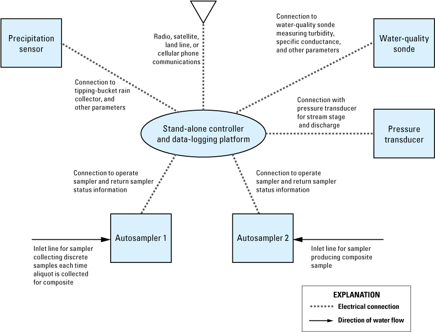
Schematic of a system configured to use a stand-alone controller or data logger to operate two autosamplers.
Analyte-Specific Considerations
When selecting autosampler equipment, careful consideration should be given to the class of analyte(s) being studied. Many analytical parameters require that only certain materials contact the sample; materials made of substances that will not contaminate or alter the sample by absorption or leaching of chemicals. The components that contact the sampled water include the intake line, pump tubing, distributor line, tubing connectors, sample containers, and any check- or diversion-valve (if used). These components are typically made of metal, plastic, glass, or possibly ceramic. The amount of reaction between the material and the sample will depend on the material composition, the chemistry of the water sampled, and the elapsed time the sampled fluid is in contact with the material. In general, the softer or more flexible forms of plastic or metal are more reactive than the rigid forms, and the more polished a surface the less reactive the material tends to be (U.S. Geological Survey, 2014). Table 2-1 in chapter A2 of the USGS “National Field Manual for the Collection of Water-Quality Data” (NFM) is a good reference to use when selecting the proper material for a given set of analytes (U.S. Geological Survey, 2014, p. 16).
For more information on the preservation requirements and holding times for specific analytes, see the National Environmental Methods Index (NEMI) at http://www.nemi.gov or contact the laboratory that will be analyzing the samples. It is not within the scope of this report to list all analyte-specific considerations for all parameters analyzed by the USGS; however, some general groups can be discussed. Table 4 lists some of the major groups of constituents for which autosamplers are commonly used, some of the criteria for preservation, and some of the general holding times typical for each parameter group. For more specific information on each analyte of interest, contact the USGS National Water Quality Laboratory or the contract laboratory doing the analysis for the project.
Table 4.
Criteria of autosampler components, preservation considerations, and general holding times for selected constituent groups.[C, Celsius; HDPE, high density polyethylene; PTFE, Polytetrafluoroethylene (Teflon); VOC, volatile organic compound; —, no comment]
Generally, for suspended sediment, major-ions, and nutrients, low-cost plastic lines and bottles can be used. For trace metals, only Teflon or Teflon-lined tubing and connectors should be used. It is often possible to replace the original metal parts in the autosampler, such as connectors, with plastic or Teflon parts. When sampling for trace organics, either Teflon (preferred) or stainless-steel tubing may be used. All parts of the autosampler, the intake lines, pump tubing and connectors that come in direct contact with a water sample should be cleaned by following USGS cleaning protocols before deployment (Appendix 2). If a permanent intake line is installed, then project-specific methods must be developed to ensure its cleanliness (or replacement) between sampling events.
Consideration must also be given to sample preservation and hold times, and the effort needed to shorten the interval between collection, preservation, and retrieval. Hydrologic event sampling is often conducted over days and weeks, and time-sensitive samples need to be removed and processed as quickly as possible after collection.
Special Sampling Situations
While most sampling conducted by the USGS involves natural systems (rivers, streams, lakes, estuaries, and groundwater), autosamplers are often used in special situations where sampling is conducted for non-typical analytes, such as pharmaceuticals or microbiological constituents. These studies may include sampling sewage from sewers, sewage treatment plant inlets and outfalls, and even septic systems. The composition of these wastes often varies greatly over the period of a day, and autosamplers afford a means to characterize the waste chemistries. Sampling raw and treated wastes requires special handling and safety considerations which are not discussed in this document, but with care, samples can be safely obtained using an autosampler. Help and advice in designing sampling systems can often be obtained from the environmental monitoring staff working at local public sewage authorities.
Drainpipes and Culverts
Autosamplers are invaluable for collecting samples from pipes and culverts that discharge intermittently. It is often possible to deploy autosamplers in temporary installations next to culverts, or in existing pump houses or diversion chambers, if present. Deployments as simple as setting the autosampler on the ground and securing it to a nearby tree, then installing a temporary sampling line and liquid detector system have been used successfully. However, a common problem encountered when sampling culverts is securing the inlet line at an appropriate depth, because flows can rapidly fluctuate between extremes (from a trickle to a deluge and back). Consider commercially available weirs and inlet-line fixtures when installing intakes in pipes, these have been designed to help keep the line in place while maintaining proper flow velocities and a sufficient water pool for sampling.
Manholes and Sewer Chambers
Because of the need for regulatory monitoring in sewer lines either in streets, or at treatment-plant inflows or outfalls, specialized sewer equipment is available. For example, special hangers are available that allow an autosampler to be suspended under the lid of a sewer manhole, with the inlet line run down into the sewer and equipped with a debris screen. Sewage treatment plants often have dedicated sampling chambers with built-in conduits designed to hold inlet lines in place, often including screens to keep solids from clogging the intake.
Considerations when deploying an autosampler for sampling sewer lines include: (1) the ability to keep the intake line in place in the sewer without introducing equipment that could permanently constrict or block flow in the sewer; (2) working safely in a confined space where explosive or corrosive gases are present; (3) maintaining the intake line in place when extremely high flow velocities are encountered, such as occurs at the intake to a large public sewage-treatment facility; and (4) exposure of personnel and equipment to biologically hazardous sewage.
Additional Features to Consider When Designing an Autosampler System
The design of autosampler systems often include features that may prove useful or necessary to achieve the project goals. Some of these include
-
Multiple control systems and sensors.—A variety of sensors can be added to an autosampler system to monitor environmental conditions, control the timing of sample collection, and record sample data. Common sensors include water pressure (to monitor water level), rain sensors and collectors to monitor precipitation (start and total), velocity meters to measure water velocity and direction, and turbidimeters to measure suspended material. Autosamplers can be set to activate upon a change in any of these parameters, and redundant sensors can be deployed to ensure that sample triggering occurs.
-
Fluid monitoring.—Autosamplers often contain a fluid detector located at the pump or along the inlet line. These monitors can be contacting (paddle wheels) or non-contacting (ultrasonic flow) types and allow actual sample volume to be detected; they also allow the sampling pump to be automatically reversed, thereby purging and rinsing the inlet line with air or water between each sample. Submersible pumping systems can also be equipped with fluid monitors but must rely upon diversion valves to allow purging.
-
Refrigeration.—Refrigerated autosamplers are available that chill the collected sample water, thereby removing the need to manually ice samples for preservation purposes. Refrigeration is essential when sampling for nutrients or bacteria, which have short holding times. It should be remembered that the interior of sampling structures, and sampling equipment, can warm considerably especially during warm seasons. However, equipment to cool collected samples will require additional power sources and will require additional oversight by field crews.
-
Heating.—Intake lines can be equipped with heated lines that keep the equipment, sample containers, and collected samples from freezing in cold weather.
-
Multiple container types.—Most commercially available autosamplers are designed to hold a variety of different bottle types and volumes that allow flexibility to meet different program goals. Commonly, autosamplers hold bottles that range in volume from 1 L to 4 L, and typically, the sample chambers can also be configured to hold a single large (10–25 L) carboy. Bottles can be glass, metal, or plastic to accommodate different requirements.
-
Programming flexibility.—Commercial equipment usually can be programmed to allow one or more discrete samples to be collected and a single sample to be prepared by compositing multiple aliquots of water. Autosamplers controlled by stand-alone data loggers and controllers can be programmed with highly complex control code that evaluates data from multiple sensors; it is often possible to reprogram or readjust sampling parameters via external communication systems. This flexibility in programming allows for replicate samples to be collected, as well as multiple complex adjustable composite sampling schemes.
-
Consistency in multiple deployments.—In conducting studies in large regional watersheds, it is often necessary to sample synoptically at multiple, widely spaced sites. The use of one type of autosampler and other equipment at all sites in these studies greatly helps ensure consistency in sampling and reduces the effort to train field personnel.
-
Telemetry.—It is possible to connect autosamplers to telemetry systems, consisting of either radio, satellite, land line, or cellular phone systems. This allows off-site notification of sampling initiation, monitoring of sampling progress, notification of autosampler equipment failure, and access to environmental parameters. In some cases, operating parameters can be changed remotely to accommodate changing weather and flow conditions. This option provides a considerable increase in efficiency of the sampling effort, thereby lowering costs for travel and field crew deployment.
-
Solar powering.—Some equipment, not only the electronic control and telemetry systems but autosamplers as well, can be powered using batteries that are kept charged using solar panels. The telemetry systems can be used to remotely monitor the status of batteries, helping the field crews to ensure that equipment is always ready for use.
Considerations for Intake-Line Design and Installation
Regardless of the water source being sampled, an autosampler deployment will involve installing an appropriate intake line at a pre-selected location in the sampled stream. In many cases, the location where a newly constructed station will depend, in large part, on the ability to set the inlet location at the best-possible point in the channel, and to safely install the intake line. Some of these factors, such as the ability to wade safely or the presence of nearby bridges to measure cross-channel flow, the stability of riverbanks and streambeds, and other physical conditions, have already been mentioned. Other, site-specific factors may also need to be considered when designing and constructing the intake lines.
It is helpful to determine the optimal location of the inlet line nozzle in the stream before addressing station construction. The intake line nozzle must be located at a point where, as much as possible, the water collected by the autosampler is reasonably equivalent to a sample collected by traditional USGS manual collection methods, such as EWI or EDI sampling. Locating the inlet point at the optimum spot in the channel is one of the most important steps in designing an autosampler deployment plan.
Selecting Location of Inlets in Rivers and Streams
In any study that uses an autosampler, it is the responsibility of the researcher to demonstrate that the intake point is located where a reasonably representative sample of the river channel can be collected. The velocity of water flowing in a stream varies within a channel’s cross section, with the highest velocity near the center of the channel (termed the thalweg). This results in a complex distribution of velocities across the channel, causing an inhomogeneous distribution of suspended sediment in the channel, both in the vertical and horizontal directions. Meanders and obstacles in the stream shift the thalweg position and cause turbulence in some areas, while other areas in the channel velocities may be much slower (even imperceptible). Input from tributaries and storm-water outfalls also affect the cross-channel distribution of dissolved components and sediment, and it is common to have inputted water travel a considerable distance downstream before the channel becomes well-mixed. For an autosampler to accurately characterize a stream, careful consideration must therefore be given to the placement of the intake.
The primary concern of the researcher is to determine how well a sample collected at a single point in the stream (the nozzle location) represents the water and suspended sediment in the entire cross section of the stream channel. A “best” or representative sample can be obtained by placing the autosampler intake at a point where the stream concentration approximates the mean cross-channel concentration of the parameters of interest, over the full range of expected streamflow. This goal has great merit, but to locate the point in the cross section where the mean cross-sectional concentration can be obtained (for each parameter of interest) may take considerable effort, and this point may change under different discharge regimes. Specific guidelines for locating the ideal intake position in a water body would have little transfer value among different reaches of a stream, or among different streams. For this reason, modifications have been applied to the findings of Edwards and Glysson (1999) and are presented as generalized guidelines in the following sections. Finding the optimal nozzle location in a cross-section is typically less a factor when sampling is for dissolved components, as turbulence in the flow usually results in good cross-sectional mixing for the dissolved phase. This may not be the case, however, for suspended sediment, where the cross-sectional distribution for sediment is controlled in large measure by the velocity distribution and velocity is seldom uniform in a channel.
Determining Mean Cross-Channel Concentration
The following guidelines aid in locating the intake of a sampling line in a stream, river, or channel. Once a location has been chosen, cross-sectional measurements should be repeated at various discharges throughout the project to demonstrate the continued suitability of the location.
Find stable banks and bed.—Select a cross section where the banks and streambed appear stable, and depth is reasonably uniform (no deep holes, for example). If the channel appears stable, then the relation between the concentration at the sampling point and the cross-section mean concentration will likely remain stable over time. If the relation between the concentration at the sampling point and the mean cross-sectional concentration is unlikely to be stable over time, then an alternate location should be considered. If the autosampler must be installed in an area where the banks are unstable (for example, along a meander), then the intake should be placed on the eroding side of the channel, helping to ensure the intake does not become buried by encroaching depositing sediment.
Find an accessible sampling location.—Select a location where the stream can be safely accessed and waded or near a bridge where cross-channel calibration sampling can be safely conducted. However, if an autosampler station is placed near a bridge or structure, it is preferable to site it upstream of the structure or where there is evidence that bridge scouring is not occurring. When siting a station near an outfall or a confluence with a tributary, it is important to locate the inlet as far downstream as possible to allow mixing to occur.
Demonstrate cross-sectional variations in flow.—Conduct a study to determine the variation in velocity, temperature, turbidity, and specific conductance across the channel. If suspended sediment is called for in the project, then collect grab samples at 10 to 20 EWI across the stream, and where depths allow, at 2–3 depths in the vertical at each sampling interval. This study should
-
• measure these parameters over as wide a range of flow regimes as possible given time and budget constraints. At a minimum, cross-channel measurements should be made when discharge is below and above the historic mean flow discharge (if known).
-
• use standard USGS procedures for wading or bridge deployments when taking flow measurements. Towed acoustic Doppler current profiler measurements are especially useful in this regard.
-
• use a portable water-quality data sonde to measure temperature, specific conductance, and turbidity.
Calibrate the autosampler intake for suspended sediment.—If velocity or turbidity data show the cross section is well mixed and the program involves studying suspended sediment, then a study should be initiated to calibrate the autosampler intake for suspended sediment using a standard USGS depth- or point-integrated sample. This study should
-
• determine the depth at which the mean concentration exists in each EWI vertical for each size class of particles smaller than 0.0625 millimeters (mm; fine-sand), from a series of carefully collected depth-integrated samples. Set the autosampler intake at this point and collect at least one discrete sample during the time period that each depth-integrated profile sample is collected. Calculate a mean concentration of suspended sediment (SSC) for the discrete samples collected by the autosampler and compare them to the mean concentration in the depth-integrated samples. Repeat this step during several different stream-discharge regimes to ensure the concentrations obtained from the autosampler intake point remain representative over the range in streamflow of interest to the project. At a minimum, these measurements should be made at base flow and above median discharge (if known).
-
• use the results of these measurements as a guide to the placement of the intake. If necessary, alter the location of the intake and repeat sediment calibration sampling outlined above.
Avoid interference or contamination from bank or bed material.—Place the intake in the stream at a distance far enough from the bank to eliminate collection of sediment from bank erosion. Ensure the intake is at a sufficient height above the bed so that migrating bed sediment is not captured, but at a depth sufficient to ensure the intake remains submerged during low flow. Avoid placing the intake in an eddy or behind a boulder or other obstruction, as the intake will probably not collect a representative sample.
Protect the intake tube.—Consideration must be given to protecting the intake nozzle and tubing from debris carried during high streamflow. The intake line should be armored, staked to the streambed, covered with large gravel, and if possible, buried in the stream bank and bed to ensure its protection. However, care should be taken to ensure that any tube armoring does not alter the general flow in the stream.
Example of Determining Channel Cross-Sectional Homogeneity
An example of data collected to determine cross-sectional homogeneity are presented in table 5 and figure 16. Discharge, specific conductance, DO, and SSC were measured at 10-ft intervals across a 290 ft wide channel in the Passaic River, approximately ¼ mile downstream of its confluence with the Pompton River, located in northern New Jersey (U.S. Geological Survey, 2024). The measurements were made using a water-quality sonde and by collecting individual grab samples. Sampling was conducted during low-flow conditions with a water depth of approximately 3 ft. Preliminary cross-section measurements of turbidity showed the river was well mixed vertically, so multi-depth measurements and samples would not be required. A three-person field crew then began sampling: one person collected samples from EWI locations across the channel, the second made sonde measurements, and the third collected discrete grab samples immediately upstream of the intake point.
Table 5.
Cross-sectional data from U.S. Geological Survey station no. 01389005 Passaic River below Pompton River at Two Bridges, New Jersey.[Data are from U.S. Geological Survey (2024). Time given in military time. ft, feet; mg/L, milligrams per liter; °C, degrees Celsius; μS/cm, microsiemens per centimeter; ft3/s, cubic feet per second; Q, rate of discharge in flowing water; LEW, left edge of water; REW, right edge of water; %, percent; NA, not applicable]
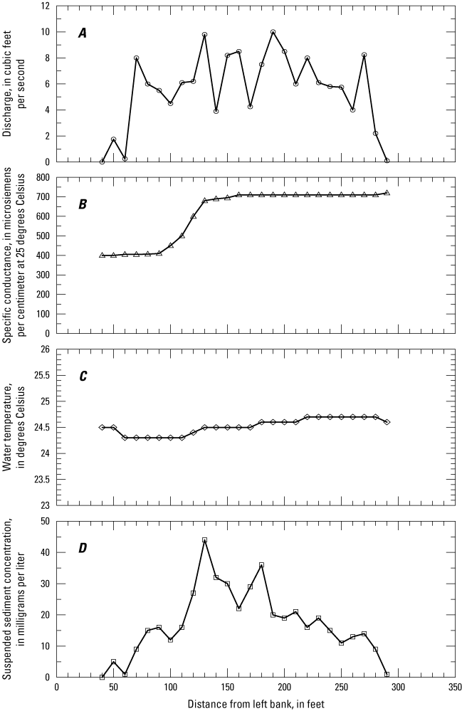
Cross-sectional water-quality data collected in a poorly mixed river channel. Plots show, A, discharge, B, specific conductance in microsiemens per centimeter (μS/cm), C, temperature, and, D, suspended-sediment concentration in milligrams per liter (mg/L).
The cross-sectional data indicated that the channel was poorly mixed at this section. Velocity varied considerably among the section, with three areas where no velocity was apparent. The specific conductance data show a demarcation between low values (approximately 400 µS/cm) near the right bank and high values (approximately 700 µS/cm) at about 100 ft from the left bank; temperature and SSC were also high near the right bank. Dissolved oxygen concentrations (not shown in figure 16) were constant across the stream channel. This was not unexpected because of the shallow water depth.
On the basis of this study, it was deemed that three inlets would be required to adequately characterize the channel: one inlet located at 75 ft, another at 150 ft, and a third at 220 ft from the right bank. A system was installed that used a submersible pump equipped with an automatic valve that allowed each sampling line to sequentially deliver water to a plastic tub in the station. A continuous water-quality sonde was deployed in this tub and set to measure water parameters each time the tub was filled. When needed, an autosampler was set besides the tub, and intake line was installed to the tub. A stand-alone data logger was used to control the pump, valve, sonde, and autosampler.
The variability in the cross-section values can be quantified by calculating the percent difference between the maximum and minimum values for each parameter using the following formula for equation 1:
The percent difference between the minimum and maximum values in the example cross section were found to be 1.6-percent for temperature, 57.2-percent for specific conductance, 182-percent for suspended-sediment concentration, and 200-percent for discharge. This demonstrates that the cross section is not well mixed for dissolved ions (specific conductance), suspended sediment, and discharge during periods of low flow. Nearly identical results were obtained from measurements made later at higher discharge conditions.
Subsequent sampling was conducted to determine if the three intake lines were placed in appropriate locations in the cross section to produce an accurate “average” sample. Water collected from the right, middle, and left intakes were compared to the flow-weighted cross-sectional mean values. Cross-sectional flow-weighted mean values were calculated to be 10.8 milligrams per liter (mg/L), 24.5 degrees Celsius (oC), 671µS/cm, and 20.4 mg/L, for DO, temperature, specific conductance, and suspended-sediment concentration, respectively. Mean values in the samples collecting through the three intake lines were 10.6 mg/L, 24.5 oC, 601µS/cm, and 21.0 mg/L for DO, temperature, specific conductance, and suspended-sediment concentration, respectively. These values correspond to percent differences of 1.9-percent for DO, 0 percent for temperature, 11-percent for specific conductance, and −2.9-percent for suspended-sediment concentration. Of the three inlets, the right inlet most closely approximates the mean DO and suspended-sediment concentration, while the middle most closely resembles the specific conductance. These results demonstrate that while cross-sectional variability is high, the intake lines are positioned such that the average sample closely resembles the flow-weighted mean of the cross-section.
Determining Flow Lines Using Dye Studies
Dye studies are another method available that, under certain circumstances, can be used to determine the cross-channel heterogeneity and the representativeness of sample intake location. Dye studies are especially useful when the sampling site is located downstream from a tributary. Rhodamine dye is introduced upstream of the sampling point and its concentration determined in a series of samples collected using the autosampler and in samples collected across the channel (EWI grab samples). Dye concentrations are then analyzed in the samples using an in-field spectrophotometer and percent differences are calculated using equation 1. If a dye study is being planned, then it is important to obtain all necessary authorization before releasing dye into a public water body.
Intake-Line Construction
After the intake location has been chosen, consideration must be given to its design and construction. Because of the myriad of configurations possible, only general suggestions are provided here.
In its simplest form, the intake line is a plastic or metal tube that extends out into the channel from the bank side or sits near the stream bottom and extends up into the flow, with its nozzle orientated in the down-flow direction. More complex installations can be devised that incorporate not only inlet lines but water-quality sondes (fig. 17). The intake line should be kept as short as possible; the shorter the line, the less power will be used to draw in a sample and to flush the line, thus reducing power usage from batteries and wear on the pump tubing. A short inlet line also reduces pumping head-loss and thus helps maintain water velocity in the line, thereby minimizing potential for sediment to deposit in the line. If left in the river, then the exposed portions of the tube line may become stained with oxides, oil, and algae (fig. 18) and will need to be either cut off and extended, or the entire line replaced before each sampling event.
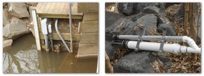
Photographs showing U.S. Geological Survey station no. 01648010, Washington, D.C.: A, the autosampler and control lines entering the creek, and, B, the inlet nozzle for the autosampler and housing for a water-quality data sonde. Photographs by the U.S. Geological Survey.
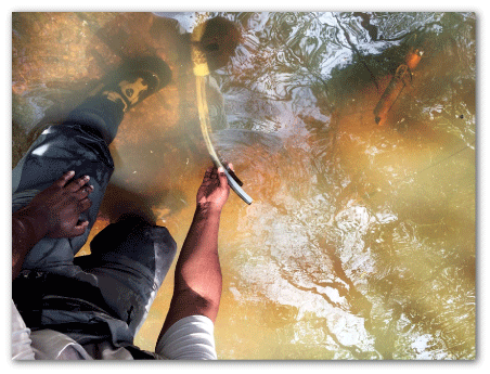
Photograph showing a new inlet being installed next to older lines. Photograph by U.S. Geological Survey.
Between the station shelter and the stream, the intake line will need to be secured against flood water, the impact of floating debris, and from vandalism (fig. 19). Burying the intake lines (encased in an armoring conduit) protects the lines from high water and places them out of sight from vandals. Once in the stream, the lines will need to be protected from trees and other objects moving through the water during floods; this can often be done using gravel or boulders taken from the stream, or riprap brought to the site. However, the intake armoring line should be designed to have minimal effect on the natural flow of the stream. As much of the armoring conduit should be buried in the streambed as possible. Steel pipes are good armoring conduits and supply more weight and stability than plastic pipes. If using steel pipes, ensure that any burs in the pipe are removed.
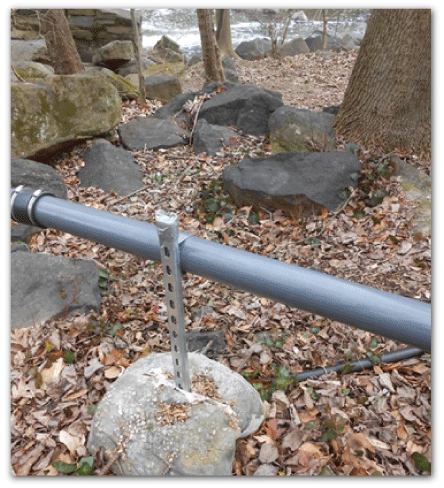
Example of steel and concrete supports used to hold intake lines in place along a riverbank. Photograph by U.S. Geological Survey.
A typical installation places the intake line at a single fixed point in the cross section, generally near the bottom in the deepest portion of the stream towards the area of highest cross-sectional velocity. This allows the intake to remain submerged during all streamflow conditions. If the intake needs to extend far into the stream, the line should be run along the stream bottom with the armoring pipe diameter being kept as small as possible. The lines can be held in place with rebar stakes or short steel fence poles driven into the streambed, and then covered with large riprap or sandbags. Care should be taken that the inlet line does not kink where it enters a structure, extra tubing length should be provided to keep bends smooth.
The intake nozzle should be raised up sufficiently so that it remains above the bed-sediment during high streamflow, thereby collecting only suspended materials and not coarser bed materials moving along the channel bottom. As much as possible, the lines should slope continually down-hill from the autosampler to the nozzle, without “dips” or low spots where sediment will accumulate. Bends where water sediment can accumulate should also be kept to a minimum, but if unavoidable, should be limited only to the ends of steep sections (down the riverbank). Where the intake line changes direction in the stream, for example, at the stream’s edge and at the nozzle, bends should be gradual, using sequential 45-degree bends. Angling the line diagonally out into the stream will help minimize the final bend used to direct the nozzle downstream. It is advantageous to install multiple intake lines, each set at different depths in the stream, to facilitate sampling over all stages (low to high). In using multiple inlet lines, the selection of the line to be used can be manual, or each line can have a dedicated autosampler, or a data logger and control system utilizing automatic valves can be deployed. Redundant lines also help to ensure that a storm event is successfully sampled if one line fails.
Intake-Line Dimensions
Consideration should be given to both the length and diameter of the intake line. The general rule is to use the shortest length and the largest diameter possible. Most commercially available autosamplers are designed to use either a 3/8 in. or ½ in. diameter intake line, so it is important to adhere to manufacture’s guidelines (ISCO, 1994). The diameter of the intake line and the pumping rate combine to control the pumping velocity in the line. If the pump rate is too low, then sand-sized materials may settle out and plug the line. If sediment is found to have settled in the line, the pumping rate should be increased, or the line diameter reduced. Table 6 lists the approximate pumping rates needed to keep silt-sized and fine-sand-sized particles in suspension in different diameter tubing. It is important that pumps are operated at a rate sufficient to maintain clay-, silt-, and sand-sized particles in suspension, and the pump rate should be checked to ensure sufficient velocity exists in the intake line under all sampling heads. This is especially important if a submersible pump equipped with larger diameter discharge tubing is used.
Table 6.
Pumping volume and rate needed to maintain medium grain-sized particles in suspension as a function of tubing diameter.[cm2, square centimeter; cm3, cubic centimeter; mm, millimeter; mL/s, milliliter per second]
An associated parameter is the volume of liquid contained in the intake line, as this is the volume of water that is required to completely flush the intake line and therefore, changes with river stage. The volume per foot of intake line, as a function of tube diameter, is listed in table 6. This volume is important when designing a system that flushes the intake line before each sample.
Armoring
In permanent or semi-permanent deployments, the intake line is typically armored (fig. 20) to protect it from damage during storm flow. Inlet lines can be armored using a steel pipe, or plastic tube (PVC; flexible or stiff) such as continuous 1–2 in. plastic waterline. Armoring should run from the sampling structure to the stream edge, then to near the inlet nozzle location. Using a continuous length of black plastic water line, with few or no connectors, allows the intake line to be easily removed and replaced (fig. 21). Between the sampling shelter and the stream bank, the line can be buried or covered with stone riprap. Within the channel, the lines can run on or be buried under the stream bottom, and kept in place using stream boulders or gravel, riprap, steel stakes (rebar or fence posts), or concrete anchor blocks. Used steel pipe (2–3 in. diameter) is an economical armoring tube and works well for armoring the lines in high velocity streams, because their extra weight helps keep them secured in the streambed.
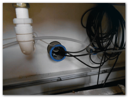
Photograph showing armored intake lines entering a sampling station. The intake line is the white plastic tube entering the conduit on the on the right. The larger conduit on the left contains cables for the pressure transducer and water-quality sonde.
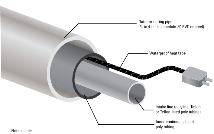
Cross section of an intake line consisting of an outside armoring pipe, an inner continuous plastic pipe, a heating tape, and the sample intake line.
Heated Lines
Where autosampler installations will be subjected to freezing temperatures, an electric heating tape, such as commonly used to heat gutters or keep water pipes from freezing, can be used to heat the intake line (fig. 21). The tape is wrapped around or placed next to the intake line within the armoring tube and extends from the autosampler out to the end of the armoring conduit. In temporary deployments in moderate climates where freezing temperatures are not expected to last, if the inlet lines are kept to a minimum length and follow a steep drop from the autosampler to the water, then heating will not usually be needed.
Use of Submersible Pumps
Where it is not possible to site the autosampler close to the water or when the elevation exceeds the ability of a peristaltic pump (approximately 25 ft), it may be necessary to use a submersible pump buried in or along the river edge. Submersible well pumps, pumps with an encased motor attached magnetically to a plastic impellor pump, can be used for these installations; an example of a submersible pump-assisted auto-sampling system is shown in figure 6.
When using a submersible pump, it is important that the electrical supply is properly installed. Waterproof electrical cable, like those used for residential water wells, is needed. In order to deliver water to the pump, a short intake tube is run out from the pump into the channel. Unless it is self-priming, the pump will need to be buried in a sump below the low water line. As a result, the sump and pump will need cleaning of sediment on a regular schedule. A submersible pump can be run continuously or if a data logger or timer is used, the pump can be started prior to sample collection. Often when using a submersible pump, an autosampler is connected to the pump outflow line. Whenever a submersible pump is used, consideration must be given to the type of materials used in the impellor pump, because the pump vanes are susceptible to abrasion by sediment.
Intake Orientation
The orientation of the intake nozzle will affect the sampling efficiency of an autosampler. There are five directions in which an intake can be oriented to the streamflow, as shown in figure 22: A, perpendicular to the stream bank, then turning and pointing upstream, B, perpendicular to the stream bank and to streamflow, C, perpendicular to the stream bank, then extending vertically upward into the water, D, perpendicular to the stream bank then extending vertically downward into the water, and, E, perpendicular to the stream bank, then turning and pointing downstream. Of these five, the orientations shown in figures 22A, 22C, and 22D should be avoided because they are known to cause high sampling errors and have problems with debris collecting on the intake (Edwards and Glysson, 1999). The orientation shown in figure 22B, with the intake positioned perpendicular into the streamflow, is the simplest to construct. However, with this orientation, sand-size particles may not be adequately captured (Edwards and Glysson, 1999). It should be emphasized that sharp turns in the inlet lines should be avoided as these often become clogged with sediment; all turns should be kept gradual and smooth.
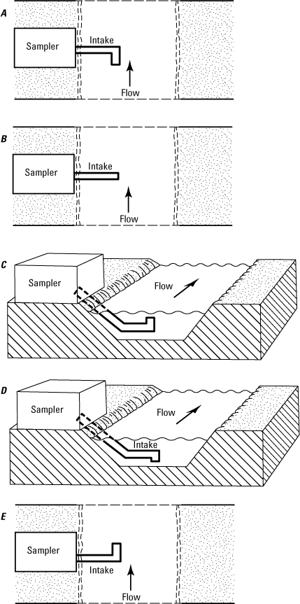
Diagrams showing the five orientations for intake lines in rivers: A, normal and pointing upstream, B, normal and horizontal to flow, C, normal and vertical with orifice pointing upward, D, normal and vertical with orifice pointing downward, and, E, normal and point downstream. Modified from Edwards and Glysson (1999).
Winterstein and Stefan (1983) and Winterstein (1986) found that sampling efficiency was highest when the intake was pointed directly downstream (fig. 22E) and decreased as the nozzle orientation was shifted towards a horizontal configuration (fig. 22B). Winterstein demonstrated that when pointed downstream, the intake causes a small eddy to form that envelops suspended particles, helping to obtain a representative sample of the suspended load, especially the coarser grain-sized material. A sampling efficiency of about 0.90 was achieved for all sands tested (Winterstein, 1986).
Winterstein (1986) further demonstrated the importance of the downstream configuration by testing the sampling efficiencies of intakes oriented at 45 degrees either side of pointing directly downstream. When positioned diagonally with respect to flow at 135 and 225 degrees, (with 180 degrees being directly downstream), sampling efficiency varied from 0.39 for 0.20 mm sized sand to 0.84 for 0.06 mm sized sand using an isokinetic withdrawal rate, and from 0.70 for the 0.20 mm sand to 0.90 for 0.06 mm sand at a rate that was twice the isokinetic rate. With an inlet line oriented diagonally across flow, a higher pump rate was necessary to match the sampling efficiency of a downstream orientation. The FISP studied the effects of non-isokinetic sampling with a nozzle (intake) pointed directly into the streamflow (Tennessee Valley Authority and others, 1941). The results of that study showed that the errors were negligible for sizes less than 0.06 mm.
Based on this information, Winterstein (1986) concluded that the size distribution of suspended-sediment samples collected by an autosampler with the intake set at any angle other than 180 degrees (directly downstream) to the streamflow will be biased towards the smaller sediment sizes. Particles in the silt-clay range will be only slightly under-represented while the sand-size material may be greatly under sampled. The bias increases with increasing particle size. It should be noted that none of the tests run by Winterstein (1986) used multiple-hole strainers placed over the intake. The use of a strainer may further affect the efficiency of the autosampler and its ability to collect a representative sample. If a screen is used, then it is instructive to compare samples collected with and without the screen to document the effect of the strainer. For more information on the orientation of the sample line, see Edwards and Glysson (1999)
Intake Nozzle Design
The intake point, or nozzle of the line, can simply be the tube end set at a fixed height above the channel bed. However, more elaborate designs can be used to maintain the intake nozzle at the same relative depth below the water surface. Similarly, the nozzle end can be left open or have a screen or strainer attached to the line.
Eads and Thomas (1983) demonstrated that an intake nozzle set at a fixed level will collect material from different portions of the flow profile, which changes as the stage and flow velocity change. They developed a depth-proportional intake device that maintains the intake nozzle at the same proportion of the stream depth regardless of stage (fig. 23). The device consists of a boom, an anchor on the streambed, a pivot, and a float. The unit is fixed in the streambed using an anchor, with the boom and float facing downstream. This design helps wash debris off the boom by the force of the flowing water. This device was originally designed for relatively small streams or culverts, as the boom length needs to be at least twice the maximum expected depth of the stream. The intake is attached to the boom at a point 0.60 times the distance from the pivot to the float; this allows the intake nozzle to remain at 0.60 times the water depth. This device is deployed with the orientation shown in figure 22E.
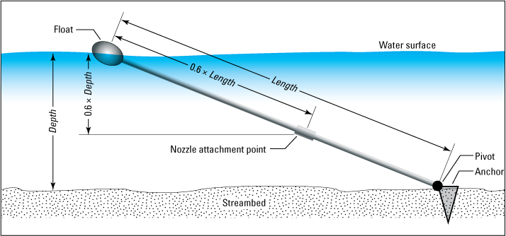
Diagram of a floating boom and mounting mechanism for anchoring inlet lines in a river. Modified from Eads and Thomas (1983).
For streams carrying a high sediment load (especially with sand), it is sometimes advantageous to attach a static mixer at the end of the intake line, as shown in figure 24. The mixer helps to (1) provide a secure mount for the intake line, (2) reduces the velocity of the water around the tube end, thereby aiding the pump suction to capture particles, and (3) helps mix the sediment in the water being sampled (Smith, 2002). Static mixers are especially helpful when sampling culverts, pipes, concrete channels, and ditches. Smith described this static mixer2 as follows:
“The static mixers were constructed from a 0.5-in. marine-grade homogenous polymer sheet and consisted of two semicircular plates 1.2 in. high at the center. Two plastic 0.5-in. bulkhead-compression fittings were attached to each side of the first plate 1.2 in. from the center and 0.6 in. from the bottom. The second plate had two semi-circular 0.7-in. holes in parallel with the bulkhead fitting to prevent sediment accumulation between the two plates and was mounted about 4 in. behind the primary plate.” (Smith, 2002, p. 14)
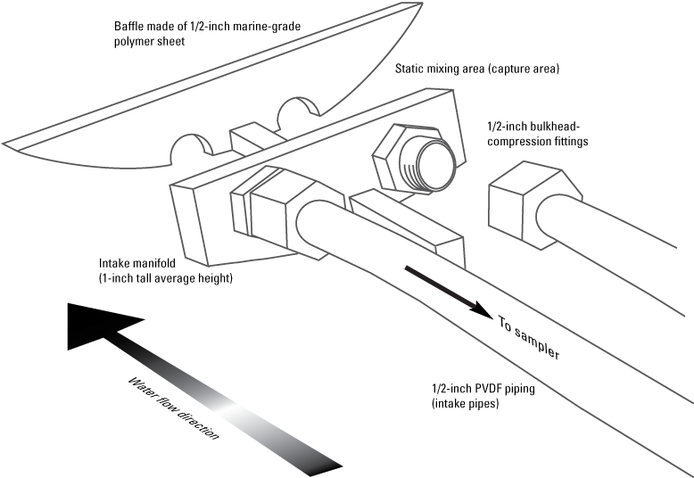
Schematic of a static mixer used in conjunction with the automatic sampler. Modified from Smith (2002).
Strainers and Screens
In most deployments the intake end of the line is simply left open, and a strainer or fine-mesh sized screen is not deployed. However, in channels where considerable amounts of floating debris, leaves, or other materials are present, it may be helpful to install a screen or strainer on the intake line. Commercial strainers are available, made of either stainless steel or plastic, and attach to the line with a barbed fitting and a hose clamp. The intake holes in the screen or strainer should be sufficiently large to allow coarse sand-sized grains to pass. Even though screens and strainers are usually streamlined, floatable debris can be expected to catch on the screen, thus increased maintenance visits should be planned. Debris captured on the screen will increase the drag on the line to the point where the intake line may become kinked or even torn free from the autosampler. Debris caught on or in the screen will change the trapping efficiency of the nozzle and can possibly alter the sediment distribution and may eventually alter the dissolved chemistry of the water being collected. Whenever a screen is being considered, it is prudent to collect and compare samples with and without the screen, under an identical flow regime to discern the effects on sample characteristics. Another strategy used in urban streams where floatable materials are common, is to install a series of small diameter rods (rebar) vertically in the streambed several yards upstream of the intake nozzle and forgo a screen or strainer. These rods will trap or deflect debris before it encounters the nozzle and will have minimum impact of the flow.
Preventing Fouling by Organic Matter or Sediment
In some settings, intake lines will be subjected to fouling by algae and weeds. Fouling from plants and algae is common when autosamplers are deployed in stream draining eutrophic ponds and near outlets from sewage treatment plants. Different strategies have been devised to help prevent this fouling, for example, the inlet end or nozzle can be encased in a copper tube or screen which will discourage growth and attachment of algae or weeds. While screens and strainers work to reduce the collection of floating debris, they will likely clog eventually and will require maintenance cleaning.
Fouling by sediment that accumulates in low spots (sags) in the line are also common, especially in environments having high concentrations of suspended sand-sized materials. Low spots or sags can occur throughout the intake lines, but are usually associated with long, nearly horizontal, runs in the lines. Good design will minimize the length of horizontal line runs. Where sediment accumulation is found to be problematic, frequent replacement of lines, or flushing of lines with high pressure air or water, will usually remove materials deposited in sags. In general, when deploying an autosampler in environments where significant algae and weeds occur or where wide range of sediment grain sizes or salinity will occur, operational plans should include frequent cleaning, replacement of intake lines, or both.
Line Removal and Replacement
It is often necessary to remove the intake line for cleaning, replacement, or to collect quality-assurance samples. The ability to easily replace the intake line is one of the paramount considerations when designing an autosampler system; many different designs and tricks have been used to simplify the task. For example, the USGS Wyoming-Montana Water Science Center developed a line-and-pulley system to help in removing the intake and tubing without the need for the field crew to enter the water (fig. 25). It consists of a plastic armoring pipe with a smaller tube attached along the outside. The intake tubing is fed through the armoring pipe using a rope attached to the end of the intake line; this rope extends back to the sampling station. A second rope is fed from the nozzle back to the station through the exterior tube. Pulling on the rope fed through the armoring brings the inlet line back into the station, while pulling on the line fed through the outer tube returns the nozzle end back to its original position in the stream.
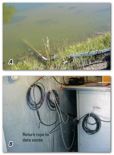
Photographs showing, A, an inlet system that utilizes a return rope to retrieve inlet lines and, B, a data sonde and the return rope inside the station. Photographs provided by U.S. Geological Survey Wyoming-Montana Water Science Center.
Special Considerations—Locating Inlets in Culverts and Pipes
Installing inlet lines in culverts and storm drains, a common task for using an autosampler, can be difficult due to the extreme flow velocity that can occur in the pipe; it is typical to have flows that rapidly cycle from zero to maximum velocity in minutes. Typically, a single intake line is used with the nozzle placed near the bottom of the pipe, with the intake line anchored to the pipe. The line is typically dropped vertically inside a box or manhole and may be anchored to the walls of the structure and to the top of the pipe. Alternatives are to attach the intake line to a heavily weighted cable hung into the pipe, or purchase or construct a metal “spider” to hold the inlet line within the pipe. In all deployments in pipes, the intake nozzle should be pointed down flow. Any wire, supports, or weights should be epoxy coated, as concrete or uncoated metal weights will react with the liquid and potentially degrade and become lost, or alter the chemistry of the liquid. In all buried pipes, extreme care must be taken to ensure that any weights or fixtures placed in the channel cannot become wedged in the pipe by debris.
Because water velocity can be extremely high in storm-water pipes, considerable effort may be required to secure the intake line in the pipe. In larger diameter storm-water pipes, the inlet lines are likely to be lost and will need to be replaced multiple times over the course of a study. Also, sediment loads may be extremely high during discharge events. Because coarse grain-sized sediment such as road grit will migrate along the floor of the pipe, sample bias will occur if the intake is not located near the middle of the pipe. In these situations, consideration should be given to a static mixer or a constant-depth fixture to keep the nozzle above the bottom of the storm drain (Barbaro, 2001).
Othmer and Berger (2002) devised a fixture that keeps the inlet nozzle at a set distance below the water surface but off the pipe floor in a partially filled pipe (fig. 26). This system floats the intake at constant depth below the liquid surface.
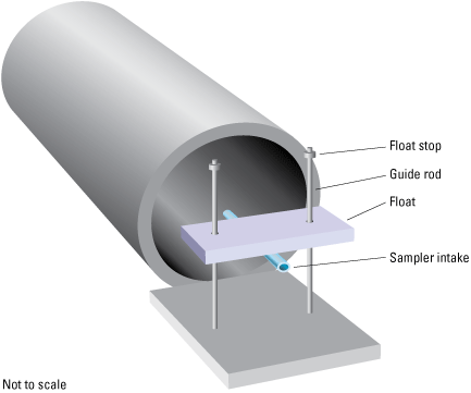
Components of a floatable system used to anchor inlet line in culverts and storm drains. Modified from Othmer and Berger (2002).
Summary—Design and Installation of Stations, Sampling Equipment, and Intakes
Several factors must be considered when selecting a site, designing an autosampler system, and locating the sampling inlet point. These include
-
• safe ingress and egress for field personnel to both the station and stream;
-
• permission to install equipment;
-
• protection from vandalism;
-
• availability of line power, or requirements for battery power;
-
• telemetry options;
-
• minimizing pumping height, tube length, and diameter of intake lines;
-
• cost and difficulty in developing, operating, and maintaining the site, including temperature control and access during storms;
-
• the ability to collect cross-sectional calibration samples under all stages of streamflow;
-
• the ability to measure the cross-sectional flow in the stream;
-
• the effort needed to determine the representativeness of the point sample intake, and the ability to adjust the sample intake point in the stream if necessary;
-
• the installation and construction of the intake lines and other efforts needed to ensure their survival during intense discharge; and
-
• the means by which intake lines can be replaced or cleaned, and quality assured.
Standard Operating Procedures and Quality Assurance Plans
Fundamental Science Practices of the USGS require that projects have documentation for all activities that produce data for the USGS (box 2; U.S. Geological Survey, 2011). The project work plan should be written after the location of sampling site and equipment are chosen and will provide details about the field and sampling procedures, equipment maintenance, quality assurance and control steps, and safety practices. It is made available to the entire project team and provides a “road map” for successful data collection and analysis. It should be updated throughout the study if procedures or protocols change during the project.
Box 2. The “U.S. Geological Survey Manual” on Project Work Plans
“The project work plan documents the timeline for the study, lists the discrete tasks that need to be completed to accomplish the objectives, and describes the relationship of discrete tasks to one another and the methods to be used (how they can be explained and defended, including exploring differences in performance, comparability of results, and so on). A project work plan also documents the budget and staffing for the study, anticipated or planned information products (including the recommended review and approval process for these products), and the process for managing and archiving scientific records.”
The components of a USGS project work plan are: (1) the scope and timeline (and in some instances the budget); (2) Standard Operating Procedures (SOP) for all planned data-collection activities and technical methods that will be implemented; (3) a Quality-Assurance Plan (QAP) to produce samples to assess and document the quality of the data being produced; (4) a data-management plan for collection, review, and approval of the data products; and (5) a plan for analyzing and publishing the data. The timeline should be included showing the major project elements, the needs of staff and equipment, and milestones where study progress is reviewed so that timely course corrections can be made during the study. The plan for analyzing and disseminating the project data should be developed and must follow all relevant USGS guidelines (U.S. Geological Survey, 2017a, b, c, d)606162. Because the SOP and QAP are central to the sample collection and field work, their elements are discussed in detail below. It is critical that the work plan is a joint effort involving all members of the project team so that the team is working towards a common goal (U.S. Geological Survey, 2018).
Components of a Standard Operating Procedure
A SOP documents the procedures and protocols that are followed for each step of collecting and processing samples for water quality. This includes instructions for
-
• traveling to the location and accessing the autosampler,
-
• retrieving samples that have already been collected in the autosampler,
-
• processing the samples for shipment to a laboratory,
-
• cleaning the autosampler and intake lines, and
-
• restocking the equipment to be ready for the next sampling event.
Table 7 provides the general components of an SOP for operating an autosampler and an annotated example SOP is provided in appendix 2.
Table 7.
Examples of metadata that may be necessary to record when servicing an autosampler.Quality-Assurance Plan and Samples
The QAP is a vital component of a work plan for any project utilizing autosamplers. The QAP provides the design for preparing quality assurance and quality control (QA/QC) samples that document any bias in environmental data caused by the sampling equipment and sample handling. QC samples that should be considered if an autosampler is to be deployed include (1) blanks of the equipment, (2) replicate samples, and (3) spiked samples. The basic premise of using an autosampler is that it duplicates the traditional manual process used to collect samples. Therefore, in addition to the QA/QC needed to ensure equipment cleanliness and repeatability of sample collection, an autosampler study also requires verification that the autosampler is deployed in a manner that collects samples that are equivalent to samples collected using traditional cross-integrated isokinetic methods (EWI or EDI). Additional guidance on quality assurance and quality control for projects that collect water quality data can be found in Mueller and others (2015). QA/QC plans can be found online for many studies that used autosamplers (for example, Ging, 1999, and Garn, 2002); accessing these plans can provide valuable insight when designing a study.
Because different QA/QC samples are used to evaluate different biases that may impact field samples, the frequency and types of QA/QC samples will depend on the objectives of the project. For this reason, the number of sampling events and total number of samples that will be collected must be considered when determining the total and frequency of QA/QC samples. In general, a target of 10–20 percent of the total number of samples is a starting place for the number of QC samples to collect, but this number will depend on the suite of analytes being studied, the experience of the sampling team, and historical water-quality (WQ) data if available. As a general rule, a higher percentage of QC samples should be collected early in the study so that the cleaning, sampling, and handling procedures being used are validated and, if necessary, adjusted so that data-quality objectives are met. Thereafter, the number of equipment, field blanks and replicate samples can be reduced over the remaining field effort.
Types of Quality-Control Samples
A list of QA/QC sample types used to verify representativeness are shown in table 8. QA samples and procedures for bacteriological samples are listed in table 9.
Table 8.
Types of quality-control sample with specific applications for autosamplers.[DSW, distilled water; IBW, inorganic-grade blank water; OBW, organic-grade blank water; EWI, equal-width increment, isokinetic sampling method; EDI, equal-discharge increment, isokinetic sampling method]
IBW is water certified for analysis of trace elements and other inorganic constituents. It is suitable for creating the blank quality-control samples necessary for analysis of inorganic constituents and dissolved organic carbon.
Table 9.
Examples of quality-assurance procedures for collecting samples for bacteria[DSW, distilled water]
| Type of quality assurance | Procedures |
|---|---|
| Cleaning | Autoclave all bottles according to the instructions given in U.S. Geological Survey (2008b). Place a small piece of clean aluminum foil on top of the bottle before autoclaving
and don’t remove until final set up of bottle in the autoclave. Before each deployment, sampling lines, pump lines, and connectors should be sterilized (if possible) by autoclaving. Rinsing with a mild solution of sodium hypochlorite bleach (5–10 percent dilution of commercial bleach by volume) is an alternative for sterilization but will require adequate rinsing with sterilized DSW1 to remove all odor of bleach. Bottles, lines, and tubing should be capped on the ends with clean foil and double-bagged for transport to the field. |
| Quality-control samples | Collect an ambient blank by placing a bacteria sampling bottle with sterile water
in the autosampler during the period of deployment and processing with the rest of
the samples. This determines potential cross contamination between samples during
deployment. Collect concurrent replicates from center of flow using standard sterile sampling techniques. Collect a spike of a field blank to determine potential false negative results. Spike reference samples are sold by equipment suppliers. Collect a post-sampling field-equipment-blank sample to check for possible cross contamination. Cycle the autosampler and lift the lines in the stream. Clean and flush the lines according to protocols described for intake lines, ending with a flush of sterile water. Collect the blank sample using sterile water to cycle through the lines. |
“Laboratory” or “field equipment blanks” are used to document bias caused by poor equipment cleanliness or crossover contamination between samples. These blanks are collected by processing water that is free of the analyte(s) of interest using the same procedures used to collect environmental samples. These blanks can be produced in the laboratory before leaving for the field or can be prepared in the field. Generally, a “field equipment blank” is preferred, as it processes blank water through all steps of collecting and processing samples in the ambient field environment. For an autosampler, this means passing certified blank water through intake lines, pump and distributor, sample-collection bottles, and any compositing, splitting, and filtration procedures conducted (in the field or laboratory). If needed, these steps can be broken down to assess contamination caused by individual pieces of equipment or isolated steps in the collection process. Collecting equipment blanks for intake lines requires additional effort and must be well planned (see “Preparing Blanks of Intake Lines”). Prior to producing a laboratory- or field- equipment blanks, all parts of the sampling equipment should be cleaned and handled in a manner identical to that used for when preparing to collect field samples. Field blanks are processed and preserved along with field samples.
“Spiked samples” are defined as samples (either native water or certified clean water) that are fortified with a known concentration of a specific analyte or analytes. The observed concentrations of analytes in the spiked sample are compared to the expected concentrations, calculated from the spike-analyte concentration in the environmental sample (if used, or the certified concentration if blank water is used), and the mass of the analyte in the spiking solution added. Spikes are used to estimate bias in analytical methods, either from matrix effects caused by substances in the natural water, and any degradation of analytes that occur during the sample process and storage. Spiking solutions with certified concentrations can be obtained from an analytic laboratory or purchased from commercial chemical suppliers. When preparing spiked QA samples, three samples are needed: a non-spiked environmental sample, a replicate non-spiked environmental sample, and the spiked environmental sample. Because sample containers are often left open in an autosampler prior to, and for a short period following sample collection, the use of spiked samples is strongly recommended when using an autosampler for semi-volatile compounds (organic compounds, mercury, and lead), biologically active compounds, and bacteria.
“Replicate samples” are collected to document variability caused by collection methods and by analytical methods (analytic variability). Replicates can be collected in multiple ways using an autosampler. “Split replicates” can be collected from an autosampler by splitting a single or composite sample into replicates. A common technique to collect replicates by splitting one container of water using a churn or sample splitter device. “Sequential replicates” can easily be collected using an autosampler by programming it to collect consecutive samples at each sample initiation signal.
“Concurrent replicates” are multiple samples collected at the same time and place using different sampling techniques. For autosampler deployments, concurrent replicates play an important role, as they are used to compare samples collected by the autosampler and traditional cross-sectional isokinetic methods (EWI or EDI cross sections). Typically, the autosampler is programmed to collect discrete samples at appropriate time intervals (for example, every 10–15 minutes) over the period of time grab samples are being collected for the composite. The samples collected by the autosampler and manual methods, can be analyzed individually, or composited before the comparison is made. The “concurrent replicate” samples can be collected at a low flow condition, or during storm flow; however, conditions in the stream may change rapidly during a storm, thereby complicating the comparison of individual samples. “Concurrent replicate” samples are used to generate box-coefficients that allow corrections to be made between the results obtained by the two sampling methods. An example of box-coefficient calculations is provided in appendix 3.
Preparing Blanks of Intake Lines
Collection of a field equipment blank must include consideration of the intake line, thereby requiring the nozzle end to be accessed and placed into a container of certified blank water and pumped up to a collection bottle in the autosampler. It is important that the lines being blanked are first cleaned, either in the laboratory or the field. If this is not possible, then at a minimum the lines must be first flushed with clean water before preparing the blank. Cleaning is described in “Intake-Line Maintenance and Cleaning.” Flushing should use a minimum of three-tubing volumes of tap water followed by three-tubing volumes of distilled water (DSW), prior to introduction of certified blank water. As a general rule, equipment blanks should be prepared on the intake lines prior to each sampling event, or whenever a sample line is replaced. It should be noted; however, that intake line cleaning and blanking is constituent dependent, that is, for some constituents such as suspended sediment, a lower effort of cleaning or blanking is suitable. However, other constituents, such as trace metals and organics, will require a greater frequency and effort.
Holding-Time Studies
Holding-time studies may be necessary to determine if there is a constituent concentration change over the time samples are held in an autosampler before preservation steps are taken. This can be evaluated during a site visit by collecting a sample (with the autosampler) and immediately splitting it into two sub-samples. One sub-sample is preserved, processed, and shipped to the laboratory for analysis, while the other sub-sample is left in the autosampler until the next scheduled site visit when it is retrieved, processed, and sent to the laboratory.
This type of study is especially necessary when samples will be exposed to elevated summer temperatures in a non-climate-controlled sampling station. It may be necessary to deploy a temperature logger in the autosampler to track changes the samples are being exposed to, even if the samples are being refrigerated in the autosampler. Any exposure of open sample bottles to high temperatures can speed up the degradation and volatilization of dissolved constituents and can increase the growth rate of bacteria.
Quality Assurance Samples for Trace Components
QA/QC samples (field blanks and field equipment blanks) are especially important when using autosamplers to collect samples for trace inorganic or organic compound analysis. Unlike grab samples, when an autosampler is used, the sampling lines (inlet, pump, and distribution tubes) may not be “single use” and therefore, may not be considered “clean” after the equipment is deployed and the first sample is collected. Field equipment blanks take on special significance because they document that the equipment was properly cleaned and not compromised during deployment. Likewise, field blanks and spiked blanks are essential for documenting the effects of cross-bottle contamination and air-borne contamination on trace component concentrations. Therefore, it is advisable that when sampling for trace components the number of QA/QC blanks (field and equipment blanks) is increased to 25-percent or more of the total samples, distributed equally across all sampling deployments. The following steps are useful to help ensure successful trace component sampling:
-
1. Replace the inlet line, pump tubing, distributor arm tubing, and all fittings with pre-cleaned tubing and fittings (acid or methanol washed when applicable) before each sampling event. Use Teflon or Teflon-lined plastic tubing for the inlet line. Keep the interior of the autosampler clean and wrap the area where sample bottles are kept in a plastic bag. Try to deploy equipment as soon as possible before use and minimize the time when sample bottles (empty of filled) are left open to the atmosphere.
-
2. Use commercially or laboratory-supplied pre-cleaned bottles when available or follow strict bottle cleaning procedures. It is sometimes possible to send bottles to the analytical laboratory for special cleaning.
-
3. Retrieve samples as soon as possible after collection, reducing the length of time the filled bottles are left open in an autosampler.
-
4. Check the inlet line carefully for signs of staining by metal-oxides, oils, or organic matter after each event. Look for sediment that may have settled out in the inlet line. Inspect the inlet nozzle area for abrasion. If any of these indications are found, replace (rather than re-use) the inlet lines.
-
5. Add additional flush cycles to help minimize sediments becoming trapped in the line.
Quality Assurance for Bacterial Constituents
Autosamplers are often used to sample rivers and waste effluents for bacteriological constituents. Generally, they should be employed only where very high bacterial values are expected, as cross-contamination is a significant concern; it is very difficult to clean and sterilize all parts of the equipment sufficiently to allow for repeatable low-level analyses. Adding extra purge-rinse cycles or using a continuously pumping system including a bypass valve on the sampling line may help ensure that each sample is collected from a well-flushed and purged intake line. However, continuous flow of water may still allow some bacterial growth to occur in the lines, especially in streams where algae is abundant. Chilling of the samples while in the autosampler is also very important, either by ice or by using a refrigerated autosampler. Aulenbach (2009) has conducted studies on the holding times of bacteria for up to 62 hours for fecal coliform by mFC agar method, and total coliform and Escherichia coli; however, it was found that samples held for 18 hours provided results similar to those found in samples analyzed after the recommended 6-hour holding time. However, they stressed the importance of maintaining proper sterile condition during collection, preservation, storage, and analysis of bacteriological samples.
The following QC procedures are suggested for sampling for bacteriological analysis:
-
• Before each deployment, sampling lines, pump lines, and connectors should be sterilized (if possible) by autoclaving, or by rinsing with a mild bleach solution (5-percent by volume) and DSW followed by rinsing in sterilized water. (Note: some bacterial cleaning procedures call for use of full-strength household bleach, which is 12-percent bleach). Autoclave all bottles according to the instructions given in chapter A7 of the NFM (U.S. Geological Survey, 2008a; Myers and others, 2014) before placing them in the autosampler. Sterilized bottles, lines, and tubing should be capped with foil and double-bagged for transport to the field.
-
• When servicing the sampler, fill a bottle in the sampler with a filtered (0.45 μm), sterilized DSW field-blank, and leave it open in the sampler during collection. It is then processed with the samples and used to determine cross-bottle contamination during sample collection.
-
• When servicing a sampler, bring a large volume container filled with sterilized DSW. Once the field samples have been collected, remove the intake line from the stream and place the intake directly into this container of water. Cycle the automatic sampler and collect a post-sampling field equipment blank sample of the filtered DSW to demonstrate the potential for cross-contamination of samples.
-
• The filtered DSW used in the laboratory should be analyzed to verify it is free of bacterial contamination. These analyses should be made before the project is initiated, and repeatedly throughout the sampling effort. For critical projects, it is recommended that the QA/QC effort be increased to (potentially) each sampled event.
Cross-Sectional Evaluation Studies
As mentioned above, concurrent replicate sampling is used to determine correction coefficients needed to adjust point sampler results (from autosampler collected data) so they correspond to results that would be obtained if multi-point manual sampling techniques were used. This is essentially a quality control issue—if point samples (collected using an autosampler) do not accurately represent the cross-section, then the interpretations made using the data risk being misconstrued or misunderstood. Concurrent replicate sampling conducted during cross-sectional studies demonstrate the heterogeneity of flow across the channel and are used to determine the “best location” for the inlet in the stream for producing an appropriate point sample. These studies should be conducted early in the project when a sampling station is being located (see “Selecting Inlet Locations” for more details). For long term studies, cross-sectional comparisons should be conducted regularly (at least yearly and at multiple flow regimes) throughout the project, to provide assurance that the sampling point and stream conditions have remained.
Cross-sectional studies also provide the information needed to do the following:
-
• Adjust raw data from samples collected by an autosampler to produce results comparable to those collected using standardized cross-channel methods. All cross-section study data should be documented in reports produced from a study.
-
• Calculate the intake efficiency, which is defined as the ratio of the concentration in a sample collected at a point (by the autosampler) to the concentration in a grab sample collected just upstream of the autosampler intake. Intake efficiency may vary as a function of discharge, so the ratio should be measured, if possible, over a range of discharges (this may not always be possible). At a minimum, intake efficiency should be measured once at base flow, once at flow near median, and at least once above median flow. Monitoring the intake efficiency throughout the project may indicate that the channel geometry has changed, and the position of the intake line requires adjustment.
-
• Calculate the cross-sectional coefficient, which is defined as the ratio of the mean cross-sectional concentration, as measured by USGS methods, to the concentration in a sample (or the mean concentration in multiple samples) collected by using an autosampler. The cross-sectional coefficient may also be a function of discharge. Collecting samples necessary to define this coefficient should be budgeted in any proposal for a project. At a minimum, the coefficient should be determined at least once at base-flow, below median, and above median flow conditions using either EWI or EDI sampling protocols.
The mean cross-sectional concentration in a stream is calculated using equation 2:
whereČmcs
is the estimated mean cross-sectional concentration;
Cm
is concentration in sample collected by autosampler;
I(q)
is intake efficiency at discharge (q); and
Bx(q)
is cross-sectional coefficient for the discharge (q) occurring at time of sampling.
The methods used to measure these variables and to adjust raw data should be documented in the project SOP and the final data publications. Conducting these studies periodically over the course of a sampling project ensures that data are adjusted properly despite changes in river or channel conditions.
As shown by equation 2, the relation between a sample collected from the stream using an autosampler and water collected directly from the stream at intake location is described by two functions: (1) the intake efficiency and (2) the cross-section coefficient. In a well-mixed stream, solid and dissolved constituents will be evenly distributed horizontally and vertically in the stream, and a sample collected from any point in the stream should provide representative concentration. Cross-sectional measurements of specific conductance and turbidity (discussed earlier in “Selecting Inlet Locations”) are used to document the cross-sectional homogeneity of dissolved and suspended sediment, respectively. However, it is more likely the case that suspended materials (as indicated by turbidity) will vary both vertically and horizontally across the stream. The case in storm-water runoff pipes and culverts can be even more complicated than in streams.
In order to properly relate a discrete point sample to the mean concentration in the stream or pipe, samples collected using an autosampler must be compared with samples that integrate across the stream under different flow-regimes. These integrated samples must be collected using standardized, manual methods such as EWI or EDI, preferably collected over a range of flows and conditions. Edwards and Glysson (1999) describe USGS methods used to properly collect depth integrated, EWI or EDI samples across flowing streams and rivers. Once this relation is established, data from samples obtained from an autosampler can be adjusted (using equation 2) to provide realistic mean cross-channel concentrations.
Despite effort spent to ensure that an autosampler inlet is located in the best point in the cross section, and that representative samples are being collected, the relation between a point-sample and the mean cross-section sample can be complex and difficult to determine under all flow regimes. However, if a stable relation can be demonstrated under at least a few flow regimes, then the autosampler results can be assumed to be suitable to provide mean cross-sectional concentrations Whenever an autosampler is used to generate mean concentrations or loads, it is the user’s responsibility to document the relation between the autosampler results and those obtained using traditional manual sampling methods. In general, the raw, unadjusted concentration data should be provided to the USGS National Water Information System (U.S. Geological Survey, 2024), and if used, the adjusted data and a description of the adjustment process should be provided in the study report.
As a general rule, an acceptable agreement is obtained if samples collected by an autosampler are within plus or minus 10-percent of the results from traditional cross-section sampling. This is based on typical uncertainties in analytic methods. Each project should define the limits of “acceptability,” defined for the range of flow conditions under which comparison sampling was conducted; the limits may change over time as river conditions change. These errors are likely to affect point-samples collected using an autosampler, especially during high discharge.
Intake Efficiency
The intake efficiency is a factor required to properly relate a point sample collected by an autosampler and the mean cross-sectional concentration (eq. 2). The intake efficiency is defined as the ratio of the constituent concentration of the pumped sample (Cp) and the constituent concentration in the stream (Cs) collected near the intake point, times 100. Intake efficiency is calculated for the discharge (Iq) under which the sampling was conducted using equation 3 (U.S. Army Corps of Engineers and others, 1966).
To determine the intake efficiency, samples must be collected simultaneously using the autosampler and grab methods at a point immediately upstream of the intake line nozzle. The preferred method is to collect the stream sample using a standard weighted-line sampler, or alternatively, as a grab sample made using a wide-mouth bottle. Care should be taken that the hand sampling does not disturb flow or stir-up bottom sediment around the intake. Intake efficiencies should be determined soon after the intake-line is installed, but after allowing the streambed to readjust from any disturbance caused by site construction. As a general rule, samples should be collected in triplicate, and if possible, should be collected over a range of stream velocities. Determining the intake efficiency is especially important when a surrogate parameter, such as turbidity, is being used to estimate suspended-sediment concentration.
Autosamplers rely on pumping speed to create an area surrounding the intake nozzle in which water velocity exceeds the settling velocity of particles in suspension. A high velocity is necessary to capture all particle-sizes in the water, and to deliver the collected sediment particles to the sample container without allowing the coarser-sized particles to settle in the sampling line. If during maintenance sediment is found trapped in the sampling line, then a representative sample is not being collected and the autosampler parameters should be changed.
The autosampler pumping creates suction at the intake orifice, bending the streamlines into the intake orifice. This force acts on particles passing the orifice to varying degrees, depending upon particle size and stream velocity (Tennessee Valley Authority and others, 1941). That is, the pumping force attempts to pull particles laterally from around the intake orifice, accelerating them as they move in the direction of the intake. When stream velocities are low and only fine silt- and clay-sized particles are being transported, typical pump velocities are sufficient to capture all particles in suspension. At stream velocities sufficient to move sand- and gravel-sized particles (larger than 0.062 mm) in suspension, the pumping force must be sufficient to overcome the downstream momentum of these larger particles to capture them. Non-isokinetic sampling methods have been demonstrated to introduce concentration errors, particularly for particles having a grain size larger than 0.062 mm (Edwards and Glysson, 1999). This decrease in efficiency biases the mixture of solids and water being captured because only sediment that passes very close to the intake is captured. Also, depending on the configuration of the structure used to fix the intake line to the streambed, eddies may develop around the nozzle that can alter the mixing of suspended sediment. This problem can be minimized by using a small diameter intake line, orienting it properly in the flow, and selecting a design for securing the inlet line (in the streambed) that minimizes disturbance of flow lines near the inlet nozzle.
Cross-Sectional Coefficients
Cross-sectional coefficients, determined as a function of discharge, are the other factor required to properly adjust a point-sample concentration (collected by an autosampler) to obtain a mean cross-sectional concentration (eq. 2). Studies conducted by Edwards and Glysson (1999) demonstrated that samples collected from a single point of streamflow within a stream cross section seldom agree with the mean cross-sectional sediment concentration. Glysson (2004) showed that differences in excess of 25-percent can occur between the suspended-sediment concentration in samples collected with autosamplers and the mean cross-sectional concentration determined using standard USGS EWI or EDI methods. Because a theoretical relation does not exist between these different concentrations, an empirical relation must be established. The cross-sectional coefficient, often referred to as a “box coefficient,” is used to adjust concentration data collected using an autosampler to obtain the mean cross-sectional concentration that would be determined from samples collected using standard sampling methods.
It is the responsibility of the researcher to determine the relation between the concentrations in point samples collected using an autosampler, and the mean cross-sectional concentration measured using traditional sampling methods (EWI or EDI) over the expected range of flow conditions, especially if autosampler data are used to estimate loadings.
In addition to adjusting the raw concentration values from periodic sampling efforts, the repeated analysis of the box coefficient throughout the study will, like intake efficiency, help in evaluating the suitability of sampling intake location. Changes in the geometry of the stream channel will alter the box coefficient, thereby indicating that an adjustment of an intake position is warranted. Given multiple measurements of the coefficient, it may be possible to adjust the intake location so that the coefficient approaches a value of 1.0 for all streamflow conditions (a value near unity implies no correction to the point-sample concentration is needed).
Cross-sectional coefficients (Bx) for a discharge (q) (eq. 2) are computed by dividing the cross-sectional concentration (Cx) by the concentration of an autosampler sample (Cas) collected at a discharge of qi using equation 4:
Cross-sectional sampling studies to determine box coefficients (and intake efficiency) should be made an integral part of year-long or multi-year projects. If possible, these studies should be made during both the rising and falling stages of a storm, and by season and include isolated events such as spring snowmelt or summer thunderstorms. Appendix 3 provides an example of the development of a box coefficient for an autosampler station in Hawai’i.
Each autosampler station needs to be calibrated at different flow conditions. As long as this calibration is performed, the exact relation between coefficient value and flow is not critical (Eads and Thomas, 1983). The cross-sectional coefficient is likely to vary with season and discharge; this can be calculated by determining the coefficient at roughly the same discharge over seasons. Plotting the value as a function of the stage and time of year will show if a simple, seasonal relation exists, and if the coefficients are related to both season and discharge. The coefficients may seem to remain steady for the typical range of discharges that occur during the summer and fall, but will change during the winter, and then slowly return to summer values during the spring season. Studies should be budgeted on the assumption that repeated measurement of the box coefficient will be needed to understand the yearly variation at the site. A record of these coefficients should be kept along with seasonal data and discharge.
Box coefficients can be applied to concentration data in different ways depending on whether the field samples are to be used for computation of a continuous daily value or published as discrete samples. Porterfield (1972) discusses the application of these coefficients in computation of daily sediment loads using two methods: (1) correction of the estimated concentration values arithmetically after concentrations have been computed from a continuous discharge-concentration graph, and (2) correction or adjustment of the concentration-discharge graph prior to using the graph to compute load values. The second method was recommended especially when the coefficient is found to vary with discharge or season. As described below, software is available to assist with these calculations.
Applying the coefficients is straight-forward: concentrations from discrete point-samples (collected by the autosampler) are multiplied by the appropriate coefficients to obtain the mean cross-sectional concentration (eq. 2). However, the manner in which the coefficient is applied can depend on the cause of the lateral variation in the distribution of constituent concentration in the stream. For example, the variation may be caused by (1) proximity and quantity of tributary inflow, (2) changes in the bed form or channel alignment, (3) the source and type of constituent, and (4) the season. Based on these conditions, each record should be analyzed in detail to determine the most accurate application of the coefficient. The USGS’s Graphical Constituent Loading Analysis System (GCLAS; Koltun and others, 2006) is a computer graphical program that will allow users to compute box coefficients and apply them to sample concentrations and compute daily loads.
Programs such as GCLAS will help in applying the coefficients correctly both with time and with stage. See Edwards and Glysson (1999) and Porterfield (1972) for more information on computing and applying coefficients.
Finally, consideration needs to be given to how the various correction coefficients (Bx and I, equation 2), when known to vary as a function of discharge, are applied to composite samples prepared during storm events. Generally, the choice of coefficient value nearest the mean discharge of the sampled storm event should be applied to the concentrations measured in the composite sample.
Summary—Quality Control and Assurance Programs
-
• Proper deployment of an autosampler entails collecting sufficient QA/QC samples needed to document the cleanliness and repeatability of the sampling process. QA/QC procedures should be documented clearly in the Standard Operating Procedure document for the project. Projects should plan and budget adequate resources to this end.
-
• As a general rule, 10–25 percent of all samples collected should be allocated for QA/QC evaluation. These samples include laboratory and field equipment blanks, replicate samples and field blanks. While QA/QC sampling should be conducted throughout the proposed sampling program, it is important that samples be collected at the start of the study to ensure adequate cleaning is being used at the onset. Various blanks and replicates should be collected for each storm event that is sampled.
-
• Laboratory and field equipment blanks should be collected each time the intake line is removed for cleaning or replacement.
-
• When sampling for trace constituents, either inorganic or organic, and for bacteriological samples, additional QA/QC samples should be collected to ensure low-level cleanliness of the sampling equipment. Plan for the additional time and effort needed for acid washing, methanol rinsing, and sterilization of tubing, bottles, and other parts of the sampling mechanisms where appropriate.
Autosampler Deployment Schemes
Following the siting, design, development of the physical infrastructure of a station, and development of QA/QC program, the next consideration is the design of the sampling scheme that will best meet the project goals. Autosamplers using internal or stand-alone programmable data logger controllers allow considerable flexibility in the design and implantation of sampling schema, and each scheme provides different types of information. With the goals of the study in mind, it is advantageous to develop a scheme that considers the hydrologic characteristics of the stream, river, or system under study. This is especially important when designing schemes for event-based sampling.
Designing a Sampling Scheme
Types of Sampling Schema
The principal types of sampling schema are based on whether samples are to be collected at a fixed time or discharge interval and produce either discrete or composited samples.
Fixed-Interval Sampling
Fixed-interval sampling refers to the scheme where discrete samples of water are obtained and placed either in individual bottles or added to a single bottle or composited. Each sample or aliquot is collected at a set time or discharge interval. Temporal sampling is a standard scheme dictated by many regulatory monitoring activities, such as treated waste discharge from treatment plants and industrial processes. In studies of rivers and streams, temporal-interval sampling is used to determine change in stream chemistry at different portions of storm hydrographs, and to demonstrate the diurnal changes, such as in dissolved iron (caused by sunlight intensity), algal abundance, or other chemical processes affected by photosynthesis. Sampling based on fixed discharge intervals is used in the preparation of flow-weighted composite samples. This scheme is often accompanied by the concurrent collection of discrete samples. As discussed in detail later in this report, if suitable stream-discharge measurements are available, it is possible to use samples collected on fixed-time intervals to produce an accurate discharge-composited sample in a laboratory.
Scheme for Collecting Discrete Samples
Autosamplers are extremely beneficial when multiple, discrete samples need to be collected at a preset increase in stage or a preset discharge interval. Examples include the studies where a sample is needed when flow first begins in a culvert, storm-water discharges from a pipe, or maximum stage is reached in a river. Automatic equipment removes the need for humans to evaluate the stream conditions and initiate (or terminate) the sample collection. A “discrete sample” may consist of a single or multiple bottles filled sequentially for each triggering signal sent from the controller. Multiple-bottle discrete samples are used when the analytes or classes of analyte cannot be measured from a single bottle of water. A common example is sampling for dissolved and total analytes, or when samples are needed for suspended sediment and particulate organic matter analysis. Collecting individual, discrete samples maximizes the amount of sediment or carbon in each bottle available for analysis and removes the chance for bias arising from incomplete homogenization when a single sample is used for analyses of multiple constituents.
Discrete samples (or aliquots) collected at preset time intervals provide information on the variation in stream chemistry. Figure 27 shows an example of the timing of sample collection when an autosampler was programed to collect discrete samples at two-hour intervals from a river during a hypothetical storm event that lasted three days. Note that because of the rapid increase in stage, only three samples were collected during the rising limb of the hydrograph, and 21 samples were collected later during the receding limb. If a shorter time interval was selected, more samples would have been collected earlier in the storm, but because autosamplers hold only a finite number of bottles (typically 24), less of the receding limb would have been characterized (unless field crews were available to replace bottles). Complete river condition data for this hypothetical storm are provided in appendix 4.
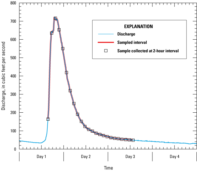
Hypothetical storm hydrograph showing the times when samples would be collected using an equal 2-hour interval. [A summary of river conditions and collection times is shown in table 4.1]
Discrete samples or aliquots (to be composited) can also be collected on fixed intervals of discharge passing the sampling station. Figure 28 shows the timing when samples would be collected during the same storm event using a preset discharge interval of 10 million gallons. In this scenario, more samples are collected during the rising limb and crest of the storm, than would be collected using a fixed-time interval approach. However, if too small a discharge interval is chosen, samples may overlap during the peak and therefore will be missed. Also, while the sampling will better characterize the rising limb and crest of the storm hydrograph, fewer samples will be collected during the receding limb and important information characterizing water entering the river from tributaries far upstream in the watershed may be missed. It should be reemphasized that only the flow-weighted sampling scheme produces an unbiased “average concentration” for the storm.
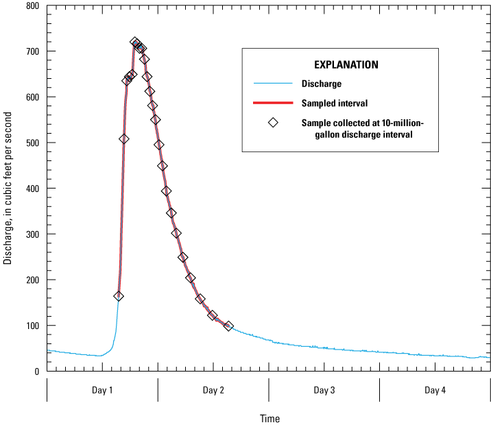
Storm hydrograph showing the times when 24 discrete samples would be collected at a constant discharge interval of 10 million gallons. [A summary of river conditions and collection times is shown in table 4.2]
Event-Based Sampling
The main advantage in deploying an autosampler is the ability for it to monitor and automatically respond to changing flow conditions, and then to begin sampling without direct human oversight. This type of sampling is termed “event-based sampling”; after the initiation of sampling (the occurrence of the event), sampling may be undertaken either on a discrete time- or flow-basis. In this document an “event” refers to a prescribed change in environmental conditions. Typically, an autosampler is set to continue sampling in a preset manner only while the environmental conditions remain within set boundaries.
The most common example of event-based sampling occurs when a stream is sampled in response to the onset of precipitation. Because autosamplers hold only a finite number of bottles (or a fixed-bottle volume), sampling may stop before the “event” has concluded. In contrast, time-based sampling allows the researcher to be aware of the timing, the number of samples collected, and when the sampling will be concluded. For example, in a monitoring program that collects samples weekly from a river, the researcher will know precisely when the autosampler will need servicing and the sample bottles replaced. As discussed below, “event-based” sampling requires much pre-planning and other considerations; these factors impact the design, servicing, cleaning, and other QA/QC aspects of the autosampler deployment.
Typical Autosampler Cycle for Collecting a Sample or Aliquot
When an autosampler receives a triggering command, the sample line is first purged with water. This purge is accomplished by reversing the direction of the peristaltic pump. The inlet line is next rinsed with stream water, re-purged, a cycle that can be repeated multiple times. The sample is then pumped into the sampler container. The line is then re-purged and the distributor system is moved to the next sample container and readied for the next trigger signal when this sampling cycle is repeated. This purge and rinse cycling can easily be performed if the autosampler is equipped with a liquid-detector that senses when the liquid has reached the pump head. It is recommended that autosampler programs include at least one rinse and one purge cycle before each sample.
Alternately, if a fluid-detection monitor is not available, the sampling system can be equipped with a valve system located past the peristaltic pump head but before the sample container (fig. 29). This allows the line to be flushed with native water without the need to reverse the pump. The valve is opened by a command from the data logger as the pump is started and allows water to be pumped to waste for a set time period. The valve is then closed, and the water is allowed to flow to the sample container.
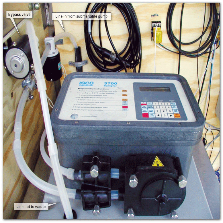
Photograph showing the key parts of a valve system for an automatic sampler: the intake line running from a submersible pump, the discharge line out to waste, and the by-pass valve. Photograph by Kevin Richards, U.S. Geological Survey.
Although more complicated, there are two advantages to the continuous flow system over the purge-and-rinse system:
-
• With the purge-and-rinse system, rinse water stops in front of the pump head at the liquid detector and does not rinse the pump tubing.
-
• With the purge-and-rinse system, debris and native water may not be completely expelled from the inlet tubing during the purge cycle. With the valve system the continuous flow of water helps keep the line clear of settled debris.
The valve system if often employed when an in-stream submersible pump system is used to bring water up to the autosampler. The submersible pump can be run continuously or at time intervals, and a valve is operated using a relay operated from the output signal of either a data logger or through the control port of the autosampler. The manufacturer of the autosampler or data logger should be consulted for the specific connections needed to operate a valve system.
Scheme for Collecting Composited Samples
Composited samples are collected to produce a sample that represents the “average” composition during a specific hydrologic event or a set time interval. Figure 30 shows the makeup of different types of composited samples. Two of the more commonly used composite samples are flow-weighted and time-averaged. These samples are produced by collecting an aliquot of stream water each time a triggering signal is received, then combining it with the previously collected aliquots. A flow-weighted composite sampling scheme is used to determine an average concentration of a constituent (such as sediment) moved during a storm or flood event. This average concentration can then be multiplied by the number of storm events, or the yearly length of time storm flow occurs, to obtain the yearly constituent load. Time-averaged composite samples are commonly collected for regulatory monitoring of discharge, for example, when monitoring to determine the daily outfall loading of nutrients from a sewage treatment plant. Regardless of the composite type, each aliquot should be collected at the specified interval and contain identical sample volumes (allowing for a reasonable margin of error).
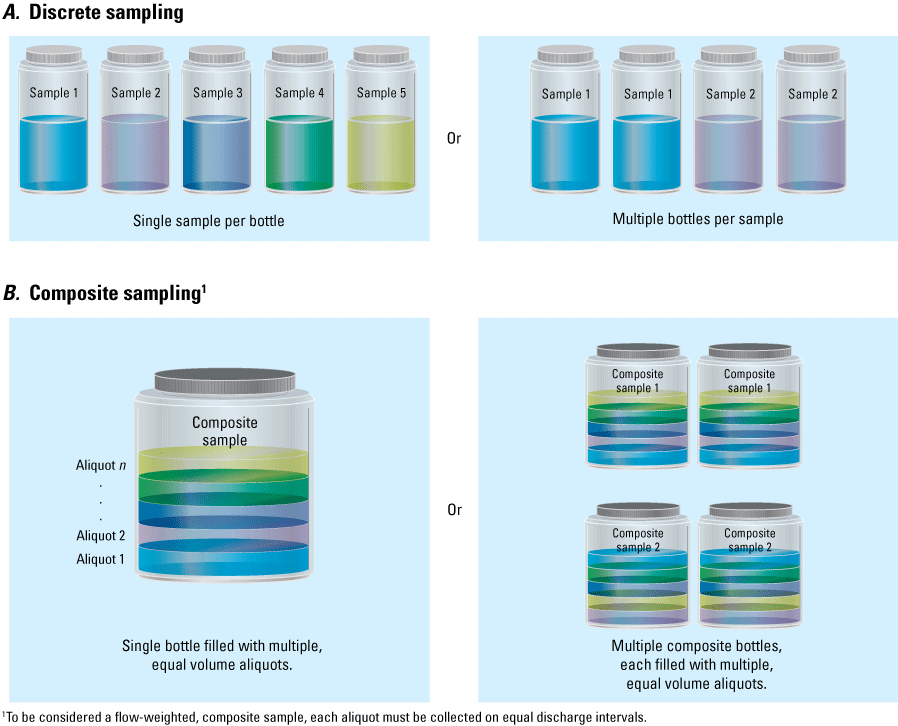
Illustration showing different bottle distribution schemes used for, A, a discrete sample, either a single bottle per sample or multiple bottles per sample; and, B, a composite sample, either a single bottle per sample or multiple bottles per sample.
Multiple-bottle composite samples can be collected by having the autosampler place identical volume aliquots sequentially into two or more bottles upon each triggering signal. Flow-weighted compositing provides a representative sample only if an accurate stage-discharge relation is available for the station, and only if an appropriate discharge interval has been chosen.
Multiple-bottle composite-samples are collected when multiple classes of parameters are to be measured that cannot be measured in a single sample; for example, when concentrations of inorganic or organic constituents are required along with suspended-sediment concentrations. As in discrete sampling, suspended sediment is best measured in its own sample.
To properly produce a flow-weighted composited sample, a system to measure, calculate, sum, and record stream discharge is needed. Stage data can be obtained at a nearby existing streamgage, or stage can be measured using a hydrostatic pressure transducer placed in the stream bottom and connected to the autosampler or data logger. In the latter case, a stage-discharge relation will need to be developed for the site. In general, flow-weighted composite samples can only be produced where an accurate stage-discharge relation has first been established. The autosampler or data logger evaluates stage, calculates discharge, sums the discharge, and initiates sampling when the appropriate volume is reached; the data logger also measures the volume of each aliquot collected using pump time, peristaltic pump rotations, the use of a flow sensor, or measured weight of the aliquot. Less sophisticated equipment is needed to produce a time-averaged composite sample; typically, only a timer is used to control the pump operation.
Collecting Large-Volume Composited Samples for Suspended-Sediment Phase Analysis
Autosamplers are particularly useful for obtaining large-volume samples from which sediment is removed for analysis of nutrients and trace organic contaminants. This approach, which is typically performed during storms, is common in total maximum daily load (TMDL) studies to provide data for hydro-geochemical modeling and is used to model the effects of reduction of nutrients (such as phosphorous), particulate carbon, and hydrophobic trace constituents such as pesticides. This type of modeling requires discharge and “realistic” sediment and contaminant concentrations for tributaries and outfalls entering the main-stream or rivers, lakes, and other water bodies. Only accurately produced input data, derived from accurate sampling, can produce realistic modeling output.
Whereas dissolved constituents can be detected at extremely low (sub-nanograms per liter) concentrations in small volumes (typically 1 liter or less), obtaining data at useable detection levels of sediment-bound trace constituents requires a large mass (10 grams or more) of suspended sediment. This is because the detection levels for sediment-bound concentrations are a function of the mass of sediment used in the chemical extraction process. In contrast to bed sediment, which can easily be obtained in hundreds of grams, the acquisition of sufficient mass of suspended sediment requires the collection of very large volumes of water, especially when suspended-sediment concentrations are low (less than 10 mg/L) during lower flow regimes. The sediment in collected water is typically filtered in the laboratory, and the sediment loaded filters sent for analysis.
Planning is needed to maximize the chance that sufficient sediment is collected during a storm event. It is of course, impossible to predict the discharge levels for an upcoming storm event, but by using historic data for the stream of interest (where available) or data from a nearby stream of similar size, the chance of obtaining sufficient sediment is increased.
Several issues need to be considered when designing a large-volume sampling program. First, it will involve collecting, transporting, and processing very large volumes of water (often up to 100 L); either requiring multiple trips to the sampling station to swap-out collection vessels of manageable size, or transporting large volumes of water from the field. Secondly, the sampling scheme will need to balance two opposing factors: sampling over as much of the storm hydrograph as possible while focusing on obtaining water containing high amounts of suspended sediment. Early in a storm event, it is common to find very high concentrations of suspended sediment; this is the sediment that has accumulated in the streambed since the last storm event. Sampling late in the storm will incorporate sediment derived from tributaries located far up in the watershed. Water late in a storm will typically contain low concentrations of sediment, so collecting this water will add very little sediment mass to the sample. A balance needs to be struck between the coverage of sampling during a storm, and the mass of sediment collected. Complicating this is that in flashy urban streams, storm flows often last only for a few hours.
Keeping these factors in mind, sampling schemes can be devised that will help ensure sufficient sediment is obtained so that representative concentrations of trace analytes can be determined in suspended sediment and POC; data needed to provide accurate load information needed for TMDL modeling. Two examples help illustrate the relation between sampling scheme and mass of sediment ultimately obtained; these examples use data collected during sampling conducted on the Northeast Branch of the Anacostia River (fig. 31) and Watts Branch, (fig. 32) both located in Washington D.C. A pair of autosamplers were used in this study, one to collect paired discrete samples for suspended-sediment concentration and POC (throughout storm events), and a second to produce a composited sample for sediment analysis. The discrete samples were collected each time an aliquot was obtained for the composite sample. The target volume for the composite sample was 75 L and was collected in a Teflon drum liner held in a covered plastic tub (fig. 9). A water-quality sonde was deployed near the inlet nozzle to measure turbidity and specific conductance. For the Northeast Branch, a relation between turbidity (T), discharge (Q), and suspended-sediment concentration (SSC) developed by Miller and others (2007) was used to predict suspended-sediment concentration using equation 5:
A similar model was developed for Watts Branch. This type of model is often not available; however, even an approximate relation based on a few historic suspended-sediment concentration and discharge values can aid in developing a sampling scheme.
Using a 0.5 ft rise in stage as a trigger, different sampling schema were evaluated to determine the mass of sediment that would be obtained in a large-volume composite sample (75 L, maximum) along with the coverage of the storm hydrograph.
For example, choosing a 10 million-gallon discharge interval and collecting 1 L aliquots, the sampling interval and stream parameters are depicted in figure 31. This interval resulted in collection of 33 aliquots; the suspended-sediment concentration in each aliquot collected and estimated using measured turbidity and discharge, would result in obtaining approximately 2.4 grams of sediment, sufficient for chemical analysis requiring a minimum of 1 gram of sediment. Importantly, over 95-percent of the total storm discharge (32.33 million gallons [Mgal] of the 34.07 Mgal passing the station), and 99-percent of the total sediment load (90.0 grams of the 90.9 grams passing the station) would be represented by the aliquots. This example illustrates how an existing hydrograph, combined with a suspended-sediment-turbidity model, can be used to determine a starting point for a sampling scheme that will provide suitable mass of sediment for chemical analysis and coverage of a storm.
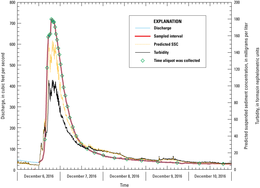
Storm hydrograph, turbidity, and estimated suspended-sediment concentration (SSC) for the Northeast Branch of the Anacostia River at Riverdale, Maryland (U.S. Geological Survey station no. 01649500) for December 6–10, 2016.
Predicting a suitable sample interval for smaller, flashy streams where storm flow typically lasts less than a day, is more difficult. Here, successful sampling (obtaining a suitable mass of sediment that is representative of the entire storm hydrograph) becomes constrained by the time required to pump a volume of aliquot (which is a function of the pumping rate) and the duration and the number of purge and rinse cycles. An example is presented in figure 32, which shows the hydrograph for a storm during December 5–7, 2016, on Watts Branch, a flashy urban stream draining an area in southeastern Washington D.C. (Wilson 2019). The suspended-sediment concentration and resulting mass of sediment in the stream were calculated using the turbidity, discharge, and suspended-sediment concentration model from Wilson (2019). The estimated mass of sediment that would be obtained using several different sampling schemes are presented in table 10; these schemes include sampling every 10 minutes (time composite sampling) or every 0.5 million liters (ML) of discharge (flow-weighted composite sampling) and collecting either 1 L or 2.5 L aliquots for different number of bottles. Using these calculations, the mass of sediment, and the percentage of the total discharge and total sediment load that would be represented by the sampling were calculated. Flashy streams are difficult to sample because if a small discharge interval (such as 0.5 ML) is chosen, the sampling may occur at extremely short time intervals (in this case, as short as 2 minutes); this short of an interval is unlikely to be possible given that several minutes will be needed to rinse and flush the sampling line. In other words, choosing a sampling interval of 0.5 ML of discharge would result in samples being missed during the times of maximum flow (in this case, anytime discharge was over 95 cubic feet per second). This example exemplifies one advantage to keeping the inlet lines as short as possible, reducing the time needed for the purge/rinse/sample cycle between samples helps ensure that samples are not missed during periods of extreme discharge.
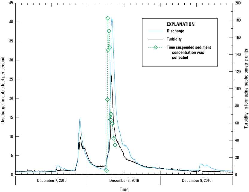
Discharge and turbidity measured in Watts Branch at Washington, D.C. (U.S. Geological Survey monitoring station 01651800), for December 7–9, 2016.
Table 10.
Summary of sediment mass collected during the storm hydrograph shown in figure 32, using different trigger points, sampling intervals, and aliquot volumes.[Data are from Wilson, 2019. ft, foot: NTU, nephelometric turbidity unit; ML, million liters; L, liter; g, grams]
Triggering point refers to change in river conditions that initiate sampling. An aliquot is taken at initiation.
Sampling intervals are the variables determining when each aliquot is collected. Intervals of river discharge are in millions of liters. Sampling at a constant discharge interval produces a flow-weighted sample, while sampling on set time intervals does not. The shortest interval possible with the equipment being used was four minutes, and at this short time interval, the autosampler misses aliquots during times of peak discharge.
As shown in table 10, however, four of these sampling schemes would cover more than 75-percent of the storm discharge and 87-percent of the mass of sediment that was ultimately transported during the storm event and would provide over 6 grams of sediment for chemical analysis. By increasing the volume of each aliquot, thereby decreasing the number of total aliquots required by the volume of sample container held by the autosampler, a suitable mass of sediment would be obtained, but the sampling would cover only about 33-percent of the total water volume and sediment mass transported during the storm. This also illustrates the tradeoffs that need to be considered when designing a large-volume sampling program.
Composite Sampling of Sewers and other Waste Streams
When using an autosampler to produce composite samples from sewers and other waste streams, particular attention must be given to the design of the sampling program. The flow in these waste streams is highly variable and can occur as many “pulses” of water originating from different upstream discharges to the sewer pipe, some very close to the sampling point and some far “upstream” from the sampling point. At the inflow to a large sewage treatment plant, the pulses inherent in a waste stream become mixed, but even still, the flow and composition can change over the course of a day (high discharge in mid-morning and early evening, low discharge in between). The flow, therefore, cannot be assumed to be well mixed temporally. Typical regulatory monitoring at a sewage treatment plant involves collecting aliquots equally spaced over a 24-hour period (usually one each hour). While appropriate for regulatory purposes, equally spaced composite sampling (in time) may not be adequate for determining “average” concentrations for loading calculations. The user is encouraged to consult up-to-date literature (for example, Ort and others, 2010), when designing a sampling program for sewers and other similar waste streams.
Bottle Types and Configuration
Commercial autosamplers typically hold up to twenty-four 1 L sample bottles, eight 2 L bottles, four 4 L bottles, or a single large carboy of varying volume. Bottles can be made of glass or plastic. Often, equipment specific bottles supplied only by the autosampler manufacture are required. Examples include the plastic wedge-shaped bottles or tall cylindrical shaped glass bottles shown in figure 33. These bottles typically require equipment-specific bottle holders or racks. It is important to use only bottle-holder cages made for a specific autosampler, as any non-specified equipment may result in missed or lost samples. As mentioned above, one alternative is to have a large volume container held outside of the autosampler.
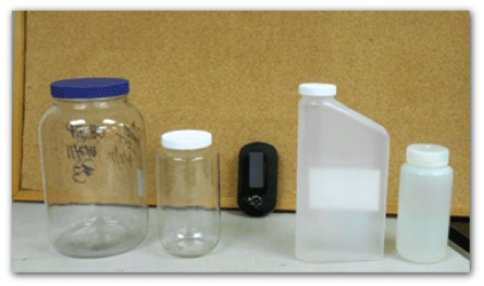
Photograph showing examples of glass and plastic bottles of various volumes that can be used in autosamplers. Photograph by U.S. Geological Survey.
For some bottle types, commercially pre-cleaned sample bottles are available from laboratory supply companies or obtained directly from analytic laboratories. For example, in figure 33, a 4 L glass, class-A level, pre-cleaned bottle is shown that can be used in an autosampler for composite sampling. These bottles are ideal for collecting large volume composite samples for trace-level organic-compound analysis. Similarly, bottles made of perfluorinated plastic (Teflon) are available for trace inorganic metals. Expensive, commercially pre-cleaned bottles are not necessary when sampling for standard inorganic analysis or for analysis of suspended sediment. Whenever glass or plastic bottles are reused, standardized cleaning procedures and blank testing should be followed to assure the cleanliness of the bottles.
Single-Bottle and Multiple-Bottle Schema
The advantage to using a single-bottle autosampler is that a complex sample bottle-distributor system is not needed. Single bottle autosamplers often suffice, for example, when attempting to capture the “first flush” in an intermittently flowing stream or culvert, or to sample when a preset stage is reached, such as at the crest of a storm.
It may be tempting to devise a system where a single composite sample is produced using a system that controls the length of time a peristaltic pump operates. This is not recommended because the efficiency of a peristaltic pump varies with changes in pumping head, and as the pump tubing wears. As a result, equal-volume aliquots will not be obtained, thereby violating a basic requirement for producing a proper composite sample. It is possible to devise a more sophisticated system utilizing a data logger and electronic flow monitor, or incorporate an electronic balance that weighs each aliquot, to produce a single-bottle composite sample.
Multiple-bottle samples, consisting of either discrete or composited samples, can be produced using many of the commercially available autosamplers. These systems utilize a distributor system that places each sample (or aliquot) in an individual bottle. The differences between a single- and multiple-bottle sample are depicted in figure 30. Multiple-bottle composite sampling is used when replicate samples are needed, or when a sufficient volume for the analysis of all components cannot be obtained from a single bottle sample. An example would be a program that samples for sediment-bound trace metals, organic compounds, along with suspended-sediment concentration in a river. To do this, it is necessary to deploy multiple autosamplers set to operate sequentially (from the same triggering signal) to obtain sufficient sample volume to meet the analytical requirements. For simplicity, when deploying multiple autosamplers, use multiple intake lines.
Initiating Autosampler Collection Routines
The triggering, or initiation of an autosampler program can be based on time, discharge, cumulative discharge, or other environmental parameters that can be detected by an electronic sensor, such as the onset of precipitation, initiation of snow melt, water or air temperature, wind direction. Sensors may be supplied by the manufacturer of the autosampler equipment, or it is possible to connect sensors to a stand-alone data logger that acts to trigger the autosampler. Basically, any sensor that produces an electrical voltage or current, or a digital signal can be used to initiate and control an autosampler. Equipment can also be obtained that allows off-site triggering by radio or phone signals.
Table 11 lists some of the environmental variables and sensing equipment that can be used to trigger an autosampler. The most common sensors are a pressure transducer buried in the streambed, a rain gage, a precipitation sensor, or a turbidity sensor deployed in the channel (Lewis, 1996; Lewis and Eads, 2001). Figure 34 shows a rain gage and precipitation sensor that can be adapted for use with programmable autosamplers.
Table 11.
Some environmental variables and sensing equipment to trigger an autosampler.[ft3/s, cubic feet per second; Mgal/min, million gallons per minute; pH, power of hydrogen]
A pressure transducer buried in a streambed is used to supply height of water columns in a stream and can either be a relative measurement or an altitude. A stage sensor is a float or contact switch that initiates sampling when the stage reaches a selected height above riverbed. Stream stage can often be obtained from a nearby U.S. Geological Survey gaging station.
Discharge is calculated using a pressure transducer to establish river stage, and a calibrated stage-discharge relation.
A precipitation sensor initiates an autosampler whenever precipitation establishes an electrical connection.
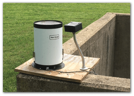
Photograph of a tipping bucket rain gage and precipitation senor to control an autosampler. Photograph by U.S. Geological Survey.
Commercially available autosamplers are equipped with various data ports (fig. 35) that allow an incoming electronic signal to initiate sampling. Autosamplers may have the ability to send out electrical signals through these ports during sampling (for example, when sampling is initiated), along with digital information on the autosampler's status (such as bottle number, sample time, and pump rotations) and time-stamped environmental data (river stage and discharge, precipitation amount, and other such data). These signals can be used to control other autosamplers, pumps, valves, sensors, or other equipment. If needed, the autosampler may be connected to a stand-alone data logging system that can be used to store, evaluate, and transmit the autosampler data through phone lines or via radio communication.
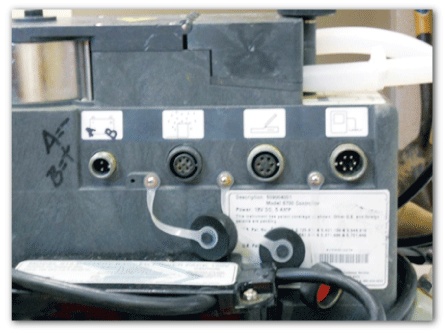
Photograph showing data and power ports on an autosampler. Photograph by U.S. Geological Survey.
Designing Sampling Systems and Routines for Capturing Storm Events
Flowing water, either in natural riverine settings or in constructed systems (stormwater removal swales, stormwater removal or retention systems, and others) exhibit many different hydrologic responses to precipitation events. These hydrologic responses are also affected by the meteorologic characteristics of the associated precipitation events (for example: short, high-intensity bursts during thunderstorms; long, slowly increasing precipitation as large-frontal systems pass; and rapid snowmelt). It is not the intent of this document to present a detailed discussion of the characteristics of watershed hydraulics during storm events. However, knowledge of the characteristics of the system under study will aid in the design of sampling equipment and control schemes.
When designing a sampling system, it is important to study any available hydrographs of the system or nearby similar systems, along with any available water-quality data; suspended sediment and specific conductance are two of the more important water-quality parameters that may aid in planning a sampling program, but turbidity and major-ion chemistry can also play a vital role (Lewis, 1996; Lewis and Eads, 2001). Other information that is helpful includes detailed maps of the watershed or sewer shed that indicate tributaries, storm drainage pipe outfalls, dams or other impediments, paved areas, and other natural and cultural features.
Hydrographs of storm events are presented throughout this document as examples and, while specific to their watershed, show some of the more general features in hydrographs associated with storm events. These include
-
• broad storm hydrographs characterized by a smooth rising limb, a broad crest, and a smooth receding limb. These are characteristic of large watersheds with a dendritic distribution of tributaries draining predominantly natural forested landscapes with minimal paved land surfaces. In larger basins, response to precipitation may occur hours or even days after the onset of precipitation. In these types of basins, substantial amounts of sediment will move during storm events.
-
• hydrographs exhibiting a skewed “log-normal” distribution characterized by a rapid rising limb, short crest period, and a long slow receding limb. These hydrographs are typical of moderate-sized watersheds covered by a mix of urban and rural landscapes. Often these storm hydrographs show flow response in the rivers that are preceded by small ancillary rises in flow. These initial peaks likely indicate precipitation had occurred in a sub-watershed located near the sampling point, or that a storm water outfall is located close upstream to the gage. Generally, the bulk of sediment is moved during the initial rise and crest of the hydrograph. These systems may show distinct seasonal differences in response to precipitation—being a function of leaf coverage, rate of snow melt, and other seasonal factors.
-
• hydrographs that exhibit very rapid rising and falling limbs, separated by a small crest. These “flashy” hydrographs are common in urbanized areas where the stream is influenced by runoff from one or more paved areas. Typically, stream response occurs shortly after, and in some case during, the precipitation. Often, multiple crests are observed in the hydrograph as water from upstream sewer-sheds reach the sampling point. These peaks may or may not coincide with peaks in suspended-sediment concentration, as the streambed becomes “sediment depleted” late in the storm hydrograph.
There are, of course, a myriad of different combinations of stream response to precipitation events. However, the general nature of the response shown by the system under study and the study goals or regulatory constraints play a role in selecting the sampling equipment and sampling schemes used in a study.
Triggering on Stage or Discharge
Perhaps the most common environmental parameter used for initiating an autosampler is stream stage or discharge. A rapid increase in stream stage associated with a precipitation event is used as a signal to initiate the sampling routine; generally, the autosampler is programmed to collect its first sample (or first composite aliquot) at this point, or it can be instructed to start summing the discharge until the first sampling interval is reached.
As mentioned previously, discharge is a required parameter for producing a flow-weighted composite sample, either by automatic or manual compositing methods. To measure stage, a pressure transducer is typically buried in the streambed or attached to the floor of a culvert, or an acoustic stage or flow monitor is used to initiate sampling. A built-in, or stand-alone data logger, uses a pre-programmed stage-discharge relation to calculate discharge, and then sums the stream discharge to trigger the next sample collection. It is clearly advantageous to locate the auto-sampling site near or at an existing streamgaging station, especially if there is a well-established stage-discharge relation available for the site. For non-gaged rivers, discharge can be obtained from a nearby gaged stream or estimated from basin characteristics until sufficient discharge measurements can be made to construct a stage-discharge relation for the site.
When using stage as a sampling trigger, historic data for the stream can be consulted to aid in programming the autosampler. A general rule is to choose an increase in stage that is at least twice the normal daily variation in base flow, as the trigger point for initiating the sampling program (the collection of the first sample or aliquot). Historic discharge data can then be evaluated to determine the typical variation during base flow.
While it is not possible to precisely predict how a river will respond to an upcoming precipitation event, rainfall data, if available, can be tabulated and combined with historic river discharge data to help in setting initiation stage and discharge intervals. For example, ranges of precipitation totals and intensity were tabulated with corresponding ranges of maximum discharge and duration of storm flow, as function of growing and non-growing season (or other classifications) for two rivers in New Jersey (table 12). This table was compiled using a 25-year dataset; however, using even the previous few years can provide useful information for designing a sampling scheme for an upcoming storm under present-day conditions in the study watershed. A spreadsheet was then developed that, using the historic precipitation or flow data, and the approximate runoff (in cubic feet) expected for a given amount of precipitation, can estimate the number of discrete samples to be collected per day. For composite sampling, the volume of the sample bottle and aliquots can be calculated. This type of spreadsheet, along with weather forecasts, can help researchers choose initial sampling parameters.
Table 12.
Example of a table of rain amount, the resulting peak flows, and average number of events of each magnitude occurring over a 25-year period for two river basins in New Jersey.[Modified from Wilson and Bonin (2007, table 60). Based on data from 1975 through 2000 water year record. ft3/s; cubic feet per second; >, greater than; <, less than]
Precipitation values are based on the 24-hour period preceding the onset of stage rise in the river.
The average yearly flow of the Passaic River during this period was 251,000 million gallons. For 35 days out of a given year, the river is expected to be at “low-flow” (125 ft3/s), meaning that no precipitation occurred in the previous 7 or more days.
When deploying an autosampler on a non-gaged stream, the stage-discharge relation for a nearby gaged stream may be helpful as a starting point for programming discharge-based triggering. However, it is important to ensure that the nearby “surrogate” stream basin is comparable to the studied stream. If data from a surrogate stream are not available, then the researcher should develop a preliminary stage-discharge curve for the study stream by making cross-sectional velocity measurements over a few different flow conditions. The preliminary stage-discharge relation can be refined over time as additional data become available. Flow-composite sampling is not advised at locations lacking an existing stage-discharge relation.
Triggering on Precipitation
Another commonly used sampling trigger is the onset of precipitation or the onset of snow or ice melt. Tipping-bucket rain gages (for example, fig. 34) can be used to initiate autosampler programs, and to collect volumetric measurements. Precipitation sensors that make an electrical connection when sufficiently wetted can be used to initiate an autosampler. These types of precipitation gages and sensors can be deployed throughout a watershed and combined with telemetry equipment to initiate sampling at downstream sites. Care should be taken that the precipitation monitor is deployed using appropriate methods, such as specified by the National Weather Service (National Weather Service, 2024) or other agency.
Triggering Using Other Parameters
Other water-quality parameters can be used to trigger an autosampler program often for specific study goals. A review of chapter A6 of the NFM provides guidance for the standard measuring procedures for these parameters across a range of scenarios and conditions (U.S. Geological Survey, 2008b). This guidance enables study designs in which the following parameters have been used:
-
• Temperature has been used in studies of rivers affected by release of cooling waters from power and industrial plants.
-
• Dissolved oxygen has been used in studies of rivers affected by sewage waste and paper-mill pulp discharge, and in diurnal studies of reduction-oxidation sensitive species such as iron and manganese.
-
• Specific conductance has been used in studies involving seawater infiltration in coastal wetlands, coastal streams, and channels. Specific conductance could be used to trigger water systems affected by evaporation.
Strategies for Triggering Composite Sampling
As described earlier, one use for autosamplers is to automatically produce a flow-weighted composite sample that provides an estimate of an average concentration in a stream over a hydrologic event. Usually this is a precipitation event, but it also can be defined over any range of flow conditions or time. The example in table 13 demonstrates the calculations involved in producing a flow-weighted composite sample from individual discrete samples, or as a single sample produced by compositing equal-volume aliquots collected at equal discharge intervals. In this example, the number of samples, the time intervals, and flow intervals were selected based upon a model, hypothetical hydrograph. For streams that are not gaged, it is often best to start by collecting, and manually compositing, discrete samples. It is also helpful to conduct (and budget for) practice sampling events. This will help the researcher predict how a stream will respond to different storm events.
Table 13.
Example of information needed for estimating flow intervals, autosampler parameters and volumes of aliquots needed to produce a composite sample.[in., inch; ft2, square feet; Mgal, million gallons]
As an example of how these calculations are used to design a sampling routine, figures 36 and 37 show stream hydrographs for a large river (the Raritan River) and a small urban river (the Elizabeth River) in New Jersey (Wilson and Bonin, 2007). Shown on the hydrographs are times that discrete 1 L samples were collected to analyze suspended-sediment concentration. These samples were collected at equal stream discharge intervals. Additionally at each time point, a second autosampler was used to collect and composite (in a 4 L glass bottle) an aliquot of river water for chemical analysis. Both autosamplers were triggered using the same stage signal.
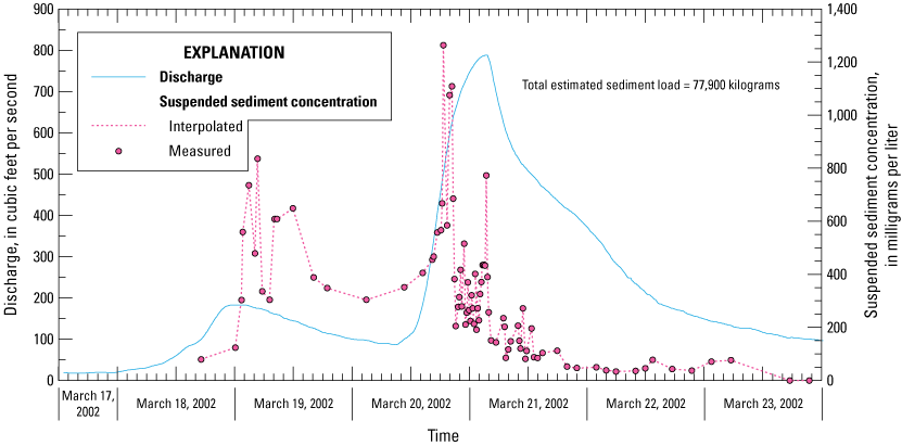
Plot showing discharge and suspended-sediment concentration in the Raritan River at Bound Brook, New Jersey, March 17–23, 2002. Modified from Wilson and Bonin (2007).
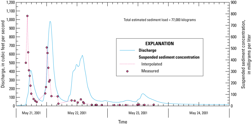
Discharge and concentrations of suspended sediment in the Elizabeth River at Hillside, New Jersey, May 21–24, 2001. Modified from Wilson and Bonin (2007).
In the larger Raritan River, two precipitation-fronts had passed through the area within two days. Multipeak hydrographs are common where large-scale cyclonic storm fronts pass through large watersheds that have several large tributaries. However, it should be noted that a similar response may be observed where a tributary enters upstream close to the sampling site. In this example, the autosampler was left operating after the first front had passed through the area. Then the larger precipitation front passed through the basin, resulting in the second much larger portion of the storm hydrograph (fig. 36). The concentrations of suspended sediment in the figure are connected using stepwise interpolation, then integrated to determine the suspended-sediment load. As can be seen, the suspended-sediment concentrations in the stream peaked early, but after the second peak, SSC decreased and remained low despite the high discharge.
In the smaller Elizabeth River, a short, high intensity rain event had resulted from a summer thunderstorm. This produced three “flashy” discharge peaks; these peaks result from discharge emanating either from nearby upstream or storm drains (fig. 37). In this case the suspended-sediment concentration reached a maximum in the first discharge peak, and lower peaks of concentration were measured in subsequent peaks of discharge. This phenomenon is likely the result of “sediment depletion” as the river and tributaries become flushed of easily moved fine-grained sediment that was stored in the river since the time the most recent storm event occurred. The discharge interval used in this sampling allowed for an accurate picture to be developed of how the sediment concentrations varied with time. However, the spacing was large enough to keep the discrete samples from overlapping during maximum discharge.
Designing a Program for Automated Composite Sampling of a Storm Event
Reviewing historic discharge and precipitation data for an area is the first step in designing a successful sampling scheme. The unknown variables are the amount and intensity of precipitation in the upcoming storm event, the appropriate discharge interval for collecting each sample, and the aliquot volume that will produce an accurate composite sample. The following are some strategies that may help in choosing these variables:
-
• Compile historic precipitation and discharge data for the area and for the sampling season(s) of interest. Combine these data with radar-based weather predictions of precipitation for these events and begin to establish the seasonally based response of the studied river.
-
• Combine the historic flow data for the studied stream (or for a nearby stream with similar basin characteristics) with the precipitation record for the drainage basin. These data can be used to estimate the likely peak discharge and flow-duration in response to a given amount of precipitation and intensity. Limit the dataset to the previous 5–10 years, as this will help reduce the effects of recent land-development in the drainage basin.
-
• Using these data, select historic storms of different magnitudes (both precipitation amount and maximum discharge for the stream) and season. Then for each selected event, choose an aliquot volume that is large enough to ensure an accurate volume would be collected for each streamflow interval, but small enough that the autosampler could pump the aliquot in a suitable length of time. If the aliquot volume is too large, or the pump rate is too slow, then samples may overlap during the periods when streamflow is high. The volume of aliquot collected, plus the discharge interval selected and the final composite volume (bottle volume), will combine to produce the maximum volume of the composite sample.
-
• Consult the tabulated historic data and aliquot volumes to decide on sampling parameters for an upcoming storm event. If it is likely that more than one composite bottle will be filled, plan on a site visit to replace bottles in the autosampler(s).
-
• Using the historic precipitation and streamflow data, prepare a spreadsheet that relates the range of expected precipitation amount to stream response and other sample parameters.
-
• Alternatively, the user can develop a simple watershed response model based on land use and precipitation data. Watershed models that are based on land use classifications, such as the SPARROW (SPatially References Regression on Watershed attributes) model (Smith and others, 1997), are useful in this endeavor if sufficient data are available.
-
• If possible, conduct practice sampling to fine-tune the relation between precipitation amount and intensity, the final number of discrete samples collected, and the volume of each sample aliquot needed to fill a composite bottle of a selected volume. These practice samplings can involve actual sampling or can be done numerically after a recent precipitation event.
-
• For making load calculations, a stream should be sampled (at a consistent flow interval) over as much of the storm hydrograph as possible. Sampling is often curtailed before the stream has returned to pre-storm stage or discharge (for example, because of equipment problems or all available bottles have been filled). It is imperative that a criterion for a “successful” sampling is developed based on the percentage of the storm hydrograph that was sampled (percent of total discharge). Criteria can be set for both discrete and composite samples. These criteria may change as more experience is gained and information is obtained on the stream basin being studied.
-
• When suspended sediment or POC were analyzed in multiple discrete samples, prepare a plot of the relation between cumulative water discharge and cumulative mass of sediment (or POC) in the stream. Use this plot to numerically quantify the collection results, and to develop criteria that define a “successfully” sampled event. This type of plot also allows the researcher to estimate the mass of sediment or POC not sampled during a storm event.
Pre-Sampling Preparation
Autosampler Maintenance and Cleaning
All autosamplers and data loggers will require servicing before each sampling event. The servicing should include general cleaning, verification that adequate battery or electrical service is available, examination (and sometimes replacement) of pump tubing and inlet lines, and restocking of clean bottles. A checklist should be provided for these steps.
Proper cleaning of all the components of the autosampler that come in contact with a sample is essential to ensuring valid results. Verification of equipment cleanliness and due-diligence by the field crews is provided by the field-equipment blanks and other QA/QC samples. Depending on the type of autosampler used, the parts that may need cleaning include the intake line, pump tubing, diversion valve (if used), distributor line tubing, sample container(s), and interior of the autosampler housing. As a general rule, the cleaning instructions for equipment used are based on the constituent(s) under study. In addition, each autosampler may have specific manufacturer’s instructions for cleaning, and should be followed.
Different classes of analytes require special cleaning needs. For general cleaning instructions for inorganic and organic sampling see chapter A3 of the NFM, “Cleaning of Equipment for Water Sampling” (U.S. Geological Survey, 2004). Table 14 summarizes the general cleaning requirements for major parameter groups. See also the “Cleaning Procedures” section of appendix 2.
Table 14.
General cleaning requirements for autosamplers deployed for sampling different constituent groups.[DSW, distilled water; IBW, inorganic-grade blank water; OBW, organic-grade blank water]
Intake-Line Maintenance and Cleaning
The intake line is one of the most vital pieces of the sampling system and has great potential to affect the integrity of samples. Deposits of sediment, organic matter, oils, and grease can affect the chemistry of each volume of water passing between a stream and sample container. For example, figure 18 shows how inlet lines can become coated when left in a river for extended periods of time. Therefore, it is important that a rigorous and thorough cleaning program is followed, especially when autosamplers are deployed in a long-term or permanent study and for trace components. Intake lines and screens (if used) should be removed, checked, cleaned, or replaced before each sampling event following steps documented in the study SOP. As a general policy, it is advisable, at a minimum, to clean the intake lines used to collect chemical samples before each event. Replacing lines with pre-cleaned tubing for each event should be considered and may in fact be necessary when sampling urban streams or waste outfalls carrying water containing oils and grease. The ability to replace intake lines should be considered carefully when designing a sampling system, especially where trace elements or organic compounds are being studied. Prudent operating procedures dictate, however, that intake lines are pulled for cleaning or replacement on at least a regular basis.
Lines used to collect only suspended sediment do not necessarily need to be replaced before each event but should be inspected periodically to determine if sediment is accumulating in low points (dips). Sediment will accumulate if pumping rates are insufficient, or if lines are left unused for extended periods of time. Pumping tap water or air under high-pressure may be used to purge this sediment from the line.
It is important to inspect the inlet line where it enters the stream, along with the nozzle and screen if used, to verify it is not kinked, obstructed, or excessively abraded. A small portion of the nozzle can often be cut to remove a kink or rough surfaces, but the cut should be sharp and clean. Screens should be removed and cleaned with hot-soapy water before each event or replaced with a pre-cleaned screen. Pump and distributor arm tubing should be replaced with new pre-cleaned tubing before each event.
Cleaning is best performed in the laboratory but in some instances (for example, lines used for suspended sediment or general inorganics) can be conducted in the field if necessary.
In the laboratory, the various inlet and pump tubes can be connected together using a plastic barbed fitting and attached to form a single line. Using a peristaltic pump, the sequence of appropriate cleaning solutions (described earlier for the different intended constituents of interest in table 14) can be pumped through the entire length. For safety, it is recommended that cleaning solutions be “pulled” through the lines, in case a break in a connection occurs. The following is a general sequence of cleaning steps:
-
1. A rinse of hot tap water
-
2. A rinse of a solution of laboratory grade detergent, made using warm or hot tap water
-
3. A rinse of warm tap water
-
4. A rinse of DSW
-
5. A rinse of dilute hydrochloric acid (5–10 percent solution)
-
6. A rinse of DSW
-
7. A rinse of new methanol
-
8. A rinse of DSW
Use a phosphate-free laboratory detergent solution no stronger than 0.2-percent (2 mL concentrated detergent per liter of water); stronger solutions do not perform better, and even a small amount of residual can be carried over or leave a residue on tubing and fittings. Although the acid and methanol rinses are not required when the lines are used for general inorganic constituents, nutrients, or sediment, they are necessary when sampling for trace metals and organic constituents and are recommended in all studies as these solutions will remove any oil or grease adhering to the inside of the previously used sampling lines. Allow the cleaning solutions to recirculate continuously for 20–30 minutes before disposal following laboratory procedures. Periodically stop the pump and let the solutions stand for several minutes in the tubing. While the solutions are circulating, periodically pinch the tubing outlet to allow the solution and air bubbles to mix. Once cleaned, the ends of the inlet lines should be capped with foil or plastic wrap, the tubing carefully wound, and placed in large plastic bag for transport.
Cleaning inlet lines in the field in situations that require removing and replacing the lines is difficult. As mentioned previously, to remove any debris that may have accumulated in the lines, it is advantageous to occasionally purge the lines with high pressure air or tap water before cleaning. The cleaning solutions can then be pumped down the lines (from the site into the stream) using a peristaltic pump or the autosampler. A waste container should be placed at the nozzle end of the line to collect solutions. Stop the pump occasionally for 5–10 minutes to allow the cleaning solutions (soap, acid solution, or methanol) to remain in the lines and soak. Try not to allow acid, soapy water, or methanol to discharge into a natural water body. Note that field cleaning is most practical for locations where large volumes (25–50 L) of tap or distilled water and necessary cleaning solutions can be easily transported to the station.
Following retrieval of samples and sampling data, the autosamplers will need servicing before the next sampling event. If events are to be separated by weeks or months, it is best to remove equipment and sampling lines. Table 15 lists many of the steps recommended when servicing an autosampler; these steps should be detailed in the project SOP. All of these steps are important; however, some are more critical to ensuring the success of subsequent sampling efforts. For example, it is critical that the sample volume is calibrated each time the autosampler is serviced, especially if composite samples are being produced, and whenever pump tubing is replaced. Follow the manufacturer’s instructions for confirming and adjusting the sample volume. Field crews should be provided step-by-step instructions for calibrating and documenting pump preparations. Where a stand-alone data logger is used to control pump equipment, the operating code should provide the capability for calibrating pumps.
Table 15.
Examples of components of a standard operating procedure (SOP) for an autosampler-based collection study.[QC, quality control; EWI, equal-width increment, isokinetic sampling method; EDI, equal-discharge increment, isokinetic sampling method; QA, quality assurance]
Consult chapter 4 of the National Field Manual for more details (U.S. Geological Survey, 2006).
Chapter 4 of the National Field Manual (U.S. Geological Survey, 2006) and Britton and Greeson (1989) provide helpful guidance on the general sequence for cleaning equipment and bottles for sampling inorganic or organic analytes. However, depending upon the analyte suite (trace metals, organics, and bacteria for example), additional cleaning and preparation steps may be required.
Preparation for Sampling for Trace Metals
When sampling for trace metals, the sampling line, pump tubing, and distribution tubing can be a significant source of contamination. Tubing will usually require a post-wash rinse or soak with dilute (5–10 percent by volume) hydrochloric acid. All metal couplings used in the autosampler should be replaced with acid-rinsed Teflon or plastic fittings and bottles. When cleaning plastic (including Teflon) tubing for inorganic-constituent samples, the general sequence of procedures summarized by U.S. Geological Survey (2006) should be followed prior to deployment for sampling:
-
1. Wash tubing with hot, soapy water (non-phosphate containing laboratory detergent), either by allowing the completely filled tubing to soak, or by continuously circulating the wash solution with a peristaltic pump.
-
2. Rinse with tap water and then DSW (three-tubing volumes or more per rinse).
-
3. Pump at least 1-tubing volume or 1 L of 5- to 10-percent hydrochloric acid solution through the tubing, discharging the used acid solution into a neutralization container. Wearing nitrile gloves, pinch and release tubing near tubing outlet while slowly pumping the acid through to ensure that all interior surfaces are acid rinsed before discarding the solution. Alternatively, the acid solution can be continuously recirculated through the intake line, pump tubing, discharge tubing, and through all connectors at a slow rate for at least 30 minutes, ensuring that all air-bubbles are moved through loops in the tubing. At the conclusion, properly dilute and neutralize the acid solutions before discarding.
-
4. Pump a minimum of two-tubing volumes of DSW through the tubing, using the pinch-and-release or recirculation methods. Neutralize the rinse water if its pH is less than 6.
-
5. Neutralized and dilute acid solutions appropriately before disposal. Typically, this required neutralization is done using calcium or sodium carbonate (baking soda).
-
6. Clean all plastic connectors (and metal, if used) using a hot-water detergent wash, then rinse with tap and DSW. Soaking plastic fittings long-term in acid solutions may cause some plastics to become brittle. Any stained or brittle connectors should be discarded.
Sampling for Organic Constituents
When sampling for organic constituents, first follow the general cleaning procedures outline above for trace metals, then rinse the tubing and all fittings in chromatographic-grade methanol. Acetone should not be used for cleaning as it often contains trace organic impurities. The dilute acid wash should be considered especially if the tubing has been used previously in iron-rich or high-organic content waters. If the tubing will be used for collecting samples for analysis of total organic carbon, the methanol rinse should be omitted (additional notes on methanol are in box 3), and the tubing and fittings washed only with hot soapy water and rinsed well with DSW. In some cases, it may be best to use a separate autosampler for total or dissolved organic carbon sample collection.
U.S. Geological Survey (2004) gives the following procedures for cleaning sampling equipment used for sampling for organic constituents:
-
1. Pump at least one tubing volume of non-phosphate, laboratory-grade detergent solution prepared in hot water through all tubing and couplers, followed by sufficient tap water or DSW to remove detergent residue. Do not use a detergent solution stronger than 0.2-percent (2 mL concentrated laboratory detergent in 1 L water) for field cleaning (stronger solutions will not provide better cleaning action). Pinch and release tubing near tubing outlet while pumping the solution to ensure that all interior surfaces are cleaned. Alternatively, the cleaning solution can be recycled through the intake line, the pump tubing, and the distributor tubing for at least 30 minutes before rinsing.
-
2. Wear safety gloves of appropriate material, goggles or a face shield, and apron.
-
3. Work in a well-ventilated area away from open flames or sparks.
-
4. Make sure that all electrically powered equipment is grounded; AC equipment must use a ground-fault interrupter outlet.
-
5. Inspect electrical wiring for cuts, breaks, or abrasions that may expose the metal wire. Do not rely on electrical tape to fix wires.
Box 3. Safely Using Methanol in the Lab
Methanol is extremely flammable and potentially explosive, emits vapors that can be inhaled, and can be absorbed through the skin if improperly handled. However, methanol, is highly soluble in water and poses no risk once dissolved in water and can be mixed with water and disposed of down the drain. Observe the following safety practices recommended by the U.S. Geological Survey (2004) when handling methanol or other organic solvents:
-
• Place one end of inlet line into the methanol container, and connect the pump to the far end, thereby pulling the methanol through the tubing, through the pump and then into the waste or recirculation bottle. This will help minimize the volume spilled if a connector becomes detached or the pump tubing breaks during cleaning.
-
• Pass at least one tubing volume of methanol through the pump system, using the pinch-and-release method, or alternatively, recirculate the methanol through the tubing.
-
• Short sections of tubing and connectors can be held over the waste container while dispensing the methanol from a fluorocarbon-polymer wash bottle instead of pumping the methanol through the tubing. Connectors can be soaked in methanol in a capped beaker or closed glass jar for short periods of time. Rinse all connectors in DSW, place under foil to evaporate dry.
-
• Tubing and fittings should not be rinsed with methanol when sampling for total particulate or dissolved organic carbon. If rinsed with methanol, then the tubing should be carefully rinsed with DSW, ensuring all air voids are eliminated from tubing loops. Collect a laboratory or field-equipment blank before sampling.
-
• Rinse tubing with a minimum of one volume of ultra-clean laboratory grade distilled water, briefly allow tubing to drain. Best-practice involves multiple rinses with draining between rinses.
-
• Place all methanol rinsed pump tubing and connectors under clean foil and allow to evaporate to dryness, then wrap in aluminum foil and store tubing in doubled plastic bags.
Sampling for Microbial Constituents
Sampling for bacteria and other bio-constituents requires all bottles and tubing to be autoclaved or sterilized after the inorganic wash described in the previous section. Closely follow the manufacturer procedures for operating the autoclave because high temperature and pressure steam is involved. Bottles should not be tightly capped during autoclaving and should be placed (along with caps and all parts) in a new sterilization bag. Attach sterilization tape to each bottle or bag to indicate that proper conditions were reached to sterilize the equipment.
If necessary, sterilization can also be performed by rinsing all tubing and fittings in a dilute (5-percent) solution of household bleach, followed by multiple rinses with DSW. The interior of the autosampler housing should be washed with a hot, soapy solution and tap-water rinse, followed by a wipe down with a 5-percent bleach solution, then by a rinse with DSW. All cleaned tubing, sample bottles and caps, and other equipment should be wrapped or capped in sterilized aluminum foil and sealed in plastic bags for transport. Additional information for sampling for biological constituents can be found in U.S. Geological Survey (2008a).
Sampling for Suspended Sediment and Particulate Carbon
It is usually sufficient to wash the line and pump tubing in hot-soapy tap water when they are only being used to collect suspended sediment. However, the sampling lines should be periodically removed and inspected (especially the intake nozzle) to ensure that they are free of debris, have not been kinked or stained by oil, and that sediment has not settled in the line. If the nozzle end of the intake line is found to be kinked or badly abraded, it should be trimmed, or the line replaced.
Post-Event Sample Collection and Equipment Maintenance
Retrieval of Samples and Data
Regardless of the purpose for which the autosampler is deployed, it is prudent to describe in the standard operating procedure (SOP) document how samples and data are to be retrieved, and how equipment is to be maintained. Table 16 lists some of the steps that may be involved in servicing an autosampler. The SOP should outline all of the steps to be followed, provide forms that help field personnel inventory and record the necessary data, and steps to verify the autosampler was properly calibrated and programmed for the next sampling event (if applicable). It should list how the data are to be downloaded from the autosampler (or data logger), and the information that should accompany samples to the analytic laboratory. An example SOP is provided in appendix 2.
Table 16.
Examples of steps to follow when servicing an autosampler station.[QA, quality assurance; QC, quality control]
Sample Processing
Samples should be retrieved as soon as possible upon the conclusion of a sampling event. Some constituents such as bacteria or VOCs have short, required holding times (if applicable), and the sampling plan should dictate the retrieval and preparation of the samples as soon as possible, perhaps even when the autosampler is still operating. The first step in retrieval should be to ensure all samples are secured, properly capped and labeled. At a minimum, the label should contain date and time of collection or retrieval, and the location of the bottle in the autosampler. These data can then be recorded on field forms. When discrete bottles are being retrieved, it is advantageous to maintain the bottles in their respective place in the autosampler carousel, and number their position directly on the bottle in permanent marker. Be very careful not to switch bottle positions in the carousel. Note: If the autosampler is being readied for the next event, replace the carousel with a new carousel containing unused bottles.
Other general guidelines include the following:
-
• Plan the sampling routine to minimize the manipulation and handling of samples. The integrity of any sample is highest when it is preserved and capped as soon as possible after collection. For example, it may be possible to place pre-measured amounts of preservatives in each bottle when installed in the autosampler. If field crew is present at the site during sampling, it may also be possible to cap and remove any filled sample bottles while the sampling program is still underway.
-
• Return the samples to a laboratory setting or use a dedicated sample processing area or sampling van for processing, especially if samples are to be filtered or manually composited. Discrete samples can often be transported in the autosampler carousel; however, if special containers are used (for large volume samples) then specific handling steps for large, heavy containers should be described in detail.
-
• If the project involves sampling both aqueous chemicals and suspended sediment (or particulate carbon), then multiple bottle-sampling routines or multiple autosamplers will be employed. Do not use a sample bottle collected for suspended sediment to sub-sample water for POC or other chemical analysis. Bacteriological samples should be collected only in dedicated bottles and remained capped until analyzed. Bottles being used for suspended sediment should be pre-weighed (tared) before use, and the bottle weight should be clearly marked on the bottle or label.
-
• When a single discrete sample has been collected that will be used both for dissolved and total species analysis then the following protocol is suggested. First, cap and shake the sample-collection bottle, or alternatively, shake and pour the sample into a pre-cleaned churn. Then remove the “total species” aliquot from the bottle by either decanting or by using a peristaltic pump with a pre-cleaned line into the sample collection bottle. Once the aliquot for “total species” analysis has been removed, the remaining water can be filtered into a separate bottle for “dissolved species” analysis. Avoid removing the “dissolved species” aliquot first, if possible, because particle settling has the potential to affect the “total species” concentration in the water remaining in the sample-collection bottle.
-
• When discrete samples are to be composited to produce multiple replicate samples (either for QA/QC purposes or when multiple suites of analytes cannot be performed on a single bottle), it is generally best to prepare a single composite, from which multiple bottles can be filled. Suitable aliquots of the discrete samples can be transferred to a churn, properly mixed, and then transferred to individual bottles. Plan to collect an excess of water in each aliquot to provide a sufficient volume for all necessary analytes.
Sample Documentation and Metadata
Metadata are the ancillary information necessary to make samples useful for study purposes. It is imperative that all needed metadata be recorded upon retrieval of samples for a sampling event. The SOP should contain a check list detailing all metadata required for each sample, along with steps for processing and labeling samples, the protocols for collecting QA/QC samples, a detailed schedule for servicing, and information on programming the autosampler. Table 7, table 17, and table 18 list some of the typical metadata that may be needed during deployment of an autosampler.
Table 17.
Examples of information and ancillary data that may be required when using an autosampler.[—, not applicable]
Table 18.
Examples of information recorded on the label of each sample bottle.Manually Producing a Flow-Weighted Composite Sample
Because the final precipitation amount (and therefore total discharge) of a storm event is unknown prior to autosampler setup, and thus an appropriate discharge interval is unknown for producing a composite sample, it is often advantageous to manually produce a composite sample using multiple discrete samples collected at regular time intervals. These discrete samples are then combined in proportion (to the discharge that occurred between collection of each sample) in the laboratory to produce a flow-weighted composite. Best practice is to combine each aliquot into a USGS-style mixing churn and follow standard USGS protocols for churning (U.S. Geological Survey, 2014) and transfer to a suitable bottle for shipping to the analytic laboratory.
While this procedure will result in an accurate composite for dissolved constituent analysis, it can be difficult to produce an accurate composited sample for analysis of suspended sediment. This is because of the inability to ensure suspended material remains uniformly distributed as aliquots are decanted from each sample bottle into a graduated cylinder, then from the cylinder to the composite vessel.
In order to calculate an accurate composite sample, the time when each discrete sample was collected (in this case, one aliquot every 4 hours), the cumulative flow volume and the percentage of the total represented by each 4-hour interval must be obtained. An example of the necessary data and calculations involved in manually compositing discrete samples are included in table 4.3 for a storm event on a small river in central New Jersey. The percentage of total volume sets the volume of each individual aliquot, which then must be combined to produce a 1 L or 4 L composite sample. One consideration in producing a composited sample is the final volume needed for laboratory analysis, and the effect of cumulative measurement errors. If the final composited volume is small (1 L), it may be difficult to accurately measure small aliquot volumes. It is often advantageous to produce a single large volume composite (in this case, 4 L) that can be split for multiple component analyses.
Preparing Equipment for Subsequent Sampling Events
After retrieving samples, the field servicing may entail preparing the autosampler for the next sampling event. This preparation will involve checking the mechanical parts of the autosampler and the condition of the station and should be specified in the SOP developed for each project. Check to ensure that all tubing connectors and parts of the autosampler are sufficiently tightened. Inspect intake line and nozzle and replace if necessary. Desiccant packs in the interior electronics of the autosampler or data-logger should be checked and replaced if necessary. Clocks and interval timers should be adjusted to the correct time immediately before starting the sampling program. Autosamplers and data loggers often have internal batteries that power internal clocks, and these should be checked monthly and replaced if needed. If the autosampler is powered by batteries, the electrical cords and electrical connectors should be inspected to ensure proper connection are in place; autosamplers often shake when operating, and it is not uncommon for electrical connectors (especially spring clips) to loosen and fail. If powered by line voltage, the cords should be periodically checked, along with the line voltage, and ground-fault outlets tested and reset. If the sampling shed is equipped with a heater, heat lamp, or air conditioner, then the operation and interior temperature setting should be checked. Ensure that the entrance door and ventilation openings are opened. Sweep the floors of any mud or debris, and check and remove any rodent nests or debris.
Summary—Autosampler Deployment
-
• Autosamplers can be used to collect discrete or composited samples in deployments where human oversight cannot be provided. Discrete samples are single samples spaced by intervals of time or flow; composited samples are produced by collecting equal volume aliquots of the sampled water in a single bottle with aliquots spaced by time or equal-flow intervals depending upon the project goals. Discrete samples can also be composited by combining aliquots proportionally to the discharge interval.
-
• Autosamplers typically can be programmed to collect single or multiple samples of a number of types of bottles and bottle volumes. Multiple bottle samples can be used for different analytic suites, for preparing replicate samples, and QA/QC samples. Project planning should include consideration of the types and number of bottles and samples needed to complete project goals, and the limitations of number of bottles each autosampler can hold.
-
• As a general rule, samples for suspended-sediment, bacterial, and chemical constituent concentrations should be analyzed from separate dedicated bottles.
-
• Autosampler programs used to complete a sampling scheme can range from a simple triggering signal to multiple complex steps. The researcher should plan on reviewing historic flow and precipitation data and conducting practice sampling (either actual sampling or by numerical simulation) to refine sampling schemes and programs.
-
• It is essential that all necessary metadata associated with each sample collected by an autosampler is recorded. Explicit instructions and a checklist should be provided to field personnel on which metadata needs to be recorded.
-
• Standard operating procedures should be developed for the cleaning, setup, and servicing of each autosampler employed. Depending upon the proposed analytical scheme, specific cleaning and servicing steps may be needed. All parts of the autosampler mechanism (intake line, pump tubing, connectors, autosampler housing, and so on) should be considered possible sources of contamination and require proper cleaning.
Troubleshooting
Autosamplers are not foolproof and require periotic oversight and servicing. The researcher should schedule field visits for servicing to help ensure successful event sampling. Users of automated sampler systems should be prepared to encounter occasional difficulties, which can be overcome through proper equipment maintenance, practice, and troubleshooting. For example, initial attempts at storm sampling may not be successful and practice with the equipment during small events will go a long way in producing success for the large, rarer storms. Project budgets should include ample time to troubleshoot and to re-sample “missed” events, especially if storm sampling is involved. Generally, it is more cost effective to plan on conducting a trial event to learn methodologies and troubleshoot the sampling equipment and the control programs, and to gain knowledge in how the stream being studied responds to precipitation events.
Information on troubleshooting common problems and technical assistance is typically provided by sampling equipment manufacturers. Some of these problems can be traced to loose tubing connections, worn pump tubing, and unforeseen problems in the autosampler control program. Other common problems and troubleshooting hints are listed in table 19.
Table 19.
Common problems and possible solutions for autosampler troubleshooting.[HIF, Hydrologic Instrumentation Facility at Stennis Space Center, Mississippi]
Additional Resources
Appendix 1 is a list of definitions commonly used in an autosampler SOP document. See appendixes 2 and 3 for examples of some components typically found in standard operating procedure (SOP) documents for projects utilizing autosamplers and the calculation and application of a box coefficient for a river station, respectively. Appendix 4 provides an example of river condition data for a hypothetical storm. The text in these examples is not intended to be exhaustive, but rather to demonstrate the detail that should be included in a project-specific SOP. The steps in an SOP should generally follow or be adapted from the standard procedures adopted by the USGS for National Programs, such as the National Water-Quality Assessment Project and Northeast Stream Quality Assessment. Standard procedures for operating an autosampler can usually be referenced to the manufacturer’s documentation. The source for all procedures should ultimately be referenced. It is also good practice to include a history page on the SOP so that the version being followed can be confirmed among field personnel. Lastly, the SOP should be updated during the project if changes in procedures are necessary, and a final version should be stored among project documents to allow for future reference.
Acknowledgements
The authors are indebted to the many individuals at the U.S. Geological Survey that provided time and support to help move this Techniques and Methods manual forward, especially Mary Heinz (editor), Jonathan Kennen (steward), and Trisha Zalesak (visual information specialist); all were integral to the successful completion of the product. We also gratefully acknowledge Fred Spitz and Bill Selbig of the U.S. Geological Survey who provided many helpful suggestions that greatly improved this manual.
References Cited
Anderson, C.W., and Rounds, S.A., 2010, Use of continuous monitors and autosamplers to predict unmeasured water-quality constituents in tributaries of the Tualatin River, Oregon: U.S. Geological Survey Scientific Investigations Report 2010–5008, 76 p., accessed December 12, 2020, at https://doi.org/10.3133/sir20105008.
Aulenbach, B.T., 2009, Bacteria holding times for fecal coliform by mFC agar method and total coliform and Escherichia coli by Colilert-18 Quanti-Tray method: Environmental Monitoring and Assessment, v. 161, no. 1-4, p. 147–159. [Also available at https://pubmed.ncbi.nlm.nih.gov/19165613/.]
Barbaro, H., 2001, Effectiveness of stormwater best management practices along the Southeast Expressway, Boston, Massachusetts, in Irwin, C.L., Garrett, P., McDermott, K.P., eds., Proceedings of the 2001 International Conference on Ecology and Transportation—Center for Transportation and the Environment, North Carolina State University, Raleigh, N.C., p. 345–356, accessed August 2, 2020, at https://repositories.cdlib.org/jmie/roadeco/Barbaro2001a.
Bartsch, L.A., Rada, R.G., and Sullivan, J.F., 1996, A comparison of solids collected in sediment traps and automated water samplers: Hydrobiologia, v. 323, no. 1, p. 61–66, accessed December 12, 2020, at https://doi.org/10.1007/BF00020547.
Bent, G.C., Gray, J.R., Smith, K.P., and Glysson, G.D., 2000, A synopsis of technical issues for monitoring sediment in highway and urban runoff: U.S. Geological Survey Open-File Report 2000–497, 51 p. [Also available at https://doi.org/10.3133/ofr2000497.]
Bonin, J.L., and Wilson, T.P., 2006, Organic compounds, trace elements, suspended sediment, and field characteristics at the heads-of-tide of the Raritan, Passaic, Hackensack, Rahway, and Elizabeth Rivers, New Jersey, 2000–3: U.S. Geological Survey Data Series 123, 32 p., accessed April 23, 2024, at https://doi.org/10.3133/ds123.
Bossong, C.R., Stevens, M.R., Doerfer, J.T., and Glass, B.R., 2006, Summary and evaluation of the quality of stormwater in Denver, Colorado, water years 1998–2001: U.S. Geological Survey Scientific Investigations Report 2005–5150, 90 p., accessed December 12, 2020, at https://doi.org/10.3133/sir20055150.
Britton, L.J., and Greeson, P.E., 1989, Methods for collection and analysis of aquatic biological and microbiological samples: U.S. Geological Survey Techniques of Water-Resources Investigations, book 5, chap. A4, 363 p. [Also available at https://doi.org/10.3133/twri05A4.]
Burton, G.A., and Pitt, R., 2001, Stormwater effects handbook—A toolbox for watershed managers, scientists, and engineers: Boca Raton, Fla., CRC Press, p. 278–290. [Also available at https://doi.org/10.1201/9781420036244.]
Clark, S.E., Siu, C.Y.S., Pitt, R., Roenning, C.D., and Treese, D.P., 2009, Peristaltic pump autosamplers for solids measurements in stormwater runoff: Water Environment Research, v. 81, no. 2, p. 192–200, accessed December 20, 2020, at https://doi.org/10.2175/106143008X325737.
Colby, B.C., 1961, The single-stage sampler for suspended sediment, report 13 in Study of methods used in measurement and analysis of sediment loads in streams: Minneapolis, Minn., St. Anthony Falls Hydraulic Laboratory, 105 p. [Also available at https://water.usgs.gov/fisp/docs/Report_13.pdf.]
Dahlgren, R.A., Tate, K.W., and Ahearn, D.S., 2004, Watershed scale, water quality monitoring—water sample collection, chap. 25 of Down, R., and Lehr, J.H., eds., Environmental Instrumentation and Analysis Handbook: Hoboken, N.J., Wiley Interscience, p. 547–556, accessed December 12, 2020, at https://doi.org/10.1002/0471473332.ch25.
Davis, A.P., Stagge, J.H., Jamil, E., and Kim, H., 2012, Hydraulic performance of grass swales for managing highway runoff: Water Research, v. 46, no. 20, p. 6775–6786, accessed December 12, 2020, at https://doi.org/10.1016/j.watres.2011.10.017.
Eads, R.E., and Thomas, R.B., 1983, Evaluation of a depth proportional intake device for automatic pumping samplers: Journal of the American Water Resources Association, v. 19, no. 2, p. 289–292, accessed December 20, 2020, at https://doi.org/10.1111/j.1752-1688.1983.tb05328.x.
Edwards, T.K., and Glysson, G.D., 1999, Field methods for measurement of fluvial sediment: U.S. Geological Survey Techniques of Water-Resources Investigations, book 3, chap. C2, 89 p. [Also available at https://pubs.usgs.gov/twri/twri3-c2/#pdf.]
Fitzgerald, N.B., 2014, The small volume autonomous water sampler (SVAWS)—An innovative, cost-effective, adaptable protocol: Portland, Oreg., Portland State University, M.S. dissertation, 82 p., accessed December 12, 2020, at https://doi.org/10.15760/etd.1533.
Garn, H.S., 2002, Surface-water quality-assurance plan for the Wisconsin District of the U.S. Geological Survey, Water Resources Division: U.S. Geological Survey Open-File Report 2002–30, 52 p., accessed December 12, 2020, at https://doi.org/10.3133/ofr0230.
Ging, P.B., 1999, Water-quality assessment of south-central Texas—Comparison of water quality in surface-water samples collected manually and by automated samplers: U.S. Geological Survey Fact Sheet 172-99, 6 p., accessed December 12, 2020, at https://doi.org/10.3133/fs17299.
Glysson, G.D., 2004, Are your sediment data reliable and comparable? [abs.] in Building and sustaining successful monitoring programs—4th National Monitoring Conference, Chattanooga, Tenn., May 17–20, 2004. [Also available at https://acwi.gov/monitoring/conference/2004/proceedings_contents/13_titlepages/8_Session_BlokG-134-153.pdf.]
Graczyk, D.J., Robertson, D.M., Rose, W.J., and Steur, J.J., 2000, Comparison of water-quality samples collected by siphon samplers and automatic samplers in Wisconsin: U.S. Geological Survey Fact Sheet 067–00, 4 p., accessed September 27, 2020, at http://hassrvares.er.usgs.gov/gclas.html. [Also available at https://doi.org/10.3133/fs06700.]
Harmel, R.D., King, K.W., and Slade, R.M., 2003, Automated storm water sampling on small watersheds: American Society of Agricultural and Biological Engineers, v. 19, no. 6, p. 667–674. [Also available at https://www.ars.usda.gov/ARSUserFiles/3013/King16.pdf#:~:text=ABSTRACT.%20Few%20guidelines%20are%20currently%20available%20to%20assist,sampling%2C%20A utomated%20sampling%2C%20Nonpoint%20source%20pollution%2C%20Water%20quality.]
Horowitz, A.J., Demas, C.R., Fitzgerald, K.K., Miller, T.L., and Rickert, D.A., 1994, U.S. Geological Survey protocol for the collection and processing of surface-water samples for the subsequent determination of inorganic constituents in filtered water: U.S. Geological Survey Open-File Report 94–539, 57 p., accessed December 12, 2020, at https://doi.org/10.3133/ofr94539.
Horowitz, A.J., Elrick, K.A., and Smith, J.J., 2008, Monitoring urban impacts on suspended sediment, trace element, and nutrient fluxes within the city of Atlanta, Georgia, USA—Program design, methodological considerations, and initial results: Hydrological Processes, v. 22, no. 10, p. 1473–1496, accessed December 12, 2020, at https://doi.org/10.1002/hyp.6699.
Horowitz, A.J., Rinella, F.A., Lamothe, P., Miller, T.L., Edwards, T.K., Roche, R.L., and Rickert, D.A., 1990, Variations in suspended sediment and associated trace element concentrations in selected riverine cross sections: Environmental Science & Technology, v. 24, no. 9, p. 1313–1320, accessed December 12, 2020, at https://doi.org/10.1021/es00079a003.
Joiner, J.K., Aulenbach, B.T., and Landers, M.N., 2014, Watershed characteristics and water-quality trends and loads in 12 watersheds in Gwinnett County, Georgia: U.S. Geological Survey Scientific Investigations Report 2014–5141, 79 p., accessed on August 2, 2016, at https://doi.org/10.3133/sir20145141.
Koltun, G.F., Eberle, M., Gray, J.R., and Glysson, G.D., 2006, User’s manual for the graphical constituent loading analysis system (GCLAS): U.S. Geological Survey Techniques and Methods, book 4, chap. C1, 51 p. [Also available at https://doi.org/10.3133/tm4C1.]
Koopman, B., Stevens, C.M., Logue, C.L., Karney, P., and Bitton, G., 1989, Automatic sampling equipment and BOD test nitrification: Water Research, v. 23, no. 12, p. 1555–1561. [Also available at https://doi.org/10.1016/0043-1354(89)90121-8.]
Krug, W.R., and Goddard, G.L., 1985, Effects of urbanization on streamflow, sediment loads, and channel morphology in Pheasant Branch Basin near Middleton, Wisconsin: U.S. Geological Survey Water-Resources Investigations Report 85–4068, 82 p. [Also available at https://doi.org/10.3133/wri854068.]
Langland, M., Blomquist, J., Moyer, D., and Hyer, K., 2012, Nutrient and suspended-sediment trends, loads, and yields and development of an indicator of streamwater quality at nontidal sites in the Chesapeake Bay watershed, 1985–2010: U.S. Geological Survey Scientific Investigations Report 2012–5093, 26 p. [Also available at https://doi.org/10.3133/sir20125093.]
Lewis, J., 1996, Turbidity-controlled suspended sediment sampling for runoff-event load estimation: Water Resources Research, v. 32, no. 7, p. 2299–2310, accessed December 12, 2020, at https://doi.org/10.1029/96WR00991.
Lewis, J., and Eads, R., 2001, Turbidity threshold sampling for suspended sediment load estimation, in Proceedings of the Seventh Federal Interagency Sedimentation Conference, March 25–29, 2001, Reno, Nev, p III-110–III-114. [Also available at https://www.fs.usda.gov/psw/publications/lewis/LewisTTS.pdf.]
Martin, G.R., Smoot, J.L., and White, K.D., 1992, A comparison of surface-grab and cross sectionally integrated stream-water-quality sampling methods: Water Environment Research, v. 64, no. 7, p. 866–876, accessed December 12, 2020, at https://doi.org/10.2175/WER.64.7.4.
Miller, C.V., Gutiérrez-Magness, A.L., Majedi, B.L., and Foster, G.D., 2007, Water quality in the upper Anacostia River, Maryland—Continuous and discrete monitoring with simulations to estimate concentrations and yields, 2003–05: U.S. Geological Survey Scientific Investigations Report 2007–5142, 43 p., accessed December 12, 2020, at https://doi.org/10.3133/sir20075142.
Mueller, D.K., Schertz, T.L., Martin, J.D., and Sandstrom, M.W., 2015, Design, analysis, and interpretation of field quality-control data for water-sampling projects: U.S. Geological Survey Techniques and Methods, book 4, chap. C4, 54 p., accessed April 23, 2024, at http://dx.doi.org/10.3133/tm4C4.
Myers, D.N., Stoeckel, D.M., Bushon, R.N., Francy, D.S., and Brady, A.M.G., 2014, Fecal indicator bacteria section 7.1: U.S. Geological Survey Techniques of Water-Resources Investigations, book 9, chap. A7, p. FIB-5–73, accessed December 12, 2020, at https://doi.org/10.3133/twri09A7.1.
National Weather Service, 2024, Advanced Hydrologic Prediction Service, accessed April 16, 2024, at https://water.weather.gov/precip/.
Ort, C., Lawrence, M.G., Rieckermann, J., and Joss, A., 2010, Sampling for pharmaceuticals and personal care products (PPCPs) and illicit drugs in wastewater systems—Are your conclusions valid?—: Environmental Science & Technology, v. 44, no. 16, p. 6024–6035, accessed December 12, 2020, at https://doi.org/10.1021/es100779n.
Othmer, E.F., Jr., and Berger, B.J., 2002, Future monitoring strategies with lessons learned on collecting representative samples, in Proceedings of StormCon 2002, San Marco Island, Fla., August 12–15, 2002, 14 p. [Also available at https://www.owp.csus.edu/research/papers/papers/PP030.pdf.]
Porterfield, G., 1972, Computation of fluvial sediment discharge: U.S. Geological Survey Techniques of Water-Resources Investigations, book 3, chap. C3, 66 p. [Also available at https://doi.org/10.3133/twri03C3.]
Selbig, W.R., and Bannerman, R.T., 2011a, Characterizing the size distribution of particles in urban stormwater by use of fixed-point sample-collection methods: U.S. Geological Survey Open-File Report 2011–1052, 14 p., accessed December 12, 2020, at https://doi.org/10.3133/ofr20111052.
Selbig, W.R., and Bannerman, R.T., 2011b, Development of a depth-integrated sample arm to reduce solids stratification bias in stormwater sampling: Water Environment Research, v. 83, no. 4, p. 347–357, accessed December 12, 2020, at https://doi.org/10.2175/106143010X12851009156006.
Selbig, W.R., Bannerman, R., and Corsi, S.R., 2013, From streets to streams—Assessing the toxicity potential of urban sediment by particle size: Science of the Total Environment, v. 444, p. 381–391, accessed December 12, 2020, at https://doi.org/10.1016/j.scitotenv.2012.11.094.
Skinner, J.V., and Beverage, J.P., 1981, Test and design of automatic fluvial suspended-sediment samplers, report W, in Study of methods used in measurement and analysis of sediment loads in streams: U.S. Army Engineer District, prepared by the Federal Interagency Sedimentation Project, 53 p. [Also available at https://water.usgs.gov/fisp/docs/Report_W.pdf.]
Smith, R.A., Schwarz, G.E., and Alexander, R.B., 1997, Regional interpretation of water-quality monitoring data: Water Resources Research, v. 33, no. 12, p. 2781–2798, accessed December 12, 2020, at https://doi.org/10.1029/97WR02171.
Tennessee Valley Authority, U.S. Army Corps of Engineers, Department of Agriculture, Geological Survey, Bureau of Reclamation, Indian Service, and Iowa Institute of Hydraulic Research, 1941, Laboratory investigations of suspended sediment samples, report 5 in Study of methods used in measurement and analysis of sediment loads in streams: Federal Interagency Sedimentation Protect, prepared by St. Paul U.S. Engineer District Sub-Office Hydraulic Laboratory, Iowa City, Iowa, 99 p. [Also available at https://water.usgs.gov/fisp/docs/Report_5.pdf.]
U.S. Army Corps of Engineers, U.S. Geological Survey, Soil Conservation Service, Bureau of Reclamation, Agricultural Research Service, Health, Education and Welfare, Tennessee Valley Authority, and Forest Service, 1966, Laboratory investigation of pumping-sampler intakes, report T in Study of methods in measurement and analysis of sediment loads in streams: Federal Interagency Sedimentation Project, Minneapolis, Minn., p. 59. [Also available at https://water.usgs.gov/fisp/docs/Report_T.pdf.]
U.S. Environmental Protection Agency, 1998, Report of the Federal Advisory Committee on the Total Maximum Daily Load (TMDL) Program: The National Advisory Council for Environmental Policy and Technology (NACEPT), Environmental Protection Agency 100-R-98-006, 75 p., 9 apps. [Also available at https://nepis.epa.gov/Exe/ZyPURL.cgi?Dockey=400001OD.txt.]
U.S. Geological Survey, 1990, Methods for collection and processing of surface-water and bed-material samples for physical and chemical analyses: Ward, J.R. and Harr, C.A., eds., U.S. Geological Survey Open-File Report 90–140, 71 p., accessed December 12, 2020, at https://doi.org/10.3133/ofr90140.
U.S. Geological Survey, 2004, Cleaning of equipment for water sampling: Wilde, F.D. eds., U.S. Geological Survey Techniques of Water-Resources Investigations, book 9, chap. A3, 68 p., accessed August 9, 2020, at https://doi.org/10.3133/twri09A3.
U.S. Geological Survey, 2006, Collection of water samples: Wilde, F.D., Radtke, D.B., Jacob, G., Iwatsubo, R.T., eds., U.S. Geological Survey Techniques of Water-Resources Investigations, book 9, chap. A4, 166 p., accessed December 12, 2020, at https://doi.org/10.3133/twri09A4.
U.S. Geological Survey, 2008a, Biological indicators: Wilde, F.D., eds., U.S. Geological Survey Techniques of Water-Resources Investigations, book 9, chap. A7, 4 p., accessed December 12, 2020, at https://doi.org/10.3133/twri09A7.
U.S. Geological Survey, 2008b, Field measurements: Wilde, F.D., eds., U.S. Geological Survey Techniques of Water-Resources Investigations, book 9, chap. A6, accessed November 28, 2012, at https://doi.org/10.3133/twri09A6.
U.S. Geological Survey, 2011, Fundamental science practices—Planning and conducting data collection and research: U.S. Geological Survey Manual, chap. 502.2, accessed December 12, 2020, at https://www2.usgs.gov/usgs-manual/500/502-2.html. [Also available at https://www.usgs.gov/survey-manual/5022-fundamental-science-practices-planning-and-conducting-data-collection-and.]
U.S. Geological Survey, 2014, Selection of equipment for water sampling (ver. 3.1, 2014): Wilde, F.D., Sandstrom M.W., and Skrobialowski S.C., eds., U.S. Geological Survey Techniques of Water-Resources Investigations, book 9, chap. A2, 78 p., accessed December 12, 2020, at https://doi.org/10.3133/twri09A2.
U.S. Geological Survey, 2017a, Fundamental science practices—Scientific Data Management: U.S. Geological Survey Manual, chap. 502.6, accessed April 16, 2024, at https://www.usgs.gov/survey-manual/5026-fundamental-science-practices-scientific-data-management.]
U.S. Geological Survey, 2017b, Fundamental science practices—Metadata for USGS Scientific Information Products Including Data: U.S. Geological Survey Manual, chap. 502.7, accessed April 16, 2024, at https://www.usgs.gov/survey-manual/5027-fundamental-science-practices-metadata-usgs-scientific-information-products.]
U.S. Geological Survey, 2017c, Fundamental science practices—Review and Approval of Scientific Data for Release: U.S. Geological Survey Manual, chap. 502.8, accessed April 16, 2024, at https://www.usgs.gov/survey-manual/5028-fundamental-science-practices-review-and-approval-scientific-data-release.]
U.S. Geological Survey, 2017d, Fundamental science practices—Preservation Requirements for Digital Scientific Data: U.S. Geological Survey Manual, chap. 502.9, accessed April 16, 2024, at https://www.usgs.gov/survey-manual/5029-fundamental-science-practices-preservation-requirements-digital-scientific-data.]
U.S. Geological Survey, 2018, Preparations for water sampling: U.S. Geological Survey Techniques and Methods, book 9, chap. A1, 42 p., accessed December 12, 2020, at https://doi.org/10.3133/tm9A1. [Supersedes USGS Techniques of Water-Resources Investigations, book 9, chap. A1, version 2.0].
U.S. Geological Survey, 2024, USGS Water Data for the Nation: U.S. Geological Survey National Water Information System database, accessed April 16, 2024, at http://dx.doi.org/10.5066/F7P55KJN.]
Wilson, T.P., and Bonin, J.L., 2007, Concentrations and loads of organic compounds and trace elements in tributaries to Newark and Raritan Bays, New Jersey: U.S. Geological Survey Scientific Investigations Report 2007–5059, 176 p., at https://doi.org/10.3133/sir20075059.
Wilson, T.P., 2019, Sediment and chemical contaminant loads in tributaries to the Anacostia River, Washington, District of Columbia, 2016–17: U.S. Geological Survey Scientific Investigations Report 2019–5092, 146 p., accessed December 12, 2020, at https://doi.org/10.3133/sir20195092.
Winterstein, T.A., and Stefan, H.G., 1983, Suspended sediment sampling in flowing water—Laboratory study of the effects of nozzle orientation, withdrawal rate and particle size: External Memorandum No. M–168, St. Anthony Falls Hydraulic Laboratory, University of Minnesota: Minneapolis, Minn. [Also available at https://water.usgs.gov/fisp/docs/SAFL_Report_M-168.pdf.]
Appendix 1. Definition of Terms Commonly Used in Autosampler Standard Operating Procedure Documentation
References Cited
American Society for Testing and Materials International, 2019, Standard guide for sampling fluvial sediment in motion: American Society for Testing and Materials D4411-03, p. 19, at https://www.astm.org/d4411-03r19.html.
Edwards, T.K., and Glysson, G.D., 1999, Field methods for measurement of fluvial sediment: U.S. Geological Survey Techniques of Water-Resources Investigations, book 3, chap. C2, 89 p. [Also available at https://pubs.usgs.gov/twri/twri3-c2/#pdf.]
U.S. Geological Survey, 2006, Collection of water samples: Wilde, F.D., Radtke D.B., Jacob, G., Iwatsubo, R.T., eds., U.S. Geological Survey Techniques of Water-Resources Investigations, book 9, chap. A4, 166 p., accessed December 12, 2020, at https://doi.org/10.3133/twri09A4.
Appendix 2. Example of a Standard Operating Procedure for Deploying Autosamplers
Abbreviations
ASR analytical-services request form
CH clean hands
CH/DH clean hands/dry hands
DH dry hands
DOC dissolved organic carbon
DSW distilled water
ft feet
IBW inorganic-grade blank water
ID identification number
L liter
mL milliliter
NFM National Field Manual for the Collection of Water Quality Data
OBW organic-grade blank water
OFBW organic-free-laboratory blank water
PFD personal floatation device
POC particulate organic carbon
RA raw, acidified
SOP standard operating procedure
TOC total organic carbon
WCA whole water, chilled, acidified
Cleaning Procedures
Auto-sampling equipment needs to be cleaned in the laboratory prior to initial deployment and in the field between each sampling event. The guidelines followed in this standard operating procedure (SOP) are based on procedures in chapter A2 of the National Field Manual (NFM; U.S. Geological Survey, 2014) and have been modified for auto-sampling applications.
Cleaning Sample Containers
-
1. Remove Teflon liners and place all bottles, containers, and lids into plastic tubs filled with phosphate-free detergent and warm tap water and allow to soak overnight, or for a minimum of one hour.
-
2. Remove any used or marked labels attached to the bottles. If bottles are written on or marked otherwise, remove all writing by scrubbing with a paper towel and acetone. (Dedicated autosampler bottles often get reused between uses and typically have bottle numbers or other identifications marked on the bottle and lids with a grease pencil or marker. These old markings can cause confusion if they are not removed.) Care should be taken to not remove tare weights from bottles if they are present.
-
3. Scrub all interior and exterior surfaces of the jars, lids, and Teflon liners using a clean plastic brush (to avoid scratching the interior plastic) and phosphorus-free detergent in hot tap water with a 2-percent Liquinox solution.
-
4. Rinse the bottle three times with tap water, being sure to list all specific steps to be taken when preparing to sample for trace metals, organic compounds, or special analytes.
-
5. If bottles are to be used for analysis of trace metals, or if bottles and (or) caps are stained, soak the interiors of jars, lids, and Teflon liners for at least 30 minutes in a 5-percent hydrochloric acid solution, followed by a triple rinse in de-ionized water (DSW).
-
6. If bottles are to be used for an analysis of organic compounds, rinse all surfaces (except lids) with a small amount of methanol, and then rinse with DSW. Do not use methanol on equipment that will be used for organic carbon (total organic carbon [TOC], dissolved organic carbon [DOC], and so on).
-
7. Rinse all interior and exterior surfaces at least three times with DSW.
-
8. Store containers, with lids and liners in place, in clear, heavy-duty plastic bags and store in a designated clean area until ready for use. If containers have been stored for longer than two weeks, then re-rinse with DSW. Note that long-term storage of capped plastic bottles that contain moisture should be avoided. Therefore, for long-term storage, it is best to leave caps removed and bag separately, or to re-rinse bottles immediately before use.
Cleaning Peristaltic and Distributor Tubing
This section is for studies that utilize autosamplers that rely upon peristaltic pumps. The tubing in the peristaltic pump should be replaced after each sampling event. Distributor tubing may be replaced less frequently but should be flushed with DSW at each service visit. Specify when the different tubing is to be replaced and specify if re-cleaned tubing can be used, or if only new tubing is to be used. Tubing should be prepared in the laboratory using the following steps, then stored in clean plastic bags prior to use in the field:
-
1. Rinse tubing in tap water and soak overnight, or for a minimum of one hour, in a solution of phosphate-free soap and hot tap water with a 2-percent Liquinox solution.
-
2. After the soak, put both ends of the tubing into the container of soapy water and use a peristaltic pump to cycle the water through for at least five minutes.
-
3. Flush tubing three times with tap water.
-
4. Rinse once with DSW.
-
5. Soak tubing for at least 30 minutes in 5-percent hydrochloric acid solution (if being used for collecting samples for trace metals). Note that some peristaltic pump tubing can become soft and gummy when left in hydrochloric acid baths, so be sure to specify the concentration and soak time for acid cleaning.
-
6. Rinse tubing three times with DSW.
-
7. For bottles dedicated for sampling organic compounds, rinse tubing with a small amount of methanol and follow with three rinses of DSW or organic-grade blank water (OBW). Do not methanol rinse equipment that will be used for total or dissolved organic carbon (TOC, DOC).
-
8. Store clean tubing in clear, heavy-duty plastic bags in a designated clean area until ready for use. Label each bag with the date that they were cleaned. If clean tubing is stored longer than two weeks, then re-flush with DSW.
Cleaning the Autosampler
-
1. Rinse all sub-units of the autosampler (sample carousel, pump head, and cover) with warm tap water. The sample bottle carousel should be wiped with hot, soapy water and rinsed with tap water. Dry with a clean paper towel.
-
2. If the unit is not used in the field, then the autosampler should be assembled and stored with the cover in place.
Cleaning Inlet Lines
All steps for cleaning and (or) replacing the inlet lines are listed below. These steps may differ between the initial laboratory cleaning and cleaning performed in the field between events.
Cleaning Inlet Tubing Before Installation in the Field
-
1. Follow the steps above for cleaning peristaltic and distributor tubing.
-
2. Cap the ends of the tubing with plastic wrap or aluminum foil by using zip ties to hold the plastic wrap or aluminum foil in place. Carefully place lines in plastic bags to avoid kinks. Label bags with the date that they were cleaned and store the bags in a dedicated clean room or freezer until deployment.
Cleaning Tubing Installed at the Site4
-
1. Disconnect the inlet line from the autosampler and connect it to a peristaltic pump.
-
2. Place the end of the tubing into a solution of phosphate-free, hot (or warm) soapy tap water and pump at least three tubing volumes of water towards the stream. Then, stop the pump and let the solution sit in the tubing for 30 minutes (U.S. Geological Survey, 2004).
-
3. Rinse tubing with at least three volumes of clean tap water.
-
4. Rinse tubing with at least three volumes of DSW.
-
5. Reconnect the intake tubing to the autosampler and continue with the calibration steps. This is a good point to prepare field equipment blanks, which will be described later in the SOP.
Servicing Visit for an Autosampler
Before field-servicing the autosampler station, review all procedures and complete a checklist for needed equipment and supplies. An example of a checklist for equipment for use of an autosampler is provided in figure 2.1, and a field form to document the retrieval of the samples is provided in figure 2.2. The SOP details all steps to be taken to service the autosampler in the field, and includes a list of equipment, cleaning supplies, and safety checks to be made before each sampling event. The SOP provides a checklist of equipment needed by the field crew, and an example of the field form for retrieving samples.
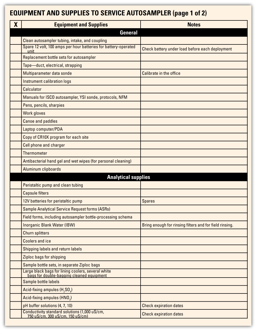
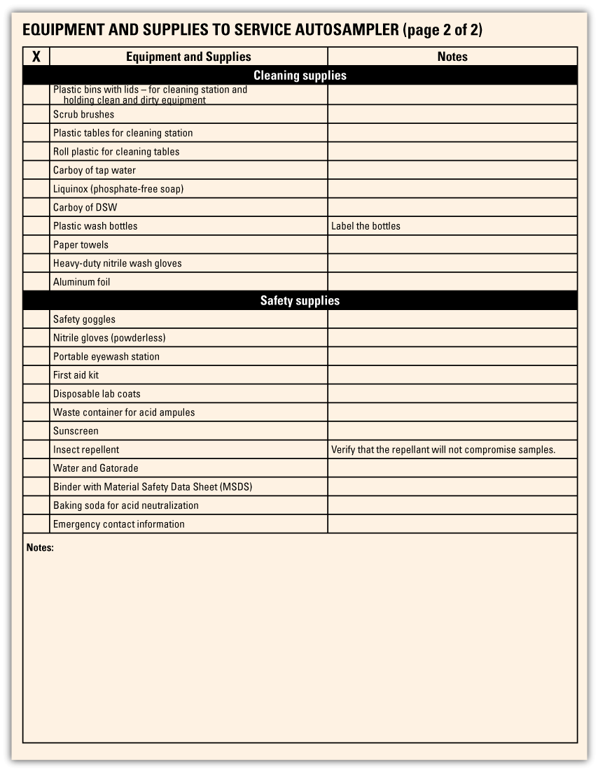
Checklist for equipment and supplies to service an autosampler.
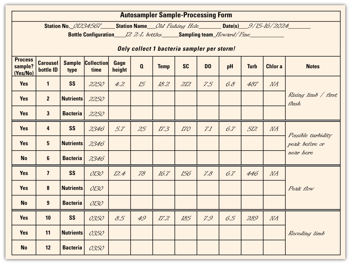
Example of completed field form for processing autosampler samples.
Before Leaving the Office for the Field
-
1. Review the checklist of needed equipment and ensure all field vehicles have the needed sampling equipment and cleaning supplies.
-
2. Ensure that tubing, bottles, and other equipment have been cleaned and packaged appropriately. They should either be double bagged in plastic bags when necessary or placed into a plastic bin labeled “clean equipment.”
-
3. Ensure that sufficient bottle sets and spares are packed. If bottles have been in storage for longer than two weeks, re-rinse the bottles three times with DSW. Ensure bottles have labels and are capped. Bottle sets can be carried in large plastic bags, coolers, or autosampler carousels.
-
4. Check that carboys and bottles of cleaning solutions are filled with fresh tap water or DSW and are properly labeled.
-
5. Calibrate the water-quality sondes and record in the equipment log. Note that a dedicated section of the SOP is included that lists steps for calibrating and servicing water-quality sondes.
Upon Arrival at Site
-
1. Park the vehicle far from the roadway. Be sure to follow all established safety procedures as outline in the job hazard analysis for the project. The rear of the vehicle (tailpipe) should be faced opposite of the sample collection site to minimize the potential for sample contamination from vehicle emissions and dust.
-
a. Before proceeding, make a quick check of the autosampler to determine if sampling occurred as planned. If it appears that the samples have been collected, continue with the SOP procedures that follow. If sampling was not successful, follow steps in section “Steps to Take if Sampling was Unsuccessful.”
-
-
2. Check the stream for flow or pooling. Estimate the flow-volume passing site in 15 minutes. If a manual sample or water-quality measurement is specified in the study, do not continue if water is pooled or appears stagnant. Document flow conditions on the water-quality field form. It may be necessary to specify stage and discharge conditions for each site before collecting water-quality-sonde data.
-
3. Check that the stream stage recording system appears to be working and record the current gage height, time, and date in field notes.
-
4. If dictated by the project workplan, prepare to make a point or cross-sectional measurement of stream parameters (temperature, turbidity, pH, specific conductance, and dissolved oxygen) using the data sonde. Place the data sonde in the stream and allow sufficient time for temperature (or other parameters) to stabilize before proceeding. Record values, time, date, and location of measurement on field form.
Retrieving Samples from an Autosampler
This section states specific, step-by-step procedures that are to be followed for each type of sample collected by the autosampler. These types include suspended sediment, particulate organic carbon, trace metals, organic compounds, and other types of constituents. The following lists examples of steps used to process samples for different types of chemical analyses. Following this level of diligence will help ensure the integrity of samples collected for all types of constituents.
-
1. Set up a clean sample-processing station that is protected from the weather and from other airborne sources of contamination. Lay the plastic sheeting over the processing table and assemble the sample-processing chamber (U.S. Geological Survey, 2014, p. 66–68). Keep the sample-processing equipment covered when not in use (sample-processing equipment kept in plastic bags, sample bottles kept capped, etc.)
-
A. Samples for trace metals.—Procedures for the preservation and handling of samples for low-level concentrations of trace elements and organic chemicals are listed in the “Clean Hands, Dirty Hands” section.
-
B. Composite or grab samples for general chemistry or nutrients.—Composite samples are to be capped and labeled in the field, including the station identification number (ID), date and time retrieved, sequence number (if used), and preservation status. If samples are to be sub-sampled for filtering and preservation in the field, then list out the steps to be taken.
-
C. Discrete sample for particulate organic carbon and suspended-sediment concentration analysis.—Processing of discrete samples for particulate organic carbon (POC) is conducted either in the field (in the field sampling vehicle or field setup) or in the Science Center’s field laboratory. Before transporting samples, ensure that each bottle is capped securely and labeled with the station ID, date and time retrieved, and location in the autosampler carousel (bottle) number. Information can be written on the cap, top shoulder, or labeled using crayon or permanent marker. Bottles should be removed individually and either replaced in their original space in the autosampler tub (if used) or replaced in the carousel with a new bottle, being careful that all samples remaining in the carousel are secured in their respective slots. Samples should be transported either in the carousel or in a cooler.
-
-
2. Mark water level on the side of each sample bottle collected using grease. Note any sample that does not appear to contain the volume of water expected by the autosampler program. These notes should be included on the bottle label and in the field notes. The safest means for transporting sample bottles is in the autosampler carousel. Removing bottles without first marking bottle numbers may allow bottles to shift slots, thereby disrupting the relation between the bottle number and the collection date and time stamp recorded by the autosampler.
Clean Hands, Dirty Hands
The Clean Hands, Dirty Hands (CH/DH) technique is a sample preparation technique outlined in chapter A5 of the NFM (U.S. Geological Survey, 2002). The technique requires two or more people to work together at the field site. When working with just two people, one is designated as Clean Hands (CH) and the second person is designated as Dirty Hands (DH). Although specific tasks are assigned at the start to the CH and DH, some tasks overlap and can be handled by either if care is taken to prevent contaminating the sample. CH and DH wear appropriate disposable, powderless gloves during the entire sampling operation and change gloves frequently, usually with each new task. Wearing multiple layers of gloves allows for rapid glove changes. Gloves must be able to withstand any acid, solvent, or other chemical substance that will be used or contacted.
Below are lists describing the specific role that the CH and DH play during sample preparation.
Role of the Clean Hands
The CH takes care of all operations that involve equipment that contacts the sample. For example, the CH
-
• Handles the surface-water sampler bottle.
-
• Handles the discharge end of the surface-water or groundwater sample tubing.
-
• Handles the inner protective bag on all equipment.
-
• Transfers sample to a churn or cone-splitter.
-
• Prepares a clean workspace inside the vehicle.
-
• Sets up processing and preservation chambers.
-
• Places equipment inside chambers (for example, sample bottles, filtration, and preservation equipment).
-
• Works exclusively inside chambers during collection, processing, and preservation.
-
• Changes chamber covers, as needed.
-
• Sets up field-cleaning equipment and cleans the equipment.
Role of the Dirty Hands
The DH takes care of all operations that involve contact with potential sources of contamination. For example, the DH
-
• Works exclusively outside of processing and preservation chambers.
-
• Prepares and operates sampling equipment, which includes pumps and discrete samplers, peristaltic pump-switch, pump controller, and the manifold system.
-
• Operates cranes, tripods, drill rigs, vehicles, or other support equipment.
-
• Handles the compressor or other means of power supply for samplers.
-
• Handles tools such as hammers, wrenches, keys, locks, and sample-flow manifolds.
-
• Handles single- or multi-parameter instruments for field measurements.
-
• Handles the churn carrier, including outer protective bags.
-
• Handles streamgaging or water-level equipment.
-
• Sets up and calibrates field-measurement instruments.
-
• Measures and records water levels and field measurements.
Retrieving Data from Autosampler
After securing and capping all samples, data should be downloaded from the autosampler equipment. This is done either manually by reviewing the sampling report and recording the relevant data (such as date and time) for each sample individually on a field form, or by attaching a computer or data-transfer device to the autosampler and downloading information electronically. The steps in this section are equipment-dependent, so each step should be completed in sequential order:
-
1. Upon arrival at the site, the autosampler should display a message, such as “Sampling program complete,” or “34, 35 Bottle No. 4, 1 Pulse to Start” or any other message indicating that the autosampler is going to take sample 34 of 35 in bottle number 4 when pulsed by the datalogger.
-
2. Make note of any error message shown on the autosampler record. If a sampling error has occurred, or if a sample bottle does not appear to have been filled as expected, then proceed to the steps in section “Steps to Take if Sampling was Unsuccessful.” A specific section is included in the SOP that outline steps to take to resolve any sampling errors that may have been encountered.
-
3. Press the red “Stop” button.
-
4. You should see the following options:
-
5. Go through the autosampler report and manually record sample data (the sample bottle number, the date and time collected, pump revolutions, and so on) in the field notes.
-
6. Connect a laptop to the autosampler with the interrogator cable and start the data interrogation application.
-
7. Select the appropriate site number from the main menu on the computer program, then click “Connect.”
-
8. Download the sampling report(s).
-
9. Disconnect the laptop from the autosampler.
-
10. If the sample report shows that samples have not been collected, then follow the procedures listed in section “Steps to Take if Sampling was Unsuccessful.”
Steps to Take if Sampling was Unsuccessful
Sampling can be unsuccessful due to various mechanical problems, electrical problems, and environmental conditions. Common causes include breakage of pump tubing, disconnection between different tubes and lines, misalignment of the distributor arm, stoppage of distributor arm movement by improperly placed bottles, and blockage of inlet lines by floating debris or sediment in lines. Electrical problems include dead batteries, power outages due to storms, and broken wires or connection. An environmental condition that could cause sampling to be unsuccessful includes freezing of water in lines and bottles. A list of common problems and suggested fixes are included in the SOP.
Refilling and Restarting the Autosampler
If the sampling program involves redeployment for subsequent sampling attempts, this section lists out steps to service the autosampler and prepare for sampling.
-
1. Put on nitrile gloves and safety goggles.
-
2. Check pump tubing and distributor arm tubing and replace, if necessary, tighten the interior connectors, wipe out any residual water in the bottle carousel, and ensure that the drain hole (if present) is open and free of debris.
-
3. Refill the carousel with clean bottles as required by the analytic suite.
-
4. Remove caps and place in a clean, plastic Ziploc bag, and store on-site.
Redeploying Sampling Equipment During Site Visit
When multiple events are sampled, the autosampler programs will generally be the same for successive events, except that the file names that contain the sampling date will change. However, it is possible that the autosampler programs may become corrupted or deleted by interruptions in power supply or other unstated ways. A copy of each station’s program is included in the SOP. The following shows example instructions for reprogramming an autosampler as they could appear in an SOP. When designed an SOP, please use the instructions provided by the autosampler’s manufacturer.
Reprogramming the Autosampler
-
1. To reprogram the autosampler, press the “Stop” button until you return to the main menu. Then, enter the programming mode.
-
2. If the autosampler program is acceptable, then enter a new date and file name using the project-defined naming convention (an example is provided in table 2.1). Provide exact naming conventions for each site where an autosampler is deployed, and for each autosampler if multiple autosamplers are being used. It is important that the file-naming convention is strictly followed.
-
3. Once a new file name has been entered, go through the program to ensure that it is correct. The correct program for each site is provided at the end of this SOP.
-
4. Select “Other Functions,” then “Manual Functions,” then “Calibrate.”
-
5. Disconnect the autosampler tubing where it runs from the pump head into the autosampler base. Insert the tip of the tubing into a graduated cylinder.
-
6. When prompted on the autosampler menu, enter “100 mL” as the desired sample size.
-
7. Select “Ready,” then wait for the autosampler to pump water into the cylinder.
-
8. When prompted, enter the actual amount of water delivered by the autosampler.
-
9. Repeat the calibration steps until the amount delivered is exactly 100 milliliters (mL).
-
10. Press the “Stop” button to return to the main menu.
-
11. From the autosampler’s main menu, select “Other Functions,” then “Manual Functions,” and then “Distributor Arm.”
-
12. When prompted for the bottle number to position the distributor arm, enter “1.” The autosampler will then move the arm to the desired position.
-
13. Press the “Stop” button to return to the main menu.
-
14. Run “LOWP FWC 1.”
-
15. The program will prompt you to enter the starting bottle number. Make sure “1” is selected and press “Enter.”
-
16. The display should then show “Bottle 1 After 1 Pulse.” Leave the autosampler as is. Do not press the power button. To interrupt the autosampler program at any time, press the “Stop” button.
-
17. If you want to force a grab sample from the autosampler for quality-control (QC) sampling purposes, press the “Stop” button, then select “Grab Sample.” The program will prompt you for a sample volume. Choose a volume large enough to field-rinse the sample bottle three times and collect a sample volume (for example, 500 mL).
-
18. Once the grab sample has been collected, press the “Stop” button, and then select “Resume Program.”
-
19. Configure the program for each autosampler as follows:
-
A. Extended Programming Mode
-
B. Program Name: “LOWP FWC”
-
C. Site Description: 8-digit station ID
-
D. Units Selected: feet (ft)
-
E. 15-minute Data Interval
-
F. Bottle Configuration: four 3.7-liter (L) bottles
-
G. X ft Suction Line (site specific)
-
H. Auto Suction Head
-
I. No. (number) of Rinse Cycles: 2
-
J. No. of Rinse Retries: 2
-
K. 1 Part Program
-
L. Pacing: Flow Pacing, Every 1 Pulse, No Sample @ Start
-
M. Distribution:
-
N. Sample Volume: 100 mL
-
O. Enable: None
-
P. Once Enabled, Stay Enabled
-
Q. Sample @ Enable
-
R. Enable: 0 Pauses and 0 Resumes
-
S. No Delay to Start
-
T. Run This Program Now? Yes
-
Reprogramming the Data Logger
If a stand-alone data logger is used at the sites, then instructions should be provided on the methods to re-install and change the sampling- or data-logging program. Similar to downloading autosampler data, the steps to download any data-logging equipment are provided as an example. Please follow all of the manufacturer’s instructions when downloading data from a data logger.
-
1. Open PC208W on your laptop. Note that each data-logging system will have a unique computer interface and control program.
-
2. Click on the “Connect” button on the PC208W toolbar.
-
3. Select the site from the list on the left side of the “Connect” window.
-
4. Click the “Connect” button in the Connect window.
-
5. You should see the plug close in the display next to the “Connect” button, and the “Connect” button should change to a “Disconnect” button.
-
6. Click the “Numeric” button in the Data Display area of the Connect window. In the Numeric window, note the items highlighted in red on the following pages of the program. These items, including the below, must be noted with the time on the field form:
-
7. Click the “Ports/Flags” button at the bottom of the Connect window. The data logger has eight user flags that are used for program control. Our program uses flags 1, 2, and 3. Their meanings are outlined below
-
Flag 1.—When flag 1 is low (0), the data logger executes the initialization subroutine and then sets flag 1 high (1). The initialization subroutine reads values into the Stage/Area Look-Up table and sets other important constants (for example, the number of samples). The user should manually set this flag low to reset the logger for the next round of sampling.
-
Flag 2.—When flag 2 is low (0), there are remaining samples to be taken. When flag 2 is high (1), sampling is complete. The user should not manually set or reset this flag.
-
Flag 3.—Flag 3 is set high (1) just after the autosampler has been triggered. The logger uses this to determine when to store the trigger data (for example, the bottle number). The user should also not manually set or reset this flag.
-
-
8. In the Ports/Flags window, flags that are high will have a black box next to them, and flags that are low will not have a black box. On your field form, note whether flags 1, 2, and 3 are high or low at the time of your visit.
-
9. To reset the datalogger for the next sampling attempt, manually set flag 1 to low using the following steps:
-
A. If using PC208W, click on the box next to flag 1 to toggle it to a “low” state. The box should no longer be black.
-
B. Using a keypad
-
• To display the flag’s status with a keypad, use the following keystrokes: *6AD (star, 6, A, D)
-
• This display has a single digit for each flag. One (1) is high and zero (0) is low.
-
• For example, if the flag’s display is “10000100,” flag 1 is high, flags 2, 3, 4, and 5 are low, flag 6 is high, and flags 7 and 8 are low. To toggle a flag to reset the logger, press the corresponding number key while the flag’s status is displayed. For example, to toggle flag 1, press the “1” key, to toggle flag 2, press the “2” key, etc.
-
-
-
10. After the logger has collected all samples, check the values in location 25, “Num_Smpls.”
-
11. The maximum number of aliquots that the autosampler is programmed to collect over 7 days is 456. This is calculated as follows:
Processing Samples from the Autosampler
This section provides detail on processing samples collected in the field. Processing may include filtering and preservation with acid. In most instances, the samples would be labeled in the field, and then returned to the laboratory for any processing.
Sample Collection
-
1. Set up the field processing station in an area to prevent sample contamination from vehicle emissions and dust. If possible, choose a spot with shade.
-
2. Assemble the folding table, sample-processing chamber, peristaltic pump, battery, sample bottles, labels, cooler, analytical-services request form (ASRs), and other equipment.
-
3. Determine who will be CH and DH during processing.
-
4. Identify the type of bottle to be used for each subsample and analytic schedule. Ensure that bottles are properly labeled based on bottle designation (table 2.2).
-
5. CH team member field rinses a 125 mL poly-whole water, chilled, acidified (WCA) bottle three times.
-
6. Using the spigot, CH draws off the sample into
-
• A 250 mL clear, poly-raw, acidified (RA) bottle for trace metals. Then, CH acidifies the RA bottle with one ampoule of fixing HNO3 (7.5 Normal, N) 125 mL clear, poly-WCA bottle for total phosphorus, total organic and ammonia nitrogen, and total nitrite and nitrate nitrogen. Then, CH acidifies the WCA bottle with one ampoule of fixing H2SO4 (4.5N).
-
-
7. Use a peristaltic pump with clean pump tubing and an inline, pre-rinsed capsule filter to collect a filtered sample into:
-
• A 250 mL clear, poly-filtered, acidified (FA) bottle for dissolved trace metals. Then, CH acidifies the FA bottle with one ampoule of fixing HNO3 (7.5N Ultrex).
-
• A 125 mL brown poly-filtered, chilled (FCC) bottle for dissolved phosphorus, ammonia, and nitrate and nitrite.
-
• A 250 mL clear, poly-filtered, unacidified (FU) bottle for chloride.
-
-
8. Place sample bottles immediately into double Ziploc bags and into a cooler with ice.
-
9. Pour any remaining samples into a clean cup and measure field parameters with the multi-parameter sonde. Record these readings with in-stream field parameters on the field form.
-
10. Make sure all bottles are labeled correctly and completely, cross-checking the field form and the ASR.
Table 2.2.
Bottle designation codes.[FA, filtered, acidified; RA, raw, acidified; WCA, whole water, chilled, acidified; FCC, filtered, chilled, acidified; FU, filtered, unacidified; NWQL, National Water Quality Laboratory]
Sample Storage in Field
-
1. Samples collected for particulate carbon, bacteria, nutrients, or trace metals, regardless of whether samples are acid-preserved, must be kept chilled below 4 degrees Celsius.
-
2. Samples collected for suspended sediment do not need to be chilled but should be stored with other samples in the sample set.
Sample Storage in Laboratory
-
1. Store autosampler samples in the large silver refrigerator in the office laboratory. Ensure that they are labeled with the date and time of collection, the station number, and the names of the project and the project chief. The SOP should provide specific locations for handling sampled water samples.
-
2. Line shipping coolers with two large plastic bags, one within the other.
-
3. Check all sample caps to be sure they are tightly secured.
-
4. Double check that all samples are properly labeled and agree with the ASR and field form.
-
5. Multiple sample bottle sets (several bottles representing one sample) can be placed in tightly secured Ziploc bags.
-
6. Glass sample bottles should be wrapped in bubble wrap or foam sleeves and bagged in Ziploc bags.
-
7. A copy of the ASR or laboratory request, chain-of-custody form (COC), and a return-shipping label for the coolers are then placed in a Ziploc bag and taped to the inside of the cooler lid.
-
8. When the cooler is full, tie the inner bag closed and then the outer bag closed over it.
-
9. Remove all old shipping labels and tape from the outside of the cooler.
-
10. If the cooler has a drain spout, make sure it is sealed with silicone or sealed temporarily with duct tape. Melting ice will drain from an open spout and alarm the shippers.
-
11. Provide specific directions for shipping samples, which include the address and account numbers, the location where samples can be picked up, and other details to the following laboratory: National Water Quality Laboratory, U.S. Geological Survey, Denver Federal Center Building 95, Entrance E3, Denver, CO 80225-0046. Phone: (303) 236-2000
-
12. Afterwards, LabHelp at the National Water Quality Laboratory (NWQL) will send a verification email to the contact provided on the ASR. Verify by the next day that the cooler was received and processed without any issues from the lab. If corrections need to be made, contact LabHelp immediately.
Collecting Field Equipment and Field Blanks
This section provides step-by-step instructions for preparing field equipment or other blanks called for in the work plan, along with a schedule to be followed. This blank is produced after all in-field cleaning and autosampler maintenance has been completed.
All field blanks are made using certified blank water, OBW, or IBW, and are processed through all equipment (autosampler, sample-collection bottles, sample splitter, and sample-submittal bottles) and filtering procedures used for native water samples. If needed, field blanks can be archived for analysis if contamination is detected at a later date. The frequency at which each blank is prepared is listed in table 2.3.
Table 2.3.
Types and frequency of blanks produced in this study.[L, liter; OBFW, organic-free-laboratory blank water]
Field Equipment Blanks
Field equipment blanks are to be prepared at the rate of one blank per event. Blanks will be rotated among all sites. At least one blank will be prepared per site. Blanks are prepared after all equipment, intake lines, and pump tubing has been cleaned or replaced. Field equipment blanks will be prepared using one unopened 4 L bottle of organic-free-laboratory blank water (OFBW) or 5 L of DSW, a 1–2-foot-long piece of pre-cleaned inlet tubing, and pre-cleaned bottles as dictated by the analytic scheme. Blanks should be created by following the below steps:
-
1. Record the lot number and expiration date of the blank water on the field form.
-
2. One field crew member will put on waders, clean gloves, and proper personal flotation devices (PFDs) and then will take the container(s) of blank water to the stream. The crew member will then pull the inlet-line nozzle out of the stream, let the river water drain, and prepare to place the inlet into the blank water bottle.
-
3. Another field crew member in the station prepares the autosampler to collect two grab samples using the same rinse-purge cycle routine used in sampling. Sample bottles are placed into the carousel and labeled. During collection of the blank water, the blank water should flow through all inlet lines, connectors, and pump and distributor arm tubing used during sampling.
-
4. The crew member in the stream watches the progression of the sampling routine. After the first tubing rinse, the inlet line is placed into the bottle of DSW and water is withdrawn. After collecting the blank water, the purge cycle begins. The inlet is pulled out of the DSW, and air is drawn into the line.
-
5. After the second sample rinse cycle is complete, the inlet line is placed into the bottle of OFBW and the second (or subsequent) blanks sample(s) are collected. Upon completion of sampling, the purge cycle should be allowed to flow into the stream and not back into the bottle of OFBW.
-
6. The blank water is collected into bottles in the autosampler. After all blank samples have been prepared, the bottles are removed, labeled, placed into a cooler with ice, and processed with the same procedures as environmental samples.
Field Blanks
Field blanks are prepared to determine if sample contamination occurs as samples sit in the autosampler carousel awaiting retrieval. Test that DSW used to clean equipment and bottles are not a source of contamination by following the steps below.
-
1. Select a bottle of equivalent material while the sample bottles are being used to collect native water. Fill this bottle with blank water appropriate for the analytic suite being scheduled. Place the filled bottle with the lid off in the last bottle slot available in the carousel. If none of the sample slots are available (for example, if 4 large volume bottles are being used in place of twenty-four 1 L bottles), then select a bottle volume that allows it to sit in the middle of the sample carousel and check that the blank bottle volume will not impede movement of the distributor arm.
-
2. Upon completion of sampling, the field equipment blanks are processed and preserved as required for each method and submitted to the lab for analysis.
References Cited
U.S. Geological Survey, 2002, Processing of water samples: Wilde, F.D., eds., U.S. Geological Survey Techniques of Water-Resources Investigations, book 9, chap A5, at https://doi.org/10.3133/twri09A5.
U.S. Geological Survey, 2004, Cleaning of equipment for water sampling: Wilde, F.D. eds., U.S. Geological Survey Techniques of Water-Resources Investigations, book 9, chap. A3, 68 p., accessed April 22, 2024, at https://doi.org/10.3133/twri09A3.
U.S. Geological Survey, 2014, Selection of equipment for water sampling (ver. 3.1, 2014): Wilde, F.D., Sandstrom M.W., and Skrobialowski S.C., eds., U.S. Geological Survey Techniques of Water-Resources Investigations, book 9, chap. A2, 78 p., accessed December 12, 2020, at https://doi.org/10.3133/twri09A2.
Appendix 3. Example of a Station Analysis Using Box Coefficients
Abbreviations
ADAPS Automated Data Processing System
BCF Duan bias correction factor
EWI equal-width increment
ft foot
ft3/s cubic feet per second
GCLAS Graphical Constituent Loading Analysis System
L liter
mg/L milligrams per liter
SCC suspended-sediment concentration
STC sediment transport curve
USGS U.S. Geological Survey
WY water year
Description of Site
The analysis was performed at the Hoaka Road station, U.S. Geological Survey (USGS) station no. 16700600 (U.S. Geological Survey, 2024), located about a quarter mile downstream of a forest reserve boundary. Upstream of the gage, the land uses are primarily forestry and conservation, but also include some residential and agricultural developments. Most of the watershed is covered by recent lava flows from Mauna Loa.
Equipment and Procedures
Equipment Setup and Quality Assurance
The autosampler is secured in a wooden streamgage instrument shelter on the right bank about 20 feet (ft) upstream of the rock ledge control feature. This autosampler was equipped with twenty-four 1-liter (L) poly-wedge-shaped bottles.
Cross-sectional equal-width increment (EWI) composite samples are collected by wading using a DH-48 sampler at a location just upstream of the gage. While provisions were not available for high-flow sampling, samples were collected through a normal range of discharges. Samples were collected directly into 1-liter wide-mouth plastic sediment bottles, then transferred directly into a polyethylene churn for compositing.
Sample Coverage
A total of 157 discrete samples were collected using the autosampler and 5 composite cross-section samples were collected using cross-sectional EWI methods. Samples were collected during water year (WY) 2005 at discharges ranging from 2 to 904 cubic feet per second (ft3/s), which covered the full range of discharge recorded for that year (0–917 ft3/s). In addition to the samples collected in WY 2005, 51 additional samples were collected using the autosampler in WY 2004. All data were combined to produce a sediment transport curve (STC) for the site. The STC demonstrates the relation between discharge and suspended-sediment concentration.
Data Computation
Sediment loading computation was performed using the Graphical Constituent Loading Analysis System (GCLAS) software package. GCLAS is an interactive cross-platform software package developed by USGS that computes the mass (load) and average concentration of a constituent that is transported in stream water over a period of time (Koltun and others, 2006).
Calibration Sampling and Computation of Box Coefficient
EWI samples were collected on October 20, 2004, November 15 and 30, 2004, February 4, 2005, and March 28, 2005, with concurrent autosamples that allowed computation of cross-section box coefficients (table 3.1).
Table 3.1.
Hypothetical results of samples collected by an autosampler and by equal-width increment (EWI) methods for calibration and computation of cross section box coefficients. Data from U.S. Geological Survey, 2024.[Dates given in month–day–year. Times given in military time. ft3/s, cubic feet per second; mg/L, milligrams per liter; Auto, automatic; —, define]
As shown in table 3.1, the computed box coefficients were found to not vary systematically as a function of discharge.
The computed box coefficients appear to decrease during the year (table 3.1), but field observations did not indicate a reason for the decrease, and the concentrations for all calibration samples were very low. Therefore, an average box coefficient was computed and applied for the entire year. First, the average for pairs of coefficients (calculated using discrete samples collected at the start and end of each EWI sampling interval) were used; these coefficients were then averaged. The resulting computed box coefficient applied for the entirety of WY 2005 was 2.25. A reviewer noted that on October 20, the EWI sample had a broken bottle, so the box coefficient was recalculated without the October 20 data, with a result of 1.98. After re-evaluating the cross-section coefficients, the average of 2.25 was retained based on the November 15 samples, which had the highest EWI concentration of all valid EWI/point sample pairs and had computed coefficients of 2.50 and 3.00. These observations indicate the typical variability in calculated box coefficients and the importance of collecting a sufficient number of EWI samples.
A total of 134 suspended-sediment concentrations (SSCs) collected over WY 2004 and WY 2005 were selected to calculate the STC equation in a spreadsheet program using ordinary least squares regression. These concentrations were first adjusted using the box coefficient (2.25) to produce estimated cross-sectional average SSCs. Both streamflow and estimated concentration data were log-transformed prior to computation of the regression relation. Box coefficients were calculated to adjust point-sample concentrations to an equivalent estimated cross-channel concentration. All samples were used except for:
-
• The EWI samples, which were used to calibrate the point (automatic) samples;
-
• Samples with concentrations of 0 milligrams per liter (mg/L), which could not be log-transformed; and
-
• Six samples collected on June 11, 2004, which were suspicious due to unusually high concentrations of suspended sediment for the observed discharge at the time of sample collection.
A Duan bias correction factor (BCF) was applied to correct the logarithmic estimated SSC (Duan 1983, Helsel and Hirsch, 2002). The least-squares regression equation used for the STC was
whereCross-section concentration at given discharges were estimated from the STC and from general relations between streamflow and concentration as determined from samples collected during WYs 2004 and 2005. Sample coverage was adequate to demonstrate that SSC concentration closely followed the hydrograph. Samples collected on April 12 and 23, 2004, as well as December 7, 2004, showed that concentrations of suspended sediment generally peaked at the same time as streamflow. Samples collected during prolonged peaks in discharge on November 15 and 29, 2004, and February 3 and 4, 2005, showed that at times when discharge remained high for several hours, sediment concentrations declined relatively quickly after the initial rise of the hydrograph.
Special Computations
Unit-value streamflow data were missing from December 11 to January 6, so daily values of streamflow were estimated for this period of the streamflow record. Concentration daily values for this period were estimated by linear regression of log-transformed daily-discharge values determined from streamflow for the remainder of the year. Daily values for sediment load for the period of missing streamflow unit values were computed by multiplying the estimated daily values for streamflow by the estimated daily mean concentrations, and then multiplying by the correction factor of 0.0027. The estimated daily values of streamflow, sediment concentration, and sediment load were typed onto the card-format file for loading to ADAPS (Automated Data Processing System) and were not computed in GCLAS.
Remarks
Daily values of load and concentration of suspended sediment were plotted versus discharge to check for outliers. One outlier for concentration of suspended sediment was found for samples collected on February 3, 2005. This day was adequately sampled, and the daily values are considered reliable.
Records were fair. Estimated daily values of suspended sediment represent 63-percent of the annual load. Total suspended-sediment load for the year was computed as 298 tons, equivalent to a yield of 9 tons per square mile per year for the drainage area of 31.92 square miles. This is a very low yield and may reflect the relatively un-weathered nature of the geologic materials in the watershed as well as the relatively dry year.
References Cited
Duan, N., 1983, Smearing estimate—A nonparametric retransformation method: Journal of the American Statistical Association, v. 78, no. 383, p. 605-610. [Also available at https://doi.org/10.2307/2288126.]
Koltun, G.F., Eberle, M., Gray, J.R., and Glysson, G.D., 2006, User’s manual for the Graphical Constituent Loading Analysis System (GCLAS), U.S. Geological Survey Techniques and Methods, book 4, chapter C1, 51 p. [Also available at https://doi.org/10.3133/tm4C1.]
U.S. Geological Survey, 2024, USGS Water Data for the Nation: U.S. Geological Survey National Water Information System database, accessed April 16, 2024, at http://dx.doi.org/10.5066/F7P55KJN.]
Appendix 4. River Condition Data for a Hypothetical Storm
Table 4.1.
Summary of river conditions at times when discrete samples would be collected using an equal 2-hour interval during the hypothetical storm shown in figure 27.[Samples collected at 2-hour intervals. Time of sample collection given in military time. ft3/s, cubic feet per second; Mgal, millions of gallons; L, liter; mL, milliliter; n.d., no data]
Table 4.2.
Summary of river conditions and times when samples would be collected at a constant discharge interval of 10 million gallons during the hypothetical storm shown in figure 28.[Samples collected at discharge interval of 10 million gallons. Time of sample collection given in military time. ft3/s, cubic feet per second; Mgal, million gallons]
Table 4.3.
Sampling schedule for collecting 24-discrete samples on a 4-hour time interval, and the aliquot volumes needed to produce a 1-liter and a 4-liter composite sample.[Times of sample collection given in military time. ft3/s, cubic feet per second; MG, million gallons; L, liter; mL, milliliter; NA, not applicable]
Conversion Factors
U.S. customary units to International System of Units
International System of Units to U.S. customary units
Temperature in degrees Celsius (°C) may be converted to degrees Fahrenheit (°F) as follows:
°F = 1.8(°C) + 32
Datum
Vertical coordinate information is referenced to the North American Vertical Datum of 1988 (NAVD 88) or the National Geodetic Vertical Datum of 1929 (NGVD 29).
Altitude, as used in this report, refers to distance above the vertical datum.
Supplemental Information
Specific conductance is reported in microsiemens per centimeter at 25 degrees Celsius (µS/cm at 25 °C).
Concentrations of chemical constituents in water are reported in milligrams per liter (mg/L), micrograms per liter (µg/L), or nanograms per liter (ng/L).
A water year is the 12-month period from October 1 through September 30 of the following year and is designated by the calendar year in which it ends.
Abbreviations
AC
alternating current
ASR
analytical-services request form
ASTM
American Society for Testing and Materials, International
DISA
depth-integrated sample arm
DO
dissolved oxygen
DOC
dissolved organic carbon
DSW
distilled water
EDI
equal-discharge increment, isokinetic sampling method
EPA
U.S. Environmental Protection Agency
EWI
equal-width increment, isokinetic sampling method
FISP
Federal Interagency Sedimentation Project
GCLAS
Graphical Constituent Loading Analysis System
IBW
inorganic-grade blank water
ID
identification number
NFM
National Field Manual for the Collection of Water Quality Data
POC
particulate organic carbon
PVC
polyvinyl chloride
QA
quality assurance
QA/QC
quality assurance and quality control
QAP
quality-assurance plan
QC
quality control
SOP
standard operating procedure
USGS
U.S. Geological Survey
WQ
water quality
XAD
ion-exchange resin
For more information, contact:
Director, New Jersey Water Science Center
3450 Princeton Pike Suite 110,
Lawrenceville, New Jersey 08648
Or go to our website at https://www.usgs.gov/centers/new-jersey-water-science-center.
Publishing support provided by the Baltimore Publishing Service Center.
Disclaimers
Any use of trade, firm, or product names is for descriptive purposes only and does not imply endorsement by the U.S. Government.
Although this information product, for the most part, is in the public domain, it also may contain copyrighted materials as noted in the text. Permission to reproduce copyrighted items must be secured from the copyright owner.
Suggested Citation
Wilson, T.P., Miller, C.V., and Lechner, E.A., 2024, Guidelines for the use of automatic samplers in collecting surface-water quality and sediment data: U.S. Geological Survey Techniques and Methods 1–D12, 89 p., https://doi.org/10.3133/tm1D12
ISSN: 2328-7055 (online)
| Publication type | Report |
|---|---|
| Publication Subtype | USGS Numbered Series |
| Title | Guidelines for the use of automatic samplers in collecting surface-water quality and sediment data |
| Series title | Techniques and Methods |
| Series number | 1-D12 |
| DOI | 10.3133/tm1D12 |
| Publication Date | July 18, 2024 |
| Year Published | 2024 |
| Language | English |
| Publisher | U.S. Geological Survey |
| Publisher location | Reston, VA |
| Contributing office(s) | New Jersey Water Science Center |
| Description | ix, 89 p. |
| Online Only (Y/N) | Y |
| Additional Online Files (Y/N) | N |