

Creating Oriented and Precisely Sectioned Mineral Mounts for In Situ Chemical Analyses—An Example Using Olivine for Diffusion Chronometry Studies
Links
- Document: Report (12 MB pdf) , HTML , XML
- Download citation as: RIS | Dublin Core
Acknowledgments
This work would not have been possible without samples of the Keanakāko‘i Tephra (in other words, the Keanakāko‘i Tephra Member, as redefined from Keanakāko‘i Ash Member of the Puna Basalt in Swanson and others [2012]) provided by Donald A. Swanson and the analytical expertise of Dawn C.S. Ruth, both of the U.S. Geological Survey, for electron backscatter diffraction data collection.
Preface
This manual presents an overview of laboratory methods that can be used to carefully orient and section minerals for in situ chemical analyses, with a focus on olivine for diffusion chronometry studies. The manual was compiled from a series of test trials and is intended to offer sample preparation solutions that significantly reduce uncertainty with modeling one-dimensional chemical data derived from two-dimensional sections of complex three-dimensional minerals. This manual aims to serve as an overview of potential techniques for the student, professional, or technician given available resources at their respective institution or home office.
Abstract
Diffusion chronometry is now a widely applied methodology for determining the rates and timescales of geologic processes from the chemical zoning observed in minerals. Despite the popularity of the method, several challenges still remain during its application, including: (1) the random sectioning of minerals either in thin sections or grain mounts in which both off-center and oblique sections contribute substantial uncertainty to modeled timescales and (2) diffusion anisotropy needs to be accounted for in models, which generally requires determining the principal crystallographic axes of the mineral using electron backscatter diffraction, a technique that is both challenging and limiting because few scanning electron microscopes have an electron backscatter detector. This guide developed by the U.S. Geological Survey focuses on a step-by-step methodology for mounting individually oriented minerals that are sectioned through their cores prior to polishing for analytical work. Using this technique, one can significantly reduce the uncertainties associated with off-center sections and minimize or completely remove the need for determining crystallographic orientation via electron backscatter diffraction analyses. This report is presented as a guide for using the technique on olivine crystals but can be applied to any minerals that can be extracted for analysis. Two variations of the methodology are included here: (1) The individual crystal method that entails mounting individually sectioned single crystals and crystal groups and (2) the whole mount method in which multiple single crystals or crystal clusters are mounted and sectioned at the same time.
Introduction
Investigating the compositional zoning in minerals has become a routine tool for determining the timescales of diffusive re-equilibration in many minerals applied across diverse geologic settings (Costa and Chakraborty, 2004; Costa and Dungan, 2005; Morgan and others, 2006; Kahl and others, 2011, 2013; Charlier and others, 2012; Ruprecht and Plank, 2013; Cooper and Kent, 2014; Barth and others, 2019; Mutch and others, 2019a, 2019b; Ferrando and others, 2020; Ruth and Costa, 2021; Couperthwaite and others, 2021; Lynn and Warren, 2021; Bloch and others, 2022). Increasing precision and resolution of in situ geochemical analyses has also allowed determining the elemental and isotopic composition of minerals to become routine (Davidson and others, 2007; Ubide and others, 2015; Lynn and others, 2020).
Diffusion chronometry, a technique that has gained wide popularity in volcano science in recent years, uses minerals that contain chemical gradients to act as time capsules of magmatic processes if the diffusivity of the elements in the mineral have been constrained (for example, Costa and others, 2020, and references therein). For this guide developed by the U.S. Geological Survey (USGS), we focus on olivine, the most common mineral phase in basaltic magmas, but this technique can also be applied to orthopyroxene and plagioclase if the habits of the mineral separates are understood well. Olivine is an orthorhombic mineral with varying rates of diffusion for many elements along its three crystallographic axes a, b, and c (Chakraborty, 1997, 2010; fig. 1). This variability, called diffusion anisotropy, occurs because the M1 octahedral sites in the crystal structure form a continuous chain along [001] (the c-axis), whereas the M2 octahedral sites are not organized in any direction (Chakraborty, 2010). Thus, for most major and minor elements in olivine, diffusion along the c-axis occurs approximately six time faster than the a- or b-axes (for example, Chakraborty, 2010). Because of this anisotropy, knowing the crystal orientation relative to any one-dimensional (1D) analytical traverse in a two-dimensional (2D) crystal section is imperative to be able to account for these relative rate differences and calculate accurate timescales (Costa and Chakraborty, 2004).
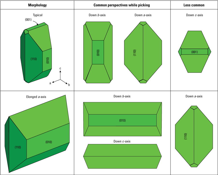
Diagrams of common olivine morphologies that are easy to orient and mount using the technique described here. Typical polyhedral single crystals are relatively easy to orient down the b- or a-crystallographic axis, whereas polyhedral crystals elongated along the a-axis are easier to orient down the b- or c-axis. Numbers in parenthesis indicate the Miller indices for the crystal faces.
However, because minerals are three-dimensional (3D) objects (fig. 1) that grow and re-equilibrate at different rates along different crystallographic axes (for example, Donaldson, 1976; Chakraborty, 1997; Welsch and others, 2013, 2014; Mourey and Shea, 2019), interpreting geochemical data measured in 2D sections cut through a 3D object can involve uncertainty (for example, Shea and others, 2015, Krimer and Costa, 2017; Couperthwaite and others, 2021; Lubbers and others, 2023). Measurements of chemical zoning are typically made on crystals exposed in 2D thin sections or grain mounts, which are planes that generally intersect crystals randomly. This means that their gradient geometry may be dependent on section orientation and distance from the crystal core (Pearce, 1984; Wallace and Bergantz, 2004) with additional influences from 3D crystal morphology (Shea and others, 2015, Couperthwaite and others, 2021; Lubbers and others, 2023). No way to correct for the uncertainty related to off-center sectioning exists, and modeled diffusion timescales from off-center sections are likely to be inaccurate and imprecise and can span anywhere from 0.1 to 25× the true diffusion time (Shea and others, 2015).
The uncertainties related to highly oblique sections and diffusion anisotropy can be reduced by determining crystal orientation via electron backscatter diffraction (EBSD; Prior and others, 1999). This technique measures the orientation of the principal crystallographic axes, after which the user can calculate the angles between each crystallographic axis and the 1D analytical traverse. Incorporation of EBSD-determined crystal orientations is imperative for reducing diffusion model uncertainty (from 0.1–25× down to 0.2–10×; Shea and others, 2015) and is a widely accepted requirement of using this technique (for example, Costa and Chakraborty, 2004; Costa and others, 2008). However, EBSD is not a standard piece of equipment in most scanning electron microscope (SEM) labs, samples require extremely high-quality polishing (usually with colloidal silica), and the analyses are challenging because they require a 70-degree sample tilt inside the SEM (Prior and others, 1999).
By using the orientation and sectioning technique outlined here, most of these uncertainties related to both off-center sectioning and degree of obliquity can be minimized or avoided altogether, thus maximizing precision and accuracy and removing the need for challenging EBSD analyses. We also recommend using this orientation and sectioning method because it allows the user to preferentially choose a type of section useful for a specific research question. For example, the user can keep the c-axis in the 2D plane of the section, which is useful for several reasons: (1) a-c and b-c sections allow you to look for different gradient lengths relative to each crystallographic axis (as a result of diffusion anisotropy; Zhang, 2010), which support interpretations that the gradients are generated by diffusive re-equilibration and not crystal growth (Costa and others, 2008), (2) a-c sections are ideal for studies of most major and minor element diffusion and hydrogen ion (H+) diffusion, which has anisotropy fastest along the a-axis over short timescales (hours) and typical anisotropy along the c-axis over longer timescales (for example, Mackwell and Kohlstedt, 1990), and (3) a-c sections are more likely to have zones rich in phosphorus (a marker of early rapid olivine growth; for example, Milman-Barris and others, 2008; Welsch and others, 2014; Mourey and Shea, 2019) which can either be targeted for trace element analysis or avoided owing to the complexities of trace element coupling (Lynn and others, 2020). Two variations of the methodology are included here: (1) The individual crystal method that entails mounting individually sectioned single crystals and crystal groups and (2) the whole mount method in which multiple single crystals or crystal clusters are mounted and sectioned at the same time.
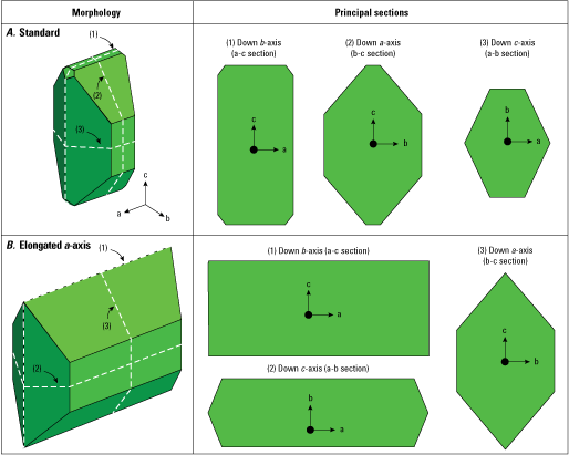
Diagram of ideal sections (dashed white lines) cut from a polyhedral single crystal. A, Typical polyhedral morphology. B, Polyhedral morphology elongated along the a-axis. Green three-dimensional diagrams show crystal face orientation. Numbers in parenthesis correspond to ideal sections shown to the right. The white dashed lines on the three-dimensional diagrams denote where the two-dimensional sections labeled (1), (2), and (3) are located.
Purpose
The objective of this guide is to present the procedures for preparing an oriented and precisely sectioned mount of minerals for the purpose of reducing uncertainty in data acquisition and subsequent modeling of chemical gradients, with particular benefit to studies of diffusive re-equilibration. This guide focuses specifically on olivine, but the method can be generally applied to any minerals of interest. For example, quartz is another mineral that is of great interest for studies of both diffusive re-equilibration and crystal growth (Charlier and others, 2012; Barbee and others, 2020). The procedures for mineral orientation, sectioning, and mounting in different mediums are discussed and several variations on the method are also presented. These methodologies have been applied and generally noted in previous studies (Lynn and others, 2017, 2020) but are presented here for the first time in full detail to support laboratory preparation.
Sample Preparation and Picking
Crystals should be separated from their host rock as carefully as possible to preserve their morphology. Thus, tephra that can be gently crushed, sieved, and picked are ideal for this technique. Lava flows and other dense rocks can be coarsely crushed and picked but crystals will more likely fragment and almost always have adhering matrix that obscures crystal morphology. If adhering dense glass from lava flows can be removed with laboratory techniques (such as dissolution in hydrogen fluoride [Lynn and others, 2017] or use of high voltage electrical fragmentation [Takehara and others, 2018]) then this orientation and mounting methodology may be applied to minerals from lavas and other dense rocks.
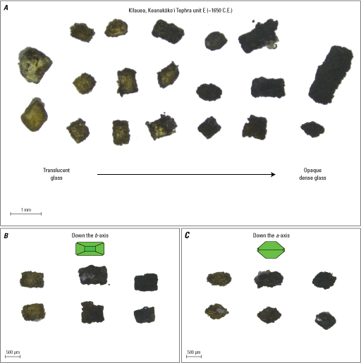
Photograph examples of olivine with a range of adhering glass textures and colors. A, Examples of olivine crystals with adhering glass textures and colors that range from translucent glass to opaque dense glass, all picked from the same tephra deposit (unit E approximately [~] 1650 C.E. [following unit naming convention of Swanson and Houghton, 2018] from Kīlauea’s Keanakāko‘i Tephra Member, a redefinition of the Keanakāko’i Ash Member of the Puna Basalt as presented in Swanson and others, 2012). B, A subset of crystals with translucent to dense glass showing similar square and rectangle outline shapes when oriented down the b-axis. C, The same crystals from B rotated 90 degrees so that they are oriented down the a-axis, all showing variations of diamond outline shapes. Green diagrams show crystal face orientation. μm, micrometer; mm, millimeter.
Sieving crushed tephra allows the user to focus on different grain size populations that may be present in the sample but may unintentionally bias the study if only one size fraction is picked. Thus, characterizing the petrography of the sample of interest in advance will aid in applying this method to achieve the best outcome. Shea and others (2015) suggest that 10–20 diffusion profiles are needed to accurately characterize a crystal population, so having a similar number for each crystal morphology would be a good starting point for assessing sample diversity. In this example, we use olivine from Kīlauea’s tholeiitic basaltic tephra, which are usually either microphenocrysts (0.1–0.5 millimeters [mm] in diameter) or phenocrysts (greater than [>] 0.5 mm in diameter). Sieve mesh sizes at 0.5, 1, and 2 mm will allow for separating out less than (<) 0.5 mm powder and >2 mm clasts that likely are not single crystals (except in rare instances of megacrysts). Using a stereographic microscope, identify and pick out olivine crystals from the 0.5–1.0 mm and the 1–2 mm fractions of the sieved tephra. Larger crystals are easier to orient and section with this technique, especially for beginning users. However, all olivine should be collected, regardless of morphology or complexity (for example, Couperthwaite and others, 2021), to best represent the full suite of crystal cargo in the sample.
Olivine crystals can still be identified during microscope aided picking even if they are obscured by darker adhering matrix (for example, microcrystalline rich) rather than translucent adhering glass. This is a common problem for tephra deposits dominated by scoria (for example, unit E of Kīlauea’s Keanakāko‘i Tephra Member, a redefinition of the Keanakāko’i Ash Member of the Puna Basalt, herein referred to as the Keanakāko’i Tephra after Swanson and others, 2012; Swanson and Houghton, 2018). Although olivine crystals can have a wide range of morphologies and complexities (fig. 2), single crystals and crystal clusters often have several easily recognizable crystal faces (fig. 3). These faces don’t always appear in exactly the same proportions, depending on a particular crystal’s growth history, but are usually recognizable regardless of these variations. For example, the (010) face, which marks the b-axis direction, is always a square or rectangular shape, regardless of its aspect ratio and whether the adhering glass is opaque or translucent (fig. 4). By looking for these features and common outlines, crystals can be picked from otherwise dark material that doesn’t have an obvious olivine showing through.
Two of the most common types of olivine morphologies are standard polyhedral crystals elongated along the c-axis (for example, Welsch and others, 2013) and polyhedral crystals elongated along the a-axis (fig. 3). Crystals elongated along the a-axis are common in eruptive products from many volcanoes, including Stromboli (Métrich and others, 2010), Mount Etna (Spilliaert and others, 2006), Piton de la Fournaise (Welsch and others, 2013), Kīlauea (Mourey and Shea, 2019), and mid-ocean ridge volcanoes (Colin and others, 2012).
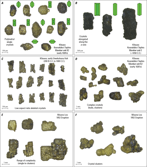
Photomicrograph examples of the most common types of olivine crystals and their morphologies found in Hawaiian tephra. A, Standard polyhedral single crystals with dense adhering glass (opaque), B, Polyhedral crystals elongated along the a-axis, C, Skeletal crystals with low aspect ratios, and D–F, twinned, budded, or complex crystal clusters. Dates and unit names for Keanakāko’i Tephra Member olivine crystals are from Swanson and others (2012), Uwekahuna Ash olivine crystals are from Fiske and others (2009), and Mauna Loa 1852 olivine crystals are from Trusdell and Lockwood (2017). Green diagrams show crystal face orientation. μm, micrometer; mm, millimeter.
Orienting, Sectioning, and Mounting Individual Single Crystals or Crystal Groups (Individual Crystal Method)
Materials
Equipment and supplies needed to use this mounting technique are categorized as either non-consumable or and consumable items. Non-consumable items include:
-
• Hot plate
-
• Glass beaker (any size)
-
• Glass stirring rod
-
• Glass petri dishes
-
• Extra beakers (any material)
-
• Forceps
-
• Stereographic microscope
-
• Hand lens (optional).
-
• Non-water-soluble temporary adhesive (such as Crystalbond; acetone soluble)
-
• Wet-dry sandpaper (400 grit recommended)
-
• Soft textured tape (masking tape recommended)
-
• Water
-
• Acetone
-
• Epoxy resin and hardener
-
• Double-sided tape.
This list is meant to be comprehensive and specific products or items are not necessarily needed to accomplish the work. For example, there are several types of temporary or removable adhesives commonly used in geologic laboratories for a variety of applications (for example, temporary adhesive such as Crystalbond versus orthodontic resin). This list of recommended supplies was generated based on trial and error (see also fig. 5), but we acknowledge that there are suitable substitutions that may work well for labs based on available supplies and budgets.
Preparing Your Workspace
After gathering the supplies, prepare the workspace to make the sectioning steps efficient:
-
1. Secure a piece of masking tape onto a rigid but transportable surface (for example, plastic dish, petri dish, glass plate, and so forth) with the sticky side facing upward. Place this near your stereographic microscope.
-
2. Set up your hotplate and cover the plate surface with aluminum foil (to collect strands of adhesive that may fall).
-
3. Prepare the temporary adhesive by breaking off small chips into a beaker. Place the beaker on the hotplate and set the temperature to 10 degrees Celsius (°C) higher than the melting point indicated on the manufacturers packaging.
-
4. Lay out one sheet of 400 grit polishing paper and have a supply of water nearby to wet the surface. Pour a drop or two of water onto the paper in preparation for sectioning. Re-wet as necessary.
-
5. Have acetone ready with two glass beakers or shallow petri dishes for acetone baths. This is usually done in a fume hood or using a snorkel.
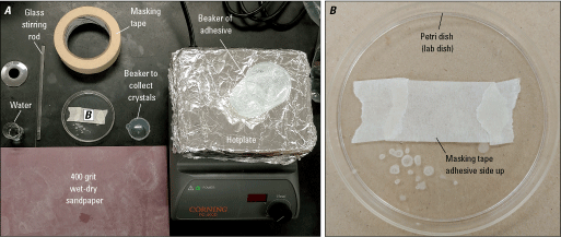
Images of an example of a workspace set up and ready for mounting and sectioning. A, Necessary supplies include masking tape, glass stirring rod, beaker of water, 400 grit wet-dry sandpaper, covered hotplate, beaker of temporary adhesive, and a spare beaker to collect crystals. B, Lab dish (or glass plate) with masking tape sticky side up, ready for olivine orientation. For a complete list of supplies see “Materials” section.
Orienting Crystals
Procedure Steps for Orienting Single Crystals
-
1. Using a stereographic microscope, select a single polyhedral crystal with recognizable faces from the suite of olivine from a sample.
-
2. Place the crystal onto the masking tape and gently orient it:
-
3. Repeat Step 2 multiple times to prepare many crystals at a time on the tape. Remember to include 10–20 crystals from each crystal population (accounting for variations in grain size, morphology) to ensure you encompass diversity in the sample. Make sure to leave at least 1 centimeter (cm) of tape between each crystal.
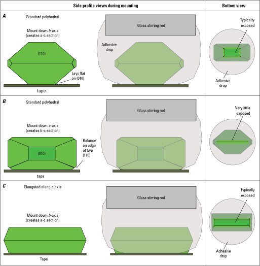
Diagrams showing orientations and mounting procedure for single standard polyhedral crystals and polyhedral crystals elongated along the a-axis. A, Mounting down the b-axis (to create an a-c section). B, Mounting down the a-axis (to create an b-c section). C, Mounting down the b-axis of a polyhedral morphology elongated along the a-axis. Numbers in parenthesis indicate the Miller indices for the crystal faces.
Procedure Description for Orienting Single Crystals
Orienting single crystals relies on using the spongey nature of the masking tape (recommended type of tape for this technique) to hold the crystals in the orientation you desire. Using forceps, place standard polyhedral crystals onto the masking tape and gently adjust them so that you are looking down either the a- or b-axis (fig. 6). This is done by making sure the crystal rests on the square, flat (010) face (fig. 6A), and you’ll be staring down the b-axis at a similar view of an (010) face (fig. 3). Alternatively, balance the crystal on the ridge created by the intersection of two (110) faces (fig. 6B), and you should be looking down the a-axis at a similar intersection (fig. 3). Using masking tape is crucial for orienting crystals down the a-axis and balancing on that edge because the spongey nature of the tape helps to hold it there better than a thinner tape such as cellophane. Orienting crystals down their c-axis is not recommended because their aspect ratio (long dimension is usually along the c-axis) makes this challenging. Furthermore, most elements in olivine diffuse faster along the c-axis (for example, Chakraborty, 2010, and references therein), and having the c-axis in the plane of your section is essential for assessing anisotropy in zoning and reducing uncertainty (for example, Zhang, 2010). When orienting polyhedral crystals elongated along the a-axis, we recommend that you orient them only down the b-axis and not down the c-axis (fig. 3) for these same reasons. At this stage, you may choose to orient many crystals on your tape to increase your sectioning efficiency (including 10–20 crystals from each crystal population to account for variations in grain size and morphology to encompass diversity in the sample). If you prepare several crystals on the tape, be sure to leave 1 cm of empty tape between each crystal so you won’t disturb their orientations during the next steps.
Procedure Steps for Orienting Twinned or Clusters of Crystals
-
1. Using a stereographic microscope, select a single complex crystal, twinned crystal, or crystal cluster with recognizable faces from the suite of olivine from a sample.
-
2. Place the crystal onto the masking tape and, if possible, gently orient it so that multiple crystals with similar orientations lie in a plane together (see fig. 7A).
-
a. Step 2 can be repeated multiple times to prepare many crystals at once on the tape. Remember to include 10–20 crystals from each crystal population (accounting for variations in grain size and morphology) to ensure you encompass diversity in the sample. If this is done, make sure to leave at least 1 cm between each crystal.
-
Procedure Description for Orienting Twinned or Clusters of Crystals
Orienting complex, twinned, or clusters of crystals is far more challenging than orienting single crystals. Only a small subset may be oriented well, but it is worth trying because focusing only on ideal single crystals can bias study datasets (Couperthwaite and others, 2021). Twinned olivine crystals may be the easiest to orient because they generally have the same a-axis (Dodd and Calef, 1971; Welsch and others, 2013), which can be leveraged for this sectioning methodology (fig. 7). Crystals that have parallel bud chains might also be straightforward to orient, provided it can be done using the largest olivine unit (which is the least susceptible to overprinting by diffusive re-equilibration). In some instances, in which clusters are quite complex, we recommend not focusing on their orientation but proceeding with their individual sectioning, outlined below in “Sectioning Individual Crystals, Twinned Crystals, or Crystal Clusters,” to reduce the uncertainty related to off-center sections. In this case, crystal clusters may be placed on the masking tape in any orientation that maximizes the area that will be sectioned.
One caveat to working with twinned or crystal clusters is that they may share similar, but not exactly the same, orientations. Misalignments (by up to 10 degrees; Welsch and others, 2013) of similarly oriented crystal units are common and should be noted for reference during later analysis. Because orienting twinned crystals or clusters is more challenging, EBSD may still be required after the mounting procedure is complete. However, properly exposing crystal cores and the sectioning methodology that follows is beneficial and still recommended for these crystal types.
Sectioning Individual Crystals, Twinned Crystals, or Crystal Clusters
-
1. Dip the end of the glass stirring rod into the heated, now liquid temporary adhesive (fig. 7).
-
2. Gently lower the rod with the droplet of adhesive onto an oriented olivine crystal, being careful not to push down, which might disturb the orientation.
-
3. Wait for the adhesive to set around the olivine crystal (about 20 seconds [s] for Crystalbond).
-
4. Gently pull the rod and adhesive puck (containing the oriented olivine crystal) off the tape.
-
5. Grind the flat side of the adhesive puck on the polishing paper. We recommend “choking up” on the glass rod and holding it several centimeters above the end of the rod where the crystal is attached to keep the rod as vertical as possible, thereby keeping the section as flat as possible.
-
6. Check exposure of the crystal every 5–10 s and repeat step 5 until approximately one half of the crystal remains (fig. 7C and D).
-
7. When satisfied with the crystal section, remove the adhesive puck from the rod and place it inside a beaker. Repeat steps 1–7 until the desired number of crystal sections have been made.
-
8. Dissolve adhesive pucks in acetone bath (or follow other steps to dissolve the temporary adhesive).
-
9. When the crystals appear free of adhesive, use forceps to move the crystals into a second clean bath of acetone for several additional minutes to ensure all adhesive is removed.
-
10. Remove crystals from the second acetone bath and ensure no adhesive residue remains.
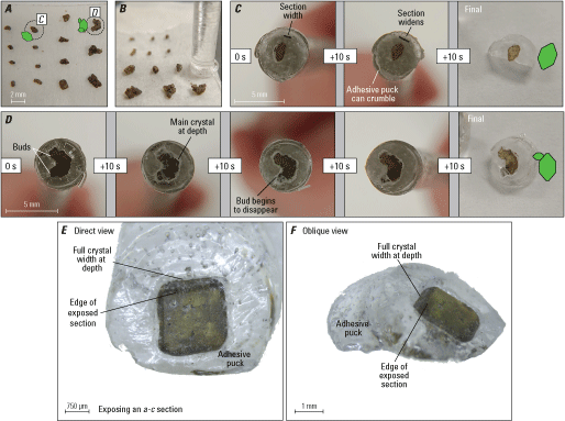
Photographs showing sectioning procedure for single olivine crystals and crystal clusters. A, Oriented single crystals and clusters on masking tape, ready for sectioning. Dashed circles and green diagrams of the crystal orientations identify two crystals featured in subsequent panels. B, Using the adhesive drop and glass rod to enclose an olivine crystal for sectioning. C, A single crystal oriented down the a-axis with progressive sectioning. Section widths increase as the crystal core is neared. D, A complex crystal with parallel buds, oriented down the a-axis. One bud (bottom left of D) is in the foreground in front of the main crystal and the other (top left of D) is in the background behind the main crystal. With progressive sectioning, the foreground crystal is removed and the background crystal begins to be exposed. Sectioning stops when main crystal is sectioned approximately in half. E–F, Direct and oblique views, respectively, of a partially sectioned olivine crystal in adhesive puck, to highlight the difference between the sectioned plane and the full width of the crystal at depth. mm, millimeter; μm, micrometer; s, second.
Procedure Description
Take the masking tape with the oriented crystals over to the hotplate area. Hold the glass stirring rod vertically and dip the end down into the beaker of temporary adhesive. Quickly pull it away while the temporary adhesive is still a liquid and gently lower the rod with the droplet of adhesive onto an oriented olivine crystal. Be careful not to forcefully push down, as this can rotate or tilt the oriented crystal (especially those oriented down the a-axis, which are balanced on the edge of two (110) faces). Usually, you can just stabilize the rod with your fingers and allow gravity to do the work. At this stage, enough temporary adhesive should be on the end of the rod that it forms a puck that encompasses the crystal and wraps up a little bit around the edge of the rod (fig. 6). This helps keep the puck adhered to the rod during the subsequent steps. Hold the rod steady here, typically for 20 s, so the temporary adhesive can set fully around the crystal.
Gently peel the rod with the temporary adhesive puck away from the masking tape. If you examine the bottom of the puck, you should see only a small amount of the crystal exposed, depending on the orientation (fig. 6). Most of the crystal will appear darker, submerged at depth beneath the adhesive puck. If large gaps exist between the crystal and the temporary adhesive and the olivine can be seen below the puck surface, the adhesive likely wasn’t hot and (or) fluid enough when you set it down on the crystal. You may proceed with the subsequent steps but be aware that sometimes this means that the crystal isn’t set well into the puck, and you might have to go back and repeat steps if it comes loose.
Start grinding the flat side of the puck on the wetted polishing paper using gentle pressure and moving in small circles. Take care not to push too hard (you can break the adhesive puck) or to tilt the rod far from vertical (which will result in grinding a section that is oblique to a crystallographic axis). We recommend “choking up” on the rod by griping the bottom of the rod close to the puck and using your wrist to stabilize the rod as vertically as possible while making small tight circles on the polishing paper. An optional training tool would be to add a bubble level or a flag to the top of the glass rod to visually monitor that it doesn’t tilt too far from vertical. These visual indicators will help to monitor how much oscillation and (or) angle you might introduce while sectioning. When grinding, you might want to balance the edge of your palm on the table and (or) polishing surface and use a full arm motion, as opposed to generating the circular motion from your wrist. This will aid in keeping the rod more level and reduce the risk of beveling owing to tilting. Add drops of water to wet the sandpaper as needed. A white suspension should be visible in the water on the paper as the temporary adhesive is removed. The sound of the polishing will also change slightly as you section deeper into the crystal—this is because more of the surface area being ground is of the harder olivine and less is of the softer temporary adhesive.
Check the bottom of the puck every 5–10 s to assess the progressive exposure of the crystal (figs. 7 and 8). Using a hand lens to quickly check the exposure of the crystal is an effective option. This exposure will start out smaller than the outline of the entire grain at depth beneath the adhesive puck. The area of crystal exposure will be relatively reflective when tilted under a light source, allowing you to discern the sectioned surface from the total width of the crystal farther at depth. As the crystal is progressively ground away, the crystal section will become larger and the relative amount of crystal at depth behind the puck will diminish (fig. 8). Check the reflective surface of the crystal frequently to avoid beveling as the crystal is ground away. Sections perpendicular to the b-axis (a-c sections) will start out as squares or rectangles, which will increase in area as sectioning proceeds (fig. 8A, C). Sections perpendicular to the a-axis (b-c sections) will likely start out as a line or narrow rectangle and will vary in shape as more crystal faces are intersected with progressive sectioning (fig. 8B), ultimately showing a roughly diamond shaped b-c section (fig. 4).
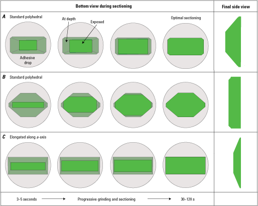
Diagrams showing progressive exposure of an olivine crystal during individual sectioning of A, a-c sections perpendicular to the b-axis, and B, b-c sections perpendicular to the a-axis. C, a-c section perpendicular to the b-axis for a polyhedral morphology elongated along the a-axis. Principal sections usually become fully exposed after 30–120 seconds (s) of progressive grinding and (or) sectioning, but this time will vary depending on starting polishing grit size (400 grit recommended), olivine crystal size, and pressure applied by individuals doing the sectioning.
When crystals are sectioned through or very near to their cores, the outline of the crystal at depth will no longer be visible and the exposed section will reach its maximum area (fig. 8). This is an ideal section, and you should stop grinding at this stage. If the exposed section area begins to decrease, you know that you have passed through the crystal core and are grinding away in the second half of the remaining crystal. As soon as you notice this, stop immediately or you will grind too far and produce an off-center section on the other side of the crystal’s core.
Sectioning complex, twinned, or clusters of crystals follows the same process as simple single crystals, but knowing when to stop is more challenging. The goal here is to grind away approximately half of the cluster volume and expose a large section through the middle of the cluster or the largest grain in the cluster, even if some smaller buds or crystals are completely removed in the process (fig. 7D).
When you are satisfied with the exposed crystal section, gently remove the adhesive puck from the rod. You can usually use your thumb or fingernail to apply pressure to one side of the puck and it generally pops off in one piece. If it fragments, check each piece to see if part of the crystal broke off with it. Keep all puck fragments with crystal pieces, as it is often possible to still use that crystal. To remove the adhesive, dissolve the entire adhesive puck in an acetone bath (or follow other steps to dissolve temporary adhesive following manufacturer’s instructions). The time required to fully dissolve the puck will depend on the volume and type of adhesive. When the olivine crystal appears free of adhesive (usually after 5–15 minutes), use forceps to move the crystal into a second bath of clean acetone to ensure it is free of adhesive residue. Let it sit in a clean acetone bath for at least 5 minutes. Remove the crystal from the second acetone bath and rinse in water.
Using the stereographic microscope, ensure that no adhesive residue is left over. If the crystal is still sticky, return to a clean acetone bath for additional 5 minutes and then check again. Removing all traces of adhesive is important because most temporary adhesives can degas under high vacuum (for example, in a secondary ion mass spectrometer [SIMS]) and yield inaccurate analyses. It may also react with epoxy, producing unwanted bubbles that reduce the integrity of the epoxy mount.
At this point you should also examine the crystal geometry, which should be very near to one half of an olivine crystal (fig. 9). If the crystal isn’t fully sectioned, repeat steps 1–10 to achieve better results. If the crystal was tilted during sectioning and is highly oblique to a crystallographic axis (fig. 9F), consider saving that crystal for a separate mount that will require EBSD analysis. The oblique sections are still valuable in that they can be precisely sectioned to the crystal’s core, and the anisotropy can be corrected for with EBSD.
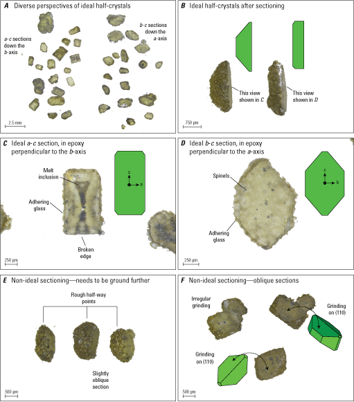
Photomicrograph examples of olivine crystals after sectioning steps. A, Diverse perspectives of ideal half crystals, showing some resting on their euhedral faces (sectioned surface up) and some resting on their sectioned surface (euhedral faces up). B, Examples of ideal half single crystals from the side, with corresponding sections shown in C, an ideal a-c section perpendicular to the b-axis, and D, an ideal b-c section perpendicular to the a-axis. E, Examples of non-ideal sectioning in which not enough material has been removed to reach the core region. F, Examples of non-ideal sectioning in which grinding has occurred on a crystal face that is highly oblique to a crystallographic axis. Green diagrams show crystal face orientation. Numbers in parenthesis indicate the Miller indices for the crystal faces; μm, micrometer; mm, millimeter.
Mounting Individually Sectioned Crystals and Crystal Clusters
After individually sectioning single crystals, twinned crystals, and crystal clusters, there are several different ways to mount the grains. You can either mount them permanently in epoxy or you can mount them in malleable indium, which allows future removal of grains and is better suited to analytical techniques that require a high vacuum (for example, SIMS).
Mounting in Epoxy
-
1. Place all half crystals with their sectioned (flat) side down in the epoxy mount mold.
-
2. Mix and add epoxy to mount mold using a pipette dropper.
-
3. Gently rearrange crystals to be sure all are flat on their sectioned surfaces and distributed throughout the mount.
-
4. Let epoxy cure following the manufacturer’s instructions.
Procedure Description
Half crystals should be placed on their sectioned surface (flat side down) across the mount mold with several millimeters of space in between each crystal (fig. 10A). Because all crystals and crystal clusters have been individually sectioned, you may mount crystals of reasonably different sizes, morphologies, and orientations all together in one mount. However, we do not recommend that you mount an extreme range of crystal sizes together, like a 5-mm megacryst and a 0.5-mm phenocryst, because their surface areas may differ by several orders of magnitude. This can lead to differential polishing (the small grain polishing faster than the large grain), which is not ideal.
After mixing epoxy following the manufacturer’s instructions, add epoxy to the mount mold relatively slowly using a pipette dropper to avoid flipping over too many of the crystals. After the mount mold is filled to the desired level, use forceps (and a stereographic microscope if necessary) to ensure all half crystals lie flat on the mount mold. Forceps can also be used to remove errant bubbles that may have formed in epoxy during mixing. Use forceps tips to gently bring bubbles to the surface (the back of the mount) where they will usually pop. Rearrange and distribute crystals so that at least a few millimeters of space exist between neighboring crystals and remove submerged bubbles where necessary (fig. 10A). Allow epoxy to cure following manufacturer’s instructions.
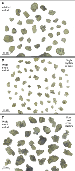
Photomicrograph examples of finished mounts with sectioned olivine crystals from Mauna Loa’s 1852 eruption. A, Crystals prepared using the individual sectioning method, then mounting them together. B, The whole mount method in which all crystals are mounted at the same time and then sectioned, for single crystals and buds. C, Whole mount method for buds and crystal clusters. mm; millimeter.
Mounting in Indium
Indium (In) is a soft metal that is malleable at room temperature and can be used in sample mounting techniques. This set of instructions assumes that you have familiarity with creating indium-filled metal mounts, and that you have a new mount filled with pressed indium at this stage.
-
1. One at a time, press all half crystals with their sectioned (flat) side up and euhedral side down into the malleable indium. Press using a standard glass slide or other sufficiently flat and rigid object.
-
2. Start on one side of the mount and place each successive crystal progressively farther away, working your way across the mount.
Procedure Description
The same general guidance about mounting crystals of reasonably different sizes, morphologies, and orientations all together in one mount (see above for epoxy mounts) applies here as well. If crystals fracture during the indium mounting process, they can generally still be used for in situ analyses.
Polishing the Mounts
Owing to the unique sectioning steps prior to mounting, we recommend these polishing steps instead of following standard polishing routines common in most geological laboratories.
Epoxy Mount Polishing Steps
-
1. Remove epoxy mount from mold.
-
2. Start polishing on 600 grit paper (or 30 micrometer [μm]) for 30 s with gentle pressure.
-
3. Polish on 1200 grit paper (or 15 μm) for several minutes with gentle pressure.
-
4. Polish on 6, 3, 1, and <1 μm grit suspension or paper following normal polishing procedures.
Procedure Description
Because crystals are already sectioned to or near to their cores, typical coarse grits should not be used at any stage of this polishing process. Crystal sections were exposed using 400 grit so the first step in this polishing procedure can begin at 600 grit paper (30 μm) for a short duration of about 30 s. This step is intended to remove any epoxy on crystal faces and gently clean up sectioned surfaces. Take care not to apply too much pressure during this or subsequent steps. Removal of additional material from the crystal sections will create progressively more off-center sections, defeating the purpose of the careful sectioning steps outlined in this guide. By the 6 μm grit polishing step, very little material is removed from sections and so standard polishing procedures may be followed.
Optional Additional Steps, Troubleshooting Non-Ideal Results
Oriented and Precisely Sectioned Doubly Polished Wafers
If the crystals are intended to be used for analytical techniques that require double polishing, such as microscope Fourier transform infrared (FTIR) polarized spectroscopy (for measurements of hydrogen [H] in the olivine lattice), we recommend additional sectioning steps. After the desired section is achieved (step 6 of “Sectioning Individual Crystals”), that section should be polished. Start with 600 grit and polish for 10 s at a time, checking frequently, for no more than a few minutes total. Then polish using 1 μm grit until a clean polished surface is achieved. After the section is fully polished, follow Steps 7–10 of “Sectioning Individual Crystals” and then re-orient the half crystal on the tape with the polished section facing up (euhedral side down). Then repeat steps 1–10 of “Sectioning Individual Crystals” to remove most of the volume of the remaining crystal. By doing this you can create a precisely sectioned and oriented crystal wafer, which can then be polished on the second side starting with 600 grit using the above instructions until a doubly polished wafer is achieved. After a final acetone bath to remove adhesive, place doubly polished wafers in a vial or other container for later analysis (do not mount them).
Making Use of Non-Ideal Results
Mastering this laboratory technique will come with practice and several issues might be common for first time users, but non-ideal results can still be useful. The orientation and sectioning technique is valuable in two ways—both to section crystals through or near to their cores and to orient that section perpendicular to a principal crystallographic axis. The most common non-ideal result is a section oblique to a crystallographic axis (fig. 9F), which usually results from the crystal tipping from its ideal orientation when the glass rod and adhesive are lowered on to the oriented grain. If this happens, which may not be clear until you dissolve away the temporary adhesive, the crystals are still usable. If the section passes generally close to the crystal’s core it should still be mounted and polished, with subsequent EBSD analysis to determine its orientation for the anisotropy correction.
Orienting, Mounting, and Sectioning Multiple Single Crystals or Crystal Clusters (Whole Mount Method)
Standard Polyhedral Morphologies, Twinned Crystals, and Crystal Clusters
Instead of individually sectioning single olivine crystals or crystal clusters, you may instead orient and section an entire mount at one time and achieve similar (but less certain) results. The key to utilizing this whole mount method is to ideally have enough crystals that are approximately the same size and morphology to fill an entire mount. This is a great option for large volume samples or crystal-rich samples such as picrites (for example, the 1959 eruption of Kīlauea volcano, Hawai‘i; Helz, 1987), oceanites (for example, many eruptions of Piton de la Fournaise, Réunion, Welsch and others, 2013), or ankaramites (for example, Karthala volcano, Comoro Islands; Bachèlery and Hémond, 2016; Haleakalā Volcano, Hawai‘i; Welsch and others, 2016).
Procedure Steps
-
1. Assess the range of crystal morphologies and sizes in suite of picked olivine from your sample.
-
2. Group similarly sized crystals or crystal clusters together to assess whether you have enough. Remember to include 10–20 crystals from each crystal population (accounting for variations in grain size, morphology) to ensure you encompass diversity in the sample.
-
3. Cut out a circle of double-sided tape with a diameter slightly less than your mount mold.
-
4. Adhere double-sided tape circle to bottom of mount mold, making sure to press the tape very flat.
-
5. Orient individual crystals down a specific crystallographic axis (using rationale presented in previous sections) on the double-sided tape circle.
-
6. Mount as many crystals as are available and (or) that will fit on the double-sided tape circle, leaving a few mm of space between individual crystals.
-
7. Mix and add epoxy to mount mold using a pipette dropper.
-
8. Check crystal orientations using stereographic microscope and adjust any that may have rotated or tilted during epoxy addition.
-
9. Let epoxy cure following manufacturer’s instructions.
-
10. Remove epoxy mount from mold.
-
11. Grind away epoxy using 320 grit for 30 s at a time, checking crystal exposures intermittently.
-
12. Stop grinding when you approach a depth near to most crystal cores.
-
13. Proceed following normal polishing procedures on 400 grit, 600 grit (30 μm), 15 μm, 6 μm, 3 μm, 1 μm, and <1 μm grit sizes.
Procedure Description
When orienting crystals for the whole mount method, be sure to leave a few millimeters of space between crystals on the tape (fig. 10). When adding epoxy, keep in mind that you may need to grind off a significant amount of material from the mount to reach the crystal cores (depending on their grain size). Make sure that you add enough epoxy to create a mount thick enough to withstand losing so much material. For large (several millimeters in diameter) crystals, this might mean creating an epoxy mount that is 0.5 cm thick or greater.
Non-Standard Morphologies
Less common, but still present in many samples, are non-standard olivine morphologies like platy (Perring and others, 2004; Couperthwaite and others, 2020; Orr and others, 2021) or dendritic (Welsch and others, 2013) crystals (fig. 4C). Despite their highly variable dimensions, these non-standard morphologies can still be similarly oriented and sectioned to provide sections through the 2D plane that constitutes most of their volume (fig. 11). This is a significant benefit of this method because platy crystals are usually sectioned perpendicular to their 2D plane (yielding rod-shaped sections) when they appear in thin sections (for example, Couperthwaite and others, 2020). By sectioning through or parallel to the 2D plane of their geometry, much more spatial information can be gleaned, although the low aspect ratio of platy crystals might not be the most suitable morphology for diffusion modeling studies.
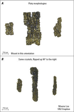
Photomicrographs of non-standard platy Mauna Loa olivine crystal morphologies with low aspect ratios (1852 eruption, Trusdell and Lockwood [2017]). A, Multiple crystal units connected in a two-dimensional plane, confirmed by the view in B, of the same crystals that have been flipped up 90° to the right. °, degree; μm, micrometer.
Procedure Steps
-
1. Select olivine crystals that are approximately the same thickness (see fig. 11B).
-
2. Mount as many crystals as are available and (or) that will fit on the mount mold, leaving a few millimeters of space between individual crystals.
-
3. Mix and add epoxy to mount mold using a pipette dropper.
-
4. Using forceps, ensure crystals are evenly spaced away from each other across the mount mold.
-
5. Let epoxy cure following manufacturer’s instructions.
-
6. Remove epoxy mount from mold.
-
7. Grind away epoxy using 320 or 400 grit for 10 s at a time, checking crystal exposures intermittently.
-
8. Stop grinding when you have exposed most crystals to most of their full 2D extent.
-
9. Proceed following normal polishing procedures on 400 grit, 600 grit (30 μm), 15 μm, 6 μm, 3 μm, 1 μm, and <1 μm grit sizes.
Procedure Description
Mounting platy or dendritic crystals follows the same general guidelines as presented above in “Orienting, Mounting, and Sectioning Multiple Single Crystals or Crystal Clusters (Whole Mount Method)” for standard morphologies. The key difference here is in the grinding step to expose the crystals. Because their geometries have relatively limited extents at depth in the epoxy (fig. 11B), it is imperative to check frequently when exposing crystals to be sure you don’t grind through them.
Proof of Concept
To demonstrate the value of this technique and its benefit to diffusion chronometry studies, we outline below, in “Individual Crystal Sectioning,” several examples of olivine crystals that were oriented and sectioned using either the individual or whole-mount methods, analyzed for major elements using electron probe micro analysis (EPMA), analyzed for orientation using EBSD, and profiles subsequently modeled for timescales of diffusive re-equilibration. These results are compared with models in which sections are assumed to be truly ideal (that is, perfect sections) to demonstrate that EBSD confirmation of orientation is not needed when this technique is properly used.
Individual Crystal Sectioning
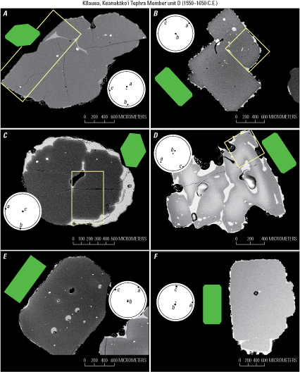
Orienting and sectioning individual olivine crystals usually yields ideal sections (fig. 2) for a variety of euhedral to subhedral single crystal morphologies (fig. 12). These examples, from the Keanakāko‘i Tephra unit D (1550–1650 C.E.; Swanson and others, 2012; Swanson and Houghton, 2018) show good results for b-c sections (oriented down the a-axis) and a-c sections (oriented down the b-axis). Note the range of textures for these grains, which many have skeletal rims (fig. 12C, E, and F) and (or) incompletely formed crystal faces (fig. 12A, B). Despite these complexities, the orientation and sectioning technique was successful, as demonstrated by the EBSD-confirmed orientations (shown as lower hemisphere stereonet projections; plotted using software of Cardozo and Allmendinger, 2013) as well as ideal section geometries (compared to ideal sections in fig. 2) that together indicate the olivine crystals are precisely oriented and sectioned.
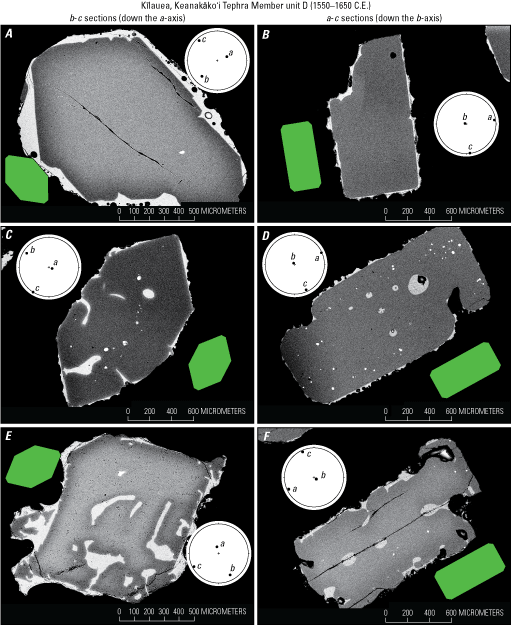
Backscattered electron images showing examples of electron backscatter diffraction (EBSD) confirmed orientations for standard morphology crystals from the Keanakāko’i Tephra Member unit D (1550 –1650 C.E.; Swanson and others, 2012). In A, C, and E, b-c sections are oriented down the a-axis, and in B, D, and F, the a-c sections are oriented down the b-axis. These crystals are examples of the individual sectioning technique. Note that despite their skeletal textures, crystals in C, E, and F were still able to be well oriented and sectioned. Green diagrams show comparative ideal crystal sections, and circular diagrams are EBSD-confirmed orientations shown as lower hemisphere stereonet projections with crystallographic a-, b-, and c-axes plotted using the software of Cardozo and Allmendinger (2013).
The orientation and sectioning technique is also successful when working with complex crystals or crystal clusters, as shown by EBSD-confirmed orientations in fig. 13. These examples include buds (for example, fig. 13A), twins (fig. 13B), and more irregular skeletal crystals (fig. 13D) and yet EBSD analysis confirms that the crystals are well oriented, so diffusion profiles would be straightforward to model in the absence of EBSD data despite the more complex 2D sectioning geometries.
Examples of images of electron backscatter diffraction (EBSD)-confirmed orientations for complex crystals and crystal clusters from the Keanakāko’i Tephra Member unit D (1550–1650 C.E.; Swanson and others, 2012). White boxes indicate regions where EBSD data were collected, otherwise the entire crystal was mapped. A, Cluster of parallel buds oriented down the a-axis (b-c section). B, Buds oriented down the b-axis (a-c section). C, An example of a crystal cluster oriented down the c-axis (a-b section), which is not generally recommended for diffusion studies because the c-axis is highly oblique to the plane of the section. D, A skeletal crystal that was still able to be well oriented down the b-axis and sectioned owing to its overall euhedral shape. E, Cluster of crystals that appears to be one polyhedral crystal in the a-c section. F, A single crystal with two smaller buds, oriented down the b-axis (a-c section). Green diagrams show comparative ideal crystal sections, and circular diagrams are EBSD-confirmed orientations shown as lower hemisphere stereonet projections with crystallographic a-, b-, and c-axes plotted using the software of Cardozo and Allmendinger (2013).
The success of the technique for the whole mount method is also clear, as shown in figure 14. These olivine crystals, from the Kulanaokuaiki Tephra Member of the Uwekahuna Ash unit 3 (900 C.E.; herein referred to as the Kulanaokuaiki Tephra following Fiske and others, 2009) had fractured crystal faces that tended to somewhat obfuscate morphology during orientation. Despite these challenges, the backscatter electron (BSE) images and orientations show that they are still very precisely oriented. Their more rounded texture is due to their fractured crystal faces, evidence that their crystal morphologies during mounting were not pristine (as compared to the Keanakāko‘i Tephra unit D, for example; fig. 12).
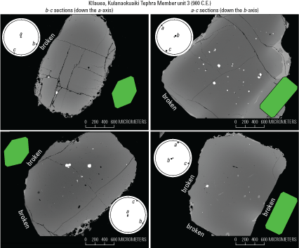
Examples of electron backscatter diffraction (EBSD) images with confirmed orientations for subhedral and fractured olivine crystals using the whole mount method. These Kulanaokuaiki Tephra unit 3 (900 C.E.; Fiske and others, 2009) olivine crystals had fractured crystal faces that tended to somewhat obfuscate morphology during orientation. Despite these challenges, the backscatter electron (BSE) images and EBSD-confirmed orientations show that they are still very precisely oriented. Their more rounded texture is due to their fractured crystal faces, evidence that their crystal morphologies during mounting were not pristine. Green diagrams show comparative ideal crystal sections, and circular diagrams are EBSD-confirmed orientations shown as lower hemisphere stereonet projections with crystallographic a-, b-, and c-axes plotted using the software of Cardozo and Allmendinger (2013).
Finally, we demonstrate that diffusion models on well-oriented and sectioned crystals can be applied without having to acquire the EBSD data. Several Keanakāko‘i Tephra unit D and Kulanaokuaiki Tephra unit 3 crystals were analyzed for their orientation using a TESCAN Vega3 SEM with an Oxford Symmetry electron backscatter (EBSD) detector at the USGS Electron Microbeams Facility at Menlo Park, California. Measurements were taken using a 70 degrees sample tilt, 15–20 kilovolt (kV) accelerating voltage, and minimum working distance (usually 17.5 mm). Area maps of whole or half olivine crystals achieved mean angular deviation values of <1 degree. Orientations were plotted in lower hemisphere stereonet projections and α, β, and γ (alpha, beta, and gamma, respectively), which are the angles between the traverse and the a-, b-, and c-axes of the olivine crystal, respectively, were calculated using the program OSXStereonet (Cardozo and Allmendinger, 2013).
Core-to-rim compositional profiles in the same olivine crystals were measured using a five-spectrometer JXA-8500F electron microprobe at the University of Hawai‘i, Hilo. Analyses used a 15 kV accelerating voltage and a 1 µm beam with a 50 nanoampere (nA) current. Major elements silicon (Si), Magnesium (Mg), and iron (Fe) were gathered using combined energy-dispersive X-ray spectroscopy (EDS) analyses on a Thermo UltraDry detector using a SystemSix analyzer with a dead time of 38 percent and live acquisition for 60 s. Calcium (Ca), nickel (Ni), and manganese (Mn) were measured by wavelength-dispersive X-ray spectroscopy (WDS), and counting times were 60 s with 20 s on both sides of the peak for backgrounds. X-ray intensities were converted to concentrations using standard ZAF corrections (which considers the effects of atomic number [Z], absorption [A], and fluorescence excitation [F] on the characteristic X-ray intensity when performing quantitative analysis; Armstrong, 1988). Analyses with totals <98.5 weight percent (wt%) or >100.5 wt% were rejected. Standards were Springwater olivine (United States National Museum [USNM] 2566, Jarosewich and others, 1980) for Si, Fe, and Mg, a synthetic nickel-oxide for Ni, Verma garnet for Mn and Kakanui Augite (USNM 122142; Jarosewich and others, 1980) for Ca. Two-sigma relative precision, based on repeated analyses of San Carlos olivine, are 0.16 wt% for SiO2, 0.12 wt% for MgO, 0.60 wt% for FeO, 0.04 wt% for MnO, 0.02 wt% for, NiO, and 0.006 wt% for CaO (app. 1, table 1.1). Analytical profiles modeled for diffusion are presented in appendix 2, tables 2.1–2.3.
Geochemical profiles of Fe-Mg from EPMA traverses were modeled using finite differences and the 1D form of Fick’s Second Law (Crank, 1975):
whereC
is concentration,
t
is time (in seconds),
D
is the diffusion coefficient (in square meters per second [m2/s]), and
x
is distance (in meters [m]).
The concentration-dependent diffusion coefficient for Fe-Mg exchange in olivine was calculated using:
whereis the oxygen fugacity (in pascals [Pa]),
XFe
is the mol fraction of iron in the olivine,
P
is pressure (in Pa),
R
is the ideal gas constant, and
T
is temperature (in Kelvin [K]).
Equation 2 (from Dohmen and Chakraborty, 2007) is for diffusion along the c-axis, which is 6 times faster than diffusion along the a- or b-axes:
To account for diffusion anisotropy (eq. 3), profiles were first modeled assuming they were taken parallel to a crystallographic axis (assumption of an ideally oriented crystal; “ideal time” in table 1). Then the same profiles were modeled using the EBSD orientation data and calculated angle between the a-, b-, and c-axes (α, β, and γ, respectively; Costa and Chakraborty, 2004) to retrieve a second timescale for the same crystal (“EBSD time” in table 1). Timescales were determined by reducing the misfit between the measured data and the diffusion model through root mean square deviation (RMSD) calculations, which finds the best model fit to the microprobe data:
whereM
is the number of points along the profile,
i
is the coordinate along the profile,
Creal
is the measured concentration, and
Cmeas
is the concentration in the diffusion model that is being evaluated (see Shea and others, 2015).
Table 1.
Diffusion modeling parameters and results for ideal and electron backscatter diffraction (EBSD)-corrected timescales for olivine crystals from Kīlauea’s Keanakāko‘i Tephra unit D (Swanson and others, 2012; Swanson and Houghton, 2018).[For images and plotted results, see fig. 15. All models utilized a pressure of 85 megapascals (MPa) (Poland and others, 2014) and an oxygen fugacity of quartz-fayalite-magnetite +0.4 (Helz and others, 2017). The angles between the traverse, α, β, and γ, and the a-, b-, and c-axes of an olivine crystal, respectively, were calculated using Stereonet (Cardozo and Allmendinger, 2013). °C, degrees Celsius; Ci, initial condition based on the forsterite content; Co, the boundary condition set to the forsterite content of the olivine rim; EBSD, electron backscatter diffraction; mol%, mole percent; Ol., olivine; T, temperature.]
Error is estimated to be ~30 percent of the calculated timescale and is largely dependent on the uncertainty in the temperature calculation (thermometer uncertainty of ±10 °C; Helz and Thornber, 1987) and the typical analytical precision of measuring olivine forsterite content (±0.1 mol%).
The initial condition (Ci) was determined based on the Fo (forsterite; the Mg number is the atomic ratio of Mg/(Mg+Fe2+)*100) content of the plateau through the olivine core. The boundary condition (Co) was set to the Fo content of the olivine rim and choice of initial condition shape was based on presence or absence of inflections preserved in CaO zoning (indicative of crystal rim growth). Intrinsic environmental parameters required for the models are relatively well constrained for Kīlauea. The likely temperature at which diffusive re-equilibration occurred was determined using a suite of olivine-melt experimental data (Helz and Thornber, 1987; Montierth and others, 1995; Matzen and others, 2011) to assess an approximate equilibrium temperature for each mole percent (mol%) increment of Fo content. Each individual olivine rim boundary condition was then used to infer an appropriate temperature for the models, which are akin to the magma temperature for pre-eruptive storage and diffusion recorded by each olivine crystal. Oxygen fugacity was set to quartz-fayalite-magnetite +0.4 based on Fe3+/∑Fe measurements in Kīlauea Iki melt inclusions, representing pre-eruptive redox conditions (Helz and others, 2017). The pressure was set to 85 megapascals (MPa) (that approximates 3.5 kilometers [km] depth), reflecting the depth of Kīlauea’s magma reservoir beneath the south caldera (for example, Poland and others, 2014).
For each model comparison, the calculated ideal time versus EBSD time is nearly identical (fig. 15), especially for the short timescale of only 7 days. The crystals with wider zoning patterns, and thus longer timescales, have differences in their ideal versus EBSD timescales of only 8–13 days in the examples provided, or <1 percent relative to the total time calculated using either method. This difference is incredibly small compared to the general error of approximately ±30 percent of a given timescale (which is mostly related to the temperature uncertainty [±10 °C thermometer uncertainty of Helz and Thornber, 1987] and analytical precision [0.1 mol%] as determined in other olivine diffusion studies at Kīlauea; Lynn and others, 2017; Lynn and Helz, 2023). Thus, diffusion chronometry studies on these well-oriented crystals do not need EBSD data to account for anisotropy effects. An assumption of ideal orientation will yield indistinguishable results within the typical uncertainty on diffusion timescales. Furthermore, the examples in figure 15 show excellent agreement between ideal and EBSD timescales for some of the most oblique sections produced by this orientation and sectioning method (compare to several nearly perfectly oriented crystals in figures 12 and 13). Despite the imperfect orientations used in the modeling examples in figure 15, the profiles can be modeled assuming ideal orientations.
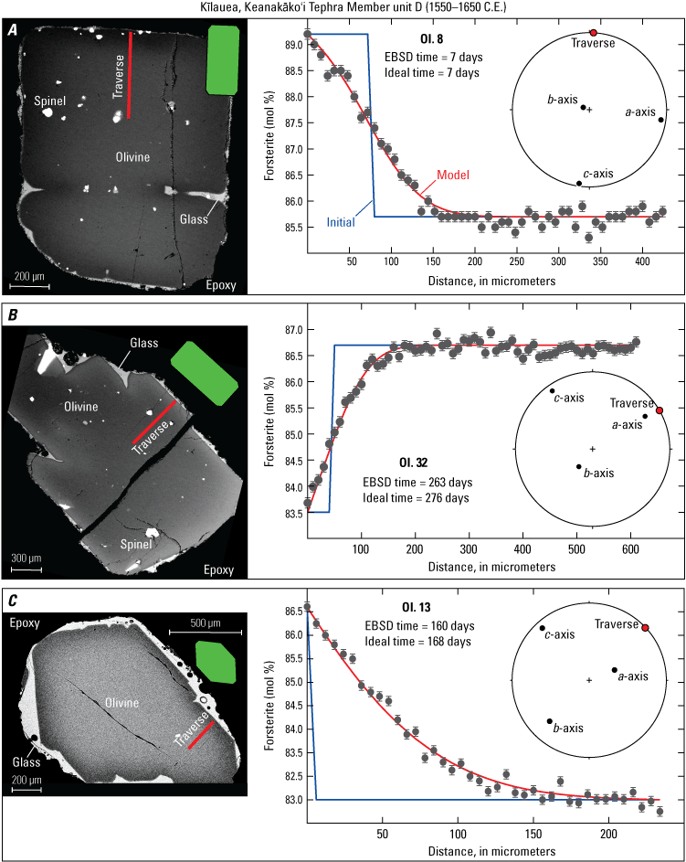
Example graphs of diffusion models (initial profiles, blue lines) and calculated timescales (from model best fits, red lines) using individually oriented and sectioned olivine crystals from Kīlauea’s Keanakāko‘i Tephra Member unit D (1550–1650 C.E., Swanson and others, 2012; Swanson and Houghton, 2018). For modeling parameters and results for ideal and electron backscatter diffraction (EBSD)-corrected timescales see table 1. A, A well-oriented olivine section with analytical traverse collected parallel to the c-axis (the fast diffusion direction). B, A fairly well-oriented, slightly oblique olivine section with analytical traverse collected parallel to the a-axis (slow diffusion direction). C, A fairly well-oriented, slightly oblique olivine section with analytical traverse collected parallel to the b-axis (slow diffusion direction). Green diagrams show comparative ideal sections, and circular diagrams are EBSD-confirmed orientations shown as lower hemisphere stereonet projections plotted using the software of Cardozo and Allmendinger (2013). μm, micrometer; EBSD, electron backscatter diffraction; mol%, mole percent; OI, olivine.
Method Summary
Drawbacks and Benefits to Using this Method
Users may ask themselves when and why this method should be employed in their research. There are several aspects of this method that might pose drawbacks or challenges:
-
1. Fine-scale laboratory work such as this may not be a strength of all users.
-
2. Individually sectioning and orienting crystals may seem tedious and time consuming.
-
3. Not all well-oriented or sectioned crystals will yield chemical gradients (that is, they do not record diffusive re-equilibration information).
However, the benefits of the orientation and sectioning technique can be substantial, and include:
-
1. Consistently well-oriented crystals would not need to have electron backscatter diffraction (EBSD)-determined orientations, resulting in a substantial time and cost savings that could make diffusion chronometry more widely accessible to diverse communities of users.
-
a. As an example, a researcher would have a cost savings of $350–$500 of analytical expenses if experienced scanning electron microscopy-EBSD users determine orientations for 10–15 crystals in a regular 8-hour workday at a cost of $35 per hour. Because about 10–20 good diffusion models are needed to sufficiently characterize a population (Shea and others, 2015), the cost savings can be up to $800 per population of interest.
-
b. Additional cost savings in the form of the difference in salary or hours that would have been required to conduct the EBSD analyses could also be a benefit of the method.
-
c. We recommend that first-time users of this method use EBSD as a self-check on at least a subset of their oriented and sectioning crystals to show that they have utilized the technique correctly. Subsequent applications of the method can then reference the first study as proof-of-concept and to support the study not needing EBSD-corrected diffusion timescales.
-
d. We recommend that users of this technique include photomicrographs or backscattered electron images of their crystals in their publications and (or) supplementary material as documentation that the technique was used effectively.
-
-
2. Removing the need for EBSD-confirmed orientations allows for diffusion modeling immediately after acquisition of geochemical-zoning data. This results in accurate diffusion datasets more quickly, a necessary addition to near-real-time chemical monitoring of volcanic eruptions (Gansecki and others, 2019; Re and others, 2021; Pankhurst and others, 2022) or other time-sensitive information needs.
-
3. The materials required to use this method include relatively common and inexpensive lab items that make it more accessible to different demographics of users.
-
4. The user saves several hours of grinding and polishing after the mount is created because they can start at a relatively fine grit size (for example, 600 or 1200 grit) and proceed quickly.
Applications in Different Scientific Communities
Several different methods and optional variations have been discussed in this paper. Factors to consider when choosing a method primarily include time and availability of personnel that are suited to fine-scale lab work and availability of EBSD and (or) funds and expertise to collect these data. Regardless of the specific circumstances, this methodology can be of use to a variety of groups and in different situations, including:
-
1. The sectioning steps to access crystal cores can be hugely beneficial for diverse types of in situ analyses, even if diffusion chronometry and compositional profiles are not the main goal of the work.
-
2. For research institutions with limited resources or lab facilities (such as but not limited to primarily undergraduate institutions, institutions without an electron backscatter detector, and groups with limited research funds for contracting analytical services or traveling to conduct analyses themselves), this methodology still allows diffusion chronometry to be a valuable asset in research endeavors.
-
3. For groups desiring timescale information derived from diffusion chronometry in a timely manner (such as volcano observatories responding to an eruption), this technique can be used quickly and efficiently to acquire compositional profiles and calculate diffusion timescales without needing to collect an additional EBSD dataset.
-
4. For research institutions with EBSD capabilities and qualified personnel to collect the data, this method might be used if the instruments were to be offline for an extended period of time owing to damage or routine maintenance.
We hope that this orientation and sectioning methodology can be used to collect better geochemical datasets and improve the interpretations made from them. Olivine was chosen as the example material for this report owing to its popularity for studies on diffusion chronometry. Our goal for outlining these methods for creating oriented and well-sectioned mineral mounts is to aid volcanologists worldwide and to facilitate further studies of diffusion chronometry on a wide variety of minerals.
References Cited
Armstrong, J.T., 1988, Quantitative analyses of silicate and oxide materials—Comparison of Monte Carlo, ZAF, and φ(ρz) procedures, in Newbury, D.E., ed., Microbeam Analysis, 23rd Annual Conference of the Microbeam Analysis Society, Milwaukee, Wis., August 8–12, 1988, Proceedings: San Francisco, San Francisco Press, p. 239–246, http://www.geology.wisc.edu/~johnf/g777/777MicrobeamAnalysis/JTA-1988-ZAF.pdf.
Bachèlery, P., and Hémond, C., 2016, Geochemical and petrological aspects of Karthala Volcano, chap. 23 of Bachèlery, P., Di Muro, A., Lénat, J.-F., and Michon, L., eds., Active volcanoes of the southwest Indian Ocean—Piton de la Fournaise and Karthala, Active Volcanoes of the World series: Berlin, Heidelberg, Springer-Verlag, p. 367–384, https://doi.org/10.1007/978-3-642-31395-0_23.
Barbee, O., Chesner, C., and Deering, C., 2020, Quartz crystals in Toba rhyolites show textures symptomatic of rapid crystallization: American Mineralogist, v. 105, no. 2, p. 194–226, https://doi.org/10.2138/am-2020-6947.
Barth, A., Newcombe, M., Plank, T., Gonnermann, H., Hajimirza, S., Soto, G.J., Saballos, A., and Hauri, E., 2019, Magma decompression rate correlates with explosivity at basaltic volcanoes—Constraints from water diffusion in olivine: Journal of Volcanology and Geothermal Research, v. 387, 48 p., https://doi.org/10.1016/j.jvolgeores.2019.106664.
Bloch, E.M., Jollands, M.C., Tollan, P., Plane, F., Bouvier, A.-S., Hervig, R., Berry, A.J., Zaubitzer, C., Escrig, S., Müntener, O., Ibañez-Mejia, M., Alleon, J., Meibom, A., Baumgartner, L.P., Marin-Carbonne, J., and Newville, M., 2022, Diffusion anisotropy of Ti in zircon and implications for Ti-in-zircon thermometry: Earth and Planetary Science Letters, v. 578, 15 p., https://doi.org/10.1016/j.epsl.2021.117317.
Cardozo, N., and Allmendinger, R.W., 2013, Spherical projections with OSXStereonet: Computers and Geosciences, v. 51, p. 193–205, https://doi.org/10.1016/j.cageo.2012.07.021.
Chakraborty, S., 1997, Rates and mechanisms of Fe-Mg interdiffusion in olivine at 980°–1300 °C: Journal of Geophysical Research—Solid Earth, v. 102, p. 12,317–12,331, https://doi.org/10.1029/97JB00208.
Chakraborty, S., 2010, Diffusion coefficients in olivine, wadsleyite, and ringwoodite: Reviews in Mineralogy and Geochemistry, v. 72, no. 1, p. 603–639, https://doi.org/10.2138/rmg.2010.72.13.
Charlier, B.L.A., Morgan, D.J., Wilson, C.J.N., Wooden, J.L., Allan, A.S.R., and Baker, J.A., 2012, Lithium concentration gradients in feldspar and quartz record the final minutes of magma ascent in an explosive supereruption: Earth and Planetary Science Letters, v. 319–320, p. 218–227, https://doi.org/10.1016/j.epsl.2011.12.016.
Colin, A., Faure, F., and Burnard, P., 2012, Timescales of convection in magma chambers below the Mid-Atlantic ridge from melt inclusions investigations: Contribution to Mineralogy and Petrology, v. 164, p. 677–691, https://doi.org/10.1007/s00410-012-0764-2.
Cooper, K.M., and Kent, A.J.R., 2014, Rapid remobilization of magmatic crystals kept in cold storage: Nature, v. 506, p. 480–483, https://doi.org/10.1038/nature12991. [Erratum published April 23, 2014, https://doi.org/10.1038/nature13280.]
Costa, F., and Chakraborty, S., 2004, Decadal time gaps between mafic intrusion and silicic eruption obtained from chemical zoning patterns in olivine: Earth and Planetary Science Letters, v. 227, nos. 3–4, p. 517–530, https://doi.org/10.1016/j.epsl.2004.08.011.
Costa, F., Dohmen, R., and Chakraborty, S., 2008, Time scales of magmatic processes from modeling the zoning patterns of crystals: Reviews in Mineralogy and Geochemistry, v. 69, no.1, p. 545–594, https://doi.org/10.2138/rmg.2008.69.14.
Costa, F., and Dungan, M., 2005, Short time scales of magmatic assimilation from diffusion modeling of multiple elements in olivine: Geology, v. 33, no. 10, p. 837–840, https://doi.org/10.1130/G21675.1.
Costa, F., Shea, T., and Ubide, T., 2020, Diffusion chronometry and the timescales of magmatic processes: Nature Reviews Earth & Environment, v. 1, p. 201–214, https://doi.org/10.1038/s43017-020-0038-x.
Couperthwaite, F.K., Morgan, D.J., Pankhurst, M.J., Lee, P.D., and Day, J.M.D., 2021, Reducing epistemic and model uncertainty in ionic inter-diffusion chronology—A 3D observation and dynamic modeling approach using olivine from Piton de la Fournaise, La Réunion: American Mineralogist, v. 106, no. 3, p. 481–494, https://doi.org/10.2138/am-2021-7296CCBY.
Couperthwaite, F.K., Thordarson, T., Morgan, D.J., Harvey, J., and Wilson, M., 2020, Diffusion timescales of magmatic processes in the Moinui lava eruption at Mauna Loa, Hawai‘i, as inferred from bimodal olivine populations: Journal of Petrology, v. 61, no. 7, https://doi.org/10.1093/petrology/egaa058.
Davidson, J.P., Morgan, D.J., Charlier, B.L.A., Harlou, R., and Hora, J.M., 2007, Microsampling and isotopic analysis of igneous rocks—Implications for the study of magmatic systems: Annual Review of Earth and Planetary Sciences, v. 35, p. 273–311, https://doi.org/10.1146/annurev.earth.35.031306.140211.
Dodd, R.T., and Calef, C., 1971, Twinning and intergrowth of olivine crystals in chondritic meteorites: Mineralogical Magazine, v. 38, no. 295, p. 324–327, https://doi.org/10.1180/minmag.1971.038.295.06.
Dohmen, R., Chakraborty, S., 2007, Fe–Mg diffusion in olivine II—Point defect chemistry, change of diffusion mechanisms and a model for calculation of diffusion coefficients in natural olivine: Physics and Chemistry of Minerals, v. 34, p. 409–430, https://doi.org/10.1007/s00269-007-0158-6. [Erratum published August 31, 2007, https://doi.org/10.1007/s00269-007-0185-3.]
Donaldson, C.H., 1976, An experimental investigation of olivine morphology: Contributions to Mineralogy and Petrology, v. 57, p. 187–213, https://doi.org/10.1007/BF00405225.
Ferrando, C., Lynn, K.J., Basch, V., Ildefonse, B., and Godard, M., 2020, Retrieving timescales of oceanic crustal evolution at Oceanic Core Complexes—Insights from diffusion modelling of geochemical profiles in olivine: Lithos, v. 367–377, article 105727, https://doi.org/10.1016/j.lithos.2020.105727.
Fiske, R.S., Rose, T.R., Swanson, D.A., Champion, D.E., and McGeehin, J.P., 2009, Kulanaokuaiki Tephra (ca. A.D. 400–1000): Newly recognized evidence for highly explosive eruptions at Kīlauea Volcano, Hawai‘i: The Geological Society of America Bulletin, v. 121, nos. 5–6, p. 712–728, https://doi.org/10.1130/B26327.1.
Gansecki, C., Lee, R.L., Shea, T., Lundblad, S.P., Hon, K., and Parcheta, C., 2019, The tangled tale of Kīlauea’s 2018 eruption as told by geochemical monitoring: Science, v. 366, no. 6470, 9 p., https://doi.org/10.1126/science.aaz0147.
Helz, R.T., 1987, Diverse olivine types in lavas of the 1959 eruption of Kilauea volcano and their bearing in eruption dynamics, chap. 25 of Decker, R.W., Wright, T.L., and Stauffer, P.H., eds., Volcanism in Hawaii: U.S. Geological Survey Professional Paper 1350, v. 1, p. 691–722, https://doi.org/10.3133/pp1350.
Helz, R.T., Cottrell, E., Brounce, M.N., and Kelley, K.A., 2017, Olivine-melt relationships and syneruptive redox variations in the 1959 eruption of Kīlauea Volcano as revealed by XANES: Journal of Volcanology and Geothermal Research, v. 333–334, p. 1–14, https://doi.org/10.1016/j.jvolgeores.2016.12.006.
Helz, R.T., and Thornber, C.R., 1987, Geothermometry of Kilauea Iki lava lake, Hawai‘i: Bulletin of Volcanology, v. 49, p. 651–668, https://doi.org/10.1007/BF01080357.
Jarosewich, E., Nelen, J.A., Norberg, J.A., 1980, Reference samples for electron microprobe analysis: Geostandards Newsletter, v. 4, no. 1, p. 43–47, https://doi.org/10.1111/j.1751-908X.1980.tb00273.x.
Kahl, M., Chakraborty, S., Costa, F., and Pompilio, M., 2011, Dynamic plumbing system beneath volcanoes revealed by kinetic modeling, and the connection to monitoring data—An example from Mt. Etna: Earth and Planetary Science Letters, v. 308, nos. 1–2, p. 11–22, https://doi.org/10.1016/j.epsl.2011.05.008.
Kahl, M., Chakraborty, S., Costa, F., Pompilio, M., Liuzzo, M., and Viccaro, M., 2013, Compositionally zoned crystals and real-time degassing data reveal changes in magma transfer dynamics during the 2006 summit eruptive episodes of Mt. Etna: Bulletin of Volcanology, v. 75, article 692, 14 p., https://doi.org/10.1007/s00445-013-0692-7.
Krimer, D., and Costa, F., 2017, Evaluation of the effects of 3D diffusion, crystal geometry, and initial conditions on retrieved time-scales from Fe-Mg zoning in natural oriented orthopyroxene crystals: Geochimica et Cosmochimica Acta, v. 196, p. 271–288, https://doi.org/10.1016/j.gca.2016.09.037.
Lubbers, J., Kent, A., Meisenheimer, D., and Wildenschild, D., 2023, 3D zoning of barium in alkali feldspar: American Mineralogist, v. 108, no. 2, p. 297–311, https://doi.org/10.2138/am-2022-8139.
Lynn, K.J., Garcia, M.O., and Shea, T., 2020, Phosphorus coupling obfuscates lithium geospeedometry in olivine: Frontiers in Earth Science, v. 8, 15 p., https://doi.org/10.3389/feart.2020.00135.
Lynn, K.J., Garcia, M.O., Shea, T., Costa, F., and Swanson, D.A., 2017, Timescales of mixing and storage for Keanakāko‘i Tephra magmas (1500–1820 C.E.), Kīlauea Volcano, Hawai‘i: Contributions to Mineralogy and Petrology, v. 172, no. 9, article 76, 20 p., https://doi.org/10.1007/s00410-017-1395-4.
Lynn, K.J., and Helz, R.T., 2023, Magma storage and transport timescales for the 1959 Kīlauea Iki eruption and implications for diffusion chronometry studies using time-series samples versus tephra deposits: Bulletin of Volcanology, v. 85, no. 1, article 3, 18 p., https://doi.org/10.1007/s00445-022-01618-9.
Lynn, K.J., and Warren, J.M., 2021, The potential for aqueous fluid-rock and silicate melt-rock interactions to re-equilibrate hydrogen in peridotite nominally anhydrous minerals: American Mineralogist, v. 106, no. 5, p. 701–714, https://doi.org/10.2138/am-2021-7435.
Mackwell, S.J., and Kohlstedt, D.L., 1990, Diffusion of hydrogen in olivine—Implications for water in the mantle: Journal of Geophysical Research—Solid Earth, v. 95, no. B4, p. 5079–5088, https://doi.org/10.1029/JB095iB04p05079.
Matzen, A.K., Baker, M.B., Beckett, J.R., and Stolper, E.M., 2011, Fe–Mg partitioning between olivine and high-magnesian melts and the nature of Hawaiian parental liquids: Journal of Petrology, v. 52, nos. 7–8, p. 1243–1263, https://doi.org/10.1093/petrology/egq089.
Métrich, N., Bertagnini, A., and Di Muro, A., 2010, Conditions of magma storage, degassing and ascent at Stromboli—New insights into the volcano plumbing system with inferences on the eruptive dynamics: Journal of Petrology, v. 51, no. 3, p. 603–626, https://doi.org/10.1093/petrology/egp083.
Milman-Barris, M.S., Beckett, J.R., Baker, M.B., Hofmann, A.E., Morgan, Z., and Crowley, M.R., Vielzeuf, D, and Stolper, E., 2008, Zoning of phosphorus in igneous olivine: Contributions to Mineralogy and Petrology, v. 155, p. 739–765, https://doi.org/10.1007/s00410-007-0268-7.
Montierth, C., Johnston, A.D., and Cashman, K.V., 1995, An empirical glass-composition-based geothermometer for Mauna Loa lavas, in Rhodes, J.M., and Lockwood, J.P., eds., Mauna Loa Revealed—Structure, composition, history, and hazards: American Geophysical Union Monograph Series, v. 92, p. 207–217, https://doi.org/10.1029/GM092p0207.
Morgan, D.J., Blake, S., Rogers, N.W., De Vivo, B., Rolandi, G., and Davidson, J.P., 2006, Magma chamber recharge at Vesuvius in the century prior to the eruption of A.D. 79: Geology, v. 34, no. 10, p. 845–848, https://doi.org/10.1130/G22604.1.
Mourey, A.J., and Shea, T., 2019, Forming olivine phenocrysts in basalt—A 3D characterization of growth rates in laboratory experiments: Frontiers in Earth Science, v. 7, 16 p, https://doi.org/10.3389/feart.2019.00300.
Mutch, E.J.F., Maclennan, J., Holland, T.J.B., and Buisman, I., 2019a, Millennial storage of near-Moho magma: Science, v. 365, no. 6450, p. 260–264, https://doi.org/10.1126/science.aax4092.
Mutch, E.J.F., Maclennan, J., Shorttle, O., Edmonds, M., and Rudge, J.F., 2019b, Rapid transcrustal magma movement under Iceland: Nature Geoscience, v. 12, p. 569–574, https://doi.org/10.1038/s41561-019-0376-9.
Orr, T.R., Hazlett, R., DeSmither, L., Kauahikaua, J., and Gaddis, B., 2021, Correcting the historical record for Kīlauea Volcano’s 1832, 1868, and 1877 summit eruptions: Journal of Volcanology and Geothermal Research, v. 410, article 107168, https://doi.org/10.1016/j.jvolgeores.2020.107168.
Pankhurst, M.J., Scarrow, J.H., Barbee, O.A., Hickey, J., Coldwell, B.C., Rollinson, G.K., Rodríguez-Losada, J.A., Martín-Lorenzo, A., Rodríguez, F., Hernández, W., Fernández, D.C., Hernández, P.A., and Pérez, N.M., 2022, Rapid response petrology for the opening eruptive phase of the 2021 Cumbre Vieja eruption, La Palma, Canary Islands: Volcanica, v. 5, no. 1, 10 p., https://doi.org/10.30909/vol.05.01.0110.
Pearce, T.H., 1984, The analysis of zoning in magmatic crystals with emphasis on olivine: Contributions to Mineralogy and Petrology, v. 86, p. 149–154, https://doi.org/10.1007/BF00381841.
Perring, C.S., Barnes, S.J., Verrall, M., and Hill, R.E.T., 2004, Using automated digital image analysis to provide quantitative petrographic data on olivine-phyric basalts: Computers and Geosciences, v. 30, no. 2, p. 183–195, https://doi.org/10.1016/j.cageo.2003.10.005.
Poland, M.P., Miklius, A., and Montgomery-Brown, E., 2014, Magma supply, storage, and transport at shield-stage Hawaiian volcanoes, chap. 5 of Poland, M.P., Takahashi, T.J., Landowski, C.M., eds., Characteristics of Hawaiian volcanoes: U.S. Geological Survey Professional Paper 1801-5, p. 179–234, https://doi.org/10.3133/pp18015.
Prior, D.J., Boyle, A.P., Brenker, F., Cheadle, M.C., Day, A., Lopez, G., Peruzzo, L., Potts, G.J., Reddy, S., Spiess, R., Timms, N.E., Trimby, P., Wheeler, J., and Zetterström, L., 1999, The application of electron backscatter diffraction and orientation contrast imaging in the SEM to textural problems in rocks: American Mineralogist, v. 84, nos. 11–12, p. 1741–1759, https://doi.org/10.2138/am-1999-11-1204.
Re, G., Corsaro, R.A., D’Oriano, C., and Pompilio, M., 2021, Petrological monitoring of active volcanoes—A review of existing procedures to achieve best practices and operative protocols during eruptions: Journal of Volcanology and Geothermal Research, v. 419, article 107365, 13 p., https://doi.org/10.1016/j.jvolgeores.2021.107365.
Ruprecht, P., and Plank, T., 2013, Feeding andesitic eruptions with a high-speed connection from the mantle: Nature, v. 500, p. 68–72, https://doi.org/10.1038/nature12342.
Ruth, D.C.S., and Costa, F., 2021, A petrological and conceptual model of Mayon volcano (Philippines) as an example of an open-vent volcano: Bulletin of Volcanology, v. 83, article 62, https://doi.org/10.1007/s00445-021-01486-9.
Shea, T., Costa, F., Krimer, D., and Hammer, J.E., 2015, Accuracy of timescales retrieved from diffusion modeling in olivine—A 3D perspective: American Mineralogist, v. 100, no. 10, p. 2026–2042, https://doi.org/10.2138/am-2015-5163.
Spilliaert, N., Allard, P., Métrich, N., and Sobolev, A.V., 2006, Melt inclusion record of the conditions of ascent, degassing, and extrusion of volatile-rich alkali basalt during the powerful 2002 flank eruption of Mount Etna (Italy): Journal of Geophysical Research—Solid Earth, v. 111, no. B4, https://doi.org/10.1029/2005JB003934.
Swanson, D.A., and Houghton, B.F., 2018, Products, processes, and implications of Keanakāko‘i volcanism, Kīlauea Volcano, Hawai‘i, in Poland, M.P., Garcia, M.O., Camp, V.E., and Grunder, A., eds., Field Volcanology—A tribute to the distinguished career of Don Swanson: The Geological Society of America Special Paper, v. 538, p. 159–190, https://doi.org/10.1130/2018.2538(07).
Swanson, D.A., Rose, T.R., Fiske, R.S., and McGeehin, J.P., 2012, Keanakāko‘i Tephra produced by 300 years of explosive eruptions following collapse of Kīlauea’s caldera in about 1500 CE: Journal of Volcanology and Geothermal Research, v. 215–216, p. 8–25, https://doi.org/10.1016/j.jvolgeores.2011.11.009.
Takehara, M., Horie, K., Hokada, T., and Kiyokawa, S., 2018, Data on recovery rates and external morphologies of zircon grains from mechanical and electrical pulverization of rock samples: Data in Brief, v. 19, p. 1537–1544, https://doi.org/10.1016/j.dib.2018.06.016.
Trusdell, F.A., and Lockwood, J.P., 2017, Geologic map of the northeast flank of Mauna Loa volcano, Island of Hawai'i, Hawaii: U.S Geological Survey Scientific Investigations Map 2932–A, 2 sheets, scale 1:50,000, 25-p. pamphlet, https://doi.org/10.3133/sim2932A.
Ubide, T., McKenna, C.A., Chew, D.M., and Kamber, B.S., 2015, High-resolution LA-ICP-MS trace element mapping of igneous minerals—In search of magma histories: Chemical Geology, v. 409, p. 157–168, https://doi.org/10.1016/j.chemgeo.2015.05.020.
Wallace, G.S., and Bergantz, G.W., 2004, Constraints on mingling of crystal populations from off-center zoning profiles—A statistical approach: American Mineralogist, v. 89, no. 1, p. 64–73, https://doi.org/10.2138/am-2004-0109.
Welsch, B., Hammer, J., Baronnet, A., Jacob, S., Hellebrand, E., and Sinton, J., 2016, Clinopyroxene in postshield Haleakala ankaramite, 2—Texture, compositional zoning and supersaturation in the magma: Contributions to Mineralogy and Petrology, v. 171, article 6, 19 p., https://doi.org/10.1007/s00410-015-1213-9.
Welsch, B., Hammer, J., and Hellebrand, E., 2014, Phosphorus zoning reveals dendritic architecture of olivine: Geology, v. 42, no. 10, p. 867–870, https://doi.org/10.1130/G35691.1.
Welsch, B., Faure, F., Famin, V., Baronnet, A., and Bachèlery, P., 2013, Dendritic crystallization—A single process for all textures of olivine in basalts?: Journal of Petrology, v. 54, no. 3, p. 539–574, https://doi.org/10.1093/petrology/egs077.
Zhang, Y, 2010, Diffusion in minerals and melts—Theoretical background: Reviews in Mineralogy and Geochemistry, v. 72, no. 1, p. 5–59, https://doi.org/10.2138/rmg.2010.72.2.
Appendix 1. Electron Microprobe Analyses of Standard San Carlos Olivine Reported as Weight Percent Oxides
Table 1.1.
Electron microprobe analyses of standard San Carlos Olivine reported as weight percent oxides.[%, percent; ave, average; Fo, forsterite [(Mg/(Mg+Fe))*100]; stdv, standard deviation; wt%, weight percent]
San Carlos Olivine USNM 111312 (Jarosewich and others, 1980).
Appendix 2. Electron Microprobe Profiles of Olivine Samples
Table 2.1.
Electron microprobe profile of olivine 8 (fig. 15A of main text).[x, core-to-rim distance in profile; μm, micrometer; wt%, weight percent; Fo, forsterite (Mg/(Mg+Fe))*100]
Table 2.2.
Electron microprobe profile of olivine 32 (fig. 15B of main text).[x, core-to-rim distance in profile; μm, micrometer; wt%, weight percent; Fo, forsterite (Mg/(Mg+Fe))*100]
Table 2.3.
Electron microprobe profile of olivine 13 (fig. 15C of main text).[x, core-to-rim distance in profile; μm, micrometer; wt%, weight percent; Fo, forsterite (Mg/(Mg+Fe))*100]
Conversion Factors
Temperature in degrees Celsius (°C) may be converted to degrees Fahrenheit (°F) as °F = (1.8 × °C) + 32.
Temperature in degrees Fahrenheit (°F) may be converted to degrees Celsius (°C) as °C = (°F – 32) / 1.8.
Temperature in degrees Kelvin (K) may be converted to degrees Celsius (°C) as °C = K – 273.15 °C.
Abbreviations
>
Greater than
<
less than
°C
degrees Celsius
1D
one-dimensional
2D
two-dimensional
3D
three-dimensional
A
absorption
BSE
backscatter electron
Ci
initial condition
Co
boundary condition
Ca
calcium
EBSD
electron backscatter diffraction
EDS
energy-dispersive X-ray spectroscopy
EPMA
electron probe micro analysis
F
fluorescence excitation
Fe
iron
Fo
forsterite, the Mg number is the atomic ratio of Mg/(Mg+Fe)*100
FTIR
Fourier transform infrared
H
hydrogen
H+
hydrogen ion
In
indium
K
Kelvin
kV
kilovolt
m
meter
m2/s
square meters per second
Mg
magnesium
Mn
manganese
mol%
mole percent
MPa
megapascal
nA
nanoampere
Ni
nickel
Pa
pascals
RMSD
root mean square deviation
s
second
SEM
scanning electron microscope
Si
silicon
SIMS
secondary ion mass spectrometer
UHH
University of Hawaii, Hilo
USGS
U.S. Geological Survey
WDS
wavelength-dispersive X-ray spectroscopy
wt%
weight percent
Z
atomic number
μm
micrometer
Moffett Field Publishing Service Center, California
Manuscript approved August 23, 2023
Edited by Alex S. Lyles and Kathryn Pauls
Layout by Cory Hurd
Illustration support by Katie Sullivan
Disclaimers
Any use of trade, firm, or product names is for descriptive purposes only and does not imply endorsement by the U.S. Government.
Although this information product, for the most part, is in the public domain, it also may contain copyrighted materials as noted in the text. Permission to reproduce copyrighted items must be secured from the copyright owner.
Suggested Citation
Lynn, K.J., and DeSmither, L.G., 2023, Creating oriented and precisely sectioned mineral mounts for in situ chemical analyses—An example using olivine for diffusion chronometry studies: U.S. Geological Survey Techniques and Methods, book 5, chap. D5, 36 p., https://doi.org/10.3133/tm5D5.
ISSN: 2328-7055 (online)
| Publication type | Report |
|---|---|
| Publication Subtype | USGS Numbered Series |
| Title | Creating oriented and precisely sectioned mineral mounts for in situ chemical analyses—An example using olivine for diffusion chronometry studies |
| Series title | Techniques and Methods |
| Series number | 5-D5 |
| DOI | 10.3133/tm5D5 |
| Publication Date | November 08, 2023 |
| Year Published | 2023 |
| Language | English |
| Publisher | U.S. Geological Survey |
| Publisher location | Reston, VA |
| Contributing office(s) | Volcano Science Center |
| Description | ix, 36 p. |
| Online Only (Y/N) | Y |