

SUTRA: A Code for Simulation of Saturated-Unsaturated, Variable-Density Groundwater Flow With Solute or Energy Transport—Documentation of the Version 4.0 Enhancements—Freeze-Thaw Capability, Saturation and Relative-Permeability Relations, Spatially Varying Properties, and Enhanced Budget and Velocity Outputs
Links
- Document: Report (3.80 MB pdf) , HTML , XML
- Software Release: USGS software release - SUTRA—A model for 2D or 3D saturated-unsaturated, variable-density groundwater flow with solute or energy transport
- Download citation as: RIS | Dublin Core
Acknowledgments
This enhancement to the U.S. Geological Survey’s Saturated-Unsaturated Transport (SUTRA) code was partly supported by the U.S. Department of Defense Strategic Environmental Research and Development Program (SERDP). SERDP supports a broad spectrum of basic and applied research and advanced development in environmental science and technology, on projects that are planned and executed in partnership with the U.S. Department of Energy and the U.S. Environmental Protection Agency. The authors much appreciate the suggestions of technical reviewers, Audrey Sawyer (Ohio State University) and Samuel Zipper (Kansas Geological Survey, University of Kansas), which have helped the authors to improve this document.
Abstract
Version 4.0 of the Saturated-Unsaturated Transport (SUTRA) software code provides the capability to simulate the freezing and thawing of groundwater during energy transport simulations under saturated and unsaturated conditions. In addition to the types of hydrogeologic processes that SUTRA has been able to simulate in the past, this version can be used to study the effects of the freeze-thaw process on the flow and energy dynamics of hydrogeologic systems. The freeze-thaw simulation capability accounts for the latent heat of fusion and allows thermal property values to vary with changing total-water saturation, liquid-water saturation, and ice saturation. It allows the effective permeability of the porous medium to change as a result of freezing and thawing. This version also provides several user-selectable relations for the dependence of total-water saturation on fluid pressure, the dependence of liquid-water saturation on temperature during freezing and thawing, and the dependence of relative permeability on liquid saturation, as well as three user-selectable formulae for defining the bulk thermal conductivity of a mixture of solid grains, liquid water, ice, and air. For unsaturated simulations without freezing, the selectable total-water saturation relations eliminate the need for the user to program these and their associated relative-permeability functions, as had been required in previous SUTRA versions. Optional nonlinear dependence of fluid density on temperature, which covers the range from supercooled (about −50 degrees Celsius) to superheated (about 400 degrees Celsius), is also provided.
Additionally, this version makes it possible to spatially vary parameters that, in previous versions of SUTRA, were required to be spatially uniform: solid-matrix properties, adsorption parameters, and parameters for production of solute mass or energy. Spatial variation is also allowed for the newly included freeze-thaw process parameters. Additional enhancements provide (1) output of water-mass and energy budgets that include values of all component terms in the governing balance equations, and (2) output of Darcy velocities (fluid fluxes), in addition to the velocity output provided by previous SUTRA versions. These enhanced outputs allow fuller interpretation of simulation results, especially for freeze-thaw phenomena.
The set of processes simulated by this version of SUTRA are useful for studying a wide range of hydrogeologic system types, conditions, and questions. For cryohydrogeologic simulations, however, this version of the code is limited in that (1) it does not simulate thermomechanical effects of freeze-thaw, (2) pressure changes due to water density change during freezing are neglected, (3) ice saturation cannot exceed the initial porosity of the simulated medium, and (4) cryosuction, the migration of liquid water toward freezing fronts, is neglected. Furthermore, this version does not account for air flow or for water vaporization and sublimation under unsaturated conditions.
Introduction
The Saturated-Unsaturated Transport (SUTRA) version 4.0 enhancements presented in this documentation allow representation of the freezing and thawing of groundwater during energy transport simulations under saturated and unsaturated conditions. All previous versions of SUTRA and the current version (code, documentation, and user-support software) may be found in U.S. Geological Survey (2022). In addition to the processes simulated by the most recent previous versions of SUTRA (Provost and Voss, 2019; Voss and Provost, 2002), this version supports simulations of (1) the effects of freezing and thawing on the flow and energy dynamics of hydrogeologic systems, ranging from small field sites to large aquifer systems and (2) hydrologic and thermal phenomena at time scales ranging from short (for example, daily temperature or laboratory experiment freeze-thaw cycles) to intermediate (for example, seasonal freeze-thaw cycles) to long (for example, freeze-thaw during climate oscillations lasting tens of thousands of years). This version can be applied to the study of groundwater flow and the potential effects of climate change in regions with permafrost or subject to seasonal ground freezing. Earlier versions of this enhanced code have been used in studies of saturated and unsaturated freeze-thaw hydrology by McKenzie and others (2006, 2007), Ge and others (2011), McKenzie and Voss (2013), Wellman and others (2013), Kurylyk and others (2014a, 2016), Briggs and others (2014), Evans and others (2018, 2020), Lamontagne-Hallé and others (2018), Walvoord and others (2019), Rey and others (2020), Rushlow and others (2020), Chen and others (2021, 2023), and Miller and others (2022).
This current version of SUTRA further extends the SUTRA saturated porous medium freeze-thaw capability developed by McKenzie and others (2007) to allow simulation of the freeze-thaw process under both saturated and unsaturated conditions, including some generalizations of the thermal energy balance equation. Development and testing versions of SUTRA leading to the current version successfully reproduce analytical solution results that consider heat transfer through conduction, advection, and latent heat released or absorbed during pore-water phase change (McKenzie and others, 2007; Kurylyk and others, 2014b) and have been successfully compared with other codes that simulate similar saturated freeze-thaw dynamics for some benchmark problems (Rühaak and others, 2015; Grenier and others, 2018).
The freeze-thaw capability of SUTRA accounts for the large effect of the latent heat of fusion on the subsurface energy balance during ice-liquid phase change. It allows the effective permeability of the porous medium to decrease when pore water freezes and to increase when pore ice melts. This version includes user-selectable functions for the dependence of total-water saturation on fluid pressure, the dependence of liquid-water and ice saturations on temperature, and the dependence of relative permeability on liquid-water saturation. The user-selectable total-water-saturation and relative-permeability functions may also be used for simulations of unsaturated conditions without freezing, providing an enhancement to the unsaturated-zone simulation capability of SUTRA; previous SUTRA versions required user programming to define these functions. In addition, this version includes user-selectable formulae for the bulk thermal conductivity of a mixture of solid grains, liquid water, ice, and air. Also provided is nonlinear dependence of fluid density on temperature (in addition to the linear dependence included in previous versions), covering the range from freezing temperatures (about −50 degrees Celsius [°C]) to superheated fluid temperatures (about 400 °C), with maximum fluid density occurring at 4 °C.
Further, this version allows for spatially variable properties that, in previous versions of SUTRA, had spatially uniform values—solid-matrix properties, adsorption parameters, and parameters for production of solute mass or energy. Spatial variation is also allowed for the new freeze-thaw process parameters. Additional enhancements provide (1) output of water-mass and energy budgets that include values of all component terms in the governing balance equations, and (2) output of Darcy velocities of liquid water (fluid fluxes), in addition to the average linear fluid velocity output provided by previous SUTRA versions. These enhanced outputs allow fuller interpretation of simulation results, especially for freeze-thaw phenomena.
This version of SUTRA is not intended for simulation of systems that involve significant cryosuction or volumetric changes in the porous medium such as those during frost heave (see for example, Rempel, 2012). Furthermore, this version does not represent ice-rich media, in which ice is the continuous medium within which mineral grains are dispersed; total porosity has a fixed value during a simulation, and the ice content never exceeds the total porosity. The dynamics of unsaturated zone air and water-vapor flow, the ice-vapor sublimation process, and dynamic concentration effects on groundwater energy are not considered in this version.
1. Freeze-Thaw Capability
The SUTRA freeze-thaw capability can be optionally activated by the user for energy transport simulations, allowing groundwater under saturated or unsaturated conditions to gradually freeze as temperature decreases below the user-selected freezing temperature, and allowing ice in the pores to gradually melt as subfreezing temperatures increase. This enhancement accounts for the latent heat of fusion, changes in relative permeability and mobile porosity (the connected volume fraction of the porous medium containing liquid water through which water can flow) due to blockage of pores by ice, and changes in bulk thermal properties of the medium due to freeze-thaw.
Groundwater flow is driven by pressure boundary conditions, fluid sources and sinks, and fluid-density differences resulting from temperature differences, as it has been for energy-transport simulations in all previous versions of SUTRA. Also, as in previous versions of SUTRA, the temperature scale is Celsius. The set of processes simulated by this version of SUTRA is expected to be useful for studying the wide range of cryohydrogeologic systems in which thermomechanical effects can be neglected (such as most systems described by Walvoord and Kurylyk, 2016).
The migration of liquid water toward freezing fronts (cryosuction), the volumetric expansion of water when it freezes, and volumetric changes in the porous medium due to freezing (such as during frost heave) cannot be simulated in this version of SUTRA. The porous medium is assumed to have a fixed volume and a time-independent total porosity, and the ice volume cannot exceed the volume of pores.
1.1. Water-Mass Balance With Freeze-Thaw
Here, the development of the total water-mass balance (the groundwater-flow equation) Voss and Provost (2002, secs. 2.1 and 2.2) is extended to include freezing. Two types of saturation must be distinguished—liquid-water saturation (SL) and frozen-water (ice) saturation (SI). These sum to equal the total-water saturation (SW) of the porous medium:
whereSW(x,y[,z],t)
[1] is total-water saturation (volume of frozen plus unfrozen water per volume of porous medium voids)
SL(x,y[,z],t)
[1] is liquid-water saturation (volume of unfrozen water per volume of voids)
SI(x,y[,z],t)
[1] is ice saturation (volume of ice per volume of voids).
The term “water” is ambiguous when describing systems in which phase change occurs. It may be understood to imply all water (H2O; including impurities such as solutes) irrespective of phase, or it may be understood to imply only the liquid phase. Thus, care must be taken when referring to all the water and to each of the water phases. Previous versions of SUTRA simulated variable-density, saturated-unsaturated groundwater flow and solute or energy transport without freezing. Therefore, in previous versions, the terms “water,” “liquid,” and “fluid” all meant liquid water. In this document, the terms “liquid” and “fluid” are used to refer to the liquid-water phase (including any dissolved species), and “ice” refers to the frozen-water phase. The terms “total water” and “water” refer to all the H2O; they include both the liquid-water phase (and any dissolved species) and the ice phase.
Note: Parameters are defined as referring to “Total Water,” “Liquid Water” and “Ice” by including the letter “W,” “L,” or “I” for each parameter as a subscript or superscript in this document, and as part of the variable name in the computer code. Depending on the context, the letter “S” as a subscript or superscript in this document, or as part of a code parameter, refers to either the porous medium matrix of “Solid” mineral grains or to the chemical species being tracked by SUTRA, wherever it exists in the porous medium (that is, to “Solute,” the dissolved portion of the chemical species, or to “Sorbate,” the portion of the chemical species that is sorbed onto and within the solid mineral grains). Generic units (app. 1) that pertain to the porous medium matrix or to individual solid mineral grains are subscripted with the letter “G” to distinguish them from generic units that pertain to chemical species, which are subscripted with the letter “S.”
Note: For simulations of nonfreezing conditions, there is no ice, and the total-water and liquid parameters become equivalent to each other and to the same parameters that existed in previous versions of SUTRA. In this case, SUTRA simulates exactly the same processes as in previous versions of the code. The nonfreezing processes are backward compatible, so this version of SUTRA includes all types of simulation provided by previous versions.
The mean total-water density (ρW) is defined by
whereρW(x,y[,z],t)
[M/L3] is mean total-water density (including both liquid water and ice);
ρL(x,y[,z],t)
[M/L3] is liquid-water density (user-specified: may be held constant, for example, at 1,000 kilograms per cubic meter [kg/m3], which is the approximate value from 0 °C to 20 °C; set to a linear function of temperature; or set to a nonlinear function of temperature, as described in section 1.5, “Nonlinear Liquid-Water Density Function;” in mass per volume); and
ρI(x,y[,z],t)
[M/L3] is ice density (user-specified as a constant value; about 917 kg/m3 at 0 °C; about 919 kg/m3 at –10 °C).
Note: For most parameters that require a user-specified value, a typical value or value range is usually provided where the parameter is first defined in this documentation. Users should refer to the scientific literature to find values that are appropriate to the system that they are simulating.
The mass balance for total water (frozen plus unfrozen) is unchanged from previous versions of SUTRA, and the ice and solid matrix of minerals are assumed to be immobile:
wheret
[s] is time (in seconds);
ε(x, y[, z])
[1] is porosity (volume of voids per total volume; user-specified value at each node; typical range for geologic materials from 10−5 to 0.5);
v(x, y[, z], t)
[L/s] is average fluid velocity; and
Qp(x, y[, z], t)
[M/(L3‧s)] is fluid-mass source (user-specified value at each fluid-source node).
Note: The quantity “total water content,” typically used by soil scientists, is the product of porosity and total-water saturation (εSW). This quantity is the total water volume given as a fraction of the total porous medium volume.
Substitution of equation 2 into 3 gives
The first term on the left-hand side of equation 4 represents the rate of change in storage of liquid water. Assuming SL is a function of pressure and temperature, this term can be written as wherep(x, y[, z], t)
[M/(L s2)] is fluid pressure and
T(x, y[, z], t)
[°C] is temperature (in degrees Celsius).
Note: All water phases and minerals are assumed to have the same temperature at any point in the porous medium; local thermal equilibrium is assumed.
Using the product rule of differentiation, and introducing compressibilities and specific pressure storativity as in the SUTRA flow equation presented in Voss and Provost (2002), the derivative with respect to p in the first term of the right-hand side of equation 5 can be written as
where [M/(L s2)]−1 is specific pressure storativity for liquid.The specific pressure storativity for liquid depends on compressibilities defined by whereαS
[M/(L‧s2)]−1 is porous-matrix compressibility (user-specified value at each node; αS ranges from about 10–10 per kilogram per meter per second squared [(kg/m‧s2)−1] for sound bedrock to about [10–7 kg/(m‧s2)]–1 for clay) and
βL
[M/(L‧s2)]−1 is liquid-water compressibility (user-specified constant value for the entire model; about 4.47×10⁻¹⁰ [kg/(m‧s2)]−1 at 20 °C to about 5.09×10⁻¹⁰ [kg/(m‧s2)]−1 at 0 °C).
Again, using the product rule, and assuming that porosity does not vary with temperature (∂ε/∂T=0), the derivative with respect to T in the second term on the right-hand side of equation 5 can be written as
Substitution of equations 6 and 10 into equation 5 then gives the following expression for the rate of change in storage of liquid water: The second term on the left-hand side of equation 4 represents the rate of change in storage of ice. An expression for this term can be derived by following a development that is analogous to the foregoing development for liquid. Assuming that SI is a function of pressure and temperature, the second term on the left-hand side of equation 4 can be written as Using the product rule of differentiation and introducing the compressibility of ice and a corresponding quantity that is mathematically analogous to the specific pressure storativity, the derivative with respect to p in the first term of the right-hand side of (12) can be expanded as where [M/(L‧s2)]−1 is a quantity mathematically analogous to the specific pressure storativity for liquid but computed using the compressibility of ice (βI) instead of the compressibility of liquid water (βL). Ice compressibility and are defined by whereβI
[M/(L‧s2)]−1 is ice compressibility (user-specified constant value for the entire model; about 1.14×10⁻¹⁰ kg/(m s2)–1 at 0 °C).
Assuming again that porosity does not vary with temperature (∂ε/∂T=0), the derivative with respect to T in the second term of the right-hand side of equation 12 can be written as
Substitution of equations 13 and 16 into equation 12 then gives the following expression for the rate of change in storage of ice:
Finally, substitution of equations 11 and 17 and Darcy’s Law
into equation 4, and rearrangement gives whereµL(x, y[, z], t)
[M/(L‧s)] is liquid viscosity (dependent on temperature for energy transport, see description of function provided in Voss and Provost (2002); user-specified constant value for the entire model for solute transport; about 1×10⁻³ kg/(m‧s) at 20 °C)
[L2] is solid matrix permeability tensor (user-specified values for principal components of this tensor for each finite element)
kr(x, y[, z], t)
[1] is relative permeability for fluid flow (assumed to be independent of direction and dependent on saturation of liquid water; preprogrammed or user-defined function user-specified for each spatial region; see sections 2.1, “Overview of Available Functions,” and 2.4, “Preprogrammed Relative-Permeability Functions”);
[L/s2] is gravitational acceleration (gravity vector; user-specified constant value for the entire model; for earth systems about 9.81 m/s2 in downward direction); and
[M/(L‧s2)]–1 is effective specific pressure storativity.
The effective specific pressure storativity (), which takes into account the compressibilities of the solid matrix, liquid water, and ice, is defined by
If ice is absent, and because, in the absence of ice, ∂SL/∂T=0 (liquid-water saturation does not depend on temperature), equation 19 reduces to the flow equation (eq. 2.24) of Voss and Provost (2002), and thus, this total water mass balance equation is backward-compatible with previous versions of SUTRA.1.1.1. Assumption Regarding Pressure Effect of Liquid-Ice Density Difference in Water-Mass Balance
SUTRA version 4.0 is not intended for simulation of thermomechanical effects of freeze-thaw. Cryosuction is neglected, and porosity changes associated with compressibility of the solid matrix are accounted for implicitly in the specific pressure storativity, but the value of porosity is not explicitly updated, and creation of new pore space such as occurs during frost heave is not represented. Therefore, in some situations, the volumetric expansion associated with freezing could cause anomalously high pressures to be simulated. To prevent this, the volumetric expansion associated with freezing is disregarded by setting the ice density equal to the liquid-water density in particular terms of the water mass balance (eq. 19) and by setting the derivative of ice density with respect to temperature equal to that of liquid water.
The effect of volumetric expansion associated with freezing caused by temperature change enters equation 19 through the terms that involve derivatives of saturations with respect to temperature: . Using equation 1 to express liquid-water saturation as SL=SW−SI, these terms can be written as
Setting ρI=ρL in the term in equation 19 zeroes the second term on the right-hand side of equation 21, that is, the term that represents the effect of volumetric expansion associated with freezing caused by temperature change.Analogously, the effect of volumetric expansion associated with freezing caused by pressure change enters equation 19 through the terms that involve derivatives of saturations with respect to pressure: . Again, using equation 1 to express liquid-water saturation as SL=SW−SI, these terms can be written as
Setting ρI=ρL in the term in equation 19 zeroes the second term on the right-hand side of equation 22, that is, the term that represents the effect of volumetric expansion associated with freezing caused by pressure change.With ρI=ρL in equations 21 and 22 and different ice and liquid density values in all other terms, substitution of equations 21 and 22 into equation 19, together with the assumption that total saturation (SW) depends only on pressure such that =0 (as discussed later regarding equation 37 in section 1.3.2, “Freeze-Thaw Under Unsaturated Conditions”), and with the assumption that the ice density temperature derivative is equal to that of liquid water , results in the form of the groundwater-flow equation that is solved by SUTRA version 4.0:
1.2. Energy Balance With Freeze-Thaw
Here, the development of the energy-balance equation in Voss and Provost (2002, section 2.3, “Energy Transport in Ground Water”) is generalized to include the freeze-thaw process. The balance of total thermal energy for liquid water, ice, and the solid matrix is
whereeL(x, y[, z], t)
[E/M] is energy per unit mass of liquid water;
eI(x, y[, z], t)
[E/M] is energy per unit mass of ice;
eS(x, y[, z], t)
[E/M] is energy per unit mass of solid mineral grains;
[E/M] is energy per unit mass of fluid source;
ρS(x, y[, z], t)
[M/L3] is density of solid grains in the mineral matrix (user-specified value at each node; about 2,600 kg/m3 for typical mineral grains);
[E/(L2‧s)] is conductive-dispersive heat flux;
[E/(M‧s)] is the rate at which thermal energy is added by an external fluid source to a point in the model domain;
[E/(M‧s)] is a distributed energy source in liquid (user-specified value at each node);
[E/(M‧s)] is a distributed energy source in ice (user-specified value at each node); and
[E/(M‧s)] is a distributed energy source in solid mineral grains (user-specified value at each node).
The term on the left-hand side of equation 24 represents the rate of change of total thermal energy in the porous medium, including energy in liquid, ice, and mineral components. The first term on the right-hand side of equation 24 represents the (negative) divergence of advective thermal energy transport (local influx of thermal energy due to groundwater flow) at a point in the modeled spatial domain. The second term represents the rate at which thermal energy enters a point in the model domain by conduction and mechanical dispersion. The last terms are distributed energy sources, which add energy to points in the model domain. These distributed energy sources may, for example, be due to radioactive decay, chemical reactions, or bacterial metabolism. These processes are not explicitly represented in SUTRA, but their total energy contribution can be included in the energy balance by user specification of values for , , and .
Using the product rule of differentiation for the terms on the left-hand side of the equation, equation 24 can be written as
Definition and specification of some terms in the above equation are required to obtain the form of the energy balance simulated by SUTRA, as described in the following paragraphs.The thermal-energy contents of liquid water, ice, and solid matrix, respectively, relative to the values they have at the freezing temperature of free water (Tff) are here defined as
whereTff
[°C] is freezing temperature of pure, free water (solute-free water not confined to pores); Tff is set to 0 °C in SUTRA;
[E/M] is thermal energy per unit mass of liquid water at free-water freezing temperature, T=Tff;
[E/M] is thermal energy per unit mass of ice at free-water freezing temperature, T=Tff;
[E/M] is thermal energy per unit mass of solid mineral grains at free-water freezing temperature, T=Tff;
cL(x, y[, z], t)
[E/(M‧°C)] is specific heat of liquid (user-specified constant value for the entire model; cL is about 4.182×10³ J/(kg‧°C) at 20 °C and about 4.218×10³ J/(kg∙°C) at 0 °C);
cI(x, y[, z], t)
[E/(M °C)] is specific heat of ice (user-specified constant value for the entire model; cI is about 2.115×10³ J/(kg‧°C) at 0°C, about 2.037×10³ J/(kg‧°C) at –10 °C, and about 1.959×10³ J/(kg‧°C) at −20 °C); and
cS(x, y[, z], t)
[E/(M‧°C)] is specific heat of solid mineral grains (user-specified value at each node; cS about 8.4×10² J/(kg‧°C) for quartz or calcite; typical range: 600 to 900 J/(kg‧°C) for other minerals).
Tf(x, y[, z])
[°C] maximum freezing temperature of pore water (user-specified constant value in each spatial region).
Note: Tf is usually set to 0 °C for water containing only dilute solutes and for a relatively coarse mineral matrix. For groundwater with high solute concentration, for groundwater in fine-grained porous media (with large surface-energy effects), or for both, the maximum freezing temperature may be set to a different value.
The difference between the thermal-energy contents of liquid water and ice when both are at the free-water freezing temperature (T=Tff) is the latent heat of fusion. Subtracting equation 26B from equation 26A yields
where∆H(x, y[, z])
[E/M] is latent heat of fusion of free water (∆H>0); usually ∆H is about +3.34×10⁵ J/kg when free water has zero solute concentration (in energy per mass units); but may be user-specified to be different from this value, to represent latent heat of fusion change (usually a decrease) resulting from presence of solutes in the groundwater. (User-specified value for each spatial region.)
Note: The dependence of thermal energy content on solute concentration causes freezing-point depression and dependence of the latent heat of fusion on solute concentration. However, in equation 26A–C, it is assumed that thermal energy content depends only on temperature; the effects of pressure, solute concentration, and surface energy are neglected. As mentioned earlier, the user-specified freezing temperature (Tf) can be used to approximate the effects of freezing-point depression, and the user-specified latent heat of fusion (∆H) can be used to account approximately for changes in the latent heat due to the presence of solute. SUTRA considers both user-specified parameters to be constant in time, but the user may vary them spatially by region within the modeled area or volume to represent the effect of, for example, different salinities in different aquifers or subsurface zones. As the current version of SUTRA does not simultaneously simulate energy transport and solute transport, these solute concentration effects must be considered to be constant with time and are implied by the user’s choices for the spatial distributions of latent heat and freezing temperature.
For SUTRA, the energy contents of liquid and solid grains at the freezing temperature of free water (Tff) are defined as zero: and . According to equation 27, when liquid and ice are both at the freezing temperature, Tff=0 °C, the difference in their energy is exactly the latent heat ∆H, with the liquid having the higher energy content. Thus, , and the energy definitions (eq. 26A–C) are simplified to
where T is the temperature, in degrees Celsius. The c[x]T terms in each energy content equation are referred to as the “sensible heat,” the energy associated with temperature change. This “sensible heat” is included in the equation for ice (eq. 28B), but the energy content of ice also includes another quantity, the latent heat of fusion (∆H), the amount of energy released from water when it freezes. On the basis of the above formal definitions of energy content, SUTRA assigns an energy content of zero to liquid water and solid mineral grains when they have a temperature of 0 °C. At the same temperature, 0 °C, ice has an energy content equal to the negative latent heat of fusion (−∆H).Following Voss and Provost (2002), the solid matrix is assumed to be immobile, so the mass balance for the solid matrix consisting of mineral grains is
Then noting that ∆H, cL, cI, and cS are constant in time, substitution of equation 28A–C and 29 into equation 25 and rearrangement gives
whereT*(x, y[, z], t)
[°C] is temperature of the fluid source (user-specified value at each fluid-source node).
The conductive-dispersive heat flux is expressed in terms of an effective, or “bulk,” thermal conductivity, which can take into account contributions from the liquid water, ice, solid matrix, and air, and a mechanical dispersion tensor:
whereλ(x, y[, z], t)
[E/(s‧L‧°C)] is bulk thermal conductivity (depends on thermal conductivity values of components specified by the user as described in section 1.4, “Thermal Conductivity Functions”), and
[L2/s] is the mechanical dispersion tensor.
Equation 30 is the so-called “divergent” form of the energy balance. However, SUTRA solves the so-called “convective” form of the energy balance, obtained by expanding the divergence term that represents the contribution of fluid advection to the energy balance (the term that contains velocity) on the right-hand side of equation 30, then subtracting the water mass balance (eq. 4) multiplied by cLT from both sides of equation 30. Using the product rule for divergence, and noting that cL is assumed to be spatially uniform, the divergence term can be written as
Substitution of equations 31 and 32 into equation 30, and subtraction of cLT times (eq. 4) from both sides of the resulting equation gives
Expansion of using equation 17 and rearrangement gives If ice is absent, equation 34 becomes equivalent to the energy-transport variant of equation 2.52 of Voss and Provost (2002), and thus, this energy balance equation is backward-compatible with previous versions of SUTRA.1.2.1. Assumption Regarding Pressure Effect of Liquid-Ice Density Difference in Energy Balance
As mentioned in section 1.1.1, “Assumption Regarding Pressure Effect of Liquid-Ice Density Difference in Water-Mass Balance” (see discussion related to equation 22), the volumetric expansion associated with freezing is removed by setting the ice density, ρI, equal to the liquid-water density (ρL) in two terms, and , of the total water mass balance (eq. 19). For consistency with the water-mass-balance equation, the value of ρI is also set equal to ρL for exactly the same two terms, where these appear in the energy balance (eq. 34). Also, as in the total water balance, it is assumed that ice density dependence on temperature, where it appears in the term , is equal to the liquid water temperature dependence: in this version of SUTRA. This results in the form of the energy transport equation that is solved by this version of SUTRA (version 4.0):
1.3. Freeze-Thaw Relations
The water-mass-balance equation (eq. 23), the energy-balance equation (eq. 35), and their associated relations described in the preceding sections require specification of how total-water saturation (SW) varies with pressure and temperature as in previous versions of SUTRA, but also for the current version require specification of “freeze-thaw” relations that describe how liquid-water saturation (SL) and ice saturation (SI) vary with pressure and temperature. SUTRA uses ad-hoc relations to compute SW, SL, and SI as functions of pressure and temperature under saturated and unsaturated conditions. For clarity of presentation, the freeze-thaw relations are first discussed here in the context of fully saturated systems and then in the more general context of unsaturated systems.
Note: All freeze-thaw and unsaturation relations ignore the possibility of hysteresis, for which properties of the porous medium may change depending on the history of freeze-thaw and unsaturation. All relations provide a single value for saturations and porous medium properties depending on temperature and pressure and may be considered to be state functions.
1.3.1. Freeze-Thaw Under Fully Saturated Conditions
When the porous medium is fully saturated, liquid-water and ice saturations, SL and SI, are assumed to depend exclusively on ambient temperature (T), not on fluid pressure (p). It is also assumed that pore water cannot freeze at temperatures above the user-specified freezing temperature, Tf (usually set by the user to 0 °C), and that freezing of pore water can occur within a range of temperatures below Tf. In a sense, Tf can be considered as analogous to the user-specified air-entry pressure (pent) for unsaturation (see section 2.2, “Preprogrammed Total-Water Saturation Functions for Unsaturated Conditions”), because air does not enter the porous medium (thereby decreasing the liquid saturation) until the pressure drops to the air-entry pressure value, and similarly, ice does not form (thereby decreasing the liquid saturation) until the temperature drops to the freezing temperature. At any temperature below Tf, SUTRA determines the amount of ice and liquid in the porous medium by first calculating the liquid-water saturation (SL), under fully saturated conditions, according to a user-specified function () that depends only on temperature:
where [1] is liquid-water saturation resulting from the freeze-thaw process in a fully saturated porous medium; a function of temperature (see section 2.3, “Preprogrammed Liquid-Water Saturation Functions for Freezing in Fully Saturated Porous Media”).Then, ice saturation under fully saturated conditions is calculated asIt is assumed that some residual liquid water always remains during freezing of groundwater, even at very low temperature, although the residual amount may be very small. Therefore, the function is formulated such that it cannot have a value less than a user-specified minimum value, , where is a dimensionless quantity [1]. The exponential liquid-water saturation function (described in section 2.3, “Preprogrammed Liquid-Water Saturation Functions for Freezing in Fully Saturated Porous Media”) approaches asymptotically. The temperature at and below which the modified power-law function has a value of is determined by the particular shape of the function, which depends on the other input parameters for that function. The temperature at and below which the piecewise-linear function has a value of is specified by the user:
[1] is minimum liquid-water saturation that can occur as a result of freezing the porous medium under saturated conditions (user-specified value for each spatial region) and
TLres(x, y[, z])
[°C] is for the piecewise-linear liquid-water saturation function, the temperature at and below which the minimum liquid-water saturation under saturated conditions, , occurs (user-specified value for each spatial region).
Note: Often, the values of and TLres are not known for the porous medium being simulated. In this case, for the processes being considered, may be set to a relatively low value and TLres (for the piecewise-linear function) may be set to an arbitrary but reasonable value. It is advisable to check the sensitivity of simulation results to the values selected, by testing with a range of values in a series of simulations.
As a freeze-thaw simulation for saturated conditions progresses, SL and SI, and their derivatives, determined from the user-specified relation , are used in the various terms of the water-mass-balance equation (eq. 23) and the energy-balance equation (eq. 35) and their associated formulae. Users may either program their own functions or use one of the preprogrammed relations provided (as discussed in section 2.3, “Preprogrammed Liquid-Water Saturation Functions for Freezing in Fully Saturated Porous Media”).
1.3.2. Freeze-Thaw Under Unsaturated Conditions
Regardless of whether or not freezing occurs at a given point in the model, the total-water saturation (sum of liquid and ice saturations, eq. 1) at that point is assumed to be a user-selected function of pressure alone:
This is the same water-saturation function used for unfrozen, unsaturated media, as implemented in previous versions of SUTRA (Voss and Provost, 2002). Preprogrammed SW(p) relations are discussed in section 2.2, “Preprogrammed Total-Water Saturation Functions for Unsaturated Conditions.” It is assumed that the porous medium cannot desaturate completely, that is, become completely devoid of water, although the remaining amount of water may be very small. Therefore, the relation SW(p) is formulated such that SW cannot be less than a user-specified minimum value, SWres, with the condition that SWres>0, whereSWres(x, y[, z])
[1] is residual total-water saturation, the value below which total-water saturation cannot fall because the fluid becomes effectively immobile in the type of porous medium (for example, silt, sand, or gravel) being simulated. This parameter is specified regionwise to be SWres>0 (constant value in each spatial region).
For unsaturated conditions (SW<1), it is assumed (just as it is for fully saturated conditions) that pore water does not freeze at temperatures above the freezing temperature, Tf, and that freezing of pore water can occur at temperatures below Tf. The liquid-water saturation (the liquid that remains after any freezing occurs), SL, is computed according to equation 36, but is subject to the limitation that SL cannot exceed the total-water saturation, SW. Thus,
where “min” is a function that selects the lesser of its arguments. The ice saturation, SI, is then given by where “max” is a function that selects the greater of its arguments. The SUTRA freeze-thaw relations under unsaturated conditions, equations 39 and 40, simplify to the freeze-thaw relations under saturated conditions, equations 36 and 37, when SW=1.The ice saturation in unsaturated conditions is determined by both the liquid water saturation and total saturation state functions (and is thus a function of both temperature and fluid pressure). The ice saturation state function represents the following behavior. For lower total water saturations in the state function due to lower fluid pressure at constant temperature, the liquid water content remains constant and ice content becomes lower. Kurylyk and Watanabe (2013) explain that, in recent laboratory measurements (Jame, 1977; Watanabe and Wake, 2009; Zhou and others, 2014), the total unsaturated water content (which is a function of pressure) does not affect the liquid water content over a range of freezing temperatures. For example, Kurylyk and Watanabe (2013) point out that this physical behavior can be observed in Watanabe and Wake (2009, fig. 2), where for a wide range of frozen soil types, the measured liquid water content depends only on temperature, and does not depend on the total water saturation. Moreover, for even lower total water saturations at which there is no longer ice in the pores, the state functions indicate the liquid saturation becomes equal to the total saturation and decreases with decreasing fluid pressure, as occurs in normal unfrozen porous media. In summary, these state functions imply that the liquid-water saturation in partially frozen unsaturated soils is independent of the total-water saturation, provided that the total water saturation is greater than the maximum possible liquid saturation (the value that occurs for fully saturated conditions as a function of temperature).
In the case where (fig. 1A), the lower limit on liquid saturation due to freezing alone has been specified by the user to be lower than the total residual water saturation. This implies that when SW=SWres, which occurs at relatively low pressure, some of the residual total water can be frozen, depending on the temperature, such that the liquid saturation is less than the total-water saturation. The minimum liquid saturation due to freezing alone, , is reached at relatively low temperature. Alternatively, in the case where (fig. 1B), the lower limit on liquid saturation due to freezing alone has been specified by the user to be higher than the total residual water saturation. This implies that when SW=SWres, none of the residual total water can freeze, irrespective of how low the temperature may be. In all cases, when both pressure desaturation and freezing are taken into account, the minimum possible liquid saturation, denoted SLres, is the lesser of and SWres. The value of SLres is determined by SUTRA from the user-specified values of and SWres.
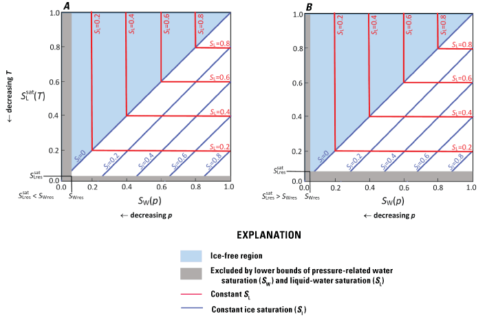
Graphs showing the SUTRA freeze-thaw relations for saturated and unsaturated conditions. A, Minimum liquid-water saturation is less than residual water saturation (), for which ice can exist in the minimum residual total water resulting from desaturation. B, Minimum liquid-water saturation is greater than residual water saturation (), for which no ice can exist in the minimum residual total water resulting from desaturation. The liquid-water saturation (SL) and the ice saturation (SI) depend on the total-water saturation [SW(p)] and on the liquid-water saturation under fully saturated conditions []. In effect, the diagram illustrates how SL and SI depend on pressure and temperature. On the horizontal axis, SW is a proxy for pressure (p), and the direction of decreasing p favors desaturation of the medium. On the vertical axis, is a proxy for temperature (T), and the direction of decreasing T favors freezing. Lines of constant SL are red, and lines of constant SI are blue. Light-blue shading indicates the ice-free region of the state diagram. Grey shading indicates the region of the state diagram excluded by the lower bounds on SW and SL. See appendix 1 for a list of symbols.
1.3.3. Permeability for Freeze-Thaw Under Saturated and Unsaturated Conditions
Under fully saturated conditions, the relative permeability (kr) of a partially frozen medium is assumed to depend exclusively on liquid-water saturation (SL). This is analogous to the approach used for the relative permeability of unfrozen unsaturated media. It is typically assumed that some small residual permeability remains during freezing and unsaturation of groundwater, even for very low liquid-water saturation, because there are still connected pathways or films of liquid water on the mineral (or ice) grains through which flow can occur. Therefore, the relative permeability relation for SUTRA is formulated such that it cannot have a value less than krmin(x, y[, z]), a dimensionless quantity [1] that may be specified by the user for each spatial region subject to the condition krmin>0. Relative permeability thus ranges from the minimum value of krmin to a maximum value of one.
Note: Commonly, the value of krmin is not known for the porous medium being simulated. In this case, it may be set to a relatively low value (for example, 10–6) for the processes being considered to essentially make liquid flow unimportant for conditions with low liquid saturations.
Note: To aid in interpreting simulation results, the value of liquid-water saturation at which kr=krmin, denoted , may be determined mathematically by the user from the user-selected relative permeability function. SUTRA does not calculate this value of liquid-water saturation, nor is it required for input. (The exception is for the piecewise-linear relative-permeability function, for which both and krmin are values that are input by the user.) It is suggested that users calculate the value for their chosen function. Then, to improve interpretation of the simulation results, this saturation, , may be compared by the user to the value of (the minimum possible liquid saturation for the frozen medium under saturated conditions) or to SWres (the minimum possible total-water saturation for unsaturated conditions) to understand whether or not the minimum relative permeability occurs in the model domain, and if so, where and when.
Relative permeability is calculated from an additional relation that must be specified by the user as a function of liquid-water saturation only:
where krmin ≤ kr ≤ 1 is greater than or equal to krmin and less than or equal to one. When SL=1, kr=1, and , kr = krmin occurs. The total effective permeability (product of permeability and minimum relative permeability, kkr) must always be greater than zero as explained in section 2, “Saturation and Relative-Permeability Functions.”In previous versions of SUTRA, freeze-thaw was not simulated, so total-water saturation, SW, was used in functions that provide relative permeability values. In this version of SUTRA, freeze-thaw can be simulated, so relative permeability is controlled by liquid-water saturation, SL, which can be less than total-water saturation. This becomes equivalent to using total-water saturation for simulations in which no ice forms, providing backward compatibility with previous versions of SUTRA. Preprogrammed kr relations are discussed in section 2, “Saturation and Relative-Permeability Functions.”
1.3.4. Behavior of the Freeze-Thaw Model
The effects of pressure and temperature on the liquid and ice saturations in the SUTRA freeze-thaw model for saturated and unsaturated conditions are illustrated in figure 1. Because the total-water saturation, SW, is a decreasing function of pressure below atmospheric pressure or below the air-entry pressure (until the lower limit SWres is reached), SW(p) can be considered as a proxy for p on the horizontal axis. Similarly, because the liquid-water saturation under fully saturated conditions, , is a decreasing function of temperature below the freezing point, Tf (until the lower limit is reached), can be considered a proxy for T on the vertical axis. The state diagram (fig. 1) can then be understood by considering two cases, as follows:
-
• Cooling at constant pressure.—A partially saturated, unfrozen medium is cooled while holding p constant. The total-water saturation, SW, remains constant throughout this process, which can be tracked on the diagram by starting at any point on the top edge () and proceeding vertically downward to . During cooling, the liquid-water saturation, SL, remains constant and the ice saturation, SI, remains zero until the temperature is cold enough to begin freezing the pore water. Thereafter, as T decreases below Tf, SL decreases while SI increases (that is, liquid becomes ice), until SL decreases to the residual liquid-water saturation, , after which further decreases in T have no effect on saturations.
-
• Desaturation at constant temperature.—A saturated, partially frozen medium is desaturated by decreasing p while holding T constant. As p decreases below the air-entry pressure, total-water saturation, SW, decreases and the ice saturation, SI, decreases. This can be tracked on the diagram by starting at any point on the right-hand edge of the state diagram (SW=1) and proceeding horizontally leftward to SW=SWres. Note that the liquid-water saturation, SL, remains constant as long as some ice remains (SI>0); thus, desaturation occurs by loss of ice. When pressure decreases to a certain value, all the ice disappears (SI=0). The liquid-water saturation, SL, then becomes equal to the total-water saturation, SW. Thereafter, as p continues to decrease, the liquid and total-water saturations remain equal, and both decrease until their value reaches the residual total-water saturation, SWres, after which further decreases in p have no effect on saturations.
1.3.5. General Procedure for Saturation Calculations
The procedure for computing total water, liquid, and ice saturations, their derivatives, and relative permeability has the following logical structure (fig. 2):
-
1. Compute total-water saturation, SW:
-
2. Compute liquid-water saturation, SL:
-
3. Compute ice saturation, SI=SW−SL.
-
4. Compute derivatives:
-
5. Compute relative permeability from the user-specified function kr(SL).
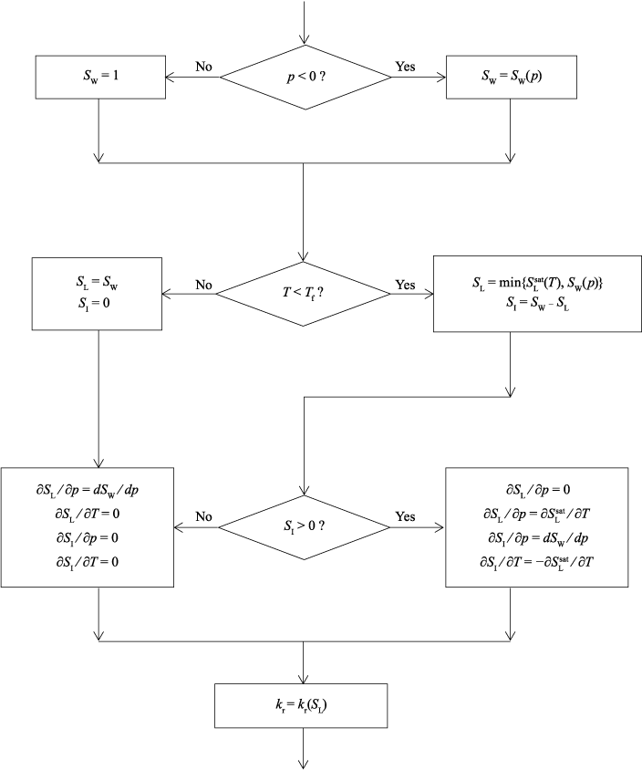
Flow chart showing general procedure for computing total-water, liquid-water, and ice saturations, their derivatives, and relative permeability. See appendix 1 for a list of symbols.
1.4. Thermal Conductivity Functions
In SUTRA version 4.0, the bulk thermal conductivity, λLIS, at any point in the model domain may be calculated as a weighted average of the thermal conductivities of liquid water, ice, solid mineral grains, and air. The thermal conductivities of liquid water, ice, and solid mineral grains are averaged by using one of three formulae, and the resulting value is volume-averaged with the thermal conductivity of air, as explained below.
For the combination of liquid, ice, and solid-mineral-grain components, the user-selectable bulk thermal conductivity formulae for three common volumetrically weighted means (Nield and Bejan, 1999) are as follows:
whereλL
[E/(s‧L‧°C)] is thermal conductivity of liquid water, user-specified value [about 0.60 J/(s‧m‧°C) at 20 °C; about 0.56 J/(s‧m‧°C) at 0°C] (user-specified constant value for the entire model);
λI
[E/(s‧L‧°C)] is thermal conductivity of ice, user-specified value [about 2.1 J/(s‧m‧°C) at 0 °C; about 2.3 J/(s‧m‧°C) at –10 °C] (user-specified constant value for the entire model);
λS
[E/(s‧L‧°C)] is thermal conductivity of a solid mineral grain, user-specified value [1 J/(s‧m‧°C)<λS<10 J/(s‧m‧°C) for most minerals] (user-specified value for each finite element); and
λLIS(x, y[, z], t)
is the effective thermal conductivity of mixture of liquid water, ice, and solid mineral grains, calculated by SUTRA according to user-selected equation 42A, B, or C.
Of the three options available, the arithmetic and harmonic means give the highest and lowest estimates, respectively, of the bulk thermal conductivity. The geometric mean gives an intermediate value that is often a good estimate when experimental data on the bulk thermal conductivity are unavailable (Lunardini, 1981; Nield and Bejan, 1999).
Unsaturated media also have an air phase with influences on effective thermal conductivity defined in the following paragraphs.
λA(x, y[, z])
[E/(s‧L‧°C)] is the effective thermal conductivity of air (user-specified value for each finite element) [about 0.025 J/(s‧m‧°C) for static air at 0 °C; for circulating air, the effective value can be orders of magnitude greater than the thermal conductivity of liquid, ice, or solid grains].
The air thermal conductivity for static air is practically negligible in comparison with the other thermal conductivities and was set to zero in previous versions of SUTRA. However, should air circulate among pores, thereby transferring energy convectively, its heat transfer effect may be much greater than would be indicated by its low thermal conductivity. Heat transfer by air circulation could be an important process to consider (for example, see Niu and others, 2016), especially in coarse, blocky material that is common in some permafrost environments (Wicky and Hauck, 2017). Because this is a different process than pure conduction, the thermal conductivity of air is not included in the volumetrically weighted λLIS values (eq. 42A–C) but is rather included later, as described just above (eq. 44).
Note: Although the physical process of air convection is not explicitly represented in the current version of SUTRA, the effective thermal conductivity of air parameter, λA, can be used to approximate the thermal effect of air circulation by setting it to a large value. Values of this parameter may be determined by converting published heat-transfer coefficients for circulating air into effective thermal conductivities. Note that in SUTRA version 4.0, thermal conductivities are constant for the entire simulation and cannot change with time; thus, any required seasonal changes in the effective thermal conductivity of air must be handled by running a series of consecutive simulations in which the parameter value is changed, as desired by the user, from one simulation to the next (that is, from one season to the next).
1.5. Nonlinear Liquid-Water Density Function
A nonlinear function describing the liquid density is implemented in the form of the empirical Thiesen-Scheel-Diesselhorst (TSD) equation (Tilton and Taylor, 1937; Kell, 1967), as described by McKenzie and Voss (2013), with the addition of constant-density limits for very low and very high temperatures. The liquid density, ρL [kg/m3], depends on temperature, T [°C], as follows:
The corresponding derivative of density (in kilograms per cubic meter per degree Celsius) with respect to temperature is
The function, as implemented in SUTRA, is shown in figure 3. In this function, density has a maximum value of 1,000 kg/m3 at 4 °C.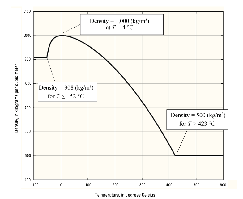
Graph showing liquid-water density as a function of temperature (T), as implemented in the SUTRA code. The curved part of the function, from –52.1784 to 422.9571 degrees Celsius is based on the Thiesen-Scheel-Diesselhorst equation (see eq. 45). Low- and high-temperature cut offs provide constant density for temperatures lower and higher, respectively, than the cut-off temperatures. See appendix 1 for a list of symbols. kg/m3, kilogram per cubic meter; °C, degree Celsius.
Note: This nonlinear function is provided as an alternative to the linear density function implemented in all previous versions of SUTRA, which remains available in the current version. Users may either select the linear density function that was available in previous versions of SUTRA (for simulated ranges of temperature in which the nonlinear density values are approximately linear) or this nonlinear function, according to their simulation needs.
For temperatures below –40 °C, density decreases rapidly. This decrease, provided by the TSD function and the constant density below 52.1784 °C, roughly approximates the density given by the two-liquid-phase super-cooled water model of Holten and Anisimov (2012) for typical earth-system fluid hydrostatic pressures between 0.1 megapascal (MPa; atmospheric pressure at ground surface) and 20 MPa (about 2-kilometer depth; Holten and Anisimov, 2012, fig. 3). Although this constant density assumption provides only approximate liquid-density values, errors in density typically will not affect fluid flow or hydraulic behavior, because at temperatures below –40 °C there will be almost no liquid-phase water. Moreover, the relative permeability for any remaining unfrozen water at such low temperatures will be extremely low. For temperatures above 625 °C, density values provided by the TSD nonlinear function become negative. Thus, at an arbitrarily selected maximum temperature, a minimum allowed liquid density value is implemented in SUTRA (fig. 3).
Note: Use of the code for high-temperature simulations must be carried out with caution. Users must be aware that fluid density also depends on fluid pressure. For very high pressure, density may be as much as 10 percent higher than calculated by the nonlinear TSD function. Furthermore, for pressure and temperature ranges encountered in hydrogeologic systems, it is possible that phase change between liquid water and steam may occur, particularly at higher temperatures. SUTRA does not simulate phase change to/from steam; this would require a code that tracks pressure or temperature plus internal energy or enthalpy as primary variables. For high temperature and low pressure, density may be only 20 or 30 percent of the value calculated by the nonlinear density function. Thus, for simulation of such high-temperature geothermal systems, the density value calculated by equation 45 (decreasing with increasing temperature and leveling off at an arbitrary density value) is only a pragmatic proxy that should be used with caution.
For simulation of systems with small ranges of temperature just above and below 4 °C, variable-density effects on fluid flow should be small (unless permeabilities are relatively high) due to near-constant density; however, for temperature ranges that are larger and perhaps more typical of cold regions where ground ice may form (for example, –20 °C mid-winter air temperature to 20 °C summer air temperature, with even greater temperatures at depth in the subsurface), fluid density differences will be sufficient to drive flow wherever the permeability of the geologic fabric is high enough.
2. Saturation and Relative-Permeability Functions
This section describes functions that must be specified for SUTRA simulations that involve unsaturated conditions, freeze-thaw conditions, or both (for saturated simulation without freezing, none of the functions described below are required):
-
• Unsaturated-flow simulations without freezing.—SUTRA requires user specification of a function to obtain values of total-water saturation and its derivative with respect to pressure, SW(p), and dSW/dp. The functionality of total-water saturation functions is discussed in the main SUTRA documentation (Voss and Provost, 2002).
-
• Saturated-flow simulations with freezing.—SUTRA computes ice saturation, SI(T), from the liquid-water saturation, . Thus, for saturated freeze-thaw simulations, SUTRA requires user specification of a saturated-conditions liquid-water saturation function, , to obtain values of liquid-water saturation and its derivative with respect to temperature, .
-
• Unsaturated-flow simulations with freezing.—SUTRA determines the ice saturation, SI(p,T), and liquid saturation, SL(p,T), from both the liquid-water saturation, , and the total-water saturation, SW(p) (see section 1.3.5, “General Procedure for Saturation Calculations;” fig. 2). Thus, for unsaturated freeze-thaw simulations, SUTRA requires user specification of a saturated-conditions liquid-water saturation function, , a total-water saturation function, SW(p), and their derivatives with respect to pressure and temperature.
The three required user-selected (or user-defined) functions are listed below:
-
1. For all unsaturated simulations (with or without freeze-thaw): SW(p), total-water saturation as a function of pressure (and dSW/dp) is required.
-
2. For all freeze-thaw simulations (saturated or unsaturated): , liquid-water saturation as a function of temperature under fully saturated conditions (and ) is required.
-
3. For all freeze-thaw simulations and for all unsaturated simulations: kr(SL), relative permeability as a function of liquid-water saturation is required (for nonfreezing unsaturated simulations, SUTRA automatically sets liquid saturation, SL, equal to total-water saturation, SL=SW).
Two user-selected (or user-defined) functions are required for unsaturated simulations (functions 1 and 3), three for unsaturated freeze-thaw simulations (functions 1, 2, and 3), and two for saturated freeze-thaw simulations (functions 2 and 3). The user-selectable forms are described in detail in this section. The expressions for the total-water, liquid-water, and ice saturations are equations 38, 39, and 40. Relative permeability is assumed to be a function of liquid-water saturation (eq. 41).
Note: The user selects these functions through the input dataset 11B–D (see app. 2). Particular user-selectable forms of these functions have been made available in SUTRA version 4.0, as described in the following section. Additionally, there is an option for the user to program other forms in Fortran subroutines UNSAT, LIQSAT and RELPERM.
2.1. Overview of Available Functions
Before SUTRA version 4.0, the freezing capability was not available, and functions defining unsaturated properties could be specified only via user-programming of subroutine UNSAT and subsequent recompilation of the source code. The source code came with the van Genuchten (1980) unsaturated functions programmed as an example, with the model parameters set to particular values that could be changed only by reprogramming.
Beginning with SUTRA version 4.0, a number of total water saturation (for unsaturated conditions), liquid-water saturation (for freezing conditions), and relative permeability functions (for unsaturated and freezing conditions) are preprogrammed, and their parameters can be specified through SUTRA input dataset 11B–D (see app. 2). Additionally, the different functions and parameter sets can be set by the user to apply in different spatial regions of the area or volume being modeled. Kurylyk and Watanabe (2013) provide a review of these and other possible functions, with some explanations of their basis and their applicability.
The available preprogrammed total-water saturation functions (for unsaturated flow simulations) are
-
• Brooks and Corey (1964), and
-
• piecewise-linear.
-
• exponential (Mottaghy and Rath, 2006),
-
• modified power-law (modified for SUTRA from Anderson and Tice, 1972), and
-
• piecewise-linear.
-
• Brooks and Corey (1964), and
-
• piecewise-linear.
-
• UNSAT (for total-water saturation, SW(p), and dSW /dp),
-
• LIQSAT (for liquid-water saturation of a saturated porous medium, , and ), and
-
• RELPERM (for relative permeability depending on liquid-water saturation, kr(SL)).
Additionally, any other functions that the user wishes to employ in simulations can be user-programmed into these subroutines. Any user-programmed functions are recognized within the same framework, which allows users to input their new function parameters through dataset 11B–D. Input instructions for the total-water saturation and liquid-water saturation functions are provided in appendix 2.
All preprogrammed and user-programmed functions operate in the following manner:
-
• For simulations of unsaturated, nonfreezing conditions, SW and dSW/dp are calculated from the user-selected (or user-programmed) total-water saturation function of pressure (and SL=SW and SI=0).
-
• For simulations of saturated, freezing conditions, and are calculated from the user-selected (or user-programmed) liquid-water saturation function of temperature (and SW=1 and , finally giving ).
-
• For simulations of unsaturated, freezing conditions,
-
• SW and dSW/dp are calculated from the user-selected (or user-programmed) total-water saturation function of pressure.
-
• Then, and are calculated from the user-selected (or user-programmed) liquid-water saturation function of temperature, assuming fully saturated conditions.
-
• Then, SL is set to the lesser of SW and , such that SL ≤ SW (finally giving SI=SW−SL).
-
-
• For simulations of unsaturated nonfreezing conditions, saturated freezing conditions and unsaturated freezing conditions, relative permeability, kr, is always based on liquid-water saturation (SL), as described in section 2.4, “Preprogrammed Relative-Permeability Functions.”
Note: Preprogrammed and user-programmed total-water saturation, relative-permeability, and liquid-water saturation functions may be used in any combination. For example, the van Genuchten total-water saturation function may be used with the piecewise-linear relative-permeability function and a user-programmed liquid-water saturation function. The function name “NONE” can be user-selected to indicate that no function will be used by SUTRA to define a saturation and relative permeability or both; in this case, SUTRA assumes that the saturation value or relative permeability value or both equal one.
2.2. Preprogrammed Total-Water Saturation Functions for Unsaturated Conditions
When pressure is nonnegative (p≥0), the porous medium is fully saturated (SW=1). When pressure is negative (p<0), SUTRA computes the total-water saturation as a function of pressure [SW=SW(p)]. In some of the functions described below, two of the parameters used are:
pent(x, y[, z])
[M/(L‧s2)] which is air-entry pressure, that is, the (negative) pressure above which the porous medium effectively remains fully saturated; normally pent<0 (user-specified value for each spatial region), and
SWres(x, y[, z])
[1] which is residual total-water saturation, that is, the value below which total-water saturation cannot fall due to decrease in pressure because the fluid becomes effectively immobile (user-specified value for each spatial region).
2.2.1. Van Genuchten Total-Water Saturation Function
In the van Genuchten function, originally formulated for unfrozen groundwater (van Genuchten, 1980), total-water saturation varies with pressure according to
with a natural minimum total water saturation value of SWres, where SWres and the following two parameters control the shape of the function:aVG(x, y[, z])
[(L‧s2)/M] the van Genuchten model parameter usually dependent on inverse of absolute value of the air-entry pressure (user-specified value for each spatial region) and
nVG(x, y[, z])
[1] the van Genuchten model parameter dependent on pore-size distribution (user-specified value for each spatial region).
2.2.2. Brooks-Corey Total-Water Saturation Function
In the Brooks-Corey function, originally formulated for unfrozen groundwater (Brooks and Corey, 1964), water saturation varies with pressure according to
with a natural minimum total water saturation value of SWres, where SWres, pent, and the following parameter control the shape of the function:λBC(x, y[, z])
[1] which is the pore-size distribution index and is user-specified value for each spatial region. In equation 49, p and pent are negative.
2.2.3. Piecewise-Linear Total-Water Saturation Function
In the piecewise-linear model, total-water saturation varies with pressure according to
where pent, SWres, and the pWres(x, y[, z]) are the parameters that control the shape of the function; pWres(x, y[, z]) [Μ/(L‧s2)] is the pressure at which the sloping linear segment of the function in equation 51 gives SW=SWres (user-specified value for each spatial region); and all pressure values are negative. Differentiation of equation 51 with respect to p yields:Note: The piecewise-linear function is often used when starting a new unsaturated simulation analysis, because the destabilizing effect of the nonlinearity of this function on the numerical solution is typically less than that of the other nonlinear functions. Once the trial simulation is working well, the user may switch to other, more appropriate functions for the particular porous-medium type being studied. This piecewise-linear saturation function is not intended to accurately represent details of physical behavior in the unsaturated zone.
Note: A useful application of the piecewise-linear function is to approximately simulate the effects of water-table movement (that is, changes in thickness of the saturated zone) on flow and drawdown, without considering behavior within the unsaturated zone in any detail. Specific yield is not explicitly included in the SUTRA equations, and this function may also be used when the only purpose of simulating unsaturated conditions is to track the movement of the water table. This function effectively provides a specific-yield value to the water balance being studied. In this case, the maximum specific yield (which occurs when the porous medium is maximally drained), Sy, is
To simulate a certain thickness of unsaturated zone, the user merely needs to specify a pressure and saturation value at the top of the unsaturated zone, where the residual or lowest-desired saturation value will occur. The value of the pressure would be a negative value equivalent to the hydrostatic pressure that would occur there from a pressure of zero at the water table that linearly decreases with upward distance from the water table, and the value of total saturation would be a residual or other user-preferred value at this location. These will define one end of the sloping segment of the piecewise-linear total saturation function, while the other end of this segment is at the water table, with pressure of zero and saturation of one.
2.3. Preprogrammed Liquid-Water Saturation Functions for Freezing in Fully Saturated Porous Media
Many studies have demonstrated that the relation between liquid-water content and subfreezing temperature in fully saturated soils can be expressed using a well-defined relation, often referred to as the soil-freezing curve (for example, Williams, 1967; Anderson and Tice, 1972; Jame, 1977; Kozlowski, 2007). For certain soil types, the soil-freezing curve can be obtained from unsaturated functions for drainage of soils without freezing (soil water characteristic curves) through the Clausius-Clapeyron equation, using sorptive or capillary theory (Koopmans and Miller, 1966; Spaans and Baker, 1996; Kurylyk and Watanabe, 2013). In SUTRA version 4.0, soil-freezing curves are specified independently of the unsaturated functions to allow maximum flexibility in functionality.
The user-specified freezing temperature below which pore water begins to freeze is Tf. Surface energies in pores and the existence of solutes may lower the freezing temperature to below 0 °C, so the user-specified value of Tf may be below 0 °C (as discussed in sections 1.2, “Energy Balance With Freeze-Thaw,” and 1.3, “Freeze-Thaw Relations”). When the temperature is above Tf (that is, T>Tf), the pore water is entirely in liquid form (SL=1). When the temperature is at or below the freezing temperature (T ≤ Tf), ice can begin to form, and SUTRA computes the liquid-water saturation as a function of temperature [SL=SL(T)].
The functions described below provide liquid-water saturation under fully saturated conditions, , as a function of temperature, T, for temperatures below the freezing temperature, Tf. For unsaturated conditions, SUTRA uses to compute the actual liquid-water saturation, SL, as described in section 1.3.5, “General Procedure for Saturation Calculations.” Then, ice saturation is computed as depending on total-water saturation (determined as described in section 2.2, “Preprogrammed Total-Water Saturation Functions for Unsaturated Conditions”) and on the liquid saturation as SI=SW−SL. Residual liquid-water saturation, , is the user-specified value below which it is assumed the liquid-water saturation cannot fall due to freezing alone.
The preprogrammed functions provide the liquid-water saturation under fully saturated conditions, . Three preprogrammed functions are currently provided in SUTRA—exponential, modified power law, and, piecewise linear (see fig. 4). Each of the three functions is expressed in terms of a relative temperature, T∆, defined as the difference between the local porous medium temperature, T, and the user-specified maximum freezing temperature of pore water, Tf:
When Tf=0 °C (the most common user choice), the relative temperature becomes the actual temperature, T∆=T.Note: The shape of each of the three preprogrammed liquid-water saturation () functions depends on one or more parameters, the values of which are set by the user. Setting Tf<0 °C simply shifts the curve in the negative direction along the temperature axis, without changing its shape. Thus, the function should be designed by the user for the un-shifted case and these parameter values should therefore always be set by the user for the unshifted case, Tf=0 °C.
The shapes of these functions for parameter values that were selected to highlight the differences in function shapes are shown in figure 4. The power law function tends to undergo a steep initial decrease in liquid water saturation as temperatures drop below the freezing temperature, and then a gradual decrease to the minimum liquid saturation. The exponential function tends to exhibit a delay in onset of freezing at temperatures just below the freezing temperature, then a steep drop in liquid saturation, quickly reaching and remaining at the minimum liquid saturation for lower temperatures. The linear function can be configured to drop slowly or quickly when freezing begins and then it reaches and remains at the minimum liquid saturation.
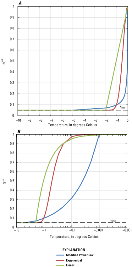
Graphs showing examples of preprogrammed liquid-water saturation function () shapes used in SUTRA simulations for freezing in fully saturated porous media. A, Plotted as function of T. B, Plotted as function of log10(T). See appendix 1 for a list of symbols. °C, degrees Celsius. Example parameter values: all functions (= 0.05, Tf=0.0 °C), modified power law (αPOW=0.1 , βPOW=−0.5, for which TPOW=−0.01 °C), exponential (wEXP=0.6 °C), and piecewise linear (TLres=−2.0 °C).
2.3.1. Exponential Liquid-Water Saturation Function
In the exponential function, adapted from Lunardini (1988) and Mottaghy and Rath (2006), liquid-water saturation during freezing, under fully saturated flow conditions, varies with temperature according to
where exp is the exponential function and TΔ is the relative temperature defined by equation 54. The shape of the function is controlled by , the asymptotic lower limit of the function, and bywEXP(x, y[, z])
[°C] an exponential-model parameter (specified by the user for each spatial region, subject to wEXP>0).
2.3.2. Modified Power-Law Liquid-Water Saturation Function
One often-used soil freezing curve relates the liquid-water saturation to the temperature in accordance with a power law in the form, (Anderson and Tice, 1972; Anderson and Morgenstern, 1973), where β<0. Although this function does fit a certain range of laboratory data on freezing geologic materials, it is not appropriate for general simulation over the full range of possible temperatures because it causes to become infinite when T=0. The following modified form of the power law function (with the desired maximum value of 1 when T=Tf) is used in SUTRA:
subject to the restriction that , where TΔ is the relative temperature defined by equation 54, and and the following parameters control the shape of the function:βPOW(x, y[, z])
[1] is the modified power-law model parameter (βPOW<0; user-specified value for each spatial region) and
αPOW(x, y[, z])
[] is the modified power-law model parameter (αPOW>0) (user-specified value for each spatial region).
Differentiation of equation 56 with respect to T yields:
Many literature sources express the power-law soil-freezing curve in terms of percent moisture content by dry weight rather than, as done for SUTRA, by volumetric liquid content (liquid-water saturation):
where is percent moisture content by dry weight (mass of liquid per mass of dry solid) under fully saturated conditions; αϕ is power-law model parameter (αϕ>0), as a percentage of , and it is assumed that Tf=0 °C (that is, that T∆=T). In that case, the value of αPOW in equation 57 can be computed from αϕ by Andersland and Ladanyi (1994, p. 40) present values of αϕ and βPOW for 33 different types of soils, and Anderson and Tice (1972) demonstrate that these parameters can be obtained empirically from the specific surface area of the soil grains.2.3.3. Piecewise-Linear Liquid-Water Saturation Function
In the piecewise-linear function, liquid-water saturation during freezing, under fully saturated flow conditions, varies with temperature according to
where T∆ is the relative temperature defined by equation 54, and and the relative temperature TLres control the shape of the function. Differentiation of equation 61 with respect to T yields2.4. Preprogrammed Relative-Permeability Functions
The relative permeability for unsaturated and freezing groundwater systems in SUTRA version 4.0 is assumed to depend only on liquid saturation. Relative-permeability functions are thus expressed below in terms of liquid-water saturation, SL (which automatically becomes equal to the total saturation, SW, should there be no ice at the point being considered).
It is also necessary that the total permeability value (kkr) always be greater than zero; if not, then numerical solution becomes impossible. This requires that kr>0. The user may specify a minimum possible value of relative permeability, krmin, to avoid the occurrence of kr=0. Then, during simulation, if the user-selected relative permeability function would provide a value lower than krmin, the value is set by SUTRA to krmin.
Note: For relative permeability functions other than the piecewise linear function, if it is desired that the relative permeability be allowed to asymptotically approach zero, and not be limited by krmin, the user may set krmin=0. For the piecewise linear relative permeability function, krmin>0 always determines the lower limit on relative permeability, which is reached at a user-specified liquid-water saturation, .
Note: If no relative permeability function is specified by the user, then relative permeability will have a constant value of one, kr=1.
For convenience and to simplify the form of most relative-permeability expressions presented below, a drainable liquid-water saturation, , (equivalent to the ratio of the volume fraction in the pores of drainable liquid, SL−SLres, to the maximum possible volume fraction of drainable liquid in the pores, 1−SLres) is defined as
where SLres is the minimum possible (residual) liquid-water saturation, taking into account both groundwater desaturation and freezing.Note: The value of SLres is not specified directly by the user. It is determined automatically by SUTRA in accordance with equation 39. When groundwater desaturation and freezing occur simultaneously, SLres is the lesser of the user-specified residual saturations and SWres. In the absence of freezing, SLres=SWres. Under fully saturated conditions with freezing, .
2.4.1. Van Genuchten Relative-Permeability Function
For the van Genuchten function, which was originally formulated for unfrozen porous media (van Genuchten, 1980), relative permeability varies with liquid-water saturation, SL, according to
where is the drainable liquid-water saturation defined by equation 63, and nVG is a model parameter that appears in equation 47. Thus, krmin and two parameters, nVG and SLres (which is the lesser of SWres and ) control the shape of this function.2.4.2. Brooks-Corey Relative-Permeability Function
For the relation presented by Brooks and Corey (1964), originally formulated for unfrozen porous media, relative permeability varies with pressure according to
where pressures are negative, and pent and λBC are the air-entry pressure and pore size distribution index, respectively, which also appear in equation 49. Solving equation 49 for p, substituting into equation 65, and replacing SW with SL gives where is the drainable liquid-water saturation defined by equation 63. The shape of this function is controlled by krmin and two parameters, λBC and SLres (which is the lesser of SWres and ).2.4.3. Piecewise-Linear Relative-Permeability Function
In the piecewise-linear model, relative permeability varies with liquid-water saturation, SL, having a value of 1 when SL=1 and decreasing to a minimum value of krmin when , according to
where Thus, user-specified parameters and krmin control the shape of this function.2.4.4. Note Regarding the “Impedance Factor” Approach
Some early studies (for example, Taylor and Luthin, 1978; Jame and Norum, 1980; Lundin, 1990) used an empirical “impedance factor” to incorporate the effect of freezing on the effective permeability (or hydraulic conductivity) of an unsaturated porous medium. The utility of the impedance factor was later questioned, however, and it is now commonly viewed as an arbitrary correction that is not physically based (Newman and Wilson, 1997; Kurylyk and Watanabe, 2013; Zhao and others, 2013). Recent studies have shown that properly parameterized classic unsaturated permeability functions can yield simulation results that concur with laboratory data of water flow in partially frozen soils without the inclusion of an impedance factor (for example, Painter, 2011; Azmatch and others, 2012). SUTRA version 4.0 therefore does not support use of an impedance function, but the following information is provided to allow users to manually program an impedance function into SUTRA, if its use is desired.
When used to describe permeability of frozen porous media, the impedance function controls effective permeability as follows:
wherekeff
[L2] is effective permeability that takes into account both partial saturation and freezing,
[L2] is effective permeability that takes into account partial saturation under unfrozen conditions, and
Ω
[1] is the impedance factor (usually in the form 10−constant).
k
[L2] is permeability under fully saturated, unfrozen conditions (entered in dataset 15 of the “.inp” file) and
kr
is the relative permeability discussed in previous sections.
Evaluation of equation 69 under unfrozen conditions and substitution into equation 68 gives
where [1] is the relative permeability under unfrozen conditions.Comparison of equations 69 and 70 indicates that the relative permeability is related to the impedance factor by
The relative permeability under unfrozen conditions is a function of the total-water saturation, , and the impedance factor is typically expressed as a function of the ice content and porosity, Ω=Ω(SI, ε). A review of impedance functions, listing three separate types, is presented by Kurylyk and Watanabe (2013). Therefore, use of the typical impedance-factor approach requires the relative permeability to be a function of the total-water and liquid-water saturations and porosity, kr=kr(SW, SL, ε).The preceding discussion was framed in terms of scalar permeability for the sake of simplicity. Analogous arguments can be made in the case of the tensor permeability allowed in SUTRA. Also note that relative permeability remains a scalar quantity.
Note: In the preprogrammed functions available in this version of SUTRA, kr is a function only of SL. However, subroutine RELPERM provides the infrastructure necessary for the user to program a more general relative-permeability function that is consistent with the impedance-factor approach. If the user wishes to make the impedance factor dependent on ice saturation, SI, this can be simply accomplished in subroutine RELPERM by using the relation SI=SW−SL (eq. 40).
3. Spatial Variation of Formerly Constant Parameters
In earlier versions of SUTRA, solid-matrix properties, adsorption parameters, and parameters for production of solute mass or energy were each assigned a single value that applied throughout the model domain. Beginning with this version of SUTRA (version 4.0), most material properties vary spatially. The region-wise values are input in datasets 11A through 11E (see app. 2).
All SUTRA parameters that describe material properties, indicating their allowed spatial variability, are listed in table 1. The spatial variability (that is, the discretization) provided for each parameter depends on how it appears in the numerical formulation of the flow and transport equations in SUTRA. Cellwise parameters are associated only with time-derivative terms and with terms that do not involve spatial derivatives. Nodewise parameters are those that vary spatially across finite elements, bilinearly in two dimensions (2D) and trilinearly in three dimensions (3D), and these are used for representing terms that involve spatial fluxes and spatial derivatives. Elementwise parameters are constant throughout each 2D or 3D finite element, which simplifies the numerical integration over each element of the terms in which they appear. (See Voss and Provost, 2002, for detailed information on numerical methods.) Some parameters have two types of spatial variability because they appear in two different types of terms. Detailed input instructions are listed in appendix 2.
Table 1.
Spatial variation of Saturated-Unsaturated Transport (SUTRA) code parameters.[The user specifies input parameters by providing a single, constant value (CONST), or by assigning a value to each node (NODE), element (ELEM), or region (REG). Within SUTRA, spatial variation of parameters can be constant (CONST), for which a single value of the parameter applies throughout the model; cellwise (CELL), for which the parameter is constant over each cell surrounding each node; nodewise (NODE), for which the parameter varies bilinearly for two dimensions (2D) and trilinearly for three dimensions (3D) among nodes within each finite element; and elementwise (ELEM), for which the parameter is constant within each finite element. Parameter superscripts/subscripts are W for total water, L for liquid, I for ice, S for solid matrix, solid mineral grain, or solute/sorbate. NA, not applicable]
4. Enhanced Output
In SUTRA version 4.0, two output options have been enhanced. These are the budget output, which has additional values that explain the model calculations, and the velocity output, to which “Darcy velocity” has been added as a further option.
4.1. Enhanced Budget Output
Budget output, an optional user-selected SUTRA capability, is a postprocessing step that reports additional simulation results on user-selected time steps. The budget output that was available in previous versions of SUTRA is enhanced in the current version to provide additional results that may be helpful in interpreting simulated behaviors, especially for understanding complex interactions that may occur in freeze-thaw simulations. The additional results include rates of change of water mass, and either solute mass or total energy, for subcomponent parts of the values previously reported and for new terms associated with ice and freeze-thaw. Enhanced budget output is here described for all possible types of SUTRA simulations, including fluid mass, energy, and solute balances.
Most budget output values reported are representative of the model domain as a whole. These consist of the total rates of gain or loss of water mass and solute mass or energy, and in the enhanced output, component rates for each process accounted for by the fluid mass balance and solute mass or energy-balance equations being solved by SUTRA. In addition, localized information within the model domain is reported in the budget output, consisting of all water mass and solute mass or energy sources that occur at user-specified boundary condition nodes, as was done in previous SUTRA versions. Budget output is written to an output file that is typically given the filename extension “.lst.” Users may select the frequency of these outputs to occur after particular or all time steps.
Detailed information about the quantitative meaning of each value listed in the enhanced budget output is provided in this section by associating terms in the SUTRA balance equations with the values that appear in the budget output. To link the equations and printed budget output, the Fortran source code variable name is shown in the sections below next to the term (or terms) in the governing equation that the value represents and next to the line in the budget output where that value is printed.
4.1.1. Water-Mass Budget for Energy-Transport Simulations
The components of the water water-mass budget output depend on whether SUTRA is simulating energy transport or solute transport. In this section, the enhanced water-mass budget for energy transport simulations is presented. The manner in which the variables are explained here is exemplified by the Fortran source code variable STW, which is shown here in the SUTRA water-mass balance (reproduced below from equation 4):
where f(p,T) indicates dependence on both pressure changes and temperature changes.This value represents the total water-mass change rate, given by the first two terms of equation 72 [STW total water-mass change rate f(p,T)]. The text that accompanies the label “STW” in equation 72 provides the meaning of this value and indicates that STW depends on changes in both p and T. Each term of the enhanced water-mass budget is defined in an equation below and, with each term, an indication is given of whether each rate depends on pressure changes, temperature changes, or both.
The value of STW is printed in the water-mass-budget output at the end of each user-selected completed time step. STW may be found in the following line of the budget output (shown in its entirety after equation 74 below):
TOTAL RATE OF CHANGE IN H2O STORED IN MODEL [ S+, S-, S] —STW—The variable name, STW, is highlighted as —STW— to indicate that this text is not actually written in the budget output and is included here for informational purposes only.
The other terms in the enhanced water-mass-balance output for energy transport are obtained by combining an expanded form of equation 4, given by equation 19, with the definition of effective storativity (eq. 20). Substitution of equation 20 into equation 19, and rearrangement of the water-mass balance two different ways to gather terms with similar physical origins, provides the definitions of the other water-mass budget for energy transport values:
whereNote that ice density values in SIP and SIU terms of equations 73 and 74 are set equal to liquid density values, and, in the SDIU term, the ice density derivative with respect to temperature is set to the value of the liquid density derivative with respect to temperature; see section 1.1.1, “Assumption Regarding Pressure Effect of Liquid-Ice Density Difference in Water-Mass Balance.” In SUTRA, all flows in and out of the model domain are conceptualized as occurring through the boundary conditions. Therefore, the divergence term () accounts only for internal redistributions of water within the model and does not contribute to the overall water budget.
The enhanced water-mass budget output has the following organization in the .lst file (each budget term in the above equations may be found below by locating its source code variable name):
H 2 O  M A S S  B U D G E T  (MASS/SECOND)
.............................................................................
RATE OF CHANGE OF H2O STORED IN MODEL DUE TO
PRESSURE CHANGE:
LIQUID-COMPRESSIVE STORAGE —SCLP—
LIQUID SATURATION —SLP—
ICE-COMPRESSIVE STORAGE —SCIP—
ICE SATURATION —SIP—
TOTAL RATE OF CHANGE OF H2O IN MODEL DUE TO PRESSURE CHANGE —STP—
.............................................................................
RATE OF CHANGE OF H2O STORED IN MODEL DUE TO
TEMPERATURE CHANGE:
LIQUID DENSITY —SDLU—
LIQUID SATURATION —SLU—
ICE DENSITY —SDIU—
ICE SATURATION —SIU—
TOTAL RATE OF CHANGE OF H2O IN MODEL DUE TO TEMPERATURE CHANGE —STU—
.............................................................................
_________________________________________________________
TOTAL RATE OF CHANGE IN H2O STORED IN MODEL [ S+, S-, S] —STW—
.............................................................................
GAIN/LOSS OF LIQUID THROUGH INFLOWS/OUTFLOWS AT:
LIQUID SOURCES AND SINKS	(sum of all —QIN— values in model)
SPECIFIED PRESSURE NODES	(sum of all —QPL— values in model)
GENERALIZED-FLOW NODES	(sum of all —QPG— values in model)
_____________________________________________________________
TOTAL RATE OF GAIN/LOSS OF LIQUID THROUGH FLOWS [ F+, F-, F] —QFF—
.............................................................................
H2O MASS BALANCE ACTIVITY [ A=((S+) - (S-)+(F+) - (F-))/2]
ABSOLUTE H2O MASS BALANCE ERROR [ S - F]
RELATIVE H2O MASS BALANCE ERROR [ 100*(S - F)/A]	(in percent)
.............................................................................
LIQUID GAINS OR LOSSES DUE TO LIQUID SOURCE NODES	(output only for time-dependent sources; list of nodal values)
LIQUID GAINS OR LOSSES DUE TO SPECIFIED PRESSURE NODES	(list of nodal values)
LIQUID GAINS OR LOSSES DUE TO GENERALIZED-FLOW NODES	(list of nodal values)
.............................................................................
The terms S+, S-, S, and F+, F-, F, are positive, negative, and net contributions to the rate of fluid-mass change in the entire model domain, respectively, with values listed in columns along the right side of the budget output in the .lst file. Water-mass gains and losses at specified pressure nodes and generalized-flow nodes are all contributions to the water-mass balance in the same manner as fluid sources and sinks (QIN) and are listed for every boundary-condition node at the end of each water-mass budget output.
4.1.2. Energy Budget
The energy budget is calculated using the divergent form of the energy-balance equation 30 (without subtraction of the fluid mass balance, which led to equation 35, the mathematically equivalent, convective form actually solved by SUTRA), because this form includes the total thermal energy of the system of most interest when interpreting results. The terms of the energy balance that are printed in the enhanced energy budget in the SUTRA .lst file are described in the following and are associated with Fortran variables used in the code for each term. Beginning with equation 30, by expanding terms using equations 11 and 17, and by gathering terms with similar physical origins, all energy budget terms are defined below. For each term in the equations, the information given provides the meaning of the term, and whether the value of the term depends on pressure changes, temperature changes, or both.
The manner in which the variables are explained here is exemplified by the Fortran source code variable STE. This value is printed in the energy budget output, representing the total energy change rate (given by the sum of terms on the left-hand side of equation 75, shown below) at the end of each user-selected completed time step. The STE value may be found in the following line of the energy budget output, which is shown in its entirety after equation 78 below:
TOTAL RATE OF CHANGE (R1+R2+R3) OF ENERGY STORED IN MODEL [S+,S-,S] —STE—The variable name STE is highlighted as —STE— to indicate that this text is not actually written in the budget output and is included here for informational purposes only.
The equations that define the energy budget terms are as follows:
In the SUTRA budget calculations, the terms DNS and UIS defined in equation 76 are further expanded using equations 11 and 17 as shown below:
The ice-density values in FLP and FLU terms are set equal to liquid-density values; and, in the USDI term, the ice density derivative with respect to temperature is set to the value of the liquid density derivative with respect to temperature; see section 1.1.1, “Assumption Regarding Pressure Effect of Liquid-Ice Density Difference in Water-Mass Balance.” The quantity (−∆H+cIT) is the energy content of ice per unit mass of ice (defined in equation 28B and in the source code it has the variable name EICE).
The enhanced energy-budget output has the following organization in the .lst file. Each budget term in the above equations may be found below by locating its variable name:
E N E R G Y  B U D G E T (ENERGY/SECOND)
.........................................................................
RATE OF CHANGE OF ENERGY STORED IN MODEL DUE TO
TEMPERATURE CHANGE IMPACTS ON THERMAL ENERGY IN:
LIQUID —FLD—
ICE —FIU—
SOLID GRAINS —SLD—
__________________________________________________________
TOTAL RATE OF ENERGY CHANGE DUE TO TEMPERATURE CHANGE (R1) —STS—
.........................................................................
RATE OF CHANGE OF ENERGY STORED IN MODEL DUE TO
CHANGE IN MASS OF LIQUID CAUSED BY PRESSURE CHANGE IMPACTS ON:
LIQUID COMPRESSIVE STORAGE —USCP—
LIQUID SATURATION —USLP—
TOTAL RATE OF ENERGY CHANGE DUE TO PRESSURE AND LIQUID MASS CHANGE —DNP—
RATE OF CHANGE OF ENERGY STORED IN MODEL DUE TO
CHANGE IN MASS OF LIQUID CAUSED BY TEMPERATURE CHANGE IMPACTS ON:
LIQUID DENSITY —USDL—
LIQUID SATURATION —USLU—
TOTAL RATE OF ENERGY CHANGE DUE TO TEMP. AND LIQUID MASS CHANGE —DNU—
_____________________________________________________________
TOTAL RATE OF CHANGE OF ENERGY DUE TO LIQUID MASS CHANGE (R2) —DNS—
.........................................................................
RATE OF CHANGE OF ENERGY STORED IN MODEL DUE TO
CHANGE IN MASS OF ICE CAUSED BY PRESSURE CHANGE IMPACTS ON:
ICE COMPRESSIVE STORAGE —USCIP—
ICE SATURATION —FLP—
TOTAL RATE OF ENERGY CHANGE DUE TO PRESSURE AND ICE MASS CHANGE —UIP—
RATE OF CHANGE OF ENERGY STORED IN MODEL DUE TO
CHANGE IN MASS OF ICE CAUSED BY TEMPERATURE CHANGE IMPACTS ON:
ICE DENSITY —USDI—
ICE SATURATION —FLU—
(INCLUDES LATENT HEAT OF FREEZE-THAW PHASE CHANGE)
TOTAL RATE OF ENERGY CHANGE DUE TO TEMP. AND ICE MASS CHANGE —UIU—
__________________________________________________________
TOTAL RATE OF CHANGE OF ENERGY DUE TO ICE MASS CHANGE (R3) —UIS—
.........................................................................
_______________________________________________________________________
TOTAL RATE OF CHANGE (R1+R2+R3) OF ENERGY STORED IN MODEL [ S+, S-, S] —STE—
.........................................................................
RATE OF CHANGE OF ENERGY STORED IN MODEL DUE TO
ZERO-ORDER PRODUCTION/DECAY OF ENERGY IN:
LIQUID —P0L—
ICE —P0I—
SOLID GRAINS —P0S—
______________________________________________________
TOTAL RATE OF PRODUCTION/DECAY OF ENERGY [ P+, P-, P] —PRS—
.........................................................................
GAIN/LOSS OF ENERGY
THROUGH INFLOWS/OUTFLOWS AT:
LIQUID SOURCES AND SINKS —QIU—
SPECIFIED PRESSURE NODES —QPU—
GENERALIZED-FLOW NODES —QPGU—
AT:
ENERGY SOURCES AND SINKS —QQU—
SPECIFIED TEMPERATURE NODES —QUL—
GENERALIZED-TRANSPORT NODES —QUG—
__________________________________________________________
TOTAL RATE OF GAIN/LOSS OF ENERGY —QFS—
THROUGH INFLOWS/OUTFLOWS & SOURCES/SINKS [ F+, F-, F]
.............................................................................
ENERGY BALANCE ACTIVITY [ A=((S+) - (S-)+(P+) - (P-)+(F+) - (F-))/2]
ABSOLUTE ENERGY BALANCE ERROR [ S - P - F]
RELATIVE ENERGY BALANCE ERROR [ 100*(S - P - F)/A]	(in percent)
.............................................................................
ENERGY SOURCES OR SINKS AT FLUID SOURCES AND SINKS	(list of nodal values)
ENERGY SOURCES OR SINKS DUE TO FLUID INFLOWS OR OUTFLOWS AT POINTS OF SPECIFIED PRESSURE	(list of nodal values)
ENERGY SOURCES OR SINKS DUE TO FLUID INFLOWS OR OUTFLOWS AT POINTS OF GENERALIZED FLOW	(list of nodal values)
TIME-DEPENDENT ENERGY SOURCES OR SINKS SET IN SUBROUTINE BCTIME	(list of nodal values)
ENERGY SOURCES OR SINKS DUE TO SPECIFIED TEMPERATURES	(list of nodal values)
ENERGY SOURCES OR SINKS DUE TO GENERALIZED-TRANSPORT CONDITIONS	(list of nodal values)
.............................................................................
The terms S+, S-, S, P+, P-, P, and F+, F-, F, are positive, negative, and net contributions to the rate of energy change in the entire model domain, respectively, with values listed in columns along the right side of the budget output in the .lst file. Energy gains and losses at liquid sources and sinks, specified pressure nodes, specified temperature nodes, and generalized-flow nodes are all contributions to the energy balance in the same manner as energy sources and sinks (QUIN) and are listed for every boundary-condition node at the end of each budget output.
4.1.3. Water-Mass Budget for Solute-Transport Simulations
The components of the water-mass budget output depend on whether SUTRA is simulating energy transport or solute transport. In this section, the enhanced water-mass budget for solute-transport simulations is presented. The manner in which the variables are explained here is exemplified by the source code variable STW, which is shown here for the SUTRA water-mass-balance equation (eq. 4) rewritten for simulation of solute-mass transport, in which the ice saturation is set to zero and temperature is replaced by solute mass fraction, C:
This value represents the total water-mass change rate, given by the first term of equation 79. The text that accompanies the label “STW” in equation 79 provides the meaning of this value and indicates that STW depends on changes in both p and C. Each term of the enhanced water-mass budget is defined in an equation below and, with each term, an indication is given of whether each rate depends on pressure changes, concentration changes, or both. The value of STW is printed in the water-mass budget output at the end of each user-selected completed time step. STW may be found in the following line of the budget output, which is shown in its entirety after equation 80 below:
TOTAL RATE OF CHANGE IN H2O STORED IN MODEL [ S+, S-, S] —STW—The variable name STW is highlighted as —STW— to indicate that this text is not actually written in the budget output and is included here for informational purposes only.
The other terms in the enhanced water-mass balance output for solute transport are obtained from an expanded form of equation 79, through a development analogous to the one used to obtain equation 73, but for solute transport. This provides the definitions of the other water-mass budget for solute-transport values:
wheref(C)
indicates dependence on concentration changes and
f(p,C)
indicates dependence on both pressure changes and concentration changes.
In SUTRA, all flows in and out of the model domain are conceptualized as occurring through the boundary conditions. Therefore, the divergence term () accounts only for internal redistributions of water within the model and does not contribute to the overall water budget.
The enhanced water-mass budget output for solute transport has the following organization in the .lst file. Each budget term in the above equations may be found below by locating its variable name in the source code:
H 2 O  M A S S  B U D G E T  (MASS/SECOND)
.............................................................................
RATE OF CHANGE OF H2O STORED IN MODEL DUE TO
PRESSURE CHANGE IMPACTS ON:
LIQUID-COMPRESSIVE STORAGE —SCLP—
LIQUID SATURATION —SLP—
TOTAL RATE OF CHANGE OF H2O IN MODEL DUE TO PRESSURE CHANGE —STP—
.............................................................................
RATE OF CHANGE OF H2O STORED IN MODEL DUE TO
CONCENTRATION CHANGE IMPACTS ON:
LIQUID DENSITY —SDLU—
TOTAL RATE OF CHANGE OF H2O IN MODEL DUE TO CONCENTRATION CHANGE —STU—
.............................................................................
_________________________________________________________
TOTAL RATE OF CHANGE IN H2O STORED IN MODEL [ S+, S-, S ] —STW—
.............................................................................
GAIN/LOSS OF LIQUID THROUGH INFLOWS/OUTFLOWS AT:
LIQUID SOURCES AND SINKS	(sum of all —QIN— values in model)
SPECIFIED PRESSURE NODES	(sum of all —QPL— values in model)
GENERALIZED-FLOW NODES	(sum of all —QPG— values in model)
_____________________________________________________________
TOTAL RATE OF GAIN/LOSS OF LIQUID THROUGH FLOWS [ F+, F-, F ] —QFF—
.............................................................................
H2O MASS BALANCE ACTIVITY [ A=((S+) - (S-)+(F+) - (F-))/2 ]
ABSOLUTE H2O MASS BALANCE ERROR [ S - F ]
RELATIVE H2O MASS BALANCE ERROR [ 100*(S - F)/A ]	(in percent)
.............................................................................
LIQUID GAINS OR LOSSES DUE TO LIQUID SOURCE NODES	(output only for time-dependent sources; list of nodal values)
LIQUID GAINS OR LOSSES DUE TO SPECIFIED PRESSURE NODES	(list of nodal values)
LIQUID GAINS OR LOSSES DUE TO GENERALIZED-FLOW NODES	(list of nodal values)
.............................................................................
The terms S+, S-, S, and F+, F-, F, are positive, negative, and net contributions to the rate of fluid-mass change in the entire model domain, respectively, with values listed in columns along the right side of the budget output in the .lst file. Water-mass gains and losses at specified pressure nodes and generalized-flow nodes are all contributions to the water-mass balance in the same manner as fluid sources and sinks (QIN) and are listed for every boundary-condition node at the end of each water-mass budget output.
4.1.4. Solute-Species Mass Budget
The solute-species mass budget is calculated using the full solute-species mass-balance equation (Voss and Provost, 2002, eq. 2.3, which is equivalent to Voss and Provost, 2002, eq. 2.47), the unified transport equation for solute-species mass or energy in terms of unified transport variable, U, given in terms of concentration. This balance is informally termed “solute transport equation,” but it is actually a complete mass balance of this chemical species within the porous medium, because it also allows simulation of the same chemical species when this species is immobile, while adsorbed on the surface or interior of solid mineral grains. This version of the solute transport equation, used for the solute-species mass-balance budget output, is without subtraction of the fluid-mass balance, because this form includes the total mass of the chemical species being tracked in the system, which is of most interest when interpreting results. [Subtraction of the fluid mass balance leads to the mathematically equivalent form actually solved for solute concentration by SUTRA (Voss and Provost, 2002, eq. 2.52), as it did for energy transport, resulting in equation 34.]
The terms of the solute-species mass balance that are printed in the enhanced solute mass budget in the SUTRA .lst file are described in the following and are associated with variables used in the Fortran source code for each term. Beginning with equation 30, by expanding one term using equation 11, both written for solute-species mass in terms of concentration rather than temperature, and by gathering terms with similar physical origins, all solute-species mass-budget terms are defined below. For each term in the equations, the information given provides the meaning of the term and whether the value of the term depends on pressure changes, solute and sorbate concentration changes, or both pressure and concentration.
The SUTRA solute-species mass-balance equation is equivalent to equation 30 rewritten for simulation of solute-mass transport of a particular chemical species, in which the ice saturation is set to zero (removing several terms from the equation); temperature is replaced by solute mass fraction, C; the specific heat of liquid, cL, is set to a value of one; the conductive-dispersive heat flux, , is replaced by its solute-species mass equivalent, , the diffusive-dispersive solute flux; zero-order energy production is replaced by zero-order solute-species mass production in the water and in or on the solid mineral grains (for example, in any sorbate), and additional terms for first-order production of the solute-species in the water and in the immobile (sorbed) phase are added (see Voss and Provost, 2002, eq. 2.37):
C(x, y[, z], t)
[MS/M] is solute-species concentration (mass fraction);
CS(x, y[, z], t)
[MS/MG] is concentration of species as sorbate on solid grains expressed as a mass fraction (mass adsorbate per mass solid grains plus adsorbate);
C*(x, y[, z], t)
[MS/M] is solute concentration of fluid sources (mass fraction);
[M/(L2‧s)] is diffusive-dispersive solute-mass flux;
[s−1] is zero-order solute-species mass production in liquid;
[s−1] is zero-order solute-species mass production in solid mineral grains;
[(MS/M)/s)] is first-order solute-species mass production in liquid; and
[(MS/MG)/s)] is first-order solute-species mass production in solid mineral grains.
The manner in which the variables of the solute-mass balance appear in the enhanced budget output are explained here, as exemplified by the Fortran source code variable STE. The STE value, which represents the total solute-species mass change rate (given by the sum of terms on the left-hand side of equation 82, shown below), is printed in the solute-species mass budget output at the end of each user-selected completed time step. Note that the terms “solute-species mass” and “solute mass” are used interchangeably in the budget output and mean the same thing. The STE value may be found in the following line of the budget output, which is shown in its entirety after equation 84 below:
TOTAL RATE OF CHANGE (R1+R2+R3) OF SOLUTE MASS STORED IN MODEL [S+,S-,S] —STE—The variable name STE is highlighted as —STE— to indicate that this text is not actually written in the budget output and is included here for informational purposes only.
The equations that define the solute-species mass-budget terms are as follows (from Voss and Provost (2002), equations 2.31 and 2.47):
wheref(C, CS)
indicates dependence on solute and sorbate concentration changes and
f(p, C, CS)
indicates dependence on both pressure changes and concentration changes.
In the SUTRA budget calculations, the DNS term defined in equation 83 is further expanded using the solute-mass equivalent of equation 11 as shown below:
where f(p) indicates dependence on pressure changes.The enhanced solute-mass-budget output has the following organization in the .lst file. Each budget term in the above equations may be found below by locating its Fortran variable name:
S O L U T E  B U D G E T  I N (SOLUTE MASS/SECOND)
...........................................................................
RATE OF CHANGE OF SOLUTE STORED IN MODEL DUE TO
CONCENTRATION CHANGE IMPACTS ON SOLUTE MASS IN:
LIQUID —FLD—
ADSORBATE —SLD—
____________________________________________________________
TOTAL RATE OF SOLUTE CHANGE DUE TO CONCENTRATION CHANGE (R1) —STS—
...........................................................................
RATE OF CHANGE OF SOLUTE STORED IN MODEL DUE TO
CHANGE IN MASS OF LIQUID CAUSED BY PRESSURE CHANGE:
LIQUID COMPRESSIVE STORAGE —USCP—
LIQUID SATURATION —USLP—
TOTAL RATE OF SOLUTE CHANGE DUE TO PRESSURE AND LIQUID MASS CHANGE —DNP—
RATE OF CHANGE OF SOLUTE STORED IN MODEL DUE TO
CHANGE IN MASS OF LIQUID CAUSED BY CONCENTRATION CHANGE:
LIQUID DENSITY —USDL—
TOTAL RATE OF SOLUTE CHANGE DUE TO CONC. AND LIQUID MASS CHANGE —DNU—
_____________________________________________________________
TOTAL RATE OF CHANGE OF SOLUTE DUE TO LIQUID MASS CHANGE (R2) —DNS—
...........................................................................
_______________________________________________________________________
TOTAL RATE OF CHANGE (R1+R2+R3) OF SOLUTE STORED IN MODEL [ S+, S-, S] —STE—
...........................................................................
RATE OF CHANGE OF SOLUTE STORED IN MODEL DUE TO
FIRST-ORDER PRODUCTION/DECAY OF SOLUTE IN:
LIQUID —P1L—
SOLID GRAINS —P1S—
ZERO-ORDER PRODUCTION/DECAY OF SOLUTE IN:
LIQUID —P0L—
SOLID GRAINS —P0S—
______________________________________________________
TOTAL RATE OF PRODUCTION/DECAY OF SOLUTE [ P+, P-, P] —PRS—
...........................................................................
GAIN/LOSS OF SOLUTE
THROUGH INFLOWS/OUTFLOWS AT:
LIQUID SOURCES AND SINKS —QIU—
SPECIFIED PRESSURE NODES —QPU—
GENERALIZED-FLOW NODES —QPGU—
THROUGH INFLUXES/OUTFLUXES AT:
SOLUTE SOURCES AND SINKS —QQU—
SPECIFIED CONCENTRATION NODES —QUL—
GENERALIZED-TRANSPORT NODES —QUG—
_______________________________________________________________
TOTAL RATE OF GAIN/LOSS OF SOLUTE
THROUGH INFLOWS/OUTFLOWS & INFLUXES/OUTFLUXES [ F+, F-, F]
...........................................................................
SOLUTE BALANCE ACTIVITY [ A=((S+) - (S-)+(P+) - (P-)+(F+) - (F-))/2
ABSOLUTE SOLUTE BALANCE ERROR [ S - P - F]
RELATIVE SOLUTE MASS BALANCE ERROR [ 100*(S - P - F)/A]
...........................................................................
SOLUTE SOURCES OR SINKS
AT FLUID SOURCES AND SINKS	(list of nodal values)
SOLUTE SOURCES OR SINKS DUE TO FLUID INFLOWS OR OUTFLOWS
AT POINTS OF SPECIFIED PRESSURE	(list of nodal values)
SOLUTE SOURCES OR SINKS DUE TO FLUID INFLOWS OR OUTFLOWS
AT POINTS OF GENERALIZED FLOW	(list of nodal values)
TIME-DEPENDENT SOLUTE SOURCES OR SINKS SET IN SUBROUTINE BCTIME	(list of nodal values)
SOLUTE SOURCES OR SINKS DUE TO SPECIFIED TEMPERATURES		(list of nodal values)
SOLUTE SOURCES OR SINKS DUE TO GENERALIZED-TRANSPORT CONDITIONS	(list of nodal values)
.............................................................................
The terms: S+, S-, S, P+, P-, P, and F+, F-, F, are positive, negative, and net contributions to the rate of solute change in the entire model domain, respectively, with values listed in columns along the right side of the budget output in the .lst file. Solute gains and losses at liquid sources and sinks, specified pressure nodes, specified temperature nodes, and generalized-flow nodes are all contributions to the solute balance in the same manner as solute sources and sinks (QUIN) and are listed for every boundary-condition node at the end of each budget output.
4.2. Enhanced Velocity Output: Darcy Velocity
The output of fluid-velocity magnitude and direction at the center of each finite element, which SUTRA has provided in all previous versions, allows visualization of the groundwater flow field. The velocity values output by SUTRA are calculated with equation 18 (repeated here):
This is Darcy’s Law, generalized for variably saturated, variable-density flow and written in terms of fluid pressure, as explained in Voss and Provost (2002, section 2.2, “Saturated-Unsaturated Groundwater Flow”).The velocity in equation 85, [L/s], is the average velocity at which a conservative tracer would move through a porous medium, also called the “tracer velocity” and “particle velocity.” Thus, is a measure of the average bulk movement of the liquid-water molecules and nonreactive substances within the liquid, relative to the stationary solid matrix. The velocity is an “average” because it aggregates velocities that vary from point to point within a porous medium due to variations in permeability, porosity, and connectivity at a spatial scale smaller than that at which typical laboratory and field measurements are made.
Visualizations of provide insight into the speed and direction of water movement but not about the quantity of water that moves through the porous medium being modeled. Interpreting the quantity of water movement from visualizations of can sometimes be misleading, as explained in the following.
Particularly for simulations of unsaturated and freezing systems, velocity magnitudes may decrease, remain unchanged, or even may increase when the porous medium desaturates or freezes. The expectation that fluid fluxes change in the same manner as fluid velocity magnitudes might contradict the intuitive expectation that total fluid flux should decrease during desaturation or freezing. This range of possible decreases or increases occurs because the change in fluid velocity resulting from a decrease in liquid saturation, SL, depends on the ratio of relative permeability to liquid saturation, kr/SL, according to equation 85. If both SL and kr decrease at the same rate when SL decreases due to desaturation or freezing (as defined by the user-selected liquid saturation and relative permeability relations; see section 2, “Saturation and Relative-Permeability Functions”), the velocity magnitude will remain constant as SL decreases. Should SL decrease faster than kr, velocity magnitude will increase as SL decreases, although total fluid flux always decreases as SL decreases.
Such fluid velocity behavior may occur in a simulation, depending on the user-selected saturation and relative permeability functions, and depending on what these functions imply about the connectivity and volume of flowing liquid zones within the porous medium. Only if kr decreases faster than SL during desaturation or freezing will velocity magnitudes decrease. As a result, the velocity output does not provide insight into the quantity of fluid (that is, the fluid flux) that is flowing during desaturation or freezing; it only shows how fast the fluid is moving.
The rate at which fluid volume is moving is instead given by the “Darcy velocity”:
where [L/s] is the Darcy velocity or volumetric fluid flux [(fluid volume per time per cross-sectional area of total porous medium)/s].Because the porosity is always less than one, the Darcy velocity, , is always less than the average fluid velocity, , and so is not a direct indicator of the speed of water movement. Rather, Darcy velocity is a flux of fluid, representing the volume of fluid flowing across a unit cross-sectional area of the porous medium, per unit time. Thus, the Darcy velocity gives information on the quantity of fluid flow, which may be expected to decrease during desaturation or freezing. Darcy velocity (eq. 86), the volumetric fluid flux, always decreases as liquid saturation, SL, decreases, irrespective of whether the saturation decrease is due to desaturation or freezing.
Therefore, to allow fuller interpretation of SUTRA unsaturated and freeze-thaw simulation results, the current version of SUTRA additionally provides output of Darcy velocities, , at the centroid of each finite element, at the end of user-selected time steps. Both Darcy velocity, , and particle velocity, , outputs are provided in SUTRA output files (with the extensions .lst and .ele).
Note: The velocities that are output (in the .lst and .ele output files) are at the centroids of each element in the finite-element mesh. These output values are provided solely for user information and postprocessing purposes. Internally, SUTRA uses only velocities at Gauss points within each element (not at element centroids) to solve the governing differential equations (see Voss and Provost, 2002, sec. 4.3, “Gaussian Integration”). The mean value of the velocities at the Gauss points in each finite element provides the value reported at the element centroid.
5. Example Simulations
Two simple examples are described in this section. These demonstrate the main new physics functionality provided by SUTRA version 4.0, highlighting saturated and unsaturated freezing and thawing.
5.1. Saturated Groundwater Freezing Example—Containment by Frozen Groundwater Wall
This example demonstrates the effect of freezing on the flow field in a groundwater system. The frozen wall is an engineered intervention that creates a region of low permeability upstream of a contaminated region of an aquifer. Shielding the contaminated area from regional groundwater flow avoids the spread of contaminants to a larger area, thereby allowing the contaminated area to be remediated. A similar “frozen wall problem” was first proposed by McKenzie, Voss, and Siegel (2007).
The model domain considered for this analysis is a 25-by-15-meter (m) area in which a hypothetical contaminant exists within a 4-by-4-m square region centered along the southern edge of the area (fig. 5). Initially (fig. 6A) the entire shallow, uniform aquifer is at a temperature of +5 °C and regional groundwater flow with the same temperature occurs uniformly from west to east, driven by the difference in hydraulic heads along the eastern and western boundaries (implemented in the model as specified pressure conditions). An L-shaped cooling system 0.5 m wide is emplaced around the contaminated zone by burying freezing coils through the entire representative 1-m thickness of the shallow aquifer. The cooling system is installed just upstream and along the lateral side of the contaminated area, at a distance of 0.5 m from the contaminated zone, to avoid entraining contaminants within the coils during emplacement. The cooling system extends 5 m in the north-south and 5 m in the east-west directions. The cooling system is implemented in the simulation in a simple manner as a zone of specified temperature conditions held at –5 °C for the duration of the simulation once the system is activated just after 0 hours.
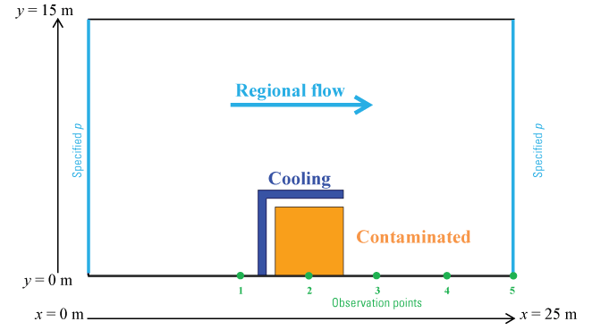
Illustration showing setup of “containment by frozen groundwater wall” saturated freezing example. This is an areal groundwater flow system, viewed from above. Observation points are located at y=0 meter (m) and x=9, 13, 17, 21, 25 m. See appendix 1 for a list of symbols.
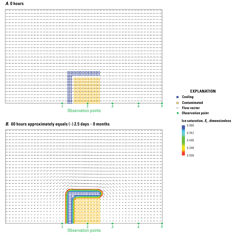
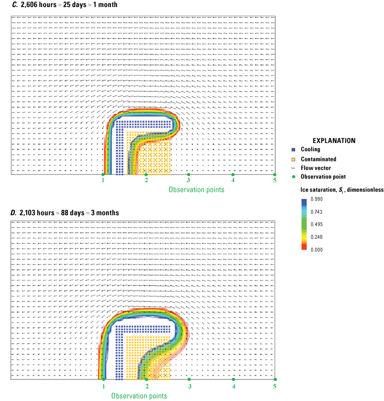
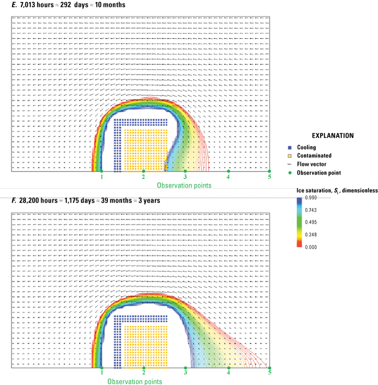
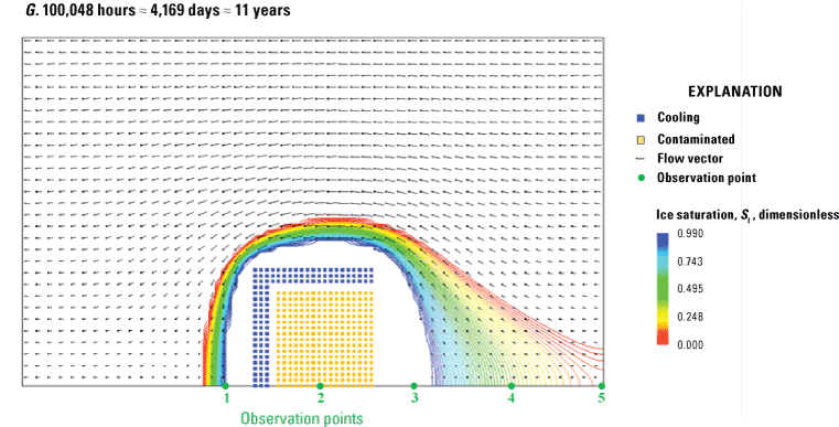
Illustrations showing simulated evolution of ice saturation (SI) for “containment by frozen groundwater wall” example. Colored contours show SI values (SI=1, represents completely frozen groundwater). Velocity vectors that show flow direction and velocity magnitude are represented in a “windsock” style: the direction of flow is indicated by the direction of the line that emanates from the dot, the dot indicates the location of the velocity vector, and the line length is proportional to the magnitude of the velocity. Velocity vectors are plotted at centroid of every second finite element in each direction, and only vectors with the three highest orders of magnitude are shown. Panel A (0 hours) shows uniform flow field before initiation of frozen wall. Orange squares show hypothetical area of contamination; blue squares show location of cooling system (nodes with specified temperature boundary condition). Small green circles denote the observation points defined in figure 5. See appendix 1 for a list of symbols.
Note that the same results as presented here for an aquifer of unit thickness are obtained for an aquifer of any thickness in which the contaminated zone and freezing coils extend from the aquifer top to the aquifer bottom. Also note that this setup may equivalently be considered as the northern half of an area with an east-west axis of symmetry. Further, note that flow field effects of varying groundwater density are neglected in this two-dimensional areal example.
The domain is discretized into 100 elements in the x-direction and 60 elements in the y-direction (∆x=∆y=0.25 m). Time steps begin at ∆t=1 hour, increasing each subsequent time step by a factor of 1.02 to a maximum of ∆t=1 month. Due to the small initial time-step size, iterations for nonlinearity are not used, so there is one iteration per time step. The initial pressure distribution is set as a simple linear function of x, causing uniform flow to occur initially from left to right before freezing begins in the wall. Five SUTRA observation points are positioned along the southern edge of the model domain. The complete model configuration and parameters are provided in figure 5 and table 2. Simulation results are shown in figures 6 and 7.
Table 2.
Parameters of “containment by frozen groundwater wall” simulation.[m, meter; kg/(m s2), kilogram per meter per second squared; J/(kg °C), joule per kilogram per degree Celsius; J/(s m °C), Joule per second per meter per degree Celsius; kg/m3, kilogram per cubic meter; °C, degree Celsius; kg/(m3 °C), kilogram per cubic meter per degree Celsius; m2, square meter; m/s, meter per second; m/s2, meter per second squared; s, second; m, meter; h, hour; cm, centimeter; ≥, greater than or equal to]
| Parameter | Value |
|---|---|
| Aquifer thickness | 1 m |
| Model extent (east-west x, north-south y) | 25 m, 15 m |
| Porosity | 0.1 |
| Fluid compressibility | 4.47×10⁻¹⁰ [kg/(m‧s2)]−1 |
| Fluid specific heat | 4,182. J/(kg‧°C) |
| Fluid thermal conductivity | 0.6 J/(s‧m‧°C) |
| Linear fluid density function: [here set to a constant density of 1,000 kg/m3] |
|
| Base density (RHOL0) | 1,000 kg/m3 |
| Base temperature (URHOL0) | 20 °C |
| Coefficient of density change (DRLDU) | 0 kg/(m3‧°C) |
| Solid matrix compressibility (COMPMA) | 1×10⁻⁸ [kg/(m‧s2)]−1 |
| Solid grain density (RHOS) | 2,600 kg/m3 |
| Solid grain specific heat | 840 J/(kg‧°C) |
| Solid grain thermal conductivity | 3.5 J/(s‧m‧°C) |
| Ice compressibility (COMPI) | 0 [kg/(m‧s2)]−1 |
| Ice density | 920 kg/m3 |
| Ice thermal conductivity | 2.14 J/(s‧m‧°C) |
| Ice specific heat | 2,108 J/(kg‧°C) |
| Latent heat of fusion | 3.34×10⁵ J/kg |
| Permeability (max and min) | 1×10⁻¹⁰ m2 (hydraulic conductivity about 10−3 m/s) |
| Longitudinal dispersivity (in max and min permeability directions) | 0.1 m |
| Transverse dispersivity (in max and min permeability directions) | 0.01 m |
| Gravity vector components (GRAVX, GRAVY) | 0, 0 m/s2 |
| Piecewise-linear liquid-water saturation function: | |
| Minimum liquid saturation (SLSATRES) | 0.01 |
| Temperature at which minimum liquid saturation occurs (TLRES) | –2 °C |
| Piecewise-linear relative permeability function: | |
| Liquid saturation at which minimum relative permeability occurs (SLRKMIN) | 0.01 |
| Minimum relative permeability (RKMIN) | 1×10⁻⁶ |
| Finite elements (in x,y directions) -fishnet mesh- | 100, 60 |
| Initial time step | 1 h |
| Time step change cycle (NTCYC) | 1 |
| Time step multiplier (TCMULT) | 1.02 |
| Maximum allowed time step (TCMAX) | 730.5 h (= 1 month) |
| Time steps in pressure and temperature solution cycle (NPCYC, NUCYC) | 1, 1 |
| Maximum time steps in simulation (NTMAX) | 1,000 (any number≥420) |
| Maximum absolute simulation time | 1×10⁵ h |
| Output cycles (NPRINT, NCOLPR, LCOLPR) | 10, 10, 10 |
| Iterations for nonlinearity (ITRMAX) | 1 |
| Solver for pressure, solver for temperature | DIRECT, DIRECT |
| Observation locations (five selected nodes along southern edge, y=0 m; fig. 5) | x=90 m, 130 m, 170 m, 210 m, 250 m |
| Initial temperature of aquifer | +5 °C |
| Temperature of cooling system | specified T=−5 °C |
| Initial pressure of aquifer | p=500−20x [kg/(m‧s2)] |
| West boundary condition for fluid mass balance | specified p=500 [kg/(m‧s2)] (about 5 cm hydraulic head) —inflowing water has T=+5 °C |
| East boundary condition for fluid mass balance | specified p=0 [kg/(m‧s2)] (0 cm hydraulic head) —any inflowing water has T=+9,999 °C (arbitrary value as no water ever flows in here) |
| East and west boundary conditions for energy balance | insulated (energy enters via the western inflow and exits via the eastern outflow) |
| North and south boundary conditions for fluid mass balance | no flow |
| North and south boundary conditions for energy balance | insulated |
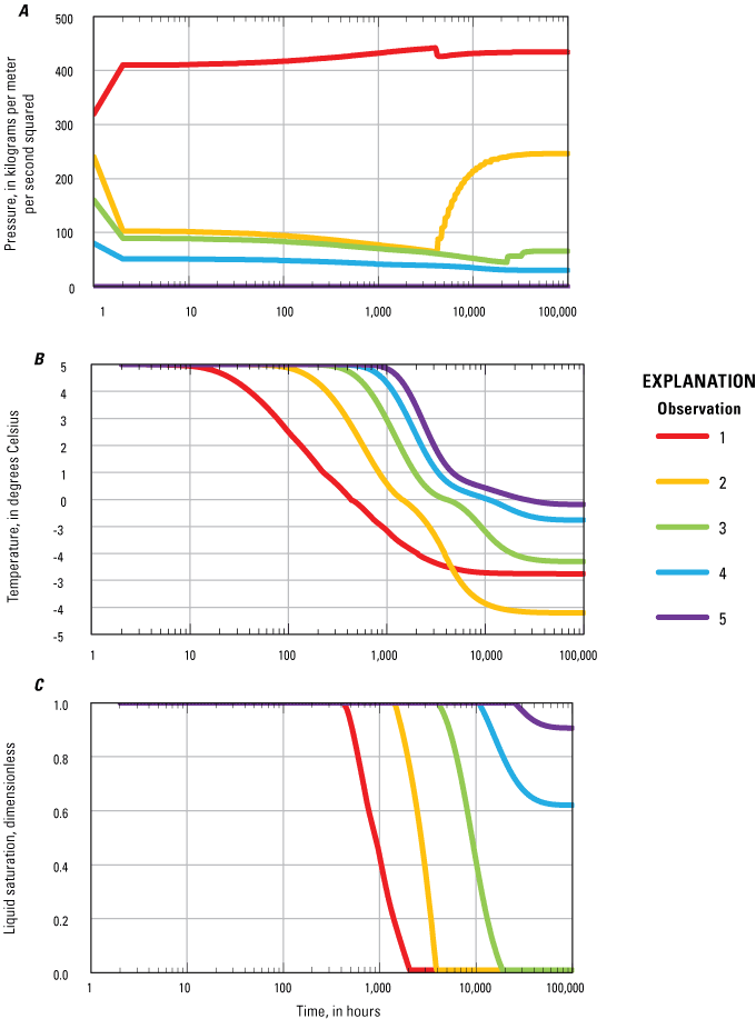
Graphs showing simulated histories of pressure, temperature, and liquid saturation (SL) at observation nodes for “containment by frozen groundwater wall” example. Colors indicate observation point location numbers (see figs. 5 and 6 for locations). See appendix 1 for a list of symbols. Liquid saturation (SL) is dimensionless. kg/m‧s2, kilogram per meter-second-squared; °C, degree Celsius.
The constant west-to-east pressure gradient initially drives a uniform eastward fluid velocity of about 1.3×10⁻⁵ meters per second (m/s; about 1.1 meters per day [m/d]). This would spread the contaminant eastward at a rate greater than 1 m/d (assuming that the contaminant does not undergo physical or chemical retardation). As soon as the groundwater within the freezing coil zone freezes (instantaneously in this simulation, immediately after the state shown in fig. 6A, because the coils are instantaneously at the specified temperature of −5 °C), a barrier is formed to flow, and fluid velocity throughout the contaminated zone decreases by about 10 times, decreasing the rate of contaminant release downstream. Thereafter, while the entire contaminated zone gradually freezes to maximum ice saturation (0.99), groundwater velocity in the growing, mostly frozen, zone decreases to less than one thousandth (1/1,000) of its initial value (fig. 6B–D), essentially immobilizing the contaminant. Finally, fluid in the entire contaminated zone becomes immobilized (fig. 6E). As the frozen wall develops with time (fig. 7A), observed pressure upstream of the wall increases, while observed pressure downstream first decreases due to the ever-increasing size of the frozen barrier blocking the flow field, then increases once the location is fully frozen. Temperatures at all observation points (fig. 7B) decrease with time, undergoing an inflection during ice formation (between 0 °C and −2 °C). Liquid saturations decrease at all observation points (fig. 7C) while ice forms. Although it takes several years for the system to reach a steady state with the coils continuously cooling the aquifer, the dynamics that cause practical immobilization of the contaminant occur within the first few months of operation. Even for this simple example of freezing in a saturated aquifer system, it can be understood that the dynamic evolution of physical and thermal conditions associated with subsurface freezing can be quite complex.
5.2. Unsaturated Groundwater Freeze-Thaw Example—Soil Column Experiment
This example demonstrates unsaturated zone freezing owing to a decrease in surface temperature and subsequent thawing owing to upward flow (water-table rise) from the unfrozen aquifer below the water table. It represents conditions of a hypothetical two-part, 1-year controlled cryohydrogeologic laboratory experiment on a 2-m-high column of soil. Part A of the experiment comprises top-down freezing of the unsaturated zone and part B comprises bottom-up thawing of the part-A column owing to liquid water inflow at the bottom.
The part-A experiment begins with an unsaturated column in steady state, in which the water table is held at the bottom, and there is a natural linear hydrostatic pressure decrease upwards. Total water saturation decreases from fully saturated conditions at the bottom edge (which represents the top of an aquifer’s saturated zone) to nearly irreducible total saturation at the top edge. Initially the entire column is at +2 °C, then at the start of the part-A experiment the top temperature is decreased to –8 °C and held at this value, while the bottom is held at +2 °C (that is, no change at the bottom). This initiates downward freezing of the unsaturated zone in the column. With these fixed top and bottom pressure and temperature settings, conditions in the column are allowed to evolve for 180 days, by which time a new near-steady-state condition has developed.
The initial condition for the part B experiment is the unsaturated, partly frozen column that developed in part A upon reaching 180 days. At the start of part B, liquid water at a temperature +2 °C is injected into the unfrozen bottom of the column at a rate of 1 centimeter (cm) of standing liquid water per day, and this injection rate is held constant for the 180-day duration of part B. The fluid injection at the bottom causes liquid to flow upward, fully saturating the empty pore space as it rises, eventually passing through the entire column and reaching the top. The top of the column is thermally insulated. Before the column becomes fully saturated to the top, there is no discharge at the top. When the column becomes fully saturated, the top pressure is then held at approximately atmospheric pressure and discharge of liquid occurs naturally at the column top. Due to supercooled initial conditions in the column (temperatures less than 0 °C, at which freezing occurs according to the freezing function specified), the upward-flowing water begins to thaw the column due to the temperature of inflowing liquid being greater than 0 °C. Eventually, from the bottom up, the column gradually becomes ice-free, and after 180 days of upward flow the temperature of the column nearly reaches the inflow temperature of +2 °C throughout.
The model configuration and parameters are shown in figure 8 and table 3. Simulation results are shown in figures 9, 10, 11, and 12.
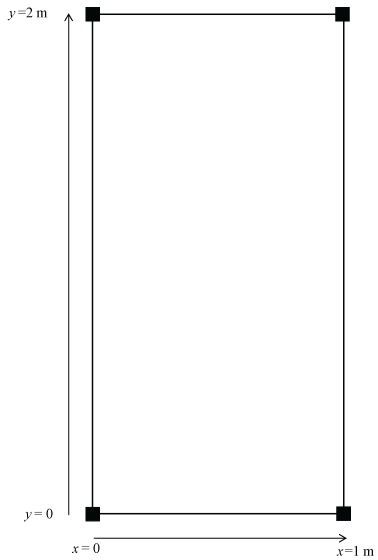
Illustration showing geometry of “soil column experiment” example. See appendix 1 for a list of symbols. m, meter.
Table 3.
Parameters of “soil column experiment” simulation.[m, meter; kg/(m s2), kilogram per meter per second squared; J/kg, joule per kilogram; °C, degree Celsius; J/(s m °C), joule per second per meter per degree Celsius; kg/m3, kilogram per cubic meter; kg/(m3 °C), kilogram per cubic meter per degree Celsius; m2, square meter; d, day]
| Parameter | Value |
|---|---|
| Column thickness and width (x-direction, x=0 m at left edge) | 1 m |
| Column height (y-direction, y=0 m at bottom) | 2 m |
| Porosity | 0.3 |
| Fluid compressibility | 4.47×10⁻¹⁰ [kg/(m‧s2)]−1 |
| Fluid specific heat | 4,182 J/(kg‧°C) |
| Fluid thermal conductivity | 0.6 J/(s‧m‧°C) |
| Linear fluid density function: [here set to a constant density of 1,000 kg/m3] | |
| Base density (RHOL0) | 1,000 kg/m3 |
| Base temperature (URHOL0) | 20 °C |
| Coefficient of density change (DRLDU) | 0 kg/(m3‧°C) |
| Solid matrix compressibility (COMPMA) | 1×10⁻⁸ [kg/(m‧s2)]−1 |
| Solid grain density (RHOS) | 2,600 kg/m3 |
| Solid grain specific heat | 840 J/(kg‧°C) |
| Solid grain thermal conductivity | 3.5 J/(s‧m‧°C) |
| Ice compressibility (COMPI) | 0 [kg/(m‧s2)]−1 |
| Ice density | 920 kg/m3 |
| Ice thermal conductivity | 2.14 J/(s‧m‧°C) |
| Ice specific heat | 2,108. J/(kg‧°C) |
| Latent heat of fusion | 3.34×10⁵ J/kg |
| Permeability (max and min) | 5×10⁻¹¹ m2 (hydraulic conductivity about 5×10⁻⁴ m/s) |
| Longitudinal dispersivity (in max and min permeability directions) | 0.001 m |
| Transverse dispersivity (in max and min permeability directions) | 0.001 m |
| Gravity vector components (GRAVX, GRAVY) | 0, –9.81 m/s2 |
| Piecewise-linear total-water saturation function: | |
| Residual total-water saturation due to pressure decrease (SWRES) | 0.01 |
| Air-entry pressure (PENT) | 0 [kg/(m s2)] |
| Pressure at residual total-water saturation (PSWRES) | –2×10+4 [kg/(m‧s2)] |
| Piecewise-linear relative permeability function: | |
| Liquid saturation at which minimum relative permeability occurs (SLRKRES) | 0.01 |
| Minimum relative permeability (RKRES) | 0.01 |
| Piecewise-linear liquid-water saturation function: | |
| Minimum liquid saturation due to temperature decrease (freezing) (SLSATRES) | 0.01 |
| Temperature at which minimum liquid saturation occurs (TLRES) | –2 °C |
| Finite elements (in horizontal, vertical directions) | 1, 100 |
| Time step | Part A: 0.01 d, Part B: 0.001 d |
| Time steps in pressure and temperature solution cycle (NPCYC, NUCYC) | 1, 1 |
| Maximum absolute simulation time | 180 d |
| Maximum time steps in simulation (NTMAX) | Part A: 1,800; Part B: 18,000 |
| Output cycles (NPRINT, NCOLPR, LCOLPR) | 100, 100, 100 |
| Solver for pressure, solver for temperature | DIRECT, DIRECT |
| Observations | at all nodes on left edge |
| Initial pressure of column (Hydrostatic, with p=0 at bottom where y=0; initial p values are calculated from the formula) |
p=(9.81)(1,000.)(−y) [kg/(m‧s2)] |
| Initial temperature of column | +2 °C |
| Top boundary condition for fluid mass balance | No−flow (implemented via ‘drain’ condition, see Part B top boundary condition for fluid mass balance) |
| Top boundary condition for energy balance | Specified T=−8 °C |
| Bottom boundary condition for fluid mass balance | Specified p=0 [kg/(m s2)] and any inflowing water has T=+2 °C |
| Bottom boundary condition for energy balance | Specified T=+2 °C |
| Iterations for Nonlinearity (ITRMAX) | 1 |
| Initial pressure of column | Pressures taken from the end of part A |
| Initial temperature of column | Temperatures taken from the end of part A |
| Top boundary condition for fluid mass balance: | 0 [kg/(m‧s2)], 0 kg/s |
| Generalized-flow boundary condition, a drain [see Provost and Voss (2019, section 1.4.5, “River and Drain”)] | |
| p at first point (PBG1), rate of inflow at first point (QPBG1) | 196.2 [kg/(m‧s2)] |
| p at second point (PBG2), rate of inflow at second point (QPBG2) | –4.96×10⁻⁴ kg/s |
| Limit on flow at point 1,2 (CPQL1, CPQL2) | Q (means that max limit is 0 [kg/(m‧s2)]), N (means no limit) |
| Temperature of any water entering top (arbitrary value as this never occurs) (temperature of any water exiting top is at temperature of ambient water at column top, changing with time) | 9,999.9999 °C |
| Top boundary condition for energy balance: | Insulated for conduction |
| Bottom boundary condition for fluid mass balance: | Specified total inflow QIN=4.96032×10⁻⁴ kg/s (equivalent to 1 centimeter per day liquid water flowing into base of column |
| Bottom boundary condition for energy balance: | Inflowing water has T=+2 °C Specified T=+2 °C |
| Max iterations for nonlinearity (ITRMAX) | 10 |
| Convergence criterion for p (RPMAX) | 275 [kg/(m‧s2)] |
| Convergence criterion for T (RUMAX) (set very large, so this does not control iterations) | 999999 °C |
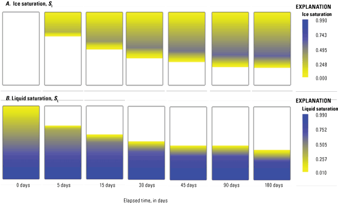
Illustrations of part A of experiment: freezing of unsaturated zone downward from the column top, showing ice and liquid-water saturations at indicated time steps (in days). The total-water saturation remains constant throughout part A, with values equivalent to the liquid saturation panel for 0 days. Minimum total and liquid saturation at 0 days is 0.02881 at top of column. Maximum ice saturation is 0.5988 at 180 days. (Ice saturation of zero and liquid saturation of 0.01 are shown as white.) See appendix 1 for a list of symbols.
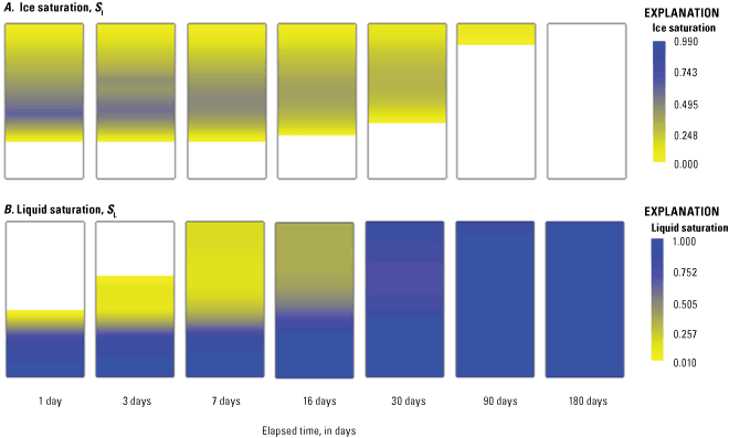
Illustration of part B of experiment: freezing and thawing of unsaturated zone due to inflow from the column bottom, showing ice and liquid-water saturations at indicated time steps (in days). Starting condition at 0 days is the same as in the last panel (180 days) in figure 9. Total-water saturation increases from the bottom up in part B; the column becomes fully water saturated (SW=1) at about 30 days. Minimum liquid saturation is exceeded at the top of column at some time between 3 and 7 days. The ice generally melts from the bottom up, completely disappearing soon after 90 days. (Ice saturation of zero and liquid saturation of 0.01 are shown as white.) See appendix 1 for a list of symbols.
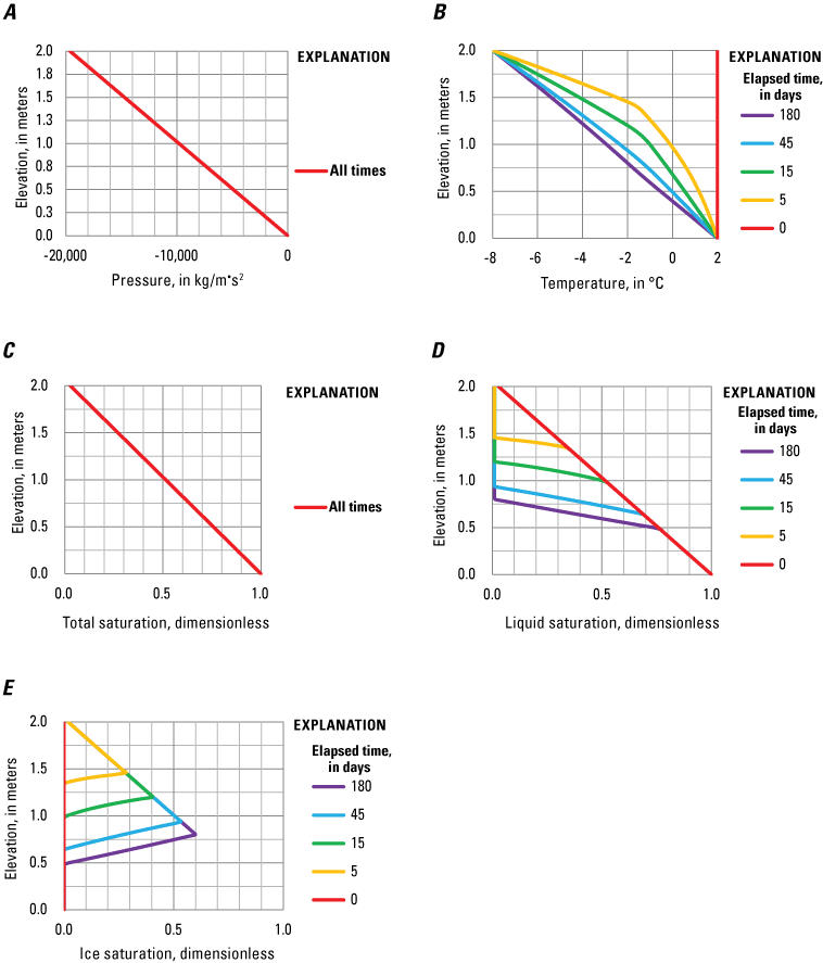
Graphs showing simulated evolution of vertical profiles along A, column of pressure, B, temperature, C, total water saturation, D, liquid saturation, and E, ice saturation for part A of the “soil-column experiment” example. Part A is simulated for 180 days. See appendix 1 for a list of symbols. kg/m‧s2, kilogram per meter per second squared; °C, degree Celsius.
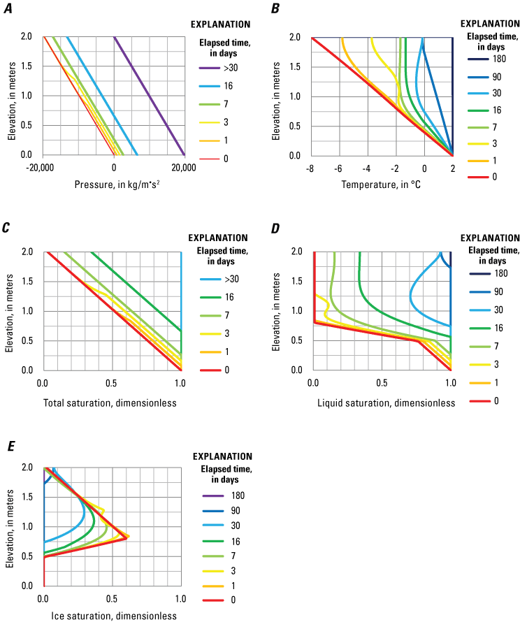
Graphs showing simulated evolution of vertical profiles along column of A, pressure, B, temperature, and C, total water saturation, D, liquid saturation, and E, ice saturation for part B of the “soil-column experiment” example. Part B is simulated for 180 days. Values for part B at 0 days are those that result from part A at 180 days. See appendix 1 for a list of symbols. m, meter; kg, kilogram; s, second; °C, degree Celsius; d, day; >, greater than.
Part A.—Following the instantaneous decrease in top temperature, simulated temperatures in the column decrease and a diffuse freezing front propagates downward through the variably saturated column, increasing ice saturations and decreasing liquid saturations (figs. 9 and 11). Nearly steady conditions in temperature and saturations develop in the soil column by about 90 days. Pressures naturally remain constant throughout the simulation, due to gravity-produced hydrostatic conditions, based on the specified pressure of 0 at the bottom. Pressures control only total-water saturation via the total-water saturation function (table 3) and do not affect apportioning of total water between liquid and ice phases. Total saturation is unchanging in part A, resulting from the steady pressure distribution, and it is equivalent to the liquid saturation at 0 days (fig. 11A). Thus, at any given location in the column, the decrease in liquid saturation is equal to the increase in ice saturation. The simulated liquid and ice saturations are controlled by temperature changes affecting the freezing function (table 3). Because column temperature increases downward and available liquid saturation decreases upward, the zone of highest ice saturation values occurs just below mid-column (figs. 9A and 11E).
Part B.—Flow of +2 °C liquid water entering the bottom of the column leads to a more complex evolution of total water, liquid, and ice saturations in part B than in part A of the experiment (figs. 10 and 12). The column resaturates from the bottom up and the newly arrived liquid begins to thaw the ice (figs. 10 and 12D–E). At about 30 days, the pressure at the top of the column exceeds zero and the boundary condition there changes from one of no flow to a generalized pressure boundary (both of which are part of the prescribed drain condition; see Provost and Voss [2019] for information on the drain condition). Thereafter the simulated top pressure remains just above 0 kg/(m‧s2). At this time (about 30 days), the column has become fully saturated with water, even though ice remains in the column until nearly 180 days.
Note that iterations for nonlinearity are required to maintain numerical stability early in the simulation when the forcing of 1 centimeter per day of liquid water into a frozen column causes numerical sensitivity of the ice-liquid transition [notice the wobbles in the ice saturation profile (fig. 12E) at an elapsed time of 3 days]. This sensitivity is also the reason that a smaller time step size is required for part B than for part A of the experiment. A finer mesh (smaller finite elements) in the vertical direction than employed here might also aid the stability of the early period of the numerical solution for part B. Another purpose of nonlinear iterations is to resolve the switchover from a no-flow condition to the generalized pressure boundary. Without such iterations, beginning at the switchover, the numerical solution for pressure at the top nodes would oscillate for the rest of the simulation with a repeating cycle of a few time steps, with the oscillations obscuring the numerical results. Nonlinearity iterations may occur only for the time step on which the switchover occurs, but to allow this to happen, such iterations must be allowed for the entire simulation (table 3). A third purpose of nonlinear iterations is to resolve the significant changes in the column that occur as soon as liquid water is injected into the column base. The convergence tolerance value for pressure, RPMAX, was selected by experimentation in a series of simulations, so that it would provide a reasonable numerical solution for these two sensitive parts of the simulated dynamics, without requiring many iterations per time step. Use of nonlinear iteration does not cause iterations on all time steps—only on those for which it is needed. The convergence tolerance for temperature, RUMAX, is set extremely high so that it is always satisfied and will never cause additional iterations.
For the entire simulated part B column experiment, thawing occurs from below, due to the warming effect of the upward-flowing liquid. This thawing occurs very slowly, taking more than 3 months, due to the relatively large latent-heat energy required to melt the ice. The energy input to the thawing process is provided by the +2 °C liquid water entering the bottom of the column. Due to the large latent-heat energy required to melt the ice, the long period required to thaw the column is a consequence of the relatively low amount of energy provided by the inflow. Almost all the ice is finally melted just after 90 days, at which time the temperature at the top of the column finally reaches 0 °C (fig. 10A [at 90 days] and 12B and E). Thereafter, the ice-free column warms to nearly +2 °C by 180 days. Nonlinear and complex interactions between groundwater flow and freeze-thaw processes occur, especially for unsaturated conditions, even for this simple one-dimensional example.
References Cited
Andersland, O.B., and Ladanyi, B., 1994, An introduction to frozen ground engineering: New York, Chapman and Hall, 352 p., accessed March 23, 2022, at https://doi.org/10.1007/978-1-4757-2290-1.
Anderson, D.M., and Morgenstern, N.R., 1973, Physics, chemistry and mechanics of frozen ground—A review, in North American Contribution, Permafrost, Second International Conference, Yakutsk, U.S.S.R., July 13–28, 1973: National Research Council of Canada and U.S. National Academy of Sciences, p. 257–288.
Anderson, D.M., and Tice, A.R., 1972, Predicting unfrozen water contents in frozen soils from surface area measurements: Highway Research Record, v. 393, p. 12–18. [Also available at https://trid.trb.org/view/126420.]
Azmatch, T.F., Sego, D.C., Arenson, L.U., and Biggar, K.W., 2012, Using soil freezing characteristic curve to estimate the hydraulic conductivity function of partially frozen soils: Cold Regions Science and Technology, v. 83–84, p. 103–109, accessed March 23, 2022, at https://doi.org/10.1016/j.coldregions.2012.07.002.
Briggs, M.A., Walvoord, M.A., McKenzie, J.M., Voss, C.I., Day-Lewis, F.D., and Lane, J.W., 2014, New permafrost is forming around shrinking Arctic lakes, but will it last?: Geophysical Research Letters, v. 41, no. 5, p. 1585–1592, accessed March 23, 2022, at https://doi.org/10.1002/2014GL059251.
Brooks, R.H., and Corey, A.T., 1964, Hydraulic properties of porous media: Colorado State University Hydrology Paper no. 3, 27 p. [Also available at https://mountainscholar.org/bitstream/handle/10217/61288/HydrologyPapers_n3.pdf.]
Chen, L., Fortier, D., McKenzie, J.M., Voss, C.I., and Lamontagne-Hallé, P., 2023, Subsurface porewater flow accelerates talik development under the Alaska highway, Yukon—A prelude to road collapse and final permafrost thaw?: Water Resources Research, v. 59, no. 4, paper e2022WR032578, 21 p., accessed June 29, 2023, at https://doi.org/10.1029/2022WR032578.
Chen, L., VossC.I., Fortier, D., and McKenzie, J.M., 2021, Surface energy balance of sub-Arctic roads with varying snow regimes and properties in permafrost regions: Permafrost and Periglacial Processes, v. 32, no. 4, p. 681-701, accessed June 29, 2023, at https://doi.org/10.1002/ppp.2129.
Evans, S.G., Ge, S., Voss, C.I., and Molotch, N.P., 2018, The role of frozen soil in groundwater discharge predictions for warming alpine watersheds: Water Resources Research, v. 54, no. 3, p. 1599–1615, accessed March 23, 2022, at https://doi.org/10.1002/2017WR022098.
Evans, S.G., Godsey, S.E., Rushlow, C.R., and Voss, C., 2020, Water tracks enhance water flow above permafrost in upland Arctic Alaska hillslopes: Journal of Geophysical Research: Earth Surface, v. 125, no. 2, paper e2019JF005256, 18 p., accessed March 23, 2022, at https://doi.org/10.1029/2019JF005256.
Ge, S., McKenzie, J.M., Voss, C.I., and Wu, Q., 2011, Exchange of groundwater and surface-water mediated by permafrost response to seasonal and long term air temperature variation: Geophysical Research Letters, v. 38, no. 14, L14402, 6 p., accessed March 23, 2022, at https://doi.org/10.1029/2011GL047911.
Grenier, C., Anbergen, H., Bense, V., Chanzy, Q., Coon, E., Collier, N., Costard, F., Ferry, M., Frampton, A., Frederick, J., Gonçalvès, J., Holmén, J., Jost, A., Kokh, S., Kurylyk, B., McKenzie, J., Molson, J., Mouche, E., Orgogozo, L., Pannetier, R., Rivière, A., Roux, N., Rühaak, W., Scheidegger, J., Selroos, J.-O., Therrien, R., Vidstrand, P., and Voss, C., 2018, Groundwater flow and heat transport for systems undergoing freeze-thaw—Intercomparison of numerical simulators for 2D test cases: Advances in Water Resources, v. 114, p. 196–218, accessed March 23, 2022, at https://doi.org/10.1016/j.advwatres.2018.02.001.
Holten, V., and Anisimov, M.A., 2012, Entropy-driven liquid–liquid separation in supercooled water: Scientific Reports, v. 2, article 713, 7 p., accessed March 23, 2022, at https://doi.org/10.1038/srep00713.
Jame, Y.-W., 1977, Heat and mass transfer in freezing soils: University of Saskatchewan dissertation, 212 p. [Also available at http://hdl.handle.net/10388/etd-11282008-091133.]
Jame, Y.-W., and Norum, D.I., 1980, Heat and mass-transfer in a freezing unsaturated porous medium: Water Resources Research, v. 16, no. 4, p. 811–819, accessed March 23, 2022, at https://doi.org/10.1029/WR016i004p00811.
Kell, G.S., 1967, Precise representation of volume properties of water at one atmosphere: Journal of Chemical & Engineering Data, v. 12, no. 1, p. 66–69, accessed March 23, 2022, at https://doi.org/10.1021/je60032a018.
Koopmans, R.W.R., and Miller, R.D., 1966, Soil freezing and soil water characteristics curves: Soil Science Society of America Journal, v. 30, no. 6, p. 680–685, accessed March 23, 2022, at https://doi.org/10.2136/sssaj1966.03615995003000060011x.
Kozlowski, T., 2007, A semi-empirical model for phase composition of water in clay-water systems: Cold Regions Science and Technology, v. 49, no. 3, p. 226–236, accessed March 23, 2022, at https://doi.org/10.1016/j.coldregions.2007.03.013.
Kurylyk, B.L., and Watanabe, K., 2013, The mathematical representation of freezing and thawing processes in variably-saturated, non-deformable soils: Advances in Water Resources, v. 60, p. 160–177, accessed March 23, 2022, at https://doi.org/10.1016/j.advwatres.2013.07.016.
Kurylyk, B.L., Hayashi, M., Quinton, W.L., McKenzie, J.M., and Voss, C.I., 2016, Influence of vertical and lateral heat transfer on permafrost thaw, peatland landscape transition, and groundwater flow: Water Resources Research, v. 52, no. 2, p. 1286–1305, accessed March 23, 2022, at https://doi.org/10.1002/2015WR018057.
Kurylyk, B.L., MacQuarrie, K.T.B., and Voss, C.I., 2014a, Climate change impacts on the temperature and magnitude of groundwater discharge from shallow, unconfined aquifers: Water Resources Research, v. 50, no. 4, p. 3253–3274, accessed March 23, 2022, at https://doi.org/10.1002/2013WR014588.
Kurylyk, B.L., McKenzie, J.M., MacQuarrie, K.T.B., and Voss, C.I., 2014b, Analytical solutions for benchmarking cold regions subsurface water flow and energy transport models—One-dimensional soil thaw with conduction and advection: Advances in Water Resources, v. 70, p. 172–184, accessed March 23, 2022, at https://doi.org/10.1016/j.advwatres.2014.05.005.
Lamontagne-Hallé, P., McKenzie, J.M., Kurylyk, B.L., and Zipper, S.C., 2018, Changing groundwater discharge dynamics in permafrost regions: Environmental Research Letters, v. 13, no. 8, article 084017, 12 p., accessed March 23, 2022, at https://doi.org/10.1088/1748-9326/aad404.
Lunardini, V.J., 1988, Freezing of soil with an unfrozen water content and variable thermal properties: U.S. Army Corps of Engineers, Cold Regions Research and Engineering Laboratory Report 88–2, 23 p. [Also available at http://hdl.handle.net/11681/9076.]
Lundin, L.-C., 1990, Hydraulic properties in an operational model of frozen soil: Journal of Hydrology, v. 118, no. 1–4, p. 289–310, accessed March 23, 2022, at https://doi.org/10.1016/0022-1694(90)90264-X.
McKenzie, J.M., and Voss, C.I., 2013, Permafrost thaw in a nested groundwater-flow system: Hydrogeology Journal, v. 21, no. 1, p. 299–316, accessed March 23, 2022. 10.1007/s10040-012-0942-3.
McKenzie, J.M., Siegel, D.I., Rosenberry, D.O., Glaser, P.H., and Voss, C.I., 2006, Heat transport in the Red Lake Bog, Glacial Lake Agassiz Peatlands: Hydrological Processes, v. 21, no. 3, p. 369–378, accessed March 23, 2022, at https://doi.org/10.1002/hyp.6239.
McKenzie, J.M., Voss, C.I., and Siegel, D.I., 2007, Groundwater flow with energy transport and water-ice phase change—Simulations, benchmarks, and application to freezing in peat bogs: Advances in Water Resources, v. 30, no. 4, p. 966–983, accessed March 23, 2022, at https://doi.org/10.1016/j.advwatres.2006.08.008.
Miller, O., Voss, C.I., Solomon, D.P, Miège, C., Forster, R., Schmerr, N., and Montgomery, L., 2022, Hydrologic modeling of a perennial firn aquifer in southeast Greenland: Journal of Glaciology, v. 69, no. 275, p. 607-622, accessed June 29, 2023, at https://doi.org/10.1017/jog.2022.88.
Mottaghy, D., and Rath, V., 2006, Latent heat effects in subsurface heat transport modelling and their impact on paleotemperature reconstructions: Geophysical Journal International, v. 164, no. 1, p. 236–245, accessed March 23, 2022, at https://doi.org/10.1111/j.1365-246X.2005.02843.x.
Newman, G., and Wilson, G., 1997, Heat and mass transfer in unsaturated soils during freezing: Canadian Geotechnical Journal, v. 34, no. 1, p. 63–70, accessed March 23, 2022, at https://doi.org/10.1139/t96-085.
Nield, D.A., and Bejan, A., 1999, Convection in porous media (2d ed.): New York, Springer-Verlag, 546 p. [Also available at https://doi.org/10.1007/978-1-4757-3033-3.]
Niu, F., Cheng, G., Niu, Y., Zhang, M., Luo, J., and Lin, Z., 2016, A naturally-occurring ‘cold earth’ spot in northern China: Scientific Reports, v. 6, article 34184, 7 p., accessed March 23, 2022, at https://doi.org/10.1038/srep34184.
Painter, S.L., 2011, Three-phase numerical model of water migration in partially frozen geological media—Model formulation, validation, and applications: Computational Geosciences, v. 15, no. 1, p. 69–85, accessed March 23, 2022, at https://doi.org/10.1007/s10596-010-9197-z.
Provost, A.M., and Voss, C.I., 2019, SUTRA, a model for saturated-unsaturated, variable-density groundwater flow with solute or energy transport—Documentation of generalized boundary conditions, a modified implementation of specified pressures and concentrations or temperatures, and the lake capability: U.S. Geological Survey Techniques and Methods, book 6, chap A52, 62 p., accessed March 23, 2022, at https://doi.org/10.3133/tm6A52.
Rempel, A.W., 2012, Hydromechanical processes in freezing soils: Vadose Zone Journal, v. 11, no. 4, article vzj2012.0045, 10 p., accessed March 23, 2022, at https://doi.org/10.2136/vzj2012.0045.
Rey, D.M., Walvoord, M.A., Minsley, B.J., Ebel, B.A., Voss, C.I., and Singha, K., 2020, Wildfire‐initiated talik development exceeds current thaw projections—Observations and models from Alaska’s continuous permafrost zone: Geophysical Research Letters, v. 47, no. 15, paper 087565, 11 p., accessed March 23, 2022, at https://doi.org/10.1029/2020GL087565.
Rühaak, W.H., Anbergen, C., Grenier, J., McKenzie, J.M., Kurylyk, B., Molson, J., Roux, N., and Sass, I., 2015, Benchmarking numerical freeze/thaw models: Energy Procedia, v. 76, p. 301–310, accessed March 23, 2022, at https://doi.org/10.1016/j.egypro.2015.07.866.
Rushlow, C.R., Sawyer, A.H., Voss, C.I., and Godsey, S.E., 2020, The influence of snow cover, air temperature, and groundwater flow on the active-layer thermal regime of Arctic hillslopes drained by water tracks: Hydrogeology Journal, v. 28, p. 2057–2069, accessed March 23, 2022, at https://doi.org/10.1007/s10040-020-02166-2.
Spaans, E.J.A., and Baker, J.M., 1996, The soil freezing characteristic—Its measurement and similarity to the soil moisture characteristic: Soil Science Society of America Journal, v. 60, no. 1, p. 13–19, accessed March 23, 2022, at https://doi.org/10.2136/sssaj1996.03615995006000010005x.
Taylor, G.S., and Luthin, J.N., 1978, A model for coupled heat and moisture transfer during soil freezing: Canadian Geotechnical Journal, v. 15, no. 4, p. 548–555, accessed March 23, 2022, at https://doi.org/10.1139/t78-058.
Tilton, L.W., and Taylor, J.K., 1937, Accurate representation of the refractivity and density of distilled water as a function of temperature: Journal of Research of the National Bureau of Standards, v. 18, paper RP971, p. 205–214. [Also available at https://nvlpubs.nist.gov/nistpubs/jres/18/jresv18n2p205_A1b.pdf.]
U.S. Geological Survey, 2022, SUTRA—A model for 2D or 3D saturated-unsaturated, variable-density ground-water flow with solute or energy transport: U.S. Geological Survey software, accessed July 22, 2022, at https://doi.org/10.5066/P9PPEHHM.
van Genuchten, M.Th., 1980, A closed-form equation for predicting the hydraulic conductivity of unsaturated soils: Soil Science Society of America Journal, v. 44, no. 5, p. 892–898, accessed March 23, 2022, at https://doi.org/10.2136/sssaj1980.03615995004400050002x.
Voss, C.I., and Provost, A.M., 2002, SUTRA—A model for 2D or 3D saturated-unsaturated, variable-density ground-water flow with solute or energy transport [version 2D3D.1, September 22, 2010]: U.S. Geological Survey Water-Resources Investigations Report 02–4231, 291 p., accessed March 23, 2022, at https://doi.org/10.3133/wri024231.
Voss, C.I., and Provost, A.M., 2024, SUTRA—A model for 2D or 3D saturated-unsaturated, variable-density groundwater flow with solute or energy transport, version 4.0: U.S. Geological Survey software release, https://doi.org/10.5066/P9OL5IYX.
Walvoord, M.A., and Kurylyk, B.L., 2016, Hydrologic impacts of thawing permafrost—A review: Vadose Zone Journal, v. 15, no. 6, article vzj2016.01.0010, 20 p., accessed March 23, 2022, at https://doi.org/10.2136/vzj2016.01.0010.
Walvoord, M.A., Voss, C.I., Ebel, B., and Minsley, B.J., 2019, Development of perennial thaw zones in boreal hillslopes enhances potential mobilization of permafrost carbon: Environmental Research Letters, v. 14, no. 1, article 015003, 11 p., accessed March 23, 2022, at https://doi.org/10.1088/1748-9326/aaf0cc.
Watanabe, K., and Wake, T., 2009, Measurement of unfrozen water content and relative permittivity of frozen unsaturated soil using NMR and TDR: Cold Regions Science and Technology, v. 59, no. 1, p. 34–41, accessed March 23, 2022, at https://doi.org/10.1016/j.coldregions.2009.05.011.
Wellman, T.P., Voss, C.I., and Walvoord, M.A., 2013, Impacts of climate, lake size, and supra- and sub-permafrost groundwater flow on lake-talik evolution, Yukon Flats, Alaska (USA): Hydrogeology Journal, v. 21, no. 1, p. 281–298, accessed March 23, 2022, at https://doi.org/10.1007/s10040-012-0941-4.
Wicky, J., and Hauck, C., 2017, Numerical modelling of convective heat transport by air flow in permafrost talus slopes: The Cryosphere, v. 11, p. 1311–1325, accessed March 23, 2022, at https://doi.org/10.5194/tc-11-1311-2017.
Zhao, Y., Nishimura, T., Hill, R., and Miyazaki, T., 2013, Determining hydraulic conductivity for air-filled porosity in an unsaturated frozen soil by the multistep outflow method: Vadose Zone Journal, v. 12, no. 1, article vzj2012.0061, 10 p., accessed March 23, 2022, at https://doi.org/10.2136/vzj2012.0061.
Zhou, X., Zhou, J., Kinzelbach, W., and Stauffer, F., 2014, Simultaneous measurement of unfrozen water content and ice content in frozen soil using gamma ray attenuation and TDR: Water Resources Research, v. 50, no. 12, p. 9630–9655, accessed March 23, 2022, at https://doi.org/10.1002/2014WR015640.
Appendix 1. List of Units, Symbols, and Abbreviations
Table 1.1.
Abbreviations and symbols used in SUTRA model version 4.0.| Abbreviation or symbol | Unit | Definition |
|---|---|---|
| [E] | energy, equivalent to [M∙L2/s2] | |
| [L] | length | |
| [L3] | volume (general) | |
| [LG3] | solid mineral grain or solid matrix volume | |
| [LI3] | ice volume | |
| [LL3] | liquid-water (fluid) volume | |
| [M] | mass (general) | |
| [MG] | solid mineral grain or solid matrix mass | |
| [MI] | ice mass | |
| [ML] | liquid-water (fluid) mass | |
| [MS] | solute or sorbate mass | |
| [1] | dimensionless | |
| [°C] | degree Celsius (unit of temperature) | |
| [cm] | centimeter (unit of [L]) | |
| [d] | day (unit of time) | |
| [gr] | gram (unit of [M]) | |
| [h] | hour (unit of time) | |
| [J] | joule (energy unit [kg∙m2/s2]) | |
| [kg] | kilogram (unit of [M]) | |
| [m] | meter (unit of [L]) | |
| [s] | second (unit of time) | |
| [yr] | year (unit of time) | |
| [°] | degree (measure of an angle) | |
| αs | [Μ/(L‧s2)]–1 | Porous-matrix compressibility (eq. 7) |
| αφ | [(percent)∙] | Power-law model parameter (eq. 59) |
| αLmax | [L] | Scaled longitudinal dispersivity value for the maximum permeability direction (defined in dataset 15; description in app. 2) |
| αLmid | [L] | Scaled longitudinal dispersivity value for the middle permeability direction (defined in dataset 15; description in app. 2) |
| αLmin | [L] | Scaled longitudinal dispersivity value for the minimum permeability direction (defined in dataset 15; description in app. 2) |
| αPOW(x, y[, z]) | [] | Modified power-law model parameter (eq. 57) |
| αTmax | [L] | Scaled transverse dispersivity value for the maximum permeability direction (defined in dataset 15; description in app. 2) |
| αTmid | [L] | Scaled transverse dispersivity value for the middle permeability direction (defined in dataset 15; description in app. 2) |
| αTmin | [L] | Scaled transverse dispersivity value for the minimum permeability direction (defined in dataset 15; description in app. 2) |
| βI | [Μ/(L∙s2)]–1 | Ice compressibility (eq. 14) |
| βL | [Μ/(L∙s2)]–1 | Liquid-water compressibility (eq. 8) |
| βPOW(x, y[, z]) | [1] | Modified power-law model parameter (eq. 57) |
| [E/(MI∙s)] | Zero-order energy source in ice (eq. 24) | |
| [E/(ML∙s)] or [(MS/ML)/s)] |
Zero-order energy or solute-species mass source in liquid water (for energy, eq. 24; for solute, eq. 82, definition before eq. 82) | |
| [E/(MG∙s)] or [(MS/MG)/s)] |
Zero-order energy or solute-species mass source in solid mineral grains (for energy, eq. 24; for solute, eq. 82, definition before eq. 82) | |
| [(MS/ML)/s)] | First-order solute-species mass production in liquid water (eq. 82, definition before eq. 82) | |
| [(MS/MG)/s)] | First-order solute-species mass production in solid mineral grains (eq. 82, definition before eq. 82) | |
| ε(x, y[, z]) | [1] | Porosity (eq. 3) |
| θ1 | [°] | Scaled first permeability angle value (defined in dataset 15; description in app. 2) |
| θ2 | [°] | Scaled second permeability angle value (defined in dataset 15; description in app. 2) |
| θ3 | [°] | Scaled third permeability angle value (defined in dataset 15; description in app. 2) |
| λ(x, y[, z], t) | [E/(s∙L∙°C)] | Bulk thermal conductivity (eq. 31) |
| λA(x, y[, z]) | [E/(s∙L∙°C)] | Effective thermal conductivity of air (eq. 44, definition before eq. 44) |
| λBC(x, y[, z]) | [1] | Pore-size distribution index for Brooks-Corey total-water saturation function (eq. 49) |
| λI | [E/(s∙L∙°C)] | Thermal conductivity of ice (eq. 42A) |
| λL | [E/(s∙L∙°C)] | Thermal conductivity of liquid water (eq. 42A) |
| λLIS(x, y[, z], t) | [E/(s∙L∙°C)] | Effective thermal conductivity of mixture of liquid water, ice, and solid mineral grains (eq. 42A) |
| λS | [E/(s∙L∙°C)] | Thermal conductivity of a solid mineral grain (eq. 42A) |
| µL(x, y[, z], t) | [M/(L∙s)] | Liquid water viscosity (eq. 19) |
| ρI(x, y[, z], t) | [MI/LI3] | Ice density (eq. 2) |
| ρL(x, y[, z], t) | [ML/LL3] | Liquid-water density (eq. 2) |
| ρS(x, y[, z], t) | [MS/LS3] | Density of solid mineral grain (eq. 24) |
| ρW(x, y[, z], t) | [M/L3] | Mean total-water density (eq. 2) |
| σA | [E/(s∙L∙°C)] | Scaled effective air thermal conductivity value, in the context of input to SUTRA (for notational consistency with σL, which is used for both energy transport and solute transport); identically equal to λA (defined in dataset 15; description in app. 2) |
| σI | [E/(s∙L∙°C)] | Thermal conductivity of ice, in the context of input to SUTRA (for notational consistency with σL, which is used for both energy transport and solute transport); identically equal to λI (defined in dataset 9; description in app. 2) |
| σL | [E/(s∙L∙°C)] or [L2/s] |
For energy transport, represents liquid-water thermal conductivity, λL; for solute transport, represents molecular diffusivity of solute in pure liquid water, Dm (defined in dataset 9; description in app. 2) |
| σS | [E/(s∙L∙°C)] | Scaled solid mineral grain thermal conductivity value, in the context of input to SUTRA (for notational consistency with σL, which is used for both energy transport and solute transport); identically equal to λS for energy transport (defined in dataset 15; description in app. 2) |
| [percent] | Percent moisture content by dry weight under fully saturated conditions (eq. 59) | |
| χ1 | [LL3/MG] | Linear, Freundlich or Langmuir adsorption distribution coefficient (defined in dataset 11A; description in app. 2) |
| χ2 | [1] | Freundlich or Langmuir adsorption coefficient (defined in dataset 11A; description in app. 2) |
| Ω | [1] | Impedance factor (eq. 68) |
| αVG(x, y[, z]) | [(L∙s2)/M] | Van Genuchten model parameter (eq. 47) |
| cI(x, y[, z], t) | [E/(MI∙°C)] | Specific heat of ice (eq. 26B) |
| cL(x, y[, z], t) | [E/(ML∙°C)] | Specific heat of liquid water (eq. 26A) |
| cS(x, y[, z], t) | [E/(MS∙°C)] | Specific heat of solid mineral grains (eq. 26C) |
| eI(x, y[, z], t) | [E/MI] | Energy per unit mass of ice (eq. 24) |
| [E/MI] | Thermal energy per unit mass of ice at free-water freezing temperature (eq. 26B) | |
| eL(x, y[, z], t) | [E/ML] | Energy per unit mass of liquid water (eq. 24) |
| [E/ML] | Energy per unit mass of fluid source (eq. 24) | |
| [E/ML] | Thermal energy per unit mass of liquid water at free-water freezing temperature (eq. 26A) | |
| eS(x, y[, z], t) | [E/MS] | Energy per unit mass of solid mineral grains (eq. 24) |
| [E/MS] | Thermal energy per unit mass of solid mineral grains at free-water freezing temperature (eq. 26C) | |
| [L/s2] | Gravitational acceleration (gravity vector) (eq. 19) | |
| k | [L2] | Permeability under fully saturated, unfrozen conditions (eq. 69) |
| [L2] | Solid matrix permeability tensor (eq. 19) | |
| keff | [L2] | Effective permeability that takes into account both partial saturation and freezing (eq. 68) |
| [L2] | Effective permeability that takes into account partial saturation under unfrozen conditions (eq. 68) | |
| kmax | [L2] | Scaled maximum permeability value (defined in dataset 15; description in app. 2) |
| kmid | [L2] | Scaled middle permeability value (defined in dataset 15; description in app. 2) |
| kmin | [L2] | Scaled minimum permeability value (defined in dataset 15; description in app. 2) |
| kr(x, y[, z], t) | [1] | Relative permeability for fluid flow (eq. 19) |
| [1] | Relative permeability under unfrozen conditions (eq. 70) | |
| krmin(x, y[, z]) | [1] | Minimum value of relative permeability (eq. 41, definition before eq. 41) |
| nVG(x, y[, z], t) | [1] | Van Genuchten model parameter (eq. 47) |
| p(x, y[, z], t) | [M/(L∙s2)] | Fluid pressure (eq. 5) |
| pent(x, y[, z], t) | [Μ/(L∙s2)] | Air-entry pressure, first appears (eq. 49, definition before eq. 47) |
| pWres(x, y[, z]) | [Μ/(L∙s2)] | Residual-saturation pressure for the piecewise-linear total-water saturation function (eq. 51) |
| [L/s] or [LL3/(L2∙s)] | Darcy velocity or volumetric fluid flux (eq. 86, definition before eq. 86) | |
| [E/(L2∙s)] | Conductive-dispersive heat flux (eq. 24) | |
| [MS/(L2∙s)] | Diffusive-dispersive solute-mass flux (eq. 82, definition before eq. 82) | |
| t | [s] | Time (eq. 3) |
| [L/s] | Average fluid velocity (eq. 3) | |
| wEXP(x, y[, z]) | [°C] | Exponential liquid-water saturation function parameter (eq. 55) |
| C(x, y[, z], t) | [MS/ML] | Solute-species concentration (mass fraction) (eq. 82, definition before eq. 82) |
| CS(x, y[, z], t) | [MS/MG] | Concentration of species as sorbate on solid mineral grains expressed as a mass fraction (eq. 82, definition before eq. 82) |
| C*(x, y[, z], t) | [MS ML] | Solute concentration of fluid sources (mass fraction; eq. 82, definition before eq. 82) |
| [L2/s] | Mechanical dispersion tensor (eq. 31) | |
| Dm | [L2/s] | Molecular diffusivity of solute in pure liquid water (defined in table 2 and dataset 9; description in app. 2) |
| ∆H(x, y[, z]) | [E/ ML] | Latent heat of fusion of free water (eq. 27) |
| Qp(x, y[, z], t) | [ML/(L3∙s)] | Fluid-mass source (eq. 3) |
| SA(x, y[, z], t) | [1] | Air saturation (eq. 44, definition before eq. 44) |
| SI(x, y[, z], t) | [1] | Ice saturation (eq. 1) |
| SL(x, y[, z], t) | [1] | Liquid-water saturation (eq. 1) |
| [1] | Liquid-water saturation as a result of the freeze-thaw process in a fully saturated porous medium (eq. 36) | |
| [1] | Drainable liquid-water saturation (defined in eq. 63) | |
| [1] | Relative, scaled saturation for the piecewise-linear relative-permeability function (defined in eq. 67B) | |
| [1] | Value of liquid-water saturation at which the relative permeability has its minimum value (kr=krmin; eq. 67B, definition before eq. 41) | |
| SLres | [1] | Minimum liquid-water saturation that can occur, taking into account both pressure desaturation and freezing (eqs. 55 and 63, definition after eq. 40) |
| [1] | Minimum liquid-water saturation that can occur as a result of freezing the porous medium (eq. 55, defined after eq. 37) | |
| [M/(L∙s2)]–1 | Effective specific pressure storativity (eq. 19) | |
| [Μ/(L∙s2)]–1 | Quantity mathematically analogous to the specific pressure storativity for liquid, but computed using the compressibility of ice (eq. 13) | |
| [Μ/(L∙s2)]–1 | Specific pressure storativity for liquid (eq. 6) | |
| SW(x, y[, z], t) | [1] | Total-water saturation (eq. 1) |
| SWres(x, y[, z], t) | [1] | Residual total-water saturation (eq. 47, definition after eq. 38) |
| Sy | [1] | Specific yield (eq. 53) |
| T(x, y[, z], t) | [°C] | Temperature (eq. 5) |
| T*(x, y[, z], t) | [°C] | Temperature of fluid source (eq. 30) |
| T∆ | [°C] | Relative temperature (eq. 54) |
| Tf(x, y[, z], t) | [°C] | Maximum freezing temperature of pore water (eq. 54, definition before eq. 27) |
| Tff | [°C] | Freezing temperature of pure, free water (eq. 26A) |
| TLres(x, y[, z], t) | [°C] | Residual-saturation temperature for the piecewise-linear liquid-water saturation function (eq. 61, definition after eq. 37) |
Appendix 2. New and Modified Input Datasets
Table 2.1.
List of main input file (.inp) input data created or modified by the newly introduced freezing capability, total-water, and liquid-water saturation functions, relative permeability function, and spatially varying properties for SUTRA model version 4.0.[Input variables of “character” type are enclosed in single quotation marks (‘ ‘) to provide maximum compatibility across computing platforms. A detailed discussion of the U.S. Geological Survey Saturated-Unsaturated Transport (SUTRA) code permeability and dispersion functions is provided at the end of the listing of dataset 15B in Voss and Provost (2002)]
References Cited
Voss, C.I., and Provost, A.M., 2002, SUTRA—A model for 2D or 3D saturated-unsaturated, variable-density ground-water flow with solute or energy transport [version 2D3D.1, September 22, 2010]: U.S. Geological Survey Water-Resources Investigations Report 02–4231, 291 p., accessed March 23, 2022, at https://doi.org/10.3133/wri024231.
Voss, C.I., and Provost, A.M., 2024, SUTRA—A model for 2D or 3D saturated-unsaturated, variable-density groundwater flow with solute or energy transport, version 4.0: U.S. Geological Survey software release, https://doi.org/10.5066/P9OL5IYX.
Conversion Factors
International System of Units to U.S. customary units
Temperature in degrees Celsius (°C) may be converted to degrees Fahrenheit (°F) as follows:
°F=(1.8×°C)+32.
For more information, contact
Director, Earth System Processes Division
U.S. Geological Survey
Mail Stop 411
12201 Sunrise Valley Drive
Reston, VA 20192
Publishing support provided by the Pembroke and Reston Publishing Service Centers
Disclaimers
Any use of trade, firm, or product names is for descriptive purposes only and does not imply endorsement by the U.S. Government.
Although this information product, for the most part, is in the public domain, it also may contain copyrighted materials as noted in the text. Permission to reproduce copyrighted items must be secured from the copyright owner.
Suggested Citation
Voss, C.I., Provost, A.M., McKenzie, J.M., and Kurylyk, B.L., 2024, SUTRA—A code for simulation of saturated-unsaturated, variable-density groundwater flow with solute or energy transport—Documentation of the version 4.0 enhancements—Freeze-thaw capability, saturation and relative-permeability relations, spatially varying properties, and enhanced budget and velocity outputs: U.S. Geological Survey Techniques and Methods, book 6, chap. A63, 91 p., https://doi.org/10.3133/tm6A63.
ISSN: 2328-7055 (online)
| Publication type | Report |
|---|---|
| Publication Subtype | USGS Numbered Series |
| Title | SUTRA— A code for simulation of saturated-unsaturated, variable-density groundwater flow with solute or energy transport—Documentation of the version 4.0 enhancements—Freeze-thaw capability, saturation and relative-permeability relations, spatially varying properties, and enhanced budget and velocity outputs |
| Series title | Techniques and Methods |
| Series number | 6-A63 |
| DOI | 10.3133/tm6A63 |
| Publication Date | December 20, 2024 |
| Year Published | 2024 |
| Language | English |
| Publisher | U.S. Geological Survey |
| Publisher location | Reston, VA |
| Contributing office(s) | WMA - Earth System Processes Division |
| Description | Report: vii, 91 p.; Software Release |
| Online Only (Y/N) | Y |
| Additional Online Files (Y/N) | N |