

Revision of ModelMuse to Support the Use of PEST Software With MODFLOW and SUTRA Models
Links
- Document: Report (9.88 MB pdf) , HTML , XML
- Data Release: USGS data release - ModelMuse version 5.4
- Software Release: USGS software release - ModelMuse: A Graphical User Interface for Groundwater Models (version 5.3.0.0)
- Download citation as: RIS | Dublin Core
Acknowledgments
I want to thank Randy Hunt and Alden Provost for their thorough and helpful reviews of this manuscript. I would also like to thank the following individuals for providing advice and feedback during the development of ModelMuse version 5: Tom Burbey (Virginia Polytechnic Institute and State University [Virginia Tech]), Erick Burns (U.S. Geological Survey [USGS]), Mary Coburn (Minnesota Department of Natural Resources), Susan Colarullo (USGS), Glen B. Carleton (USGS, retired; MidAtlantic Geophysics, LLC), John Doherty (Watermark Numerical Computing), Sarken E. Dressler (New York State Department of Environmental Conservation ), Timothy Eaton (School of Earth and Environmental Sciences, Queens College City University of New York), Michael N. Fienen (USGS), Alex R. Fiore (USGS), Robel Gebrekristos (Digby Wells Environmental), Javier González (Bluedot Consulting), Dale Groff (Pacific Habitat Services, Inc.), Kevin Hansen (Hydrogeologist, Thurston County, Washington), Mary C. Hill (USGS), Paul A. Hsieh (USGS), Cathleen Humm (Virginia Tech), Scott James (Department of Geosciences, Baylor University), Haili Jia (Hydrogeologist.com.au), Leon J. Kauffman (USGS), Julien Kirmaier (Arcadis), Frederic Lalbat (Environmental Defense Fund [EDF]), Mark Lemon, Francesca Lotti (Kataclima), Auguste Matteo (EDF), Paul Misut (USGS), Ramon C. Naranjo (USGS), Alden Provost (USGS), Nathan Roethlisberger (Virginia Tech), Jim Van de Water (Thomas Harder & Co.), Andrew Watson (Stellenbosch University), Jeremy White (Intera), and Shixian Xu (University of Twente). I would also like to thank Stokely J. Klasovsky (USGS) for excellent editorial advice.
Executive Summary
ModelMuse is a graphical user interface for several groundwater modeling programs. ModelMuse was updated to generate the input files for the parameter estimation software suite PEST. The software is used with MODFLOW or SUTRA models to run PEST-based parameter estimation and display the updated model inputs after parameter estimation. The PEST input files can also be used with the PEST++ version 5 software suite.
Parameter estimation typically requires defining the parameters being adjusted during calibration and observations for assessing calibration quality. After a parameter is defined in ModelMuse, it can be applied to all or part of a model dataset. Pilot points—a parameterization device that facilitates higher levels of parameterization—can be used to assign spatially variable distributions of model inputs. Parameters can be applied to temporally varying features, such as boundary conditions, by either applying them to all the values in a series in one step or by applying separate parameters to individual members of a series. ModelMuse allows the definition of many observation types from various model output files. For MODFLOW 6 and SUTRA models, new options were added to ModelMuse to allow it to display the changed input after parameter estimation is complete. For MODFLOW–2005 and MODFLOW–NWT models, ModelMuse can import an entire model for visualization. An example illustrates the use of PEST with a MODFLOW 6 model in ModelMuse.
Introduction
ModelMuse (Winston, 2009, 2014, 2019; Winston and Goode, 2017) is a graphical user interface for several modeling programs, including MODFLOW (Harbaugh, 2005; Langevin and others, 2017) and SUTRA (Voss and Provost, 2002; Provost and Voss, 2019). ModelMuse can interact with ModelMate (Banta, 2011) and UCODE (Poeter and Hill, 1998; Poeter and others, 2005, 2014) to estimate parameters in MODFLOW–2005 models or models based on MODFLOW–2005, such as MODFLOW–NWT (Niswonger and others, 2011) and MODFLOW–OWHM (Hanson and others, 2014). The approach used for estimating parameters with MODFLOW–2005 and related models does not work with MODFLOW 6 models because of the elimination of code-specific ways of handling parameters and observations available in MODFLOW–2005 from MODFLOW 6. ModelMuse was modified to allow parameter estimation using the PEST software suite (Doherty, 2015; https://pesthomepage.org/) and compatibility with the PEST++ software suite (White and others, 2020) to ensure continued access to widely used parameter estimation capabilities. In addition to allowing parameter estimation with MODFLOW 6 models, ModelMuse now facilitates parameter estimation using PEST with MODFLOW–2005 and SUTRA models.
Before starting to work with any model, it is vital to have clear goals for the model (Anderson and others, 2015). What question should the model answer? What decision needs to be made, and how can the model assist? For example, if a farmer applies for a permit to pump additional groundwater for irrigation, a regulator might grant or deny the permit by using a model to predict how the pumping may affect other users. A city might want a new well to supply drinking water, but there could be concerns about seawater intrusion. A model can help predict whether a proposed well location is suitable. In each case, the model’s purpose determines which features of the natural system need to be retained and which can be omitted, which subsequently determines how the model is constructed and calibrated (Anderson and others, 2015).
A groundwater model must incorporate the processes that govern groundwater flow in the area of interest. Gordan Bennett (former director of the former USGS Office of Groundwater) expressed this well:
“When you started to have that problem, when you couldn't get a solution, you could get help with that. You could not get any help if you had a conceptual [error] in your understanding of the regional hydrology. If you didn't have a rough idea of what the evapotranspiration was, of what the big streams were doing, and how the streamflow was related to groundwater, there's where you could get into trouble….” (G. Bennett, recorded oral commun., February 21, 2019).
A brief discussion of parameter estimation use is provided here as a necessarily small subset of an expansive subject; those interested in using PEST for groundwater model calibration are referred to Doherty and Hunt (2010) and Anderson and others (2015).
PEST assists model calibration by varying selected inputs to the model (parameters) so that the simulated values generated by the model more closely approach comparable observed values. The model reduces prediction uncertainty by more closely matching observations, although overfitting the model is a danger that a modeler must avoid (Anderson and others, 2015). PEST runs the model many times during this analytical process.
The model needs to run well—it should not terminate prematurely because of problems with the input or from convergence failure; nor should it take too long to run, as it may be impractical to calibrate using PEST without parallel computing. For many parameter-estimation algorithms, the greater the number of parameters estimated, the longer it takes to calibrate the model and the more advantageous it is to have a shorter runtime for a single model run. However, recent advances in calibration algorithms have appreciably reduced the computational burden of calibration (Hunt and others, 2021), thereby reducing the correlation between the number of parameters and the runtime of the estimation process.
Installing PEST
Installing PEST requires downloading and extracting the distribution file to an empty directory. ModelMuse uses the parameters list processor PLPROC and some groundwater utilities for PEST, all of which can be downloaded from the PEST software web page (https://pesthomepage.org/). The ModelMuse software defaults to looking for PEST, PLPROC, and groundwater utilities in the same directory. The directory in which PEST is installed must be specified in the “Basic” pane of the “PEST Properties” dialog box.
There are alternate versions of the PEST executable files that can be downloaded.
For example, with PEST version 18, PEST can be installed from the pest18.zip or i64execs.zip files. The executable files in i64execs.zip typically have “i64” as a filename prefix. When running PEST or its utility programs,
ModelMuse searches for all versions of the executable file in the PEST directory in
the order i64pest.exe, pest.exe, and pest_hp.exe and then uses the first one it finds, and it generates an error message if it does
not find an appropriate executable file. The PEST utility “PSTCLEAN” does not have
an “i64” prefix; therefore, it must be installed from the pest18.zip file or a more recent version of PEST, if one exists. Before use with a model, PEST
must be activated in the “Basic” pane of the “PEST Properties” dialog box.
Using Parameters With Datasets
When PEST calibrates a model, it changes some of the model inputs (parameters). As detailed in Doherty and Hunt (2010), the decisions about which inputs become parameters influence model calibration and how the model can be used (for example, uncertainty analysis). The user decides which model inputs PEST can vary by first defining the parameters in the “Manage Parameters” dialog box, or, for some MODFLOW packages, in the “MODFLOW Packages and Programs” dialog box in coordination with the parameters in the “Data Sets” dialog box or the “Object Properties” dialog box.
For MODFLOW–2005 and related models, parameters can be defined for some packages using capabilities built directly into MODFLOW. Built-in parameters were eliminated from MODFLOW 6, but ModelMuse still allows use of MODFLOW–2005 style parameters for some packages by generating MODFLOW 6 input files based on how parameters were used with MODFLOW–2005. The user can also define parameters unrelated to any software package for SUTRA, MODFLOW 6, MODFLOW–2005, and related models. The subsequent parameter type is identified as “PEST” in the “Manage Parameters” dialog box.
The types of parameters used in both MODFLOW–2005 and PEST can be used with the PEST software. However, the way PEST parameters are applied to datasets differs from how MODFLOW–2005 parameters are applied. With MODFLOW–2005 parameters for array data, the user can define zone and multiplier arrays. When a zone array is used, the parameter is applied to cells where the zone-array dataset is set to “true.” If a multiplier array is used, the value applied to a cell is the parameter value multiplied by the multiplier array value. More than one MODFLOW–2005 parameter can be applied to the same cell of the same dataset by setting the zone arrays for two or more parameters to “true” for the same cell. In that case, the value applied to the cell would be the sum of the values applied by each parameter.
If PEST parameters are assigned to a dataset, the “PEST Parameters Used” box is checked on the “PEST Parameters” tab of the “Data Sets” dialog box. The “PEST Parameters” tab is only present for some datasets. PEST parameters cannot be used with a dataset when the tab is absent. ModelMuse only allows PEST parameters to be used with real-number datasets. PEST parameters cannot be used with datasets that define the layer structure of the model despite their being real number datasets. In SUTRA models, parameters can only be applied to datasets corresponding to PMID, PMIN, ALMID, ALMIN, ATMID, and ATMIN (refer to Provost and Voss, 2019) if anisotropy has not been selected for those datasets on the “Anisotropy” pane of the “SUTRA Options” dialog box.
For every dataset having a checked “PEST Parameters used” checkbox, a corresponding text dataset is created when the “Apply” button in the “Data Sets” dialog box is clicked. The name of the corresponding dataset is the same as its parent dataset with “_Parameter_Names” added as a suffix. This “_Parameter_Names” dataset designates the locations where a PEST parameter is applied. A PEST parameter is applied to any cell in the parent dataset for which the value of the “_Parameter_Names” data is set to the name of one of the PEST parameters. For example, in a MODFLOW model, if a PEST parameter named “MyKx” exists and the “PEST Parameters used” checkbox is checked for the “Kx” dataset, then a polygon object can be used to set the value of the “Kx_Parameter_Names” dataset to “MyKx” for some cells. Running the model would result in the “MyKx” parameter being used with the “Kx” dataset in the cells for which “Kx_Parameter_Names” equaled “MyKx.” At other cells, either a different PEST parameters or no PEST parameter might be applied. The “Formula Editor” dialog box lists all PEST parameters that can be used as the formula for a “_Parameter_Names” dataset either as the default formula in the “Data Sets” dialog box or in the “Data Sets” tab of the “Object Properties” dialog box. When a PEST parameter is applied to a cell or element in a dataset, the value at that cell or element is multiplied by the parameter value.
Using Pilot Points
A PEST parameter can be associated with pilot points (Doherty, 2003; Doherty and others, 2011). Pilot point approaches used in ModelMuse5 are explained in the manuals for PLPROC and the PEST Groundwater Utilities, both of which are available from the PEST home page (https://pesthomepage.org/). ModelMuse uses PLPROC to implement pilot points. Section 4 of the documentation for the PEST Groundwater Utilities provides a conceptual description of pilot points and how they are used.
In brief, pilot points are a parameterization device that facilitates increased parameter flexibility by estimating properties at user-specified locations in the grid; the remainder of the grid is then filled by kriging. Pilot points can be grouped with zonation, but zonation is not required. For example, if the hydraulic conductivity of an aquifer is being estimated, it may be known, from aquifer tests, that the hydraulic conductivity varies from place to place, but the spatial variation might not be well defined. One way to approach this would be to specify zones within the aquifer and have PEST estimate separate uniform-parameter values within each zone. A potential drawback of this approach is that the chosen zonation might not be optimal, but pilot points provide a way to get around this problem. The modeler designates a number of points and assigns a value to each point. Between points, values are assigned to each cell via kriging. Within PEST, the value assigned to each pilot point is a parameter that can be adjusted by PEST to improve the fit between the observed and simulated values. If all pilot points are tied in the PEST control file, they act like a zone. Likewise, a zone with zero or one associated pilot points also produces zone-like results. Such features can be useful in stepwise modeling, where model complexity is added in sequential steps as a response to model performance.
Doherty and Hunt (2010, p. 9) provide suggestions for pilot point placement. Candidate pilot point locations are defined in the “Pilot Points” pane of the “PEST Properties” dialog box. Pilot points can be specified in several ways: they can occur in a regular pattern, be between point-observations, be specified individually, or be a combination of these methods. The modeler also specifies a pilot point buffer that affects how pilot points are defined.
Whether or not a particular parameter is associated with pilot points is specified in the “Manage Parameters” dialog box. If pilot points are used with a parameter, the treatment of the parameter is somewhat modified while the parameter estimation process is running—instead of multiplying the dataset value by the parameter value, each pilot point is an independent parameter. The PEST utility program PLPROC is used to interpolate among the pilot point values, and the interpolated values are assigned to the dataset wherever the parent parameter is used. The pilot points used with a particular parameter for a particular dataset are any of the candidate pilot points defined on the “Pilot Points” pane of the “PEST Properties” dialog box that are no farther away than the pilot point buffer from a cell center (MODFLOW) or node location or element center (SUTRA) that is part of the zone where the parameter applies. The initial value assigned to a pilot point is the value in the corresponding dataset in ModelMuse. However, if the parent parameter for a pilot point is not used for the pilot point location, the nearest location for which it is used supplies the initial value for the pilot point.A simple model with 10 rows, 10 columns, and 1 layer can be used to clarify how ModelMuse attributes initial values. In this example, the rows and columns have a spacing of 100 meters (m). The model has two parameters defined—“KLeft” and “KRight” (fig. 1)—that are used to define the hydraulic conductivity in the “X” direction on the left and right halves of the model, respectively. Both parameters have initial values of 1. Pilot points are used with “KRight” but not with “KLeft.” There are 25 candidate pilot points defined, and they are spaced 200 m apart (fig. 2). Nine of the pilot points are outside the model grid.
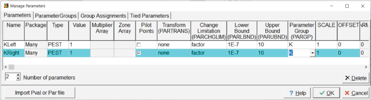
Screen capture of the “Manage Parameters” dialog box in which two parameters, “KLeft” and “KRight,” are defined.
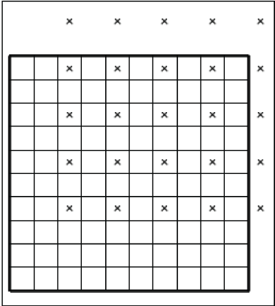
Screen capture illustrating the locations of the candidate pilot points on a simple 10-row × 10-column, 1-layer grid.
The pilot point buffer in this model is 290 m. Because the leftmost column of pilot points is more than 290 m from the center of any cell in the right half of the model (where pilot points are applied), that column of pilot points is not used (fig. 2). On the other hand, the pilot points above and to the right of the grid (except the one in the column 1) are within the pilot point buffer and are, therefore, used. Their initial values come from the cell to which each pilot point is closest. In addition, the second column of candidate pilot points is used because they are within 290 m of the right-hand side of the model where the “KRight” parameter is applied. The initial values of these pilot points come from the nearest cell on the right-hand side of the model.
The model has specified heads in the first and last columns (0.1 m in column 1 and 1.0 m in column 10). The model has four head observations: 0.45 m in row 2, column 3; 0.75 m in row 2, column 6; 0.35 m in row 8, column 3; and 0.65 m in row 8, column 6.
After PEST finishes running, the values assigned to the “Kx” data can be displayed
using “File|Import|Gridded Data Files....” Select the file containing the final values
in the “arrays” subdirectory of the directory in which the model ran to display the
values. The file has the extension .arrays. The final distribution of “Kx” is shown in figure 3. Note that the left half of the model, where no pilot points were used, has a uniform
distribution of “Kx” values; in the right half, where pilot points were used, the
hydraulic conductivity varies among the cells.
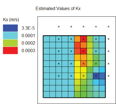
Diagram showing distribution of “Kx” values after PEST estimated parameters. Pilot points are shown on a simple 10-row × 10-column, 1-layer grid, with colors representing each of the 4 estimated “Kx” values (3.3×10⁻⁵, 0.0001, 0.0002, 0.0003).
Important PEST Usage Caveat
PEST is a universal parameter estimation code that can be applied to almost any forward-run model. PEST achieves this wide application because it operates—adjusts parameters and evaluates outputs—outside of the forward model code itself. Therefore, formulas assigning values to datasets are only applied in ModelMuse to create the files run by PEST. This aspect is especially important when a dataset is related to a direction such as the “Kx,” “Ky,” and “Kz” datasets in MODFLOW. Having PEST assign values to the “Kx” dataset does not mean that the “Ky” and “Kz” datasets are automatically updated to the MODFLOW forward run, too. Moreover, when “Kx,” “Ky,” and “Kz” are specified as independent parameters, there can be no expectation that geologically reasonable anisotropy is maintained as the parameter estimation proceeds. As far as PEST is concerned, those properties are independent unless specifically linked through parameter preprocessing outside of ModelMuse (for example, the PEST utility “PAR2PAR”; see the PEST manual for additional discussion [Doherty, 2018a, b]).
For MODFLOW models, there are options to estimate horizontal and vertical anisotropy instead of independently estimating “Ky” and “Kz”—this allows the use of parameter bounds to enforce geologically realistic anisotropy during the exploration of parameter space. For MODFLOW 6, these are options in the Node Property Flow (NPF) package (“K22OVERK” and “K33OVERK”). For the Layer Property Flow (LPF) package and Upstream Weighting (UPW) package, horizontal anisotropy is used automatically but vertical anisotropy can be specified by an option on the “Basics” tab of the MODFLOW “Layer Groups” dialog box. For the Block-Centered Flow (BCF) package, horizontal anisotropy is used automatically. Vertical leakance in the BCF package is a function of the vertical hydraulic conductivities of more than one layer. In the Hydrogeologic Unit Flow (HUF) package, all data are specified using parameters. You can define parameters for horizontal and vertical anisotropy in the HUF package. When working with the HUF package, the values assigned to cells can be a composite value from several hydrogeologic units. Values for individual hydrogeological units can be generated using HUFPrint (Banta and Provost, 2008) or functions built into ModelMuse for comparison with the conceptual model.
With SUTRA models, having PEST assign values to the dispersivity, permeability, or hydraulic conductivity in the “max” direction does not mean PEST will assign values in the “mid” or “min” directions unless anisotropy is used. ModelMuse allows the use of horizontal and vertical anisotropy for those datasets and anisotropy is used by default. The anisotropy options are specified on the “Anisotropy” pane of the “SUTRA Options” dialog box. When these options are used, ModelMuse generates a template file for the main SUTRA input file that uses a formula to relate the “mid” or “min” datasets to the corresponding “max” dataset.
Using PEST Parameters With Model Features
Model features include boundary conditions and other inputs that affect groundwater flow such as wells in MODFLOW models or specified pressures in SUTRA models. Model features are used to define model inputs having a spatial component that does not necessarily apply to every cell, node, or element in the model. Many, but not all, model features vary with time. For model features that do not vary with time, a formula can be specified that is either a PEST parameter name or the name of a dataset for which PEST parameters are used. If the name of a PEST parameter is specified, the value of the PEST parameter is substituted into the model input file when PEST estimates parameters. If the name of a dataset whose values are modified by PEST is specified, the updated value from the dataset is substituted into the model input file.
In cases where temporal variation exists in a model feature, the times and formulas for the model feature are entered in a table in the “Object Properties” dialog box. The top two rows of these tables are reserved for the PEST modifier and the modification method (fig. 4). The PEST modifier is optional. If the PEST modifier is specified, it must be either a PEST parameter or the name of a dataset for which PEST parameters are used.
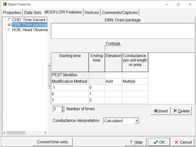
Screen capture of the “Object Properties” dialog box showing new rows for the PEST modifier and the modification method.
The modification method determines how the PEST modifier is used. The method must be either “Add” or “Multiply.” If “Add” is used, all values for all times have the value from the PEST modifier added to them. If “Multiply” is used, all values for all times are multiplied by the value from the PEST modifier. PEST modifiers are used when the modeler wants all values for a particular feature to be varied in a coordinated fashion. The modification method is generally set to “Add” for elevation-related items and to “Multiply” for all others.
If the modeler wants to use different parameters for different times, this can be done by using the name of a PEST parameter or a dataset for which PEST parameters are used as the formula for an individual time. When generating the input files for the model, the value of the PEST parameter or the value from the dataset is substituted into the input file.
It is possible to use a formula determined by a PEST parameter for an individual time and at the same time use a PEST modifier for the entire series. When generating the model input file, the value supplied in the model input file is affected by both.
PEST Calibration Observations
When PEST estimates parameters, it compares simulated values from the model with measurements representing the modeled system. From a model calibration standpoint, it is important to have a variety of observation types. For example, head observations are widely available for calibrating models, but head observations alone are usually insufficient to constrain many important model inputs. For example, if the model parameters include recharge and hydraulic conductivity, head-observation data alone only allow for estimation of the ratio of the recharge rate to the hydraulic conductivity but do not allow for independent estimation of both the recharge rate and the hydraulic conductivity (for example, Haitjema, 2006). PEST provides the means to overcome such parameter correlation (for example, the Tikhonov regularization application of Hunt and others, 2019), but, generally, a minimum of head- and flow-type observations are considered necessary for calibration (Anderson and others, 2015). The inclusion of many types of observations, however, typically provides more robust calibration results (Hunt and others., 2006).
Sometimes the difference between two simulated values is more helpful in estimating
parameters than the simulated values themselves (Doherty and Hunt, 2010; Anderson and others, 2015). Typically, such comparisons involve simulated values of the same type and time
at different locations that define a spatial gradient or simulated values of the same
type and location at different times that define a temporal change. Both types can
be defined in the “Comparison Observations” dialog box. Temporal changes are typically
defined when a single object is used to specify observations at different time. In
such cases, the user can define comparison observations in the same dialog where the
direct observations are defined—usually this is the “Object Properties” dialog box.
When ModelMuse generates the model input files, it also generates two input files
for one of the utility programs: “Mf6ObsExtractor,” “Mf2005ObsExtractor,” or “SutraObsExtractor.”
Depending on the version of the forward model selected, the utility program processes
the model output files to generate simulated values that can be compared with observed
values. The other input file causes the utility to generate an instruction file used
by PEST to read the model results. The instruction file is generated when the model
is run from ModelMuse. The simulated values are extracted when PEST is running the
model through the RunModel.bat batch file.
For all calibration observations for PEST, an observation name, the observed value, the observation weight, and an observations group must be defined. Observation weights are important for prioritizing calibration tradeoffs that arise; Doherty and Hunt (2010) and chapter 9 of Anderson and others (2015), among others, discuss the importance of weighting for the parameter estimation process. Observation groups are defined in the “Observation Group Properties” pane of the “PEST Properties” dialog box.
MODFLOW 6
MODFLOW 6 provides the “Observation Utility” to generate time-series of simulated values of many sorts, including heads and flows through boundaries. The simulated values are written at each time step and may refer to values at a single cell or for a group of cells. ModelMuse allows the user to define calibration observations for use with PEST based on the output of the “Observation Utility.” For head observations, calibration observations are computed by interpolating in space and time to the observation location and time. For structured grids, bilinear interpolation is used from the surrounding cell centers within a layer to the observation location. For unstructured (discretization by vertices [DISV]) grids, a linear, triangular, or quadrilateral basis function (Wang and Anderson, 1982) is used for spatial interpolation within a layer. The type of basis function is chosen automatically depending on the number of active cells surrounding the observation. Spatial interpolation among more than four points is not supported. Temporal interpolation is performed by linear interpolation between the time preceding and succeeding the observation time. Flows through boundaries may involve adding the flows from several objects. All calibration observations are defined on the “Calibration” tab of the “Observation Utility” pane of the “Object Properties” dialog box.
Multilayer head observations are defined in horizontal space by point observations on the top view of the model in which the “Multilayer” checkbox on the “Calibration” tab is checked and in which the object has information that tells ModelMuse that the point object intersects more than one layer. The information takes the form of “Z formulas” that define the well-screened interval. If the “Multilayer” checkbox is not checked, the observation is treated as a single-cell observation and the cell that has the longest length of intersection between the cell and the well screen is the cell used for the observation. Transmissivity weighting is applied to the individual cells that make up the multilayer head observations based on the product of the cell hydraulic conductivity in the x direction (“Kx”) and the length of intersection between the well screen and the cell. The transmissivity weights used for the composite head calculation remain constant during parameter estimation even if “Kx” is changed during parameter estimation.
MODFLOW–2005
MODFLOW–2005 and related models, such as MODFLOW–NWT, have a built-in mechanism for defining head and flow observations at specified locations and times. Several other packages also generate simulated values that can be compared with observed values. As described in the MODFLOW–2005 documentation (Harbaugh, 2005; see also Hill and others, 2000), MODFLOW–2005 interpolates head observations in time and space to the location and time of the head observation. Head observations are defined in the Head Observation Package. Individual head observations are specified in the “Head Observations” pane of the “Object Properties” dialog box. Observations of flow through boundaries can be defined in the CHOB, DROB, GBOB, RVOB, and STOB packages.1 Individual flow observations are defined in the “Manage Flow Observations” dialog box.
The abbreviations are as follows: CHOB, Specified-Head Flow Observation package; DROB, Drain Observation package; GBOB, General-Head-Boundary Observation package; RVOB, River Observation package; and STOB, Stream Observation package.
ModelMuse generates input for “Mf2005ObsExtractor” so that output files from several other packages can be used for model calibration (for example, the Gage package [GAGE]). If the Lake package (LAK) is used, lake gages can be used to export various lake properties such as the lake stage or the inflow or outflow from the lake. These can be used to define calibration observations on the “Calibration” tab for the Lake package in the “Object Properties” dialog box. On the “Gage” tab, ensure that data of the desired feature type will be saved. If the Multi-Node Well package version 2 (MNW2) is used, the head in the well or well flows can be used as calibration observations. These are defined on the “Calibration” tab on the “MNW2 Package” pane in the “Object Properties” dialog box. If the Streamflow-Routing package (SFR) is used, calibration observations for it can be defined on the “Calibration” tab on the “SFR” pane and the “Calibration” tab of the “GAGE” pane, which are both in the “Object Properties” dialog box. If subsidence is simulated using either the Subsidence and Aquifer-System Compaction (SUB) or Subsidence and Aquifer-System Compaction Package for Water-Table Aquifers Pane (SWT) packages, observations related to subsidence can be defined on the “SUB” and “SWT” panes, which are both in the “Object Properties” dialog box. If the Seawater Intrusion package (SWI2) is used and observations are used, the “SWI2” pane in the “Object Properties” dialog box can be used to define observations of Zeta. Observations defined for the SUB, SWT, or SWI2 packages are interpolated by “Mf2005ObsExtractor” in the same way that head observations are interpolated by MODFLOW–2005.
SUTRA
SUTRA has built-in capabilities for defining observations at particular places and times. These fall into two classes. Observations of state variables are specified in the Sutra State “Calibration Observations” pane of the “Object Properties” dialog box. Observations of flow-through boundaries and related variables are specified in the “Manage SUTRA Boundary Observations” dialog box.
PEST Control Variables
Besides the definitions of parameters and observations, there are other variables
required in the PEST control file. These are specified in the “PEST Properties” dialog
box. The help for the “Pest Properties” dialog box contains abbreviated descriptions
of the functions of these variables. For fuller documentation, see the PEST documentation
distributed with PEST (Doherty, 2018a). Most commonly, the NOPTMAX variable (Number OPTimization MAXimum) is varied to
specify the PEST run mode, such as 1 forward run to assess the PEST workflow (NOPTMAX=0) or maximum number of parameter estimation tries to improve the model fit (for example,
15 tries would be NOPTMAX=15).
Running PEST
When creating the files needed to run the forward model and PEST, ModelMuse creates
two separate batch files to run the model. One of them is named RunModel.bat and is used by PEST to run the model. The other is named either RunModflow.bat or RunSutra.bat. Depending on the type of model, one or the other of the latter batch files must
be run once before starting PEST to run a utility program to create an instruction
file for PEST. Typically, running this latter batch file is the last step taken by
ModelMuse when exporting the model input files. The batch file may also have instructions
to run PLPROC scripts that calculate kriging factors. The RunModel.bat file runs a utility program to extract simulated values in the format specified in
the instruction file. The RunModel.bat file may also perform kriging interpolation among pilot points using the kriging
factors generated with the RunModflow.bat or RunSutra.bat files.
If pilot points are used, ModelMuse also creates a covariance matrix file for each set of pilot points on each layer. The covariance files help constrain the values assigned to pilot points by assigning it to the PEST variable “COVFLE” in the “Observations Groups” section of the PEST control file. Each covariance matrix file is created in a separate batch file. The modeler can examine the input to each batch file and rerun them with different options, if desired. The covariance matrix files are created using two utility programs from the PEST groundwater utilities: “MKPPSTAT” and “PPCOV_SVA.”
Once the model is running properly (before using PEST but with all the parameters and calibration observations defined), the modeler runs the model once from ModelMuse. Doing this ensures that the instruction file for PEST and any required kriging factors files are created. Next, the modeler runs PEST by selecting “File|Export|PEST|Export” PEST control file. There are three radio buttons at the bottom of the “Save As” dialog box: “Don't run,” “Run PESTCHEK,” and “Run PEST.” By default, “Run PESTCHEK” is selected. Always running “PESTCHEK,” a utility program that checks PEST settings before running PEST, is important. If “PESTCHEK” detects errors, the modeler must correct them before attempting to run PEST. If the errors involve parameters or observations, the modeler may need to rerun the ModelMuse model-building utilities. Otherwise, the modeler may be able to make corrections in the “PEST Properties” dialog box and export the PEST control file again without exporting all the model input files or running the model.
Once no errors are detected by “PESTCHEK,” the modeler can run PEST by selecting “Run
PEST” in the “Save As” dialog box. It is also possible to run “PESTCHEK” or PEST using
batch files named RunPestChek.bat and RunPest.bat. The batch files are created at the same time the model input files are created.
Using SVD-Assist
“SVD-Assist” is described in chapter 10 of the PEST user manual (Doherty, 2018a, p. 199) and in Doherty and Hunt (2010). “SVD-Assist” appreciably reduces the computational burden of calibration. Using SVD-Assist requires the use of the “PSTCLEAN” utility program. If the “i64” version of PEST is used, it may be necessary to install the “PSTCLEAN” utility program from one of the other distributions in the PEST directory because, at the time of this writing, it is not included in the 64-bit distribution file.
If “SVD-Assist” is used with “Singular Value Decomposition” in PEST, “super-parameters” can be used to reduce the PEST execution time. The general sequence of actions to use “SVD-Assist” is as follows:
-
1. Generate the Jacobian matrix by running PEST with the maximum number of PEST iterations (NOPTMAX) generally set to –2.
-
2. Choose the number of “super-parameters” to use. The PEST utility program “SUPCALC” can be used to assist with this and the previous step.
-
3. Generate a modified PEST control file with “SVDAPREP.”
-
4. Run PEST with the modified PEST control file.
-
5. Use “PARREP” to generate new model input files using the best estimated parameter values or the parameter values from any of the PEST iterations.
-
6. Assess the final model and its results.
If the modeler chooses to use “SUPCALC” to estimate an appropriate number of super-parameters
to use, the modeler can select “File|Export|PEST|Calculate Number of Super-Parameters”
to display the “SUPCALC Options” dialog box. In it, the modeler can select an existing
PEST control file and specify a value greater than zero for the expected value of
the measurement-objective function. ModelMuse backs up the existing PEST control file,
creates a new PEST control file with NOPTMAX set to –2, and (optionally) runs PEST
to generate the Jacobian matrix. The Jacobian matrix (.jco file), is created through a base run at initial values and additional runs where
each parameter is perturbed independently; therefore, one run more than the number
of adjustable parameters is required. Next, the original PEST control file is restored
and “SUPCALC” modifies the PEST control file. Running PEST is only required to generate
the Jacobian matrix if the Jacobian matrix file (*.jco) does not already exist. “SUPCALC” displays the minimum and maximum number of super-parameters
to use to achieve the expected value of the measurement objective function. These
guidelines can assist the user in selecting the number of super-parameters in the
next step.
The time required to run the model may place an upper limit on the number of super-parameters that is practical. One option is to limit the number of super-parameters to the number that allows PEST to finish parameter estimation in 1 day followed by performing a sensitivity analysis using the “SENSAN” utility described in the PEST documentation with a varying number of super-parameters.
Next, the user can select “File|Export|PEST|Modify PEST Control File” with “SVDAPREP” to display the “SVDAPREP Input” dialog box. This dialog box allows generation of a PEST control file suitable for use with “Singular Value Decomposition” by running the “SVDAPREP” PEST utility program and then run PEST with the modified PEST control file.
Though automatically handled within the utility, the following discussion covers what
steps occur when modifying the PEST control file with “SVDAPREP.” A new PEST control
file is exported followed by an input file for “SVDAPREP.” After creating the input
file for “SVDAPREP,” ModelMuse checks whether the working directory contains the PEST
utility programs “PARCALC” (parcalc.exe) and “PICALC” (picalc.exe). If not, ModelMuse copies the files from the PEST directory into the working directory.
These programs are used by PEST to convert super-parameters into base parameters when
running the parameter estimation. ModelMuse then creates a batch file to run “SVDAPREP,”
which is described in detail in chapter 10.2 of the PEST documentation (Doherty, 2018a, p. 203). The first command in the batch file calls the PEST utility program “PSTCLEAN,”
which removes comments from the PEST control file and creates a new PEST control file.
The name of the file is the same as the original name but with _Svda added to the file root. The next command in the batch file causes “SVDAPREP” to generate
another PEST control file. The name of the file is the same as the original name but
with _PostSvda added to the file root. If the option to run PEST is selected, the final command
in the batch file runs PEST with the control file generated by “SVDAPREP.” If the
option to run “SVDAPREP” is selected, ModelMuse starts the batch file that runs “SVDAPREP.”
When parameter estimation is complete, PEST normally conducts a final run using the
estimated parameter values, but this is not possible when “SVD-Assist” is used. However,
the user can initiate a run by using the PEST utility program “PARREP.” This action
is accomplished by selecting “File|Export|PEST|Replace Parameters in PEST Control
File” and then selecting the .bpa file generated by PEST. The root of the .bpa file is the PEST control file used as the input for “SVDAPREP.” Note that the user
can also select any of the parameter sets from any of the individual iterations. “PARREP”
creates a new PEST control file having a root that ends with _svda_parrep. PEST then runs the model once with the estimated parameter values.
Visualizing Residuals
One way of assessing the quality of model calibration is to look at the residuals,
which are the differences between the observed values and the simulated values generated
by the model. Ideally, the residuals should be small and not exhibit obvious trends.
ModelMuse can display the weighted residuals on the top view of the model using the
“PEST Observation Results” pane of the “Data Visualization” dialog box. To display
the residuals, select the residuals file (.res) generated by PEST and click the “Apply” button in the “Data Visualization” dialog
box. ModelMuse reads the file and displays its data in a table sorted by the absolute
value of the residual. The weighted residuals are plotted as circles on the top view
of the model. The area of the circles varies with the absolute value of the weighted
residual and the color of the circle represents the sign of the weighted residual
as calculated, observed minus simulated.
Only some types of residuals can be plotted spatially as described above. The spatial plot includes only those residuals related to a single object having a single vertex so that there is a unique location for the residual. In addition to the spatial plot, the “PEST Observation Results” pane generates a graph of the weighted residual versus observed value. This graph includes all the data from the residuals file, including residuals for prior information equations.
Visualizing Modified Model Input
PEST operates by modifying the input files for MODFLOW and SUTRA. Those changes to the input files do not affect how the model is defined in ModelMuse. If a model is run again from ModelMuse, all the inputs are the same as they were before parameter estimation was performed. However, ModelMuse provides ways of importing and visualizing the modified model inputs created by PEST. The methods vary depending upon the type of model and the type of input:
• If PEST parameters are used with a dataset, a file for each layer of the dataset in the model is created in the “arrays” subdirectory of the working directory of the model. Data in the files can be imported into ModelMuse with the “File|Import Gridded Data” command.
• For MODFLOW–2005 and related models, the entire model can be imported into a new ModelMuse project with the “File|Import|MODFLOW–2005” or “–NWT Model” command. Once this is done, any part of the model can be visualized with the “Data Visualization” dialog box.
• For MODFLOW 6 models, model feature values can be visualized using “File|Import|MODFLOW 6 Feature.”
• For SUTRA models, model feature values can be visualized using “File|Import|SUTRA Feature.” In addition, data from datasets 14B, 15B, and the “SUTRA Initial Conditions” file can be imported using “File|Import|SUTRA Files.” SUTRA also generates boundary-condition output files that indicate how boundary conditions were applied in the model. Data from these files can be imported by selecting “File|Import|Model Results.”
Model feature datasets imported from both MODFLOW 6 and SUTRA models are classified under “Optional|Model Results|Model Features” in the “Data Visualization” dialog box.
Limitations
-
• ModelMuse does not currently support parameter estimation of models that employ local grid refinement such as MODFLOW–LGR (Mehl and Hill, 2013).
-
• ModelMuse does not currently support parameter estimation of PHAST (Parkhurst and others, 2004), MT3DMS (Zheng and Wang, 1999), MT3D–USGS (Bedekar and others, 2016), or MODPATH (Pollock, 2016) models.
-
• ModelMuse was not specifically designed to support the use of PEST++ (White and others, 2020). However, the PEST control file generated by ModelMuse can be used with PEST++, although it may require small modifications in some cases.
-
• ModelMuse can only import MODFLOW–2005 and MODFLOW–NWT models, even though it can be used for parameter estimation for other MODFLOW–2005 based models such as MODFLOW–OWHM (Hanson and others, 2014).
Example
The example presented here is a variation of the Rocky Mountain Arsenal example included in the “Help” section and in previous versions of ModelMuse (Winston, 2009, 2014, 2019; Winston and Goode, 2017). A previous tutorial showed how to simulate this conceptual model with MODFLOW–2005. For users unfamiliar with ModelMuse, it is advisable to go through one or more of the previous examples to gain familiarity with ModelMuse. Instructions for the examples can be found under “Help|Examples.”
The example used here starts with a working MODFLOW 6 version of the model and demonstrates
how to use PEST with it. ModelMuse is distributed with three ModelMuse files. One
of the files is used as the starting point of the exercise. Another model is a modified
version of the first with spatially varying hydraulic conductivity and a different
infiltration rate in a discharge pond. This model was treated as the “true” model
and used to generate simulated values for the exercise. The final file contains the
completed model—it has been set up to perform parameter estimation. The installer
places these files in the C:\Users\Public\Documents\ModelMuse Examples\examples\PEST\MODFLOW 6 folder. If ModelMuse is installed manually, the files are in the examples\PEST\MODFLOW 6 folder of the distribution file.
This exercise teaches users (1) how to specify observations and use parameters for both datasets and boundary conditions in ModelMuse and (2) how to visualize the characteristics of the calibrated model. Two additional exercises for PEST are included in the ModelMuse “Help.” One exercise is for a MODFLOW–2005 model and the other is for a SUTRA model.
Before explaining how to use PEST with this example, the conceptual model must be reviewed. The aquifer is simulated as confined. The steady-state model has a lake at the northern end and a stream at the southern end, both of which are modeled as specified head boundaries (fig. 5). The lake has a head of 75 m. The stream head varies from 23.5 m near its eastern end to 5 m near its western end. Bedrock outcrops on the east, west, and south sides are considered impermeable and partially delimit the active area of the model. In addition, two bedrock outcrops within the model area are treated as inactive areas. A disposal pond in the northern half of the study area acts as a source of water and solute in addition to the lake. There are two production wells in the southern half of the model. The disposal pond is a potential source of contaminants to the production wells. The model is intended to help assess this problem.
In the uncalibrated version of the model, the flow rate out of the disposal pond is estimated at 0.03 cubic meter per second (m3/s). The estimated hydraulic conductivity is 0.0001 meter per second (m/s). The models all have head observations and a flow observation. The head observations are scattered throughout the model area. The flow observation encompasses part of the discharge into the stream. The parameters to be estimated are the hydraulic conductivity and the flow rate of the disposal pond.
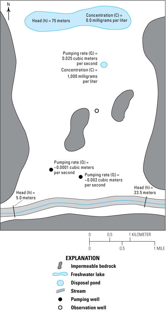
Diagram of Rocky Mountain Arsenal example model area showing a freshwater lake, a disposal pond, pumping and observation wells, impermeable bedrock, and a stream.
Because this model has only confined layers and the only boundary conditions are specified heads and specified flows, it is a linear model. That should make estimating parameters for this model easier than would often be the case in practice.
The MODFLOW 6 model differs from the MODFLOW–2005 version of the model by having a DISV grid. The DISV grid has a refined area around the extraction wells in the southern half of the model. The Ghost Node Correction package is used with the explicit option; the implicit option makes the model unstable. To use PEST with the model, the following tasks are performed:
-
• Activate PEST.
-
• Define parameters to use in the model.
-
• Define parameter groups and assign parameters to them.
-
• Apply parameters to datasets.
-
• If desired, define pilot points.
-
• Apply parameters to boundary conditions.
-
• Define observations.
-
• Define observation groups.
-
• Assign observations to observation groups.
-
• Define prior information equations for Tikhonov regularization (Doherty, 2018a).
-
• Run PEST.
-
• Visualize weighted residuals.
-
• Visualize the modified model input.
Use Anisotropy
There are two things to estimate in the example model: the hydraulic conductivity distribution and the seepage rate from the disposal pond. Initially, a uniform hydraulic conductivity of 0.0001 m/s was assigned because only information on the bulk properties of the system was available, not the actual spatial distribution; this value was a best guess about the average hydraulic conductivity.
In MODFLOW, there are three components of the hydraulic conductivity to assign, as represented by the datasets “Kx,” “Ky,” and “Kz.” In this case, “Kz” is unimportant because there is only one layer. It is important to note that “Kx,” “Ky,” and “Kz” are all independent datasets, so if only “Kx” is estimated, “Ky” is unaffected. In ModelMuse, the default formula for “Ky” is “Kx” (so that the system is horizontally isotropic), so normally, keeping them in sync with one another is not a concern (assuming that is the desired goal).
Once the MODFLOW input files are being modified by PEST, however, that is not the default situation. The NPF package has options for using horizontal and vertical anisotropy instead of directly specifying “Ky” and “Kz.” To use those options, select “Model|MODFLOW Packages and Programs,” and, in the NPF package, select the option to use horizontal anisotropy (fig. 6). Typically, the option to use vertical anisotropy would be selected, but that has no effect in this model because there is only one layer.
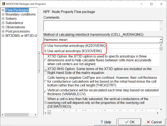
Screen capture of the “MODFLOW Packages and Programs” dialog box illustrating activation of the options to use horizontal and vertical hydraulic conductivity by checking the “Use horizontal anisotropy (K22OVERK)” and “Use vertical anisotropy (K33OVERK)” checkboxes.
Continue if No Convergence
PEST runs models multiple times. During the testing of potential parameters, the model might not always meet the convergence criteria but still reach an acceptable solution. If the model halts prematurely because of this, PEST may not be able to continue. There is an option in MODFLOW 6 to deal with this situation. Select “Model|MODFLOW Packages and Programs” and go to the pane for the “IMS solver.” Check the “Continue even if no convergence” checkbox (fig. 7).
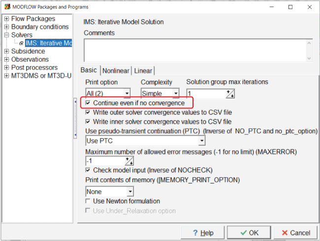
Screen capture of the “MODFLOW Packages and Programs” dialog box illustrating use of the “Continue even if no convergence” option by checking the associated checkbox.
Activate PEST
To activate PEST, select “Model|PEST Properties...” and check the checkbox labeled “Use PEST” on the “Basic” pane (fig. 8). Be sure that the PEST directory is set to the directory where PEST is installed. By default, the PEST mode is set to “regularization” on the “Control Data|Mode and Dimensions” pane. The regularization mode activates Tikhonov regularization.
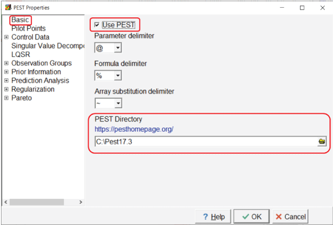
Screen capture of the “PEST Properties” dialog box illustrating activating PEST. The “Use
PEST” checkbox is checked and C:\Pest17.3 is entered in the “PEST Directory” field.
Define Parameters and Parameter Groups
The next step is to define parameters. Select “Model|Manage Parameters...” In the “Manage Parameters” dialog box, set the number of parameters to 2. Two parameters are then defined: “K” and “Seepage.” During parameter estimation, the data values already specified in the model are multiplied by the parameter value. Initially, both parameters are assigned a value of 1 so that the multiplication leaves the model data unchanged.
“K” affects the hydraulic conductivity, and “Seepage” affects the flow rate from the seepage pond. For “K,” “PEST” must be selected as the parameter type (fig. 9). For “Seepage,” either “PEST” or “Q” can be selected. In this case, “PEST” is chosen. A value of 1 is assigned to both parameters. The estimated distribution of hydraulic conductivity is desired, not just its average value. Pilot points can be used for making spatially distributed estimates, so pilot points are used with the “K” parameter. Parameters that cannot have negative values are typically log transformed (Doherty and Hunt, 2010) so the “K” parameter is log transformed, but no transformation is used for the “Seepage” parameter, as the pond can gain from (negative sign) or lose to (positive sign) the groundwater system. “Factor” is used for the change limitation for the “K” parameter and “relative” for the “Seepage” parameter. The lower and upper bounds for the “K” parameter are 0.01 and 100, respectively. The lower and upper bounds for the Seepage parameter are –0.001 and 100, respectively. The scale and offset are set to 1 and 0, respectively, for both parameters. On the “Parameter Groups” tab, set the number of parameter groups to 2. Name the parameter groups “KGrp” and “WellGr” (fig. 10). All of the default values are used for the parameter groups.
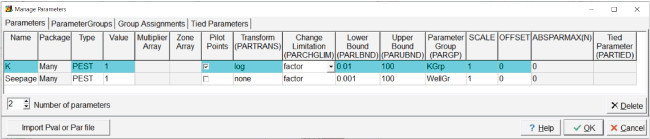
Screen capture of the “Manage Parameters” dialog box showing properties assigned to “K” and “Seepage” parameters.
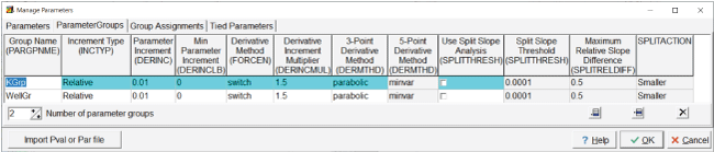
Screen capture of the “Manage Parameters” dialog box showing properties assigned to “KGrp” and “WellGr” parameter groups.
Define Pilot Points
To define pilot points, select “Model|PEST Properties” and go to the “Pilot Points” pane (fig. 11). Consistent with suggestions of Doherty and Hunt (2010), regularly spaced pilot points with a square pattern and a pilot point spacing of 800 m are used. The pilot point buffer is set to 1,200 m and the candidate pilot points are shown.
ModelMuse allows pilot points to be defined outside of the model. If a parameter is assigned to the entire model, the initial value for a pilot point inside the active area of the model is the dataset value at the pilot point location. If the pilot point is outside of the model or in an inactive cell but the distance from the pilot point to an active cell is less than the pilot point buffer, the value assigned to the pilot point is the value of the dataset at the closest cell that assigns a value to that parameter.
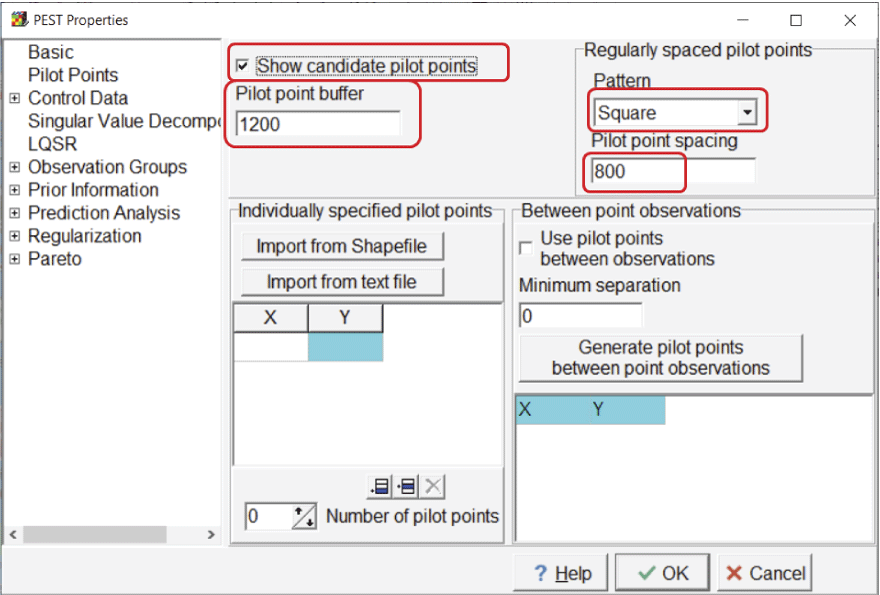
Screen capture of the “PEST Properties” dialog box showing options for pilot points. The “Show candidate pilot points” checkbox is checked, the “Pilot point buffer” field has an entry of “1200,” the “Pattern” dropdown list selection is “Square,” and the “Pilot point spacing” field has an entry of “800.”
Apply K Parameter
So far, the “K” parameter has been defined but not applied to any dataset. To apply the “K” parameter to the “Kx” dataset, select “Data|Edit Data Sets...” and select the “Kx” dataset. On the “PEST Parameters” tab, check the “PEST parameters used” checkbox and select the “Apply” button. A new dataset is created and named “Kx_Parameter_Names.” Set the default formula for it to “K” and select the “Apply” button again (fig. 12). If only the “K” parameter is to be applied to part of the grid, it can be done by assigning the formula for “Kx_Parameter_Names” with an object. Wherever the parameter is applied, “Kx” is multiplied by the parameter value. In this case, the parameter value is 1, so “Kx” remains thus far unchanged.
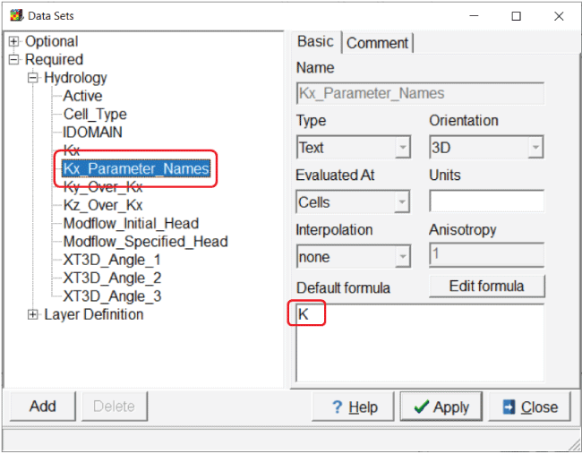
Screen capture of the “Data Sets” dialog box illustrating the default formula for the “Kx_Parameter_Names” dataset. “K” is entered in the “Default formula” field.
Apply Seepage Parameter
Apply the Seepage parameter to the well flow rate for the “Disposal_Pond” object by opening the “Object Properties” dialog box and double-click the “Disposal_Pond” object on the top view of the model. On the “MODFLOW Features” tab, select “Seepage” as the “PEST Modifier” (fig. 13). The “Modification Method” can be left at the default value of “Multiply.” In addition to the PEST parameters, the “Kx” dataset can be chosen because it is a dataset modified by PEST. In this case, choosing “Kx” does not make sense. The value of the “Seepage” parameter could also be set to 0.03, and instead of specifying a PEST modifier, “Seepage” could be used as the formula for the pumping rate.
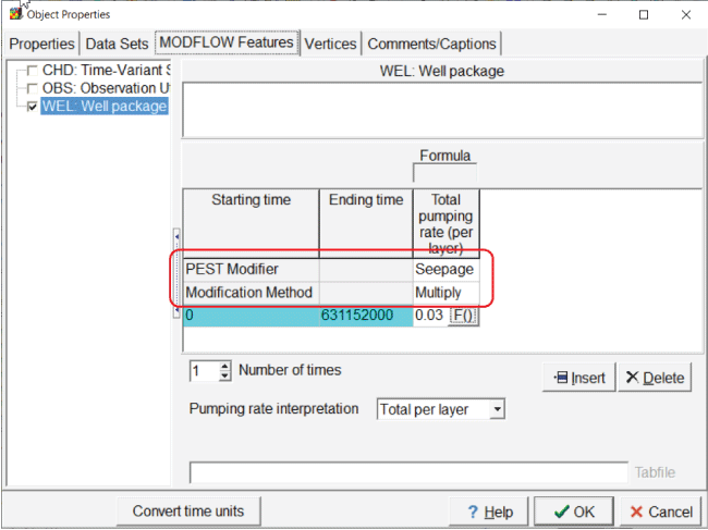
Screen capture of the “Object Properties” dialog box illustrating the application of the “Seepage” parameter to the disposal pond flow rate. In the “Total pumping rate (per layer)” column, “Seepage” is entered for the “Pest Modifier” row and “Multiply” is entered for the “Modification Method” row.
Define Observations
MODFLOW 6 has an “Observation Utility” that can generate a time series of simulated values of various types of data generated by the model. ModelMuse can create an input file for “Mf6ObsExtractor” that causes Mf6ObsExtractor to extract simulated values from the time series for use with PEST. For head observations, ModelMuse spatially interpolates to the observation location, and it also interpolates in time to the observation time. Note that observation times must be relative to the time “0” used for the MODFLOW stress periods. Calibration observations must have an observed value, which is compared with the simulated value and must also be assigned a weight. Depending on the observation type, other types of information might be required.
Eight head observation and one flow observation were already defined in the model (table 1). Now these need to become calibration observations. A comparison observation that represents a head gradient between two of the head observations is also assigned. The head observations are defined by point objects. The flow observation is defined by a polygon object that surrounds part of the object that defines the constant-head boundary near the southern edge of the model. Only those constant head cells whose centers are inside the polygon object are part of the flow observation. The observation values are shown in table 1. In this example, the observation locations were already defined. It is also possible to import multiple observations from shapefiles using the “Import Shapefile” dialog box.
Open each of the objects that defines a head observation one at a time in the “Object Properties” dialog box and go to the “Observation Utility” pane on the “MODFLOW Features” tab. Beneath the “Observation” location name, select the “Calibration” tab. In the table for direct observations, enter the observation name, set the series type to “General” and the “Observation” type to “Head.” Leave the observation group (OBGNME) empty for now, and specify the observation time as “631152000,” which is the ending time of the model. Set the observed value according to table 1 and set the weight to 1 (fig. 14). Repeat this for each of the head observations. If the model had multiple time steps, multiple direct observations using different times could be specified. Comparison observations can also be specified in the table in the lower half of the “Calibration” tab. For heads, a comparison observation is the equivalent of a drawdown observation.
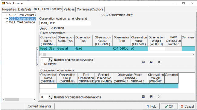
Screen capture of the “Object Properties” dialog box showing the properties of the head observation. The “Observation Time” field is set to “631152000,” and the “Observation Weight “ field is set to “1.”
The observation of flow through the southern stream is defined with the object “CHD_Obs.” The flow observation is defined similarly to the head observation, except that the observation type is CHD and the observation weight is 10 instead of 1 (fig. 15).
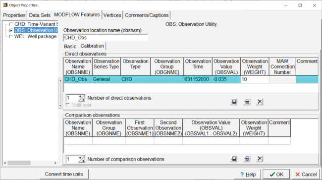
Screen capture of the “Object Properties” dialog box showing the properties of the flow observation. The “Observation Time” field is set to “631152000,” the “Observation Value” field is set to “–0.035,” and the “Observation Weight” field is set to “10.”
The observed gradient in head between head observations 5 and 8 is also used as a calibration observation. To add this observation, select “Model|Edit Comparison Observations...” Specify the observation name, value, and weight (= 3) and select the Head_Obs5 as the first observations and Head_Obs8 as the second observation (fig. 16).
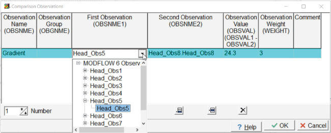
Screen capture of the “Comparison Observations” dialog box illustrating how to specify a comparison observation. In the “First Observation” directory, “Head_Obs5” is selected; in the “Second Observation” column, “Head_Obs8.Head_Obs8” is selected. In the “Observation Value” and “Observation Weight” fields, the values “24.3” and “3” are entered, respectively.
Define Observation Groups
PEST requires that observations be assigned to observation groups, so the observation groups must be defined, and this is done in the “PEST Properties” dialog box. Select “Model|Pest Properties” and the “Observation Group Properties” pane, change the number of observation groups, and specify the names of the observation groups: “Heads,” “CHD,” and “Comparison” (fig. 17). The use of separate observation group names is not required for the parameter estimation, but this is recommended because it facilitates tracking how well different observations are simulated.
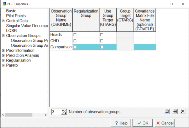
Screen capture of the “Pest Properties” dialog box illustrating the definition of the observation groups. “Heads,” “CHD,” and “Comparison” are listed in the fields under the “Observation Group Name” column head.
Next, go to the “Observation Group Assignments” tab, expand the list, and select all head observations. Select these by clicking on the first observation, holding the shift key down, and then clicking on the last observation. Click on one of the observations again, and, while holding the mouse button down, drag the cursor down to the “Heads” group and release the mouse button. Assign the other two observations to the “CHD” and “Comparison” groups, respectively (fig. 18).
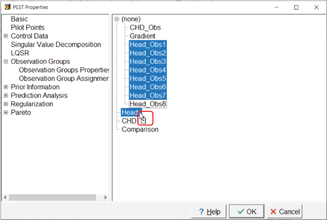
Screen capture of the “Pest Properties” dialog box illustrating the assignment of observation groups. “Head_Obs1” through “Head_Obs8” are highlighted and the cursor is shown as dragging them to the “Heads” group in the directory.
Tikhonov Regularization
By default, ModelMuse defines several regularization equations. Including such equations allows the user to inform the level of fit and help stabilize the parameter estimation process. Tikhonov regularization information is defined on the “Prior Information Group Properties,” “Initial Value Prior Information,” “Within-Layer Continuity Prior Information,” and “Between-Layer Continuity Prior Information” panes in the “PEST Properties” dialog box.
When PEST performs parameter estimation in regularization mode, each parameter is compared with a preferred value. The first type of regularization equation compares the current value of the parameter with its preferred value, as represented by the initial value specified by the modeler at the beginning of parameter estimation. This preferred condition is applicable to all parameters. A second type, a preferred homogeneity condition, only applies to parameters associated with pilot points. In that situation, the current value of a pilot point is compared with the values of neighboring pilot points applied to the same zone. The third type of regularization equation also only applies to parameters that are associated with pilot points, but the preferred homogeneity condition is evaluated at the same parameter at the same location on adjacent layers.
Finally, the degree of fit the modeler desires is specified by the PEST “PHIMLIM” variable (Fienen and others, 2009; Doherty and Hunt, 2010; Anderson and others, 2015, chap. 9). “PHIMLIM” represents a target-measurement objective function, which controls the tradeoff between fit and adherence to preferred parameter conditions. Typically, for the first run of PEST, “PHIMLIM” is set very low (10–10) to discard the parameter preference and assess the best fit possible for a given conceptual model; that best-fit objective function is then increased (for example, 110 percent of the best fit value), specified as the new “PHIMLIM” value, and PEST is rerun. Typically, “PHIMACCEPT” is changed to be 5–10 percent larger than “PHIMLIM.” Users should review Fienen and others (2009) and chapter 9 in Anderson and others (2015) for additional discussion of this critically important PEST variable. “PHIMACCEPT” is used in choosing new Marquardt lambdas and is explained in more detail in the “Help” for the “Regularization Controls” pane.
Open the “PEST Properties” dialog box and go to the “Prior Information Group Properties” pane. Define two groups and make them regularization groups (fig. 19).
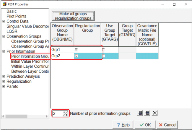
Screen capture of the “PEST Properties” dialog box after creating two prior information groups. In the “Observation Group Name” column, “Grp1” and “Grp2” are, respectively, in the first two fields. In the “Regularization Group” column, the two associated checkboxes are checked. The “Number of prior information groups” field is set to “2.”
On the “Initial Value Prior Information” pane, assign both parameters to one of the groups (fig. 20).
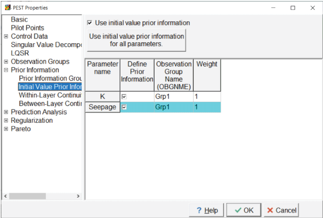
Screen capture of the “PEST Properties” dialog box showing the assignment of parameters to a prior information group. The “Use initial value prior information” checkbox is checked.
Next, go to the “Within-Layer Continuity Prior Information” pane and specify the search distance and the observation-group name (fig. 21).
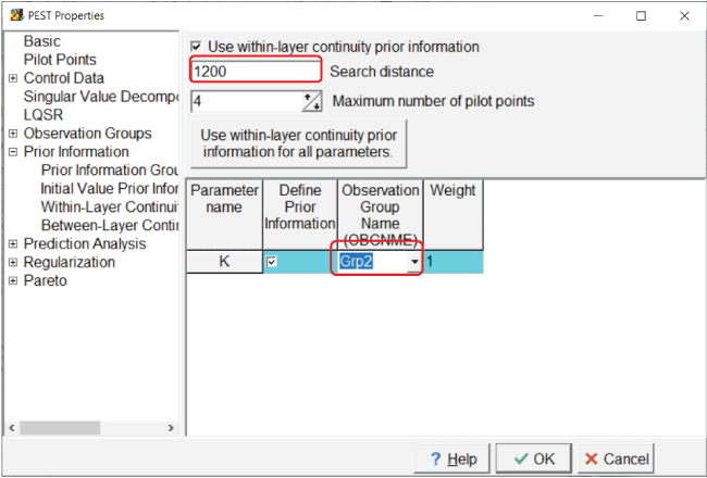
Screen capture of the “Within-Layer Continuity Prior Information” pane showing the definition of prior information. In the “Search distance” field, “1200” is entered; in the first field of the “Observation Group Name” column, “Grp2” is entered.
Modifying the between-layer prior information is unnecessary because the model only has one layer.
Run PEST
After making all the changes to the model, the model must be run from ModelMuse. Select “File|Export|MODFLOW 6 Input Files.” While creating the MODFLOW input files, ModelMuse creates and runs a batch file that creates a covariance matrix file for the pilot point parameters. After all the input files are created, ModelMuse starts a command line window that starts “ModelMonitor,” which runs the model. “ModelMonitor” may display a warning that the model will continue even if convergence is not achieved. In this case, the warning may be ignored. The warning appears because the “Continue even if no convergence” checkbox is checked in the IMS package as previously described. When the model finishes running, close “ModelMonitor.” Several more operations are performed in the command line window and then the MODFLOW listing file is opened in a text editor. The operations performed between the closing of “ModelMonitor” and the opening of the MODFLOW listing file are described below.
The first thing that happens after “ModelMonitor” is closed is that “Mf6ObsExtractor” is run (fig. 22), creating an instruction file used by PEST to extract model results that can be compared with observed values. The second thing that happens is that “PLPROC” is run. “PLPROC” is a utility program that can be downloaded from the PEST homepage (https://pesthomepage.org/) that creates a file used to populate the model grid among the pilot points.
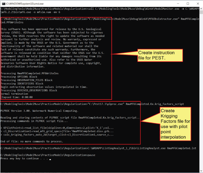
Annotated screen capture of the Microsoft Windows command-line interface identifying
the purposes of commands in the RunModflow.bat batchfile. The “Create instruction file for PEST” and “Create Krigging Factors file
for use with pilot point interpolation” sections of the code are labeled.
In addition to creating the input files for MODFLOW, ModelMuse also creates the PEST
control file when it runs MODFLOW along with two batch files named RunPestChek.bat and RunPest.bat. “PESTCHEK” is a PEST utility program that checks the PEST input for errors. Running
“PESTCHEK” before attempting to run PEST is always recommended. “PESTCHEK” can be
run by double clicking on the RunPestChek.bat file in Windows Explorer. It is normal for some warnings to be present with control
files generated by ModelMuse. However, if errors are reported, they must be fixed.
Problems with parameters, observations, pilot points, or delimiters, require rerunning
the model after the problems are fixed. Otherwise, the solution is probably exporting
the PEST control file again after fixing the problem in the “PEST Properties” dialog
box. To export the PEST control file again, select “File|Export|PEST|Export PEST Control
File.” The “Save File” dialog box has options for running “PESTCHEK” or PEST or not
running anything. Choose the preferred option. When “PESTCHECK” does not report errors,
PEST can now be run. When running this example on a standard desktop, PEST may take
more than twenty minutes to finish. The operation may happen more quickly depending
on the characteristics of the computer and on how many other programs are running.
Monitoring PEST performance during the parameter estimation by opening and inspecting
the PEST run record (.rec) file is a good practice.
When PEST finishes running, backing up the model input and output files is advisable to avoid accidentally overwriting them later if ModelMuse is run again.
Understanding the RunModel Batch File
The command line for running the model in the PEST control file is RunModel.Bat. Besides running MODFLOW, many operations are performed in the RunModel.Bat batchfile. The commands in the batch file are shown below. The commands vary depending
upon the model used.
if exist "arrays\RmaMf6Completed.Kx_1.arrays" del "arrays\RmaMf6Completed.Kx_1.arrays"
if exist "RmaMf6Completed.Mf6Values" del "RmaMf6Completed.Mf6Values"
if exist "RmaMf6Completed.wel" del "RmaMf6Completed.wel"
if exist "mfsim.lst" del "mfsim.lst"
if exist "RmaMf6Completed.bhd" del "RmaMf6Completed.bhd"
if exist "RmaMf6Completed.cbc" del "RmaMf6Completed.cbc"
if exist "RmaMf6Completed.chob_out_chd.csv" del "RmaMf6Completed.chob_out_chd.csv"
if exist "RmaMf6Completed.InnerSolution.CSV" del "RmaMf6Completed.InnerSolution.CSV"
if exist "RmaMf6Completed.lst" del "RmaMf6Completed.lst"
if exist "RmaMf6Completed.ob_gw_out_head.csv" del "RmaMf6Completed.ob_gw_out_head.csv"
if exist "RmaMf6Completed.OuterSolution.CSV" del "RmaMf6Completed.OuterSolution.CSV"
"plproc.exe" RmaMf6Completed.Kx.script
"EnhancedTemplateProcessor.exe" RmaMf6Completed.wel.tpl RmaMf6Completed.pval
mf6.exe
"Mf6ObsExtractor.exe" RmaMf6Completed.Mf6ExtractValues
The first 11 commands delete output files and some input files from MODFLOW. This process happens so that if something goes wrong with running the model, PEST can halt the process rather than continue to read the old output files from MODFLOW. The input files deleted are those containing the “Kx” dataset (command 1) and the Well package input files (command 3). The simulated values from the model are deleted in command 2. Other model output files are deleted in commands 4–11.
After the files are deleted, the last four commands do the following:
-
• “PLPROC” runs a script that generates the “Kx” dataset.
-
• “EnhancedTemplateProcessor” generates the input file for the Well package. “EnhancedTemplateProcessor” is a utility program for processing model input files to insert updated parameter values and is described in appendix 1.
-
• MODFLOW runs the model.
-
• “Mf6ObsExtractor” extracts the simulated values from the MODFLOW output files. “Mf6ObsExtractor” is a utility program for extracting simulated values from MODFLOW 6 output files and is described in appendix 2. Two similar utility programs are “MF2005ObsExtractor” and “SutraObsExtractor.” “MF2005ObsExtractor” is used for extracting simulated values from MODFLOW–2005 and MODFLOW–NWT output files and is described in appendix 3. “SutraObsExtractor” is used for extracting simulated values from SUTRA models and is described in appendix 4.
To facilitate the use of a parallel version of PEST in which individual model runs are executed on separate computers, ModelMuse copies executable files used for the flow model into the model directory so that the commands refer to the local versions of the programs.
Visualize Residuals
PEST prints the weighted residuals and other information from the run with the best
fit in a .res file. Data from this file can be plotted on the top view of the model or in a graph
using the “PEST Observation Results” pane of the “Data Visualization” dialog box.
Select “Data|Data Visualization” and select the “PEST Observation Results” pane. Select
the .res file for the model and click the “Apply” button and the weighted residuals are plotted
on the top view of the model (fig. 23). Only observations associated with a single object having a single vertex are plotted.
Weighted residuals for prior information equations are not plotted. In addition, the
“Graphs” tab can show plots of simulated values, residuals, or weighted residuals
versus observed values. Ideally, the weighted residuals should be equally distributed
on each side of the zero line on the graph (fig. 24). The simulated values should all lie close to the 1:1 line of simulated versus observed
(fig. 25).
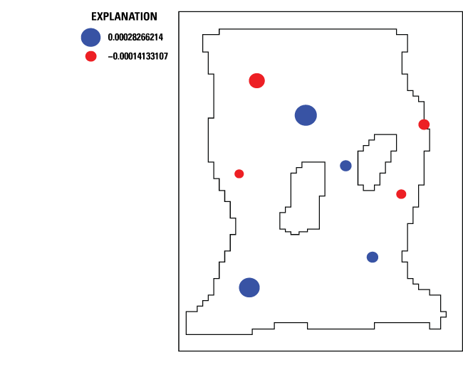
Plot showing weighted residuals after parameter estimation in a MODFLOW 6 model. Refer to figure 5 for diagram of Rocky Mountain Arsenal example model area referenced in this figure. Two distinct values, “0.00028266214” and “–0.00014133107,” are used on the plot.
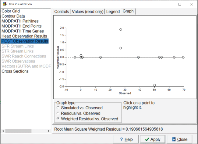
Screen capture of “Data Visualization” dialog box showing a graph of weighted residuals versus observed values in an example MODFLOW 6 model. “PEST Observation Results” is highlighted and under “Graph Type” the “Weighted Residuals vs. Observed” radio button is selected.
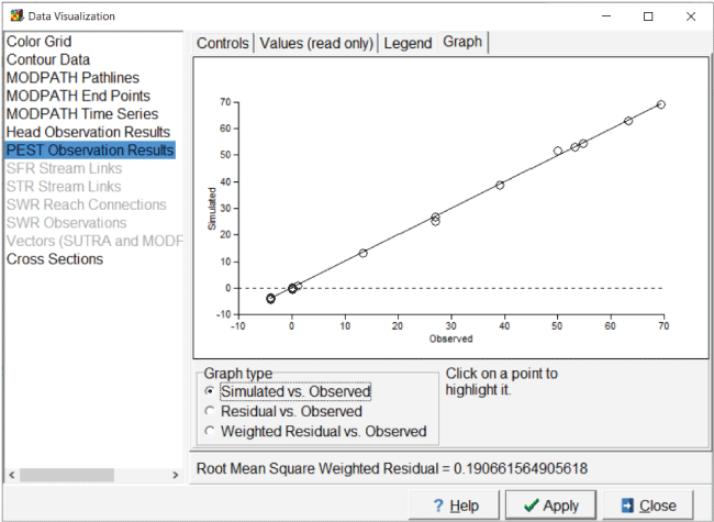
Screen capture of “Data Visualization” dialog box showing a graph of simulated values versus observed values in a MODFLOW 6 model. The “PEST Observation Results” is highlighted and under “Graph Type” the “Simulated vs. Observed” radio button is selected.
Visualize Modified Model Input
The model created by PEST after parameter estimation now has a different flow rate through the disposal pond and a nonuniform hydraulic conductivity distribution. ModelMuse provides ways to import and visualize both sets of data.
Visualizing Well Flow Rates
Select “File|Import|MODFLOW 6 Features.” Select the input file for the Well package. In the dialog box, select the appropriate stress period to see the pumping rates. In this case, there is only one stress period, therefore stress period 1 is chosen. ModelMuse creates a dataset named “Well_Pumping_Rate_SP_1” that has the pumping rates in each cell. The dataset is classified under “Optional|Model Results|Model Features.” The grid can be colored for this dataset. The sum of the pumping rates for the wells that are part of the disposal pond is 0.030 m3/s. The true value is 0.025 m3/s. This new dataset does not change how the pumping rate is defined in ModelMuse, so if the model input files are exported from ModelMuse again, the original pumping rates defined in ModelMuse are used, not those generated by PEST.
Visualizing “Kx”
Select “File|Import|Gridded Data Files” and select the file for the “Kx” dataset in the arrays subdirectory of the model directory. The new dataset is classified under “User Defined|Created from text file.” The name of the new dataset is based on the name of the file. A diagram of the estimated distribution of “Kx” is shown in figure 26.
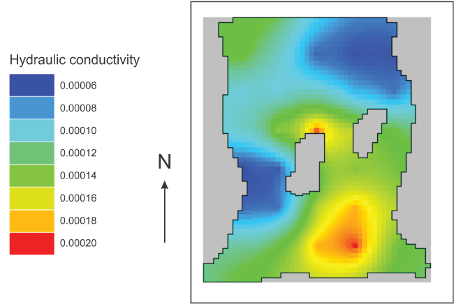
Diagram displaying the estimated hydraulic conductivity distribution of “Kx.” Refer to figure 5 for diagram of Rocky Mountain Arsenal example model area referenced in this figure. The hydraulic conductivity values, ranging from 0.00006–0.00020 (in 0.00002 step increments), are shown on the graph.
The “true” distribution from the model used to generate the observed values for the parameter estimation exercise is shown in figure 27.
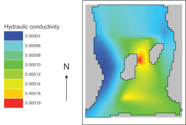
Diagram displaying the “true” hydraulic conductivity distribution of “Kx.” Refer to figure 5 for diagram of Rocky Mountain Arsenal example model area referenced in this figure. The discrete hydraulic conductivity values, ranging from 0.00001–0.00019, are shown on the graph.
Both the estimated and true hydraulic conductivity distributions (figs. 26 and 27) show patches of low hydraulic conductivity on the west and northeast portions of the model with a higher hydraulic conductivity between the two bedrock islands. The true distribution has more extreme high and low values (fig. 27).
Next Steps
The goal of this model is to understand the risk posed by the contaminants in the flow from the disposal pond to the water supply wells. To further calculate this risk, users can run MODPATH or even a solute transport simulation. MODPATH and solute transport simulations are covered in other examples, such as the original Rocky Mountain Arsenal example on which this example is based. At present, ModelMuse does not support using PEST with MODPATH or solute transport models.
Examining how well the model matched the true hydraulic conductivity and pumping rates, as was done here, is not something that can be done in a real groundwater-system model. A very low value of “PHIMLIM,” the target measurement objective function, was used. To avoid overfitting the model, the next step would be to run PEST again but with “PHIMLIM” and “PHIMACCEPT” set to larger values. Anderson and others (2015, p. 418) suggest a value 10 percent higher than in the best fit value recorded in the PEST run record. “PHIMACCEPT” is typically 5–10 percent larger than “PHIMLIM” (Doherty, 2018a).
PEST comes with utility programs for a variety of purposes, such as statistical postprocessing utilities used to gain a better understanding of the information content of the calibration dataset and of the estimability of individual parameters. Other utility programs explore the uncertainty of the predictions made by the model.
ModelMuse was not designed to directly support PEST++ (White and others, 2020). Nevertheless, PEST++ was designed to be backwards compatible with PEST so it should be possible to use PEST control files generated by ModelMuse with PEST++. If the user wishes to use capabilities of PEST++ that are not included in PEST, that can be done by appropriately altering the PEST control file.
Summary
ModelMuse was modified to support parameter estimation using PEST with MODFLOW and SUTRA models. Implementing these changes involves adding new dialog boxes for PEST and modifying existing dialog boxes to enable the user to define parameters and observations for PEST. These changes are most notable in the “Object Properties,” “Data Sets,” and “Manage Parameters” dialog boxes. Internally, the process of exporting the model input files was substantially altered to support the creation of instruction and template files for use by PEST. Four utility programs were created to support creation of instruction and template files. New procedures were also created for displaying the properties of input files modified by PEST.
References Cited
Banta, E.R., 2011, ModelMate—A graphical user interface for model analysis: U.S. Geological Survey Techniques and Methods, book 6, chap. E4, 31 p., accessed May 23, 2023, at https://doi.org/10.3133/tm6E4.
Banta, E.R., and Provost, A.M., 2008, User guide for HUFPrint, a tabulation and visualization utility for the Hydrogeologic-Unit Flow (HUF) package of MODFLOW: U.S. Geological Survey Techniques and Methods book 6, chap. A27, 13 p., accessed May 23, 2023, at https://doi.org/10.3133/tm6A27.
Bedekar, V., Morway, E.D., Langevin, C.D., and Tonkin, M., 2016, MT3D–USGS version 1—A U.S. Geological Survey release of MT3DMS updated with new and expanded transport capabilities for use with MODFLOW: U.S. Geological Survey Techniques and Methods, book 6, chap. A53, 69 p., accessed May 23, 2023, at https://doi.org/10.3133/tm6A53.
Doherty, J., 2003, Ground water model calibration using pilot points and regularization: Groundwater, v. 41, no. 2, p. 170–177, accessed May 23, 2023, at https://doi.org/10.1111/j.1745-6584.2003.tb02580.x.
Doherty, J., 2015, Calibration and uncertainty analysis for complex environmental models: Brisbane, Australia, Watermark Numerical Computing, 227 p., accessed May 15, 2015, at https://pesthomepage.org/pest-book.
Doherty, J.E., 2018a, Model-independent parameter estimation user manual part I—PEST, SENSAN and global optimisers (7th ed.): Brisbane, Australia, Watermark Numerical Computing, 369 p. [Also available at https://pesthomepage.org/documentation.]
Doherty, J.E., 2018b, Model-independent parameter estimation user manual part II—PEST utility software support (7th ed.): Brisbane, Australia, Watermark Numerical Computing, 276 p. [Also available at https://pesthomepage.org/documentation.]
Doherty, J.E., Fienen, M.N., and Hunt, R.J., 2011, Approaches to highly parameterized inversion—Pilot-point theory, guidelines, and research directions: U.S. Geological Survey Scientific Investigations Report 2010–5168, 36 p., accessed May 23, 2023, at https://doi.org/10.3133/sir20105168.
Doherty, J.E., and Hunt, R.J., 2010, Approaches to highly parameterized inversion—A guide to using PEST for groundwater-model calibration: U.S. Geological Survey Scientific Investigations Report 2010–5169, 59 p., accessed May 23, 2023, at https://doi.org/10.3133/sir20105169.
Fienen, M.N., Muffels, C.T., and Hunt, R.J., 2009, On constraining pilot point calibration with regularization in PEST: Groundwater, v. 47, no. 6, p. 835–844, accessed May 23, 2023, at https://doi.org/10.1111/j.1745-6584.2009.00579.x.
Haitjema, H., 2006, The role of hand calculations in ground water flow modeling: Groundwater, v. 44, no. 6, p. 786–791, accessed May 23, 2023, at https://doi.org/10.1111/j.1745-6584.2006.00189.x.
Hanson, R.T., Boyce, S.E., Schmid, W., Hughes, J.D., Mehl, S.W., Leake, S.A., Maddock, T., III, and Niswonger, R.G., 2014, One-Water Hydrologic Flow Model (MODFLOW–OWHM): U.S. Geological Survey Techniques and Methods, book 6, chap. A51, 120 p., accessed May 24, 2023, at https://doi.org/10.3133/tm6A51.
Harbaugh, A.W., 2005, MODFLOW–2005, the U.S. Geological Survey modular ground-water model—The ground-water flow process: U.S. Geological Survey Techniques and Methods, book 6, chap. A16, [variously paged], accessed May 24, 2023, at https://doi.org/10.3133/tm6A16.
Hill, M.C., Banta, E.R., Harbaugh, A.W., and Anderman, E.R., 2000, Geological Survey modular ground‐water model—User guide to the observation, sensitivity, and parameter‐estimation processes and three post‐processing programs: U.S. Geological Survey Open‐File Report 00–184, accessed May 24, 2023, at https://doi.org/10.3133/ofr00184.
Hunt, R.J., Feinstein, D.T., Pint, C.D., and Anderson, M.P., 2006, The importance of diverse data types to calibrate a watershed model of the Trout Lake Basin, northern Wisconsin, USA: Journal of Hydrology, v. 321, nos. 1–4, p. 286–296, accessed May 24, 2023, at https://doi.org/10.1016/j.jhydrol.2005.08.005.
Hunt, R.J., Fienen, M.N., and White, J.T., 2019, Revisiting “An exercise in groundwater model calibration and prediction” after 30 years—Insights and new directions: Groundwater, v. 58, no. 2, p. 168–182, accessed May 24, 2023, at https://doi.org/10.1111/gwat.12907.
Hunt, R.J., White, J.T., Duncan, L.L., Haugh, C.J., and Doherty, J., 2021, Evaluating lower computational burden approaches for calibration of large environmental models: Groundwater, v. 59, no. 6, p. 788–798, accessed May 24, 2023, at https://doi.org/10.1111/gwat.13106.
Langevin, C.D., Hughes, J.D., Banta, E.R., Niswonger, R.G., Panday, S., and Provost, A.M., 2017, Documentation for the MODFLOW 6 Groundwater Flow Model: U.S. Geological Survey Techniques and Methods, book 6, chap. A55, 197 p., accessed May 24, 2023, at https://doi.org/10.3133/tm6A55.
Mehl, S.W., and Hill, M.C., 2013, MODFLOW–LGR—Documentation of ghost node local grid refinement (LGR2) for multiple areas and the boundary flow and head (BFH2) package: U.S. Geological Survey Techniques and Methods, book 6, chap. A44, 43 p., accessed May 24, 2023, at https://doi.org/10.3133/tm6A44.
Niswonger, R.G., Panday, S., and Ibaraki, M., 2011, MODFLOW–NWT, A Newton formulation for MODFLOW–2005: U.S. Geological Survey Techniques and Methods, book 6, chap. A37, 44 p., accessed May 24, 2023, at https://doi.org/10.3133/tm6A37.
Parkhurst, D.L., Kipp, K.L., Engesgaard, P., and Charlton, S.R., 2004, PHAST—A program for simulating ground-water flow, solute transport, and multicomponent geochemical reactions: U.S. Geological Survey Techniques and Methods, book 6, chap. A8, 154 p., accessed May 24, 2023, at https://doi.org/10.3133/tm6A8.
Poeter, E.P., and Hill, M.C., 1998, Documentation of UCODE, a computer code for universal inverse modeling: U.S. Geological Survey Water-Resources Investigations Report 98–4080, 116 p., accessed May 24, 2023, at https://doi.org/10.3133/wri984080.
Poeter, E.P., Hill, M.C., Banta, E.R., Mehl, S., and Christensen, S., 2005, UCODE_2005 and six other computer codes for universal sensitivity analysis, calibration, and uncertainty evaluation: U.S. Geological Survey Techniques and Methods, book 6, chap. A11, 283 p., accessed May 24, 2023, at https://doi.org/10.3133/tm6A11.
Poeter, E.P., Hill, M.C., Lu, D., Tiedeman, C.R., and Mehl, S., 2014, UCODE_2014, with new capabilities to define parameters unique to predictions, calculate weights using simulated values, estimate parameters with SVD, evaluate uncertainty with MCMC, and more: Integrated Groundwater Modeling Center Report GWMI 2014–02, 172 p., accessed May 24, 2023, at https://igwmc.mines.edu/wp-content/uploads/sites/117/2018/11/UCODE_2014_User_Manual-version02.pdf.
Pollock, D.W., 2016, User guide for MODPATH Version 7—A particle-tracking model for MODFLOW: U.S. Geological Survey Open-File Report 2016–1086, 35 p., https://doi.org/10.3133/ofr20161086.
Provost, A.M., and Voss, C.I., 2019, SUTRA, a model for saturated-unsaturated, variable-density groundwater flow with solute or energy transport—Documentation of generalized boundary conditions, a modified implementation of specified pressures and concentrations or temperatures, and the lake capability: U.S. Geological Survey Techniques and Methods, book 6, chap. A52, 62 p., accessed May 24, 2023, at https://doi.org/10.3133/tm6A52.
Voss, C.I., and Provost, A.M., 2002, SUTRA, a model for saturated-unsaturated variable-density ground-water flow with solute or energy transport (ver. 2.2, September 22, 2010): U.S. Geological Survey Water-Resources Investigations Report 02–4231, 291 p., accessed May 24, 2023, at https://doi.org/10.3133/wri024231.
White, J.T., Hunt, R.J., Fienen, M.N., and Doherty, J.E., 2020, Approaches to highly parameterized inversion—PEST++ version 5, a software suite for parameter estimation, uncertainty analysis, management optimization and sensitivity analysis: U.S. Geological Survey Techniques and Methods, book 7, chap. C26, 52 p., accessed May 24, 2023, at https://doi.org/10.3133/tm7C26.
Winston, R.B., 2009, ModelMuse—A graphical user interface for MODFLOW–2005 and PHAST: U.S. Geological Survey Techniques and Methods, book 6, chap. A29, 52 p., accessed May 24, 2023, at https://doi.org/10.3133/tm6A29.]
Winston, R.B., 2014, Modifications made to ModelMuse to add support for the Saturated-Unsaturated Transport model (SUTRA): U.S. Geological Survey Techniques and Methods, book 6, chap. A49, 6 p., accessed May 24, 2023, at https://doi.org/10.3133/tm6A49.
Winston, R.B., 2019, ModelMuse version 4—A graphical user interface for MODFLOW 6: U.S. Geological Survey Scientific Investigations Report 2019–5036, 10 p., accessed May 24, 2023, at https://doi.org/10.3133/sir20195036.
Winston, R.B., and Goode, D.J., 2017, Visualization of groundwater withdrawals: U.S. Geological Survey Open-File Report 2017–1137, 8 p., accessed May 24, 2023, at https://doi.org/10.3133/ofr20171137.
Zheng, C., and Wang, P.P., 1999, MT3DMS—A modular three-dimensional multispecies transport model for simulation of advection, dispersion, and chemical reactions of contaminants in groundwater systems; documentation and user’s guide—Final report: U.S. Army Engineer Research and Development Center, Strategic Environmental Research and Development Program, Contract Report SERDP–99–1, prepared by authors under contract (work unit no. CU–1062), 202 p. [Also available at https://erdc-library.erdc.dren.mil/jspui/handle/11681/4734.]
Appendix 1. “EnhancedTemplateProcessor”
Usage
EnhancedTemplateProcessor <template name> [<PVAL file name> [<Arrays file name>]]
Items enclosed by square brackets are optional. Items between angled brackets are user-supplied input values.
Run “EnhancedTemplateProcessor” from the command line followed by the name of a template file and (optionally) the name of a “PVAL” file containing the names and values of the parameters that should be substituted into the file and the name of an “Arrays” file containing the names of arrays, their dimensions, and the names of files containing their data. If the file names contain whitespace, the names must be enclosed in quotation marks. If the file names do not contain whitespace, quotation marks around the file names are optional. The template file name must contain an extension. The output of the program is a file that has the same name as the template, except that the extension is removed from the file name. The contents of the output file are the postprocessed contents of the input file.
PVAL File Format
The “PVAL” file format is the same as documented for MODFLOW–2005. However, if a line
starts with "#--", the remainder of the line is treated as defining a parameter for the purposes of
“EnhancedTemplateProcessor.” All such lines must follow the lines defining parameters
for MODFLOW–2005 to ensure that the lines are ignored by MODFLOW–2005. The number
of parameters specified at the beginning of the “PVAL” file must be the number of
MODFLOW–2005 parameters and not include any of the additional parameters for “EnhancedTemplateProcessor.”
Arrays File Format
The first line in the “Arrays” file must contain a single character that is used to delineate array substitutions within the template. This is the array delimiter and (1) must not be the space character and (2) must be different from the parameter delimiter and formula delimiter used in template files. If multiple ”Array” files are used in a single template, they must all use the same array delimiter.
Empty lines or lines that start with the character “#” in the arrays file are skipped. All other lines define three-dimensional arrays
of real numbers. Each such line has the name of an array immediately followed by an
open bracket character “[”. The open bracket character is followed by three positive integers and then a close
bracket character “].” The integers represent the number of layers, rows, and columns in the array, respectively.
The array dimensions must be separated by commas or one or more spaces. Following
the close bracket character are the names of one or more files containing the data
for the array. If the file names contain spaces, they must be enclosed in double quotation
marks. Each line of these files must contain one or more values for the array. The
values in a line must be separated by commas or one or more space characters. When
reading the array values, the column index is incremented most frequently, and the
layer index is incremented least frequently. Array names are not case sensitive and
consist only of the characters “A” through “Z,” “a” through “z,” “0” through “9” and
“_”. Array names must not start with a digit.
Template File Format
If parameter names are to be replaced by parameter values, the first line of the file must begin with either “ptf ” or “jtf ” followed by a single character. This character, known as the “parameter delimiter,” is used to specify locations in the file where parameter names are replaced by parameter values. The parameter names must be surrounded by a pair of the parameter delimiters. Extra spaces are allowed and encouraged before and after the parameter name but within the pair of parameter delimiters. When the parameter name is replaced, everything between the parameter delimiters and the delimiters themselves are replaced by the parameter value. If the parameter value is too long to fit within the available space, it is truncated to fit.
The next line of the template (or the first line if the parameter delimiter line is not included) must begin with “etf” followed by a single character. This character is the formula delimiter, which plays a role similar to the parameter delimiter. A formula should be included between a pair of formula delimiters. However, the width of the available space is indicated differently from how it is expressed with parameter delimiters. The available space extends from the first formula delimiter through the first character before the formula begins. The following are related guidelines:
• The parameter delimiter must be different from the formula delimiter.
• The parameter delimiter character cannot occur anywhere in the template except where it functions as a parameter delimiter.
• The formula delimiter character cannot occur anywhere in the template except where it functions as a formula delimiter.
• There is no restriction imposed by EnhancedTemplateProcessor on the length of lines in template or PVAL files.
• There is no restriction imposed by EnhancedTemplateProcessor on the length of parameter names in PVAL files or template files.
• Parameter names must not include whitespace.
Array Substitution
An array used for substitution can be read in either of two ways. Either the name
of an arrays file can be included on the command line after the PVAL file name or
it can be read using a ReadArrays command included in the template. The ReadArrays commands must be in lines that immediately follow the formula delimiter (see above).
The ReadArrays command has a pair of parentheses enclosing the name of an arrays file. An example
is shown here in which “%” is the formula delimiter:
%ReadArrays(Drntest.drn.arrays)%
Any line containing the ReadArrays command is processed for one arrays file. No other operations are performed on that
line and the line is not included in the final output file.
In each line of a template file that does not include a ReadArrays command, the first operation is replacing references to arrays with the array values.
Each array reference must be preceded and followed by the array delimiter defined
on the first line of the array file. The number of spaces between the initial array
delimiter and the beginning of the array name determines the number of characters
used to print the array value. In the text between the array delimiters, the array
name must appear immediately followed by the open bracket character, the layer, row,
and column indices and the closed bracket character. The layer, row, and column indices
must be greater than or equal to 1 and less than or equal to the layer count, row
count, or column count, respectively. The corresponding value is printed—right justified—in
place of the text between the array delimiters.
Parameter Substitution
Parameter names and values are read from a “PVAL” file specified on the command line. Any parameter names in the template that are enclosed by parameter delimiters are replaced by the parameter value. The value is printed, right justified, in place of the text between the array delimiters.
Formulas Substitution
Formulas enclosed in formula delimiters are replaced in the input file by the value to which the formula “evaluates.” Formulas typically enclose parameter names enclosed by parameter delimiters or array references enclosed by array delimiters. Unlike parameter substitution, the space reserved for the formula value is not determined by the character distance between the formula delimiters. Instead, it is the number of space characters between the first formula delimiter and the beginning of the formula itself.
A formula must evaluate to a real number. Although logical operations can be used, a formula that depends on parameter values should be a continuous function of the parameters. Failure to follow this rule can result in a failure of the parameter estimation process.
Operators
The operators in table 1.1 are available for formulas. For the >, <, >=, and <= operators, “true” is considered larger than “false” when applied to Booleans. For the same operators, applied to text, alphabetical order is used to decide which argument is larger.
Table 1.1.
Operators used in formulas.The operator precedence rules are shown in table 1.2. Operators that are part of the same group have equal precedence. Operators of equal precedence are evaluated in order from left to right.
Description of Operations
“EnhancedTemplateProcessor” does not have equivalents of the “PRECIS” or “DPOINT” variables in PEST.
“EnhancedTemplateProcessor” processes a template file in the following sequence.
-
• “EnhancedTemplateProcessor” reads the names of the template file, “PVAL” file, and array file from the command line. The “PVAL” and array file are optional.
-
• The “PVAL” file is read, if specified, and each parameter name is associated with a real-number value.
-
• The array file is read, if specified. If an array file is specified, a “PVAL” file must also be specified.
-
• The template file is opened and the parameter delimiter (if specified) and formula delimiter are read.
-
• The lines are read one by one.
-
• If the line contains a
ReadArrayscommand, the array is read. This is a mechanism for including an arrays file if a “PVAL” file is not used. -
• In each line, array references are replaced by array values.
-
• In each line, any parameter names enclosed within parameter delimiters are replaced by the associated values.
-
• In each line, any formulas in the line are evaluated and replaced with the evaluated values.
Template Example
ptf @
etf !
this is a line with nothing to replace in it.
This is a line with a parameter value "@ HK1@"
This is a line with a formula "! 2/3*100000!"
This is a line with formula containing two parameters and a formula "! @ HK2 @ + @ HK3 @!"
This is a line with two array substitutions "~ Kx[1,5,5]~," "~ Kx[2,5,5]~"
Array substitution and a parameter inside a formula "!~ Kx[1,5,5]~ + @ HK1 @ !"
“PVAL” File Example
18
HK1 1
HK2 0.01
HK3 0.0001
HK4 1E-6
VKA12_1 0.25
VKA12_2 0.0025
VKA12_3 2.5E-5
VKA12_4 2.5E-7
VKA3_1 1
VKA3_2 0.01
VKA3_3 0.0001
VKA3_4 1E-6
KDEP_Par1 0.9
LVDA_Par1 1
GHB 1
DRAIN 1
RCH 0.00031
ETM 0.0004
Example Arrays File
~
Kx[3, 10, 10] "Drn test.lpf.Kx_1.txt," "Drn test.lpf.Kx_2.txt" "Drn test.lpf.Kx_3.txt"
Example Output File
This is a line with nothing to replace in it.
This is a line with a parameter value " 1"
This is a line with a formula "66666."
This is a line with formula containing two parameters and a formula "0.0101"
This is a line with two array substitutions " 0.044," " 0.144"
Array substitution and a parameter inside a formula " 1.044"
Appendix 2. “Mf6ObsExtractor”
-
• Keywords are written in
ALL CAPITAL LETTERS; -
• Optional instructions are enclosed in
[square brackets];
“OPTIONS” Block
Purpose
The “OPTIONS” block is used to specify the output files to be generated by “Mf6ObsExtractor.”
Structure
BEGIN OPTIONS
	[LISTING <filename>]
	[VALUES <filename>]
	[INSTRUCTION <filename> [<instruction_file_type>]]
END OPTIONS
Explanations
The “OPTIONS” section is used for specifying the names of output files from “Mf6ObsExtractor.” Each nonblank and noncomment line in the “OPTIONS” section must begin with one of the following keywords: “LISTING,” “VALUES,” or “INSTRUCTION.” Each of these keywords must be followed by a file name. The “INSTRUCTION” file name may be optionally followed by either “UCODE” or “PEST.”
The “LISTING” file is optional. If specified, it contains a record of the steps taken during execution of “Mf6ObsExtractor.” It will end either with a line indicating that it terminated normally or with an error message. The “LISTING” file is useful for identifying errors in the input.
Either a “VALUES” or “INSTRUCTION” file is required. Typically, only one or the other is specified, but both may be specified in the same input file.
The “VALUES” file contains the simulated values extracted from the MODFLOW output file or files. Each line in the “VALUES” file contains an observation name followed by the simulated value associated with that name.
The “INSTRUCTION” file contains instructions for either UCODE or PEST to extract simulated
values from the “VALUES” file. The desired format may be specified with <instruction_file_type>.
<filename> is the name of a file. If the file name contains whitespace characters, the file
name must be surrounded by double quotes.
<instruction_file_type> must be either “UCODE” or “PEST,” which indicates whether the instruction file is
designed to be used with the UCODE or PEST parameter estimation programs. If <instruction_file_type> is not specified, it defaults to PEST.
Example
BEGIN OPTIONS
# The file name for the listing file contains white space so it must be enclosed in double quotes
	LISTING "MyListing file.txt"
# The VALUES file contains the values extracted from the observation file.
	VALUES Example.der_obs
# The INSTRUCTION file contains instructions for PEST to extract the values from the
# VALUES file.
	INSTRUCTION Example.ins
END OPTIONS
“OBSERVATION_FILES” Block
Purpose
The “OBSERVATION_FILES” block identifies the file or files from which observations are to be extracted.
Structure
BEGIN OBSERVATION_FILES
FILENAME <filename> <file type>
[FILENAME <filename> <file type>]
[FILENAME <filename> <file type>]
...
[FILENAME <filename> <file type>]
END OBSERVATION_FILES
Explanations
Each nonblank, noncomment line in the “OBSERVATION_FILES” group must begin with the keyword “FILENAME” followed by the name of the file and the file type.
<filename> is the name of a file generated by MODFLOW 6 that contains information about simulated
values that can be compared with observations. If the file name contains whitespace
characters, the file name must be surrounded by double quotes.
<file type> is a keyword indicating the type of MODFLOW 6 output file that will be read. <file type> must be either “BINARY” or “TEXT.”
“IDENTIFIERS” Block
Purpose
The “IDENTIFIERS” block is used to extract values from the MODFLOW 6 output files corresponding to user-specified times. Optionally, locations can be associated with specific observed values. These locations can be used for interpolating to observation locations using a linear, triangular, or quadrilateral basis function. The extracted values may either represent values that should be directly compared with observed values or combined with other extracted values using the methods available in the “DERIVED_OBSERVATIONS” section.
Structure
BEGIN IDENTIFIERS
ID <identifier>
[LOCATION <x> <y>]
OBSNAME <Observation_name> <observation_time> [PRINT]
[OBSNAME <Observation_name> <observation_time> [PRINT]]
[OBSNAME <Observation_name> <observation_time> [PRINT]]
...
ID <identifier>
[LOCATION <x> <y>]
OBSNAME <Observation_name> <observation_time> [PRINT]
[OBSNAME <Observation_name> <observation_time> [PRINT]]
[OBSNAME <Observation_name> <observation_time> [PRINT]]
END IDENTIFIERS
Explanations
“ID” is a keyword used to indicate that the following values on the line will be used to identify a particular time series from which values are to be extracted.
<identifier> is the name assigned to the time series from which values are to be extracted.
LOCATION is an optional keyword indicating that the x- and y-coordinates that follow are the coordinates of the cell center of the observation
time series.
<x> is the x-coordinate of the cell center of the time series associated with <identifier>.
<y> is the y-coordinate of the cell center of the time series associated with <identifier>.
“OBSNAME” is a keyword indicating that the line specifies an observation name and time.
<Observation_name> is the name of the observation. <Observation_name> must start with a letter or the underscore character. The remaining characters in
<Observation_name> must be letters, digits, or the underscore character. All observation names must
be unique. “Mf6ObsExtractor” does not limit the length of observation names.
<observation_time> is a real number that indicates the time at which the simulated value is desired.
If the specified time is not included in the output file, “Mf6ObsExtractor” interpolates
to the time in question from the values recorded for the preceding and following times.
If the observation time is before the first recorded time, the value for the first
recorded time is used. If the observation time is after the last recorded observation
time, “Mf6ObsExtractor” ignores it.
“PRINT” is an optional keyword. If included, the <Observation_name> and simulated value are printed to the extracted values file or instructions for
reading the <Observation_name> and simulated values are written into the instruction file. Printing the name and
value implies direct use by PEST or UCODE. If the values are not printed, they may
still be used in the “DERIVED_OBSERVATIONS” section. Regardless of whether “PRINT”
is present or not, the name and simulated value are written to the listing file. “Mf6ObsExtractor”
does not limit the length of observation names, but to be used by PEST or UCODE, the
observation name must conform to the requirements of those programs.
Example
BEGIN IDENTIFIERS
# heads in layer 1
# heads will be interpolated in time to times 3.5 and 6.5.
# Locations are provided for spatial interpolation.
	ID HEAD1
	LOCATION 550 -550
	OBSNAME H1_1 3.5
	OBSNAME H1_2 6.5
	ID HEAD2
	LOCATION 550 -650
	OBSNAME H2_1 3.5
	OBSNAME H2_2 6.5
	ID HEAD3
	LOCATION 650 -650
	OBSNAME H3_1 3.5
	OBSNAME H3_2 6.5
	ID HEAD4
	LOCATION 650 -550
	OBSNAME H4_1 3.5
	OBSNAME H4_2 6.5
#heads in layer 2
	ID HEAD5
	LOCATION 550 -550
	OBSNAME H5_1 3.5
	OBSNAME H5_2 6.5
	ID HEAD6
	LOCATION 550 -650
	OBSNAME H6_1 3.5
	OBSNAME H6_2 6.5
	ID HEAD7
	LOCATION 650 -650
	OBSNAME H7_1 3.5
	OBSNAME H7_2 6.5
	ID HEAD8
	LOCATION 650 -550
	OBSNAME H8_1 3.5
	OBSNAME H8_2 6.5
# These heads (H9_1 and H9_2) will be printed to the Example.der_obs file.
# The rest won't be printed.
# No locations are required for H9_1 and H9_2 because they will not
# be used for spatial interpolation.
	ID HEAD9
	OBSNAME H9_1 3.5 PRINT
	OBSNAME H9_2 6.5 PRINT
# River observations
# Rivers will be interpolated in time to times 3.5 and 6.5
# Only the rivers associated RIVER1 will be printed to the Example.der_obs file.
# The rest won't be printed.
	ID RIVER1
	OBSNAME RIV1_1 3.5 PRINT
	OBSNAME RIV1_2 6.5 PRINT
	ID RIVER2
	OBSNAME RIV2_1 3.5
	OBSNAME RIV2_2 6.5
	ID RIVER3
	OBSNAME RIV3_1 3.5
	OBSNAME RIV3_2 6.5
	ID RIVER4
	OBSNAME RIV4_1 3.5
	OBSNAME RIV4_2 6.5
END IDENTIFIERS
“DERIVED_OBSERVATIONS” Block
Purpose
The “DERIVED_OBSERVATIONS” block defines how to combine multiple values extracted from the MODFLOW 6 observation files to generate values that can be compared with observed values. Two methods can be used for this purpose. First, values can be interpolated in space using a linear, triangular, or quadrilateral basis function. Second, mathematical formulas can be defined that manipulate previously extracted values.
The “DERIVED_OBSERVATIONS” section is optional.
Structure
BEGIN DERIVED_OBSERVATIONS
	OBSNAME <Observation_name> [PRINT]
	FORMULA <formula>
	...
	OBSNAME <Observation_name> [PRINT]
	INTERPOLATE <x> <y> <obs> [<obs> <obs> <obs>]
END DERIVED_OBSERVATIONS
Explanations
“OBSNAME” is a keyword indicating that the line specifies an observation name.
<Observation_name> is the name of the observation. <Observation_name> must start with a letter or the underscore character. The remaining characters in
<Observation_name> must be letters, digits, or the underscore character. All observation names must
be unique. “Mf6ObsExtractor” does not limit the length of observation names. An “OBSNAME”
line must be followed by either a single “FORMULA” line or a single “INTERPOLATE”
line.
“PRINT” is an optional keyword. If included, the <Observation_name> and simulated value are printed to the extracted values file, or instructions for
reading the <Observation_name> and simulated value are written to the instruction file. Printing the name and value
implies direct use by PEST or UCODE. If the values are not printed, they may still
be used in the “DERIVED_OBSERVATIONS” section. Regardless of whether “PRINT” is present
or not, the name and simulated value are written to the listing file. “Mf6ObsExtractor”
does not limit the length of observation names, but to be used by PEST or UCODE, the
observation name must conform to the requirements of those programs.
“FORMULA” is a keyword indicating that the remainder of the line is a mathematical
formula that evaluates to a real number. The result of the formula is the value assigned
to <Observation_name>. Variables in the formula can be any of the observation names defined in the “IDENTIFIERS”
section or any observation name defined previously in the “DERIVED_OBSERVATIONS” section.
<formula> is a mathematical formula that evaluates to a real number. The result of the formula
is the value assigned to <Observation_name>. Variables in the formula can be any of the observation names defined in the “IDENTIFIERS”
section or any observation name defined previously in the “DERIVED_OBSERVATIONS” section.
The operators and functions available for use in formulas are the same as in “EnhancedTemplateProcessor.”
“INTERPOLATE” is a keyword indicating that the remainder of the line consists of an
x-coordinate, a y-coordinate, and from one to four previously defined <Observation_name> names, each of which has an associated location.
<x> and <y> are the x- and y-coordinates associated with <Observation_name>. Together, they define the observation point at which a value is desired.
<obs> is a previously defined <Observation_name> that has an associated pair of x- and y-coordinates. If only one <obs> is included, its value is taken as the value of <Observation_name>. If two to four <obs> are defined, those values define the nodes and values of a linear, triangular, or
quadrilateral basis function and the value of <Observation_name> is defined using a linear, triangular, or quadrilateral basis function.
Example
#(Optional)
BEGIN DERIVED_OBSERVATIONS
# Spatially Interpolate the head in layer 1 at (575, -575) at time 3.5
	OBSNAME H_Layer1_Time1
	INTERPOLATE 575 -575 H1_1 H2_1 H3_1 H4_1
# Spatially Interpolate the head in layer 1 at (575, -575) at time 6.5
	OBSNAME H_Layer1_Time2
	INTERPOLATE 575 -575 H1_2 H2_2 H3_2 H4_2
# Spatially Interpolate the head in layer 2 at (575, -575) at time 3.5
	OBSNAME H_Layer2_Time1
	INTERPOLATE 575 -575 H5_1 H6_1 H7_1 H8_1
# Spatially Interpolate the head in layer 2 at (575, -575) at time 6.5
	OBSNAME H_Layer2_Time2
	INTERPOLATE 575 -575 H5_2 H6_2 H7_2 H8_2
# Calculate multilayer head observations at times 3.5 and 6.5 weighted by transmissivity
# Transmissivity of layer 1 = 3
# Transmissivity of layer 2 = 6
# Print the multilayer head observations
	OBSNAME H_Time1 PRINT
	FORMULA (H_Layer1_Time1 * 3 + H_Layer2_Time1 * 6) / (3 + 6)
	OBSNAME H_Time2 PRINT
	FORMULA (H_Layer1_Time2 * 3 + H_Layer2_Time2 * 6) / (3 + 6)
# Calculate a drawdown observation too.
	OBSNAME Drawdown PRINT
	FORMULA H_Time1 - H_Time2
# Calculate a river observation by combining several separate river observations.
# Only half of rivers 2 and 4 will be used.
	OBSNAME MyRiver_1 PRINT
	FORMULA RIV2_1*0.5 + RIV3_1 + RIV4_1*0.5
	OBSNAME MyRiver_2 PRINT
	FORMULA RIV2_2*0.5 + RIV3_2 + RIV4_2*0.5
END DERIVED_OBSERVATIONS
Appendix 3. “Mf2005ObsExtractor”
-
• MNWI (Multi-Node Well Information package) output files;
-
• GAGE package output files for individual streams and lakes; and
-
• output files for the Subsidence, SFR, SWI, SUB, SWT, HOB, CHOB, DROB, RVOB, GBOB, and STOB packages.1
<filename> is the name of the file. If the file name contains spaces, it must be surrounded
by single or double quotation marks.Mf2005ObsExtractor <filename> Mf2005ObsExtractor -f <filename> Mf2005ObsExtractor --file <filename>
“MF2005ObsExtractor” Name File
The “Mf2005ObsExtractor” name file lists the input and output files for “Mf2005ObsExtractor.” Items in square brackets are optional. Items in angled brackets are input variables.
The name file for “Mf2005ObsExtractor” is specified in blocks. Each block starts with the keyword “Begin” followed by the block name. Each block ends with the keyword “End” followed by the block name. The keywords and block names are not case sensitive. Any line whose first nonwhitespace character is “#” is treated as a comment. Comments are printed to the listing file.
Structure of Blocks
BEGIN OUTPUT_FILES
LIST <filename>
[INSTRUCTION_FILE <filename>]
[OBSERVATIONS_FILE <filename>]
END OUTPUT_FILES
BEGIN INPUT_FILES
[<file_type> <filename>]
[MNW2 <filename>]
[LAK <filename>]
[SFR <filename>]
[SUB <filename>]
[SWT <filename>]
[SWI <filename>]
[HOB <filename>]
[CHOB <filename>]
[DROB <filename>]
[RVOB <filename>]
[GBOB <filename>]
[STOB <filename>]
[DERIVED <filename>]
END INPUT_FILES
Explanation of Variables
Block: “OUTPUT_FILES.”
The “OUTPUT_FILES” block is required.
“LIST” is a keyword to indicate that the following file name is the listing file for “Mf2005ObsExtractor.” The listing file provides a record of what “Mf2005ObsExtractor” has done. The listing file can be useful for locating errors in the input for “Mf2005ObsExtractor.”
<filename> is the name of a file. <filename> may be enclosed in single or double quotation marks.
“INSTRUCTION_FILE” is an optional keyword indicating that the following output file is an instruction file for PEST to read the simulated values from the model. Typically, “Mf2005ObsExtractor” is run with “INSTRUCTION_FILE” after that model has run successfully once but before starting PEST.
“OBSERVATIONS_FILE” is an optional keyword indicating that the following output file contains the extracted values from the model output files. Typically, the PEST command to run the model contains a command to run “Mf2005ObsExtractor” with the “OBSERVATIONS_FILE” keyword.
Block: “INPUT_FILES.”
The “INPUT_FILES” block is required. All the items in the “INPUT_FILES” block are optional, but at least one item in the block must be present.
“file_type” is an optional keyword.
“MNW2” indicates that the file in the following <filename> defines observations extracted from the output of the Multi-Node Well Information
(MNWI) package.
“LAK” indicates that the file in the following <filename> defines observations related to lakes extracted from the output of the GAGE package.
“SFR” indicates that the file in the following <filename> defines observations related to streams extracted from the output of the GAGE package.
“SUB” indicates that the file in the following <filename> defines observations related to subsidence extracted from the output of the Subsidence
and Aquifer-System Compaction (SUB) package.
“SWT” indicates that the file in the following <filename> defines observations related to subsidence extracted from the output of the Subsidence
and Aquifer-System Compaction Package for Water-Table Aquifers (SWT) package.
“SWI” indicates that the file in the following <filename> defines observations related to seawater intrusion extracted from the output of the
Seawater Intrusion (SWI) package.
“HOB” indicates that the file in the following <filename> is the output file of the Head-Observation (HOB) package.
“CHOB” indicates that the file in the following <filename> is the output file of the Specified-Head Flow Observation (CHOB) package.
“DROB” indicates that the file in the following <filename> is the output file of the Drain Observation (DROB) package.
“RVOB” indicates that the file in the following <filename> is the output file of the River Observation (RVOB) package.
“GBOB” indicates that the file in the following <filename> is the output file of the General-Head-Boundary Observation (GBOB) package.
“STOB” indicates that the file in the following <filename> is the output file of the Stream Observation (STOB) package.
“DERIVED” indicates that the file in the following <filename> defines observations derived from previously defined observations.
<filename> is the name of a file. <filename> may be enclosed in single or double quotation marks.
Observation Definition Files
The input observation definition files for “Mf2005ObsExtractor” are specified in blocks. Each block starts with the keyword “BEGIN” followed by the block name. Each block ends with the keyword “END” followed by the block name. The keywords and block names are not case sensitive. Any line whose first nonwhitespace character is “#” is treated as a comment. Comments are printed to the listing file.
Structure of Observation Definition Files
BEGIN OBSERVATIONS
FILENAME <filename>
OBSERVATION <Observation_name> <Observation_type> <Observation_time> <Observed_value> <Weight> [PRINT|NO_PRINT]
[NUMBER_OF_ZETA_SURFACES <number_of_zeta_surfaces>]
[TOTAL_NUMBER_OF_OBSERVATIONS <number_of_observation_locations_in_SWI_observation_file>]
[SWI_OBS_FORMAT (ASCII | BINARY SINGLE | BINARY DOUBLE)]
OBSERVATION <Observation_name> <Observation_type> <Observation_time> <Observed_value> <Weight> [PRINT|NO_PRINT]
[ZETA_SURFACE_NUMBER <zeta_surface_number>]
[SWI_OBSERVATION <number> <fraction> <name>]
FILENAME <filename>
OBSERVATION <Observation_name> <Observation_type> <Observation_time> <Observed_value> <Weight> [PRINT|NO_PRINT]
OBSERVATION <Observation_name> <Observation_type> <Observation_time> <Observed_value> <Weight> [PRINT|NO_PRINT]
[CELL <layer_or_interbed_system> <row> <column> <cellweight>]
END OBSERVATIONS
[BEGIN DERIVED_OBSERVATIONS]
[DIFFERENCE <Observation_name> <Prior_observation_name> <Prior_observation_name>] <Observed value> <Weight> [PRINT|NO_PRINT]
[SUM <Observation_name> <Prior_observation_name1> <Prior_observation_name2> ... <Prior_observation_nameN>] <Observed value> <Weight> [PRINT|NO_PRINT]
[END DERIVED_OBSERVATIONS]
Explanation of Variables
Block: OBSERVATIONS.
The “OBSERVATIONS” block is required in all but the “DERIVED” input file. The “OBSERVATIONS” block cannot be included in the “DERIVED” input file.
“FILENAME” is a keyword indicating that the filename that follows is the name of an output file containing the data from which simulated values will be extracted. A “FILENAME” line can be followed by one or more “OBSERVATION” lines.
<filename> is the name of a file. It may be enclosed in either single or double quotation marks.
“NUMBER_OF_ZETA_SURFACES” is a keyword indicating that the integer that follows is the number of zeta surfaces defined in the SWI package. “NUMBER_OF_ZETA_SURFACES” can only be used with SWI observation files. “NUMBER_OF_ZETA_SURFACES” is required for SWI observation files.
<number_of_zeta_surfaces> is the number of zeta surfaces defined in the SWI package.
“TOTAL_NUMBER_OF_OBSERVATIONS” is a keyword indicating that the integer that follows is the number of observation locations in the “SWI observation” output file. “TOTAL_NUMBER_OF_OBSERVATIONS” can only be used with “SWI observation” files. “TOTAL_NUMBER_OF_OBSERVATIONS” is required for “SWI observation” files.
<number_of_observation_locations_in_SWI_observation_file> is the number of observation locations in the “SWI observation” output file.
“SWI_OBS_FORMAT” is a keyword indicating that the text that follows designates the file type of the “SWI observation” output file. “SWI_OBS_FORMAT” must be followed by either “ASCII,” “BINARY SINGLE,” or “BINARY DOUBLE.” “SWI_OBS_FORMAT” can only be used with “SWI observation” files. “SWI_OBS_FORMAT” is required for “SWI observation” files.
“ASCII” is a keyword indicating that the “SWI observation” output file is a text file.
“BINARY SINGLE” is a pair of keywords indicating that the “SWI observation” output file is a single-precision binary file.
“BINARY DOUBLE” is a pair of keywords indicating that the “SWI observation” output file is a double-precision binary file.
“OBSERVATION” is a keyword indicating that the values that follow define a simulated value that should be extracted from the previously specified output file. An “OBSERVATION” line must follow a “FILENAME” line.
<Observation_name> is the name of an observation. All observation names must be unique. Observation
names are not case sensitive. An observation name can contain white space if the name
is enclosed in double quotation marks. However, observation names containing spaces
are not recommended.
<Observation_type> The observation type indicates the type of data to be extracted from the output file.
Valid observation types depend on the type of file from which the observations are
extracted. Note that the names of the observation types contain periods.
For “MNWI,” the type must be one of the following: “Qin,” “Qout,” “Qnet,” “QCumu,” or “hwell.” (Other observation types may be included in the “MNWI” output file, but they are not included here.)
For lake “GAGE” output files, the type must be one of the following: “Stage(H),” “Volume,” “Precip.,” “Evap.,” “Runoff,” “GW-Inflw,” “GW-Outflw,” “SW-Inflw,” “SW-Outflw,” “Withdrawal,” “Lake-Inflx,” “Total-Cond.,” “Del-H-TS,” “Del-V-TS,” “Del-H-Cum,” or “Del-V-Cum.”
For stream “GAGE” output files, the type must be one of the following: “Stage,” “Flow,” “Depth,” “Width,” “Midpt-Flow,” “Precip.,” “ET,” “Runoff,” “Conductance,” “HeadDiff,” “Hyd.Grad.” or “GW_FLOW.” “GW_FLOW” is not part of the stream “GAGE” output file but will be calculated by multiplying the values for “Conductance” and “HeadDiff.”
For “SUB” observations, the type must be one of the following: “LAYER COMPACTION,” “NDSYS COMPACTION,” “DSYS COMPACTION,” “Z DISPLACEMENT,” “ND CRITICAL HEAD,” or “D CRITICAL HEAD.”
For “SWT” observations, the type must be one of the following: “SUBSIDENCE,” “LAYER COMPACTION,” “SYSTM COMPACTION,” “Z DISPLACEMENT,” “PRECONSOL STRESS,” “CHANGE IN PCSTRS,” “GEOSTATIC STRESS,” “CHANGE IN G-STRS,” “EFFECTIVE STRESS,” “CHANGE IN EFF-ST,” “VOID RATIO,” “THICKNESS,” or “CENTER ELEVATION.”
For “SWI” observations, the observation type must be “ZETA.”
Observation types are not case sensitive. If an observation type contains any space characters, the observation type must be enclosed in single or double quotation marks.
<Observation_time> is the time for which a simulated value is desired. If the time at which a simulated
value is desired is not included in the “MNWI” output file, linear interpolation is
used to calculate a simulated value at the observation time. If the observation time
is before the first time recorded in the output file, the first value from the file
is used. If the time is after the last time recorded in the “MNWI” output file, a
value of –1E31 is used to indicate that the data are missing
<Observed_value> is the measured value for the observation.
<Weight> is the weight assigned to the observation.
“PRINT” and “NO_PRINT” are optional keywords used to indicate that a simulated value either should or should not be printed in the “OBSERVATIONS_FILE.” If these keywords are omitted, the simulated value is printed. Regardless of the “PRINT” or “NO_PRINT” options, all simulated values are printed in the listing file.
“ZETA_SURFACE_NUMBER” is a keyword indicating that the zeta surface number from an “SWI observation” output file is specified.
<zeta_surface_number> is the number of the zeta surface that is used for the observation.
“SWI_OBSERVATION” is a keyword indicating that the following three pieces of data specify an observation series in the “SWI” output file that is used for interpolating the simulated value to the location and time of the observation. Each observation from an “SWI” output file includes one or more observation series from which the observed value is interpolated. “SWI_OBSERVATION” can only be used with “SWI” observation files. “SWI_OBSERVATION” is required for “SWI” observation files.
<number> indicates the position of the observation series in the list of observation series
stored in the “SWI” output file.
<fraction> indicates the fractional weight applied to this observation used to interpolate among
all the “SWI” values extracted from the “SWI observation” output file.
<name> indicates the name of the observation series used for interpolating to the observation
location. <name> is only used for “ASCII SWI” observation files but must be specified for all observations.
“CELL” is a keyword indicating that one or more cell locations will be specified. Cells can only be specified for “SUB” and “SWT” observations. Each “SUB” or “SWT” observation must include one or more cell locations. Cell locations are used to spatially interpolate to the observation location. The first cell listed must contain the observation location.
<layer_or_interbed_system> is the layer number or interbed system of the cell used for spatial interpolation
to the observation location. <layer_or_interbed_system> must be specified for all observation types but is only used for “LAYER COMPACTION,”
“Z DISPLACEMENT,” “NDSYS COMPACTION,” and “DSYS COMPACTION” among subsidence observations.
It is used for all but the “SUBSIDENCE SWT” observation types. <layer_or_interbed_system> represents a layer for “LAYER COMPACTION,” “Z DISPLACEMENT” among subsidence observations.
It represents an interbed system for “NDSYS COMPACTION” and “DSYS COMPACTION” among
subsidence observations. <layer_or_interbed_system> represents an interbed system for “SYSTM COMPACTION”, “VOID RATIO”, and “THICKNESS”
among “SWT” observations.
<row> is the row number of the cell used for spatial interpolation to the observation location.
<column> is the column number of the cell used for spatial interpolation to the observation
location.
<cellweight> is the weight used for spatial interpolation for this cell.
Block: “DERIVED_OBSERVATIONS.”
The “DERIVED_OBSERVATIONS” block is optional. If present, it must follow the “OBSERVATIONS” block unless the file type is “DERIVED.”
“DIFFERENCE” is a keyword indicating that the derived observation is calculated as the difference between two previously defined observations.
“SUM” is a keyword indicating that the derived observation are calculated as the sum of two or more previously defined observations.
<Observation_name> is the name of an observation. All observation names must be unique. Observation
names are not case sensitive. An observation name can contain white space if the name
is enclosed in double quotation marks. However, observation names containing spaces
are not recommended.
<Prior_observation_name> is the name of a previously defined observation. Two prior observation names must
be specified. The simulated value is the simulated value for the first observation
minus the simulated value for the second observation.
<Prior_observation_name1>, <Prior_observation_name2>, through <Prior_observation_nameN> are the names of previously defined observations. Two or more prior observation names
must be specified. The simulated value is the sum of the simulated values of the prior
observations.
<Observed value> is the measured value for the derived observation.
<Weight> is the weight assigned to the derived observation.
“[PRINT|NO_PRINT]”—“PRINT” and “NO_PRINT” are optional keywords used to indicate that a simulated value either should or should not be printed in the “OBSERVATIONS_FILE.” If these keywords are omitted, the simulated value is printed. Regardless of the “PRINT” or “NO_PRINT” options, all simulated values are printed in the listing file.
Examples
Observation Definition file for MNW2
BEGIN OBSERVATIONS
# Observations defined in Well3
FILENAME Mnw2ObsTest_Well3.mnwi_out
OBSERVATION Mnw2_1MnwObs Hwell 1.000000000000E+000 1.000000000000E+000 1.000000000000E+000 PRINT
END OBSERVATIONS
Observation Definition file for SUB
BEGIN OBSERVATIONS
FILENAME "SubObs.SubSubOut"
OBSERVATION Sub_1SubObs0 "SUBSIDENCE" 1.000000000000E+003 1.000000000000E-002 1.000000000000E+000 PRINT
CELL 1 5 5 6.966249525976E-001
CELL 1 5 6 3.167880496423E-015
CELL 1 4 6 1.379588675633E-015
CELL 1 4 5 3.033750474023E-001
OBSERVATION Sub_2SubObs1 "SUBSIDENCE" 5.000000000000E+003 5.000000000000E-001 0.000000000000E+000 PRINT
CELL 1 5 5 6.966249525976E-001
CELL 1 5 6 3.167880496423E-015
CELL 1 4 6 1.379588675633E-015
CELL 1 4 5 3.033750474023E-001
OBSERVATION Sub_3SubObs2 "SUBSIDENCE" 1.096000000000E+004 1.000000000000E+000 0.000000000000E+000 PRINT
CELL 1 5 5 6.966249525976E-001
CELL 1 5 6 3.167880496423E-015
CELL 1 4 6 1.379588675633E-015
CELL 1 4 5 3.033750474023E-001
END OBSERVATIONS
BEGIN DERIVED_OBSERVATIONS
# Observation comparisons defined in Object6
DIFFERENCE Sub_1SubComp Sub_3SubObs2 Sub_2SubObs1 5.000000000000E-001 1.000000000000E+000 PRINT
END DERIVED_OBSERVATIONS
Observation Definition file for SWT
BEGIN OBSERVATIONS
FILENAME "SwtObsTest.Swt_Out"
OBSERVATION Swt_1SwtObs "SUBSIDENCE" 4.383100000000E+004 1.000000000000E+000 1.000000000000E+000 PRINT
CELL 1 14 5 2.956578414865E-002
CELL 1 14 6 7.863713651218E-001
CELL 1 13 6 1.773932653095E-001
CELL 1 13 5 6.669585420053E-003
END OBSERVATIONS
Observation Definition file for LAK
BEGIN OBSERVATIONS
# Observations defined in Object4
FILENAME C:\ModelingTools\ModelMuse\PestTest\lakeTestObs.lakg2
OBSERVATION Lak_2Lake Stage(H) 1.000000000000E+000 1.000000000000E+000 1.000000000000E+000 PRINT
END OBSERVATIONS
Observation Definition file for SWI
BEGIN OBSERVATIONS
FILENAME "SWI1.swi_obs"
SWI_OBS_FORMAT ASCII
TOTAL_NUMBER_OF_OBSERVATIONS 2
NUMBER_OF_ZETA_SURFACES 1
OBSERVATION SwiObs "Zeta" 4.000000000000E+002 2.000000000000E+001 1.000000000000E+002 PRINT
ZETA_SURFACE_NUMBER 1
SWI_OBSERVATION 1 1.082862523540E-001 Obs_1
SWI_OBSERVATION 2 8.917137476460E-001 Obs_2
END OBSERVATIONS
Observation Definition file for SFR
BEGIN OBSERVATIONS
# Observations defined in Object10
FILENAME C:\ModelingTools\ModelMuse\PestTest\DryCells.sfrg1
OBSERVATION SFR_1sfr Stage 1.000000000000E+000 0.000000000000E+000 1.000000000000E+000 PRINT
END OBSERVATIONS
Appendix 4. “SutraObsExtractor”
SutraObsExtractor can extract simulated values from the following file types:.obc output file (observations).bcof output file (specifications and results at fluid-source/sink nodes).bcop output file (specifications and results at specified-pressure nodes).bcou output file (specifications and results at specified-concentration/temperature nodes).bcopg output file (specifications and results at generalized-flow nodes).bcoug output file (specifications and results at generalized-transport nodes).lkst output file (lake stages)SutraObsExtractor -f <filename> SutraObsExtractor --file <filename> SutraObsExtractor <filename>
<filename> is the name of the file. Any file names that include whitespace must be enclosed
in single or double quotation marks. Single or double quotation marks around other
file names are optional.OPTIONS Block
Purpose
The “OPTIONS” block is used for specifying the names of output files from “SutraObsExtractor.”
Structure
BEGIN OPTIONS
[LISTING <filename>]
[INSTRUCTION <filename> [<instruction_file_type>]]
[VALUES <filename>]
END OPTIONS
Explanations
Each nonblank and noncomment line in the “OPTIONS” section must begin with one of the following keywords: “LISTING,” “VALUES,” or “INSTRUCTION.” Each of these keywords must be followed by a file name. The “INSTRUCTION” file name may be optionally followed by either “UCODE” or “PEST.”
The “LISTING” file is optional. If specified, it contains a record of the steps taken during execution of “SutraObsExtractor.” The file ends either with a line indicating that it terminated normally or with an error message. The “LISTING” file is useful for identifying errors in the input.
Either a “VALUES” or “INSTRUCTION” file is required. Typically, only one or the other is specified, but both may be specified in the same input file.
The “VALUES” file contains the simulated values extracted from the SUTRA output file or files. Each line in the “VALUES” file contains an observation name followed by the simulated value associated with that name.
The “INSTRUCTION” file contains instructions for either UCODE or PEST to extract simulated
values from the “VALUES” file. The desired format may be specified with <instruction_file_type>.
<filename> is the name of a file. If the file name contains whitespace characters, the file
name must be surrounded by double quotes.
<instruction_file_type> must be either “UCODE” or “PEST.” It indicates whether the instruction file is designed
to be used with the UCODE or PEST parameter estimation programs. If <instruction_file_type> is not specified, it defaults to PEST.
OBSERVATION_FILES Block
Purpose
The “OBSERVATION_FILES” section functions to identify the files from which simulated values are extracted.
Structure
BEGIN OBSERVATION_FILES
FILENAME <filename> <file type>
[FILENAME <filename> <file type>]
[FILENAME <filename> <file type>]
...
[FILENAME <filename> <file type>]
END OBSERVATION_FILES
Explanations
Each nonblank, noncomment line in the “OBSERVATION_FILES” group must begin with the keyword “FILENAME” followed by the name of the file and the file type.
<filename> is the name of a file generated by SUTRA that contains information about simulated
values that can be compared with observations. If the file name contains whitespace
characters, the file name must be surrounded by double quotes.
<file type> is a keyword indicating the type of SUTRA output file that is read. <file type> must be one of the following “OBC,” “LKST,” “BCOP,” “BCOF,” “BCOU,” “BCOPG,” or “BCOUG.”
For more information about these file types, see the documentation for SUTRA version
2.2 (Voss and Provost, 2002).
Example
BEGIN OBSERVATION_FILES
FILENAME SutraLake2_Object9.obc OBC
FILENAME SutraLake2_Object16.obc OBC
# this is a comment.
# Note that there is more than one OBC file is included in the OBSERVATION_FILES
# section.
# This is the only file type supported by SutraObsExtractor for which SUTRA will create
# more
# than one file for the same model.
FILENAME SutraLake2.lkst LKST
FILENAME SutraLake2.bcop BCOP
FILENAME SutraLake2.bcof BCOF
FILENAME SutraLake2.bcou BCOU
FILENAME SutraLake2.bcopg BCOPG
FILENAME SutraLake2.bcoug BCOUG
END OBSERVATION_FILES
IDENTIFIERS Block
Purpose
The “IDENTIFIERS” section is used to identify simulated values to be extracted from the SUTRA output files corresponding to user-specified times. These values may either represent values that should be directly compared with observed values or combined with other extracted values using the methods available in the “DERIVED_OBSERVATIONS” section.
Structure
BEGIN IDENTIFIERS
ID <identifier> <observation_type> [<secondary_identifier>]
OBSNAME <Observation_name> <observation_time> [PRINT]
OBSNAME <Observation_name> <observation_time> [PRINT]
...
OBSNAME <Observation_name> <observation_time> [PRINT]
ID <identifier> <observation_type> [<secondary_identifier>]
OBSNAME <Observation_name> <observation_time> [PRINT]
OBSNAME <Observation_name> <observation_time> [PRINT]
...
OBSNAME <Observation_name> <observation_time> [PRINT]
END IDENTIFIERS
Explanations
“ID” is a keyword used to indicate that the following values on the line are used to identify a particular time series from which values are to be extracted.
<identifier> is a value in the output file that identifies a particular time series. The nature
of <identifier> varies depending on the type of file from which the simulated value is to be extracted.
For OBC files, <identifier> is the “Name” listed in the “OBC” file.
For LKST files, <identifier> is the node number listed in the “LKST” file.
For all other files, <identifier> is the sequence number in which the values appear in the file for each time step
for which values are recorded.
<observation_type> is used to identify the type of data to be extracted. The allowed values of <observation_type> depend on the type of file from which values are to be extracted:
P: Pressure in an “OBC” file.
U: Temperature or concentration in an “OBC” file.
S: Saturation in an “OBC” file.
LKST: Lake stage in an “LKST” file.
PF: Resultant source/sink (+/–) of fluid in a “BCOP” file.
PU: Solute concentration/temperature of fluid source/sink in a “BCOP” file.
PR: Resultant source/sink (+/–) of mass/energy in a “BCOP” file.
FF: Specified flow rate in a “BCOF” file.
FU: Solute concentration/temperature of fluid source/sink in a “BCOF” file.
FR: Resultant source/sink (+/–) of mass/energy in a “BCOF” file.
UR: Resultant source/sink (+/–) of mass/energy in a “BCOU” file.
PGF: Resultant source/sink (+/–) of fluid in a “BCOPG” file.
PGU: Solute concentration/temperature of fluid source/sink in a “BCOPG” file.
PGR: Resultant source/sink (+/–) of mass/energy in a “BCOPG” file.
UGR: Resultant source/sink (+/–) of mass/energy in a “BCOUG” file.
UGU: Computed concentration/temperature in a “BCOUG” file.
<secondary_identifier> is a second value on a line that helps identify a particular time series. It is required
for observations in “BCOP,” “BCOF,” “BCOU,” “BCOPG,” and “BCOUG” files. It must not
be included for observations in “OBC” and “LKST” files. For the file types that require
it, <secondary_identifier> must be the node number. Note that the same node number may be repeated more than
once for a single time step if the same node is specified more than once for the appropriate
boundary condition in the SUTRA input file. However, it is not clear that SUTRA handles
specified pressure, specified flows, or specified concentration or temperature boundary
conditions that are specified more than once at the same node. It appears that generalized-flow
and generalized-transport boundaries are handled appropriately if specified more than
once for the same node in the input file. <secondary_identifier> serves as a check that <identifier> has been specified correctly.
After each “ID” line, there must be one or more “OBSNAME” lines. Each such line specifies an observation name and a time at which a simulated value is desired. The value is from the time series identified in the “ID” line.
“OBSNAME” is a keyword indicating that the line specifies an observation name and time.
<Observation_name> is the name of the observation. <Observation_name> must start with a letter or the underscore character. The remaining characters in
<Observation_name> must be letters, digits, or the underscore character. All observation names must
be unique. “SutraObsExtractor” does not limit the length of observation names.
<observation_time> is a real number that indicates the time at which the simulated value is desired.
If the specified time is not included in the output file, “SutraObsExtractor” interpolates
to the time in question from the values recorded for the preceding and following times.
If the <observation_time> is before the first recorded time, it is ignored. If it is after the last recorded
time, the value for the last recorded time is used.
“PRINT” is an optional keyword. If included, the <Observation_name> and simulated value are printed to the extracted values file or instructions for
reading the <Observation_name> and simulated value are written to the instruction file. Printing the name and value
implies direct use by PEST or UCODE. If the values are not printed, they may still
be used in the “DERIVED_OBSERVATIONS” section. Regardless of whether “PRINT” is present
or not, the name and simulated value are written to the listing file. “SutraObsExtractor”
does not limit the length of observation names, but to be used by PEST or UCODE, the
observation name must conform to the requirements of those programs.
Example
BEGIN IDENTIFIERS
ID Object9 P
OBSNAME Test1_P 1.000000000000E+006 PRINT
ID Object9 P
OBSNAME Test2_P 2.000000000000E+006 PRINT
ID Object16 U
OBSNAME ConcOb1_U 1.000000000000E+006 PRINT
ID Object16 U
OBSNAME ConcOb2_U 2.000000000000E+006 PRINT
ID 5435 LKST
OBSNAME lakeobs 1.600000000000E+008 PRINT
# This is an example of a comment because it starts with "#."
# Note that the simulated values for most of these observations are not printed to
# the values output file but instead are used in calculations in the
# DERIVED_OBSERVATIONS section.
ID 367 PF 4027
OBSNAME PF367_4027_0 6.048000000000E+005
OBSNAME PF367_4027_1 5.866600000000E+007
ID 367 PR 4027
OBSNAME PR367_4027_0 6.048000000000E+005
OBSNAME PR367_4027_1 5.866600000000E+007
ID 387 PF 4247
OBSNAME PF387_4247_0 6.048000000000E+005
OBSNAME PF387_4247_1 5.866600000000E+007
ID 387 PR 4247
OBSNAME PR387_4247_0 6.048000000000E+005
OBSNAME PR387_4247_1 5.866600000000E+007
ID 388 PF 4258
OBSNAME PF388_4258_0 6.048000000000E+005
OBSNAME PF388_4258_1 5.866600000000E+007
ID 388 PR 4258
OBSNAME PR388_4258_0 6.048000000000E+005
OBSNAME PR388_4258_1 5.866600000000E+007
ID 1 FF 4731
OBSNAME FF1_4731_0 1.191500000000E+008
ID 1 FR 4731
OBSNAME FR1_4731_0 1.191500000000E+008
ID 1 UR 4552
OBSNAME UR1_4552_0 1.191500000000E+008
OBSNAME UR1_4552_1 2.395000000000E+008
ID 2 UR 4553
OBSNAME UR2_4553_0 1.191500000000E+008
OBSNAME UR2_4553_1 2.395000000000E+008
ID 3 UR 4554
OBSNAME UR3_4554_0 1.191500000000E+008
OBSNAME UR3_4554_1 2.395000000000E+008
ID 1 PGF 5688
OBSNAME PGF1_0_5688 5.866600000000E+007
OBSNAME PGF1_1_5688 5.866600000000E+007
ID 1 PGR 5688
OBSNAME PGR1_1_5688 5.866600000000E+007
OBSNAME PGR1_2_5688 5.866600000000E+007
ID 2 PGF 5689
OBSNAME PGF2_0_5689 5.866600000000E+007
OBSNAME PGF2_1_5689 5.866600000000E+007
ID 2 PGR 5689
OBSNAME PGR2_1_5689 5.866600000000E+007
OBSNAME PGR2_2_5689 5.866600000000E+007
# Note that nodes 6161 and 6162 are each identified in two separate lines.
# This is because two generalized flow boundaries were defined for those nodes.
ID 3 PGF 6161
OBSNAME PGF3_0_6161 5.866600000000E+007
OBSNAME PGF3_1_6161 5.866600000000E+007
ID 3 PGR 6161
OBSNAME PGR3_1_6161 5.866600000000E+007
OBSNAME PGR3_2_6161 5.866600000000E+007
ID 4 PGF 6162
OBSNAME PGF4_0_6162 5.866600000000E+007
OBSNAME PGF4_1_6162 5.866600000000E+007
ID 4 PGR 6162
OBSNAME PGR4_1_6162 5.866600000000E+007
OBSNAME PGR4_2_6162 5.866600000000E+007
ID 5 PGF 6161
OBSNAME PGF5_0_6161 5.866600000000E+007
OBSNAME PGF5_1_6161 5.866600000000E+007
ID 5 PGR 6161
OBSNAME PGR5_1_6161 5.866600000000E+007
OBSNAME PGR5_2_6161 5.866600000000E+007
ID 6 PGF 6162
OBSNAME PGF6_0_6162 5.866600000000E+007
OBSNAME PGF6_1_6162 5.866600000000E+007
ID 6 PGR 6162
OBSNAME PGR6_1_6162 5.866600000000E+007
OBSNAME PGR6_2_6162 5.866600000000E+007
ID 1 UGR 3125
OBSNAME UGR1_0_3125 5.866600000000E+007
ID 2 UGR 3126
OBSNAME UGR2_0_3126 5.866600000000E+007
END IDENTIFIERS
DERIVED_OBSERVATIONS Block
Purpose
The “DERIVED_OBSERVATIONS” section is used to define how to combine multiple values extracted from the “SUTRA Observations” files to generate values that can be compared with observed values.
Structure
BEGIN DERIVED_OBSERVATIONS
OBSNAME <Observation_name> [PRINT]
FORMULA <formula>
OBSNAME <Observation_name> [PRINT]
FORMULA <formula>
...
OBSNAME <Observation_name> [PRINT]
FORMULA <formula>
END DERIVED_OBSERVATIONS
Explanations
“OBSNAME” is a keyword indicating that the line will specify an observation name.
<Observation_name> is the name of the observation. See the description under “IDENTIFIERS.”
“PRINT” is an optional keyword. If included, the <Observation_name> and simulated value are printed to the extracted values file or instructions for
reading the <Observation_name> and simulated value will be written to the instruction file. See the description
under “IDENTIFIERS.”
“FORMULA” is a keyword indicating that the remainder of the line is a mathematical
formula that evaluates to a real number. The result of the formula is the value assigned
to <Observation_name>. Variables in the formula can be any of the observation names defined in the “IDENTIFIERS”
section or any observation names defined previously in the “DERIVED_OBSERVATIONS”
section.
<formula> is a mathematical formula that evaluates to a real number. The result of the formula
is the value assigned to <Observation_name>. Variables in the formula can be any of the observation names defined in the “IDENTIFIERS”
section or any <Observation_name> defined previously in the “DERIVED_OBSERVATIONS” section. The functions and operators
available for use in formulas are the same as in “EnhancedTemplateProcessor.”
Example
In the following example, some formulas may be printed on multiple lines because there is not enough space on a page to print them on a single line. In the actual file, however, they would each be on a single line.
BEGIN DERIVED_OBSERVATIONS
# The observation named "a" is assigned the sum of the flow rates
# at three specified pressure nodes.
OBSNAME a PRINT
FORMULA PF367_4027_0 + PF387_4247_0 + PF388_4258_0
# The observation named "b" is assigned the resultant source/sink (+/-) of mass in three
# specified pressure nodes divided by the sum of the flow rates at those nodes. Assuming fluid
# leaves the system through all these specified pressure nodes, the result is the concentration
# of the combined flow through those nodes.
OBSNAME b PRINT
FORMULA (PR367_4027_1 + PR387_4247_1 + PR388_4258_1)/(PF367_4027_1 + PF387_4247_1 + PF388_4258_1)
# The formula used for the observation named "Well" gives the concentration of solute leaving
# through the well (assuming the specified flow rate is negative.) Because only one node is
# involved, an alternative would be to use a concentration (FU) observation in the
# IDENTIFIERS section.
OBSNAME Wel1 PRINT
FORMULA (FR1_4731_0)/(FF1_4731_0)
# The formula for "Wel2" simply retrieves the value from an observation defined in the
# IDENTIFIERS section.
OBSNAME Wel2 PRINT
FORMULA FR1_4731_0
# The formulas for "SpecConc1" and "SpecConc2" sum the resultant solute mass flux at three
# specified concentration nodes.
OBSNAME SpecConc1 PRINT
FORMULA UR1_4552_0 + UR2_4553_0 + UR3_4554_0
OBSNAME SpecConc2 PRINT
FORMULA UR1_4552_1 + UR2_4553_1 + UR3_4554_1
# The formula for "GenFlow1" sums the flow rates at several generalized-flow boundaries.
# However, two of the flow rates are multiplied by 0.6. If these generalized-flow boundaries
# represent a river but the observed value represents only 60% of the flow into or out of the river
# at these nodes, the 0.6 factor could be used to ensure that the simulated value more closely
# represented what was observed.
OBSNAME GenFlow1 PRINT
FORMULA PGF1_0_5688 + PGF2_0_5689 + PGF3_0_6161 + PGF4_0_6162 + 0.6*PGF5_0_6161 + 0.6*PGF6_0_6162
# For "GenFlow2," the formula calculates a concentration by dividing the weighted sum of the
# resultant mass flows by the weighted sum of the fluid flows.
OBSNAME GenFlow2 PRINT
FORMULA (PGR1_1_5688 + PGR2_1_5689 + PGR3_1_6161 + PGR4_1_6162 + 0.6*PGR5_1_6161 + 0.6*PGR6_1_6162)/(PGF1_1_5688 + PGF2_1_5689 + PGF3_1_6161 + PGF4_1_6162 + 0.6*PGF5_1_6161 + 0.6*PGF6_1_6162)
# "GenFlow3" represents the sum of the resultant flow through several generalized-flow
# boundaries.
OBSNAME GenFlow3 PRINT
FORMULA PGR1_2_5688 + PGR2_2_5689 + PGR3_2_6161 + PGR4_2_6162 + 0.6*PGR5_2_6161 + 0.6*PGR6_2_6162
# "GenTrans1" represents the sum of the resultant mass flows through two generalized-transport
# boundaries.
OBSNAME GenTrans1 PRINT
FORMULA UGR1_0_3125 + UGR2_0_3126
# "test3" represents the difference in pressure between two pressure observations.
OBSNAME test3 PRINT
FORMULA Test1_P - Test2_P
# "c" represents a difference between two previously defined derived observations. "a" is a
# pressure observation and a concentration observation. That doesn't make any sense for a real
# model. The modeler is responsible for ensuring that the formulas result in meaningful values.
OBSNAME c PRINT
FORMULA a - b
# This is another case where the values being compared have different units.
OBSNAME WelComp PRINT
FORMULA Wel1 - Wel2
# "DeltaSpecConc" represents the change in resultant mass flux at a specified concentration
# boundary at two different times.
OBSNAME DeltaSpecConc PRINT
FORMULA SpecConc1 - SpecConc2
# "Comp" computes the difference between a stage observation and the pressure at an
# observation location. Assuming that SUTRA is set up so that head rather than pressure is
# calculated, this value could be compared with an observed head gradient multiplied by the
# distance between the lake and the observation location.
OBSNAME Comp PRINT
FORMULA lakeobs - Test1_P
END DERIVED_OBSERVATIONS
Abbreviations
BCF
Block-Centered Flow [software package]
CHOB
Specified-Head Flow Observation [software package]
DISV
Discretization by Vertices [software package]
DROB
Drain Observation [software package]
GAGE
Gage [software package]
GBOB
General-Head-Boundary Observation [software package]
HOB
Head-Observation [software package]
HUF
Hydrogeologic Unit Flow [software package]
LPF
Layer Property Flow [software package]
m
meter
m/s
meter per second
m3/s
cubic meter per second
MNW2
Multi-Node Well version 2 [software package]
MODFLOW
Finite-difference groundwater flow model [modeling software]
NOPTMAX
Number OPTimization MAXimum
NPF
Node Property Flow [software package]
NWT
Newton Solver [software package]
OWHM
One-Water Hydrologic Flow Model [modeling software]
PEST
Model Independent Parameter Estimation and Uncertainty Analysis [software]
PLPROC
parameters list processor [software]
RVOB
River Observation [software package]
SFR
Streamflow-Routing [software package]
STOB
Stream Observation [software package]
SUB
Subsidence and Aquifer-System Compaction [software package]
SUTRA
Saturated-unsaturated, variable-density groundwater flow with solute or energy transport [modeling software]
SWI2
Seawater Intrusion [software package]
SWT
Subsidence and Aquifer-System Compaction Package for Water-Table Aquifers [software package]
UCODE
Computer Code for Universal Inverse Modeling [software]
Director
Integrated Modeling and Prediction Division
12201 Sunrise Valley Drive
Reston VA, 20192
Visit our web page at
https://www.usgs.gov/software/modelmuse-a-graphical-user-interface-groundwater-models
Disclaimers
Any use of trade, firm, or product names is for descriptive purposes only and does not imply endorsement by the U.S. Government.
Although this information product, for the most part, is in the public domain, it also may contain copyrighted materials as noted in the text. Permission to reproduce copyrighted items must be secured from the copyright owner.
Suggested Citation
Winston, R.B., 2024, Revision of ModelMuse to support the use of PEST software with MODFLOW and SUTRA models: U.S. Geological Survey Techniques and Methods book 6, chap. A64, 56 p., https://doi.org/10.3133/tm6A64.
ISSN: 2328-7055 (online)
| Publication type | Report |
|---|---|
| Publication Subtype | USGS Numbered Series |
| Title | Revision of ModelMuse to support the use of PEST software with MODFLOW and SUTRA models |
| Series title | Techniques and Methods |
| Series number | 6-A64 |
| DOI | 10.3133/tm6A64 |
| Publication Date | August 12, 2024 |
| Year Published | 2024 |
| Language | English |
| Publisher | U.S. Geological Survey |
| Publisher location | Reston, VA |
| Contributing office(s) | WMA - Integrated Modeling and Prediction Division |
| Description | Report viii, 56 p.; Software Release |
| Online Only (Y/N) | Y |
| Additional Online Files (Y/N) | N |