

Bayesian Mapping of Regionally Grouped, Sparse, Univariate Earth Science Data
Links
- Document: Report (9.98 MB pdf) , HTML , XML
- Software Release: USGS software release Software for Bayesian mapping of regionally grouped, sparse, univariate earth science data (program BMRGSU)
- Download citation as: RIS | Dublin Core
Abstract
Some earth science data are naturally grouped by region, and it is often desirable to map these data by region. However, if there are only a few samples within each region, then the map should be smoothed in an appropriate way to mitigate the problems that arise from having only a few samples. A smoothing algorithm based on a Bayesian hierarchical model is developed and presented in this report. This algorithm has several features that make it especially suitable for mapping earth science data: it can account for measurements that are censored, it can process multiple datasets with different measurement errors and different censoring thresholds, and it can calculate the uncertainty in any statistic that is mapped. The algorithm is demonstrated by mapping gold concentrations that are measured in streambed sediments in the Taylor Mountains quadrangle in southwestern Alaska.
Introduction
Some earth science data are naturally grouped by region. For example, geochemists sometimes collect samples of streambed sediments in many adjoining watersheds. Likewise, hydrologists sometimes collect samples of water in adjoining watersheds. For both examples, the natural grouping of the data is by watershed.
If there are regions with only a few samples, then a summary statistic of the measured values in those regions (for example, the mean concentration of mercury in a watershed) will have a high degree of uncertainty. Consequently, a map based on the summary statistic is likely to have spurious statistics in those regions with few samples, and these spurious statistics may lead to misinterpretation of the map. A straightforward solution to this problem is to collect more samples until the uncertainty is reduced to an acceptable level. However, collecting and analyzing samples is usually expensive, so this solution may be impractical.
The problem of spurious statistics in a map may be mitigated by using the grouping to create a spatially smooth map. To this end, a summary statistic for a region is made to depend on both the samples in that region and the statistics for the adjoining regions (Banerjee and others, 2015, p. 160). This concept is the basis of a new smoothing algorithm that is appropriate for regionally grouped, sparse measurements. The measurements pertain to a single property (that is, the measurements are univariate), the measurements are real valued, and the measurements do not depend on time. The algorithm is discussed in this report and is presented in a software release associated with this report (Ellefsen and others, 2024). Such an algorithm apparently has not been developed heretofore.
The smoothing algorithm is implemented with the Bayesian method (Schabenberger and Gotway, 2005, p. 383–393; Lawson, 2013; Banerjee and others, 2015, p. 150–159) because it has several advantages that are pertinent to earth science data. First, the method can account for measurements that are censored, which means that the measurement is either below the smallest accurately measured value or above the largest accurately measured value. This advantage is important because censored measurements are common in earth science data. Second, the method can process multiple datasets with different measurement errors and different censoring thresholds. Third, the method can readily calculate the uncertainty in any statistic that is mapped; knowing this uncertainty is crucial to properly interpreting the map.
The report has three major sections. The “Method” section presents the algorithm. The “Demonstration of the Method” section shows how the method is used to generate various smooth maps of gold concentration in the watersheds of the Taylor Mountains quadrangle in Alaska. Finally, the “Future Developments” section suggests some technical improvements to the method, such as accounting for various types of measurement error.
Method
Background
The geographic regions that are used to group the earth science data are called regions. The collection of all regions is called the domain (Cressie, 1993, p. 383–385; Schabenberger and Gotway, 2005, p. 6–10). The domain and its regions are usually defined by geologic, hydrologic, biologic, or other suitable criteria. For example, a domain could be the watershed for the Mississippi River, and the regions in this domain could be the watersheds for the Missouri River, the Ohio River, and so on.
Within a region, the number of data values is usually small (for example, 1, 2, or 3). With such a small number, an analysis that accounts for spatial location within the region is infeasible. Consequently, these data are pooled (aggregated) and are assumed to be representative of the entire region. Because of the small number of data values within the region, statistics that summarize the data have a high degree of uncertainty. This problem is mitigated by assuming that the adjoining regions have similar statistics. A common observation is that spatial data that are close together are likely to have similar values; this observation becomes an assumption in many statistical methods for spatial data (Cressie, 1993, p. 3–4), including the method presented here. With this assumption, a model is used to smooth the statistics across the domain. Many different models have been developed for such data (Schabenberger and Gotway, 2005, p. 299–399); this report focuses only on a Bayesian hierarchical model because it has the advantages that are listed in the “Introduction” section.
Bayesian Hierarchical Model
Data Submodel
A helpful way to understand the Bayesian hierarchical model involves separating it into three submodels (Berliner, 1996; Cressie and Wikle, 2011, p. 21–23): (1) the “data submodel,” (2) the “process submodel,” and (3) the “parameter submodel.” The data submodel is explained in this section; the process and parameter submodels are explained in subsequent sections.
The data submodel accounts for the measurement of the physical property. To specify the data submodel, a measurement is represented, in general, by variable . However, it is necessary to indicate how the measurement is associated with both the region in which the measurement is located and the measurement method. This association is indicated by in which index refers to a specific measurement that is within region and is measured with method .
A measurement may be decomposed into two parts. One part is the actual, but unknown, value of the physical property in region , which is denoted and is discussed further in the “Process Submodel” section. The other part is the measurement error; because this error depends on the measurement method , the error is denoted . It is assumed that the measurement error is unbiased, or equivalently that the measurement error has a mean of . In mathematical terms, the decomposition is expressed as
The measurement error is assumed to be represented by a normal probability density function (pdf): This pdf has a mean of , which is consistent with the unbiasedness assumption. This pdf has a standard deviation of , which depends on measurement method . The standard deviation may be estimated, for example, from repeated measurements that are commonly collected as part of quality control.Process Submodel
The process submodel represents the physical property in every region. The physical property does not depend on time. For each region , physical property is unknown, so its actual value is uncertain. This uncertainty is assumed to be represented by a normal pdf:
The mean of the pdf is . Statistic represents the average value of the physical property in all regions. Statistic is a constant in the statistical model and is estimated from the data. To estimate , an average is calculated for each region, and then the mean of these averages is the estimated . Variable is an additive adjustment to that is specific to region . This adjustment makes the sum a suitable estimate of the mean for region . The standard deviation of the distribution is . Statistic represents the average value of the standard deviation in all regions. Statistic is a constant in the statistical model and is estimated from the data. The procedure to estimate is analogous to the procedure to estimate . Expression is a positive-valued, multiplicative adjustment to that is specific to region . This adjustment makes the product a suitable estimate of the standard deviation for region .Parameter Submodel
The parameter submodel specifies the prior pdfs for the variables in the process submodel, which are and for all regions. Consider first the prior pdfs for all . These prior pdfs are specified simultaneously; to this end, all are stored in a vector . An appropriate prior pdf for vector must satisfy two requirements. First, the mean of the elements of vector must be approximately zero, because this condition is inherent in equation 3. In other words, if the mean of the elements of vector were not approximately zero, then statistic would not be the average of the physical property in domain . Second, the elements of vector must be constrained because most regions have only a few measurements, making it difficult to estimate the associated elements of vector . An appropriate constraint is that the elements for adjoining regions are like one another. The effect of this constraint is that the means for adjoining regions are similar; that is, this constraint implements the smoothing that is discussed in the “Background” section.
To satisfy these two requirements, vector is represented by a multivariate normal pdf:
The mean of the pdf is a vector of zeros, so the first requirement is satisfied. The covariance matrix is chosen so that the elements of vector for adjacent regions are like one another. Thus, the second requirement is satisfied. Equation 4 is called a conditional autoregressive (CAR) model (Banerjee and others, 2015, p. 80–84). In a CAR model, the covariance matrix is decomposed in the following manner:The number of regions is denoted , so the covariance matrix has dimension . Matrix , which also has dimension , is a proximity matrix (Banerjee and others, 2015, p. 74); each row in matrix corresponds to one region (say, region ), and the elements of the row indicate which other regions are adjacent to region . Matrix , which also has dimension , is diagonal and is derived from matrix . Scalar parameter ensures that the covariance matrix is nonsingular (Strang, 1988, p. 13–14). This parameter is restricted to the open interval (Banerjee and others, 2015, p. 82) and affects the association among the elements of vector . The closer that is to , the stronger the association. Conversely, the closer that is to , the weaker the association. Scalar parameter represents precision; its reciprocal quantifies the variation among the elements of vector .
A suitable prior pdf for parameter must satisfy two criteria. First, it must limit the range of to the open interval . Second, it must be as uninformative as possible. These two criteria are satisfied with the beta pdf:
The beta pdf limits to the open interval , so the first criterion is satisfied. The two parameters, which are both , make the pdf almost flat in the interval and hence uninformative. So, the second criterion is satisfied.A suitable prior pdf for parameter must satisfy two criteria. First, it must ensure that because a nonpositive precision is impossible. Second, it must be as uninformative as possible. These two criteria are satisfied with the truncated Cauchy pdf:
To understand this pdf, consider a Cauchy pdf with a center of zero and a scale parameter of . Then, truncate the Cauchy pdf at zero and remove the negative-valued part. The resulting pdf ensures that the has a positive value, so the first criterion is satisfied. The large value of the scale parameter ensures that the pdf is uninformative, so the second criterion is satisfied.Now consider the prior pdfs for all . These prior pdfs are specified simultaneously; to this end, all are stored in a vector . The prior pdf for vector is chosen to have the same form as the prior pdf for . Thus, the prior pdf for vector is specified by equations 4, 5, 6, and 7 with replaced by . Because of this similarity, the equations for are not presented in this report.
Bayes’ Rule
Although the hierarchical model is completely specified, the model in its current formulation is unsuitable for numerical calculation because the posterior pdf has regions of high curvature where the Monte Carlo sampler can be trapped. This phenomenon causes the model parameters to be almost constant during the numerical solution; hence, this phenomenon is detected by examining the parameter traces. The regions of high curvature are caused by the sum of the random variables in equation 1. This problem can be overcome with a slight change in the formulation. Because and are normally distributed (eqs. 2 and 3), their sum (eq. 1) is normally distributed (Grimmett and Stirzaker, 2001, p. 114). Consequently, the data submodel and the process submodel can be represented by one normal pdf:
With this change, Bayes’ rule is formulated from equations 4, 5, 6, 7, and 8:The expression on the left side of the proportional-to symbol () is the posterior pdf for the model parameters. Vector comprises all measurements . On the right side of the proportional-to symbol, the product over is the likelihood function. This function is complicated because the data are grouped by region and because, for each region, the data are further grouped by the status of the censoring. This status is indicated by indicator variable . If measurement is noncensored (), then the contribution to the likelihood function is just the normal pdf of equation 8. If measurement is left censored (), then the contribution is the probability that the measurement value is less than the left-censoring threshold . This probability is calculated by integrating equation 8 over the appropriate interval. If measurement is right censored (), then the contribution is the probability that the measurement value is greater than the right-censoring threshold . Again, this probability is calculated by integrating equation 8 over the appropriate interval. Note that the censoring thresholds and depend on the measurement method , and these thresholds are known constants. The last six pdfs on the right side, which are outside of the braces, are already described.
Numerical Solution and Checks
Equation 9 is coded in the Stan probabilistic programming language (Carpenter and others, 2017). The CAR model is coded in the manner proposed by Joseph (2016), which executes quickly and requires little computer memory because it accounts for sparsity in the matrices. This method has been generalized to proximity matrices that have values between 0 and 1. Samples of the posterior pdf are obtained using the Hamiltonian Monte Carlo method (Neal, 2011; Gelman and others, 2014, p. 300–305), which is implemented within Stan. The Hamiltonian Monte Carlo method is used instead of the traditional Markov Chain Monte Carlo method because the former uses the geometry of the posterior pdf to improve the convergence of the numerical solution (Neal, 2011). The numerical solution is checked by examining parameter traces and various statistics associated with the solution (Gelman and others, 2014, p. 281–288).
Demonstration of the Method
Field Data
During the summers of 2004, 2005, 2006, and 2008, U.S. Geological Survey (USGS) personnel conducted a reconnaissance geochemical survey of the watersheds in the Taylor Mountains quadrangle within Alaska (fig. 1) (Bailey and others, 2007). The purpose of this survey was to locate areas that are likely to have mineral deposits; to develop regional-scale chemical element baselines; and to provide information that assists geologic mapping and mineral resource assessments. For the geochemical survey, 848 samples of streambed sediments were collected, and the concentrations of various chemical elements were measured. This demonstration of the method in this report focuses on just gold because its measured concentrations have several complications that are readily addressed by the Bayesian mapping method. Consequently, the usefulness of the method will be apparent.

Map showing the location of the Taylor Mountains quadrangle in Alaska.
Of the 848 samples, 9 samples have no reported gold concentration (because, for example, there was insufficient sample material for chemical analyses), 65 samples are field duplicates, and 7 samples are in watersheds that are partially isolated from the main group of watersheds. These 81 samples are removed from the dataset, leaving 767 samples.
The locations of the 767 samples within the Taylor Mountains quadrangle are shown in figure 2A. This map also includes the watersheds within the quadrangle. These watersheds are defined with a hierarchy that was developed by the U.S. Geological Survey and U.S. Department of Agriculture, Natural Resources Conservation Service (2013). The levels in the hierarchy are specified with decimal digits, and watersheds at each level are given the generic name “hydrologic unit.” Thus, the watersheds within the Taylor Mountains quadrangle are 12-digit hydrologic units. Every watershed contains at least one sample, except for one watershed that contains no samples (fig. 2A).
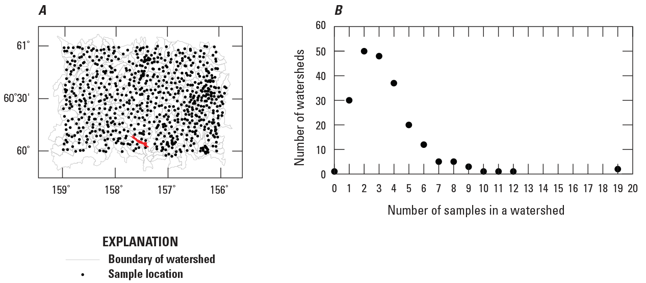
Map and plot showing spatial information about the 767 streambed sediment samples in the Taylor Mountains quadrangle in Alaska. A, Map showing the location of the samples and the boundaries of the watersheds. B, Plot of the number of watersheds as a function of the number of samples in a watershed. The red watershed does not contain a sample.
The information in the map (fig. 2A) is summarized with a plot of the number of watersheds as function of the number of samples in a watershed (fig. 2B). Seventy-seven percent of the watersheds have four or fewer samples. Ninety-six percent have eight or fewer samples. That is, almost all watersheds have few samples, which is the very situation for which the Bayesian mapping is developed.
The measurements of gold concentrations in these 767 samples are summarized in table 1. The 77 samples collected in 2004 were measured with atomic absorption spectrophotometry (AAS), for which the lower reporting limit (Arbogast, 1996, p. viii) is 5 parts per billion (ppb). Of these 77 samples, the concentrations of 20 samples are noncensored (which means that the measured concentration is greater than or equal to the lower reporting limit), and the concentrations of 57 samples are left censored (which means that the measured concentration is less than the lower reporting limit and hence its value is not specified). The 690 samples collected in subsequent years were measured with inductively coupled plasma mass spectrometry (ICPMS), for which the lower reporting limit is 1 ppb. Of these 690 samples, the concentrations of 639 samples are noncensored, and the concentrations of 51 samples are left censored.
Table 1.
Summary of gold-concentration measurements of 767 streambed sediment samples from the Taylor Mountains quadrangle, Alaska.[Terms: AAS, atomic absorption spectrophotometry; ICPMS, inductively coupled plasma mass spectrometry; ppb, parts per billion]
The empirical cumulative distribution functions of the gold concentrations are shown in figure 3. Because of the enormous range of the concentrations, the horizontal axis is logarithmic. For the 20 noncensored concentrations that are measured with AAS, the concentrations range from 5 to 60 ppb; 87 percent of these concentrations are less than 10 ppb. For the 639 noncensored concentrations that are measured with ICPMS, the concentration values range from 1 to 961 ppb; 94 percent of these concentrations are less than 10 ppb, and 79 percent of the concentrations are less than 5 ppb.
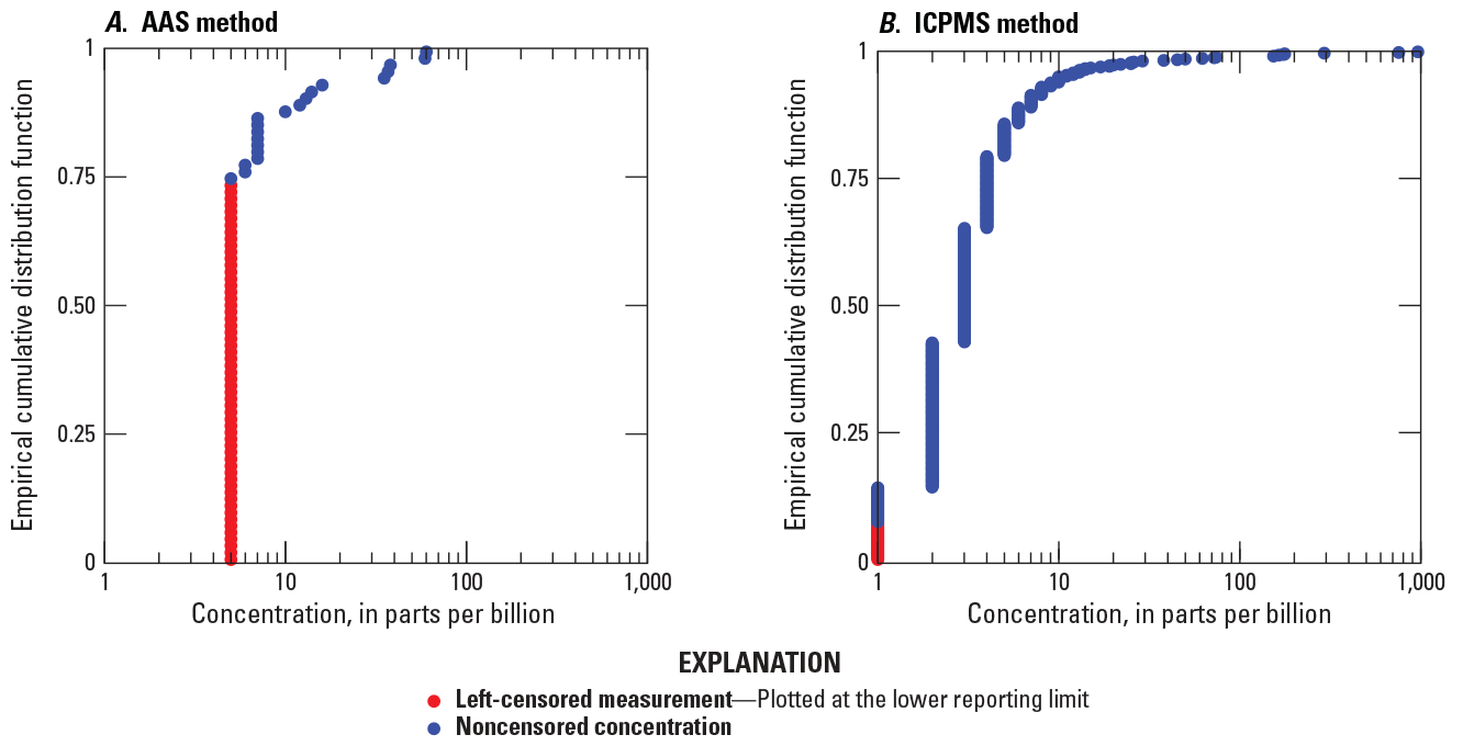
Plots showing the empirical cumulative distribution functions of gold concentrations from streambed sediment samples in the Taylor Mountains quadrangle in Alaska as measured by two methods. A, Plot showing the 77 samples that are measured with atomic absorption spectrophotometry (AAS). B, Plot showing the 690 samples that are measured with inductively coupled plasma mass spectrometry (ICPMS). The lower reporting limit for AAS is 5 parts per billion (ppb) and the lower reporting limit for ICPMS is 1 ppb.
The three maps in figure 4 are used for spatial analysis of the field data. The first map shows the locations of the samples for which the gold concentrations are noncensored (fig. 4A). The map shows that the concentrations are not spatially random. Rather, the samples with high concentrations tend to be clustered. Likewise, the samples with low concentrations tend to be clustered. The second map shows the locations of the samples for which the concentrations are left censored at 1 ppb (fig. 4B). There is a large cluster of samples in the southwestern corner. The third map shows the locations of the samples for which the concentrations are left censored at 5 ppb (fig. 4C). There is a large cluster of samples in the northeastern corner.

Three maps that are used for spatial analysis of the streambed sediment samples in the Taylor Mountains quadrangle in Alaska. A, Map showing the sample locations and corresponding gold concentrations that are noncensored. B, Map showing the sample locations where gold concentrations are left censored at 1 part per billion. C, Map showing the sample locations where gold concentrations are left censored at 5 parts per billion.
This spatial analysis indicates the major map features that are expected from the Bayesian mapping. The large clusters of high concentrations (fig. 4A) should be associated highs in the Bayesian map. Conversely, the large clusters of low concentrations (fig. 4A) should be associated lows in the Bayesian map. In the southwestern corner, the few noncensored concentrations are relatively low (fig. 4A), and there is a large cluster of left-censored concentrations at 1 ppb (fig. 4B), which indicates that the gold concentrations are relatively low. Hence, in the southwestern corner there should be a low in the Bayesian map. Conversely, in the northeastern corner, the concentrations are relatively high (fig. 4A) and there is a large cluster of left-censored concentrations at 5 ppb (fig. 4C) which, because of its relatively high value, provides little information about gold concentration (fig. 3B). Nonetheless, the relatively few noncensored concentrations have a high value so, in the northeastern corner, there should be a high in the Bayesian map.
Data for Bayesian Model
Regions and Domain
For the Bayesian model, the regions are the watersheds whose boundaries are shown in figure 2A. Each region satisfies two criteria. First, each region must contain at least one sample, so that there are some data to estimate statistics for that region. Second, each region must share a portion of its boundary with the boundaries of at least two other regions. This criterion is necessary for adequate smoothing across regions (see the “Parameter Submodel” section).
Of the 216 watersheds shown in figure 2A, these two criteria are satisfied for 215 watersheds but are not satisfied for one watershed because it has no samples. Thus, the number of regions is 215, and these 215 regions constitute the domain. The domain has a hole corresponding to the one watershed with no samples. Such a domain is unusual but acceptable.
Data Transformation
The gold concentrations are defined in a mathematical entity called the simplex (Pawlowsky-Glahn and others, 2015, p. 8–12). Mathematical operations in the simplex are different from the corresponding operations in a Euclidean space. The problem is that the Bayesian hierarchical model is developed for data in a Euclidean space, not data in the simplex. The simplest way to address this problem is to transform the concentrations to their equivalent values in a Euclidean space. The appropriate transformation is the isometric log-ratio transformation (Filzmoser and others, 2009; Pawlowsky-Glahn and others, 2015, p. 36–38). Let represent a gold concentration that is expressed in ppb. Then the isometric log-ratio (ilr) transformation is
for which is the equivalent value in the one-dimensional Euclidean space. This transformed concentration does not have units. The transformed concentrations are the measurements in the Bayesian model.Measurement Error
Recall that the Bayesian hierarchical model requires the standard deviation of the measurement error for each measurement method (eq. 2). The standard deviation is estimated from repeated measurements of standard reference materials that are used for quality control. The repeated measurements, which are gold concentrations, are transformed using the ilr transformation (eq. 10). With these transformed concentrations, the standard deviations are estimated to be 0.28 for AAS and 0.26 for ICPMS.
The implicit assumption in this procedure is that the measurement error for the transformed gold concentration is additive (eq. 1). This assumption raises the question of what the corresponding assumption for the untransformed gold concentrations is. Because the untransformed gold concentrations are small (that is, always less than 961 ppb), the ilr transformation (eq. 10) is very close to a logarithmic transformation. Thus, an additive measurement error in the transformed gold concentration is approximately equivalent to a multiplicative measurement error in the untransformed gold concentration. A general discussion of multiplicative measurement error in untransformed concentrations is in Aitchison (2003, p. 256–266).
Proximity Matrix
Recall that the proximity matrix specifies which regions are adjacent to a particular region (see the “Parameter Submodel” section). For this demonstration, two regions are deemed adjacent if their centroids are less than 15.4 kilometers apart or if the length of their common border is greater than 8.3 kilometers. A sensitivity analysis shows that the model results are practically unaffected by the chosen thresholds of 15.4 and 8.3 kilometers. If either of these two criteria are satisfied, then the two elements in the proximity matrix that are associated with these two regions are set to 1. Otherwise, the two elements are set to 0.
Bayesian Model
The data that are described in the previous section are the input to the Bayesian hierarchical model. The parameters for this model are estimated using the procedure that is described in the “Numerical Solution and Checks” section. Details about the numerical solution and the associated checks of the solution are presented in the user’s guide that accompanies the software package (Ellefsen and others, 2024).
Checks of Model Results
There are at least three ways to check the model results. The first, and most important, check is that the maps of the model results are consistent with the data from which the maps are generated. This check is presented in the “Model Results as Concentrations and Model-Data Consistency Checks” section. The second check is that the maps of the model results are consistent with independent geologic information. This check is beyond the scope of this report. The third check involves a comparison of three maps. One map is perfectly smooth; the mapped value for each region is the mean for the domain. Another map is perfectly rough; the mapped value for each region is the mean for the region. Between these two extremes must be the map from the Bayesian model. This check is presented in the user’s guide that accompanies the software package (Ellefsen and others, 2024).
Model Results as Transformed Concentrations
Recall that, in the Bayesian model, the distribution of a physical property in each region is represented by a normal pdf (see the “Process Submodel” section). This pdf is completely specified by two parameters: a mean and a standard deviation. The mean and the standard deviation for every region are presented as maps (fig. 5A, B) and are explained in a graph (fig 5C). When viewing these maps, it is important to remember that the physical property is the transformed gold concentration, not the gold concentration. Transformed gold concentrations do not have units.
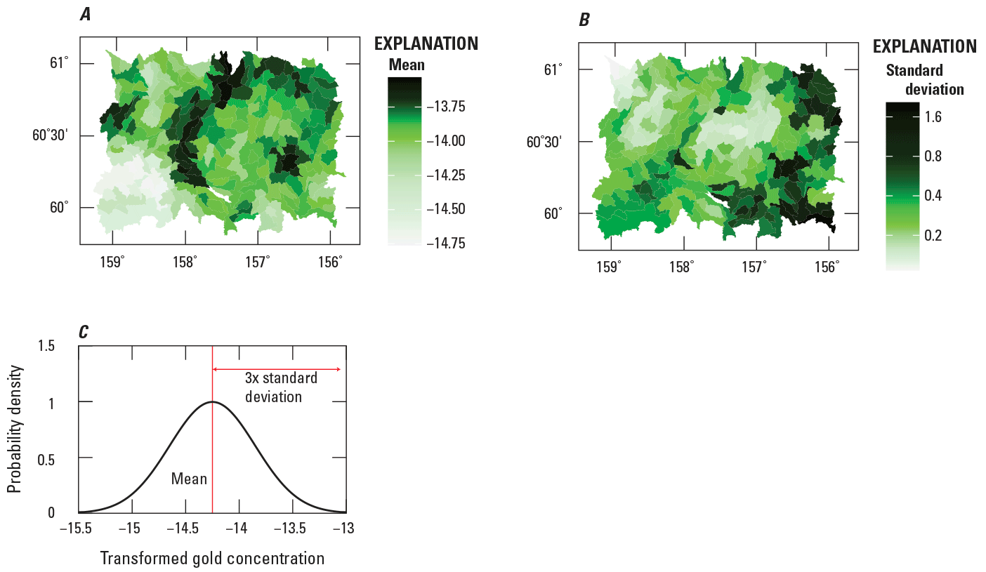
Maps and a graph depicting model results for transformed gold concentrations from streambed sediment samples in the Taylor Mountains quadrangle in Alaska. Maps showing, for each watershed, the (A) mean and (B) standard deviation. The color scale for each map (parts A and B) has been stretched so that the proportions of colors are more balanced and easier to interpret. C, Graph explaining the mean and the standard deviation of the normal probability density function (pdf) that represents the distribution of the transformed gold concentration in a region. The mean is the center of the normal pdf and the standard deviation measures the width of the pdf. No feature in the pdf corresponds to the standard deviation. Nonetheless, at a distance of three times the standard deviation from the mean, the pdf is approximately zero.
The maps in figure 5 are presented simply because they are the solution for the Bayesian model. However, for geochemical data, these maps are somewhat difficult to analyze because they pertain to transformed gold concentrations. Consequently, the model results are re-expressed as concentrations in the next section.
Model Results as Concentrations and Model-Data Consistency Checks
The maps that pertain to transformed concentrations (fig. 5) are re-expressed in terms of concentrations because concentrations are familiar to geochemists and many other earth scientists. This re-expression will make the analysis of these maps easier than it would be otherwise. The statistical values depicted in the maps in figure 6A–D are explained in graphs in figure 6E–G.
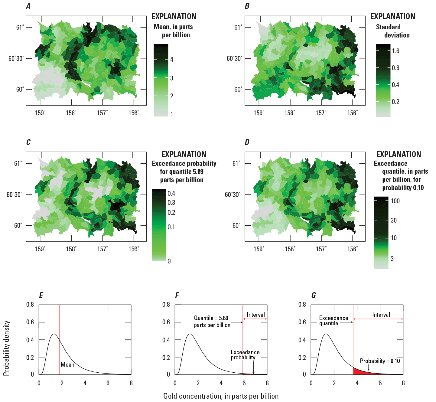
Maps and graphs depicting model results for gold concentrations from streambed sediment samples in the Taylor Mountains quadrangle in Alaska. Maps showing, for each watershed, the (A) mean, (B) standard deviation, (C) exceedance probability for quantile 5.89 parts per billion, and (D) exceedance quantile for probability 0.10. The color scale for each map (parts A, B, C, and D) has been stretched so that the proportions of colors are balanced and easy to interpret. The mean, the exceedance probability, and the exceedance quantile are attributes of the probability density function (pdf) that represents the distribution of the gold concentration in a region. These attributes are explained in the graphs (parts E, F, and G). The mean (part E) is the center of the pdf. No feature in the pdf corresponds to the standard deviation. The exceedance probability (part F) and the exceedance quantile (part G) are closely related. Both involve intervals of the gold concentration; for both intervals, the right boundaries are at positive infinity. Each interval is associated with a probability (namely, the probability that the gold concentration occurs with the interval). The probability equals the area of the red polygon in the right tail of the pdf. For the exceedance probability (part F), the left boundary of the interval (that is, quantile) is specified, and then the probability associated with this interval (that is, the exceedance probability) is calculated. For part C, the specified quantile is 5.89 ppb. In contrast, for the exceedance quantile (part G), the probability is specified and then the left boundary of the interval (that is, the exceedance quantile) is calculated. For part D, the specified probability is 0.10.
Recall that, in each region, the distribution of the physical property is represented by a normal pdf (see the “Process Submodel” section). From this normal pdf, random samples of the transformed gold concentration are drawn. These random samples are back transformed to gold concentration using the inverse of equation 10. An example of the distribution for one region is shown in figure 6E; this distribution is not a normal pdf. From these random samples, the mean gold concentration is calculated (Pawlowsky-Glahn and others, 2015, p. 66), and the means for all regions are presented as a map (fig. 6A). This map is visually similar to the map of transformed gold concentration (fig. 5A) because of the stretching of the color scale.
Compare the map of the mean (fig. 6A) with the maps used for spatial analysis of the field data (fig. 4). The mean is high where the gold concentrations of the field samples are high and the mean is low where the gold concentrations of the field samples are low (fig. 4A). In the northeastern corner of the domain, there is a large cluster of samples for which the concentration is left censored at 5 ppb (fig. 4C). Because the threshold, 5 ppb, is relatively high compared to most gold concentrations (fig. 3), this large cluster provides little information about the actual concentrations. Hence, in the northeastern corner, the Bayesian solution is mostly affected by the few field samples with moderate to high concentrations (fig. 4A). Consequently, the mean in the northeastern corner is high (fig. 6A).
In contrast, in the southwestern corner of the domain, there is a large cluster of samples for which the concentration is left censored at 1 ppb (fig. 4B). Because the threshold, 1 ppb, is relatively low compared to most gold concentrations (fig. 3), this cluster provides significant information about the actual concentrations. Hence, the Bayesian solution is strongly affected by both this cluster and the few field samples with low concentrations (fig. 4A). Consequently, the mean in the southwestern corner is low (fig. 6A).
For compositional data such as concentrations, the standard deviation is the same for the transformed and the untransformed concentrations (Pawlowsky-Glahn and others, 2015, p. 66–67, 110–111). Consequently, the map in figure 5B is repeated in figure 6B. Compare the map of the standard deviation (fig. 6B) with the maps used for spatial analysis of the field data (fig. 4). The standard deviation is high where the gold concentrations of the field samples have significant variability (for example, the southeastern corner of the domain). Conversely, the standard deviation is low where the gold concentrations of the field samples have little variability (for example, the northwestern corner of the domain).
Recall that, in the northeastern corner of the domain (fig. 4C), there is a large cluster of samples that provides little information about the actual concentrations. Consequently, in this corner, the standard deviations are high (fig. 6B). Recall that, in the southwestern corner of the domain (fig. 4B), there is a large cluster of samples that provides significant information about the actual concentrations. However, this information is still less than the information that is provided by noncensored concentrations. Consequently, in this corner, the standard deviations are moderately high.
From the Bayesian solution, two additional maps are generated that indicate the potential for high gold concentration. The first map displays the probabilities that the gold concentrations exceed 5.89 ppb (fig. 6C); these probabilities are called exceedance probabilities and are explained in figure 6F. There is nothing special about the quantile 5.89 ppb; any suitable quantile could be chosen. Nonetheless, the quantile 5.89 ppb is chosen so that the resulting map (fig. 6C) looks like the map of the mean (fig. 6A). The second map displays the quantiles at which the gold concentrations, or greater value of the gold concentrations, have a 0.10 probability of occurrence (fig. 6D); these quantiles are called exceedance quantiles and are explained in figure 6G. There is nothing special about the 0.10 probability; any suitable probability could be chosen. Nonetheless, the 0.10 probability is chosen so that the resulting map (fig. 6D) looks like the map of the mean (fig. 6A).
Recall that a cluster of left-censored measurements affects the maps of the means and of the standard deviations. Because these quantities are used to calculate exceedance probabilities and exceedance quantiles, a cluster of left-censored measurements also affects exceedance probabilities and exceedance quantiles. For example, the cluster of left-censored measurements in the northeastern corner (fig. 4C) is associated with high exceedance probabilities (fig. 6C) and high exceedance quantiles (fig. 6D). The important point is that, if there is a cluster of left-censored measurements, then it is necessary to account for its effect when interpreting the maps of exceedance probabilities and exceedance quantiles.
Analysis of Uncertainty
The maps of the mean and the standard deviation (fig. 5) are estimates, respectively, of the actual mean and the actual standard deviation. That these two statistics are estimates implies that they are uncertain. This uncertainty is analyzed in this section.
Recall that, in the Bayesian hierarchical model, the distribution of a physical property in each region is represented by a normal pdf, which is completely specified by its mean and its standard deviation. The mean is the process mean (eq. 3). In the numerical solution for Bayes’ rule (eq. 9), the process mean is not a single value; rather, the process mean has a range of values that are represented by a pdf. Similarly, the standard deviation is the process standard deviation (eq. 3); the process standard deviation also has a range of values that are represented by another pdf. The mean of the pdf for the process mean and the mean of the pdf for the process standard deviation are used for the maps in figure 5.
That the process mean is specified by a pdf indicates that there is uncertainty in its value. This uncertainty is quantified by the standard deviation of the pdf, which is called the standard deviation of . The standard deviation of for every region is presented as a map (fig. 7). The causes of the high and low standard deviations, namely the causes of uncertainty, may be discerned by analyzing the mapped values in conjunction with other information about the measurements.
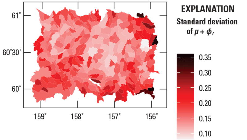
Map of the standard deviation of . This standard deviation measures the uncertainty in the process mean of the Bayesian model. This map is used to assess the uncertainty in the map of gold concentrations in streambed sediment samples from the Taylor Mountains quadrangle in Alaska (figs. 5A, 6A). Colored polygons represent watersheds.
The analysis uses scatterplots of the standard deviation of versus three different explanatory variables (fig. 8). In each scatterplot, a point is associated with a region; there are 215 points for the 215 regions. For each scatterplot, a trend line is added to help discern the relationship between the standard deviation of and the explanatory variable. The trend line is based on the median, making it robust to outliers. The trend lines are either exponential or linear, and both are estimated using Bayesian quantile regression (appendixes 1–2).
For the first scatterplot (fig. 8A), the explanatory variable is the number of samples in region . The plot shows that the median, as observed in the trend line, increases nonlinearly as the number of samples decreases. The number of samples is directly related to the amount of information that is available to calculate , so the plot shows that, as the amount of information decreases, the uncertainty increases.
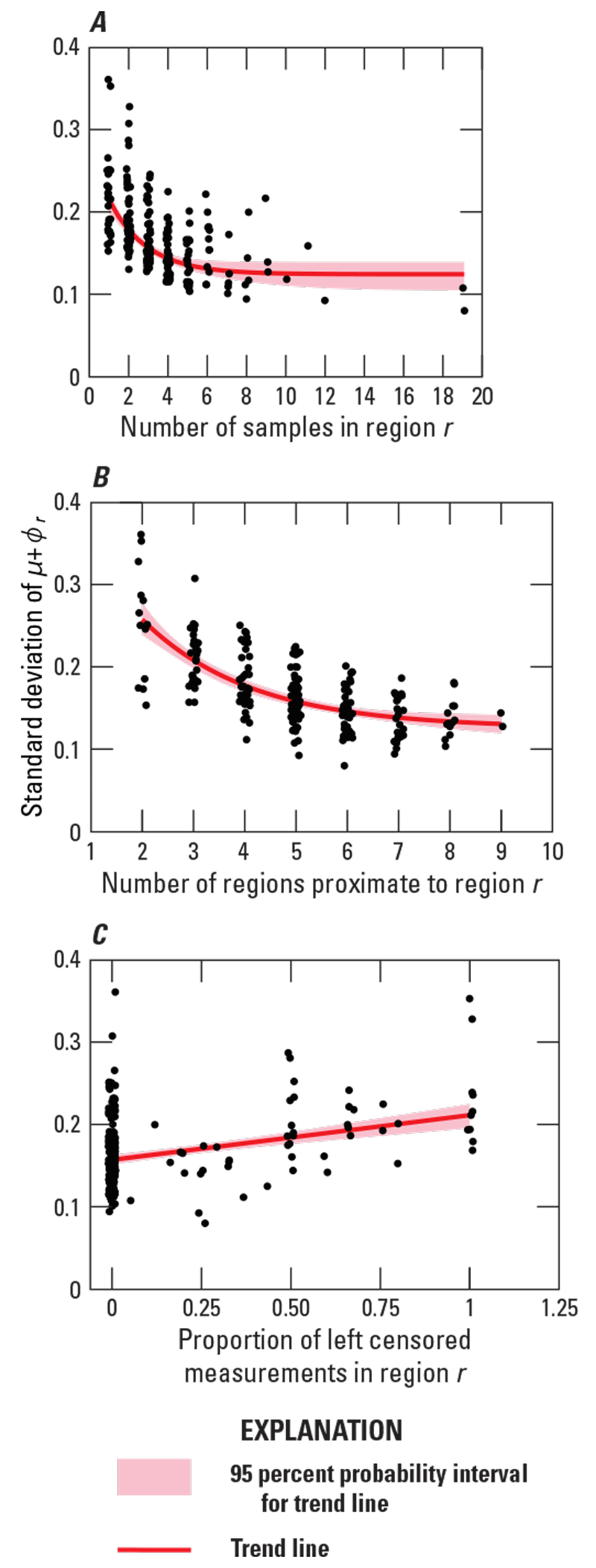
Scatterplots and trend lines of the standard deviation of for region versus (A) the number of samples in region , (B) the number of regions that are proximate to region , and (C) the proportion of measurements that are left censored in region . The standard deviation of for each region is presented in figure 7. For the plots, a small amount of random noise is added to the horizontal component of the points to reduce the number of points plotting atop one another.
For the second scatterplot (fig. 8B), the explanatory variable is the number of regions that are proximate to region , which is specified in the proximity matrix. The plot shows that the median, as observed in the trend line, increases nonlinearly as the number of proximate regions decreases. The number of proximate regions is directly related to the amount of information that is available to calculate , so the plot shows that, as the amount of information decreases, the uncertainty increases. Because the number of proximate regions is likely to be small along the border of the domain, the uncertainty here is likely to be high. This phenomenon is sometimes called an edge effect.
For the third scatterplot (fig. 8C), the explanatory variable is the proportion of left-censored measurements in region . The plot shows that the median, as observed in the trend line, increases as the proportion increases. The proportion is inversely related to the amount of information that is available to calculate , so the plot shows that, as the amount of information decreases, the uncertainty increases.
That the process standard deviation is specified by a pdf indicates that there is uncertainty in its value. This uncertainty is quantified by the standard deviation of the pdf, which is called the standard deviation of . The standard deviation of for every region is presented as a map (fig. 9). Again, the causes of the high and low standard deviations are discerned by analyzing the mapped values in conjunction with other information about the measurements.
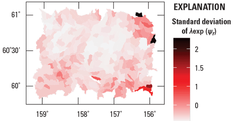
Map of the standard deviation of . This standard deviation measures the uncertainty in the process standard deviation of the Bayesian model. This map is used to assess the uncertainty in the map of gold concentrations in streambed sediment samples from the Taylor Mountains quadrangle in Alaska. Colored polygons represent watersheds.
The analysis of the standard deviation of is based on the scatterplots and trend lines that are presented in figure 10. The graphs in the upper row (fig. 10A, B, C) show all data. Because four standard deviations are large, it is difficult to discern the important features in the data and the trend lines. Consequently, to better view these features, the graphs in the bottom row (fig. 10D, E, F) show the same data but without the four large standard deviations. The interpretations of these scatterplots and trend lines are identical to the corresponding interpretations for the standard deviation of , so they are not repeated.
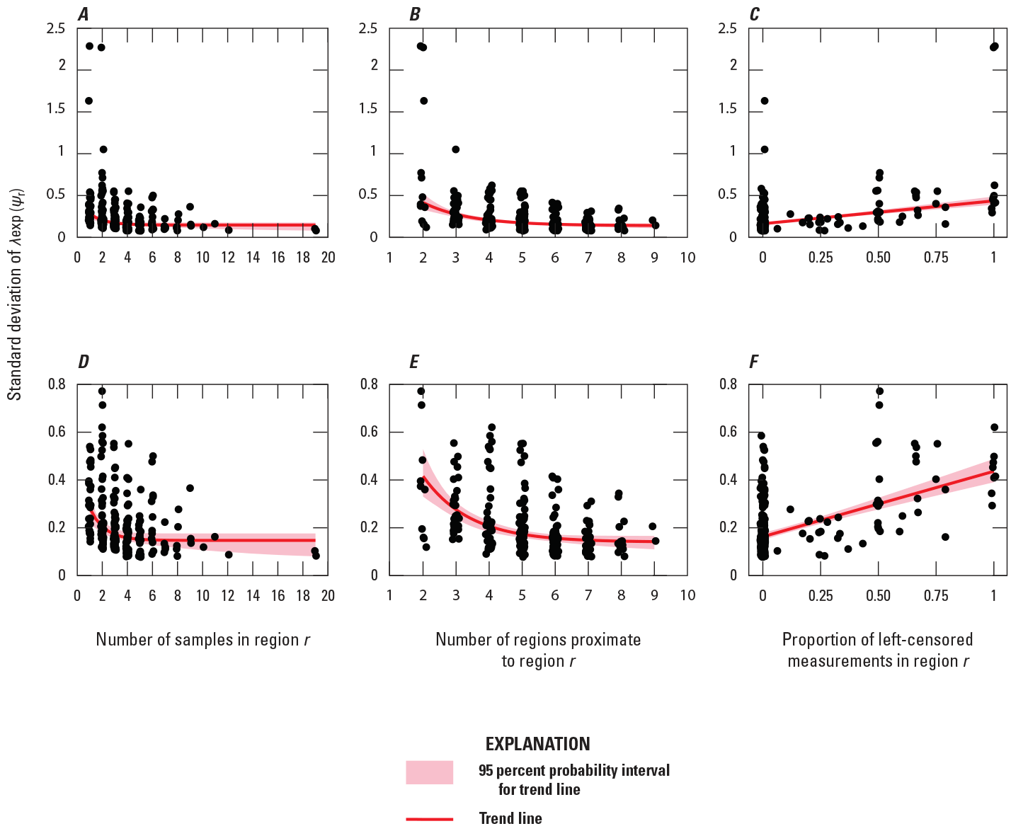
Scatterplots and trend lines of the standard deviation of for region versus (A) the number of samples in region , (B) the number of regions that are proximate to region , and (C) the proportion of measurements that are left censored in region . Parts D, E, and F are views of parts A, B, and C, respectively, but exclude the four largest standard deviations so the data are more readily visible. The standard deviation of for each region is presented in figure 9. For the plots, a small amount of random noise is added to the horizontal component of the points to reduce the number of points plotting atop one another.
The previous two analyses show that, if a region has only a few samples, has few neighboring regions (such as along the border of the domain), or has a high proportion of left-censored measurements, then the estimated statistics for that region are likely to have greater uncertainty than they would otherwise. This uncertainty should be considered when interpreting the maps of the mean and the standard deviation (fig. 5). For geochemical data, this uncertainty also affects the maps related to concentrations (fig. 6) and also should be considered when interpreting these maps.
The similarity of the corresponding trends in figures 8 and 10, and the general similarity of the map patterns in figures 7 and 9, raise the question of whether the two standard deviations are related. This question is addressed with the scatterplot of the standard deviation of versus the standard deviation of (fig. 11). The scatterplot shows that there is a nonlinear relation between the standard deviations, that the variability in the relation increases as the standard deviations increase, and that the standard deviation of is much larger than the standard deviation of .
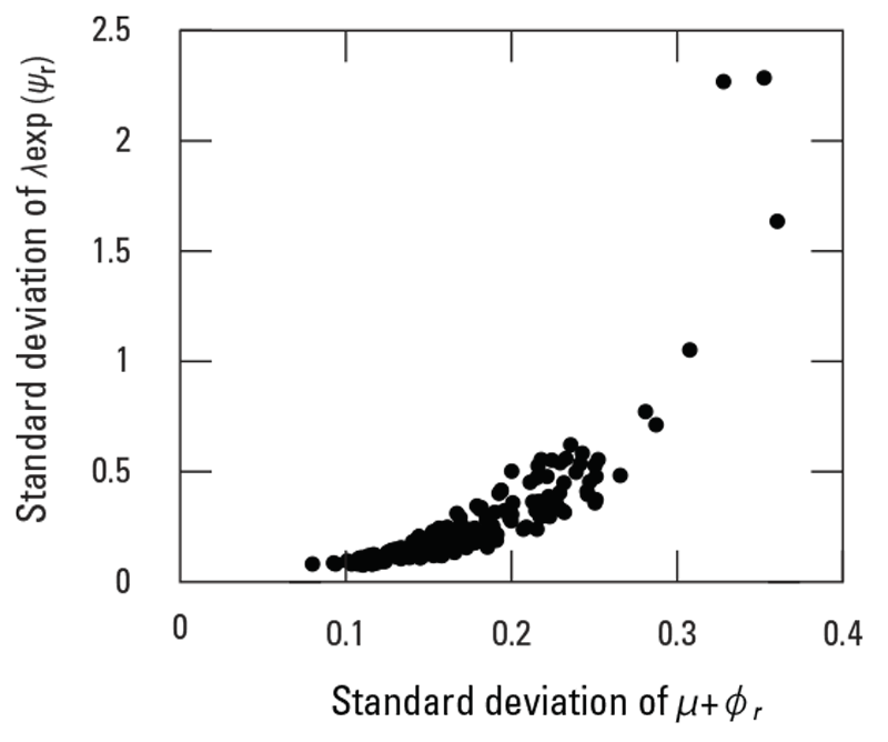
Scatterplot of the standard deviation of versus the standard deviation of . The standard deviation of for each region is presented in figure 7, and the standard deviation of for each region is presented in figure 9.
Future Developments
In the current formulation of the Bayesian hierarchical model, the measurement error is assumed to be normally distributed (eq. 2). However, analyses of several large sets of quality control data suggest that the distribution for the measurement error is more complex than a normal distribution. Thus, a suitable topic for future development is generalizing the distribution for the measurement error and then implementing the numerical solution of the revised Bayesian hierarchical model. The implementation will be difficult. To understand the reason for the difficulty, consider equation 2; the distribution for the sum of two random variables is the convolution of their respective distributions (Grimmett and Stirzaker, 2001, p. 113–114). The current formulation of the model includes this convolution implicitly: the convolution of two normal pdfs is another normal pdf. The convolution or an approximation of it may require significant computation.
Recall that, in the parameter submodel, the prior distributions for vectors and were chosen to be the CAR model. For such a model, the effect of one region on another is symmetric. For example, assume that regions 1 and 2 are adjoined. In the CAR model, the effect of region 1 on region 2 equals the effect of region 2 on region 1. However, for some earth science applications, the effect is asymmetric. An important topic of future development is investigating whether the prior distributions for vectors and can account for such asymmetry and, if so, how it can be implemented in the numerical solution.
Recall that, for the demonstration of the method, one watershed had no samples (fig. 2). Consequently, this watershed was not a region in the domain (see the “Regions and Domain” section), and model statistics (namely, mean and standard deviation) were not estimated for it. The model can be modified for such no-data regions; the means and standard deviations from the surrounding regions can be interpolated into these no-data regions. If such a modification is made, it will be crucial to assess the uncertainty due to the interpolation.
Software, Data, and Reproducibility
The software for the Bayesian mapping is written in the R statistical programming language and is published in the USGS software repository (Ellefsen and others, 2024). The gold data that are used in this report are included in the R package. The R scripts that are used to perform the calculations for this report and to generate the figures for this report are also included the R package. In summary, the software, the gold data, and the scripts are publicly available and can be used to reproduce all results in this report.
Acknowledgments
Jared Smith and Jacob Zwart of the U.S. Geological Survey (USGS) reviewed this manuscript, and their suggestions improved its quality. This report was funded by the Mineral Resources Program of the USGS and the emeritus program of the USGS.
References Cited
Arbogast, B.F., ed., 1996, Analytical methods manual for the Mineral Resource Surveys Program, U.S. Geological Survey: U.S. Geological Survey Open-File Report 96–525, 248 p., accessed June 3, 2024, at https://doi.org/10.3133/ofr96525.
Bailey, E.A., Lee, G.K., Mueller, S.H., Wang, B., Brown, Z.A., and Beischer, G.A., 2007, Major- and trace-element data from stream-sediment and rock samples collected in the Taylor Mountains 1:250,000-scale quadrangle, Alaska (ver. 1.1, May 2010): U.S. Geological Survey Open-File Report 2007–1196, 9 p., accessed June 3, 2024, at https://doi.org/10.3133/ofr20071196. [Supersedes version 1.0, released in 2007.]
Berliner, L.M., 1996, Hierarchical Bayesian time series models, in Hanson, K.M., and Silver, R.N., eds., Maximum entropy and Bayesian methods—Proceedings of the Fifteenth International Workshop on Maximum Entropy and Bayesian Methods, Santa Fe, N. Mex., July 31–August 4, 1995: [Santa Fe, N. Mex.], Kluwer Academic Publishers, p. 15–22. [Also available at https://doi.org/10.1007/978-94-011-5430-7_3.]
Carpenter, B., Gelman, A., Hoffman, M.D., Lee, D., Goodrich, B., Betancourt, M., Brubaker, M.A., Guo, J., Li, P., and Riddell, A., 2017, Stan—A probabilistic programming language: Journal of Statistical Software, v. 76, no. 1, 32 p., accessed June 3, 2024, at https://doi.org/10.18637/jss.v076.i01.
Ellefsen, K.J., Goldman, M.A., and Wang, B., 2024, Software for Bayesian mapping of regionally grouped, sparse, univariate earth science data (program BMRGSU): U.S. Geological Survey software release, https://doi.org/10.5066/P14X4CKG.
Filzmoser, P., Hron, K., and Reimann, C., 2009, Univariate statistical analysis of environmental (compositional) data—Problems and possibilities: Science of the Total Environment, v. 407, no. 23, p. 6100–6108. [Also available at https://doi.org/10.1016/j.scitotenv.2009.08.008.]
Joseph, M., 2016, Exact sparse CAR models in Stan: Stan web page, accessed June 3, 2024, at http://mc-stan.org/documentation/case-studies/mbjoseph-CARStan.html.
U.S. Geological Survey and U.S. Department of Agriculture, Natural Resources Conservation Service, 2013, Federal standards and procedures for the National Watershed Boundary Dataset (WBD) (4th ed.): U.S. Geological Survey Techniques and Methods 11–A3, 63 p., accessed June 3, 2024, at https://doi.org/10.3133/tm11A3.
Appendix 1. Bayesian Quantile Regression for an Exponential Trend
Introduction
This appendix presents the Bayesian quantile regression for an exponential trend that is used in figures 8A, 8B, 10A, 10B, 10D, and 10E. The topics in this appendix include the Bayesian formulation of the model and Bayes’ rule for this model. This appendix does not present the numerical solution because that topic is presented in the “Numerical Solution and Checks” section in the report.
Mathematical Formulation
When the regression pertains to the number of samples in region (figs. 8A, 10A, 10D), the explanatory variable is the number of samples in region minus . When the regression pertains to the number of regions proximate to region (figs. 8B, 10B, 10E), the explanatory variable is the number of regions proximate to region minus . The subtractions shift the data so that the explanatory variable begins at , which greatly improves the convergence of the numerical solution. The explanatory variable is denoted . The dependent variable is either the standard deviation of or the standard deviation of . Both standard deviations are represented by the same symbol, .
The quantile regression is based on the asymmetric Laplace distribution (ALD) (Yu and Moyeed, 2001):
in which is the exponential curve representing the median. Parameter translates the exponential curve, parameter scales the exponential curve, parameter controls the rate at which the exponential curve decreases, parameter is the scale of the ALD, and parameter is the quantile (0.5).The prior probability density function (pdf) for parameter must satisfy two criteria. First, it must ensure that because figures 8A, 8B, 10A, 10B, 10D, and 10E show that the translation is positive. Second, it must be as uninformative as possible. These two criteria are satisfied with the truncated normal pdf:
To understand this pdf, consider a normal pdf with a center of zero and a variance of . Then, truncate the normal pdf at zero and remove the negative-valued part. The resulting pdf ensures that is positive, so the first criterion is satisfied. The large value of the variance ensures that the pdf is uninformative, so the second criterion is satisfied.The prior pdf for parameter must satisfy two criteria. First, it must ensure that because figures 8A, 8B, 10A, 10B, 10D, and 10E show that the scaling is positive. Second, it must be as uninformative as possible. These two criteria are satisfied with the truncated normal pdf:
The prior pdf for parameter must satisfy two criteria. First, it must ensure that because figures 8A, 8B, 10A, 10B, 10D, and 10E show that the exponential curve decreases as increases. Second, it must be as uninformative as possible. These two criteria are satisfied with the truncated normal pdf:
The variance for this pdf is small compared to the variances of the previous two pdfs (eqs. 1.2 and 1.3). This small variance is necessary because the posterior pdf has multiple modes. By restricting the variance, the numerical solution finds the appropriate mode in the posterior pdf, ensuring that the exponential trend fits the data.The prior pdf for the scale parameter must satisfy two criteria. First, it must ensure that because a scale parameter is impossible. Second, it must be as uninformative as possible. These two criteria are satisfied with the truncated Cauchy pdf:
This pdf is described in the “Parameter Submodel” section in the report, so the description is not repeated here.Bayes’ Rule
Bayes’ rule is formulated directly from the previous five equations:
The expression on the left side of the proportional-to symbol () is the posterior pdf for the model parameters, namely , , , and . Vector comprises all standard deviations . The first expression on the right side of the proportional-to symbol is the likelihood function. The other four expressions on the right side are discussed in the previous section.Appendix 2. Bayesian Quantile Regression for a Linear Trend
Introduction
This appendix presents the Bayesian quantile regression for a linear trend that is used in figures 8C, 10C, and 10F. The topics in this appendix include the Bayesian formulation of the model and Bayes’ rule for this model. This appendix does not present the numerical solution because that topic is presented in the “Numerical Solution and Checks” section in the report.
Mathematical Formulation
The explanatory variable is the proportion of left-censored measurements in region , which is denoted . The dependent variable is either the standard deviation of or the standard deviation of . Both standard deviations are represented by the same symbol, . The quantile regression is based on the asymmetric Laplace distribution (ALD) (Yu and Moyeed, 2001):
in which is the straight line representing the median. Parameter is the intercept of the line, parameter is the slope of the line, parameter is the scale of the ALD, and parameter is the quantile (0.5).The prior probability density functions (pdfs) for parameters and need to be as uninformative as possible. Thus, suitable pdfs are
andThe prior pdf for the scale parameter must satisfy two criteria. First, it must ensure that because a scale parameter is impossible. Second, it must be as uninformative as possible. These two criteria are satisfied with the truncated Cauchy pdf:
This pdf is described in the “Parameter Submodel” section in the report, so the description is not repeated here.Bayes’ Rule
Bayes’ rule is formulated directly from the previous four equations:
The expression on the left side of the proportional-to symbol () is the posterior pdf for the model parameters, namely , , and . Vector comprises all standard deviations . The first expression on the right side of the proportional-to symbol is the likelihood function. The other three expressions on the right side are discussed in the previous section.Director, Geology, Geophysics, and Geochemistry Science Center
U.S. Geological Survey
Box 25046, Mail Stop 973
Denver, CO 80225
Or visit our website at:
https://www.usgs.gov/centers/gggsc/
Publishing support provided by the USGS Science Publishing Network,
Reston and Denver Publishing Service Centers
Disclaimers
Any use of trade, firm, or product names is for descriptive purposes only and does not imply endorsement by the U.S. Government.
Although this information product, for the most part, is in the public domain, it also may contain copyrighted materials as noted in the text. Permission to reproduce copyrighted items must be secured from the copyright owner.
Suggested Citation
Ellefsen, K.J., Wang, B., and Goldman, M.A., 2025, Bayesian mapping of regionally grouped, sparse, univariate earth science data: U.S. Geological Survey Techniques and Methods, book 7, chap. C29, 20 p., https://doi.org/10.3133/tm7C29.
ISSN: 2328-7055 (online)
Study Area
| Publication type | Report |
|---|---|
| Publication Subtype | USGS Numbered Series |
| Title | Bayesian mapping of regionally grouped, sparse, univariate earth science data |
| Series title | Techniques and Methods |
| Series number | 7-C29 |
| DOI | 10.3133/tm7C29 |
| Publication Date | May 08, 2025 |
| Year Published | 2025 |
| Language | English |
| Publisher | U.S. Geological Survey |
| Publisher location | Reston VA |
| Contributing office(s) | Geology, Geophysics, and Geochemistry Science Center |
| Description | iv, 20 p. |
| Larger Work Type | Report |
| Larger Work Subtype | USGS Numbered Series |
| Larger Work Title | Section C: Computer programs in Book 7: Bayesian Mapping of Regionally Grouped, Sparse, Univariate Earth Science Data |
| Country | United States |
| State | Alaska |
| Other Geospatial | Taylor Mountains quadrangle |
| Online Only (Y/N) | Y |